Compact Muon Solenoid
LHC, CERN
 Visit us: CMS Public Website, CMS Physics ;
Contact us: CMS Publications Committee
| CMS-PAS-TOP-25-004 | ||
| Measurement of the $ \mathrm{tW}\gamma $ production cross section at $ \sqrt{s}= $ 13 TeV | ||
| CMS Collaboration | ||
| 2026-10-12 | ||
| Abstract: The first measurement is presented of single top quark production in association with a W boson and a photon, $ \mathrm{tW}\gamma $, in proton-proton collisions at $ \sqrt{s}= $ 13 TeV. The data were recorded by the CMS experiment at the CERN LHC in the years 2016 to 2018 and correspond to an integrated luminosity of 138 fb$ ^{-1} $. Events are selected with two leptons (electrons or muons) in the final state. A graph neural network discriminator is used to separate the signal from the background. The signal cross section is measured using a fit to the discriminator output and to dedicated distributions in control regions. The cross section in the fiducial region, defined at generator level for events containing a photon with transverse momentum greater than 15 GeV and two leptons with an invariant mass of at least 30 GeV, is measured to be 20 $ ^{+6}_{-5} $ fb, with an observed (expected) significance of 4.7 (5.6) standard deviations. The result is in agreement with the standard model prediction at next-to-leading order accuracy in quantum chromodynamics. | ||
| Links: CDS record (PDF) ; CADI line (restricted) ; | ||
| Figures | |
png pdf |
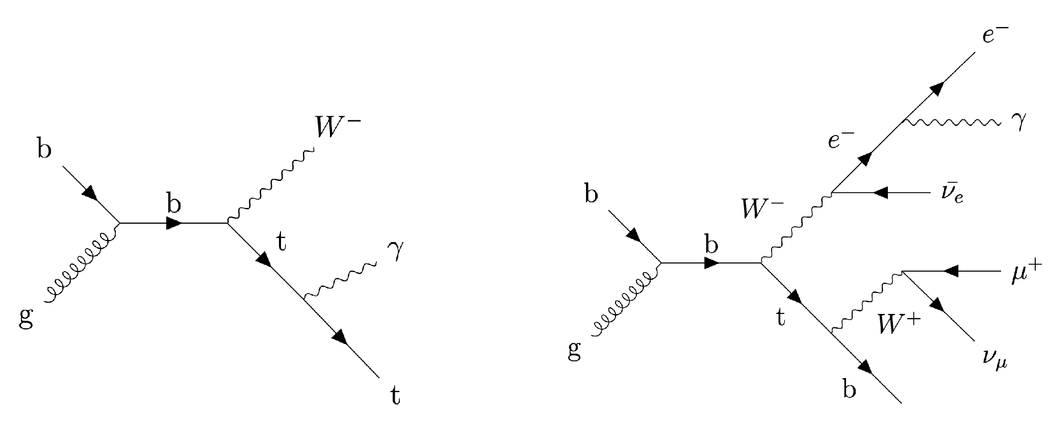
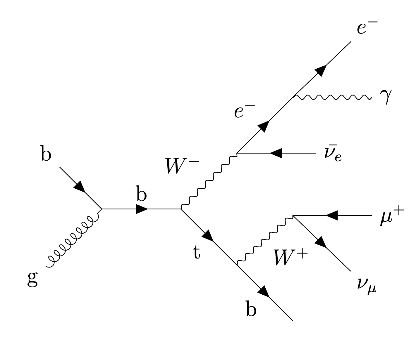
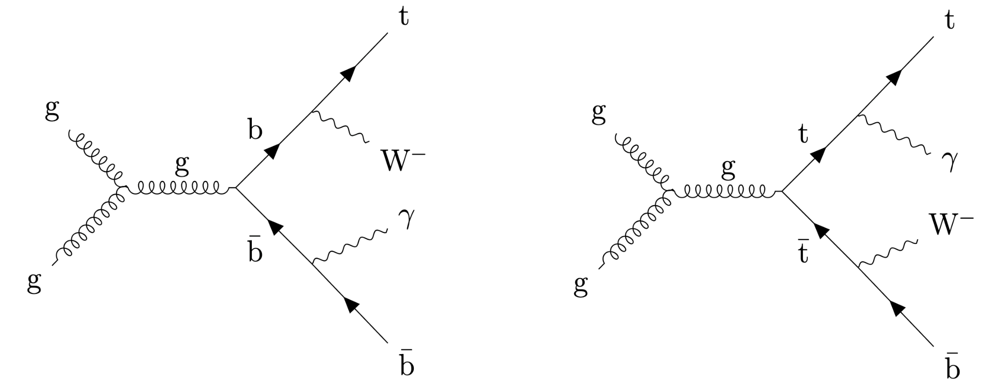
Figure 1:
Examples of Feynman diagrams of the $ \mathrm{t} \mathrm{W} \gamma $ process at LO in QCD with the HP (left) and decay (right) photon. |
png |
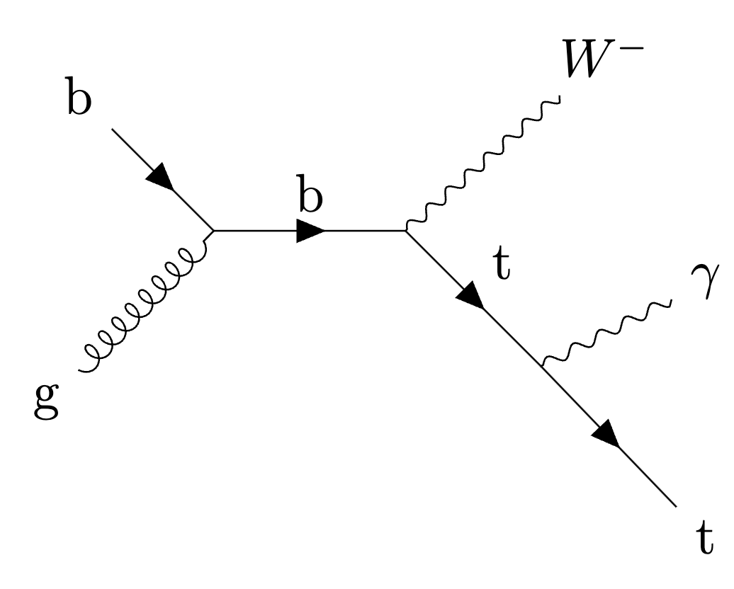
Figure 1-a:
Examples of Feynman diagrams of the $ \mathrm{t} \mathrm{W} \gamma $ process at LO in QCD with the HP (left) and decay (right) photon. |
png |
Figure 1-b:
Examples of Feynman diagrams of the $ \mathrm{t} \mathrm{W} \gamma $ process at LO in QCD with the HP (left) and decay (right) photon. |
png pdf |
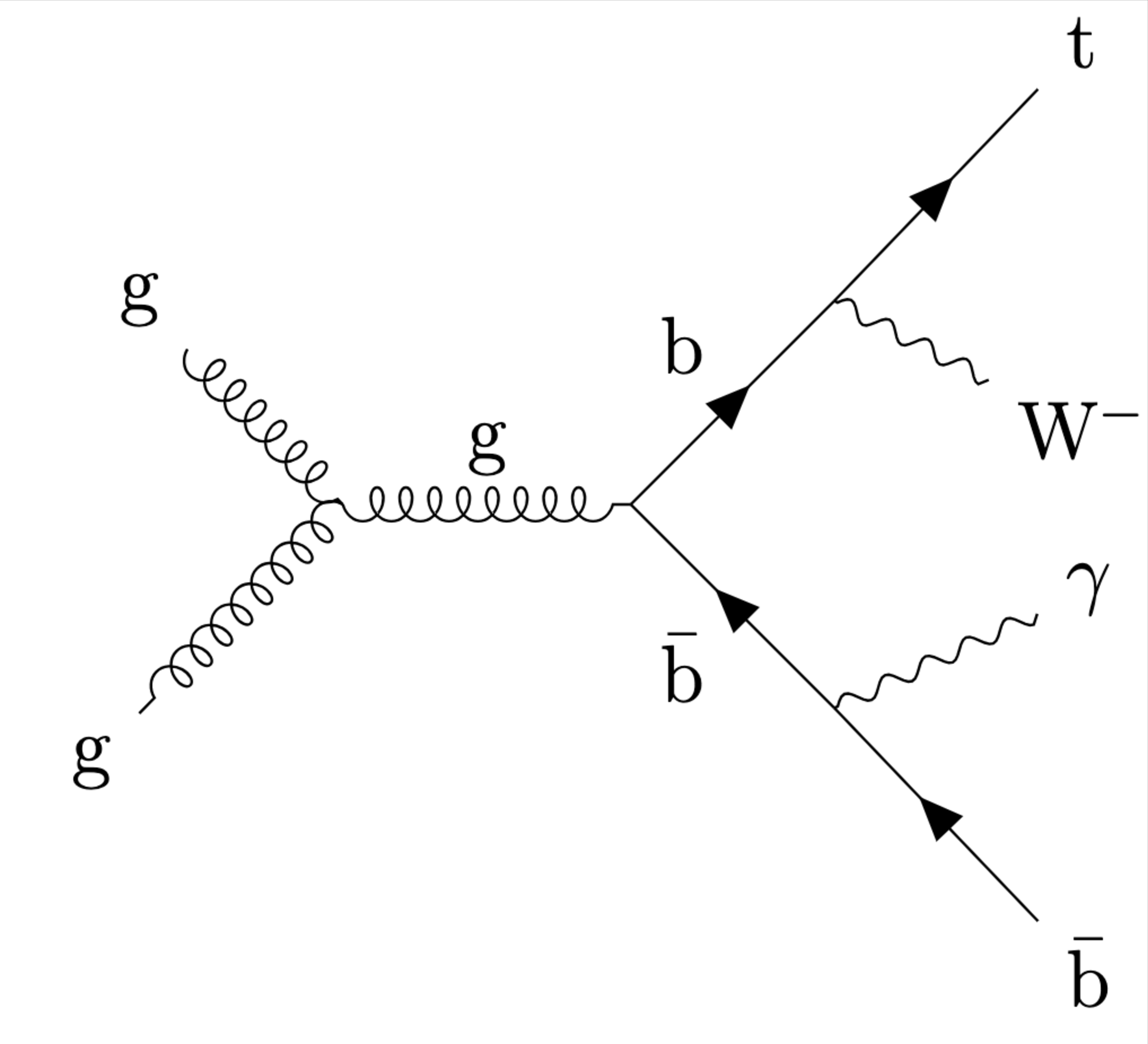
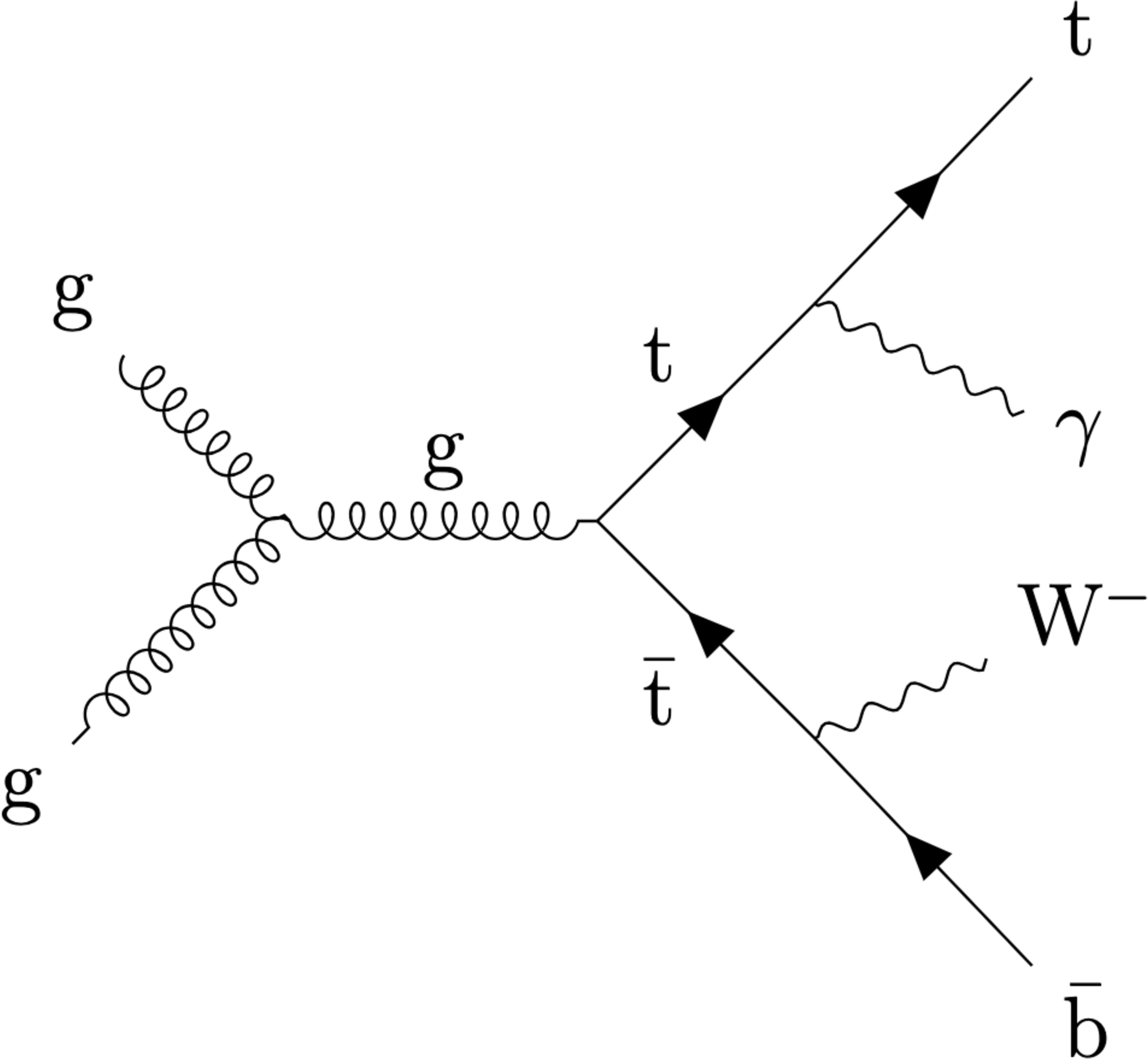
Figure 2:
A Feynman diagram of the $ \mathrm{t} \mathrm{W} \gamma $ process at NLO in QCD (left) together with that of $ \mathrm{t} \overline{\mathrm{t}} \gamma $ at LO (right). |
png pdf |
Figure 2-a:
A Feynman diagram of the $ \mathrm{t} \mathrm{W} \gamma $ process at NLO in QCD (left) together with that of $ \mathrm{t} \overline{\mathrm{t}} \gamma $ at LO (right). |
png pdf |
Figure 2-b:
A Feynman diagram of the $ \mathrm{t} \mathrm{W} \gamma $ process at NLO in QCD (left) together with that of $ \mathrm{t} \overline{\mathrm{t}} \gamma $ at LO (right). |
png pdf |
Figure 3:
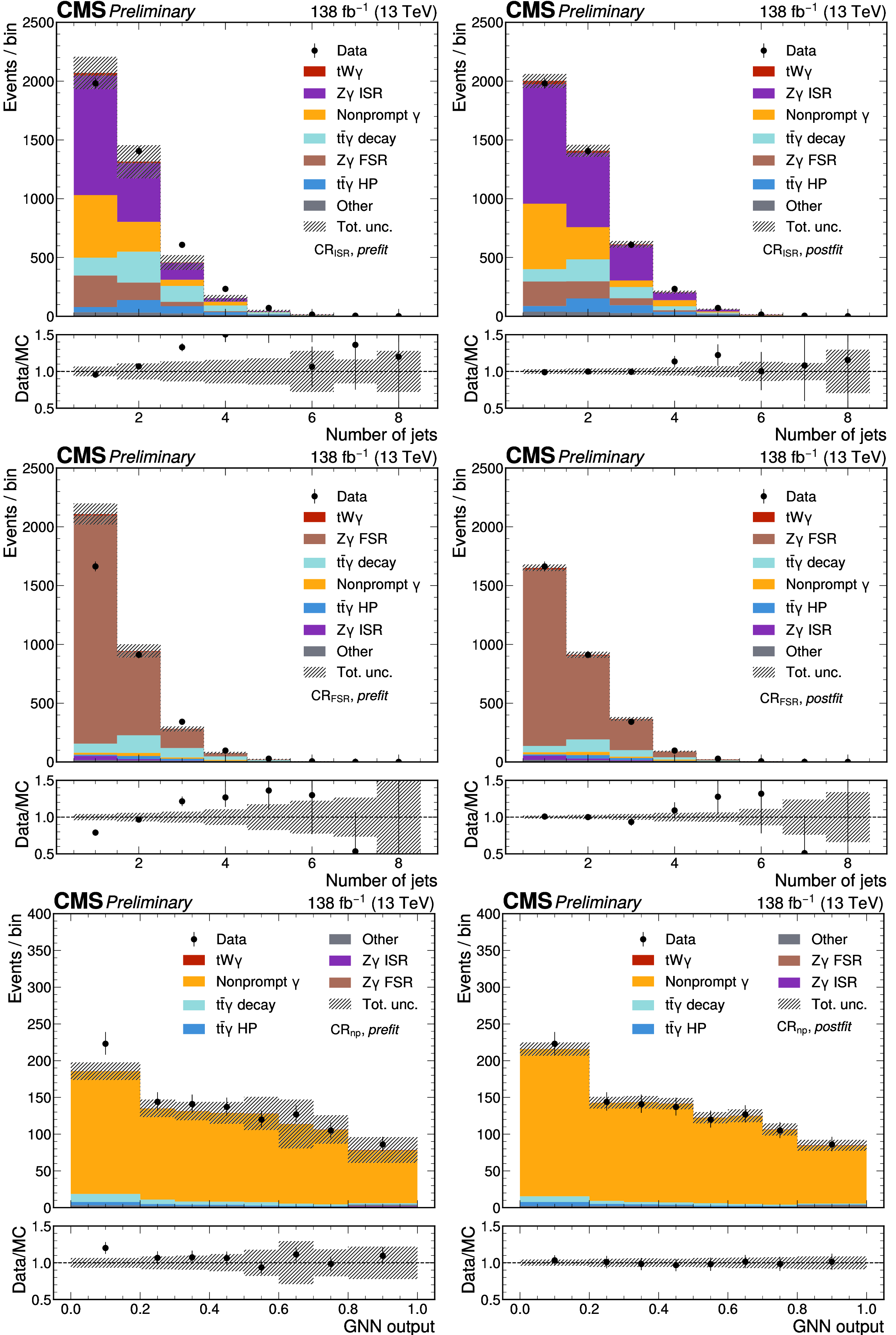
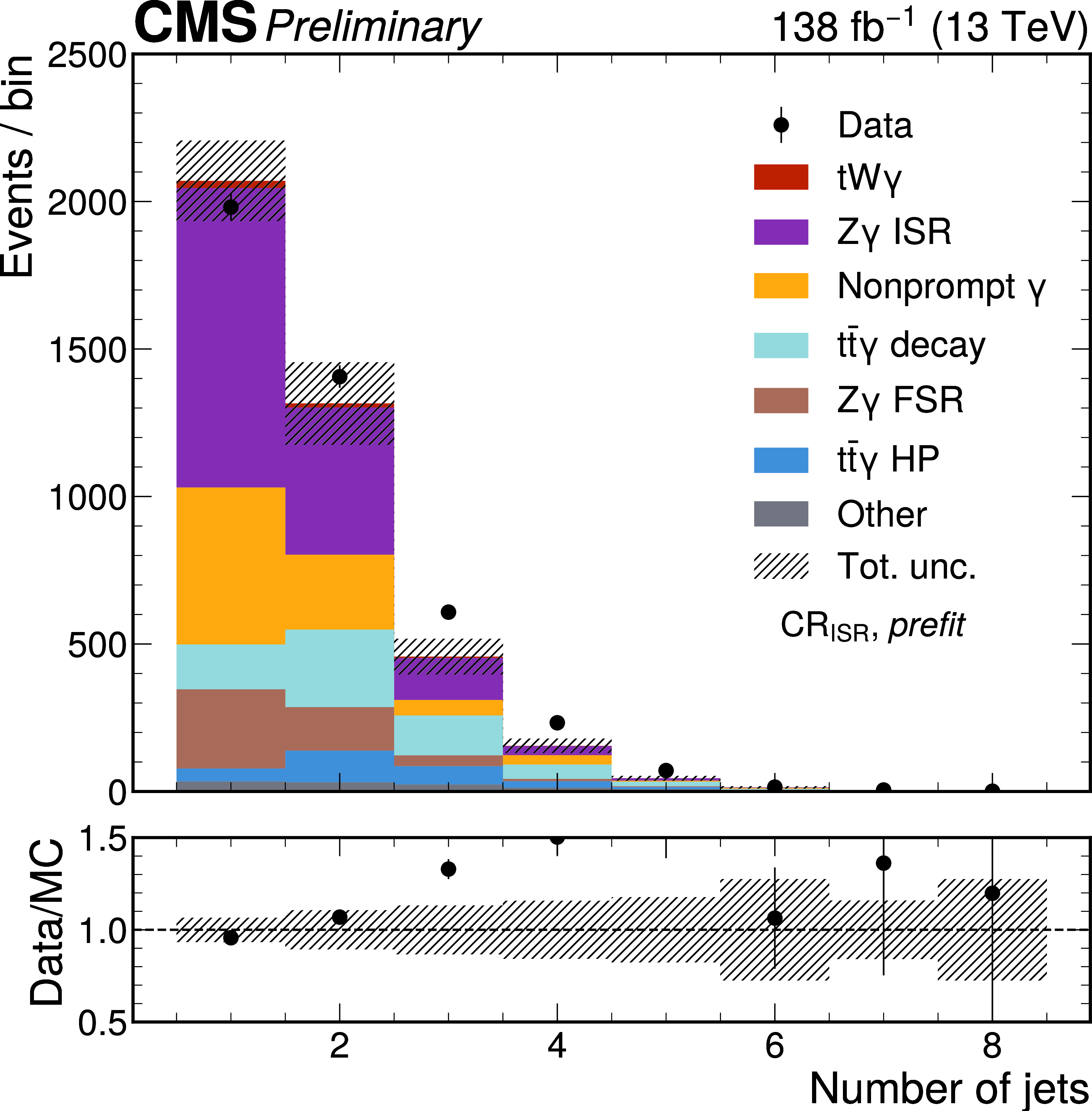
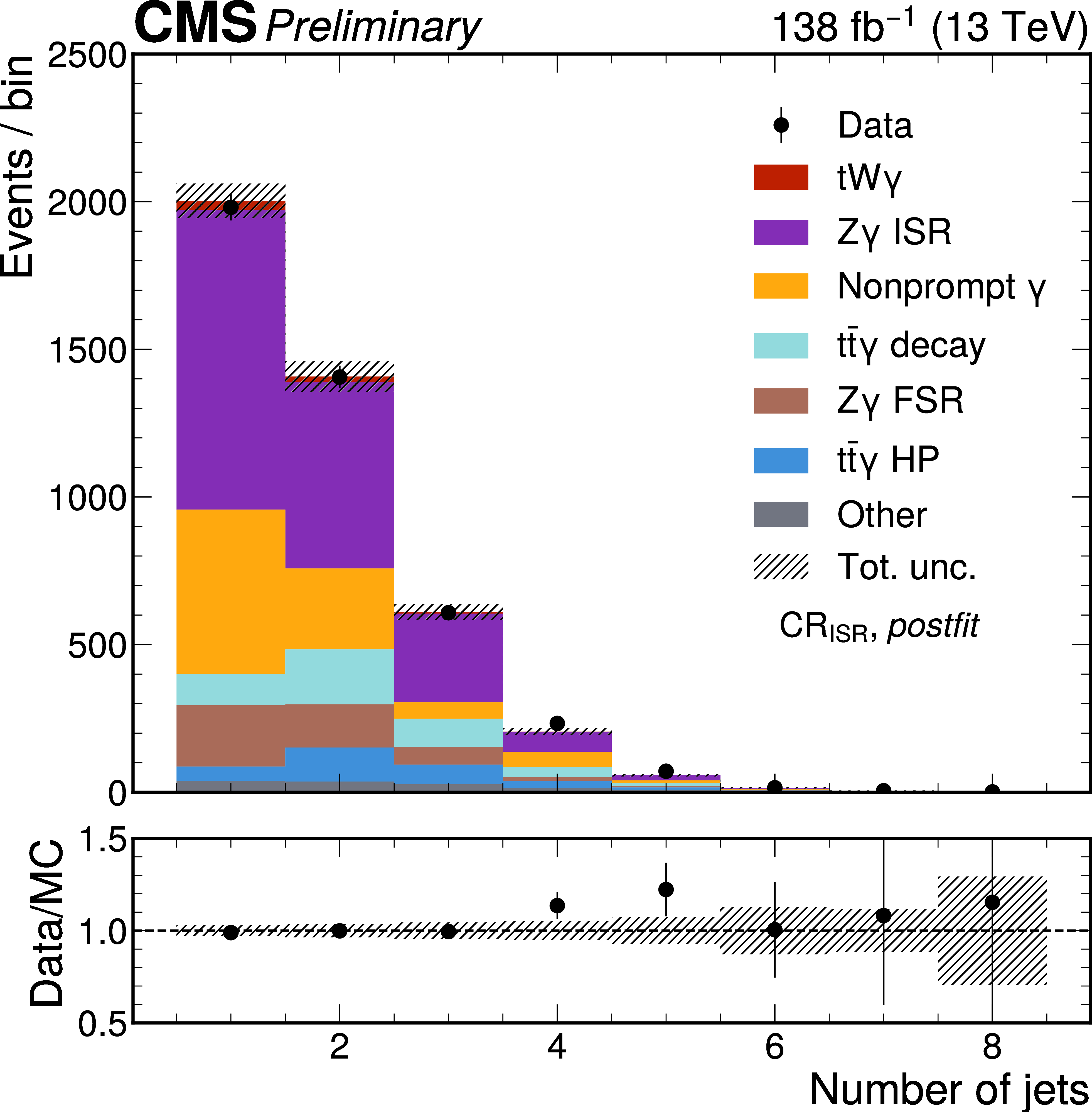
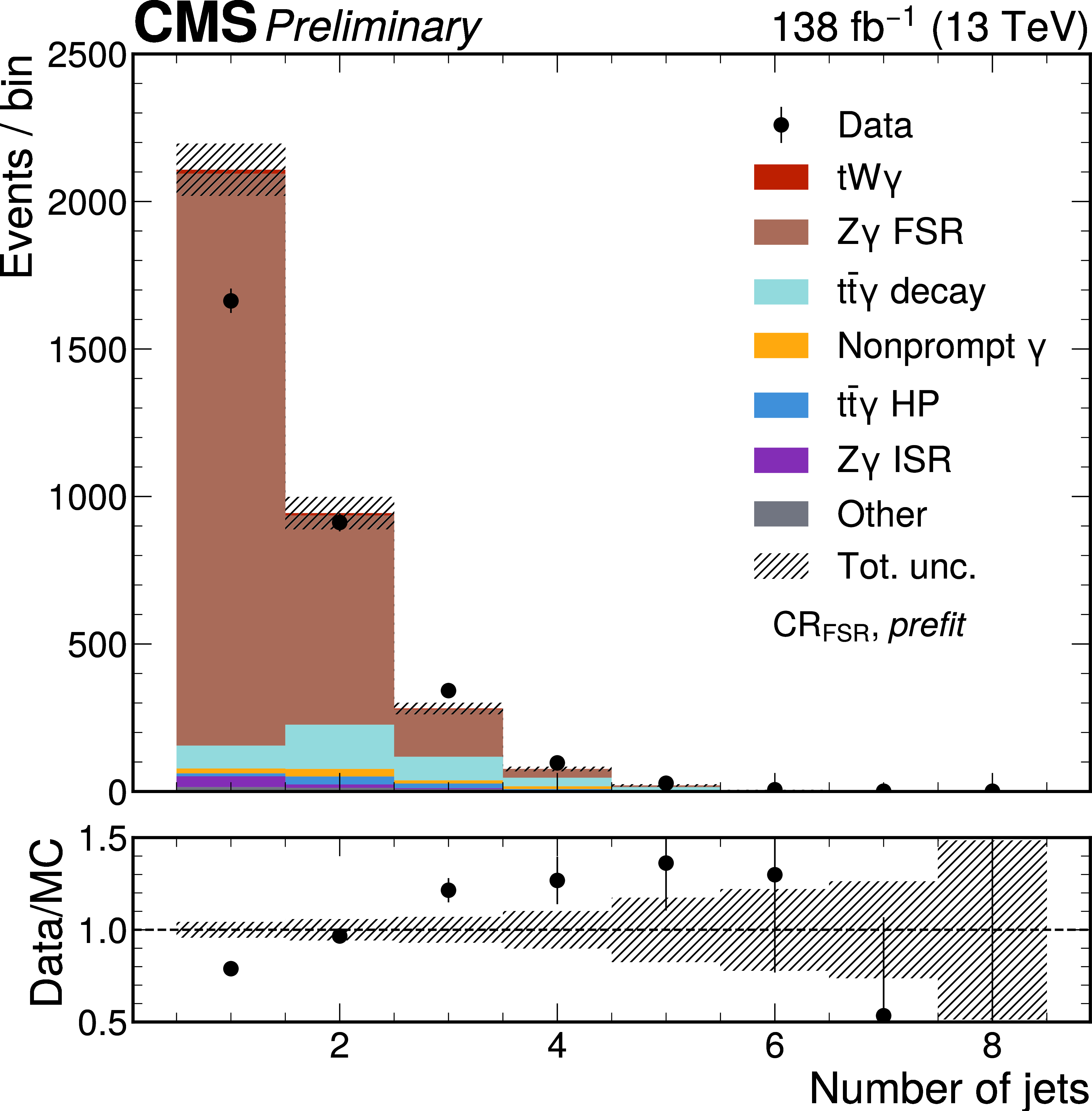
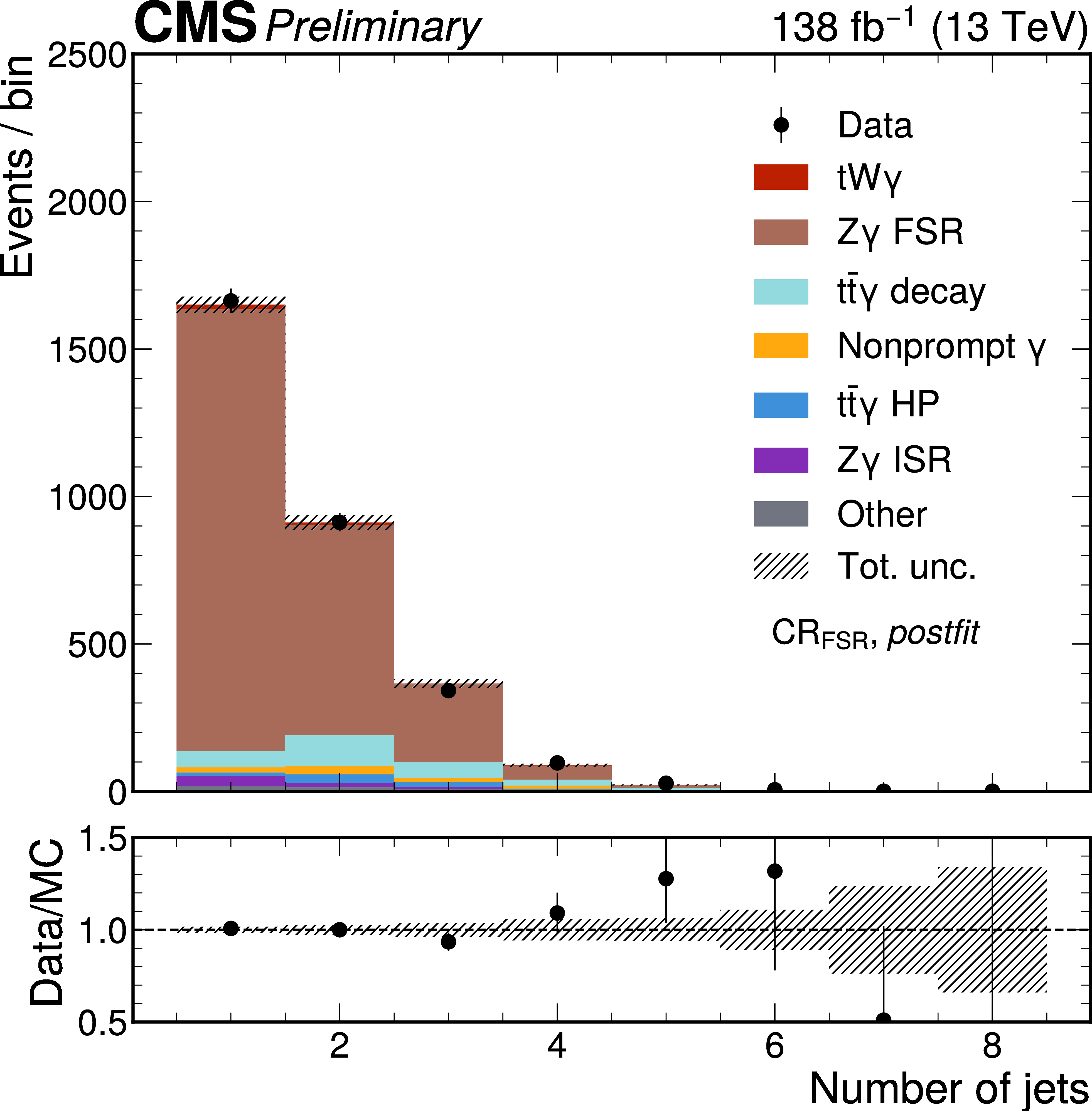
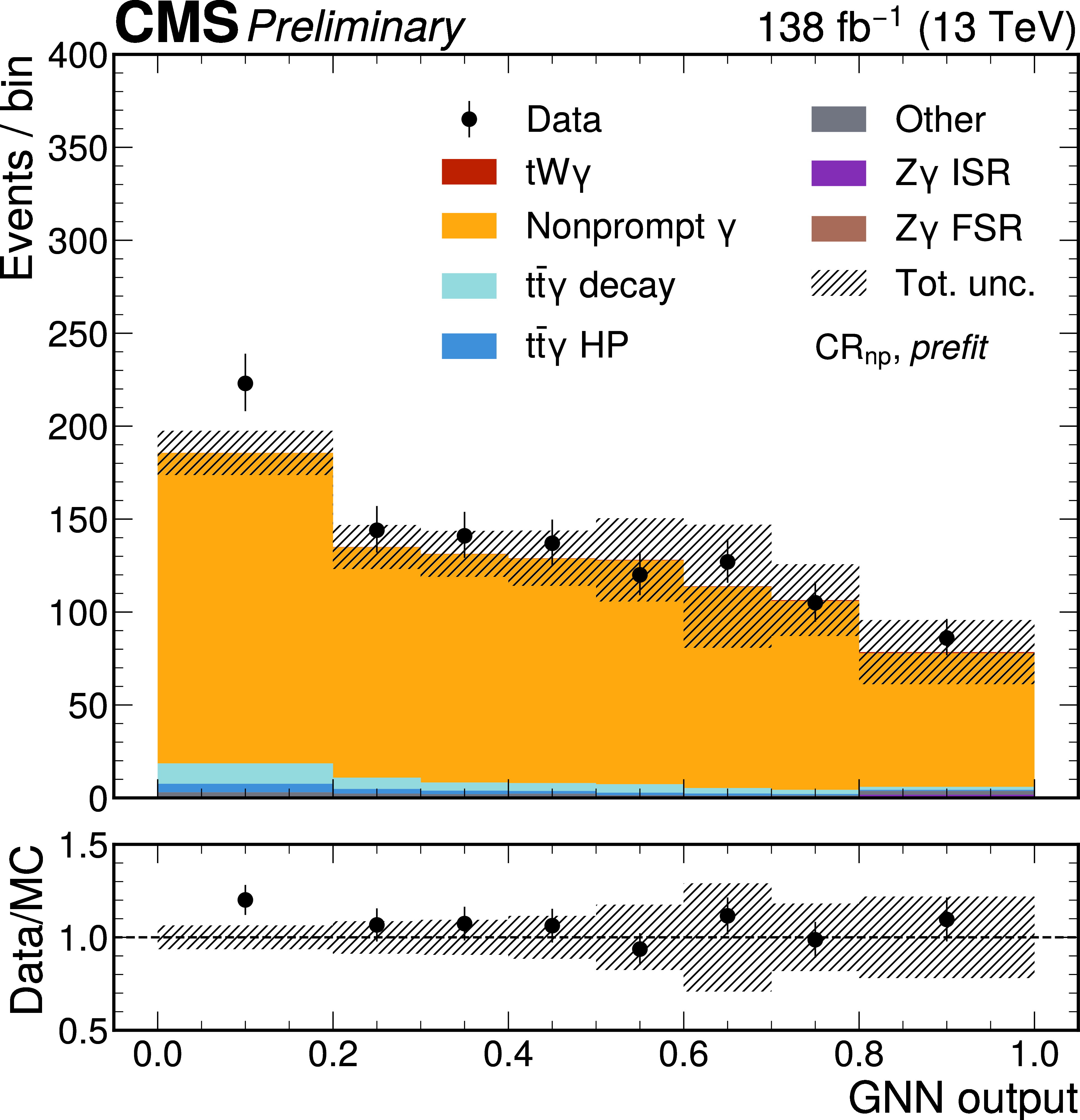
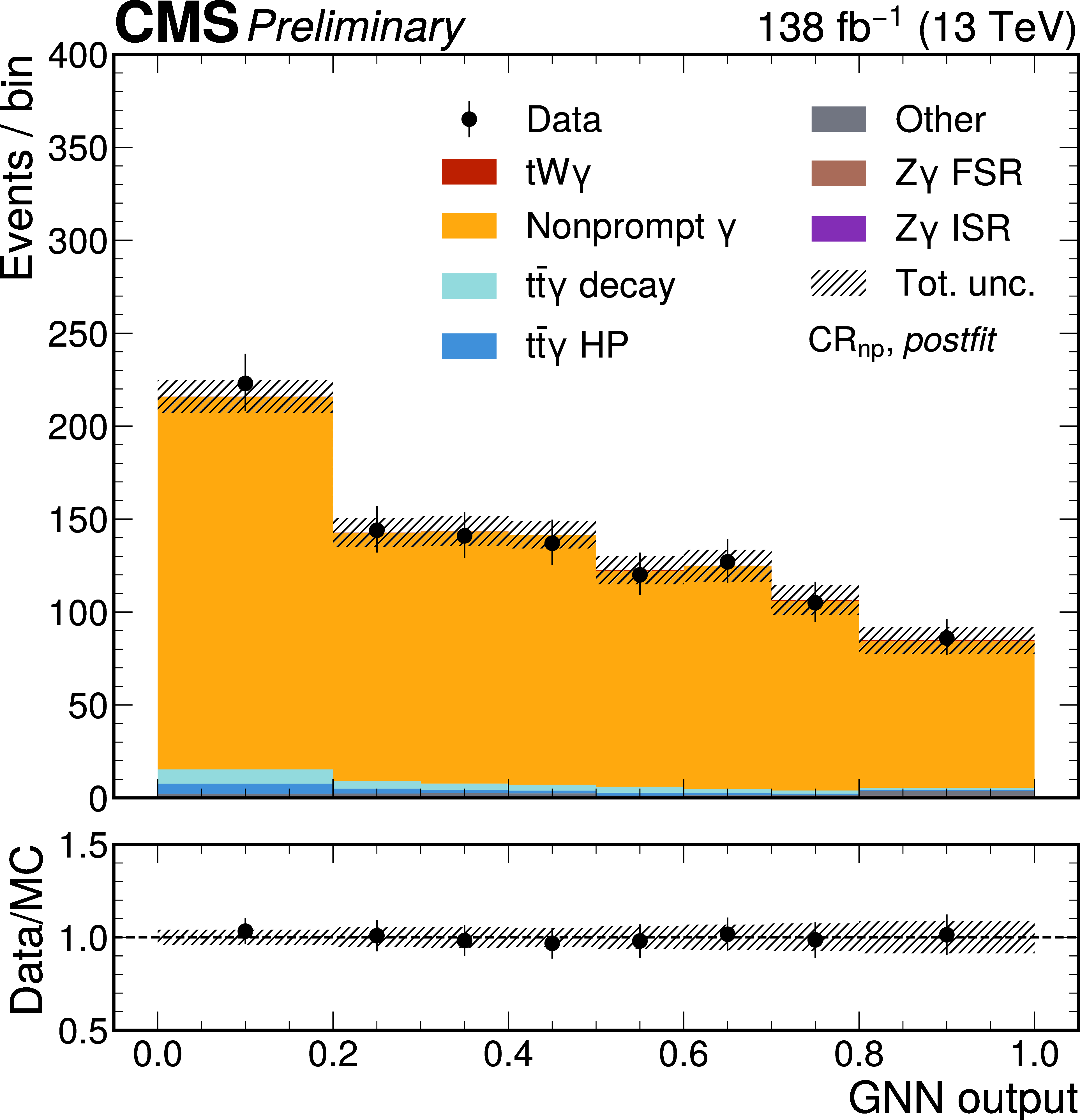
The prefit (left) and postfit (right) distributions of the fit variables in the control regions $ \text{CR}_\text{ISR} $ (upper), $ \text{CR}_\text{FSR} $ (middle), and $ \text{CR}_{\text{np}} $ (lower). Colored histograms represent simulation whereas data points are shown as black dots with statistical uncertainties. The hashed bands represent the total uncertainty. For the prefit distributions, the unconstrained uncertainties for $ \mathrm{t} \overline{\mathrm{t}} \gamma $ and $ \mathrm{Z} \gamma $ backgrounds are not included in the band. The ratio between data and MC simulation is shown in the lower panels. |
png pdf |
Figure 3-a:
The prefit (left) and postfit (right) distributions of the fit variables in the control regions $ \text{CR}_\text{ISR} $ (upper), $ \text{CR}_\text{FSR} $ (middle), and $ \text{CR}_{\text{np}} $ (lower). Colored histograms represent simulation whereas data points are shown as black dots with statistical uncertainties. The hashed bands represent the total uncertainty. For the prefit distributions, the unconstrained uncertainties for $ \mathrm{t} \overline{\mathrm{t}} \gamma $ and $ \mathrm{Z} \gamma $ backgrounds are not included in the band. The ratio between data and MC simulation is shown in the lower panels. |
png pdf |
Figure 3-b:
The prefit (left) and postfit (right) distributions of the fit variables in the control regions $ \text{CR}_\text{ISR} $ (upper), $ \text{CR}_\text{FSR} $ (middle), and $ \text{CR}_{\text{np}} $ (lower). Colored histograms represent simulation whereas data points are shown as black dots with statistical uncertainties. The hashed bands represent the total uncertainty. For the prefit distributions, the unconstrained uncertainties for $ \mathrm{t} \overline{\mathrm{t}} \gamma $ and $ \mathrm{Z} \gamma $ backgrounds are not included in the band. The ratio between data and MC simulation is shown in the lower panels. |
png pdf |
Figure 3-c:
The prefit (left) and postfit (right) distributions of the fit variables in the control regions $ \text{CR}_\text{ISR} $ (upper), $ \text{CR}_\text{FSR} $ (middle), and $ \text{CR}_{\text{np}} $ (lower). Colored histograms represent simulation whereas data points are shown as black dots with statistical uncertainties. The hashed bands represent the total uncertainty. For the prefit distributions, the unconstrained uncertainties for $ \mathrm{t} \overline{\mathrm{t}} \gamma $ and $ \mathrm{Z} \gamma $ backgrounds are not included in the band. The ratio between data and MC simulation is shown in the lower panels. |
png pdf |
Figure 3-d:
The prefit (left) and postfit (right) distributions of the fit variables in the control regions $ \text{CR}_\text{ISR} $ (upper), $ \text{CR}_\text{FSR} $ (middle), and $ \text{CR}_{\text{np}} $ (lower). Colored histograms represent simulation whereas data points are shown as black dots with statistical uncertainties. The hashed bands represent the total uncertainty. For the prefit distributions, the unconstrained uncertainties for $ \mathrm{t} \overline{\mathrm{t}} \gamma $ and $ \mathrm{Z} \gamma $ backgrounds are not included in the band. The ratio between data and MC simulation is shown in the lower panels. |
png pdf |
Figure 3-e:
The prefit (left) and postfit (right) distributions of the fit variables in the control regions $ \text{CR}_\text{ISR} $ (upper), $ \text{CR}_\text{FSR} $ (middle), and $ \text{CR}_{\text{np}} $ (lower). Colored histograms represent simulation whereas data points are shown as black dots with statistical uncertainties. The hashed bands represent the total uncertainty. For the prefit distributions, the unconstrained uncertainties for $ \mathrm{t} \overline{\mathrm{t}} \gamma $ and $ \mathrm{Z} \gamma $ backgrounds are not included in the band. The ratio between data and MC simulation is shown in the lower panels. |
png pdf |
Figure 3-f:
The prefit (left) and postfit (right) distributions of the fit variables in the control regions $ \text{CR}_\text{ISR} $ (upper), $ \text{CR}_\text{FSR} $ (middle), and $ \text{CR}_{\text{np}} $ (lower). Colored histograms represent simulation whereas data points are shown as black dots with statistical uncertainties. The hashed bands represent the total uncertainty. For the prefit distributions, the unconstrained uncertainties for $ \mathrm{t} \overline{\mathrm{t}} \gamma $ and $ \mathrm{Z} \gamma $ backgrounds are not included in the band. The ratio between data and MC simulation is shown in the lower panels. |
png pdf |
Figure 4:
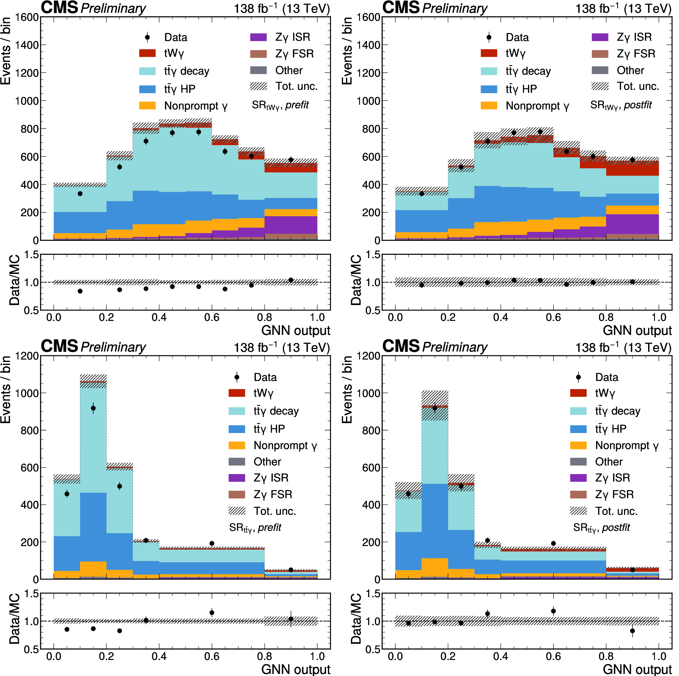
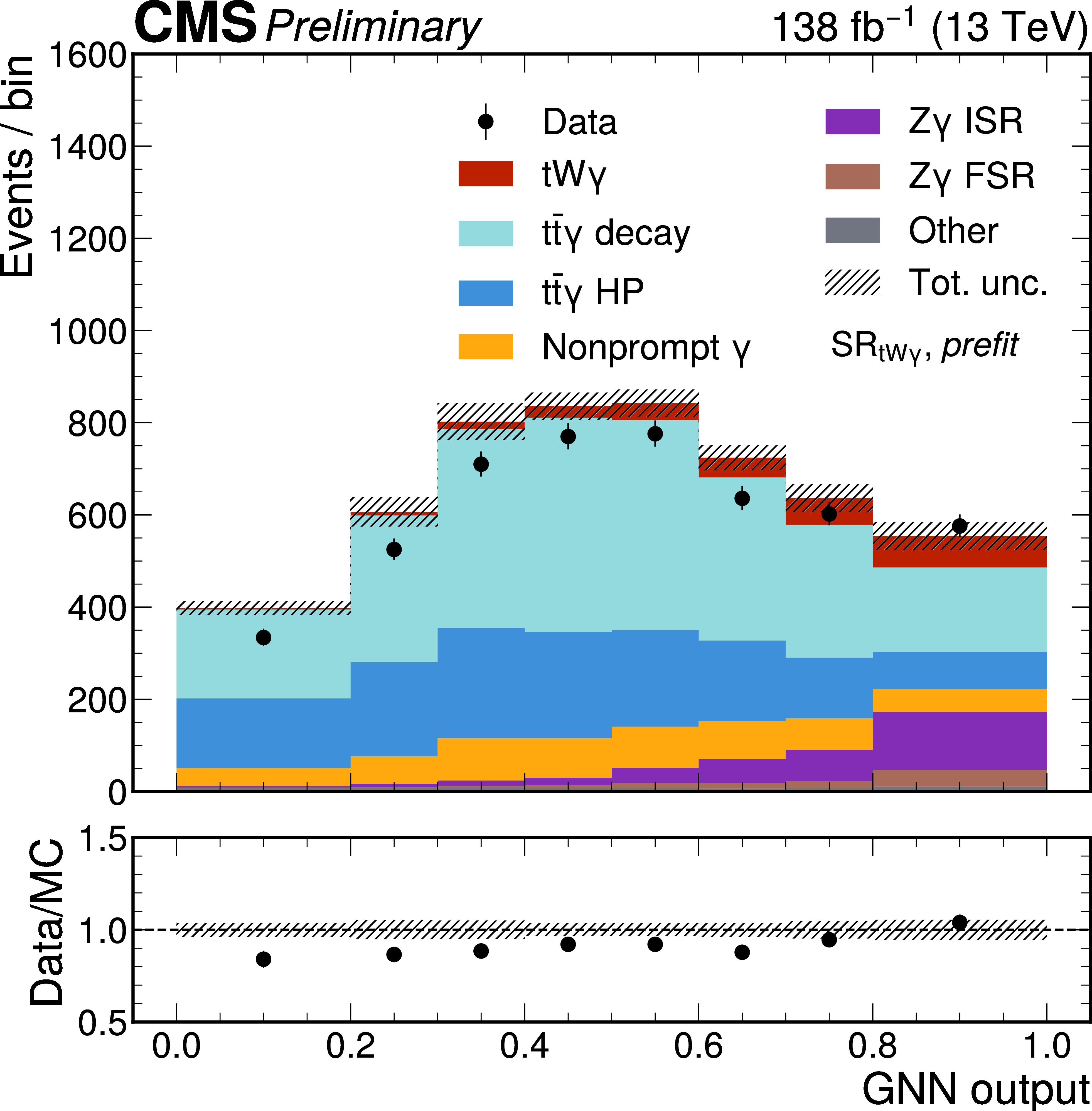
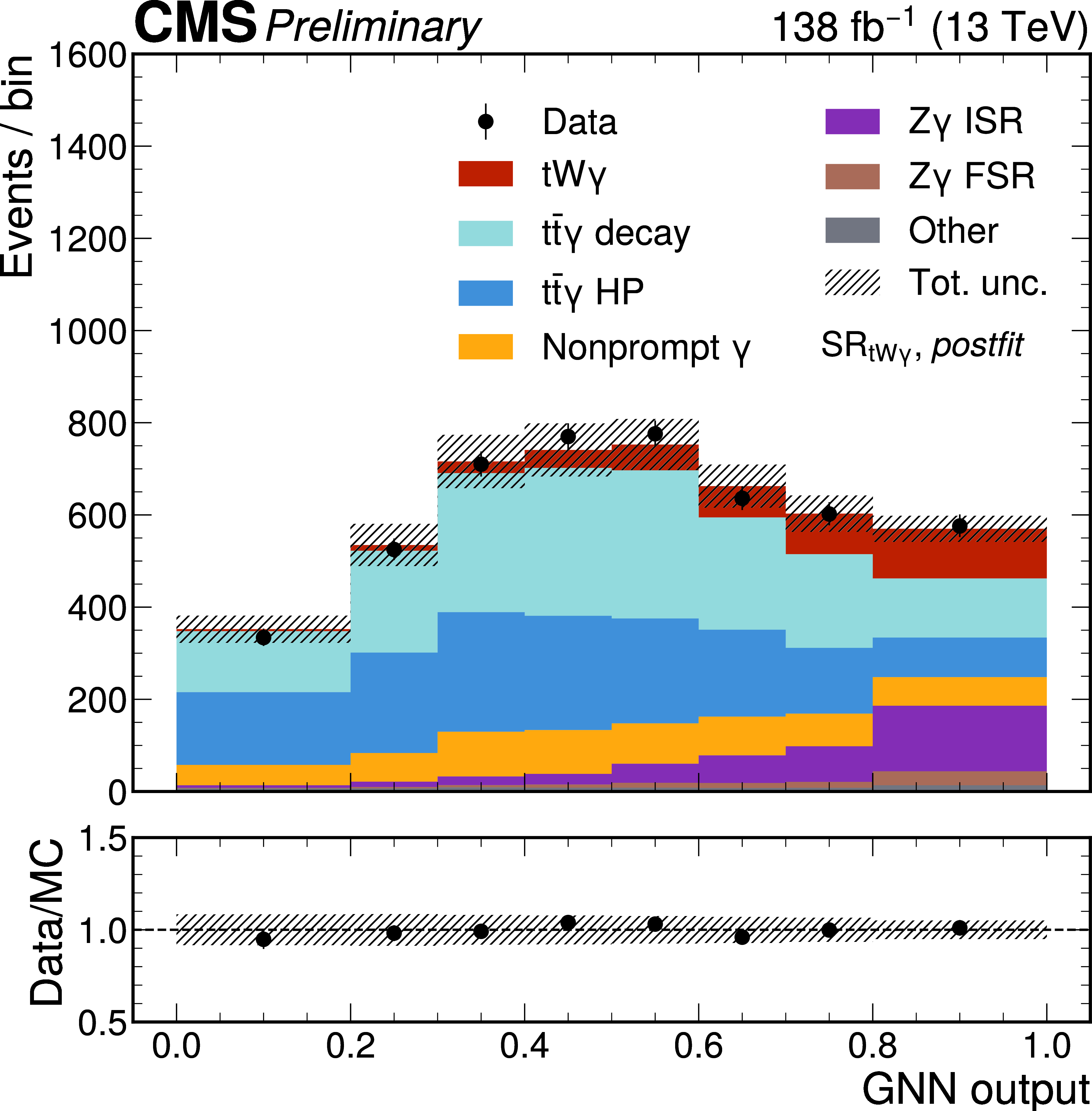
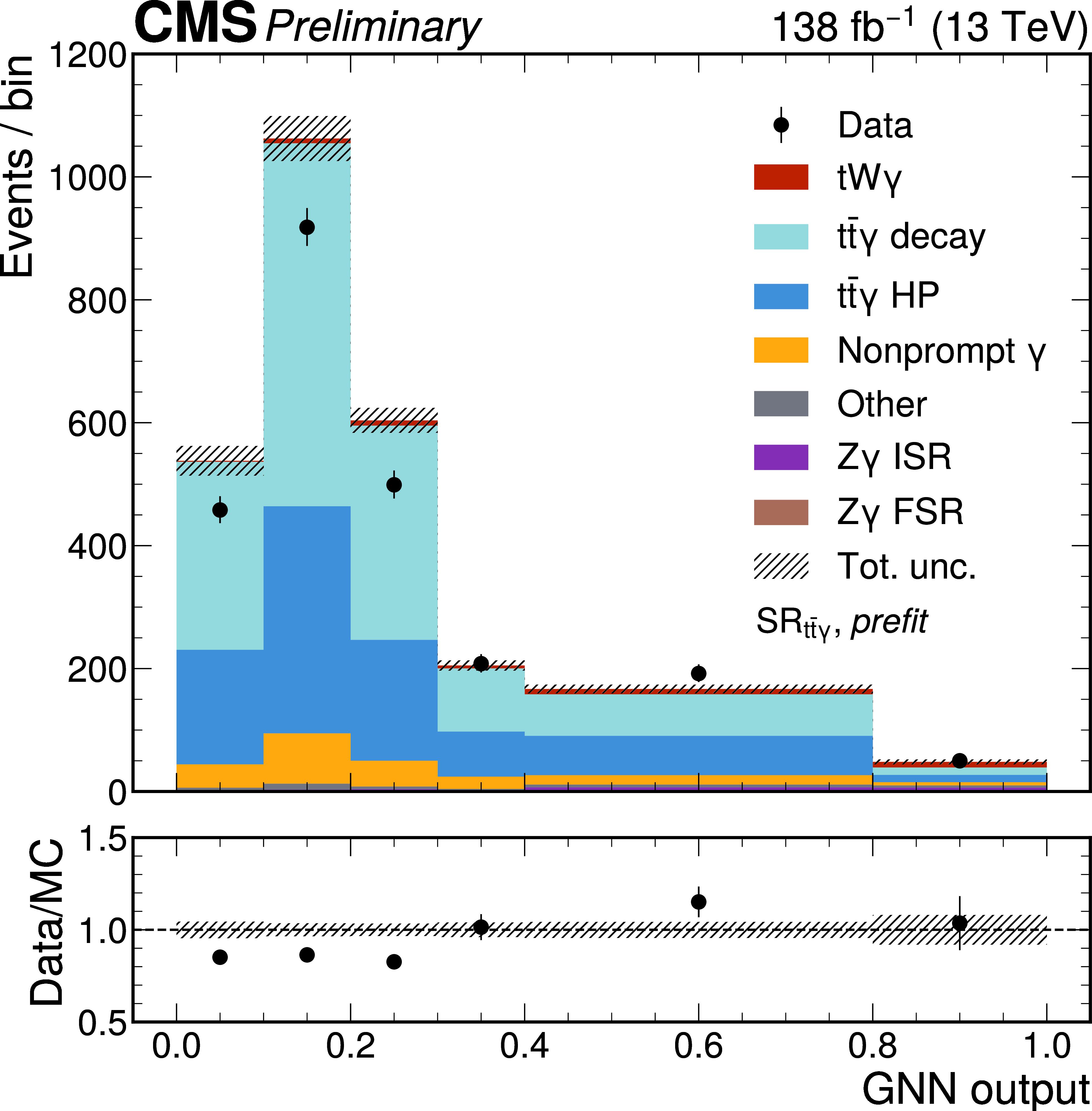
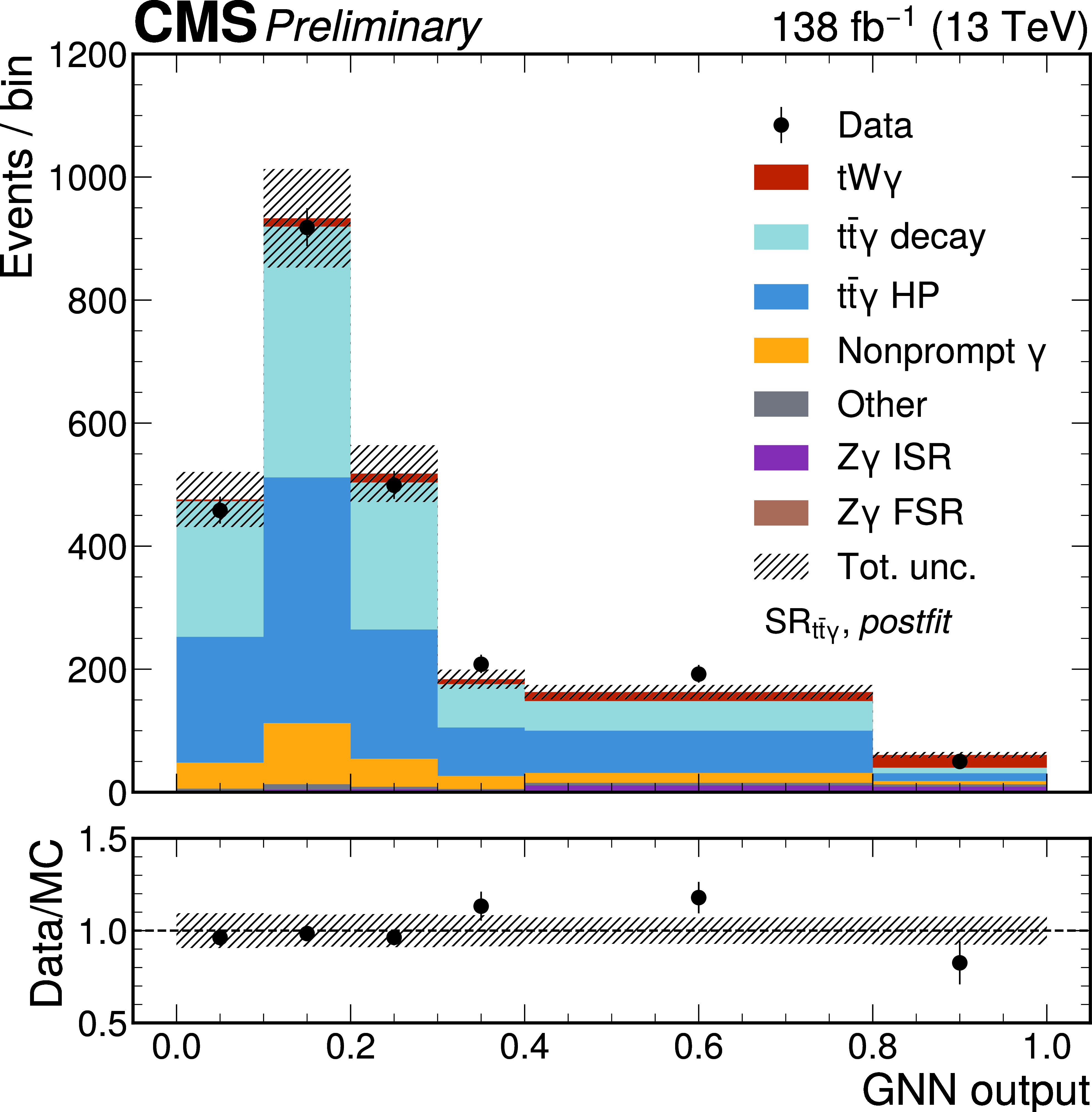
The prefit (left) and postfit (right) GNN distributions in the signal regions $ \text{SR}_{\mathrm{t} \mathrm{W} \gamma} $ (upper) and $ \text{SR}_{\mathrm{t} \overline{\mathrm{t}} \gamma} $ (lower). Colored histograms represent simulation whereas data points are shown as black dots with statistical uncertainties. The hashed bands represent the total uncertainty. For the prefit distributions, the unconstrained uncertainties for $ \mathrm{t} \overline{\mathrm{t}} \gamma $ and $ \mathrm{Z} \gamma $ backgrounds are not included in the band. The ratio between data and MC simulation is shown in the lower panels. |
png pdf |
Figure 4-a:
The prefit (left) and postfit (right) GNN distributions in the signal regions $ \text{SR}_{\mathrm{t} \mathrm{W} \gamma} $ (upper) and $ \text{SR}_{\mathrm{t} \overline{\mathrm{t}} \gamma} $ (lower). Colored histograms represent simulation whereas data points are shown as black dots with statistical uncertainties. The hashed bands represent the total uncertainty. For the prefit distributions, the unconstrained uncertainties for $ \mathrm{t} \overline{\mathrm{t}} \gamma $ and $ \mathrm{Z} \gamma $ backgrounds are not included in the band. The ratio between data and MC simulation is shown in the lower panels. |
png pdf |
Figure 4-b:
The prefit (left) and postfit (right) GNN distributions in the signal regions $ \text{SR}_{\mathrm{t} \mathrm{W} \gamma} $ (upper) and $ \text{SR}_{\mathrm{t} \overline{\mathrm{t}} \gamma} $ (lower). Colored histograms represent simulation whereas data points are shown as black dots with statistical uncertainties. The hashed bands represent the total uncertainty. For the prefit distributions, the unconstrained uncertainties for $ \mathrm{t} \overline{\mathrm{t}} \gamma $ and $ \mathrm{Z} \gamma $ backgrounds are not included in the band. The ratio between data and MC simulation is shown in the lower panels. |
png pdf |
Figure 4-c:
The prefit (left) and postfit (right) GNN distributions in the signal regions $ \text{SR}_{\mathrm{t} \mathrm{W} \gamma} $ (upper) and $ \text{SR}_{\mathrm{t} \overline{\mathrm{t}} \gamma} $ (lower). Colored histograms represent simulation whereas data points are shown as black dots with statistical uncertainties. The hashed bands represent the total uncertainty. For the prefit distributions, the unconstrained uncertainties for $ \mathrm{t} \overline{\mathrm{t}} \gamma $ and $ \mathrm{Z} \gamma $ backgrounds are not included in the band. The ratio between data and MC simulation is shown in the lower panels. |
png pdf |
Figure 4-d:
The prefit (left) and postfit (right) GNN distributions in the signal regions $ \text{SR}_{\mathrm{t} \mathrm{W} \gamma} $ (upper) and $ \text{SR}_{\mathrm{t} \overline{\mathrm{t}} \gamma} $ (lower). Colored histograms represent simulation whereas data points are shown as black dots with statistical uncertainties. The hashed bands represent the total uncertainty. For the prefit distributions, the unconstrained uncertainties for $ \mathrm{t} \overline{\mathrm{t}} \gamma $ and $ \mathrm{Z} \gamma $ backgrounds are not included in the band. The ratio between data and MC simulation is shown in the lower panels. |
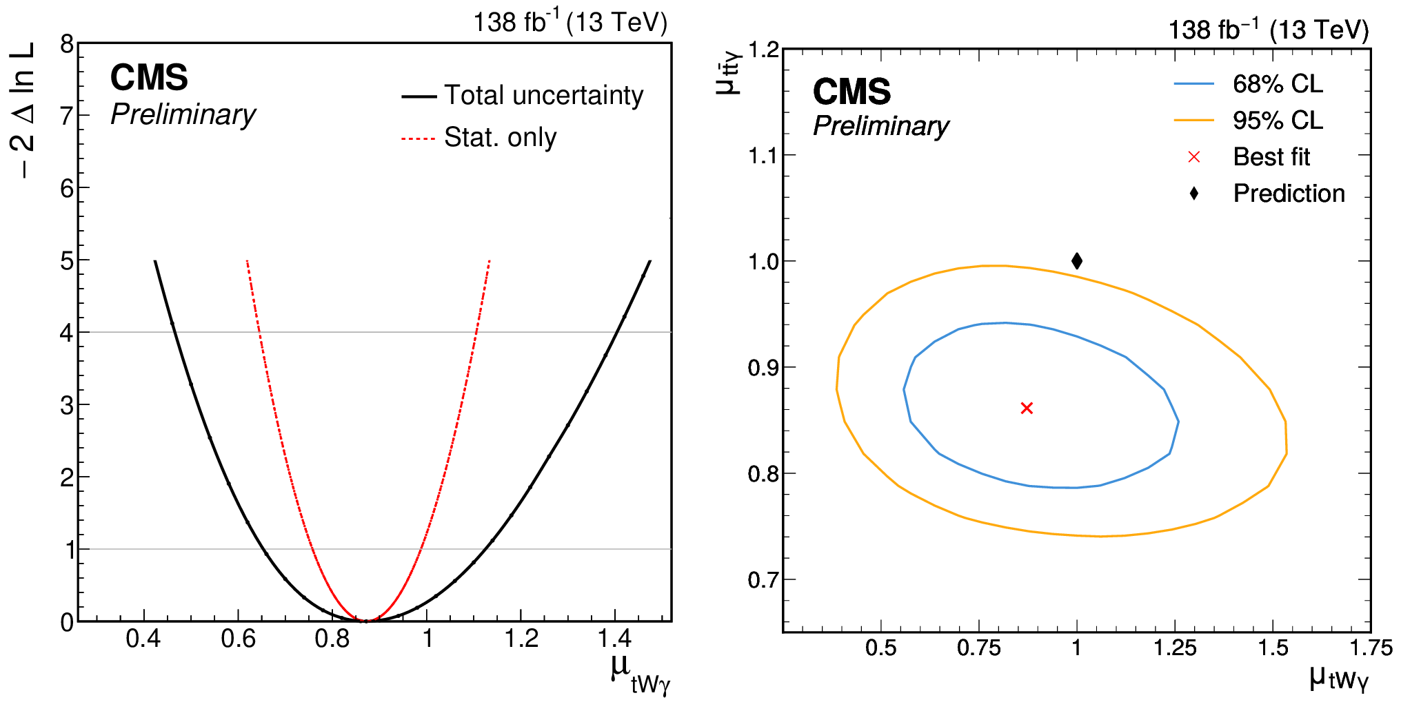
png pdf |
Figure 5:
The left plot shows the one-dimensional likelihood scan of $ \mu_{\mathrm{t} \mathrm{W} \gamma} $ in which the solid (dotted) curve represents the total (statistical) uncertainty. The right plot contains the likelihood scan in two dimensions, $ (\mu_{\mathrm{t} \mathrm{W} \gamma},\mu_{\mathrm{t} \overline{\mathrm{t}} \gamma}) $, where the contour corresponding to 68% (95%) confidence level (CL) is shown in blue (orange). The red cross stands for the best-fit values, compared with the black diamond representing predictions. |
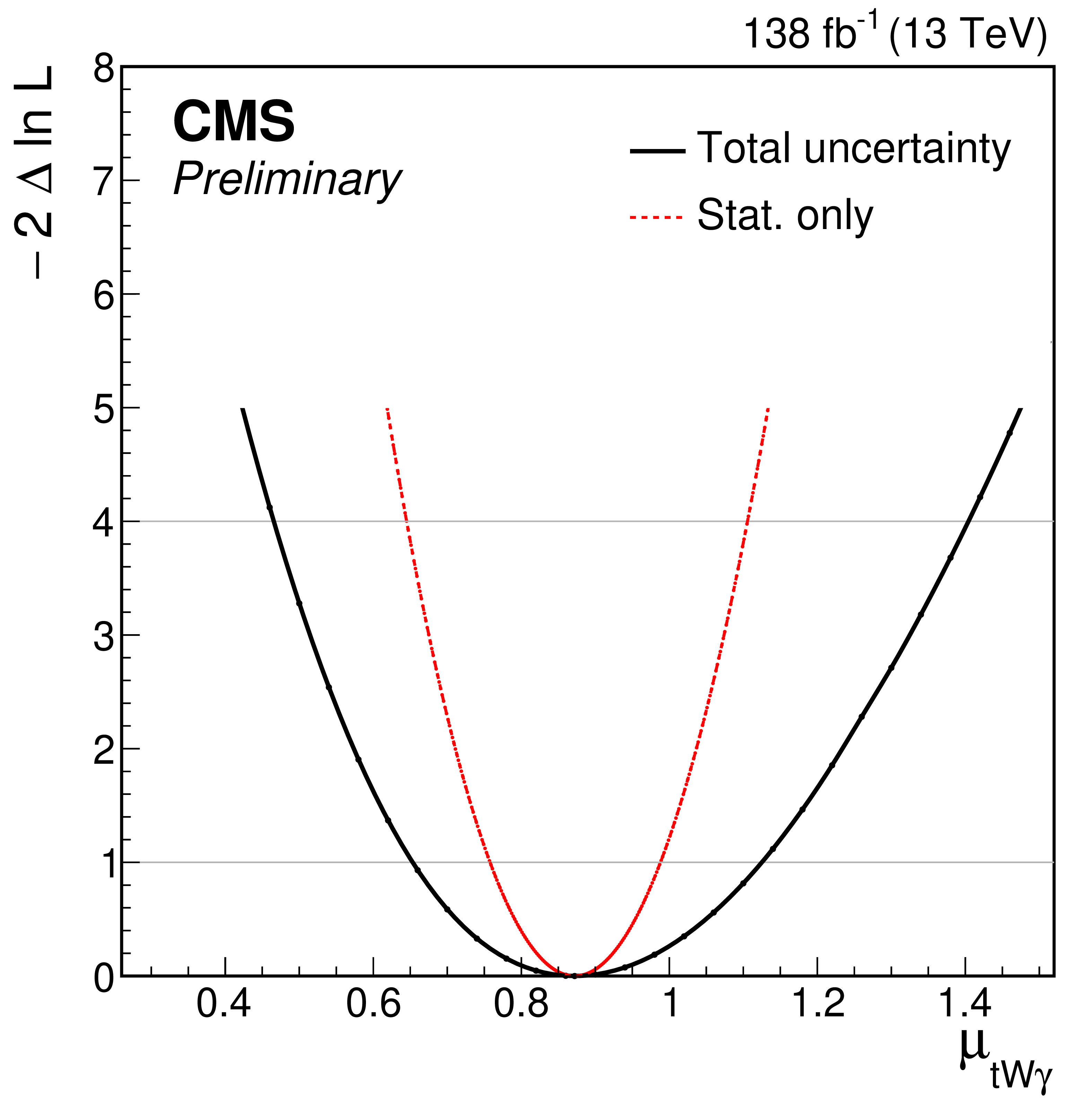
png pdf |
Figure 5-a:
The left plot shows the one-dimensional likelihood scan of $ \mu_{\mathrm{t} \mathrm{W} \gamma} $ in which the solid (dotted) curve represents the total (statistical) uncertainty. The right plot contains the likelihood scan in two dimensions, $ (\mu_{\mathrm{t} \mathrm{W} \gamma},\mu_{\mathrm{t} \overline{\mathrm{t}} \gamma}) $, where the contour corresponding to 68% (95%) confidence level (CL) is shown in blue (orange). The red cross stands for the best-fit values, compared with the black diamond representing predictions. |
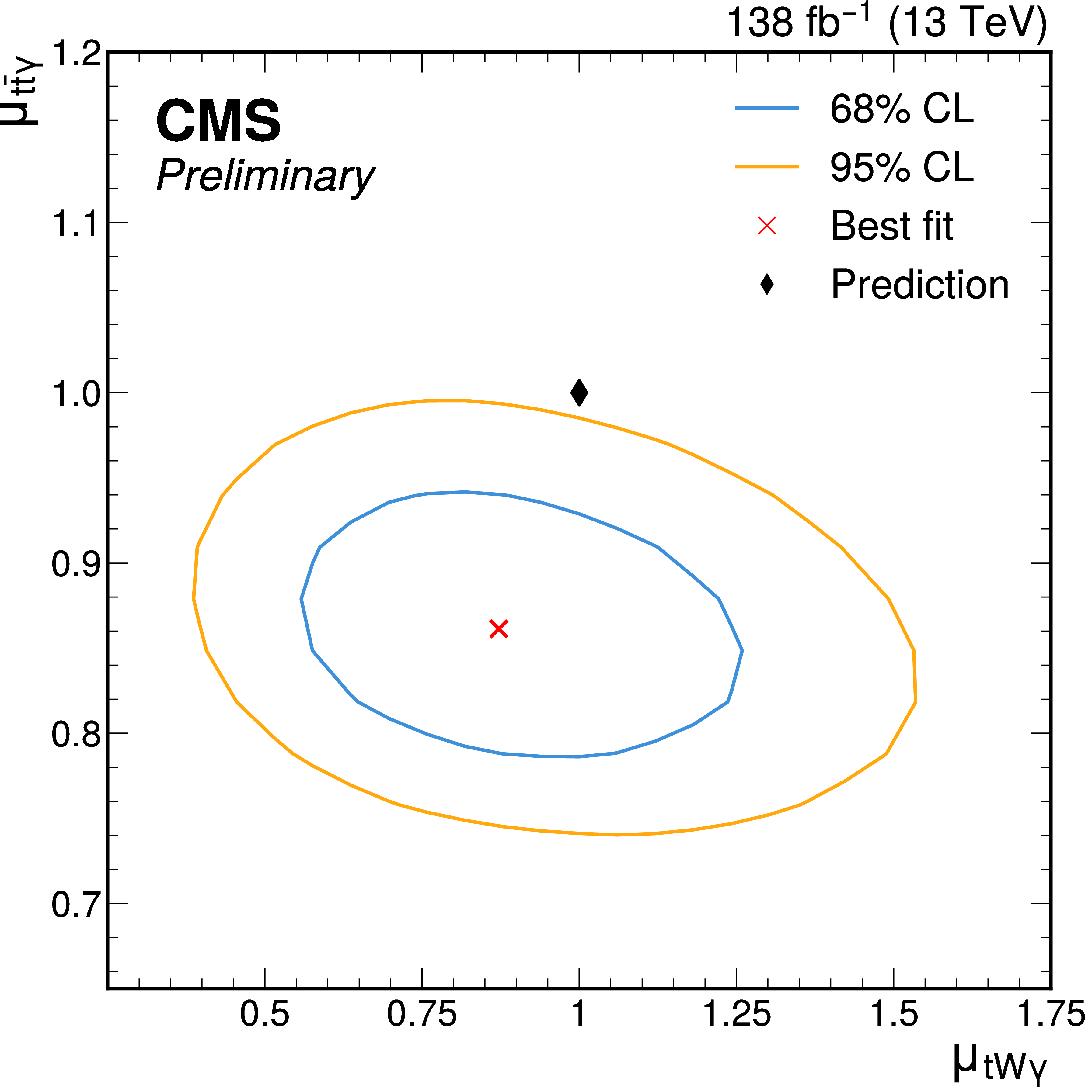
png pdf |
Figure 5-b:
The left plot shows the one-dimensional likelihood scan of $ \mu_{\mathrm{t} \mathrm{W} \gamma} $ in which the solid (dotted) curve represents the total (statistical) uncertainty. The right plot contains the likelihood scan in two dimensions, $ (\mu_{\mathrm{t} \mathrm{W} \gamma},\mu_{\mathrm{t} \overline{\mathrm{t}} \gamma}) $, where the contour corresponding to 68% (95%) confidence level (CL) is shown in blue (orange). The red cross stands for the best-fit values, compared with the black diamond representing predictions. |
| Summary |
| In summary, the first measurement of the $ \mathrm{tW}\gamma $ process is reported using proton-proton collisions recorded by the CMS experiment in the years 2016 to 2018, corresponding to an integrated luminosity of 138 fb$ ^{-1} $. The analysis combines the wealth of the data with state-of-the-art Monte Carlo simulation and the power of graph neural networks to establish the signal. The overlap between $ \mathrm{tW}\gamma $ and $ \mathrm{t} \overline{\mathrm{t}} \gamma $ at next-to-leading order (NLO) accuracy in perturbative quantum chromodynamics is addressed, and the origin of the photon is taken into account in the modeling, from either the hard scattering process or the top quark decay products. The $ \mathrm{tW}\gamma $ cross section in the fiducial region of the analysis is measured to be 20 $ ^{+6}_{-5} $ fb, in agreement with standard model predictions at NLO, with an observed (expected) statistical significance of 4.7 (5.6) standard deviations. This result marks a milestone in the area of vector-boson associated production of top quarks and calls for further scrutiny of top quark production with a W boson and an additional neutral boson with more data. |
| References | ||||
| 1 | CMS Collaboration | Inclusive and differential measurements of the $ {{\mathrm{t}\overline{\mathrm{t}}} \gamma} $ cross section and the $ {{\mathrm{t}\overline{\mathrm{t}}} \gamma/{\mathrm{t}\overline{\mathrm{t}}} } $ cross section ratio in proton-proton collisions at $ \sqrt{s}= $ 13 TeV | JHEP 04 (2026) 086 | CMS-TOP-23-002 2511.01995 |
| 2 | CMS Collaboration | Measurement of single top quark and $ \mathrm{t} \overline{\mathrm{t}} $ production cross sections in association with a photon in proton-proton collisions at $ \sqrt{s}= $ 13 TeV | CMS Physics Analysis Summary, 2026 CMS-PAS-TOP-25-003 |
CMS-PAS-TOP-25-003 |
| 3 | ATLAS Collaboration | Measurements of inclusive and differential cross-sections of $ {{\mathrm{t}\overline{\mathrm{t}}} \gamma} $ production in $ {\mathrm{p}\mathrm{p}} $ collisions at $ \sqrt{s}= $ 13 TeV with the ATLAS detector | JHEP 10 (2024) 191 | 2403.09452 |
| 4 | CMS Collaboration | Measurements of inclusive and differential cross sections for top quark production in association with a Z boson in proton-proton collisions at $ \sqrt{s}= $ 13 TeV | JHEP 02 (2025) 177 | CMS-TOP-23-004 2410.23475 |
| 5 | ATLAS Collaboration | Inclusive and differential cross-section measurements of $ {{\mathrm{t}\overline{\mathrm{t}}} \mathrm{Z}} $ production in $ {\mathrm{p}\mathrm{p}} $ collisions at $ \sqrt{s}= $ 13 TeV with the ATLAS detector, including EFT and spin-correlation interpretations | JHEP 07 (2024) 163 | 2312.04450 |
| 6 | CMS Collaboration | Inclusive and differential cross section measurements of single top quark production in association with a Z boson in proton-proton collisions at $ \sqrt{s}= $ 13 TeV | JHEP 02 (2022) 107 | CMS-TOP-20-010 2111.02860 |
| 7 | ATLAS Collaboration | Measurement of $ {\mathrm{t}\mathrm{Z}\mathrm{q}} $ inclusive and differential cross-sections in $ {\mathrm{p}\mathrm{p}} $ collisions at $ \sqrt{s}= $ 13 TeV with the ATLAS detector | Submitted to Eur. Phys. J. C, 2026 | 2608.25476 |
| 8 | CMS Collaboration | Evidence for $ {\mathrm{t}\mathrm{W}\mathrm{Z}} $ production in proton-proton collisions at $ \sqrt{s}= $ 13 TeV in multilepton final states | PLB 855 (2024) 138815 | CMS-TOP-22-008 2312.11668 |
| 9 | CMS Collaboration | Observation of $ {\mathrm{t}\mathrm{W}\mathrm{Z}} $ production at the CMS experiment | PRL 136 (2026) 081802 | CMS-TOP-24-009 2510.19080 |
| 10 | ATLAS Collaboration | Measurements of inclusive and differential cross-sections of combined $ {{\mathrm{t}\overline{\mathrm{t}}} \gamma} $ and $ {\mathrm{t}\mathrm{W}\gamma} $ production in the $ {\mathrm{e}\mu} $ channel at 13 TeV with the ATLAS detector | JHEP 09 (2020) 049 | 2007.06946 |
| 11 | CMS Collaboration | Measurement of the inclusive and differential $ {{\mathrm{t}\overline{\mathrm{t}}} \gamma} $ cross sections in the dilepton channel and effective field theory interpretation in proton-proton collisions at $ \sqrt{s}= $ 13 TeV | JHEP 05 (2022) 091 | CMS-TOP-21-004 2201.07301 |
| 12 | J. Zhou et al. | Graph neural networks: A review of methods and applications | AI Open 1 (2021) 57 | 1812.08434 |
| 13 | CMS Collaboration | The CMS experiment at the CERN LHC | JINST 3 (2008) S08004 | |
| 14 | CMS Collaboration | Development of the CMS detector for the CERN LHC \mboxRun 3 | JINST 19 (2024) P05064 | CMS-PRF-21-001 2309.05466 |
| 15 | CMS Collaboration | Performance of the CMS Level-1 trigger in proton-proton collisions at $ \sqrt{s}= $ 13 TeV | JINST 15 (2020) P10017 | CMS-TRG-17-001 2006.10165 |
| 16 | CMS Collaboration | The CMS trigger system | JINST 12 (2017) P01020 | CMS-TRG-12-001 1609.02366 |
| 17 | CMS Collaboration | Performance of the CMS high-level trigger during LHC \mboxRun 2 | JINST 19 (2024) P11021 | CMS-TRG-19-001 2410.17038 |
| 18 | CMS Collaboration | Electron and photon reconstruction and identification with the CMS experiment at the CERN LHC | JINST 16 (2021) P05014 | CMS-EGM-17-001 2012.06888 |
| 19 | CMS Collaboration | Performance of the CMS muon detector and muon reconstruction with proton-proton collisions at $ \sqrt{s}= $ 13 TeV | JINST 13 (2018) P06015 | CMS-MUO-16-001 1804.04528 |
| 20 | CMS Collaboration | Description and performance of track and primary-vertex reconstruction with the CMS tracker | JINST 9 (2014) P10009 | CMS-TRK-11-001 1405.6569 |
| 21 | CMS Collaboration | Particle-flow reconstruction and global event description with the CMS detector | JINST 12 (2017) P10003 | CMS-PRF-14-001 1706.04965 |
| 22 | CMS Collaboration | Technical proposal for the Phase-II upgrade of the Compact Muon Solenoid | CMS Technical Proposal CERN-LHCC-2015-010, CMS-TDR-15-02, 2015 link |
|
| 23 | CMS Collaboration | Performance of reconstruction and identification of $ \tau $ leptons decaying to hadrons and $ \nu_{\!\tau} $ in $ {\mathrm{p}\mathrm{p}} $ collisions at $ \sqrt{s}= $ 13 TeV | JINST 13 (2018) P10005 | CMS-TAU-16-003 1809.02816 |
| 24 | CMS Collaboration | Jet energy scale and resolution in the CMS experiment in $ {\mathrm{p}\mathrm{p}} $ collisions at 8 TeV | JINST 12 (2017) P02014 | CMS-JME-13-004 1607.03663 |
| 25 | CMS Collaboration | Performance of missing transverse momentum reconstruction in proton-proton collisions at $ \sqrt{s}= $ 13 TeV using the CMS detector | JINST 14 (2019) P07004 | CMS-JME-17-001 1903.06078 |
| 26 | M. Cacciari, G. P. Salam, and G. Soyez | The anti-$ k_{\mathrm{T}} $ jet clustering algorithm | JHEP 04 (2008) 063 | 0802.1189 |
| 27 | M. Cacciari, G. P. Salam, and G. Soyez | FASTJET user manual | EPJC 72 (2012) 1896 | 1111.6097 |
| 28 | CMS Collaboration | Pileup mitigation at CMS in 13 TeV data | JINST 15 (2020) P09018 | CMS-JME-18-001 2003.00503 |
| 29 | T. Sjöstrand, S. Mrenna, and P. Z. Skands | A brief introduction to PYTHIA8.1 | Comput. Phys. Commun. 178 (2008) 852 | 0710.3820 |
| 30 | NNPDF Collaboration | Parton distributions for the LHC \mboxRun 2 | JHEP 04 (2015) 040 | 1410.8849 |
| 31 | NNPDF Collaboration | Parton distributions from high-precision collider data | EPJC 77 (2017) 663 | 1706.00428 |
| 32 | CMS Collaboration | Measurement of the inelastic proton-proton cross section at $ \sqrt{s}= $ 13 TeV | JHEP 07 (2018) 161 | CMS-FSQ-15-005 1802.02613 |
| 33 | GEANT4 Collaboration | GEANT 4---a simulation toolkit | NIM A 506 (2003) 250 | |
| 34 | J. Alwall et al. | The automated computation of tree-level and next-to-leading order differential cross sections, and their matching to parton shower simulations | JHEP 07 (2014) 079 | 1405.0301 |
| 35 | S. Frixione | Isolated photons in perturbative QCD | PLB 429 (1998) 369 | hep-ph/9801442 |
| 36 | P. Artoisenet, R. Frederix, O. Mattelaer, and R. Rietkerk | Automatic spin-entangled decays of heavy resonances in Monte Carlo simulations | JHEP 03 (2013) 015 | 1212.3460 |
| 37 | S. Frixione et al. | Single-top hadroproduction in association with a W boson | JHEP 07 (2008) 029 | 0805.3067 |
| 38 | C. D. White, S. Frixione, E. Laenen, and F. Maltoni | Isolating $ {\mathrm{W}\mathrm{t}} $ production at the LHC | JHEP 11 (2009) 074 | 0908.0631 |
| 39 | S. Frixione et al. | Automated simulations beyond the standard model: supersymmetry | JHEP 12 (2019) 008 | 1907.04898 |
| 40 | P. Nason | A new method for combining NLO QCD with shower Monte Carlo algorithms | JHEP 11 (2004) 040 | hep-ph/0409146 |
| 41 | S. Frixione, P. Nason, and C. Oleari | Matching NLO QCD computations with parton shower simulations: the POWHEG method | JHEP 11 (2007) 070 | 0709.2092 |
| 42 | S. Alioli, P. Nason, C. Oleari, and E. Re | A general framework for implementing NLO calculations in shower Monte Carlo programs: the POWHEG box | JHEP 06 (2010) 043 | 1002.2581 |
| 43 | H. B. Hartanto, B. J ä ger, L. Reina, and D. Wackeroth | Higgs boson production in association with top quarks in the POWHEG box | PRD 91 (2015) 094003 | 1501.04498 |
| 44 | CMS Collaboration | Observation of four top quark production in proton-proton collisions at $ \sqrt{s}= $ 13 TeV | PLB 847 (2023) 138290 | CMS-TOP-22-013 2305.13439 |
| 45 | Particle Data Group , F. Takahashi et al. | Review of particle physics | Int. J. Mod. Phys. A 41 (2026) 2630011 | |
| 46 | CMS Collaboration | Identification of heavy-flavour jets with the CMS detector in $ {\mathrm{p}\mathrm{p}} $ collisions at 13 TeV | JINST 13 (2018) P05011 | CMS-BTV-16-002 1712.07158 |
| 47 | CMS Collaboration | Performance summary of AK4 jet b tagging with data from proton-proton collisions at 13 TeV with the CMS detector | CMS Detector Performance Note CMS-DP-2023-005, 2023 CDS |
|
| 48 | E. Bols et al. | Jet flavour classification using DeepJet | JINST 15 (2020) P12012 | 2008.10519 |
| 49 | A. Paszke et al. | PyTorch: An imperative style, high-performance deep learning library | in 33rd Conference on Neural Information Processing Systems (NeurIPS ): Vancouver, Canada, December 08--14,, 2019 Proc. 3 (2019) 3 |
1912.01703 |
| 50 | A.~Paszke et al. | Automatic differentiation in PyTorch | in 31st Conference on Neural Information Processing Systems (NIPS ): Long Beach CA, USA, December 04--09,, 2017 Proc. 3 (2017) 1 |
|
| 51 | M. Fey and J. E. Lenssen | Fast graph representation learning with PyTorch Geometric | in Proc. 7th International Conference on Learning Representations (): New Orleans LA, USA, May 06--09,, 2019 ICLR 201 (2019) 9 |
1903.02428 |
| 52 | CMS Collaboration | The CMS statistical analysis and combination tool: combine | Comput. Softw. Big Sci. 8 (2024) 19 | CMS-CAT-23-001 2404.06614 |
| 53 | CMS Collaboration | Precision luminosity measurement in proton-proton collisions at a center-of-mass energy of 13 TeV with the CMS detector at the Large Hadron Collider | Submitted to Phys. Rev. X, 2026 | CMS-LUM-20-001 2606.26832 |
| 54 | CMS Collaboration | Precision luminosity measurement in proton-proton collisions at $ \sqrt{s}= $ 13 TeV in 2015 and 2016 at CMS | EPJC 81 (2021) 800 | CMS-LUM-17-003 2104.01927 |
| 55 | CMS Collaboration | CMS luminosity measurement for the 2017 data-taking period at $ \sqrt{s}= $ 13 TeV | CMS Physics Analysis Summary, 2018 CMS-PAS-LUM-17-004 |
CMS-PAS-LUM-17-004 |
| 56 | CMS Collaboration | CMS luminosity measurement for the 2018 data-taking period at $ \sqrt{s}= $ 13 TeV | CMS Physics Analysis Summary, 2019 CMS-PAS-LUM-18-002 |
CMS-PAS-LUM-18-002 |
| 57 | R. Barlow and C. Beeston | Fitting using finite Monte Carlo samples | Comput. Phys. Commun. 77 (1993) 219 | |
| 58 | J. Butterworth et al. | PDF4LHC recommendations for LHC \mboxRun 2 | JPG 43 (2016) 023001 | 1510.03865 |
|
|
Compact Muon Solenoid LHC, CERN |

|
|
|
|
|
|