
Compact Muon Solenoid
LHC, CERN
 Visit us: CMS Public Website, CMS Physics ;
Contact us: CMS Publications Committee
Visit us: CMS Public Website, CMS Physics ;
Contact us: CMS Publications Committee
| CMS-LUM-20-001 ; CERN-EP-2026-134 | ||
| Precision luminosity measurement in proton-proton collisions at a center-of-mass energy of 13 TeV with the CMS detector at the Large Hadron Collider | ||
| CMS Collaboration | ||
| 25 June 2026 | ||
| Submitted to Physical Review X | ||
| Abstract: Discovering new fundamental physics requires spotting subtle deviations between theoretical predictions and experimental data. This delicate comparison hinges on the precise knowledge of the integrated luminosity, the measure of how many particle interactions were actually delivered by the collider. Here, we report a landmark measurement of the integrated luminosity by the Compact Muon Solenoid (CMS) experiment for proton-proton collisions at a center-of-mass energy of 13 TeV at the CERN Large Hadron Collider (LHC). By calibrating multiple independent monitors through specialized beam-separation techniques and rigorously validating their long-term stability against well-understood Z boson production rates, we comprehensively map and minimize systematic uncertainties. Combining the findings yields a total integrated luminosity precision of 0.73% for the entire data set. This marks the most precise luminosity measurement ever achieved at a bunched-beam hadron collider. Crossing the sub-percent precision threshold per data taking year fundamentally sharpens our ability to test the standard model and establishes a vital baseline for the upcoming High-Luminosity LHC era. | ||
| Links: e-print arXiv:2606.26832 [hep-ex] (PDF) ; CDS record ; inSPIRE record ; CADI line (restricted) ; | ||
| Figures | |
png pdf |
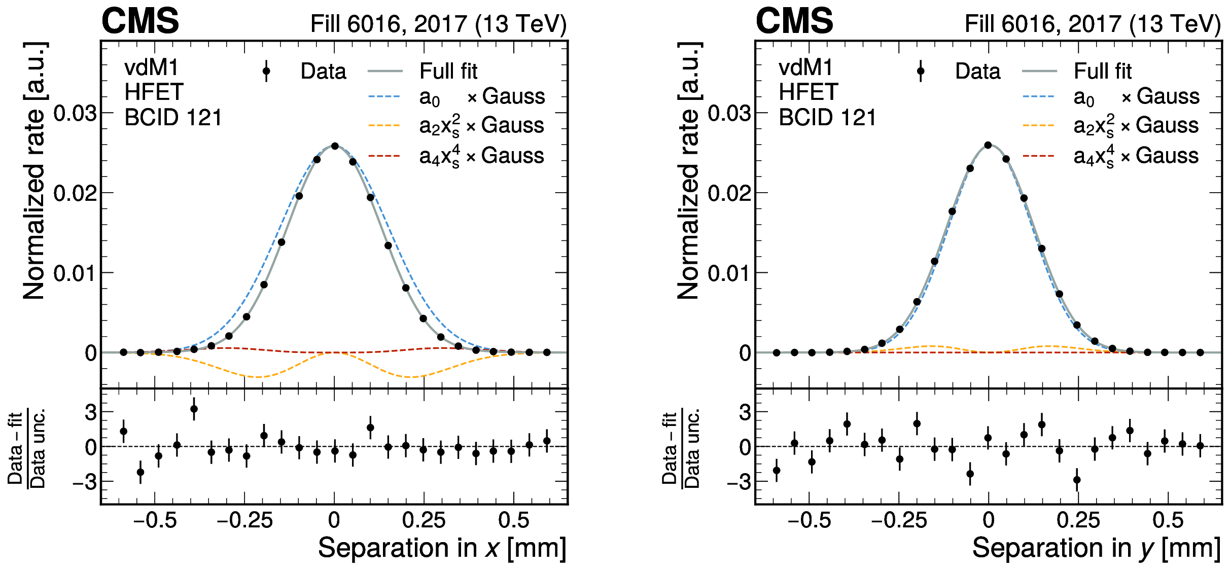
Figure 1:
An illustration of the vdM fit procedure for the HFET method in the 2017 vdM fill after all corrections are applied. The luminometer rate (normalized by the product of the bunch proton multiplicity values) is shown for a single bunch (BCID 121) as a function of the transverse separation of the two beams in the horizontal (left) and vertical (right) directions. The data are fitted by the product of a fourth-order positive symmetric polynomial and a Gaussian function. The three additive components, as well as the full analytic function, are plotted. The variable $ x_s $ signifies coordinates standardized with the width and mean of the Gaussian function, $ x_s=(x-\mu)/\sigma $. The effective widths of the fitted curves, $ \Sigma_x $ and $ \Sigma_y $, are defined by Eq. \eqrefeq:capsigma, and the peak value is the head-on rate normalized by the bunch intensities ($ R(0,0)/(N_1N_2) $) in Eq. \eqrefeq:SigmaVis. The lower panel shows the difference between the measured data and the fitted function, divided by the statistical uncertainty of the normalized rate. |
png pdf |
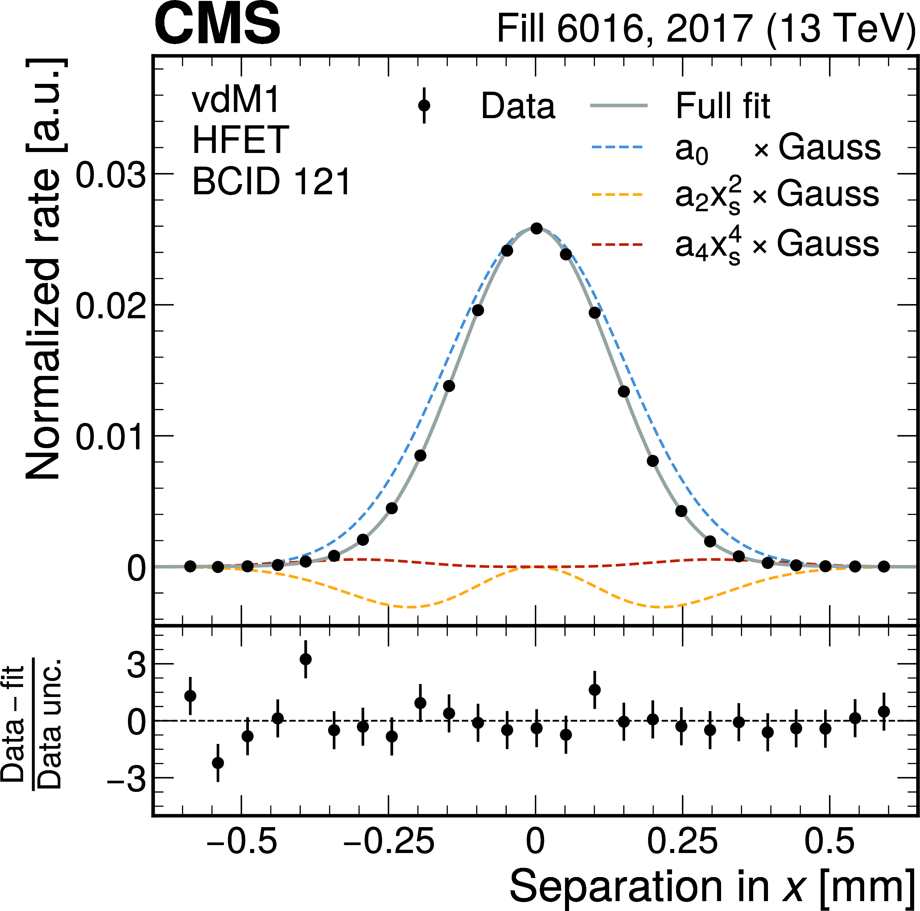
Figure 1-a:
An illustration of the vdM fit procedure for the HFET method in the 2017 vdM fill after all corrections are applied. The luminometer rate (normalized by the product of the bunch proton multiplicity values) is shown for a single bunch (BCID 121) as a function of the transverse separation of the two beams in the horizontal (left) and vertical (right) directions. The data are fitted by the product of a fourth-order positive symmetric polynomial and a Gaussian function. The three additive components, as well as the full analytic function, are plotted. The variable $ x_s $ signifies coordinates standardized with the width and mean of the Gaussian function, $ x_s=(x-\mu)/\sigma $. The effective widths of the fitted curves, $ \Sigma_x $ and $ \Sigma_y $, are defined by Eq. \eqrefeq:capsigma, and the peak value is the head-on rate normalized by the bunch intensities ($ R(0,0)/(N_1N_2) $) in Eq. \eqrefeq:SigmaVis. The lower panel shows the difference between the measured data and the fitted function, divided by the statistical uncertainty of the normalized rate. |
png pdf |
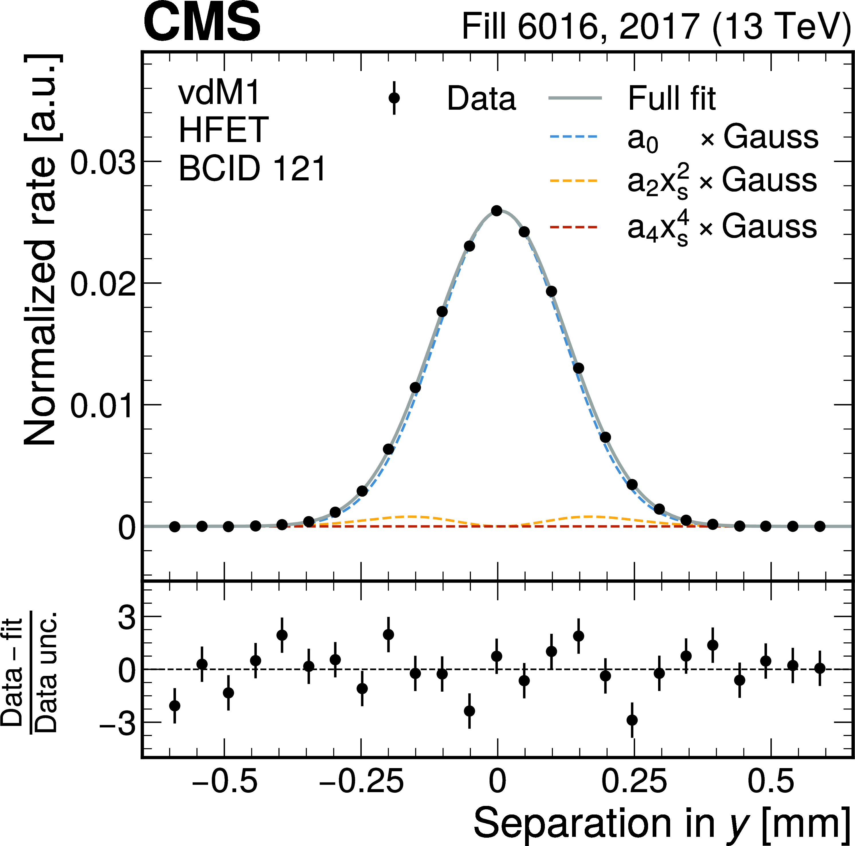
Figure 1-b:
An illustration of the vdM fit procedure for the HFET method in the 2017 vdM fill after all corrections are applied. The luminometer rate (normalized by the product of the bunch proton multiplicity values) is shown for a single bunch (BCID 121) as a function of the transverse separation of the two beams in the horizontal (left) and vertical (right) directions. The data are fitted by the product of a fourth-order positive symmetric polynomial and a Gaussian function. The three additive components, as well as the full analytic function, are plotted. The variable $ x_s $ signifies coordinates standardized with the width and mean of the Gaussian function, $ x_s=(x-\mu)/\sigma $. The effective widths of the fitted curves, $ \Sigma_x $ and $ \Sigma_y $, are defined by Eq. \eqrefeq:capsigma, and the peak value is the head-on rate normalized by the bunch intensities ($ R(0,0)/(N_1N_2) $) in Eq. \eqrefeq:SigmaVis. The lower panel shows the difference between the measured data and the fitted function, divided by the statistical uncertainty of the normalized rate. |
png pdf |
Figure 2:
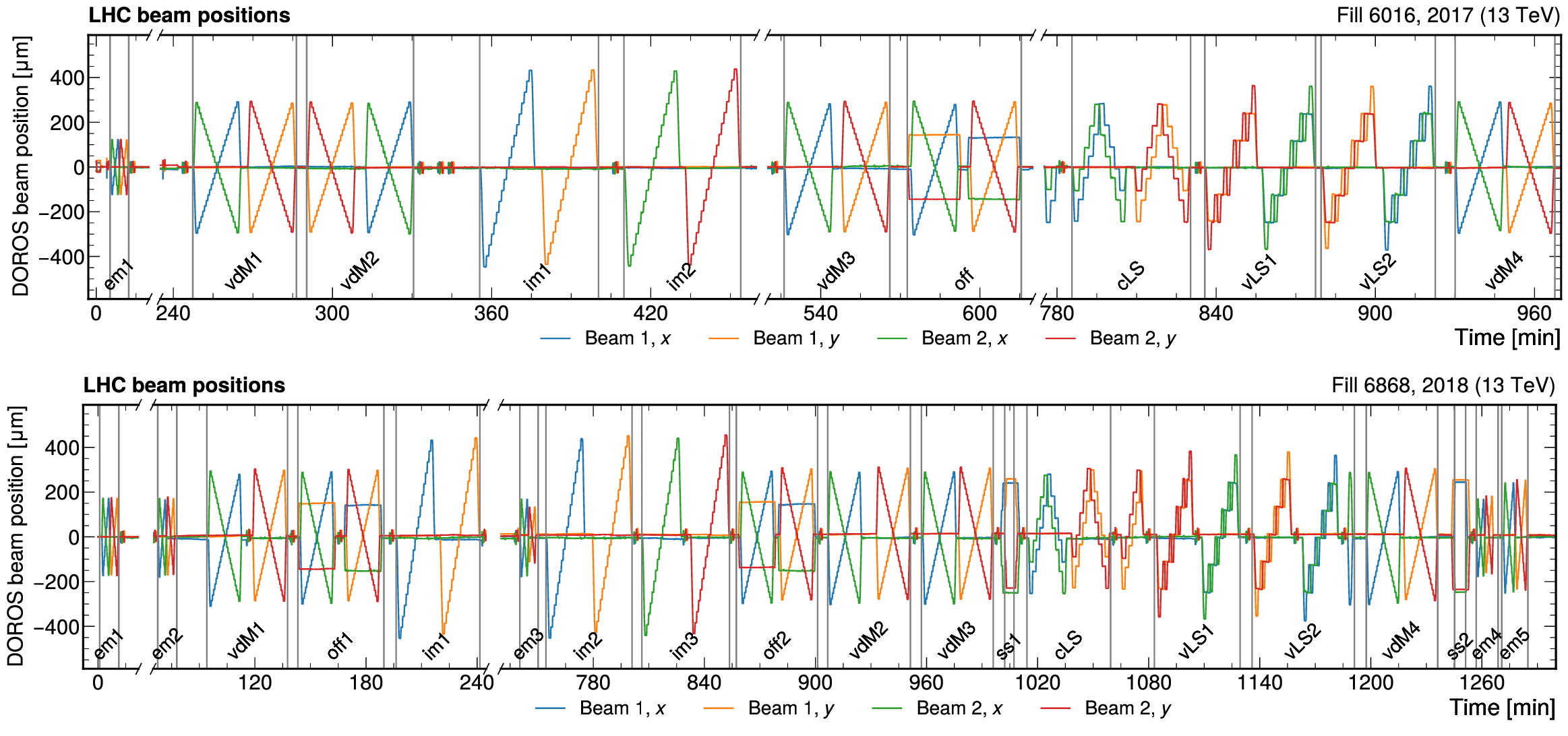
Beam positions in $ x $ and $ y $ for both LHC beams as functions of time during LHC fills 6016 (upper) and 6868 (lower), as measured with the DOROS BPMs with 1\units time granularity. Time is indicated relative to the first included data point. The beginning and end of individual scans are indicated by vertical lines. Each vdM -like scan pair consists of a scan along the $ x $ axis and one along the $ y $ axis, and is labeled by the abbreviation of the corresponding scan type: ``vdM'', ``em'', ``im'', and ``off'' for standard vdM, emittance, beam imaging, and offset scans, respectively. Variable- and constant-separation length scale scans are marked with ``vLS'' and ``cLS'', respectively. The super separation periods in 2018 are marked with ``ss''. |
png pdf |
Figure 2-a:
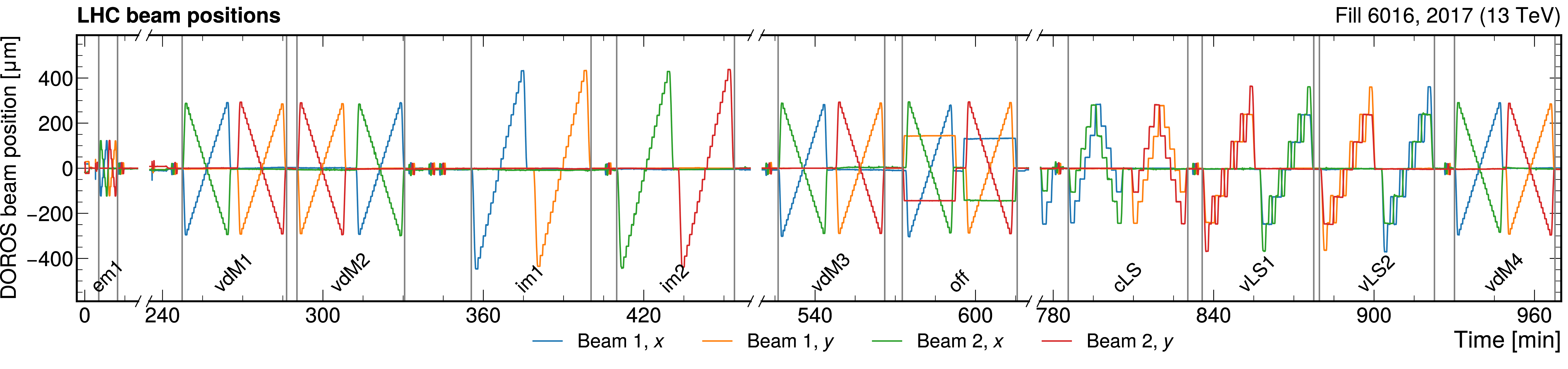
Beam positions in $ x $ and $ y $ for both LHC beams as functions of time during LHC fills 6016 (upper) and 6868 (lower), as measured with the DOROS BPMs with 1\units time granularity. Time is indicated relative to the first included data point. The beginning and end of individual scans are indicated by vertical lines. Each vdM -like scan pair consists of a scan along the $ x $ axis and one along the $ y $ axis, and is labeled by the abbreviation of the corresponding scan type: ``vdM'', ``em'', ``im'', and ``off'' for standard vdM, emittance, beam imaging, and offset scans, respectively. Variable- and constant-separation length scale scans are marked with ``vLS'' and ``cLS'', respectively. The super separation periods in 2018 are marked with ``ss''. |
png pdf |
Figure 2-b:
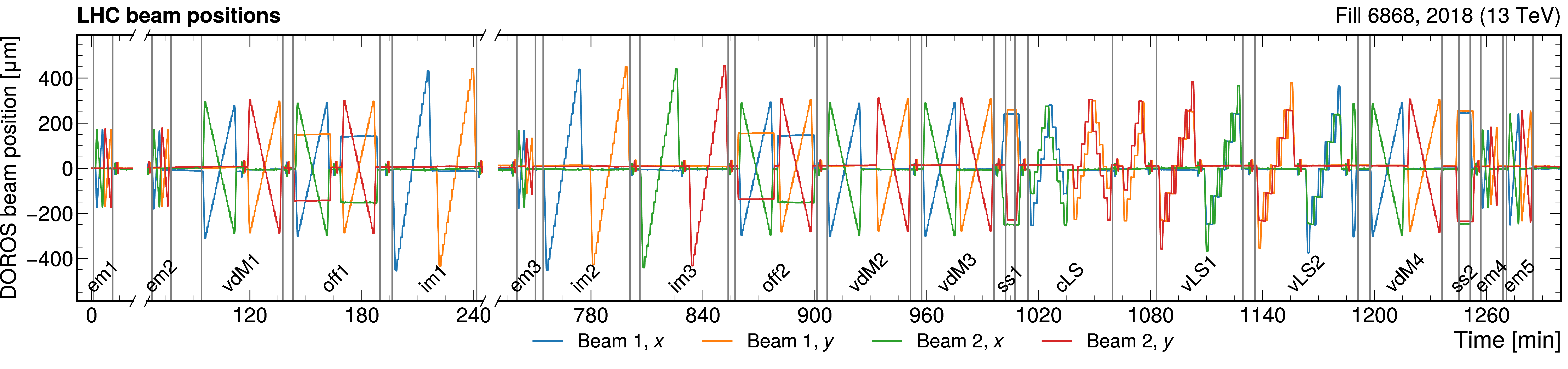
Beam positions in $ x $ and $ y $ for both LHC beams as functions of time during LHC fills 6016 (upper) and 6868 (lower), as measured with the DOROS BPMs with 1\units time granularity. Time is indicated relative to the first included data point. The beginning and end of individual scans are indicated by vertical lines. Each vdM -like scan pair consists of a scan along the $ x $ axis and one along the $ y $ axis, and is labeled by the abbreviation of the corresponding scan type: ``vdM'', ``em'', ``im'', and ``off'' for standard vdM, emittance, beam imaging, and offset scans, respectively. Variable- and constant-separation length scale scans are marked with ``vLS'' and ``cLS'', respectively. The super separation periods in 2018 are marked with ``ss''. |
png pdf |
Figure 3:
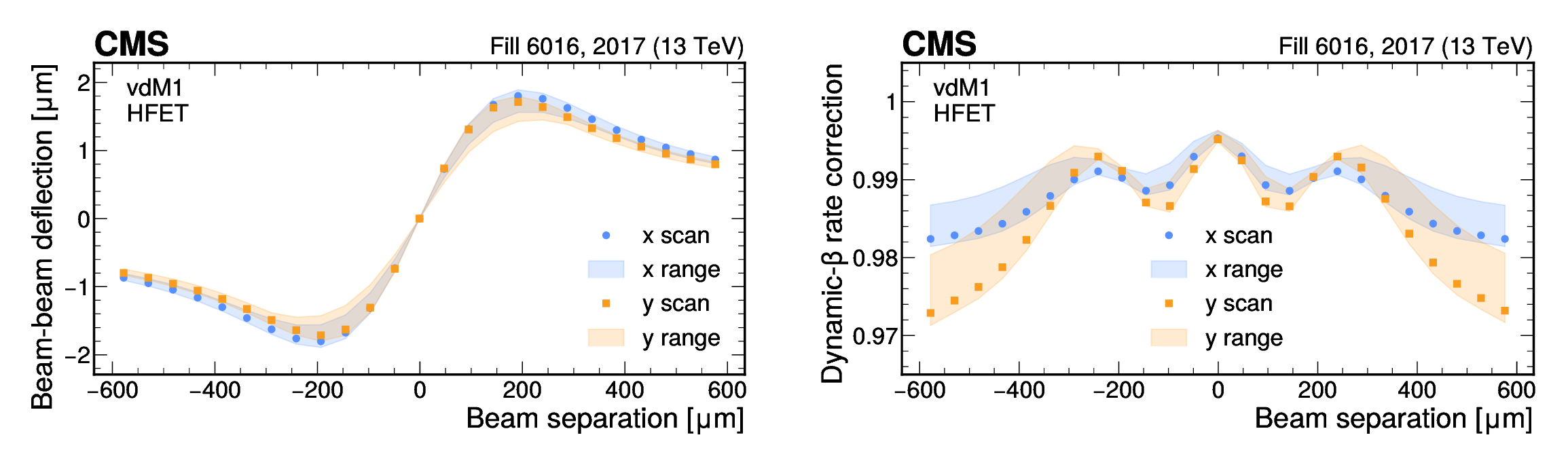
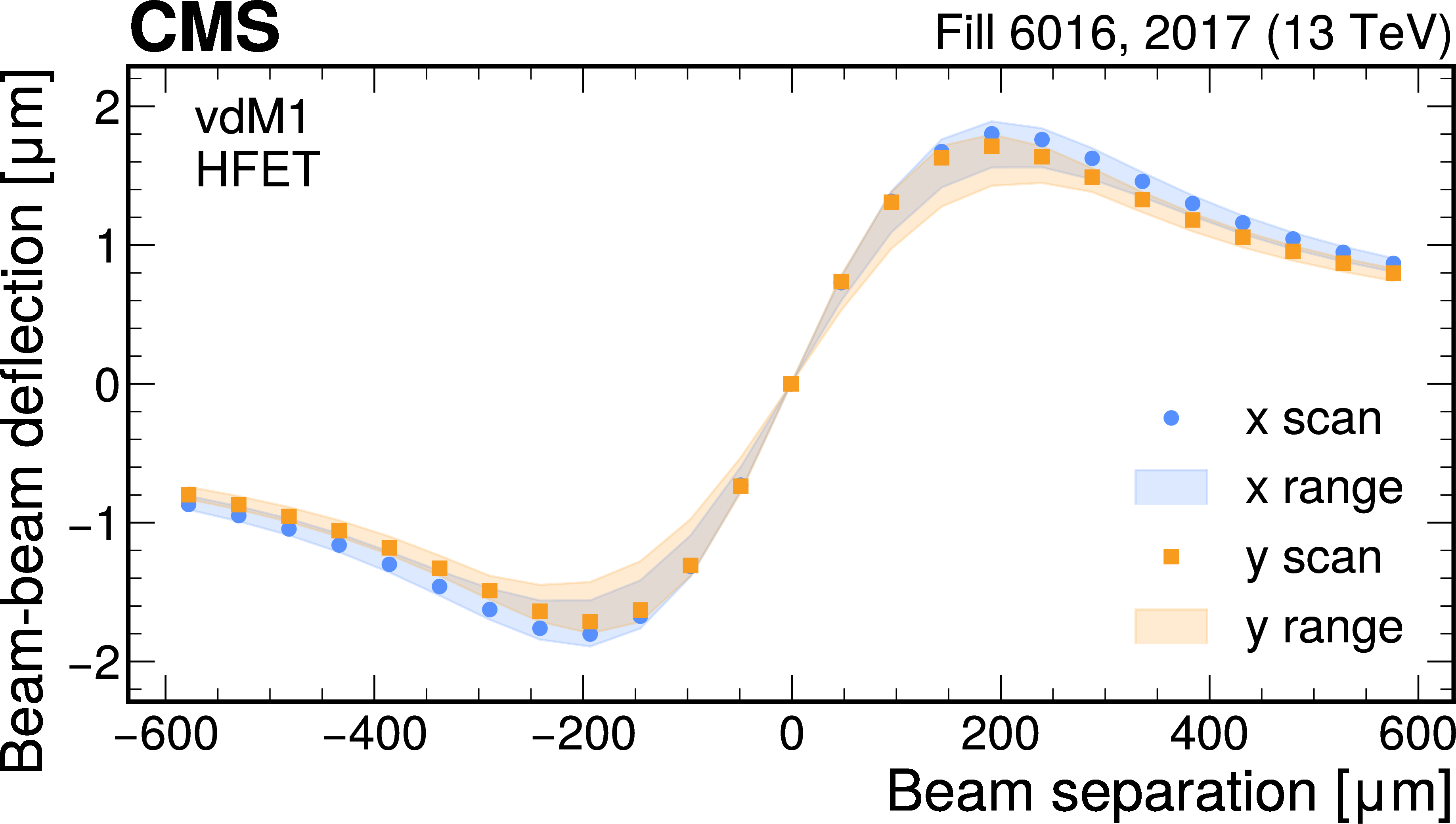
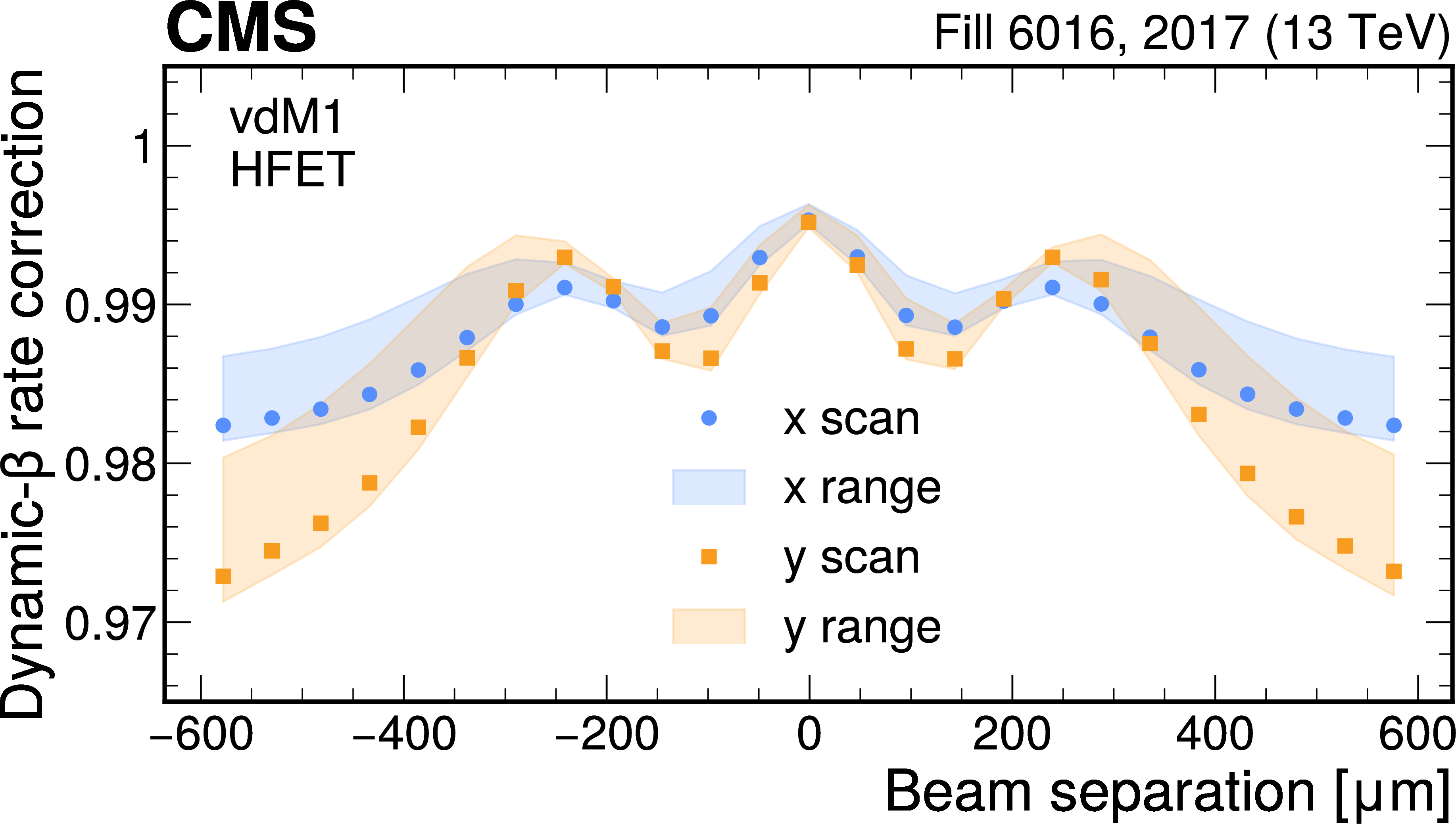
Beam-beam deflection (left) and dynamic-$ \beta $ correction (right) for the first scan pair in fill 6016, separately for scans in $ x $ and $ y $. The corrections are computed individually for each colliding bunch pair. The points represent the average over all bunch pairs, and the shaded area covers the minimum and maximum values obtained for any bunch pair. |
png pdf |
Figure 3-a:
Beam-beam deflection (left) and dynamic-$ \beta $ correction (right) for the first scan pair in fill 6016, separately for scans in $ x $ and $ y $. The corrections are computed individually for each colliding bunch pair. The points represent the average over all bunch pairs, and the shaded area covers the minimum and maximum values obtained for any bunch pair. |
png pdf |
Figure 3-b:
Beam-beam deflection (left) and dynamic-$ \beta $ correction (right) for the first scan pair in fill 6016, separately for scans in $ x $ and $ y $. The corrections are computed individually for each colliding bunch pair. The points represent the average over all bunch pairs, and the shaded area covers the minimum and maximum values obtained for any bunch pair. |
png pdf |
Figure 4:
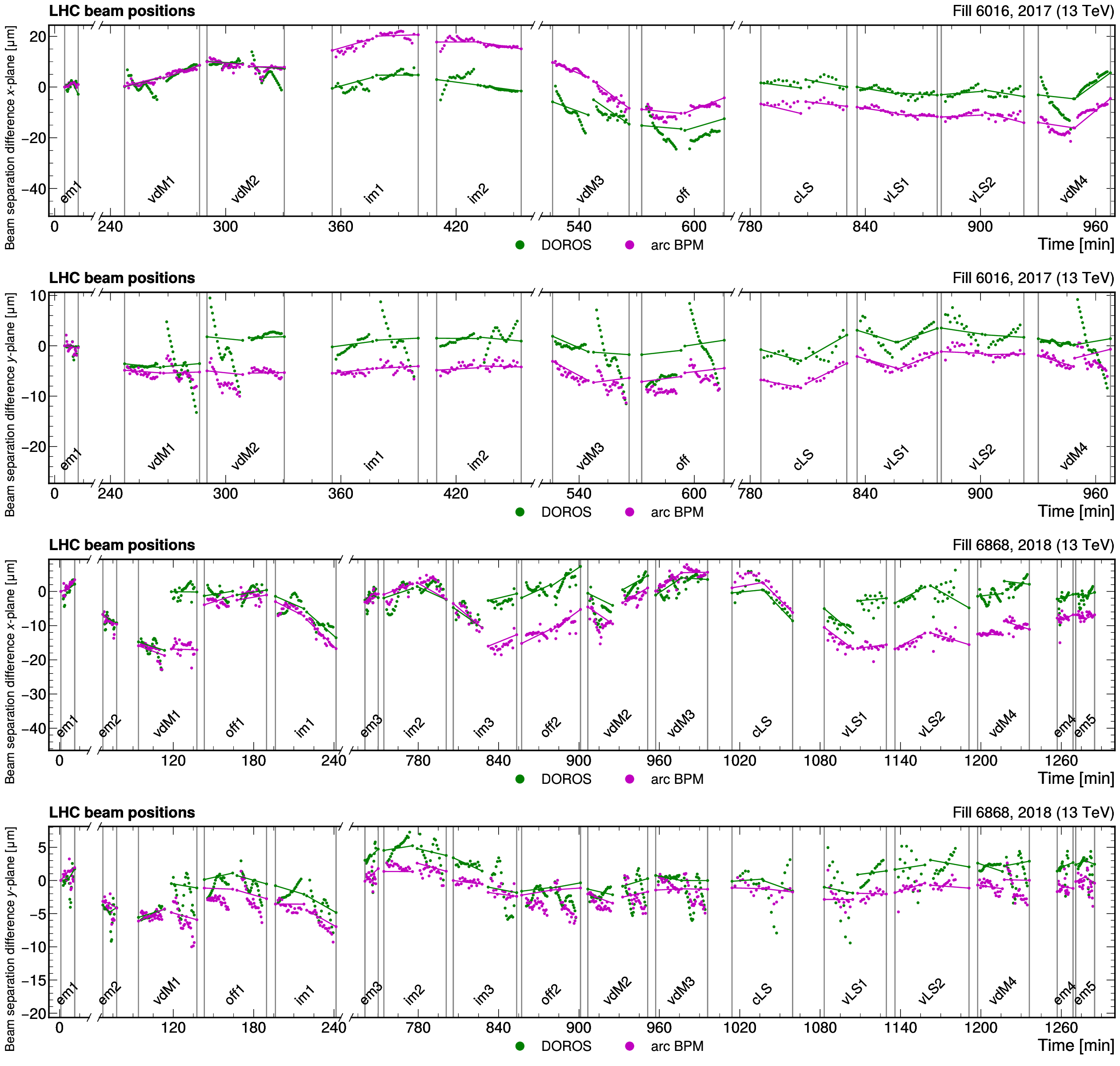
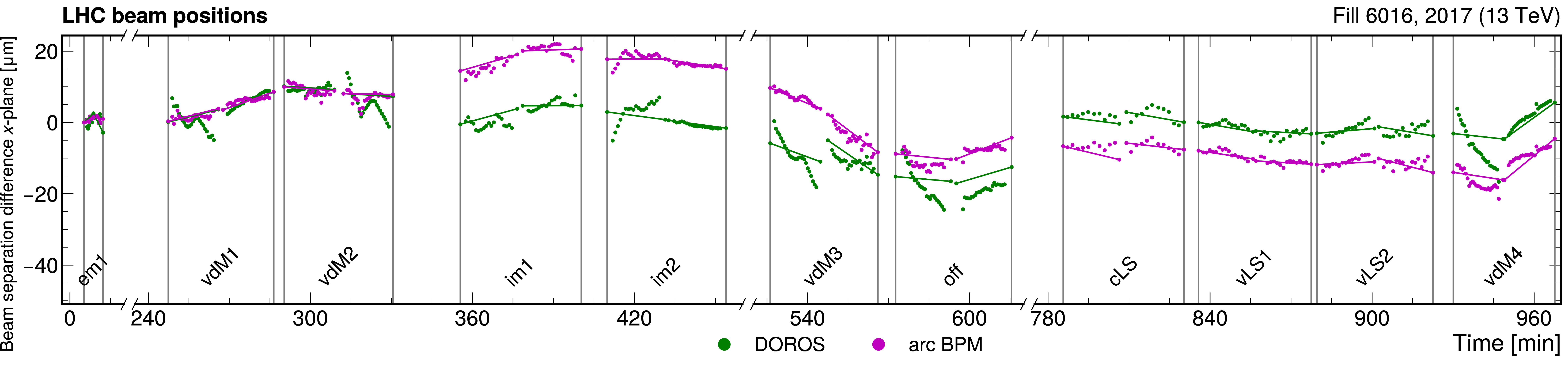
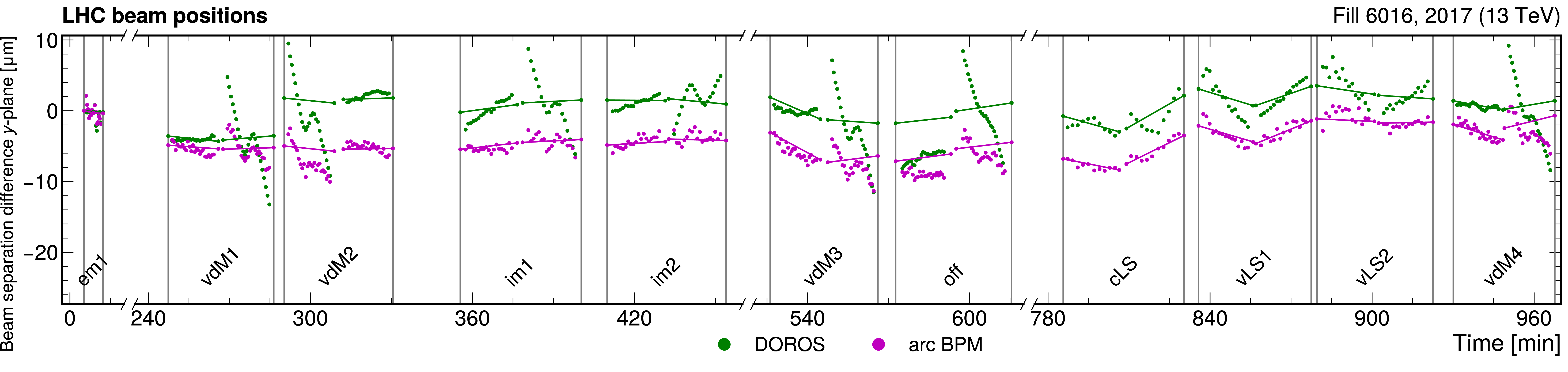
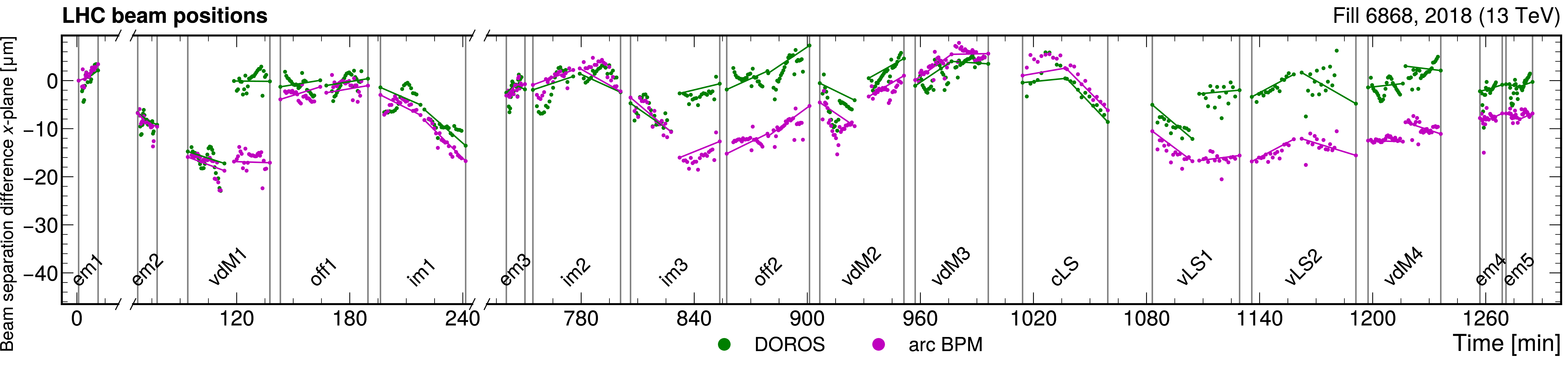
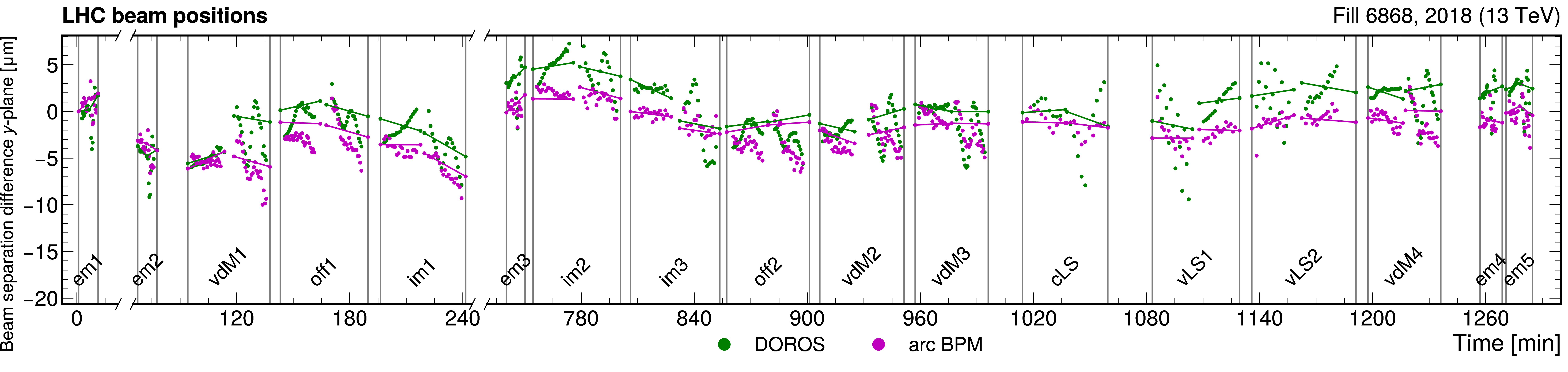
Difference between nominal and measured beam separation per scan step as a function of time for the vdM scans during LHC fills 6016 (upper two figures) and 6868 (lower two figures). The scan boundaries are marked by vertical lines and labeled with the corresponding scan identifiers. The solid green and magenta lines represent the linear interpolation between the head-on reference points before and after each scan, showing the linear orbit drift. The individual data points demonstrate the beam-beam deflection nicely in the scanning direction. Differences between the two BPMs, DOROS and arc BPM, are expected due to differing sensitivity to the beam-beam deflection, scan-dependent offsets, and length scale differences. |
png pdf |
Figure 4-a:
Difference between nominal and measured beam separation per scan step as a function of time for the vdM scans during LHC fills 6016 (upper two figures) and 6868 (lower two figures). The scan boundaries are marked by vertical lines and labeled with the corresponding scan identifiers. The solid green and magenta lines represent the linear interpolation between the head-on reference points before and after each scan, showing the linear orbit drift. The individual data points demonstrate the beam-beam deflection nicely in the scanning direction. Differences between the two BPMs, DOROS and arc BPM, are expected due to differing sensitivity to the beam-beam deflection, scan-dependent offsets, and length scale differences. |
png pdf |
Figure 4-b:
Difference between nominal and measured beam separation per scan step as a function of time for the vdM scans during LHC fills 6016 (upper two figures) and 6868 (lower two figures). The scan boundaries are marked by vertical lines and labeled with the corresponding scan identifiers. The solid green and magenta lines represent the linear interpolation between the head-on reference points before and after each scan, showing the linear orbit drift. The individual data points demonstrate the beam-beam deflection nicely in the scanning direction. Differences between the two BPMs, DOROS and arc BPM, are expected due to differing sensitivity to the beam-beam deflection, scan-dependent offsets, and length scale differences. |
png pdf |
Figure 4-c:
Difference between nominal and measured beam separation per scan step as a function of time for the vdM scans during LHC fills 6016 (upper two figures) and 6868 (lower two figures). The scan boundaries are marked by vertical lines and labeled with the corresponding scan identifiers. The solid green and magenta lines represent the linear interpolation between the head-on reference points before and after each scan, showing the linear orbit drift. The individual data points demonstrate the beam-beam deflection nicely in the scanning direction. Differences between the two BPMs, DOROS and arc BPM, are expected due to differing sensitivity to the beam-beam deflection, scan-dependent offsets, and length scale differences. |
png pdf |
Figure 4-d:
Difference between nominal and measured beam separation per scan step as a function of time for the vdM scans during LHC fills 6016 (upper two figures) and 6868 (lower two figures). The scan boundaries are marked by vertical lines and labeled with the corresponding scan identifiers. The solid green and magenta lines represent the linear interpolation between the head-on reference points before and after each scan, showing the linear orbit drift. The individual data points demonstrate the beam-beam deflection nicely in the scanning direction. Differences between the two BPMs, DOROS and arc BPM, are expected due to differing sensitivity to the beam-beam deflection, scan-dependent offsets, and length scale differences. |
png pdf |
Figure 5:
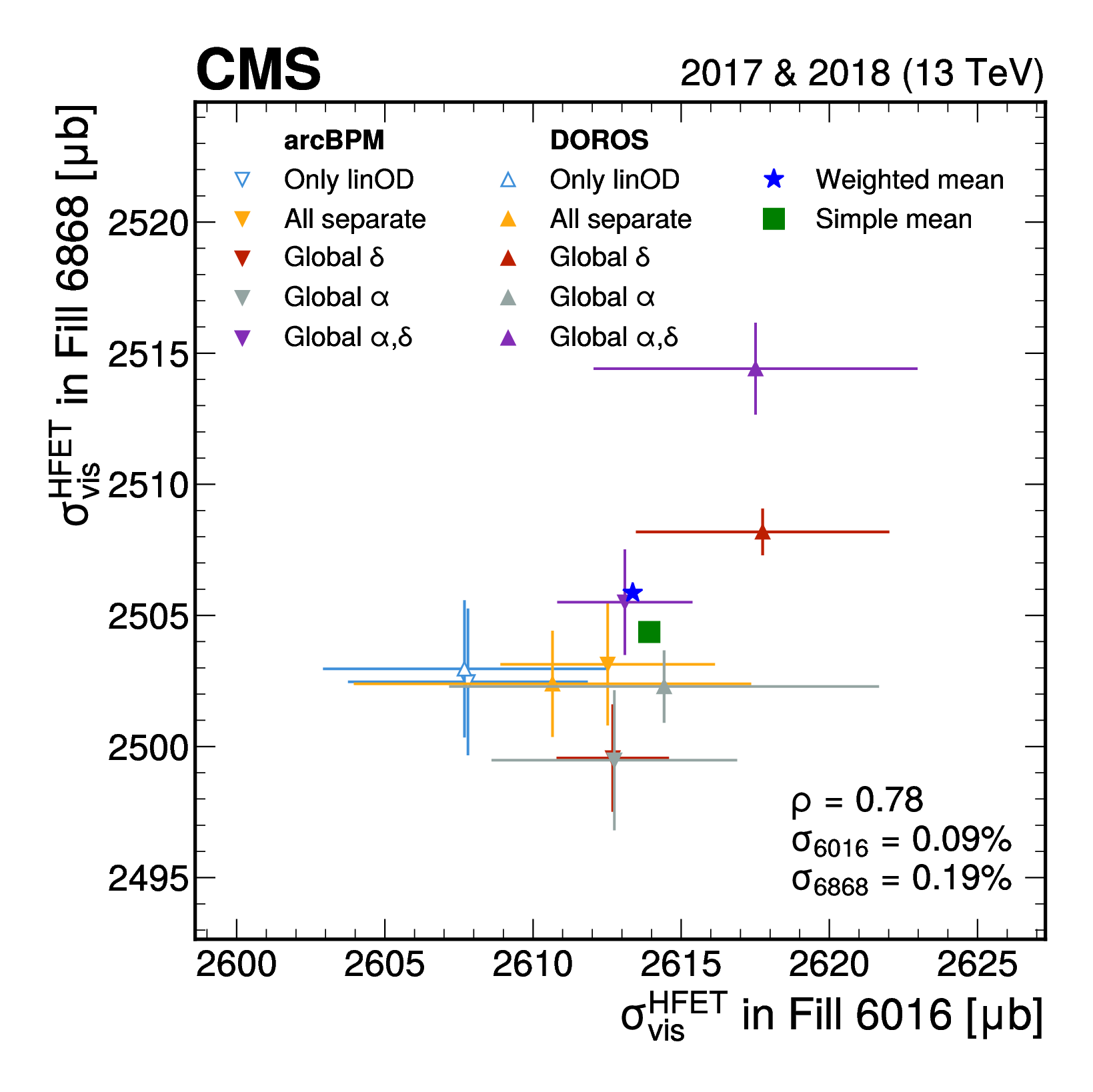
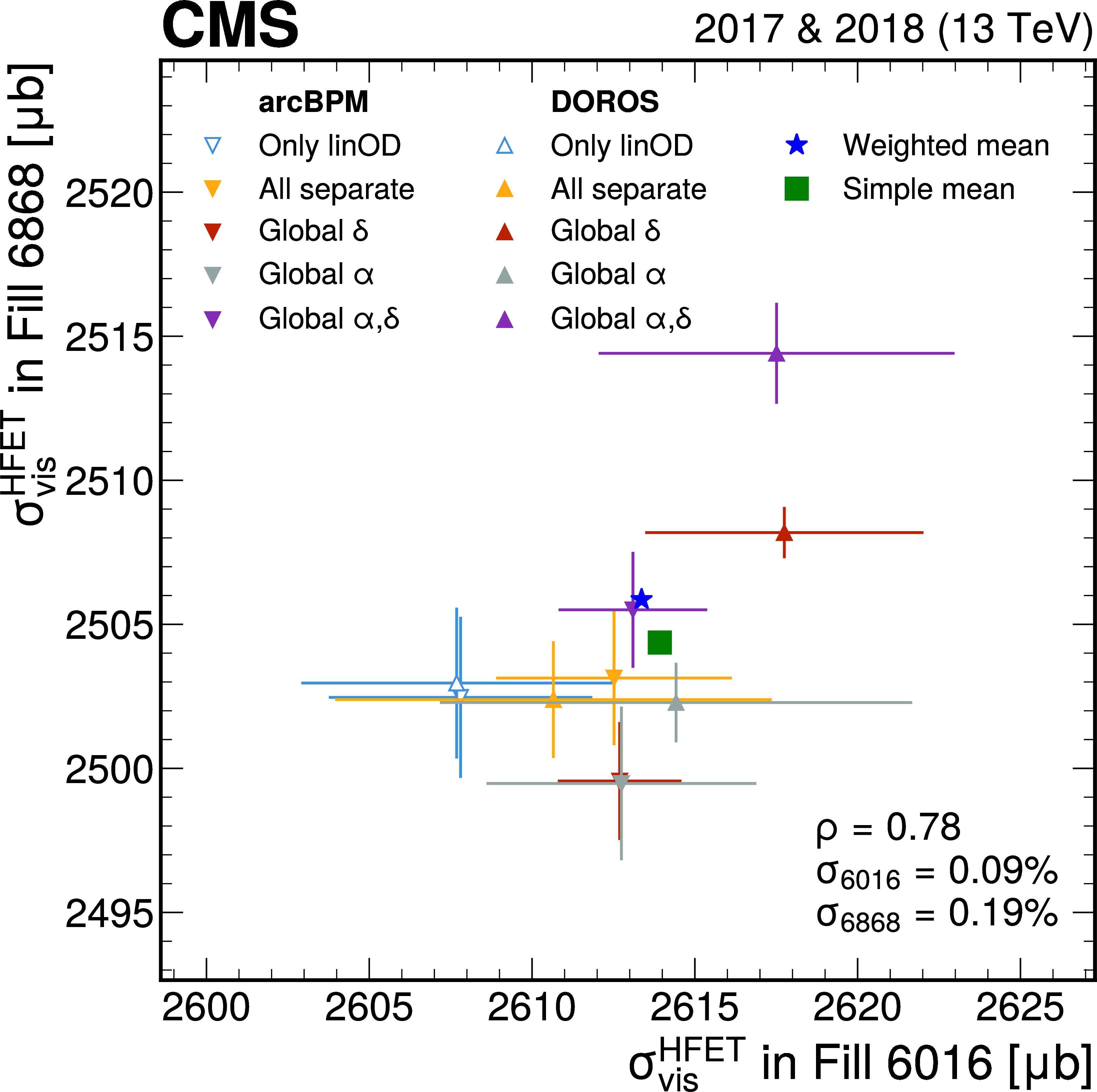
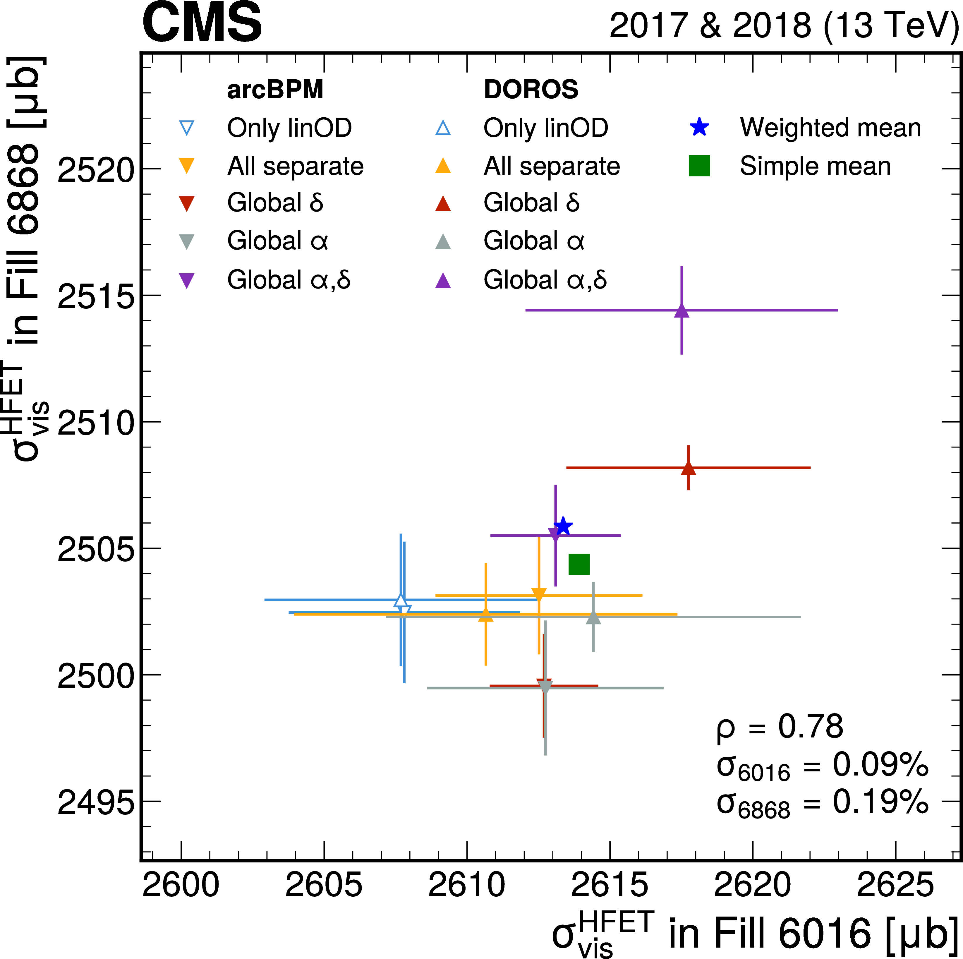
Visible cross section estimates for the HFET luminometer with all corrections applied for the 2017 and 2018 calibration fills (6016 and 6868). Results are shown for various orbit drift correction methods, corresponding to different assumptions of the $ \alpha $ and $ \delta $ parameters in the residual orbit drift fits. These parameters describe the BPM (arc or DOROS) length scale and the dilution of the beam--beam deflection, respectively. The markers represent the average over all scans, while the error bars correspond to the standard deviation, reflecting scan-to-scan reproducibility. The baseline method (purple downward-facing triangle) uses arc BPM measurements and assumes common $ \alpha $ and $ \delta $ values for all scans within a given year. The corresponding $ \sigma_{\text{vis}} $ value is closest to the mean of all residual orbit drift configurations (blue star and green square) and is taken as the central correction method. The empty triangles, representing the linear-only orbit drift corrections, are excluded from the averages and from the other metrics shown. The correlation between the years, shown in the lower right corner, is large (0.78). The standard deviations, taken as the uncertainty associated with the choice of method, are also indicated. The difference in $ \sigma_{\text{vis}} $ between the two years is consistent with the expected efficiency loss of HFET due to radiation-induced aging. |
png pdf |
Figure 5-a:
Visible cross section estimates for the HFET luminometer with all corrections applied for the 2017 and 2018 calibration fills (6016 and 6868). Results are shown for various orbit drift correction methods, corresponding to different assumptions of the $ \alpha $ and $ \delta $ parameters in the residual orbit drift fits. These parameters describe the BPM (arc or DOROS) length scale and the dilution of the beam--beam deflection, respectively. The markers represent the average over all scans, while the error bars correspond to the standard deviation, reflecting scan-to-scan reproducibility. The baseline method (purple downward-facing triangle) uses arc BPM measurements and assumes common $ \alpha $ and $ \delta $ values for all scans within a given year. The corresponding $ \sigma_{\text{vis}} $ value is closest to the mean of all residual orbit drift configurations (blue star and green square) and is taken as the central correction method. The empty triangles, representing the linear-only orbit drift corrections, are excluded from the averages and from the other metrics shown. The correlation between the years, shown in the lower right corner, is large (0.78). The standard deviations, taken as the uncertainty associated with the choice of method, are also indicated. The difference in $ \sigma_{\text{vis}} $ between the two years is consistent with the expected efficiency loss of HFET due to radiation-induced aging. |
png pdf |
Figure 5-b:
Visible cross section estimates for the HFET luminometer with all corrections applied for the 2017 and 2018 calibration fills (6016 and 6868). Results are shown for various orbit drift correction methods, corresponding to different assumptions of the $ \alpha $ and $ \delta $ parameters in the residual orbit drift fits. These parameters describe the BPM (arc or DOROS) length scale and the dilution of the beam--beam deflection, respectively. The markers represent the average over all scans, while the error bars correspond to the standard deviation, reflecting scan-to-scan reproducibility. The baseline method (purple downward-facing triangle) uses arc BPM measurements and assumes common $ \alpha $ and $ \delta $ values for all scans within a given year. The corresponding $ \sigma_{\text{vis}} $ value is closest to the mean of all residual orbit drift configurations (blue star and green square) and is taken as the central correction method. The empty triangles, representing the linear-only orbit drift corrections, are excluded from the averages and from the other metrics shown. The correlation between the years, shown in the lower right corner, is large (0.78). The standard deviations, taken as the uncertainty associated with the choice of method, are also indicated. The difference in $ \sigma_{\text{vis}} $ between the two years is consistent with the expected efficiency loss of HFET due to radiation-induced aging. |
png pdf |
Figure 6:
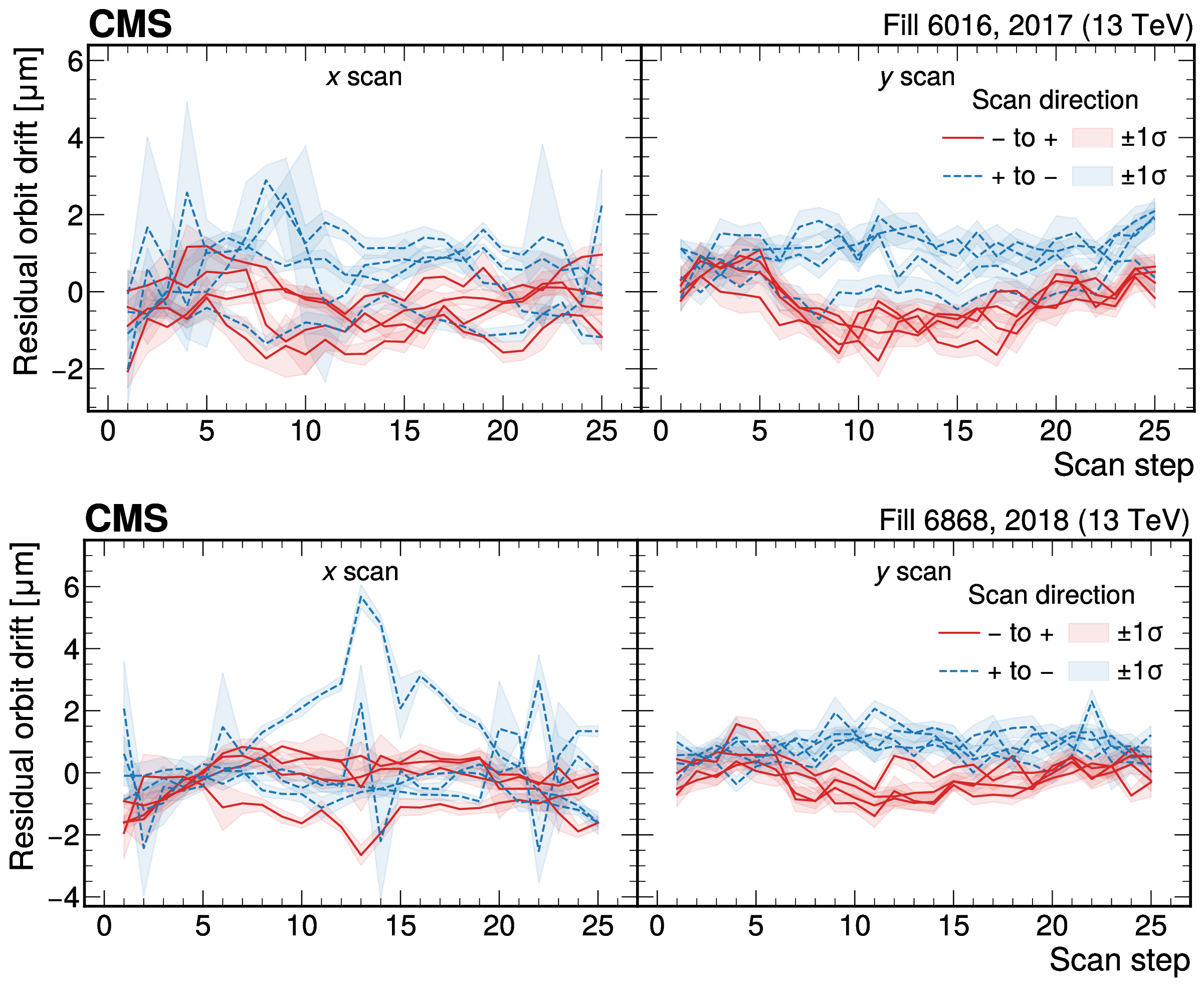
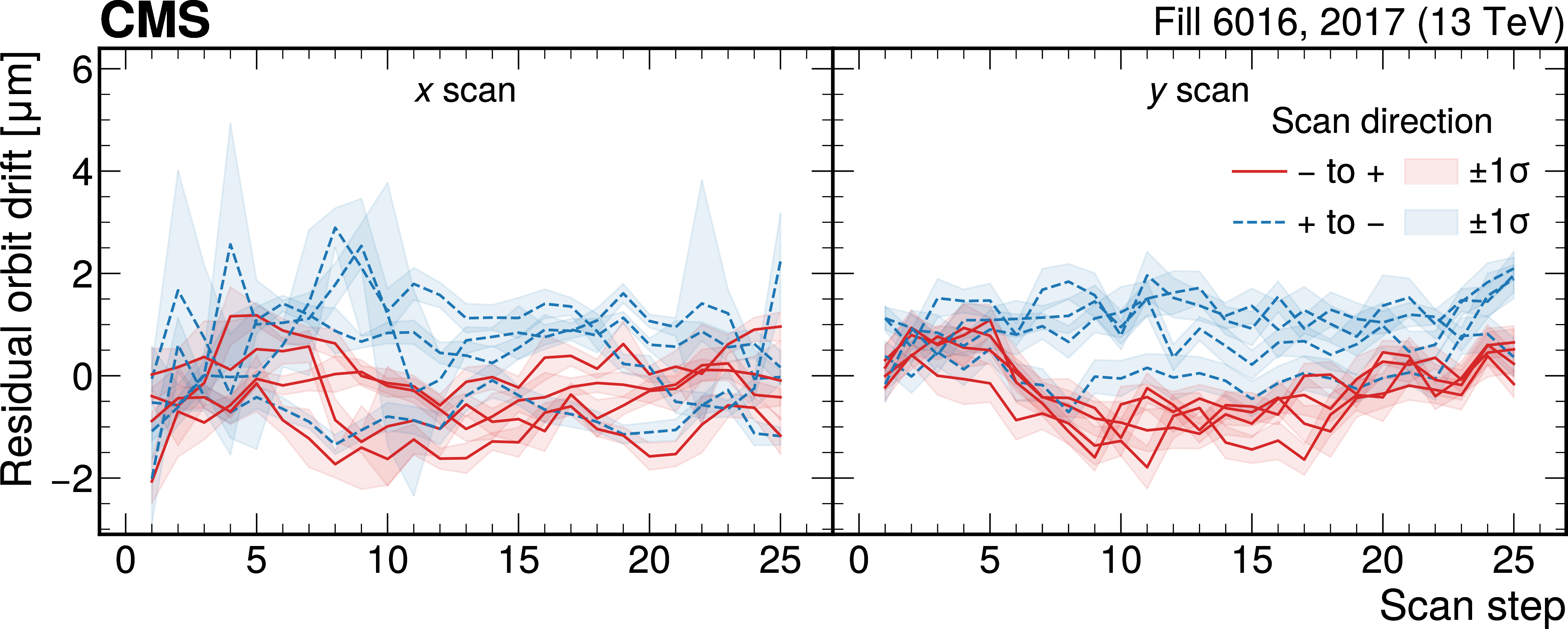
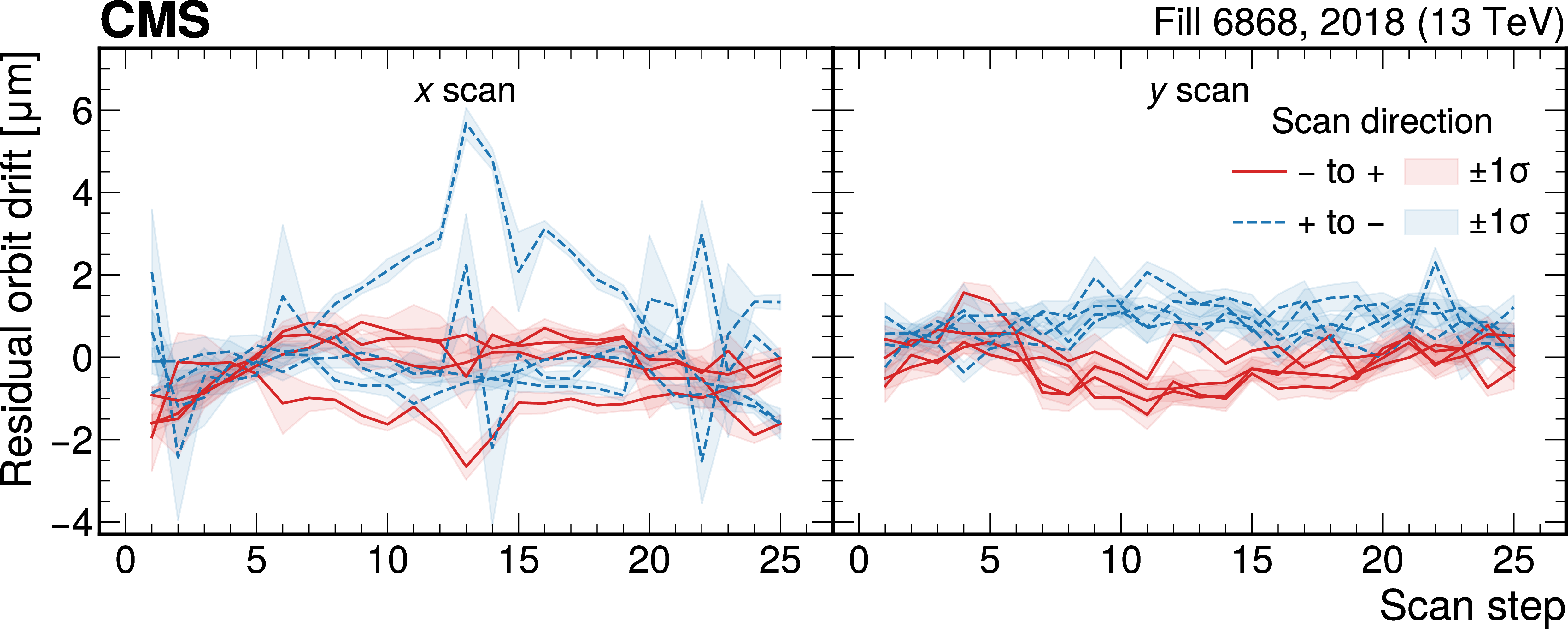
Residual orbit drift corrections to the single-beam positions as a function of the scan step number for each regular vdM scan, as derived from the arc BPM measurements using a fit with common $ \alpha $ and $ \delta $ parameters for all scans within a year, shown for 2017 (upper) and 2018 (lower). The red (blue) lines correspond to residuals for the beam moving from negative (positive) to positive (negative) direction in the transverse plane with respect to the LHC reference frame, as illustrated in Fig. 2. This convention is adopted to enhance the visibility of reproducible features, e.g., those arising from magnetic nonlinearities. The uncertainty bands represent the standard deviation of the individual BPM readings within each scan step. |
png pdf |
Figure 6-a:
Residual orbit drift corrections to the single-beam positions as a function of the scan step number for each regular vdM scan, as derived from the arc BPM measurements using a fit with common $ \alpha $ and $ \delta $ parameters for all scans within a year, shown for 2017 (upper) and 2018 (lower). The red (blue) lines correspond to residuals for the beam moving from negative (positive) to positive (negative) direction in the transverse plane with respect to the LHC reference frame, as illustrated in Fig. 2. This convention is adopted to enhance the visibility of reproducible features, e.g., those arising from magnetic nonlinearities. The uncertainty bands represent the standard deviation of the individual BPM readings within each scan step. |
png pdf |
Figure 6-b:
Residual orbit drift corrections to the single-beam positions as a function of the scan step number for each regular vdM scan, as derived from the arc BPM measurements using a fit with common $ \alpha $ and $ \delta $ parameters for all scans within a year, shown for 2017 (upper) and 2018 (lower). The red (blue) lines correspond to residuals for the beam moving from negative (positive) to positive (negative) direction in the transverse plane with respect to the LHC reference frame, as illustrated in Fig. 2. This convention is adopted to enhance the visibility of reproducible features, e.g., those arising from magnetic nonlinearities. The uncertainty bands represent the standard deviation of the individual BPM readings within each scan step. |
png pdf |
Figure 7:
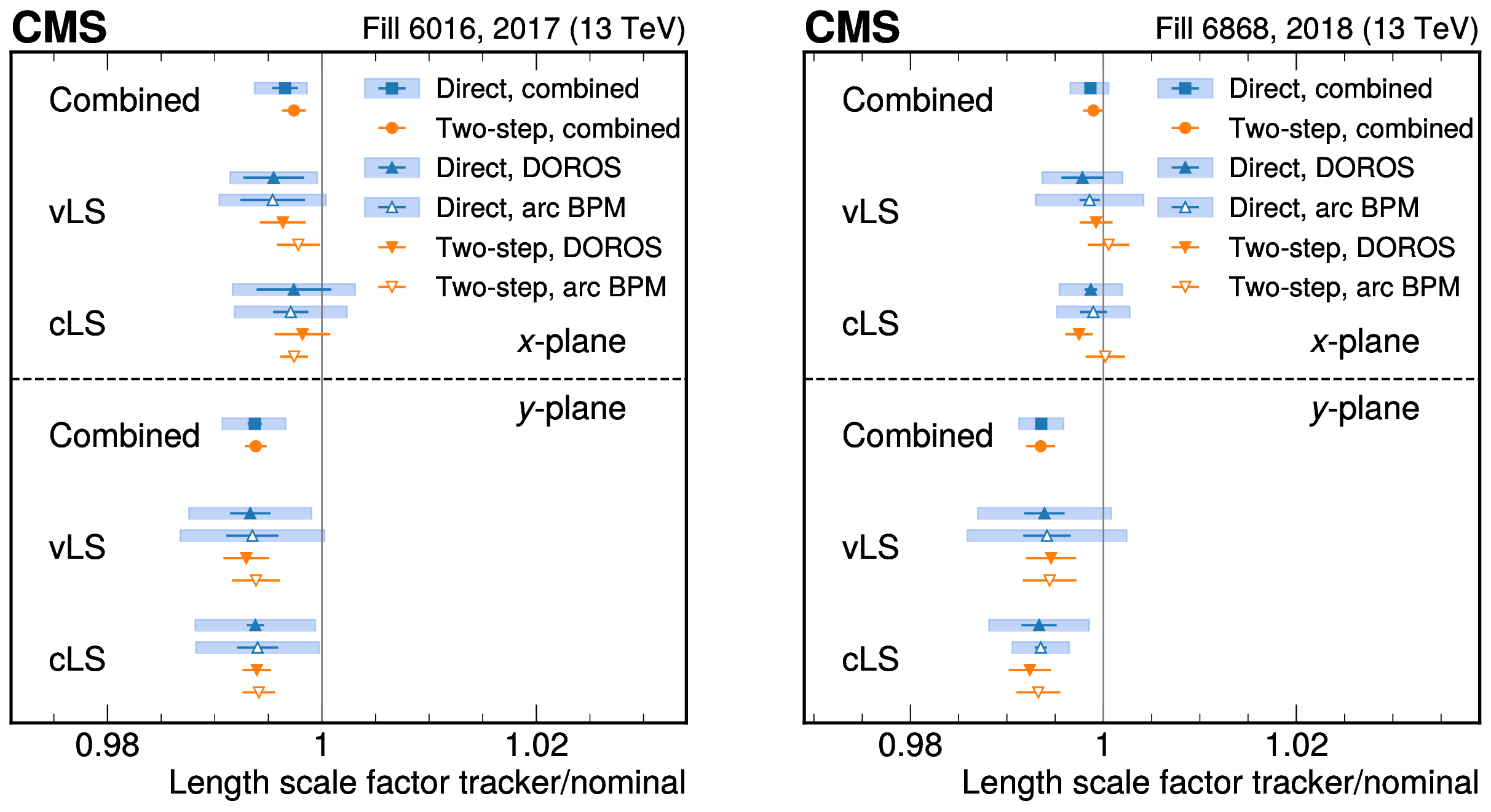
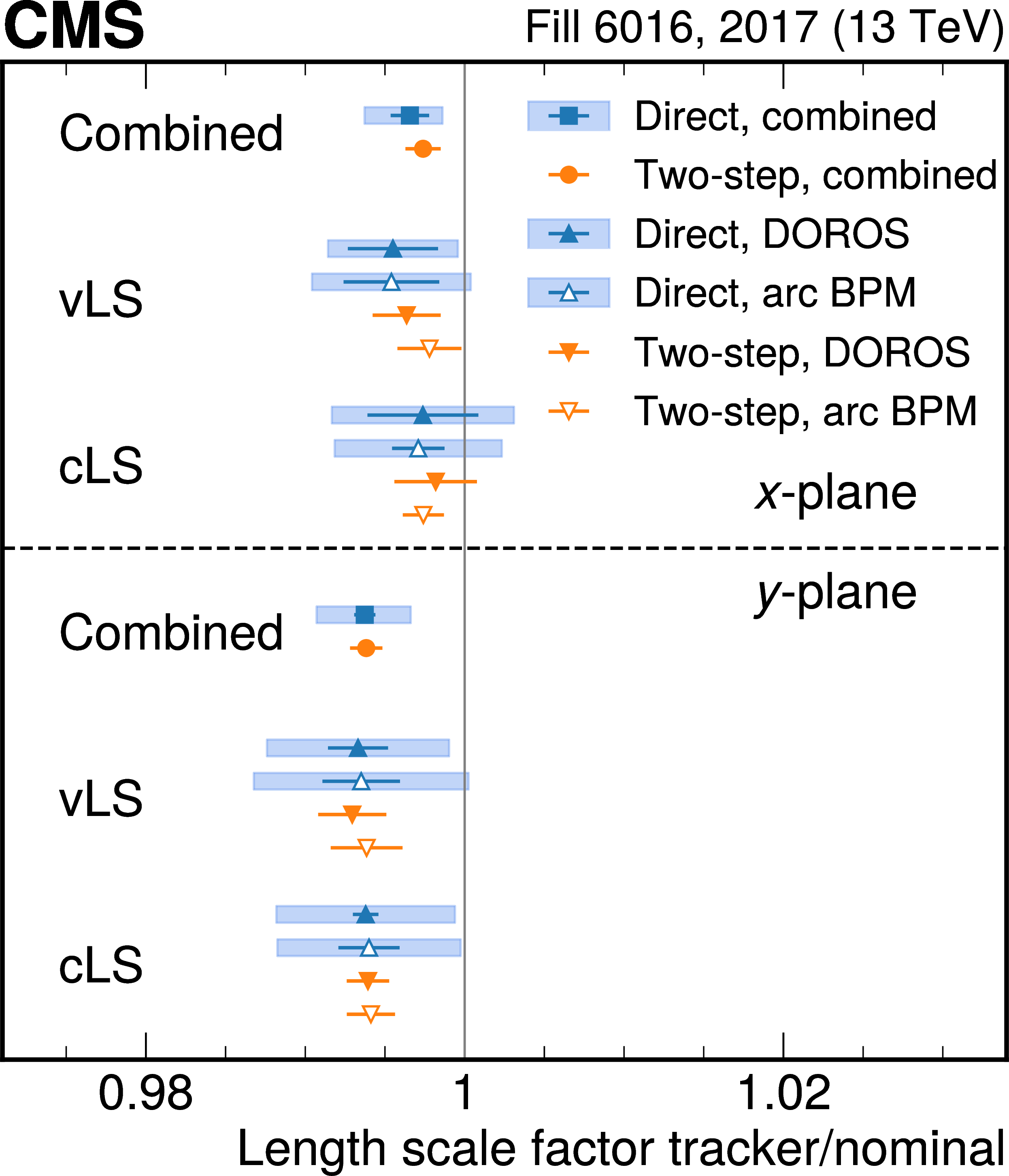
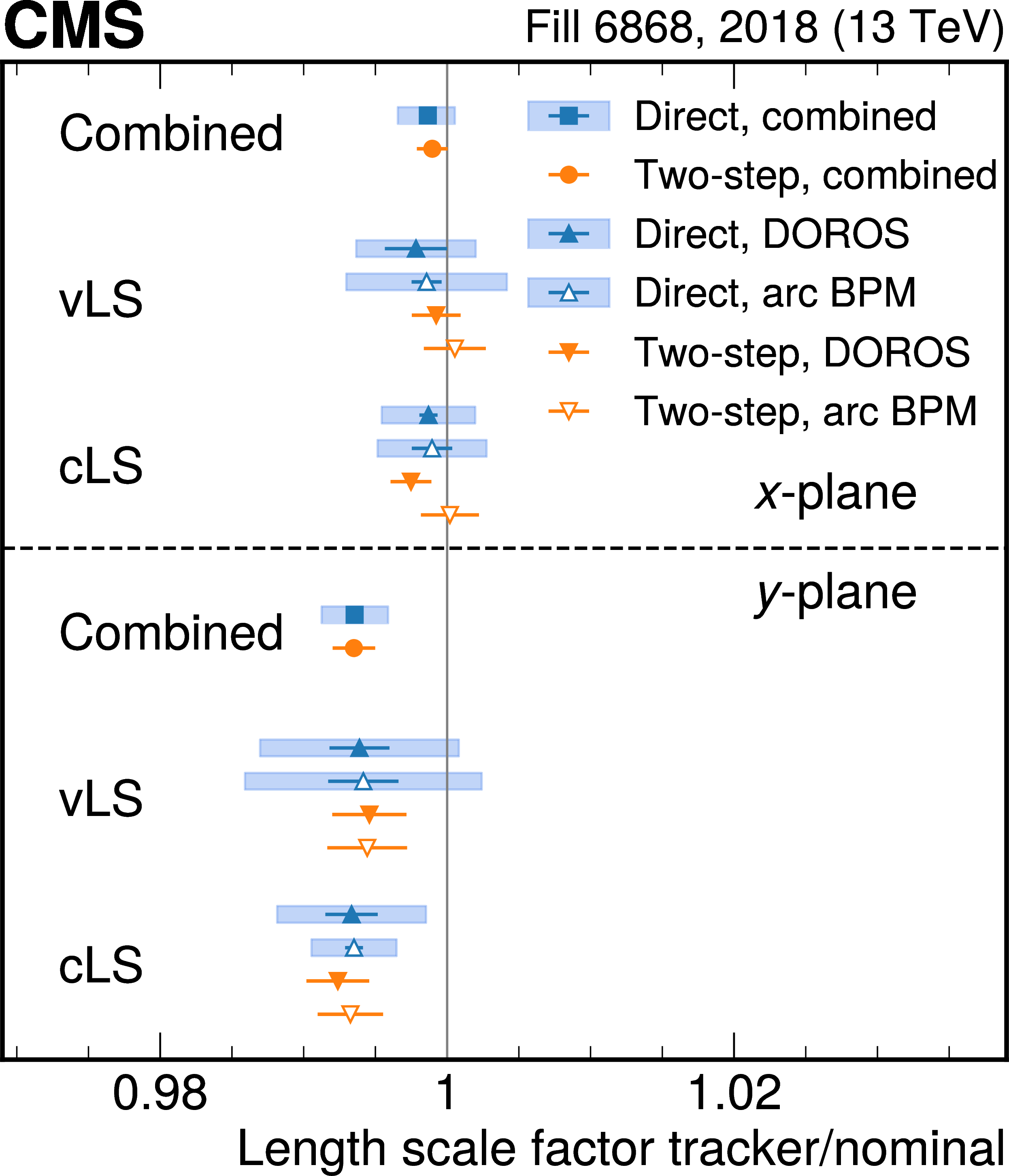
Length scale factors $ \alpha_{\text{TR}/\text{NOM}} $ obtained with the direct (blue squares and upward triangles) and two-step (orange points and downward triangles) approaches for 2017 (left) and 2018 (right). Results are shown separately for cLS and vLS scans, using either the DOROS (filled triangles) or arc (empty triangles) BPMs, as well as their combination (squares and circles). For the direct approach, the error bars represent the total uncertainty, with the orbit drift component estimated from the difference between results obtained with and without outlier removal, likely underestimating this source. The shaded bands also denote the total uncertainty, where the OD contribution is instead computed as the standard deviation of the measured step sizes, providing a conservative estimate. Since the combination of the vLS and cLS results is computed as a weighted mean, the shaded band is not necessarily centered on the blue squares. For the two-step approach, the error bars represent the total uncertainty. |
png pdf |
Figure 7-a:
Length scale factors $ \alpha_{\text{TR}/\text{NOM}} $ obtained with the direct (blue squares and upward triangles) and two-step (orange points and downward triangles) approaches for 2017 (left) and 2018 (right). Results are shown separately for cLS and vLS scans, using either the DOROS (filled triangles) or arc (empty triangles) BPMs, as well as their combination (squares and circles). For the direct approach, the error bars represent the total uncertainty, with the orbit drift component estimated from the difference between results obtained with and without outlier removal, likely underestimating this source. The shaded bands also denote the total uncertainty, where the OD contribution is instead computed as the standard deviation of the measured step sizes, providing a conservative estimate. Since the combination of the vLS and cLS results is computed as a weighted mean, the shaded band is not necessarily centered on the blue squares. For the two-step approach, the error bars represent the total uncertainty. |
png pdf |
Figure 7-b:
Length scale factors $ \alpha_{\text{TR}/\text{NOM}} $ obtained with the direct (blue squares and upward triangles) and two-step (orange points and downward triangles) approaches for 2017 (left) and 2018 (right). Results are shown separately for cLS and vLS scans, using either the DOROS (filled triangles) or arc (empty triangles) BPMs, as well as their combination (squares and circles). For the direct approach, the error bars represent the total uncertainty, with the orbit drift component estimated from the difference between results obtained with and without outlier removal, likely underestimating this source. The shaded bands also denote the total uncertainty, where the OD contribution is instead computed as the standard deviation of the measured step sizes, providing a conservative estimate. Since the combination of the vLS and cLS results is computed as a weighted mean, the shaded band is not necessarily centered on the blue squares. For the two-step approach, the error bars represent the total uncertainty. |
png pdf |
Figure 8:
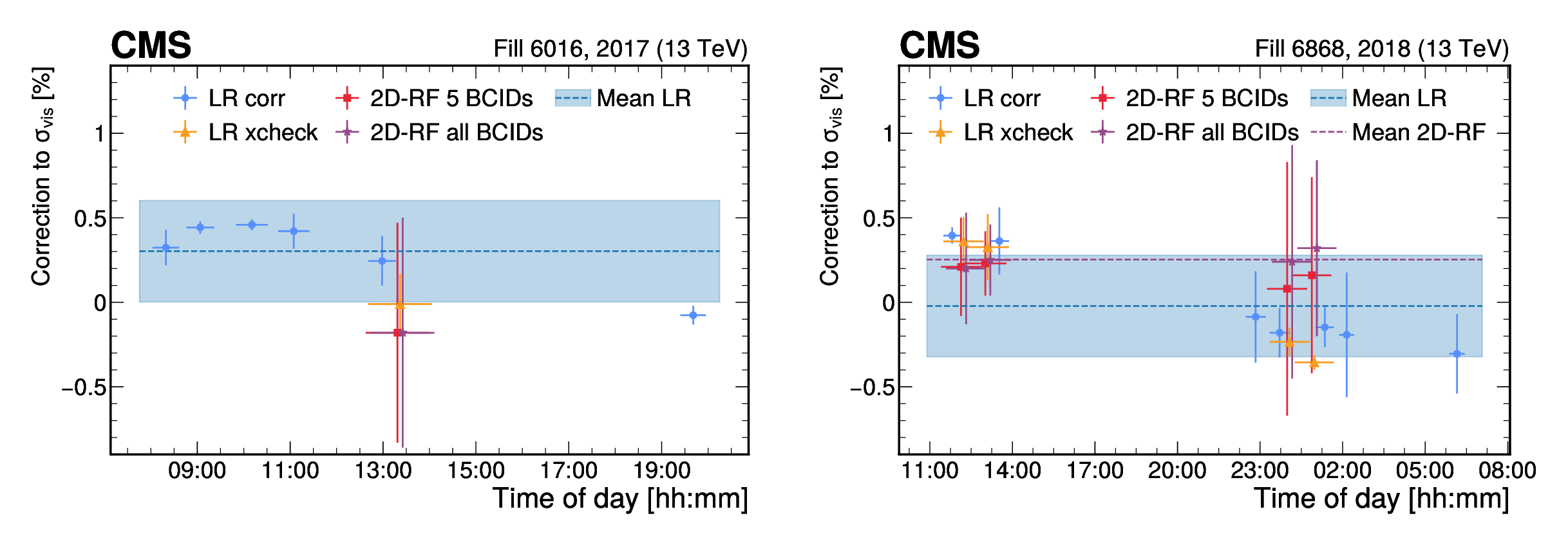
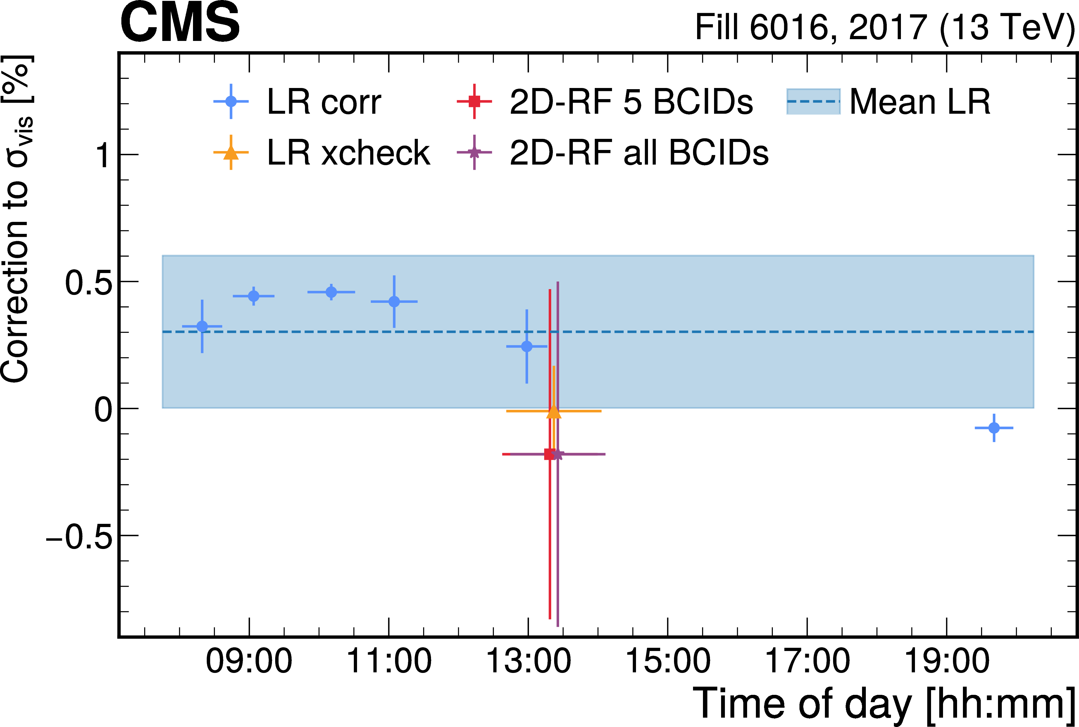
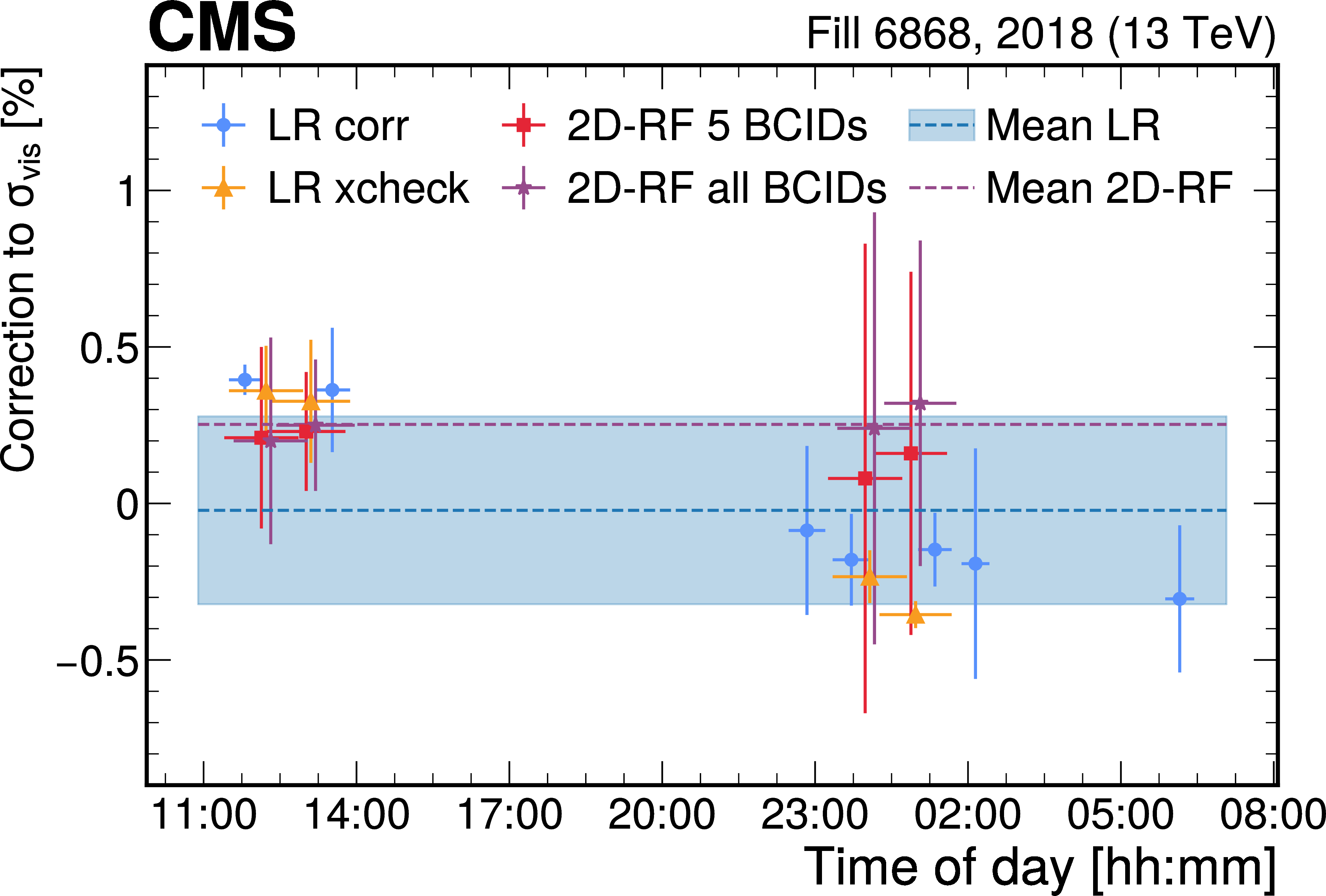
Nonfactorization estimates for 2017 (left) and 2018 (right) using the luminous region (LR) and 2D rate fit (2D-RF) methods. For all markers, the horizontal error bars indicate the time period during which the input data for the fit were collected. For the LR method (blue), both per-scan and average corrections are shown. The vertical error bars correspond to the standard deviation of the BCIDs, while the markers show the average value. The shaded band represents the total uncertainty of the LR method, dominated by the closure uncertainty. The final correction is based on the per-scan LR measurement. The orange markers indicate LR results obtained using the same input scans as the 2D-RF method, i.e., a combination of one on-axis and one off-axis scan pair. The red and green markers show the corrections derived using the 2D-RF method for the five BCIDs used in the LR fit and for all colliding BCIDs, respectively. The vertical error bars on these markers reflect the full uncertainty associated with the 2D-RF method. The difference between the two methods is included in the total factorization uncertainty. |
png pdf |
Figure 8-a:
Nonfactorization estimates for 2017 (left) and 2018 (right) using the luminous region (LR) and 2D rate fit (2D-RF) methods. For all markers, the horizontal error bars indicate the time period during which the input data for the fit were collected. For the LR method (blue), both per-scan and average corrections are shown. The vertical error bars correspond to the standard deviation of the BCIDs, while the markers show the average value. The shaded band represents the total uncertainty of the LR method, dominated by the closure uncertainty. The final correction is based on the per-scan LR measurement. The orange markers indicate LR results obtained using the same input scans as the 2D-RF method, i.e., a combination of one on-axis and one off-axis scan pair. The red and green markers show the corrections derived using the 2D-RF method for the five BCIDs used in the LR fit and for all colliding BCIDs, respectively. The vertical error bars on these markers reflect the full uncertainty associated with the 2D-RF method. The difference between the two methods is included in the total factorization uncertainty. |
png pdf |
Figure 8-b:
Nonfactorization estimates for 2017 (left) and 2018 (right) using the luminous region (LR) and 2D rate fit (2D-RF) methods. For all markers, the horizontal error bars indicate the time period during which the input data for the fit were collected. For the LR method (blue), both per-scan and average corrections are shown. The vertical error bars correspond to the standard deviation of the BCIDs, while the markers show the average value. The shaded band represents the total uncertainty of the LR method, dominated by the closure uncertainty. The final correction is based on the per-scan LR measurement. The orange markers indicate LR results obtained using the same input scans as the 2D-RF method, i.e., a combination of one on-axis and one off-axis scan pair. The red and green markers show the corrections derived using the 2D-RF method for the five BCIDs used in the LR fit and for all colliding BCIDs, respectively. The vertical error bars on these markers reflect the full uncertainty associated with the 2D-RF method. The difference between the two methods is included in the total factorization uncertainty. |
png pdf |
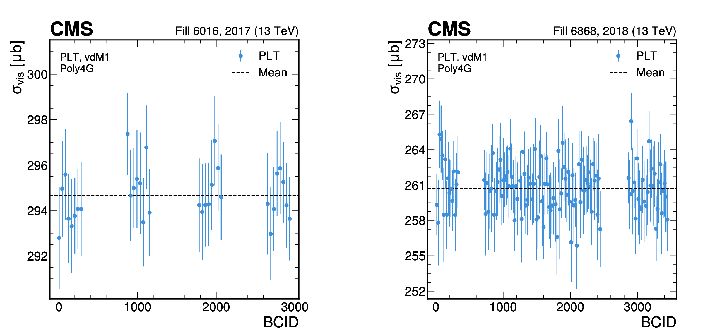
Figure 9:
Per BCID $ \sigma_{\text{vis}} $ values in the first scan in 2017 (left) and 2018 (right) as measured for the PLT luminometer. The error bars represent the uncertainty propagated from the fit. |
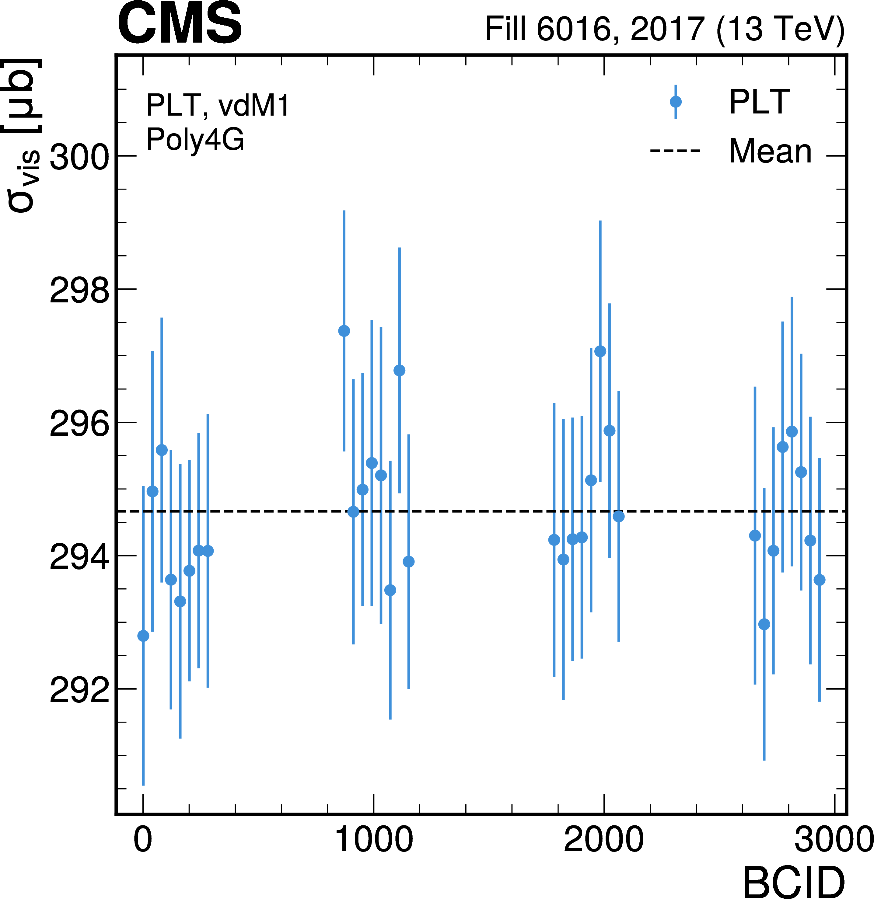
png pdf |
Figure 9-a:
Per BCID $ \sigma_{\text{vis}} $ values in the first scan in 2017 (left) and 2018 (right) as measured for the PLT luminometer. The error bars represent the uncertainty propagated from the fit. |
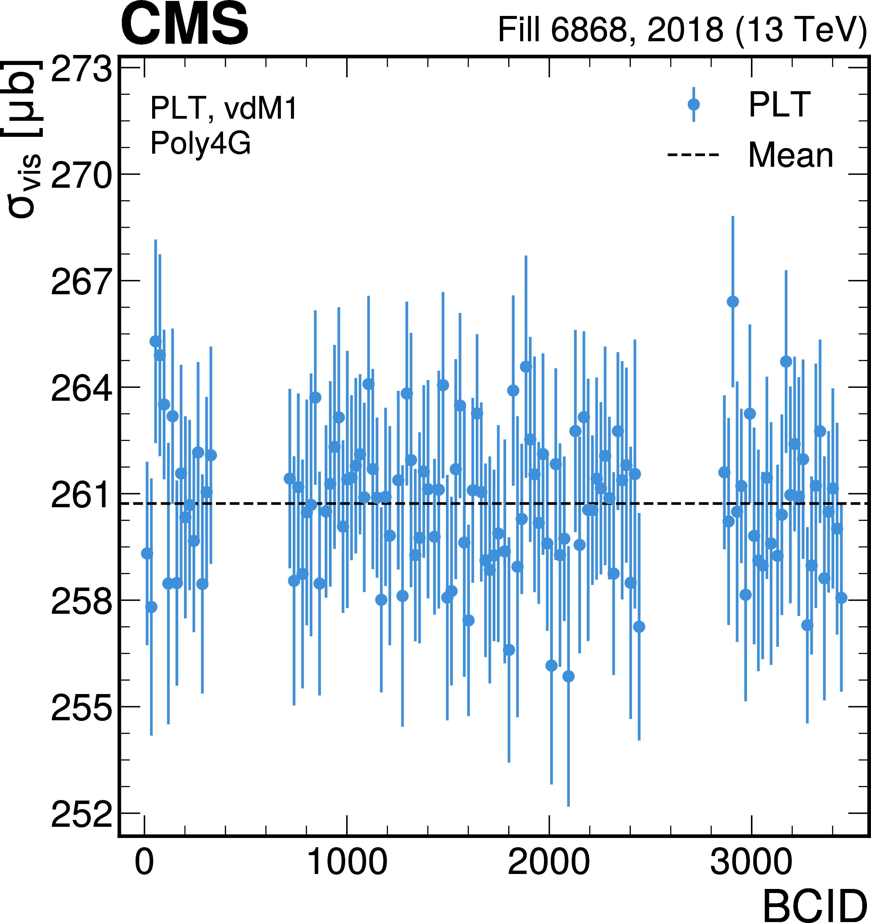
png pdf |
Figure 9-b:
Per BCID $ \sigma_{\text{vis}} $ values in the first scan in 2017 (left) and 2018 (right) as measured for the PLT luminometer. The error bars represent the uncertainty propagated from the fit. |
png pdf |
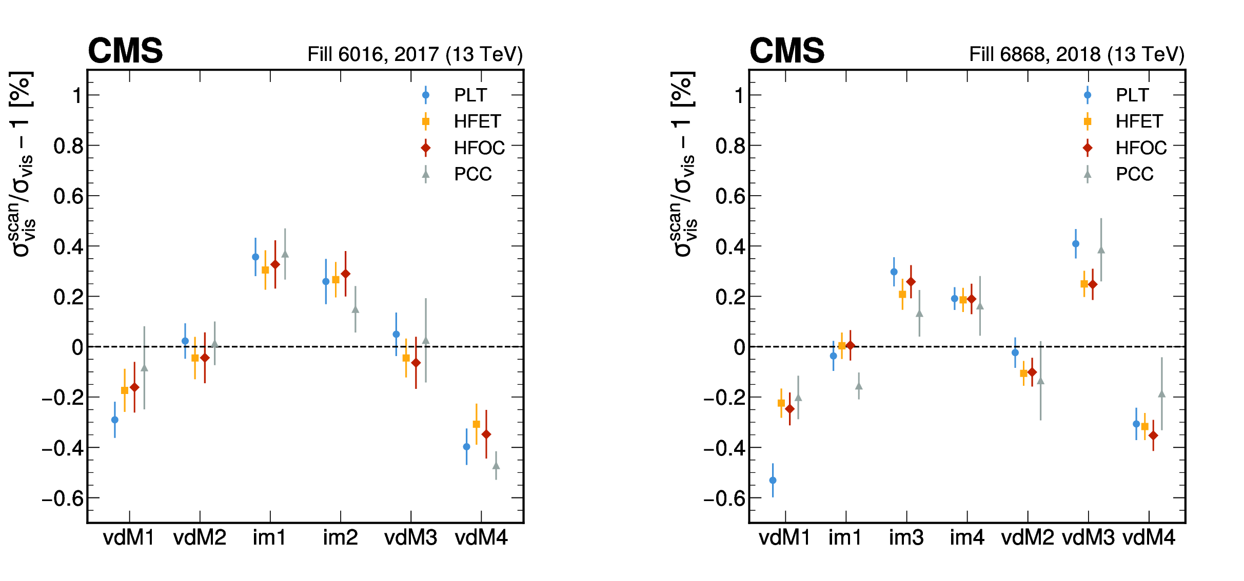
Figure 10:
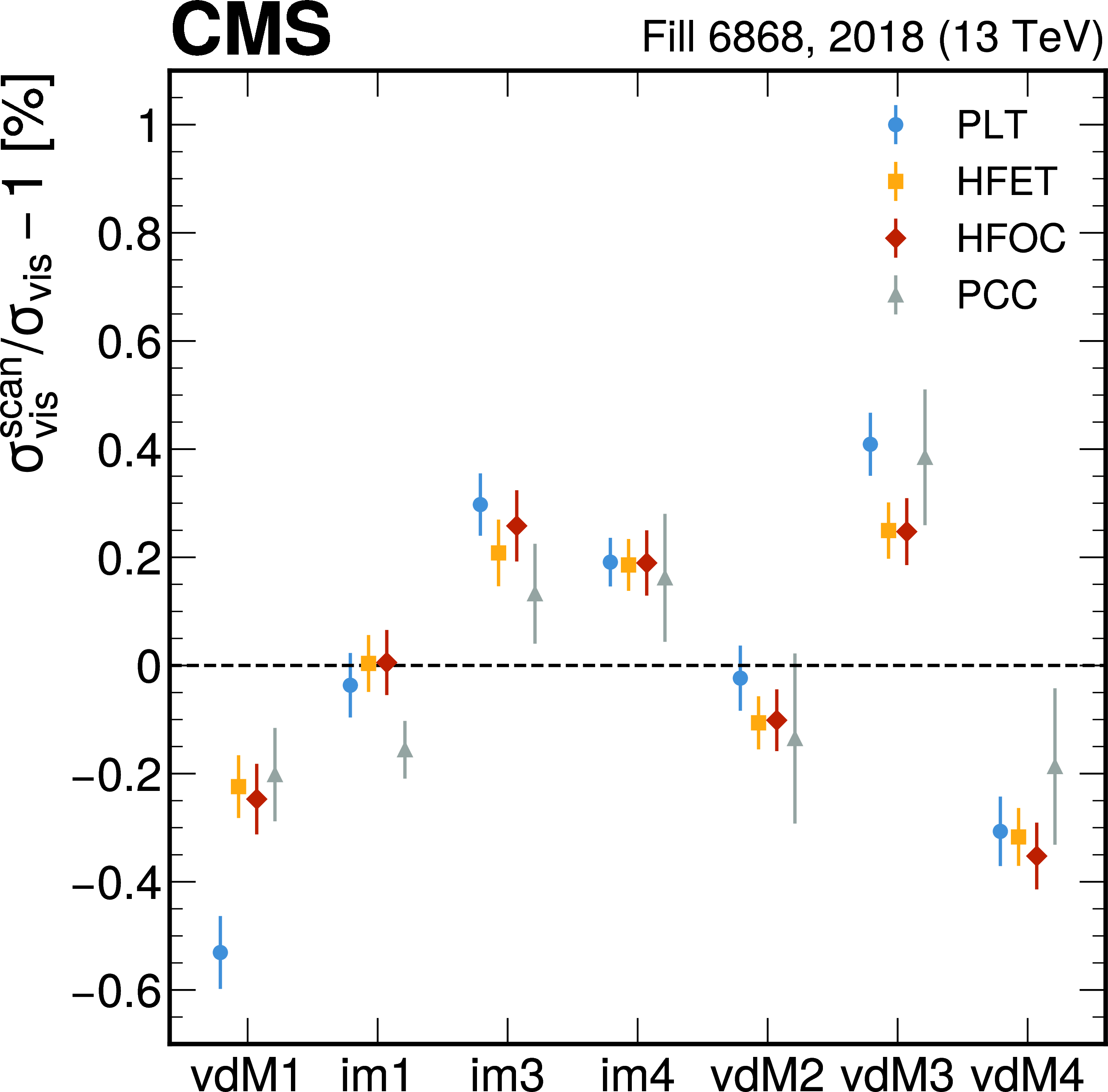
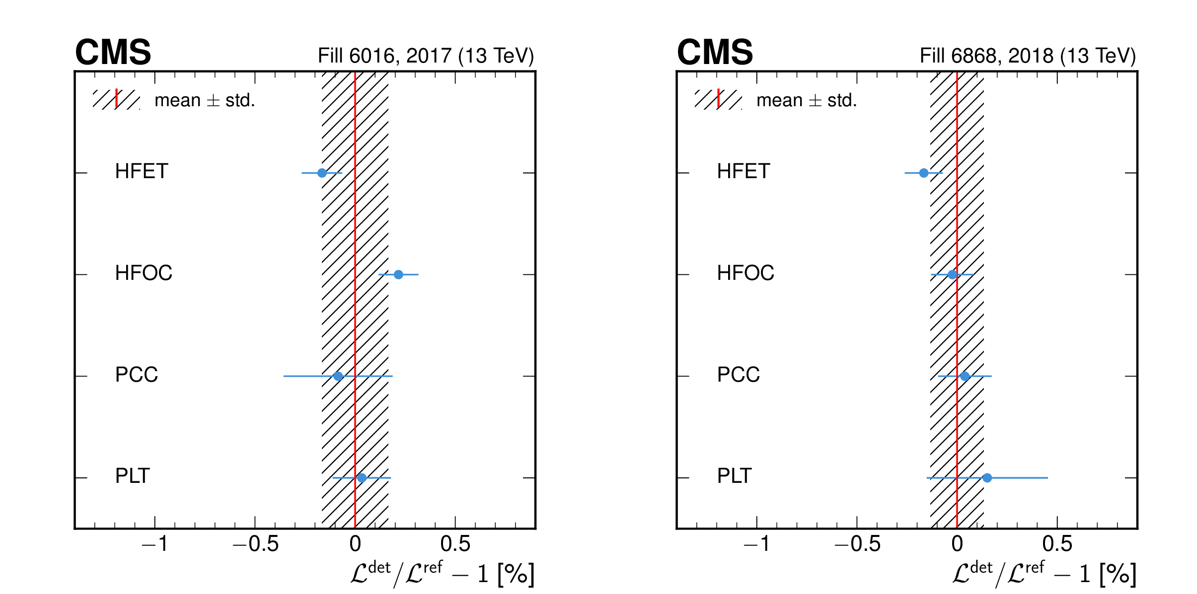
The relative deviation of the BCID-averaged $ \sigma_{\text{vis}} $ values divided by the average value taken over all scans for all independently calibrated detectors and all scans using the Poly4G fit function in 2017 (left) and 2018 (right). The error bars signify the standard deviation over the BCIDs divided by the square root of the number of BCIDs. |
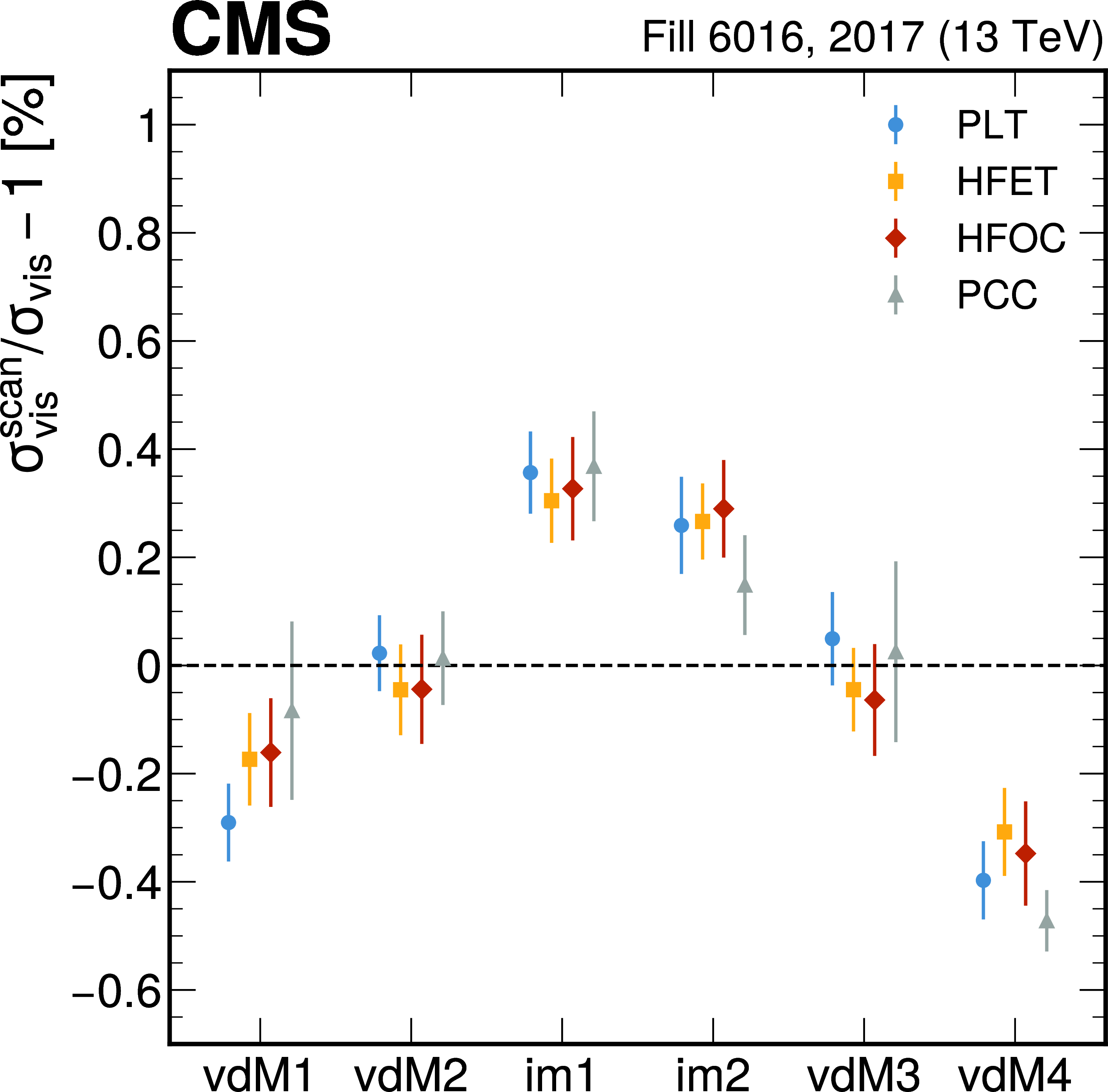
png pdf |
Figure 10-a:
The relative deviation of the BCID-averaged $ \sigma_{\text{vis}} $ values divided by the average value taken over all scans for all independently calibrated detectors and all scans using the Poly4G fit function in 2017 (left) and 2018 (right). The error bars signify the standard deviation over the BCIDs divided by the square root of the number of BCIDs. |
png pdf |
Figure 10-b:
The relative deviation of the BCID-averaged $ \sigma_{\text{vis}} $ values divided by the average value taken over all scans for all independently calibrated detectors and all scans using the Poly4G fit function in 2017 (left) and 2018 (right). The error bars signify the standard deviation over the BCIDs divided by the square root of the number of BCIDs. |
png pdf |
Figure 11:
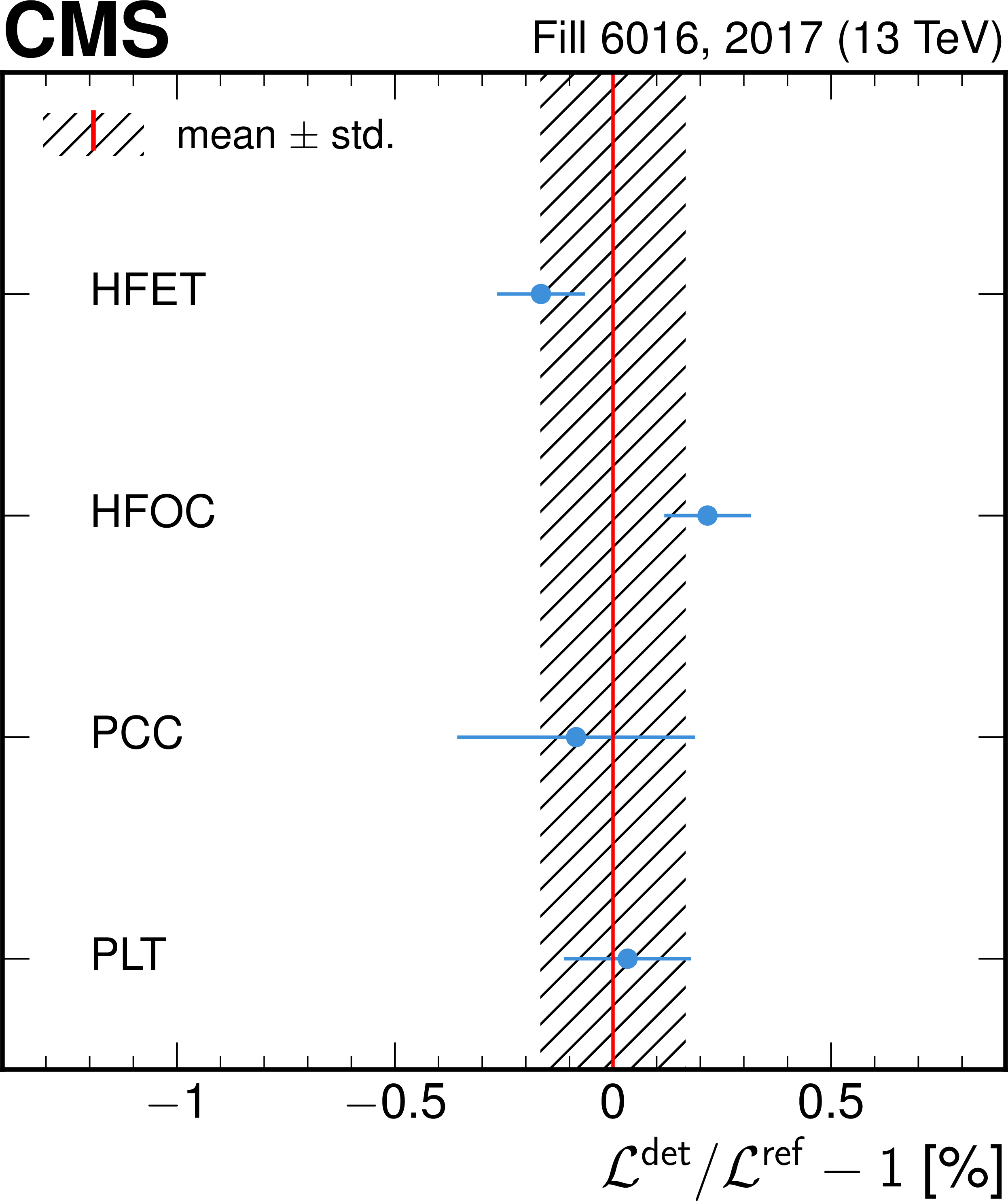
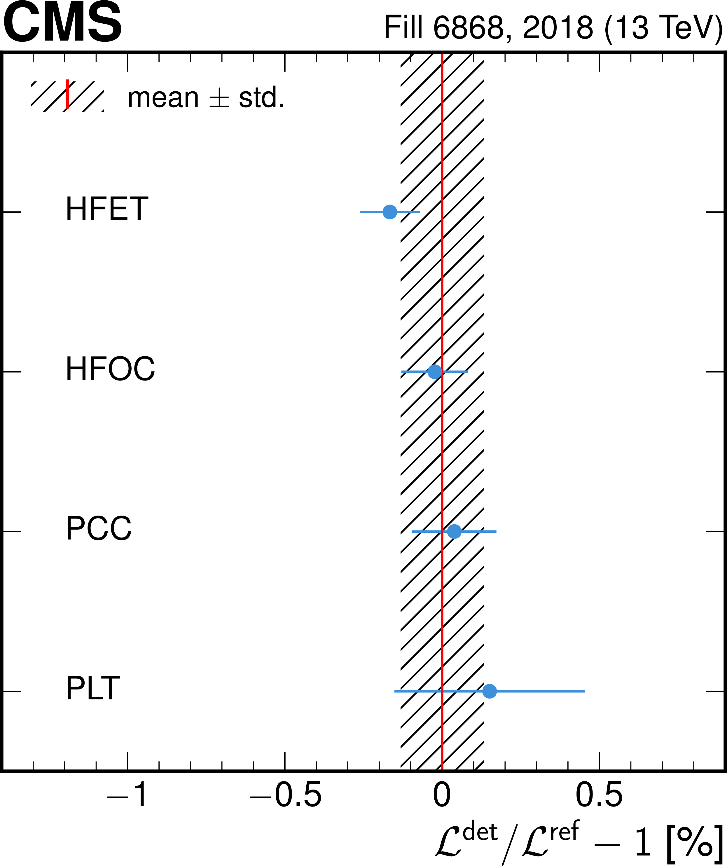
Relative differences of the luminosity measured by the HFET, HFOC, PLT, and PCC detectors to the detector-averaged luminosity in the vdM fill for the head-on periods for 2017 (left) and 2018 (right). The markers represent the average of ratios computed in approximately three-minute intervals, while the error bars indicate the standard deviation of the ratio distribution. The shaded area corresponds to the standard deviation of the individual averages. |
png pdf |
Figure 11-a:
Relative differences of the luminosity measured by the HFET, HFOC, PLT, and PCC detectors to the detector-averaged luminosity in the vdM fill for the head-on periods for 2017 (left) and 2018 (right). The markers represent the average of ratios computed in approximately three-minute intervals, while the error bars indicate the standard deviation of the ratio distribution. The shaded area corresponds to the standard deviation of the individual averages. |
png pdf |
Figure 11-b:
Relative differences of the luminosity measured by the HFET, HFOC, PLT, and PCC detectors to the detector-averaged luminosity in the vdM fill for the head-on periods for 2017 (left) and 2018 (right). The markers represent the average of ratios computed in approximately three-minute intervals, while the error bars indicate the standard deviation of the ratio distribution. The shaded area corresponds to the standard deviation of the individual averages. |
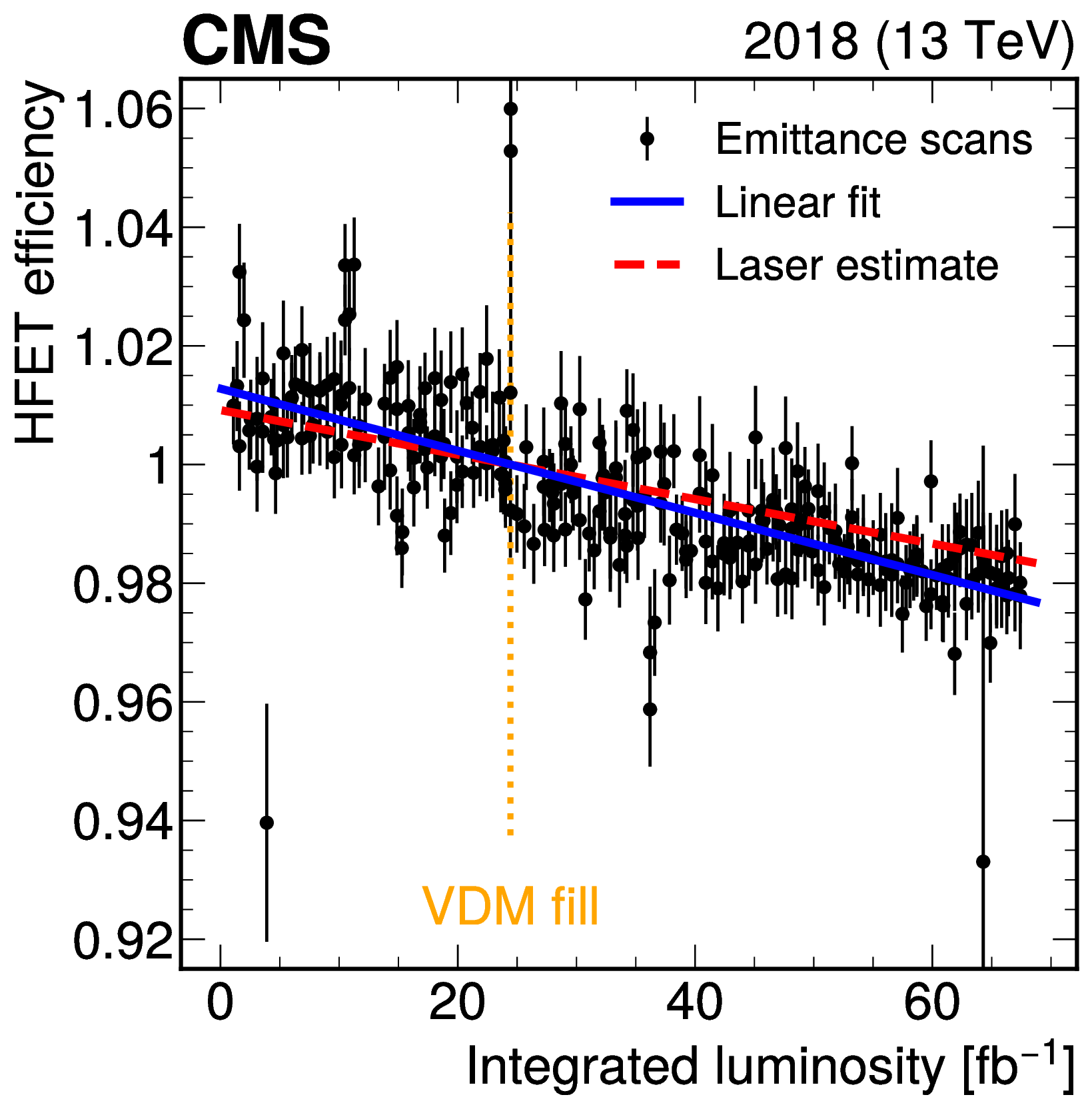
png pdf |
Figure 12:
The decrease in efficiency as a consequence of HFET aging in 2018 as measured using emittance scans. The black points represent the efficiency of the HFET counting method relative to the efficiency at the time of the vdM scan (indicated by the vertical orange line), as a function of the total integrated luminosity in 2018. Significant outliers were examined for potential fit quality problems, however, none were identified. The uncertainties shown are the standard deviations computed over the BCIDs. The blue line is a linear fit to the data. The expected aging from laser calibration monitoring of the fibers and photomultipliers is indicated by a red line and shows a good agreement with the emittance scan data. |
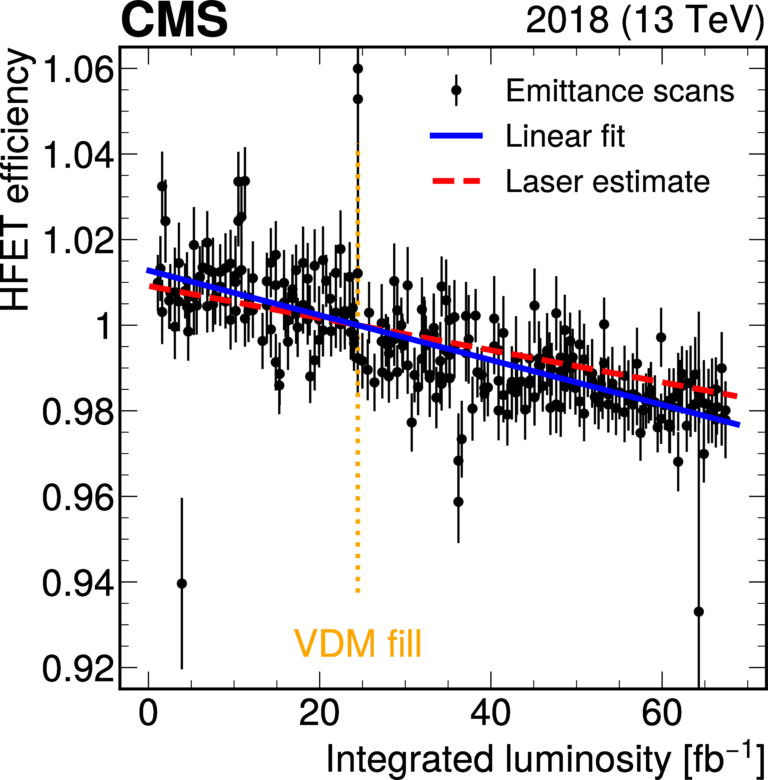
png pdf |
Figure 12-a:
The decrease in efficiency as a consequence of HFET aging in 2018 as measured using emittance scans. The black points represent the efficiency of the HFET counting method relative to the efficiency at the time of the vdM scan (indicated by the vertical orange line), as a function of the total integrated luminosity in 2018. Significant outliers were examined for potential fit quality problems, however, none were identified. The uncertainties shown are the standard deviations computed over the BCIDs. The blue line is a linear fit to the data. The expected aging from laser calibration monitoring of the fibers and photomultipliers is indicated by a red line and shows a good agreement with the emittance scan data. |
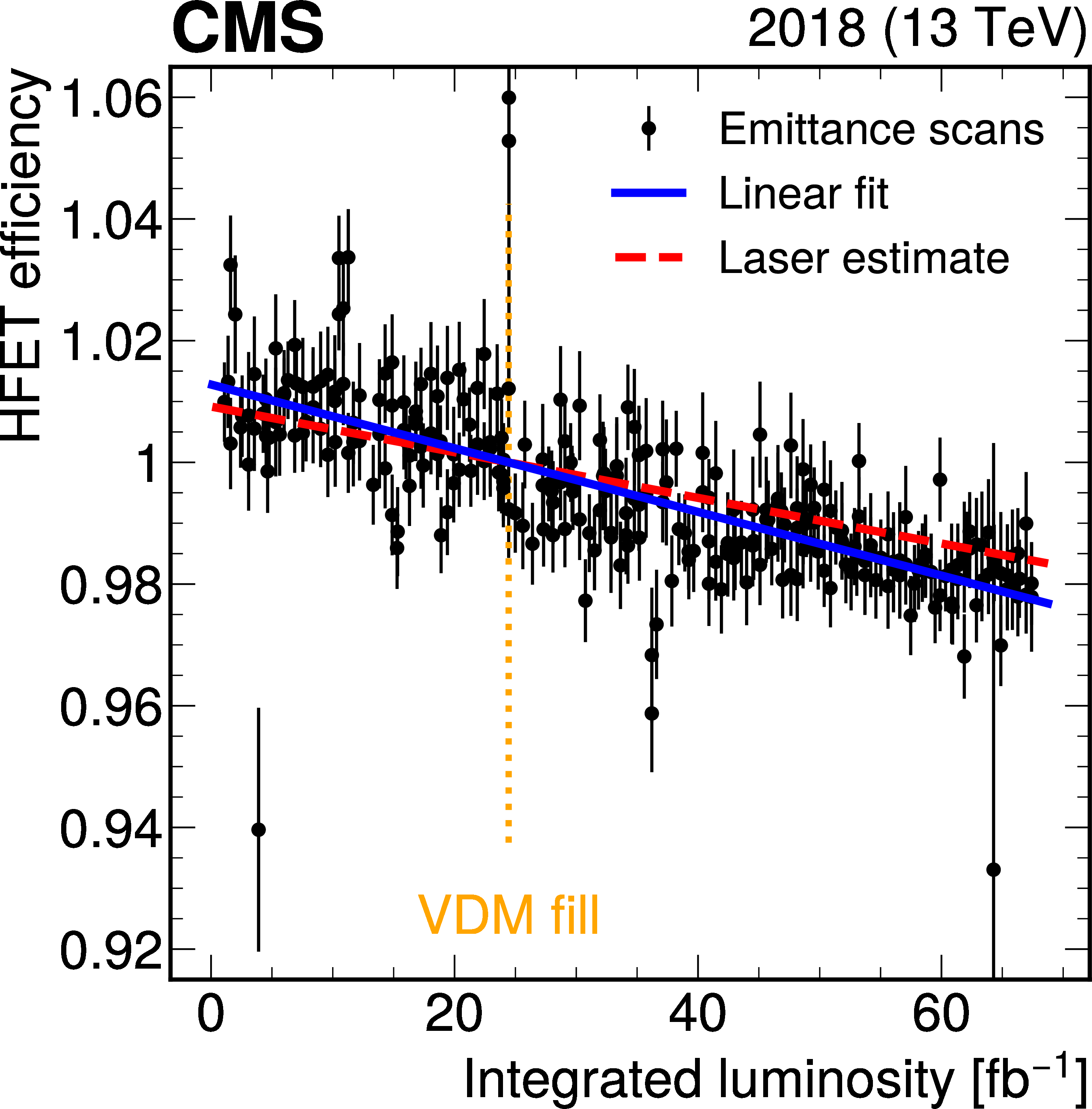
png pdf |
Figure 12-b:
The decrease in efficiency as a consequence of HFET aging in 2018 as measured using emittance scans. The black points represent the efficiency of the HFET counting method relative to the efficiency at the time of the vdM scan (indicated by the vertical orange line), as a function of the total integrated luminosity in 2018. Significant outliers were examined for potential fit quality problems, however, none were identified. The uncertainties shown are the standard deviations computed over the BCIDs. The blue line is a linear fit to the data. The expected aging from laser calibration monitoring of the fibers and photomultipliers is indicated by a red line and shows a good agreement with the emittance scan data. |
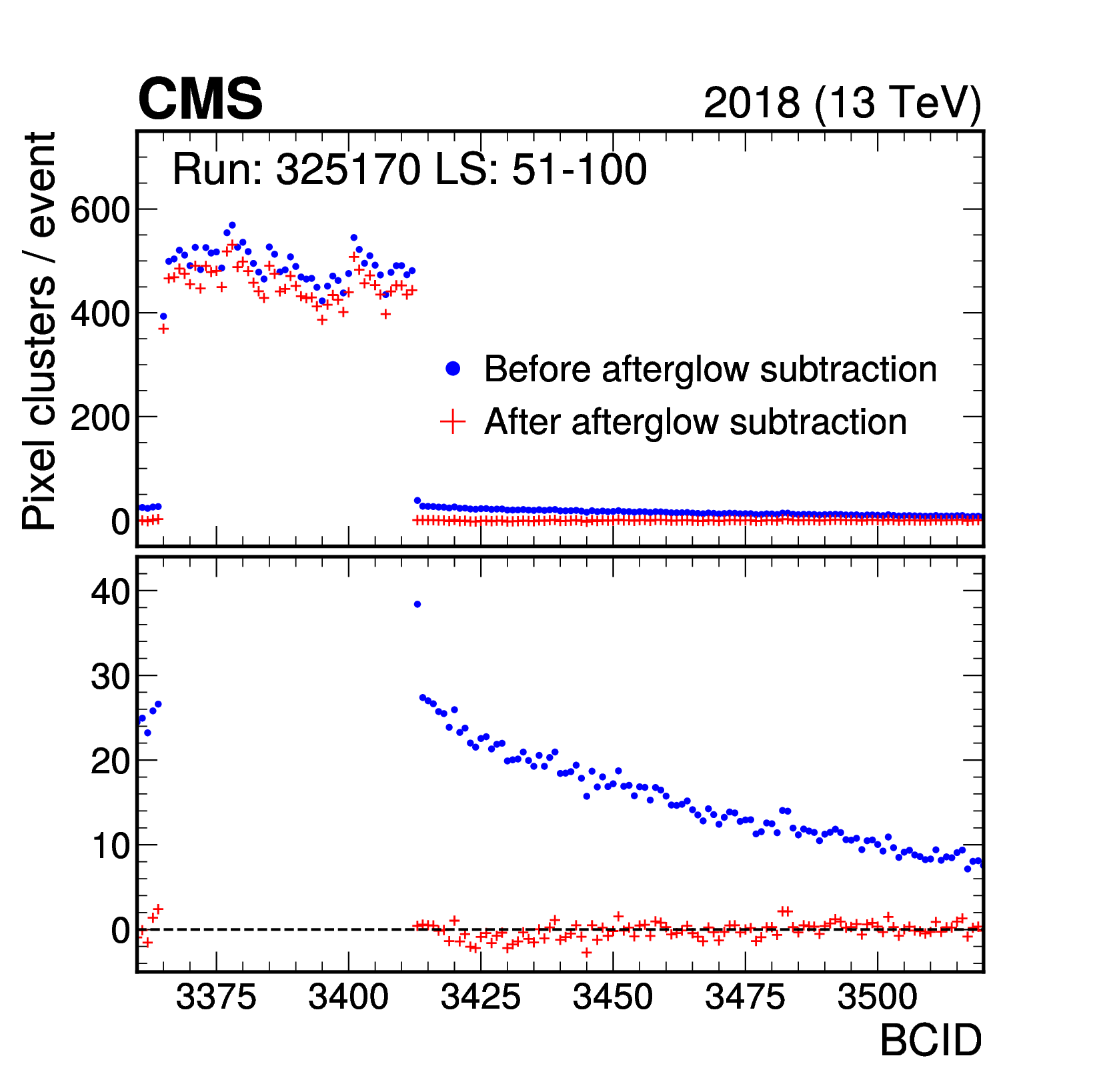
png pdf |
Figure 13:
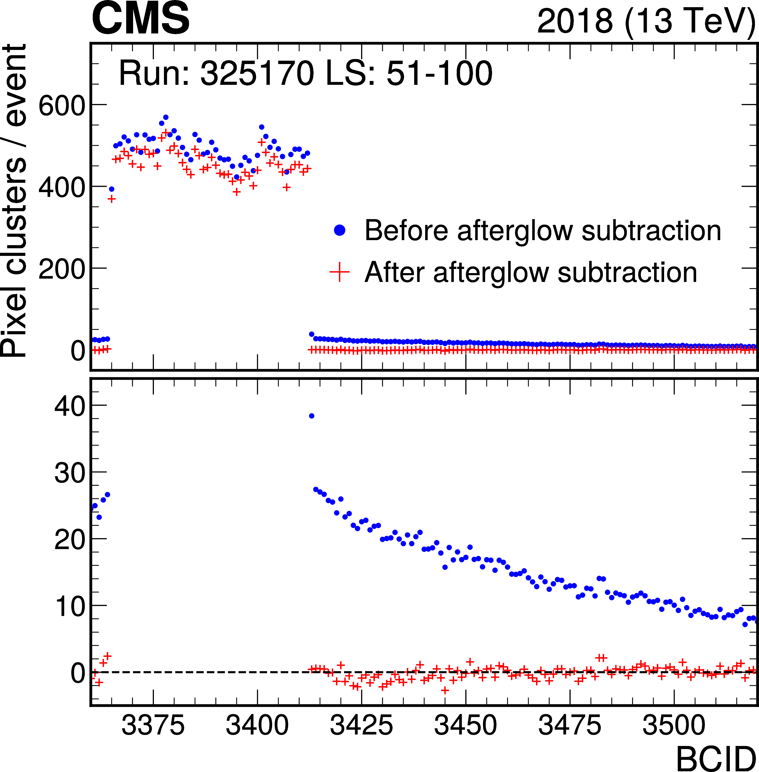
The number of clusters in the pixel tracker per event is shown as a function of the BCID for the last bunch train of the orbit. Blue points represent the values before correction, while red crosses indicate the results after applying out-of-time corrections. The upper panel displays the full count range, encompassing both colliding and empty BCIDs, while the lower panel focuses on empty bunch crossings with a different scale for improved visibility. In the lower panel, the red crosses, representing the residual rate, are close to zero, demonstrating the excellent performance of the correction. |
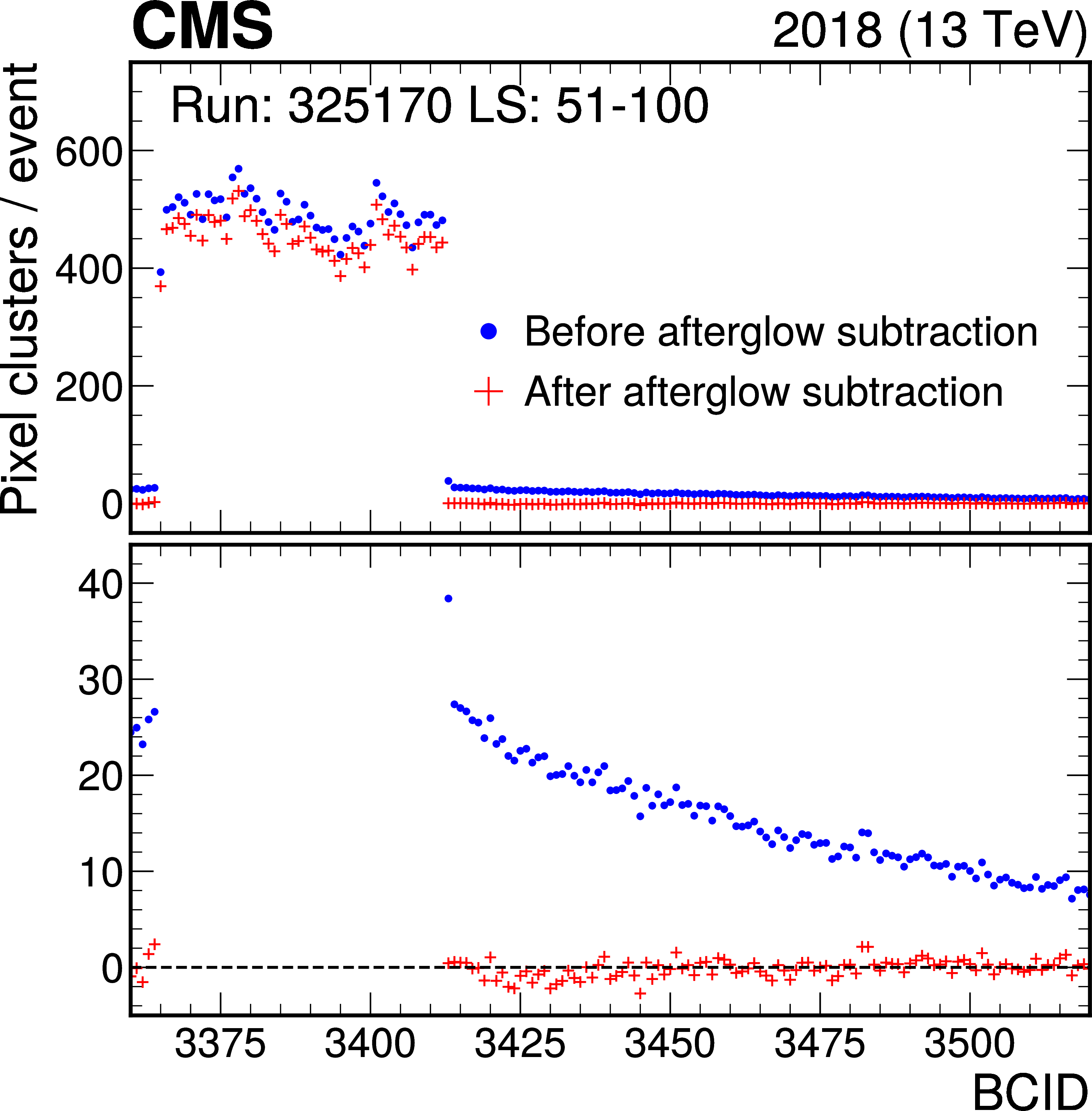
png pdf |
Figure 13-a:
The number of clusters in the pixel tracker per event is shown as a function of the BCID for the last bunch train of the orbit. Blue points represent the values before correction, while red crosses indicate the results after applying out-of-time corrections. The upper panel displays the full count range, encompassing both colliding and empty BCIDs, while the lower panel focuses on empty bunch crossings with a different scale for improved visibility. In the lower panel, the red crosses, representing the residual rate, are close to zero, demonstrating the excellent performance of the correction. |
png pdf |
Figure 13-b:
The number of clusters in the pixel tracker per event is shown as a function of the BCID for the last bunch train of the orbit. Blue points represent the values before correction, while red crosses indicate the results after applying out-of-time corrections. The upper panel displays the full count range, encompassing both colliding and empty BCIDs, while the lower panel focuses on empty bunch crossings with a different scale for improved visibility. In the lower panel, the red crosses, representing the residual rate, are close to zero, demonstrating the excellent performance of the correction. |
png pdf |
Figure 14:
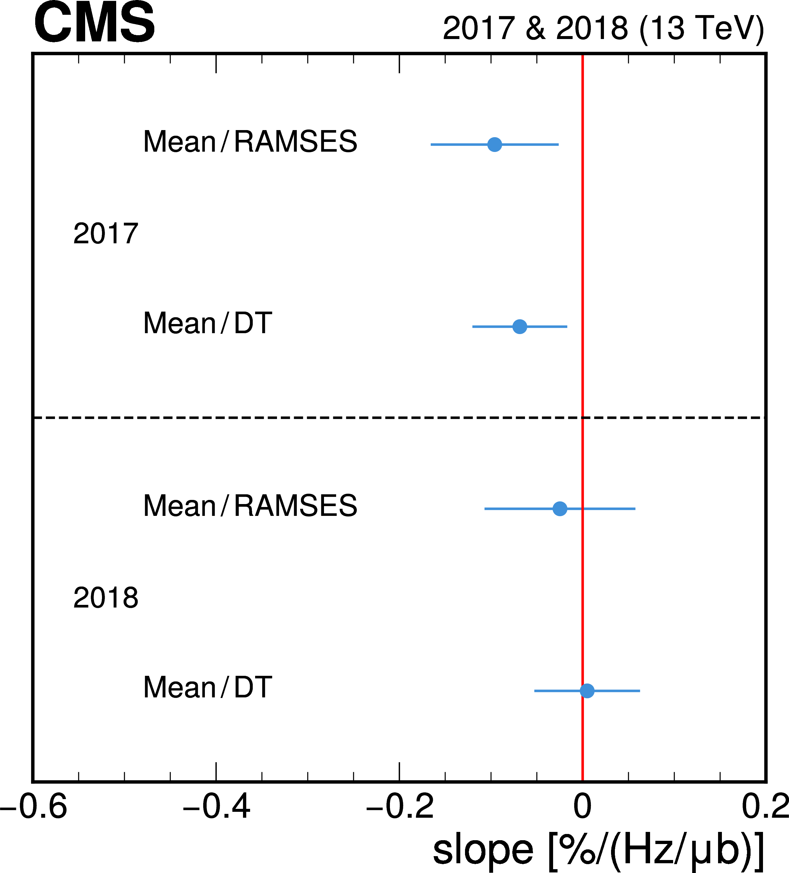
The luminosity-weighted average of the measured residual nonlinearity between the mean luminosity and DT or RAMSES for 2017 and 2018. The error bars signify the weighted standard deviation over the individual fills. |
png pdf |
Figure 15:
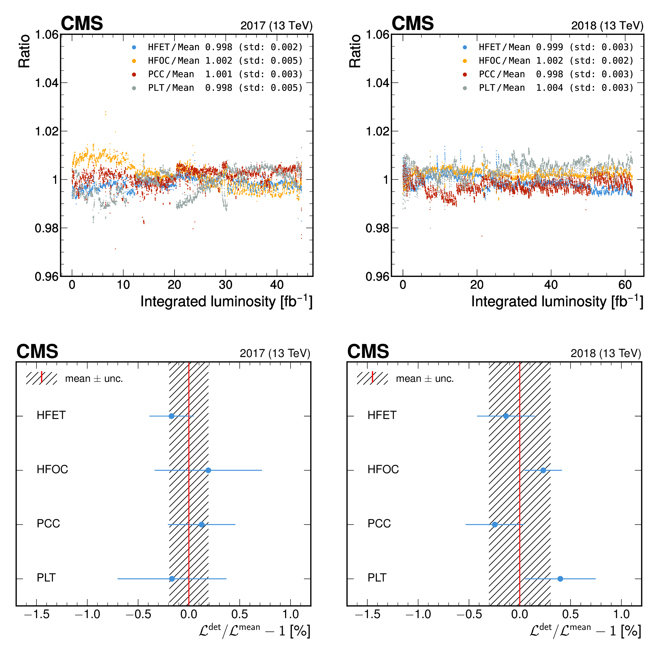
The ratio of the luminosity measured by HFET, HFOC, PLT, and PCC to their mean per 20-minute blocks for 2017 (left) and 2018 (right). The upper row shows the ratio as a function of integrated luminosity, while the lower row displays the luminosity-weighted average of the ratios. The error bars signify the weighted standard deviation over the 20-minute units. The striped area represents the unweighted standard deviation of the four average ratio values. |
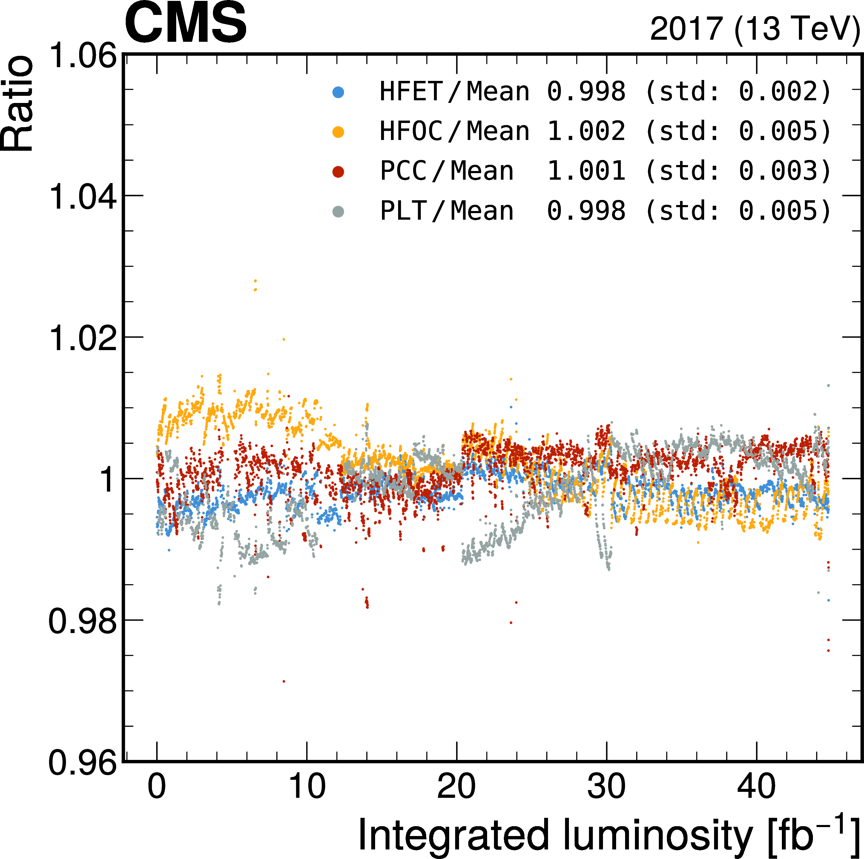
png pdf |
Figure 15-a:
The ratio of the luminosity measured by HFET, HFOC, PLT, and PCC to their mean per 20-minute blocks for 2017 (left) and 2018 (right). The upper row shows the ratio as a function of integrated luminosity, while the lower row displays the luminosity-weighted average of the ratios. The error bars signify the weighted standard deviation over the 20-minute units. The striped area represents the unweighted standard deviation of the four average ratio values. |
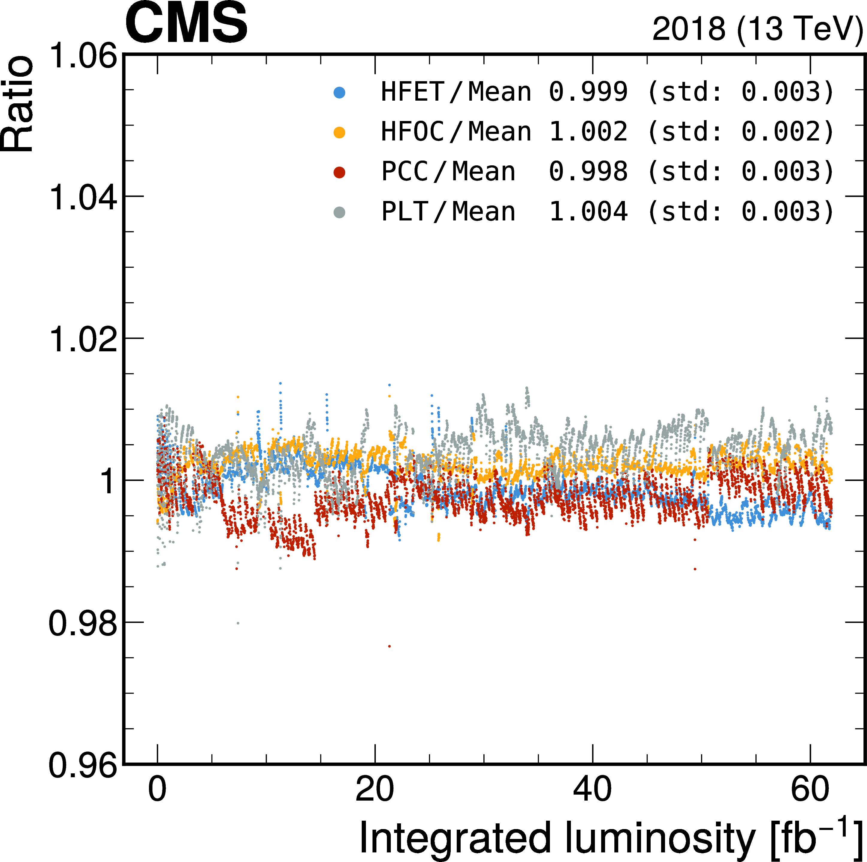
png pdf |
Figure 15-b:
The ratio of the luminosity measured by HFET, HFOC, PLT, and PCC to their mean per 20-minute blocks for 2017 (left) and 2018 (right). The upper row shows the ratio as a function of integrated luminosity, while the lower row displays the luminosity-weighted average of the ratios. The error bars signify the weighted standard deviation over the 20-minute units. The striped area represents the unweighted standard deviation of the four average ratio values. |
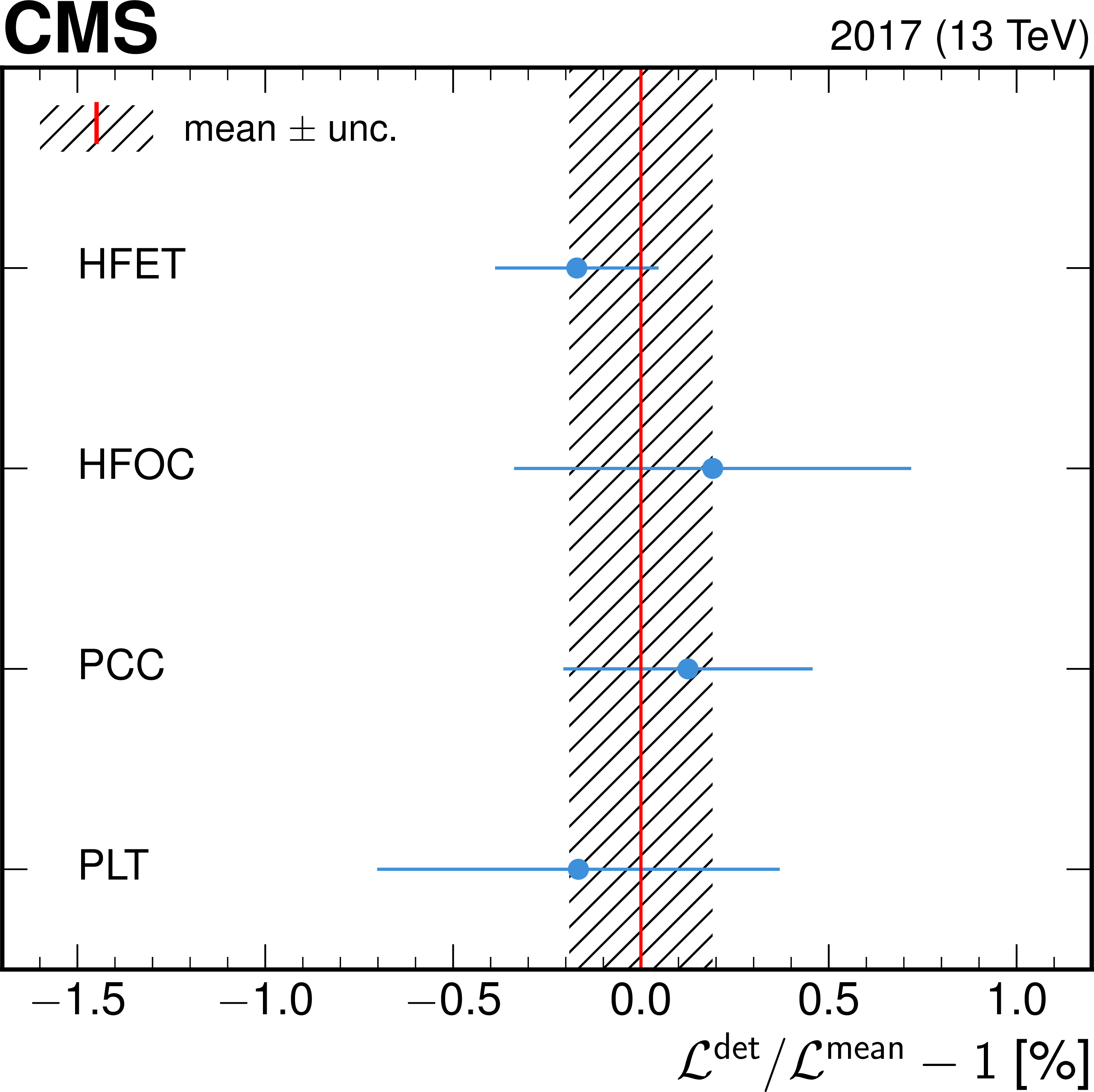
png pdf |
Figure 15-c:
The ratio of the luminosity measured by HFET, HFOC, PLT, and PCC to their mean per 20-minute blocks for 2017 (left) and 2018 (right). The upper row shows the ratio as a function of integrated luminosity, while the lower row displays the luminosity-weighted average of the ratios. The error bars signify the weighted standard deviation over the 20-minute units. The striped area represents the unweighted standard deviation of the four average ratio values. |
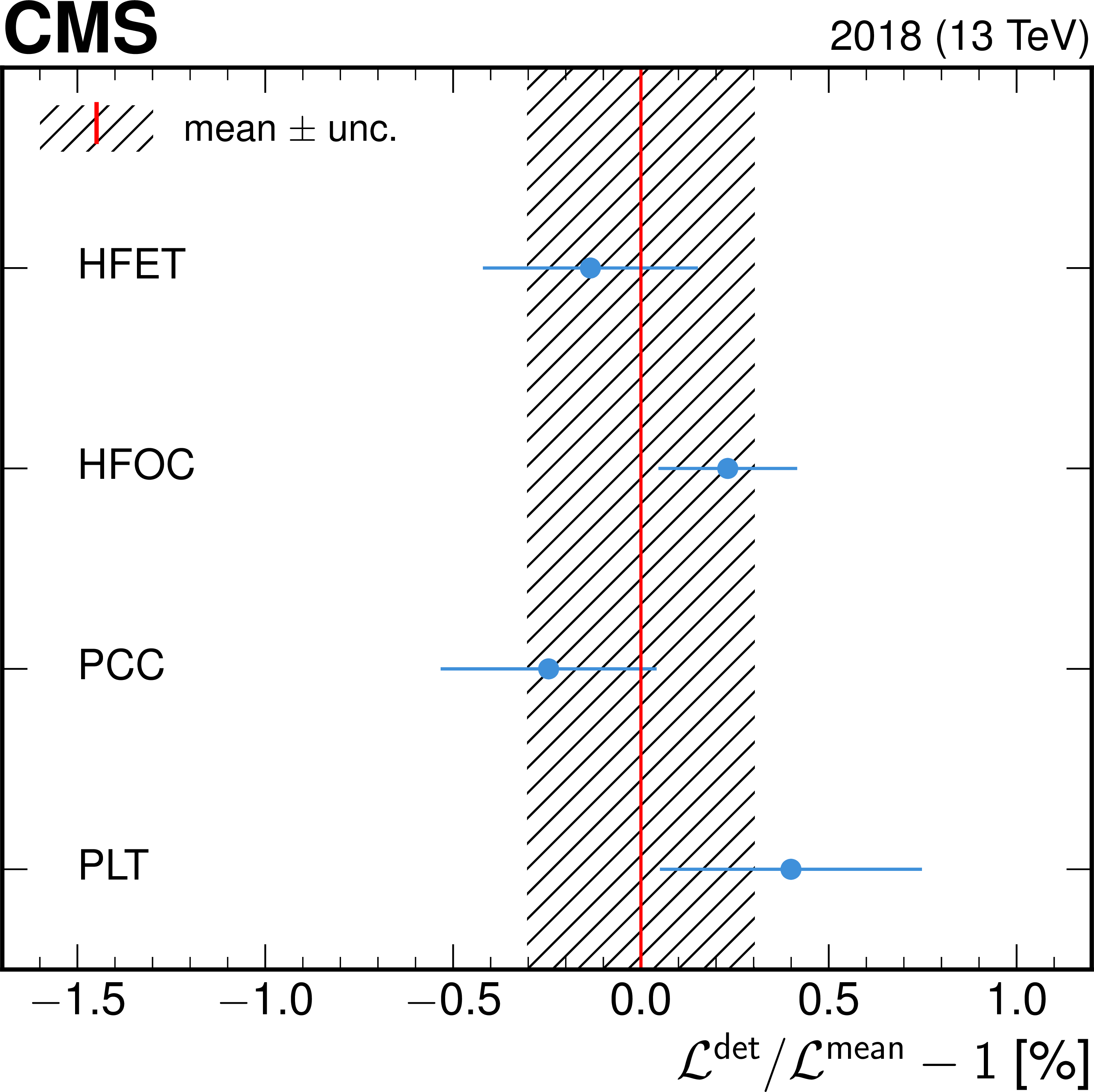
png pdf |
Figure 15-d:
The ratio of the luminosity measured by HFET, HFOC, PLT, and PCC to their mean per 20-minute blocks for 2017 (left) and 2018 (right). The upper row shows the ratio as a function of integrated luminosity, while the lower row displays the luminosity-weighted average of the ratios. The error bars signify the weighted standard deviation over the 20-minute units. The striped area represents the unweighted standard deviation of the four average ratio values. |
png pdf |
Figure 16:
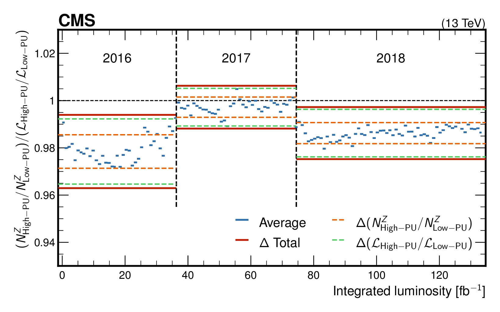
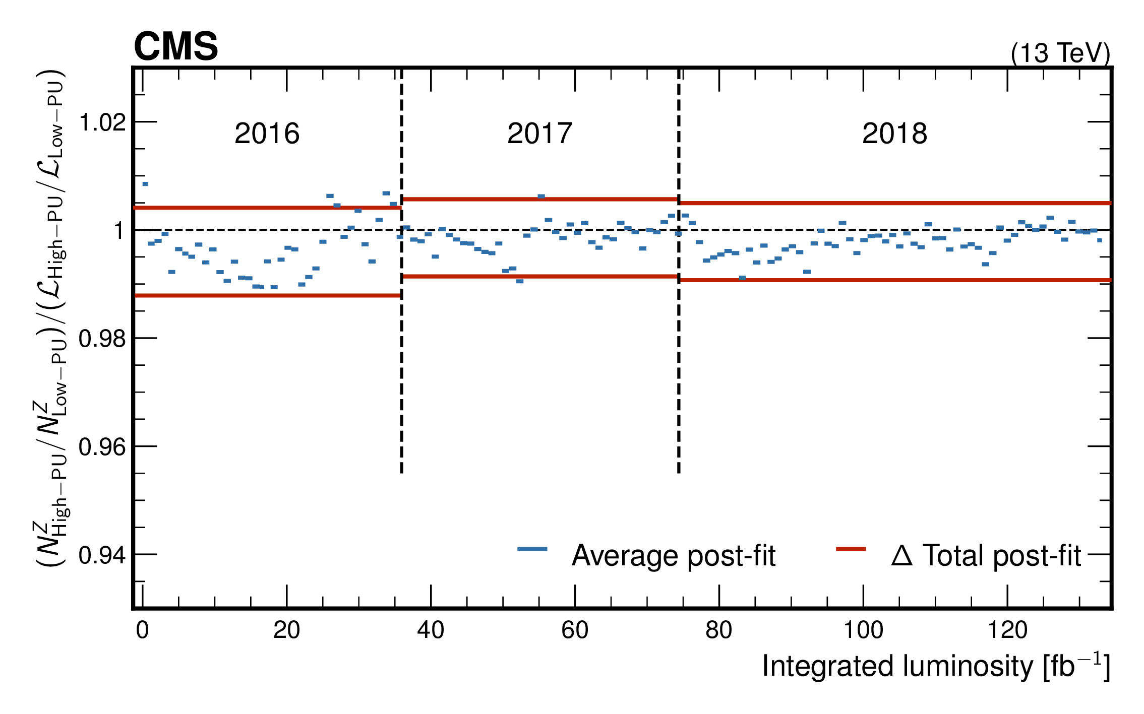
The luminosity as determined by Z boson production rates divided by the reference luminosity as a function of the reference integrated luminosity for the 2016--2018 high-PU data set. Each blue line section corresponds to the luminosity values measured in about 1 fb$ ^{-1} $ of data, used for the measurement of $ N^\mathrm{Z} $. The green and orange dashed lines indicate the uncertainties from the $ N^\mathrm{Z} $ ratio and reference luminosity ratios, respectively, for each year of data taking. Accordingly, the red lines indicate the total uncertainty in the double ratio. The vertical dashed lines separate the 2016, 2017, and 2018 data. |
png pdf |
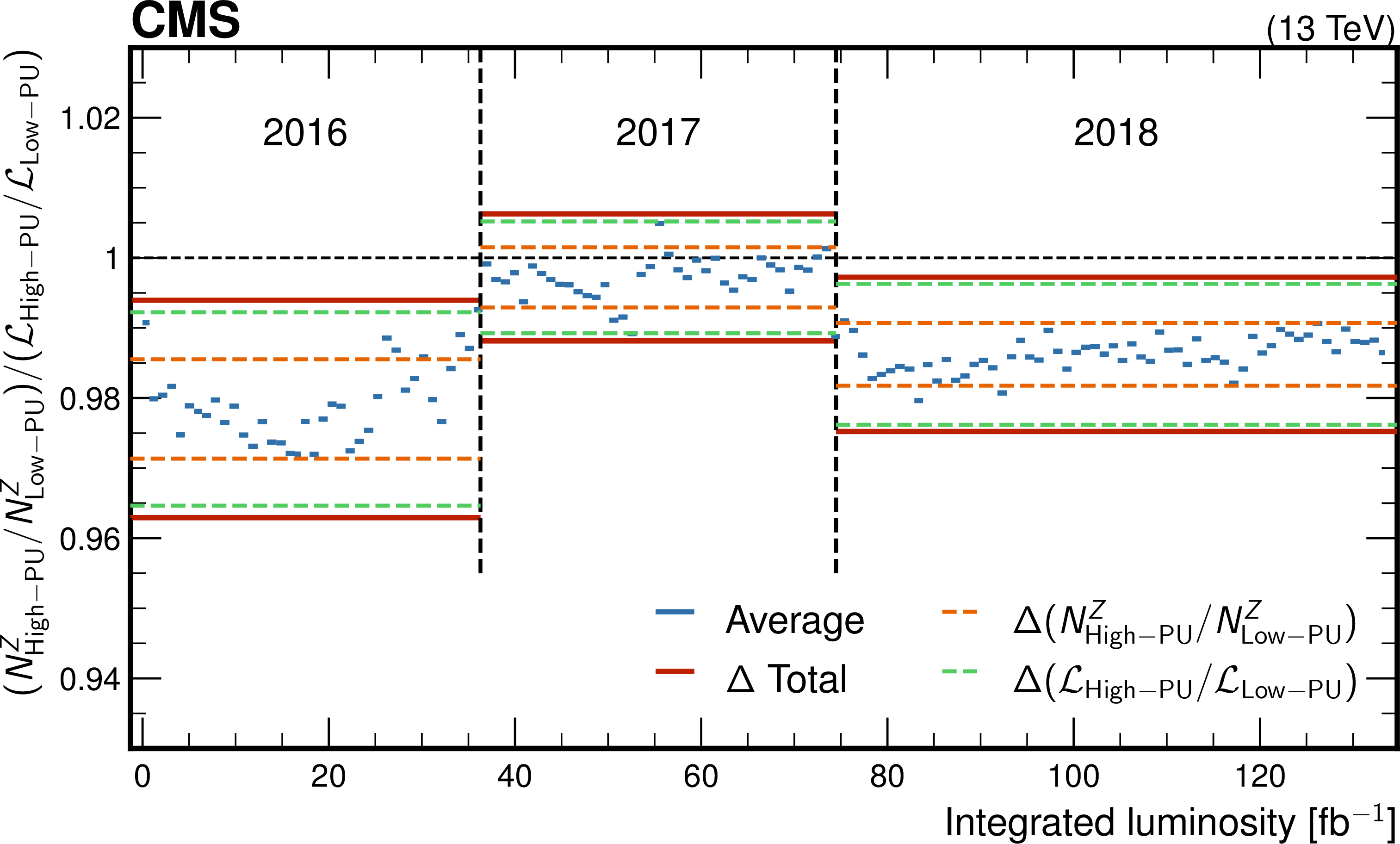
Figure 16-a:
The luminosity as determined by Z boson production rates divided by the reference luminosity as a function of the reference integrated luminosity for the 2016--2018 high-PU data set. Each blue line section corresponds to the luminosity values measured in about 1 fb$ ^{-1} $ of data, used for the measurement of $ N^\mathrm{Z} $. The green and orange dashed lines indicate the uncertainties from the $ N^\mathrm{Z} $ ratio and reference luminosity ratios, respectively, for each year of data taking. Accordingly, the red lines indicate the total uncertainty in the double ratio. The vertical dashed lines separate the 2016, 2017, and 2018 data. |
png pdf |
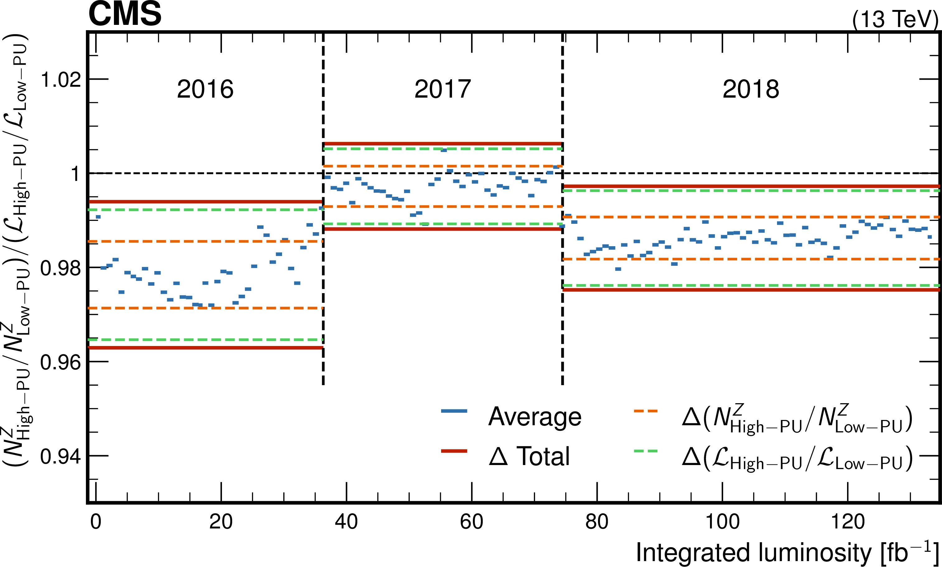
Figure 16-b:
The luminosity as determined by Z boson production rates divided by the reference luminosity as a function of the reference integrated luminosity for the 2016--2018 high-PU data set. Each blue line section corresponds to the luminosity values measured in about 1 fb$ ^{-1} $ of data, used for the measurement of $ N^\mathrm{Z} $. The green and orange dashed lines indicate the uncertainties from the $ N^\mathrm{Z} $ ratio and reference luminosity ratios, respectively, for each year of data taking. Accordingly, the red lines indicate the total uncertainty in the double ratio. The vertical dashed lines separate the 2016, 2017, and 2018 data. |
png pdf |
Figure 17:
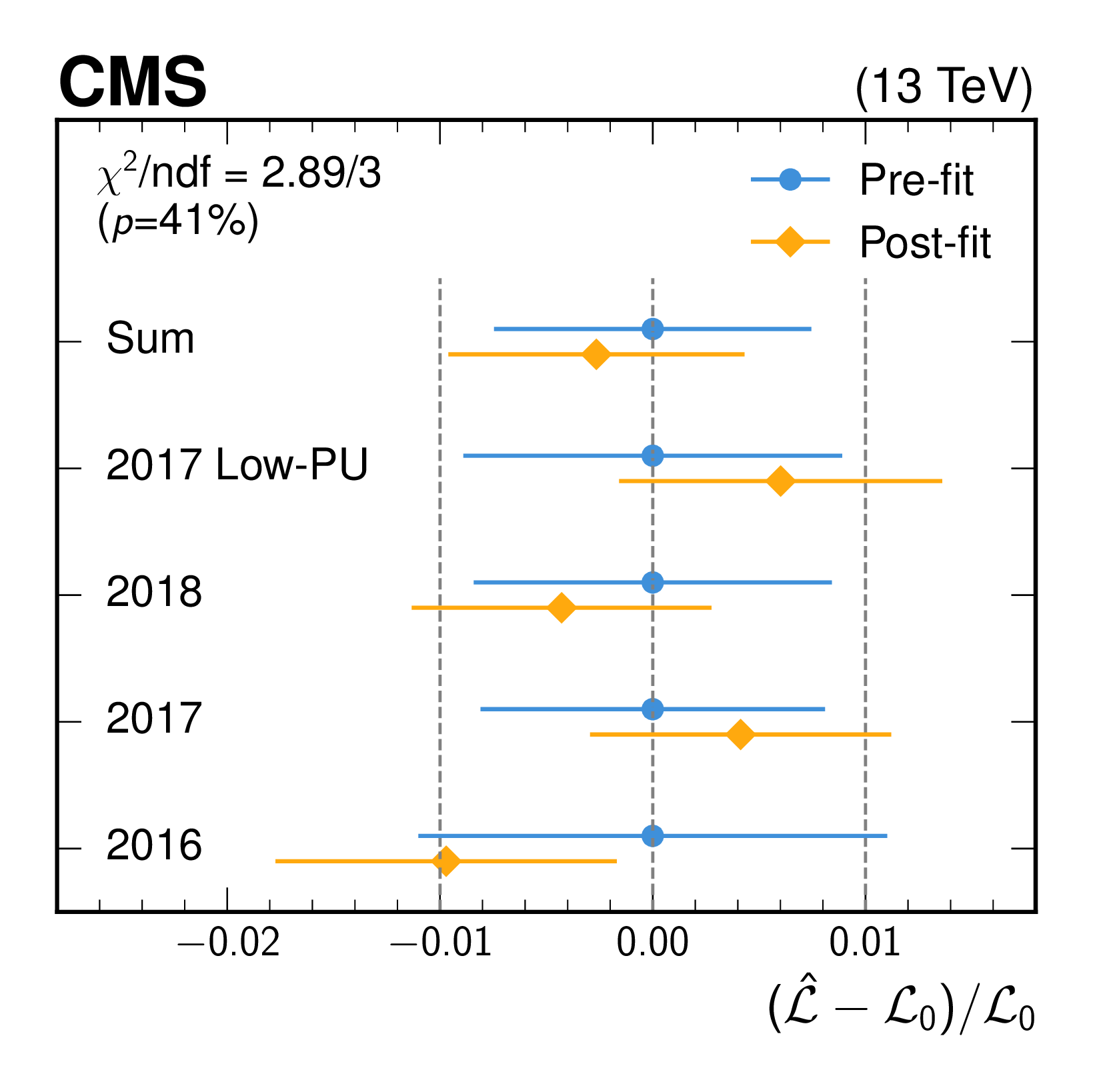
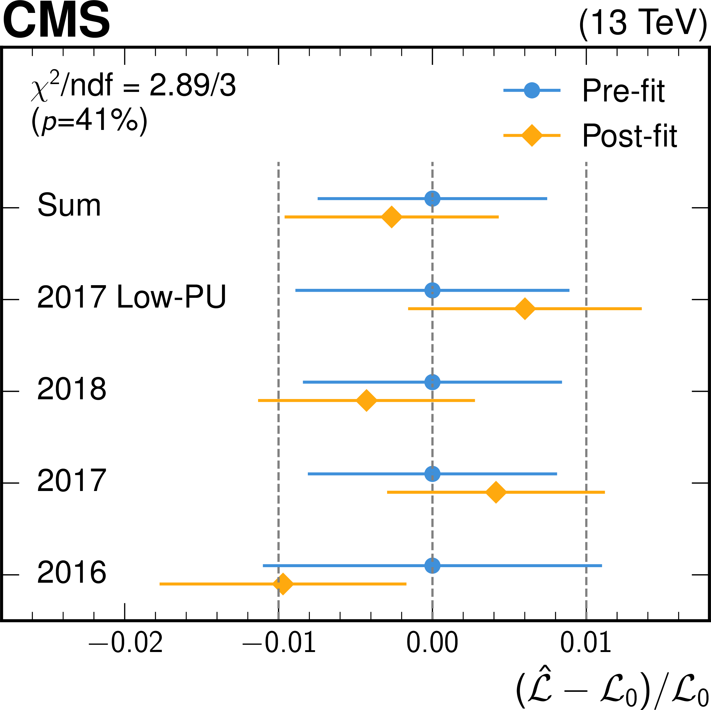
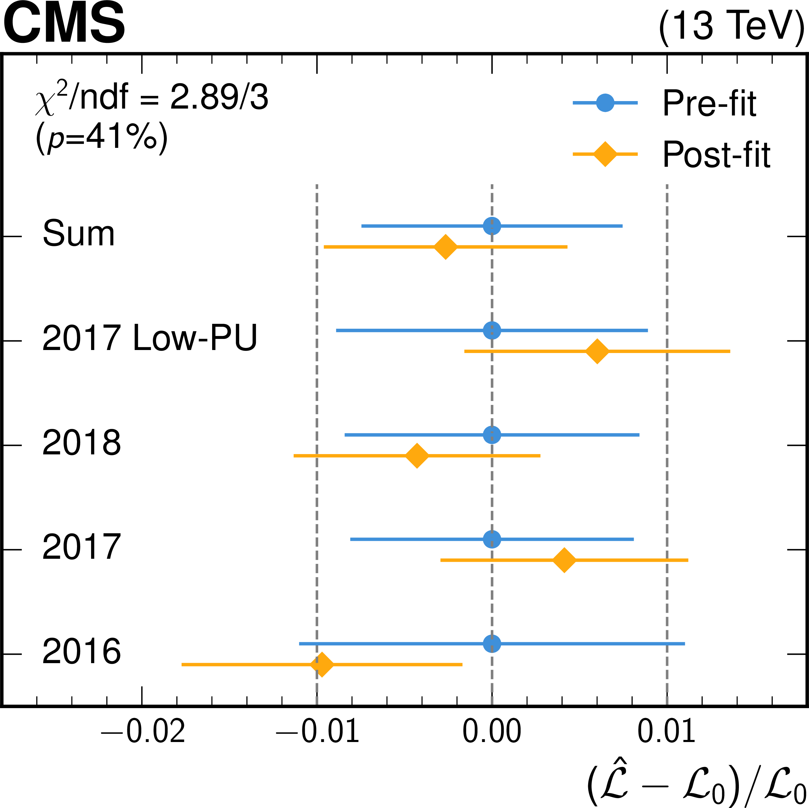
The relative uncertainty and the shifts of the luminosity values before and after the likelihood fit. The pre-fit (blue) results originate from the traditional luminosity estimation using the luminometers, while the post-fit (orange) values also include the Z boson rate data. The figure also shows the reduced $ \chi^2 $ and the $ p $-value of the fit. |
png pdf |
Figure 17-a:
The relative uncertainty and the shifts of the luminosity values before and after the likelihood fit. The pre-fit (blue) results originate from the traditional luminosity estimation using the luminometers, while the post-fit (orange) values also include the Z boson rate data. The figure also shows the reduced $ \chi^2 $ and the $ p $-value of the fit. |
png pdf |
Figure 17-b:
The relative uncertainty and the shifts of the luminosity values before and after the likelihood fit. The pre-fit (blue) results originate from the traditional luminosity estimation using the luminometers, while the post-fit (orange) values also include the Z boson rate data. The figure also shows the reduced $ \chi^2 $ and the $ p $-value of the fit. |
png pdf |
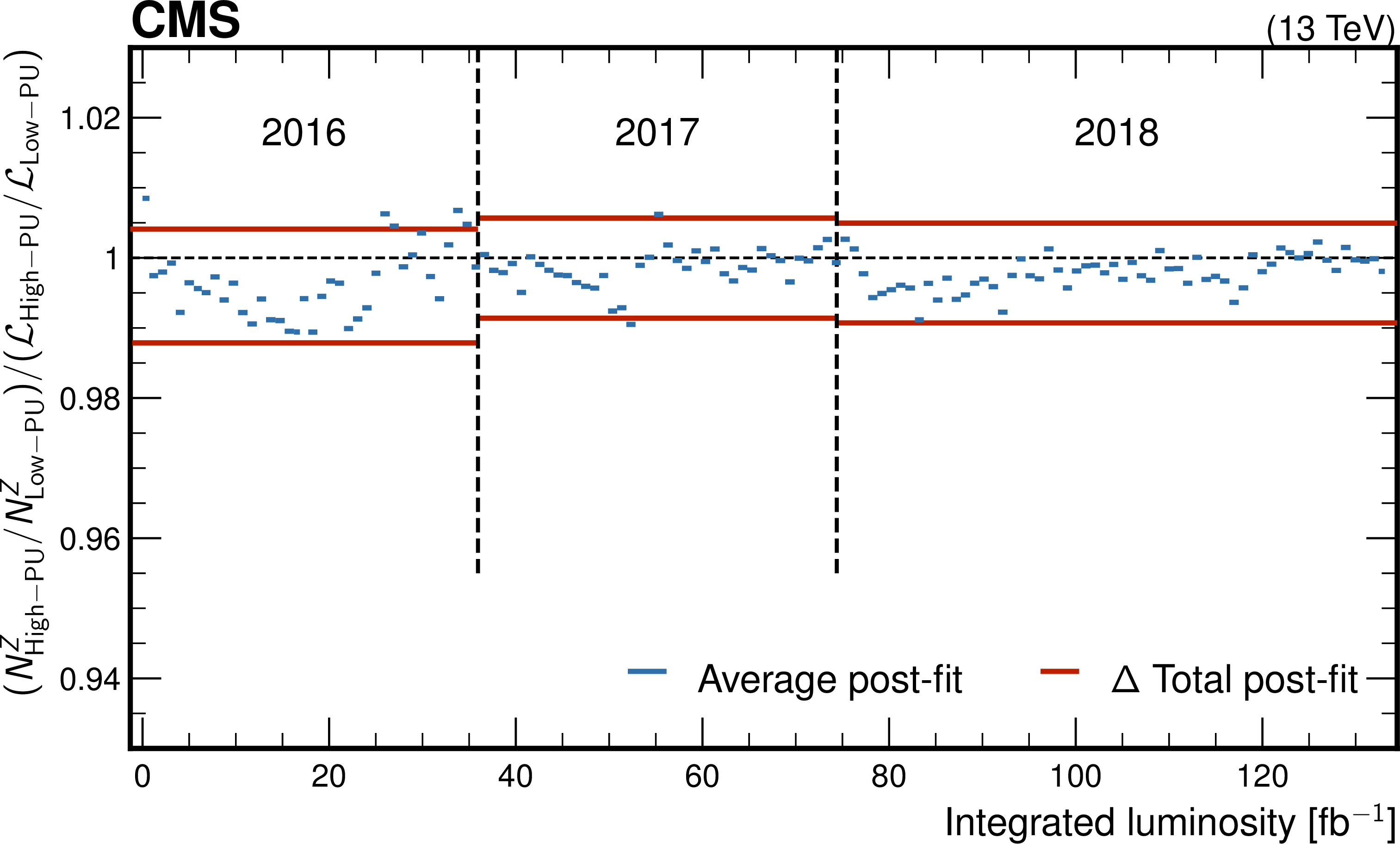
Figure 18:
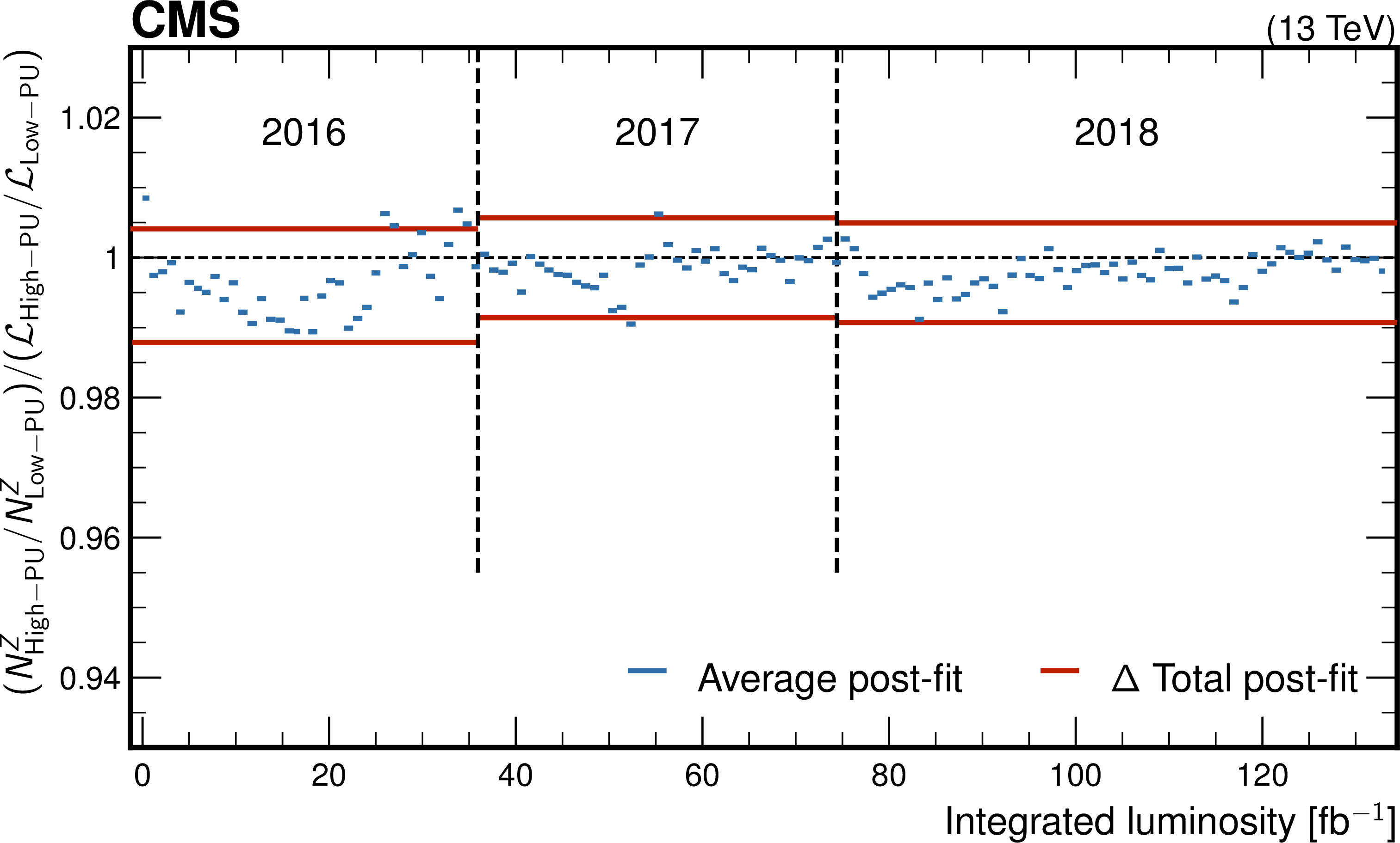
The post-fit ratio of the luminosity based on measured Z boson production rates and the reference luminosity as a function of the reference integrated luminosity for the 2016--2018 high-PU data set. Each blue line section corresponds to the luminosity values measured in about 1 fb$ ^{-1} $ of data. The red lines indicate the total uncertainty in the double ratio. The vertical dashed lines separate the 2016, 2017, and 2018 data. |
png pdf |
Figure 18-a:
The post-fit ratio of the luminosity based on measured Z boson production rates and the reference luminosity as a function of the reference integrated luminosity for the 2016--2018 high-PU data set. Each blue line section corresponds to the luminosity values measured in about 1 fb$ ^{-1} $ of data. The red lines indicate the total uncertainty in the double ratio. The vertical dashed lines separate the 2016, 2017, and 2018 data. |
png pdf |
Figure 18-b:
The post-fit ratio of the luminosity based on measured Z boson production rates and the reference luminosity as a function of the reference integrated luminosity for the 2016--2018 high-PU data set. Each blue line section corresponds to the luminosity values measured in about 1 fb$ ^{-1} $ of data. The red lines indicate the total uncertainty in the double ratio. The vertical dashed lines separate the 2016, 2017, and 2018 data. |
| Tables | |
png pdf |
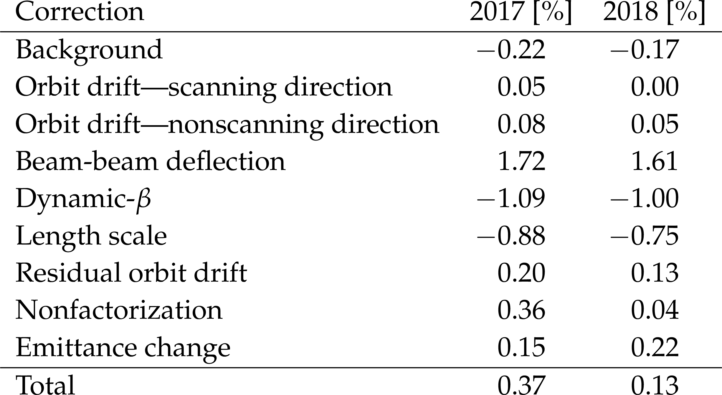
Table 1:
The impact of the corrections applied in the vdM calibration procedure on the final (i.e.,, bunch- and scan-averaged) $ \sigma_{\text{vis}} $ value for HFET in 2017 and 2018. |
png pdf |
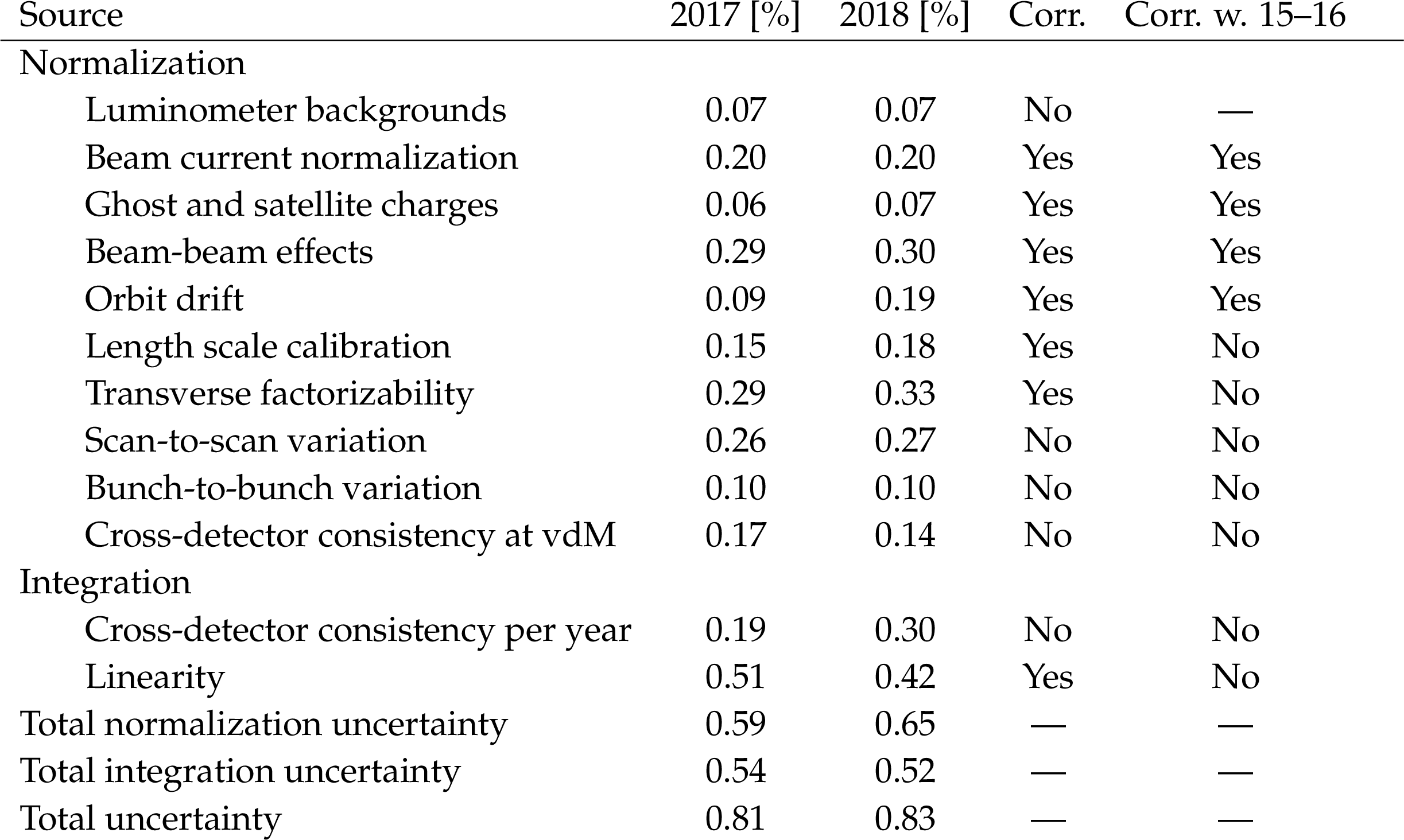
Table 2:
Summary of the luminosity uncertainties in 2017 and 2018, divided into two groups affecting the vdM calibration at low luminosity (normalization), and the measurement of the luminosity in physics conditions (integration). The ``Corr.'' column indicates whether the uncertainties are fully positively correlated between the two years or independent, while the last column lists the presumed correlation with the 2015--2016 data set. |
png pdf |
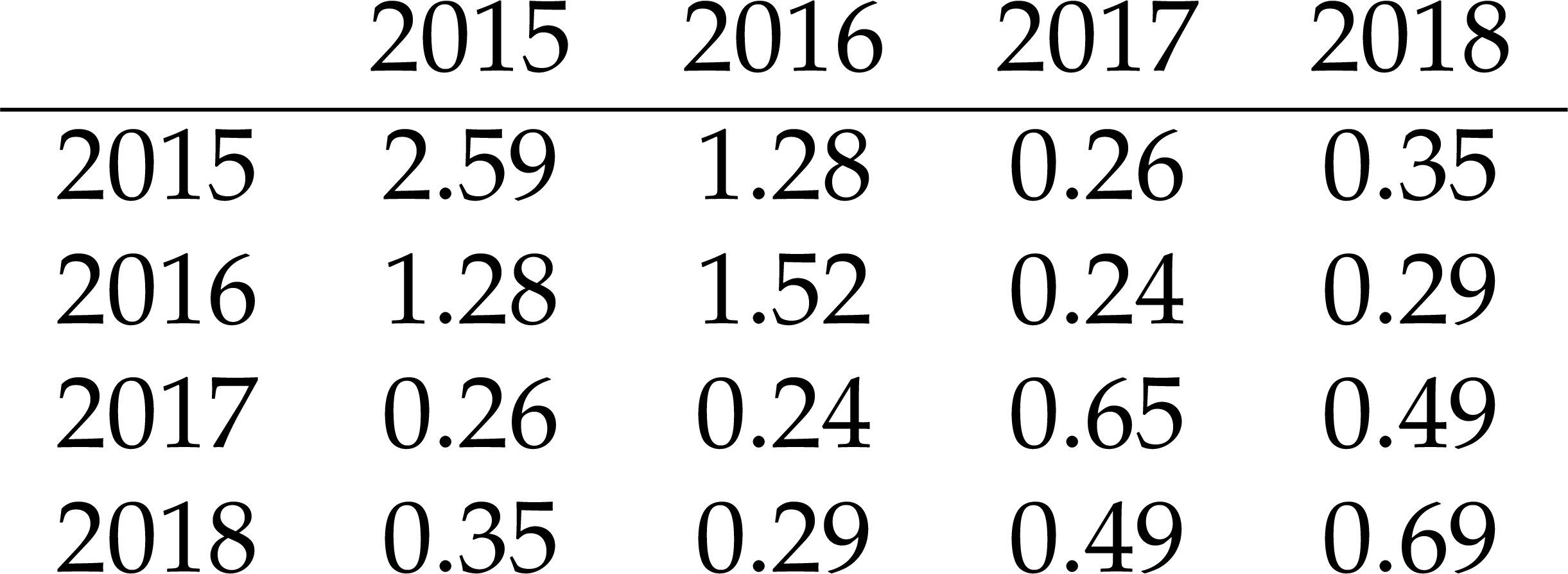
Table 3:
The relative covariance matrix of the luminosity measurements for high-pileup proton-proton collision data recorded by the CMS experiment during the Run 2 period, where each element is given as $ \sigma_{i,j}/(\mathcal{L}_i \mathcal{L}_j)\times 10^4 $. |
| Summary |
| In this work, we presented the legacy measurement of the integrated luminosity recorded by the Compact Muon Solenoid (CMS) detector in proton-proton collisions at a center-of-mass energy of 13 TeV during the Run 2 data-taking period (2015--2018) at the CERN Large Hadron Collider (LHC). This measurement significantly improves upon previous CMS results, reducing the single-year uncertainties to the sub-percent level. This gain in precision was achieved through the introduction of new and refined methods to evaluate and correct several sources of bias. These include effects related to micrometer-scale beam position monitoring, for which residual orbit drift corrections are introduced, as well as the calibration of the beam position length scale with respect to the CMS tracker coordinate system, for which a two-step approach is presented for the first time. The impact of the factorization assumption for the bunch proton densities is addressed using a refined luminous region method which is also compared to an independent measurement based on two-dimensional luminometer rate fits. Improvements are introduced in the estimation of the uncertainties associated with beam-beam interactions. In addition, meticulous corrections to the luminometer rates for out-of-time contributions, followed by the analysis of the emittance scan data to monitor detector performance, lead to a deeper understanding of the linearity and of the efficiency variations. The excellent agreement among the four independently calibrated and operated luminometers, using different detector technologies and counting methods, provides a rigorous cross-check of the absolute measurement. By combining them for the first time, the overall uncertainty is further reduced. The long-term stability and cross-year consistency of the luminosity calibration are conclusively validated using the Z boson production rate in the dimuon final state. The precision of the van der Meer calibration procedure has reached the sub-percent level target set forward by the CMS Collaboration for achieving the physics goals of the (High-Luminosity) LHC. The extrapolation to standard physics data-taking conditions (luminosity integration) remains the leading source of uncertainty and is expected to become even more challenging with the intensity increase foreseen in the HL-LHC era. Further improvements in the emittance scan analysis methodology, as well as in Z boson rate measurements, will play an important role in overcoming this limitation. The 0.73% relative precision achieved for the complete Run 2 proton-proton data set stands as the most precise luminosity measurement ever performed at a bunched-beam hadron collider. This milestone establishes a pivotal benchmark for the broader physics community, strengthening the impact of LHC data on precision measurements and constraints on new physics. |
| References | ||||
| 1 | M. L. Mangano | Motivations and precision targets for an accurate luminosity determination at the LHC | in Proc. LHC Lumi Days: Geneva, Switzerland, --14,,. [CERN-Proceedings-2011-001], 2011 January 1 (2011) 1 |
|
| 2 | CMS Collaboration | Stairway to discovery: a report on the CMS program of cross section measurements from millibarns to femtobarns | Phys. Rep. 1115 (2024) 3 | CMS-SMP-23-004 2405.18661 |
| 3 | CMS Collaboration | Measurement of the $ \mathrm{t} \overline{\mathrm{t}} $ production cross section, the top quark mass, and the strong coupling constant using dilepton events in $ {\mathrm{p}\mathrm{p}} $ collisions at $ \sqrt{s}= $ 13 TeV | EPJC 79 (2019) 368 | CMS-TOP-17-001 1812.10505 |
| 4 | CMS Collaboration | Measurements of differential Z boson production cross sections in proton-proton collisions at $ \sqrt{s}= $ 13 TeV | JHEP 12 (2019) 061 | CMS-SMP-17-010 1909.04133 |
| 5 | CMS Collaboration | Measurements of the W boson rapidity, helicity, double-differential cross sections, and charge asymmetry in $ {\mathrm{p}\mathrm{p}} $ collisions at 13 TeV | PRD 102 (2020) 092012 | CMS-SMP-18-012 2008.04174 |
| 6 | CMS Collaboration | First measurement of the top quark pair production cross section in proton-proton collisions at $ \sqrt{s}= $ 13.6 TeV | JHEP 08 (2023) 204 | CMS-TOP-22-012 2303.10680 |
| 7 | CMS Collaboration | Measurement of the inclusive cross sections for W and Z boson production in proton-proton collisions at $ \sqrt{s}= $ 5.02 and 13 TeV | JHEP 04 (2025) 162 | CMS-SMP-20-004 2408.03744 |
| 8 | CMS Collaboration | CMS Physics: Technical design report volume 1: Detector performance and software | Technical Report CERN/LHCC-2006-001, CMS-TDR-08-1, 2006 CDS |
|
| 9 | ATLAS and CMS Collaborations | Report on the physics at the HL-LHC and perspectives for the HE-LHC | Technical Report CERN-LPCC-2019-01, 2019 link |
1902.10229 |
| 10 | CMS Collaboration | The Phase-2 upgrade of the CMS beam radiation, instrumentation, and luminosity detectors | CMS Technical Proposal CERN-LHCC-2021-008, CMS-TDR-023, 2021 CDS |
|
| 11 | CMS Collaboration | The Phase-2 upgrade of the CMS beam radiation, instrumentation, and luminosity detectors: conceptual design | CMS Technical Proposal, 2019 CMS-PAS-TDR-19-003 |
|
| 12 | LHCb Collaboration | Precision luminosity measurements at LHCb | JINST 9 (2014) P12005 | 1410.0149 |
| 13 | CMS Collaboration | Precision luminosity measurement in proton-proton collisions at $ \sqrt{s}= $ 13 TeV in 2015 and 2016 at CMS | EPJC 81 (2021) 800 | CMS-LUM-17-003 2104.01927 |
| 14 | ALICE Collaboration | ALICE luminosity determination for PbPb collisions at $ {\sqrt{\smash[b]{s_{_{\mathrm{NN}}}}}= $ 5.02 TeV | JINST 19 (2024) P02039 | 2204.10148 |
| 15 | ATLAS Collaboration | Luminosity determination in $ {\mathrm{p}\mathrm{p}} $ collisions at $ \sqrt{s}= $ 13 TeV using the ATLAS detector at the LHC | EPJC 83 (2023) 982 | 2212.09379 |
| 16 | P. Grafström and W. Kozanecki | Luminosity determination at proton colliders | Prog. Part. Nucl. Phys. 81 (2015) 97 | |
| 17 | S. van der Meer | Calibration of the effective beam height in the ISR | ISR Report CERN-ISR-PO-68-31, 1968 | |
| 18 | CMS Collaboration | Instrumentation for beam radiation and luminosity measurement in the CMS experiment using novel detector technologies | NIM A 845 (2017) 565 | |
| 19 | CMS Collaboration | Development of the CMS detector for the CERN LHC \mboxRun 3 | JINST 19 (2024) P05064 | CMS-PRF-21-001 2309.05466 |
| 20 | J. Salfeld-Nebgen and D. Marlow | Data-driven precision luminosity measurements with Z bosons at the LHC and HL-LHC | JINST 13 (2018) P12016 | 1806.02184 |
| 21 | CMS Collaboration | Luminosity determination using Z boson production at the CMS experiment | EPJC 84 (2024) 26 | CMS-LUM-21-001 2309.01008 |
| 22 | CMS Collaboration | Luminosity measurement for lead-lead collisions at $ \sqrt{\smash[b]{s_{_{\mathrm{NN}}}}}= $ 5.02 TeV in 2015 and 2018 at CMS | Submitted to Eur. Phys. J. C, 2025 | CMS-LUM-20-002 2503.03946 |
| 23 | CMS Collaboration | CMS luminosity measurement for the 2017 data-taking period at $ \sqrt{s}= $ 13 TeV | CMS Physics Analysis Summary, 2018 CMS-PAS-LUM-17-004 |
CMS-PAS-LUM-17-004 |
| 24 | CMS Collaboration | CMS luminosity measurement for the 2018 data-taking period at $ \sqrt{s}= $ 13 TeV | CMS Physics Analysis Summary, 2019 CMS-PAS-LUM-18-002 |
CMS-PAS-LUM-18-002 |
| 25 | CMS Collaboration | The CMS experiment at the CERN LHC | JINST 3 (2008) S08004 | |
| 26 | CMS Collaboration | Performance of the CMS Level-1 trigger in proton-proton collisions at $ \sqrt{s}= $ 13 TeV | JINST 15 (2020) P10017 | CMS-TRG-17-001 2006.10165 |
| 27 | CMS Collaboration | The CMS trigger system | JINST 12 (2017) P01020 | CMS-TRG-12-001 1609.02366 |
| 28 | CMS Collaboration | Performance of the CMS high-level trigger during LHC \mboxRun 2 | JINST 19 (2024) P11021 | CMS-TRG-19-001 2410.17038 |
| 29 | CMS Collaboration | Electron and photon reconstruction and identification with the CMS experiment at the CERN LHC | JINST 16 (2021) P05014 | CMS-EGM-17-001 2012.06888 |
| 30 | CMS Collaboration | Performance of the CMS muon detector and muon reconstruction with proton-proton collisions at $ \sqrt{s}= $ 13 TeV | JINST 13 (2018) P06015 | CMS-MUO-16-001 1804.04528 |
| 31 | CMS Collaboration | Description and performance of track and primary-vertex reconstruction with the CMS tracker | JINST 9 (2014) P10009 | CMS-TRK-11-001 1405.6569 |
| 32 | CMS HCAL Collaboration | Design, performance, and calibration of CMS forward calorimeter wedges | EPJC 53 (2008) 139 | |
| 33 | CMS Collaboration | CMS technical design report for the Level-1 trigger upgrade | CMS Technical Proposal CERN-LHCC-2013-011, CMS-TDR-012, 2013 CDS |
|
| 34 | CMS BRIL Collaboration | The pixel luminosity telescope: a detector for luminosity measurement at CMS using silicon pixel sensors | EPJC 83 (2023) 673 | 2206.08870 |
| 35 | CMS Collaboration | The new fast beam condition monitor using poly-crystalline diamond sensors for luminosity measurement at CMS | NIM A 936 (2019) 717 | |
| 36 | G. Segura Millan, D. Perrin, and L. Scibile | RAMSES: the LHC radiation monitoring system for the environment and safety | in Proc. 10th Int. Conf. on Accelerator and Large Experimental Physics Control Systems (ICALEPCS ): Geneva, Switzerland.. [.1-3O], 2005 Conf. Proc. C 051010 (2005) TH3B |
|
| 37 | A. Ledeul et al. | CERN supervision, control and data acquisition system for radiation and environmental protection | in the Workshop on Emerging Technologies and Scientific Facilities Controls (PCaPAC): Hsinchu, Taiwan.. [JACoW (PCaPAC) 248], 2018 Proc. 1 (2018) 2 |
|
| 38 | M. G \c a sior, G. Baud, J. Olexa, and G. Valentino | First operational experience with the LHC diode orbit and oscillation (DOROS) system | in Proc. 5th International Beam Instrumentation Conference (): Barcelona, Spain.. [JACoW (IBIC) 43], 2016 IBIC 201 (2016) 6 |
|
| 39 | M. G \c a sior, J. Olexa, and R. Steinhagen | BPM electronics based on compensated diode detectors---results from development systems | in Proc. 15th Beam Instrumentation Workshop (BIW12): Newport News, USA.. [], 2012 Conf. Proc. C 1204151 (2012) 4 |
|
| 40 | J. Olexa | Design and optimization of the beam orbit and oscillation measurement system for the Large Hadron Collider | PhD thesis, Slovenska technicka univerzita v Bratislave, CERN-THESIS-2018-185, 2018 link |
|
| 41 | W. Kozanecki, T. Pieloni, and J. Wenninger | Observation of beam-beam deflections with LHC orbit data | CERN Report CERN-ACC-NOTE-2013-0006, 2013 | |
| 42 | D. Belohrad et al. | The LHC fast BCT system: A comparison of design parameters with initial performance | CERN Report CERN-BE-2010-010, 2010 | |
| 43 | D. Belohrad, D. Esperante Pereira, J. Kral, and S. Pedersen | Upgrade of the LHC bunch by bunch intensity measurement acquisition system | in Proc. 5th International Beam Instrumentation Conference (): Barcelona, Spain.. [JACoW (IBIC) 135], 2016 IBIC 201 (2016) 6 |
|
| 44 | M. Krupa and M. G \c a sior | The wall current transformer---a new sensor for precise bunch-by-bunch intensity measurements in the LHC | in Proc. 5th International Beam Instrumentation Conference (): Barcelona, Spain, September 11--15,. [JACoW (IBIC) 568], 2016 IBIC 201 (2016) 6 |
|
| 45 | C. Barschel et al. | Results of the LHC DCCT calibration studies | ||
| 46 | A. Jeff et al. | Longitudinal density monitor for the LHC | Phys. Rev. ST Accel. Beams 15 (2012) 032803 | |
| 47 | A. Jeff | A longitudinal density monitor for the LHC | PhD thesis, University of Liverpool, CERN-THESIS-2012-240, 2012 link |
|
| 48 | C. Barschel | Precision luminosity measurement at LHCb with beam-gas imaging | PhD thesis, RWTH Aachen University, CERN-THESIS-2013-301, 2014 link |
|
| 49 | G. Coombs, M. Ferro-Luzzi, and R. Matev | Beam-gas imaging measurements at LHCb | in Proc. 7th International Beam Instrumentation Conference (): Shanghai, China.. [JACoW (IBIC) 459], 2018 IBIC 201 (2018) 8 |
|
| 50 | A. Babaev et al. | Impact of beam-beam effects on absolute luminosity calibrations at the CERN Large Hadron Collider | EPJC 84 (2024) 17 | 2306.10394 |
| 51 | M. Bassetti and G. A. Erskine | Closed expression for the electrical field of a two-dimensional Gaussian charge | ISR Report CERN-ISR-TH-80-06, 1980 | |
| 52 | A. Babaev | Coherent deflection of elliptic bunches colliding at crossing angle | 2104.02595 | |
| 53 | J. Wenninger | Operation and configuration of the LHC in \mboxRun 2 | CERN Report CERN-ACC-NOTE-2019-0007, 2019 | |
| 54 | V. Balagura | Van der Meer scan luminosity measurement and beam-beam correction | EPJC 81 (2021) 26 | 2012.07752 |
| 55 | S. V. Furuseth and X. Buffat | Parallel high-performance multi-beam multi-bunch simulations | Comput. Phys. Commun. 244 (2019) 180 | |
| 56 | A. Chmieli \'n ska, L. Fiscarelli, W. Kozanecki, and E. Todesco | Magnetic measurements of MCBC and MCBY orbit correctors under special cycling conditions | CERN Report CERN-ACC-NOTE-2022-0013, 2022 | |
| 57 | H. Bartosik and G. Rumolo | Production of single Gaussian bunches for Van der Meer scans in the LHC injector chain | CERN Report CERN-ACC-NOTE-2013-0008, 2013 | |
| 58 | S. N. Webb | Factorisation of beams in van der Meer scans and measurements of the $ \phi^\ast_\eta $ distribution of $ {\mathrm{Z}\to\mathrm{e}^+\mathrm{e}^-} $ events in $ {\mathrm{p}\mathrm{p}} $ collisions at $ \sqrt{s}= $ 8 TeV with the ATLAS detector | PhD thesis, University of Manchester, CERN-THESIS-2015-054, 2015 link |
|
| 59 | P. Major | Probing New Physics: Search for supersymmetry with Higgs particles and high-precision luminosity determination at the CMS experiment | PhD thesis, ELTE Eötvös Lorand University, CMS TS-2026/002, 2024 link |
|
| 60 | T. Becher and T. Neumann | Fiducial $ q_{\mathrm{t}} $ resummation of color-singlet processes at N\textsuperscript3LL+NNLO | JHEP 03 (2021) 199 | 2009.11437 |
|
|
Compact Muon Solenoid LHC, CERN |

|
|
|
|
|
|