

Compact Muon Solenoid
LHC, CERN
| CMS-PAS-SUS-23-005 | ||
| Search for a light pseudoscalar Higgs boson in final states with boosted $ \mu\mu $ and $ \tau\tau $ pairs in proton-proton collisions at $ \sqrt{s}= $ 13 TeV | ||
| CMS Collaboration | ||
| 2026-03-18 | ||
| Abstract: A search for a light pseudoscalar Higgs boson ($ \mathrm{a} $) is performed using LHC data collected at $ \sqrt{s}= $ 13 TeV by the CMS experiment from 2016 to 2018, targeting the process $ \mathrm{H} \to \mathrm{a}\mathrm{a} \to \mu\mu\tau\tau $, where the scalar H can be either the 125 GeV state or a heavier one. Due to the large mass difference between H and $ \mathrm{a} $, the two tau leptons are highly boosted and collimated, often failing standard CMS tau lepton reconstruction. To address this, dedicated di-tau reconstruction techniques, including a deep neural network, are developed to increase efficiency for cases where at least one tau decays to hadrons. No significant excess over standard model (SM) backgrounds is observed, and upper limits at the 95% confidence level are set on this process. Model-independent upper limits on the branching ratio for $ m_{\mathrm{H}}= $ 125 GeV range from 5 $ \times10^{-5} $ to 3 $ \times10^{-4} $ for pseudoscalar masses between 3.6 and 21 GeV. For the first time using LHC data, upper limits are obtained in final states with tau leptons for hypothetical scalar boson masses up to 1 TeV, with $ m_{\mathrm{H}}= $ 1 TeV limits ranging from 4 $ \times10^{-4} $ to 1.5 $ \times10^{-3} $ for pseudoscalar masses between 10 and 50 GeV. In addition, limits for SM extensions involving two-Higgs-doublet plus singlet models are set for $ m_{\mathrm{H}}= $ 125 GeV and extend previous LHC results. | ||
| Links: CDS record (PDF) ; CADI line (restricted) ; | ||
| Figures | |
png pdf |
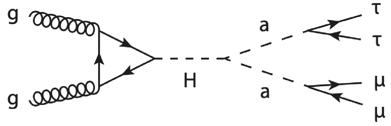
Figure 1:
Diagram of a Higgs boson produced by gluon-gluon fusion, decaying into two pseudoscalar bosons, with subsequent decays into two muons and two tau leptons. |
png pdf |
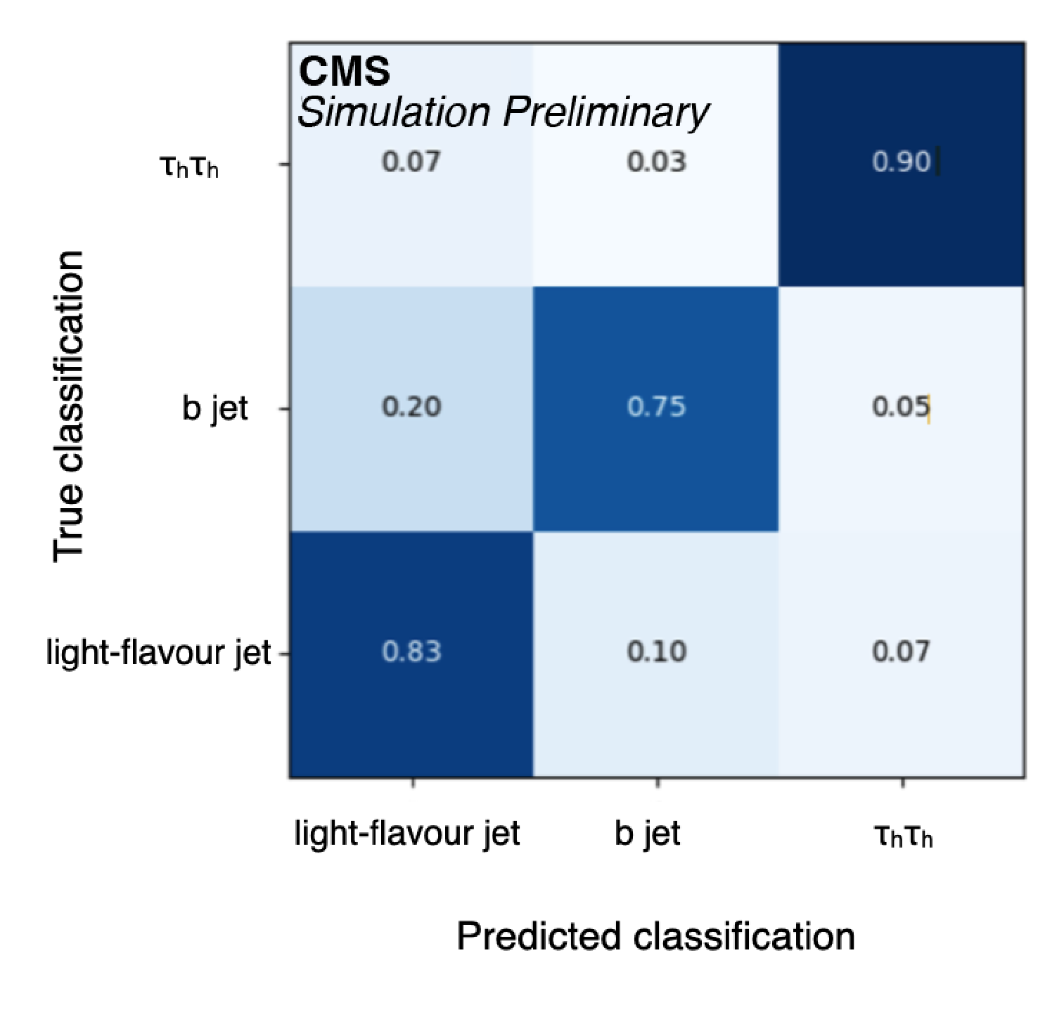
Figure 2:
Confusion matrix for the DEEPDITAU classifier. |
png pdf |
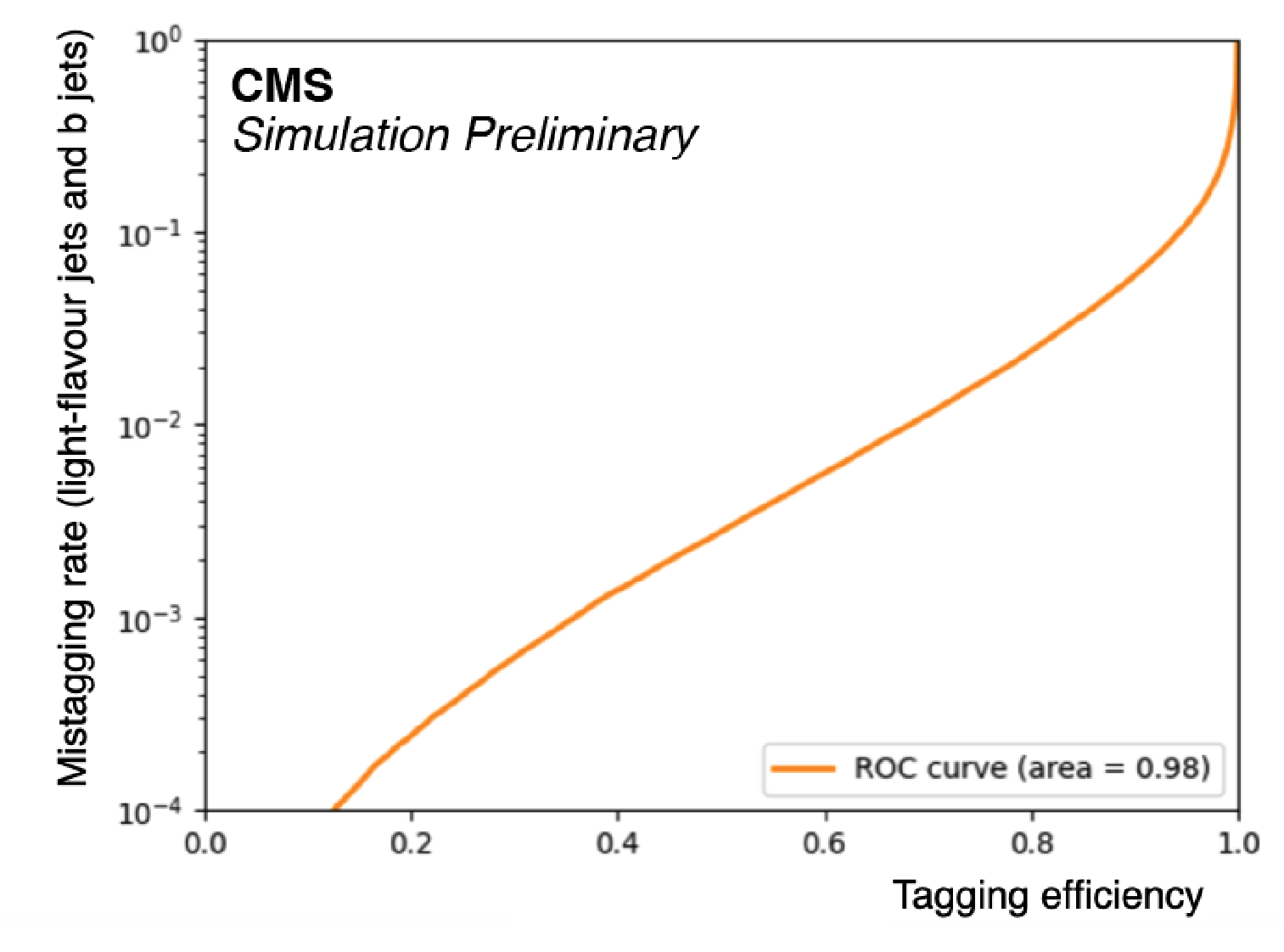
Figure 3:
Receiver operating characteristic (ROC) curve for the DEEPDITAU classifier. The true positive rate is the rate of correct classification of $ \tau_\mathrm{h}\tau_\mathrm{h} $ jets, and the false positive rate is the rate of classifying light-flavor jets and b jets as $ \tau_\mathrm{h}\tau_\mathrm{h} $ jets. |
png pdf |
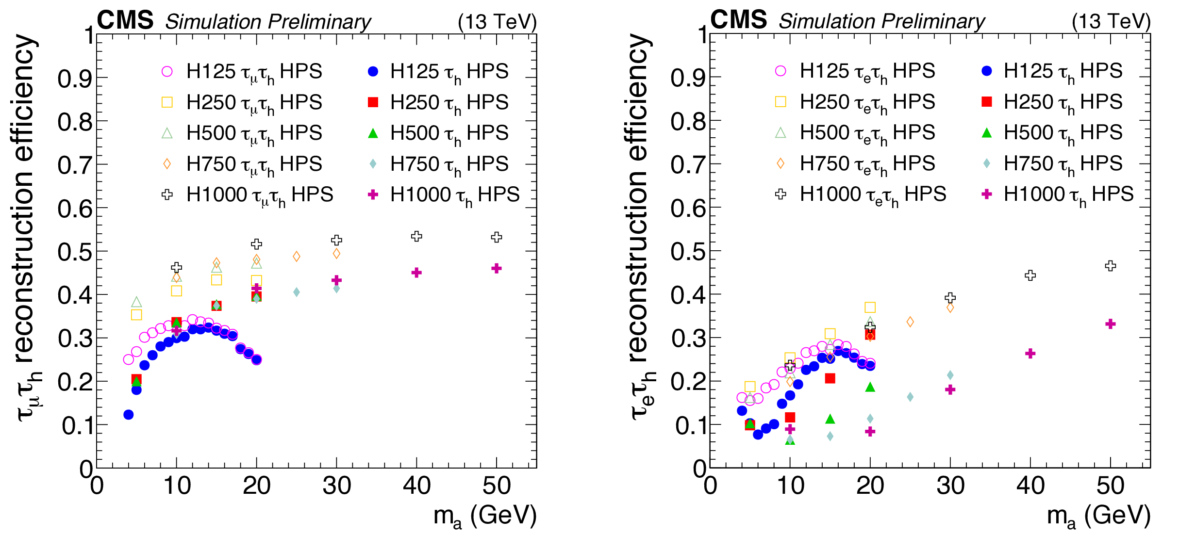
Figure 4:
The $ \tau\tau $ reconstruction efficiency of the standard $ \tau $ HPS (dashed lines) and a modified $ \tau_{\mu}\tau_\mathrm{h} $ (left) or $ \tau_{\mathrm{e}}\tau_\mathrm{h} $ (right) HPS (solid lines) reconstruction as a function of $ m_{\mathrm{a}} $ for $ m_{\mathrm{H}} = $ 125, 250, 500, 750, and 1000 GeV. Due to the requirement of $ \Delta R(\tau_{\ell}, \tau_\mathrm{h}) < $ 0.8, the efficiency for $ m_{\mathrm{H}} = $ 125 GeV drops above $ m_{\mathrm{a}} = $ 12 GeV ($ \tau_{\mu}\tau_\mathrm{h} $) and $ m_{\mathrm{a}} = $ 14 GeV ($ \tau_{\mathrm{e}}\tau_\mathrm{h} $), the region with increasingly more resolved $ \tau\tau $ topologies. In the right plot, the dip in the the standard HPS efficiency for the low $ m_{\mathrm{a}} $ region is due to two competing effects: the requirement of $ p_{\mathrm{T}}^{\mathrm{e}} > $ 10 GeV, which loses efficiency with increasing $ m_{\mathrm{a}} $, and the requirement of passing an anti-electron discriminant, which increases in efficiency as $ m_{\mathrm{a}} $ increases. Our analysis deploys the modified HPS reconstruction which shows a significantly higher efficiency than the standard $ \tau $ HPS scenario. |
png pdf |
Figure 4-a:
The $ \tau\tau $ reconstruction efficiency of the standard $ \tau $ HPS (dashed lines) and a modified $ \tau_{\mu}\tau_\mathrm{h} $ (left) or $ \tau_{\mathrm{e}}\tau_\mathrm{h} $ (right) HPS (solid lines) reconstruction as a function of $ m_{\mathrm{a}} $ for $ m_{\mathrm{H}} = $ 125, 250, 500, 750, and 1000 GeV. Due to the requirement of $ \Delta R(\tau_{\ell}, \tau_\mathrm{h}) < $ 0.8, the efficiency for $ m_{\mathrm{H}} = $ 125 GeV drops above $ m_{\mathrm{a}} = $ 12 GeV ($ \tau_{\mu}\tau_\mathrm{h} $) and $ m_{\mathrm{a}} = $ 14 GeV ($ \tau_{\mathrm{e}}\tau_\mathrm{h} $), the region with increasingly more resolved $ \tau\tau $ topologies. In the right plot, the dip in the the standard HPS efficiency for the low $ m_{\mathrm{a}} $ region is due to two competing effects: the requirement of $ p_{\mathrm{T}}^{\mathrm{e}} > $ 10 GeV, which loses efficiency with increasing $ m_{\mathrm{a}} $, and the requirement of passing an anti-electron discriminant, which increases in efficiency as $ m_{\mathrm{a}} $ increases. Our analysis deploys the modified HPS reconstruction which shows a significantly higher efficiency than the standard $ \tau $ HPS scenario. |
png pdf |
Figure 4-b:
The $ \tau\tau $ reconstruction efficiency of the standard $ \tau $ HPS (dashed lines) and a modified $ \tau_{\mu}\tau_\mathrm{h} $ (left) or $ \tau_{\mathrm{e}}\tau_\mathrm{h} $ (right) HPS (solid lines) reconstruction as a function of $ m_{\mathrm{a}} $ for $ m_{\mathrm{H}} = $ 125, 250, 500, 750, and 1000 GeV. Due to the requirement of $ \Delta R(\tau_{\ell}, \tau_\mathrm{h}) < $ 0.8, the efficiency for $ m_{\mathrm{H}} = $ 125 GeV drops above $ m_{\mathrm{a}} = $ 12 GeV ($ \tau_{\mu}\tau_\mathrm{h} $) and $ m_{\mathrm{a}} = $ 14 GeV ($ \tau_{\mathrm{e}}\tau_\mathrm{h} $), the region with increasingly more resolved $ \tau\tau $ topologies. In the right plot, the dip in the the standard HPS efficiency for the low $ m_{\mathrm{a}} $ region is due to two competing effects: the requirement of $ p_{\mathrm{T}}^{\mathrm{e}} > $ 10 GeV, which loses efficiency with increasing $ m_{\mathrm{a}} $, and the requirement of passing an anti-electron discriminant, which increases in efficiency as $ m_{\mathrm{a}} $ increases. Our analysis deploys the modified HPS reconstruction which shows a significantly higher efficiency than the standard $ \tau $ HPS scenario. |
png pdf |
Figure 5:
Schematic of the analysis strategy. In the Z mass range, the tight-to-loose ratio is derived from the $ \mathrm{Z}_{\mu\mu}+ $jet control region and sideband (yellow). In the analysis mass range, events with two isolated muons and no loosely selected $ \tau\tau $ candidates enter the control region (yellow). Events that additionally contain a loosely selected $ \tau\tau $ candidate are further categorized into the signal region or sideband, as described in the text. The sideband data, weighted by the tight-to-loose ratio, are used to estimate the background in the signal region. Additionally, by inverting the isolation requirement on the muon that did not trigger the event, two analogous regions are formed for validating the tight-to-loose method (gray). |
png pdf |
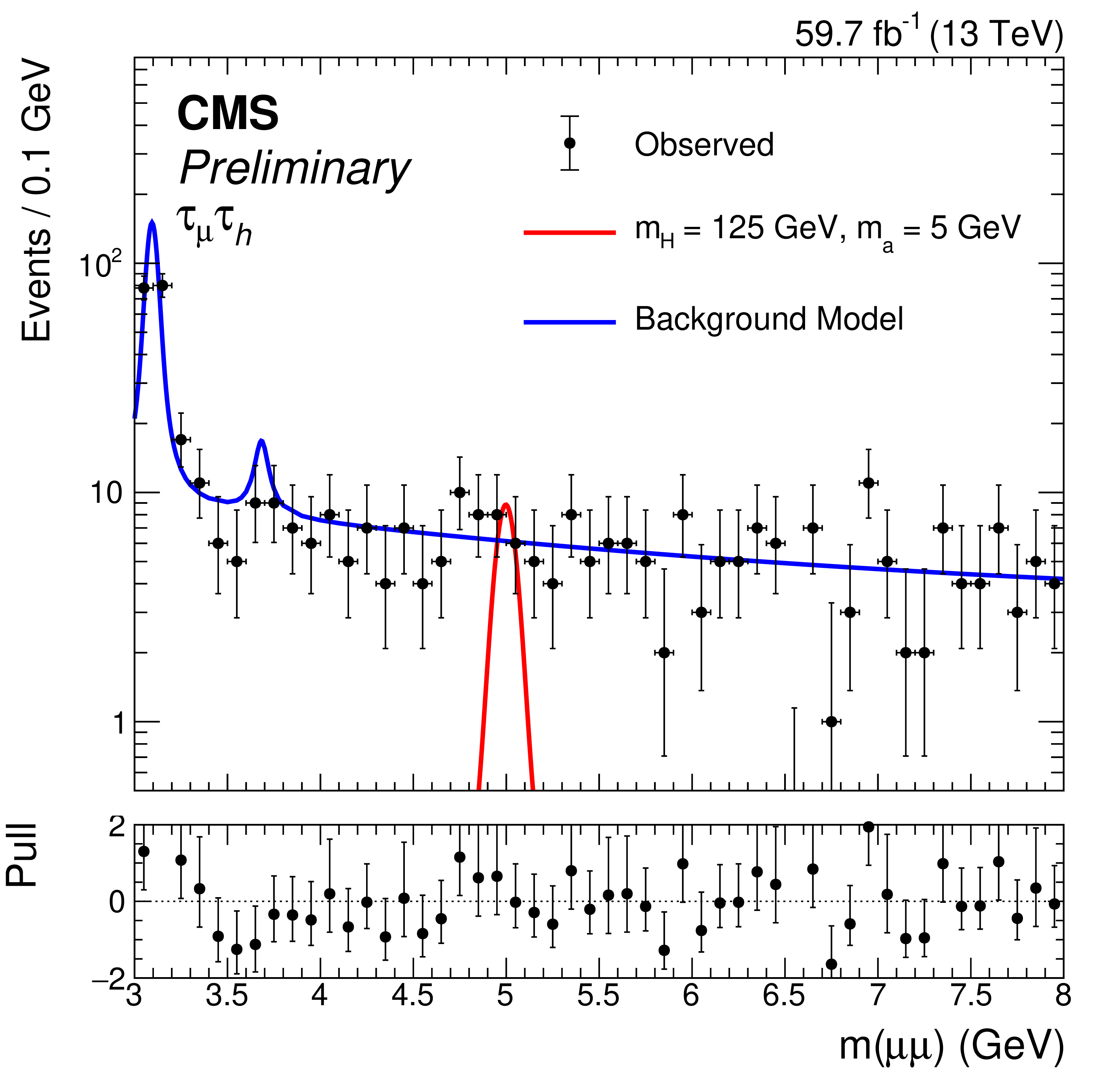
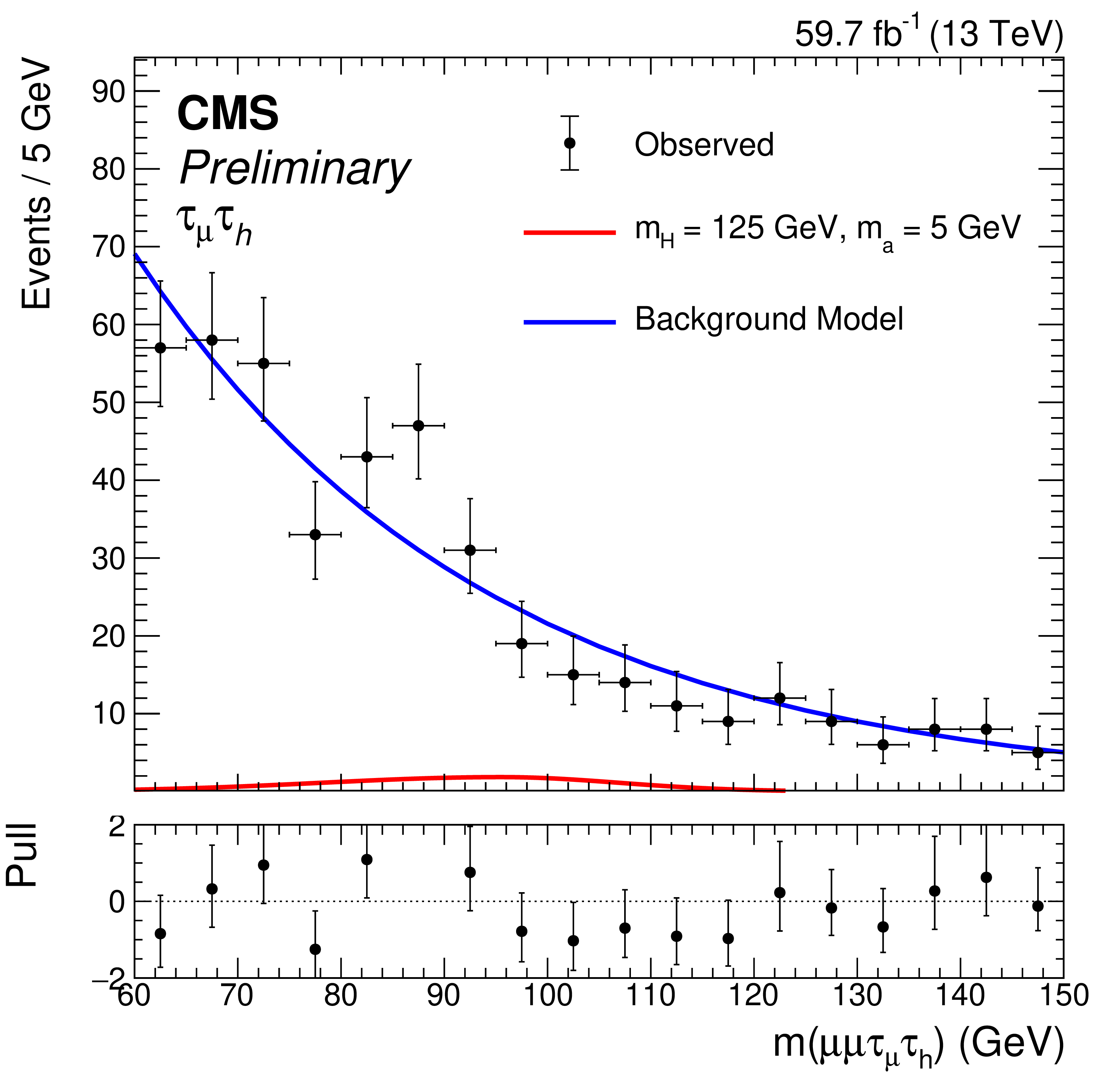
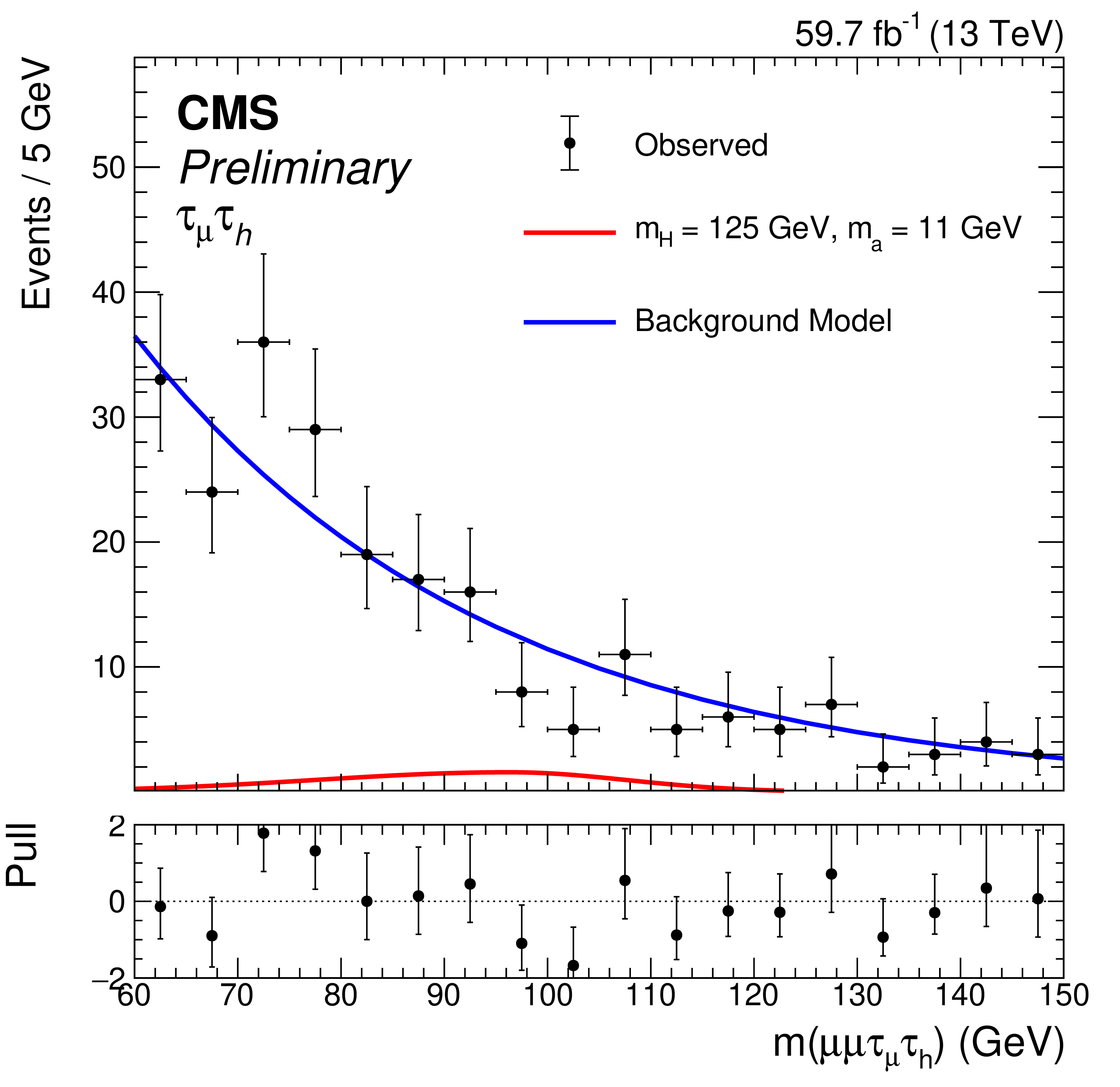
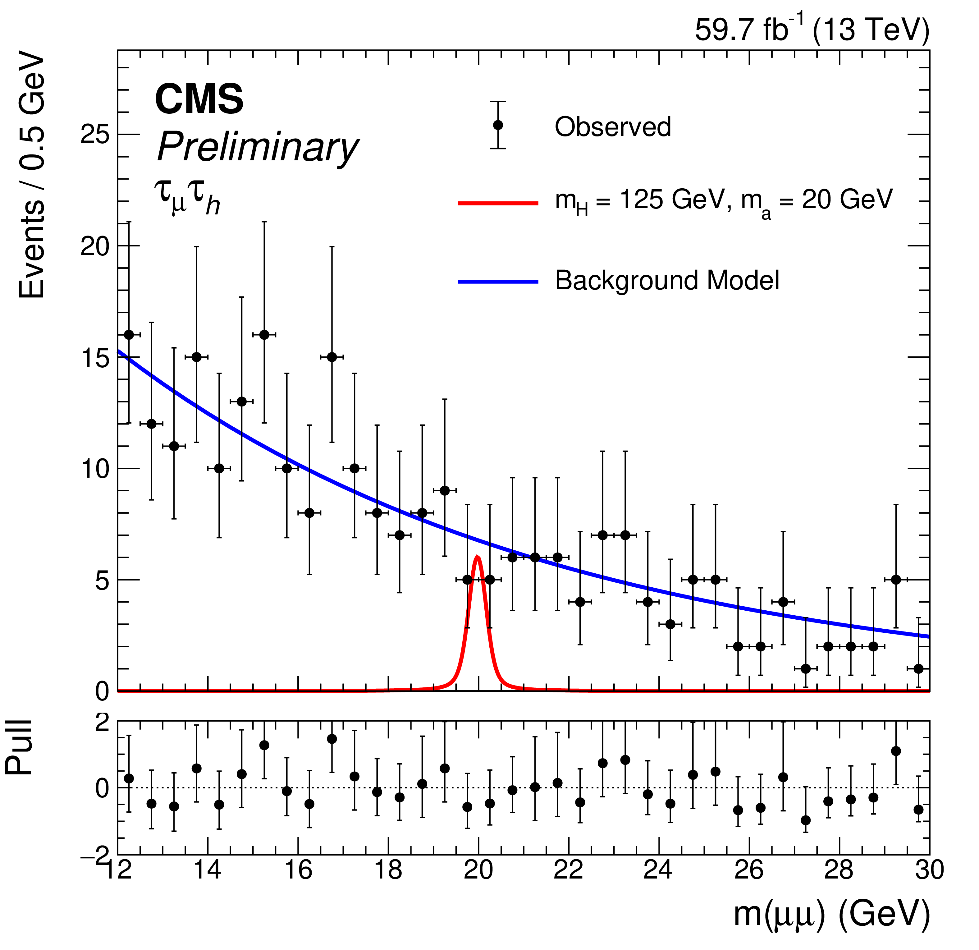
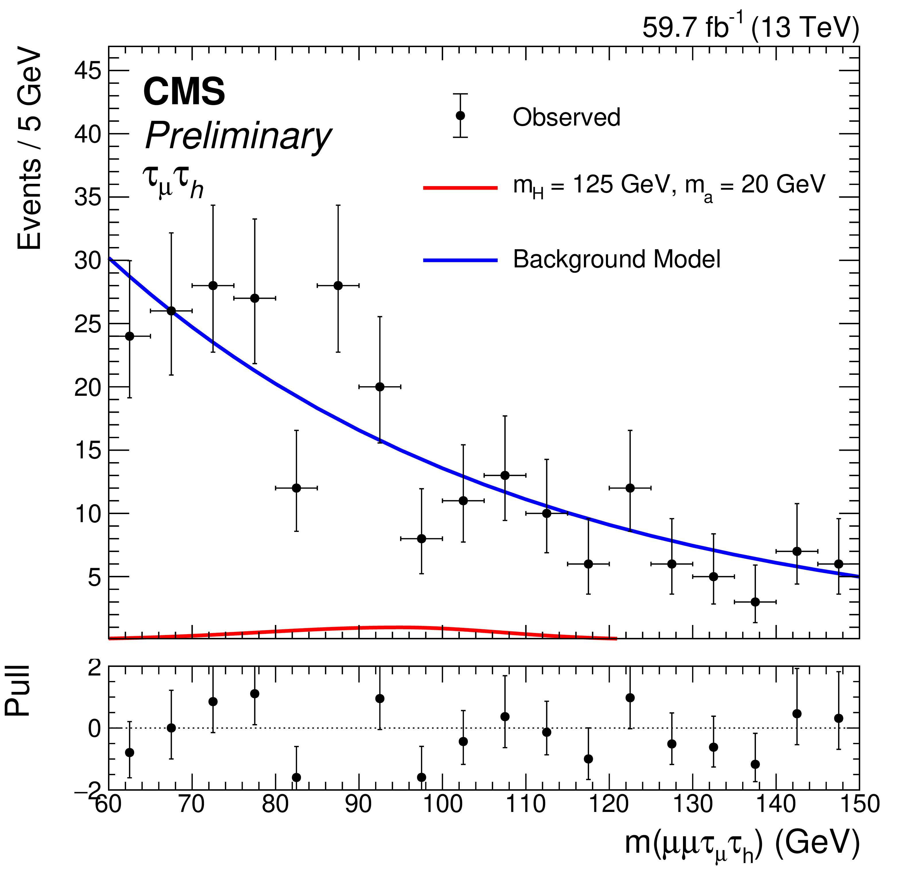
Figure 6:
Projections of the post-fit two-dimensional background PDFs (blue) and observed data onto the $ m_{\mu\mu} $ (left) and four-body visible mass (right) axes for the $ \tau_{\mu}\tau_\mathrm{h} $ channel for $ m_{\mathrm{H}} = 125 \text{GeV} $ using 2018 data. The rows correspond to pseudoscalar masses $ m_{\mathrm{a}} = $ 5, 11, and 20 GeV (from top to bottom). Sample signal distributions (red) are overlaid assuming $ \mathcal{B}(\mathrm{H}\to\mathrm{a}\mathrm{a}\to\mu\mu\tau\tau) = 5 \times 10^{-4} $. |
png pdf |
Figure 6-a:
Projections of the post-fit two-dimensional background PDFs (blue) and observed data onto the $ m_{\mu\mu} $ (left) and four-body visible mass (right) axes for the $ \tau_{\mu}\tau_\mathrm{h} $ channel for $ m_{\mathrm{H}} = 125 \text{GeV} $ using 2018 data. The rows correspond to pseudoscalar masses $ m_{\mathrm{a}} = $ 5, 11, and 20 GeV (from top to bottom). Sample signal distributions (red) are overlaid assuming $ \mathcal{B}(\mathrm{H}\to\mathrm{a}\mathrm{a}\to\mu\mu\tau\tau) = 5 \times 10^{-4} $. |
png pdf |
Figure 6-b:
Projections of the post-fit two-dimensional background PDFs (blue) and observed data onto the $ m_{\mu\mu} $ (left) and four-body visible mass (right) axes for the $ \tau_{\mu}\tau_\mathrm{h} $ channel for $ m_{\mathrm{H}} = 125 \text{GeV} $ using 2018 data. The rows correspond to pseudoscalar masses $ m_{\mathrm{a}} = $ 5, 11, and 20 GeV (from top to bottom). Sample signal distributions (red) are overlaid assuming $ \mathcal{B}(\mathrm{H}\to\mathrm{a}\mathrm{a}\to\mu\mu\tau\tau) = 5 \times 10^{-4} $. |

png pdf |
Figure 6-c:
Projections of the post-fit two-dimensional background PDFs (blue) and observed data onto the $ m_{\mu\mu} $ (left) and four-body visible mass (right) axes for the $ \tau_{\mu}\tau_\mathrm{h} $ channel for $ m_{\mathrm{H}} = 125 \text{GeV} $ using 2018 data. The rows correspond to pseudoscalar masses $ m_{\mathrm{a}} = $ 5, 11, and 20 GeV (from top to bottom). Sample signal distributions (red) are overlaid assuming $ \mathcal{B}(\mathrm{H}\to\mathrm{a}\mathrm{a}\to\mu\mu\tau\tau) = 5 \times 10^{-4} $. |
png pdf |
Figure 6-d:
Projections of the post-fit two-dimensional background PDFs (blue) and observed data onto the $ m_{\mu\mu} $ (left) and four-body visible mass (right) axes for the $ \tau_{\mu}\tau_\mathrm{h} $ channel for $ m_{\mathrm{H}} = 125 \text{GeV} $ using 2018 data. The rows correspond to pseudoscalar masses $ m_{\mathrm{a}} = $ 5, 11, and 20 GeV (from top to bottom). Sample signal distributions (red) are overlaid assuming $ \mathcal{B}(\mathrm{H}\to\mathrm{a}\mathrm{a}\to\mu\mu\tau\tau) = 5 \times 10^{-4} $. |
png pdf |
Figure 6-e:
Projections of the post-fit two-dimensional background PDFs (blue) and observed data onto the $ m_{\mu\mu} $ (left) and four-body visible mass (right) axes for the $ \tau_{\mu}\tau_\mathrm{h} $ channel for $ m_{\mathrm{H}} = 125 \text{GeV} $ using 2018 data. The rows correspond to pseudoscalar masses $ m_{\mathrm{a}} = $ 5, 11, and 20 GeV (from top to bottom). Sample signal distributions (red) are overlaid assuming $ \mathcal{B}(\mathrm{H}\to\mathrm{a}\mathrm{a}\to\mu\mu\tau\tau) = 5 \times 10^{-4} $. |
png pdf |
Figure 6-f:
Projections of the post-fit two-dimensional background PDFs (blue) and observed data onto the $ m_{\mu\mu} $ (left) and four-body visible mass (right) axes for the $ \tau_{\mu}\tau_\mathrm{h} $ channel for $ m_{\mathrm{H}} = 125 \text{GeV} $ using 2018 data. The rows correspond to pseudoscalar masses $ m_{\mathrm{a}} = $ 5, 11, and 20 GeV (from top to bottom). Sample signal distributions (red) are overlaid assuming $ \mathcal{B}(\mathrm{H}\to\mathrm{a}\mathrm{a}\to\mu\mu\tau\tau) = 5 \times 10^{-4} $. |
png pdf |
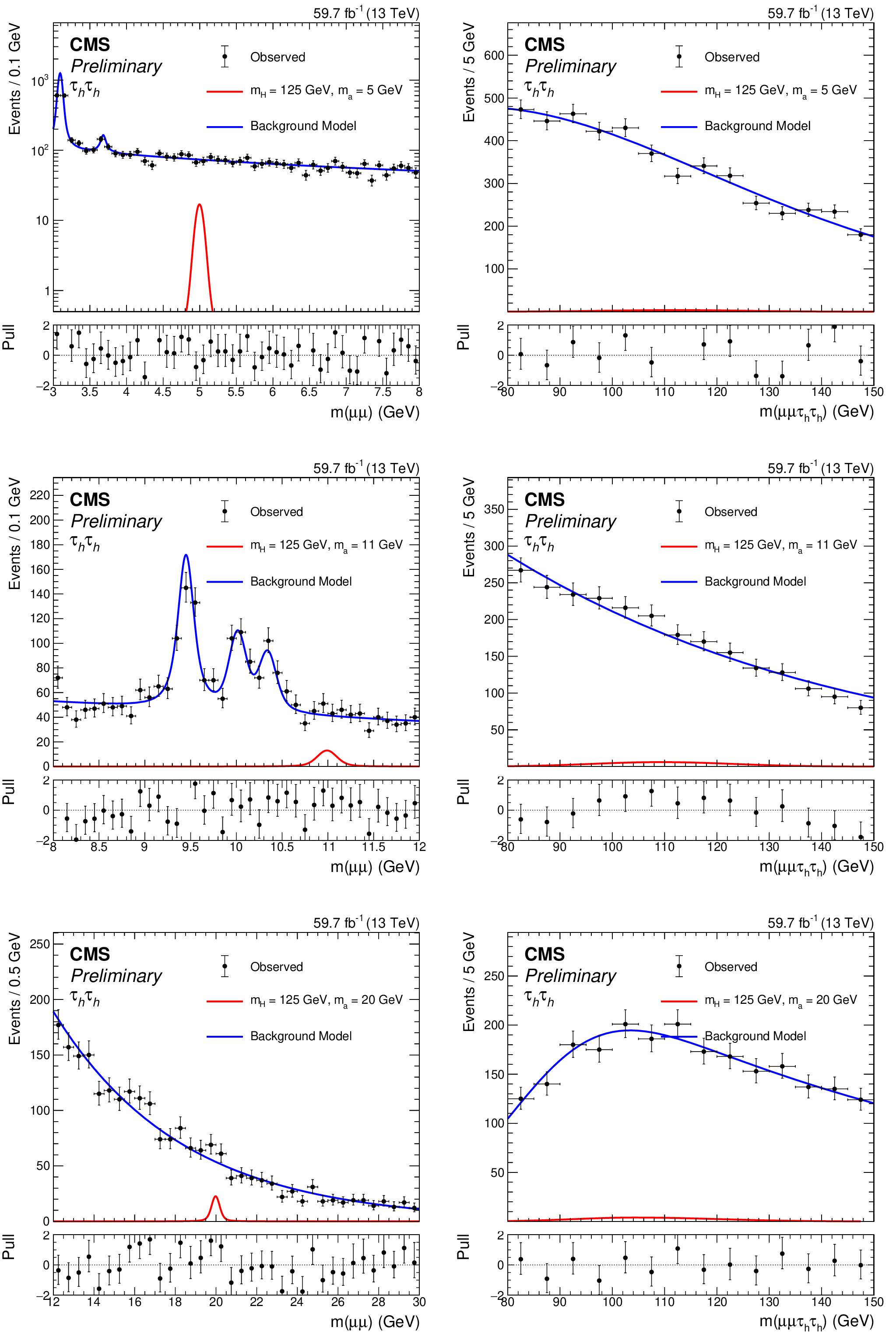
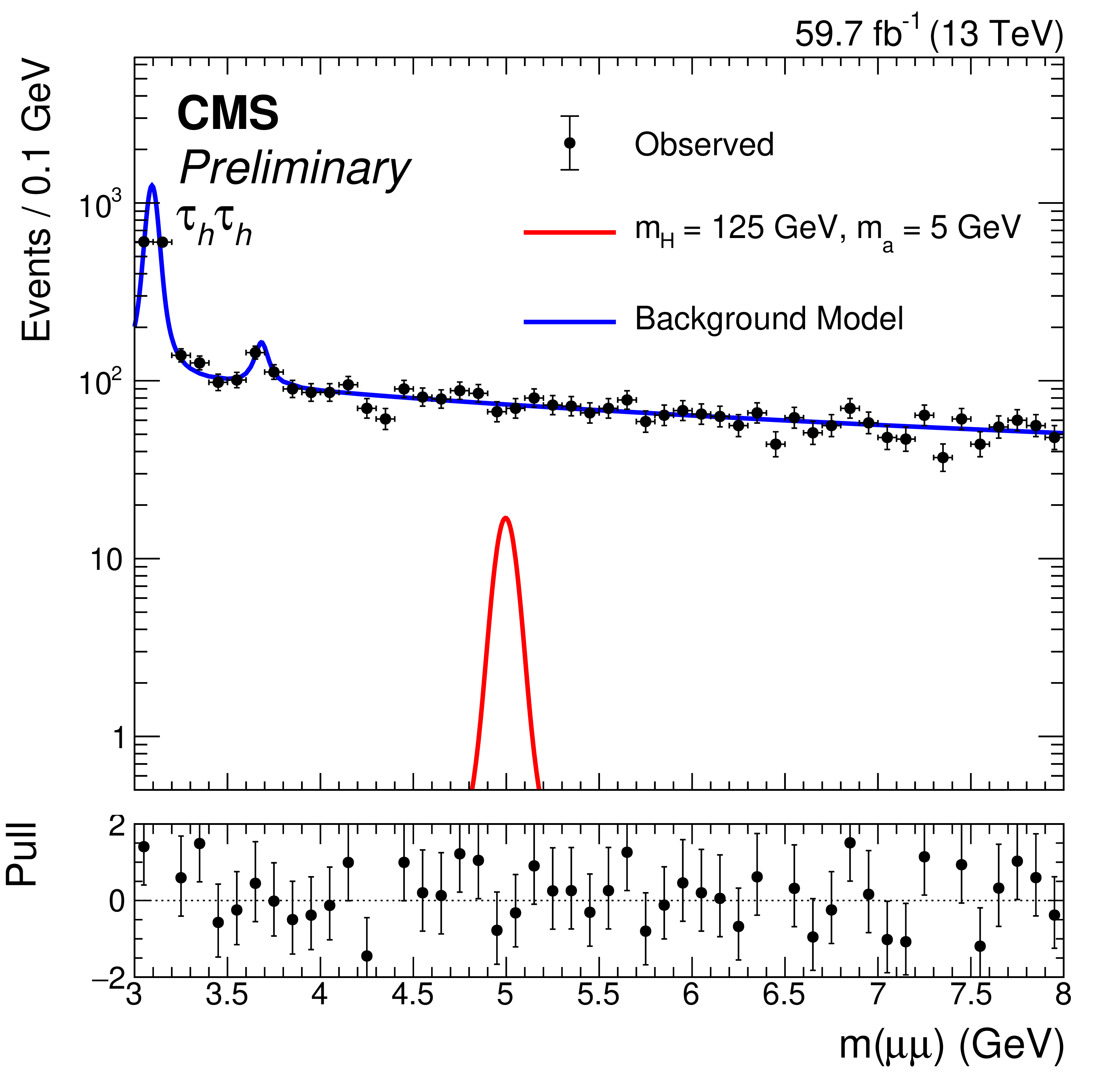
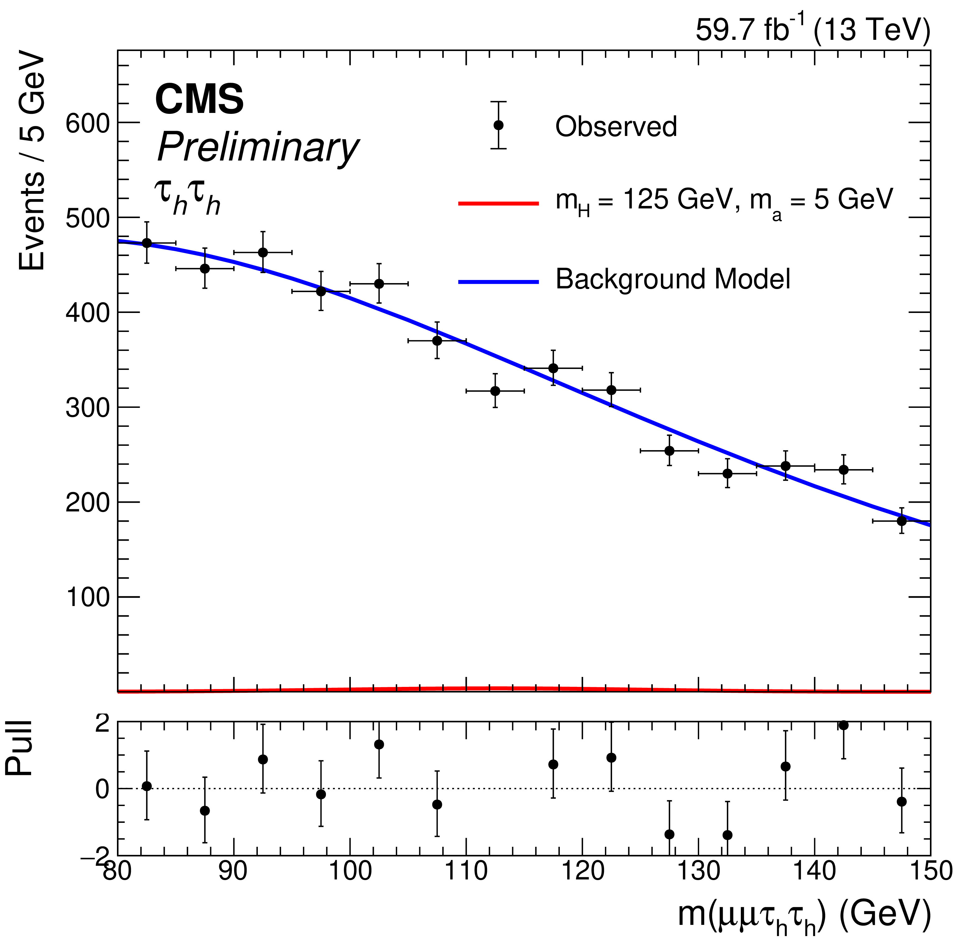
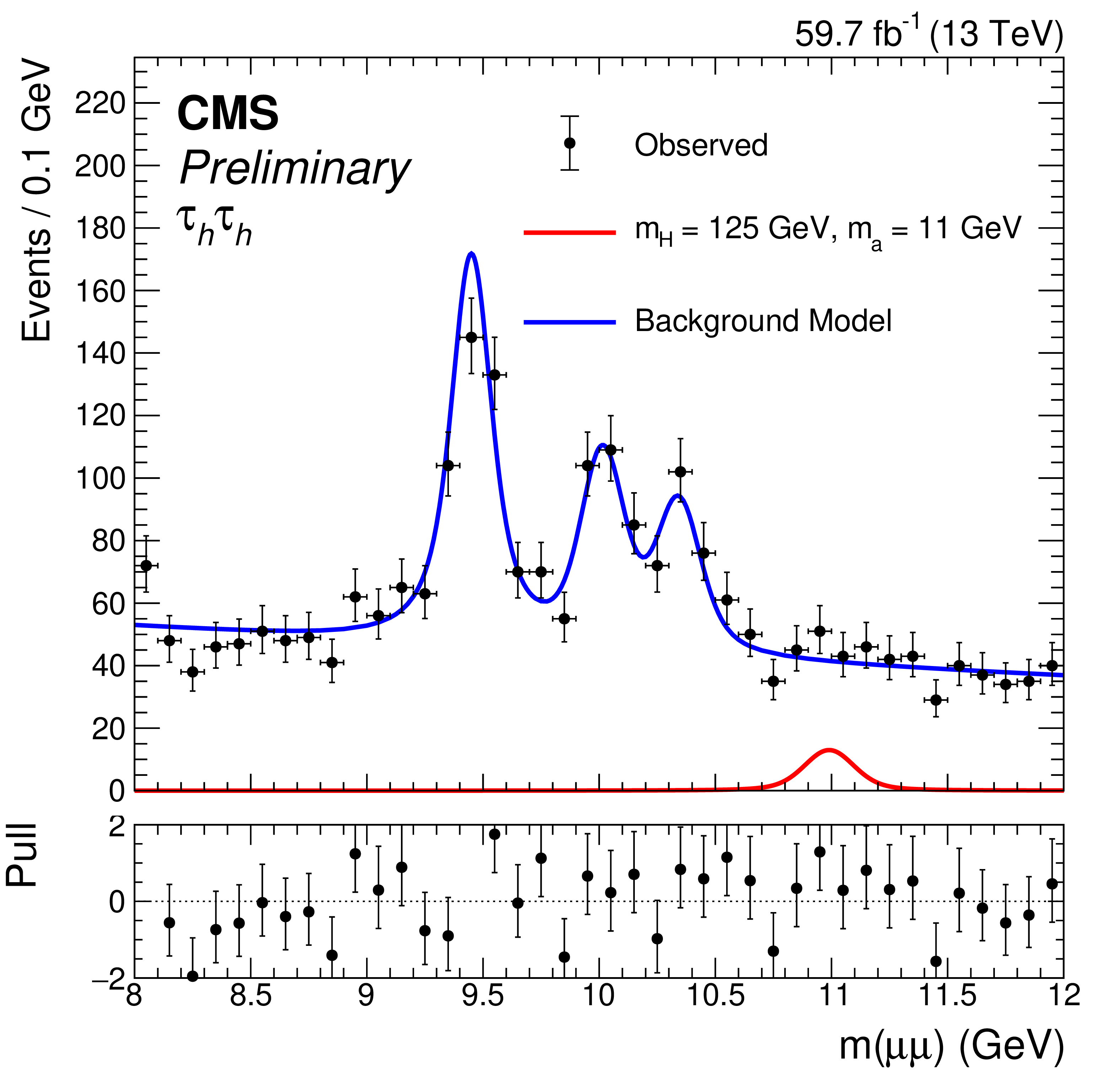
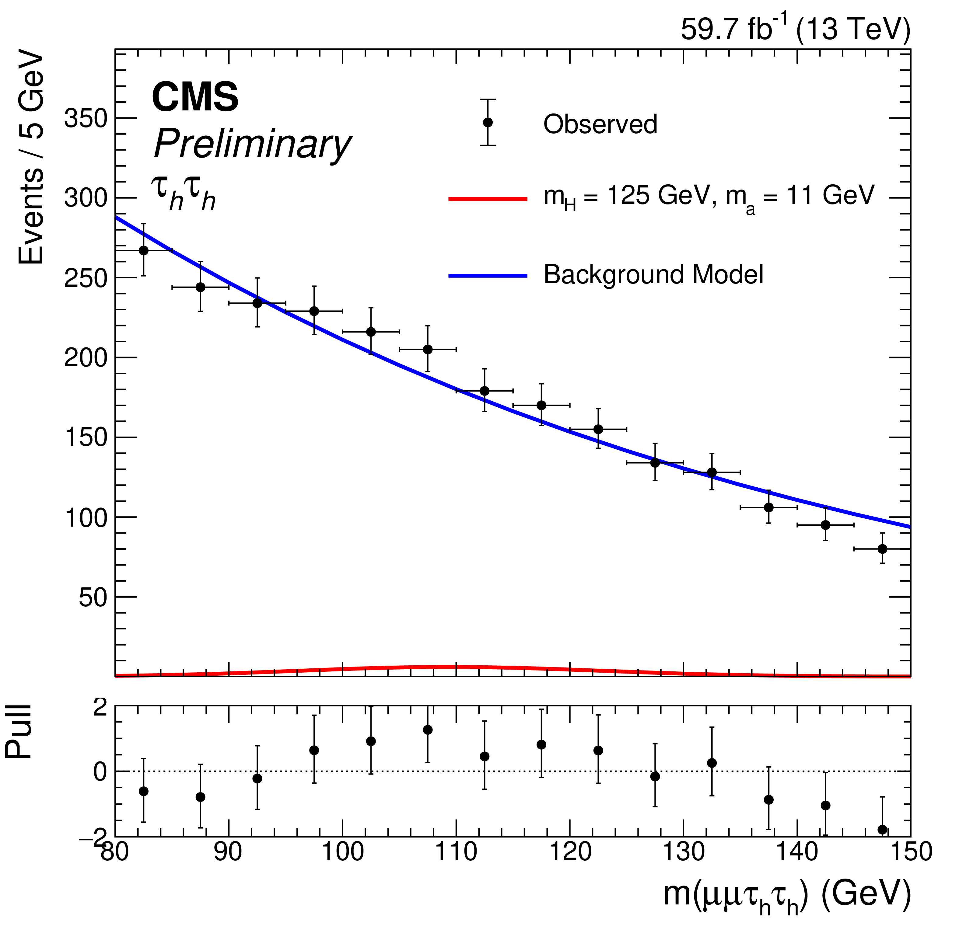
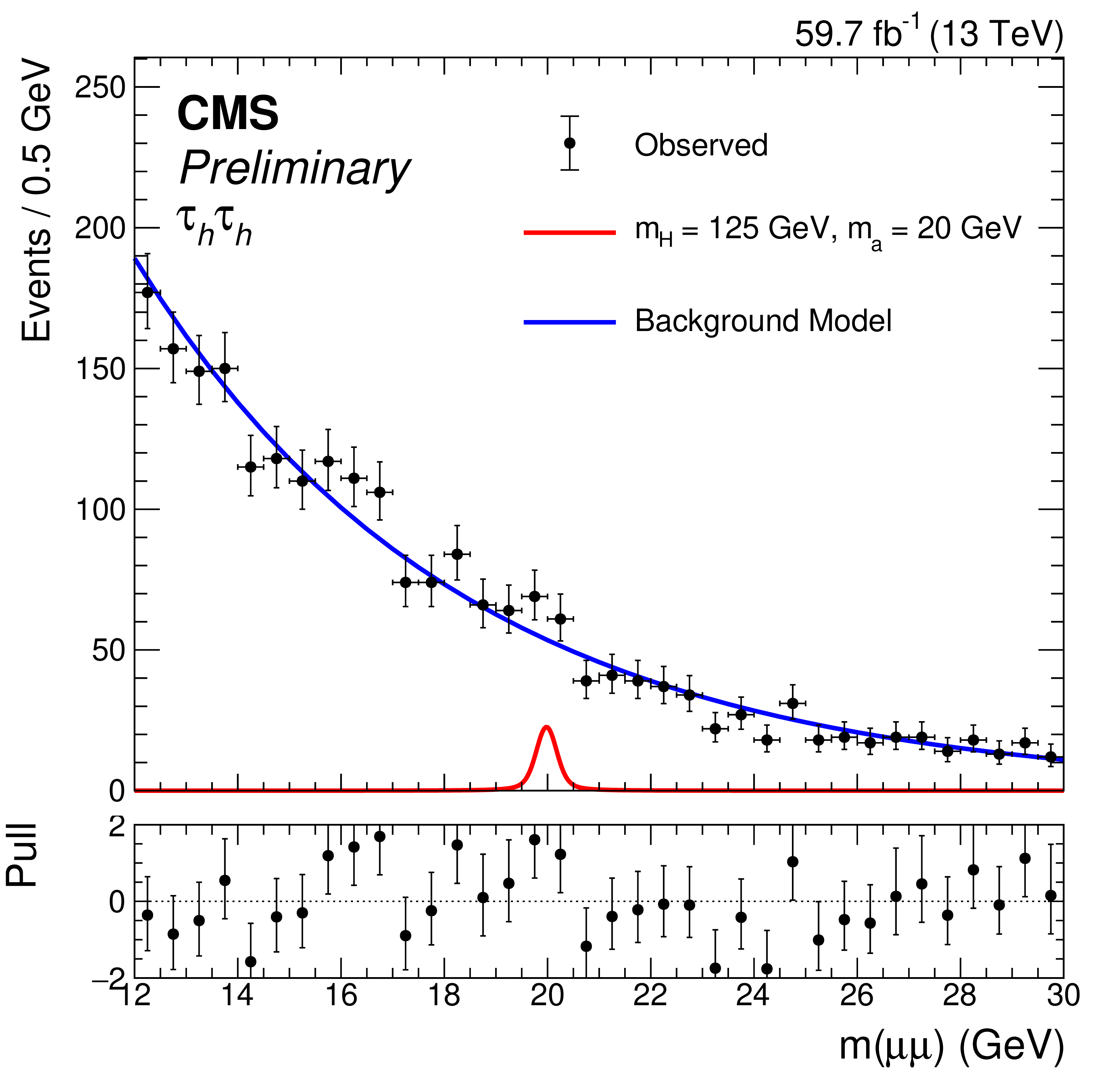
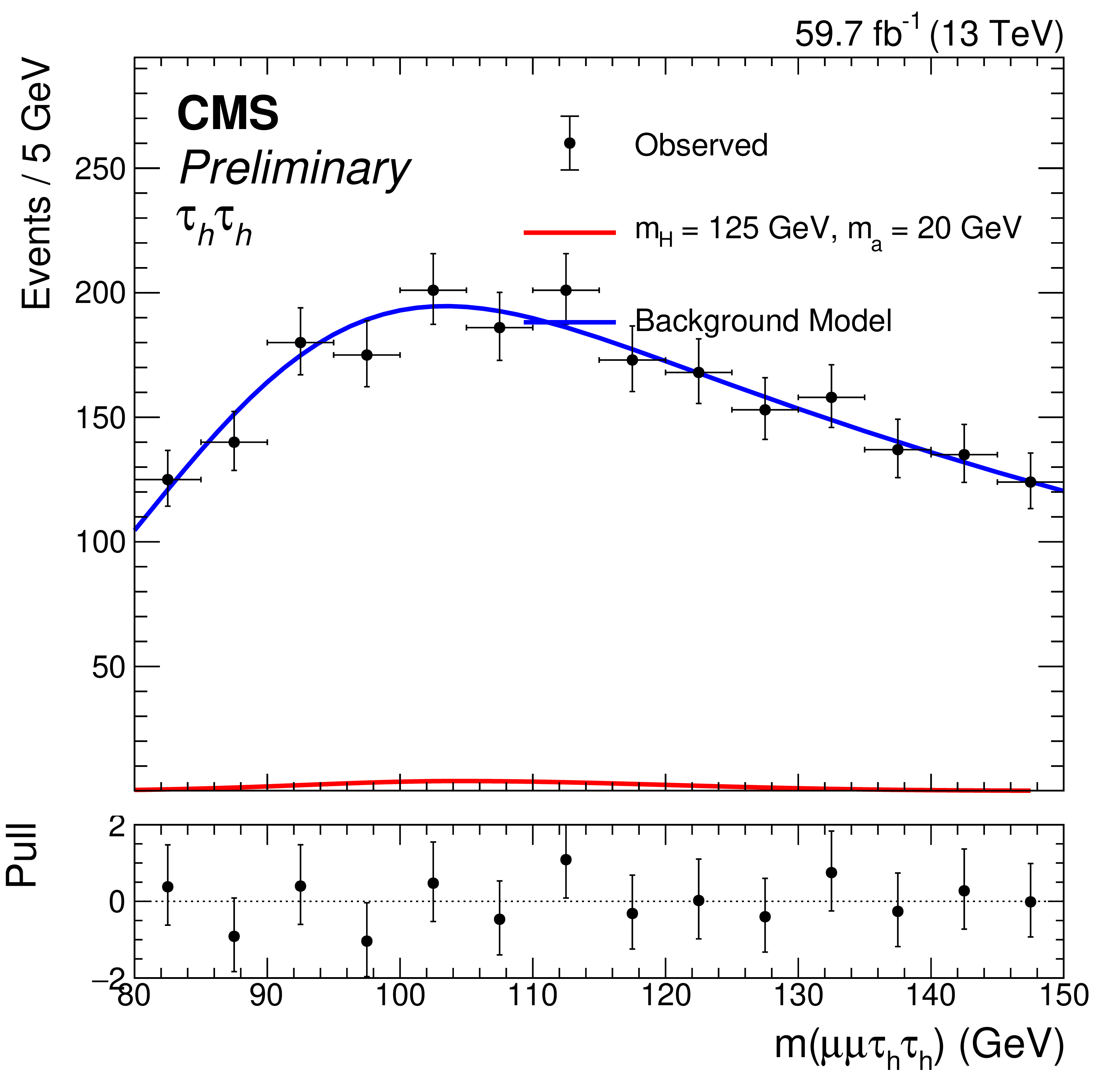
Figure 7:
Projections of the post-fit two-dimensional background PDFs (blue) and observed data onto the $ m_{\mu\mu} $ (left) and four-body visible mass (right) axes for the $ \tau_\mathrm{h}\tau_\mathrm{h} $ channel for $ m_{\mathrm{H}} = 125 \text{GeV} $ using 2018 data. The rows correspond to pseudoscalar masses $ m_{\mathrm{a}} = $ 5, 11, and 20 GeV (from top to bottom). Sample signal distributions (red) are overlaid assuming $ \mathcal{B}(\mathrm{H}\to\mathrm{a}\mathrm{a}\to\mu\mu\tau\tau) = $ 5 $ \times 10^{-4} $. |
png pdf |
Figure 7-a:
Projections of the post-fit two-dimensional background PDFs (blue) and observed data onto the $ m_{\mu\mu} $ (left) and four-body visible mass (right) axes for the $ \tau_\mathrm{h}\tau_\mathrm{h} $ channel for $ m_{\mathrm{H}} = 125 \text{GeV} $ using 2018 data. The rows correspond to pseudoscalar masses $ m_{\mathrm{a}} = $ 5, 11, and 20 GeV (from top to bottom). Sample signal distributions (red) are overlaid assuming $ \mathcal{B}(\mathrm{H}\to\mathrm{a}\mathrm{a}\to\mu\mu\tau\tau) = $ 5 $ \times 10^{-4} $. |
png pdf |
Figure 7-b:
Projections of the post-fit two-dimensional background PDFs (blue) and observed data onto the $ m_{\mu\mu} $ (left) and four-body visible mass (right) axes for the $ \tau_\mathrm{h}\tau_\mathrm{h} $ channel for $ m_{\mathrm{H}} = 125 \text{GeV} $ using 2018 data. The rows correspond to pseudoscalar masses $ m_{\mathrm{a}} = $ 5, 11, and 20 GeV (from top to bottom). Sample signal distributions (red) are overlaid assuming $ \mathcal{B}(\mathrm{H}\to\mathrm{a}\mathrm{a}\to\mu\mu\tau\tau) = $ 5 $ \times 10^{-4} $. |
png pdf |
Figure 7-c:
Projections of the post-fit two-dimensional background PDFs (blue) and observed data onto the $ m_{\mu\mu} $ (left) and four-body visible mass (right) axes for the $ \tau_\mathrm{h}\tau_\mathrm{h} $ channel for $ m_{\mathrm{H}} = 125 \text{GeV} $ using 2018 data. The rows correspond to pseudoscalar masses $ m_{\mathrm{a}} = $ 5, 11, and 20 GeV (from top to bottom). Sample signal distributions (red) are overlaid assuming $ \mathcal{B}(\mathrm{H}\to\mathrm{a}\mathrm{a}\to\mu\mu\tau\tau) = $ 5 $ \times 10^{-4} $. |
png pdf |
Figure 7-d:
Projections of the post-fit two-dimensional background PDFs (blue) and observed data onto the $ m_{\mu\mu} $ (left) and four-body visible mass (right) axes for the $ \tau_\mathrm{h}\tau_\mathrm{h} $ channel for $ m_{\mathrm{H}} = 125 \text{GeV} $ using 2018 data. The rows correspond to pseudoscalar masses $ m_{\mathrm{a}} = $ 5, 11, and 20 GeV (from top to bottom). Sample signal distributions (red) are overlaid assuming $ \mathcal{B}(\mathrm{H}\to\mathrm{a}\mathrm{a}\to\mu\mu\tau\tau) = $ 5 $ \times 10^{-4} $. |
png pdf |
Figure 7-e:
Projections of the post-fit two-dimensional background PDFs (blue) and observed data onto the $ m_{\mu\mu} $ (left) and four-body visible mass (right) axes for the $ \tau_\mathrm{h}\tau_\mathrm{h} $ channel for $ m_{\mathrm{H}} = 125 \text{GeV} $ using 2018 data. The rows correspond to pseudoscalar masses $ m_{\mathrm{a}} = $ 5, 11, and 20 GeV (from top to bottom). Sample signal distributions (red) are overlaid assuming $ \mathcal{B}(\mathrm{H}\to\mathrm{a}\mathrm{a}\to\mu\mu\tau\tau) = $ 5 $ \times 10^{-4} $. |
png pdf |
Figure 7-f:
Projections of the post-fit two-dimensional background PDFs (blue) and observed data onto the $ m_{\mu\mu} $ (left) and four-body visible mass (right) axes for the $ \tau_\mathrm{h}\tau_\mathrm{h} $ channel for $ m_{\mathrm{H}} = 125 \text{GeV} $ using 2018 data. The rows correspond to pseudoscalar masses $ m_{\mathrm{a}} = $ 5, 11, and 20 GeV (from top to bottom). Sample signal distributions (red) are overlaid assuming $ \mathcal{B}(\mathrm{H}\to\mathrm{a}\mathrm{a}\to\mu\mu\tau\tau) = $ 5 $ \times 10^{-4} $. |
png pdf |
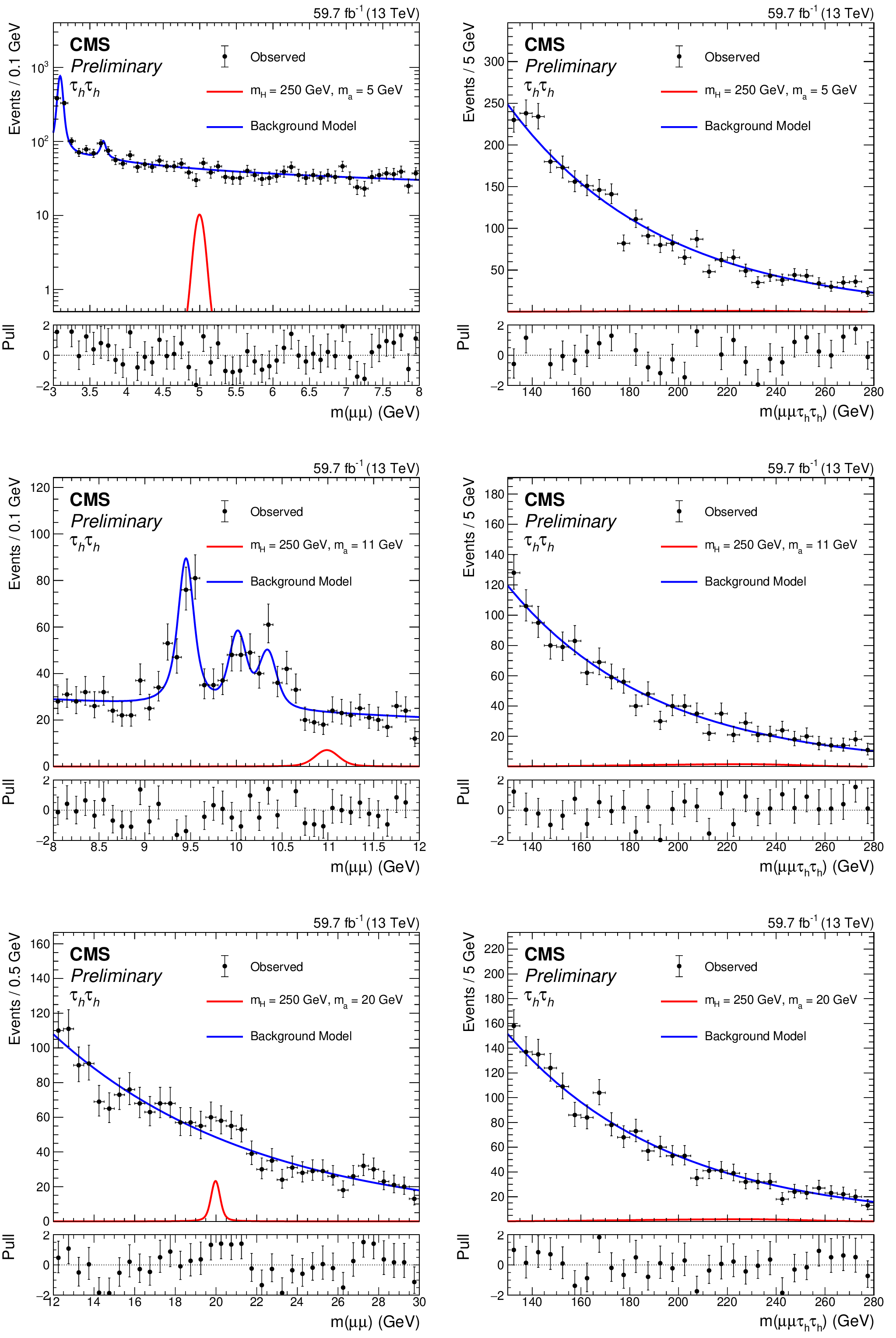
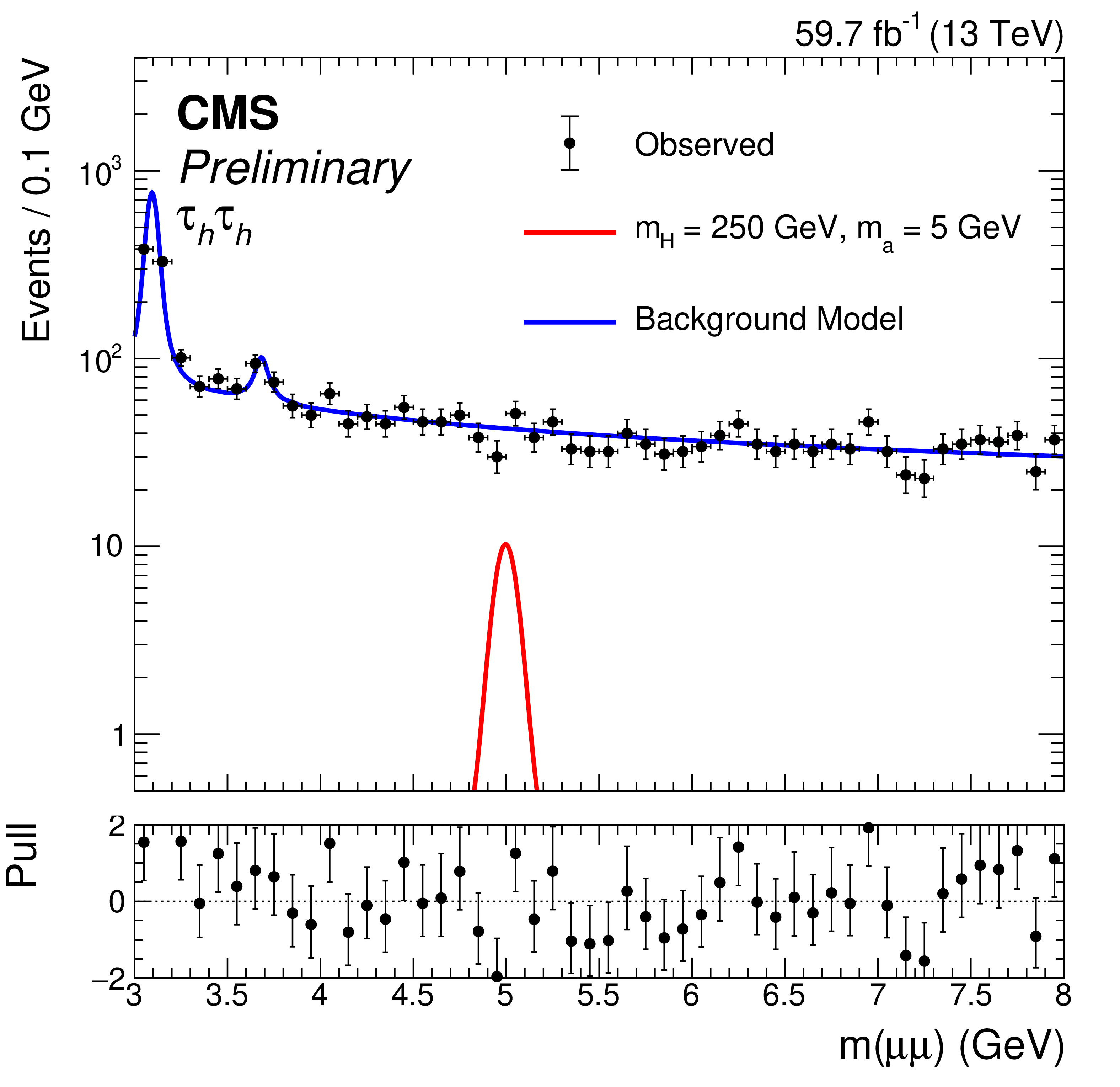
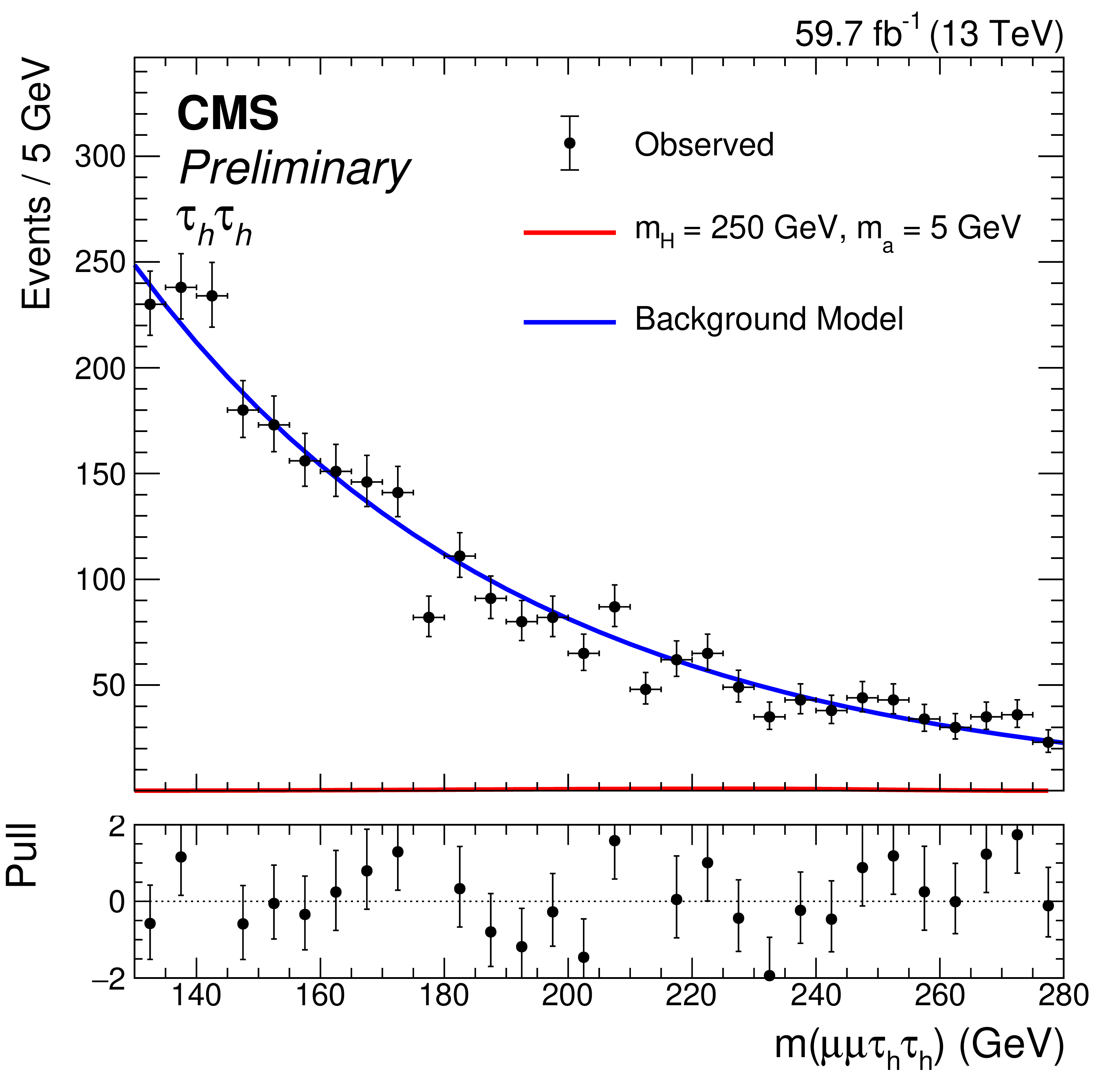
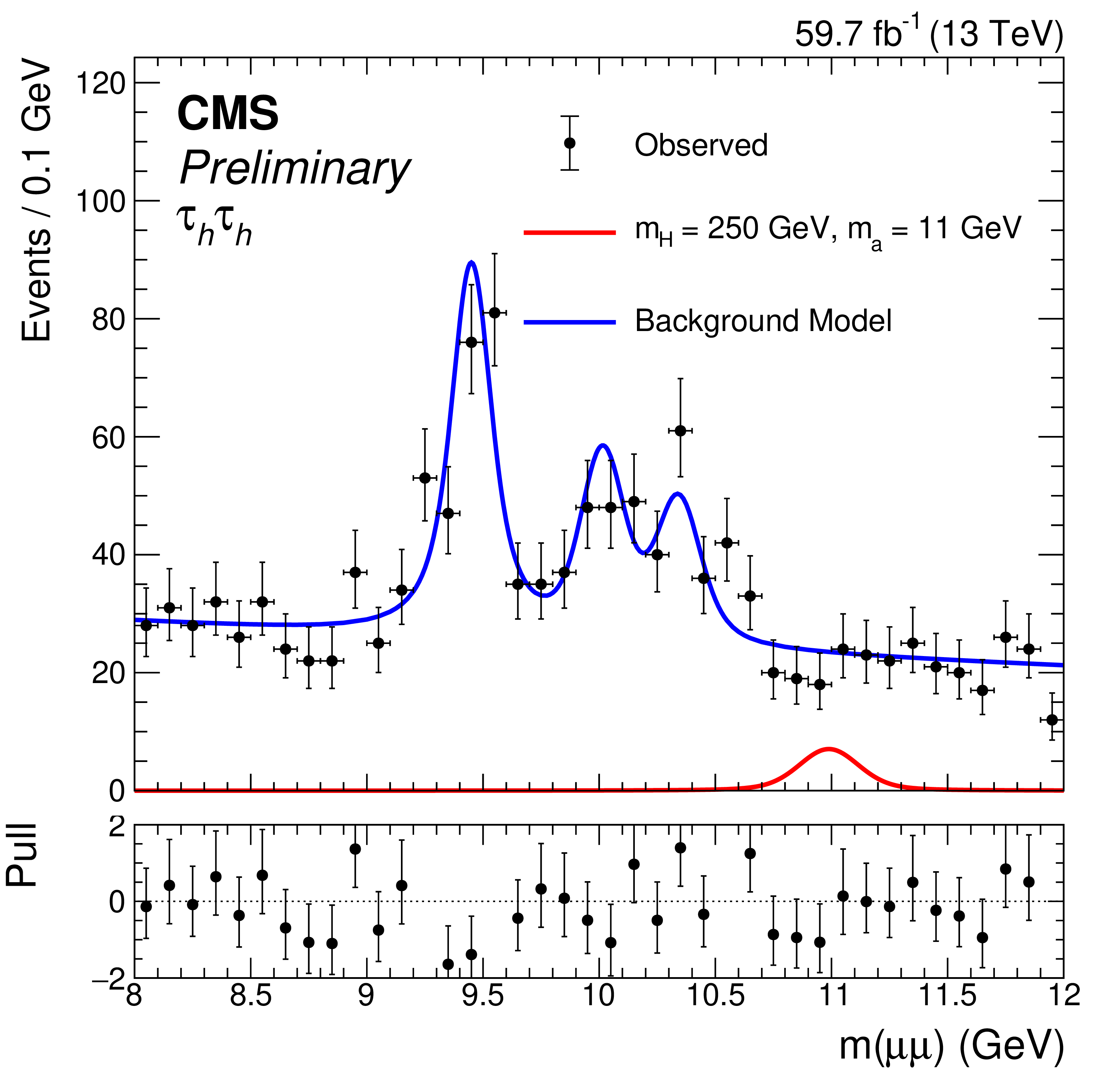
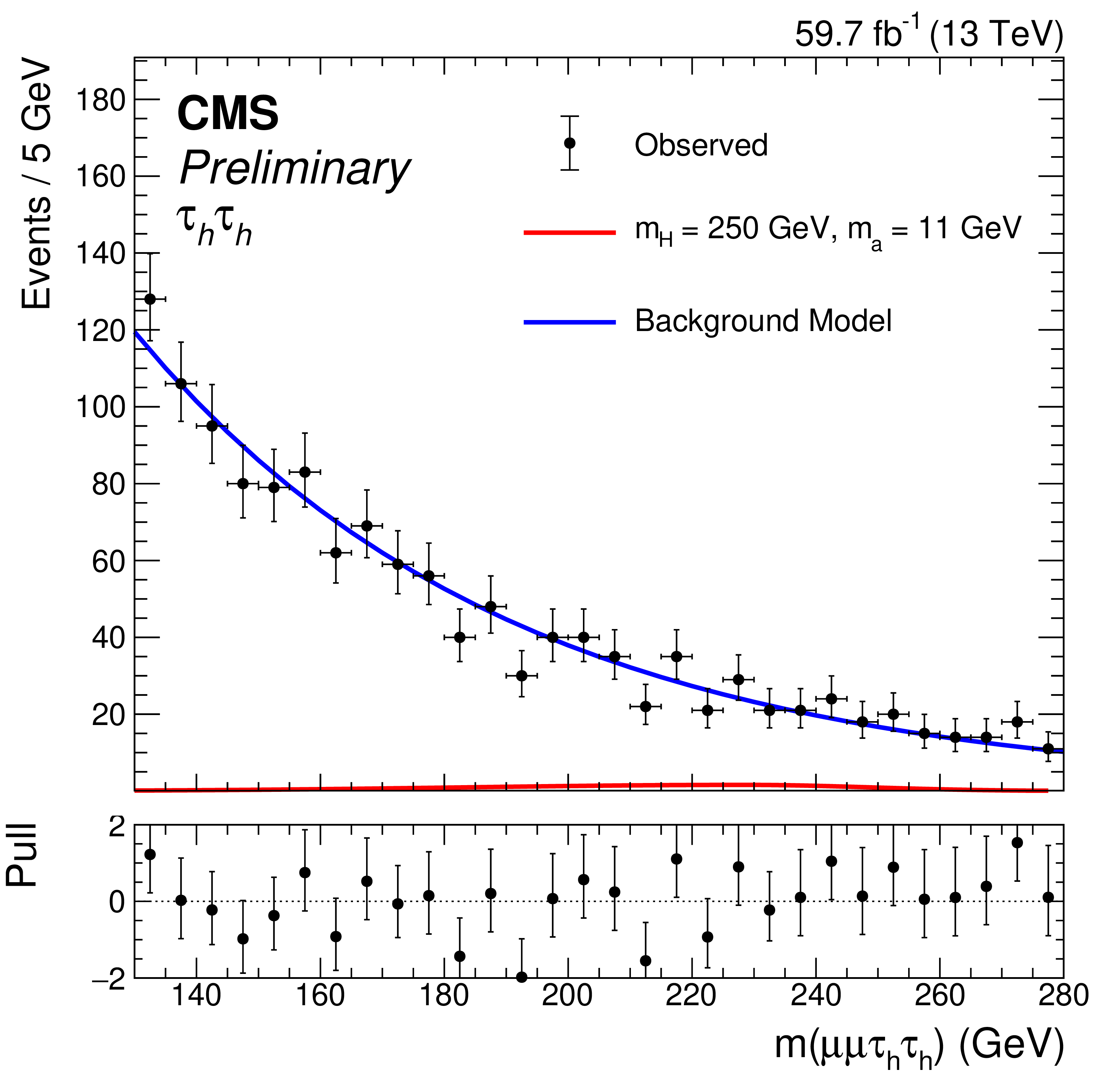
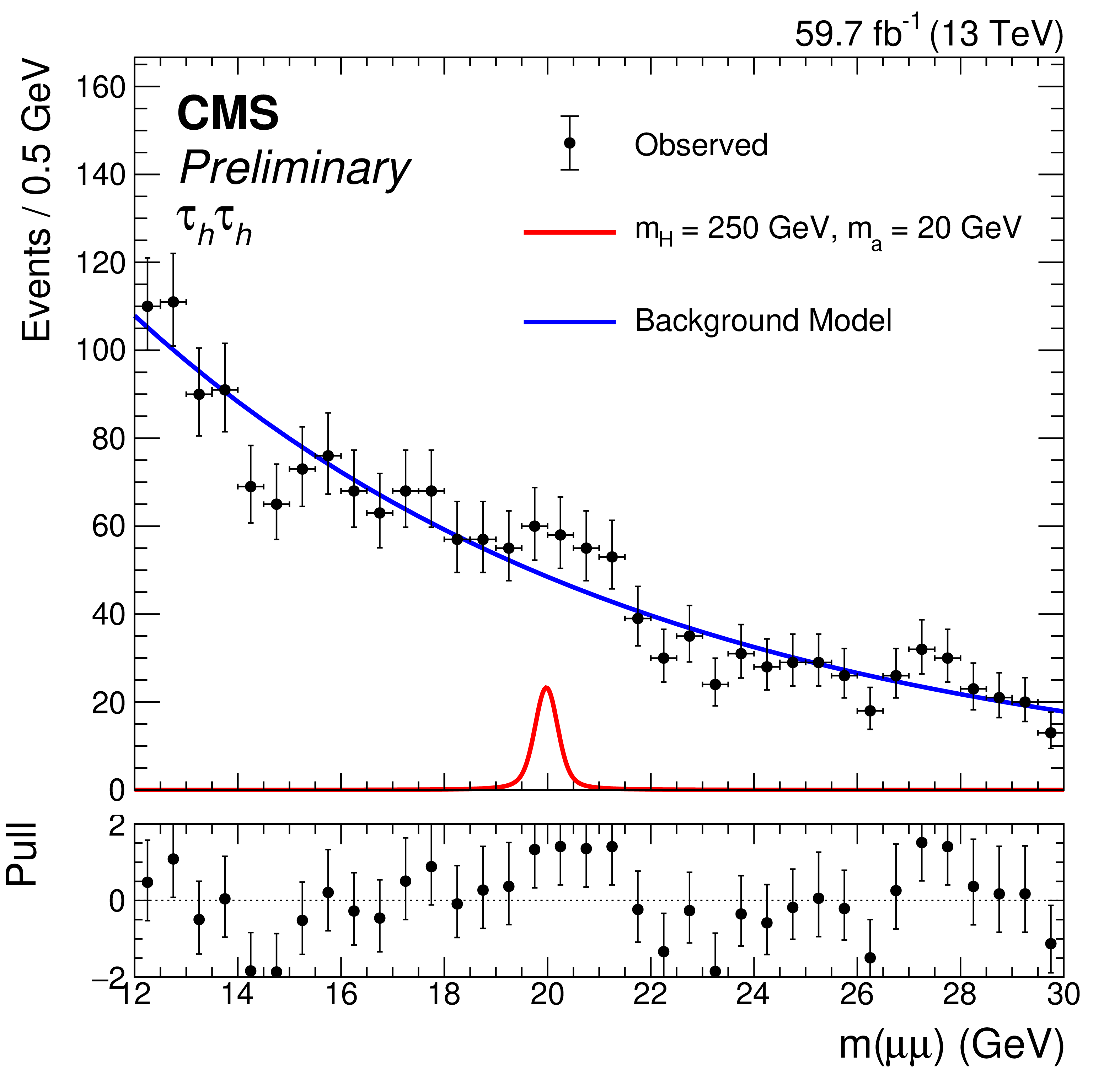
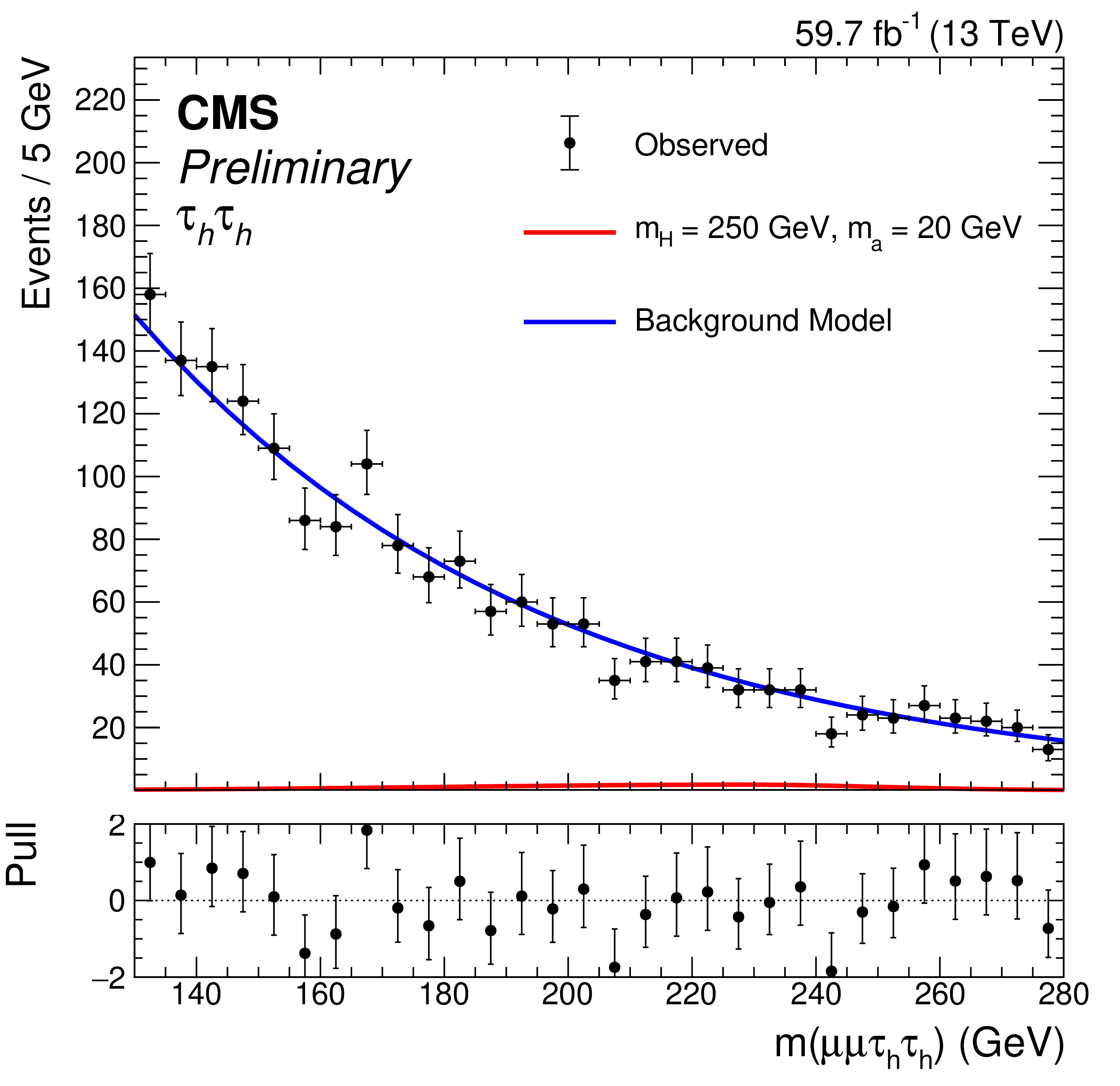
Figure 8:
Projections of the post-fit two-dimensional background PDFs (blue) and observed data onto the $ m_{\mu\mu} $ (left) and four-body visible mass (right) axes for the $ \tau_\mathrm{h}\tau_\mathrm{h} $ channel for $ m_{\mathrm{H}} = 250 \text{GeV} $ using 2018 data. The rows correspond to pseudoscalar masses $ m_{\mathrm{a}} = $ 5, 11, and 20 GeV (from top to bottom). Sample signal distributions (red) are overlaid assuming $ \mathcal{B}(\mathrm{H}\to\mathrm{a}\mathrm{a}\to\mu\mu\tau\tau) = $ 5 $ \times 10^{-4} $. |
png pdf |
Figure 8-a:
Projections of the post-fit two-dimensional background PDFs (blue) and observed data onto the $ m_{\mu\mu} $ (left) and four-body visible mass (right) axes for the $ \tau_\mathrm{h}\tau_\mathrm{h} $ channel for $ m_{\mathrm{H}} = 250 \text{GeV} $ using 2018 data. The rows correspond to pseudoscalar masses $ m_{\mathrm{a}} = $ 5, 11, and 20 GeV (from top to bottom). Sample signal distributions (red) are overlaid assuming $ \mathcal{B}(\mathrm{H}\to\mathrm{a}\mathrm{a}\to\mu\mu\tau\tau) = $ 5 $ \times 10^{-4} $. |
png pdf |
Figure 8-b:
Projections of the post-fit two-dimensional background PDFs (blue) and observed data onto the $ m_{\mu\mu} $ (left) and four-body visible mass (right) axes for the $ \tau_\mathrm{h}\tau_\mathrm{h} $ channel for $ m_{\mathrm{H}} = 250 \text{GeV} $ using 2018 data. The rows correspond to pseudoscalar masses $ m_{\mathrm{a}} = $ 5, 11, and 20 GeV (from top to bottom). Sample signal distributions (red) are overlaid assuming $ \mathcal{B}(\mathrm{H}\to\mathrm{a}\mathrm{a}\to\mu\mu\tau\tau) = $ 5 $ \times 10^{-4} $. |
png pdf |
Figure 8-c:
Projections of the post-fit two-dimensional background PDFs (blue) and observed data onto the $ m_{\mu\mu} $ (left) and four-body visible mass (right) axes for the $ \tau_\mathrm{h}\tau_\mathrm{h} $ channel for $ m_{\mathrm{H}} = 250 \text{GeV} $ using 2018 data. The rows correspond to pseudoscalar masses $ m_{\mathrm{a}} = $ 5, 11, and 20 GeV (from top to bottom). Sample signal distributions (red) are overlaid assuming $ \mathcal{B}(\mathrm{H}\to\mathrm{a}\mathrm{a}\to\mu\mu\tau\tau) = $ 5 $ \times 10^{-4} $. |
png pdf |
Figure 8-d:
Projections of the post-fit two-dimensional background PDFs (blue) and observed data onto the $ m_{\mu\mu} $ (left) and four-body visible mass (right) axes for the $ \tau_\mathrm{h}\tau_\mathrm{h} $ channel for $ m_{\mathrm{H}} = 250 \text{GeV} $ using 2018 data. The rows correspond to pseudoscalar masses $ m_{\mathrm{a}} = $ 5, 11, and 20 GeV (from top to bottom). Sample signal distributions (red) are overlaid assuming $ \mathcal{B}(\mathrm{H}\to\mathrm{a}\mathrm{a}\to\mu\mu\tau\tau) = $ 5 $ \times 10^{-4} $. |
png pdf |
Figure 8-e:
Projections of the post-fit two-dimensional background PDFs (blue) and observed data onto the $ m_{\mu\mu} $ (left) and four-body visible mass (right) axes for the $ \tau_\mathrm{h}\tau_\mathrm{h} $ channel for $ m_{\mathrm{H}} = 250 \text{GeV} $ using 2018 data. The rows correspond to pseudoscalar masses $ m_{\mathrm{a}} = $ 5, 11, and 20 GeV (from top to bottom). Sample signal distributions (red) are overlaid assuming $ \mathcal{B}(\mathrm{H}\to\mathrm{a}\mathrm{a}\to\mu\mu\tau\tau) = $ 5 $ \times 10^{-4} $. |
png pdf |
Figure 8-f:
Projections of the post-fit two-dimensional background PDFs (blue) and observed data onto the $ m_{\mu\mu} $ (left) and four-body visible mass (right) axes for the $ \tau_\mathrm{h}\tau_\mathrm{h} $ channel for $ m_{\mathrm{H}} = 250 \text{GeV} $ using 2018 data. The rows correspond to pseudoscalar masses $ m_{\mathrm{a}} = $ 5, 11, and 20 GeV (from top to bottom). Sample signal distributions (red) are overlaid assuming $ \mathcal{B}(\mathrm{H}\to\mathrm{a}\mathrm{a}\to\mu\mu\tau\tau) = $ 5 $ \times 10^{-4} $. |
png pdf |
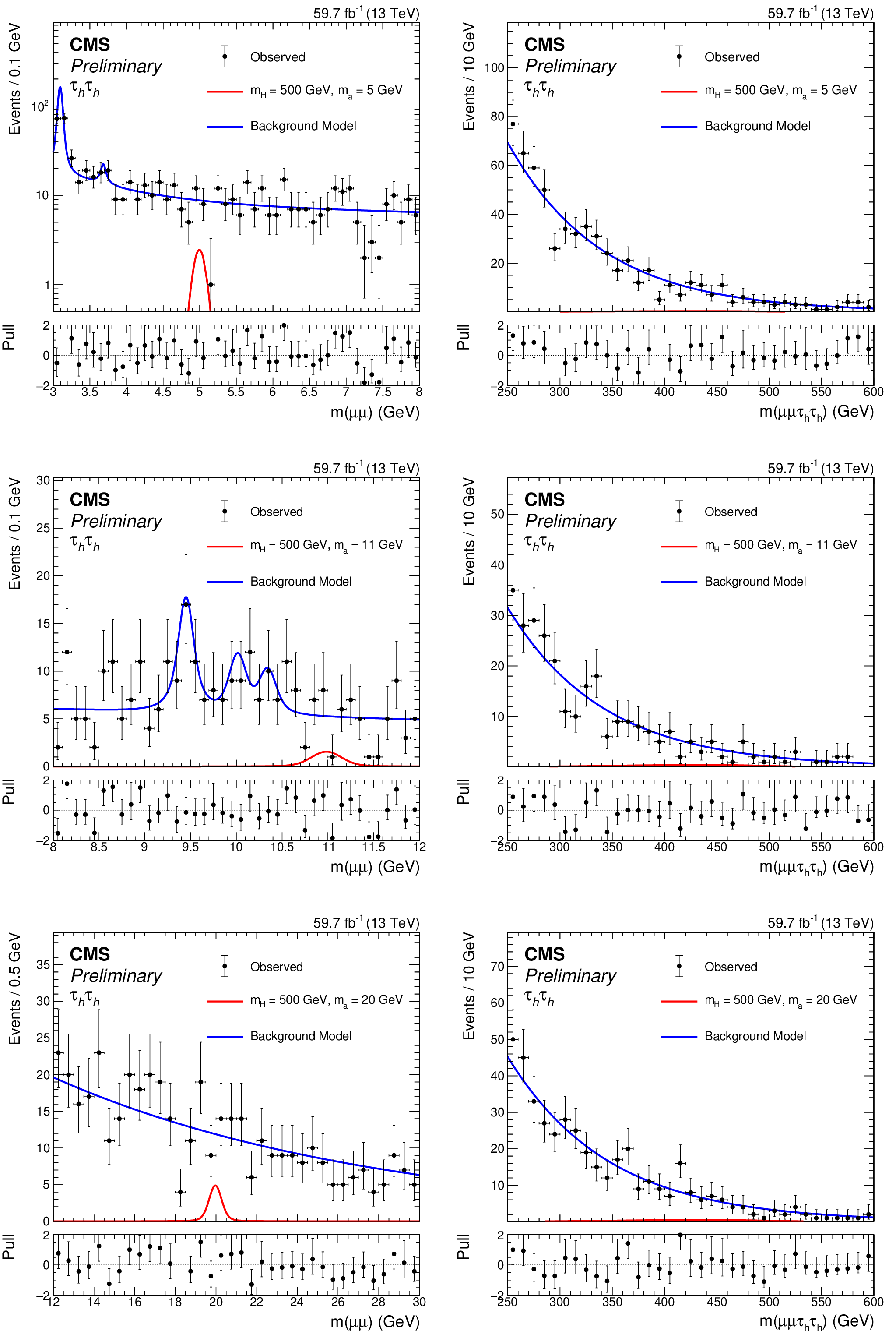
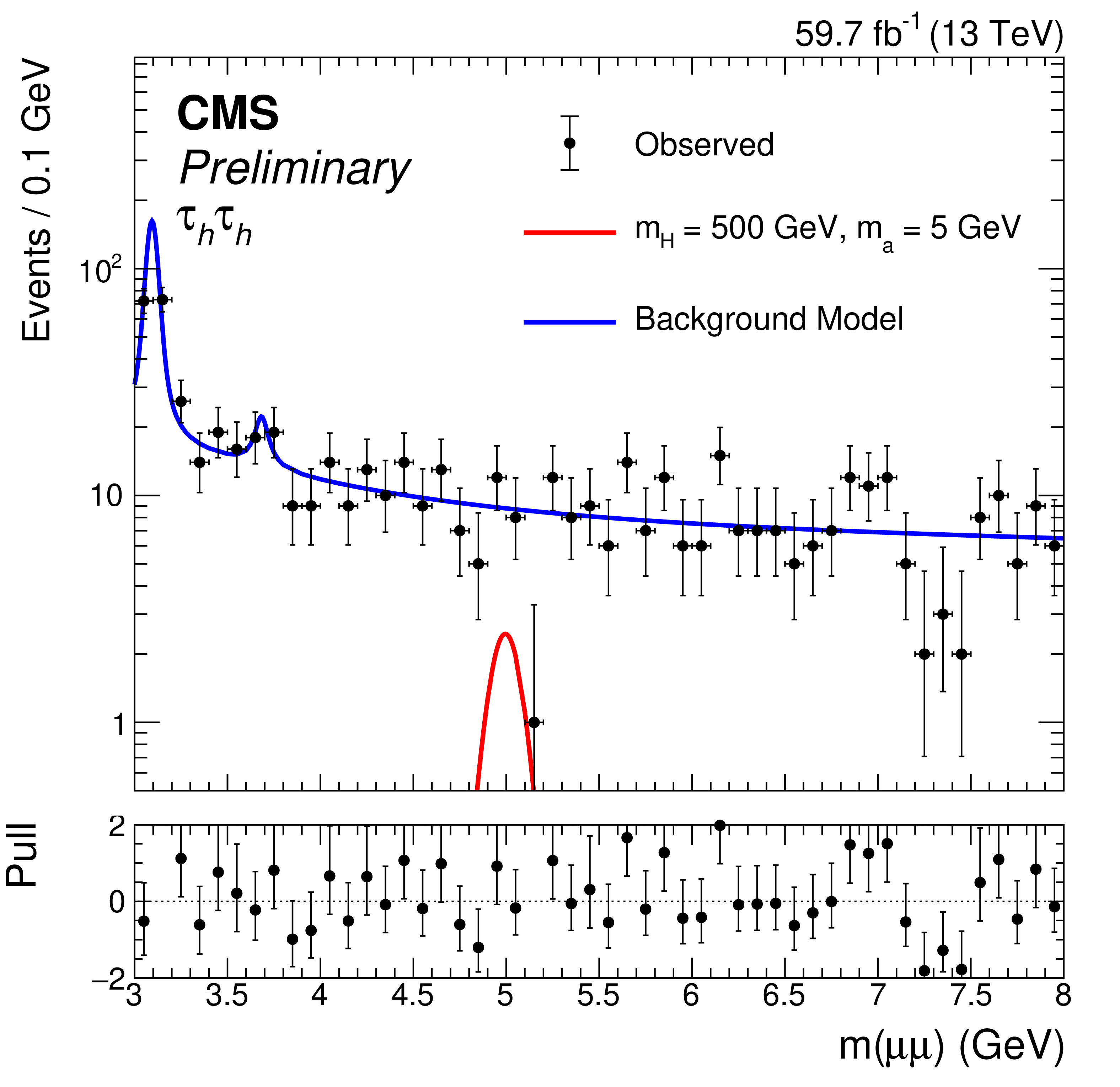
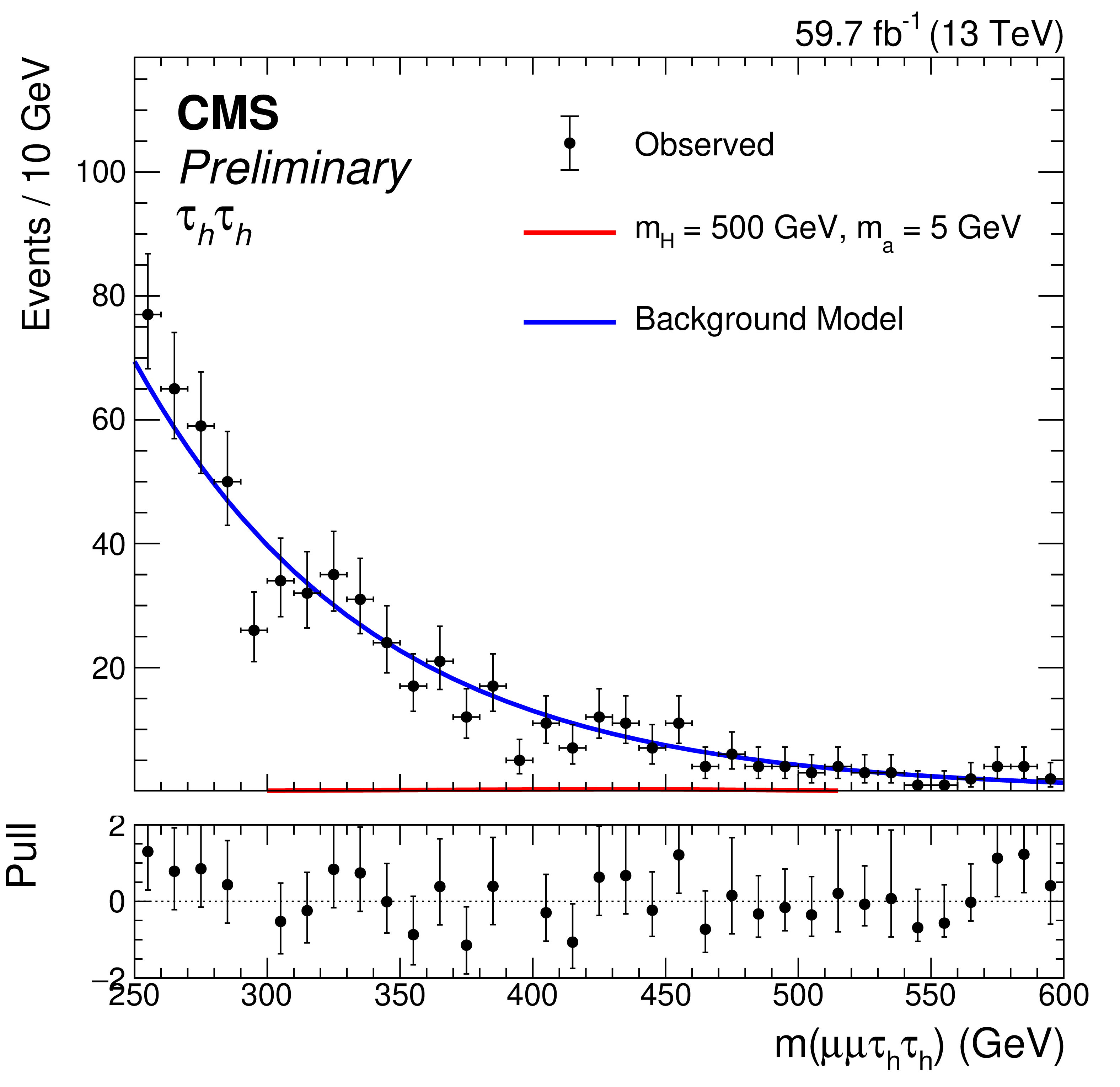
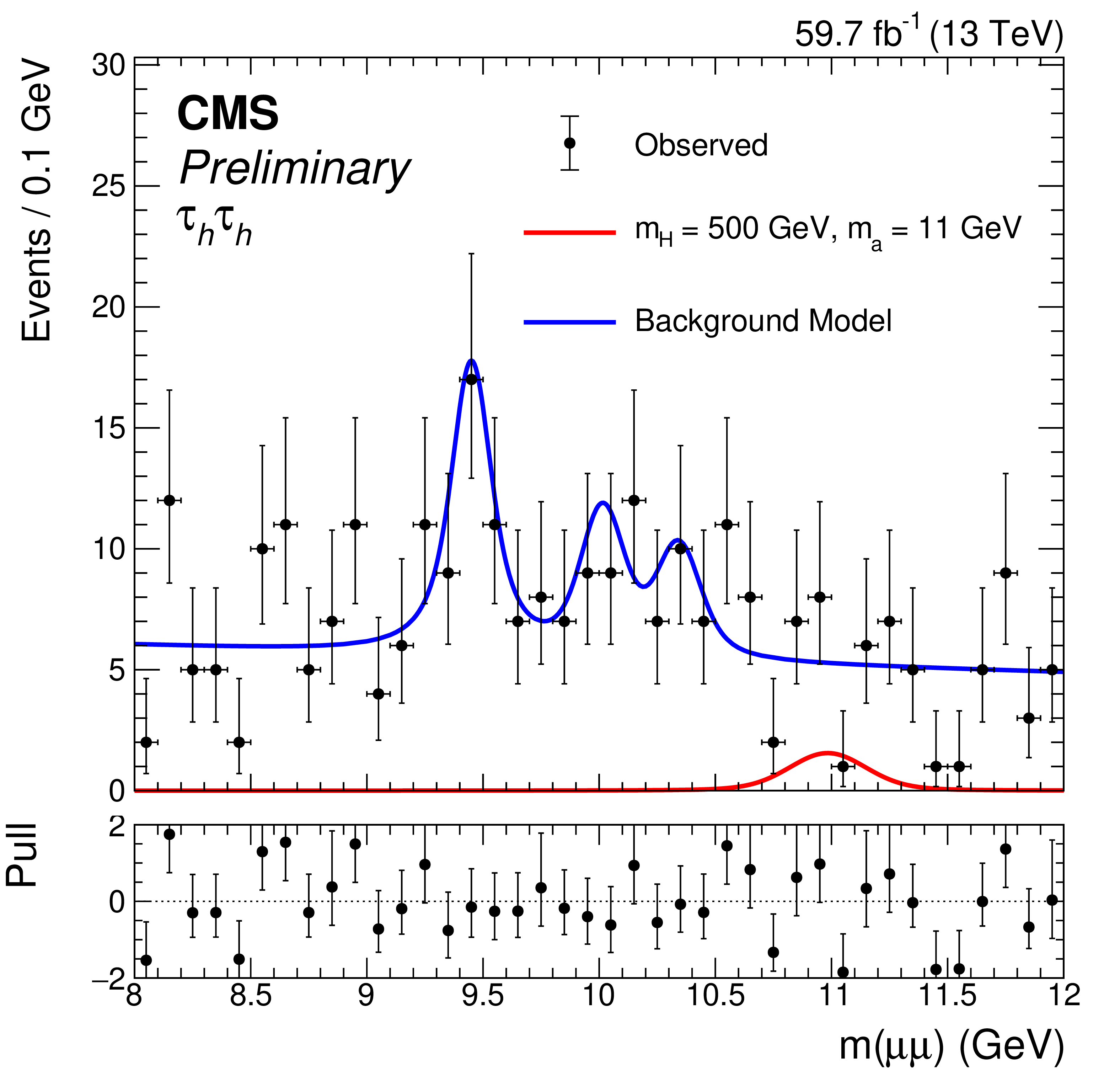
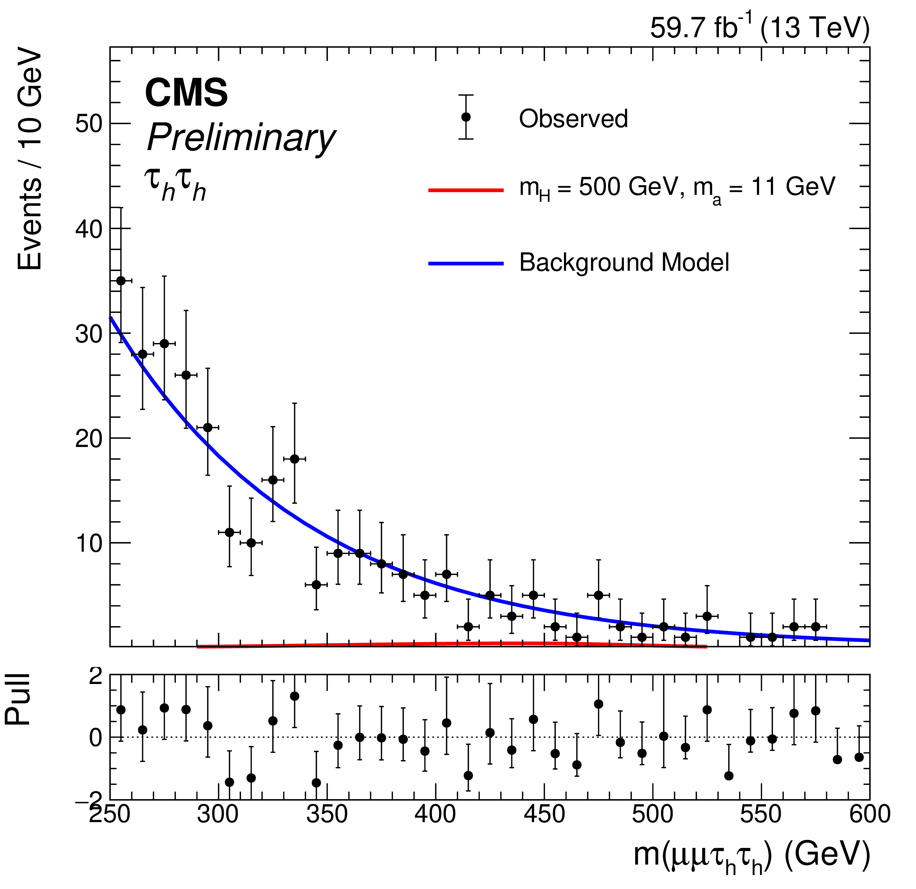
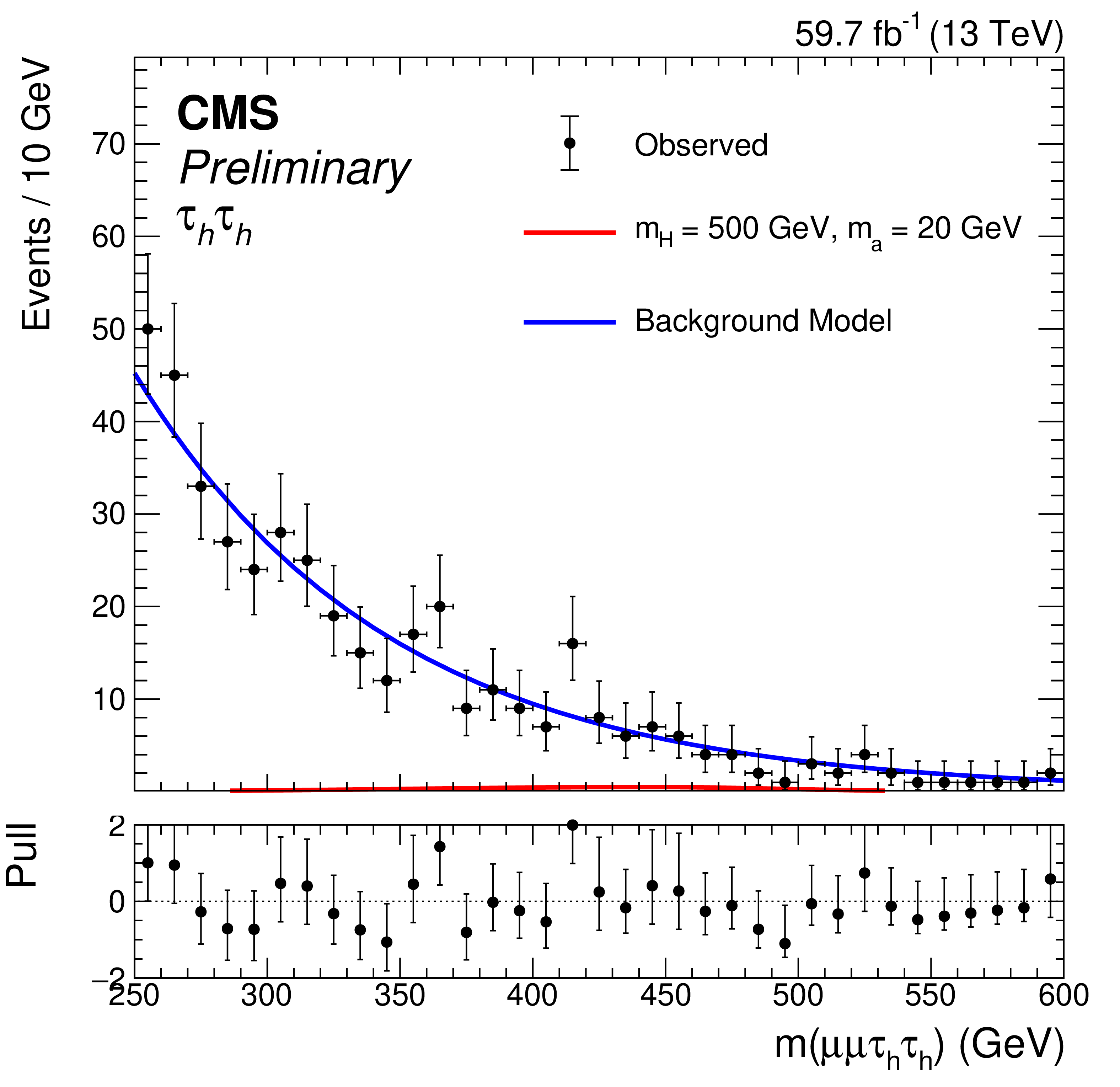
Figure 9:
Projections of the post-fit two-dimensional background PDFs (blue) and observed data onto the $ m_{\mu\mu} $ (left) and four-body visible mass (right) axes for the $ \tau_\mathrm{h}\tau_\mathrm{h} $ channel for $ m_{\mathrm{H}} = 500 \text{GeV} $ using 2018 data. The rows correspond to pseudoscalar masses $ m_{\mathrm{a}} = $ 5, 11, and 20 GeV (from top to bottom). Sample signal distributions (red) are overlaid assuming $ \mathcal{B}(\mathrm{H}\to\mathrm{a}\mathrm{a}\to\mu\mu\tau\tau) = $ 5 $ \times 10^{-4} $. |
png pdf |
Figure 9-a:
Projections of the post-fit two-dimensional background PDFs (blue) and observed data onto the $ m_{\mu\mu} $ (left) and four-body visible mass (right) axes for the $ \tau_\mathrm{h}\tau_\mathrm{h} $ channel for $ m_{\mathrm{H}} = 500 \text{GeV} $ using 2018 data. The rows correspond to pseudoscalar masses $ m_{\mathrm{a}} = $ 5, 11, and 20 GeV (from top to bottom). Sample signal distributions (red) are overlaid assuming $ \mathcal{B}(\mathrm{H}\to\mathrm{a}\mathrm{a}\to\mu\mu\tau\tau) = $ 5 $ \times 10^{-4} $. |
png pdf |
Figure 9-b:
Projections of the post-fit two-dimensional background PDFs (blue) and observed data onto the $ m_{\mu\mu} $ (left) and four-body visible mass (right) axes for the $ \tau_\mathrm{h}\tau_\mathrm{h} $ channel for $ m_{\mathrm{H}} = 500 \text{GeV} $ using 2018 data. The rows correspond to pseudoscalar masses $ m_{\mathrm{a}} = $ 5, 11, and 20 GeV (from top to bottom). Sample signal distributions (red) are overlaid assuming $ \mathcal{B}(\mathrm{H}\to\mathrm{a}\mathrm{a}\to\mu\mu\tau\tau) = $ 5 $ \times 10^{-4} $. |
png pdf |
Figure 9-c:
Projections of the post-fit two-dimensional background PDFs (blue) and observed data onto the $ m_{\mu\mu} $ (left) and four-body visible mass (right) axes for the $ \tau_\mathrm{h}\tau_\mathrm{h} $ channel for $ m_{\mathrm{H}} = 500 \text{GeV} $ using 2018 data. The rows correspond to pseudoscalar masses $ m_{\mathrm{a}} = $ 5, 11, and 20 GeV (from top to bottom). Sample signal distributions (red) are overlaid assuming $ \mathcal{B}(\mathrm{H}\to\mathrm{a}\mathrm{a}\to\mu\mu\tau\tau) = $ 5 $ \times 10^{-4} $. |
png pdf |
Figure 9-d:
Projections of the post-fit two-dimensional background PDFs (blue) and observed data onto the $ m_{\mu\mu} $ (left) and four-body visible mass (right) axes for the $ \tau_\mathrm{h}\tau_\mathrm{h} $ channel for $ m_{\mathrm{H}} = 500 \text{GeV} $ using 2018 data. The rows correspond to pseudoscalar masses $ m_{\mathrm{a}} = $ 5, 11, and 20 GeV (from top to bottom). Sample signal distributions (red) are overlaid assuming $ \mathcal{B}(\mathrm{H}\to\mathrm{a}\mathrm{a}\to\mu\mu\tau\tau) = $ 5 $ \times 10^{-4} $. |

png pdf |
Figure 9-e:
Projections of the post-fit two-dimensional background PDFs (blue) and observed data onto the $ m_{\mu\mu} $ (left) and four-body visible mass (right) axes for the $ \tau_\mathrm{h}\tau_\mathrm{h} $ channel for $ m_{\mathrm{H}} = 500 \text{GeV} $ using 2018 data. The rows correspond to pseudoscalar masses $ m_{\mathrm{a}} = $ 5, 11, and 20 GeV (from top to bottom). Sample signal distributions (red) are overlaid assuming $ \mathcal{B}(\mathrm{H}\to\mathrm{a}\mathrm{a}\to\mu\mu\tau\tau) = $ 5 $ \times 10^{-4} $. |
png pdf |
Figure 9-f:
Projections of the post-fit two-dimensional background PDFs (blue) and observed data onto the $ m_{\mu\mu} $ (left) and four-body visible mass (right) axes for the $ \tau_\mathrm{h}\tau_\mathrm{h} $ channel for $ m_{\mathrm{H}} = 500 \text{GeV} $ using 2018 data. The rows correspond to pseudoscalar masses $ m_{\mathrm{a}} = $ 5, 11, and 20 GeV (from top to bottom). Sample signal distributions (red) are overlaid assuming $ \mathcal{B}(\mathrm{H}\to\mathrm{a}\mathrm{a}\to\mu\mu\tau\tau) = $ 5 $ \times 10^{-4} $. |
png pdf |
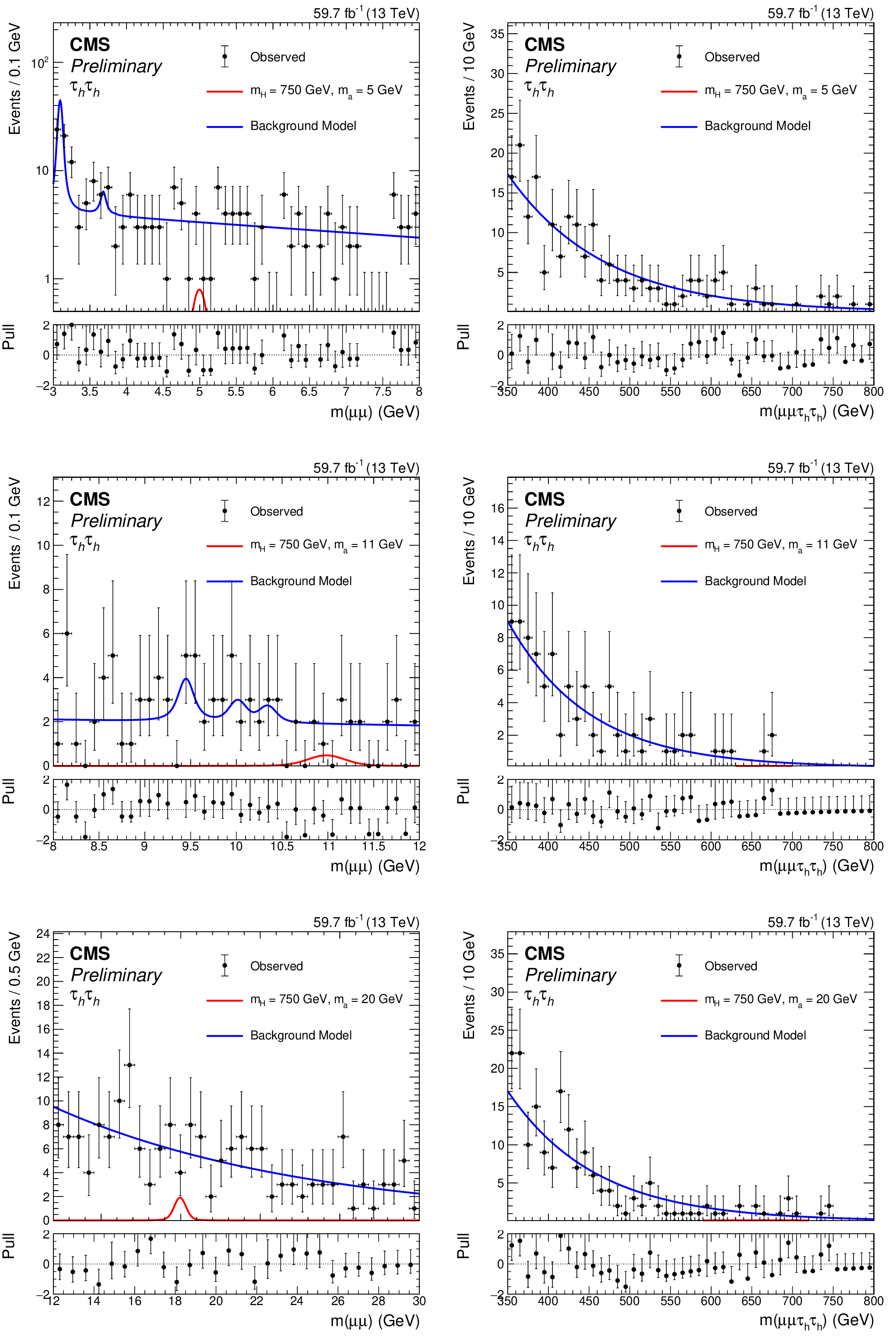
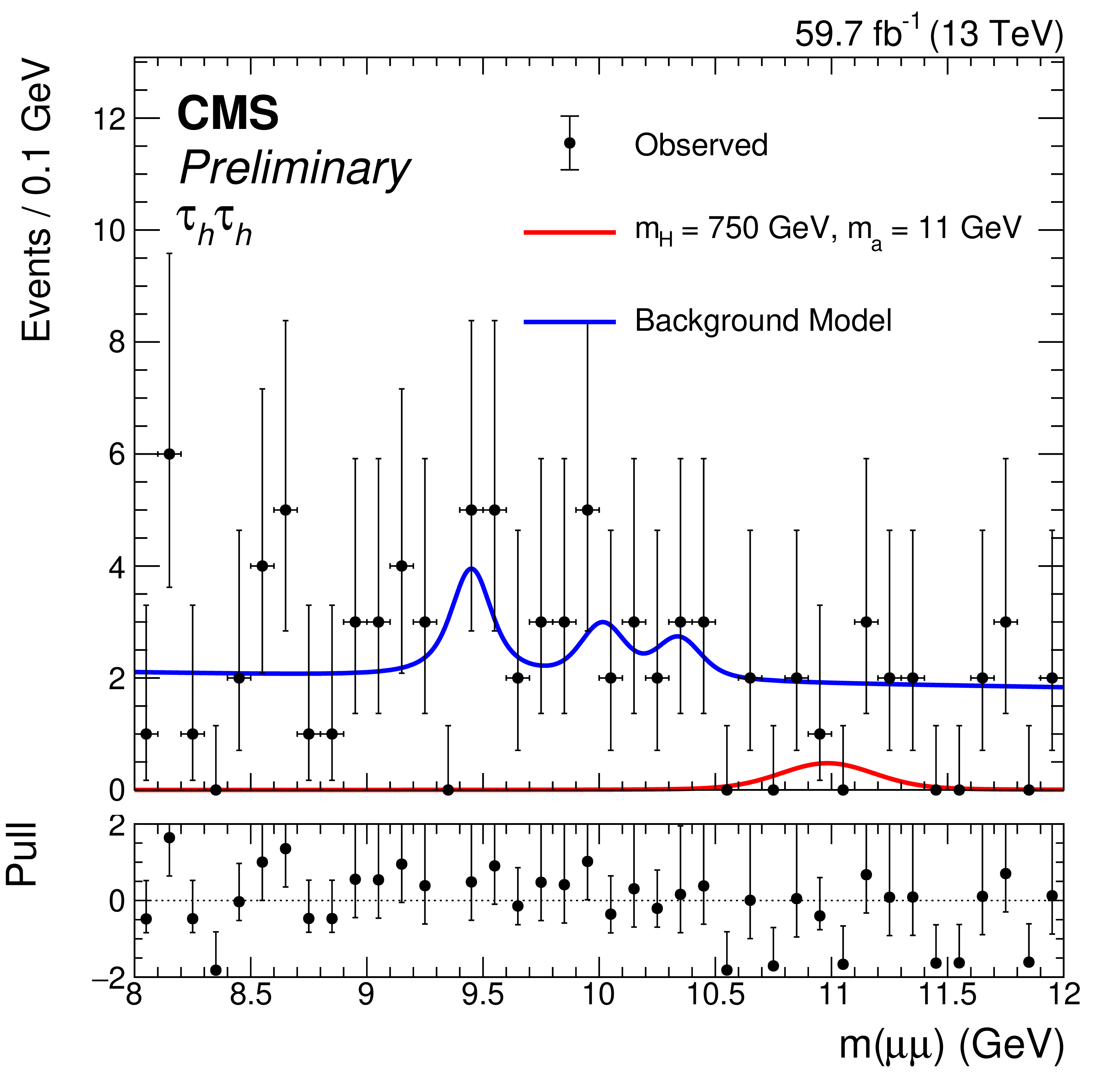
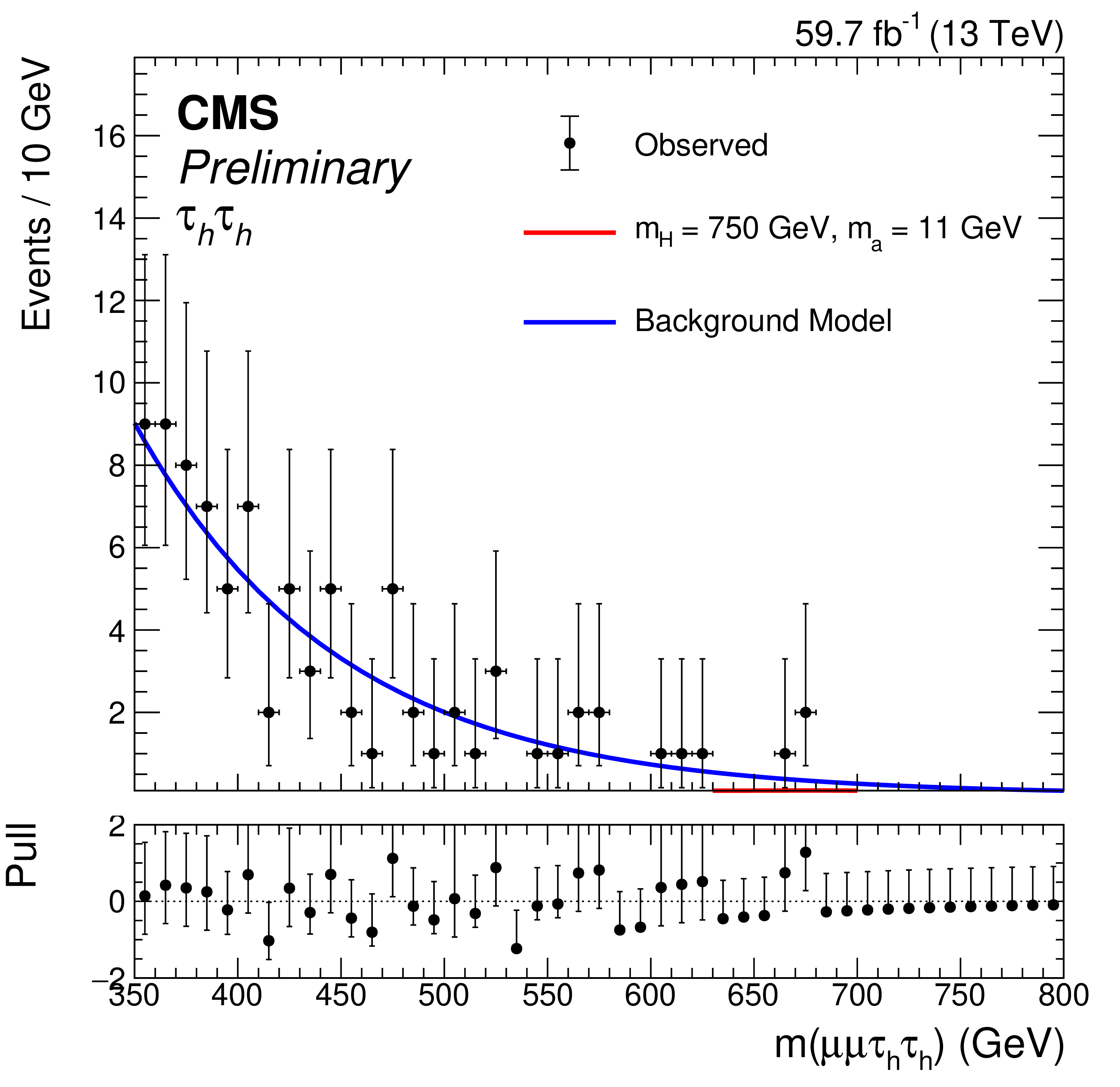
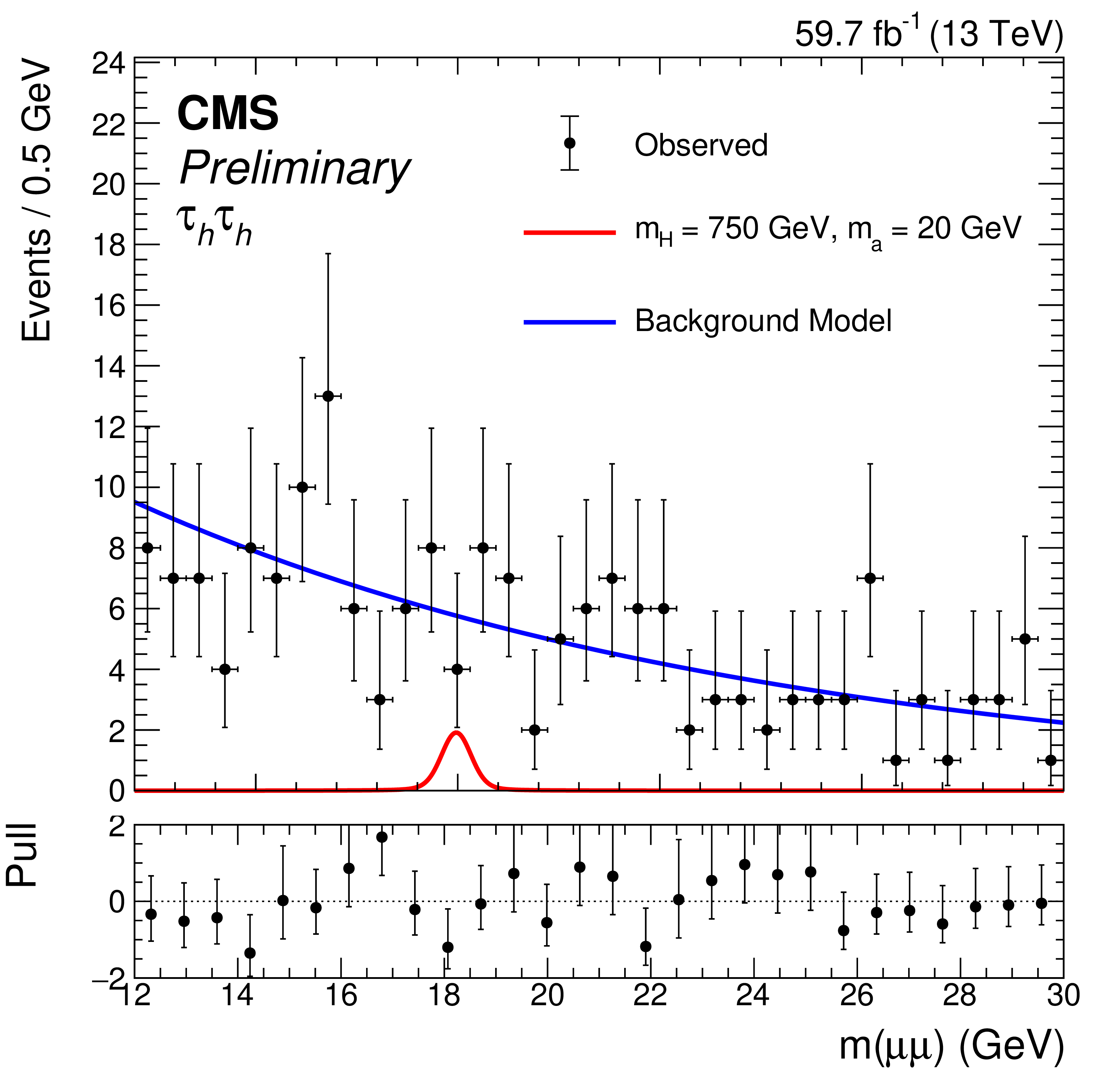
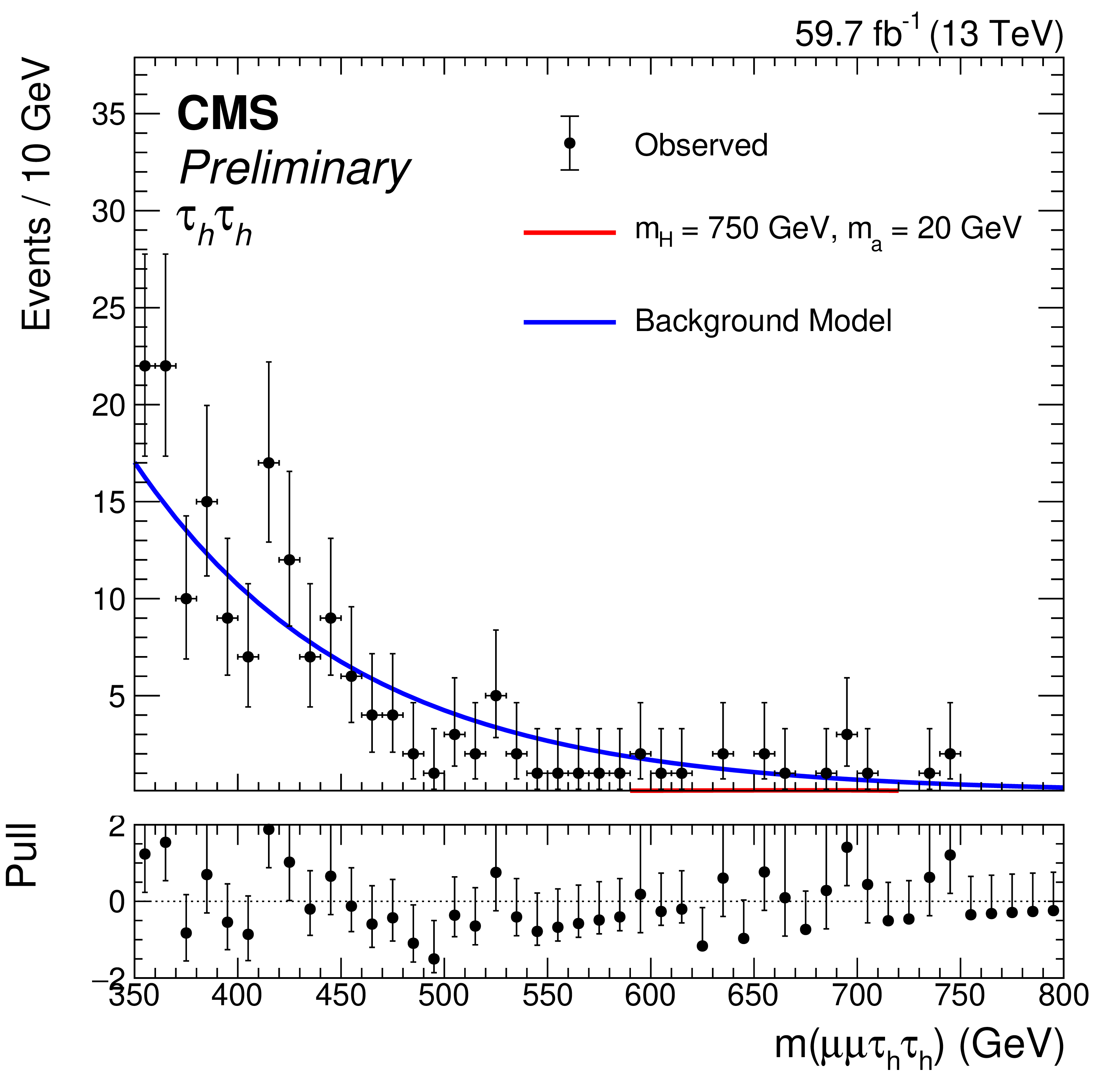
Figure 10:
Projections of the post-fit two-dimensional background PDFs (blue) and observed data onto the $ m_{\mu\mu} $ (left) and four-body visible mass (right) axes for the $ \tau_\mathrm{h}\tau_\mathrm{h} $ channel for $ m_{\mathrm{H}} = 750 \text{GeV} $ using 2018 data. The rows correspond to pseudoscalar masses $ m_{\mathrm{a}} = $ 5, 11, and 20 GeV (from top to bottom). Sample signal distributions (red) are overlaid assuming $ \mathcal{B}(\mathrm{H}\to\mathrm{a}\mathrm{a}\to\mu\mu\tau\tau) = $ 5 $ \times 10^{-4} $. |

png pdf |
Figure 10-a:
Projections of the post-fit two-dimensional background PDFs (blue) and observed data onto the $ m_{\mu\mu} $ (left) and four-body visible mass (right) axes for the $ \tau_\mathrm{h}\tau_\mathrm{h} $ channel for $ m_{\mathrm{H}} = 750 \text{GeV} $ using 2018 data. The rows correspond to pseudoscalar masses $ m_{\mathrm{a}} = $ 5, 11, and 20 GeV (from top to bottom). Sample signal distributions (red) are overlaid assuming $ \mathcal{B}(\mathrm{H}\to\mathrm{a}\mathrm{a}\to\mu\mu\tau\tau) = $ 5 $ \times 10^{-4} $. |

png pdf |
Figure 10-b:
Projections of the post-fit two-dimensional background PDFs (blue) and observed data onto the $ m_{\mu\mu} $ (left) and four-body visible mass (right) axes for the $ \tau_\mathrm{h}\tau_\mathrm{h} $ channel for $ m_{\mathrm{H}} = 750 \text{GeV} $ using 2018 data. The rows correspond to pseudoscalar masses $ m_{\mathrm{a}} = $ 5, 11, and 20 GeV (from top to bottom). Sample signal distributions (red) are overlaid assuming $ \mathcal{B}(\mathrm{H}\to\mathrm{a}\mathrm{a}\to\mu\mu\tau\tau) = $ 5 $ \times 10^{-4} $. |
png pdf |
Figure 10-c:
Projections of the post-fit two-dimensional background PDFs (blue) and observed data onto the $ m_{\mu\mu} $ (left) and four-body visible mass (right) axes for the $ \tau_\mathrm{h}\tau_\mathrm{h} $ channel for $ m_{\mathrm{H}} = 750 \text{GeV} $ using 2018 data. The rows correspond to pseudoscalar masses $ m_{\mathrm{a}} = $ 5, 11, and 20 GeV (from top to bottom). Sample signal distributions (red) are overlaid assuming $ \mathcal{B}(\mathrm{H}\to\mathrm{a}\mathrm{a}\to\mu\mu\tau\tau) = $ 5 $ \times 10^{-4} $. |
png pdf |
Figure 10-d:
Projections of the post-fit two-dimensional background PDFs (blue) and observed data onto the $ m_{\mu\mu} $ (left) and four-body visible mass (right) axes for the $ \tau_\mathrm{h}\tau_\mathrm{h} $ channel for $ m_{\mathrm{H}} = 750 \text{GeV} $ using 2018 data. The rows correspond to pseudoscalar masses $ m_{\mathrm{a}} = $ 5, 11, and 20 GeV (from top to bottom). Sample signal distributions (red) are overlaid assuming $ \mathcal{B}(\mathrm{H}\to\mathrm{a}\mathrm{a}\to\mu\mu\tau\tau) = $ 5 $ \times 10^{-4} $. |
png pdf |
Figure 10-e:
Projections of the post-fit two-dimensional background PDFs (blue) and observed data onto the $ m_{\mu\mu} $ (left) and four-body visible mass (right) axes for the $ \tau_\mathrm{h}\tau_\mathrm{h} $ channel for $ m_{\mathrm{H}} = 750 \text{GeV} $ using 2018 data. The rows correspond to pseudoscalar masses $ m_{\mathrm{a}} = $ 5, 11, and 20 GeV (from top to bottom). Sample signal distributions (red) are overlaid assuming $ \mathcal{B}(\mathrm{H}\to\mathrm{a}\mathrm{a}\to\mu\mu\tau\tau) = $ 5 $ \times 10^{-4} $. |
png pdf |
Figure 10-f:
Projections of the post-fit two-dimensional background PDFs (blue) and observed data onto the $ m_{\mu\mu} $ (left) and four-body visible mass (right) axes for the $ \tau_\mathrm{h}\tau_\mathrm{h} $ channel for $ m_{\mathrm{H}} = 750 \text{GeV} $ using 2018 data. The rows correspond to pseudoscalar masses $ m_{\mathrm{a}} = $ 5, 11, and 20 GeV (from top to bottom). Sample signal distributions (red) are overlaid assuming $ \mathcal{B}(\mathrm{H}\to\mathrm{a}\mathrm{a}\to\mu\mu\tau\tau) = $ 5 $ \times 10^{-4} $. |
png pdf |
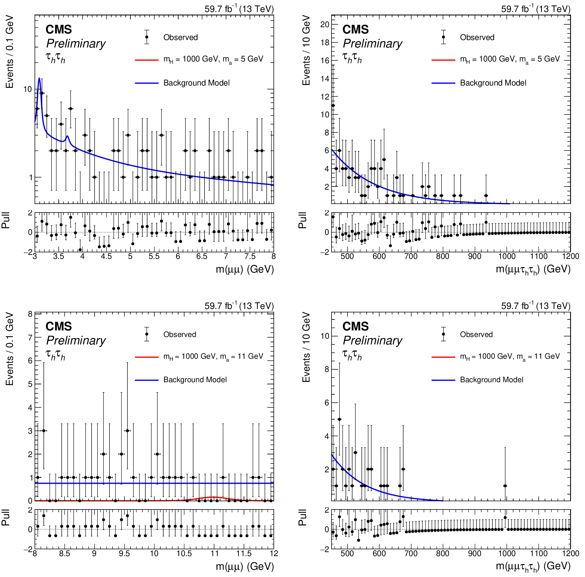
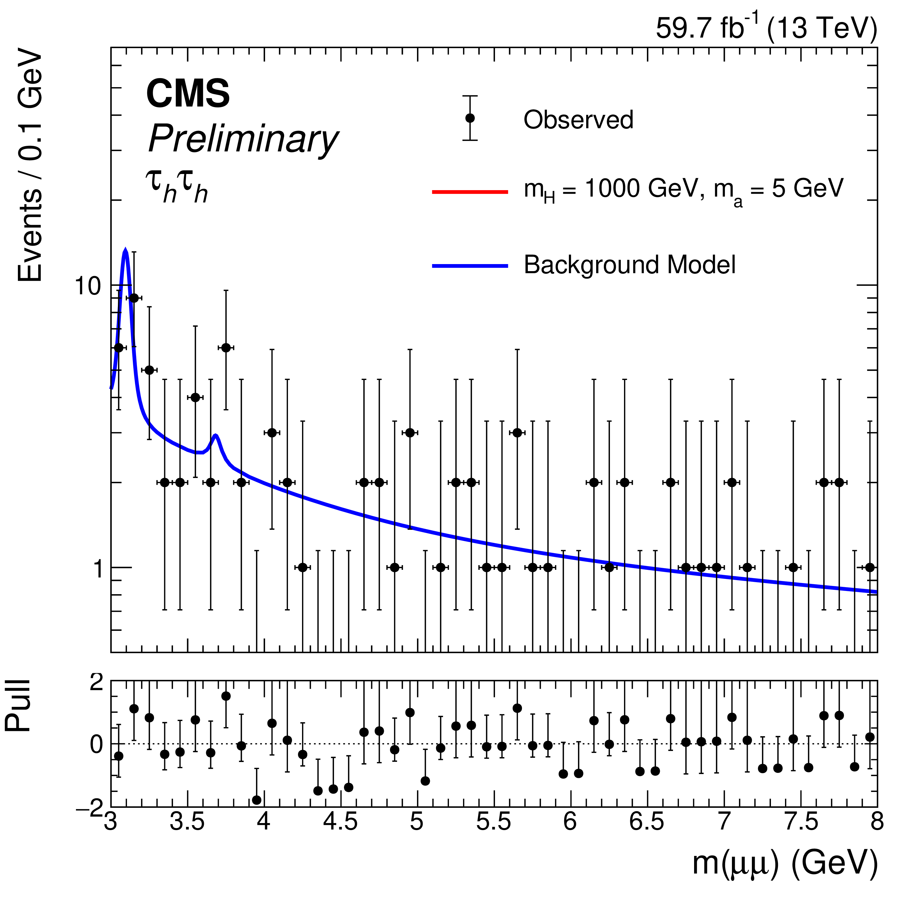
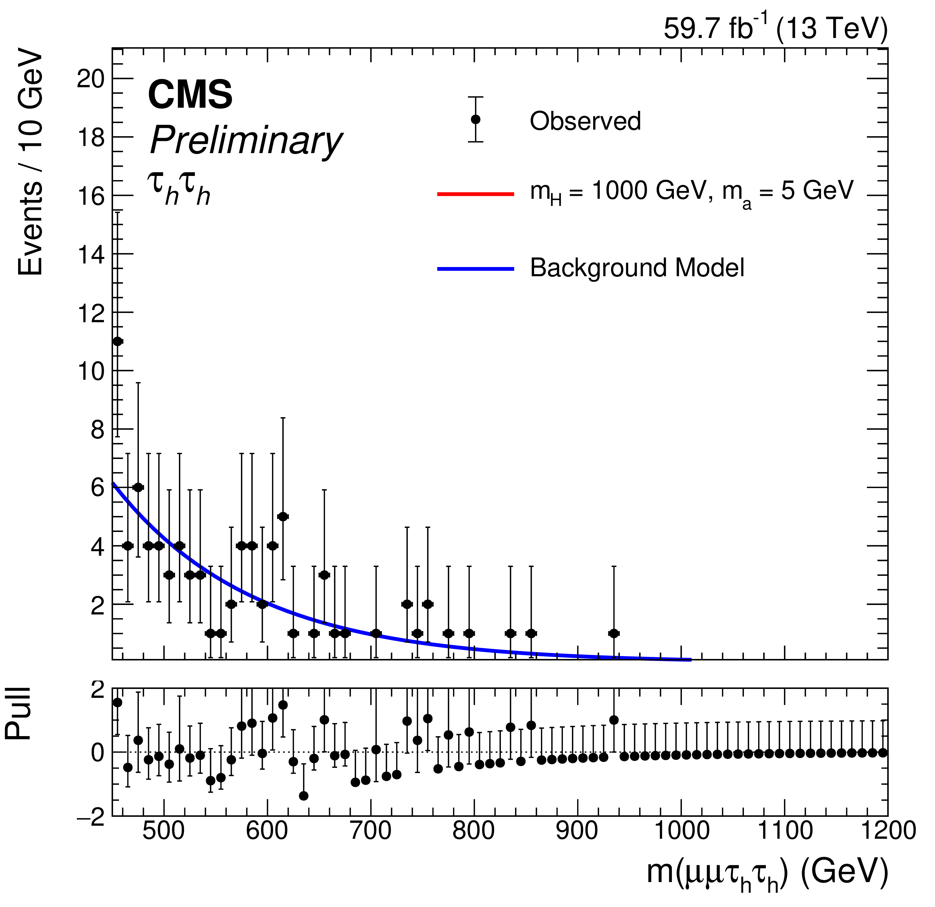
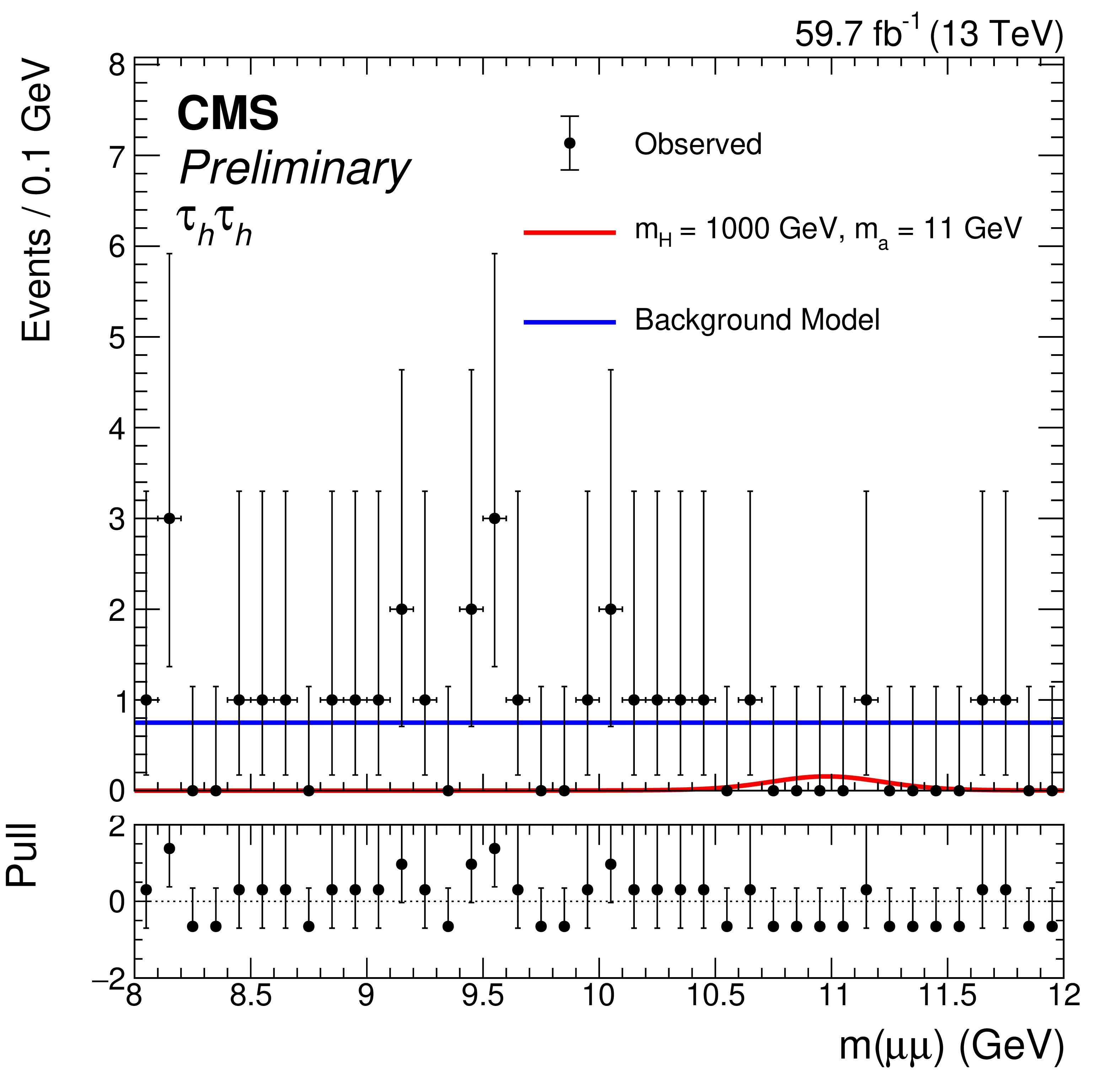
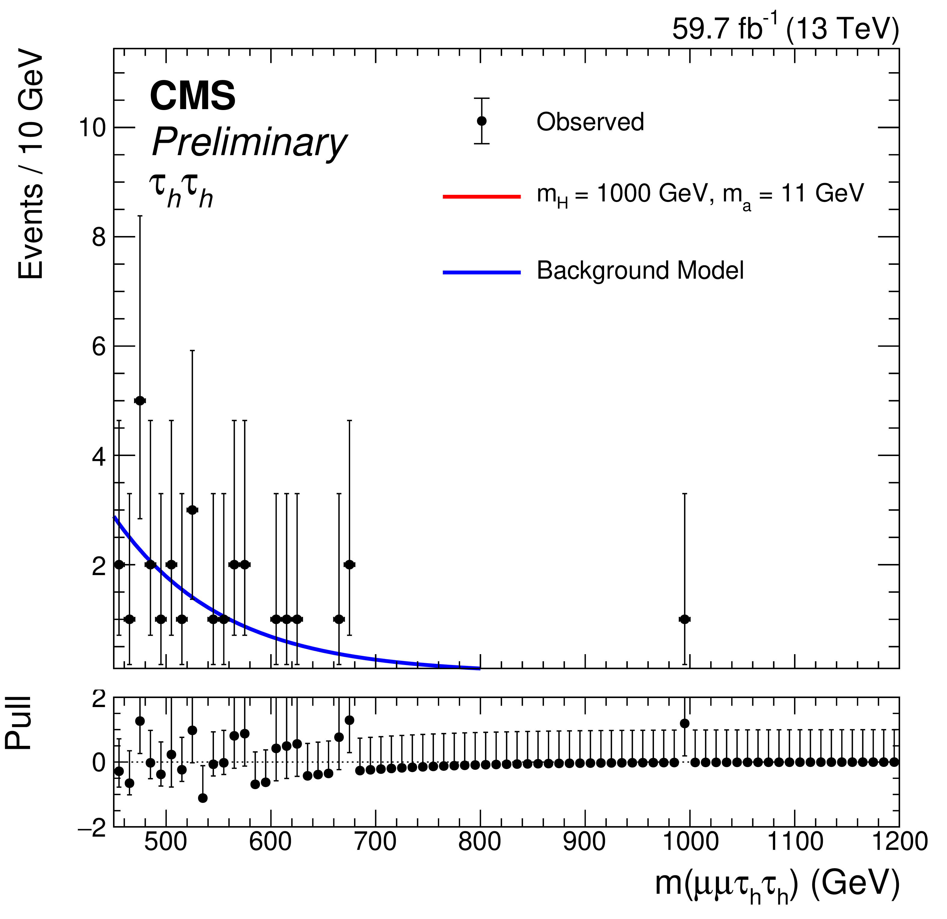
Figure 11:
Projections of the post-fit two-dimensional background PDFs (blue) and observed data onto the $ m_{\mu\mu} $ (left) and four-body visible mass (right) axes for the $ \tau_\mathrm{h}\tau_\mathrm{h} $ channel for the lower two $ m_{\mu\mu} $ mass ranges for $ m_{\mathrm{H}} = 1000 \text{GeV} $ using 2018 data. The rows correspond to pseudoscalar masses $ m_{\mathrm{a}} = $ 5 and 11 GeV (from top to bottom). Sample signal distributions (red) are overlaid assuming $ \mathcal{B}(\mathrm{H}\to\mathrm{a}\mathrm{a}\to\mu\mu\tau\tau) = $ 5 $ \times 10^{-4} $. |
png pdf |
Figure 11-a:
Projections of the post-fit two-dimensional background PDFs (blue) and observed data onto the $ m_{\mu\mu} $ (left) and four-body visible mass (right) axes for the $ \tau_\mathrm{h}\tau_\mathrm{h} $ channel for the lower two $ m_{\mu\mu} $ mass ranges for $ m_{\mathrm{H}} = 1000 \text{GeV} $ using 2018 data. The rows correspond to pseudoscalar masses $ m_{\mathrm{a}} = $ 5 and 11 GeV (from top to bottom). Sample signal distributions (red) are overlaid assuming $ \mathcal{B}(\mathrm{H}\to\mathrm{a}\mathrm{a}\to\mu\mu\tau\tau) = $ 5 $ \times 10^{-4} $. |
png pdf |
Figure 11-b:
Projections of the post-fit two-dimensional background PDFs (blue) and observed data onto the $ m_{\mu\mu} $ (left) and four-body visible mass (right) axes for the $ \tau_\mathrm{h}\tau_\mathrm{h} $ channel for the lower two $ m_{\mu\mu} $ mass ranges for $ m_{\mathrm{H}} = 1000 \text{GeV} $ using 2018 data. The rows correspond to pseudoscalar masses $ m_{\mathrm{a}} = $ 5 and 11 GeV (from top to bottom). Sample signal distributions (red) are overlaid assuming $ \mathcal{B}(\mathrm{H}\to\mathrm{a}\mathrm{a}\to\mu\mu\tau\tau) = $ 5 $ \times 10^{-4} $. |
png pdf |
Figure 11-c:
Projections of the post-fit two-dimensional background PDFs (blue) and observed data onto the $ m_{\mu\mu} $ (left) and four-body visible mass (right) axes for the $ \tau_\mathrm{h}\tau_\mathrm{h} $ channel for the lower two $ m_{\mu\mu} $ mass ranges for $ m_{\mathrm{H}} = 1000 \text{GeV} $ using 2018 data. The rows correspond to pseudoscalar masses $ m_{\mathrm{a}} = $ 5 and 11 GeV (from top to bottom). Sample signal distributions (red) are overlaid assuming $ \mathcal{B}(\mathrm{H}\to\mathrm{a}\mathrm{a}\to\mu\mu\tau\tau) = $ 5 $ \times 10^{-4} $. |
png pdf |
Figure 11-d:
Projections of the post-fit two-dimensional background PDFs (blue) and observed data onto the $ m_{\mu\mu} $ (left) and four-body visible mass (right) axes for the $ \tau_\mathrm{h}\tau_\mathrm{h} $ channel for the lower two $ m_{\mu\mu} $ mass ranges for $ m_{\mathrm{H}} = 1000 \text{GeV} $ using 2018 data. The rows correspond to pseudoscalar masses $ m_{\mathrm{a}} = $ 5 and 11 GeV (from top to bottom). Sample signal distributions (red) are overlaid assuming $ \mathcal{B}(\mathrm{H}\to\mathrm{a}\mathrm{a}\to\mu\mu\tau\tau) = $ 5 $ \times 10^{-4} $. |
png pdf |
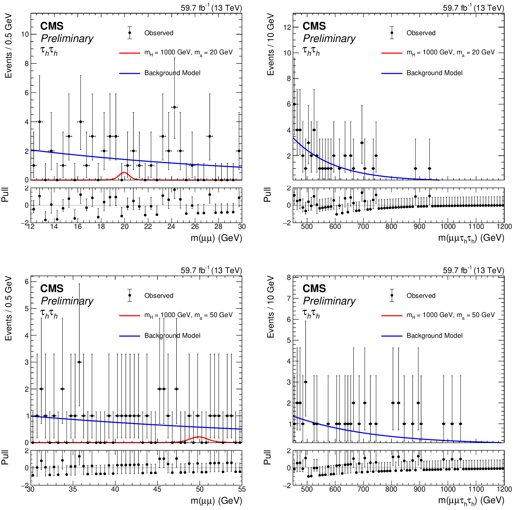
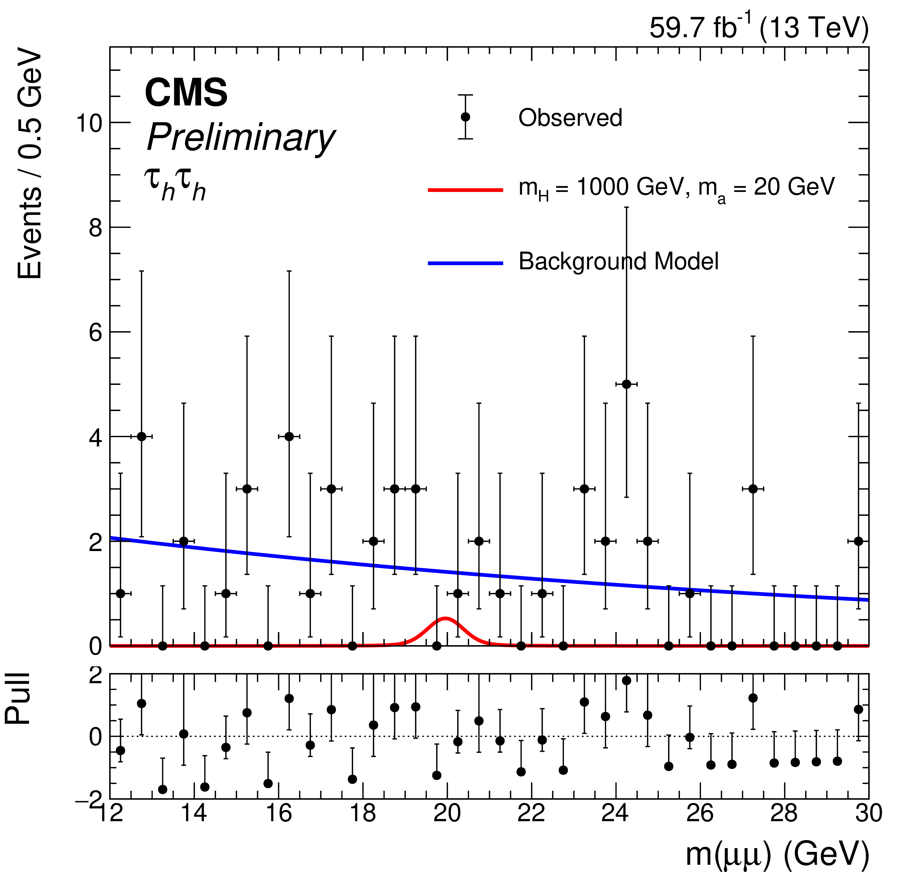
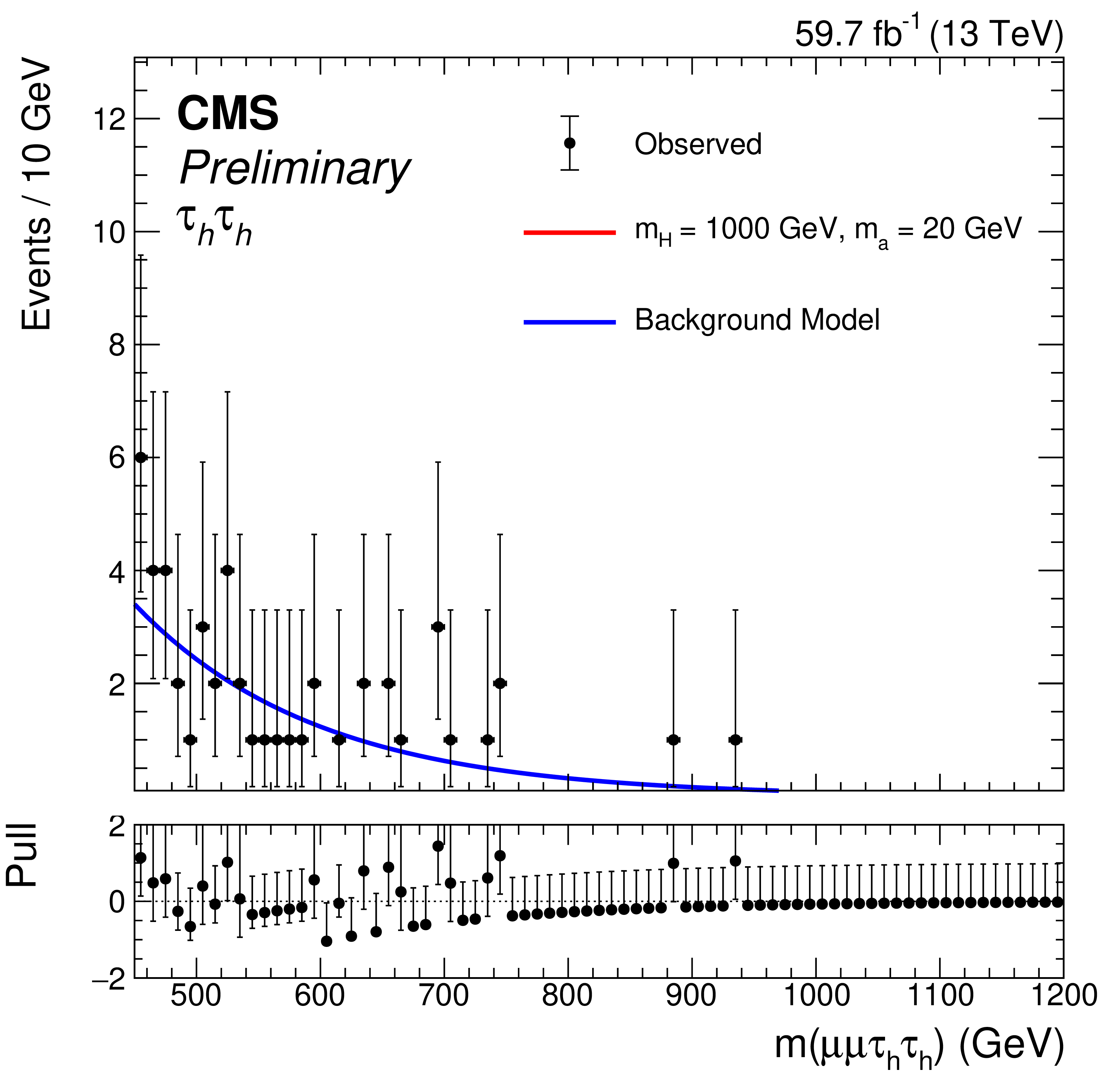
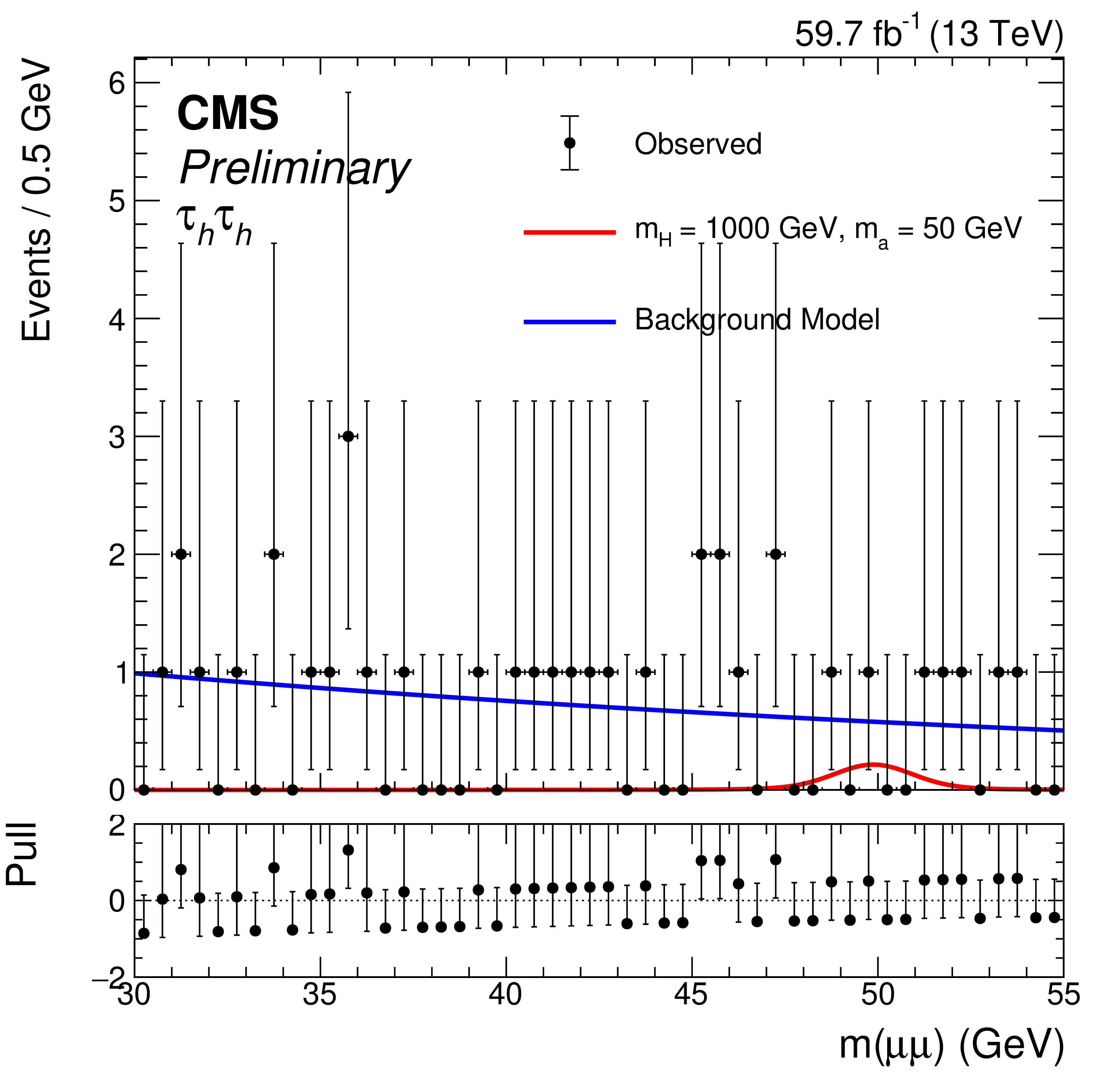
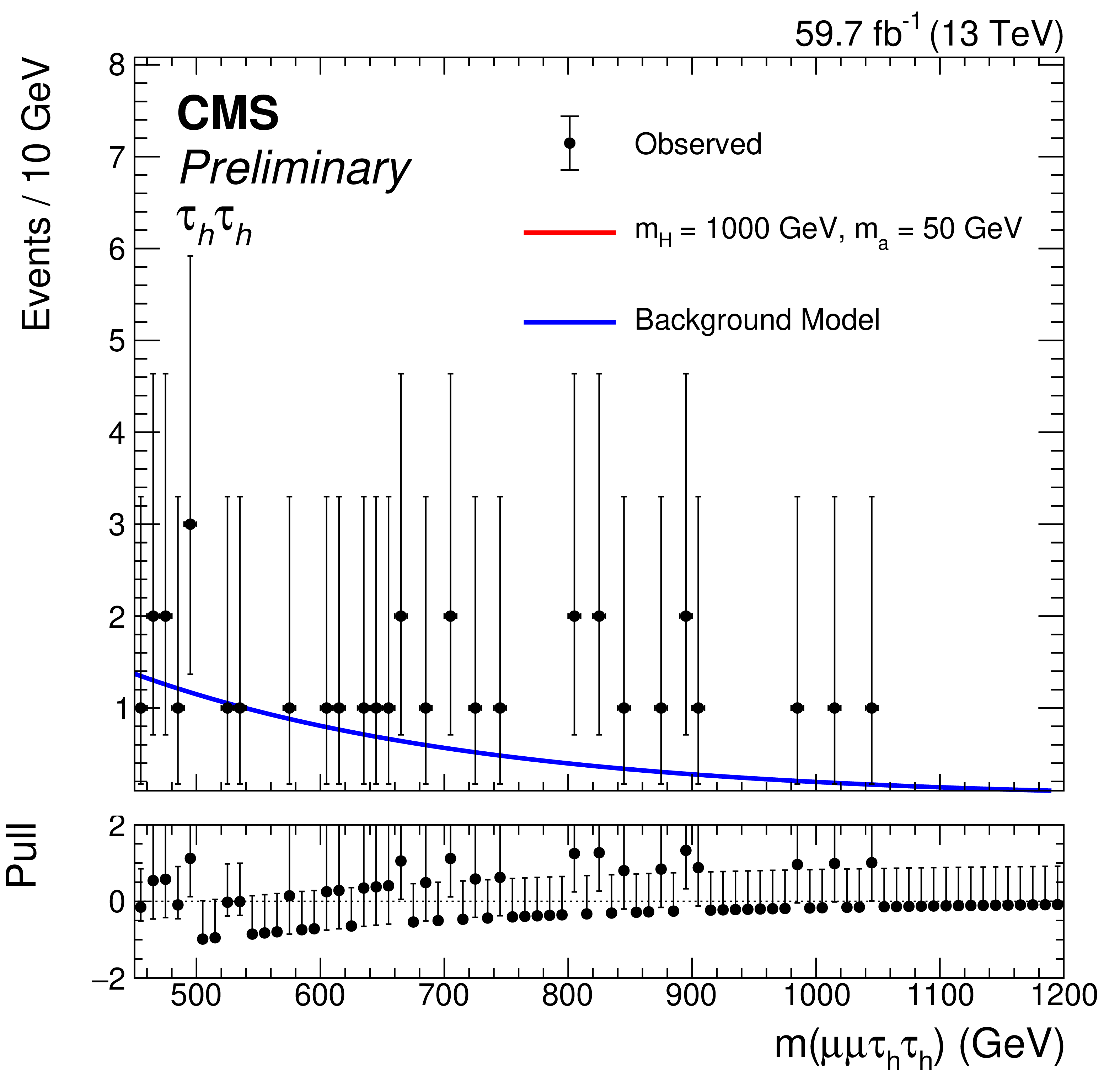
Figure 12:
Projections of the post-fit two-dimensional background PDFs (blue) and observed data onto the $ m_{\mu\mu} $ (left) and four-body visible mass (right) axes for the $ \tau_\mathrm{h}\tau_\mathrm{h} $ channel for the higher two $ m_{\mu\mu} $ mass ranges for $ m_{\mathrm{H}} = 1000 \text{GeV} $ using 2018 data. The rows correspond to pseudoscalar masses $ m_{\mathrm{a}} = $ 20 and 50 GeV (from top to bottom). Sample signal distributions (red) are overlaid assuming $ \mathcal{B}(\mathrm{H}\to\mathrm{a}\mathrm{a}\to\mu\mu\tau\tau) = $ 5 $ \times 10^{-4} $. |
png pdf |
Figure 12-a:
Projections of the post-fit two-dimensional background PDFs (blue) and observed data onto the $ m_{\mu\mu} $ (left) and four-body visible mass (right) axes for the $ \tau_\mathrm{h}\tau_\mathrm{h} $ channel for the higher two $ m_{\mu\mu} $ mass ranges for $ m_{\mathrm{H}} = 1000 \text{GeV} $ using 2018 data. The rows correspond to pseudoscalar masses $ m_{\mathrm{a}} = $ 20 and 50 GeV (from top to bottom). Sample signal distributions (red) are overlaid assuming $ \mathcal{B}(\mathrm{H}\to\mathrm{a}\mathrm{a}\to\mu\mu\tau\tau) = $ 5 $ \times 10^{-4} $. |
png pdf |
Figure 12-b:
Projections of the post-fit two-dimensional background PDFs (blue) and observed data onto the $ m_{\mu\mu} $ (left) and four-body visible mass (right) axes for the $ \tau_\mathrm{h}\tau_\mathrm{h} $ channel for the higher two $ m_{\mu\mu} $ mass ranges for $ m_{\mathrm{H}} = 1000 \text{GeV} $ using 2018 data. The rows correspond to pseudoscalar masses $ m_{\mathrm{a}} = $ 20 and 50 GeV (from top to bottom). Sample signal distributions (red) are overlaid assuming $ \mathcal{B}(\mathrm{H}\to\mathrm{a}\mathrm{a}\to\mu\mu\tau\tau) = $ 5 $ \times 10^{-4} $. |
png pdf |
Figure 12-c:
Projections of the post-fit two-dimensional background PDFs (blue) and observed data onto the $ m_{\mu\mu} $ (left) and four-body visible mass (right) axes for the $ \tau_\mathrm{h}\tau_\mathrm{h} $ channel for the higher two $ m_{\mu\mu} $ mass ranges for $ m_{\mathrm{H}} = 1000 \text{GeV} $ using 2018 data. The rows correspond to pseudoscalar masses $ m_{\mathrm{a}} = $ 20 and 50 GeV (from top to bottom). Sample signal distributions (red) are overlaid assuming $ \mathcal{B}(\mathrm{H}\to\mathrm{a}\mathrm{a}\to\mu\mu\tau\tau) = $ 5 $ \times 10^{-4} $. |
png pdf |
Figure 12-d:
Projections of the post-fit two-dimensional background PDFs (blue) and observed data onto the $ m_{\mu\mu} $ (left) and four-body visible mass (right) axes for the $ \tau_\mathrm{h}\tau_\mathrm{h} $ channel for the higher two $ m_{\mu\mu} $ mass ranges for $ m_{\mathrm{H}} = 1000 \text{GeV} $ using 2018 data. The rows correspond to pseudoscalar masses $ m_{\mathrm{a}} = $ 20 and 50 GeV (from top to bottom). Sample signal distributions (red) are overlaid assuming $ \mathcal{B}(\mathrm{H}\to\mathrm{a}\mathrm{a}\to\mu\mu\tau\tau) = $ 5 $ \times 10^{-4} $. |
png pdf |
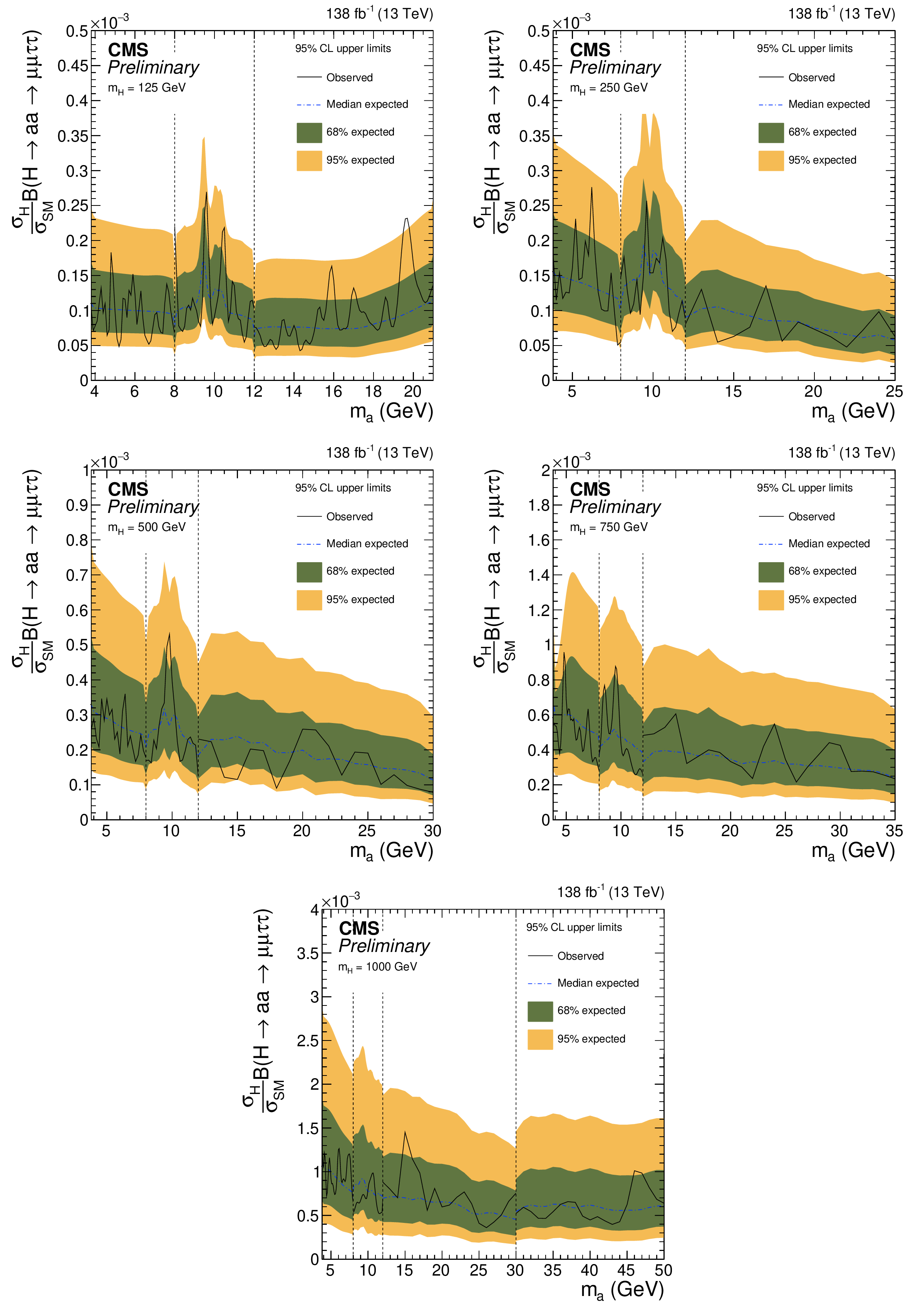
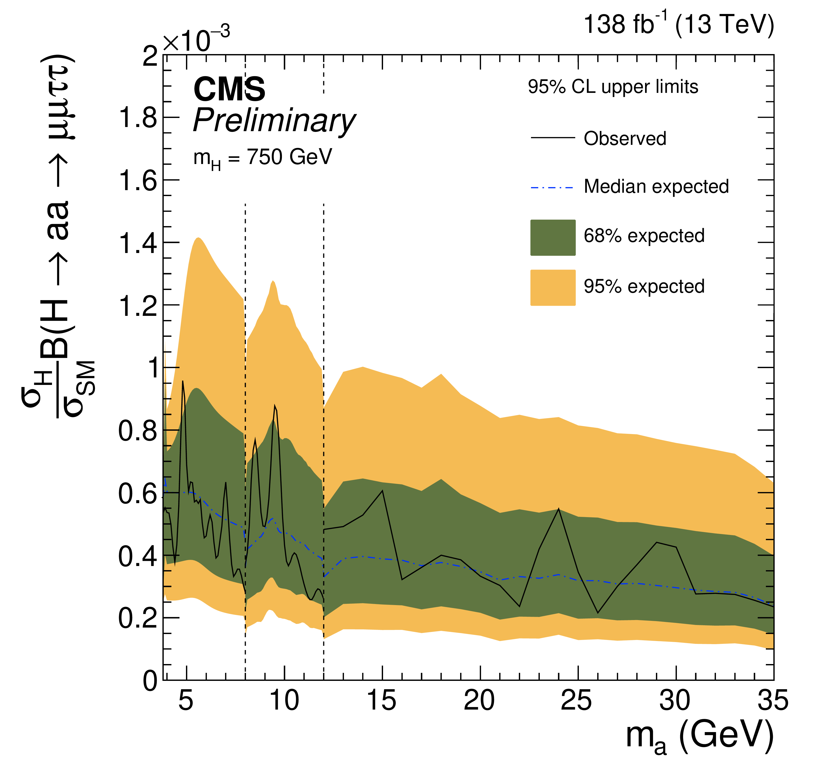
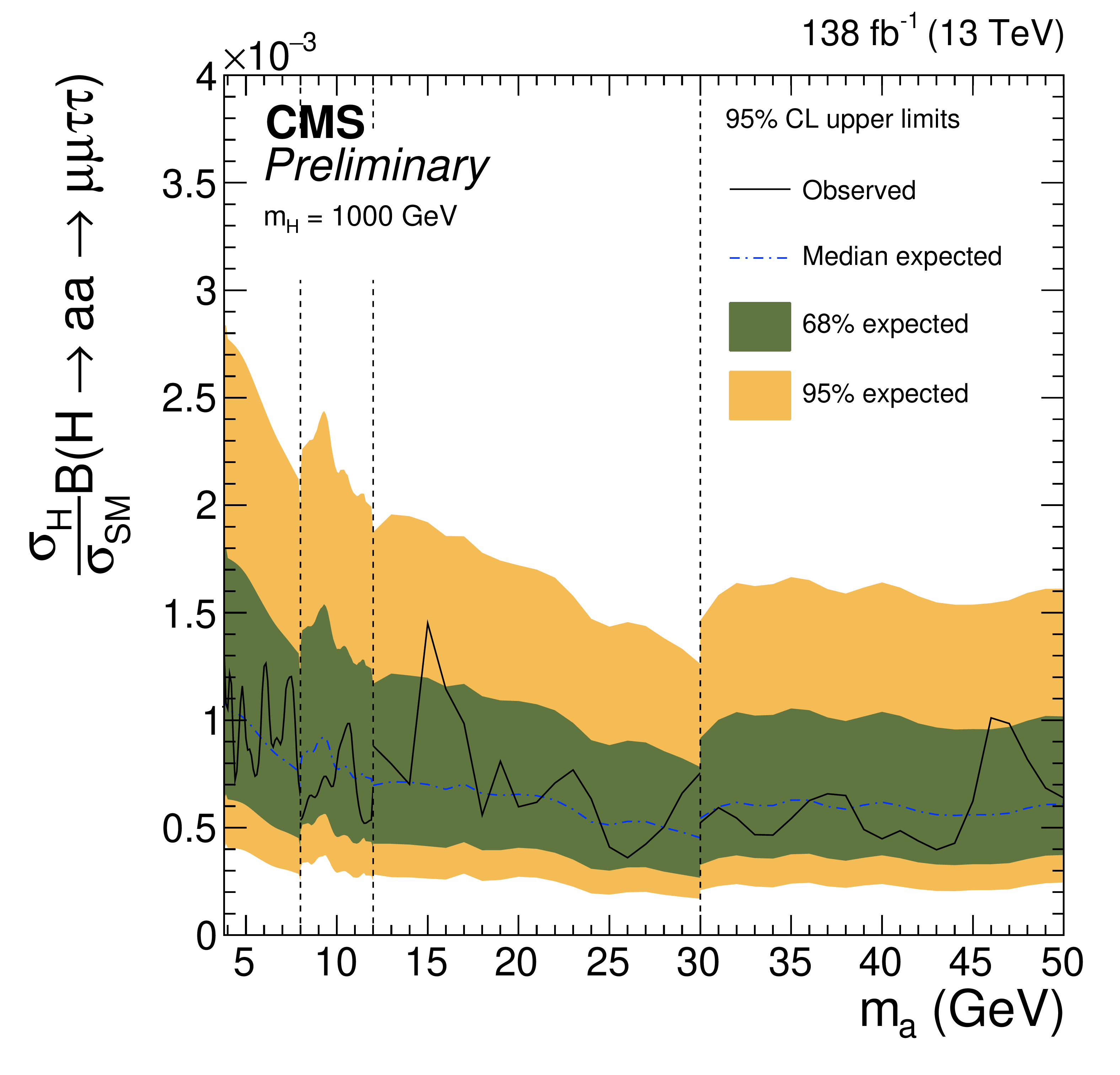
Figure 13:
Expected and observed limits on $ \sigma_{\mathrm{H}} \mathcal{B}(\mathrm{H}\to\mathrm{a}\mathrm{a}\to\mu\mu\tau\tau)/\sigma_{SM} $ for the full Run 2 dataset of the $ \tau_{\mu}\tau_{\mathrm{e}} $, $ \tau_{\mu}\tau_\mathrm{h} $, $ \tau_{\mathrm{e}}\tau_\mathrm{h} $, and $ \tau_\mathrm{h}\tau_\mathrm{h} $ final states combined, for $ m_{\mathrm{H}} = $ 125, 250, 500, 750, and 1000 GeV. |
png pdf |
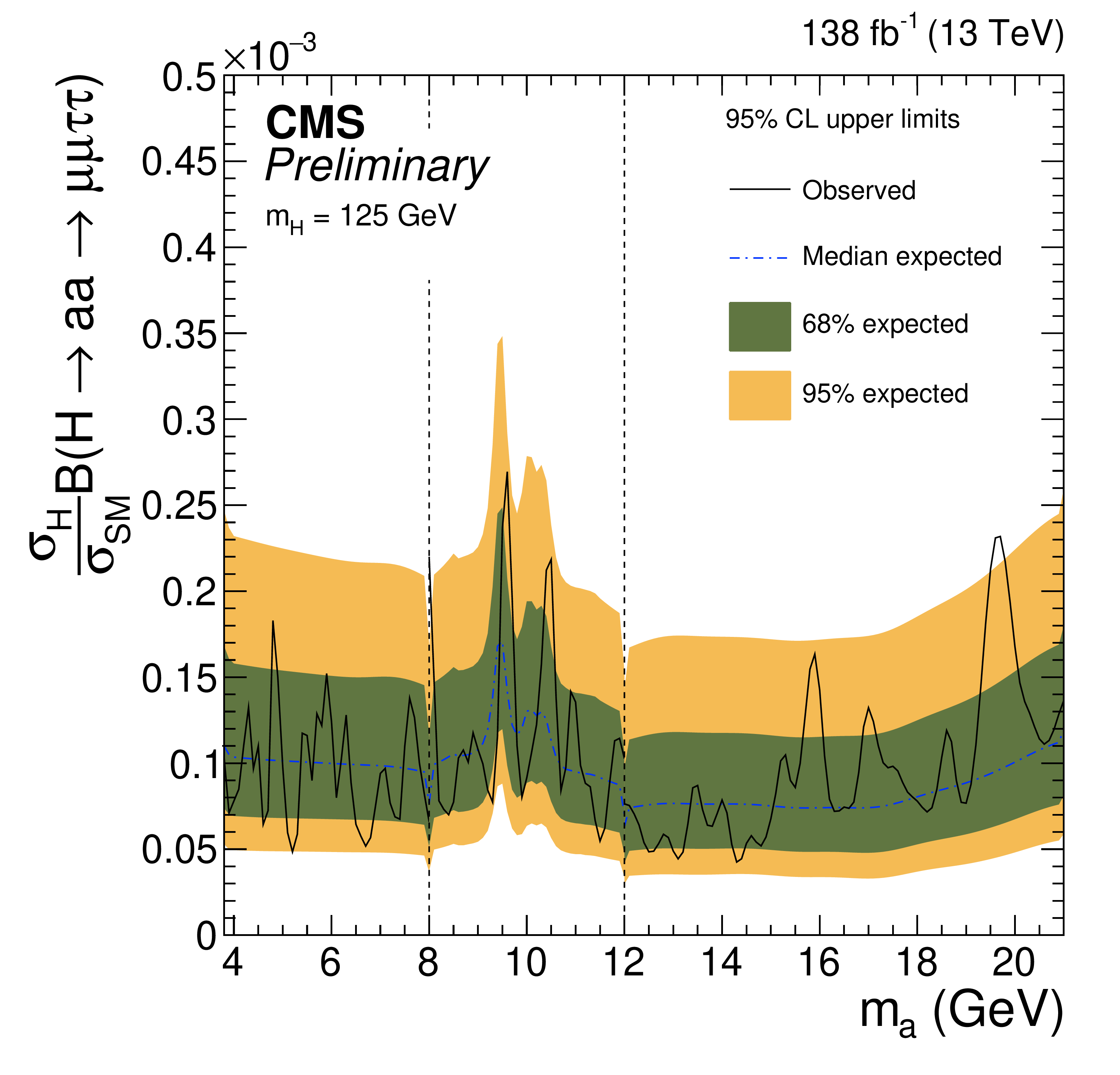
Figure 13-a:
Expected and observed limits on $ \sigma_{\mathrm{H}} \mathcal{B}(\mathrm{H}\to\mathrm{a}\mathrm{a}\to\mu\mu\tau\tau)/\sigma_{SM} $ for the full Run 2 dataset of the $ \tau_{\mu}\tau_{\mathrm{e}} $, $ \tau_{\mu}\tau_\mathrm{h} $, $ \tau_{\mathrm{e}}\tau_\mathrm{h} $, and $ \tau_\mathrm{h}\tau_\mathrm{h} $ final states combined, for $ m_{\mathrm{H}} = $ 125, 250, 500, 750, and 1000 GeV. |
png pdf |
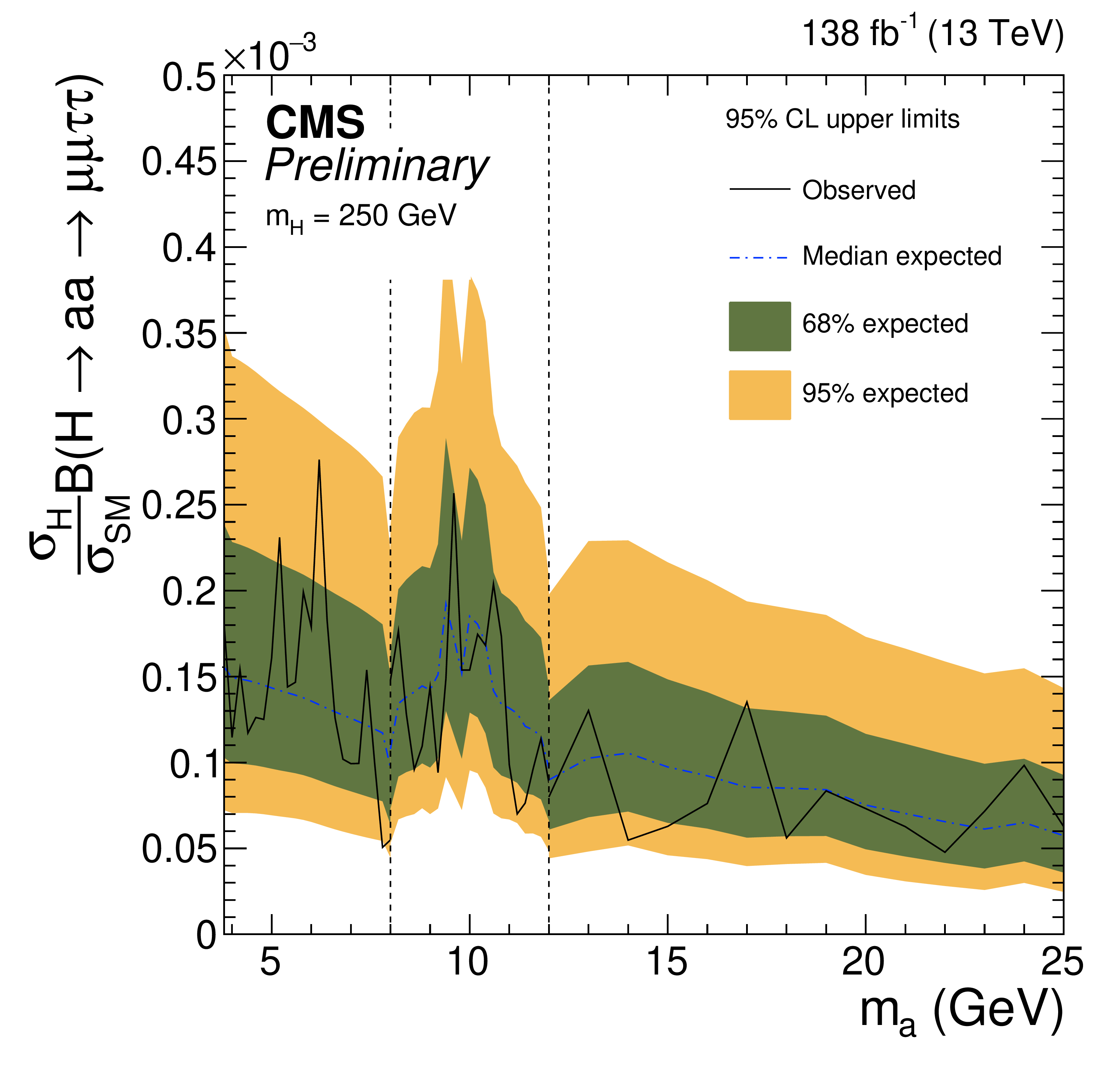
Figure 13-b:
Expected and observed limits on $ \sigma_{\mathrm{H}} \mathcal{B}(\mathrm{H}\to\mathrm{a}\mathrm{a}\to\mu\mu\tau\tau)/\sigma_{SM} $ for the full Run 2 dataset of the $ \tau_{\mu}\tau_{\mathrm{e}} $, $ \tau_{\mu}\tau_\mathrm{h} $, $ \tau_{\mathrm{e}}\tau_\mathrm{h} $, and $ \tau_\mathrm{h}\tau_\mathrm{h} $ final states combined, for $ m_{\mathrm{H}} = $ 125, 250, 500, 750, and 1000 GeV. |
png pdf |
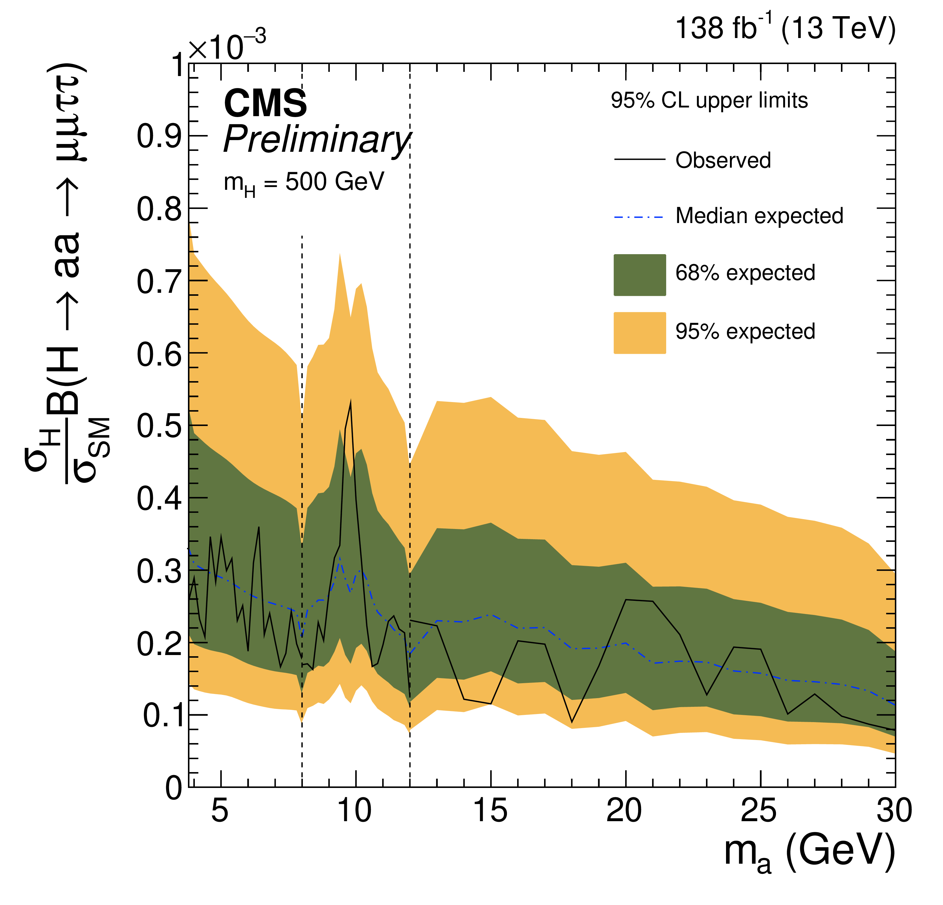
Figure 13-c:
Expected and observed limits on $ \sigma_{\mathrm{H}} \mathcal{B}(\mathrm{H}\to\mathrm{a}\mathrm{a}\to\mu\mu\tau\tau)/\sigma_{SM} $ for the full Run 2 dataset of the $ \tau_{\mu}\tau_{\mathrm{e}} $, $ \tau_{\mu}\tau_\mathrm{h} $, $ \tau_{\mathrm{e}}\tau_\mathrm{h} $, and $ \tau_\mathrm{h}\tau_\mathrm{h} $ final states combined, for $ m_{\mathrm{H}} = $ 125, 250, 500, 750, and 1000 GeV. |
png pdf |
Figure 13-d:
Expected and observed limits on $ \sigma_{\mathrm{H}} \mathcal{B}(\mathrm{H}\to\mathrm{a}\mathrm{a}\to\mu\mu\tau\tau)/\sigma_{SM} $ for the full Run 2 dataset of the $ \tau_{\mu}\tau_{\mathrm{e}} $, $ \tau_{\mu}\tau_\mathrm{h} $, $ \tau_{\mathrm{e}}\tau_\mathrm{h} $, and $ \tau_\mathrm{h}\tau_\mathrm{h} $ final states combined, for $ m_{\mathrm{H}} = $ 125, 250, 500, 750, and 1000 GeV. |
png pdf |
Figure 13-e:
Expected and observed limits on $ \sigma_{\mathrm{H}} \mathcal{B}(\mathrm{H}\to\mathrm{a}\mathrm{a}\to\mu\mu\tau\tau)/\sigma_{SM} $ for the full Run 2 dataset of the $ \tau_{\mu}\tau_{\mathrm{e}} $, $ \tau_{\mu}\tau_\mathrm{h} $, $ \tau_{\mathrm{e}}\tau_\mathrm{h} $, and $ \tau_\mathrm{h}\tau_\mathrm{h} $ final states combined, for $ m_{\mathrm{H}} = $ 125, 250, 500, 750, and 1000 GeV. |
png pdf |
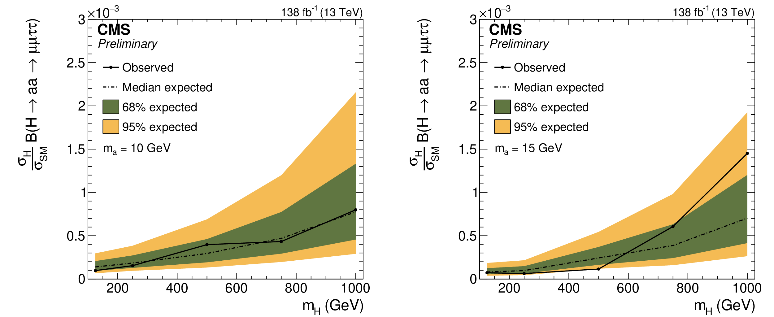
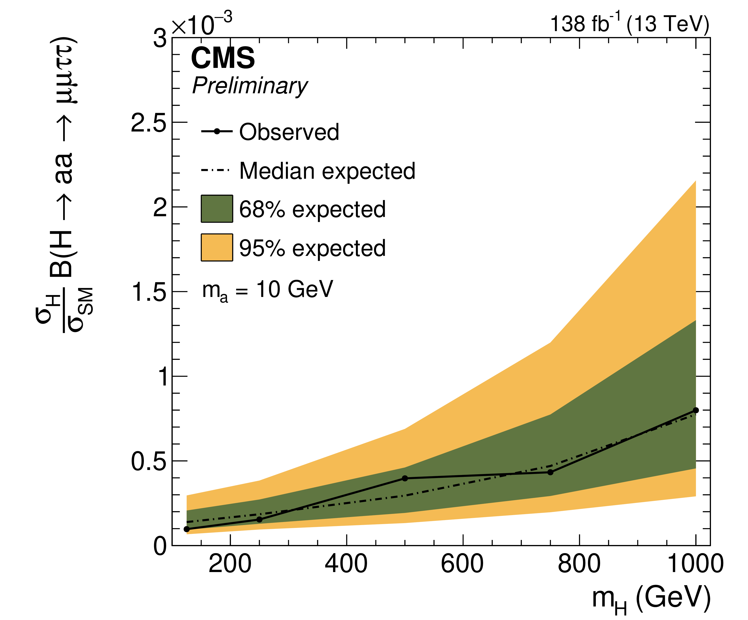
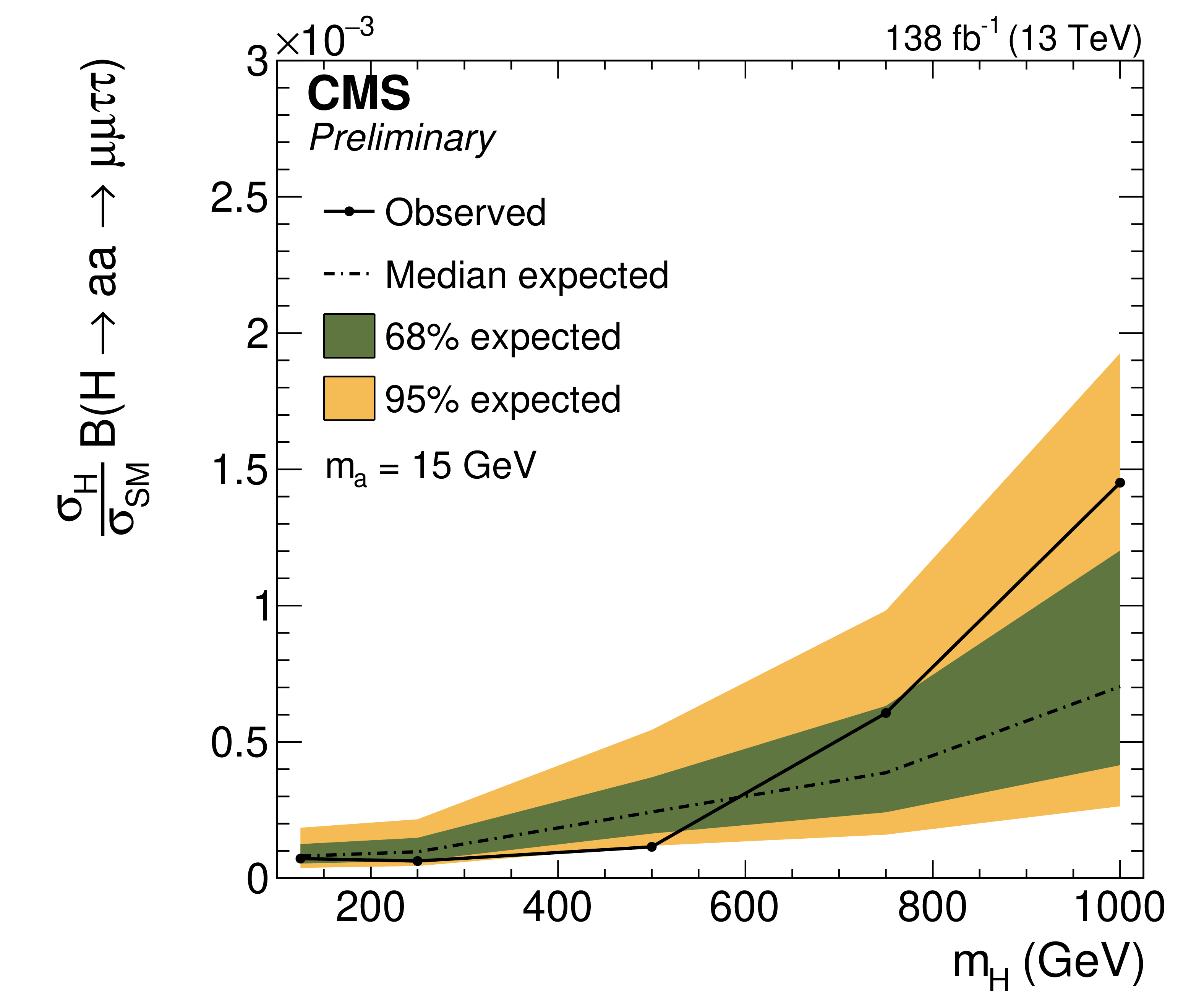
Figure 14:
Expected and observed limits on $ \sigma_{\mathrm{H}} \mathcal{B}(\mathrm{H}\to\mathrm{a}\mathrm{a}\to\mu\mu\tau\tau)/\sigma_{SM} $ for the full Run 2 dataset, with the combined final states of the Higgs boson at different mass points when the pseudoscalar mass is (right) 10 GeV and (left) 15 GeV. |
png pdf |
Figure 14-a:
Expected and observed limits on $ \sigma_{\mathrm{H}} \mathcal{B}(\mathrm{H}\to\mathrm{a}\mathrm{a}\to\mu\mu\tau\tau)/\sigma_{SM} $ for the full Run 2 dataset, with the combined final states of the Higgs boson at different mass points when the pseudoscalar mass is (right) 10 GeV and (left) 15 GeV. |
png pdf |
Figure 14-b:
Expected and observed limits on $ \sigma_{\mathrm{H}} \mathcal{B}(\mathrm{H}\to\mathrm{a}\mathrm{a}\to\mu\mu\tau\tau)/\sigma_{SM} $ for the full Run 2 dataset, with the combined final states of the Higgs boson at different mass points when the pseudoscalar mass is (right) 10 GeV and (left) 15 GeV. |
png pdf |
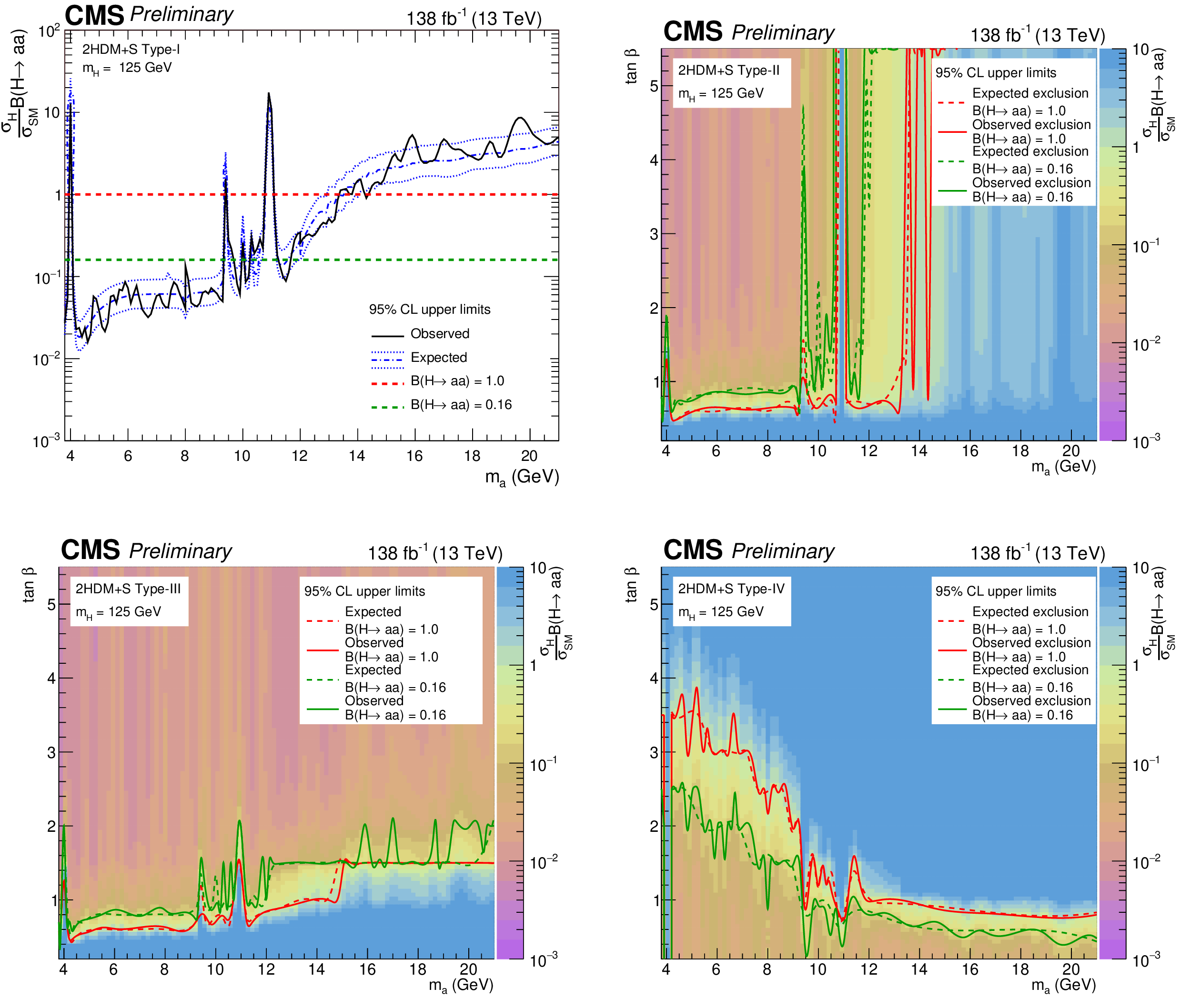
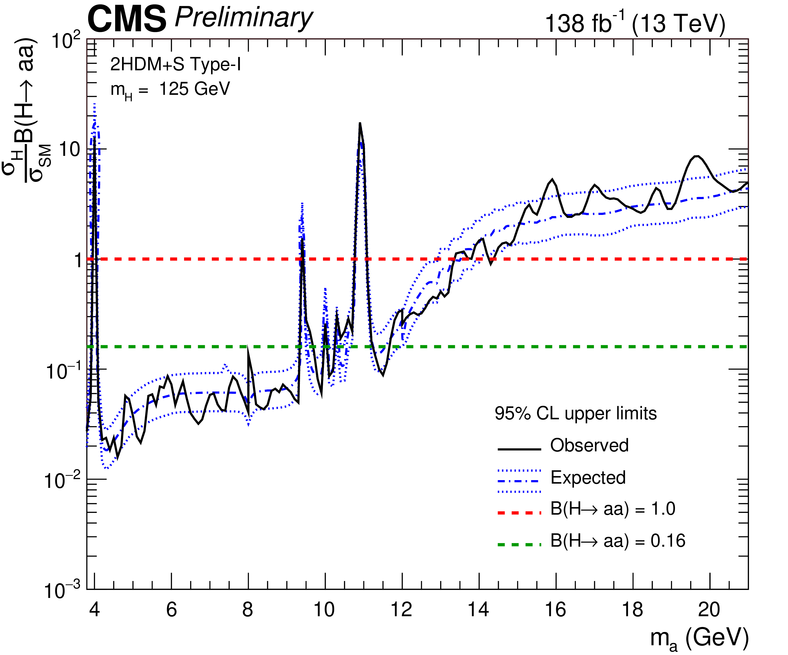
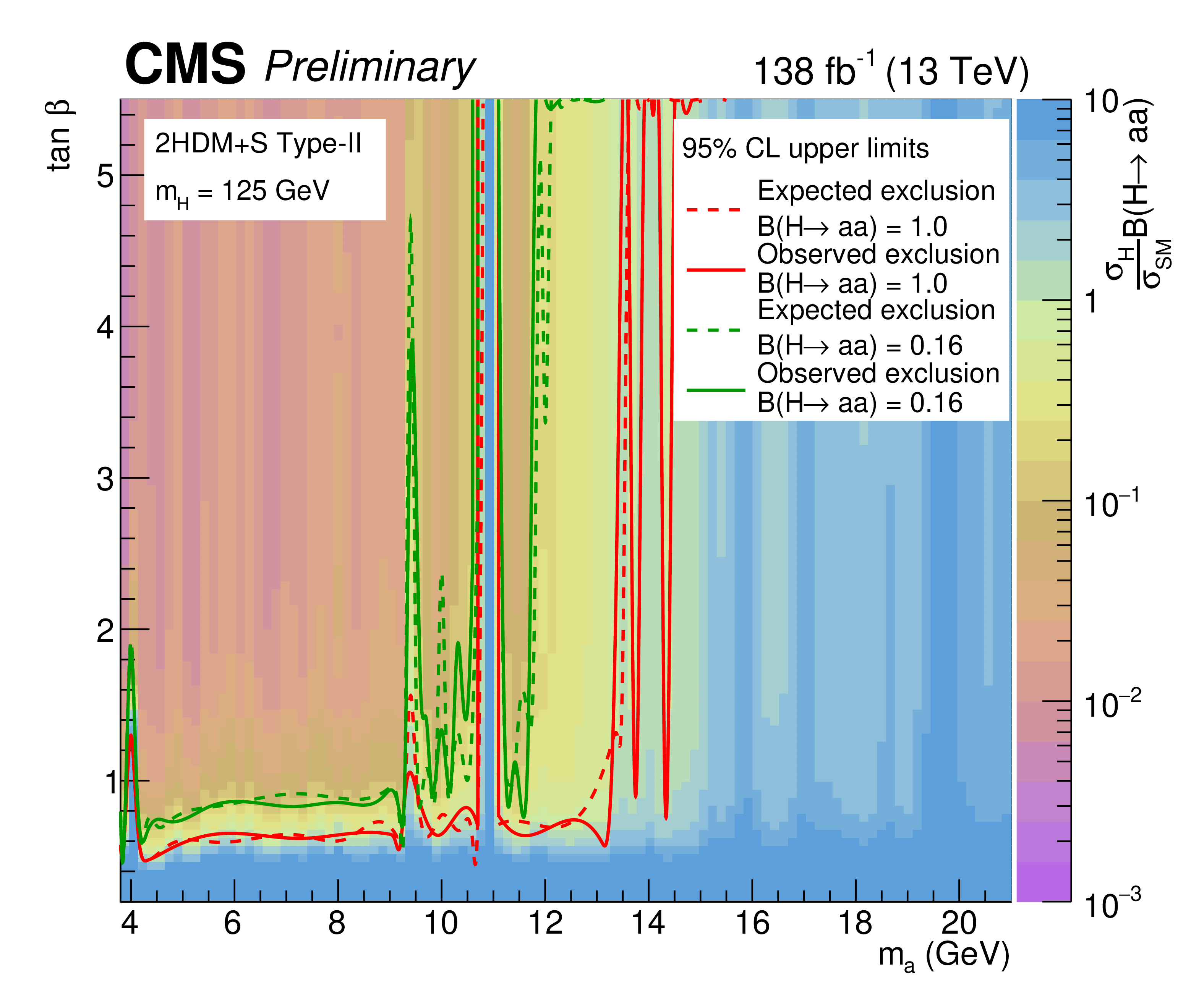
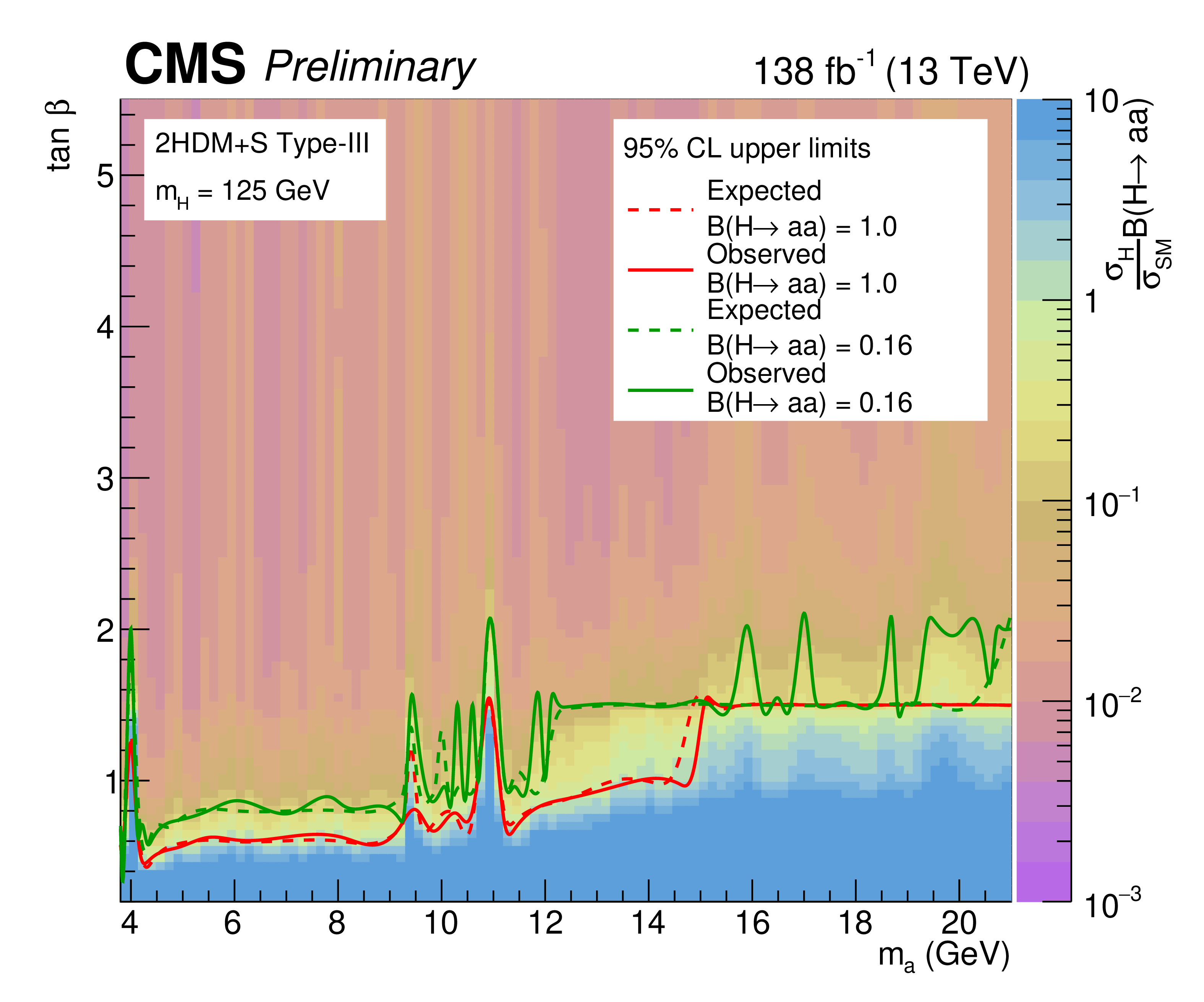
Figure 15:
Observed and expected limits in 2HDM+S models of various types. The contours at a branching fraction of 0.16 are motivated by a CMS meta-analysis that sets limits on decays that would not be detected by the standard channels, such as those from boosted topologies considered in this analysis [18]. |
png pdf |
Figure 15-a:
Observed and expected limits in 2HDM+S models of various types. The contours at a branching fraction of 0.16 are motivated by a CMS meta-analysis that sets limits on decays that would not be detected by the standard channels, such as those from boosted topologies considered in this analysis [18]. |
png pdf |
Figure 15-b:
Observed and expected limits in 2HDM+S models of various types. The contours at a branching fraction of 0.16 are motivated by a CMS meta-analysis that sets limits on decays that would not be detected by the standard channels, such as those from boosted topologies considered in this analysis [18]. |
png pdf |
Figure 15-c:
Observed and expected limits in 2HDM+S models of various types. The contours at a branching fraction of 0.16 are motivated by a CMS meta-analysis that sets limits on decays that would not be detected by the standard channels, such as those from boosted topologies considered in this analysis [18]. |

png pdf |
Figure 15-d:
Observed and expected limits in 2HDM+S models of various types. The contours at a branching fraction of 0.16 are motivated by a CMS meta-analysis that sets limits on decays that would not be detected by the standard channels, such as those from boosted topologies considered in this analysis [18]. |
| Tables | |
png pdf |
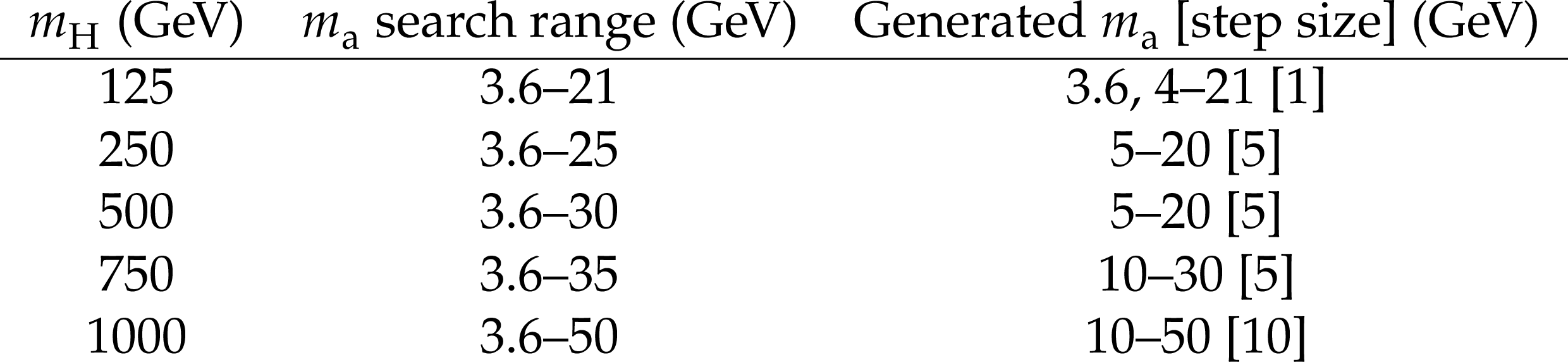
Table 1:
Values of the scalar mass $ m_{\mathrm{H}} $ and pseudoscalar mass $ m_{\mathrm{a}} $ considered in the search for $ \mathrm{H}\to\mathrm{a}\mathrm{a}\to\mu\mu\tau\tau $. The third column lists the generated pseudoscalar mass points; ranges are shown together with the step size in parentheses. As $ m_{\mathrm{H}} $ increases, the maximum value of $ m_{\mathrm{a}} $ to which the search is sensitive also increases. For $ m_{\mathrm{H}}=125 \text{GeV} $, the lightest neutral scalar corresponds to the SM Higgs boson. |
png pdf |
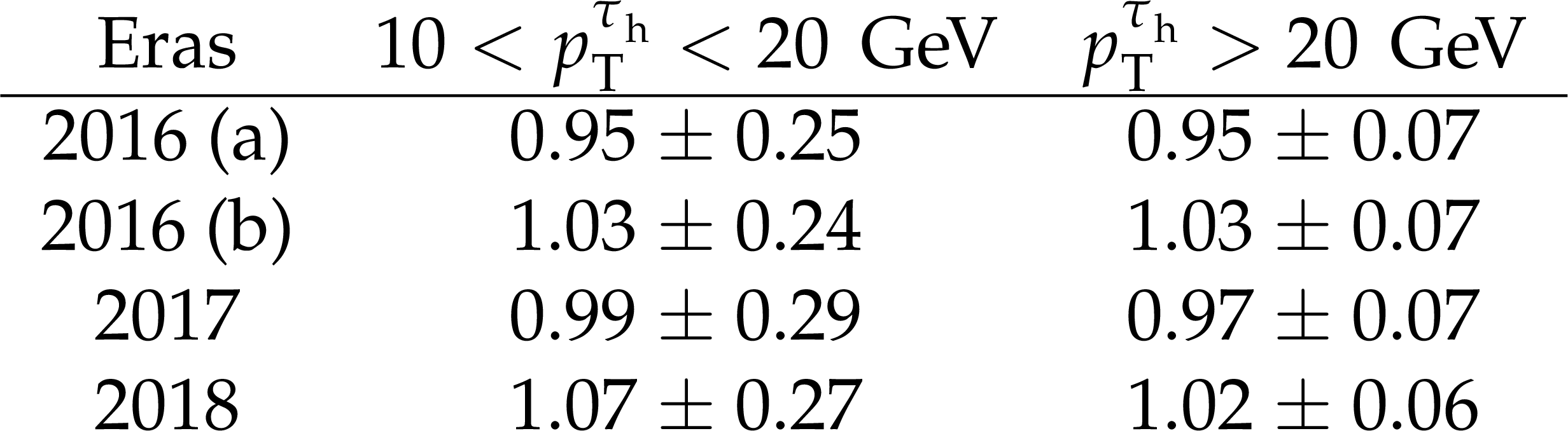
Table 2:
The measured scale factors and their uncertainties for $ \tau_\mathrm{h} $ candidates using the full dataset. Data from 2016 comprise two eras with different strip tracker running conditions [65]. |
png pdf |
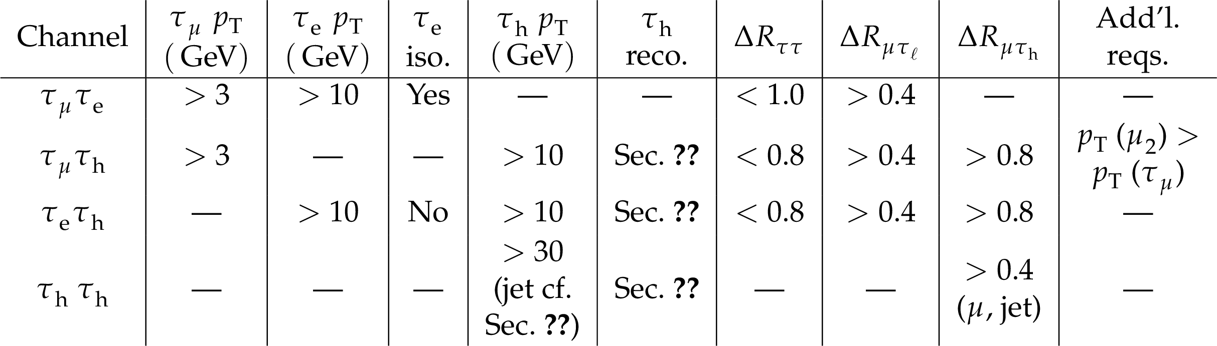
Table 3:
Tau lepton selection criteria in the four different channels. In the columns labeled $ \Delta R_{\mu\tau_{\ell}} $ and $ \Delta R_{\mu\tau_\mathrm{h}} $, $ \mu $ refers to either of the two muons reconstructed as the $ \mathrm{a}\rightarrow\mu\mu $ candidate. In the column labeled $ \Delta R_{\mu\tau_{\ell}} $, $ \tau_{\ell} $ refers to either of the $ \tau_{\mu} $ or $ \tau_{\mathrm{e}} $ candidates. $ \mu_{2} $ refers to the non-triggering muon in the $ \mathrm{a}\rightarrow\mu\mu $ pair. |
png pdf |
Table 4:
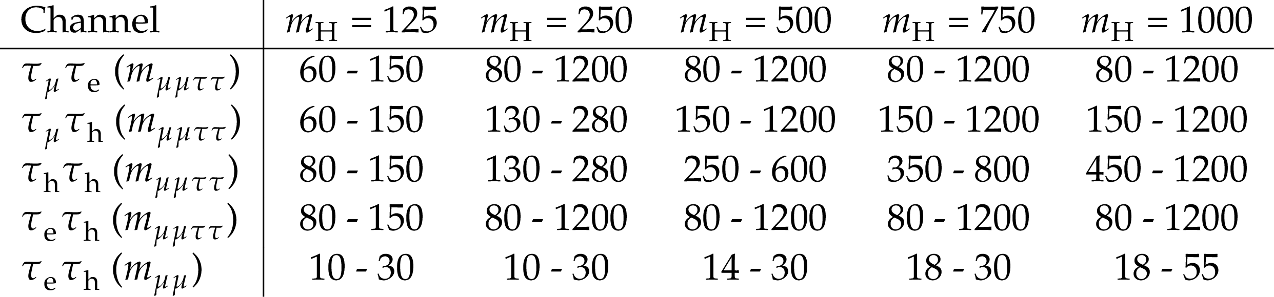
Four-body mass ranges utilized for the two-dimensional fit. For the $ \tau_{\mathrm{e}}\tau_\mathrm{h} $ channel an additional requirement is imposed on $ m_{\mu\mu} $, shown in the last row. All entries are in GeV. |

png pdf |
Table 5:
The $ \mu\mu $ background model includes five meson resonances, modeled using a Voigt function over an exponential continuum. The four-body background model is described by an error function multiplied by the sum of two exponential distributions. Two types of fit region relationships are used: (a) shared, where the parameters are identical in the indicated regions, and (b) independent, where the parameters vary freely and are not constrained by any other region. |
| Summary |
| A search for Higgs boson (H) decays to a pair of light pseudoscalar bosons ($ \mathrm{a} $) is presented, both for a SM Higgs and for a SM-like scalar with masses in the range 250 $ \text{GeV} $ - 1 $ \text{TeV} $. The light pseudoscalars decay to $ \mu\mu $ and $ \tau\tau $, with substantial overlap for each pair because of the large Lorentz boosts. This nonstandard topology motivates the development of dedicated $ \tau_{\mu}\tau_\mathrm{h} $, $ \tau_{\mathrm{e}}\tau_\mathrm{h} $, and $ \tau_\mathrm{h}\tau_\mathrm{h} $ reconstruction and tagging methods to increase acceptance. For the first time a neural network is developed to enable the inclusion of high-rate but high-background $ \tau_\mathrm{h}\tau_\mathrm{h} $ decays. Data collected by the CMS Collaboration at $ \sqrt{s} = 13 \text{TeV} $, corresponding to an integrated luminosity of 138 fb$ ^{-1} $, are examined. As no significant excess over standard model (SM) processes is observed, this analysis obtains model-independent upper limits at the 95% confidence level on the branching fraction $ (\mathcal{B}) $ of an SM-like Higgs boson (H), decaying to a pair of pseudoscalar bosons ($ \mathrm{a} $) in the $ \mu\mu\tau\tau $ final state, $ \sigma_{\mathrm{H}}\mathcal{B}(\mathrm{H} \to \mathrm{a}\mathrm{a} \to \mu\mu\tau\tau) / \sigma_{\text{SM}} $, with a maximum exclusion of $ \approx 5 \times 10^{-5} $ for $ m_{\mathrm{H}} = 125 \text{GeV} $ and a maximum exclusion of $ \approx 4 \times 10^{-4} $ for $ m_{\mathrm{H}} = 1000 \text{GeV} $. Model-specific upper limits on $ \sigma_{\mathrm{H}}\mathcal{B}(\mathrm{H} \to \mathrm{a}\mathrm{a}) / \sigma_{\text{SM}} $ are extracted for $ m_{\mathrm{H}} = 125 \text{GeV} $ in Type-I, -II, -III, and -IV two Higgs doublet plus singlet models. These results significantly extend the upper limits obtained by earlier searches by the CMS and ATLAS Collaborations, such as those obtained by CMS with partial 13 TeV data [45], and are complementary to present searches, $ \mbox{e.g.} $, Ref. [77], at higher $ m_{\mathrm{a}} $ that lead to resolved $ \mu\mu $ and $ \tau\tau $ final states. |
| References | ||||
| 1 | CMS Collaboration | Measurement of the Higgs boson mass and width using the four-lepton final state in proton-proton collisions at $ \sqrt{s} = $ 13 TeV | PRD 111 (2025) 092014 | CMS-HIG-21-019 2409.13663 |
| 2 | CMS Collaboration | Constraints on anomalous Higgs boson couplings from its production and decay using the WW channel in proton-proton collisions at $ \sqrt{s} = 13 \text {TeV} $ | EPJC 84 (2024) 779 | CMS-HIG-22-008 2403.00657 |
| 3 | CMS Collaboration | Measurement of simplified template cross sections of the Higgs boson produced in association with W or Z bosons in the H$ \rightarrow $bb decay channel in proton-proton collisions at $ \sqrt{s} = 13 \text {TeV} $ | PRD 109 (2024) 092011 | CMS-HIG-20-001 2312.07562 |
| 4 | ATLAS and CMS Collaborations | Evidence for the Higgs Boson Decay to a Z Boson and a Photon at the LHC | PRL 132 (2024) 021803 | 2309.03501 |
| 5 | CMS Collaboration | Measurements of inclusive and differential cross sections for the Higgs boson production and decay to four-leptons in proton-proton collisions at $ \sqrt{s} = $ 13 TeV | JHEP 08 (2023) 040 | CMS-HIG-21-009 2305.07532 |
| 6 | CMS Collaboration | Measurement of the Higgs boson inclusive and differential fiducial production cross sections in the diphoton decay channel with pp collisions at $ \sqrt{s} = $ 13 TeV | JHEP 07 (2023) 091 | CMS-HIG-19-016 2208.12279 |
| 7 | ATLAS Collaboration | Measurements of $ WH $ and $ ZH $ production with Higgs boson decays into bottom quarks and direct constraints on the charm Yukawa coupling in 13 TeV$ pp $ collisions with the ATLAS detector | JHEP 04 (2025) 075 | 2410.19611 |
| 8 | ATLAS Collaboration | Differential cross-section measurements of Higgs boson production in the H $ \rightarrow $ \ensuremath\tau$ ^{+} $\ensuremath\tau$ ^{-} $ decay channel in pp collisions at $ \sqrt{s} = $ 13 TeV with the ATLAS detector | JHEP 03 (2025) 010 | 2407.16320 |
| 9 | ATLAS Collaboration | Measurement of the associated production of a top-antitop-quark pair and a Higgs boson decaying into a $ b\bar{b} $ pair in pp collisions at $ \sqrt{s}= $ 13 TeV using the ATLAS detector at the LHC | EPJC 85 (2025) 210 | 2407.10904 |
| 10 | ATLAS Collaboration | Determination of the Relative Sign of the Higgs Boson Couplings to W and Z Bosons Using WH Production via Vector-Boson Fusion with the ATLAS Detector | PRL 133 (2024) 141801 | 2402.00426 |
| 11 | ATLAS Collaboration | Measurement of the VH,H$ \rightarrow $\ensuremath\tau\ensuremath\tau process with the ATLAS detector at 13 TeV | PLB 855 (2024) 138817 | 2312.02394 |
| 12 | ATLAS Collaboration | Measurement of the Higgs boson mass with H$ \rightarrow $\ensuremath\gamma\ensuremath\gamma decays in 140 fb$ ^{-1} $ of $ \sqrt{s} = 13 \text {TeV} $ pp collisions with the ATLAS detector | PLB 847 (2023) 138315 | 2308.07216 |
| 13 | ATLAS Collaboration | Combined Measurement of the Higgs Boson Mass from the H$ \rightarrow $\ensuremath\gamma\ensuremath\gamma and H$ \rightarrow $ZZ*$ \rightarrow $4\ensuremath\ell Decay Channels with the ATLAS Detector Using $ \sqrt s = $ 7, 8, and 13 TeV pp Collision Data | PRL 131 (2023) 251802 | 2308.04775 |
| 14 | ATLAS Collaboration | Integrated and differential fiducial cross-section measurements for the vector boson fusion production of the Higgs boson in the $ H \rightarrow WW^{\ast}\rightarrow e\nu\mu\nu $ decay channel at 13 $ \text{TeV} $ with the ATLAS detector | PRD 108 (2023) 072003 | 2304.03053 |
| 15 | G. C. Branco et al. | Theory and phenomenology of two-Higgs-doublet models | Phys. Rept. 516 (2012) 1 | 1106.0034 |
| 16 | D. Curtin et al. | Exotic decays of the 125 GeV Higgs boson | PRD 90 (2014) 075004 | 1312.4992 |
| 17 | U. Ellwanger, C. Hugonie, and A. M. Teixeira | The next-to-minimal supersymmetric standard model | Phys. Rept. 496 (2010) 1 | 0910.1785 |
| 18 | CMS Collaboration | A portrait of the Higgs boson by the CMS experiment ten years after the discovery. | Nature 607 (2022) 60 | CMS-HIG-22-001 2207.00043 |
| 19 | R. Dermisek and J. F. Gunion | Escaping the large fine tuning and little hierarchy problems in the next to minimal supersymmetric model and $ h\rightarrow aa $ decays | PRL 95 (2005) 041801 | hep-ph/0502105 |
| 20 | R. Dermisek and J. F. Gunion | The NMSSM close to the R-symmetry limit and naturalness in $ h\rightarrow aa $ decays for $ m(a) < 2m(b) $ | PRD 75 (2007) 075019 | hep-ph/0611142 |
| 21 | S. Chang, R. Dermisek, J. F. Gunion, and N. Weiner | Nonstandard Higgs boson decays | Ann. Rev. Nucl. Part. Sci. 58 (2008) 75 | 0801.4554 |
| 22 | S. F. King, M. Muhlleitner, R. Nevzorov, and K. Walz | Natural NMSSM Higgs bosons | NPB 870 (2013) 323 | 1211.5074 |
| 23 | A. Celis, V. Ilisie, and A. Pich | LHC constraints on two-Higgs doublet models | JHEP 07 (2013) 053 | 1302.4022 |
| 24 | B. Grinstein and P. Uttayarat | Carving out parameter space in Type-II two Higgs doublets model | JHEP 06 (2013) 094 | 1304.0028 |
| 25 | B. Coleppa, F. Kling, and S. Su | Constraining Type II 2HDM in light of LHC Higgs searches | JHEP 01 (2014) 161 | 1305.0002 |
| 26 | C.-Y. Chen, S. Dawson, and M. Sher | Heavy Higgs searches and constraints on two Higgs doublet models | PRD 88 (2013) 015018 | 1305.1624 |
| 27 | N. Craig, J. Galloway, and S. Thomas | Searching for signs of the second Higgs doublet | 1305.2424 | |
| 28 | L. Wang and X.-F. Han | Status of the aligned two-Higgs-doublet model confronted with the Higgs data | JHEP 04 (2014) 128 | 1312.4759 |
| 29 | J. Cao et al. | A light Higgs scalar in the NMSSM confronted with the latest LHC Higgs data | JHEP 11 (2013) 018 | 1309.4939 |
| 30 | N. D. Christensen, T. Han, Z. Liu, and S. Su | Low-mass Higgs bosons in the NMSSM and their LHC implications | JHEP 08 (2013) 019 | 1303.2113 |
| 31 | D. G. Cerdeno, P. Ghosh, and C. B. Park | Probing the two light Higgs scenario in the NMSSM with a low-mass pseudoscalar | JHEP 06 (2013) 031 | 1301.1325 |
| 32 | G. Chalons and F. Domingo | Analysis of the Higgs potentials for two doublets and a singlet | PRD 86 (2012) 115024 | 1209.6235 |
| 33 | A. Ahriche, A. Arhrib, and S. Nasri | Higgs phenomenology in the two-singlet model | JHEP 02 (2014) 042 | 1309.5615 |
| 34 | J. Baglio, O. Eberhardt, U. Nierste, and M. Wiebusch | Benchmarks for Higgs pair production and heavy Higgs boson searches in the two-Higgs-doublet model of Type II | PRD 90 (2014) 015008 | 1403.1264 |
| 35 | B. Dumont, J. F. Gunion, Y. Jiang, and S. Kraml | Constraints on and future prospects for two-Higgs-doublet models in light of the LHC Higgs signal | PRD 90 (2014) 035021 | 1405.3584 |
| 36 | H. Davoudiasl, R. Marcarelli, N. Miesch, and E. T. Neil | Searching for flavor-violating ALPs in Higgs boson decays | PRD 104 (2021) 055022 | 2105.05866 |
| 37 | M. Bauer, M. Neubert, and A. Thamm | Collider Probes of Axion-Like Particles | JHEP 12 (2017) 044 | 1708.00443 |
| 38 | ATLAS Collaboration | Search for Higgs boson decays into a pair of pseudoscalar particles in the $ bb\mu\mu $ final state with the ATLAS detector in $ pp $ collisions at $ \sqrt s = $ 13 TeV | PRD 105 (2022) 012006 | 2110.00313 |
| 39 | CMS Collaboration | Search for the decay of the Higgs boson to a pair of light pseudoscalar bosons in the final state with four bottom quarks in proton-proton collisions at $ \sqrt{\textrm{s}} = $ 13 TeV | JHEP 06 (2024) 097 | CMS-HIG-18-026 2403.10341 |
| 40 | CMS Collaboration | Search for exotic Higgs boson decays $ H \to \mathcal{A}\mathcal{A} \to 4\gamma $ with events containing two merged diphotons in proton-proton collisions at $ \sqrt{s} = $ 13 TeV | PRL 131 (2023) 101801 | CMS-HIG-21-016 2209.06197 |
| 41 | CMS Collaboration | Search for the exotic decay of the Higgs boson into two light pseudoscalars with four photons in the final state in proton-proton collisions at $ \sqrt{s} = $ 13 TeV | JHEP 07 (2023) 148 | CMS-HIG-21-003 2208.01469 |
| 42 | CMS Collaboration | Search for exotic decays of the Higgs boson to a pair of pseudoscalars in the $ \mu\mu $bb and $ \tau\tau $bb final states | EPJC 84 (2024) 493 | CMS-HIG-22-007 2402.13358 |
| 43 | CMS Collaboration | Model-independent search for pair production of new bosons decaying into muons in proton-proton collisions at $ \sqrt{s} = $ 13 TeV | JHEP 12 (2024) 172 | CMS-HIG-21-004 2407.20425 |
| 44 | CMS Collaboration | Search for light bosons in decays of the 125 GeV Higgs boson in proton-proton collisions at $ \sqrt{s}= $ 8 TeV | JHEP 10 (2017) 076 | CMS-HIG-16-015 1701.02032 |
| 45 | CMS Collaboration | Search for a light pseudoscalar Higgs boson in the boosted $ \mu\mu\tau\tau $ final state in proton-proton collisions at $ \sqrt{s}= $ 13 TeV | JHEP 08 (2020) 139 | CMS-HIG-18-024 2005.08694 |
| 46 | LHC Higgs Cross Section Working Group | Handbook of LHC Higgs Cross Sections: 4. Deciphering the Nature of the Higgs Sector | Collaboration, D. de Florian et al., CERN Yellow Reports: Monographs. CERN, Geneva, 2017 link |
|
| 47 | J. Bernon et al. | Scrutinizing the alignment limit in two-Higgs-doublet models: m$ _h = $ 125 GeV | PRD 92 (2015) 075004 | 1507.00933 |
| 48 | J. Bernon, J. F. Gunion, Y. Jiang, and S. Kraml | Light Higgs bosons in two-Higgs-doublet models | PRD 91 (2015) 075019 | 1412.3385 |
| 49 | CMS Collaboration | The CMS trigger system | JINST 12 (2017) P01020 | CMS-TRG-12-001 1609.02366 |
| 50 | CMS Collaboration | The CMS experiment at the CERN LHC | JINST 3 (2008) S08004 | 0805.1757 |
| 51 | J. Alwall et al. | The automated computation of tree-level and next-to-leading order differential cross sections, and their matching to parton shower simulations | JHEP 07 (2014) 079 | 1405.0301 |
| 52 | T. Sjöstrand et al. | An introduction to PYTHIA 8.2 | Comput. Phys. Commun. 191 (2015) 159 | 1410.3012 |
| 53 | CMS Collaboration | Event generator tunes obtained from underlying event and multiparton scattering measurements | EPJC 76 (2016) 155 | CMS-GEN-14-001 1512.00815 |
| 54 | NNPDF Collaboration | Parton distributions from high-precision collider data | EPJC 77 (2017) 663 | 1706.00428 |
| 55 | GEANT4 Collaboration | GEANT 4---a simulation toolkit | NIM A 506 (2003) 250 | |
| 56 | CMS Collaboration | Particle-flow reconstruction and global event description with the CMS detector | JINST 12 (2017) P10003 | CMS-PRF-14-001 1706.04965 |
| 57 | M. Cacciari, G. P. Salam, and G. Soyez | The anti-$ k_{\mathrm{T}} $ jet clustering algorithm | JHEP 04 (2008) 063 | 0802.1189 |
| 58 | M. Cacciari, G. P. Salam, and G. Soyez | FastJet user manual | EPJC 72 (2012) 1896 | 1111.6097 |
| 59 | CMS Collaboration | Performance of the CMS muon detector and muon reconstruction with proton-proton collisions at $ \sqrt{s}= $ 13 TeV | JINST 13 (2018) P06015 | CMS-MUO-16-001 1804.04528 |
| 60 | CMS Collaboration | Performance of electron reconstruction and selection with the CMS detector in proton-proton collisions at $ \sqrt{s} = $ 8 TeV | JINST 10 (2015) P06005 | CMS-EGM-13-001 1502.02701 |
| 61 | CMS Collaboration | Determination of jet energy calibration and transverse momentum resolution in CMS | JINST 6 (2011) P11002 | CMS-JME-10-011 1107.4277 |
| 62 | CMS Collaboration | Pileup mitigation at CMS in 13 TeV data | JINST 15 (2020) P09018 | CMS-JME-18-001 2003.00503 |
| 63 | CMS Collaboration | Performance of reconstruction and identification of $ \tau $ leptons decaying to hadrons and $ \nu_\tau $ in pp collisions at $ \sqrt{s}= $ 13 TeV | JINST 13 (2018) P10005 | CMS-TAU-16-003 1809.02816 |
| 64 | CMS Collaboration | Measurement of the inclusive W and Z production cross sections in pp collisions at $ \sqrt{s}= $ 7 TeV with the CMS experiment | JHEP 10 (2011) 132 | CMS-EWK-10-005 1107.4789 |
| 65 | CMS Collaboration | Operation and performance of the CMS silicon strip tracker with proton-proton collisions at the CERN LHC | JINST 20 (2025) P08027 | CMS-TRK-20-002 2506.17195 |
| 66 | CMS Collaboration | Performance of the CMS high-level trigger during LHC Run 2 | JINST 19 (2024) P11021 | CMS-TRG-19-001 2410.17038 |
| 67 | CMS Collaboration | Precision luminosity measurement in proton-proton collisions at $ \sqrt{s} = $ 13 TeV in 2015 and 2016 at CMS | EPJC 81 (2021) 800 | CMS-LUM-17-003 2104.01927 |
| 68 | CMS Collaboration | CMS luminosity measurement for the 2017 data-taking period at $ \sqrt{s} = $ 13 TeV | technical report, CERN, Geneva, 2018 CDS |
|
| 69 | CMS Collaboration | CMS luminosity measurement for the 2018 data-taking period at $ \sqrt{s} = $ 13 TeV | technical report, CERN, Geneva, 2019 CDS |
|
| 70 | CMS Collaboration | Precision luminosity measurement with proton-proton collisions at the CMS experiment in Run 2 | PoS ICHEP 638, 2022 link |
2208.08214 |
| 71 | CMS Collaboration | Measurement of the inelastic proton-proton cross section at $ \sqrt{s}= $ 13 TeV | JHEP 07 (2018) 161 | CMS-FSQ-15-005 1802.02613 |
| 72 | T. Junk | Confidence level computation for combining searches with small statistics | NIM A 434 (1999) 435 | hep-ex/9902006 |
| 73 | A. L. Read | Presentation of search results: The CL$ _{\rm{s}} $ technique | JPG 28 (2002) 2693 | |
| 74 | Particle Data Group Collaboration | Review of Particle Physics | PTEP 083 (2022) C01 | |
| 75 | ATLAS and CMS Collaborations, and The LHC Higgs Combination Group | Procedure for the LHC Higgs boson search combination in Summer 2011 | Technical Report CMS-NOTE-2011-005. ATL-PHYS-PUB-2011-11, 2011 | |
| 76 | CMS Collaboration | The CMS Statistical Analysis and Combination Tool: Combine | Comput. Softw. Big Sci. 8 (2024) 19 | CMS-CAT-23-001 2404.06614 |
| 77 | CMS Collaboration | Search for an exotic decay of the Higgs boson to a pair of light pseudoscalars in the final state of two muons and two $ \tau $ leptons in proton-proton collisions at $ \sqrt{s}= $ 13 TeV | JHEP 11 (2018) 018 | CMS-HIG-17-029 1805.04865 |
|
|
Compact Muon Solenoid LHC, CERN |
|

|

|

|

|

|