

Compact Muon Solenoid
LHC, CERN
| CMS-PAS-EXO-24-015 | ||
| Search for long-lived heavy neutral leptons in proton-proton collisions with one prompt muon and a secondary vertex from two displaced muons | ||
| CMS Collaboration | ||
| 2026-03-24 | ||
| Abstract: A search for heavy neutral leptons (HNLs) is performed in final states with three muons, with one originating from the prompt primary interaction vertex and the other two originate from a common displaced vertex. The analysis strategy is optimized for large HNL decay lengths by considering very displaced muons reconstructed only outside the tracker of the CMS experiment at the CERN LHC. This enhances the analysis reach in the high HNL lifetime region, corresponding to low HNL masses and small mixing with standard model neutrinos, where prompt and tracker-based displaced analyses have limited acceptance. The analysed proton-proton collision data correspond to integrated luminosities of 138 fb$ ^{-1} $ recorded at a centre-of-mass energy of 13 TeV in 2016 $ {-} $ 2018, and of 34.6 fb$ ^{-1} $ recorded at 13.6 TeV in 2022. No excess over the background prediction is found. Exclusion limits at 95% confidence level are set on the HNL mixing parameter as a function of its mass, in the mass range 1 $ {-} $ 5 GeV. | ||
| Links: CDS record (PDF) ; CADI line (restricted) ; | ||
| Figures | |
png pdf |
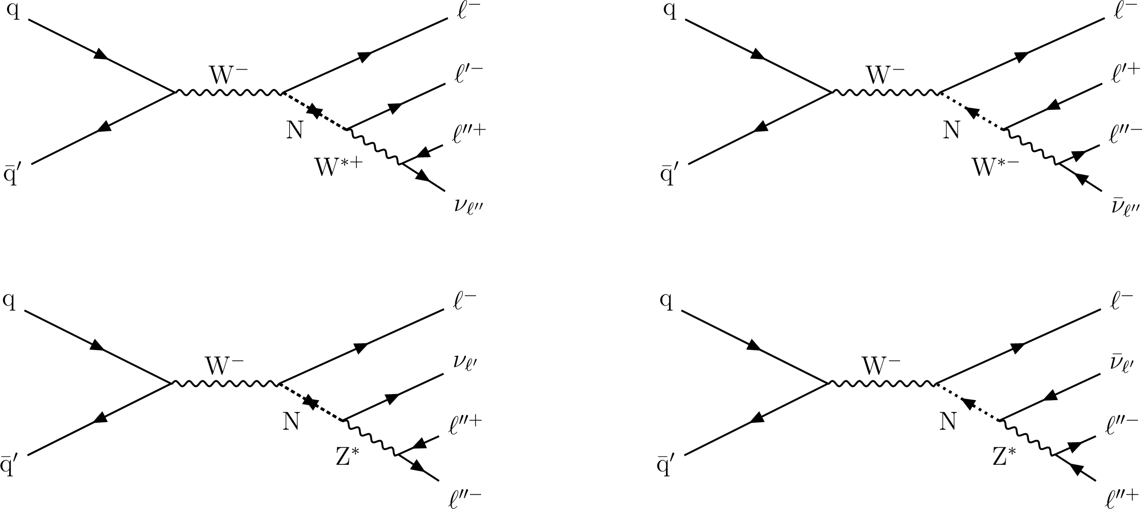
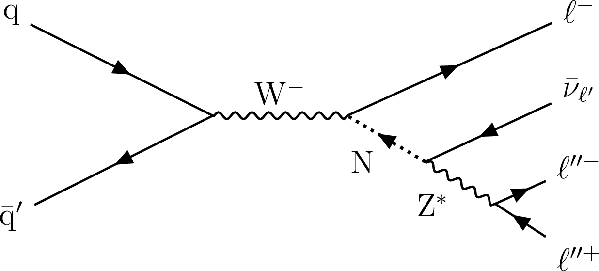
Figure 1:
Feynman diagrams for the production of an HNL (denoted as $ \mathrm{N} $) through its mixing with an SM neutrino, resulting in a final state with three charged leptons and a neutrino. In the used notation, \ell originates from the primary $ \mathrm{W^-} $ decay, {\HepParticle\ell\prime} from the HNL decay directly, and {\HepParticle\ell\prime\prime} from the leptonic decay of the virtual electroweak boson. The HNL decay is mediated by a {\HepParticleW\ast} boson in the upper row and by a $ \mathrm{Z}^{*} $ boson in the lower row. On the left, the HNL is assumed to be a Majorana neutrino, allowing \ell and {\HepParticle\ell\prime} to have the same charge in the {\HepParticleW\ast} -mediated diagram, with consequent lepton-number violation. On the right, instead, the HNL can be either a Dirac or a Majorana particle. |
png pdf |
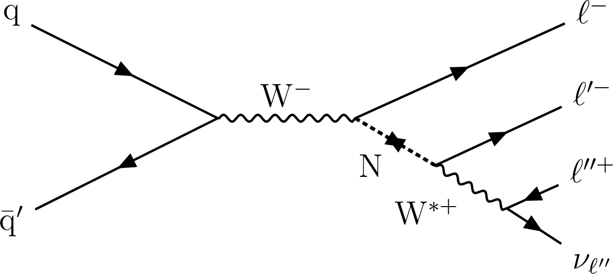
Figure 1-a:
Feynman diagrams for the production of an HNL (denoted as $ \mathrm{N} $) through its mixing with an SM neutrino, resulting in a final state with three charged leptons and a neutrino. In the used notation, \ell originates from the primary $ \mathrm{W^-} $ decay, {\HepParticle\ell\prime} from the HNL decay directly, and {\HepParticle\ell\prime\prime} from the leptonic decay of the virtual electroweak boson. The HNL decay is mediated by a {\HepParticleW\ast} boson in the upper row and by a $ \mathrm{Z}^{*} $ boson in the lower row. On the left, the HNL is assumed to be a Majorana neutrino, allowing \ell and {\HepParticle\ell\prime} to have the same charge in the {\HepParticleW\ast} -mediated diagram, with consequent lepton-number violation. On the right, instead, the HNL can be either a Dirac or a Majorana particle. |
png pdf |
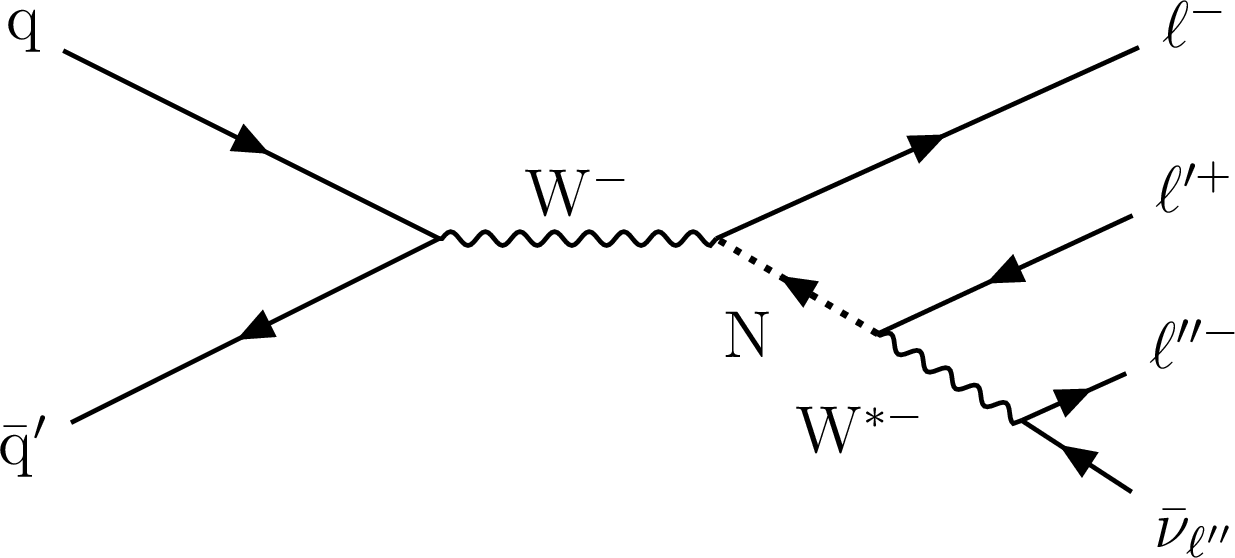
Figure 1-b:
Feynman diagrams for the production of an HNL (denoted as $ \mathrm{N} $) through its mixing with an SM neutrino, resulting in a final state with three charged leptons and a neutrino. In the used notation, \ell originates from the primary $ \mathrm{W^-} $ decay, {\HepParticle\ell\prime} from the HNL decay directly, and {\HepParticle\ell\prime\prime} from the leptonic decay of the virtual electroweak boson. The HNL decay is mediated by a {\HepParticleW\ast} boson in the upper row and by a $ \mathrm{Z}^{*} $ boson in the lower row. On the left, the HNL is assumed to be a Majorana neutrino, allowing \ell and {\HepParticle\ell\prime} to have the same charge in the {\HepParticleW\ast} -mediated diagram, with consequent lepton-number violation. On the right, instead, the HNL can be either a Dirac or a Majorana particle. |
png pdf |
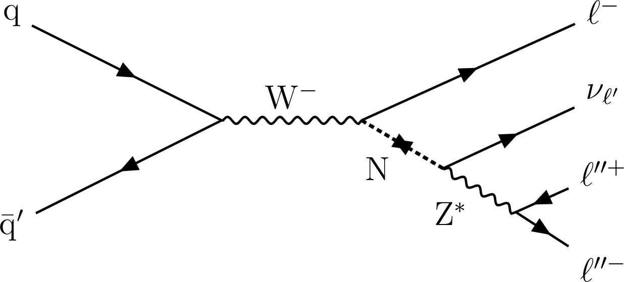
Figure 1-c:
Feynman diagrams for the production of an HNL (denoted as $ \mathrm{N} $) through its mixing with an SM neutrino, resulting in a final state with three charged leptons and a neutrino. In the used notation, \ell originates from the primary $ \mathrm{W^-} $ decay, {\HepParticle\ell\prime} from the HNL decay directly, and {\HepParticle\ell\prime\prime} from the leptonic decay of the virtual electroweak boson. The HNL decay is mediated by a {\HepParticleW\ast} boson in the upper row and by a $ \mathrm{Z}^{*} $ boson in the lower row. On the left, the HNL is assumed to be a Majorana neutrino, allowing \ell and {\HepParticle\ell\prime} to have the same charge in the {\HepParticleW\ast} -mediated diagram, with consequent lepton-number violation. On the right, instead, the HNL can be either a Dirac or a Majorana particle. |
png pdf |
Figure 1-d:
Feynman diagrams for the production of an HNL (denoted as $ \mathrm{N} $) through its mixing with an SM neutrino, resulting in a final state with three charged leptons and a neutrino. In the used notation, \ell originates from the primary $ \mathrm{W^-} $ decay, {\HepParticle\ell\prime} from the HNL decay directly, and {\HepParticle\ell\prime\prime} from the leptonic decay of the virtual electroweak boson. The HNL decay is mediated by a {\HepParticleW\ast} boson in the upper row and by a $ \mathrm{Z}^{*} $ boson in the lower row. On the left, the HNL is assumed to be a Majorana neutrino, allowing \ell and {\HepParticle\ell\prime} to have the same charge in the {\HepParticleW\ast} -mediated diagram, with consequent lepton-number violation. On the right, instead, the HNL can be either a Dirac or a Majorana particle. |
png pdf |
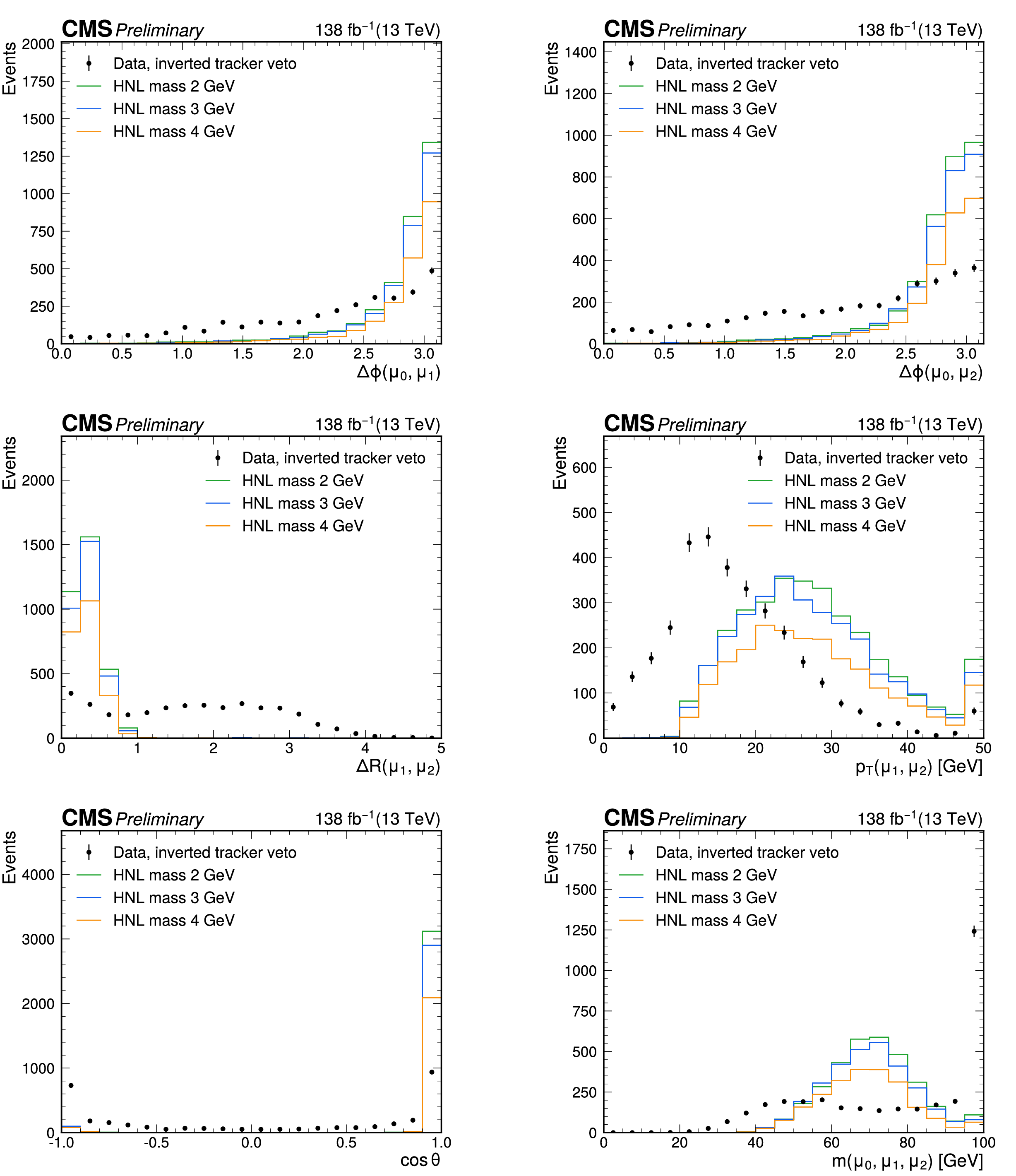
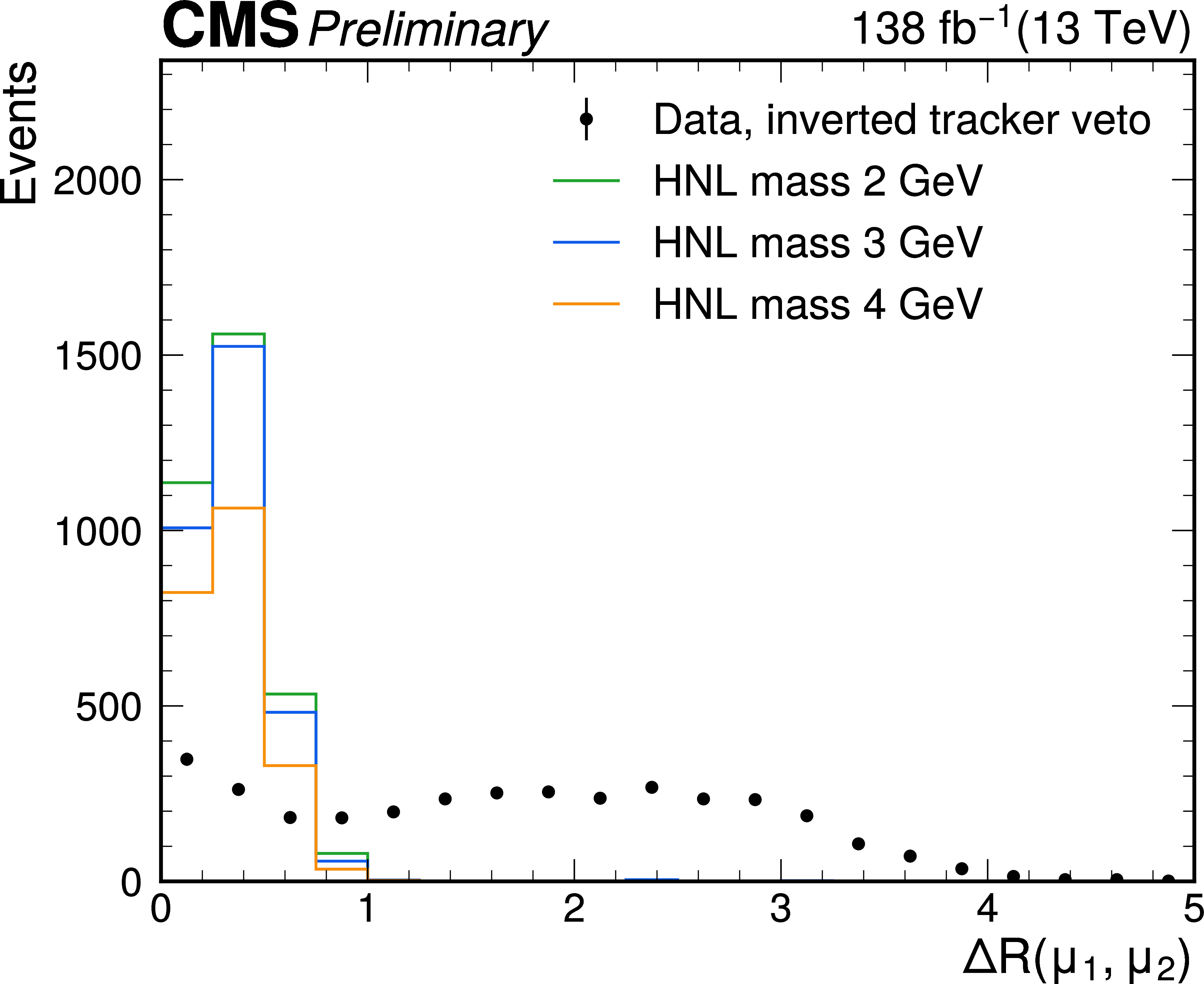
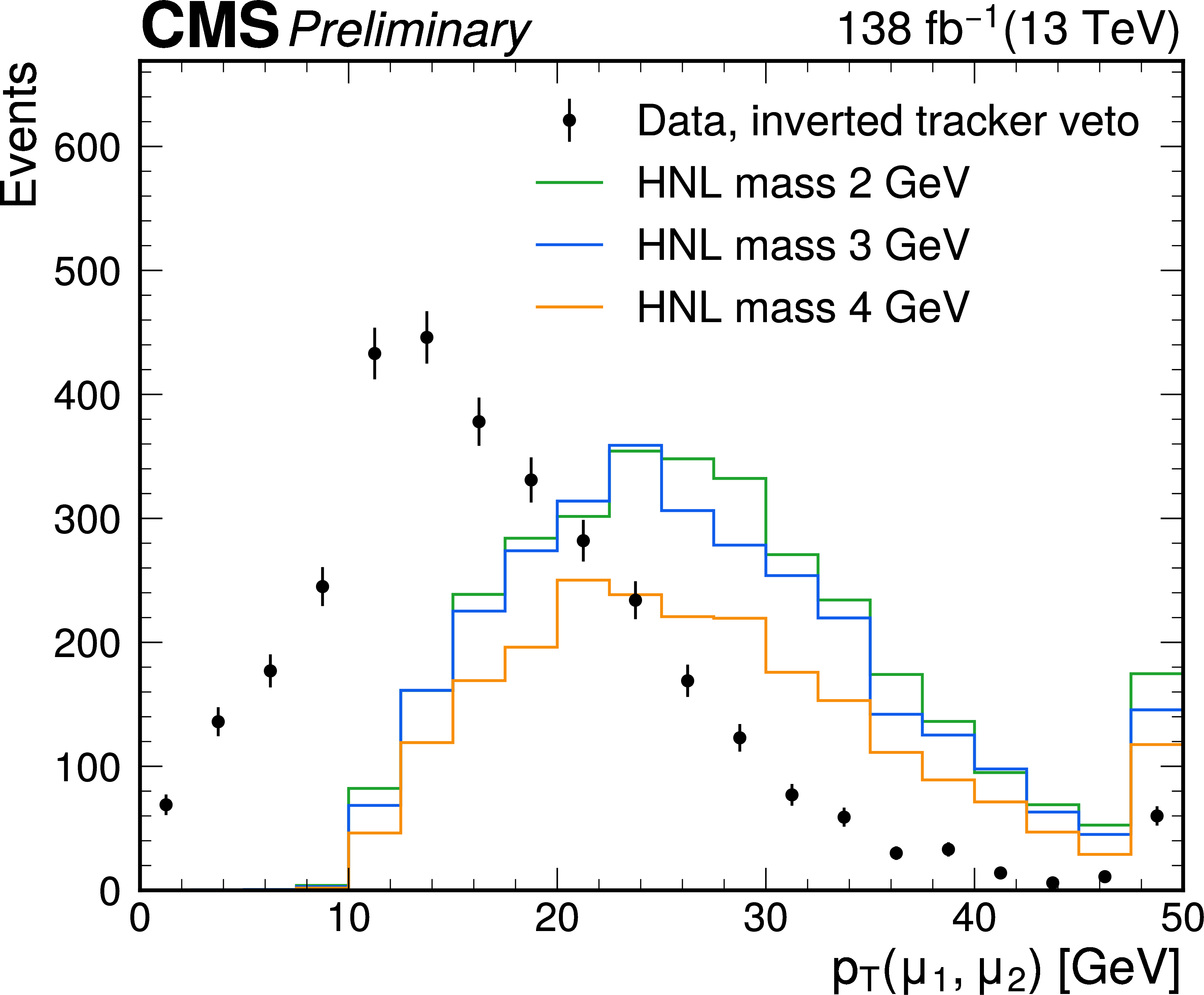
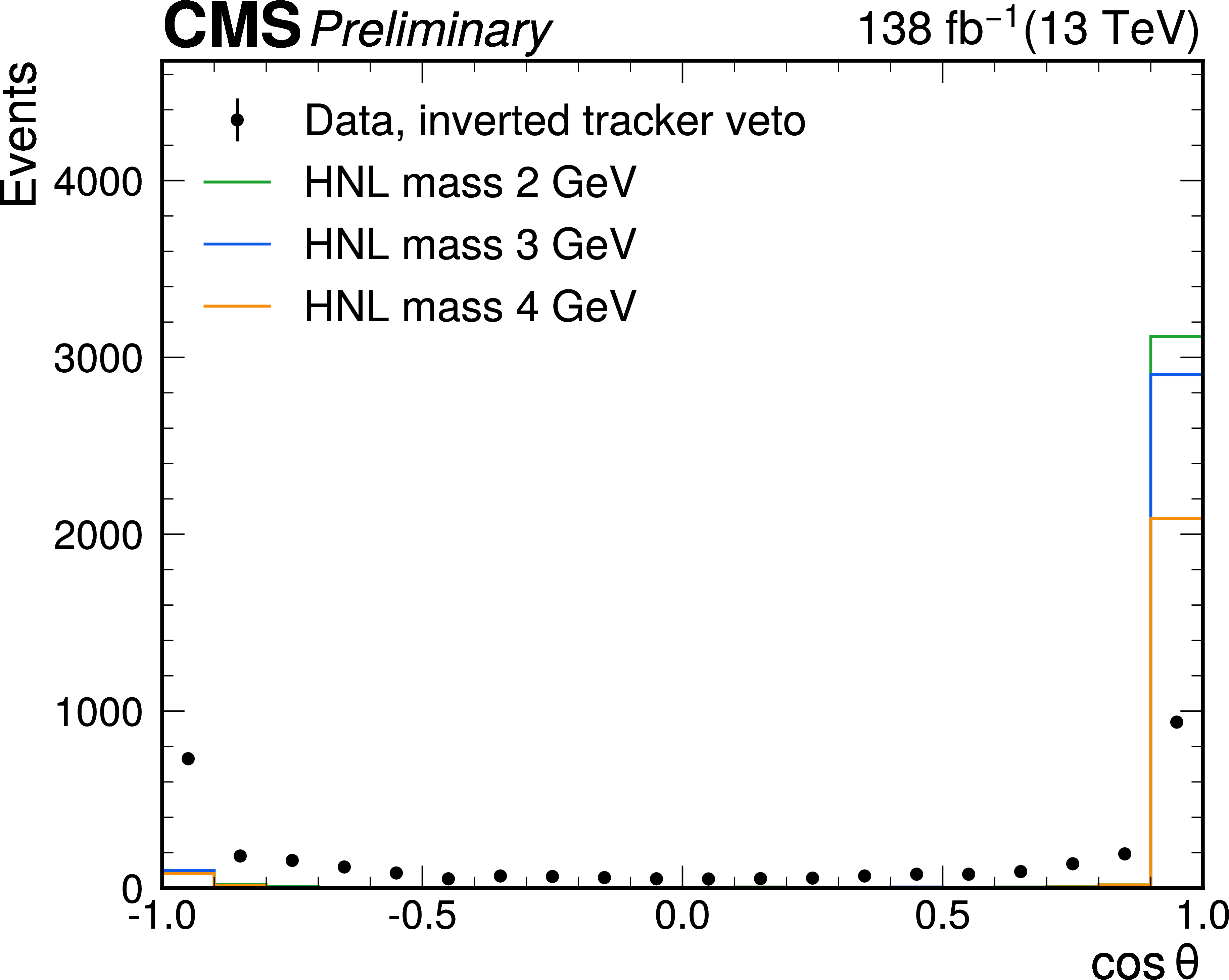
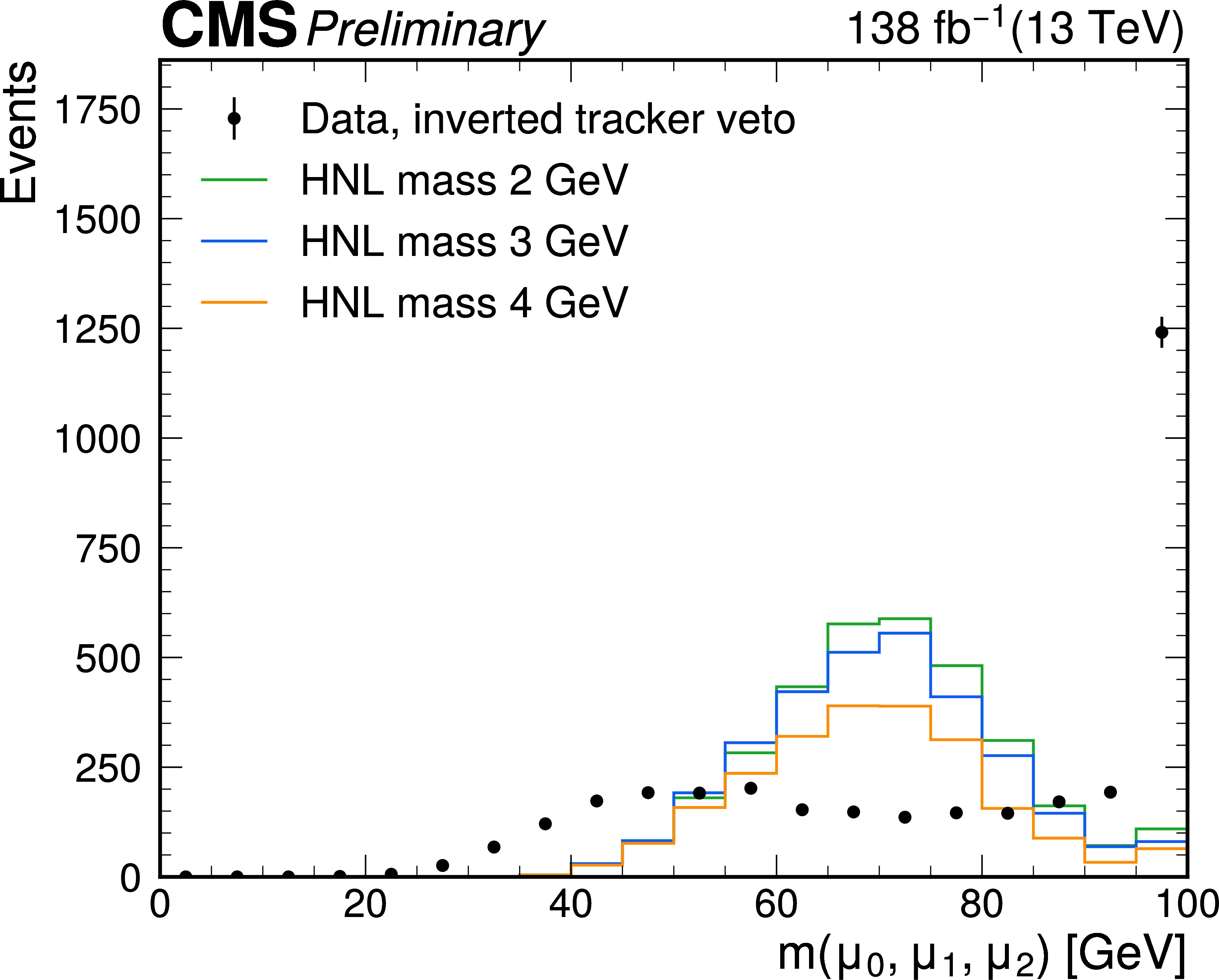
Figure 2:
Distributions of $ \Delta\phi(\mu_0,\mu_1) $ (upper left), $ \Delta\phi(\mu_0,\mu_2) $ (upper right), $ \Delta R(\mu_1,\mu_2) $ (middle left), $ p_{\mathrm{T}}(\mu_1,\mu_2) $ (middle right), $ \cos\theta(\mu_1,\mu_2) $ (lower left), and $ m(\mu_0,\mu_1,\mu_2) $ (lower right), shown for HNL predictions with three different $ m_{\mathrm{N}} $ values after the muon selection and compared to data from the control region with inverted tracker veto on $ \mu_1 $. The HNL predictions are scaled with a single normalization factor such that the integral of the HNL prediction with $ m_{\mathrm{N}}= $ 2 GeV matches the integral of the data distribution, with relative normalization differences between different HNL hypotheses retained. Overflow contributions are included in the last bin of the histograms. |
png pdf |
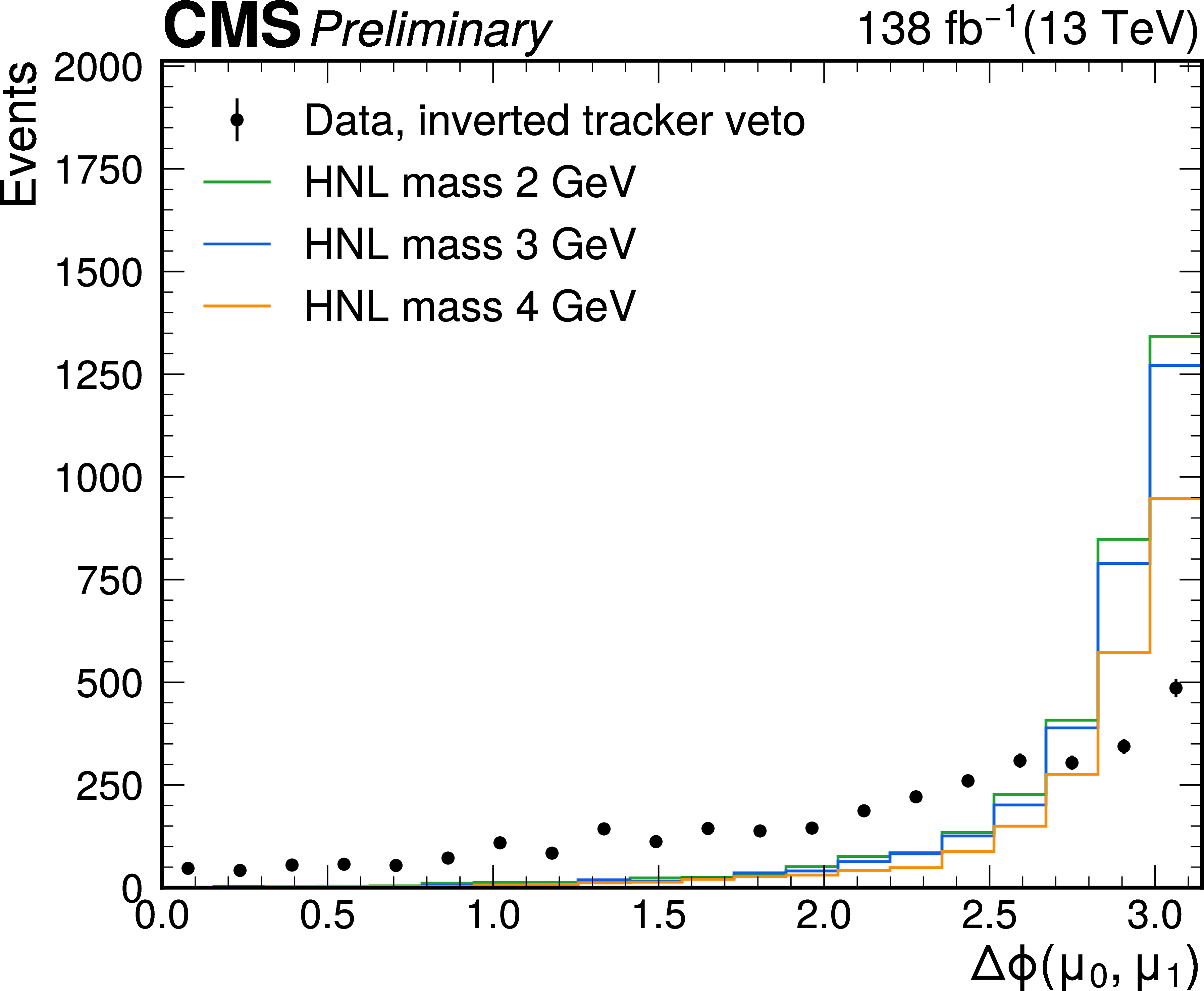
Figure 2-a:
Distributions of $ \Delta\phi(\mu_0,\mu_1) $ (upper left), $ \Delta\phi(\mu_0,\mu_2) $ (upper right), $ \Delta R(\mu_1,\mu_2) $ (middle left), $ p_{\mathrm{T}}(\mu_1,\mu_2) $ (middle right), $ \cos\theta(\mu_1,\mu_2) $ (lower left), and $ m(\mu_0,\mu_1,\mu_2) $ (lower right), shown for HNL predictions with three different $ m_{\mathrm{N}} $ values after the muon selection and compared to data from the control region with inverted tracker veto on $ \mu_1 $. The HNL predictions are scaled with a single normalization factor such that the integral of the HNL prediction with $ m_{\mathrm{N}}= $ 2 GeV matches the integral of the data distribution, with relative normalization differences between different HNL hypotheses retained. Overflow contributions are included in the last bin of the histograms. |
png pdf |
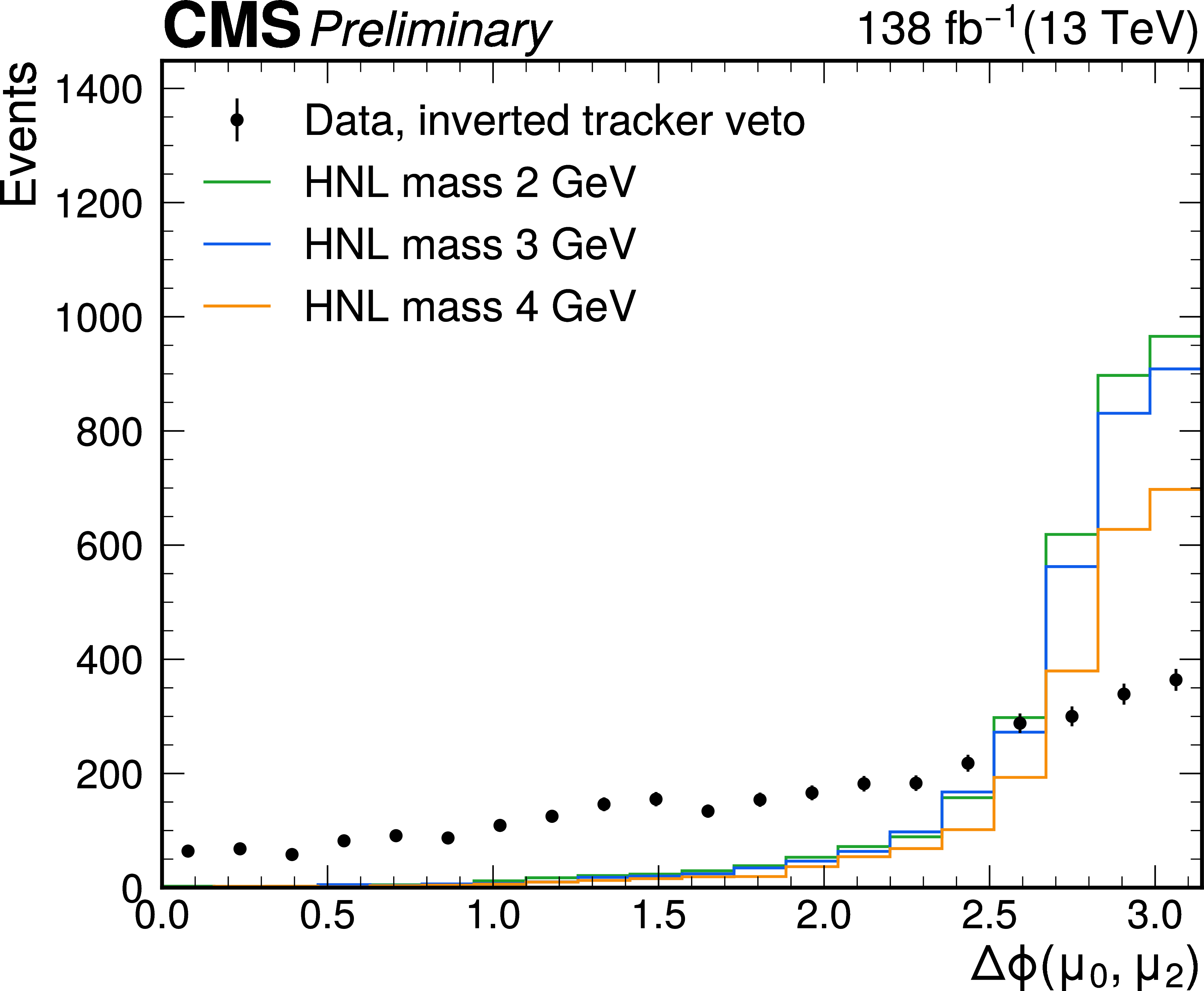
Figure 2-b:
Distributions of $ \Delta\phi(\mu_0,\mu_1) $ (upper left), $ \Delta\phi(\mu_0,\mu_2) $ (upper right), $ \Delta R(\mu_1,\mu_2) $ (middle left), $ p_{\mathrm{T}}(\mu_1,\mu_2) $ (middle right), $ \cos\theta(\mu_1,\mu_2) $ (lower left), and $ m(\mu_0,\mu_1,\mu_2) $ (lower right), shown for HNL predictions with three different $ m_{\mathrm{N}} $ values after the muon selection and compared to data from the control region with inverted tracker veto on $ \mu_1 $. The HNL predictions are scaled with a single normalization factor such that the integral of the HNL prediction with $ m_{\mathrm{N}}= $ 2 GeV matches the integral of the data distribution, with relative normalization differences between different HNL hypotheses retained. Overflow contributions are included in the last bin of the histograms. |
png pdf |
Figure 2-c:
Distributions of $ \Delta\phi(\mu_0,\mu_1) $ (upper left), $ \Delta\phi(\mu_0,\mu_2) $ (upper right), $ \Delta R(\mu_1,\mu_2) $ (middle left), $ p_{\mathrm{T}}(\mu_1,\mu_2) $ (middle right), $ \cos\theta(\mu_1,\mu_2) $ (lower left), and $ m(\mu_0,\mu_1,\mu_2) $ (lower right), shown for HNL predictions with three different $ m_{\mathrm{N}} $ values after the muon selection and compared to data from the control region with inverted tracker veto on $ \mu_1 $. The HNL predictions are scaled with a single normalization factor such that the integral of the HNL prediction with $ m_{\mathrm{N}}= $ 2 GeV matches the integral of the data distribution, with relative normalization differences between different HNL hypotheses retained. Overflow contributions are included in the last bin of the histograms. |
png pdf |
Figure 2-d:
Distributions of $ \Delta\phi(\mu_0,\mu_1) $ (upper left), $ \Delta\phi(\mu_0,\mu_2) $ (upper right), $ \Delta R(\mu_1,\mu_2) $ (middle left), $ p_{\mathrm{T}}(\mu_1,\mu_2) $ (middle right), $ \cos\theta(\mu_1,\mu_2) $ (lower left), and $ m(\mu_0,\mu_1,\mu_2) $ (lower right), shown for HNL predictions with three different $ m_{\mathrm{N}} $ values after the muon selection and compared to data from the control region with inverted tracker veto on $ \mu_1 $. The HNL predictions are scaled with a single normalization factor such that the integral of the HNL prediction with $ m_{\mathrm{N}}= $ 2 GeV matches the integral of the data distribution, with relative normalization differences between different HNL hypotheses retained. Overflow contributions are included in the last bin of the histograms. |
png pdf |
Figure 2-e:
Distributions of $ \Delta\phi(\mu_0,\mu_1) $ (upper left), $ \Delta\phi(\mu_0,\mu_2) $ (upper right), $ \Delta R(\mu_1,\mu_2) $ (middle left), $ p_{\mathrm{T}}(\mu_1,\mu_2) $ (middle right), $ \cos\theta(\mu_1,\mu_2) $ (lower left), and $ m(\mu_0,\mu_1,\mu_2) $ (lower right), shown for HNL predictions with three different $ m_{\mathrm{N}} $ values after the muon selection and compared to data from the control region with inverted tracker veto on $ \mu_1 $. The HNL predictions are scaled with a single normalization factor such that the integral of the HNL prediction with $ m_{\mathrm{N}}= $ 2 GeV matches the integral of the data distribution, with relative normalization differences between different HNL hypotheses retained. Overflow contributions are included in the last bin of the histograms. |
png pdf |
Figure 2-f:
Distributions of $ \Delta\phi(\mu_0,\mu_1) $ (upper left), $ \Delta\phi(\mu_0,\mu_2) $ (upper right), $ \Delta R(\mu_1,\mu_2) $ (middle left), $ p_{\mathrm{T}}(\mu_1,\mu_2) $ (middle right), $ \cos\theta(\mu_1,\mu_2) $ (lower left), and $ m(\mu_0,\mu_1,\mu_2) $ (lower right), shown for HNL predictions with three different $ m_{\mathrm{N}} $ values after the muon selection and compared to data from the control region with inverted tracker veto on $ \mu_1 $. The HNL predictions are scaled with a single normalization factor such that the integral of the HNL prediction with $ m_{\mathrm{N}}= $ 2 GeV matches the integral of the data distribution, with relative normalization differences between different HNL hypotheses retained. Overflow contributions are included in the last bin of the histograms. |
png pdf |
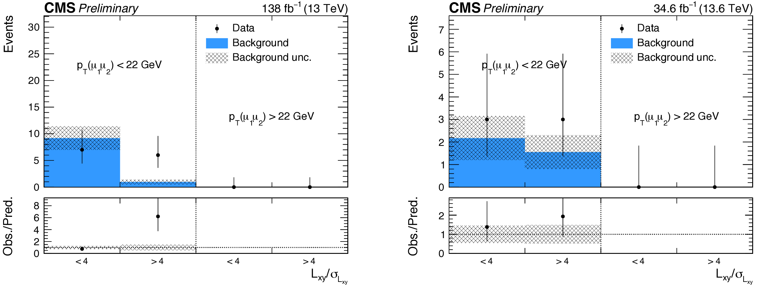
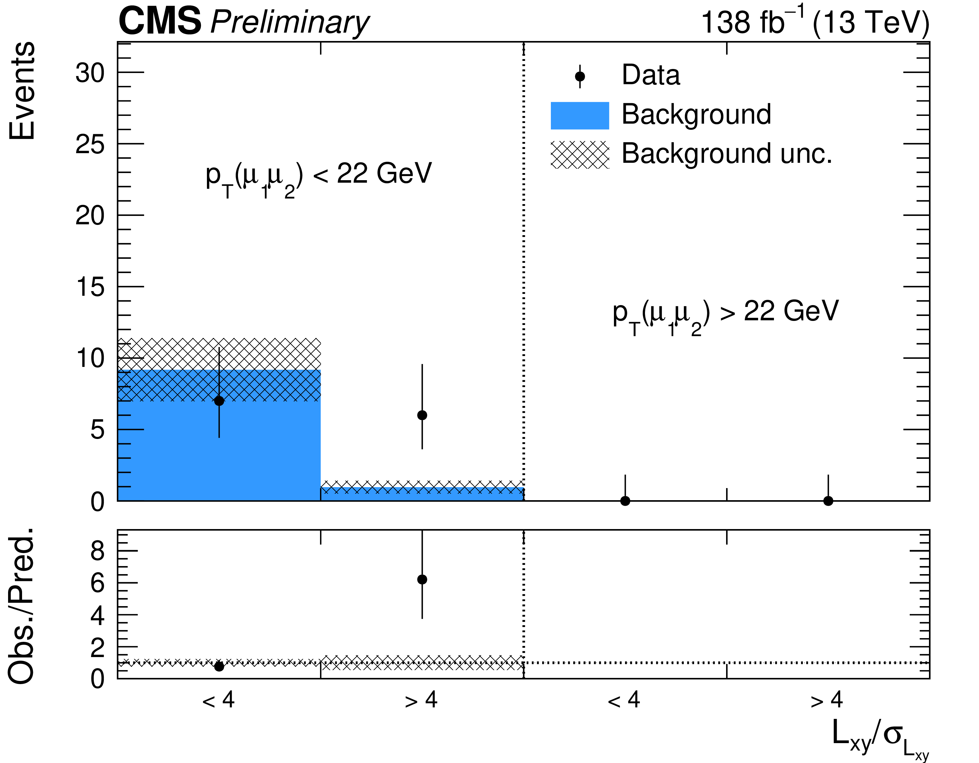
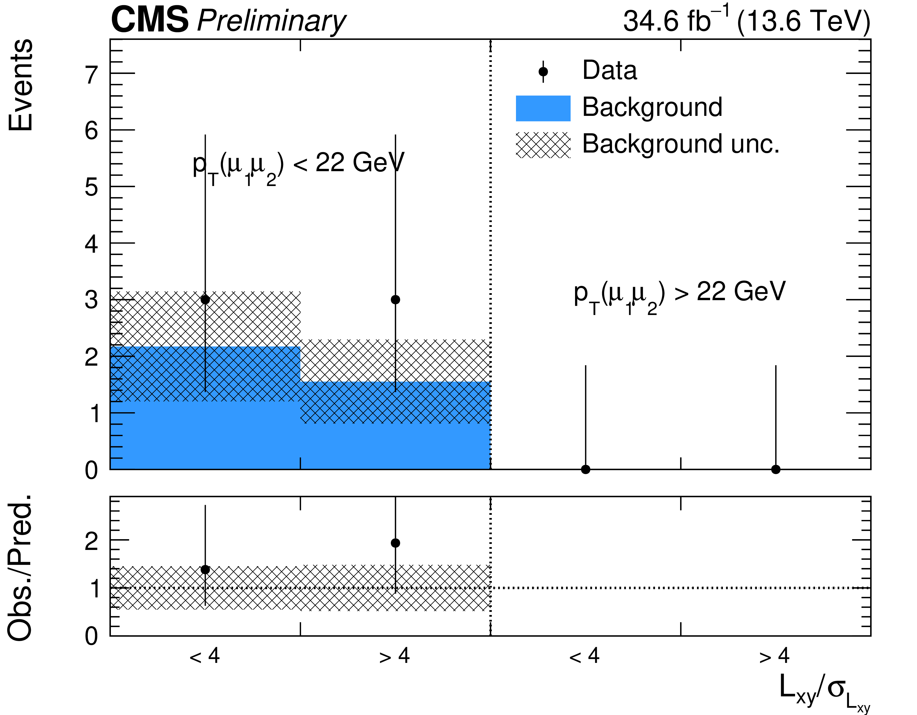
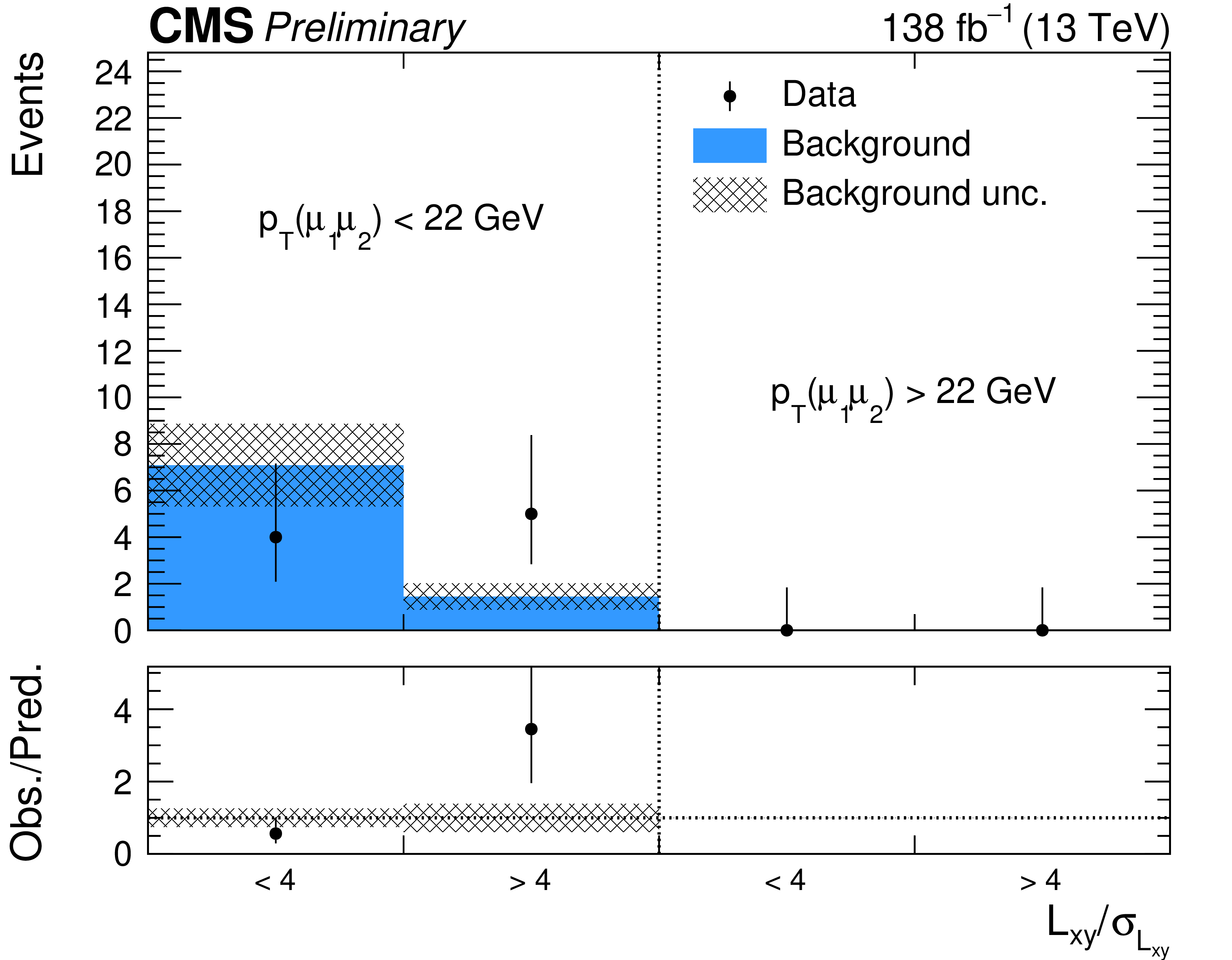
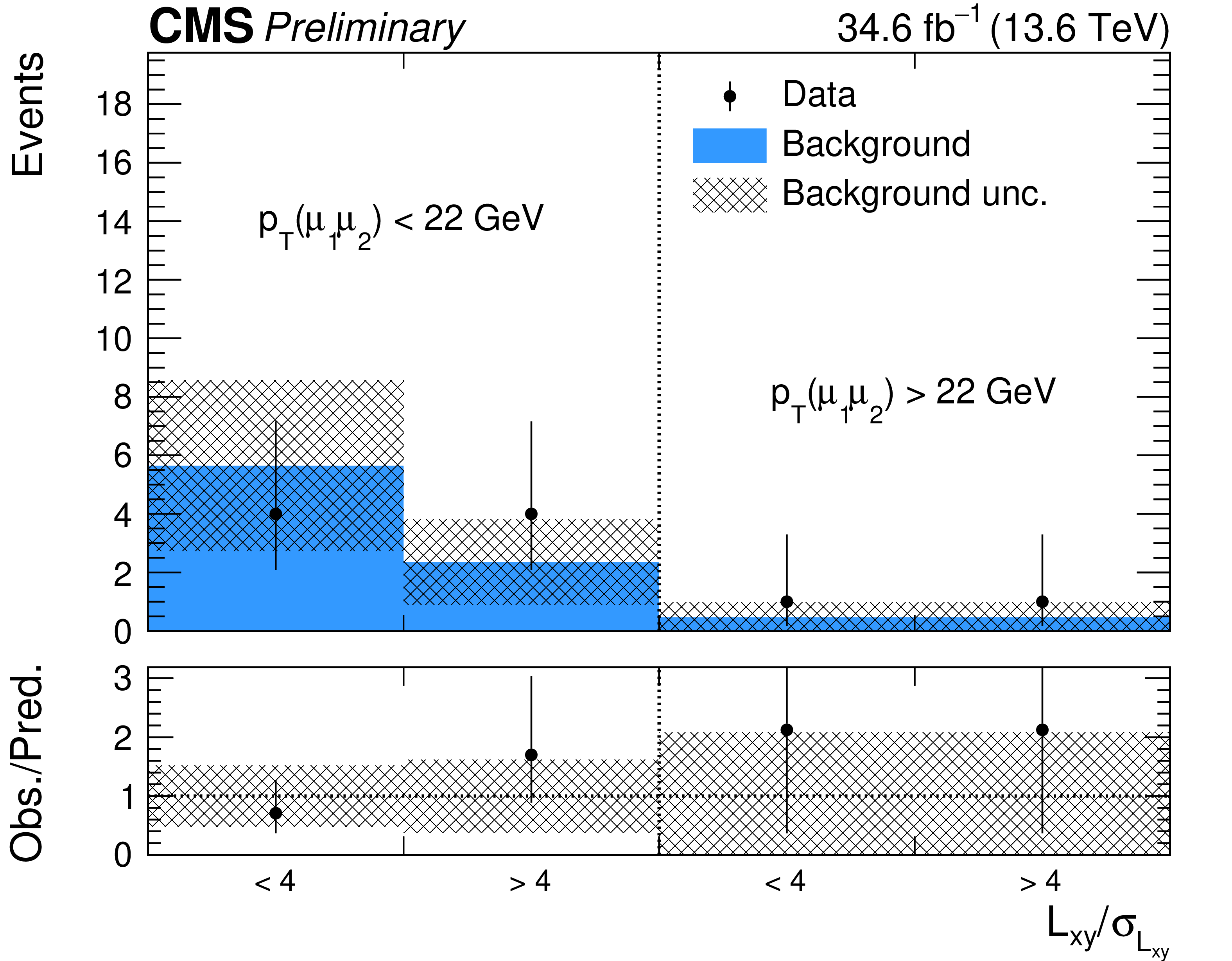
Figure 3:
Observed (black points) and predicted (blue histograms) yields in the low-$ p_{\mathrm{T}} $ validation region in \Run2 (left) and in 2022 with relaxed DSA isolation requirements (right). The grey bands represent the statistical uncertainty in the background prediction. The lower panels show the ratio between observed and predicted yields in each bin. Both predicted and observed yields are exactly zero in the last two bins by construction of the low-$ p_{\mathrm{T}} $ validation region. |
png pdf |
Figure 3-a:
Observed (black points) and predicted (blue histograms) yields in the low-$ p_{\mathrm{T}} $ validation region in \Run2 (left) and in 2022 with relaxed DSA isolation requirements (right). The grey bands represent the statistical uncertainty in the background prediction. The lower panels show the ratio between observed and predicted yields in each bin. Both predicted and observed yields are exactly zero in the last two bins by construction of the low-$ p_{\mathrm{T}} $ validation region. |
png pdf |
Figure 3-b:
Observed (black points) and predicted (blue histograms) yields in the low-$ p_{\mathrm{T}} $ validation region in \Run2 (left) and in 2022 with relaxed DSA isolation requirements (right). The grey bands represent the statistical uncertainty in the background prediction. The lower panels show the ratio between observed and predicted yields in each bin. Both predicted and observed yields are exactly zero in the last two bins by construction of the low-$ p_{\mathrm{T}} $ validation region. |
png pdf |
Figure 4:
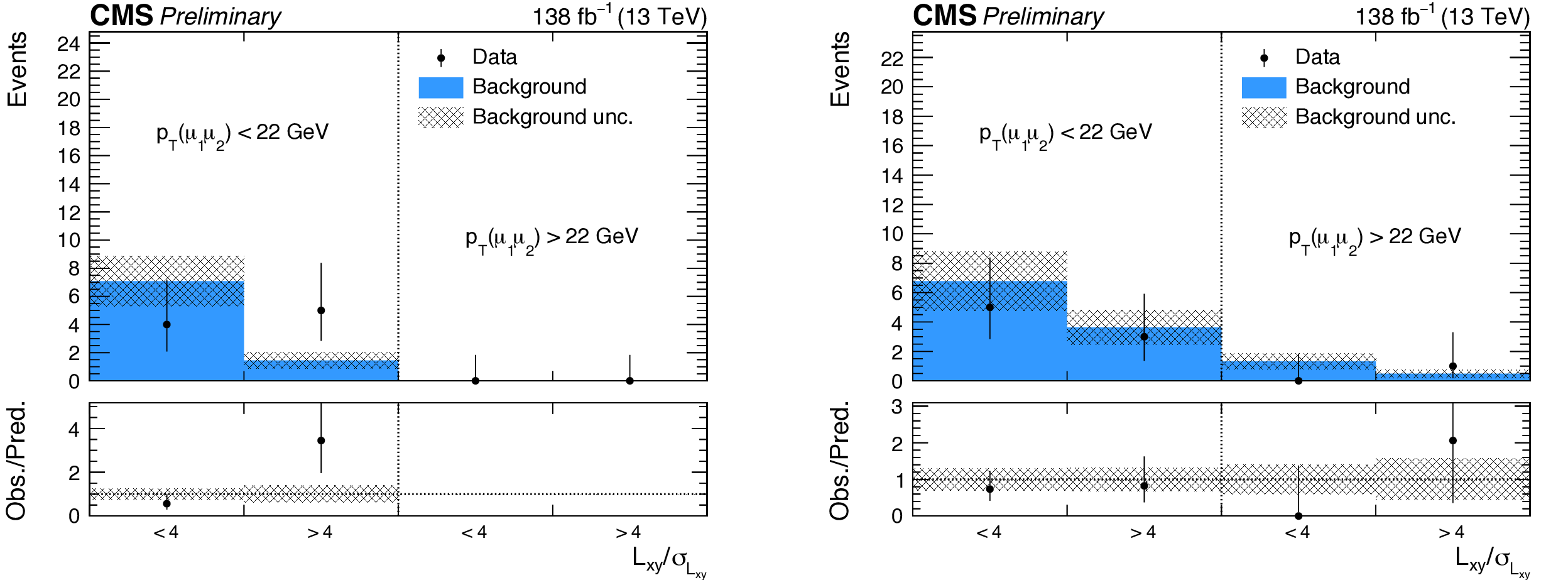
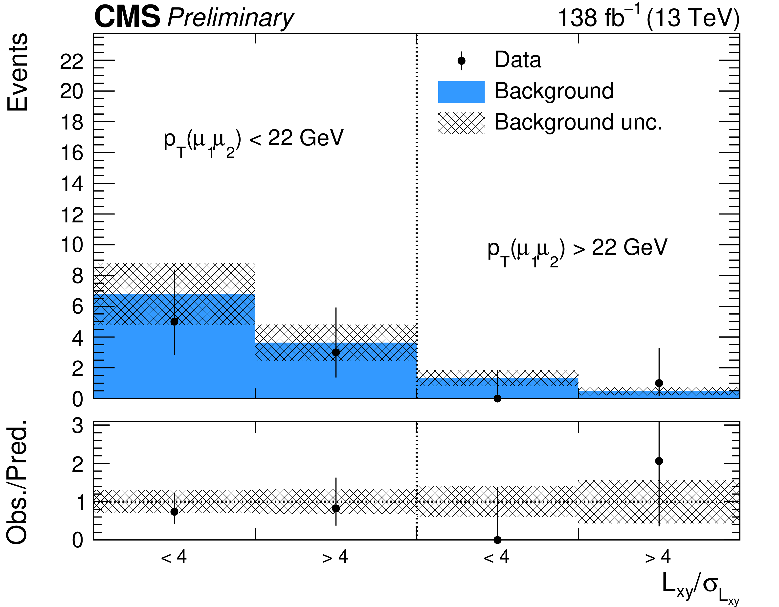
Observed (black points) and predicted (blue histograms) yields in the sideband with at least one non-isolated DSA muon of the low-$ p_{\mathrm{T}} $ validation region (left) and the signal region (right) in \Run2. The grey bands represent the statistical uncertainty in the background prediction. The lower panels show the ratio between observed and predicted yields in each bin. In the left figure, both predicted and observed yields are exactly zero in the last two bins by construction of the low-$ p_{\mathrm{T}} $ validation region. |
png pdf |
Figure 4-a:
Observed (black points) and predicted (blue histograms) yields in the sideband with at least one non-isolated DSA muon of the low-$ p_{\mathrm{T}} $ validation region (left) and the signal region (right) in \Run2. The grey bands represent the statistical uncertainty in the background prediction. The lower panels show the ratio between observed and predicted yields in each bin. In the left figure, both predicted and observed yields are exactly zero in the last two bins by construction of the low-$ p_{\mathrm{T}} $ validation region. |
png pdf |
Figure 4-b:
Observed (black points) and predicted (blue histograms) yields in the sideband with at least one non-isolated DSA muon of the low-$ p_{\mathrm{T}} $ validation region (left) and the signal region (right) in \Run2. The grey bands represent the statistical uncertainty in the background prediction. The lower panels show the ratio between observed and predicted yields in each bin. In the left figure, both predicted and observed yields are exactly zero in the last two bins by construction of the low-$ p_{\mathrm{T}} $ validation region. |
png pdf |
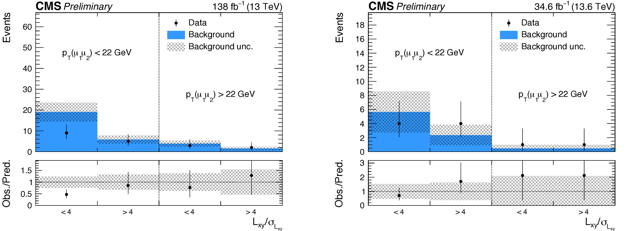
Figure 5:
Observed (black points) and predicted (blue histograms) yields in the inverted tracker veto validation region in \Run2 (left) and in 2022 with relaxed DSA isolation requirements (right). The grey bands represent the statistical uncertainty in the background prediction. The lower panels show the ratio between observed and predicted yields in each bin. |
png pdf |
Figure 5-a:
Observed (black points) and predicted (blue histograms) yields in the inverted tracker veto validation region in \Run2 (left) and in 2022 with relaxed DSA isolation requirements (right). The grey bands represent the statistical uncertainty in the background prediction. The lower panels show the ratio between observed and predicted yields in each bin. |
png pdf |
Figure 5-b:
Observed (black points) and predicted (blue histograms) yields in the inverted tracker veto validation region in \Run2 (left) and in 2022 with relaxed DSA isolation requirements (right). The grey bands represent the statistical uncertainty in the background prediction. The lower panels show the ratio between observed and predicted yields in each bin. |
png pdf |
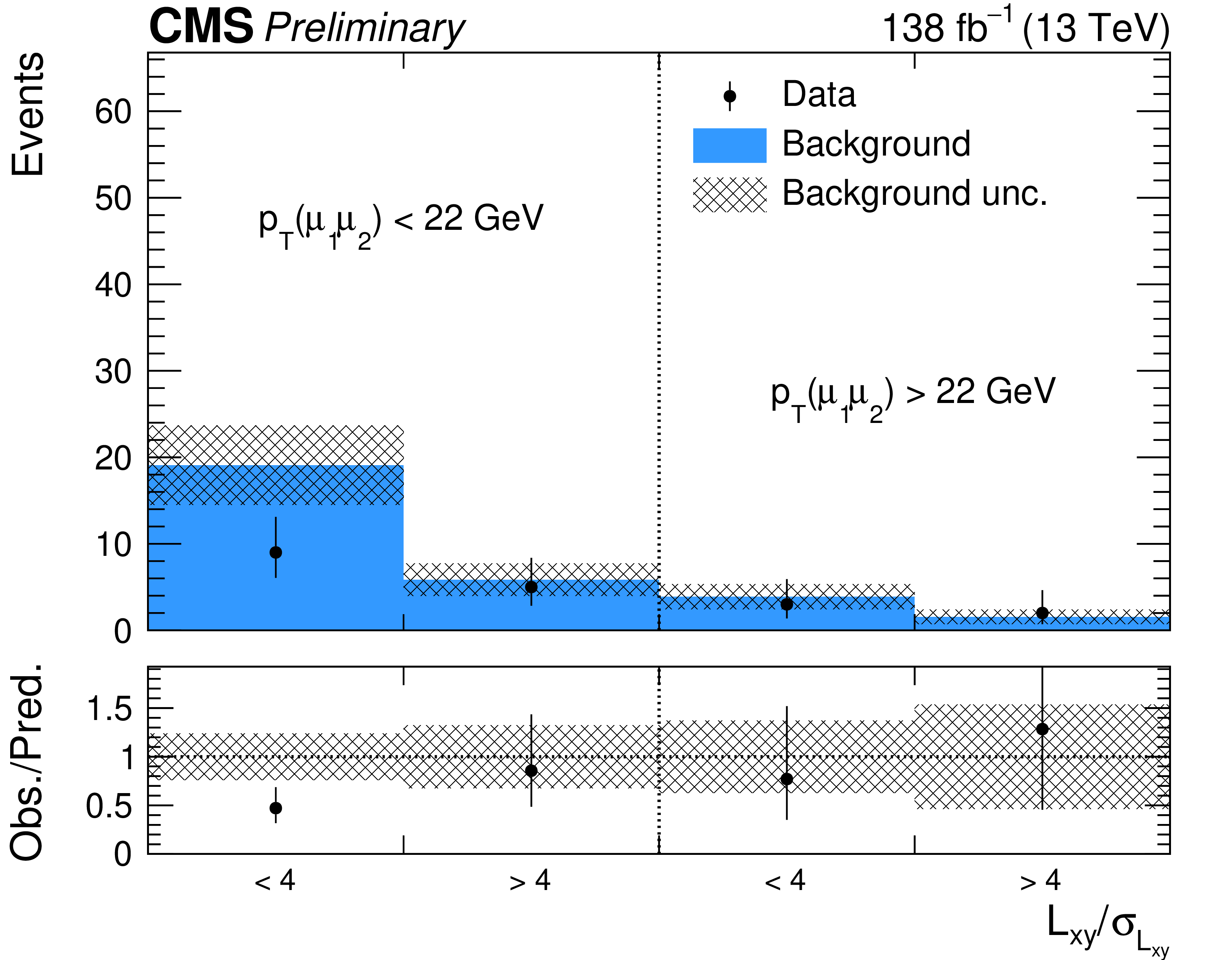
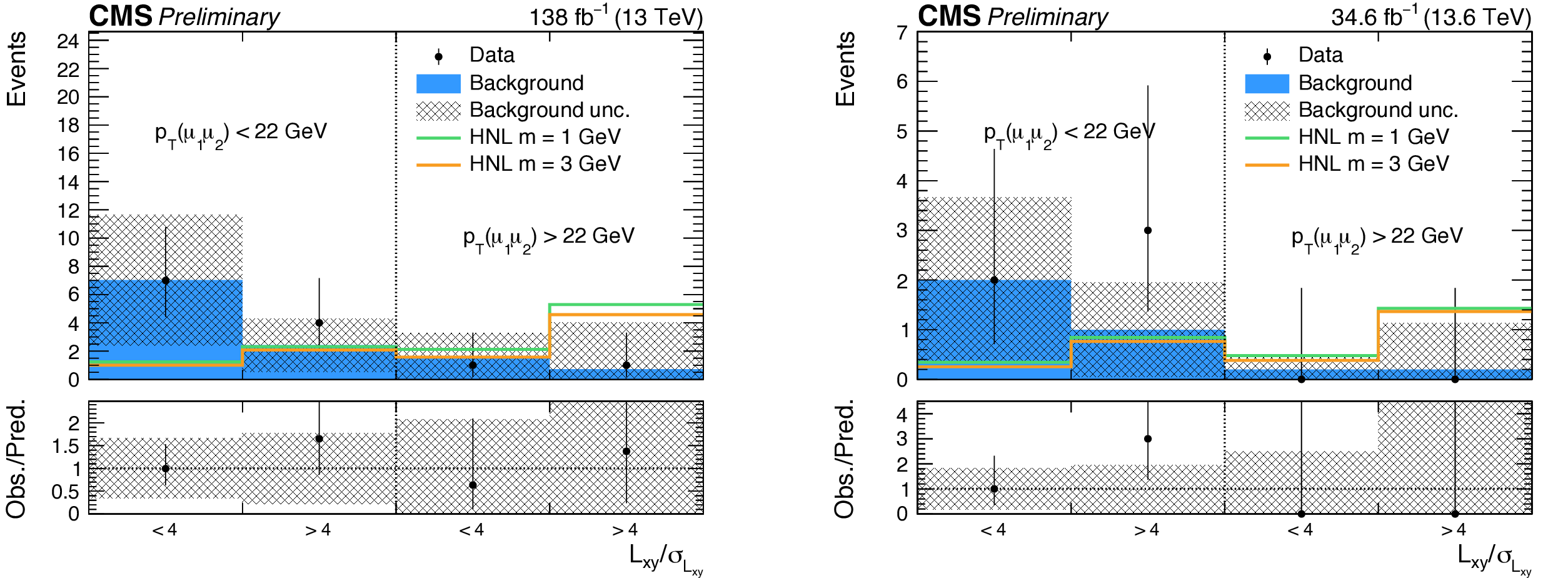
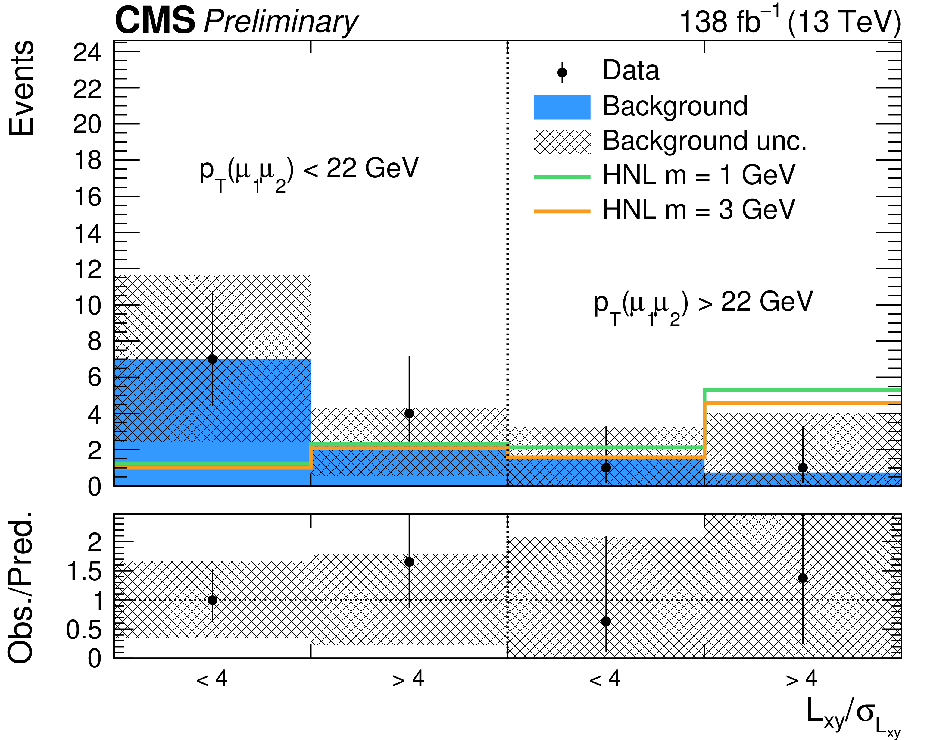
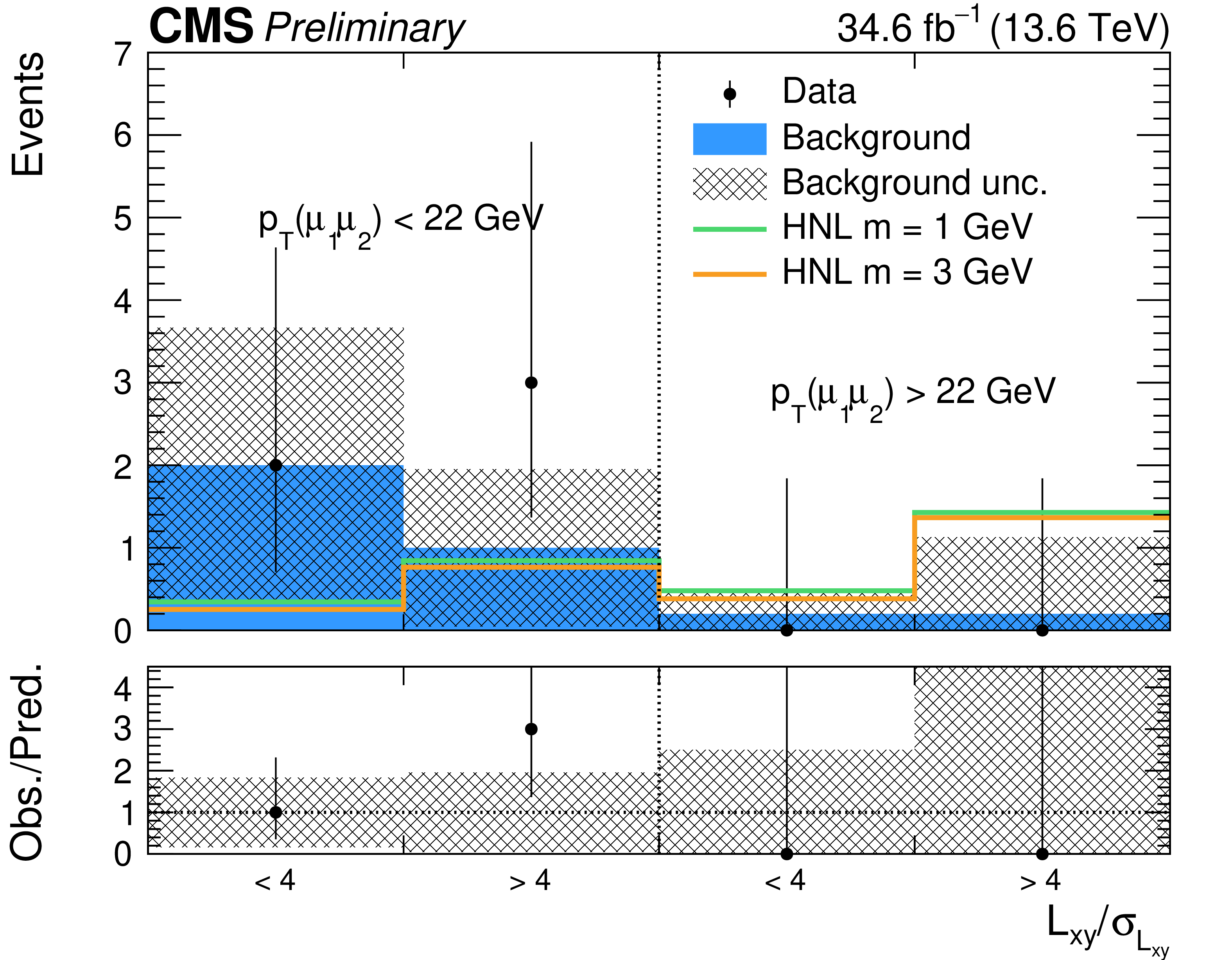
Figure 6:
Observed (black points) and predicted (blue histograms) yields in the signal region in \Run2 (left) and in 2022 (right). The grey bands represent the total uncertainty in the background prediction. The green and orange histograms show the signal distributions for two different hypotheses, corresponding to $ m_{\mathrm{N}}= $ 1 and 3 GeV, and respective $ |V_{\mathrm{N}\mu}|^2 $ values equal to the smallest excluded values at 95% CL by Ref. [36]. The lower panels show the ratio between observed yields and predicted background yields in each bin. |
png pdf |
Figure 6-a:
Observed (black points) and predicted (blue histograms) yields in the signal region in \Run2 (left) and in 2022 (right). The grey bands represent the total uncertainty in the background prediction. The green and orange histograms show the signal distributions for two different hypotheses, corresponding to $ m_{\mathrm{N}}= $ 1 and 3 GeV, and respective $ |V_{\mathrm{N}\mu}|^2 $ values equal to the smallest excluded values at 95% CL by Ref. [36]. The lower panels show the ratio between observed yields and predicted background yields in each bin. |
png pdf |
Figure 6-b:
Observed (black points) and predicted (blue histograms) yields in the signal region in \Run2 (left) and in 2022 (right). The grey bands represent the total uncertainty in the background prediction. The green and orange histograms show the signal distributions for two different hypotheses, corresponding to $ m_{\mathrm{N}}= $ 1 and 3 GeV, and respective $ |V_{\mathrm{N}\mu}|^2 $ values equal to the smallest excluded values at 95% CL by Ref. [36]. The lower panels show the ratio between observed yields and predicted background yields in each bin. |
png pdf |
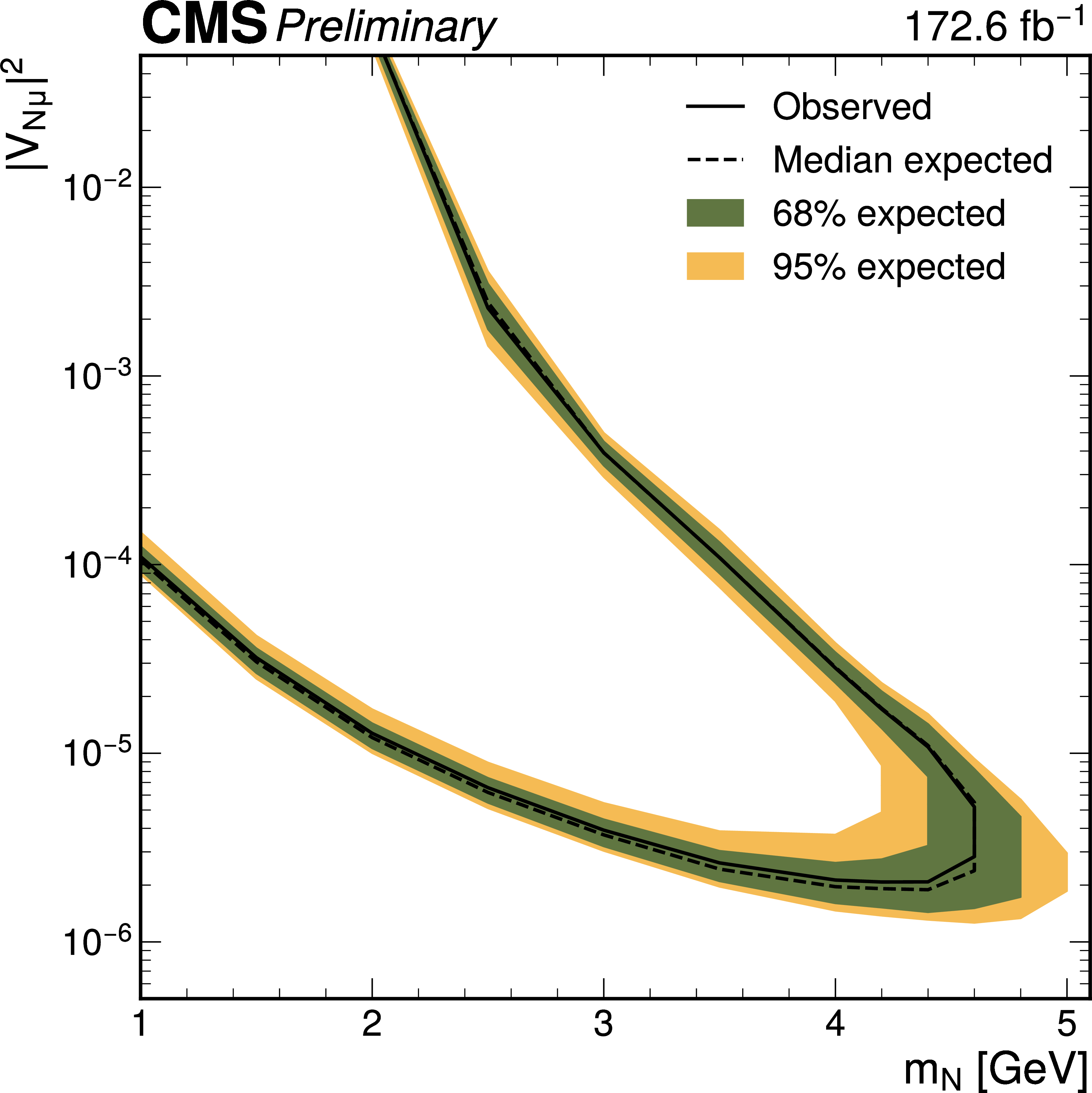
Figure 7:
Exclusion limits at 95% CL on $ |V_{\mathrm{N}\mu}|^2 $ as a function of $ m_{\mathrm{N}} $ for a Majorana HNL, obtained with the combination of \Run2 and 2022 data. The solid (dashed) black curve indicates the observed (expected) exclusion, where the parameter combinations inside the curve are excluded. |
png pdf |
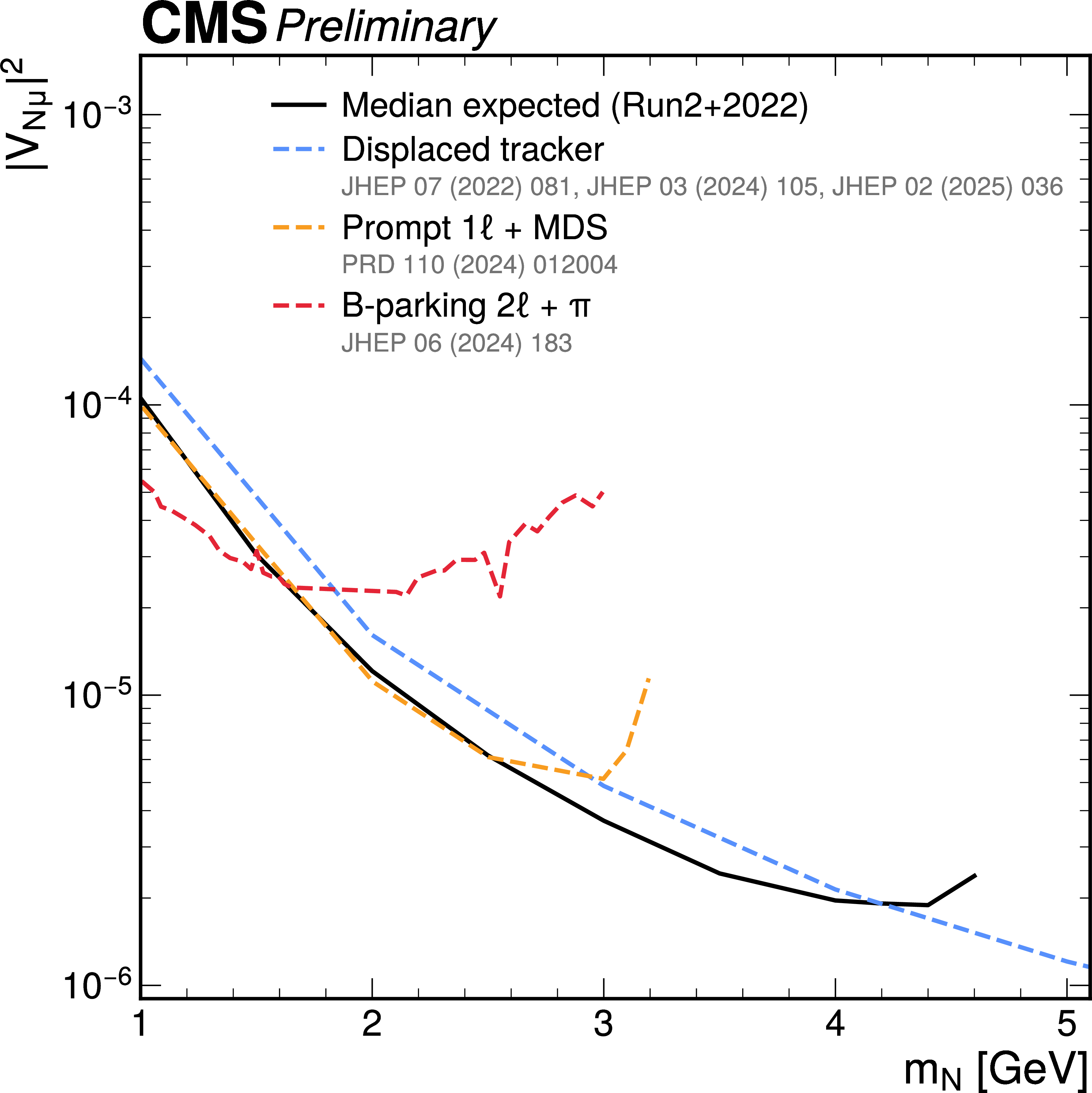
Figure 8:
Lower expected exclusion limits at 95% CL on $ |V_{\mathrm{N}\mu}|^2 $ as a function of $ m_{\mathrm{N}} $ for a Majorana HNL, obtained with the combination of \Run2 and 2022 data (solid black line), compared with the expected limits obtained by other CMS analyses in the same mass range (dashed coloured lines). |
| Tables | |
png pdf |
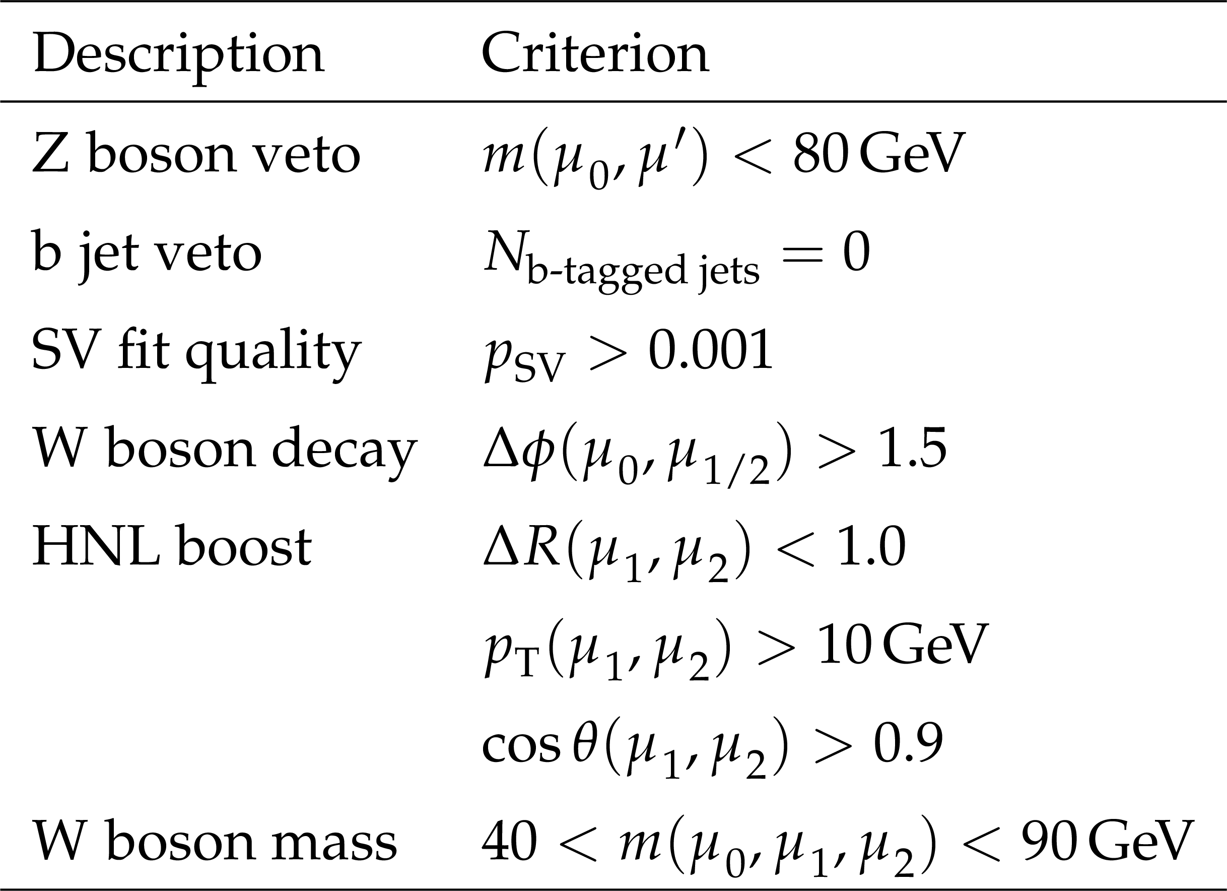
Table 1:
Summary of event selection criteria. |
png pdf |
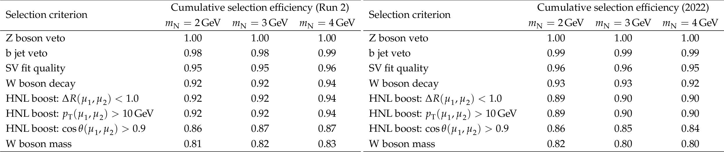
Table 2:
Cumulative selection efficiency after each kinematic selection criterion with \Run2 (upper) and 2022 (lower) conditions. The efficiencies are evaluated for three signal samples: $ m_{\mathrm{N}}= $ 2 GeV with $ |V_{\mathrm{N}\mu}|^2=1.61\times10^{-5} $, $ m_{\mathrm{N}}= $ 3 GeV with $ |V_{\mathrm{N}\mu}|^2=4.87\times10^{-6} $, and $ m_{\mathrm{N}}= $ 4 GeV with $ |V_{\mathrm{N}\mu}|^2=2.14\times10^{-6} $. The denominator for each efficiency corresponds to the signal yield after the prompt and displaced muon selections described in Section 5.1. |
png pdf |
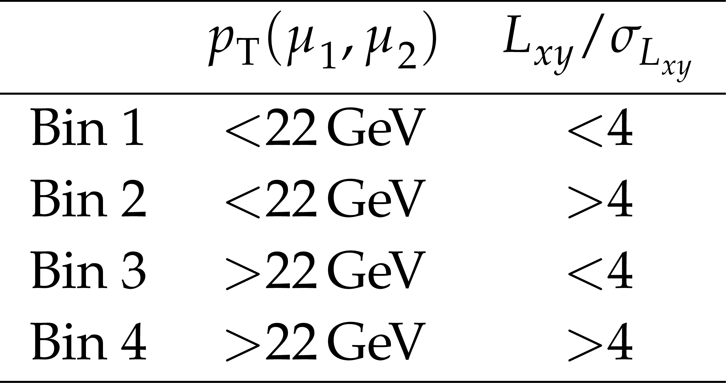
Table 3:
Definition of the signal region bins. |
png pdf |
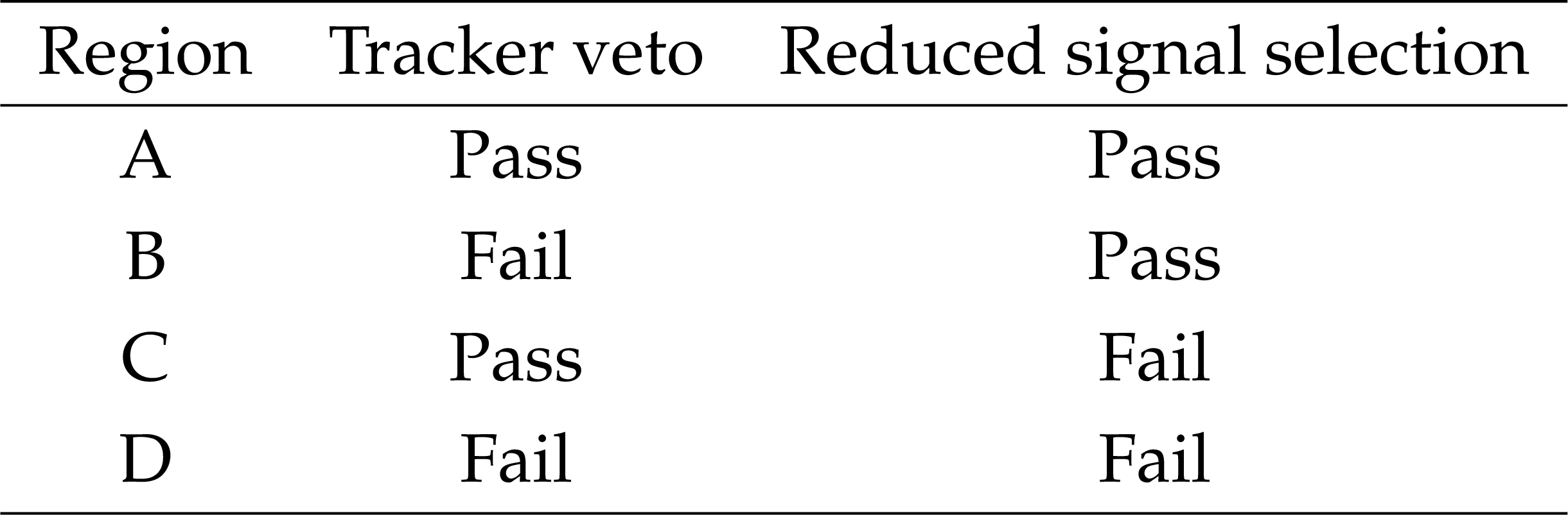
Table 4:
Definition of the regions used in the ABCD method. |
png pdf |
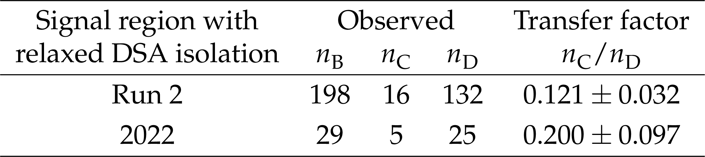
Table 5:
Observed yields in the regions B, C, D for the selection with relaxed DSA isolation requirements, and corresponding transfer factor obtained as the ratio of events in the regions C and D. |
png pdf |
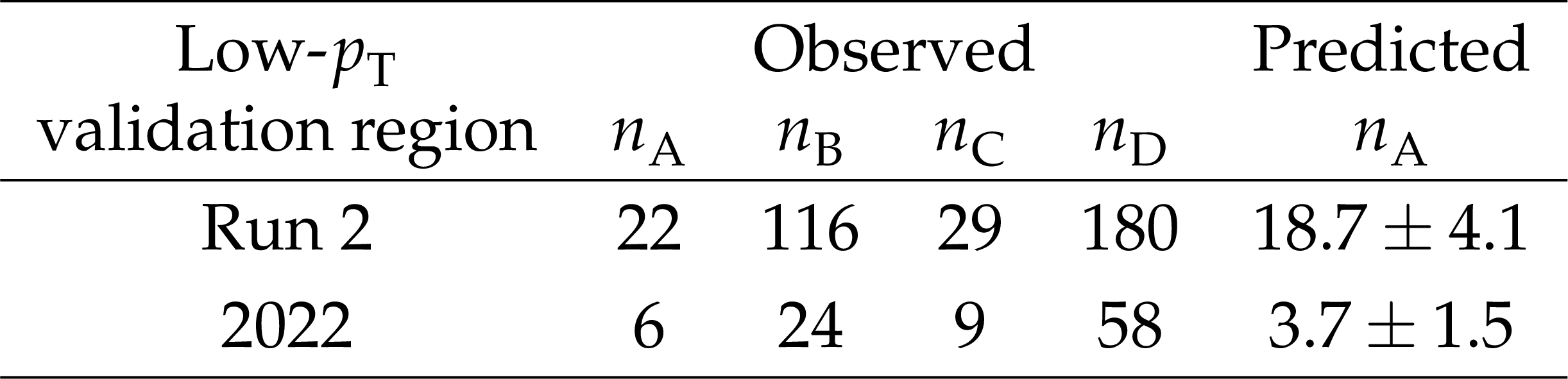
Table 6:
Observed yields in the regions A, B, C, D for the low-$ p_{\mathrm{T}} $ validation region with relaxed DSA isolation requirements, and predicted yield in region A using the ABCD method. |
png pdf |
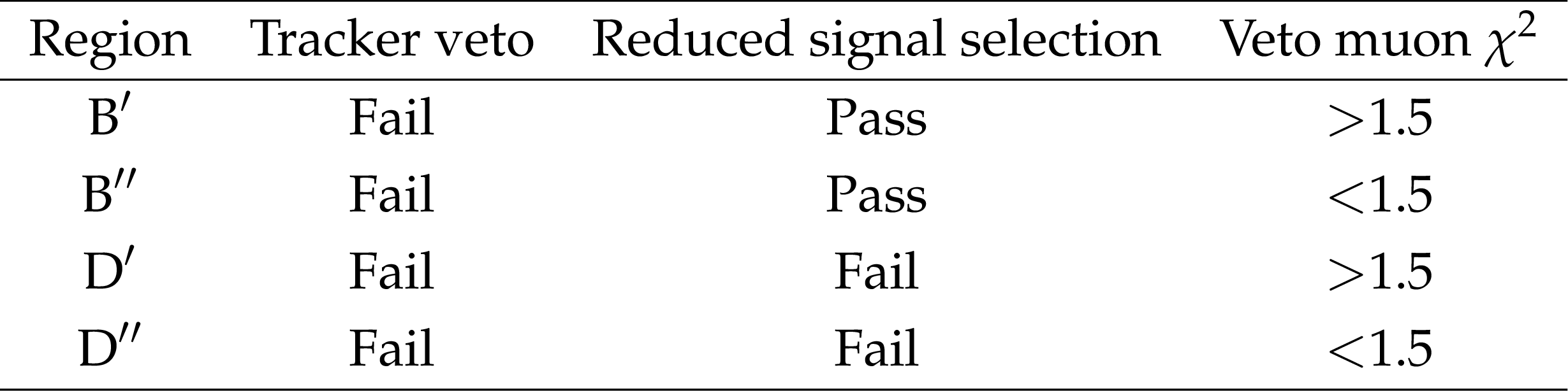
Table 7:
Definition of the regions used in the ABCD method for the inverted tracker veto validation region. |
png pdf |
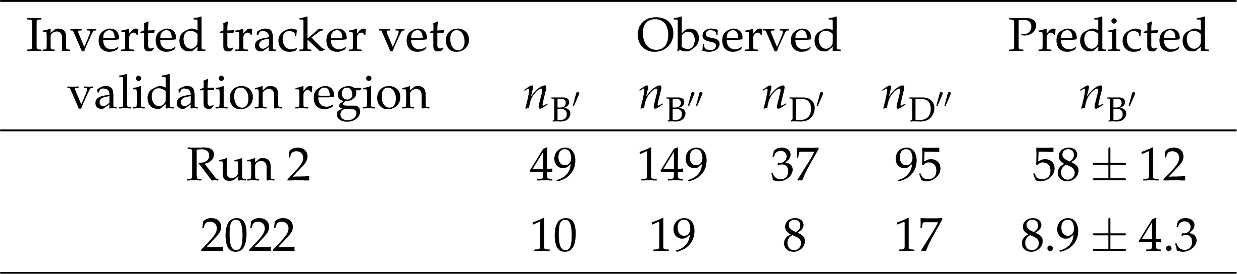
Table 8:
Observed yields in the regions $ \text{B}^\prime $, $ \text{B}^{\prime\prime} $, $ \text{D}^\prime $, $ \text{D}^{\prime\prime} $ for the inverted tracker veto validation region with relaxed DSA isolation requirements, and predicted yield in region $ \text{B}^\prime $ using the ABCD method. |
png pdf |
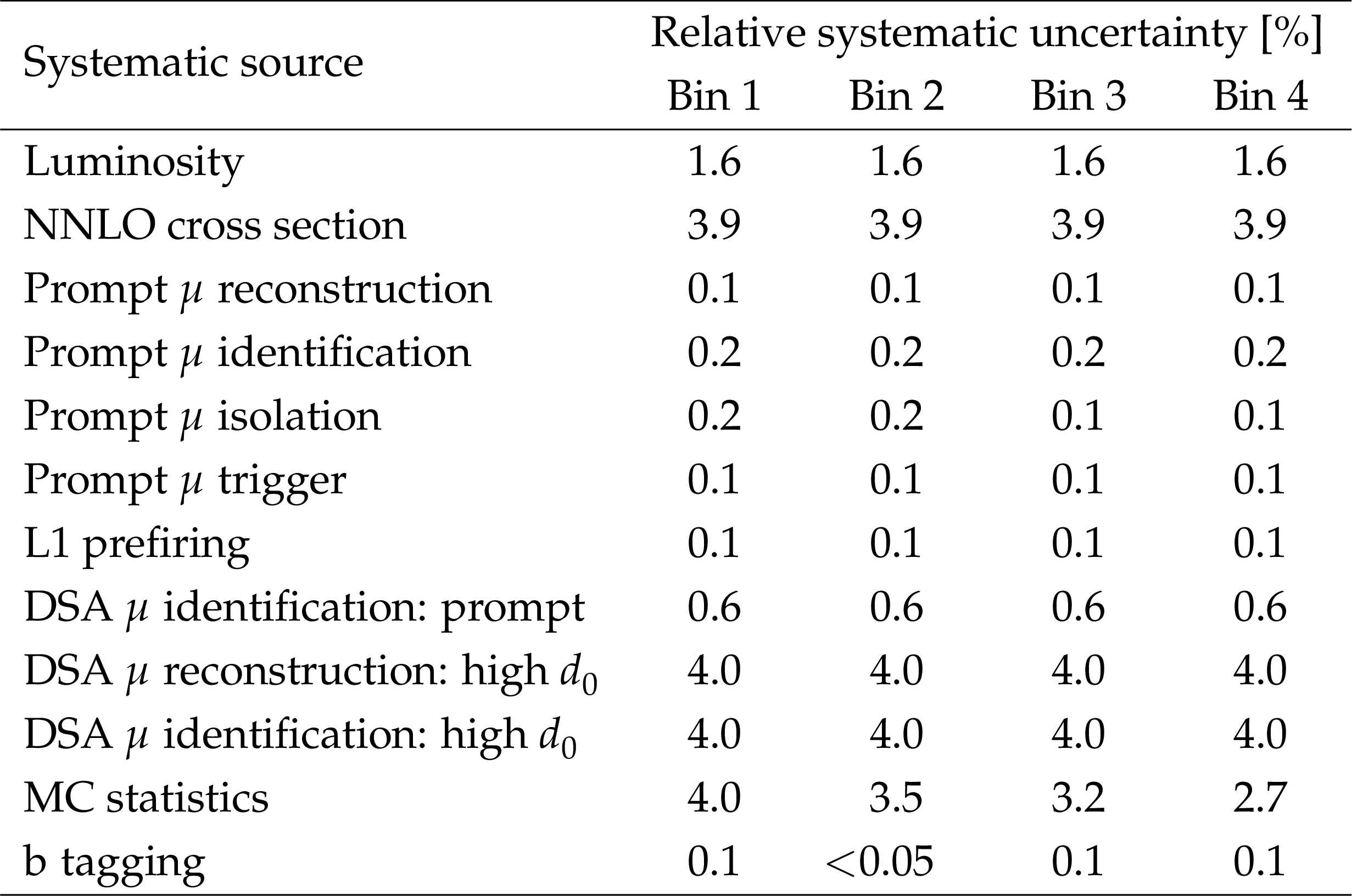
Table 9:
Magnitude of the systematic uncertainty on the signal yields in the four search regions. Details on each source of systematic uncertainty are provided in the text. The numbers in the table are computed for an HNL signal corresponding to $ m_{\mathrm{N}}= $ 3 GeV and $ |V_{\mathrm{N}\mu}|^2= $ 4.9e-6, but no significant variation is observed for different signal hypotheses. |
| Summary |
| A search for heavy neutral leptons (HNLs) has been performed using proton-proton collision events with one prompt muon and two highly displaced muons. The analysed data set was recorded by the CMS experiment at the LHC and corresponds to an integrated luminosity of 138 fb$ ^{-1} $ recorded at $ \sqrt{s}= $ 13 TeV in 2016--2018 and 34.6 fb$ ^{-1} $ recorded at $ \sqrt{s}= $ 13.6 TeV in 2022. The target process is HNL production in association with a prompt muon through decays of W bosons, with a delayed HNL decay to two muons and one standard model neutrino. The two displaced muons are reconstructed using only information from the CMS muon system, thus significantly extending the sensitivity of the analysis to HNLs with longer decay lengths compared to previous searches for long-lived HNLs. No significant deviation from the SM background estimated from control samples in data is found. Exclusion limits at 95% confidence level are set on the HNL mixing parameter as a function of its mass. This analysis surpasses previous experimental results in terms of the sensitivity to HNLs with masses between 2.5 and 4.2 GeV. |
| References | ||||
| 1 | Super-Kamiokande Collaboration | Evidence for oscillation of atmospheric neutrinos | PRL 81 (1998) 1562 | hep-ex/9807003 |
| 2 | SNO Collaboration | Direct evidence for neutrino flavor transformation from neutral-current interactions in the Sudbury Neutrino Observatory | PRL 89 (2002) 011301 | nucl-ex/0204008 |
| 3 | OPERA Collaboration | Final results of the OPERA experiment on $ \nu_{\!\tau} $ appearance in the CNGS neutrino beam | PRL 120 (2018) 211801 | 1804.04912 |
| 4 | Z. Chacko et al. | Cosmological limits on the neutrino mass and lifetime | JHEP 04 (2020) 020 | 1909.05275 |
| 5 | eBOSS Collaboration | Completed SDSS-IV extended baryon oscillation spectroscopic survey: Cosmological implications from two decades of spectroscopic surveys at the Apache Point Observatory | PRD 103 (2021) 083533 | 2007.08991 |
| 6 | J. Formaggio, A. de Gouv \^e a, and R. Robertson | Direct measurements of neutrino mass | Phys. Rept. 914 (2021) 1 | 2102.00594 |
| 7 | KATRIN Collaboration | Direct neutrino-mass measurement with sub-electronvolt sensitivity | Nature Phys. 18 (2022) 160 | 2105.08533 |
| 8 | P. Minkowski | $ {\mu\to\mathrm{e}\gamma} $ at a rate of one out of $ 10^9 $ muon decays? | PLB 67 (1977) 421 | |
| 9 | T. Yanagida | Horizontal gauge symmetry and masses of neutrinos | in Proc. Workshop on the Unified Theories and the Baryon Number in the Universe: Tsukuba, Japan, February 13--14,. [], 1979 Conf. Proc. C 7902131 (1979) 95 |
|
| 10 | J. Schechter and J. Valle | Neutrino masses in $ \mathrm{SU}(2)\otimes\mathrm{U}(1) $ theories | PRD 22 (1980) 2227 | |
| 11 | R. Mohapatra and G. Senjanovi \'c | Neutrino mass and spontaneous parity nonconservation | PRL 44 (1980) 912 | |
| 12 | S. Dodelson and L. Widrow | Sterile neutrinos as dark matter | PRL 72 (1994) 17 | hep-ph/9303287 |
| 13 | A. D. Dolgov and S. H. Hansen | Massive sterile neutrinos as warm dark matter | Astropart. Phys. 16 (2002) 339 | hep-ph/0009083 |
| 14 | T. Asaka and M. Shaposhnikov | The \PGnMSM, dark matter and baryon asymmetry of the universe | PLB 620 (2005) 17 | hep-ph/0505013 |
| 15 | T. Asaka, S. Blanchet, and M. Shaposhnikov | The \PGnMSM, dark matter and neutrino masses | PLB 631 (2005) 151 | hep-ph/0503065 |
| 16 | A. Boyarsky, O. Ruchayskiy, and M. Shaposhnikov | The role of sterile neutrinos in cosmology and astrophysics | Ann. Rev. Nucl. Part. Sci. 59 (2009) 191 | 0901.0011 |
| 17 | E. K. Akhmedov, V. A. Rubakov, and A. Y. Smirnov | Baryogenesis via neutrino oscillations | PRL 81 (1998) 1359 | hep-ph/9803255 |
| 18 | F. del Aguila and J. Aguilar-Saavedra | Distinguishing seesaw models at LHC with multi-lepton signals | NPB 813 (2009) 22 | 0808.2468 |
| 19 | A. Atre, T. Han, S. Pascoli, and B. Zhang | The search for heavy Majorana neutrinos | JHEP 05 (2009) 030 | 0901.3589 |
| 20 | V. Tello et al. | Left-right symmetry: from LHC to neutrinoless double beta decay | PRL 106 (2011) 151801 | 1011.3522 |
| 21 | F. Deppisch, P. Bhupal Dev, and A. Pilaftsis | Neutrinos and collider physics | New J. Phys. 17 (2015) 075019 | 1502.06541 |
| 22 | Y. Cai, T. Han, T. Li, and R. Ruiz | Lepton number violation: Seesaw models and their collider tests | Front. Phys. 6 (2018) 40 | 1711.02180 |
| 23 | S. Pascoli, R. Ruiz, and C. Weiland | Heavy neutrinos with dynamic jet vetoes: multilepton searches at $ \sqrt{s}= $ 14, 27, and 100 TeV | JHEP 06 (2019) 049 | 1812.08750 |
| 24 | J. Alimena et al. | Searching for long-lived particles beyond the standard model at the Large Hadron Collider | JPG 47 (2020) 090501 | 1903.04497 |
| 25 | K. Bondarenko et al. | Probing new physics with displaced vertices: muon tracker at CMS | PRD 100 (2019) 075015 | 1903.11918 |
| 26 | A. Abdullahi et al. | The present and future status of heavy neutral leptons | JPG 50 (2023) 020501 | 2203.08039 |
| 27 | C. Antel et al. | Feebly interacting particles: FIPs 2022 workshop report | EPJC 83 (2023) 1122 | 2305.01715 |
| 28 | CMS Collaboration | Search for heavy Majorana neutrinos in $ {\mu^{\pm}\mu^{\pm}}+ $jets and $ {\mathrm{e}^{\pm}\mathrm{e}^{\pm}}+ $jets events in $ {\mathrm{p}\mathrm{p}} $ collisions at $ \sqrt{s}= $ 7 TeV | PLB 717 (2012) 109 | CMS-EXO-11-076 1207.6079 |
| 29 | CMS Collaboration | Search for heavy Majorana neutrinos in $ {\mu^{\pm}\mu^{\pm}}+ $jets events in proton-proton collisions at $ \sqrt{s}= $ 8 TeV | PLB 748 (2015) 144 | CMS-EXO-12-057 1501.05566 |
| 30 | ATLAS Collaboration | Search for heavy Majorana neutrinos with the ATLAS detector in $ {\mathrm{p}\mathrm{p}} $ collisions at $ \sqrt{s}= $ 8 TeV | JHEP 07 (2015) 162 | 1506.06020 |
| 31 | CMS Collaboration | Search for heavy Majorana neutrinos in $ {\mathrm{e}^{\pm}\mathrm{e}^{\pm}}+ $jets and $ {\mathrm{e}^{\pm}\mu^{\pm}}+ $jets events in proton-proton collisions at $ \sqrt{s}= $ 8 TeV | JHEP 04 (2016) 169 | CMS-EXO-14-014 1603.02248 |
| 32 | CMS Collaboration | Search for heavy neutral leptons in events with three charged leptons in proton-proton collisions at $ \sqrt{s}= $ 13 TeV | PRL 120 (2018) 221801 | CMS-EXO-17-012 1802.02965 |
| 33 | CMS Collaboration | Search for heavy Majorana neutrinos in same-sign dilepton channels in proton-proton collisions at $ \sqrt{s}= $ 13 TeV | JHEP 01 (2019) 122 | CMS-EXO-17-028 1806.10905 |
| 34 | ATLAS Collaboration | Search for heavy neutral leptons in decays of W bosons produced in 13 TeV $ {\mathrm{p}\mathrm{p}} $ collisions using prompt and displaced signatures with the ATLAS detector | JHEP 10 (2019) 265 | 1905.09787 |
| 35 | LHCb Collaboration | Search for heavy neutral leptons in $ {\mathrm{W^+}\to\mu^{+}\mu^{\pm} \text{jet}} $ decays | EPJC 81 (2021) 248 | 2011.05263 |
| 36 | CMS Collaboration | Search for long-lived heavy neutral leptons with displaced vertices in proton-proton collisions at $ \sqrt{s}= $ 13 TeV | JHEP 07 (2022) 081 | CMS-EXO-20-009 2201.05578 |
| 37 | ATLAS Collaboration | Search for heavy neutral leptons in decays of W bosons using a dilepton displaced vertex in $ \sqrt{s}= $ 13 TeV $ {\mathrm{p}\mathrm{p}} $ collisions with the ATLAS detector | PRL 131 (2023) 061803 | 2204.11988 |
| 38 | CMS Collaboration | Probing heavy Majorana neutrinos and the Weinberg operator through vector boson fusion processes in proton-proton collisions at $ \sqrt{s}= $ 13 TeV | PRL 131 (2023) 011803 | CMS-EXO-21-003 2206.08956 |
| 39 | ATLAS Collaboration | Search for Majorana neutrinos in same-sign $ {\mathrm{W}\mathrm{W}} $ scattering events from $ {\mathrm{p}\mathrm{p}} $ collisions at $ \sqrt{s}= $ 13 TeV | EPJC 83 (2023) 824 | 2305.14931 |
| 40 | CMS Collaboration | Search for long-lived heavy neutral leptons with lepton flavour conserving or violating decays to a jet and a charged lepton | JHEP 03 (2024) 105 | CMS-EXO-21-013 2312.07484 |
| 41 | CMS Collaboration | Search for long-lived heavy neutral leptons decaying in the CMS muon detectors in proton-proton collisions at $ \sqrt{s}= $ 13 TeV | PRD 110 (2024) 012004 | CMS-EXO-22-017 2402.18658 |
| 42 | CMS Collaboration | Search for heavy neutral leptons in final states with electrons, muons, and hadronically decaying tau leptons in proton-proton collisions at $ \sqrt{s}= $ 13 TeV | JHEP 06 (2024) 123 | CMS-EXO-22-011 2403.00100 |
| 43 | CMS Collaboration | Search for long-lived heavy neutrinos in the decays of $ {\mathrm{B}} $ mesons produced in proton-proton collisions at $ \sqrt{s}= $ 13 TeV | JHEP 06 (2024) 183 | CMS-EXO-22-019 2403.04584 |
| 44 | ATLAS Collaboration | Search for heavy Majorana neutrinos in $ {\mathrm{e}^{\pm}\mathrm{e}^{\pm}} $ and $ {\mathrm{e}^{\pm}\mu^{\pm}} $ final states via $ {\mathrm{W}\mathrm{W}} $ scattering in $ {\mathrm{p}\mathrm{p}} $ collisions at $ \sqrt{s}= $ 13 TeV with the ATLAS detector | PLB 856 (2024) 138865 | 2403.15016 |
| 45 | CMS Collaboration | Review of searches for vector-like quarks, vector-like leptons, and heavy neutral leptons in proton-proton collisions at $ \sqrt{s}= $ 13 TeV at the CMS experiment | Phys. Rept. 1115 (2025) 570 | CMS-EXO-23-006 2405.17605 |
| 46 | CMS Collaboration | Search for long-lived heavy neutral leptons in proton-proton collision events with a lepton-jet pair associated with a secondary vertex at $ \sqrt{s}= $ 13 TeV | JHEP 02 (2025) 036 | CMS-EXO-21-011 2407.10717 |
| 47 | ATLAS Collaboration | Search for heavy right-handed Majorana neutrinos in the decay of top quarks produced in proton-proton collisions at $ \sqrt{s}= $ 13 TeV with the ATLAS detector | PRD 110 (2024) 112004 | 2408.05000 |
| 48 | ATLAS Collaboration | Search for heavy neutral leptons in decays of W bosons using leptonic and semi-leptonic displaced vertices in $ \sqrt{s}= $ 13 TeV $ {\mathrm{p}\mathrm{p}} $ collisions with the ATLAS detector | JHEP 07 (2025) 196 | 2503.16213 |
| 49 | ATLAS Collaboration | Search for heavy neutral leptons in decays of W bosons produced in 13 TeV $ {\mathrm{p}\mathrm{p}} $ collisions using prompt signatures in the ATLAS detector | EPJC 86 (2026) 153 | 2508.20929 |
| 50 | LHCb Collaboration | Search for heavy neutral leptons in $ {\mathrm{B}} $-meson decays | Submitted to JHEP | 2512.14551 |
| 51 | CMS Collaboration | Performance of the CMS muon detector and muon reconstruction with proton-proton collisions at $ \sqrt{s}= $ 13 TeV | JINST 13 (2018) P06015 | CMS-MUO-16-001 1804.04528 |
| 52 | CMS Collaboration | The CMS experiment at the CERN LHC | JINST 3 (2008) S08004 | |
| 53 | CMS Collaboration | Development of the CMS detector for the CERN LHC \mboxRun 3 | JINST 19 (2024) P05064 | CMS-PRF-21-001 2309.05466 |
| 54 | CMS Collaboration | Performance of the CMS Level-1 trigger in proton-proton collisions at $ \sqrt{s}= $ 13 TeV | JINST 15 (2020) P10017 | CMS-TRG-17-001 2006.10165 |
| 55 | CMS Collaboration | The CMS trigger system | JINST 12 (2017) P01020 | CMS-TRG-12-001 1609.02366 |
| 56 | CMS Collaboration | Performance of the CMS high-level trigger during LHC \mboxRun 2 | JINST 19 (2024) P11021 | CMS-TRG-19-001 2410.17038 |
| 57 | CMS Collaboration | Particle-flow reconstruction and global event description with the CMS detector | JINST 12 (2017) P10003 | CMS-PRF-14-001 1706.04965 |
| 58 | CMS Collaboration | Technical proposal for the Phase-II upgrade of the Compact Muon Solenoid | CMS Technical Proposal CERN-LHCC-2015-010, CMS-TDR-15-02, 2015 link |
|
| 59 | CMS Collaboration | Pileup mitigation at CMS in 13 TeV data | JINST 15 (2020) P09018 | CMS-JME-18-001 2003.00503 |
| 60 | D. Bertolini, P. Harris, M. Low, and N. Tran | Pileup per particle identification | JHEP 10 (2014) 059 | 1407.6013 |
| 61 | CMS Collaboration | Jet energy scale and resolution in the CMS experiment in $ {\mathrm{p}\mathrm{p}} $ collisions at 8 TeV | JINST 12 (2017) P02014 | CMS-JME-13-004 1607.03663 |
| 62 | E. Bols et al. | Jet flavour classification using DeepJet | JINST 15 (2020) P12012 | 2008.10519 |
| 63 | CMS Collaboration | Identification of heavy-flavour jets with the CMS detector in $ {\mathrm{p}\mathrm{p}} $ collisions at 13 TeV | JINST 13 (2018) P05011 | CMS-BTV-16-002 1712.07158 |
| 64 | CMS Collaboration | Performance summary of AK4 jet b tagging with data from proton-proton collisions at 13 TeV with the CMS detector | CMS Detector Performance Note CMS-DP-2023-005, 2023 CDS |
|
| 65 | CMS Collaboration | A first look at early 2022 proton-proton collisions at $ \sqrt{s}= $ 13.6 TeV for heavy-flavor jet tagging | CMS Detector Performance Note CMS-DP-2023-012, 2023 CDS |
|
| 66 | CMS Collaboration | Performance of CMS muon reconstruction in $ {\mathrm{p}\mathrm{p}} $ collision events at $ \sqrt{s}= $ 7 TeV | JINST 7 (2012) P10002 | CMS-MUO-10-004 1206.4071 |
| 67 | CMS Collaboration | CMS physics technical design report, volume I: Detector performance and software | CMS Technical Proposal CERN-LHCC-2006-001, CMS-TDR-8.1, 2006 CDS |
|
| 68 | CMS Collaboration | Muon reconstruction and identification improvements for \mboxRun 2 and first results with 2015 run data | CMS Detector Performance Note CMS-DP-2015-015, 2015 CDS |
|
| 69 | J. Alwall et al. | The automated computation of tree-level and next-to-leading order differential cross sections, and their matching to parton shower simulations | JHEP 07 (2014) 079 | 1405.0301 |
| 70 | D. Alva, T. Han, and R. Ruiz | Heavy Majorana neutrinos from $ {\mathrm{W}\gamma} $ fusion at hadron colliders | JHEP 02 (2015) 072 | 1411.7305 |
| 71 | C. Degrande, O. Mattelaer, R. Ruiz, and J. Turner | Fully-automated precision predictions for heavy neutrino production mechanisms at hadron colliders | PRD 94 (2016) 053002 | 1602.06957 |
| 72 | NNPDF Collaboration | Parton distributions from high-precision collider data | EPJC 77 (2017) 663 | 1706.00428 |
| 73 | T. Sjöstrand et al. | An introduction to PYTHIA8.2 | Comput. Phys. Commun. 191 (2015) 159 | 1410.3012 |
| 74 | C. Bierlich et al. | A comprehensive guide to the physics and usage of PYTHIA8.3 | SciPost Phys. Codeb. 8 (2022) | 2203.11601 |
| 75 | K. Melnikov and F. Petriello | Electroweak gauge boson production at hadron colliders through $ \mathcal{O}({\alpha_\mathrm{S}^2}) $ | PRD 74 (2006) 114017 | hep-ph/0609070 |
| 76 | R. Gavin, Y. Li, F. Petriello, and S. Quackenbush | FEWZ 2.0: A code for hadronic Z production at next-to-next-to-leading order | Comput. Phys. Commun. 182 (2011) 2388 | 1011.3540 |
| 77 | R. Gavin, Y. Li, F. Petriello, and S. Quackenbush | W physics at the LHC with FEWZ 2.1 | Comput. Phys. Commun. 184 (2013) 208 | 1201.5896 |
| 78 | Y. Li and F. Petriello | Combining QCD and electroweak corrections to dilepton production in FEWZ | PRD 86 (2012) 094034 | 1208.5967 |
| 79 | GEANT4 Collaboration | GEANT 4---a simulation toolkit | NIM A 506 (2003) 250 | |
| 80 | R. Fr \"u hwirth | Application of Kalman filtering to track and vertex fitting | NIM A 262 (1987) 444 | |
| 81 | CMS Collaboration | Performance of the CMS muon trigger system in proton-proton collisions at $ \sqrt{s}= $ 13 TeV | JINST 16 (2021) P07001 | CMS-MUO-19-001 2102.04790 |
| 82 | CMS Collaboration | Performance of CMS muon reconstruction in cosmic-ray events | JINST 5 (2010) T03022 | CMS-CFT-09-014 0911.4994 |
| 83 | CMS Collaboration | Precision luminosity measurement in proton-proton collisions at $ \sqrt{s}= $ 13 TeV in 2015 and 2016 at CMS | EPJC 81 (2021) 800 | CMS-LUM-17-003 2104.01927 |
| 84 | CMS Collaboration | CMS luminosity measurement for the 2017 data-taking period at $ \sqrt{s}= $ 13 TeV | CMS Physics Analysis Summary, 2018 CMS-PAS-LUM-17-004 |
CMS-PAS-LUM-17-004 |
| 85 | CMS Collaboration | CMS luminosity measurement for the 2018 data-taking period at $ \sqrt{s}= $ 13 TeV | CMS Physics Analysis Summary, 2019 CMS-PAS-LUM-18-002 |
CMS-PAS-LUM-18-002 |
| 86 | CMS Collaboration | Luminosity measurement in proton-proton collisions at 13.6 TeV in 2022 at CMS | CMS Physics Analysis Summary, 2024 CMS-PAS-LUM-22-001 |
CMS-PAS-LUM-22-001 |
| 87 | A. L. Read | Presentation of search results: The $ \text{CL}_\text{s} $ technique | JPG 28 (2002) 2693 | |
| 88 | ATLAS and CMS Collaborations, and LHC Higgs Combination Group | Procedure for the LHC Higgs boson search combination in Summer 2011 | Technical Report CMS-NOTE-2011-005, ATL-PHYS-PUB-2011-11, 2011 | |
| 89 | CMS Collaboration | The CMS statistical analysis and combination tool: combine | Comput. Softw. Big Sci. 8 (2024) 19 | CMS-CAT-23-001 2404.06614 |
| 90 | W. Verkerke and D. Kirkby | The RooFit toolkit for data modeling | in the International Conference on Computing in High Energy and Nuclear Physics (CHEP ): La Jolla CA, United States, March 24--28,.. [eConf C0303241 MOLT007], 2003 Proc. 1 (2003) 3 |
physics/0306116 |
| 91 | L. Moneta et al. | The RooStats project | in the International Workshop on Advanced Computing and Analysis Techniques in Physics Research (ACAT ): Jaipur, India, February 22--27,.. [PoS (ACAT) 057], 2010 Proc. 1 (2010) 3 |
1009.1003 |
|
|
Compact Muon Solenoid LHC, CERN |
|

|

|

|

|

|