

Compact Muon Solenoid
LHC, CERN
| CMS-PAS-SUS-19-005 | ||
| Searches for new phenomena in events with jets and high values of the $M_{\mathrm{T2}}$ variable, including signatures with disappearing tracks, in proton-proton collisions at $\sqrt{s}= $ 13 TeV | ||
| CMS Collaboration | ||
| March 2019 | ||
| Abstract: Searches for new phenomena are performed using events with jets and significant transverse momentum imbalance. In events with at least two jets, the transverse momentum imbalance is inferred through the $M_{\mathrm{T2}}$ variable. The results are based on a sample of proton-proton collisions collected with the CMS detector during the LHC Run II (2016-2018) and correspond to an integrated luminosity of 137 fb$^{-1}$ taken at a center-of-mass energy of 13 TeV. Two related searches are performed. The first is an inclusive search based on signal regions defined by the hadronic energy in the event, the jet multiplicity, the number of jets identified as originating from bottom quarks, and the value of $M_{\mathrm{T2}}$ for events with at least two jets, or the tranverse momentum of the jet for events with just one jet. The second is a search for disappearing tracks produced by new long-lived charged particles, decaying within the volume of the CMS tracking detector. No excess event yield is observed above the predicted standard model background, leading to exclusion limits on pair-produced gluinos and squarks in simplified models of $R$-parity conserving supersymmetry. Mass limits as high as 2250 GeV, 1770 GeV, 1260 GeV and 1225 GeV are obtained from the inclusive $M_{\mathrm{T2}}$ search for gluinos, light-flavor squarks, bottom squarks and top squarks, respectively. The search for disappearing tracks extends the gluino mass limit to as much as 2460 GeV, and the $\tilde{\chi}^{0}_{1}$ mass limit to as much as 2000 GeV, in models where the gluino can decay with equal probability to $\tilde{\chi}^{0}_{1}$, $\tilde{\chi}^{+}_{1}$, and $\tilde{\chi}^{-}_{1}$, and the $\tilde{\chi}^{\pm}_{1}$ are long-lived. | ||
|
Links:
CDS record (PDF) ;
CADI line (restricted) ;
These preliminary results are superseded in this paper, EPJC 80 (2020) 3. The superseded preliminary plots can be found here. |
||
| Figures | |
png pdf |
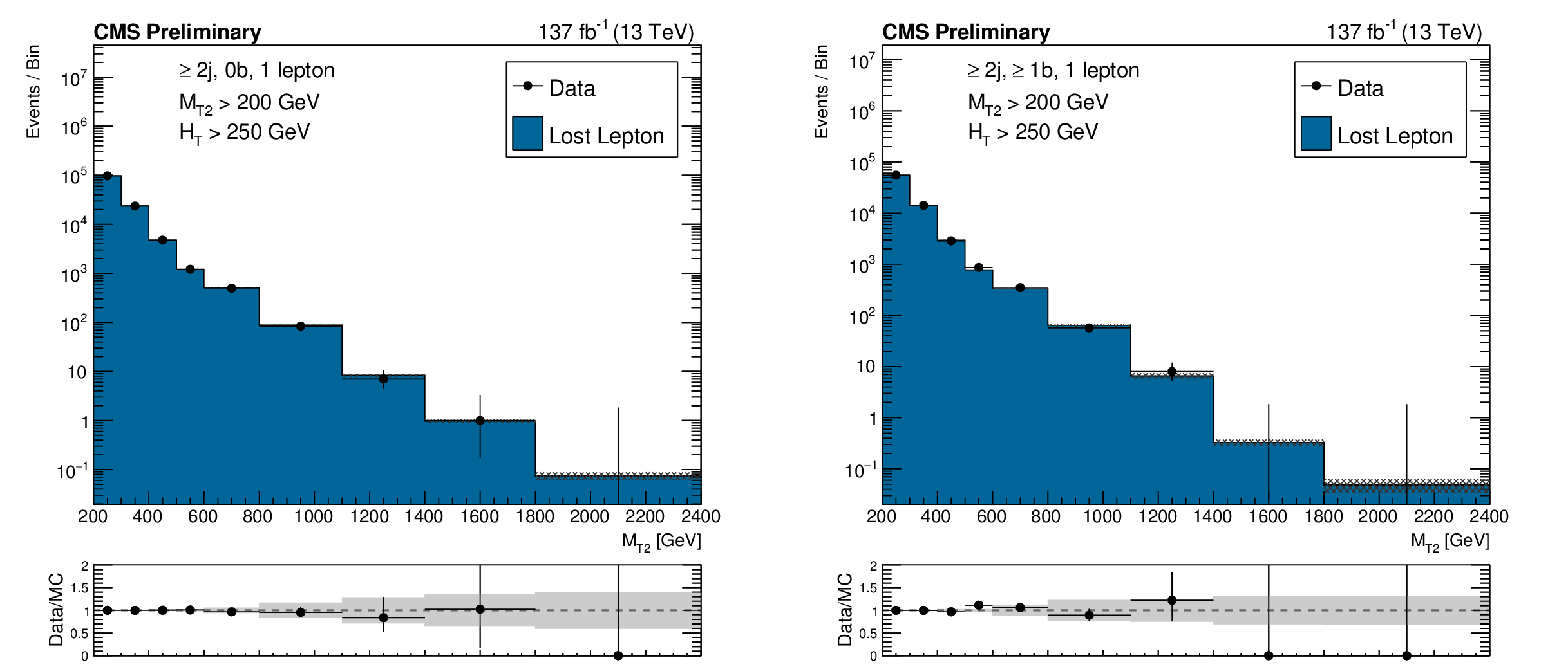
Figure 1:
Distributions of the ${M_{\mathrm {T2}}}$ variable in data and simulation for the single-lepton control region selection, after normalizing the simulation to data in the control region bins of ${H_{\mathrm {T}}}$, ${N_{\mathrm {j}}}$, and ${N_{\mathrm{b}}}$ for events with no b-tagged jets (left), and events with at least one b-tagged jet (right). The hatched bands on the top panels show the MC statistical uncertainty, while the solid gray bands in the ratio plots show the systematic uncertainty in the ${M_{\mathrm {T2}}}$ shape. |

png pdf |
Figure 1-a:
Distributions of the ${M_{\mathrm {T2}}}$ variable in data and simulation for the single-lepton control region selection, after normalizing the simulation to data in the control region bins of ${H_{\mathrm {T}}}$, ${N_{\mathrm {j}}}$, and ${N_{\mathrm{b}}}$ for events with no b-tagged jets. The hatched bands on the top panel show the MC statistical uncertainty, while the solid gray bands in the ratio plot shows the systematic uncertainty in the ${M_{\mathrm {T2}}}$ shape. |

png pdf |
Figure 1-b:
Distributions of the ${M_{\mathrm {T2}}}$ variable in data and simulation for the single-lepton control region selection, after normalizing the simulation to data in the control region bins of ${H_{\mathrm {T}}}$, ${N_{\mathrm {j}}}$, and ${N_{\mathrm{b}}}$ for events with at least one b-tagged jet. The hatched bands on the top panel show the MC statistical uncertainty, while the solid gray bands in the ratio plot shows the systematic uncertainty in the ${M_{\mathrm {T2}}}$ shape. |
png pdf |
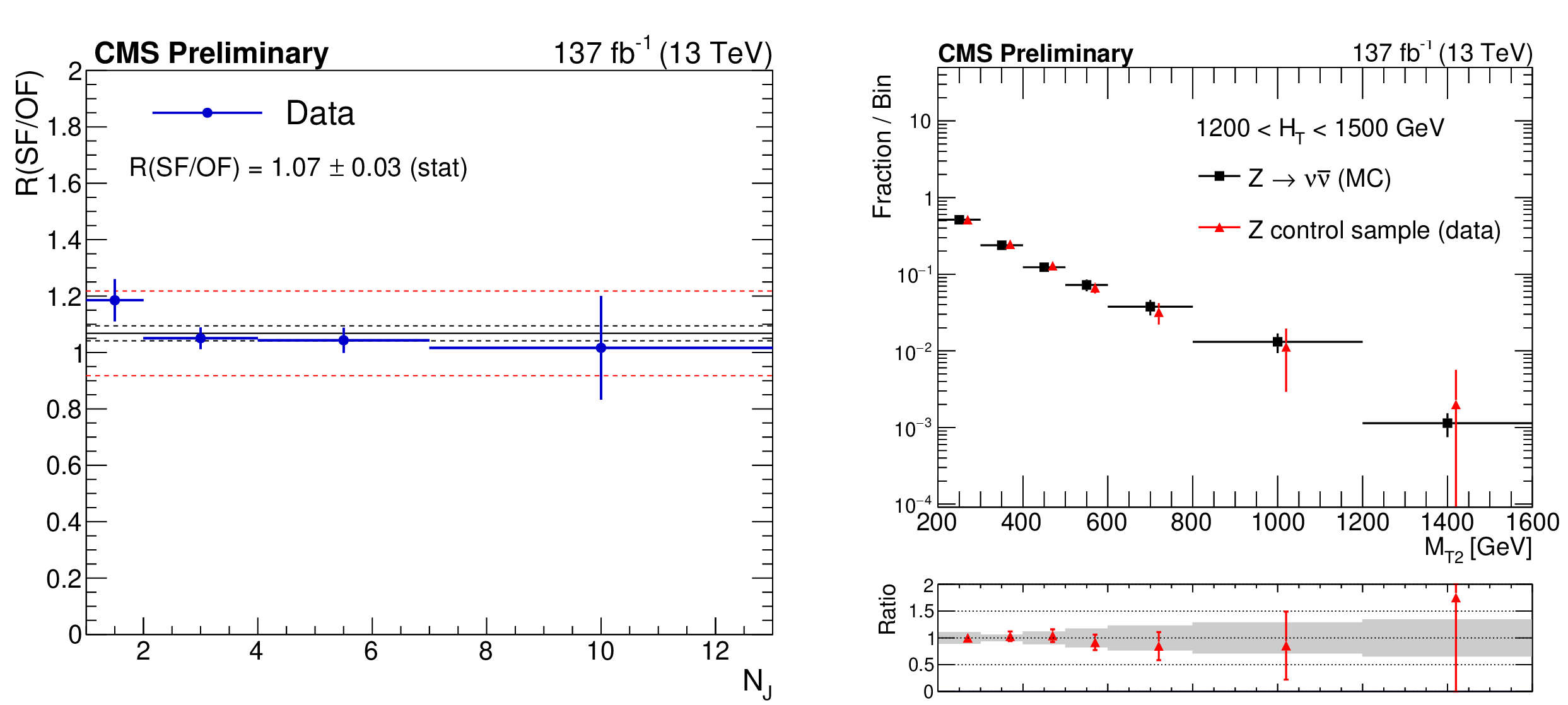
Figure 2:
(Left) Ratio $R^{\mathrm {SF}/\mathrm {OF}}$ in data as a function of ${N_{\mathrm {j}}}$. The solid black line enclosed by the red dashed lines corresponds to a value of 1.07 $\pm$ 0.15 that is observed to be stable with respect to event kinematics, while the two dashed black lines denote the statistical uncertainty in the $R^{\mathrm {SF}/\mathrm {OF}}$ value. (Right) The shape of the ${M_{\mathrm {T2}}}$ distribution in $\mathrm{Z} \to \nu \bar{\nu} $ simulation compared to the one obtained from the $\mathrm{Z} \to \ell ^{+}\ell ^{-}$ data control sample, in a region with 1200 $ < {H_{\mathrm {T}}} < $ 1500 GeV and $ {N_{\mathrm {j}}} \geq $ 2, inclusive in ${N_{\mathrm{b}}}$. The solid gray band on the ratio plot shows the systematic uncertainty in the ${M_{\mathrm {T2}}}$ shape. |

png pdf |
Figure 2-a:
Ratio $R^{\mathrm {SF}/\mathrm {OF}}$ in data as a function of ${N_{\mathrm {j}}}$. The solid black line enclosed by the red dashed lines corresponds to a value of 1.07 $\pm$ 0.15 that is observed to be stable with respect to event kinematics, while the two dashed black lines denote the statistical uncertainty in the $R^{\mathrm {SF}/\mathrm {OF}}$ value. |
png pdf |
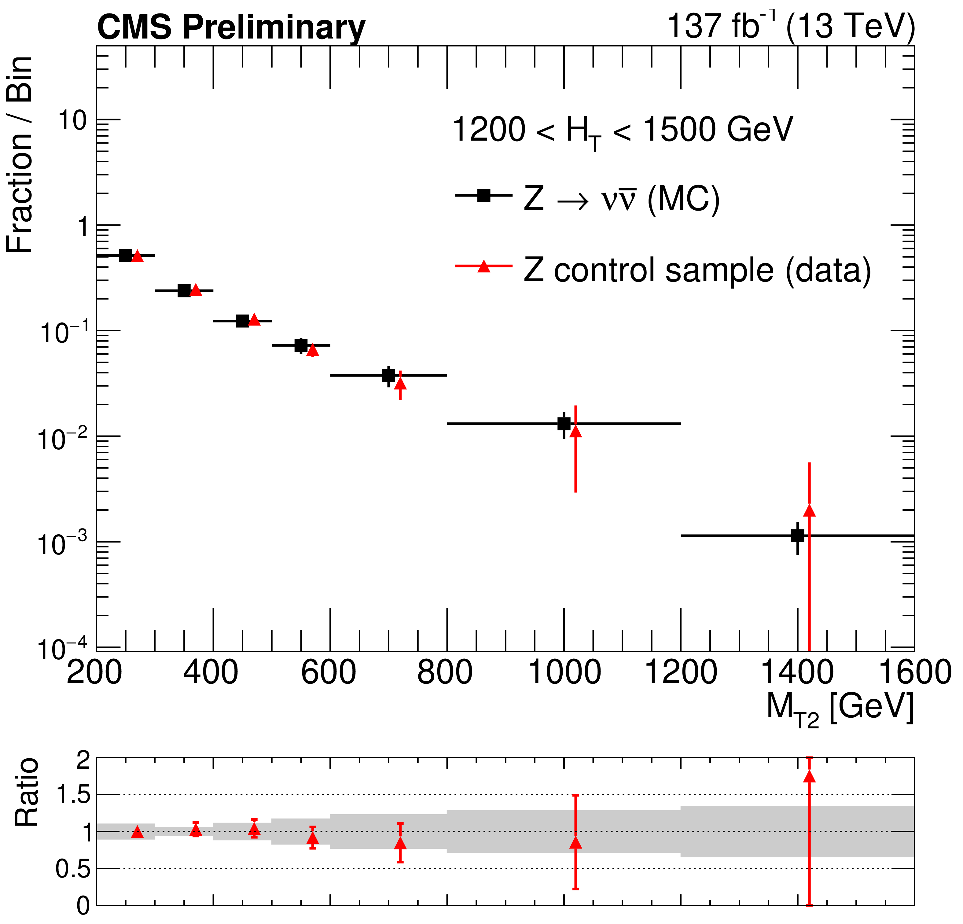
Figure 2-b:
The shape of the ${M_{\mathrm {T2}}}$ distribution in $\mathrm{Z} \to \nu \bar{\nu} $ simulation compared to the one obtained from the $\mathrm{Z} \to \ell ^{+}\ell ^{-}$ data control sample, in a region with 1200 $ < {H_{\mathrm {T}}} < $ 1500 GeV and $ {N_{\mathrm {j}}} \geq $ 2, inclusive in ${N_{\mathrm{b}}}$. The solid gray band on the ratio plot shows the systematic uncertainty in the ${M_{\mathrm {T2}}}$ shape. |
png pdf |
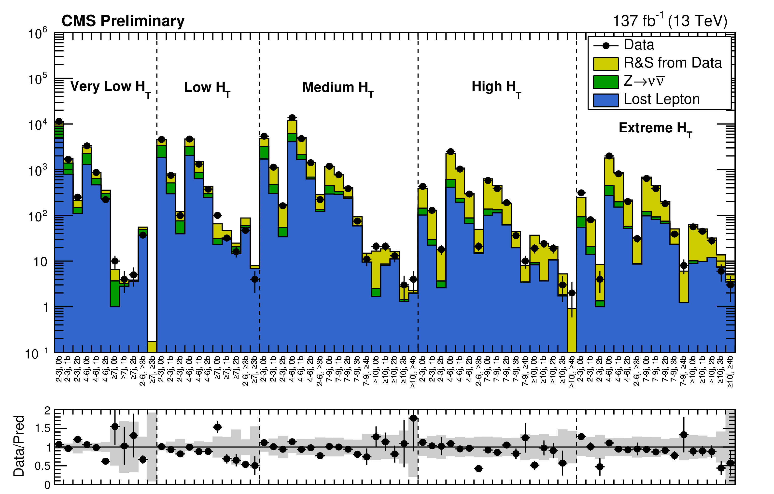
Figure 3:
Validation of the R&S multijet background prediction, in control regions in data selected with $ {\Delta \phi _{\text {min}}} < $ 0.3. Electroweak backgrounds are estimated from data. In regions where statistics in data is insufficient to estimate the electroweak backgrounds, the corresponding yields are taken directly from simulation. Bins on the x-axis are the (${H_{\mathrm {T}}}$, $N_\text {jet}$, $N_\text {b-jet}$) topological regions. The gray band represents the total uncertainty on the prediction. |
png pdf |
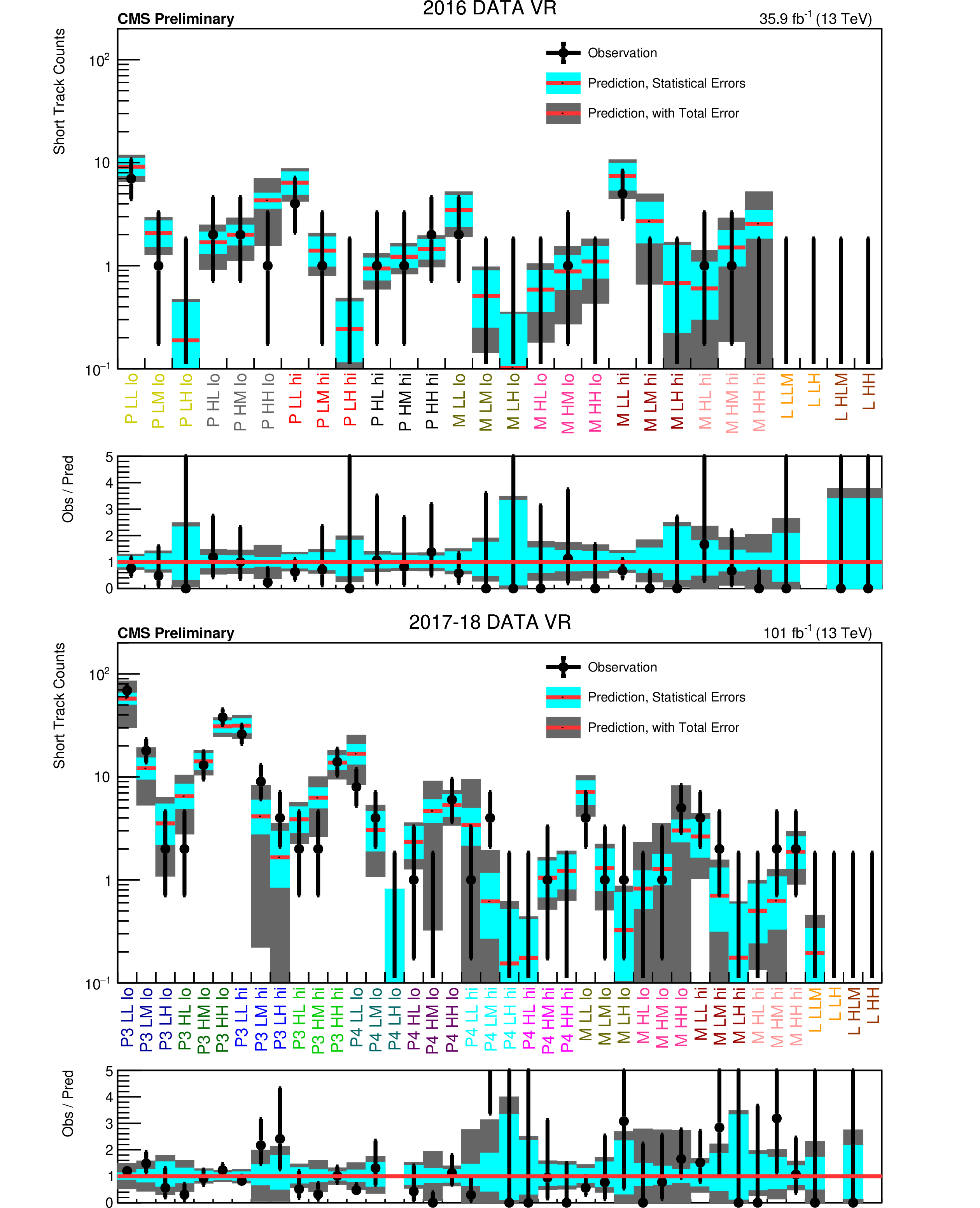
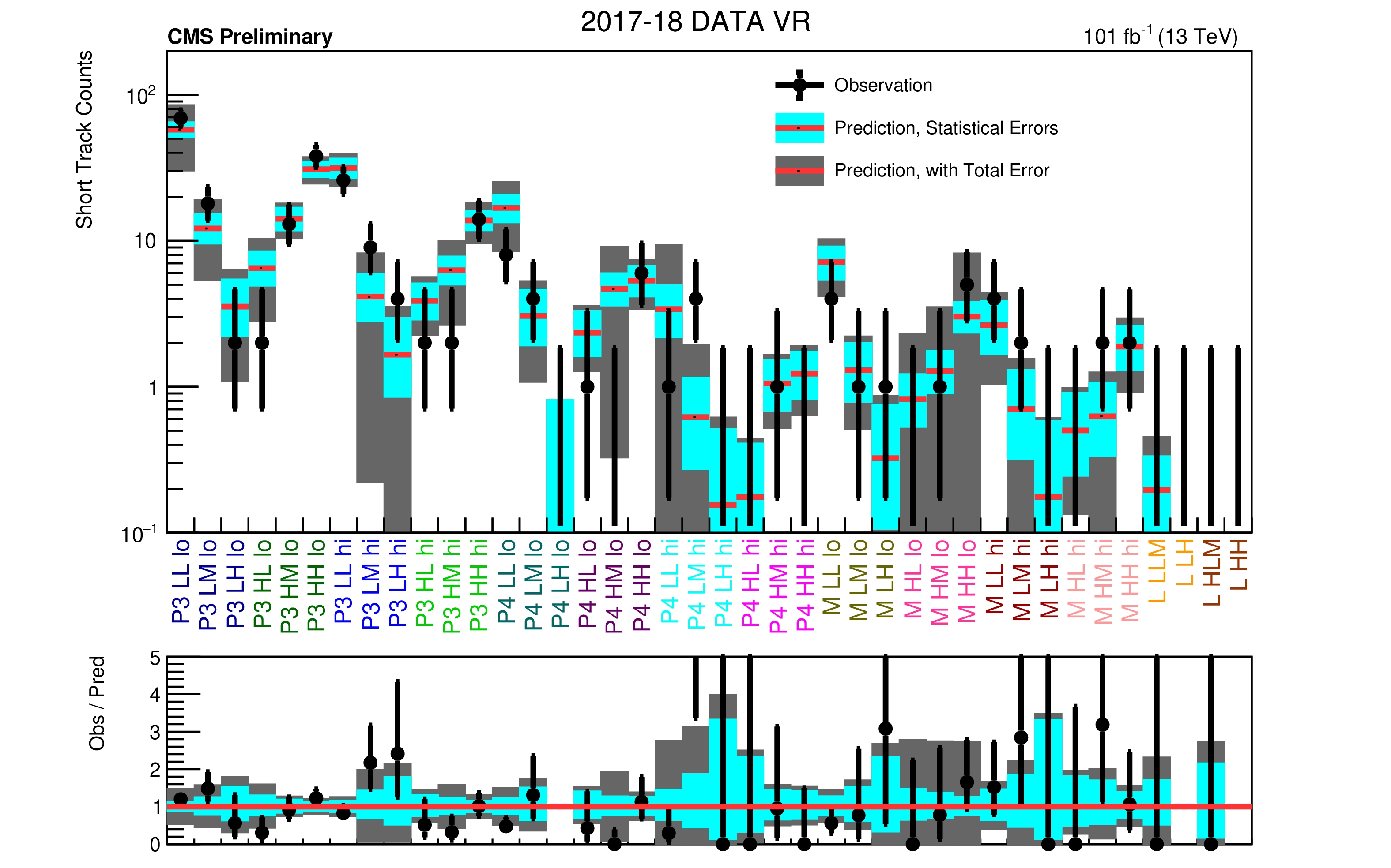
Figure 4:
Validation of the background prediction method in (upper) the 2016 data validation region, and in (lower) the 2017-2018 data validation region, in the search for disappearing tracks. The red histogram represents the predicted background, while the black points are the actual observed data counts. The cyan band represents the statistical uncertainty on the prediction. The gray band represents the total uncertainty. The labels on the $x$-axes are explained in Tables 7-8 of Appendix B.2. Regions whose predictions use the same measurement of $f_{\mathrm {short}}$ are identified by the colors of the labels. Bins with no entry in the ratio have zero predicted background. |

png pdf |
Figure 4-a:
Validation of the background prediction method in the 2016 data validation region, in the search for disappearing tracks. The red histogram represents the predicted background, while the black points are the actual observed data counts. The cyan band represents the statistical uncertainty on the prediction. The gray band represents the total uncertainty. The labels on the $x$-axes are explained in Tables 7-8 of Appendix B.2. Regions whose predictions use the same measurement of $f_{\mathrm {short}}$ are identified by the colors of the labels. Bins with no entry in the ratio have zero predicted background. |
png pdf |
Figure 4-b:
Validation of the background prediction method in the 2017-2018 data validation region, in the search for disappearing tracks. The red histogram represents the predicted background, while the black points are the actual observed data counts. The cyan band represents the statistical uncertainty on the prediction. The gray band represents the total uncertainty. The labels on the $x$-axes are explained in Tables 7-8 of Appendix B.2. Regions whose predictions use the same measurement of $f_{\mathrm {short}}$ are identified by the colors of the labels. Bins with no entry in the ratio have zero predicted background. |

png pdf |
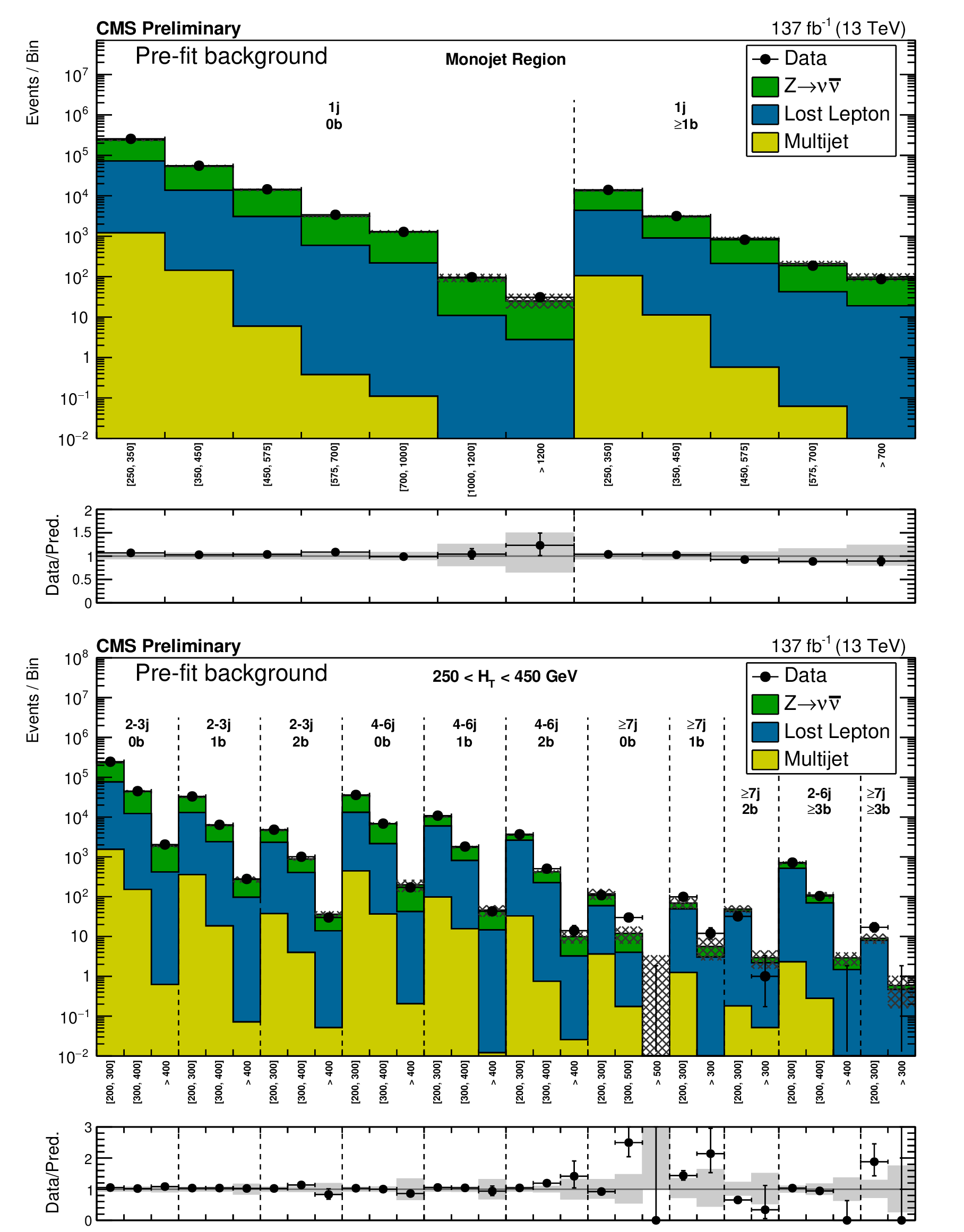
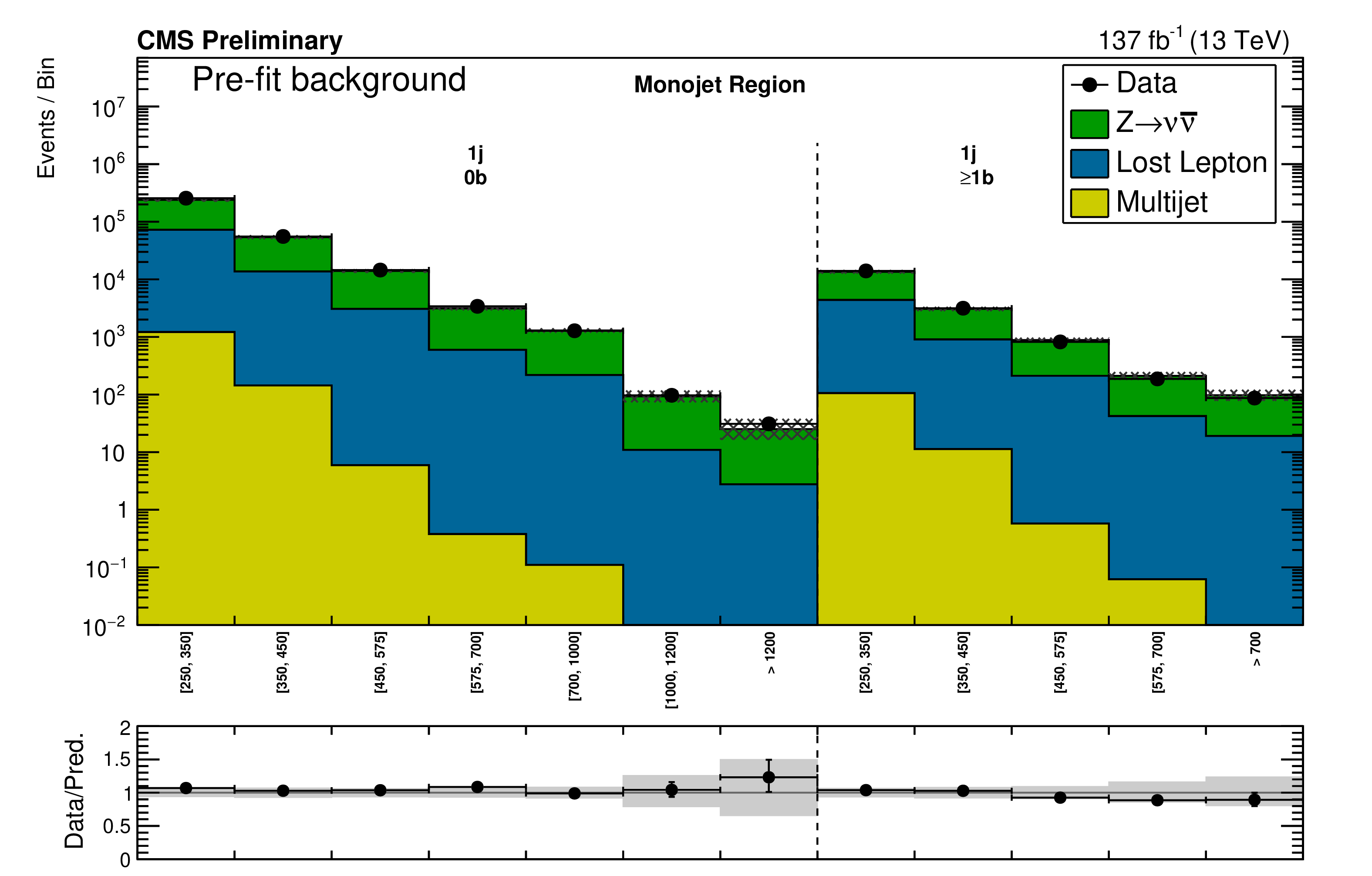
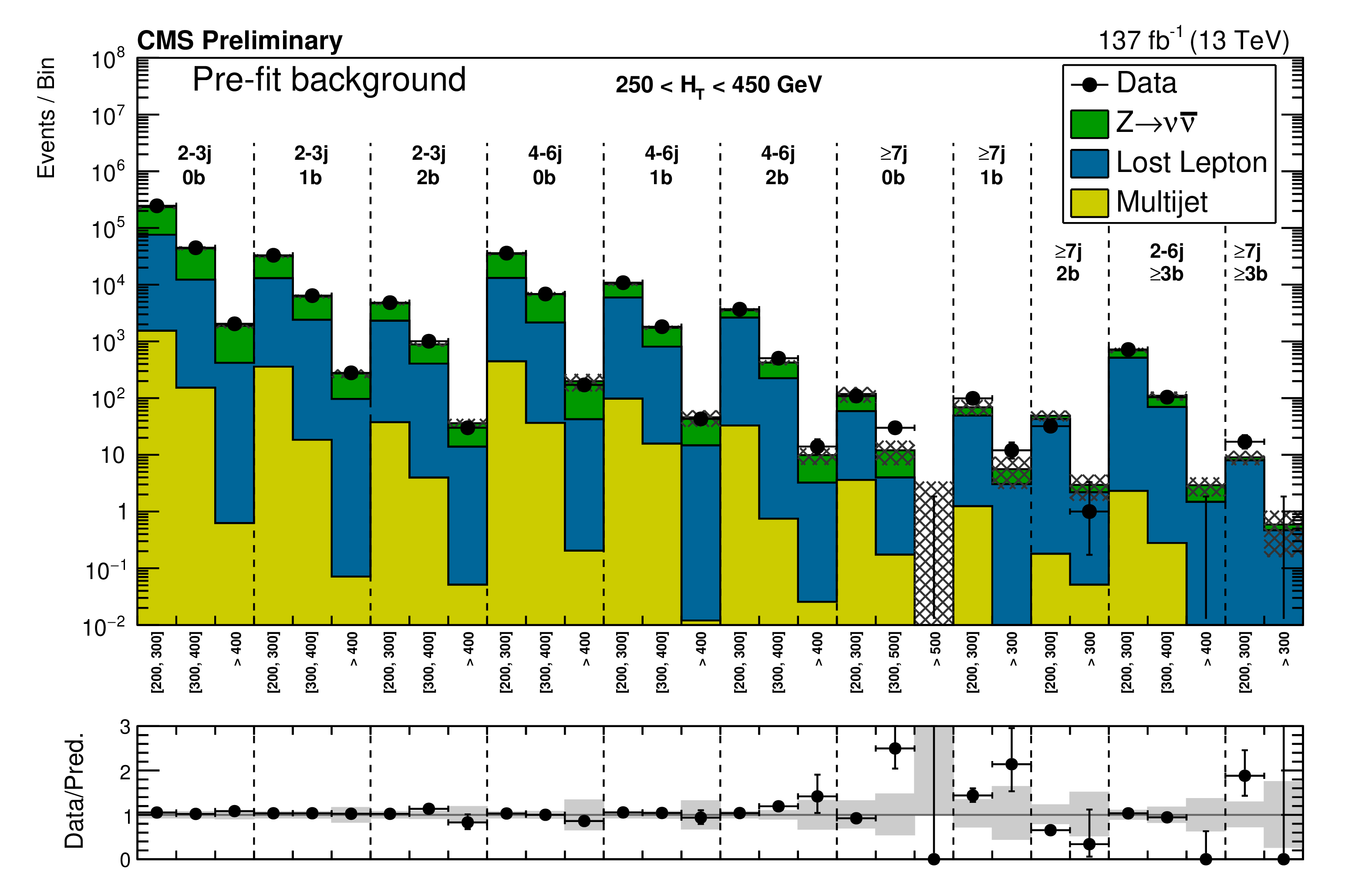
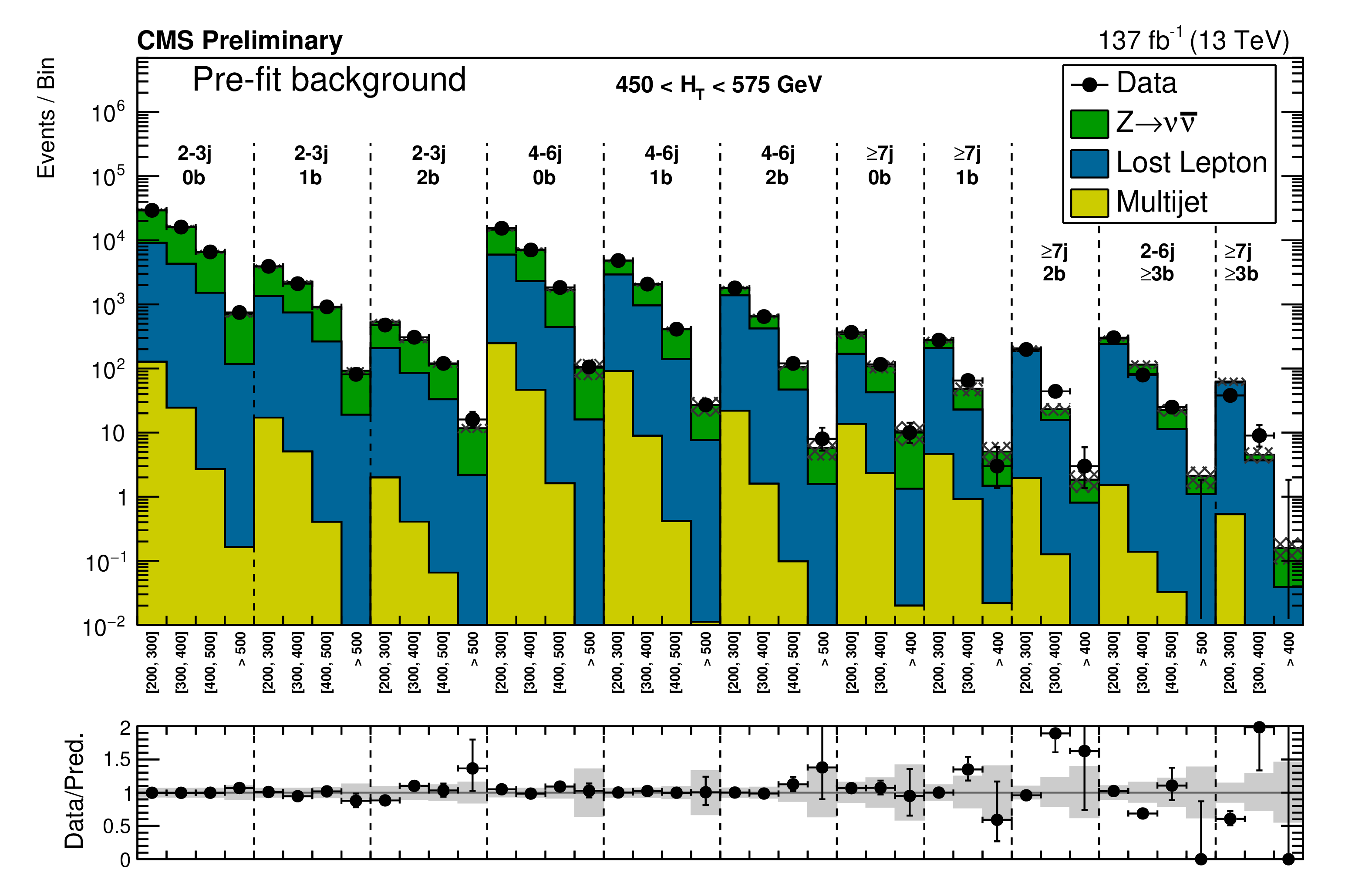
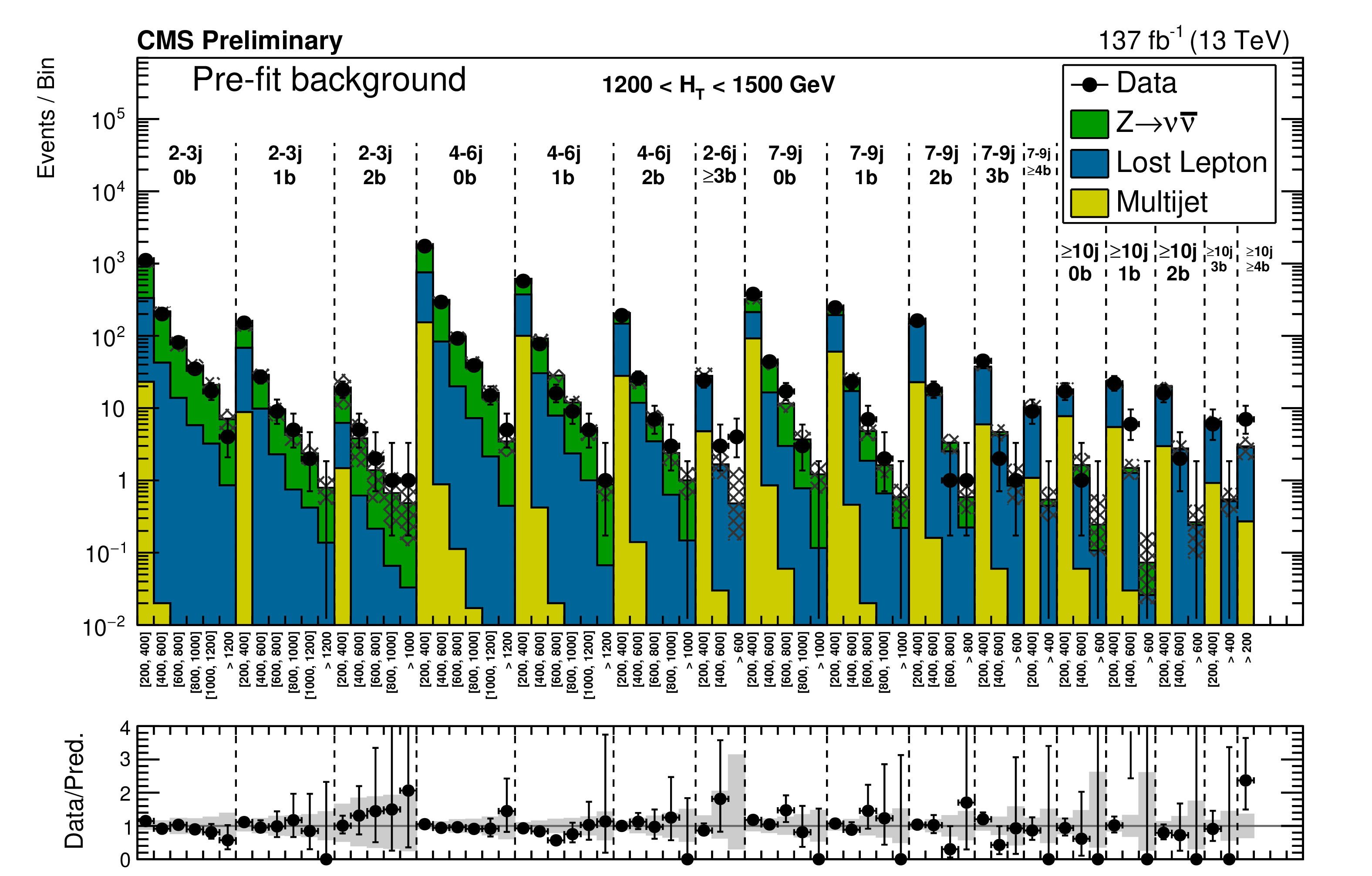
Figure 5:
(Upper) Comparison of estimated (pre-fit) background and observed data events in each topological region. Hatched bands represent the full uncertainty in the background estimate. The monojet regions ($ {N_{\mathrm {j}}} = $ 1) are identified by the labels "1j, 0b'' and "1j, 1b'', and are binned in jet ${p_{\mathrm {T}}}$. The multijet ones are shown for each ${H_{\mathrm {T}}}$ region separately, and are labeled accordingly. The notations j, b indicate ${N_{\mathrm {j}}}$, ${N_{\mathrm{b}}}$ labeling. (Lower) Same for individual ${M_{\mathrm {T2}}}$ signal bins in the medium ${H_{\mathrm {T}}}$ region. On the $x$-axis, the ${M_{\mathrm {T2}}}$ binning is shown in units of GeV. |

png pdf |
Figure 5-a:
Comparison of estimated (pre-fit) background and observed data events in each topological region. Hatched bands represent the full uncertainty in the background estimate. The monojet regions ($ {N_{\mathrm {j}}} = $ 1) are identified by the labels "1j, 0b'' and "1j, 1b'', and are binned in jet ${p_{\mathrm {T}}}$. The multijet ones are shown for each ${H_{\mathrm {T}}}$ region separately, and are labeled accordingly. The notations j, b indicate ${N_{\mathrm {j}}}$, ${N_{\mathrm{b}}}$ labeling. |

png pdf |
Figure 5-b:
Same for individual ${M_{\mathrm {T2}}}$ signal bins in the medium ${H_{\mathrm {T}}}$ region. On the $x$-axis, the ${M_{\mathrm {T2}}}$ binning is shown in units of GeV. |
png pdf |
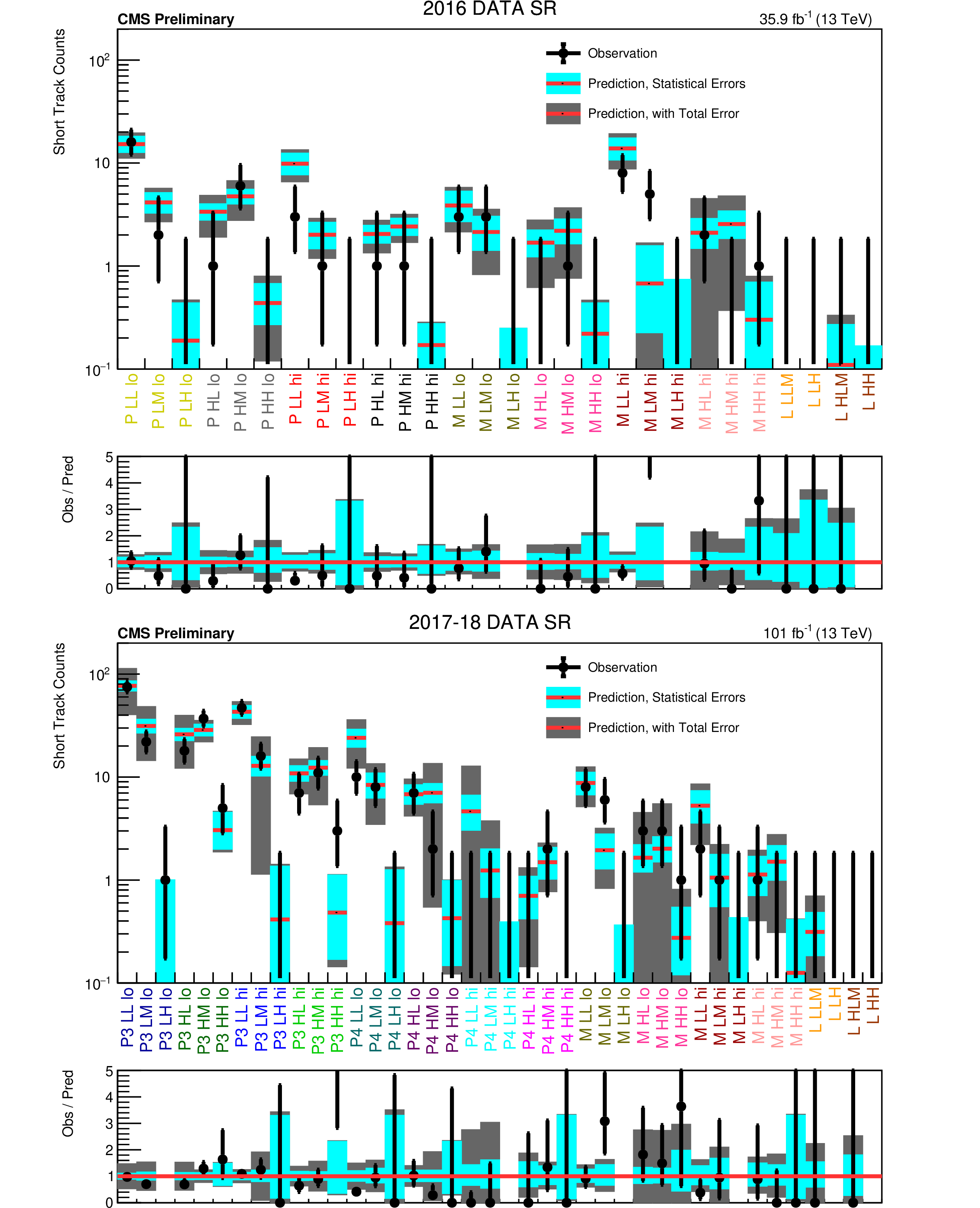
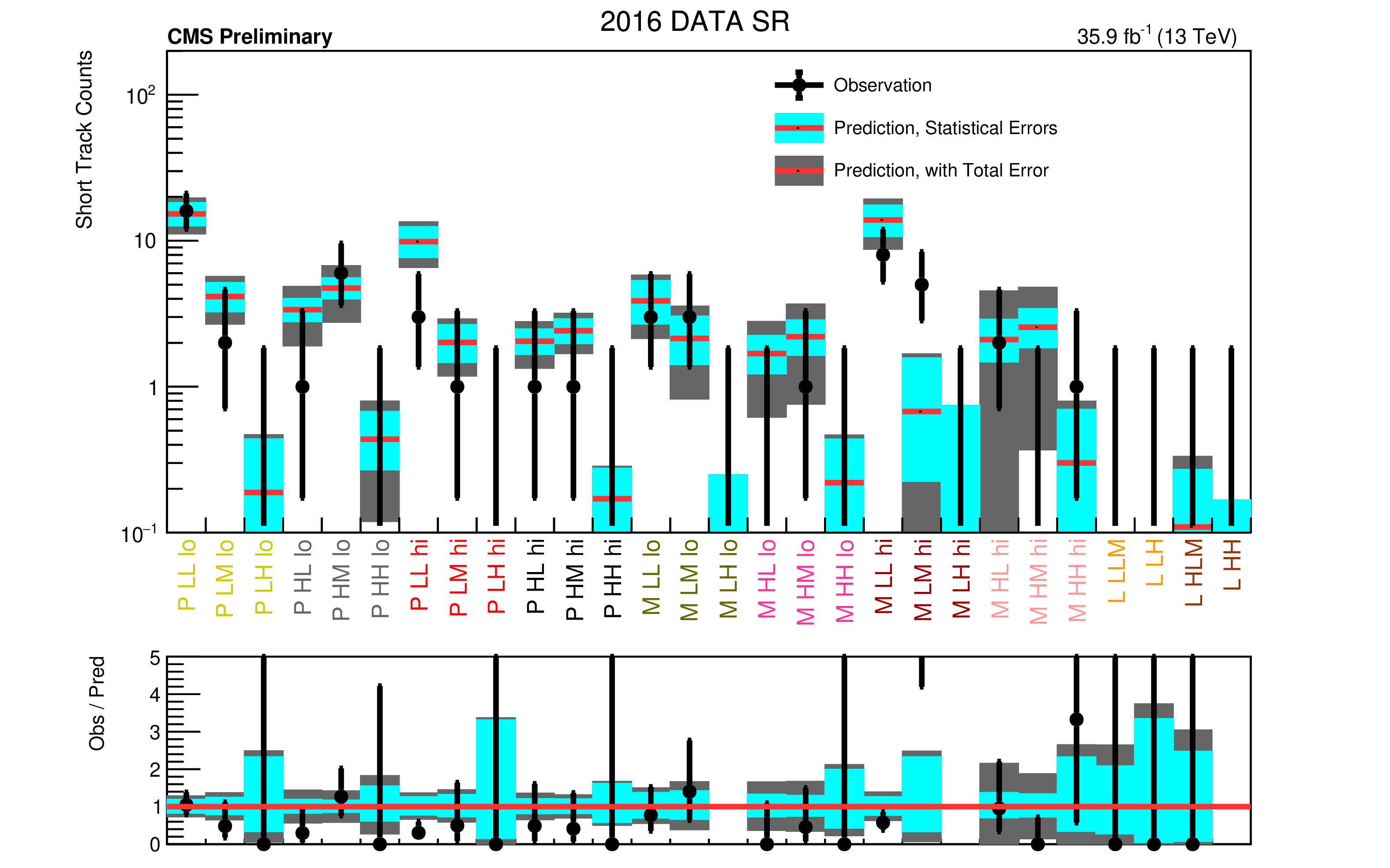
Figure 6:
Comparison of estimated (pre-fit) background and observed data events in (upper) each of the 2016 search regions, and in (lower) each of the 2017-2018 search regions, in the search for disappearing tracks. The red histogram represents the predicted background, while the black points are the actual observed data counts. The cyan band represents the statistical uncertainty on the prediction. The gray band represents the total uncertainty. The labels on the $x$-axes are explained in Tables 7-8 of Appendix B.2. Regions whose predictions use the same measurement of $f_{\mathrm {short}}$ are identified by the colors of the labels. Bins with no entry in the ratio have zero (pre-fit) predicted background. |
png pdf |
Figure 6-a:
Comparison of estimated (pre-fit) background and observed data events in each of the 2016 search regions, in the search for disappearing tracks. The red histogram represents the predicted background, while the black points are the actual observed data counts. The cyan band represents the statistical uncertainty on the prediction. The gray band represents the total uncertainty. The labels on the $x$-axes are explained in Tables 7-8 of Appendix B.2. Regions whose predictions use the same measurement of $f_{\mathrm {short}}$ are identified by the colors of the labels. Bins with no entry in the ratio have zero (pre-fit) predicted background. |

png pdf |
Figure 6-b:
Comparison of estimated (pre-fit) background and observed data events in each of the 2017-2018 search regions, in the search for disappearing tracks. The red histogram represents the predicted background, while the black points are the actual observed data counts. The cyan band represents the statistical uncertainty on the prediction. The gray band represents the total uncertainty. The labels on the $x$-axes are explained in Tables 7-8 of Appendix B.2. Regions whose predictions use the same measurement of $f_{\mathrm {short}}$ are identified by the colors of the labels. Bins with no entry in the ratio have zero (pre-fit) predicted background. |
png pdf |
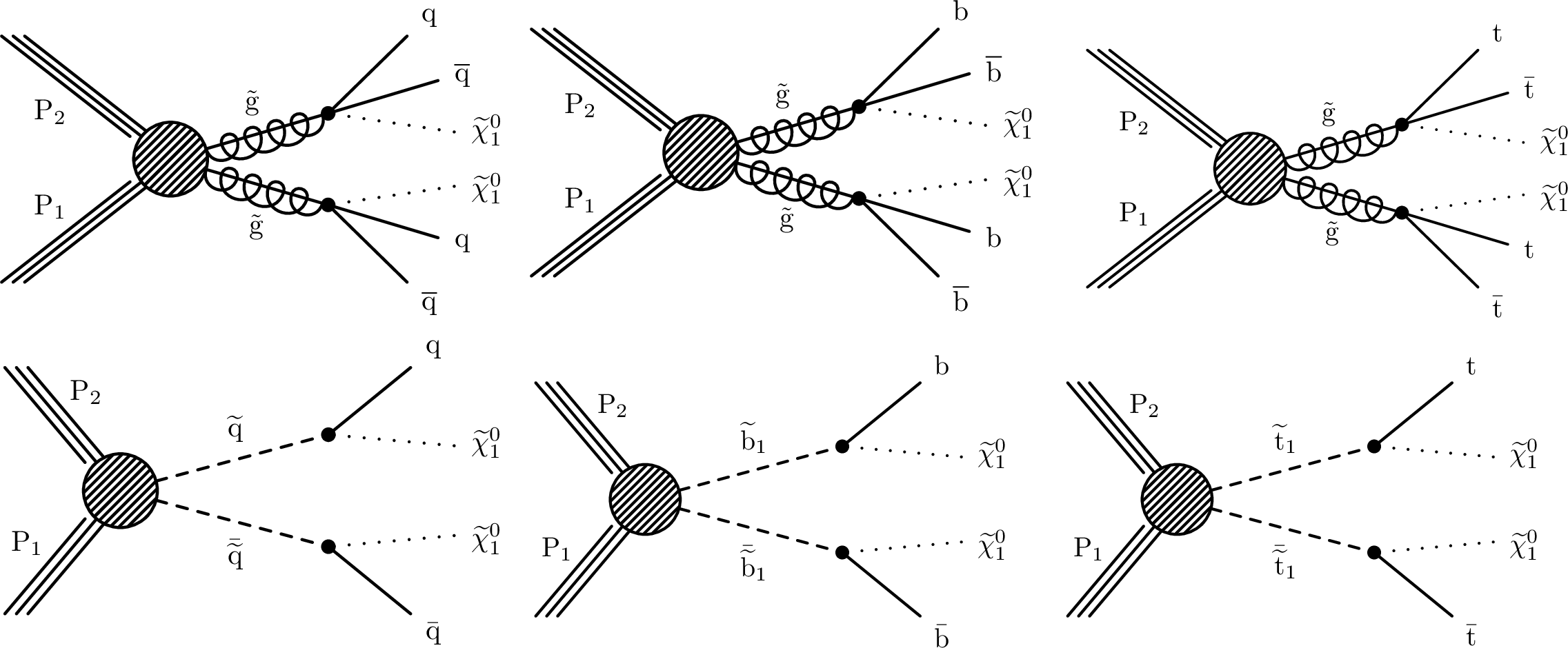
Figure 7:
(Upper) Diagrams for the three scenarios of gluino-mediated light-flavor squark, bottom squark and top squark production considered. (Lower) Diagrams for the direct production of light-flavor, bottom and top squark pairs. |

png pdf |
Figure 7-a:
Diagram for the gluino-mediated light-flavor squark, bottom squark and top squark production. |
png pdf |
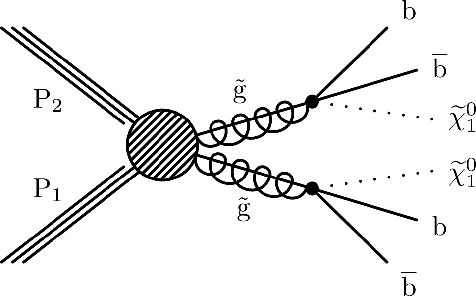
Figure 7-b:
Diagram for the gluino-mediated light-flavor squark, bottom squark and top squark production. |

png pdf |
Figure 7-c:
Diagram for the gluino-mediated light-flavor squark, bottom squark and top squark production. |
png pdf |
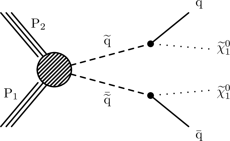
Figure 7-d:
Diagram for the direct production of light-flavor, bottom and top squark pairs. |

png pdf |
Figure 7-e:
Diagram for the direct production of light-flavor, bottom and top squark pairs. |
png pdf |
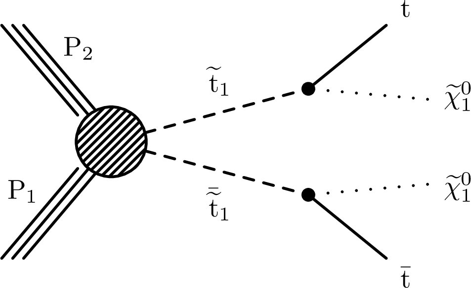
Figure 7-f:
Diagram for the direct production of light-flavor, bottom and top squark pairs. |

png pdf |
Figure 8:
Diagram showing the decays of a gluino via a long-lived ${\tilde{\chi}^{\pm}_{1}}$. The mass of the ${\tilde{\chi}^{\pm}_{1}}$ is larger than the mass of the $\tilde{\chi}^0_1$ by few hundred MeV. The ${\tilde{\chi}^{\pm}_{1}}$ decays to a $\tilde{\chi}^0_1$ via a pion, too soft to be detected. |

png pdf |
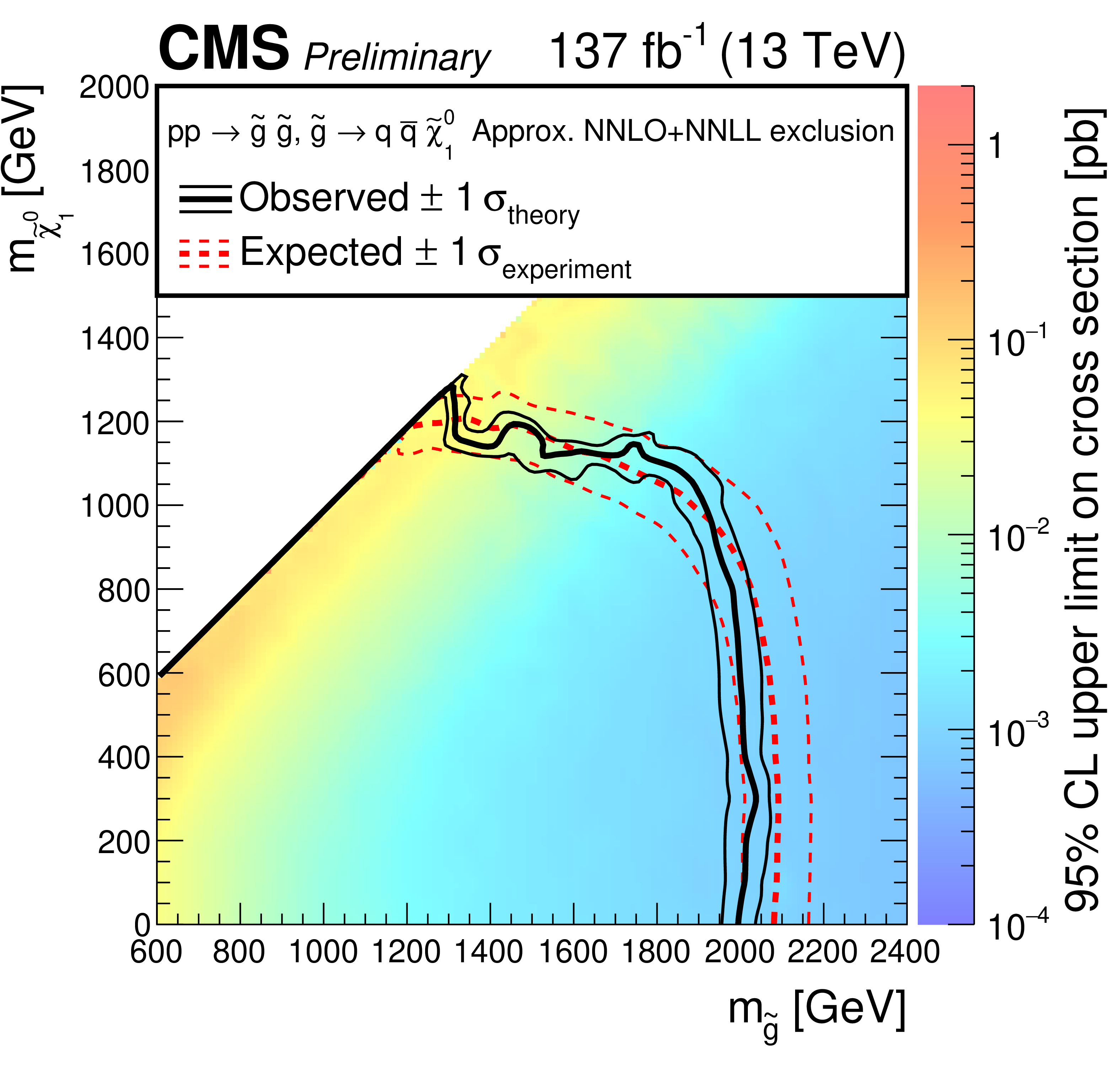
Figure 9:
Exclusion limits at 95% CL for gluino-mediated light-flavor (u, d, s, c) squark production (above left), gluino-mediated bottom squark production (above right), and gluino-mediated top squark production (below). The area enclosed by the thick black curve represents the observed exclusion region, while the dashed red lines indicate the expected limits and their $\pm $1 standard deviation ranges. The thin black lines show the effect of the theoretical uncertainties on the signal cross section. |
png pdf |
Figure 9-a:
Exclusion limits at 95% CL for gluino-mediated light-flavor (u, d, s, c) squark production. The area enclosed by the thick black curve represents the observed exclusion region, while the dashed red lines indicate the expected limits and their $\pm $1 standard deviation ranges. The thin black lines show the effect of the theoretical uncertainties on the signal cross section. |
png pdf |
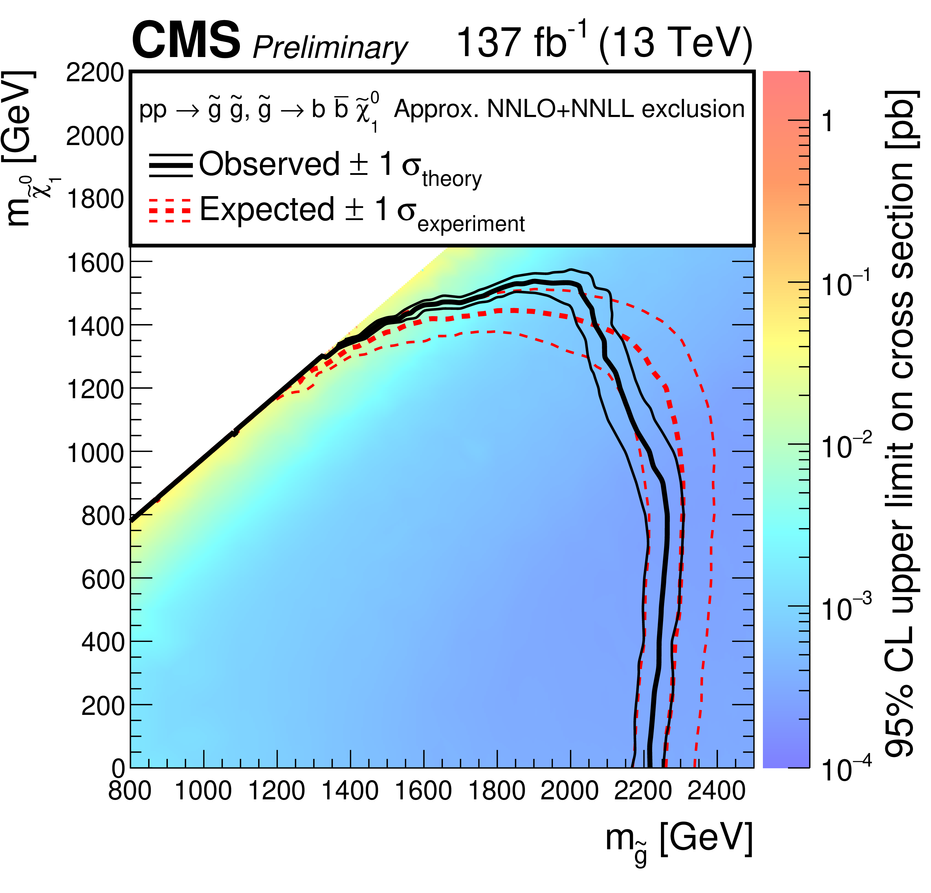
Figure 9-b:
Exclusion limits at 95% CL for gluino-mediated bottom squark production. The area enclosed by the thick black curve represents the observed exclusion region, while the dashed red lines indicate the expected limits and their $\pm $1 standard deviation ranges. The thin black lines show the effect of the theoretical uncertainties on the signal cross section. |
png pdf |
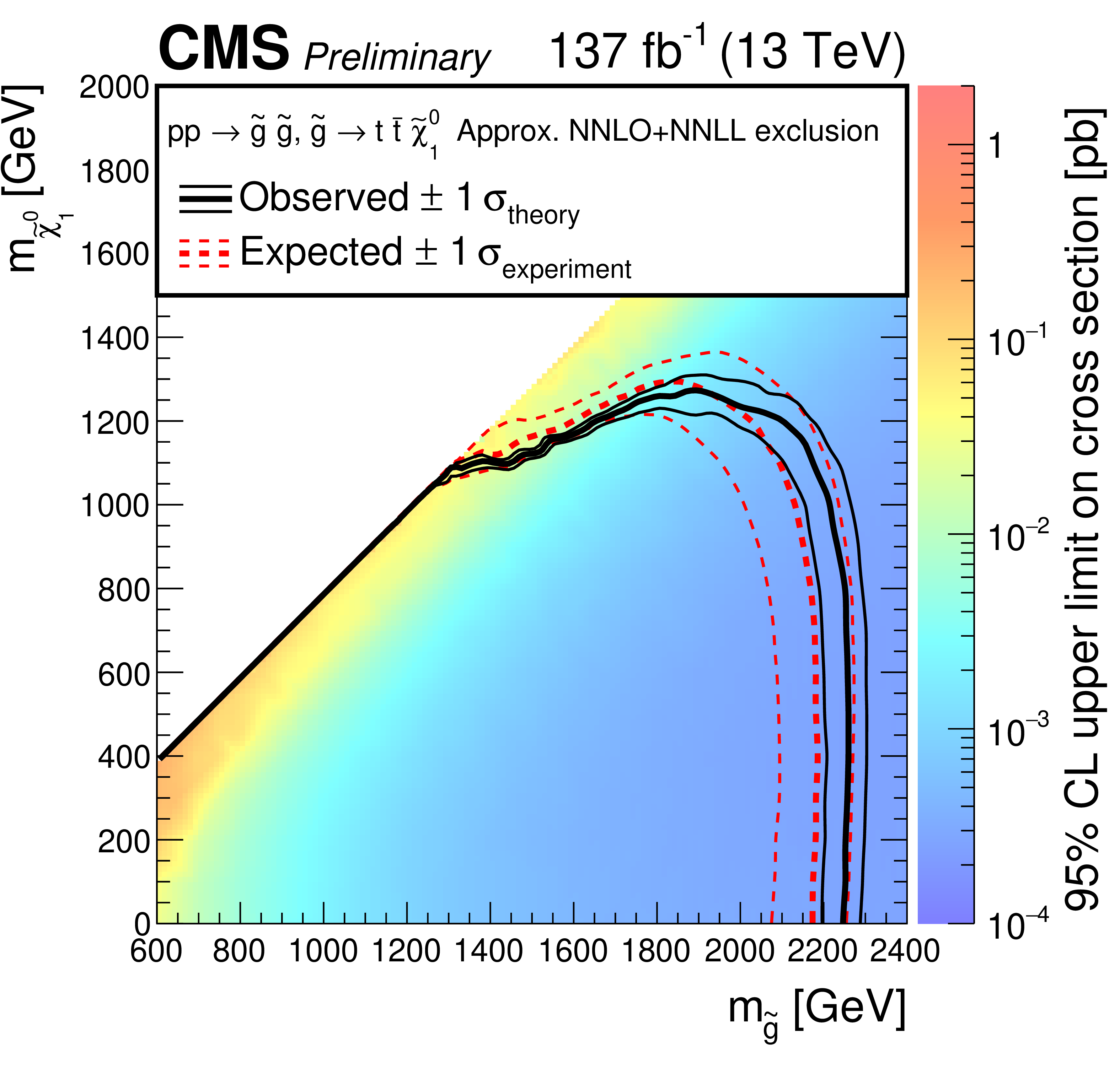
Figure 9-c:
Exclusion limits at 95% CL for gluino-mediated top squark production. The area enclosed by the thick black curve represents the observed exclusion region, while the dashed red lines indicate the expected limits and their $\pm $1 standard deviation ranges. The thin black lines show the effect of the theoretical uncertainties on the signal cross section. |

png pdf |
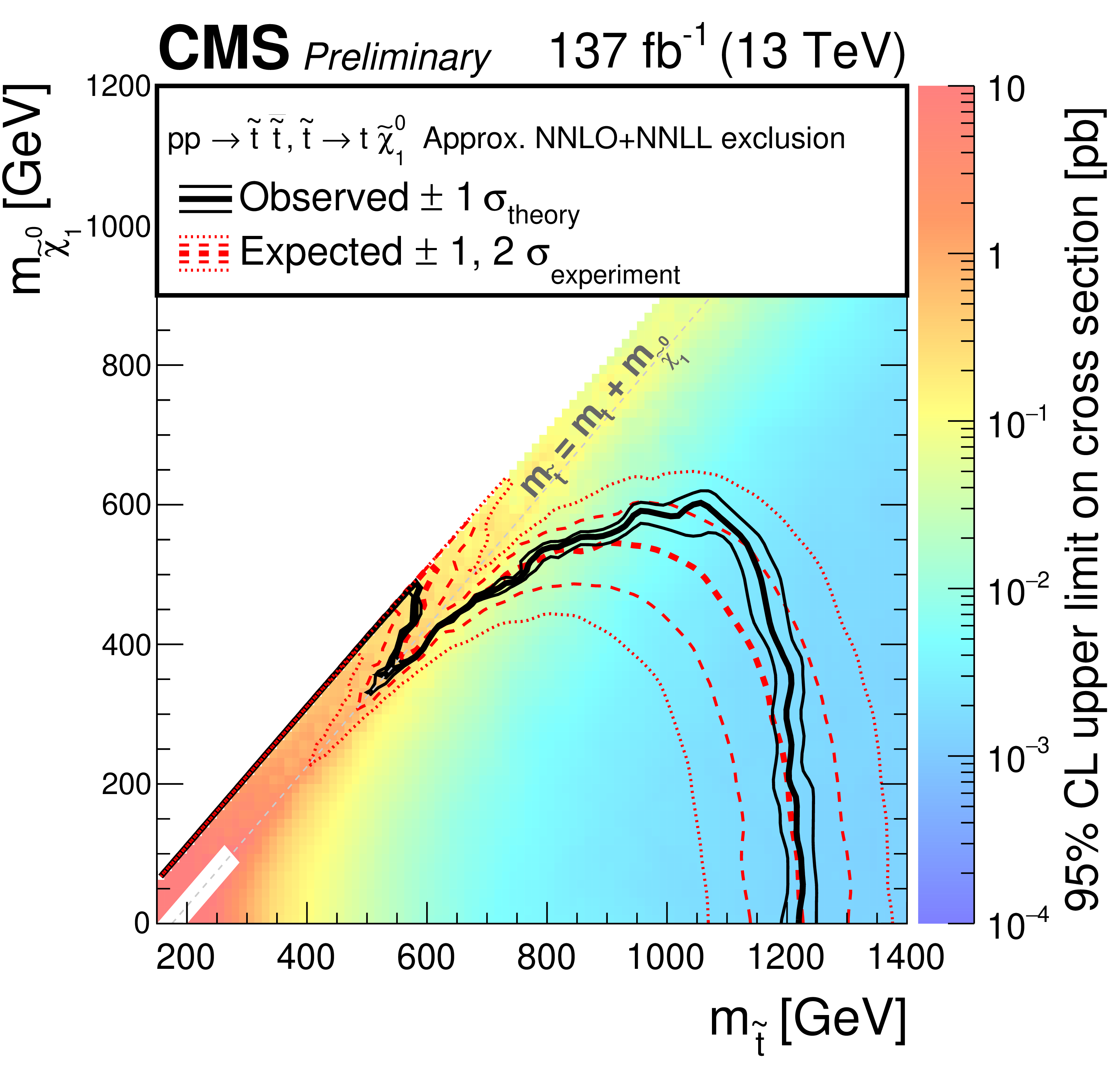
Figure 10:
Exclusion limit at 95% CL for light-flavor squark pair production (above left), bottom squark pair production (above right), and top squark pair production (below). The area enclosed by the thick black curve represents the observed exclusion region, while the dashed red lines indicate the expected limits and their $\pm $1 and $\pm $2 standard deviation ranges. The thin black lines show the effect of the theoretical uncertainties on the signal cross section. The white diagonal band in the top squark pair production exclusion limit corresponds to the region $ {| m_{\tilde{\mathrm{t}}}-m_{\mathrm{t}}-m_{\tilde{\chi}^0_1} |} < $ 25 GeV and small $m_{\tilde{\chi}^0_1}$. Here the efficiency of the selection is a strong function of $m_{\tilde{\mathrm{t}}}-m_{\tilde{\chi}^0_1}$, and as a result the precise determination of the cross section upper limit is uncertain because of the finite granularity of the available MC samples in this region of the ($m_{\tilde{\mathrm{t}}}, m_{\tilde{\chi}^0_1}$) plane. |

png pdf |
Figure 10-a:
Exclusion limit at 95% CL for light-flavor squark pair production. The area enclosed by the thick black curve represents the observed exclusion region, while the dashed red lines indicate the expected limits and their $\pm $1 and $\pm $2 standard deviation ranges. The thin black lines show the effect of the theoretical uncertainties on the signal cross section. |
png pdf |
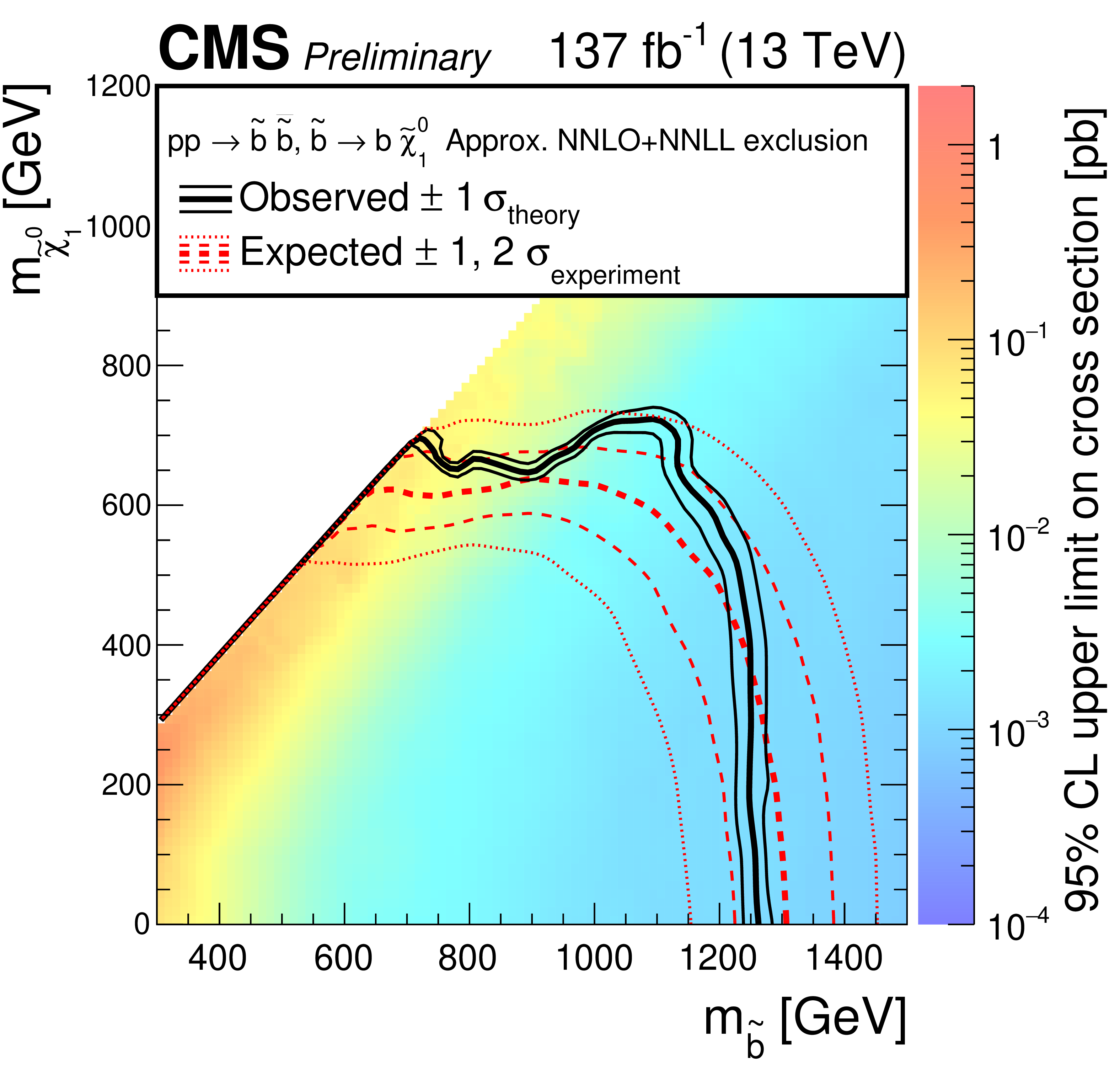
Figure 10-b:
Exclusion limit at 95% CL for bottom squark pair production. The area enclosed by the thick black curve represents the observed exclusion region, while the dashed red lines indicate the expected limits and their $\pm $1 and $\pm $2 standard deviation ranges. The thin black lines show the effect of the theoretical uncertainties on the signal cross section. |
png pdf |
Figure 10-c:
Exclusion limit at 95% CL for top squark pair production. The area enclosed by the thick black curve represents the observed exclusion region, while the dashed red lines indicate the expected limits and their $\pm $1 and $\pm $2 standard deviation ranges. The thin black lines show the effect of the theoretical uncertainties on the signal cross section. The white diagonal band corresponds to the region $ {| m_{\tilde{\mathrm{t}}}-m_{\mathrm{t}}-m_{\tilde{\chi}^0_1} |} < $ 25 GeV and small $m_{\tilde{\chi}^0_1}$. Here the efficiency of the selection is a strong function of $m_{\tilde{\mathrm{t}}}-m_{\tilde{\chi}^0_1}$, and as a result the precise determination of the cross section upper limit is uncertain because of the finite granularity of the available MC samples in this region of the ($m_{\tilde{\mathrm{t}}}, m_{\tilde{\chi}^0_1}$) plane. |
png pdf |
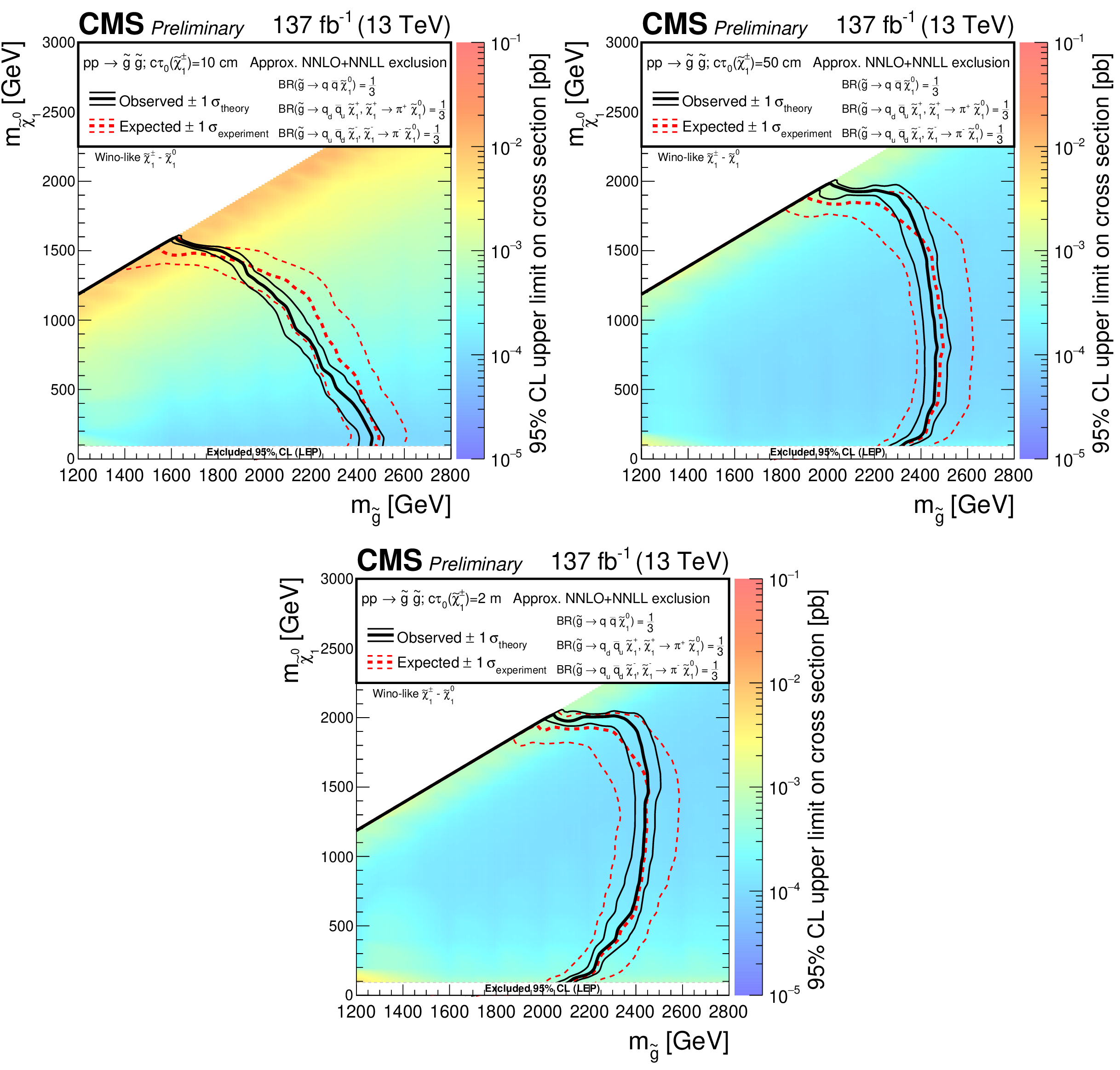
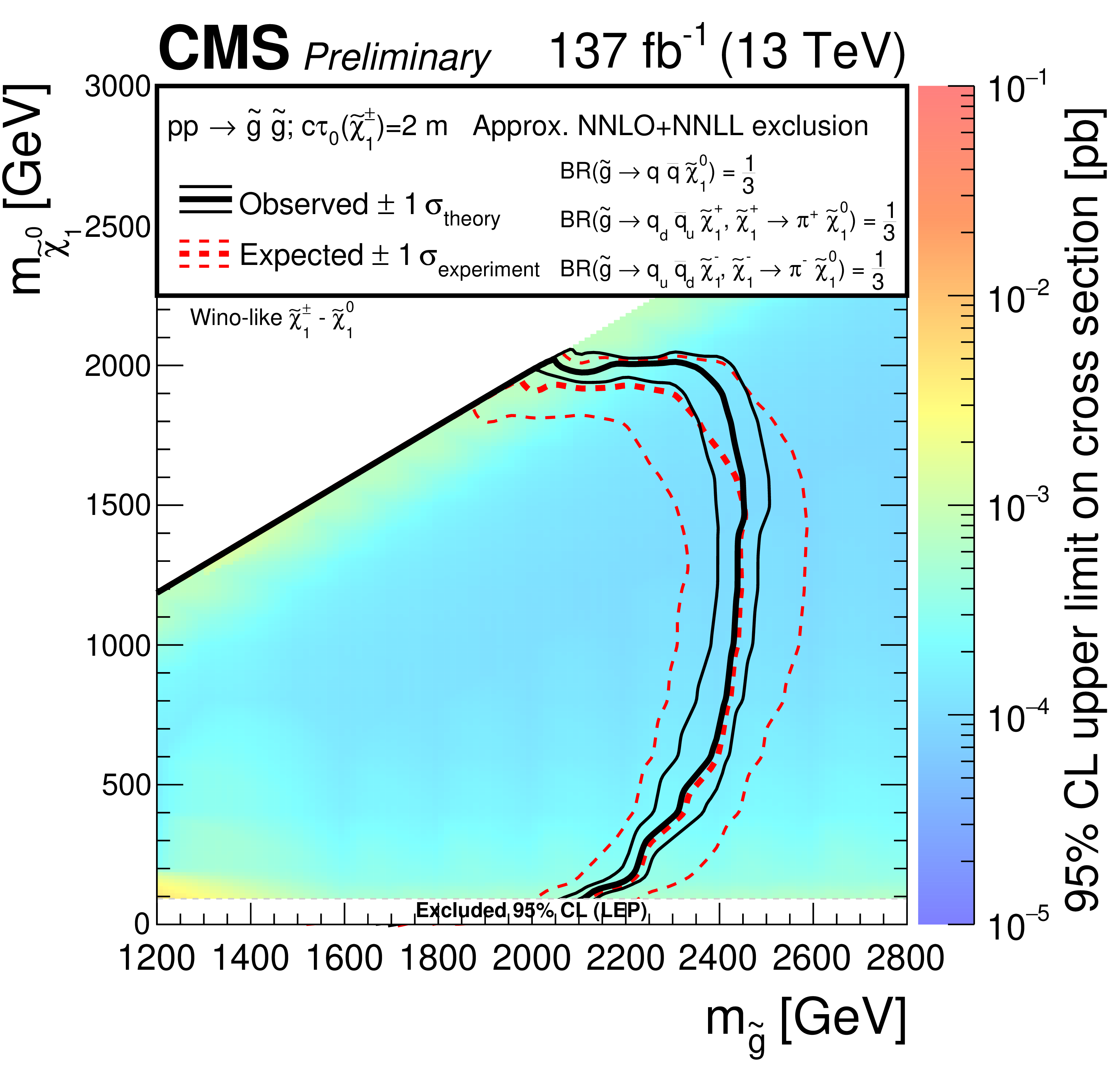
Figure 11:
Exclusion limits at 95% CL for gluino-mediated light-flavor (u, d, s, c) squark production with $c\tau _{0}({\tilde{\chi}^{\pm}_{1}}) =$ 10 cm (above left), 50 cm (above right), and 200 cm (below). The area enclosed by the thick black curve represents the observed exclusion region, while the dashed red lines indicate the expected limits and their $\pm $1 standard deviation ranges. The thin black lines show the effect of the theoretical uncertainties on the signal cross section. The white band for masses of the $\tilde{\chi}^0_1$ below 91.9 GeV represent the region of the mass plane excluded at LEP [65]. |
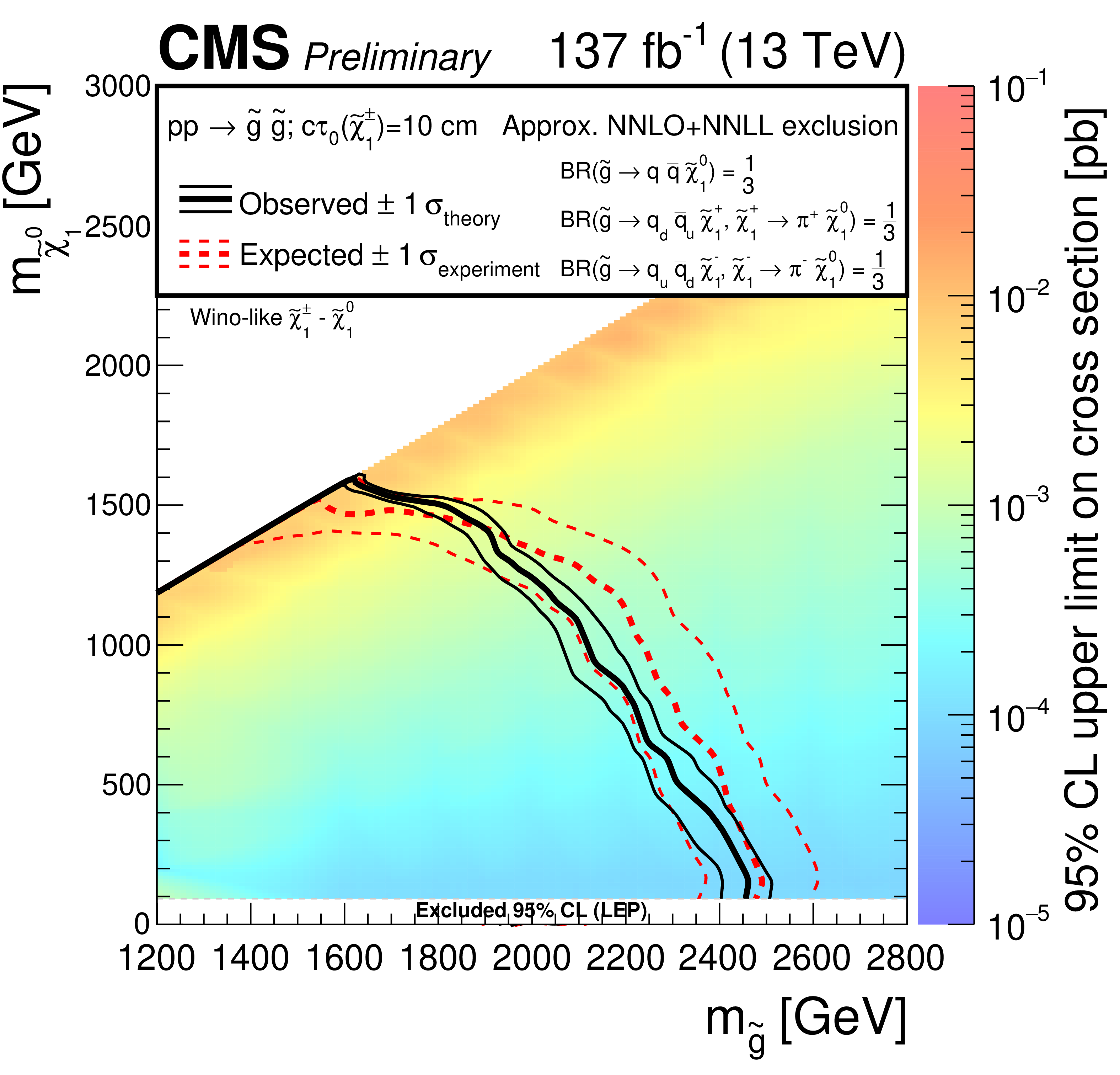
png pdf |
Figure 11-a:
Exclusion limits at 95% CL for gluino-mediated light-flavor (u, d, s, c) squark production with $c\tau _{0}({\tilde{\chi}^{\pm}_{1}}) =$ 10 cm. The area enclosed by the thick black curve represents the observed exclusion region, while the dashed red lines indicate the expected limits and their $\pm $1 standard deviation ranges. The thin black lines show the effect of the theoretical uncertainties on the signal cross section. The white band for masses of the $\tilde{\chi}^0_1$ below 91.9 GeV represent the region of the mass plane excluded at LEP [65]. |
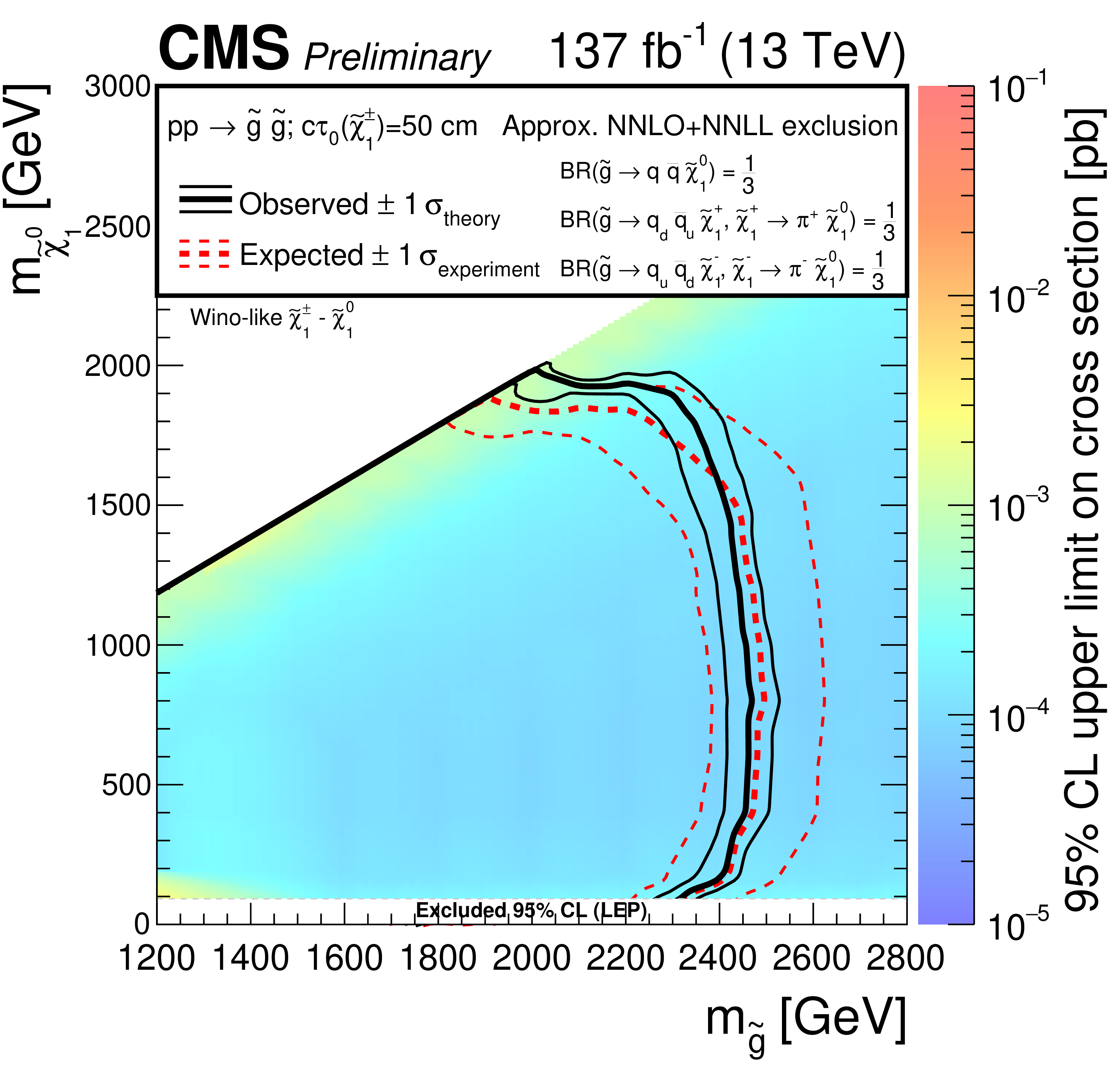
png pdf |
Figure 11-b:
Exclusion limits at 95% CL for gluino-mediated light-flavor (u, d, s, c) squark production with $c\tau _{0}({\tilde{\chi}^{\pm}_{1}}) =$ 50 cm. The area enclosed by the thick black curve represents the observed exclusion region, while the dashed red lines indicate the expected limits and their $\pm $1 standard deviation ranges. The thin black lines show the effect of the theoretical uncertainties on the signal cross section. The white band for masses of the $\tilde{\chi}^0_1$ below 91.9 GeV represent the region of the mass plane excluded at LEP [65]. |
png pdf |
Figure 11-c:
Exclusion limits at 95% CL for gluino-mediated light-flavor (u, d, s, c) squark production with $c\tau _{0}({\tilde{\chi}^{\pm}_{1}}) =$ 200 cm. The area enclosed by the thick black curve represents the observed exclusion region, while the dashed red lines indicate the expected limits and their $\pm $1 standard deviation ranges. The thin black lines show the effect of the theoretical uncertainties on the signal cross section. The white band for masses of the $\tilde{\chi}^0_1$ below 91.9 GeV represent the region of the mass plane excluded at LEP [65]. |
png pdf |
Figure 12:
(Upper) Comparison of the estimated background and observed data events in each signal bin in the monojet region. On the $x$-axis, the ${{p_{\mathrm {T}}} ^{\text {jet1}}}$ binning is shown in units of GeV. Hatched bands represent the full uncertainty in the background estimate. The notations j, b indicate ${N_{\mathrm {j}}}$, ${N_{\mathrm{b}}}$ labeling. (Lower) Same for the very low ${H_{\mathrm {T}}}$ region. On the $x$-axis, the ${M_{\mathrm {T2}}}$ binning is shown in units of GeV. |
png pdf |
Figure 12-a:
Comparison of the estimated background and observed data events in each signal bin in the monojet region. On the $x$-axis, the ${{p_{\mathrm {T}}} ^{\text {jet1}}}$ binning is shown in units of GeV. Hatched bands represent the full uncertainty in the background estimate. The notations j, b indicate ${N_{\mathrm {j}}}$, ${N_{\mathrm{b}}}$ labeling. |
png pdf |
Figure 12-b:
Same for the very low ${H_{\mathrm {T}}}$ region. On the $x$-axis, the ${M_{\mathrm {T2}}}$ binning is shown in units of GeV. |

png pdf |
Figure 13:
(Upper) Comparison of the estimated background and observed data events in each signal bin in the low-${H_{\mathrm {T}}}$ region. Hatched bands represent the full uncertainty in the background estimate. The notations j, b indicate ${N_{\mathrm {j}}}$, ${N_{\mathrm{b}}}$ labeling. Same for the high- (middle) and extreme- (lower) ${H_{\mathrm {T}}}$ regions. On the $x$-axis, the ${M_{\mathrm {T2}}}$ binning is shown in units of GeV. |
png pdf |
Figure 13-a:
(Upper) Comparison of the estimated background and observed data events in each signal bin in the low-${H_{\mathrm {T}}}$ region. Hatched bands represent the full uncertainty in the background estimate. The notations j, b indicate ${N_{\mathrm {j}}}$, ${N_{\mathrm{b}}}$ labeling. Same for the high- (middle) and extreme- (lower) ${H_{\mathrm {T}}}$ regions. On the $x$-axis, the ${M_{\mathrm {T2}}}$ binning is shown in units of GeV. |
png pdf |
Figure 13-b:
(Upper) Comparison of the estimated background and observed data events in each signal bin in the low-${H_{\mathrm {T}}}$ region. Hatched bands represent the full uncertainty in the background estimate. The notations j, b indicate ${N_{\mathrm {j}}}$, ${N_{\mathrm{b}}}$ labeling. Same for the high- (middle) and extreme- (lower) ${H_{\mathrm {T}}}$ regions. On the $x$-axis, the ${M_{\mathrm {T2}}}$ binning is shown in units of GeV. |

png pdf |
Figure 13-c:
(Upper) Comparison of the estimated background and observed data events in each signal bin in the low-${H_{\mathrm {T}}}$ region. Hatched bands represent the full uncertainty in the background estimate. The notations j, b indicate ${N_{\mathrm {j}}}$, ${N_{\mathrm{b}}}$ labeling. Same for the high- (middle) and extreme- (lower) ${H_{\mathrm {T}}}$ regions. On the $x$-axis, the ${M_{\mathrm {T2}}}$ binning is shown in units of GeV. |

png pdf |
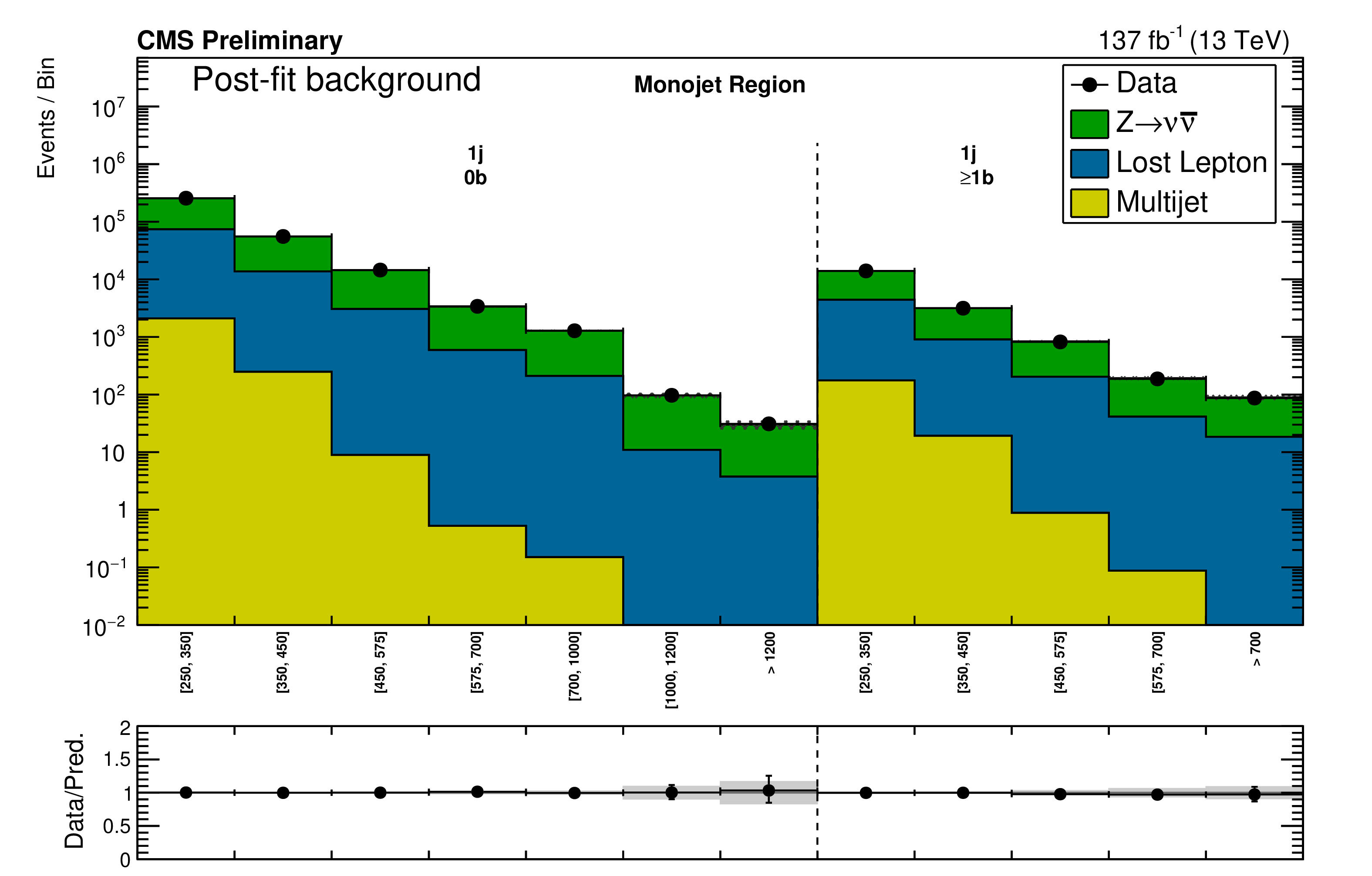
Figure 14:
(Upper) Comparison of the post-fit estimated background and observed data events in each signal bin in the monojet region. On the $x$-axis, the ${{p_{\mathrm {T}}} ^{\text {jet1}}}$ binning is shown in units of GeV. Hatched bands represent the full uncertainty in the background estimate. The notations j, b indicate ${N_{\mathrm {j}}}$, ${N_{\mathrm{b}}}$ labeling. (Lower) Same for the very low-${H_{\mathrm {T}}}$ region. On the $x$-axis, the ${M_{\mathrm {T2}}}$ binning is shown in units of GeV. |
png pdf |
Figure 14-a:
Comparison of the post-fit estimated background and observed data events in each signal bin in the monojet region. On the $x$-axis, the ${{p_{\mathrm {T}}} ^{\text {jet1}}}$ binning is shown in units of GeV. Hatched bands represent the full uncertainty in the background estimate. The notations j, b indicate ${N_{\mathrm {j}}}$, ${N_{\mathrm{b}}}$ labeling. |
png pdf |
Figure 14-b:
Same for the very low-${H_{\mathrm {T}}}$ region. On the $x$-axis, the ${M_{\mathrm {T2}}}$ binning is shown in units of GeV. |

png pdf |
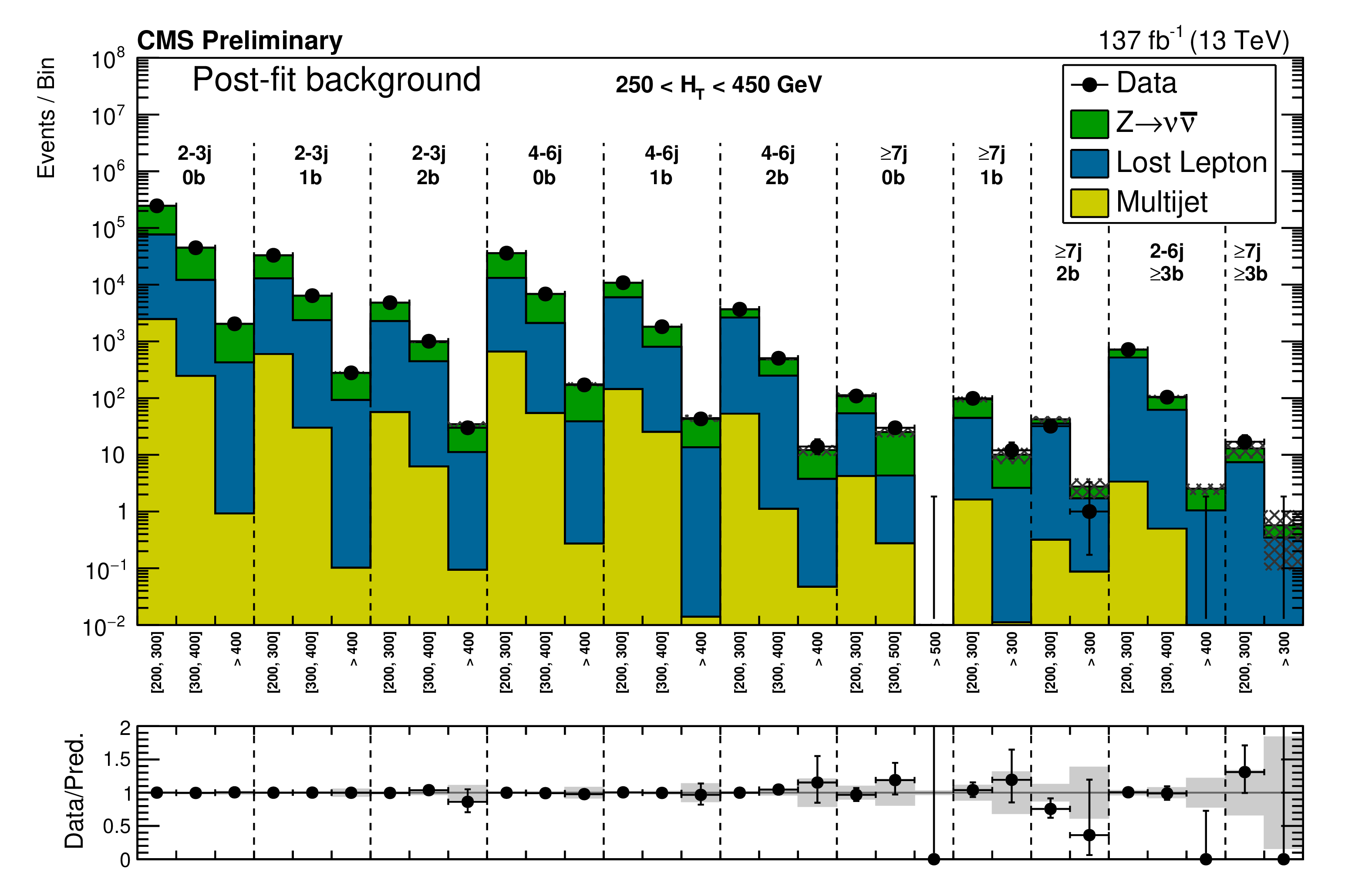
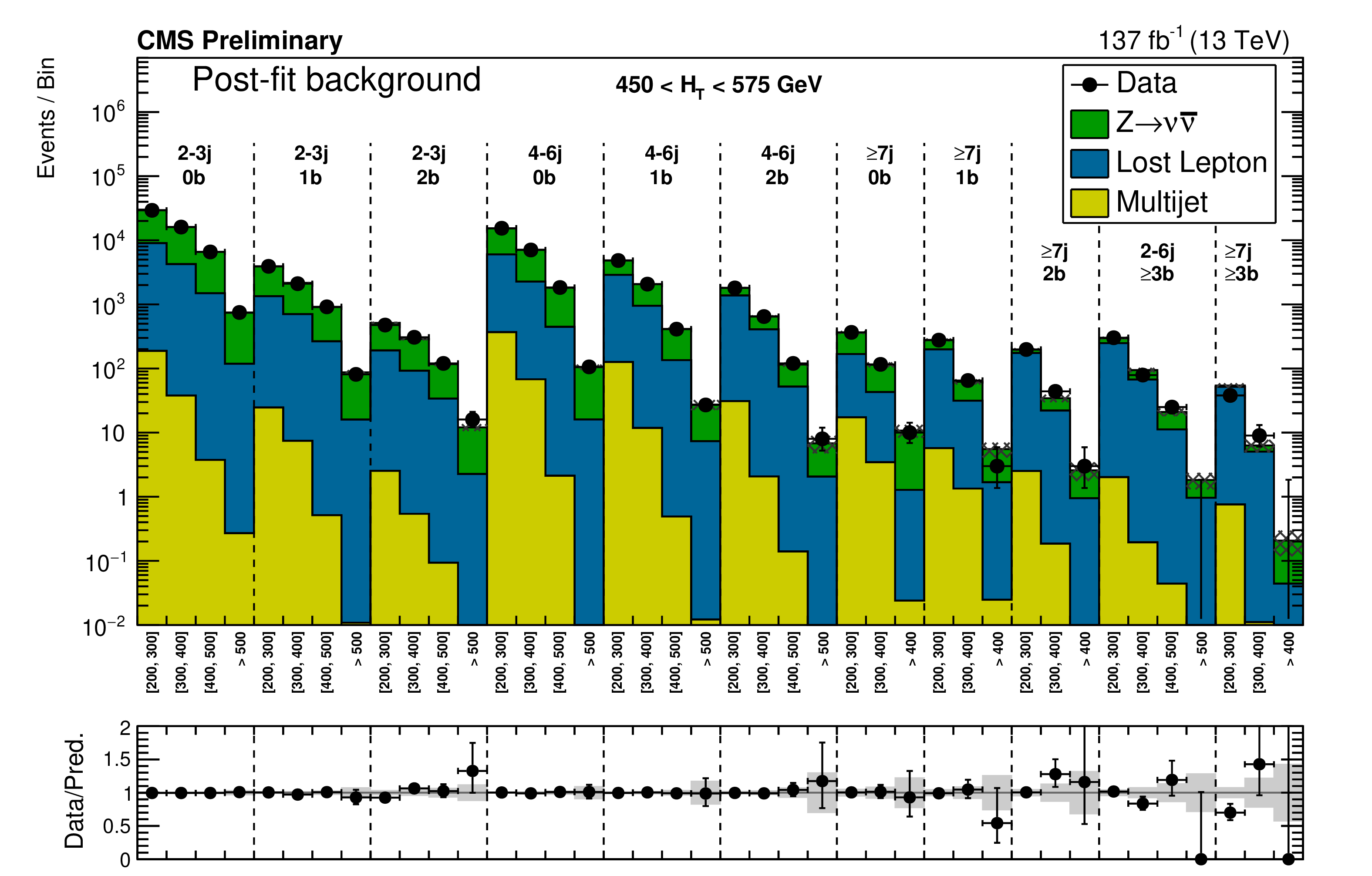
Figure 15:
(Upper) Comparison of the post-fit estimated background and observed data events in each signal bin in the low-${H_{\mathrm {T}}}$ region. Hatched bands represent the full uncertainty in the background estimate. The notations j, b indicate ${N_{\mathrm {j}}}$, ${N_{\mathrm{b}}}$ labeling. (Lower) Same for the medium-${H_{\mathrm {T}}}$ region. On the $x$-axis, the ${M_{\mathrm {T2}}}$ binning is shown in units of GeV. |
png pdf |
Figure 15-a:
Comparison of the post-fit estimated background and observed data events in each signal bin in the low-${H_{\mathrm {T}}}$ region. Hatched bands represent the full uncertainty in the background estimate. The notations j, b indicate ${N_{\mathrm {j}}}$, ${N_{\mathrm{b}}}$ labeling. |
png pdf |
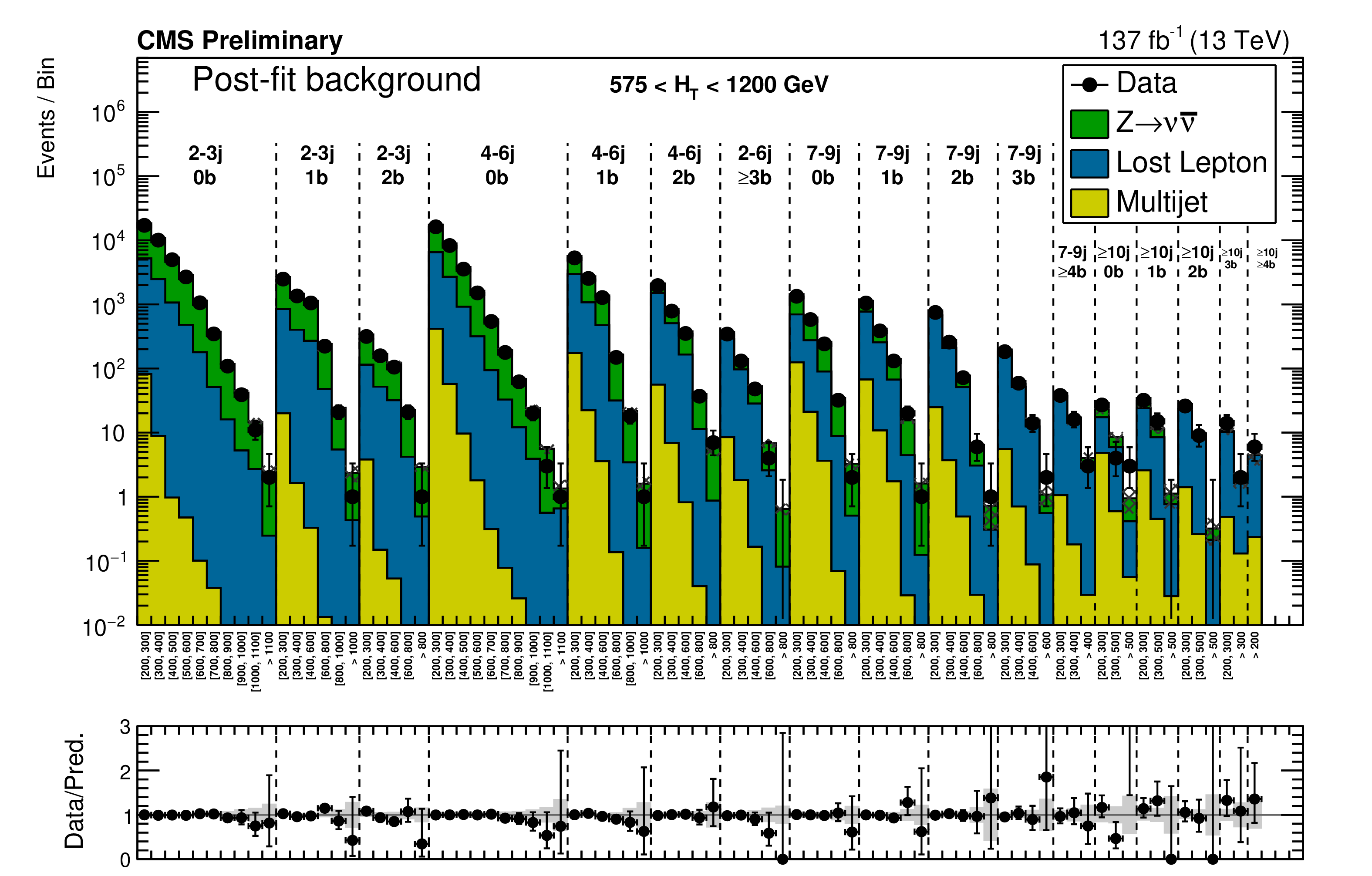
Figure 15-b:
Same for the medium-${H_{\mathrm {T}}}$ region. On the $x$-axis, the ${M_{\mathrm {T2}}}$ binning is shown in units of GeV. |

png pdf |
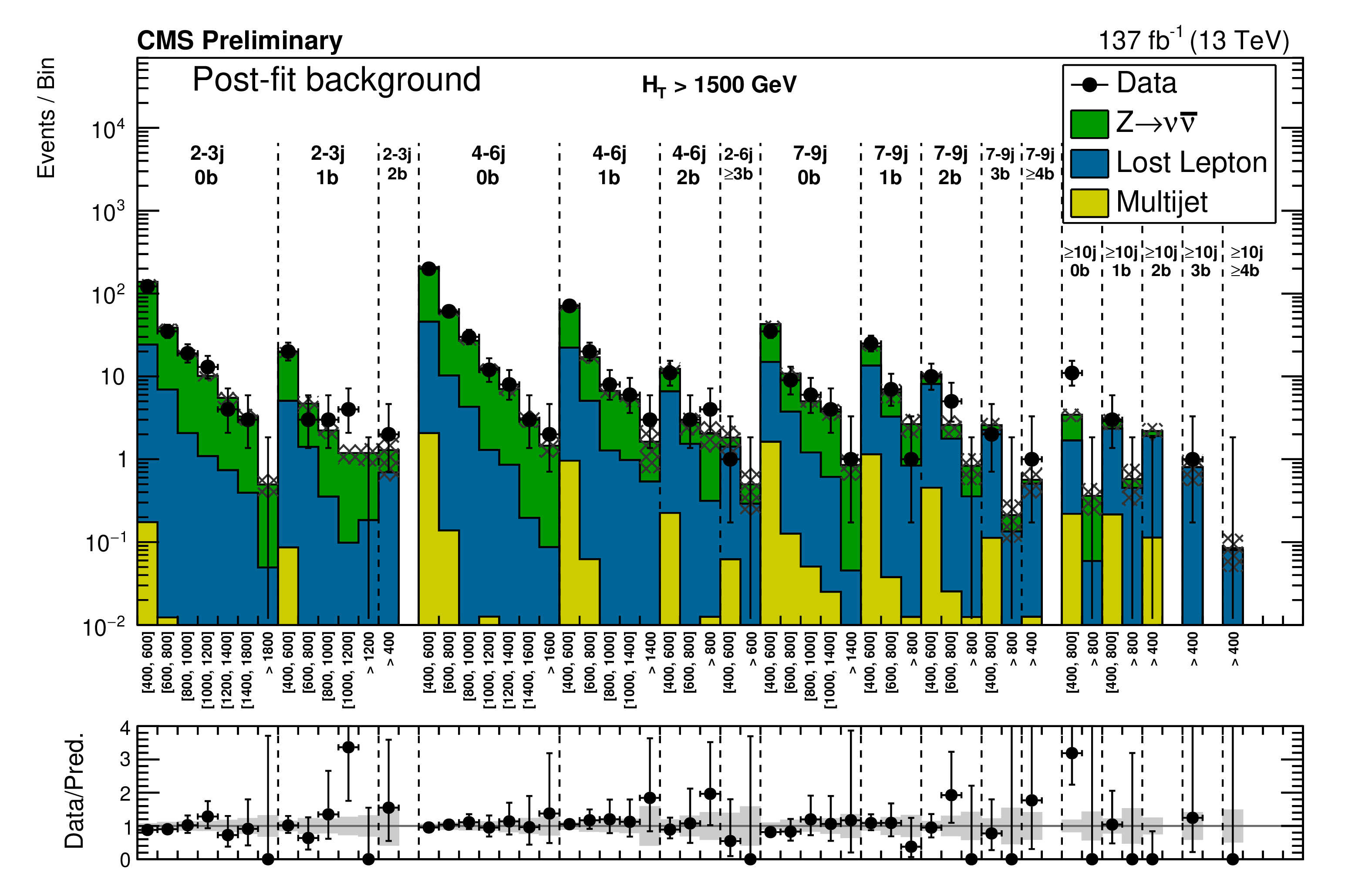
Figure 16:
(Upper) Comparison of the post-fit estimated background and observed data events in each signal bin in the high-${H_{\mathrm {T}}}$ region. Hatched bands represent the full uncertainty in the background estimate. The notations j, b indicate ${N_{\mathrm {j}}}$, ${N_{\mathrm{b}}}$ labeling. (Lower) Same for the extreme-${H_{\mathrm {T}}}$ region. On the $x$-axis, the ${M_{\mathrm {T2}}}$ binning is shown in units of GeV. |

png pdf |
Figure 16-a:
Comparison of the post-fit estimated background and observed data events in each signal bin in the high-${H_{\mathrm {T}}}$ region. Hatched bands represent the full uncertainty in the background estimate. The notations j, b indicate ${N_{\mathrm {j}}}$, ${N_{\mathrm{b}}}$ labeling. |
png pdf |
Figure 16-b:
Same for the extreme-${H_{\mathrm {T}}}$ region. On the $x$-axis, the ${M_{\mathrm {T2}}}$ binning is shown in units of GeV. |
png pdf |
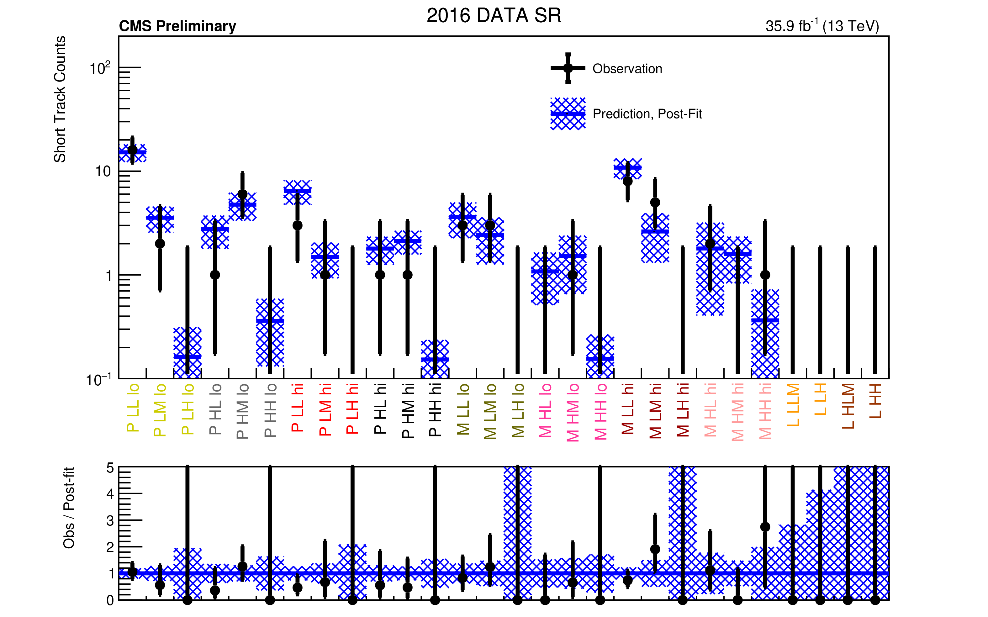
Figure 17:
Background prediction (post-fit) and observation in the 2016 data signal region, in the full analysis binning of the search for disappearing tracks. The blue histogram represents the predicted (post-fit) background, while the black points are the actual observed data counts. The blue band represents the uncertainty on the prediction. The labels on the $x$-axes are explained in Tables 7-8 of Appendix B.2. Regions whose predictions use the same measurement of $f_{\mathrm {short}}$ are identified by the colors of the labels. |

png pdf |
Figure 18:
Background prediction (post-fit) and observation in the 2017-2018 data signal region, in the full analysis binning of the search for disappearing tracks. The blue histogram represents the predicted (post-fit) background, while the black points are the actual observed data counts. The blue band represents the uncertainty on the prediction. The labels on the $x$-axes are explained in Tables 7-8 of Appendix B.2. Regions whose predictions use the same measurement of $f_{\mathrm {short}}$ are identified by the colors of the labels. |
| Tables | |
png pdf |
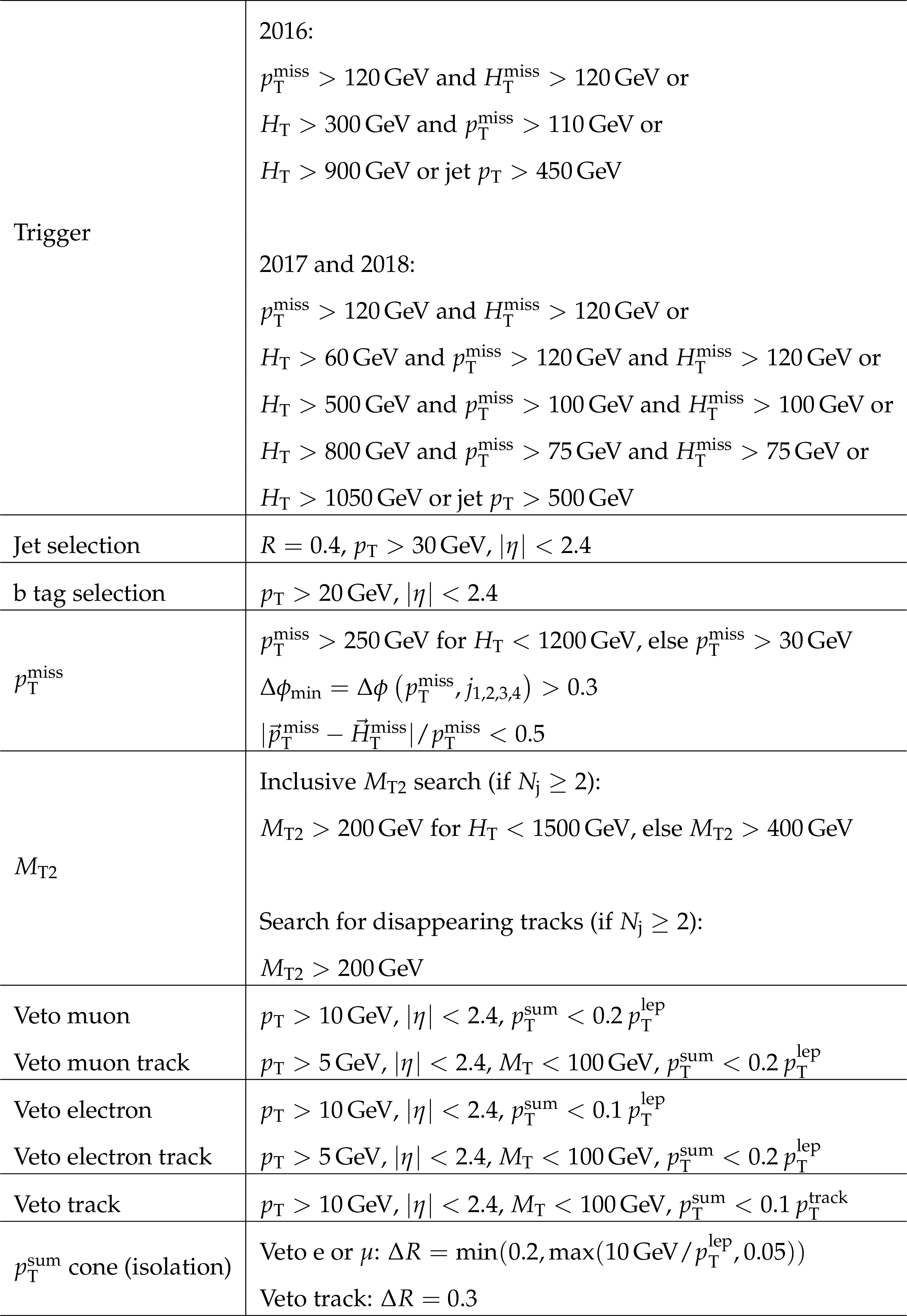
Table 1:
Summary of the trigger requirements and the kinematic offline event preselection requirements on the reconstructed physics objects, for both the inclusive ${M_{\mathrm {T2}}}$ search and the search for disappearing tracks. Here $R$ is the distance parameter of the anti-$ {k_{\mathrm {T}}}$ algorithm. For veto leptons and tracks, the transverse mass ${M_{\mathrm {T}}}$ is determined using the veto object and the $\vec{p}_{\mathrm{T}}^{\text{miss}}$. The variable $ {p_{\mathrm {T}}} ^{\text {sum}}$ is a measure of isolation and it denotes the sum of the transverse momenta of all the PF candidates in a cone around the lepton or the track. The size of the cone, in units of $\Delta R \equiv \sqrt {\smash [b]{(\Delta \phi)^2 + (\Delta \eta)^2}}$ is given in the table. Further details of the lepton selection are described in Refs. [2,3]. The $i$th highest-$ {p_{\mathrm {T}}} $ jet is denoted as j$_i$. |

png pdf |
Table 2:
Typical values of the systematic uncertainties as evaluated for the simplified models of SUSY used in the context of this search. The high statistical uncertainty in the simulated signal sample corresponds to a small number of signal bins with low acceptance, which are typically not among the most sensitive signal bins to that model point. |
png pdf |
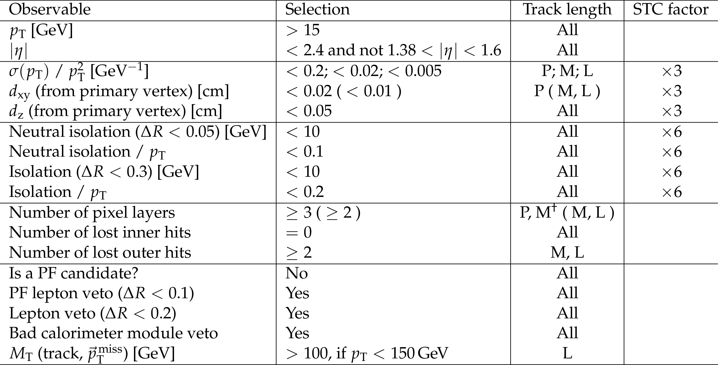
Table 3:
Selection requirements for short tracks (ST) and short track candidates (STC). For the subset of medium length (M) tracks that have just four tracking layers with a measurement, the minimum required number of layers of the pixel tracking detector with a measurement is three ($\dagger $). The selected tracks are required to not overlap with identified leptons. For this selection, all electrons and muons are considered, either identified as PF candidates or not. The selected tracks are as well required to not be identified as PF candidates. The factor by which the selection requirement is relaxed in order to select short track candidates is also reported. If no factor is reported, the requirement is not relaxed for the selection of short track candidates. |
png pdf |
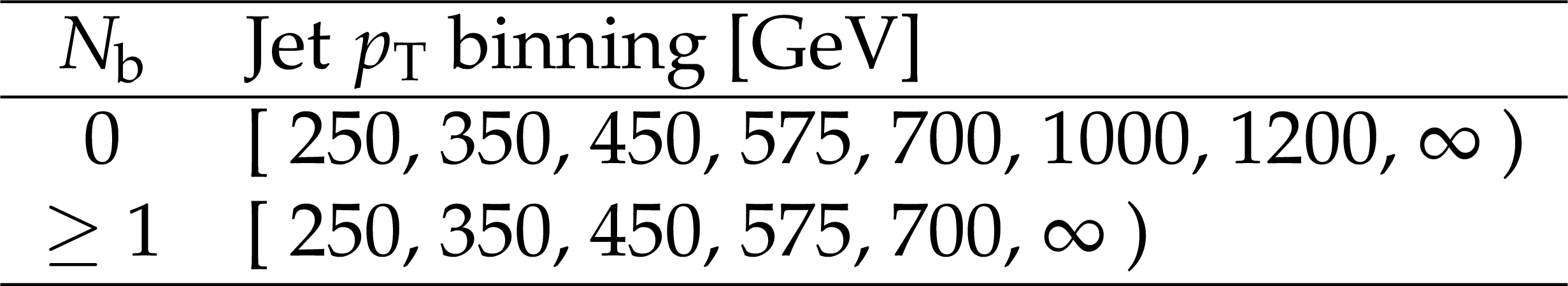
Table 4:
Summary of signal regions for the monojet selection. |
png pdf |
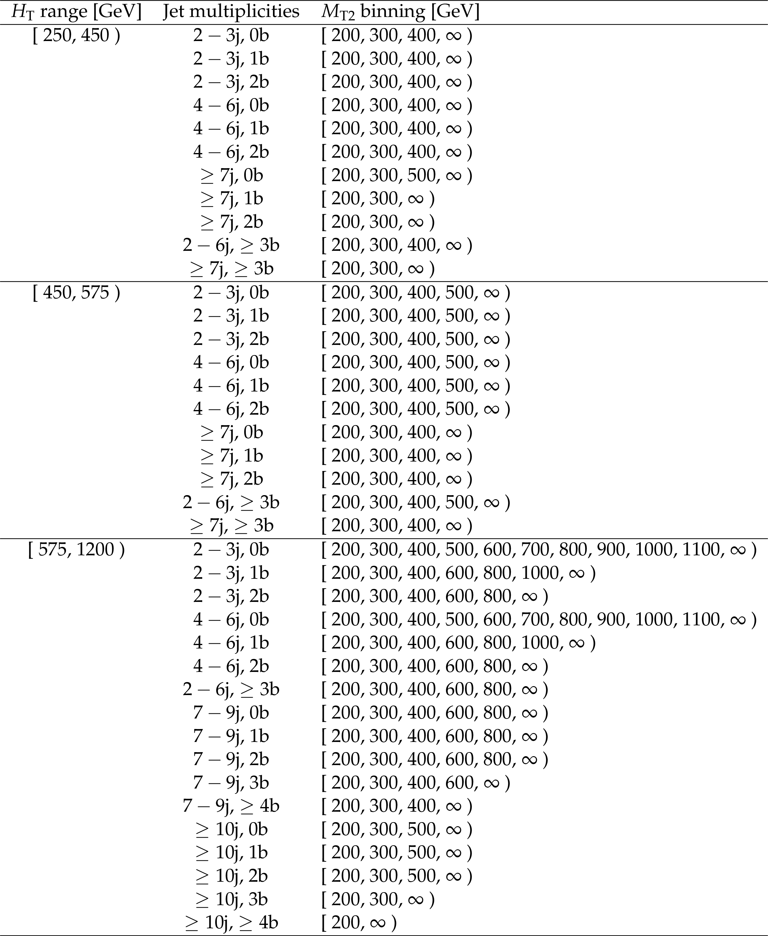
Table 5:
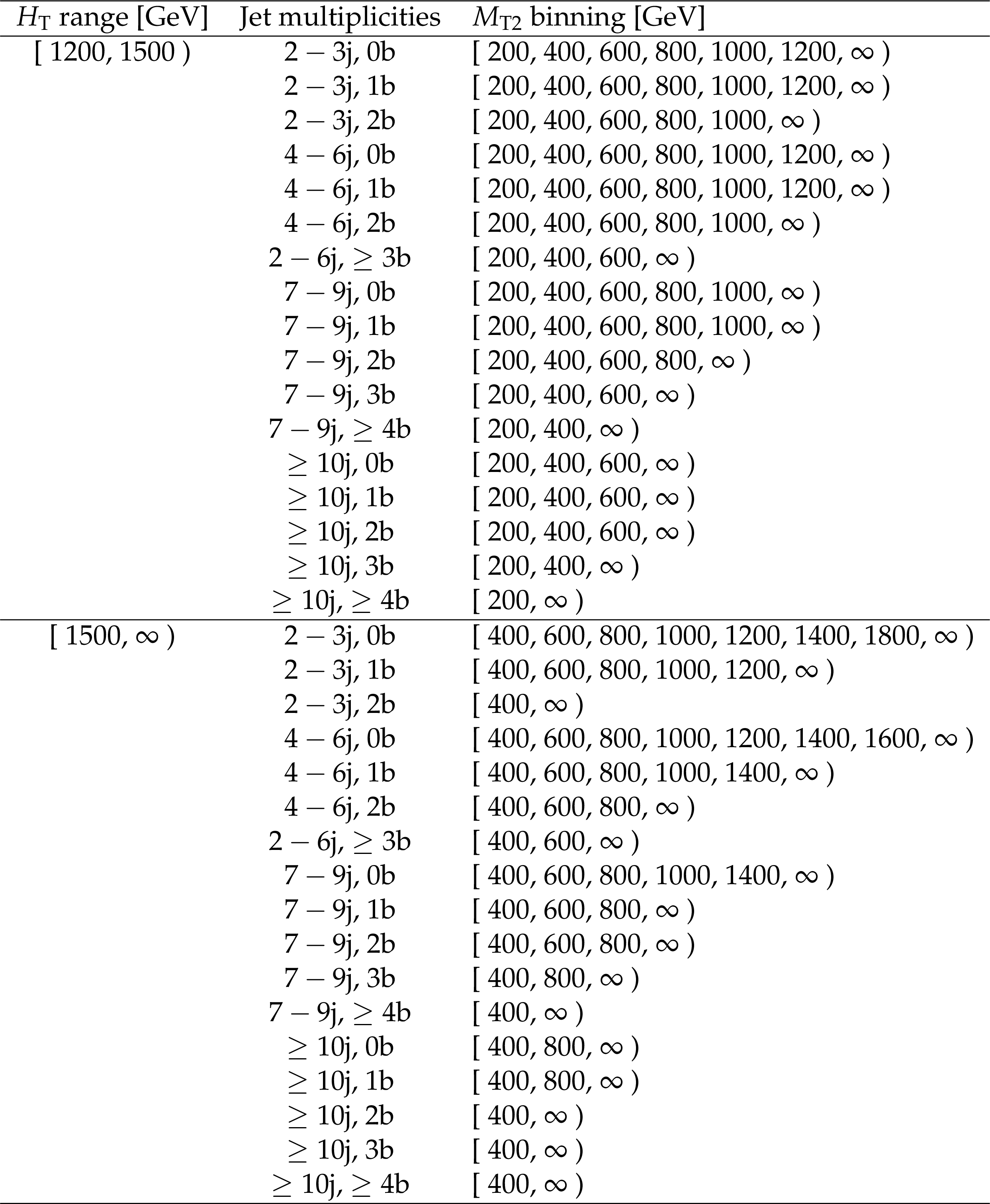
The ${M_{\mathrm {T2}}}$ binning in each topological region of the multi-jet search regions, for the very low, low and medium ${H_{\mathrm {T}}}$ regions. |
png pdf |
Table 6:
The ${M_{\mathrm {T2}}}$ binning in each topological region of the multi-jet search regions, for the high and extreme ${H_{\mathrm {T}}}$ regions. |
png pdf |
Table 7:
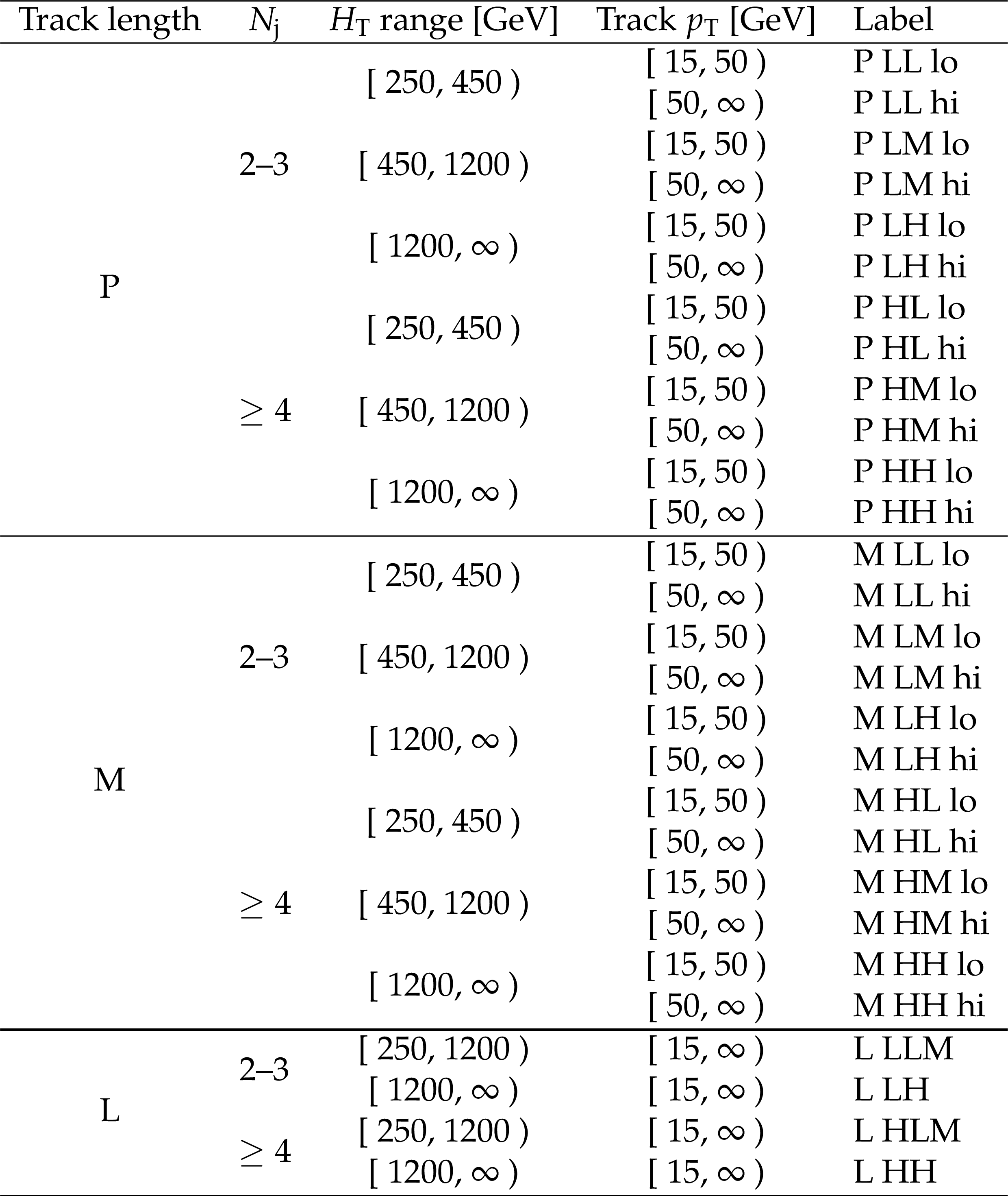
Summary of the signal regions of the search for disappearing tracks, for the 2016 data set. |
png pdf |
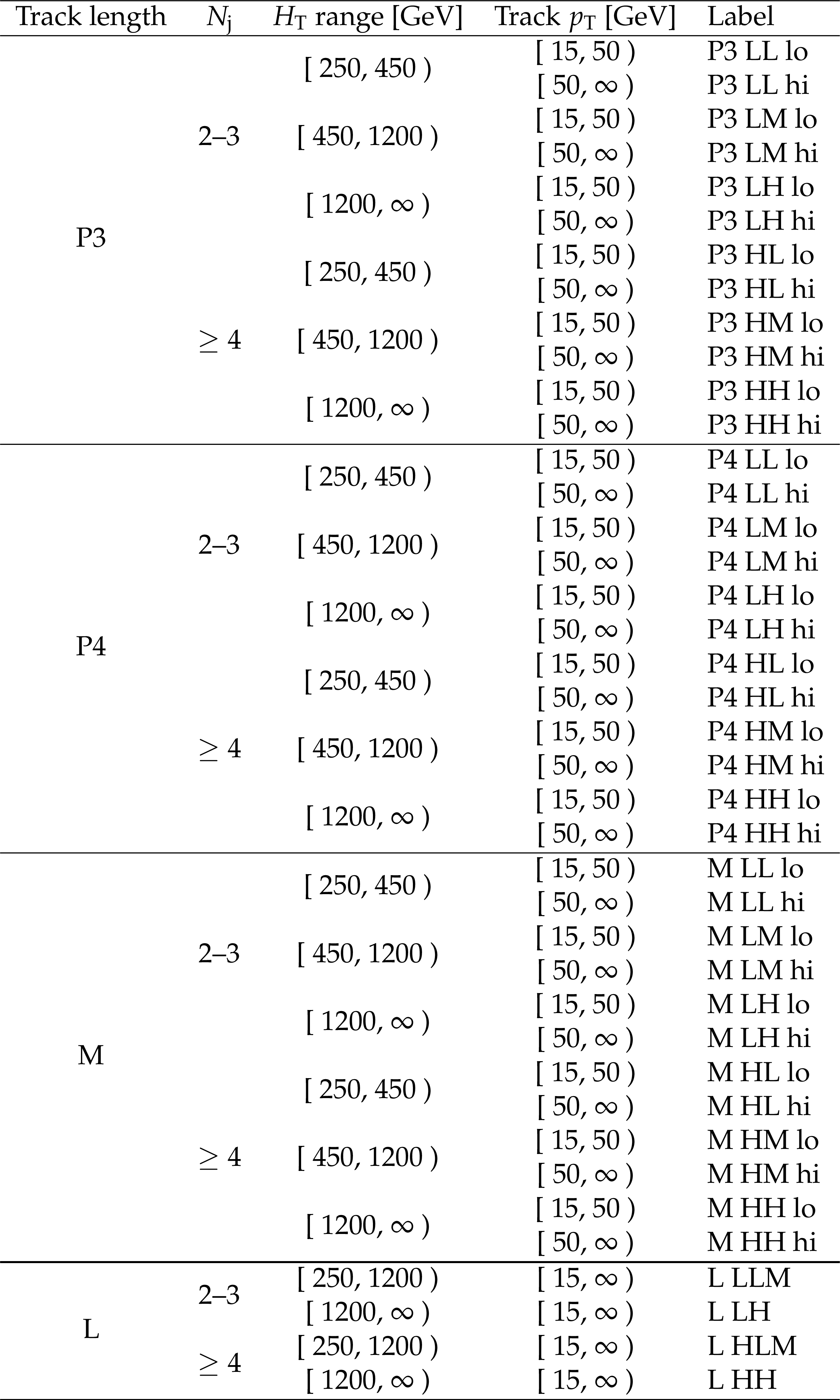
Table 8:
Summary of the signal regions of the search for disappearing tracks, for the 2017-2018 data set. |
| Summary |
| This note presents the results of two related searches for new phenomena using events with jets and large ${M_{\mathrm{T2}}}$. Results are based on a 137 fb$^{-1}$ data sample of proton-proton collisions at $\sqrt{s} = $ 13 TeV collected in 2016, 2017 and 2018 with the CMS detector. No significant deviations from the standard model expectations are observed. The results are interpreted as limits on pair-produced gluinos and squarks in simplified models of $R$-parity conserving supersymmetry. The inclusive ${M_{\mathrm{T2}}}$ search probes gluino masses up to 2250 GeV and $\tilde{\chi}^0_1$ masses up to 1525 GeV, as well as light-flavor, bottom, and top squark masses up to 1770, 1260, and 1225 GeV, respectively, and $\tilde{\chi}^0_1$ masses up to 975, 725, and 600 GeV in each scenario. The search for disappearing tracks extends the gluino mass limit to as much as 2460 GeV, and the $\tilde{\chi}^0_1$ mass limit to as much as 2000 GeV, in models where the gluino can decay with equal probability to $\tilde{\chi}^0_1$, ${\tilde{\chi}^{+}_{1}} $, and ${\tilde{\chi}^{-}_{1}} $, and the ${\tilde{\chi}^{\pm}_{1}}$ are long-lived. |
| References | ||||
| 1 | C. G. Lester and D. J. Summers | Measuring masses of semiinvisibly decaying particles pair produced at hadron colliders | PLB 463 (1999) 99 | hep-ph/9906349 |
| 2 | CMS Collaboration | Search for new phenomena with the $ M_{\mathrm {T2}} $ variable in the all-hadronic final state produced in proton-proton collisions at $ \sqrt{s} = $ 13 TeV | EPJC77 (2017), no. 10, 710 | CMS-SUS-16-036 1705.04650 |
| 3 | CMS Collaboration | Search for new physics with the M$ _{T2} $ variable in all-jets final states produced in pp collisions at $ \sqrt{s}= $ 13 TeV | JHEP 10 (2016) 006 | CMS-SUS-15-003 1603.04053 |
| 4 | CMS Collaboration | Searches for supersymmetry using the m$ _{T2} $ variable in hadronic events produced in pp collisions at 8 tev | JHEP 05 (2015) 078 | CMS-SUS-13-019 1502.04358 |
| 5 | CMS Collaboration | Search for supersymmetry in hadronic final states using $ M_\mathrm{T2} $ in pp collisions at $ \sqrt{s} = $ 7 TeV | JHEP 10 (2012) 018 | CMS-SUS-12-002 1207.1798 |
| 6 | ATLAS Collaboration | Search for squarks and gluinos in final states with jets and missing transverse momentum using 36 fb$ ^{-1} $ of $ \sqrt{s}= $ 13 TeV pp collision data with the ATLAS detector | PRD97 (2018), no. 11, 112001 | 1712.02332 |
| 7 | ATLAS Collaboration | Search for new phenomena with large jet multiplicities and missing transverse momentum using large-radius jets and flavour-tagging at ATLAS in 13 $ TeV pp $ collisions | JHEP 12 (2017) 034 | 1708.02794 |
| 8 | ATLAS Collaboration | Search for dark matter and other new phenomena in events with an energetic jet and large missing transverse momentum using the ATLAS detector | JHEP 01 (2018) 126 | 1711.03301 |
| 9 | ATLAS Collaboration | Search for supersymmetry in final states with missing transverse momentum and multiple $ b $-jets in proton-proton collisions at $ \sqrt{s}= $ 13 TeV with the ATLAS detector | JHEP 06 (2018) 107 | 1711.01901 |
| 10 | ATLAS Collaboration | Search for a scalar partner of the top quark in the jets plus missing transverse momentum final state at $ \sqrt{s} = $ 13 TeV with the ATLAS detector | JHEP 12 (2017) 085 | 1709.04183 |
| 11 | ATLAS Collaboration | Search for supersymmetry in events with $ b $-tagged jets and missing transverse momentum in $ pp $ collisions at $ \sqrt{s}= $ 13 TeV with the ATLAS detector | JHEP 11 (2017) 195 | 1708.09266 |
| 12 | CMS Collaboration | Constraints on models of scalar and vector leptoquarks decaying to a quark and a neutrino at $ \sqrt{s}= $ 13 TeV | PRD98 (2018), no. 3, 032005 | CMS-SUS-18-001 1805.10228 |
| 13 | CMS Collaboration | Search for supersymmetry in multijet events with missing transverse momentum in proton-proton collisions at 13 TeV | PRD96 (2017), no. 3, 032003 | CMS-SUS-16-033 1704.07781 |
| 14 | CMS Collaboration | Search for natural and split supersymmetry in proton-proton collisions at $ \sqrt{s}= $ 13 TeV in final states with jets and missing transverse momentum | JHEP 05 (2018) 025 | CMS-SUS-16-038 1802.02110 |
| 15 | CMS Collaboration | Inclusive search for supersymmetry in pp collisions at $ \sqrt{s}= $ 13 TeV using razor variables and boosted object identification in zero and one lepton final states | Submitted to: JHEP | CMS-SUS-16-017 1812.06302 |
| 16 | G. F. Giudice, M. A. Luty, H. Murayama, and R. Rattazzi | Gaugino mass without singlets | JHEP 12 (1998) 027 | hep-ph/9810442 |
| 17 | L. Randall and R. Sundrum | Out of this world supersymmetry breaking | NPB557 (1999) 79--118 | hep-th/9810155 |
| 18 | ATLAS Collaboration | Search for long-lived charginos based on a disappearing-track signature in pp collisions at $ \sqrt{s}= $ 13 TeV with the ATLAS detector | JHEP 06 (2018) 022 | 1712.02118 |
| 19 | CMS Collaboration | Search for disappearing tracks as a signature of new long-lived particles in proton-proton collisions at $ \sqrt{s} = $ 13 TeV | JHEP 08 (2018) 016 | CMS-EXO-16-044 1804.07321 |
| 20 | CMS Collaboration | Search for long-lived charged particles in proton-proton collisions at $ \sqrt s= $ 13 TeV | PRD94 (2016), no. 11, 112004 | CMS-EXO-15-010 1609.08382 |
| 21 | CMS Collaboration | Constraints on the pMSSM, AMSB model and on other models from the search for long-lived charged particles in proton-proton collisions at sqrt(s) = 8 TeV | EPJC75 (2015), no. 7, 325 | CMS-EXO-13-006 1502.02522 |
| 22 | P. Ramond | Dual theory for free fermions | PRD 3 (1971) 2415 | |
| 23 | Y. A. Gol'fand and E. P. Likhtman | Extension of the algebra of Poincar$ \'e $ group generators and violation of P invariance | JEPTL 13 (1971)323 | |
| 24 | A. Neveu and J. H. Schwarz | Factorizable dual model of pions | NPB 31 (1971) 86 | |
| 25 | D. V. Volkov and V. P. Akulov | Possible universal neutrino interaction | JEPTL 16 (1972)438 | |
| 26 | J. Wess and B. Zumino | A lagrangian model invariant under supergauge transformations | PLB 49 (1974) 52 | |
| 27 | J. Wess and B. Zumino | Supergauge transformations in four dimensions | NPB 70 (1974) 39 | |
| 28 | P. Fayet | Supergauge invariant extension of the Higgs mechanism and a model for the electron and its neutrino | NPB 90 (1975) 104 | |
| 29 | H. P. Nilles | Supersymmetry, supergravity and particle physics | Phys. Rep. 110 (1984) 1 | |
| 30 | CMS Collaboration | The CMS experiment at the CERN LHC | JINST 3 (2008) S08004 | CMS-00-001 |
| 31 | CMS Collaboration | The CMS trigger system | JINST 12 (2017), no. 01, P01020 | CMS-TRG-12-001 1609.02366 |
| 32 | CMS Collaboration | Particle-flow reconstruction and global event description with the CMS detector | JINST 12 (2017), no. 10, P10003 | CMS-PRF-14-001 1706.04965 |
| 33 | M. Cacciari, G. P. Salam, and G. Soyez | The anti-$ k_t $ jet clustering algorithm | JHEP 04 (2008) 063 | 0802.1189 |
| 34 | M. Cacciari, G. P. Salam, and G. Soyez | FastJet user manual | EPJC 72 (2012) 1896 | 1111.6097 |
| 35 | M. Cacciari and G. P. Salam | Pileup subtraction using jet areas | PLB 659 (2008) 119 | 0707.1378 |
| 36 | CMS Collaboration | Identification of heavy-flavour jets with the CMS detector in pp collisions at 13 TeV | JINST 13 (2018), no. 05, P05011 | CMS-BTV-16-002 1712.07158 |
| 37 | CMS Collaboration | Missing transverse energy performance of the CMS detector | JINST 6 (2011) P09001 | CMS-JME-10-009 1106.5048 |
| 38 | CMS Collaboration | Performance of missing transverse momentum in pp collisions at sqrt(s)=13 TeV using the CMS detector | CMS-PAS-JME-17-001 | CMS-PAS-JME-17-001 |
| 39 | T. Sjostrand | The Lund Monte Carlo for e$ ^{+} $e$ ^{-} $ jet physics | CPC 28 (1983) 229 | |
| 40 | T. Sjostrand, S. Mrenna, and P. Skands | PYTHIA 6.4 physics and manual | JHEP 05 (2006) 026 | hep-ph/0603175 |
| 41 | UA1 Collaboration | Experimental Observation of Isolated Large Transverse Energy Electrons with Associated Missing Energy at s**(1/2) = 540-GeV | PLB122 (1983) 103--116, .[,611(1983)] | |
| 42 | J. Alwall et al. | The automated computation of tree-level and next-to-leading order differential cross sections, and their matching to parton shower simulations | JHEP 07 (2014) 079 | 1405.0301 |
| 43 | J. Alwall et al. | Comparative study of various algorithms for the merging of parton showers and matrix elements in hadronic collisions | EPJC 53 (2008) 473 | 0706.2569 |
| 44 | T. Sjostrand, S. Mrenna, and P. Skands | A brief introduction to PYTHIA 8.1 | Comp. Phys. Comm. 178 (2008) 852 | 0710.3820 |
| 45 | S. Alioli, P. Nason, C. Oleari, and E. Re | NLO single-top production matched with shower in POWHEG: $ s $- and $ t $-channel contributions | JHEP 09 (2009) 111 | 0907.4076 |
| 46 | E. Re | Single-top $ Wt $-channel production matched with parton showers using the POWHEG method | EPJC 71 (2011) 1547 | 1009.2450 |
| 47 | GEANT4 Collaboration | GEANT4---a simulation toolkit | NIMA 506 (2003) 250 | |
| 48 | S. Abdullin et al. | The fast simulation of the CMS detector at LHC | J. Phys. Conf. Ser. 331 (2011) 032049 | |
| 49 | R. Gavin, Y. Li, F. Petriello, and S. Quackenbush | FEWZ 2.0: A code for hadronic Z production at next-to-next-to-leading order | CPC 182 (2011) 2388 | 1011.3540 |
| 50 | R. Gavin, Y. Li, F. Petriello, and S. Quackenbush | W physics at the LHC with FEWZ 2.1 | CPC 184 (2013) 208 | 1201.5896 |
| 51 | M. Czakon and A. Mitov | Top++: A program for the calculation of the top-pair cross-section at hadron colliders | CPC 185 (2014) 2930 | 1112.5675 |
| 52 | J. Alwall et al. | The automated computation of tree-level and next-to-leading order differential cross sections, and their matching to parton shower simulations | JHEP 07 (2014) 079 | 1405.0301 |
| 53 | C. Borschensky et al. | Squark and gluino production cross sections in pp collisions at $ \sqrt{s} = $ 13 , 14, 33 and 100 TeV | EPJC 74 (2014) 3174 | 1407.5066 |
| 54 | CMS Collaboration | Measurements of $ t\bar{t} $ cross sections in association with $ b $ jets and inclusive jets and their ratio using dilepton final states in pp collisions at $ \sqrt{s} = $ 13 TeV | PLB776 (2018) 355--378 | CMS-TOP-16-010 1705.10141 |
| 55 | CMS Collaboration | Jet energy scale and resolution performance with 13 TeV data collected by CMS in 2016 | CDS | |
| 56 | CMS Collaboration | Interpretation of searches for supersymmetry with simplified models | PRD 88 (2013), no. 5, 052017 | CMS-SUS-11-016 1301.2175 |
| 57 | W. Beenakker et al. | NNLL-fast: predictions for coloured supersymmetric particle production at the LHC with threshold and Coulomb resummation | JHEP 12 (2016) 133 | 1607.07741 |
| 58 | W. Beenakker, R. Hopker, M. Spira, and P. M. Zerwas | Squark and gluino production at hadron colliders | NPB 492 (1997) 51 | hep-ph/9610490 |
| 59 | A. Kulesza and L. Motyka | Threshold resummation for squark-antisquark and gluino-pair production at the LHC | PRL 102 (2009) 111802 | 0807.2405 |
| 60 | A. Kulesza and L. Motyka | Soft gluon resummation for the production of gluino-gluino and squark-antisquark pairs at the LHC | PRD 80 (2009) 095004 | 0905.4749 |
| 61 | W. Beenakker et al. | Soft-gluon resummation for squark and gluino hadroproduction | JHEP 12 (2009) 041 | 0909.4418 |
| 62 | W. Beenakker et al. | Squark and gluino hadroproduction | Int. J. Mod. Phys. A 26 (2011) 2637 | 1105.1110 |
| 63 | CMS Collaboration | CMS luminosity measurements for the 2016 data taking period | CMS-PAS-LUM-17-001 | CMS-PAS-LUM-17-001 |
| 64 | CMS Collaboration | CMS luminosity measurement for the 2017 data-taking period at $ \sqrt{s} = $ 13 TeV | CMS-PAS-LUM-17-004 | CMS-PAS-LUM-17-004 |
| 65 | LEP2 SUSY Working Group, ALEPH, DELPHI, L3 and OPAL experiments | Combined LEP Chargino Results, up to 208 GeV for low DM | link | |
|
|
Compact Muon Solenoid LHC, CERN |
|

|

|

|

|

|