

Compact Muon Solenoid
LHC, CERN
| CMS-PAS-HIG-21-010 | ||
| Search for a charged Higgs boson decaying into a heavy neutral Higgs boson and a W boson in proton-proton collisions at $\sqrt{s}= $ 13 TeV | ||
| CMS Collaboration | ||
| March 2022 | ||
| Abstract: A search for a charged Higgs boson H$^{\pm}$ decaying into a heavy neutral Higgs boson H and a W boson is presented. The analysis targets the H boson decay into a pair of tau leptons with at least one of them decaying hadronically and with an additional electron or muon present in the event. The search is based on proton-proton collision data recorded by the CMS experiment during 2016$-$2018 at $\sqrt{s} = $ 13 TeV, corresponding to an integrated luminosity of 138 fb$^{-1}$. The observed data are consistent with standard model expectations. Upper limits at 95% confidence level are set on the product of the cross section and branching fraction for an H$^{\pm}$ in the mass range of 300 to 700 GeV, assuming an H with a mass of 200 GeV. The observed limit ranges from 0.080 pb at 300 GeV to 0.013 pb at 700 GeV. These are the first limits on this process at the LHC. | ||
|
Links:
CDS record (PDF) ;
CADI line (restricted) ;
These preliminary results are superseded in this paper, Submitted to JHEP. The superseded preliminary plots can be found here. |
||
| Figures | |

png pdf |
Figure 1:
LO Feynman diagrams for the production of a heavy H$^{+}$ at the LHC through ${{\mathrm{p}} {\mathrm{p}} \to \mathrm{t} (\mathrm{b}) \mathrm{H} ^{+}}$ in the 4FS (left) and 5FS (right). |
png pdf |
Figure 1-a:
LO Feynman diagrams for the production of a heavy H$^{+}$ at the LHC through ${{\mathrm{p}} {\mathrm{p}} \to \mathrm{t} (\mathrm{b}) \mathrm{H} ^{+}}$ in the 4FS (left) and 5FS (right). |
png pdf |
Figure 1-b:
LO Feynman diagrams for the production of a heavy H$^{+}$ at the LHC through ${{\mathrm{p}} {\mathrm{p}} \to \mathrm{t} (\mathrm{b}) \mathrm{H} ^{+}}$ in the 4FS (left) and 5FS (right). |
png pdf |
Figure 2:
Feynman diagrams showing the production of a heavy H$^{+}$ in the 4FS, followed by the ${\mathrm{H} ^{+} \to \mathrm{H} \mathrm{W} ^{+}}$ and ${\mathrm{H} \to \tau \tau}$ decays, resulting in ${\ell {\tau _\mathrm {h}}}$ (left) and ${\ell {\tau _\mathrm {h}} {\tau _\mathrm {h}}}$ (right) final states. |
png pdf |
Figure 2-a:
Feynman diagrams showing the production of a heavy H$^{+}$ in the 4FS, followed by the ${\mathrm{H} ^{+} \to \mathrm{H} \mathrm{W} ^{+}}$ and ${\mathrm{H} \to \tau \tau}$ decays, resulting in ${\ell {\tau _\mathrm {h}}}$ (left) and ${\ell {\tau _\mathrm {h}} {\tau _\mathrm {h}}}$ (right) final states. |

png pdf |
Figure 2-b:
Feynman diagrams showing the production of a heavy H$^{+}$ in the 4FS, followed by the ${\mathrm{H} ^{+} \to \mathrm{H} \mathrm{W} ^{+}}$ and ${\mathrm{H} \to \tau \tau}$ decays, resulting in ${\ell {\tau _\mathrm {h}}}$ (left) and ${\ell {\tau _\mathrm {h}} {\tau _\mathrm {h}}}$ (right) final states. |
png pdf |
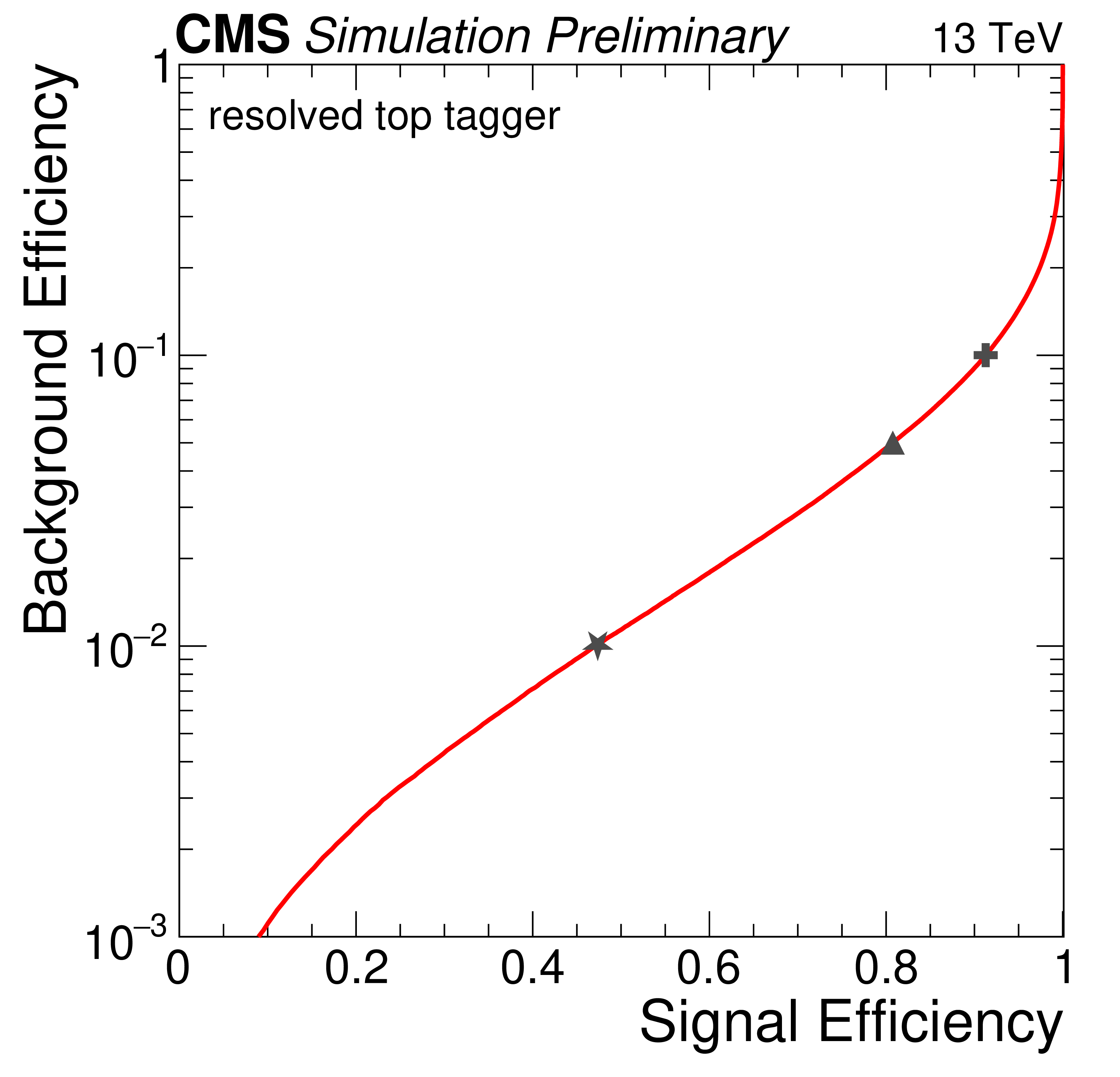
Figure 3:
Receiver operating characteristic curve of the ${\mathrm{t} ^{\text {res}}}$ tagger. The cross-, triangle-, and star-shaped markers indicate the loose, medium, and tight working points with 10$%$, 5$%$ and 1$%$ background misidentification probability. The corresponding identification efficiencies are 91$%$, 81$%$ and 47$%$, respectively. |
png pdf |
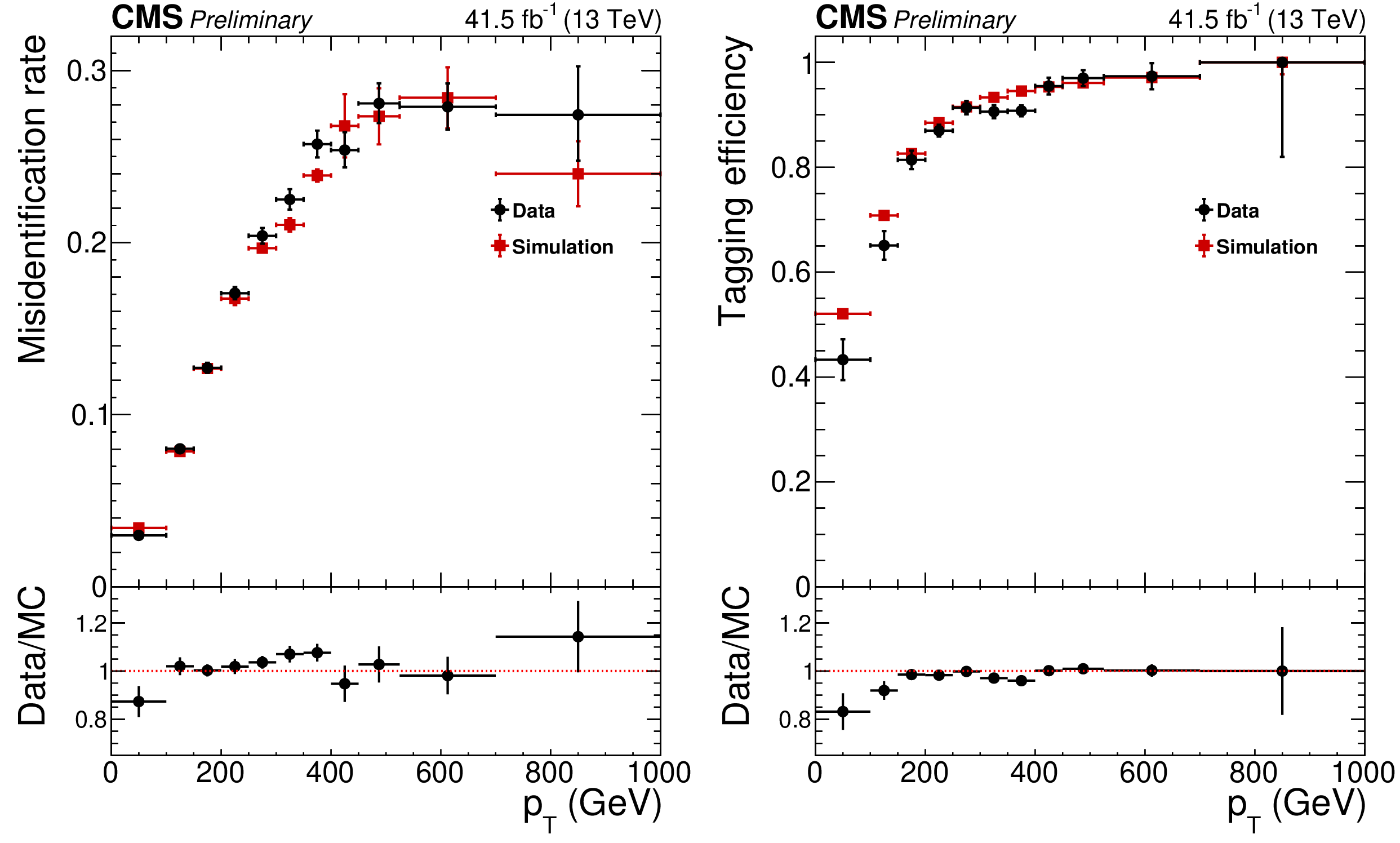
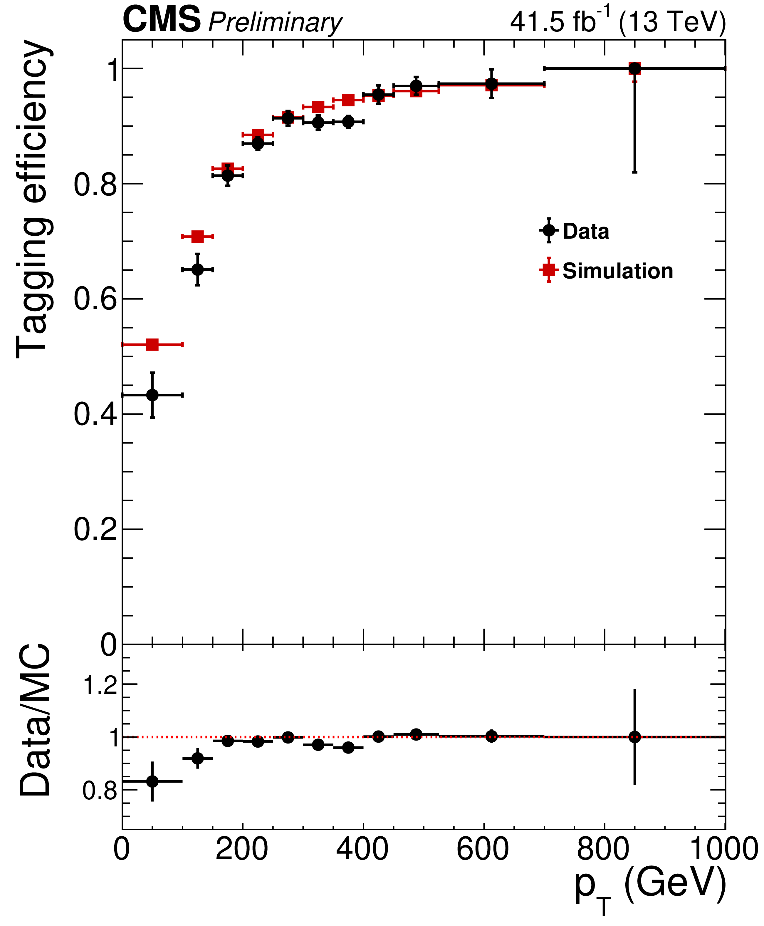
Figure 4:
Misidentification rate (left) and ${\mathrm{t} ^{\text {res}}}$-tagging efficiency (right) in data and simulation, as a function of the ${\mathrm{t} ^{\text {res}}}$-candidate ${p_{\mathrm {T}}}$ for the loose working point, using the 2017 data. |

png pdf |
Figure 4-a:
Misidentification rate (left) and ${\mathrm{t} ^{\text {res}}}$-tagging efficiency (right) in data and simulation, as a function of the ${\mathrm{t} ^{\text {res}}}$-candidate ${p_{\mathrm {T}}}$ for the loose working point, using the 2017 data. |
png pdf |
Figure 4-b:
Misidentification rate (left) and ${\mathrm{t} ^{\text {res}}}$-tagging efficiency (right) in data and simulation, as a function of the ${\mathrm{t} ^{\text {res}}}$-candidate ${p_{\mathrm {T}}}$ for the loose working point, using the 2017 data. |

png pdf |
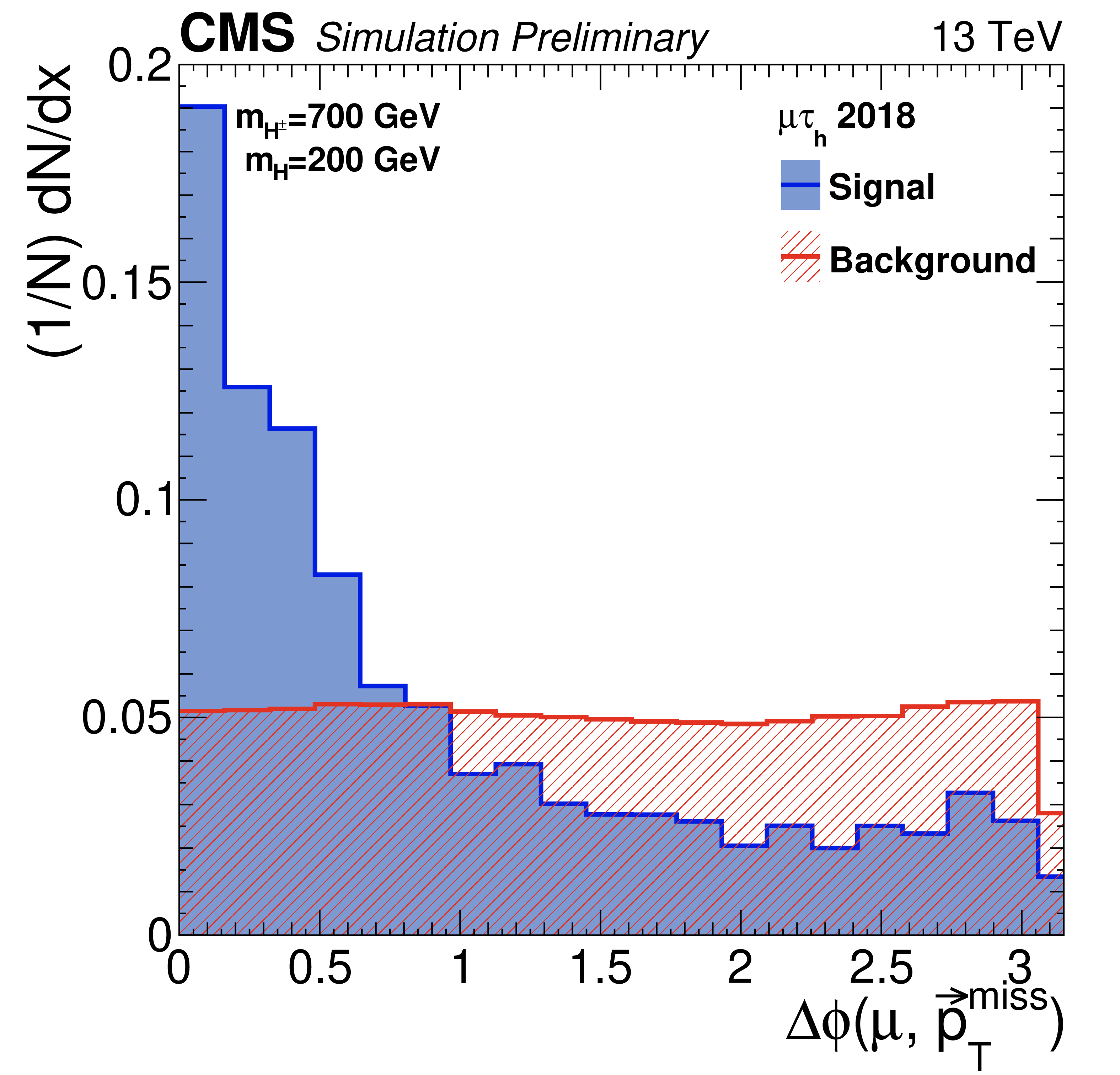
Figure 5:
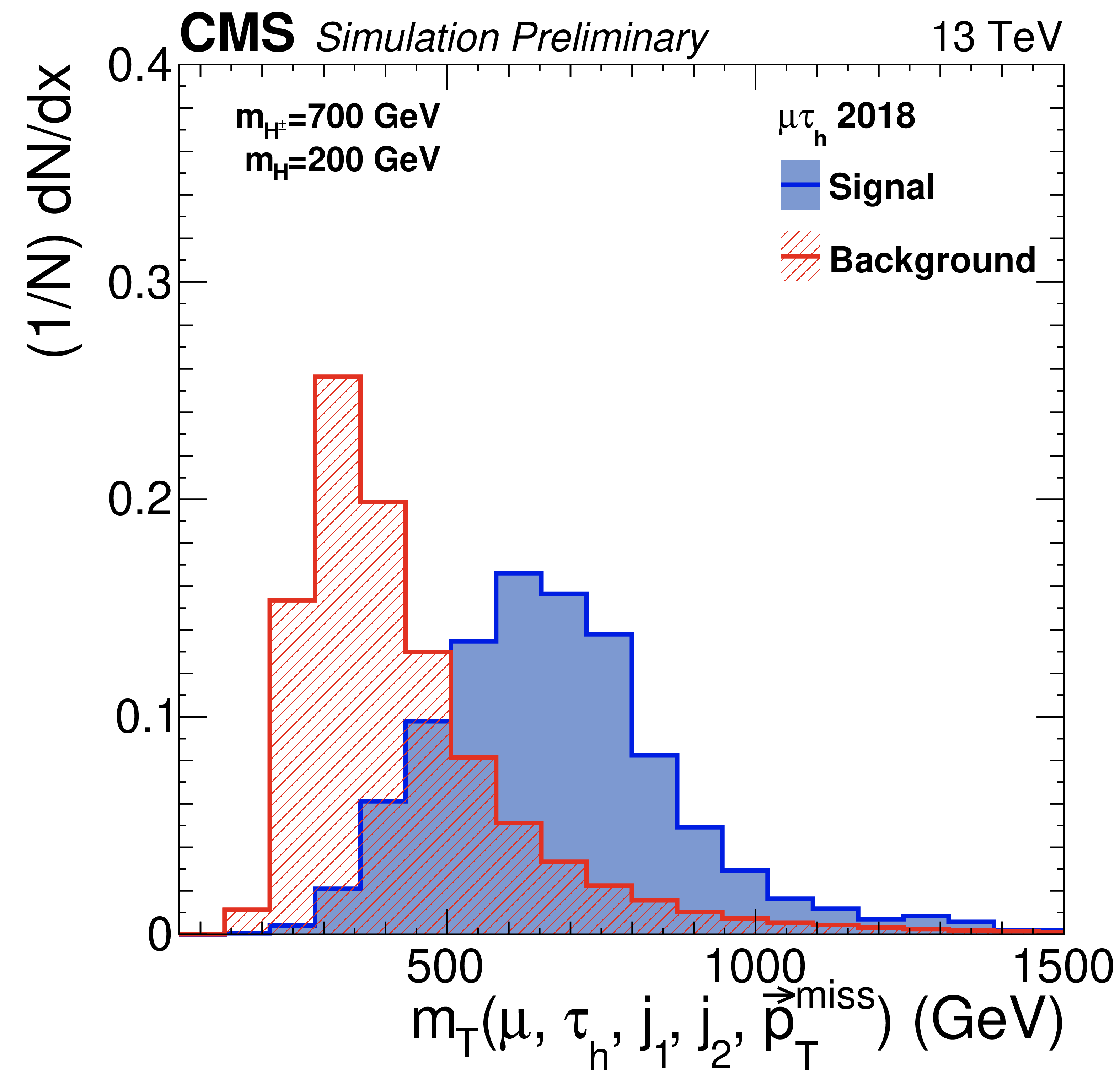
Three of the BDTG input variables used for the ${\mu {\tau _\mathrm {h}}}$ final state, assuming a signal with mass $m_{{\mathrm{\tilde{H}^{\pm_j}}}} = $ 700 GeV and 2018 data-taking conditions; the azimuthal angle between the $\mu $ and ${\vec{p}}_{\mathrm {T}}^{\,\text {miss}}$ objects (left), the ratio of the ${p_{\mathrm {T}}}$ of the third leading jet and the ${H_{\mathrm {T}}}$ (middle), and the transverse mass reconstructed from the $\mu $, $\tau _\mathrm {h}$, $j_{1}$, $j_{2}$, and ${\vec{p}}_{\mathrm {T}}^{\,\text {miss}}$ objects (right). Both signal and background distributions are normalized to unit area. |
png pdf |
Figure 5-a:
Three of the BDTG input variables used for the ${\mu {\tau _\mathrm {h}}}$ final state, assuming a signal with mass $m_{{\mathrm{\tilde{H}^{\pm_j}}}} = $ 700 GeV and 2018 data-taking conditions; the azimuthal angle between the $\mu $ and ${\vec{p}}_{\mathrm {T}}^{\,\text {miss}}$ objects (left), the ratio of the ${p_{\mathrm {T}}}$ of the third leading jet and the ${H_{\mathrm {T}}}$ (middle), and the transverse mass reconstructed from the $\mu $, $\tau _\mathrm {h}$, $j_{1}$, $j_{2}$, and ${\vec{p}}_{\mathrm {T}}^{\,\text {miss}}$ objects (right). Both signal and background distributions are normalized to unit area. |

png pdf |
Figure 5-b:
Three of the BDTG input variables used for the ${\mu {\tau _\mathrm {h}}}$ final state, assuming a signal with mass $m_{{\mathrm{\tilde{H}^{\pm_j}}}} = $ 700 GeV and 2018 data-taking conditions; the azimuthal angle between the $\mu $ and ${\vec{p}}_{\mathrm {T}}^{\,\text {miss}}$ objects (left), the ratio of the ${p_{\mathrm {T}}}$ of the third leading jet and the ${H_{\mathrm {T}}}$ (middle), and the transverse mass reconstructed from the $\mu $, $\tau _\mathrm {h}$, $j_{1}$, $j_{2}$, and ${\vec{p}}_{\mathrm {T}}^{\,\text {miss}}$ objects (right). Both signal and background distributions are normalized to unit area. |
png pdf |
Figure 5-c:
Three of the BDTG input variables used for the ${\mu {\tau _\mathrm {h}}}$ final state, assuming a signal with mass $m_{{\mathrm{\tilde{H}^{\pm_j}}}} = $ 700 GeV and 2018 data-taking conditions; the azimuthal angle between the $\mu $ and ${\vec{p}}_{\mathrm {T}}^{\,\text {miss}}$ objects (left), the ratio of the ${p_{\mathrm {T}}}$ of the third leading jet and the ${H_{\mathrm {T}}}$ (middle), and the transverse mass reconstructed from the $\mu $, $\tau _\mathrm {h}$, $j_{1}$, $j_{2}$, and ${\vec{p}}_{\mathrm {T}}^{\,\text {miss}}$ objects (right). Both signal and background distributions are normalized to unit area. |
png pdf |
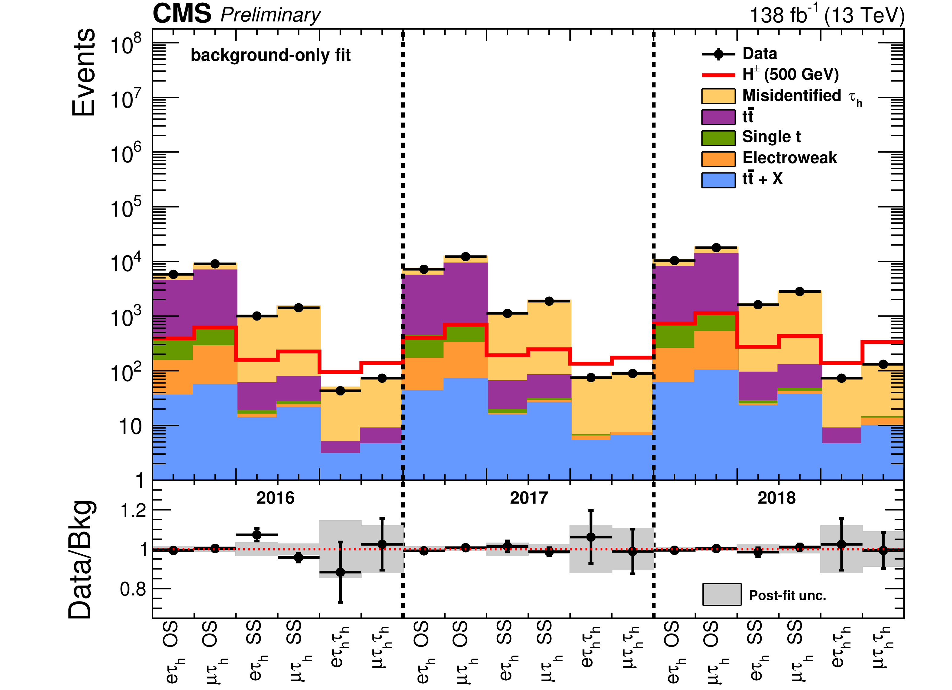
Figure 6:
Observed event yields (black markers) for the 18 categories considered in this analysis, grouped into data sets that are represented by vertical dashed lines. The expected event yields (stacked histograms) resulting from a background-only fit to the data are also shown, broken down into various background processes. The solid red line represents the expected signal yields from ${{\mathrm{\tilde{H}^{\pm_j}}} \to \mathrm{H} \mathrm{W^{\pm}}}$ with masses $m_{{\mathrm{\tilde{H}^{\pm_j}}}} = $ 500 GeV and $ {m_{\mathrm{H}}} = $ 200 GeV, assuming $ {\sigma _{{\mathrm{\tilde{H}^{\pm_j}}}} {\mathcal {B}({{\mathrm{\tilde{H}^{\pm_j}}} \to \mathrm{H} \mathrm{W^{\pm}}}, {\mathrm{H} \to \tau \tau})}}= $ 1 pb. |
png pdf |
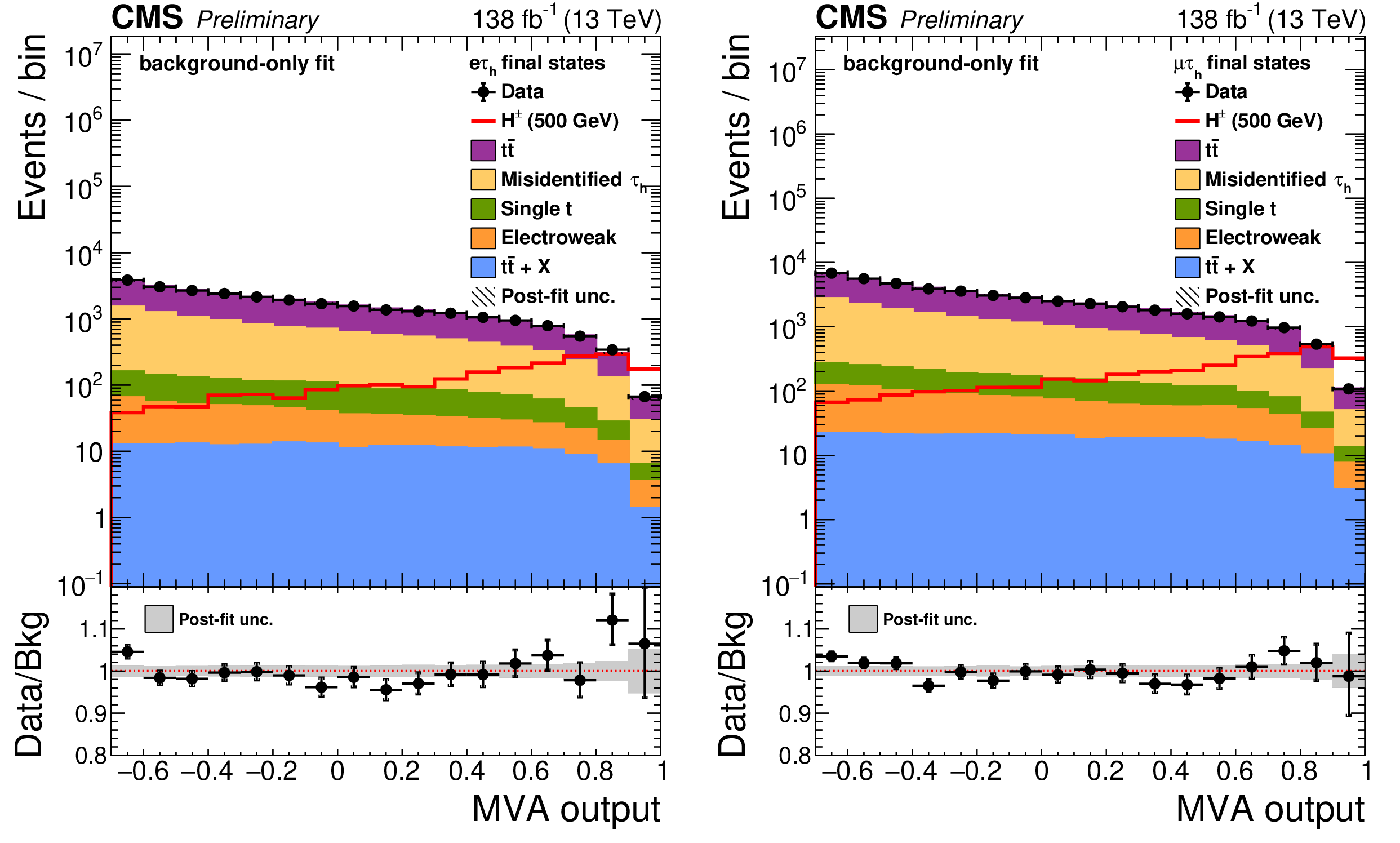
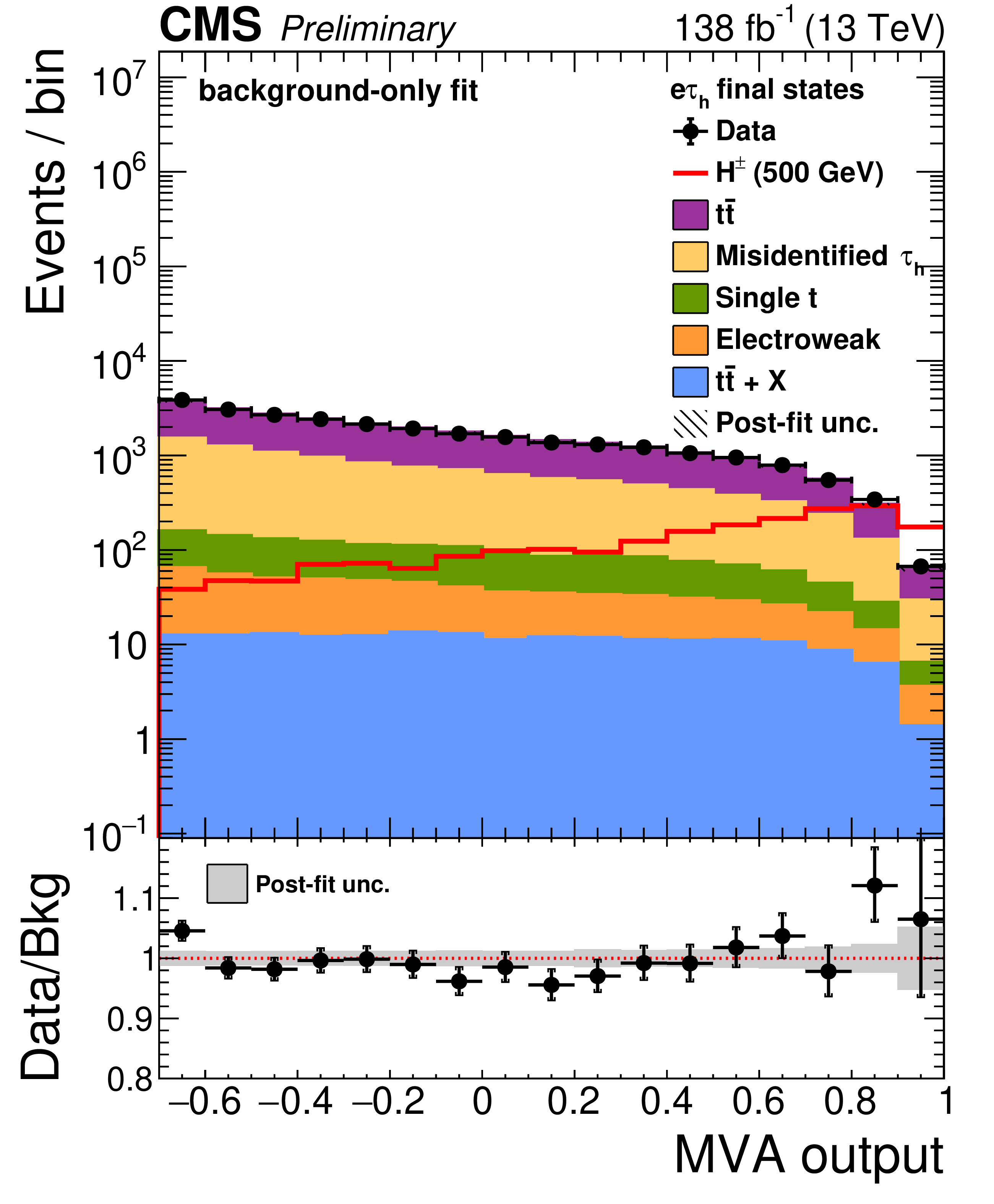
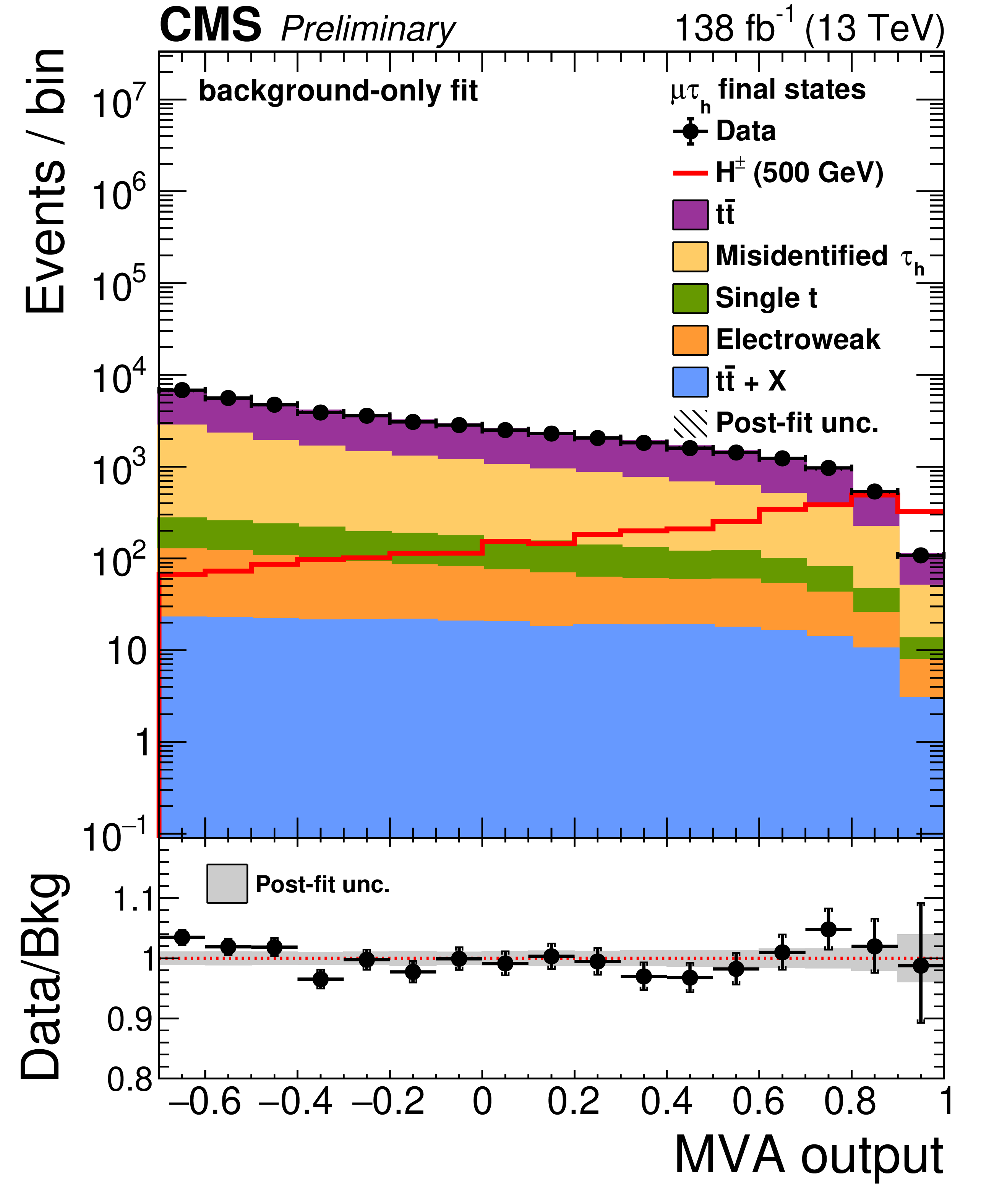
Figure 7:
The MVA\ output of the BDTG for the e${\tau _\mathrm {h}}$ (left) and ${\mu {\tau _\mathrm {h}}}$ (right) final states used in the limit extraction, after a background-only fit to the data. The data sets of all years and all categories have been added. The prefit contribution from ${{\mathrm{\tilde{H}^{\pm_j}}} \to \mathrm{H} \mathrm{W^{\pm}}}$ with masses ${m_{{\mathrm{\tilde{H}^{\pm_j}}}}} = $ 500 GeV and $ {m_{\mathrm{H}}} = $ 200 GeV and $ {\sigma _{{\mathrm{\tilde{H}^{\pm_j}}}} {\mathcal {B}({{\mathrm{\tilde{H}^{\pm_j}}} \to \mathrm{H} \mathrm{W^{\pm}}}, {\mathrm{H} \to \tau \tau})}}= $ 1 pb is also shown. |
png pdf |
Figure 7-a:
The MVA\ output of the BDTG for the e${\tau _\mathrm {h}}$ (left) and ${\mu {\tau _\mathrm {h}}}$ (right) final states used in the limit extraction, after a background-only fit to the data. The data sets of all years and all categories have been added. The prefit contribution from ${{\mathrm{\tilde{H}^{\pm_j}}} \to \mathrm{H} \mathrm{W^{\pm}}}$ with masses ${m_{{\mathrm{\tilde{H}^{\pm_j}}}}} = $ 500 GeV and $ {m_{\mathrm{H}}} = $ 200 GeV and $ {\sigma _{{\mathrm{\tilde{H}^{\pm_j}}}} {\mathcal {B}({{\mathrm{\tilde{H}^{\pm_j}}} \to \mathrm{H} \mathrm{W^{\pm}}}, {\mathrm{H} \to \tau \tau})}}= $ 1 pb is also shown. |
png pdf |
Figure 7-b:
The MVA\ output of the BDTG for the e${\tau _\mathrm {h}}$ (left) and ${\mu {\tau _\mathrm {h}}}$ (right) final states used in the limit extraction, after a background-only fit to the data. The data sets of all years and all categories have been added. The prefit contribution from ${{\mathrm{\tilde{H}^{\pm_j}}} \to \mathrm{H} \mathrm{W^{\pm}}}$ with masses ${m_{{\mathrm{\tilde{H}^{\pm_j}}}}} = $ 500 GeV and $ {m_{\mathrm{H}}} = $ 200 GeV and $ {\sigma _{{\mathrm{\tilde{H}^{\pm_j}}}} {\mathcal {B}({{\mathrm{\tilde{H}^{\pm_j}}} \to \mathrm{H} \mathrm{W^{\pm}}}, {\mathrm{H} \to \tau \tau})}}= $ 1 pb is also shown. |

png pdf |
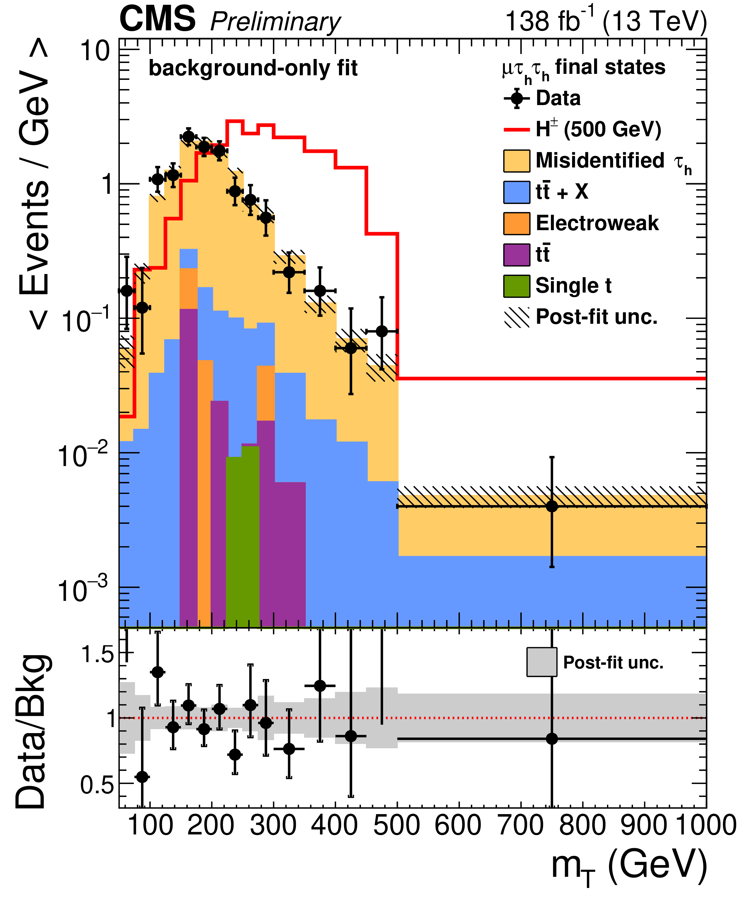
Figure 8:
The $m_{\mathrm {T}}$ distributions for the e${\tau _\mathrm {h}} {\tau _\mathrm {h}}$ (left) and $\mu {\tau _\mathrm {h}} {\tau _\mathrm {h}}$ (right) final states used in the limit extraction, after a background-only fit to the data. The data sets of all years have been added. The prefit contribution from ${{\mathrm{\tilde{H}^{\pm_j}}} \to \mathrm{H} \mathrm{W^{\pm}}}$ with masses ${m_{{\mathrm{\tilde{H}^{\pm_j}}}}} = $ 500 GeV and $ {m_{\mathrm{H}}} = $ 200 GeV and $ {\sigma _{{\mathrm{\tilde{H}^{\pm_j}}}} {\mathcal {B}({{\mathrm{\tilde{H}^{\pm_j}}} \to \mathrm{H} \mathrm{W^{\pm}}}, {\mathrm{H} \to \tau \tau})}}= $ 1 pb is also shown. |

png pdf |
Figure 8-a:
The $m_{\mathrm {T}}$ distributions for the e${\tau _\mathrm {h}} {\tau _\mathrm {h}}$ (left) and $\mu {\tau _\mathrm {h}} {\tau _\mathrm {h}}$ (right) final states used in the limit extraction, after a background-only fit to the data. The data sets of all years have been added. The prefit contribution from ${{\mathrm{\tilde{H}^{\pm_j}}} \to \mathrm{H} \mathrm{W^{\pm}}}$ with masses ${m_{{\mathrm{\tilde{H}^{\pm_j}}}}} = $ 500 GeV and $ {m_{\mathrm{H}}} = $ 200 GeV and $ {\sigma _{{\mathrm{\tilde{H}^{\pm_j}}}} {\mathcal {B}({{\mathrm{\tilde{H}^{\pm_j}}} \to \mathrm{H} \mathrm{W^{\pm}}}, {\mathrm{H} \to \tau \tau})}}= $ 1 pb is also shown. |
png pdf |
Figure 8-b:
The $m_{\mathrm {T}}$ distributions for the e${\tau _\mathrm {h}} {\tau _\mathrm {h}}$ (left) and $\mu {\tau _\mathrm {h}} {\tau _\mathrm {h}}$ (right) final states used in the limit extraction, after a background-only fit to the data. The data sets of all years have been added. The prefit contribution from ${{\mathrm{\tilde{H}^{\pm_j}}} \to \mathrm{H} \mathrm{W^{\pm}}}$ with masses ${m_{{\mathrm{\tilde{H}^{\pm_j}}}}} = $ 500 GeV and $ {m_{\mathrm{H}}} = $ 200 GeV and $ {\sigma _{{\mathrm{\tilde{H}^{\pm_j}}}} {\mathcal {B}({{\mathrm{\tilde{H}^{\pm_j}}} \to \mathrm{H} \mathrm{W^{\pm}}}, {\mathrm{H} \to \tau \tau})}}= $ 1 pb is also shown. |
png pdf |
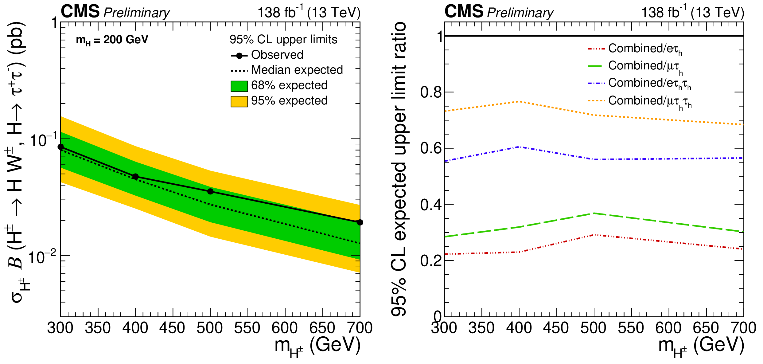
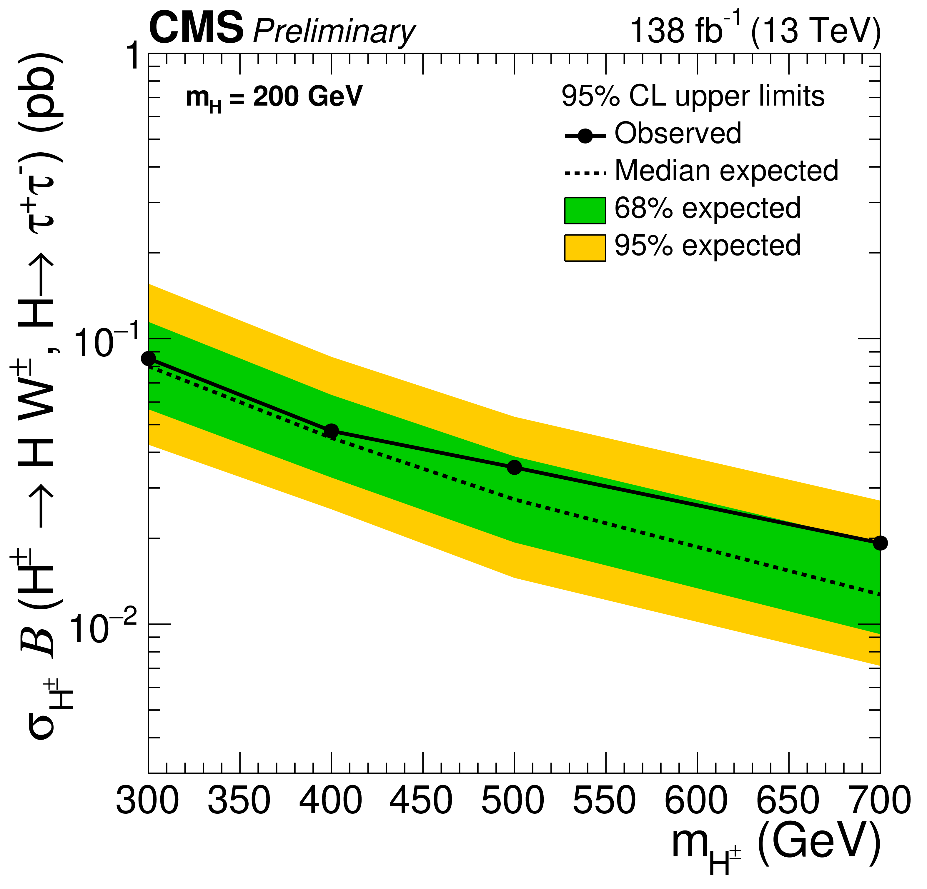
Figure 9:
Expected and observed upper limits at 95% CL on the product of cross section and branching fraction $ {\sigma _{{\mathrm{\tilde{H}^{\pm_j}}}} {\mathcal {B}({{\mathrm{\tilde{H}^{\pm_j}}} \to \mathrm{H} \mathrm{W^{\pm}}}, {\mathrm{H} \to \tau \tau})}}$ as a function of $m_{{\mathrm{\tilde{H}^{\pm_j}}}}$ and assuming $ {m_{\mathrm{H}}} = $ 200 GeV for the combination of all final states considered (left). The observed upper limits are represented by a solid black line and circle markers. The median expected limit (dashed line), 68% (inner green band), and 95% (outer yellow band) confidence intervals are also shown. The relative expected contributions of each final state to the overall combination are also presented (right). The black solid line corresponds to the combined expected limit, while the red dash-dotted, green dashed, blue dashed-dotted, and orange dashed lines represent the relative contributions from the e${\tau _\mathrm {h}}$, $\mu {\tau _\mathrm {h}}$, e${\tau _\mathrm {h}} {\tau _\mathrm {h}}$, and $\mu {\tau _\mathrm {h}} {\tau _\mathrm {h}}$ channels, respectively. |
png pdf |
Figure 9-a:
Expected and observed upper limits at 95% CL on the product of cross section and branching fraction $ {\sigma _{{\mathrm{\tilde{H}^{\pm_j}}}} {\mathcal {B}({{\mathrm{\tilde{H}^{\pm_j}}} \to \mathrm{H} \mathrm{W^{\pm}}}, {\mathrm{H} \to \tau \tau})}}$ as a function of $m_{{\mathrm{\tilde{H}^{\pm_j}}}}$ and assuming $ {m_{\mathrm{H}}} = $ 200 GeV for the combination of all final states considered (left). The observed upper limits are represented by a solid black line and circle markers. The median expected limit (dashed line), 68% (inner green band), and 95% (outer yellow band) confidence intervals are also shown. The relative expected contributions of each final state to the overall combination are also presented (right). The black solid line corresponds to the combined expected limit, while the red dash-dotted, green dashed, blue dashed-dotted, and orange dashed lines represent the relative contributions from the e${\tau _\mathrm {h}}$, $\mu {\tau _\mathrm {h}}$, e${\tau _\mathrm {h}} {\tau _\mathrm {h}}$, and $\mu {\tau _\mathrm {h}} {\tau _\mathrm {h}}$ channels, respectively. |
png pdf |
Figure 9-b:
Expected and observed upper limits at 95% CL on the product of cross section and branching fraction $ {\sigma _{{\mathrm{\tilde{H}^{\pm_j}}}} {\mathcal {B}({{\mathrm{\tilde{H}^{\pm_j}}} \to \mathrm{H} \mathrm{W^{\pm}}}, {\mathrm{H} \to \tau \tau})}}$ as a function of $m_{{\mathrm{\tilde{H}^{\pm_j}}}}$ and assuming $ {m_{\mathrm{H}}} = $ 200 GeV for the combination of all final states considered (left). The observed upper limits are represented by a solid black line and circle markers. The median expected limit (dashed line), 68% (inner green band), and 95% (outer yellow band) confidence intervals are also shown. The relative expected contributions of each final state to the overall combination are also presented (right). The black solid line corresponds to the combined expected limit, while the red dash-dotted, green dashed, blue dashed-dotted, and orange dashed lines represent the relative contributions from the e${\tau _\mathrm {h}}$, $\mu {\tau _\mathrm {h}}$, e${\tau _\mathrm {h}} {\tau _\mathrm {h}}$, and $\mu {\tau _\mathrm {h}} {\tau _\mathrm {h}}$ channels, respectively. |
| Tables | |
png pdf |
Table 1:
Offline selections applied to the reconstructed objects to obtain the SRs of the ${\ell {\tau _\mathrm {h}}}$ and ${\ell {\tau _\mathrm {h}} {\tau _\mathrm {h}}}$ final states. The ${p_{\mathrm {T}}}$, ${{p_{\mathrm {T}}} ^\text {miss}}$, and ${S_{\mathrm {T}}}$ variables are reported in units of GeV, and ${Q_{}}$ in units of $e$. Selection criteria that depend on the year of data taking are presented in parentheses with the order corresponding to (2016, 2017, 2018). The symbol $\star $ is used to represent an electron (muon) for the e${\tau _\mathrm {h}}$ ($\mu {\tau _\mathrm {h}}$) final states, and a ${\tau _\mathrm {h}}$ object in the e${\tau _\mathrm {h}} {\tau _\mathrm {h}}$ and $\mu {\tau _\mathrm {h}} {\tau _\mathrm {h}}$ final states. |
png pdf |
Table 2:
Offline selections applied to the reconstructed objects to obtain the CRs and VRs for the misidentified ${\tau _\mathrm {h}}$ estimation in the ${\ell {\tau _\mathrm {h}}}$ and ${\ell {\tau _\mathrm {h}} {\tau _\mathrm {h}}}$ final states. Only differences with respect to the corresponding SRs are shown. The ${p_{\mathrm {T}}}$, ${{p_{\mathrm {T}}} ^\text {miss}}$, and ${S_{\mathrm {T}}}$ variables are reported in units of GeV, and ${Q_{}}$ in units of $e$. The symbol $\star $ is used to represent an electron (muon) for the e${\tau _\mathrm {h}}$ ($\mu {\tau _\mathrm {h}}$) final states, and a ${\tau _\mathrm {h}}$ object in the e${\tau _\mathrm {h}} {\tau _\mathrm {h}}$ and $\mu {\tau _\mathrm {h}} {\tau _\mathrm {h}}$ final states. |

png pdf |
Table 3:
Variables included in the training of the BDTG used for the ${\ell {\tau _\mathrm {h}}}$ final states and $ {m_{{\mathrm{\tilde{H}^{\pm_j}}}}} = $ 700 GeV, in descending order of post-training ranking. It is derived by counting how often the variables are used to split decision tree nodes, and by weighting each split occurrence by the separation gain squared it has achieved and by the number of events in the node. |
png pdf |
Table 4:
Summary of all sources of systematic uncertainties, for all categories considered. Their impact on the expected event yields is presented as a percentage% and is evaluated before simultaneous fitting the data for the background-only hypothesis. They describe the effect of each nuisance parameter on the overall normalization of the signal model or the total background. The quoted range represents the minimum and maximum values observed through the different samples and data eras. Nuisance parameters with a check mark (v) also affect the shape of the fit discriminant shape, while those marked with a dash (---) do not. |
| Summary |
| Results are presented from a search for a charged Higgs boson ${{\mathrm{\tilde{H}^{\pm_j}}}}$ decaying into a heavy neutral Higgs boson H and a W boson, a first such effort carried out by an LHC experiment. Events are selected with exactly one isolated electron or muon, targeting event topologies whereby the H boson decays into a pair of tau leptons with at least one decaying hadronically. Four distinct final states are considered; e${\tau_\mathrm{h}}$, $\mu{\tau_\mathrm{h}}$, e${\tau_\mathrm{h}}{\tau_\mathrm{h}}$, and $\mu{\tau_\mathrm{h}}{\tau_\mathrm{h}}$. The analysis uses proton-proton collision data recorded by the CMS detector at $\sqrt{s} = $ 13 TeV, corresponding to an integrated luminosity of 138 fb$^{-1}$. No significant deviation is observed from standard model expectations. Upper limits at 95% confidence level are set on the product of the ${{\mathrm{\tilde{H}^{\pm_j}}}}$ production cross section and its branching fraction to $\mathrm{H}\mathrm{W^{\pm}}$ with ${H_{\mathrm{T}}}$. The observed limit is found to range from 0.080 to 0.013 pb for ${{\mathrm{\tilde{H}^{\pm_j}}}}$ masses in the range of 300 to 700 GeV, assuming an H with a mass of 200 GeV. |
| References | ||||
| 1 | P. W. Higgs | Broken symmetries, massless particles and gauge fields | PL12 (1964) 132 | |
| 2 | P. W. Higgs | Broken symmetries and the masses of gauge bosons | PRL 13 (1964) 508 | |
| 3 | G. S. Guralnik, C. R. Hagen, and T. W. B. Kibble | Global conservation laws and massless particles | PRL 13 (1964) 585 | |
| 4 | F. Englert and R. Brout | Broken symmetry and the mass of gauge vector mesons | PRL 13 (1964) 321 | |
| 5 | P. W. Higgs | Spontaneous symmetry breakdown without massless bosons | PR145 (1966) 1156 | |
| 6 | T. W. B. Kibble | Symmetry breaking in non-Abelian gauge theories | PR155 (1967) 1554 | |
| 7 | ATLAS Collaboration | Observation of a new particle in the search for the standard model Higgs boson with the ATLAS detector at the LHC | PLB 716 (2012) 1 | 1207.7214 |
| 8 | CMS Collaboration | Observation of a new boson at a mass of 125 GeV with the CMS experiment at the LHC | PLB 716 (2012) 30 | CMS-HIG-12-028 1207.7235 |
| 9 | CMS Collaboration | Observation of a new boson with mass near 125 GeV in $ {\mathrm{p}}{\mathrm{p}} $ collisions at $ \sqrt{s} = $ 7 and 8 TeV | JHEP 06 (2013) 081 | CMS-HIG-12-036 1303.4571 |
| 10 | ATLAS and CMS Collaborations | Measurements of the Higgs boson production and decay rates and constraints on its couplings from a combined ATLAS and CMS analysis of the LHC pp collision data at $ \sqrt{s} = $ 7 and 8 TeV | JHEP 08 (2016) 045 | 1606.02266 |
| 11 | CMS Collaboration | Combined measurements of Higgs boson couplings in proton-proton collisions at $ \sqrt{s}=$ 13 TeV | EPJC 79 (2019) 421 | CMS-HIG-17-031 1809.10733 |
| 12 | ATLAS Collaboration | Combined measurements of Higgs boson production and decay using up to 80 fb$ ^{-1} $ of proton-proton collision data at $ \sqrt{s}= $ 13 TeV collected with the ATLAS experiment | PRD 101 (2020) 012002 | 1909.02845 |
| 13 | CMS Collaboration | Measurements of the Higgs boson width and anomalous $ \mathrm{H}\mathrm{V}\mathrm{V} $ couplings from on-shell and off-shell production in the four-lepton final state | PRD 99 (2019) 112003 | CMS-HIG-18-002 1901.00174 |
| 14 | J. F. Gunion and H. E. Haber | The CP conserving two Higgs doublet model: the approach to the decoupling limit | PRD 67 (2003) 075019 | hep-ph/0207010 |
| 15 | A. G. Akeroyd et al. | Prospects for charged Higgs searches at the LHC | EPJC 77 (2017) 276 | 1607.01320 |
| 16 | G. C. Branco et al. | Theory and phenomenology of two-Higgs-doublet models | PR 516 (2012) 1 | 1106.0034 |
| 17 | N. Craig and S. Thomas | Exclusive signals of an extended Higgs sector | JHEP 11 (2012) 083 | 1207.4835 |
| 18 | M. Carena, I. Low, N. R. Shah, and C. E. M. Wagner | Impersonating the standard model Higgs boson: alignment without decoupling | JHEP 04 (2014) 015 | 1310.2248 |
| 19 | H. Bahl, T. Stefaniak, and J. Wittbrodt | The forgotten channels: charged Higgs boson decays to a $ {\mathrm{W^{\pm}}} $ and a non-SM-like Higgs boson | JHEP 06 (2021) | 2103.07484 |
| 20 | ATLAS Collaboration | Search for charged Higgs bosons decaying via $ {{\mathrm{\widetilde{H}^{\pm_j}}}} \rightarrow \tau^{\pm}\nu $ in fully hadronic final states using $ {\mathrm{p}}{\mathrm{p}} $ collision data at $ \sqrt{s} = $ 8 TeV with the ATLAS detector | JHEP 03 (2015) 088 | 1412.6663 |
| 21 | CMS Collaboration | Search for a charged Higgs boson in pp collisions at $ \sqrt{s} = $ 8 TeV | JHEP 11 (2015) 018 | CMS-HIG-14-023 1508.07774 |
| 22 | ATLAS Collaboration | Search for charged Higgs bosons decaying via $ {{\mathrm{\widetilde{H}^{\pm_j}}}} \to \tau^{\pm}\nu_{\tau} $ in the $ \tau $+jets and $ \tau $+lepton final states with 36 fb$ ^{-1} $ of $ {\mathrm{p}}{\mathrm{p}} $ collision data recorded at $ \sqrt{s} = $ 13 TeV with the ATLAS experiment | JHEP 09 (2018) 139 | 1807.07915 |
| 23 | CMS Collaboration | Search for charged Higgs bosons in the H$ ^{\pm} \to \tau^{\pm}\nu_\tau $ decay channel in proton-proton collisions at $ \sqrt{s} = $ 13 TeV | JHEP 07 (2019) 142 | CMS-HIG-18-014 1903.04560 |
| 24 | CMS Collaboration | Search for a light charged Higgs boson decaying to $ \mathrm{c}\overline{\mathrm{s}} $ in pp collisions at $ \sqrt{s} = $ 8 TeV | JHEP 12 (2015) 178 | CMS-HIG-13-035 1510.04252 |
| 25 | ATLAS Collaboration | Search for a light charged Higgs boson in the decay channel $ H^+ \to c\bar{s} $ in $ t\bar{t} $ events using pp collisions at $ \sqrt{s} = $ 7 TeV with the ATLAS detector | EPJC 73 (2013) 2465 | 1302.3694 |
| 26 | CMS Collaboration | Search for a charged Higgs boson decaying to charm and bottom quarks in proton-proton collisions at $ \sqrt{s} = $ 8 TeV | JHEP 11 (2018) 115 | CMS-HIG-16-030 1808.06575 |
| 27 | CMS Collaboration | Search for a light charged Higgs boson decaying to a W boson and a CP-odd Higgs boson in final states with e$ \mu\mu $ or $ \mu\mu\mu $ in proton-proton collisions at $ \sqrt{s} = $ 13 TeV | PRL 123 (2019), no. 13, 131802 | CMS-HIG-18-020 1905.07453 |
| 28 | ATLAS Collaboration | Search for charged Higgs bosons in the $ {{\mathrm{\widetilde{H}^{\pm_j}}}} \rightarrow tb $ decay channel in $ {\mathrm{p}}{\mathrm{p}} $ collisions at $ \sqrt{s} = $ 8 TeV using the ATLAS detector | JHEP 03 (2016) 127 | 1512.03704 |
| 29 | ATLAS Collaboration | Search for charged Higgs bosons decaying into top and bottom quarks at $ \sqrt{s} = $ 13 TeV with the ATLAS detector | JHEP 11 (2018) 085 | 1808.03599 |
| 30 | CMS Collaboration | Search for a charged Higgs boson decaying into top and bottom quarks in events with electrons or muons in proton-proton collisions at $ \sqrt{\mathrm{s}} = $ 13 TeV | JHEP 01 (2020) 096 | CMS-HIG-18-004 1908.09206 |
| 31 | ATLAS Collaboration | Search for charged Higgs bosons produced in association with a top quark and decaying via $ {{\mathrm{\widetilde{H}^{\pm_j}}}} \rightarrow \tau\nu $ using $ {\mathrm{p}}{\mathrm{p}} $ collision data recorded at $ \sqrt{s} = $ 13 TeV by the ATLAS detector | PLB 759 (2016) 555 | 1603.09203 |
| 32 | CMS Collaboration | Search for charged Higgs bosons decaying into a top and a bottom quark in the all-jet final state of pp collisions at $ \sqrt{s} = $ 13 TeV | JHEP 07 (2020) 126 | CMS-HIG-18-015 2001.07763 |
| 33 | BaBar and Belle Collaborations | The physics of the B factories | EPJC 74 (2014) 3026 | 1406.6311 |
| 34 | Belle II Collaboration | The Belle II Physics Book | PTEP 2019 (2019), no. 12, 123C01 | 1808.10567 |
| 35 | G. Senjanovic and R. N. Mohapatra | Exact left-right symmetry and spontaneous Violation of parity | PRD 12 (1975) 1502 | |
| 36 | J. F. Gunion, R. Vega, and J. Wudka | Higgs triplets in the standard model | PRD 42 (1990) 1673 | |
| 37 | H. Georgi and M. Machacek | Doubly charged Higgs bosons | NPB 262 (1985) 463 | |
| 38 | ATLAS Collaboration | Search for a charged Higgs boson produced in the vector-boson fusion mode with decay $ {{\mathrm{\widetilde{H}^{\pm_j}}}} \to \mathrm{W^{\pm}} \mathrm{Z} $ using $ {\mathrm{p}}{\mathrm{p}} $ collisions at $ \sqrt{s}= $ 8 TeV with the ATLAS experiment | PRL 114 (2015), no. 23, 231801 | 1503.04233 |
| 39 | CMS Collaboration | Search for charged Higgs bosons produced via vector boson fusion and decaying into a pair of W and Z bosons using pp collisions at $ \sqrt{s} = $ 13 TeV | PRL 119 (2017) 141802 | CMS-HIG-16-027 1705.02942 |
| 40 | CMS Collaboration | Observation of electroweak production of same-sign W boson pairs in the two jet and two same-sign lepton final state in proton-proton collisions at $ \sqrt{s} = $ 13 TeV | PRL 120 (2018) 081801 | CMS-SMP-17-004 1709.05822 |
| 41 | CMS Collaboration | Search for charged Higgs bosons produced in vector boson fusion processes and decaying into vector boson pairs in proton-proton collisions at $ \sqrt{s} = 13 { TeV} $ | EPJC 81 (2021), no. 8, 723 | CMS-HIG-20-017 2104.04762 |
| 42 | ATLAS Collaboration | Search for dijet resonances in events with an isolated charged lepton using $ \sqrt{s} = $ 13 TeV proton-proton collision data collected by the ATLAS detector | JHEP 06 (2020) 151 | 2002.11325 |
| 43 | CMS Collaboration | The CMS trigger system | JINST 12 (2017) P01020 | CMS-TRG-12-001 1609.02366 |
| 44 | CMS Collaboration | Performance of the CMS Level-1 trigger in proton-proton collisions at $ \sqrt{s} = $ 13 TeV | JINST 15 (2020) P10017 | CMS-TRG-17-001 2006.10165 |
| 45 | CMS Collaboration | The CMS experiment at the CERN LHC | JINST 3 (2008) S08004 | CMS-00-001 |
| 46 | J. Alwall et al. | The automated computation of tree-level and next-to-leading order differential cross sections, and their matching to parton shower simulations | JHEP 07 (2014) 079 | 1405.0301 |
| 47 | P. Artoisenet, R. Frederix, O. Mattelaer, and R. Rietkerk | Automatic spin-entangled decays of heavy resonances in Monte Carlo simulations | JHEP 03 (2013) 015 | 1212.3460 |
| 48 | P. Nason | A new method for combining NLO QCD with shower Monte Carlo algorithms | JHEP 11 (2004) 040 | hep-ph/0409146 |
| 49 | S. Frixione, P. Nason, and C. Oleari | Matching NLO QCD computations with parton shower simulations: the POWHEG method | JHEP 11 (2007) 070 | 0709.2092 |
| 50 | S. Alioli, P. Nason, C. Oleari, and E. Re | A general framework for implementing NLO calculations in shower monte carlo programs: the POWHEG BOX | JHEP 06 (2010) 043 | 1002.2581 |
| 51 | S. Alioli et al. | Jet pair production in POWHEG | JHEP 04 (2011) 081 | 1012.3380 |
| 52 | S. Alioli, P. Nason, C. Oleari, and E. Re | NLO Higgs boson production via gluon fusion matched with shower in POWHEG | JHEP 04 (2009) 002 | 0812.0578 |
| 53 | E. Bagnaschi, G. Degrassi, P. Slavich, and A. Vicini | Higgs production via gluon fusion in the POWHEG approach in the SM and in the MSSM | JHEP 02 (2012) 088 | 1111.2854 |
| 54 | M. Czakon and A. Mitov | Top++: A program for the calculation of the top-pair cross-section at hadron colliders | CPC 185 (2014) | 1112.5675 |
| 55 | R. Frederix, E. Re, and P. Torrielli | Single-top $ t $-channel hadroproduction in the four-flavour scheme with POWHEG and aMC@NLO | JHEP 09 (2012) 130 | 1207.5391 |
| 56 | E. Re | Single-top W$ t $-channel production matched with parton showers using the POWHEG method | EPJC 71 (2011) 1547 | 1009.2450 |
| 57 | H. B. Hartanto, B. Jager, L. Reina, and D. Wackeroth | Higgs boson production in association with top quarks in the POWHEG BOX | PRD 91 (2015) 094003 | 1501.04498 |
| 58 | T. Sjostrand et al. | An introduction to PYTHIA 8.2 | CPC 191 (2015) 159 | 1410.3012 |
| 59 | J. Alwall et al. | Comparative study of various algorithms for the merging of parton showers and matrix elements in hadronic collisions | EPJC 53 (2008) | 0706.2569 |
| 60 | R. Frederix and S. Frixione | Merging meets matching in MC@NLO | JHEP 12 (2012) | 1209.6215 |
| 61 | NNPDF Collaboration | Parton distributions for the LHC Run II | JHEP 04 (2015) 040 | 1410.8849 |
| 62 | NNPDF Collaboration | Parton distributions from high-precision collider data | EPJC 77 (2017) | 1706.00428 |
| 63 | CMS Collaboration | Event generator tunes obtained from underlying event and multiparton scattering measurements | EPJC 76 (2016) 155 | CMS-GEN-14-001 1512.00815 |
| 64 | CMS Collaboration | Extraction and validation of a new set of CMS Pythia8 tunes from underlying-event measurements | EPJC 80 (2020) 4 | |
| 65 | GEANT4 Collaboration | GEANT4--a simulation toolkit | NIMA 506 (2003) 250 | |
| 66 | CMS Collaboration | Particle-flow reconstruction and global event description with the CMS detector | JINST 12 (2017) P10003 | CMS-PRF-14-001 1706.04965 |
| 67 | CMS Collaboration | Technical proposal for the Phase-II upgrade of the Compact Muon Solenoid | CMS-PAS-TDR-15-002 | CMS-PAS-TDR-15-002 |
| 68 | CMS Collaboration | Performance of electron reconstruction and selection with the CMS detector in proton-proton collisions at $ \sqrt{s} = $ 8 TeV | JINST 10 (2015) P06005 | CMS-EGM-13-001 1502.02701 |
| 69 | CMS Collaboration | Performance of the CMS muon detector and muon reconstruction with proton-proton collisions at $ \sqrt{s}= $ 13 TeV | JINST 13 (2018) P06015 | CMS-MUO-16-001 1804.04528 |
| 70 | M. Cacciari, G. P. Salam, and G. Soyez | The anti-$ {k_{\mathrm{T}}} $ jet clustering algorithm | JHEP 04 (2008) 063 | 0802.1189 |
| 71 | M. Cacciari, G. P. Salam, and G. Soyez | FastJet user manual | EPJC 72 (2012) 1896 | 1111.6097 |
| 72 | CMS Collaboration | Pileup mitigation at CMS in 13 TeV data | JINST 15 (2020) P09018 | CMS-JME-18-001 2003.00503 |
| 73 | CMS Collaboration | Jet energy scale and resolution in the CMS experiment in pp collisions at 8 TeV | JINST 12 (2017) P02014 | CMS-JME-13-004 1607.03663 |
| 74 | E. Bols et al. | Jet flavour classification using DeepJet | JINST 15 (2020) P12012 | 2008.10519 |
| 75 | CMS Collaboration | Performance of the DeepJet b tagging algorithm using 41.9 fb$ ^{-1} $ of data from proton-proton collisions at 13 TeV with Phase 1 CMS detector | CDS | |
| 76 | CMS Collaboration | Identification of heavy-flavour jets with the CMS detector in pp collisions at 13 TeV | JINST 13 (2018) P05011 | CMS-BTV-16-002 1712.07158 |
| 77 | CMS Collaboration | Performance of reconstruction and identification of $ \tau $ leptons decaying to hadrons and $ \nu_\tau $ in pp collisions at $ \sqrt{s}= $ 13 TeV | JINST 13 (2018) P10005 | CMS-TAU-16-003 1809.02816 |
| 78 | CMS Collaboration | Identification of hadronic tau lepton decays using a deep neural network | Submitted to JINST | CMS-TAU-20-001 2201.08458 |
| 79 | CMS Collaboration | Performance of the DeepTau algorithm for the discrimination of taus against jets, electron, and muons | CDS | |
| 80 | CMS Collaboration | Performance of missing transverse momentum reconstruction in proton-proton collisions at $ \sqrt{s} = $ 13 TeV using the CMS detector | JINST 14 (2019) P07004 | CMS-JME-17-001 1903.06078 |
| 81 | F. Chollet et al. | Keras: Deep learning library for theano and tensorflow | URL: https://keras. io/k 7 (2015), no. 8, T1 | |
| 82 | M. Abadi et al. | TensorFlow: Large-scale machine learning on heterogeneous systems | 2015 Software available from tensorflow.org. \url https://www.tensorflow.org/ | |
| 83 | F. Pedregosa et al. | Scikit-learn: Machine learning in Python | Journal of Machine Learning Research 12 (2011) 2825--2830 | |
| 84 | A. Hocker et al. | TMVA - Toolkit for Multivariate Data Analysis | physics/0703039 | |
| 85 | R. J. Barlow and C. Beeston | Fitting using finite Monte Carlo samples | CPC 77 (1993) 219 | |
| 86 | J. S. Conway | Incorporating Nuisance Parameters in Likelihoods for Multisource Spectra | in PHYSTAT 2011 3 | 1103.0354 |
| 87 | CMS Collaboration | Precision luminosity measurement in proton-proton collisions at $ \sqrt{s} = $ 13 TeV in 2015 and 2016 at CMS | EPJC 81 (2021) 800 | CMS-LUM-17-003 2104.01927 |
| 88 | CMS Collaboration | CMS luminosity measurement for the 2017 data-taking period at $ \sqrt{s} = $ 13 TeV | CMS-PAS-LUM-17-004 | |
| 89 | CMS Collaboration | CMS luminosity measurement for the 2018 data-taking period at $ \sqrt{s} = $ 13 TeV | CMS-PAS-LUM-18-002 | |
| 90 | LHC Higgs Cross Section Working Group Collaboration | Handbook of LHC Higgs Cross Sections: 3. Higgs Properties | 1307.1347 | |
| 91 | LHC Higgs Cross Section Working Group | Handbook of LHC Higgs cross sections: 4. deciphering the nature of the Higgs sector | CERN (2016) | 1610.07922 |
| 92 | J. Butterworth et al. | PDF4LHC recommendations for LHC Run II | JPG 43 (2016) 023001 | 1510.03865 |
| 93 | T. Junk | Confidence level computation for combining searches with small statistics | NIMA 434 (1999) | hep-ex/9902006 |
| 94 | A. L. Read | Presentation of search results: The CL$ _{\text{s}} $ technique | JPG 28 (2002) 2693 | |
| 95 | CMS Collaboration | Combined results of searches for the standard model Higgs boson in $ {\mathrm{p}}{\mathrm{p}} $ collisions at $ \sqrt{s} = $ 7 TeV | PLB 710 (2012) 26 | CMS-HIG-11-032 1202.1488 |
| 96 | G. Cowan, K. Cranmer, E. Gross, and O. Vitells | Asymptotic formulae for likelihood-based tests of new physics | EPJC 71 (2011) 1554 | 1007.1727 |
|
|
Compact Muon Solenoid LHC, CERN |
|

|

|

|

|

|