

Compact Muon Solenoid
LHC, CERN
| CMS-PAS-HIG-20-010 | ||
| Search for nonresonant Higgs boson pair production in final states with two bottom quarks and two tau leptons in proton-proton collisions at $\sqrt{s} = $ 13 TeV | ||
| CMS Collaboration | ||
| March 2022 | ||
| Abstract: A search for the nonresonant production of Higgs boson pairs (HH) via gluon-gluon and vector boson fusion processes in final states with two bottom quarks and two tau leptons is presented. The search uses data from proton-proton collisions at a center-of-mass energy of $\sqrt{s}= $ 13 TeV recorded with the CMS detector at the LHC, corresponding to an integrated luminosity of 138 fb$^{-1}$. Events in which at least one tau lepton decays hadronically are considered and multiple machine learning techniques are used to identify and extract the signal. The data are found to be consistent, within uncertainties, with the standard model background predictions. Upper limits on the HH production cross section are set to constrain the parameter space for anomalous Higgs boson couplings. The observed (expected) upper limit at 95% confidence level corresponds to 3.3 (5.2) times the standard model prediction for the inclusive HH cross section and to 124 (154) times the standard model prediction for the vector boson fusion HH cross section. At a 95% confidence level, the Higgs field self-coupling is constrained to be within $-$1.8 and 8.8 times the standard model expectation, and the coupling of two Higgs bosons to two vector bosons is constrained to be within $-$0.4 and 2.6. | ||
|
Links:
CDS record (PDF) ;
CADI line (restricted) ;
These preliminary results are superseded in this paper, Submitted to PLB. The superseded preliminary plots can be found here. |
||
| Figures & Tables | Summary | Additional Figures | References | CMS Publications |
|---|
| Figures | |
png pdf |
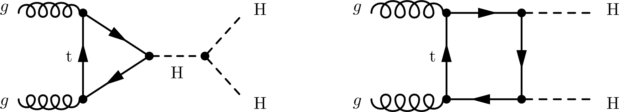
Figure 1:
Feynman diagrams contributing to Higgs boson pair production via gluon-gluon fusion in the SM at leading order. |
png pdf |
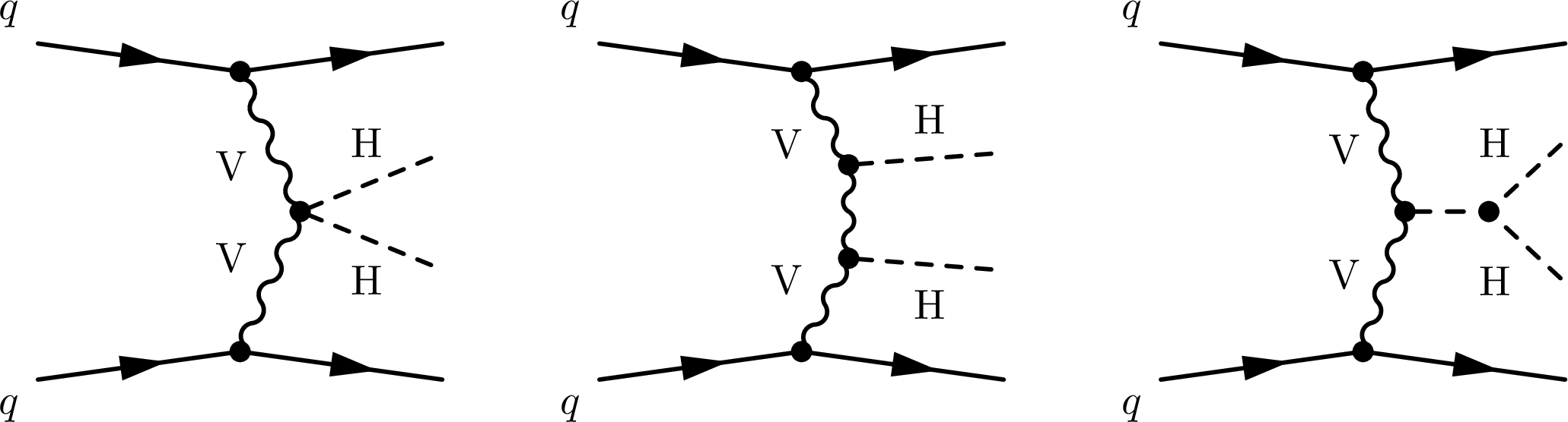
Figure 2:
Feynman diagrams contributing to Higgs boson pair production via vector boson fusion in the SM at leading order. |
png pdf |
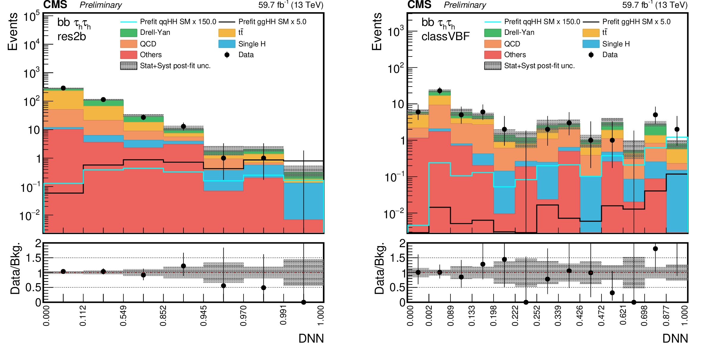
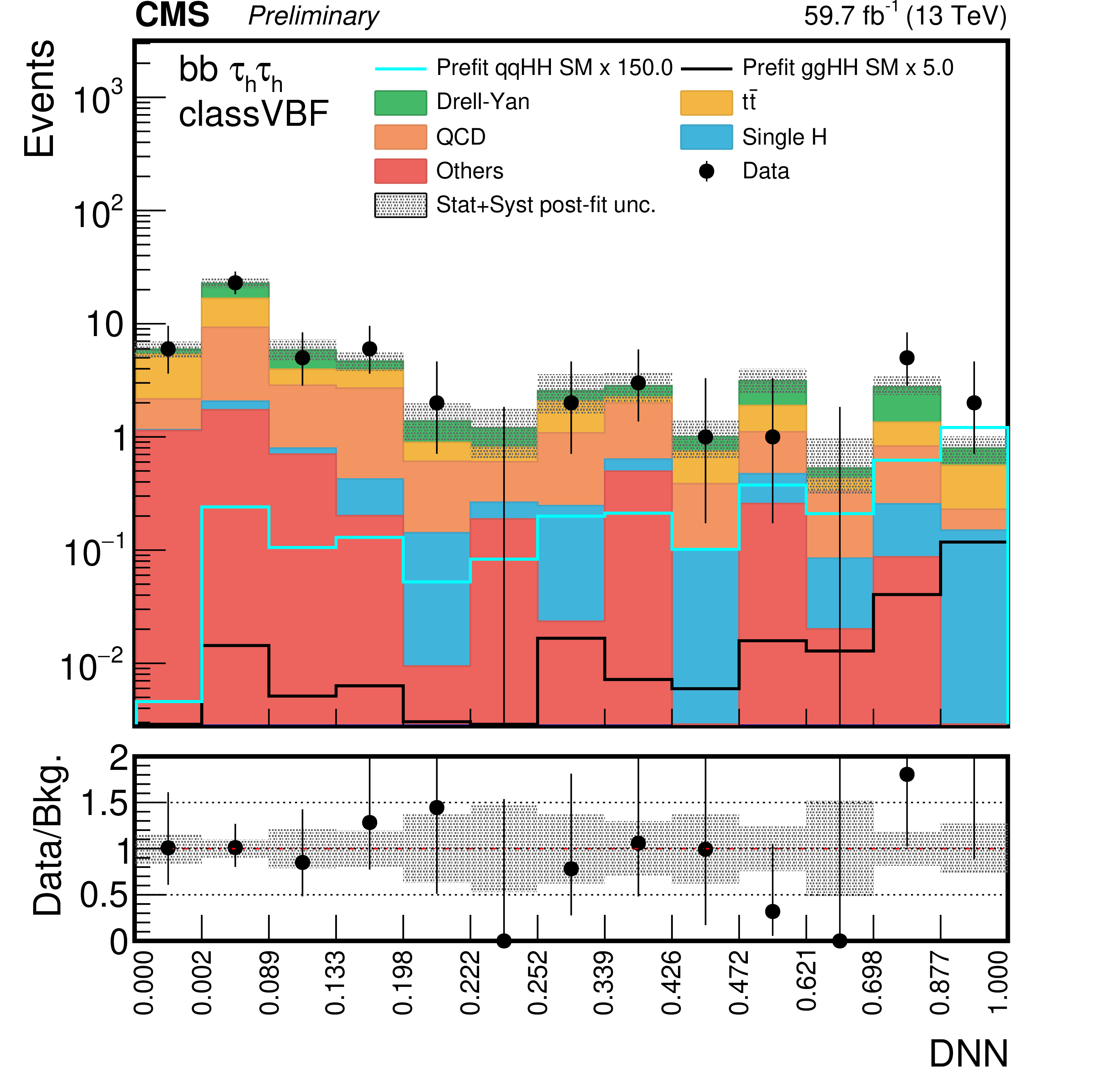
Figure 3:
DNN prediction distributions in the ${\tau _{{\text h}}\tau _{{\text h}}}$ channel in 2018 for the most sensitive category in the ggF (left) and VBF (right) searches. The shaded band in the plots represents the statistical plus systematic uncertainty. |
png pdf |
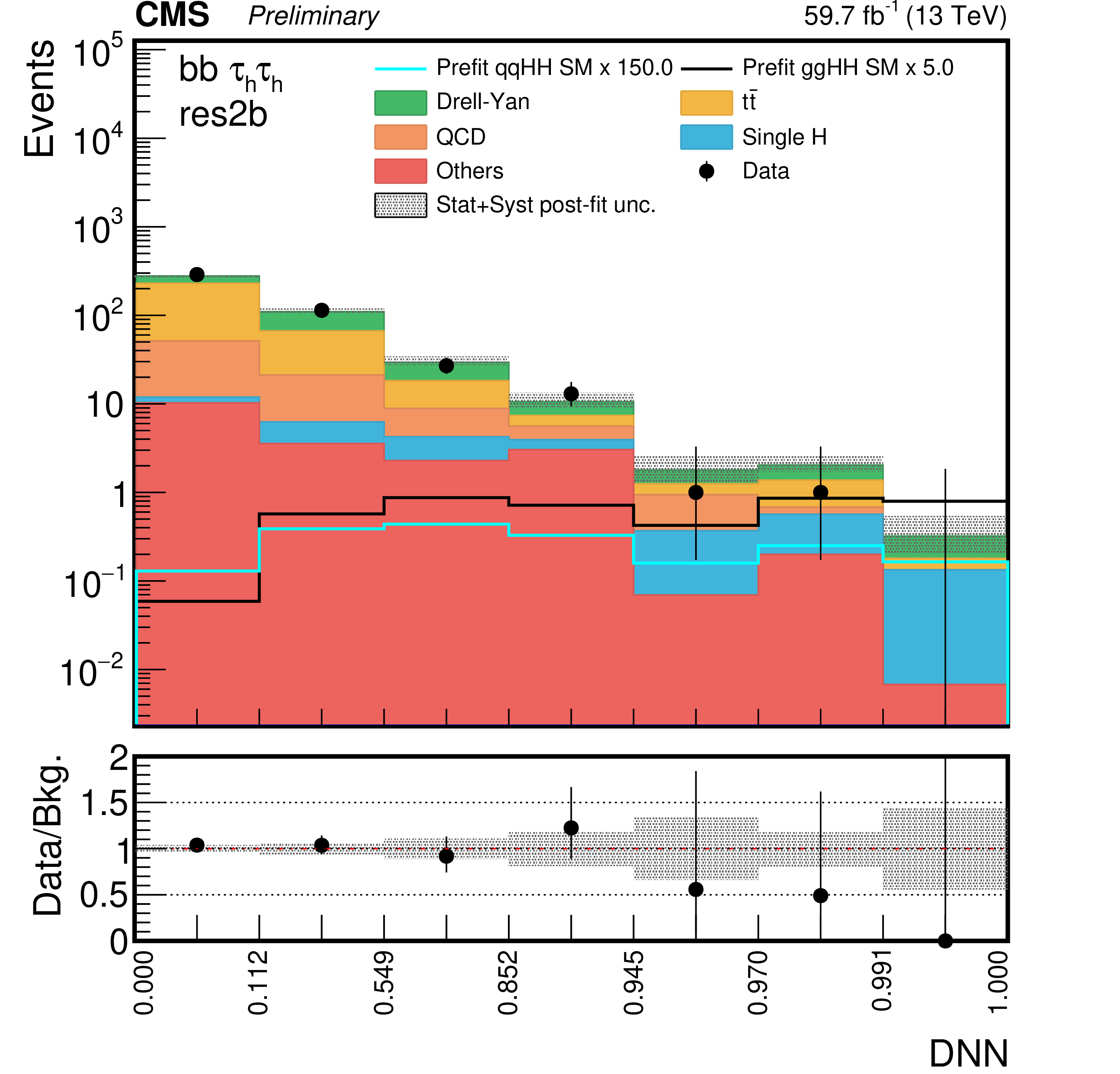
Figure 3-a:
DNN prediction distributions in the ${\tau _{{\text h}}\tau _{{\text h}}}$ channel in 2018 for the most sensitive category in the ggF search. The shaded band in the plots represents the statistical plus systematic uncertainty. |
png pdf |
Figure 3-b:
DNN prediction distributions in the ${\tau _{{\text h}}\tau _{{\text h}}}$ channel in 2018 for the most sensitive category in the VBF search. The shaded band in the plots represents the statistical plus systematic uncertainty. |
png pdf |
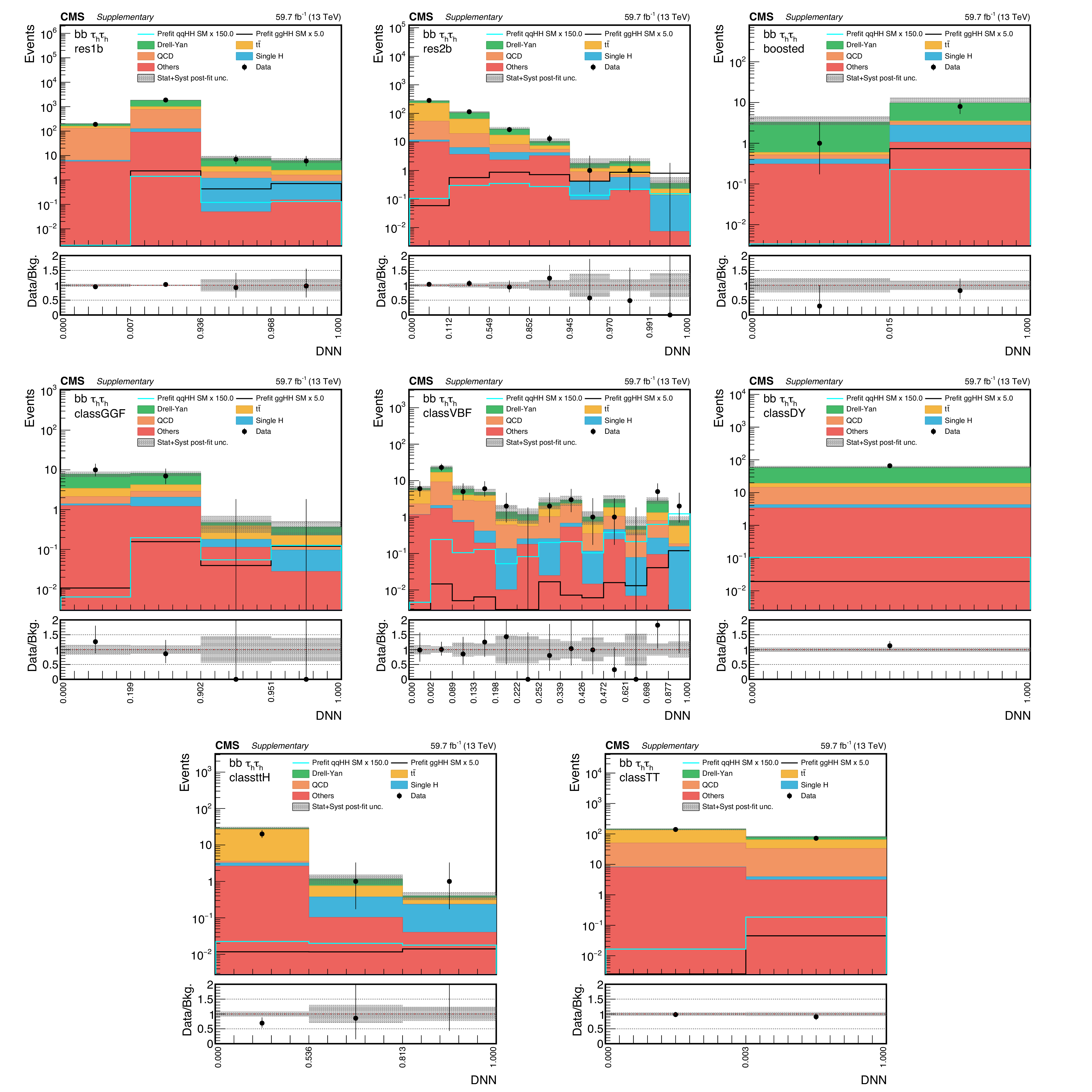
Figure 4:
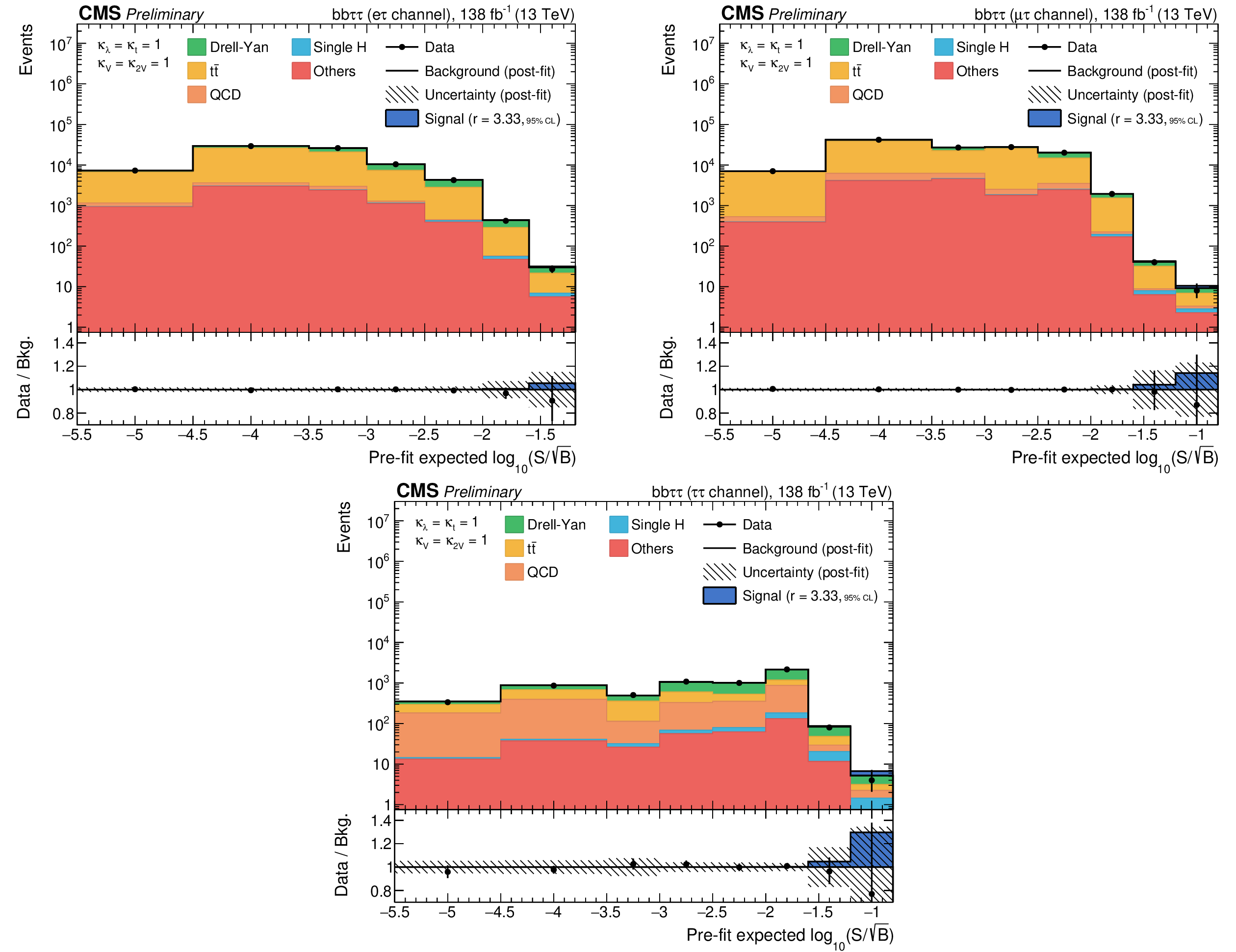
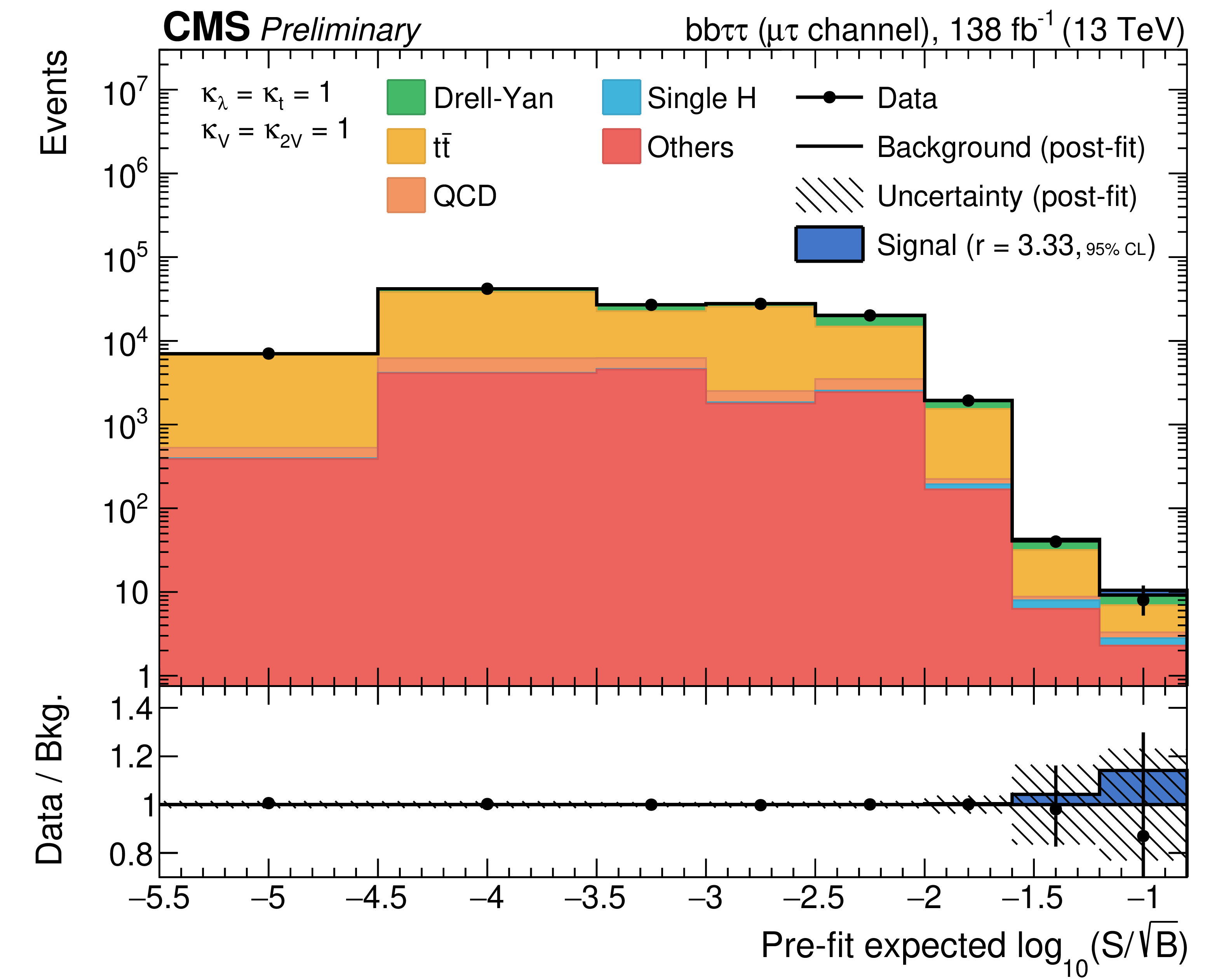
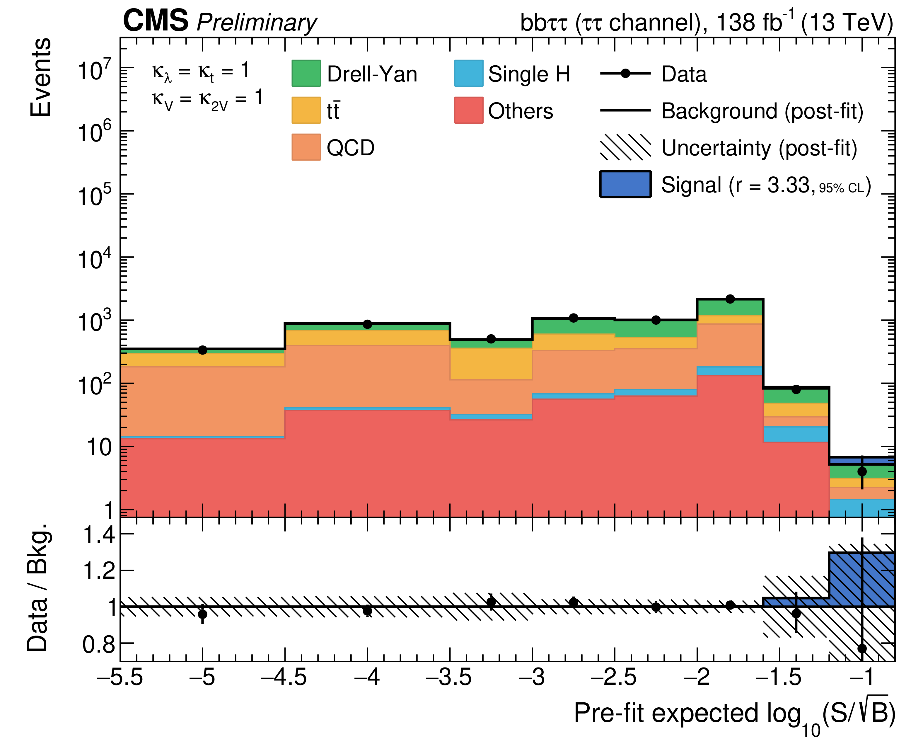
Combination of bins of all postfit distributions, ordered and merged according to their prefit signal-to-background ratio, separately for the ${\tau _{\mathrm{e}} \tau _{{\text h}}}$ channel (top left), the ${\tau _{\mu} \tau _{{\text h}}}$ channel (top right), and ${\tau _{{\text h}}\tau _{{\text h}}}$ channel (bottom). The ratio also shows the signal scaled to the observed exclusion limit (see Table 2). |

png pdf |
Figure 4-a:
Combination of bins of all postfit distributions, ordered and merged according to their prefit signal-to-background ratio, separately for the ${\tau _{\mathrm{e}} \tau _{{\text h}}}$ channel. The ratio also shows the signal scaled to the observed exclusion limit (see Table 2). |
png pdf |
Figure 4-b:
Combination of bins of all postfit distributions, ordered and merged according to their prefit signal-to-background ratio, separately for the ${\tau _{\mu} \tau _{{\text h}}}$ channel. The ratio also shows the signal scaled to the observed exclusion limit (see Table 2). |
png pdf |
Figure 4-c:
Combination of bins of all postfit distributions, ordered and merged according to their prefit signal-to-background ratio, separately for the ${\tau _{{\text h}}\tau _{{\text h}}}$ channel. The ratio also shows the signal scaled to the observed exclusion limit (see Table 2). |

png pdf |
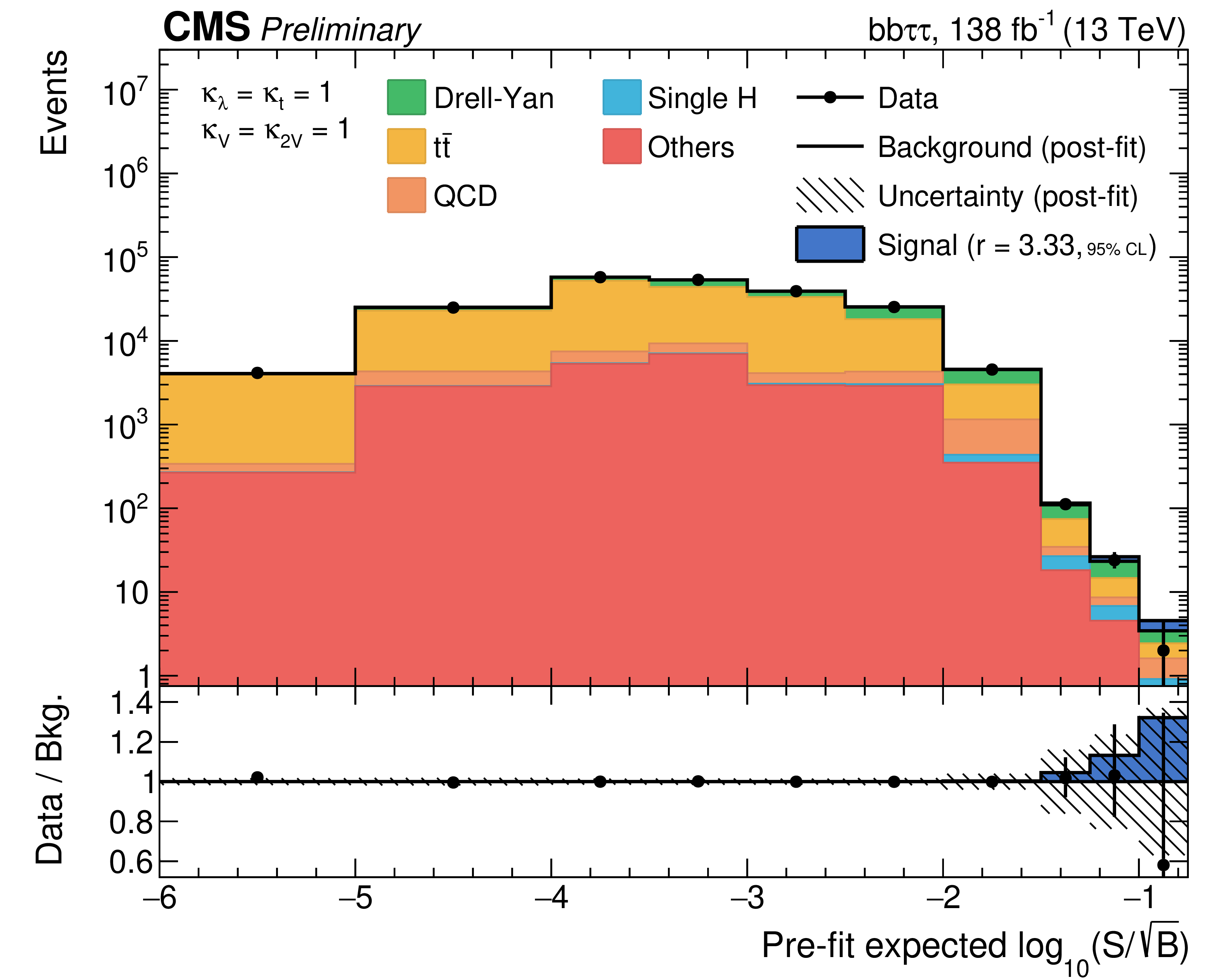
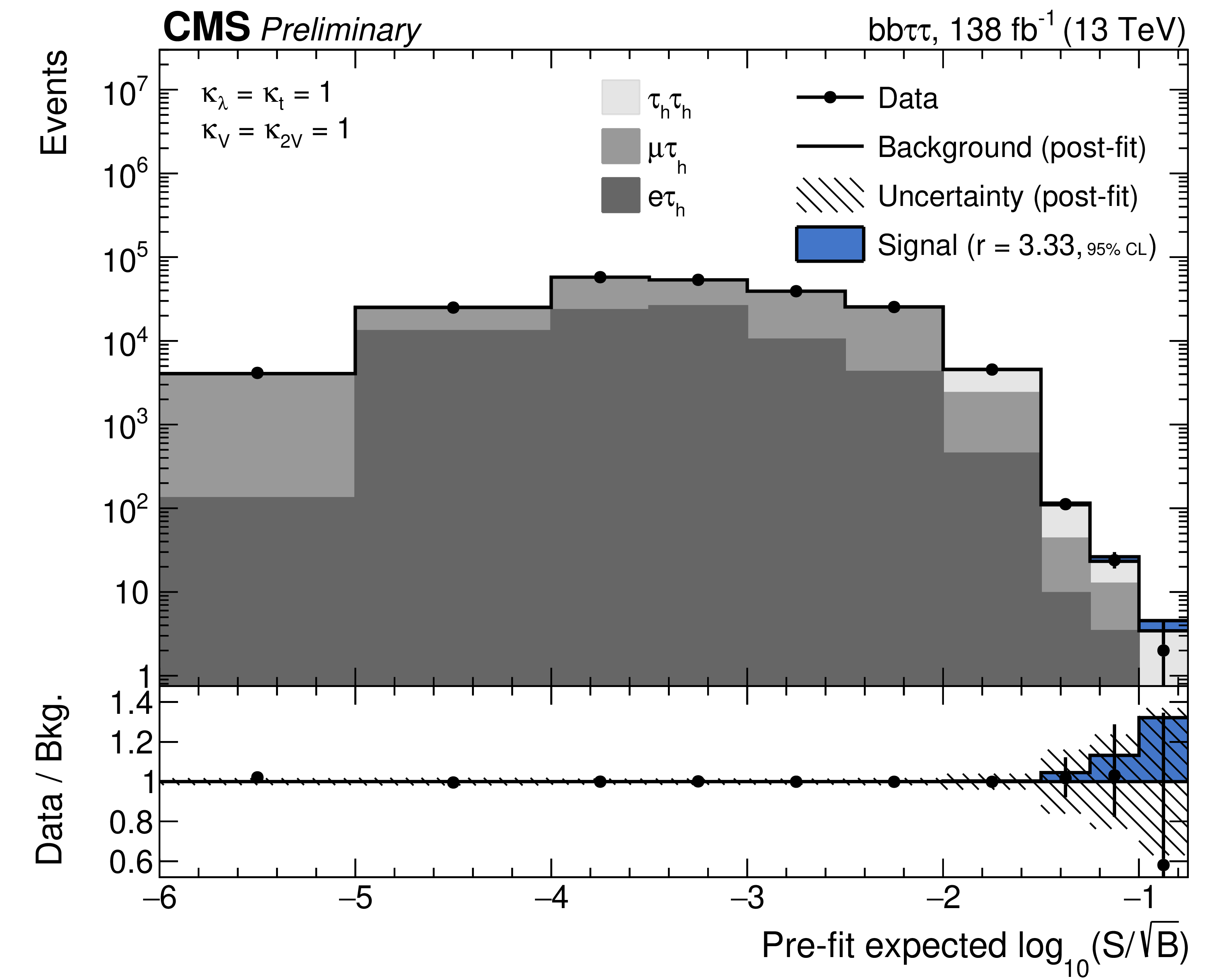
Figure 5:
Combination of bins of all postfit distributions, ordered and merged according to their prefit signal-to-background ratio, separately for the background contribution split into physics processes (left), and split into the three considered final state channels (right). The ratio also shows the signal scaled to the observed exclusion limit (see Table 2). |
png pdf |
Figure 5-a:
Combination of bins of all postfit distributions, ordered and merged according to their prefit signal-to-background ratio, separately for the background contribution split into physics processes. The ratio also shows the signal scaled to the observed exclusion limit (see Table 2). |
png pdf |
Figure 5-b:
Combination of bins of all postfit distributions, ordered and merged according to their prefit signal-to-background ratio, separately for the background contribution split into the three considered final state channels. The ratio also shows the signal scaled to the observed exclusion limit (see Table 2). |
png pdf |
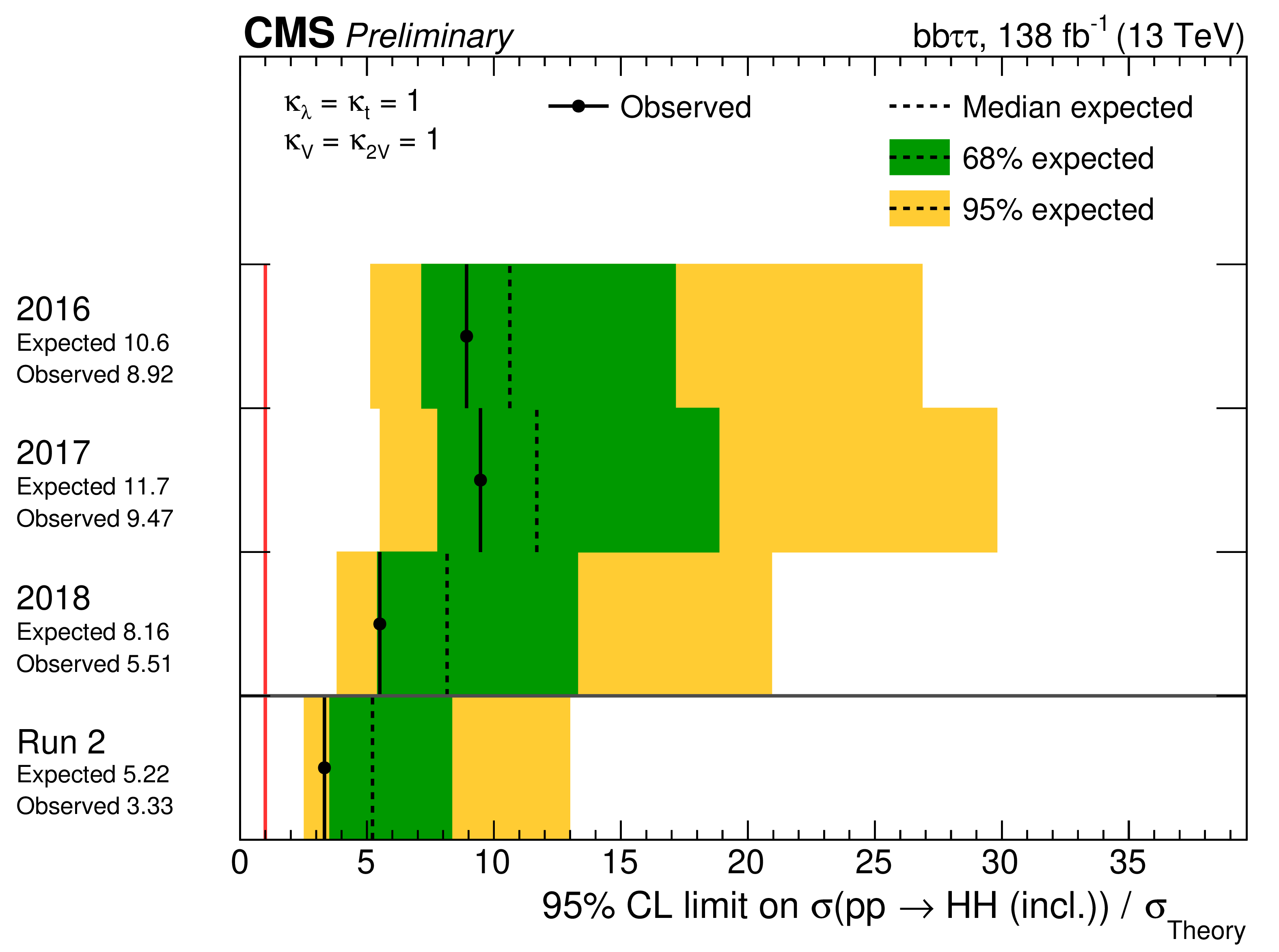
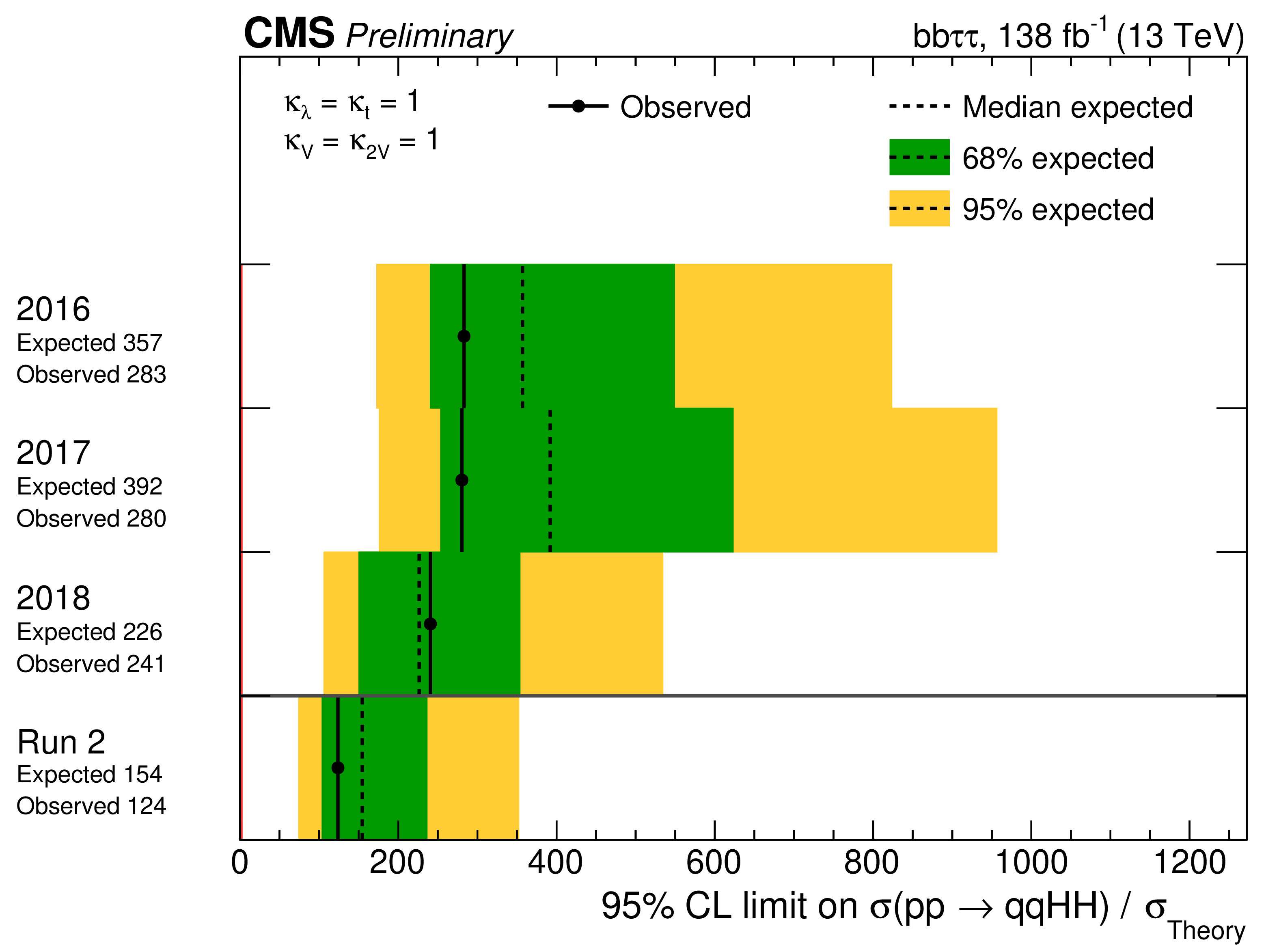
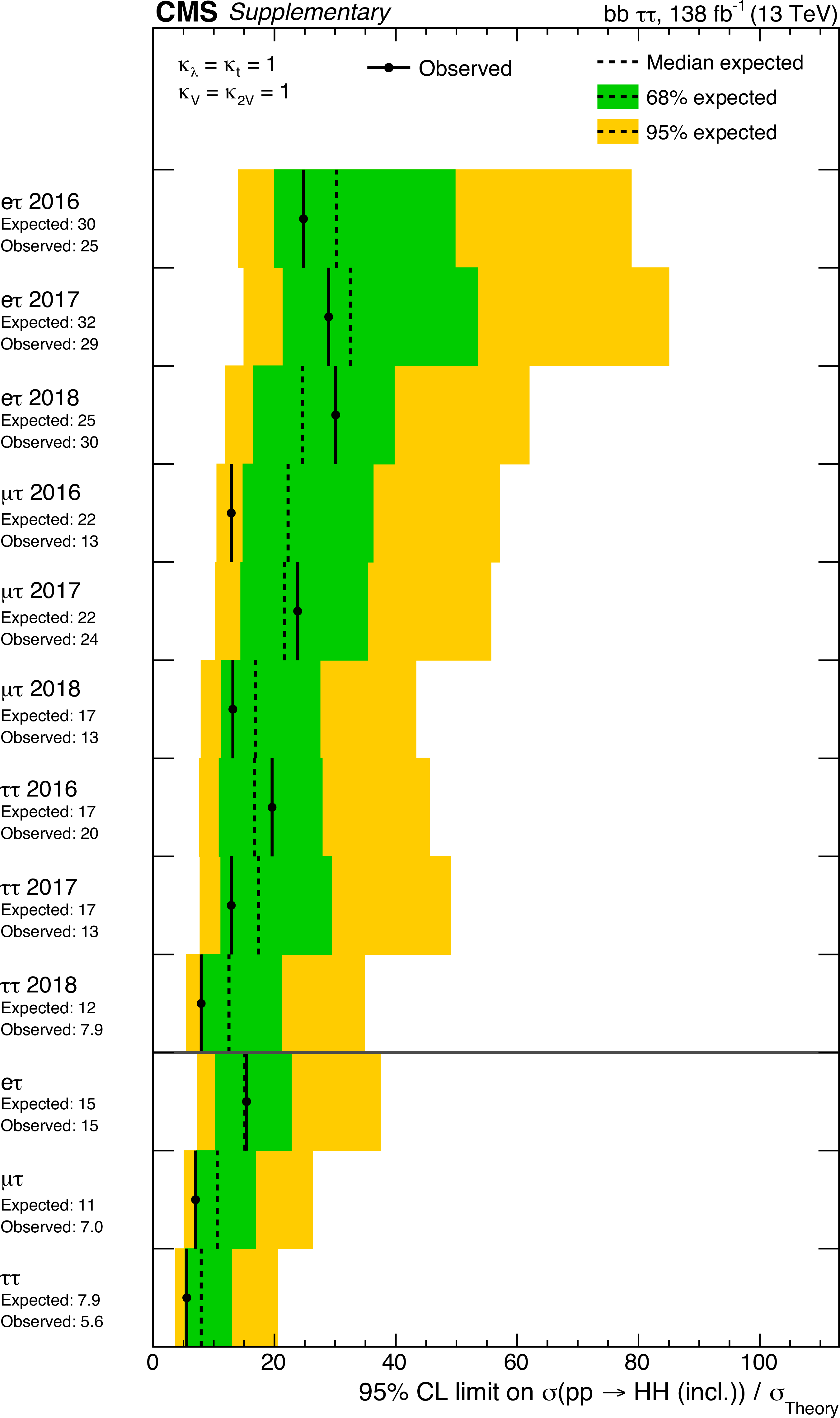
Figure 6:
Upper limit on the HH ggF + VBF signal strength at 95% CL for $\kappa _{\lambda} = $ 1, separated into different years and combined for the full Run 2 data set. |
png pdf |
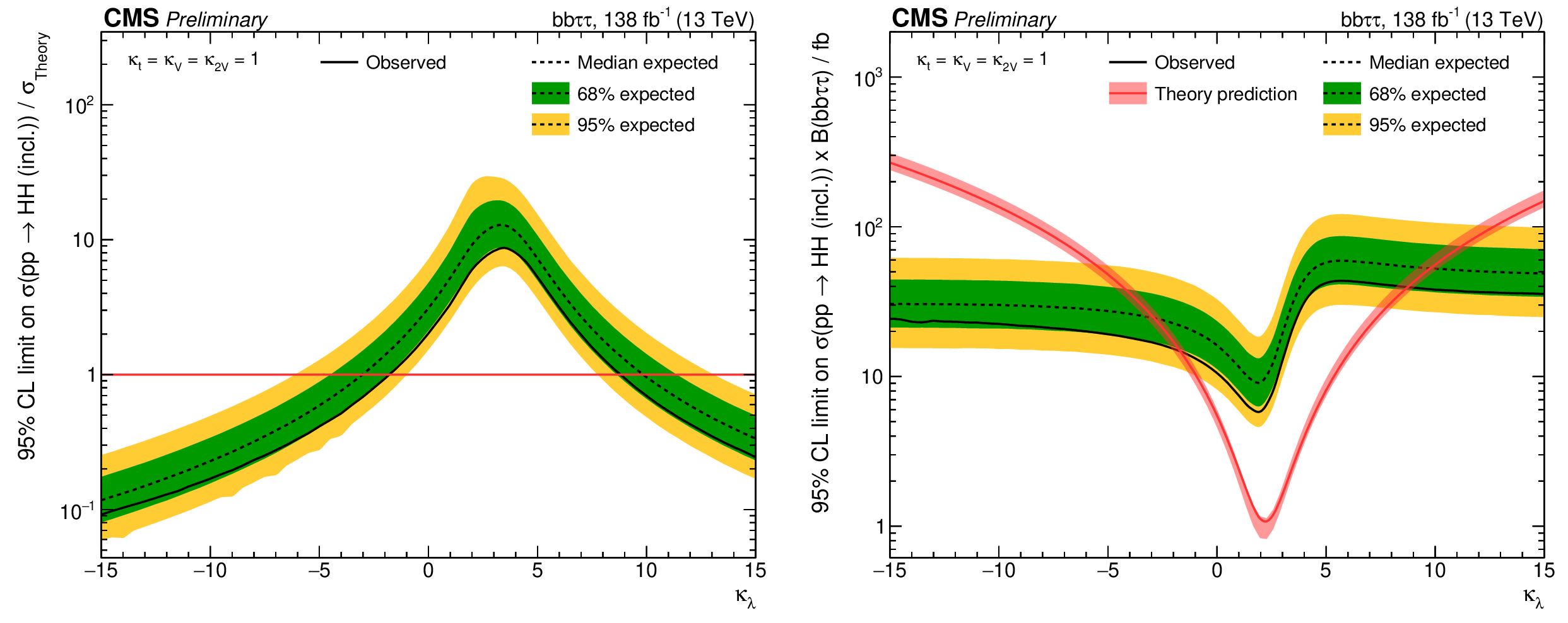
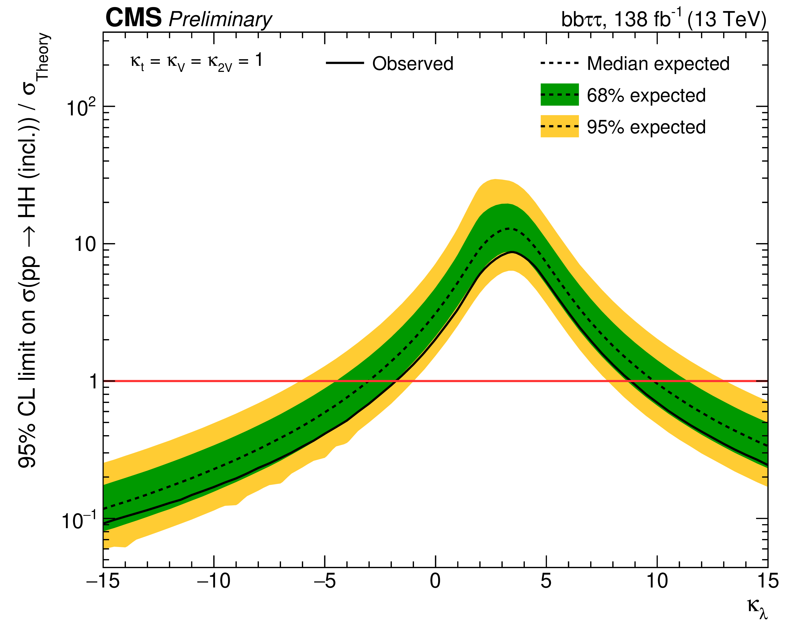
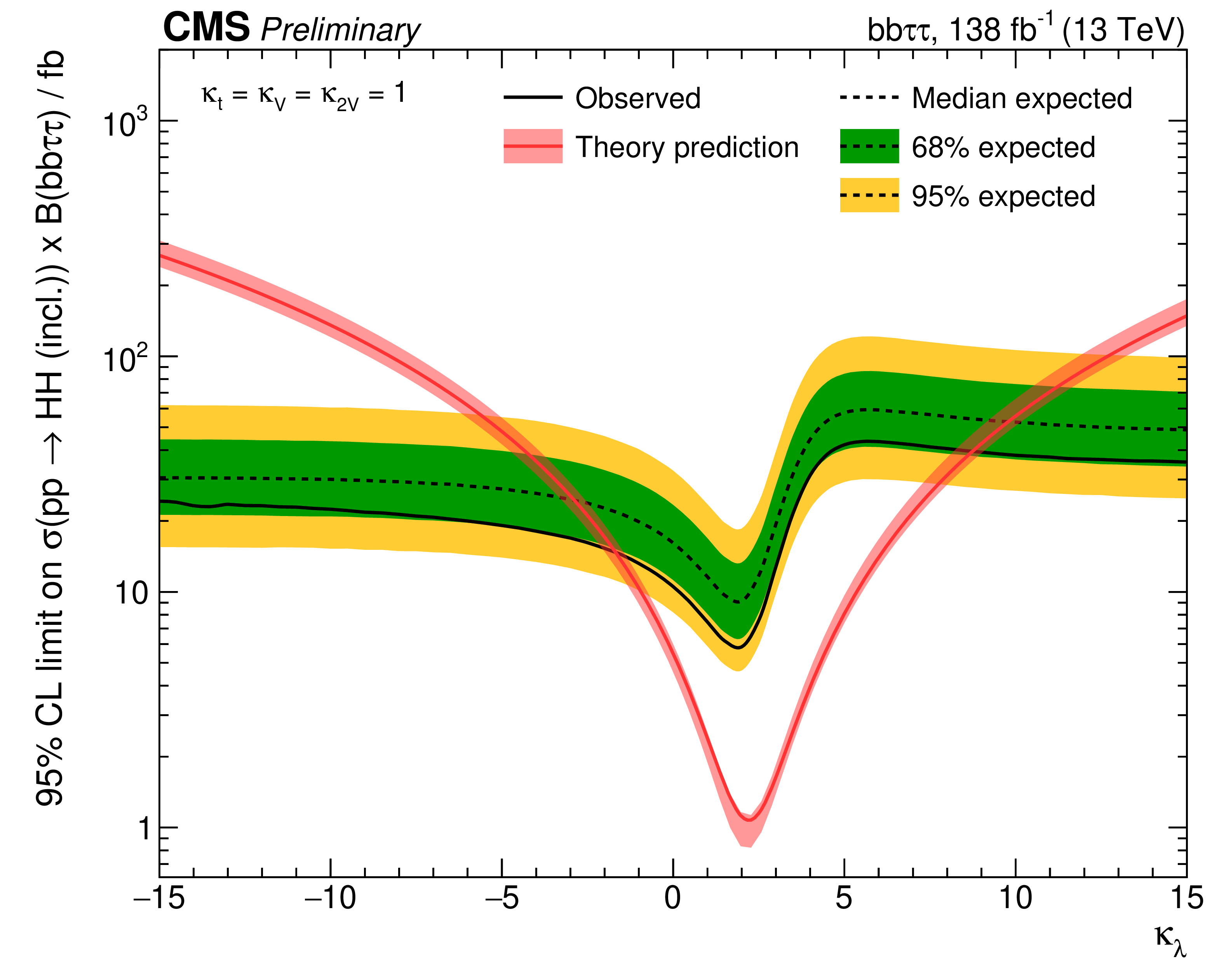
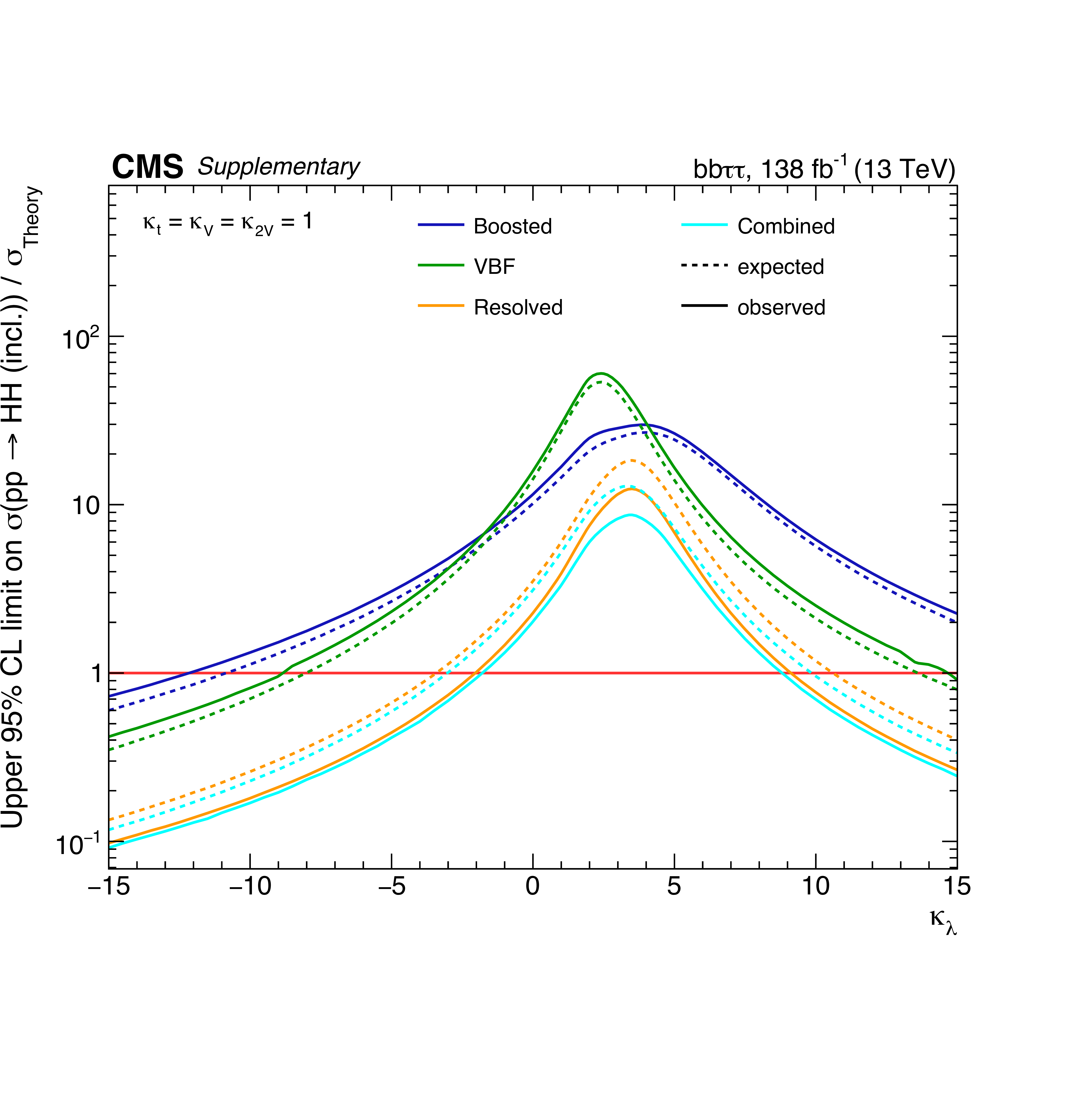
Figure 7:
Observed and expected upper limits at 95% CL as a function of $\kappa _{\lambda}$ on the HH ggF + VBF signal strength (left) and on the HH ggF + VBF cross section times the bb$ \tau \tau $ branching ratio (right). In both cases all other couplings are set to their SM expectation. |
png pdf |
Figure 7-a:
Observed and expected upper limits at 95% CL as a function of $\kappa _{\lambda}$ on the HH ggF + VBF signal strength. All other couplings are set to their SM expectation. |
png pdf |
Figure 7-b:
Observed and expected upper limits at 95% CL as a function of $\kappa _{\lambda}$ on the HH ggF + VBF cross section times the bb$ \tau \tau $ branching ratio. All other couplings are set to their SM expectation. |
png pdf |
Figure 8:
Upper limit on the HH VBF signal strength at 95% CL for $\kappa _{2{\mathrm{V}}} = $ 1, separated into different years and combined for the full Run 2 data set. |
png pdf |
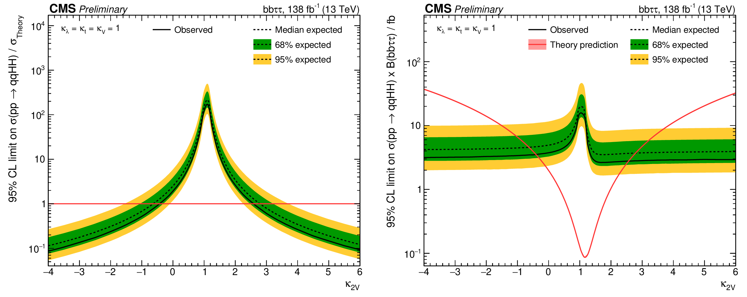
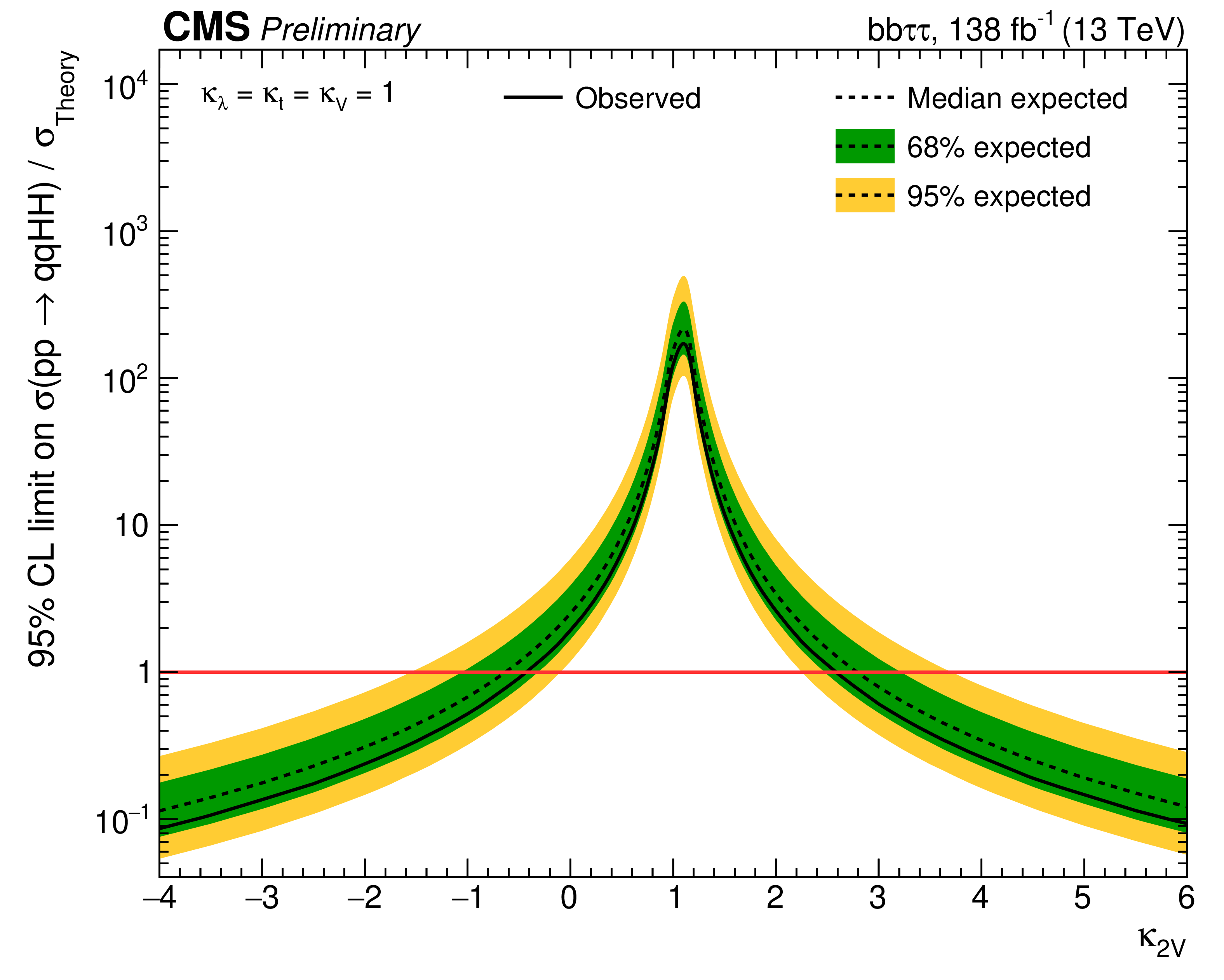
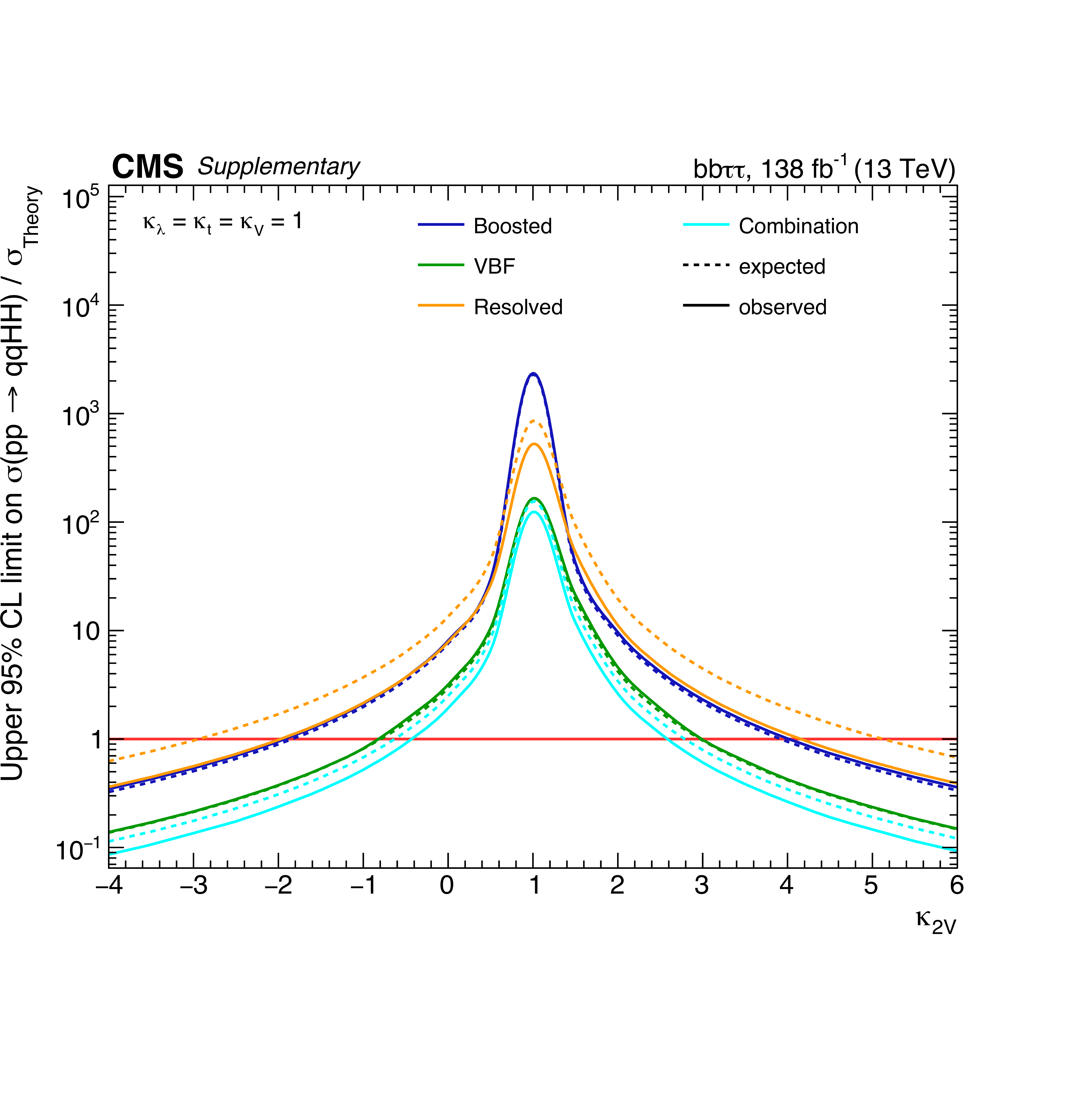
Figure 9:
Observed and expected upper limits at 95% CL as a function of $\kappa _{2{\mathrm{V}}}$ on the HH VBF signal strength (left) and on the HH VBF cross section times the bb$ \tau \tau $ branching ratio (right). In both cases all other couplings are set to their SM expectation. |
png pdf |
Figure 9-a:
Observed and expected upper limits at 95% CL as a function of $\kappa _{2{\mathrm{V}}}$ on the HH VBF signal strength. All other couplings are set to their SM expectation. |

png pdf |
Figure 9-b:
Observed and expected upper limits at 95% CL as a function of $\kappa _{2{\mathrm{V}}}$ on the HH VBF cross section times the bb$ \tau \tau $ branching ratio. All other couplings are set to their SM expectation. |
png pdf |
Figure 10:
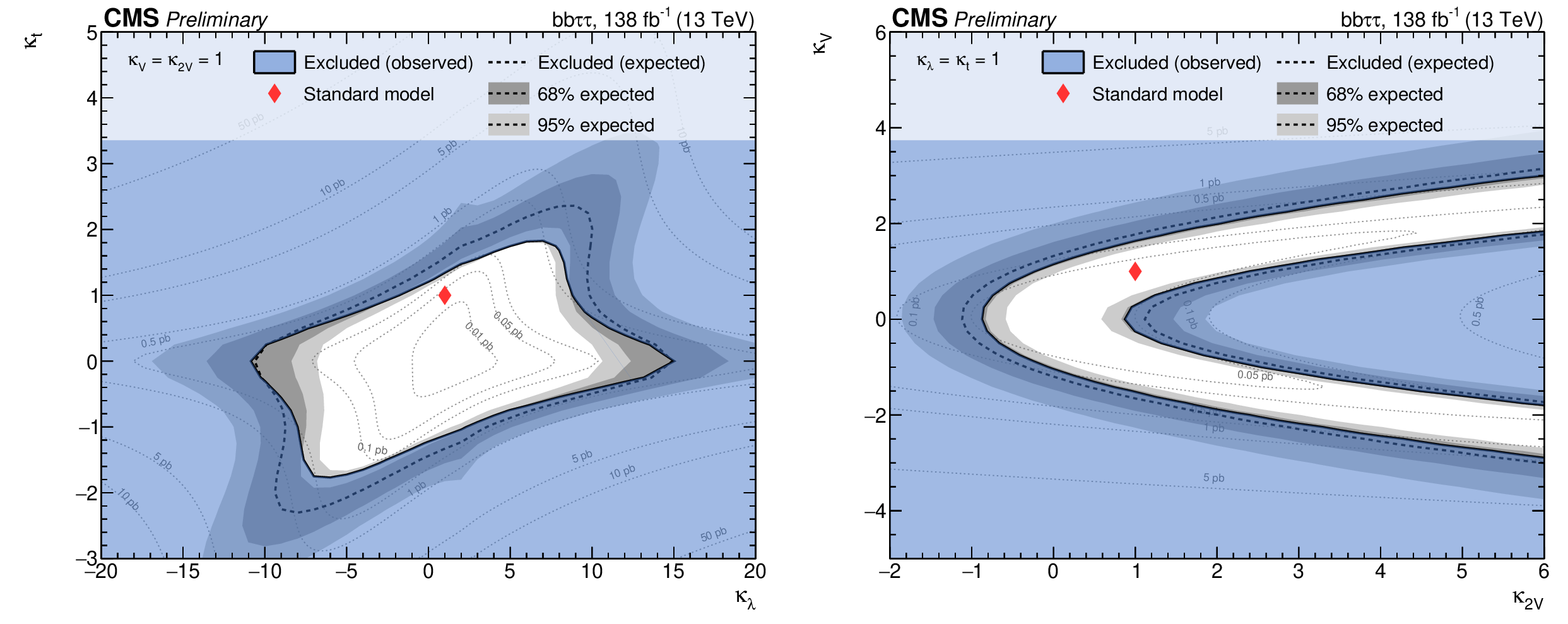
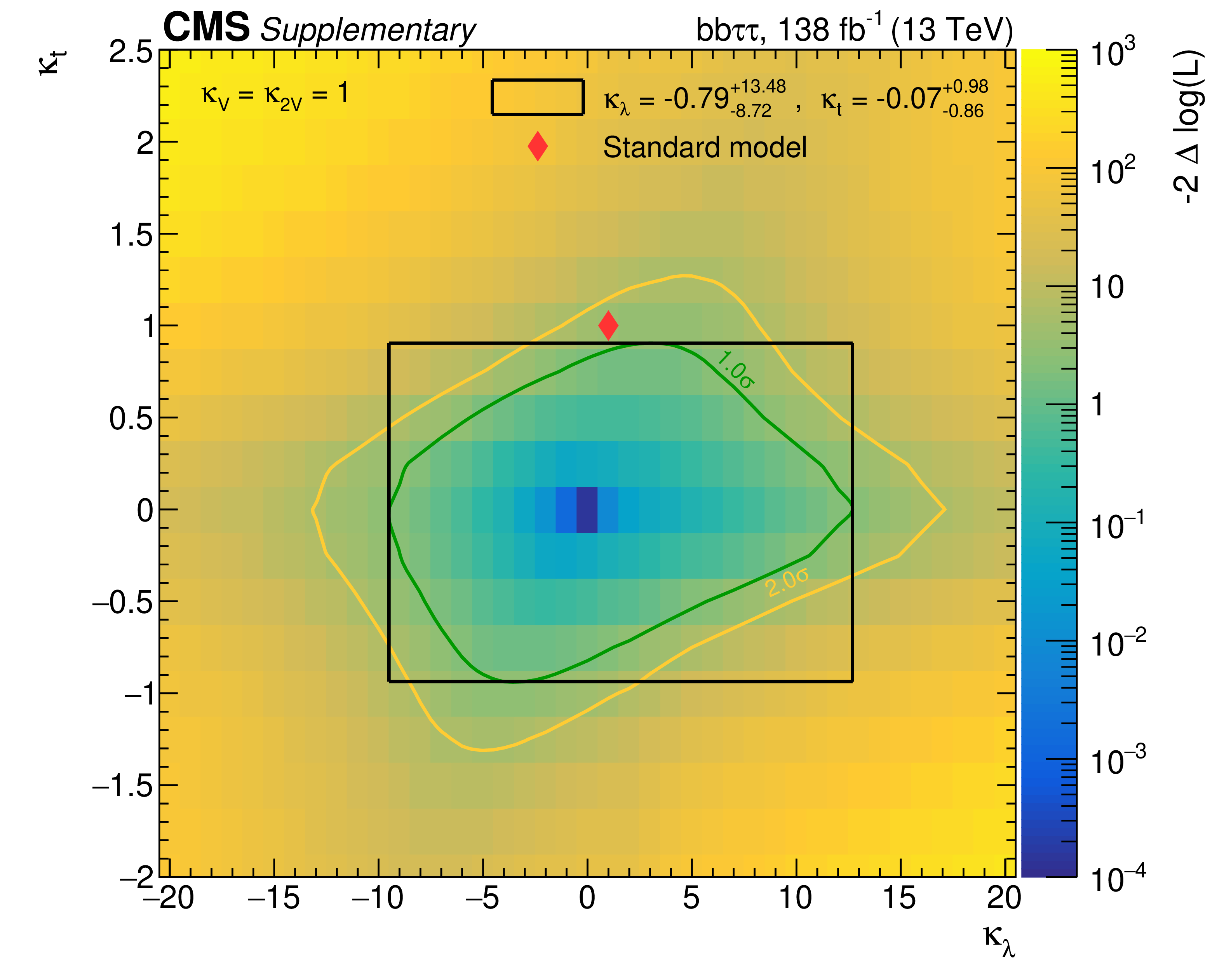
Two-dimensional exclusion regions as a function of the $\kappa _{\lambda}$ and $\kappa _{\mathrm{t}}$ couplings for the full Run2 combination (left), both $\kappa _{2{\mathrm{V}}}$ and $\kappa _{{\mathrm{V}}}$ are fixed to unity. Two-dimensional exclusion regions as a function of the $\kappa _{2{\mathrm{V}}}$ and $\kappa _{{\mathrm{V}}}$ couplings (right), both $\kappa _{\lambda}$ and $\kappa _{\mathrm{t}}$ are set to unity. Expected uncertainties on exclusion boundaries are inferred from uncertainty bands of the limit calculation, and are denoted by dark and light grey areas. The blue area marks parameter combinations that are observed to be excluded. For visual guidance, theoretical cross section values are illustrated by thin, labeled contour lines with the SM configuration denoted by a red diamond. |
png pdf |
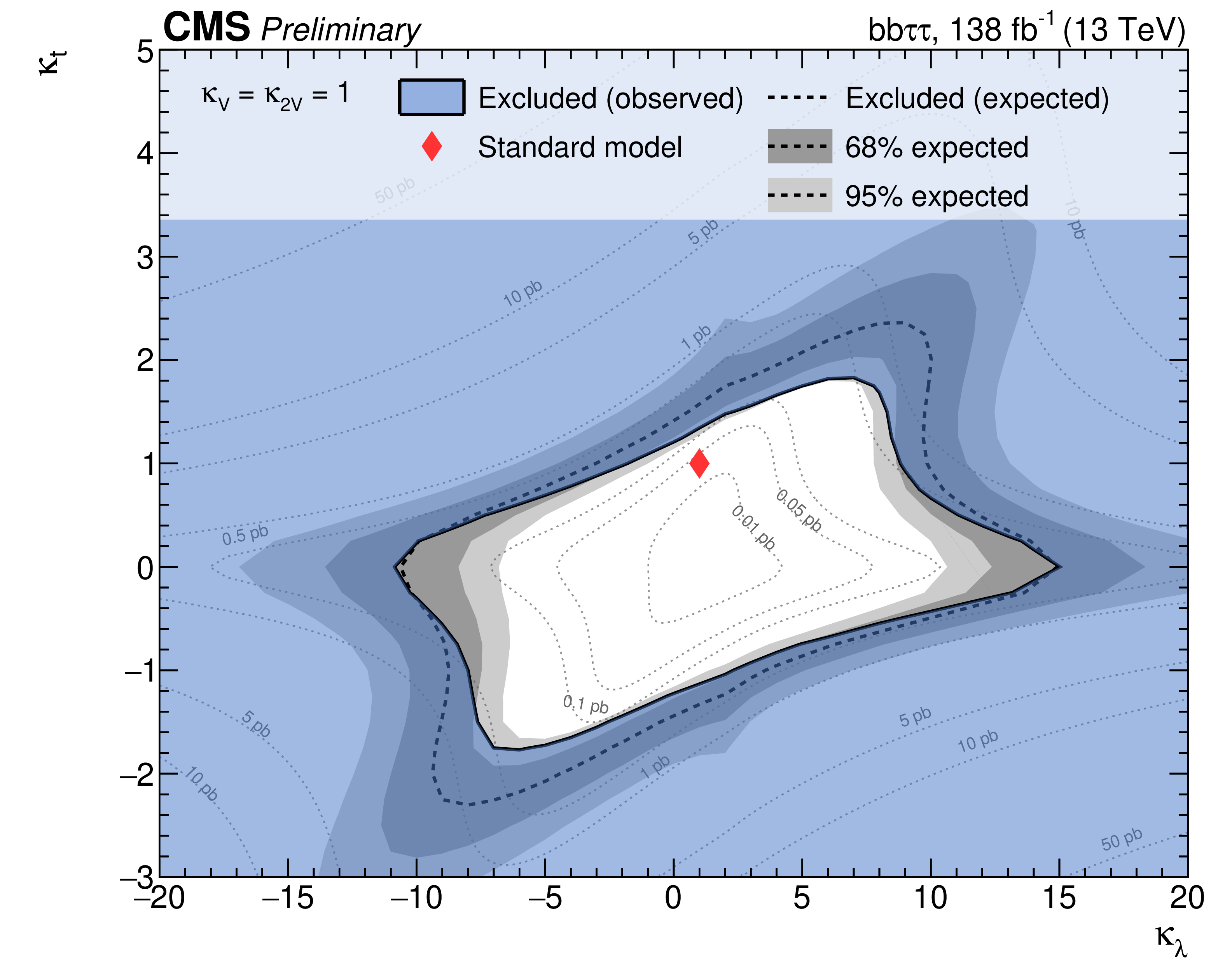
Figure 10-a:
Two-dimensional exclusion regions as a function of the $\kappa _{\lambda}$ and $\kappa _{\mathrm{t}}$ couplings for the full Run2 combination, both $\kappa _{2{\mathrm{V}}}$ and $\kappa _{{\mathrm{V}}}$ are fixed to unity. Expected uncertainties on exclusion boundaries are inferred from uncertainty bands of the limit calculation, and are denoted by dark and light grey areas. The blue area marks parameter combinations that are observed to be excluded. For visual guidance, theoretical cross section values are illustrated by thin, labeled contour lines with the SM configuration denoted by a red diamond. |
png pdf |
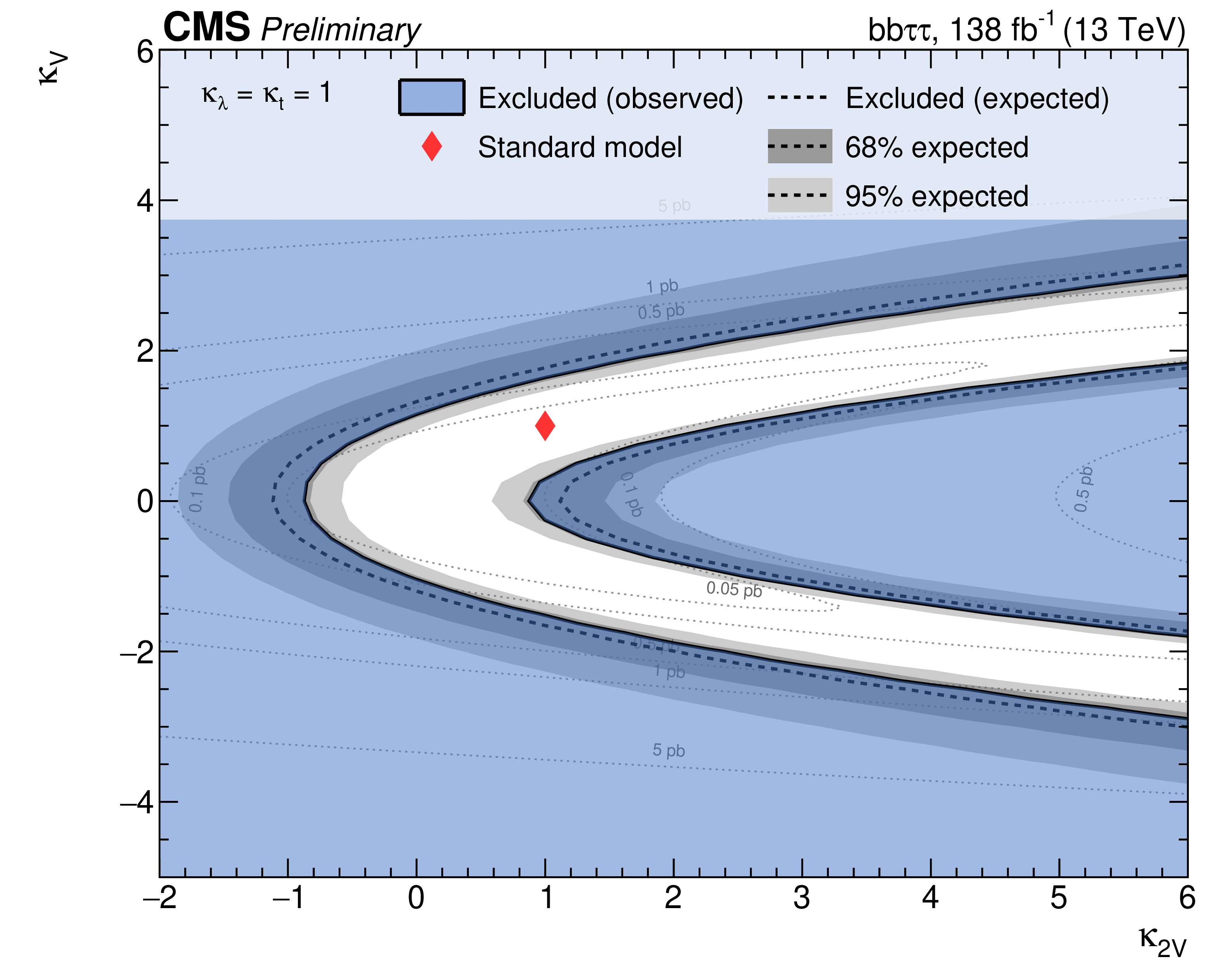
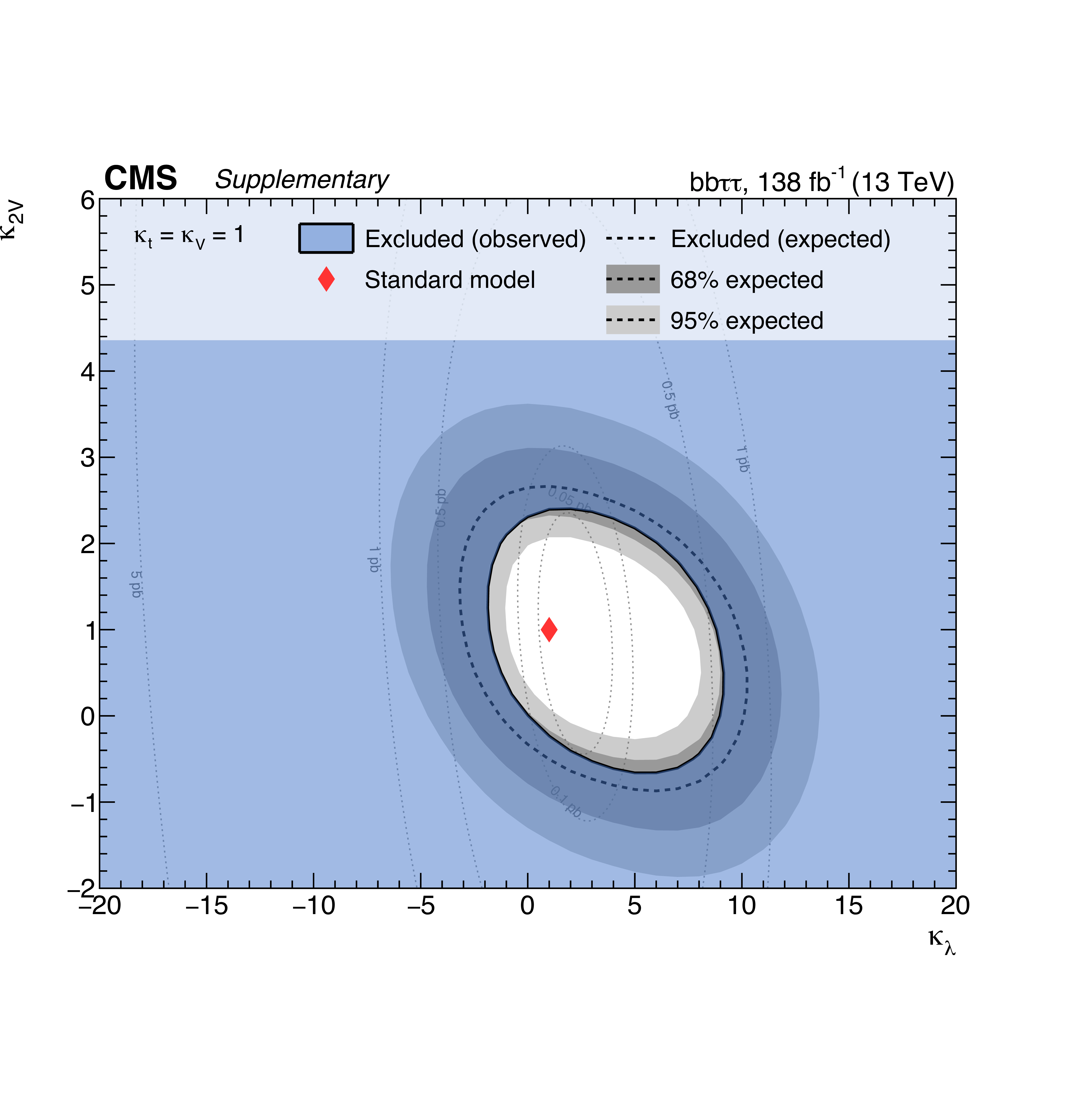
Figure 10-b:
Two-dimensional exclusion regions as a function of the $\kappa _{2{\mathrm{V}}}$ and $\kappa _{{\mathrm{V}}}$ couplings, both $\kappa _{\lambda}$ and $\kappa _{\mathrm{t}}$ are set to unity. Expected uncertainties on exclusion boundaries are inferred from uncertainty bands of the limit calculation, and are denoted by dark and light grey areas. The blue area marks parameter combinations that are observed to be excluded. For visual guidance, theoretical cross section values are illustrated by thin, labeled contour lines with the SM configuration denoted by a red diamond. |
png pdf |
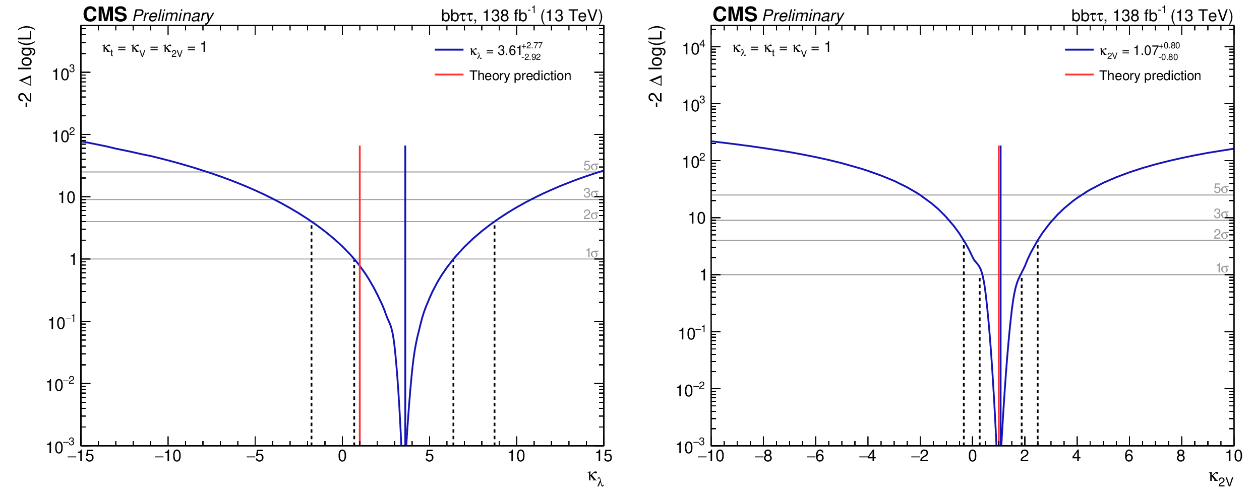
Figure 11:
Observed likelihood scan as a function of $\kappa _{\lambda}$ (left) and $\kappa _{2{\mathrm{V}}}$ (right) for the full Run 2 combination. The dashed lines show the intersection with threshold values one and four, corresponding to 68% and 95% confidence intervals, respectively. |
png pdf |
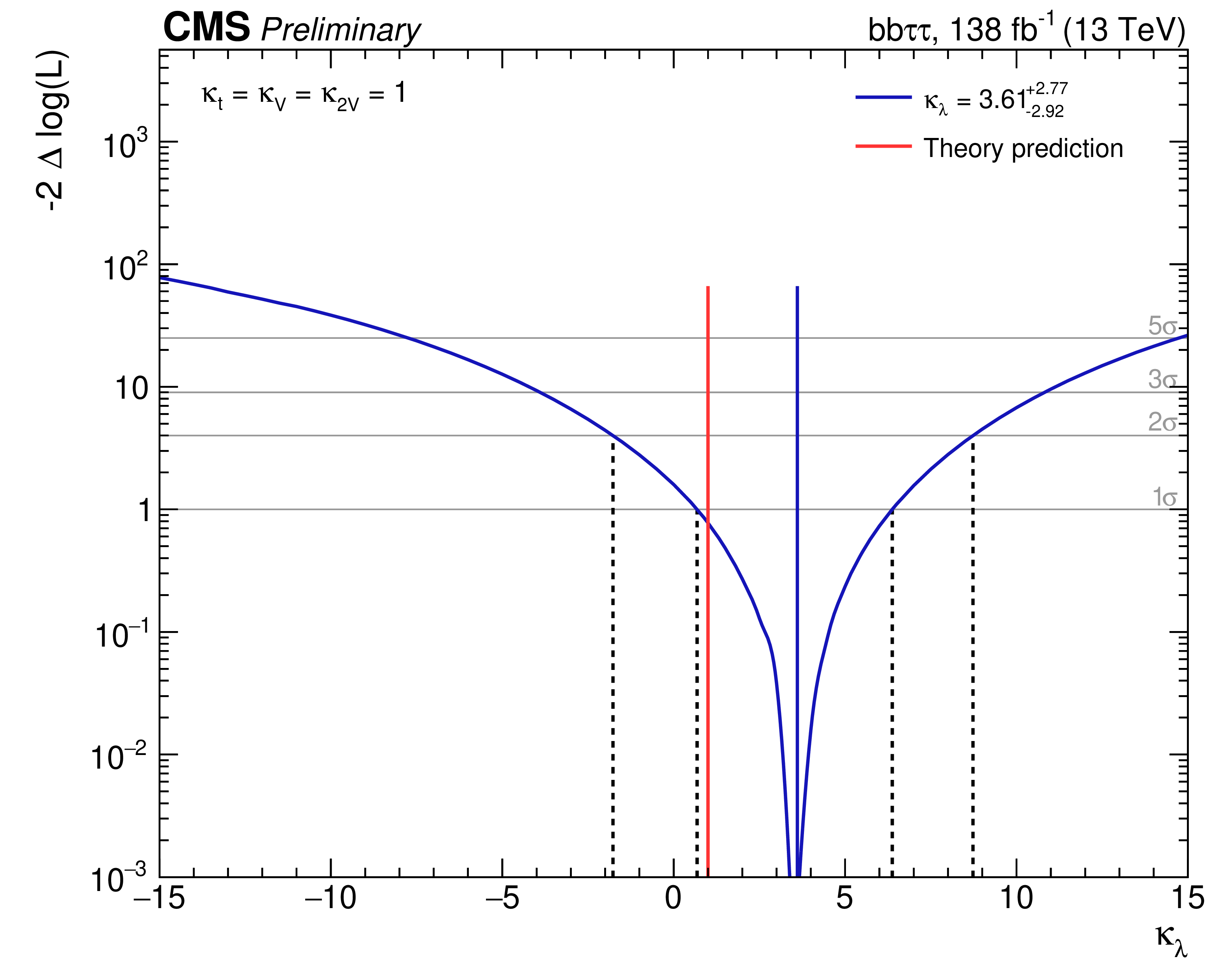
Figure 11-a:
Observed likelihood scan as a function of $\kappa _{\lambda}$ for the full Run 2 combination. The dashed lines show the intersection with threshold values one and four, corresponding to 68% and 95% confidence intervals, respectively. |
png pdf |
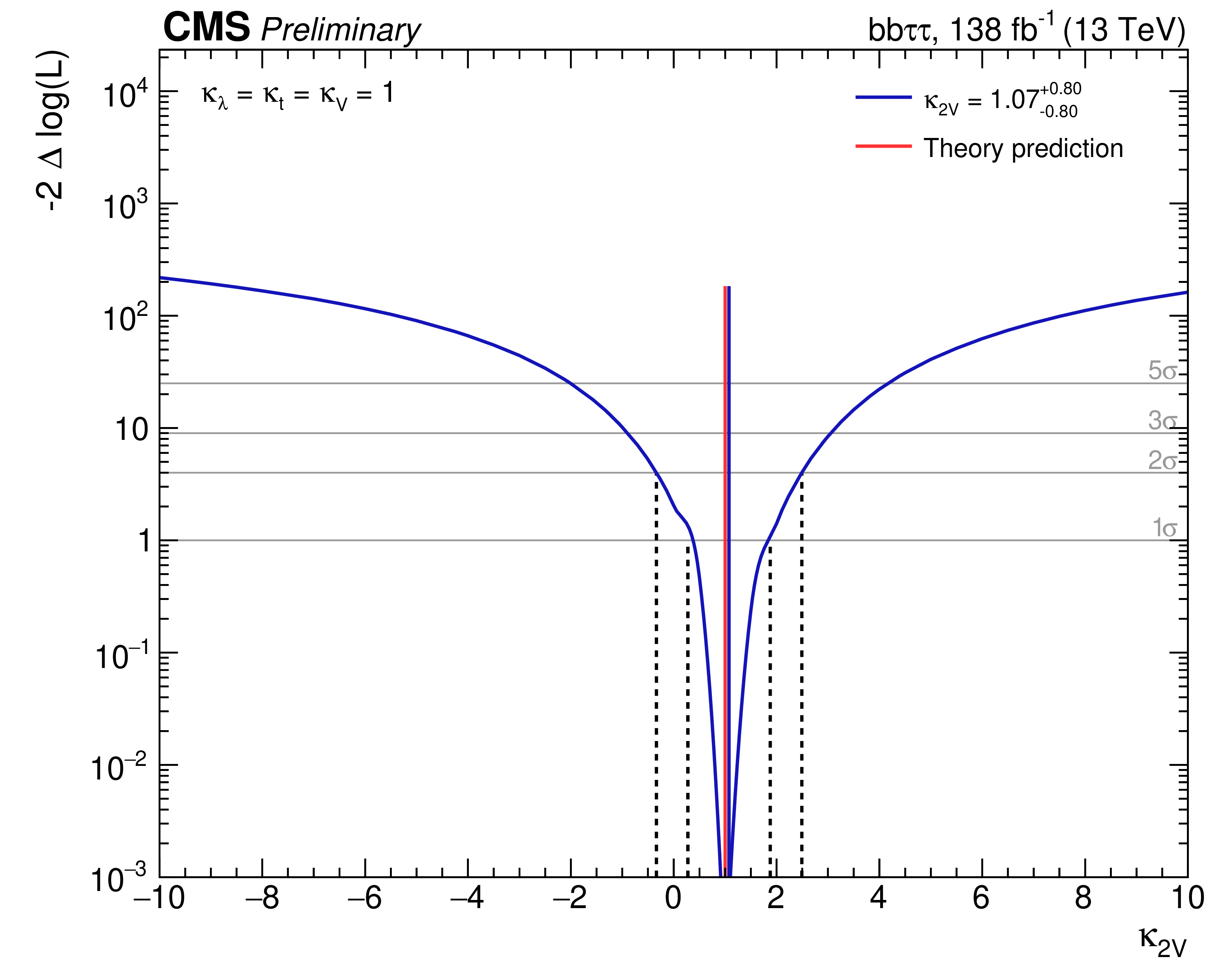
Figure 11-b:
Observed likelihood scan as a function of $\kappa _{2{\mathrm{V}}}$ for the full Run 2 combination. The dashed lines show the intersection with threshold values one and four, corresponding to 68% and 95% confidence intervals, respectively. |
| Tables | |
png pdf |
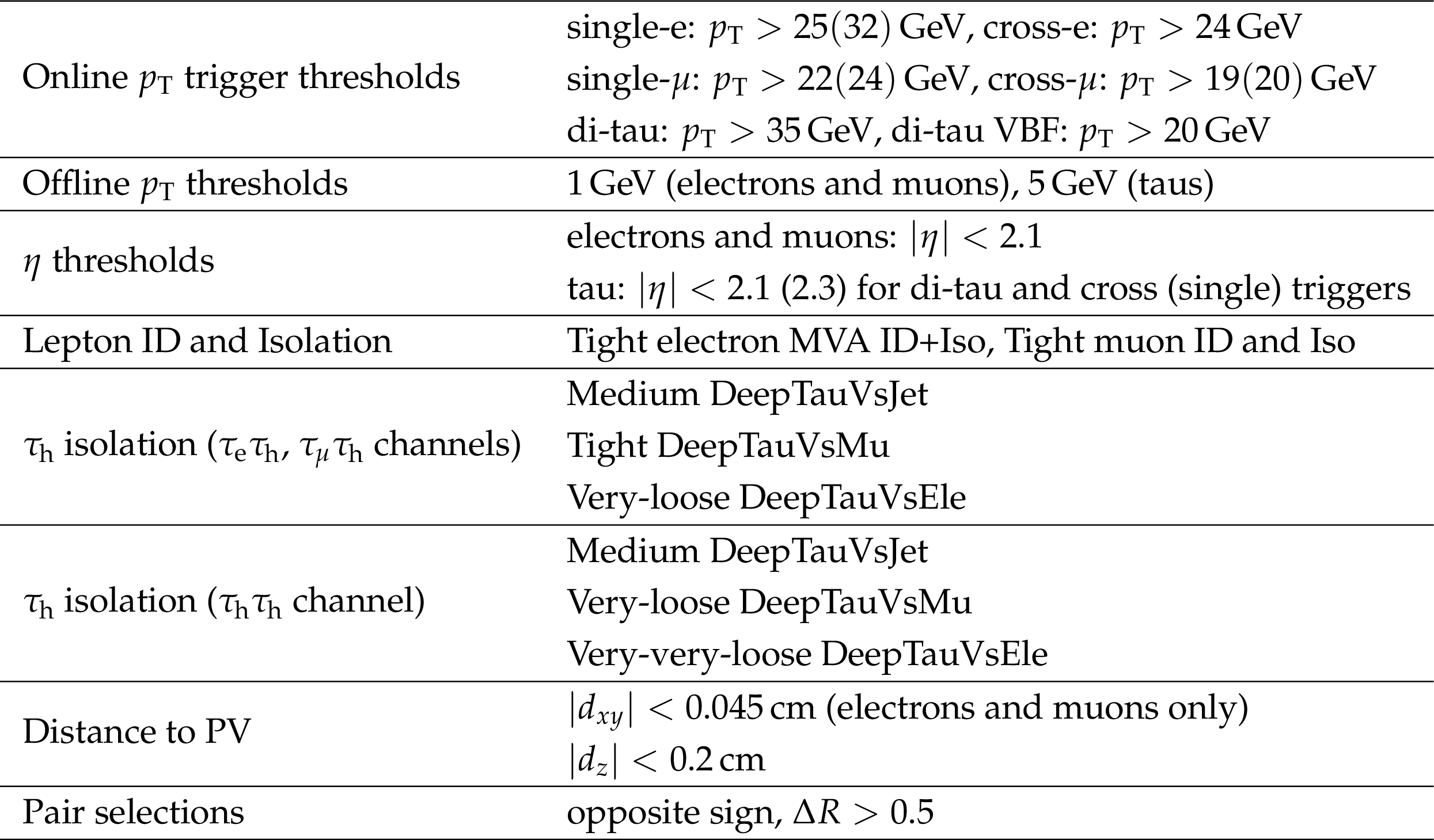
Table 1:
Summary of selections applied to the $\tau \tau $ pair. Trigger thresholds in parentheses refer to the 2017-2018 data-taking period. |
png pdf |
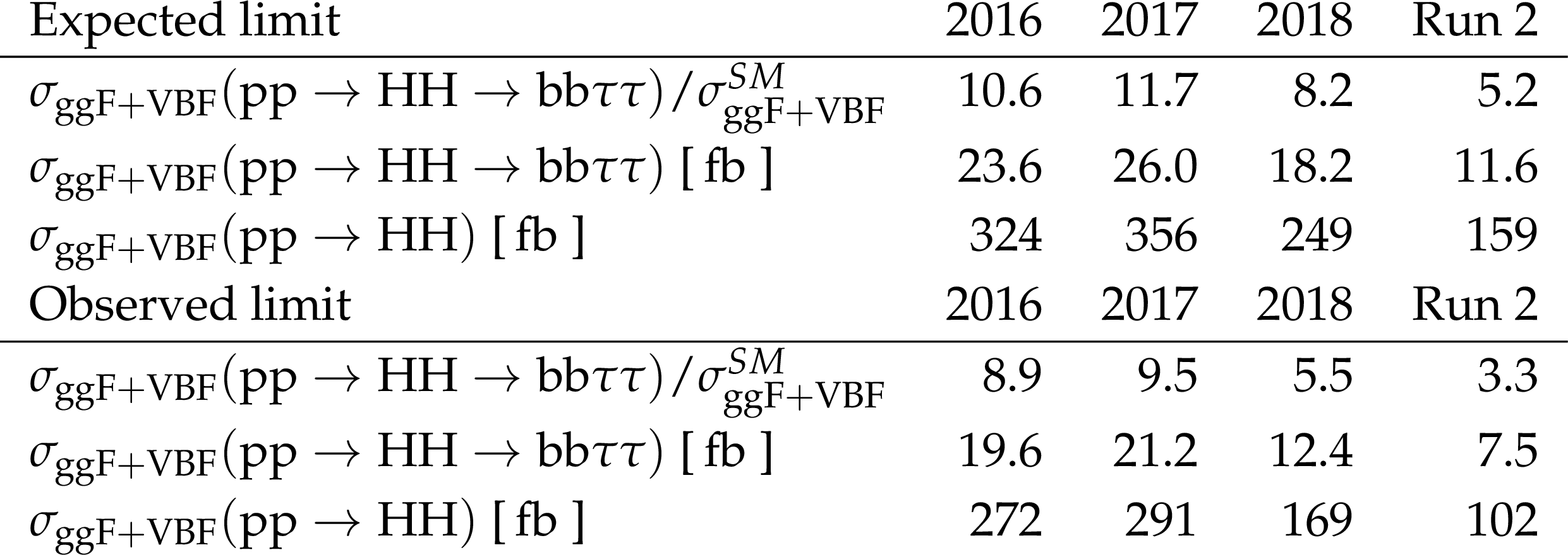
Table 2:
Expected and observed upper limits at 95% CL for the SM point ($\kappa _{\lambda} = $ 1), where $\sigma _{ggF + \text {VBF}}^{SM}=$ 2.39 fb represents the product of the ggF plus VBF HH cross section (32.776 fb) and the branching fraction $\mathcal {B}({\mathrm{H} \mathrm{H}} \to \mathrm{b} \mathrm{b} \tau \tau)=$ 0.073. |

png pdf |
Table 3:
Expected and observed upper limits at 95% CL for the SM point ($\kappa _{2{\mathrm{V}}} = $ 1), where $\sigma _{\text {VBF}}^{SM}=$ 0.126 fb represents the product of the VBF HH cross section (1.726 fb) and the branching fraction $\mathcal {B}({\mathrm{H} \mathrm{H}} \to \mathrm{b} \mathrm{b} \tau \tau)=$ 0.073. |
| Summary |
|
A search for nonresonant Higgs boson pair (HH) production via gluon-gluon fusion and vector boson fusion (VBF) processes in final states with two bottom quarks and two $\tau$ leptons was presented. The search uses the full Run 2 data set of proton-proton collisions at a center-of-mass energy of $\sqrt{s} = $ 13 TeV recorded with the CMS detector at the LHC, corresponding to an integrated luminosity of 138 fb$^{-1}$. The three decay modes of the $\tau\tau$ pair with the largest branching fraction have been selected, requiring one $\tau$ to be always decaying hadronically and the other one either leptonically or hadronically. Upper limits at the 95% confidence level (CL) on the inclusive HH production cross sections are set, as well as on the VBF HH production cross sections. This analysis benefits from an improved trigger strategy as well as from a series of techniques developed especially for this search: among others, several neural networks to identify the b jets from the H decay, categorize the events, and perform signal extraction. At the same time, this analysis builds up on the improvements made by the CMS Collaboration in the jet and $\tau$ lepton identification and reconstruction algorithms. All these techniques enable the achievement of particularly stringent results on the HH production cross sections. The observed 95% CL upper limit on HH total production cross section corresponds to 3.3 times the theoretical SM prediction, and the expected limit is 5.2 times the SM prediction. The observed 95% CL upper limit for the VBF HH SM cross section corresponds to 124 times the theoretical SM prediction and the expected limits is about 154 times the SM prediction. The observed (expected) 95% CL constraints on $\kappa_{\lambda}$ and $\kappa_{2\mathrm{V}}$, derived from limits on the HH production cross section times the bb$\tau\tau$ branching ratio, are found to be $-$1.8 $< \kappa_{\lambda} < $ 8.8 ($-$3 $ < \kappa_{\lambda} < $ 9.9) and $-$0.4 $ < \kappa_{2\mathrm{V}} < $ 2.6 ($-$0.6 $ < \kappa_{2\mathrm{V}} < $ 2.8), respectively. |
| Additional Figures | |
png pdf |
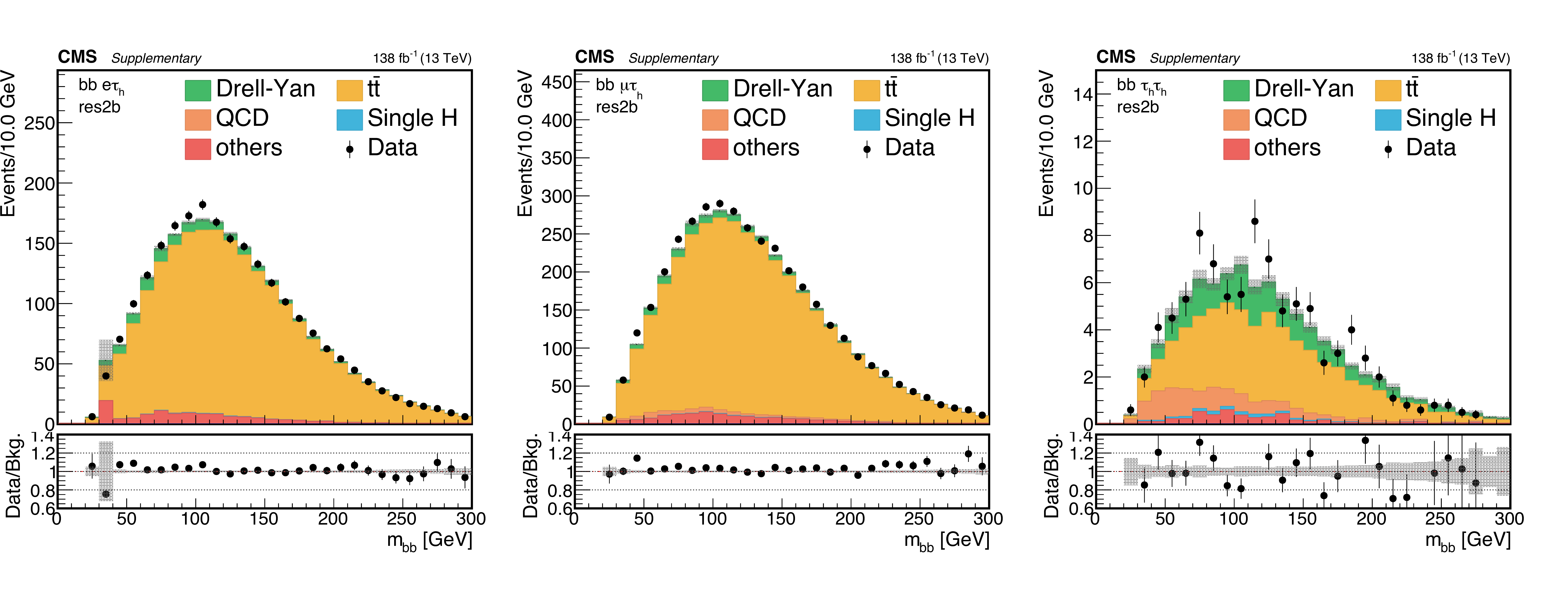
Additional Figure 1:
Distributions of the reconstructed mass of the bb pair in the most sensitive category of the analysis (res2b). Events are shown in the $\mathrm{e} {{\tau} _\mathrm {h}} $ (left), $\mu {{\tau} _\mathrm {h}} $ (center), and ${{\tau} _{{\text h}} {\tau} _{{\text h}}}$ (right) channels for the full Run 2 combination, after the selection on the reconstructed masses of the $ {\tau} {\tau} $ and bb pairs, as described in the paper, has been applied. |

png pdf |
Additional Figure 2:
Distributions of the mass of the $ {\tau} {\tau} $ pair, reconstructed using the SVfit algorithm [47], in the most sensitive category of the analysis (res2b). Events are shown in the $\mathrm{e} {{\tau} _\mathrm {h}} $ (left), $\mu {{\tau} _\mathrm {h}} $ (center), and ${{\tau} _{{\text h}} {\tau} _{{\text h}}}$ (right) channels for the full Run 2 combination, after the selection on the reconstructed masses of the $ {\tau} {\tau} $ and bb pairs, as described in the paper, has been applied. |
png pdf |
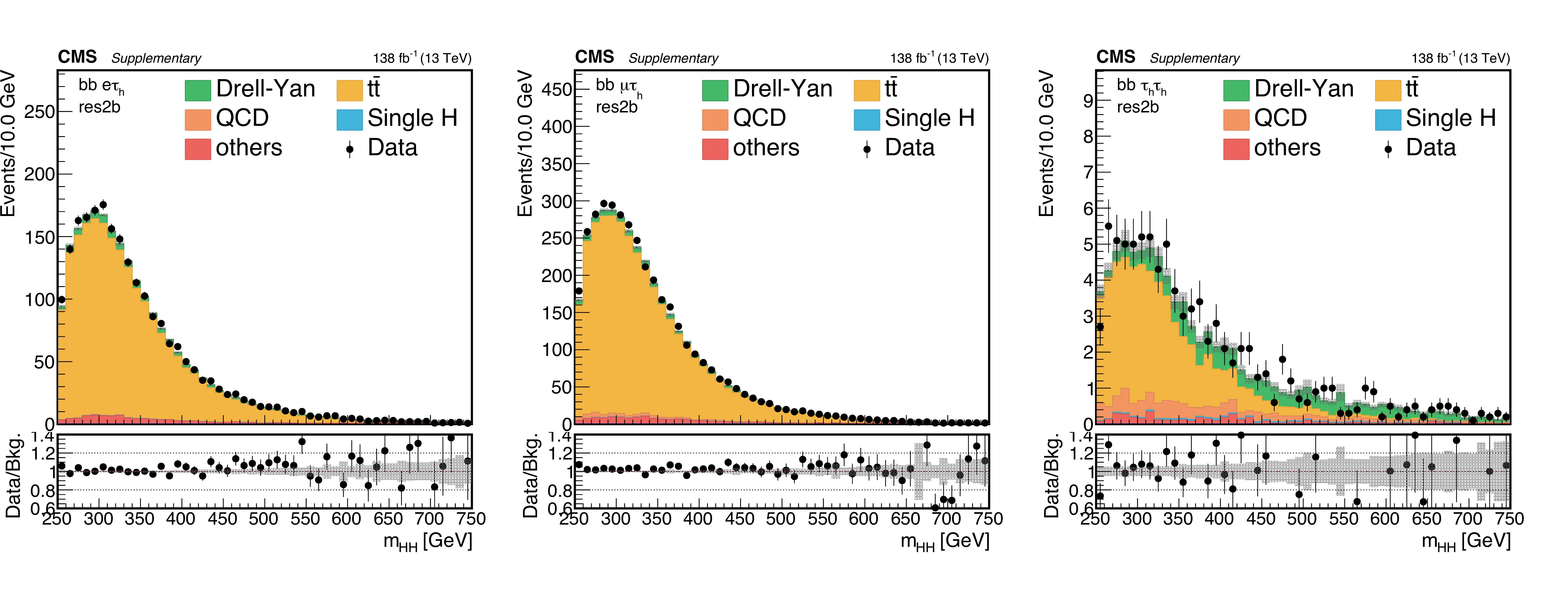
Additional Figure 3:
Distributions of the reconstructed mass of the HH pair in the most sensitive category of the analysis (res2b). Events are shown in the $\mathrm{e} {{\tau} _\mathrm {h}} $ (left), $\mu {{\tau} _\mathrm {h}} $ (center), and ${{\tau} _{{\text h}} {\tau} _{{\text h}}}$ (right) channels for the full Run 2 combination, after the selection on the reconstructed masses of the $ {\tau} {\tau} $ and bb pairs, as described in the paper, has been applied. |
png pdf |
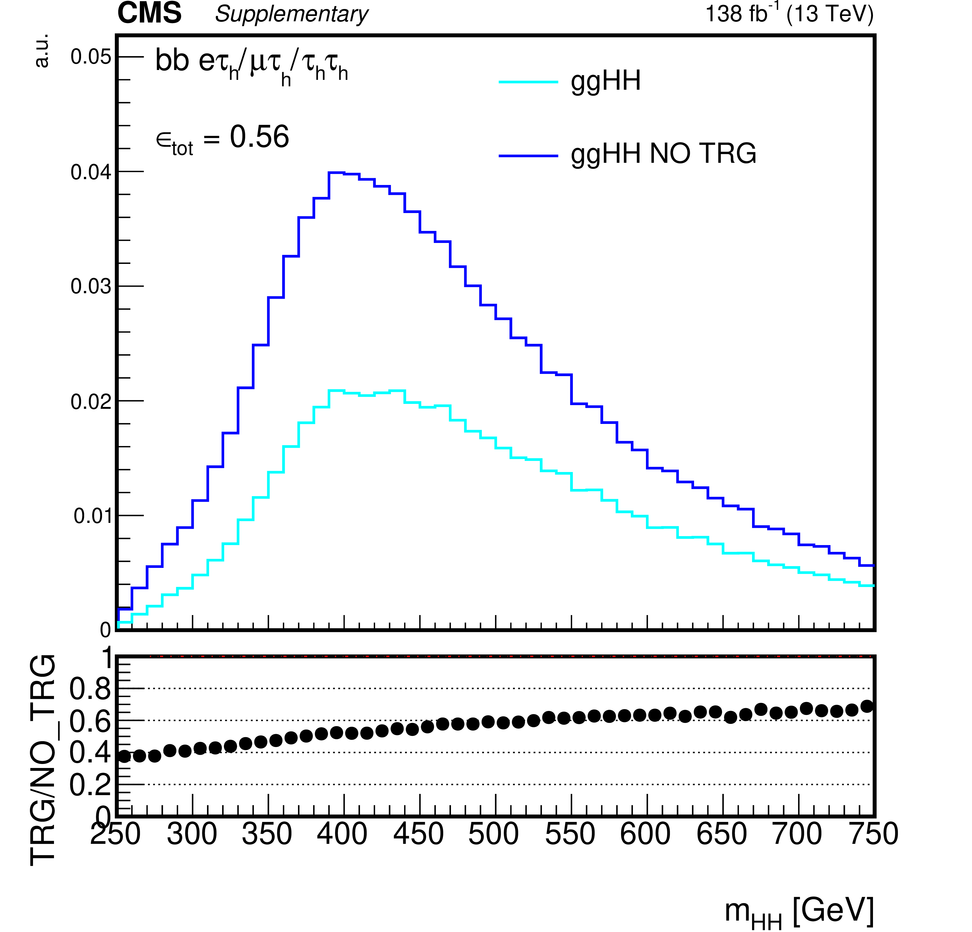
Additional Figure 4:
Normalized distribution of reconstructed $m_{{{\mathrm {H}} {\mathrm {H}}}}$ for the gluon fusion simulated signal events (ggHH) in a common baseline selection for the combination in the three channels, with and without trigger selection applied. Two b jet and two ${\tau}$ lepton candidates are required in the event. The efficiency of the trigger selection is shown in the bottom frame. |
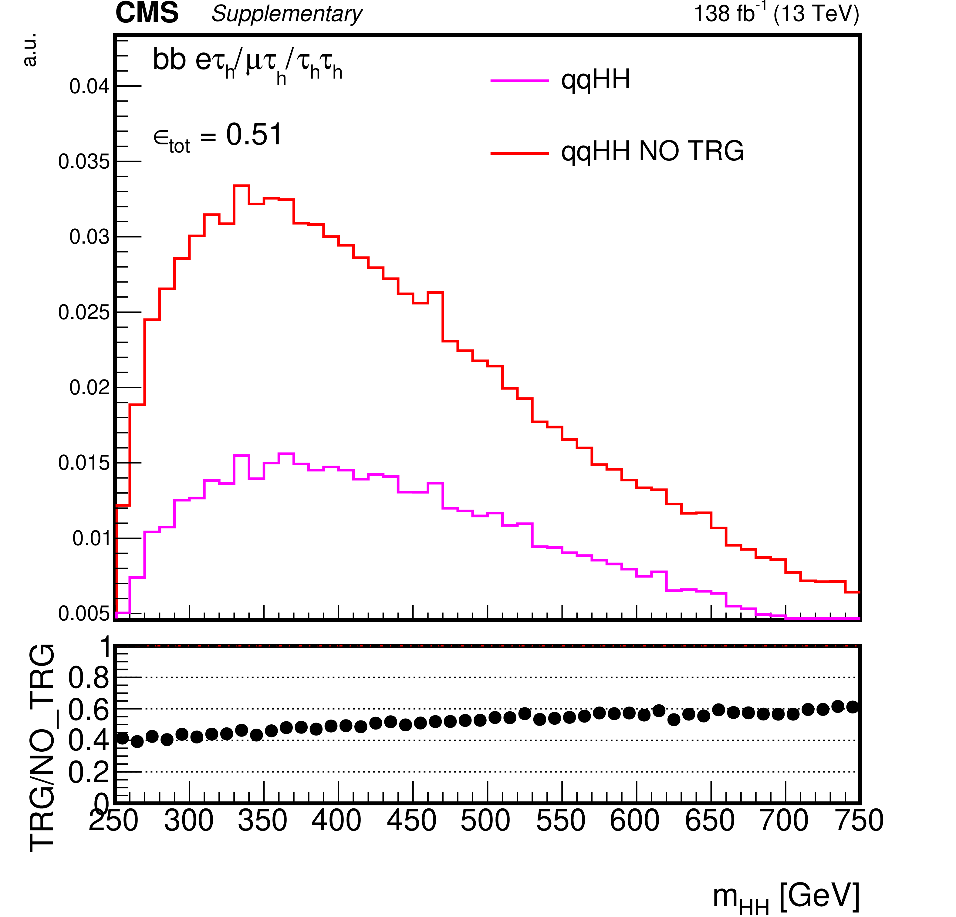
png pdf |
Additional Figure 5:
Normalized distribution of reconstructed $m_{{{\mathrm {H}} {\mathrm {H}}}}$ for the vector boson fusion simulated signal events (qqHH) in a common baseline selection for the combination in the three channels, with and without trigger selection applied. Two b jet and two ${\tau}$ lepton candidates are required in the event. The efficiency of the trigger selection is shown in the bottom frame. |
png pdf |
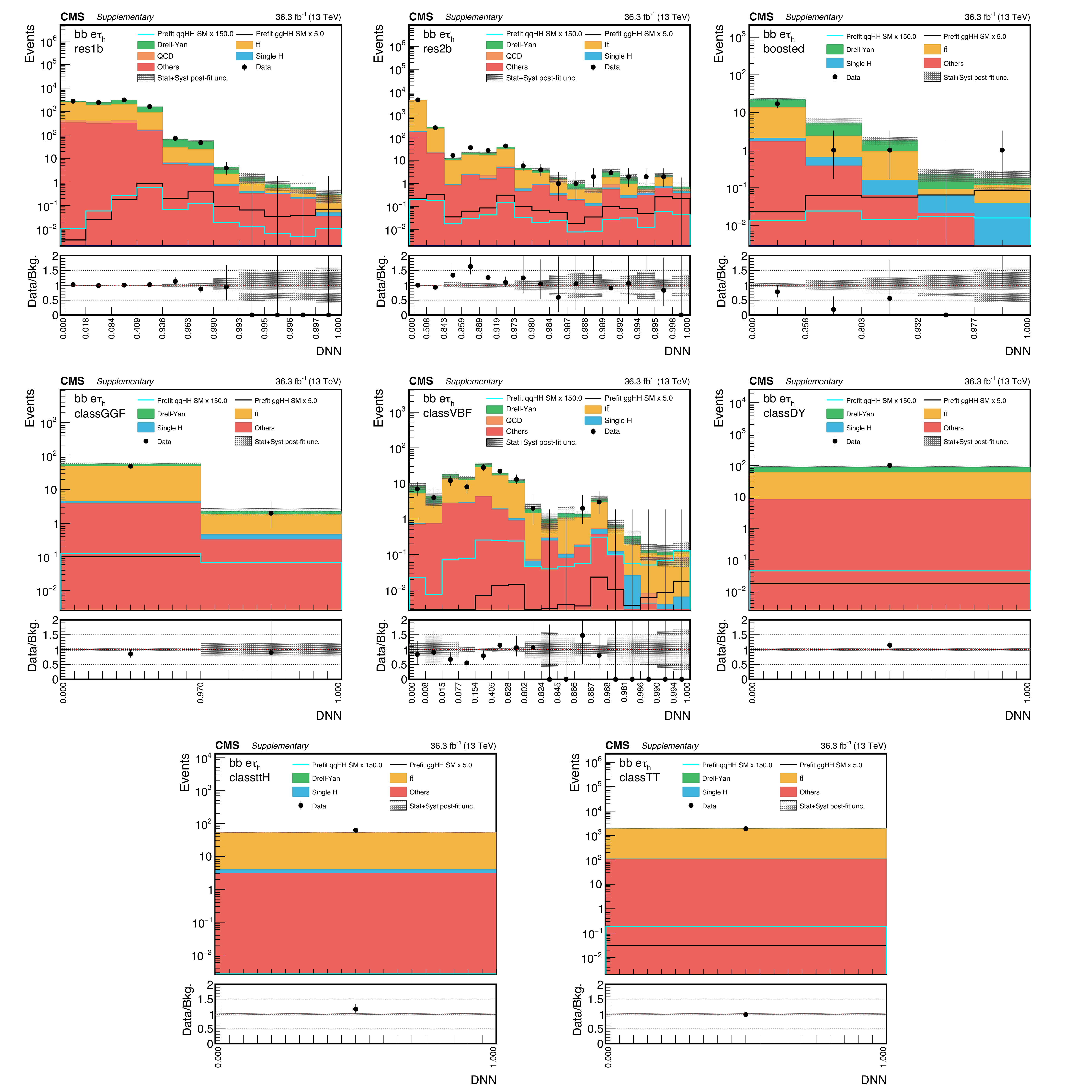
Additional Figure 6:
DNN prediction distributions in the $\mathrm{e} {{\tau} _\mathrm {h}} $ channel in 2016 for the eight analysis categories. The shaded band in the plots represents the statistical plus systematic uncertainty. |
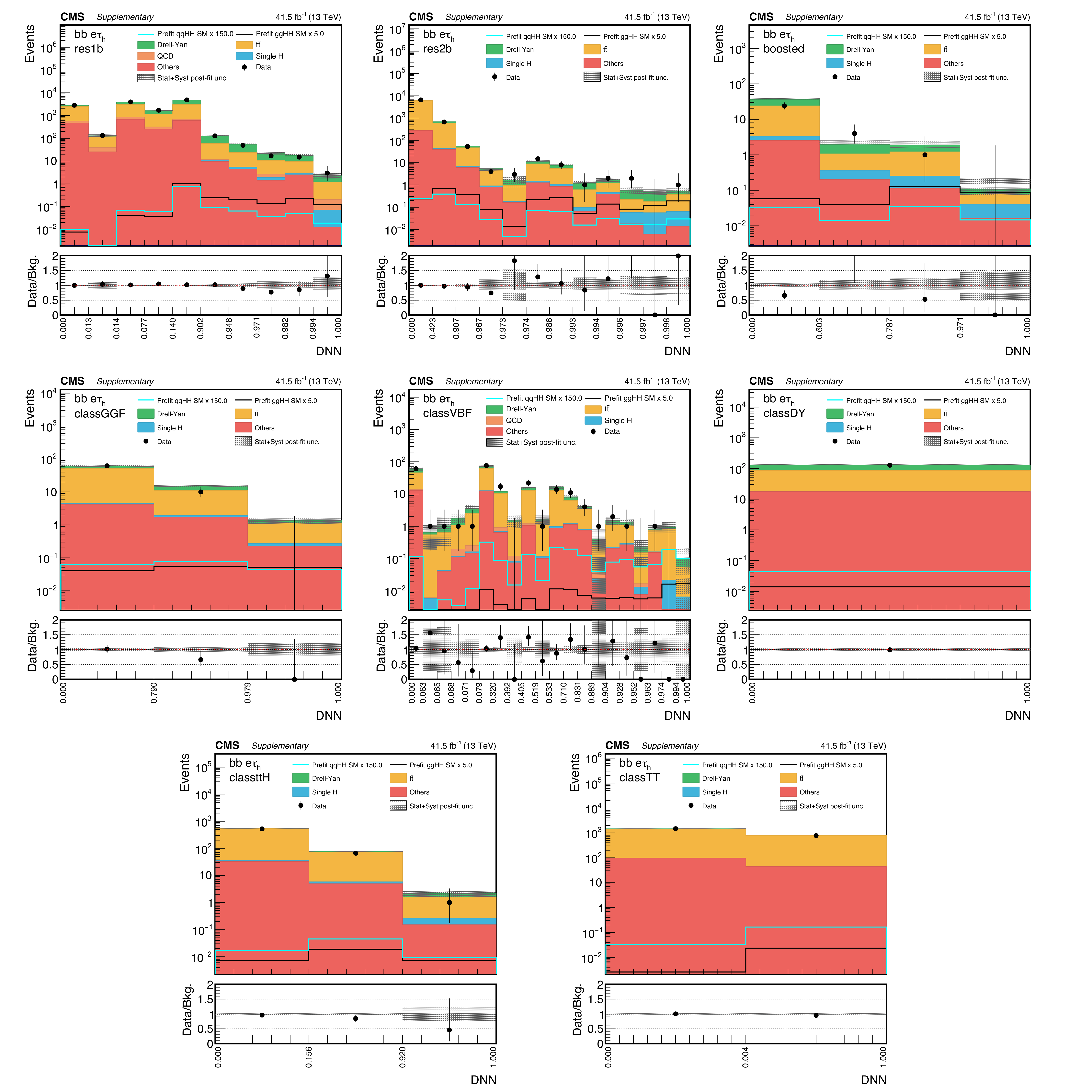
png pdf |
Additional Figure 7:
DNN prediction distributions in the $\mathrm{e} {{\tau} _\mathrm {h}} $ channel in 2017 for the eight analysis categories. The shaded band in the plots represents the statistical plus systematic uncertainty. |
png pdf |
Additional Figure 8:
DNN prediction distributions in the $\mathrm{e} {{\tau} _\mathrm {h}} $ channel in 2017 for the eight analysis categories. The shaded band in the plots represents the statistical plus systematic uncertainty. |
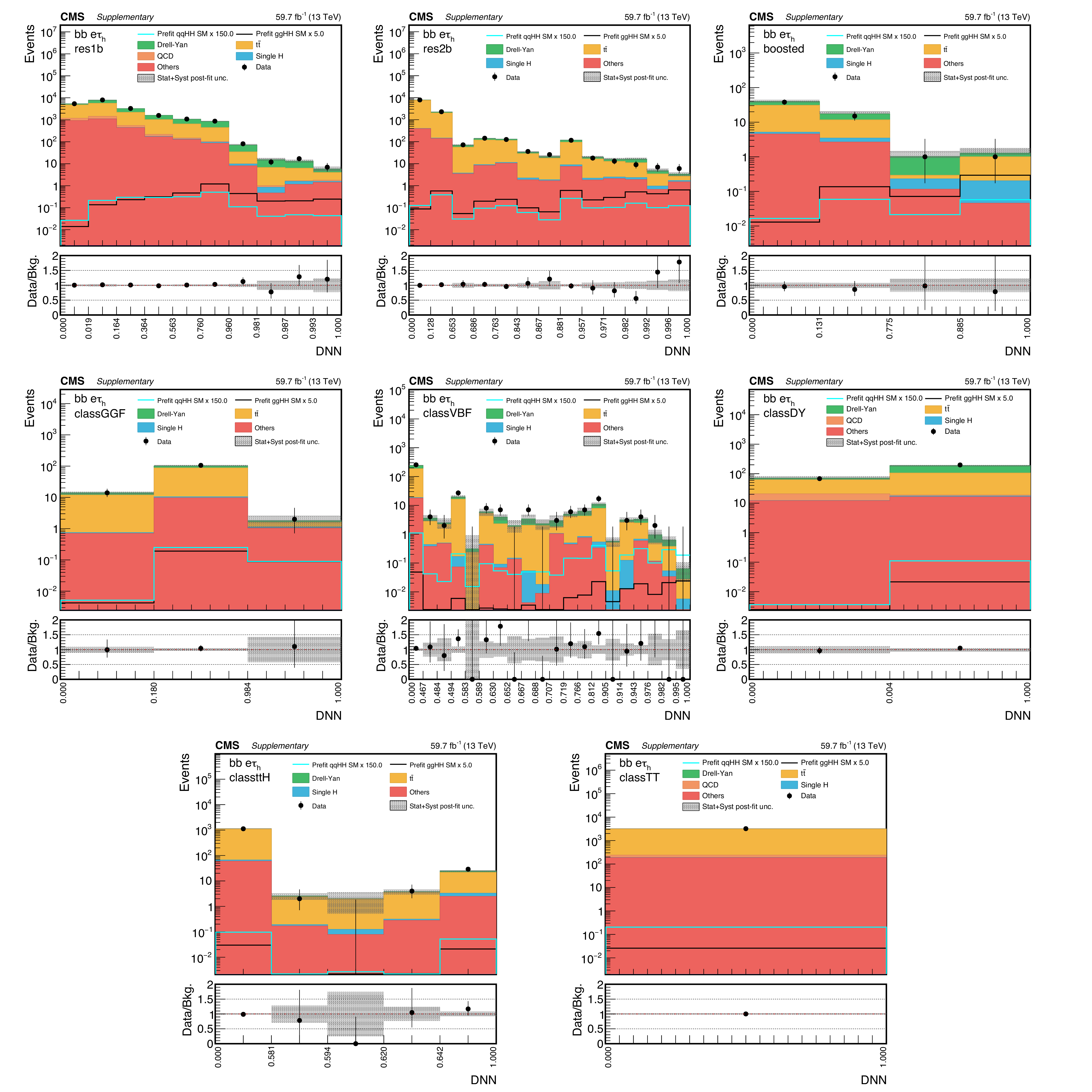
png pdf |
Additional Figure 9:
DNN prediction distributions in the $\mu {{\tau} _\mathrm {h}} $ channel in 2016 for the eight analysis categories. The shaded band in the plots represents the statistical plus systematic uncertainty. |
png pdf |
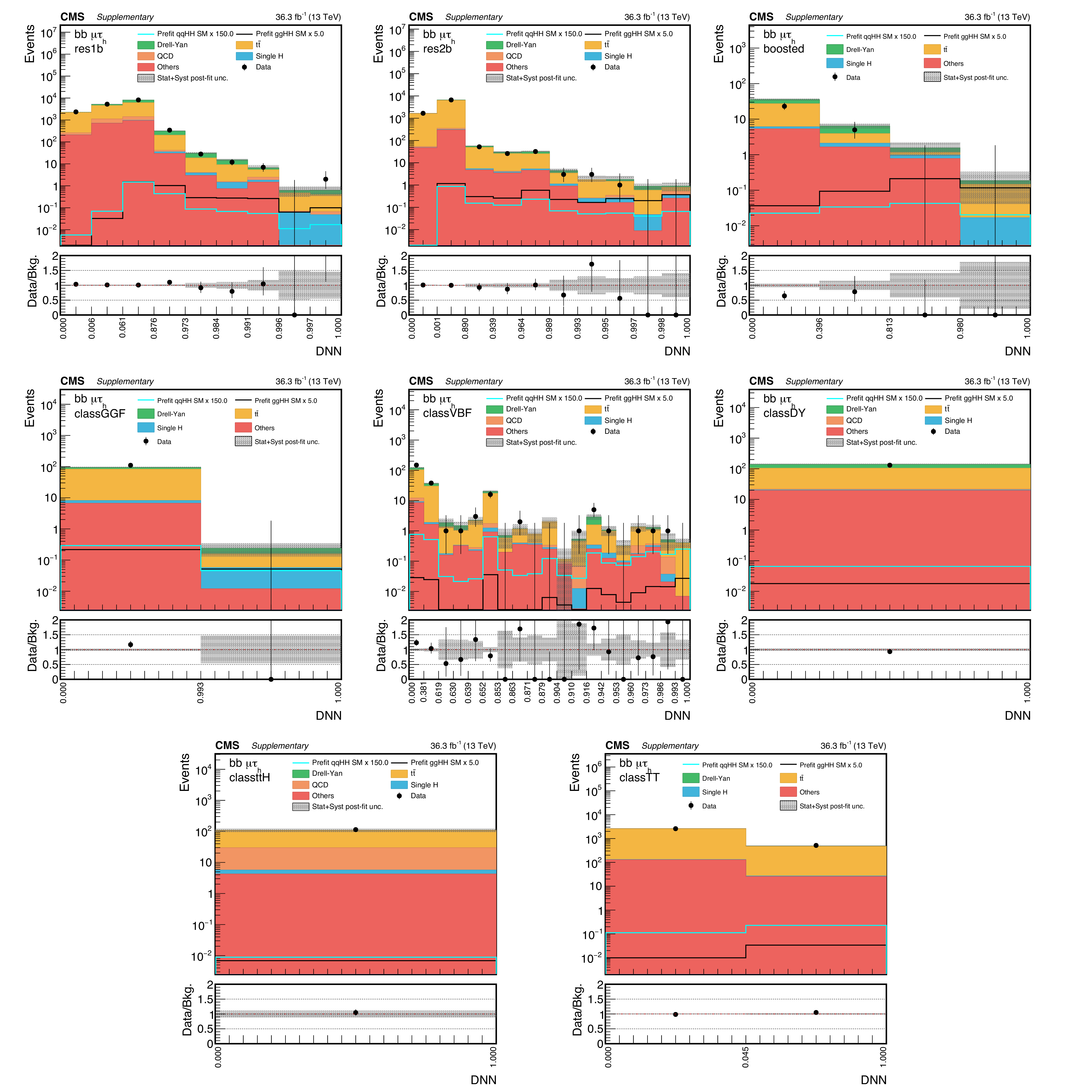
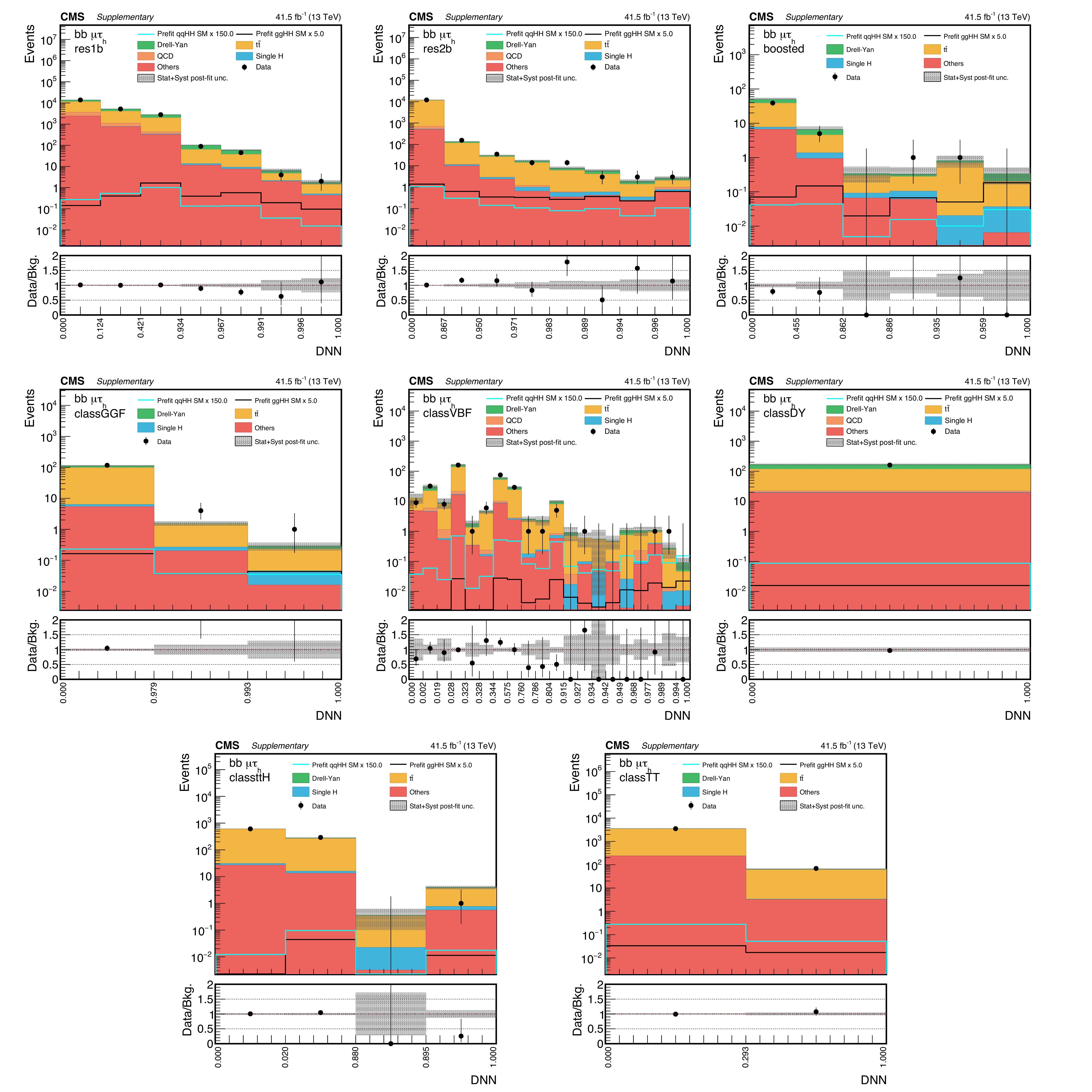
Additional Figure 10:
DNN prediction distributions in the $\mu {{\tau} _\mathrm {h}} $ channel in 2017 for the eight analysis categories. The shaded band in the plots represents the statistical plus systematic uncertainty. |
png pdf |
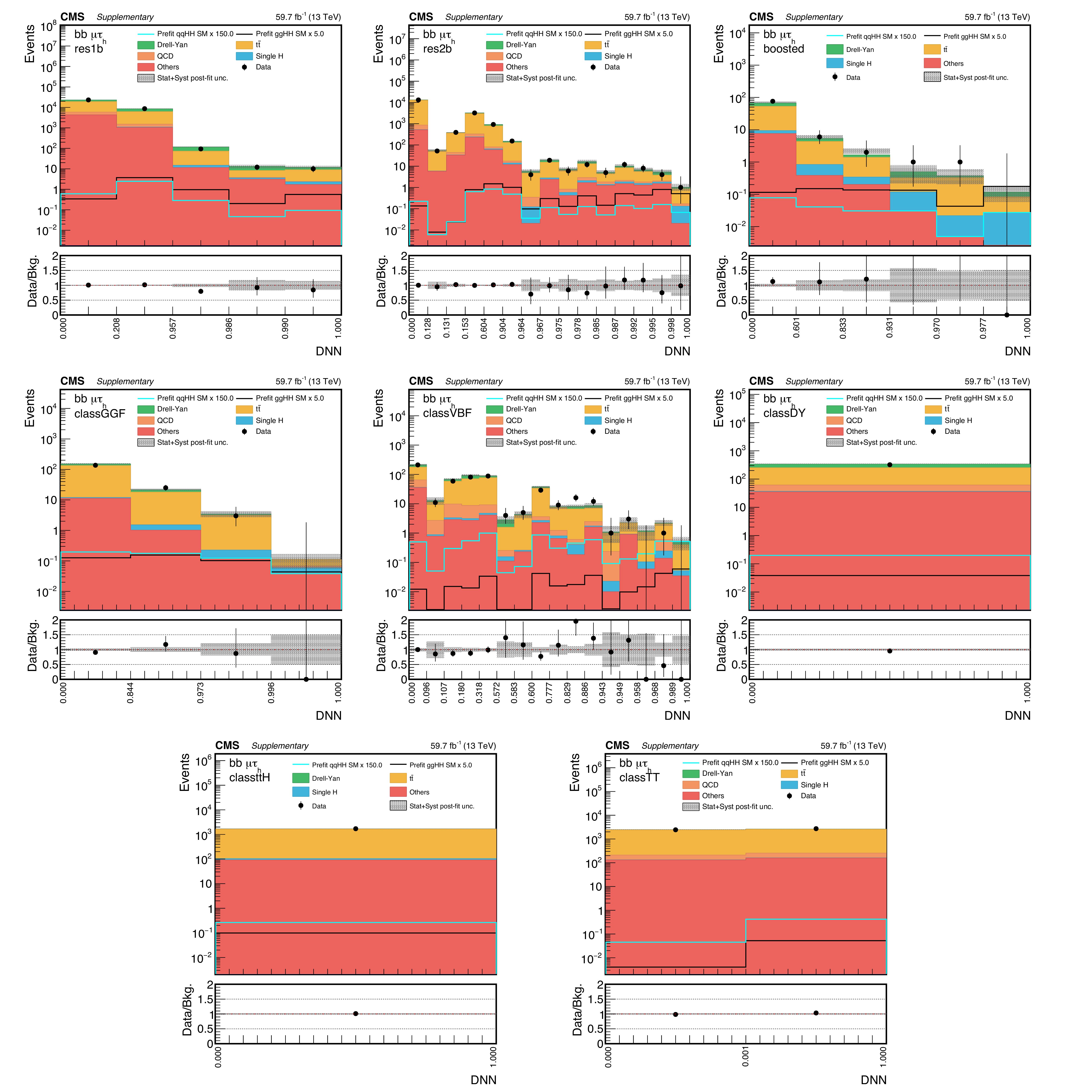
Additional Figure 11:
DNN prediction distributions in the $\mu {{\tau} _\mathrm {h}} $ channel in 2018 for the eight analysis categories. The shaded band in the plots represents the statistical plus systematic uncertainty. |

png pdf |
Additional Figure 12:
DNN prediction distributions in the ${{\tau} _{{\text h}} {\tau} _{{\text h}}}$ channel in 2016 for the eight analysis categories. The shaded band in the plots represents the statistical plus systematic uncertainty. |
png pdf |
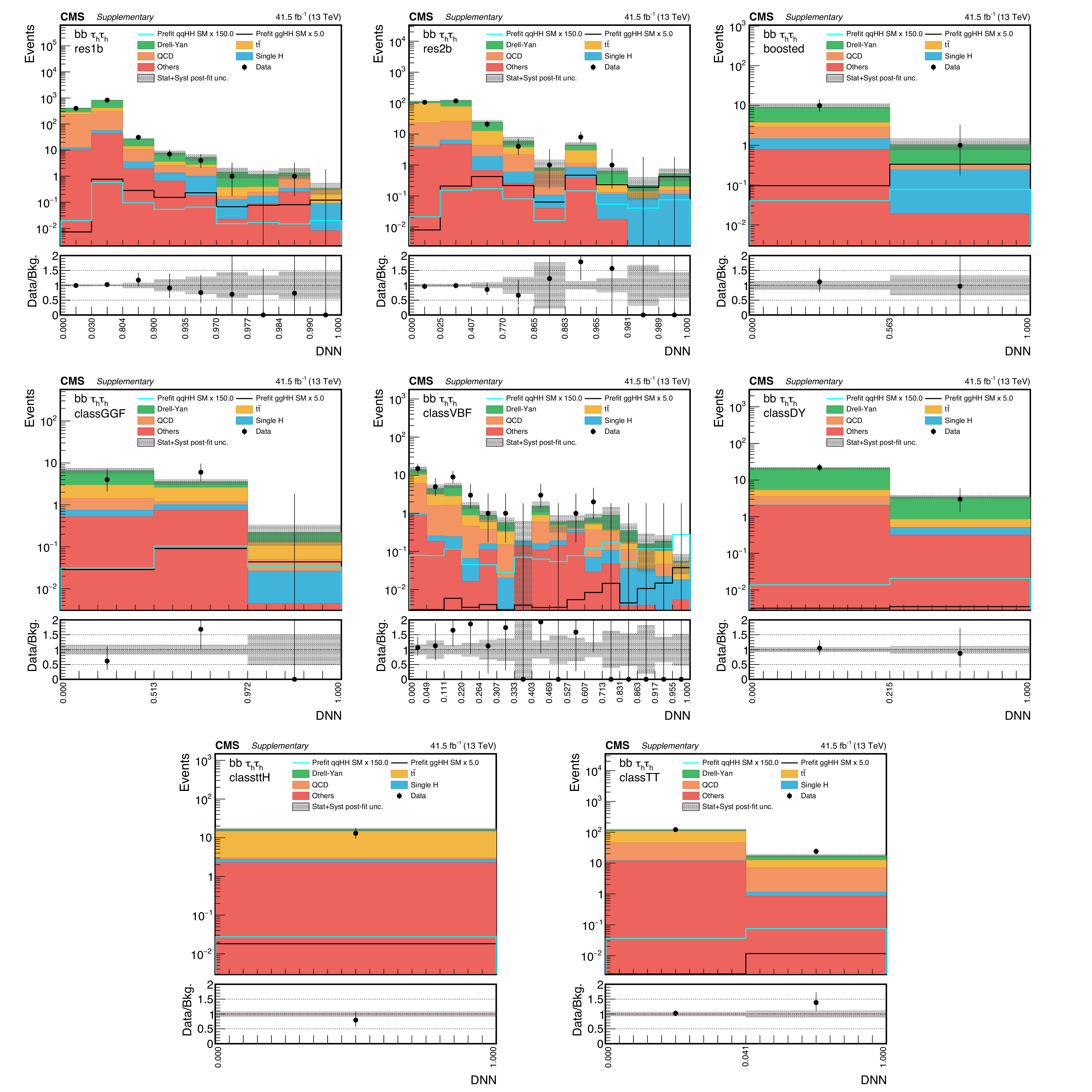
Additional Figure 13:
DNN prediction distributions in the ${{\tau} _{{\text h}} {\tau} _{{\text h}}}$ channel in 2017 for the eight analysis categories. The shaded band in the plots represents the statistical plus systematic uncertainty. |
png pdf |
Additional Figure 14:
DNN prediction distributions in the ${{\tau} _{{\text h}} {\tau} _{{\text h}}}$ channel in 2018 for the eight analysis categories. The shaded band in the plots represents the statistical plus systematic uncertainty. |
png pdf |
Additional Figure 15:
Upper limit on the HH ggF + VBF signal strength at 95% CL, separated into different years and channels, and combined in different channels. All Higgs couplings are set to their SM expectation. |

png pdf |
Additional Figure 16:
Upper limit on the HH VBF signal strength at 95% CL, separated into different years and channels, and combined in different channels. All Higgs couplings are set to their SM expectation. |
png pdf |
Additional Figure 17:
Observed and expected upper limits, separated into categories, on the HH ggF + VBF signal strength at 95% CL as a function of $\kappa _{\lambda}$, with all other couplings set to their SM expectation. |
png pdf |
Additional Figure 18:
Observed and expected upper limits, separated into categories, on the HH VBF signal strength at 95% CL as a function of $\kappa _{2}$, with all other couplings set to their SM expectation. |
png pdf |
Additional Figure 19:
Two-dimensional exclusion regions as a function of the $\kappa _{\lambda}$ and $\kappa _{2}$ coupling modifiers for the full Run2 combination, both $\kappa _{}$ and $\kappa _{\mathrm{t}}$ are fixed to unity. Expected uncertainties on exclusion boundaries are inferred from uncertainty bands of the limit calculation, and are denoted by dark and light grey areas. The blue area marks parameter combinations that are observed to be excluded. For visual guidance, theoretical cross section values are illustrated by thin, labeled contour lines with the SM configuration denoted by a red diamond. |

png pdf |
Additional Figure 20:
Observed likelihood scan as a function of $\kappa _{\mathrm{t}}$ for the full Run 2 combination. The dashed lines show the intersection with threshold values one and four, corresponding to 68% and 95% confidence intervals, respectively. |
png pdf |
Additional Figure 21:
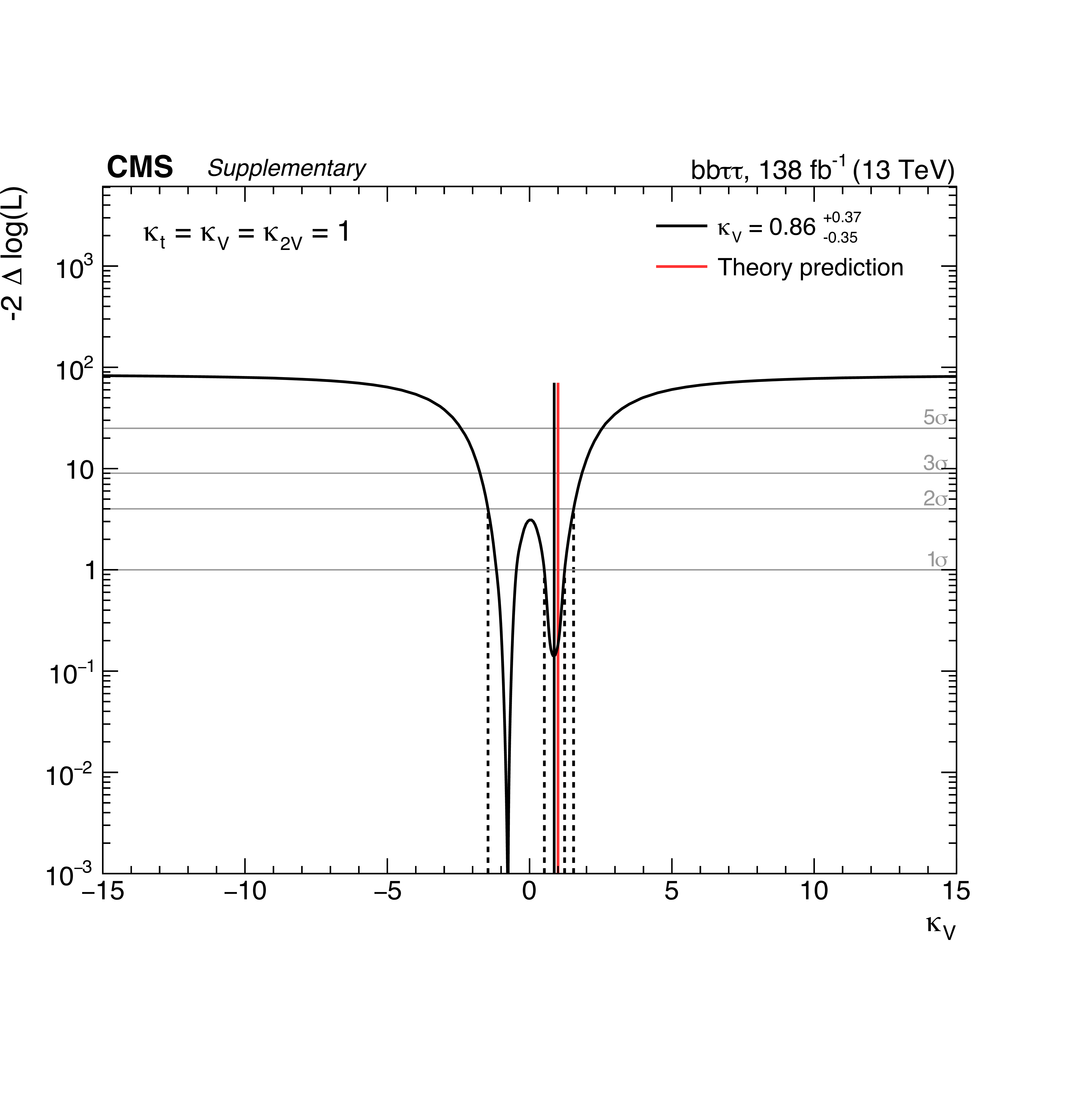
Observed likelihood scan as a function of $\kappa _{}$ for the full Run 2 combination. The dashed lines show the intersection with threshold values one and four, corresponding to 68% and 95% confidence intervals, respectively. |
png pdf |
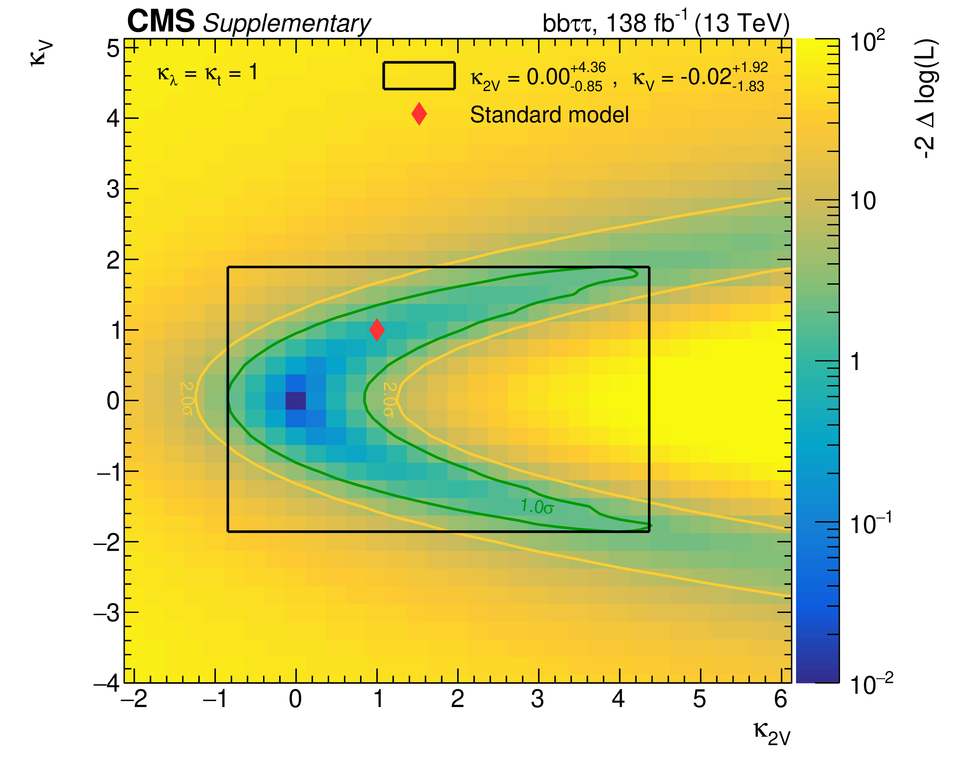
Additional Figure 22:
2D likelihood scan as function of $\kappa _{2}$ and $\kappa _{}$, assuming $r=\kappa _{\mathrm{t}}=\kappa _{\lambda}=1$. The best fit value and its uncertainty are denoted by the black marker and lines, whereas the full uncertainty contours referring to one and two standard deviations are visualized by the green and yellow lines, respectively. The enclosing box refers to the uncertainty construction as described in [62], Figure 40.5. The red diamond represents the SM prediction. |
png pdf |
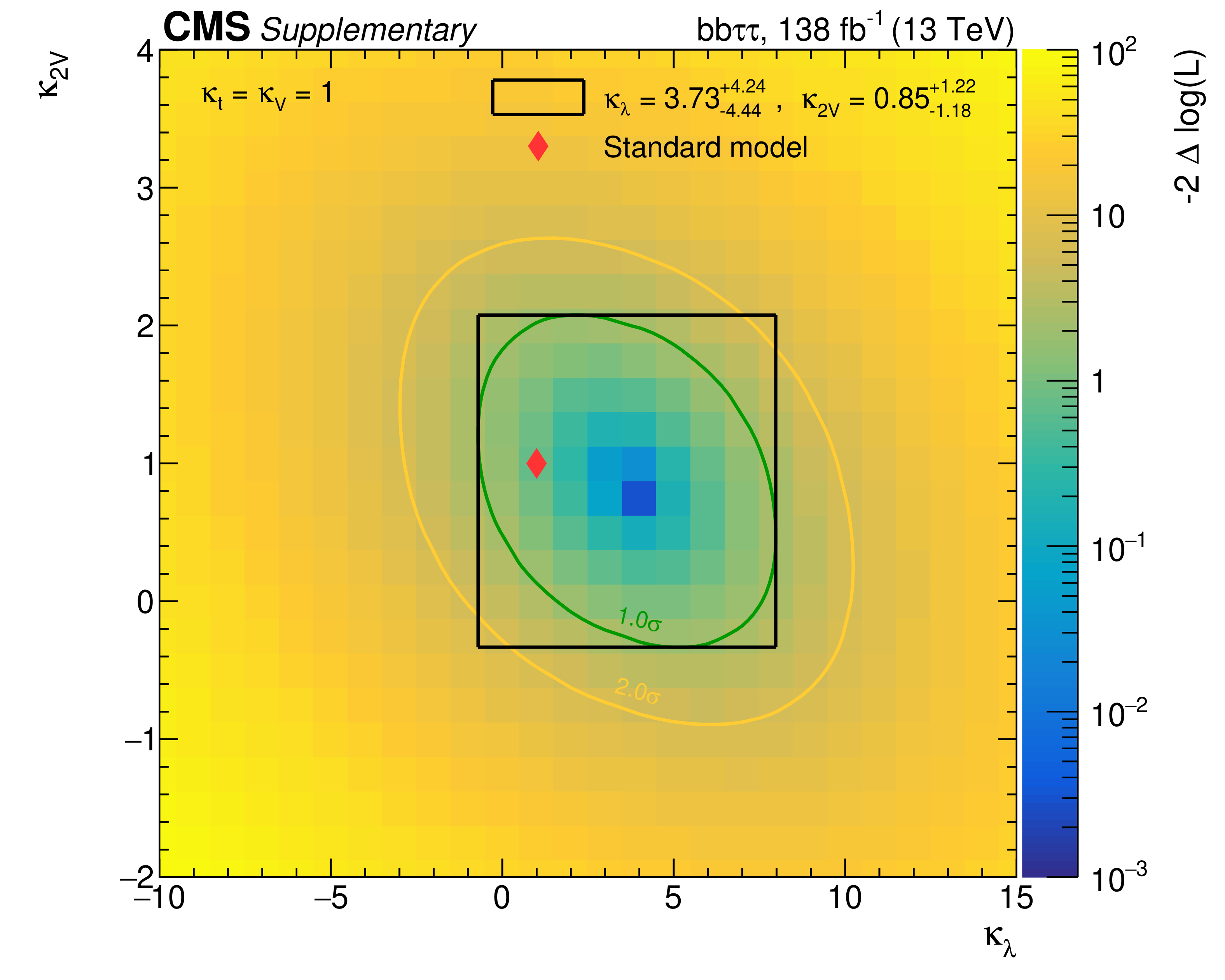
Additional Figure 23:
2D likelihood scan as function of $\kappa _{\lambda}$ and $\kappa _{2}$, assuming $r=\kappa _{\mathrm{t}}=\kappa _{}=1$. The best fit value and its uncertainty are denoted by the black marker and lines, whereas the full uncertainty contours referring to one and two standard deviations are visualized by the green and yellow lines, respectively. The enclosing box refers to the uncertainty construction as described in [62], Figure 40.5. The red diamond represents the SM prediction. |
png pdf |
Additional Figure 24:
2D likelihood scan as function of $\kappa _{\lambda}$ and $\kappa _{\mathrm{t}}$, assuming $r=\kappa _{2}=\kappa _{}=1$. The best fit value and its uncertainty are denoted by the black marker and lines, whereas the full uncertainty contours referring to one and two standard deviations are visualized by the green and yellow lines, respectively. The enclosing box refers to the uncertainty construction as described in [62], Figure 40.5. The red diamond represents the SM prediction. |
png pdf |
Additional Figure 25:
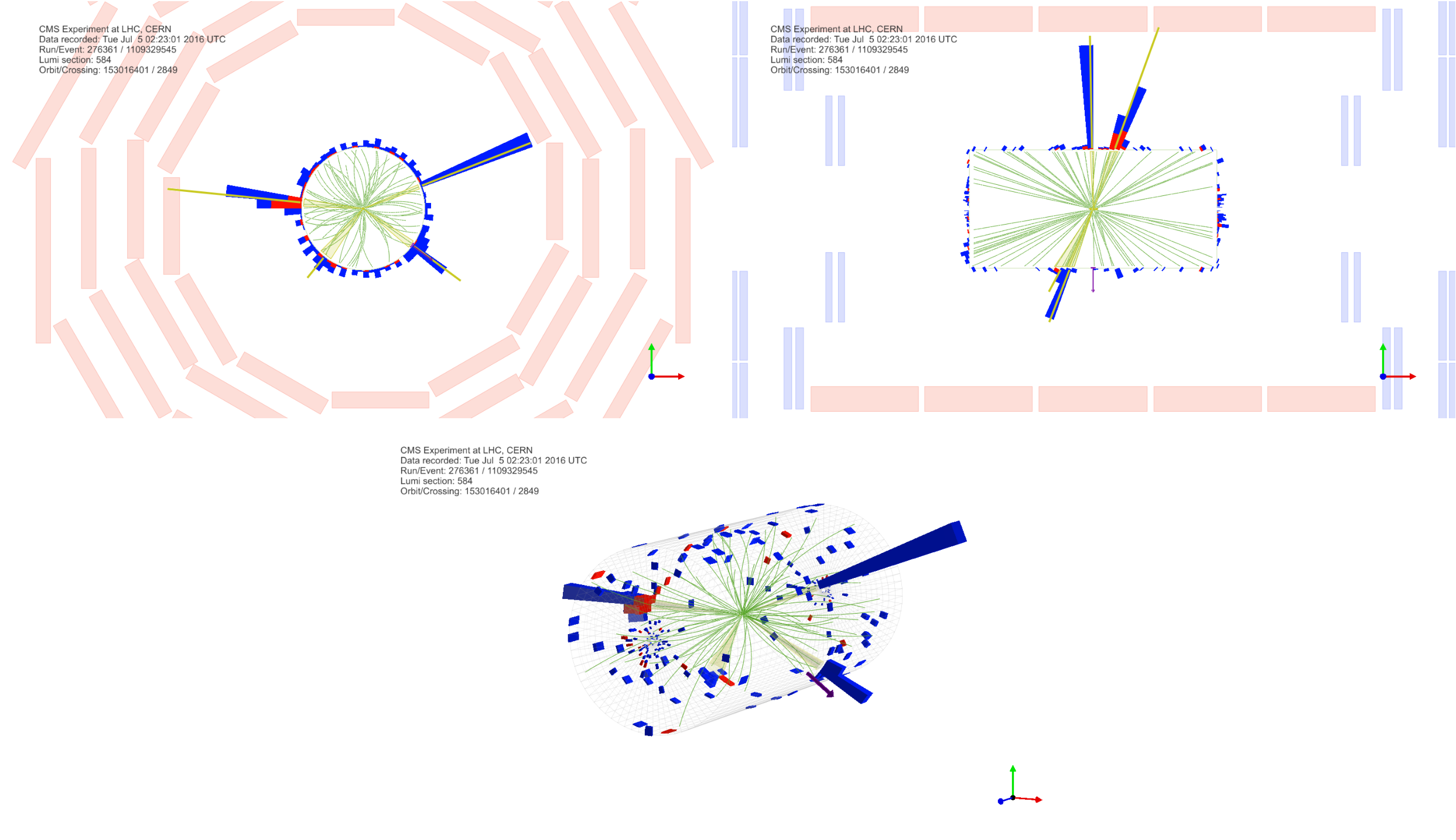
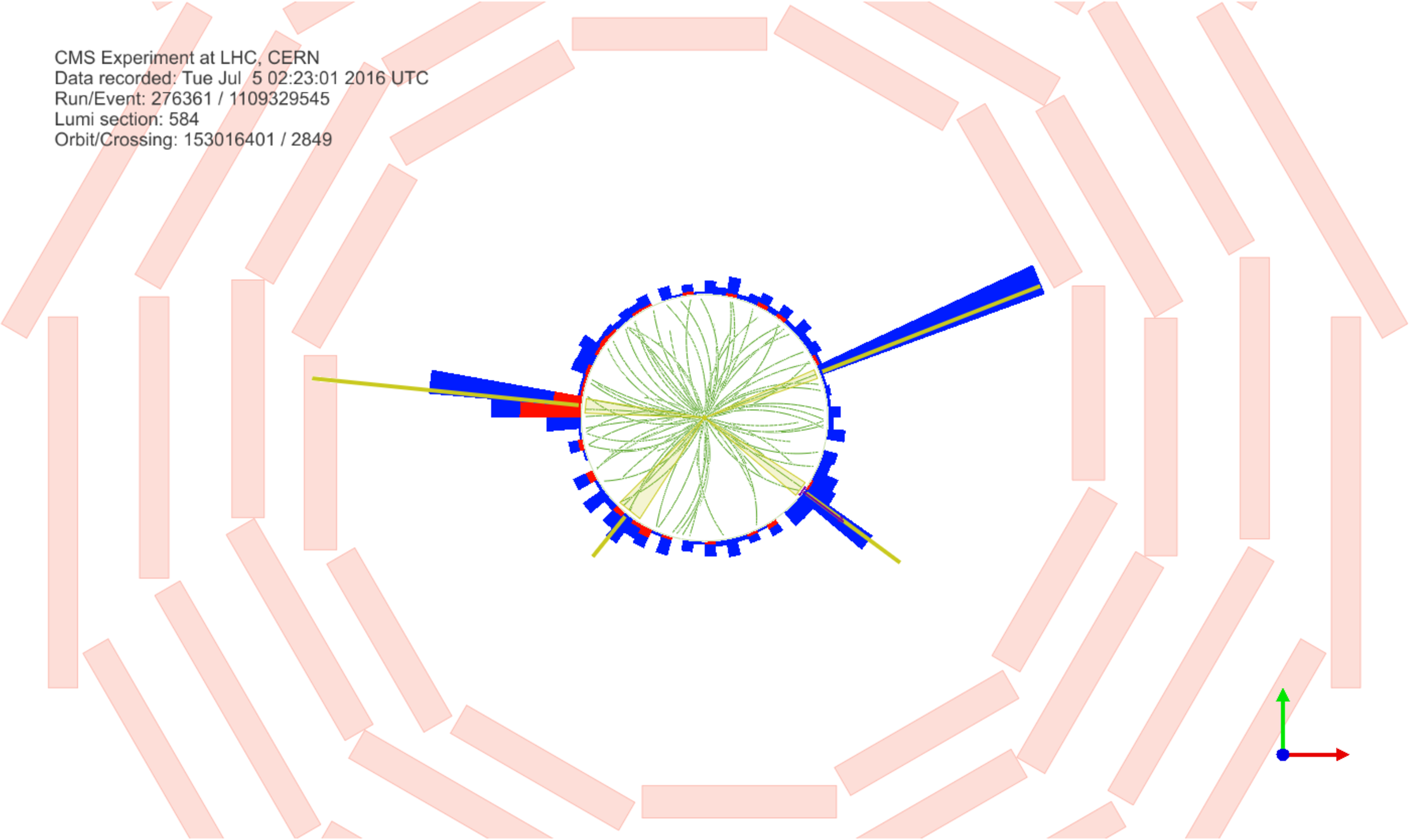
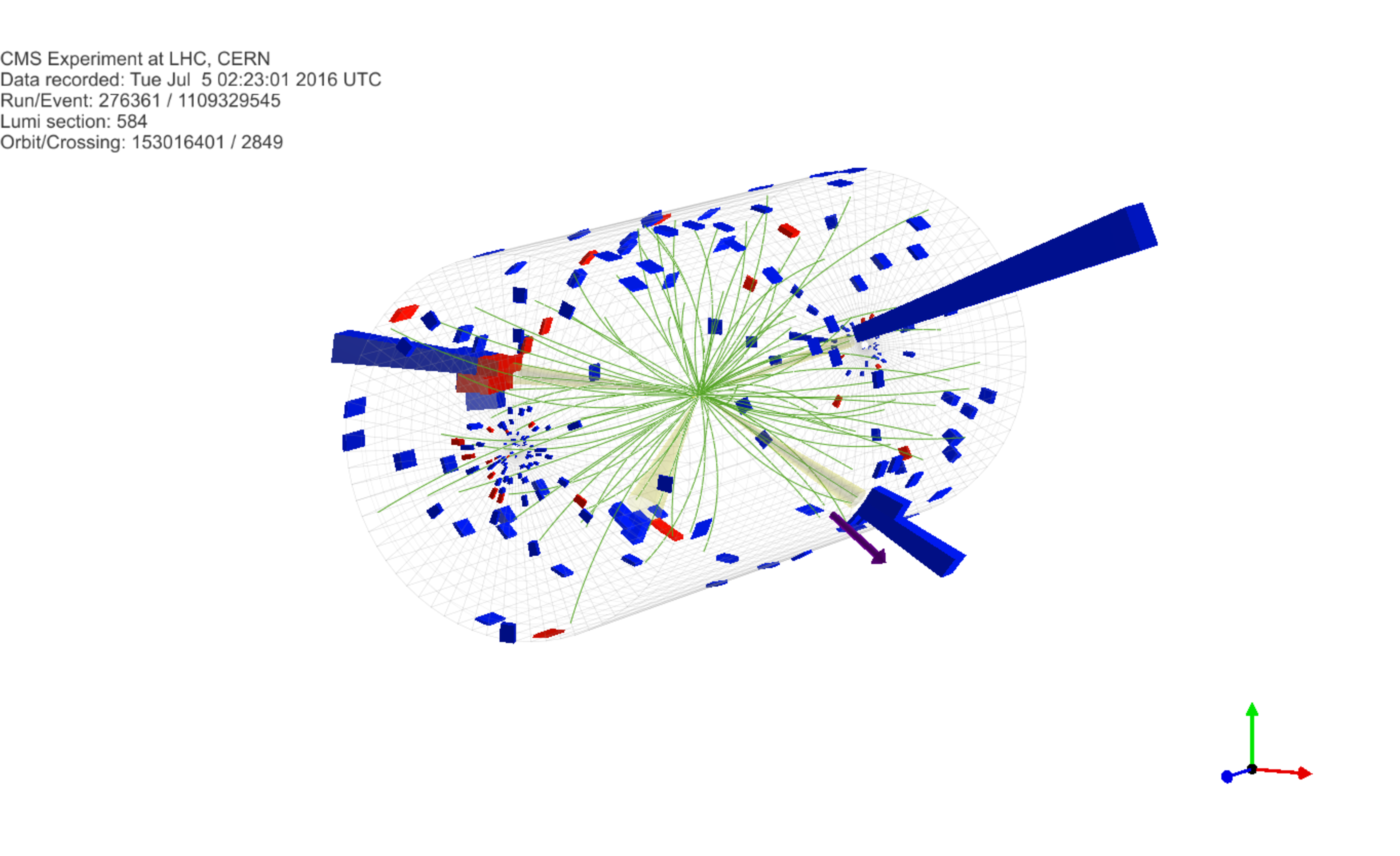
Displays in the transverse (top left) and longitudinal (top right) planes and tridimensional (bottom) view of a candidate $ {{\mathrm {H}} {\mathrm {H}}} \to {\tau} {\tau} {\mathrm {b}} {\mathrm {b}} $ event in the res2b category of the ${{\tau} _{{\text h}} {\tau} _{{\text h}}}$ channel in 2016. |
png pdf |
Additional Figure 25-a:
Displays in the transverse (top left) and longitudinal (top right) planes and tridimensional (bottom) view of a candidate $ {{\mathrm {H}} {\mathrm {H}}} \to {\tau} {\tau} {\mathrm {b}} {\mathrm {b}} $ event in the res2b category of the ${{\tau} _{{\text h}} {\tau} _{{\text h}}}$ channel in 2016. |

png pdf |
Additional Figure 25-b:
Displays in the transverse (top left) and longitudinal (top right) planes and tridimensional (bottom) view of a candidate $ {{\mathrm {H}} {\mathrm {H}}} \to {\tau} {\tau} {\mathrm {b}} {\mathrm {b}} $ event in the res2b category of the ${{\tau} _{{\text h}} {\tau} _{{\text h}}}$ channel in 2016. |
png pdf |
Additional Figure 25-c:
Displays in the transverse (top left) and longitudinal (top right) planes and tridimensional (bottom) view of a candidate $ {{\mathrm {H}} {\mathrm {H}}} \to {\tau} {\tau} {\mathrm {b}} {\mathrm {b}} $ event in the res2b category of the ${{\tau} _{{\text h}} {\tau} _{{\text h}}}$ channel in 2016. |

png pdf |
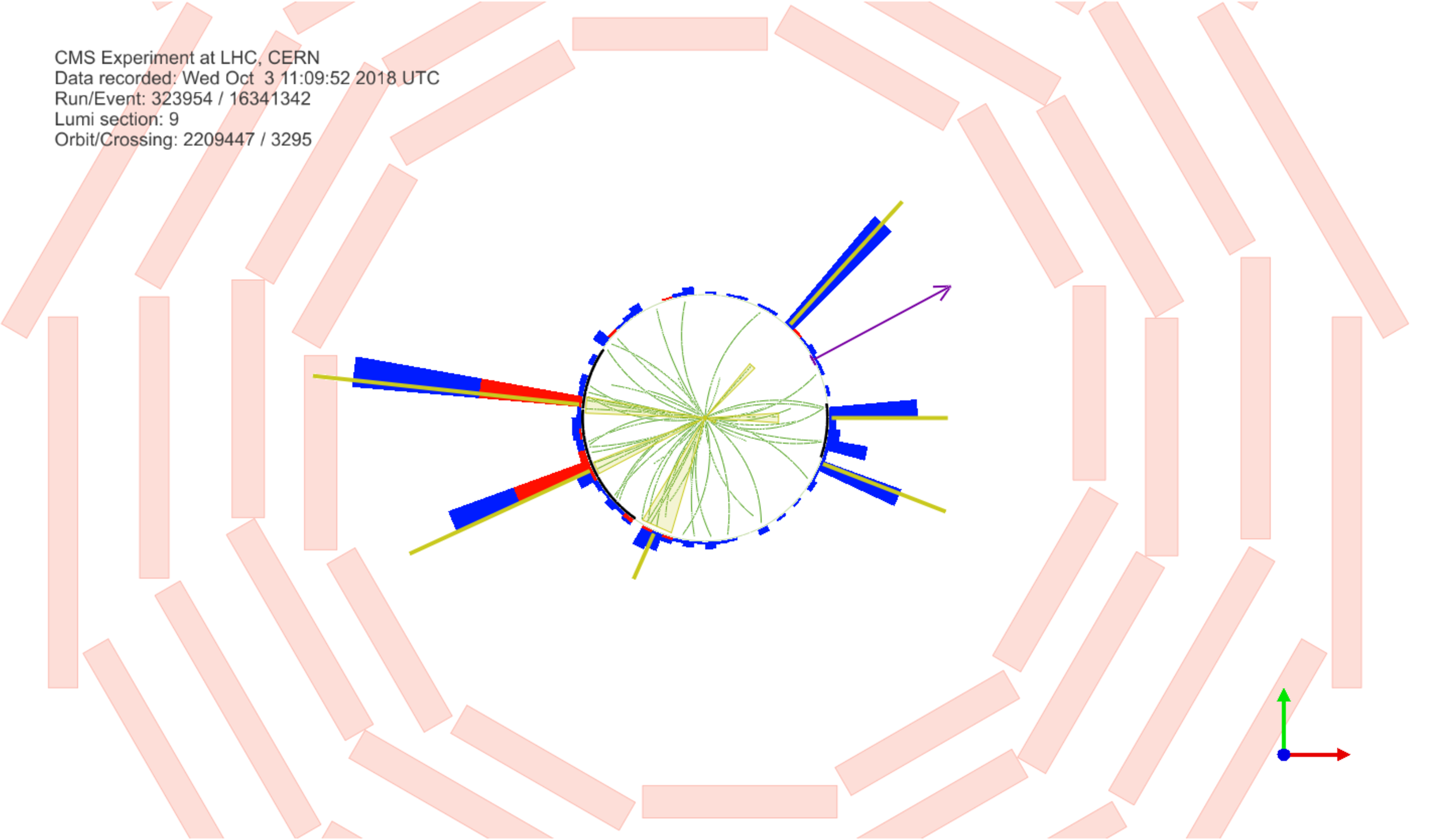
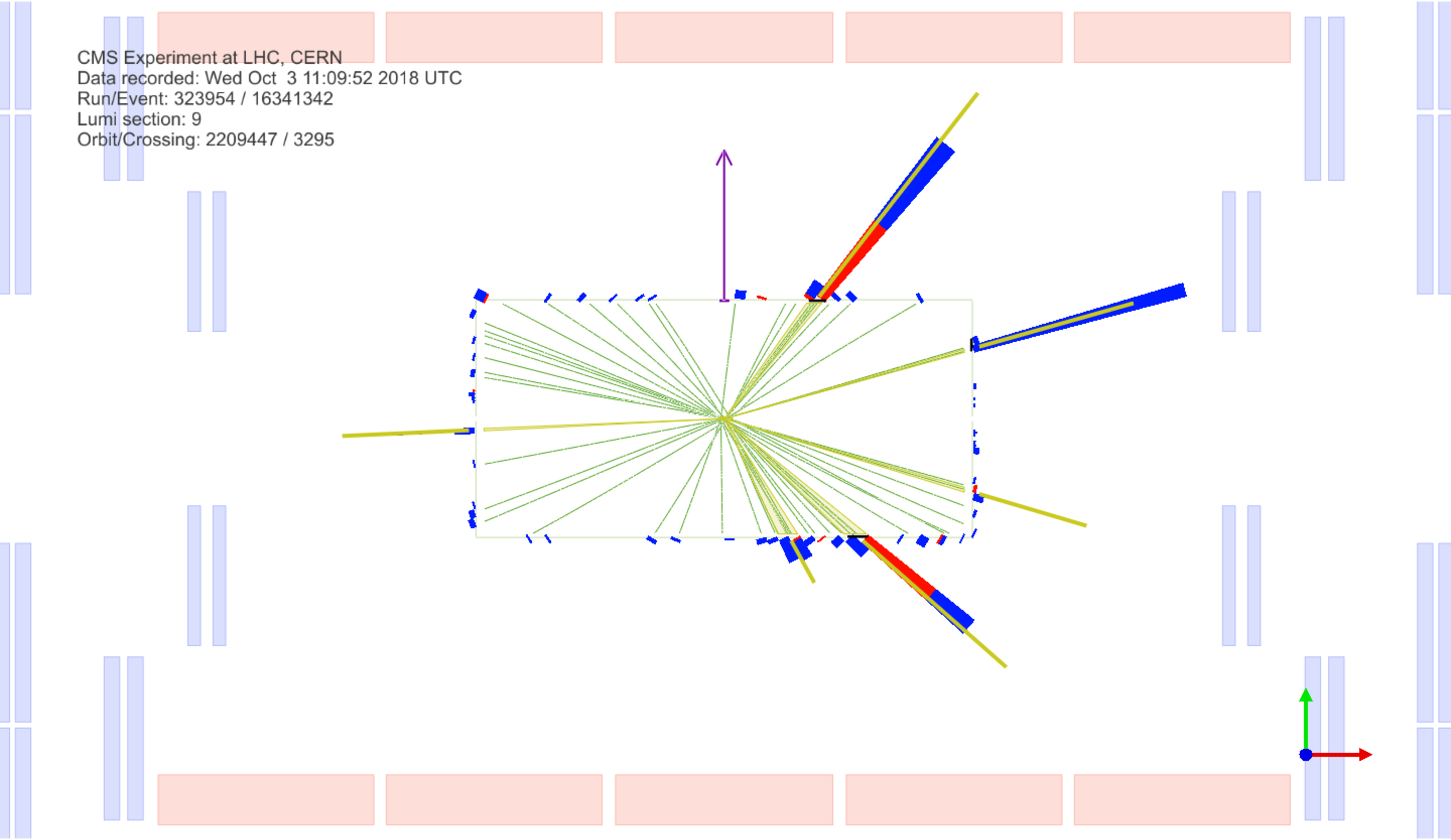
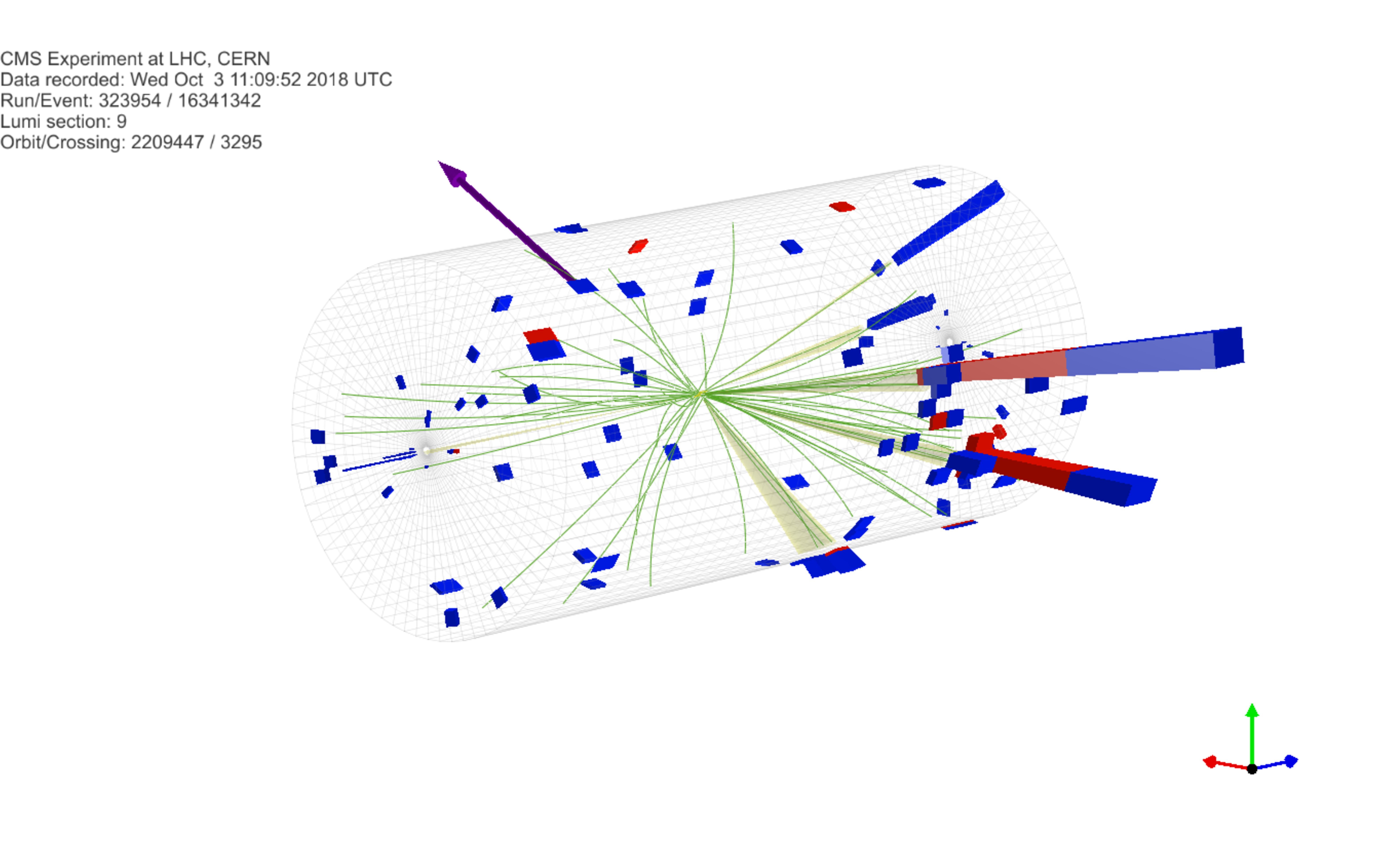
Additional Figure 26:
Displays in the transverse (top left) and longitudinal (top right) planes and tridimensional (bottom) view of a candidate $ {{\mathrm {H}} {\mathrm {H}}} \to {\tau} {\tau} {\mathrm {b}} {\mathrm {b}} $ event in the \textit {classVBF} category of the ${{\tau} _{{\text h}} {\tau} _{{\text h}}}$ channel in 2018. |
png pdf |
Additional Figure 26-a:
Displays in the transverse (top left) and longitudinal (top right) planes and tridimensional (bottom) view of a candidate $ {{\mathrm {H}} {\mathrm {H}}} \to {\tau} {\tau} {\mathrm {b}} {\mathrm {b}} $ event in the \textit {classVBF} category of the ${{\tau} _{{\text h}} {\tau} _{{\text h}}}$ channel in 2018. |
png pdf |
Additional Figure 26-b:
Displays in the transverse (top left) and longitudinal (top right) planes and tridimensional (bottom) view of a candidate $ {{\mathrm {H}} {\mathrm {H}}} \to {\tau} {\tau} {\mathrm {b}} {\mathrm {b}} $ event in the \textit {classVBF} category of the ${{\tau} _{{\text h}} {\tau} _{{\text h}}}$ channel in 2018. |
png pdf |
Additional Figure 26-c:
Displays in the transverse (top left) and longitudinal (top right) planes and tridimensional (bottom) view of a candidate $ {{\mathrm {H}} {\mathrm {H}}} \to {\tau} {\tau} {\mathrm {b}} {\mathrm {b}} $ event in the \textit {classVBF} category of the ${{\tau} _{{\text h}} {\tau} _{{\text h}}}$ channel in 2018. |
| References | ||||
| 1 | ATLAS Collaboration | Observation of a new particle in the search for the Standard Model Higgs boson with the ATLAS detector at the LHC | PLB 716 (2012) 1 | 1207.7214 |
| 2 | CMS Collaboration | Observation of a new boson at a mass of 125 GeV with the CMS experiment at the LHC | PLB 716 (2012) 30 | CMS-HIG-12-028 1207.7235 |
| 3 | CMS Collaboration | Observation of a new boson with mass near 125 GeV in proton-proton collisions at $ \sqrt{s}= $ 7 and 8 TeV | JHEP 06 (2013) 081 | CMS-HIG-12-036 1303.4571 |
| 4 | ATLAS, CMS Collaboration | Combined measurement of the Higgs boson mass in proton-proton collisions at $ \sqrt{s}= $ 7 and 8 TeV with the ATLAS and CMS Experiments | PRL 114 (2015) 191803 | 1503.07589 |
| 5 | ATLAS, CMS Collaboration | Measurements of the Higgs boson production and decay rates and constraints on its couplings from a combined ATLAS and CMS analysis of the LHC proton-proton collision data at $ \sqrt{s}= $ 7 and 8 TeV | JHEP 08 (2016) 045 | 1606.02266 |
| 6 | M. Grazzini et al. | Higgs boson pair production at NNLO with top quark mass effects | JHEP 05 (2018) | 1803.0246 |
| 7 | F. A. Dreyer and A. Karlberg | Vector-boson fusion Higgs pair production at $ {\mathrm{N}}^{3}\mathrm{LO} $ | PRD 98 (2018) 114016 | 1811.07906 |
| 8 | B. Di Micco et al. | Higgs boson pair production at colliders: status and perspectives | Rev. Phys. 5 (2020) 100045 | 1910.00012 |
| 9 | CMS Collaboration | Search for Higgs boson pair production in events with two bottom quarks and two tau leptons in proton-proton collisions at $ \sqrt{s} = $ 13 TeV | PLB 778 (2017) 101 | CMS-HIG-17-002 1707.02909 |
| 10 | ATLAS Collaboration | Search for resonant and nonresonant Higgs boson pair production in the $ \mathrm{b}\mathrm{\bar{b}}\tau^{+}\tau^{-} $ decay channel in proton-proton collisions at $ \sqrt{s} = $ 13 TeV with the ATLAS detector | PRL 121 (2018) 191801 | 1808.00336 |
| 11 | CMS Collaboration | Identification of hadronic tau lepton decays using a deep neural network | 2022. Submitted to JINST | CMS-TAU-20-001 2201.08458 |
| 12 | E. Bols et al. | Jet flavour classification using DeepJet | JINST 15 (2020) P12012 | 2008.10519 |
| 13 | CMS Collaboration | Performance of the CMS Level-1 trigger in proton-proton collisions at $ \sqrt{s} = $ 13 TeV | JINST 15 (2020) P10017 | CMS-TRG-17-001 2006.10165 |
| 14 | CMS Collaboration | The CMS trigger system | JINST 12 (2017) P01020 | CMS-TRG-12-001 1609.02366 |
| 15 | CMS Collaboration | The CMS experiment at the CERN LHC | JINST 3 (2008) S08004 | CMS-00-001 |
| 16 | CMS Collaboration | CMS luminosity measurements for the 2016 data-taking period | CMS-PAS-LUM-17-001 | CMS-PAS-LUM-17-001 |
| 17 | CMS Collaboration | CMS luminosity measurement for the 2017 data-taking period at $ \sqrt{s} = $ 13 TeV | CMS-PAS-LUM-17-004 | CMS-PAS-LUM-17-004 |
| 18 | CMS Collaboration | Precision luminosity measurement in proton-proton collisions at $ \sqrt{s} = $ 13 TeV in 2015 and 2016 at CMS | EPJC 81 (2021) 800 | CMS-LUM-17-003 2104.01927 |
| 19 | CMS Collaboration | CMS luminosity measurement for the 2018 data-taking period at $ \sqrt{s} = $ 13 TeV | CMS-PAS-LUM-18-002 | CMS-PAS-LUM-18-002 |
| 20 | J. Alwall et al. | The automated computation of tree-level and next-to-leading order differential cross sections, and their matching to parton shower simulations | JHEP 07 (2014) | 1405.0301 |
| 21 | E. Re | Single-top Wt-channel production matched with parton showers using the POWHEG method | EPJC 71 (2011) | 1009.2450 |
| 22 | J. M. Campbell, R. K. Ellis, P. Nason, and E. Re | Top-pair production and decay at NLO matched with parton showers | JHEP 04 (2015) | 1412.1828 |
| 23 | G. Heinrich et al. | Probing the trilinear Higgs boson coupling in di-Higgs production at NLO QCD including parton shower effects | JHEP 06 (2019) | 1903.08137 |
| 24 | J. Alwall et al. | Comparative study of various algorithms for the merging of parton showers and matrix elements in hadronic collisions | EPJC 53 (2007) | 0706.2569 |
| 25 | R. Frederix and S. Frixione | Merging meets matching in MC@NLO | JHEP 12 (2012) | 1209.6215 |
| 26 | T. Sjostrand et al. | An introduction to PYTHIA 8.2 | Computer Physics Communications 191 (2015) | 1410.3012 |
| 27 | CMS Collaboration | Event generator tunes obtained from underlying event and multiparton scattering measurements | EPJC 76 (2016) | CMS-GEN-14-001 1512.00815 |
| 28 | CMS Collaboration | Investigations of the impact of the parton shower tuning in PYTHIA 8 in the modelling of $ \mathrm{t}\mathrm{\bar{t}} $ at $ \sqrt{s}= $ 8 and 13 TeV | CMS-PAS-TOP-16-021 | CMS-PAS-TOP-16-021 |
| 29 | CMS Collaboration | Extraction and validation of a new set of CMS PYTHIA 8 tunes from underlying-event measurements | EPJC 80 (2020) | CMS-GEN-17-001 1903.12179 |
| 30 | CMS Collaboration | Particle-flow reconstruction and global event description with the CMS detector | JINST 12 (2017) P10003 | CMS-PRF-14-001 1706.04965 |
| 31 | CMS Collaboration | Performance of missing transverse momentum reconstruction in proton-proton collisions at $ \sqrt{s} = $ 13 TeV using the CMS detector | JINST 14 (2019) P07004 | CMS-JME-17-001 1903.06078 |
| 32 | CMS Collaboration | Electron and photon reconstruction and identification with the CMS experiment at the CERN LHC | JINST 16 (2021) P05014 | CMS-EGM-17-001 2012.06888 |
| 33 | CMS Collaboration | Performance of the CMS muon detector and muon reconstruction with proton-proton collisions at $ \sqrt{s} = $ 13 TeV | JINST 13 (2018) P06015 | CMS-MUO-16-001 1804.04528 |
| 34 | CMS Collaboration | Performance of $ \tau $-lepton reconstruction and identification in CMS | JINST 7 (2012) P01001 | CMS-TAU-11-001 1109.6034 |
| 35 | CMS Collaboration | Reconstruction and identification of $ \tau $ lepton decays to hadrons and $ \nu_\tau $ at CMS | JINST 11 (2016) P01019 | CMS-TAU-14-001 1510.07488 |
| 36 | CMS Collaboration | Performance of reconstruction and identification of $ \tau $ leptons decaying to hadrons and $ \nu_\tau $ in proton-proton collisions at $ \sqrt{s}= $ 13 TeV | JINST 13 (2018) P10005 | CMS-TAU-16-003 1809.02816 |
| 37 | M. Cacciari, G. P. Salam, and G. Soyez | The anti-$ {k_{\mathrm{T}}} $ jet clustering algorithm | JHEP 04 (2008) 063 | 0802.1189 |
| 38 | M. Cacciari, G. P. Salam, and G. Soyez | FastJet user manual | EPJC 72 (2012) 1896 | 1111.6097 |
| 39 | Y. L. Dokshitzer, G. D. Leder, S. Moretti, and B. R. Webber | Better jet clustering algorithms | JHEP 08 (1997) 001 | hep-ph/9707323 |
| 40 | M. Wobisch and T. Wengler | Hadronization corrections to jet cross-sections in deep inelastic scattering | in Proceedings of the Workshop on Monte Carlo Generators for HERA Physics, Hamburg, Germany, p. 270 1998 | hep-ph/9907280 |
| 41 | M. Dasgupta, A. Fregoso, S. Marzani, and G. P. Salam | Towards an understanding of jet substructure | JHEP 09 (2013) 029 | 1307.0007 |
| 42 | J. M. Butterworth, A. R. Davison, M. Rubin, and G. P. Salam | Jet substructure as a new Higgs search channel at the LHC | PRL 100 (2008) 242001 | 0802.2470 |
| 43 | CMS Collaboration | Pileup mitigation at CMS in $ \sqrt{s} = $ 13 TeV data | JINST 15 (2020) P09018 | CMS-JME-18-001 2003.00503 |
| 44 | D. Bertolini, P. Harris, M. Low, and N. Tran | Pileup per particle identification | JHEP 10 (2014) 059 | 1407.6013 |
| 45 | CMS Collaboration | Jet energy scale and resolution in the CMS experiment in proton-proton collisions at $ \sqrt{s} = $ 8 TeV | JINST 12 (2017) P02014 | CMS-JME-13-004 1607.03663 |
| 46 | CMS Collaboration | Jet energy scale and resolution measurement with Run-2 legacy data collected by CMS at $ \sqrt{s} = $ 13 TeV | CDS | |
| 47 | L. Bianchini, J. Conway, E. K. Friis, and C. Veelken | Reconstruction of the Higgs mass in $ \mathrm{H}{}\to\tau\tau $ events by dynamical likelihood techniques | Journal of Physics: Conference Series 513 (2014) 022035 | |
| 48 | G. C. Strong | On the impact of selected modern deep-learning techniques to the performance and celerity of classification models in an experimental high-energy physics use case | Machine Learning: Science and Technology (2020) | 2002.01427 |
| 49 | S. J. Hanson | A stochastic version of the delta rule | Physica D: Nonlinear Phenomena 42 (1990) 265 | |
| 50 | N. Srivastava et al. | Dropout: a simple way to prevent neural networks from overfitting | Journal of Machine Learning Research 15 (2014) 1929 | |
| 51 | F. Rosenblatt | The perceptron: a probabilistic model for information storage and organization in the brain | Psychological Review 65 (1957) 386 | |
| 52 | S. Linnainmaa | The representation of the cumulative rounding error of an algorithm as a Taylor expansion of the local rounding errors | Master's thesis, Univ. Helsinki | |
| 53 | P. J. Werbos | Applications of advances in nonlinear sensitivity analysis | in Proceedings of the 10th IFIP Conference, 31.8 - 4.9, NYC, p. 762 1981 | |
| 54 | D. E. Rumelhart, G. E. Hinton, and R. J. Williams | Learning representations by back-propagating errors | Nature 323 (1986) 533 | |
| 55 | CMS Collaboration | Prospects for HH measurements at the HL-LHC | CMS-PAS-FTR-18-019 | CMS-PAS-FTR-18-019 |
| 56 | E. M. Cepeda et al. | Higgs physics at the HL-LHC and HE-LHC | CERN Yellow Rep. Monogr. 7 (2018) 221 | 1902.00134 |
| 57 | D. de Florian et al. | Handbook of LHC Higgs cross sections: 4. Deciphering the Nature of the Higgs sector | CERN Yellow Reports: Monographs - Volume 2/2017 (2016) | 1610.07922 |
| 58 | B. Cabouat and Sjostrand, Torbjorn | Some dipole shower studies | EPJC 78 (2018), no. 3, 226 | 1710.00391v2 |
| 59 | A. L. Read | Presentation of search results: the CL$ _{\text{s}} $ technique | JPG 28 (2002) 2693 | |
| 60 | T. Junk | Confidence level computation for combining searches with small statistics | NIMA 434 (1999) 435 | hep-ex/9902006 |
| 61 | J. B. Močkus and L. J. Močkus | Bayesian approach to global optimization and application to multiobjective and constrained problems | Journal of Optimization Theory and Applications 70 (1991) 157 | 2108.00002 |
| 62 | Particle Data Group, P.A. Zyla et al. | Review of Particle Physics | PTEP 8 (2020) 083C01 | |
|
|
Compact Muon Solenoid LHC, CERN |
|

|

|

|

|

|