Compact Muon Solenoid
LHC, CERN

Visit us: CMS Public Website, CMS Physics ; Contact us: CMS Publications Committee

CMS-PAS-HIG-20-006

Analysis of the CP structure of the Yukawa coupling between the Higgs boson and $\tau$ leptons in proton-proton collisions at $\sqrt{s}= $ 13 TeV

CMS Collaboration

July 2020

Abstract: The first measurement of the CP structure of the Yukawa coupling between the Higgs boson and $\tau$ leptons is presented. The measurement is based on data collected in proton-proton collisions at $\sqrt{s}= $ 13 TeV by the CMS experiment at the CERN LHC in 2016, 2017 and 2018, corresponding to an integrated luminosity of 137 fb$^{-1}$. Events are selected where one $\tau$ decays to a muon and the other hadronically, and where both $\tau$ leptons decay hadronically. These are the most sensitive decay modes for this analysis and together cover about 50% of all Higgs-to-tau decays. The analysis uses the angular correlation between the decay planes of $\tau$ leptons produced in Higgs boson decays. Machine learning techniques are deployed to distinguish between signal and background events, and dedicated analysis techniques are used to optimise the reconstruction of the $\tau$ decay planes. The mixing angle between CP-even and CP-odd $\tau$ Yukawa couplings was found to be 4 $\pm$ 17$^{\circ}$, compared to an expected uncertainty of $ \pm $ 23$^{\circ}$ at the 68% confidence level, while at the 95% confidence level the observed (expected) uncertainties were $ \pm $ 36 ($\pm$ 55)$^{\circ}$. The observed (expected) significance of the separation between the CP-even and CP-odd hypotheses is 3.2 (2.3) standard deviations. The results are compatible with predictions for the standard model Higgs boson.

Links: CDS record (PDF) ; inSPIRE record ; CADI line (restricted) ; These preliminary results are superseded in this paper, Submitted to JHEP. The superseded preliminary plots can be found here.

Figures
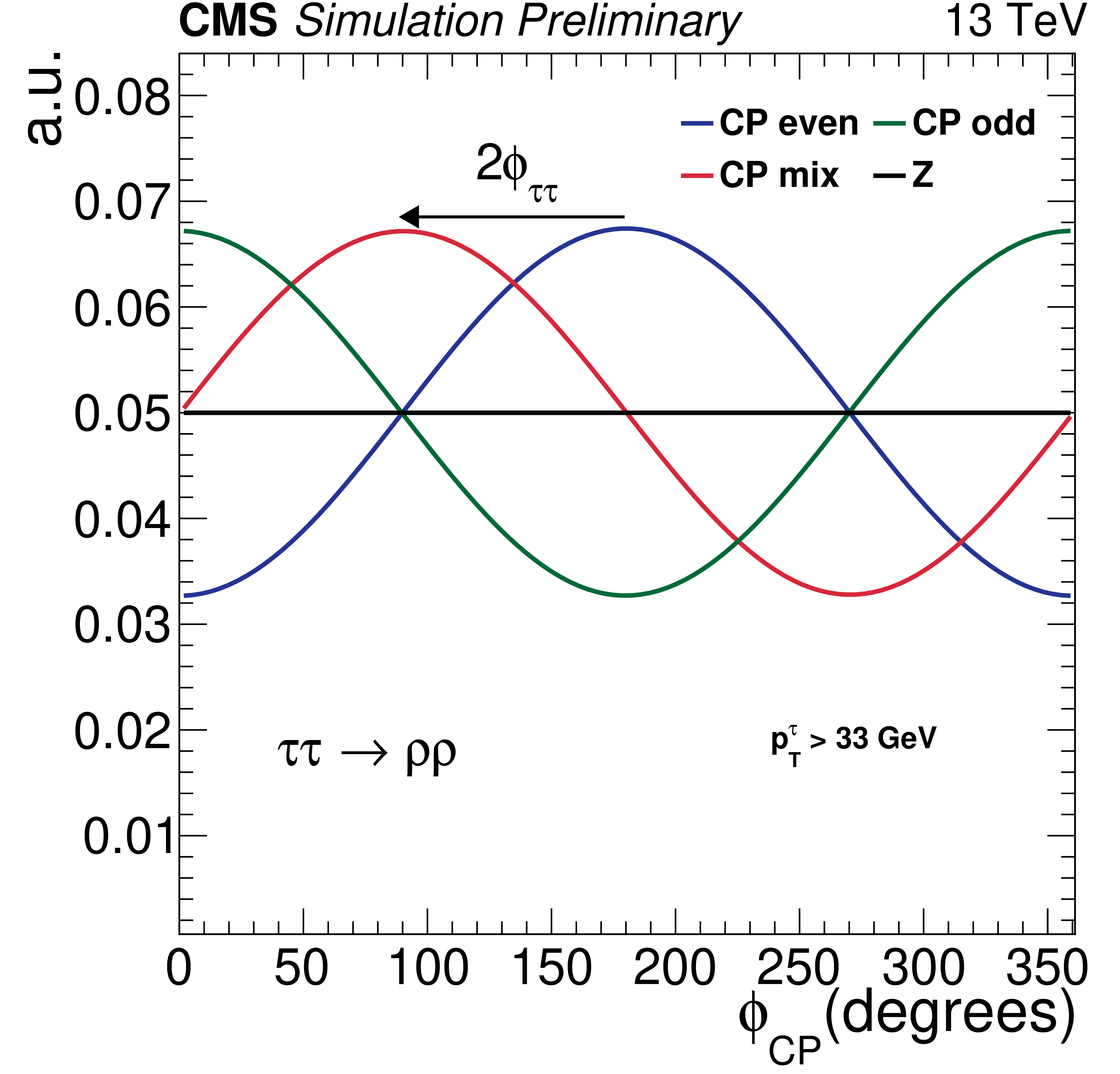
png pdf	Figure 1: The normalised distribution of ${\phi _{\text {CP}}}$ between the $\tau$ decay planes in the boson rest frame, for both $\tau$ leptons decaying to a charged pion and a neutrino. The distributions are for a decaying scalar (CP even, blue), pseudoscalar (CP odd, green), a maximal mixing angle of 45$^{\circ}$ (CP mix, red), and a Z vector boson (black). A ${p_{\mathrm {T}}}$ cutoff of 33 GeV is applied on the visible $\tau$ decay products.
png pdf	Figure 2: Left: illustration of the decay plane for the decay $\tau ^{-}\rightarrow \pi ^{-}+\nu $. Middle: illustration of the decay plane as reconstructed from the neutral and charged pion momentum. Right: illustration of ${\phi _{\text {CP}}}$ for the mixed scenario, in which one $\tau$ lepton decays to a single charged pion while the other decays via an intermediate $\rho$ meson. The illustrations are in the zero-momentum frame of the charged particles.
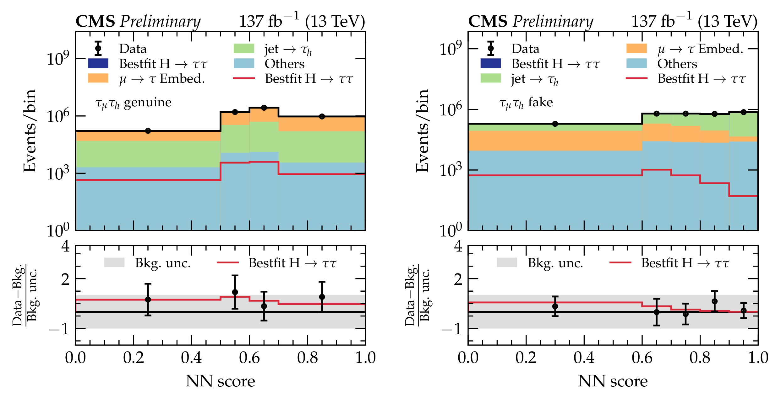
png pdf	Figure 3: The postfit genuine $\tau$ (left), and jet-fake (right) NN scores for the ${\tau _{\mu} {\tau _\mathrm {h}}}$ channel. The distributions are inclusive in decay mode. The best-fit signal distributions are overlaid. In the bottom plot the data minus the background template divided by the uncertainty in the background template is displayed, as well as the signal samples divided by the uncertainty in the background template. The uncertainty band consists of the sum of the postfit uncertainties in the background templates.
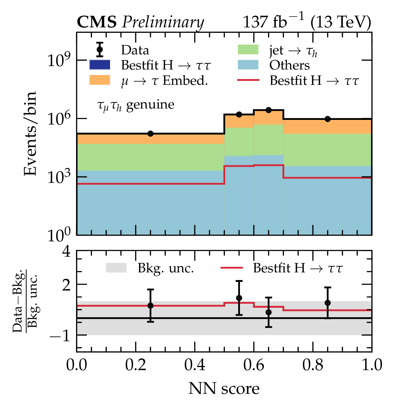
png pdf	Figure 3-a: The postfit genuine $\tau$ (left), and jet-fake (right) NN scores for the ${\tau _{\mu} {\tau _\mathrm {h}}}$ channel. The distributions are inclusive in decay mode. The best-fit signal distributions are overlaid. In the bottom plot the data minus the background template divided by the uncertainty in the background template is displayed, as well as the signal samples divided by the uncertainty in the background template. The uncertainty band consists of the sum of the postfit uncertainties in the background templates.
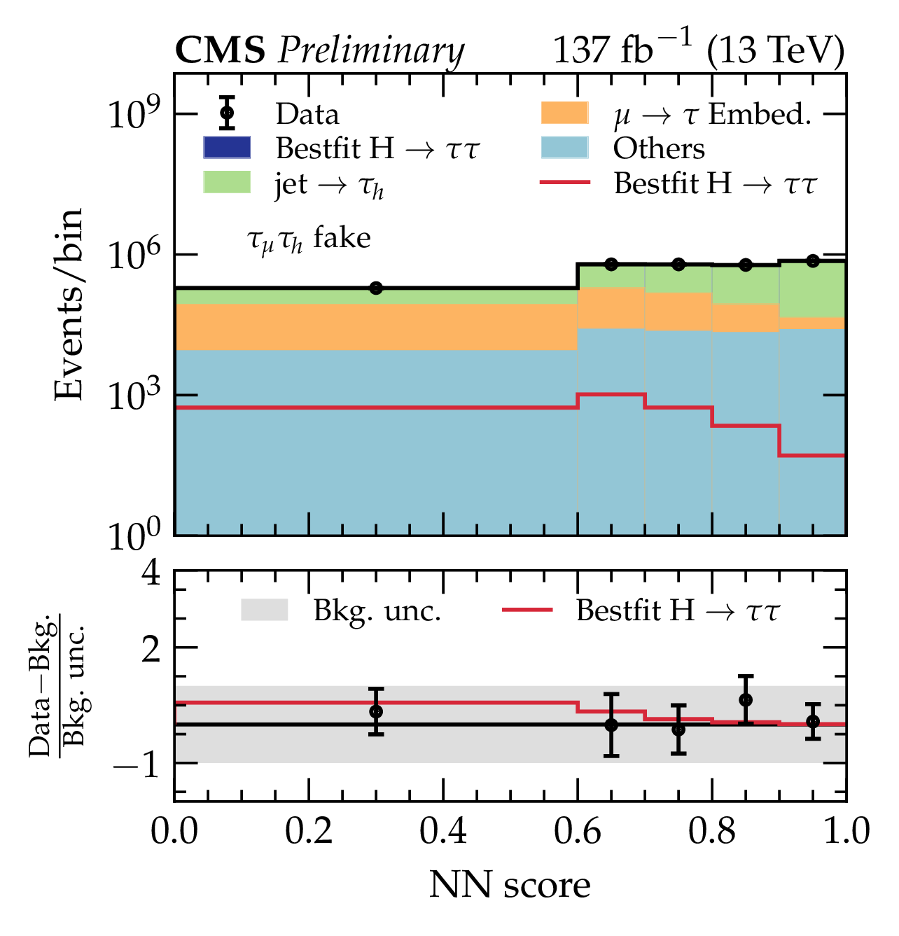
png pdf	Figure 3-b: The postfit genuine $\tau$ (left), and jet-fake (right) NN scores for the ${\tau _{\mu} {\tau _\mathrm {h}}}$ channel. The distributions are inclusive in decay mode. The best-fit signal distributions are overlaid. In the bottom plot the data minus the background template divided by the uncertainty in the background template is displayed, as well as the signal samples divided by the uncertainty in the background template. The uncertainty band consists of the sum of the postfit uncertainties in the background templates.
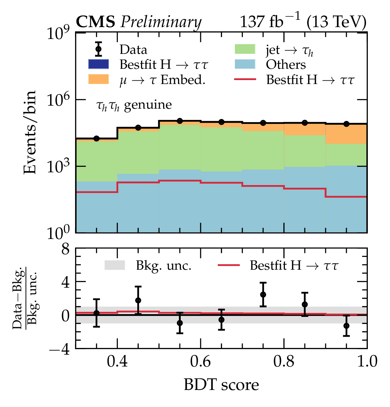
png pdf	Figure 4: The postfit genuine $\tau$ (left), and jet-fake (right) BDT scores for the ${{\tau _\mathrm {h}} {\tau _\mathrm {h}}}$ channel. The distributions are inclusive in decay mode. The best-fit signal distributions are overlaid. In the bottom plot the data minus the background template divided by the uncertainty in the background template is displayed, as well as the signal samples divided by the uncertainty in the background template. The uncertainty band consists of the sum of the postfit uncertainties in the background templates.
png pdf	Figure 4-a: The postfit genuine $\tau$ (left), and jet-fake (right) BDT scores for the ${{\tau _\mathrm {h}} {\tau _\mathrm {h}}}$ channel. The distributions are inclusive in decay mode. The best-fit signal distributions are overlaid. In the bottom plot the data minus the background template divided by the uncertainty in the background template is displayed, as well as the signal samples divided by the uncertainty in the background template. The uncertainty band consists of the sum of the postfit uncertainties in the background templates.
png pdf	Figure 4-b: The postfit genuine $\tau$ (left), and jet-fake (right) BDT scores for the ${{\tau _\mathrm {h}} {\tau _\mathrm {h}}}$ channel. The distributions are inclusive in decay mode. The best-fit signal distributions are overlaid. In the bottom plot the data minus the background template divided by the uncertainty in the background template is displayed, as well as the signal samples divided by the uncertainty in the background template. The uncertainty band consists of the sum of the postfit uncertainties in the background templates.
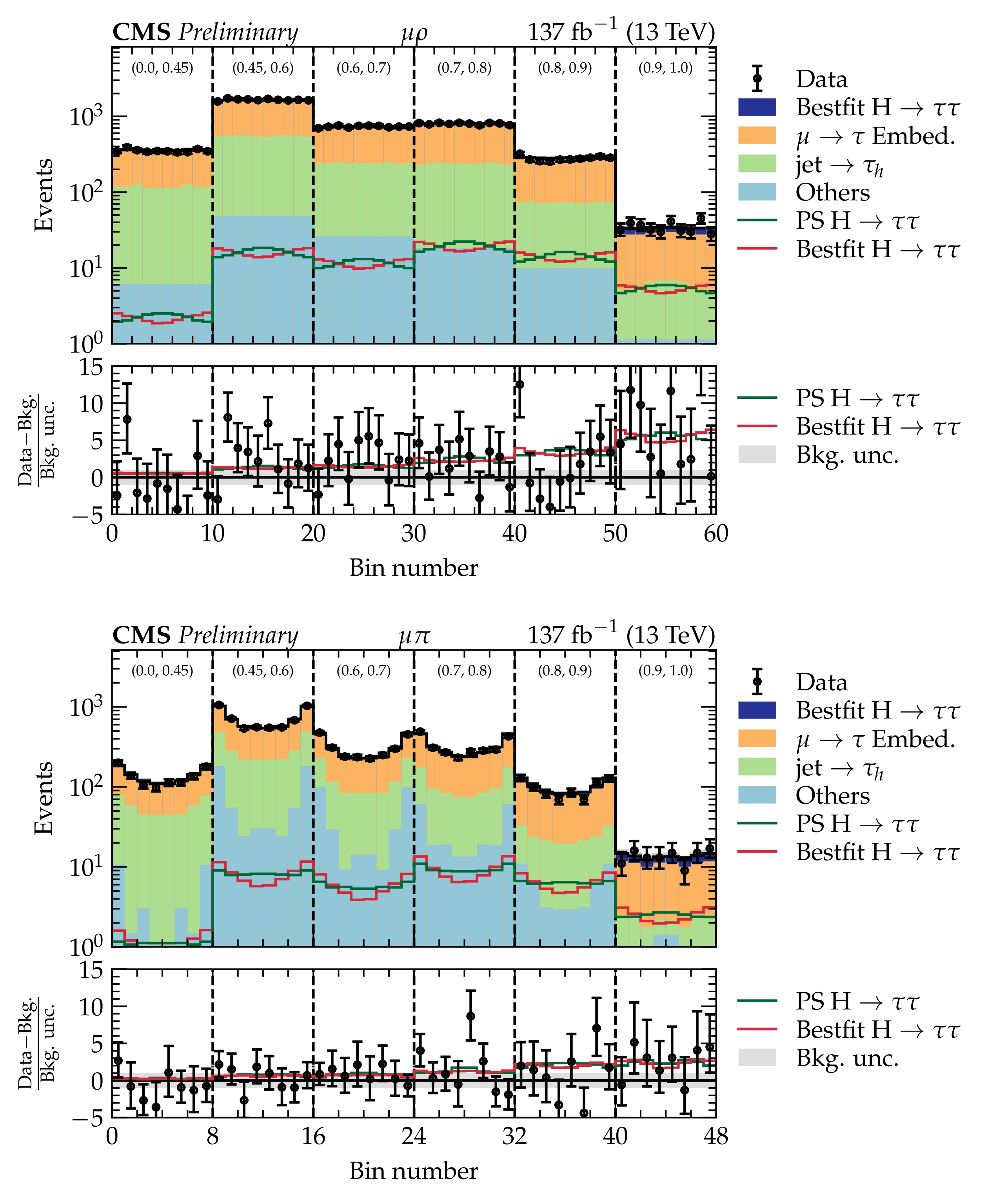
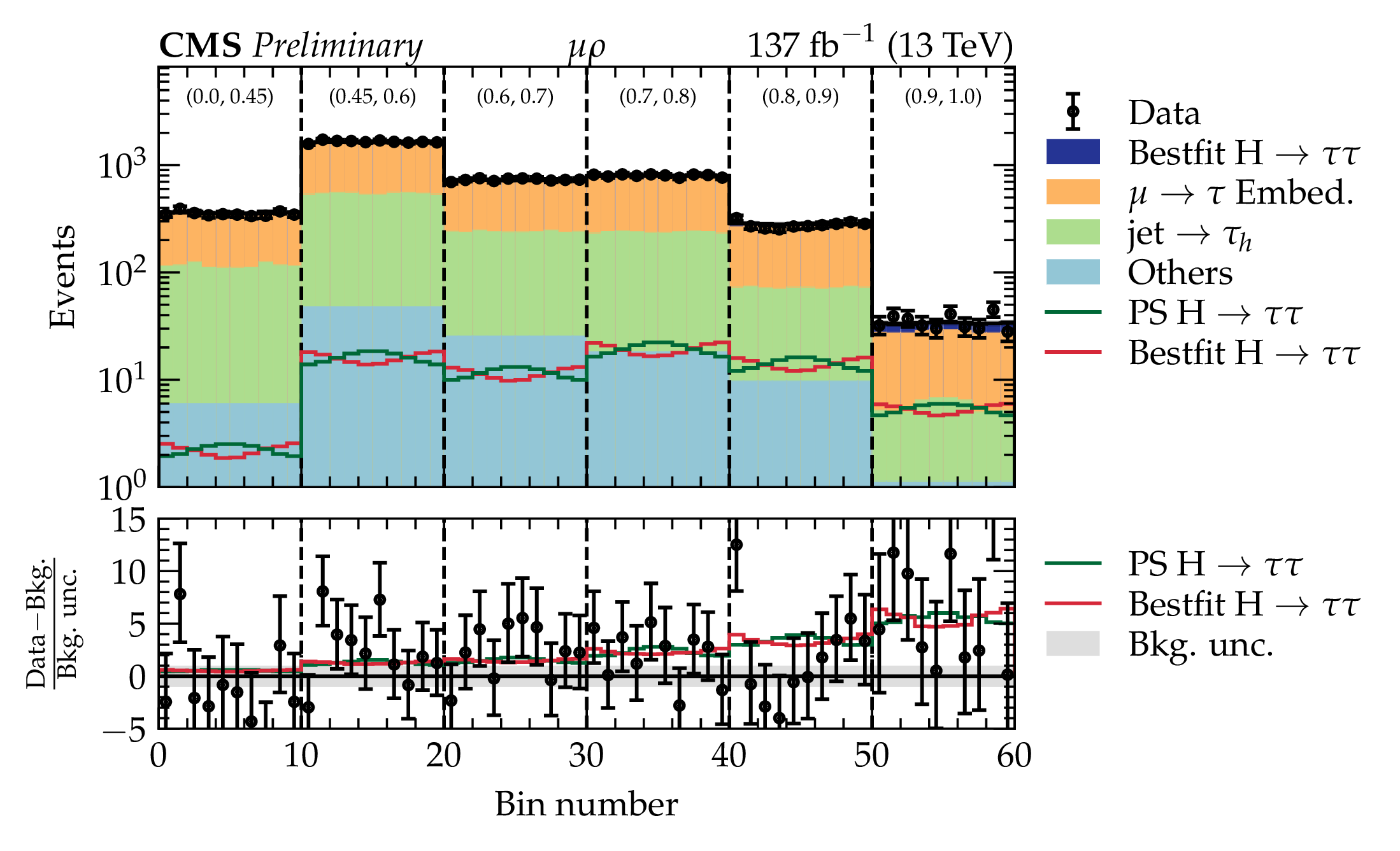
png pdf	Figure 5: Distributions of ${\phi _{\text {CP}}}$ in the $\mu {\rho} $ (top) and $\mu \pi $ (bottom) channel in windows of increasing neural net score. The best-fit and pseudoscalar (PS) signal distributions are overlaid. The $x$ axis represents the cyclic bins in ${\phi _{\text {CP}}}$ in the range of (0, 360$^{\circ}$). In the bottom plot the data minus the background template divided by the uncertainty in the background template is displayed, as well as the signal samples divided by the uncertainty in the background template. The uncertainty band consists of the sum of the postfit uncertainties in the background templates.
png pdf	Figure 5-a: Distributions of ${\phi _{\text {CP}}}$ in the $\mu {\rho} $ (top) and $\mu \pi $ (bottom) channel in windows of increasing neural net score. The best-fit and pseudoscalar (PS) signal distributions are overlaid. The $x$ axis represents the cyclic bins in ${\phi _{\text {CP}}}$ in the range of (0, 360$^{\circ}$). In the bottom plot the data minus the background template divided by the uncertainty in the background template is displayed, as well as the signal samples divided by the uncertainty in the background template. The uncertainty band consists of the sum of the postfit uncertainties in the background templates.
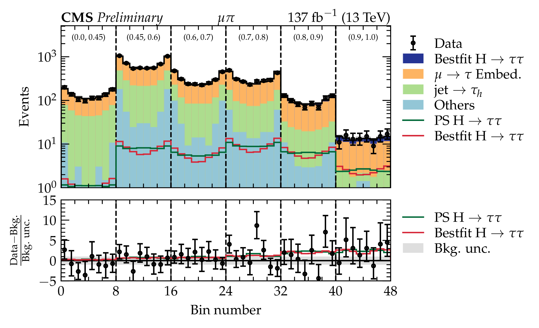
png pdf	Figure 5-b: Distributions of ${\phi _{\text {CP}}}$ in the $\mu {\rho} $ (top) and $\mu \pi $ (bottom) channel in windows of increasing neural net score. The best-fit and pseudoscalar (PS) signal distributions are overlaid. The $x$ axis represents the cyclic bins in ${\phi _{\text {CP}}}$ in the range of (0, 360$^{\circ}$). In the bottom plot the data minus the background template divided by the uncertainty in the background template is displayed, as well as the signal samples divided by the uncertainty in the background template. The uncertainty band consists of the sum of the postfit uncertainties in the background templates.
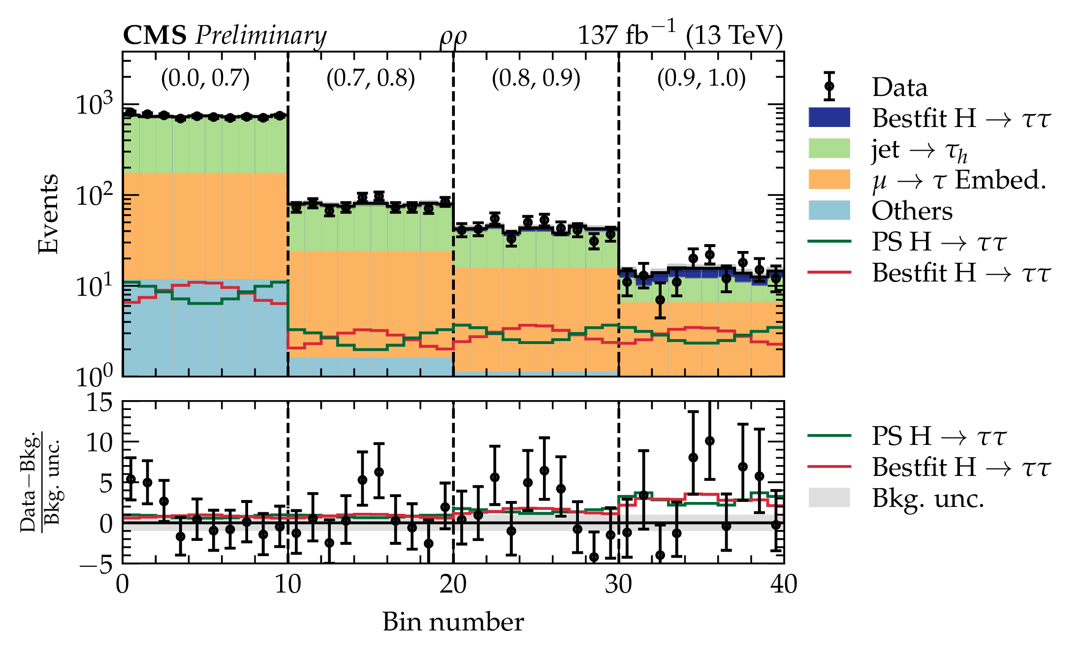
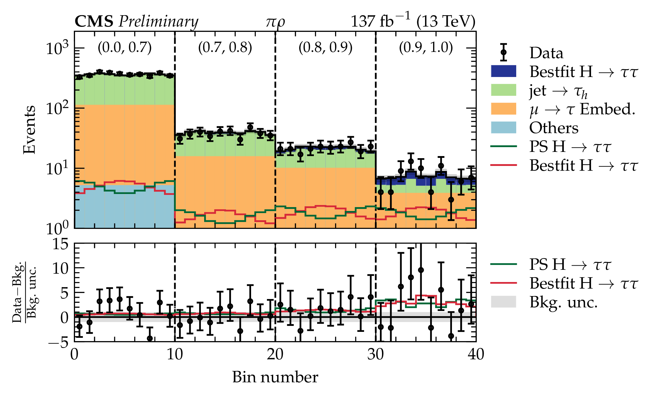
png pdf	Figure 6: Distributions of ${\phi _{\text {CP}}}$ in the $ {\rho} {\rho} $ (top) and $\pi {\rho} $ (bottom) channel in windows of increasing BDT score. The best-fit and pseudoscalar (PS) signal distributions are overlaid. The $x$ axis represents the cyclic bins in ${\phi _{\text {CP}}}$ in the range of (0, 360$^{\circ}$). In the bottom plot the data minus the background template divided by the uncertainty in the background template is displayed, as well as the signal samples divided by the uncertainty in the background template. The uncertainty band consists of the sum of the postfit uncertainties in the background templates.
png pdf	Figure 6-a: Distributions of ${\phi _{\text {CP}}}$ in the $ {\rho} {\rho} $ (top) and $\pi {\rho} $ (bottom) channel in windows of increasing BDT score. The best-fit and pseudoscalar (PS) signal distributions are overlaid. The $x$ axis represents the cyclic bins in ${\phi _{\text {CP}}}$ in the range of (0, 360$^{\circ}$). In the bottom plot the data minus the background template divided by the uncertainty in the background template is displayed, as well as the signal samples divided by the uncertainty in the background template. The uncertainty band consists of the sum of the postfit uncertainties in the background templates.
png pdf	Figure 6-b: Distributions of ${\phi _{\text {CP}}}$ in the $ {\rho} {\rho} $ (top) and $\pi {\rho} $ (bottom) channel in windows of increasing BDT score. The best-fit and pseudoscalar (PS) signal distributions are overlaid. The $x$ axis represents the cyclic bins in ${\phi _{\text {CP}}}$ in the range of (0, 360$^{\circ}$). In the bottom plot the data minus the background template divided by the uncertainty in the background template is displayed, as well as the signal samples divided by the uncertainty in the background template. The uncertainty band consists of the sum of the postfit uncertainties in the background templates.
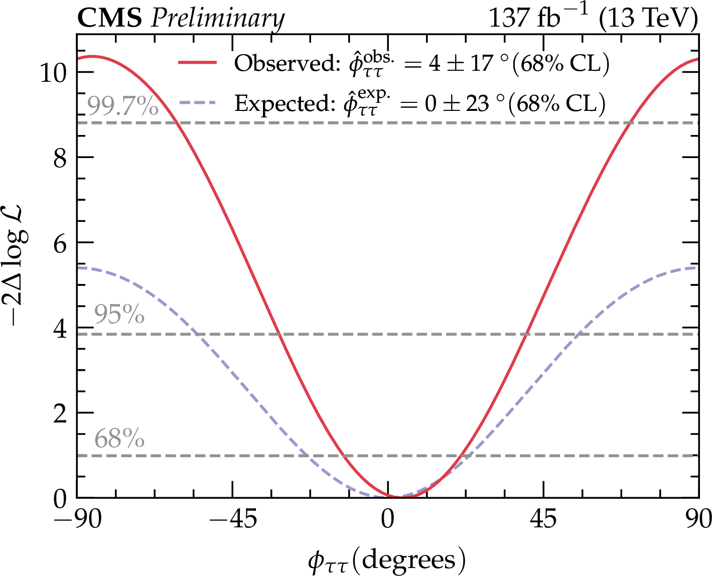
png pdf	Figure 7: Negative log-likelihood scan for the combination of the ${\tau _{\mu} {\tau _\mathrm {h}}}$ and ${{\tau _\mathrm {h}} {\tau _\mathrm {h}}}$ channel. The observed (expected) sensitivity to distinguish between the scalar and pseudo-scalar hypotheses, defined at $ {\phi _{\tau \tau}} = $ 0 and $ \pm $ 90$ ^{\circ}$, respectively, is 3.2 (2.3) standard deviations. The observed (expected) value for ${\phi _{\tau \tau}}$ is 4 $\pm$ 17$ ^{\circ}$ (0 $\pm$ 23$ ^{\circ}$) at the 68% CL, at the 95% CL the value is $ \pm $ 36$ ^{\circ}$ ($ \pm$ 55$ ^{\circ}$), and at the 99.7% CL we obtain an observed $ \pm$ 66$ ^{\circ}$.
png pdf	Figure 8: Two-dimensional scan of the branching fraction modifier with respect to the SM value $\mu ^{\tau \tau}$ versus ${\phi _{\tau \tau}}$. All other Higgs couplings are fixed to the SM expectation values.
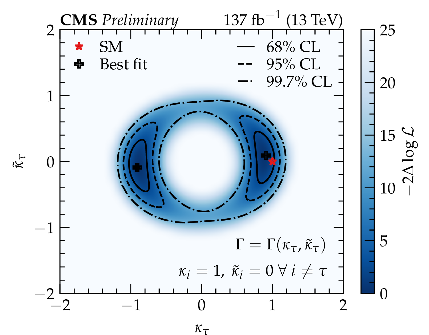
png pdf	Figure 9: Two-dimensional scan of the (reduced) CP-even ($\kappa $) and CP-odd ($\tilde{\kappa}$) $\tau$ Yukawa couplings.
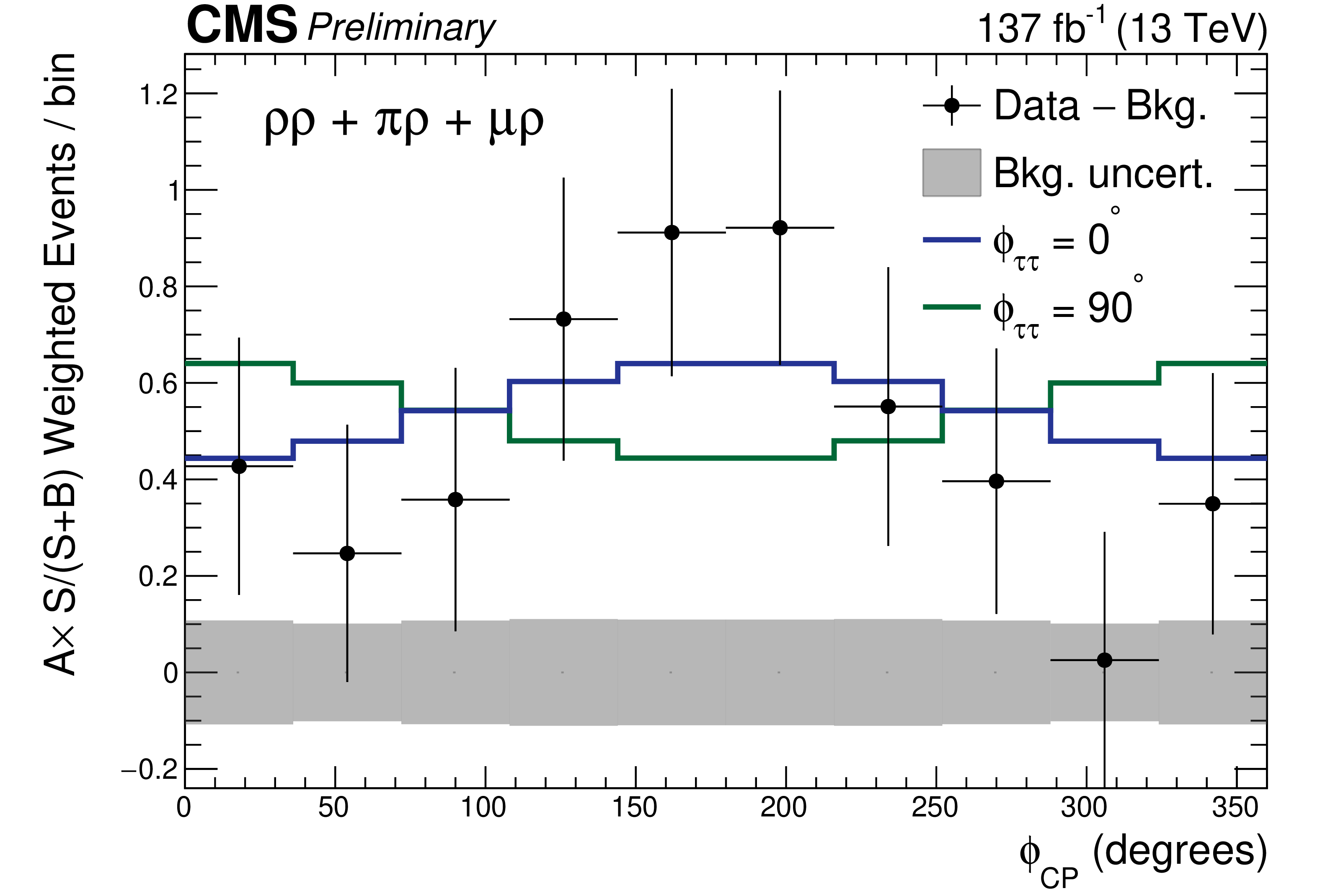
png pdf	Figure 10: The ${\phi _{\text {CP}}}$ distribution for the three most sensitive channels combined. Events were collected from all years and NN/BDT bins in the three signal categories. The background is subtracted from the data. The events are reweighed via $A\,S/(S+B)$, in which $S$ and $B$ are the signal and background rates, respectively, and $A$ is a measure for the average asymmetry between the scalar and pseudoscalar distributions. The definition of the value of $A$ per bin is $|\text {CP}^{\text {even}}-\text {CP}^{\text {odd}}|/(\text {CP}^{\text {even}}+\text {CP}^{\text {odd}})$, and $A$ is normalised to the total number of bins. In this equation $\text {CP}^{\text {even}}$ and $\text {CP}^{\text {odd}}$ are the scalar and pseudoscalar contributions per bin. The scalar distribution is depicted in blue, while the pseudoscalar is displayed in green. In the predictions, the rate parameters are taken from their best-fit values. The grey uncertainty band indicates the uncertainty on the subtracted background component. In combining the channels, a phase-shift of 180$^{\circ}$ was applied to the channel involving a muon since this channel has a phase difference of 180$^{\circ}$ with respect to the two hadronic channels due to a sign-flip in the muon spectral function.

Tables
png pdf	Table 1: Weak decays of $\tau$ leptons used in this analysis and their branching fractions $\mathcal {B}$ in% [35] are given, rounded to one decimal place. Also, where appropriate, we indicate the known intermediate resonances of all the hadrons listed. The muon is accompanied by two neutrinos, while the hadronic modes involve one neutrino. The third row gives the shorthand notation for the decays used throughout this note.
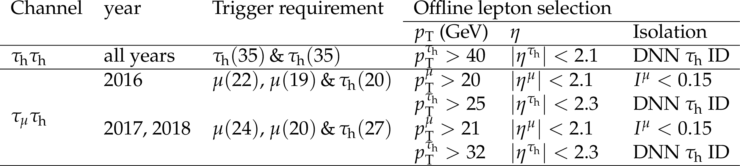
png pdf	Table 2: Kinematic trigger and offline requirements applied for the ${\tau _{\mu} {\tau _\mathrm {h}}}$ and ${{\tau _\mathrm {h}} {\tau _\mathrm {h}}}$ channel. The trigger ${p_{\mathrm {T}}}$ requirement is indicated in parentheses (in GeV). The pseudorapidity constraints originate from trigger and reconstruction requirements.
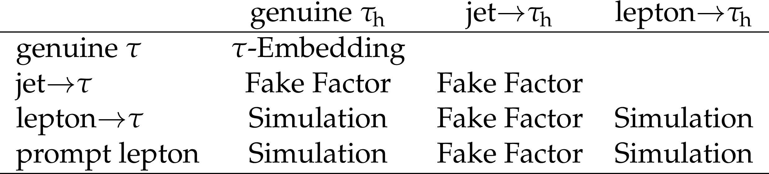
png pdf	Table 3: The different sources of di-$\tau$ backgrounds are depicted on the rows and columns. The entries in the table represent the possible di-$\tau$ background contribution from different processes and misidentifications and encapsulate the different experimental techniques that are deployed to estimate the background contributions. Processes involving two prompt leptons, i.e. two electrons, muons, or and electron and a muon, are not considered in this analysis.
png pdf	Table 4: Input variables to the MVA discriminants for the ${\tau _{\mu} {\tau _\mathrm {h}}}$ and ${{\tau _\mathrm {h}} {\tau _\mathrm {h}}}$ channel. For all variables only the visible decay products of the $\tau$ leptons are implied, except for the ${\tau _{\mu} {\tau _\mathrm {h}}}$ and ${{\tau _\mathrm {h}} {\tau _\mathrm {h}}}$ mass, for which the {Svfit} algorithm is used.
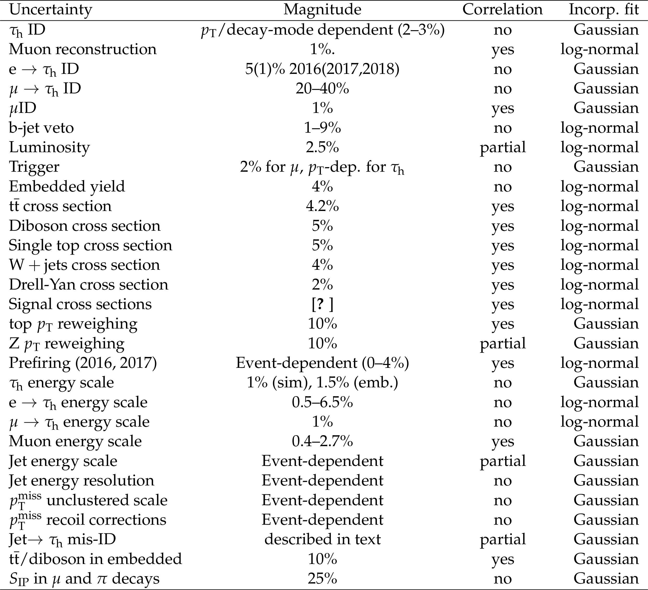
png pdf	Table 5: Sources of systematic uncertainties. The third column indicates if the source of uncertainty was treated as being correlated between the years in the fit described in Section 11. The fourth column indicates the probability density for the uncertainty applied in the fit

Summary

The first measurement of the effective mixing angle $\phi_{\tau\tau}$ between a scalar and pseudoscalar H${\tau\tau}$ coupling has been presented for a data set of pp collisions at $\sqrt{s} = $ 13 TeV of 137 fb$^{-1}$. The data were collected with the CMS experiment at the LHC in the period 2016-2018. The fully hadronic channel was included as well as the $\tau_{\mu}\tau_{\mathrm{h}}$ channel, in which one $\tau$ lepton decayed via a muon and the other to hadrons. Machine learning techniques were applied to separate the signal from background events and distinguish between the hadronic $\tau$ decay modes. Dedicated strategies were adopted to reconstruct the angle $\phi_{CP}$ between the $\tau$ decay planes for the various $\tau$ decay modes, and the reconstruction of the primary vertex was optimised for the measurement. The hypothesis for a pure CP-odd pseudoscalar boson is rejected with $3.2$ (2.3) observed (expected) standard deviations. The observed mixing angle is found to be 4 $\pm$ 17$ ^{\circ}$, while the expected value is determined as 0 $\pm$ 23$ ^{\circ}$ at the 68% confidence level. At the 95% confidence level the observed and expected uncertainties are found to be $ \pm$ 36$ ^{\circ}$ and $ \pm$ 55$ ^{\circ}$, respectively, and the observed sensitivity at the 99.7% CL is $ \pm$ 66$ ^{\circ}$. The $\mu\rho$ channel is estimated to be the most sensitive mode, followed by the $\rho\rho$ and $\pi\rho$ channels. The driving uncertainties in the measurement presented are of statistical nature, implying that the precision of the measurement will increase with the accumulation of more collision data. The measurement is consistent with the standard model expectation, and reduces the allowed parameter space for extensions of the standard model.

Additional Figures
png pdf	Additional Figure 1: The normalised distribution of ${\phi _{\text {CP}}}$ between the ${\tau}$ decay planes in the boson rest frame, for both ${\tau}$ leptons decaying to a muon and an intermediate $\rho $ meson. The distributions are for a decaying scalar (CP even, blue), pseudoscalar (CP odd, green), a maximal mixing angle of 45$^{\circ}$ (CP mix, red), and a Z vector boson (black). A ${p_{\mathrm {T}}}$ cutoff of 19 (16) GeV is applied on the visible leptonic (hadronic) tau decay products.
png pdf	Additional Figure 2: The normalised distribution of ${\phi _{\text {CP}}}$ between the ${\tau}$ decay planes in the boson rest frame, for both ${\tau}$ leptons decaying to a charged pion and an intermediate $\rho $ meson. The distributions are for a decaying scalar (CP even, blue), pseudoscalar (CP odd, green), a maximal mixing angle of 45$^{\circ}$ (CP mix, red), and a Z vector boson (black). A ${p_{\mathrm {T}}}$ cutoff of 33 GeV is applied on the visible tau decay products.
png pdf	Additional Figure 3: The normalised distribution of ${\phi _{\text {CP}}}$ between the ${\tau}$ decay planes in the boson rest frame, for both ${\tau}$ leptons decaying to two intermediate $\rho $ mesons. The distributions are for a decaying scalar (CP even, blue), pseudoscalar (CP odd, green), a maximal mixing angle of 45$^{\circ}$ (CP mix, red), and a Z vector boson (black). A ${p_{\mathrm {T}}}$ cutoff of 33 GeV is applied on the visible tau decay products.
png pdf	Additional Figure 4: The ${\phi _{\text {CP}}}$ distribution in the $ {{\mu}} {\rho} $ channel. Events were collected from all years and NN/BDT bins. The background is subtracted from the data. The events are reweighed via $A\,S/(S+B)$, in which $S$ and $B$ are the signal and background rates, respectively, and $A$ is a measure for the average asymmetry between the scalar and pseudoscalar distributions. The definition of the value of $A$ per bin is $|\text {CP}^{\text {even}}-\text {CP}^{\text {odd}}|/(\text {CP}^{\text {even}}+\text {CP}^{\text {odd}})$, and $A$ is normalised to the total number of bins. In this equation $\text {CP}^{\text {even}}$ and $\text {CP}^{\text {odd}}$ are the scalar and pseudoscalar contributions per bin. The scalar distribution is depicted in blue, while the pseudoscalar is displayed in green. In the predictions the rate parameters are taken from their best-fit values. The grey uncertainty band indicates the uncertainty on the subtracted background component. It should be noted that an overall phase-shift of 180$^{\circ}$ was applied to the channel involving a muon.
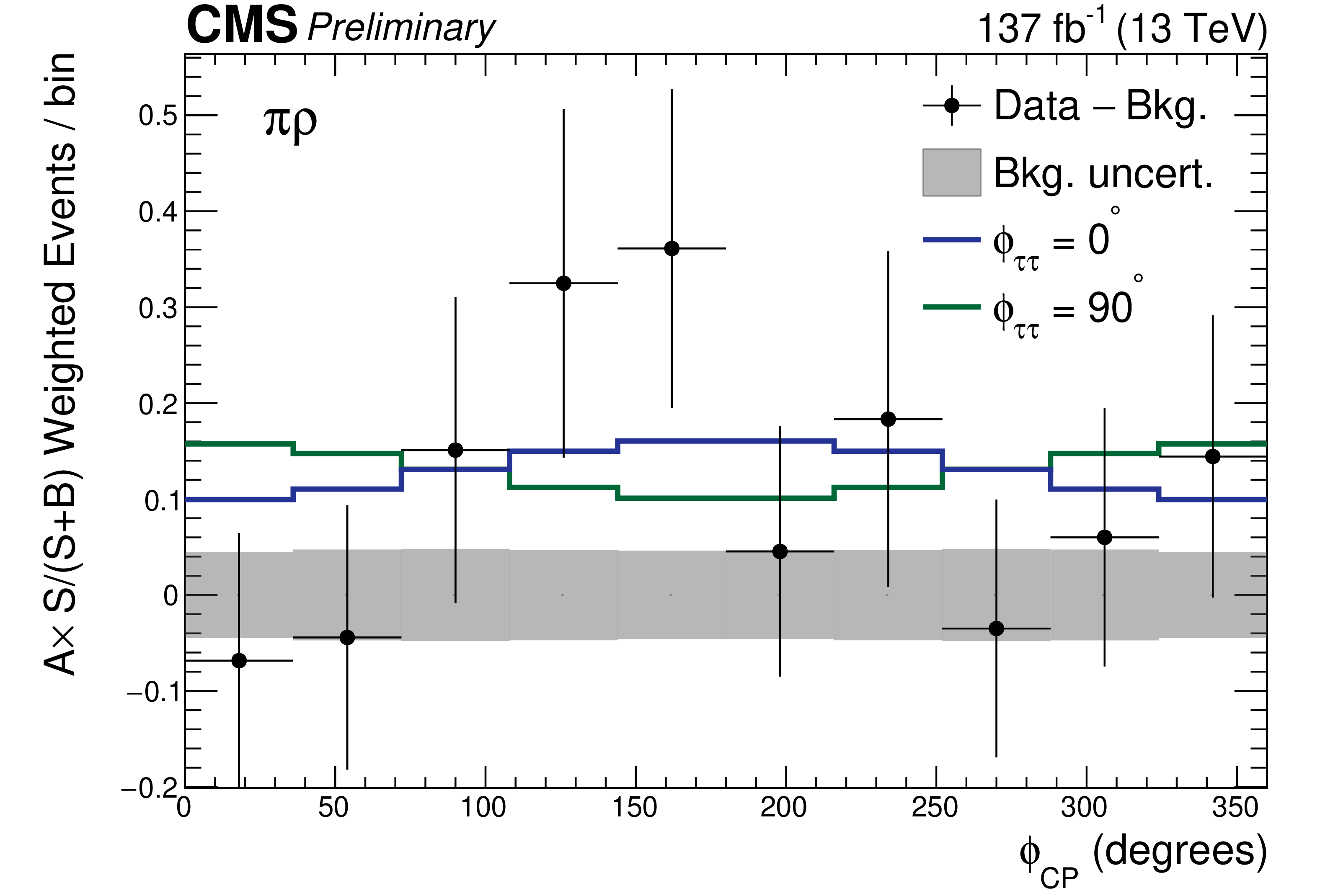
png pdf	Additional Figure 5: The ${\phi _{\text {CP}}}$ distribution in the $ {\pi} {\rho} $ channel. Events were collected from all years and NN/BDT bins. The background is subtracted from the data. The events are reweighed via $A\,S/(S+B)$, in which $S$ and $B$ are the signal and background rates, respectively, and $A$ is a measure for the average asymmetry between the scalar and pseudoscalar distributions. The definition of the value of $A$ per bin is $|\text {CP}^{\text {even}}-\text {CP}^{\text {odd}}|/(\text {CP}^{\text {even}}+\text {CP}^{\text {odd}})$, and $A$ is normalised to the total number of bins. In this equation $\text {CP}^{\text {even}}$ and $\text {CP}^{\text {odd}}$ are the scalar and pseudoscalar contributions per bin. The scalar distribution is depicted in blue, while the pseudoscalar is displayed in green. In the predictions the rate parameters are taken from their best-fit values. The grey uncertainty band indicates the uncertainty on the subtracted background component.
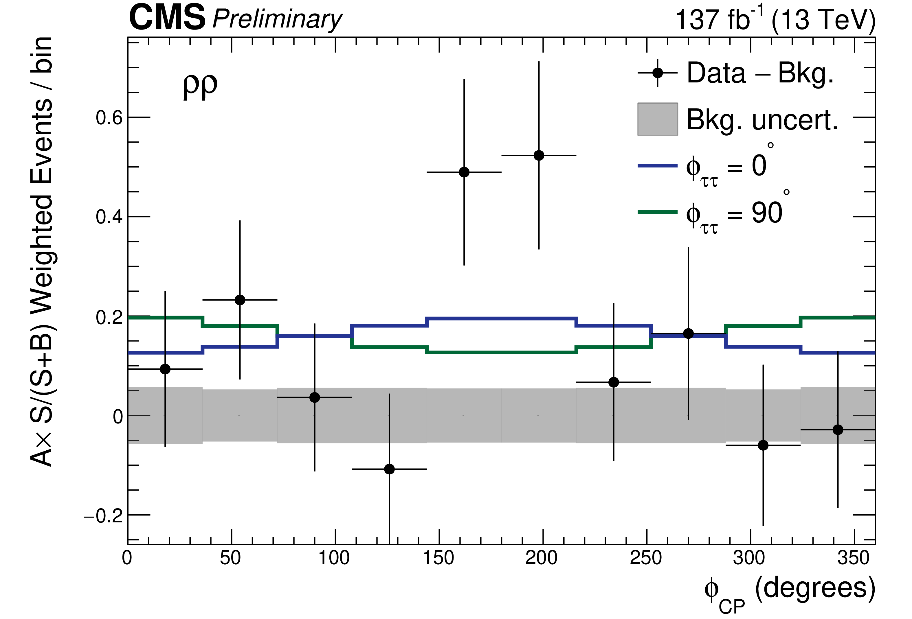
png pdf	Additional Figure 6: The ${\phi _{\text {CP}}}$ distribution in the $ {\rho} {\rho} $ channel. Events were collected from all years and NN/BDT bins. The background is subtracted from the data. The events are reweighed via $A\,S/(S+B)$, in which $S$ and $B$ are the signal and background rates, respectively, and $A$ is a measure for the average asymmetry between the scalar and pseudoscalar distributions. The definition of the value of $A$ per bin is $|\text {CP}^{\text {even}}-\text {CP}^{\text {odd}}|/(\text {CP}^{\text {even}}+\text {CP}^{\text {odd}})$, and $A$ is normalised to the total number of bins. In this equation $\text {CP}^{\text {even}}$ and $\text {CP}^{\text {odd}}$ are the scalar and pseudoscalar contributions per bin. The scalar distribution is depicted in blue, while the pseudoscalar is displayed in green. In the predictions the rate parameters are taken from their best-fit values. The grey uncertainty band indicates the uncertainty on the subtracted background component.
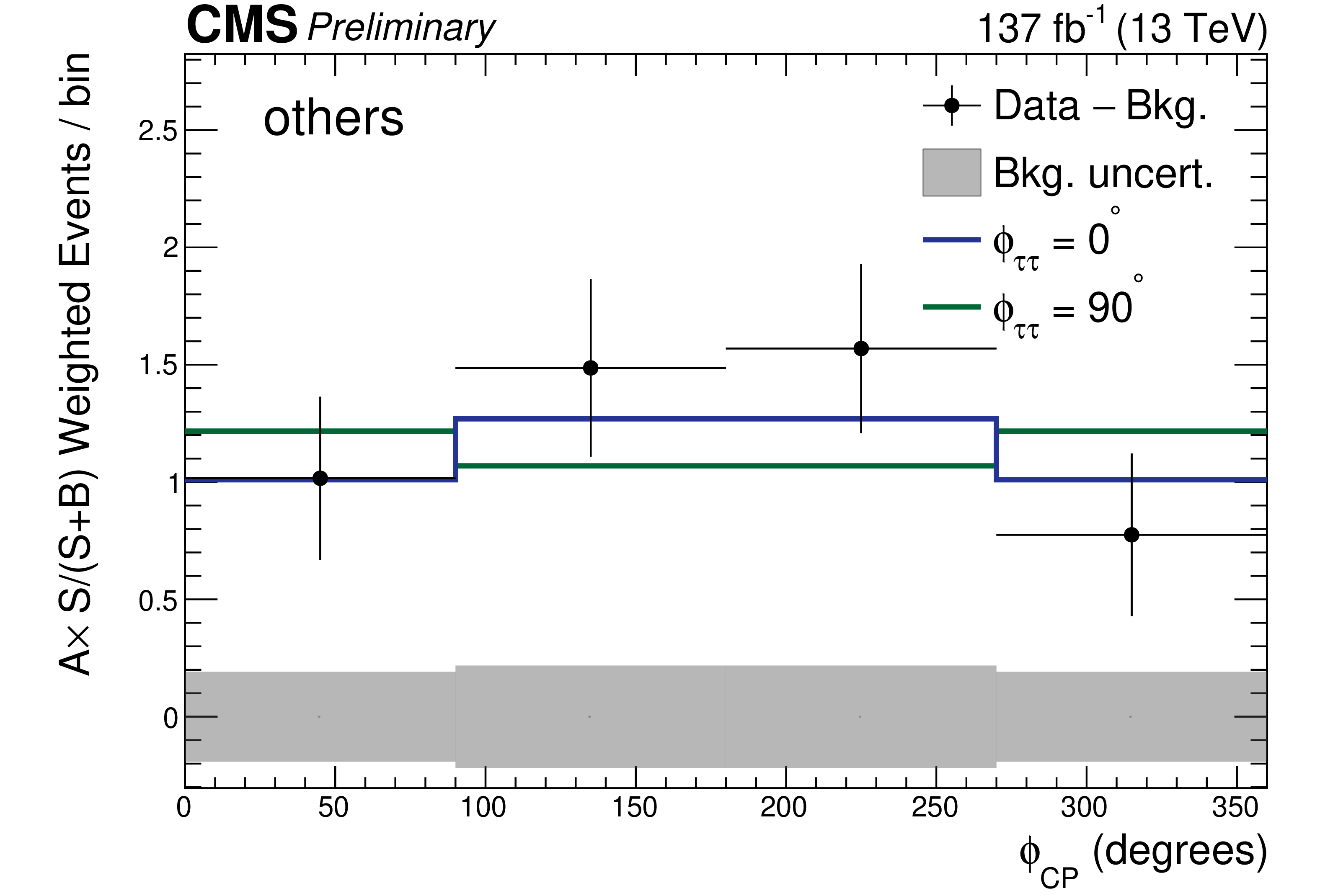
png pdf	Additional Figure 7: The ${\phi _{\text {CP}}}$ distribution for combination of the nine least sensitive ${\tau _{{{\mu}}} {{\tau} _\mathrm {h}}}$ and ${{{\tau} _\mathrm {h}} {{\tau} _\mathrm {h}}}$ channels added together. Events were collected from all years and NN/BDT bins. The background is subtracted from the data. The events are reweighed via $A\,S/(S+B)$, in which $S$ and $B$ are the signal and background rates, respectively, and $A$ is a measure for the average asymmetry between the scalar and pseudoscalar distributions. The definition of the value of $A$ per bin is $|\text {CP}^{\text {even}}-\text {CP}^{\text {odd}}|/(\text {CP}^{\text {even}}+\text {CP}^{\text {odd}})$, and $A$ is normalised to the total number of bins. In this equation $\text {CP}^{\text {even}}$ and $\text {CP}^{\text {odd}}$ are the scalar and pseudoscalar contributions per bin. The scalar distribution is depicted in blue, while the pseudoscalar is displayed in green. In the predictions the rate parameters are taken from their best-fit values. The grey uncertainty band indicates the uncertainty on the subtracted background component. In combining the channels, a phase-shift of 180$^{\circ}$ was applied to the channels involving a muon since this channel has a phase difference of 180$^{\circ}$ with respect to the two hadronic channels due to a sign-flip in the muon spectral function.
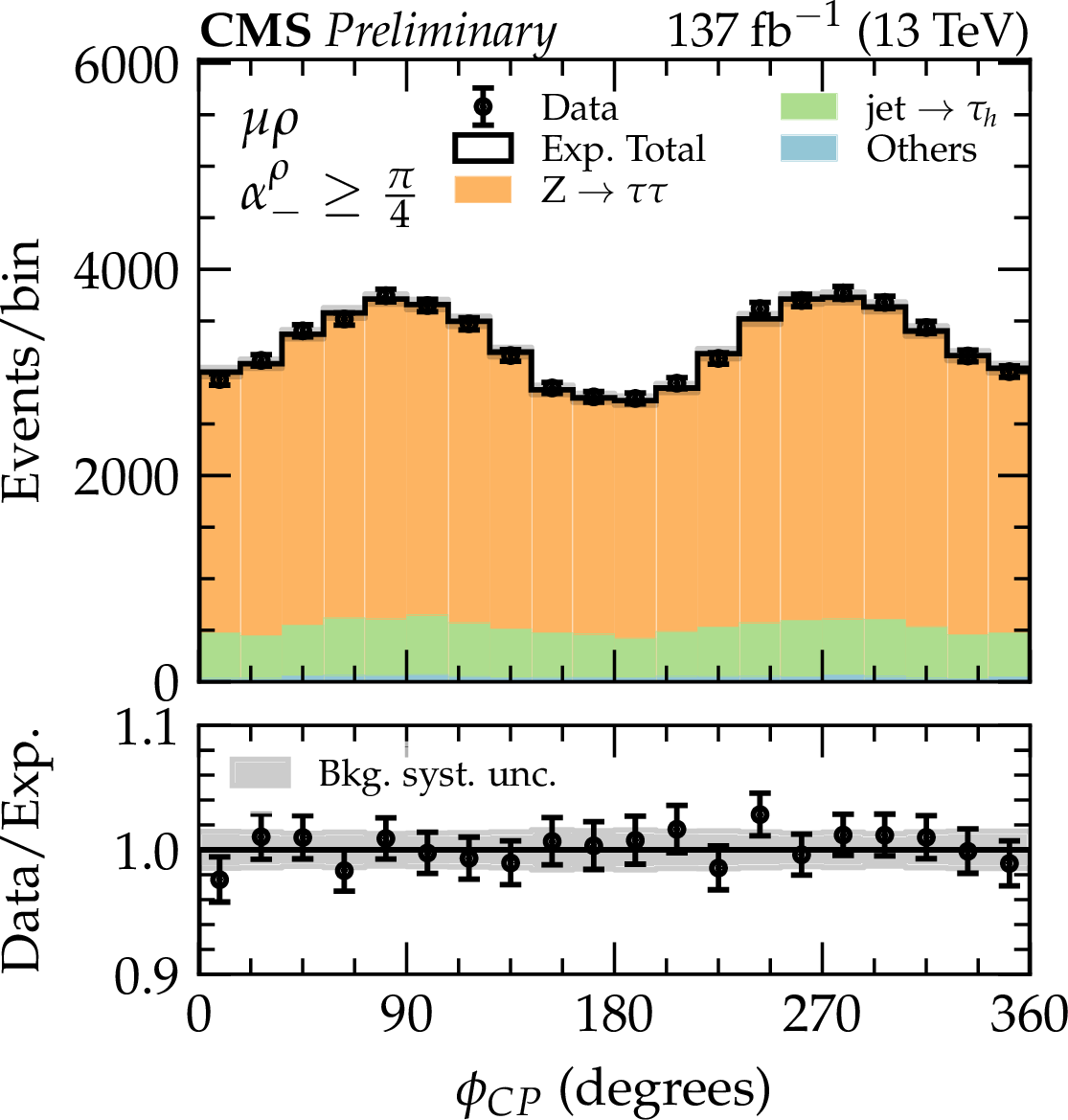
png pdf	Additional Figure 8: Distributions of ${\phi _{\text {CP}}}$ in the $ {{\mu}} {\rho} $ channel for an event sample dominated by Drell-Yan events. Events were selected for which $\alpha _{-}^{\rho}\geq \pi /4$. The Drell-Yan background template is extracted from simulation, while the jet-fake background is obtained from the fake-factor method. The remaining backgrounds are summarised in the template named Other. In the lower plot the ratio between data and the prediction is displayed together with the systematic uncertainty band.
png pdf	Additional Figure 9: Distributions of ${\phi _{\text {CP}}}$ in the $ {{\mu}} {\pi}$ channel for an event sample dominated by Drell-Yan events. Events were selected for which $\alpha _{-}^{\pi}\geq \pi /4$. The Drell-Yan background template is extracted from simulation, while the jet-fake background is obtained from the fake-factor method. The remaining backgrounds are summarised in the template named Other. In the lower plot the ratio between data and the prediction is displayed together with the systematic uncertainty band.
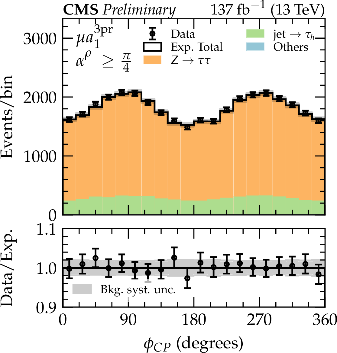
png pdf	Additional Figure 10: Distributions of ${\phi _{\text {CP}}}$ in the $ {{\mu}} {\mathrm {a_{1}^{3pr}}} $ channel for an event sample dominated by Drell-Yan events. Events were selected for which $\alpha _{-}^{\rho}\geq \pi /4$ for the intermediate ${\rho}$. The Drell-Yan background template is extracted from simulation, while the jet-fake background is obtained from the fake-factor method. The remaining backgrounds are summarised in the template named Other. In the lower plot the ratio between data and the prediction is displayed together with the systematic uncertainty band.
png pdf	Additional Figure 11: Distributions of ${\phi _{\text {CP}}}$ in the $ {{\mu}} {\mathrm {a_{1}^{1pr}}} $ channel for an event sample dominated by Drell-Yan events. Events were selected for which $\alpha _{-}$, calculated for the intermediate $ {\mathrm {a_{1}^{1pr}}} $, was $\geq \pi /4$. The Drell-Yan background template is extracted from simulation, while the jet-fake background is obtained from the fake-factor method. The remaining backgrounds are summarised in the template named Other. In the lower plot the ratio between data and the prediction is displayed together with the systematic uncertainty band.
png pdf	Additional Figure 12: Distributions of ${\phi _{\text {CP}}}$ in the $ {{\mu}} {\rho} $ channel for an event sample dominated by Drell-Yan events. Events were selected for which $\alpha _{-}^{\rho} < \pi /4$. The Drell-Yan background template is extracted from simulation, while the jet-fake background is obtained from the fake-factor method. The remaining backgrounds are summarised in the template named Other. In the lower plot the ratio between data and the prediction is displayed together with the systematic uncertainty band.
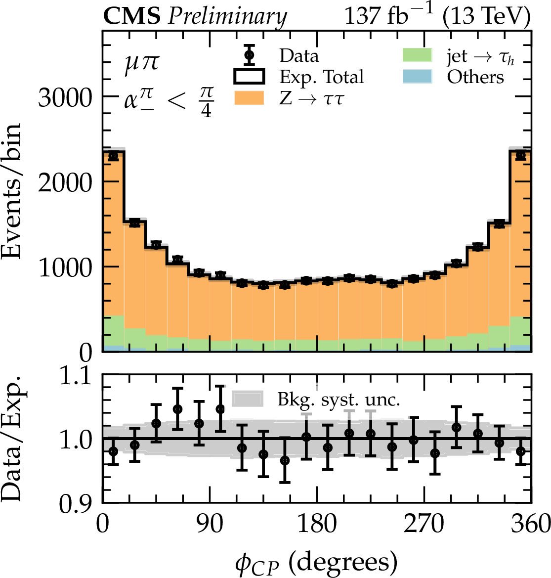
png pdf	Additional Figure 13: Distributions of ${\phi _{\text {CP}}}$ in the $ {{\mu}} {\pi}$ channel for an event sample dominated by Drell-Yan events. Events were selected for which $\alpha _{-}^{\pi} < \pi /4$. The Drell-Yan background template is extracted from simulation, while the jet-fake background is obtained from the fake-factor method. The remaining backgrounds are summarised in the template named Other. In the lower plot the ratio between data and the prediction is displayed together with the systematic uncertainty band.
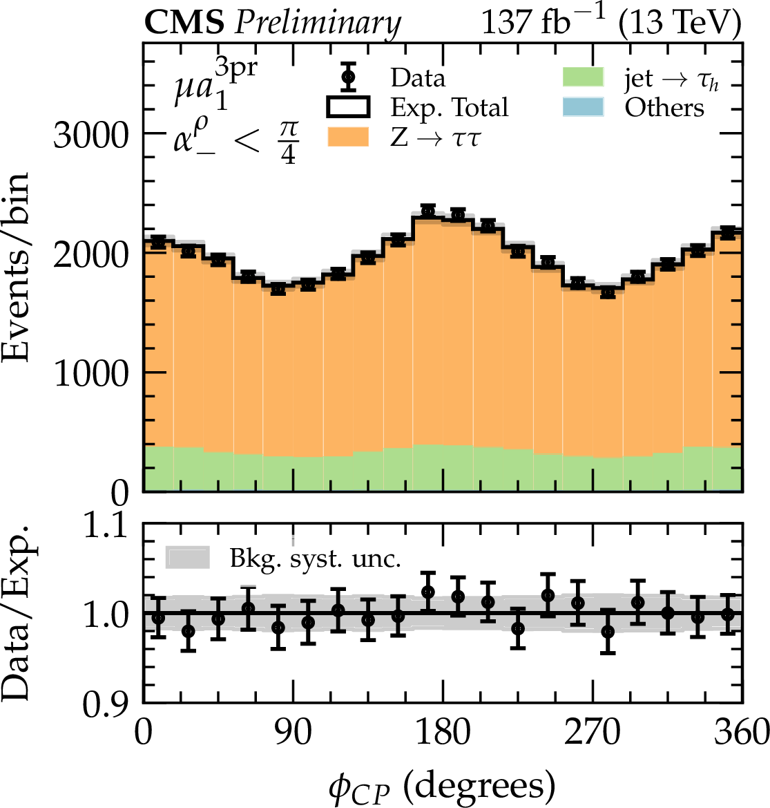
png pdf	Additional Figure 14: Distributions of ${\phi _{\text {CP}}}$ in the $ {{\mu}} {\mathrm {a_{1}^{3pr}}} $ channel for an event sample dominated by Drell-Yan events. Events were selected for which $\alpha _{-}^{\rho} < \pi /4$ for the intermediate ${\rho}$. The Drell-Yan background template is extracted from simulation, while the jet-fake background is obtained from the fake-factor method. The remaining backgrounds are summarised in the template named Other. In the lower plot the ratio between data and the prediction is displayed together with the systematic uncertainty band.
png pdf	Additional Figure 15: Distributions of ${\phi _{\text {CP}}}$ in the $ {{\mu}} {\mathrm {a_{1}^{1pr}}} $ channel for an event sample dominated by Drell-Yan events. Events were selected for which $\alpha _{-}$, calculated for the intermediate $ {\mathrm {a_{1}^{1pr}}} $, was $ < \pi /4$. The Drell-Yan background template is extracted from simulation, while the jet-fake background is obtained from the fake-factor method. The remaining backgrounds are summarised in the template named Other. In the lower plot the ratio between data and the prediction is displayed together with the systematic uncertainty band.
png pdf	Additional Figure 16: Distributions of ${\phi _{\text {CP}}}$ in the $ {{\mu}} {\mathrm {a_{1}^{3pr}}} $ channel in windows of increasing neural net score. The best-fit and pseudoscalar (PS) signal distributions are overlaid. The $x$ axis represents the cyclic bins in ${\phi _{\text {CP}}}$ in the range of (0, 360$^{\circ}$). In the bottom plot the data minus the background template divided by the uncertainty in the background template is displayed, as well as the signal samples divided by the uncertainty in the background template. The uncertainty band consists of the sum of the postfit uncertainties in the background templates.
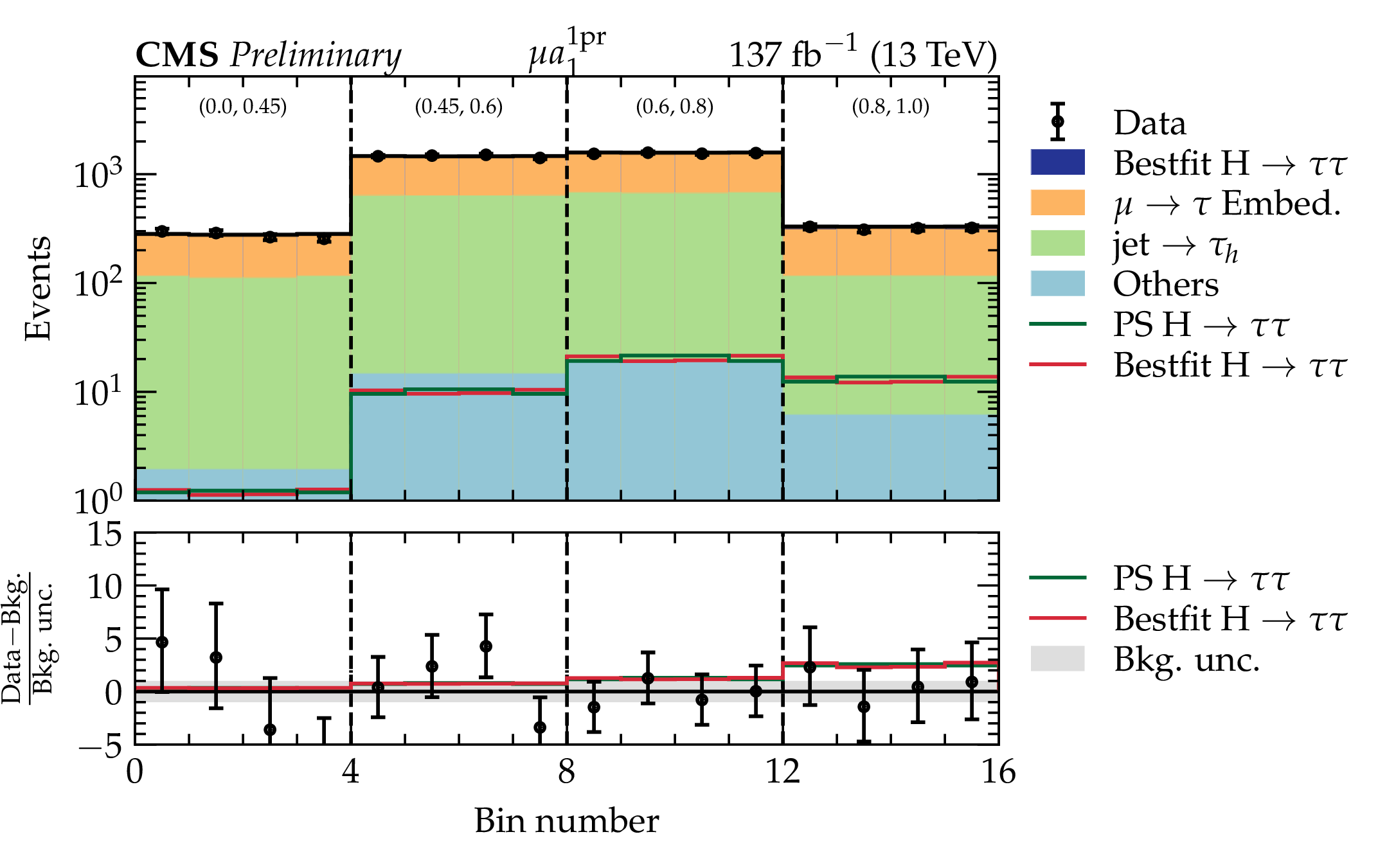
png pdf	Additional Figure 17: Distributions of ${\phi _{\text {CP}}}$ in the $ {{\mu}} {\mathrm {a_{1}^{1pr}}} $ channel in windows of increasing neural net score. The best-fit and pseudoscalar (PS) signal distributions are overlaid. The $x$ axis represents the cyclic bins in ${\phi _{\text {CP}}}$ in the range of (0, 360$^{\circ}$). In the bottom plot the data minus the background template divided by the uncertainty in the background template is displayed, as well as the signal samples divided by the uncertainty in the background template. The uncertainty band consists of the sum of the postfit uncertainties in the background templates.
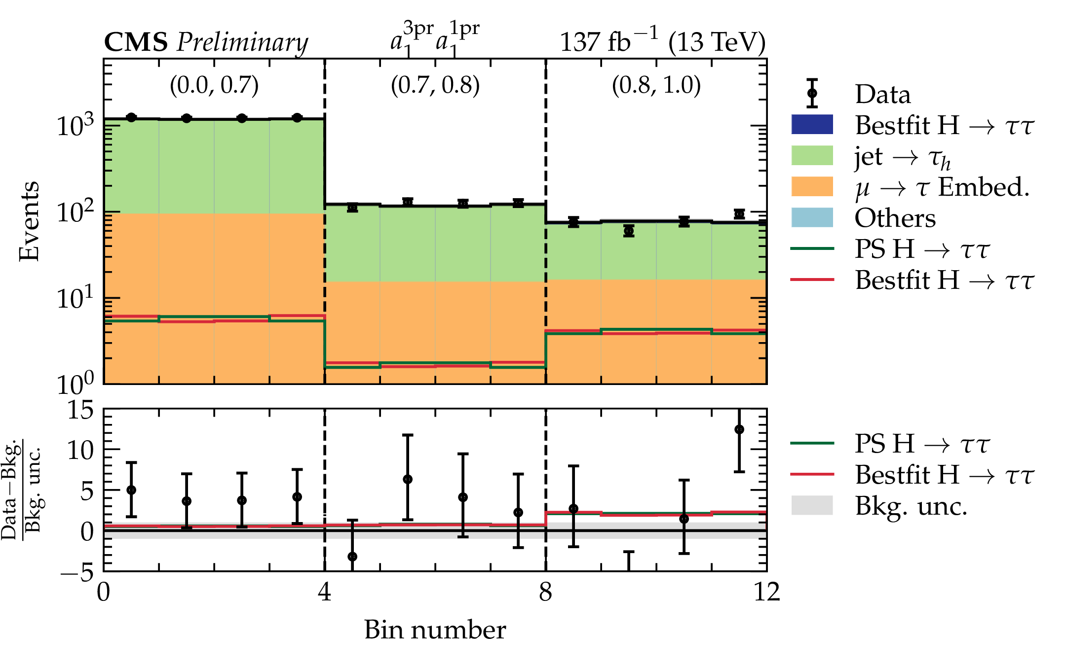
png pdf	Additional Figure 18: Distributions of ${\phi _{\text {CP}}}$ in the $ {\mathrm {a_{1}^{1pr}}} {\rho} + {\mathrm {a_{1}^{1pr}}} {\mathrm {a_{1}^{1pr}}} $ channel in windows of increasing boosted decision tree score. The best-fit and pseudoscalar (PS) signal distributions are overlaid. The $x$ axis represents the cyclic bins in ${\phi _{\text {CP}}}$ in the range of (0, 360$^{\circ}$). In the bottom plot the data minus the background template divided by the uncertainty in the background template is displayed, as well as the signal samples divided by the uncertainty in the background template. The uncertainty band consists of the sum of the postfit uncertainties in the background templates.
png pdf	Additional Figure 19: Distributions of ${\phi _{\text {CP}}}$ in the $ {\mathrm {a_{1}^{3pr}}} {\mathrm {a_{1}^{1pr}}} $ channel in windows of increasing boosted decision tree score. The best-fit and pseudoscalar (PS) signal distributions are overlaid. The $x$ axis represents the cyclic bins in ${\phi _{\text {CP}}}$ in the range of (0, 360$^{\circ}$). In the bottom plot the data minus the background template divided by the uncertainty in the background template is displayed, as well as the signal samples divided by the uncertainty in the background template. The uncertainty band consists of the sum of the postfit uncertainties in the background templates.
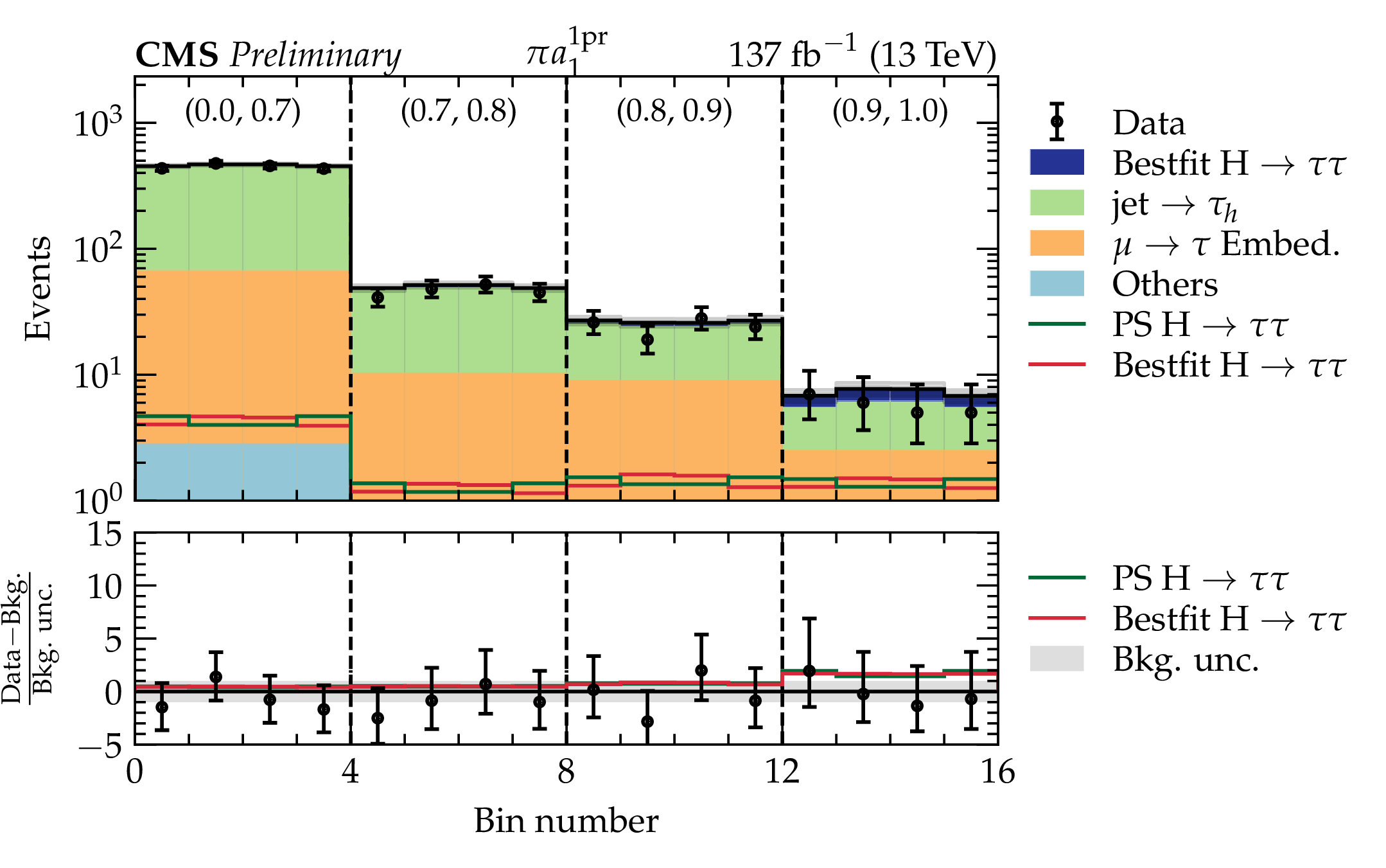
png pdf	Additional Figure 20: Distributions of ${\phi _{\text {CP}}}$ in the $ {\pi} {\mathrm {a_{1}^{1pr}}} $ channel in windows of increasing boosted decision tree score. The best-fit and pseudoscalar (PS) signal distributions are overlaid. The $x$ axis represents the cyclic bins in ${\phi _{\text {CP}}}$ in the range of (0, 360$^{\circ}$). In the bottom plot the data minus the background template divided by the uncertainty in the background template is displayed, as well as the signal samples divided by the uncertainty in the background template. The uncertainty band consists of the sum of the postfit uncertainties in the background templates.
png pdf	Additional Figure 21: Distributions of ${\phi _{\text {CP}}}$ in the $ {\mathrm {a_{1}^{3pr}}} {\mathrm {a_{1}^{3pr}}} $ channel in windows of increasing boosted decision tree score. The best-fit and pseudoscalar (PS) signal distributions are overlaid. The $x$ axis represents the cyclic bins in ${\phi _{\text {CP}}}$ in the range of (0, 360$^{\circ}$). In the bottom plot the data minus the background template divided by the uncertainty in the background template is displayed, as well as the signal samples divided by the uncertainty in the background template. The uncertainty band consists of the sum of the postfit uncertainties in the background templates.
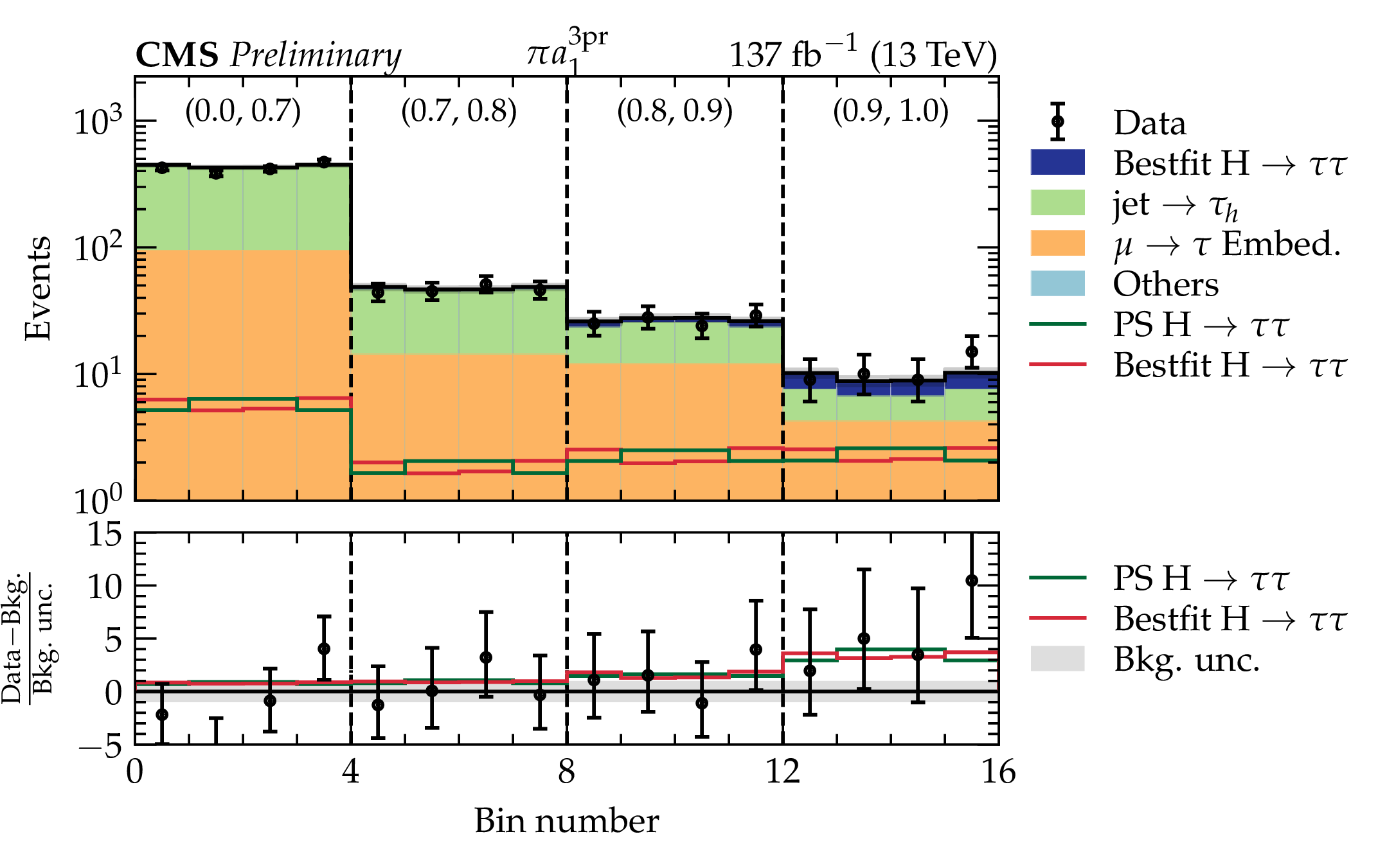
png pdf	Additional Figure 22: Distributions of ${\phi _{\text {CP}}}$ in the $ {\pi} {\mathrm {a_{1}^{3pr}}} $ channel in windows of increasing boosted decision tree score. The best-fit and pseudoscalar (PS) signal distributions are overlaid. The $x$ axis represents the cyclic bins in ${\phi _{\text {CP}}}$ in the range of (0, 360$^{\circ}$). In the bottom plot the data minus the background template divided by the uncertainty in the background template is displayed, as well as the signal samples divided by the uncertainty in the background template. The uncertainty band consists of the sum of the postfit uncertainties in the background templates.
png pdf	Additional Figure 23: Distributions of ${\phi _{\text {CP}}}$ in the $ {\mathrm {a_{1}^{3pr}}} {\rho} $ channel in windows of increasing neural net score. The best-fit and pseudoscalar (PS) signal distributions are overlaid. The $x$ axis represents the cyclic bins in ${\phi _{\text {CP}}}$ in the range of (0, 360$^{\circ}$). In the bottom plot the data minus the background template divided by the uncertainty in the background template is displayed, as well as the signal samples divided by the uncertainty in the background template. The uncertainty band consists of the sum of the postfit uncertainties in the background templates.
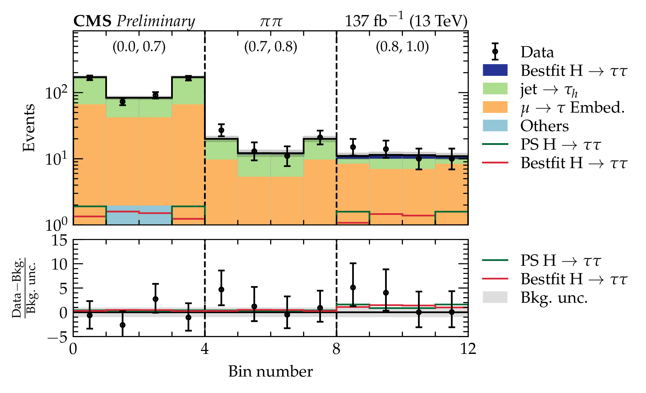
png pdf	Additional Figure 24: Distributions of ${\phi _{\text {CP}}}$ in the $ {\pi} {\pi}$ channel in windows of increasing boosted decision tree score. The best-fit and pseudoscalar (PS) signal distributions are overlaid. The $x$ axis represents the cyclic bins in ${\phi _{\text {CP}}}$ in the range of (0, 360$^{\circ}$). In the bottom plot the data minus the background template divided by the uncertainty in the background template is displayed, as well as the signal samples divided by the uncertainty in the background template. The uncertainty band consists of the sum of the postfit uncertainties in the background templates.
png pdf	Additional Figure 25-a: A candidate event featuring a Higgs decaying into two ${\tau}$ leptons is depicted. The ${\tau}$ leptons decay into a muon (in red) and an ${\mathrm {a_{1}^{3pr}}}$ that decays in three charged pions (indicated by the orange cone and the calorimeter cells).
png pdf	Additional Figure 25-b: A zoomed view on the same event is featured revealing the displaced secondary vertex of which the tracks of the three charged pions candidate are emerging. The pileup vertices are also indicated.

Additional Tables
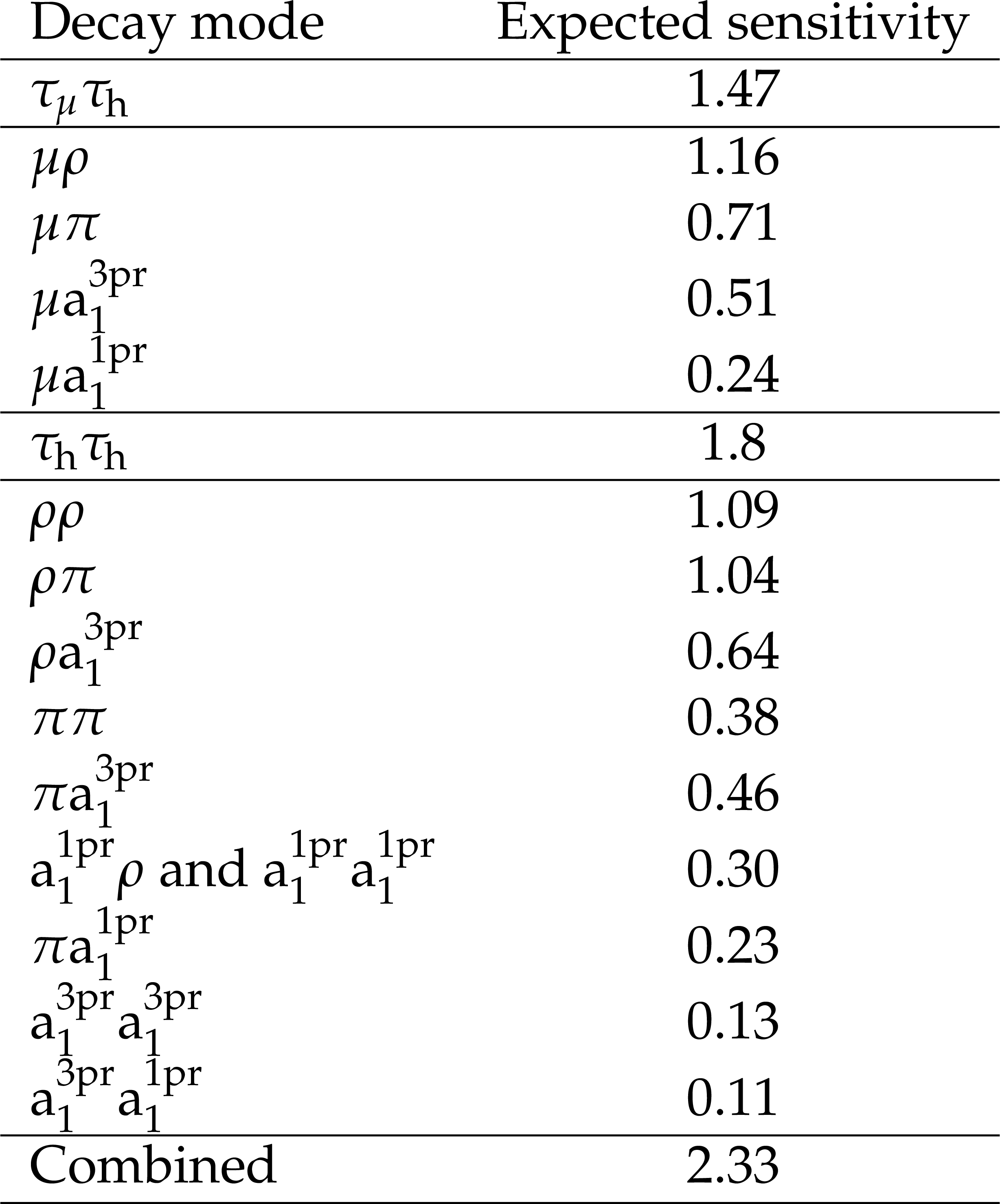
png pdf	Additional Table 1: The obtained expected sensitivities in standard deviations to distinguish between a CP-even and odd ${{\mathrm {H}} {\tau} {\tau}}$ coupling. Results are displayed for the individual decay modes, the combined ${\tau _{{{\mu}}} {{\tau} _\mathrm {h}}}$ and ${{{\tau} _\mathrm {h}} {{\tau} _\mathrm {h}}}$ channel, and the overall combination.
png pdf	Additional Table 2: The primary vertex resolution in cm. The resolution is stated for the nominal primary vertex as reconstructed by default reconstruction algorithms utilised by the CMS experiment, as well as the refitted beamspot-corrected primary vertex as used throughout this analysis.

References
1	F. Englert and R. Brout	Broken symmetry and the mass of gauge vector mesons	PRL 13 (1964) 321
2	P. W. Higgs	Broken symmetries and the masses of gauge bosons	PRL 13 (1964) 508
3	G. S. Guralnik, C. R. Hagen, and T. W. B. Kibble	Global conservation laws and massless particles	PRL 13 (1964) 585
4	ATLAS Collaboration	Observation of a new particle in the search for the Standard Model Higgs boson with the ATLAS detector at the LHC	Physics Letters B 716 (2012), no. 1, 1	1207.7214
5	CMS Collaboration	Observation of a new boson at a mass of 125 GeV with the CMS experiment at the LHC	Physics Letters B 716 (2012), no. 1, 30	CMS-HIG-12-028 1207.7235
6	ATLAS, CMS Collaboration	Measurements of the Higgs boson production and decay rates and constraints on its couplings from a combined ATLAS and CMS analysis of the LHC pp collision data at $ \sqrt{s}= $ 7 and 8 TeV	JHEP 08 (2016) 045	1606.02266
7	CMS Collaboration	Observation of the Higgs boson decay to a pair of $ \tau $ leptons with the CMS detector	Physics Letters B 779 (2018) 283	CMS-HIG-16-043 1708.00373
8	ATLAS Collaboration	Cross-section measurements of the Higgs boson decaying into a pair of $ \tau $-leptons in proton-proton collisions at a centre-of-mass energy of 13~TeV with the ATLAS detector	Physical Review D 99 (2019), no. 7	1811.08856
9	CMS Collaboration	On the mass and spin-parity of the Higgs boson candidate via its decays to Z boson pairs	PRL 110 (2013) 081803	CMS-HIG-12-041 1212.6639
10	CMS Collaboration	Measurement of the properties of a Higgs boson in the four-lepton final state	PRD 89 (2014) 092007	CMS-HIG-13-002 1312.5353
11	CMS Collaboration	Constraints on the spin-parity and anomalous HVV couplings of the Higgs boson in proton collisions at 7 and 8 TeV	PRD 92 (2015) 012004	CMS-HIG-14-018 1411.3441
12	CMS Collaboration	Limits on the Higgs boson lifetime and width from its decay to four charged leptons	PRD 92 (2015) 072010	CMS-HIG-14-036 1507.06656
13	CMS Collaboration	Combined search for anomalous pseudoscalar HVV couplings in VH(H $ \to b \bar b $) production and H $ \to $ VV decay	PLB 759 (2016) 672	CMS-HIG-14-035 1602.04305
14	CMS Collaboration	Constraints on anomalous Higgs boson couplings using production and decay information in the four-lepton final state	PLB 775 (2017) 1	CMS-HIG-17-011 1707.00541
15	CMS Collaboration	Constraints on anomalous HVV couplings from the production of Higgs bosons decaying to $ \tau $ lepton pairs	Physical Review D 100 (2019), no. 11	CMS-HIG-17-034 1903.06973
16	ATLAS Collaboration	Evidence for the spin-0 nature of the Higgs boson using ATLAS data	PLB 726 (2013) 120	1307.1432
17	ATLAS Collaboration	Study of the spin and parity of the Higgs boson in diboson decays with the ATLAS detector	EPJC 75 (2015) 476	1506.05669
18	ATLAS Collaboration	Test of CP Invariance in vector-boson fusion production of the Higgs boson using the Optimal Observable method in the ditau decay channel with the ATLAS detector	EPJC 76 (2016) 658	1602.04516
19	ATLAS Collaboration	Measurement of inclusive and differential cross sections in the $ H \rightarrow ZZ^* \rightarrow 4\ell $ decay channel in $ pp $ collisions at $ \sqrt{s}= $ 13 TeV with the ATLAS detector	JHEP 10 (2017) 132	1708.02810
20	ATLAS Collaboration	Measurement of the Higgs boson coupling properties in the $ H\rightarrow ZZ^{*} \rightarrow 4\ell $ decay channel at $ \sqrt{s} = $ 13 TeV with the ATLAS detector	JHEP 03 (2018) 095	1712.02304
21	ATLAS Collaboration	Measurements of Higgs boson properties in the diphoton decay channel with 36 fb$ ^{-1} $ of $ pp $ collision data at $ \sqrt{s} = $ 13 TeV with the ATLAS detector	PRD 98 (2018) 052005	1802.04146
22	C. Zhang and S. Willenbrock	Effective-field-theory approach to top-quark production and decay	Physical Review D 83 (2011), no. 3	1008.3869
23	R. Harnik et al.	Measuring CP violation in $ h\rightarrow\tau^{+}\tau^{-} $ at colliders	Physical Review D 88 (2013), no. 7	1308.1094
24	T. Ghosh, R. Godbole, and X. Tata	Determining the spacetime structure of bottom-quark couplings to spin-zero particles	Physical Review D 100 (2019), no. 1	1904.09895
25	A. V. Gritsan, R. Rontsch, M. Schulze, and M. Xiao	Constraining anomalous Higgs boson couplings to the heavy-flavor fermions using matrix element techniques	Physical Review D 94 (2016), no. 5	1606.03107
26	CMS Collaboration	Measurements of $ \mathrm{t\bar{t}} $H production and the CP structure of the Yukawa interaction between the Higgs boson and top quark in the diphoton decay channel	Submitted to PRL	CMS-HIG-19-013 2003.10866
27	ATLAS Collaboration	Study of the CP properties of the interaction of the Higgs boson with top quarks using top quark associated production of the Higgs boson and its decay into two photons with the ATLAS detector at the LHC	Submitted to PRLett	2004.04545
28	D. Fontes, J. C. Romão, R. Santos, and J. P. Silva	Large pseudoscalar Yukawa couplings in the complex 2HDM	JHEP 06 (2015) 060	1502.01720
29	S. King, M. Muhlleitner, R. Nevzorov, and K. Walz	Exploring the CP-violating NMSSM: EDM constraints and phenomenology	Nuclear Physics B 901 (2015) 526	1508.03255
30	S. Berge, W. Bernreuther, and S. Kirchner	Determination of the Higgs CP-mixing angle in the tau decay channels at the LHC including the Drell--Yan background	The European Physical Journal C 74 (2014), no. 11	1408.0798
31	ATLAS Collaboration	Probing the $ \mathcal{CP} $ nature of the Higgs boson coupling to $ \tau $ leptons at HL-LHC	ATL-PHYS-PUB-2019-008
32	M. Kramer, J. Kuhn, M. L. Stong, and P. M. Zerwas	Prospects of measuring the parity of Higgs particles	Zeitschrift f\"ur Physik C Particles and Fields 64 (1994), no. 1, 21	hep-ph/9404280
33	V. Barger et al.	Higgs bosons: Intermediate mass range at e+e- colliders	Physical Review D 49 (1994), no. 1, 79	hep-ph/9306270
34	J. R. Dell'Aquila and C. A. Nelson	Distinguishing a spin-0 technipion and an elementary Higgs boson: $ {V}_{1} {V}_{2} $ modes with decays into $ \text{I}^-_a \boldsymbol{l}_b $ and/or $ \text{q}^-_a \boldsymbol{q}_b $	PRD 33 (1986) 93
35	K. Olive	Review of particle physics	Chinese Physics C 40 (2016), no. 10, 100001
36	S. Berge, W. Bernreuther, B. Niepelt, and H. Spiesberger	How to pin down the CP quantum numbers of a Higgs boson in its $ \tau $ decays at the LHC	Physical Review D 84 (2011), no. 11	1108.0670
37	K. Desch, A. Imhof, Z. Was, and M. Worek	Probing the CP nature of the Higgs boson at linear colliders with $ \tau $ spin correlations; the case of mixed scalar-pseudoscalar couplings	Physics Letters B 579 (2004), no. 1-2, 157	0307.331
38	G. Bower, T. Pierzchala, Z. Was, and M. Worek	Measuring the Higgs boson's parity using $ \tau\rightarrow\rho\nu $	Physics Letters B 543 (2002), no. 3-4, 227	hep-ph/0204292
39	CMS Collaboration	The CMS trigger system	JINST 12 (2017) P01020	CMS-TRG-12-001 1609.02366
40	CMS Collaboration	The CMS experiment at the CERN LHC	JINST 3 (2008) S08004	CMS-00-001
41	P. Nason	A new method for combining NLO QCD with shower Monte Carlo algorithms	JHEP 11 (2004) 040	hep-ph/0409146
42	S. Frixione, P. Nason, and C. Oleari	Matching NLO QCD computations with parton shower simulations: the POWHEG method	JHEP 11 (2007) 070	0709.2092
43	S. Alioli, P. Nason, C. Oleari, and E. Re	A general framework for implementing NLO calculations in shower Monte Carlo programs: the POWHEG BOX	JHEP 06 (2010) 043	1002.2581
44	S. Alioli et al.	Jet pair production in POWHEG	JHEP 04 (2011) 081	1012.3380
45	S. Alioli, P. Nason, C. Oleari, and E. Re	NLO Higgs boson production via gluon fusion matched with shower in POWHEG	JHEP 04 (2009) 002	0812.0578
46	D. de Florian, G. Ferrera, M. Grazzini, and D. Tommasini	Higgs boson production at the LHC: transverse momentum resummation effects in the $ \text{H}\rightarrow\gamma\gamma $, $ \text{H}\rightarrow\text{WW}\rightarrow\text{l}\nu\text{l}\nu $ and $ \text{H}\rightarrow\text{ZZ}\rightarrow{4\text{l}} $ decay modes	Journal of High Energy Physics 2012 (2012), no. 6	1203.6321
47	M. Grazzini and H. Sargsyan	Heavy-quark mass effects in Higgs boson production at the LHC	Journal of High Energy Physics 2013 (2013), no. 9	1306.4581
48	T. Sjostrand, S. Mrenna, and P. Z. Skands	A Brief Introduction to PYTHIA 8.1	CPC 178 (2008) 852	0710.3820
49	T. Sjostrand et al.	An introduction to PYTHIA 8.2	CPC 191 (2015) 159	1410.3012
50	T. Przedzinski, E. Richter-Was, and Z. Was	Documentation of $ TauSpinner $ algorithms: program for simulating spin effects in $ \tau $ -lepton production at LHC	EPJC 79 (2019), no. 2, 91	1802.05459
51	J. Alwall et al.	The automated computation of tree-level and next-to-leading order differential cross sections, and their matching to parton shower simulations	JHEP 07 (2014) 079	1405.0301
52	J. Alwall et al.	Comparative study of various algorithms for the merging of parton showers and matrix elements in hadronic collisions	EPJC 53 (2008) 473	0706.2569
53	CMS Collaboration	Event generator tunes obtained from underlying event and multiparton scattering measurements	EPJC 76 (2016) 155	CMS-GEN-14-001 1512.00815
54	GEANT4 Collaboration	GEANT4--a simulation toolkit	NIMA 506 (2003) 250
55	CMS Collaboration	Particle-flow reconstruction and global event description with the CMS detector	JINST 12 (2017), no. 10, P10003	CMS-PRF-14-001 1706.04965
56	CMS Collaboration	Performance of CMS muon reconstruction in pp collision events at $ \sqrt{s}= $ 7 TeV	JINST 7 (2012) P10002	CMS-MUO-10-004 1206.4071
57	CMS Collaboration	Performance of electron reconstruction and selection with the CMS detector in proton-proton collisions at $ \sqrt{s} = $ 8 TeV	JINST 10 (2015) P06005	CMS-EGM-13-001 1502.02701
58	M. Cacciari, G. P. Salam, and G. Soyez	The anti-$ k_t $ jet clustering algorithm	JHEP 04 (2008) 063	0802.1189
59	CMS Collaboration	Jet algorithms performance in 13 TeV data	CMS-PAS-JME-16-003	CMS-PAS-JME-16-003
60	CMS Collaboration	Identification of heavy-flavour jets with the CMS detector in pp collisions at 13 TeV	Journal of Instrumentation 13 (2018), no. 05, P05011	CMS-BTV-16-002 1712.07158
61	CMS Collaboration	Performance of missing transverse momentum in pp collisions at $ \sqrt{s}= $ 13 TeV using the CMS detector	CMS-PAS-JME-17-001	CMS-PAS-JME-17-001
62	CMS Collaboration	Performance of reconstruction and identification of $ \tau $ leptons decaying to hadrons and $ \nu_{\tau} $ in pp collisions at $ \sqrt{s}= $ 13 TeV	Journal of Instrumentation 13 (2018), no. 10, P10005	CMS-TAU-16-003 1809.02816
63	CMS Collaboration	Performance of the DeepTau algorithm for the discrimination of taus against jets, electron, and muons	CDS
64	T. Chen and C. Guestrin	Xgboost: A scalable tree boosting system	in Proceedings of the 22nd ACM SIGKDD International Conference on Knowledge Discovery and Data Mining, KDD '16, p. 785 Association for Computing Machinery, New York, NY, USA	1603.02754
65	CMS Collaboration	Description and performance of track and primary-vertex reconstruction with the CMS tracker	JINST 9 (2014) P10009	CMS-TRK-11-001 1405.6569
66	K. Rose	Deterministic annealing for clustering, compression, classification, regression, and related optimization problems	Proceedings of the IEEE 86 (1998), no. 11
67	W. Waltenberger, R. Fruhwirth, and P. Vanlaer	Adaptive vertex fitting	Journal of Physics G: Nuclear and Particle Physics 34 (2007), no. 12, N343
68	CMS Collaboration	An embedding technique to determine $ \tau\tau $ backgrounds in proton-proton collision data	Journal of Instrumentation 14 (2019), no. 06, P06032	CMS-TAU-18-001 1903.01216
69	CMS Collaboration	Measurement of the $ \mathrm{Z}\gamma^{*} \to \tau\tau $ cross section in pp collisions at $ \sqrt{s} = $ 13 TeV and validation of $ \tau $ lepton analysis techniques	EPJC 78 (2018), no. 9, 708	CMS-HIG-15-007 1801.03535
70	CMS Collaboration	Measurements of inclusive W and Z cross sections in pp collisions at $ \sqrt {s} = $ 7 TeV	Journal of High Energy Physics 2011 (2011), no. 1	CMS-EWK-10-002 1012.2466
71	CMS Collaboration	Determination of jet energy calibration and transverse momentum resolution in CMS	Journal of Instrumentation 6 (2011), no. 11, 11002	CMS-JME-10-011 1107.4277
72	CMS Collaboration	Measurement of the differential cross section for top quark pair production in pp collisions at $ \sqrt{s} = $ 8 TeV	The European Physical Journal C 75 (2015), no. 11	CMS-TOP-12-028 1505.04480
73	CMS Collaboration	Measurement of Higgs boson production and decay to the $ \tau\tau $ final state	CMS-PAS-HIG-18-032	CMS-PAS-HIG-18-032
74	S. Berge, W. Bernreuther, and S. Kirchner	Prospects of constraining the Higgs boson's CP nature in the tau decay channel at the LHC	Physical Review D 92 (2015), no. 9	1510.03850
75	CMS Collaboration	CMS Luminosity Measurements for the 2016 Data Taking Period	CMS-PAS-LUM-17-001	CMS-PAS-LUM-17-001
76	CMS Collaboration	CMS luminosity measurement for the 2017 data-taking period at $ \sqrt{s} = $ 13 TeV	CMS-PAS-LUM-17-004	CMS-PAS-LUM-17-004
77	CMS Collaboration	CMS luminosity measurement for the 2018 data-taking period at $ \sqrt{s} = $ 13 TeV	CMS-PAS-LUM-18-002	CMS-PAS-LUM-18-002
78	Y. Li and F. Petriello	Combining QCD and electroweak corrections to dilepton production in the framework of the FEWZ simulation code	Physical Review D 86 (2012), no. 9	1208.5967
79	M. Czakon and A. Mitov	Top++: A program for the calculation of the top-pair cross-section at hadron colliders	Computer Physics Communications 185 (2014), no. 11	1112.5675
80	CMS Collaboration	Measurement of the WZ production cross section in pp collisions at $ \sqrt{s}= $ 13 TeV	Physics Letters B 766 (2017) 268	CMS-SMP-16-002 1607.06943
81	CMS Collaboration	Cross section measurement of t-channel single top quark production in pp collisions at $ \sqrt{s}= $ 13 TeV	Physics Letters B 772 (2017) 752	CMS-TOP-16-003 1610.00678
82	LHC Higgs Cross Section Working Group	Handbook of LHC Higgs cross sections: 4. deciphering the nature of the Higgs sector	CERN (2016)	1610.07922
83	R. Barlow and C. Beeston	Fitting using finite monte carlo samples	Computer Physics Communications 77 (1993) 219
84	J. S. Conway	Incorporating Nuisance Parameters in Likelihoods for Multisource Spectra	To be published in a CERN Yellow Report	1103.0354
85	The ATLAS Collaboration, The CMS Collaboration, The LHC Higgs Combination Group	Procedure for the LHC Higgs boson search combination in Summer 2011	CMS-NOTE-2011-005
86	CMS Collaboration	Precise determination of the mass of the Higgs boson and tests of compatibility of its couplings with the standard model predictions using proton collisions at 7 and 8 TeV	EPJC 75 (2015) 212	CMS-HIG-14-009 1412.8662

Compact Muon Solenoid LHC, CERN

© Copyright CERN 2018 for the benefit of the CMS Collaboration