

Compact Muon Solenoid
LHC, CERN
| CMS-PAS-HIG-18-032 | ||
| Measurement of Higgs boson production and decay to the $\tau\tau$ final state | ||
| CMS Collaboration | ||
| March 2019 | ||
| Abstract: A measurement of the inclusive cross section $\sigma_{\text{incl}}$ for the production of a Higgs boson decaying into a pair of tau leptons, $\text{H}\to\tau\tau$, is presented. The measurement is based on pp collision data collected by the CMS experiment in 2016 and 2017 corresponding to an integrated luminosity of 77.4 fb$^{-1}$ at a center-of-mass energy of 13 TeV. A value of $\sigma_{\text{incl}}\,\mathcal{B}(\text{H} \rightarrow \tau\tau)=$ 2.56 $\pm$ 0.48 (stat) $\pm$ 0.34 (syst) pb is obtained. Results are also presented in terms of cross sections for individual production modes and kinematic regimes. | ||
| Links: CDS record (PDF) ; inSPIRE record ; CADI line (restricted) ; | ||
| Figures | |
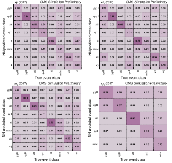
png pdf |
Figure 1:
Confusion matrices for the NN classification task described in Section 5.4, for the (upper left) $\mathrm{e} \mu $, (upper right) $\mathrm{e} \tau _{\text {h}} $, (lower left) $\mu \tau _{\text {h}} $, and (lower right) $\tau _{\text {h}} \tau _{\text {h}} $ final states evaluated on the 2017 dataset. Each matrix is normalized such that all entries in each column, corresponding to a given event class, sum up to unity. All event classes enter the matrix with the same statistical weight (i.e. with uniform prevalence). |
png pdf |
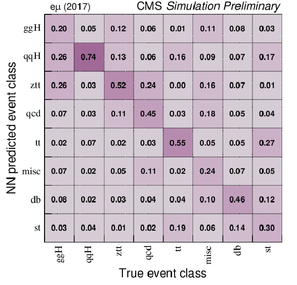
Figure 1-a:
Confusion matrices for the NN classification task described in Section 5.4, for the (upper left) $\mathrm{e} \mu $, (upper right) $\mathrm{e} \tau _{\text {h}} $, (lower left) $\mu \tau _{\text {h}} $, and (lower right) $\tau _{\text {h}} \tau _{\text {h}} $ final states evaluated on the 2017 dataset. Each matrix is normalized such that all entries in each column, corresponding to a given event class, sum up to unity. All event classes enter the matrix with the same statistical weight (i.e. with uniform prevalence). |
png pdf |
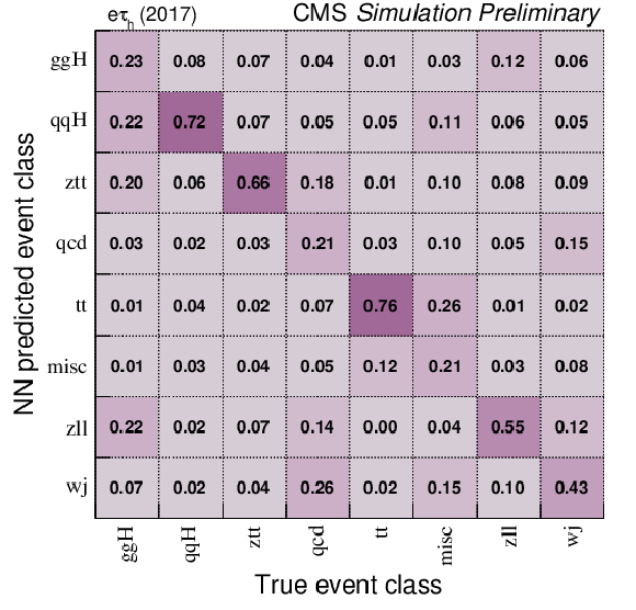
Figure 1-b:
Confusion matrices for the NN classification task described in Section 5.4, for the (upper left) $\mathrm{e} \mu $, (upper right) $\mathrm{e} \tau _{\text {h}} $, (lower left) $\mu \tau _{\text {h}} $, and (lower right) $\tau _{\text {h}} \tau _{\text {h}} $ final states evaluated on the 2017 dataset. Each matrix is normalized such that all entries in each column, corresponding to a given event class, sum up to unity. All event classes enter the matrix with the same statistical weight (i.e. with uniform prevalence). |
png pdf |
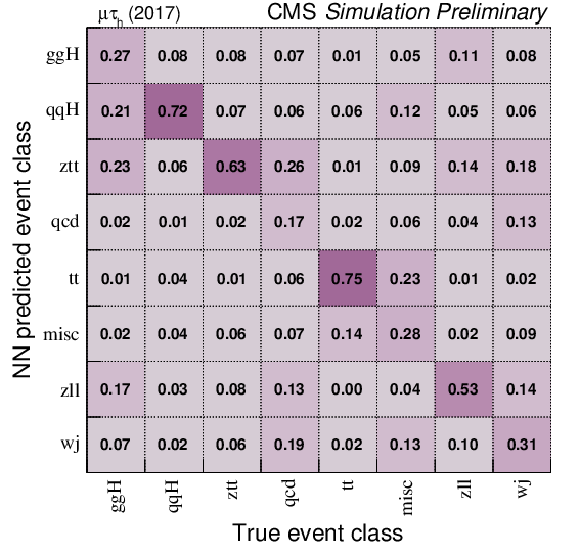
Figure 1-c:
Confusion matrices for the NN classification task described in Section 5.4, for the (upper left) $\mathrm{e} \mu $, (upper right) $\mathrm{e} \tau _{\text {h}} $, (lower left) $\mu \tau _{\text {h}} $, and (lower right) $\tau _{\text {h}} \tau _{\text {h}} $ final states evaluated on the 2017 dataset. Each matrix is normalized such that all entries in each column, corresponding to a given event class, sum up to unity. All event classes enter the matrix with the same statistical weight (i.e. with uniform prevalence). |
png pdf |
Figure 1-d:
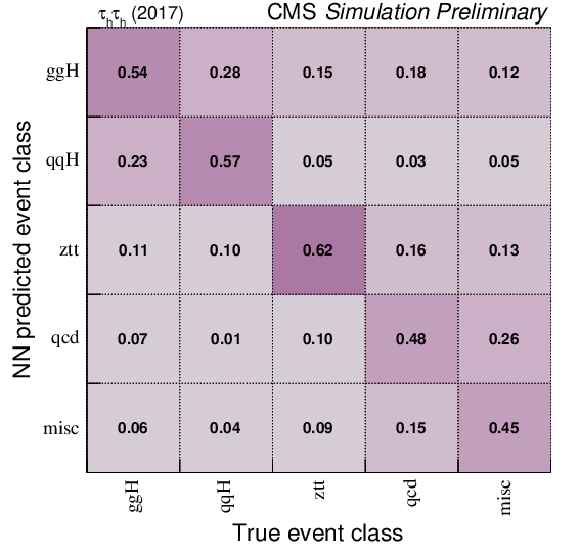
Confusion matrices for the NN classification task described in Section 5.4, for the (upper left) $\mathrm{e} \mu $, (upper right) $\mathrm{e} \tau _{\text {h}} $, (lower left) $\mu \tau _{\text {h}} $, and (lower right) $\tau _{\text {h}} \tau _{\text {h}} $ final states evaluated on the 2017 dataset. Each matrix is normalized such that all entries in each column, corresponding to a given event class, sum up to unity. All event classes enter the matrix with the same statistical weight (i.e. with uniform prevalence). |

png pdf |
Figure 2:
Distributions of the NN output used for the determination of the event categories in the (upper left) ztt, (upper right) qcd, (middle left) tt, (middle right) zll, (lower left) wj, and (lower right) misc event categories, in the $\mu \tau _{\text {h}} $ final state. All distributions and uncertainties are shown after the fit that has been applied to the data. |
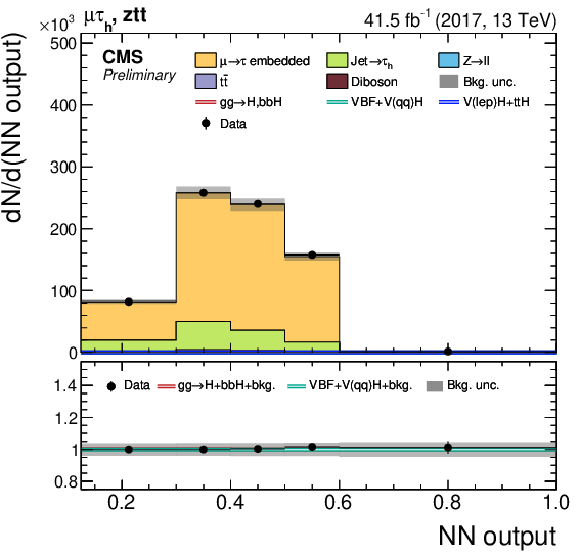
png pdf |
Figure 2-a:
Distributions of the NN output used for the determination of the event categories in the (upper left) ztt, (upper right) qcd, (middle left) tt, (middle right) zll, (lower left) wj, and (lower right) misc event categories, in the $\mu \tau _{\text {h}} $ final state. All distributions and uncertainties are shown after the fit that has been applied to the data. |

png pdf |
Figure 2-b:
Distributions of the NN output used for the determination of the event categories in the (upper left) ztt, (upper right) qcd, (middle left) tt, (middle right) zll, (lower left) wj, and (lower right) misc event categories, in the $\mu \tau _{\text {h}} $ final state. All distributions and uncertainties are shown after the fit that has been applied to the data. |
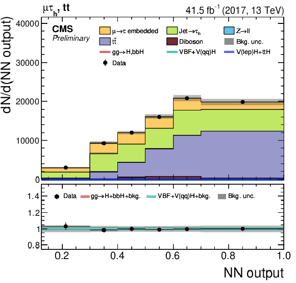
png pdf |
Figure 2-c:
Distributions of the NN output used for the determination of the event categories in the (upper left) ztt, (upper right) qcd, (middle left) tt, (middle right) zll, (lower left) wj, and (lower right) misc event categories, in the $\mu \tau _{\text {h}} $ final state. All distributions and uncertainties are shown after the fit that has been applied to the data. |
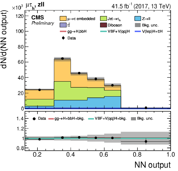
png pdf |
Figure 2-d:
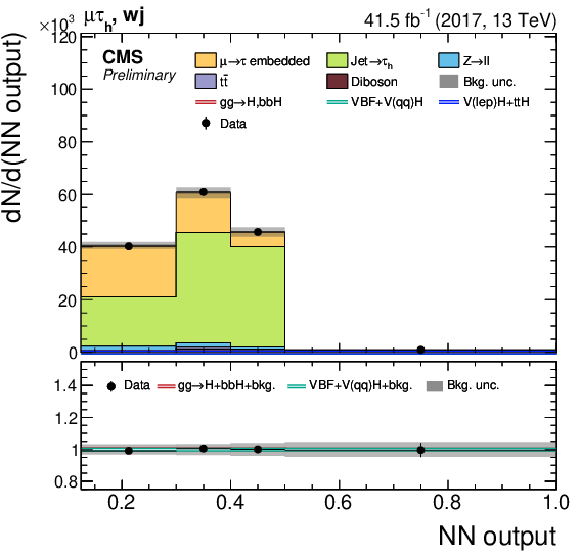
Distributions of the NN output used for the determination of the event categories in the (upper left) ztt, (upper right) qcd, (middle left) tt, (middle right) zll, (lower left) wj, and (lower right) misc event categories, in the $\mu \tau _{\text {h}} $ final state. All distributions and uncertainties are shown after the fit that has been applied to the data. |
png pdf |
Figure 2-e:
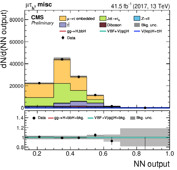
Distributions of the NN output used for the determination of the event categories in the (upper left) ztt, (upper right) qcd, (middle left) tt, (middle right) zll, (lower left) wj, and (lower right) misc event categories, in the $\mu \tau _{\text {h}} $ final state. All distributions and uncertainties are shown after the fit that has been applied to the data. |
png pdf |
Figure 2-f:
Distributions of the NN output used for the determination of the event categories in the (upper left) ztt, (upper right) qcd, (middle left) tt, (middle right) zll, (lower left) wj, and (lower right) misc event categories, in the $\mu \tau _{\text {h}} $ final state. All distributions and uncertainties are shown after the fit that has been applied to the data. |

png pdf |
Figure 3:
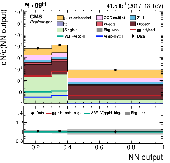
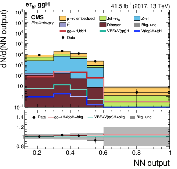
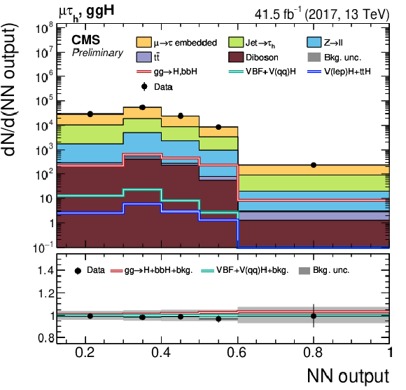
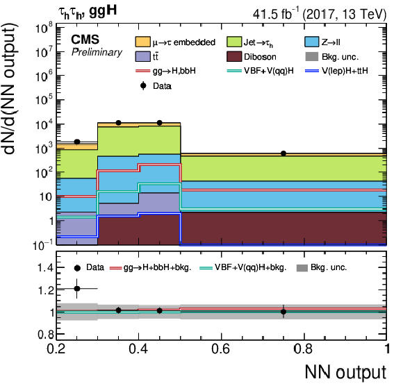
Distributions of the output of the NN used for the determination of the event categories, in the ggH event category, in the (upper left) $\mathrm{e} \mu $, (upper right) $\mathrm{e} \tau _{\text {h}} $, (lower left) $\mu \tau _{\text {h}} $, and (lower right) $\tau _{\text {h}} \tau _{\text {h}} $ final states, on the 2017 dataset. All distributions and uncertainties are shown after the fit that has been applied to the data. For each channel, all event categories relevant for the extraction of ${{\mathrm{g} \mathrm{g} \to \mathrm{H},\mathrm{b} \mathrm{b} \mathrm{H}}}$ production have been summed. |
png pdf |
Figure 3-a:
Distributions of the output of the NN used for the determination of the event categories, in the ggH event category, in the (upper left) $\mathrm{e} \mu $, (upper right) $\mathrm{e} \tau _{\text {h}} $, (lower left) $\mu \tau _{\text {h}} $, and (lower right) $\tau _{\text {h}} \tau _{\text {h}} $ final states, on the 2017 dataset. All distributions and uncertainties are shown after the fit that has been applied to the data. For each channel, all event categories relevant for the extraction of ${{\mathrm{g} \mathrm{g} \to \mathrm{H},\mathrm{b} \mathrm{b} \mathrm{H}}}$ production have been summed. |
png pdf |
Figure 3-b:
Distributions of the output of the NN used for the determination of the event categories, in the ggH event category, in the (upper left) $\mathrm{e} \mu $, (upper right) $\mathrm{e} \tau _{\text {h}} $, (lower left) $\mu \tau _{\text {h}} $, and (lower right) $\tau _{\text {h}} \tau _{\text {h}} $ final states, on the 2017 dataset. All distributions and uncertainties are shown after the fit that has been applied to the data. For each channel, all event categories relevant for the extraction of ${{\mathrm{g} \mathrm{g} \to \mathrm{H},\mathrm{b} \mathrm{b} \mathrm{H}}}$ production have been summed. |
png pdf |
Figure 3-c:
Distributions of the output of the NN used for the determination of the event categories, in the ggH event category, in the (upper left) $\mathrm{e} \mu $, (upper right) $\mathrm{e} \tau _{\text {h}} $, (lower left) $\mu \tau _{\text {h}} $, and (lower right) $\tau _{\text {h}} \tau _{\text {h}} $ final states, on the 2017 dataset. All distributions and uncertainties are shown after the fit that has been applied to the data. For each channel, all event categories relevant for the extraction of ${{\mathrm{g} \mathrm{g} \to \mathrm{H},\mathrm{b} \mathrm{b} \mathrm{H}}}$ production have been summed. |
png pdf |
Figure 3-d:
Distributions of the output of the NN used for the determination of the event categories, in the ggH event category, in the (upper left) $\mathrm{e} \mu $, (upper right) $\mathrm{e} \tau _{\text {h}} $, (lower left) $\mu \tau _{\text {h}} $, and (lower right) $\tau _{\text {h}} \tau _{\text {h}} $ final states, on the 2017 dataset. All distributions and uncertainties are shown after the fit that has been applied to the data. For each channel, all event categories relevant for the extraction of ${{\mathrm{g} \mathrm{g} \to \mathrm{H},\mathrm{b} \mathrm{b} \mathrm{H}}}$ production have been summed. |

png pdf |
Figure 4:
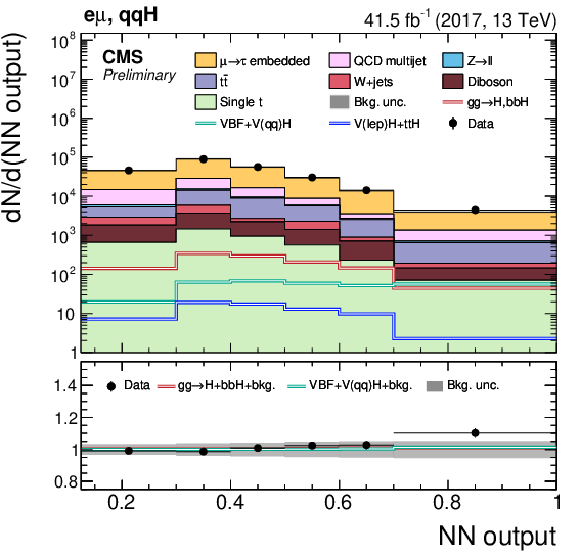
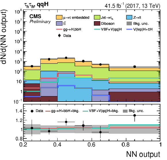
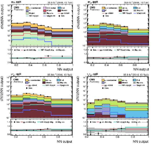
Distributions of the output of the NN used for the determination of the event categories, in the qqH event category, in the (upper left) $\mathrm{e} \mu $, (upper right) $\mathrm{e} \tau _{\text {h}} $, (lower left) $\mu \tau _{\text {h}} $, and (lower right) $\tau _{\text {h}} \tau _{\text {h}} $ final states, on the 2017 dataset. All distributions and uncertainties are shown after the fit that has been applied to the data. For each channel, all event categories relevant for the extraction of ${{\text {VBF}{+} {\mathrm {V}}(\mathrm{q} \mathrm{q})\mathrm{H}}}$ production have been summed. |
png pdf |
Figure 4-a:
Distributions of the output of the NN used for the determination of the event categories, in the qqH event category, in the (upper left) $\mathrm{e} \mu $, (upper right) $\mathrm{e} \tau _{\text {h}} $, (lower left) $\mu \tau _{\text {h}} $, and (lower right) $\tau _{\text {h}} \tau _{\text {h}} $ final states, on the 2017 dataset. All distributions and uncertainties are shown after the fit that has been applied to the data. For each channel, all event categories relevant for the extraction of ${{\text {VBF}{+} {\mathrm {V}}(\mathrm{q} \mathrm{q})\mathrm{H}}}$ production have been summed. |

png pdf |
Figure 4-b:
Distributions of the output of the NN used for the determination of the event categories, in the qqH event category, in the (upper left) $\mathrm{e} \mu $, (upper right) $\mathrm{e} \tau _{\text {h}} $, (lower left) $\mu \tau _{\text {h}} $, and (lower right) $\tau _{\text {h}} \tau _{\text {h}} $ final states, on the 2017 dataset. All distributions and uncertainties are shown after the fit that has been applied to the data. For each channel, all event categories relevant for the extraction of ${{\text {VBF}{+} {\mathrm {V}}(\mathrm{q} \mathrm{q})\mathrm{H}}}$ production have been summed. |

png pdf |
Figure 4-c:
Distributions of the output of the NN used for the determination of the event categories, in the qqH event category, in the (upper left) $\mathrm{e} \mu $, (upper right) $\mathrm{e} \tau _{\text {h}} $, (lower left) $\mu \tau _{\text {h}} $, and (lower right) $\tau _{\text {h}} \tau _{\text {h}} $ final states, on the 2017 dataset. All distributions and uncertainties are shown after the fit that has been applied to the data. For each channel, all event categories relevant for the extraction of ${{\text {VBF}{+} {\mathrm {V}}(\mathrm{q} \mathrm{q})\mathrm{H}}}$ production have been summed. |
png pdf |
Figure 4-d:
Distributions of the output of the NN used for the determination of the event categories, in the qqH event category, in the (upper left) $\mathrm{e} \mu $, (upper right) $\mathrm{e} \tau _{\text {h}} $, (lower left) $\mu \tau _{\text {h}} $, and (lower right) $\tau _{\text {h}} \tau _{\text {h}} $ final states, on the 2017 dataset. All distributions and uncertainties are shown after the fit that has been applied to the data. For each channel, all event categories relevant for the extraction of ${{\text {VBF}{+} {\mathrm {V}}(\mathrm{q} \mathrm{q})\mathrm{H}}}$ production have been summed. |
png pdf |
Figure 5:
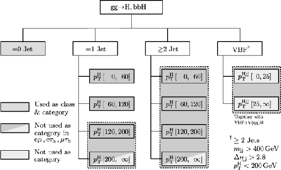
Classification scheme as proposed by the LHC HXSWG to further investigate the kinematic properties of ${{\mathrm{g} \mathrm{g} \to \mathrm{H},\mathrm{b} \mathrm{b} \mathrm{H}}}$ production. All proposed classes are indicated by gray boxes. The darker color indicates classes that are also used as categories in the analysis. The lighter colored classes are not used as categories (in all final states). All bin boundaries are given in ${GeV}$. For the statistical inference of the signal some event classes are combined as indicated by the dashed lines. |

png pdf |
Figure 6:
Classification scheme as proposed by the LHC HXSWG to further investigate the kinematic properties of ${{\text {VBF}{+} {\mathrm {V}}(\mathrm{q} \mathrm{q})\mathrm{H}}}$ production. All proposed classes are indicated by gray boxes. They are also used as categories in the analysis. All bin boundaries are given in ${GeV}$. For the statistical inference of the signal two event classes are combined as indicated by the dashed lines. |

png pdf |
Figure 7:
Distribution of the decimal logarithm of the signal purity (after the fit to the data), evaluated in the bins of the signal categories used to extract the results. The signal contribution and the background contributions from each decay channel are stacked on top of each other. The inset shows the relative excess with respect to the estimated background. |

png pdf |
Figure 8:
Results of the maximum likelihood fit to the data, for a model with one signal strength parameter, as discussed in Section 8, split by final state and inclusively, for all final states combined. The ${{\mathrm{t} \mathrm{t} \mathrm{H}}}$ and $ {\mathrm {V}}\mathrm{H} $ production modes with leptonic $ {\mathrm {V}}$ decays have a negligible effect on the shown results and are not included as signal. |
png pdf |
Figure 9:
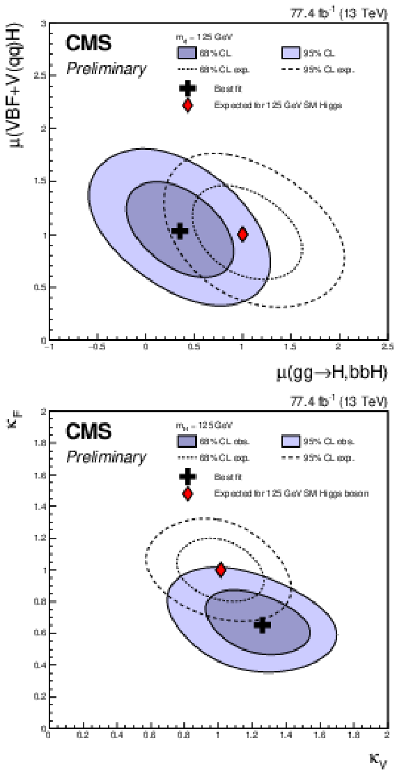
Two-dimensional contours corresponding to 68% and 95% confidence level (CL) (top) for the signal strength of the ${{\mathrm{g} \mathrm{g} \to \mathrm{H},\mathrm{b} \mathrm{b} \mathrm{H}}}$ and ${{\text {VBF}{+} {\mathrm {V}}(\mathrm{q} \mathrm{q})\mathrm{H}}}$ production modes and (bottom) for the coupling strength modifiers $\kappa _{\text {V}}$ and $\kappa _{\text {F}}$. All nuisance parameters are profiled at each point evaluated in the two-dimensional parameter space. For the scan of $\kappa _{\text {V}}$ and $\kappa _{\text {F}}$, the contribution of $\mathrm{H} \to \mathrm{W} \mathrm{W} $ to the $\mathrm{e} \mu $ final state, and the ${{\mathrm{t} \mathrm{t} \mathrm{H}}}$ and $ {\mathrm {V}}\mathrm{H} $ production modes with leptonic $ {\mathrm {V}}$ decays are treated as a signal processes. |

png pdf |
Figure 9-a:
Two-dimensional contours corresponding to 68% and 95% confidence level (CL) (top) for the signal strength of the ${{\mathrm{g} \mathrm{g} \to \mathrm{H},\mathrm{b} \mathrm{b} \mathrm{H}}}$ and ${{\text {VBF}{+} {\mathrm {V}}(\mathrm{q} \mathrm{q})\mathrm{H}}}$ production modes and (bottom) for the coupling strength modifiers $\kappa _{\text {V}}$ and $\kappa _{\text {F}}$. All nuisance parameters are profiled at each point evaluated in the two-dimensional parameter space. For the scan of $\kappa _{\text {V}}$ and $\kappa _{\text {F}}$, the contribution of $\mathrm{H} \to \mathrm{W} \mathrm{W} $ to the $\mathrm{e} \mu $ final state, and the ${{\mathrm{t} \mathrm{t} \mathrm{H}}}$ and $ {\mathrm {V}}\mathrm{H} $ production modes with leptonic $ {\mathrm {V}}$ decays are treated as a signal processes. |

png pdf |
Figure 9-b:
Two-dimensional contours corresponding to 68% and 95% confidence level (CL) (top) for the signal strength of the ${{\mathrm{g} \mathrm{g} \to \mathrm{H},\mathrm{b} \mathrm{b} \mathrm{H}}}$ and ${{\text {VBF}{+} {\mathrm {V}}(\mathrm{q} \mathrm{q})\mathrm{H}}}$ production modes and (bottom) for the coupling strength modifiers $\kappa _{\text {V}}$ and $\kappa _{\text {F}}$. All nuisance parameters are profiled at each point evaluated in the two-dimensional parameter space. For the scan of $\kappa _{\text {V}}$ and $\kappa _{\text {F}}$, the contribution of $\mathrm{H} \to \mathrm{W} \mathrm{W} $ to the $\mathrm{e} \mu $ final state, and the ${{\mathrm{t} \mathrm{t} \mathrm{H}}}$ and $ {\mathrm {V}}\mathrm{H} $ production modes with leptonic $ {\mathrm {V}}$ decays are treated as a signal processes. |
png pdf |
Figure 10:
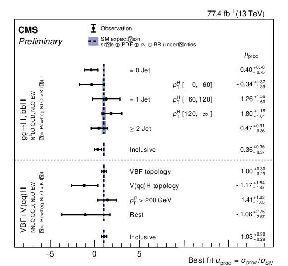
Results of the maximum likelihood fit to the data, for a model with 9 signal strength parameters, as discussed in Section 8. Also shown are the results from an inclusive fit with separate signal strength parameters for the ${{\mathrm{g} \mathrm{g} \to \mathrm{H},\mathrm{b} \mathrm{b} \mathrm{H}}}$ and ${{\text {VBF}{+} {\mathrm {V}}(\mathrm{q} \mathrm{q})\mathrm{H}}}$ production processes. The ${{\mathrm{t} \mathrm{t} \mathrm{H}}}$ and $ {\mathrm {V}}\mathrm{H} $ production modes with leptonic $ {\mathrm {V}}$ decays have a negligible effect on the shown results and are not included as signal. |

png pdf |
Figure 11:
Correlation matrix of the maximum likelihood fit with 9 signal strength parameters, as discussed in Section 8. The corresponding fit results are shown in Figure 10. |

png pdf |
Figure 12:
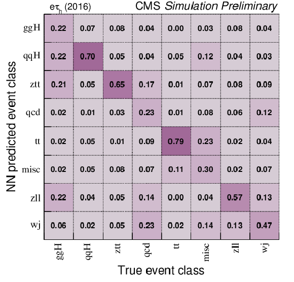
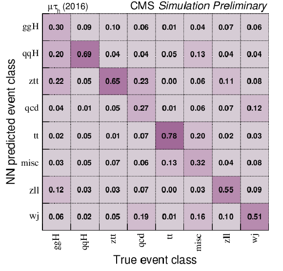
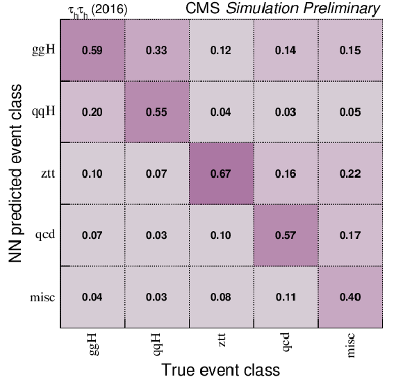
Confusion matrices for the NN classification task described in Section 5.4, for the (upper left) $\mathrm{e} \mu $, (upper right) $\mathrm{e} \tau _{\text {h}} $, (lower left) $\mu \tau _{\text {h}} $, and (lower right) $\tau _{\text {h}} \tau _{\text {h}} $ final states evaluated on the 2016 dataset. Each matrix is normalized such that all entries in each column, corresponding to a given event class, sum up to unity. All event classes enter the matrix with the same statistical weight (uniform prevalence). |
png pdf |
Figure 12-a:
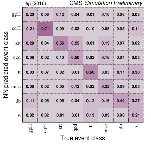
Confusion matrices for the NN classification task described in Section 5.4, for the (upper left) $\mathrm{e} \mu $, (upper right) $\mathrm{e} \tau _{\text {h}} $, (lower left) $\mu \tau _{\text {h}} $, and (lower right) $\tau _{\text {h}} \tau _{\text {h}} $ final states evaluated on the 2016 dataset. Each matrix is normalized such that all entries in each column, corresponding to a given event class, sum up to unity. All event classes enter the matrix with the same statistical weight (uniform prevalence). |
png pdf |
Figure 12-b:
Confusion matrices for the NN classification task described in Section 5.4, for the (upper left) $\mathrm{e} \mu $, (upper right) $\mathrm{e} \tau _{\text {h}} $, (lower left) $\mu \tau _{\text {h}} $, and (lower right) $\tau _{\text {h}} \tau _{\text {h}} $ final states evaluated on the 2016 dataset. Each matrix is normalized such that all entries in each column, corresponding to a given event class, sum up to unity. All event classes enter the matrix with the same statistical weight (uniform prevalence). |
png pdf |
Figure 12-c:
Confusion matrices for the NN classification task described in Section 5.4, for the (upper left) $\mathrm{e} \mu $, (upper right) $\mathrm{e} \tau _{\text {h}} $, (lower left) $\mu \tau _{\text {h}} $, and (lower right) $\tau _{\text {h}} \tau _{\text {h}} $ final states evaluated on the 2016 dataset. Each matrix is normalized such that all entries in each column, corresponding to a given event class, sum up to unity. All event classes enter the matrix with the same statistical weight (uniform prevalence). |
png pdf |
Figure 12-d:
Confusion matrices for the NN classification task described in Section 5.4, for the (upper left) $\mathrm{e} \mu $, (upper right) $\mathrm{e} \tau _{\text {h}} $, (lower left) $\mu \tau _{\text {h}} $, and (lower right) $\tau _{\text {h}} \tau _{\text {h}} $ final states evaluated on the 2016 dataset. Each matrix is normalized such that all entries in each column, corresponding to a given event class, sum up to unity. All event classes enter the matrix with the same statistical weight (uniform prevalence). |
png pdf |
Figure 13:
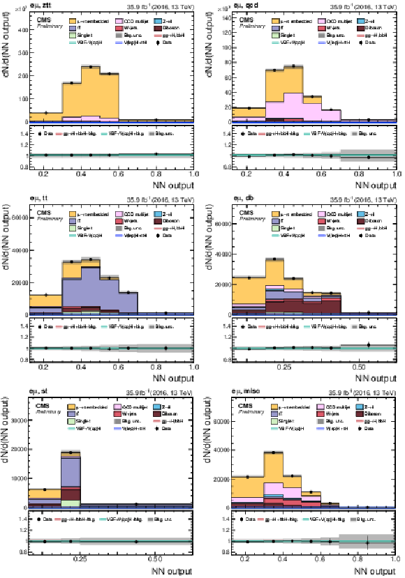
Distributions of the NN output used for the determination of the event categories in the (upper left) ztt, (upper right) qcd, (middle left) tt, (middle right) db, (lower left) st, and (lower right) misc event categories, in the $\mathrm{e} \mu $ final state, on the 2016 dataset. |

png pdf |
Figure 13-a:
Distributions of the NN output used for the determination of the event categories in the (upper left) ztt, (upper right) qcd, (middle left) tt, (middle right) db, (lower left) st, and (lower right) misc event categories, in the $\mathrm{e} \mu $ final state, on the 2016 dataset. |
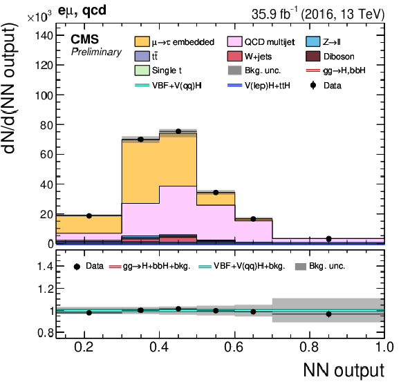
png pdf |
Figure 13-b:
Distributions of the NN output used for the determination of the event categories in the (upper left) ztt, (upper right) qcd, (middle left) tt, (middle right) db, (lower left) st, and (lower right) misc event categories, in the $\mathrm{e} \mu $ final state, on the 2016 dataset. |
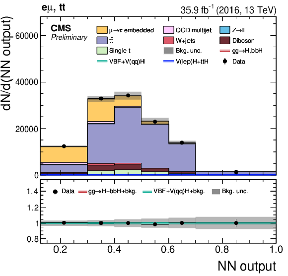
png pdf |
Figure 13-c:
Distributions of the NN output used for the determination of the event categories in the (upper left) ztt, (upper right) qcd, (middle left) tt, (middle right) db, (lower left) st, and (lower right) misc event categories, in the $\mathrm{e} \mu $ final state, on the 2016 dataset. |

png pdf |
Figure 13-d:
Distributions of the NN output used for the determination of the event categories in the (upper left) ztt, (upper right) qcd, (middle left) tt, (middle right) db, (lower left) st, and (lower right) misc event categories, in the $\mathrm{e} \mu $ final state, on the 2016 dataset. |
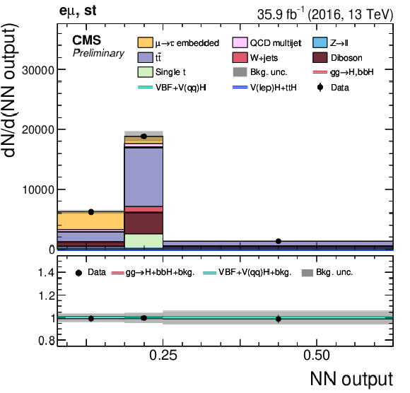
png pdf |
Figure 13-e:
Distributions of the NN output used for the determination of the event categories in the (upper left) ztt, (upper right) qcd, (middle left) tt, (middle right) db, (lower left) st, and (lower right) misc event categories, in the $\mathrm{e} \mu $ final state, on the 2016 dataset. |
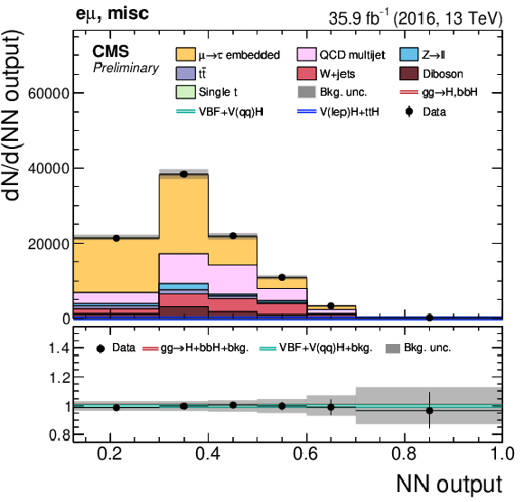
png pdf |
Figure 13-f:
Distributions of the NN output used for the determination of the event categories in the (upper left) ztt, (upper right) qcd, (middle left) tt, (middle right) db, (lower left) st, and (lower right) misc event categories, in the $\mathrm{e} \mu $ final state, on the 2016 dataset. |
png pdf |
Figure 14:
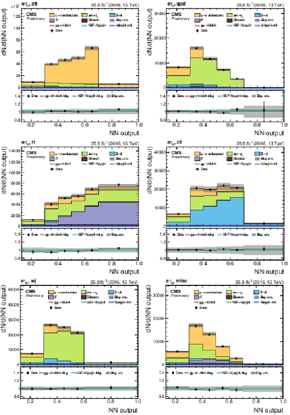
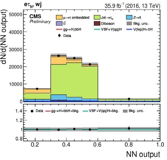
Distributions of the NN output used for the determination of the event categories in the (upper left) ztt, (upper right) qcd, (middle left) tt, (middle right) zll, (lower left) wj, and (lower right) misc event categories, in the $\mathrm{e} \tau _{\text {h}} $ final state, on the 2016 dataset. |
png pdf |
Figure 14-a:
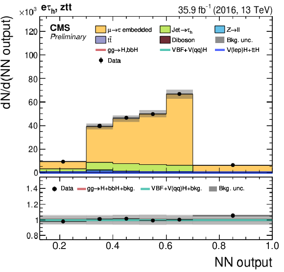
Distributions of the NN output used for the determination of the event categories in the (upper left) ztt, (upper right) qcd, (middle left) tt, (middle right) zll, (lower left) wj, and (lower right) misc event categories, in the $\mathrm{e} \tau _{\text {h}} $ final state, on the 2016 dataset. |

png pdf |
Figure 14-b:
Distributions of the NN output used for the determination of the event categories in the (upper left) ztt, (upper right) qcd, (middle left) tt, (middle right) zll, (lower left) wj, and (lower right) misc event categories, in the $\mathrm{e} \tau _{\text {h}} $ final state, on the 2016 dataset. |
png pdf |
Figure 14-c:
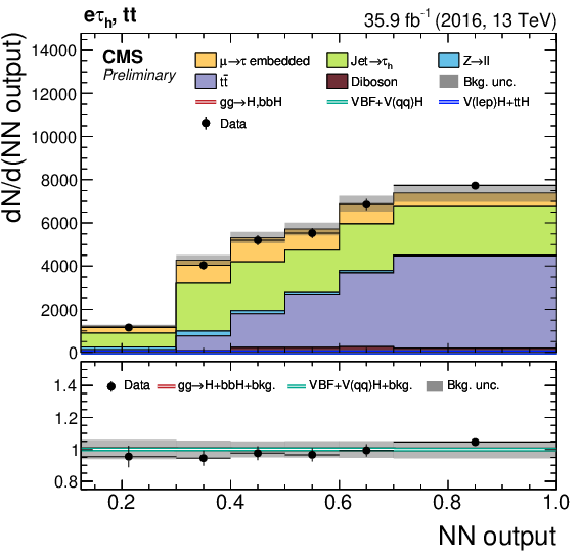
Distributions of the NN output used for the determination of the event categories in the (upper left) ztt, (upper right) qcd, (middle left) tt, (middle right) zll, (lower left) wj, and (lower right) misc event categories, in the $\mathrm{e} \tau _{\text {h}} $ final state, on the 2016 dataset. |
png pdf |
Figure 14-d:
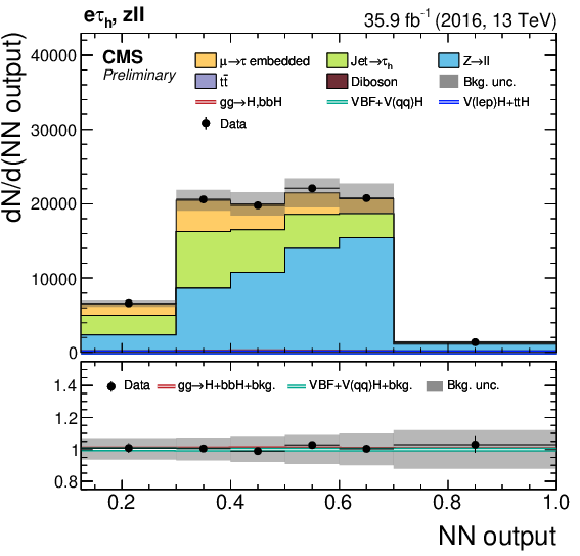
Distributions of the NN output used for the determination of the event categories in the (upper left) ztt, (upper right) qcd, (middle left) tt, (middle right) zll, (lower left) wj, and (lower right) misc event categories, in the $\mathrm{e} \tau _{\text {h}} $ final state, on the 2016 dataset. |
png pdf |
Figure 14-e:
Distributions of the NN output used for the determination of the event categories in the (upper left) ztt, (upper right) qcd, (middle left) tt, (middle right) zll, (lower left) wj, and (lower right) misc event categories, in the $\mathrm{e} \tau _{\text {h}} $ final state, on the 2016 dataset. |

png pdf |
Figure 14-f:
Distributions of the NN output used for the determination of the event categories in the (upper left) ztt, (upper right) qcd, (middle left) tt, (middle right) zll, (lower left) wj, and (lower right) misc event categories, in the $\mathrm{e} \tau _{\text {h}} $ final state, on the 2016 dataset. |

png pdf |
Figure 15:
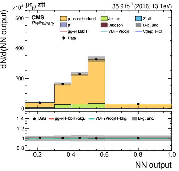
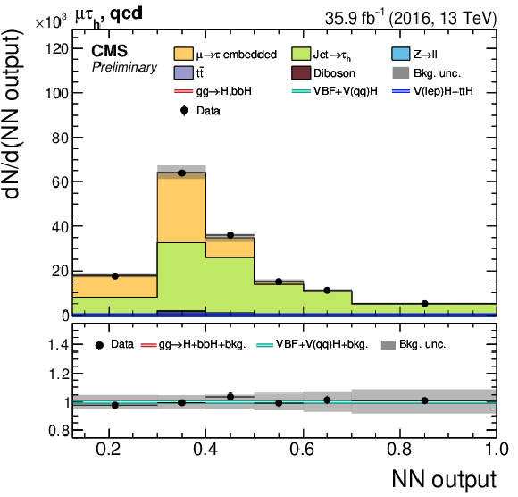
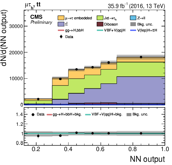
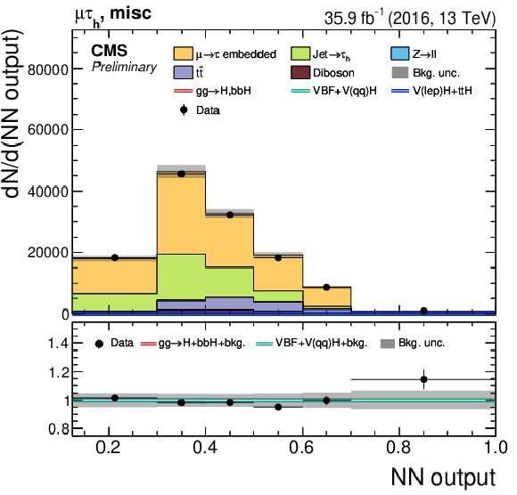
Distributions of the NN output used for the determination of the event categories in the (upper left) ztt, (upper right) qcd, (middle left) tt, (middle right) zll, (lower left) wj, and (lower right) misc event categories, in the $\mu \tau _{\text {h}} $ final state, on the 2016 dataset. |
png pdf |
Figure 15-a:
Distributions of the NN output used for the determination of the event categories in the (upper left) ztt, (upper right) qcd, (middle left) tt, (middle right) zll, (lower left) wj, and (lower right) misc event categories, in the $\mu \tau _{\text {h}} $ final state, on the 2016 dataset. |
png pdf |
Figure 15-b:
Distributions of the NN output used for the determination of the event categories in the (upper left) ztt, (upper right) qcd, (middle left) tt, (middle right) zll, (lower left) wj, and (lower right) misc event categories, in the $\mu \tau _{\text {h}} $ final state, on the 2016 dataset. |
png pdf |
Figure 15-c:
Distributions of the NN output used for the determination of the event categories in the (upper left) ztt, (upper right) qcd, (middle left) tt, (middle right) zll, (lower left) wj, and (lower right) misc event categories, in the $\mu \tau _{\text {h}} $ final state, on the 2016 dataset. |

png pdf |
Figure 15-d:
Distributions of the NN output used for the determination of the event categories in the (upper left) ztt, (upper right) qcd, (middle left) tt, (middle right) zll, (lower left) wj, and (lower right) misc event categories, in the $\mu \tau _{\text {h}} $ final state, on the 2016 dataset. |

png pdf |
Figure 15-e:
Distributions of the NN output used for the determination of the event categories in the (upper left) ztt, (upper right) qcd, (middle left) tt, (middle right) zll, (lower left) wj, and (lower right) misc event categories, in the $\mu \tau _{\text {h}} $ final state, on the 2016 dataset. |
png pdf |
Figure 15-f:
Distributions of the NN output used for the determination of the event categories in the (upper left) ztt, (upper right) qcd, (middle left) tt, (middle right) zll, (lower left) wj, and (lower right) misc event categories, in the $\mu \tau _{\text {h}} $ final state, on the 2016 dataset. |

png pdf |
Figure 16:
Distributions of the NN output used for the determination of the event categories in the (upper left) ztt, (upper right) qcd, (lower left) misc event categories, in the $\tau _{\text {h}} \tau _{\text {h}} $ final state, on the 2016 dataset. |

png pdf |
Figure 16-a:
Distributions of the NN output used for the determination of the event categories in the (upper left) ztt, (upper right) qcd, (lower left) misc event categories, in the $\tau _{\text {h}} \tau _{\text {h}} $ final state, on the 2016 dataset. |

png pdf |
Figure 16-b:
Distributions of the NN output used for the determination of the event categories in the (upper left) ztt, (upper right) qcd, (lower left) misc event categories, in the $\tau _{\text {h}} \tau _{\text {h}} $ final state, on the 2016 dataset. |

png pdf |
Figure 16-c:
Distributions of the NN output used for the determination of the event categories in the (upper left) ztt, (upper right) qcd, (lower left) misc event categories, in the $\tau _{\text {h}} \tau _{\text {h}} $ final state, on the 2016 dataset. |

png pdf |
Figure 17:
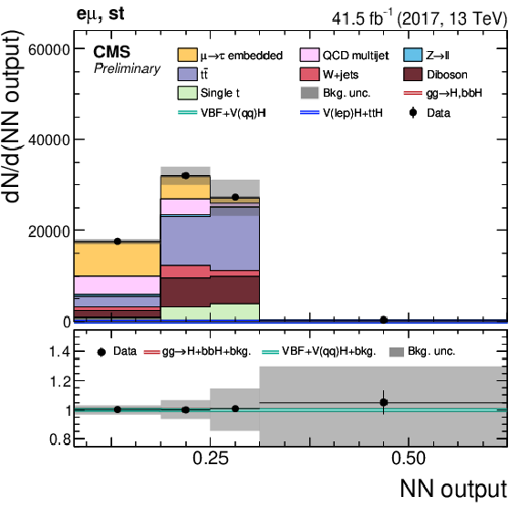
Distributions of the NN output used for the determination of the event categories in the (upper left) ztt, (upper right) qcd, (middle left) tt, (middle right) db, (lower left) st, and (lower right) misc event categories, in the $\mathrm{e} \mu $ final state, on the 2017 dataset. |

png pdf |
Figure 17-a:
Distributions of the NN output used for the determination of the event categories in the (upper left) ztt, (upper right) qcd, (middle left) tt, (middle right) db, (lower left) st, and (lower right) misc event categories, in the $\mathrm{e} \mu $ final state, on the 2017 dataset. |

png pdf |
Figure 17-b:
Distributions of the NN output used for the determination of the event categories in the (upper left) ztt, (upper right) qcd, (middle left) tt, (middle right) db, (lower left) st, and (lower right) misc event categories, in the $\mathrm{e} \mu $ final state, on the 2017 dataset. |

png pdf |
Figure 17-c:
Distributions of the NN output used for the determination of the event categories in the (upper left) ztt, (upper right) qcd, (middle left) tt, (middle right) db, (lower left) st, and (lower right) misc event categories, in the $\mathrm{e} \mu $ final state, on the 2017 dataset. |

png pdf |
Figure 17-d:
Distributions of the NN output used for the determination of the event categories in the (upper left) ztt, (upper right) qcd, (middle left) tt, (middle right) db, (lower left) st, and (lower right) misc event categories, in the $\mathrm{e} \mu $ final state, on the 2017 dataset. |
png pdf |
Figure 17-e:
Distributions of the NN output used for the determination of the event categories in the (upper left) ztt, (upper right) qcd, (middle left) tt, (middle right) db, (lower left) st, and (lower right) misc event categories, in the $\mathrm{e} \mu $ final state, on the 2017 dataset. |

png pdf |
Figure 17-f:
Distributions of the NN output used for the determination of the event categories in the (upper left) ztt, (upper right) qcd, (middle left) tt, (middle right) db, (lower left) st, and (lower right) misc event categories, in the $\mathrm{e} \mu $ final state, on the 2017 dataset. |
png pdf |
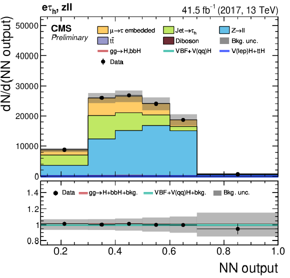
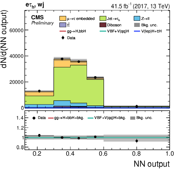
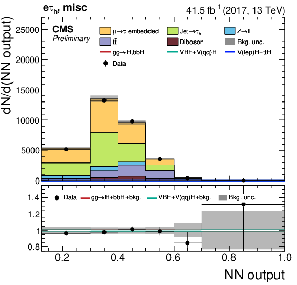
Figure 18:
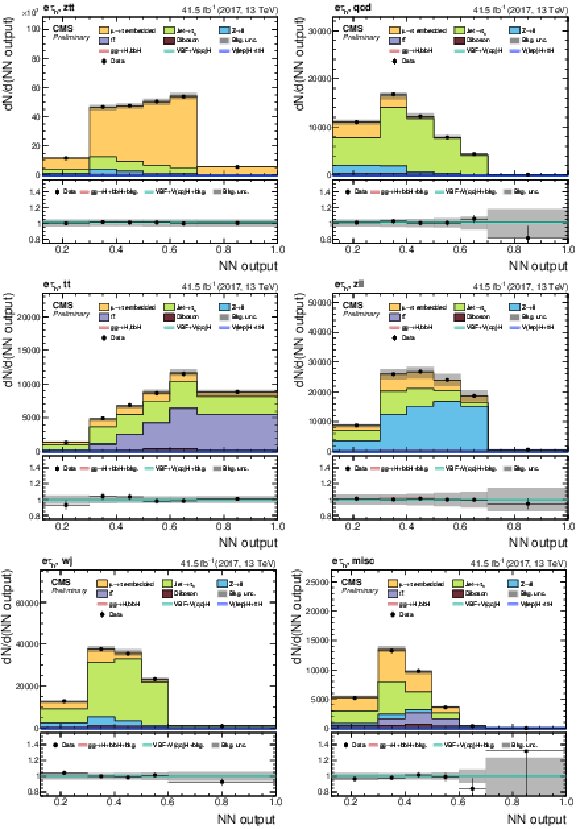
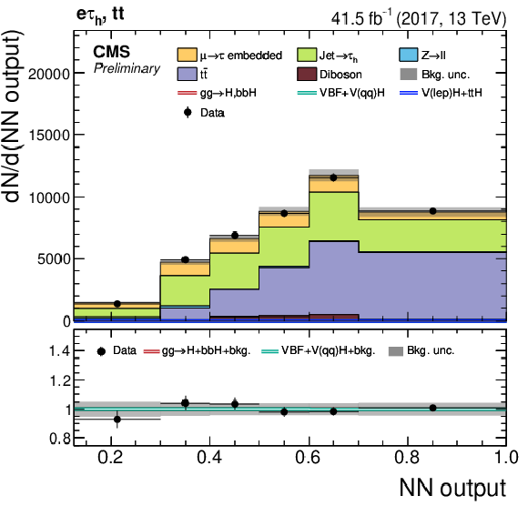
Distributions of the NN output used for the determination of the event categories in the (upper left) ztt, (upper right) qcd, (middle left) tt, (middle right) zll, (lower left) wj, and (lower right) misc event categories, in the $\mathrm{e} \tau _{\text {h}} $ final state, on the 2017 dataset. |

png pdf |
Figure 18-a:
Distributions of the NN output used for the determination of the event categories in the (upper left) ztt, (upper right) qcd, (middle left) tt, (middle right) zll, (lower left) wj, and (lower right) misc event categories, in the $\mathrm{e} \tau _{\text {h}} $ final state, on the 2017 dataset. |

png pdf |
Figure 18-b:
Distributions of the NN output used for the determination of the event categories in the (upper left) ztt, (upper right) qcd, (middle left) tt, (middle right) zll, (lower left) wj, and (lower right) misc event categories, in the $\mathrm{e} \tau _{\text {h}} $ final state, on the 2017 dataset. |
png pdf |
Figure 18-c:
Distributions of the NN output used for the determination of the event categories in the (upper left) ztt, (upper right) qcd, (middle left) tt, (middle right) zll, (lower left) wj, and (lower right) misc event categories, in the $\mathrm{e} \tau _{\text {h}} $ final state, on the 2017 dataset. |
png pdf |
Figure 18-d:
Distributions of the NN output used for the determination of the event categories in the (upper left) ztt, (upper right) qcd, (middle left) tt, (middle right) zll, (lower left) wj, and (lower right) misc event categories, in the $\mathrm{e} \tau _{\text {h}} $ final state, on the 2017 dataset. |
png pdf |
Figure 18-e:
Distributions of the NN output used for the determination of the event categories in the (upper left) ztt, (upper right) qcd, (middle left) tt, (middle right) zll, (lower left) wj, and (lower right) misc event categories, in the $\mathrm{e} \tau _{\text {h}} $ final state, on the 2017 dataset. |
png pdf |
Figure 18-f:
Distributions of the NN output used for the determination of the event categories in the (upper left) ztt, (upper right) qcd, (middle left) tt, (middle right) zll, (lower left) wj, and (lower right) misc event categories, in the $\mathrm{e} \tau _{\text {h}} $ final state, on the 2017 dataset. |

png pdf |
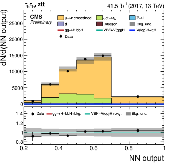
Figure 19:
Distributions of the NN output used for the determination of the event categories in the (upper left) ztt, (upper right) qcd, (lower left) misc event categories, in the $\tau _{\text {h}} \tau _{\text {h}} $ final state, on the 2017 dataset. |
png pdf |
Figure 19-a:
Distributions of the NN output used for the determination of the event categories in the (upper left) ztt, (upper right) qcd, (lower left) misc event categories, in the $\tau _{\text {h}} \tau _{\text {h}} $ final state, on the 2017 dataset. |

png pdf |
Figure 19-b:
Distributions of the NN output used for the determination of the event categories in the (upper left) ztt, (upper right) qcd, (lower left) misc event categories, in the $\tau _{\text {h}} \tau _{\text {h}} $ final state, on the 2017 dataset. |

png pdf |
Figure 19-c:
Distributions of the NN output used for the determination of the event categories in the (upper left) ztt, (upper right) qcd, (lower left) misc event categories, in the $\tau _{\text {h}} \tau _{\text {h}} $ final state, on the 2017 dataset. |

png pdf |
Figure 20:
Distributions of the output of the NN used for the determination of the event categories, in the ggH event category, in the (upper left) $\mathrm{e} \mu $, (upper right) $\mathrm{e} \tau _{\text {h}} $, (lower left) $\mu \tau _{\text {h}} $, and (lower right) $\tau _{\text {h}} \tau _{\text {h}} $ final state, on the 2016 dataset. |
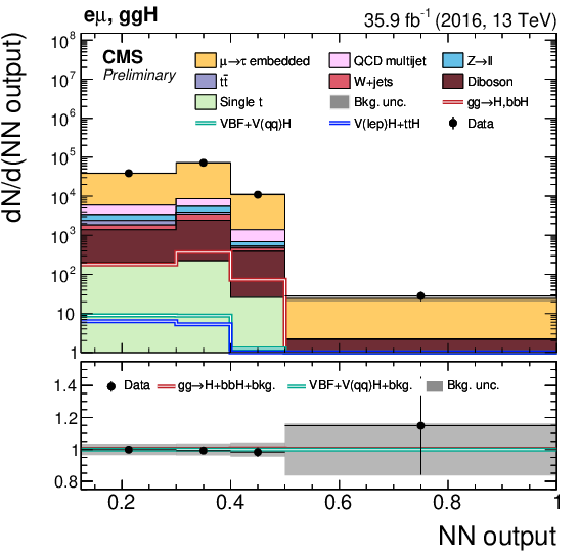
png pdf |
Figure 20-a:
Distributions of the output of the NN used for the determination of the event categories, in the ggH event category, in the (upper left) $\mathrm{e} \mu $, (upper right) $\mathrm{e} \tau _{\text {h}} $, (lower left) $\mu \tau _{\text {h}} $, and (lower right) $\tau _{\text {h}} \tau _{\text {h}} $ final state, on the 2016 dataset. |
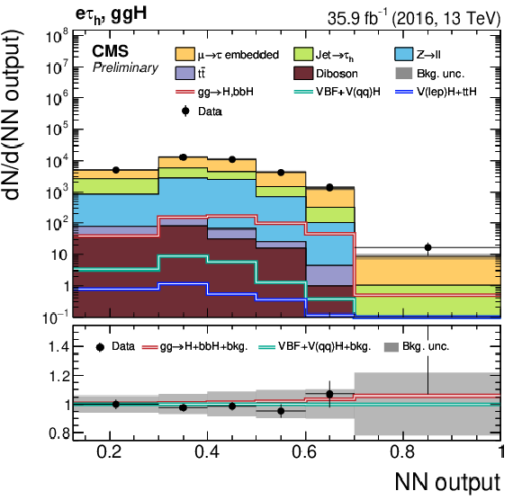
png pdf |
Figure 20-b:
Distributions of the output of the NN used for the determination of the event categories, in the ggH event category, in the (upper left) $\mathrm{e} \mu $, (upper right) $\mathrm{e} \tau _{\text {h}} $, (lower left) $\mu \tau _{\text {h}} $, and (lower right) $\tau _{\text {h}} \tau _{\text {h}} $ final state, on the 2016 dataset. |
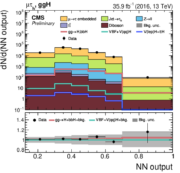
png pdf |
Figure 20-c:
Distributions of the output of the NN used for the determination of the event categories, in the ggH event category, in the (upper left) $\mathrm{e} \mu $, (upper right) $\mathrm{e} \tau _{\text {h}} $, (lower left) $\mu \tau _{\text {h}} $, and (lower right) $\tau _{\text {h}} \tau _{\text {h}} $ final state, on the 2016 dataset. |
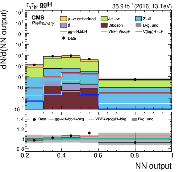
png pdf |
Figure 20-d:
Distributions of the output of the NN used for the determination of the event categories, in the ggH event category, in the (upper left) $\mathrm{e} \mu $, (upper right) $\mathrm{e} \tau _{\text {h}} $, (lower left) $\mu \tau _{\text {h}} $, and (lower right) $\tau _{\text {h}} \tau _{\text {h}} $ final state, on the 2016 dataset. |
png pdf |
Figure 21:
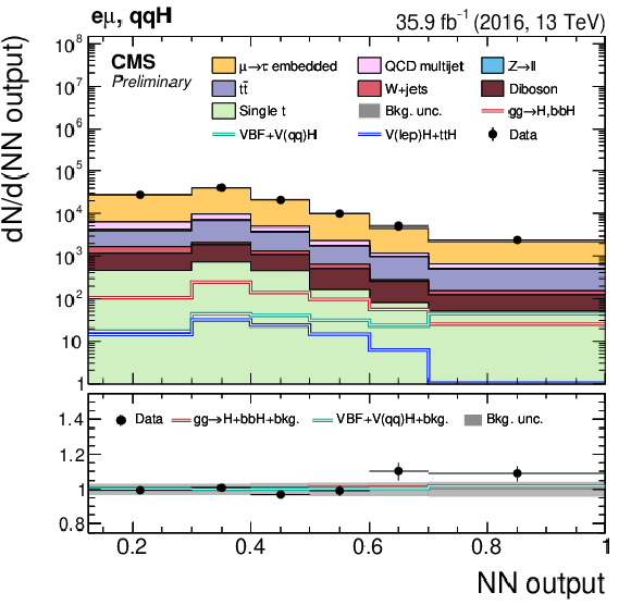
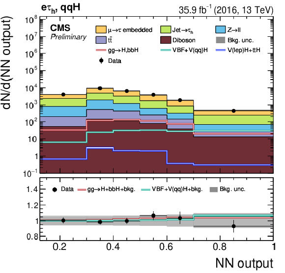
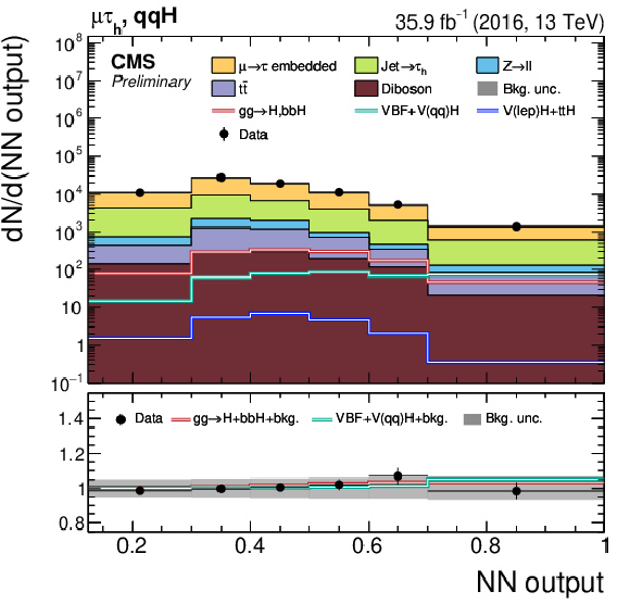
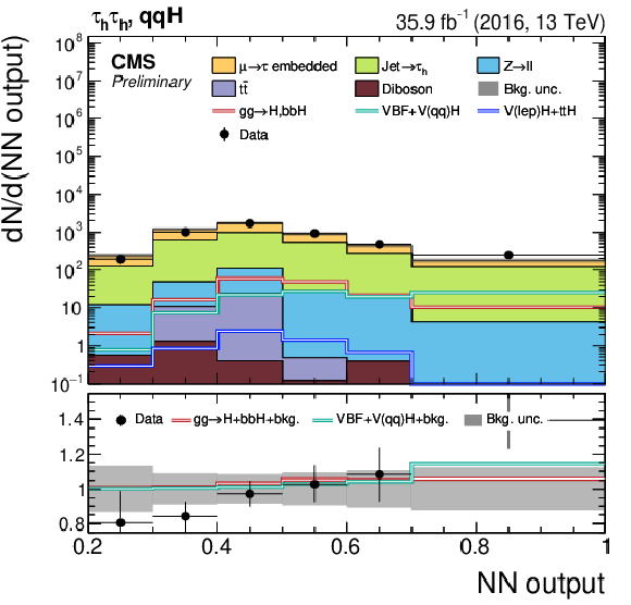
Distributions of the output of the NN used for the determination of the event categories, in the qqH event category, in the (upper left) $\mathrm{e} \mu $, (upper right) $\mathrm{e} \tau _{\text {h}} $, (lower left) $\mu \tau _{\text {h}} $, and (lower right) $\tau _{\text {h}} \tau _{\text {h}} $ final state, on the 2016 dataset. |
png pdf |
Figure 21-a:
Distributions of the output of the NN used for the determination of the event categories, in the qqH event category, in the (upper left) $\mathrm{e} \mu $, (upper right) $\mathrm{e} \tau _{\text {h}} $, (lower left) $\mu \tau _{\text {h}} $, and (lower right) $\tau _{\text {h}} \tau _{\text {h}} $ final state, on the 2016 dataset. |
png pdf |
Figure 21-b:
Distributions of the output of the NN used for the determination of the event categories, in the qqH event category, in the (upper left) $\mathrm{e} \mu $, (upper right) $\mathrm{e} \tau _{\text {h}} $, (lower left) $\mu \tau _{\text {h}} $, and (lower right) $\tau _{\text {h}} \tau _{\text {h}} $ final state, on the 2016 dataset. |
png pdf |
Figure 21-c:
Distributions of the output of the NN used for the determination of the event categories, in the qqH event category, in the (upper left) $\mathrm{e} \mu $, (upper right) $\mathrm{e} \tau _{\text {h}} $, (lower left) $\mu \tau _{\text {h}} $, and (lower right) $\tau _{\text {h}} \tau _{\text {h}} $ final state, on the 2016 dataset. |
png pdf |
Figure 21-d:
Distributions of the output of the NN used for the determination of the event categories, in the qqH event category, in the (upper left) $\mathrm{e} \mu $, (upper right) $\mathrm{e} \tau _{\text {h}} $, (lower left) $\mu \tau _{\text {h}} $, and (lower right) $\tau _{\text {h}} \tau _{\text {h}} $ final state, on the 2016 dataset. |

png pdf |
Figure 22:
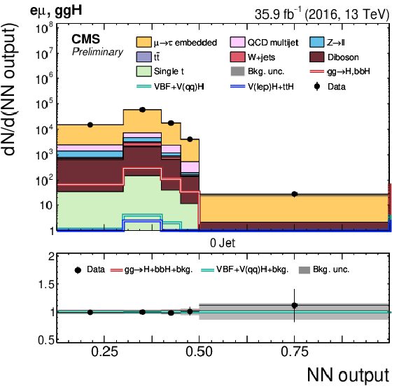
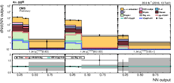
Distributions of the NN output in the event categories used for the determination of the stage-1 simplified template cross sections for ${{\mathrm{g} \mathrm{g} \to \mathrm{H},\mathrm{b} \mathrm{b} \mathrm{H}}}$ in the $\mathrm{e} \mu $ final state. Shown are the (upper left) $=0\text {Jet}$, (middle row) $=1\text {Jet}$, and (lower row) $\geq 2\text {Jet}$ event categories in bins of $ {{p_{\mathrm {T}}} ^{\tau \tau +\text {miss}}} $, on the 2016 dataset. |
png pdf |
Figure 22-a:
Distributions of the NN output in the event categories used for the determination of the stage-1 simplified template cross sections for ${{\mathrm{g} \mathrm{g} \to \mathrm{H},\mathrm{b} \mathrm{b} \mathrm{H}}}$ in the $\mathrm{e} \mu $ final state. Shown are the (upper left) $=0\text {Jet}$, (middle row) $=1\text {Jet}$, and (lower row) $\geq 2\text {Jet}$ event categories in bins of $ {{p_{\mathrm {T}}} ^{\tau \tau +\text {miss}}} $, on the 2016 dataset. |
png pdf |
Figure 22-c:
Distributions of the NN output in the event categories used for the determination of the stage-1 simplified template cross sections for ${{\mathrm{g} \mathrm{g} \to \mathrm{H},\mathrm{b} \mathrm{b} \mathrm{H}}}$ in the $\mathrm{e} \mu $ final state. Shown are the (upper left) $=0\text {Jet}$, (middle row) $=1\text {Jet}$, and (lower row) $\geq 2\text {Jet}$ event categories in bins of $ {{p_{\mathrm {T}}} ^{\tau \tau +\text {miss}}} $, on the 2016 dataset. |
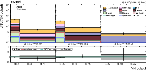
png pdf |
Figure 22-d:
Distributions of the NN output in the event categories used for the determination of the stage-1 simplified template cross sections for ${{\mathrm{g} \mathrm{g} \to \mathrm{H},\mathrm{b} \mathrm{b} \mathrm{H}}}$ in the $\mathrm{e} \mu $ final state. Shown are the (upper left) $=0\text {Jet}$, (middle row) $=1\text {Jet}$, and (lower row) $\geq 2\text {Jet}$ event categories in bins of $ {{p_{\mathrm {T}}} ^{\tau \tau +\text {miss}}} $, on the 2016 dataset. |

png pdf |
Figure 23:
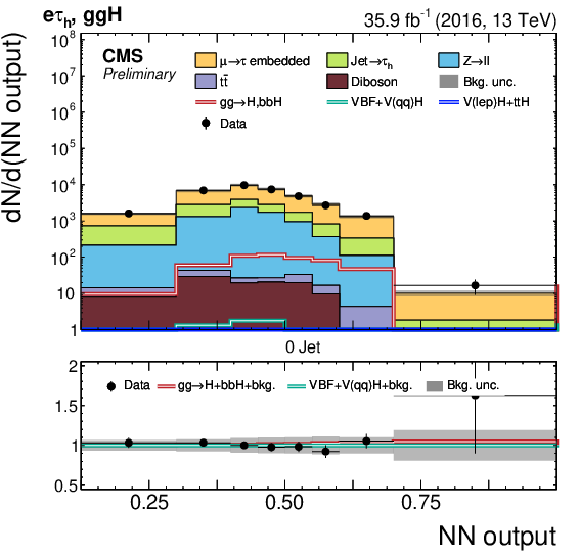
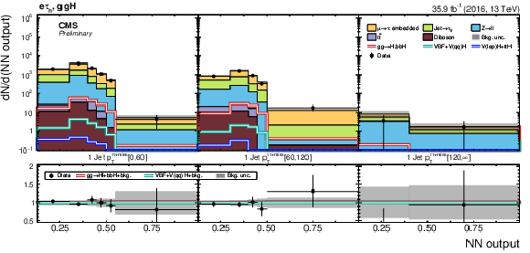
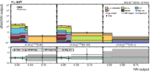
Distributions of the NN output in the event categories used for the determination of the stage-1 simplified template cross sections for ${{\mathrm{g} \mathrm{g} \to \mathrm{H},\mathrm{b} \mathrm{b} \mathrm{H}}}$ in the $\mathrm{e} \tau _{\text {h}} $ final state. Shown are the (upper left) $=0\text {Jet}$, (middle row) $=1\text {Jet}$, and (lower row) $\geq 2\text {Jet}$ event categories in bins of $ {{p_{\mathrm {T}}} ^{\tau \tau +\text {miss}}} $, on the 2016 dataset. |
png pdf |
Figure 23-a:
Distributions of the NN output in the event categories used for the determination of the stage-1 simplified template cross sections for ${{\mathrm{g} \mathrm{g} \to \mathrm{H},\mathrm{b} \mathrm{b} \mathrm{H}}}$ in the $\mathrm{e} \tau _{\text {h}} $ final state. Shown are the (upper left) $=0\text {Jet}$, (middle row) $=1\text {Jet}$, and (lower row) $\geq 2\text {Jet}$ event categories in bins of $ {{p_{\mathrm {T}}} ^{\tau \tau +\text {miss}}} $, on the 2016 dataset. |
png pdf |
Figure 23-c:
Distributions of the NN output in the event categories used for the determination of the stage-1 simplified template cross sections for ${{\mathrm{g} \mathrm{g} \to \mathrm{H},\mathrm{b} \mathrm{b} \mathrm{H}}}$ in the $\mathrm{e} \tau _{\text {h}} $ final state. Shown are the (upper left) $=0\text {Jet}$, (middle row) $=1\text {Jet}$, and (lower row) $\geq 2\text {Jet}$ event categories in bins of $ {{p_{\mathrm {T}}} ^{\tau \tau +\text {miss}}} $, on the 2016 dataset. |
png pdf |
Figure 23-d:
Distributions of the NN output in the event categories used for the determination of the stage-1 simplified template cross sections for ${{\mathrm{g} \mathrm{g} \to \mathrm{H},\mathrm{b} \mathrm{b} \mathrm{H}}}$ in the $\mathrm{e} \tau _{\text {h}} $ final state. Shown are the (upper left) $=0\text {Jet}$, (middle row) $=1\text {Jet}$, and (lower row) $\geq 2\text {Jet}$ event categories in bins of $ {{p_{\mathrm {T}}} ^{\tau \tau +\text {miss}}} $, on the 2016 dataset. |

png pdf |
Figure 24:
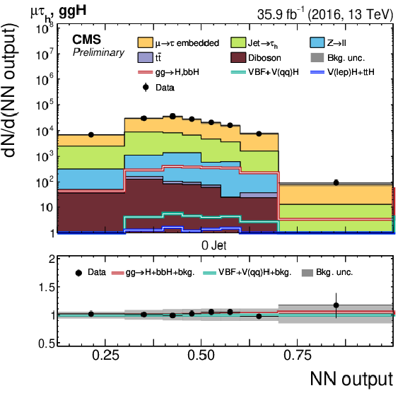
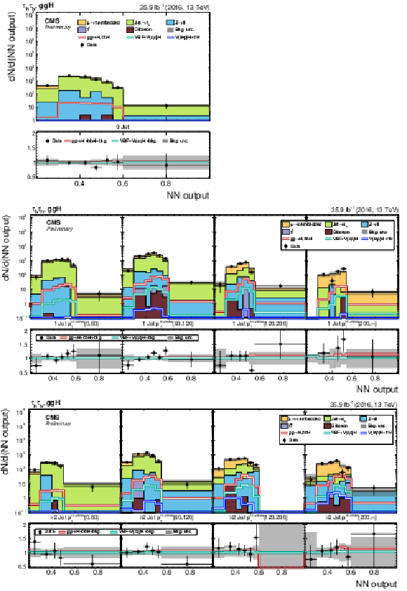
Distributions of the NN output in the event categories used for the determination of the stage-1 simplified template cross sections for ${{\mathrm{g} \mathrm{g} \to \mathrm{H},\mathrm{b} \mathrm{b} \mathrm{H}}}$ in the $\mu \tau _{\text {h}} $ final state. Shown are the (upper left) $=0\text {Jet}$, (middle row) $=1\text {Jet}$, and (lower row) $\geq 2\text {Jet}$ event categories in bins of $ {{p_{\mathrm {T}}} ^{\tau \tau +\text {miss}}} $, on the 2016 dataset. |
png pdf |
Figure 24-a:
Distributions of the NN output in the event categories used for the determination of the stage-1 simplified template cross sections for ${{\mathrm{g} \mathrm{g} \to \mathrm{H},\mathrm{b} \mathrm{b} \mathrm{H}}}$ in the $\mu \tau _{\text {h}} $ final state. Shown are the (upper left) $=0\text {Jet}$, (middle row) $=1\text {Jet}$, and (lower row) $\geq 2\text {Jet}$ event categories in bins of $ {{p_{\mathrm {T}}} ^{\tau \tau +\text {miss}}} $, on the 2016 dataset. |
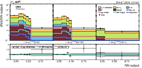
png pdf |
Figure 24-c:
Distributions of the NN output in the event categories used for the determination of the stage-1 simplified template cross sections for ${{\mathrm{g} \mathrm{g} \to \mathrm{H},\mathrm{b} \mathrm{b} \mathrm{H}}}$ in the $\mu \tau _{\text {h}} $ final state. Shown are the (upper left) $=0\text {Jet}$, (middle row) $=1\text {Jet}$, and (lower row) $\geq 2\text {Jet}$ event categories in bins of $ {{p_{\mathrm {T}}} ^{\tau \tau +\text {miss}}} $, on the 2016 dataset. |
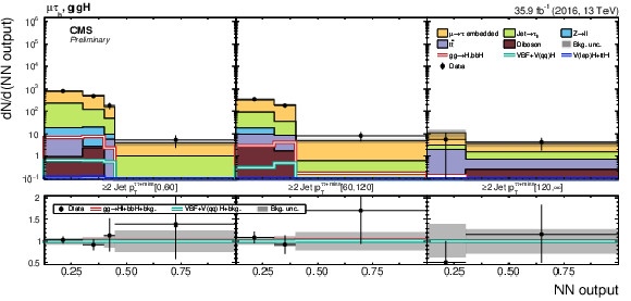
png pdf |
Figure 24-d:
Distributions of the NN output in the event categories used for the determination of the stage-1 simplified template cross sections for ${{\mathrm{g} \mathrm{g} \to \mathrm{H},\mathrm{b} \mathrm{b} \mathrm{H}}}$ in the $\mu \tau _{\text {h}} $ final state. Shown are the (upper left) $=0\text {Jet}$, (middle row) $=1\text {Jet}$, and (lower row) $\geq 2\text {Jet}$ event categories in bins of $ {{p_{\mathrm {T}}} ^{\tau \tau +\text {miss}}} $, on the 2016 dataset. |
png pdf |
Figure 25:
Distributions of the NN output in the event categories used for the determination of the stage-1 simplified template cross sections for ${{\mathrm{g} \mathrm{g} \to \mathrm{H},\mathrm{b} \mathrm{b} \mathrm{H}}}$ in the $\tau _{\text {h}} \tau _{\text {h}} $ final state. Shown are the (upper left) $=0\text {Jet}$, (middle row) $=1\text {Jet}$, and (lower row) $\geq 2\text {Jet}$ event categories in bins of $ {{p_{\mathrm {T}}} ^{\tau \tau +\text {miss}}} $, on the 2016 dataset. |

png pdf |
Figure 25-a:
Distributions of the NN output in the event categories used for the determination of the stage-1 simplified template cross sections for ${{\mathrm{g} \mathrm{g} \to \mathrm{H},\mathrm{b} \mathrm{b} \mathrm{H}}}$ in the $\tau _{\text {h}} \tau _{\text {h}} $ final state. Shown are the (upper left) $=0\text {Jet}$, (middle row) $=1\text {Jet}$, and (lower row) $\geq 2\text {Jet}$ event categories in bins of $ {{p_{\mathrm {T}}} ^{\tau \tau +\text {miss}}} $, on the 2016 dataset. |

png pdf |
Figure 25-c:
Distributions of the NN output in the event categories used for the determination of the stage-1 simplified template cross sections for ${{\mathrm{g} \mathrm{g} \to \mathrm{H},\mathrm{b} \mathrm{b} \mathrm{H}}}$ in the $\tau _{\text {h}} \tau _{\text {h}} $ final state. Shown are the (upper left) $=0\text {Jet}$, (middle row) $=1\text {Jet}$, and (lower row) $\geq 2\text {Jet}$ event categories in bins of $ {{p_{\mathrm {T}}} ^{\tau \tau +\text {miss}}} $, on the 2016 dataset. |
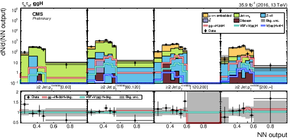
png pdf |
Figure 25-d:
Distributions of the NN output in the event categories used for the determination of the stage-1 simplified template cross sections for ${{\mathrm{g} \mathrm{g} \to \mathrm{H},\mathrm{b} \mathrm{b} \mathrm{H}}}$ in the $\tau _{\text {h}} \tau _{\text {h}} $ final state. Shown are the (upper left) $=0\text {Jet}$, (middle row) $=1\text {Jet}$, and (lower row) $\geq 2\text {Jet}$ event categories in bins of $ {{p_{\mathrm {T}}} ^{\tau \tau +\text {miss}}} $, on the 2016 dataset. |
png pdf |
Figure 26:
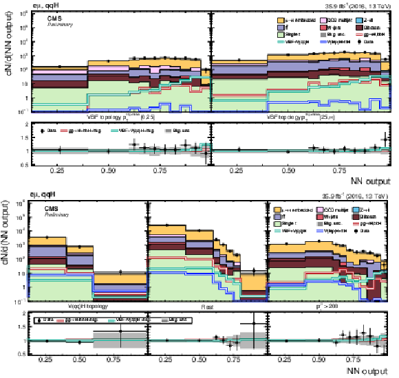
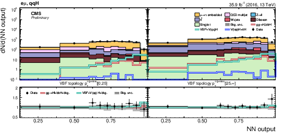
Distributions of the NN output in the event categories used for the determination of the stage-1 simplified template cross sections for ${{\text {VBF}{+} {\mathrm {V}}(\mathrm{q} \mathrm{q})\mathrm{H}}}$ in the $\mathrm{e} \mu $ final state. Shown are the (upper row) categories with VBF topology in bins of $ {{p_{\mathrm {T}}} ^{\tau \tau \text {jj+miss}}} $ and (lower row) the event category with $\mathrm{Z} (\mathrm{W})\mathrm{H} $ topology, the "Rest'' category and the event category with $ {p_{\mathrm {T}}} ^{\text {j}_{1}} > $ 200 GeV, on the 2016 dataset. |
png pdf |
Figure 26-a:
Distributions of the NN output in the event categories used for the determination of the stage-1 simplified template cross sections for ${{\text {VBF}{+} {\mathrm {V}}(\mathrm{q} \mathrm{q})\mathrm{H}}}$ in the $\mathrm{e} \mu $ final state. Shown are the (upper row) categories with VBF topology in bins of $ {{p_{\mathrm {T}}} ^{\tau \tau \text {jj+miss}}} $ and (lower row) the event category with $\mathrm{Z} (\mathrm{W})\mathrm{H} $ topology, the "Rest'' category and the event category with $ {p_{\mathrm {T}}} ^{\text {j}_{1}} > $ 200 GeV, on the 2016 dataset. |

png pdf |
Figure 26-b:
Distributions of the NN output in the event categories used for the determination of the stage-1 simplified template cross sections for ${{\text {VBF}{+} {\mathrm {V}}(\mathrm{q} \mathrm{q})\mathrm{H}}}$ in the $\mathrm{e} \mu $ final state. Shown are the (upper row) categories with VBF topology in bins of $ {{p_{\mathrm {T}}} ^{\tau \tau \text {jj+miss}}} $ and (lower row) the event category with $\mathrm{Z} (\mathrm{W})\mathrm{H} $ topology, the "Rest'' category and the event category with $ {p_{\mathrm {T}}} ^{\text {j}_{1}} > $ 200 GeV, on the 2016 dataset. |
png pdf |
Figure 27:
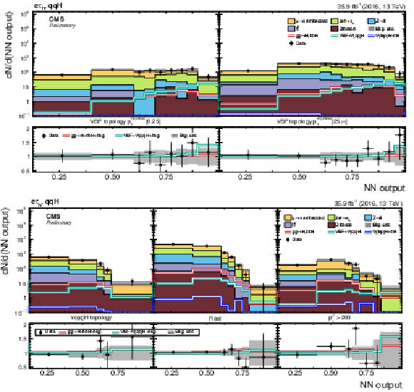
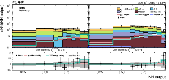
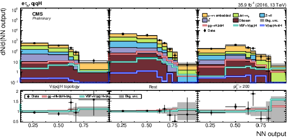
Distributions of the NN output in the event categories used for the determination of the stage-1 simplified template cross sections for ${{\text {VBF}{+} {\mathrm {V}}(\mathrm{q} \mathrm{q})\mathrm{H}}}$ in the $\mathrm{e} \tau _{\text {h}} $ final state. Shown are the (upper row) categories with VBF topology in bins of $ {{p_{\mathrm {T}}} ^{\tau \tau \text {jj+miss}}} $ and (lower row) the event category with $\mathrm{Z} (\mathrm{W})\mathrm{H} $ topology, the "Rest'' category and the event category with $ {p_{\mathrm {T}}} ^{\text {j}_{1}} > $ 200 GeV, on the 2016 dataset. |
png pdf |
Figure 27-a:
Distributions of the NN output in the event categories used for the determination of the stage-1 simplified template cross sections for ${{\text {VBF}{+} {\mathrm {V}}(\mathrm{q} \mathrm{q})\mathrm{H}}}$ in the $\mathrm{e} \tau _{\text {h}} $ final state. Shown are the (upper row) categories with VBF topology in bins of $ {{p_{\mathrm {T}}} ^{\tau \tau \text {jj+miss}}} $ and (lower row) the event category with $\mathrm{Z} (\mathrm{W})\mathrm{H} $ topology, the "Rest'' category and the event category with $ {p_{\mathrm {T}}} ^{\text {j}_{1}} > $ 200 GeV, on the 2016 dataset. |
png pdf |
Figure 27-b:
Distributions of the NN output in the event categories used for the determination of the stage-1 simplified template cross sections for ${{\text {VBF}{+} {\mathrm {V}}(\mathrm{q} \mathrm{q})\mathrm{H}}}$ in the $\mathrm{e} \tau _{\text {h}} $ final state. Shown are the (upper row) categories with VBF topology in bins of $ {{p_{\mathrm {T}}} ^{\tau \tau \text {jj+miss}}} $ and (lower row) the event category with $\mathrm{Z} (\mathrm{W})\mathrm{H} $ topology, the "Rest'' category and the event category with $ {p_{\mathrm {T}}} ^{\text {j}_{1}} > $ 200 GeV, on the 2016 dataset. |

png pdf |
Figure 28:
Distributions of the NN output in the event categories used for the determination of the stage-1 simplified template cross sections for ${{\text {VBF}{+} {\mathrm {V}}(\mathrm{q} \mathrm{q})\mathrm{H}}}$ in the $\mu \tau _{\text {h}} $ final state. Shown are the (upper row) categories with VBF topology in bins of $ {{p_{\mathrm {T}}} ^{\tau \tau \text {jj+miss}}} $ and (lower row) the event category with $\mathrm{Z} (\mathrm{W})\mathrm{H} $ topology, the "Rest'' category and the event category with $ {p_{\mathrm {T}}} ^{\text {j}_{1}} > $ 200 GeV, on the 2016 dataset. |

png pdf |
Figure 28-a:
Distributions of the NN output in the event categories used for the determination of the stage-1 simplified template cross sections for ${{\text {VBF}{+} {\mathrm {V}}(\mathrm{q} \mathrm{q})\mathrm{H}}}$ in the $\mu \tau _{\text {h}} $ final state. Shown are the (upper row) categories with VBF topology in bins of $ {{p_{\mathrm {T}}} ^{\tau \tau \text {jj+miss}}} $ and (lower row) the event category with $\mathrm{Z} (\mathrm{W})\mathrm{H} $ topology, the "Rest'' category and the event category with $ {p_{\mathrm {T}}} ^{\text {j}_{1}} > $ 200 GeV, on the 2016 dataset. |

png pdf |
Figure 28-b:
Distributions of the NN output in the event categories used for the determination of the stage-1 simplified template cross sections for ${{\text {VBF}{+} {\mathrm {V}}(\mathrm{q} \mathrm{q})\mathrm{H}}}$ in the $\mu \tau _{\text {h}} $ final state. Shown are the (upper row) categories with VBF topology in bins of $ {{p_{\mathrm {T}}} ^{\tau \tau \text {jj+miss}}} $ and (lower row) the event category with $\mathrm{Z} (\mathrm{W})\mathrm{H} $ topology, the "Rest'' category and the event category with $ {p_{\mathrm {T}}} ^{\text {j}_{1}} > $ 200 GeV, on the 2016 dataset. |

png pdf |
Figure 29:
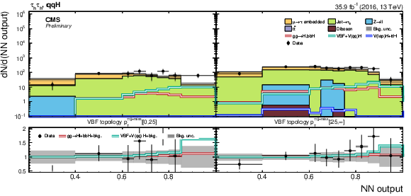
Distributions of the NN output in the event categories used for the determination of the stage-1 simplified template cross sections for ${{\text {VBF}{+} {\mathrm {V}}(\mathrm{q} \mathrm{q})\mathrm{H}}}$ in the $\tau _{\text {h}} \tau _{\text {h}} $ final state. Shown are the (upper row) categories with VBF topology in bins of $ {{p_{\mathrm {T}}} ^{\tau \tau \text {jj+miss}}} $ and (lower row) the event category with $\mathrm{Z} (\mathrm{W})\mathrm{H} $ topology, the "Rest'' category and the event category with $ {p_{\mathrm {T}}} ^{\text {j}_{1}} > $ 200 GeV, on the 2016 dataset. |
png pdf |
Figure 29-a:
Distributions of the NN output in the event categories used for the determination of the stage-1 simplified template cross sections for ${{\text {VBF}{+} {\mathrm {V}}(\mathrm{q} \mathrm{q})\mathrm{H}}}$ in the $\tau _{\text {h}} \tau _{\text {h}} $ final state. Shown are the (upper row) categories with VBF topology in bins of $ {{p_{\mathrm {T}}} ^{\tau \tau \text {jj+miss}}} $ and (lower row) the event category with $\mathrm{Z} (\mathrm{W})\mathrm{H} $ topology, the "Rest'' category and the event category with $ {p_{\mathrm {T}}} ^{\text {j}_{1}} > $ 200 GeV, on the 2016 dataset. |

png pdf |
Figure 29-b:
Distributions of the NN output in the event categories used for the determination of the stage-1 simplified template cross sections for ${{\text {VBF}{+} {\mathrm {V}}(\mathrm{q} \mathrm{q})\mathrm{H}}}$ in the $\tau _{\text {h}} \tau _{\text {h}} $ final state. Shown are the (upper row) categories with VBF topology in bins of $ {{p_{\mathrm {T}}} ^{\tau \tau \text {jj+miss}}} $ and (lower row) the event category with $\mathrm{Z} (\mathrm{W})\mathrm{H} $ topology, the "Rest'' category and the event category with $ {p_{\mathrm {T}}} ^{\text {j}_{1}} > $ 200 GeV, on the 2016 dataset. |

png pdf |
Figure 30:
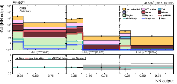
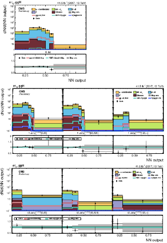
Distributions of the NN output in the event categories used for the determination of the stage-1 simplified template cross sections for ${{\mathrm{g} \mathrm{g} \to \mathrm{H},\mathrm{b} \mathrm{b} \mathrm{H}}}$ in the $\mathrm{e} \mu $ final state. Shown are the (upper left) $=0\text {Jet}$, (middle row) $=1\text {Jet}$, and (lower row) $\geq 2\text {Jet}$ event categories in bins of $ {{p_{\mathrm {T}}} ^{\tau \tau +\text {miss}}} $, on the 2017 dataset. |

png pdf |
Figure 30-a:
Distributions of the NN output in the event categories used for the determination of the stage-1 simplified template cross sections for ${{\mathrm{g} \mathrm{g} \to \mathrm{H},\mathrm{b} \mathrm{b} \mathrm{H}}}$ in the $\mathrm{e} \mu $ final state. Shown are the (upper left) $=0\text {Jet}$, (middle row) $=1\text {Jet}$, and (lower row) $\geq 2\text {Jet}$ event categories in bins of $ {{p_{\mathrm {T}}} ^{\tau \tau +\text {miss}}} $, on the 2017 dataset. |
png pdf |
Figure 30-c:
Distributions of the NN output in the event categories used for the determination of the stage-1 simplified template cross sections for ${{\mathrm{g} \mathrm{g} \to \mathrm{H},\mathrm{b} \mathrm{b} \mathrm{H}}}$ in the $\mathrm{e} \mu $ final state. Shown are the (upper left) $=0\text {Jet}$, (middle row) $=1\text {Jet}$, and (lower row) $\geq 2\text {Jet}$ event categories in bins of $ {{p_{\mathrm {T}}} ^{\tau \tau +\text {miss}}} $, on the 2017 dataset. |

png pdf |
Figure 30-d:
Distributions of the NN output in the event categories used for the determination of the stage-1 simplified template cross sections for ${{\mathrm{g} \mathrm{g} \to \mathrm{H},\mathrm{b} \mathrm{b} \mathrm{H}}}$ in the $\mathrm{e} \mu $ final state. Shown are the (upper left) $=0\text {Jet}$, (middle row) $=1\text {Jet}$, and (lower row) $\geq 2\text {Jet}$ event categories in bins of $ {{p_{\mathrm {T}}} ^{\tau \tau +\text {miss}}} $, on the 2017 dataset. |
png pdf |
Figure 31:
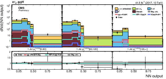
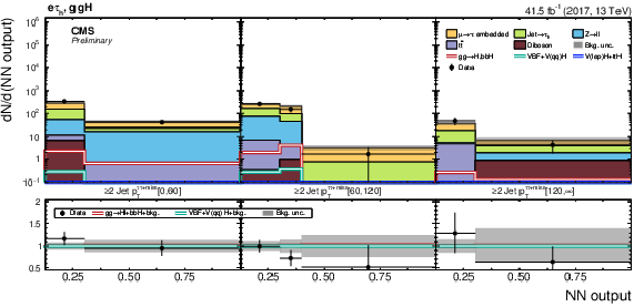
Distributions of the NN output in the event categories used for the determination of the stage-1 simplified template cross sections for ${{\mathrm{g} \mathrm{g} \to \mathrm{H},\mathrm{b} \mathrm{b} \mathrm{H}}}$ in the $\mathrm{e} \tau _{\text {h}} $ final state. Shown are the (upper left) $=0\text {Jet}$, (middle row) $=1\text {Jet}$, and (lower row) $\geq 2\text {Jet}$ event categories in bins of $ {{p_{\mathrm {T}}} ^{\tau \tau +\text {miss}}} $, on the 2017 dataset. |

png pdf |
Figure 31-a:
Distributions of the NN output in the event categories used for the determination of the stage-1 simplified template cross sections for ${{\mathrm{g} \mathrm{g} \to \mathrm{H},\mathrm{b} \mathrm{b} \mathrm{H}}}$ in the $\mathrm{e} \tau _{\text {h}} $ final state. Shown are the (upper left) $=0\text {Jet}$, (middle row) $=1\text {Jet}$, and (lower row) $\geq 2\text {Jet}$ event categories in bins of $ {{p_{\mathrm {T}}} ^{\tau \tau +\text {miss}}} $, on the 2017 dataset. |
png pdf |
Figure 31-c:
Distributions of the NN output in the event categories used for the determination of the stage-1 simplified template cross sections for ${{\mathrm{g} \mathrm{g} \to \mathrm{H},\mathrm{b} \mathrm{b} \mathrm{H}}}$ in the $\mathrm{e} \tau _{\text {h}} $ final state. Shown are the (upper left) $=0\text {Jet}$, (middle row) $=1\text {Jet}$, and (lower row) $\geq 2\text {Jet}$ event categories in bins of $ {{p_{\mathrm {T}}} ^{\tau \tau +\text {miss}}} $, on the 2017 dataset. |
png pdf |
Figure 31-d:
Distributions of the NN output in the event categories used for the determination of the stage-1 simplified template cross sections for ${{\mathrm{g} \mathrm{g} \to \mathrm{H},\mathrm{b} \mathrm{b} \mathrm{H}}}$ in the $\mathrm{e} \tau _{\text {h}} $ final state. Shown are the (upper left) $=0\text {Jet}$, (middle row) $=1\text {Jet}$, and (lower row) $\geq 2\text {Jet}$ event categories in bins of $ {{p_{\mathrm {T}}} ^{\tau \tau +\text {miss}}} $, on the 2017 dataset. |

png pdf |
Figure 32:
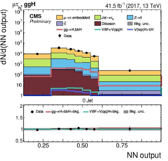
Distributions of the NN output in the event categories used for the determination of the stage-1 simplified template cross sections for ${{\mathrm{g} \mathrm{g} \to \mathrm{H},\mathrm{b} \mathrm{b} \mathrm{H}}}$ in the $\mu \tau _{\text {h}} $ final state. Shown are the (upper left) $=0\text {Jet}$, (middle row) $=1\text {Jet}$, and (lower row) $\geq 2\text {Jet}$ event categories in bins of $ {{p_{\mathrm {T}}} ^{\tau \tau +\text {miss}}} $, on the 2017 dataset. |
png pdf |
Figure 32-a:
Distributions of the NN output in the event categories used for the determination of the stage-1 simplified template cross sections for ${{\mathrm{g} \mathrm{g} \to \mathrm{H},\mathrm{b} \mathrm{b} \mathrm{H}}}$ in the $\mu \tau _{\text {h}} $ final state. Shown are the (upper left) $=0\text {Jet}$, (middle row) $=1\text {Jet}$, and (lower row) $\geq 2\text {Jet}$ event categories in bins of $ {{p_{\mathrm {T}}} ^{\tau \tau +\text {miss}}} $, on the 2017 dataset. |

png pdf |
Figure 32-c:
Distributions of the NN output in the event categories used for the determination of the stage-1 simplified template cross sections for ${{\mathrm{g} \mathrm{g} \to \mathrm{H},\mathrm{b} \mathrm{b} \mathrm{H}}}$ in the $\mu \tau _{\text {h}} $ final state. Shown are the (upper left) $=0\text {Jet}$, (middle row) $=1\text {Jet}$, and (lower row) $\geq 2\text {Jet}$ event categories in bins of $ {{p_{\mathrm {T}}} ^{\tau \tau +\text {miss}}} $, on the 2017 dataset. |

png pdf |
Figure 32-d:
Distributions of the NN output in the event categories used for the determination of the stage-1 simplified template cross sections for ${{\mathrm{g} \mathrm{g} \to \mathrm{H},\mathrm{b} \mathrm{b} \mathrm{H}}}$ in the $\mu \tau _{\text {h}} $ final state. Shown are the (upper left) $=0\text {Jet}$, (middle row) $=1\text {Jet}$, and (lower row) $\geq 2\text {Jet}$ event categories in bins of $ {{p_{\mathrm {T}}} ^{\tau \tau +\text {miss}}} $, on the 2017 dataset. |
png pdf |
Figure 33:
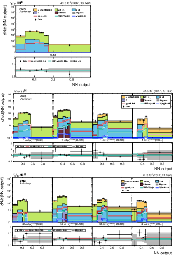
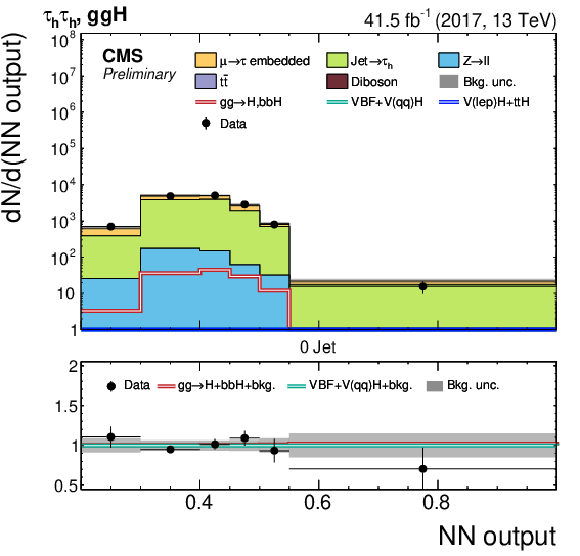
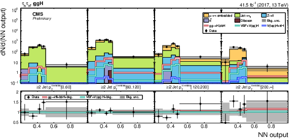
Distributions of the NN output in the event categories used for the determination of the stage-1 simplified template cross sections for ${{\mathrm{g} \mathrm{g} \to \mathrm{H},\mathrm{b} \mathrm{b} \mathrm{H}}}$ in the $\tau _{\text {h}} \tau _{\text {h}} $ final state. Shown are the (upper left) $=0\text {Jet}$, (middle row) $=1\text {Jet}$, and (lower row) $\geq 2\text {Jet}$ event categories in bins of $ {{p_{\mathrm {T}}} ^{\tau \tau +\text {miss}}} $, on the 2017 dataset. |
png pdf |
Figure 33-a:
Distributions of the NN output in the event categories used for the determination of the stage-1 simplified template cross sections for ${{\mathrm{g} \mathrm{g} \to \mathrm{H},\mathrm{b} \mathrm{b} \mathrm{H}}}$ in the $\tau _{\text {h}} \tau _{\text {h}} $ final state. Shown are the (upper left) $=0\text {Jet}$, (middle row) $=1\text {Jet}$, and (lower row) $\geq 2\text {Jet}$ event categories in bins of $ {{p_{\mathrm {T}}} ^{\tau \tau +\text {miss}}} $, on the 2017 dataset. |

png pdf |
Figure 33-c:
Distributions of the NN output in the event categories used for the determination of the stage-1 simplified template cross sections for ${{\mathrm{g} \mathrm{g} \to \mathrm{H},\mathrm{b} \mathrm{b} \mathrm{H}}}$ in the $\tau _{\text {h}} \tau _{\text {h}} $ final state. Shown are the (upper left) $=0\text {Jet}$, (middle row) $=1\text {Jet}$, and (lower row) $\geq 2\text {Jet}$ event categories in bins of $ {{p_{\mathrm {T}}} ^{\tau \tau +\text {miss}}} $, on the 2017 dataset. |
png pdf |
Figure 33-d:
Distributions of the NN output in the event categories used for the determination of the stage-1 simplified template cross sections for ${{\mathrm{g} \mathrm{g} \to \mathrm{H},\mathrm{b} \mathrm{b} \mathrm{H}}}$ in the $\tau _{\text {h}} \tau _{\text {h}} $ final state. Shown are the (upper left) $=0\text {Jet}$, (middle row) $=1\text {Jet}$, and (lower row) $\geq 2\text {Jet}$ event categories in bins of $ {{p_{\mathrm {T}}} ^{\tau \tau +\text {miss}}} $, on the 2017 dataset. |
png pdf |
Figure 34:
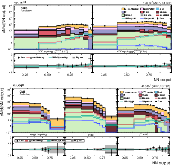
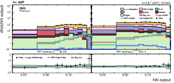
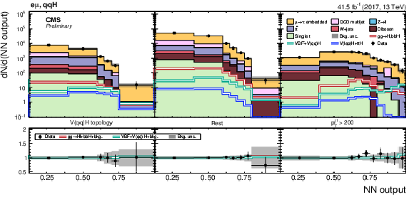
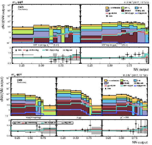
Distributions of the NN output in the event categories used for the determination of the stage-1 simplified template cross sections for ${{\text {VBF}{+} {\mathrm {V}}(\mathrm{q} \mathrm{q})\mathrm{H}}}$ in the $\mathrm{e} \mu $ final state. Shown are the (upper row) categories with VBF topology in bins of $ {{p_{\mathrm {T}}} ^{\tau \tau \text {jj+miss}}} $ and (lower row) the event category with $\mathrm{Z} (\mathrm{W})\mathrm{H} $ topology, the "Rest'' category and the event category with $ {p_{\mathrm {T}}} ^{\text {j}_{1}} > $ 200 GeV, on the 2017 dataset. |
png pdf |
Figure 34-a:
Distributions of the NN output in the event categories used for the determination of the stage-1 simplified template cross sections for ${{\text {VBF}{+} {\mathrm {V}}(\mathrm{q} \mathrm{q})\mathrm{H}}}$ in the $\mathrm{e} \mu $ final state. Shown are the (upper row) categories with VBF topology in bins of $ {{p_{\mathrm {T}}} ^{\tau \tau \text {jj+miss}}} $ and (lower row) the event category with $\mathrm{Z} (\mathrm{W})\mathrm{H} $ topology, the "Rest'' category and the event category with $ {p_{\mathrm {T}}} ^{\text {j}_{1}} > $ 200 GeV, on the 2017 dataset. |
png pdf |
Figure 34-b:
Distributions of the NN output in the event categories used for the determination of the stage-1 simplified template cross sections for ${{\text {VBF}{+} {\mathrm {V}}(\mathrm{q} \mathrm{q})\mathrm{H}}}$ in the $\mathrm{e} \mu $ final state. Shown are the (upper row) categories with VBF topology in bins of $ {{p_{\mathrm {T}}} ^{\tau \tau \text {jj+miss}}} $ and (lower row) the event category with $\mathrm{Z} (\mathrm{W})\mathrm{H} $ topology, the "Rest'' category and the event category with $ {p_{\mathrm {T}}} ^{\text {j}_{1}} > $ 200 GeV, on the 2017 dataset. |
png pdf |
Figure 35:
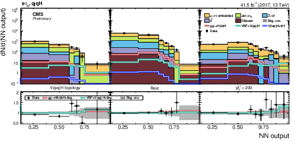
Distributions of the NN output in the event categories used for the determination of the stage-1 simplified template cross sections for ${{\text {VBF}{+} {\mathrm {V}}(\mathrm{q} \mathrm{q})\mathrm{H}}}$ in the $\mathrm{e} \tau _{\text {h}} $ final state. Shown are the (upper row) categories with VBF topology in bins of $ {{p_{\mathrm {T}}} ^{\tau \tau \text {jj+miss}}} $ and (lower row) the event category with $\mathrm{Z} (\mathrm{W})\mathrm{H} $ topology, the "Rest'' category and the event category with $ {p_{\mathrm {T}}} ^{\text {j}_{1}} > $ 200 GeV, on the 2017 dataset. |
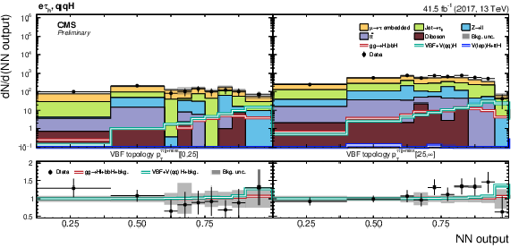
png pdf |
Figure 35-a:
Distributions of the NN output in the event categories used for the determination of the stage-1 simplified template cross sections for ${{\text {VBF}{+} {\mathrm {V}}(\mathrm{q} \mathrm{q})\mathrm{H}}}$ in the $\mathrm{e} \tau _{\text {h}} $ final state. Shown are the (upper row) categories with VBF topology in bins of $ {{p_{\mathrm {T}}} ^{\tau \tau \text {jj+miss}}} $ and (lower row) the event category with $\mathrm{Z} (\mathrm{W})\mathrm{H} $ topology, the "Rest'' category and the event category with $ {p_{\mathrm {T}}} ^{\text {j}_{1}} > $ 200 GeV, on the 2017 dataset. |
png pdf |
Figure 35-b:
Distributions of the NN output in the event categories used for the determination of the stage-1 simplified template cross sections for ${{\text {VBF}{+} {\mathrm {V}}(\mathrm{q} \mathrm{q})\mathrm{H}}}$ in the $\mathrm{e} \tau _{\text {h}} $ final state. Shown are the (upper row) categories with VBF topology in bins of $ {{p_{\mathrm {T}}} ^{\tau \tau \text {jj+miss}}} $ and (lower row) the event category with $\mathrm{Z} (\mathrm{W})\mathrm{H} $ topology, the "Rest'' category and the event category with $ {p_{\mathrm {T}}} ^{\text {j}_{1}} > $ 200 GeV, on the 2017 dataset. |

png pdf |
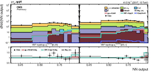
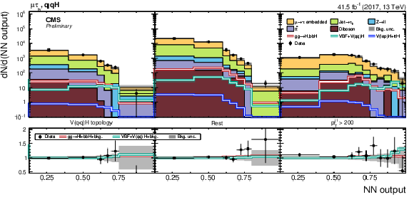
Figure 36:
Distributions of the NN output in the event categories used for the determination of the stage-1 simplified template cross sections for ${{\text {VBF}{+} {\mathrm {V}}(\mathrm{q} \mathrm{q})\mathrm{H}}}$ in the $\mu \tau _{\text {h}} $ final state. Shown are the (upper row) categories with VBF topology in bins of $ {{p_{\mathrm {T}}} ^{\tau \tau \text {jj+miss}}} $ and (lower row) the event category with $\mathrm{Z} (\mathrm{W})\mathrm{H} $ topology, the "Rest'' category and the event category with $ {p_{\mathrm {T}}} ^{\text {j}_{1}} > $ 200 GeV, on the 2017 dataset. |
png pdf |
Figure 36-a:
Distributions of the NN output in the event categories used for the determination of the stage-1 simplified template cross sections for ${{\text {VBF}{+} {\mathrm {V}}(\mathrm{q} \mathrm{q})\mathrm{H}}}$ in the $\mu \tau _{\text {h}} $ final state. Shown are the (upper row) categories with VBF topology in bins of $ {{p_{\mathrm {T}}} ^{\tau \tau \text {jj+miss}}} $ and (lower row) the event category with $\mathrm{Z} (\mathrm{W})\mathrm{H} $ topology, the "Rest'' category and the event category with $ {p_{\mathrm {T}}} ^{\text {j}_{1}} > $ 200 GeV, on the 2017 dataset. |
png pdf |
Figure 36-b:
Distributions of the NN output in the event categories used for the determination of the stage-1 simplified template cross sections for ${{\text {VBF}{+} {\mathrm {V}}(\mathrm{q} \mathrm{q})\mathrm{H}}}$ in the $\mu \tau _{\text {h}} $ final state. Shown are the (upper row) categories with VBF topology in bins of $ {{p_{\mathrm {T}}} ^{\tau \tau \text {jj+miss}}} $ and (lower row) the event category with $\mathrm{Z} (\mathrm{W})\mathrm{H} $ topology, the "Rest'' category and the event category with $ {p_{\mathrm {T}}} ^{\text {j}_{1}} > $ 200 GeV, on the 2017 dataset. |

png pdf |
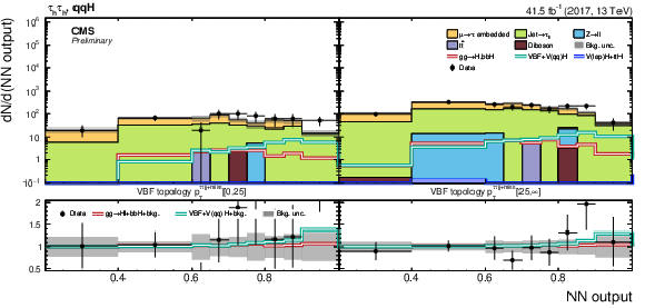
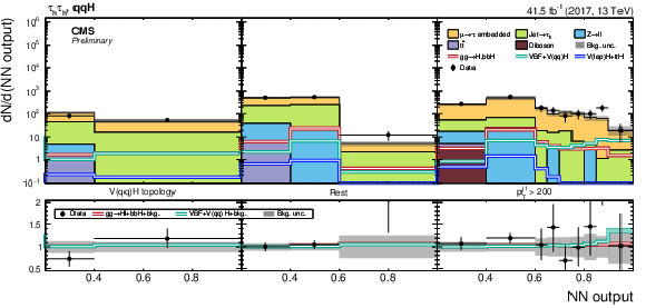
Figure 37:
Distributions of the NN output in the event categories used for the determination of the stage-1 simplified template cross sections for ${{\text {VBF}{+} {\mathrm {V}}(\mathrm{q} \mathrm{q})\mathrm{H}}}$ in the $\tau _{\text {h}} \tau _{\text {h}} $ final state. Shown are the (upper row) categories with VBF topology in bins of $ {{p_{\mathrm {T}}} ^{\tau \tau \text {jj+miss}}} $ and (lower row) the event category with $\mathrm{Z} (\mathrm{W})\mathrm{H} $ topology, the "Rest'' category and the event category with $ {p_{\mathrm {T}}} ^{\text {j}_{1}} > $ 200 GeV, on the 2017 dataset. |
png pdf |
Figure 37-a:
Distributions of the NN output in the event categories used for the determination of the stage-1 simplified template cross sections for ${{\text {VBF}{+} {\mathrm {V}}(\mathrm{q} \mathrm{q})\mathrm{H}}}$ in the $\tau _{\text {h}} \tau _{\text {h}} $ final state. Shown are the (upper row) categories with VBF topology in bins of $ {{p_{\mathrm {T}}} ^{\tau \tau \text {jj+miss}}} $ and (lower row) the event category with $\mathrm{Z} (\mathrm{W})\mathrm{H} $ topology, the "Rest'' category and the event category with $ {p_{\mathrm {T}}} ^{\text {j}_{1}} > $ 200 GeV, on the 2017 dataset. |
png pdf |
Figure 37-b:
Distributions of the NN output in the event categories used for the determination of the stage-1 simplified template cross sections for ${{\text {VBF}{+} {\mathrm {V}}(\mathrm{q} \mathrm{q})\mathrm{H}}}$ in the $\tau _{\text {h}} \tau _{\text {h}} $ final state. Shown are the (upper row) categories with VBF topology in bins of $ {{p_{\mathrm {T}}} ^{\tau \tau \text {jj+miss}}} $ and (lower row) the event category with $\mathrm{Z} (\mathrm{W})\mathrm{H} $ topology, the "Rest'' category and the event category with $ {p_{\mathrm {T}}} ^{\text {j}_{1}} > $ 200 GeV, on the 2017 dataset. |
| Tables | |

png pdf |
Table 1:
Background processes contributing to the event selection as given in Section 5. The further splitting of the processes in the second column refers only to final states that contain a $\tau _{\text {h}} $ candidate. "MC'' implies that the process is taken from simulation, $ {F_{\text {F}}}$ that the process is determined from data using the $ {F_{\text {F}}}$ method as described in Ref. [12]. "EMB'' implies that the process is estimated from the $\tau $-embedding technique as described in Ref. [11], "CR'' that both shape and normalization of QCD multijet events are estimated from control regions in data. The label $\ell $ corresponds to an electron or muon. |
png pdf |
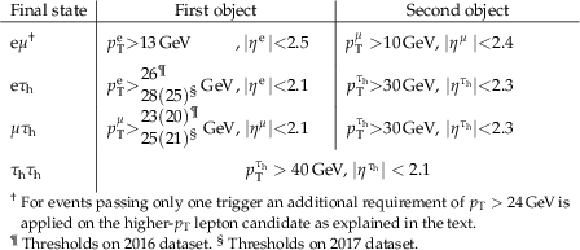
Table 2:
Kinematic selection of the $\tau $ decay products in the $\mathrm{e} \mu $, $\mathrm{e} \tau _{\text {h}} $, $\mu \tau _{\text {h}} $, and $\tau _{\text {h}} \tau _{\text {h}} $ final states. The expression "First (Second) object'' refers to the final state label used in the first column. In the $\mathrm{e} \tau _{\text {h}} $ ($\mu \tau _{\text {h}} $) final state the values in braces correspond to the thresholds used when the event has been selected by an $\mathrm{e} \tau _{\text {h}} $ ($\mu \tau _{\text {h}} $) trigger. The upper (lower) values correspond to the thresholds used on the 2016 (2017) dataset. |

png pdf |
Table 3:
Processes and event classes/categories for each $\tau \tau $ final state. The values given in braces for each event class correspond to the positive predictive value of the classification task after training, on the 2017 dataset. All event classes (labelled below ggH, qqH, ztt, qcd, tt, misc, zll, wj, db, st) enter the training with the same statistical weight (i.e. with uniform prevalence). |
png pdf |
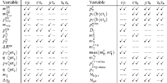
Table 4:
Parameters selected for the NN classification task used for the event categorization in each final state. The checkmarks (dashes) indicate that the variable was (not) used for the corresponding final state. The first (second) entry per column corresponds to the choice for the 2016 (2017) dataset. |
png pdf |
Table 5:
Observed number of selected events ($ {N_{\text {data}}}$) and the relative contribution of the expected processes in all event categories in the $\mathrm{e} \mu $ and $\mathrm{e} \tau _{\text {h}} $ final states on the 2017 dataset. The relative contribution of the expected processes is given in $%$, and prior to the fit used for the signal extraction. In the $\mathrm{e} \tau _{\text {h}} $ final state, processes in which a jet is misidentified as a $\tau _{\text {h}} $ decay are subsumed into a common $ {\text {jet}\to \tau _{\text {h}}}$ background class, which is estimated from data. The $ {\mathrm {V}}\mathrm{H} $ with leptonic $ {\mathrm {V}}$ decay and ${{\mathrm{t} \mathrm{t} \mathrm{H}}}$ production modes are omitted from the table due to their low expected event yields of $\leq 1$ event. |
| Summary |
| Measurements of the product of the cross section for the production of the Higgs boson and the branching fraction for its subsequent decay into tau leptons have been presented. The measurements are based on the data collected with the CMS experiment, during the years 2016 and 2017. They amount to a luminosity of 77.4 fb$^{-1}$ at a center-of-mass energy of the pp collisions of 13 TeV. The product of the inclusive Higgs boson production with the branching fraction into tau leptons is measured to be $\sigma_{\text{incl}}\,\mathcal{B}(\mathrm{H}\to\tau\tau)=$ 2.56 $\pm$ 0.48 (stat) $\pm$ 0.34 (syst) pb. When split by the ggH, bbH and VBF production modes these cross sections are found to be $\sigma({{{\mathrm{g}\mathrm{g}\to\mathrm{H},\mathrm{b}\mathrm{b}\mathrm{H}}}})\,\mathcal{B}(\mathrm{H}\to\tau\tau)=$ 1.11 $\pm$ 0.81 (stat) $\pm$ 0.78 (syst) pb and $\sigma(\text{VBF+V(qq)H})\,\mathcal{B}(\mathrm{H}\to\tau\tau)=$ 0.34 $\pm$ 0.08 (stat) $\pm$ 0.09 (syst) pb. In addition the kinematic properties of the production have been investigated in terms of simplified template cross sections. |
| References | ||||
| 1 | ATLAS Collaboration | Observation of a new particle in the search for the standard model Higgs boson with the ATLAS detector at the LHC | Phys.Lett. B 716 (2012) 1--29 | 1207.7214 |
| 2 | CMS Collaboration | Observation of a new boson at a mass of 125 GeV with the CMS experiment at the LHC | PLB 716 (2012) 30--61 | CMS-HIG-12-028 1207.7235 |
| 3 | CMS Collaboration | Observation of a new boson with mass near 125 GeV in pp collisions at $ \sqrt{s} = $ 7 and 8 TeV | JHEP 06 (2013) 081 | CMS-HIG-12-036 1303.4571 |
| 4 | ATLAS, CMS Collaboration | Combined measurement of the Higgs boson mass in $ {\mathrm{p}}{\mathrm{p}} $ collisions at $ \sqrt{s}= $ 7 and 8 TeV with the ATLAS and CMS experiments | PRL 114 (2015) 191803 | 1503.07589 |
| 5 | ATLAS, CMS Collaboration | Measurements of the Higgs boson production and decay rates and constraints on its couplings from a combined ATLAS and CMS analysis of the LHC pp collision data at $ \sqrt{s}= $ 7 and 8 TeV | JHEP 08 (2016) 045 | 1606.02266 |
| 6 | \relax Yu. A. Golfand and E. P. Likhtman | Extension of the algebra of Poincare group generators and violation of p invariance | JEPTL 13 (1971) 323--326.[Pisma Zh. Eksp. Teor. Fiz.13,452(1971)] | |
| 7 | J. Wess and B. Zumino | Supergauge transformations in four-dimensions | NPB 70 (1974) 39--50 | |
| 8 | ATLAS Collaboration | Cross-section measurements of the Higgs boson decaying into a pair of $ \tau $-leptons in proton-proton collisions at $ \sqrt{s}= $ 13 TeV with the ATLAS detector | Submitted to: PR(2018) | 1811.08856 |
| 9 | CMS Collaboration | Observation of the Higgs boson decay to a pair of $ \tau $ leptons with the CMS detector | PLB 779 (2018) 283--316 | CMS-HIG-16-043 1708.00373 |
| 10 | LHC Higgs Cross Section Working Group Collaboration | Handbook of LHC Higgs cross sections: 4. deciphering the nature of the Higgs sector | 1610.07922 | |
| 11 | CMS Collaboration | An embedding technique to determine $ \tau\tau $ backgrounds in proton-proton collision data | Submitted to \it JINST | CMS-TAU-18-001 1903.01216 |
| 12 | CMS Collaboration | Measurement of the $ \mathrm{Z}\gamma^{*}\to\tau\tau $ cross section in pp collisions at $ \sqrt{s} = $ 13 TeV and validation of $ \tau $ lepton analysis techniques | EPJC 78 (2018), no. 9, 708 | CMS-HIG-15-007 1801.03535 |
| 13 | CMS Collaboration | Description and performance of track and primary-vertex reconstruction with the CMS tracker | JINST 9 (2014) P10009 | CMS-TRK-11-001 1405.6569 |
| 14 | CMS Collaboration | Performance of electron reconstruction and selection with the CMS detector in proton-proton collisions at $ \sqrt{s} = $ 8 TeV | JINST 10 (2015), no. 06, P06005 | CMS-EGM-13-001 1502.02701 |
| 15 | CMS Collaboration | Performance of CMS muon reconstruction in $ {\mathrm{p}}{\mathrm{p}} $ collision events at $ \sqrt{s} = $ 7 TeV | JINST 7 (2012) P10002 | CMS-MUO-10-004 1206.4071 |
| 16 | CMS Collaboration | Performance of photon reconstruction and identification with the CMS detector in proton-proton collisions at $ \sqrt{s} = $ 8 TeV | JINST 10 (2015) P08010 | CMS-EGM-14-001 1502.02702 |
| 17 | CMS Collaboration | The CMS trigger system | JINST 12 (2017) P01020 | CMS-TRG-12-001 1609.02366 |
| 18 | CMS Collaboration | The CMS experiment at the CERN LHC | JINST 3 (2008) S08004 | CMS-00-001 |
| 19 | CMS Collaboration | Particle-flow reconstruction and global event description with the CMS detector | JINST 12 (2017), no. 10, P10003 | CMS-PRF-14-001 1706.04965 |
| 20 | K. Rose | Deterministic annealing for clustering, compression, classification, regression, and related optimization problems | Proceedings of the IEEE 86 (Nov, 1998) 2210 | |
| 21 | M. Cacciari, G. P. Salam, and G. Soyez | The anti-$ k_t $ jet clustering algorithm | JHEP 04 (2008) 063 | 0802.1189 |
| 22 | M. Cacciari, G. P. Salam, and G. Soyez | FastJet user manual | EPJC 72 (2012) 1896 | 1111.6097 |
| 23 | CMS Collaboration | Identification of heavy-flavour jets with the CMS detector in $ {\mathrm{p}}{\mathrm{p}} $ collisions at 13 TeV | JINST 13 (2018) P05011 | CMS-BTV-16-002 1712.07158 |
| 24 | CMS Collaboration | Performance of reconstruction and identification of $ \tau $ leptons decaying to hadrons and $ \nu_\tau $ in pp collisions at $ \sqrt{s} = $ 13 TeV | JINST 13 (2018), no. 10, P10005 | CMS-TAU-16-003 1809.02816 |
| 25 | L. Bianchini, J. Conway, E. K. Friis, and C. Veelken | Reconstruction of the Higgs mass in $ \mathrm{H}\to\tau\tau $ events by dynamical likelihood techniques | J. Phys. Conf. Ser. 513 (2014) 022035 | |
| 26 | J. Alwall et al. | MadGraph 5: Going beyond | JHEP 06 (2011) 128 | 1106.0522 |
| 27 | J. Alwall et al. | The automated computation of tree-level and next-to-leading order differential cross sections, and their matching to parton shower simulations | JHEP 07 (2014) 079 | 1405.0301 |
| 28 | P. Nason | A new method for combining NLO QCD with shower Monte Carlo algorithms | JHEP 11 (2004) 040 | hep-ph/0409146 |
| 29 | S. Frixione, P. Nason, and C. Oleari | Matching NLO QCD computations with parton shower simulations: the POWHEG method | JHEP 11 (2007) 070 | 0709.2092 |
| 30 | S. Alioli, P. Nason, C. Oleari, and E. Re | NLO Higgs boson production via gluon fusion matched with shower in POWHEG | JHEP 04 (2009) 002 | 0812.0578 |
| 31 | S. Alioli, P. Nason, C. Oleari, and E. Re | A general framework for implementing NLO calculations in shower Monte Carlo programs: the POWHEG BOX | JHEP 06 (2010) 043 | 1002.2581 |
| 32 | S. Alioli et al. | Jet pair production in POWHEG | JHEP 04 (2011) 081 | 1012.3380 |
| 33 | E. Bagnaschi, G. Degrassi, P. Slavich, and A. Vicini | Higgs production via gluon fusion in the POWHEG approach in the SM and in the MSSM | JHEP 02 (2012) 088 | 1111.2854 |
| 34 | K. Melnikov and F. Petriello | Electroweak gauge boson production at hadron colliders through $ \mathcal{O}(\alpha_\text{s}^{2}) $ | PRD 74 (2006) 114017 | hep-ph/0609070 |
| 35 | M. Czakon and A. Mitov | Top++: A program for the calculation of the top-pair cross-section at hadron colliders | CPC 185 (2014) 2930 | 1112.5675 |
| 36 | N. Kidonakis | Top quark production | in Proceedings, Helmholtz International Summer School on Physics of Heavy Quarks and Hadrons (HQ 2013): JINR, Dubna, Russia, July 15-28, 2013, pp. 139--168 2014 | 1311.0283 |
| 37 | J. M. Campbell, R. K. Ellis, and C. Williams | Vector boson pair production at the LHC | JHEP 07 (2011) 018 | 1105.0020 |
| 38 | T. Gehrmann et al. | $ W^+W^- $ Production at Hadron Colliders in Next to Next to Leading Order QCD | PRL 113 (2014), no. 21, 212001 | 1408.5243 |
| 39 | NNPDF Collaboration | Parton distributions for the LHC run II | JHEP 04 (2015) 040 | 1410.8849 |
| 40 | CMS Collaboration | Event generator tunes obtained from underlying event and multiparton scattering measurements | EPJC 76 (2016), no. 3, 155 | CMS-GEN-14-001 1512.00815 |
| 41 | S. Agostinelli et al. | GEANT4--a simulation toolkit | NIMA 506 (2003) 250 | |
| 42 | CMS Collaboration | Measurements of inclusive $ \mathrm{W} $ and $ \mathrm{Z} $ cross sections in $ {\mathrm{p}}{\mathrm{p}} $ collisions at $ \sqrt{s} = $ 7 TeV | JHEP 01 (2011) 080 | CMS-EWK-10-002 1012.2466 |
| 43 | CMS Collaboration | Measurement of the differential cross section for top quark pair production in pp collisions at $ \sqrt{s} = $ 8 TeV | EPJC 75 (2015), no. 11, 542 | CMS-TOP-12-028 1505.04480 |
| 44 | CDF Collaboration | Search for neutral Higgs bosons of the minimal supersymmetric standard model decaying to $ \tau $ pairs in $ {\mathrm{p}}\bar{{\mathrm{p}}} $ collisions at $ \sqrt{s} = $ 1.96 TeV | PRL 96 (2006) 011802 | hep-ex/0508051 |
| 45 | X. Glorot and Y. Bengio | Understanding the difficulty of training deep feedforward neural networks | in Proceedings of the thirteenth international conference on artificial intelligence and statistics, p. 249 2010 | |
| 46 | D. P. Kingma and J. Ba | Adam: A method for stochastic optimization | 1412.6980 | |
| 47 | A. N. Tikhonov | Solution of incorrectly formulated problems and the regularization method | Soviet Math. Dokl. 4 (1963) 1035 | |
| 48 | S. Baker and R. D. Cousins | Clarification of the use of chi square and likelihood functions in fits to histograms | NIM221 (1984) 437 | |
| 49 | S. Wunsch, R. Friese, R. Wolf, and G. Quast | Identifying the relevant dependencies of the neural network response on characteristics of the input space | Comput. Softw. Big Sci. 2 (2018), no. 1, 5 | 1803.08782 |
| 50 | J. S. Conway | Nuisance parameters in likelihoods for multisource spectra | Proceedings of PHYSTAT 2011 Workshop on Statistical Issues Related to Discovery Claims in Search Experiments and Unfolding, CERN, Geneva, Switzerland, 17-20 January 2011, edited by H.B. Propser and L. Lyons CERN-2011-006 (2011) 115--120 | |
| 51 | CMS Collaboration | CMS luminosity measurements for the 2016 data taking period | CMS-PAS-LUM-17-001, CERN, Geneva | |
| 52 | CMS Collaboration | CMS luminosity measurement for the 2017 data-taking period at $ \sqrt{s} = $ 13 TeV | CMS-PAS-LUM-17-004, CERN, Geneva | |
| 53 | Y. Li and F. Petriello | Combining QCD and electroweak corrections to dilepton production in FEWZ | PRD 86 (2012) 094034 | 1208.5967 |
| 54 | CMS Collaboration | Cross section measurement of t-channel single top quark production in $ {\mathrm{p}}{\mathrm{p}} $ collisions at $ \sqrt{s} = $ 13 TeV | PLB 772 (2017) 752 | CMS-TOP-16-003 1610.00678 |
| 55 | CMS Collaboration | Measurement of the $ \mathrm{W}\mathrm{Z} $ production cross section in $ {\mathrm{p}}{\mathrm{p}} $ collisions at $ \sqrt{s} = $ 13 TeV | PLB 766 (2017) 268 | CMS-SMP-16-002 1607.06943 |

|
Compact Muon Solenoid LHC, CERN |

|

|

|

|

|

|