

Compact Muon Solenoid
LHC, CERN
| CMS-HIG-24-003 ; CERN-EP-2026-080 | ||
| Search for associated production of a Higgs boson and two vector bosons via vector boson scattering at $ \sqrt{s} = $ 13 TeV | ||
| CMS Collaboration | ||
| 27 April 2026 | ||
| Accepted for publication in Physical Review Letters | ||
| Abstract: A search for Higgs boson (H) production in association with two vector bosons ($ \mathrm{V} = \mathrm{W} $, Z) via vector boson scattering (VBS) is presented using proton-proton collision data collected at $ \sqrt{s}= $ 13 TeV by the CMS experiment, corresponding to an integrated luminosity of 138 fb$ ^{-1} $. Events containing two forward jets consistent with VBS, a large-radius jet from the decay of a boosted H to a pair of b quarks, and 0, 1, or 2 charged leptons coming from V decays are selected. The process is excluded at 95%CL for observed (expected) values of the $ \mathrm{V}\mathrm{V}\mathrm{H}\mathrm{H} $ coupling modifier $ \kappa_{2\mathrm{V}} $ outside the interval 0.40 $ < \kappa_{2\mathrm{V}} < $ 1.60 (0.34 $ < \kappa_{2\mathrm{V}} < $ 1.66), assuming standard model values for all other couplings, thus establishing a novel probe of the $ \mathrm{V}\mathrm{V}\mathrm{H}\mathrm{H} $ interaction. Constraints are also set on the individual $ \kappa_{2\mathrm{W}} $ and $ \kappa_{2\mathrm{Z}} $ coupling modifiers, and on the allowed region in the $ \kappa_{2\mathrm{W}}-\kappa_{2\mathrm{Z}} $ plane. | ||
| Links: e-print arXiv:2604.24531 [hep-ex] (PDF) ; CDS record ; inSPIRE record ; HepData record ; CADI line (restricted) ; | ||
| Figures | |
png pdf |
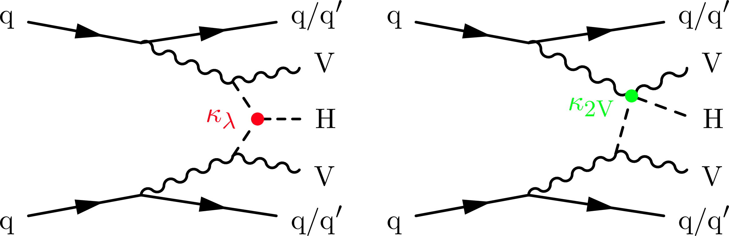
Figure 1:
Examples of tree-level Feynman diagrams for the production of $ \mathrm{V}\mathrm{V}\mathrm{H} $ via VBS, with dependencies on the H self-coupling (left) and the $ \mathrm{V}\mathrm{V}\mathrm{H}\mathrm{H} $ quartic coupling (right). The corresponding vertices are denoted by the $ \kappa_{\lambda} $ and $ \kappa_{2\mathrm{V}} $ modifiers, respectively. |
png pdf |
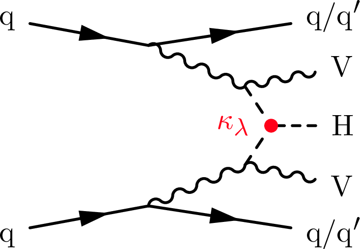
Figure 1-a:
Examples of tree-level Feynman diagrams for the production of $ \mathrm{V}\mathrm{V}\mathrm{H} $ via VBS, with dependencies on the H self-coupling (left) and the $ \mathrm{V}\mathrm{V}\mathrm{H}\mathrm{H} $ quartic coupling (right). The corresponding vertices are denoted by the $ \kappa_{\lambda} $ and $ \kappa_{2\mathrm{V}} $ modifiers, respectively. |
png pdf |
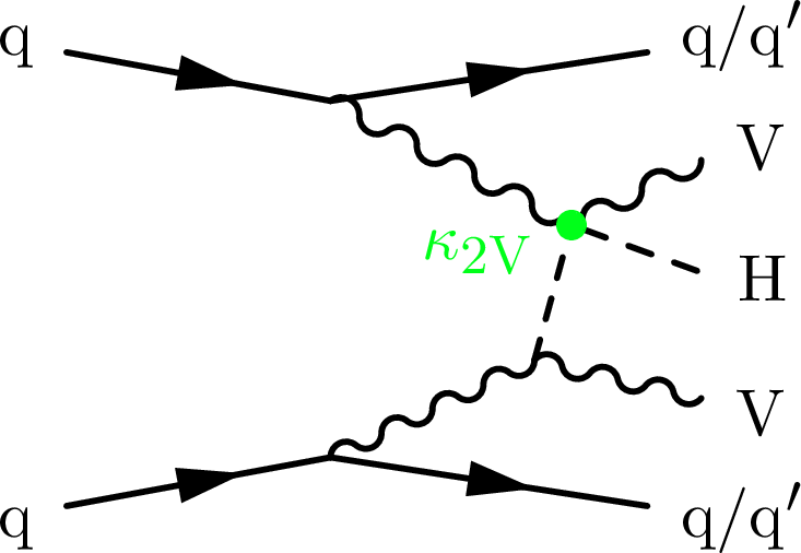
Figure 1-b:
Examples of tree-level Feynman diagrams for the production of $ \mathrm{V}\mathrm{V}\mathrm{H} $ via VBS, with dependencies on the H self-coupling (left) and the $ \mathrm{V}\mathrm{V}\mathrm{H}\mathrm{H} $ quartic coupling (right). The corresponding vertices are denoted by the $ \kappa_{\lambda} $ and $ \kappa_{2\mathrm{V}} $ modifiers, respectively. |
png pdf |
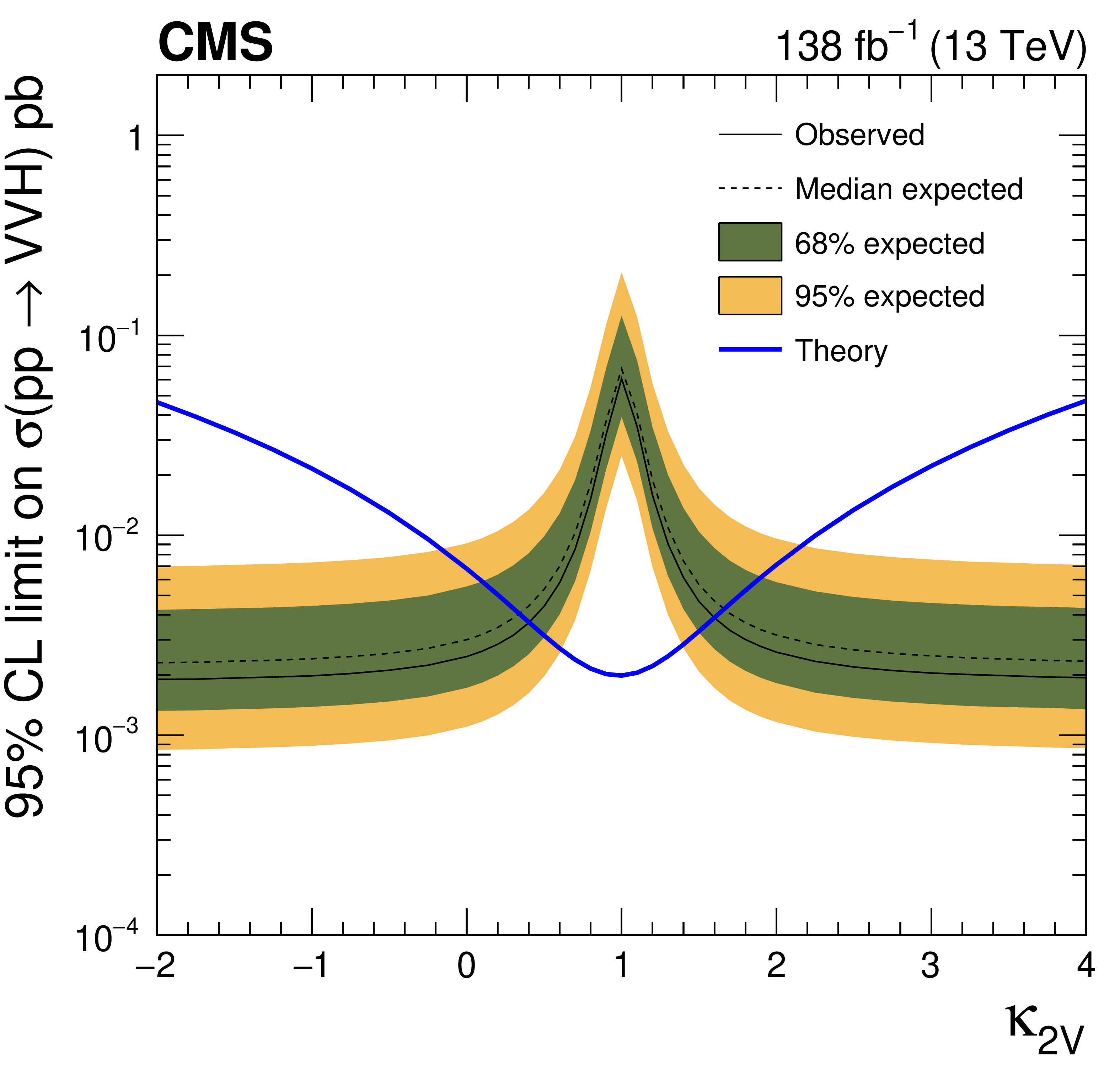
Figure 2:
Observed (solid) and expected (dashed) 95% CL constraints on the VBS $ \mathrm{V}\mathrm{V}\mathrm{H} $ production cross section as a function of $ \kappa_{2\mathrm{V}} $, with other couplings fixed to their SM values. The intersections with the predicted cross section (blue) indicate the excluded $ \kappa_{2\mathrm{V}} $ ranges. |
png pdf |
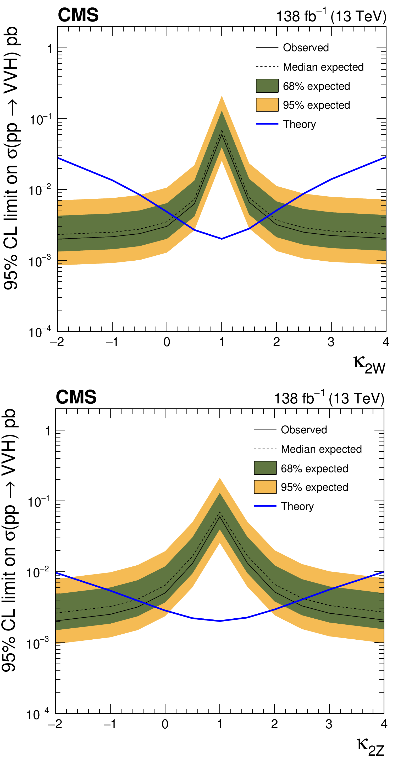
Figure 3:
Observed (solid) and expected (dashed) 95% CL constraints on the VBS $ \mathrm{V}\mathrm{V}\mathrm{H} $ production cross section as a function of $ \kappa_{2\mathrm{W}} $ (left) and $ \kappa_{2\mathrm{Z}} $ (right). The intersections with the predicted cross section (blue) indicate excluded coupling ranges. |
png pdf |
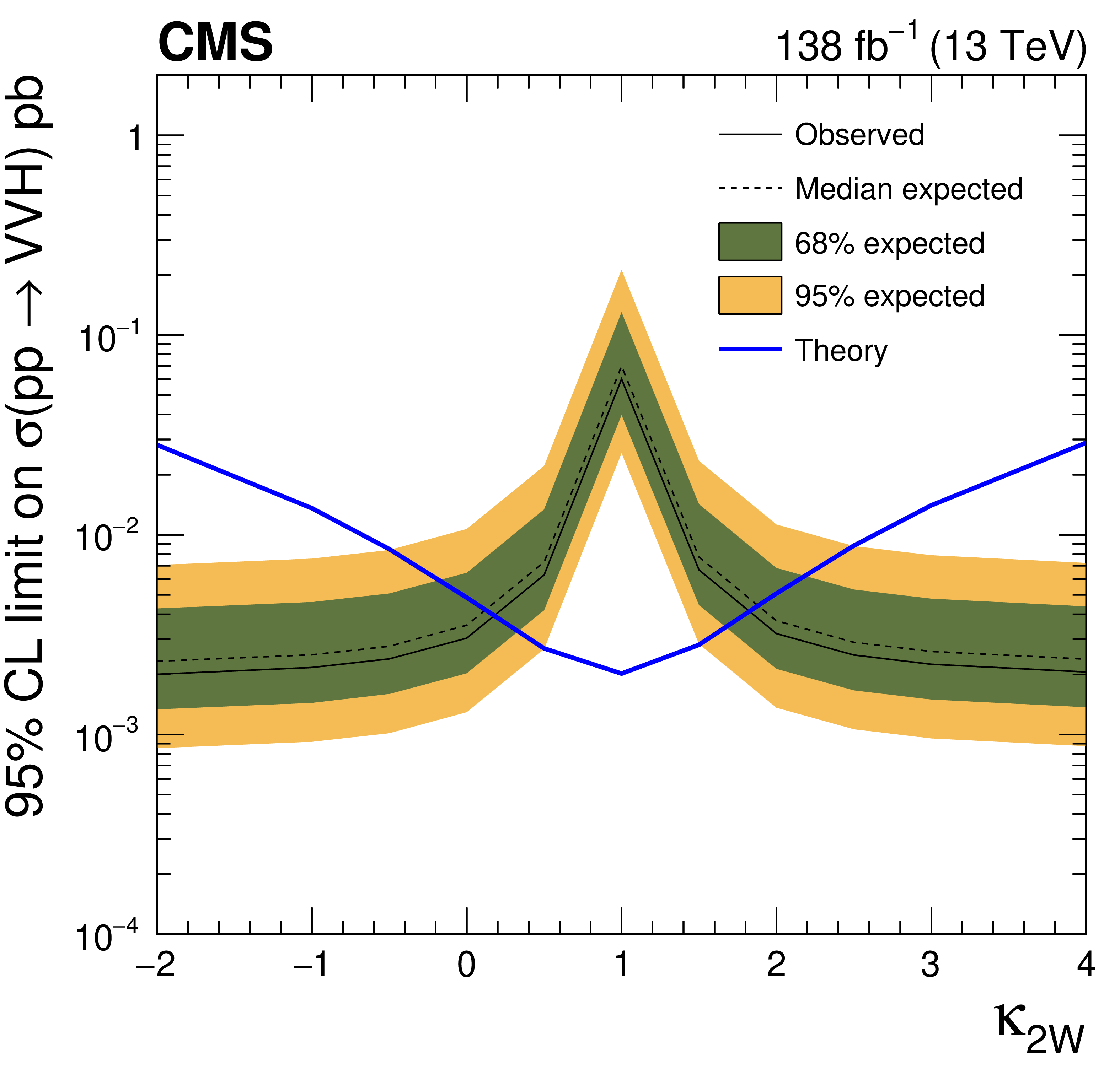
Figure 3-a:
Observed (solid) and expected (dashed) 95% CL constraints on the VBS $ \mathrm{V}\mathrm{V}\mathrm{H} $ production cross section as a function of $ \kappa_{2\mathrm{W}} $ (left) and $ \kappa_{2\mathrm{Z}} $ (right). The intersections with the predicted cross section (blue) indicate excluded coupling ranges. |
png pdf |
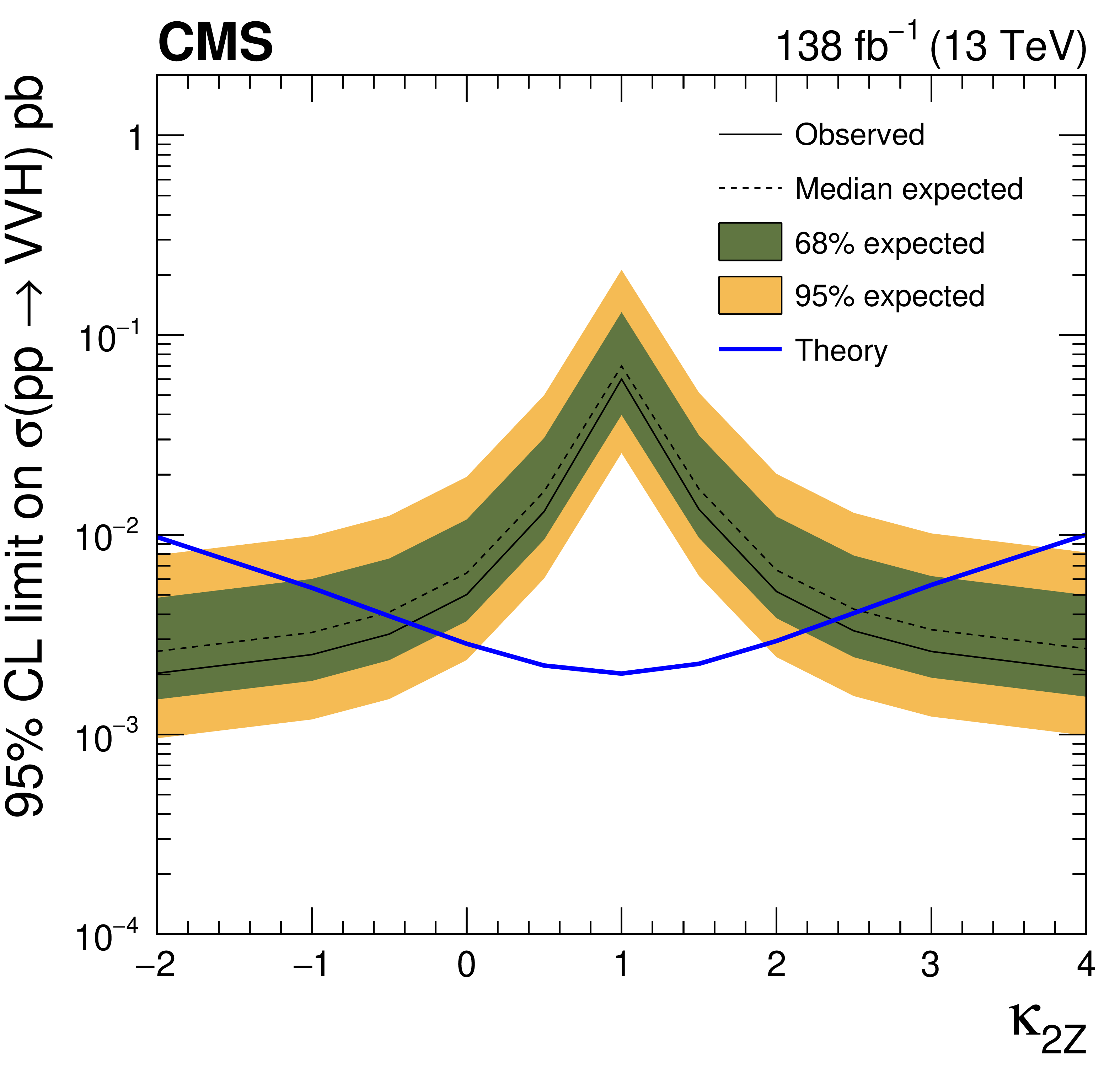
Figure 3-b:
Observed (solid) and expected (dashed) 95% CL constraints on the VBS $ \mathrm{V}\mathrm{V}\mathrm{H} $ production cross section as a function of $ \kappa_{2\mathrm{W}} $ (left) and $ \kappa_{2\mathrm{Z}} $ (right). The intersections with the predicted cross section (blue) indicate excluded coupling ranges. |
png pdf |
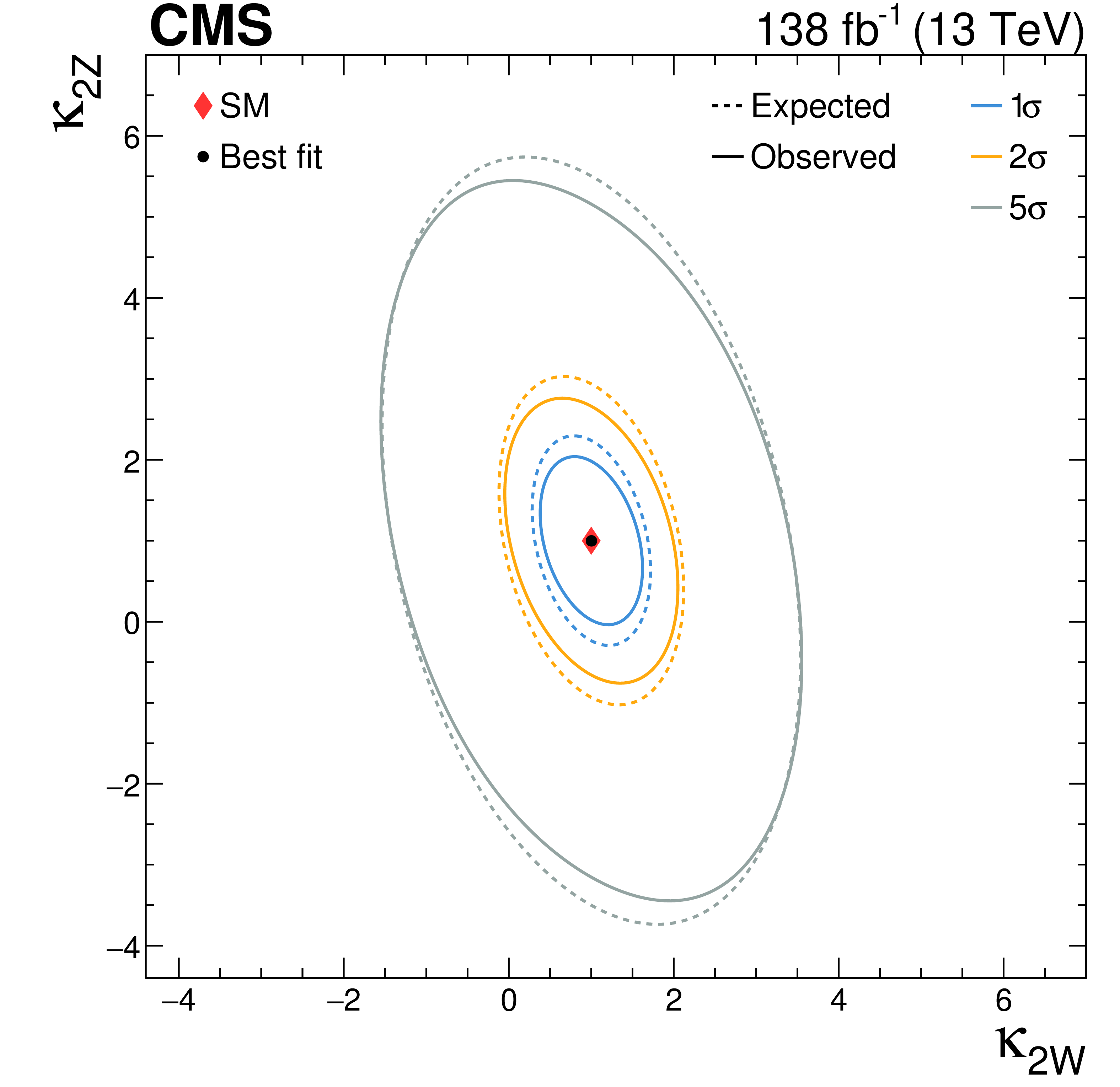
Figure 4:
Observed (solid) and expected (dashed) exclusion regions corresponding to 1, 2, and 5 standard deviations ($ \sigma $), as obtained from a likelihood scan in the two-dimensional $ \kappa_{2\mathrm{W}}-\kappa_{2\mathrm{Z}} $ plane. |
png pdf |
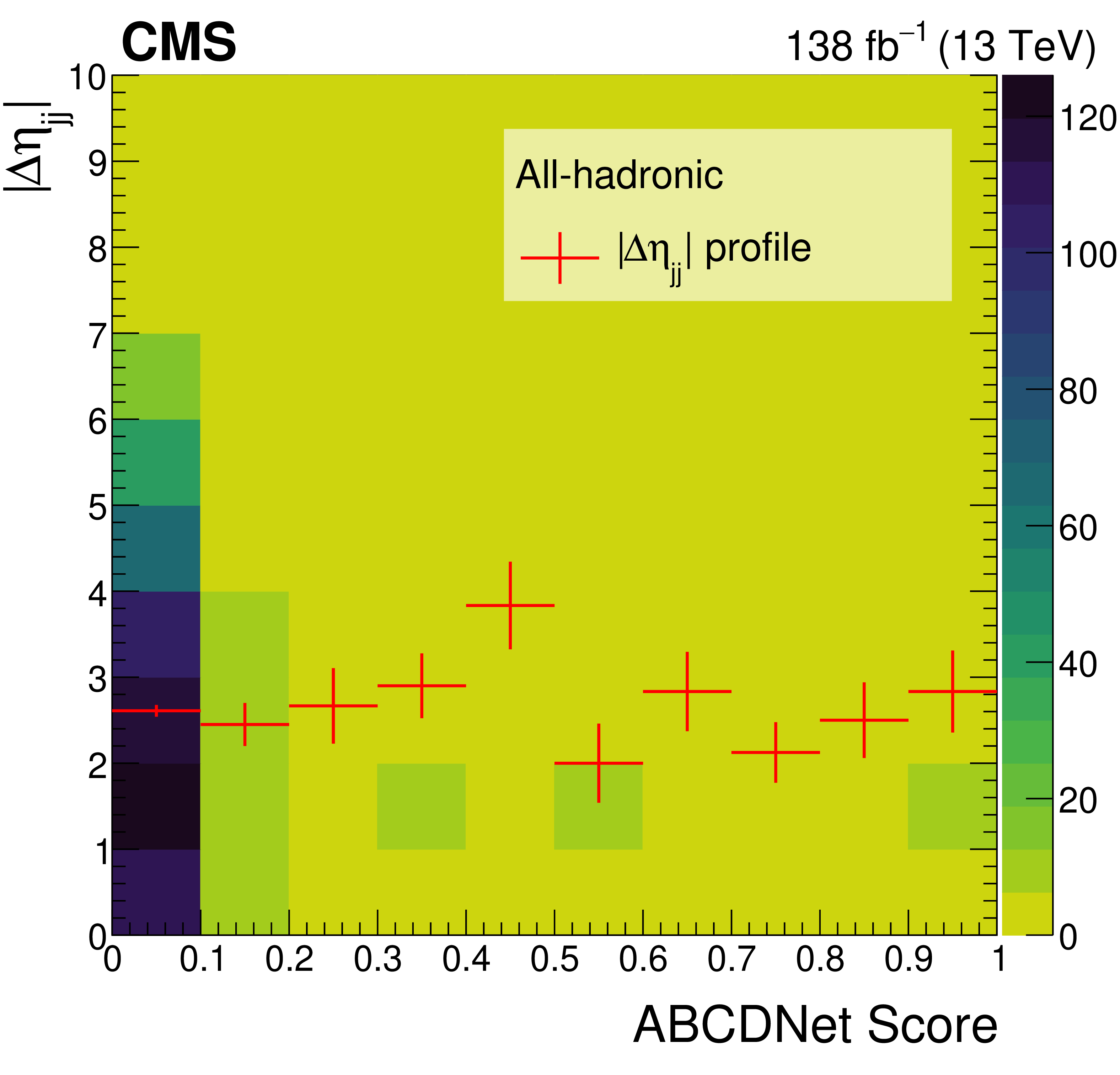
Figure A1:
Two-dimensional distributions of the DNN output and the $ |\Delta\eta_{\mathrm{j}\mathrm{j}}| $ in the all-hadronic channel, as obtained in data. These are the axes used in this channel to define the ABCD samples. A profile histogram is overlaid to better depict the statistical independence of the two variables. |
png pdf |
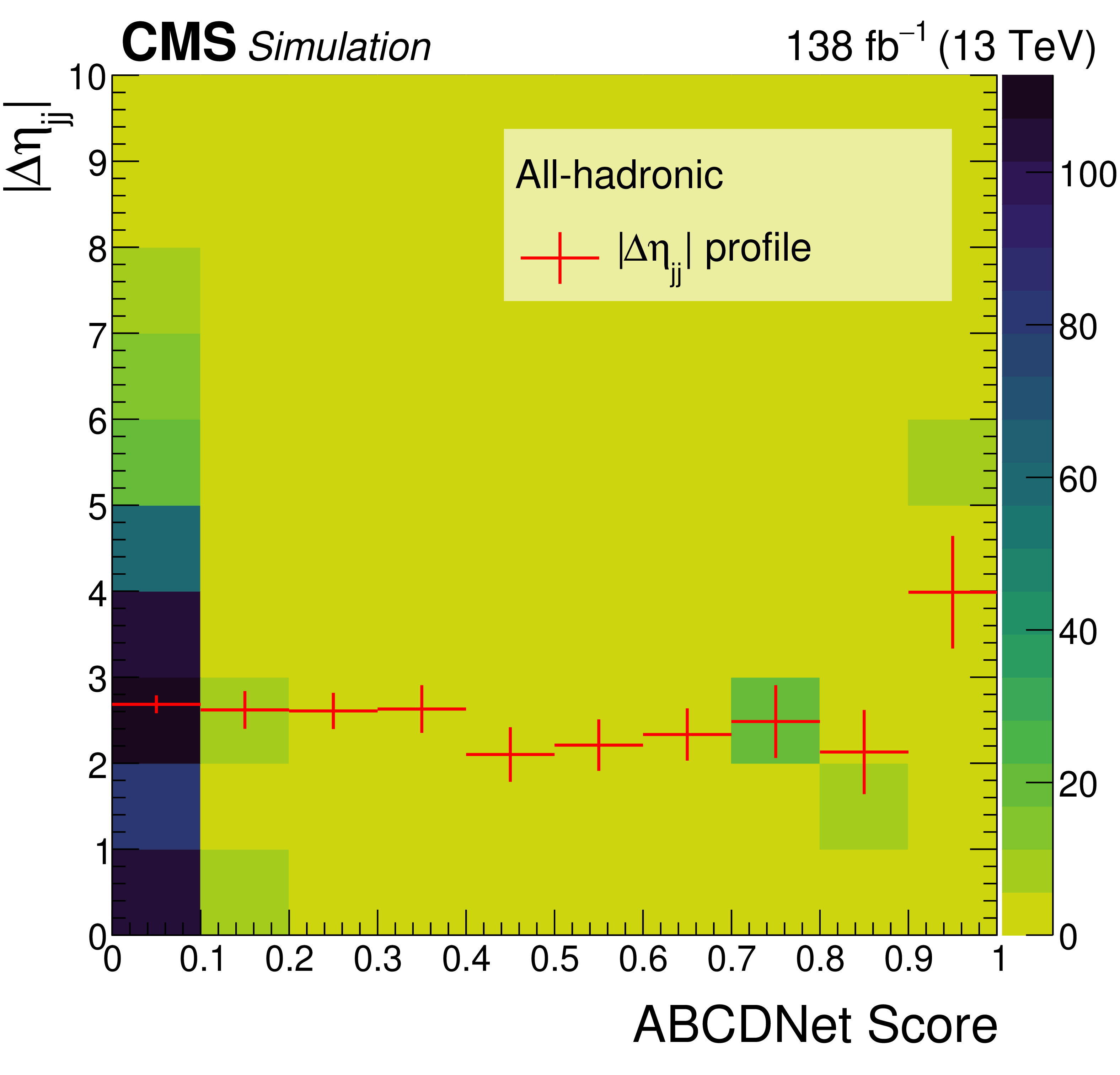
Figure A2:
Two-dimensional distributions of the DNN output and the $ |\Delta\eta_{\mathrm{j}\mathrm{j}}| $ in the all-hadronic channel, as obtained in background simulated events. These are the axes used in this channel to define the ABCD samples. A profile histogram is overlaid to better depict the statistical independence of the two variables. |
png pdf |
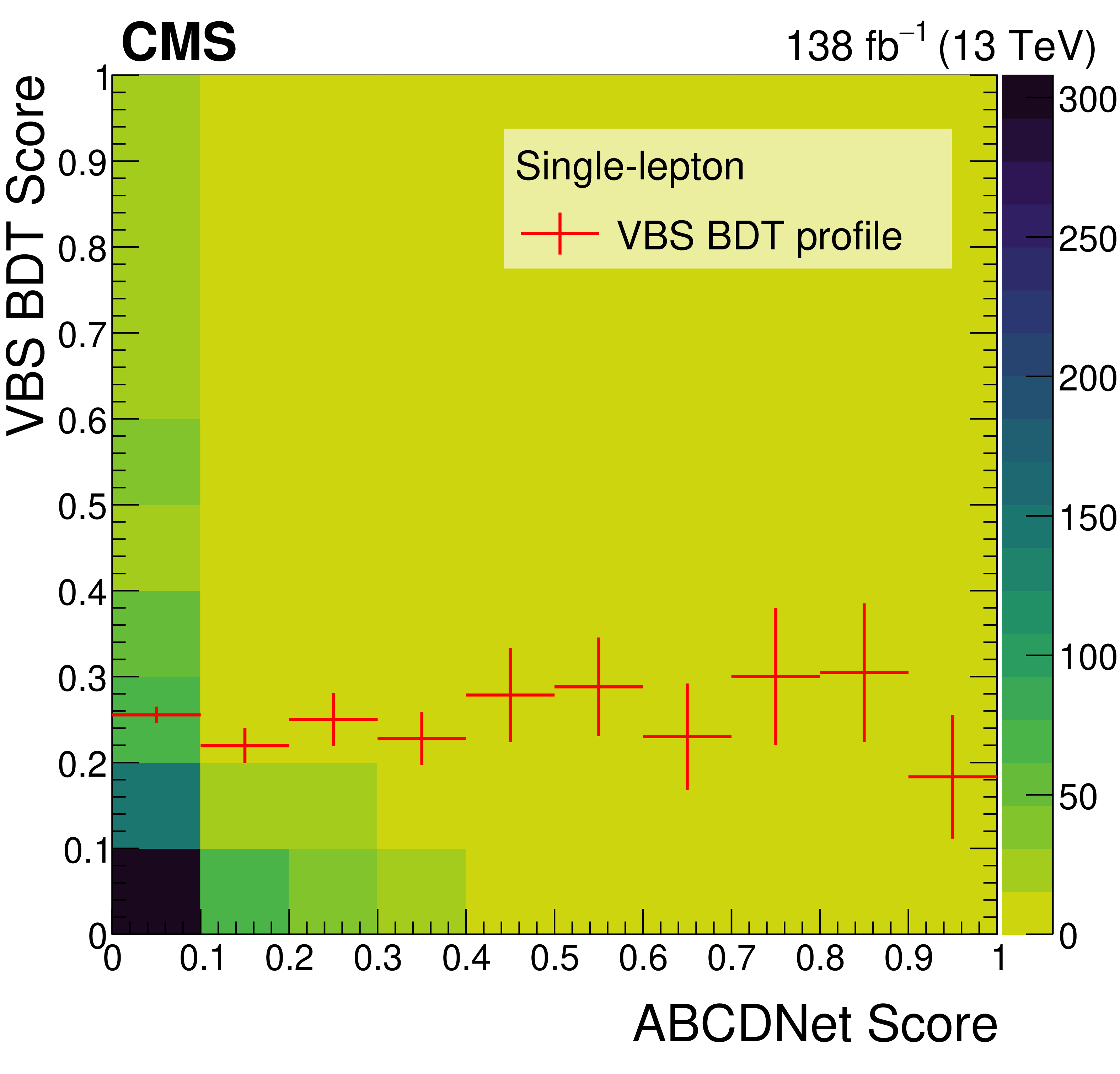
Figure A3:
Two-dimensional distributions of the DNN output and the VBS BDT output in the single-lepton channel, as obtained in data. These are the axes used in this channel to define the ABCD samples. A profile histogram is overlaid to better depict the statistical independence of the two variables. |
png pdf |
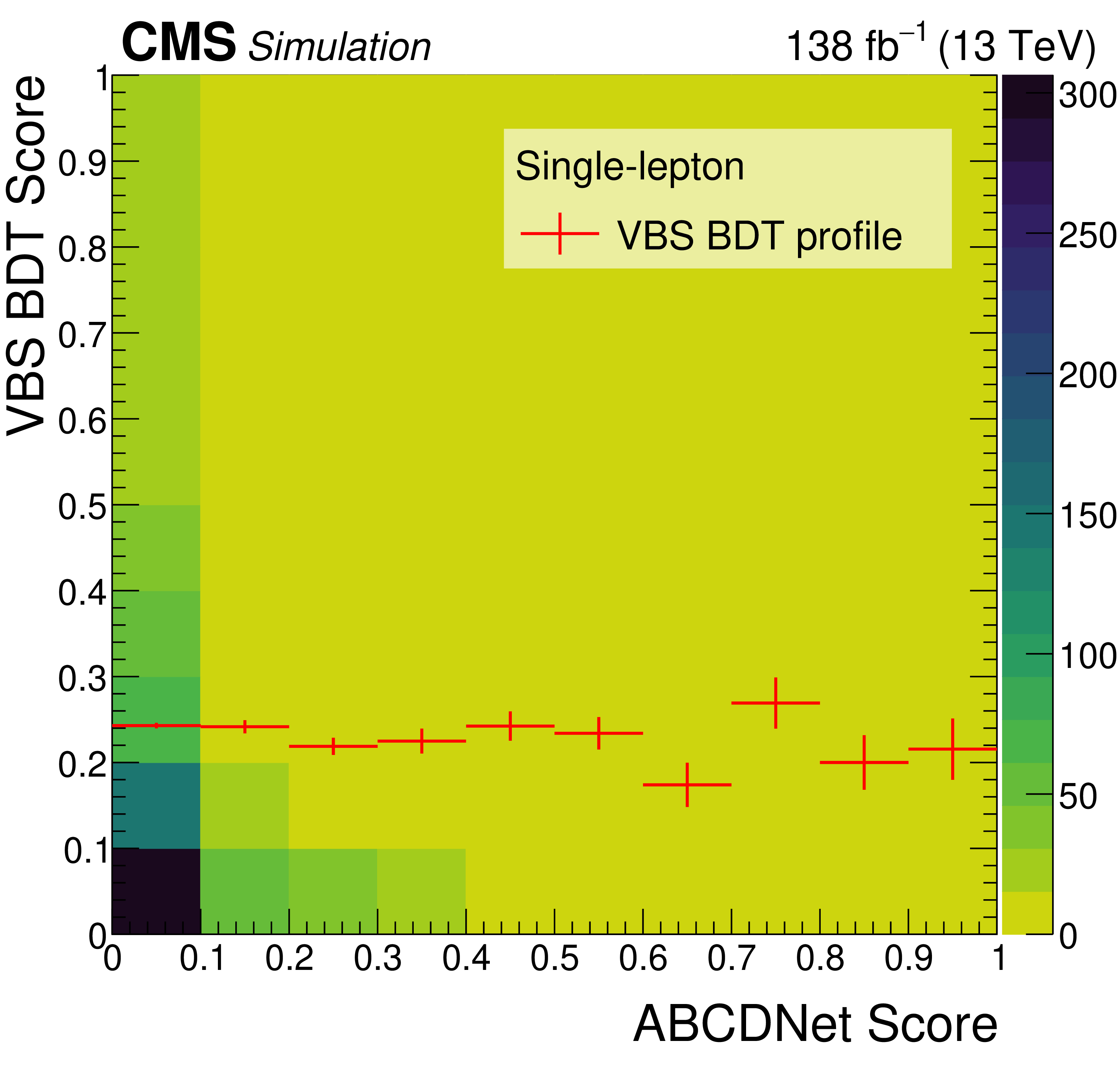
Figure A4:
Two-dimensional distributions of the DNN output and the VBS BDT output in the single-lepton channel, as obtained in background simulated events. These are the axes used in this channel to define the ABCD samples. A profile histogram is overlaid to better depict the statistical independence of the two variables. |
png pdf |
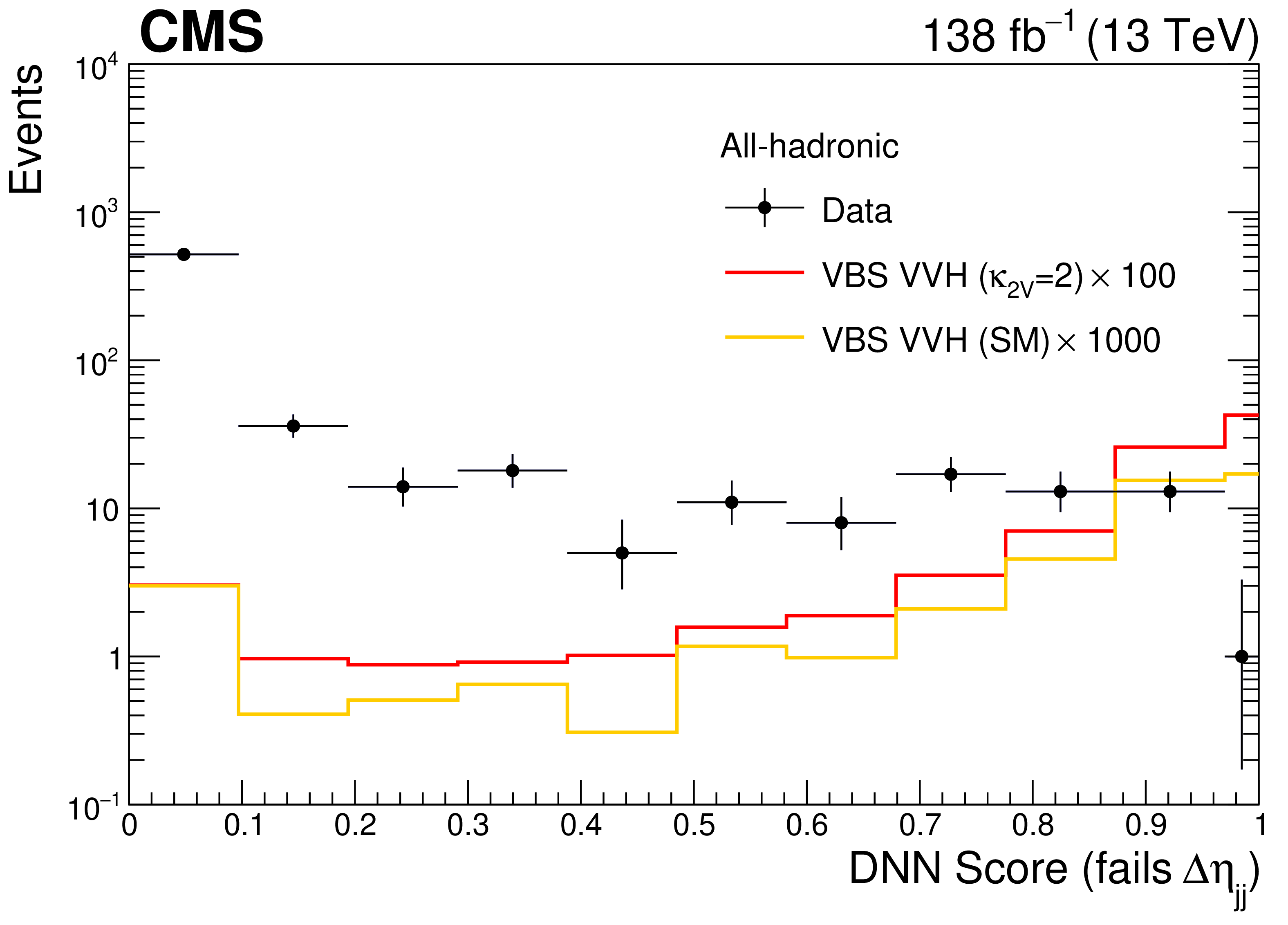
Figure A5:
Distribution of the DNN output in the regions B and D of the all-hadronic channel. The expected signal for the standard model scenario (orange) and for $ \kappa_{2\mathrm{V}} = $ 2 (red) is superimposed to the data (black markers). The cross section used for signal is computed at leading order using MADGRAPH, and is scaled by a factor 1000 (100) for the SM ($ \kappa_{2\mathrm{V}} = $ 2) signal to improve visibility. |
png pdf |
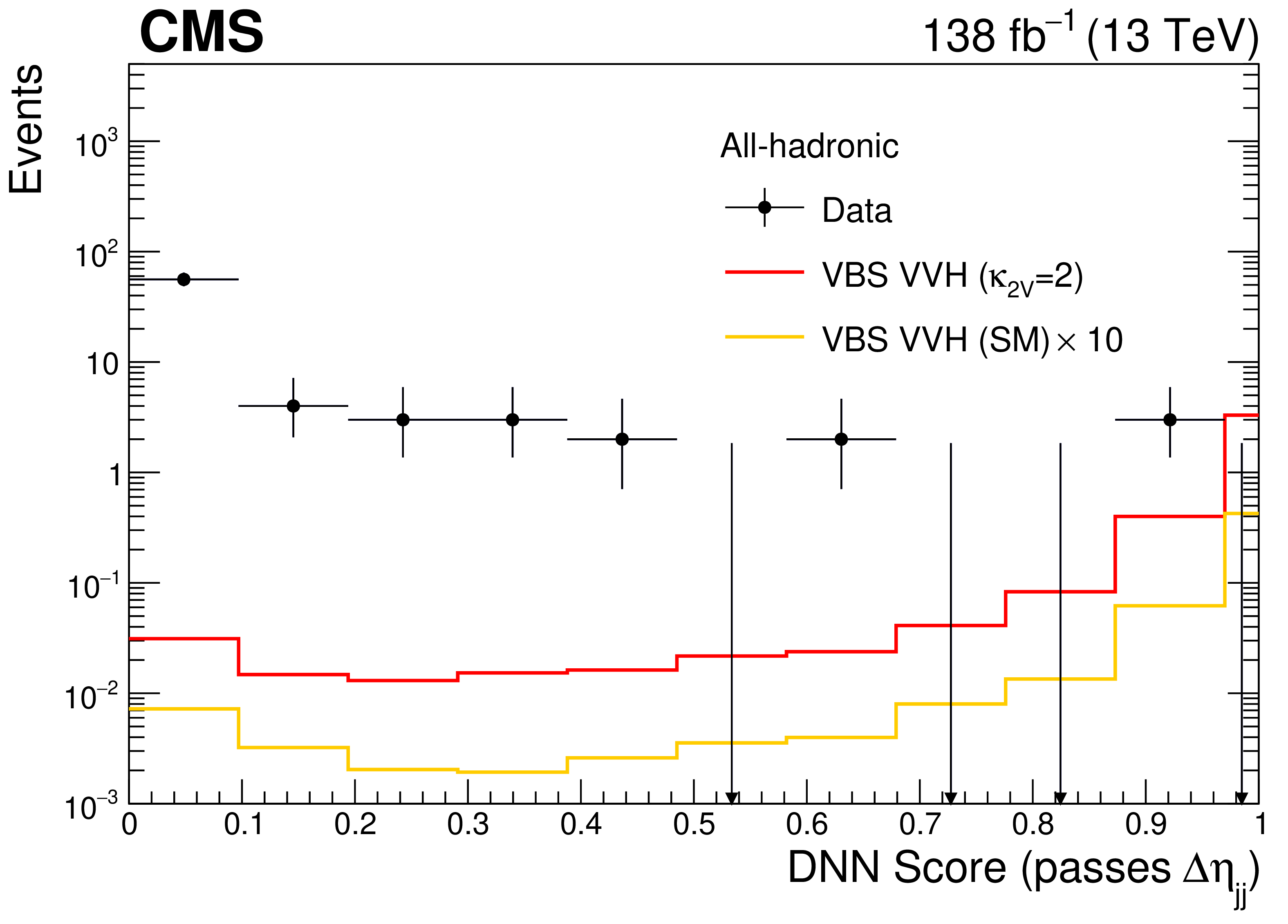
Figure A6:
Distribution of the DNN output in the regions A and C of the all-hadronic channel. The expected signal for the standard model scenario (orange) and for $ \kappa_{2\mathrm{V}} = $ 2 (red) is superimposed to the data (black markers). The cross section used for signal is computed at leading order using MADGRAPH, and is scaled by a factor 10 for the SM signal to improve visibility. |
png pdf |
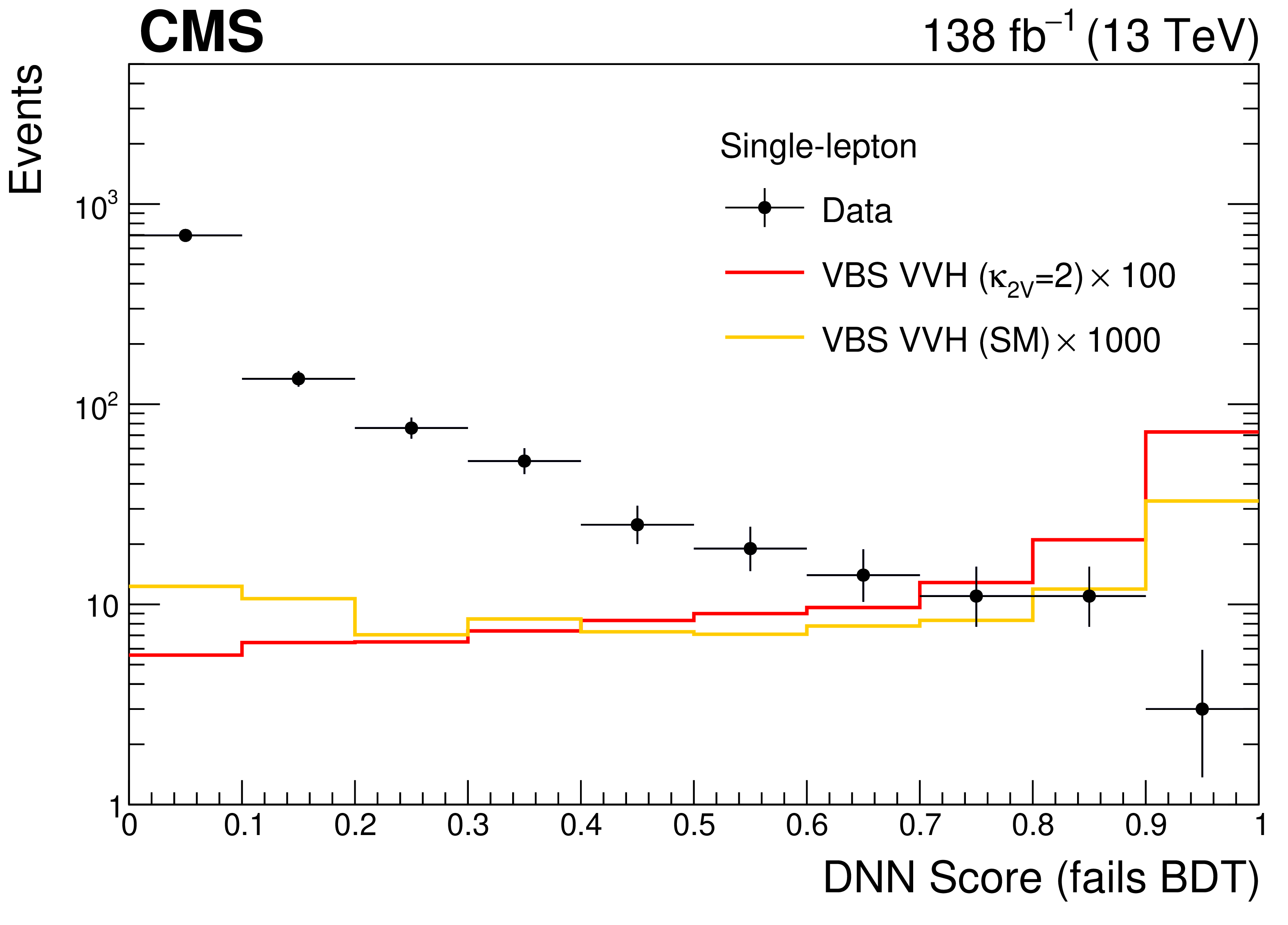
Figure A7:
Distribution of the DNN output in the regions B and D of the single-lepton channel. The expected signal for the standard model scenario (orange) and for $ \kappa_{2\mathrm{V}} = $ 2 (red) is superimposed to the data (black markers). The cross section used for signal is computed at leading order using MADGRAPH, and is scaled by a factor 1000 (100) for the SM ($ \kappa_{2\mathrm{V}} = $ 2) signal to improve visibility. |
png pdf |
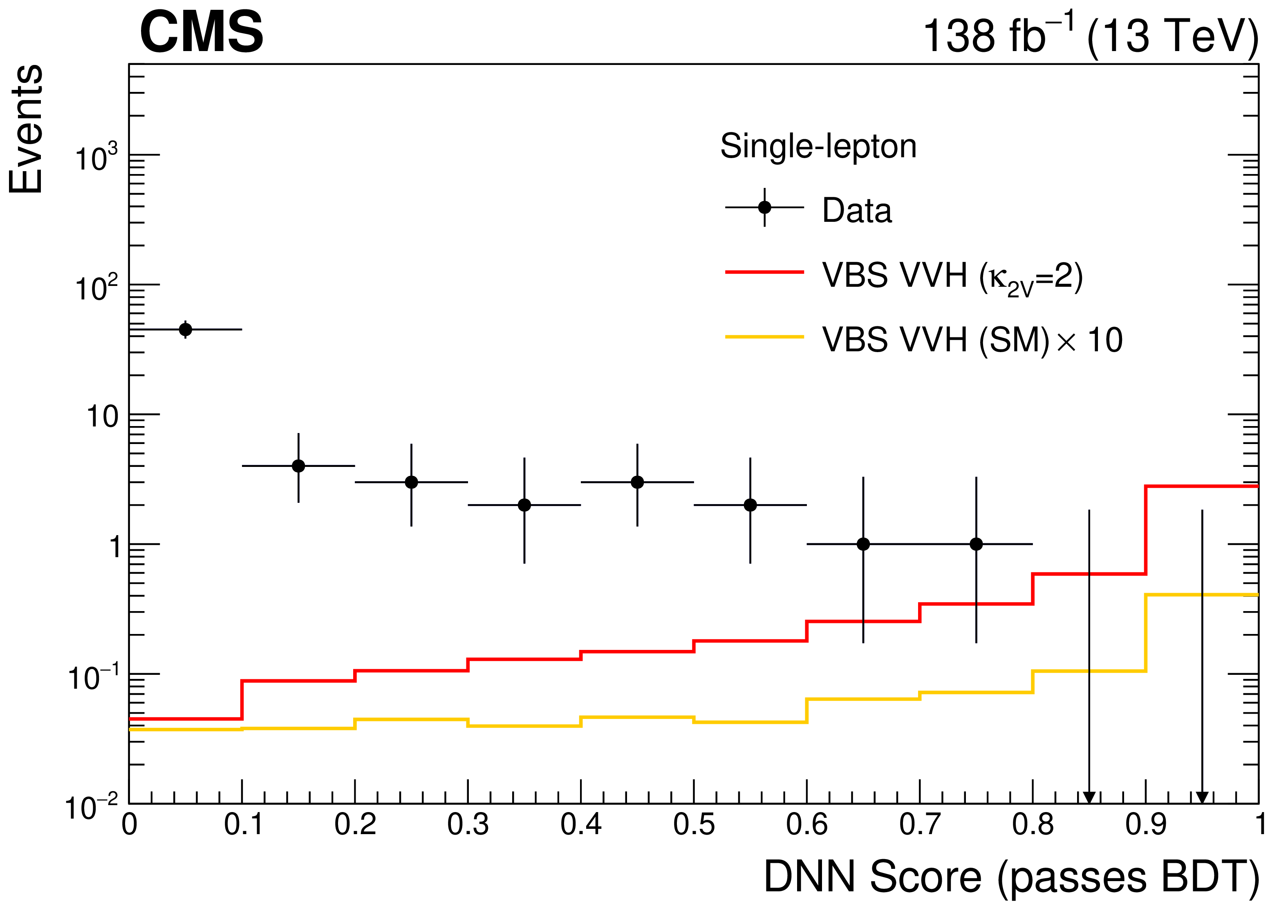
Figure A8:
Distribution of the DNN output in the regions A and C of the single-lepton channel. The expected signal for the standard model scenario (orange) and for $ \kappa_{2\mathrm{V}} = $ 2 (red) is superimposed to the data (black markers). The cross section used for signal is computed at leading order using MADGRAPH, and is scaled by a factor 10 for the SM signal to improve visibility. |
png pdf |
Figure A9:
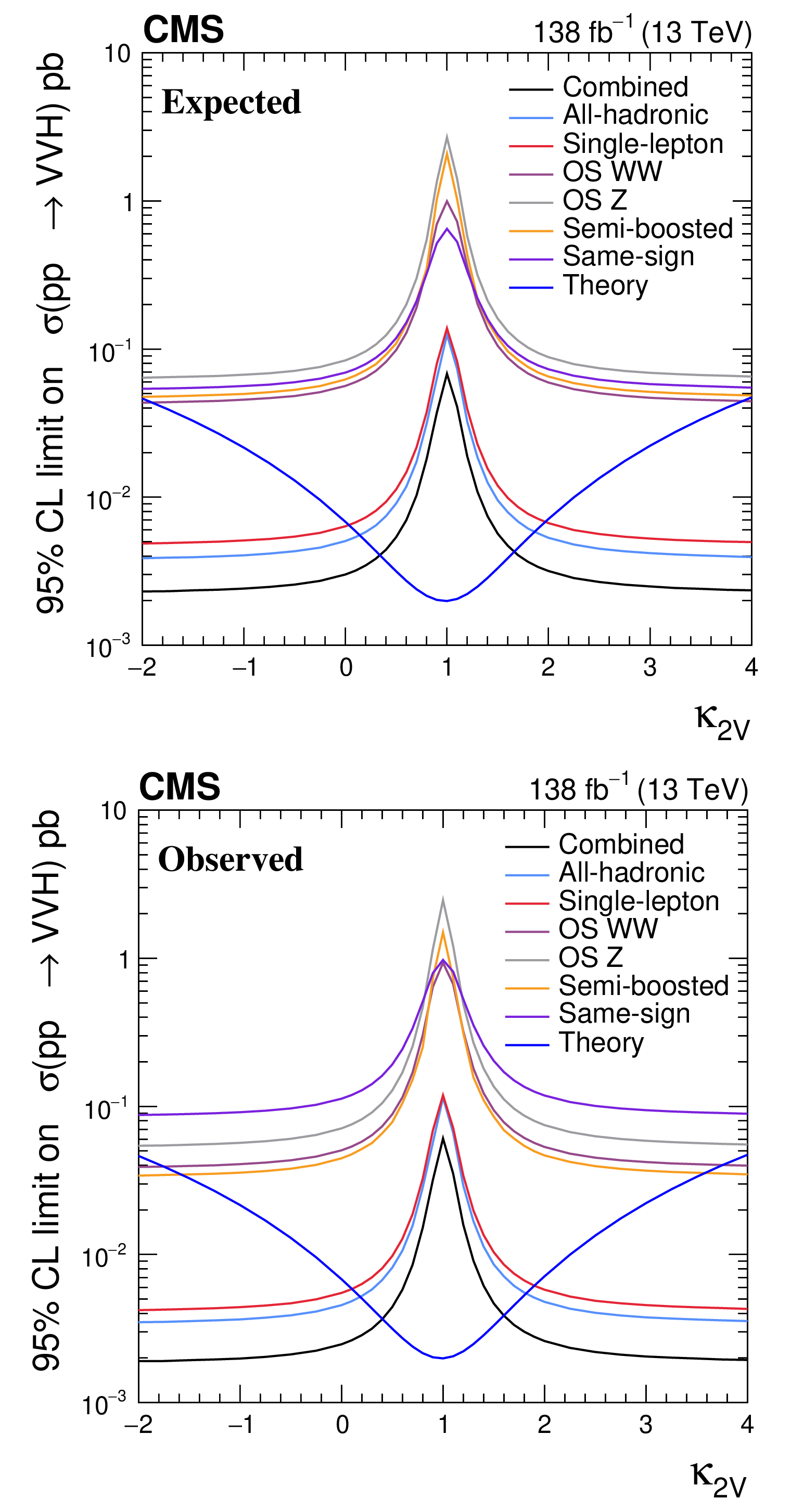
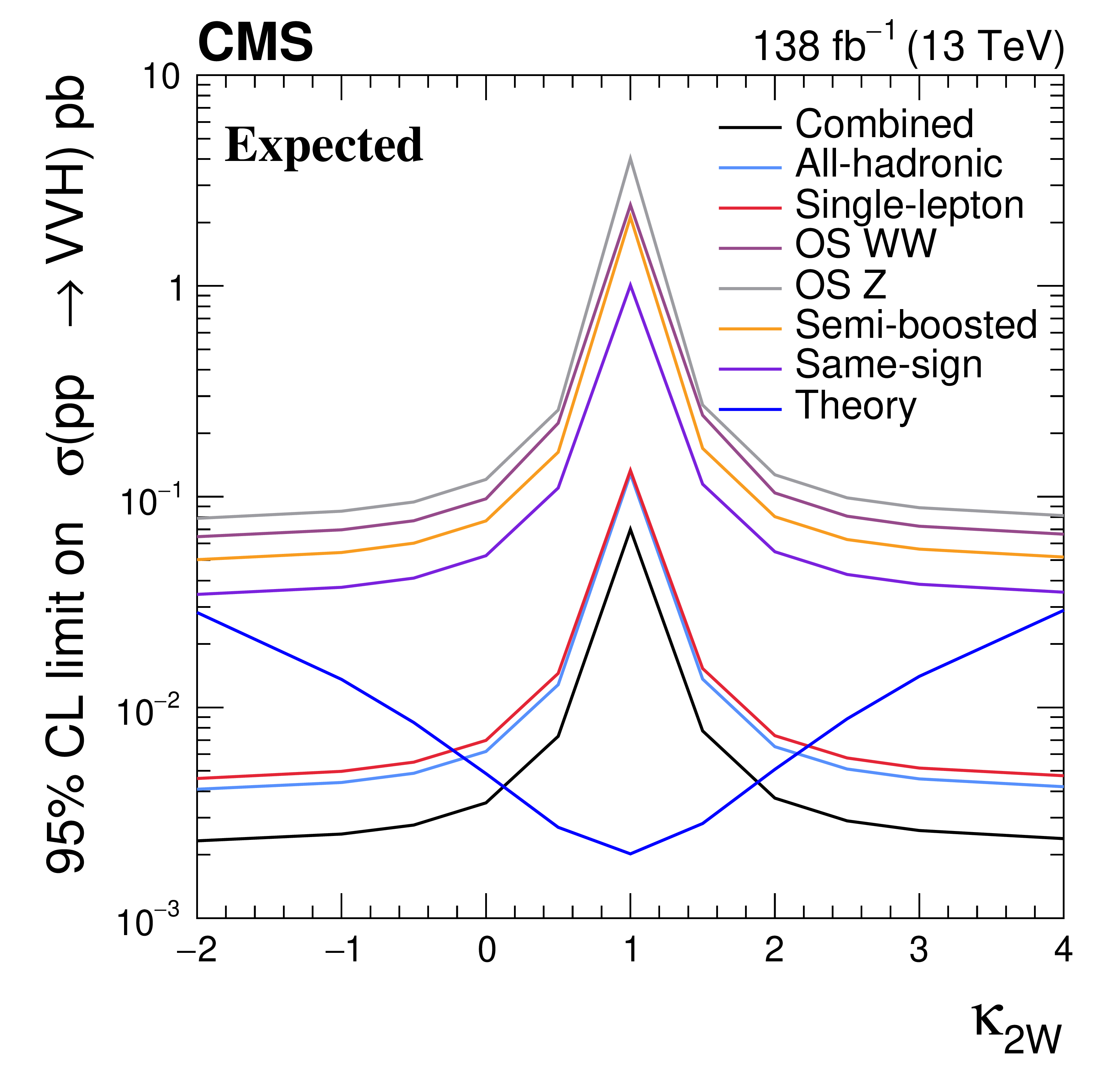
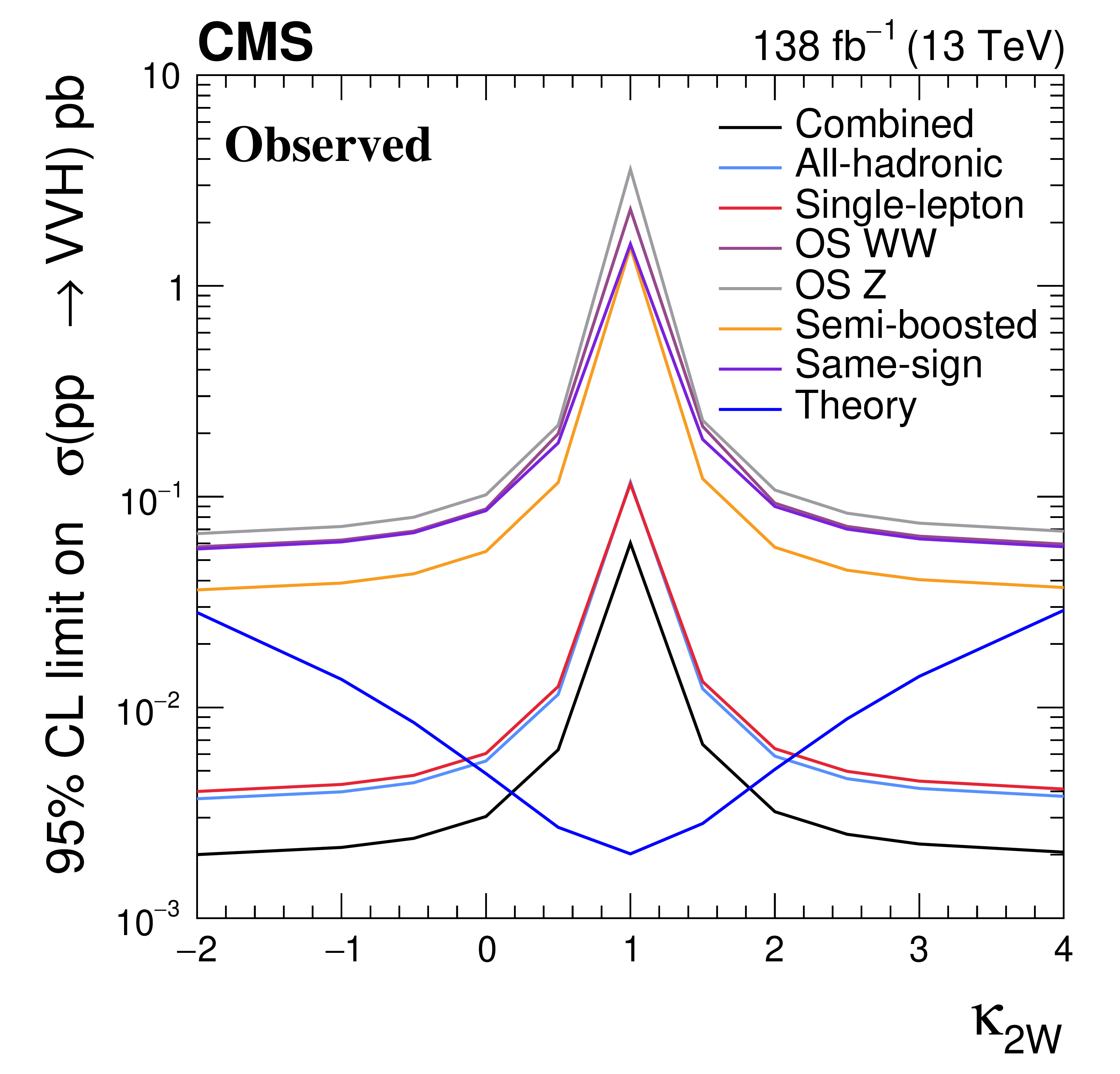
Comparison of the expected (left) and observed (right) 95% CL limits on $ \kappa_{2\mathrm{V}} $. The combined limit is shown as in black, while the limits obtained in individual channel are shown as colored lines. |
png pdf |
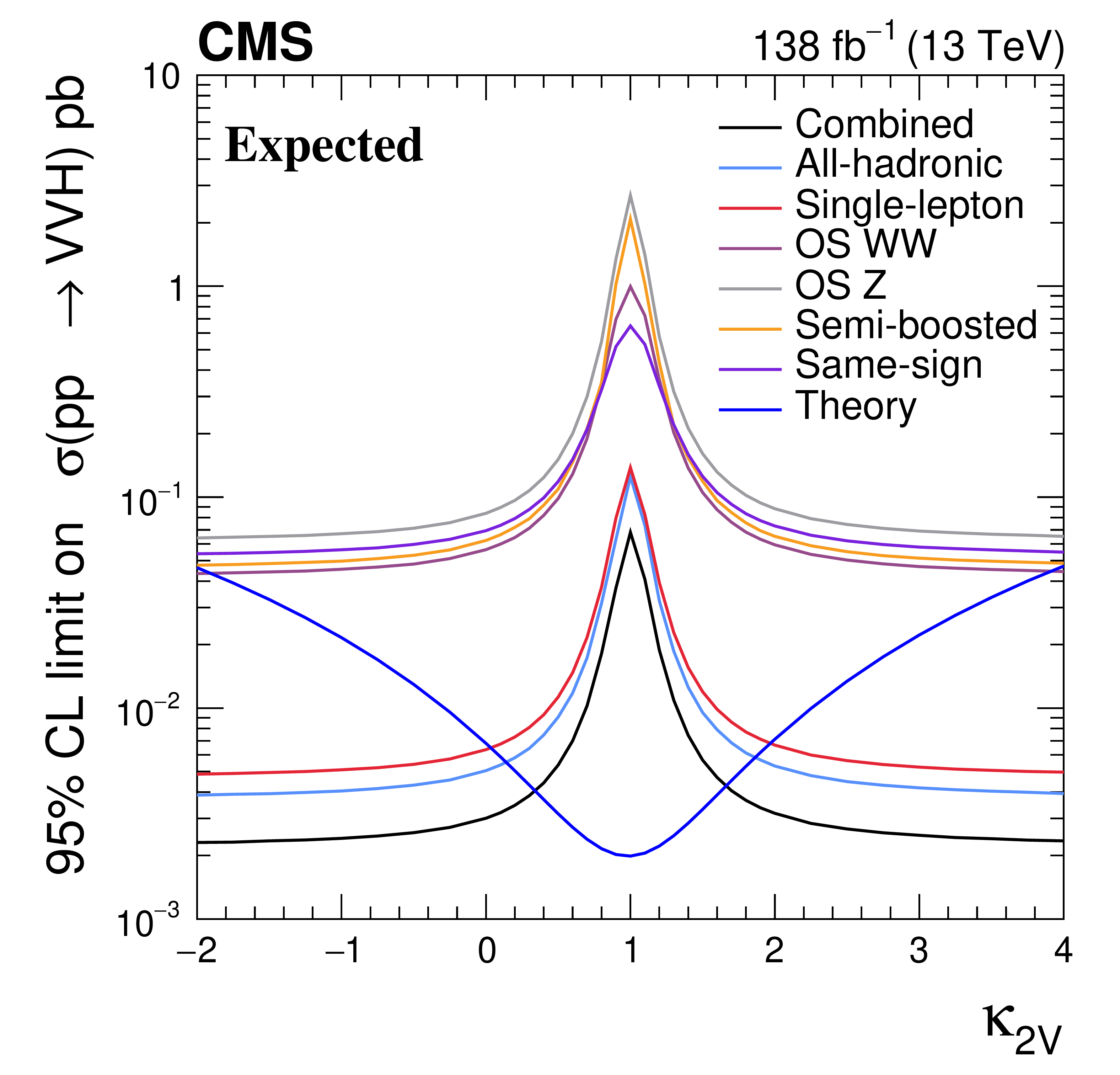
Figure A9-a:
Comparison of the expected (left) and observed (right) 95% CL limits on $ \kappa_{2\mathrm{V}} $. The combined limit is shown as in black, while the limits obtained in individual channel are shown as colored lines. |
png pdf |
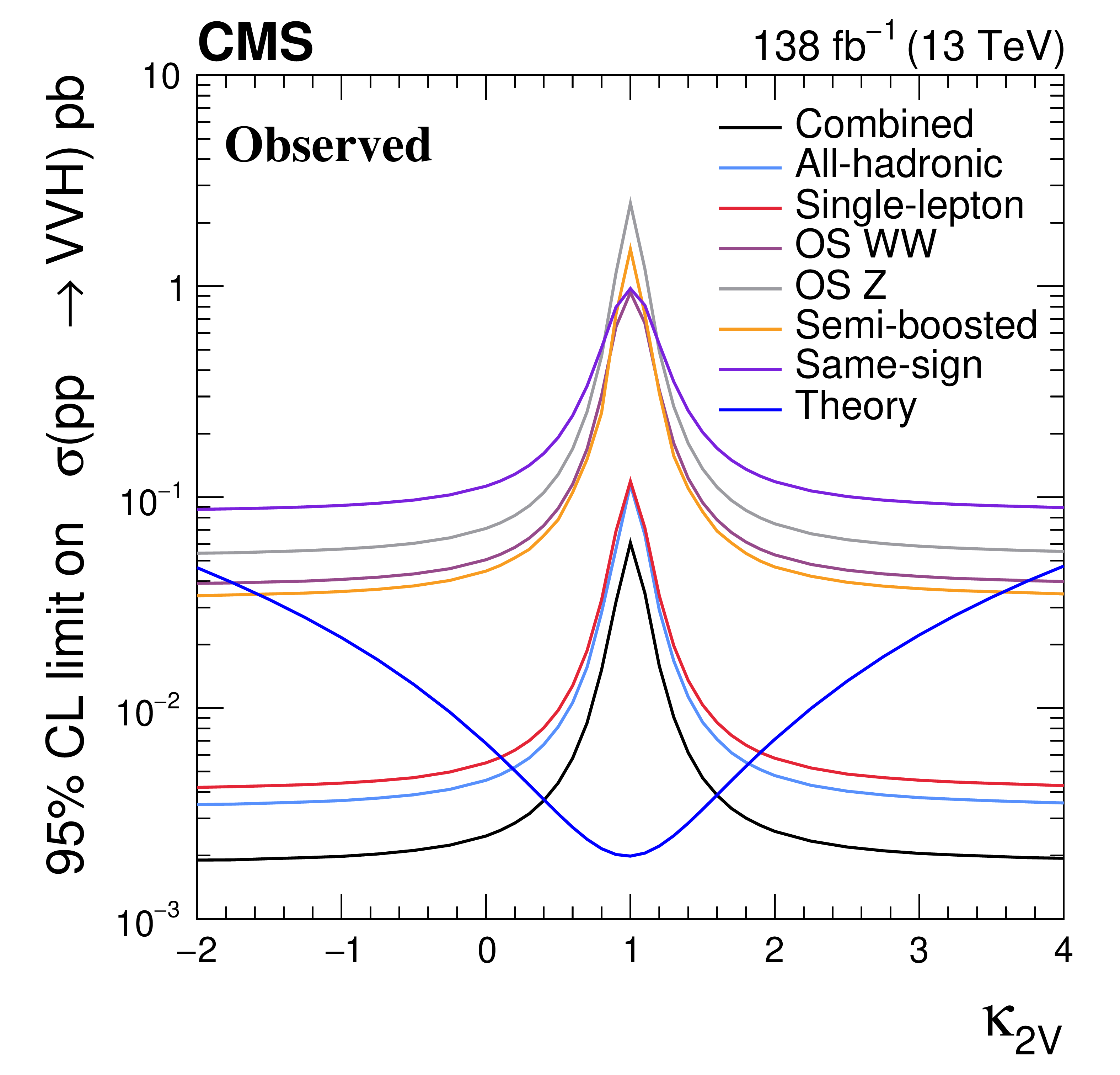
Figure A9-b:
Comparison of the expected (left) and observed (right) 95% CL limits on $ \kappa_{2\mathrm{V}} $. The combined limit is shown as in black, while the limits obtained in individual channel are shown as colored lines. |
png pdf |
Figure A10:
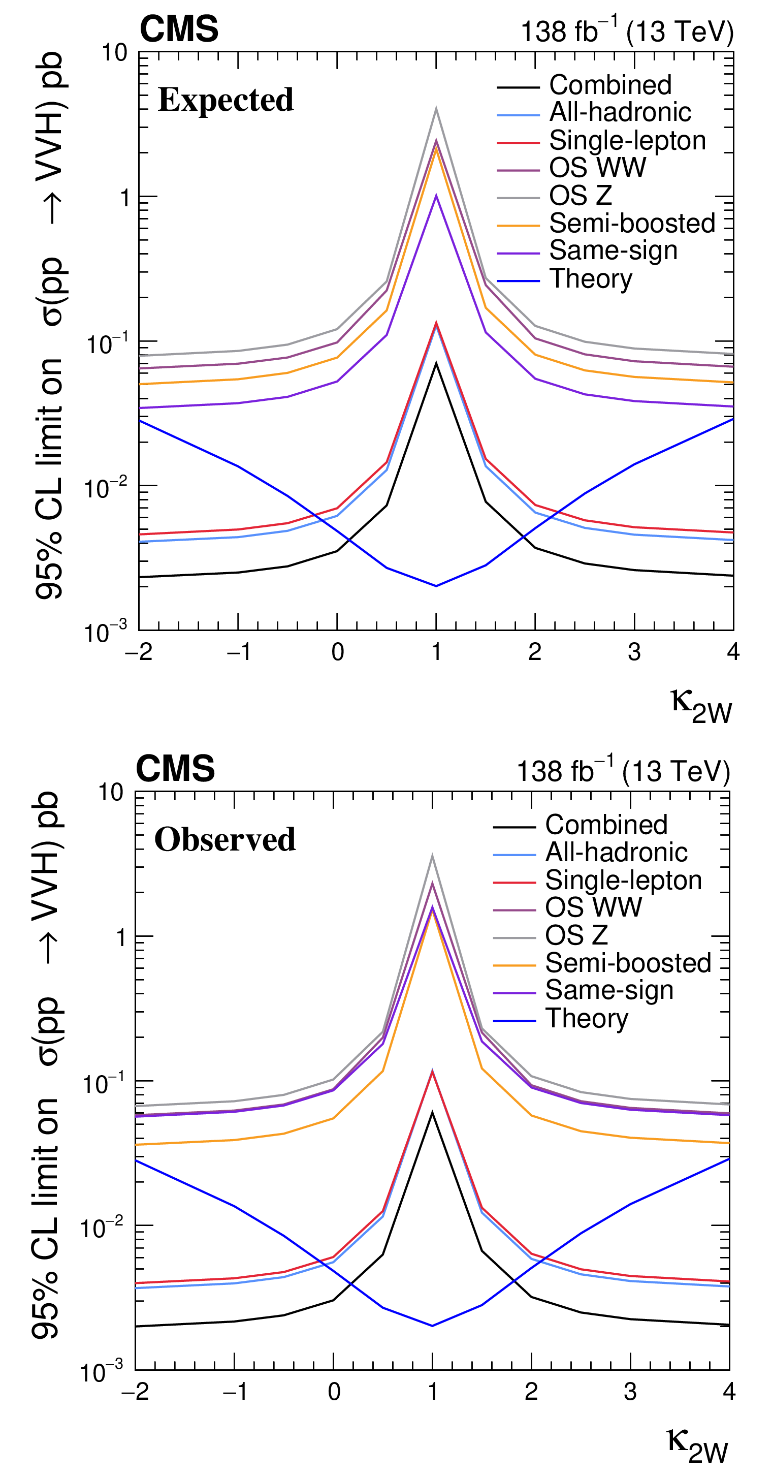
Comparison of the expected (left) and observed (right) 95% CL limits on $ \kappa_{2\mathrm{W}} $. The combined limit is shown as in black, while the limits obtained in individual channel are shown as colored lines. |
png pdf |
Figure A10-a:
Comparison of the expected (left) and observed (right) 95% CL limits on $ \kappa_{2\mathrm{W}} $. The combined limit is shown as in black, while the limits obtained in individual channel are shown as colored lines. |
png pdf |
Figure A10-b:
Comparison of the expected (left) and observed (right) 95% CL limits on $ \kappa_{2\mathrm{W}} $. The combined limit is shown as in black, while the limits obtained in individual channel are shown as colored lines. |
png pdf |
Figure A11:
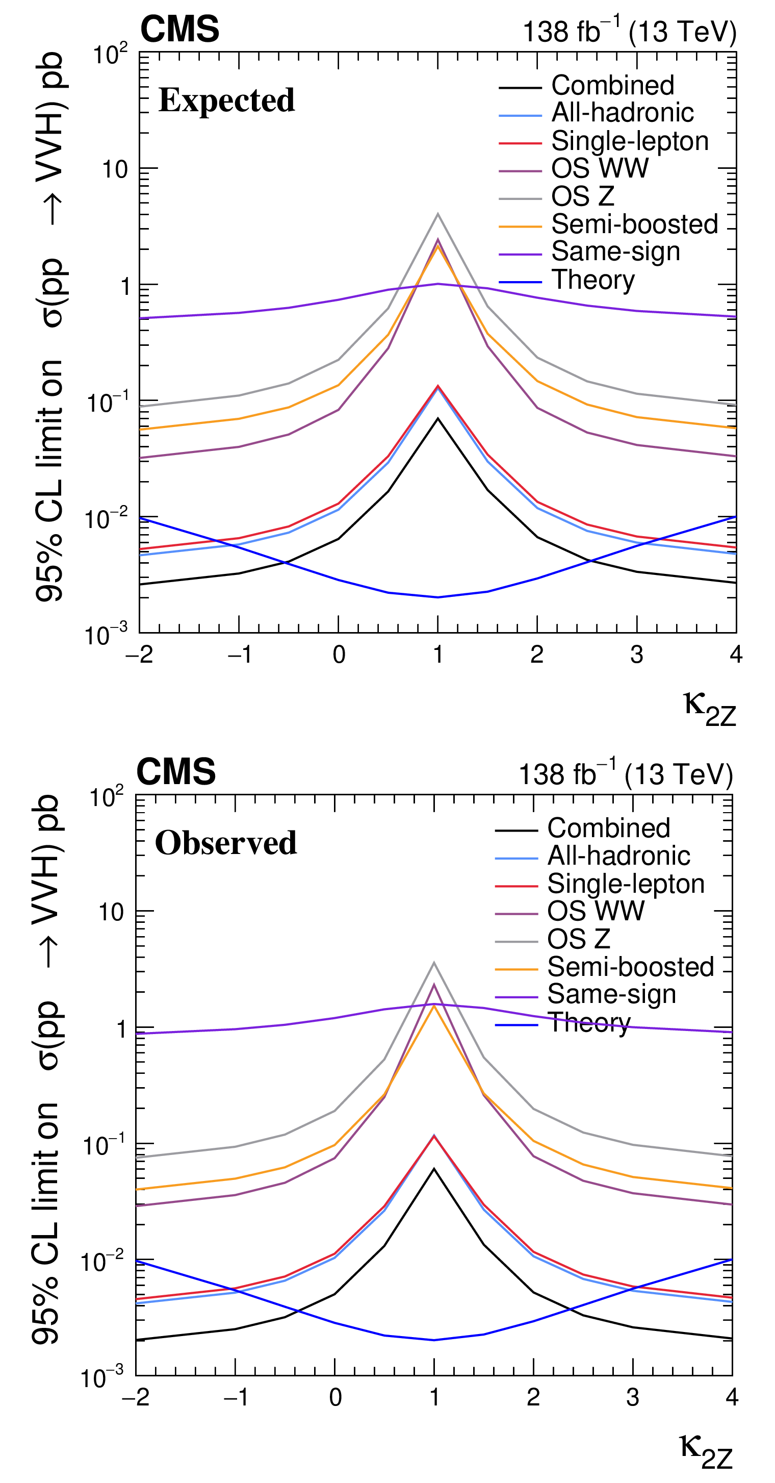
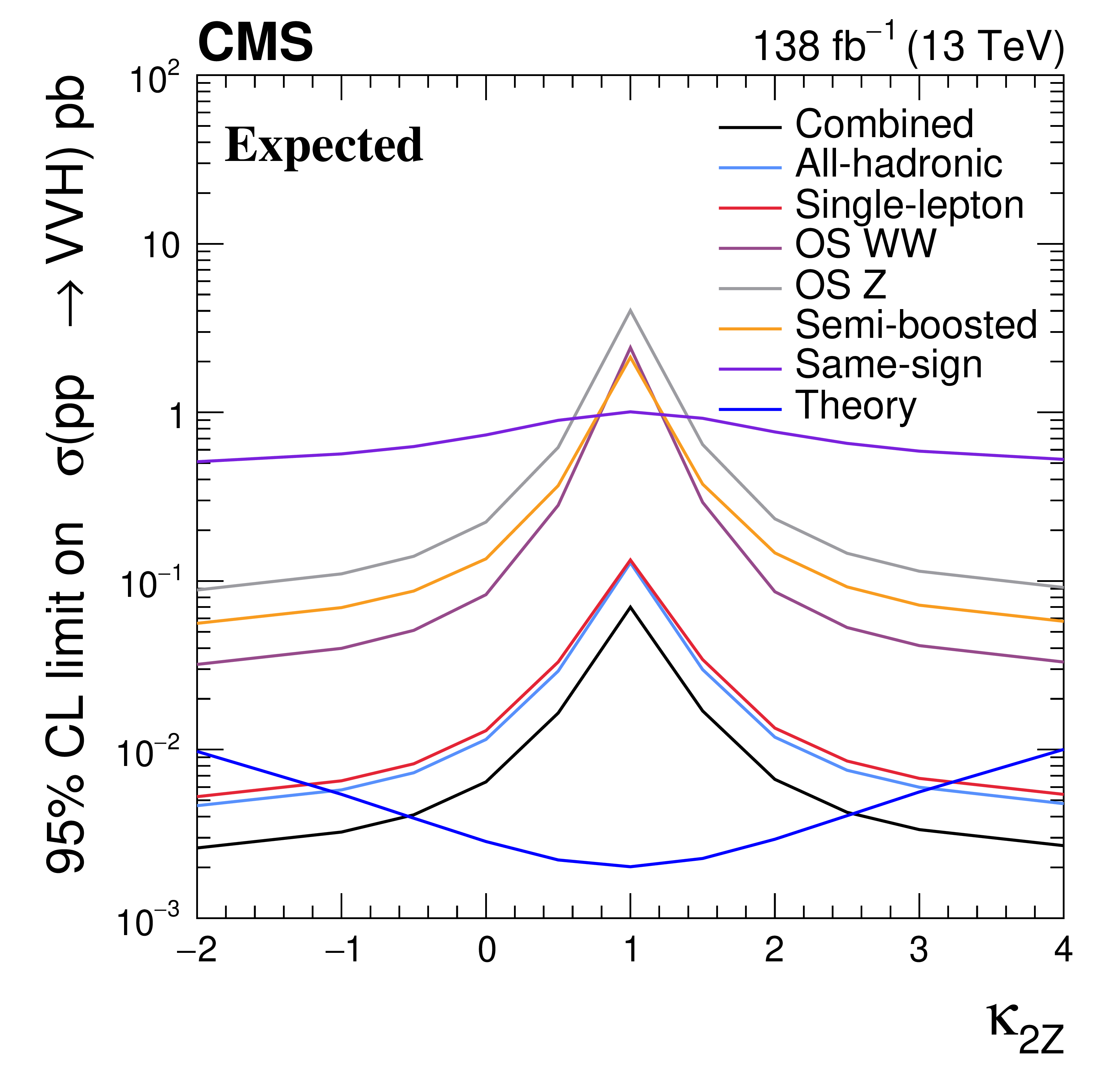
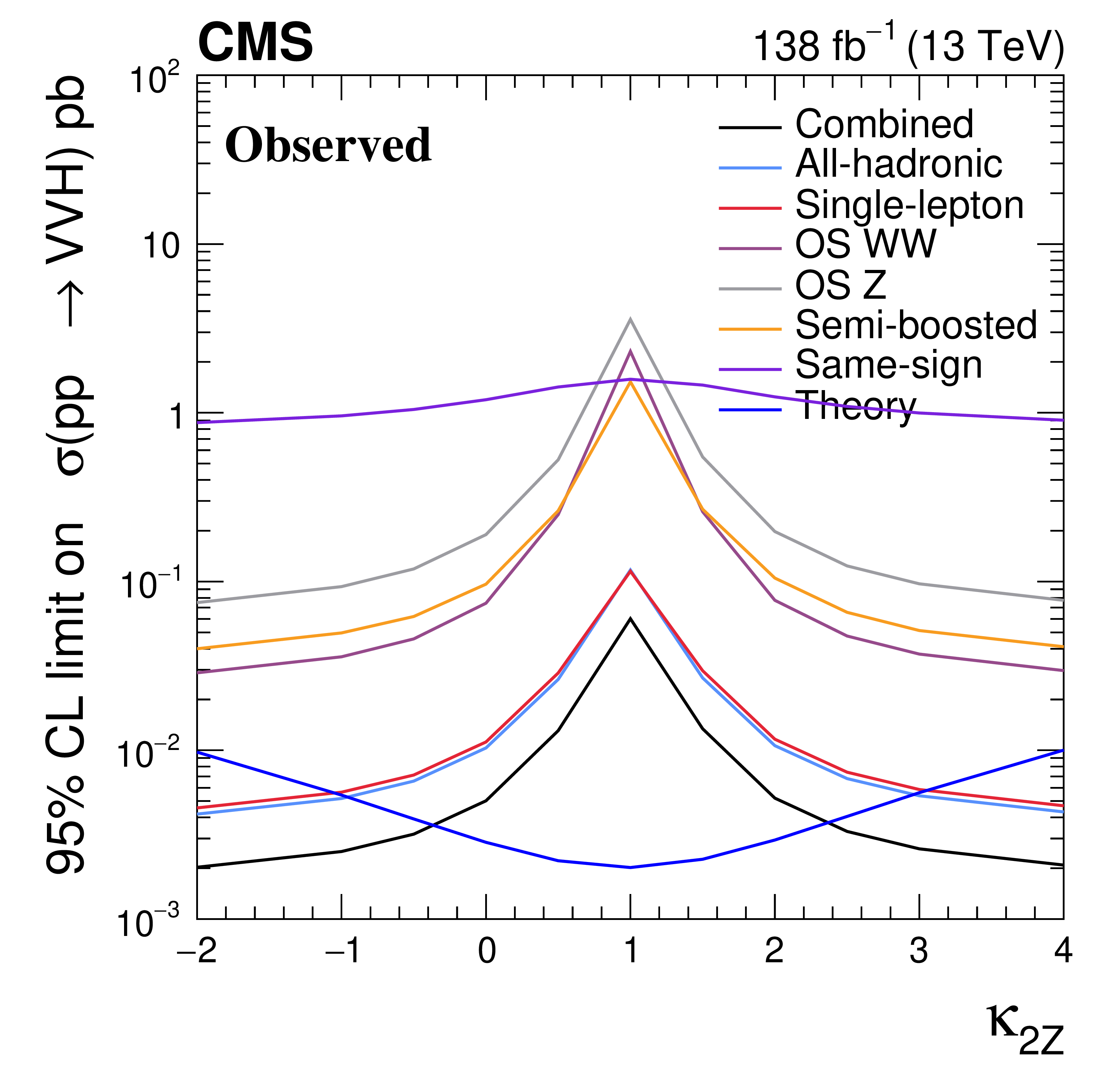
Comparison of the expected (left) and observed (right) 95% CL limits on $ \kappa_{2\mathrm{Z}} $. The combined limit is shown as in black, while the limits obtained in individual channel are shown as colored lines. |
png pdf |
Figure A11-a:
Comparison of the expected (left) and observed (right) 95% CL limits on $ \kappa_{2\mathrm{Z}} $. The combined limit is shown as in black, while the limits obtained in individual channel are shown as colored lines. |
png pdf |
Figure A11-b:
Comparison of the expected (left) and observed (right) 95% CL limits on $ \kappa_{2\mathrm{Z}} $. The combined limit is shown as in black, while the limits obtained in individual channel are shown as colored lines. |
png pdf |
Figure A12:
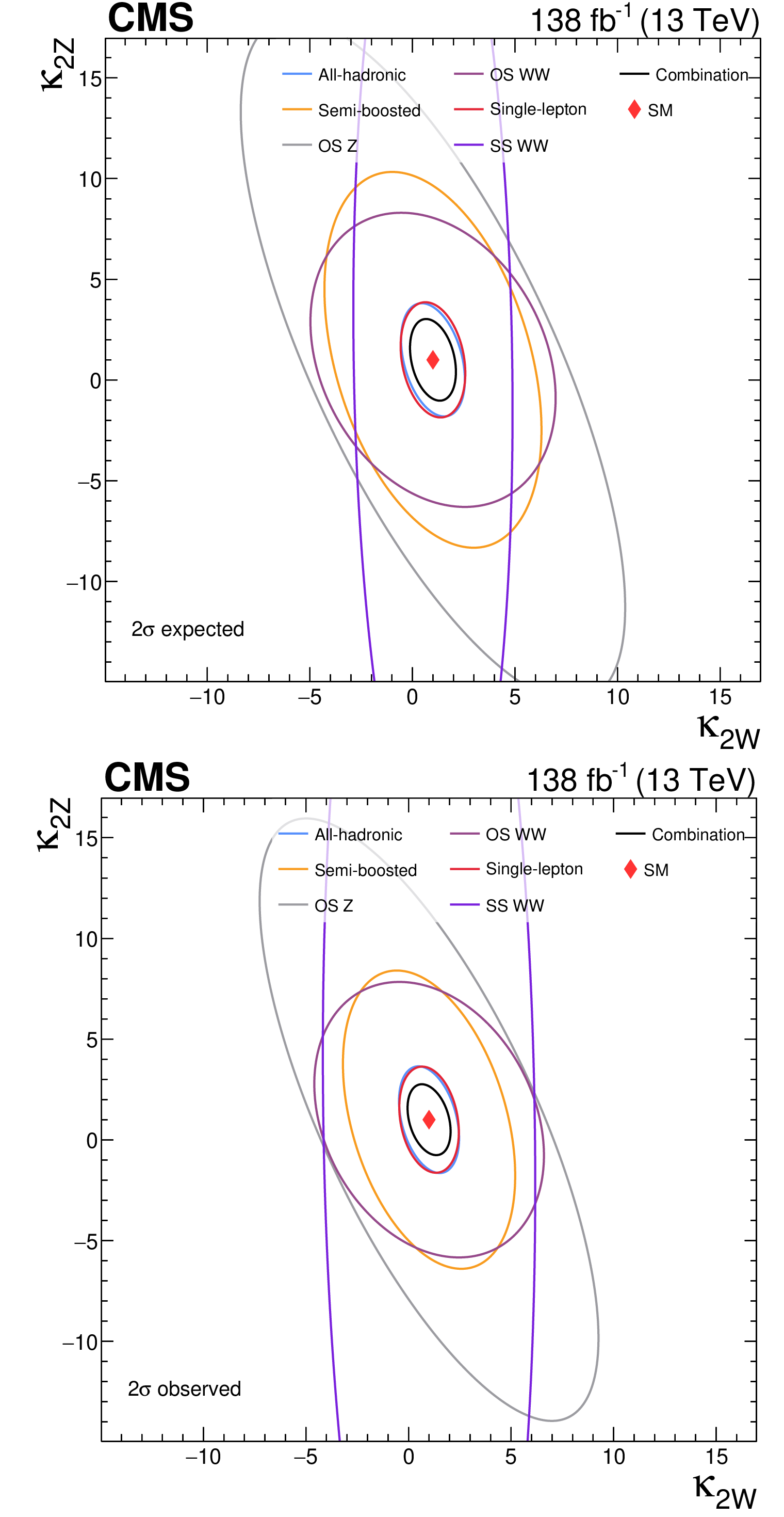
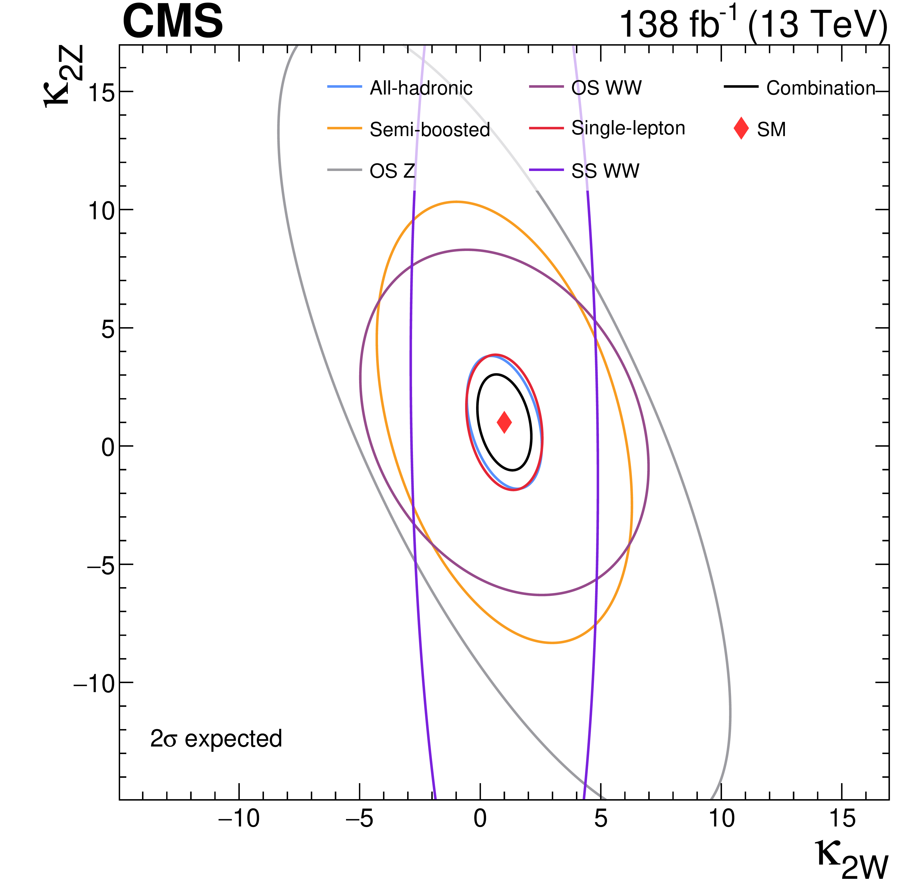
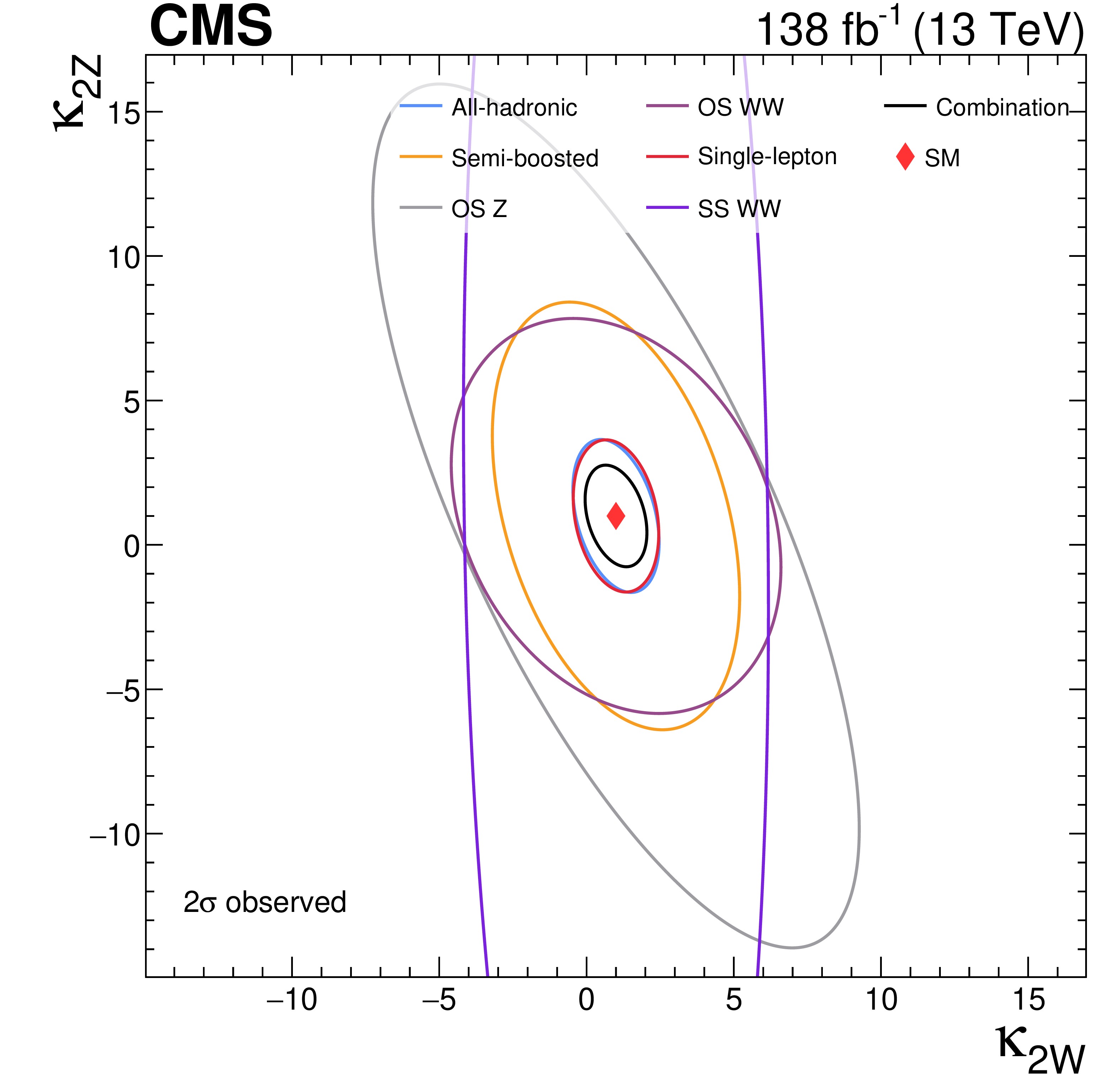
Comparison of the expected (left) and observed (right) exclusion regions corresponding to 2 standard deviations ($ \sigma $), in the two-dimensional $ \kappa_{2\mathrm{W}}-\kappa_{2\mathrm{Z}} $ plane. The combined exclusion region is shown as in black, while the exclusion regions obtained in individual channel are shown as colored lines. |
png pdf |
Figure A12-a:
Comparison of the expected (left) and observed (right) exclusion regions corresponding to 2 standard deviations ($ \sigma $), in the two-dimensional $ \kappa_{2\mathrm{W}}-\kappa_{2\mathrm{Z}} $ plane. The combined exclusion region is shown as in black, while the exclusion regions obtained in individual channel are shown as colored lines. |
png pdf |
Figure A12-b:
Comparison of the expected (left) and observed (right) exclusion regions corresponding to 2 standard deviations ($ \sigma $), in the two-dimensional $ \kappa_{2\mathrm{W}}-\kappa_{2\mathrm{Z}} $ plane. The combined exclusion region is shown as in black, while the exclusion regions obtained in individual channel are shown as colored lines. |
| Tables | |
png pdf |
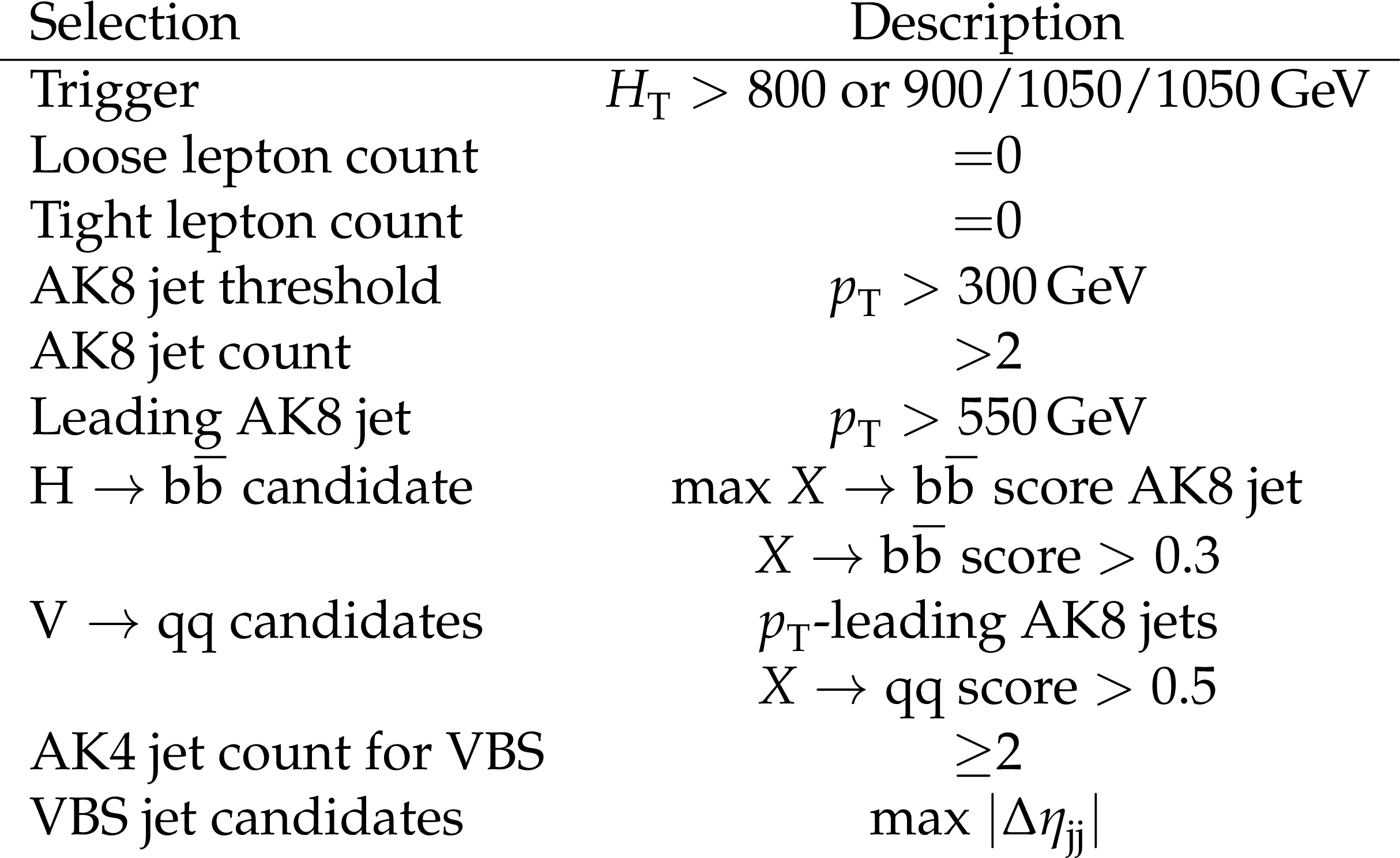
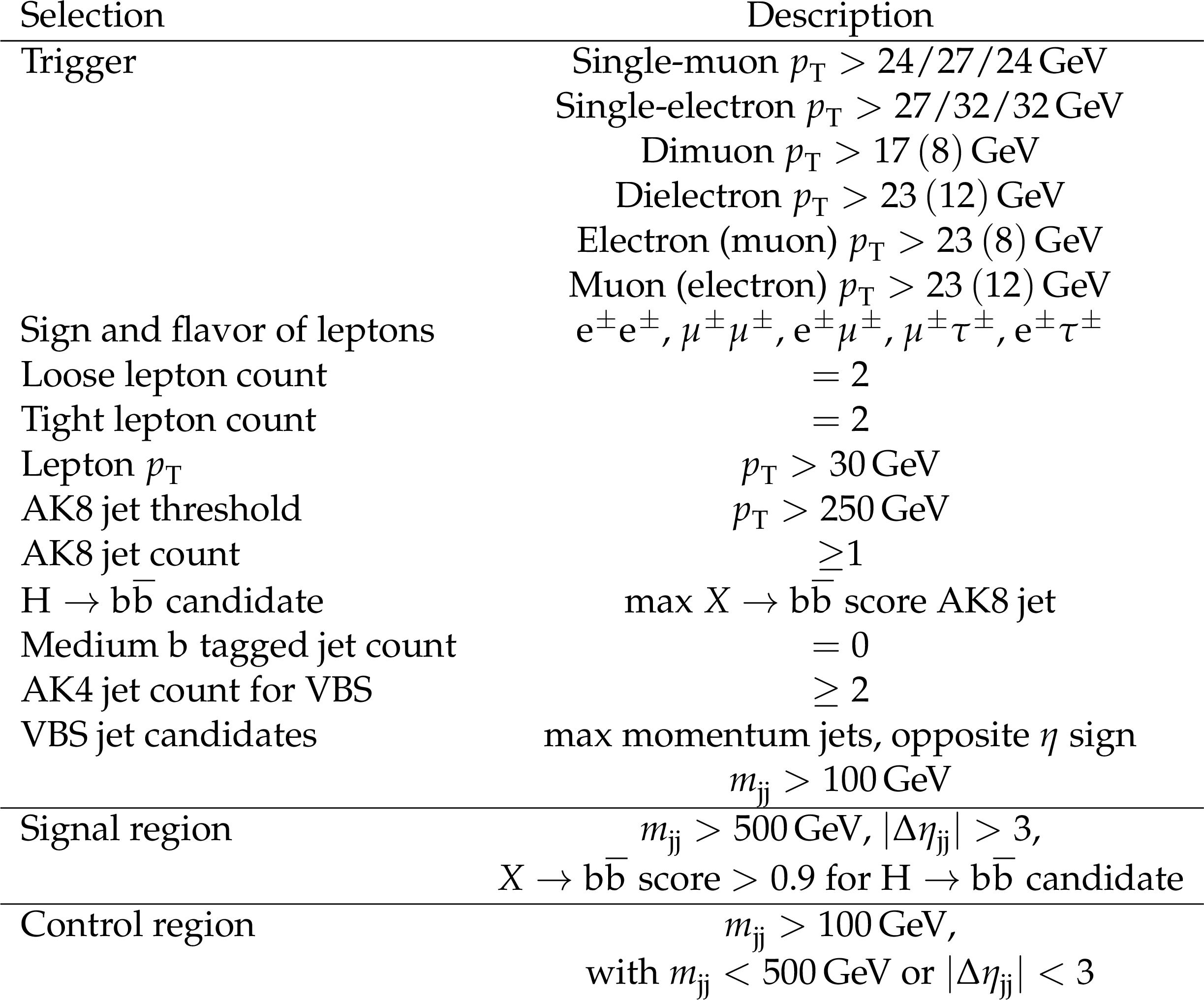
Table 1:
Selection criteria used in the all-hadronic fully boosted channel. If selection criteria differ across years, they are quoted as ``2016/2017/2018''. |
png pdf |
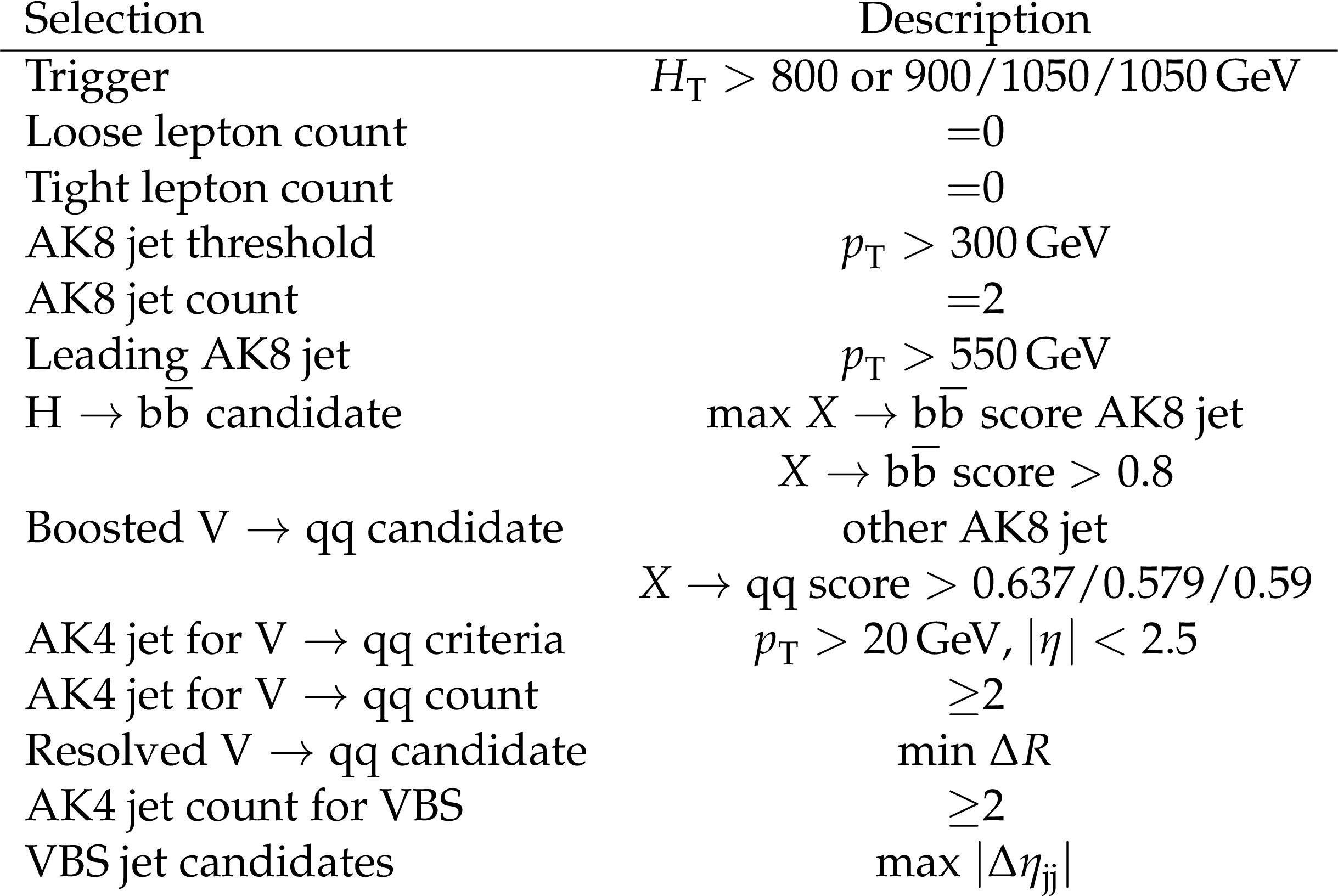
Table 2:
Selection criteria used in the all-hadronic semi-boosted channel. If the selection criteria differ across years, they are quoted as ``2016/2017/2018''. |
png pdf |
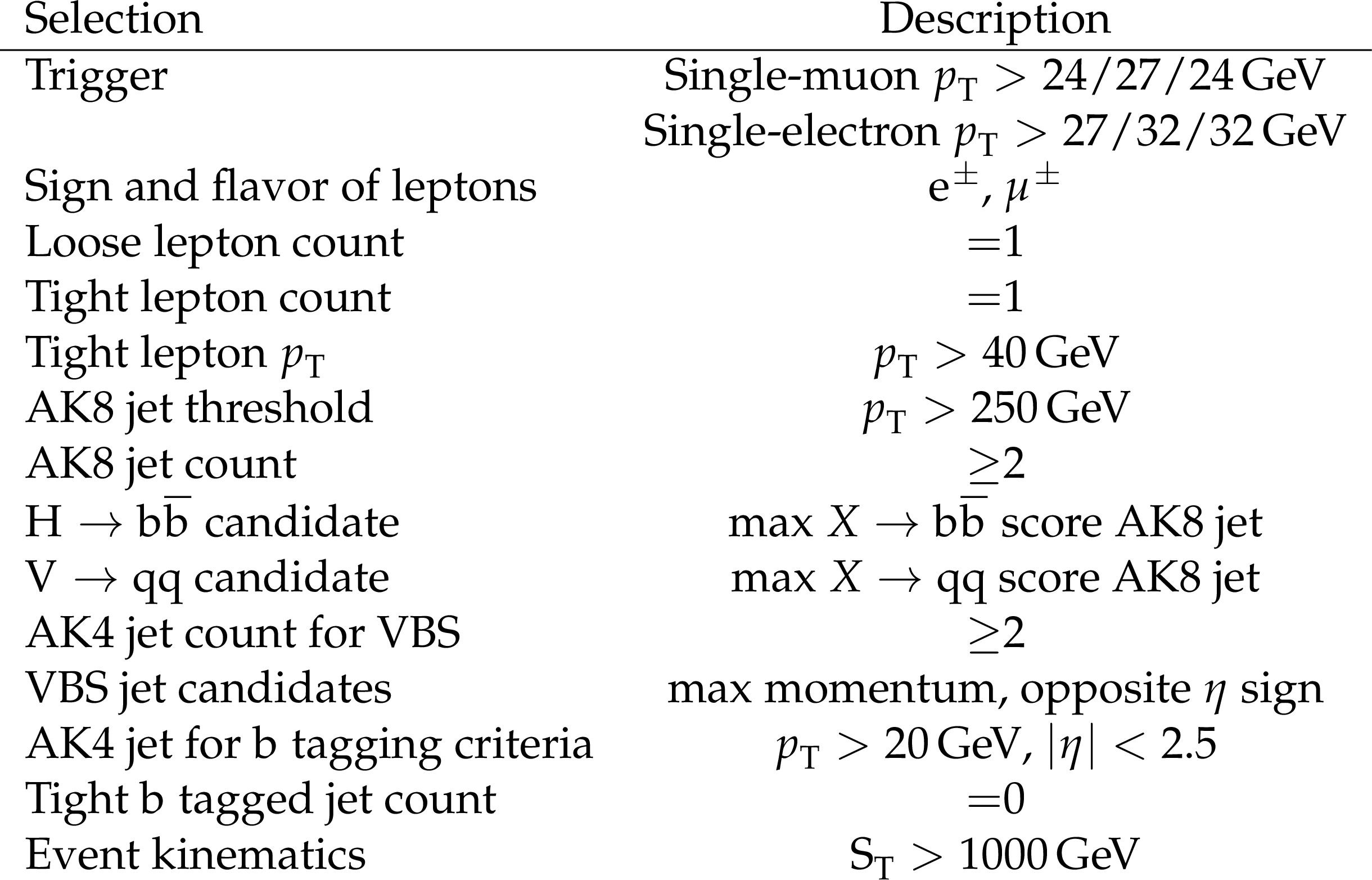
Table 3:
Selection criteria used in the single-lepton channel. If the selection criteria differ across years, they are quoted as ``2016/2017/2018''. |
png pdf |
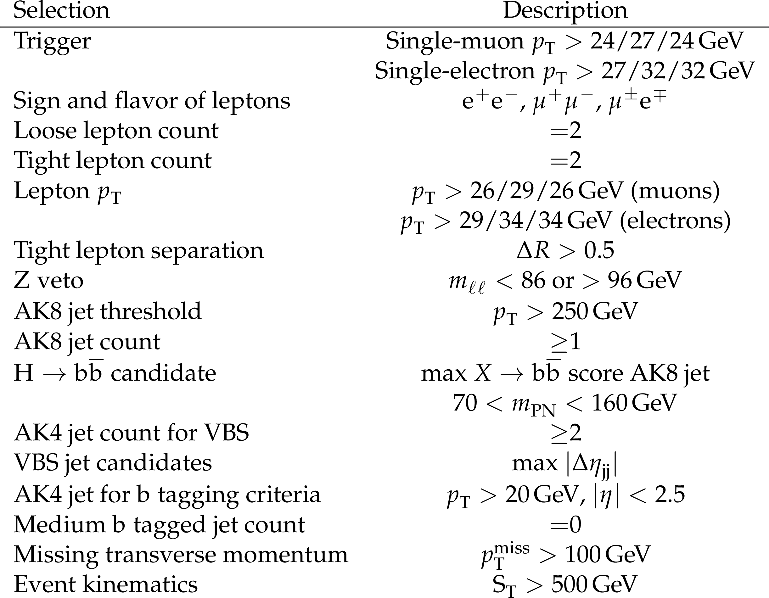
Table 4:
Selection criteria in used the OS WW dilepton channel. If the selection criteria differ across years, they are quoted as ``2016/2017/2018''. |

png pdf |
Table 5:
Selection criteria used in the OS Z dilepton channel. If the selection criteria differ across years, they are quoted as ``2016/2017/2018''. |
png pdf |
Table 6:
Selection criteria used in the SS dilepton channel. If the selection criteria differ across years, they are quoted as ``2016/2017/2018''. |
png pdf |
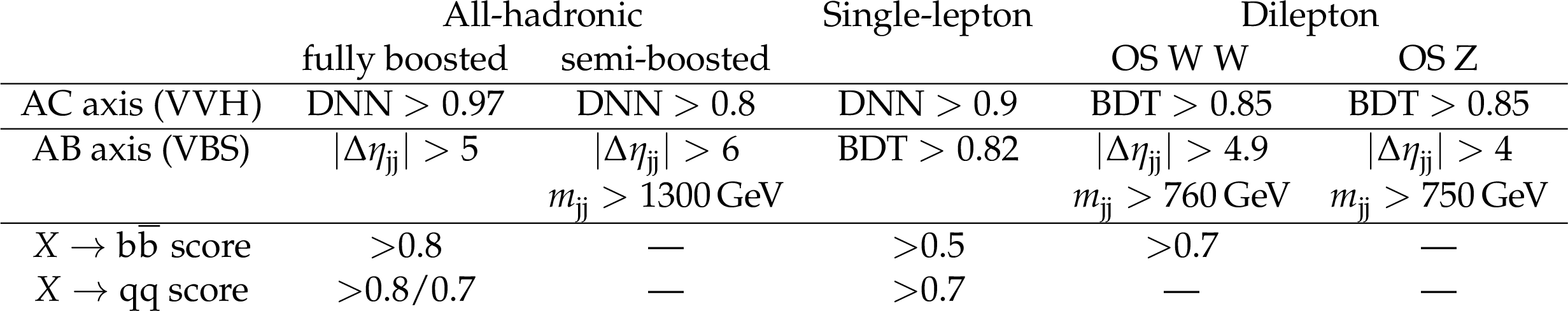
Table 7:
Summary of the selections used to define the signal region, or region A, in the all-hadronic, single-lepton, and OS dilepton channels. The selections on the ``AB axis'' and ``AC axis'' are inverted to define the regions B, C and D. Additional selections on the $ X\to\mathrm{b}\overline{\mathrm{b}} $ and $ X\to\mathrm{qq} $ scores are applied after the training to further improve the sensitivity of the search. For the all-hadronic fully boosted channel, the selections on the $ X\to\mathrm{qq} $ score are applied on the $ p_{\mathrm{T}} $-leading/subleading vector boson candidates. |
png pdf |
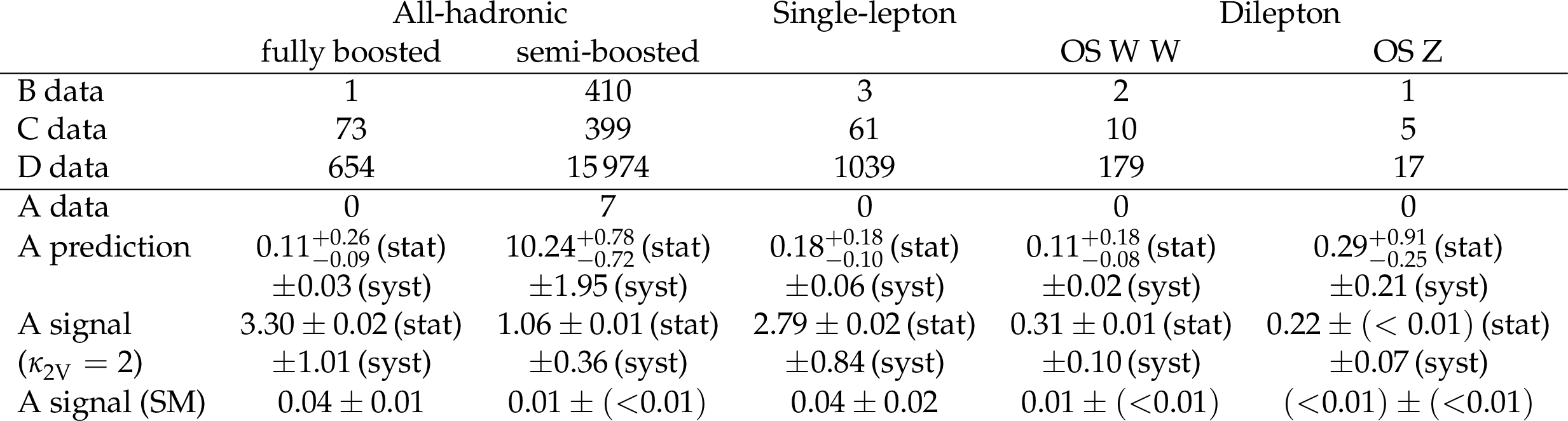
Table 8:
Data yields in regions B, C and D, used to estimate the background in region A, along with data, predicted background, and expected signal in region A. Signal yields are shown for the SM and $ \kappa_{2\mathrm{V}}= $ 2 benchmarks. |
png pdf |
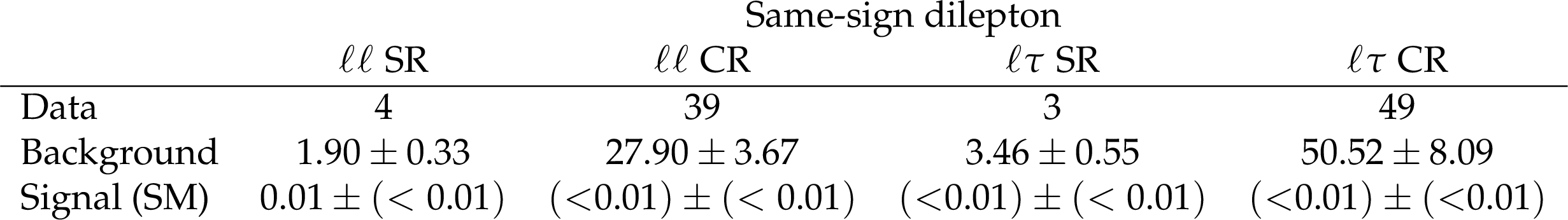
Table 9:
Data yields, predicted background and expected signal in signal (SR) and control regions (CR) of the same-sign dilepton channel. |
| Summary |
| In summary, the first study of VVH production through vector boson scattering is presented, using proton-proton collision data recorded by the CMS experiment at the LHC in 2016--2018, at $\sqrt{s} = 13$ TeV, corresponding to an integrated luminosity of 138 fb$ ^{-1}$. Selected events are consistent with the presence of two jets originating from VBS and an H decaying into a pair of b quarks, reconstructed as a single large-radius jet. Final states with zero, one, or two charged leptons arising from the decay of two vector bosons are studied. The VBS VVH production is excluded at 95% CL for values of the $k_{2V}$ coupling modifier outside the observed (expected) range of $0.40 < k_{2V} < 1.60$ ($0.34 < k_{2V} < 1.66$), assuming all other H couplings are equal to their values in the standard model.The results represent one of the best constraints to date on $k_{2V}$ using CMS data, complementing the results obtained from searches for H pair production, and laying the foundation for future, similar studies.The $k_{2W}$ and $k_{2Z}$ coupling modifiers are also constrained independently in the observed (expected) ranges of $0.17 < k_{2W}< 1.84$ ($0.11 < k_{2W} < 1.89$) and $-0.37 < k_{2Z} < 2.38$ ($-0.54 < k_{2Z} < 2.54$), respectively. A two-dimensional scan, determining exclusion regions in the $k_{2W}-k_{2Z}$ plane, is also provided, which largely improves on the constraints coming from the CMS search for VHH production. |
| References | ||||
| 1 | ATLAS Collaboration | Observation of a new particle in the search for the standard model Higgs boson with the ATLAS detector at the LHC | PLB 716 (2012) 1 | 1207.7214 |
| 2 | CMS Collaboration | Observation of a new boson at a mass of 125 GeV with the CMS experiment at the LHC | PLB 716 (2012) 30 | CMS-HIG-12-028 1207.7235 |
| 3 | CMS Collaboration | Observation of a new boson with mass near 125 GeV in pp collisions at $ \sqrt{s}= $ 7 and 8 TeV | JHEP 06 (2013) 081 | CMS-HIG-12-036 1303.4571 |
| 4 | LHC Higgs Cross Section Working Group , S. Heinemeyer et al. | Handbook of LHC Higgs cross sections: 3. Higgs properties | CERN Report CERN-2013-004, 2013 link |
1307.1347 |
| 5 | LHC Higgs Cross Section Working Group , D. de Florian et al. | Handbook of LHC Higgs cross sections: 4. Deciphering the nature of the Higgs sector | CERN Report CERN-2017-002-M, 2016 link |
1610.07922 |
| 6 | CMS Collaboration | Combination of searches for nonresonant Higgs boson pair production in proton-proton collisions at $ \sqrt{s} = $ 13 TeV | Submitted to Journal of Physics G, 2025 | CMS-HIG-20-011 2510.07527 |
| 7 | ATLAS Collaboration | Combination of searches for Higgs boson pair production in pp collisions at $ \sqrt{s} = $ 13 TeV with the ATLAS detector | PRL 133 (2024) 101801 | 2406.09971 |
| 8 | J. Alwall et al. | The automated computation of tree-level and next-to-leading order differential cross sections, and their matching to parton shower simulations | JHEP 07 (2014) 079 | 1405.0301 |
| 9 | CMS Collaboration | Search for Higgs boson pair production with one associated vector boson in proton-proton collisions at $ \sqrt{s} = $ 13 TeV | JHEP 10 (2024) 061 | CMS-HIG-22-006 2404.08462 |
| 10 | CMS Collaboration | The CMS experiment at the CERN LHC | JINST 3 (2008) S08004 | |
| 11 | CMS Collaboration | Development of the CMS detector for the CERN LHC Run 3 | JINST 19 (2024) P05064 | CMS-PRF-21-001 2309.05466 |
| 12 | CMS Collaboration | Performance of the CMS Level-1 trigger in proton-proton collisions at $ \sqrt{s} = $ 13 TeV | JINST 15 (2020) P10017 | CMS-TRG-17-001 2006.10165 |
| 13 | CMS Collaboration | The CMS trigger system | JINST 12 (2017) P01020 | CMS-TRG-12-001 1609.02366 |
| 14 | CMS Collaboration | Performance of the CMS high-level trigger during LHC Run 2 | JINST 19 (2024) P11021 | CMS-TRG-19-001 2410.17038 |
| 15 | CMS Collaboration | Electron and photon reconstruction and identification with the CMS experiment at the CERN LHC | JINST 16 (2021) P05014 | CMS-EGM-17-001 2012.06888 |
| 16 | CMS Collaboration | Performance of the CMS muon detector and muon reconstruction with proton-proton collisions at $ \sqrt{s}= $ 13 TeV | JINST 13 (2018) P06015 | CMS-MUO-16-001 1804.04528 |
| 17 | CMS Collaboration | Description and performance of track and primary-vertex reconstruction with the CMS tracker | JINST 9 (2014) P10009 | CMS-TRK-11-001 1405.6569 |
| 18 | CMS Collaboration | Particle-flow reconstruction and global event description with the CMS detector | JINST 12 (2017) P10003 | CMS-PRF-14-001 1706.04965 |
| 19 | CMS Collaboration | Performance of reconstruction and identification of $ \tau $ leptons decaying to hadrons and $ \nu_\tau $ in pp collisions at $ \sqrt{s}= $ 13 TeV | JINST 13 (2018) P10005 | CMS-TAU-16-003 1809.02816 |
| 20 | CMS Collaboration | Jet energy scale and resolution in the CMS experiment in pp collisions at 8 TeV | JINST 12 (2017) P02014 | CMS-JME-13-004 1607.03663 |
| 21 | CMS Collaboration | Performance of missing transverse momentum reconstruction in proton-proton collisions at $ \sqrt{s} = $ 13 TeV using the CMS detector | JINST 14 (2019) P07004 | CMS-JME-17-001 1903.06078 |
| 22 | CMS Collaboration | Technical proposal for the Phase-II upgrade of the Compact Muon Solenoid | CMS Technical Proposal CERN-LHCC-2015-010, CMS-TDR-15-02, 2015 CDS |
|
| 23 | CMS Collaboration | ECAL 2016 refined calibration and Run2 summary plots | CMS Detector Performance Summary CMS-DP-2020-021, 2020 CDS |
|
| 24 | CMS Collaboration | Measurement of the Higgs boson production rate in association with top quarks in final states with electrons, muons, and hadronically decaying tau leptons at $ \sqrt{s} = $ 13 TeV | EPJC 81 (2021) 378 | CMS-HIG-19-008 2011.03652 |
| 25 | CMS Collaboration | Identification of hadronic tau lepton decays using a deep neural network | JINST 17 (2022) P07023 | CMS-TAU-20-001 2201.08458 |
| 26 | M. Cacciari, G. P. Salam, and G. Soyez | The anti-$ k_{\mathrm{T}} $ jet clustering algorithm | JHEP 04 (2008) 063 | 0802.1189 |
| 27 | M. Cacciari, G. P. Salam, and G. Soyez | FastJet user manual | EPJC 72 (2012) 1896 | 1111.6097 |
| 28 | CMS Collaboration | Pileup mitigation at CMS in 13 TeV data | JINST 15 (2020) P09018 | CMS-JME-18-001 2003.00503 |
| 29 | D. Bertolini, P. Harris, M. Low, and N. Tran | Pileup per particle identification | JHEP 10 (2014) 059 | 1407.6013 |
| 30 | H. Qu and L. Gouskos | ParticleNet: Jet tagging via particle clouds | PRD 101 (2020) 056019 | 1902.08570 |
| 31 | A. J. Larkoski, S. Marzani, G. Soyez, and J. Thaler | Soft drop | JHEP 05 (2014) 146 | 1402.2657 |
| 32 | M. Dasgupta, A. Fregoso, S. Marzani, and G. P. Salam | Towards an understanding of jet substructure | JHEP 09 (2013) 029 | 1307.0007 |
| 33 | J. M. Butterworth, A. R. Davison, M. Rubin, and G. P. Salam | Jet substructure as a new Higgs search channel at the LHC | PRL 100 (2008) 242001 | 0802.2470 |
| 34 | CMS Collaboration | Identification of heavy-flavour jets with the CMS detector in pp collisions at 13 TeV | JINST 13 (2018) P05011 | CMS-BTV-16-002 1712.07158 |
| 35 | E. Bols et al. | Jet flavour classification using DeepJet | JINST 15 (2020) P12012 | 2008.10519 |
| 36 | CMS Collaboration | Performance of the DeepJet b tagging algorithm using 41.9 fb$^{-1}$ of data from proton-proton collisions at 13 TeV with Phase 1 CMS detector | CMS Detector Performance Summary CMS-DP-2018-058, 2018 CDS |
|
| 37 | T. Sjöstrand et al. | An introduction to PYTHIA 8.2 | Comput. Phys. Commun. 191 (2015) 159 | 1410.3012 |
| 38 | B. Cabouat and T. Sjöstrand | Some dipole shower studies | EPJC 78 (2018) 226 | 1710.00391 |
| 39 | O. Mattelaer | On the maximal use of Monte Carlo samples: re-weighting events at NLO accuracy | EPJC 76 (2016) 674 | 1607.00763 |
| 40 | S. Frixione, P. Nason, and G. Ridolfi | A positive-weight next-to-leading-order Monte Carlo for heavy flavour hadroproduction | JHEP 09 (2007) 126 | 0707.3088 |
| 41 | P. Nason | A new method for combining NLO QCD with shower Monte Carlo algorithms | JHEP 11 (2004) 040 | hep-ph/0409146 |
| 42 | S. Frixione, P. Nason, and C. Oleari | Matching NLO QCD computations with parton shower simulations: the POWHEG method | JHEP 11 (2007) 070 | 0709.2092 |
| 43 | S. Alioli, P. Nason, C. Oleari, and E. Re | A general framework for implementing NLO calculations in shower Monte Carlo programs: the POWHEG BOX | JHEP 06 (2010) 043 | 1002.2581 |
| 44 | J. Alwall et al. | Comparative study of various algorithms for the merging of parton showers and matrix elements in hadronic collisions | EPJC 53 (2008) 473 | 0706.2569 |
| 45 | CMS Collaboration | Extraction and validation of a new set of CMS PYTHIA8 tunes from underlying-event measurements | EPJC 80 (2020) 4 | CMS-GEN-17-001 1903.12179 |
| 46 | NNPDF Collaboration | Parton distributions for the LHC Run II | JHEP 04 (2015) 040 | 1410.8849 |
| 47 | NNPDF Collaboration | Parton distributions from high-precision collider data | EPJC 77 (2017) 663 | 1706.00428 |
| 48 | GEANT4 Collaboration | GEANT 4---a simulation toolkit | NIM A 506 (2003) 250 | |
| 49 | CDF Collaboration | Measurement of $ \sigma B (W \to e \nu) $ and $ \sigma B (Z^0 \to e^+ e^-) $ in $ \bar{p}p $ collisions at $ \sqrt{s} = $ 1800 GeV | PRD 44 (1991) 29 | |
| 50 | G. Kasieczka, B. Nachman, M. D. Schwartz, and D. Shih | Automating the ABCD method with machine learning | PRD 103 (2021) 035021 | 2007.14400 |
| 51 | Particle Data Group , S. Navas et al. | Review of particle physics | PRD 110 (2024) 030001 | |
| 52 | CMS Collaboration | The CMS statistical analysis and combination tool: Combine | Comput. Softw. Big Sci. 8 (2024) 19 | CMS-CAT-23-001 2404.06614 |
| 53 | W. Verkerke and D. Kirkby | The RooFit toolkit for data modeling | in the Int. Conf. on Computing in High Energy and Nuclear Physics (CHEP ): La Jolla CA, United States, March 24--28, 2003 Proc. 1 (2003) 3 |
physics/0306116 |
| 54 | L. Moneta et al. | The RooStats project | in the Int. Workshop on Advanced Computing and Analysis Techniques in Physics Research (ACAT ): Jaipur, India, February 22--27, 2010 Proc. 1 (2010) 3 |
1009.1003 |
| 55 | CMS Collaboration | Precision luminosity measurement in proton-proton collisions at $ \sqrt{s} = $ 13 TeV in 2015 and 2016 at CMS | EPJC 81 (2021) 800 | CMS-LUM-17-003 2104.01927 |
| 56 | CMS Collaboration | CMS luminosity measurement for the 2017 data-taking period at $ \sqrt{s}= $ 13 TeV | CMS Physics Analysis Summary, 2018 link |
CMS-PAS-LUM-17-004 |
| 57 | CMS Collaboration | CMS luminosity measurement for the 2018 data-taking period at $ \sqrt{s}= $ 13 TeV | CMS Physics Analysis Summary, 2019 link |
CMS-PAS-LUM-18-002 |
| 58 | CMS Collaboration | HEPData record for this analysis | link | |
| 59 | CMS Collaboration | Supplemental Material | URL will be inserted by publisher | |
|
|
Compact Muon Solenoid LHC, CERN |
|

|

|

|

|

|