

Compact Muon Solenoid
LHC, CERN
| CMS-HIG-20-012 ; CERN-EP-2026-010 | ||
| Search for a new heavy scalar resonance decaying into the Higgs boson and a new scalar particle in the $ \mathrm{b}\overline{\mathrm{b}}\mathrm{b}\overline{\mathrm{b}} $ final state using proton-proton collisions at $ \sqrt{s}= $ 13 TeV | ||
| CMS Collaboration | ||
| 4 May 2026 | ||
| Submitted to Physical Review D | ||
| Abstract: A search for a new heavy scalar resonance ($ \mathrm{X} $) decaying into the 125 GeV standard model Higgs boson (H) and a new scalar particle ($ \mathrm{Y} $) in proton-proton collisions at a center-of-mass energy of 13 TeV is presented. The analysis is performed using a data sample corresponding to an integrated luminosity of 138 fb$ ^{-1} $ collected with the CMS detector during LHC Run 2. The $ \mathrm{b}\overline{\mathrm{b}}\mathrm{b}\overline{\mathrm{b}} $ final state is used as a probe to search for phenomena beyond the standard model where, in the $ \mathrm{X} \to \mathrm{Y}\mathrm{H} $ process, the Y and H each decay into a bottom quark-antiquark pair. A range of masses from 400 GeV to 1.6 TeV for the resonance $ \mathrm{X} $ and from 60 GeV to 1.4 TeV for the scalar Y is investigated. The observations are in agreement with the background-only hypothesis. The largest excess, with a local (global) significance of 3.47 (2.44) standard deviations, is observed for hypothetical $ \mathrm{X} $ and Y masses of 600 and 400 GeV, respectively. Upper limits at 95% confidence level on the production cross section times branching fraction are presented for signal mass hypotheses in the range of the search. Results are interpreted within the next-to-minimal supersymmetric standard model scenario. | ||
| Links: e-print arXiv:2605.02848 [hep-ex] (PDF) ; CDS record ; inSPIRE record ; HepData record ; CADI line (restricted) ; | ||
| Figures | |

png pdf |
Figure 1:
Depiction of the process under investigation, $ \mathrm{X} \to \mathrm{Y}\mathrm{H} \to \mathrm{b}\overline{\mathrm{b}}\mathrm{b}\overline{\mathrm{b}} $. |
png pdf |
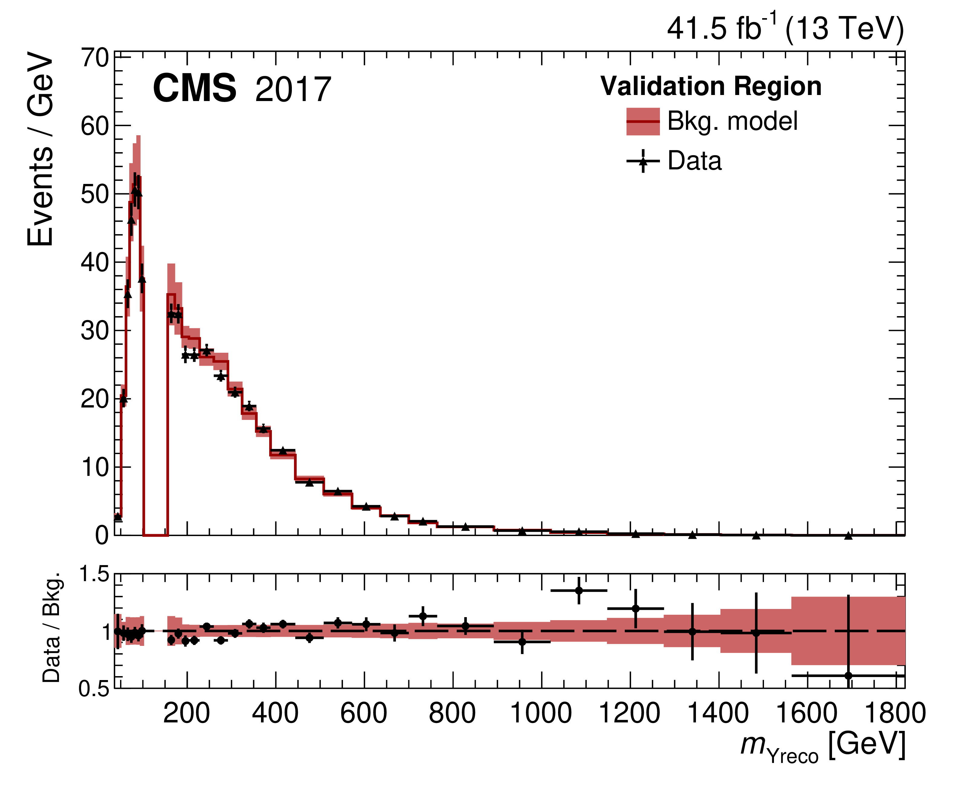
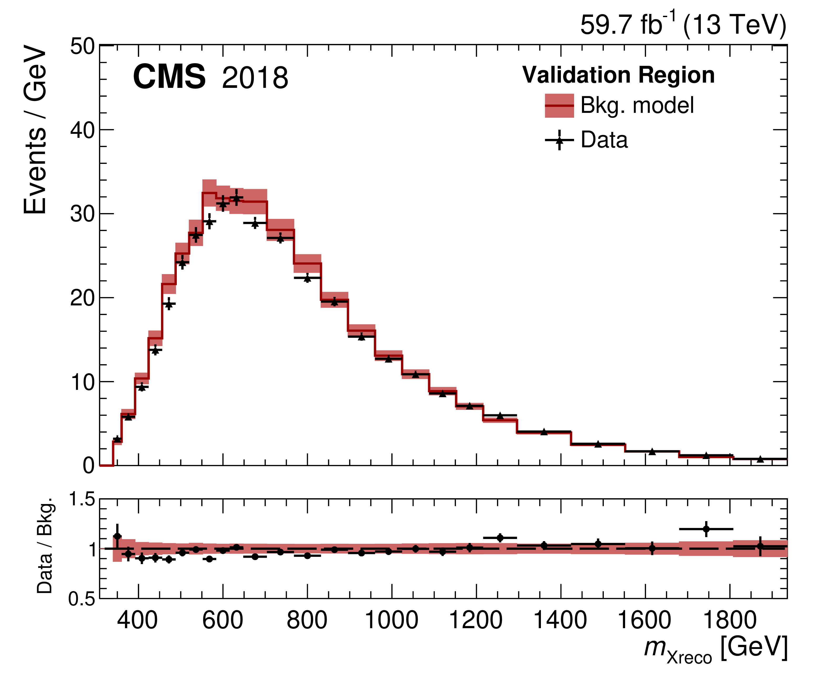
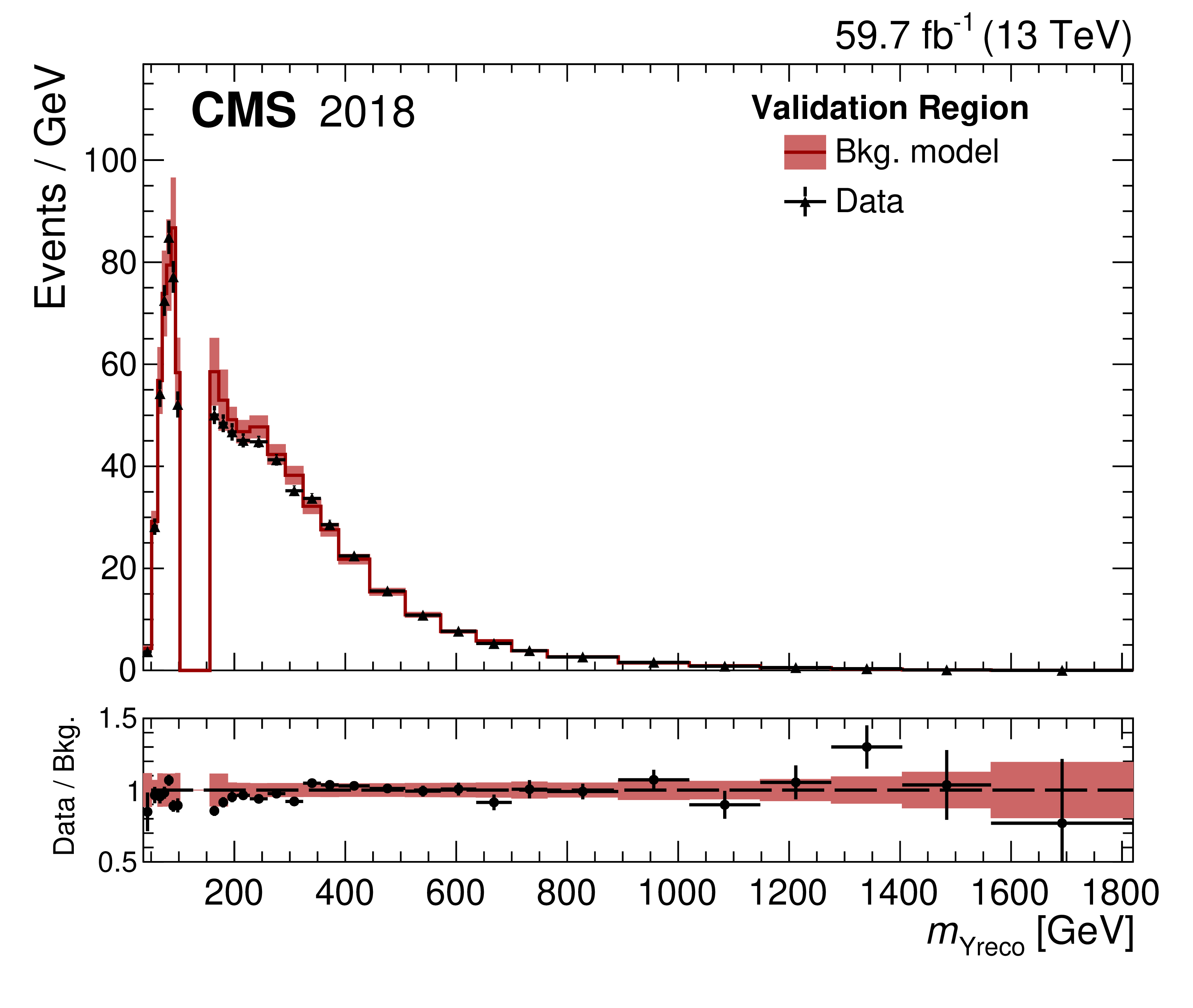
Figure 2:
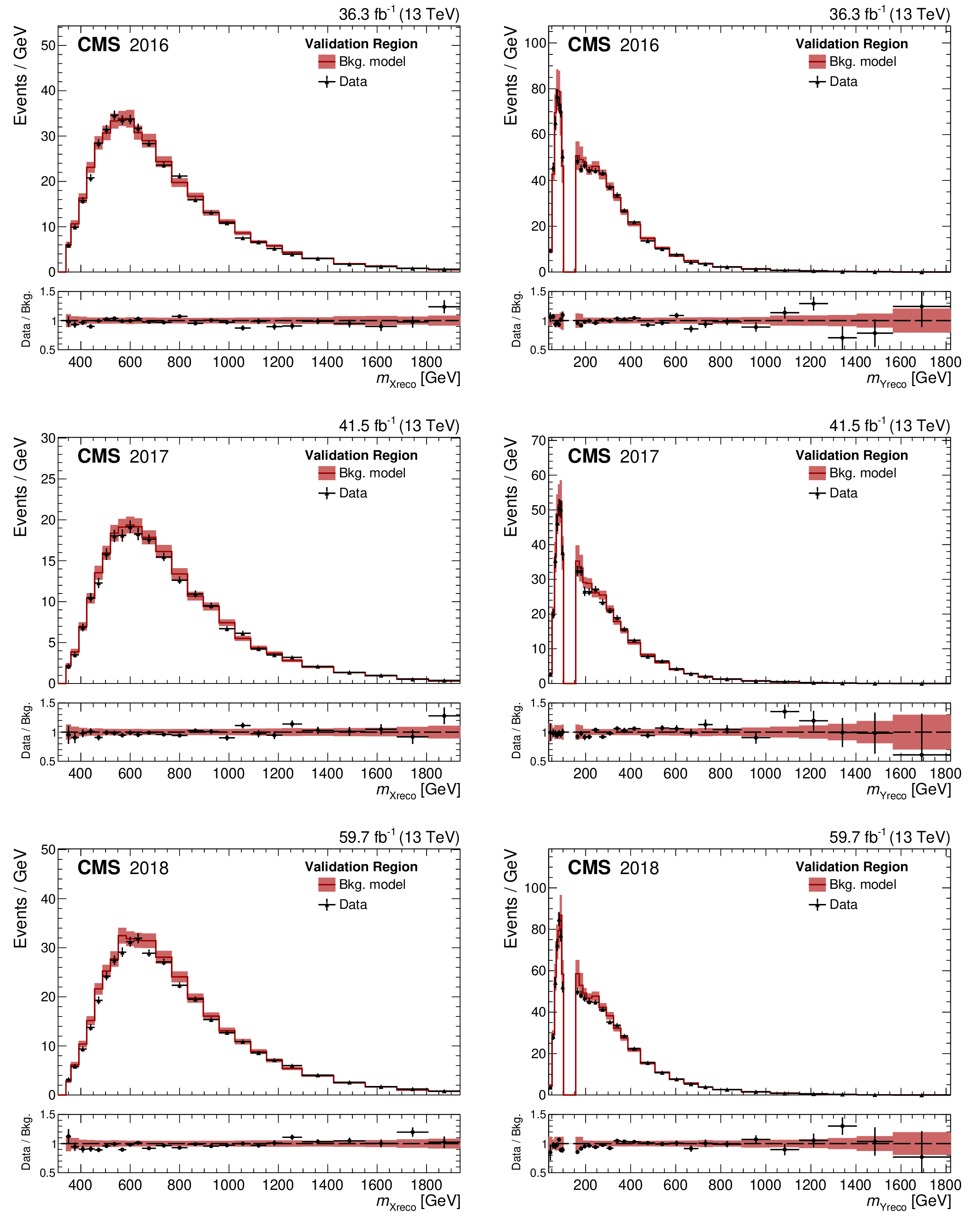
Event distributions in the validation regions for $ m_{\text{Xreco}} $ (left column) and $ m_{\text{Yreco}} $ (right column), shown separately for the three data-taking years: 2016, 2017, and 2018 (upper, middle, and lower rows, respectively). The VR(4b) data are shown in black and BDT reweighted VR(3b) model in red. The uncertainties include the statistical component added in quadrature with the uncertainties described in Section 7. The ratios of VR(4b) to VR(3b) (target over model) are in the lower panels. The ratio of the VR(3b) model uncertainty to the central value of the model is shown with the red band in the lower panel. |
png pdf |
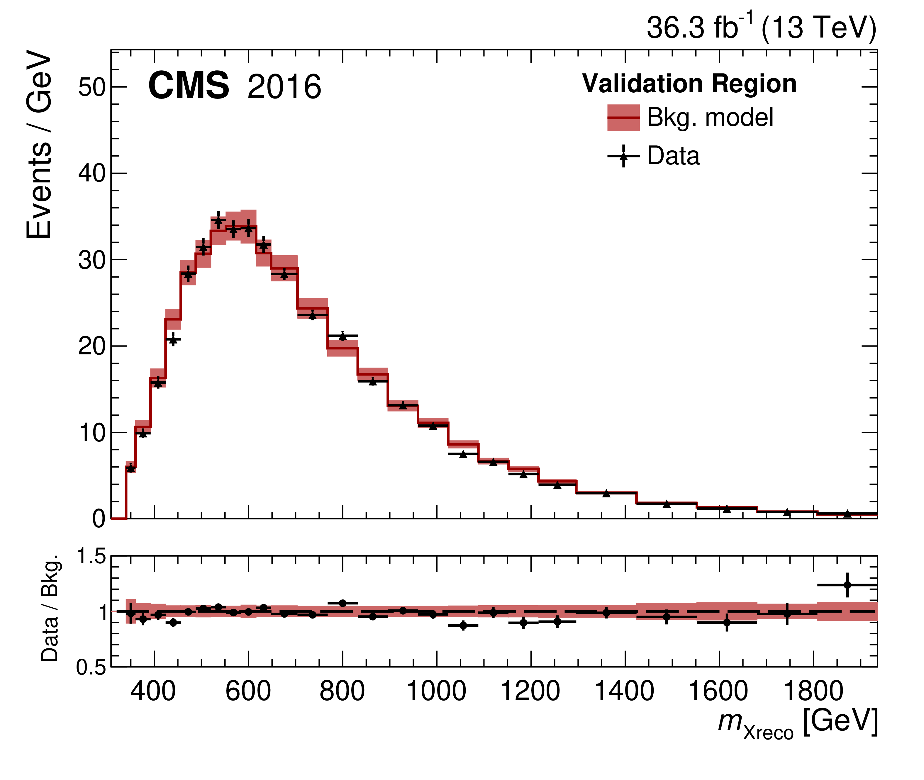
Figure 2-a:
Event distributions in the validation regions for $ m_{\text{Xreco}} $ (left column) and $ m_{\text{Yreco}} $ (right column), shown separately for the three data-taking years: 2016, 2017, and 2018 (upper, middle, and lower rows, respectively). The VR(4b) data are shown in black and BDT reweighted VR(3b) model in red. The uncertainties include the statistical component added in quadrature with the uncertainties described in Section 7. The ratios of VR(4b) to VR(3b) (target over model) are in the lower panels. The ratio of the VR(3b) model uncertainty to the central value of the model is shown with the red band in the lower panel. |
png pdf |
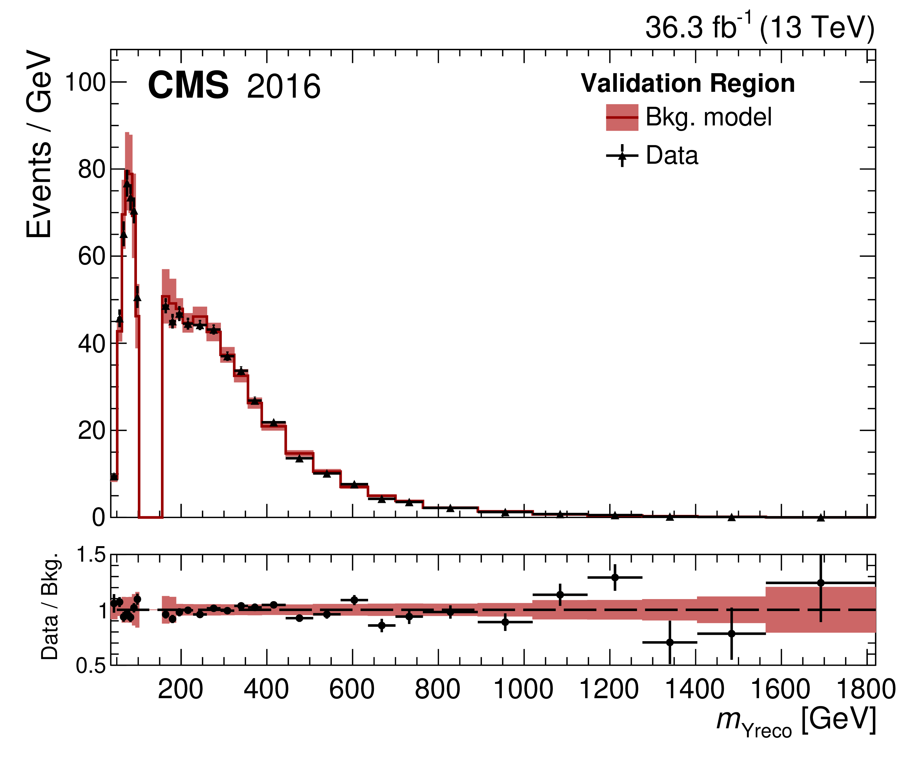
Figure 2-b:
Event distributions in the validation regions for $ m_{\text{Xreco}} $ (left column) and $ m_{\text{Yreco}} $ (right column), shown separately for the three data-taking years: 2016, 2017, and 2018 (upper, middle, and lower rows, respectively). The VR(4b) data are shown in black and BDT reweighted VR(3b) model in red. The uncertainties include the statistical component added in quadrature with the uncertainties described in Section 7. The ratios of VR(4b) to VR(3b) (target over model) are in the lower panels. The ratio of the VR(3b) model uncertainty to the central value of the model is shown with the red band in the lower panel. |
png pdf |
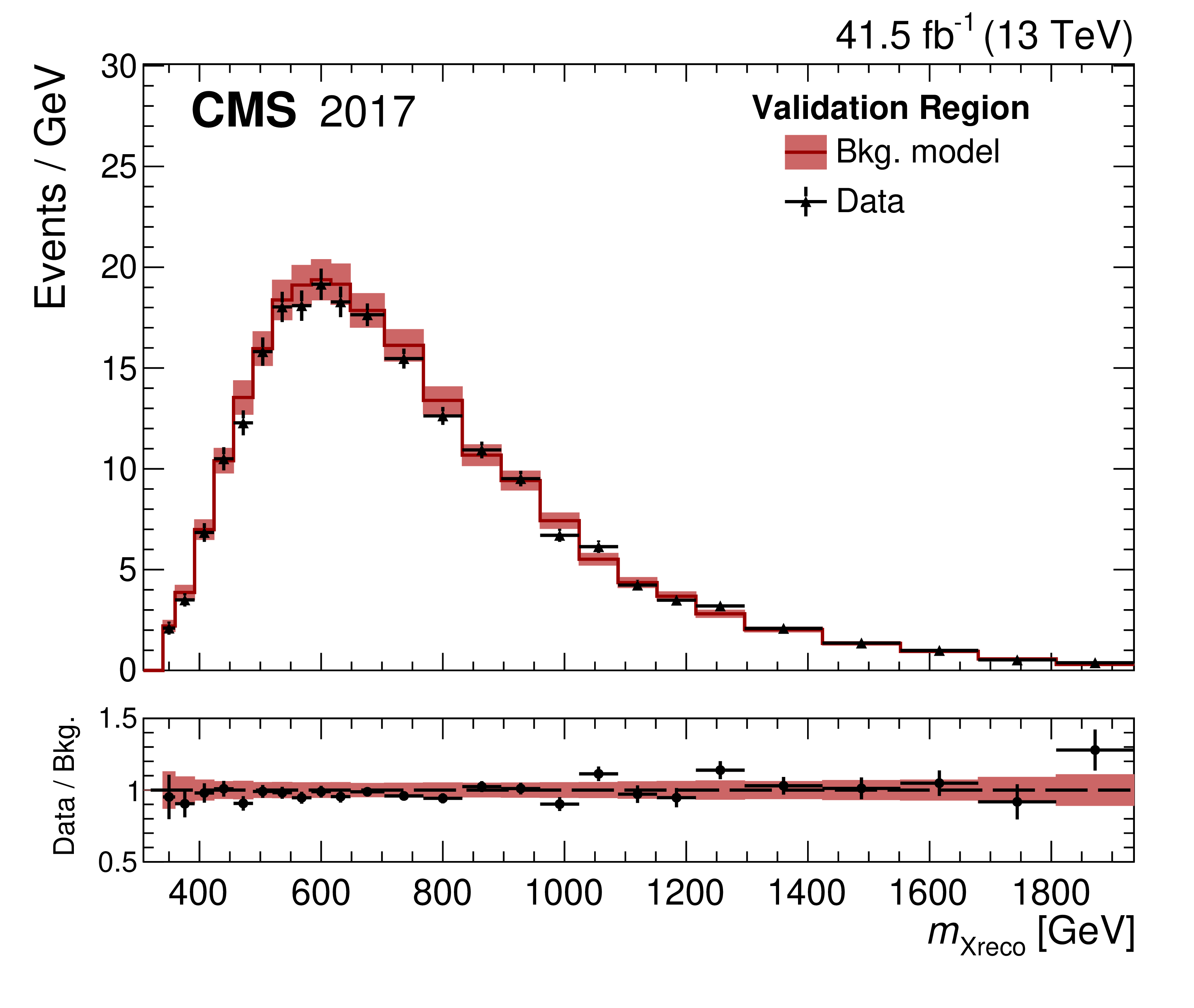
Figure 2-c:
Event distributions in the validation regions for $ m_{\text{Xreco}} $ (left column) and $ m_{\text{Yreco}} $ (right column), shown separately for the three data-taking years: 2016, 2017, and 2018 (upper, middle, and lower rows, respectively). The VR(4b) data are shown in black and BDT reweighted VR(3b) model in red. The uncertainties include the statistical component added in quadrature with the uncertainties described in Section 7. The ratios of VR(4b) to VR(3b) (target over model) are in the lower panels. The ratio of the VR(3b) model uncertainty to the central value of the model is shown with the red band in the lower panel. |
png pdf |
Figure 2-d:
Event distributions in the validation regions for $ m_{\text{Xreco}} $ (left column) and $ m_{\text{Yreco}} $ (right column), shown separately for the three data-taking years: 2016, 2017, and 2018 (upper, middle, and lower rows, respectively). The VR(4b) data are shown in black and BDT reweighted VR(3b) model in red. The uncertainties include the statistical component added in quadrature with the uncertainties described in Section 7. The ratios of VR(4b) to VR(3b) (target over model) are in the lower panels. The ratio of the VR(3b) model uncertainty to the central value of the model is shown with the red band in the lower panel. |
png pdf |
Figure 2-e:
Event distributions in the validation regions for $ m_{\text{Xreco}} $ (left column) and $ m_{\text{Yreco}} $ (right column), shown separately for the three data-taking years: 2016, 2017, and 2018 (upper, middle, and lower rows, respectively). The VR(4b) data are shown in black and BDT reweighted VR(3b) model in red. The uncertainties include the statistical component added in quadrature with the uncertainties described in Section 7. The ratios of VR(4b) to VR(3b) (target over model) are in the lower panels. The ratio of the VR(3b) model uncertainty to the central value of the model is shown with the red band in the lower panel. |
png pdf |
Figure 2-f:
Event distributions in the validation regions for $ m_{\text{Xreco}} $ (left column) and $ m_{\text{Yreco}} $ (right column), shown separately for the three data-taking years: 2016, 2017, and 2018 (upper, middle, and lower rows, respectively). The VR(4b) data are shown in black and BDT reweighted VR(3b) model in red. The uncertainties include the statistical component added in quadrature with the uncertainties described in Section 7. The ratios of VR(4b) to VR(3b) (target over model) are in the lower panels. The ratio of the VR(3b) model uncertainty to the central value of the model is shown with the red band in the lower panel. |
png pdf |
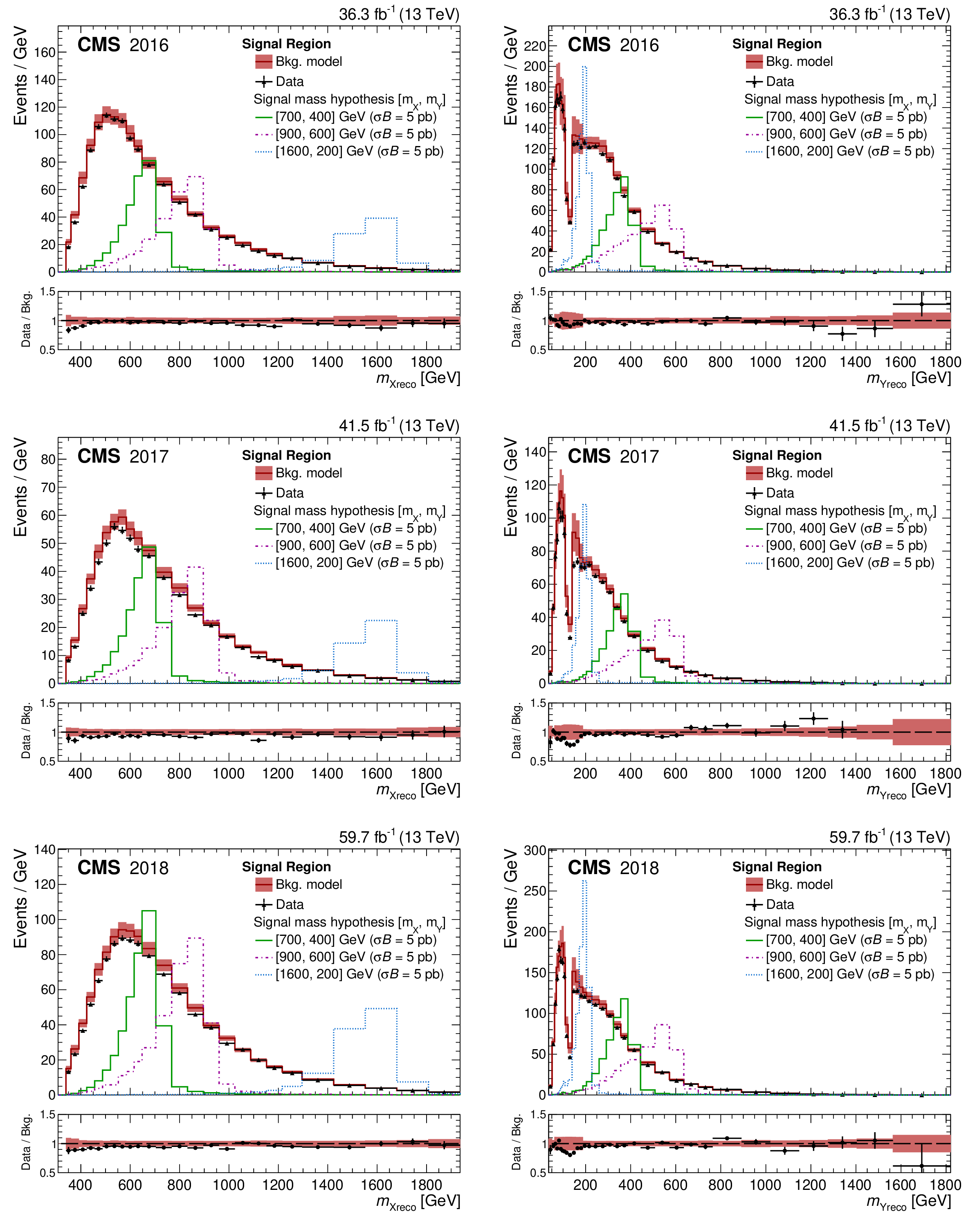
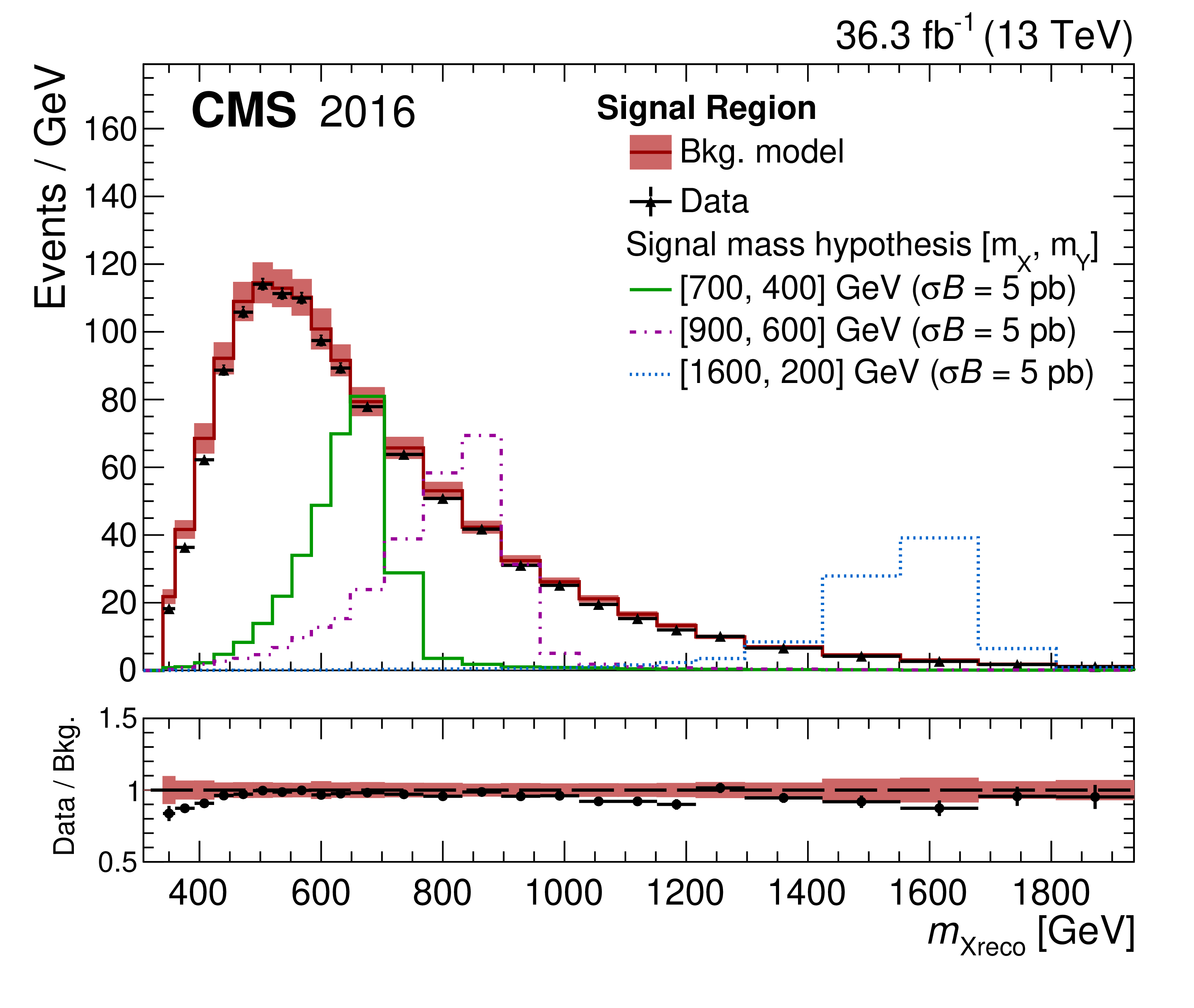
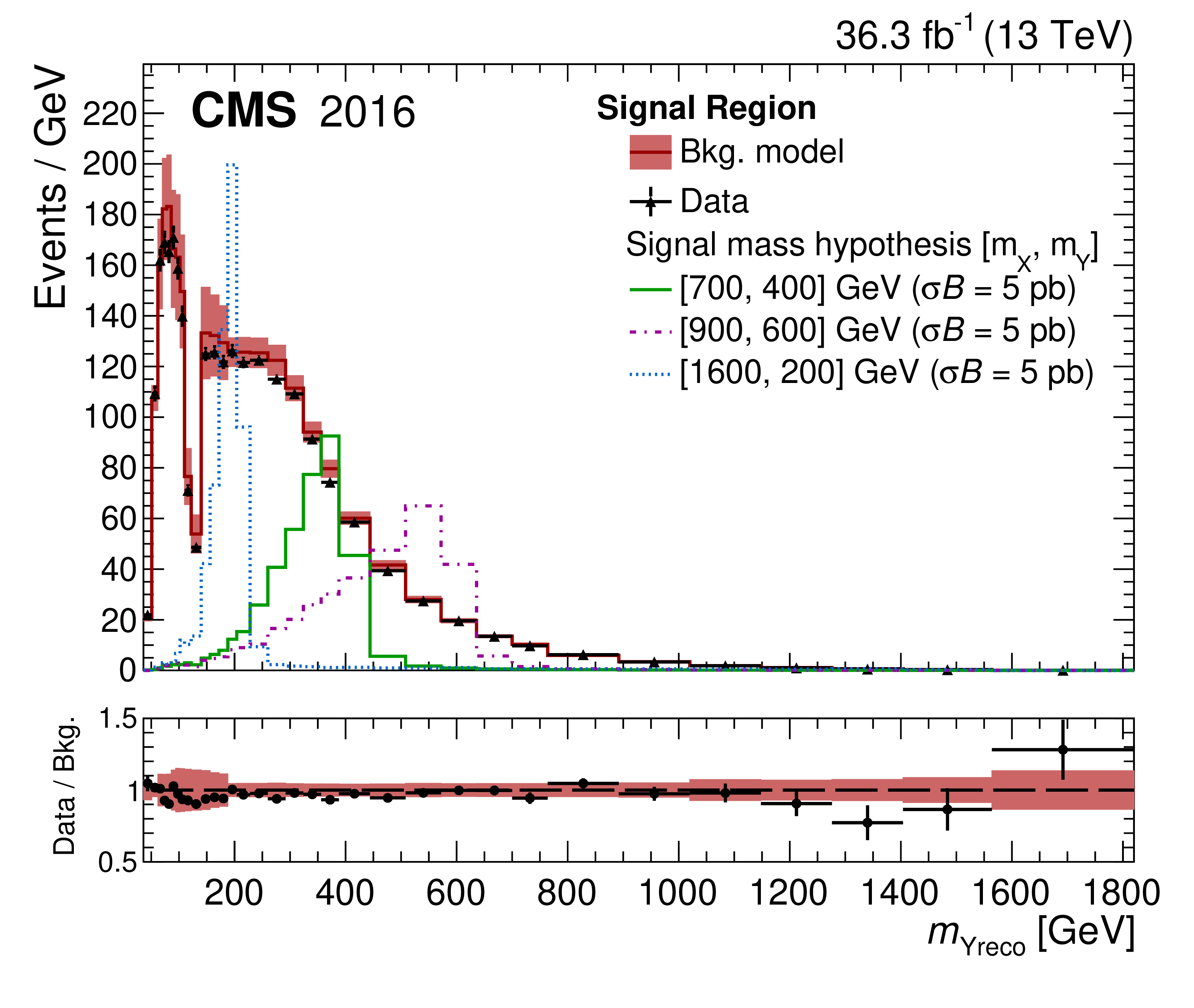
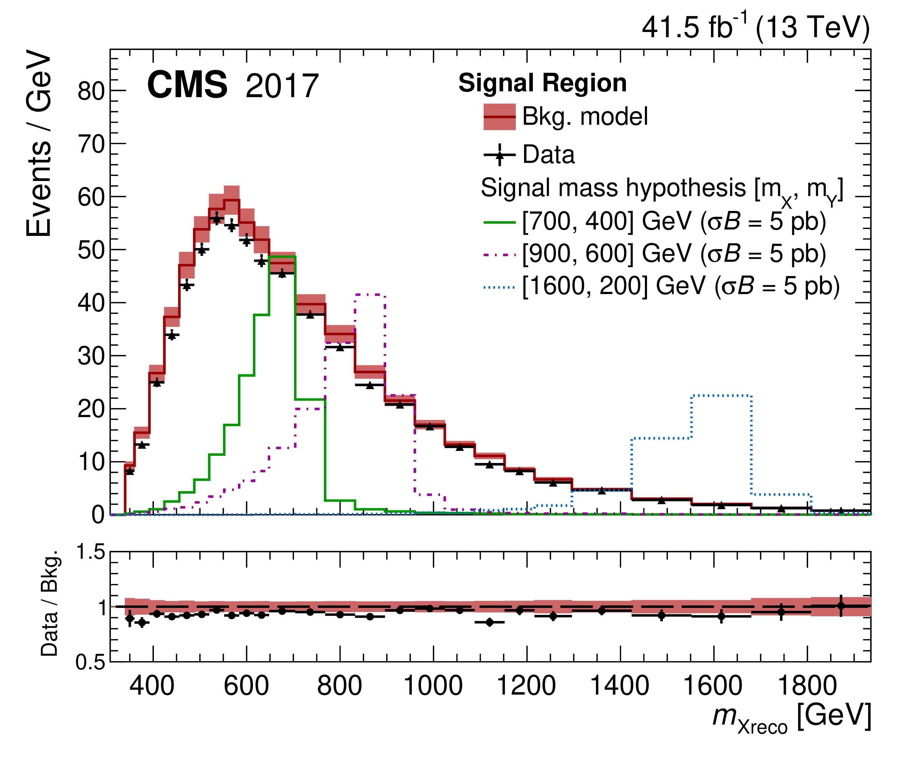
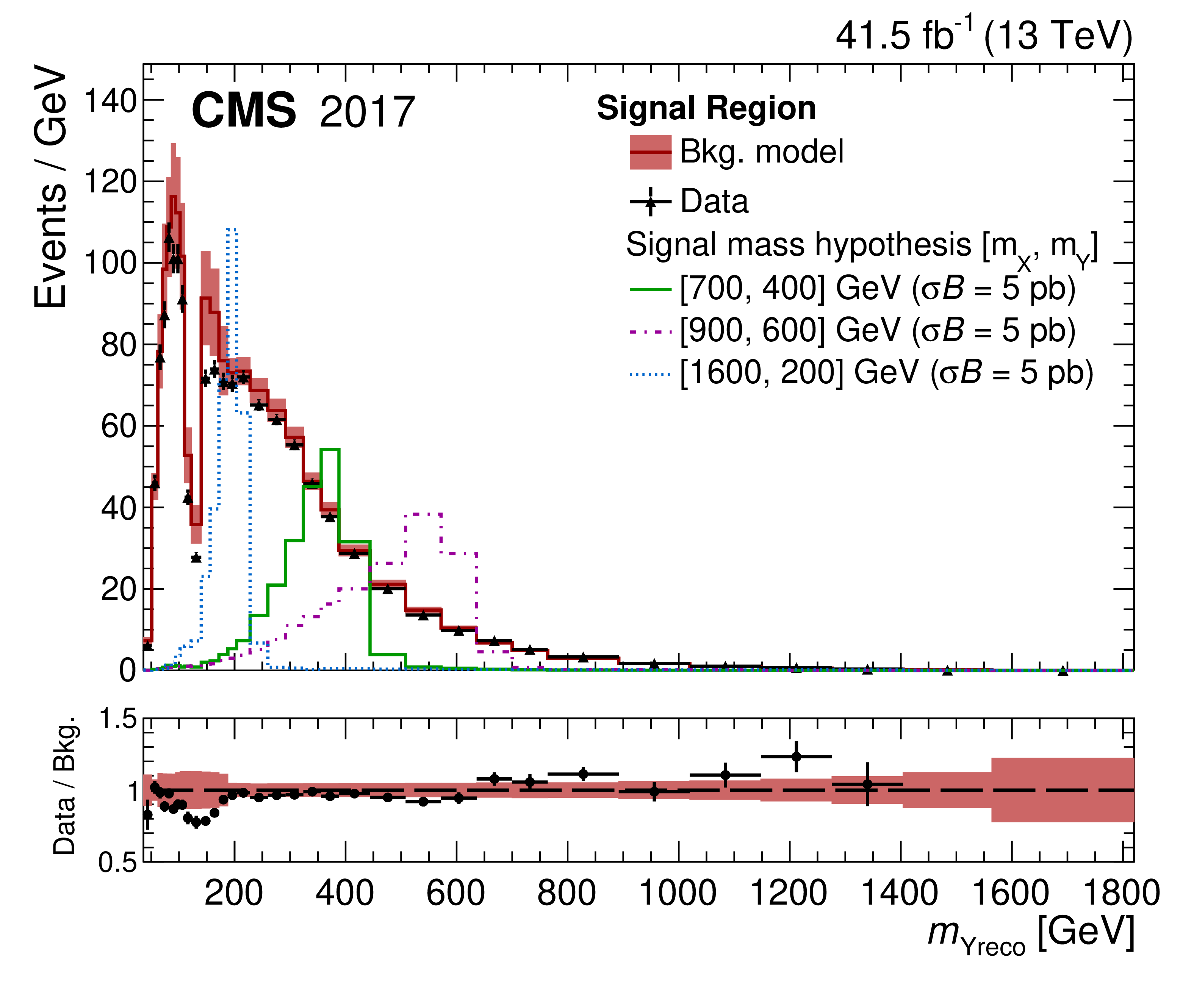
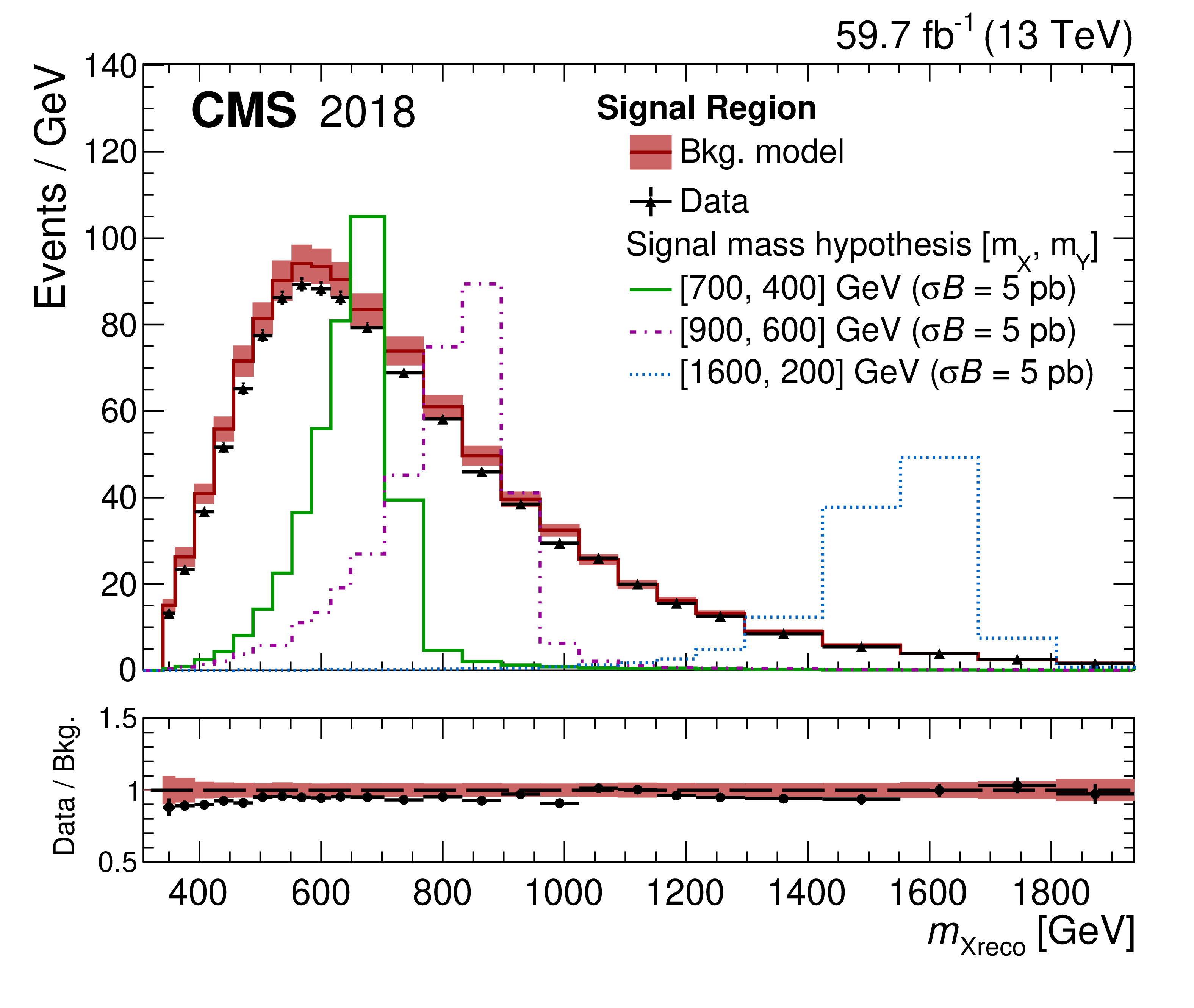
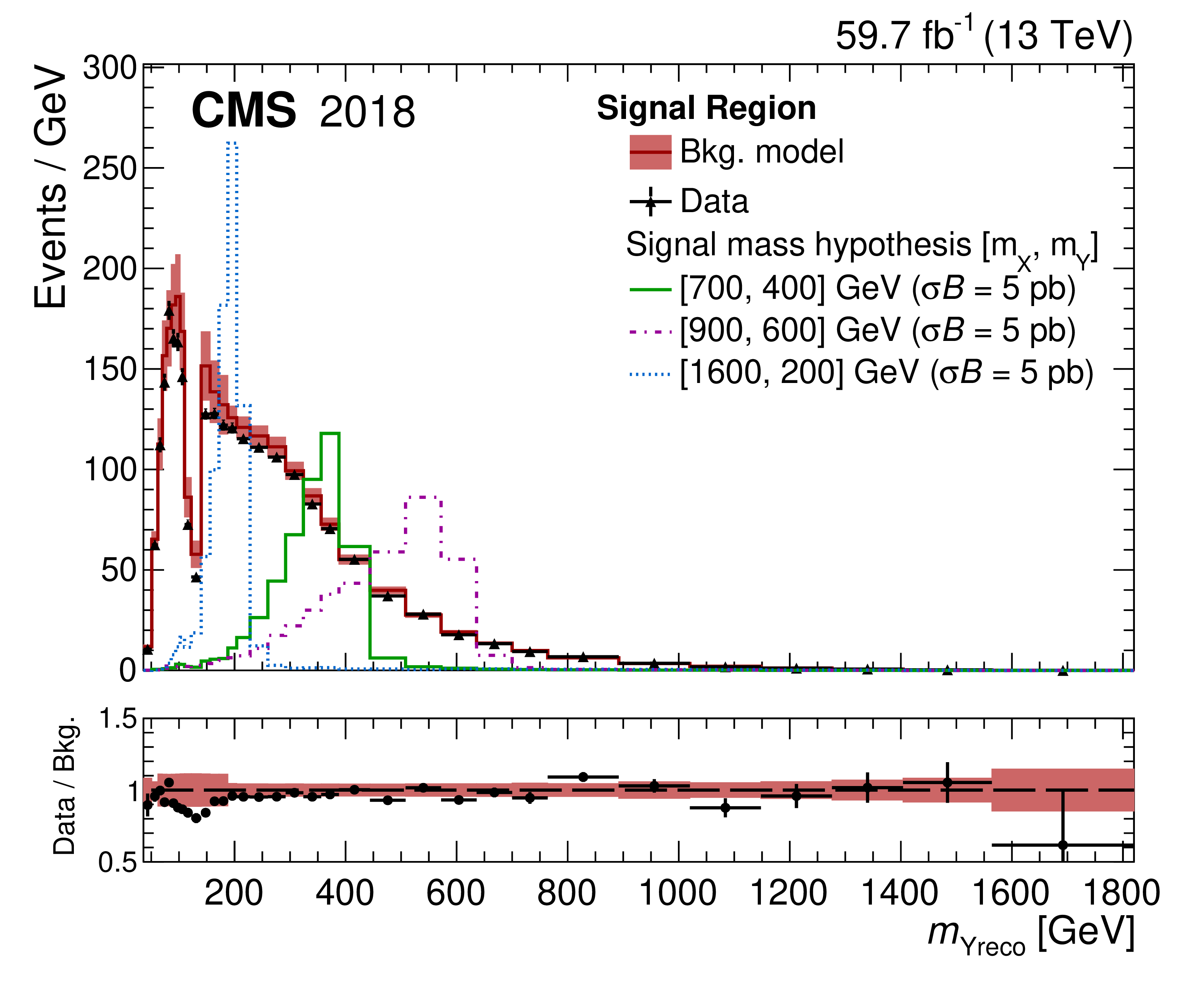
Figure 3:
Event distributions in the signal region for $ m_{\text{Xreco}} $ (left column) and $ m_{\text{Yreco}} $ (right column), shown separately for the three data-taking years: 2016, 2017, and 2018 (upper, middle, and lower rows, respectively). The SR(4b) data are shown in black and BDT reweighted SR(3b) model in red. The uncertainties include the statistical component added in quadrature with the uncertainties described in Section 7. Three selected signal mass hypotheses are overlaid. The signal histograms are scaled to have $ \sigma \mathcal{B} $ values of 5\unitpb. The ratios of SR(4b) to SR(3b) (target over model) are in the lower panels. The ratio of the SR(3b) model uncertainty to the central value of the model is shown with the red band in the lower panel. |
png pdf |
Figure 3-a:
Event distributions in the signal region for $ m_{\text{Xreco}} $ (left column) and $ m_{\text{Yreco}} $ (right column), shown separately for the three data-taking years: 2016, 2017, and 2018 (upper, middle, and lower rows, respectively). The SR(4b) data are shown in black and BDT reweighted SR(3b) model in red. The uncertainties include the statistical component added in quadrature with the uncertainties described in Section 7. Three selected signal mass hypotheses are overlaid. The signal histograms are scaled to have $ \sigma \mathcal{B} $ values of 5\unitpb. The ratios of SR(4b) to SR(3b) (target over model) are in the lower panels. The ratio of the SR(3b) model uncertainty to the central value of the model is shown with the red band in the lower panel. |
png pdf |
Figure 3-b:
Event distributions in the signal region for $ m_{\text{Xreco}} $ (left column) and $ m_{\text{Yreco}} $ (right column), shown separately for the three data-taking years: 2016, 2017, and 2018 (upper, middle, and lower rows, respectively). The SR(4b) data are shown in black and BDT reweighted SR(3b) model in red. The uncertainties include the statistical component added in quadrature with the uncertainties described in Section 7. Three selected signal mass hypotheses are overlaid. The signal histograms are scaled to have $ \sigma \mathcal{B} $ values of 5\unitpb. The ratios of SR(4b) to SR(3b) (target over model) are in the lower panels. The ratio of the SR(3b) model uncertainty to the central value of the model is shown with the red band in the lower panel. |
png pdf |
Figure 3-c:
Event distributions in the signal region for $ m_{\text{Xreco}} $ (left column) and $ m_{\text{Yreco}} $ (right column), shown separately for the three data-taking years: 2016, 2017, and 2018 (upper, middle, and lower rows, respectively). The SR(4b) data are shown in black and BDT reweighted SR(3b) model in red. The uncertainties include the statistical component added in quadrature with the uncertainties described in Section 7. Three selected signal mass hypotheses are overlaid. The signal histograms are scaled to have $ \sigma \mathcal{B} $ values of 5\unitpb. The ratios of SR(4b) to SR(3b) (target over model) are in the lower panels. The ratio of the SR(3b) model uncertainty to the central value of the model is shown with the red band in the lower panel. |
png pdf |
Figure 3-d:
Event distributions in the signal region for $ m_{\text{Xreco}} $ (left column) and $ m_{\text{Yreco}} $ (right column), shown separately for the three data-taking years: 2016, 2017, and 2018 (upper, middle, and lower rows, respectively). The SR(4b) data are shown in black and BDT reweighted SR(3b) model in red. The uncertainties include the statistical component added in quadrature with the uncertainties described in Section 7. Three selected signal mass hypotheses are overlaid. The signal histograms are scaled to have $ \sigma \mathcal{B} $ values of 5\unitpb. The ratios of SR(4b) to SR(3b) (target over model) are in the lower panels. The ratio of the SR(3b) model uncertainty to the central value of the model is shown with the red band in the lower panel. |
png pdf |
Figure 3-e:
Event distributions in the signal region for $ m_{\text{Xreco}} $ (left column) and $ m_{\text{Yreco}} $ (right column), shown separately for the three data-taking years: 2016, 2017, and 2018 (upper, middle, and lower rows, respectively). The SR(4b) data are shown in black and BDT reweighted SR(3b) model in red. The uncertainties include the statistical component added in quadrature with the uncertainties described in Section 7. Three selected signal mass hypotheses are overlaid. The signal histograms are scaled to have $ \sigma \mathcal{B} $ values of 5\unitpb. The ratios of SR(4b) to SR(3b) (target over model) are in the lower panels. The ratio of the SR(3b) model uncertainty to the central value of the model is shown with the red band in the lower panel. |
png pdf |
Figure 3-f:
Event distributions in the signal region for $ m_{\text{Xreco}} $ (left column) and $ m_{\text{Yreco}} $ (right column), shown separately for the three data-taking years: 2016, 2017, and 2018 (upper, middle, and lower rows, respectively). The SR(4b) data are shown in black and BDT reweighted SR(3b) model in red. The uncertainties include the statistical component added in quadrature with the uncertainties described in Section 7. Three selected signal mass hypotheses are overlaid. The signal histograms are scaled to have $ \sigma \mathcal{B} $ values of 5\unitpb. The ratios of SR(4b) to SR(3b) (target over model) are in the lower panels. The ratio of the SR(3b) model uncertainty to the central value of the model is shown with the red band in the lower panel. |
png pdf |
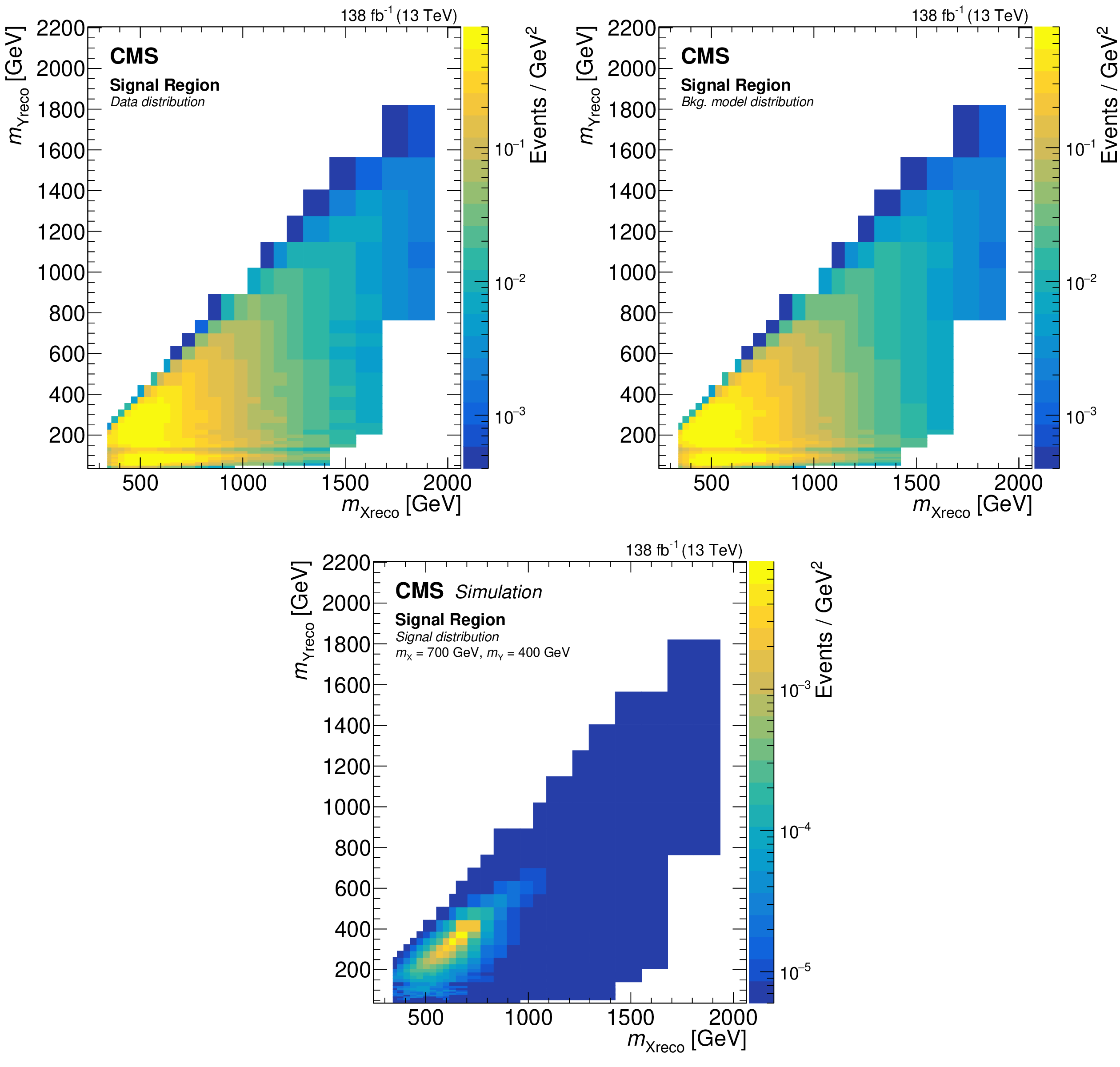
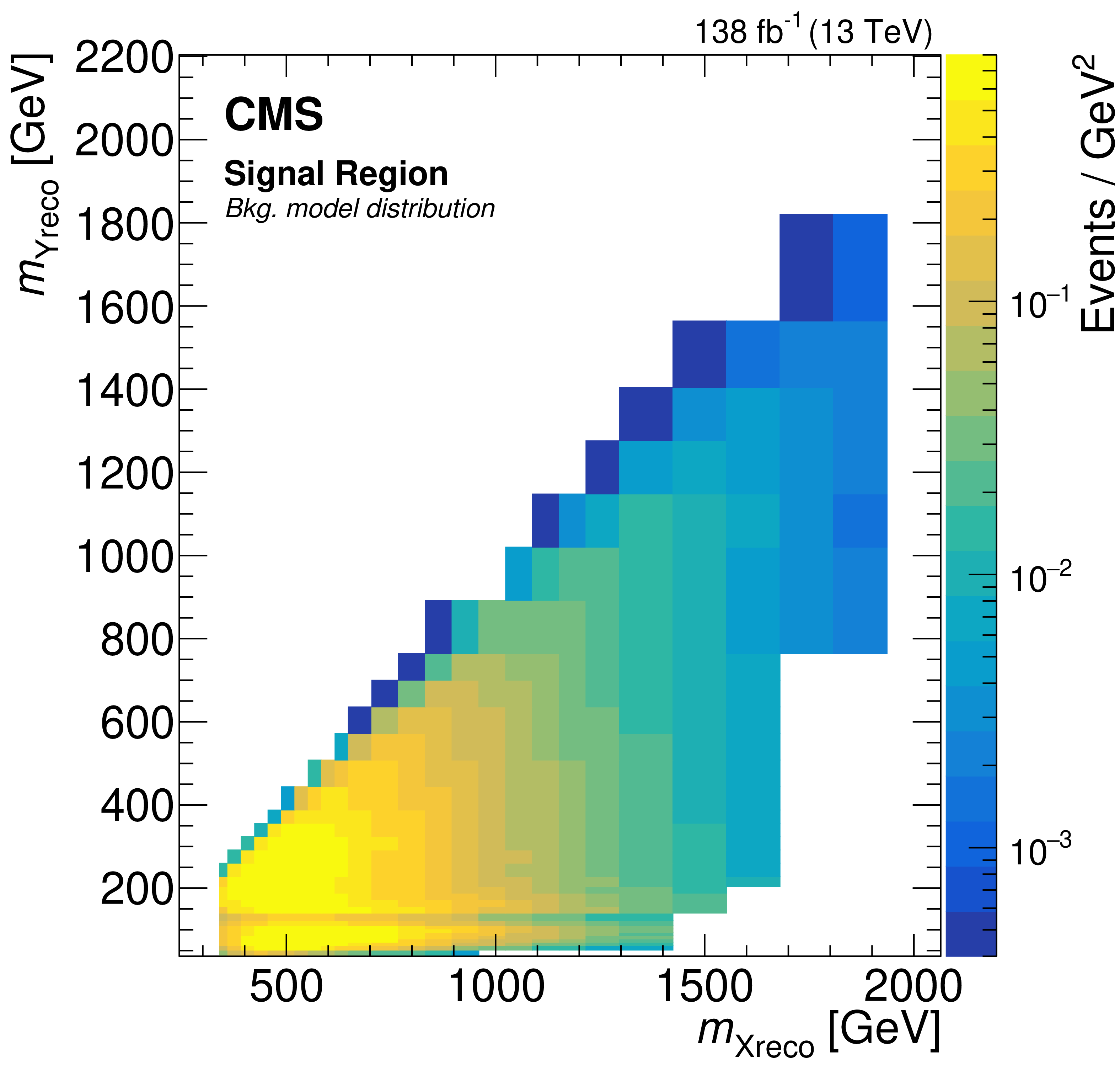
Figure 4:
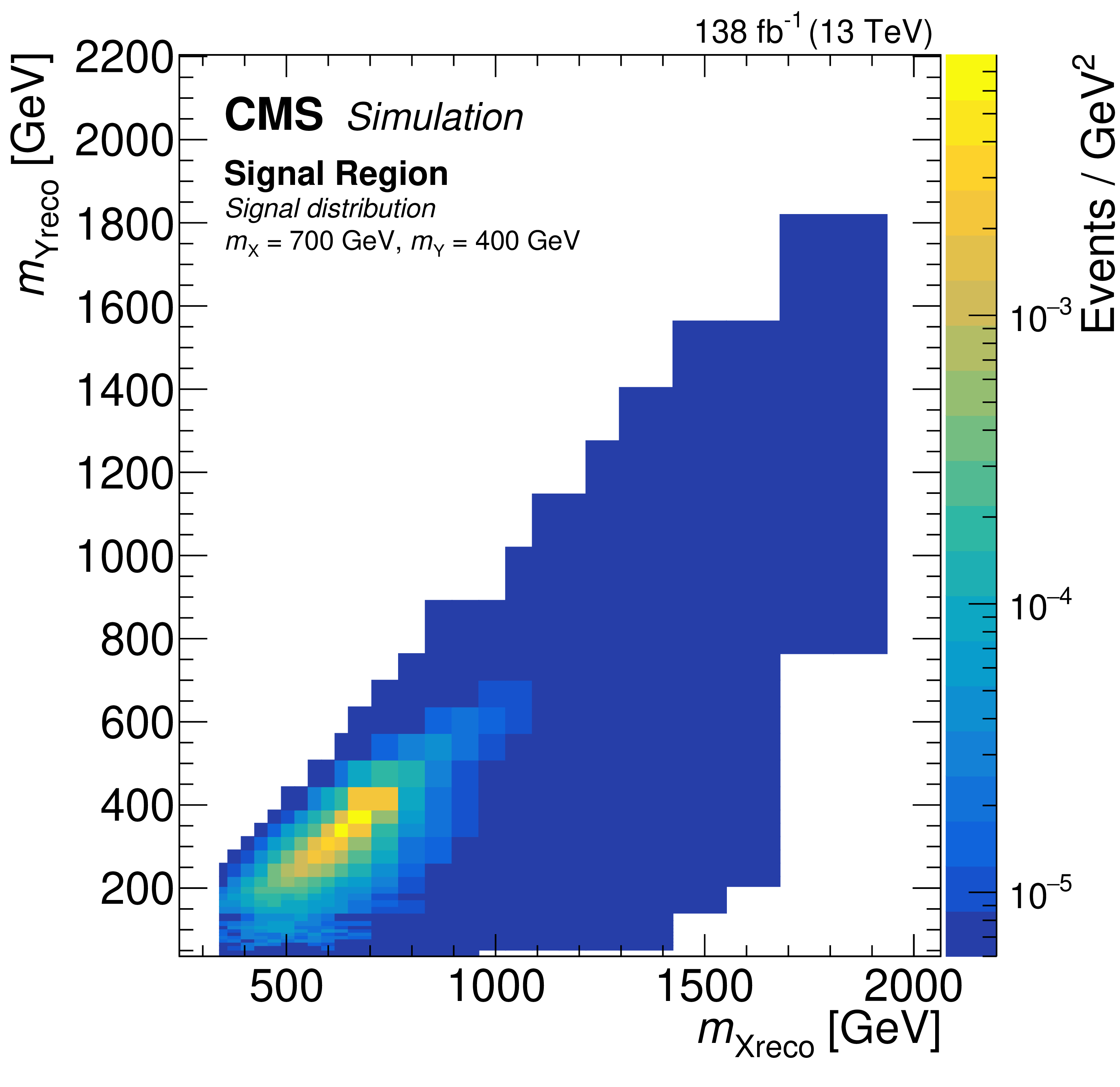
Distributions of the events in the ($ m_{\text{Xreco}} $, $ m_{\text{Yreco}} $) plane observed in the SR(4b). The upper plots show events in data (left) and the background model (right). The lower plot shows the distribution of events for the signal hypothesis corresponding to $ m_{\mathrm{X}} = $ 700 GeV and $ m_{\mathrm{Y}} = $ 400 GeV. In each plot, there are empty bins in the high-$ m_{\text{Xreco}} $ and low-$ m_{\text{Yreco}} $ region. These areas have been excluded because the events have highly boosted topology. |

png pdf |
Figure 4-a:
Distributions of the events in the ($ m_{\text{Xreco}} $, $ m_{\text{Yreco}} $) plane observed in the SR(4b). The upper plots show events in data (left) and the background model (right). The lower plot shows the distribution of events for the signal hypothesis corresponding to $ m_{\mathrm{X}} = $ 700 GeV and $ m_{\mathrm{Y}} = $ 400 GeV. In each plot, there are empty bins in the high-$ m_{\text{Xreco}} $ and low-$ m_{\text{Yreco}} $ region. These areas have been excluded because the events have highly boosted topology. |
png pdf |
Figure 4-b:
Distributions of the events in the ($ m_{\text{Xreco}} $, $ m_{\text{Yreco}} $) plane observed in the SR(4b). The upper plots show events in data (left) and the background model (right). The lower plot shows the distribution of events for the signal hypothesis corresponding to $ m_{\mathrm{X}} = $ 700 GeV and $ m_{\mathrm{Y}} = $ 400 GeV. In each plot, there are empty bins in the high-$ m_{\text{Xreco}} $ and low-$ m_{\text{Yreco}} $ region. These areas have been excluded because the events have highly boosted topology. |
png pdf |
Figure 4-c:
Distributions of the events in the ($ m_{\text{Xreco}} $, $ m_{\text{Yreco}} $) plane observed in the SR(4b). The upper plots show events in data (left) and the background model (right). The lower plot shows the distribution of events for the signal hypothesis corresponding to $ m_{\mathrm{X}} = $ 700 GeV and $ m_{\mathrm{Y}} = $ 400 GeV. In each plot, there are empty bins in the high-$ m_{\text{Xreco}} $ and low-$ m_{\text{Yreco}} $ region. These areas have been excluded because the events have highly boosted topology. |
png pdf |
Figure 5:
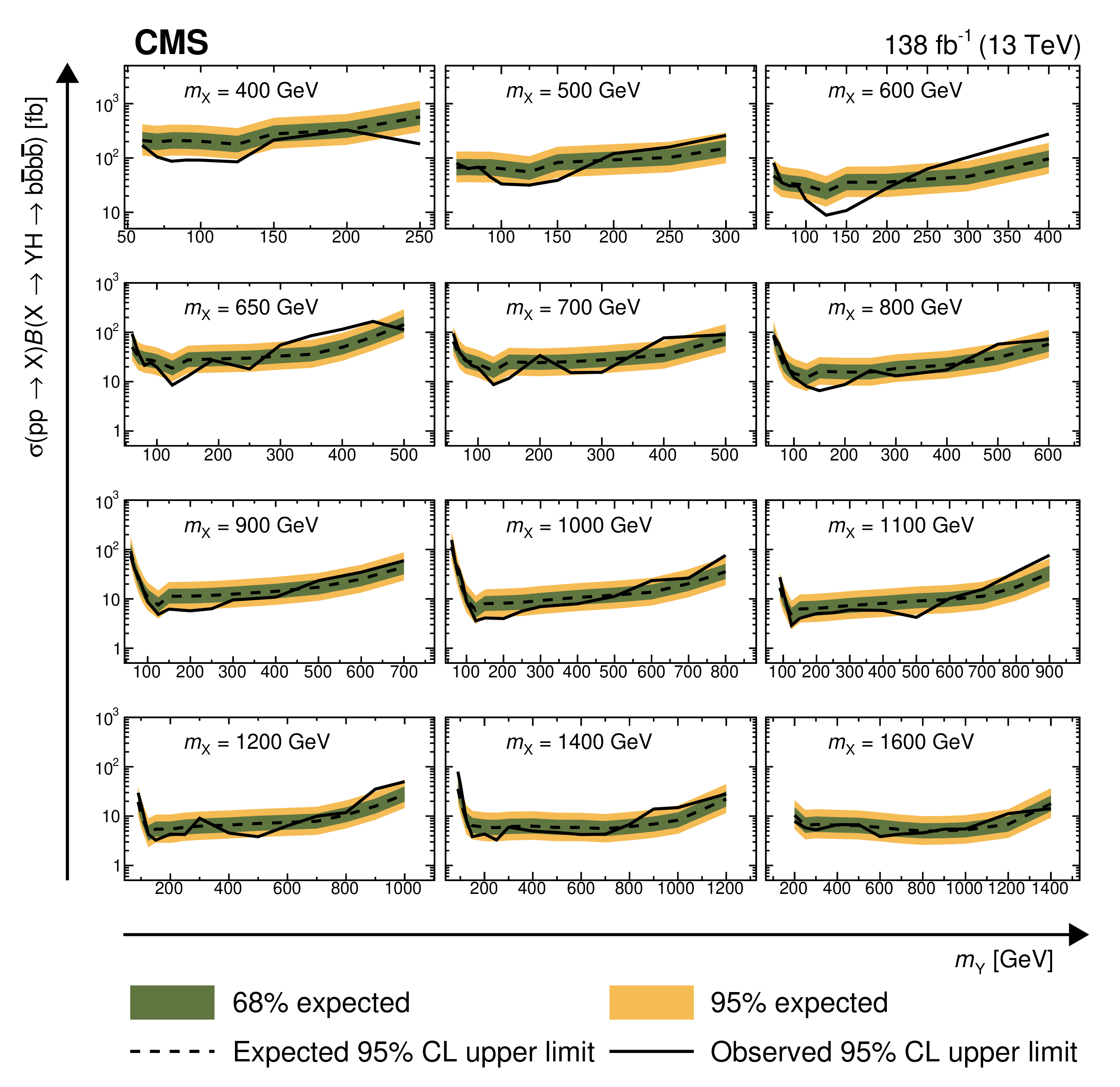
Expected and observed 95% CL upper limits on $ \sigma(\mathrm{p}\mathrm{p} \to \mathrm{X}) \mathcal{B} (\mathrm{X} \to \mathrm{Y}\mathrm{H} \to \mathrm{b}\overline{\mathrm{b}}\mathrm{b}\overline{\mathrm{b}}) $. The limits are shown as functions of $ m_{\text{Yreco}} $ for selected values of $ m_{\text{Xreco}} $. The black dashed and solid lines represent expected and observed limits, respectively. The dark green and light yellow bands represent the $ \pm $ 1 and $ \pm $ 2 standard deviations for the expected limit, respectively. The largest excess (deficit) of the observed limit compared with the expected limit is for $ m_{\text{Xreco}} = $ 600 GeV and $ m_{\text{Yreco}} = $ 400 GeV ($ m_{\text{Xreco}} = $ 600 GeV and $ m_{\text{Yreco}} = $ 150 GeV). |
png pdf |
Figure 6:
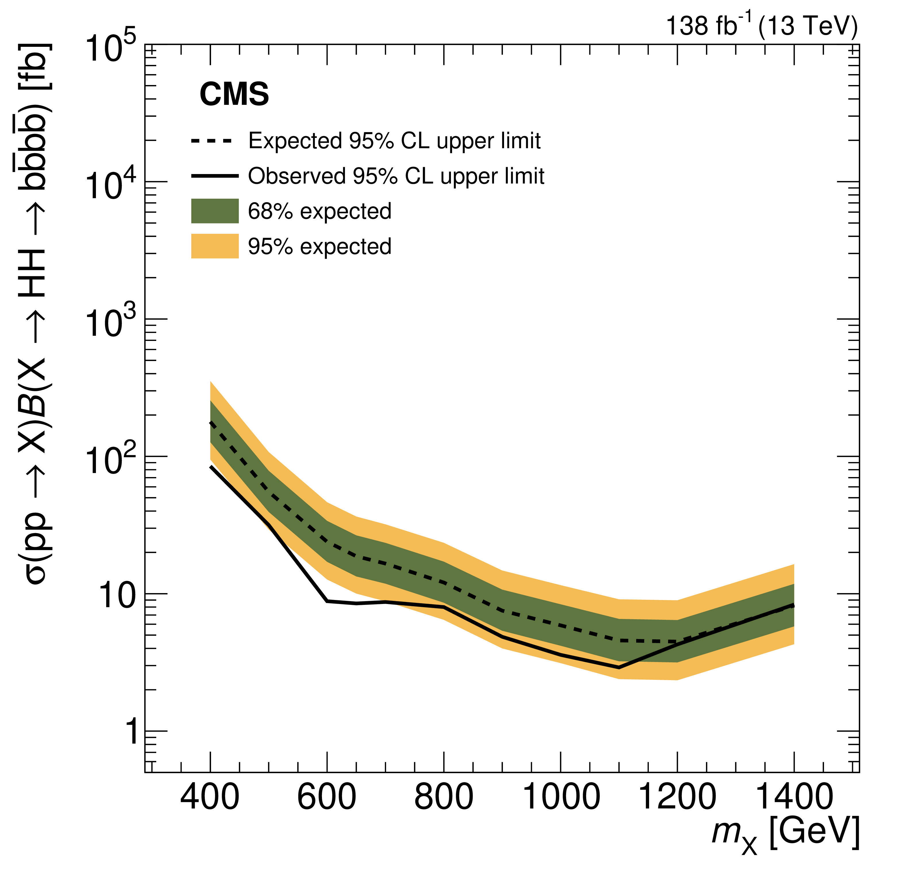
Expected and observed 95% CL upper limits on $ \sigma(\textrm{pp} \to \mathrm{X}) \mathcal{B} (\mathrm{X} \to \mathrm{H} \mathrm{H} \to \mathrm{b}\overline{\mathrm{b}}\mathrm{b}\overline{\mathrm{b}}) $. The black dashed and solid lines represent expected and observed limits, respectively. The dark green and light yellow bands represent the $ \pm $1 and $ \pm $2 standard deviations for the expected limit, respectively. |
png pdf |
Figure 7:
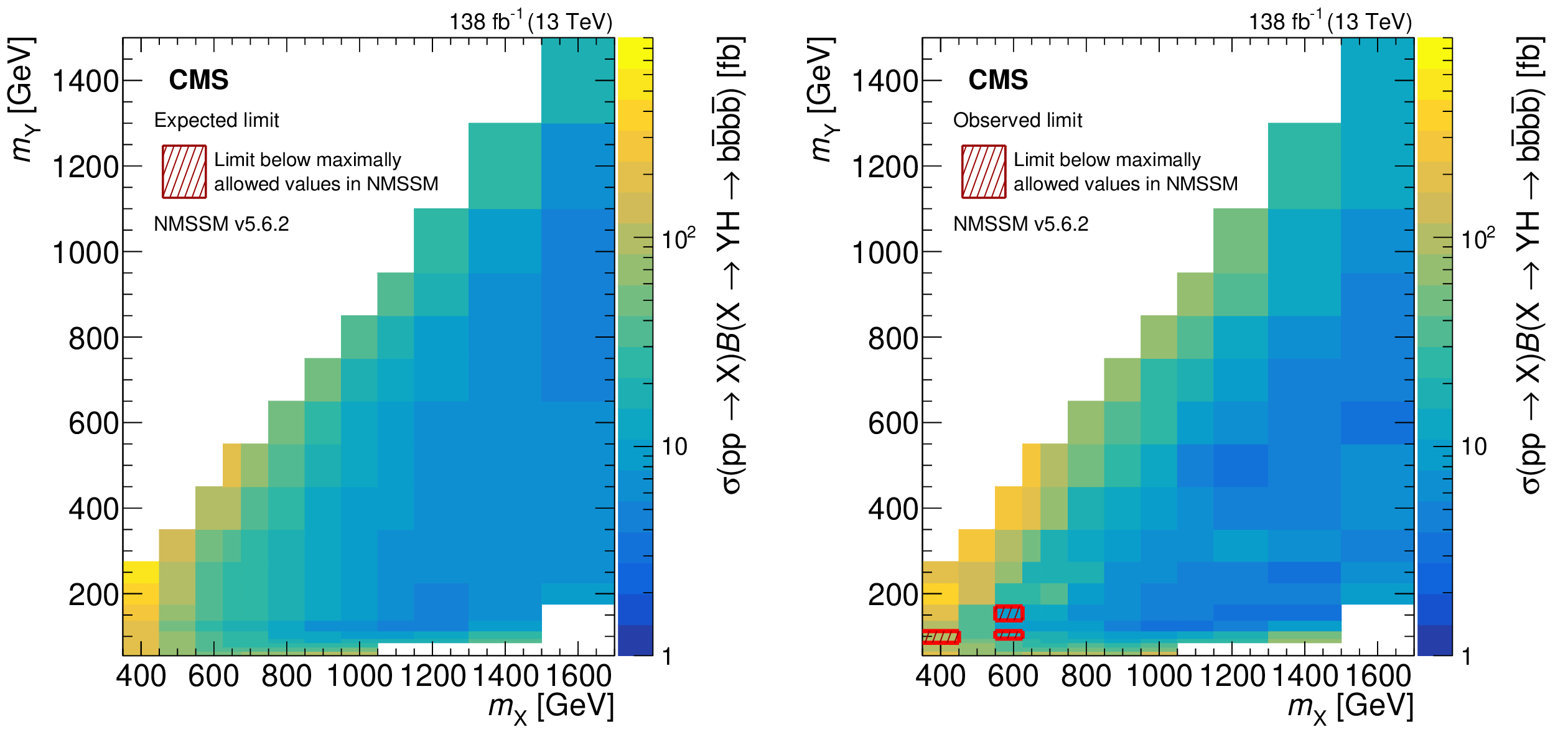
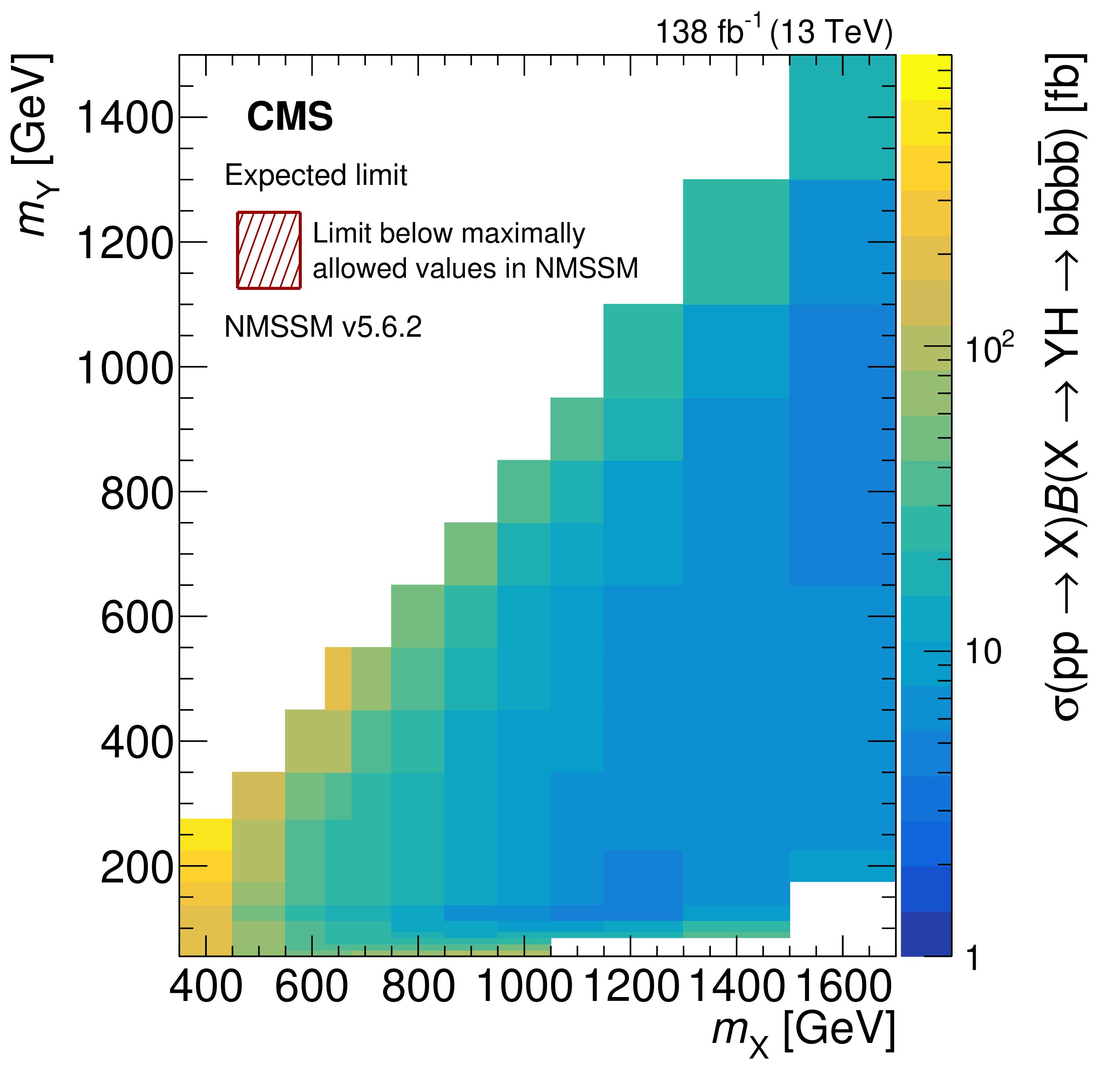
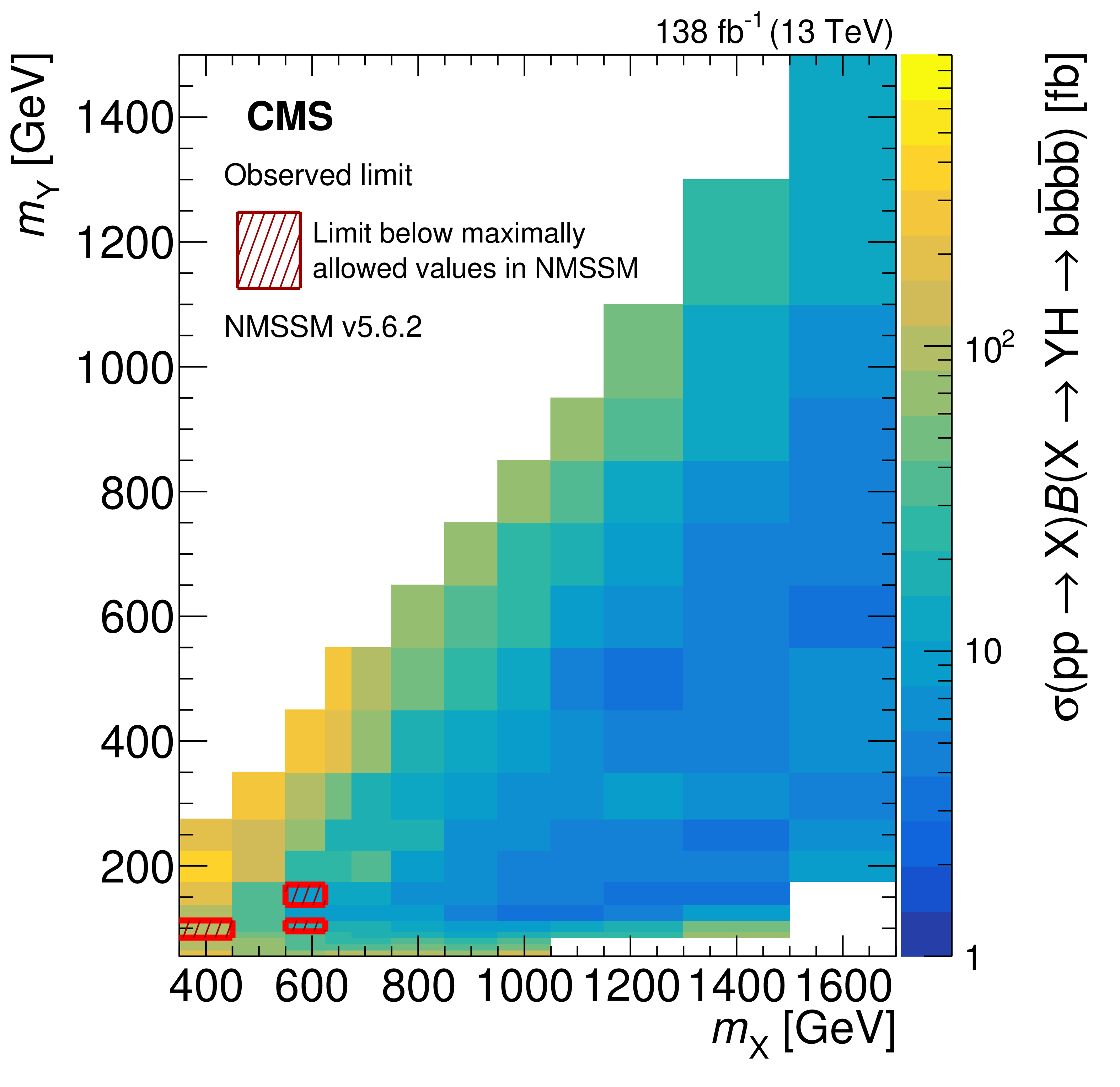
Expected (left) and observed (right) 95% CL upper limits on $ \sigma(\mathrm{p}\mathrm{p} \to \mathrm{X}) \mathcal{B} (\mathrm{X} \to \mathrm{Y}\mathrm{H} \to \mathrm{b}\overline{\mathrm{b}}\mathrm{b}\overline{\mathrm{b}}) $ shown in the ($ m_{\mathrm{X}} $, $ m_{\mathrm{Y}} $) plane. These limits are compared to the maximally allowed $ \sigma(\mathrm{p}\mathrm{p} \to \mathrm{X}) \mathcal{B} (\mathrm{X} \to \mathrm{Y}\mathrm{H} \to \mathrm{b}\overline{\mathrm{b}}\mathrm{b}\overline{\mathrm{b}}) $ values determined with NMSSM and taking into account previous experimental constraints. The NMSSM limits are obtained with NMSSMTOOLS 5.6.2 and appear in Ref. [79]. A few mass hypotheses where the observed limits are more restrictive than the NMSSM limits are indicated by the red hatched areas. |
png pdf |
Figure 7-a:
Expected (left) and observed (right) 95% CL upper limits on $ \sigma(\mathrm{p}\mathrm{p} \to \mathrm{X}) \mathcal{B} (\mathrm{X} \to \mathrm{Y}\mathrm{H} \to \mathrm{b}\overline{\mathrm{b}}\mathrm{b}\overline{\mathrm{b}}) $ shown in the ($ m_{\mathrm{X}} $, $ m_{\mathrm{Y}} $) plane. These limits are compared to the maximally allowed $ \sigma(\mathrm{p}\mathrm{p} \to \mathrm{X}) \mathcal{B} (\mathrm{X} \to \mathrm{Y}\mathrm{H} \to \mathrm{b}\overline{\mathrm{b}}\mathrm{b}\overline{\mathrm{b}}) $ values determined with NMSSM and taking into account previous experimental constraints. The NMSSM limits are obtained with NMSSMTOOLS 5.6.2 and appear in Ref. [79]. A few mass hypotheses where the observed limits are more restrictive than the NMSSM limits are indicated by the red hatched areas. |
png pdf |
Figure 7-b:
Expected (left) and observed (right) 95% CL upper limits on $ \sigma(\mathrm{p}\mathrm{p} \to \mathrm{X}) \mathcal{B} (\mathrm{X} \to \mathrm{Y}\mathrm{H} \to \mathrm{b}\overline{\mathrm{b}}\mathrm{b}\overline{\mathrm{b}}) $ shown in the ($ m_{\mathrm{X}} $, $ m_{\mathrm{Y}} $) plane. These limits are compared to the maximally allowed $ \sigma(\mathrm{p}\mathrm{p} \to \mathrm{X}) \mathcal{B} (\mathrm{X} \to \mathrm{Y}\mathrm{H} \to \mathrm{b}\overline{\mathrm{b}}\mathrm{b}\overline{\mathrm{b}}) $ values determined with NMSSM and taking into account previous experimental constraints. The NMSSM limits are obtained with NMSSMTOOLS 5.6.2 and appear in Ref. [79]. A few mass hypotheses where the observed limits are more restrictive than the NMSSM limits are indicated by the red hatched areas. |
| Tables | |
png pdf |
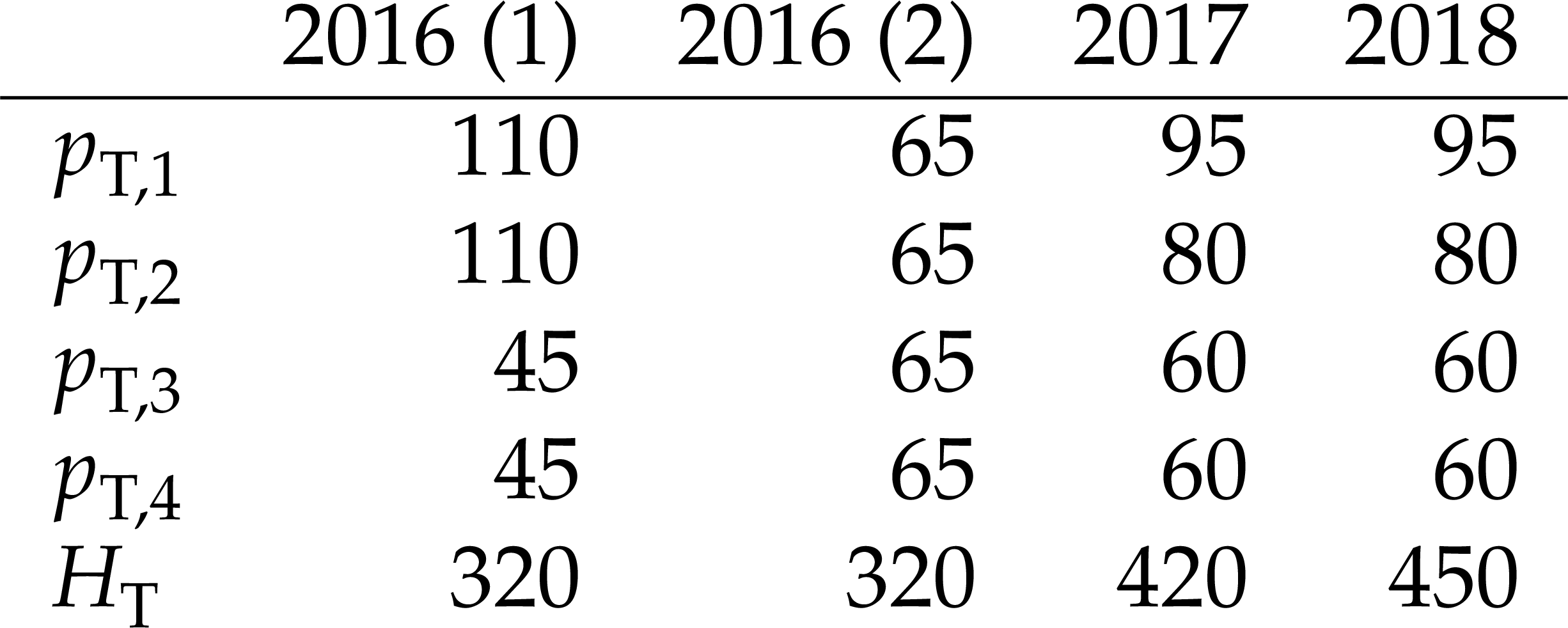
Table 1:
Offline selection thresholds at 90% of HLT trigger turn-on curves. The values represent the lower bounds on $ p_{\mathrm{T}} $ and $ H_{\mathrm{T}} $ for the four highest $ p_{\mathrm{T}} $ jets in an event for each data-taking year. The values in the table are in units of GeVns. For data-taking year 2016, events that pass either of two trigger algorithms are used. |
png pdf |
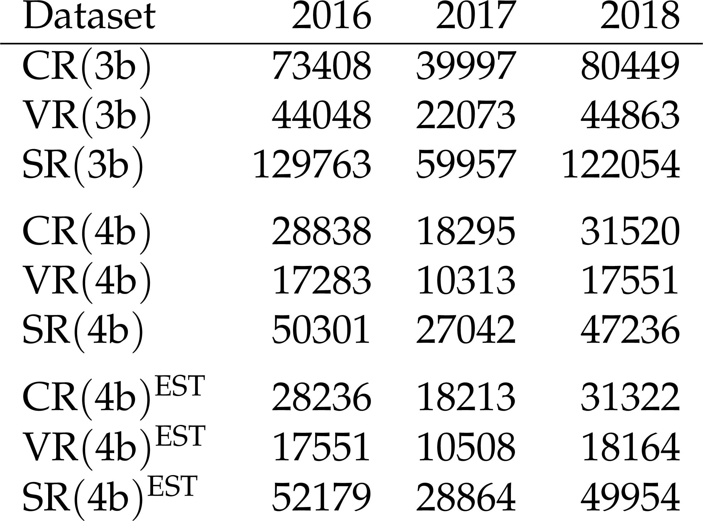
Table 2:
Summary of the number of events in the samples and analysis regions for each data-taking year. The last three rows provide the estimated event yields derived from the background model (EST) and can be compared to those in the 4b dataset. Systematics uncertainties associated with these estimates are discussed in Section 7. |
| Summary |
| This analysis presents a search for a new heavy scalar resonance ($ \mathrm{X} $) decaying into the 125 GeV standard model Higgs boson and a new scalar particle (Y ), in the $ \mathrm{b}\overline{\mathrm{b}}\mathrm{b}\overline{\mathrm{b}} $ decay channel. The search explores a range of masses from 400 GeV to 1.6 TeV for X and from 60 GeV up to 1.4 TeV for Y. A data sample corresponding to an integrated luminosity of 138 fb$ ^{-1} $ collected in proton-proton collisions at $ \sqrt{s} = $ 13 TeV is used for the search. No evidence for a new signal is observed. Upper limits on the signal cross section times branching fraction are set at the 95% confidence level. Results are interpreted in the context of the next-to-minimal supersymmetric standard model scenario and constrain the phase space of this model beyond previous experimental exclusion limits. |
| References | ||||
| 1 | ATLAS Collaboration | Observation of a new particle in the search for the standard model Higgs boson with the ATLAS detector at the LHC | PLB 716 (2012) 1 | 1207.7214 |
| 2 | CMS Collaboration | Observation of a new boson at a mass of 125 GeV with the CMS experiment at the LHC | PLB 716 (2012) 30 | CMS-HIG-12-028 1207.7235 |
| 3 | CMS Collaboration | Observation of a new boson with mass near 125 GeV in pp collisions at $ \sqrt{s} = $ 7 and 8 TeV | JHEP 06 (2013) 081 | CMS-HIG-12-036 1303.4571 |
| 4 | U. Ellwanger, C. Hugonie, and A. M. Teixeira | The next-to-minimal supersymmetric standard model | Phys. Rep. 496 (2010) 1 | 0910.1785 |
| 5 | M. Maniatis | The next-to-minimal supersymmetric extension of the standard model reviewed | Int. J. Mod. Phys. A 25 (2010) 3505 | 0906.0777 |
| 6 | T. Robens, T. Stefaniak, and J. Wittbrodt | Two-real-scalar-singlet extension of the SM: LHC phenomenology and benchmark scenarios | EPJC 80 (2020) 151 | 1908.08554 |
| 7 | A. Carvalho | Gravity particles from warped extra dimensions, predictions for LHC | 1404.0102 | |
| 8 | U. Ellwanger and M. Rodriguez-Vazquez | Simultaneous search for extra light and heavy Higgs bosons via cascade decays | JHEP 11 (2017) 008 | 1707.08522 |
| 9 | Z. Kang et al. | Probing the CP-even Higgs sector via $ H_3 \rightarrow H_2H_1 $ in the natural next-to-minimal supersymmetric standard model | PRD 88 (2013) 015006 | 1301.0453 |
| 10 | S. F. King, M. M \"u hlleitner, R. Nevzorov, and K. Walz | Discovery prospects for NMSSM Higgs bosons at the high-energy Large Hadron Collider | PRD 90 (2014) 095014 | 1408.1120 |
| 11 | M. Carena et al. | Alignment limit of the NMSSM Higgs sector | PRD 93 (2016) 035013 | 1510.09137 |
| 12 | U. Ellwanger and M. Rodriguez-Vazquez | Discovery prospects of a light scalar in the NMSSM | JHEP 02 (2016) 096 | 1512.04281 |
| 13 | R. Costa, M. M \"u hlleitner, M. O. P. Sampaio, and R. Santos | Singlet extensions of the standard model at LHC Run 2: benchmarks and comparison with the NMSSM | JHEP 06 (2016) 034 | 1512.05355 |
| 14 | ATLAS Collaboration | Search for a resonance decaying into a scalar particle and a Higgs boson in the final state with two bottom quarks and two photons in proton-proton collisions at $ \sqrt{s} = $ 13 TeV with the ATLAS detector | JHEP 11 (2024) 047 | 2404.12915 |
| 15 | CMS Collaboration | Search for a new resonance decaying into two spin-0 bosons in a final state with two photons and two bottom quarks in proton-proton collisions at $ \sqrt{s} = $ 13 TeV | JHEP 05 (2024) 316 | CMS-HIG-21-011 2310.01643 |
| 16 | CMS Collaboration | Search for a heavy Higgs boson decaying into two lighter Higgs bosons in the $ \tau\tau $bb final state at 13 TeV | JHEP 11 (2021) 057 | CMS-HIG-20-014 2106.10361 |
| 17 | CMS Collaboration | Search for a massive scalar resonance decaying to a light scalar and a Higgs boson in the four b quarks final state with boosted topology | PLB 842 (2023) 137392 | 2204.12413 |
| 18 | CMS Collaboration | Searches for Higgs boson production through decays of heavy resonances | Phys. Rept. 36 (2025) 8 | 2403.16926 |
| 19 | C. Cs \'a ki, J. Hubisz, and S. J. Lee | Radion phenomenology in realistic warped space models | PRD 76 (2007) 125015 | 0705.3844 |
| 20 | M. Gouzevitch et al. | Scale-invariant resonance tagging in multijet events and new physics in Higgs pair production | JHEP 07 (2013) 148 | 1303.6636 |
| 21 | R. Barbieri et al. | Exploring the Higgs sector of a most natural NMSSM | PRD 87 (2013) 115018 | 1304.3670 |
| 22 | CMS Collaboration | Search for resonant pair production of Higgs bosons decaying to bottom quark-antiquark pairs in proton-proton collisions at 13 TeV | JHEP 08 (2018) 152 | CMS-HIG-17-009 1806.03548 |
| 23 | ATLAS Collaboration | Search for pair production of Higgs bosons in the $ \mathrm{b}\overline{\mathrm{b}}\mathrm{b}\overline{\mathrm{b}} $ final state using proton-proton collisions at $ \sqrt{s} = $ 13 TeV with the ATLAS detector | JHEP 01 (2019) 30 | 1804.06174 |
| 24 | ATLAS Collaboration | Search for resonant pair production of Higgs bosons in the $ b\bar{b}b\bar{b} $ final state using $ pp $ collisions at $ \sqrt{s} = $ 13 TeV with the ATLAS detector | PRD 105 (2022) 092002 | 2202.07288 |
| 25 | CMS Collaboration | Search for Higgs boson pair production in events with two bottom quarks and two tau leptons in proton-proton collisions at $ \sqrt{s} = $ 13 TeV | PLB 778 (2018) 101 | CMS-HIG-17-002 1707.02909 |
| 26 | ATLAS Collaboration | Combination of searches for heavy resonances decaying into bosonic and leptonic final states using 36 fb$ ^{-1} $ of proton-proton collision data at $ \sqrt{s} = $ 13 TeV with the ATLAS detector | PRD 98 (2018) 052008 | 1808.02380 |
| 27 | CMS Collaboration | Search for Higgs boson pair production in the $ \gamma\gamma\mathrm{b\overline{b}} $ final state in pp collisions at $ \sqrt{s}= $ 13 TeV | PLB 788 (2019) 7 | CMS-HIG-17-008 1806.00408 |
| 28 | CMS Collaboration | Search for resonant and nonresonant Higgs boson pair production in the $ \mathrm{b}\overline{\mathrm{b}}\ell\nu\ell\nu $ final state in proton-proton collisions at $ \sqrt{s}= $ 13 TeV | JHEP 01 (2018) 54 | CMS-HIG-17-006 1708.04188 |
| 29 | CMS Collaboration | Search for resonant pair production of Higgs bosons in the $ bbZZ $ channel in proton-proton collisions at $ \sqrt{s}= $ 13 TeV | PRD 102 (2020) 032003 | CMS-HIG-18-013 2006.06391 |
| 30 | CMS Collaboration | Search for Higgs boson pairs decaying to WW*WW*, WW*$ \tau\tau $, and $ \tau\tau\tau\tau $ in proton-proton collisions at $ \sqrt{s} = $ 13 TeV | JHEP 07 (2023) 095 | CMS-HIG-21-002 2206.10268 |
| 31 | ATLAS Collaboration | Combination of searches for resonant Higgs boson pair production using pp collisions at $ \sqrt{s} = $ 13 TeV with the ATLAS detector | PRL 132 (2024) 231801 | 2311.15956 |
| 32 | ATLAS Collaboration | Combination of searches for Higgs boson pair production in pp collisions at $ \sqrt{s} = $ 13 TeV with the ATLAS detector | PRL 133 (2024) 101801 | 2406.09971 |
| 33 | CMS Collaboration | HEPData record for this analysis | link | |
| 34 | CMS Collaboration | The CMS experiment at the CERN LHC | JINST 3 (2008) S08004 | |
| 35 | CMS Collaboration | Development of the CMS detector for the CERN LHC Run 3 | JINST 19 (2024) P05064 | CMS-PRF-21-001 2309.05466 |
| 36 | CMS Collaboration | Performance of the CMS Level-1 trigger in proton-proton collisions at $ \sqrt{s} = $ 13 TeV | JINST 15 (2020) P10017 | CMS-TRG-17-001 2006.10165 |
| 37 | CMS Collaboration | The CMS trigger system | JINST 12 (2017) P01020 | CMS-TRG-12-001 1609.02366 |
| 38 | CMS Collaboration | Electron and photon reconstruction and identification with the CMS experiment at the CERN LHC | JINST 16 (2021) P05014 | CMS-EGM-17-001 2012.06888 |
| 39 | CMS Collaboration | Performance of the CMS muon detector and muon reconstruction with proton-proton collisions at $ \sqrt{s}= $ 13 TeV | JINST 13 (2018) P06015 | CMS-MUO-16-001 1804.04528 |
| 40 | CMS Collaboration | Description and performance of track and primary-vertex reconstruction with the CMS tracker | JINST 9 (2014) P10009 | CMS-TRK-11-001 1405.6569 |
| 41 | CMS Collaboration | Particle-flow reconstruction and global event description with the CMS detector | JINST 12 (2017) P10003 | CMS-PRF-14-001 1706.04965 |
| 42 | CMS Collaboration | Performance of reconstruction and identification of $ \tau $ leptons decaying to hadrons and $ \nu_\tau $ in pp collisions at $ \sqrt{s}= $ 13 TeV | JINST 13 (2018) P10005 | CMS-TAU-16-003 1809.02816 |
| 43 | CMS Collaboration | Jet energy scale and resolution in the CMS experiment in pp collisions at 8 TeV | JINST 12 (2017) P02014 | CMS-JME-13-004 1607.03663 |
| 44 | CMS Collaboration | Performance of missing transverse momentum reconstruction in proton-proton collisions at $ \sqrt{s} = $ 13 TeV using the CMS detector | JINST 14 (2019) P07004 | CMS-JME-17-001 1903.06078 |
| 45 | CMS Collaboration | Performance of the CMS high-level trigger during LHC Run 2 | JINST 19 (2024) P11021 | CMS-TRG-19-001 2410.17038 |
| 46 | M. Cacciari, G. P. Salam, and G. Soyez | The anti-$ k_{\mathrm{T}} $ jet clustering algorithm | JHEP 04 (2008) 063 | 0802.1189 |
| 47 | M. Cacciari, G. P. Salam, and G. Soyez | FastJet user manual | EPJC 72 (2012) 1896 | 1111.6097 |
| 48 | CMS Collaboration | The CMS Phase-1 pixel detector - experience and lessons learned from two years of operation | JINST 14 (2019) C07008 | |
| 49 | CMS Collaboration | Pileup mitigation at CMS in 13 TeV data | JINST 15 (2020) P09018 | CMS-JME-18-001 2003.00503 |
| 50 | E. Bols et al. | Jet flavour classification using DeepJet | JINST 15 (2020) P12012 | 2008.10519 |
| 51 | CMS Collaboration | Identification of heavy-flavour jets with the CMS detector in pp collisions at 13 TeV | JINST 13 (2018) P05011 | CMS-BTV-16-002 1712.07158 |
| 52 | J. Alwall et al. | The automated computation of tree-level and next-to-leading order differential cross sections, and their matching to parton shower simulations | JHEP 07 (2014) 079 | 1405.0301 |
| 53 | NNPDF Collaboration | Parton distributions for the LHC run II | JHEP 04 (2015) 040 | 1410.8849 |
| 54 | NNPDF Collaboration | Parton distributions from high-precision collider data | EPJC 77 (2017) 663 | 1706.00428 |
| 55 | S. Alioli, P. Nason, C. Oleari, and E. Re | NLO vector-boson production matched with shower in POWHEG | JHEP 07 (2008) 060 | 0805.4802 |
| 56 | P. Nason | A new method for combining NLO QCD with shower Monte Carlo algorithms | JHEP 11 (2004) 040 | hep-ph/0409146 |
| 57 | M. Czakon and A. Mitov | Top++: A program for the calculation of the top-pair cross-section at hadron colliders | Comput. Phys. Commun. 185 (2014) 2930 | 1112.5675 |
| 58 | J. M. Campbell, R. K. Ellis, and C. Williams | Vector boson pair production at the LHC | JHEP 07 (2011) 018 | 1105.0020 |
| 59 | T. Sjöstrand et al. | An introduction to PYTHIA 8.2 | Comput. Phys. Commun. 191 (2015) 159 | 1410.3012 |
| 60 | \GEANTfour Collaboration | GEANT 4---a simulation toolkit | NIM A 506 (2003) 250 | |
| 61 | CMS Collaboration | Jet algorithms performance in 13 TeV data | CMS Physics Analysis Summary, 2017 CMS-PAS-JME-16-003 |
CMS-PAS-JME-16-003 |
| 62 | CMS Collaboration | A deep neural network for simultaneous estimation of b jet energy and resolution | Comput. Softw. Big Sci. 4 (2020) 10 | CMS-HIG-18-027 1912.06046 |
| 63 | J. D'Hondt et al. | Fitting of event topologies with external kinematic constraints in CMS | CMS Note CERN-CMS-NOTE-2006-023, 2006 | |
| 64 | A. Rogozhnikov | Reweighting with boosted decision trees | J. Phys. Conf. Ser. 762 (2016) 012036 | 1608.05806 |
| 65 | I. M. Chakravarti, R. G. Laha, and J. Roy | Handbook of Methods of Applied Statistics, Volume I | John Wiley and Sons, 1967 | |
| 66 | CMS Collaboration | Measurement of the inelastic proton-proton cross section at $ \sqrt{s}= $ 13 TeV | JHEP 07 (2018) 161 | CMS-FSQ-15-005 1802.02613 |
| 67 | CMS Collaboration | Search for Higgs boson pair production in the four b quark final state in proton-proton collisions at $ \sqrt{s} = $ 13 TeV | PRL 129 (2022) 081802 | CMS-HIG-20-005 2202.09617 |
| 68 | CMS Collaboration | Precision luminosity measurement in proton-proton collisions at $ \sqrt{s} = $ 13 TeV in 2015 and 2016 at CMS | EPJC 81 (2021) 800 | CMS-LUM-17-003 2104.01927 |
| 69 | CMS Collaboration | CMS luminosity measurement for the 2017 data-taking period at $ \sqrt{s} = $ 13 TeV | CMS Physics Analysis Summary, 2018 link |
CMS-PAS-LUM-17-004 |
| 70 | CMS Collaboration | CMS luminosity measurement for the 2018 data-taking period at $ \sqrt{s} = $ 13 TeV | CMS Physics Analysis Summary, 2019 link |
CMS-PAS-LUM-18-002 |
| 71 | CMS Collaboration | The CMS statistical analysis and combination tool: Combine | Comput. Softw. Big Sci. 8 (2024) 19 | CMS-CAT-23-001 2404.06614 |
| 72 | W. Verkerke and D. P. Kirkby | The RooFit toolkit for data modeling | Conf 0303241 (2003) MOLT007 | physics/0306116 |
| 73 | L. Moneta et al. | The RooStats Project | PoS ACAT 057, 2010 link |
1009.1003 |
| 74 | T. Junk | Confidence level computation for combining searches with small statistics | NIM A 434 (1999) 435 | hep-ex/9902006 |
| 75 | A. L. Read | Presentation of search results: the $ CL_s $ technique | JPG 28 (2002) 2693 | |
| 76 | G. Cowan, K. Cranmer, E. Gross, and O. Vitells | Asymptotic formulae for likelihood-based tests of new physics | EPJC 71 (2011) 1554 | 1007.1727 |
| 77 | E. Gross and O. Vitells | Trial factors for the look elsewhere effect in high energy physics | EPJC 70 (2010) 525 | 1005.1891 |
| 78 | O. Vitells and E. Gross | Estimating the significance of a signal in a multi-dimensional search | Astropart. Phys. 35 (2011) 230 | 1105.4355 |
| 79 | U. Ellwanger and C. Hugonie | Benchmark planes for Higgs-to-Higgs decays in the NMSSM | EPJC 82 (2022) 406 | 2203.05049 |
|
|
Compact Muon Solenoid LHC, CERN |
|

|

|

|

|

|