

Compact Muon Solenoid
LHC, CERN
| CMS-B2G-24-007 ; CERN-EP-2025-217 | ||
| Search for heavy H$\gamma $ and Z$\gamma $ resonances with a bottom quark-antiquark pair in the final state in proton-proton collisions at $ \sqrt{s}= $ 13 TeV | ||
| CMS Collaboration | ||
| 18 November 2025 | ||
| Accepted for publication in Science Bulletin | ||
| Abstract: A search for heavy resonances decaying into a Higgs boson (H) or a Z boson and a photon ($ \gamma $), with the H or Z bosons decaying to a bottom quark-antiquark pair ($ \mathrm{b}\overline{\mathrm{b}} $) is presented. The analysis is performed using proton-proton collision data at $ \sqrt{s} = $ 13 TeV collected by the CMS experiment at the CERN Large Hadron Collider, corresponding to an integrated luminosity of 138 fb$ ^{-1} $. The analyzed events contain a photon and a massive large-radius jet originating from a Lorentz-boosted $ \mathrm{b}\overline{\mathrm{b}} $ system. An advanced transformer-based algorithm classifies jets according to their substructure and quark flavors, forming a tagger that identifies jets as candidates from $\mathrm{H} / \mathrm{Z}\to\mathrm{b}\overline{\mathrm{b}} $ decays. A set of parametric functions is used to fit the photon-jet invariant mass spectrum and to extract potential signals. No significant excess is observed above the standard model expectations. The results set upper limits at 95% confidence level on the product of the cross section and the branching fraction for spin-1 H$\gamma $ resonances and spin-0 Z$\gamma $ resonances, below 0.1 and 0.3 fb, respectively, representing the most stringent limits to date. | ||
| Links: e-print arXiv:2511.14583 [hep-ex] (PDF) ; CDS record ; inSPIRE record ; HepData record ; CADI line (restricted) ; | ||
| Figures | |
png pdf |
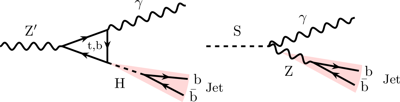
Figure 1:
Schematic illustration indicating the topology of the signal processes under consideration in this search. The spin-1 $\mathrm{Z}^{'}\to\mathrm{H}\gamma\to\mathrm{b}\overline{\mathrm{b}}\gamma $ signal scenario is shown on the left, and the spin-0 $ \mathrm{S}\to\mathrm{Z}\gamma\to\mathrm{b}\overline{\mathrm{b}}\gamma $ signal scenario is shown on the right. |
png pdf |
Figure 2:
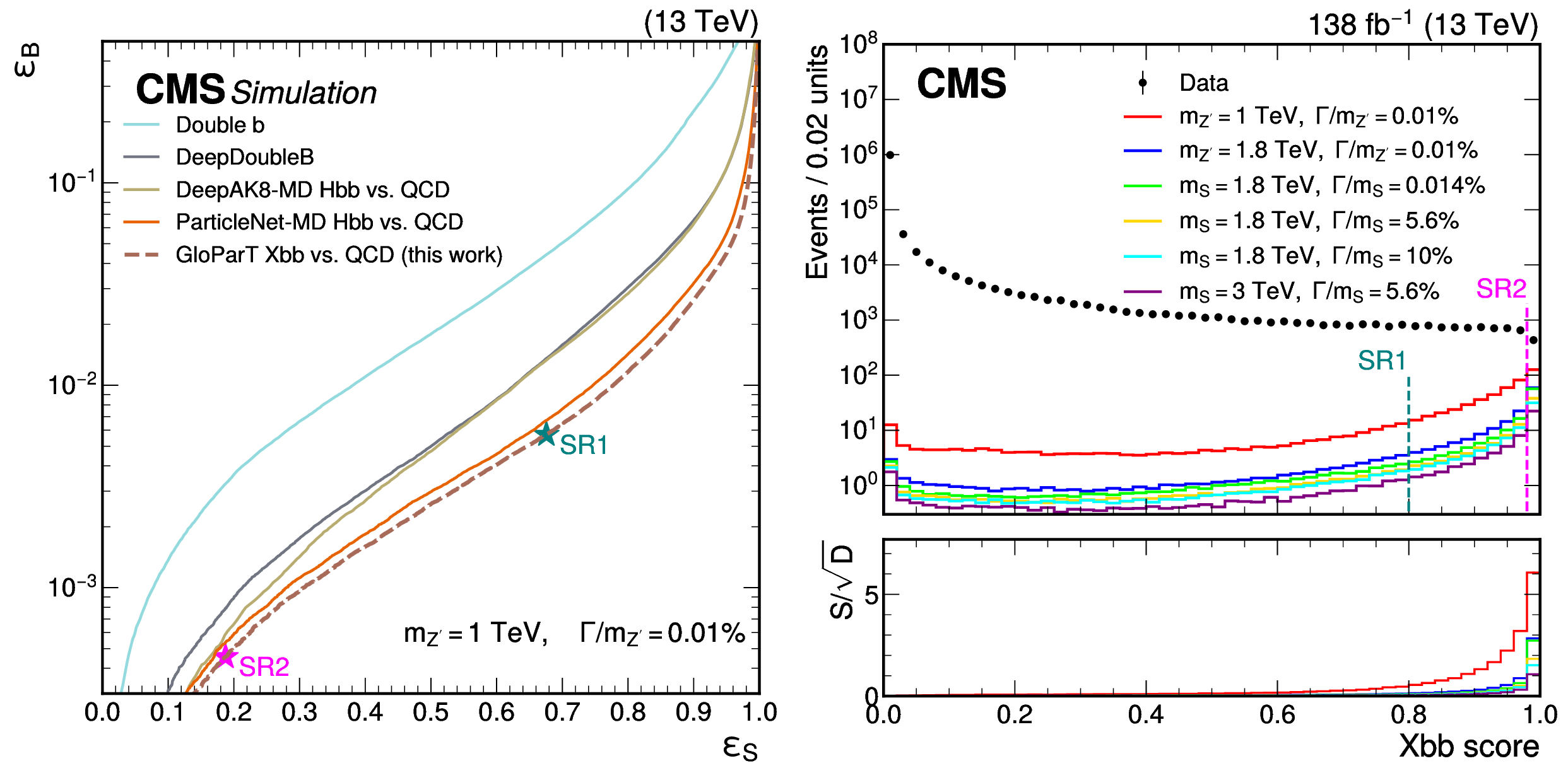
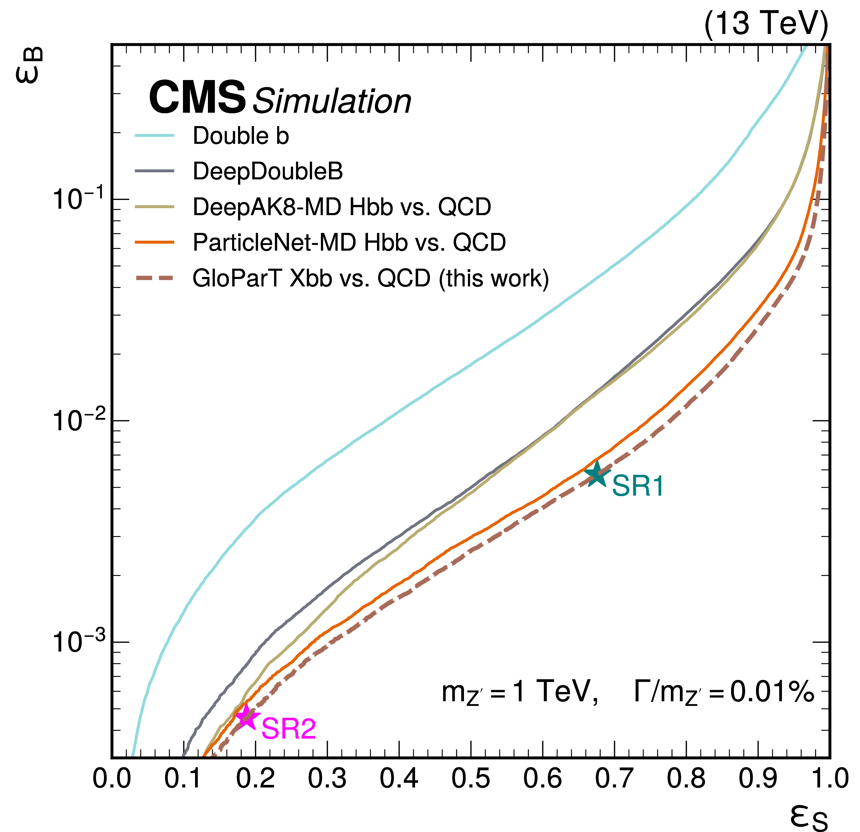
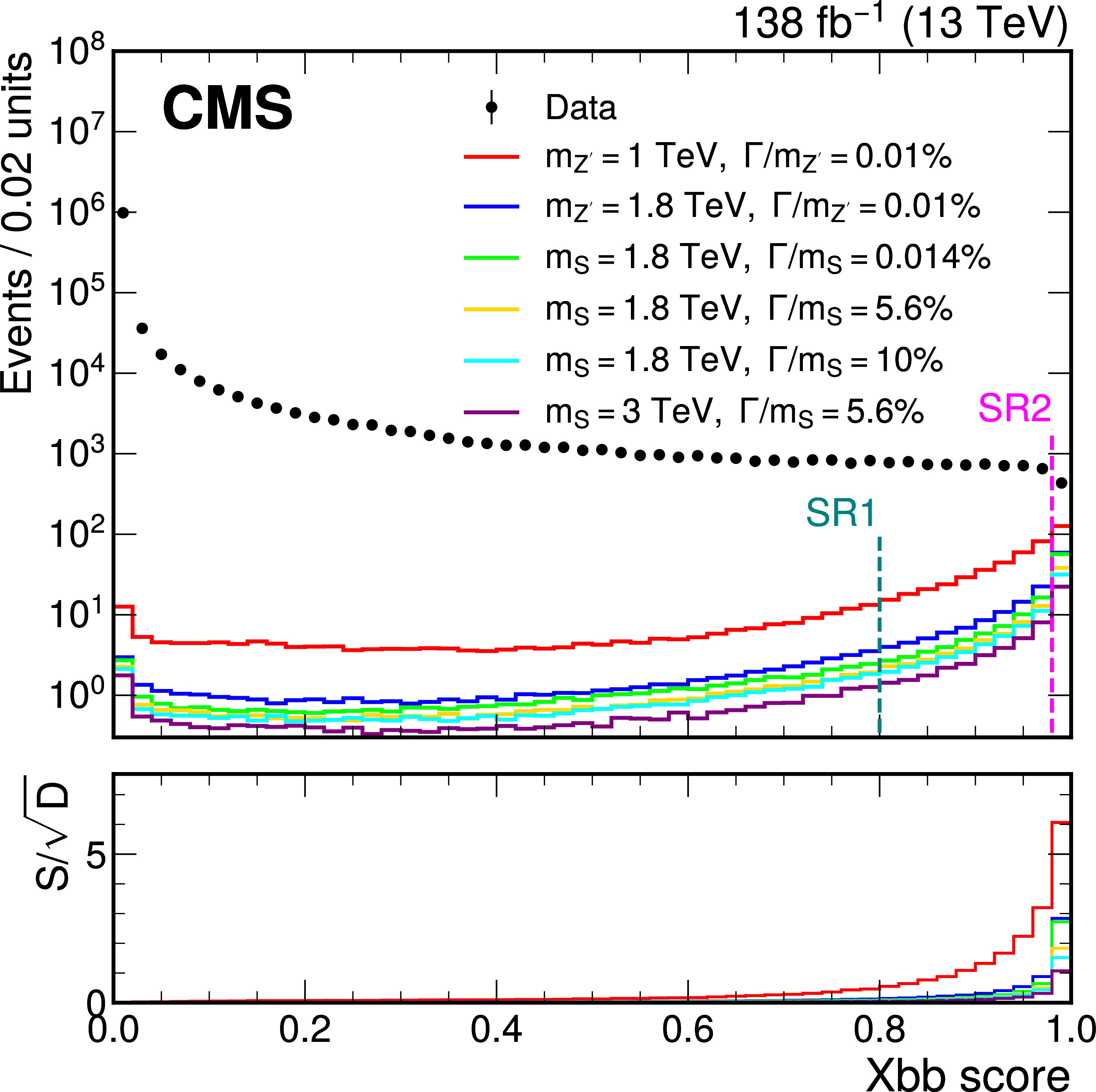
The ROC curves of background efficiency ($ \epsilon_\text{B} $) vs. signal efficiency ($ \epsilon_\text{S} $) for the Xbb tagger and other taggers from previous analyses, evaluated using a $ m_{\mathrm{Z}^{'}} = $ 1 TeV signal sample and SM background, are shown on the left. The taggers are listed in chronological order in the legend, based on their first use in similar searches (Refs. [10,69,70,71]). The right plot shows the Xbb score distributions for data and simulated signal samples, along with the significance metric, $ S/\sqrt{D} $, as defined in the text. Both plots use the preselection, with the Z' (S) signals normalized by setting $ \sigma\mathcal{B} $ to the benchmark values (10 fb). |
png pdf |
Figure 2-a:
The ROC curves of background efficiency ($ \epsilon_\text{B} $) vs. signal efficiency ($ \epsilon_\text{S} $) for the Xbb tagger and other taggers from previous analyses, evaluated using a $ m_{\mathrm{Z}^{'}} = $ 1 TeV signal sample and SM background, are shown on the left. The taggers are listed in chronological order in the legend, based on their first use in similar searches (Refs. [10,69,70,71]). The right plot shows the Xbb score distributions for data and simulated signal samples, along with the significance metric, $ S/\sqrt{D} $, as defined in the text. Both plots use the preselection, with the Z' (S) signals normalized by setting $ \sigma\mathcal{B} $ to the benchmark values (10 fb). |
png pdf |
Figure 2-b:
The ROC curves of background efficiency ($ \epsilon_\text{B} $) vs. signal efficiency ($ \epsilon_\text{S} $) for the Xbb tagger and other taggers from previous analyses, evaluated using a $ m_{\mathrm{Z}^{'}} = $ 1 TeV signal sample and SM background, are shown on the left. The taggers are listed in chronological order in the legend, based on their first use in similar searches (Refs. [10,69,70,71]). The right plot shows the Xbb score distributions for data and simulated signal samples, along with the significance metric, $ S/\sqrt{D} $, as defined in the text. Both plots use the preselection, with the Z' (S) signals normalized by setting $ \sigma\mathcal{B} $ to the benchmark values (10 fb). |
png pdf |
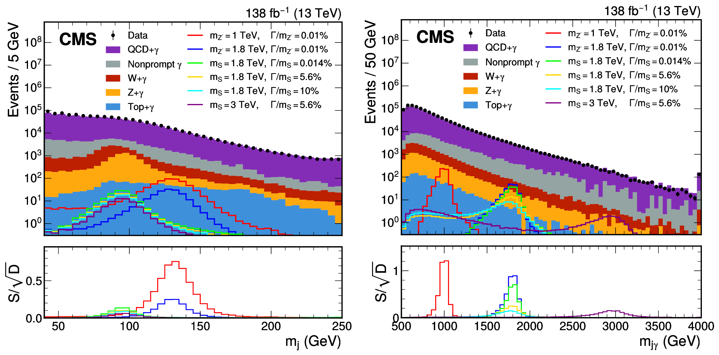
Figure 3:
The left and right plots present the distributions of $ m_{\text{j}} $ and $ m_{\text{j}\gamma} $, respectively, in data, MC background, and signal samples, with preselection criteria applied. Both plots use the preselection, with the Z' (S) signals normalized by setting $ \sigma\mathcal{B} $ to the benchmark (10 fb) values. |
png pdf |
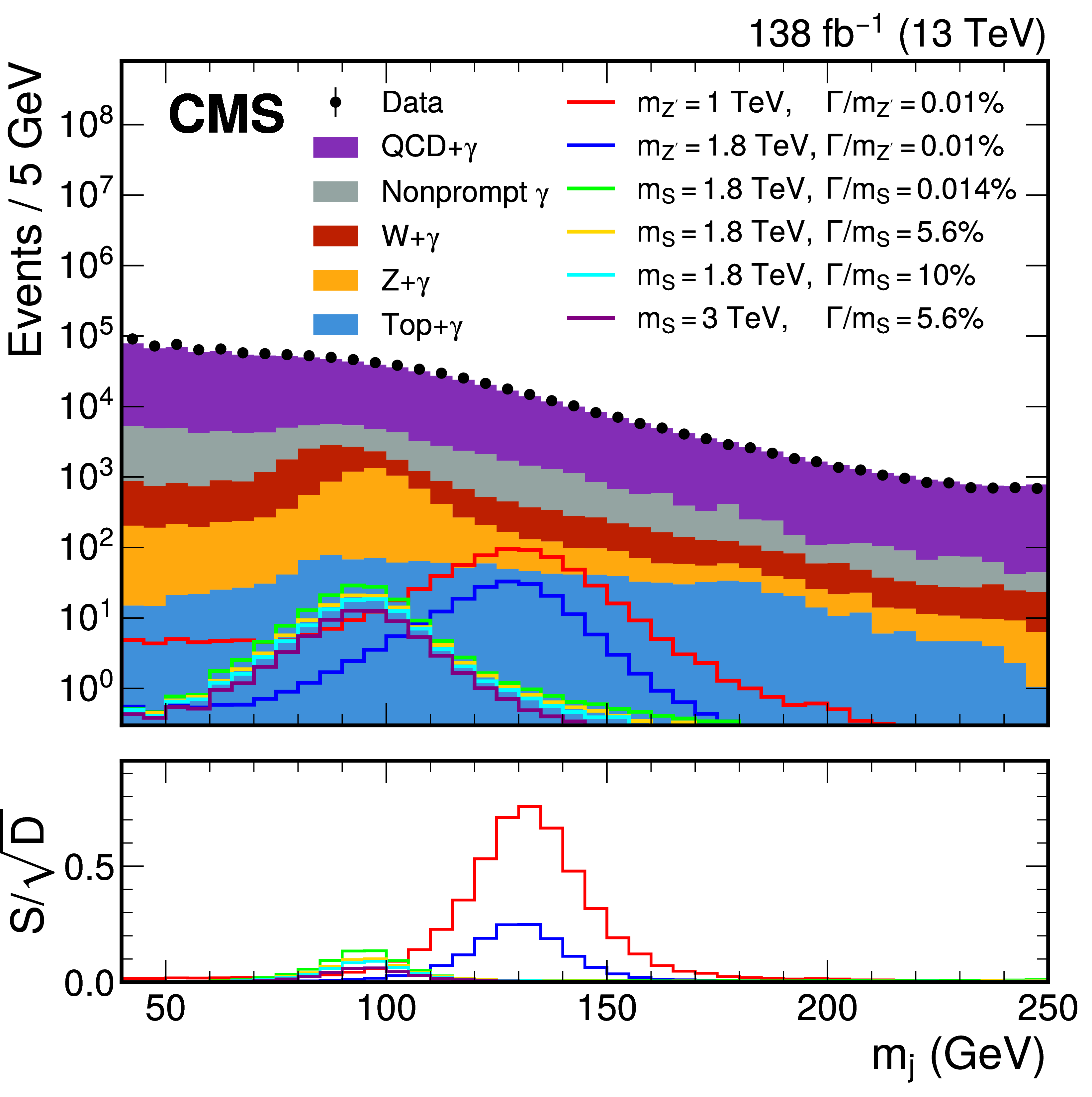
Figure 3-a:
The left and right plots present the distributions of $ m_{\text{j}} $ and $ m_{\text{j}\gamma} $, respectively, in data, MC background, and signal samples, with preselection criteria applied. Both plots use the preselection, with the Z' (S) signals normalized by setting $ \sigma\mathcal{B} $ to the benchmark (10 fb) values. |
png pdf |
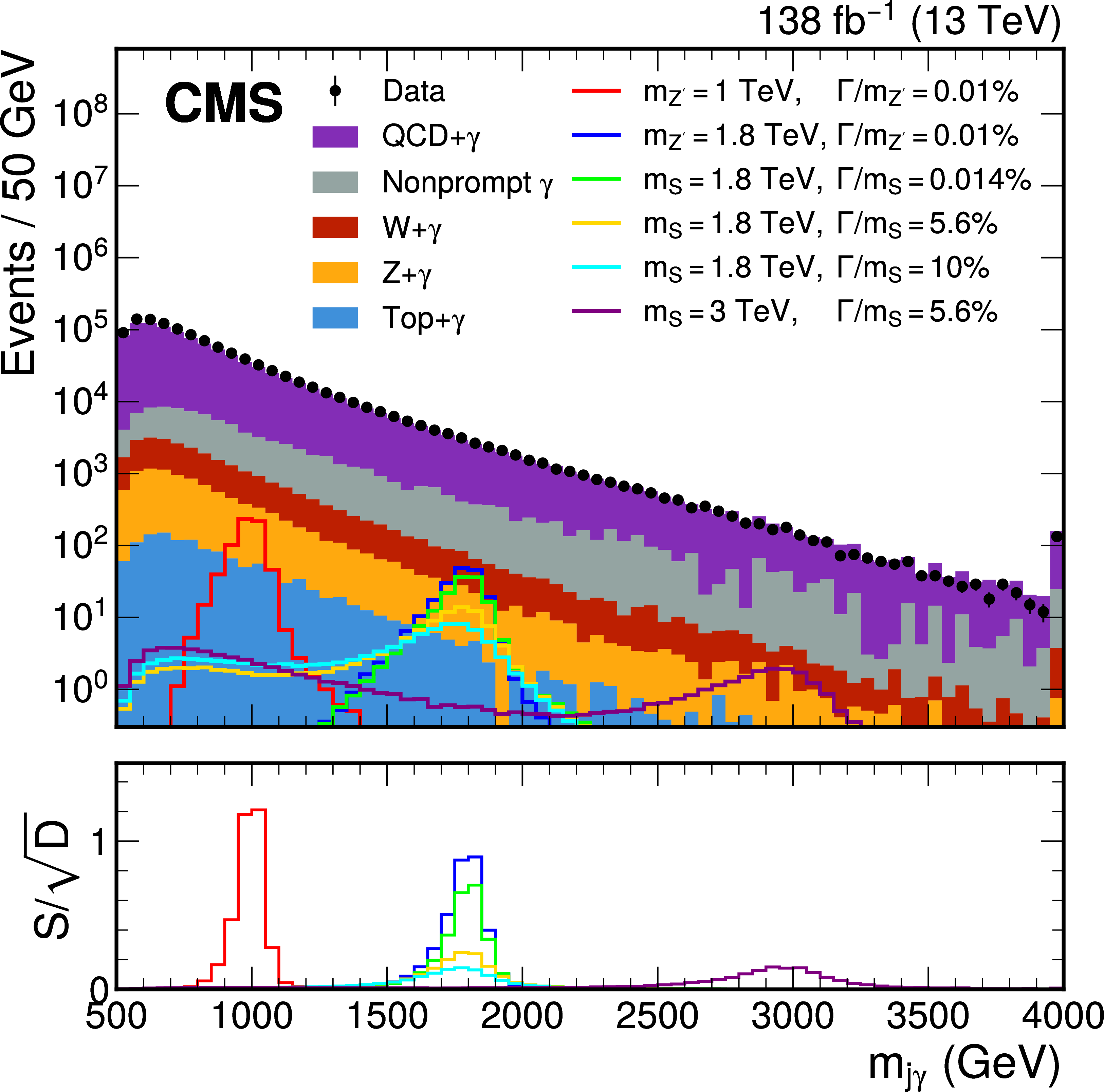
Figure 3-b:
The left and right plots present the distributions of $ m_{\text{j}} $ and $ m_{\text{j}\gamma} $, respectively, in data, MC background, and signal samples, with preselection criteria applied. Both plots use the preselection, with the Z' (S) signals normalized by setting $ \sigma\mathcal{B} $ to the benchmark (10 fb) values. |
png pdf |
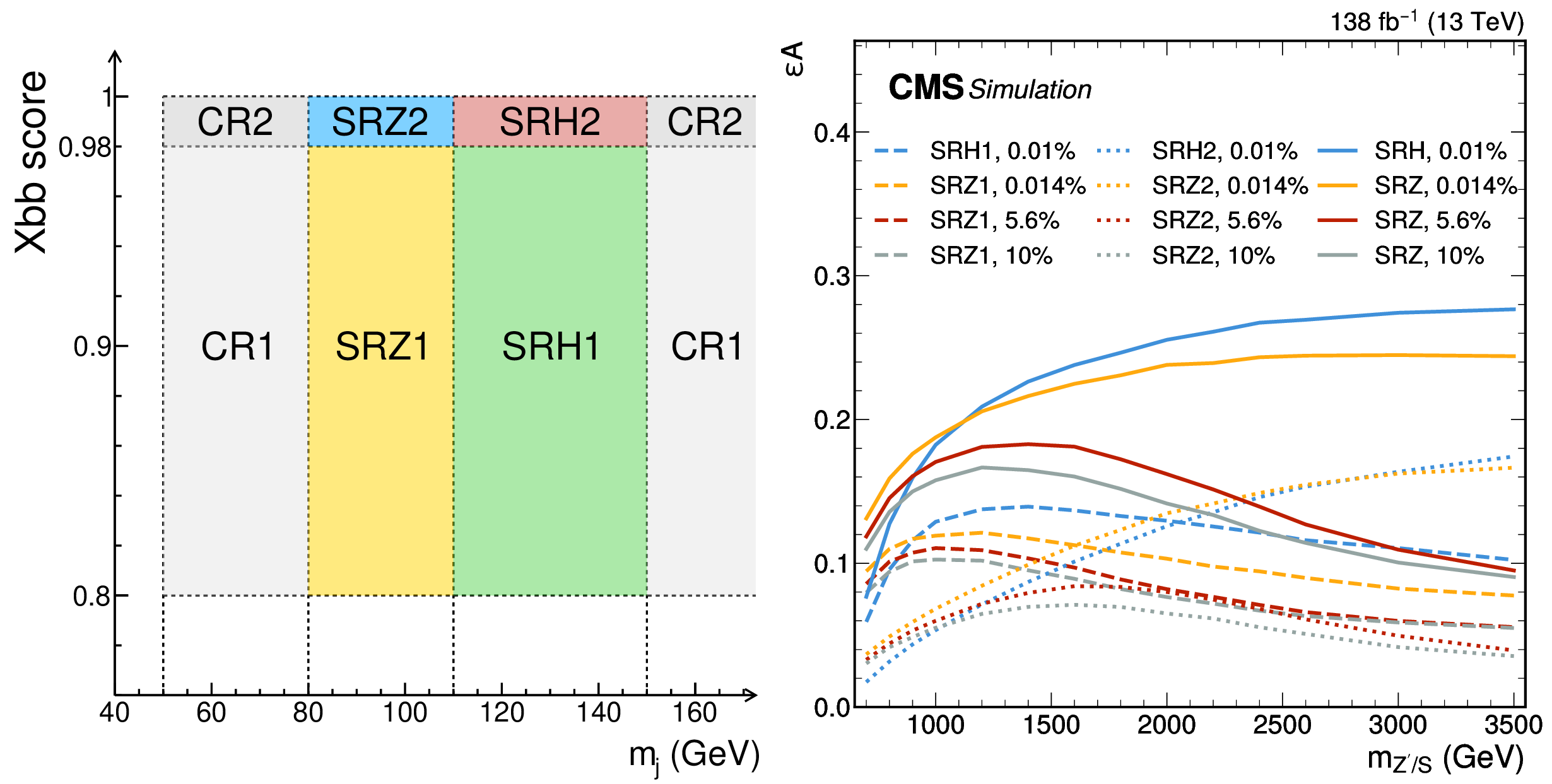
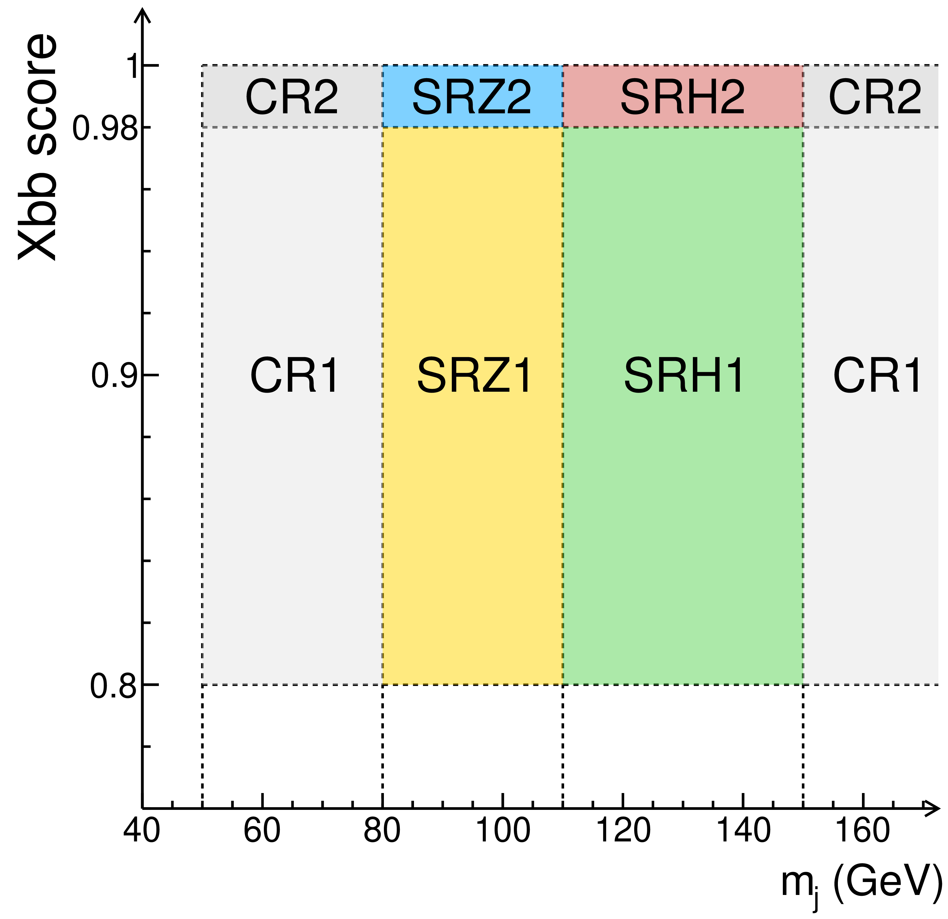
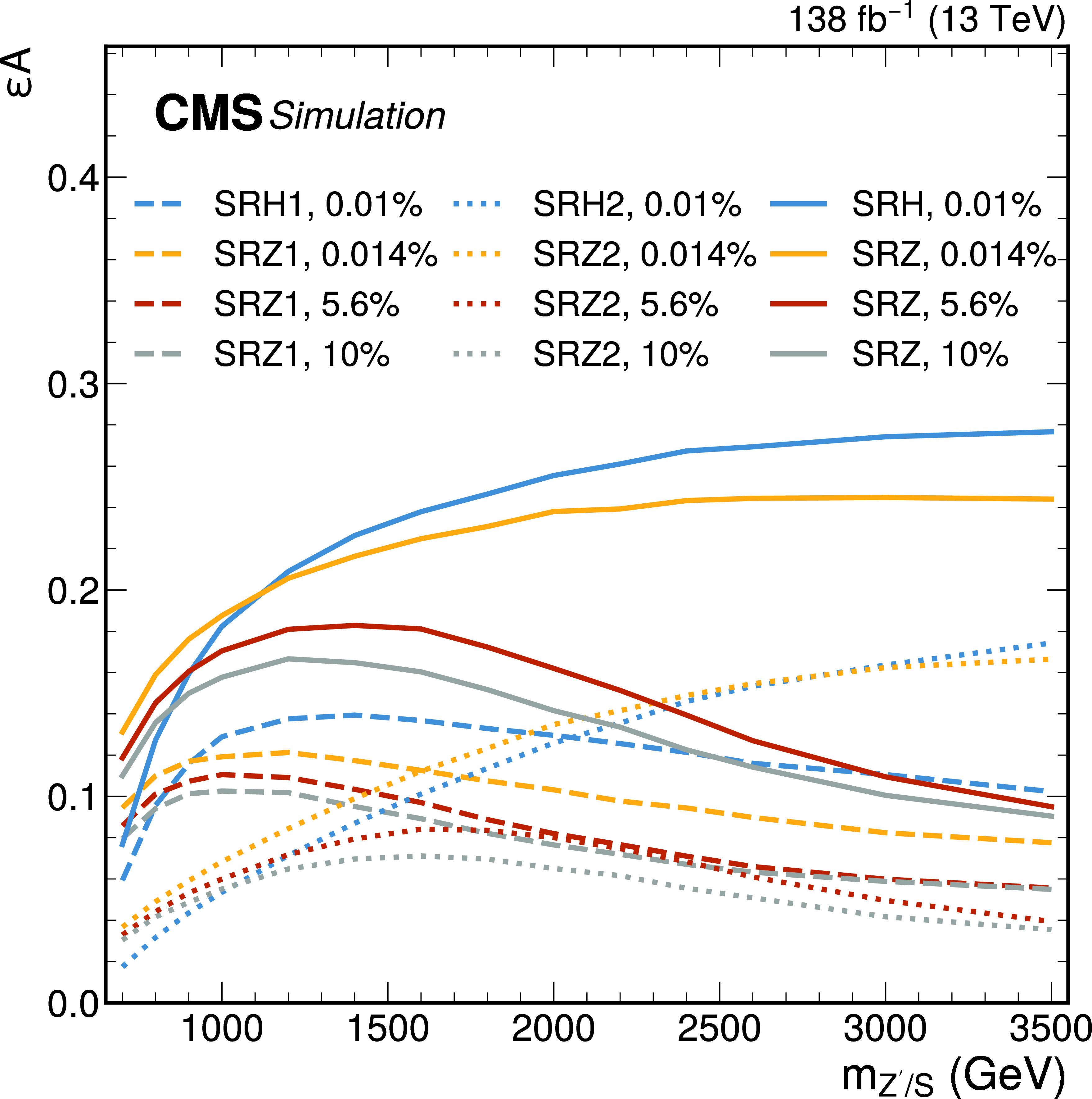
Figure 4:
A schematic illustration of the SR and CR definitions in the $ m_{\text{j}} $-Xbb plane is shown on the left. On the right, the product of signal efficiency and acceptance is plotted as a function of the resonance mass for the simulated signal samples in the relevant SRs. The percentages in the legend refer to the corresponding $ \Gamma/m $ values. Here, SRZ(H) denotes SRZ(H)1+SRZ(H)2. |
png pdf |
Figure 4-a:
A schematic illustration of the SR and CR definitions in the $ m_{\text{j}} $-Xbb plane is shown on the left. On the right, the product of signal efficiency and acceptance is plotted as a function of the resonance mass for the simulated signal samples in the relevant SRs. The percentages in the legend refer to the corresponding $ \Gamma/m $ values. Here, SRZ(H) denotes SRZ(H)1+SRZ(H)2. |
png pdf |
Figure 4-b:
A schematic illustration of the SR and CR definitions in the $ m_{\text{j}} $-Xbb plane is shown on the left. On the right, the product of signal efficiency and acceptance is plotted as a function of the resonance mass for the simulated signal samples in the relevant SRs. The percentages in the legend refer to the corresponding $ \Gamma/m $ values. Here, SRZ(H) denotes SRZ(H)1+SRZ(H)2. |
png pdf |
Figure 5:
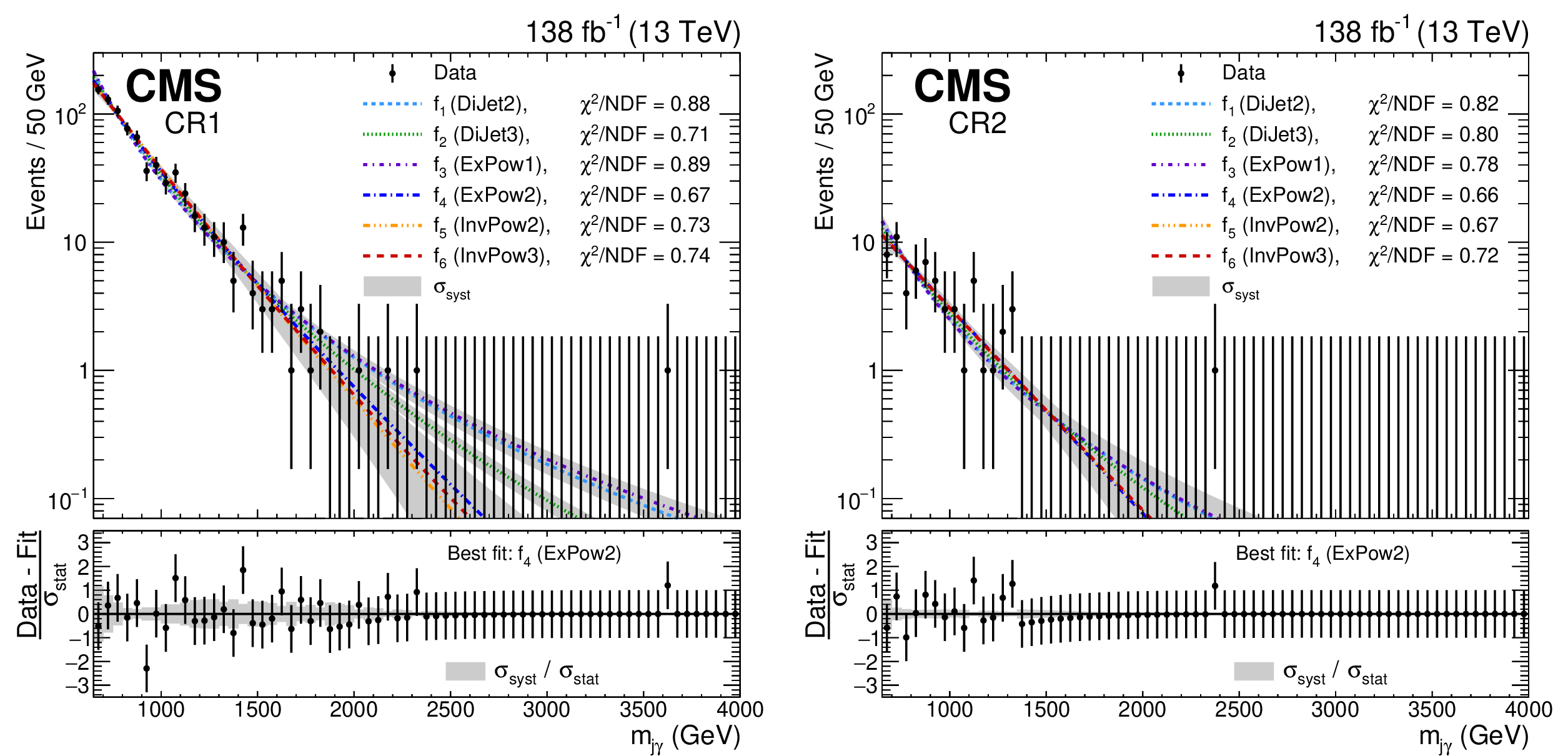
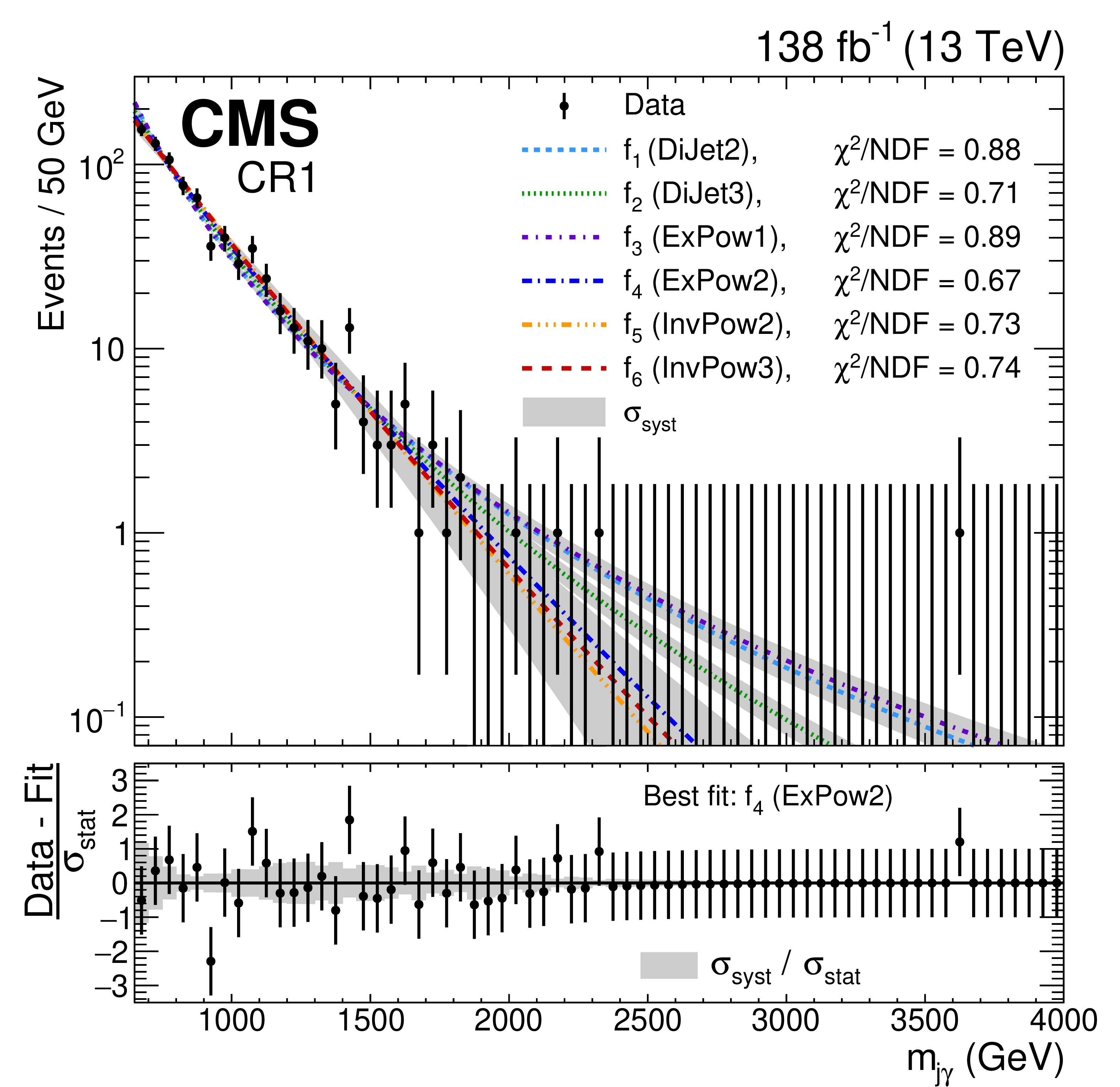
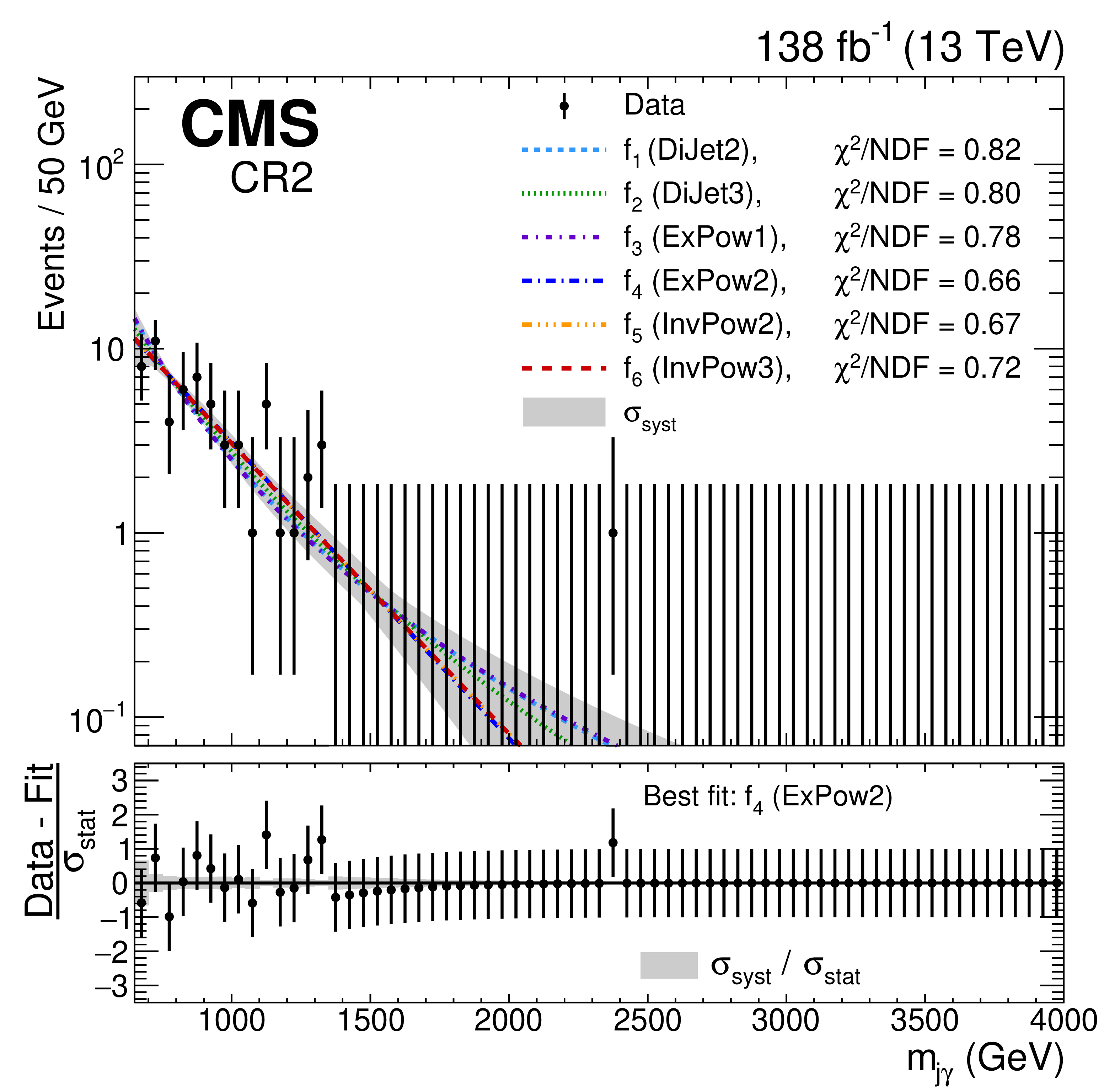
The $ m_{\text{j}\gamma} $ distributions of the data in CR1 (left) and CR2 (right) fitted with the six parametric functions. The legends specify the $ \chi^2/\text{ndf} $ for each fit. The lower panels show the pull distributions as defined in the text, with respect to the best fit function specified in the legend. |
png pdf |
Figure 5-a:
The $ m_{\text{j}\gamma} $ distributions of the data in CR1 (left) and CR2 (right) fitted with the six parametric functions. The legends specify the $ \chi^2/\text{ndf} $ for each fit. The lower panels show the pull distributions as defined in the text, with respect to the best fit function specified in the legend. |
png pdf |
Figure 5-b:
The $ m_{\text{j}\gamma} $ distributions of the data in CR1 (left) and CR2 (right) fitted with the six parametric functions. The legends specify the $ \chi^2/\text{ndf} $ for each fit. The lower panels show the pull distributions as defined in the text, with respect to the best fit function specified in the legend. |
png pdf |
Figure 6:
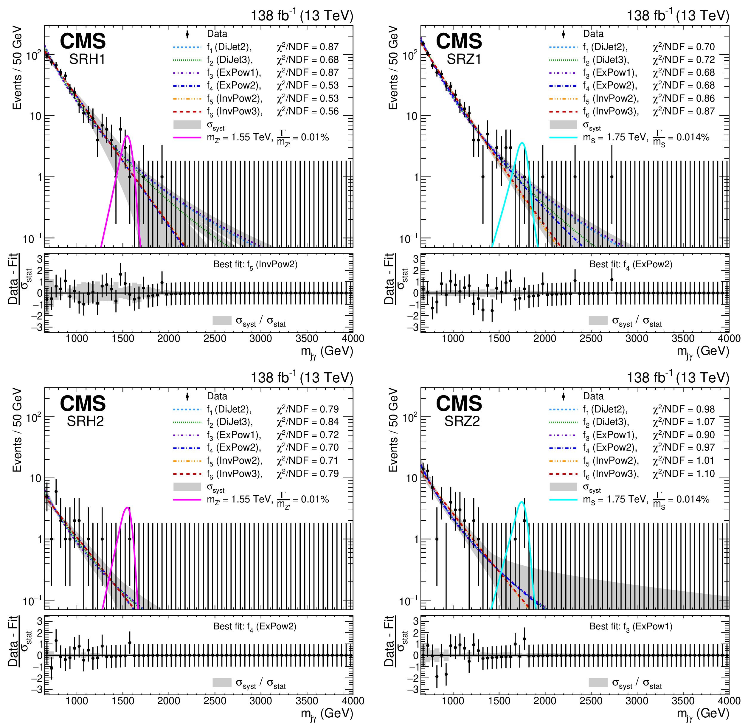
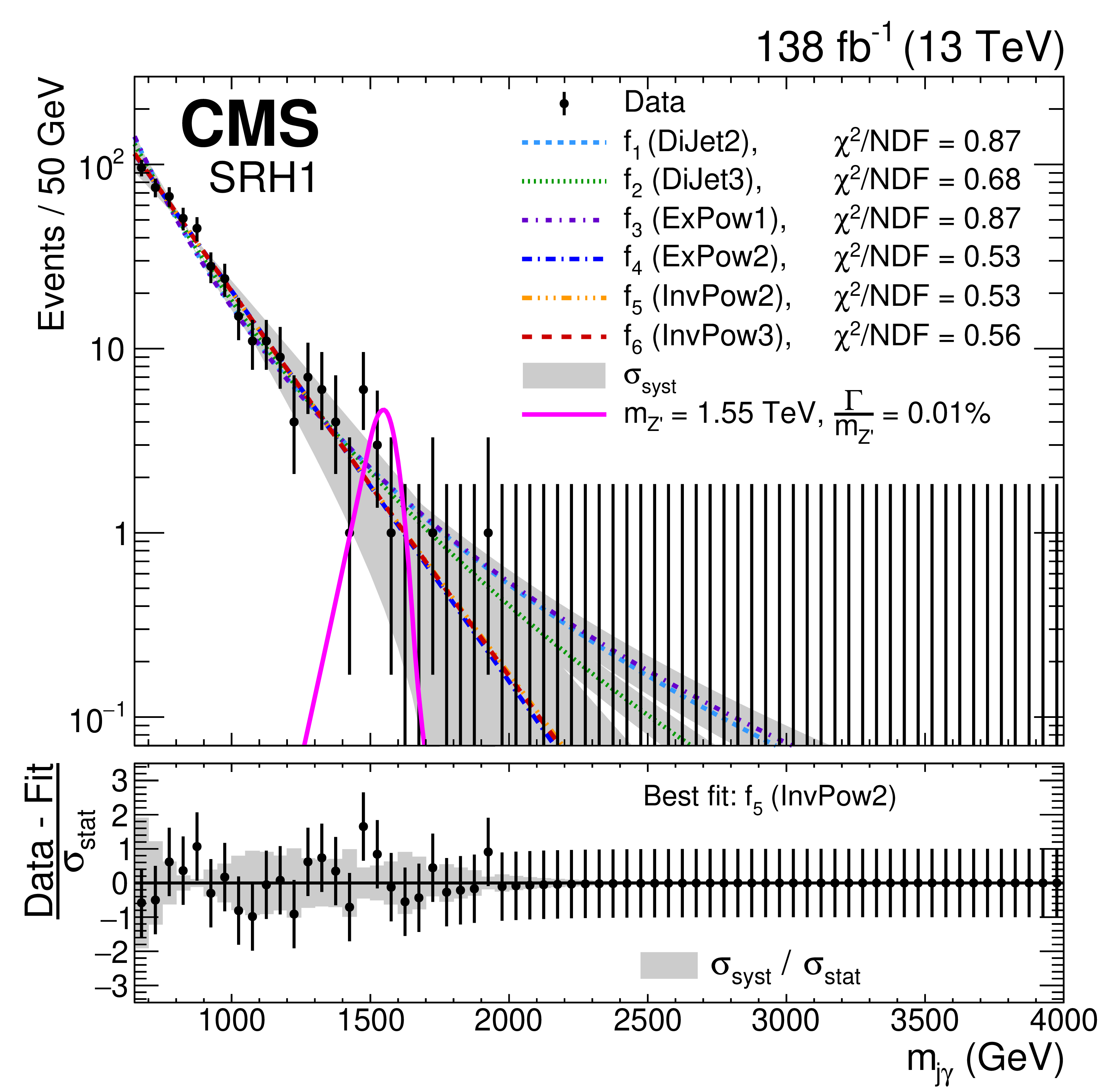
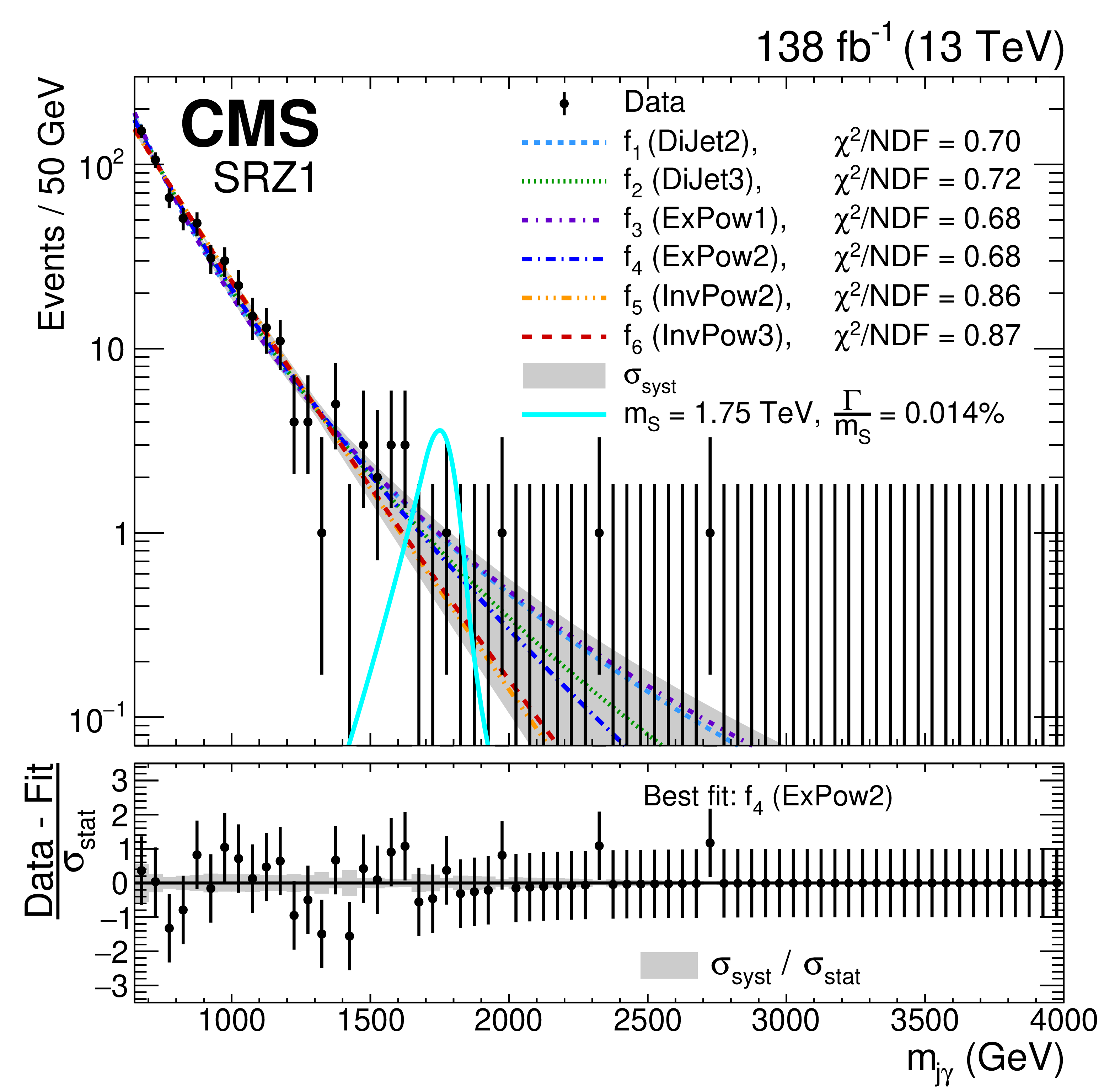
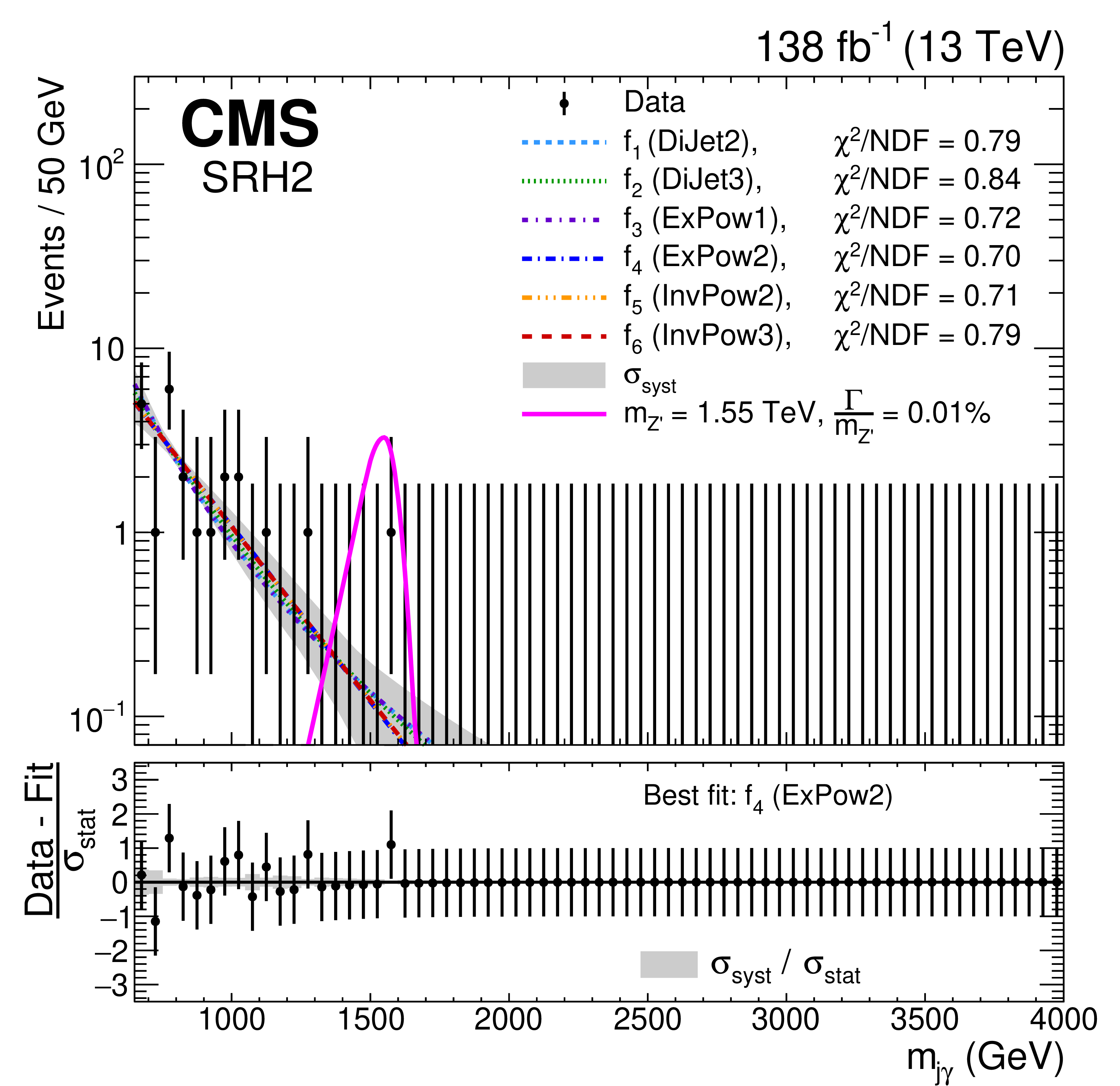
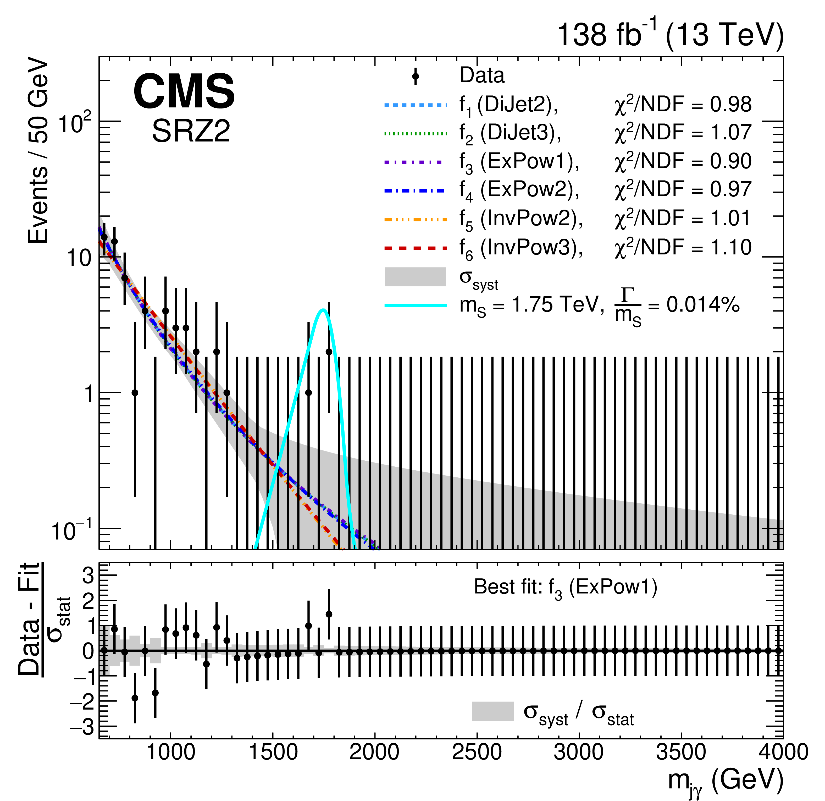
Post-fit $ m_{\text{j}\gamma} $ spectra in the four SRs: SRH1 (upper left), SRZ1 (upper right), SRH2 (lower left), and SRZ2 (lower right). The legends specify the $ \chi^2/\text{ndf} $ for each fit. The lower panels show the pull distributions with respect to the best fit function specified in the legend. The signals with the largest local significances are shown with continuous lines in each SR and are normalized to the observed $ \sigma\mathcal{B} $ upper limits. |
png pdf |
Figure 6-a:
Post-fit $ m_{\text{j}\gamma} $ spectra in the four SRs: SRH1 (upper left), SRZ1 (upper right), SRH2 (lower left), and SRZ2 (lower right). The legends specify the $ \chi^2/\text{ndf} $ for each fit. The lower panels show the pull distributions with respect to the best fit function specified in the legend. The signals with the largest local significances are shown with continuous lines in each SR and are normalized to the observed $ \sigma\mathcal{B} $ upper limits. |
png pdf |
Figure 6-b:
Post-fit $ m_{\text{j}\gamma} $ spectra in the four SRs: SRH1 (upper left), SRZ1 (upper right), SRH2 (lower left), and SRZ2 (lower right). The legends specify the $ \chi^2/\text{ndf} $ for each fit. The lower panels show the pull distributions with respect to the best fit function specified in the legend. The signals with the largest local significances are shown with continuous lines in each SR and are normalized to the observed $ \sigma\mathcal{B} $ upper limits. |
png pdf |
Figure 6-c:
Post-fit $ m_{\text{j}\gamma} $ spectra in the four SRs: SRH1 (upper left), SRZ1 (upper right), SRH2 (lower left), and SRZ2 (lower right). The legends specify the $ \chi^2/\text{ndf} $ for each fit. The lower panels show the pull distributions with respect to the best fit function specified in the legend. The signals with the largest local significances are shown with continuous lines in each SR and are normalized to the observed $ \sigma\mathcal{B} $ upper limits. |
png pdf |
Figure 6-d:
Post-fit $ m_{\text{j}\gamma} $ spectra in the four SRs: SRH1 (upper left), SRZ1 (upper right), SRH2 (lower left), and SRZ2 (lower right). The legends specify the $ \chi^2/\text{ndf} $ for each fit. The lower panels show the pull distributions with respect to the best fit function specified in the legend. The signals with the largest local significances are shown with continuous lines in each SR and are normalized to the observed $ \sigma\mathcal{B} $ upper limits. |
png pdf |
Figure 7:
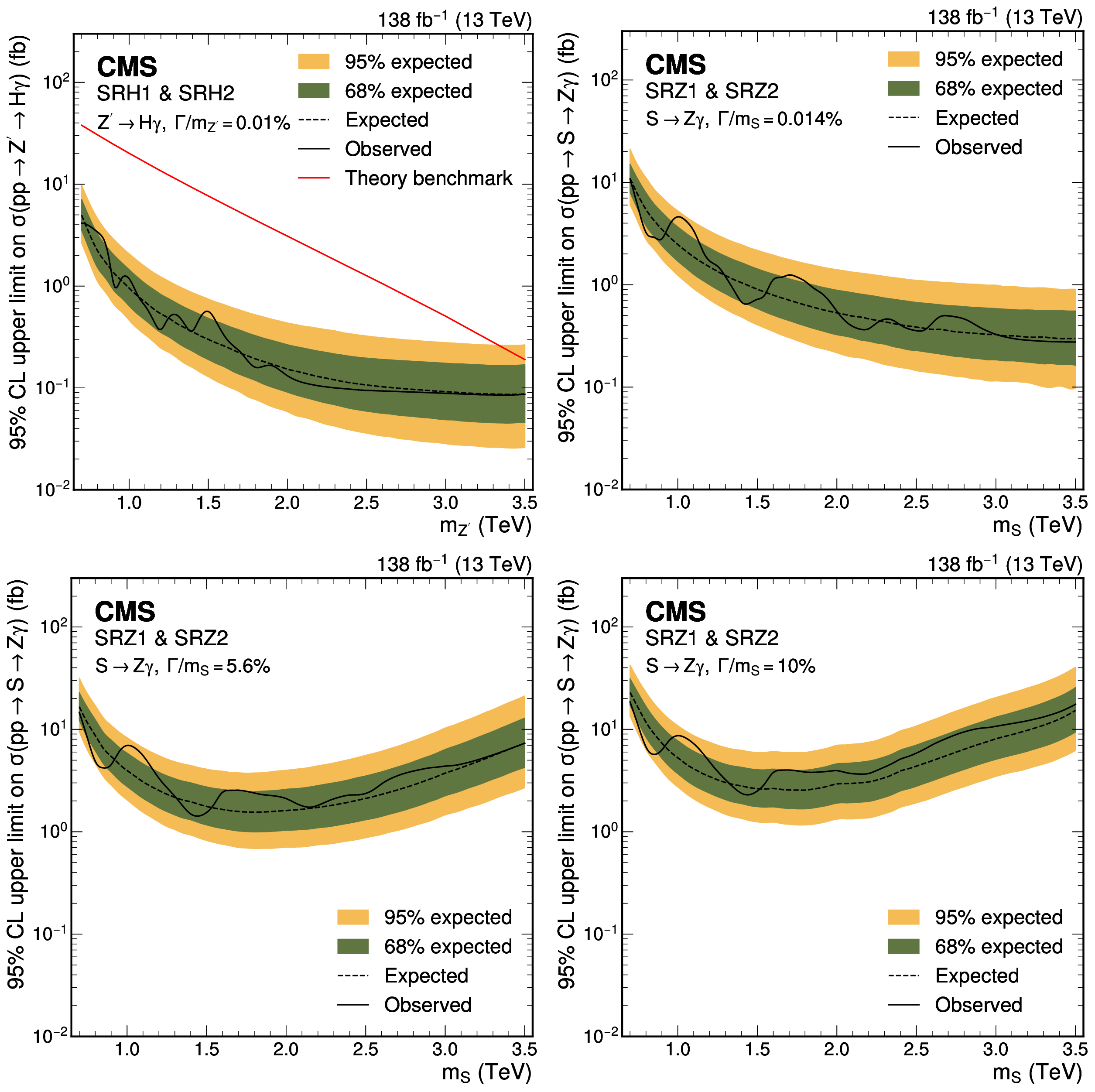
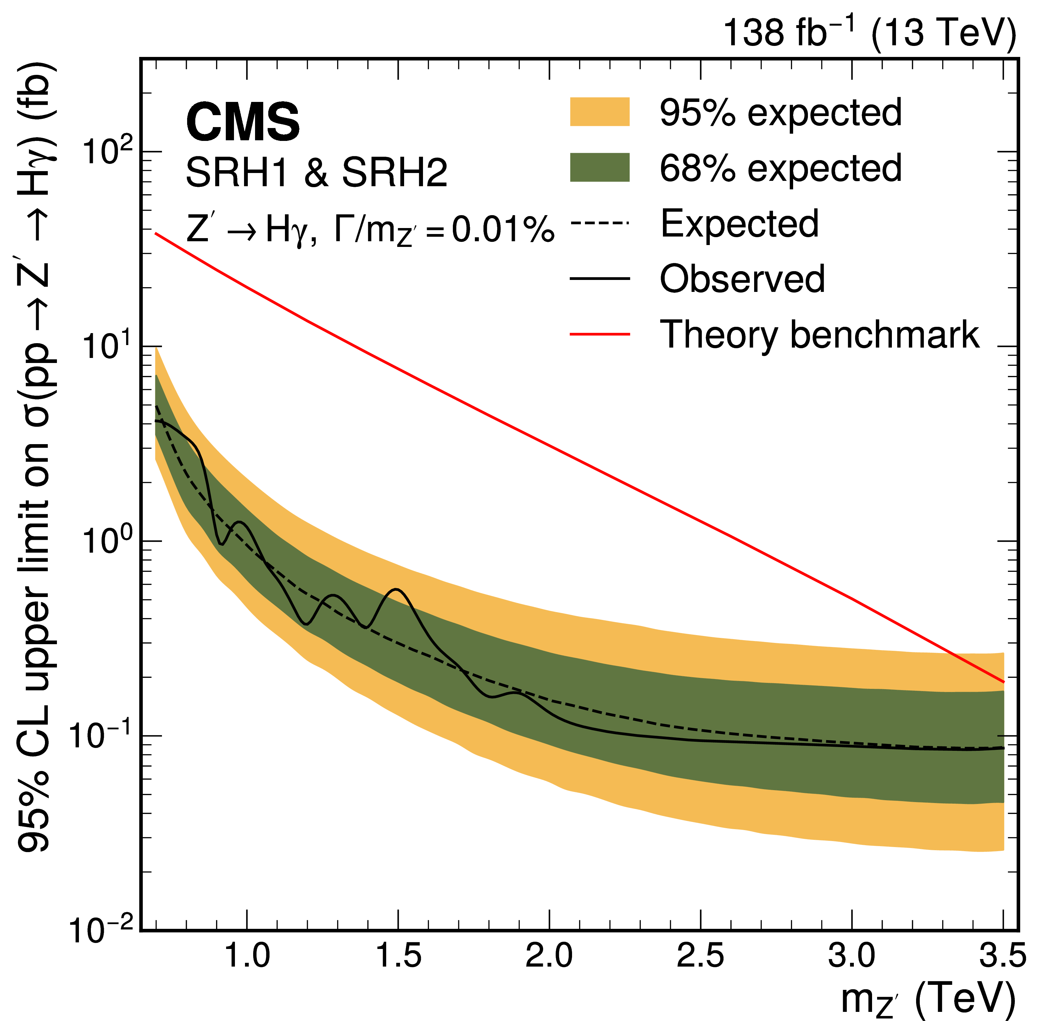
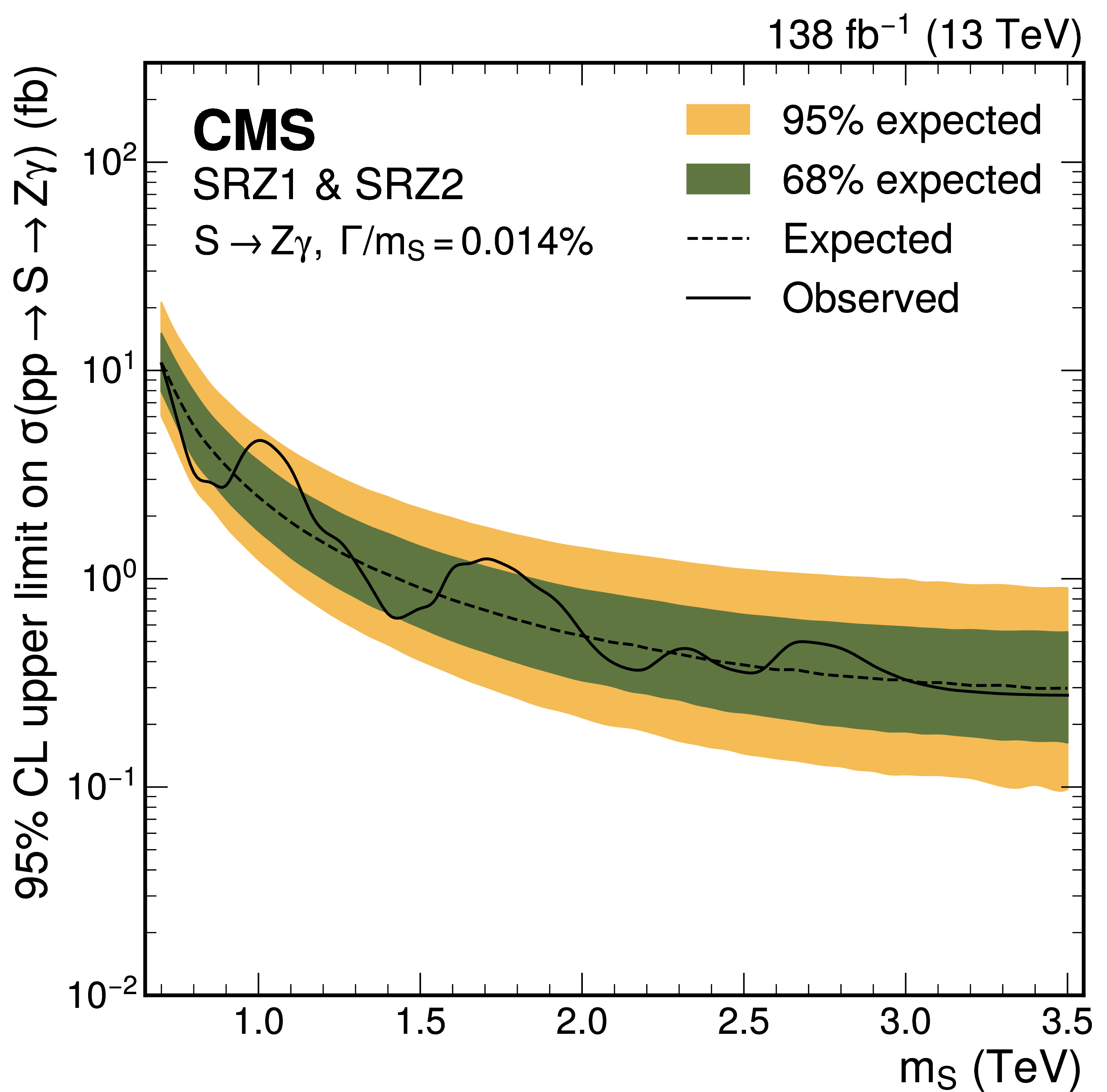
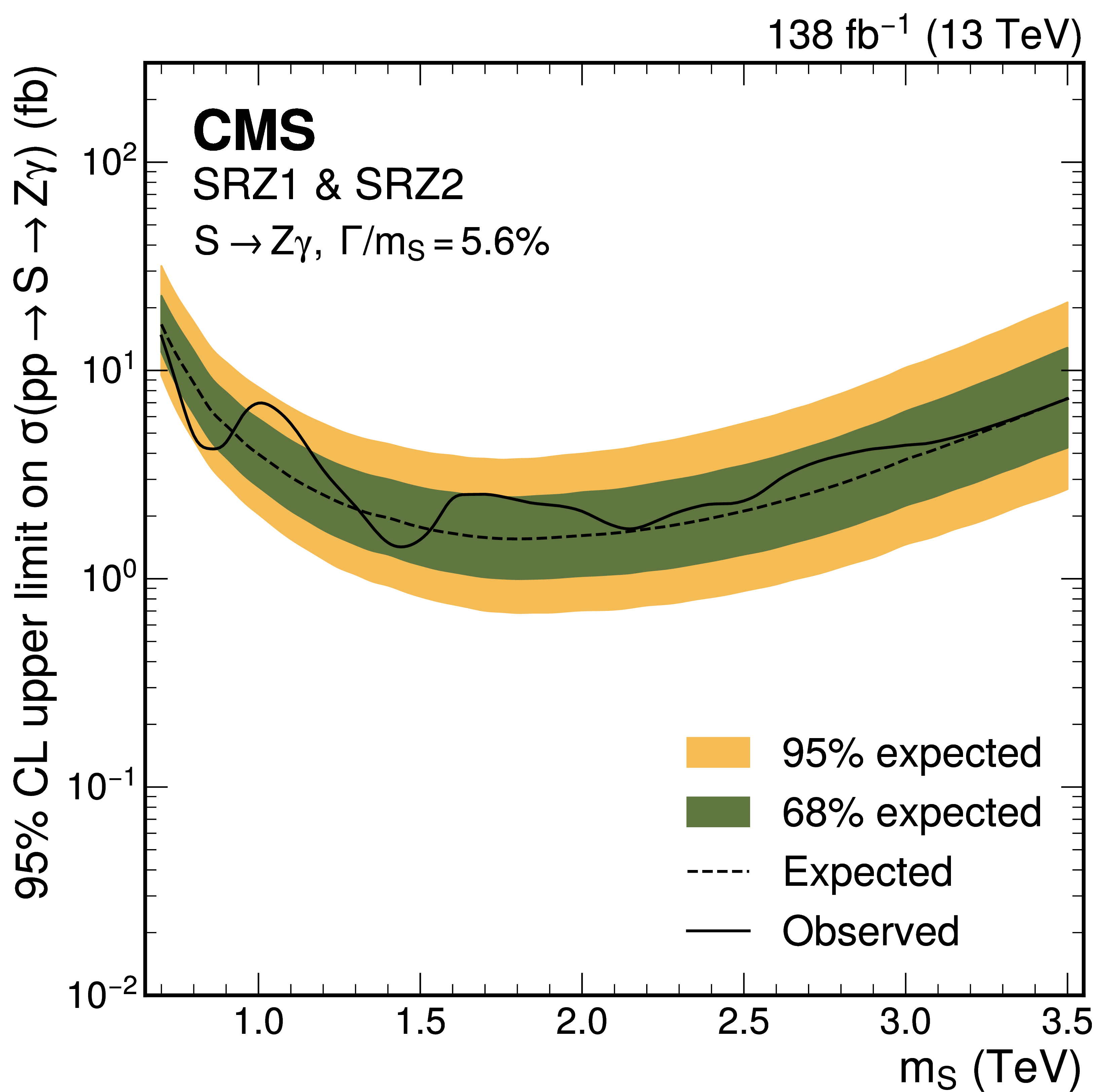
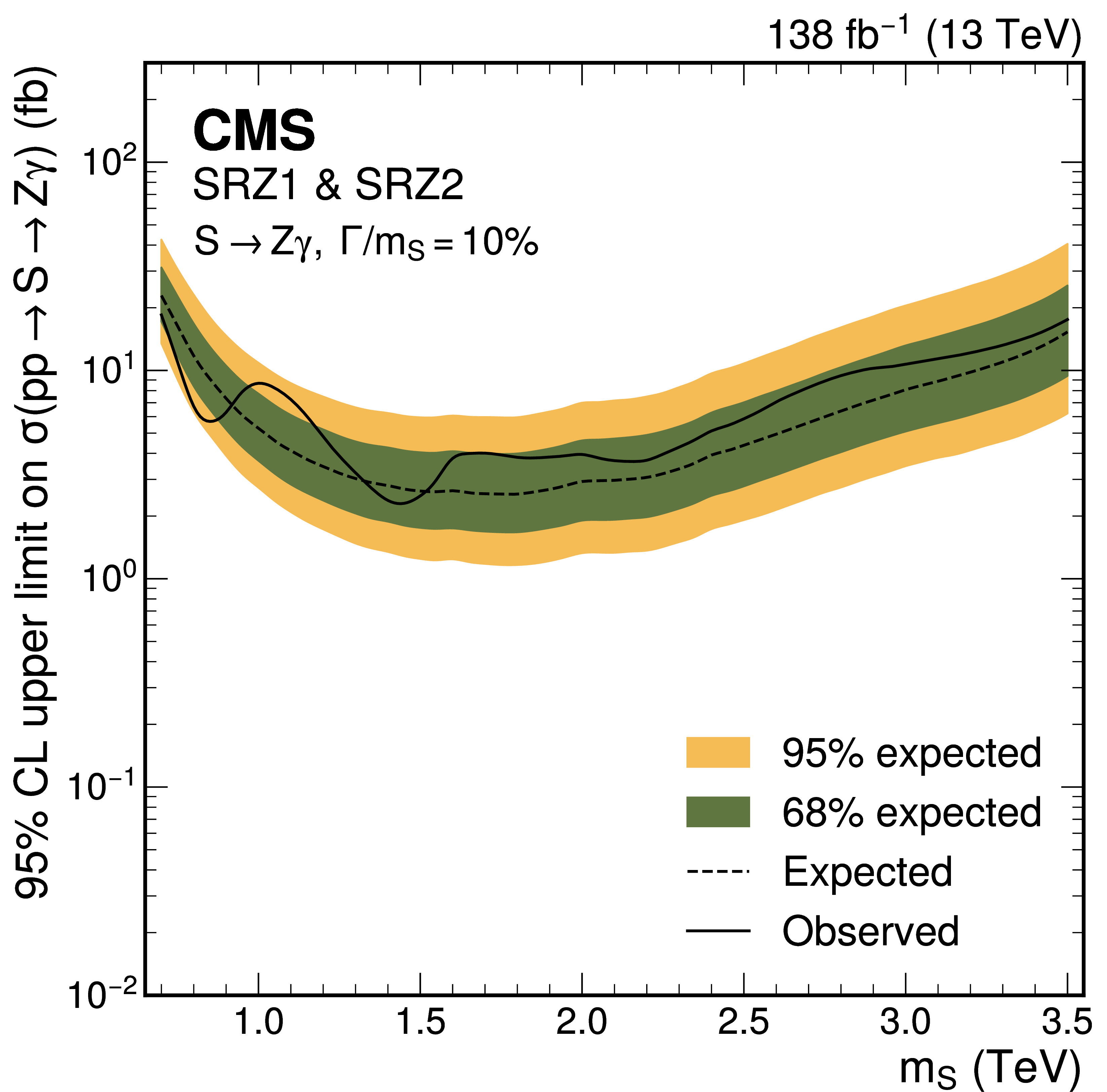
The 95% CL upper limits on the product of production cross section and branching fraction $ \sigma\mathcal{B} $ for $ \mathrm{Z}^{'}\to\mathrm{H}\gamma $ (upper left) and $ \mathrm{S}\to\mathrm{Z}\gamma $ with a narrow width (upper right), 5.6% width (lower left), and 10% width (lower right). Observed (expected) limits are shown with solid (dashed) lines. The colored bands represent the 68 and 95% CL intervals for the expected limits. The red line represents the theory benchmark model used for Z' signal simulation. |
png pdf |
Figure 7-a:
The 95% CL upper limits on the product of production cross section and branching fraction $ \sigma\mathcal{B} $ for $ \mathrm{Z}^{'}\to\mathrm{H}\gamma $ (upper left) and $ \mathrm{S}\to\mathrm{Z}\gamma $ with a narrow width (upper right), 5.6% width (lower left), and 10% width (lower right). Observed (expected) limits are shown with solid (dashed) lines. The colored bands represent the 68 and 95% CL intervals for the expected limits. The red line represents the theory benchmark model used for Z' signal simulation. |
png pdf |
Figure 7-b:
The 95% CL upper limits on the product of production cross section and branching fraction $ \sigma\mathcal{B} $ for $ \mathrm{Z}^{'}\to\mathrm{H}\gamma $ (upper left) and $ \mathrm{S}\to\mathrm{Z}\gamma $ with a narrow width (upper right), 5.6% width (lower left), and 10% width (lower right). Observed (expected) limits are shown with solid (dashed) lines. The colored bands represent the 68 and 95% CL intervals for the expected limits. The red line represents the theory benchmark model used for Z' signal simulation. |
png pdf |
Figure 7-c:
The 95% CL upper limits on the product of production cross section and branching fraction $ \sigma\mathcal{B} $ for $ \mathrm{Z}^{'}\to\mathrm{H}\gamma $ (upper left) and $ \mathrm{S}\to\mathrm{Z}\gamma $ with a narrow width (upper right), 5.6% width (lower left), and 10% width (lower right). Observed (expected) limits are shown with solid (dashed) lines. The colored bands represent the 68 and 95% CL intervals for the expected limits. The red line represents the theory benchmark model used for Z' signal simulation. |
png pdf |
Figure 7-d:
The 95% CL upper limits on the product of production cross section and branching fraction $ \sigma\mathcal{B} $ for $ \mathrm{Z}^{'}\to\mathrm{H}\gamma $ (upper left) and $ \mathrm{S}\to\mathrm{Z}\gamma $ with a narrow width (upper right), 5.6% width (lower left), and 10% width (lower right). Observed (expected) limits are shown with solid (dashed) lines. The colored bands represent the 68 and 95% CL intervals for the expected limits. The red line represents the theory benchmark model used for Z' signal simulation. |
| Tables | |
png pdf |
Table 1:
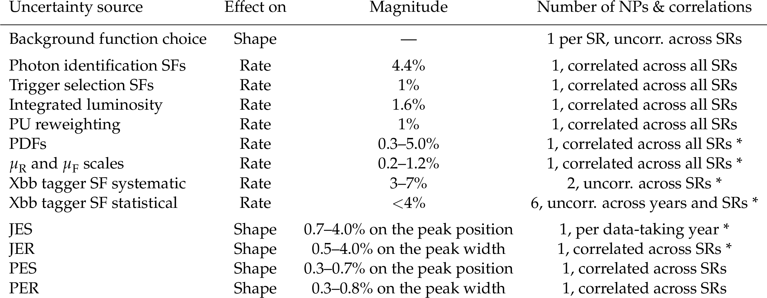
The sources of systematic uncertainties included in the analysis. The second column indicates whether the uncertainty affects the background or signal shape or its rate. The third column from the left lists the magnitude of the corresponding pre-fit systematic uncertainty. The last column indicates the total number of nuisance parameters (NPs) and whether or not they are treated as correlated across all SRs. An asterisk (*) denotes a value or shape template unique to each signal scenario. |
| Summary |
| A search for heavy resonances decaying to a photon and a Z or a Higgs boson (H) in the $ \gamma $+jet final state, using $ \sqrt{s} = $ 13 TeV proton-proton collision data collected with the CMS detector in 2016--2018, corresponding to an integrated luminosity of 138 fb$ ^{-1} $, has been presented. For the H$\gamma $ resonance analysis, a benchmark spin-1 resonance model with a narrow width is considered, while the Z$\gamma $ analysis considers a standard model Higgs-like heavy spin-0 resonance, using several different width hypotheses. The final states of these resonant processes feature a photon and a massive, large-radius jet, containing the decay products of $ \mathrm{H},\,\mathrm{Z}\to\mathrm{b}\overline{\mathrm{b}} $, identified using the particle transformer jet substructure algorithm GLOPART for jet classification and the PARTICLENET algorithm for jet mass regression. These advanced machine-learning techniques greatly improve sensitivity over previous searches. The results are consistent with the predictions of the standard model within the measurement uncertainties. Exclusion limits at 95% confidence level are set on the product of the production cross section and the branching fraction for the resonance decay into H$\gamma $ or Z$\gamma $, with observed values below 0.1 and 0.3 fb for the spin-1 and spin-0 scenarios, respectively. This result establishes the most stringent constraints to date on the production and relevant decay of such heavy resonances. |
| References | ||||
| 1 | CMS Collaboration | Search for heavy resonances decaying to Z($ \nu\bar{\nu} $)V(q$ \bar{\text{q}} $') in proton-proton collisions at $ \sqrt{s} = $ 13 TeV | PRD 106 (2022) 012004 | 2109.08268 |
| 2 | CMS Collaboration | Search for new heavy resonances decaying to WW, WZ, ZZ, WH, or ZH boson pairs in the all-jets final state in proton-proton collisions at $ \sqrt{s} = $ 13 TeV | PLB 844 (2023) 137813 | 2210.00043 |
| 3 | CMS Collaboration | Search for heavy resonances decaying to WW, WZ, or WH boson pairs in the lepton plus merged jet final state in proton-proton collisions at $ \sqrt{s} = $ 13 TeV | PRD 105 (2022) 032008 | 2109.06055 |
| 4 | CMS Collaboration | Search for high mass dijet resonances with a new background prediction method in proton-proton collisions at $ \sqrt{s} = $ 13 TeV | JHEP 05 (2020) 033 | CMS-EXO-19-012 1911.03947 |
| 5 | CMS Collaboration | Search for a heavy resonance decaying into a Z and a Higgs boson in events with an energetic jet and two electrons, two muons, or missing transverse momentum in proton-proton collisions at $ \sqrt{s} = $ 13 TeV | JHEP 02 (2025) 089 | 2411.00202 |
| 6 | CMS Collaboration | Search for heavy resonances decaying to ZZ or ZW and axion-like particles mediating nonresonant ZZ or ZH production at $ \sqrt{s} = $ 13 TeV | JHEP 04 (2022) 087 | 2111.13669 |
| 7 | CMS Collaboration | Search for a heavy vector resonance decaying to a Z boson and a Higgs boson in proton-proton collisions at $ \sqrt{s} = $ 13 TeV | EPJC 81 (2021) 688 | 2102.08198 |
| 8 | CMS Collaboration | Searches for Higgs boson production through decays of heavy resonances | Phys. Rept. 1115 (2025) 368 | 2403.16926 |
| 9 | CMS Collaboration | Search for Z$ \gamma $ resonances using leptonic and hadronic final states in proton-proton collisions at $ \sqrt{s}= $ 13 TeV | JHEP 09 (2018) 148 | CMS-EXO-17-005 1712.03143 |
| 10 | CMS Collaboration | Search for narrow H$ \gamma $ resonances in proton-proton collisions at $ \sqrt{s} = $ 13 TeV | PRL 122 (2019) 081804 | CMS-EXO-17-019 1808.01257 |
| 11 | CMS Collaboration | Search for W$ \gamma $ resonances in proton-proton collisions at $ \sqrt{s} = $ 13 TeV using hadronic decays of Lorentz-boosted W bosons | PLB 826 (2022) 136888 | CMS-EXO-20-001 2106.10509 |
| 12 | CMS Collaboration | Search for new physics in high-mass diphoton events from proton-proton collisions at $ \sqrt{\textrm{s}} = $ 13 TeV | JHEP 08 (2024) 215 | CMS-EXO-22-024 2405.09320 |
| 13 | ATLAS Collaboration | Search for resonances decaying into a weak vector boson and a Higgs boson in the fully hadronic final state produced in proton-proton collisions at $ \sqrt{s} = $ 13 TeV with the ATLAS detector | PRD 102 (2020) 112008 | 2007.05293 |
| 14 | ATLAS Collaboration | Search for heavy diboson resonances in semileptonic final states in pp collisions at $ \sqrt{s}= $ 13 TeV with the ATLAS detector | EPJC 80 (2020) 1165 | 2004.14636 |
| 15 | ATLAS Collaboration | Search for diboson resonances in hadronic final states in 139 fb$ ^{-1} $ of $ pp $ collisions at $ \sqrt{s} = $ 13 TeV with the ATLAS detector | JHEP 09 (2019) 091 | 1906.08589 |
| 16 | ATLAS Collaboration | Combination of searches for heavy spin-1 resonances using 139 fb$ ^{-1} $ of proton-proton collision data at $ \sqrt{s} = $ 13 TeV with the ATLAS detector | JHEP 04 (2024) 118 | 2402.10607 |
| 17 | ATLAS Collaboration | Search for resonant WZ production in the fully leptonic final state in proton-proton collisions at $ \sqrt{s} = $ 13 TeV with the ATLAS detector | EPJC 83 (2023) 633 | 2207.03925 |
| 18 | ATLAS Collaboration | Search for heavy resonances decaying into a $ Z $ or $ W $ boson and a Higgs boson in final states with leptons and $ b $-jets in 139 $ $fb$ ^{-1} $ of $ pp $ collisions at $ \sqrt{s}=13 $TeV with the ATLAS detector | JHEP 06 (2023) 016 | 2207.00230 |
| 19 | ATLAS Collaboration | Search for new resonances in mass distributions of jet pairs using 139 fb$ ^{-1} $ of $ pp $ collisions at $ \sqrt{s}= $ 13 TeV with the ATLAS detector | JHEP 03 (2020) 145 | 1910.08447 |
| 20 | B. A. Dobrescu, P. J. Fox, and J. Kearney | Higgs-photon resonances | EPJC 77 (2017) 704 | 1705.08433 |
| 21 | ATLAS Collaboration | Search for heavy resonances decaying into a photon and a hadronically decaying Higgs boson in $ pp $ collisions at $ \sqrt{s}= $ 13 TeV with the ATLAS detector | PRL 125 (2020) 251802 | 2008.05928 |
| 22 | E. Eichten and K. Lane | Low-scale technicolor at the Tevatron and LHC | PLB 669 (2008) 235 | 0706.2339 |
| 23 | A. Freitas and P. Schwaller | Multi-photon signals from composite models at LHC | JHEP 01 (2011) 022 | 1010.2528 |
| 24 | R. Barbieri and R. Torre | Signals of single particle production at the earliest LHC | PLB 695 (2011) 259 | 1008.5302 |
| 25 | I. Low, J. Lykken, and G. Shaughnessy | Singlet scalars as Higgs imposters at the Large Hadron Collider | PRD 84 (2011) 035027 | 1105.4587 |
| 26 | H. Davoudiasl, J. L. Hewett, and T. G. Rizzo | Experimental probes of localized gravity: On and off the wall | PRD 63 (2001) 075004 | hep-ph/0006041 |
| 27 | B. C. Allanach, J. P. Skittrall, and K. Sridhar | Z boson decay to photon plus Kaluza-Klein graviton in large extra dimensions | JHEP 11 (2007) 089 | 0705.1953 |
| 28 | ATLAS Collaboration | Search for heavy resonances decaying to a photon and a hadronically decaying $ Z/W/H $ boson in $ pp $ collisions at $ \sqrt{s}= $ 13 TeV with the ATLAS detector | PRD 98 (2018) 032015 | 2103.02708 |
| 29 | ATLAS Collaboration | Searches for the $ Z\gamma $ decay mode of the Higgs boson and for new high-mass resonances in $ pp $ collisions at $ \sqrt{s} = $ 13 TeV with the ATLAS detector | JHEP 10 (2017) 112 | 1708.00212 |
| 30 | H. Qu and L. Gouskos | ParticleNet: Jet Tagging via Particle Clouds | PRD 101 (2020) 056019 | 1902.08570 |
| 31 | CMS Collaboration | Mass regression of highly-boosted jets using graph neural networks | CMS Detector Performance Note CMS-DP-2021-017, 2021 CDS |
|
| 32 | A. J. Larkoski, S. Marzani, G. Soyez, and J. Thaler | Soft drop | JHEP 05 (2014) 146 | 1402.2657 |
| 33 | H. Qu, C. Li, and S. Qian | Particle Transformer for Jet Tagging | ar, 2022 Xiv preprint 162 (2022) |
2202.03772 |
| 34 | CMS Collaboration | Precision luminosity measurement in proton-proton collisions at $ \sqrt{s} = $ 13 TeV in 2015 and 2016 at CMS | EPJC 81 (2021) 800 | CMS-LUM-17-003 2104.01927 |
| 35 | CMS Collaboration | CMS luminosity measurement for the 2017 data-taking period at $ \sqrt{s} = $ 13 TeV | CMS Physics Analysis Summary, 2018 link |
CMS-PAS-LUM-17-004 |
| 36 | CMS Collaboration | CMS luminosity measurement for the 2018 data-taking period at $ \sqrt{s} = $ 13 TeV | CMS Physics Analysis Summary, 2019 link |
CMS-PAS-LUM-18-002 |
| 37 | CMS Collaboration | HEPData record for this analysis | link | |
| 38 | CMS Collaboration | The CMS experiment at the CERN LHC | JINST 3 (2008) | 0802.2978 |
| 39 | CMS Collaboration | Development of the CMS detector for the CERN LHC Run 3 | JINST 19 (2024) P05064 | CMS-PRF-21-001 2309.05466 |
| 40 | CMS Collaboration | Performance of the CMS Level-1 trigger in proton-proton collisions at $ \sqrt{s} = $ 13 TeV | JINST 15 (2020) P10017 | CMS-TRG-17-001 2006.10165 |
| 41 | CMS Collaboration | The CMS trigger system | JINST 12 (2017) P01020 | CMS-TRG-12-001 1609.02366 |
| 42 | CMS Collaboration | Performance of the CMS high-level trigger during LHC Run 2 | JINST 19 (2024) P11021 | CMS-TRG-19-001 2410.17038 |
| 43 | CMS Collaboration | Electron and photon reconstruction and identification with the CMS experiment at the CERN LHC | JINST 16 (2021) P05014 | CMS-EGM-17-001 2012.06888 |
| 44 | CMS Collaboration | Performance of the CMS muon detector and muon reconstruction with proton-proton collisions at $ \sqrt{s}= $ 13 TeV | JINST 13 (2018) P06015 | CMS-MUO-16-001 1804.04528 |
| 45 | CMS Collaboration | Description and performance of track and primary-vertex reconstruction with the CMS tracker | JINST 9 (2014) P10009 | CMS-TRK-11-001 1405.6569 |
| 46 | CMS Collaboration | Performance of photon reconstruction and identification with the CMS detector in proton-proton collisions at $ \sqrt{s}= $ 8 TeV | JINST 10 (2015) P08010 | CMS-EGM-14-001 1502.02702 |
| 47 | CMS Tracker Group Collaboration | The CMS Phase-1 pixel detector upgrade | JINST 16 (2021) P02027 | 2012.14304 |
| 48 | CMS Collaboration | Track impact parameter resolution for the full pseudo rapidity coverage in the 2017 dataset with the CMS Phase-1 pixel detector | CMS Detector Performance Summary CMS-DP-2020-049, 2020 CDS |
|
| 49 | J. Alwall et al. | The automated computation of tree-level and next-to-leading order differential cross sections, and their matching to parton shower simulations | JHEP 07 (2014) 079 | 1405.0301 |
| 50 | T. Sjostrand et al. | An introduction to PYTHIA 8.2 | Comput. Phys. Commun. 191 (2015) 159 | 1410.3012 |
| 51 | CMS Collaboration | Extraction and validation of a new set of CMS PYTHIA8 tunes from underlying-event measurements | EPJC 80 (2020) 4 | CMS-GEN-17-001 1903.12179 |
| 52 | GEANT4 Collaboration | GEANT 4---a simulation toolkit | NIM A 506 (2003) 250 | |
| 53 | M. J. Oreglia | A study of the reactions $ \psi^\prime \to \gamma \gamma \psi $ | PhD thesis, Stanford University, SLAC Report SLAC-R-236, 1980 link |
|
| 54 | J. E. Gaiser | Charmonium spectroscopy from radiative decays of the $ J/\psi $ and $ \psi^\prime $ | PhD thesis, Stanford University, SLAC Report SLAC-R-255, 1982 link |
|
| 55 | A. L. Read | Linear interpolation of histograms | NIM A 425 (1999) 357 | |
| 56 | CMS Collaboration | Technical proposal for the Phase-II upgrade of the Compact Muon Solenoid | CMS Technical Proposal CERN-LHCC-2015-010, CMS-TDR-15-02, 2015 CDS |
|
| 57 | CMS Collaboration | Pileup mitigation at CMS in 13 TeV data | JINST 15 (2020) P09018 | CMS-JME-18-001 2003.00503 |
| 58 | CMS Collaboration | Particle-flow reconstruction and global event description with the CMS detector | JINST 12 (2017) P10003 | CMS-PRF-14-001 1706.04965 |
| 59 | M. Cacciari, G. P. Salam, and G. Soyez | The anti-$ k_{\mathrm{T}} $ jet clustering algorithm | JHEP 04 (2008) 063 | 0802.1189 |
| 60 | M. Cacciari, G. P. Salam, and G. Soyez | FastJet user manual | EPJC 72 (2012) 1896 | 1111.6097 |
| 61 | CMS Collaboration | Jet energy scale and resolution in the CMS experiment in pp collisions at 8 TeV | JINST 12 (2017) P02014 | CMS-JME-13-004 1607.03663 |
| 62 | D. Bertolini, P. Harris, M. Low, and N. Tran | Pileup per particle identification | JHEP 10 (2014) 059 | 1407.6013 |
| 63 | CMS Collaboration | Jet algorithms performance in 13 TeV data | CMS Physics Analysis Summary CMS-NOTE-2011-005, ATL-PHYS-PUB-2011-11, 2017 CDS |
|
| 64 | E. Bols et al. | Jet flavour classification using DeepJet | JINST 15 (2020) P12012 | 2008.10519 |
| 65 | CMS Collaboration | Performance of the DeepJet b tagging algorithm using 41.9 fb$ ^{-1} $ of data from proton-proton collisions at 13 TeV with Phase-1 CMS detector | CMS Detector Performance Note CMS-DP-2018-058, 2018 CDS |
|
| 66 | CMS Collaboration | Performance of missing transverse momentum reconstruction in proton-proton collisions at $ \sqrt{s} = $ 13 TeV using the CMS detector | JINST 14 (2019) P07004 | CMS-JME-17-001 1903.06078 |
| 67 | C. Li et al. | Accelerating Resonance Searches via Signature-Oriented Pre-training | PRD 112 (2025) 015015 | 2405.12972 |
| 68 | CMS Collaboration | Identification of highly Lorentz-boosted heavy particles using graph neural networks and new mass decorrelation techniques | CMS Detector Performance Note CMS-DP-2020-002, 2020 CDS |
|
| 69 | CMS Collaboration | Inclusive search for highly boosted Higgs bosons decaying to bottom quark-antiquark pairs in proton-proton collisions at $ \sqrt{s} = $ 13 TeV | JHEP 12 (2020) 085 | CMS-HIG-19-003 2006.13251 |
| 70 | CMS Collaboration | Search for heavy resonances decaying to a pair of Lorentz-boosted Higgs bosons in final states with leptons and a bottom quark pair at $ \sqrt{s} = $ 13 TeV | JHEP 05 (2022) 005 | 2112.03161 |
| 71 | CMS Collaboration | Search for nonresonant pair production of highly energetic Higgs bosons decaying to bottom quarks | PRL 131 (2023) 041803 | 2205.06667 |
| 72 | CMS Collaboration | A search for the standard model Higgs boson decaying to charm quarks | JHEP 03 (2020) 131 | CMS-HIG-18-031 1912.01662 |
| 73 | CMS Collaboration | Search for Higgs boson pair production with one associated vector boson in proton-proton collisions at $ \sqrt{s} = $ 13 TeV | JHEP 10 (2024) 061 | CMS-HIG-22-006 2404.08462 |
| 74 | CMS Collaboration | Calibration of the mass-decorrelated particlenet tagger for boosted $ \mathrm{b}\bar{\mathrm{b}} $ and $ \mathrm{c}\bar{\mathrm{c}} $ jets using \textLHC Run 2 data | CMS Detector Performance Note CMS-DP-2022-005, 2022 CDS |
|
| 75 | CMS Collaboration | Performance of heavy-flavour jet identification in Lorentz-boosted topologies in proton-proton collisions at $ \sqrt{s} = $ 13 TeV | CMS-BTV-22-001 2510.10228 |
|
| 76 | CMS Collaboration | The CMS statistical analysis and combination tool: Combine | Comput. Softw. Big Sci. 8 (2024) 19 | CMS-CAT-23-001 2404.06614 |
| 77 | P. D. Dauncey, M. Kenzie, N. Wardle, and G. J. Davies | Handling uncertainties in background shapes: the discrete profiling method | JINST 10 (2015) P04015 | 1408.6865 |
| 78 | CMS Collaboration | Observation of the diphoton decay of the Higgs boson and measurement of its properties | EPJC 74 (2014) 3076 | CMS-HIG-13-001 1407.0558 |
| 79 | ATLAS and CMS Collaboration | Combined measurement of the Higgs boson mass in $ pp $ collisions at $ \sqrt{s}= $ 7 and 8 TeV with the ATLAS and CMS experiments | PRL 114 (2015) 191803 | 1503.07589 |
| 80 | CMS Collaboration | Search for physics beyond the standard model in high-mass diphoton events from proton-proton collisions at $ \sqrt{s} = $ 13 TeV | PRD 98 (2018) 092001 | CMS-EXO-17-017 1809.00327 |
| 81 | CMS Collaboration | Search for resonant and nonresonant production of pairs of dijet resonances in proton-proton collisions at $ \sqrt{s} = $ 13 TeV | JHEP 07 (2023) 161 | CMS-EXO-21-010 2206.09997 |
| 82 | H. F. Tsoi et al. | SymbolFit: Automatic parametric modeling with symbolic regression | Comput. Softw. Big Sci. 9 (2025) 12 | 2411.09851 |
| 83 | CMS Collaboration | Measurement of the inelastic proton-proton cross section at $ \sqrt{s}= $ 13 TeV | JHEP 07 (2018) 161 | CMS-FSQ-15-005 1802.02613 |
| 84 | T. Junk | Confidence level computation for combining searches with small statistics | NIM A 434 (1999) 435 | hep-ex/9902006 |
| 85 | A. L. Read | Presentation of search results: The CL$ _{\text{s}} $ technique | JPG 28 (2002) 2693 | hep-ph/0203228 |
| 86 | G. Cowan, K. Cranmer, E. Gross, and O. Vitells | Asymptotic formulae for likelihood-based tests of new physics | EPJC 71 (2011) 1554 | 1007.1727 |
| 87 | ATLAS Collaboration | Search for the Z$\gamma $ decay mode of new high-mass resonances in pp collisions at $ \sqrt{s} = $ 13 TeV with the ATLAS detector | PLB 848 (2024) 138394 | 2309.04364 |
|
|
Compact Muon Solenoid LHC, CERN |
|

|

|

|

|

|