

Compact Muon Solenoid
LHC, CERN
| CMS-B2G-23-004 ; CERN-EP-2024-250 | ||
| Search for high-mass resonances in a final state comprising a gluon and two hadronically decaying W bosons in proton-proton collisions at $ \sqrt{s} = $ 13 TeV | ||
| CMS Collaboration | ||
| 22 October 2024 | ||
| JHEP 02 (2025) 199 | ||
| Abstract: A search for high-mass resonances decaying into a gluon, $ \mathrm{g} $, and two W bosons is presented. A Kaluza--Klein gluon, $ \mathrm{g}_{\text{KK}} $, decaying in cascade via a scalar radion $ \mathrm{R} $, $ \mathrm{g}_{\text{KK}}\to\mathrm{g}\mathrm{R}\to\mathrm{g}\mathrm{W}\mathrm{W} $, is considered. The final state studied consists of three large-radius jets, two of which contain the products of hadronically decaying W bosons, and the third one the hadronization products of the gluon. The analysis is performed using proton-proton collision data at $ \sqrt{s}= $ 13 TeV collected by the CMS experiment at the CERN LHC during 2016--2018, corresponding to an integrated luminosity of 138 fb$ ^{-1} $. The masses of the $ \mathrm{g}_{\text{KK}} $ and $ \mathrm{R} $ candidates are reconstructed as trijet and dijet masses, respectively.These are used for event categorization and signal extraction. No excess of data events above the standard model background expectation is observed. Upper limits are set on the product of the $ \mathrm{g}_{\text{KK}} $ production cross section and its branching fraction via a radion $ \mathrm{R} $ to $ \mathrm{g}\mathrm{W}\mathrm{W} $. This is the first analysis examining the resonant WW+jet signature and setting limits on the two resonance masses in an extended warped extra-dimensional model. | ||
| Links: e-print arXiv:2410.17303 [hep-ex] (PDF) ; CDS record ; inSPIRE record ; CADI line (restricted) ; | ||
| Figures | |
png pdf |
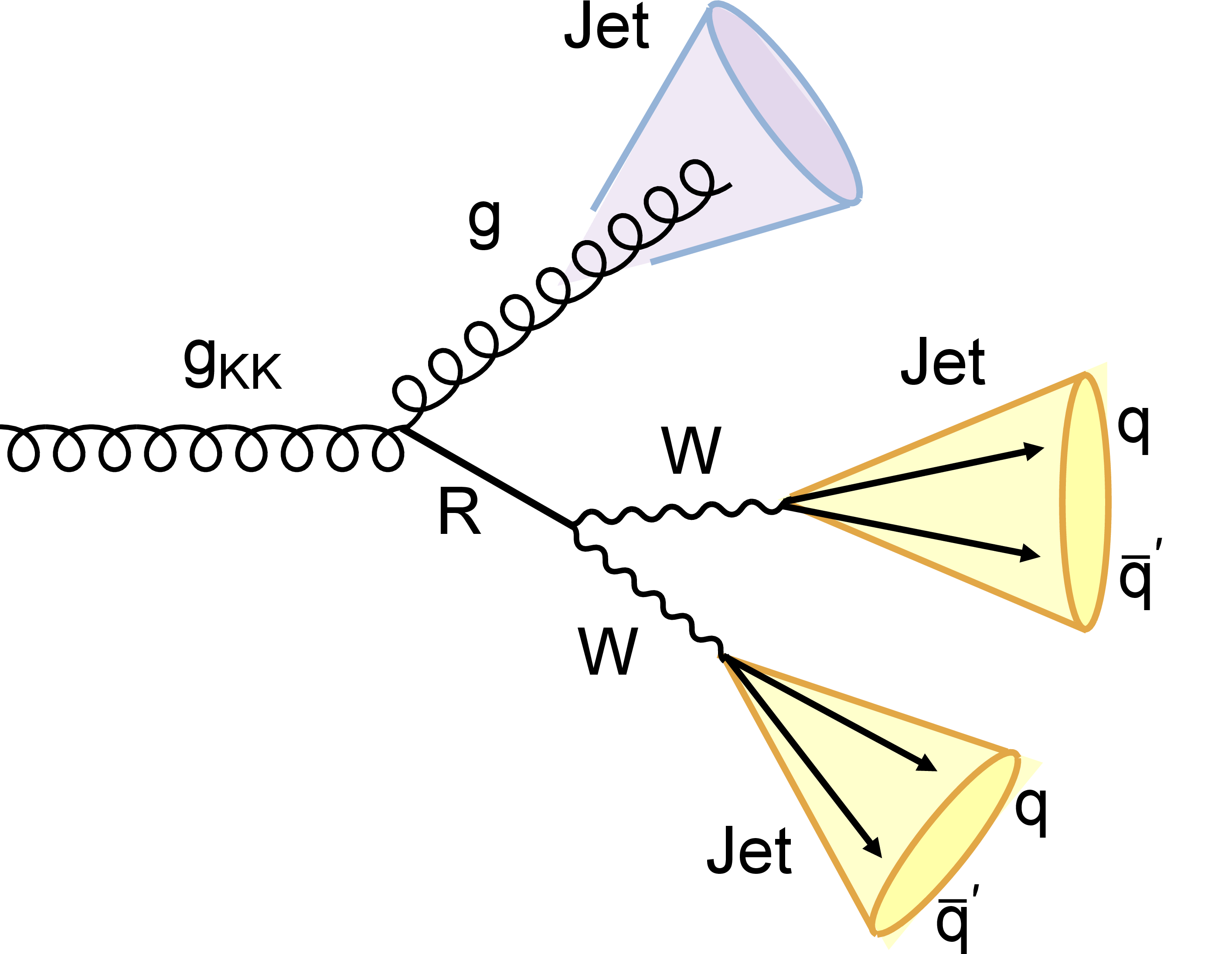
Figure 1:
A schematic diagram of the decay of a $ \mathrm{g}_{\text{KK}} $ boson via a radion $ \mathrm{R} $ to the final state considered in this analysis. |
png pdf |
Figure 2:
Upper left (right): the one-dimensional distributions of $ s_{\text{ja}} $ ($ s_{\text{jb}} $) for the labeled signal scenario compared to the simulated background. Black dashed lines indicate the SR selection boundaries. Lower: the two-dimensional ($ s_{\text{ja}} $, $ s_{\text{jb}} $) distribution in data. For the hypothesized signal ($ {m}_{\mathrm{R}}= $ 0.75 TeV, $ {m}_{\mathrm{g}_{\text{KK}}}= $ 1.5 TeV), contours representing constant event yield fractions (80, 60, 40, and 20% of the maximum yield) are shown to illustrate the shape. White dashed lines indicate the boundaries between SRa, SRb samples, and regions of rejected events. All distributions are shown after event preselection. |
png pdf |
Figure 2-a:
Upper left (right): the one-dimensional distributions of $ s_{\text{ja}} $ ($ s_{\text{jb}} $) for the labeled signal scenario compared to the simulated background. Black dashed lines indicate the SR selection boundaries. Lower: the two-dimensional ($ s_{\text{ja}} $, $ s_{\text{jb}} $) distribution in data. For the hypothesized signal ($ {m}_{\mathrm{R}}= $ 0.75 TeV, $ {m}_{\mathrm{g}_{\text{KK}}}= $ 1.5 TeV), contours representing constant event yield fractions (80, 60, 40, and 20% of the maximum yield) are shown to illustrate the shape. White dashed lines indicate the boundaries between SRa, SRb samples, and regions of rejected events. All distributions are shown after event preselection. |
png pdf |
Figure 2-b:
Upper left (right): the one-dimensional distributions of $ s_{\text{ja}} $ ($ s_{\text{jb}} $) for the labeled signal scenario compared to the simulated background. Black dashed lines indicate the SR selection boundaries. Lower: the two-dimensional ($ s_{\text{ja}} $, $ s_{\text{jb}} $) distribution in data. For the hypothesized signal ($ {m}_{\mathrm{R}}= $ 0.75 TeV, $ {m}_{\mathrm{g}_{\text{KK}}}= $ 1.5 TeV), contours representing constant event yield fractions (80, 60, 40, and 20% of the maximum yield) are shown to illustrate the shape. White dashed lines indicate the boundaries between SRa, SRb samples, and regions of rejected events. All distributions are shown after event preselection. |
png pdf |
Figure 2-c:
Upper left (right): the one-dimensional distributions of $ s_{\text{ja}} $ ($ s_{\text{jb}} $) for the labeled signal scenario compared to the simulated background. Black dashed lines indicate the SR selection boundaries. Lower: the two-dimensional ($ s_{\text{ja}} $, $ s_{\text{jb}} $) distribution in data. For the hypothesized signal ($ {m}_{\mathrm{R}}= $ 0.75 TeV, $ {m}_{\mathrm{g}_{\text{KK}}}= $ 1.5 TeV), contours representing constant event yield fractions (80, 60, 40, and 20% of the maximum yield) are shown to illustrate the shape. White dashed lines indicate the boundaries between SRa, SRb samples, and regions of rejected events. All distributions are shown after event preselection. |
png pdf |
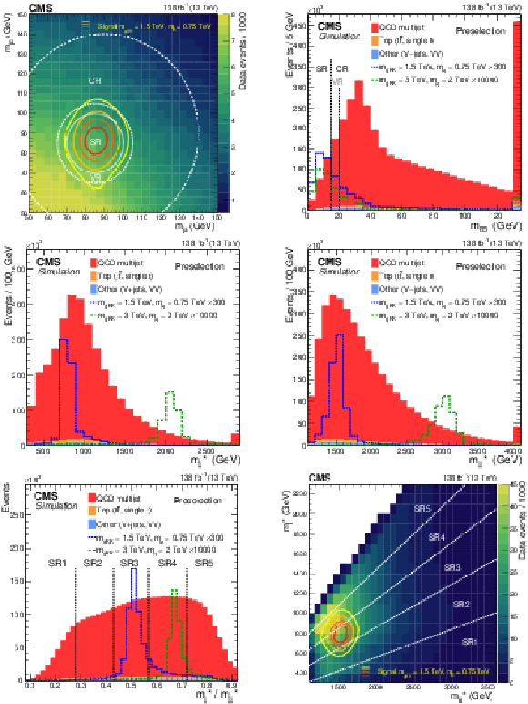
Figure 3:
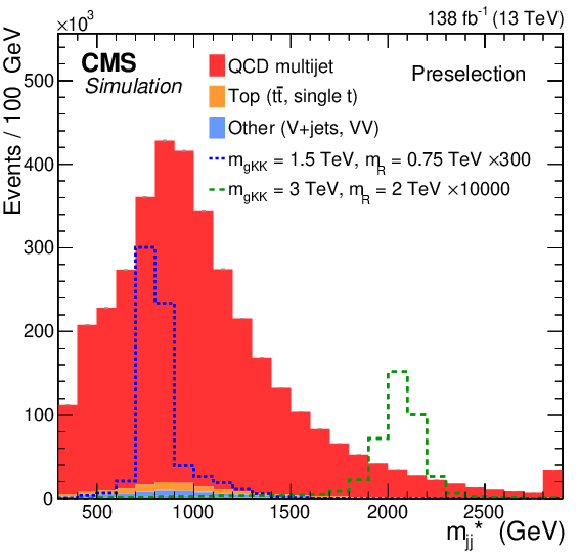
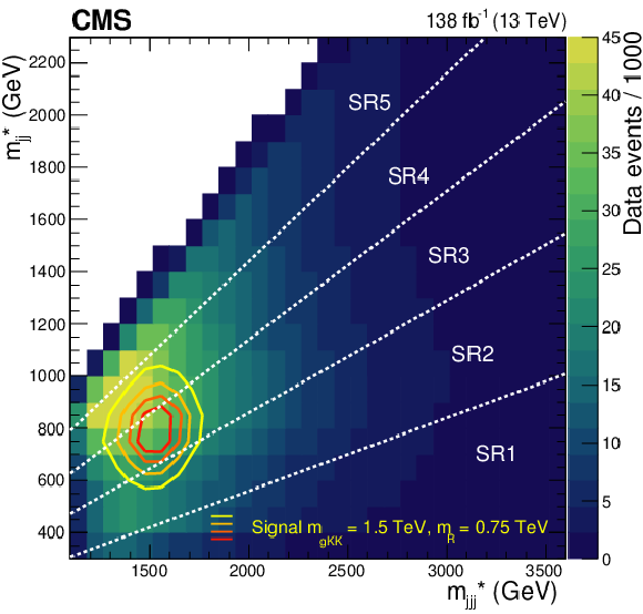
Distributions after event preselection. Upper left: the two-dimensional ($ m_{\text{ja}} $, $ m_{\text{jb}} $) distribution for a posited signal ($ {m}_{\mathrm{R}}= $ 0.75 TeV, $ {m}_{\mathrm{g}_{\text{KK}}}= $ 1.5 TeV) compared to the background-dominated data. For signal, contours corresponding to 80, 60, 40, and 20% of the maximum signal event yield are shown for shape visualization. White dashed curves indicate boundaries between SR, VR (defined in Section 6.1), and CR areas. The one-dimensional histograms show the $ m_{\text{85}} $ (upper right), $ m^*_{\mathrm{jj}} $ (middle left), $ m^*_{\mathrm{jjj}} $ (middle right), and $ m^*_{\mathrm{jj}} $/$ m^*_{\mathrm{jjj}} $ (lower left) distributions using simulated signal and background events, as indicated in the legends. The signal events are scaled by the labeled factors times the theoretical cross sections for visibility. Lower right: the two-dimensional ($ m^*_{\mathrm{jj}} $, $ m^*_{\mathrm{jjj}} $) distribution in data. White dashed lines indicate the SR splitting. |
png pdf |
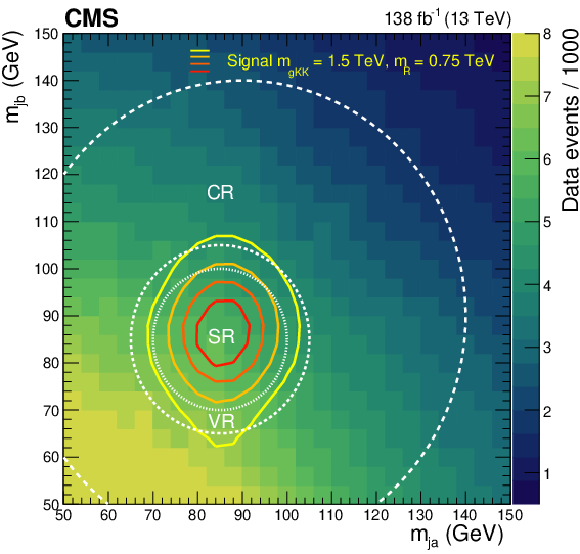
Figure 3-a:
Distributions after event preselection. Upper left: the two-dimensional ($ m_{\text{ja}} $, $ m_{\text{jb}} $) distribution for a posited signal ($ {m}_{\mathrm{R}}= $ 0.75 TeV, $ {m}_{\mathrm{g}_{\text{KK}}}= $ 1.5 TeV) compared to the background-dominated data. For signal, contours corresponding to 80, 60, 40, and 20% of the maximum signal event yield are shown for shape visualization. White dashed curves indicate boundaries between SR, VR (defined in Section 6.1), and CR areas. The one-dimensional histograms show the $ m_{\text{85}} $ (upper right), $ m^*_{\mathrm{jj}} $ (middle left), $ m^*_{\mathrm{jjj}} $ (middle right), and $ m^*_{\mathrm{jj}} $/$ m^*_{\mathrm{jjj}} $ (lower left) distributions using simulated signal and background events, as indicated in the legends. The signal events are scaled by the labeled factors times the theoretical cross sections for visibility. Lower right: the two-dimensional ($ m^*_{\mathrm{jj}} $, $ m^*_{\mathrm{jjj}} $) distribution in data. White dashed lines indicate the SR splitting. |
png pdf |
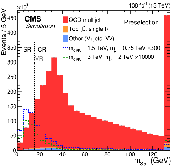
Figure 3-b:
Distributions after event preselection. Upper left: the two-dimensional ($ m_{\text{ja}} $, $ m_{\text{jb}} $) distribution for a posited signal ($ {m}_{\mathrm{R}}= $ 0.75 TeV, $ {m}_{\mathrm{g}_{\text{KK}}}= $ 1.5 TeV) compared to the background-dominated data. For signal, contours corresponding to 80, 60, 40, and 20% of the maximum signal event yield are shown for shape visualization. White dashed curves indicate boundaries between SR, VR (defined in Section 6.1), and CR areas. The one-dimensional histograms show the $ m_{\text{85}} $ (upper right), $ m^*_{\mathrm{jj}} $ (middle left), $ m^*_{\mathrm{jjj}} $ (middle right), and $ m^*_{\mathrm{jj}} $/$ m^*_{\mathrm{jjj}} $ (lower left) distributions using simulated signal and background events, as indicated in the legends. The signal events are scaled by the labeled factors times the theoretical cross sections for visibility. Lower right: the two-dimensional ($ m^*_{\mathrm{jj}} $, $ m^*_{\mathrm{jjj}} $) distribution in data. White dashed lines indicate the SR splitting. |
png pdf |
Figure 3-c:
Distributions after event preselection. Upper left: the two-dimensional ($ m_{\text{ja}} $, $ m_{\text{jb}} $) distribution for a posited signal ($ {m}_{\mathrm{R}}= $ 0.75 TeV, $ {m}_{\mathrm{g}_{\text{KK}}}= $ 1.5 TeV) compared to the background-dominated data. For signal, contours corresponding to 80, 60, 40, and 20% of the maximum signal event yield are shown for shape visualization. White dashed curves indicate boundaries between SR, VR (defined in Section 6.1), and CR areas. The one-dimensional histograms show the $ m_{\text{85}} $ (upper right), $ m^*_{\mathrm{jj}} $ (middle left), $ m^*_{\mathrm{jjj}} $ (middle right), and $ m^*_{\mathrm{jj}} $/$ m^*_{\mathrm{jjj}} $ (lower left) distributions using simulated signal and background events, as indicated in the legends. The signal events are scaled by the labeled factors times the theoretical cross sections for visibility. Lower right: the two-dimensional ($ m^*_{\mathrm{jj}} $, $ m^*_{\mathrm{jjj}} $) distribution in data. White dashed lines indicate the SR splitting. |
png pdf |
Figure 3-d:
Distributions after event preselection. Upper left: the two-dimensional ($ m_{\text{ja}} $, $ m_{\text{jb}} $) distribution for a posited signal ($ {m}_{\mathrm{R}}= $ 0.75 TeV, $ {m}_{\mathrm{g}_{\text{KK}}}= $ 1.5 TeV) compared to the background-dominated data. For signal, contours corresponding to 80, 60, 40, and 20% of the maximum signal event yield are shown for shape visualization. White dashed curves indicate boundaries between SR, VR (defined in Section 6.1), and CR areas. The one-dimensional histograms show the $ m_{\text{85}} $ (upper right), $ m^*_{\mathrm{jj}} $ (middle left), $ m^*_{\mathrm{jjj}} $ (middle right), and $ m^*_{\mathrm{jj}} $/$ m^*_{\mathrm{jjj}} $ (lower left) distributions using simulated signal and background events, as indicated in the legends. The signal events are scaled by the labeled factors times the theoretical cross sections for visibility. Lower right: the two-dimensional ($ m^*_{\mathrm{jj}} $, $ m^*_{\mathrm{jjj}} $) distribution in data. White dashed lines indicate the SR splitting. |
png pdf |
Figure 3-e:
Distributions after event preselection. Upper left: the two-dimensional ($ m_{\text{ja}} $, $ m_{\text{jb}} $) distribution for a posited signal ($ {m}_{\mathrm{R}}= $ 0.75 TeV, $ {m}_{\mathrm{g}_{\text{KK}}}= $ 1.5 TeV) compared to the background-dominated data. For signal, contours corresponding to 80, 60, 40, and 20% of the maximum signal event yield are shown for shape visualization. White dashed curves indicate boundaries between SR, VR (defined in Section 6.1), and CR areas. The one-dimensional histograms show the $ m_{\text{85}} $ (upper right), $ m^*_{\mathrm{jj}} $ (middle left), $ m^*_{\mathrm{jjj}} $ (middle right), and $ m^*_{\mathrm{jj}} $/$ m^*_{\mathrm{jjj}} $ (lower left) distributions using simulated signal and background events, as indicated in the legends. The signal events are scaled by the labeled factors times the theoretical cross sections for visibility. Lower right: the two-dimensional ($ m^*_{\mathrm{jj}} $, $ m^*_{\mathrm{jjj}} $) distribution in data. White dashed lines indicate the SR splitting. |
png pdf |
Figure 3-f:
Distributions after event preselection. Upper left: the two-dimensional ($ m_{\text{ja}} $, $ m_{\text{jb}} $) distribution for a posited signal ($ {m}_{\mathrm{R}}= $ 0.75 TeV, $ {m}_{\mathrm{g}_{\text{KK}}}= $ 1.5 TeV) compared to the background-dominated data. For signal, contours corresponding to 80, 60, 40, and 20% of the maximum signal event yield are shown for shape visualization. White dashed curves indicate boundaries between SR, VR (defined in Section 6.1), and CR areas. The one-dimensional histograms show the $ m_{\text{85}} $ (upper right), $ m^*_{\mathrm{jj}} $ (middle left), $ m^*_{\mathrm{jjj}} $ (middle right), and $ m^*_{\mathrm{jj}} $/$ m^*_{\mathrm{jjj}} $ (lower left) distributions using simulated signal and background events, as indicated in the legends. The signal events are scaled by the labeled factors times the theoretical cross sections for visibility. Lower right: the two-dimensional ($ m^*_{\mathrm{jj}} $, $ m^*_{\mathrm{jjj}} $) distribution in data. White dashed lines indicate the SR splitting. |
png pdf |
Figure 4:
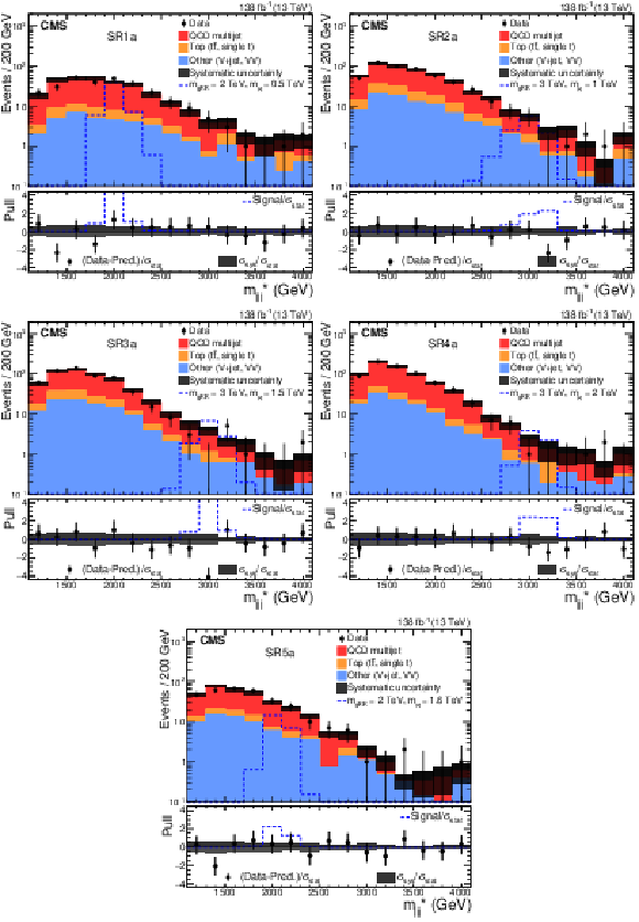
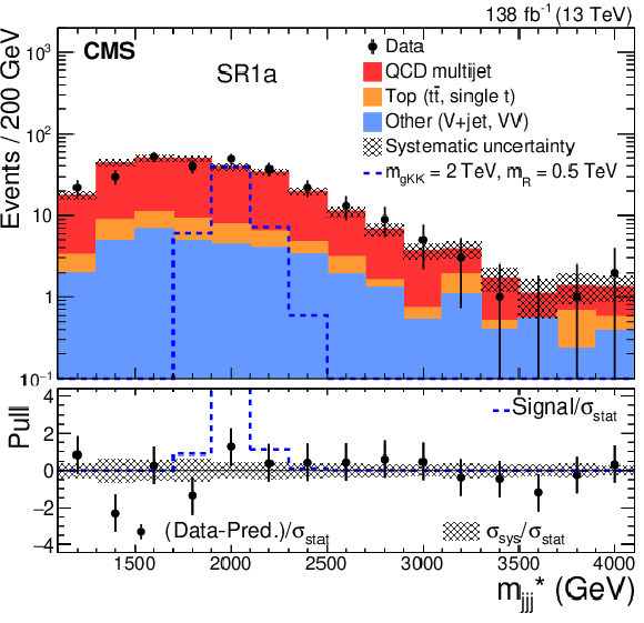
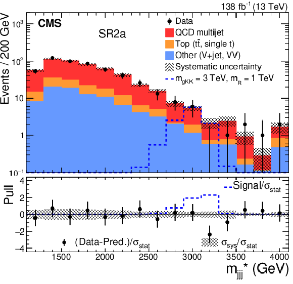
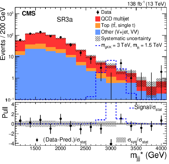
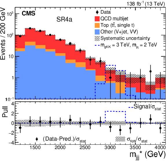
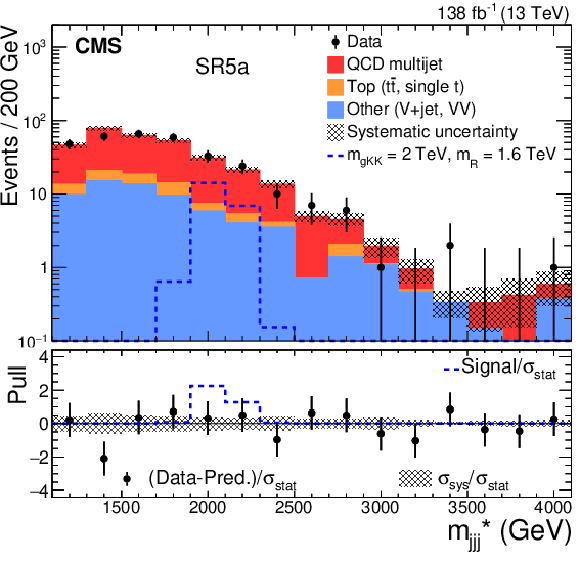
The $ m^*_{\mathrm{jjj}} $ postfit spectra in the five SRxa. Upper to lower, and left to right: SR1a, SR2a, SR3a, SR4a, and SR5a. The lower panels show the pull distributions, as defined in the text, together with expected signal event yields and the systematic uncertainty normalized to $ \sigma_{\text{stat}} $. |
png pdf |
Figure 4-a:
The $ m^*_{\mathrm{jjj}} $ postfit spectra in the five SRxa. Upper to lower, and left to right: SR1a, SR2a, SR3a, SR4a, and SR5a. The lower panels show the pull distributions, as defined in the text, together with expected signal event yields and the systematic uncertainty normalized to $ \sigma_{\text{stat}} $. |

png pdf |
Figure 4-b:
The $ m^*_{\mathrm{jjj}} $ postfit spectra in the five SRxa. Upper to lower, and left to right: SR1a, SR2a, SR3a, SR4a, and SR5a. The lower panels show the pull distributions, as defined in the text, together with expected signal event yields and the systematic uncertainty normalized to $ \sigma_{\text{stat}} $. |
png pdf |
Figure 4-c:
The $ m^*_{\mathrm{jjj}} $ postfit spectra in the five SRxa. Upper to lower, and left to right: SR1a, SR2a, SR3a, SR4a, and SR5a. The lower panels show the pull distributions, as defined in the text, together with expected signal event yields and the systematic uncertainty normalized to $ \sigma_{\text{stat}} $. |

png pdf |
Figure 4-d:
The $ m^*_{\mathrm{jjj}} $ postfit spectra in the five SRxa. Upper to lower, and left to right: SR1a, SR2a, SR3a, SR4a, and SR5a. The lower panels show the pull distributions, as defined in the text, together with expected signal event yields and the systematic uncertainty normalized to $ \sigma_{\text{stat}} $. |
png pdf |
Figure 4-e:
The $ m^*_{\mathrm{jjj}} $ postfit spectra in the five SRxa. Upper to lower, and left to right: SR1a, SR2a, SR3a, SR4a, and SR5a. The lower panels show the pull distributions, as defined in the text, together with expected signal event yields and the systematic uncertainty normalized to $ \sigma_{\text{stat}} $. |

png pdf |
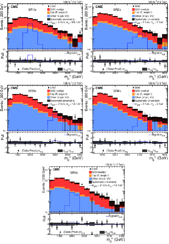
Figure 5:
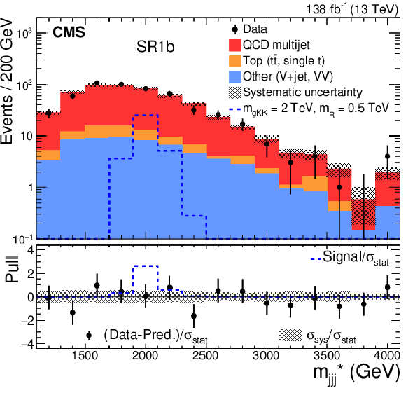
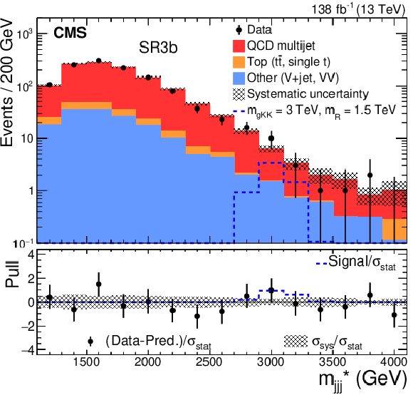
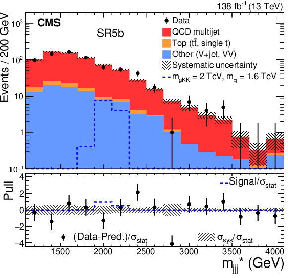
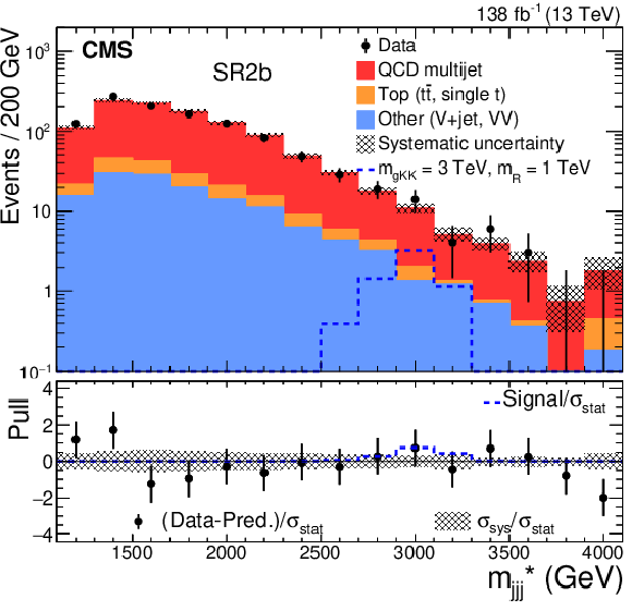
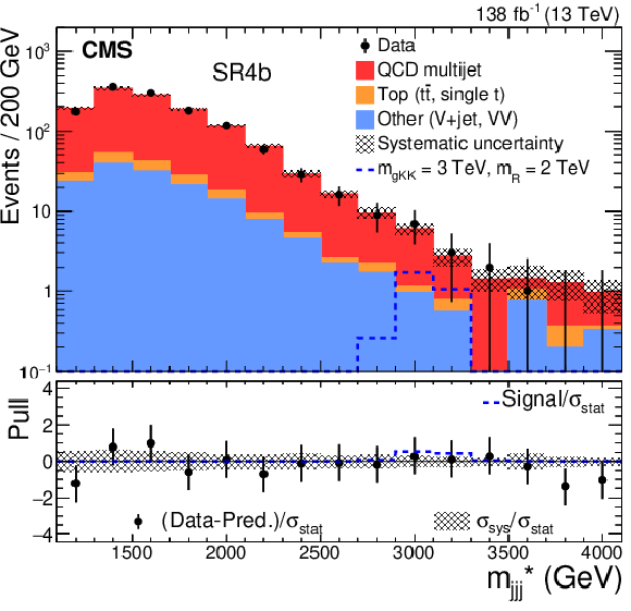
The $ m^*_{\mathrm{jjj}} $ postfit spectra in the five SRxb. Upper to lower, and left to right: SR1b, SR2b, SR3b, SR4b, and SR5b. The lower panels show the pull distributions, as defined in the text, together with expected signal event yields and the systematic uncertainty normalized to $ \sigma_{\text{stat}} $. |

png pdf |
Figure 5-a:
The $ m^*_{\mathrm{jjj}} $ postfit spectra in the five SRxb. Upper to lower, and left to right: SR1b, SR2b, SR3b, SR4b, and SR5b. The lower panels show the pull distributions, as defined in the text, together with expected signal event yields and the systematic uncertainty normalized to $ \sigma_{\text{stat}} $. |
png pdf |
Figure 5-b:
The $ m^*_{\mathrm{jjj}} $ postfit spectra in the five SRxb. Upper to lower, and left to right: SR1b, SR2b, SR3b, SR4b, and SR5b. The lower panels show the pull distributions, as defined in the text, together with expected signal event yields and the systematic uncertainty normalized to $ \sigma_{\text{stat}} $. |

png pdf |
Figure 5-c:
The $ m^*_{\mathrm{jjj}} $ postfit spectra in the five SRxb. Upper to lower, and left to right: SR1b, SR2b, SR3b, SR4b, and SR5b. The lower panels show the pull distributions, as defined in the text, together with expected signal event yields and the systematic uncertainty normalized to $ \sigma_{\text{stat}} $. |
png pdf |
Figure 5-d:
The $ m^*_{\mathrm{jjj}} $ postfit spectra in the five SRxb. Upper to lower, and left to right: SR1b, SR2b, SR3b, SR4b, and SR5b. The lower panels show the pull distributions, as defined in the text, together with expected signal event yields and the systematic uncertainty normalized to $ \sigma_{\text{stat}} $. |

png pdf |
Figure 5-e:
The $ m^*_{\mathrm{jjj}} $ postfit spectra in the five SRxb. Upper to lower, and left to right: SR1b, SR2b, SR3b, SR4b, and SR5b. The lower panels show the pull distributions, as defined in the text, together with expected signal event yields and the systematic uncertainty normalized to $ \sigma_{\text{stat}} $. |
png pdf |
Figure 6:
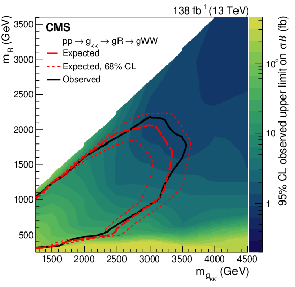
The 95% CL upper limits on the production cross section times branching fraction $ \sigma\mathcal{B} $, for the process $ \mathrm{p}\mathrm{p}\to\mathrm{g}_{\text{KK}}\to\mathrm{g}\mathrm{R}\to\mathrm{g}\mathrm{W}\mathrm{W} $. The black solid (red dashed) line contour indicates the observed (expected) exclusion region of the $ \mathrm{g}_{\text{KK}} $ and $ \mathrm{R} $ masses. The red dotted lines show the 68% CL band of the expected limit contour. |
| Tables | |
png pdf |
Table 1:
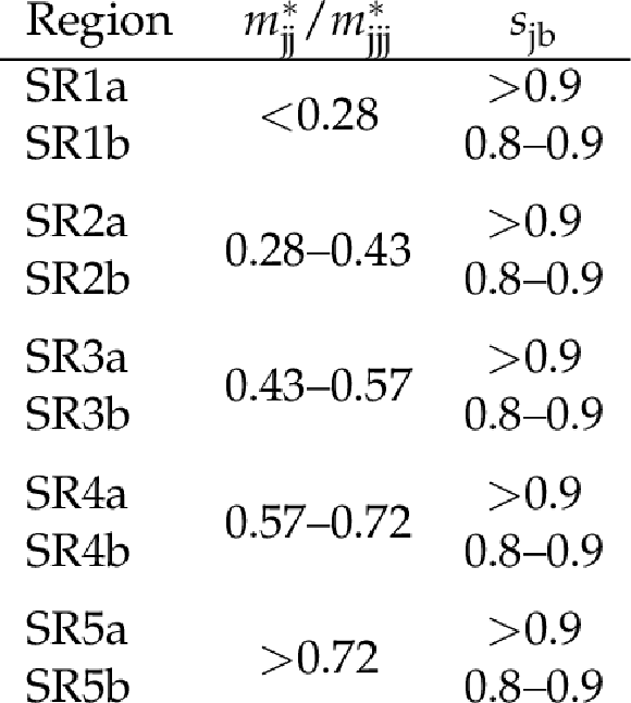
Definition of the different SRs based on the $ m^*_{\mathrm{jj}} $/$ m^*_{\mathrm{jjj}} $ ratio and $ s_{\text{jb}} $. |

png pdf |
Table 2:
The $ \text{PNet}_\mathrm{W} $ scale factors calculated for exclusive $ p_{\mathrm{T}} $ and $ \text{PNet}_\mathrm{W} $ tagger score ranges of W boson matched jets. |

png pdf |
Table 3:
The sources of systematic uncertainties accounted for in the analysis. From left to right: indication of whether an uncertainty is evaluated for the background (B) or signal (S), whether the uncertainty affects shape or rate, magnitudes (where applicable, or standard deviations ($ \sigma $)), and the total number of nuisance parameters (NPs) used along with their correlations across SRs. The ``*'' indicates a value or a shape template different for each signal scenario. |
| Summary |
| A search for heavy resonances decaying, via an intermediate resonance, to a gluon and a pair of W bosons in the all-hadronic final states has been presented. A benchmark model, in which a Kaluza--Klein gluon decays into a radion and a gluon, $ \mathrm{g}_{\text{KK}}\to\mathrm{g}\mathrm{R}\to\mathrm{g}\mathrm{W}\mathrm{W} $, has been considered. The search is performed using proton-proton collision data at a center-of-mass energy of 13 TeV, collected by the CMS experiment, corresponding to a total integrated luminosity of 138 fb$ ^{-1} $. The final states include three large-radius jets, at least two of which are required to be massive, containing the decay products of the hadronically decaying W bosons. The topology corresponds to events where each W boson from the $ \mathrm{R} $ decay is reconstructed as a single merged jet. In this analysis, a previously unexplored signature is probed using jet substructure techniques relying on deep learning. No resonant signal above the standard model background prediction is found in the data analyzed. Exclusion limits are set at 95% confidence level on the masses of the $ \mathrm{g}_{\text{KK}} $ and $ \mathrm{R} $ bosons, up to 3.55 and 2.18 TeV, respectively, and on the product of the production cross section and the branching fraction to a gluon and two W bosons in an extended warped extra-dimensional model. This result is the first analyzing the resonant WW+jet signature and complements constraints set on similar scenarios [25,26,27,28]. |
| References | ||||
| 1 | CMS Collaboration | Search for heavy resonances decaying to Z($ \nu\bar{\nu} $)V(q$ \bar{\text{q}} $') in proton-proton collisions at $ \sqrt{s} = $ 13 TeV | PRD 106 (2022) 012004 | CMS-B2G-20-008 2109.08268 |
| 2 | CMS Collaboration | Search for new heavy resonances decaying to WW, WZ, ZZ, WH, or ZH boson pairs in the all-jets final state in proton-proton collisions at $ \sqrt{s} = $ 13 TeV | PLB 844 (2023) 137813 | CMS-B2G-20-009 2210.00043 |
| 3 | CMS Collaboration | Search for heavy resonances decaying to WW, WZ, or WH boson pairs in the lepton plus merged jet final state in proton-proton collisions at $ \sqrt{s} = $ 13 TeV | PRD 105 (2022) 032008 | CMS-B2G-19-002 2109.06055 |
| 4 | CMS Collaboration | Search for high mass dijet resonances with a new background prediction method in proton-proton collisions at $ \sqrt{s} = $ 13 TeV | JHEP 05 (2020) 033 | CMS-EXO-19-012 1911.03947 |
| 5 | CMS Collaboration | Search for a heavy resonance decaying into \textZH in events with an energetic jet and two electrons, two muons, or missing transverse momentum in proton-proton collisions at $ \sqrt{s} = $ 13 TeV | CMS Physics Analysis Summary CMS-PAS-B2G-23-008. To be submitted. CMS-PAS-B2G-23-008 |
CMS-PAS-B2G-23-008 |
| 6 | CMS Collaboration | Search for heavy resonances decaying to ZZ or ZW and axion-like particles mediating nonresonant ZZ or ZH production at $ \sqrt{s} = $ 13 TeV | JHEP 04 (2022) 087 | CMS-B2G-20-013 2111.13669 |
| 7 | CMS Collaboration | Search for a heavy vector resonance decaying to a Z boson and a Higgs boson in proton-proton collisions at $ \sqrt{s} = $ 13 TeV | EPJC 81 (2021) 688 | CMS-B2G-19-006 2102.08198 |
| 8 | CMS Collaboration | Searches for Higgs boson production through decays of heavy resonances | Submitted to Physics Reports. | CMS-B2G-23-002 2403.16926 |
| 9 | ATLAS Collaboration | Search for resonances decaying into a weak vector boson and a Higgs boson in the fully hadronic final state produced in proton-proton collisions at $ \sqrt{s} = $ 13 TeV with the ATLAS detector | PRD 102 (2020) 112008 | 2007.05293 |
| 10 | ATLAS Collaboration | Search for heavy diboson resonances in semileptonic final states in pp collisions at $ \sqrt{s}= $ 13 TeV with the ATLAS detector | EPJC 80 (2020) 1165 | 2004.14636 |
| 11 | ATLAS Collaboration | Search for diboson resonances in hadronic final states in 139 fb$ ^{-1} $ of $ pp $ collisions at $ \sqrt{s} = $ 13 TeV with the ATLAS detector | JHEP 09 (2019) 091 | 1906.08589 |
| 12 | ATLAS Collaboration | Combination of searches for heavy spin-1 resonances using 139 fb$ ^{-1} $ of proton-proton collision data at $ \sqrt{s} = $ 13 TeV with the ATLAS detector | JHEP 04 (2024) 118 | 2402.10607 |
| 13 | ATLAS Collaboration | Search for resonant WZ production in the fully leptonic final state in proton-proton collisions at $ \mathbf {\sqrt{s} = 13} $ TeV with the ATLAS detector | EPJC 83 (2023) 633 | 2207.03925 |
| 14 | ATLAS Collaboration | Search for heavy resonances decaying into a $ Z $ or $ W $ boson and a Higgs boson in final states with leptons and $ b $-jets in 139 $ $fb$ ^{-1} $ of $ pp $ collisions at $ \sqrt{s}=13 $TeV with the ATLAS detector | JHEP 06 (2023) 016 | 2207.00230 |
| 15 | ATLAS Collaboration | Search for new resonances in mass distributions of jet pairs using 139 fb$ ^{-1} $ of $ pp $ collisions at $ \sqrt{s}= $ 13 TeV with the ATLAS detector | JHEP 03 (2020) 145 | 1910.08447 |
| 16 | K. Agashe, P. Du, S. Hong, and R. Sundrum | Flavor universal resonances and warped gravity | JHEP 01 (2017) 016 | 1608.00526 |
| 17 | K. S. Agashe et al. | LHC signals from cascade decays of warped vector resonances | JHEP 05 (2017) 078 | 1612.00047 |
| 18 | K. Agashe et al. | Dedicated strategies for triboson signals from cascade decays of vector resonances | PRD 99 (2019) 075016 | 1711.09920 |
| 19 | K. Agashe et al. | Detecting a boosted diboson resonance | JHEP 11 (2018) 027 | 1809.07334 |
| 20 | Y.-P. Kuang, H.-Y. Ren, and L.-H. Xia | Further investigation of the model-independent probe of heavy neutral Higgs bosons at LHC Run 2 | Chin. Phys. C 40 (2016) 023101 | 1506.08007 |
| 21 | Y.-P. Kuang, H.-Y. Ren, and L.-H. Xia | Model-independent probe of anomalous heavy neutral Higgs bosons at the LHC | PRD 90 (2014) 115002 | 1404.6367 |
| 22 | W. D. Goldberger and M. B. Wise | Modulus stabilization with bulk fields | PRL 83 (1999) 4922 | hep-ph/9907447 |
| 23 | S. Weinberg | Implications of dynamical symmetry breaking | PRD 13 (1976) 974 | |
| 24 | L. Susskind | Dynamics of spontaneous symmetry breaking in the Weinberg-Salam theory | PRD 20 (1979) 2619 | |
| 25 | CMS Collaboration | Search for resonances decaying to three W bosons in proton-proton collisions at $ \sqrt{s} = $ 13 TeV | PRL 129 (2022) 021802 | CMS-B2G-20-001 2201.08476 |
| 26 | CMS Collaboration | Search for resonances decaying to three $ W $ bosons in the hadronic final state in proton-proton collisions at $ \sqrt s = $ 13 TeV | PRD 106 (2022) 012002 | CMS-B2G-21-002 2112.13090 |
| 27 | CMS Collaboration | Search for high-mass resonances decaying to a jet and a Lorentz-boosted resonance in proton-proton collisions at $ \sqrt s = $ 13 TeV | PLB 832 (2022) 137263 | CMS-EXO-20-007 2201.02140 |
| 28 | CMS Collaboration | Search for Narrow Trijet Resonances in Proton-Proton Collisions at $ \sqrt s = $ 13 TeV | PRL 133 (2024) 011801 | CMS-EXO-22-008 2310.14023 |
| 29 | ATLAS Collaboration | Search for new phenomena in multi-body invariant masses in events with at least one isolated lepton and two jets using $ \sqrt{s} = $ 13 TeV proton-proton collision data collected by the ATLAS detector | JHEP 07 (2023) 202 | 2211.08945 |
| 30 | CMS Collaboration | Precision luminosity measurement in proton-proton collisions at $ \sqrt{s} = $ 13 TeV in 2015 and 2016 at CMS | EPJC 81 (2021) 800 | CMS-LUM-17-003 2104.01927 |
| 31 | CMS Collaboration | CMS luminosity measurement for the 2017 data-taking period at $ \sqrt{s} = $ 13 TeV | CMS Physics Analysis Summary, 2018 link |
CMS-PAS-LUM-17-004 |
| 32 | CMS Collaboration | CMS luminosity measurement for the 2018 data-taking period at $ \sqrt{s} = $ 13 TeV | CMS Physics Analysis Summary, 2019 link |
CMS-PAS-LUM-18-002 |
| 33 | CMS Collaboration | Identification of heavy, energetic, hadronically decaying particles using machine-learning techniques | JINST 15 (2020) P06005 | CMS-JME-18-002 2004.08262 |
| 34 | H. Qu and L. Gouskos | Jet tagging via particle clouds | PRD 101 (2020) 056019 | 1902.08570 |
| 35 | CMS Collaboration | HEPData record for this analysis | link | |
| 36 | CMS Collaboration | Performance of the CMS Level-1 trigger in proton-proton collisions at $ \sqrt{s} = $ 13 TeV | JINST 15 (2020) P10017 | CMS-TRG-17-001 2006.10165 |
| 37 | CMS Collaboration | The CMS trigger system | JINST 12 (2017) P01020 | CMS-TRG-12-001 1609.02366 |
| 38 | CMS Collaboration | The CMS experiment at the CERN LHC | JINST 3 (2008) S08004 | |
| 39 | CMS Collaboration | Development of the CMS detector for the CERN LHC Run 3 | no.~05, P05064, 2024 JINST 19 (2024) |
CMS-PRF-21-001 2309.05466 |
| 40 | J. Alwall et al. | The automated computation of tree-level and next-to-leading order differential cross sections, and their matching to parton shower simulations | JHEP 07 (2014) 079 | 1405.0301 |
| 41 | J. Alwall et al. | Comparative study of various algorithms for the merging of parton showers and matrix elements in hadronic collisions | EPJC 53 (2008) 473 | 0706.2569 |
| 42 | P. Nason | A new method for combining NLO QCD with shower Monte Carlo algorithms | JHEP 11 (2004) 040 | hep-ph/0409146 |
| 43 | S. Frixione, P. Nason, and C. Oleari | Matching NLO QCD computations with parton shower simulations: the POWHEG method | JHEP 11 (2007) 070 | 0709.2092 |
| 44 | S. Alioli, P. Nason, C. Oleari, and E. Re | A general framework for implementing NLO calculations in shower Monte Carlo programs: the POWHEG BOX | JHEP 06 (2010) 043 | 1002.2581 |
| 45 | S. Alioli, S.-O. Moch, and P. Uwer | Hadronic top-quark pair-production with one jet and parton showering | JHEP 01 (2012) 137 | 1110.5251 |
| 46 | S. Alioli, P. Nason, C. Oleari, and E. Re | NLO single-top production matched with shower in POWHEG: $ s $- and $ t $-channel contributions | JHEP 09 (2009) 111 | 0907.4076 |
| 47 | R. Frederix, E. Re, and P. Torrielli | Single-top $ t $-channel hadroproduction in the four-flavour scheme with POWHEG and aMC@NLO | JHEP 09 (2012) 130 | 1207.5391 |
| 48 | NNPDF Collaboration | Parton distributions for the LHC run II | JHEP 04 (2015) 040 | 1410.8849 |
| 49 | T. Sjöstrand et al. | An introduction to PYTHIA 8.2 | Comput. Phys. Commun. 191 (2015) 159 | 1410.3012 |
| 50 | CMS Collaboration | Extraction and validation of a new set of CMS PYTHIA8 tunes from underlying-event measurements | EPJC 80 (2020) 4 | CMS-GEN-17-001 1903.12179 |
| 51 | GEANT4 Collaboration | GEANT 4---a simulation toolkit | NIM A 506 (2003) 250 | |
| 52 | CMS Collaboration | Technical proposal for the Phase-II upgrade of the Compact Muon Solenoid | CMS Technical Proposal CERN-LHCC-2015-010, CMS-TDR-15-02, 2015 CDS |
|
| 53 | CMS Collaboration | Particle-flow reconstruction and global event description with the CMS detector | JINST 12 (2017) P10003 | CMS-PRF-14-001 1706.04965 |
| 54 | M. Cacciari, G. P. Salam, and G. Soyez | The anti-$ k_{\mathrm{T}} $ jet clustering algorithm | JHEP 04 (2008) 063 | 0802.1189 |
| 55 | M. Cacciari, G. P. Salam, and G. Soyez | FastJet user manual | EPJC 72 (2012) 1896 | 1111.6097 |
| 56 | CMS Collaboration | Jet energy scale and resolution in the CMS experiment in pp collisions at 8 TeV | JINST 12 (2017) P02014 | CMS-JME-13-004 1607.03663 |
| 57 | CMS Collaboration | Pileup mitigation at CMS in 13 TeV data | JINST 15 (2020) P09018 | CMS-JME-18-001 2003.00503 |
| 58 | D. Bertolini, P. Harris, M. Low, and N. Tran | Pileup Per Particle Identification | JHEP 10 (2014) 059 | 1407.6013 |
| 59 | CMS Collaboration | Jet algorithms performance in 13 TeV data | CMS Physics Analysis Summary, 2017 CMS-PAS-JME-16-003 |
CMS-PAS-JME-16-003 |
| 60 | E. Bols et al. | Jet flavour classification using DeepJet | JINST 15 (2020) P12012 | 2008.10519 |
| 61 | CMS Collaboration | Performance of the DeepJet b tagging algorithm using 41.9 fb$ ^{-1} $ of data from proton-proton collisions at 13 TeV with Phase-1 CMS detector | CMS Detector Performance Note CMS-DP-2018-058, 2018 CDS |
|
| 62 | CMS Collaboration | Performance of missing transverse momentum reconstruction in proton-proton collisions at $ \sqrt{s} = $ 13 TeV using the CMS detector | JINST 14 (2019) P07004 | CMS-JME-17-001 1903.06078 |
| 63 | G. Louppe, M. Kagan, and K. Cranmer | Learning to pivot with adversarial networks | 1611.01046 | |
| 64 | M. Dasgupta, A. Fregoso, S. Marzani, and G. P. Salam | Towards an understanding of jet substructure | JHEP 09 (2013) 029 | 1307.0007 |
| 65 | J. M. Butterworth, A. R. Davison, M. Rubin, and G. P. Salam | Jet substructure as a new Higgs search channel at the LHC | PRL 100 (2008) 242001 | 0802.2470 |
| 66 | A. J. Larkoski, S. Marzani, G. Soyez, and J. Thaler | Soft drop | JHEP 05 (2014) 146 | 1402.2657 |
| 67 | CMS Collaboration | Identification techniques for highly boosted W bosons that decay into hadrons | JHEP 12 (2014) 017 | CMS-JME-13-006 1410.4227 |
| 68 | CMS Collaboration | Performance of the CMS muon detector and muon reconstruction with proton-proton collisions at $ \sqrt{s}= $ 13 TeV | JINST 13 (2018) P06015 | CMS-MUO-16-001 1804.04528 |
| 69 | CMS Collaboration | Performance of electron reconstruction and selection with the CMS detector in proton-proton collisions at $ \sqrt{s} = $ 8 TeV | JINST 10 (2015) P06005 | CMS-EGM-13-001 1502.02701 |
| 70 | D. Krohn, J. Thaler, and L.-T. Wang | Jet trimming | JHEP 02 (2010) 084 | 0912.1342 |
| 71 | CMS Collaboration | Measurement of the inelastic proton-proton cross section at $ \sqrt{s}= $ 13 TeV | JHEP 07 (2018) 161 | CMS-FSQ-15-005 1802.02613 |
| 72 | CMS Collaboration | The CMS statistical analysis and combination tool: COMBINE | Accepted for publication by Computing and Software for Big Science, 2024 | CMS-CAT-23-001 2404.06614 |
| 73 | G. Cowan, K. Cranmer, E. Gross, and O. Vitells | Asymptotic formulae for likelihood-based tests of new physics | EPJC 71 (2011) 1554 | 1007.1727 |

|
Compact Muon Solenoid LHC, CERN |

|

|

|

|

|

|