

Compact Muon Solenoid
LHC, CERN
| CMS-PAS-TOP-24-017 | ||
| Four-top-quark production in final states with hadronically decaying tau leptons and search for vector-like leptons at $ \sqrt{s}= $ 13 TeV | ||
| CMS Collaboration | ||
| 2026-03-21 | ||
| Abstract: The first study of four top quark production in final states with hadronically decaying tau leptons ($ \tau_\mathrm{h} $) is presented using proton-proton collision data collected by the CMS experiment at a center-of-mass energy of 13 TeV during the 2016--2018 period at the CERN LHC. This dataset corresponds to an integrated luminosity of 138 fb$ ^{-1} $. Tau lepton final states provide sensitivity to BSM scenarios with enhanced third-generation couplings and complement established multilepton searches. The analysis is divided into subchannels with one $ \tau_\mathrm{h} $ and zero, one, or two additional electrons and muons to optimize sensitivity. Combining the three channels, the observed (expected) significance of the measured $ \mathrm{t\bar{t}t\bar{t}} $ signal with respect to the standard model background-only hypothesis is 1.1 $ (1.0) $ standard deviations. The production cross section of four top quarks is measured to be 16 $ ^{+14}_{-12} $ ($ \mathrm{stat} $)^+12_-8 ($ \mathrm{syst} $) $ \mathrm{fb} $. Additionally, a search is performed for vector-like leptons within the framework of the 4321 model in the same $ \tau_\mathrm{h} $ phase space. No significant excess is observed, and a lower limit of 830 GeV is set at 95% confidence level on the vector-like lepton mass, providing the first constraints from final states containing electrons and muons. | ||
| Links: CDS record (PDF) ; CADI line (restricted) ; | ||
| Figures | |

png pdf |
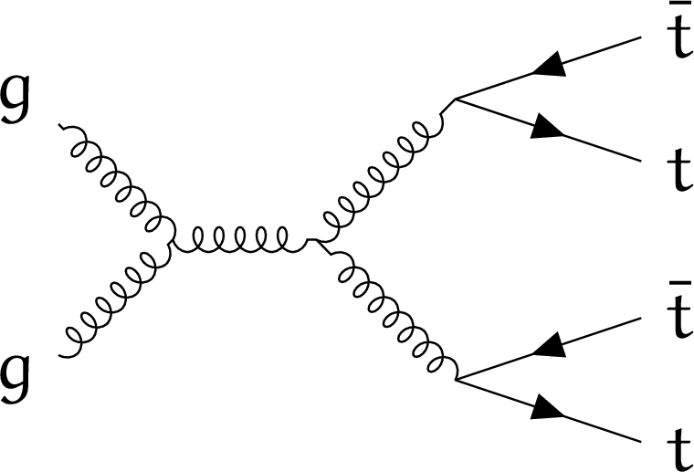
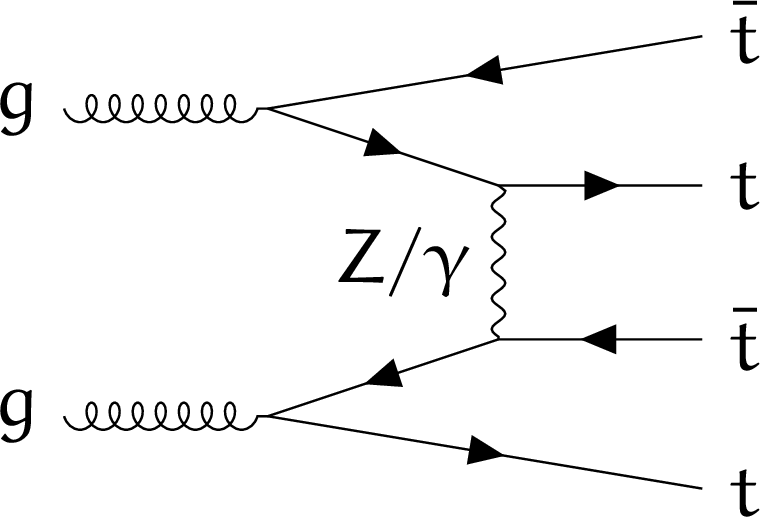
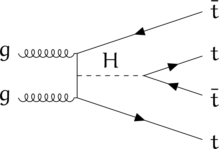
Figure 1:
Examples of leading Feynman diagrams contributing to $ {\mathrm{t}\overline{\mathrm{t}}} {\mathrm{t}\overline{\mathrm{t}}} $ production. The first diagram (left ) involves only the strong interaction. The other two diagrams involve both strong and electroweak interactions with the exchange of a virtual Z boson or photon (middle ), or a virtual Higgs boson (right ). |
png pdf |
Figure 1-a:
Examples of leading Feynman diagrams contributing to $ {\mathrm{t}\overline{\mathrm{t}}} {\mathrm{t}\overline{\mathrm{t}}} $ production. The first diagram (left ) involves only the strong interaction. The other two diagrams involve both strong and electroweak interactions with the exchange of a virtual Z boson or photon (middle ), or a virtual Higgs boson (right ). |
png pdf |
Figure 1-b:
Examples of leading Feynman diagrams contributing to $ {\mathrm{t}\overline{\mathrm{t}}} {\mathrm{t}\overline{\mathrm{t}}} $ production. The first diagram (left ) involves only the strong interaction. The other two diagrams involve both strong and electroweak interactions with the exchange of a virtual Z boson or photon (middle ), or a virtual Higgs boson (right ). |
png pdf |
Figure 1-c:
Examples of leading Feynman diagrams contributing to $ {\mathrm{t}\overline{\mathrm{t}}} {\mathrm{t}\overline{\mathrm{t}}} $ production. The first diagram (left ) involves only the strong interaction. The other two diagrams involve both strong and electroweak interactions with the exchange of a virtual Z boson or photon (middle ), or a virtual Higgs boson (right ). |
png pdf |
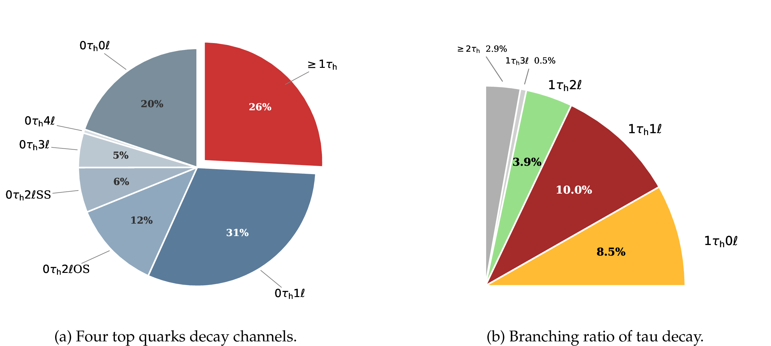
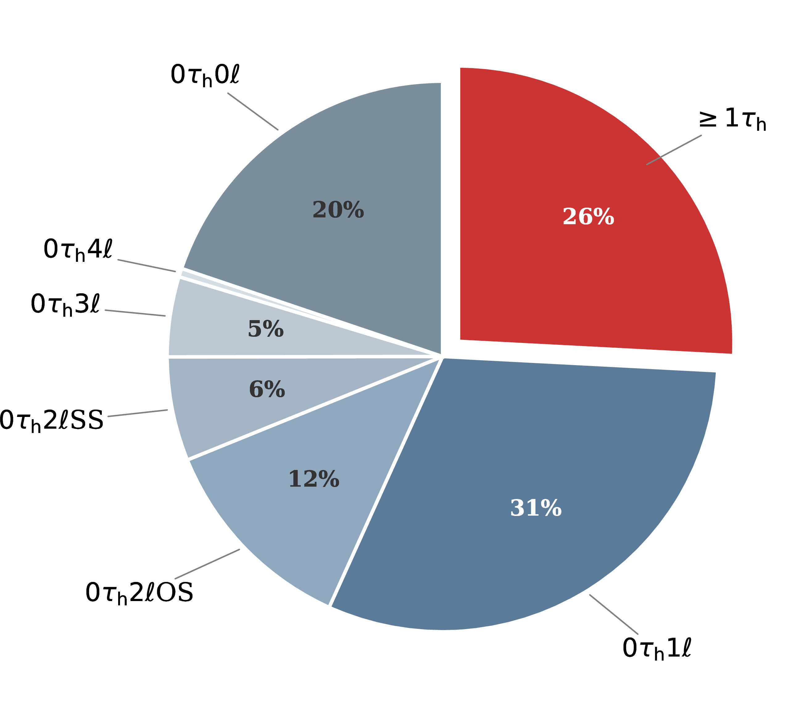
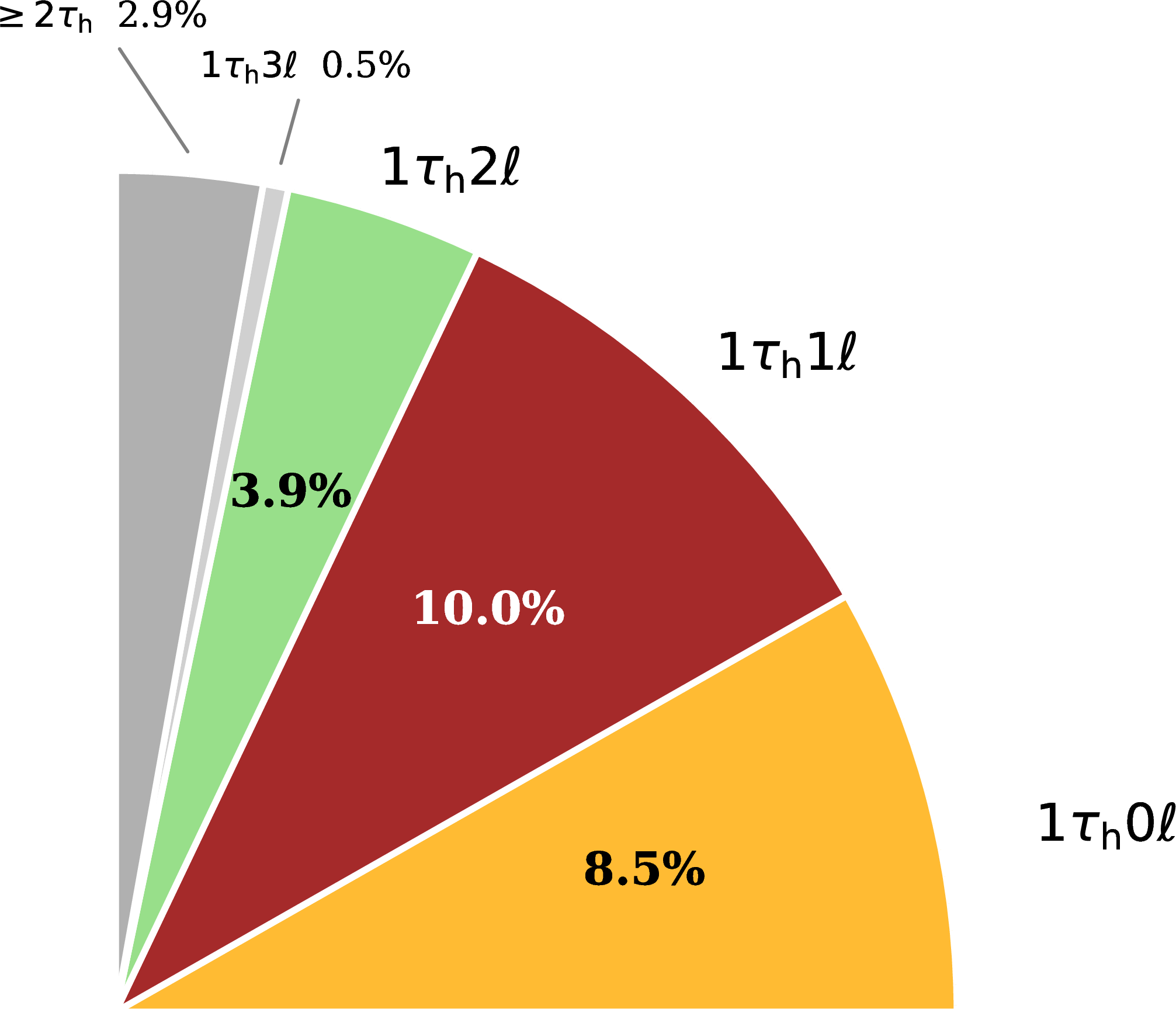
Figure 2:
Branching ratios for the decay channels of $ {\mathrm{t}\overline{\mathrm{t}}} {\mathrm{t}\overline{\mathrm{t}}} $. The decay channels are characterized by the decay modes of individual top quarks and the charge of the resulting leptons in the final state. For instance, 1 $ \tau_{\text{h}}0\ell $ indicates that one top quark decays into hadronic tau leptons, zero top quarks decay leptonically, and three top quarks decay hadronically. Conversely, 0 $ \tau_{\text{h}}2\ell $SS signifies that two top quarks decay leptonically with same-sign leptons, whereas the other two top quarks decay hadronically. |
png pdf |
Figure 2-a:
Branching ratios for the decay channels of $ {\mathrm{t}\overline{\mathrm{t}}} {\mathrm{t}\overline{\mathrm{t}}} $. The decay channels are characterized by the decay modes of individual top quarks and the charge of the resulting leptons in the final state. For instance, 1 $ \tau_{\text{h}}0\ell $ indicates that one top quark decays into hadronic tau leptons, zero top quarks decay leptonically, and three top quarks decay hadronically. Conversely, 0 $ \tau_{\text{h}}2\ell $SS signifies that two top quarks decay leptonically with same-sign leptons, whereas the other two top quarks decay hadronically. |
png pdf |
Figure 2-b:
Branching ratios for the decay channels of $ {\mathrm{t}\overline{\mathrm{t}}} {\mathrm{t}\overline{\mathrm{t}}} $. The decay channels are characterized by the decay modes of individual top quarks and the charge of the resulting leptons in the final state. For instance, 1 $ \tau_{\text{h}}0\ell $ indicates that one top quark decays into hadronic tau leptons, zero top quarks decay leptonically, and three top quarks decay hadronically. Conversely, 0 $ \tau_{\text{h}}2\ell $SS signifies that two top quarks decay leptonically with same-sign leptons, whereas the other two top quarks decay hadronically. |
png pdf |
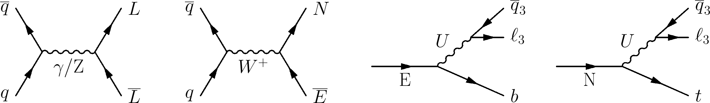
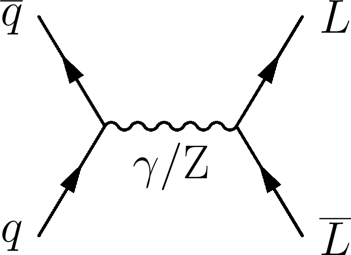
Figure 3:
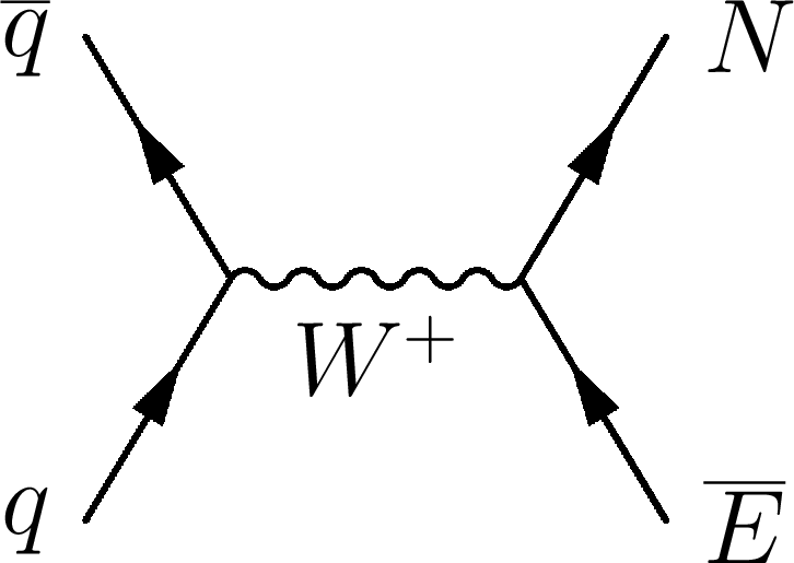
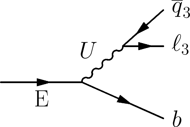
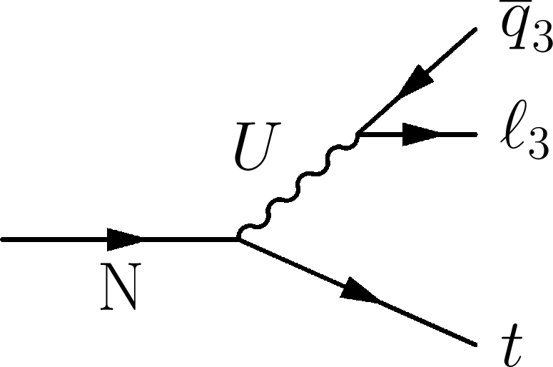
Examples of Feynman diagrams for VLL pair production and decay. The diagrams on the left show electroweak pair production of VLLs through $ s $-channel $ \mathrm{Z}/\gamma $ and W bosons at the LHC, where L represents either the neutral component N or the charged component E of the VLL doublet. The diagrams on the right illustrate the VLL decay process, mediated by a virtual vector leptoquark U, which proceeds primarily to third-generation leptons and quarks. |
png pdf |
Figure 3-a:
Examples of Feynman diagrams for VLL pair production and decay. The diagrams on the left show electroweak pair production of VLLs through $ s $-channel $ \mathrm{Z}/\gamma $ and W bosons at the LHC, where L represents either the neutral component N or the charged component E of the VLL doublet. The diagrams on the right illustrate the VLL decay process, mediated by a virtual vector leptoquark U, which proceeds primarily to third-generation leptons and quarks. |
png pdf |
Figure 3-b:
Examples of Feynman diagrams for VLL pair production and decay. The diagrams on the left show electroweak pair production of VLLs through $ s $-channel $ \mathrm{Z}/\gamma $ and W bosons at the LHC, where L represents either the neutral component N or the charged component E of the VLL doublet. The diagrams on the right illustrate the VLL decay process, mediated by a virtual vector leptoquark U, which proceeds primarily to third-generation leptons and quarks. |
png pdf |
Figure 3-c:
Examples of Feynman diagrams for VLL pair production and decay. The diagrams on the left show electroweak pair production of VLLs through $ s $-channel $ \mathrm{Z}/\gamma $ and W bosons at the LHC, where L represents either the neutral component N or the charged component E of the VLL doublet. The diagrams on the right illustrate the VLL decay process, mediated by a virtual vector leptoquark U, which proceeds primarily to third-generation leptons and quarks. |
png pdf |
Figure 3-d:
Examples of Feynman diagrams for VLL pair production and decay. The diagrams on the left show electroweak pair production of VLLs through $ s $-channel $ \mathrm{Z}/\gamma $ and W bosons at the LHC, where L represents either the neutral component N or the charged component E of the VLL doublet. The diagrams on the right illustrate the VLL decay process, mediated by a virtual vector leptoquark U, which proceeds primarily to third-generation leptons and quarks. |
png pdf |
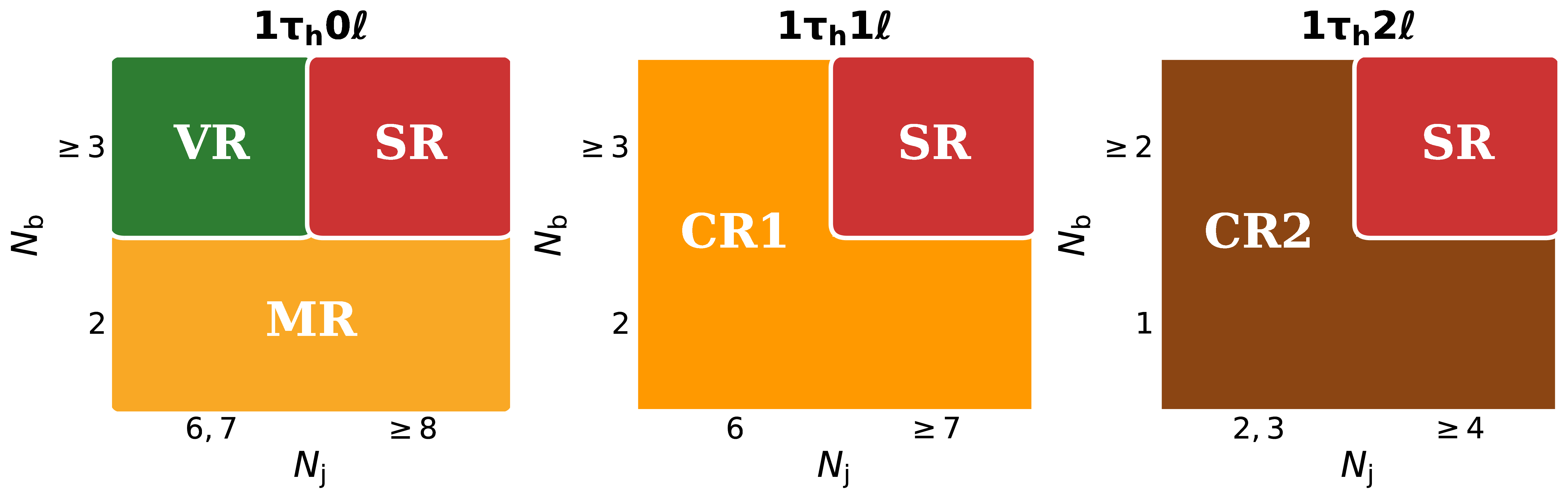
Figure 4:
Region definitions for the 1 $ \tau_{\text{h}}0\ell $ (left), 1 $ \tau_{\text{h}}1\ell $ (middle), and 1 $ \tau_{\text{h}}2\ell $ (right) channels. The baseline selection for 1 $ \tau_{\text{h}}0\ell $ and 1 $ \tau_{\text{h}}1\ell $ is different from that of 1 $ \tau_{\text{h}}2\ell $. |
png pdf |
Figure 5:
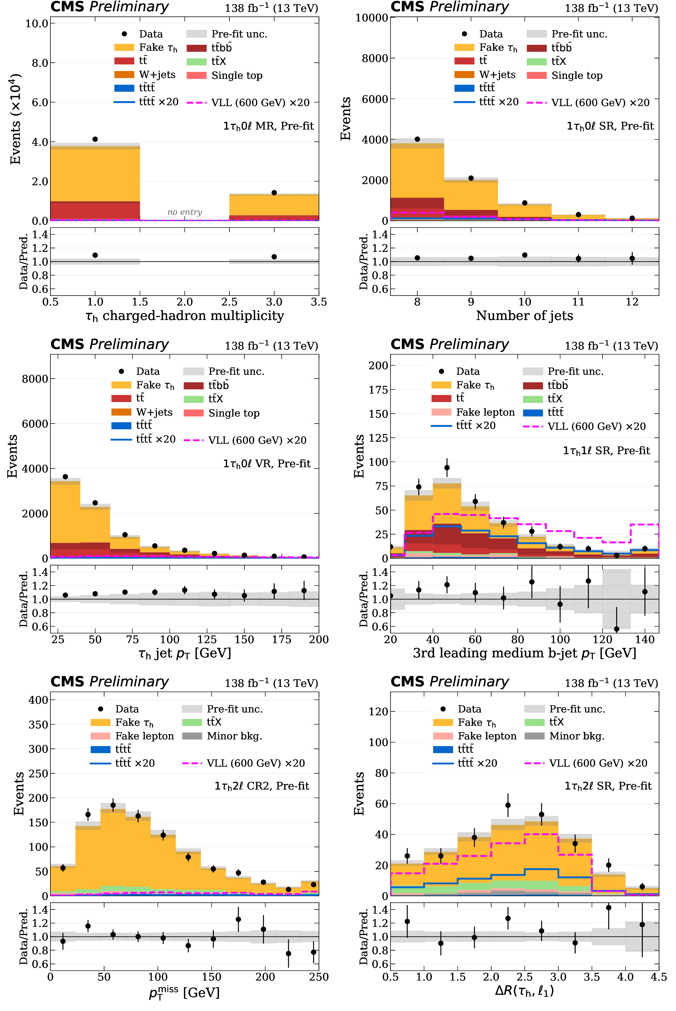
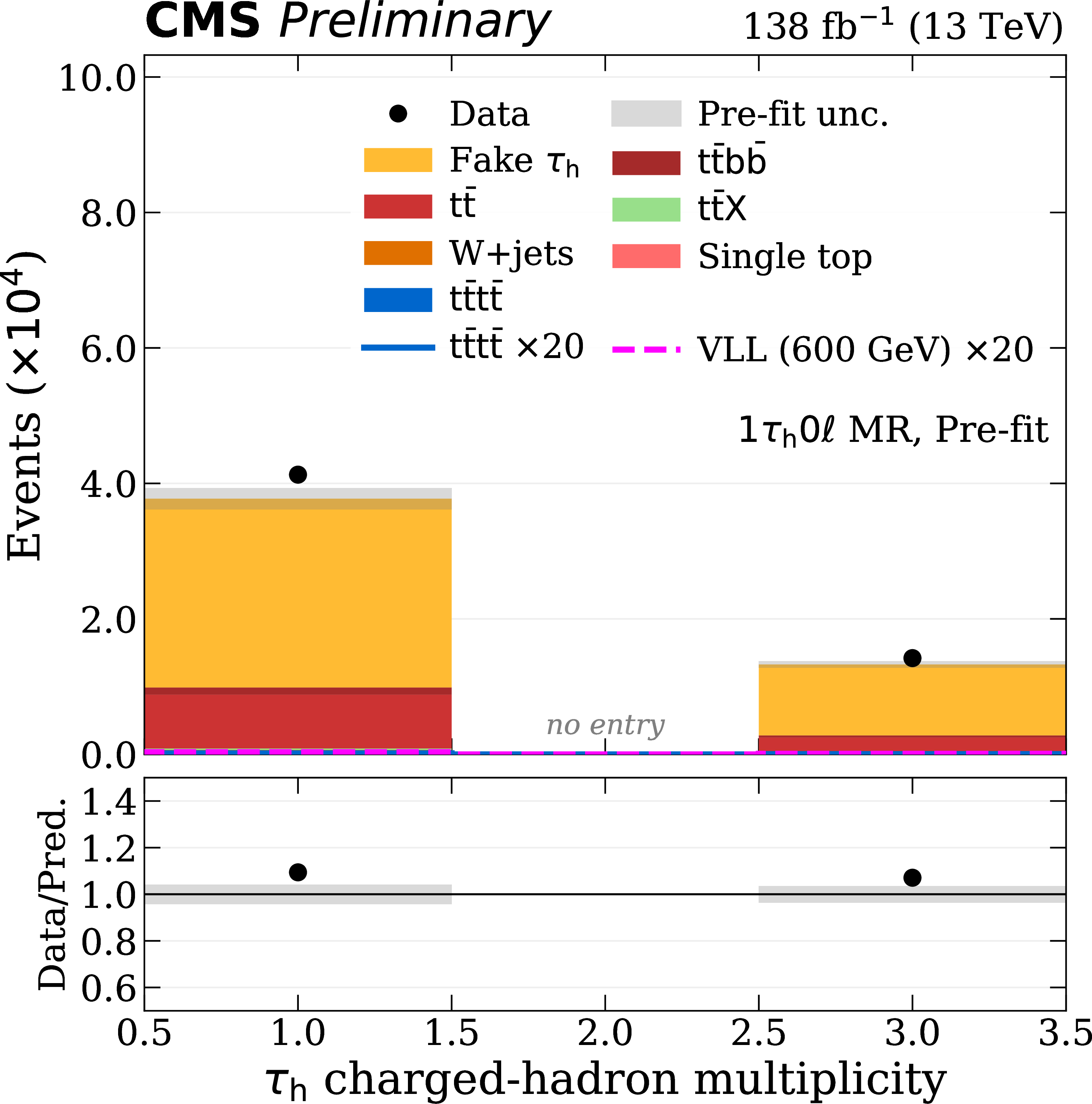
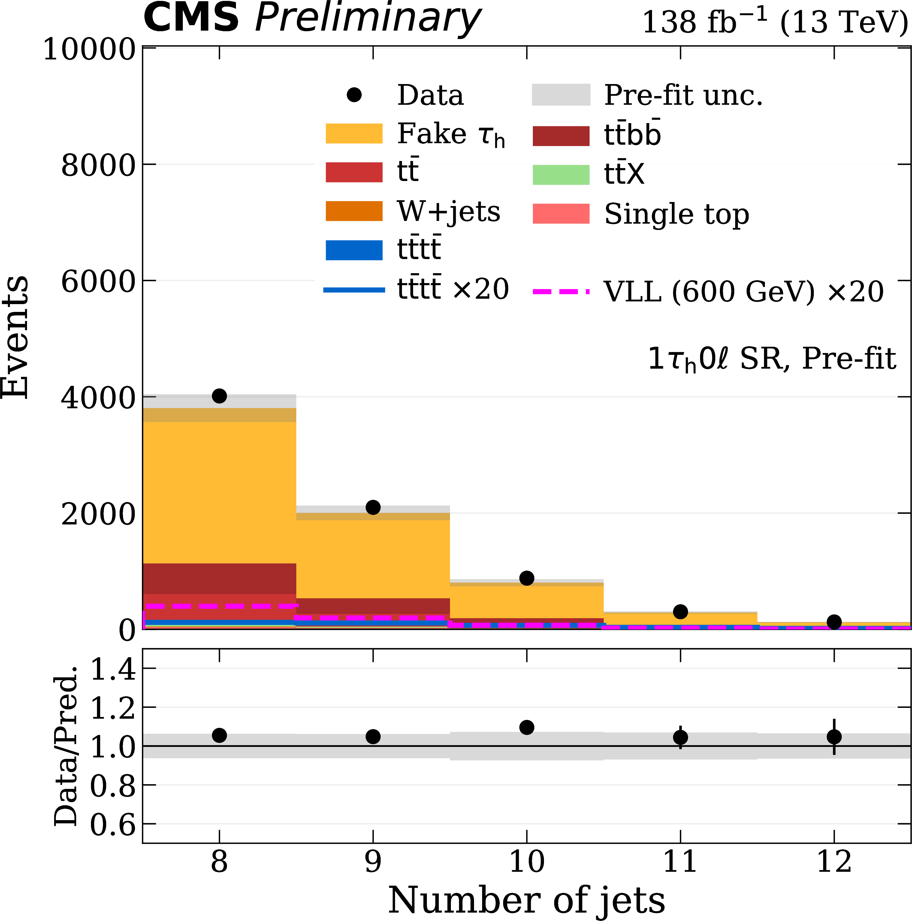
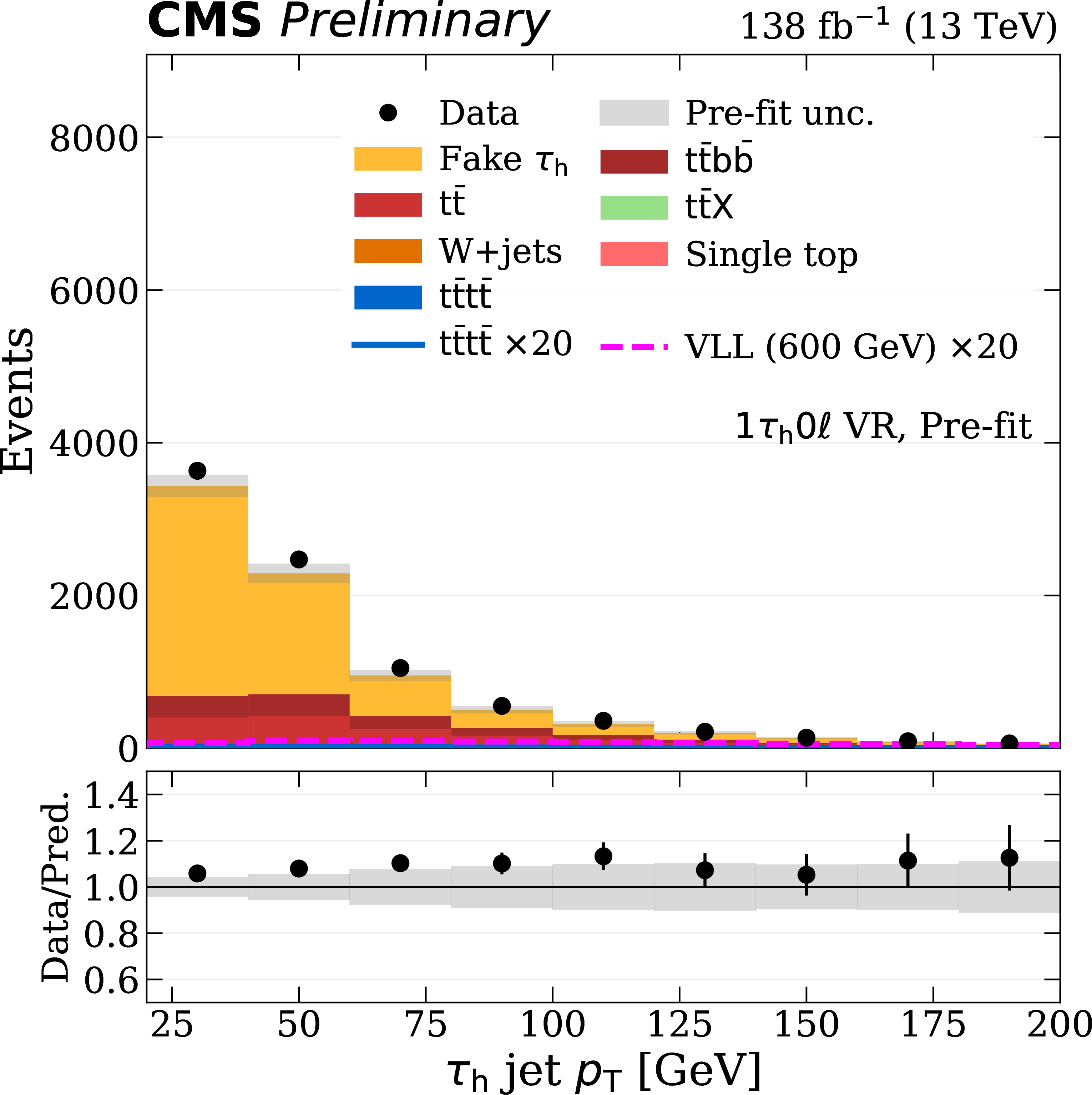
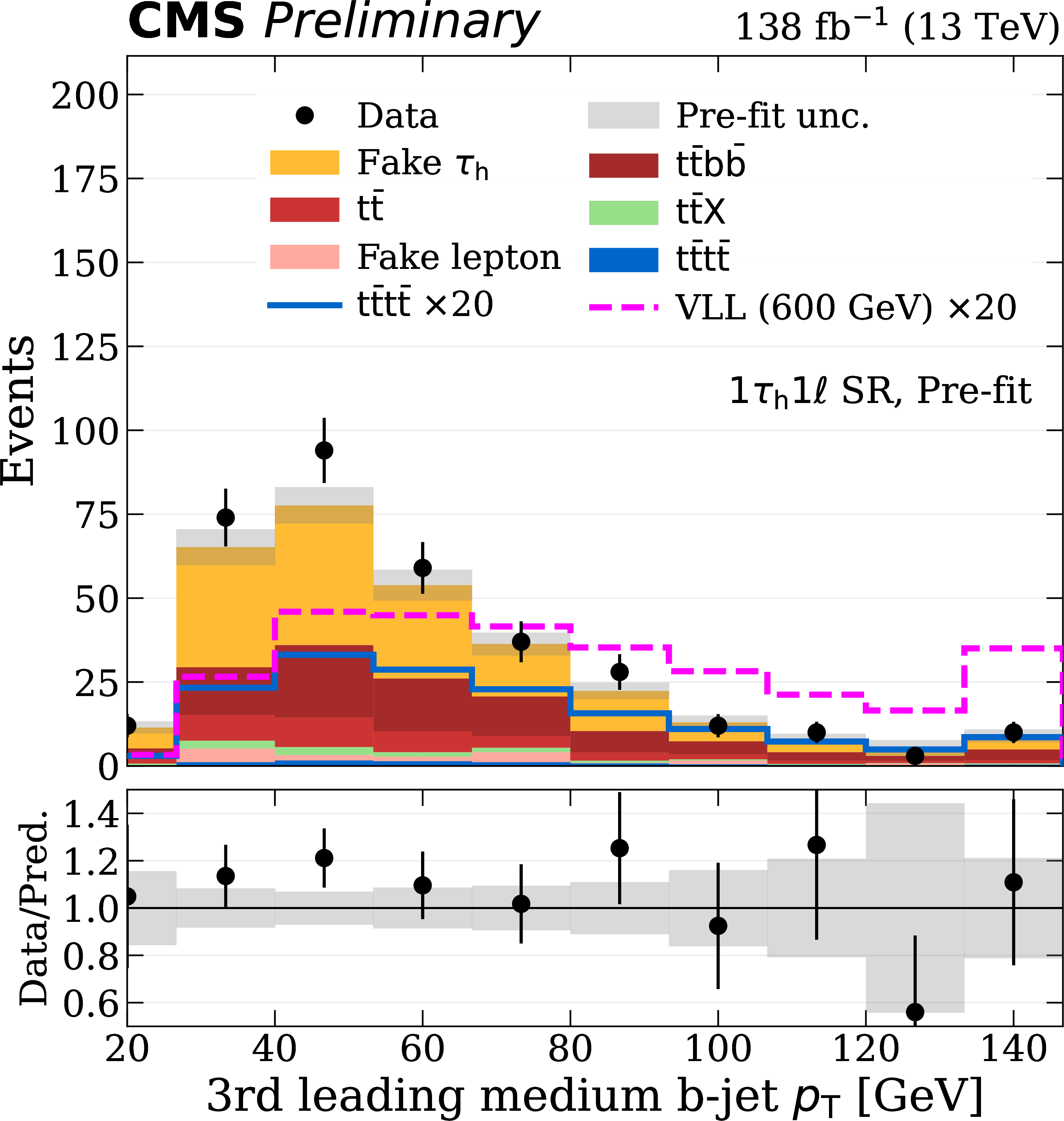
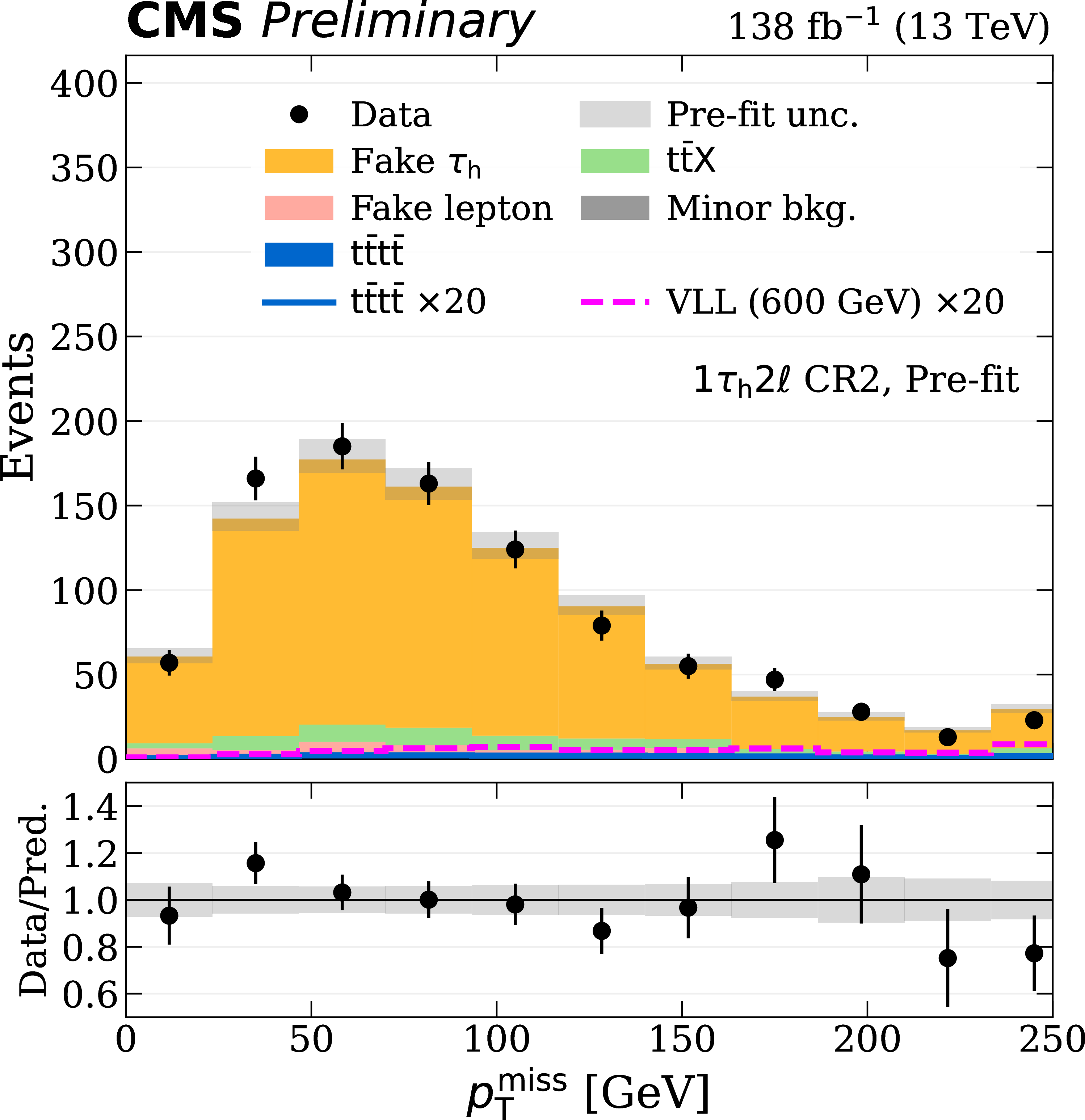
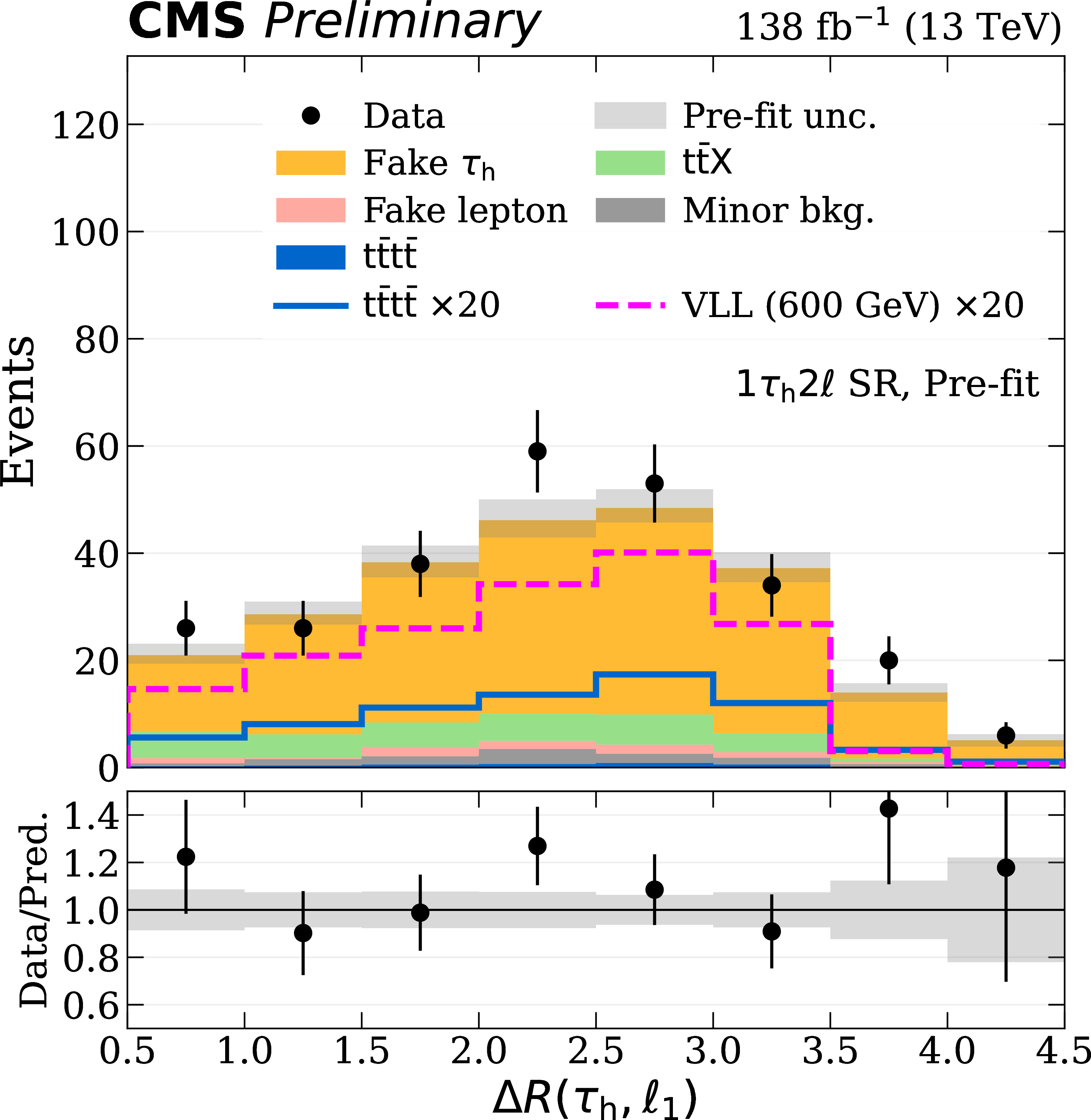
Comparison of observed data (points) and predicted events (colored histograms) for selected variables in the analysis regions: the $ \tau_{\text{h}} $ charged-hadron multiplicity in 1 $ \tau_{\text{h}}0\ell \text{MR} $ (upper left), the jet multiplicity in 1 $ \tau_{\text{h}}0\ell \text{SR} $ (upper right), the $ p_{\mathrm{T}} $ of the jet associated with the $ \tau_{\text{h}} $ candidate in 1 $ \tau_{\text{h}}0\ell \text{VR} $ (middle left), the third-leading medium b-tagged jet $ p_{\mathrm{T}} $ in 1 $ \tau_{\text{h}}1\ell \text{SR} $ (middle right), the $ p_{\mathrm{T}}^\text{miss} $ in 1 $ \tau_{\text{h}}2\ell \text{CR2} $ (lower left), and the $ \Delta R $ between the $ \tau_{\text{h}} $ and the leading lepton in 1 $ \tau_{\text{h}}2\ell \text{SR} $ (lower right). The vertical bars on the data points represent statistical uncertainties, and the hatched bands indicate the total uncertainty in the predictions. |
png pdf |
Figure 5-a:
Comparison of observed data (points) and predicted events (colored histograms) for selected variables in the analysis regions: the $ \tau_{\text{h}} $ charged-hadron multiplicity in 1 $ \tau_{\text{h}}0\ell \text{MR} $ (upper left), the jet multiplicity in 1 $ \tau_{\text{h}}0\ell \text{SR} $ (upper right), the $ p_{\mathrm{T}} $ of the jet associated with the $ \tau_{\text{h}} $ candidate in 1 $ \tau_{\text{h}}0\ell \text{VR} $ (middle left), the third-leading medium b-tagged jet $ p_{\mathrm{T}} $ in 1 $ \tau_{\text{h}}1\ell \text{SR} $ (middle right), the $ p_{\mathrm{T}}^\text{miss} $ in 1 $ \tau_{\text{h}}2\ell \text{CR2} $ (lower left), and the $ \Delta R $ between the $ \tau_{\text{h}} $ and the leading lepton in 1 $ \tau_{\text{h}}2\ell \text{SR} $ (lower right). The vertical bars on the data points represent statistical uncertainties, and the hatched bands indicate the total uncertainty in the predictions. |
png pdf |
Figure 5-b:
Comparison of observed data (points) and predicted events (colored histograms) for selected variables in the analysis regions: the $ \tau_{\text{h}} $ charged-hadron multiplicity in 1 $ \tau_{\text{h}}0\ell \text{MR} $ (upper left), the jet multiplicity in 1 $ \tau_{\text{h}}0\ell \text{SR} $ (upper right), the $ p_{\mathrm{T}} $ of the jet associated with the $ \tau_{\text{h}} $ candidate in 1 $ \tau_{\text{h}}0\ell \text{VR} $ (middle left), the third-leading medium b-tagged jet $ p_{\mathrm{T}} $ in 1 $ \tau_{\text{h}}1\ell \text{SR} $ (middle right), the $ p_{\mathrm{T}}^\text{miss} $ in 1 $ \tau_{\text{h}}2\ell \text{CR2} $ (lower left), and the $ \Delta R $ between the $ \tau_{\text{h}} $ and the leading lepton in 1 $ \tau_{\text{h}}2\ell \text{SR} $ (lower right). The vertical bars on the data points represent statistical uncertainties, and the hatched bands indicate the total uncertainty in the predictions. |
png pdf |
Figure 5-c:
Comparison of observed data (points) and predicted events (colored histograms) for selected variables in the analysis regions: the $ \tau_{\text{h}} $ charged-hadron multiplicity in 1 $ \tau_{\text{h}}0\ell \text{MR} $ (upper left), the jet multiplicity in 1 $ \tau_{\text{h}}0\ell \text{SR} $ (upper right), the $ p_{\mathrm{T}} $ of the jet associated with the $ \tau_{\text{h}} $ candidate in 1 $ \tau_{\text{h}}0\ell \text{VR} $ (middle left), the third-leading medium b-tagged jet $ p_{\mathrm{T}} $ in 1 $ \tau_{\text{h}}1\ell \text{SR} $ (middle right), the $ p_{\mathrm{T}}^\text{miss} $ in 1 $ \tau_{\text{h}}2\ell \text{CR2} $ (lower left), and the $ \Delta R $ between the $ \tau_{\text{h}} $ and the leading lepton in 1 $ \tau_{\text{h}}2\ell \text{SR} $ (lower right). The vertical bars on the data points represent statistical uncertainties, and the hatched bands indicate the total uncertainty in the predictions. |
png pdf |
Figure 5-d:
Comparison of observed data (points) and predicted events (colored histograms) for selected variables in the analysis regions: the $ \tau_{\text{h}} $ charged-hadron multiplicity in 1 $ \tau_{\text{h}}0\ell \text{MR} $ (upper left), the jet multiplicity in 1 $ \tau_{\text{h}}0\ell \text{SR} $ (upper right), the $ p_{\mathrm{T}} $ of the jet associated with the $ \tau_{\text{h}} $ candidate in 1 $ \tau_{\text{h}}0\ell \text{VR} $ (middle left), the third-leading medium b-tagged jet $ p_{\mathrm{T}} $ in 1 $ \tau_{\text{h}}1\ell \text{SR} $ (middle right), the $ p_{\mathrm{T}}^\text{miss} $ in 1 $ \tau_{\text{h}}2\ell \text{CR2} $ (lower left), and the $ \Delta R $ between the $ \tau_{\text{h}} $ and the leading lepton in 1 $ \tau_{\text{h}}2\ell \text{SR} $ (lower right). The vertical bars on the data points represent statistical uncertainties, and the hatched bands indicate the total uncertainty in the predictions. |
png pdf |
Figure 5-e:
Comparison of observed data (points) and predicted events (colored histograms) for selected variables in the analysis regions: the $ \tau_{\text{h}} $ charged-hadron multiplicity in 1 $ \tau_{\text{h}}0\ell \text{MR} $ (upper left), the jet multiplicity in 1 $ \tau_{\text{h}}0\ell \text{SR} $ (upper right), the $ p_{\mathrm{T}} $ of the jet associated with the $ \tau_{\text{h}} $ candidate in 1 $ \tau_{\text{h}}0\ell \text{VR} $ (middle left), the third-leading medium b-tagged jet $ p_{\mathrm{T}} $ in 1 $ \tau_{\text{h}}1\ell \text{SR} $ (middle right), the $ p_{\mathrm{T}}^\text{miss} $ in 1 $ \tau_{\text{h}}2\ell \text{CR2} $ (lower left), and the $ \Delta R $ between the $ \tau_{\text{h}} $ and the leading lepton in 1 $ \tau_{\text{h}}2\ell \text{SR} $ (lower right). The vertical bars on the data points represent statistical uncertainties, and the hatched bands indicate the total uncertainty in the predictions. |
png pdf |
Figure 5-f:
Comparison of observed data (points) and predicted events (colored histograms) for selected variables in the analysis regions: the $ \tau_{\text{h}} $ charged-hadron multiplicity in 1 $ \tau_{\text{h}}0\ell \text{MR} $ (upper left), the jet multiplicity in 1 $ \tau_{\text{h}}0\ell \text{SR} $ (upper right), the $ p_{\mathrm{T}} $ of the jet associated with the $ \tau_{\text{h}} $ candidate in 1 $ \tau_{\text{h}}0\ell \text{VR} $ (middle left), the third-leading medium b-tagged jet $ p_{\mathrm{T}} $ in 1 $ \tau_{\text{h}}1\ell \text{SR} $ (middle right), the $ p_{\mathrm{T}}^\text{miss} $ in 1 $ \tau_{\text{h}}2\ell \text{CR2} $ (lower left), and the $ \Delta R $ between the $ \tau_{\text{h}} $ and the leading lepton in 1 $ \tau_{\text{h}}2\ell \text{SR} $ (lower right). The vertical bars on the data points represent statistical uncertainties, and the hatched bands indicate the total uncertainty in the predictions. |
png pdf |
Figure 6:
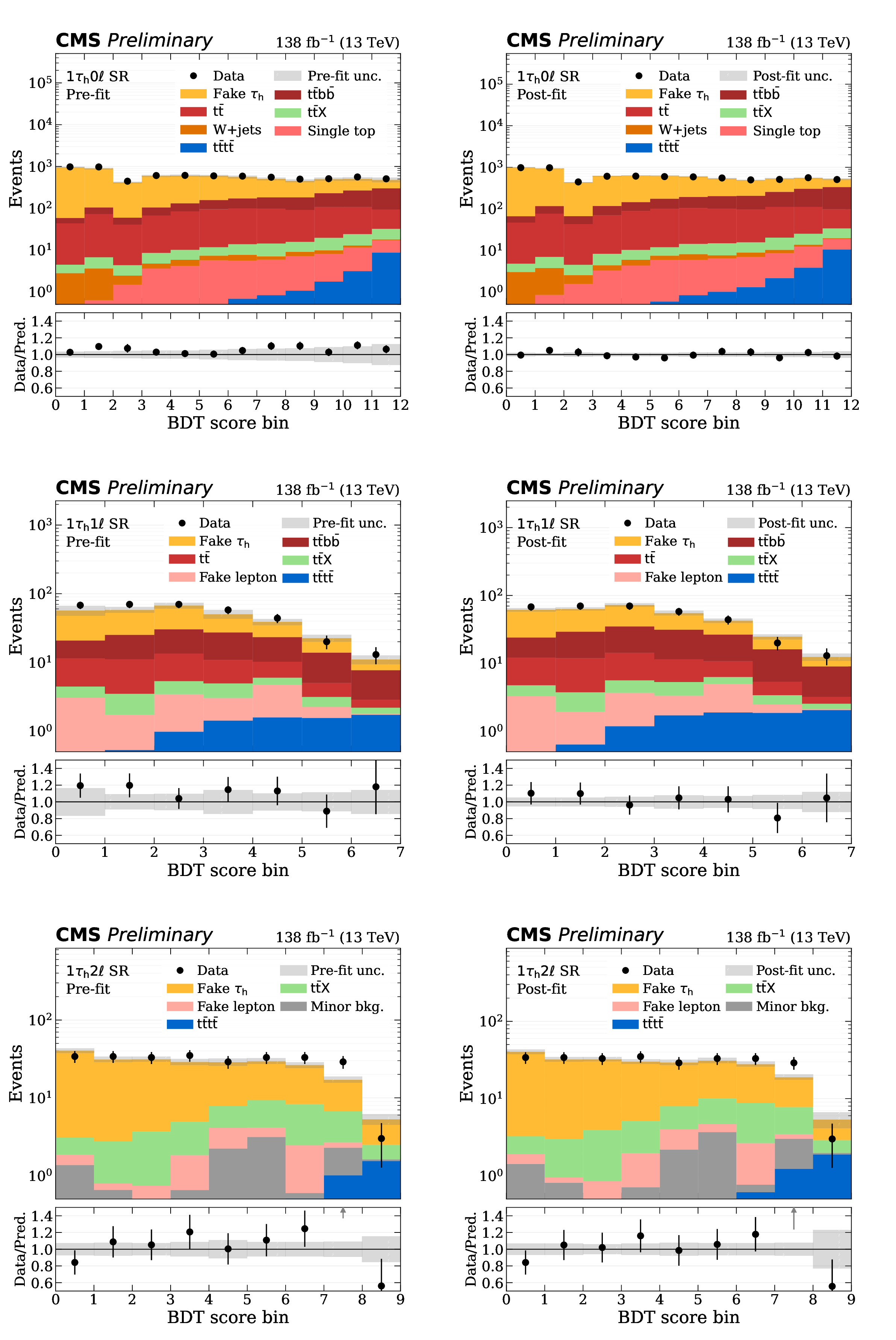
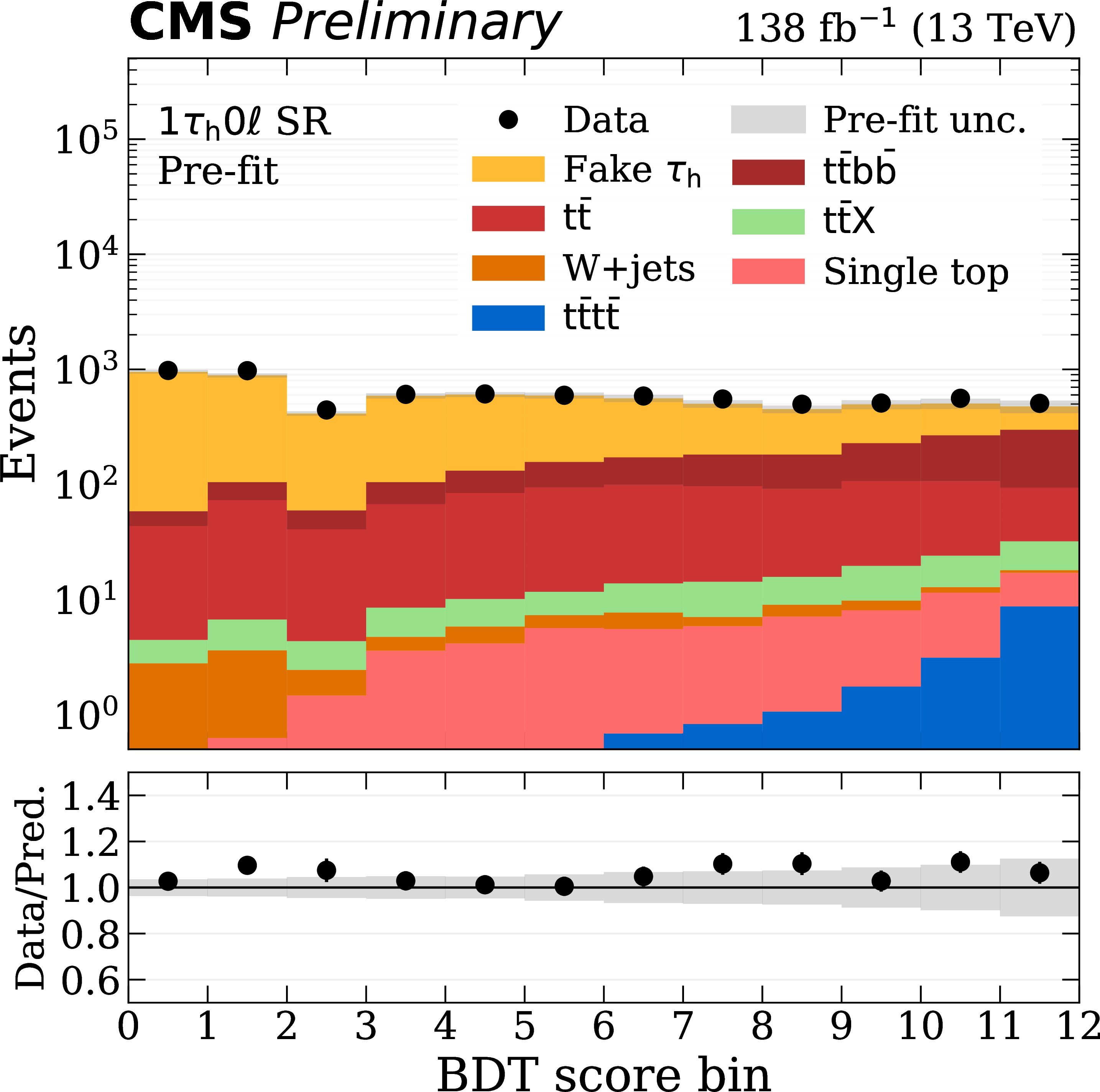
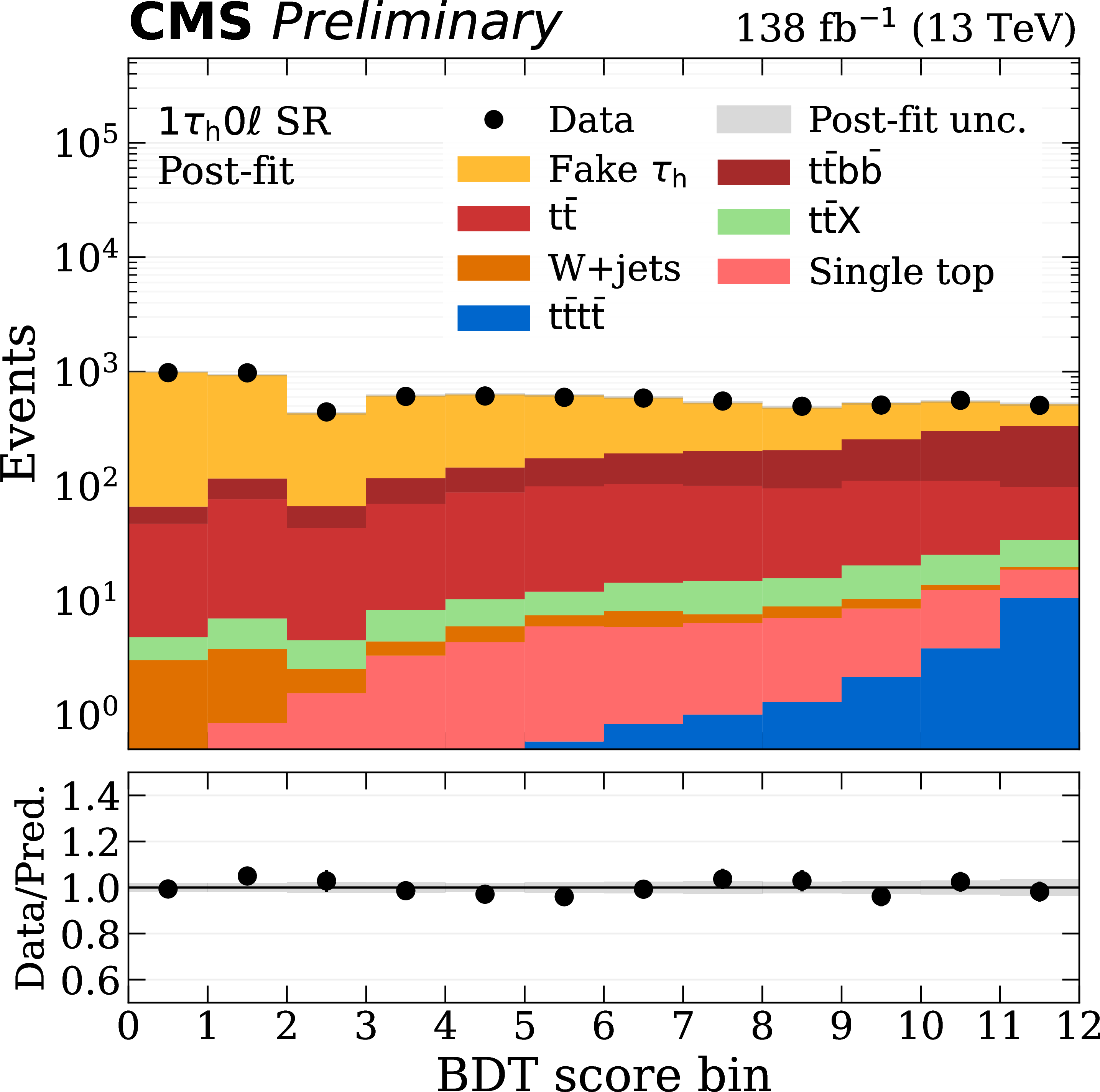
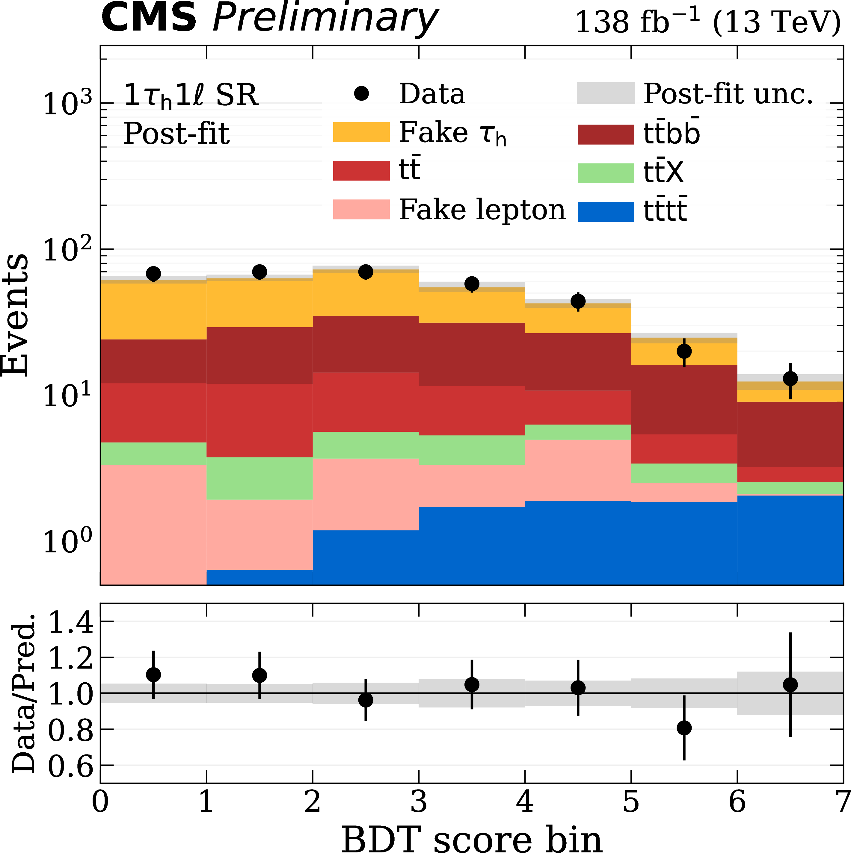
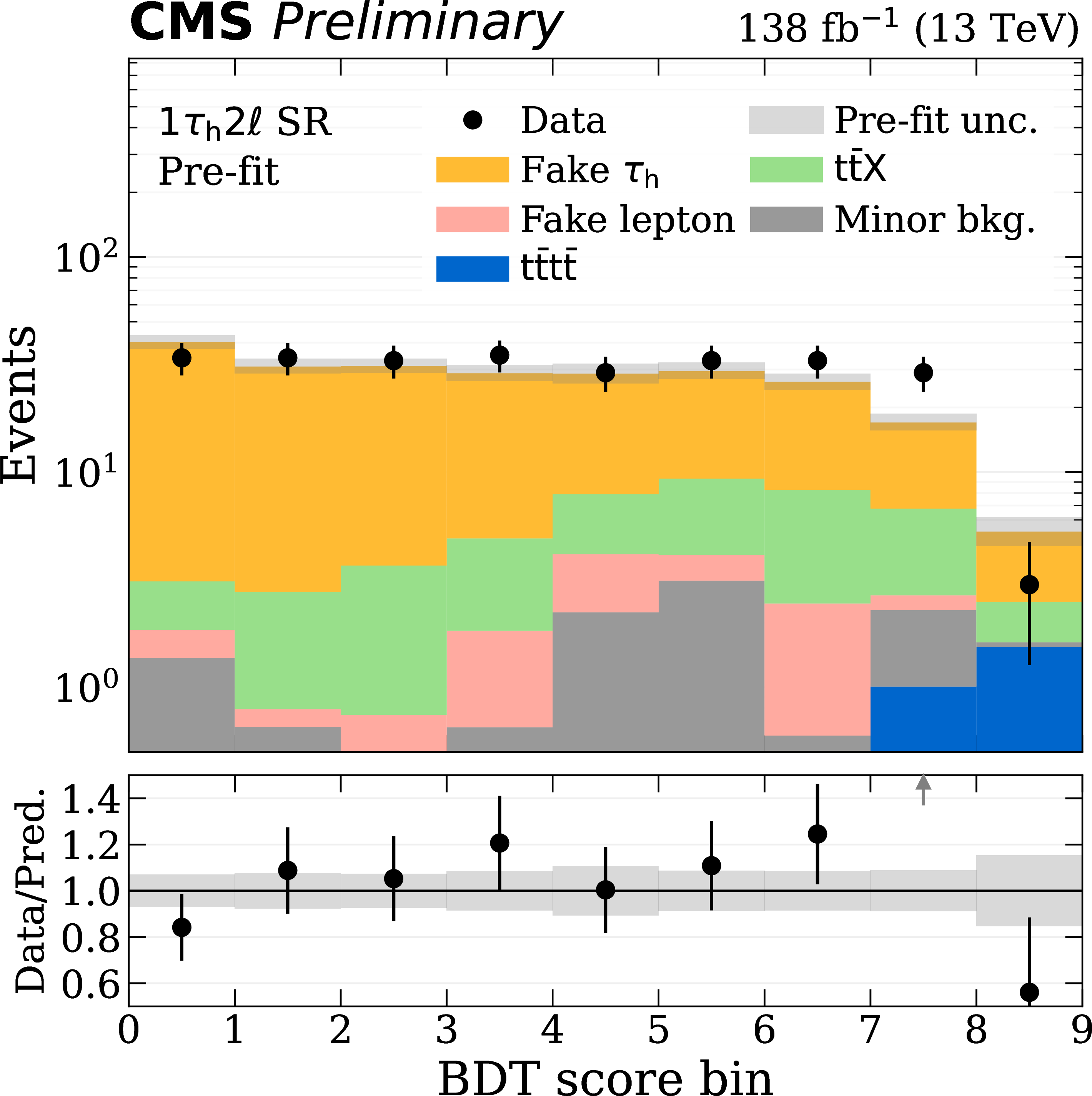
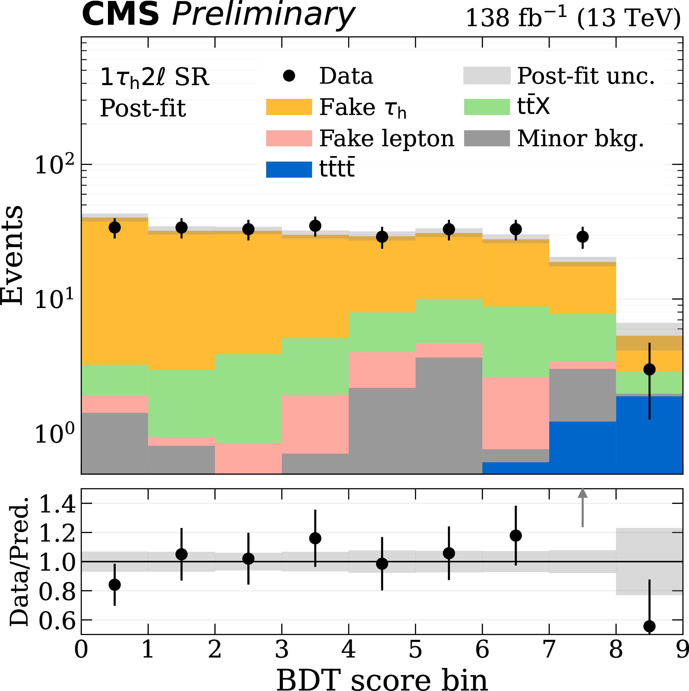
Distributions of the binned BDT discriminant for the $ {\mathrm{t}\overline{\mathrm{t}}} {\mathrm{t}\overline{\mathrm{t}}} $ production measurement in the three signal regions: 1 $ \tau_{\text{h}}0\ell \text{SR} $ (top), 1 $ \tau_{\text{h}}1\ell \text{SR} $ (middle), and 1 $ \tau_{\text{h}}2\ell \text{SR} $ (bottom). Pre-fit distributions are shown on the left and post-fit on the right. Each bin corresponds to a range of the BDT output score, with increasing bin number corresponding to higher signal purity. The points represent the observed data, and the stacked histograms show the predicted backgrounds and $ {\mathrm{t}\overline{\mathrm{t}}} {\mathrm{t}\overline{\mathrm{t}}} $ signal. The hatched bands indicate the total uncertainty in the predictions. |
png pdf |
Figure 6-a:
Distributions of the binned BDT discriminant for the $ {\mathrm{t}\overline{\mathrm{t}}} {\mathrm{t}\overline{\mathrm{t}}} $ production measurement in the three signal regions: 1 $ \tau_{\text{h}}0\ell \text{SR} $ (top), 1 $ \tau_{\text{h}}1\ell \text{SR} $ (middle), and 1 $ \tau_{\text{h}}2\ell \text{SR} $ (bottom). Pre-fit distributions are shown on the left and post-fit on the right. Each bin corresponds to a range of the BDT output score, with increasing bin number corresponding to higher signal purity. The points represent the observed data, and the stacked histograms show the predicted backgrounds and $ {\mathrm{t}\overline{\mathrm{t}}} {\mathrm{t}\overline{\mathrm{t}}} $ signal. The hatched bands indicate the total uncertainty in the predictions. |
png pdf |
Figure 6-b:
Distributions of the binned BDT discriminant for the $ {\mathrm{t}\overline{\mathrm{t}}} {\mathrm{t}\overline{\mathrm{t}}} $ production measurement in the three signal regions: 1 $ \tau_{\text{h}}0\ell \text{SR} $ (top), 1 $ \tau_{\text{h}}1\ell \text{SR} $ (middle), and 1 $ \tau_{\text{h}}2\ell \text{SR} $ (bottom). Pre-fit distributions are shown on the left and post-fit on the right. Each bin corresponds to a range of the BDT output score, with increasing bin number corresponding to higher signal purity. The points represent the observed data, and the stacked histograms show the predicted backgrounds and $ {\mathrm{t}\overline{\mathrm{t}}} {\mathrm{t}\overline{\mathrm{t}}} $ signal. The hatched bands indicate the total uncertainty in the predictions. |

png pdf |
Figure 6-c:
Distributions of the binned BDT discriminant for the $ {\mathrm{t}\overline{\mathrm{t}}} {\mathrm{t}\overline{\mathrm{t}}} $ production measurement in the three signal regions: 1 $ \tau_{\text{h}}0\ell \text{SR} $ (top), 1 $ \tau_{\text{h}}1\ell \text{SR} $ (middle), and 1 $ \tau_{\text{h}}2\ell \text{SR} $ (bottom). Pre-fit distributions are shown on the left and post-fit on the right. Each bin corresponds to a range of the BDT output score, with increasing bin number corresponding to higher signal purity. The points represent the observed data, and the stacked histograms show the predicted backgrounds and $ {\mathrm{t}\overline{\mathrm{t}}} {\mathrm{t}\overline{\mathrm{t}}} $ signal. The hatched bands indicate the total uncertainty in the predictions. |
png pdf |
Figure 6-d:
Distributions of the binned BDT discriminant for the $ {\mathrm{t}\overline{\mathrm{t}}} {\mathrm{t}\overline{\mathrm{t}}} $ production measurement in the three signal regions: 1 $ \tau_{\text{h}}0\ell \text{SR} $ (top), 1 $ \tau_{\text{h}}1\ell \text{SR} $ (middle), and 1 $ \tau_{\text{h}}2\ell \text{SR} $ (bottom). Pre-fit distributions are shown on the left and post-fit on the right. Each bin corresponds to a range of the BDT output score, with increasing bin number corresponding to higher signal purity. The points represent the observed data, and the stacked histograms show the predicted backgrounds and $ {\mathrm{t}\overline{\mathrm{t}}} {\mathrm{t}\overline{\mathrm{t}}} $ signal. The hatched bands indicate the total uncertainty in the predictions. |
png pdf |
Figure 6-e:
Distributions of the binned BDT discriminant for the $ {\mathrm{t}\overline{\mathrm{t}}} {\mathrm{t}\overline{\mathrm{t}}} $ production measurement in the three signal regions: 1 $ \tau_{\text{h}}0\ell \text{SR} $ (top), 1 $ \tau_{\text{h}}1\ell \text{SR} $ (middle), and 1 $ \tau_{\text{h}}2\ell \text{SR} $ (bottom). Pre-fit distributions are shown on the left and post-fit on the right. Each bin corresponds to a range of the BDT output score, with increasing bin number corresponding to higher signal purity. The points represent the observed data, and the stacked histograms show the predicted backgrounds and $ {\mathrm{t}\overline{\mathrm{t}}} {\mathrm{t}\overline{\mathrm{t}}} $ signal. The hatched bands indicate the total uncertainty in the predictions. |
png pdf |
Figure 6-f:
Distributions of the binned BDT discriminant for the $ {\mathrm{t}\overline{\mathrm{t}}} {\mathrm{t}\overline{\mathrm{t}}} $ production measurement in the three signal regions: 1 $ \tau_{\text{h}}0\ell \text{SR} $ (top), 1 $ \tau_{\text{h}}1\ell \text{SR} $ (middle), and 1 $ \tau_{\text{h}}2\ell \text{SR} $ (bottom). Pre-fit distributions are shown on the left and post-fit on the right. Each bin corresponds to a range of the BDT output score, with increasing bin number corresponding to higher signal purity. The points represent the observed data, and the stacked histograms show the predicted backgrounds and $ {\mathrm{t}\overline{\mathrm{t}}} {\mathrm{t}\overline{\mathrm{t}}} $ signal. The hatched bands indicate the total uncertainty in the predictions. |
png pdf |
Figure 7:
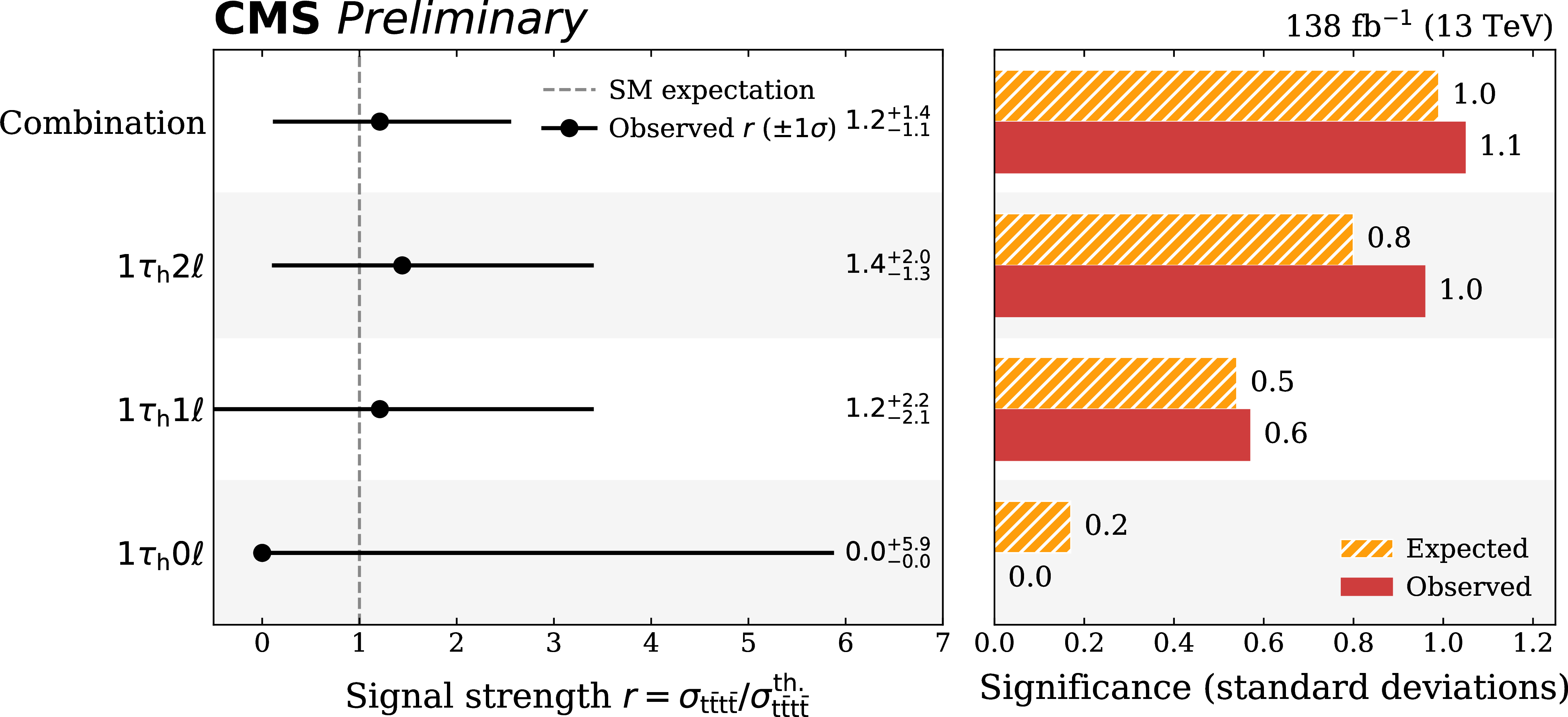
Results of the $ {\mathrm{t}\overline{\mathrm{t}}} {\mathrm{t}\overline{\mathrm{t}}} $ production measurement for the individual channels (1 $ \tau_{\text{h}}0\ell $, 1 $ \tau_{\text{h}}1\ell $, and 1 $ \tau_{\text{h}}2\ell $) and their combination. The left panel shows the observed signal strength $ r = \sigma_{{\mathrm{t}\overline{\mathrm{t}}} {\mathrm{t}\overline{\mathrm{t}}} }/\sigma^{\text{th.}}_{{\mathrm{t}\overline{\mathrm{t}}} {\mathrm{t}\overline{\mathrm{t}}} } $ with $ \pm $ 1 standard deviation uncertainties, compared with the SM expectation (dashed line). The right panel shows the observed and expected significances for rejecting the background-only hypothesis. |
png pdf |
Figure 8:
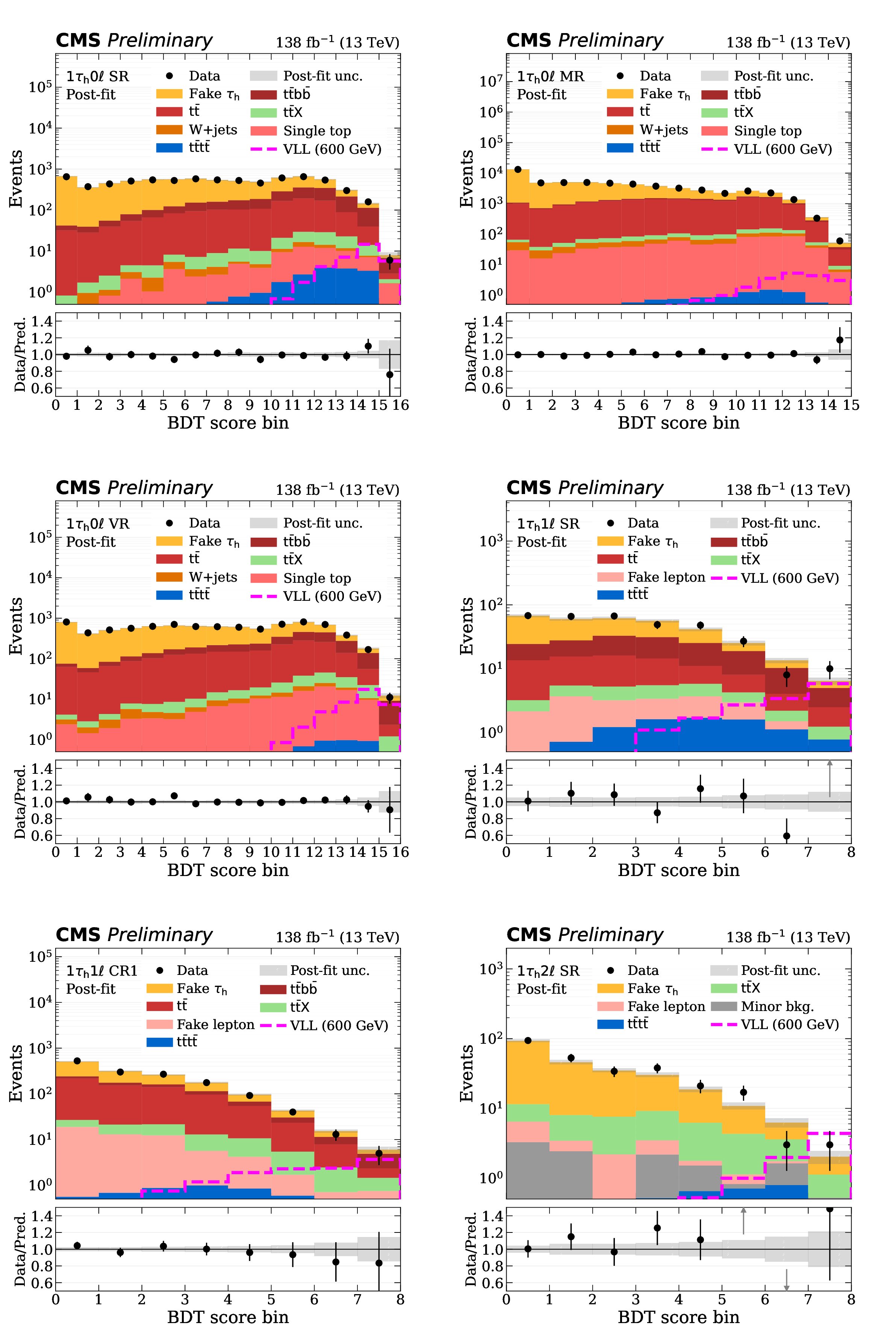
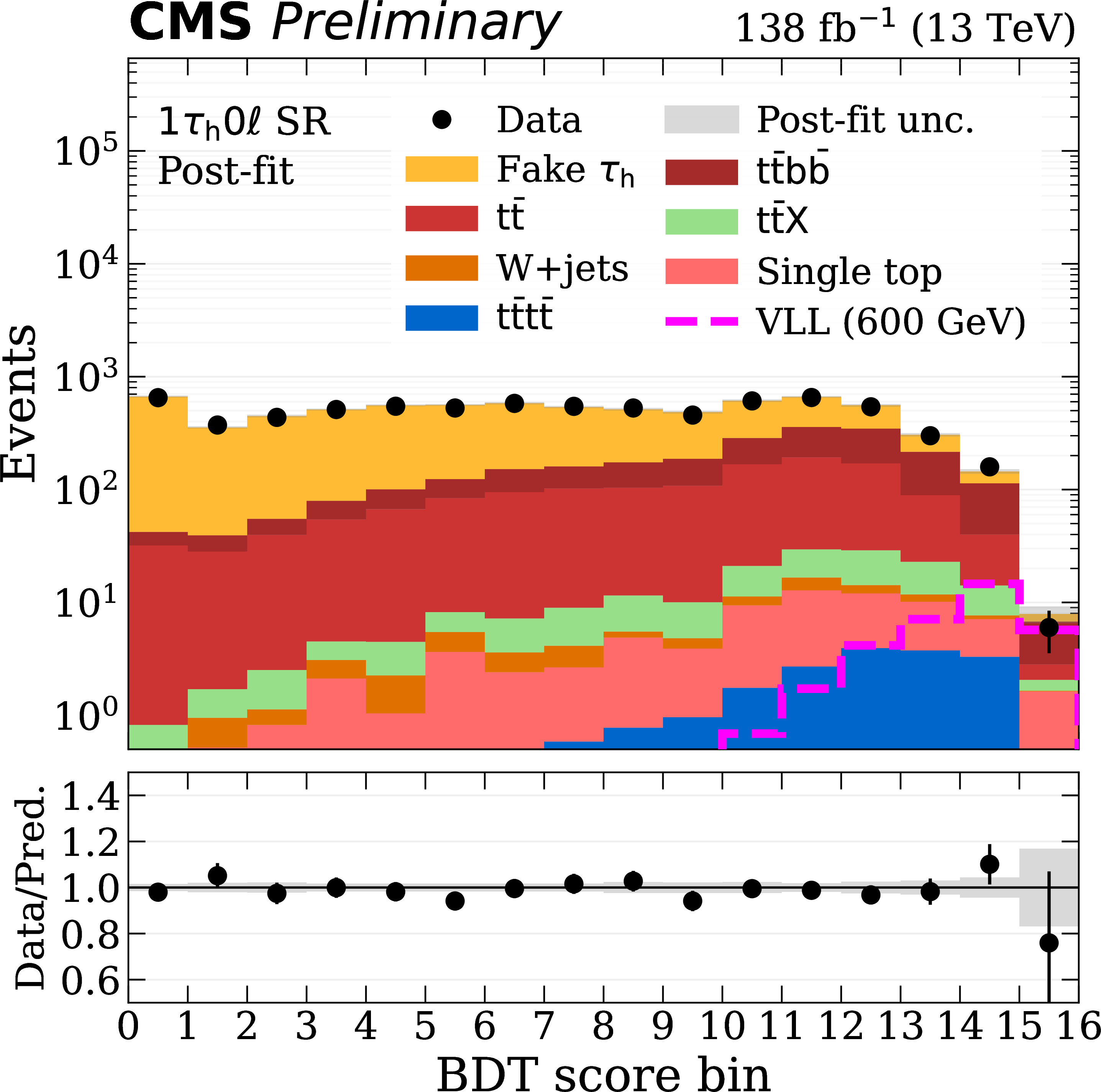
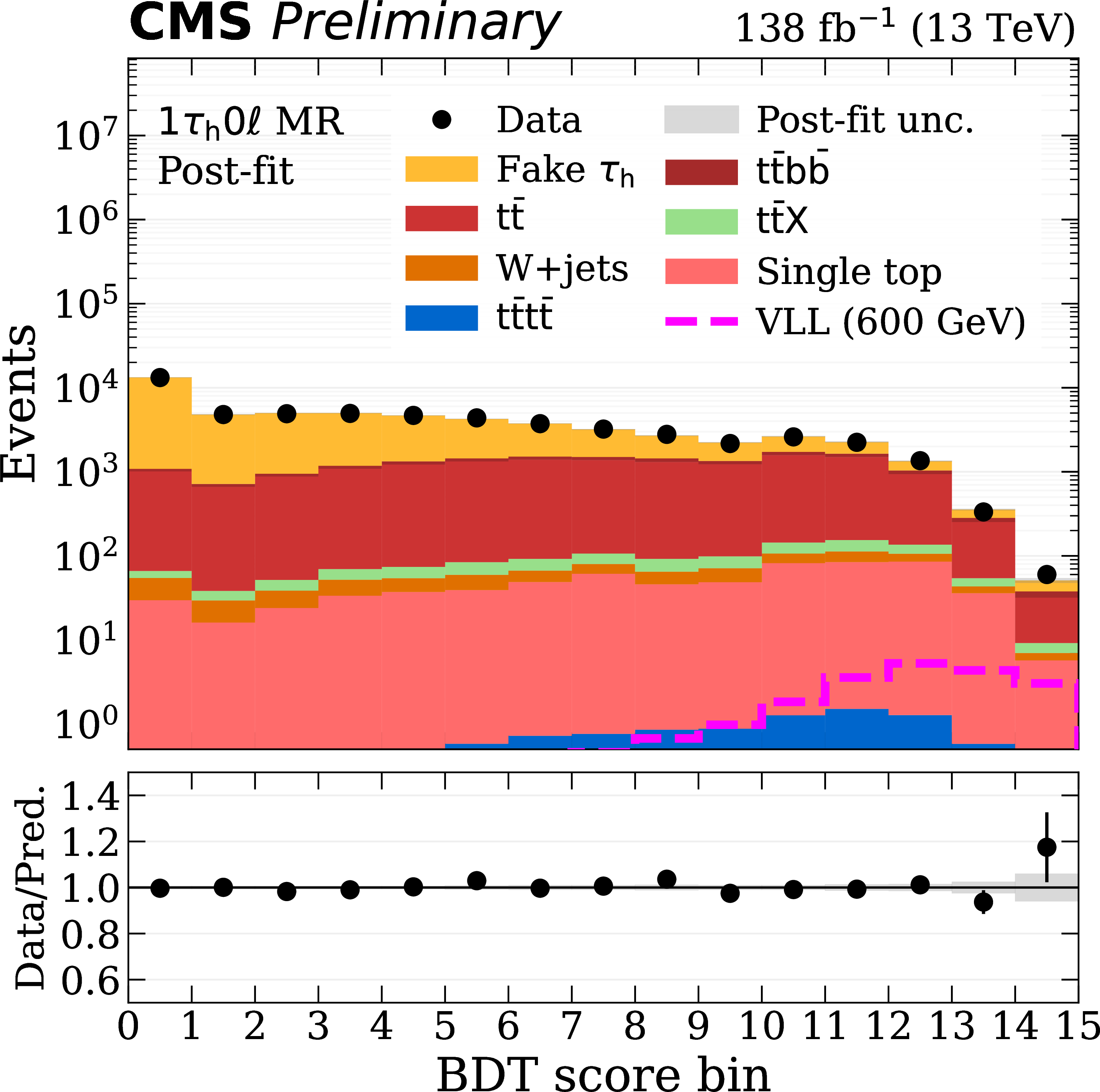
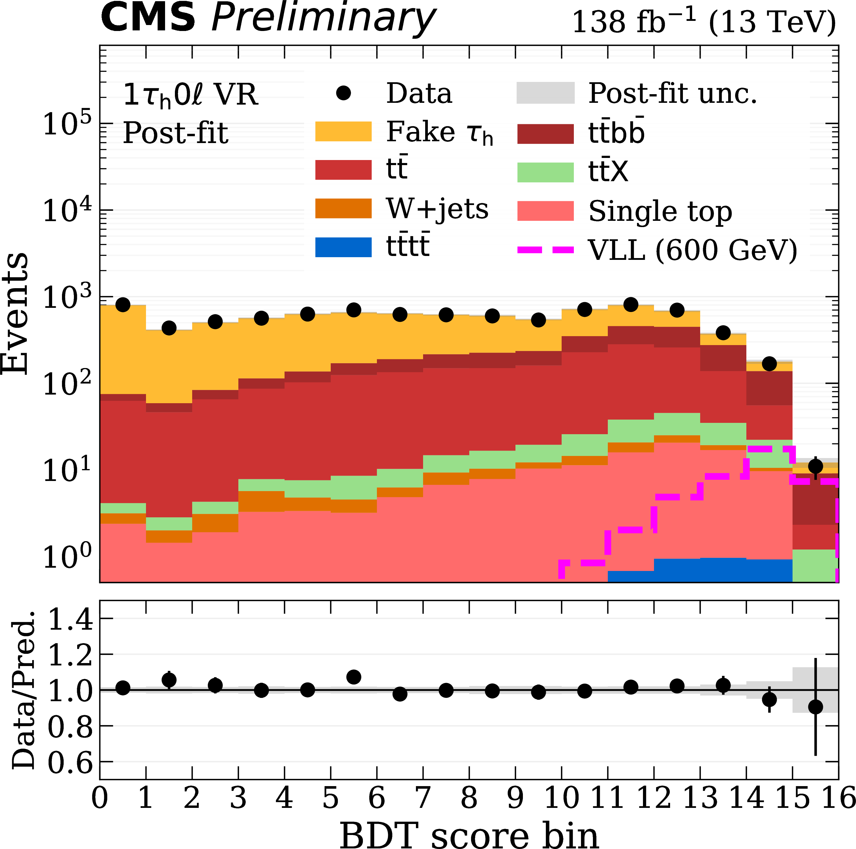
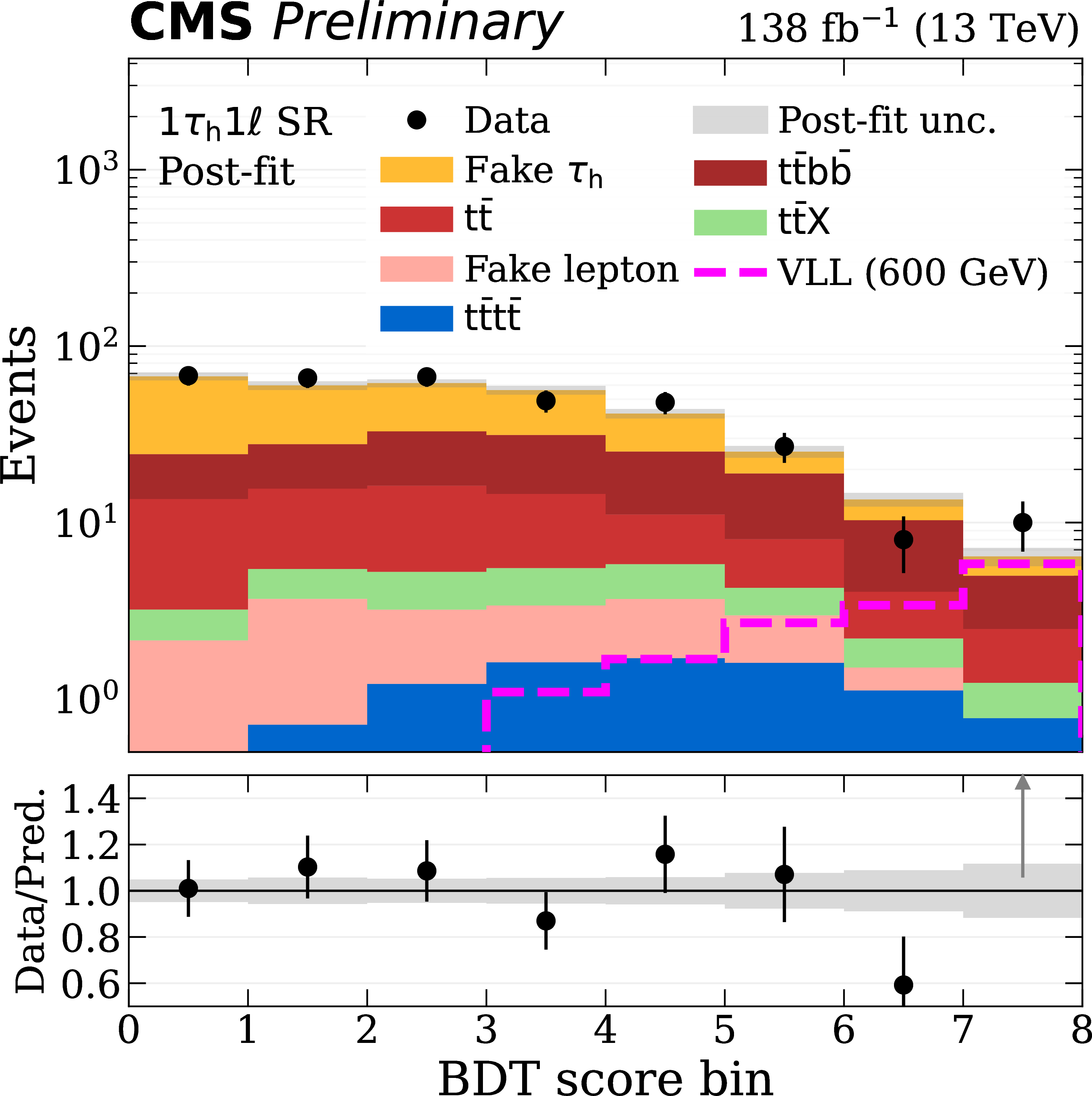
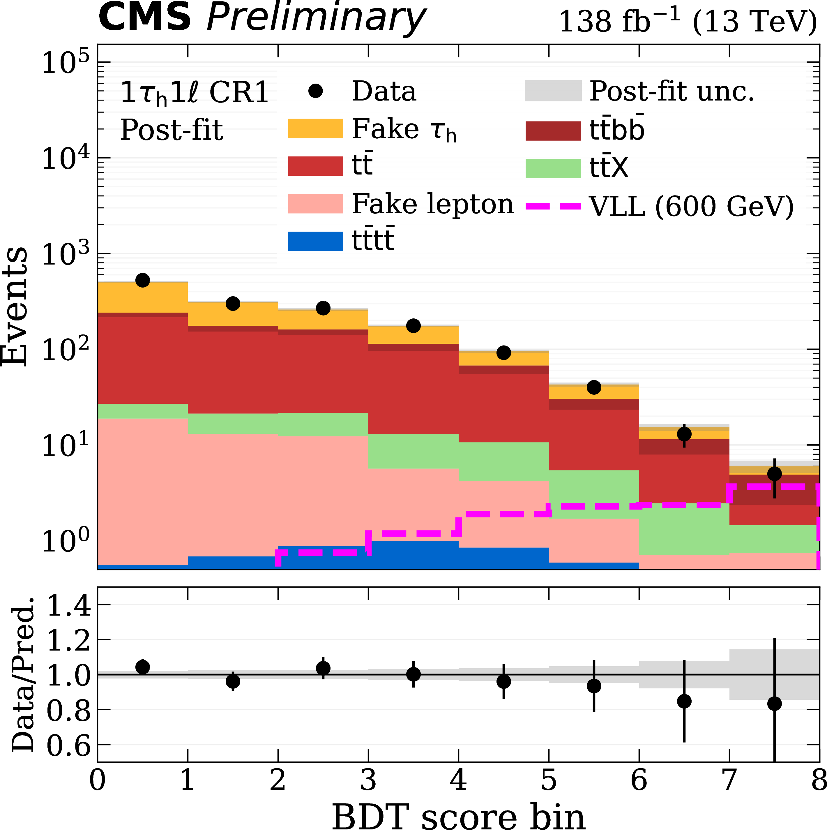
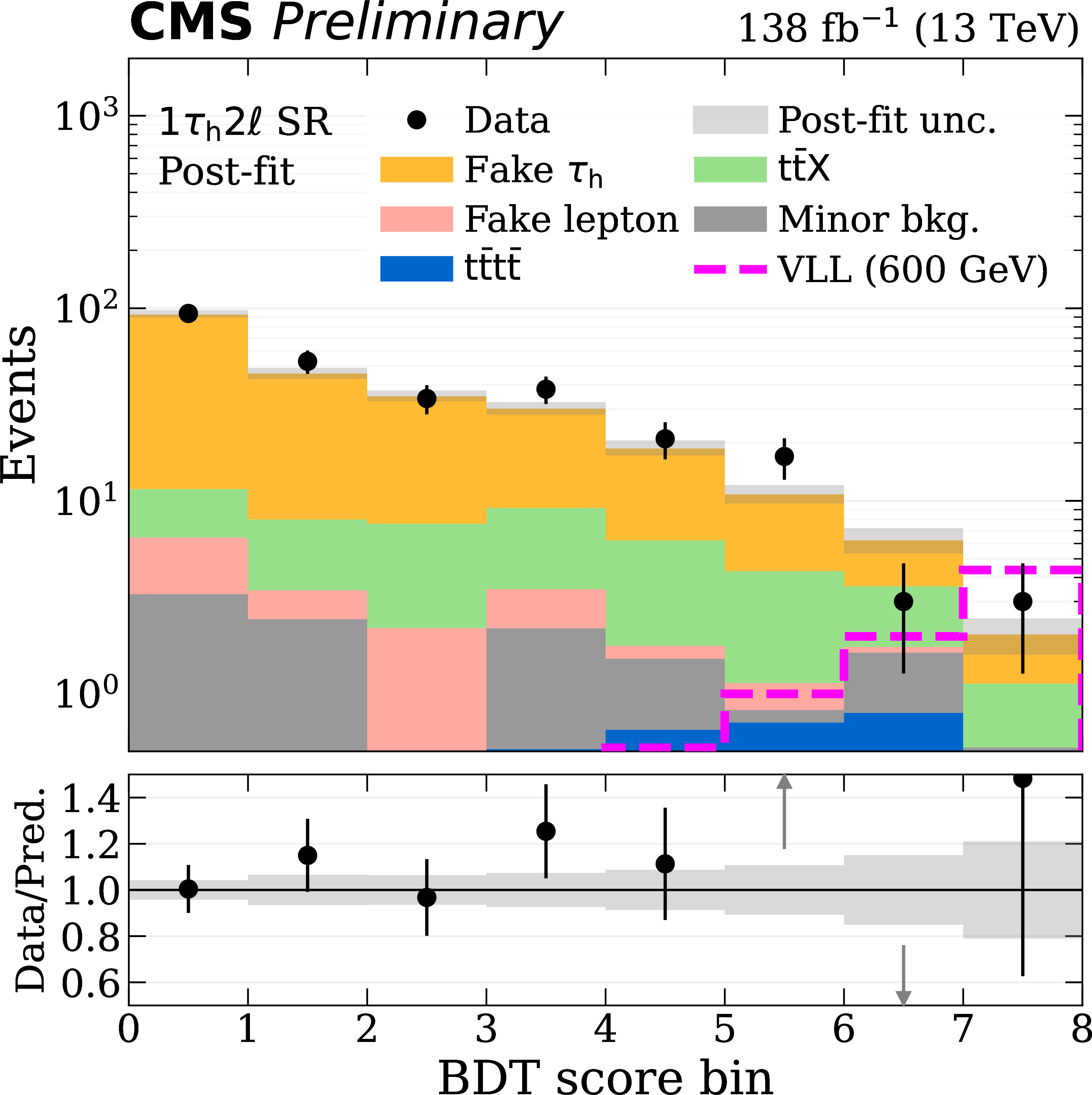
Post-fit (background-only) BDT discriminant distributions for the VLL search at $ m_{\mathrm{VLL}} = $ 600 GeV, for all regions used in the extraction of limit on mass across the 1 $ \tau_{\text{h}}0\ell $ (top and middle-left), 1 $ \tau_{\text{h}}1\ell $ (middle-right and bottom-left), and 1 $ \tau_{\text{h}}2\ell $ (bottom-right) channels. The stacked histograms represent the SM background predictions, with the expected VLL signal overlaid as a magenta line normalized to the 4321 model cross section. Hatched bands indicate the total uncertainty. Lower panels show the data-to-prediction ratio. |
png pdf |
Figure 8-a:
Post-fit (background-only) BDT discriminant distributions for the VLL search at $ m_{\mathrm{VLL}} = $ 600 GeV, for all regions used in the extraction of limit on mass across the 1 $ \tau_{\text{h}}0\ell $ (top and middle-left), 1 $ \tau_{\text{h}}1\ell $ (middle-right and bottom-left), and 1 $ \tau_{\text{h}}2\ell $ (bottom-right) channels. The stacked histograms represent the SM background predictions, with the expected VLL signal overlaid as a magenta line normalized to the 4321 model cross section. Hatched bands indicate the total uncertainty. Lower panels show the data-to-prediction ratio. |
png pdf |
Figure 8-b:
Post-fit (background-only) BDT discriminant distributions for the VLL search at $ m_{\mathrm{VLL}} = $ 600 GeV, for all regions used in the extraction of limit on mass across the 1 $ \tau_{\text{h}}0\ell $ (top and middle-left), 1 $ \tau_{\text{h}}1\ell $ (middle-right and bottom-left), and 1 $ \tau_{\text{h}}2\ell $ (bottom-right) channels. The stacked histograms represent the SM background predictions, with the expected VLL signal overlaid as a magenta line normalized to the 4321 model cross section. Hatched bands indicate the total uncertainty. Lower panels show the data-to-prediction ratio. |
png pdf |
Figure 8-c:
Post-fit (background-only) BDT discriminant distributions for the VLL search at $ m_{\mathrm{VLL}} = $ 600 GeV, for all regions used in the extraction of limit on mass across the 1 $ \tau_{\text{h}}0\ell $ (top and middle-left), 1 $ \tau_{\text{h}}1\ell $ (middle-right and bottom-left), and 1 $ \tau_{\text{h}}2\ell $ (bottom-right) channels. The stacked histograms represent the SM background predictions, with the expected VLL signal overlaid as a magenta line normalized to the 4321 model cross section. Hatched bands indicate the total uncertainty. Lower panels show the data-to-prediction ratio. |
png pdf |
Figure 8-d:
Post-fit (background-only) BDT discriminant distributions for the VLL search at $ m_{\mathrm{VLL}} = $ 600 GeV, for all regions used in the extraction of limit on mass across the 1 $ \tau_{\text{h}}0\ell $ (top and middle-left), 1 $ \tau_{\text{h}}1\ell $ (middle-right and bottom-left), and 1 $ \tau_{\text{h}}2\ell $ (bottom-right) channels. The stacked histograms represent the SM background predictions, with the expected VLL signal overlaid as a magenta line normalized to the 4321 model cross section. Hatched bands indicate the total uncertainty. Lower panels show the data-to-prediction ratio. |
png pdf |
Figure 8-e:
Post-fit (background-only) BDT discriminant distributions for the VLL search at $ m_{\mathrm{VLL}} = $ 600 GeV, for all regions used in the extraction of limit on mass across the 1 $ \tau_{\text{h}}0\ell $ (top and middle-left), 1 $ \tau_{\text{h}}1\ell $ (middle-right and bottom-left), and 1 $ \tau_{\text{h}}2\ell $ (bottom-right) channels. The stacked histograms represent the SM background predictions, with the expected VLL signal overlaid as a magenta line normalized to the 4321 model cross section. Hatched bands indicate the total uncertainty. Lower panels show the data-to-prediction ratio. |
png pdf |
Figure 8-f:
Post-fit (background-only) BDT discriminant distributions for the VLL search at $ m_{\mathrm{VLL}} = $ 600 GeV, for all regions used in the extraction of limit on mass across the 1 $ \tau_{\text{h}}0\ell $ (top and middle-left), 1 $ \tau_{\text{h}}1\ell $ (middle-right and bottom-left), and 1 $ \tau_{\text{h}}2\ell $ (bottom-right) channels. The stacked histograms represent the SM background predictions, with the expected VLL signal overlaid as a magenta line normalized to the 4321 model cross section. Hatched bands indicate the total uncertainty. Lower panels show the data-to-prediction ratio. |
png pdf |
Figure 9:
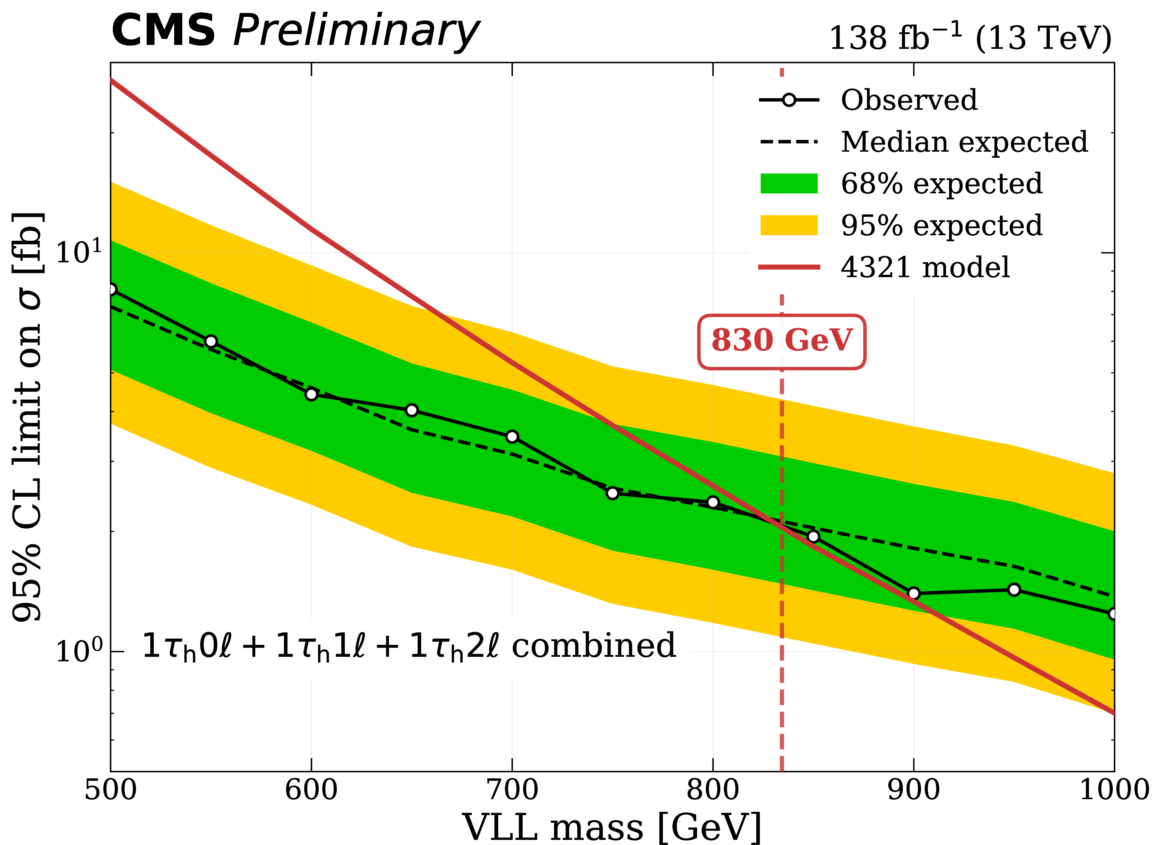
Observed and expected 95% confidence level upper limits on the VLL pair production cross section as a function of the VLL mass in the context of the 4321 model. The solid black line shows the observed limit, while the dashed black line shows the expected limit. The green and yellow bands represent the $ \pm1\sigma $ and $ \pm2\sigma $ uncertainty ranges on the expected limit. The red line shows the theoretical prediction for VLL pair production. |
| Tables | |

png pdf |
Table 1:
Decay modes of vector-like lepton (VLL) pairs and the resulting final-state particles in the 1 $ \tau_{\text{h}}0\ell $, 1 $ \tau_{\text{h}}1\ell $, and 1 $ \tau_{\text{h}}2\ell $ channels. Each VLL decays via an off-shell leptoquark: $ {E} \to \mathrm{b} (\mathrm{b}\tau) $ or b (t}\nu_{\!\tau) and $ {N} \to \mathrm{t} (\mathrm{b}\tau) $ or t (t}\nu_{\!\tau), where the decay products in parentheses originate from the intermediate vector leptoquark U. No distinction is made between particles and antiparticles. In the final-state column, b\ denotes bottom quarks, $ \mathrm{q} $\ denotes quarks from hadronic W boson decays, $ \nu_{\!\tau} $\ denotes tau neutrinos (from the leptoquark or W boson decay), and $ \nu_{\ell} $ denotes electron or muon neutrinos. |
png pdf |
Table 2:
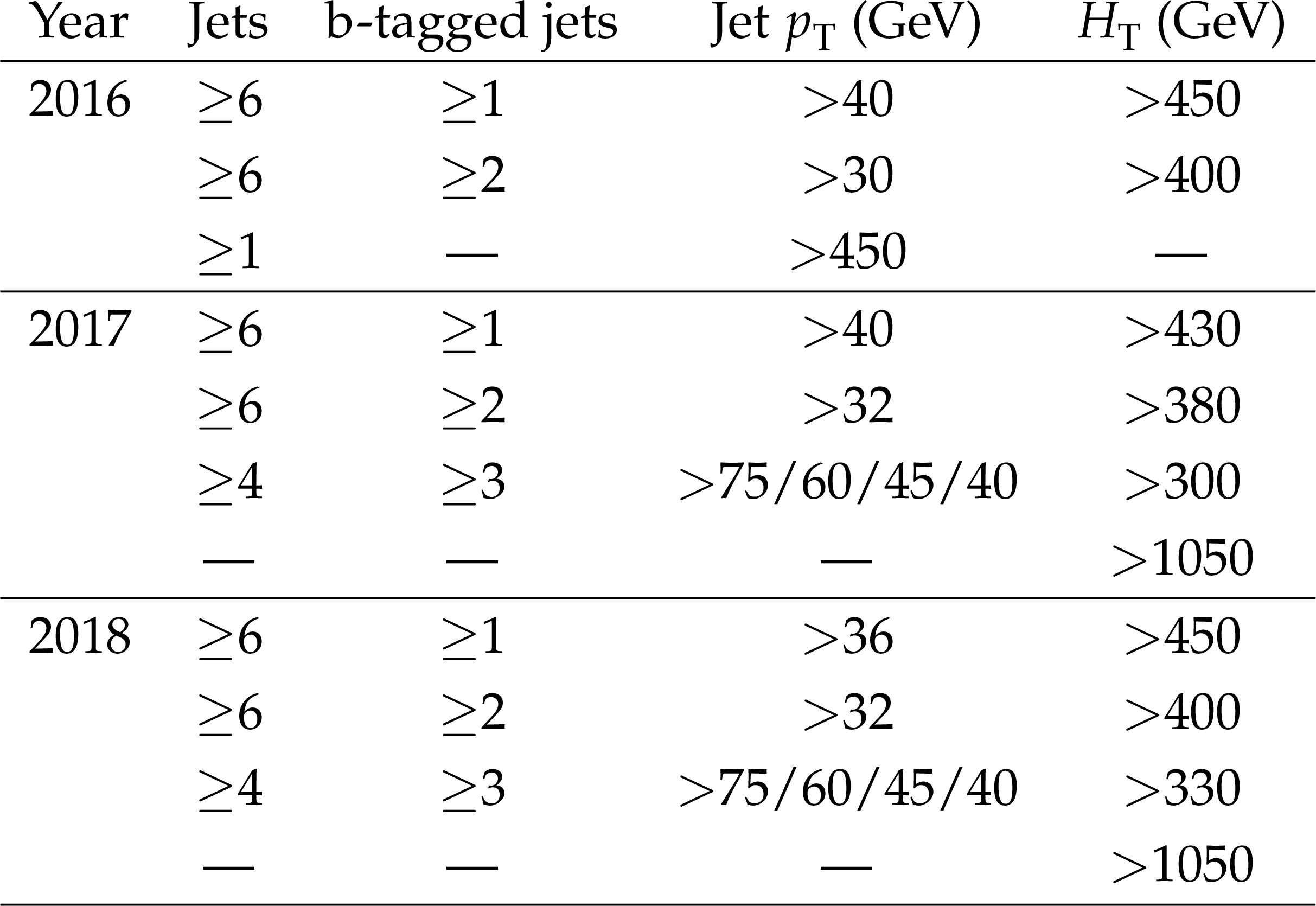
Selection criteria for the hadronic triggers in the 1 $ \tau_{\text{h}}0\ell $ and 1 $ \tau_{\text{h}}1\ell $ channels. Multiple criteria, each represented by one row, are used per year and combined with a logical OR. In the case of the four-jet trigger, the minimum jet $ p_{\mathrm{T}} $ is different for each jet and separated by a slash (/). |
png pdf |
Table 3:
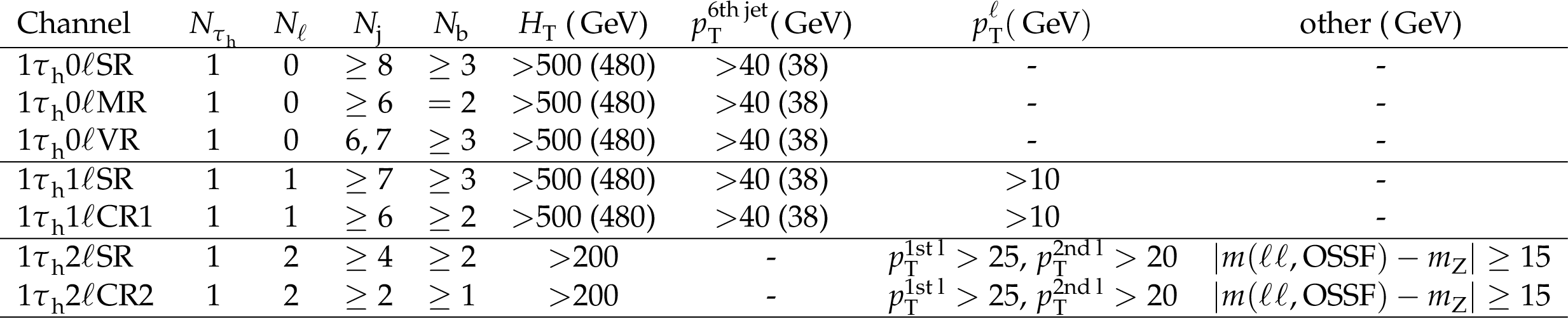
Region definition for the 1 $ \tau_{\text{h}}0\ell $, 1 $ \tau_{\text{h}}1\ell $ and 1 $ \tau_{\text{h}}2\ell $ channels. Values in parentheses in the $ H_{\mathrm{T}} $ and $ p_{\mathrm{T}}^{\text{6th jet}} $ columns apply to the $ N_{\mathrm{b}} \geq $ 3 region. For 1 $ \tau_{\text{h}}1\ell \text{CR1} $ and 1 $ \tau_{\text{h}}2\ell \text{CR2} $, the selection of $ N_{{{j}} } $ and $ N_{\mathrm{b}} $ of corresponding signal regions is vetoed to ensure no overlap with signal regions. |
png pdf |
Table 4:
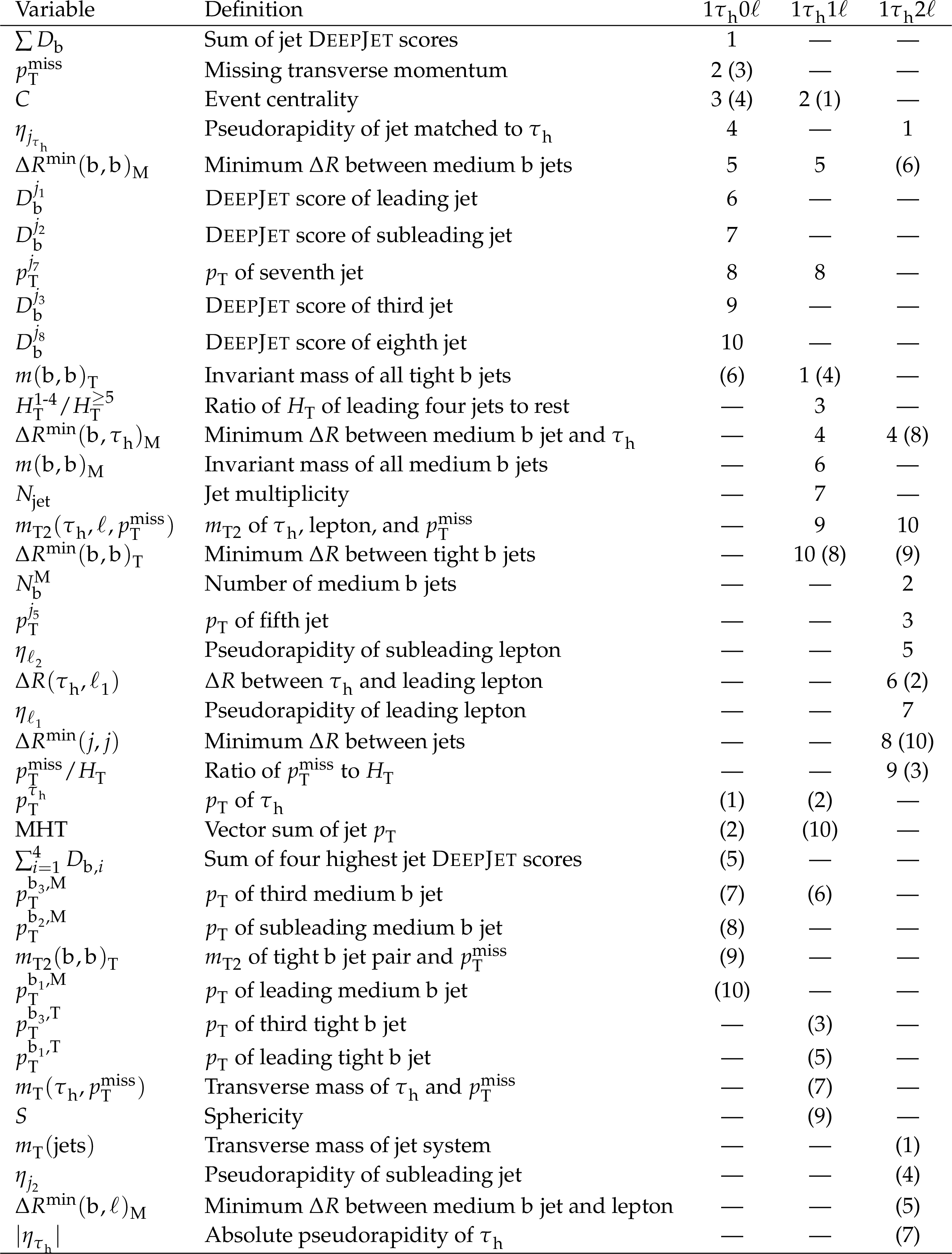
Summary of the most important BDT input variables for the $ {\mathrm{t}\overline{\mathrm{t}}} {\mathrm{t}\overline{\mathrm{t}}} $ and VLL searches. Variables are ranked by their importance, defined as the weighted fraction of training events in the nodes where that variable is used for splitting, as implemented in the TMVA toolkit [none-none]. Only variables ranked in the top 10 for at least one channel are shown. Rankings are shown as ``$ {\mathrm{t}\overline{\mathrm{t}}} {\mathrm{t}\overline{\mathrm{t}}} $ (VLL)'', where the VLL ranking corresponds to the 600 GeV mass point; a dash ($ \text{---} $) indicates the variable is not in the top 10 for that channel. |
| Summary |
| A measurement of $ {\mathrm{t}\overline{\mathrm{t}}} {\mathrm{t}\overline{\mathrm{t}}} $ production and a search for vector-like lepton pairs in the context of the 4321 model are performed using proton-proton collision data at $ \sqrt{s}=13 \text{Te\hspace{-.08em}V} $, corresponding to an integrated luminosity of 138 fb$ ^{-1} $. The analysis uses final states with hadronically decaying tau leptons, categorized into 1 $ \tau_{\text{h}}0\ell $, 1 $ \tau_{\text{h}}1\ell $, and 1 $ \tau_{\text{h}}2\ell $ channels, representing the first exploration of $ {\mathrm{t}\overline{\mathrm{t}}} {\mathrm{t}\overline{\mathrm{t}}} $ in tau-enriched topologies. The $ {\mathrm{t}\overline{\mathrm{t}}} {\mathrm{t}\overline{\mathrm{t}}} $ production cross section is measured to be $16^{+18}_{-15} $ fb, consistent with the SM prediction. An observed (expected) significance of 1.1 (1.0) SDs with respect to the background-only hypothesis is obtained, demonstrating that the $ \tau_{\text{h}} $ channel provides complementary sensitivity to $ {\mathrm{t}\overline{\mathrm{t}}} {\mathrm{t}\overline{\mathrm{t}}} $ production. The VLL search finds no significant excess, establishing observed (expected) exclusion limits of 830 (830) GeV at 95% confidence level. This constitutes the first search for VLL pairs in the 4321 model in final states containing light leptons, complementing the hadronic searches by CMS [48] and ATLAS [49]. Together with the ATLAS result excluding VLL masses below 910 GeV, these results are consistent with standard model predictions and do not confirm the 2.8 SD excess previously observed in the CMS all-hadronic channel. |
| References | ||||
| 1 | ATLAS Collaboration | The ATLAS experiment at the CERN Large Hadron Collider | JINST 3 (2008) S08003 | |
| 2 | CMS Collaboration | The CMS experiment at the CERN LHC | JINST 3 (2008) S08004 | |
| 3 | G. Bevilacqua and M. Worek | Constraining BSM physics at the LHC: Four top final states with NLO accuracy in perturbative QCD | JHEP 07 (2012) 111 | 1206.3064 |
| 4 | J. Alwall et al. | The automated computation of tree-level and next-to-leading order differential cross sections, and their matching to parton shower simulations | JHEP 07 (2014) 079 | 1405.0301 |
| 5 | F. Maltoni, D. Pagani, and I. Tsinikos | Associated production of a top-quark pair with vector bosons at NLO in QCD: impact on $ {{\mathrm{t}\overline{\mathrm{t}}} \mathrm{H}} $ searches at the LHC | JHEP 02 (2016) 113 | 1507.05640 |
| 6 | R. Frederix, D. Pagani, and M. Zaro | Large NLO corrections in $ {{\mathrm{t}\overline{\mathrm{t}}} \mathrm{W}^{\pm}} $ and $ {\mathrm{t}\overline{\mathrm{t}}} {\mathrm{t}\overline{\mathrm{t}}} $ hadroproduction from supposedly subleading EW contributions | JHEP 02 (2018) 031 | 1711.02116 |
| 7 | T. Je \v z o and M. Kraus | Hadroproduction of four top quarks in the POWHEG box | PRD 105 (2022) 114024 | 2110.15159 |
| 8 | M. van Beekveld, A. Kulesza, and L. Moreno Valero | Threshold resummation for the production of four top quarks at the LHC | 2212.03259 | |
| 9 | Q.-H. Cao, S.-L. Chen, and Y. Liu | Probing Higgs width and top quark Yukawa coupling from $ {\mathrm{t}\overline{\mathrm{t}}} \mathrm{H} $ and $ {\mathrm{t}\overline{\mathrm{t}}} {\mathrm{t}\overline{\mathrm{t}}} $ productions | PRD 95 (2017) 053004 | 1602.01934 |
| 10 | Q.-H. Cao et al. | Limiting top quark-Higgs boson interaction and Higgs-boson width from multitop productions | PRD 99 (2019) 113003 | 1901.04567 |
| 11 | CMS Collaboration | Measurement of the Higgs boson production rate in association with top quarks in final states with electrons, muons, and hadronically decaying tau leptons at $ \sqrt{s}= $ 13 TeV | EPJC 81 (2021) 378 | CMS-HIG-19-008 2011.03652 |
| 12 | CMS Collaboration | Measurement of the top quark Yukawa coupling from $ \mathrm{t} \overline{\mathrm{t}} $ kinematic distributions in the lepton+jets final state in proton-proton collisions at $ \sqrt{s}= $ 13 TeV | PRD 100 (2019) 072007 | CMS-TOP-17-004 1907.01590 |
| 13 | CMS Collaboration | Measurement of the top quark Yukawa coupling from $ \mathrm{t} \overline{\mathrm{t}} $ kinematic distributions in the dilepton final state in proton-proton collisions at $ \sqrt{s}= $ 13 TeV | PRD 102 (2020) 092013 | CMS-TOP-19-008 2009.07123 |
| 14 | H. Nilles | Supersymmetry, supergravity and particle physics | Phys. Rept. 110 (1984) 1 | |
| 15 | G. R. Farrar and P. Fayet | Phenomenology of the production, decay, and detection of new hadronic states associated with supersymmetry | PLB 76 (1978) 575 | |
| 16 | T. Plehn and T. M. P. Tait | Seeking sgluons | JPG 36 (2009) 075001 | 0810.3919 |
| 17 | S. Calvet, B. Fuks, P. Gris, and L. Valery | Searching for sgluons in multitop events at a center-of-mass energy of 8 TeV | JHEP 04 (2013) 043 | 1212.3360 |
| 18 | D. Dicus, A. Stange, and S. Willenbrock | Higgs decay to top quarks at hadron colliders | PLB 333 (1994) 126 | hep-ph/9404359 |
| 19 | N. Craig et al. | The hunt for the rest of the Higgs bosons | JHEP 06 (2015) 137 | 1504.04630 |
| 20 | N. Craig et al. | Heavy Higgs bosons at low $ \tan \beta $: from the LHC to 100 TeV | JHEP 01 (2017) 018 | 1605.08744 |
| 21 | A. Pomarol and J. Serra | Top quark compositeness: Feasibility and implications | PRD 78 (2008) 074026 | 0806.3247 |
| 22 | CMS Collaboration | Search for physics beyond the standard model in events with two leptons of same sign, missing transverse momentum, and jets in proton-proton collisions at $ \sqrt{s}= $ 13 TeV | EPJC 77 (2017) 578 | CMS-SUS-16-035 1704.07323 |
| 23 | CMS Collaboration | Search for standard model production of four top quarks with same-sign and multilepton final states in proton-proton collisions at $ \sqrt{s}= $ 13 TeV | EPJC 78 (2018) 140 | CMS-TOP-17-009 1710.10614 |
| 24 | ATLAS Collaboration | Search for new phenomena in events with same-charge leptons and b jets in pp collisions at $ \sqrt{s}=13 \text{TeV} $ with the ATLAS detector | JHEP 12 (2018) 039 | 1807.11883 |
| 25 | ATLAS Collaboration | Search for four-top-quark production in the single-lepton and opposite-sign dilepton final states in pp collisions at $ \sqrt{s}=13 \text{TeV} $ with the ATLAS detector | PRD 99 (2019) 052009 | 1811.02305 |
| 26 | CMS Collaboration | Search for the production of four top quarks in the single-lepton and opposite-sign dilepton final states in proton-proton collisions at $ \sqrt{s}= $ 13 TeV | JHEP 11 (2019) 082 | CMS-TOP-17-019 1906.02805 |
| 27 | CMS Collaboration | Search for production of four top quarks in final states with same-sign or multiple leptons in proton-proton collisions at $ \sqrt{s}= $ 13 TeV | EPJC 80 (2020) 75 | CMS-TOP-18-003 1908.06463 |
| 28 | ATLAS Collaboration | Evidence for $ {\mathrm{t}\overline{\mathrm{t}}} {\mathrm{t}\overline{\mathrm{t}}} $ production in the multilepton final state in proton-proton collisions at $ \sqrt{s}=13 \text{TeV} $ with the ATLAS detector | EPJC 80 (2020) 1085 | 2007.14858 |
| 29 | ATLAS Collaboration | Measurement of the $ {\mathrm{t}\overline{\mathrm{t}}} {\mathrm{t}\overline{\mathrm{t}}} $ production cross section in pp collisions at $ \sqrt{s}=13 \text{TeV} $ with the ATLAS detector | JHEP 11 (2021) 118 | 2106.11683 |
| 30 | CMS Collaboration | Evidence for four-top quark production in proton-proton collisions at $ \sqrt{s}= $ 13 TeV | PLB 844 (2023) 138076 | CMS-TOP-21-005 2303.03864 |
| 31 | F. Blekman, F. D é liot, V. Dutta, and E. Usai | Four-top quark physics at the LHC | Universe 8 (2022) 638 | 2208.04085 |
| 32 | CMS Collaboration | Measurement of the four top quark production cross section in \(pp\) Collisions at \($ \sqrt{s}=13 \text{TeV} = $ 13\) TeV | JHEP 07 (2023) 048 | CMS-TOP-22-013 2305.13439 |
| 33 | ATLAS Collaboration | Observation of four-top-quark production in the multilepton final state with the ATLAS detector | PRL 131 (2023) 041802 | 2303.15061 |
| 34 | L. Di Luzio, A. Greljo, and M. Nardecchia | Gauge leptoquark as the origin of B-physics anomalies | PRD 96 (2017) 115011 | 1708.08450 |
| 35 | L. Di Luzio et al. | Maximal flavour violation: a Cabibbo mechanism for leptoquarks | JHEP 11 (2018) 081 | 1808.00942 |
| 36 | M. Bordone, C. Cornella, J. Fuentes-Martin, and G. Isidori | A three-site gauge model for flavor hierarchies and flavor anomalies | PLB 779 (2018) 317 | 1712.01368 |
| 37 | A. Greljo and B. A. Stefanek | Third family quark-lepton unification at the TeV scale | PLB 782 (2018) 131 | 1802.04274 |
| 38 | BaBar Collaboration | Evidence for an excess of $ \bar{B} \to D^{(*)} \tau^-\bar{\nu}_\tau $ decays | PRL 109 (2012) 101802 | 1205.5442 |
| 39 | BaBar Collaboration | Measurement of an excess of $ \bar{B} \to D^{(*)}\tau^- \bar{\nu}_\tau $ decays and implications for charged Higgs bosons | PRD 88 (2013) 072012 | 1303.0571 |
| 40 | LHCb Collaboration | Measurement of the ratio of branching fractions $ \mathcal{B}(\bar{B}^0 \to D^{*+}\tau^{-}\bar{\nu}_{\tau})/\mathcal{B}(\bar{B}^0 \to D^{*+}\mu^{-}\bar{\nu}_{\mu}) $ | PRL 115 (2015) 111803 | 1506.08614 |
| 41 | Belle Collaboration | Measurement of the branching ratio of $ \bar{B} \to D^{(\ast)} \tau^- \bar{\nu}_\tau $ relative to $ \bar{B} \to D^{(\ast)} \ell^- \bar{\nu}_\ell $ decays with hadronic tagging at Belle | PRD 92 (2015) 072014 | 1507.03233 |
| 42 | Belle Collaboration | Measurement of the $ \tau $ lepton polarization and $ R(D^*) $ in the decay $ \bar{B} \to D^* \tau^- \bar{\nu}_\tau $ | PRL 118 (2017) 211801 | 1612.00529 |
| 43 | LHCb Collaboration | Test of lepton flavor universality by the measurement of the $ B^0 \to D^{*-} \tau^+ \nu_{\tau} $ branching fraction using three-prong $ \tau $ decays | PRD 97 (2018) 072013 | 1711.02505 |
| 44 | Belle Collaboration | Measurement of the $ \tau $ lepton polarization and $ R(D^*) $ in the decay $ \bar{B} \rightarrow D^* \tau^- \bar{\nu}_\tau $ with one-prong hadronic $ \tau $ decays at Belle | PRD 97 (2018) 012004 | 1709.00129 |
| 45 | LHCb Collaboration | Measurement of the ratio of the $ B^0 \to D^{*-} \tau^+ \nu_{\tau} $ and $ B^0 \to D^{*-} \mu^+ \nu_{\mu} $ branching fractions using three-prong $ \tau $-lepton decays | PRL 120 (2018) 171802 | 1708.08856 |
| 46 | Belle Collaboration | Measurement of $ \mathcal{R}(D) $ and $ \mathcal{R}(D^*) $ with a semileptonic tagging method | PRL 124 (2020) 161803 | 1910.05864 |
| 47 | C. Cornella et al. | Reading the footprints of the B-meson flavor anomalies | JHEP 08 (2021) 050 | 2103.16558 |
| 48 | CMS Collaboration | Search for pair-produced vector-like leptons in final states with third-generation leptons and at least three b quark jets in proton-proton collisions at $ \sqrt{s}= $ 13 TeV | PLB 846 (2023) 137713 | 2303.05441 |
| 49 | ATLAS Collaboration | Search for electroweak production of vector-like leptons in $ \tau $-lepton and $ b $-jet final states in $ pp $ collisions at $ \sqrt{s} = $ 13 TeV with the ATLAS detector | EPJC 85 (2025) 1335 | 2503.22581 |
| 50 | CMS Collaboration | Performance of the CMS Level-1 trigger in proton-proton collisions at $ \sqrt{s}= $ 13 TeV | JINST 15 (2020) P10017 | CMS-TRG-17-001 2006.10165 |
| 51 | CMS Collaboration | The CMS trigger system | JINST 12 (2017) P01020 | CMS-TRG-12-001 1609.02366 |
| 52 | CMS Collaboration | Particle-flow reconstruction and global event description with the CMS detector | JINST 12 (2017) P10003 | CMS-PRF-14-001 1706.04965 |
| 53 | CMS Collaboration | Technical proposal for the Phase-II upgrade of the Compact Muon Solenoid | CMS Technical Proposal CERN-LHCC-2015-010, CMS-TDR-15-02, 2015 CDS |
|
| 54 | M. Cacciari, G. P. Salam, and G. Soyez | The anti-$ k_{\mathrm{T}} $ jet clustering algorithm | JHEP 04 (2008) 063 | 0802.1189 |
| 55 | M. Cacciari, G. P. Salam, and G. Soyez | FASTJET user manual | EPJC 72 (2012) 1896 | 1111.6097 |
| 56 | CMS Collaboration | Pileup mitigation at cms in $ \sqrt{s}= $ 13 TeV data | JINST 15 (2020) no. 09, P09018 | CMS-JME-18-001 2003.00503 |
| 57 | CMS Collaboration | Jet energy scale and resolution in the CMS experiment in $ {\mathrm{p}\mathrm{p}} $ collisions at 8 TeV | JINST 12 (2017) P02014 | CMS-JME-13-004 1607.03663 |
| 58 | CMS Collaboration | Performance of missing transverse momentum reconstruction in proton-proton collisions at $ \sqrt{s}= $ 13 TeV using the CMS detector | JINST 14 (2019) P07004 | CMS-JME-17-001 1903.06078 |
| 59 | CMS Collaboration | Identification of heavy-flavour jets with the CMS detector in $ {\mathrm{p}\mathrm{p}} $ collisions at 13 TeV | JINST 13 (2018) P05011 | CMS-BTV-16-002 1712.07158 |
| 60 | E. Bols et al. | Jet flavour classification using DeepJet | JINST 15 (2020) P12012 | 2008.10519 |
| 61 | CMS Collaboration | Performance summary of AK4 jet b tagging with data from proton-proton collisions at 13 TeV with the CMS detector | CMS Detector Performance Note CMS-DP-2023-005, 2023 CDS |
|
| 62 | NNPDF Collaboration | Parton distributions from high-precision collider data | EPJC 77 (2017) 663 | 1706.00428 |
| 63 | T. Sjöstrand et al. | An introduction to PYTHIA8.2 | Comput. Phys. Commun. 191 (2015) 159 | 1410.3012 |
| 64 | CMS Collaboration | Extraction and validation of a new set of CMS PYTHIA8 tunes from underlying-event measurements | EPJC 80 (2020) 4 | CMS-GEN-17-001 1903.12179 |
| 65 | GEANT4 Collaboration | GEANT 4---a simulation toolkit | NIM A 506 (2003) 250 | |
| 66 | P. Artoisenet, R. Frederix, O. Mattelaer, and R. Rietkerk | Automatic spin-entangled decays of heavy resonances in Monte Carlo simulations | JHEP 03 (2013) 015 | 1212.3460 |
| 67 | R. Frederix and S. Frixione | Merging meets matching in MC@NLO | JHEP 12 (2012) 061 | 1209.6215 |
| 68 | L. Ferencz et al. | Study of $ {\mathrm{t}\overline{\mathrm{t}}} \mathrm{b}\overline{\mathrm{b}} $ and $ {{\mathrm{t}\overline{\mathrm{t}}} \mathrm{W}} $ background modelling for $ {{\mathrm{t}\overline{\mathrm{t}}} \mathrm{H}} $ analyses | LHC Higgs Working Group Public Note LHCHWG-2022-003, 2023 | 2301.11670 |
| 69 | J. Alwall et al. | Comparative study of various algorithms for the merging of parton showers and matrix elements in hadronic collisions | EPJC 53 (2008) 473 | 0706.2569 |
| 70 | P. Nason | A new method for combining NLO QCD with shower Monte Carlo algorithms | JHEP 11 (2004) 040 | hep-ph/0409146 |
| 71 | S. Frixione, G. Ridolfi, and P. Nason | A positive-weight next-to-leading-order Monte Carlo for heavy flavour hadroproduction | JHEP 09 (2007) 126 | 0707.3088 |
| 72 | S. Frixione, P. Nason, and C. Oleari | Matching NLO QCD computations with parton shower simulations: the POWHEG method | JHEP 11 (2007) 070 | 0709.2092 |
| 73 | S. Alioli, P. Nason, C. Oleari, and E. Re | NLO single-top production matched with shower in POWHEG: $ s $- and $ t $-channel contributions | JHEP 09 (2009) 111 | 0907.4076 |
| 74 | P. Nason and C. Oleari | NLO Higgs boson production via vector-boson fusion matched with shower in POWHEG | JHEP 02 (2010) 037 | 0911.5299 |
| 75 | S. Alioli, P. Nason, C. Oleari, and E. Re | A general framework for implementing NLO calculations in shower Monte Carlo programs: the POWHEG box | JHEP 06 (2010) 043 | 1002.2581 |
| 76 | E. Re | Single-top $ {\mathrm{W}\mathrm{t}} $-channel production matched with parton showers using the POWHEG method | EPJC 71 (2011) 1547 | 1009.2450 |
| 77 | E. Bagnaschi, G. Degrassi, P. Slavich, and A. Vicini | Higgs production via gluon fusion in the POWHEG approach in the SM and in the MSSM | JHEP 02 (2012) 088 | 1111.2854 |
| 78 | P. Nason and G. Zanderighi | $ {\mathrm{W^+}\mathrm{W^-}} $, $ {\mathrm{W}\mathrm{Z}} $ and $ {\mathrm{Z}\mathrm{Z}} $ production in the POWHEG -box-v2 | EPJC 74 (2014) 2702 | 1311.1365 |
| 79 | CMS Collaboration | Measurement of the $ \mathrm{t\bar{t}H} $ and $ \mathrm{tH} $ production rates in the $ \mathrm{H} \to \mathrm{b\bar{b}} $ decay channel using proton-proton collision data at $ \sqrt{s} = $ 13 TeV | JHEP 02 (2025) 097 | CMS-HIG-19-011 2407.10896 |
| 80 | A. Alloul et al. | FeynRules 2.0 -- a complete toolbox for tree-level phenomenology | Comput. Phys. Commun. 185 (2014) 2250 | 1310.1921 |
| 81 | CMS Collaboration | Electron and photon reconstruction and identification with the CMS experiment at the CERN LHC | JINST 16 (2021) P05014 | CMS-EGM-17-001 2012.06888 |
| 82 | CMS Collaboration | ECAL 2016 refined calibration and Run2 summary plots | CMS Detector Performance Note CMS-DP-2020-021, 2020 CDS |
|
| 83 | CMS Collaboration | Performance of electron reconstruction and selection with the CMS detector in proton-proton collisions at $ \sqrt{s}= $ 8 TeV | JINST 10 (2015) P06005 | CMS-EGM-13-001 1502.02701 |
| 84 | CMS Collaboration | Performance of the CMS muon detector and muon reconstruction with proton-proton collisions at $ \sqrt{s}= $ 13 TeV | JINST 13 (2018) P06015 | CMS-MUO-16-001 1804.04528 |
| 85 | CMS Collaboration | Performance of CMS muon reconstruction in cosmic-ray events | JINST 5 (2010) T03022 | CMS-CFT-09-014 0911.4994 |
| 86 | CMS Collaboration | Performance of the reconstruction and identification of high-momentum muons in proton-proton collisions at $ \sqrt{s}= $ 13 TeV | JINST 15 (2020) P02027 | CMS-MUO-17-001 1912.03516 |
| 87 | T. Chen and C. Guestrin | XGBoost: A scalable tree boosting system | in ACM SIGKDD Int. Conf. on Knowledge Discovery and Data Mining: San Francisco CA, USA, August 13--17,, 2016 Proc. 2 (2016) 2 |
1603.02754 |
| 88 | CMS Collaboration | Muon identification using multivariate techniques in the CMS experiment in proton-proton collisions at $ \sqrt{s}= $ 13 TeV | JINST 19 (2024) P02031 | CMS-MUO-22-001 2310.03844 |
| 89 | CMS Collaboration | Performance of reconstruction and identification of $ \tau $ leptons decaying to hadrons and $ \nu_\tau $ in pp collisions at $ \sqrt{s}= $ 13 TeV | JINST 13 (2018) P10005 | CMS-TAU-16-003 1809.02816 |
| 90 | CMS Collaboration | Identification of hadronic tau lepton decays using a deep neural network | JINST 17 (2022) P07023 | CMS-TAU-20-001 2201.08458 |
| 91 | H. Voss, A. Höcker, J. Stelzer, and F. Tegenfeldt | TMVA, the toolkit for multivariate data analysis with ROOT | in the Int. Workshop on Advanced Computing and Analysis Techniques in Phys. Research (ACAT ): Amsterdam, The Netherlands, April 23--27,.. [PoS (ACAT) 040], 2017 Proc. 1 (2017) 1 |
physics/0703039 |
| 92 | J. D. Bjorken and S. J. Brodsky | Statistical Model for electron-Positron Annihilation Into Hadrons | PRD 1 (1970) 1416 | |
| 93 | C. G. Lester and D. J. Summers | Measuring masses of semi-invisibly decaying particles pair produced at hadron colliders | PLB 463 (1999) 99 | hep-ph/9906349 |
| 94 | LHC Higgs Cross Section Working Group | NNLO+NNLL top-quark-pair cross sections | ttps://twiki.cern.ch/twiki/bin/view/LHCPhysics/TtbarNNLO | |
| 95 | M. Czakon and A. Mitov | Top++: A program for the calculation of the top-pair cross-section at hadron colliders | Comput. Phys. Commun. 185 (2014) 2930 | 1112.5675 |
| 96 | ATLAS Collaboration | Measurement of the $ t\bar{t} $ production cross-section in the lepton+jets channel at $ \sqrt{s}= $ 13 TeV with the ATLAS experiment | PLB 810 (2020) 135797 | 2006.13076 |
| 97 | R. Frederix and I. Tsinikos | On improving NLO merging for $ {{\mathrm{t}\overline{\mathrm{t}}} \mathrm{W}} $ production | JHEP 11 (2021) 029 | 2108.07826 |
| 98 | A. Kulesza et al. | Associated top quark pair production with a heavy boson: differential cross sections at NLO+NNLL accuracy | EPJC 80 (2020) 428 | 2001.03031 |
| 99 | E. L. Berger, J. Gao, C.-P. Yuan, and H. X. Zhu | Nnlo QCD corrections to $ t $-channel single top-quark production and decay | PRD 94 (2016) 071501 | 1606.08463 |
| 100 | CMS Collaboration | Cross section measurement of $ t $-channel single top quark production in pp collisions at $ \sqrt{s}= $ 13 TeV | PLB 772 (2017) 752 | CMS-TOP-16-003 1610.00678 |
| 101 | CMS Collaboration | Measurement of differential cross sections and charge ratios for $ t $-channel single top quark production in proton-proton collisions at $ \sqrt{s}= $ 13 TeV | EPJC 80 (2020) 370 | CMS-TOP-17-023 1907.08330 |
| 102 | N. Kidonakis | Differential and total cross sections for top pair and single top production | Proceedings of XX Workshop on Deep-Inelastic Scattering, Bonn, Germany | 1205.3453 |
| 103 | ATLAS Collaboration | Measurement of single top-quark production in the $ s $-channel in proton-proton collisions at $ \sqrt{s}= $ 13 TeV with the ATLAS detector | JHEP 06 (2023) 191 | 2302.01283 |
| 104 | CMS Collaboration | Measurement of the cross section for top quark pair production in association with a W or Z boson in proton-proton collisions at $ \sqrt{s}= $ 13 TeV | JHEP 08 (2018) 011 | CMS-TOP-17-005 1711.02547 |
| 105 | CMS Collaboration | Inclusive and differential cross section measurements of single top quark production in association with a Z boson in proton-proton collisions at $ \sqrt{s}= $ 13 TeV | JHEP 02 (2022) 107 | CMS-TOP-20-010 2111.02860 |
| 106 | ATLAS Collaboration | Measurement of the production cross-section of a single top quark in association with a Z boson in proton-proton collisions at $ \sqrt{s}= $ 13 TeV with the ATLAS detector | PLB 780 (2018) 557 | 1710.03659 |
| 107 | CMS Collaboration | Inclusive and differential measurements of the $ \mathrm{t\bar{t}}\gamma $ and $ \mathrm{t\bar{t}}\gamma/\mathrm{t\bar{t}} $ cross sections in the single-lepton channel and effective field theory interpretation in proton-proton collisions at $ \sqrt{s}= $ 13 TeV | JHEP 12 (2022) 058 | CMS-TOP-21-004 2201.07301 |
| 108 | CMS Collaboration | Measurements of production cross sections of WZ and same-sign WW boson pairs in association with two jets in proton-proton collisions at $ \sqrt{s}= $ 13 TeV | PLB 809 (2020) 135710 | CMS-SMP-19-012 2005.01173 |
| 109 | CMS Collaboration | Search for WW$ \gamma $ and WZ$ \gamma $ production and constraints on anomalous quartic gauge couplings in pp collisions at $ \sqrt{s}= $ 8 TeV | PRD 96 (2017) 012004 | 1704.00674 |
| 110 | CMS Collaboration | Search for new physics in same-sign dilepton events in proton-proton collisions at $ \sqrt{s}= $ 13 TeV | EPJC 76 (2016) 439 | CMS-SUS-15-008 1605.03171 |
| 111 | CMS Collaboration | Measurement of the cross section of top quark-antiquark pair production in association with a W boson in proton-proton collisions at $ \sqrt{s}= $ 13 TeV | JHEP 07 (2023) 219 | CMS-TOP-21-011 2208.06485 |
| 112 | ATLAS and CMS Collaborations, and LHC Higgs Combination Group | Procedure for the LHC Higgs boson search combination in Summer 2011 | Technical Report CMS-NOTE-2011-005, ATL-PHYS-PUB-2011-11, 2011 | |
| 113 | CMS Collaboration | Precision luminosity measurement in proton-proton collisions at $ \sqrt{s}= $ 13 TeV in 2015 and 2016 at CMS | EPJC 81 (2021) 800 | CMS-LUM-17-003 2104.01927 |
| 114 | CMS Collaboration | CMS luminosity measurement for the 2017 data-taking period at $ \sqrt{s}= $ 13 TeV | CMS Physics Analysis Summary, 2018 CMS-PAS-LUM-17-004 |
CMS-PAS-LUM-17-004 |
| 115 | CMS Collaboration | CMS luminosity measurement for the 2018 data-taking period at $ \sqrt{s}= $ 13 TeV | CMS Physics Analysis Summary, 2019 CMS-PAS-LUM-18-002 |
CMS-PAS-LUM-18-002 |
| 116 | CMS Collaboration | Measurements of inclusive W and Z cross sections in $ {\mathrm{p}\mathrm{p}} $ collisions at $ \sqrt{s}= $ 7 TeV | JHEP 01 (2011) 080 | CMS-EWK-10-002 1012.2466 |
| 117 | M. Cacciari et al. | The $ \mathrm{t} \overline{\mathrm{t}} $ cross-section at 1.8 and 1.96 TeV: a study of the systematics due to parton densities and scale dependence | JHEP 04 (2004) 068 | hep-ph/0303085 |
| 118 | J. Butterworth et al. | PDF4LHC recommendations for LHC Run II | JPG 43 (2016) 023001 | 1510.03865 |
| 119 | G. Cowan, K. Cranmer, E. Gross, and O. Vitells | Asymptotic formulae for likelihood-based tests of new physics | EPJC 71 (2011) 1554 | 1007.1727 |
| 120 | R. Barlow and C. Beeston | Fitting using finite Monte Carlo samples | Comput. Phys. Commun. 77 (1993) 219 | |
| 121 | J. S. Conway | Incorporating nuisance parameters in likelihoods for multisource spectra | in orkshop on Statistical Issues Related to Discovery Claims in Search Experiments and Unfolding (PHYSTAT ): Geneva, Switzerland, January 17--20,, 2011 Proc. 2011 (2011) W |
1103.0354 |
|
|
Compact Muon Solenoid LHC, CERN |
|

|

|

|

|

|