

Compact Muon Solenoid
LHC, CERN
| CMS-PAS-HIG-25-011 | ||
| Study of spin correlations in Higgs boson decays to four leptons at CMS | ||
| CMS Collaboration | ||
| 2025-11-28 | ||
| Abstract: Kinematic distributions in Higgs boson decay to four leptons $ \mathrm{H} \to 4\ell $ are studied using matrix element techniques, optimizing sensitivity to the tensor structure of Higgs boson interactions and spin correlations in the decay process. The data were collected by the CMS experiment at the LHC, corresponding to integrated luminosities of 138 and 62 fb$ ^{-1} $ at proton-proton center of mass energies of 13 and 13.6 TeV, respectively, covering the 2016-2018 and 2022-2023 data-taking periods. A simultaneous measurement of eight Higgs boson couplings to electroweak vector bosons is carried out within the frameworks of anomalous couplings and effective field theory. Under the assumption of CP symmetry conservation, the polarization density matrix in the $ \mathrm{H} \to \mathrm{ZZ} $ decay is measured, and a search for CP violation in the polarization of the Z bosons is conducted. Quantum mechanical interference is tested through the permutation of identical leptons. Implications regarding quantum entanglement and the violation of a Bell-type inequality are discussed. | ||
| Links: CDS record (PDF) ; Physics Briefing ; CADI line (restricted) ; | ||
| Figures | |
png pdf |
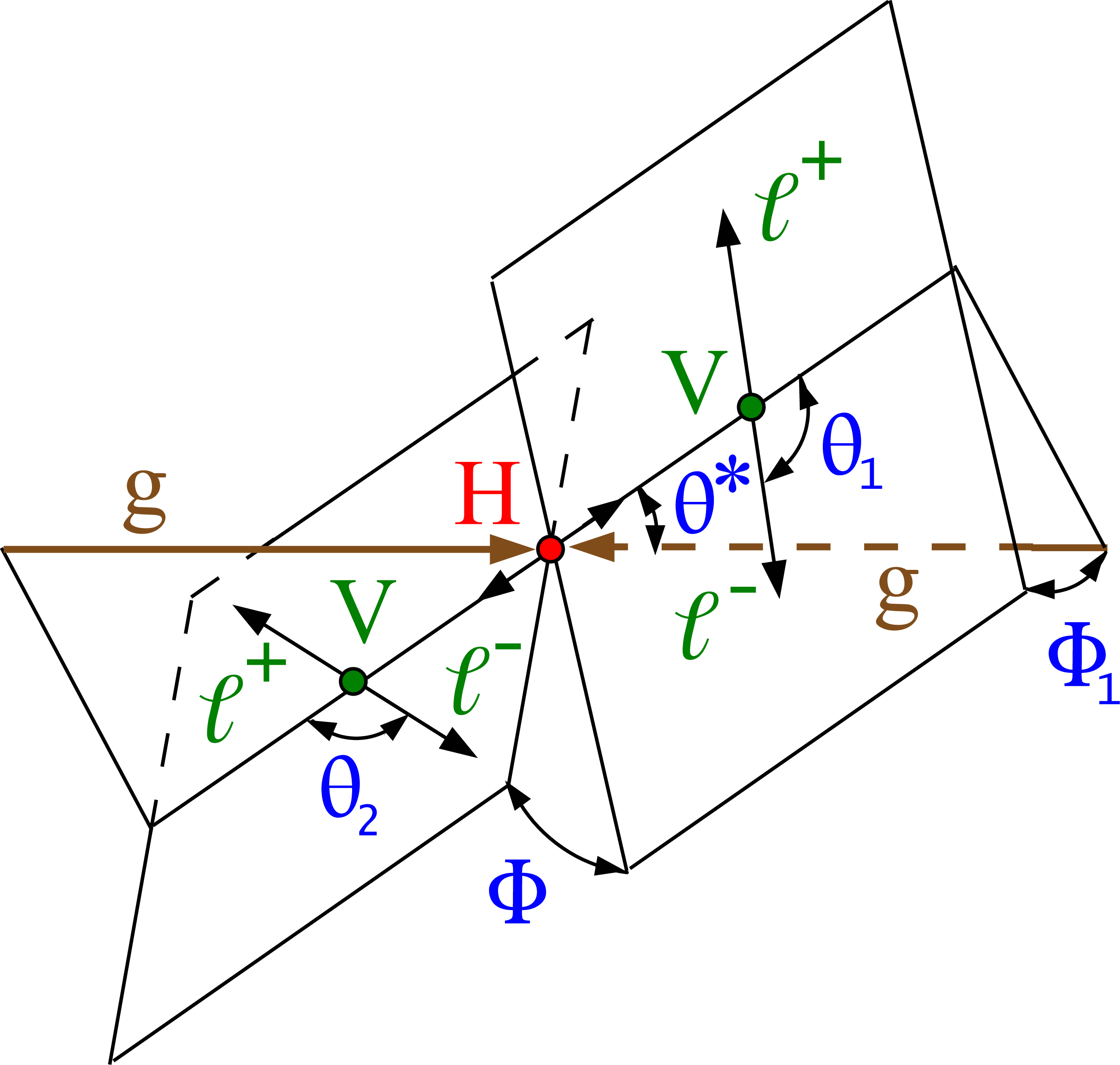
Figure 1:
The diagram depicting the decay of the H boson $ \mathrm{g}\mathrm{g} \to \mathrm{H} \to \mathrm{VV} \to 4\ell $. The incoming particles are represented in brown, the intermediate vector bosons and their fermion decay products in green, the H boson in red, and the angles in blue. The angles are defined in the respective rest frames of the particles [46,47]. |
png pdf |
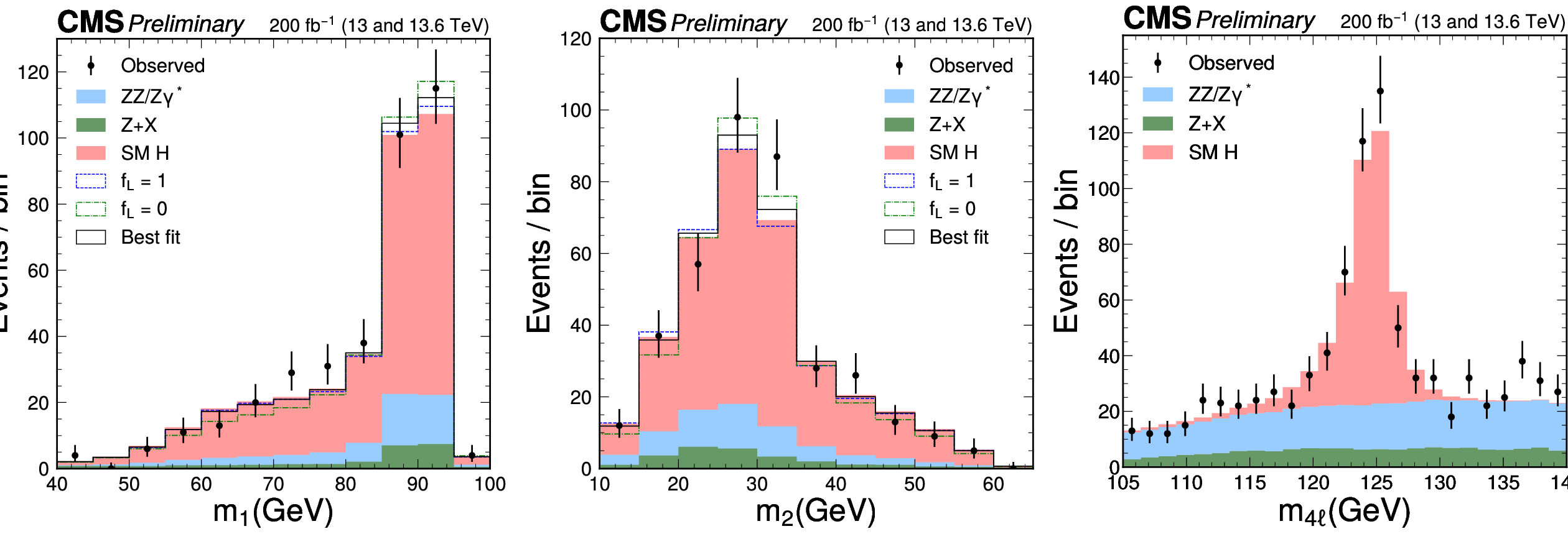
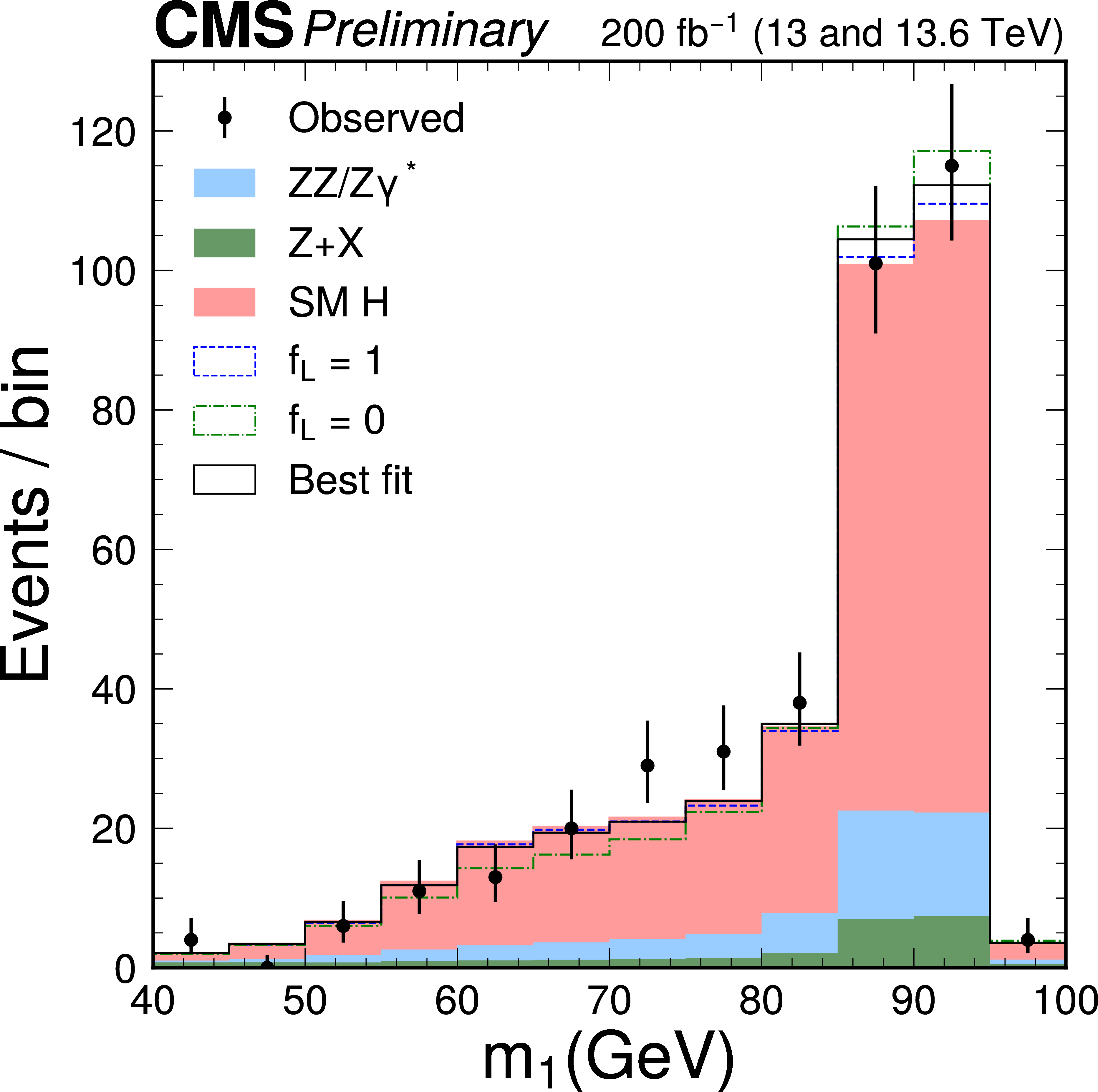
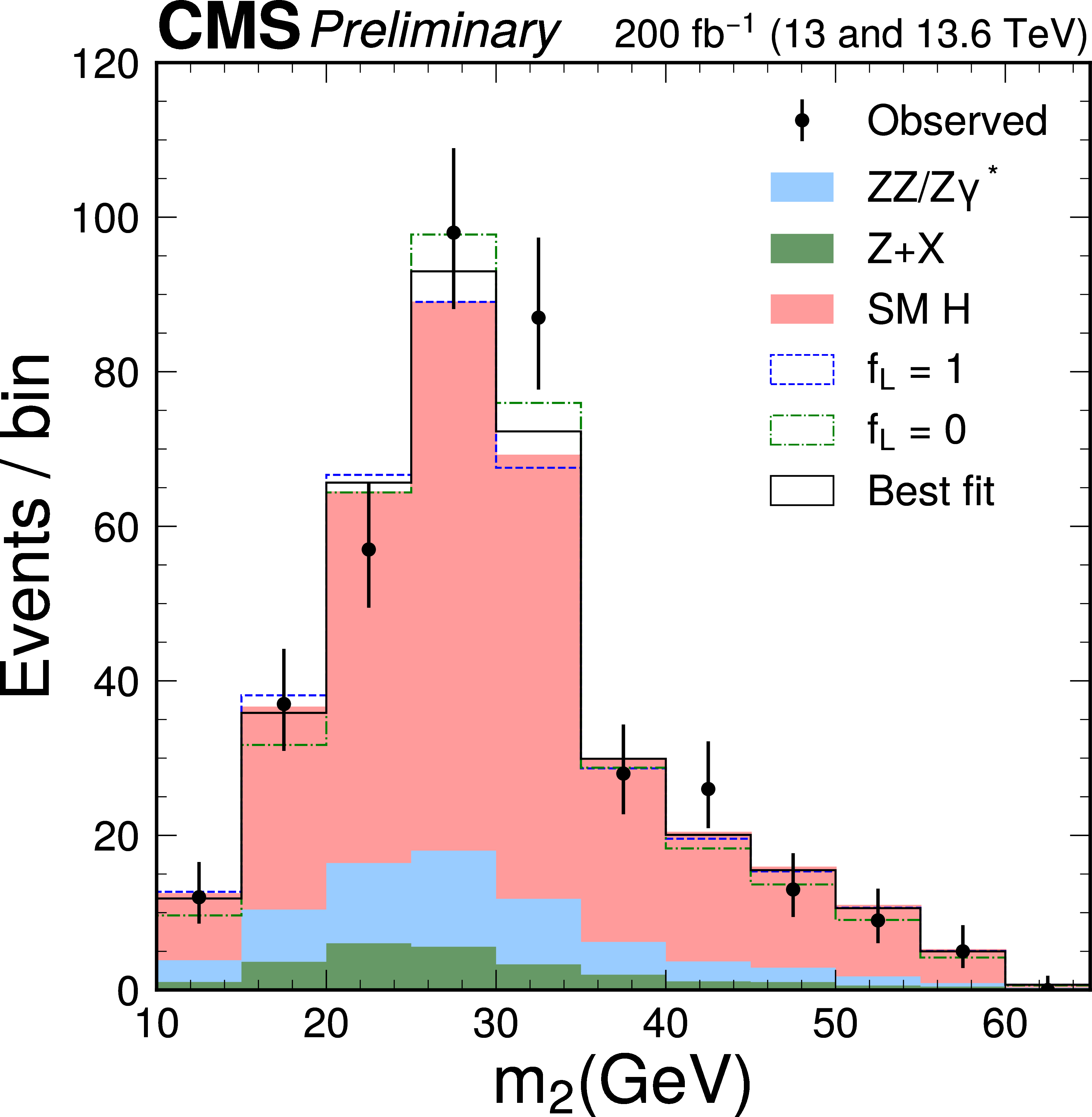
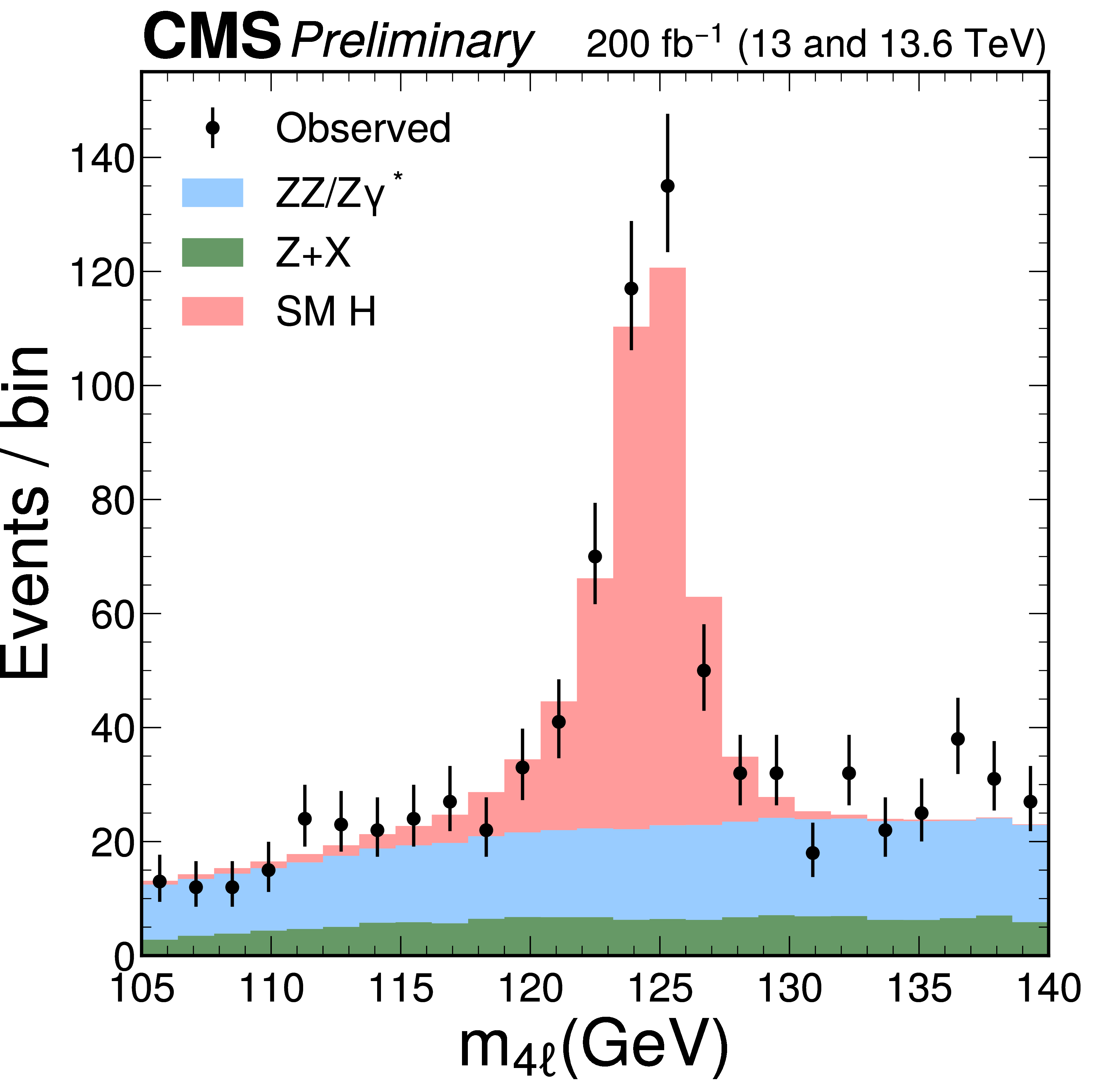
Figure 2:
The distributions of $ m_1 $, $ m_2 $, and $ m_{4\ell} $ in the decay $ \mathrm{H}\to \mathrm{Z}\mathrm{Z}\to 4\ell $ are shown in comparison with the expected distributions from the SM (shaded red), purely longitudinal polarization of the Z bosons (dashed blue), or purely transverse polarization (dot-dashed green), all stacked on top of the background contributions (shaded blue and green). The best-fit distribution corresponds to results presented in Section 6.2 and Table 3 with $ f_\perp $ and $ f_L $ unconstrained. A selection of $ {\mathcal{D}}_{\text{bkg}} > $ 0.6 is applied solely for visualization purposes, to enhance signal-to-background discrimination in the $ m_1 $ and $ m_2 $ plots, where $ {\mathcal{D}}_{\text{bkg}} $ is introduced in Fig. 4 and text. |
png pdf |
Figure 2-a:
The distributions of $ m_1 $, $ m_2 $, and $ m_{4\ell} $ in the decay $ \mathrm{H}\to \mathrm{Z}\mathrm{Z}\to 4\ell $ are shown in comparison with the expected distributions from the SM (shaded red), purely longitudinal polarization of the Z bosons (dashed blue), or purely transverse polarization (dot-dashed green), all stacked on top of the background contributions (shaded blue and green). The best-fit distribution corresponds to results presented in Section 6.2 and Table 3 with $ f_\perp $ and $ f_L $ unconstrained. A selection of $ {\mathcal{D}}_{\text{bkg}} > $ 0.6 is applied solely for visualization purposes, to enhance signal-to-background discrimination in the $ m_1 $ and $ m_2 $ plots, where $ {\mathcal{D}}_{\text{bkg}} $ is introduced in Fig. 4 and text. |
png pdf |
Figure 2-b:
The distributions of $ m_1 $, $ m_2 $, and $ m_{4\ell} $ in the decay $ \mathrm{H}\to \mathrm{Z}\mathrm{Z}\to 4\ell $ are shown in comparison with the expected distributions from the SM (shaded red), purely longitudinal polarization of the Z bosons (dashed blue), or purely transverse polarization (dot-dashed green), all stacked on top of the background contributions (shaded blue and green). The best-fit distribution corresponds to results presented in Section 6.2 and Table 3 with $ f_\perp $ and $ f_L $ unconstrained. A selection of $ {\mathcal{D}}_{\text{bkg}} > $ 0.6 is applied solely for visualization purposes, to enhance signal-to-background discrimination in the $ m_1 $ and $ m_2 $ plots, where $ {\mathcal{D}}_{\text{bkg}} $ is introduced in Fig. 4 and text. |
png pdf |
Figure 2-c:
The distributions of $ m_1 $, $ m_2 $, and $ m_{4\ell} $ in the decay $ \mathrm{H}\to \mathrm{Z}\mathrm{Z}\to 4\ell $ are shown in comparison with the expected distributions from the SM (shaded red), purely longitudinal polarization of the Z bosons (dashed blue), or purely transverse polarization (dot-dashed green), all stacked on top of the background contributions (shaded blue and green). The best-fit distribution corresponds to results presented in Section 6.2 and Table 3 with $ f_\perp $ and $ f_L $ unconstrained. A selection of $ {\mathcal{D}}_{\text{bkg}} > $ 0.6 is applied solely for visualization purposes, to enhance signal-to-background discrimination in the $ m_1 $ and $ m_2 $ plots, where $ {\mathcal{D}}_{\text{bkg}} $ is introduced in Fig. 4 and text. |
png pdf |
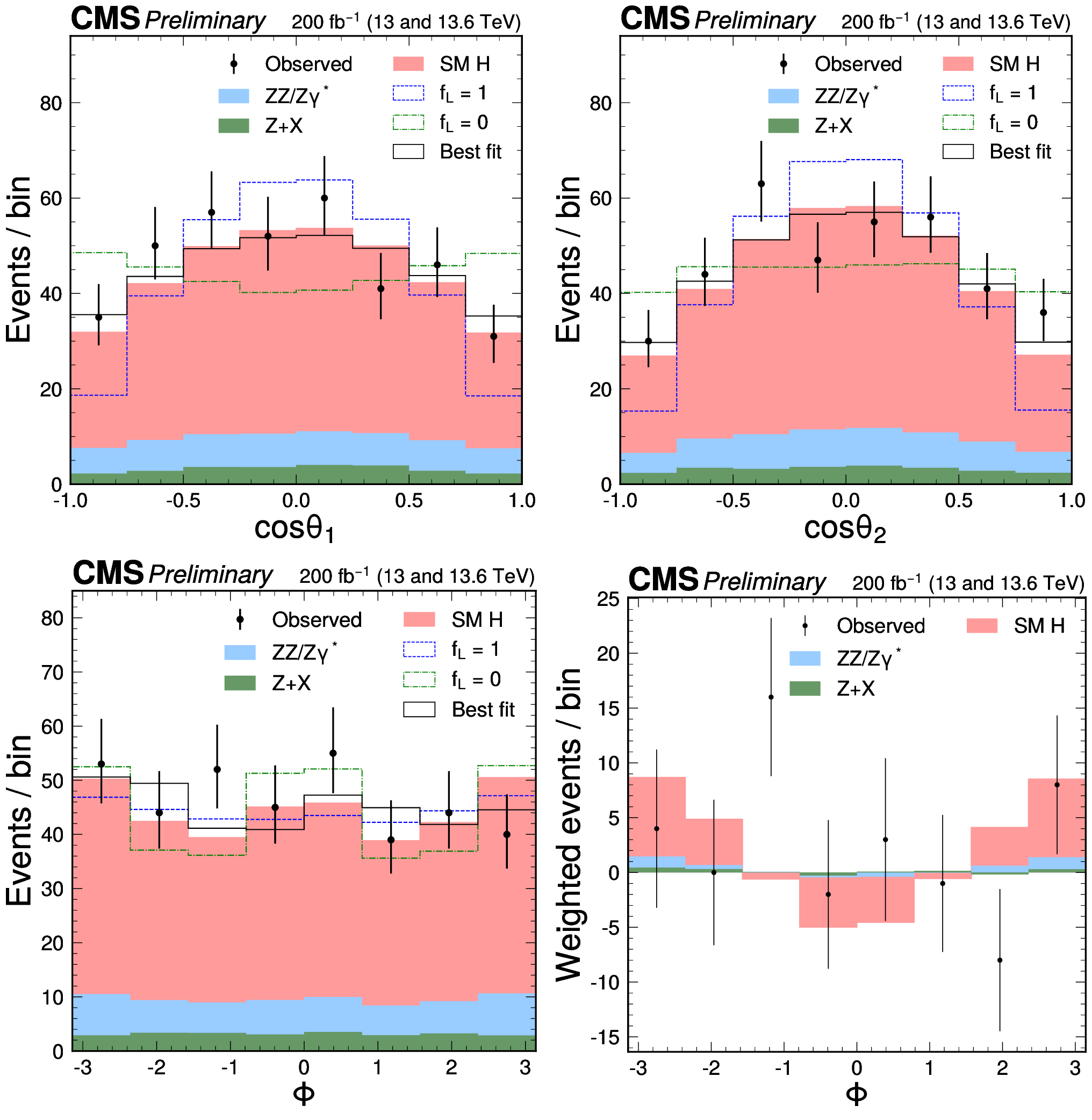
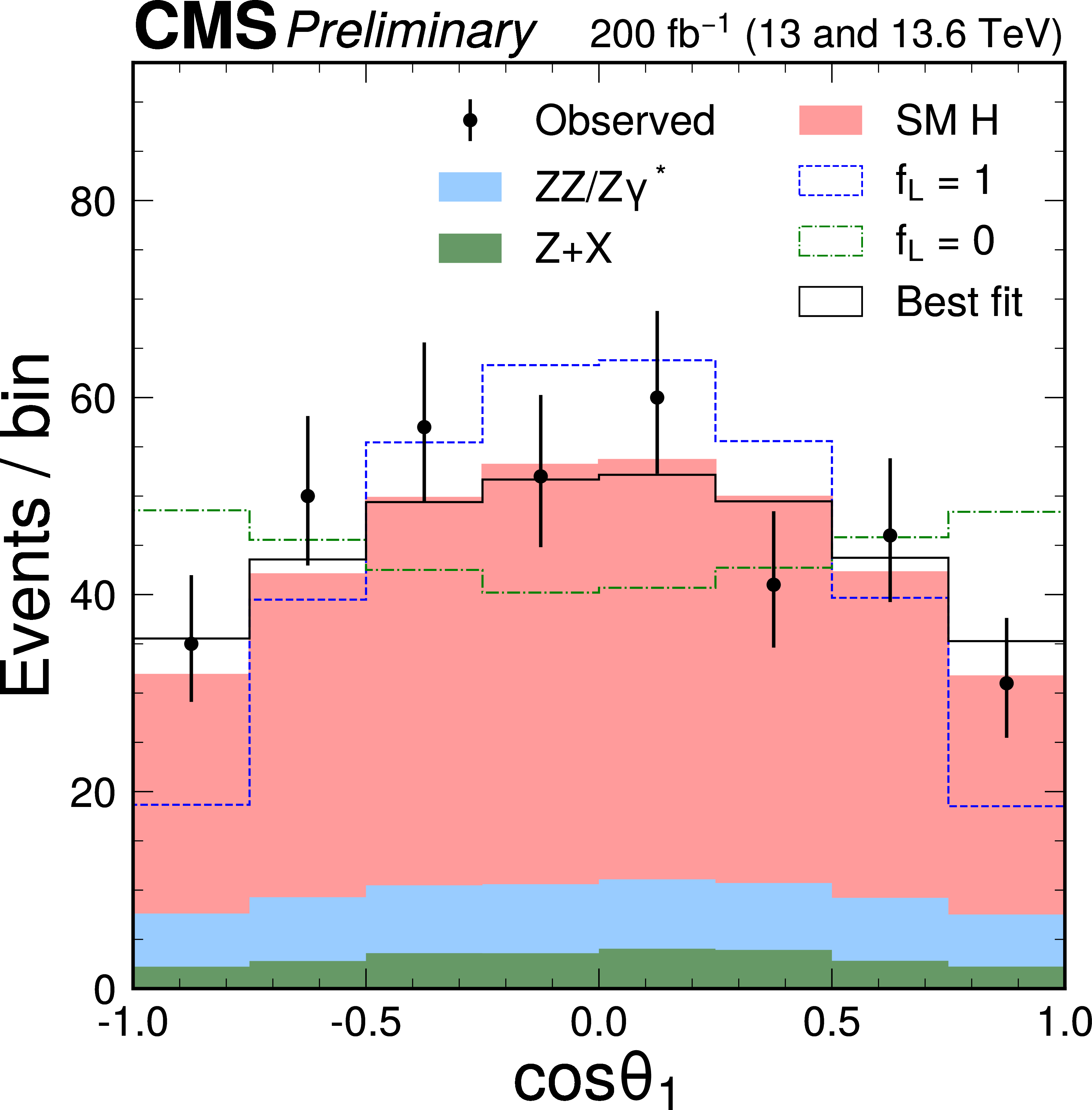
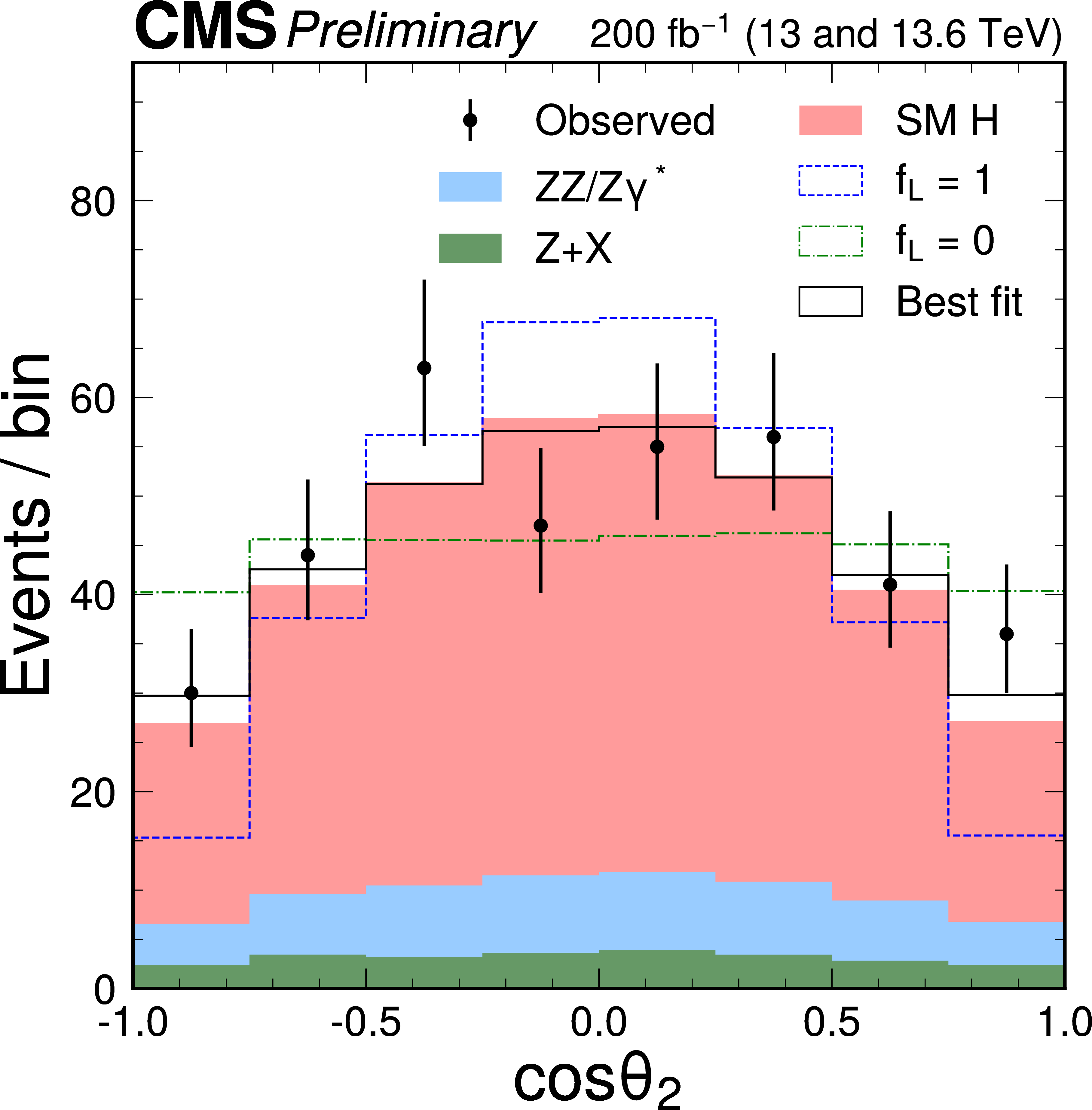
Figure 3:
The distributions of $ \cos\theta_1 $, $ \cos\theta_2 $, and $ \Phi $ are shown following the notation used in Fig. 2. The distribution of $ \Phi $ is also shown with events assigned a weight of either $ + $1 or $-$1, determined by the sign of $ (\cos\theta_1 \cdot \cos\theta_2) $. A selection of $ {\mathcal{D}}_{\text{bkg}} > $ 0.6 is applied solely for visualization purposes, to enhance signal-to-background discrimination in the plots. |
png pdf |
Figure 3-a:
The distributions of $ \cos\theta_1 $, $ \cos\theta_2 $, and $ \Phi $ are shown following the notation used in Fig. 2. The distribution of $ \Phi $ is also shown with events assigned a weight of either $ + $1 or $-$1, determined by the sign of $ (\cos\theta_1 \cdot \cos\theta_2) $. A selection of $ {\mathcal{D}}_{\text{bkg}} > $ 0.6 is applied solely for visualization purposes, to enhance signal-to-background discrimination in the plots. |
png pdf |
Figure 3-b:
The distributions of $ \cos\theta_1 $, $ \cos\theta_2 $, and $ \Phi $ are shown following the notation used in Fig. 2. The distribution of $ \Phi $ is also shown with events assigned a weight of either $ + $1 or $-$1, determined by the sign of $ (\cos\theta_1 \cdot \cos\theta_2) $. A selection of $ {\mathcal{D}}_{\text{bkg}} > $ 0.6 is applied solely for visualization purposes, to enhance signal-to-background discrimination in the plots. |

png pdf |
Figure 3-c:
The distributions of $ \cos\theta_1 $, $ \cos\theta_2 $, and $ \Phi $ are shown following the notation used in Fig. 2. The distribution of $ \Phi $ is also shown with events assigned a weight of either $ + $1 or $-$1, determined by the sign of $ (\cos\theta_1 \cdot \cos\theta_2) $. A selection of $ {\mathcal{D}}_{\text{bkg}} > $ 0.6 is applied solely for visualization purposes, to enhance signal-to-background discrimination in the plots. |
png pdf |
Figure 3-d:
The distributions of $ \cos\theta_1 $, $ \cos\theta_2 $, and $ \Phi $ are shown following the notation used in Fig. 2. The distribution of $ \Phi $ is also shown with events assigned a weight of either $ + $1 or $-$1, determined by the sign of $ (\cos\theta_1 \cdot \cos\theta_2) $. A selection of $ {\mathcal{D}}_{\text{bkg}} > $ 0.6 is applied solely for visualization purposes, to enhance signal-to-background discrimination in the plots. |
png pdf |
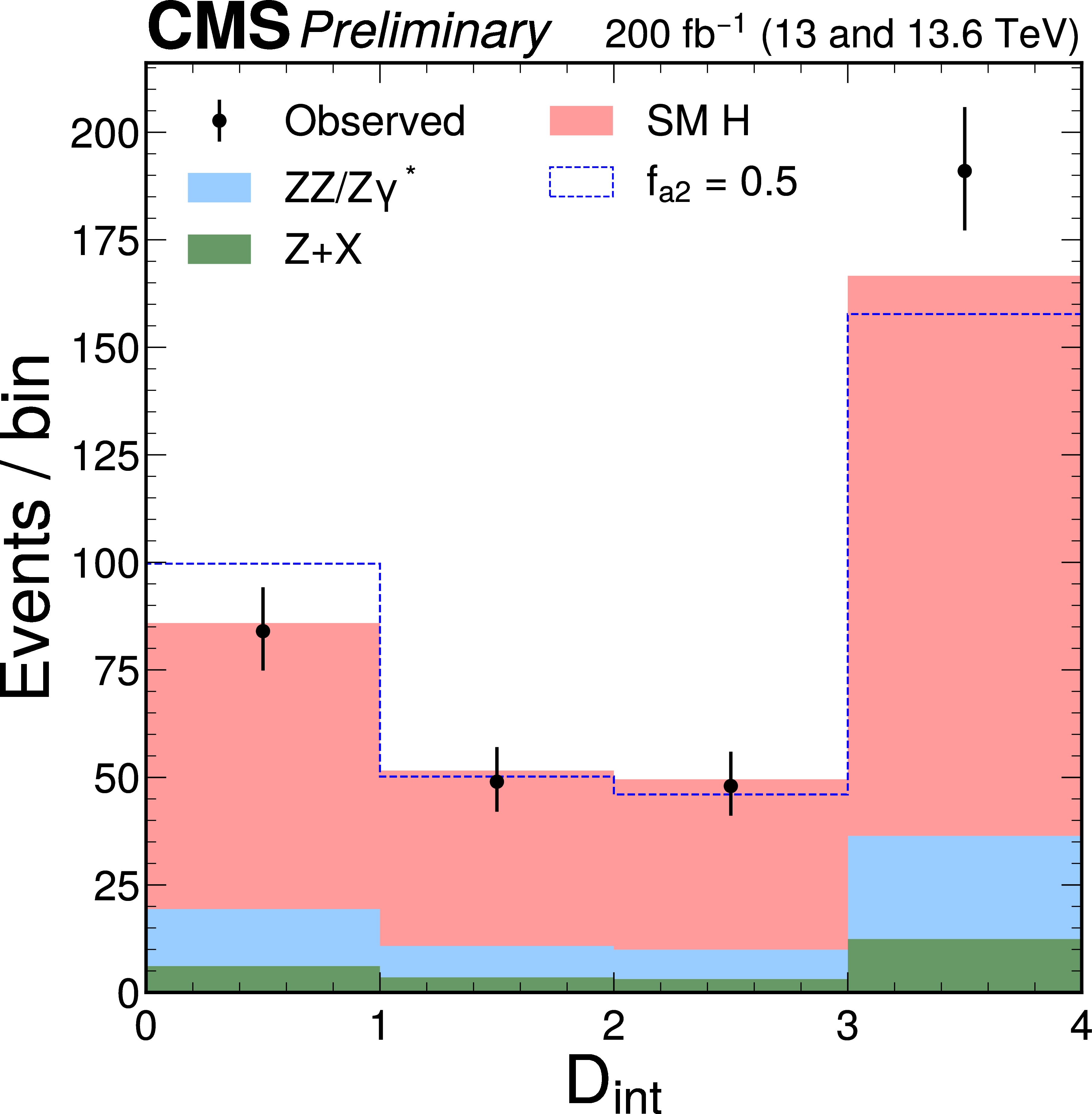
Figure 4:
The distributions of $ {\mathcal{D}}_{\text{bkg}} $ (left) and $ {\cal D}_{\Lambda1} $ (right), following the notation used in Fig. 2. The $ {\cal D}_{\Lambda1} $ discriminant is sensitive to the interference between the $ c_{z\Box} $ contribution and the SM. The right plot illustrates an exaggerated BSM effect, corresponding to a $ c_{z\Box} $ value that produces a cross section equal to that of the SM ($ f_{\Lambda1} = $ 0.5). A selection of $ {\mathcal{D}}_{\text{bkg}} > $ 0.6 is applied solely for visualization purposes, to enhance signal-to-background discrimination in the $ {\cal D}_{\Lambda1} $ plot. |
png pdf |
Figure 4-a:
The distributions of $ {\mathcal{D}}_{\text{bkg}} $ (left) and $ {\cal D}_{\Lambda1} $ (right), following the notation used in Fig. 2. The $ {\cal D}_{\Lambda1} $ discriminant is sensitive to the interference between the $ c_{z\Box} $ contribution and the SM. The right plot illustrates an exaggerated BSM effect, corresponding to a $ c_{z\Box} $ value that produces a cross section equal to that of the SM ($ f_{\Lambda1} = $ 0.5). A selection of $ {\mathcal{D}}_{\text{bkg}} > $ 0.6 is applied solely for visualization purposes, to enhance signal-to-background discrimination in the $ {\cal D}_{\Lambda1} $ plot. |
png pdf |
Figure 4-b:
The distributions of $ {\mathcal{D}}_{\text{bkg}} $ (left) and $ {\cal D}_{\Lambda1} $ (right), following the notation used in Fig. 2. The $ {\cal D}_{\Lambda1} $ discriminant is sensitive to the interference between the $ c_{z\Box} $ contribution and the SM. The right plot illustrates an exaggerated BSM effect, corresponding to a $ c_{z\Box} $ value that produces a cross section equal to that of the SM ($ f_{\Lambda1} = $ 0.5). A selection of $ {\mathcal{D}}_{\text{bkg}} > $ 0.6 is applied solely for visualization purposes, to enhance signal-to-background discrimination in the $ {\cal D}_{\Lambda1} $ plot. |
png pdf |
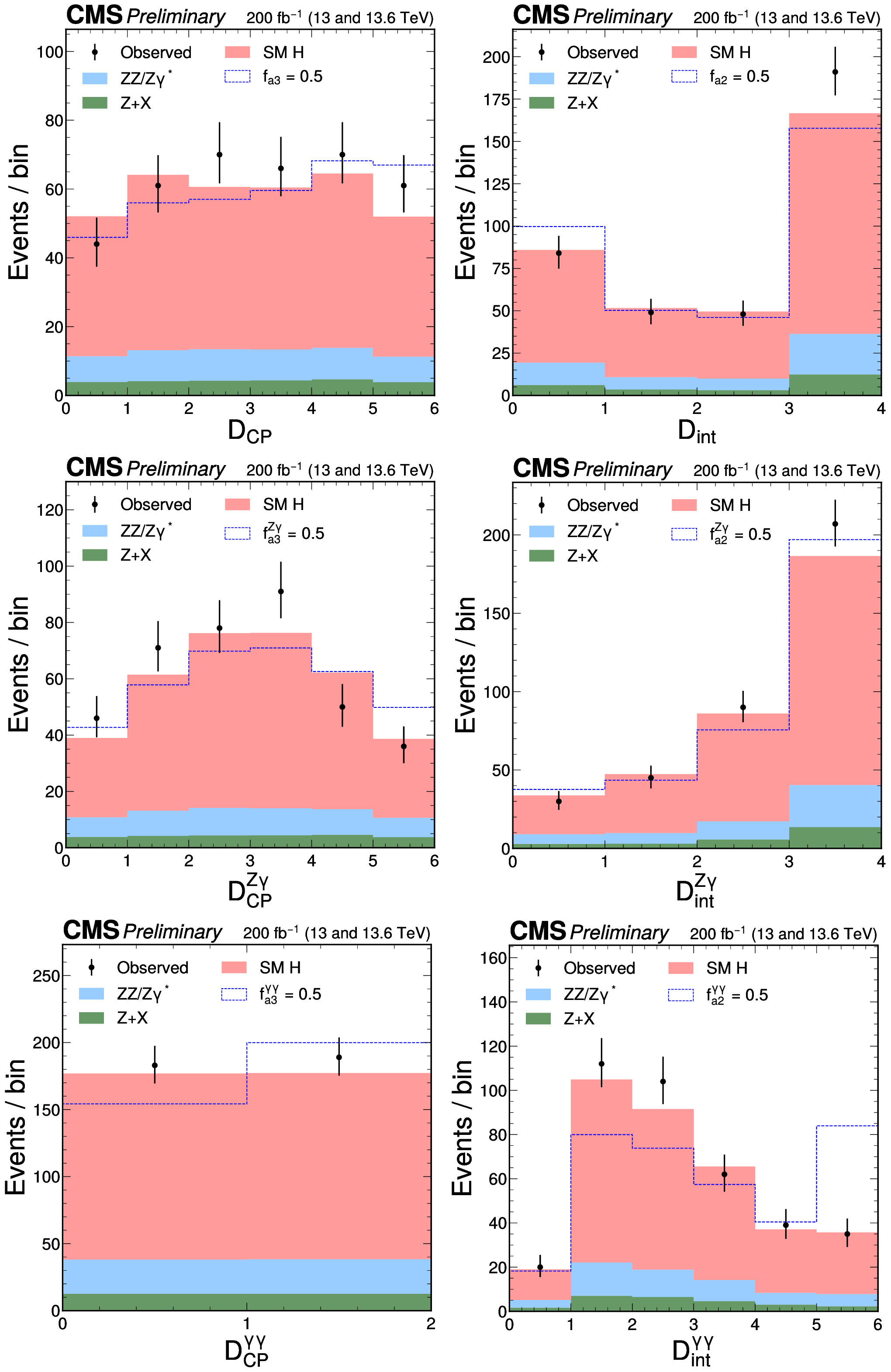
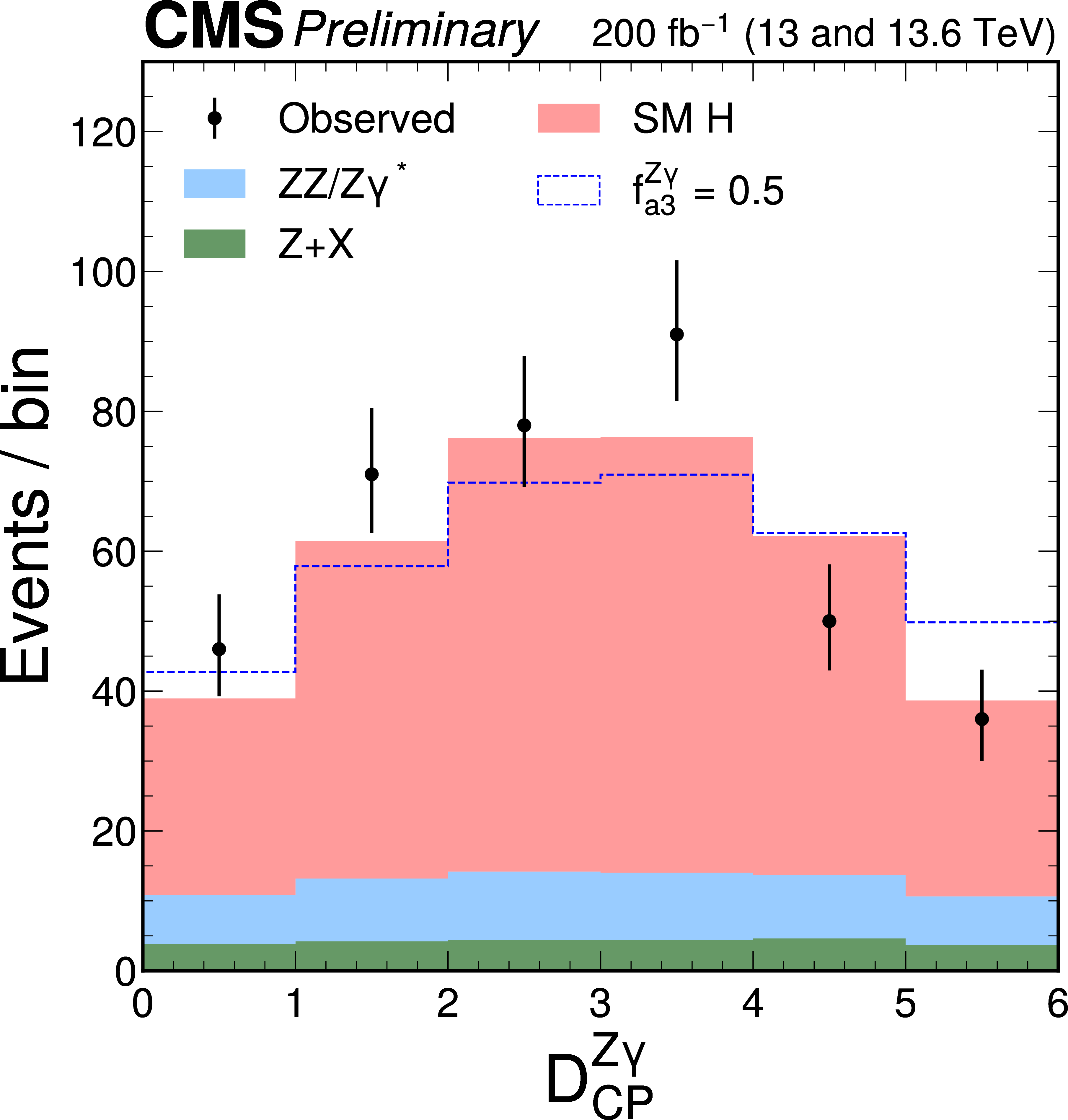
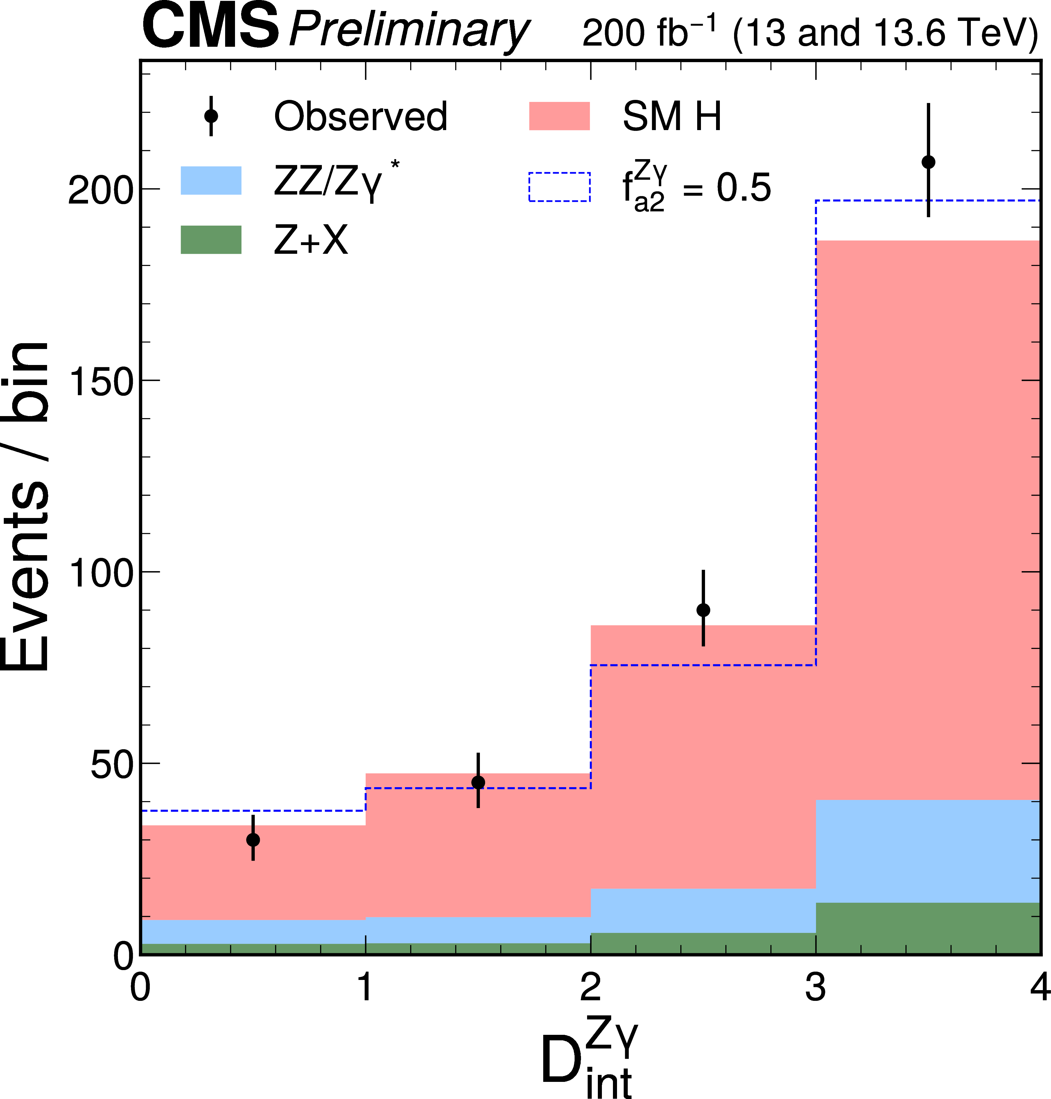
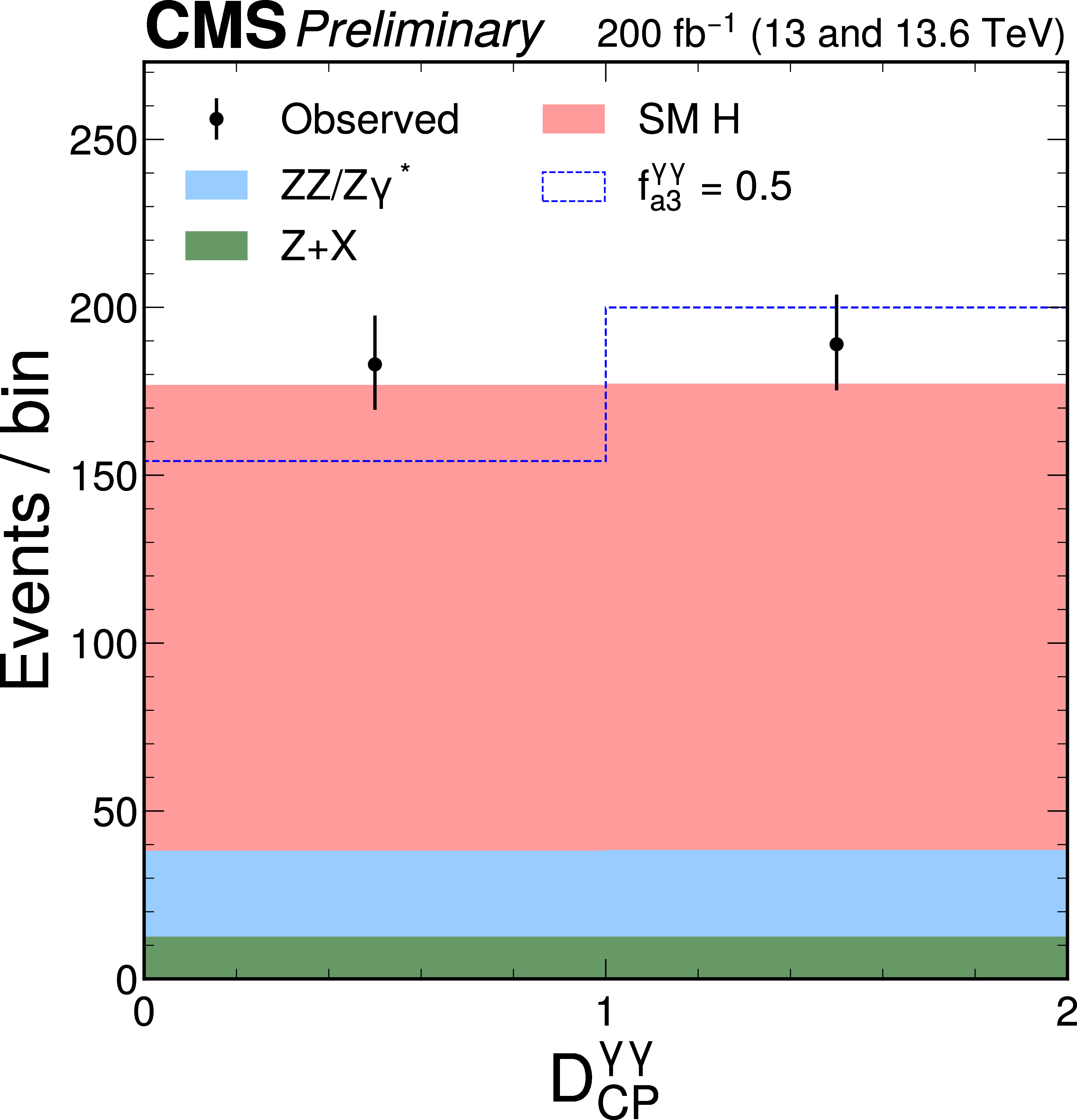
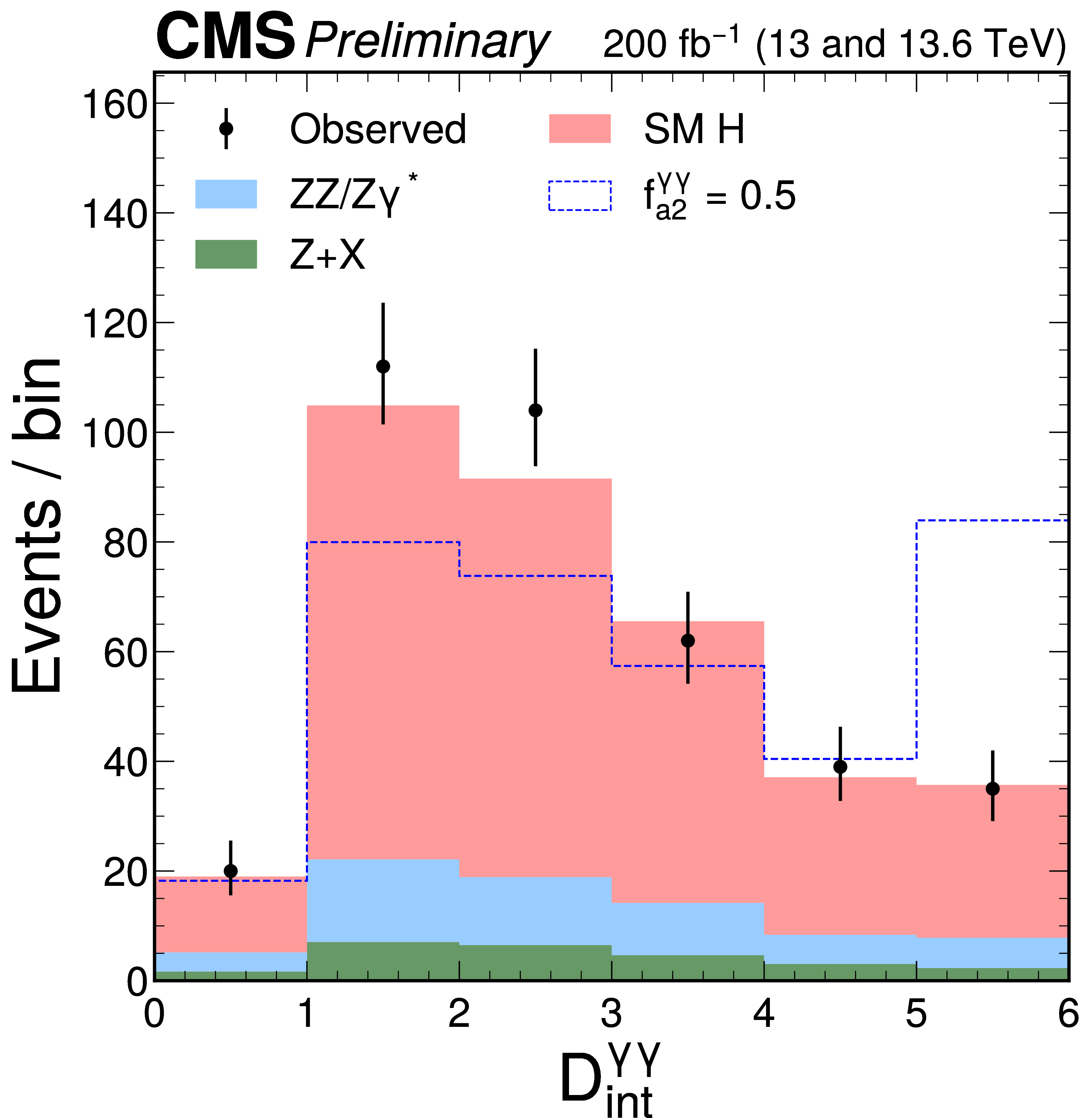
Figure 5:
The distributions of $ {\cal D}_{CP} $, $ {\cal D}_\mathrm{int} $, $ {\cal D}^{\mathrm{Z}\gamma}_{CP} $, $ {\cal D}^{\mathrm{Z}\gamma}_\mathrm{int} $, $ {\cal D}^{\gamma\gamma}_{CP} $, and $ {\cal D}^{\gamma\gamma}_\mathrm{int} $, are shown following the notation of Fig. 2. As is done in Fig. 4, the alternative model includes an exaggerated enhancement of a BSM effect, corresponding to a coupling with $ f_{ai} = $ 0.5. A selection of $ {\mathcal{D}}_{\text{bkg}} > $ 0.6 is applied solely for visualization purposes, to enhance signal-to-background discrimination in the plots. |

png pdf |
Figure 5-a:
The distributions of $ {\cal D}_{CP} $, $ {\cal D}_\mathrm{int} $, $ {\cal D}^{\mathrm{Z}\gamma}_{CP} $, $ {\cal D}^{\mathrm{Z}\gamma}_\mathrm{int} $, $ {\cal D}^{\gamma\gamma}_{CP} $, and $ {\cal D}^{\gamma\gamma}_\mathrm{int} $, are shown following the notation of Fig. 2. As is done in Fig. 4, the alternative model includes an exaggerated enhancement of a BSM effect, corresponding to a coupling with $ f_{ai} = $ 0.5. A selection of $ {\mathcal{D}}_{\text{bkg}} > $ 0.6 is applied solely for visualization purposes, to enhance signal-to-background discrimination in the plots. |
png pdf |
Figure 5-b:
The distributions of $ {\cal D}_{CP} $, $ {\cal D}_\mathrm{int} $, $ {\cal D}^{\mathrm{Z}\gamma}_{CP} $, $ {\cal D}^{\mathrm{Z}\gamma}_\mathrm{int} $, $ {\cal D}^{\gamma\gamma}_{CP} $, and $ {\cal D}^{\gamma\gamma}_\mathrm{int} $, are shown following the notation of Fig. 2. As is done in Fig. 4, the alternative model includes an exaggerated enhancement of a BSM effect, corresponding to a coupling with $ f_{ai} = $ 0.5. A selection of $ {\mathcal{D}}_{\text{bkg}} > $ 0.6 is applied solely for visualization purposes, to enhance signal-to-background discrimination in the plots. |
png pdf |
Figure 5-c:
The distributions of $ {\cal D}_{CP} $, $ {\cal D}_\mathrm{int} $, $ {\cal D}^{\mathrm{Z}\gamma}_{CP} $, $ {\cal D}^{\mathrm{Z}\gamma}_\mathrm{int} $, $ {\cal D}^{\gamma\gamma}_{CP} $, and $ {\cal D}^{\gamma\gamma}_\mathrm{int} $, are shown following the notation of Fig. 2. As is done in Fig. 4, the alternative model includes an exaggerated enhancement of a BSM effect, corresponding to a coupling with $ f_{ai} = $ 0.5. A selection of $ {\mathcal{D}}_{\text{bkg}} > $ 0.6 is applied solely for visualization purposes, to enhance signal-to-background discrimination in the plots. |
png pdf |
Figure 5-d:
The distributions of $ {\cal D}_{CP} $, $ {\cal D}_\mathrm{int} $, $ {\cal D}^{\mathrm{Z}\gamma}_{CP} $, $ {\cal D}^{\mathrm{Z}\gamma}_\mathrm{int} $, $ {\cal D}^{\gamma\gamma}_{CP} $, and $ {\cal D}^{\gamma\gamma}_\mathrm{int} $, are shown following the notation of Fig. 2. As is done in Fig. 4, the alternative model includes an exaggerated enhancement of a BSM effect, corresponding to a coupling with $ f_{ai} = $ 0.5. A selection of $ {\mathcal{D}}_{\text{bkg}} > $ 0.6 is applied solely for visualization purposes, to enhance signal-to-background discrimination in the plots. |
png pdf |
Figure 5-e:
The distributions of $ {\cal D}_{CP} $, $ {\cal D}_\mathrm{int} $, $ {\cal D}^{\mathrm{Z}\gamma}_{CP} $, $ {\cal D}^{\mathrm{Z}\gamma}_\mathrm{int} $, $ {\cal D}^{\gamma\gamma}_{CP} $, and $ {\cal D}^{\gamma\gamma}_\mathrm{int} $, are shown following the notation of Fig. 2. As is done in Fig. 4, the alternative model includes an exaggerated enhancement of a BSM effect, corresponding to a coupling with $ f_{ai} = $ 0.5. A selection of $ {\mathcal{D}}_{\text{bkg}} > $ 0.6 is applied solely for visualization purposes, to enhance signal-to-background discrimination in the plots. |
png pdf |
Figure 5-f:
The distributions of $ {\cal D}_{CP} $, $ {\cal D}_\mathrm{int} $, $ {\cal D}^{\mathrm{Z}\gamma}_{CP} $, $ {\cal D}^{\mathrm{Z}\gamma}_\mathrm{int} $, $ {\cal D}^{\gamma\gamma}_{CP} $, and $ {\cal D}^{\gamma\gamma}_\mathrm{int} $, are shown following the notation of Fig. 2. As is done in Fig. 4, the alternative model includes an exaggerated enhancement of a BSM effect, corresponding to a coupling with $ f_{ai} = $ 0.5. A selection of $ {\mathcal{D}}_{\text{bkg}} > $ 0.6 is applied solely for visualization purposes, to enhance signal-to-background discrimination in the plots. |
png pdf |
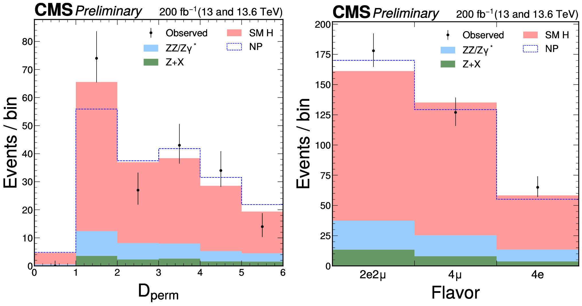
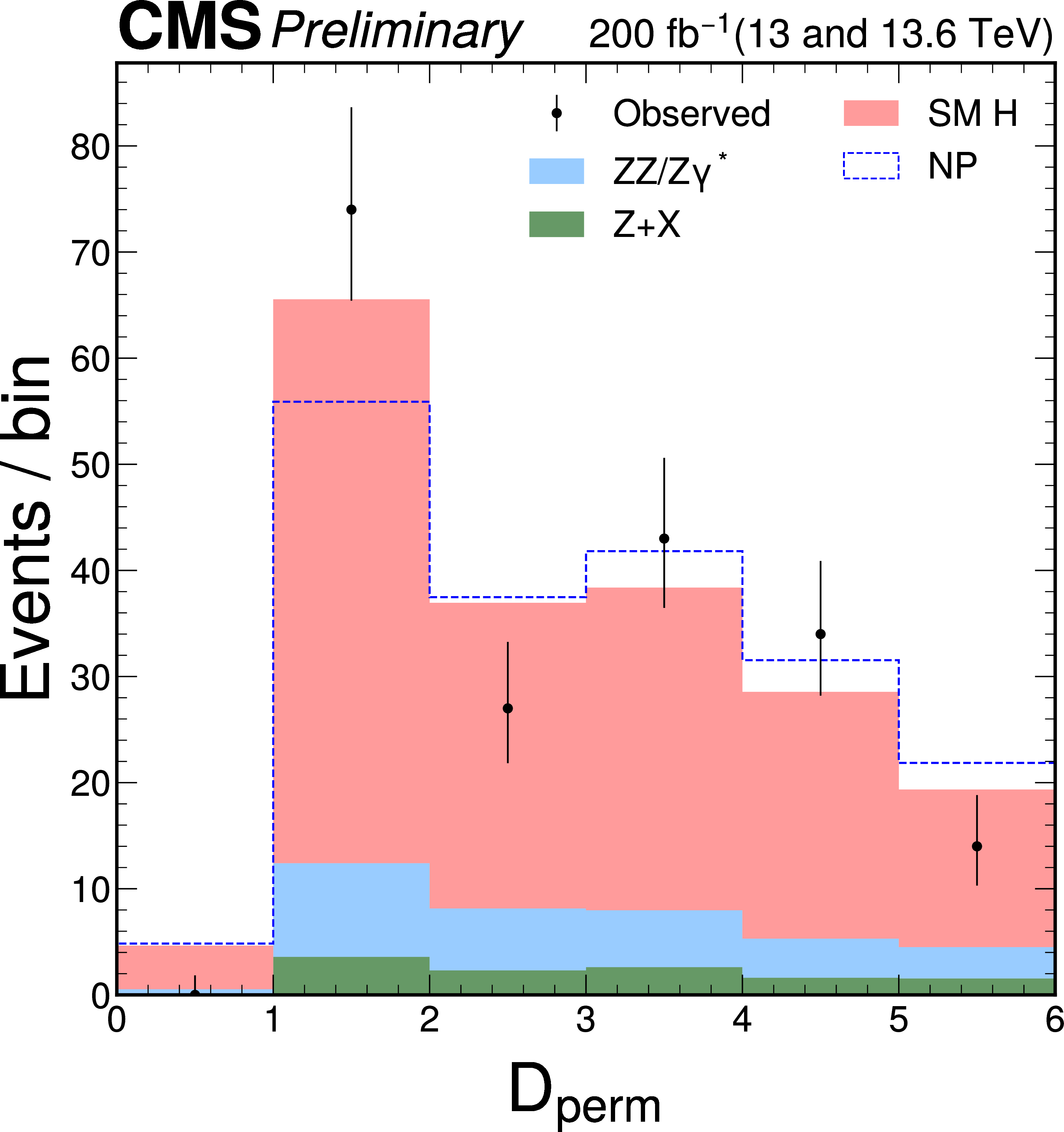
Figure 6:
The distributions of events as a function of the $ \mathcal{D}_\mathrm{perm} $ discriminant for $ \mathrm{H} \to 4\mathrm{e} $ and 4 $ \mu $ events (left) and across the three lepton flavor categories 4 e, 4 $ \mu $, and 2 $ \mathrm{e}2\mu $ (right). The blue open histogram corresponds to a hypothetical case in which no lepton permutation occurs (NP). The notation from Fig. 2 is used, and a selection of $ {\mathcal{D}}_{\text{bkg}} > $ 0.6 is applied solely for visualization purposes, to enhance signal-to-background discrimination in the plots. |
png pdf |
Figure 6-a:
The distributions of events as a function of the $ \mathcal{D}_\mathrm{perm} $ discriminant for $ \mathrm{H} \to 4\mathrm{e} $ and 4 $ \mu $ events (left) and across the three lepton flavor categories 4 e, 4 $ \mu $, and 2 $ \mathrm{e}2\mu $ (right). The blue open histogram corresponds to a hypothetical case in which no lepton permutation occurs (NP). The notation from Fig. 2 is used, and a selection of $ {\mathcal{D}}_{\text{bkg}} > $ 0.6 is applied solely for visualization purposes, to enhance signal-to-background discrimination in the plots. |
png pdf |
Figure 6-b:
The distributions of events as a function of the $ \mathcal{D}_\mathrm{perm} $ discriminant for $ \mathrm{H} \to 4\mathrm{e} $ and 4 $ \mu $ events (left) and across the three lepton flavor categories 4 e, 4 $ \mu $, and 2 $ \mathrm{e}2\mu $ (right). The blue open histogram corresponds to a hypothetical case in which no lepton permutation occurs (NP). The notation from Fig. 2 is used, and a selection of $ {\mathcal{D}}_{\text{bkg}} > $ 0.6 is applied solely for visualization purposes, to enhance signal-to-background discrimination in the plots. |
png pdf |
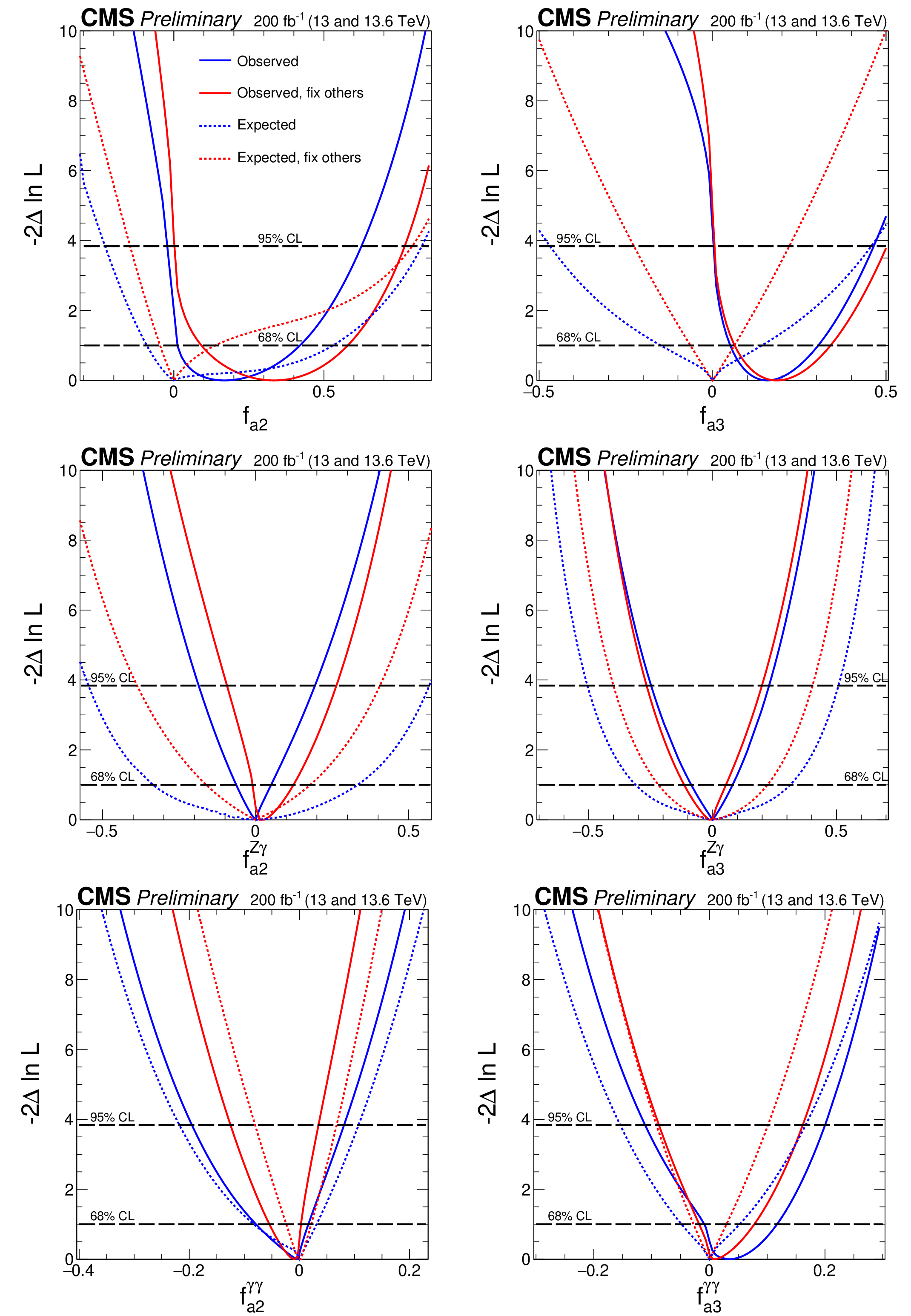
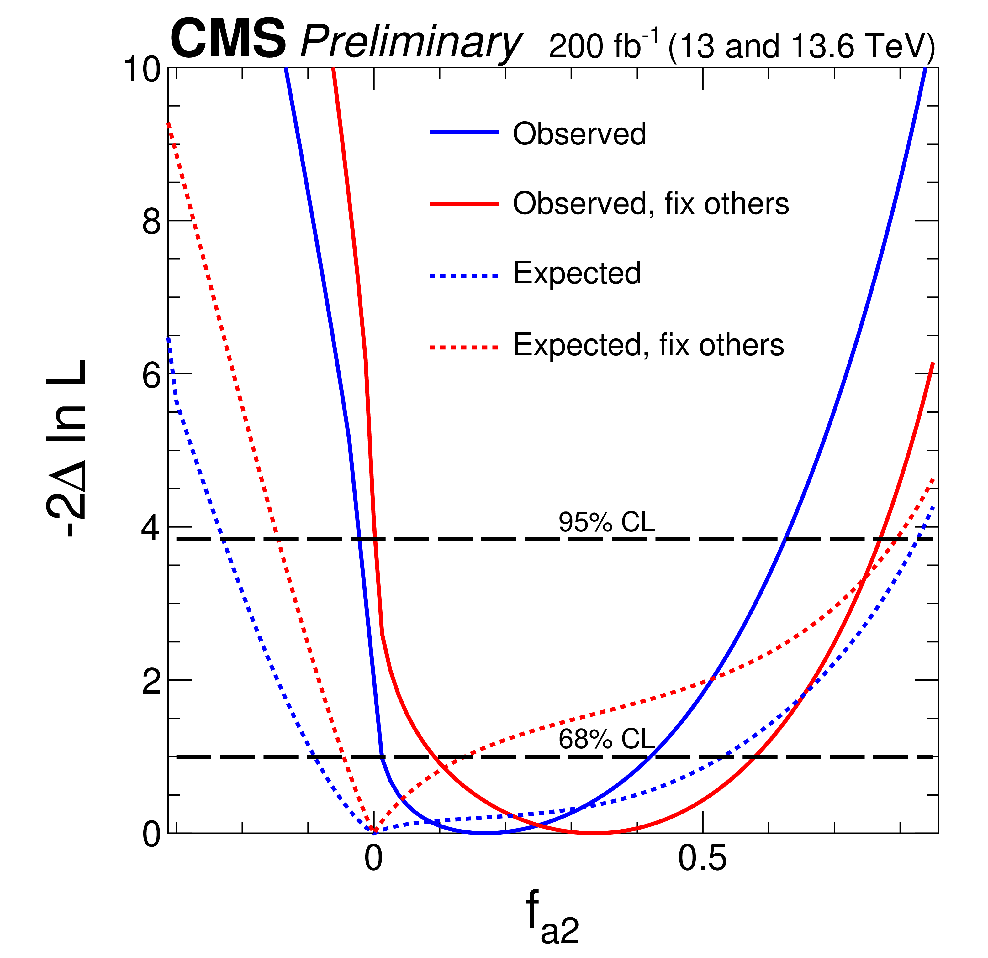
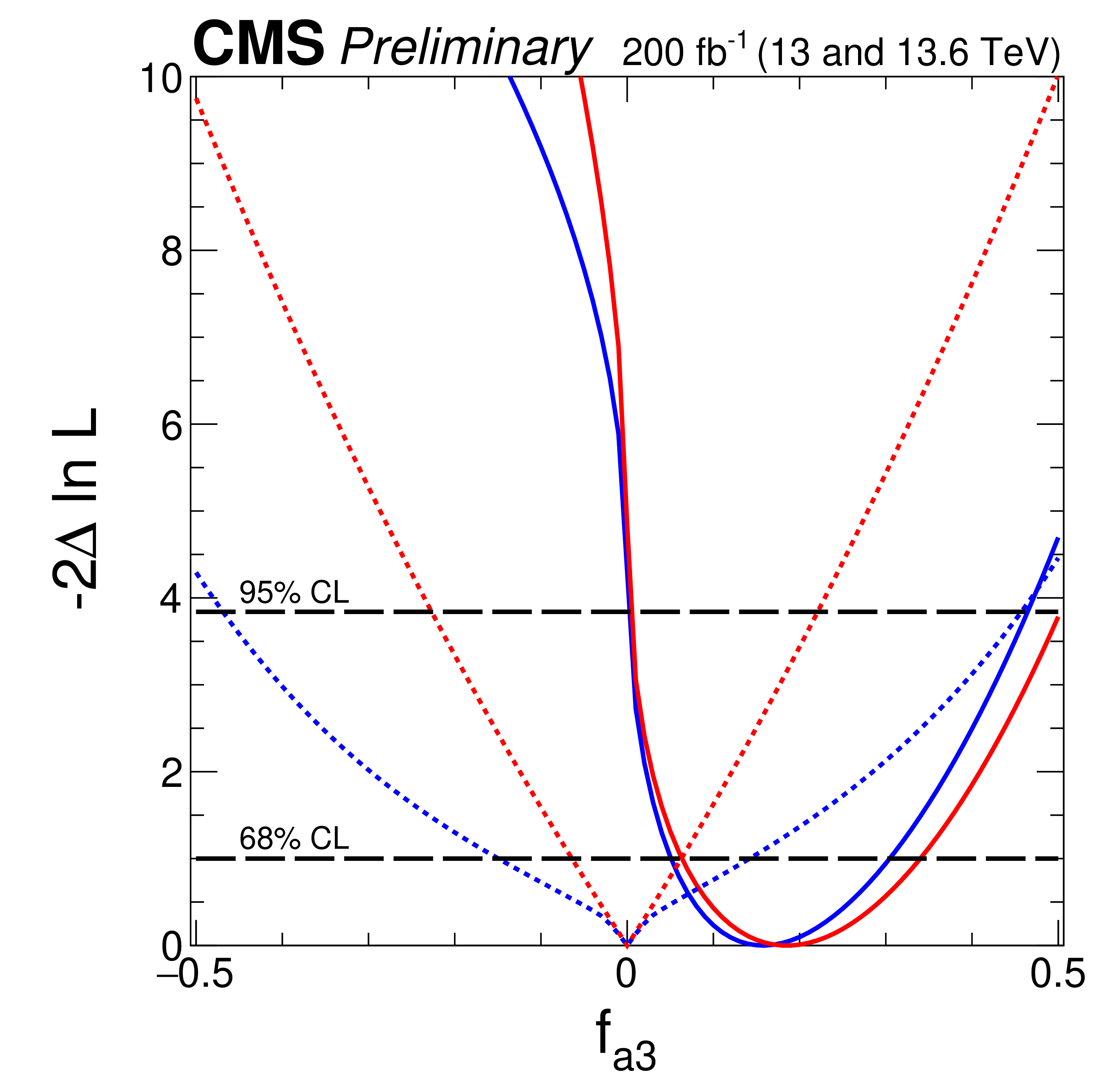
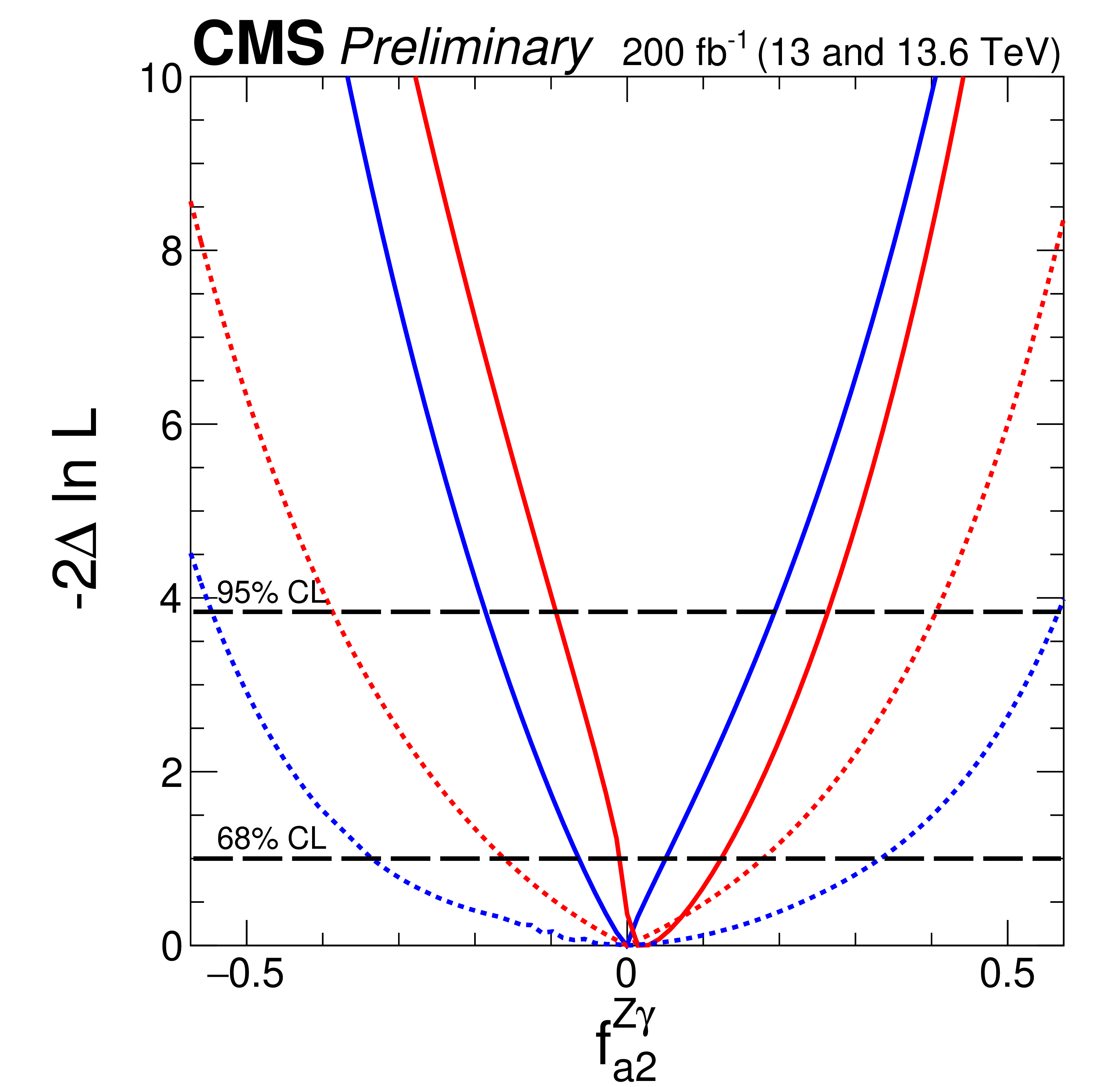
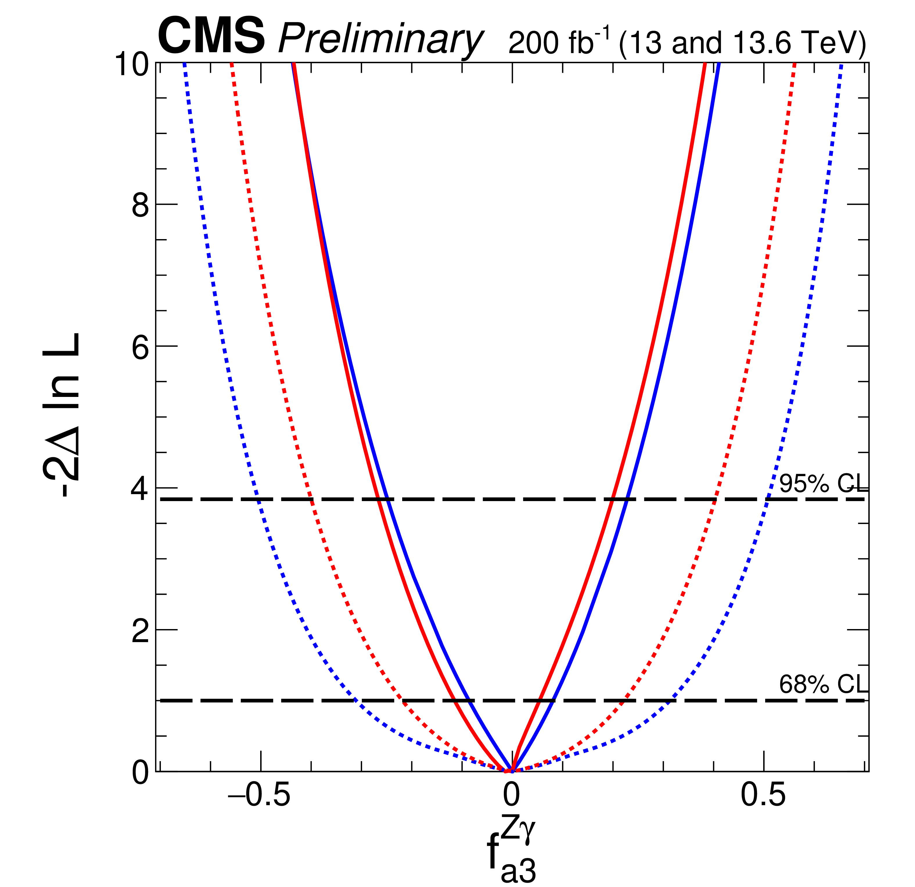
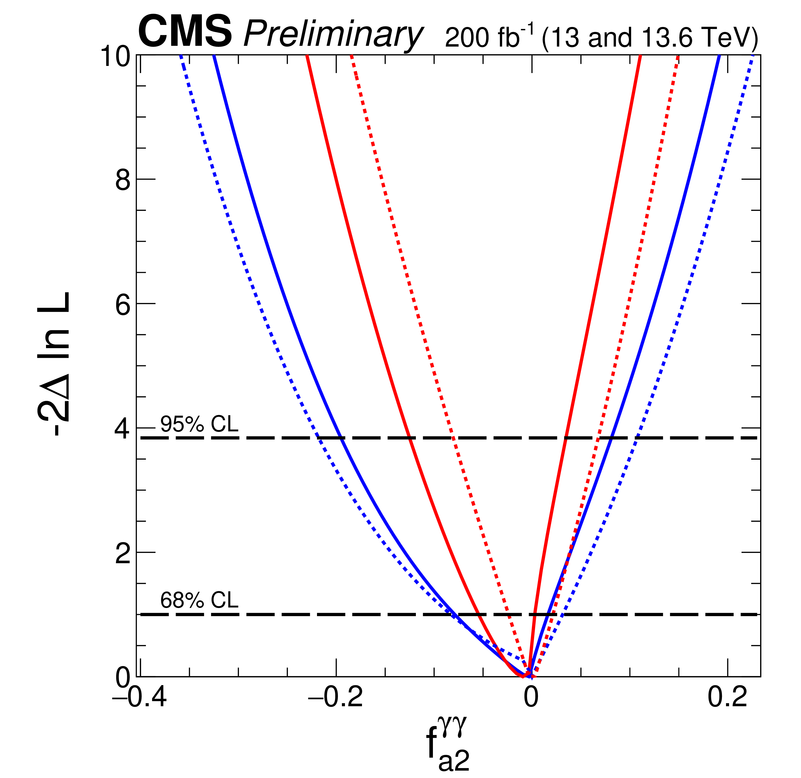
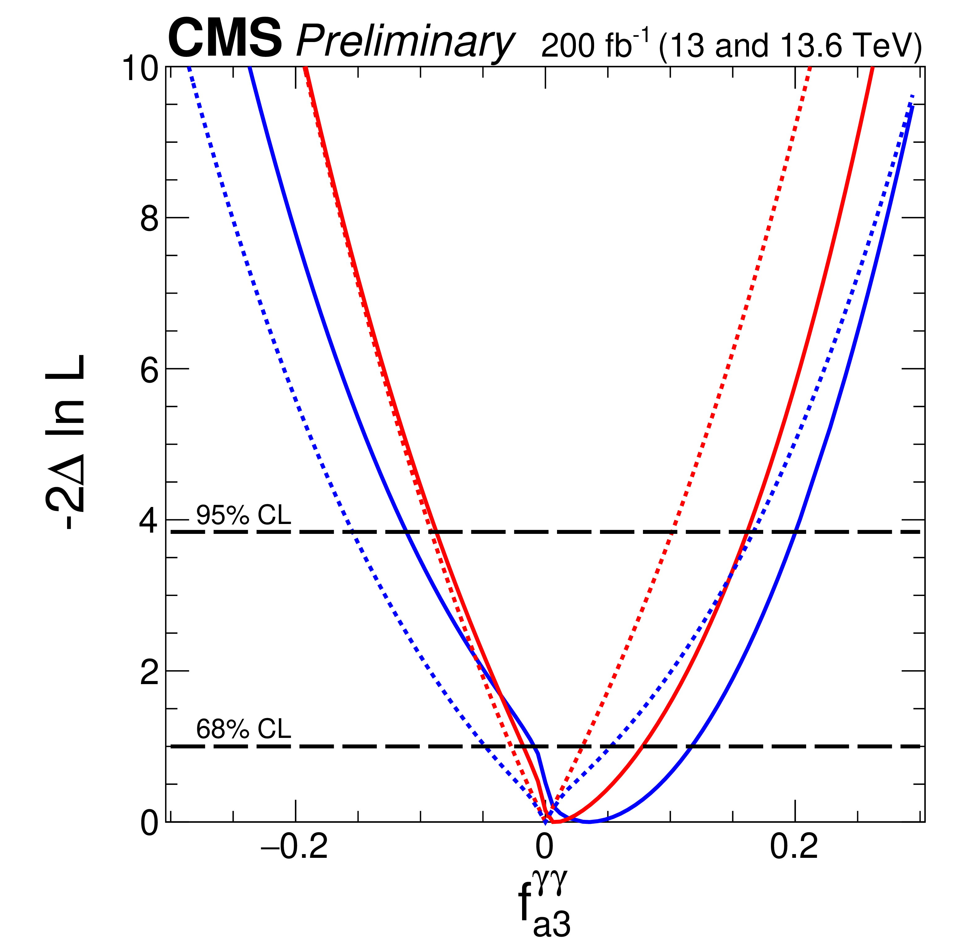
Figure 7:
Observed (solid) and expected (dashed) likelihood scans of the fractional contribution for $ c^\prime_{zz} $ (upper left), $ \tilde{c}^\prime_{zz} $ (upper right), $ c^\prime_{z\gamma} $ (middle left), $ \tilde{c}^\prime_{z\gamma} $ (middle right), $ c^\prime_{\gamma\gamma} $ (lower left), and $ \tilde{c}^\prime_{\gamma\gamma} $ (lower right). The results are presented for each coupling individually, with the remaining couplings either set to zero (red) or left unconstrained in the fit (blue). Solid lines indicate observed results, and dashed lines indicate expected average results. The long-dashed horizontal lines show the 68 and 95% CL exclusion regions. |
png pdf |
Figure 7-a:
Observed (solid) and expected (dashed) likelihood scans of the fractional contribution for $ c^\prime_{zz} $ (upper left), $ \tilde{c}^\prime_{zz} $ (upper right), $ c^\prime_{z\gamma} $ (middle left), $ \tilde{c}^\prime_{z\gamma} $ (middle right), $ c^\prime_{\gamma\gamma} $ (lower left), and $ \tilde{c}^\prime_{\gamma\gamma} $ (lower right). The results are presented for each coupling individually, with the remaining couplings either set to zero (red) or left unconstrained in the fit (blue). Solid lines indicate observed results, and dashed lines indicate expected average results. The long-dashed horizontal lines show the 68 and 95% CL exclusion regions. |
png pdf |
Figure 7-b:
Observed (solid) and expected (dashed) likelihood scans of the fractional contribution for $ c^\prime_{zz} $ (upper left), $ \tilde{c}^\prime_{zz} $ (upper right), $ c^\prime_{z\gamma} $ (middle left), $ \tilde{c}^\prime_{z\gamma} $ (middle right), $ c^\prime_{\gamma\gamma} $ (lower left), and $ \tilde{c}^\prime_{\gamma\gamma} $ (lower right). The results are presented for each coupling individually, with the remaining couplings either set to zero (red) or left unconstrained in the fit (blue). Solid lines indicate observed results, and dashed lines indicate expected average results. The long-dashed horizontal lines show the 68 and 95% CL exclusion regions. |
png pdf |
Figure 7-c:
Observed (solid) and expected (dashed) likelihood scans of the fractional contribution for $ c^\prime_{zz} $ (upper left), $ \tilde{c}^\prime_{zz} $ (upper right), $ c^\prime_{z\gamma} $ (middle left), $ \tilde{c}^\prime_{z\gamma} $ (middle right), $ c^\prime_{\gamma\gamma} $ (lower left), and $ \tilde{c}^\prime_{\gamma\gamma} $ (lower right). The results are presented for each coupling individually, with the remaining couplings either set to zero (red) or left unconstrained in the fit (blue). Solid lines indicate observed results, and dashed lines indicate expected average results. The long-dashed horizontal lines show the 68 and 95% CL exclusion regions. |
png pdf |
Figure 7-d:
Observed (solid) and expected (dashed) likelihood scans of the fractional contribution for $ c^\prime_{zz} $ (upper left), $ \tilde{c}^\prime_{zz} $ (upper right), $ c^\prime_{z\gamma} $ (middle left), $ \tilde{c}^\prime_{z\gamma} $ (middle right), $ c^\prime_{\gamma\gamma} $ (lower left), and $ \tilde{c}^\prime_{\gamma\gamma} $ (lower right). The results are presented for each coupling individually, with the remaining couplings either set to zero (red) or left unconstrained in the fit (blue). Solid lines indicate observed results, and dashed lines indicate expected average results. The long-dashed horizontal lines show the 68 and 95% CL exclusion regions. |
png pdf |
Figure 7-e:
Observed (solid) and expected (dashed) likelihood scans of the fractional contribution for $ c^\prime_{zz} $ (upper left), $ \tilde{c}^\prime_{zz} $ (upper right), $ c^\prime_{z\gamma} $ (middle left), $ \tilde{c}^\prime_{z\gamma} $ (middle right), $ c^\prime_{\gamma\gamma} $ (lower left), and $ \tilde{c}^\prime_{\gamma\gamma} $ (lower right). The results are presented for each coupling individually, with the remaining couplings either set to zero (red) or left unconstrained in the fit (blue). Solid lines indicate observed results, and dashed lines indicate expected average results. The long-dashed horizontal lines show the 68 and 95% CL exclusion regions. |
png pdf |
Figure 7-f:
Observed (solid) and expected (dashed) likelihood scans of the fractional contribution for $ c^\prime_{zz} $ (upper left), $ \tilde{c}^\prime_{zz} $ (upper right), $ c^\prime_{z\gamma} $ (middle left), $ \tilde{c}^\prime_{z\gamma} $ (middle right), $ c^\prime_{\gamma\gamma} $ (lower left), and $ \tilde{c}^\prime_{\gamma\gamma} $ (lower right). The results are presented for each coupling individually, with the remaining couplings either set to zero (red) or left unconstrained in the fit (blue). Solid lines indicate observed results, and dashed lines indicate expected average results. The long-dashed horizontal lines show the 68 and 95% CL exclusion regions. |
png pdf |
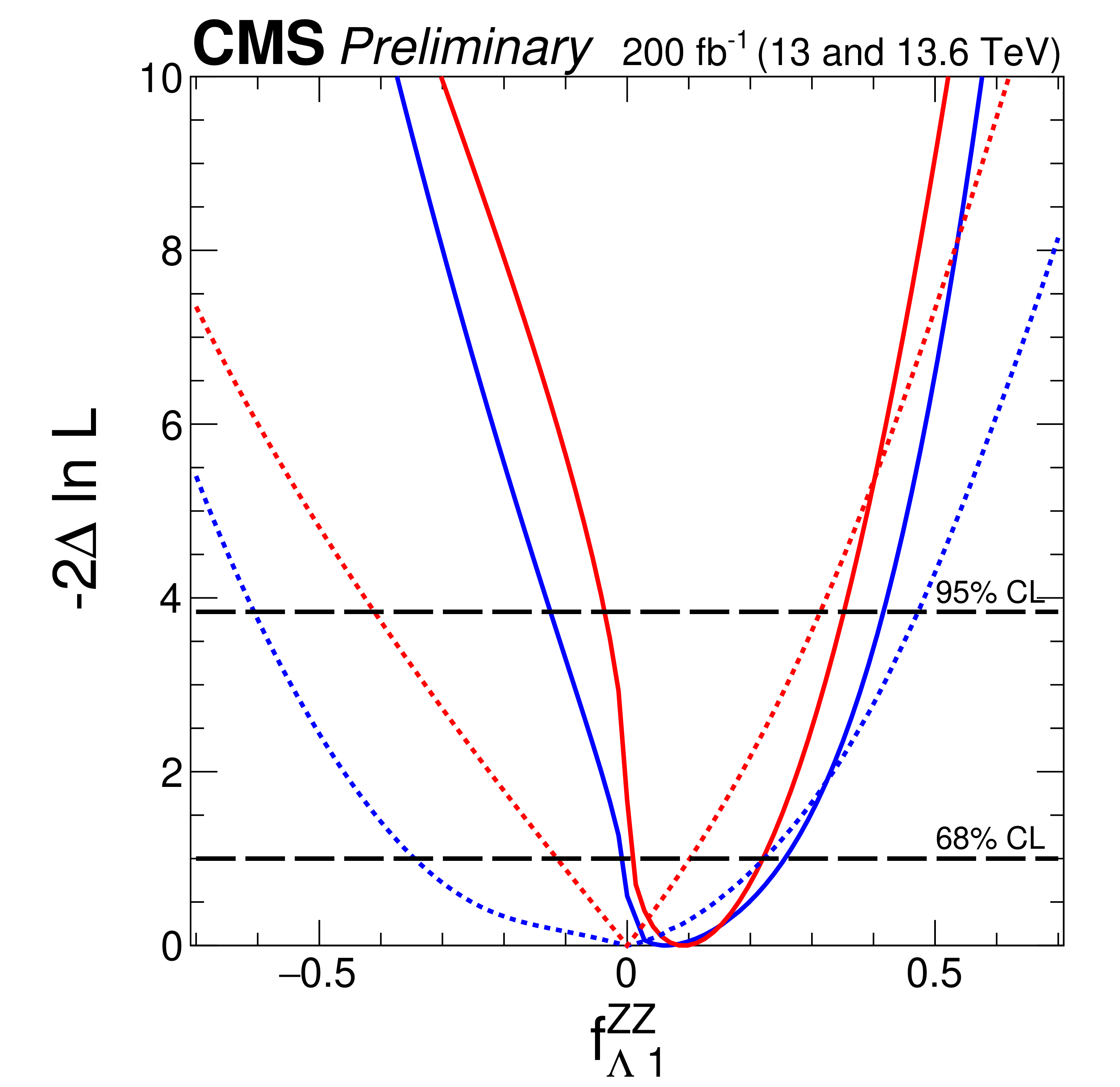
Figure 8:
Observed (solid) and expected (dashed) likelihood scans of the fractional contribution for $ c^\prime_{z\Box} $. The conventions used in Fig. 7 have been adopted. |
png pdf |
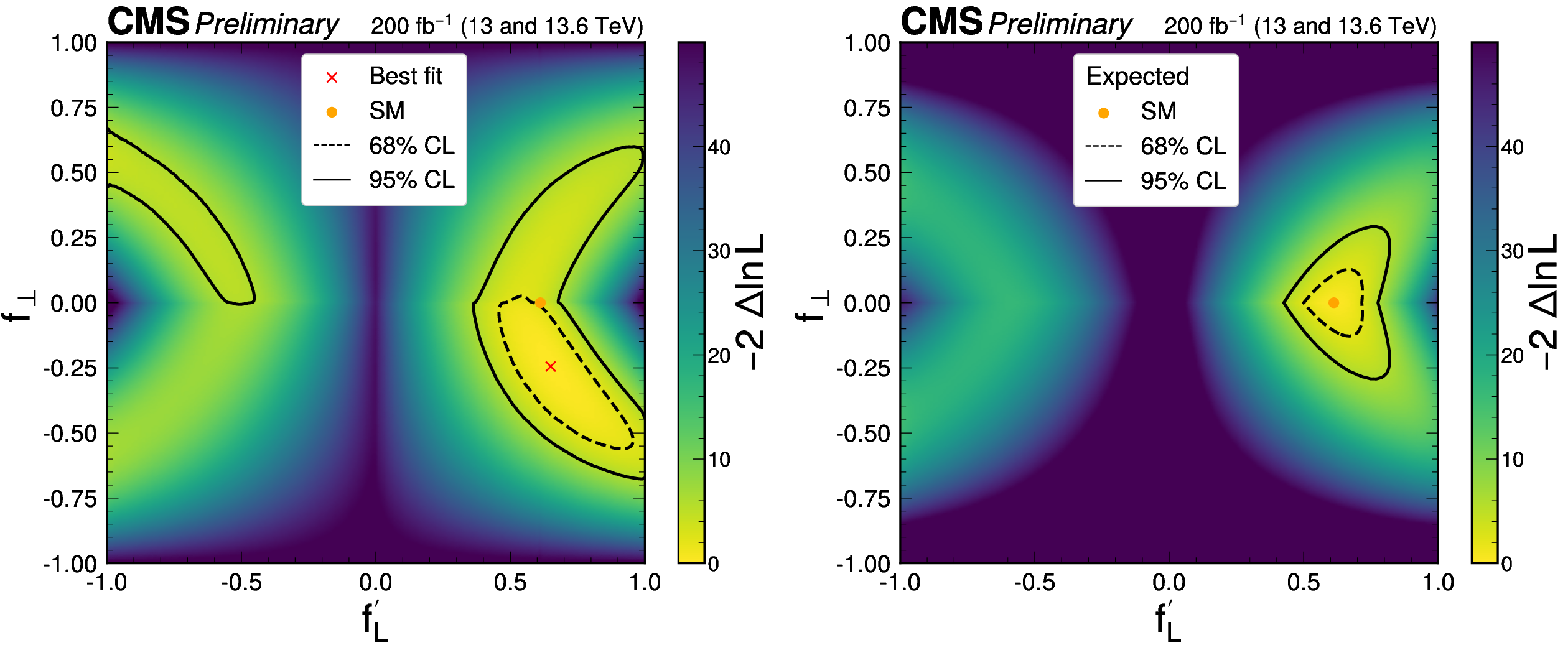
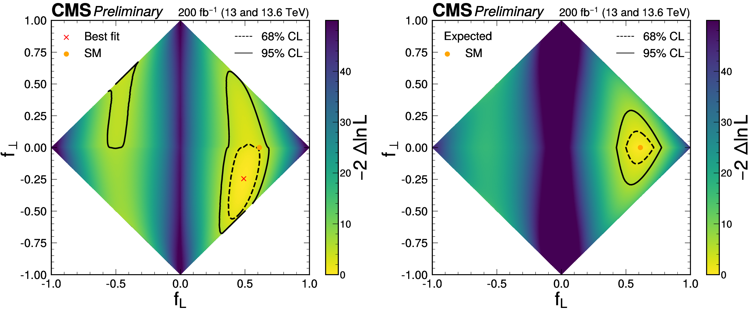
Figure 9:
The observed (left) and expected (right) likelihood scans in the $ (f^\prime_{L},f_{\perp}) $ parameter plane, where $ f^\prime_{L}=f_L/(1-|f_\perp|) $. The yellow point, corresponding to $ f_{L} = $ 0.61 and $ f_{\perp} = $ 0, represents the SM. |
png pdf |
Figure 9-a:
The observed (left) and expected (right) likelihood scans in the $ (f^\prime_{L},f_{\perp}) $ parameter plane, where $ f^\prime_{L}=f_L/(1-|f_\perp|) $. The yellow point, corresponding to $ f_{L} = $ 0.61 and $ f_{\perp} = $ 0, represents the SM. |
png pdf |
Figure 9-b:
The observed (left) and expected (right) likelihood scans in the $ (f^\prime_{L},f_{\perp}) $ parameter plane, where $ f^\prime_{L}=f_L/(1-|f_\perp|) $. The yellow point, corresponding to $ f_{L} = $ 0.61 and $ f_{\perp} = $ 0, represents the SM. |
png pdf |
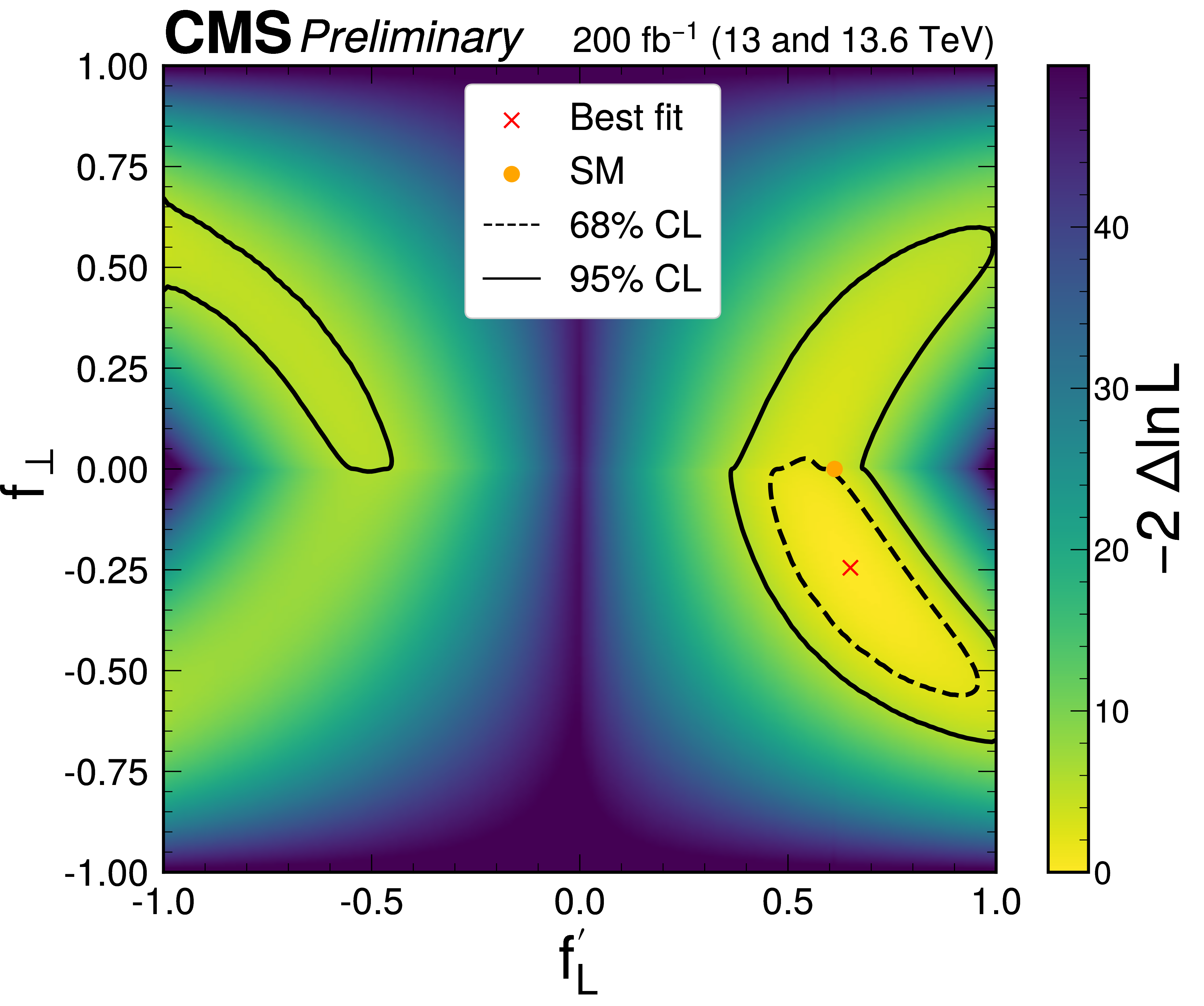
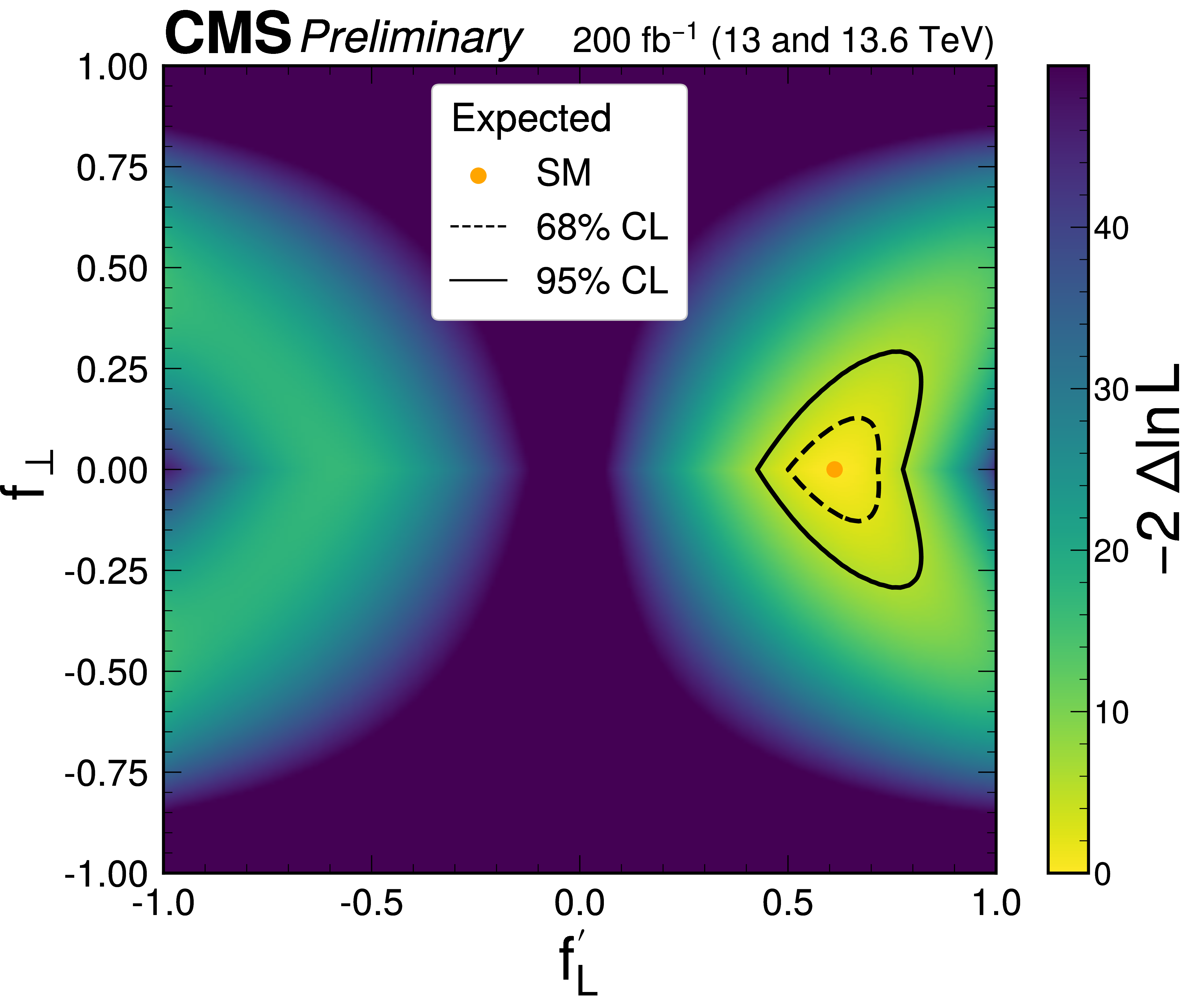
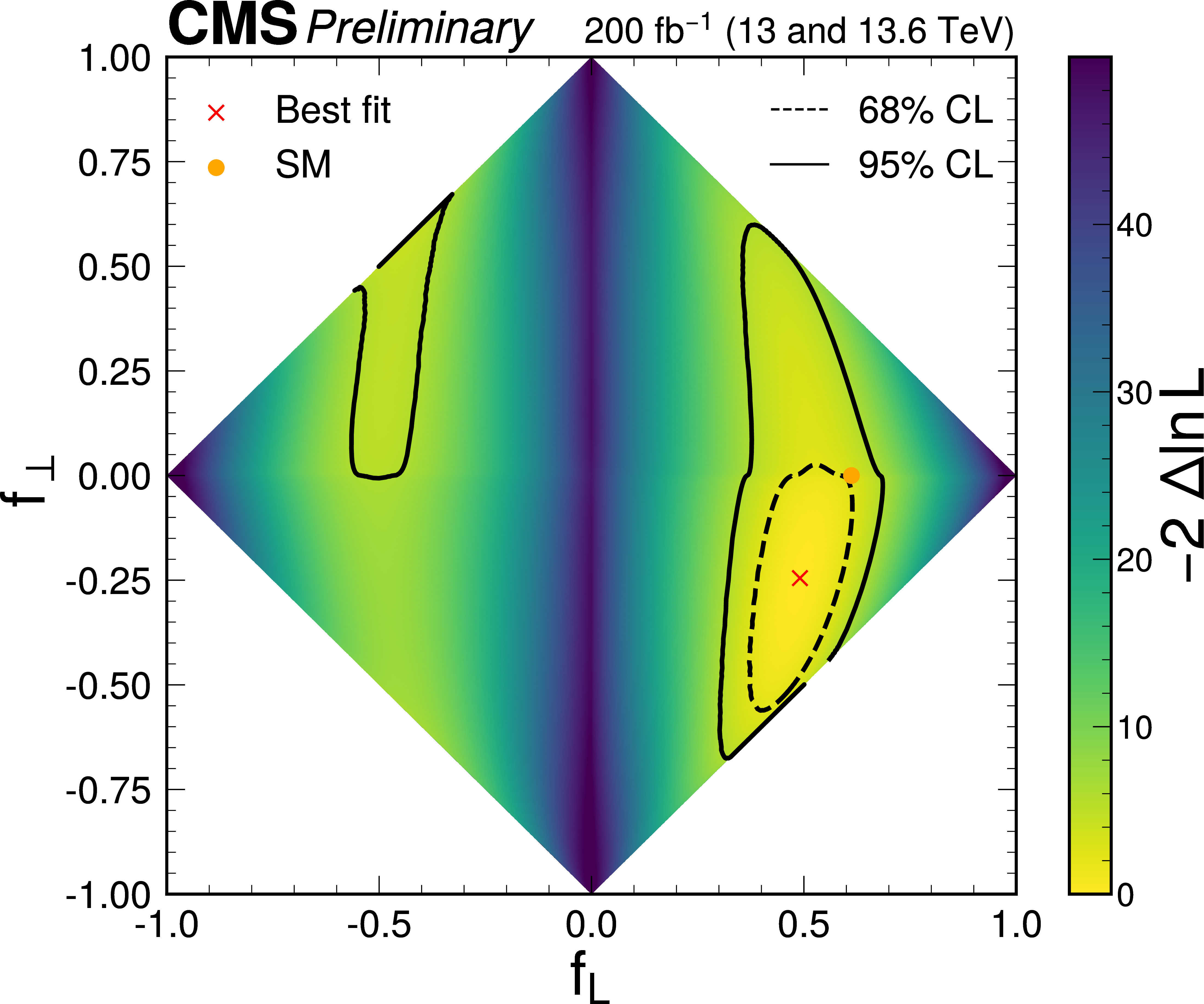
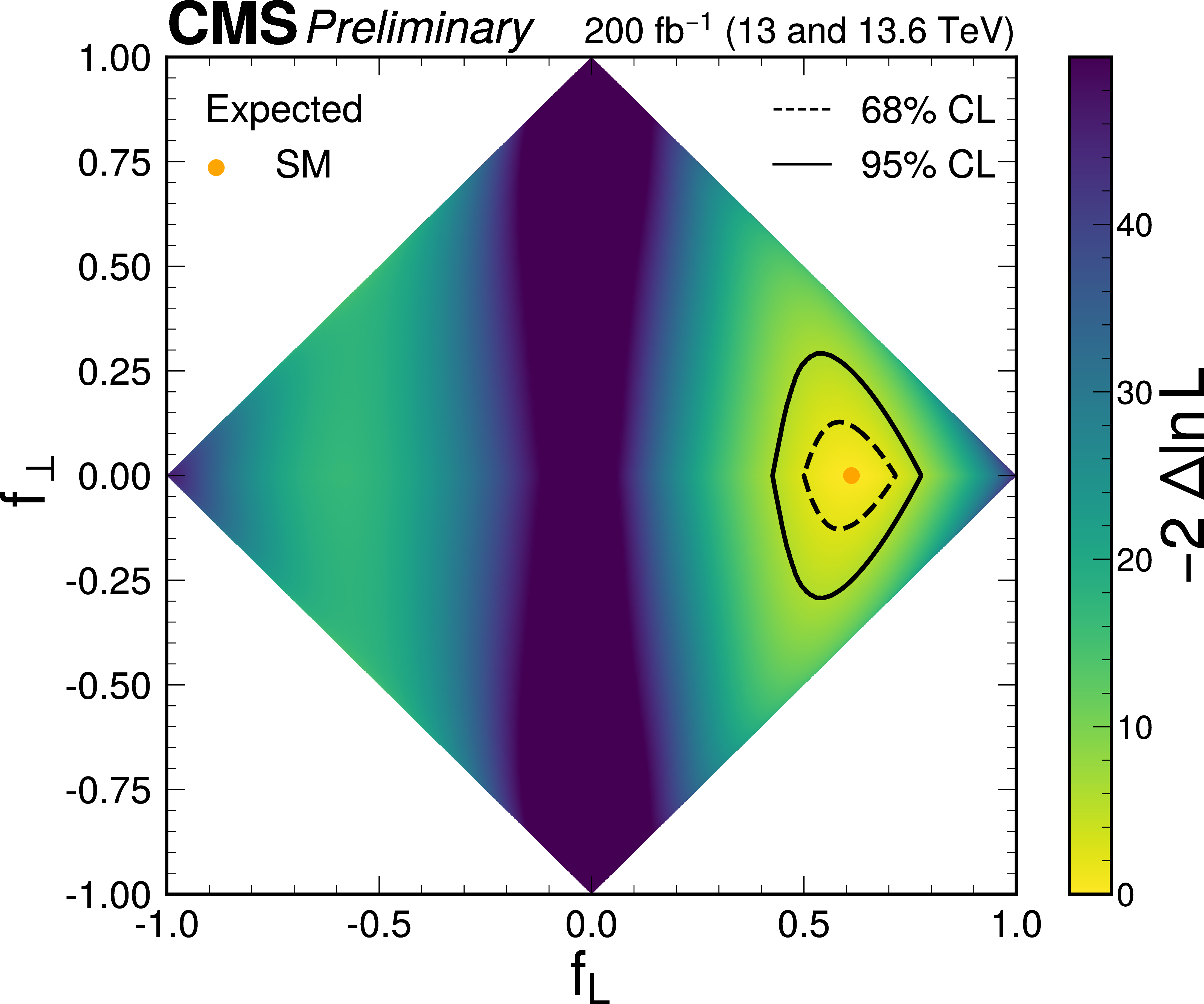
Figure 10:
The observed (left) and expected (right) likelihood scans in the $ (f_{L},f_{\perp}) $ parameter plane, which are equivalent to scans in Fig. 9. |
png pdf |
Figure 10-a:
The observed (left) and expected (right) likelihood scans in the $ (f_{L},f_{\perp}) $ parameter plane, which are equivalent to scans in Fig. 9. |
png pdf |
Figure 10-b:
The observed (left) and expected (right) likelihood scans in the $ (f_{L},f_{\perp}) $ parameter plane, which are equivalent to scans in Fig. 9. |
png pdf |
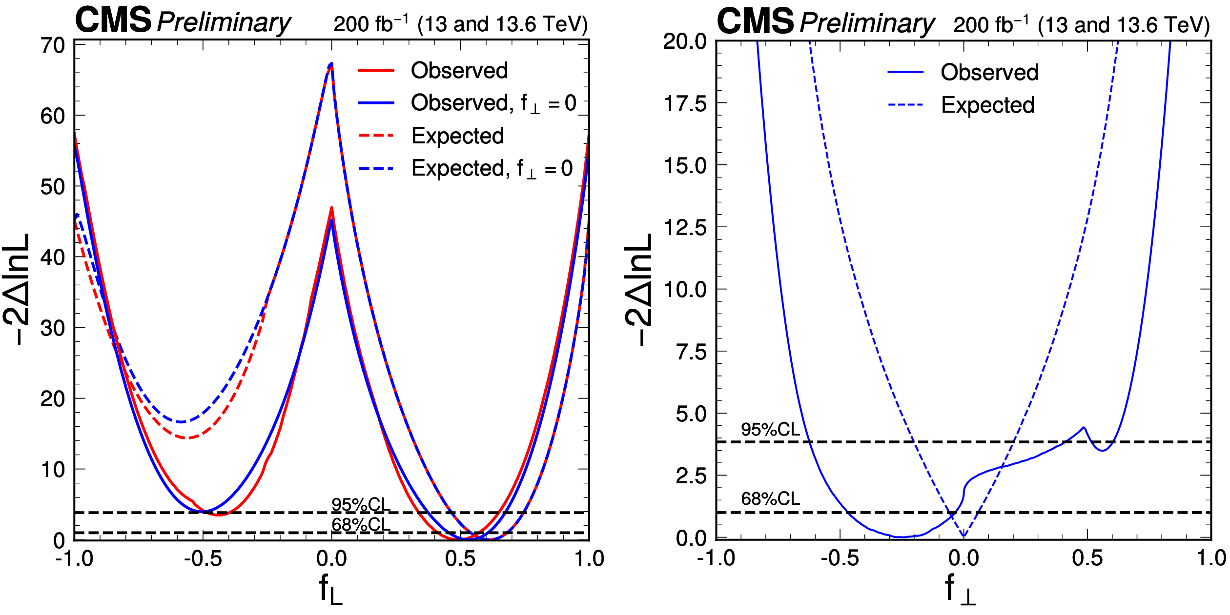
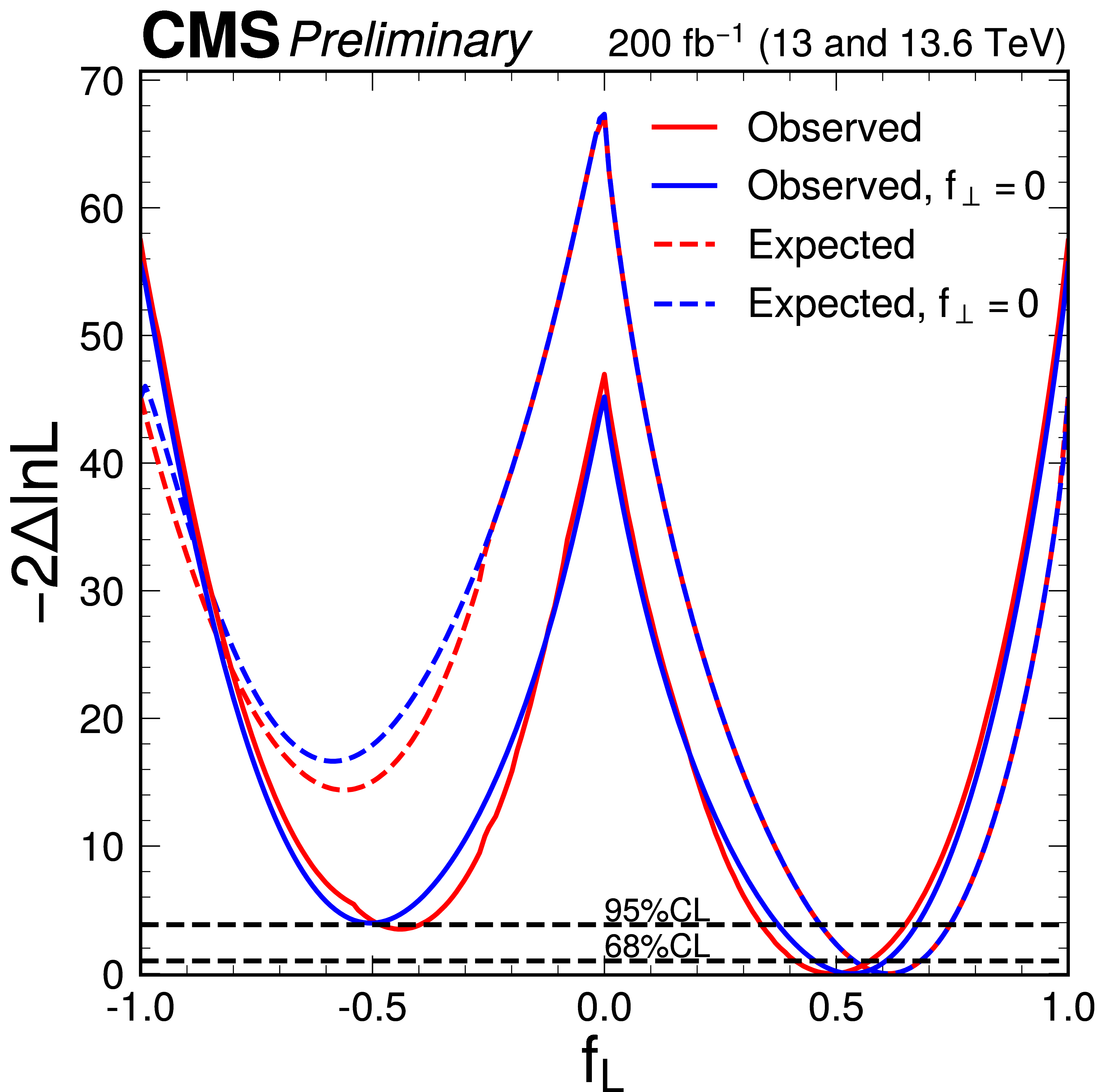
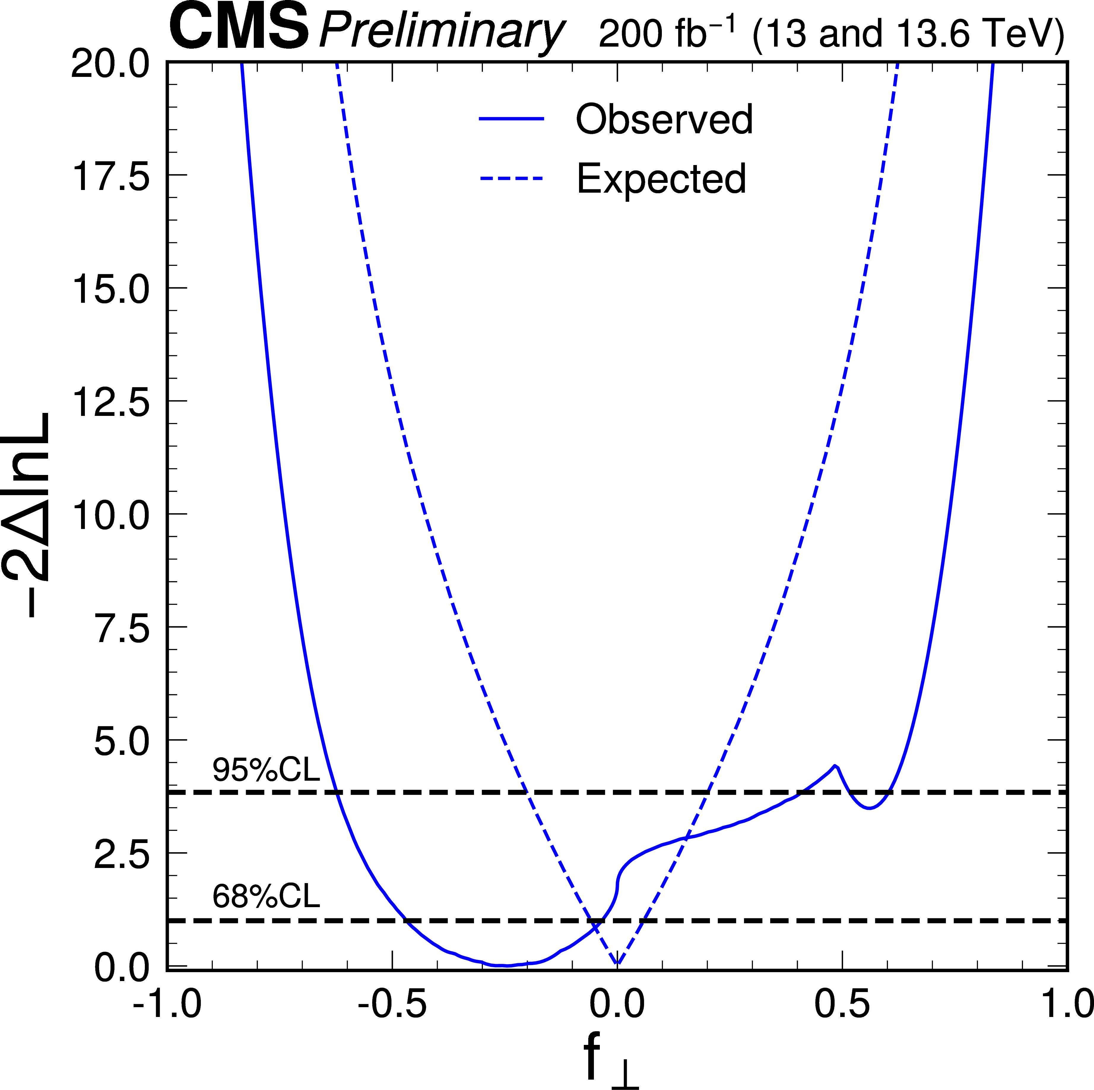
Figure 11:
The observed (solid) and expected (dashed) likelihood scans of $ f_L $ (left) and $ f_{\perp} $ (right). The $ f_L $ scan corresponds to either $ f_{\perp} $ profiled (red) or $ f_{\perp}= $ 0 (blue) in Fig. 9. The $ f_{\perp} $ scan is performed with the $ f^\prime_{L} $ profiled in Fig. 9. The expectation corresponds to the SM scenario $ f_{L} = $ 0.61 and $ f_{\perp} = $ 0. |
png pdf |
Figure 11-a:
The observed (solid) and expected (dashed) likelihood scans of $ f_L $ (left) and $ f_{\perp} $ (right). The $ f_L $ scan corresponds to either $ f_{\perp} $ profiled (red) or $ f_{\perp}= $ 0 (blue) in Fig. 9. The $ f_{\perp} $ scan is performed with the $ f^\prime_{L} $ profiled in Fig. 9. The expectation corresponds to the SM scenario $ f_{L} = $ 0.61 and $ f_{\perp} = $ 0. |
png pdf |
Figure 11-b:
The observed (solid) and expected (dashed) likelihood scans of $ f_L $ (left) and $ f_{\perp} $ (right). The $ f_L $ scan corresponds to either $ f_{\perp} $ profiled (red) or $ f_{\perp}= $ 0 (blue) in Fig. 9. The $ f_{\perp} $ scan is performed with the $ f^\prime_{L} $ profiled in Fig. 9. The expectation corresponds to the SM scenario $ f_{L} = $ 0.61 and $ f_{\perp} = $ 0. |
png pdf |
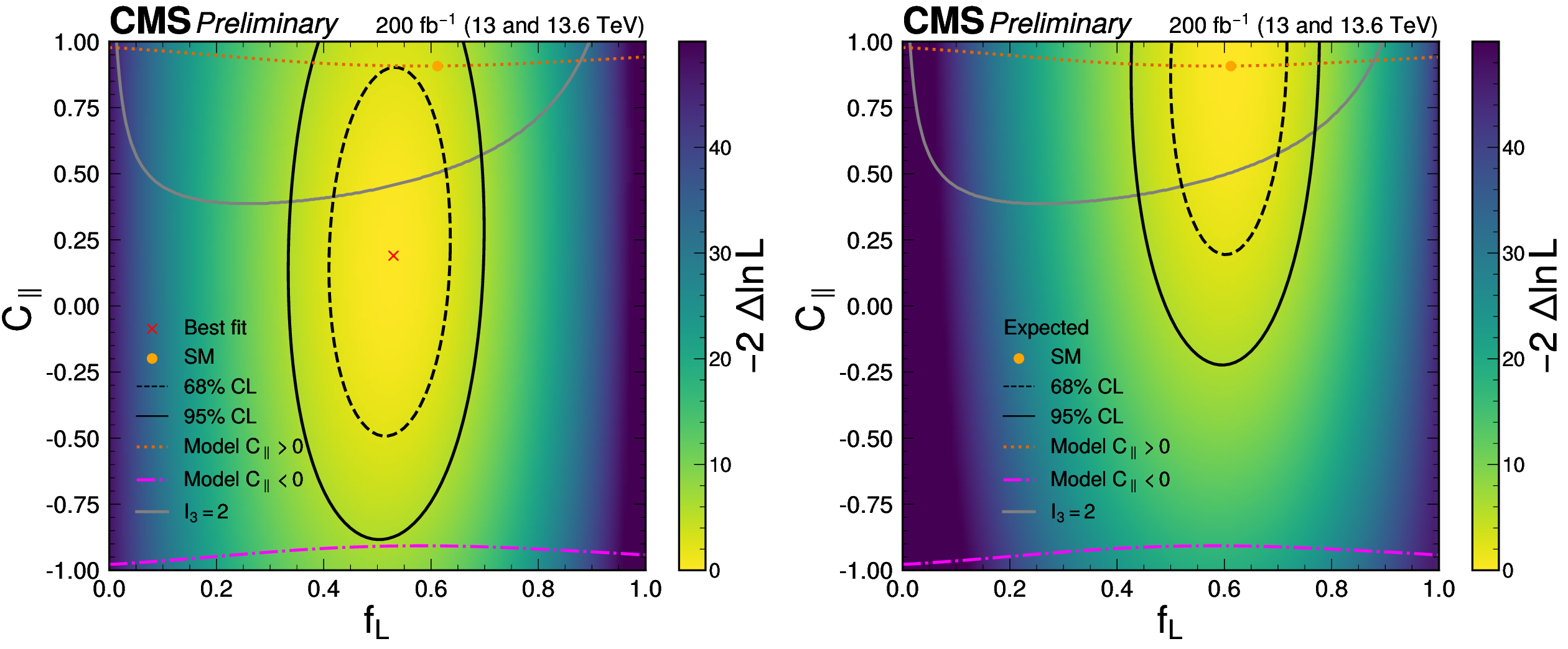
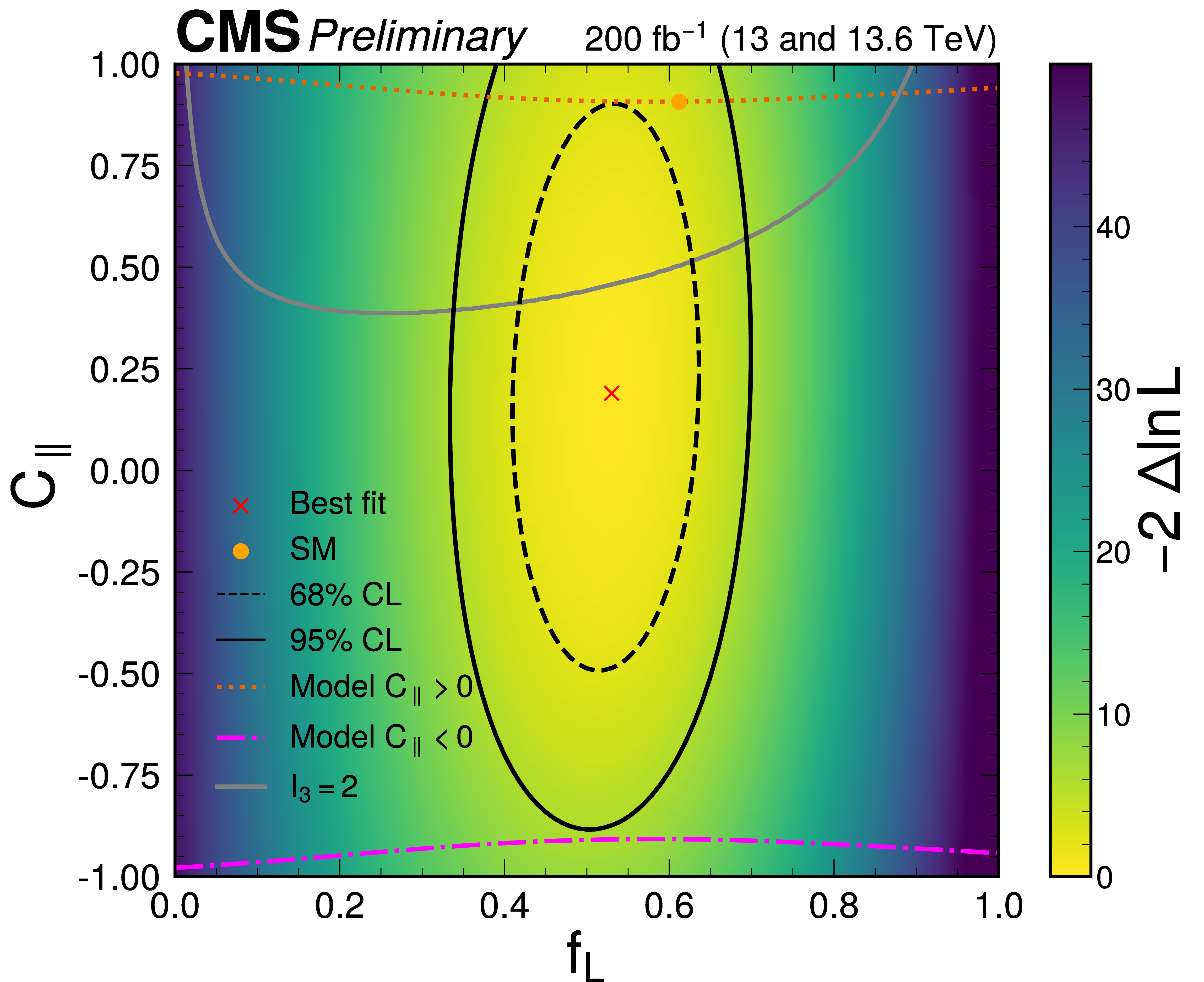
Figure 12:
The observed (left) and expected (right) likelihood scans in the $ (f_{L},C_{\parallel}) $ parameter plane. The yellow point, corresponding to $ f_{L} = $ 0.61 and $ C_{\parallel} = $ 0.91, represents the SM. The dotted line passing through the SM point indicates the values of $ C_{\parallel} $ associated with a model of smoothly interpolated amplitudes between different $ f_{L} $ values resulting in strong coherence between the transverse and longitudinal amplitudes. The dot-dashed line shows the corresponding values for negative $ C_{\parallel} $. The grey curve represents the case $ I_3 = $ 2, with points above this curve corresponding to $ I_3 > $ 2, while points below correspond to $ I_3 < $ 2. |
png pdf |
Figure 12-a:
The observed (left) and expected (right) likelihood scans in the $ (f_{L},C_{\parallel}) $ parameter plane. The yellow point, corresponding to $ f_{L} = $ 0.61 and $ C_{\parallel} = $ 0.91, represents the SM. The dotted line passing through the SM point indicates the values of $ C_{\parallel} $ associated with a model of smoothly interpolated amplitudes between different $ f_{L} $ values resulting in strong coherence between the transverse and longitudinal amplitudes. The dot-dashed line shows the corresponding values for negative $ C_{\parallel} $. The grey curve represents the case $ I_3 = $ 2, with points above this curve corresponding to $ I_3 > $ 2, while points below correspond to $ I_3 < $ 2. |
png pdf |
Figure 12-b:
The observed (left) and expected (right) likelihood scans in the $ (f_{L},C_{\parallel}) $ parameter plane. The yellow point, corresponding to $ f_{L} = $ 0.61 and $ C_{\parallel} = $ 0.91, represents the SM. The dotted line passing through the SM point indicates the values of $ C_{\parallel} $ associated with a model of smoothly interpolated amplitudes between different $ f_{L} $ values resulting in strong coherence between the transverse and longitudinal amplitudes. The dot-dashed line shows the corresponding values for negative $ C_{\parallel} $. The grey curve represents the case $ I_3 = $ 2, with points above this curve corresponding to $ I_3 > $ 2, while points below correspond to $ I_3 < $ 2. |
png pdf |
Figure 13:
The observed (solid) and expected (dashed) likelihood scan of $ f_L $ with $ C_{\parallel} $ profiled (left) and $ C_{\parallel} $ with $ f_L $ profiled (right), both from the fit corresponding to Fig. 12 with expectation corresponding to the SM scenario with $ f_L = $ 0.61 and $ C_{\parallel} = $ 0.91. |
png pdf |
Figure 13-a:
The observed (solid) and expected (dashed) likelihood scan of $ f_L $ with $ C_{\parallel} $ profiled (left) and $ C_{\parallel} $ with $ f_L $ profiled (right), both from the fit corresponding to Fig. 12 with expectation corresponding to the SM scenario with $ f_L = $ 0.61 and $ C_{\parallel} = $ 0.91. |
png pdf |
Figure 13-b:
The observed (solid) and expected (dashed) likelihood scan of $ f_L $ with $ C_{\parallel} $ profiled (left) and $ C_{\parallel} $ with $ f_L $ profiled (right), both from the fit corresponding to Fig. 12 with expectation corresponding to the SM scenario with $ f_L = $ 0.61 and $ C_{\parallel} = $ 0.91. |
png pdf |
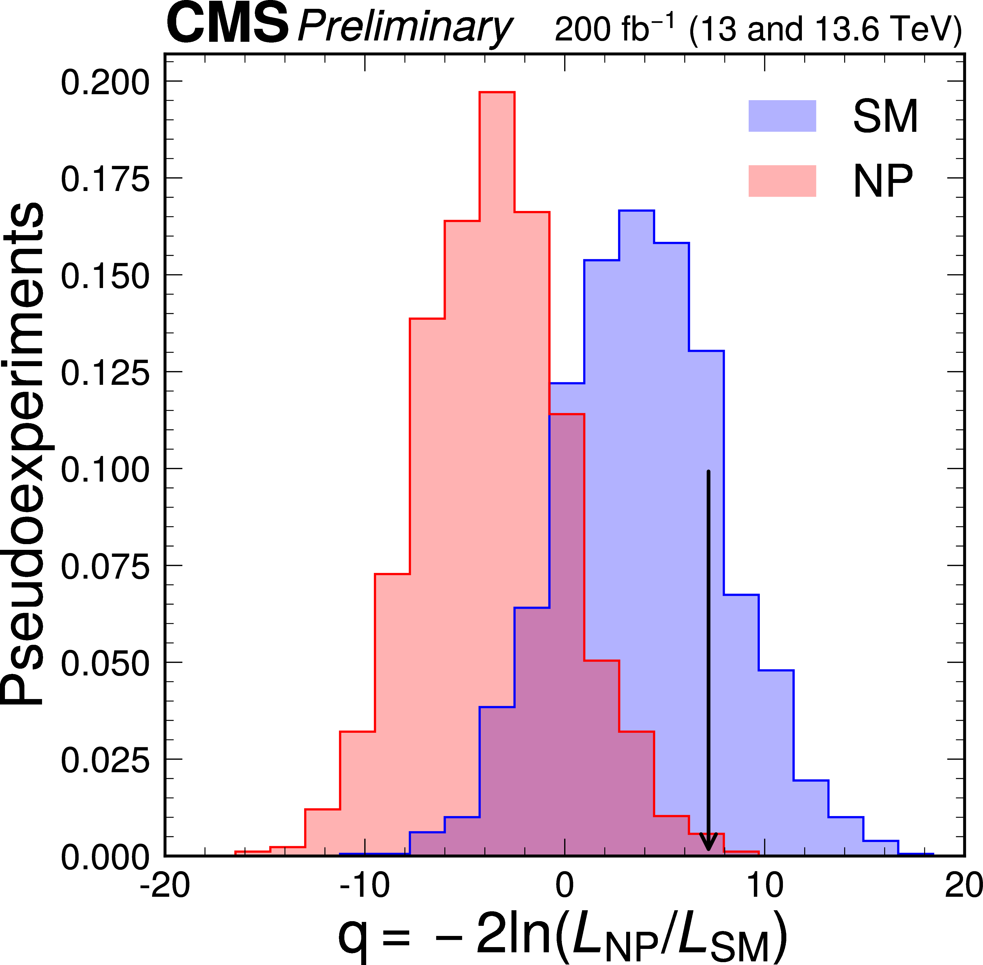
Figure 14:
The observed value ($ q_\mathrm{obs} $, black arrow) and expected distributions of the test statistic $ q $ for the SM (blue) and the model with no permutation of leptons (NP, red) in the analysis of the $ \mathrm{H}\to\mathrm{Z}\mathrm{Z}\to 4\ell $ decays. |
png pdf |
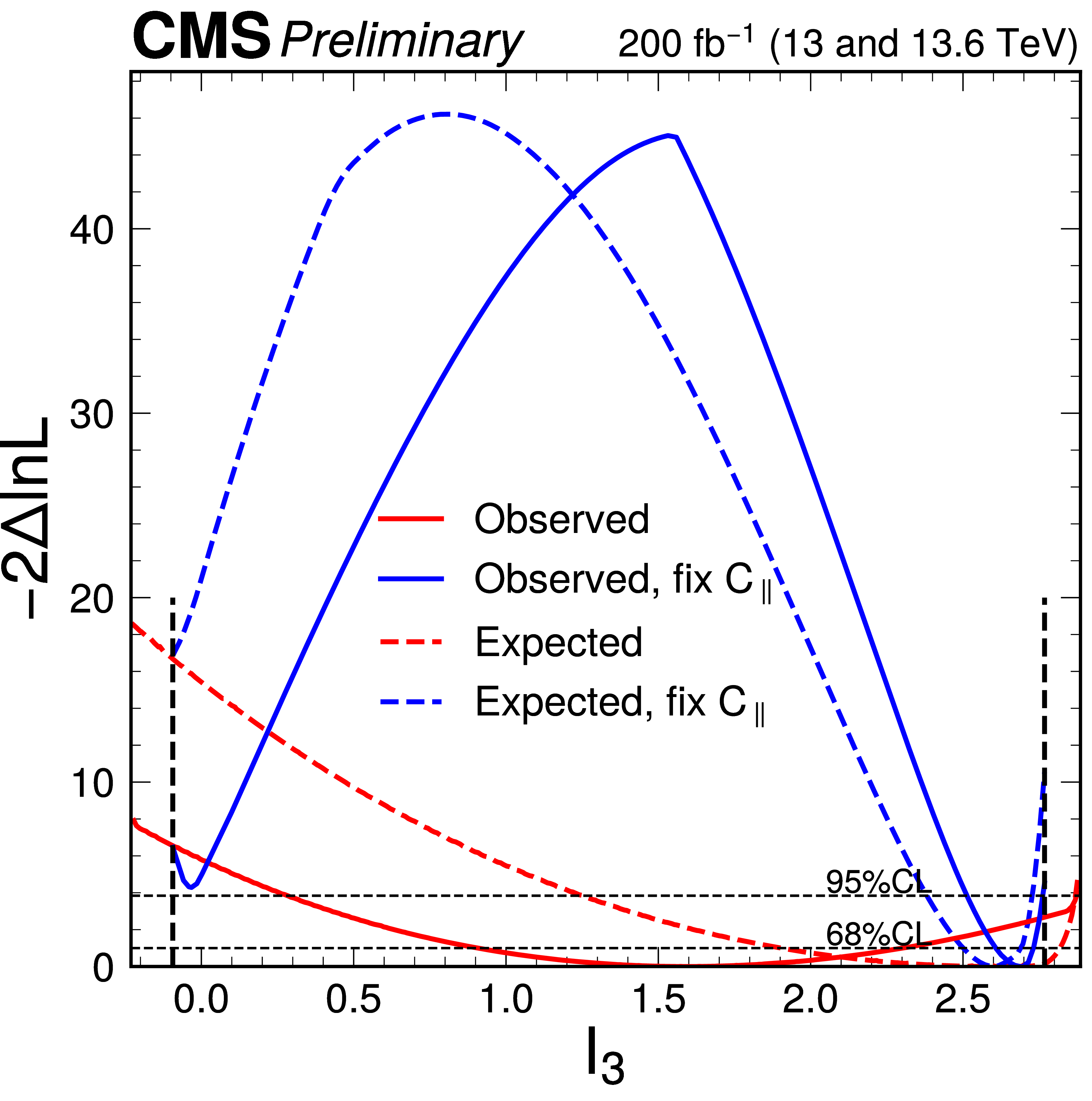
Figure 15:
Observed (solid) and expected (dashed) likelihood scans of $ I_3 $ in two scenarios, with $ |C_\parallel| $ fixed to large values (blue) and with both $ f_L $ and $ C_\parallel $ unconstrained (red). The two vertical dashed lines indicate the bounds $ -0.09 < I_3 < $ 2.77 for fixed large values of $ |C_\parallel| $. |
| Tables | |
png pdf |
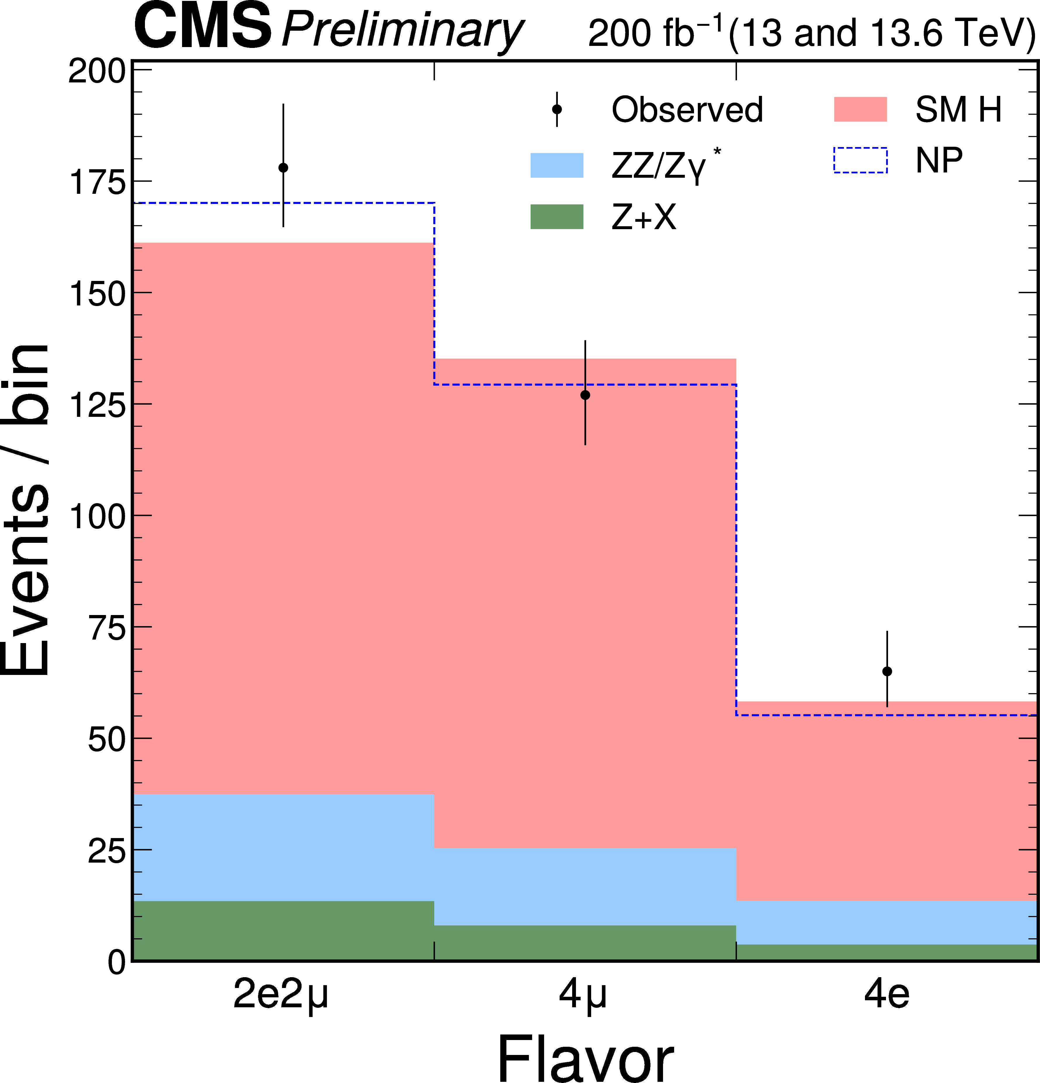
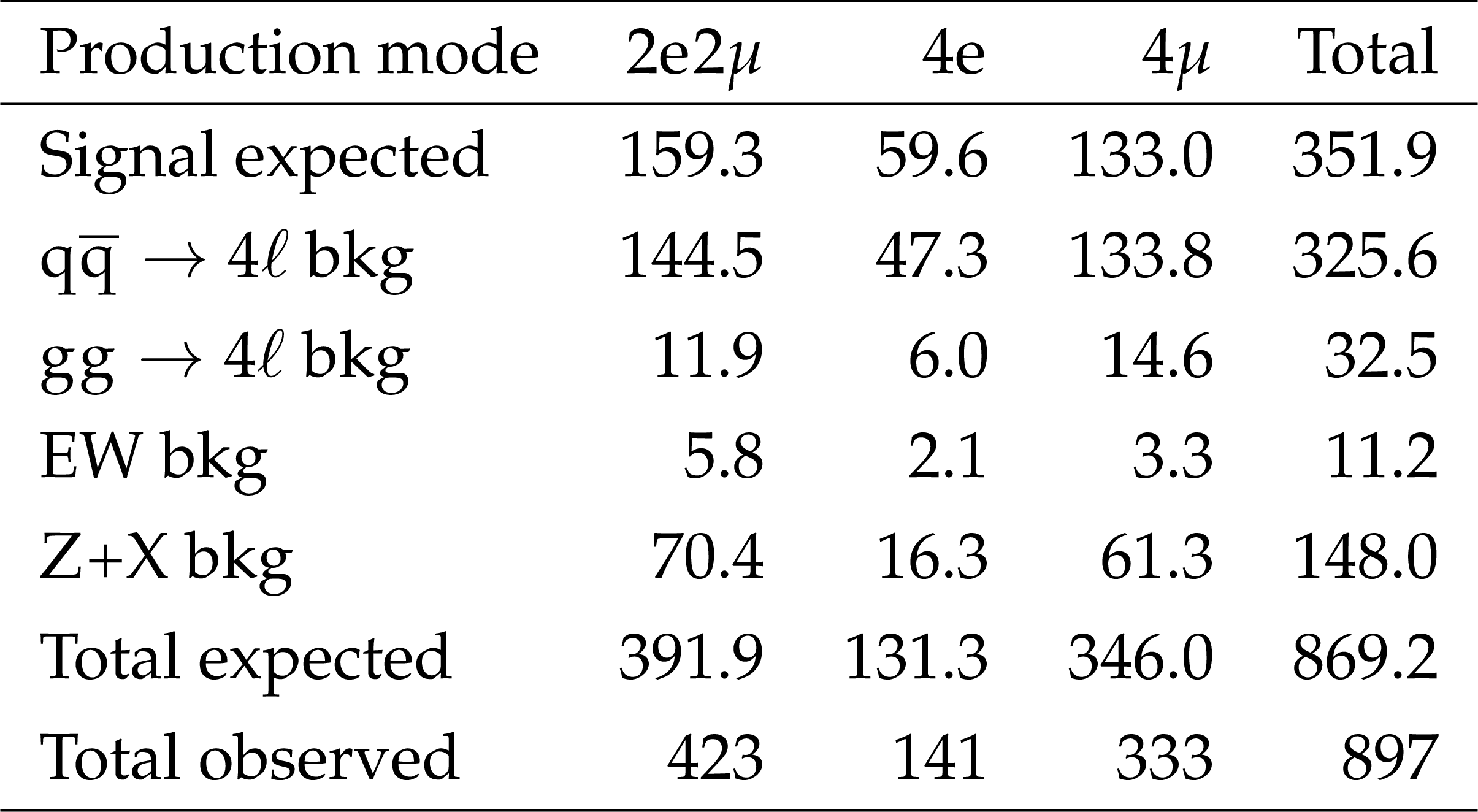
Table 1:
The observed event yields within the mass range 105 $ < m_{4\ell} < $ 140 GeV, along with the expected signal and background (bkg) yields, are presented for each of the three individual final states and their combination in the $ \mathrm{H} \to 4\ell $ analysis. |
png pdf |
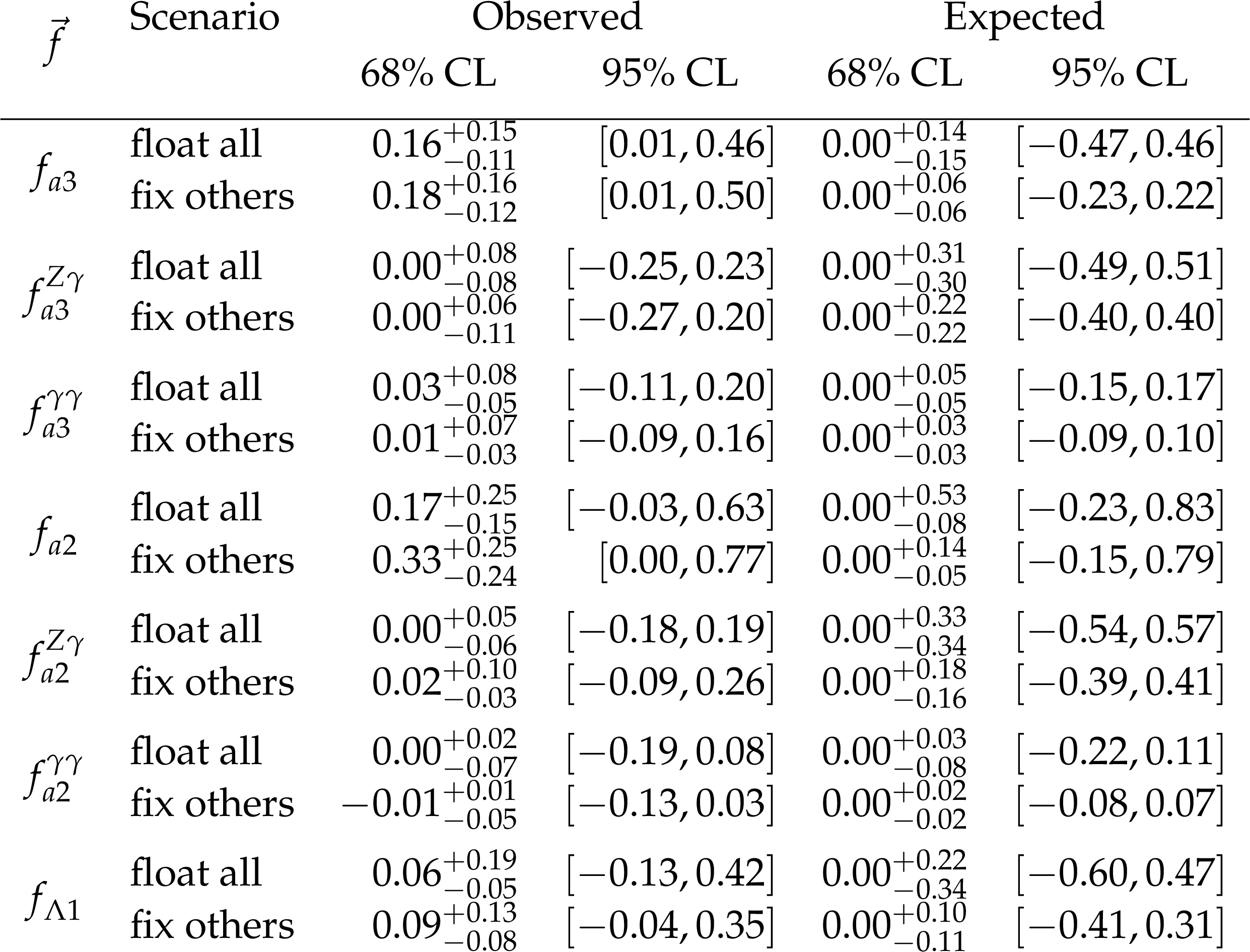
Table 2:
Observed and expected constraints on fractional contribution in the EFT framework. |
png pdf |
Table 3:
Observed and expected constraints on $ f_L $, $ f_\perp $, and $ C_\parallel $ in three fitting scenarios. The three $ f_L $ measurements are reported with either $ f_\perp $ or $ C_\parallel $ profiled in the fits corresponding to Fig. 9 or 12, respectively, or with both fixed as indicated in the second column. The $ f_\perp $ and $ C_\parallel $ results are presented with $ f_L $ profiled in the corresponding fits. The reported correlation coefficients correspond to the observed / average expected values in the SM. |
png pdf |
Table 4:
The observed and average expected values of the $ p $-value and the associated $ Z $-score are shown for a model with no permutation of identical leptons (NP) in the decay $ \mathrm{H}\to\mathrm{Z}\mathrm{Z}\to 4\ell $ tested against the SM. |
png pdf |
Table 5:
Observed and expected constraints on the parameter $ I_3 $ are shown for two scenarios: one where $ |C_\parallel| $ is fixed at large values for each value of $ f_L $, reflecting smoothly varying amplitudes across different $ f_L $ values, and another where both $ f_L $ and $ C_\parallel $ are profiled. |
| Summary |
| Kinematic effects in the Higgs boson decay to four leptons $ \mathrm{H} \to 4\ell $ have been studied using full detector simulation and matrix element techniques, optimizing sensitivity to the tensor structure of Higgs boson interactions and spin correlations in the decay process. A simultaneous measurement of eight H boson couplings to electroweak vector bosons has been carried out within the frameworks of anomalous couplings and effective field theory. This represents the most general analysis of kinematic distributions in the $ \mathrm{H} \to 4\ell $ decay channel to date. Quantum mechanical interference has been tested through the permutation of identical leptons and the model of no permutation is excluded at 2.7$ \sigma $. A search for CP violation in the polarization of the Z bosons has been conducted, with results consistent with the SM. Under the assumption of CP symmetry conservation, the polarization density matrix in the $ \mathrm{H} \to\mathrm{Z}\mathrm{Z} $ decay has been measured with two free parameters, the fraction of longitudinal polarization and the amplitude coherence parameter. The fully longitudinal and fully transverse polarization of the Z bosons are excluded at more than 6$ \sigma $. This establishes the entangled state of qutrits under the assumptions of Quantum Mechanics and CP conservation. With an additional assumption of large coherence of the transverse and longitudinal amplitudes, it has been established that conditions exist for measuring violation of the Bell-type inequality in the $ \mathrm{H} \to\mathrm{Z}\mathrm{Z} $ decays. |
| References | ||||
| 1 | ATLAS Collaboration | Observation of a new particle in the search for the Standard Model Higgs boson with the ATLAS detector at the LHC | PLB 716 (2012) 1 | 1207.7214 |
| 2 | CMS Collaboration | Observation of a new boson at a mass of 125 GeV with the CMS experiment at the LHC | PLB 716 (2012) 30 | CMS-HIG-12-028 1207.7235 |
| 3 | CMS Collaboration | Observation of a new boson with mass near 125 GeV in pp collisions at $ \sqrt{s}= $ 7 and 8 TeV | JHEP 06 (2013) 081 | CMS-HIG-12-036 1303.4571 |
| 4 | S. L. Glashow | Partial-symmetries of weak interactions | NP 22 (1961) 579 | |
| 5 | F. Englert and R. Brout | Broken symmetry and the mass of gauge vector mesons | PRL 13 (1964) 321 | |
| 6 | P. W. Higgs | Broken symmetries, massless particles and gauge fields | PL 12 (1964) 132 | |
| 7 | P. W. Higgs | Broken symmetries and the masses of gauge bosons | PRL 13 (1964) 508 | |
| 8 | G. S. Guralnik, C. R. Hagen, and T. W. B. Kibble | Global conservation laws and massless particles | PRL 13 (1964) 585 | |
| 9 | S. Weinberg | A model of leptons | PRL 19 (1967) 1264 | |
| 10 | A. Salam | Weak and Electromagnetic Interactions | Conf. Proc. C 690519 (1968) 367 | |
| 11 | CMS Collaboration | On the mass and spin-parity of the Higgs boson candidate via its decays to Z boson pairs | PRL 110 (2013) 081803 | CMS-HIG-12-041 1212.6639 |
| 12 | CMS Collaboration | Measurement of the properties of a Higgs boson in the four-lepton final state | PRD 89 (2014) 092007 | CMS-HIG-13-002 1312.5353 |
| 13 | CMS Collaboration | Constraints on the spin-parity and anomalous $ \mathrm{H}\mathrm{V}\mathrm{V} $ couplings of the Higgs boson in proton collisions at 7 and 8 TeV | PRD 92 (2015) 012004 | CMS-HIG-14-018 1411.3441 |
| 14 | CMS Collaboration | Limits on the Higgs boson lifetime and width from its decay to four charged leptons | PRD 92 (2015) 072010 | CMS-HIG-14-036 1507.06656 |
| 15 | CMS Collaboration | Combined search for anomalous pseudoscalar $ \mathrm{H}\mathrm{V}\mathrm{V} $ couplings in VH ($ \mathrm{H}\to\mathrm{b}\overline{\mathrm{b}} $) production and $ \mathrm{H}\to\mathrm{VV} $ decay | PLB 759 (2016) 672 | CMS-HIG-14-035 1602.04305 |
| 16 | CMS Collaboration | Constraints on anomalous Higgs boson couplings using production and decay information in the four-lepton final state | PLB 775 (2017) 1 | CMS-HIG-17-011 1707.00541 |
| 17 | CMS Collaboration | Measurements of the Higgs boson width and anomalous HVV couplings from on-shell and off-shell production in the four-lepton final state | PRD 99 (2019) 112003 | CMS-HIG-18-002 1901.00174 |
| 18 | CMS Collaboration | Constraints on anomalous $ HVV $ couplings from the production of Higgs bosons decaying to $ \tau $ lepton pairs | PRD 100 (2019) 112002 | CMS-HIG-17-034 1903.06973 |
| 19 | CMS Collaboration | Constraints on anomalous Higgs boson couplings to vector bosons and fermions in its production and decay using the four-lepton final state | PRD 104 (2021) 052004 | CMS-HIG-19-009 2104.12152 |
| 20 | CMS Collaboration | Measurement of the Higgs boson width and evidence of its off-shell contributions to ZZ production | Nature Phys. 18 (2022) 1329 | CMS-HIG-21-013 2202.06923 |
| 21 | CMS Collaboration | Constraints on anomalous Higgs boson couplings to vector bosons and fermions from the production of Higgs bosons using the $\tau\tau$ final state | PRD 108 (2023) 032013 | CMS-HIG-20-007 2205.05120 |
| 22 | CMS Collaboration | Constraints on anomalous Higgs boson couplings from its production and decay using the WW channel in proton-proton collisions at $ \sqrt{s} = $ 13 TeV | EPJC 84 (2024) 779 | CMS-HIG-22-008 2403.00657 |
| 23 | ATLAS Collaboration | Evidence for the spin-0 nature of the Higgs boson using ATLAS data | PLB 726 (2013) 120 | 1307.1432 |
| 24 | ATLAS Collaboration | Study of the spin and parity of the Higgs boson in diboson decays with the ATLAS detector | EPJC 75 (2015) 476 | 1506.05669 |
| 25 | ATLAS Collaboration | Test of CP Invariance in vector-boson fusion production of the Higgs boson using the Optimal Observable method in the ditau decay channel with the ATLAS detector | EPJC 76 (2016) 658 | 1602.04516 |
| 26 | ATLAS Collaboration | Measurement of inclusive and differential cross sections in the $ \mathrm{H} \rightarrow \mathrm{Z}\mathrm{Z}^{*} \rightarrow 4\ell $ decay channel in pp collisions at $ \sqrt{s}= $ 13 TeV with the ATLAS detector | JHEP 10 (2017) 132 | 1708.02810 |
| 27 | ATLAS Collaboration | Measurement of the Higgs boson coupling properties in the $ H\rightarrow ZZ^{*} \rightarrow 4\ell $ decay channel at $ \sqrt{s} = $ 13 TeV with the ATLAS detector | JHEP 03 (2018) 095 | 1712.02304 |
| 28 | ATLAS Collaboration | Higgs boson production cross-section measurements and their EFT interpretation in the 4 $ \ell $ decay channel at $ \sqrt{s}= $13 TeV with the ATLAS detector | EPJC 80 (2020) 957 | 2004.03447 |
| 29 | ATLAS Collaboration | Measurement of the properties of Higgs boson production at $ \sqrt{s} = $ 13 TeV in the $ H\to\gamma\gamma $ channel using 139 fb$ ^{-1} $ of $ pp $ collision data with the ATLAS experiment | JHEP 07 (2023) 088 | 2207.00348 |
| 30 | ATLAS Collaboration | Test of CP Invariance in Higgs Boson Vector-Boson-Fusion Production Using the H$ \rightarrow{\gamma}{\gamma} $ Channel with the ATLAS Detector | PRL 131 (2023) 061802 | 2208.02338 |
| 31 | ATLAS Collaboration | Test of CP-invariance of the Higgs boson in vector-boson fusion production and in its decay into four leptons | JHEP 05 (2024) 105 | 2304.09612 |
| 32 | I. Brivio et al. | Truncation, validity, uncertainties | link | 2201.04974 |
| 33 | J. Davis et al. | Constraining anomalous Higgs boson couplings to virtual photons | PRD 105 (2022) 096027 | 2109.13363 |
| 34 | J. S. Bell | On the Einstein-Podolsky-Rosen paradox | Physics Physique Fizika 1 (1964) 195 | |
| 35 | D. Collins et al. | Bell Inequalities for Arbitrarily High-Dimensional Systems | PRL 88 (2002) 040404 | quant-ph/0106024 |
| 36 | J. A. Aguilar-Saavedra, A. Bernal, J. A. Casas, and J. M. Moreno | Testing entanglement and Bell inequalities in $ H\to ZZ $ | PRD 107 (2023) 016012 | 2209.13441 |
| 37 | M. Grossi, G. Pelliccioli, and A. Vicini | From angular coefficients to quantum observables: a phenomenological appraisal in di-boson systems | JHEP 12 (2024) 120 | 2409.16731 |
| 38 | M. Del Gratta et al. | Quantum properties of $ H\to VV^{*} $: precise predictions in the SM and sensitivity to new physics | JHEP 09 (2025) 013 | 2504.03841 |
| 39 | D. Gon \c c alves, A. Kaladharan, F. Krauss, and A. Navarro | Quantum Entanglement is Quantum: ZZ Production at the LHC | link | 2505.12125 |
| 40 | M. Del Gratta et al. | Z-boson quantum tomography at next-to-leading order | link | 2509.20456 |
| 41 | D. de Florian et al. | Handbook of LHC Higgs cross sections: 4. deciphering the nature of the Higgs sector | CERN Report CERN-2017-002-M, 2016 link |
1610.07922 |
| 42 | B. Grzadkowski, M. Iskrzynski, M. Misiak, and J. Rosiek | Dimension-Six Terms in the Standard Model Lagrangian | JHEP 10 (2010) 085 | 1008.4884 |
| 43 | C. N. Leung, S. T. Love, and S. Rao | Low-Energy Manifestations of a New Interaction Scale: Operator Analysis | Z. Phys. C 31 (1986) 433 | |
| 44 | A. Dedes et al. | Feynman rules for the Standard Model Effective Field Theory in R$ _{?} $ -gauges | JHEP 06 (2017) 143 | 1704.03888 |
| 45 | D. Barducci et al. | Parametrisation and dictionary for CP violating Higgs boson interactions | link | 2511.07905 |
| 46 | Y. Gao et al. | Spin determination of single-produced resonances at hadron colliders | PRD 81 (2010) 075022 | 1001.3396 |
| 47 | S. Bolognesi et al. | Spin and parity of a single-produced resonance at the LHC | PRD 86 (2012) 095031 | 1208.4018 |
| 48 | A. Gritsan and the Particle Data Group | Polarization in $ B $ decays | Review of Particle Physics 110 (2024) 030001 | |
| 49 | BaBar Collaboration | Vector-tensor and vector-vector decay amplitude analysis of $ B^0 \to \phi K^{*0} $ | PRL 98 (2007) 051801 | hep-ex/0610073 |
| 50 | ATLAS Collaboration | Measurements of Higgs boson properties in the diphoton decay channel with 36 fb$ ^{-1} $ of pp collision data at $ \sqrt{s} = $ 13 TeV with the ATLAS detector | PRD 98 (2018) 052005 | 1802.04146 |
| 51 | S. A. Abel, M. Dittmar, and H. K. Dreiner | Testing locality at colliders via Bell's inequality? | PLB 280 (1992) 304 | |
| 52 | P. Bechtle, C. Breuning, H. K. Dreiner, and C. Duhr | A critical appraisal of tests of locality and of entanglement versus non-entanglement at colliders | link | 2507.15947 |
| 53 | S. A. Abel, H. K. Dreiner, R. Sengupta, and L. Ubaldi | Colliders are Testing neither Locality via Bell's Inequality nor Entanglement versus Non-Entanglement | link | 2507.15949 |
| 54 | A. Einstein, B. Podolsky, and N. Rosen | Can quantum mechanical description of physical reality be considered complete? | PR 47 (1935) | |
| 55 | D. Bohm | A Suggested interpretation of the quantum theory in terms of hidden variables. 1. | PR 85 (1952) 166 | |
| 56 | CMS Collaboration | The CMS experiment at the CERN LHC | JINST 3 (2008) S08004 | |
| 57 | CMS Collaboration | Development of the CMS detector for the CERN LHC Run 3 | JINST 19 (2024) P05064 | CMS-PRF-21-001 2309.05466 |
| 58 | CMS Collaboration | Performance of the CMS Level-1 trigger in proton-proton collisions at $ \sqrt{s} = $ 13 TeV | JINST 15 (2020) P10017 | CMS-TRG-17-001 2006.10165 |
| 59 | CMS Collaboration | The CMS trigger system | JINST 12 (2017) P01020 | CMS-TRG-12-001 1609.02366 |
| 60 | I. Anderson et al. | Constraining anomalous $ \mathrm{H}\mathrm{V}\mathrm{V} $ interactions at proton and lepton colliders | PRD 89 (2014) 035007 | 1309.4819 |
| 61 | A. V. Gritsan, R. Rontsch, M. Schulze, and M. Xiao | Constraining anomalous Higgs boson couplings to the heavy flavor fermions using matrix element techniques | PRD 94 (2016) 055023 | 1606.03107 |
| 62 | J. M. Campbell and R. K. Ellis | MCFM for the Tevatron and the LHC | -206 10, 2010 Nucl. Phys. Proc. Suppl. 20 (2010) 5 |
1007.3492 |
| 63 | P. Nason | A New method for combining NLO QCD with shower Monte Carlo algorithms | JHEP 11 (2004) 040 | hep-ph/0409146 |
| 64 | S. Alioli, P. Nason, C. Oleari, and E. Re | A general framework for implementing NLO calculations in shower Monte Carlo programs: the POWHEG BOX | JHEP 06 (2010) 043 | 1002.2581 |
| 65 | S. Frixione, P. Nason, and C. Oleari | Matching NLO QCD computations with parton shower simulations: the POWHEG method | JHEP 11 (2007) 070 | 0709.2092 |
| 66 | E. Bagnaschi, G. Degrassi, P. Slavich, and A. Vicini | Higgs production via gluon fusion in the POWHEG approach in the SM and in the MSSM | JHEP 02 (2012) 088 | 1111.2854 |
| 67 | P. Nason and C. Oleari | NLO Higgs boson production via vector-boson fusion matched with shower in POWHEG | JHEP 02 (2010) 037 | 0911.5299 |
| 68 | G. Luisoni, P. Nason, C. Oleari, and F. Tramontano | $ \mathrm{H}\mathrm{W}^{\pm} $/HZ + 0 and 1 jet at NLO with the POWHEG BOX interfaced to GoSam and their merging within MiNLO | JHEP 10 (2013) 083 | 1306.2542 |
| 69 | H. B. Hartanto, B. Jager, L. Reina, and D. Wackeroth | Higgs boson production in association with top quarks in the POWHEG BOX | PRD 91 (2015) 094003 | 1501.04498 |
| 70 | M. Grazzini, S. Kallweit, and D. Rathlev | ZZ production at the LHC: fiducial cross sections and distributions in NNLO QCD | PLB 750 (2015) 407 | 1507.06257 |
| 71 | S. Gieseke, T. Kasprzik, and J. H. Kuehn | Vector-boson pair production and electroweak corrections in HERWIG++ | EPJC 74 (2014) 2988 | 1401.3964 |
| 72 | J. Baglio, L. D. Ninh, and M. M. Weber | Massive gauge boson pair production at the LHC: a next-to-leading order story | PRD 88 (2013) 113005 | 1307.4331 |
| 73 | J. M. Campbell, R. K. Ellis, and C. Williams | Vector boson pair production at the LHC | JHEP 07 (2011) 018 | 1105.0020 |
| 74 | J. M. Campbell, R. K. Ellis, and C. Williams | Bounding the Higgs width at the LHC using full analytic results for $ \mathrm{g}\mathrm{g}\to \mathrm{e}^{-}\mathrm{e}^{+} \mu^{-} \mu^{+} $ | JHEP 04 (2014) 060 | 1311.3589 |
| 75 | J. M. Campbell and R. K. Ellis | Higgs constraints from vector boson fusion and scattering | JHEP 04 (2015) 030 | 1502.02990 |
| 76 | J. Alwall et al. | The automated computation of tree-level and next-to-leading order differential cross sections, and their matching to parton shower simulations | JHEP 07 (2014) 079 | 1405.0301 |
| 77 | F. Demartin et al. | Higgs characterisation at NLO in QCD: CP properties of the top-quark Yukawa interaction | EPJC 74 (2014) 3065 | 1407.5089 |
| 78 | NNPDF Collaboration | Unbiased global determination of parton distributions and their uncertainties at NNLO and at LO | NPB 855 (2012) 153 | 1107.2652 |
| 79 | T. Sjostrand et al. | An introduction to PYTHIA 8.2 | Comput. Phys. Commun. 191 (2015) 159 | 1410.3012 |
| 80 | GEANT4 Collaboration | GEANT 4 -- a simulation toolkit | NIM A 506 (2003) 250 | |
| 81 | CMS Collaboration | Measurements of properties of the Higgs boson decaying into the four-lepton final state in pp collisions at $ \sqrt{s}= $ 13 TeV | JHEP 11 (2017) 047 | CMS-HIG-16-041 1706.09936 |
| 82 | CMS Collaboration | Measurements of production cross sections of the Higgs boson in the four-lepton final state in proton-proton collisions at $ \sqrt{s} = $ 13 TeV | EPJC 81 (2021) 488 | CMS-HIG-19-001 2103.04956 |
| 83 | CMS Collaboration | Measurements of the Higgs boson production cross section in the four-lepton final state in proton-proton collisions at $ \sqrt{s} = $ 13.6 TeV | JHEP 05 (2025) 079 | CMS-HIG-24-013 2501.14849 |
| 84 | CMS Collaboration | Particle-flow reconstruction and global event description with the cms detector | JINST 12 (2017) P10003 | CMS-PRF-14-001 1706.04965 |
| 85 | M. Cacciari, G. P. Salam, and G. Soyez | The anti-$ k_{\mathrm{T}} $ jet clustering algorithm | JHEP 04 (2008) 063 | 0802.1189 |
| 86 | M. Cacciari, G. P. Salam, and G. Soyez | FastJet user manual | EPJC 72 (2012) 1896 | 1111.6097 |
| 87 | T. Chen and C. Guestrin | XGBoost: A Scalable Tree Boosting System | in Proceedings of the 22nd ACM SIGKDD International Conference on Knowledge Discovery and Data Mining, KDD '16, p. 785. Association for Computing Machinery, 2016 link |
1603.02754 |
| 88 | R. J. Barlow | Extended maximum likelihood | NIM A 297 (1990) 496 | |
| 89 | CMS Collaboration | The CMS Statistical Analysis and Combination Tool: Combine | Comput. Softw. Big Sci. 8 (2024) 19 | CMS-CAT-23-001 2404.06614 |
| 90 | W. Verkerke and D. P. Kirkby | The RooFit toolkit for data modeling | in 13$ ^\text{th} $ International Conference for Computing in High-Energy and Nuclear Physics (CHEP03). 2003.. CHEP-2003-MOLT007 | physics/0306116 |
| 91 | R. Brun and F. Rademakers | ROOT: An object oriented data analysis framework | NIM A 389 (1997) 81 | |
| 92 | S. S. Wilks | The large-sample distribution of the likelihood ratio for testing composite hypotheses | Annals Math. Statist. 9 (1938) 60 | |
| 93 | A. L. Read | Presentation of search results: the $ CL_s $ technique | JPG 28 (2002) 2693 | |
| 94 | T. Junk | Confidence level computation for combining searches with small statistics | NIM A 434 (1999) 435 | hep-ex/9902006 |
| 95 | CMS Collaboration | Precision luminosity measurement in proton-proton collisions at $ \sqrt{s} = $ 13 TeV in 2015 and 2016 at CMS | EPJC 81 (2021) 800 | CMS-LUM-17-003 2104.01927 |
| 96 | CMS Collaboration | CMS luminosity measurement for the 2017 data taking period at $ \sqrt{s} = $ 13 TeV | CMS Physics Analysis Summary, 2018 CMS-PAS-LUM-17-004 |
CMS-PAS-LUM-17-004 |
| 97 | CMS Collaboration | CMS luminosity measurement for the 2018 data-taking period at $ \sqrt{s} = $ 13 TeV | CMS Physics Analysis Summary, 2019 CMS-PAS-LUM-18-002 |
CMS-PAS-LUM-18-002 |
| 98 | CMS Collaboration | Luminosity measurement in proton-proton collisions at 13.6 TeV in 2022 at CMS | Technical Report, CERN, Geneva, 2024 CMS-PAS-LUM-22-001 |
CMS-PAS-LUM-22-001 |
|
|
Compact Muon Solenoid LHC, CERN |
|

|

|

|

|

|