

Compact Muon Solenoid
LHC, CERN
| CMS-PAS-SMP-20-014 | ||
| Measurement of the pp $\to$ WZ inclusive and differential cross sections, polarization angles and search for anomalous gauge couplings at $\sqrt{s} = $ 13 TeV | ||
| CMS Collaboration | ||
| March 2021 | ||
| Abstract: The associated production of a W and a Z boson is studied in multileptonic final states produced in proton-proton collisions at a centre-of-mass energy of $\sqrt{s} = $ 13 TeV using 137 fb$^{-1}$ of data collected with the CMS detector. A measurement of the total production cross section yields a result of $\sigma_{\textrm{Tot}}(\mathrm{pp} \rightarrow \mathrm{WZ}) = $ 50.6 $\pm$ 0.8 (stat) $\pm$ 1.5 (syst) $\pm$ 1.1 (lumi) $\pm$ 0.5 (theo) pb. Measurements of the fiducial and differential cross sections, for several key observables, are also performed in all the different final state lepton flavour and charge compositions. All results are compared with theoretical predictions computed up to next-to-next-to-leading order in quantum chromodynamics plus next-to-leading order in electroweak theory and for different sets of parton distribution functions. Several interpretations of the results are performed to study the properties of the W and Z bosons in WZ production, including direct measurements of the charge asymmetry and vector boson polarization states. The first observation of longitudinally polarized W bosons in WZ production is reported. An interpretation of the results in terms of a search for the presence of anomalous gauge couplings is performed and leads to new constraints on the presence of beyond-the-standard-model anomalies in the WWZ triple gauge coupling. | ||
|
Links:
CDS record (PDF) ;
inSPIRE record ;
CADI line (restricted) ;
These preliminary results are superseded in this paper, Submitted to JHEP. The superseded preliminary plots can be found here. |
||
| Figures | |
png pdf |
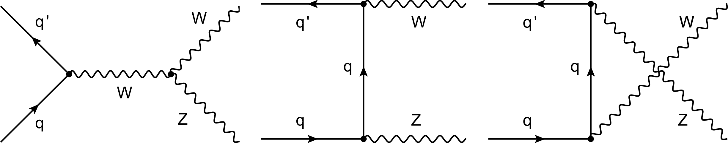
Figure 1:
Feynman diagrams for WZ production at leading order in pp collisions. The contributions from the $s$ channel (left), $t$ channel (middle), and $u$ channel (right) are presented. The contribution from the $s$ channel proceeds through TGC. |
png pdf |
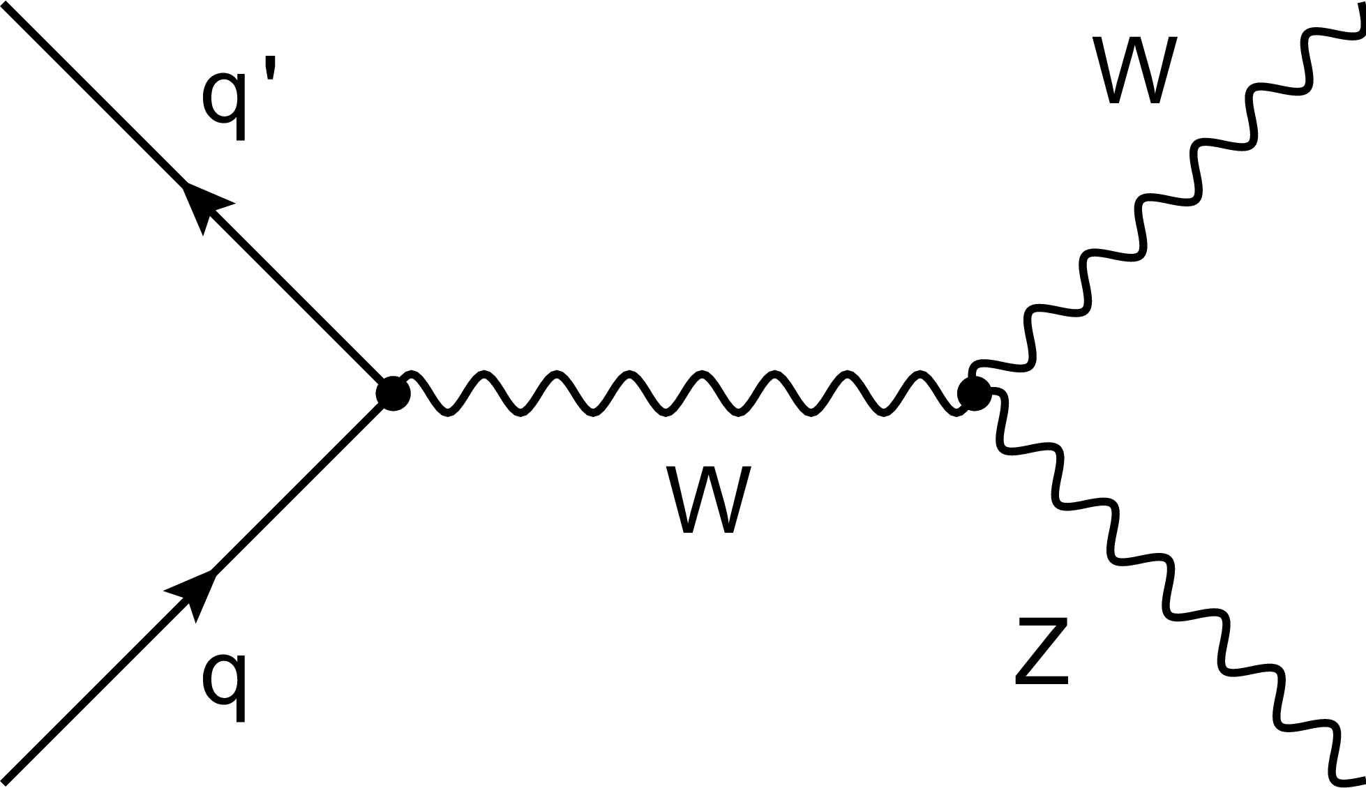
Figure 1-a:
Feynman diagrams for WZ production at leading order in pp collisions. The contributions from the $s$ channel (left), $t$ channel (middle), and $u$ channel (right) are presented. The contribution from the $s$ channel proceeds through TGC. |
png pdf |
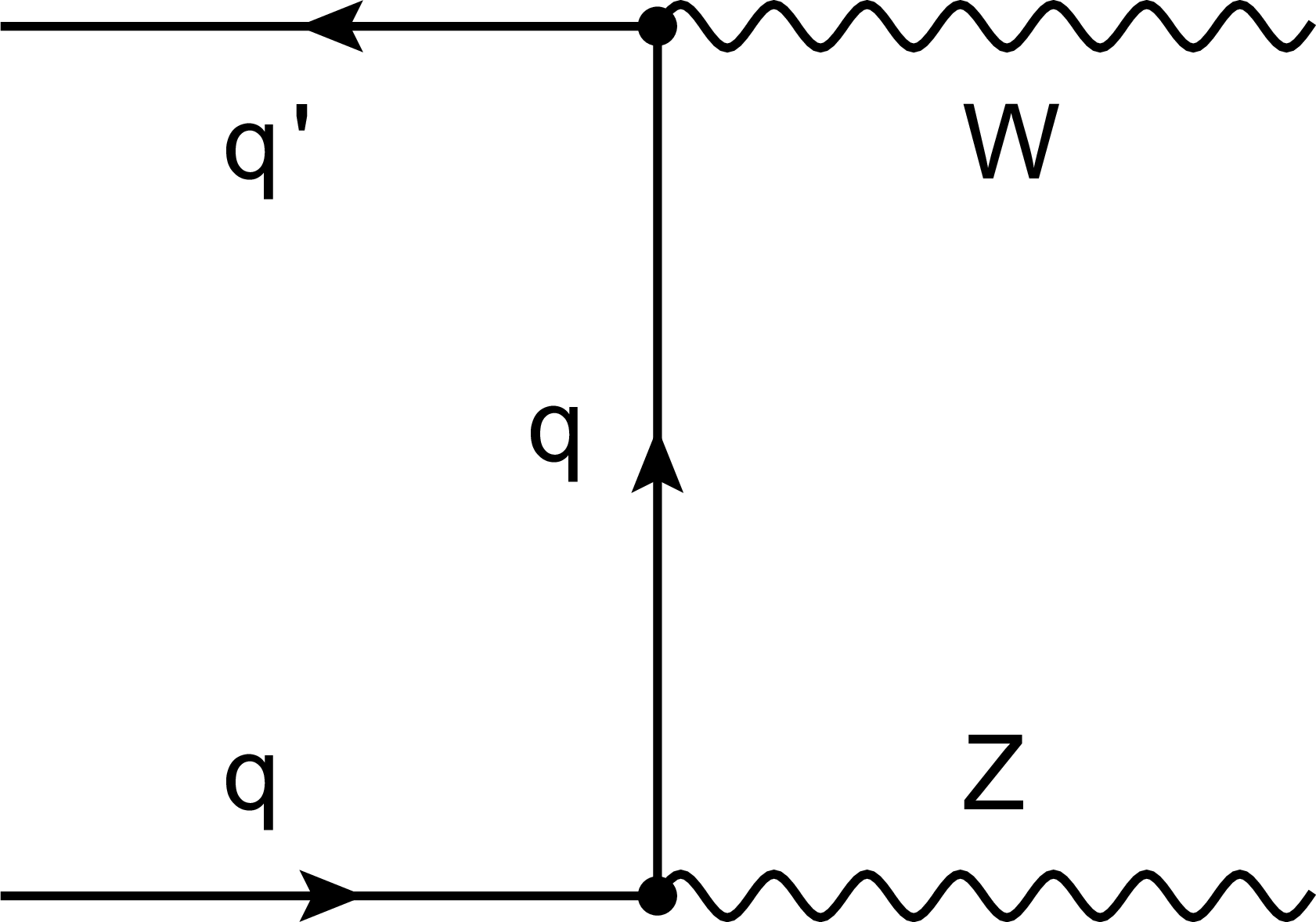
Figure 1-b:
Feynman diagrams for WZ production at leading order in pp collisions. The contributions from the $s$ channel (left), $t$ channel (middle), and $u$ channel (right) are presented. The contribution from the $s$ channel proceeds through TGC. |
png pdf |
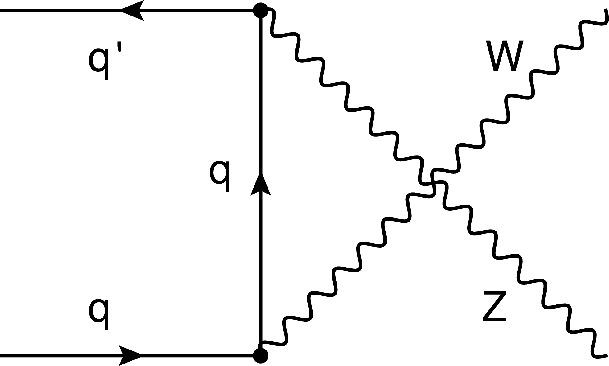
Figure 1-c:
Feynman diagrams for WZ production at leading order in pp collisions. The contributions from the $s$ channel (left), $t$ channel (middle), and $u$ channel (right) are presented. The contribution from the $s$ channel proceeds through TGC. |
png pdf |
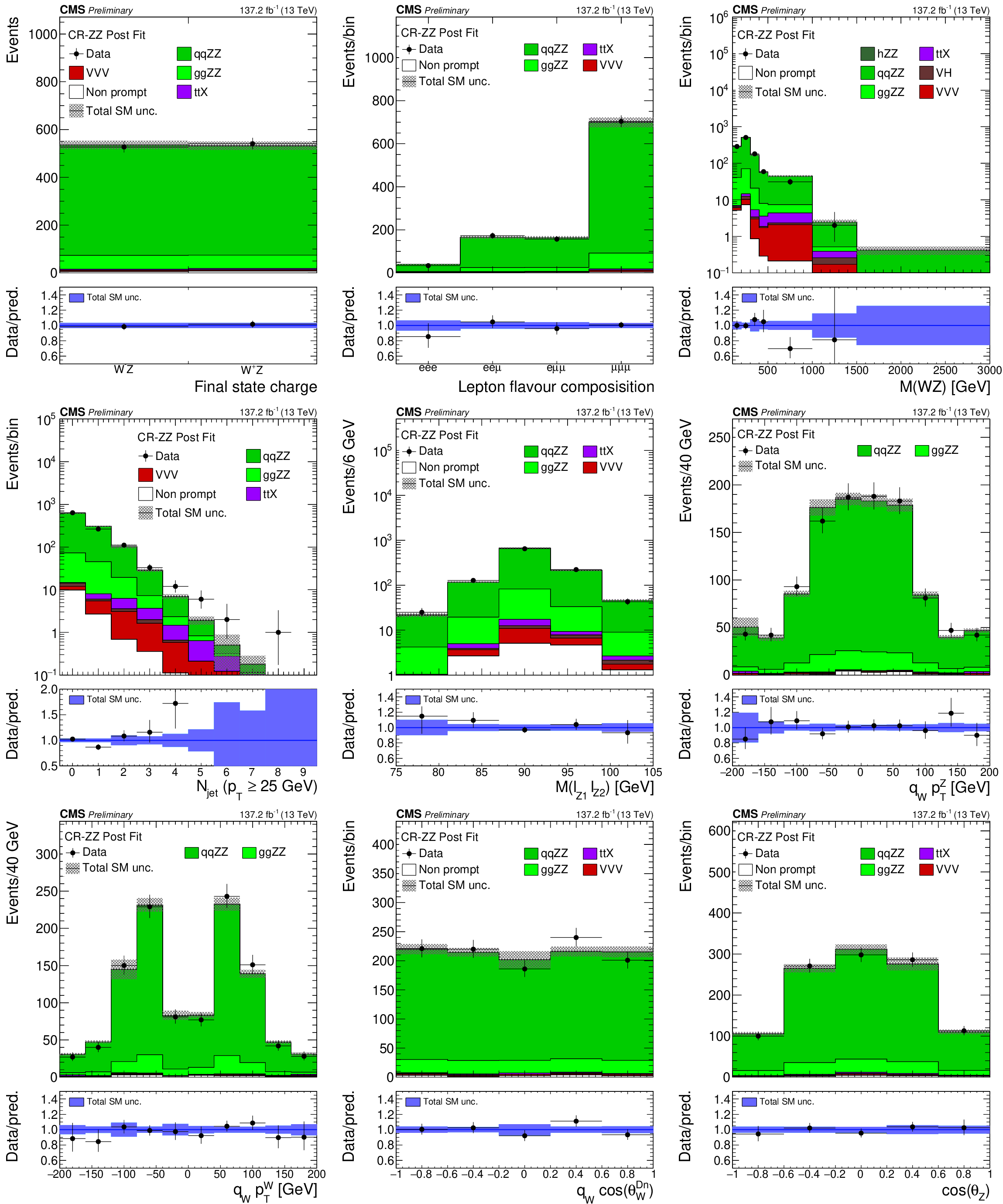
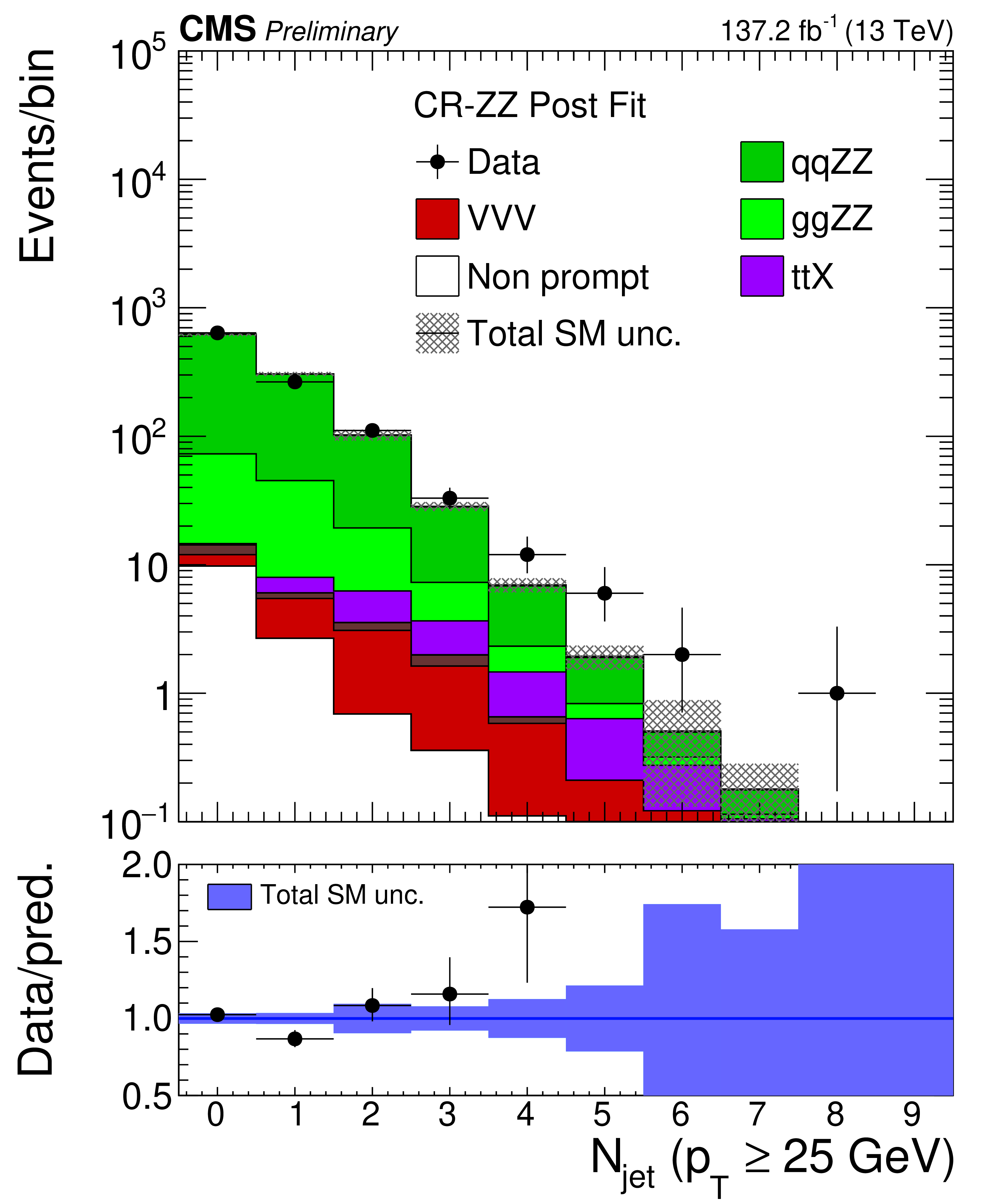
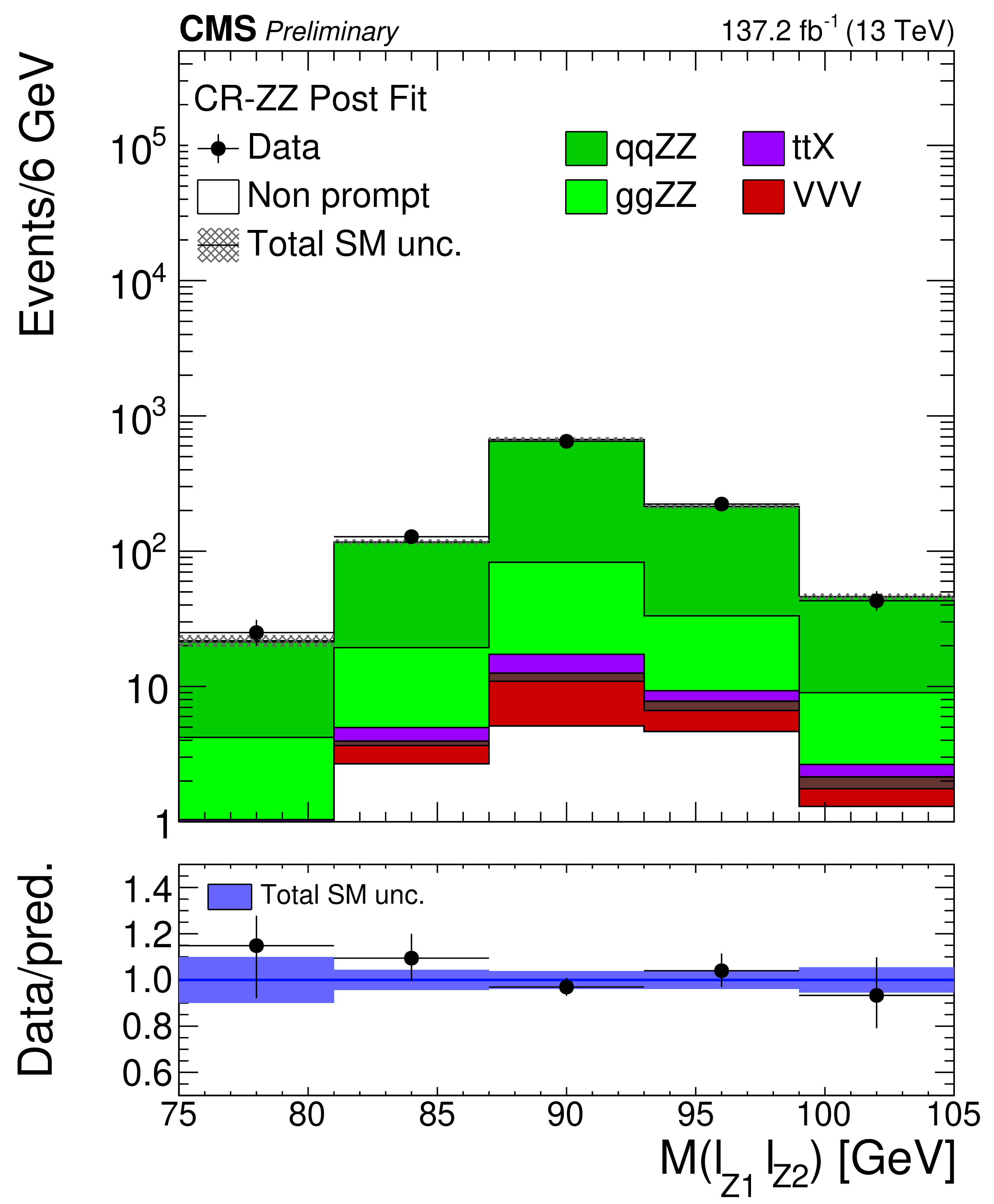
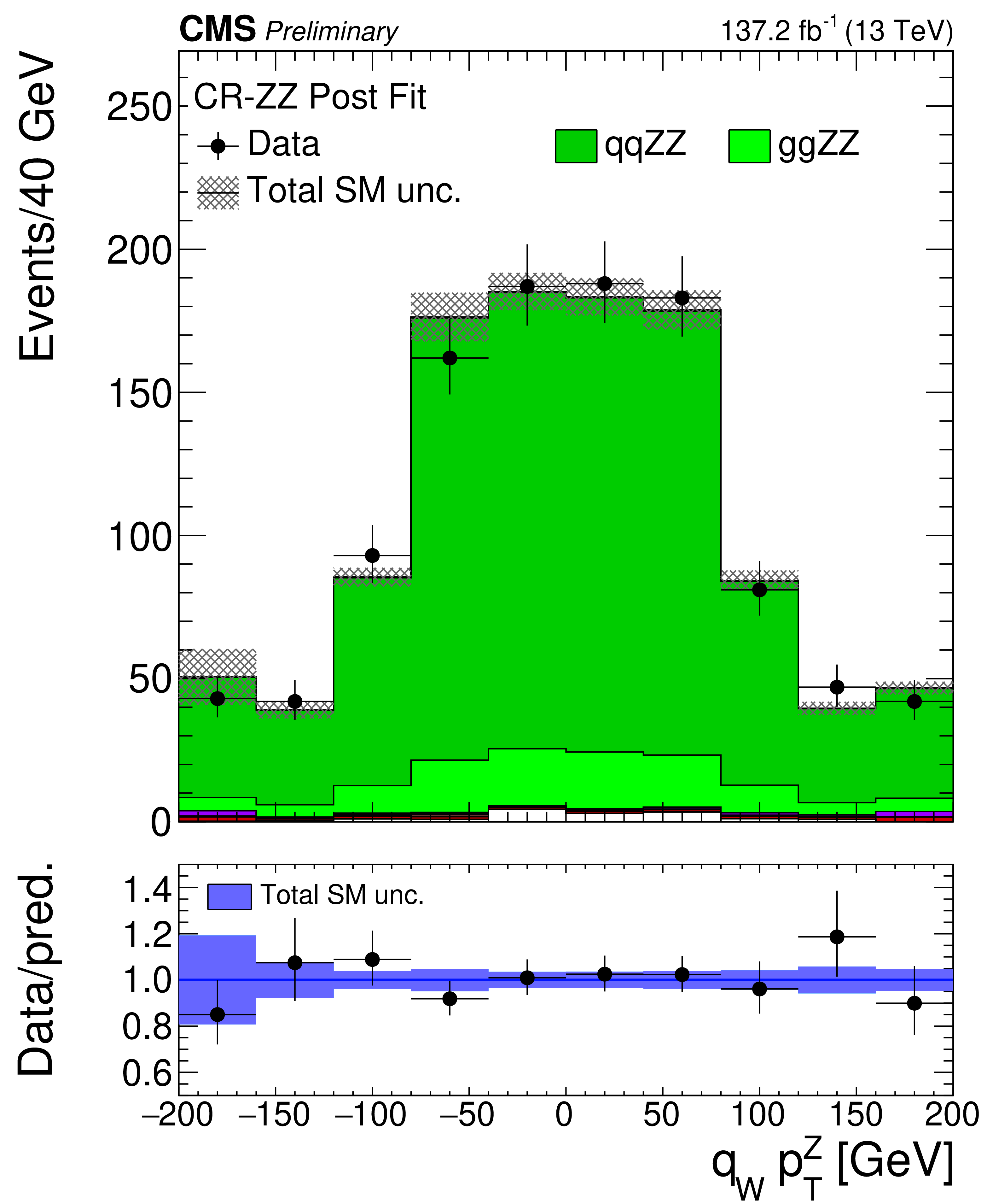
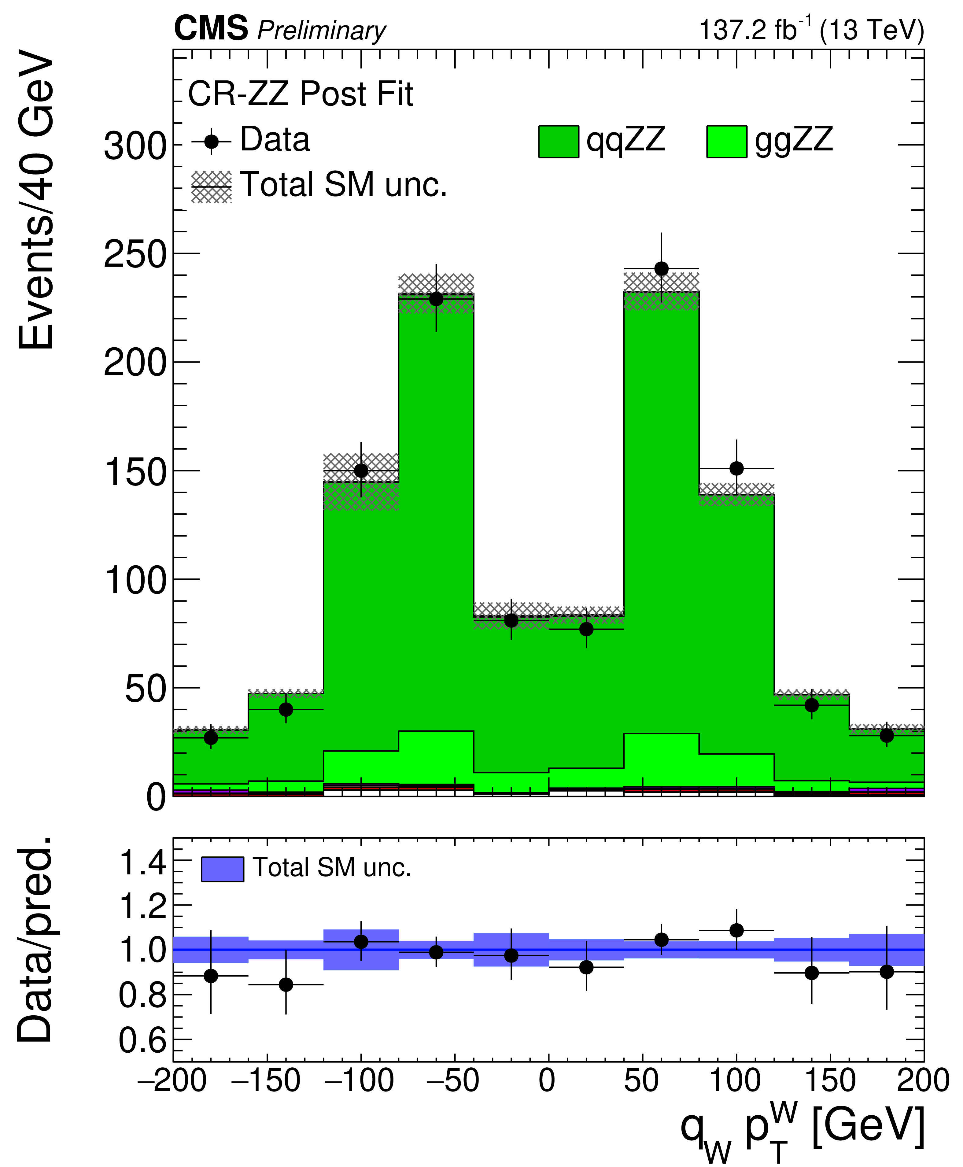
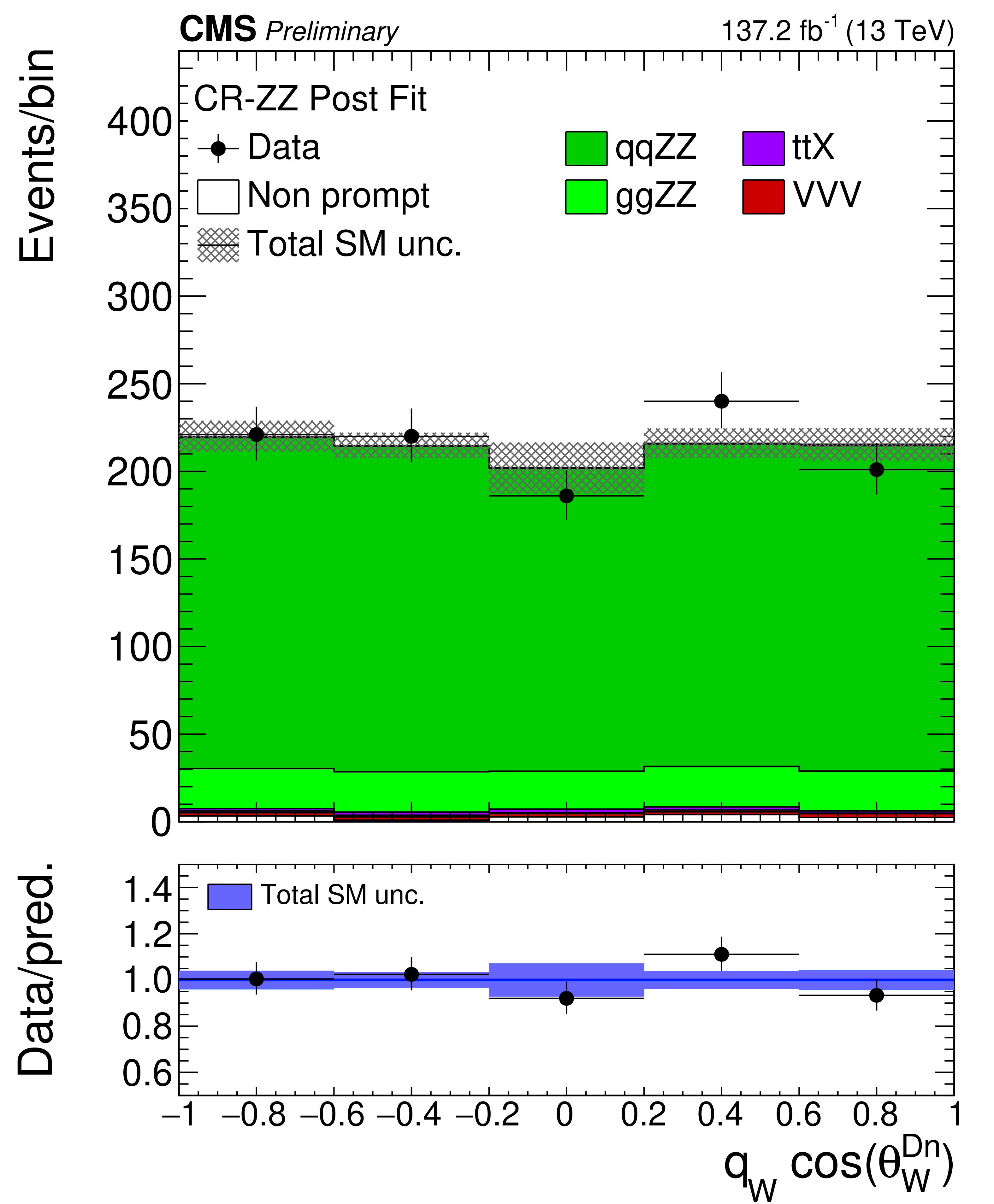
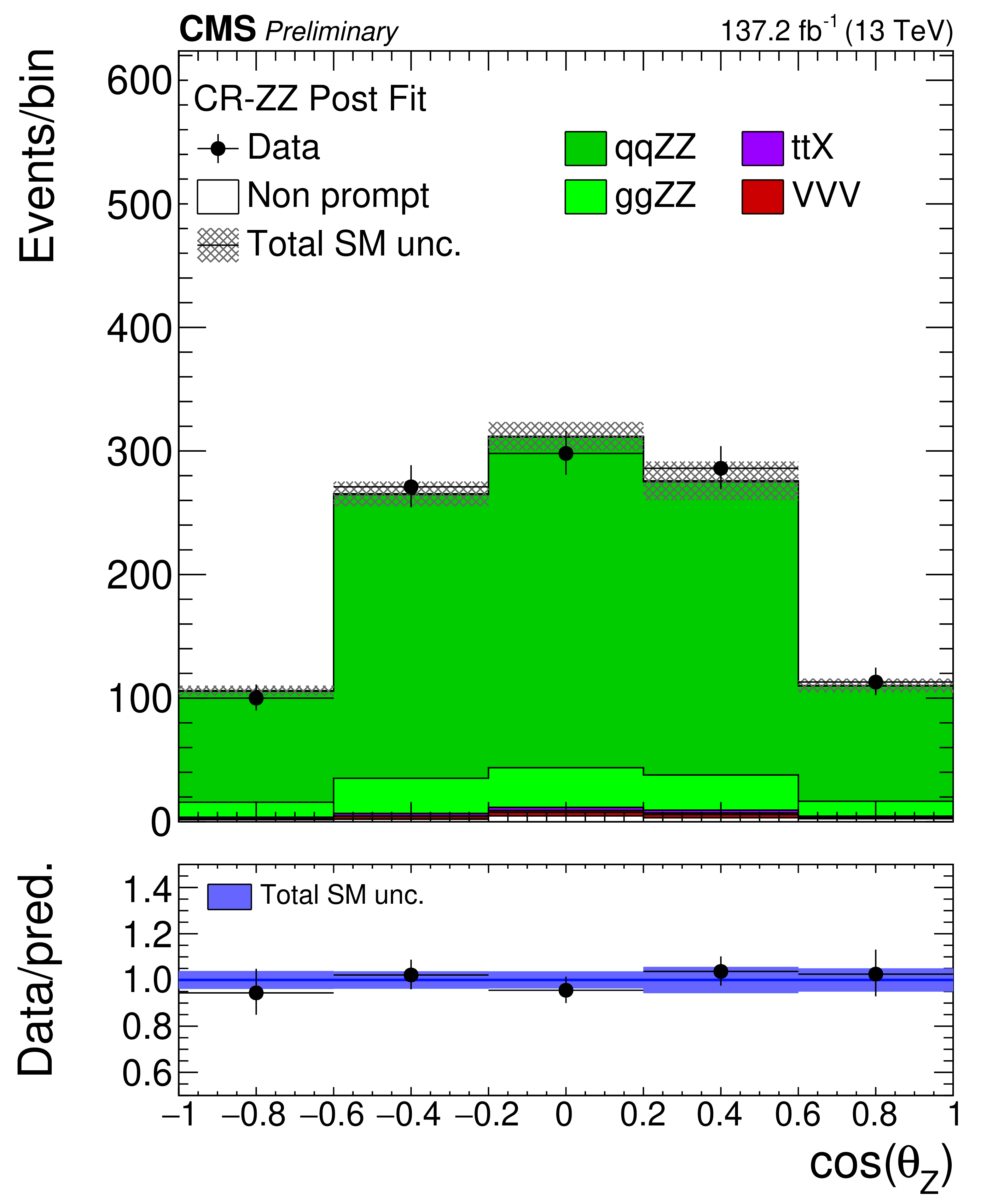
Figure 2:
Distribution of analysis-relevant observables in the ZZ control region evaluated with the uncertainties obtained after the signal extraction fit described in Section 8. From left to right and top to bottom: charge of the three leading lepton system, flavour distribution of the three leading lepton system, invariant mass of the three lepton plus ${{p_{\mathrm {T}}} ^\text {miss}}$ system, number of reconstructed jets, invariant mass of the leptonic pair with mass closest to that of the Z boson, reconstructed ${p_{\mathrm {T}}}$ of the Z boson times charge of the three leading lepton final state, reconstructed ${p_{\mathrm {T}}}$ of the W boson times final state charge constructed with ${{p_{\mathrm {T}}} ^\text {miss}}$ and the three leading lepton system, cosine of the polarization angle corresponding to the W angle, and cosine of the polarization angle corresponding to the Z boson. The label ttX includes both ttZ, ttW and ttH production. The shaded band in the ratio corresponds to the total uncertainty in the SM yields. |
png pdf |
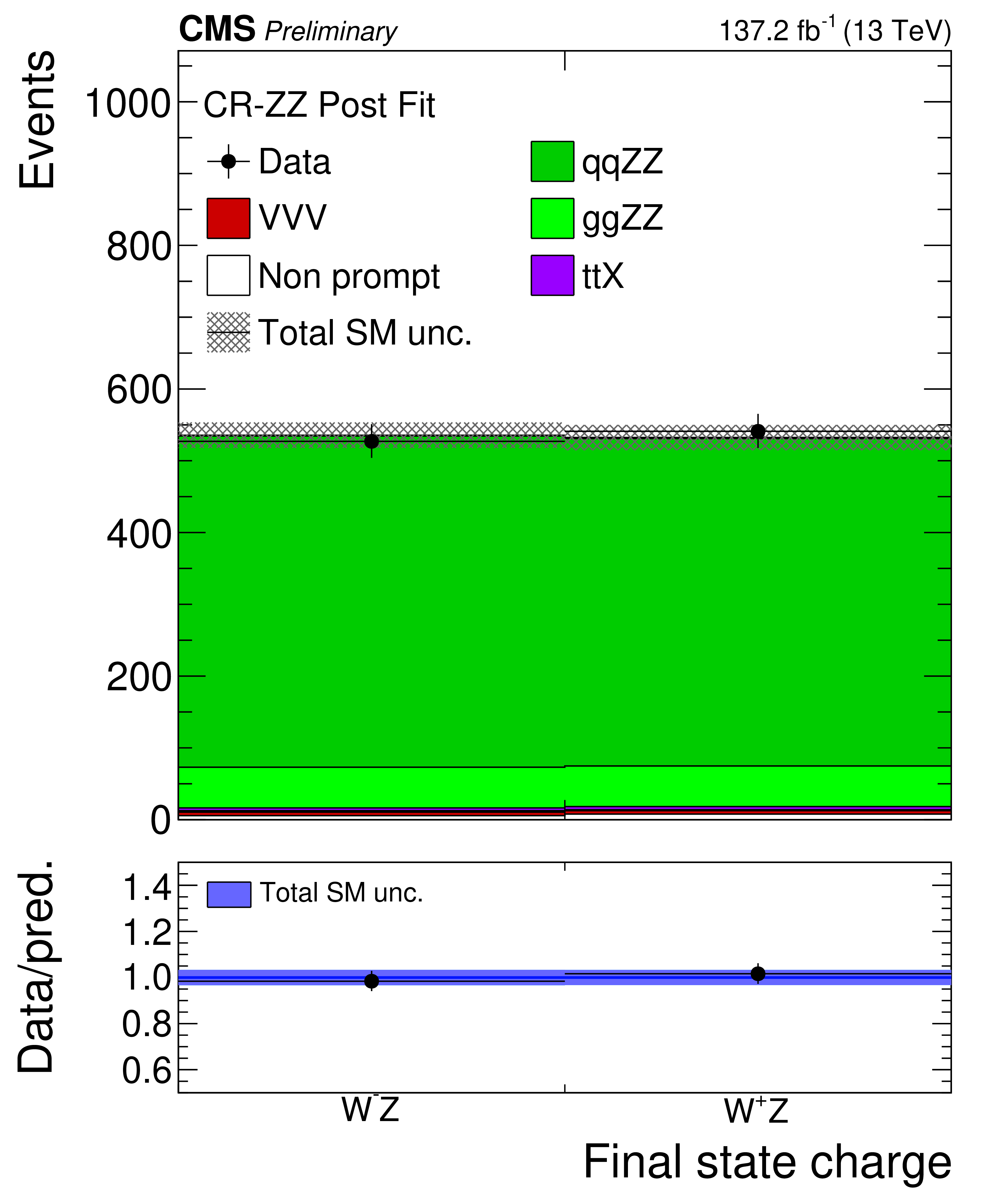
Figure 2-a:
Distribution of analysis-relevant observables in the ZZ control region evaluated with the uncertainties obtained after the signal extraction fit described in Section 8. From left to right and top to bottom: charge of the three leading lepton system, flavour distribution of the three leading lepton system, invariant mass of the three lepton plus ${{p_{\mathrm {T}}} ^\text {miss}}$ system, number of reconstructed jets, invariant mass of the leptonic pair with mass closest to that of the Z boson, reconstructed ${p_{\mathrm {T}}}$ of the Z boson times charge of the three leading lepton final state, reconstructed ${p_{\mathrm {T}}}$ of the W boson times final state charge constructed with ${{p_{\mathrm {T}}} ^\text {miss}}$ and the three leading lepton system, cosine of the polarization angle corresponding to the W angle, and cosine of the polarization angle corresponding to the Z boson. The label ttX includes both ttZ, ttW and ttH production. The shaded band in the ratio corresponds to the total uncertainty in the SM yields. |
png pdf |
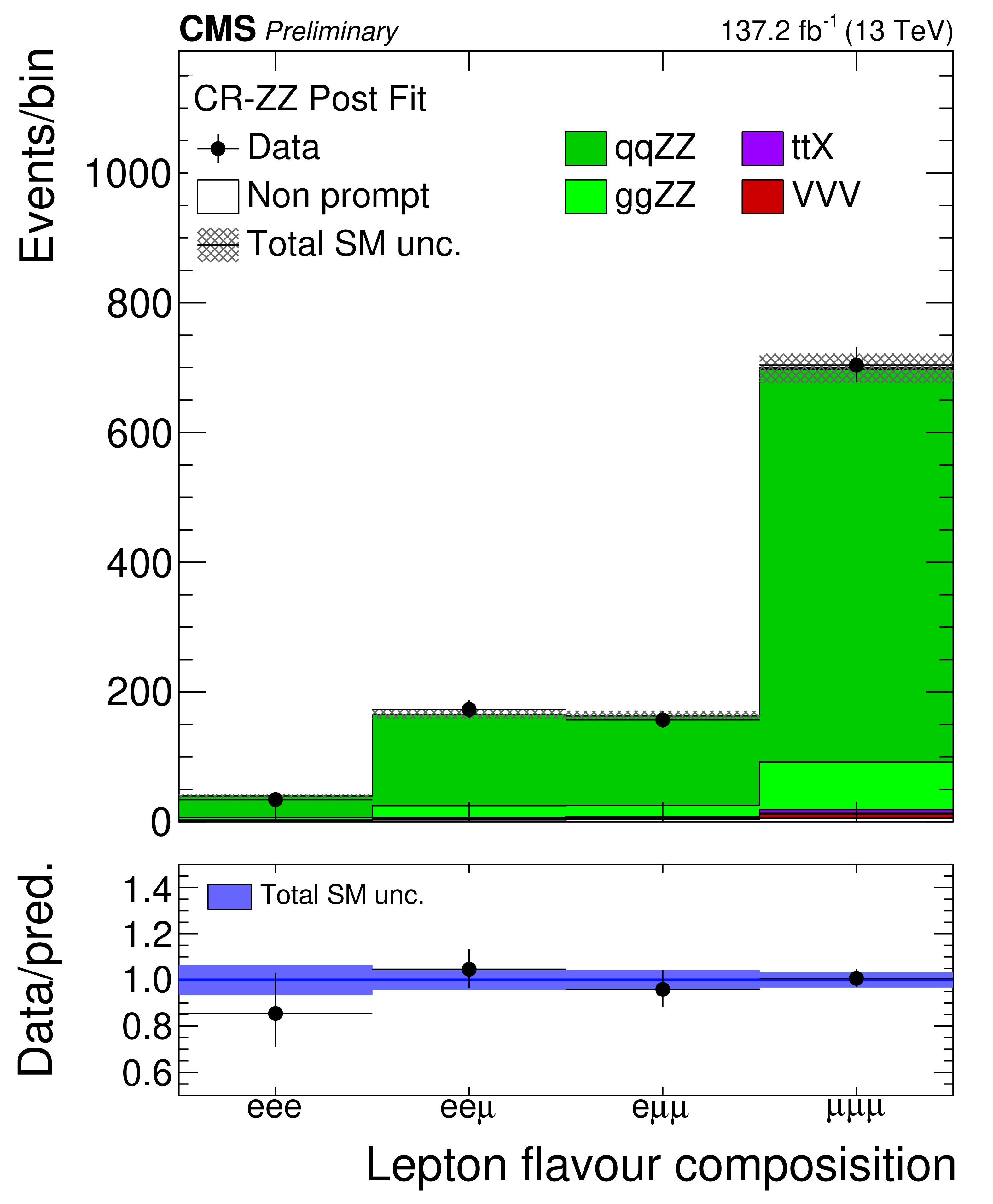
Figure 2-b:
Distribution of analysis-relevant observables in the ZZ control region evaluated with the uncertainties obtained after the signal extraction fit described in Section 8. From left to right and top to bottom: charge of the three leading lepton system, flavour distribution of the three leading lepton system, invariant mass of the three lepton plus ${{p_{\mathrm {T}}} ^\text {miss}}$ system, number of reconstructed jets, invariant mass of the leptonic pair with mass closest to that of the Z boson, reconstructed ${p_{\mathrm {T}}}$ of the Z boson times charge of the three leading lepton final state, reconstructed ${p_{\mathrm {T}}}$ of the W boson times final state charge constructed with ${{p_{\mathrm {T}}} ^\text {miss}}$ and the three leading lepton system, cosine of the polarization angle corresponding to the W angle, and cosine of the polarization angle corresponding to the Z boson. The label ttX includes both ttZ, ttW and ttH production. The shaded band in the ratio corresponds to the total uncertainty in the SM yields. |
png pdf |
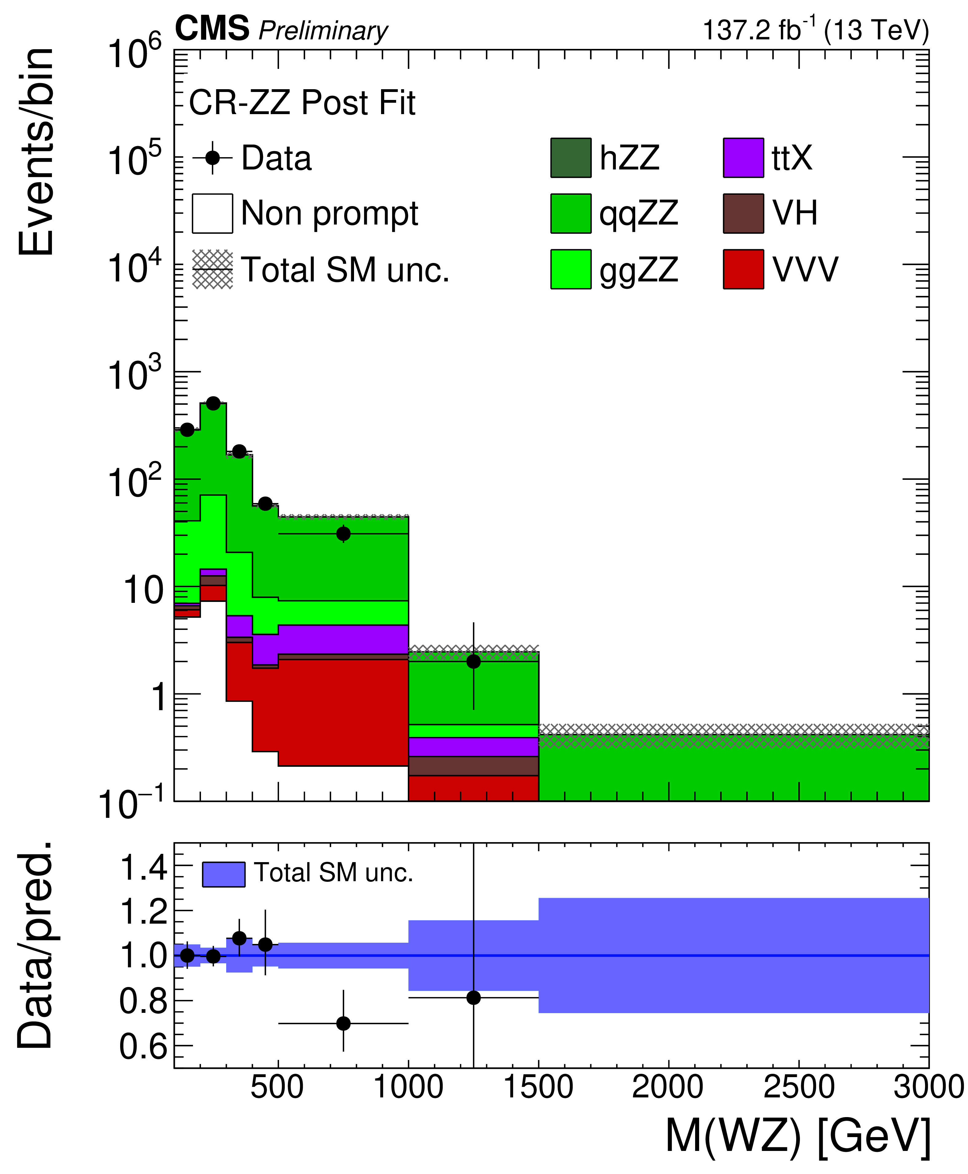
Figure 2-c:
Distribution of analysis-relevant observables in the ZZ control region evaluated with the uncertainties obtained after the signal extraction fit described in Section 8. From left to right and top to bottom: charge of the three leading lepton system, flavour distribution of the three leading lepton system, invariant mass of the three lepton plus ${{p_{\mathrm {T}}} ^\text {miss}}$ system, number of reconstructed jets, invariant mass of the leptonic pair with mass closest to that of the Z boson, reconstructed ${p_{\mathrm {T}}}$ of the Z boson times charge of the three leading lepton final state, reconstructed ${p_{\mathrm {T}}}$ of the W boson times final state charge constructed with ${{p_{\mathrm {T}}} ^\text {miss}}$ and the three leading lepton system, cosine of the polarization angle corresponding to the W angle, and cosine of the polarization angle corresponding to the Z boson. The label ttX includes both ttZ, ttW and ttH production. The shaded band in the ratio corresponds to the total uncertainty in the SM yields. |
png pdf |
Figure 2-d:
Distribution of analysis-relevant observables in the ZZ control region evaluated with the uncertainties obtained after the signal extraction fit described in Section 8. From left to right and top to bottom: charge of the three leading lepton system, flavour distribution of the three leading lepton system, invariant mass of the three lepton plus ${{p_{\mathrm {T}}} ^\text {miss}}$ system, number of reconstructed jets, invariant mass of the leptonic pair with mass closest to that of the Z boson, reconstructed ${p_{\mathrm {T}}}$ of the Z boson times charge of the three leading lepton final state, reconstructed ${p_{\mathrm {T}}}$ of the W boson times final state charge constructed with ${{p_{\mathrm {T}}} ^\text {miss}}$ and the three leading lepton system, cosine of the polarization angle corresponding to the W angle, and cosine of the polarization angle corresponding to the Z boson. The label ttX includes both ttZ, ttW and ttH production. The shaded band in the ratio corresponds to the total uncertainty in the SM yields. |
png pdf |
Figure 2-e:
Distribution of analysis-relevant observables in the ZZ control region evaluated with the uncertainties obtained after the signal extraction fit described in Section 8. From left to right and top to bottom: charge of the three leading lepton system, flavour distribution of the three leading lepton system, invariant mass of the three lepton plus ${{p_{\mathrm {T}}} ^\text {miss}}$ system, number of reconstructed jets, invariant mass of the leptonic pair with mass closest to that of the Z boson, reconstructed ${p_{\mathrm {T}}}$ of the Z boson times charge of the three leading lepton final state, reconstructed ${p_{\mathrm {T}}}$ of the W boson times final state charge constructed with ${{p_{\mathrm {T}}} ^\text {miss}}$ and the three leading lepton system, cosine of the polarization angle corresponding to the W angle, and cosine of the polarization angle corresponding to the Z boson. The label ttX includes both ttZ, ttW and ttH production. The shaded band in the ratio corresponds to the total uncertainty in the SM yields. |
png pdf |
Figure 2-f:
Distribution of analysis-relevant observables in the ZZ control region evaluated with the uncertainties obtained after the signal extraction fit described in Section 8. From left to right and top to bottom: charge of the three leading lepton system, flavour distribution of the three leading lepton system, invariant mass of the three lepton plus ${{p_{\mathrm {T}}} ^\text {miss}}$ system, number of reconstructed jets, invariant mass of the leptonic pair with mass closest to that of the Z boson, reconstructed ${p_{\mathrm {T}}}$ of the Z boson times charge of the three leading lepton final state, reconstructed ${p_{\mathrm {T}}}$ of the W boson times final state charge constructed with ${{p_{\mathrm {T}}} ^\text {miss}}$ and the three leading lepton system, cosine of the polarization angle corresponding to the W angle, and cosine of the polarization angle corresponding to the Z boson. The label ttX includes both ttZ, ttW and ttH production. The shaded band in the ratio corresponds to the total uncertainty in the SM yields. |
png pdf |
Figure 2-g:
Distribution of analysis-relevant observables in the ZZ control region evaluated with the uncertainties obtained after the signal extraction fit described in Section 8. From left to right and top to bottom: charge of the three leading lepton system, flavour distribution of the three leading lepton system, invariant mass of the three lepton plus ${{p_{\mathrm {T}}} ^\text {miss}}$ system, number of reconstructed jets, invariant mass of the leptonic pair with mass closest to that of the Z boson, reconstructed ${p_{\mathrm {T}}}$ of the Z boson times charge of the three leading lepton final state, reconstructed ${p_{\mathrm {T}}}$ of the W boson times final state charge constructed with ${{p_{\mathrm {T}}} ^\text {miss}}$ and the three leading lepton system, cosine of the polarization angle corresponding to the W angle, and cosine of the polarization angle corresponding to the Z boson. The label ttX includes both ttZ, ttW and ttH production. The shaded band in the ratio corresponds to the total uncertainty in the SM yields. |
png pdf |
Figure 2-h:
Distribution of analysis-relevant observables in the ZZ control region evaluated with the uncertainties obtained after the signal extraction fit described in Section 8. From left to right and top to bottom: charge of the three leading lepton system, flavour distribution of the three leading lepton system, invariant mass of the three lepton plus ${{p_{\mathrm {T}}} ^\text {miss}}$ system, number of reconstructed jets, invariant mass of the leptonic pair with mass closest to that of the Z boson, reconstructed ${p_{\mathrm {T}}}$ of the Z boson times charge of the three leading lepton final state, reconstructed ${p_{\mathrm {T}}}$ of the W boson times final state charge constructed with ${{p_{\mathrm {T}}} ^\text {miss}}$ and the three leading lepton system, cosine of the polarization angle corresponding to the W angle, and cosine of the polarization angle corresponding to the Z boson. The label ttX includes both ttZ, ttW and ttH production. The shaded band in the ratio corresponds to the total uncertainty in the SM yields. |
png pdf |
Figure 2-i:
Distribution of analysis-relevant observables in the ZZ control region evaluated with the uncertainties obtained after the signal extraction fit described in Section 8. From left to right and top to bottom: charge of the three leading lepton system, flavour distribution of the three leading lepton system, invariant mass of the three lepton plus ${{p_{\mathrm {T}}} ^\text {miss}}$ system, number of reconstructed jets, invariant mass of the leptonic pair with mass closest to that of the Z boson, reconstructed ${p_{\mathrm {T}}}$ of the Z boson times charge of the three leading lepton final state, reconstructed ${p_{\mathrm {T}}}$ of the W boson times final state charge constructed with ${{p_{\mathrm {T}}} ^\text {miss}}$ and the three leading lepton system, cosine of the polarization angle corresponding to the W angle, and cosine of the polarization angle corresponding to the Z boson. The label ttX includes both ttZ, ttW and ttH production. The shaded band in the ratio corresponds to the total uncertainty in the SM yields. |
png pdf |
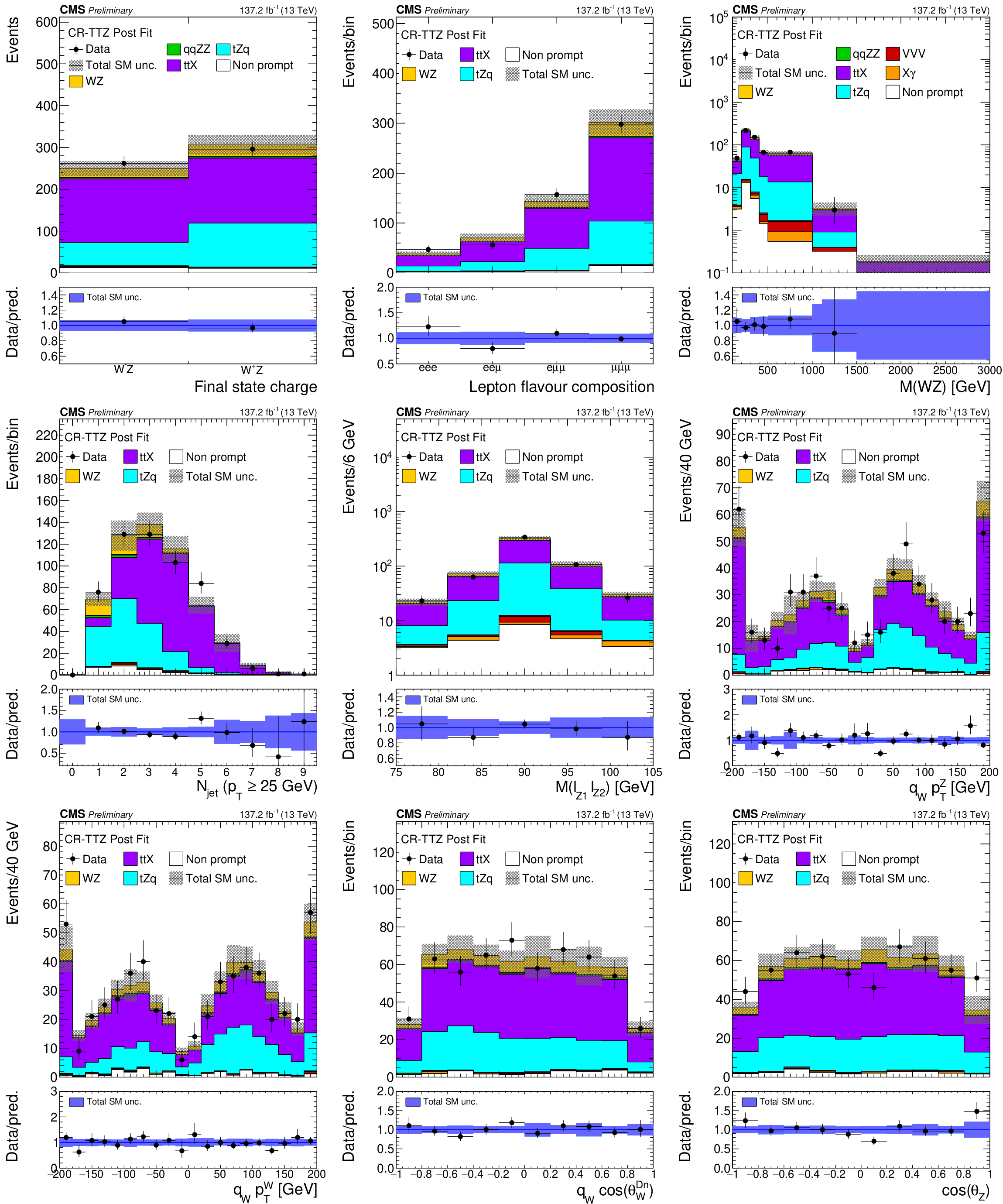
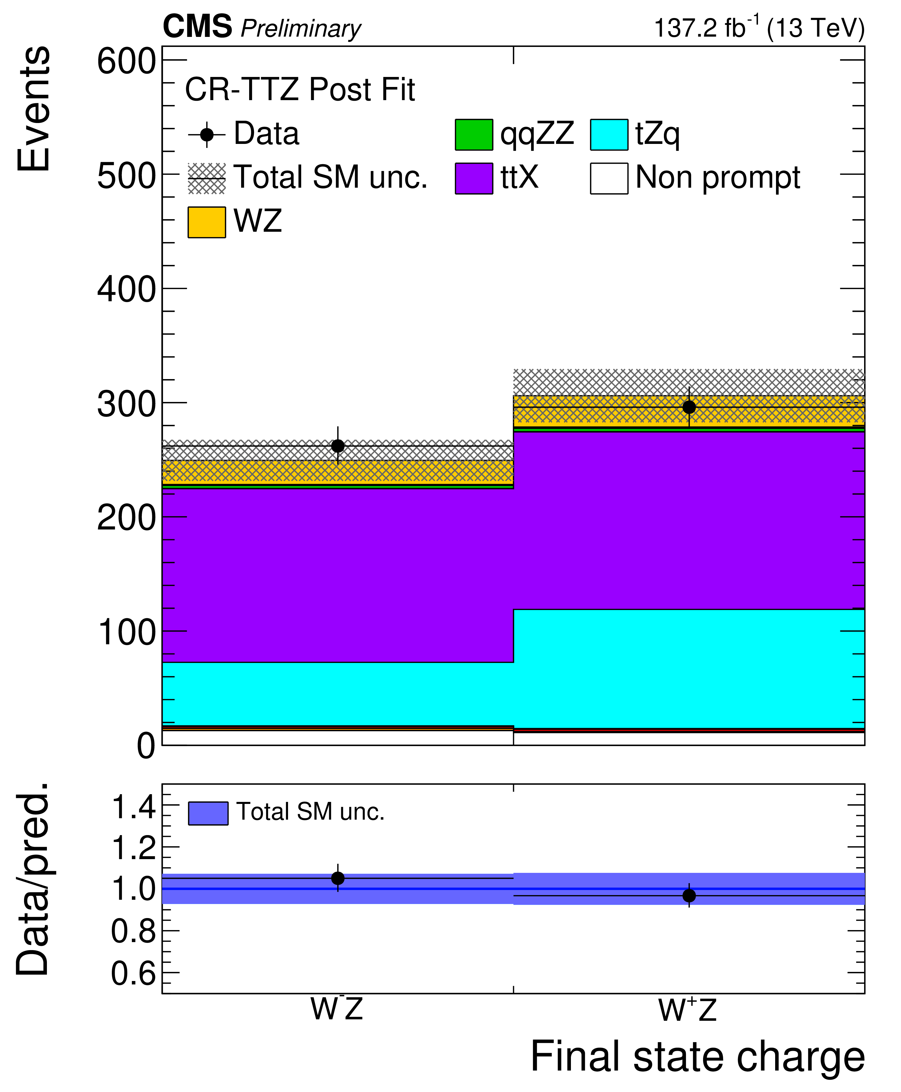
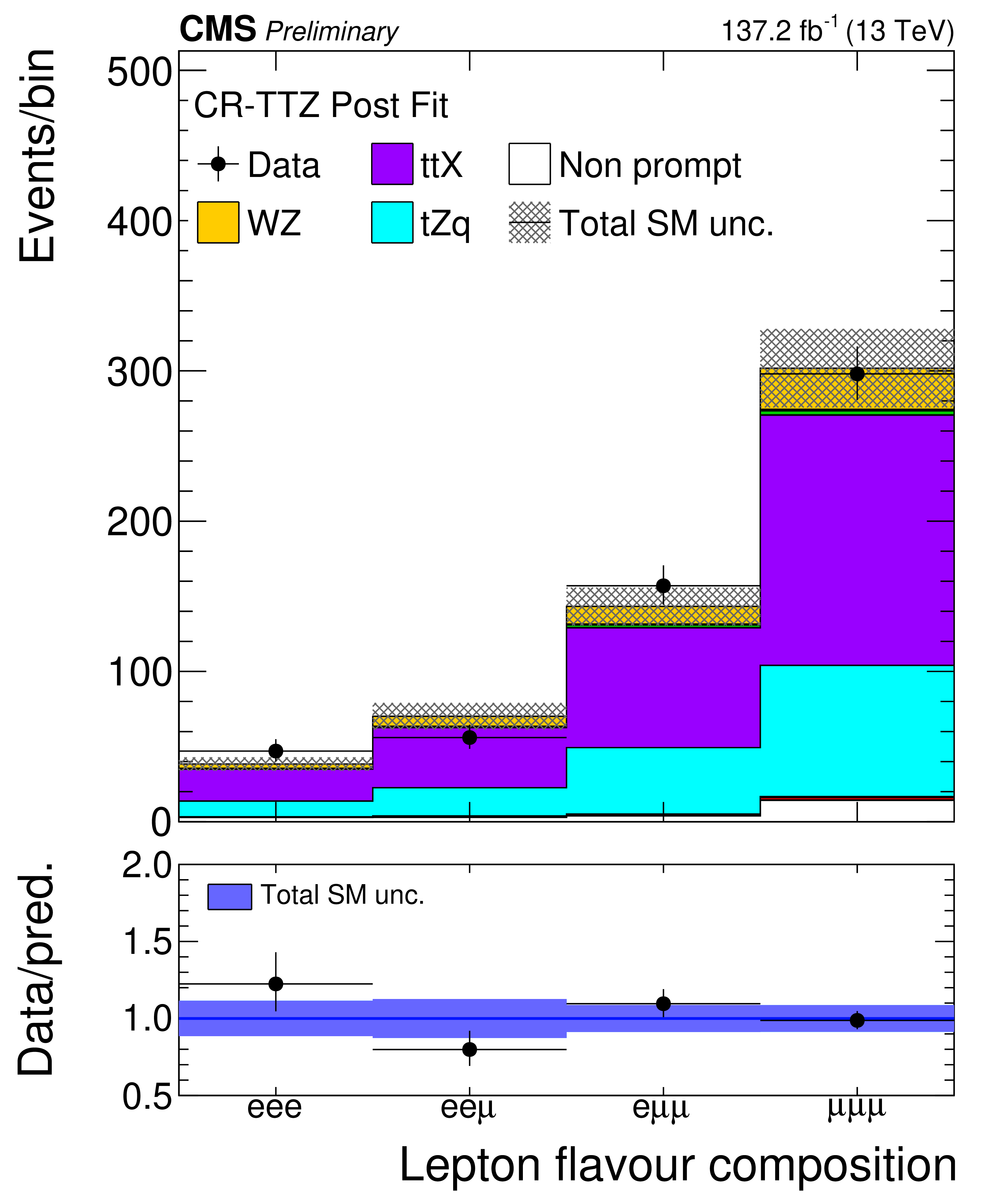
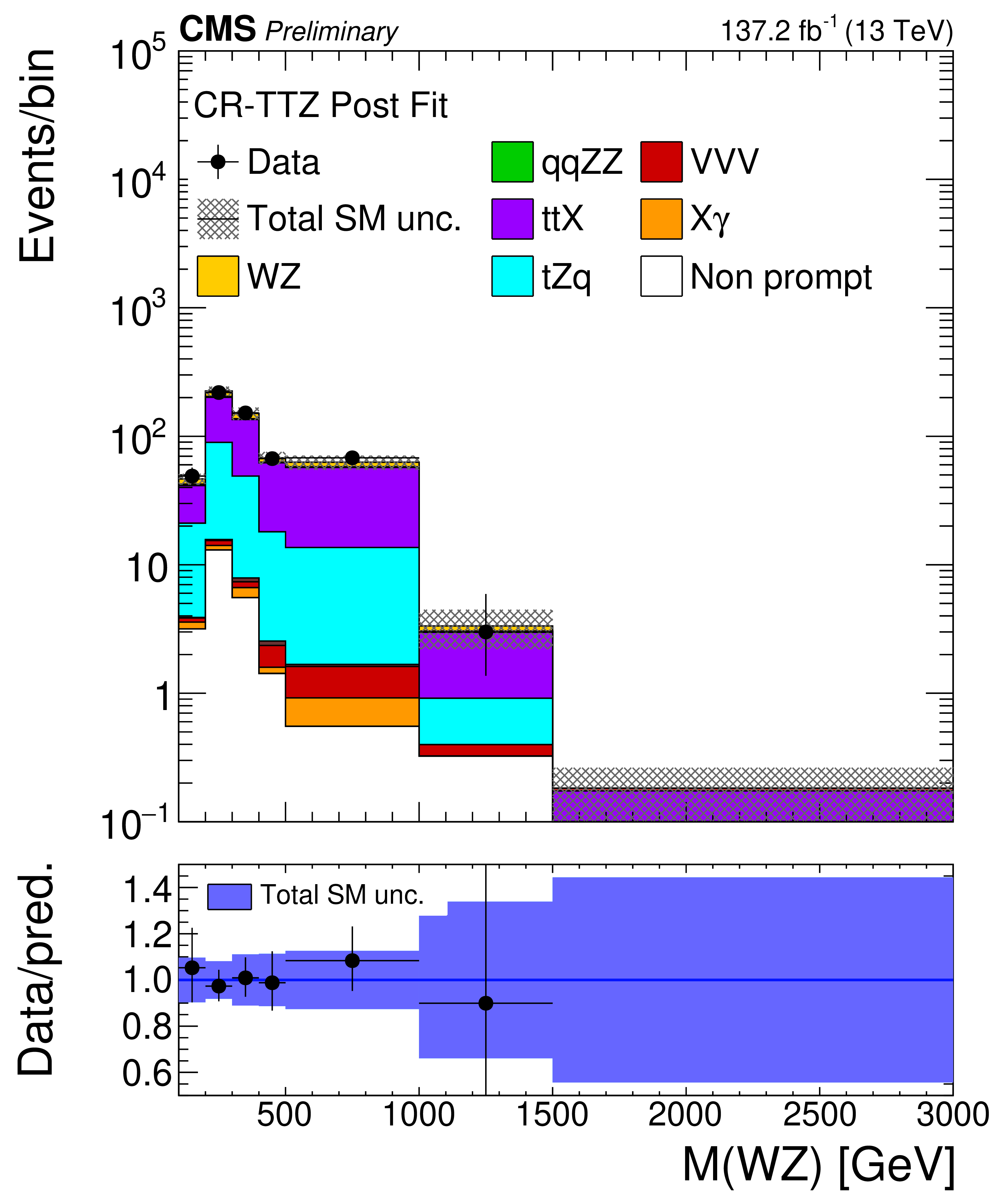
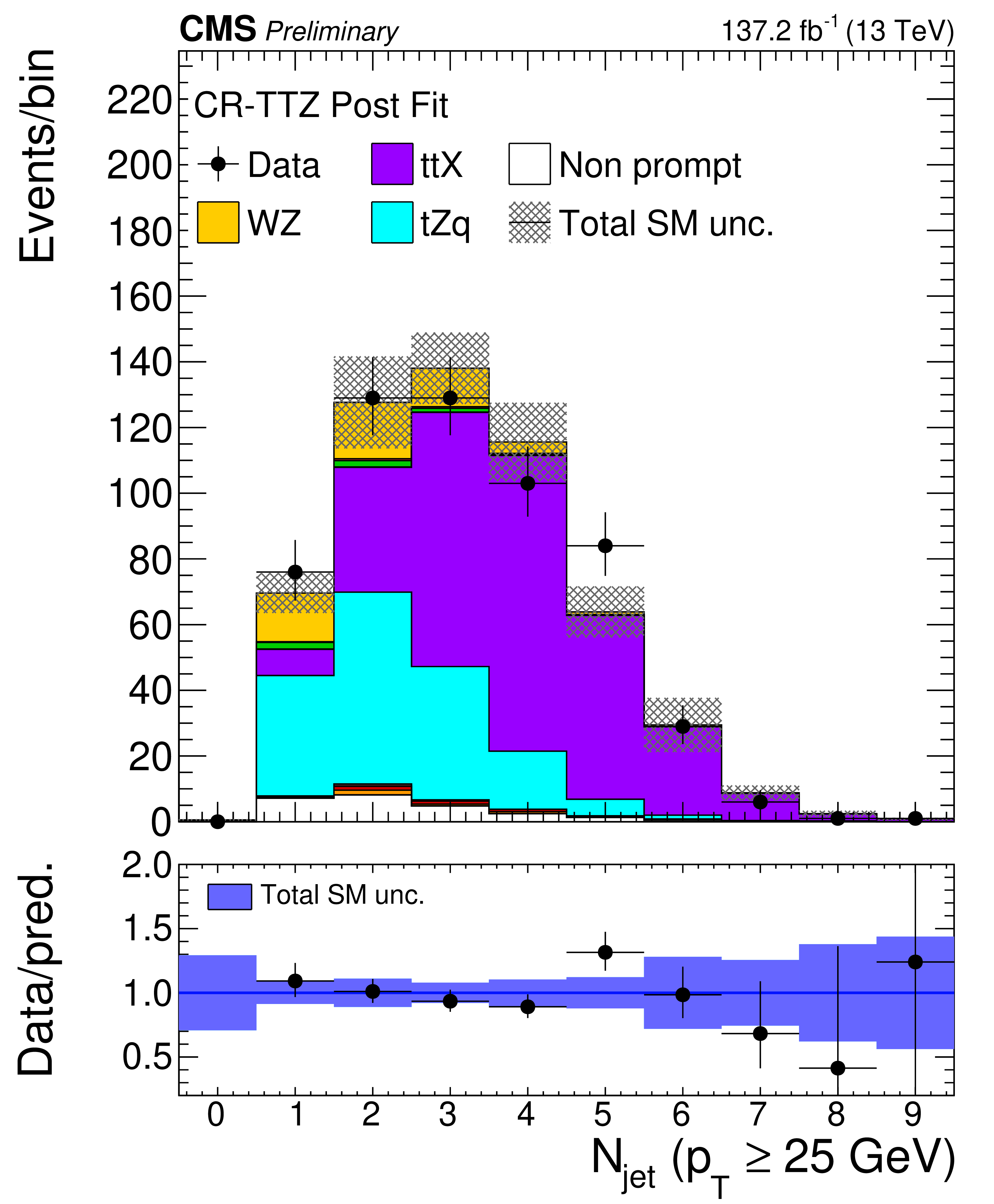
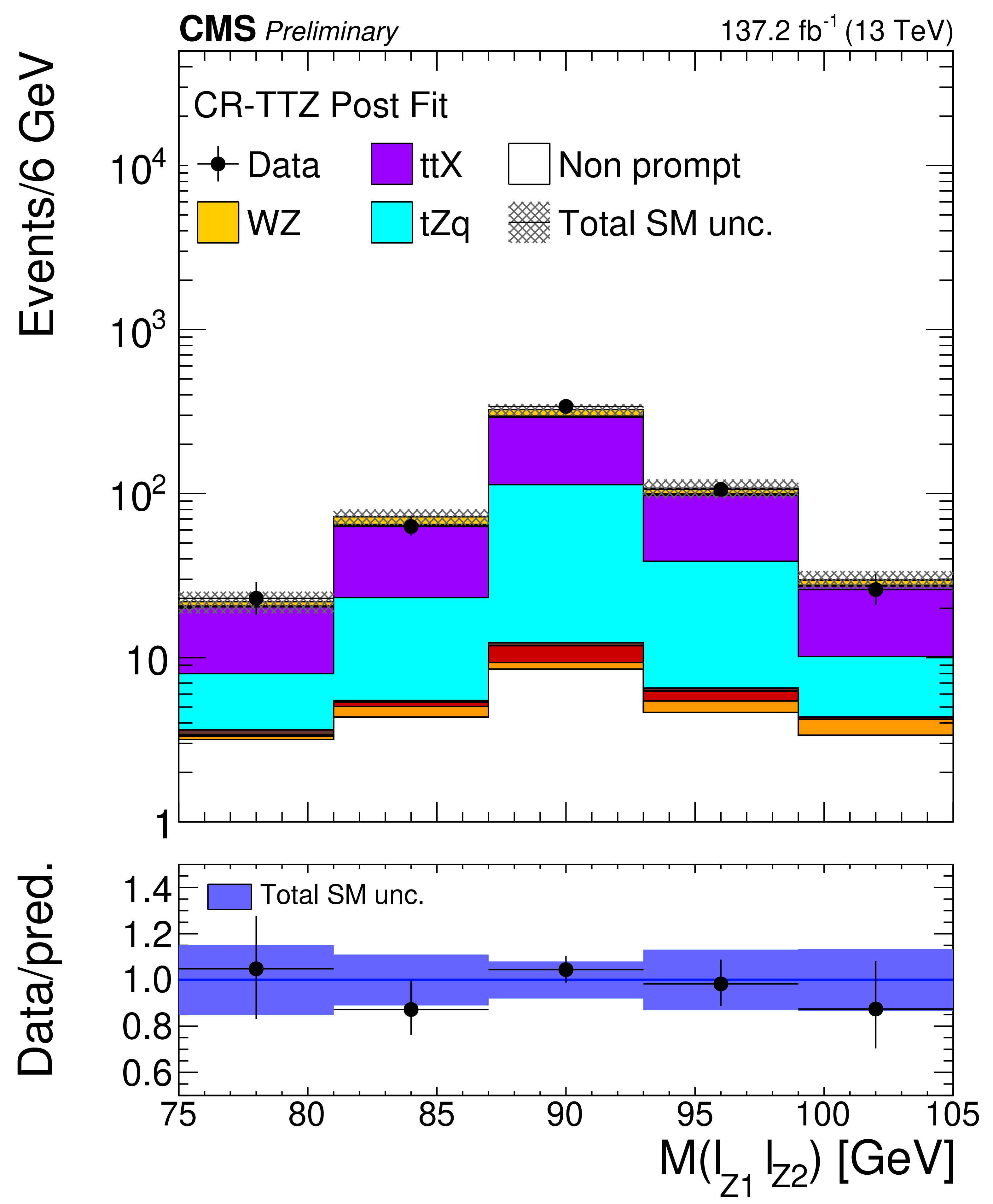
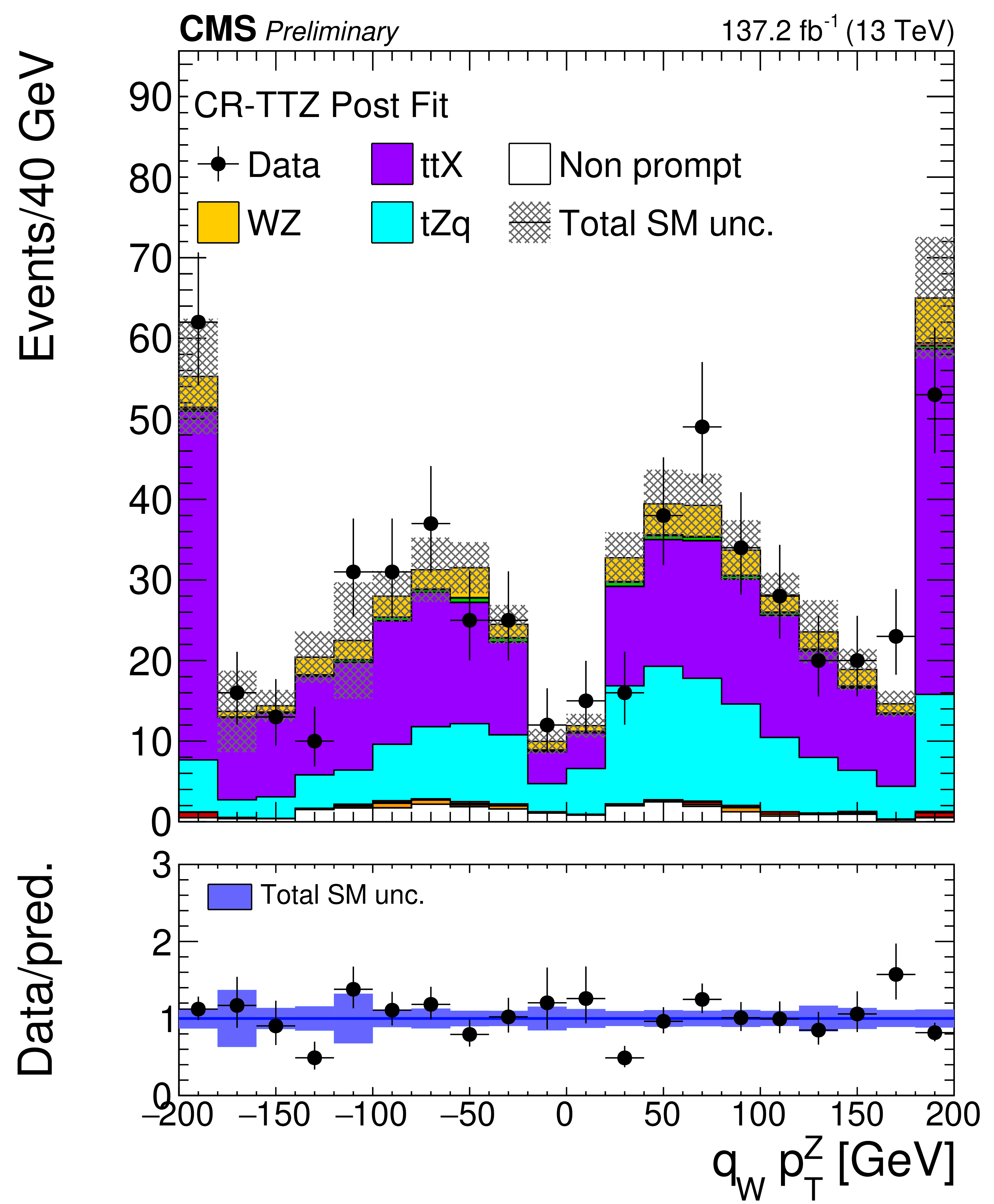
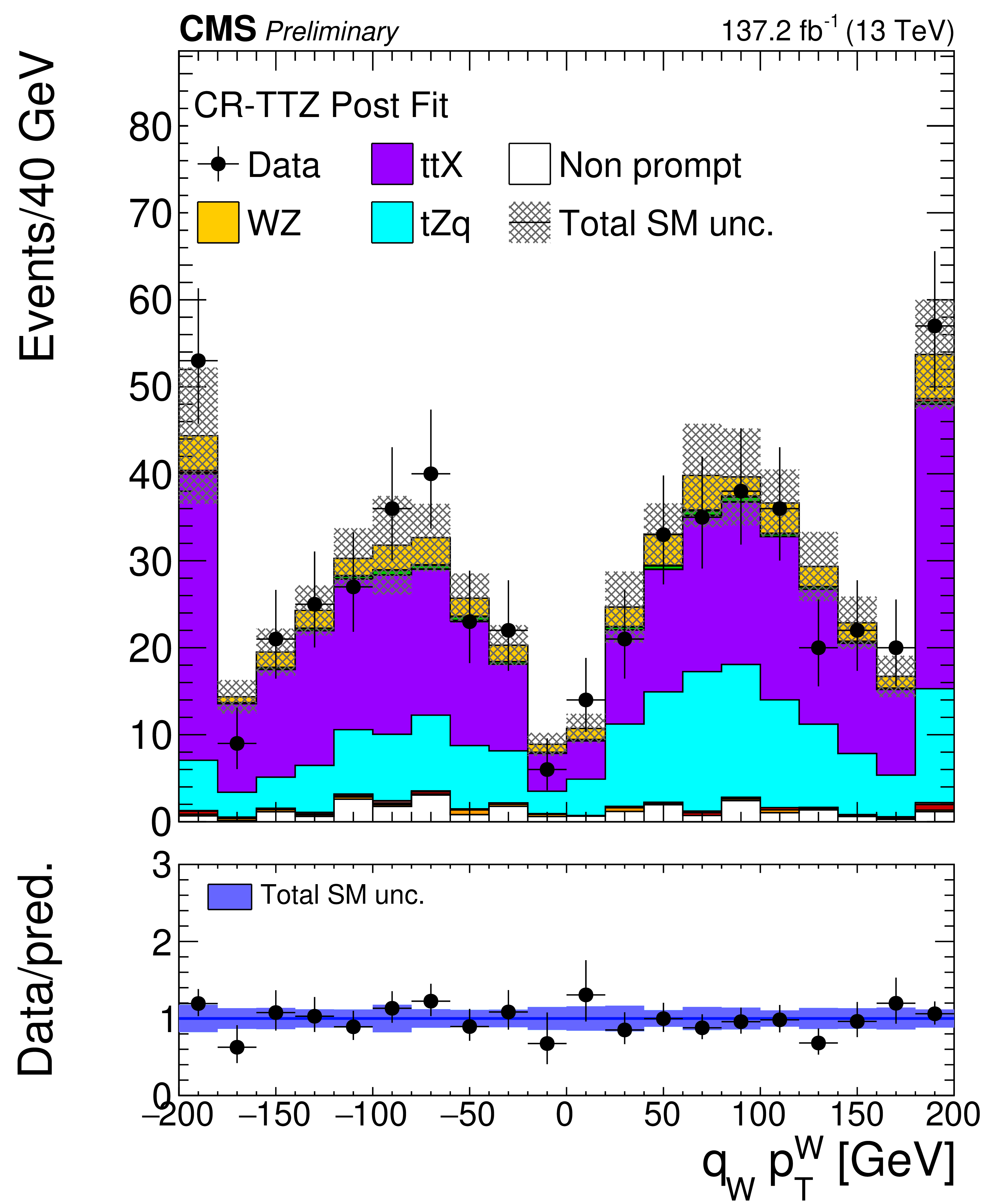
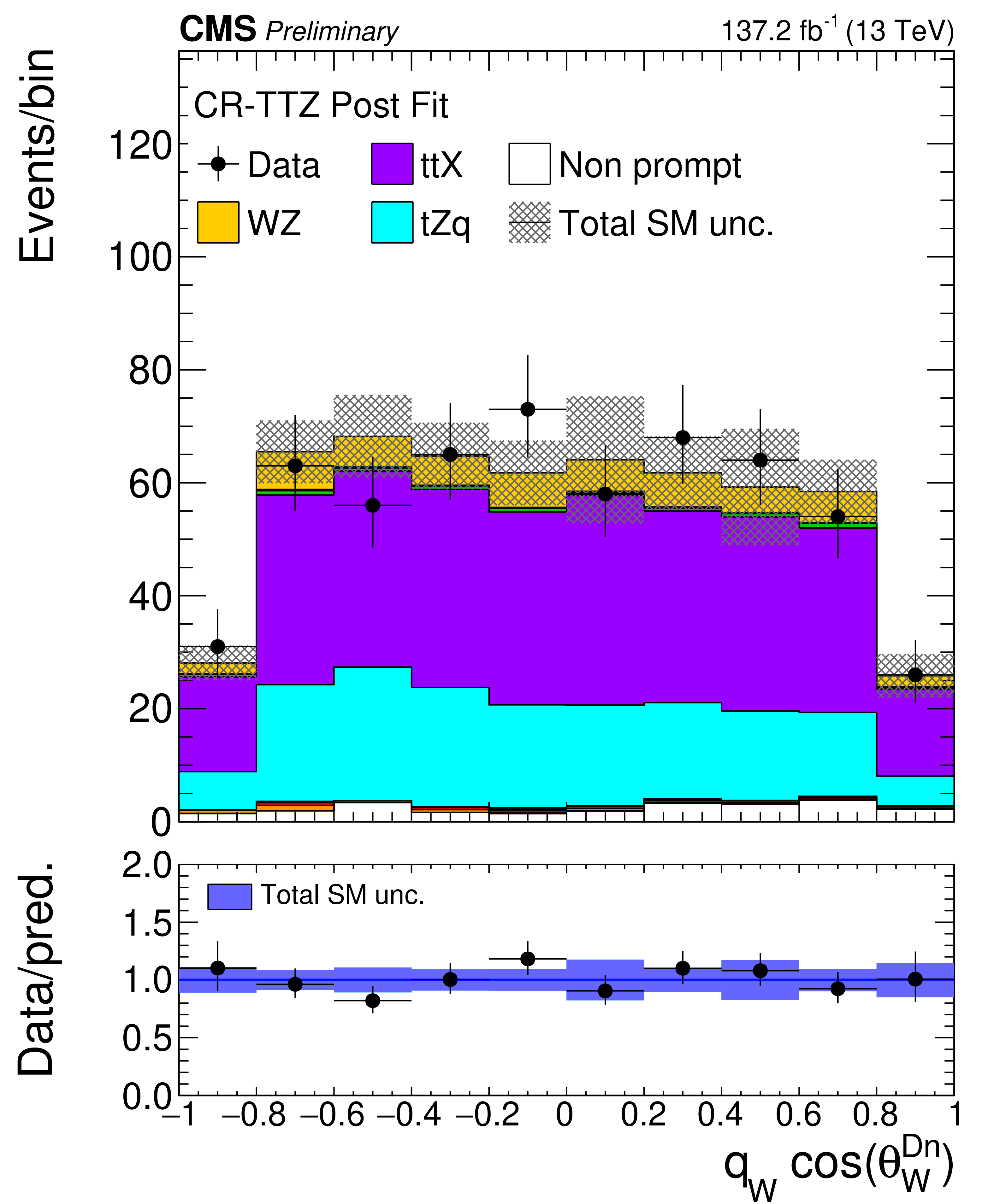
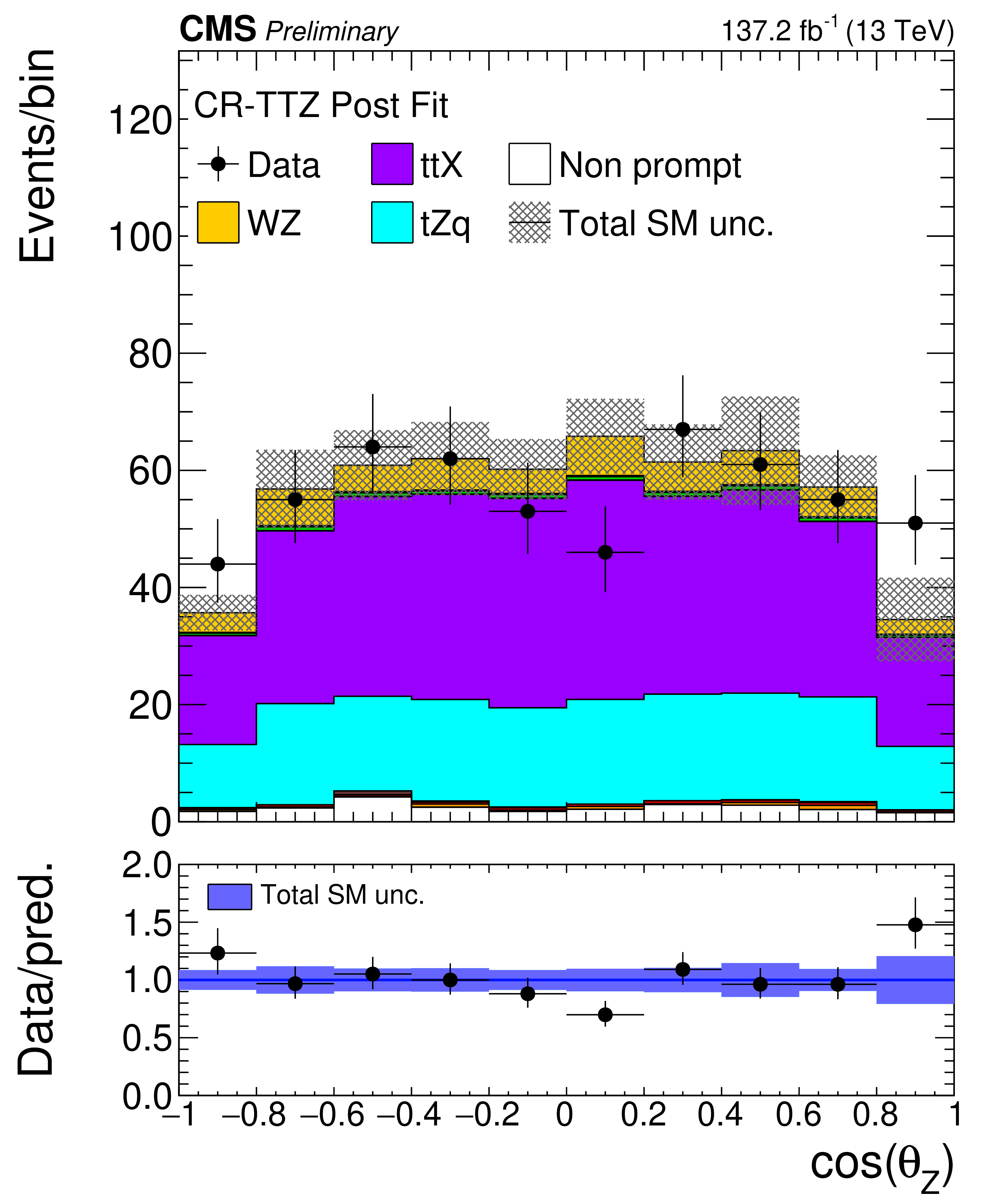
Figure 3:
Distribution of analysis-relevant observables in the TTZ control region evaluated with the uncertainties obtained after the signal extraction fit described in Section 8. From left to right and top to bottom: charge of the three leading lepton system, flavour distribution of the three leading lepton system, invariant mass of the three lepton plus ${{p_{\mathrm {T}}} ^\text {miss}}$ system, number of reconstructed jets, invariant mass of the leptonic pair with mass closest to that of the Z boson, reconstructed ${p_{\mathrm {T}}}$ of the Z boson times charge of the three leading lepton final state, reconstructed ${p_{\mathrm {T}}}$ of the W boson times final state charge constructed with ${{p_{\mathrm {T}}} ^\text {miss}}$ and the three leading lepton system, cosine of the polarization angle corresponding to the W angle, and cosine of the polarization angle corresponding to the Z boson. The label ttX includes both ttZ, ttW and ttH production. The shaded band in the ratio corresponds to the total uncertainty in the SM yields. |
png pdf |
Figure 3-a:
Distribution of analysis-relevant observables in the TTZ control region evaluated with the uncertainties obtained after the signal extraction fit described in Section 8. From left to right and top to bottom: charge of the three leading lepton system, flavour distribution of the three leading lepton system, invariant mass of the three lepton plus ${{p_{\mathrm {T}}} ^\text {miss}}$ system, number of reconstructed jets, invariant mass of the leptonic pair with mass closest to that of the Z boson, reconstructed ${p_{\mathrm {T}}}$ of the Z boson times charge of the three leading lepton final state, reconstructed ${p_{\mathrm {T}}}$ of the W boson times final state charge constructed with ${{p_{\mathrm {T}}} ^\text {miss}}$ and the three leading lepton system, cosine of the polarization angle corresponding to the W angle, and cosine of the polarization angle corresponding to the Z boson. The label ttX includes both ttZ, ttW and ttH production. The shaded band in the ratio corresponds to the total uncertainty in the SM yields. |
png pdf |
Figure 3-b:
Distribution of analysis-relevant observables in the TTZ control region evaluated with the uncertainties obtained after the signal extraction fit described in Section 8. From left to right and top to bottom: charge of the three leading lepton system, flavour distribution of the three leading lepton system, invariant mass of the three lepton plus ${{p_{\mathrm {T}}} ^\text {miss}}$ system, number of reconstructed jets, invariant mass of the leptonic pair with mass closest to that of the Z boson, reconstructed ${p_{\mathrm {T}}}$ of the Z boson times charge of the three leading lepton final state, reconstructed ${p_{\mathrm {T}}}$ of the W boson times final state charge constructed with ${{p_{\mathrm {T}}} ^\text {miss}}$ and the three leading lepton system, cosine of the polarization angle corresponding to the W angle, and cosine of the polarization angle corresponding to the Z boson. The label ttX includes both ttZ, ttW and ttH production. The shaded band in the ratio corresponds to the total uncertainty in the SM yields. |
png pdf |
Figure 3-c:
Distribution of analysis-relevant observables in the TTZ control region evaluated with the uncertainties obtained after the signal extraction fit described in Section 8. From left to right and top to bottom: charge of the three leading lepton system, flavour distribution of the three leading lepton system, invariant mass of the three lepton plus ${{p_{\mathrm {T}}} ^\text {miss}}$ system, number of reconstructed jets, invariant mass of the leptonic pair with mass closest to that of the Z boson, reconstructed ${p_{\mathrm {T}}}$ of the Z boson times charge of the three leading lepton final state, reconstructed ${p_{\mathrm {T}}}$ of the W boson times final state charge constructed with ${{p_{\mathrm {T}}} ^\text {miss}}$ and the three leading lepton system, cosine of the polarization angle corresponding to the W angle, and cosine of the polarization angle corresponding to the Z boson. The label ttX includes both ttZ, ttW and ttH production. The shaded band in the ratio corresponds to the total uncertainty in the SM yields. |
png pdf |
Figure 3-d:
Distribution of analysis-relevant observables in the TTZ control region evaluated with the uncertainties obtained after the signal extraction fit described in Section 8. From left to right and top to bottom: charge of the three leading lepton system, flavour distribution of the three leading lepton system, invariant mass of the three lepton plus ${{p_{\mathrm {T}}} ^\text {miss}}$ system, number of reconstructed jets, invariant mass of the leptonic pair with mass closest to that of the Z boson, reconstructed ${p_{\mathrm {T}}}$ of the Z boson times charge of the three leading lepton final state, reconstructed ${p_{\mathrm {T}}}$ of the W boson times final state charge constructed with ${{p_{\mathrm {T}}} ^\text {miss}}$ and the three leading lepton system, cosine of the polarization angle corresponding to the W angle, and cosine of the polarization angle corresponding to the Z boson. The label ttX includes both ttZ, ttW and ttH production. The shaded band in the ratio corresponds to the total uncertainty in the SM yields. |
png pdf |
Figure 3-e:
Distribution of analysis-relevant observables in the TTZ control region evaluated with the uncertainties obtained after the signal extraction fit described in Section 8. From left to right and top to bottom: charge of the three leading lepton system, flavour distribution of the three leading lepton system, invariant mass of the three lepton plus ${{p_{\mathrm {T}}} ^\text {miss}}$ system, number of reconstructed jets, invariant mass of the leptonic pair with mass closest to that of the Z boson, reconstructed ${p_{\mathrm {T}}}$ of the Z boson times charge of the three leading lepton final state, reconstructed ${p_{\mathrm {T}}}$ of the W boson times final state charge constructed with ${{p_{\mathrm {T}}} ^\text {miss}}$ and the three leading lepton system, cosine of the polarization angle corresponding to the W angle, and cosine of the polarization angle corresponding to the Z boson. The label ttX includes both ttZ, ttW and ttH production. The shaded band in the ratio corresponds to the total uncertainty in the SM yields. |
png pdf |
Figure 3-f:
Distribution of analysis-relevant observables in the TTZ control region evaluated with the uncertainties obtained after the signal extraction fit described in Section 8. From left to right and top to bottom: charge of the three leading lepton system, flavour distribution of the three leading lepton system, invariant mass of the three lepton plus ${{p_{\mathrm {T}}} ^\text {miss}}$ system, number of reconstructed jets, invariant mass of the leptonic pair with mass closest to that of the Z boson, reconstructed ${p_{\mathrm {T}}}$ of the Z boson times charge of the three leading lepton final state, reconstructed ${p_{\mathrm {T}}}$ of the W boson times final state charge constructed with ${{p_{\mathrm {T}}} ^\text {miss}}$ and the three leading lepton system, cosine of the polarization angle corresponding to the W angle, and cosine of the polarization angle corresponding to the Z boson. The label ttX includes both ttZ, ttW and ttH production. The shaded band in the ratio corresponds to the total uncertainty in the SM yields. |
png pdf |
Figure 3-g:
Distribution of analysis-relevant observables in the TTZ control region evaluated with the uncertainties obtained after the signal extraction fit described in Section 8. From left to right and top to bottom: charge of the three leading lepton system, flavour distribution of the three leading lepton system, invariant mass of the three lepton plus ${{p_{\mathrm {T}}} ^\text {miss}}$ system, number of reconstructed jets, invariant mass of the leptonic pair with mass closest to that of the Z boson, reconstructed ${p_{\mathrm {T}}}$ of the Z boson times charge of the three leading lepton final state, reconstructed ${p_{\mathrm {T}}}$ of the W boson times final state charge constructed with ${{p_{\mathrm {T}}} ^\text {miss}}$ and the three leading lepton system, cosine of the polarization angle corresponding to the W angle, and cosine of the polarization angle corresponding to the Z boson. The label ttX includes both ttZ, ttW and ttH production. The shaded band in the ratio corresponds to the total uncertainty in the SM yields. |
png pdf |
Figure 3-h:
Distribution of analysis-relevant observables in the TTZ control region evaluated with the uncertainties obtained after the signal extraction fit described in Section 8. From left to right and top to bottom: charge of the three leading lepton system, flavour distribution of the three leading lepton system, invariant mass of the three lepton plus ${{p_{\mathrm {T}}} ^\text {miss}}$ system, number of reconstructed jets, invariant mass of the leptonic pair with mass closest to that of the Z boson, reconstructed ${p_{\mathrm {T}}}$ of the Z boson times charge of the three leading lepton final state, reconstructed ${p_{\mathrm {T}}}$ of the W boson times final state charge constructed with ${{p_{\mathrm {T}}} ^\text {miss}}$ and the three leading lepton system, cosine of the polarization angle corresponding to the W angle, and cosine of the polarization angle corresponding to the Z boson. The label ttX includes both ttZ, ttW and ttH production. The shaded band in the ratio corresponds to the total uncertainty in the SM yields. |
png pdf |
Figure 3-i:
Distribution of analysis-relevant observables in the TTZ control region evaluated with the uncertainties obtained after the signal extraction fit described in Section 8. From left to right and top to bottom: charge of the three leading lepton system, flavour distribution of the three leading lepton system, invariant mass of the three lepton plus ${{p_{\mathrm {T}}} ^\text {miss}}$ system, number of reconstructed jets, invariant mass of the leptonic pair with mass closest to that of the Z boson, reconstructed ${p_{\mathrm {T}}}$ of the Z boson times charge of the three leading lepton final state, reconstructed ${p_{\mathrm {T}}}$ of the W boson times final state charge constructed with ${{p_{\mathrm {T}}} ^\text {miss}}$ and the three leading lepton system, cosine of the polarization angle corresponding to the W angle, and cosine of the polarization angle corresponding to the Z boson. The label ttX includes both ttZ, ttW and ttH production. The shaded band in the ratio corresponds to the total uncertainty in the SM yields. |

png pdf |
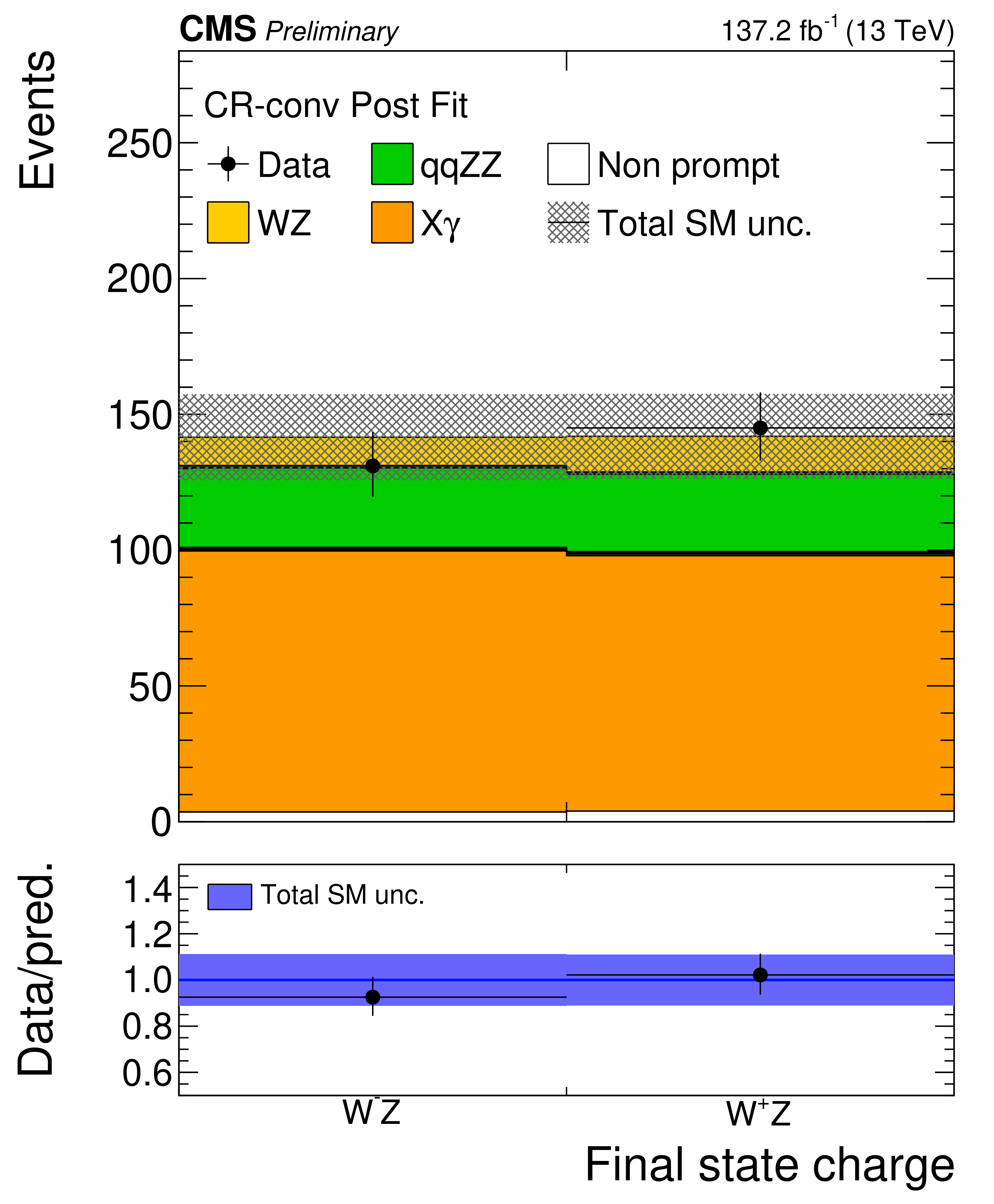
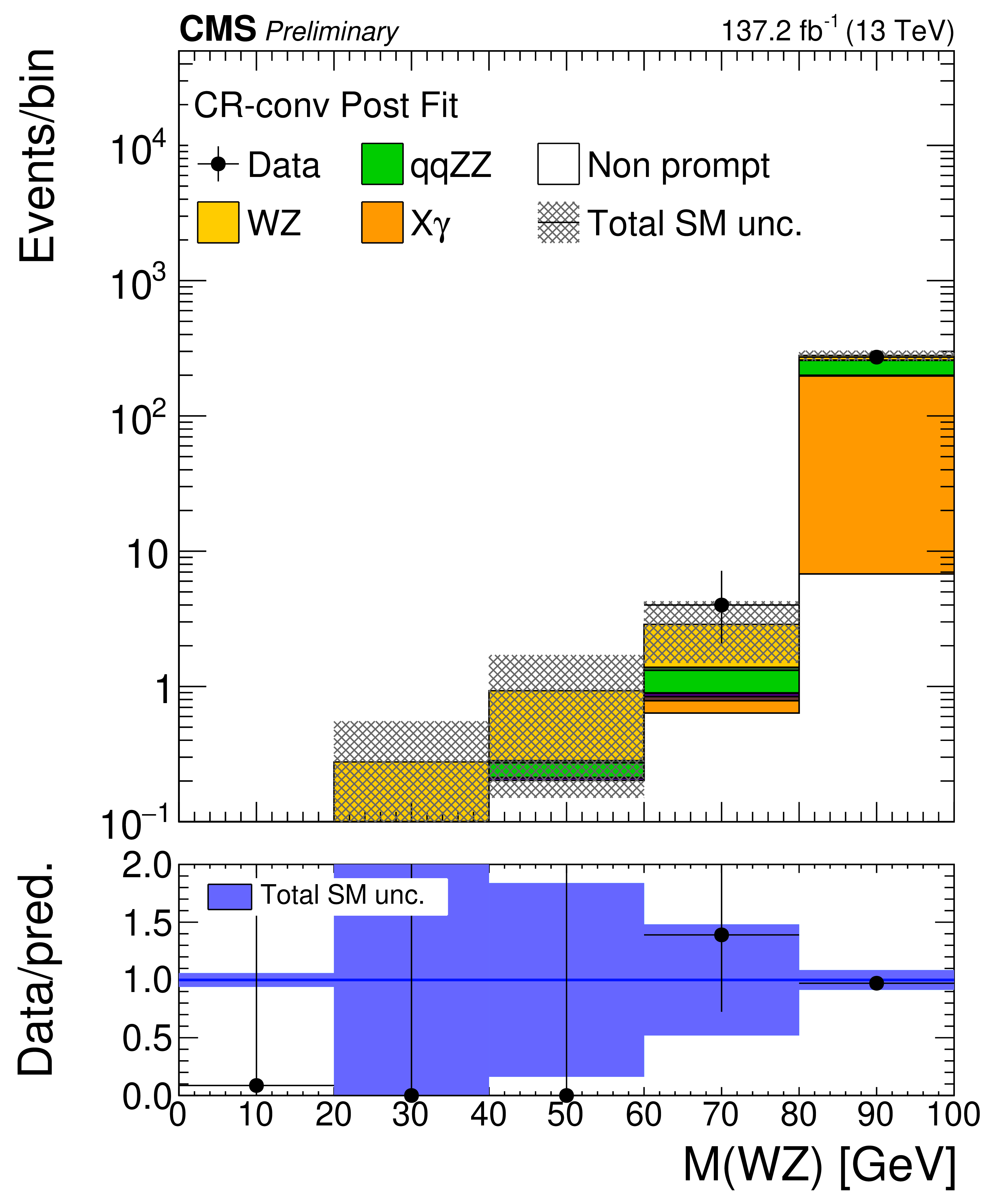
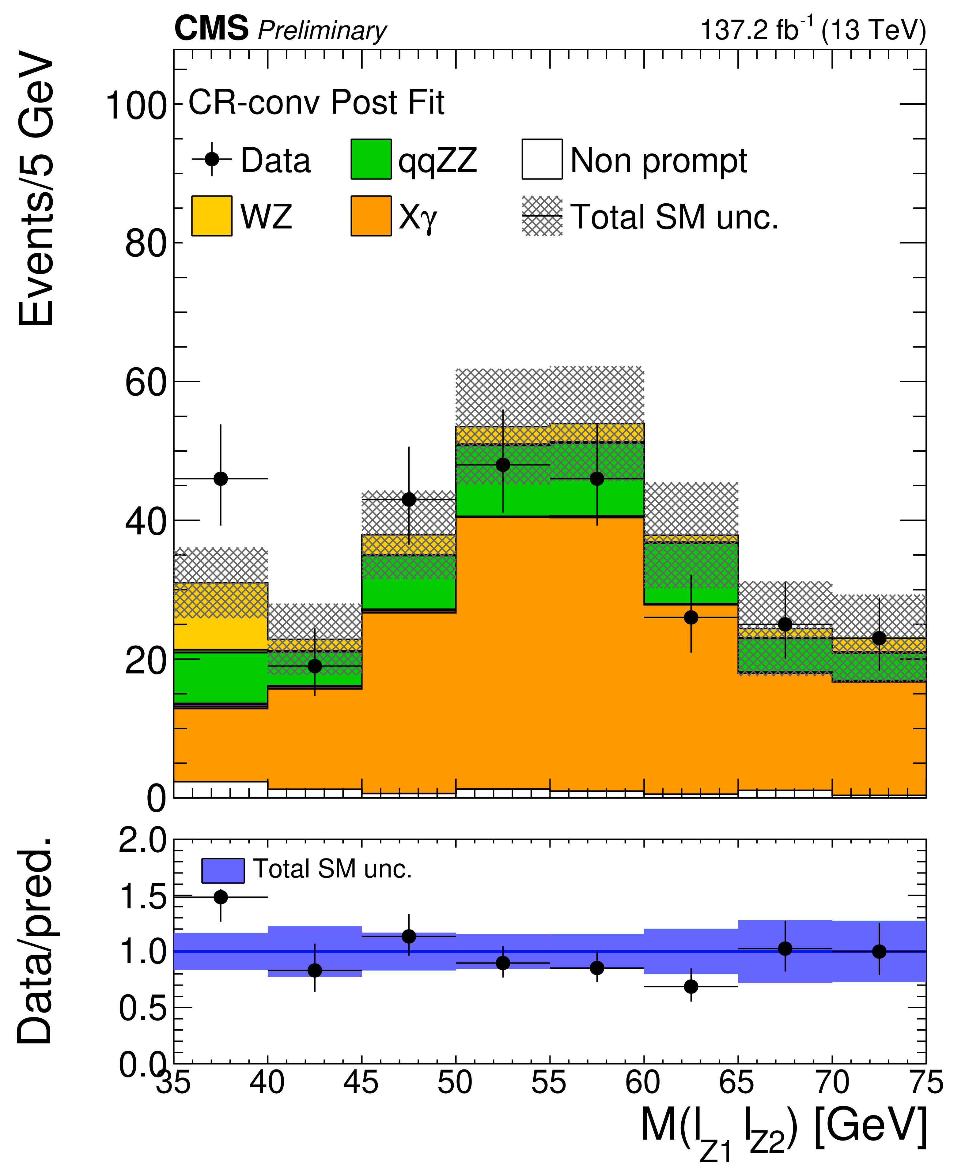
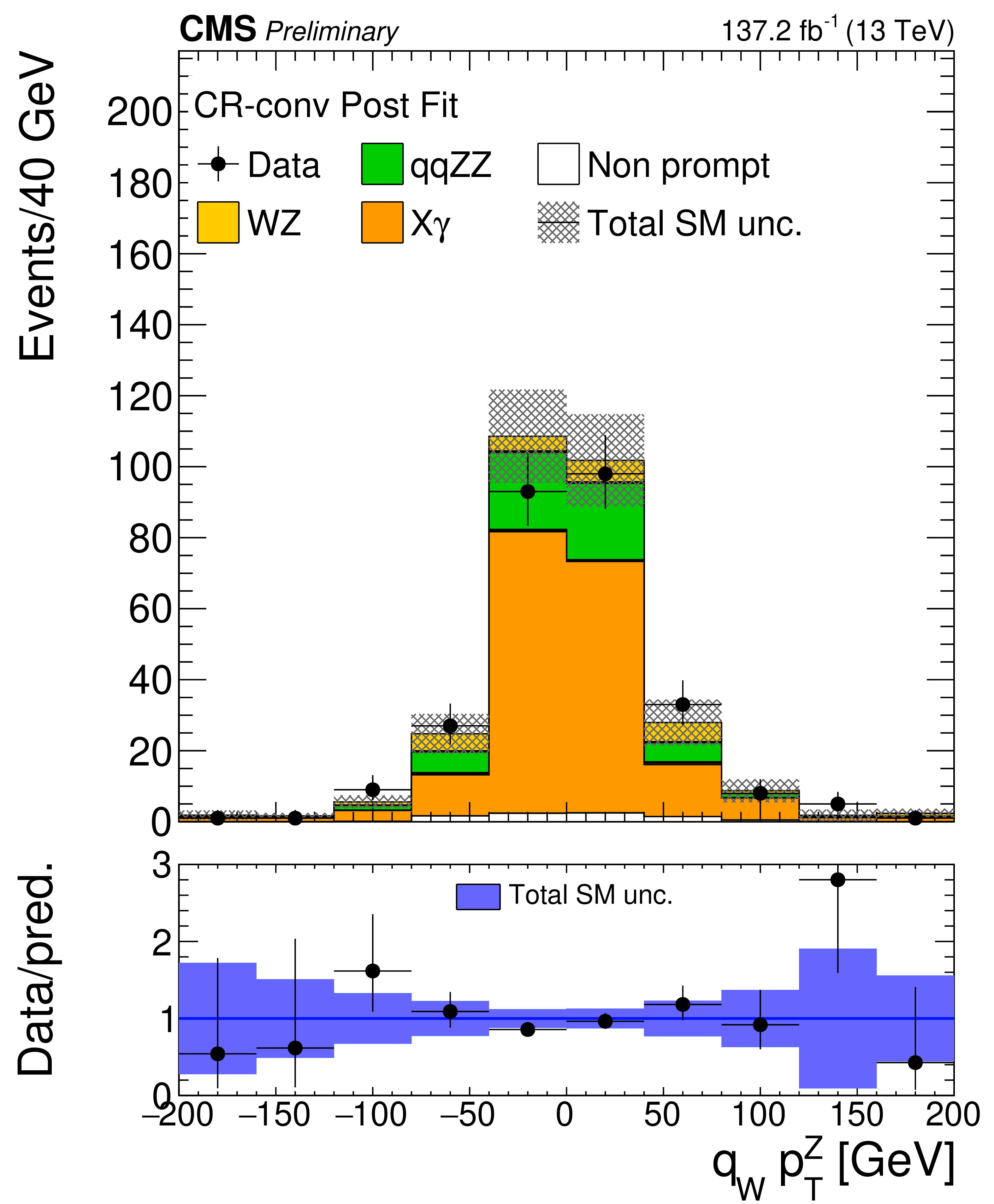
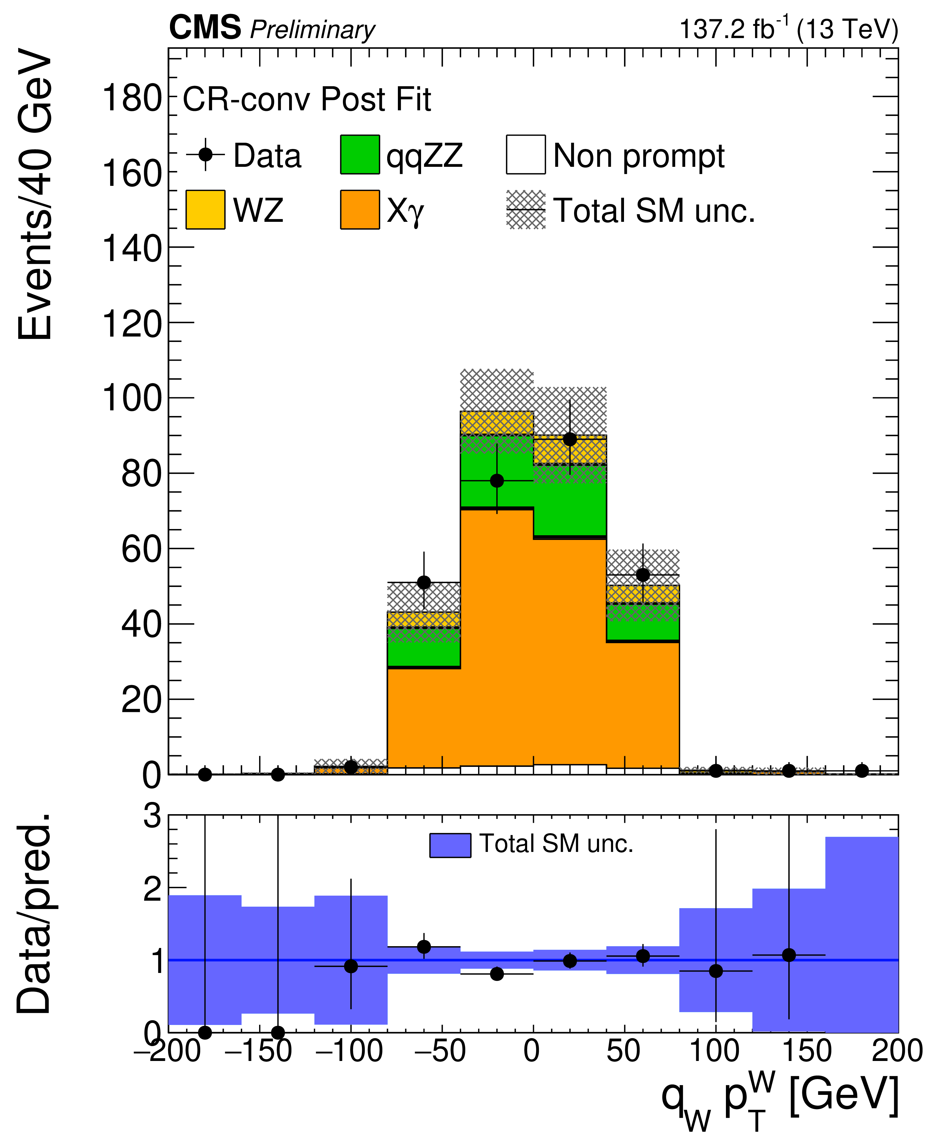
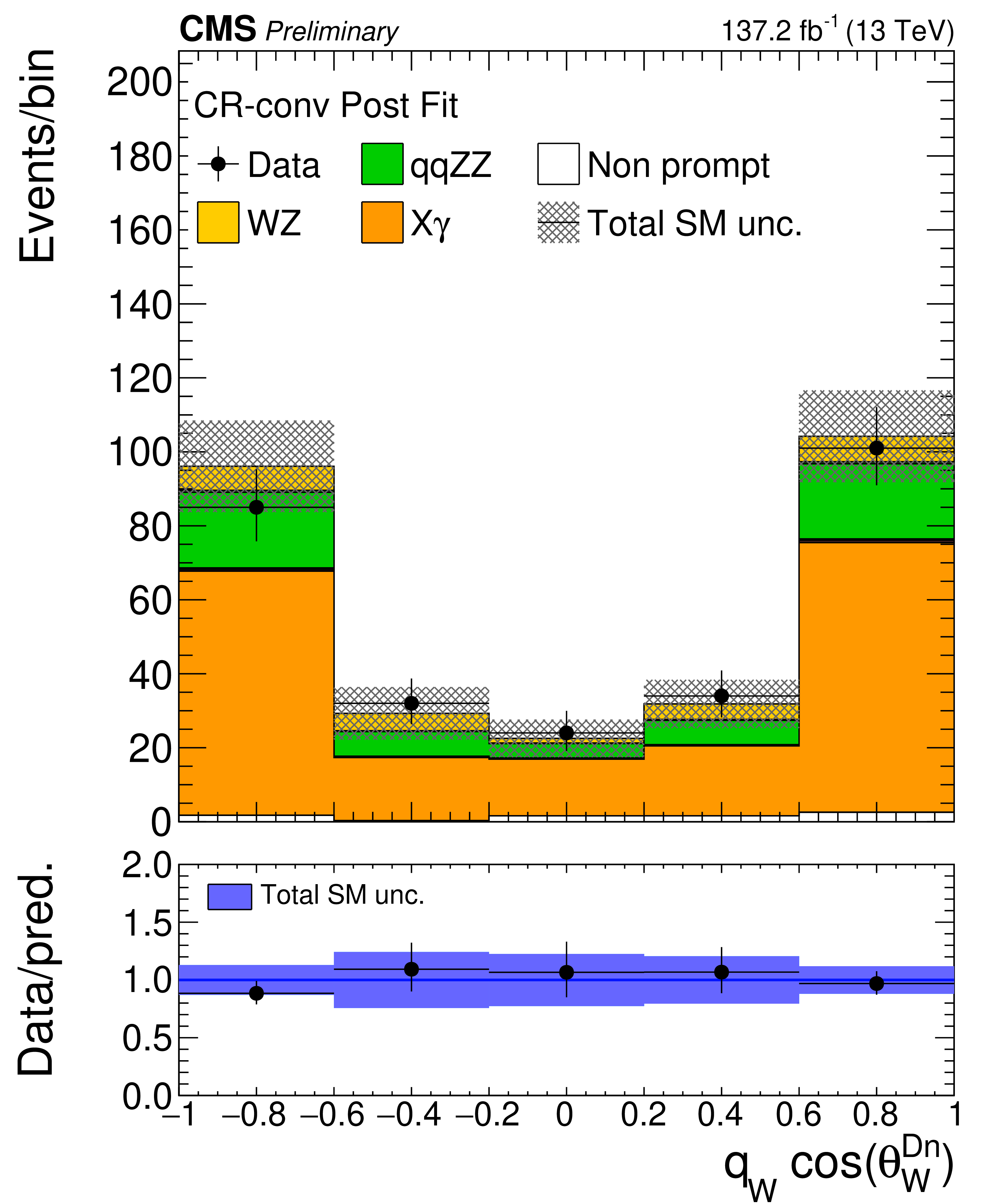
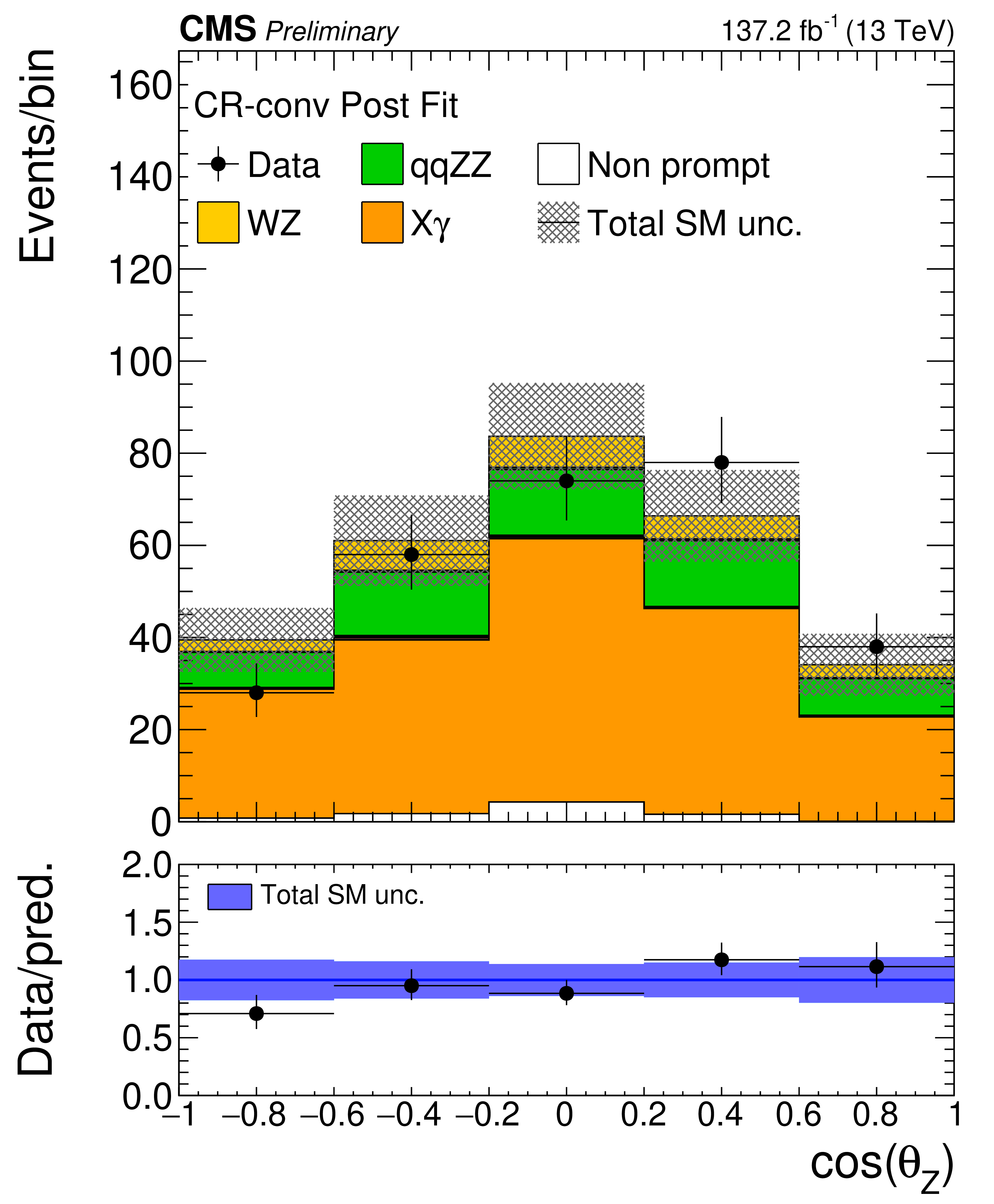
Figure 4:
Distribution of analysis-relevant observables in the conversion control region evaluated with the uncertainties obtained after the signal extraction fit described in Section 8. From left to right and top to bottom: charge of the three leading lepton system, flavour distribution of the three leading lepton system, invariant mass of the three lepton plus ${{p_{\mathrm {T}}} ^\text {miss}}$ system, number of reconstructed jets, invariant mass of the leptonic pair with mass closest to that of the Z boson, reconstructed ${p_{\mathrm {T}}}$ of the Z boson times charge of the three leading lepton final state, reconstructed ${p_{\mathrm {T}}}$ of the W boson times final state charge constructed with ${{p_{\mathrm {T}}} ^\text {miss}}$ and the three leading lepton system, cosine of the polarization angle corresponding to the W angle, and cosine of the polarization angle corresponding to the Z boson. Only normalization and statistical uncertainties are included in the plot. X$\gamma$ includes Z$\gamma$, W$\gamma$, tt$\gamma$ and WZ$\gamma$ production. The shaded band in the ratio corresponds to the total uncertainty in the SM yields. |
png pdf |
Figure 4-a:
Distribution of analysis-relevant observables in the conversion control region evaluated with the uncertainties obtained after the signal extraction fit described in Section 8. From left to right and top to bottom: charge of the three leading lepton system, flavour distribution of the three leading lepton system, invariant mass of the three lepton plus ${{p_{\mathrm {T}}} ^\text {miss}}$ system, number of reconstructed jets, invariant mass of the leptonic pair with mass closest to that of the Z boson, reconstructed ${p_{\mathrm {T}}}$ of the Z boson times charge of the three leading lepton final state, reconstructed ${p_{\mathrm {T}}}$ of the W boson times final state charge constructed with ${{p_{\mathrm {T}}} ^\text {miss}}$ and the three leading lepton system, cosine of the polarization angle corresponding to the W angle, and cosine of the polarization angle corresponding to the Z boson. Only normalization and statistical uncertainties are included in the plot. X$\gamma$ includes Z$\gamma$, W$\gamma$, tt$\gamma$ and WZ$\gamma$ production. The shaded band in the ratio corresponds to the total uncertainty in the SM yields. |

png pdf |
Figure 4-b:
Distribution of analysis-relevant observables in the conversion control region evaluated with the uncertainties obtained after the signal extraction fit described in Section 8. From left to right and top to bottom: charge of the three leading lepton system, flavour distribution of the three leading lepton system, invariant mass of the three lepton plus ${{p_{\mathrm {T}}} ^\text {miss}}$ system, number of reconstructed jets, invariant mass of the leptonic pair with mass closest to that of the Z boson, reconstructed ${p_{\mathrm {T}}}$ of the Z boson times charge of the three leading lepton final state, reconstructed ${p_{\mathrm {T}}}$ of the W boson times final state charge constructed with ${{p_{\mathrm {T}}} ^\text {miss}}$ and the three leading lepton system, cosine of the polarization angle corresponding to the W angle, and cosine of the polarization angle corresponding to the Z boson. Only normalization and statistical uncertainties are included in the plot. X$\gamma$ includes Z$\gamma$, W$\gamma$, tt$\gamma$ and WZ$\gamma$ production. The shaded band in the ratio corresponds to the total uncertainty in the SM yields. |
png pdf |
Figure 4-c:
Distribution of analysis-relevant observables in the conversion control region evaluated with the uncertainties obtained after the signal extraction fit described in Section 8. From left to right and top to bottom: charge of the three leading lepton system, flavour distribution of the three leading lepton system, invariant mass of the three lepton plus ${{p_{\mathrm {T}}} ^\text {miss}}$ system, number of reconstructed jets, invariant mass of the leptonic pair with mass closest to that of the Z boson, reconstructed ${p_{\mathrm {T}}}$ of the Z boson times charge of the three leading lepton final state, reconstructed ${p_{\mathrm {T}}}$ of the W boson times final state charge constructed with ${{p_{\mathrm {T}}} ^\text {miss}}$ and the three leading lepton system, cosine of the polarization angle corresponding to the W angle, and cosine of the polarization angle corresponding to the Z boson. Only normalization and statistical uncertainties are included in the plot. X$\gamma$ includes Z$\gamma$, W$\gamma$, tt$\gamma$ and WZ$\gamma$ production. The shaded band in the ratio corresponds to the total uncertainty in the SM yields. |

png pdf |
Figure 4-d:
Distribution of analysis-relevant observables in the conversion control region evaluated with the uncertainties obtained after the signal extraction fit described in Section 8. From left to right and top to bottom: charge of the three leading lepton system, flavour distribution of the three leading lepton system, invariant mass of the three lepton plus ${{p_{\mathrm {T}}} ^\text {miss}}$ system, number of reconstructed jets, invariant mass of the leptonic pair with mass closest to that of the Z boson, reconstructed ${p_{\mathrm {T}}}$ of the Z boson times charge of the three leading lepton final state, reconstructed ${p_{\mathrm {T}}}$ of the W boson times final state charge constructed with ${{p_{\mathrm {T}}} ^\text {miss}}$ and the three leading lepton system, cosine of the polarization angle corresponding to the W angle, and cosine of the polarization angle corresponding to the Z boson. Only normalization and statistical uncertainties are included in the plot. X$\gamma$ includes Z$\gamma$, W$\gamma$, tt$\gamma$ and WZ$\gamma$ production. The shaded band in the ratio corresponds to the total uncertainty in the SM yields. |
png pdf |
Figure 4-e:
Distribution of analysis-relevant observables in the conversion control region evaluated with the uncertainties obtained after the signal extraction fit described in Section 8. From left to right and top to bottom: charge of the three leading lepton system, flavour distribution of the three leading lepton system, invariant mass of the three lepton plus ${{p_{\mathrm {T}}} ^\text {miss}}$ system, number of reconstructed jets, invariant mass of the leptonic pair with mass closest to that of the Z boson, reconstructed ${p_{\mathrm {T}}}$ of the Z boson times charge of the three leading lepton final state, reconstructed ${p_{\mathrm {T}}}$ of the W boson times final state charge constructed with ${{p_{\mathrm {T}}} ^\text {miss}}$ and the three leading lepton system, cosine of the polarization angle corresponding to the W angle, and cosine of the polarization angle corresponding to the Z boson. Only normalization and statistical uncertainties are included in the plot. X$\gamma$ includes Z$\gamma$, W$\gamma$, tt$\gamma$ and WZ$\gamma$ production. The shaded band in the ratio corresponds to the total uncertainty in the SM yields. |
png pdf |
Figure 4-f:
Distribution of analysis-relevant observables in the conversion control region evaluated with the uncertainties obtained after the signal extraction fit described in Section 8. From left to right and top to bottom: charge of the three leading lepton system, flavour distribution of the three leading lepton system, invariant mass of the three lepton plus ${{p_{\mathrm {T}}} ^\text {miss}}$ system, number of reconstructed jets, invariant mass of the leptonic pair with mass closest to that of the Z boson, reconstructed ${p_{\mathrm {T}}}$ of the Z boson times charge of the three leading lepton final state, reconstructed ${p_{\mathrm {T}}}$ of the W boson times final state charge constructed with ${{p_{\mathrm {T}}} ^\text {miss}}$ and the three leading lepton system, cosine of the polarization angle corresponding to the W angle, and cosine of the polarization angle corresponding to the Z boson. Only normalization and statistical uncertainties are included in the plot. X$\gamma$ includes Z$\gamma$, W$\gamma$, tt$\gamma$ and WZ$\gamma$ production. The shaded band in the ratio corresponds to the total uncertainty in the SM yields. |
png pdf |
Figure 4-g:
Distribution of analysis-relevant observables in the conversion control region evaluated with the uncertainties obtained after the signal extraction fit described in Section 8. From left to right and top to bottom: charge of the three leading lepton system, flavour distribution of the three leading lepton system, invariant mass of the three lepton plus ${{p_{\mathrm {T}}} ^\text {miss}}$ system, number of reconstructed jets, invariant mass of the leptonic pair with mass closest to that of the Z boson, reconstructed ${p_{\mathrm {T}}}$ of the Z boson times charge of the three leading lepton final state, reconstructed ${p_{\mathrm {T}}}$ of the W boson times final state charge constructed with ${{p_{\mathrm {T}}} ^\text {miss}}$ and the three leading lepton system, cosine of the polarization angle corresponding to the W angle, and cosine of the polarization angle corresponding to the Z boson. Only normalization and statistical uncertainties are included in the plot. X$\gamma$ includes Z$\gamma$, W$\gamma$, tt$\gamma$ and WZ$\gamma$ production. The shaded band in the ratio corresponds to the total uncertainty in the SM yields. |
png pdf |
Figure 4-h:
Distribution of analysis-relevant observables in the conversion control region evaluated with the uncertainties obtained after the signal extraction fit described in Section 8. From left to right and top to bottom: charge of the three leading lepton system, flavour distribution of the three leading lepton system, invariant mass of the three lepton plus ${{p_{\mathrm {T}}} ^\text {miss}}$ system, number of reconstructed jets, invariant mass of the leptonic pair with mass closest to that of the Z boson, reconstructed ${p_{\mathrm {T}}}$ of the Z boson times charge of the three leading lepton final state, reconstructed ${p_{\mathrm {T}}}$ of the W boson times final state charge constructed with ${{p_{\mathrm {T}}} ^\text {miss}}$ and the three leading lepton system, cosine of the polarization angle corresponding to the W angle, and cosine of the polarization angle corresponding to the Z boson. Only normalization and statistical uncertainties are included in the plot. X$\gamma$ includes Z$\gamma$, W$\gamma$, tt$\gamma$ and WZ$\gamma$ production. The shaded band in the ratio corresponds to the total uncertainty in the SM yields. |
png pdf |
Figure 4-i:
Distribution of analysis-relevant observables in the conversion control region evaluated with the uncertainties obtained after the signal extraction fit described in Section 8. From left to right and top to bottom: charge of the three leading lepton system, flavour distribution of the three leading lepton system, invariant mass of the three lepton plus ${{p_{\mathrm {T}}} ^\text {miss}}$ system, number of reconstructed jets, invariant mass of the leptonic pair with mass closest to that of the Z boson, reconstructed ${p_{\mathrm {T}}}$ of the Z boson times charge of the three leading lepton final state, reconstructed ${p_{\mathrm {T}}}$ of the W boson times final state charge constructed with ${{p_{\mathrm {T}}} ^\text {miss}}$ and the three leading lepton system, cosine of the polarization angle corresponding to the W angle, and cosine of the polarization angle corresponding to the Z boson. Only normalization and statistical uncertainties are included in the plot. X$\gamma$ includes Z$\gamma$, W$\gamma$, tt$\gamma$ and WZ$\gamma$ production. The shaded band in the ratio corresponds to the total uncertainty in the SM yields. |
png pdf |
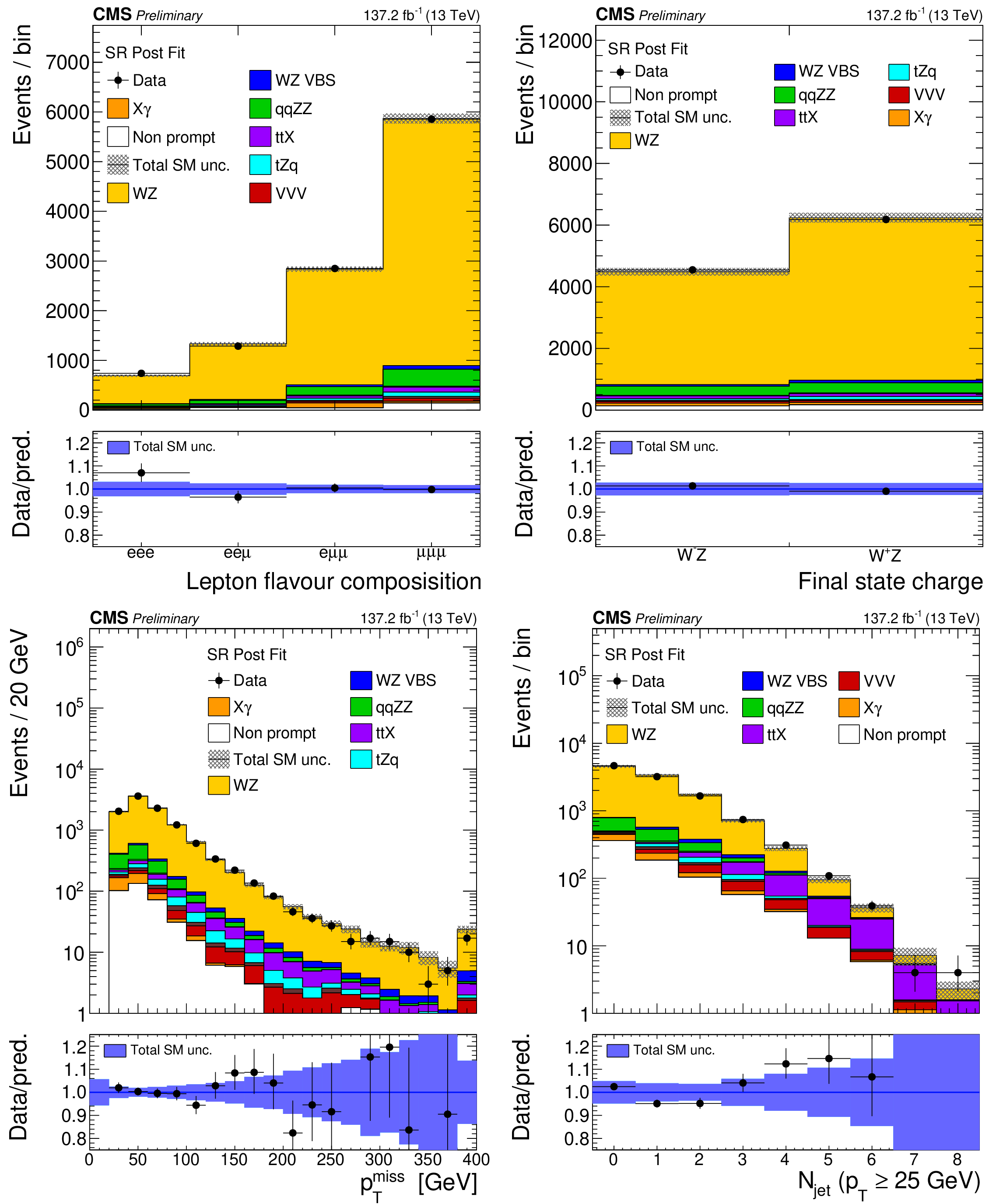
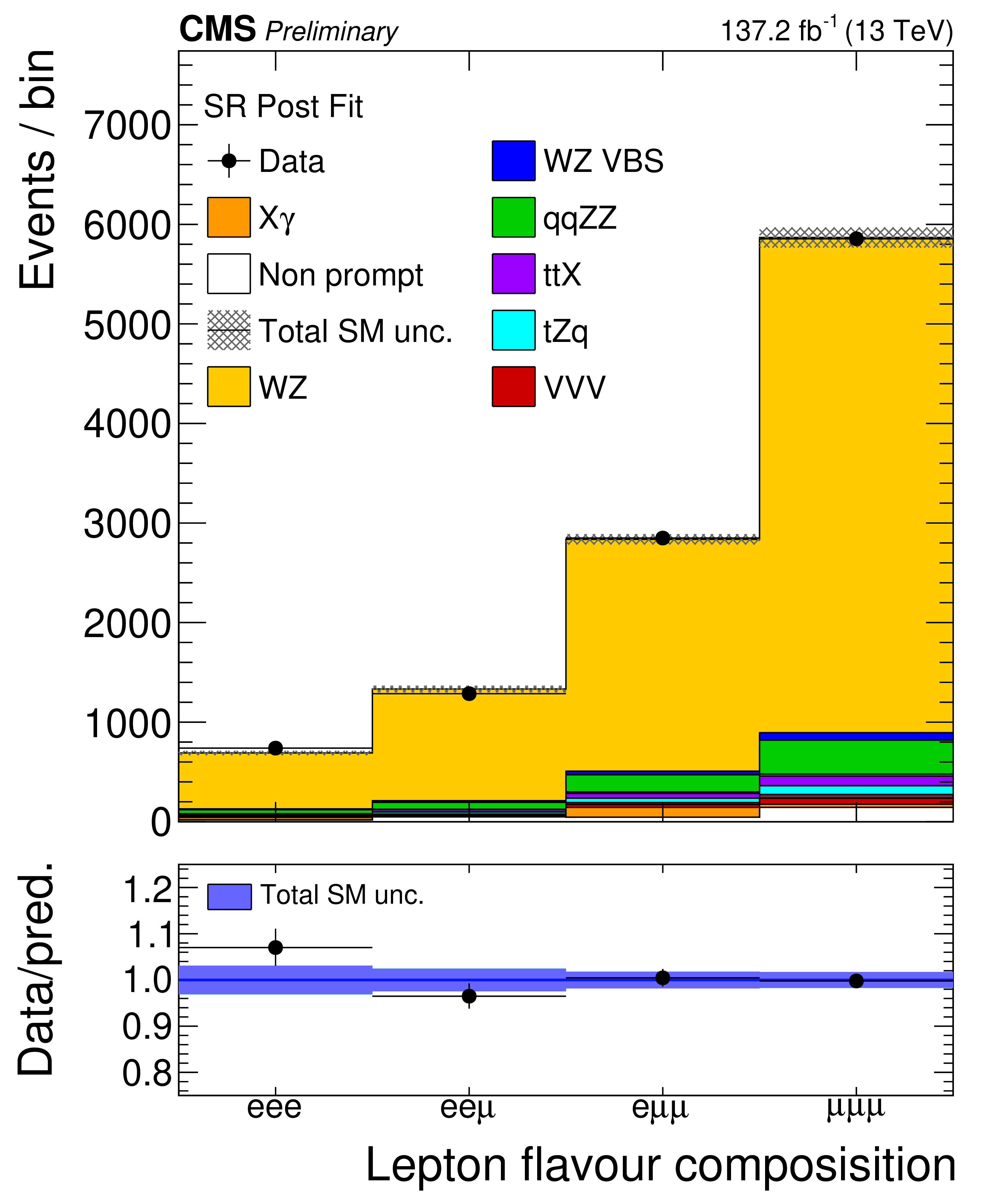
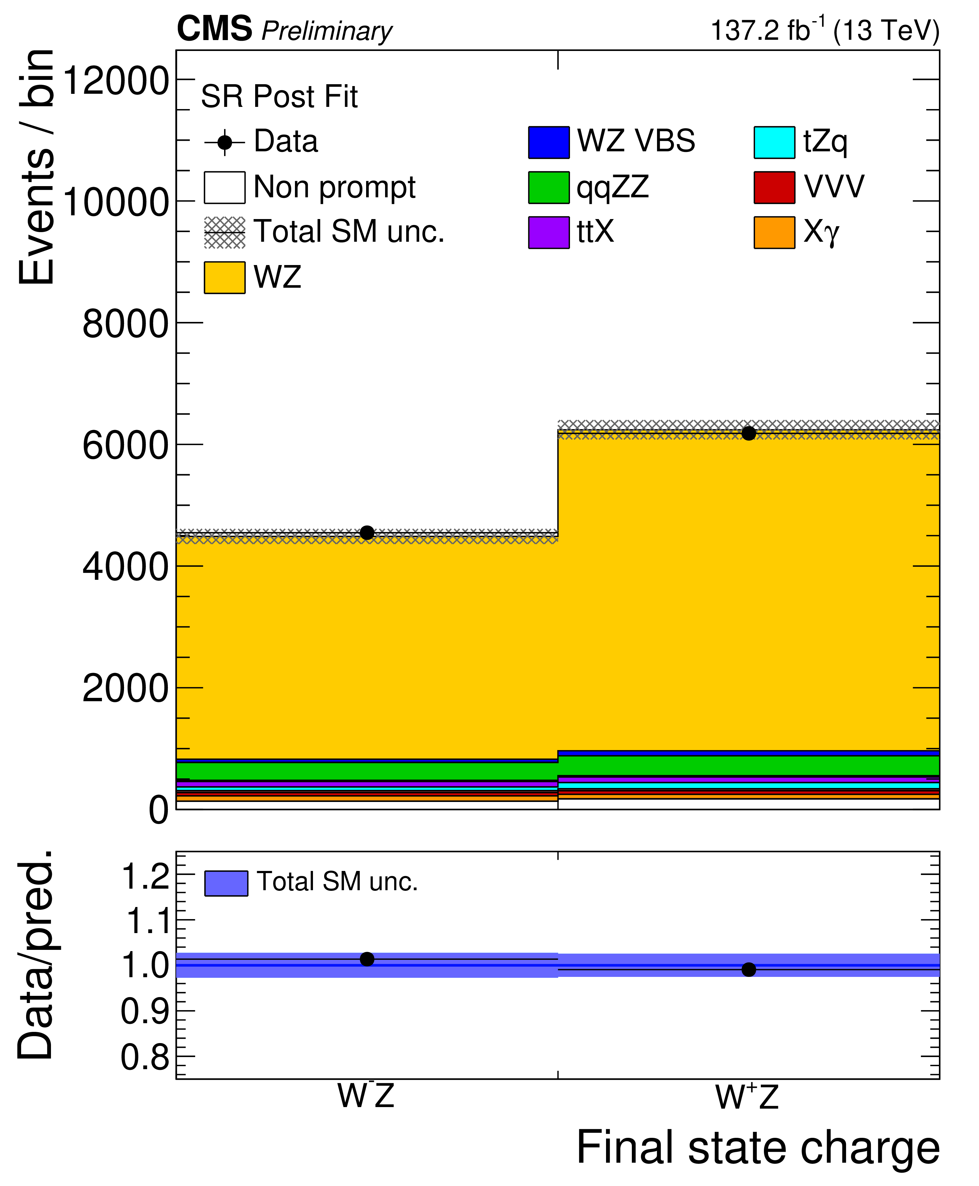
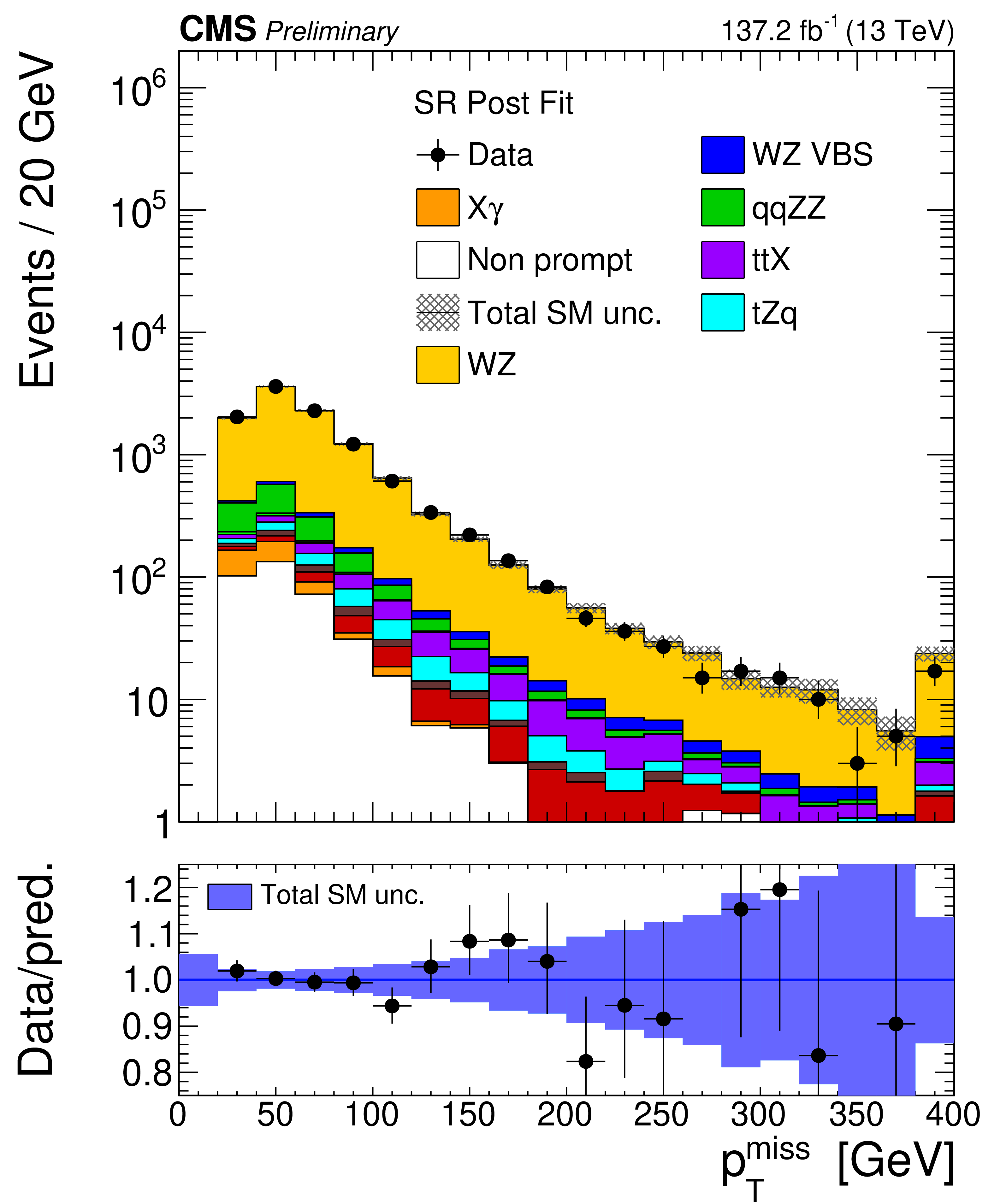
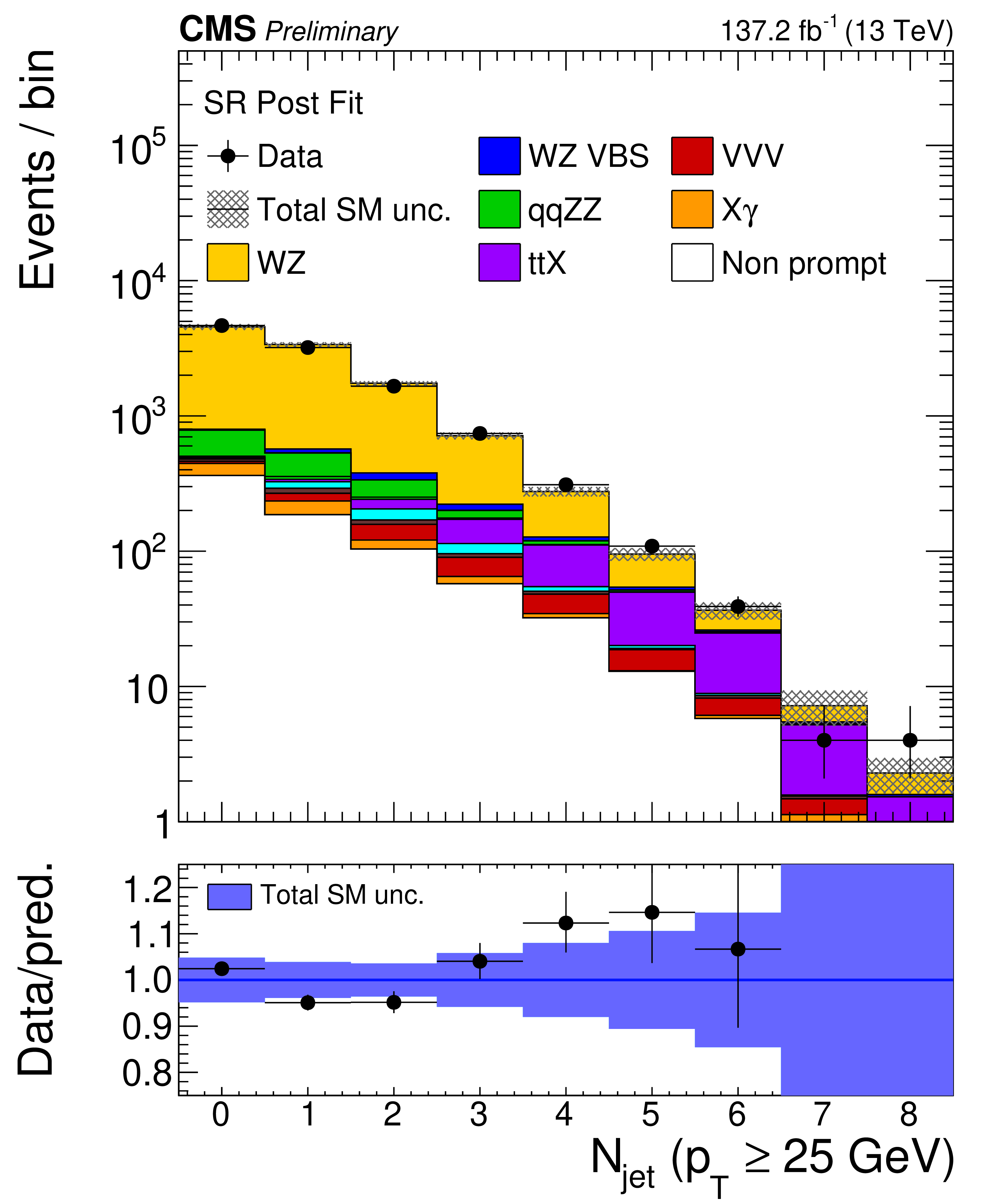
Figure 5:
Distribution of event observables in the signal region after the combined fit to all years and flavour final states: flavour composition of the three lepton final state (top left), sum of charge of the final state leptons (top right), missing transverse momentum (bottom left), and number of reconstructed jets with ${p_{\mathrm {T}}}$ greater than 25 GeV (bottom right). The shaded band in the ratio includes the effects of all analysis uncertainties on the background and signal yields. X$\gamma$ includes Z$\gamma$, W$\gamma$, tt$\gamma$ and WZ$\gamma$ production. The label ttX includes both ttZ, ttW and ttH production. The shaded band in the ratio corresponds to the total uncertainty in the SM yields. |
png pdf |
Figure 5-a:
Distribution of event observables in the signal region after the combined fit to all years and flavour final states: flavour composition of the three lepton final state (top left), sum of charge of the final state leptons (top right), missing transverse momentum (bottom left), and number of reconstructed jets with ${p_{\mathrm {T}}}$ greater than 25 GeV (bottom right). The shaded band in the ratio includes the effects of all analysis uncertainties on the background and signal yields. X$\gamma$ includes Z$\gamma$, W$\gamma$, tt$\gamma$ and WZ$\gamma$ production. The label ttX includes both ttZ, ttW and ttH production. The shaded band in the ratio corresponds to the total uncertainty in the SM yields. |
png pdf |
Figure 5-b:
Distribution of event observables in the signal region after the combined fit to all years and flavour final states: flavour composition of the three lepton final state (top left), sum of charge of the final state leptons (top right), missing transverse momentum (bottom left), and number of reconstructed jets with ${p_{\mathrm {T}}}$ greater than 25 GeV (bottom right). The shaded band in the ratio includes the effects of all analysis uncertainties on the background and signal yields. X$\gamma$ includes Z$\gamma$, W$\gamma$, tt$\gamma$ and WZ$\gamma$ production. The label ttX includes both ttZ, ttW and ttH production. The shaded band in the ratio corresponds to the total uncertainty in the SM yields. |
png pdf |
Figure 5-c:
Distribution of event observables in the signal region after the combined fit to all years and flavour final states: flavour composition of the three lepton final state (top left), sum of charge of the final state leptons (top right), missing transverse momentum (bottom left), and number of reconstructed jets with ${p_{\mathrm {T}}}$ greater than 25 GeV (bottom right). The shaded band in the ratio includes the effects of all analysis uncertainties on the background and signal yields. X$\gamma$ includes Z$\gamma$, W$\gamma$, tt$\gamma$ and WZ$\gamma$ production. The label ttX includes both ttZ, ttW and ttH production. The shaded band in the ratio corresponds to the total uncertainty in the SM yields. |
png pdf |
Figure 5-d:
Distribution of event observables in the signal region after the combined fit to all years and flavour final states: flavour composition of the three lepton final state (top left), sum of charge of the final state leptons (top right), missing transverse momentum (bottom left), and number of reconstructed jets with ${p_{\mathrm {T}}}$ greater than 25 GeV (bottom right). The shaded band in the ratio includes the effects of all analysis uncertainties on the background and signal yields. X$\gamma$ includes Z$\gamma$, W$\gamma$, tt$\gamma$ and WZ$\gamma$ production. The label ttX includes both ttZ, ttW and ttH production. The shaded band in the ratio corresponds to the total uncertainty in the SM yields. |
png pdf |
Figure 6:
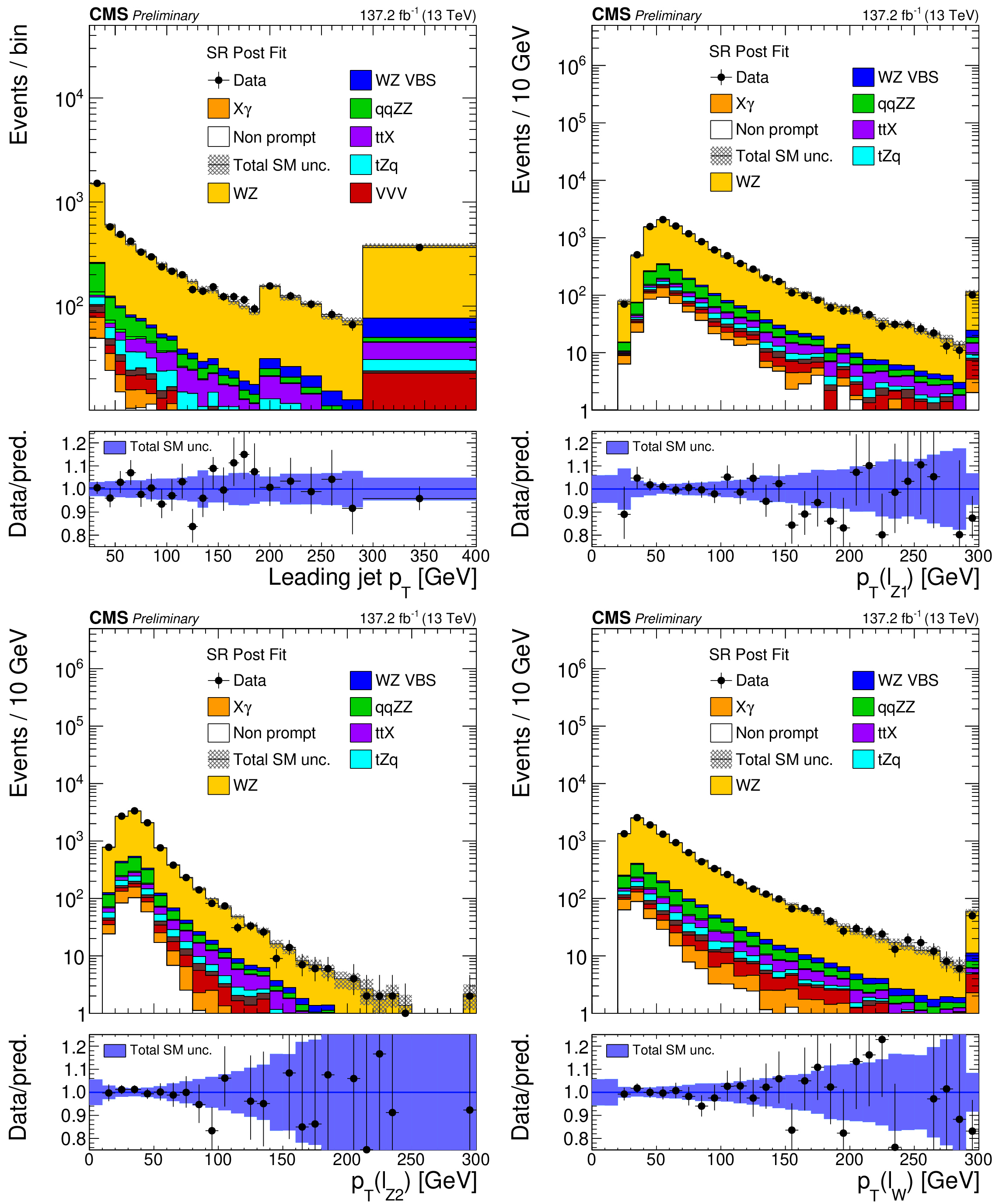
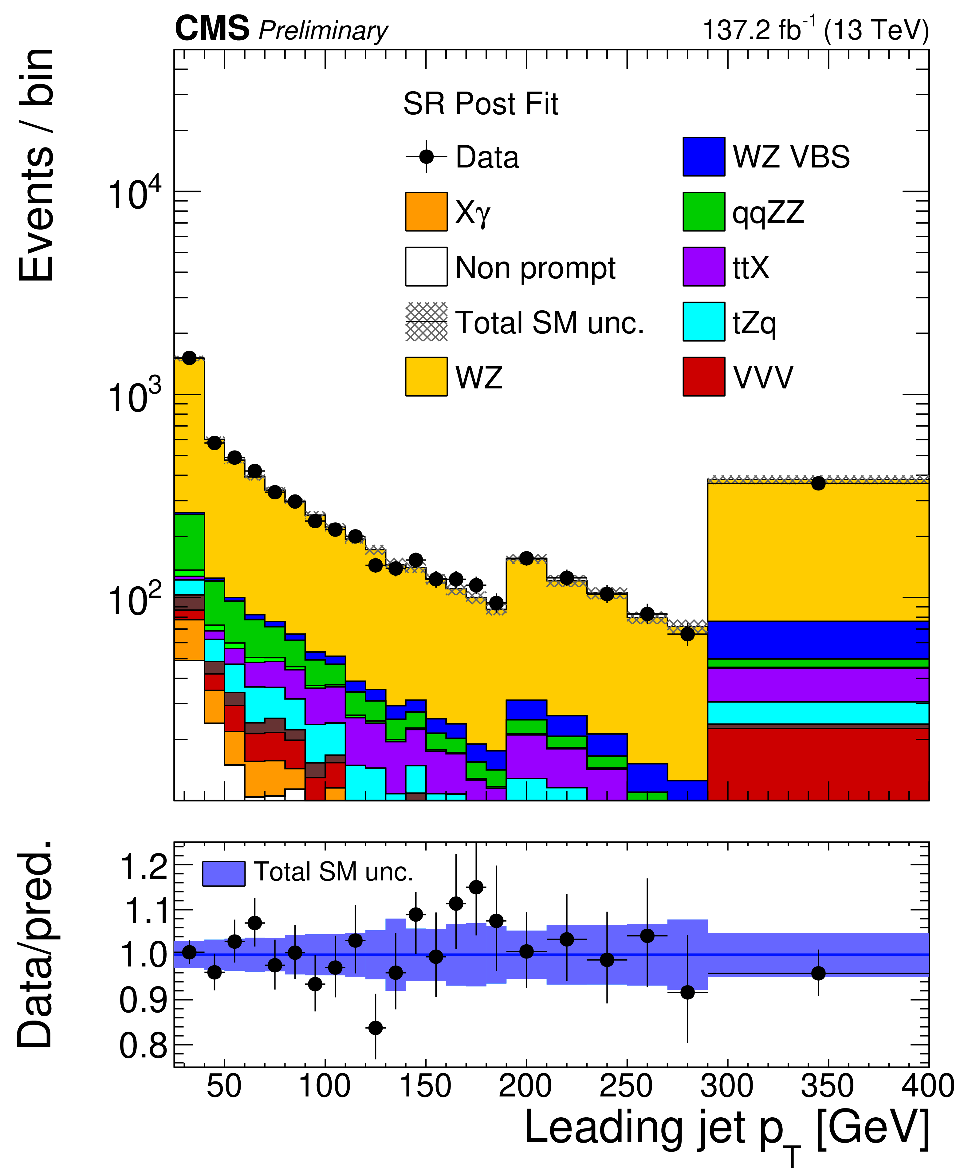
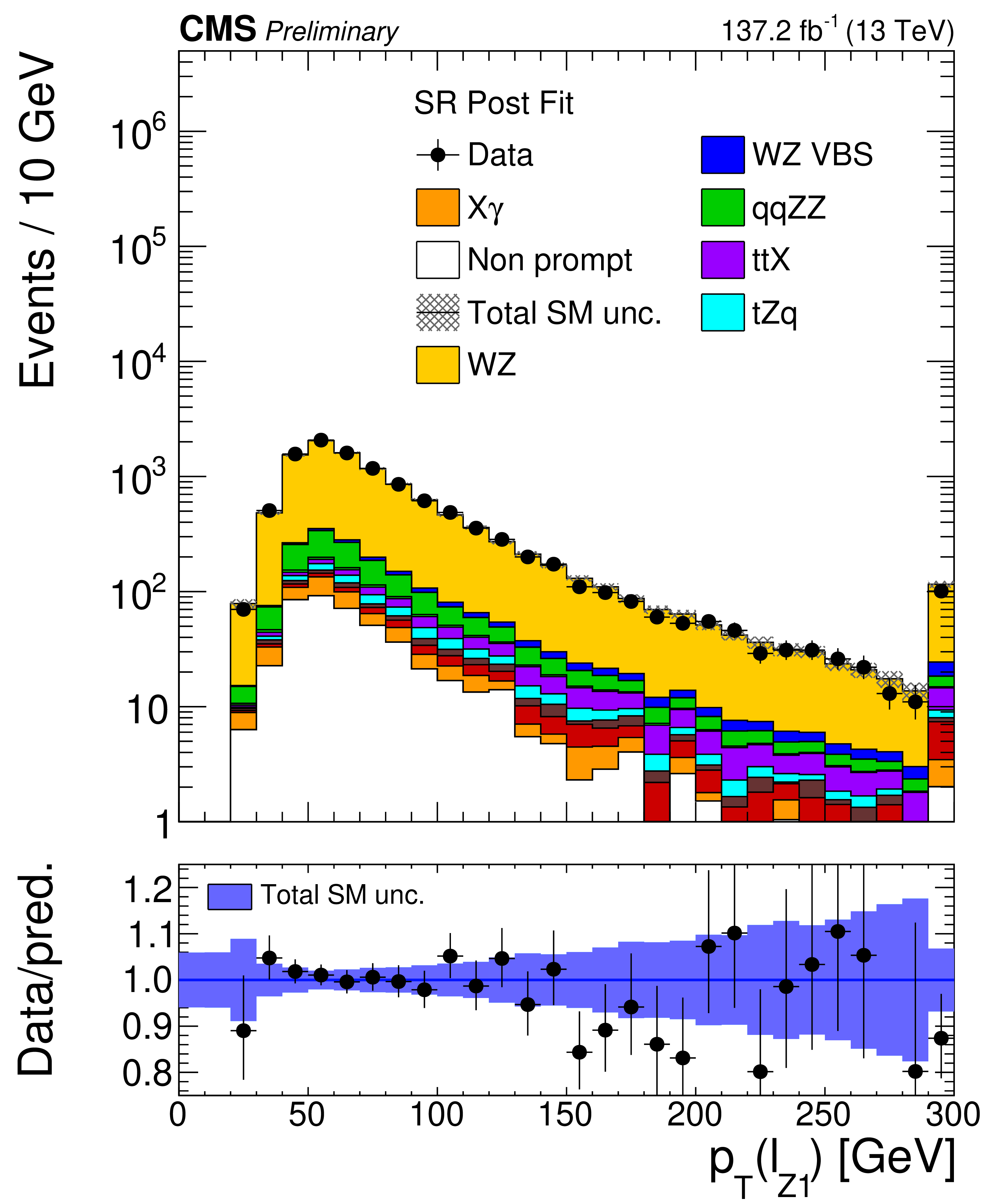
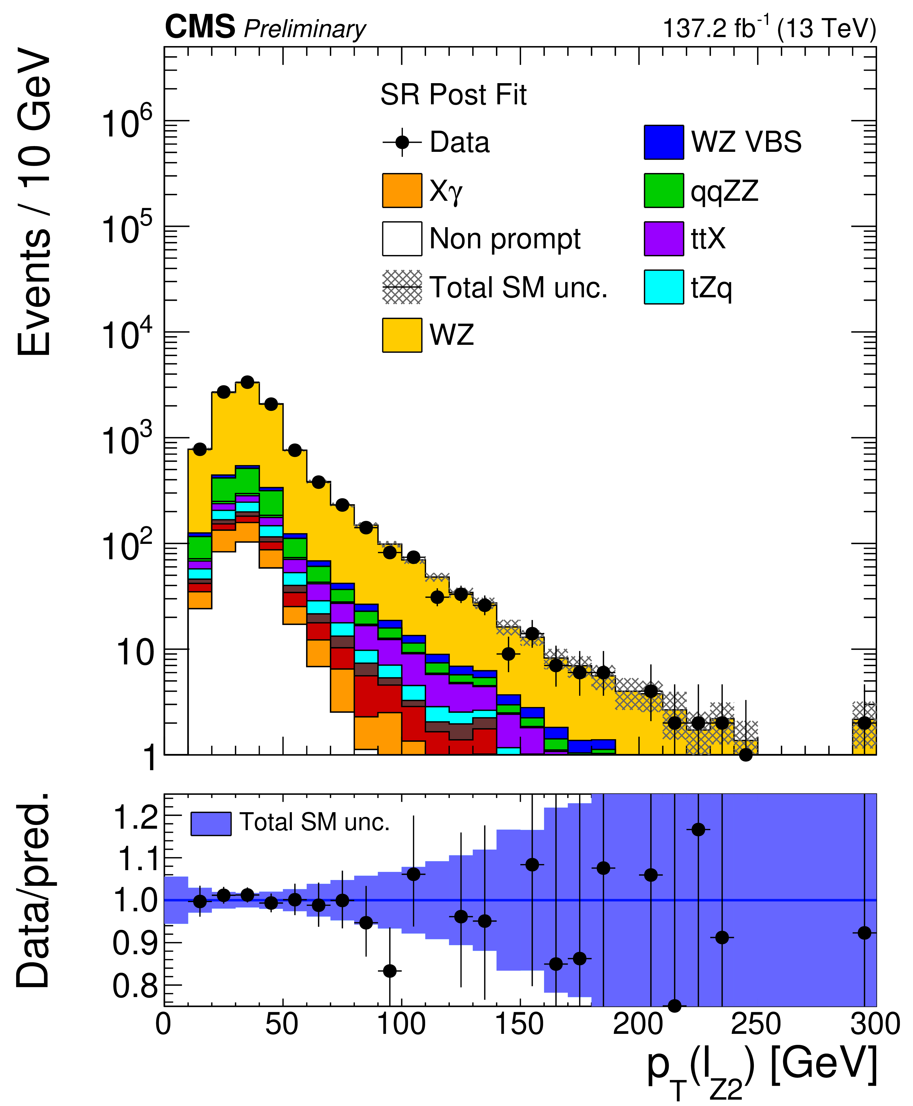
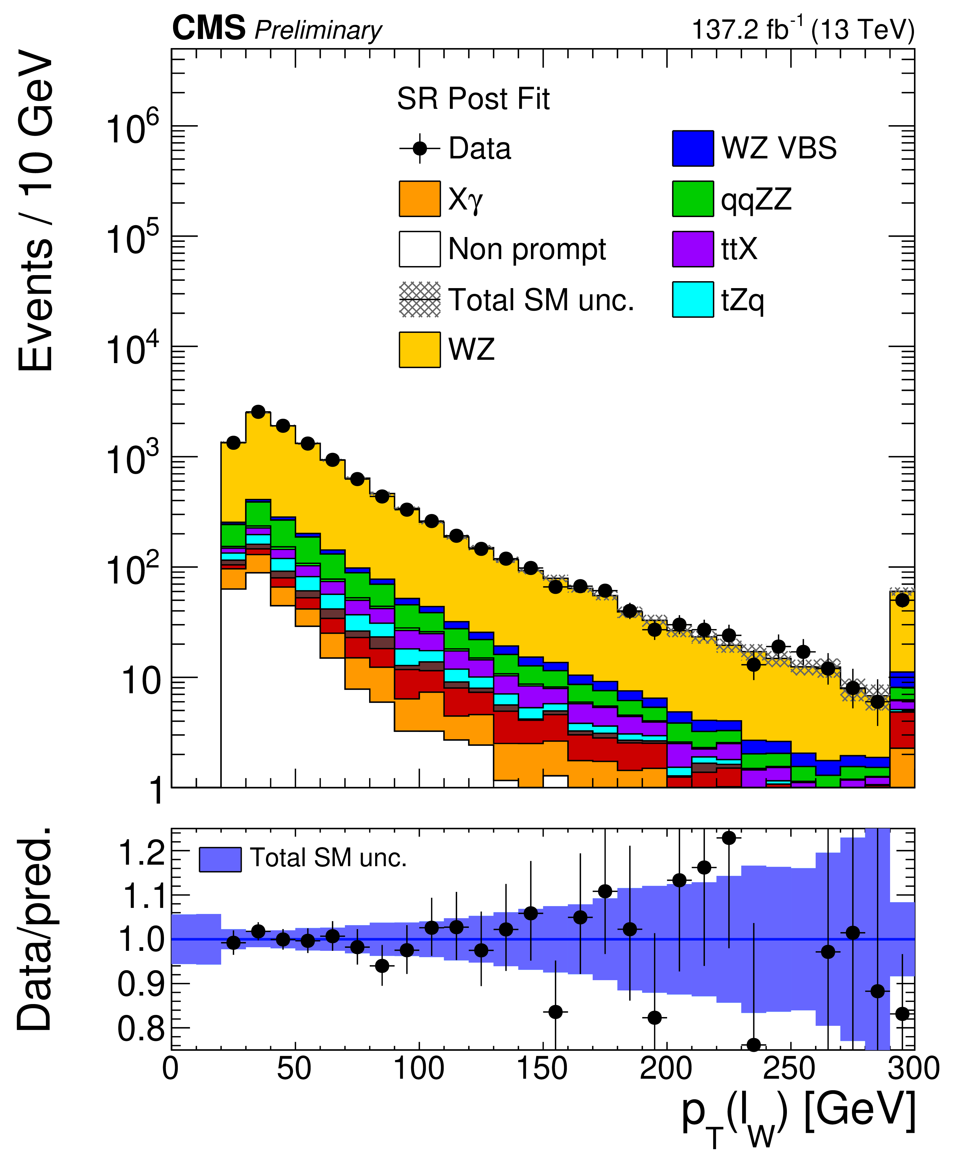
Distribution of event observables in the signal region after the combined fit to all years and flavour final states: ${p_{\mathrm {T}}}$ of the leading jet with no ${p_{\mathrm {T}}}$ requirements (top left), transverse momentum of the ${\ell _{\mathrm{Z} 1}}$ lepton (top right), transverse momentum of the ${\ell _{\mathrm{Z} 2}}$ lepton (bottom left) and transverse momentum of the ${\ell _{\mathrm{W}}}$ lepton (bottom right). The shaded band in the ratio includes the effects of all analysis uncertainties on the background and signal yields. X$\gamma$ includes Z$\gamma$, W$\gamma$, tt$\gamma$ and WZ$\gamma$ production. The label ttX includes both ttZ, ttW and ttH production. The shaded band in the ratio corresponds to the total uncertainty in the SM yields. |
png pdf |
Figure 6-a:
Distribution of event observables in the signal region after the combined fit to all years and flavour final states: ${p_{\mathrm {T}}}$ of the leading jet with no ${p_{\mathrm {T}}}$ requirements (top left), transverse momentum of the ${\ell _{\mathrm{Z} 1}}$ lepton (top right), transverse momentum of the ${\ell _{\mathrm{Z} 2}}$ lepton (bottom left) and transverse momentum of the ${\ell _{\mathrm{W}}}$ lepton (bottom right). The shaded band in the ratio includes the effects of all analysis uncertainties on the background and signal yields. X$\gamma$ includes Z$\gamma$, W$\gamma$, tt$\gamma$ and WZ$\gamma$ production. The label ttX includes both ttZ, ttW and ttH production. The shaded band in the ratio corresponds to the total uncertainty in the SM yields. |
png pdf |
Figure 6-b:
Distribution of event observables in the signal region after the combined fit to all years and flavour final states: ${p_{\mathrm {T}}}$ of the leading jet with no ${p_{\mathrm {T}}}$ requirements (top left), transverse momentum of the ${\ell _{\mathrm{Z} 1}}$ lepton (top right), transverse momentum of the ${\ell _{\mathrm{Z} 2}}$ lepton (bottom left) and transverse momentum of the ${\ell _{\mathrm{W}}}$ lepton (bottom right). The shaded band in the ratio includes the effects of all analysis uncertainties on the background and signal yields. X$\gamma$ includes Z$\gamma$, W$\gamma$, tt$\gamma$ and WZ$\gamma$ production. The label ttX includes both ttZ, ttW and ttH production. The shaded band in the ratio corresponds to the total uncertainty in the SM yields. |
png pdf |
Figure 6-c:
Distribution of event observables in the signal region after the combined fit to all years and flavour final states: ${p_{\mathrm {T}}}$ of the leading jet with no ${p_{\mathrm {T}}}$ requirements (top left), transverse momentum of the ${\ell _{\mathrm{Z} 1}}$ lepton (top right), transverse momentum of the ${\ell _{\mathrm{Z} 2}}$ lepton (bottom left) and transverse momentum of the ${\ell _{\mathrm{W}}}$ lepton (bottom right). The shaded band in the ratio includes the effects of all analysis uncertainties on the background and signal yields. X$\gamma$ includes Z$\gamma$, W$\gamma$, tt$\gamma$ and WZ$\gamma$ production. The label ttX includes both ttZ, ttW and ttH production. The shaded band in the ratio corresponds to the total uncertainty in the SM yields. |
png pdf |
Figure 6-d:
Distribution of event observables in the signal region after the combined fit to all years and flavour final states: ${p_{\mathrm {T}}}$ of the leading jet with no ${p_{\mathrm {T}}}$ requirements (top left), transverse momentum of the ${\ell _{\mathrm{Z} 1}}$ lepton (top right), transverse momentum of the ${\ell _{\mathrm{Z} 2}}$ lepton (bottom left) and transverse momentum of the ${\ell _{\mathrm{W}}}$ lepton (bottom right). The shaded band in the ratio includes the effects of all analysis uncertainties on the background and signal yields. X$\gamma$ includes Z$\gamma$, W$\gamma$, tt$\gamma$ and WZ$\gamma$ production. The label ttX includes both ttZ, ttW and ttH production. The shaded band in the ratio corresponds to the total uncertainty in the SM yields. |
png pdf |
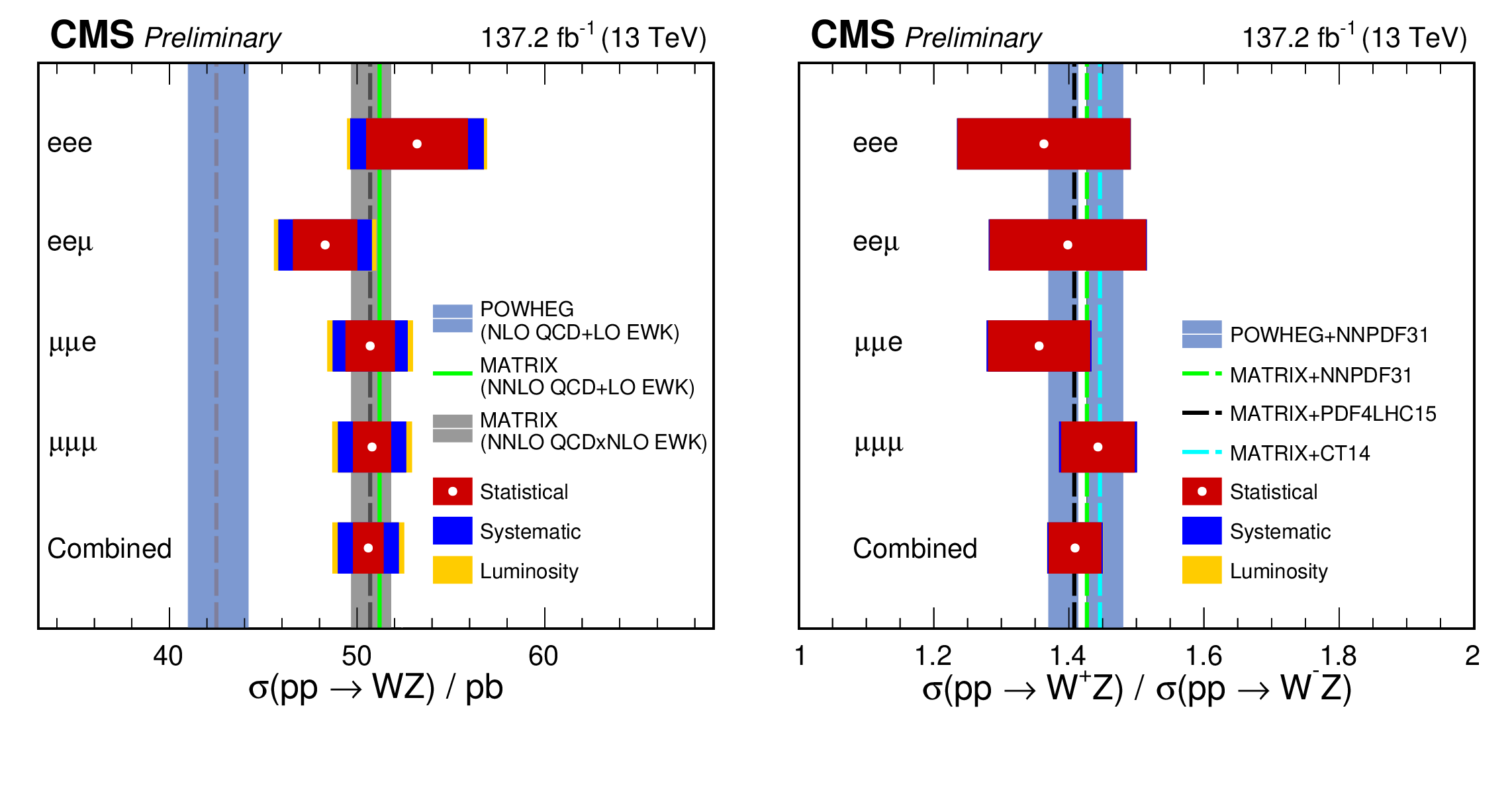
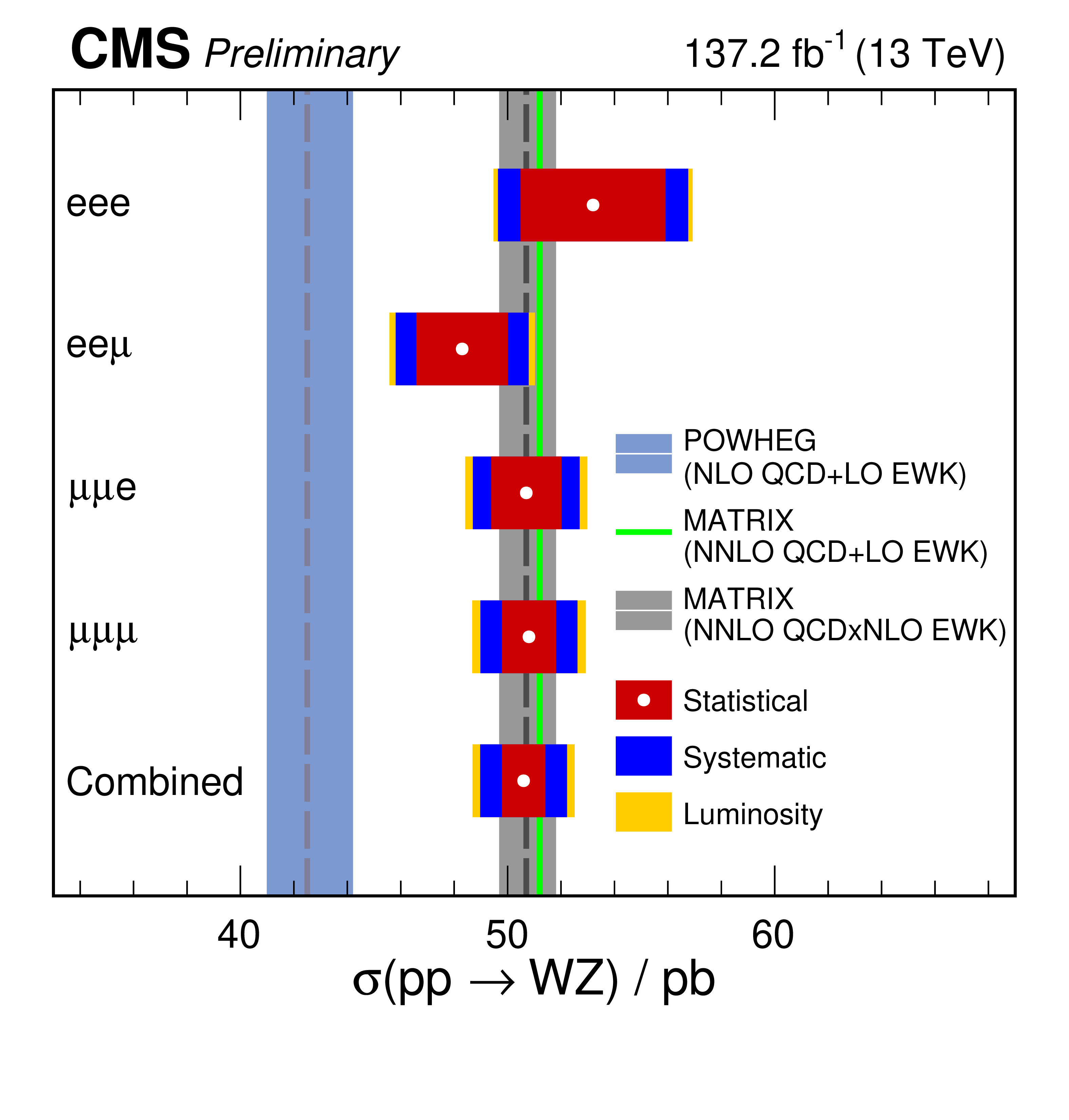
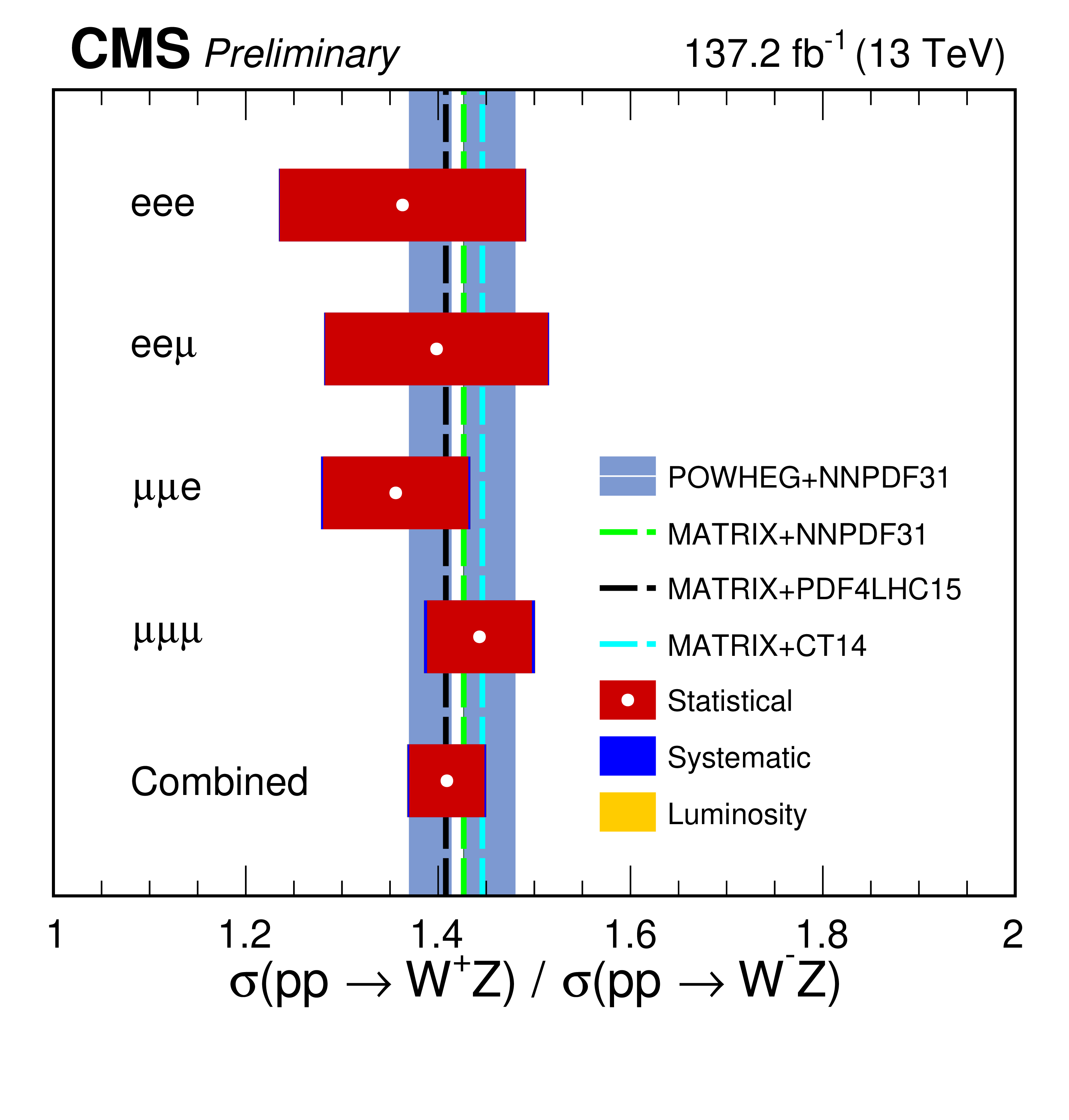
Figure 7:
Total WZ production cross section (left) and charge asymmetry ratio (right) for each of the flavour exclusive and inclusive categories. The shaded vertical bands correspond to the the theoretical predictions from POWHEG (blue) and matrix (grey). For each of the measurements, the best fit value is denoted with a white point and three main groups of uncertainties (statistical, systematic and luminosity) are denoted as differently coloured (red, blue, orange) bands with each one being added quadratically on top of the previous one. For the charge asymmetry ratio both POWHEG and matrix predictions are close to exact agreement, leading to the blue and grey lines to overlap in the plot. Predictions obtained using matrix and several central replicas of different PDF sets are also shown as individual lines in the figure. |
png pdf |
Figure 7-a:
Total WZ production cross section (left) and charge asymmetry ratio (right) for each of the flavour exclusive and inclusive categories. The shaded vertical bands correspond to the the theoretical predictions from POWHEG (blue) and matrix (grey). For each of the measurements, the best fit value is denoted with a white point and three main groups of uncertainties (statistical, systematic and luminosity) are denoted as differently coloured (red, blue, orange) bands with each one being added quadratically on top of the previous one. For the charge asymmetry ratio both POWHEG and matrix predictions are close to exact agreement, leading to the blue and grey lines to overlap in the plot. Predictions obtained using matrix and several central replicas of different PDF sets are also shown as individual lines in the figure. |
png pdf |
Figure 7-b:
Total WZ production cross section (left) and charge asymmetry ratio (right) for each of the flavour exclusive and inclusive categories. The shaded vertical bands correspond to the the theoretical predictions from POWHEG (blue) and matrix (grey). For each of the measurements, the best fit value is denoted with a white point and three main groups of uncertainties (statistical, systematic and luminosity) are denoted as differently coloured (red, blue, orange) bands with each one being added quadratically on top of the previous one. For the charge asymmetry ratio both POWHEG and matrix predictions are close to exact agreement, leading to the blue and grey lines to overlap in the plot. Predictions obtained using matrix and several central replicas of different PDF sets are also shown as individual lines in the figure. |

png pdf |
Figure 8:
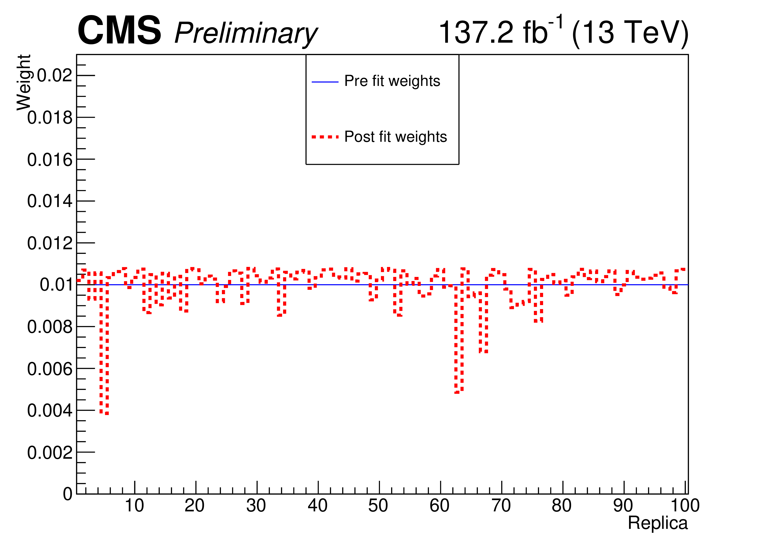
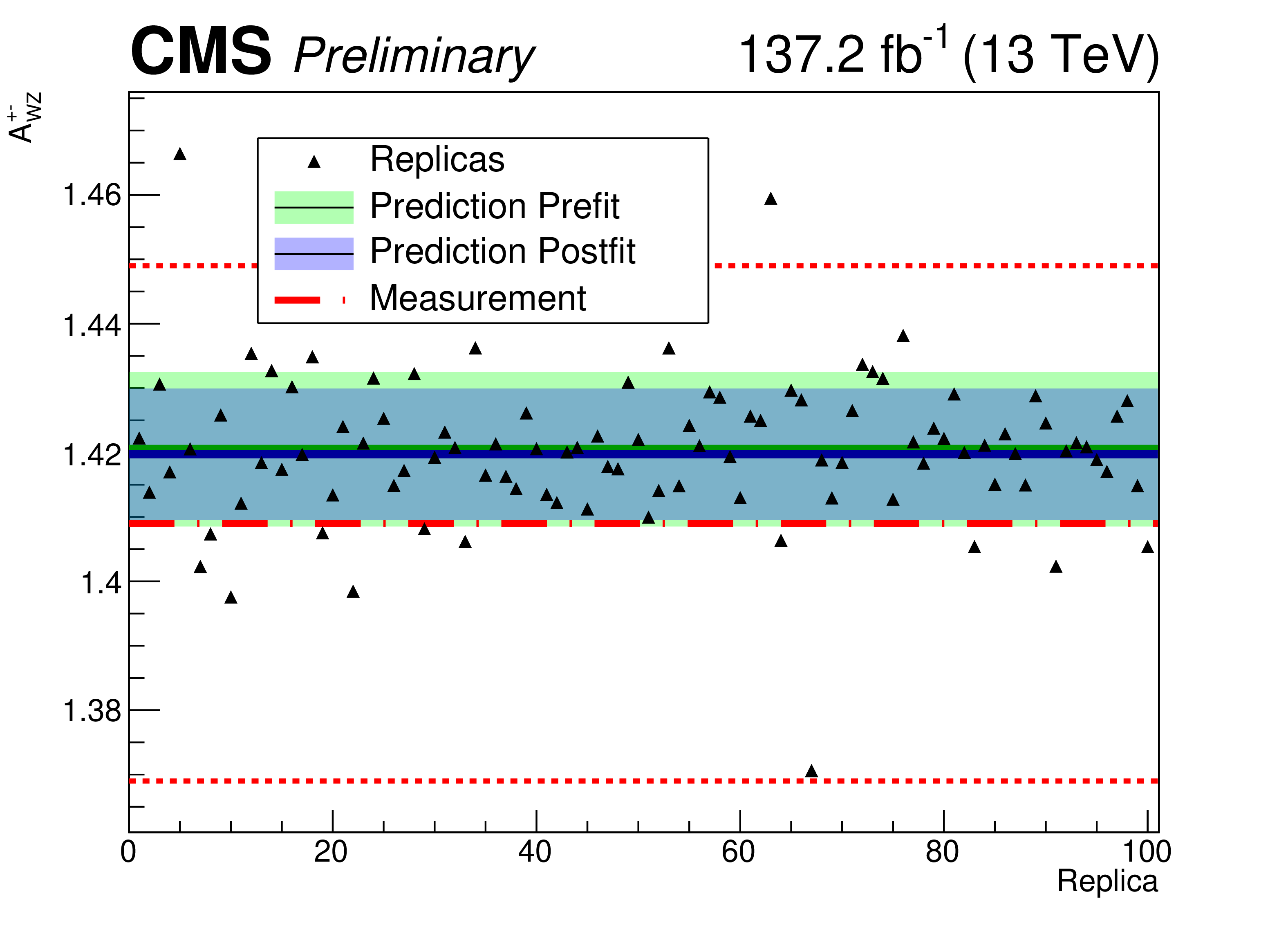
(Left) Weights associated to each PDF replica in the NNPDF30_nlo_as118 set before (blue) and after (red) the Bayesian reweighting technique is applied based on the charge ratio asymmetry measurement. (Right) Predictions and (expected) measurements of the charge asymmetry ratio in WZ production using the nominal POWHEG sample with the NNPDF30_nlo_as118 PDF set. The central green line corresponds to the nominal predicted values, the shaded bands include the total uncertainty corresponding to the PDF set computed using the sample variance of the predictions obtained with each replica and each of the triangles corresponds to the individual replica predictions. The red lines corresponds to the measured value and uncertainties of the analysis. The blue bands correspond to the predicted central value and uncertainties obtained after the Bayesian Reweighting procedure. |
png pdf |
Figure 8-a:
(Left) Weights associated to each PDF replica in the NNPDF30_nlo_as118 set before (blue) and after (red) the Bayesian reweighting technique is applied based on the charge ratio asymmetry measurement. (Right) Predictions and (expected) measurements of the charge asymmetry ratio in WZ production using the nominal POWHEG sample with the NNPDF30_nlo_as118 PDF set. The central green line corresponds to the nominal predicted values, the shaded bands include the total uncertainty corresponding to the PDF set computed using the sample variance of the predictions obtained with each replica and each of the triangles corresponds to the individual replica predictions. The red lines corresponds to the measured value and uncertainties of the analysis. The blue bands correspond to the predicted central value and uncertainties obtained after the Bayesian Reweighting procedure. |
png pdf |
Figure 8-b:
(Left) Weights associated to each PDF replica in the NNPDF30_nlo_as118 set before (blue) and after (red) the Bayesian reweighting technique is applied based on the charge ratio asymmetry measurement. (Right) Predictions and (expected) measurements of the charge asymmetry ratio in WZ production using the nominal POWHEG sample with the NNPDF30_nlo_as118 PDF set. The central green line corresponds to the nominal predicted values, the shaded bands include the total uncertainty corresponding to the PDF set computed using the sample variance of the predictions obtained with each replica and each of the triangles corresponds to the individual replica predictions. The red lines corresponds to the measured value and uncertainties of the analysis. The blue bands correspond to the predicted central value and uncertainties obtained after the Bayesian Reweighting procedure. |
png pdf |
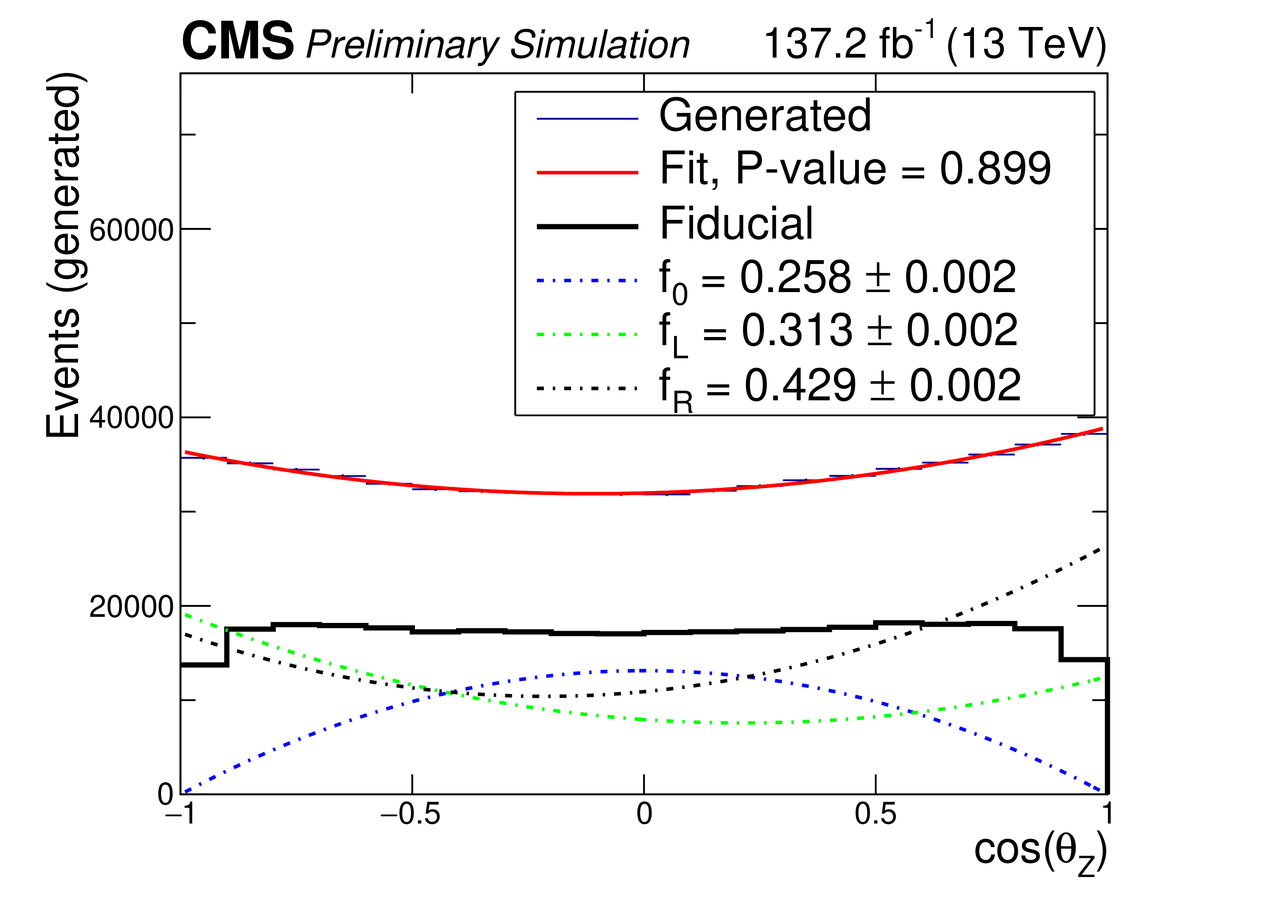
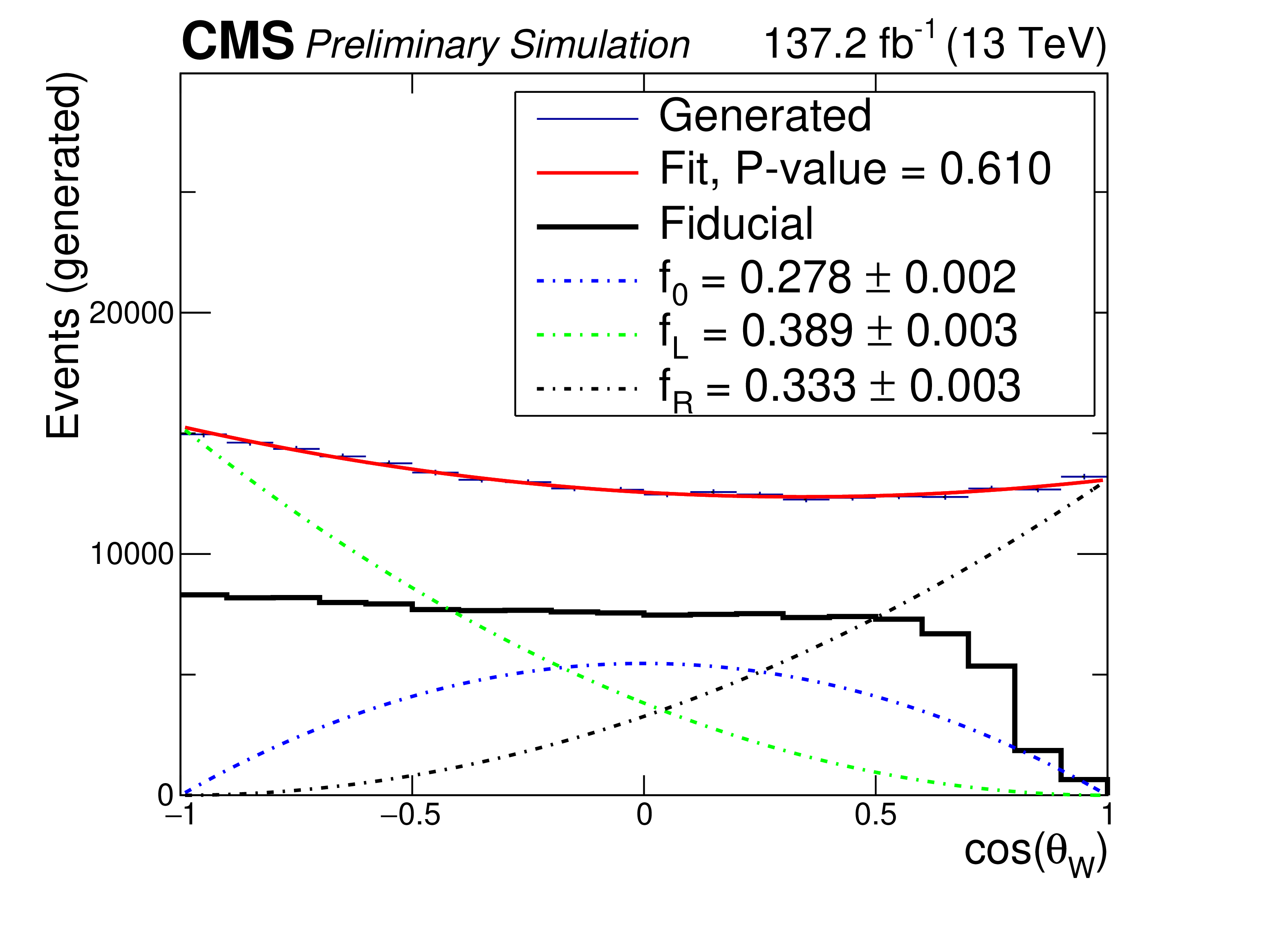
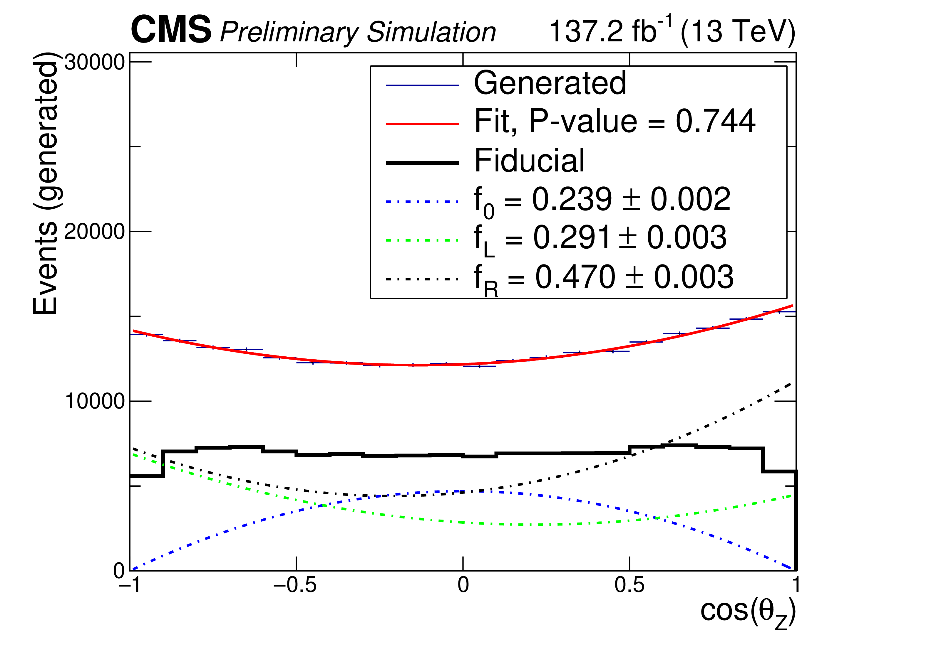
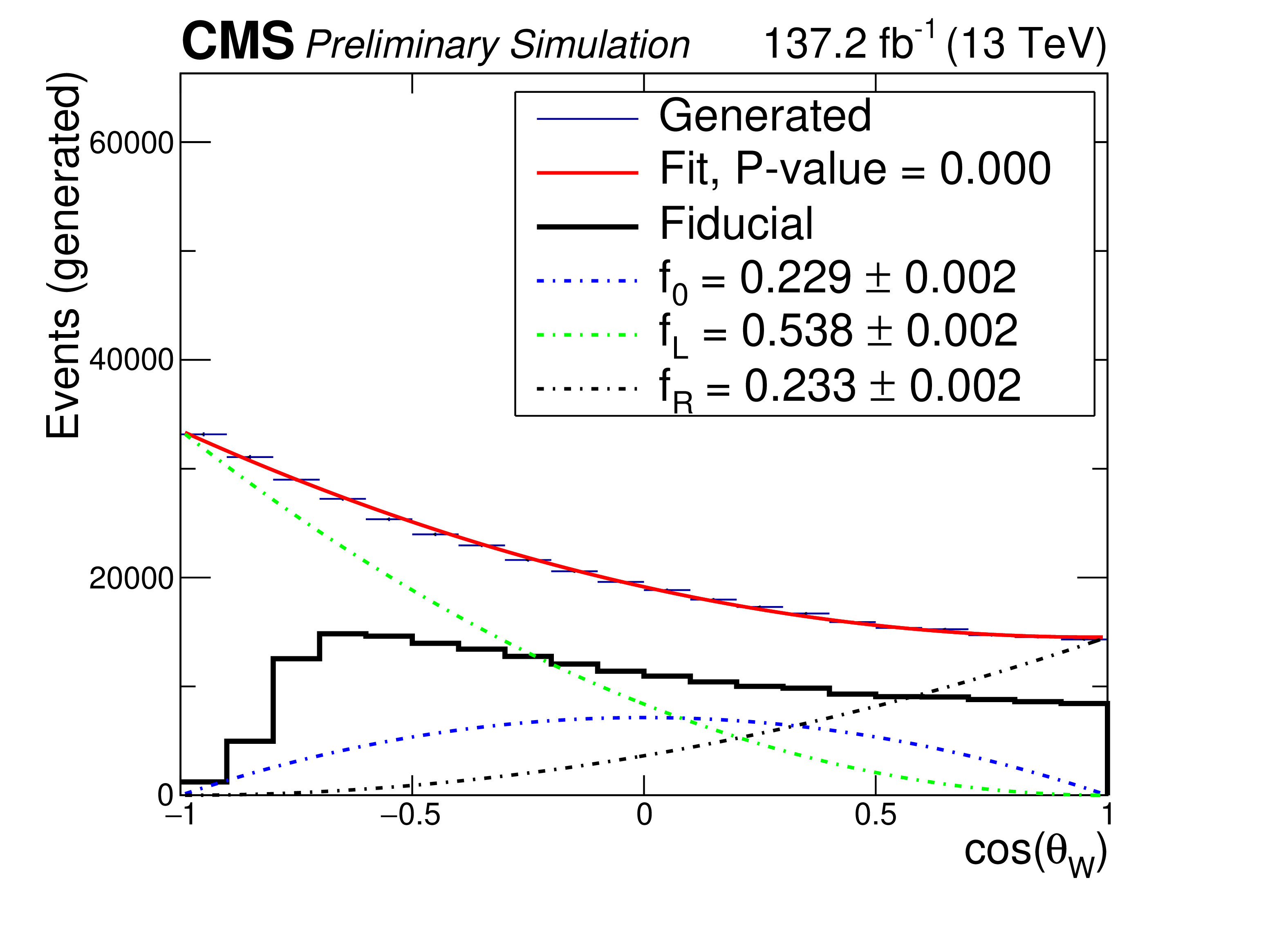
Figure 9:
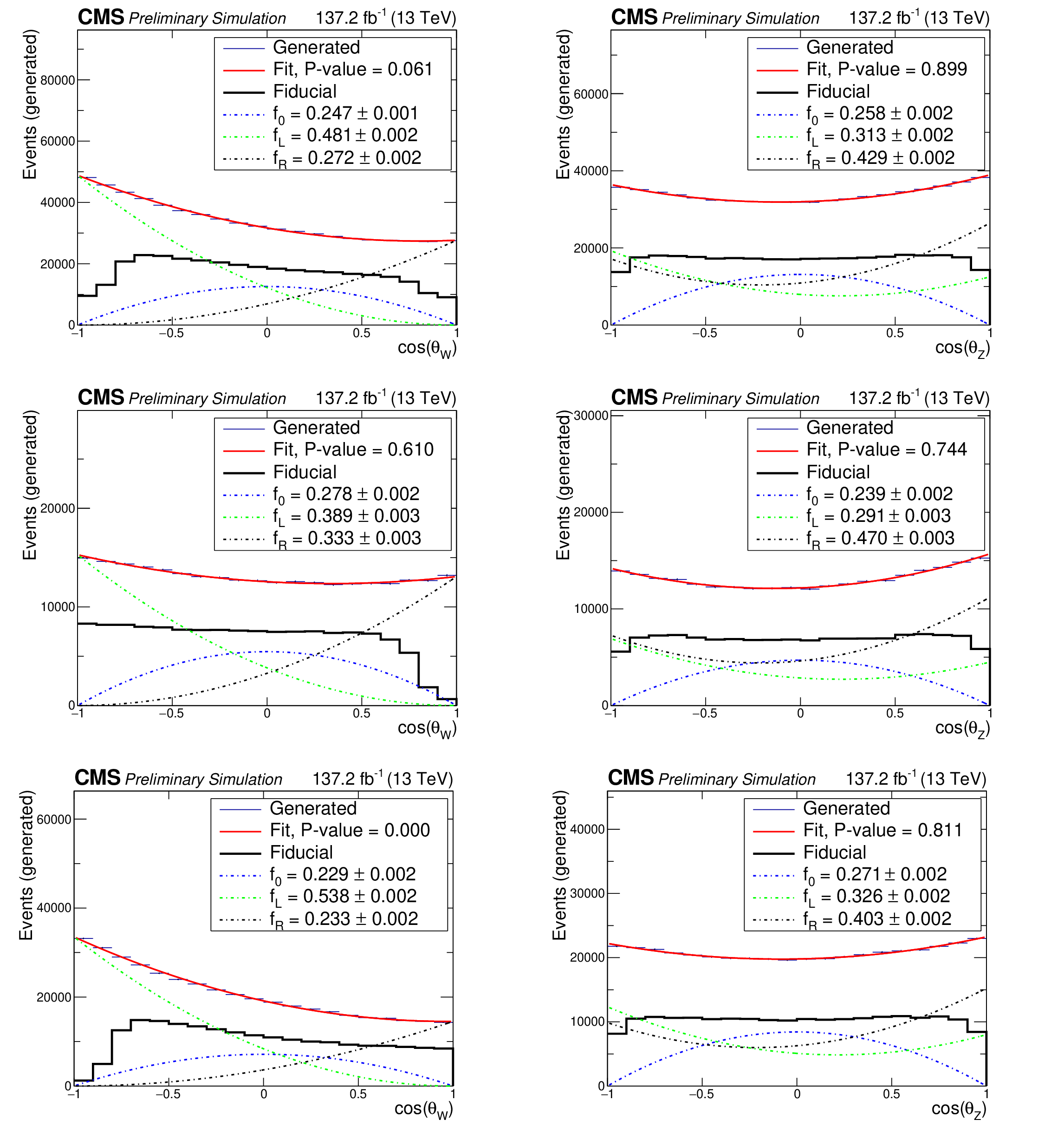
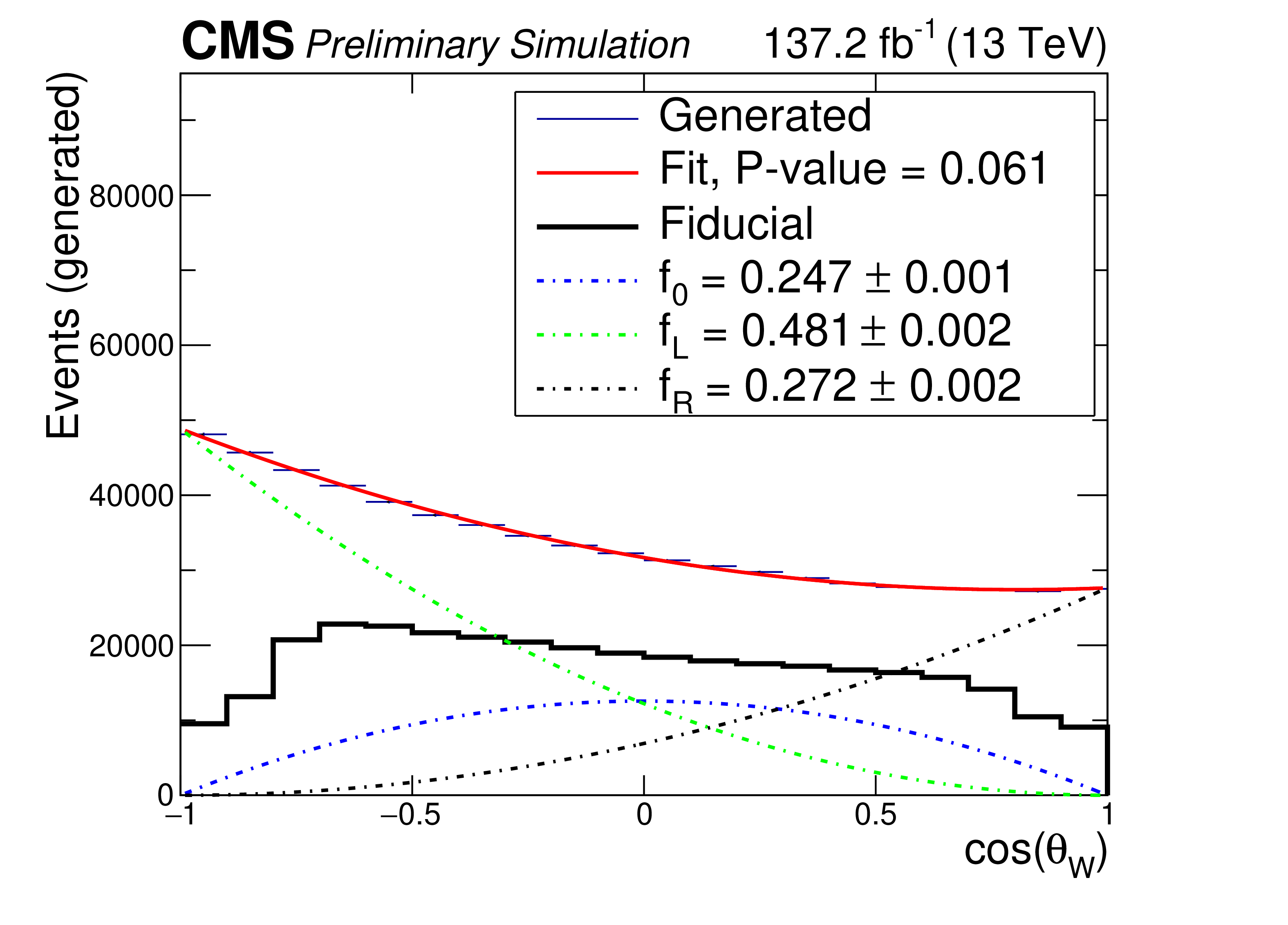
Distribution of the cosine of the polarization angle in the helicity frame at generator level for the nominal signal sample. The blue points correspond to the MC prediction in the total phase space, the solid red line corresponds to the best quadratic fit and the different dashed lines to each of the polarization components obtained in the fit. The thick black line corresponds to the distribution of the same variable restricted to the fiducial phase space showing how kinematic cuts break the quadratic dependence of the differential cross section. The p value corresponding to the goodness of the fit -obtained through a $\chi ^2$ test is included in the legend. From left to right: W and Z bosons. From top to bottom: total (inclusive) final state, negatively charged final state and positively charged final state. |
png pdf |
Figure 9-a:
Distribution of the cosine of the polarization angle in the helicity frame at generator level for the nominal signal sample. The blue points correspond to the MC prediction in the total phase space, the solid red line corresponds to the best quadratic fit and the different dashed lines to each of the polarization components obtained in the fit. The thick black line corresponds to the distribution of the same variable restricted to the fiducial phase space showing how kinematic cuts break the quadratic dependence of the differential cross section. The p value corresponding to the goodness of the fit -obtained through a $\chi ^2$ test is included in the legend. From left to right: W and Z bosons. From top to bottom: total (inclusive) final state, negatively charged final state and positively charged final state. |
png pdf |
Figure 9-b:
Distribution of the cosine of the polarization angle in the helicity frame at generator level for the nominal signal sample. The blue points correspond to the MC prediction in the total phase space, the solid red line corresponds to the best quadratic fit and the different dashed lines to each of the polarization components obtained in the fit. The thick black line corresponds to the distribution of the same variable restricted to the fiducial phase space showing how kinematic cuts break the quadratic dependence of the differential cross section. The p value corresponding to the goodness of the fit -obtained through a $\chi ^2$ test is included in the legend. From left to right: W and Z bosons. From top to bottom: total (inclusive) final state, negatively charged final state and positively charged final state. |
png pdf |
Figure 9-c:
Distribution of the cosine of the polarization angle in the helicity frame at generator level for the nominal signal sample. The blue points correspond to the MC prediction in the total phase space, the solid red line corresponds to the best quadratic fit and the different dashed lines to each of the polarization components obtained in the fit. The thick black line corresponds to the distribution of the same variable restricted to the fiducial phase space showing how kinematic cuts break the quadratic dependence of the differential cross section. The p value corresponding to the goodness of the fit -obtained through a $\chi ^2$ test is included in the legend. From left to right: W and Z bosons. From top to bottom: total (inclusive) final state, negatively charged final state and positively charged final state. |
png pdf |
Figure 9-d:
Distribution of the cosine of the polarization angle in the helicity frame at generator level for the nominal signal sample. The blue points correspond to the MC prediction in the total phase space, the solid red line corresponds to the best quadratic fit and the different dashed lines to each of the polarization components obtained in the fit. The thick black line corresponds to the distribution of the same variable restricted to the fiducial phase space showing how kinematic cuts break the quadratic dependence of the differential cross section. The p value corresponding to the goodness of the fit -obtained through a $\chi ^2$ test is included in the legend. From left to right: W and Z bosons. From top to bottom: total (inclusive) final state, negatively charged final state and positively charged final state. |
png pdf |
Figure 9-e:
Distribution of the cosine of the polarization angle in the helicity frame at generator level for the nominal signal sample. The blue points correspond to the MC prediction in the total phase space, the solid red line corresponds to the best quadratic fit and the different dashed lines to each of the polarization components obtained in the fit. The thick black line corresponds to the distribution of the same variable restricted to the fiducial phase space showing how kinematic cuts break the quadratic dependence of the differential cross section. The p value corresponding to the goodness of the fit -obtained through a $\chi ^2$ test is included in the legend. From left to right: W and Z bosons. From top to bottom: total (inclusive) final state, negatively charged final state and positively charged final state. |

png pdf |
Figure 9-f:
Distribution of the cosine of the polarization angle in the helicity frame at generator level for the nominal signal sample. The blue points correspond to the MC prediction in the total phase space, the solid red line corresponds to the best quadratic fit and the different dashed lines to each of the polarization components obtained in the fit. The thick black line corresponds to the distribution of the same variable restricted to the fiducial phase space showing how kinematic cuts break the quadratic dependence of the differential cross section. The p value corresponding to the goodness of the fit -obtained through a $\chi ^2$ test is included in the legend. From left to right: W and Z bosons. From top to bottom: total (inclusive) final state, negatively charged final state and positively charged final state. |
png pdf |
Figure 10:
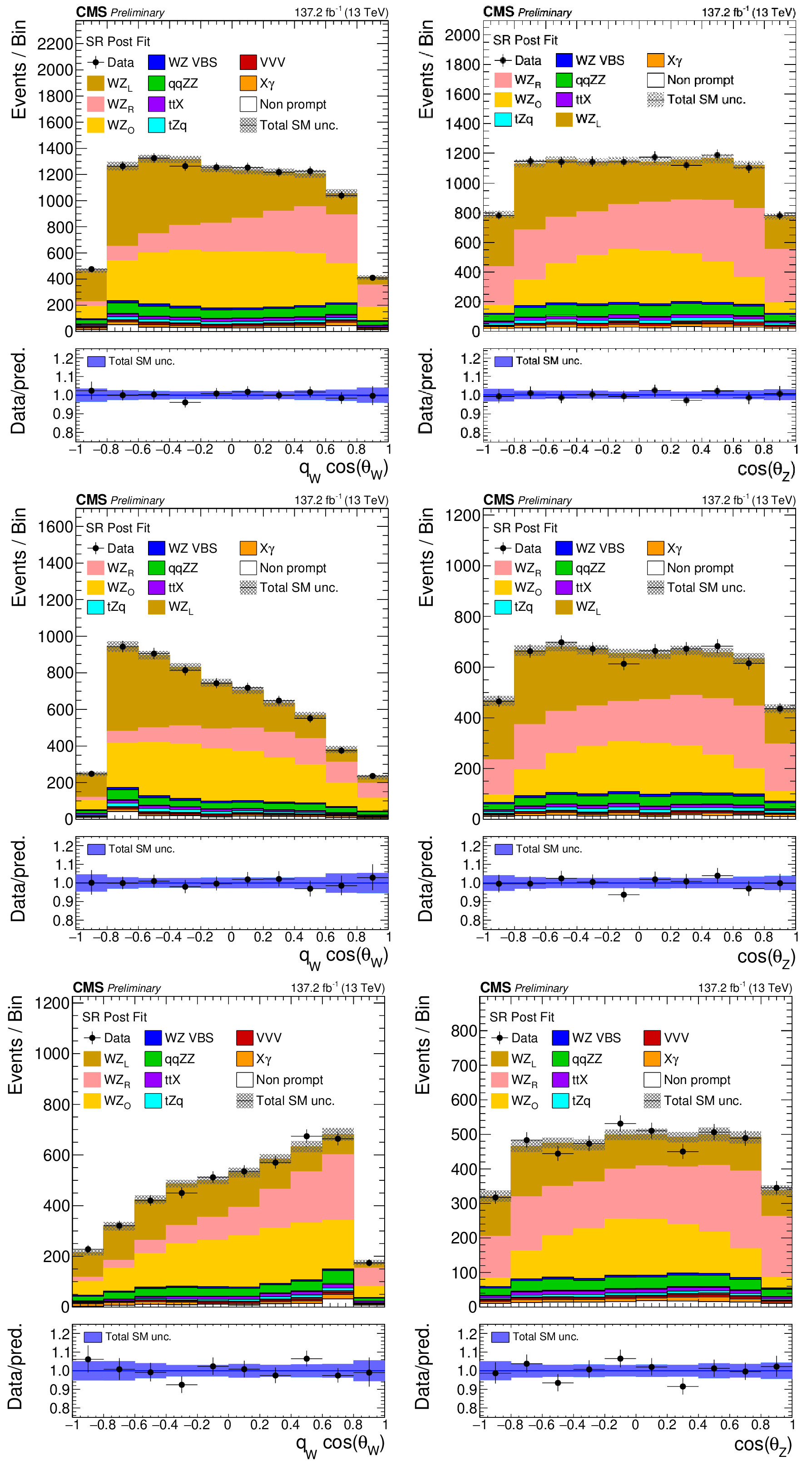
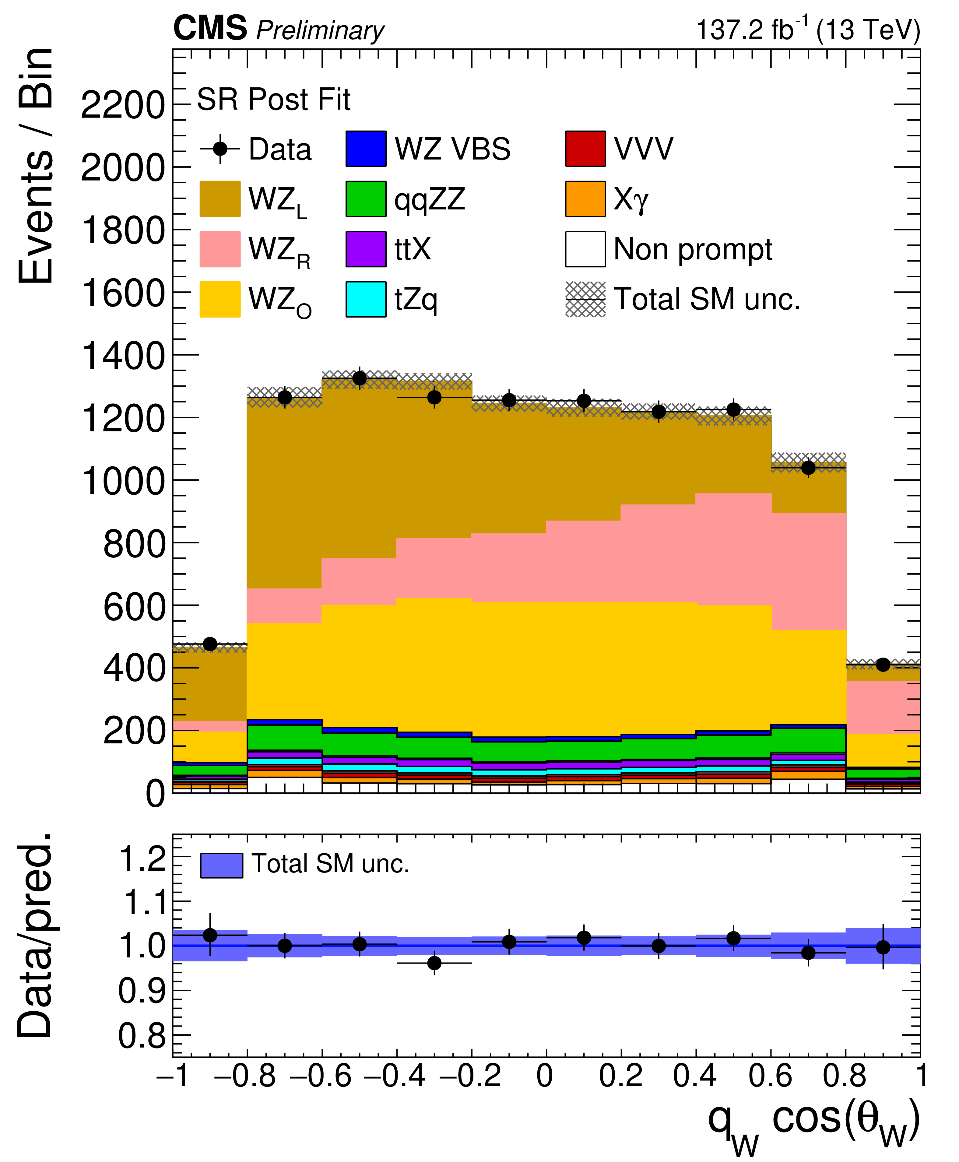
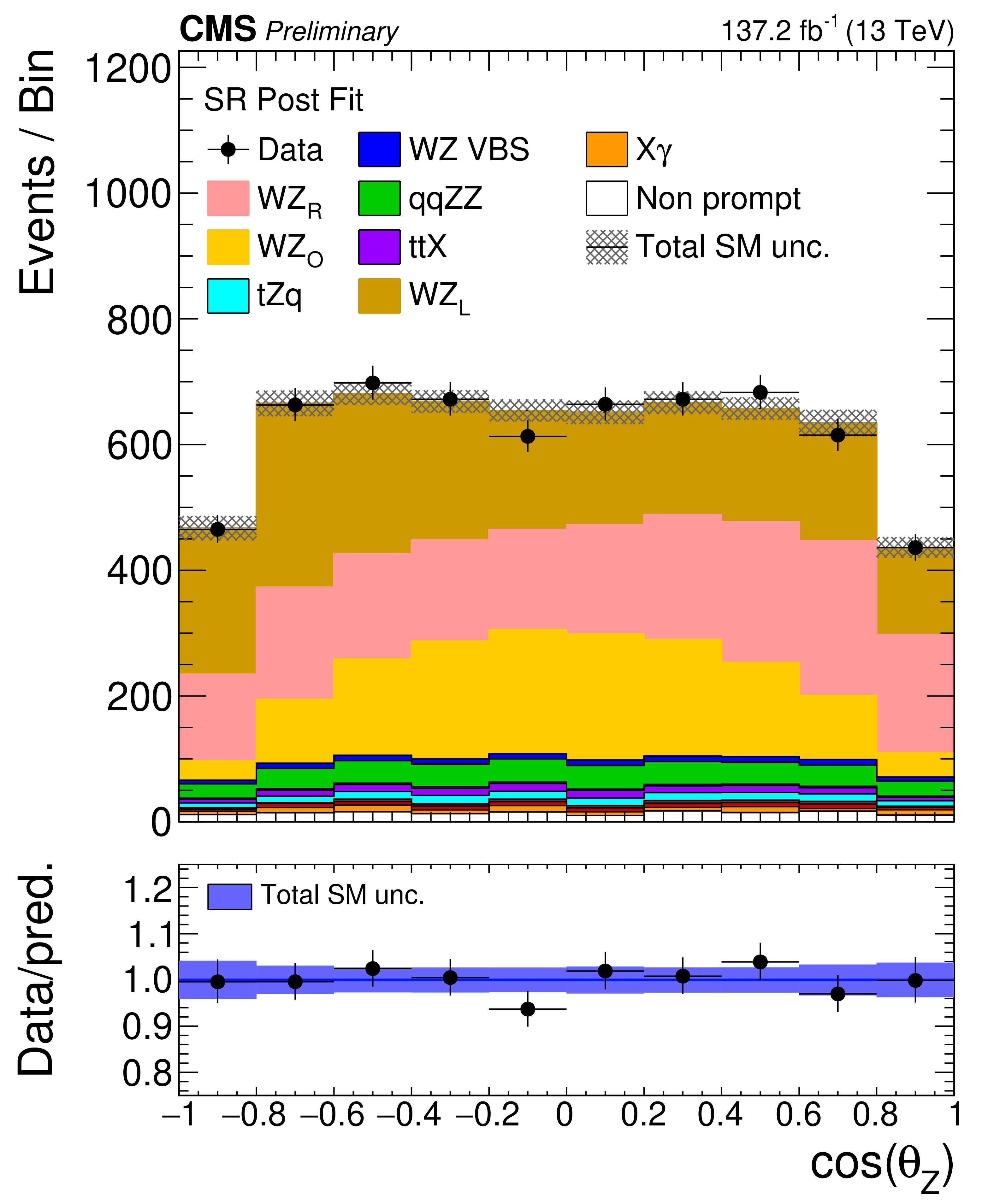
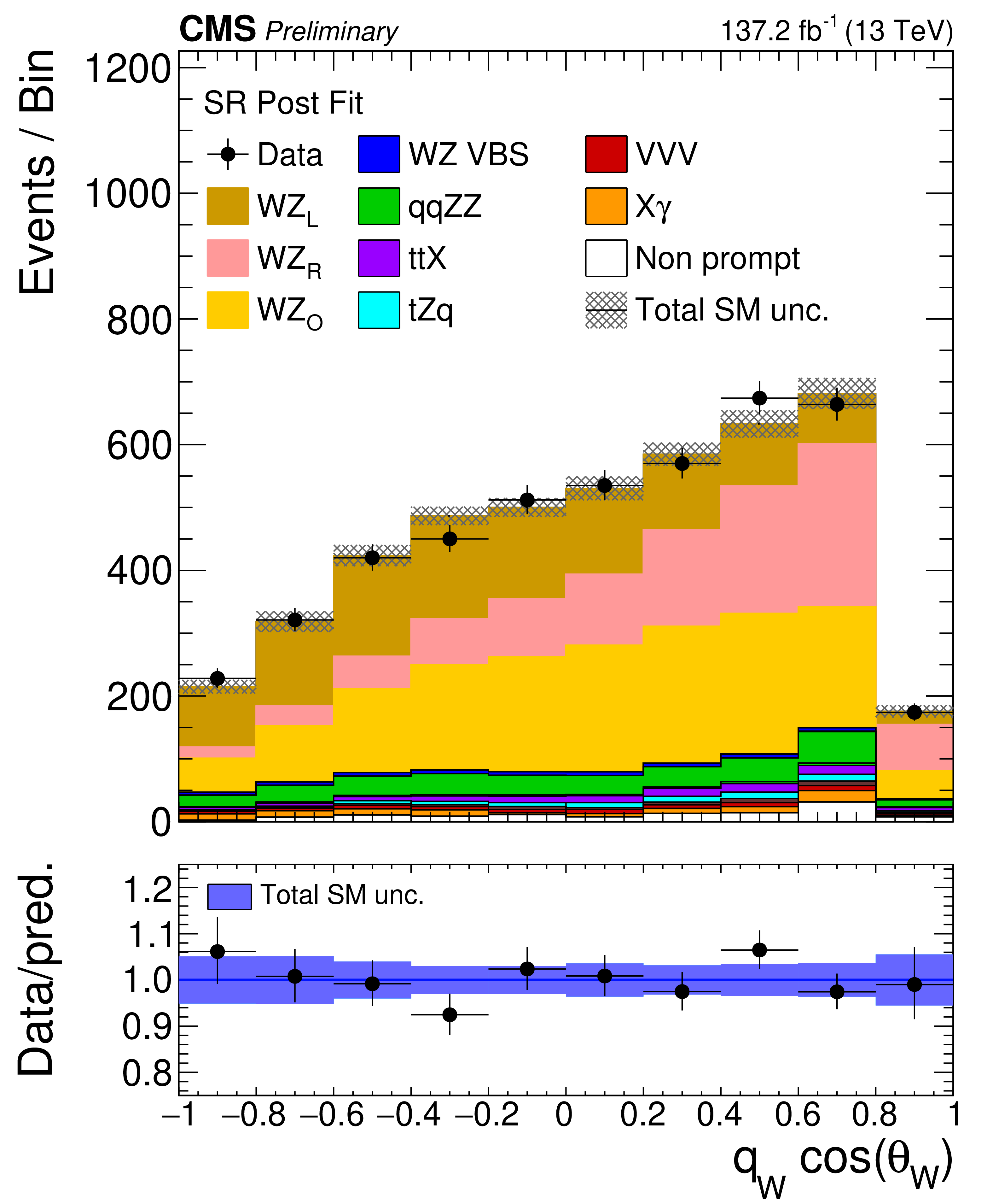
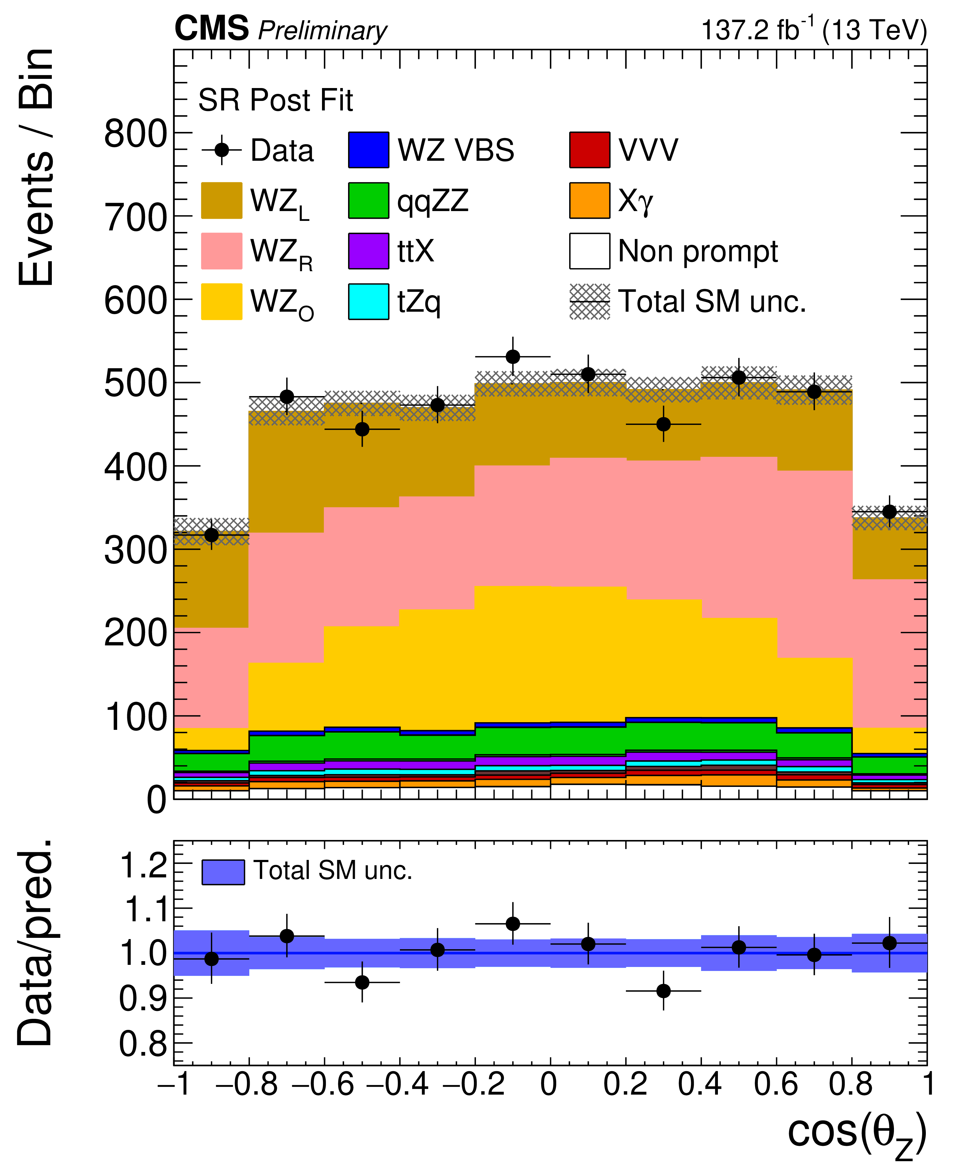
Distribution of the cosine of the polarization angle for different final state charges and boson flavours after the fits corresponding to each case. From left to right: W and Z bosons. From top to bottom: final state charge inclusive (total), positive final state charge and negative final state charge. The differently polarized final states of the corresponding boson are shown in each of the cases. X$\gamma$ includes Z$\gamma$, W$\gamma$, tt$\gamma$ and WZ$\gamma$ production. The label ttX includes both ttZ, ttW and ttH production. The shaded band in the ratio corresponds to the total uncertainty in the SM yields. |
png pdf |
Figure 10-a:
Distribution of the cosine of the polarization angle for different final state charges and boson flavours after the fits corresponding to each case. From left to right: W and Z bosons. From top to bottom: final state charge inclusive (total), positive final state charge and negative final state charge. The differently polarized final states of the corresponding boson are shown in each of the cases. X$\gamma$ includes Z$\gamma$, W$\gamma$, tt$\gamma$ and WZ$\gamma$ production. The label ttX includes both ttZ, ttW and ttH production. The shaded band in the ratio corresponds to the total uncertainty in the SM yields. |
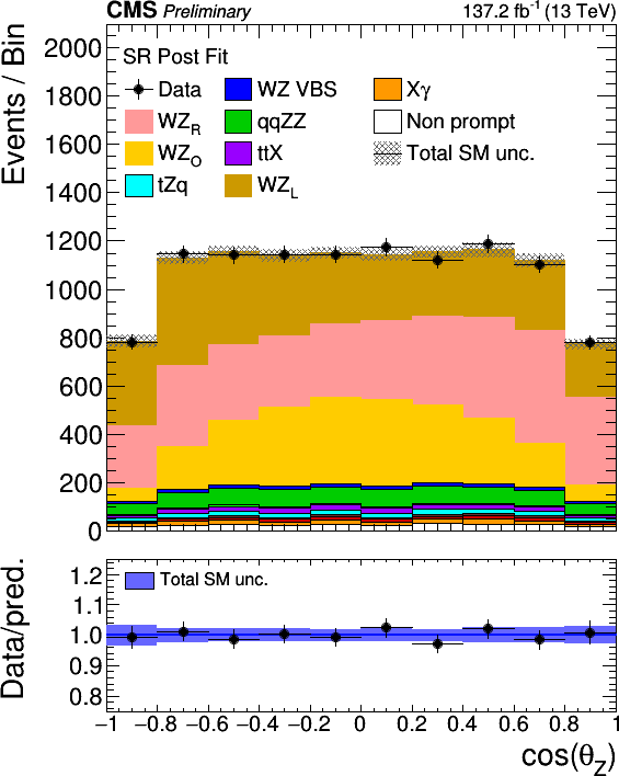
png pdf |
Figure 10-b:
Distribution of the cosine of the polarization angle for different final state charges and boson flavours after the fits corresponding to each case. From left to right: W and Z bosons. From top to bottom: final state charge inclusive (total), positive final state charge and negative final state charge. The differently polarized final states of the corresponding boson are shown in each of the cases. X$\gamma$ includes Z$\gamma$, W$\gamma$, tt$\gamma$ and WZ$\gamma$ production. The label ttX includes both ttZ, ttW and ttH production. The shaded band in the ratio corresponds to the total uncertainty in the SM yields. |
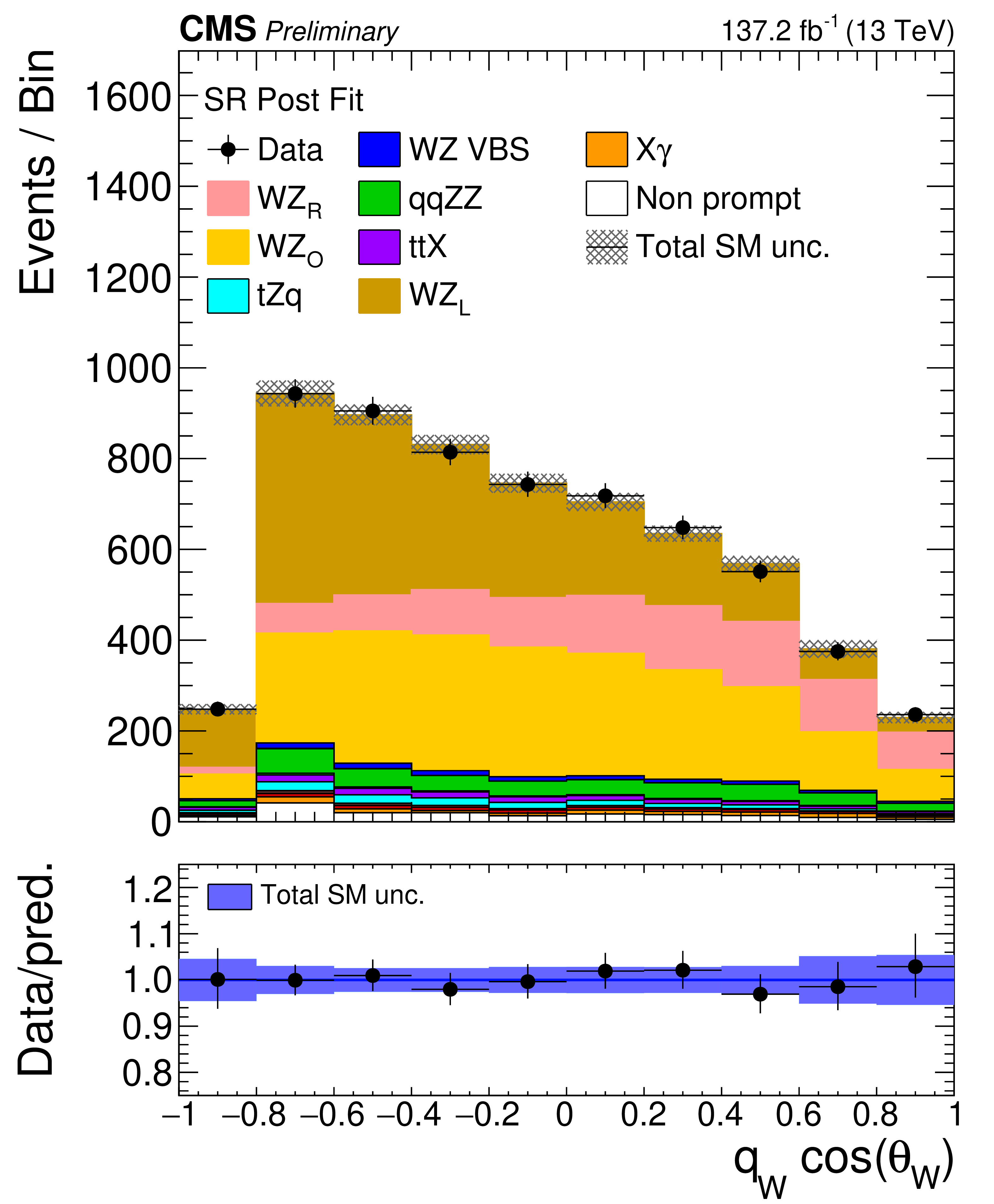
png pdf |
Figure 10-c:
Distribution of the cosine of the polarization angle for different final state charges and boson flavours after the fits corresponding to each case. From left to right: W and Z bosons. From top to bottom: final state charge inclusive (total), positive final state charge and negative final state charge. The differently polarized final states of the corresponding boson are shown in each of the cases. X$\gamma$ includes Z$\gamma$, W$\gamma$, tt$\gamma$ and WZ$\gamma$ production. The label ttX includes both ttZ, ttW and ttH production. The shaded band in the ratio corresponds to the total uncertainty in the SM yields. |
png pdf |
Figure 10-d:
Distribution of the cosine of the polarization angle for different final state charges and boson flavours after the fits corresponding to each case. From left to right: W and Z bosons. From top to bottom: final state charge inclusive (total), positive final state charge and negative final state charge. The differently polarized final states of the corresponding boson are shown in each of the cases. X$\gamma$ includes Z$\gamma$, W$\gamma$, tt$\gamma$ and WZ$\gamma$ production. The label ttX includes both ttZ, ttW and ttH production. The shaded band in the ratio corresponds to the total uncertainty in the SM yields. |
png pdf |
Figure 10-e:
Distribution of the cosine of the polarization angle for different final state charges and boson flavours after the fits corresponding to each case. From left to right: W and Z bosons. From top to bottom: final state charge inclusive (total), positive final state charge and negative final state charge. The differently polarized final states of the corresponding boson are shown in each of the cases. X$\gamma$ includes Z$\gamma$, W$\gamma$, tt$\gamma$ and WZ$\gamma$ production. The label ttX includes both ttZ, ttW and ttH production. The shaded band in the ratio corresponds to the total uncertainty in the SM yields. |
png pdf |
Figure 10-f:
Distribution of the cosine of the polarization angle for different final state charges and boson flavours after the fits corresponding to each case. From left to right: W and Z bosons. From top to bottom: final state charge inclusive (total), positive final state charge and negative final state charge. The differently polarized final states of the corresponding boson are shown in each of the cases. X$\gamma$ includes Z$\gamma$, W$\gamma$, tt$\gamma$ and WZ$\gamma$ production. The label ttX includes both ttZ, ttW and ttH production. The shaded band in the ratio corresponds to the total uncertainty in the SM yields. |
png pdf |
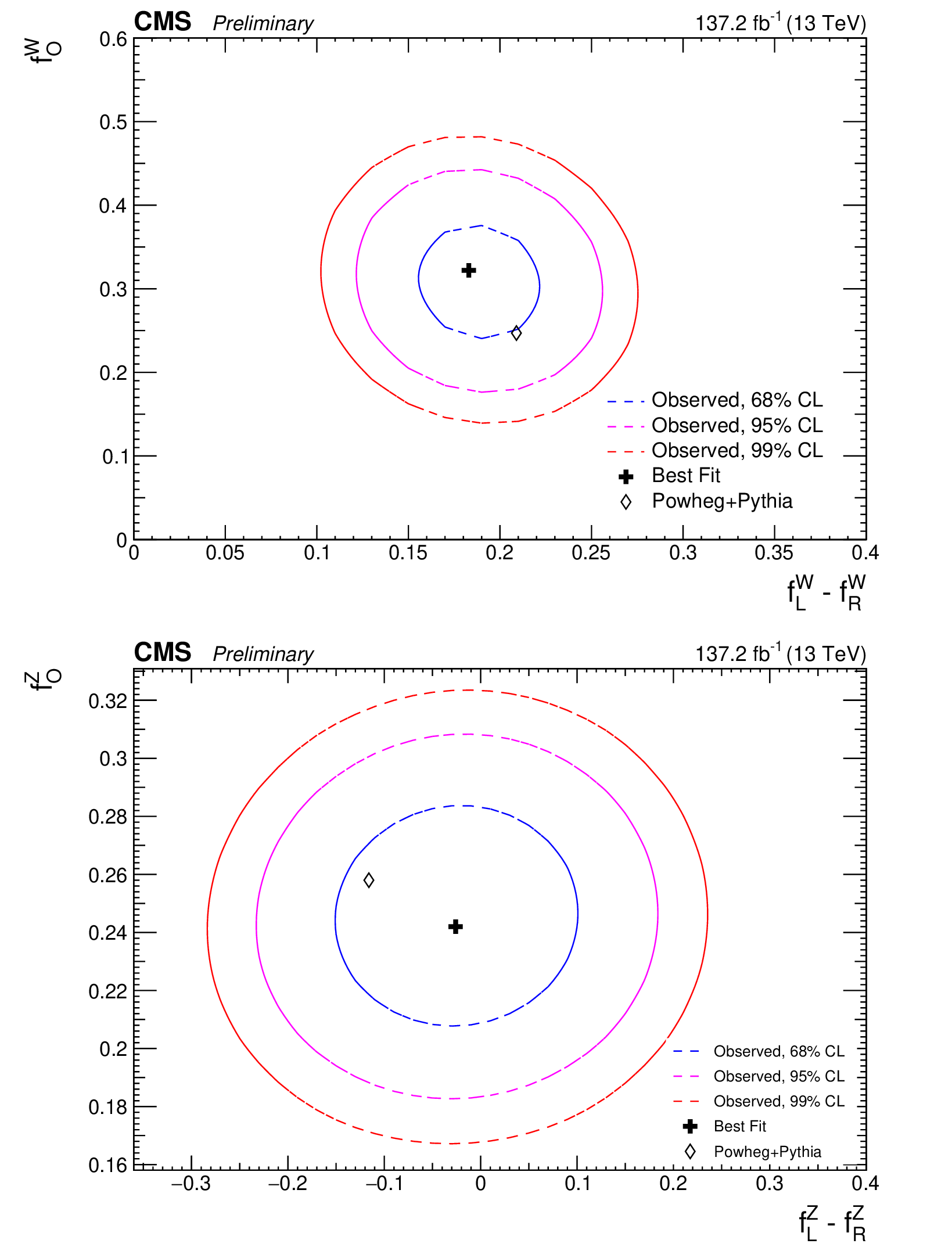
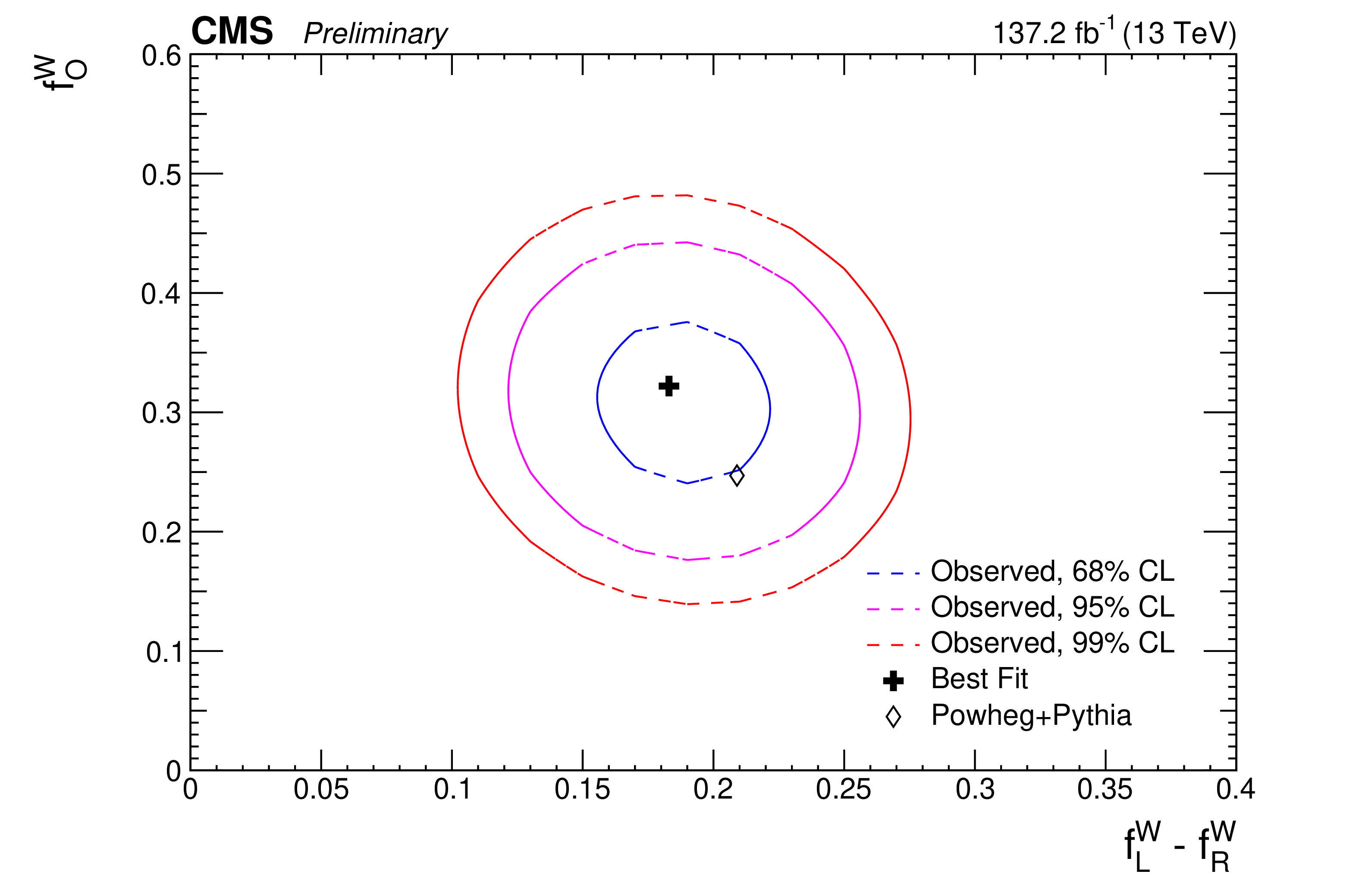
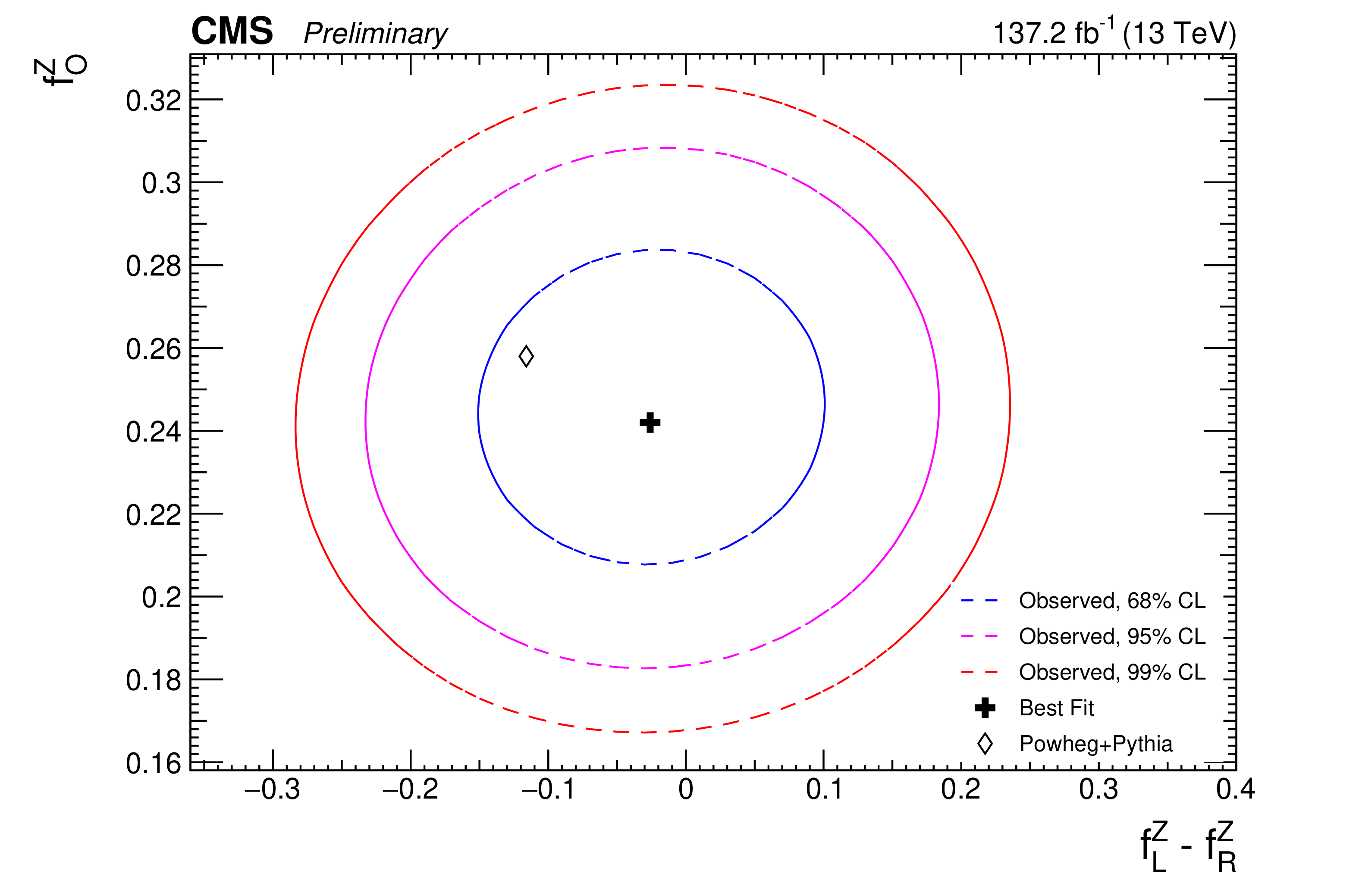
Figure 11:
Confidence regions in the $f_{LR}$-$f_{0}$ parameter plane for the W (left) and Z (right) boson polarization. The results are obtained with no additional requirement in the charge of the produced W boson. The blue, violet and red bands correspond to the 68, 95, and 99% confidence levels. |
png pdf |
Figure 11-a:
Confidence regions in the $f_{LR}$-$f_{0}$ parameter plane for the W (left) and Z (right) boson polarization. The results are obtained with no additional requirement in the charge of the produced W boson. The blue, violet and red bands correspond to the 68, 95, and 99% confidence levels. |
png pdf |
Figure 11-b:
Confidence regions in the $f_{LR}$-$f_{0}$ parameter plane for the W (left) and Z (right) boson polarization. The results are obtained with no additional requirement in the charge of the produced W boson. The blue, violet and red bands correspond to the 68, 95, and 99% confidence levels. |
png pdf |
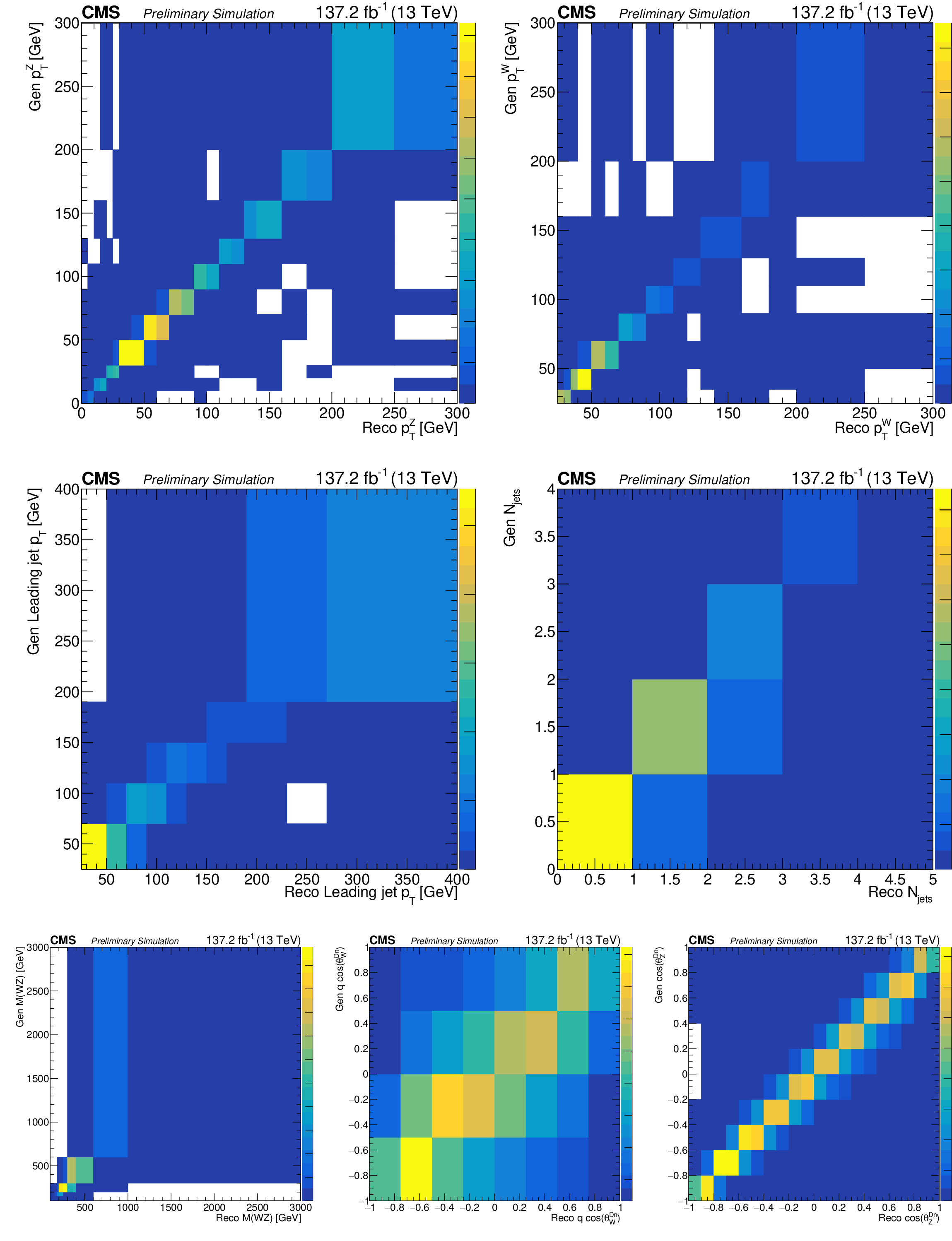
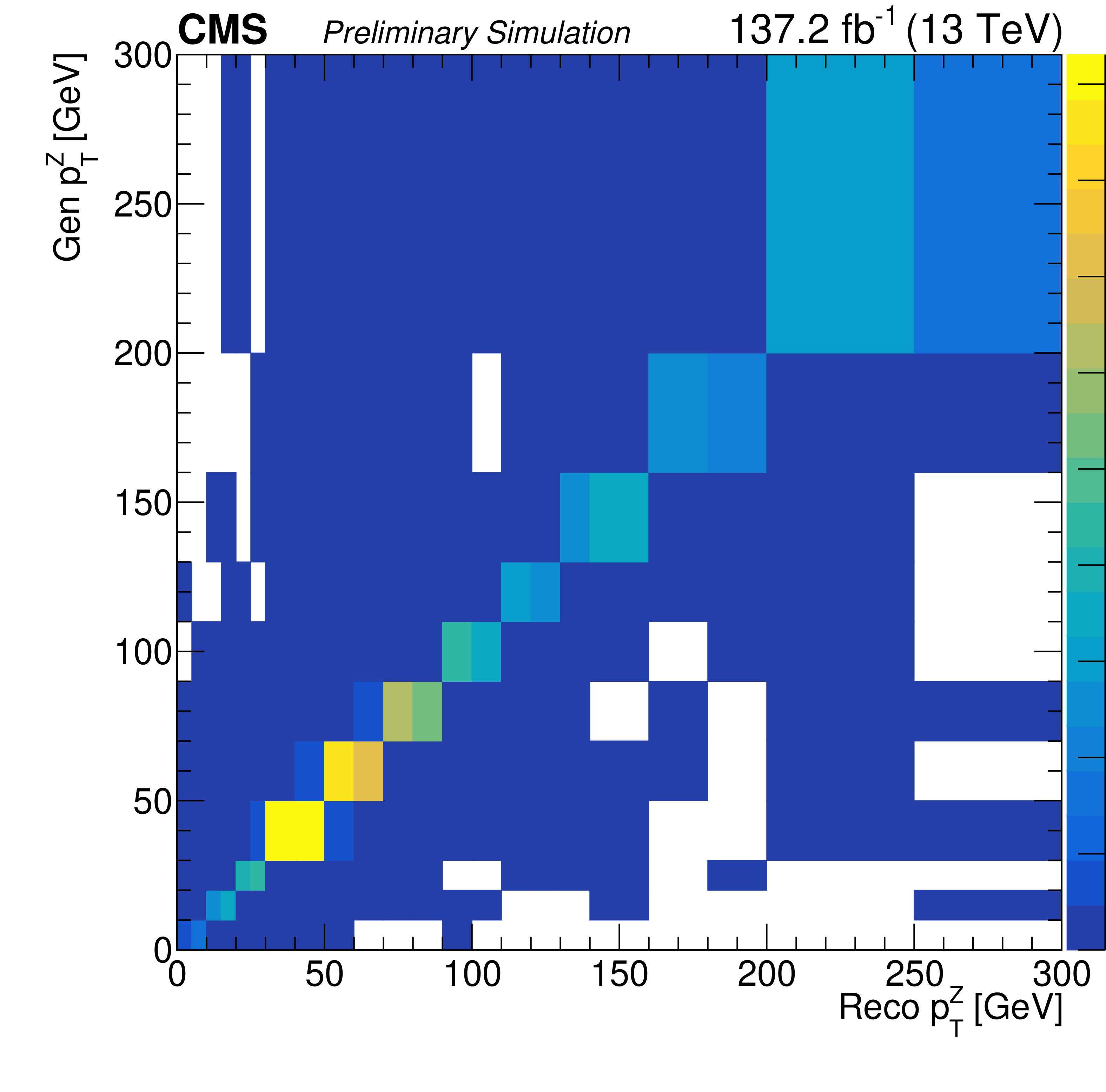
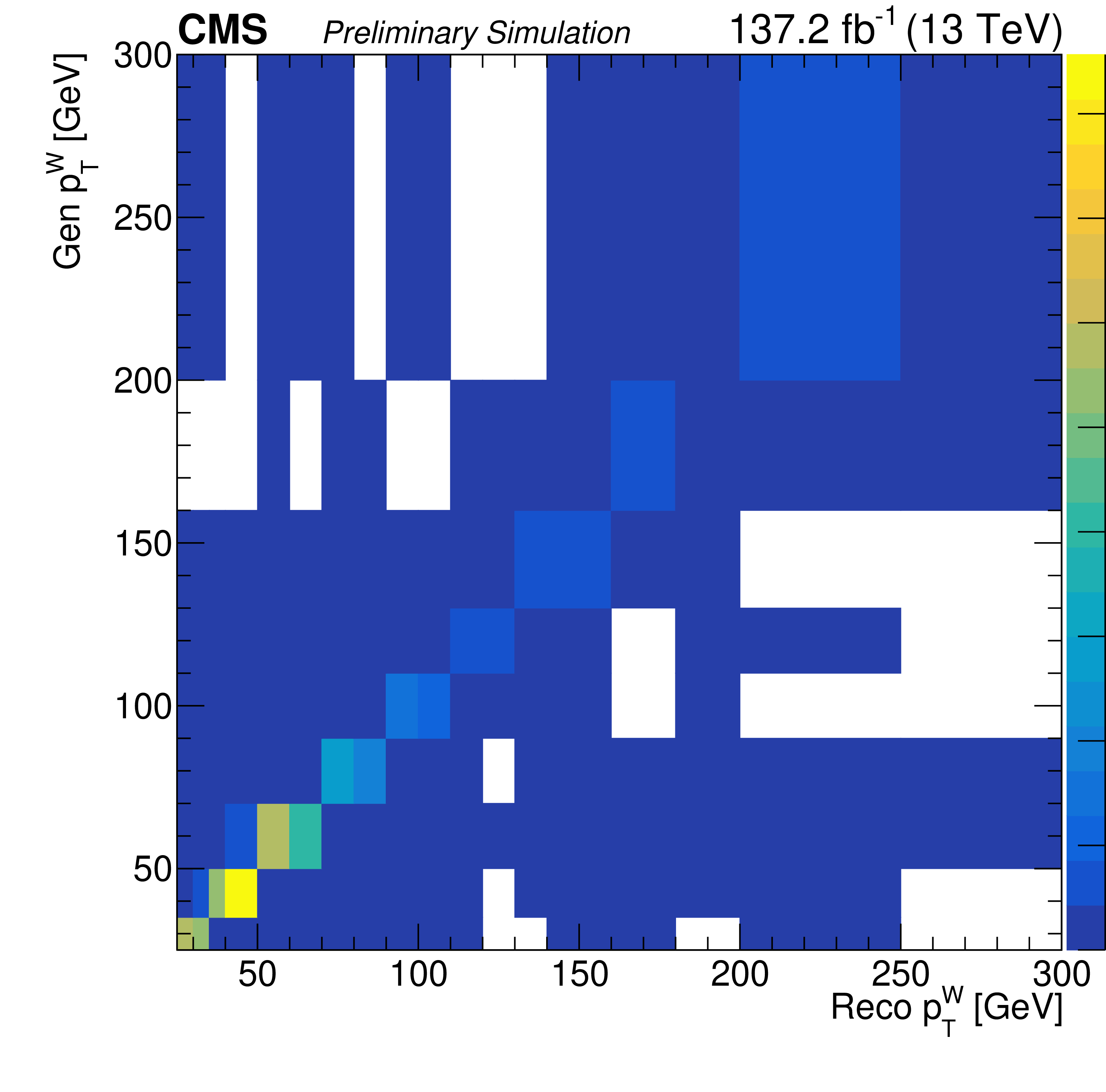
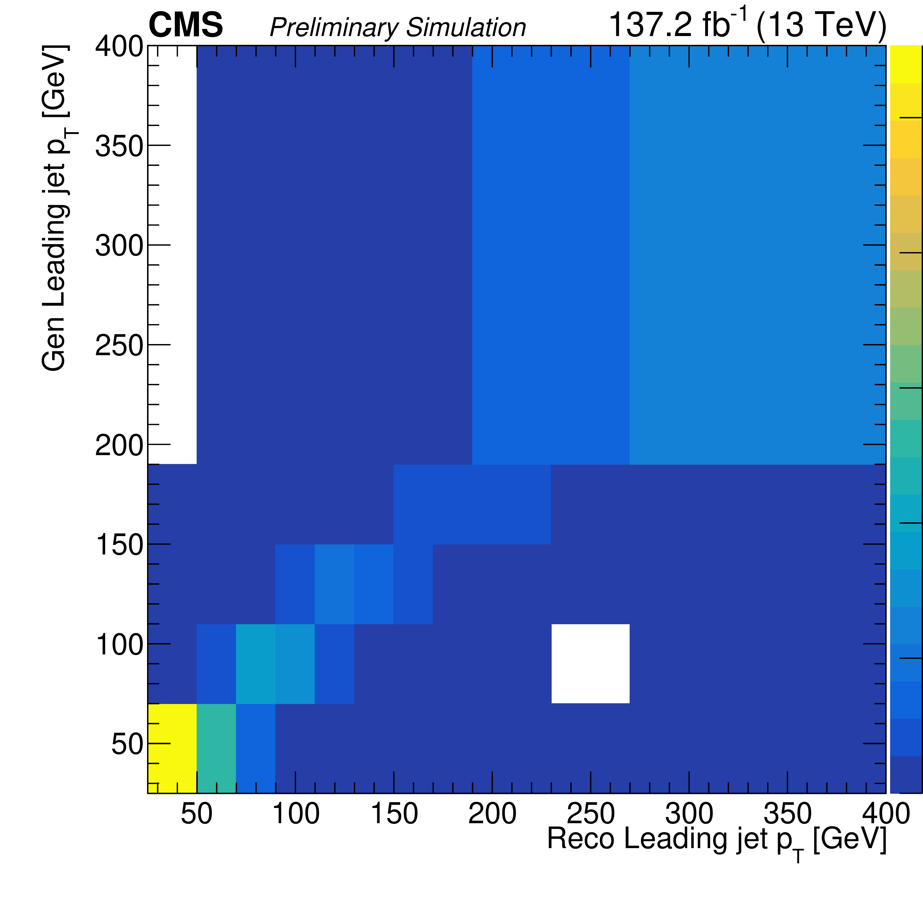
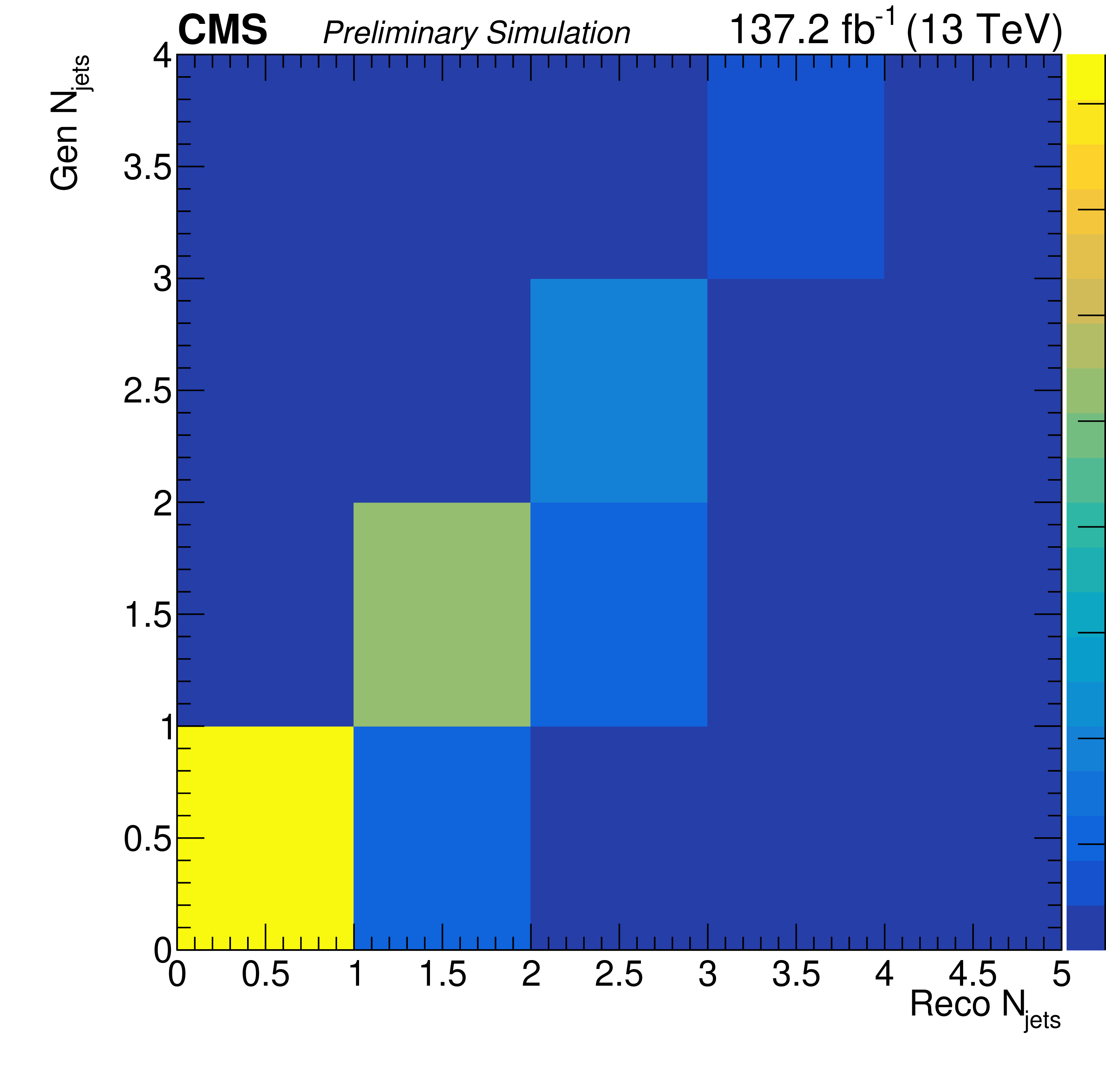
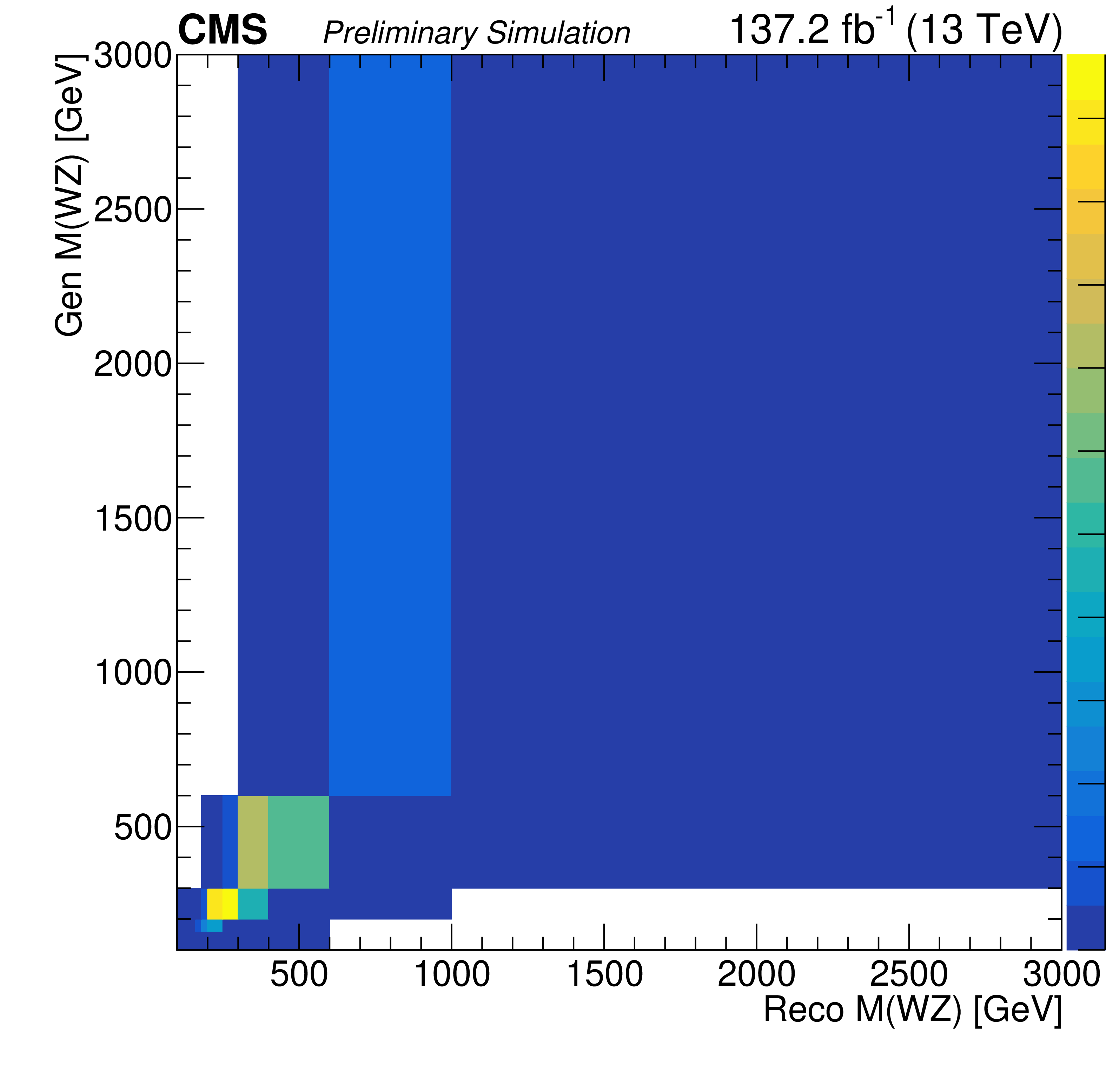
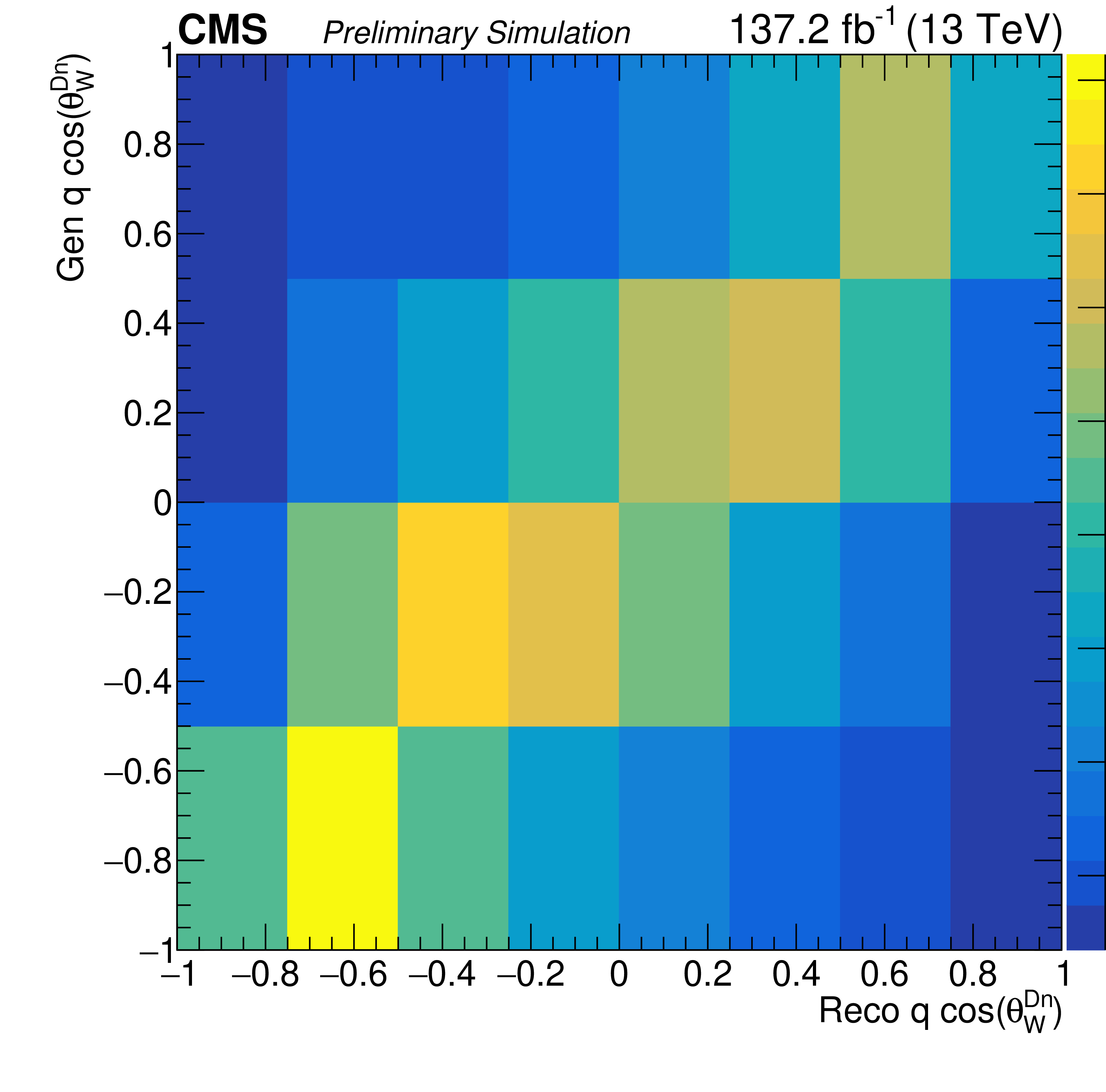
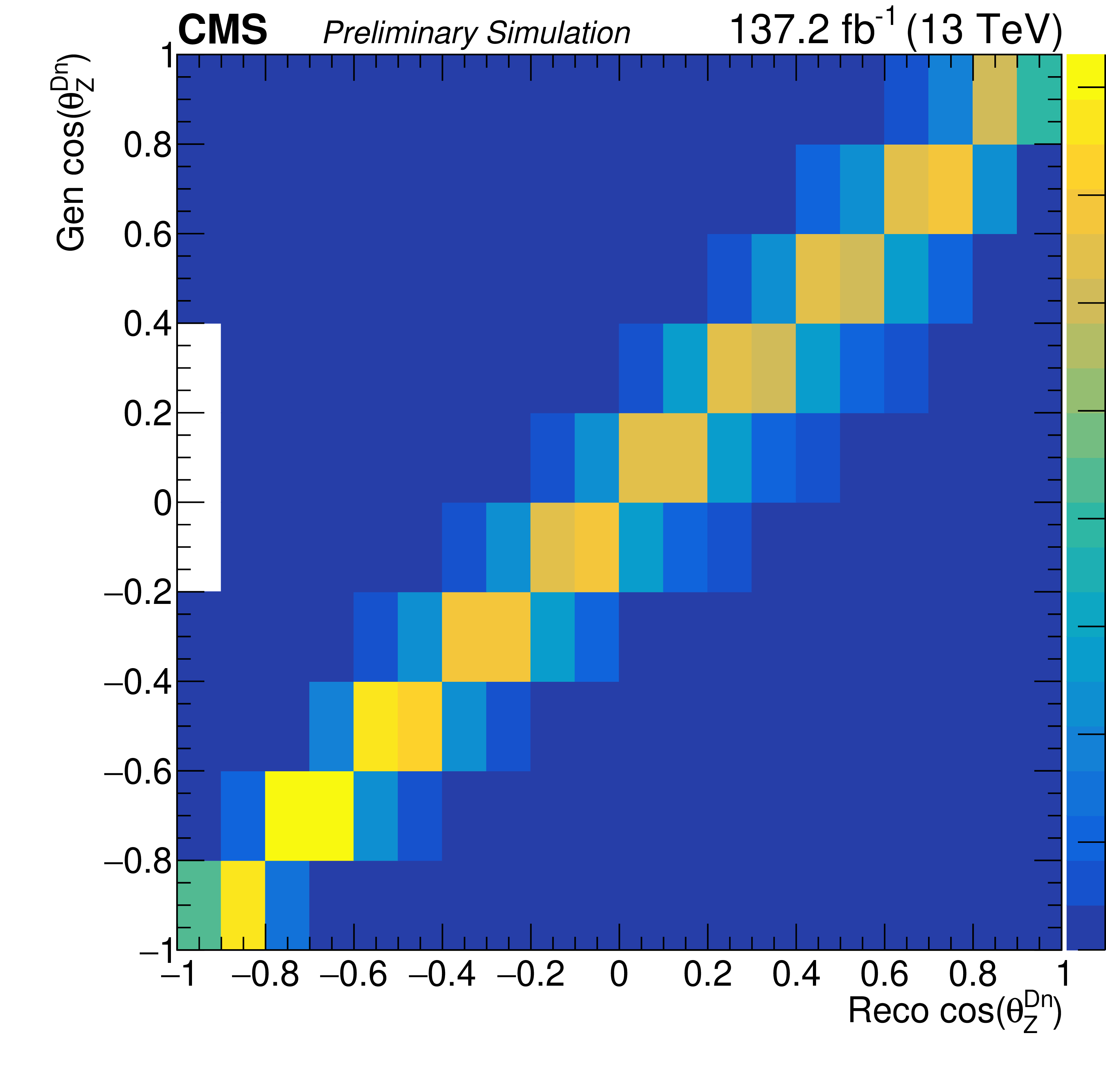
Figure 12:
Response matrices obtained at NLO in QCD using the POWHEG generator. Reconstructed ${p_{\mathrm {T}}}$ of the Z boson (top left), ${p_{\mathrm {T}}}$ of the lepton from the W decay (top right), ${p_{\mathrm {T}}}$ of the leading jet (middle left), jet multiplicity (middle right), invariant mass of the WZ system ${M({\mathrm{W} \mathrm{Z}})}$ (bottom left), cosine of the polarization angle ${\theta ^{\mathrm{W}}}$ (bottom middle), and cosine of the polarization angle ${\theta ^{\mathrm{Z}}}$ (bottom right). |
png pdf |
Figure 12-a:
Response matrices obtained at NLO in QCD using the POWHEG generator. Reconstructed ${p_{\mathrm {T}}}$ of the Z boson (top left), ${p_{\mathrm {T}}}$ of the lepton from the W decay (top right), ${p_{\mathrm {T}}}$ of the leading jet (middle left), jet multiplicity (middle right), invariant mass of the WZ system ${M({\mathrm{W} \mathrm{Z}})}$ (bottom left), cosine of the polarization angle ${\theta ^{\mathrm{W}}}$ (bottom middle), and cosine of the polarization angle ${\theta ^{\mathrm{Z}}}$ (bottom right). |
png pdf |
Figure 12-b:
Response matrices obtained at NLO in QCD using the POWHEG generator. Reconstructed ${p_{\mathrm {T}}}$ of the Z boson (top left), ${p_{\mathrm {T}}}$ of the lepton from the W decay (top right), ${p_{\mathrm {T}}}$ of the leading jet (middle left), jet multiplicity (middle right), invariant mass of the WZ system ${M({\mathrm{W} \mathrm{Z}})}$ (bottom left), cosine of the polarization angle ${\theta ^{\mathrm{W}}}$ (bottom middle), and cosine of the polarization angle ${\theta ^{\mathrm{Z}}}$ (bottom right). |
png pdf |
Figure 12-c:
Response matrices obtained at NLO in QCD using the POWHEG generator. Reconstructed ${p_{\mathrm {T}}}$ of the Z boson (top left), ${p_{\mathrm {T}}}$ of the lepton from the W decay (top right), ${p_{\mathrm {T}}}$ of the leading jet (middle left), jet multiplicity (middle right), invariant mass of the WZ system ${M({\mathrm{W} \mathrm{Z}})}$ (bottom left), cosine of the polarization angle ${\theta ^{\mathrm{W}}}$ (bottom middle), and cosine of the polarization angle ${\theta ^{\mathrm{Z}}}$ (bottom right). |
png pdf |
Figure 12-d:
Response matrices obtained at NLO in QCD using the POWHEG generator. Reconstructed ${p_{\mathrm {T}}}$ of the Z boson (top left), ${p_{\mathrm {T}}}$ of the lepton from the W decay (top right), ${p_{\mathrm {T}}}$ of the leading jet (middle left), jet multiplicity (middle right), invariant mass of the WZ system ${M({\mathrm{W} \mathrm{Z}})}$ (bottom left), cosine of the polarization angle ${\theta ^{\mathrm{W}}}$ (bottom middle), and cosine of the polarization angle ${\theta ^{\mathrm{Z}}}$ (bottom right). |
png pdf |
Figure 12-e:
Response matrices obtained at NLO in QCD using the POWHEG generator. Reconstructed ${p_{\mathrm {T}}}$ of the Z boson (top left), ${p_{\mathrm {T}}}$ of the lepton from the W decay (top right), ${p_{\mathrm {T}}}$ of the leading jet (middle left), jet multiplicity (middle right), invariant mass of the WZ system ${M({\mathrm{W} \mathrm{Z}})}$ (bottom left), cosine of the polarization angle ${\theta ^{\mathrm{W}}}$ (bottom middle), and cosine of the polarization angle ${\theta ^{\mathrm{Z}}}$ (bottom right). |
png pdf |
Figure 12-f:
Response matrices obtained at NLO in QCD using the POWHEG generator. Reconstructed ${p_{\mathrm {T}}}$ of the Z boson (top left), ${p_{\mathrm {T}}}$ of the lepton from the W decay (top right), ${p_{\mathrm {T}}}$ of the leading jet (middle left), jet multiplicity (middle right), invariant mass of the WZ system ${M({\mathrm{W} \mathrm{Z}})}$ (bottom left), cosine of the polarization angle ${\theta ^{\mathrm{W}}}$ (bottom middle), and cosine of the polarization angle ${\theta ^{\mathrm{Z}}}$ (bottom right). |
png pdf |
Figure 12-g:
Response matrices obtained at NLO in QCD using the POWHEG generator. Reconstructed ${p_{\mathrm {T}}}$ of the Z boson (top left), ${p_{\mathrm {T}}}$ of the lepton from the W decay (top right), ${p_{\mathrm {T}}}$ of the leading jet (middle left), jet multiplicity (middle right), invariant mass of the WZ system ${M({\mathrm{W} \mathrm{Z}})}$ (bottom left), cosine of the polarization angle ${\theta ^{\mathrm{W}}}$ (bottom middle), and cosine of the polarization angle ${\theta ^{\mathrm{Z}}}$ (bottom right). |
png pdf |
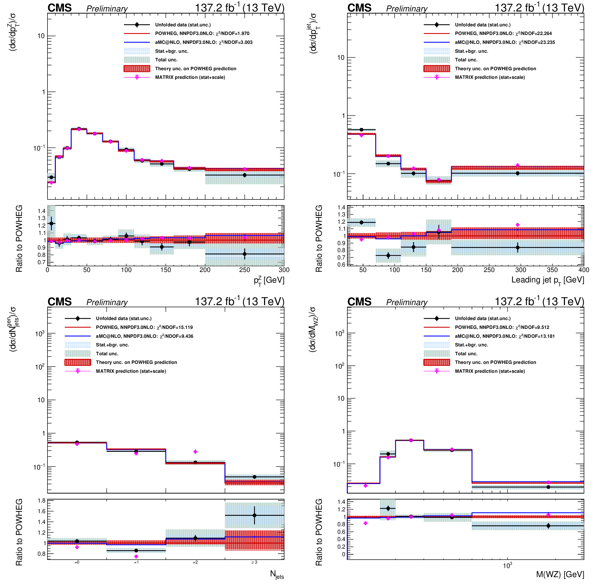
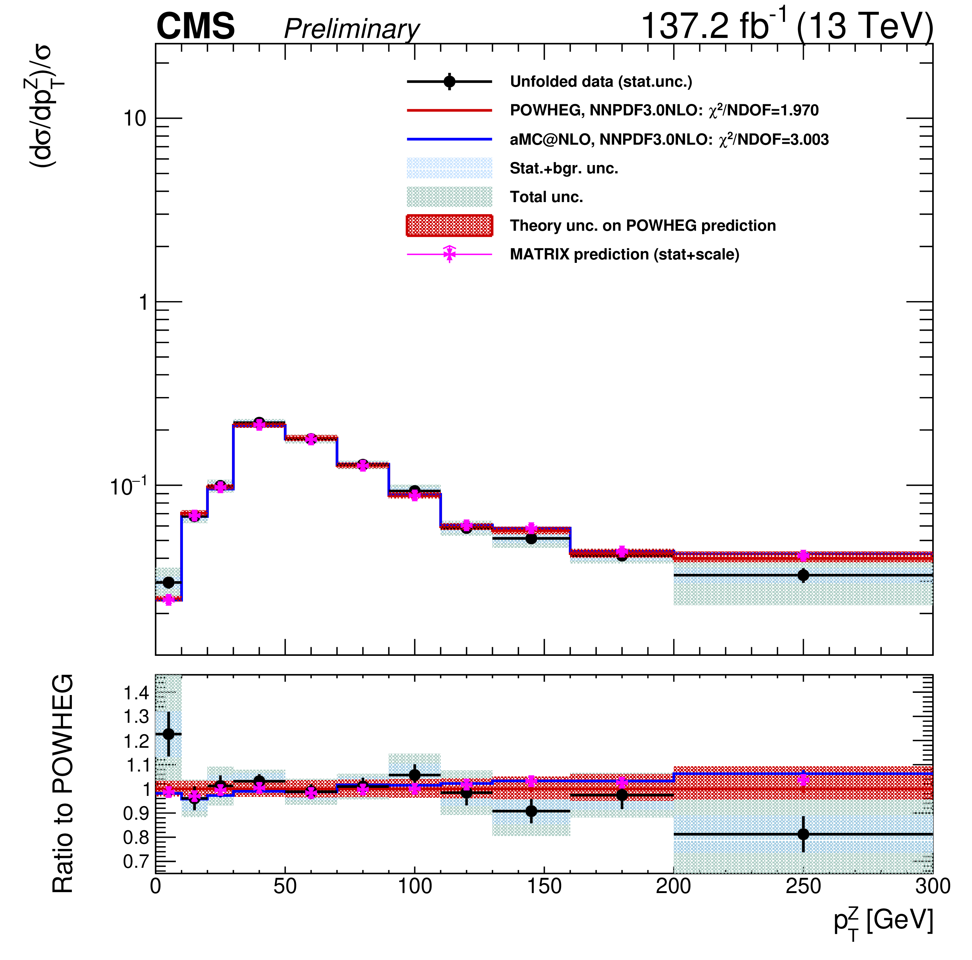
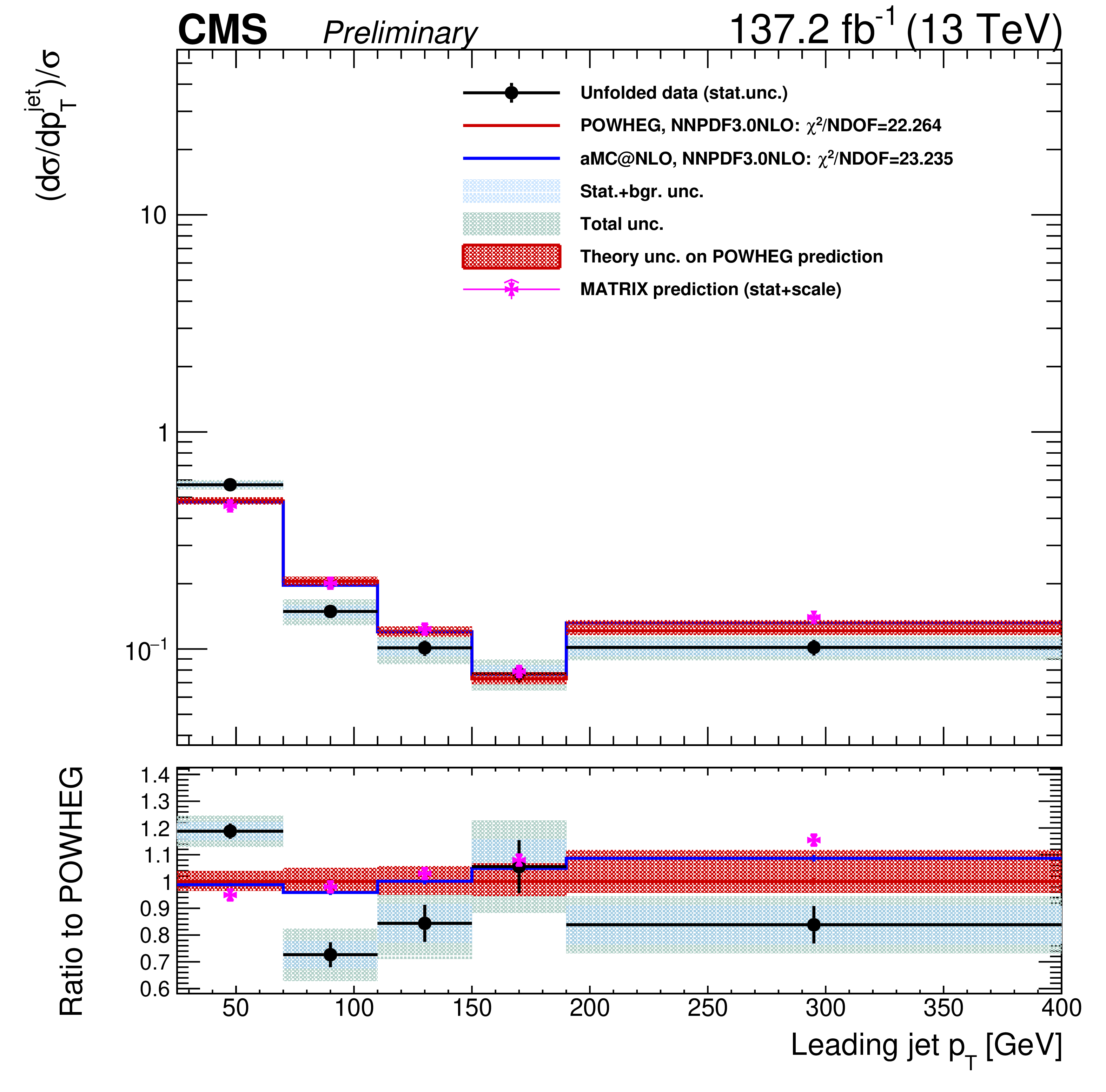
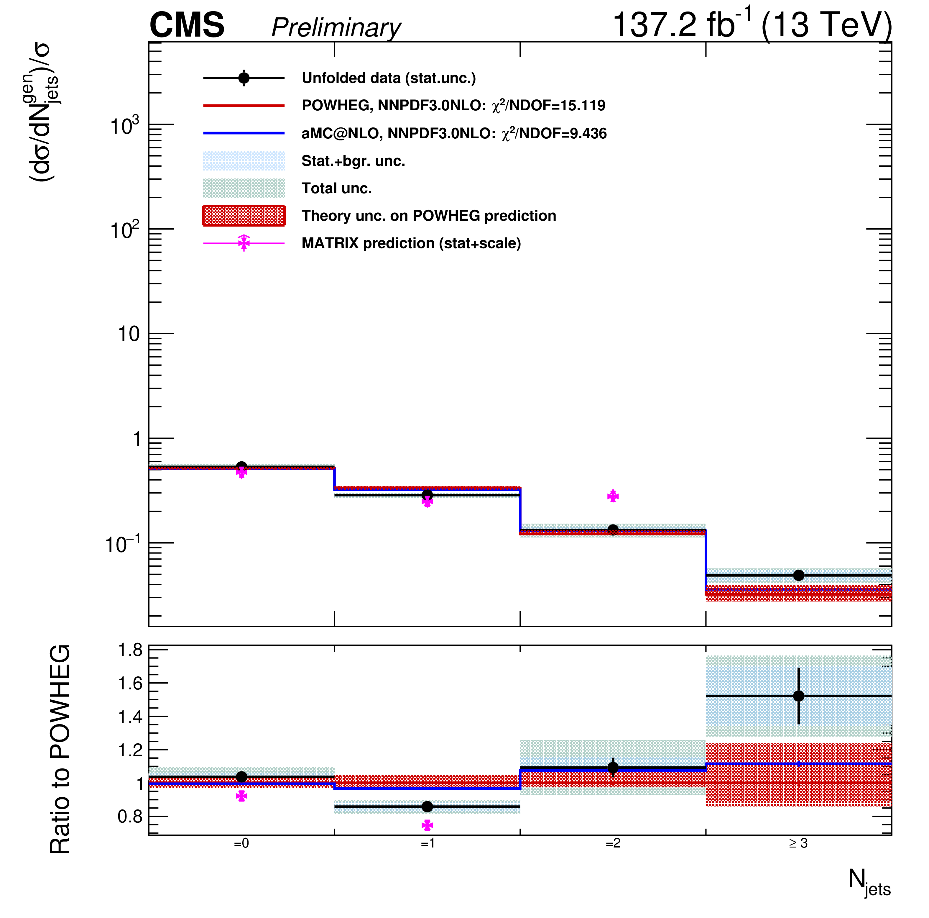
Figure 13:
Unfolding results using NNLO bias, area constraint, and no additional regularization term for several variables: the ${p_{\mathrm {T}}}$ of the Z boson (top left), the ${p_{\mathrm {T}}}$ of the leading jet in the event (top right), the jet multiplicity (bottom left) and the ${M({\mathrm{W} \mathrm{Z}})}$ variable (bottom right). Black dots represent unfolded data results for which black bars denote statistical uncertainties, shaded blue bands represent statistical plus background related uncertainties and the green band represent the total unfolding uncertainty. The red histogram and shadow bands are the POWHEG prediction and its theoretical uncertainty. The blue histogram represents the MadGraph 5_aMC@NLO prediction and the violet points show the matrix prediction including error bands representing numerical and scale uncertainties. matrix predictions for the jet multiplicity are available only up to two jets. |
png pdf |
Figure 13-a:
Unfolding results using NNLO bias, area constraint, and no additional regularization term for several variables: the ${p_{\mathrm {T}}}$ of the Z boson (top left), the ${p_{\mathrm {T}}}$ of the leading jet in the event (top right), the jet multiplicity (bottom left) and the ${M({\mathrm{W} \mathrm{Z}})}$ variable (bottom right). Black dots represent unfolded data results for which black bars denote statistical uncertainties, shaded blue bands represent statistical plus background related uncertainties and the green band represent the total unfolding uncertainty. The red histogram and shadow bands are the POWHEG prediction and its theoretical uncertainty. The blue histogram represents the MadGraph 5_aMC@NLO prediction and the violet points show the matrix prediction including error bands representing numerical and scale uncertainties. matrix predictions for the jet multiplicity are available only up to two jets. |
png pdf |
Figure 13-b:
Unfolding results using NNLO bias, area constraint, and no additional regularization term for several variables: the ${p_{\mathrm {T}}}$ of the Z boson (top left), the ${p_{\mathrm {T}}}$ of the leading jet in the event (top right), the jet multiplicity (bottom left) and the ${M({\mathrm{W} \mathrm{Z}})}$ variable (bottom right). Black dots represent unfolded data results for which black bars denote statistical uncertainties, shaded blue bands represent statistical plus background related uncertainties and the green band represent the total unfolding uncertainty. The red histogram and shadow bands are the POWHEG prediction and its theoretical uncertainty. The blue histogram represents the MadGraph 5_aMC@NLO prediction and the violet points show the matrix prediction including error bands representing numerical and scale uncertainties. matrix predictions for the jet multiplicity are available only up to two jets. |
png pdf |
Figure 13-c:
Unfolding results using NNLO bias, area constraint, and no additional regularization term for several variables: the ${p_{\mathrm {T}}}$ of the Z boson (top left), the ${p_{\mathrm {T}}}$ of the leading jet in the event (top right), the jet multiplicity (bottom left) and the ${M({\mathrm{W} \mathrm{Z}})}$ variable (bottom right). Black dots represent unfolded data results for which black bars denote statistical uncertainties, shaded blue bands represent statistical plus background related uncertainties and the green band represent the total unfolding uncertainty. The red histogram and shadow bands are the POWHEG prediction and its theoretical uncertainty. The blue histogram represents the MadGraph 5_aMC@NLO prediction and the violet points show the matrix prediction including error bands representing numerical and scale uncertainties. matrix predictions for the jet multiplicity are available only up to two jets. |

png pdf |
Figure 13-d:
Unfolding results using NNLO bias, area constraint, and no additional regularization term for several variables: the ${p_{\mathrm {T}}}$ of the Z boson (top left), the ${p_{\mathrm {T}}}$ of the leading jet in the event (top right), the jet multiplicity (bottom left) and the ${M({\mathrm{W} \mathrm{Z}})}$ variable (bottom right). Black dots represent unfolded data results for which black bars denote statistical uncertainties, shaded blue bands represent statistical plus background related uncertainties and the green band represent the total unfolding uncertainty. The red histogram and shadow bands are the POWHEG prediction and its theoretical uncertainty. The blue histogram represents the MadGraph 5_aMC@NLO prediction and the violet points show the matrix prediction including error bands representing numerical and scale uncertainties. matrix predictions for the jet multiplicity are available only up to two jets. |
png pdf |
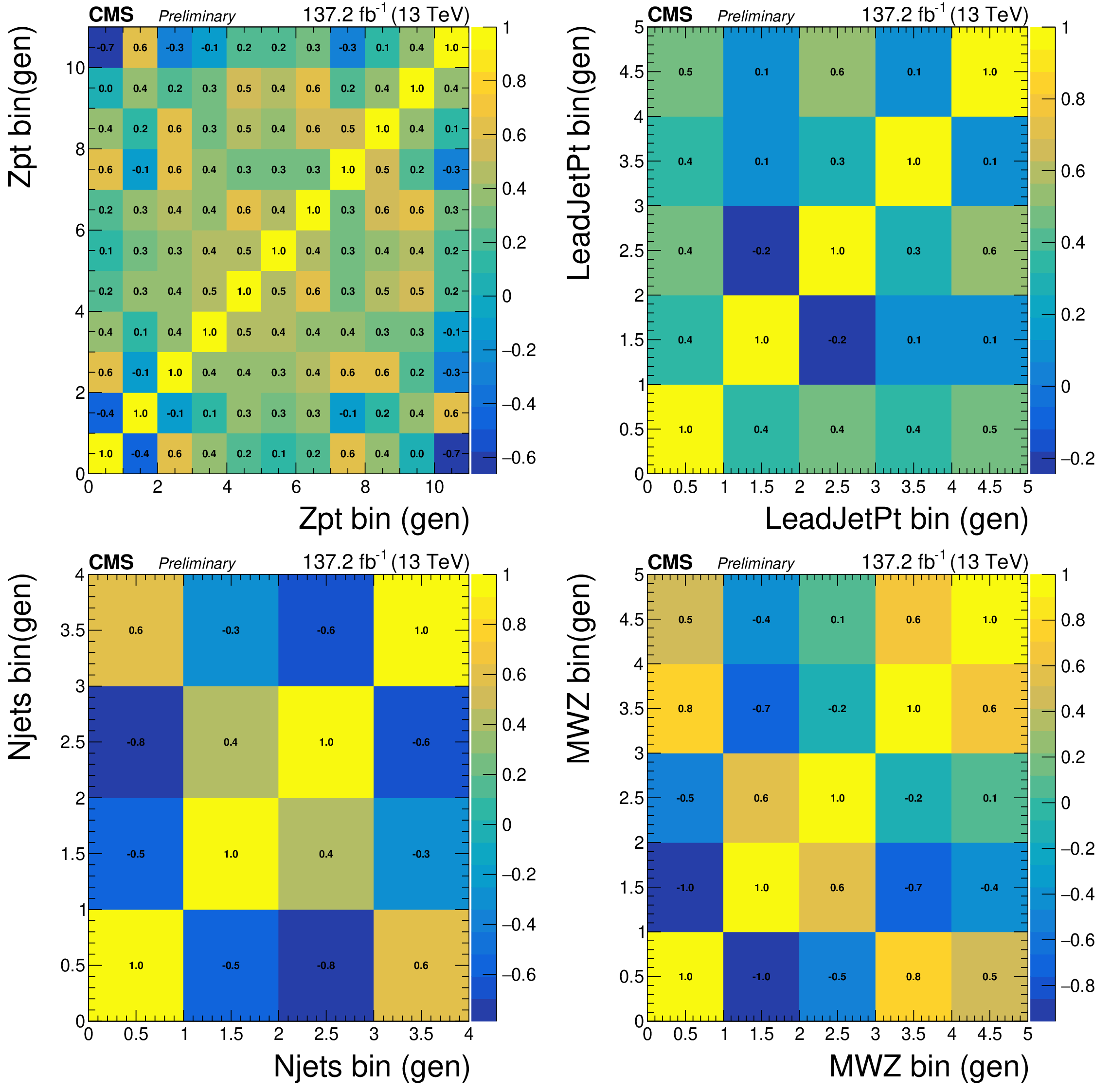
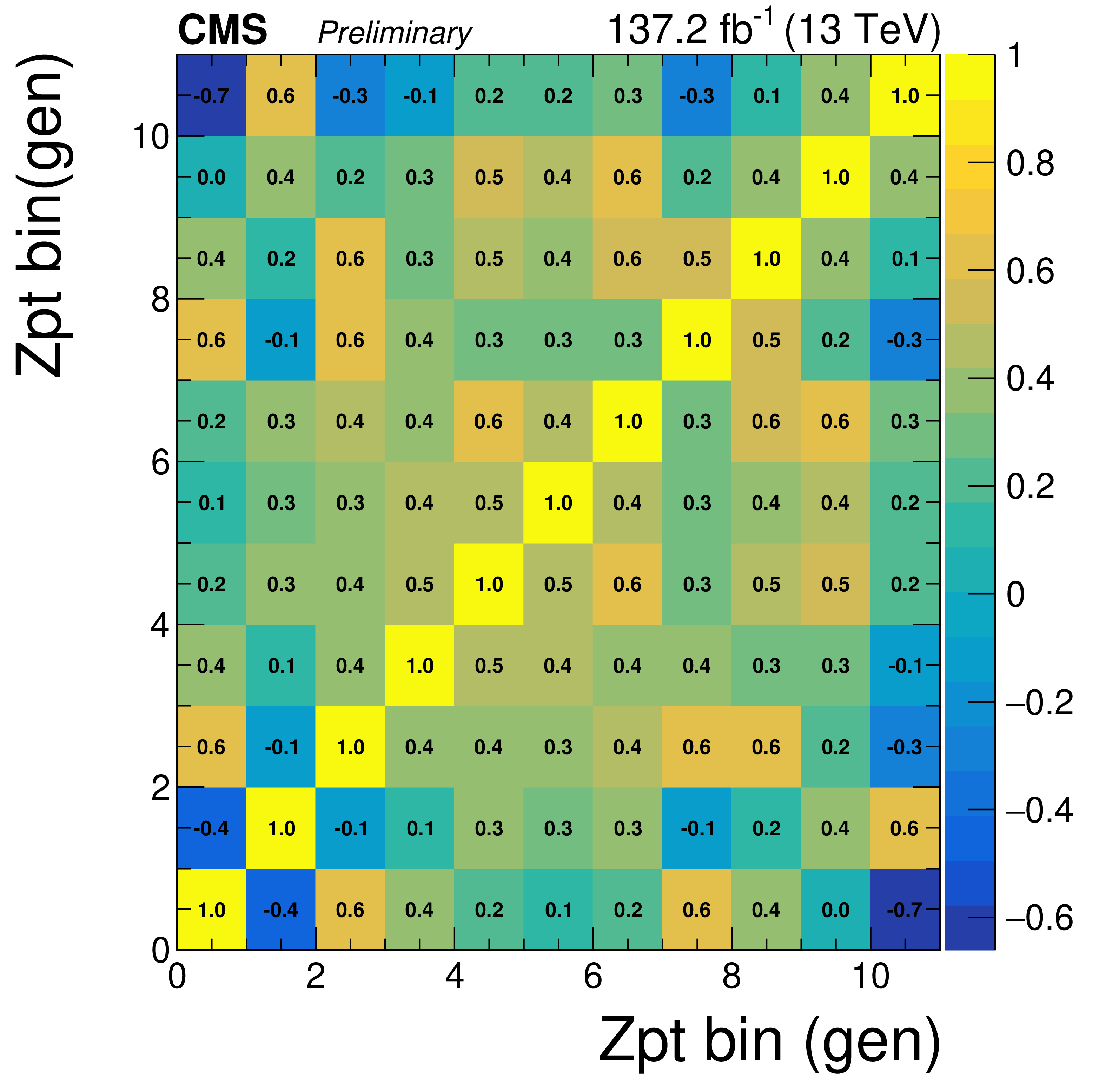
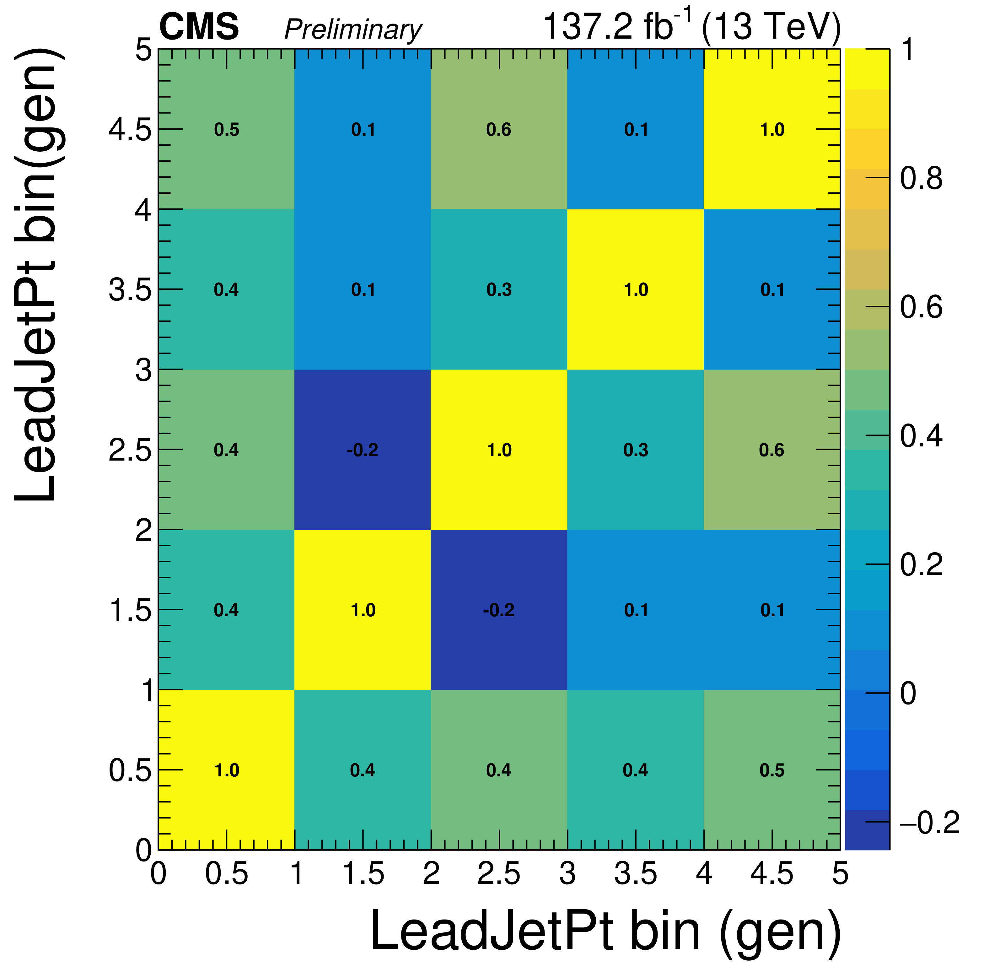
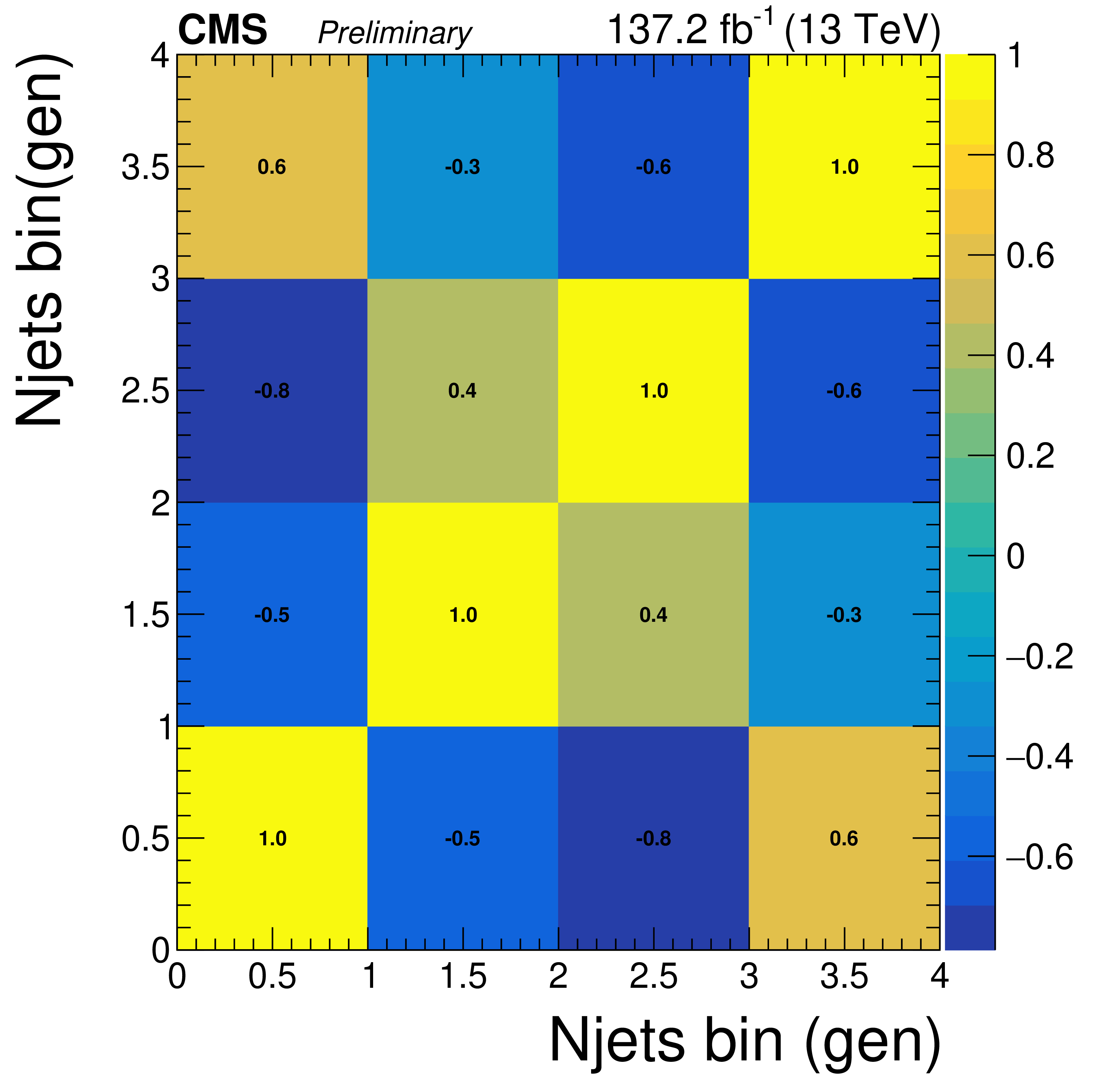
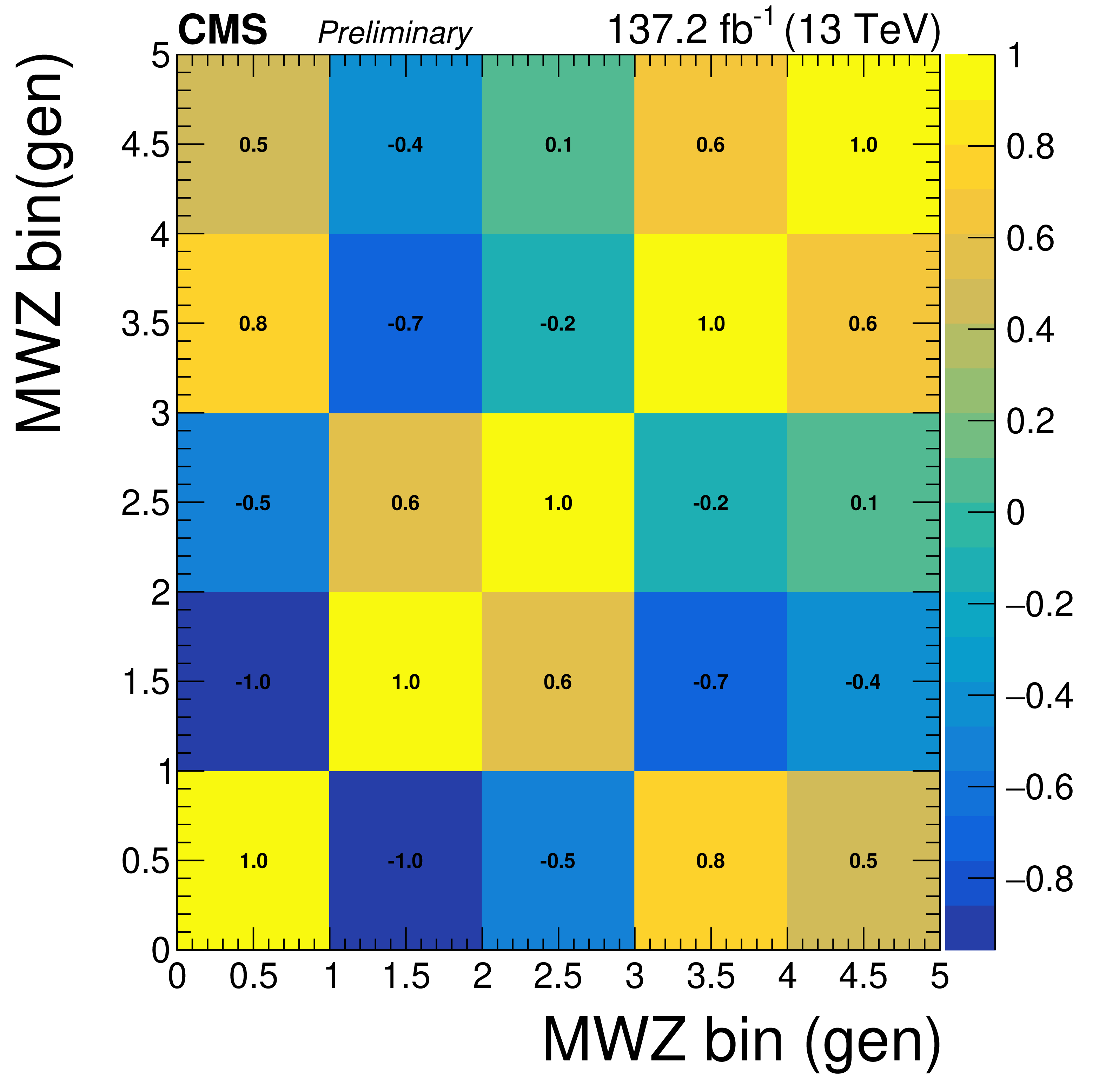
Figure 14:
Correlation matrices for the unfolded results obtained using NNLO bias, area constraint, and no additional regularization term for several variables: the ${p_{\mathrm {T}}}$ of the Z boson (top left), the ${p_{\mathrm {T}}}$ of the leading jet in the event (top right), the jet multiplicity (bottom left) and the ${M({\mathrm{W} \mathrm{Z}})}$ variable (bottom right). |
png pdf |
Figure 14-a:
Correlation matrices for the unfolded results obtained using NNLO bias, area constraint, and no additional regularization term for several variables: the ${p_{\mathrm {T}}}$ of the Z boson (top left), the ${p_{\mathrm {T}}}$ of the leading jet in the event (top right), the jet multiplicity (bottom left) and the ${M({\mathrm{W} \mathrm{Z}})}$ variable (bottom right). |
png pdf |
Figure 14-b:
Correlation matrices for the unfolded results obtained using NNLO bias, area constraint, and no additional regularization term for several variables: the ${p_{\mathrm {T}}}$ of the Z boson (top left), the ${p_{\mathrm {T}}}$ of the leading jet in the event (top right), the jet multiplicity (bottom left) and the ${M({\mathrm{W} \mathrm{Z}})}$ variable (bottom right). |
png pdf |
Figure 14-c:
Correlation matrices for the unfolded results obtained using NNLO bias, area constraint, and no additional regularization term for several variables: the ${p_{\mathrm {T}}}$ of the Z boson (top left), the ${p_{\mathrm {T}}}$ of the leading jet in the event (top right), the jet multiplicity (bottom left) and the ${M({\mathrm{W} \mathrm{Z}})}$ variable (bottom right). |
png pdf |
Figure 14-d:
Correlation matrices for the unfolded results obtained using NNLO bias, area constraint, and no additional regularization term for several variables: the ${p_{\mathrm {T}}}$ of the Z boson (top left), the ${p_{\mathrm {T}}}$ of the leading jet in the event (top right), the jet multiplicity (bottom left) and the ${M({\mathrm{W} \mathrm{Z}})}$ variable (bottom right). |
png pdf |
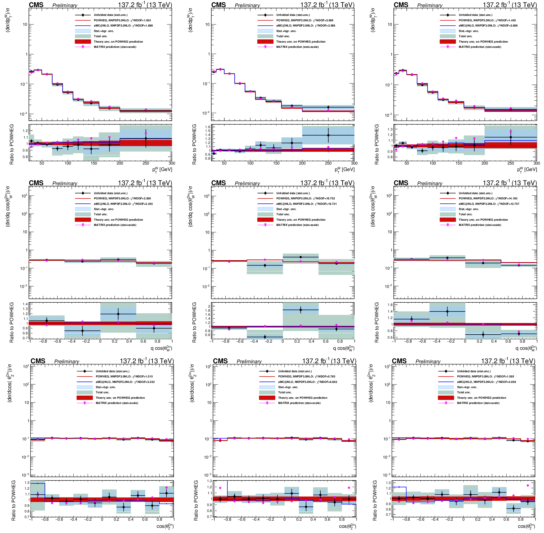
Figure 15:
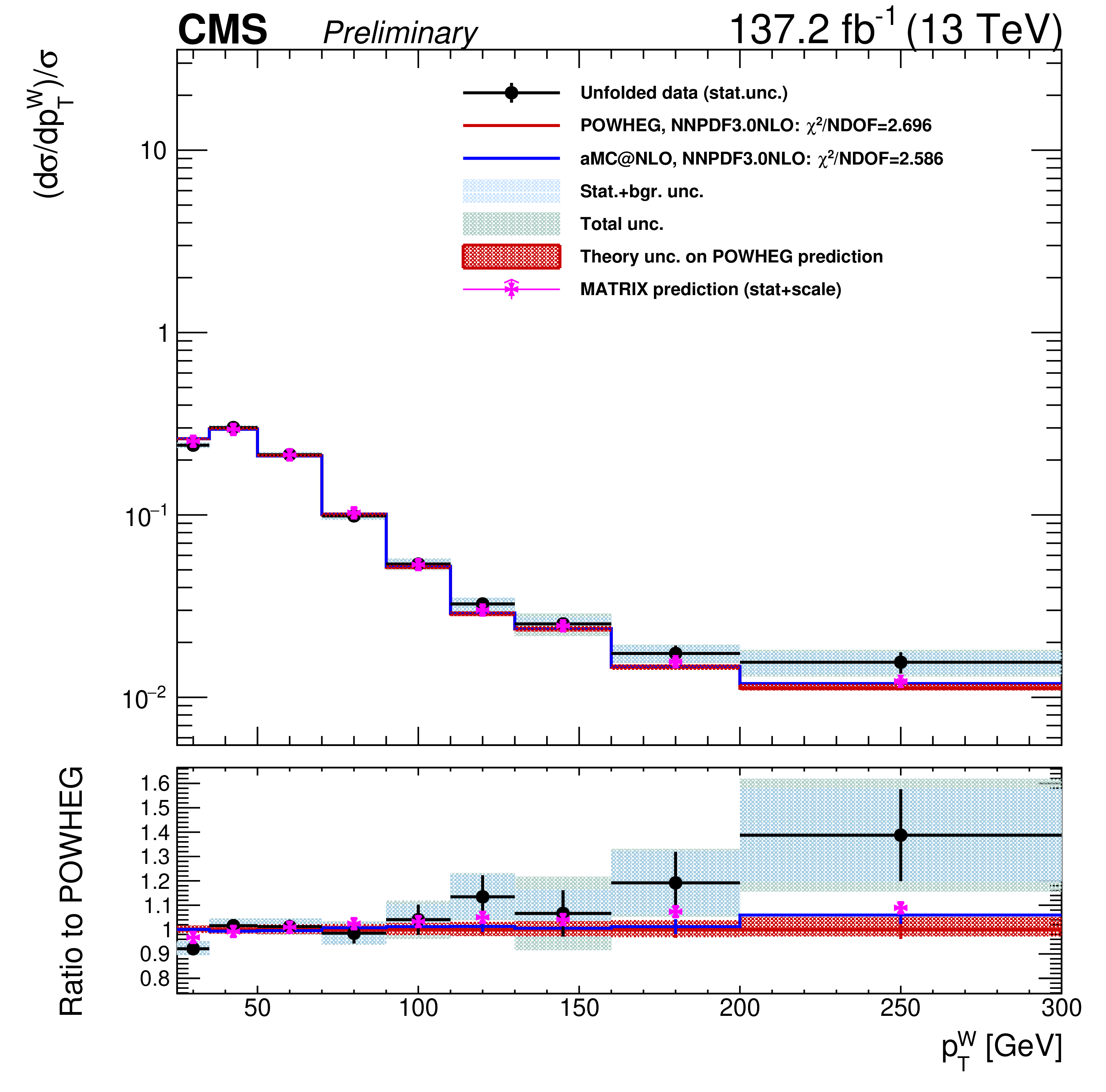
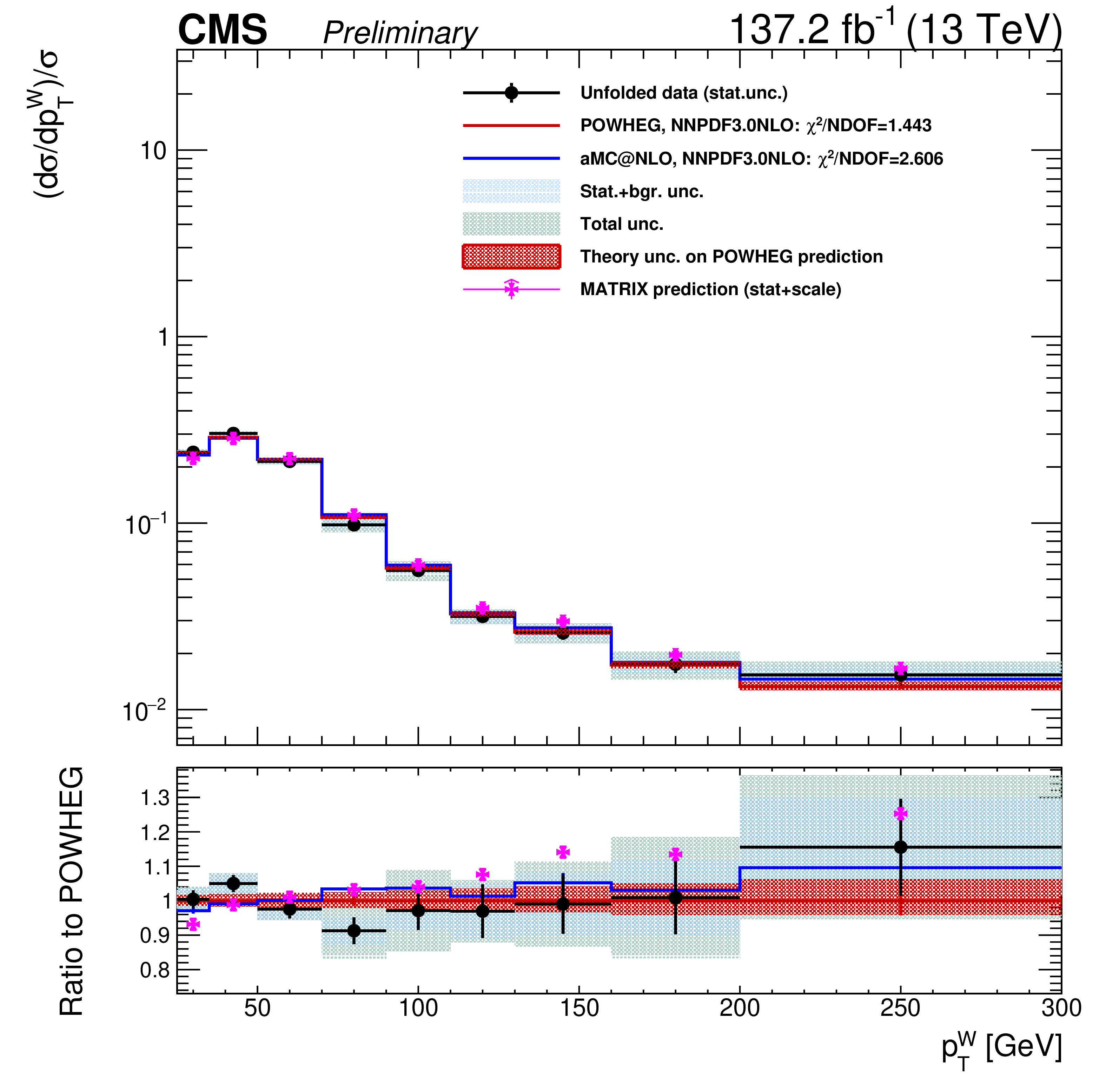
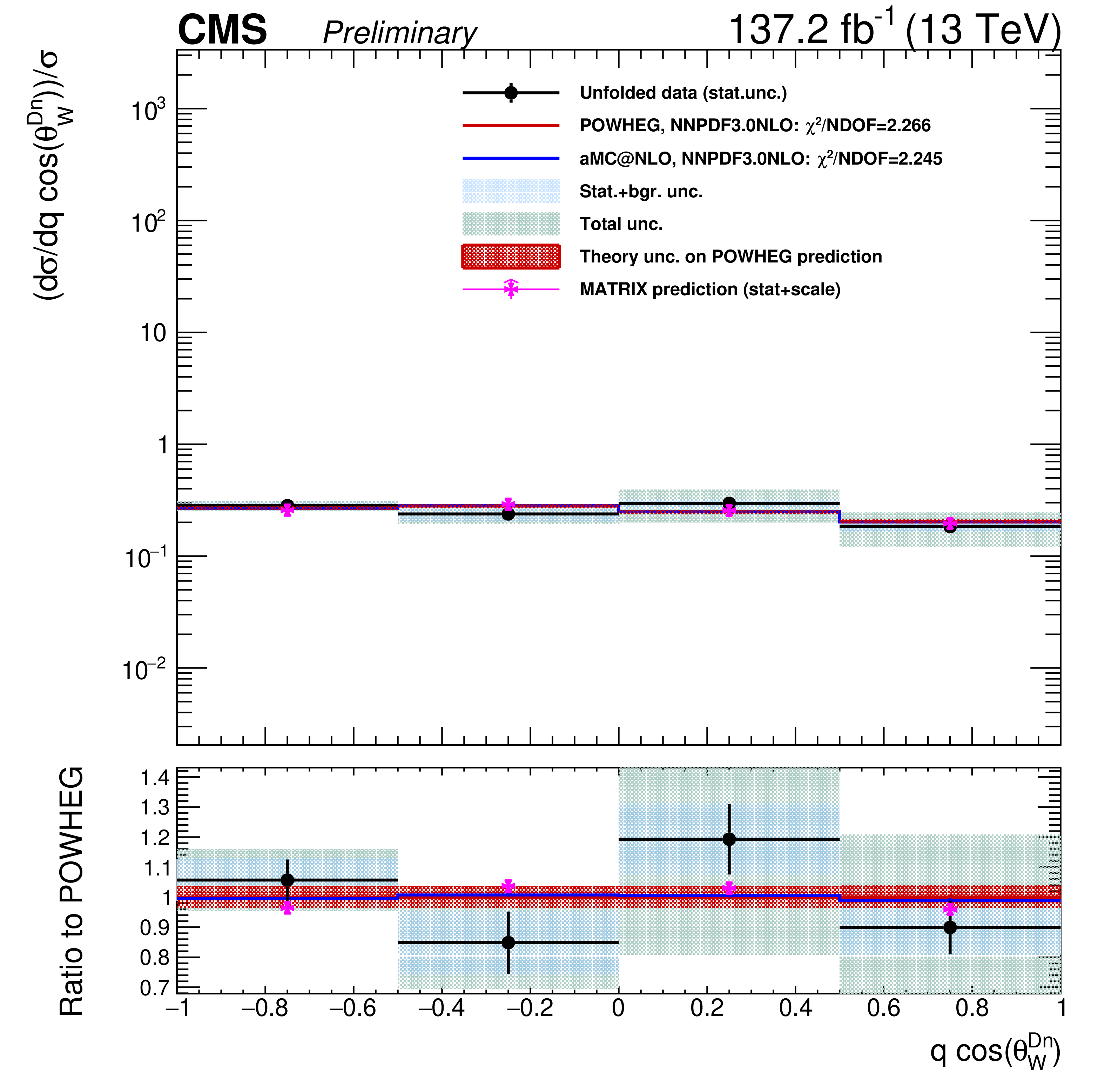
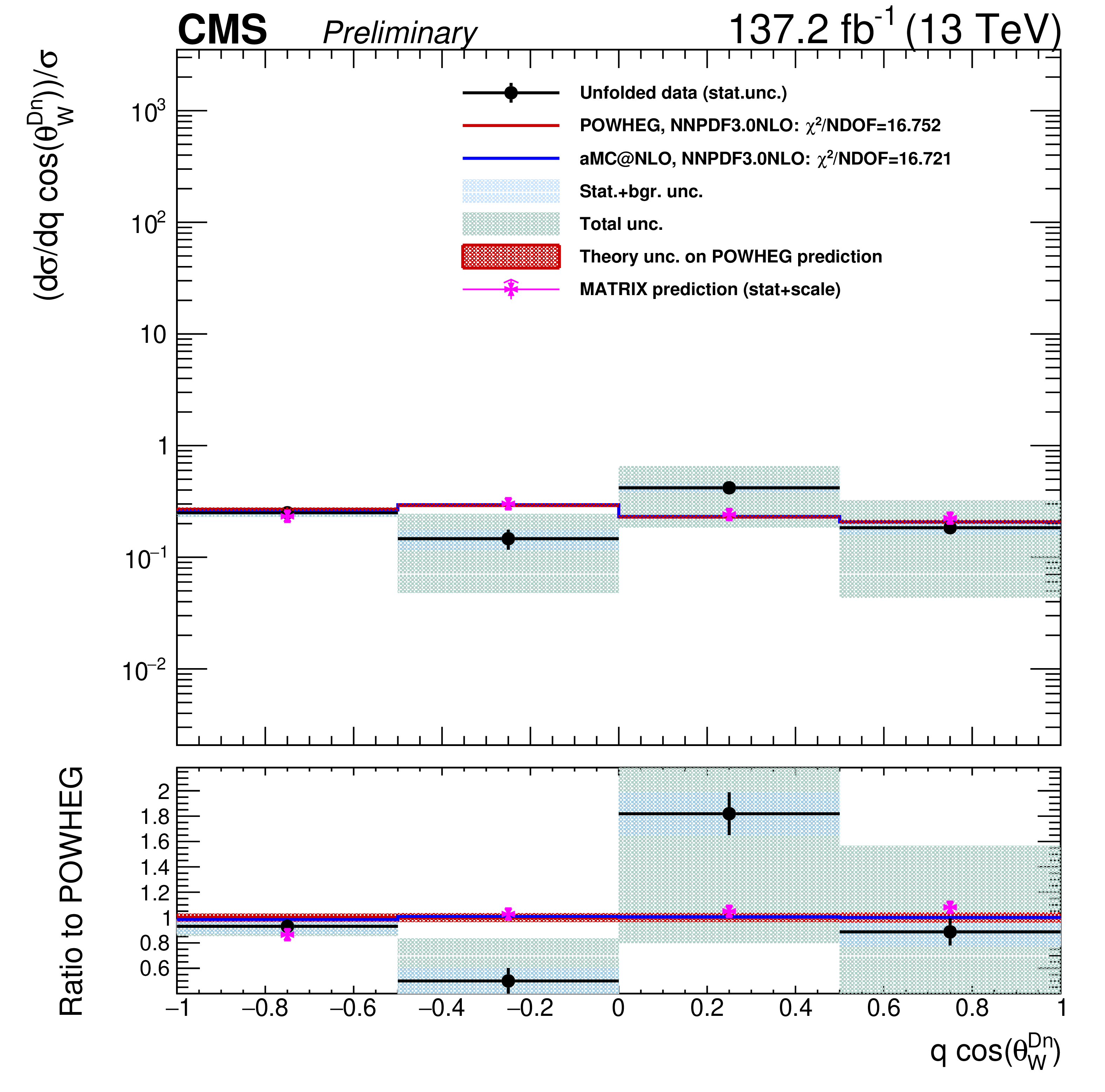
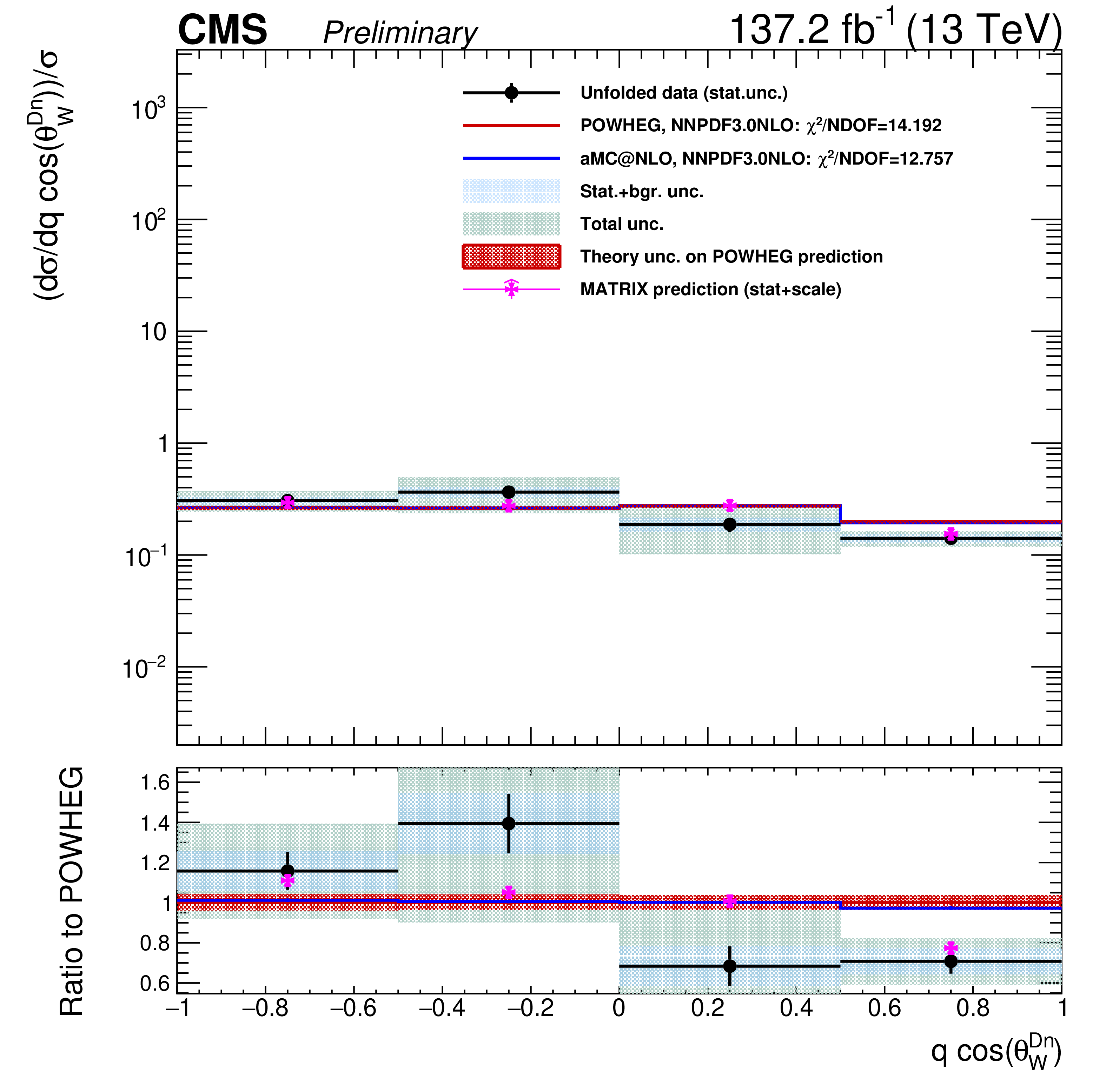
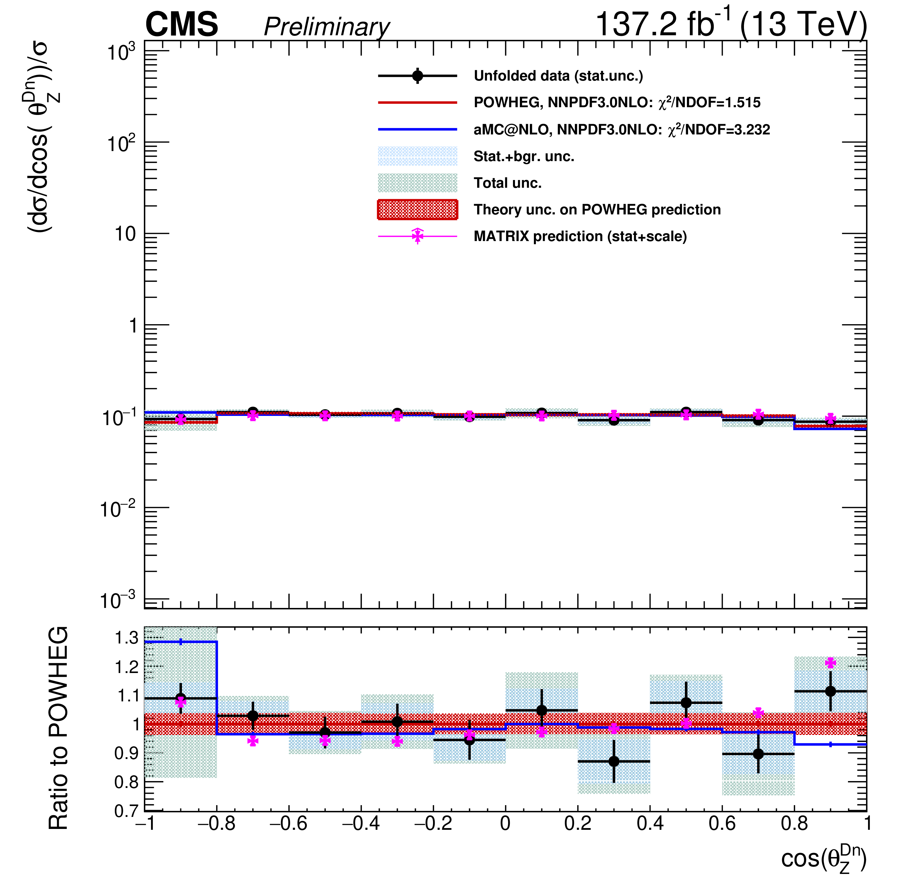
Unfolding results using NNLO bias, area constraint, and no additional regularization term for several variables and charged final states. From top to bottom: ${p_{\mathrm {T}}}$ of the lepton in the W decay, cosine of the polarization angle of the W boson, and cosine of the polarization angle of the Z boson. From left to right: charge inclusive, positive charge, and negative charge final states. Black dots represent unfolded data results for which black bars denote statistical uncertainties, shaded blue bands represent statistical plus background related uncertainties and the green band represent the total unfolding uncertainty. The red histogram and shadow bands are the POWHEG prediction and its theoretical uncertainty. The blue histogram represents the MadGraph 5_aMC@NLO prediction and the violet points show the matrix prediction including error bands representing numerical and scale uncertainties. |
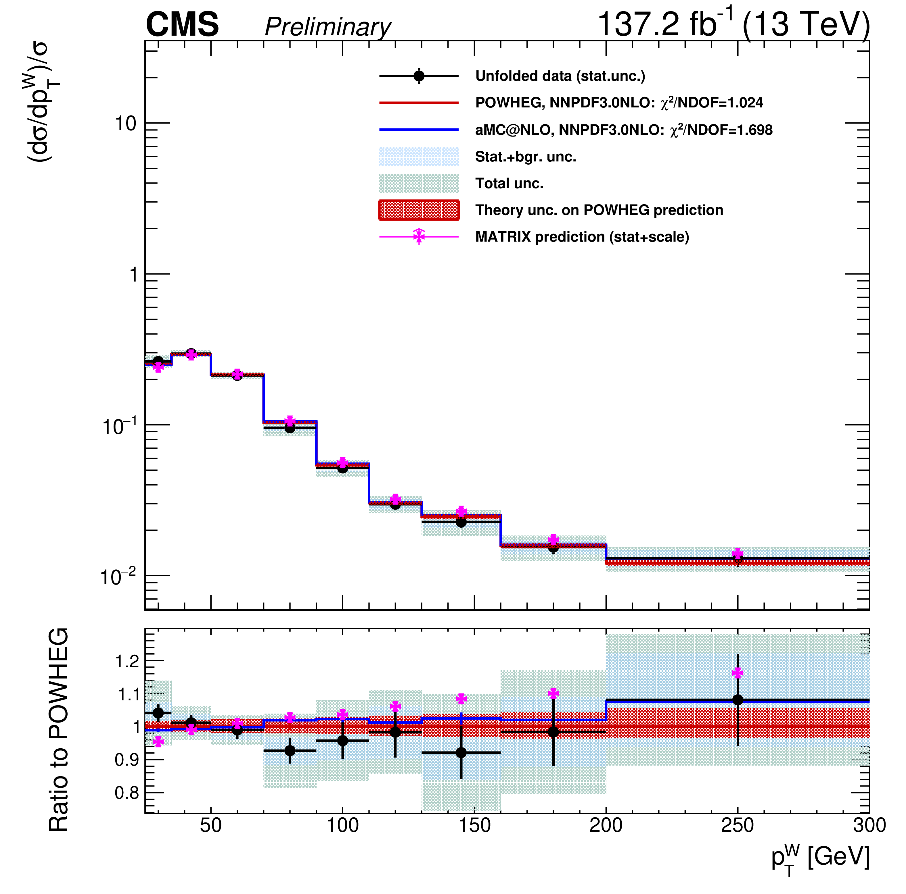
png pdf |
Figure 15-a:
Unfolding results using NNLO bias, area constraint, and no additional regularization term for several variables and charged final states. From top to bottom: ${p_{\mathrm {T}}}$ of the lepton in the W decay, cosine of the polarization angle of the W boson, and cosine of the polarization angle of the Z boson. From left to right: charge inclusive, positive charge, and negative charge final states. Black dots represent unfolded data results for which black bars denote statistical uncertainties, shaded blue bands represent statistical plus background related uncertainties and the green band represent the total unfolding uncertainty. The red histogram and shadow bands are the POWHEG prediction and its theoretical uncertainty. The blue histogram represents the MadGraph 5_aMC@NLO prediction and the violet points show the matrix prediction including error bands representing numerical and scale uncertainties. |
png pdf |
Figure 15-b:
Unfolding results using NNLO bias, area constraint, and no additional regularization term for several variables and charged final states. From top to bottom: ${p_{\mathrm {T}}}$ of the lepton in the W decay, cosine of the polarization angle of the W boson, and cosine of the polarization angle of the Z boson. From left to right: charge inclusive, positive charge, and negative charge final states. Black dots represent unfolded data results for which black bars denote statistical uncertainties, shaded blue bands represent statistical plus background related uncertainties and the green band represent the total unfolding uncertainty. The red histogram and shadow bands are the POWHEG prediction and its theoretical uncertainty. The blue histogram represents the MadGraph 5_aMC@NLO prediction and the violet points show the matrix prediction including error bands representing numerical and scale uncertainties. |
png pdf |
Figure 15-c:
Unfolding results using NNLO bias, area constraint, and no additional regularization term for several variables and charged final states. From top to bottom: ${p_{\mathrm {T}}}$ of the lepton in the W decay, cosine of the polarization angle of the W boson, and cosine of the polarization angle of the Z boson. From left to right: charge inclusive, positive charge, and negative charge final states. Black dots represent unfolded data results for which black bars denote statistical uncertainties, shaded blue bands represent statistical plus background related uncertainties and the green band represent the total unfolding uncertainty. The red histogram and shadow bands are the POWHEG prediction and its theoretical uncertainty. The blue histogram represents the MadGraph 5_aMC@NLO prediction and the violet points show the matrix prediction including error bands representing numerical and scale uncertainties. |
png pdf |
Figure 15-d:
Unfolding results using NNLO bias, area constraint, and no additional regularization term for several variables and charged final states. From top to bottom: ${p_{\mathrm {T}}}$ of the lepton in the W decay, cosine of the polarization angle of the W boson, and cosine of the polarization angle of the Z boson. From left to right: charge inclusive, positive charge, and negative charge final states. Black dots represent unfolded data results for which black bars denote statistical uncertainties, shaded blue bands represent statistical plus background related uncertainties and the green band represent the total unfolding uncertainty. The red histogram and shadow bands are the POWHEG prediction and its theoretical uncertainty. The blue histogram represents the MadGraph 5_aMC@NLO prediction and the violet points show the matrix prediction including error bands representing numerical and scale uncertainties. |
png pdf |
Figure 15-e:
Unfolding results using NNLO bias, area constraint, and no additional regularization term for several variables and charged final states. From top to bottom: ${p_{\mathrm {T}}}$ of the lepton in the W decay, cosine of the polarization angle of the W boson, and cosine of the polarization angle of the Z boson. From left to right: charge inclusive, positive charge, and negative charge final states. Black dots represent unfolded data results for which black bars denote statistical uncertainties, shaded blue bands represent statistical plus background related uncertainties and the green band represent the total unfolding uncertainty. The red histogram and shadow bands are the POWHEG prediction and its theoretical uncertainty. The blue histogram represents the MadGraph 5_aMC@NLO prediction and the violet points show the matrix prediction including error bands representing numerical and scale uncertainties. |
png pdf |
Figure 15-f:
Unfolding results using NNLO bias, area constraint, and no additional regularization term for several variables and charged final states. From top to bottom: ${p_{\mathrm {T}}}$ of the lepton in the W decay, cosine of the polarization angle of the W boson, and cosine of the polarization angle of the Z boson. From left to right: charge inclusive, positive charge, and negative charge final states. Black dots represent unfolded data results for which black bars denote statistical uncertainties, shaded blue bands represent statistical plus background related uncertainties and the green band represent the total unfolding uncertainty. The red histogram and shadow bands are the POWHEG prediction and its theoretical uncertainty. The blue histogram represents the MadGraph 5_aMC@NLO prediction and the violet points show the matrix prediction including error bands representing numerical and scale uncertainties. |
png pdf |
Figure 15-g:
Unfolding results using NNLO bias, area constraint, and no additional regularization term for several variables and charged final states. From top to bottom: ${p_{\mathrm {T}}}$ of the lepton in the W decay, cosine of the polarization angle of the W boson, and cosine of the polarization angle of the Z boson. From left to right: charge inclusive, positive charge, and negative charge final states. Black dots represent unfolded data results for which black bars denote statistical uncertainties, shaded blue bands represent statistical plus background related uncertainties and the green band represent the total unfolding uncertainty. The red histogram and shadow bands are the POWHEG prediction and its theoretical uncertainty. The blue histogram represents the MadGraph 5_aMC@NLO prediction and the violet points show the matrix prediction including error bands representing numerical and scale uncertainties. |
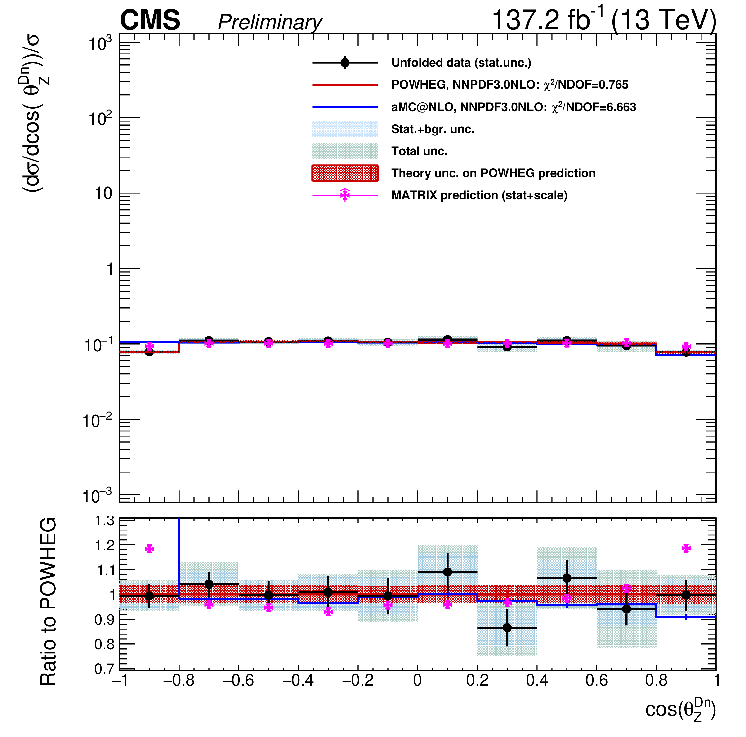
png pdf |
Figure 15-h:
Unfolding results using NNLO bias, area constraint, and no additional regularization term for several variables and charged final states. From top to bottom: ${p_{\mathrm {T}}}$ of the lepton in the W decay, cosine of the polarization angle of the W boson, and cosine of the polarization angle of the Z boson. From left to right: charge inclusive, positive charge, and negative charge final states. Black dots represent unfolded data results for which black bars denote statistical uncertainties, shaded blue bands represent statistical plus background related uncertainties and the green band represent the total unfolding uncertainty. The red histogram and shadow bands are the POWHEG prediction and its theoretical uncertainty. The blue histogram represents the MadGraph 5_aMC@NLO prediction and the violet points show the matrix prediction including error bands representing numerical and scale uncertainties. |
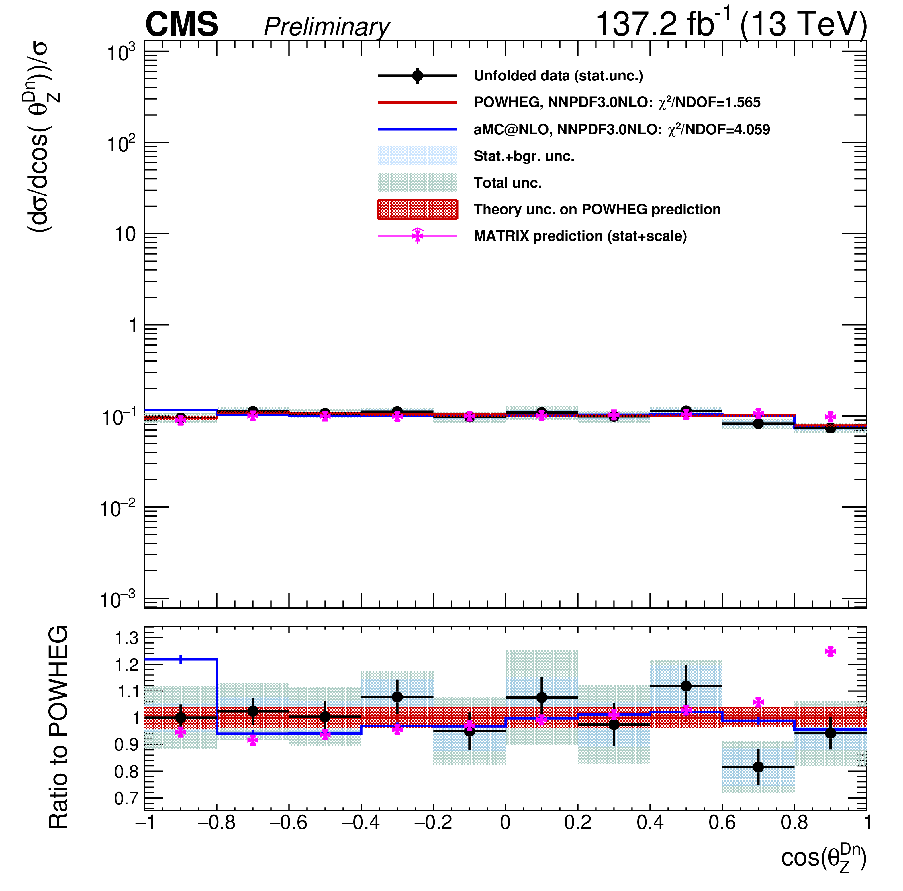
png pdf |
Figure 15-i:
Unfolding results using NNLO bias, area constraint, and no additional regularization term for several variables and charged final states. From top to bottom: ${p_{\mathrm {T}}}$ of the lepton in the W decay, cosine of the polarization angle of the W boson, and cosine of the polarization angle of the Z boson. From left to right: charge inclusive, positive charge, and negative charge final states. Black dots represent unfolded data results for which black bars denote statistical uncertainties, shaded blue bands represent statistical plus background related uncertainties and the green band represent the total unfolding uncertainty. The red histogram and shadow bands are the POWHEG prediction and its theoretical uncertainty. The blue histogram represents the MadGraph 5_aMC@NLO prediction and the violet points show the matrix prediction including error bands representing numerical and scale uncertainties. |
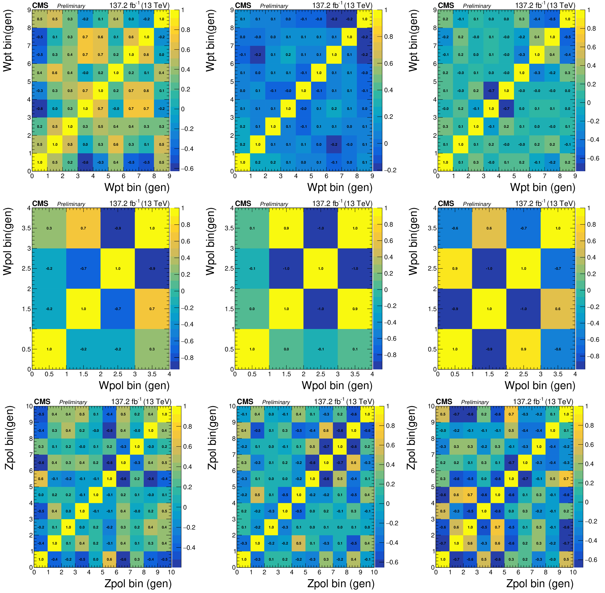
png pdf |
Figure 16:
Correlation matrices for the unfolded results using NNLO bias, area constraint, and no additional regularization term for several variables and charged final states. From top to bottom: ${p_{\mathrm {T}}}$ of the lepton in the W decay, cosine of the polarization angle of the W boson, and cosine of the polarization angle of the Z boson. From left to right: charge inclusive, positive charge, and negative charge final states. |
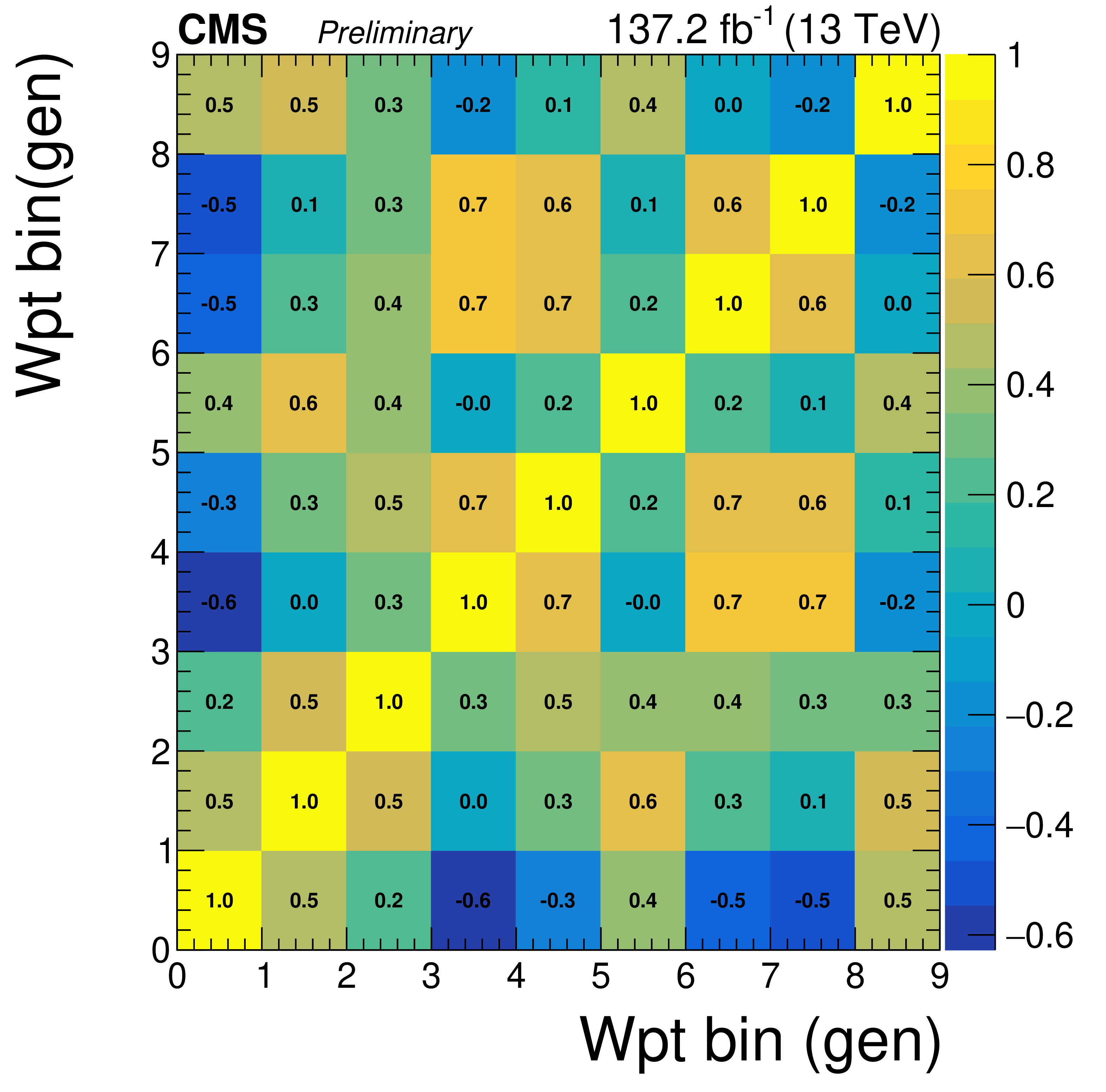
png pdf |
Figure 16-a:
Correlation matrices for the unfolded results using NNLO bias, area constraint, and no additional regularization term for several variables and charged final states. From top to bottom: ${p_{\mathrm {T}}}$ of the lepton in the W decay, cosine of the polarization angle of the W boson, and cosine of the polarization angle of the Z boson. From left to right: charge inclusive, positive charge, and negative charge final states. |
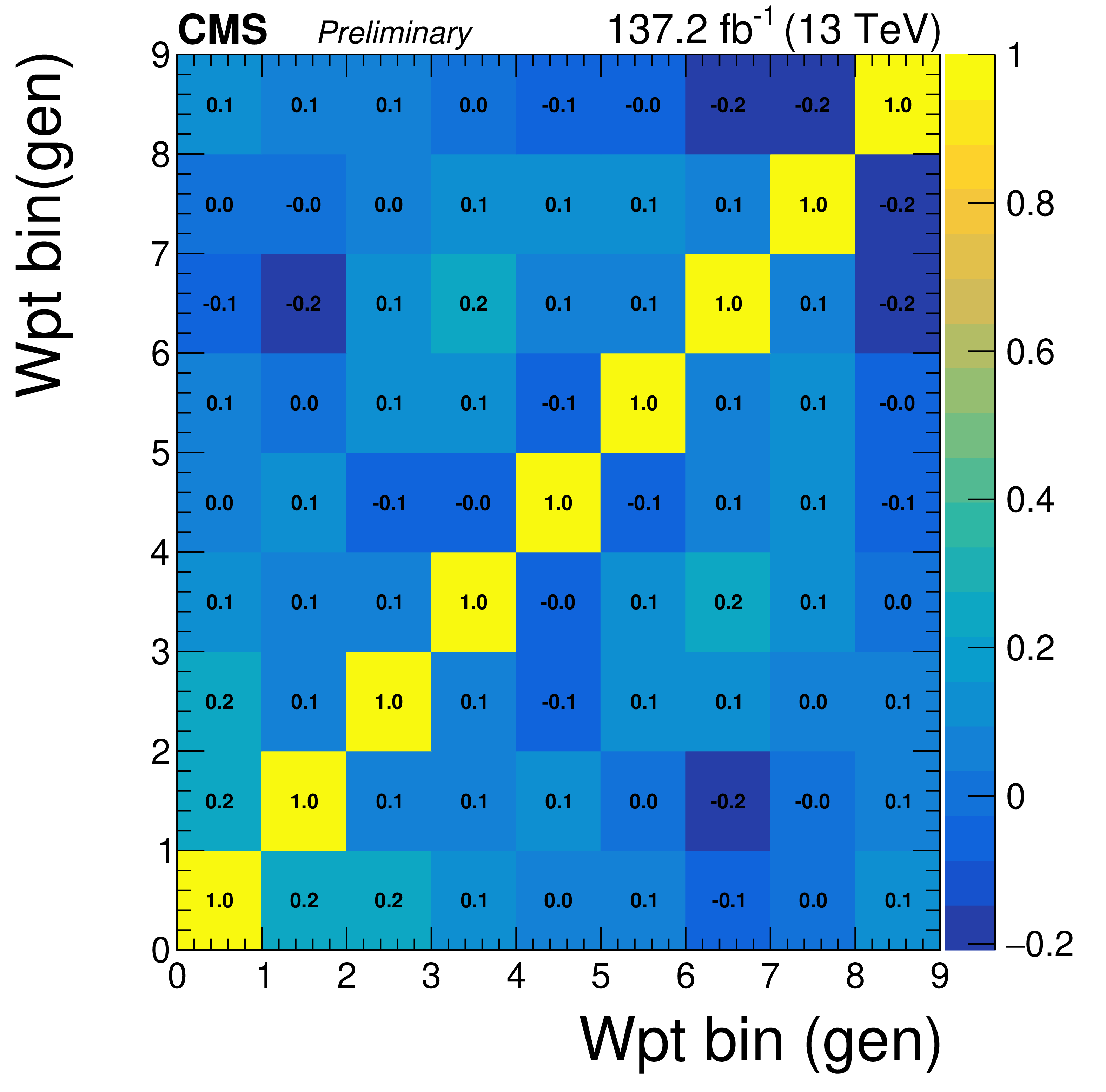
png pdf |
Figure 16-b:
Correlation matrices for the unfolded results using NNLO bias, area constraint, and no additional regularization term for several variables and charged final states. From top to bottom: ${p_{\mathrm {T}}}$ of the lepton in the W decay, cosine of the polarization angle of the W boson, and cosine of the polarization angle of the Z boson. From left to right: charge inclusive, positive charge, and negative charge final states. |
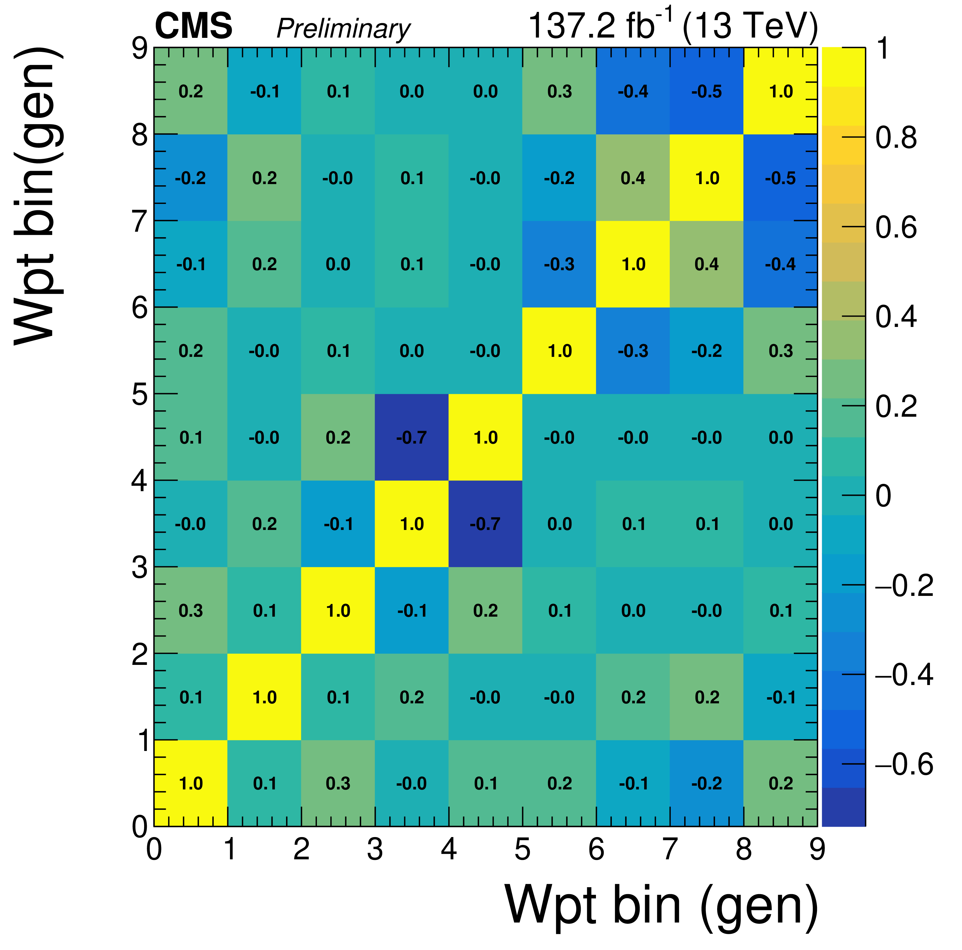
png pdf |
Figure 16-c:
Correlation matrices for the unfolded results using NNLO bias, area constraint, and no additional regularization term for several variables and charged final states. From top to bottom: ${p_{\mathrm {T}}}$ of the lepton in the W decay, cosine of the polarization angle of the W boson, and cosine of the polarization angle of the Z boson. From left to right: charge inclusive, positive charge, and negative charge final states. |
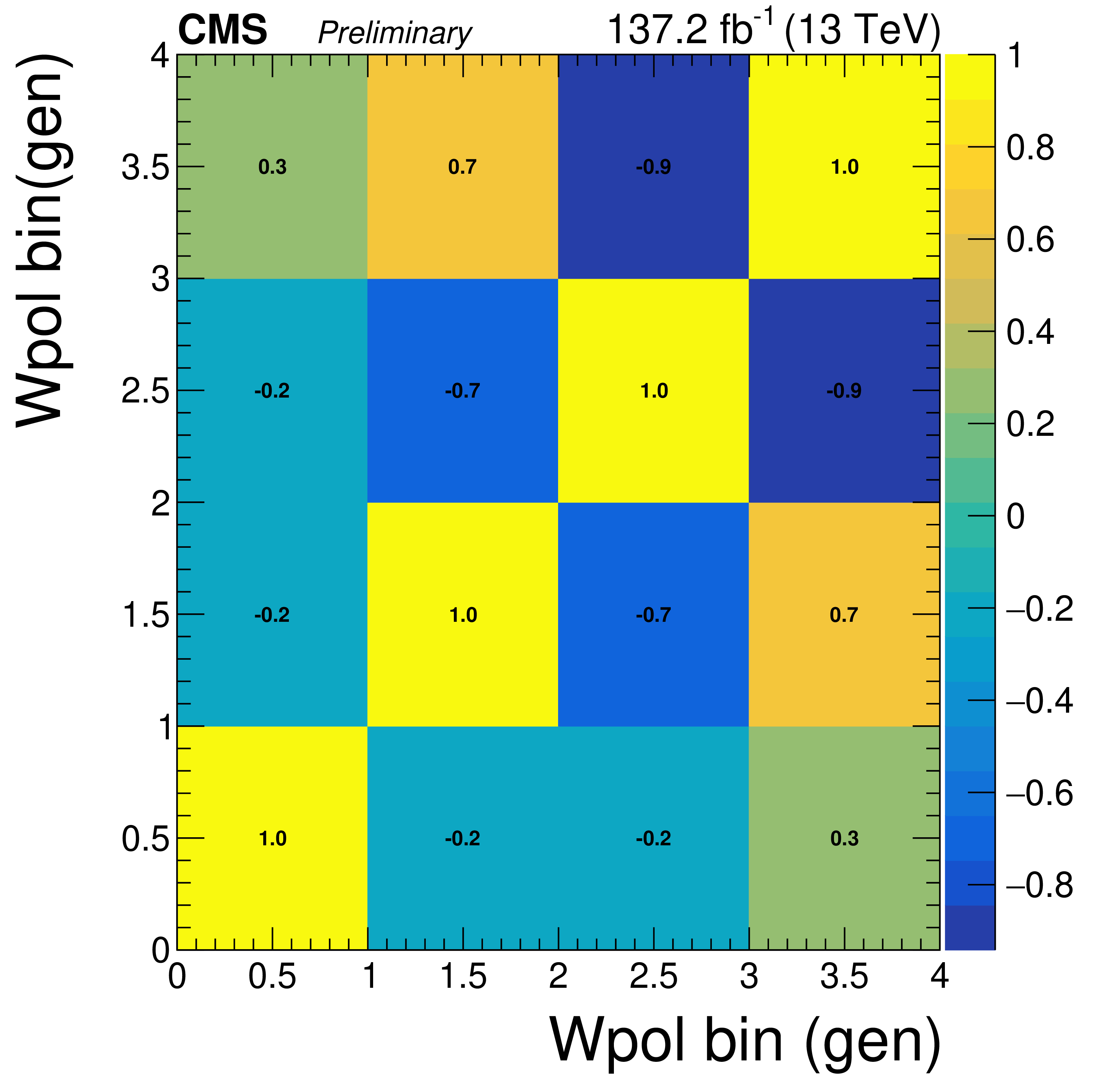
png pdf |
Figure 16-d:
Correlation matrices for the unfolded results using NNLO bias, area constraint, and no additional regularization term for several variables and charged final states. From top to bottom: ${p_{\mathrm {T}}}$ of the lepton in the W decay, cosine of the polarization angle of the W boson, and cosine of the polarization angle of the Z boson. From left to right: charge inclusive, positive charge, and negative charge final states. |
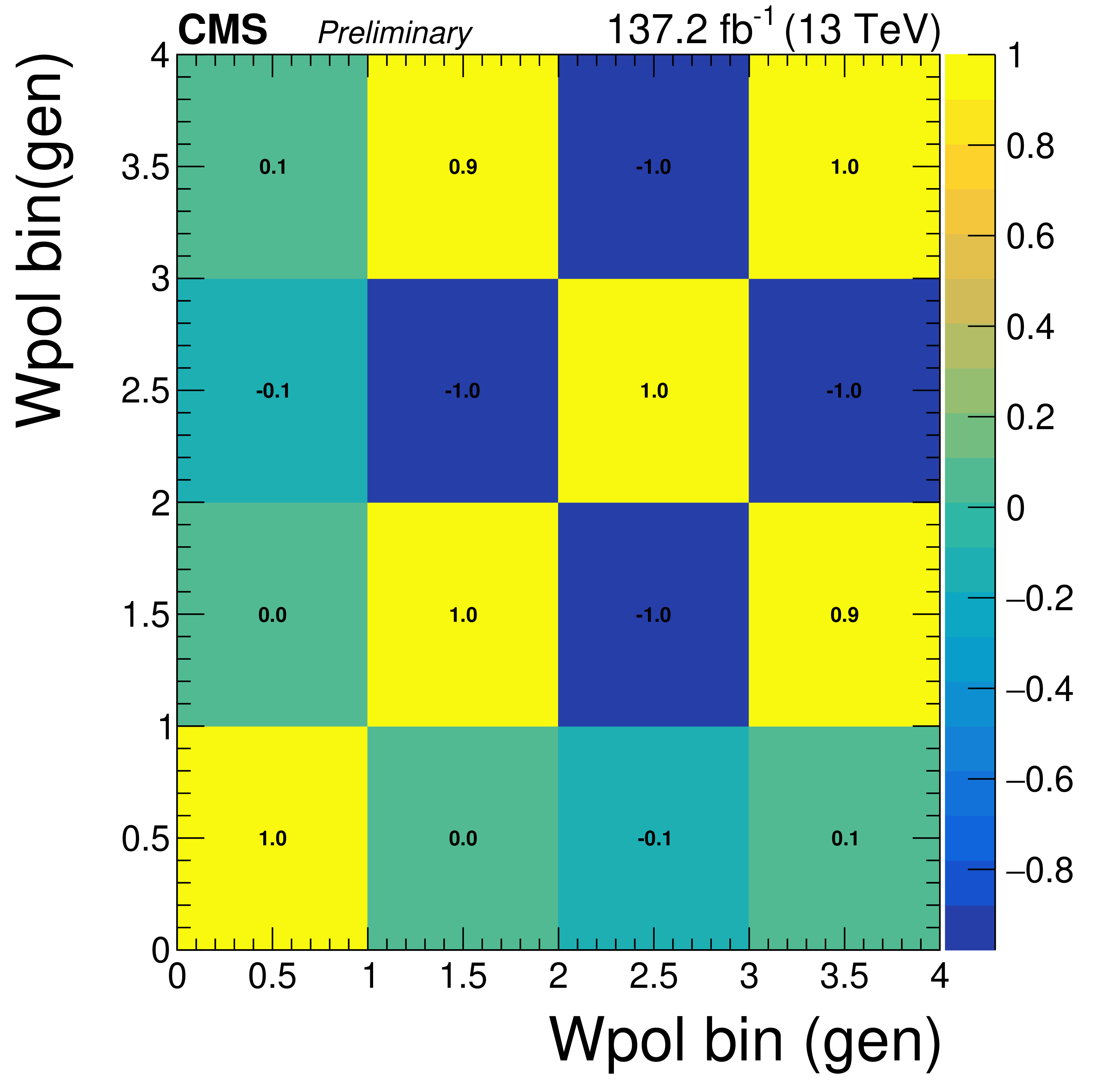
png pdf |
Figure 16-e:
Correlation matrices for the unfolded results using NNLO bias, area constraint, and no additional regularization term for several variables and charged final states. From top to bottom: ${p_{\mathrm {T}}}$ of the lepton in the W decay, cosine of the polarization angle of the W boson, and cosine of the polarization angle of the Z boson. From left to right: charge inclusive, positive charge, and negative charge final states. |

png pdf |
Figure 16-f:
Correlation matrices for the unfolded results using NNLO bias, area constraint, and no additional regularization term for several variables and charged final states. From top to bottom: ${p_{\mathrm {T}}}$ of the lepton in the W decay, cosine of the polarization angle of the W boson, and cosine of the polarization angle of the Z boson. From left to right: charge inclusive, positive charge, and negative charge final states. |

png pdf |
Figure 16-g:
Correlation matrices for the unfolded results using NNLO bias, area constraint, and no additional regularization term for several variables and charged final states. From top to bottom: ${p_{\mathrm {T}}}$ of the lepton in the W decay, cosine of the polarization angle of the W boson, and cosine of the polarization angle of the Z boson. From left to right: charge inclusive, positive charge, and negative charge final states. |
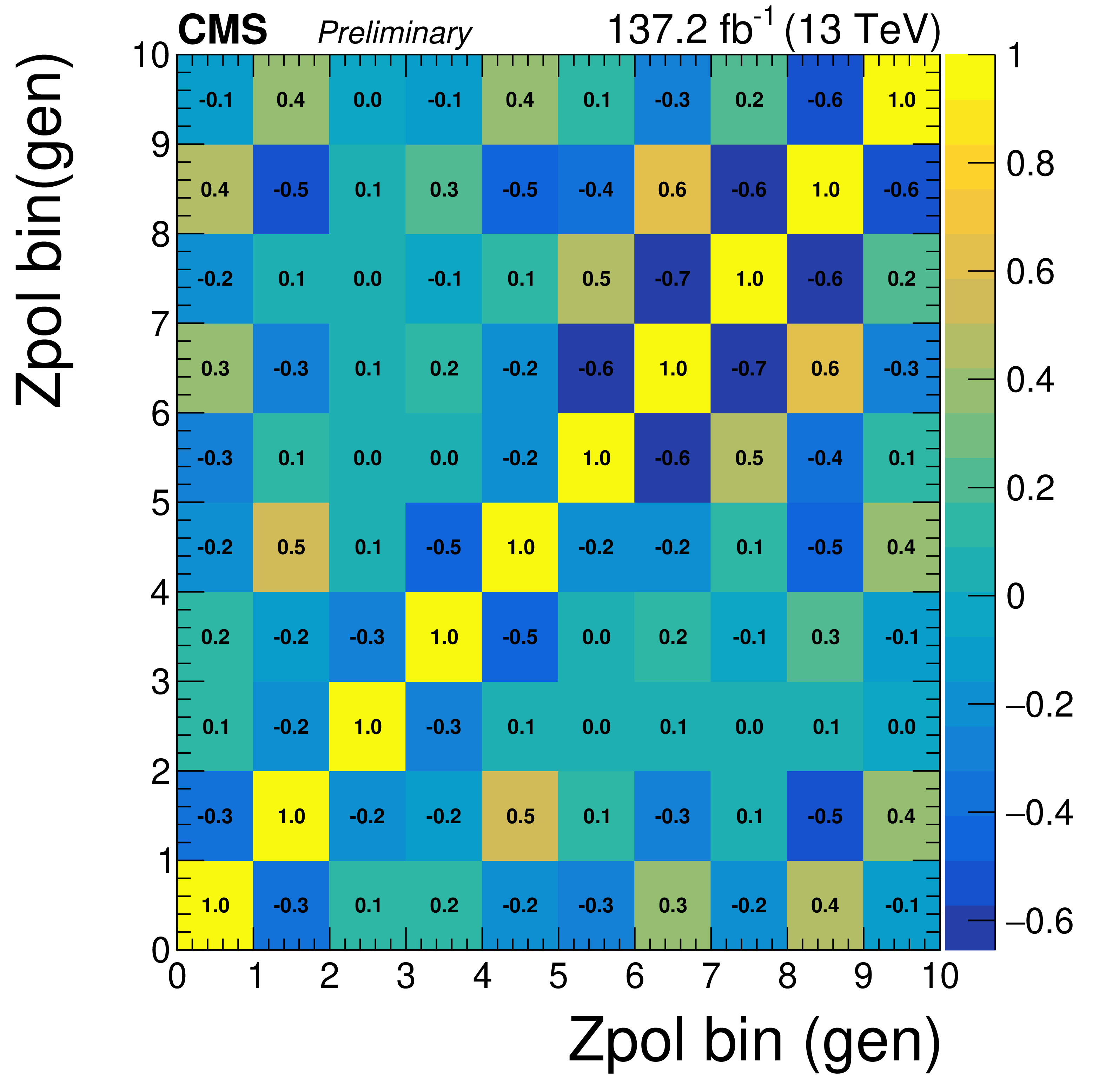
png pdf |
Figure 16-h:
Correlation matrices for the unfolded results using NNLO bias, area constraint, and no additional regularization term for several variables and charged final states. From top to bottom: ${p_{\mathrm {T}}}$ of the lepton in the W decay, cosine of the polarization angle of the W boson, and cosine of the polarization angle of the Z boson. From left to right: charge inclusive, positive charge, and negative charge final states. |
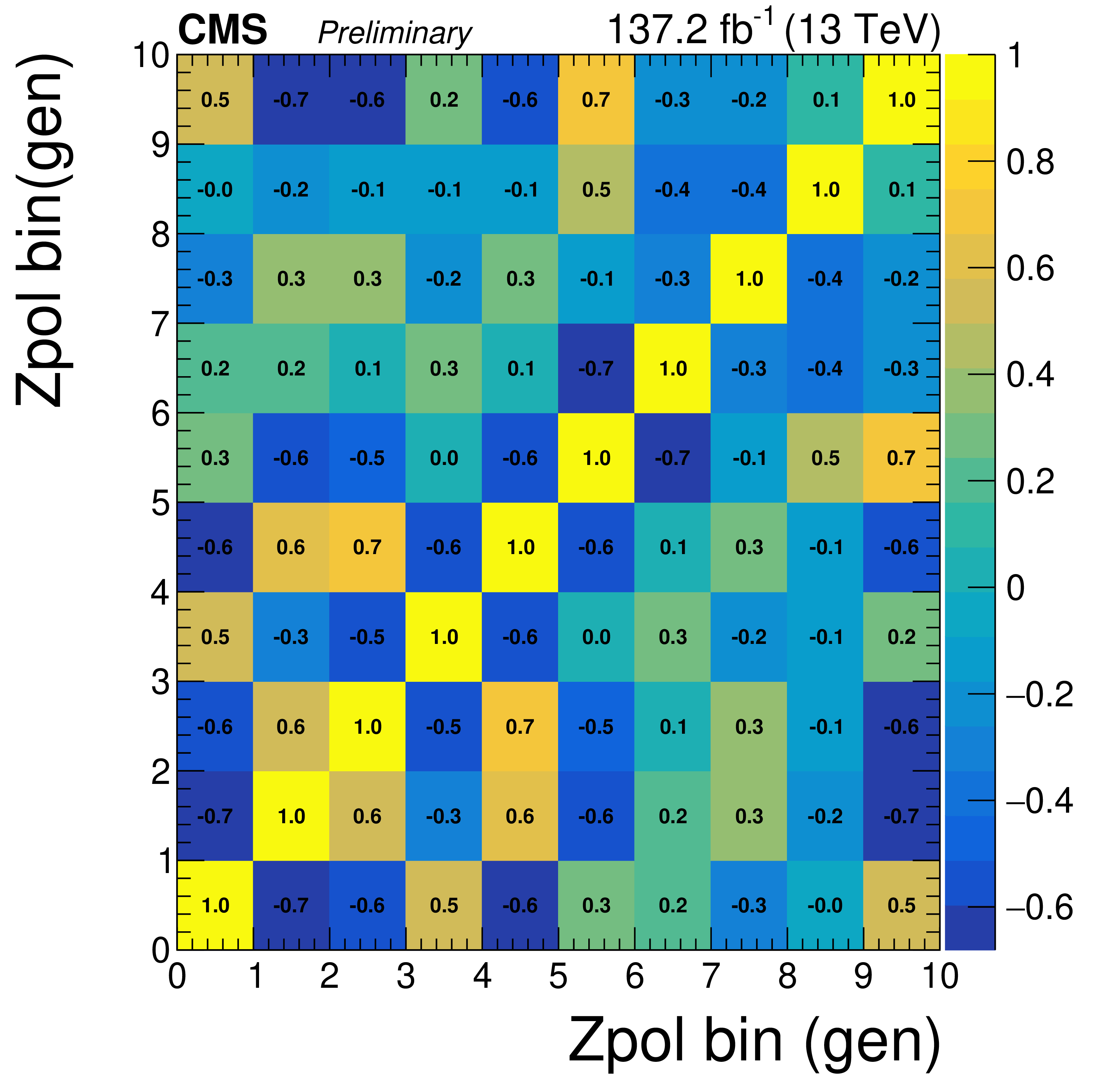
png pdf |
Figure 16-i:
Correlation matrices for the unfolded results using NNLO bias, area constraint, and no additional regularization term for several variables and charged final states. From top to bottom: ${p_{\mathrm {T}}}$ of the lepton in the W decay, cosine of the polarization angle of the W boson, and cosine of the polarization angle of the Z boson. From left to right: charge inclusive, positive charge, and negative charge final states. |
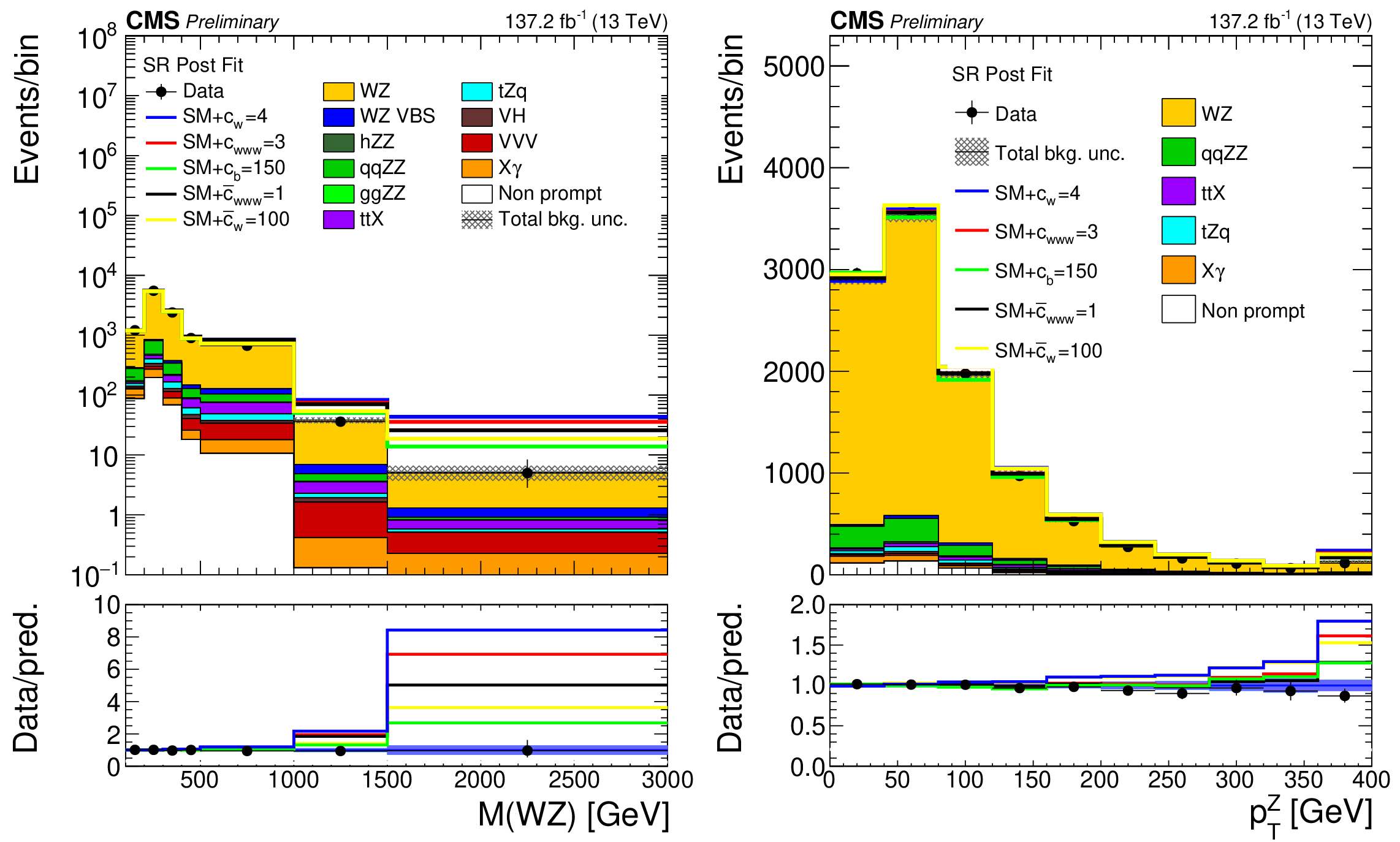
png pdf |
Figure 17:
Distribution of several observables in the SR comparing SM distributions and several possible configurations of EFT parameters after the fit to the SM-only model. From left to right: invariant mass of the WZ system assuming a neutrino with no longitudinal momentum (${M({\mathrm{W} \mathrm{Z}})}$), and transverse momentum of the reconstructed Z boson. The SM contribution is shown as the stacked filled histograms, while each of the individual coloured lines corresponds to the expected SM yields plus the contributions from a possible configuration of EFT parameter values. The ratio shows the quotient between the BSM contributions and the nominal SM yields. X$\gamma$ includes Z$\gamma$, W$\gamma$, tt$\gamma$ and WZ$\gamma$ production. The label ttX includes both ttZ, ttW and ttH production. The shaded band in the ratio corresponds to the total uncertainty in the SM yields. |
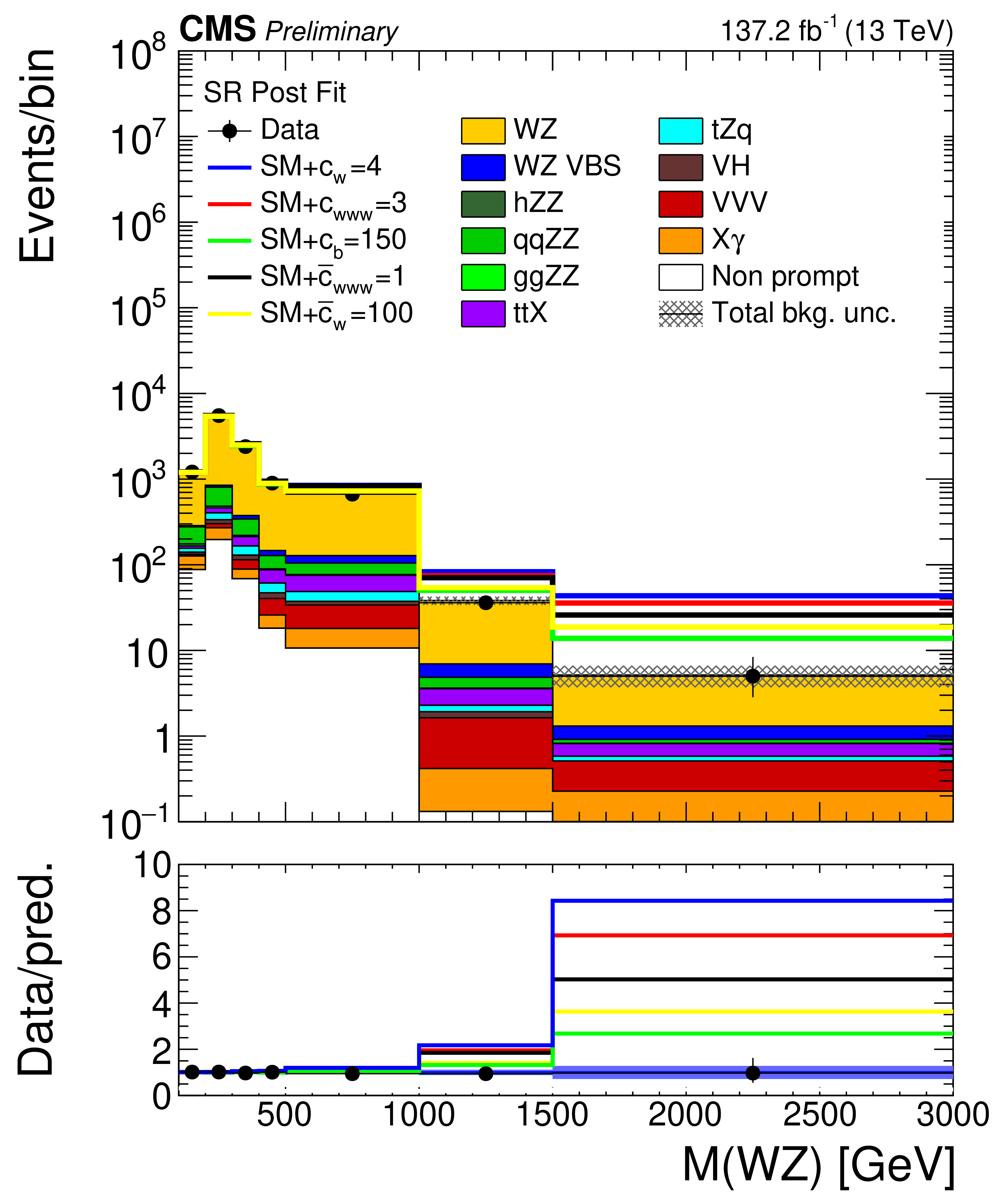
png pdf |
Figure 17-a:
Distribution of several observables in the SR comparing SM distributions and several possible configurations of EFT parameters after the fit to the SM-only model. From left to right: invariant mass of the WZ system assuming a neutrino with no longitudinal momentum (${M({\mathrm{W} \mathrm{Z}})}$), and transverse momentum of the reconstructed Z boson. The SM contribution is shown as the stacked filled histograms, while each of the individual coloured lines corresponds to the expected SM yields plus the contributions from a possible configuration of EFT parameter values. The ratio shows the quotient between the BSM contributions and the nominal SM yields. X$\gamma$ includes Z$\gamma$, W$\gamma$, tt$\gamma$ and WZ$\gamma$ production. The label ttX includes both ttZ, ttW and ttH production. The shaded band in the ratio corresponds to the total uncertainty in the SM yields. |
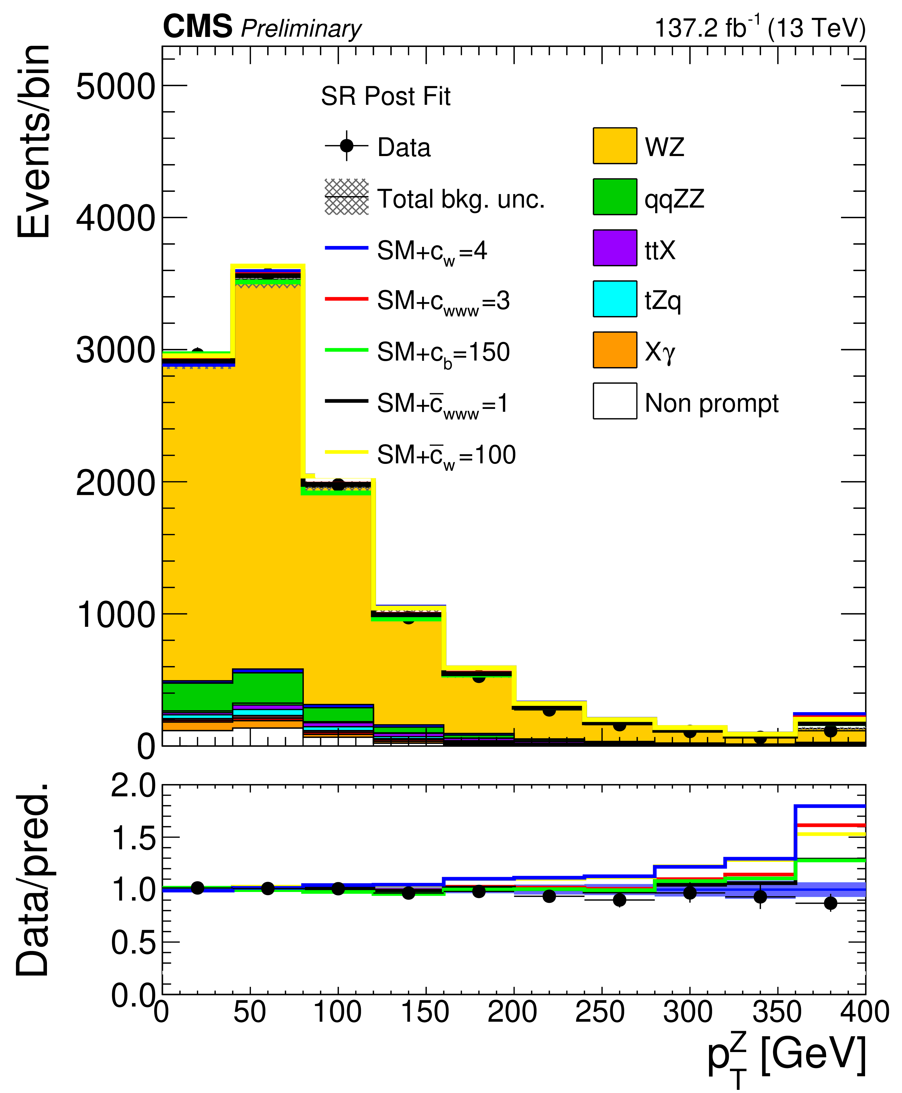
png pdf |
Figure 17-b:
Distribution of several observables in the SR comparing SM distributions and several possible configurations of EFT parameters after the fit to the SM-only model. From left to right: invariant mass of the WZ system assuming a neutrino with no longitudinal momentum (${M({\mathrm{W} \mathrm{Z}})}$), and transverse momentum of the reconstructed Z boson. The SM contribution is shown as the stacked filled histograms, while each of the individual coloured lines corresponds to the expected SM yields plus the contributions from a possible configuration of EFT parameter values. The ratio shows the quotient between the BSM contributions and the nominal SM yields. X$\gamma$ includes Z$\gamma$, W$\gamma$, tt$\gamma$ and WZ$\gamma$ production. The label ttX includes both ttZ, ttW and ttH production. The shaded band in the ratio corresponds to the total uncertainty in the SM yields. |
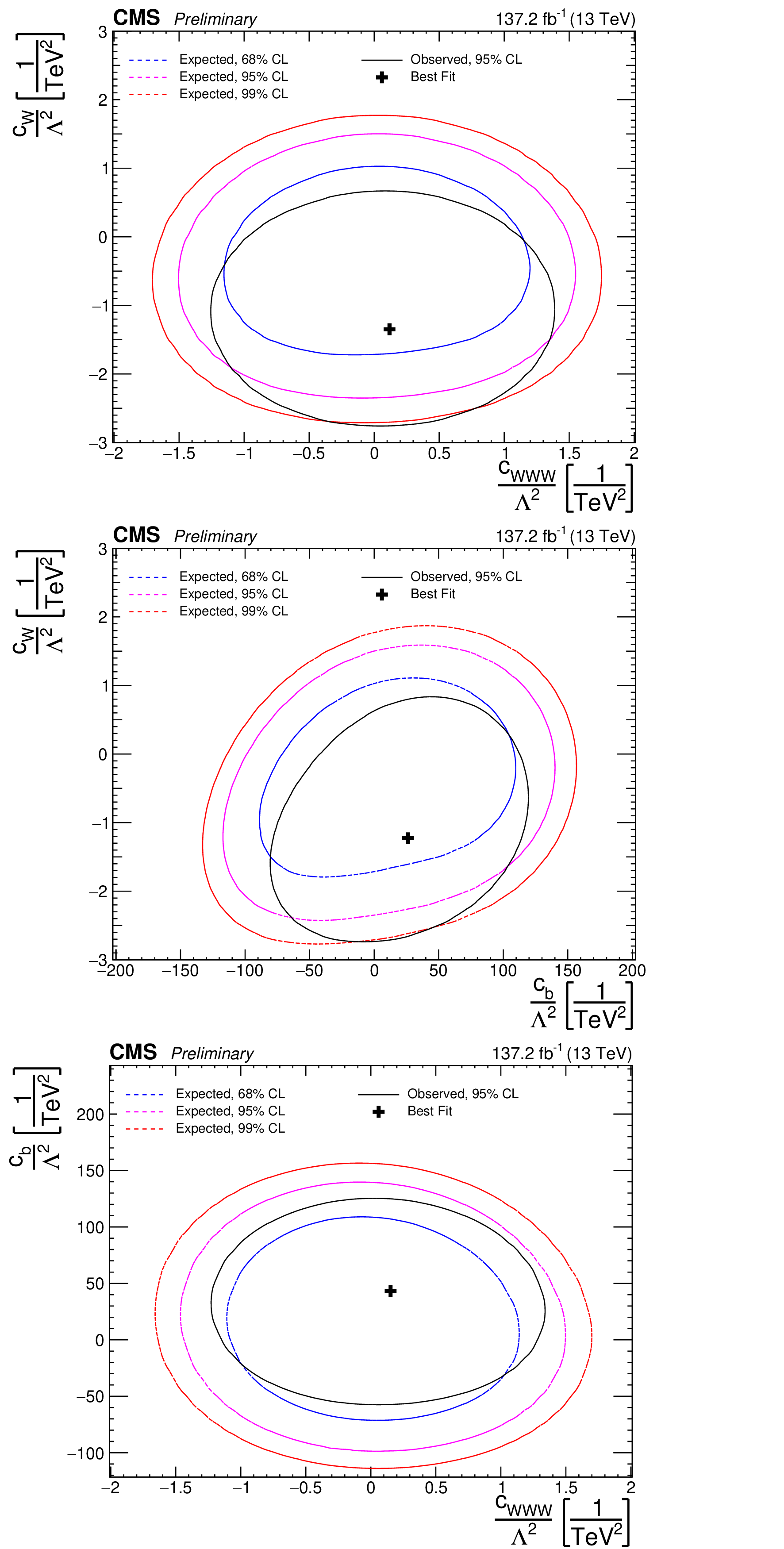
png pdf |
Figure 18:
Two-dimensional confidence regions for each of the possible combinations of the considered EFT parameters. The contours of the expected confidence regions for $68%$ and $95%$ confidence level are presented in each case. The parameters considered in each plot are $c_{\text {w}}/\Lambda ^2-c_{\text {www}}/\Lambda ^2$ (top), $c_{\text {w}}/\Lambda ^2-c_{\text {b}}/\Lambda ^2$ (middle), and $c_{\text {b}}/\Lambda ^2-c_{\text {www}}/\Lambda ^2$ (bottom). |
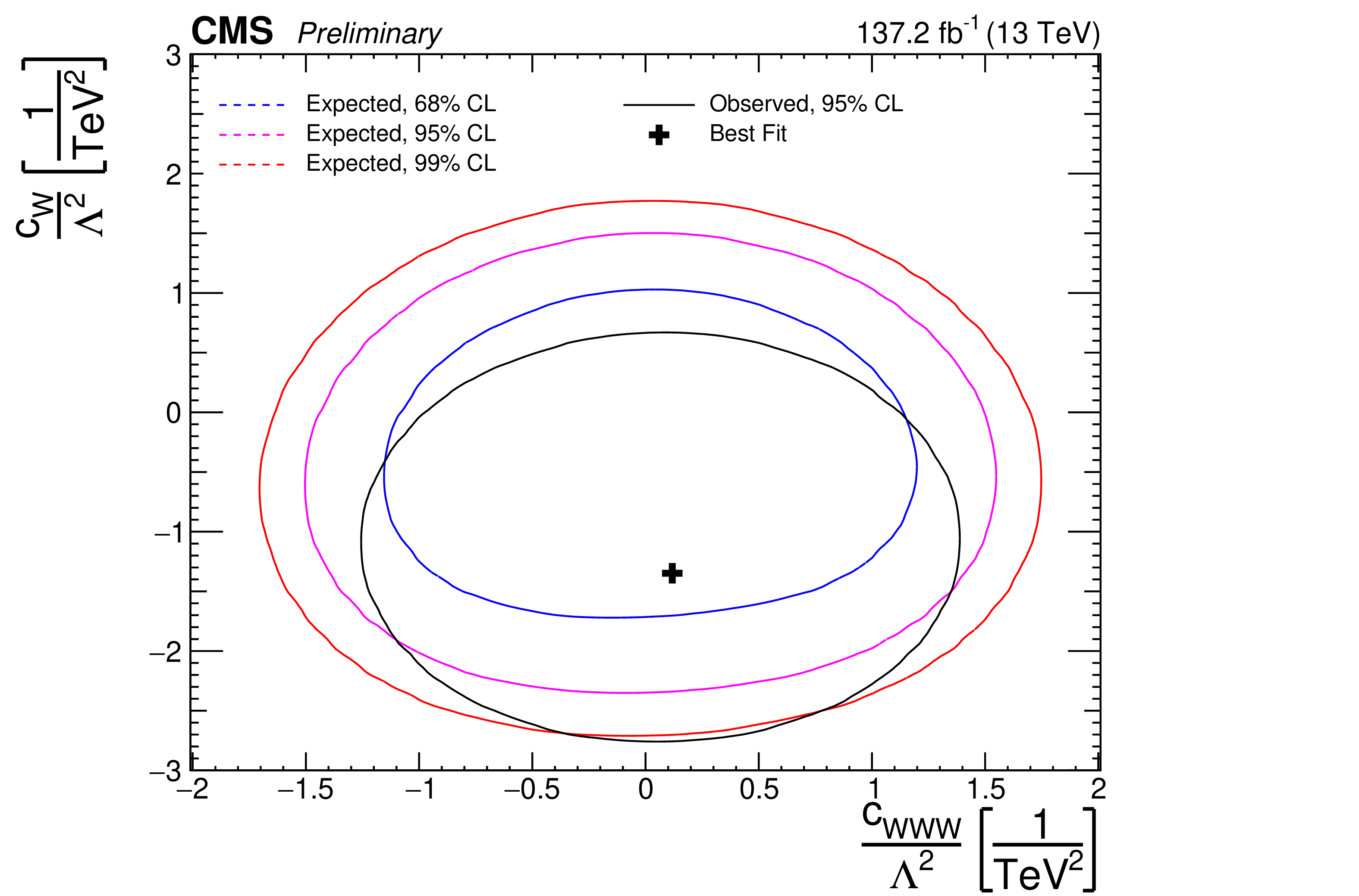
png pdf |
Figure 18-a:
Two-dimensional confidence regions for each of the possible combinations of the considered EFT parameters. The contours of the expected confidence regions for $68%$ and $95%$ confidence level are presented in each case. The parameters considered in each plot are $c_{\text {w}}/\Lambda ^2-c_{\text {www}}/\Lambda ^2$ (top), $c_{\text {w}}/\Lambda ^2-c_{\text {b}}/\Lambda ^2$ (middle), and $c_{\text {b}}/\Lambda ^2-c_{\text {www}}/\Lambda ^2$ (bottom). |
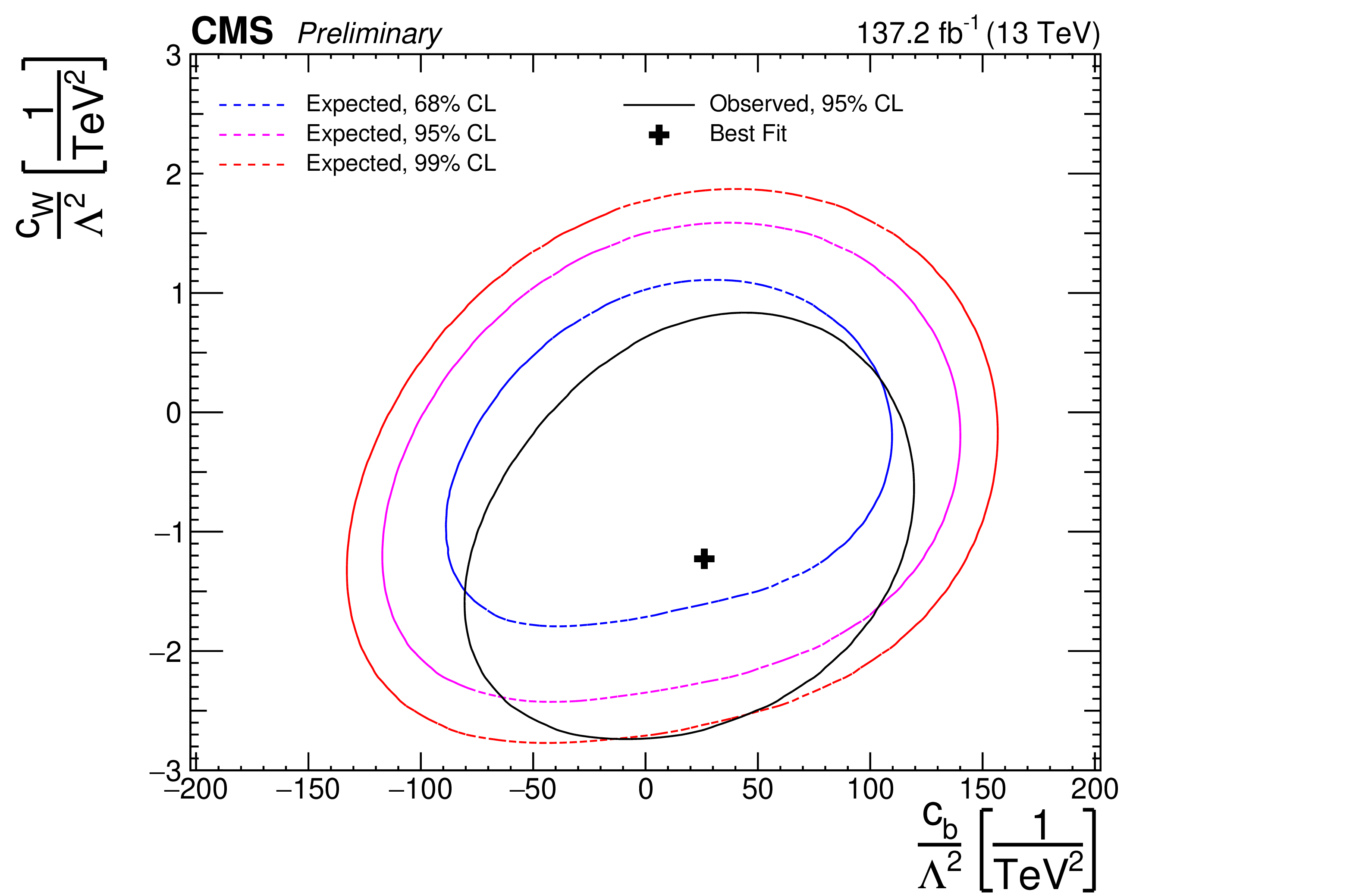
png pdf |
Figure 18-b:
Two-dimensional confidence regions for each of the possible combinations of the considered EFT parameters. The contours of the expected confidence regions for $68%$ and $95%$ confidence level are presented in each case. The parameters considered in each plot are $c_{\text {w}}/\Lambda ^2-c_{\text {www}}/\Lambda ^2$ (top), $c_{\text {w}}/\Lambda ^2-c_{\text {b}}/\Lambda ^2$ (middle), and $c_{\text {b}}/\Lambda ^2-c_{\text {www}}/\Lambda ^2$ (bottom). |
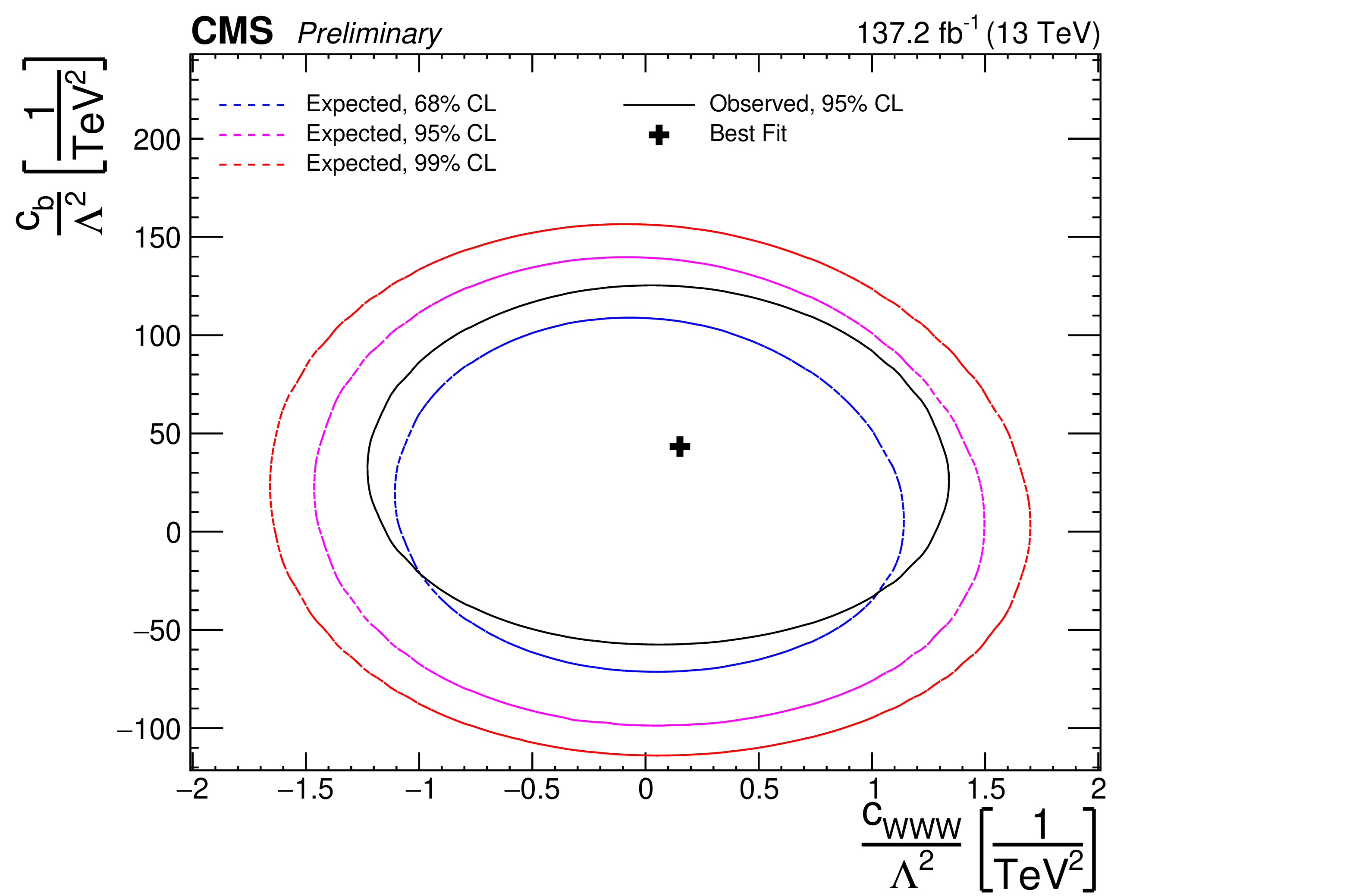
png pdf |
Figure 18-c:
Two-dimensional confidence regions for each of the possible combinations of the considered EFT parameters. The contours of the expected confidence regions for $68%$ and $95%$ confidence level are presented in each case. The parameters considered in each plot are $c_{\text {w}}/\Lambda ^2-c_{\text {www}}/\Lambda ^2$ (top), $c_{\text {w}}/\Lambda ^2-c_{\text {b}}/\Lambda ^2$ (middle), and $c_{\text {b}}/\Lambda ^2-c_{\text {www}}/\Lambda ^2$ (bottom). |

png pdf |
Figure 19:
Observed and expected evolution of the log likelihood of the best fit point as a function of each of the considered EFT parameters for both the linear (only interference between SM and BSM physics) and quadratic (both interference and purely BSM term) approaches to the EFT signal modelling. The parameter considered in each plot is: ${c_{\text {w}}}$/$\Lambda ^2$ (top left), ${c_{\text {b}}}$/$\Lambda ^2$ (top right), ${c_{\text {www}}}$/$\Lambda ^2$ (middle), ${\tilde{c}_{\text {www}}}$/$\Lambda ^2$ (bottom left), and ${\tilde{c}_{\text {w}}}$/$\Lambda ^2$ (bottom right). Very low sensitivity to the interference only term corresponding to ${\tilde{c}_{\text {w}}}$/$\Lambda ^2$ is observed so the corresponding curve is not shown into the plot. |
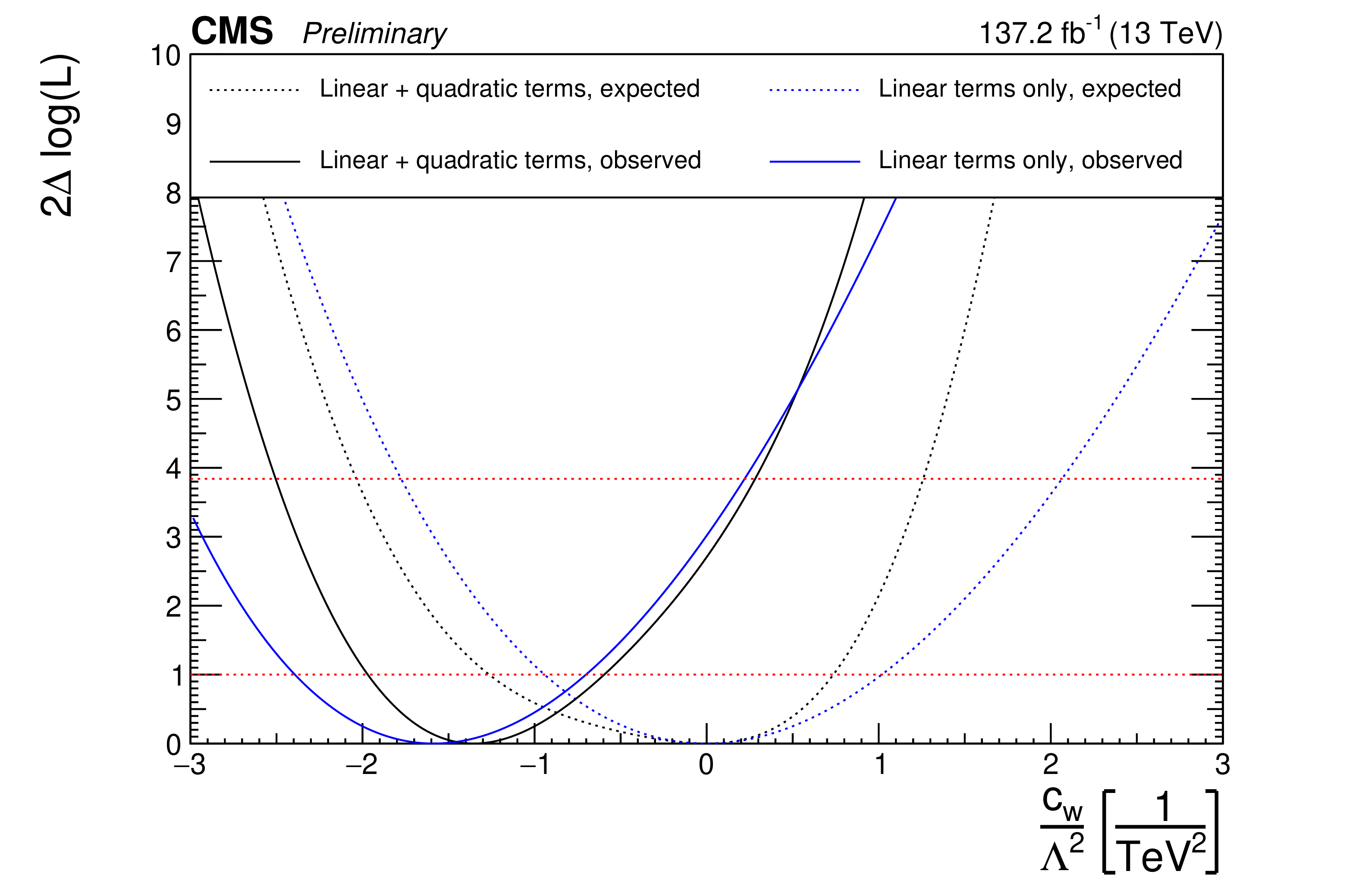
png pdf |
Figure 19-a:
Observed and expected evolution of the log likelihood of the best fit point as a function of each of the considered EFT parameters for both the linear (only interference between SM and BSM physics) and quadratic (both interference and purely BSM term) approaches to the EFT signal modelling. The parameter considered in each plot is: ${c_{\text {w}}}$/$\Lambda ^2$ (top left), ${c_{\text {b}}}$/$\Lambda ^2$ (top right), ${c_{\text {www}}}$/$\Lambda ^2$ (middle), ${\tilde{c}_{\text {www}}}$/$\Lambda ^2$ (bottom left), and ${\tilde{c}_{\text {w}}}$/$\Lambda ^2$ (bottom right). Very low sensitivity to the interference only term corresponding to ${\tilde{c}_{\text {w}}}$/$\Lambda ^2$ is observed so the corresponding curve is not shown into the plot. |
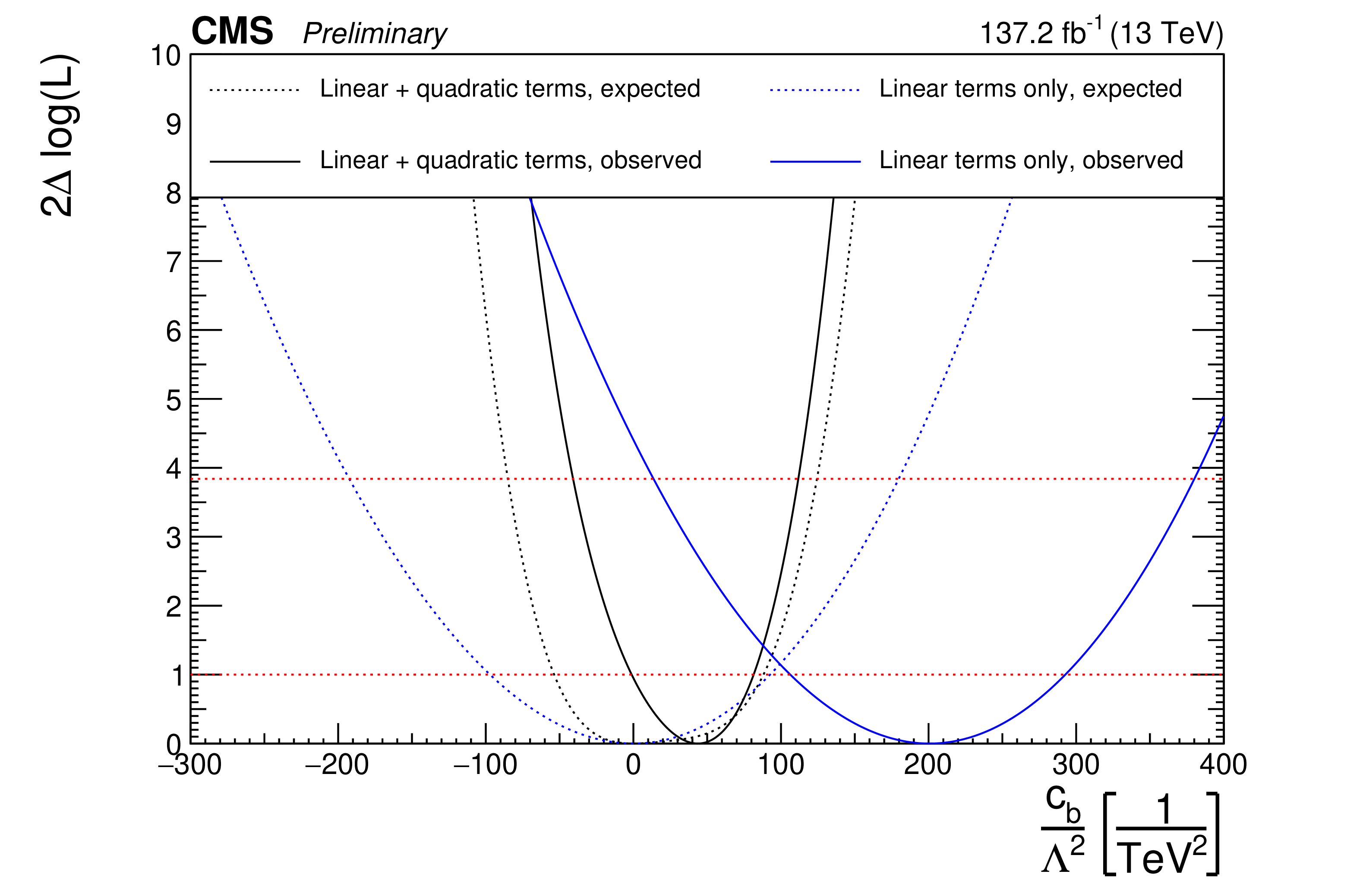
png pdf |
Figure 19-b:
Observed and expected evolution of the log likelihood of the best fit point as a function of each of the considered EFT parameters for both the linear (only interference between SM and BSM physics) and quadratic (both interference and purely BSM term) approaches to the EFT signal modelling. The parameter considered in each plot is: ${c_{\text {w}}}$/$\Lambda ^2$ (top left), ${c_{\text {b}}}$/$\Lambda ^2$ (top right), ${c_{\text {www}}}$/$\Lambda ^2$ (middle), ${\tilde{c}_{\text {www}}}$/$\Lambda ^2$ (bottom left), and ${\tilde{c}_{\text {w}}}$/$\Lambda ^2$ (bottom right). Very low sensitivity to the interference only term corresponding to ${\tilde{c}_{\text {w}}}$/$\Lambda ^2$ is observed so the corresponding curve is not shown into the plot. |
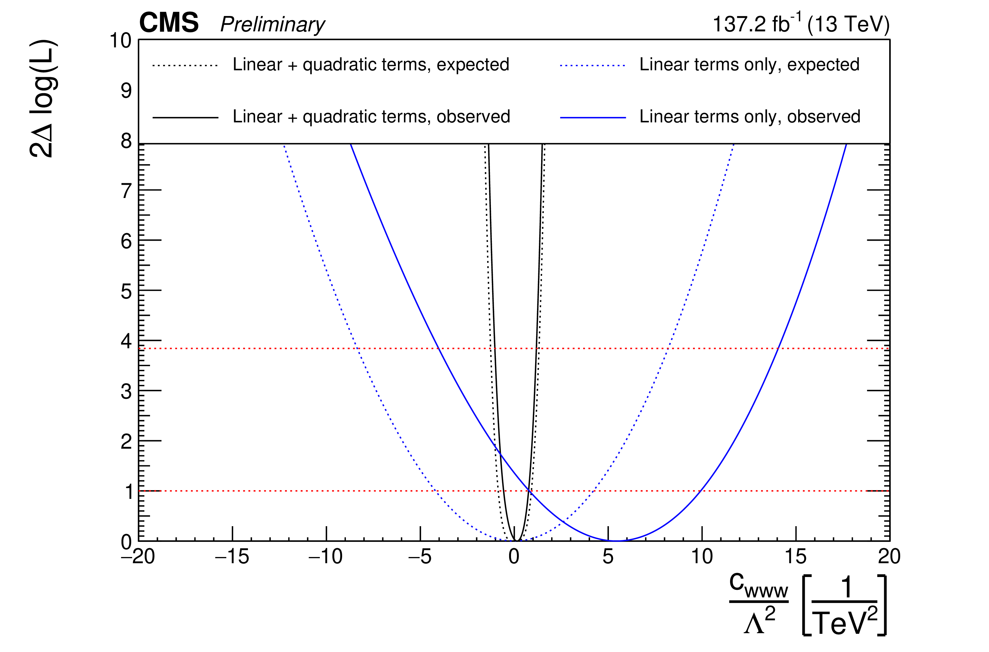
png pdf |
Figure 19-c:
Observed and expected evolution of the log likelihood of the best fit point as a function of each of the considered EFT parameters for both the linear (only interference between SM and BSM physics) and quadratic (both interference and purely BSM term) approaches to the EFT signal modelling. The parameter considered in each plot is: ${c_{\text {w}}}$/$\Lambda ^2$ (top left), ${c_{\text {b}}}$/$\Lambda ^2$ (top right), ${c_{\text {www}}}$/$\Lambda ^2$ (middle), ${\tilde{c}_{\text {www}}}$/$\Lambda ^2$ (bottom left), and ${\tilde{c}_{\text {w}}}$/$\Lambda ^2$ (bottom right). Very low sensitivity to the interference only term corresponding to ${\tilde{c}_{\text {w}}}$/$\Lambda ^2$ is observed so the corresponding curve is not shown into the plot. |
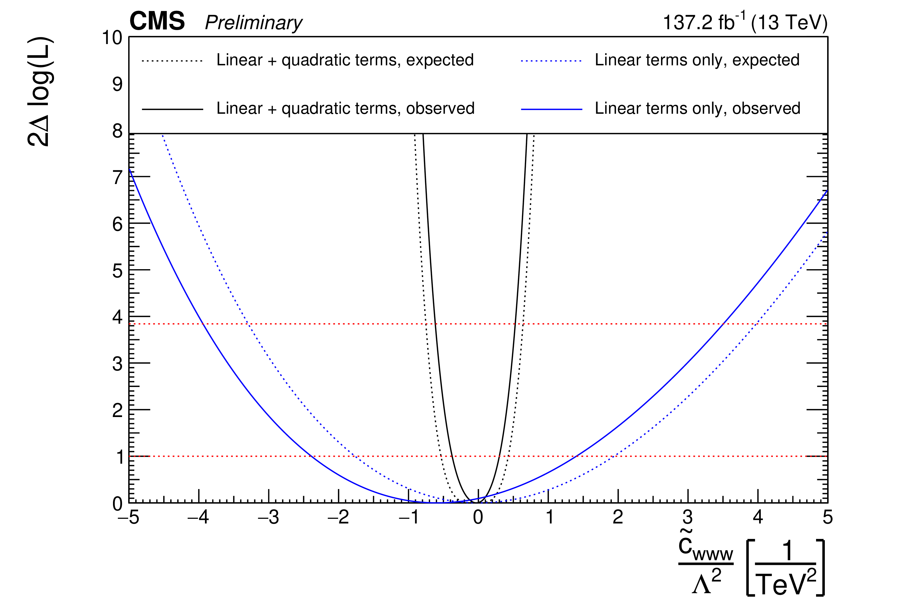
png pdf |
Figure 19-d:
Observed and expected evolution of the log likelihood of the best fit point as a function of each of the considered EFT parameters for both the linear (only interference between SM and BSM physics) and quadratic (both interference and purely BSM term) approaches to the EFT signal modelling. The parameter considered in each plot is: ${c_{\text {w}}}$/$\Lambda ^2$ (top left), ${c_{\text {b}}}$/$\Lambda ^2$ (top right), ${c_{\text {www}}}$/$\Lambda ^2$ (middle), ${\tilde{c}_{\text {www}}}$/$\Lambda ^2$ (bottom left), and ${\tilde{c}_{\text {w}}}$/$\Lambda ^2$ (bottom right). Very low sensitivity to the interference only term corresponding to ${\tilde{c}_{\text {w}}}$/$\Lambda ^2$ is observed so the corresponding curve is not shown into the plot. |
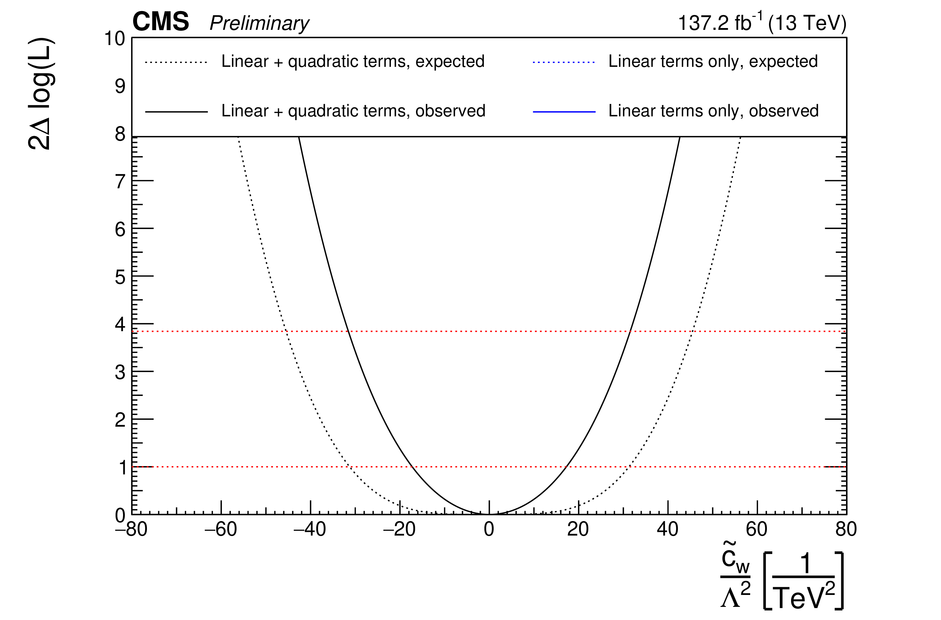
png pdf |
Figure 19-e:
Observed and expected evolution of the log likelihood of the best fit point as a function of each of the considered EFT parameters for both the linear (only interference between SM and BSM physics) and quadratic (both interference and purely BSM term) approaches to the EFT signal modelling. The parameter considered in each plot is: ${c_{\text {w}}}$/$\Lambda ^2$ (top left), ${c_{\text {b}}}$/$\Lambda ^2$ (top right), ${c_{\text {www}}}$/$\Lambda ^2$ (middle), ${\tilde{c}_{\text {www}}}$/$\Lambda ^2$ (bottom left), and ${\tilde{c}_{\text {w}}}$/$\Lambda ^2$ (bottom right). Very low sensitivity to the interference only term corresponding to ${\tilde{c}_{\text {w}}}$/$\Lambda ^2$ is observed so the corresponding curve is not shown into the plot. |
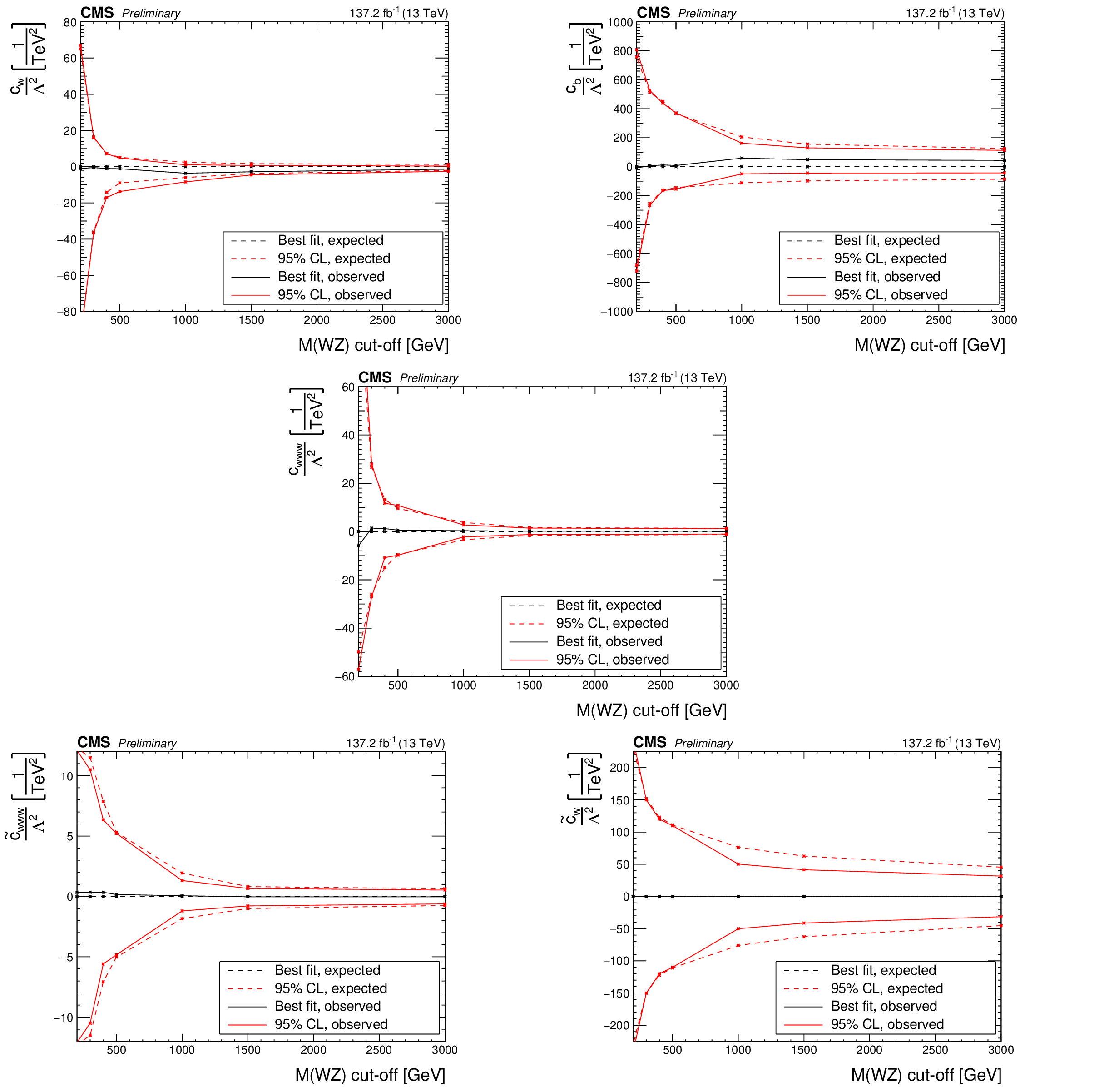
png pdf |
Figure 20:
Evolution of the expected confidence intervals in the EFT anomalous coupling parameters in terms of the cutoff scale given by different restrictions in the $M_{\mathrm{W} \mathrm{Z}}$ variable. For each point and parameter, the confidence intervals are computed imposing the additional restriction of no anomalous coupling contribution on top of SM prediction over the given value of $M_{\mathrm{W} \mathrm{Z}}$. Due to the statistical limitations in our simulation the last point is equivalent to no cut-off requirement being imposed. The parameter considered in each plot is: ${c_{\text {w}}}$/$\Lambda ^2$ (top left), ${c_{\text {b}}}$/$\Lambda ^2$ (top right), ${c_{\text {www}}}$/$\Lambda ^2$ (middle), ${\tilde{c}_{\text {www}}}$/$\Lambda ^2$ (bottom left), and ${\tilde{c}_{\text {w}}}$/$\Lambda ^2$ (bottom right). |
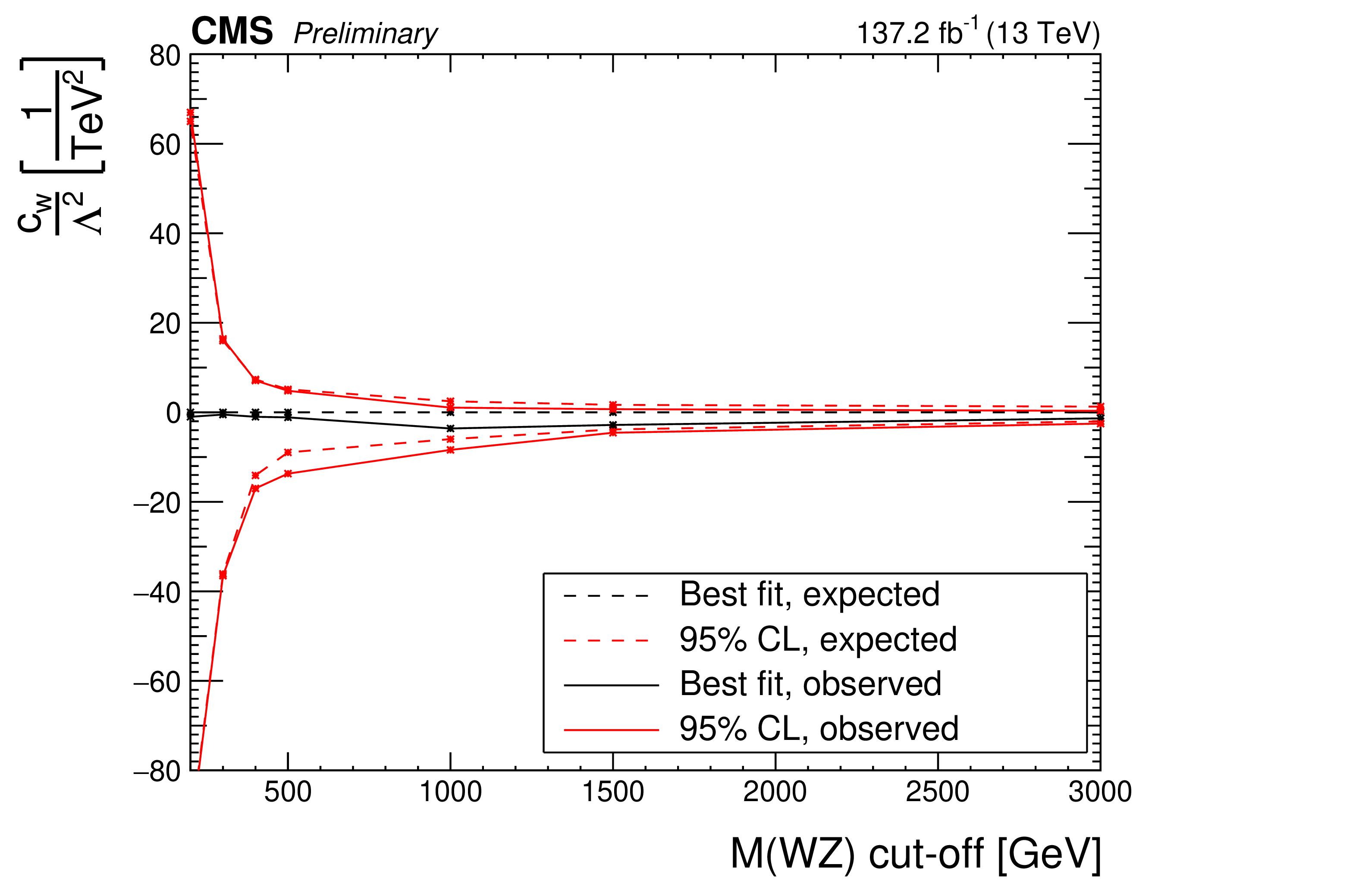
png pdf |
Figure 20-a:
Evolution of the expected confidence intervals in the EFT anomalous coupling parameters in terms of the cutoff scale given by different restrictions in the $M_{\mathrm{W} \mathrm{Z}}$ variable. For each point and parameter, the confidence intervals are computed imposing the additional restriction of no anomalous coupling contribution on top of SM prediction over the given value of $M_{\mathrm{W} \mathrm{Z}}$. Due to the statistical limitations in our simulation the last point is equivalent to no cut-off requirement being imposed. The parameter considered in each plot is: ${c_{\text {w}}}$/$\Lambda ^2$ (top left), ${c_{\text {b}}}$/$\Lambda ^2$ (top right), ${c_{\text {www}}}$/$\Lambda ^2$ (middle), ${\tilde{c}_{\text {www}}}$/$\Lambda ^2$ (bottom left), and ${\tilde{c}_{\text {w}}}$/$\Lambda ^2$ (bottom right). |
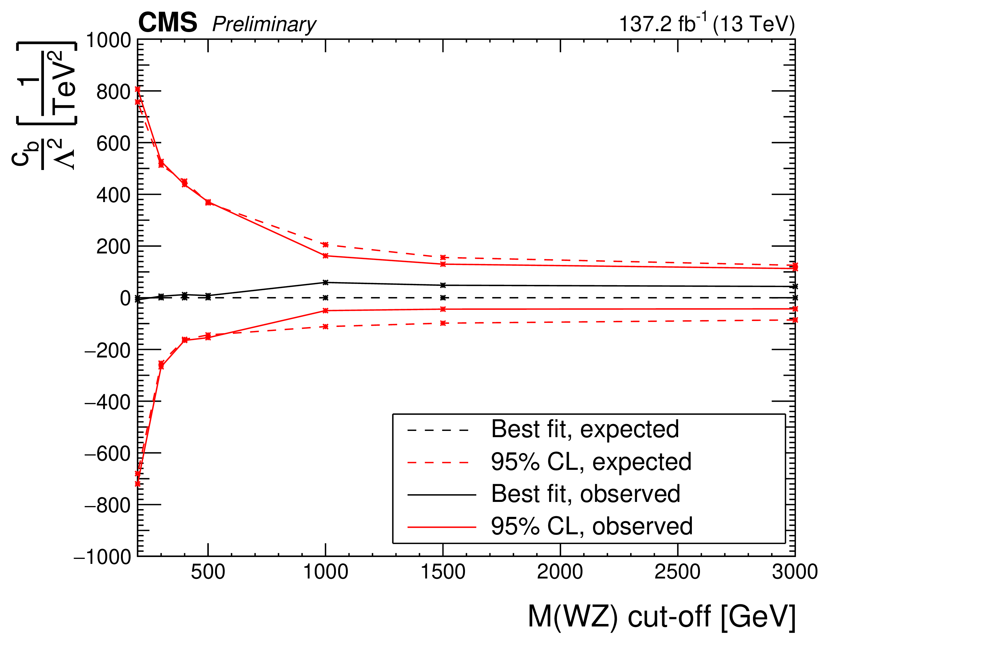
png pdf |
Figure 20-b:
Evolution of the expected confidence intervals in the EFT anomalous coupling parameters in terms of the cutoff scale given by different restrictions in the $M_{\mathrm{W} \mathrm{Z}}$ variable. For each point and parameter, the confidence intervals are computed imposing the additional restriction of no anomalous coupling contribution on top of SM prediction over the given value of $M_{\mathrm{W} \mathrm{Z}}$. Due to the statistical limitations in our simulation the last point is equivalent to no cut-off requirement being imposed. The parameter considered in each plot is: ${c_{\text {w}}}$/$\Lambda ^2$ (top left), ${c_{\text {b}}}$/$\Lambda ^2$ (top right), ${c_{\text {www}}}$/$\Lambda ^2$ (middle), ${\tilde{c}_{\text {www}}}$/$\Lambda ^2$ (bottom left), and ${\tilde{c}_{\text {w}}}$/$\Lambda ^2$ (bottom right). |
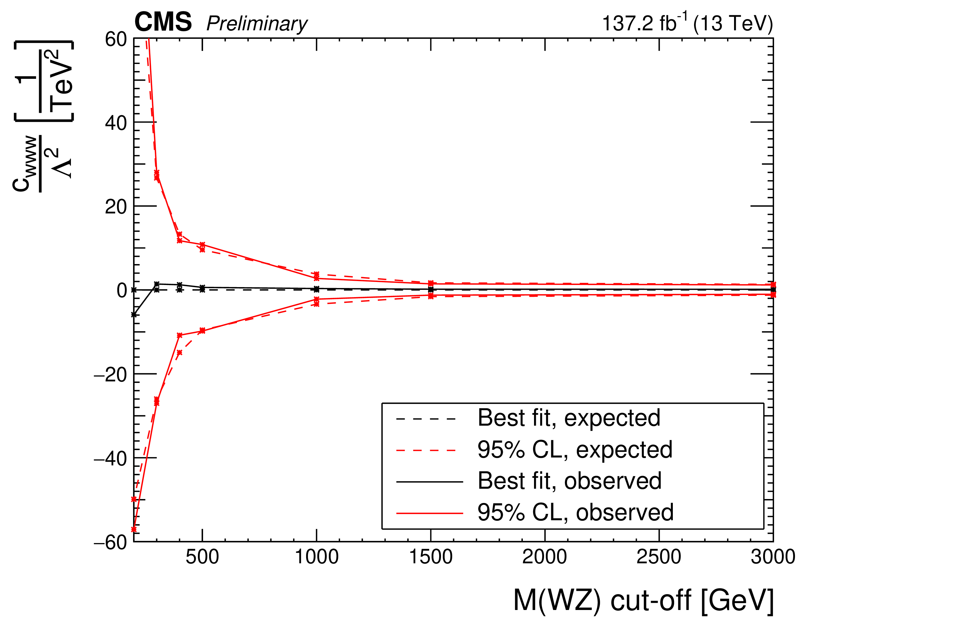
png pdf |
Figure 20-c:
Evolution of the expected confidence intervals in the EFT anomalous coupling parameters in terms of the cutoff scale given by different restrictions in the $M_{\mathrm{W} \mathrm{Z}}$ variable. For each point and parameter, the confidence intervals are computed imposing the additional restriction of no anomalous coupling contribution on top of SM prediction over the given value of $M_{\mathrm{W} \mathrm{Z}}$. Due to the statistical limitations in our simulation the last point is equivalent to no cut-off requirement being imposed. The parameter considered in each plot is: ${c_{\text {w}}}$/$\Lambda ^2$ (top left), ${c_{\text {b}}}$/$\Lambda ^2$ (top right), ${c_{\text {www}}}$/$\Lambda ^2$ (middle), ${\tilde{c}_{\text {www}}}$/$\Lambda ^2$ (bottom left), and ${\tilde{c}_{\text {w}}}$/$\Lambda ^2$ (bottom right). |
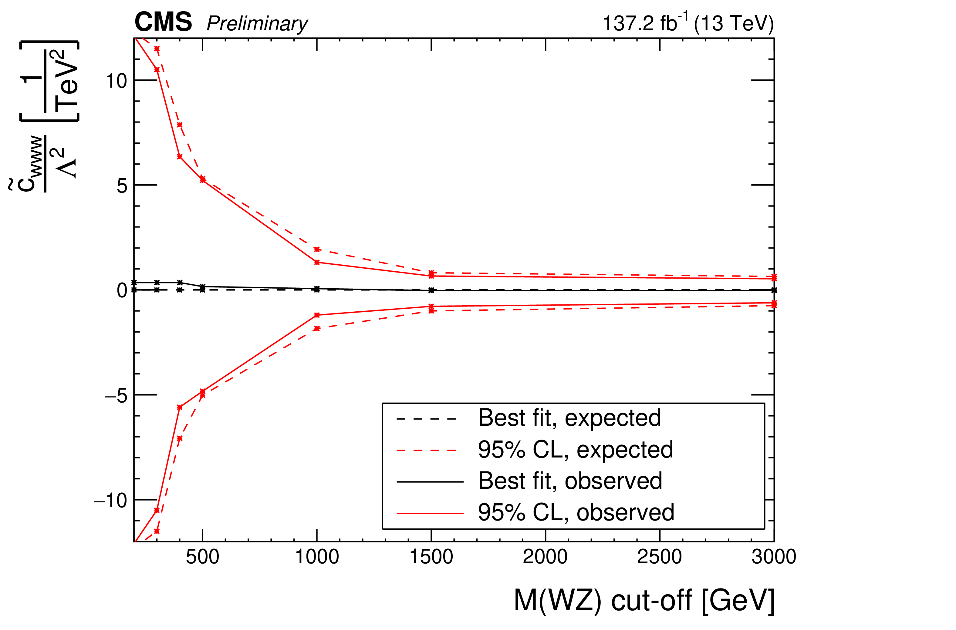
png pdf |
Figure 20-d:
Evolution of the expected confidence intervals in the EFT anomalous coupling parameters in terms of the cutoff scale given by different restrictions in the $M_{\mathrm{W} \mathrm{Z}}$ variable. For each point and parameter, the confidence intervals are computed imposing the additional restriction of no anomalous coupling contribution on top of SM prediction over the given value of $M_{\mathrm{W} \mathrm{Z}}$. Due to the statistical limitations in our simulation the last point is equivalent to no cut-off requirement being imposed. The parameter considered in each plot is: ${c_{\text {w}}}$/$\Lambda ^2$ (top left), ${c_{\text {b}}}$/$\Lambda ^2$ (top right), ${c_{\text {www}}}$/$\Lambda ^2$ (middle), ${\tilde{c}_{\text {www}}}$/$\Lambda ^2$ (bottom left), and ${\tilde{c}_{\text {w}}}$/$\Lambda ^2$ (bottom right). |
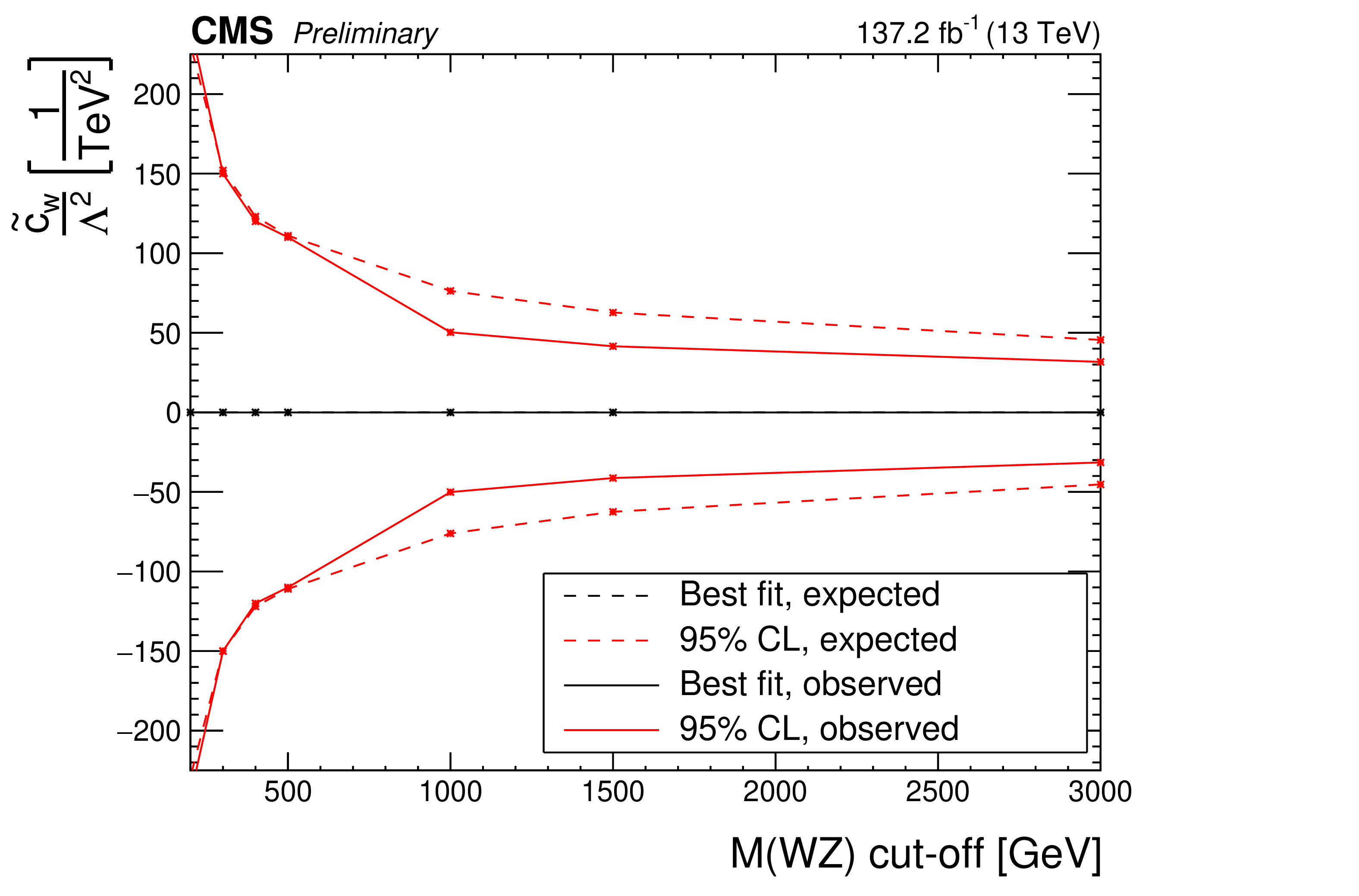
png pdf |
Figure 20-e:
Evolution of the expected confidence intervals in the EFT anomalous coupling parameters in terms of the cutoff scale given by different restrictions in the $M_{\mathrm{W} \mathrm{Z}}$ variable. For each point and parameter, the confidence intervals are computed imposing the additional restriction of no anomalous coupling contribution on top of SM prediction over the given value of $M_{\mathrm{W} \mathrm{Z}}$. Due to the statistical limitations in our simulation the last point is equivalent to no cut-off requirement being imposed. The parameter considered in each plot is: ${c_{\text {w}}}$/$\Lambda ^2$ (top left), ${c_{\text {b}}}$/$\Lambda ^2$ (top right), ${c_{\text {www}}}$/$\Lambda ^2$ (middle), ${\tilde{c}_{\text {www}}}$/$\Lambda ^2$ (bottom left), and ${\tilde{c}_{\text {w}}}$/$\Lambda ^2$ (bottom right). |
| Tables | |
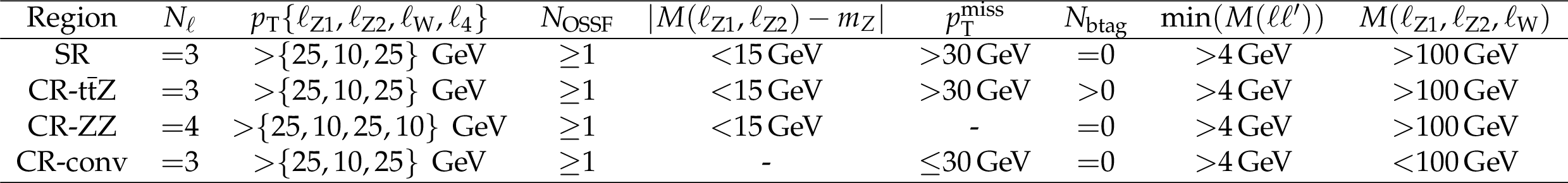
png pdf |
Table 1:
Requirements for the definition of the signal region (SR) and the three different control regions (CRs) designed to estimate the main background sources. |
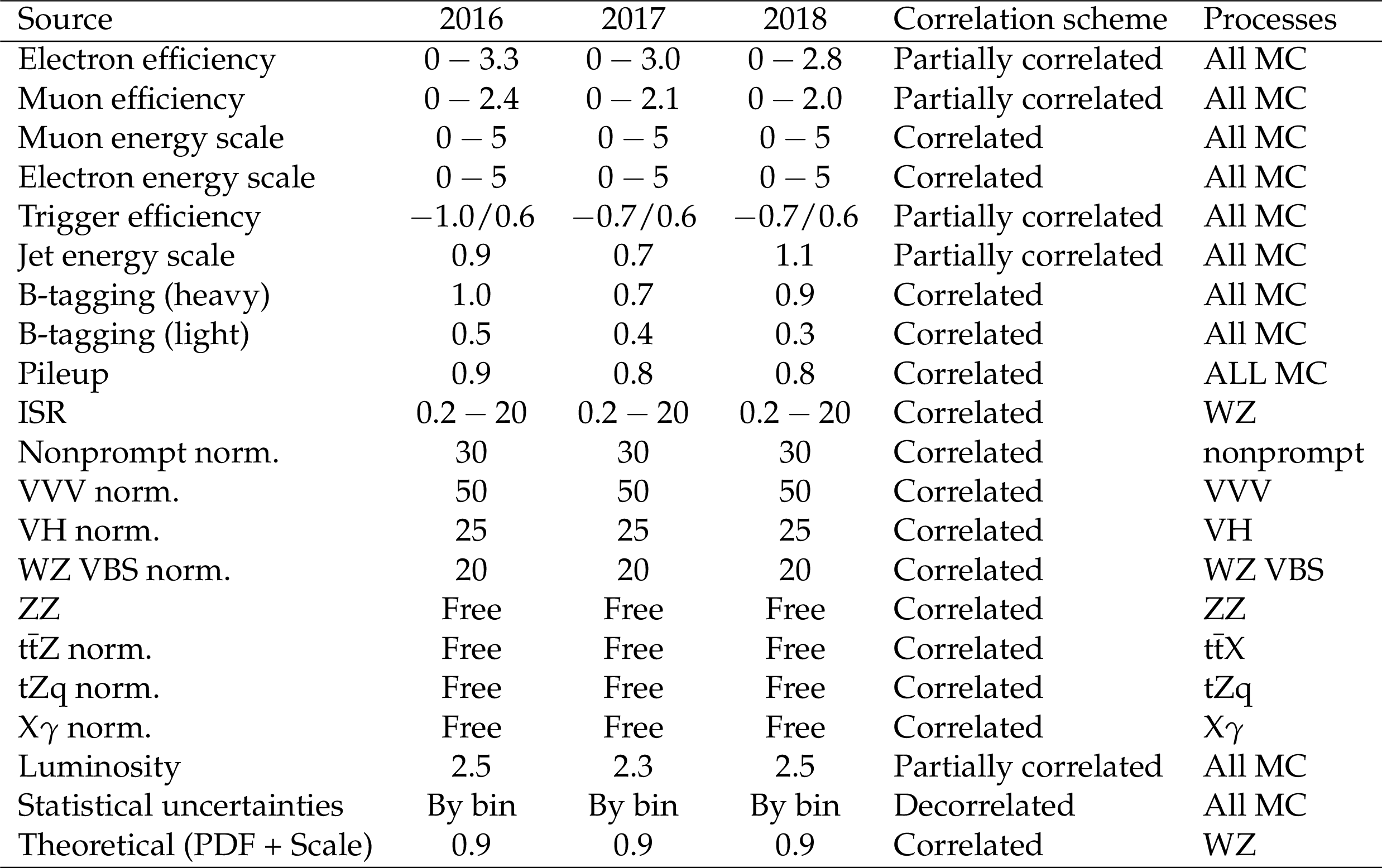
png pdf |
Table 2:
Summary of uncertainties in the analysis, their relative effect for each of the data-taking years, and the correlation scheme followed to combine those years and which processes are affected by them. Uncertainties related to experimental measurements of efficiencies and energy scales are presented as percentages over the predicted signal yield. Uncertainties related to normalization of specific background processes are described as percentages over the yields of the specific processes or as free if the process is free floating in the fits. Lepton-related uncertainties are shown as a range as most measurements of the analysis are split in flavour channels with which the size of these uncertainty is strongly correlated. Systematic uncertainties with an asymmetric effect are marked with a $/$ separating the upwards and downwards variations. |
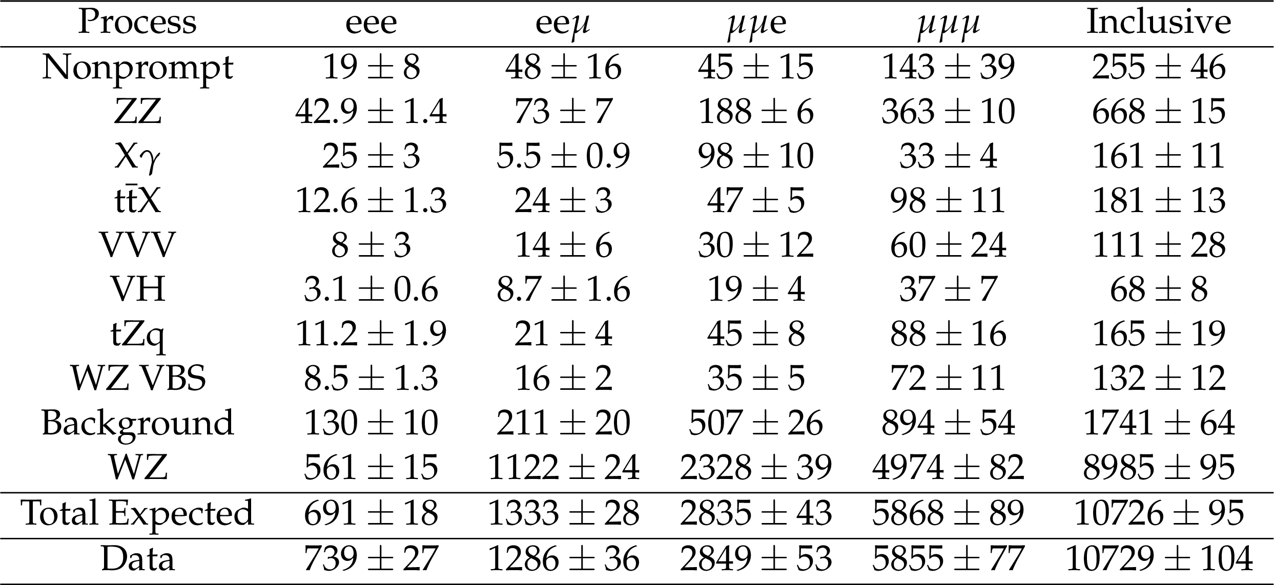
png pdf |
Table 3:
Observed and expected yields after the combined fit for the relevant SM processes in the signal region of the analysis in each of the different lepton flavour combinations and for all final states. Total uncertainties affecting each process are included at their postfit values next to the predicted yields. |
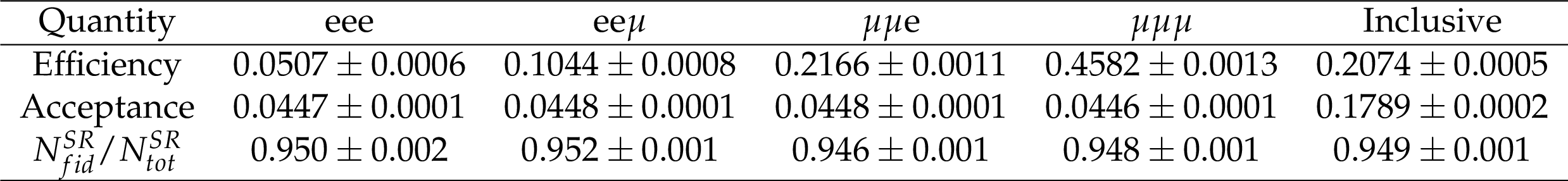
png pdf |
Table 4:
Measured efficiencies, acceptances and proportion of fiducial signal events in the signal region for the combined selection and each of the considered flavour channels separately as measured using the POWHEG WZ MC sample. Uncertainties are statistical only. Notice that while the fiducial region is defined separately per flavour, and thus the inclusive efficiency is a weighted average of the per channel ones, the TR is always flavour inclusive so the inclusive acceptance is by definition the sum of the ones split by category. |
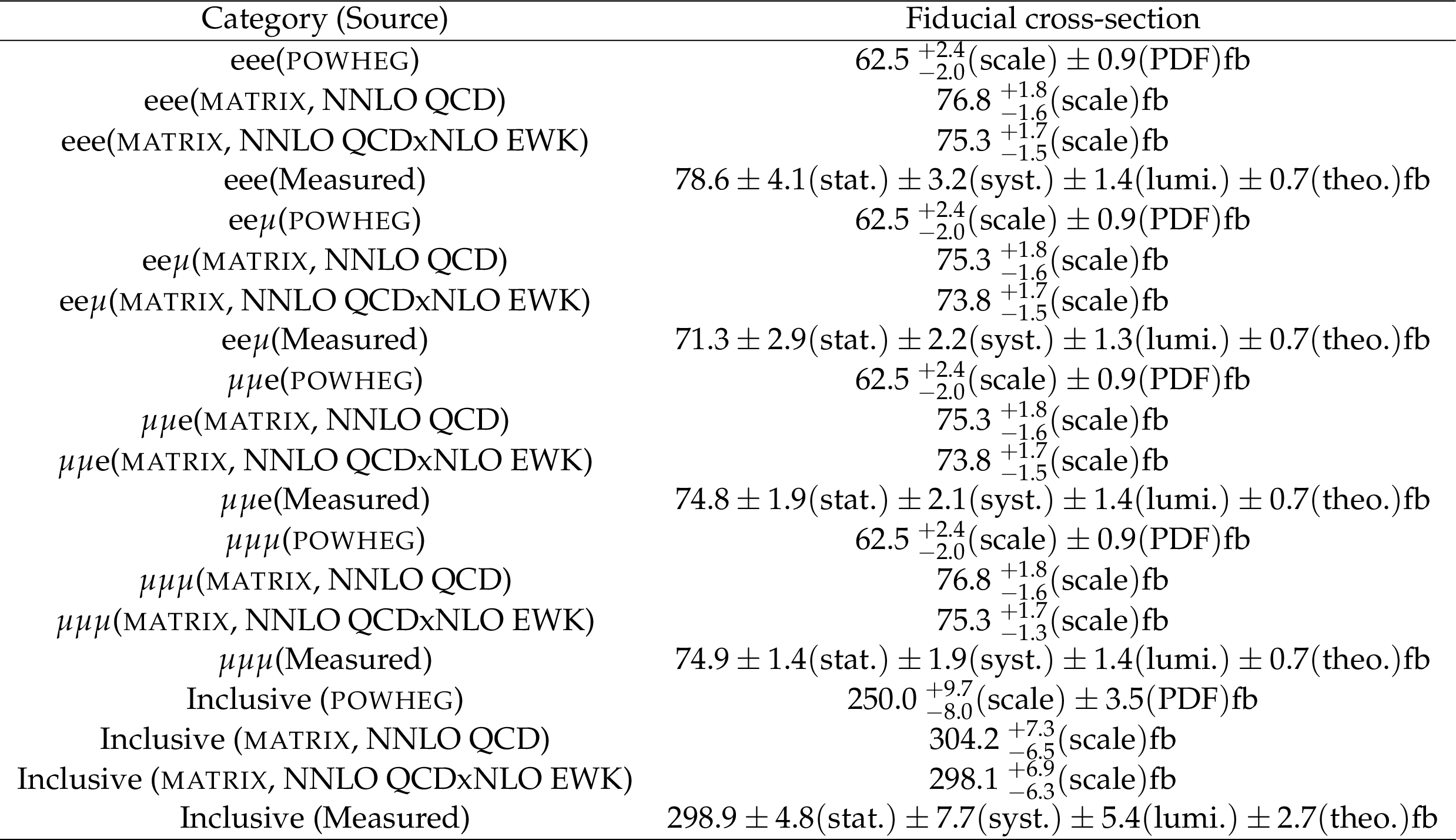
png pdf |
Table 5:
Measured fiducial cross sections and their corresponding uncertainties for the flavour exclusive and flavour inclusive categories. The predictions from both POWHEG at NLO in QCD and LO EWK as well as several ones obtained from matrix (NNLO QCD, NNLO QCDxNLO EWK) are also included. |
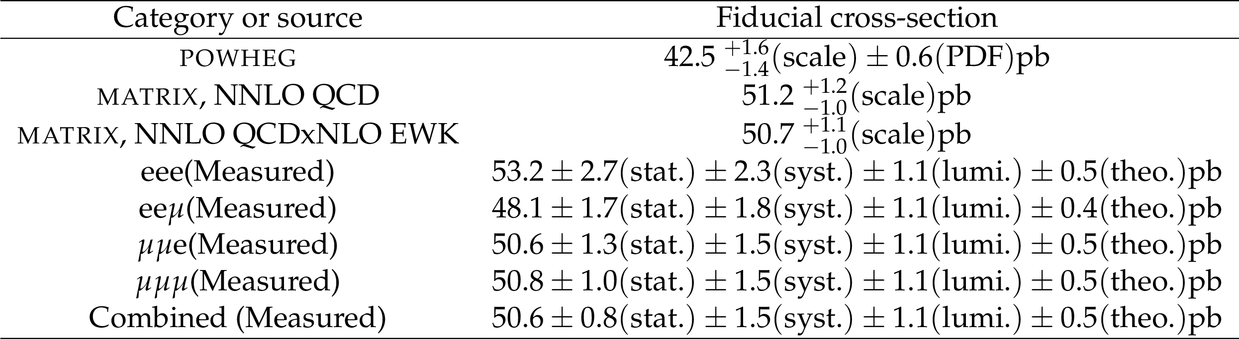
png pdf |
Table 6:
Measured total cross sections and their corresponding uncertainties for the flavour exclusive and flavour inclusive categories. The predictions from both POWHEG at NLO in QCD and LO EWK as well as several ones obtained from matrix (NNLO QCD, NNLO QCDxNLO EWK) are also included. |
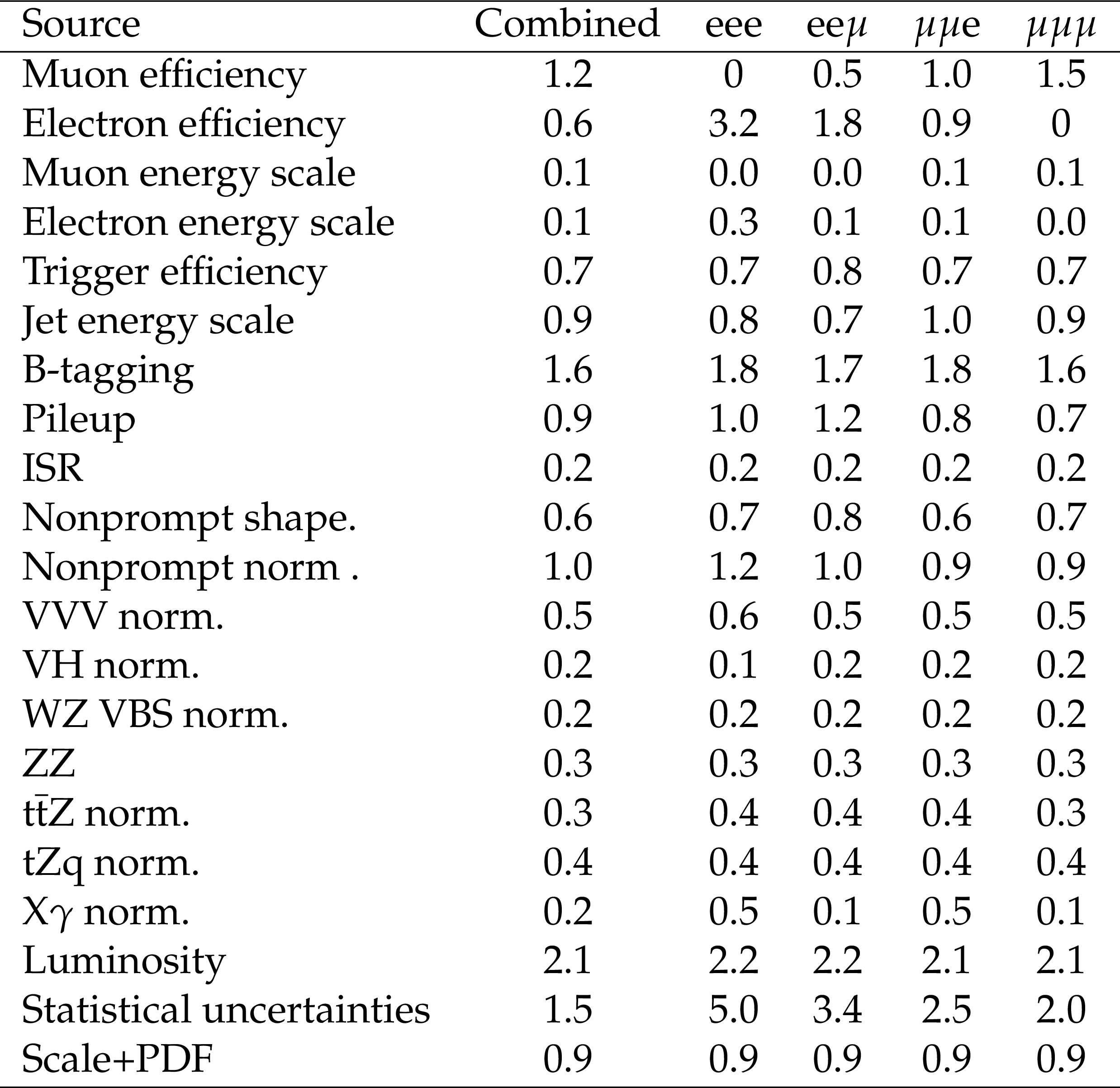
png pdf |
Table 7:
Summary of postfit effects of each uncertainty source in the total cross section WZ measurement separated by flavour categories. Numbers are measured in percentage contribution to the cross section uncertainty. For the scale and PDF uncertainties which are not included in the fit, the effect on the acceptance measurements is shown. |
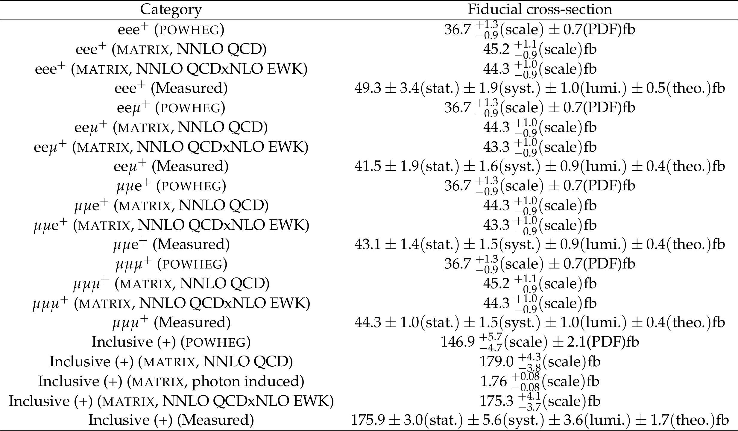
png pdf |
Table 8:
Measured fiducial cross-sections and their corresponding uncertainties for each of the individual flavour categories as well as for its combination. The predictions from both matrix (at NNLO QCD and NNLO QCDxNLO EWK) and POWHEG (at NLO QCD) are also included. Positively charged final states only. |
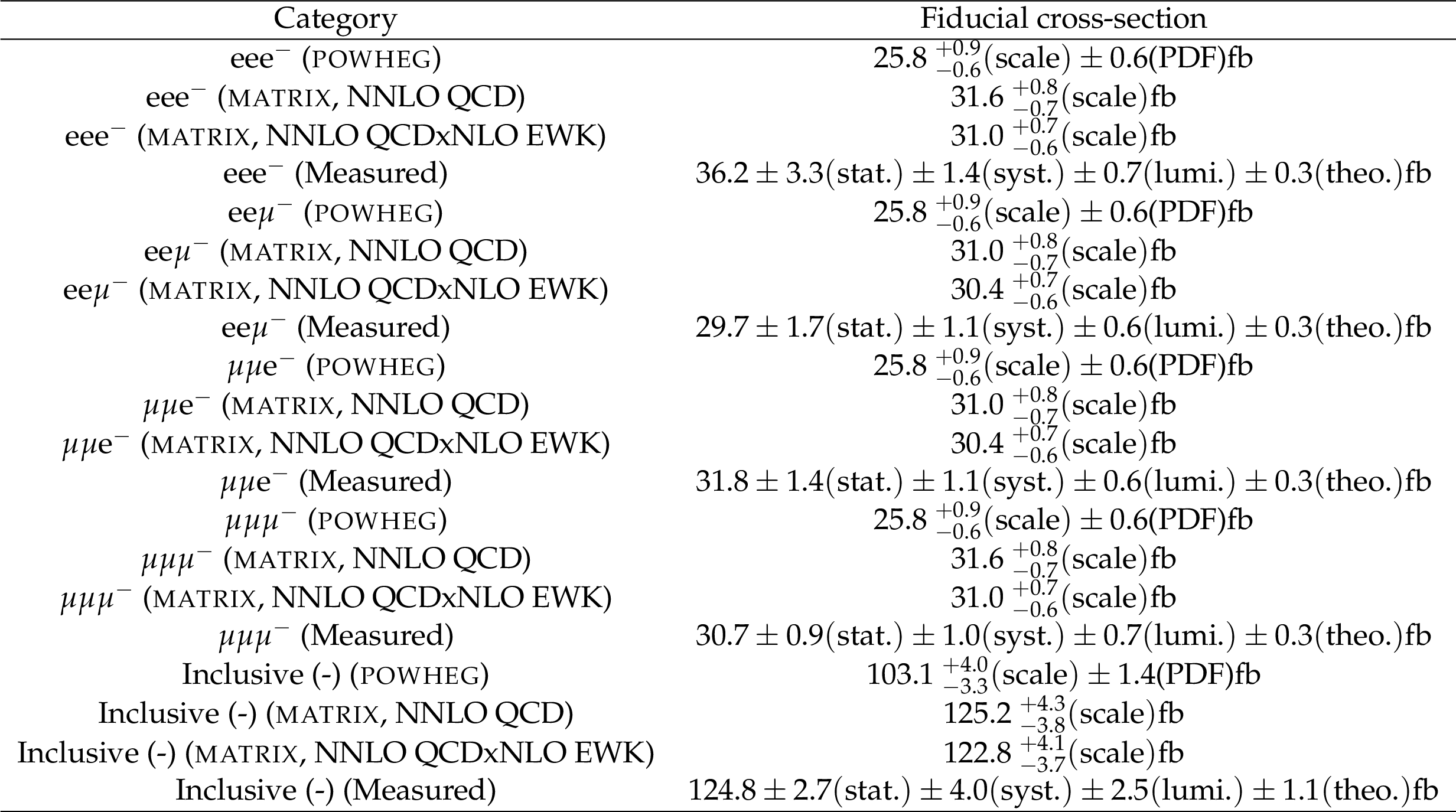
png pdf |
Table 9:
Measured fiducial cross-sections and their corresponding uncertainties for each of the individual flavour categories as well as for its combination. The predictions from both matrix (at NNLO QCD and NNLO QCDxNLO EWK) and POWHEG (at NLO QCD) are also included. Negatively charged final states only. |
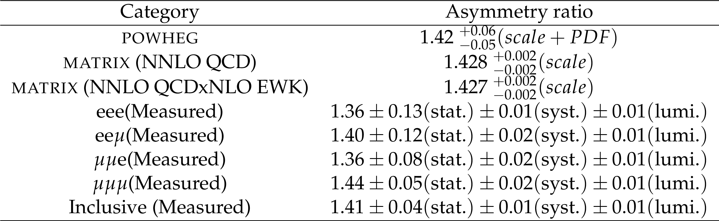
png pdf |
Table 10:
Measured fiducial cross-sections ratio and their corresponding uncertainties for each of the individual flavour categories as well as for its combination. The predictions from both matrix (at NNLO QCD and NNLO QCDxNLO EWK) and POWHEG (at NLO QCD) are also included. |
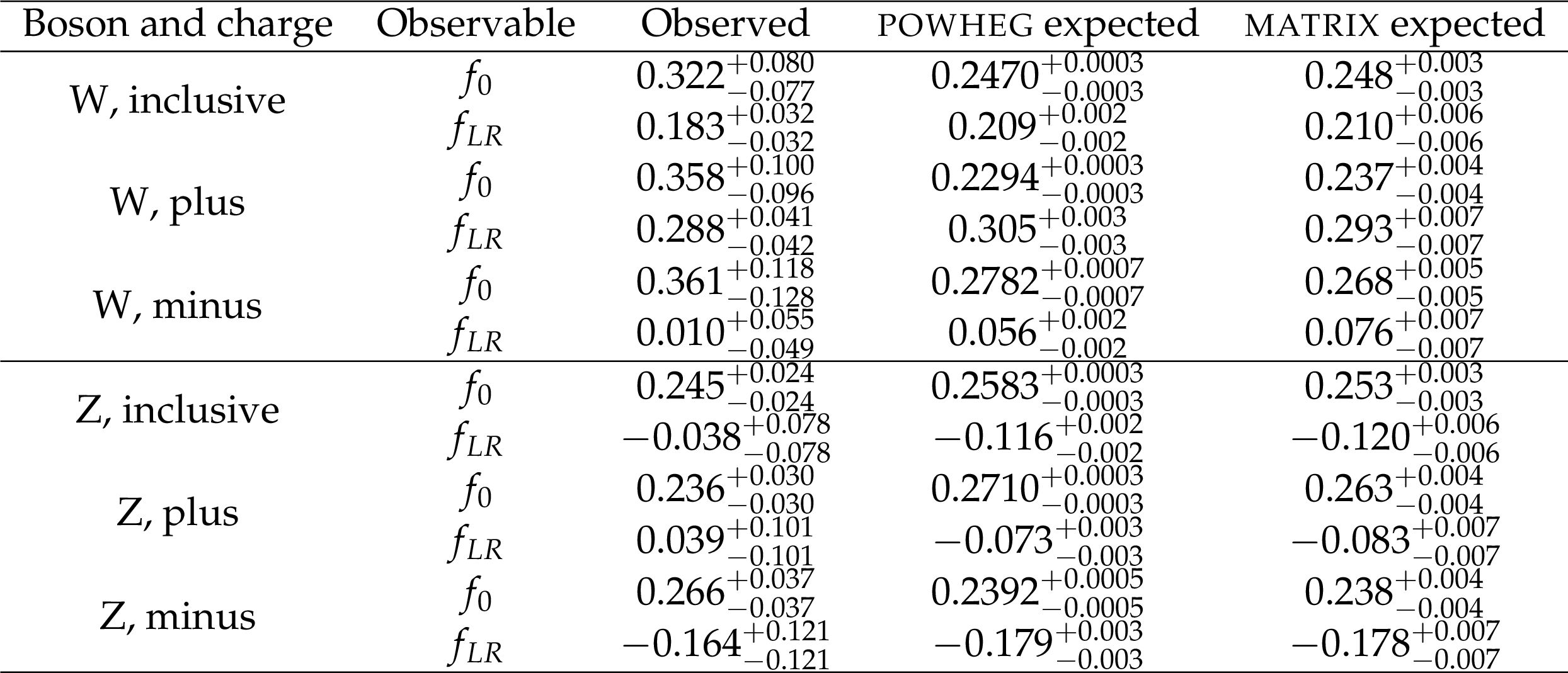
png pdf |
Table 11:
Standard model predictions and measured values of the W and Z polarization parameters for inclusive WZ production and each of the charged final state cases. The SM values are estimated from the nominal POWHEG sample and the matrix shapes by performing a quadratic fit to the generator level cosine of the polarization angle with no fiducial cuts applied and computing the polarization fractions from the fitting parameters. Uncertainties in the POWHEG measurements correspond to PDF uncertainties while those included for MATRIX relate to the overall numerical uncertainty. |
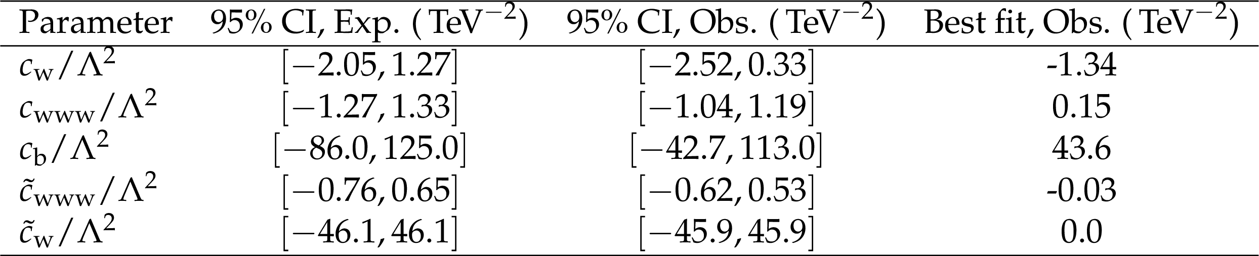
png pdf |
Table 12:
Best fit, and expected and observed one-dimensional confidence intervals at 95% confidence level for each of the considered EFT parameters. Both the purely dimension-8 BSM contribution as well as the dimension-6 interference term are included to compute the EFT effect in the high tails of ${M({\mathrm{W} \mathrm{Z}})}$ for this results. In computing confidence intervals for each parameter the other ones are fixed to their SM values. |

png pdf |
Table 13:
Best fit, and expected and observed one-dimensional confidence intervals at 95% confidence level for each of the considered EFT parameters. Only the dimension-six interference term are included to compute the EFT effect in the high tails of ${M({\mathrm{W} \mathrm{Z}})}$ for this results. In computing confidence intervals for each parameter the other ones are fixed to their SM values. No sensitivity is observed for the interference only term for the ${\tilde{c}_{\text {w}}}$ parameter. |
| Summary |
|
The pp $\to$ WZ production is studied in the trilepton final state at $\sqrt{s}=$ 13 TeV, using a data set corresponding to a total integrated luminosity of 137.2 fb$^{-1}$. The production cross sections in the total and fiducial phase spaces are measured in the inclusive case as well as in up to eight different combinations of final-state flavour composition and total final-state charge. The total inclusive cross-section is measured to be $\sigma_{\textrm{Tot}}({\mathrm{p}} {\mathrm{p}} \rightarrow \mathrm{W}\mathrm{Z}) = $ 50.6 $\pm$ 1.9 pb $=$ 50.6 $\pm$ 0.8 (stat) $\pm$ 1.5 (syst) $\pm$ 1.1 (lumi) $\pm$ 0.5 (theo) pb, which favours the computations performed at NNLO QCDxNLO EWK order with matrix of $\sigma_{MATRIX} = $ 50.7 $^{+1.1}_{-1.0}$ (scale) pb over the ones obtained at NLO QCD order with POWHEG of $\sigma_{POWHEG} = $ 42.5 $^{+1.6}_{-1.4}$ (scale) $\pm$ 0.6 (PDF) pb. The charge asymmetry in the production, derived from the dominant qq' production mode, is also measured in terms of a charge asymmetry ratio of $A^{+-}_{{\mathrm{W}\mathrm{Z}} }=$ 1.409 $\pm$ 0.04 with a relative precision under 3% and in quite good agreement with SM predictions performed at NLO QCD order of $A^{+-,POWHEG}_{{\mathrm{W}\mathrm{Z}} } = $ 1.42 $\pm$ 0.05. Consistency of the measurement is also found with the NNPDF30_nlo_as118 PDF set and a Bayesian reweighting technique is applied to estimate possible constraints on PDFs that could be derived from this measurement. Differential distributions are produced for multiple high-level analysis observables in both the inclusive and the different-flavour and charge-exclusive final states. The distributions are compared with predictions at NLO in QCD from POWHEG and MadGraph5+MCatNLO as well as with predictions at NNLO in QCD obtained with matrix . The polarization of the W and Z bosons in WZ production in the helicity frame is studied in the charge inclusive and charge exclusive final states, yielding to an observed significance pointing to the observation of longitudinally-polarized massive vector bosons at 5.6$\sigma$ (4.3$\sigma$) observed (expected) significance for the W boson, and both observed and expected significances way above 5$\sigma$ for the Z boson. A search for anomalous values of the charged triple gauge coupling WWZ is performed by looking at the high-energy tails in the distribution of the mass of the WZ system. The search provides stronger constraints than previous iterations of the analysis by a factor 2, mostly caused by the increased available luminosity. The effect of CP-violating dimension-six operators is introduced for the first time in WZ production in CMS, leading to similar confidence regions to the ones obtained in the CP-conserving ones. |
| References | ||||
| 1 | UA1 Collaboration | Production of W's with large transverse momentum at the CERN proton-antiproton collider | Physics Letters B 193 (1987) 389 | |
| 2 | D0 Collaboration | Measurement of the $ \mathrm{W}\mathrm{Z}\rightarrow \ell\nu\ell\ell $ cross section and limits on anomalous triple gauge couplings in $ \mathrm{t\bar{t}} $ collisions at $ \sqrt{s} = $ 1.96 TeV | PLB 695 (2011) 67 | 1006.0761 |
| 3 | CDF Collaboration | Observation of $ \mathrm{W}\mathrm{Z} $ production | PRLett 98 (2007) 161801 | hep-ex/0702027 |
| 4 | ATLAS Collaboration | Measurement of the $ \mathrm{W}^\pm \mathrm{Z} $ production cross section and limits on anomalous triple gauge couplings in proton-proton collisions at $ \sqrt{s}= $ 7 TeV with the ATLAS detector | PLB 709 (2012) 341 | 1111.5570 |
| 5 | ATLAS Collaboration | Measurement of $ \mathrm{W}\mathrm{Z} $ production in proton-proton collisions at $ \sqrt{s}= $ 7 TeV with the ATLAS detector | EPJC 72 (2012) 2173 | 1208.1390 |
| 6 | ATLAS Collaboration | Measurement of the $ \mathrm{W}\mathrm{W}+\mathrm{W}\mathrm{Z} $ cross section and limits on anomalous triple gauge couplings using final states with one lepton, missing transverse momentum, and two jets with the ATLAS detector at $ \sqrt{\rm{s}} = $ 7 TeV | JHEP 01 (2015) 049 | 1410.7238 |
| 7 | ATLAS Collaboration | Measurements of $ \mathrm{W}^\pm \mathrm{Z} $ production cross sections in $ {\mathrm{p}}{\mathrm{p}} $ collisions at $ \sqrt{s} = $ 8 TeV with the ATLAS detector and limits on anomalous gauge boson self-couplings | PRD 93 (2016) 092004 | 1603.02151 |
| 8 | ATLAS Collaboration | Measurement of the $ \mathrm{W}^{\pm}\mathrm{Z} $ boson pair-production cross section in pp collisions at $ \sqrt{s}= $ 13 TeV with the ATLAS detector | PLB 762 (2016) 1 | 1606.04017 |
| 9 | ATLAS Collaboration | Search for anomalous electroweak production of $ \mathrm{W}\mathrm{W}/\mathrm{W}\mathrm{Z} $ in association with a high-mass dijet system in pp collisions at $ \sqrt{s}= $ 8 TeV with the ATLAS detector | PRD 95 (2017) 032001 | 1609.05122 |
| 10 | ATLAS Collaboration | Measurement of $ \mathrm{W}\mathrm{W}/\mathrm{W}\mathrm{Z} \rightarrow \ell \nu q q^{\prime} $ production with the hadronically decaying boson reconstructed as one or two jets in $ {\mathrm{p}}{\mathrm{p}} $ collisions at $ \sqrt{s}= $ 8 TeV with ATLAS, and constraints on anomalous gauge couplings | EPJC 77 (2017) 563 | 1706.01702 |
| 11 | ATLAS Collaboration | Search for the electroweak diboson production in association with a high-mass dijet system in semileptonic final states in pp collisions at $ \sqrt{s}= $ 13 TeV with the ATLAS detector | PRD 100 (2019) 032007 | 1905.07714 |
| 12 | ATLAS Collaboration | Measurement of $ W^{\pm}Z $ production cross sections and gauge boson polarisation in pp collisions at $ \sqrt{s} = $ 13 TeV with the ATLAS detector | EPJC 79 (2019) 535 | 1902.05759 |
| 13 | CMS Collaboration | Study of the dijet mass spectrum in $ {\mathrm{p}}{\mathrm{p}} \rightarrow \mathrm{W} + $ jets events at $ \sqrt{s}= $ 7 TeV | PRL 109 (2012) 251801 | CMS-EWK-11-017 1208.3477 |
| 14 | CMS Collaboration | Measurement of the sum of $ \mathrm{W}\mathrm{W} $ and $ \mathrm{W}\mathrm{Z} $ production with $ \mathrm{W}+ $dijet events in $ {\mathrm{p}}{\mathrm{p}} $ collisions at $ \sqrt{s}= $ 7 TeV | EPJC 73 (2013) 2283 | CMS-SMP-12-015 1210.7544 |
| 15 | CMS Collaboration | Measurement of $ \mathrm{W}\mathrm{Z} $ and $ \mathrm{Z}\mathrm{Z} $ production in pp collisions at $ \sqrt{s}= $ 8 TeV in final states with b-tagged jets | EPJC 74 (2014) 2973 | CMS-SMP-13-011 1403.3047 |
| 16 | CMS Collaboration | Measurement of the $ \mathrm{W}\mathrm{Z} $ production cross section in $ {\mathrm{p}}{\mathrm{p}} $ collisions at $ \sqrt{s}= $ 13 TeV | PLB 766 (2017) 268 | CMS-SMP-16-002 1607.06943 |
| 17 | CMS Collaboration | Measurement of the $ \mathrm{W}\mathrm{Z} $ production cross section in pp collisions at $ \sqrt{s} = $ 7 and 8 TeV and search for anomalous triple gauge couplings at $ \sqrt{s}= $ 8 TeV | EPJC 77 (2017) 236 | CMS-SMP-14-014 1609.05721 |
| 18 | CMS Collaboration | Search for anomalous couplings in boosted $ \mathrm{W}\mathrm{W}/\mathrm{W}\mathrm{Z}\to\ell\nu\mathrm{q\bar{q}} $ production in proton-proton collisions at $ \sqrt{s}= $ 8 TeV | PLB 772 (2017) 21 | CMS-SMP-13-008 1703.06095 |
| 19 | CMS Collaboration | Search for anomalous electroweak production of vector boson pairs in association with two jets in proton-proton collisions at 13 TeV | PLB 798 (2019) 134985 | CMS-SMP-18-006 1905.07445 |
| 20 | CMS Collaboration | Search for anomalous triple gauge couplings in $ \mathrm{W}\mathrm{W} $ and $ \mathrm{W}\mathrm{Z} $ production in lepton + jet events in proton-proton collisions at $ \sqrt{s}= $ 13 TeV | JHEP 12 (2019) | CMS-SMP-18-008 1907.08354 |
| 21 | CMS Collaboration | Measurement of electroweak $ \mathrm{W}\mathrm{Z} $ boson production and search for new physics in $ \mathrm{W}\mathrm{Z} $ + two jets events in pp collisions at $ \sqrt{s}= $ 13 TeV | PLB 795 (2019) 281 | CMS-SMP-18-001 1901.04060 |
| 22 | CMS Collaboration | Measurements of the pp $ \to \mathrm{W}\mathrm{Z} $ inclusive and differential production cross section and constraints on charged anomalous triple gauge couplings at $ \sqrt{s} = $ 13 TeV | JHEP 04 (2019) 122 | CMS-SMP-18-002 1901.03428 |
| 23 | CMS Collaboration | The CMS trigger system | JINST 12 (2017) P01020 | CMS-TRG-12-001 1609.02366 |
| 24 | CMS Collaboration | The CMS experiment at the CERN LHC | JINST 3 (2008) S08004 | CMS-00-001 |
| 25 | CMS Collaboration | Performance of missing energy reconstruction in 13 TeV pp collision data using the CMS detector | CMS-PAS-JME-16-004 | CMS-PAS-JME-16-004 |
| 26 | P. Nason | A New method for combining NLO QCD with shower Monte Carlo algorithms | JHEP 11 (2004) 040 | hep-ph/0409146 |
| 27 | S. Frixione, P. Nason, and C. Oleari | Matching NLO QCD computations with Parton Shower simulations: the POWHEG method | JHEP 11 (2007) 070 | 0709.2092 |
| 28 | S. Alioli, P. Nason, C. Oleari, and E. Re | A general framework for implementing NLO calculations in shower Monte Carlo programs: the POWHEG BOX | JHEP 06 (2010) 043 | 1002.2581 |
| 29 | T. Melia, P. Nason, R. Rontsch, and G. Zanderighi | $ \mathrm{W}^+ \mathrm{W}^- $, $ \mathrm{W} \mathrm{Z} $, and $ \mathrm{Z} \mathrm{Z} $ production in the POWHEGbox | JHEP 11 (2011) 078 | 1107.5051 |
| 30 | P. Nason and G. Zanderighi | $ \mathrm{W}^+ \mathrm{W}^- $, $ \mathrm{W} \mathrm{Z} $ and $ \mathrm{Z} \mathrm{Z} $ production in the POWHEGbox-v2 | EPJC 74 (2014) 2702 | 1311.1365 |
| 31 | J. Alwall et al. | The automated computation of tree-level and next-to-leading order differential cross sections, and their matching to parton shower simulations | JHEP 07 (2014) 079 | 1405.0301 |
| 32 | R. Frederix and S. Frixione | Merging meets matching in $ MadGraph5+MCatNLO $ | JHEP 12 (2012) 061 | 1209.6215 |
| 33 | T. Sjostrand et al. | An introduction to $ PYTHIA $ 8.2 | Computer Physics Communications 191 (2015) 159 | 1410.3012 |
| 34 | CMS Collaboration | Event generator tunes obtained from underlying event and multiparton scattering measurements | EPJ76 (2016) 155 | CMS-GEN-14-001 1512.00815 |
| 35 | CMS Collaboration | Extraction and validation of a new set of CMS PYTHIA8 tunes from underlying-event measurements | EPJC 80 (2020) 4 | CMS-GEN-17-001 1903.12179 |
| 36 | O. Mattelaer | On the maximal use of Monte Carlo samples: re-weighting events at NLO accuracy | The European Physical Journal C 76 (2016) 674 | 1607.00763 |
| 37 | C. Degrande et al. | Effective Field Theory: A Modern Approach to Anomalous Couplings | Annals Phys. 335 (2013) 21 | 1205.4231 |
| 38 | M. Grazzini, S. Kallweit, D. Rathlev, and M. Wiesemann | $ W^{\pm}Z $ production at hadron colliders in NNLO QCD | PLB 761 (2016) 179 | 1604.08576 |
| 39 | M. Grazzini, S. Kallweit, D. Rathlev, and M. Wiesemann | $ \mathrm{W}^\pm \mathrm{Z} $ production at the LHC: fiducial cross sections and distributions in NNLO QCD | JHEP 05 (2017) | 1703.09065 |
| 40 | M. Grazzini, S. Kallweit, and M. Wiesemann | Fully differential NNLO computations with MATRIX | EPJC 78 (2018) 537 | 1711.06631 |
| 41 | F. Cascioli, P. Maierhofer, and S. Pozzorini | Scattering amplitudes with open loops | PRL 108 (2012) 111601 | 1111.5206 |
| 42 | A. Denner, S. Dittmaier, and L. Hofer | Collier: a fortran-based complex one-loop library in extended regularizations | CPC 212 (2017) 220 | 1604.06792 |
| 43 | S. Catani et al. | Vector boson production at hadron colliders: hard-collinear coefficients at the NNLO | EPJC 72 (2012) 2195 | 1209.0158 |
| 44 | S. Catani and M. Grazzini | An NNLO subtraction formalism in hadron collisions and its application to Higgs boson production at the LHC | PRL 98 (2007) 222002 | hep-ph/0703012 |
| 45 | M. Cacciari, G. P. Salam, and G. Soyez | The anti-$ {k_{\mathrm{T}}} $ jet clustering algorithm | J. High Ener. Phys. 04 (2008) 063 | 0802.1189 |
| 46 | M. Cacciari, G. P. Salam, and G. Soyez | FastJet user manual | EPJC 72 (2012) 1896 | 1111.6097 |
| 47 | CMS Collaboration | Electron and photon reconstruction and identification with the CMS experiment at the CERN LHC | Submitted to JINST | CMS-EGM-17-001 2012.06888 |
| 48 | CMS Collaboration | Evidence for associated production of a Higgs boson with a top quark pair in final states with electrons, muons, and hadronically decaying $ \tau $ leptons at $ \sqrt{s}= $ 13 TeV | JHEP 08 (2018) 066 | CMS-HIG-17-018 1803.05485 |
| 49 | CMS Collaboration | Performance of the CMS muon detector and muon reconstruction with proton-proton collisions at $ \sqrt{s}= $ 13 TeV | Journal of Instrumentation 13 (2018) P06015 | CMS-MUO-16-001 1804.04528 |
| 50 | CMS Collaboration | Jet algorithms performance in 13 TeV data | CMS-PAS-JME-16-003 | CMS-PAS-JME-16-003 |
| 51 | CMS Collaboration | Identification of heavy-flavour jets with the CMS detector in pp collisions at 13 TeV | JINST 13 (2018) P05011 | CMS-BTV-16-002 1712.07158 |
| 52 | CMS Collaboration | Performance of missing transverse momentum reconstruction in proton-proton collisions at $ \sqrt{s}= $ 13 TeV using the cms detector | Journal of Instrumentation 14 (2019) 7004 | CMS-JME-17-001 1903.06078 |
| 53 | CMS Collaboration | Jet energy scale and resolution in the CMS experiment in pp collisions at 8 TeV | JINST 12 (2017) P02014 | CMS-JME-13-004 1607.03663 |
| 54 | CMS Collaboration | Search for new physics in same-sign dilepton events in proton-proton collisions at $ \sqrt{s} = $ 13 TeV | EPJC 76 (2016) 439 | CMS-SUS-15-008 1605.03171 |
| 55 | CMS Collaboration | Combined Higgs boson production and decay measurements with up to 137 fb-1 of proton-proton collision data at $ \sqrt{s} = $ 13 TeV | CMS-PAS-HIG-19-005 | CMS-PAS-HIG-19-005 |
| 56 | CMS Collaboration | Measurements of production cross sections of $ \mathrm{W}\mathrm{Z} $ and same-sign $ \mathrm{W}\mathrm{W} $ boson pairs in association with two jets in proton-proton collisions at $ \sqrt{s}= $ 13 TeV | Physics Letters B 809 (2020) 135710 | CMS-SMP-19-012 2005.01173 |
| 57 | CMS Collaboration | Measurements of inclusive $ \mathrm{W} $ and $ \mathrm{Z} $ cross sections in pp collisions at $ \sqrt{s}= $ 7 TeV | JHEP 01 (2011) 080 | CMS-EWK-10-002 1012.2466 |
| 58 | CMS Collaboration | CMS luminosity measurements for the 2016 data-taking period | ||
| 59 | CMS Collaboration | CMS luminosity measurement for the 2017 data-taking period at $ \sqrt{s} = $ 13 TeV | ||
| 60 | CMS Collaboration | CMS luminosity measurement for the 2018 data-taking period at $ \sqrt{s} = $ 13 TeV | ||
| 61 | J. Butterworth et al. | PDF4LHC recommendations for LHC Run II | Journal of Physics G: Nuclear and Particle Physics 43 (2016) 023001 | 1510.03865 |
| 62 | S. Mrenna and P. Skands | Automated Parton-Shower Variations in $ PYTHIA $ 8 | PRD 94 (2016) 074005 | 1605.08352 |
| 63 | Particle Data Group Collaboration | Review of Particle Physics | Prog. Theor. Exp. Phys. 2020 (2020) 083C01 | |
| 64 | W. T. Giele and S. Keller | Implications of hadron collider observables on parton distribution function uncertainties | Physical Review D 58 (1998) 094023 | hep-ph/9803393 |
| 65 | N. Sato, J. F. Owens, and H. B. Prosper | Bayesian reweighting for global fits | Physical Review D 89 (2014) 11420 | 1310.1089 |
| 66 | J. A. Aguilar-Saavedra and J. Bernabeu | Breaking down the entire $ \mathrm{W} $ boson spin observables from its decay | PRD 93 (2016) 011301 | 1508.04592 |
| 67 | J. A. Aguilar-Saavedra, J. Bernabeu, V. A. Mitsou, and A. Segarra | The $ \mathrm{Z} $ boson spin observables as messengers of new physics | EPJC 77 (2017) 234 | 1701.03115 |
| 68 | Z. Bern et al. | Left-handed $ \mathrm{W} $ bosons at the LHC | PRD 84 (2011) 034008 | 1103.5445 |
| 69 | G. Cowan | Statistical Data Analysis | Oxford Science Publications | |
| 70 | S. Schmitt | Data unfolding methods in High Energy Physics | EPJ Web Conf. 137 (2017) 11008 | 1611.01927 |
| 71 | S. Schmitt | TUnfold: an algorithm for correcting migration effects in high energy physics | JINST 7 (2012) T10003 | 1205.6201 |
|
|
Compact Muon Solenoid LHC, CERN |
|

|

|

|

|

|