

Compact Muon Solenoid
LHC, CERN
| CMS-PAS-SMP-18-002 | ||
| Measurements of the $\mathrm{pp}\to\mathrm{WZ}$ inclusive and differential production cross section and constraints on charged anomalous triple gauge couplings at $\sqrt{s} = $ 13 TeV. | ||
| CMS Collaboration | ||
| July 2018 | ||
| Abstract: The WZ production cross section is measured in proton-proton collisions using 35.9 fb$^{-1}$ of data collected with the CMS detector. An estimate of the inclusive cross section yields a result of $\sigma_{\textrm{tot}}(\mathrm{pp} \rightarrow \mathrm{WZ}) = $ 48.09 $^{+1.00}_{-0.96}$ (stat) $^{+0.44}_{-0.37}$ (theo) $^{+2.39}_{-2.17}$ (syst) $\pm$ 1.39 (lumi) pb, for a total uncertainty of $-2.78$ and $+2.98$ pb. Fiducial and charge asymmetry measurements are provided. Differential cross section measurements are also presented with respect to three variables: the Z boson $p_{\mathrm{T}}$, the leading jet $p_{\mathrm{T}}$, and the $M_{\mathrm{WZ}}$ variable, defined as the invariant mass of the system composed of the three leptons and the missing transverse momentum. Differential measurements with respect to the W boson $p_{\mathrm{T}}$, split by charge, are also shown. Results are consistent with standard model predictions, favouring next-to-next-to-leading-order calculations. Constraints on anomalous triple gauge couplings are derived via a binned maximum likelihood fit to the $M_{\mathrm{WZ}}$ variable. | ||
|
Links:
CDS record (PDF) ;
CADI line (restricted) ;
These preliminary results are superseded in this paper, JHEP 04 (2019) 122. The superseded preliminary plots can be found here. |
||
| Figures | |

png pdf |
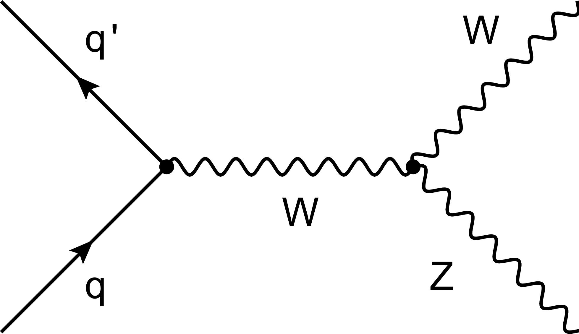
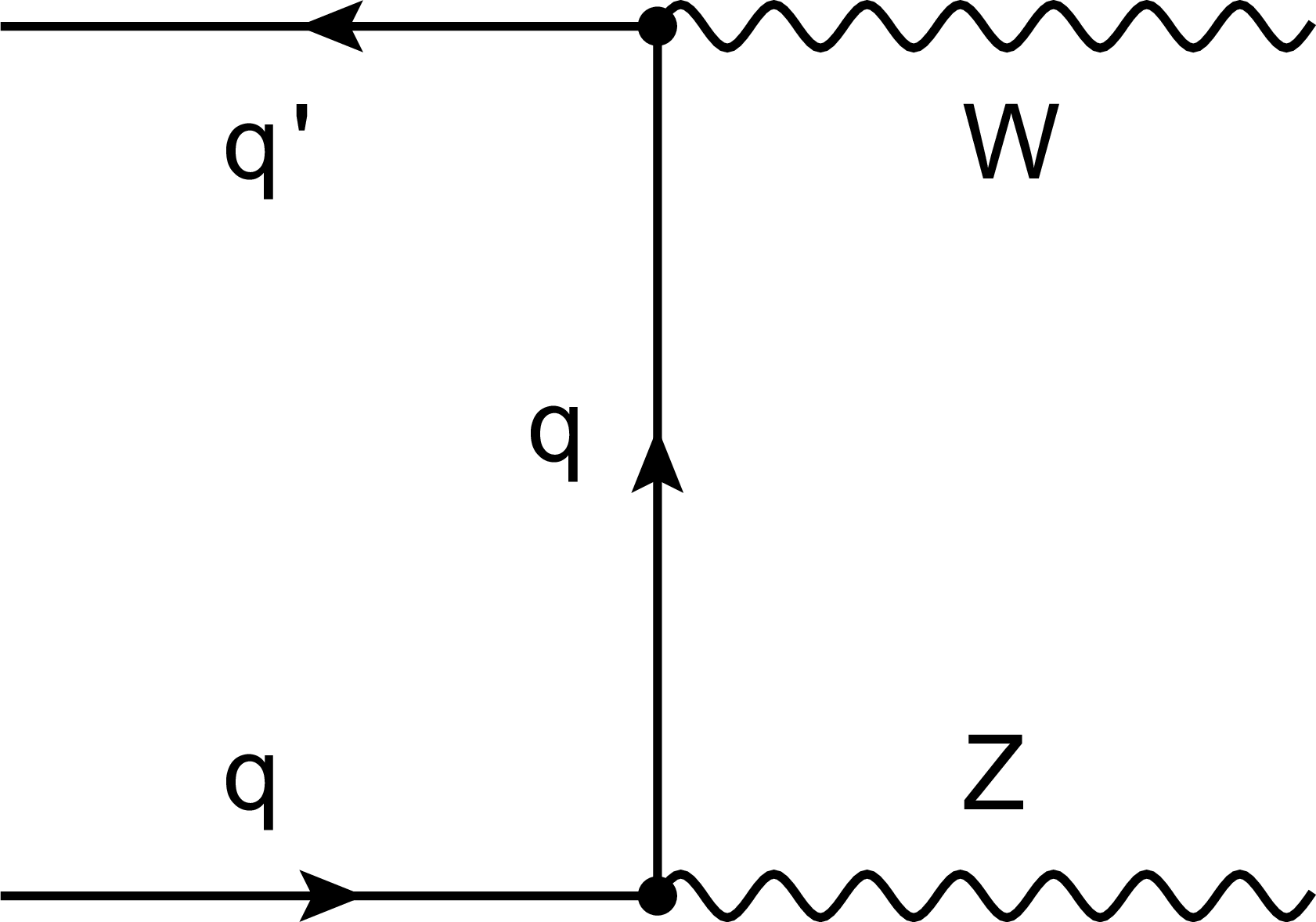
Figure 1:
Feynman diagrams for WZ production at leading order in proton-proton collisions. The contributions from the s-channel (left), t-channel (middle), and u-channel (right) are presented. The contribution from s-channel proceeds through TGC. |
png pdf |
Figure 1-a:
Feynman diagrams for WZ production at leading order in proton-proton collisions. The contributions from the s-channel (left), t-channel (middle), and u-channel (right) are presented. The contribution from s-channel proceeds through TGC. |
png pdf |
Figure 1-b:
Feynman diagrams for WZ production at leading order in proton-proton collisions. The contributions from the s-channel (left), t-channel (middle), and u-channel (right) are presented. The contribution from s-channel proceeds through TGC. |

png pdf |
Figure 1-c:
Feynman diagrams for WZ production at leading order in proton-proton collisions. The contributions from the s-channel (left), t-channel (middle), and u-channel (right) are presented. The contribution from s-channel proceeds through TGC. |
png pdf |
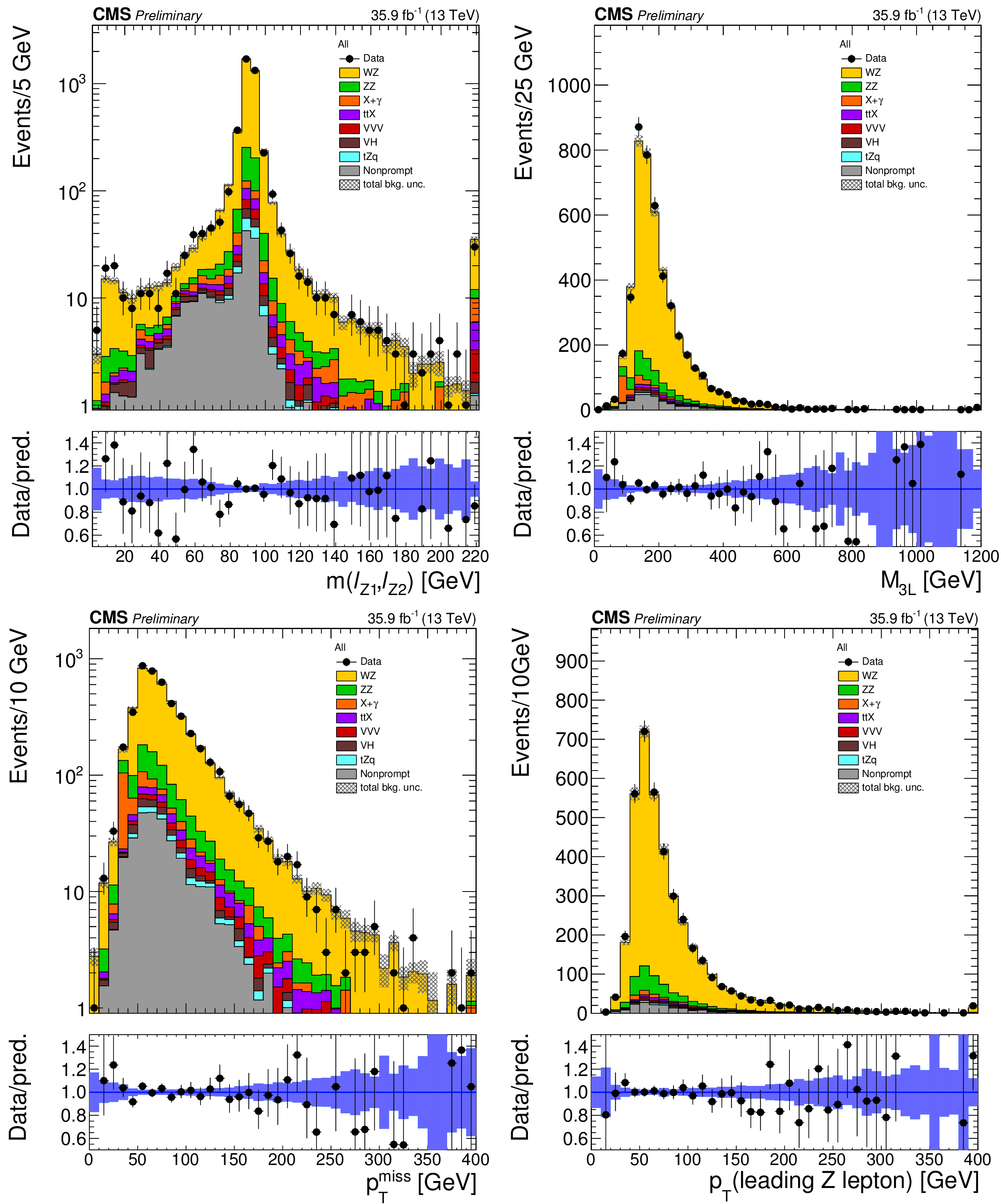
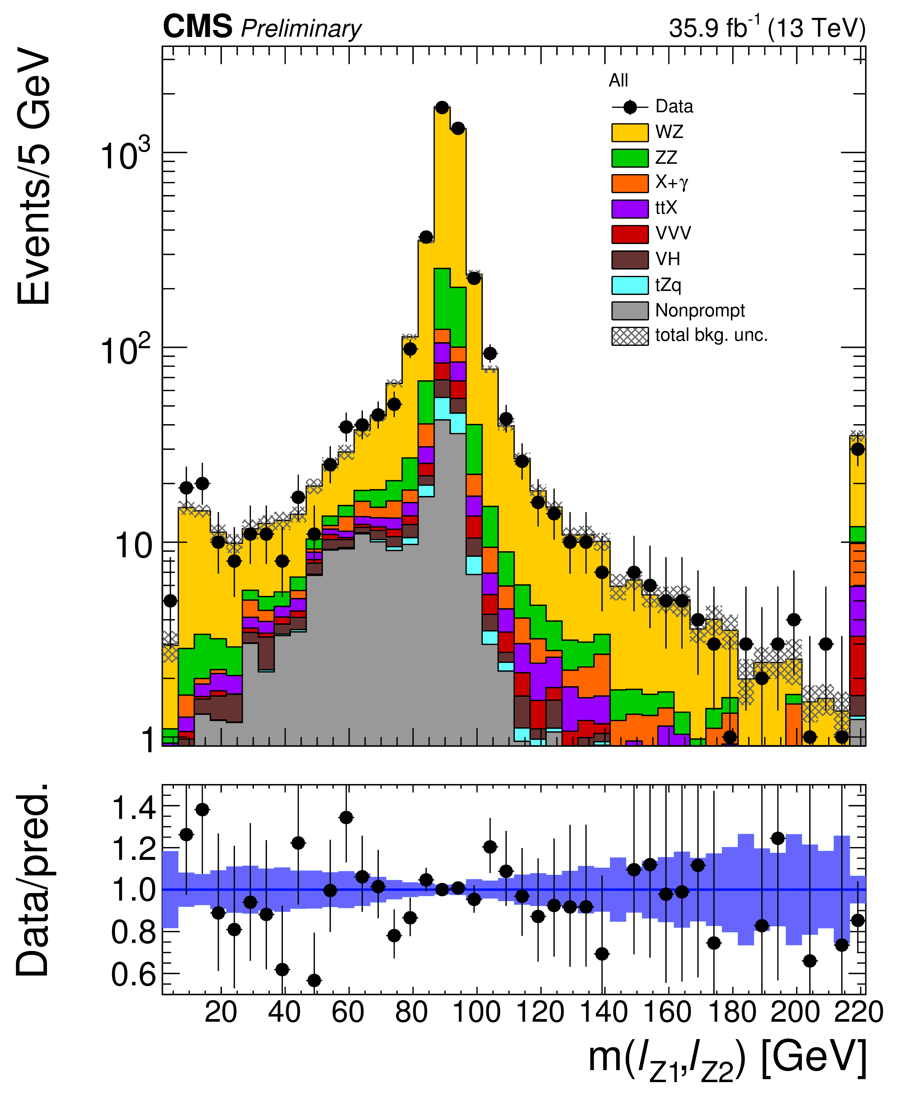
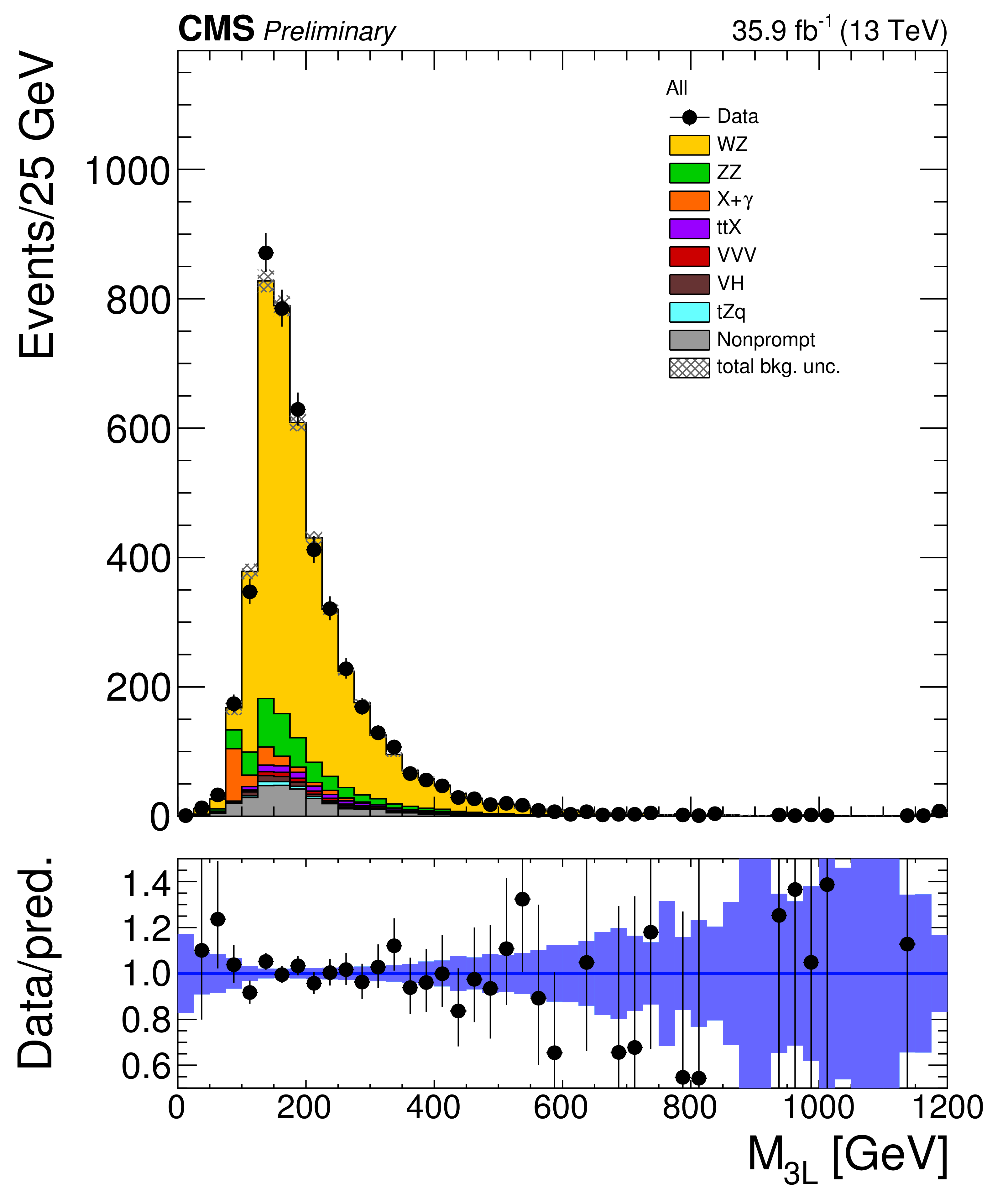
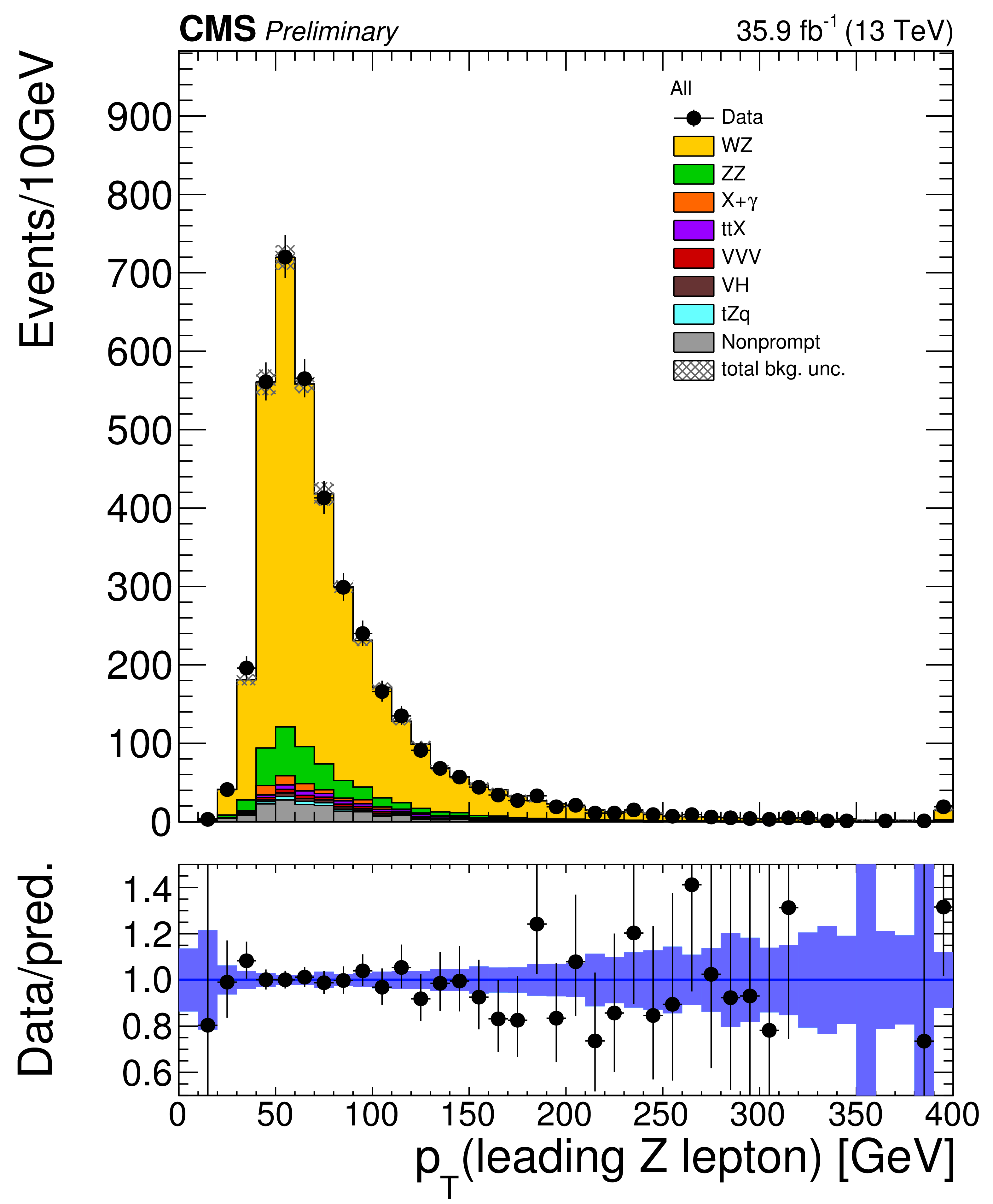
Figure 2:
Distribution of key observables in the signal region: invariant mass of the lepton pair assigned to the Z boson (top left), invariant mass of the three lepton system (top right), missing transverse momentum (bottom left), and momentum of the leading lepton assigned to the Z boson. Each of the distributions is represented applying the signal region requirements minus the one directly related to itself so the effect of its separation can be easily observed. The last bin contains the overflow. Vertical bars on the data points include their statistical uncertainty and shaded bands over the prediction include the contributions of the different sources of uncertainty at their values after the signal extraction fit. |
png pdf |
Figure 2-a:
Distribution of key observables in the signal region: invariant mass of the lepton pair assigned to the Z boson (top left), invariant mass of the three lepton system (top right), missing transverse momentum (bottom left), and momentum of the leading lepton assigned to the Z boson. Each of the distributions is represented applying the signal region requirements minus the one directly related to itself so the effect of its separation can be easily observed. The last bin contains the overflow. Vertical bars on the data points include their statistical uncertainty and shaded bands over the prediction include the contributions of the different sources of uncertainty at their values after the signal extraction fit. |
png pdf |
Figure 2-b:
Distribution of key observables in the signal region: invariant mass of the lepton pair assigned to the Z boson (top left), invariant mass of the three lepton system (top right), missing transverse momentum (bottom left), and momentum of the leading lepton assigned to the Z boson. Each of the distributions is represented applying the signal region requirements minus the one directly related to itself so the effect of its separation can be easily observed. The last bin contains the overflow. Vertical bars on the data points include their statistical uncertainty and shaded bands over the prediction include the contributions of the different sources of uncertainty at their values after the signal extraction fit. |

png pdf |
Figure 2-c:
Distribution of key observables in the signal region: invariant mass of the lepton pair assigned to the Z boson (top left), invariant mass of the three lepton system (top right), missing transverse momentum (bottom left), and momentum of the leading lepton assigned to the Z boson. Each of the distributions is represented applying the signal region requirements minus the one directly related to itself so the effect of its separation can be easily observed. The last bin contains the overflow. Vertical bars on the data points include their statistical uncertainty and shaded bands over the prediction include the contributions of the different sources of uncertainty at their values after the signal extraction fit. |
png pdf |
Figure 2-d:
Distribution of key observables in the signal region: invariant mass of the lepton pair assigned to the Z boson (top left), invariant mass of the three lepton system (top right), missing transverse momentum (bottom left), and momentum of the leading lepton assigned to the Z boson. Each of the distributions is represented applying the signal region requirements minus the one directly related to itself so the effect of its separation can be easily observed. The last bin contains the overflow. Vertical bars on the data points include their statistical uncertainty and shaded bands over the prediction include the contributions of the different sources of uncertainty at their values after the signal extraction fit. |
png pdf |
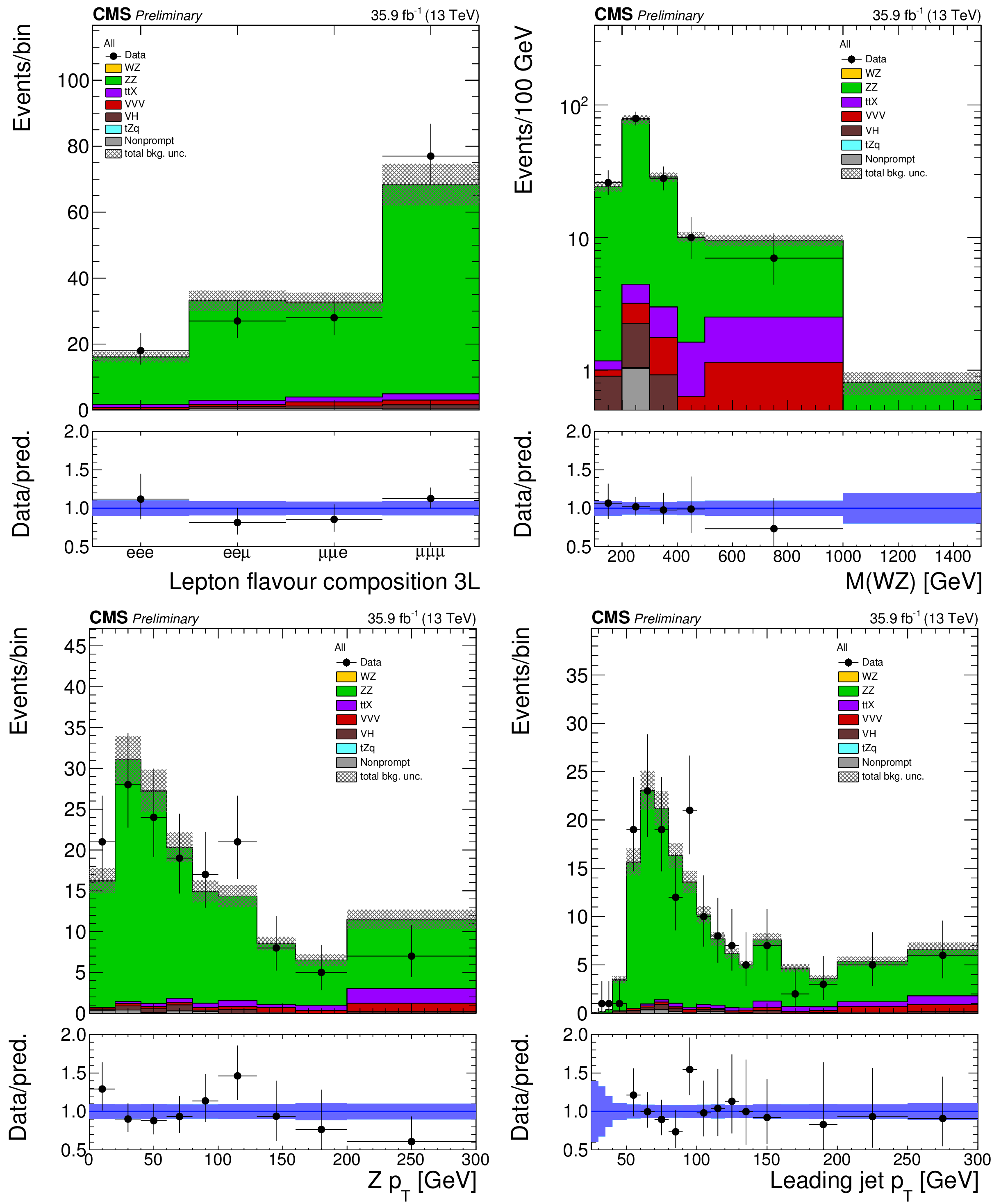
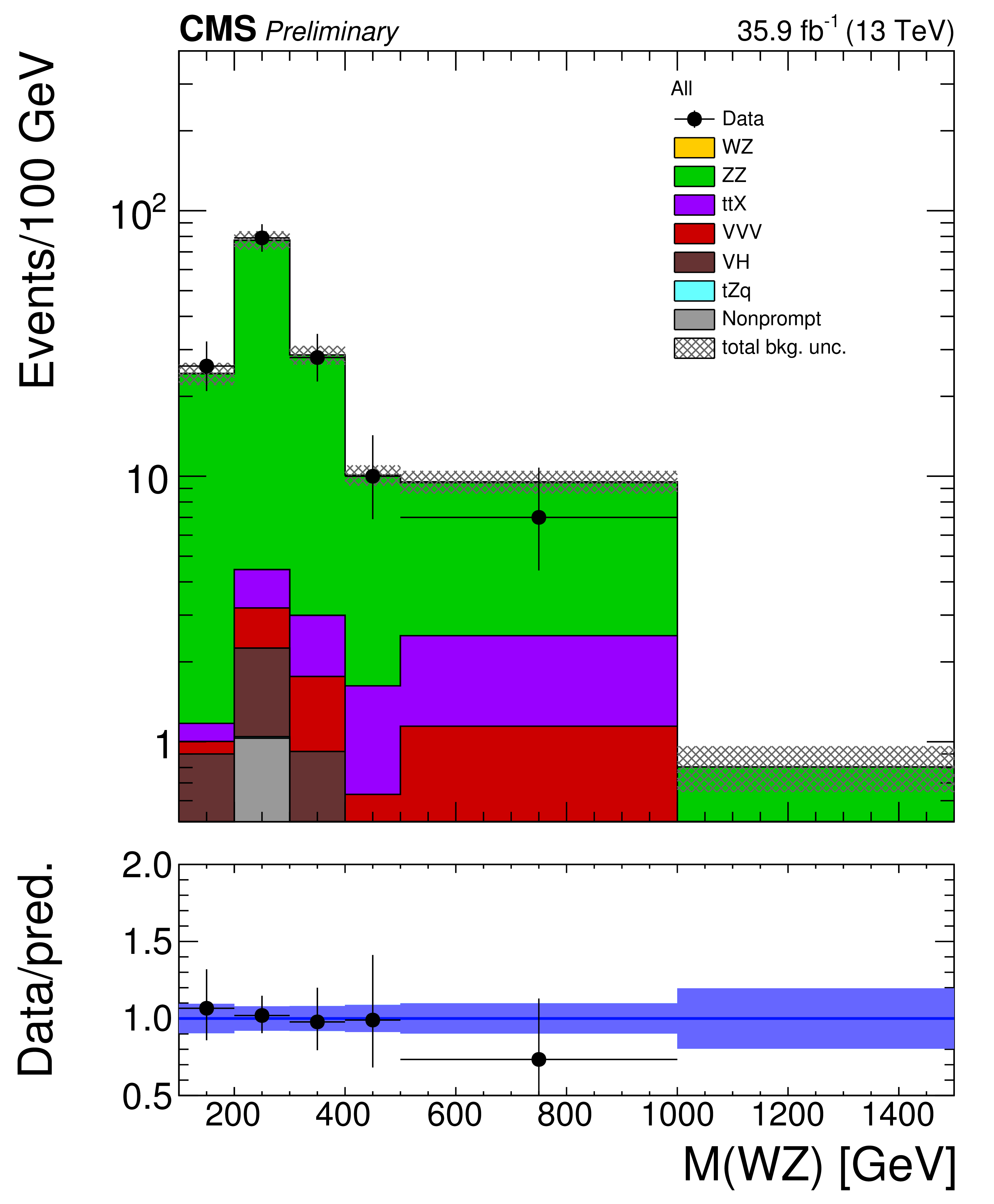
Figure 3:
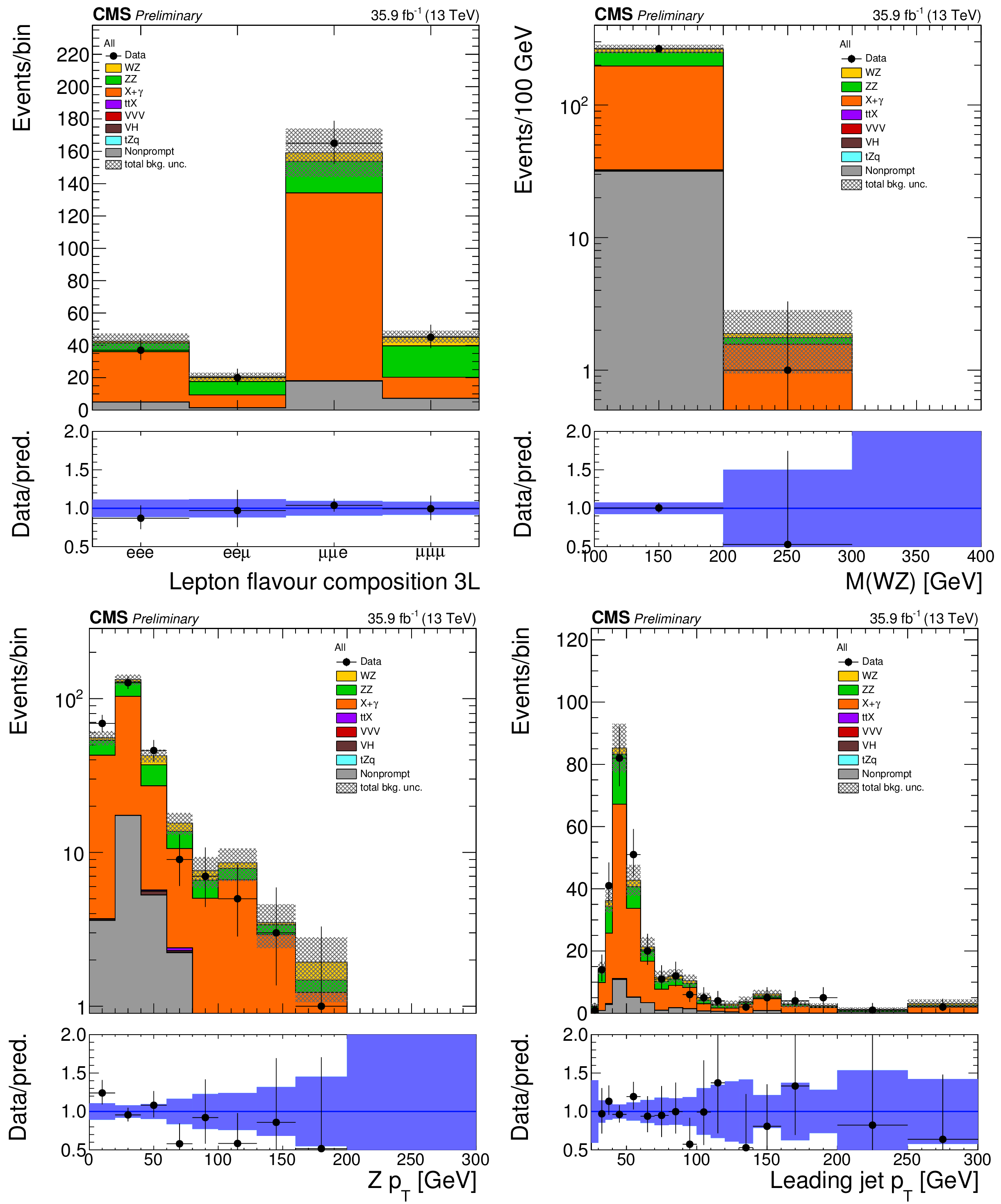
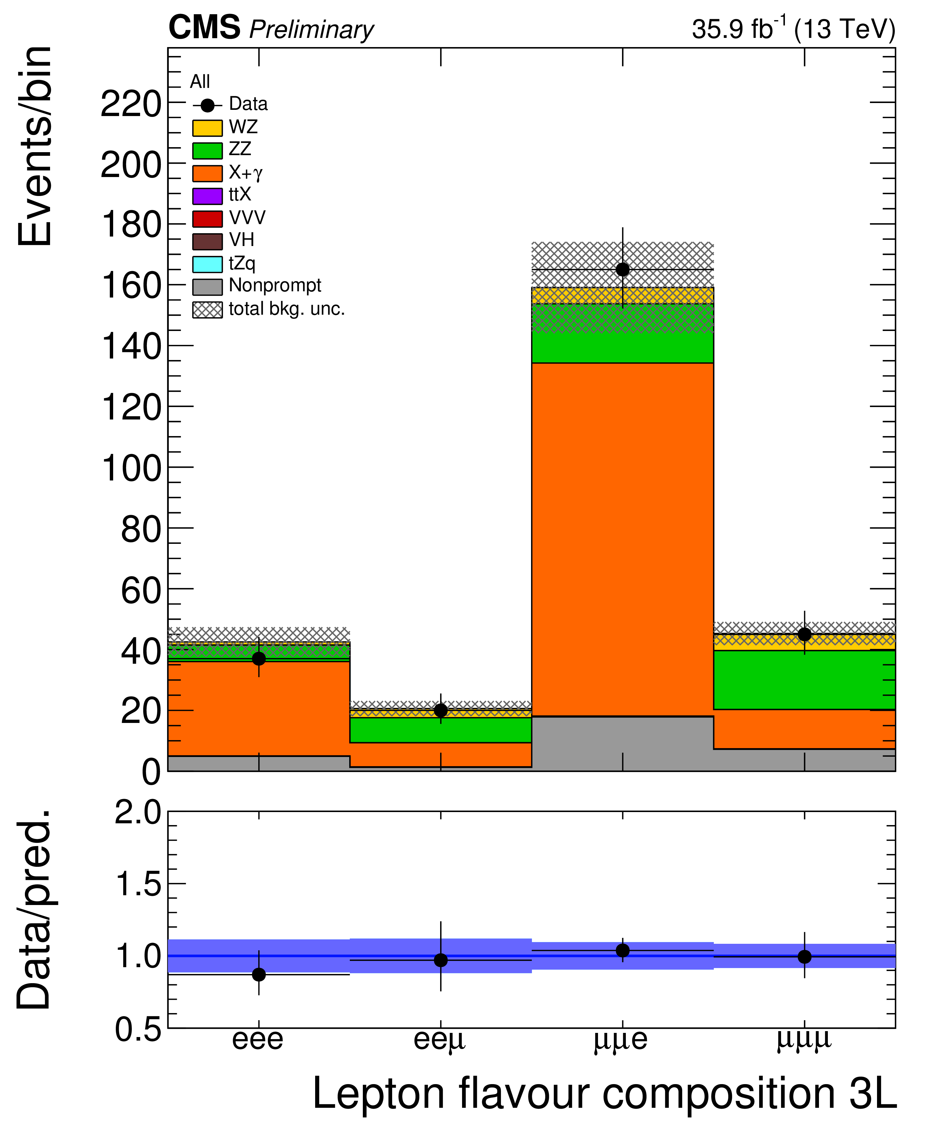
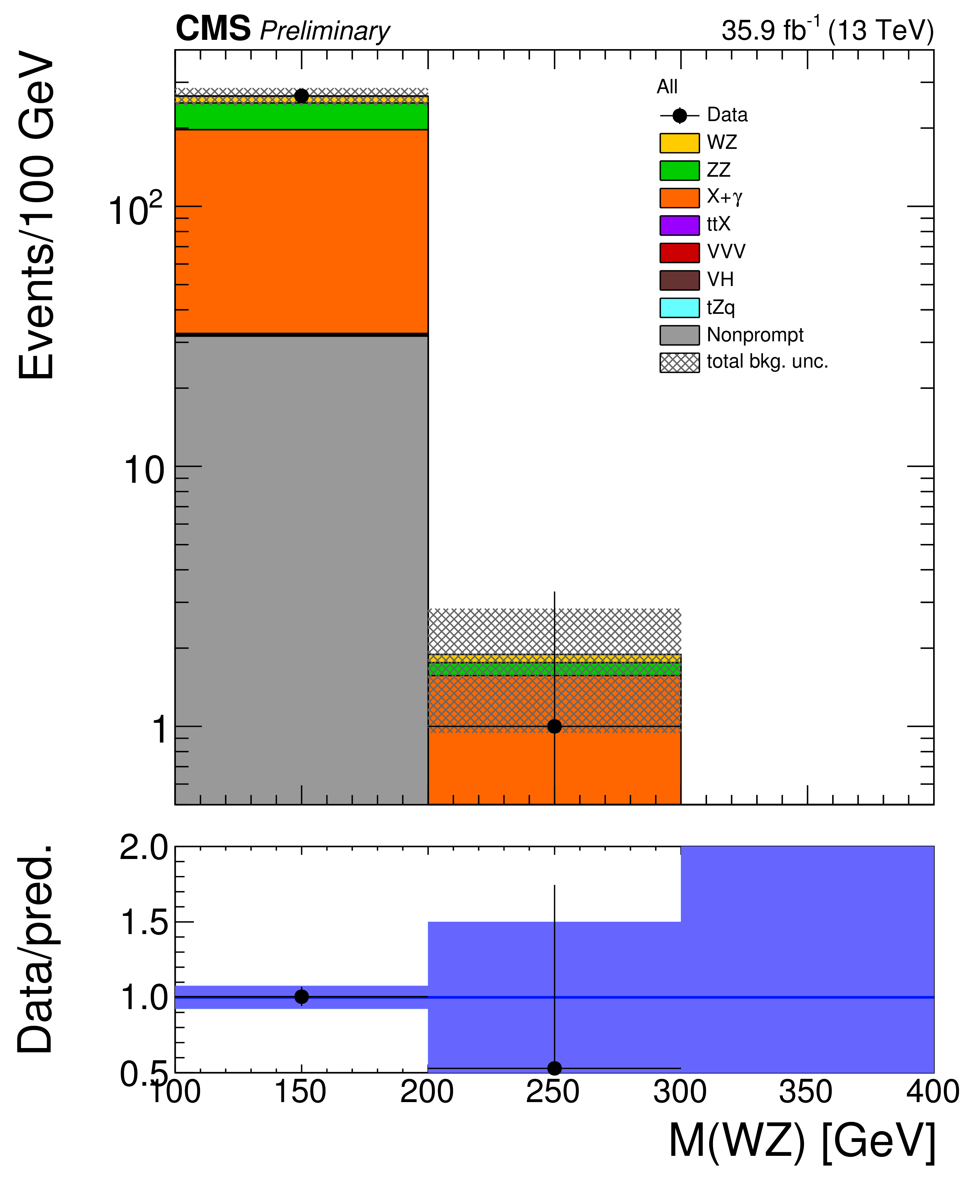
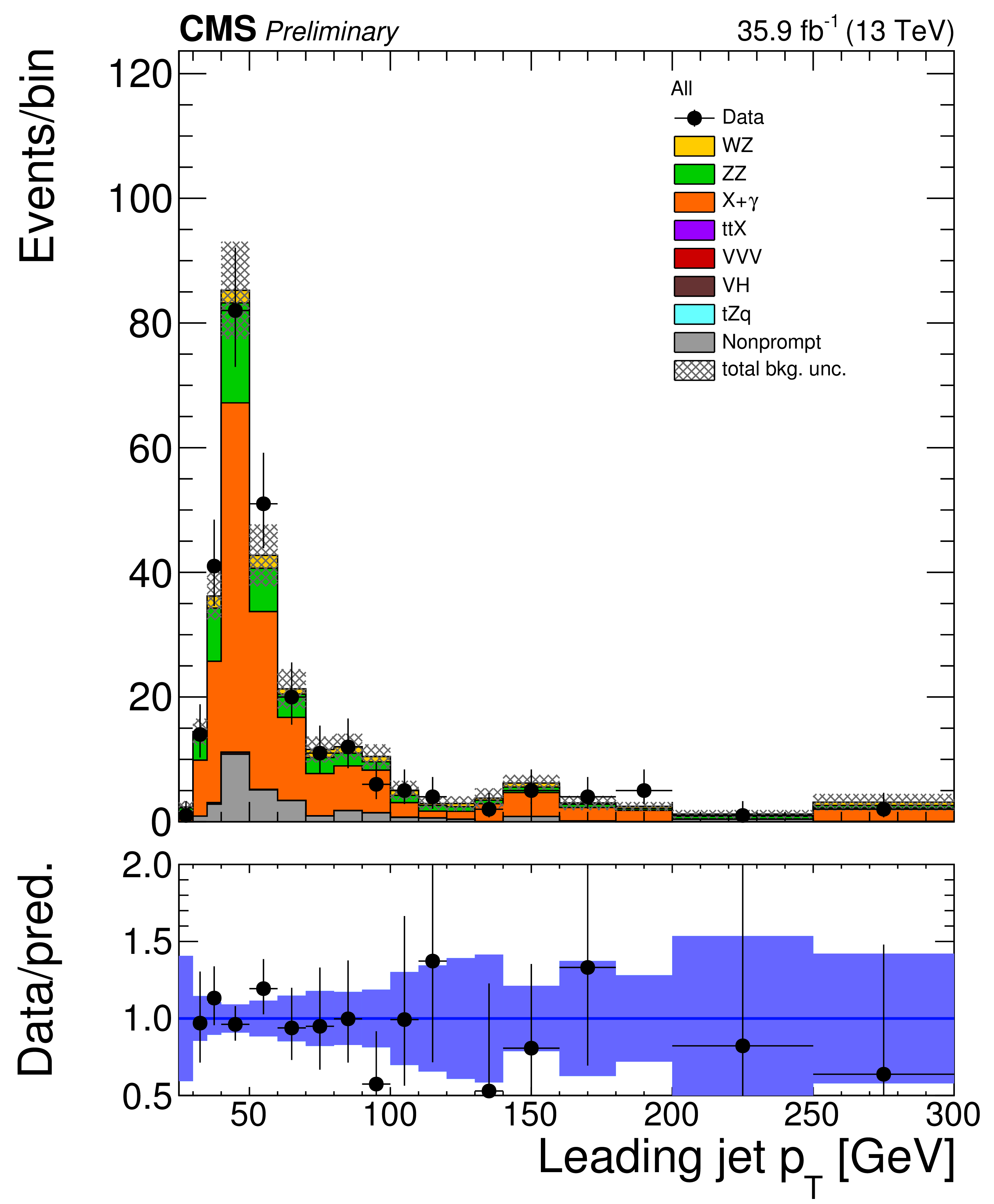
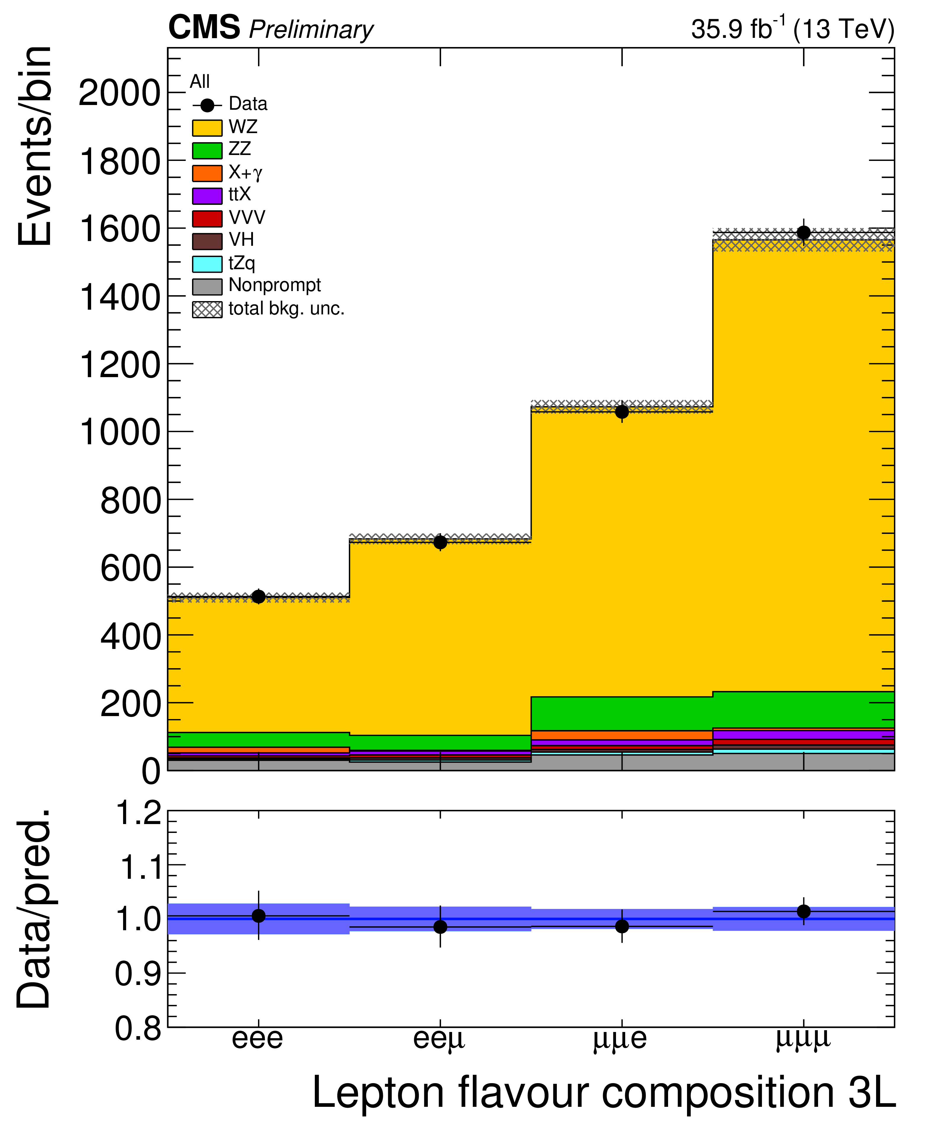
Distribution of key observables of the analysis in the ZZ control region: flavour composition of the three leading leptons (top left), invariant mass of the three leptons plus missing transverse momentum (top right), transverse momentum of the Z boson reconstructed from the ${p_{\mathrm {T}}}$ of the two leptons assigned to it, and transverse momentum of the leading jet. Vertical bars on the data points include their statistical uncertainty and shaded bands over the prediction include the contributions of the different sources of uncertainty evaluated after the signal extraction fit. |

png pdf |
Figure 3-a:
Distribution of key observables of the analysis in the ZZ control region: flavour composition of the three leading leptons (top left), invariant mass of the three leptons plus missing transverse momentum (top right), transverse momentum of the Z boson reconstructed from the ${p_{\mathrm {T}}}$ of the two leptons assigned to it, and transverse momentum of the leading jet. Vertical bars on the data points include their statistical uncertainty and shaded bands over the prediction include the contributions of the different sources of uncertainty evaluated after the signal extraction fit. |
png pdf |
Figure 3-b:
Distribution of key observables of the analysis in the ZZ control region: flavour composition of the three leading leptons (top left), invariant mass of the three leptons plus missing transverse momentum (top right), transverse momentum of the Z boson reconstructed from the ${p_{\mathrm {T}}}$ of the two leptons assigned to it, and transverse momentum of the leading jet. Vertical bars on the data points include their statistical uncertainty and shaded bands over the prediction include the contributions of the different sources of uncertainty evaluated after the signal extraction fit. |

png pdf |
Figure 3-c:
Distribution of key observables of the analysis in the ZZ control region: flavour composition of the three leading leptons (top left), invariant mass of the three leptons plus missing transverse momentum (top right), transverse momentum of the Z boson reconstructed from the ${p_{\mathrm {T}}}$ of the two leptons assigned to it, and transverse momentum of the leading jet. Vertical bars on the data points include their statistical uncertainty and shaded bands over the prediction include the contributions of the different sources of uncertainty evaluated after the signal extraction fit. |
png pdf |
Figure 3-d:
Distribution of key observables of the analysis in the ZZ control region: flavour composition of the three leading leptons (top left), invariant mass of the three leptons plus missing transverse momentum (top right), transverse momentum of the Z boson reconstructed from the ${p_{\mathrm {T}}}$ of the two leptons assigned to it, and transverse momentum of the leading jet. Vertical bars on the data points include their statistical uncertainty and shaded bands over the prediction include the contributions of the different sources of uncertainty evaluated after the signal extraction fit. |
png pdf |
Figure 4:
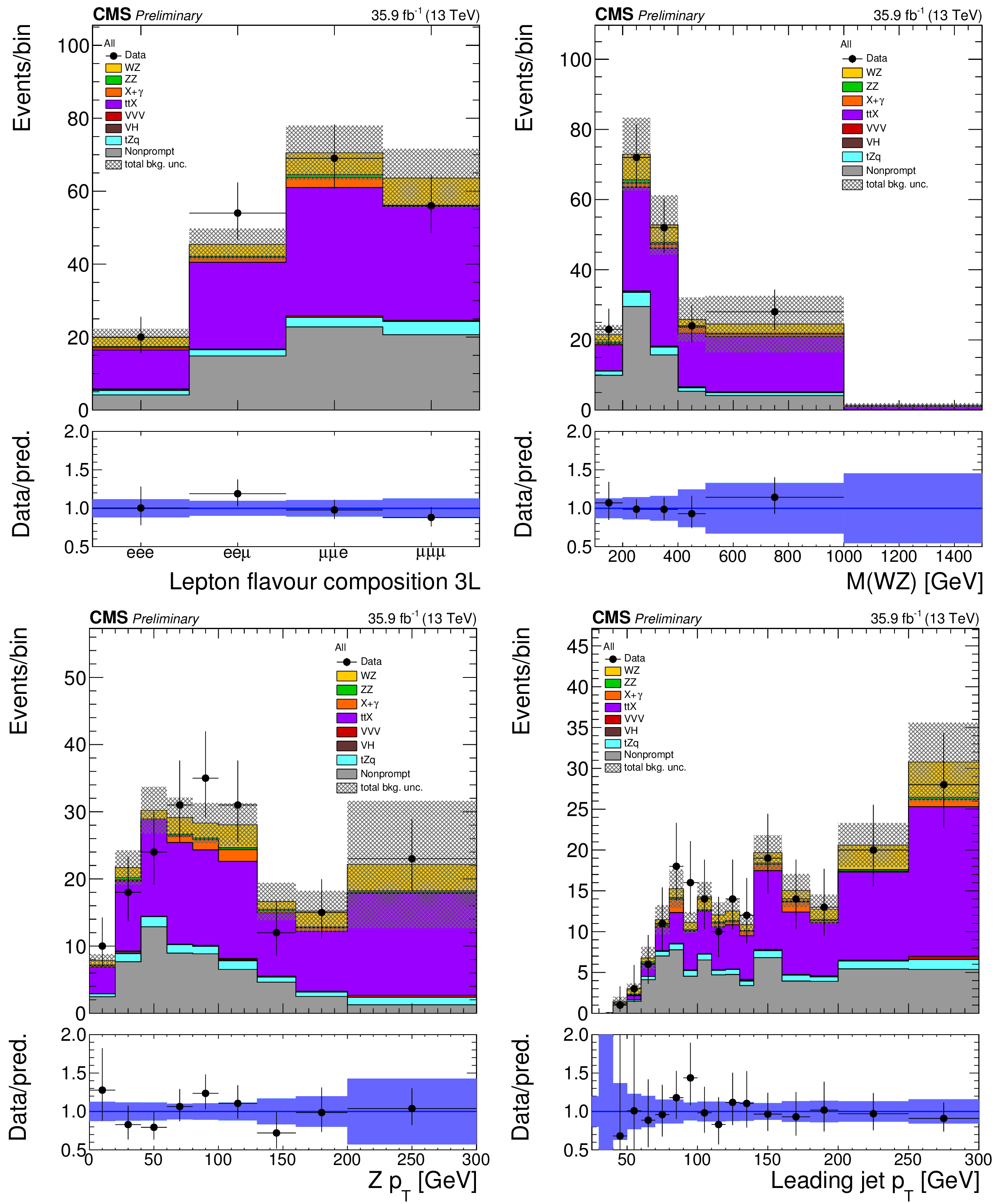
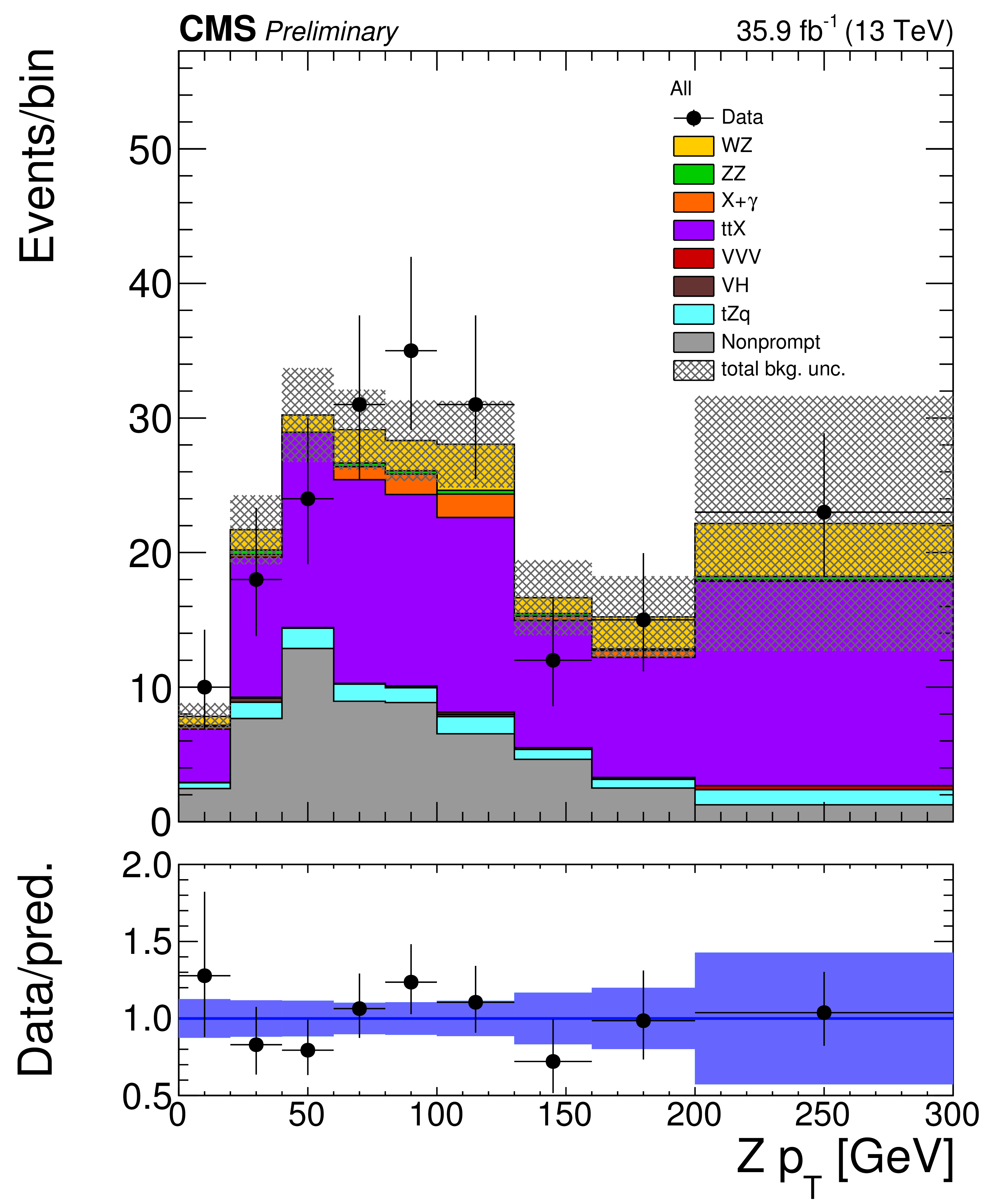
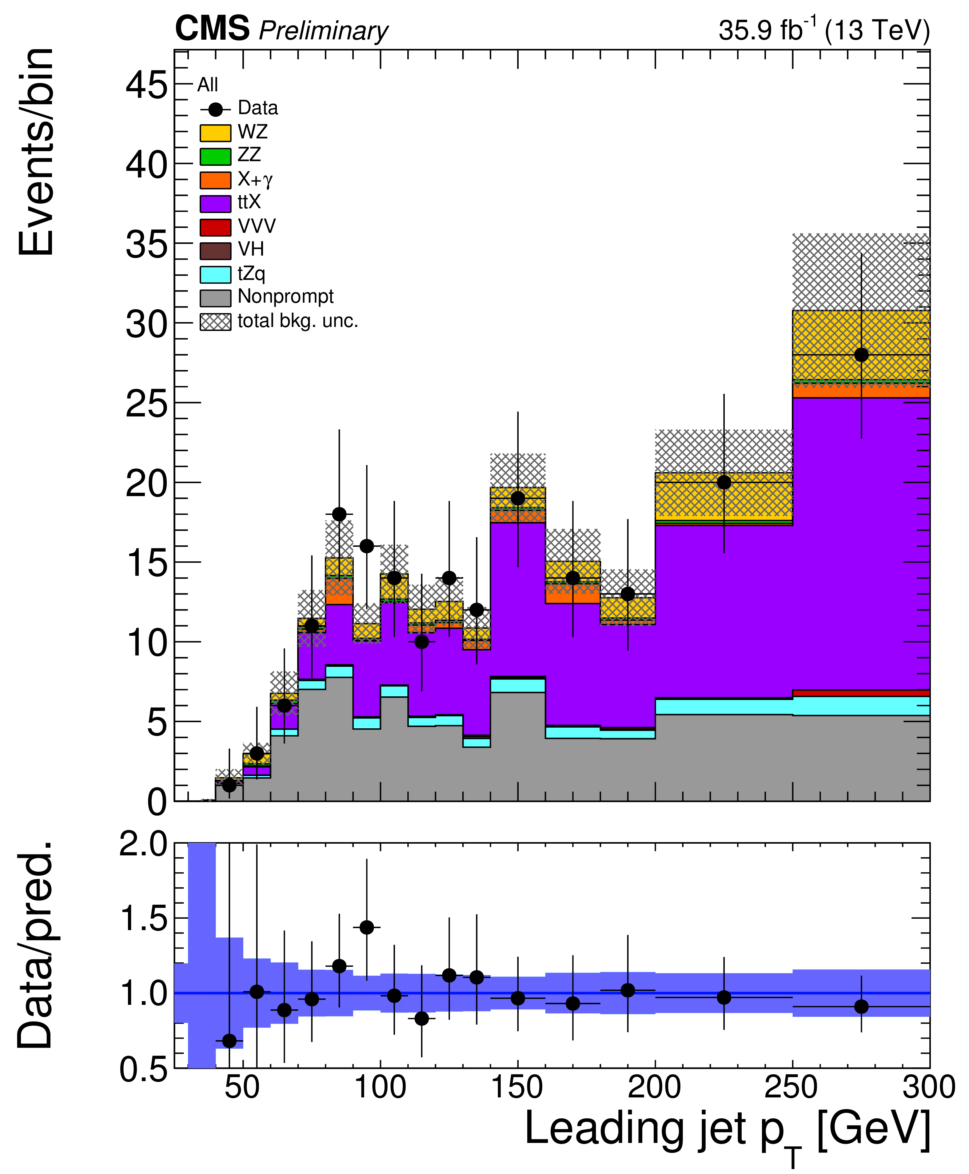
Distribution of key observables of the analysis in the top enriched control region: flavour composition of the three leading leptons (top left), invariant mass of the three lepton plus missing transverse momentum (top right), transverse momentum of the Z boson reconstructed from the ${p_{\mathrm {T}}}$ of the two leptons assigned to it and transverse momentum of the leading jet. Vertical bars on the data points include their statistical uncertainty and shaded bands over the prediction include the contributions of the different sources of uncertainty evaluated after the signal extraction fit. |

png pdf |
Figure 4-a:
Distribution of key observables of the analysis in the top enriched control region: flavour composition of the three leading leptons (top left), invariant mass of the three lepton plus missing transverse momentum (top right), transverse momentum of the Z boson reconstructed from the ${p_{\mathrm {T}}}$ of the two leptons assigned to it and transverse momentum of the leading jet. Vertical bars on the data points include their statistical uncertainty and shaded bands over the prediction include the contributions of the different sources of uncertainty evaluated after the signal extraction fit. |

png pdf |
Figure 4-b:
Distribution of key observables of the analysis in the top enriched control region: flavour composition of the three leading leptons (top left), invariant mass of the three lepton plus missing transverse momentum (top right), transverse momentum of the Z boson reconstructed from the ${p_{\mathrm {T}}}$ of the two leptons assigned to it and transverse momentum of the leading jet. Vertical bars on the data points include their statistical uncertainty and shaded bands over the prediction include the contributions of the different sources of uncertainty evaluated after the signal extraction fit. |
png pdf |
Figure 4-c:
Distribution of key observables of the analysis in the top enriched control region: flavour composition of the three leading leptons (top left), invariant mass of the three lepton plus missing transverse momentum (top right), transverse momentum of the Z boson reconstructed from the ${p_{\mathrm {T}}}$ of the two leptons assigned to it and transverse momentum of the leading jet. Vertical bars on the data points include their statistical uncertainty and shaded bands over the prediction include the contributions of the different sources of uncertainty evaluated after the signal extraction fit. |
png pdf |
Figure 4-d:
Distribution of key observables of the analysis in the top enriched control region: flavour composition of the three leading leptons (top left), invariant mass of the three lepton plus missing transverse momentum (top right), transverse momentum of the Z boson reconstructed from the ${p_{\mathrm {T}}}$ of the two leptons assigned to it and transverse momentum of the leading jet. Vertical bars on the data points include their statistical uncertainty and shaded bands over the prediction include the contributions of the different sources of uncertainty evaluated after the signal extraction fit. |
png pdf |
Figure 5:
Distribution of key observables of the analysis in the conversion control region: flavour composition of the three leading leptons (top left), invariant mass of the three lepton plus missing transverse momentum (top right), transverse momentum of the Z boson reconstructed from the ${p_{\mathrm {T}}}$ of the two leptons assigned to it and transverse momentum of the leading jet. Vertical bars on the data points include their statistical uncertainty and shaded bands over the prediction include the contributions of the different sources of uncertainty evaluated after the signal extraction fit. |
png pdf |
Figure 5-a:
Distribution of key observables of the analysis in the conversion control region: flavour composition of the three leading leptons (top left), invariant mass of the three lepton plus missing transverse momentum (top right), transverse momentum of the Z boson reconstructed from the ${p_{\mathrm {T}}}$ of the two leptons assigned to it and transverse momentum of the leading jet. Vertical bars on the data points include their statistical uncertainty and shaded bands over the prediction include the contributions of the different sources of uncertainty evaluated after the signal extraction fit. |
png pdf |
Figure 5-b:
Distribution of key observables of the analysis in the conversion control region: flavour composition of the three leading leptons (top left), invariant mass of the three lepton plus missing transverse momentum (top right), transverse momentum of the Z boson reconstructed from the ${p_{\mathrm {T}}}$ of the two leptons assigned to it and transverse momentum of the leading jet. Vertical bars on the data points include their statistical uncertainty and shaded bands over the prediction include the contributions of the different sources of uncertainty evaluated after the signal extraction fit. |

png pdf |
Figure 5-c:
Distribution of key observables of the analysis in the conversion control region: flavour composition of the three leading leptons (top left), invariant mass of the three lepton plus missing transverse momentum (top right), transverse momentum of the Z boson reconstructed from the ${p_{\mathrm {T}}}$ of the two leptons assigned to it and transverse momentum of the leading jet. Vertical bars on the data points include their statistical uncertainty and shaded bands over the prediction include the contributions of the different sources of uncertainty evaluated after the signal extraction fit. |
png pdf |
Figure 5-d:
Distribution of key observables of the analysis in the conversion control region: flavour composition of the three leading leptons (top left), invariant mass of the three lepton plus missing transverse momentum (top right), transverse momentum of the Z boson reconstructed from the ${p_{\mathrm {T}}}$ of the two leptons assigned to it and transverse momentum of the leading jet. Vertical bars on the data points include their statistical uncertainty and shaded bands over the prediction include the contributions of the different sources of uncertainty evaluated after the signal extraction fit. |
png pdf |
Figure 6:
Distribution of expected and observed event yields in the four flavour categories used for the cross section measurement. Vertical bars on the data points include their statistical uncertainty and shaded bands over the prediction include the contributions of the different sources of uncertainty evaluated after the signal extraction fit. |
png pdf |
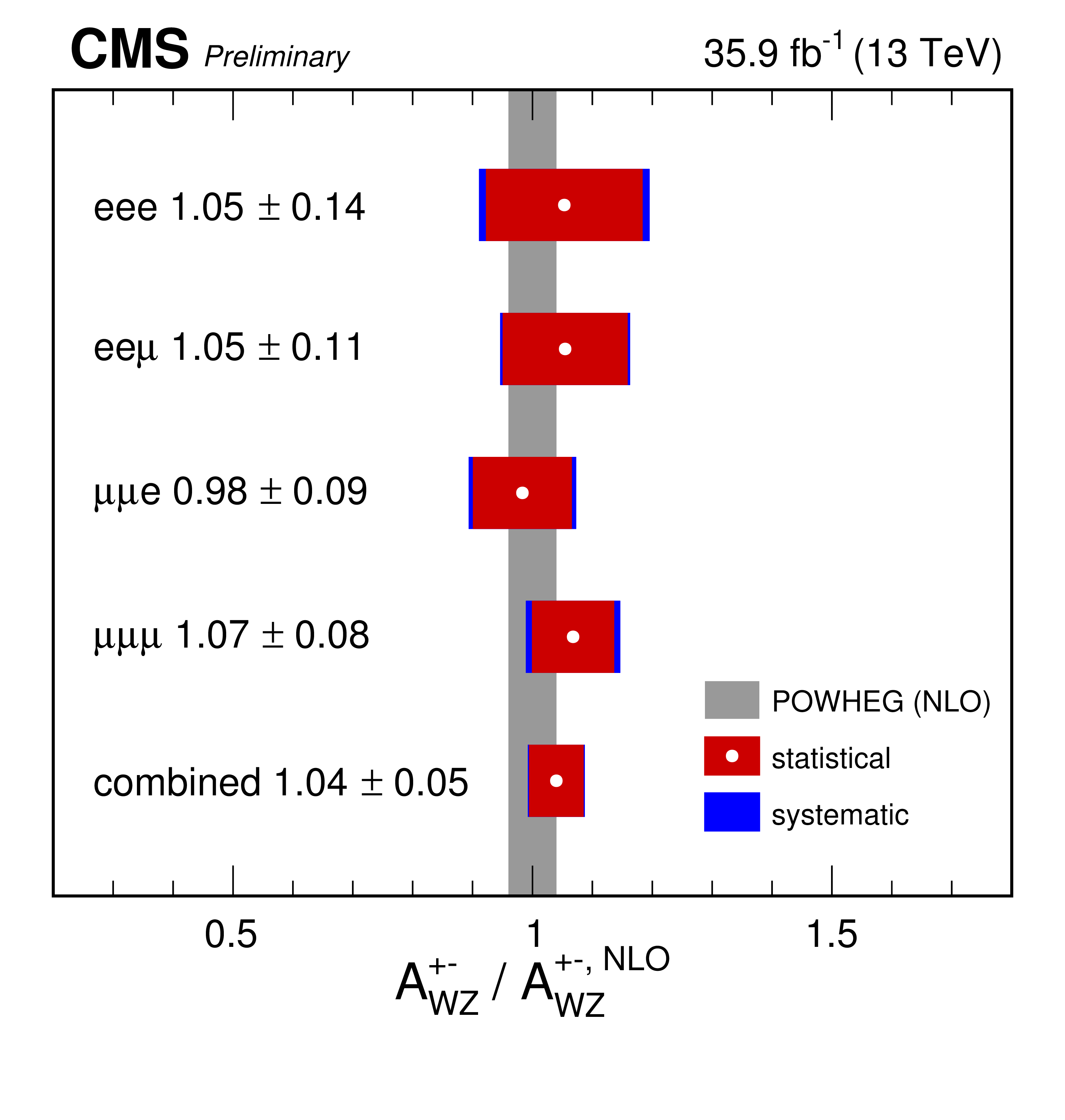
Figure 7:
Measured ratio of cross sections for the two charge channels for each of the flavour categories and their combination. Coloured bands for each of the points include both systematic and statistical uncertainties. Shaded bands correspond to the Monte Carlo prediction from the nominal {powheg} sample and its associated uncertainty. |

png pdf |
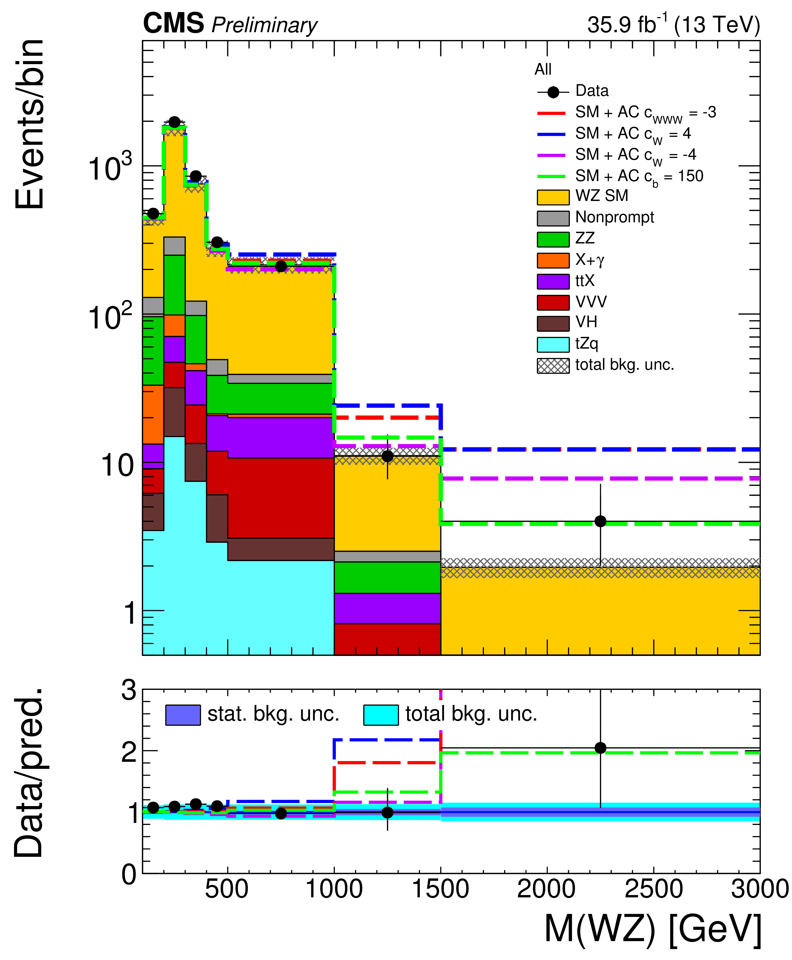
Figure 8:
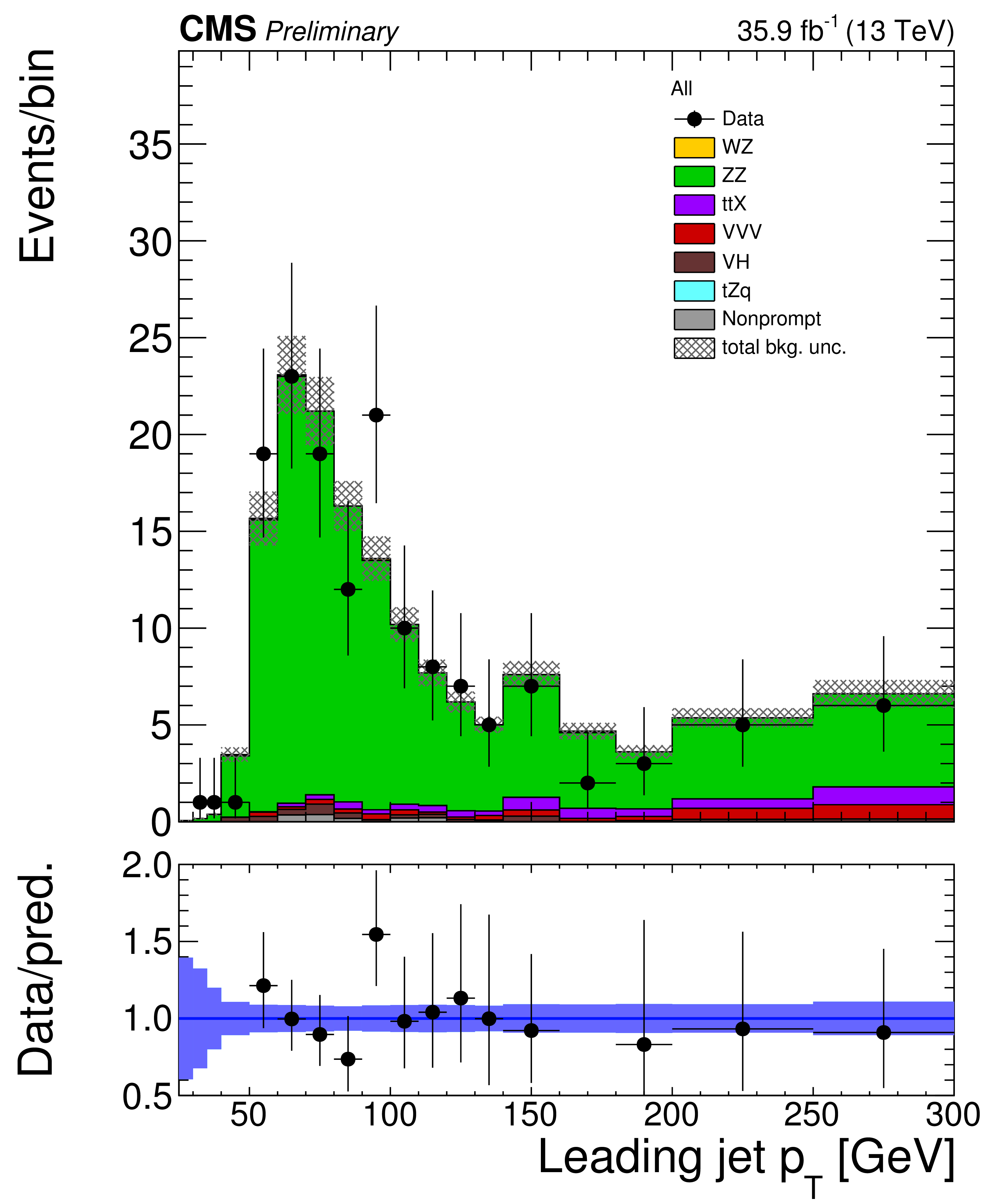
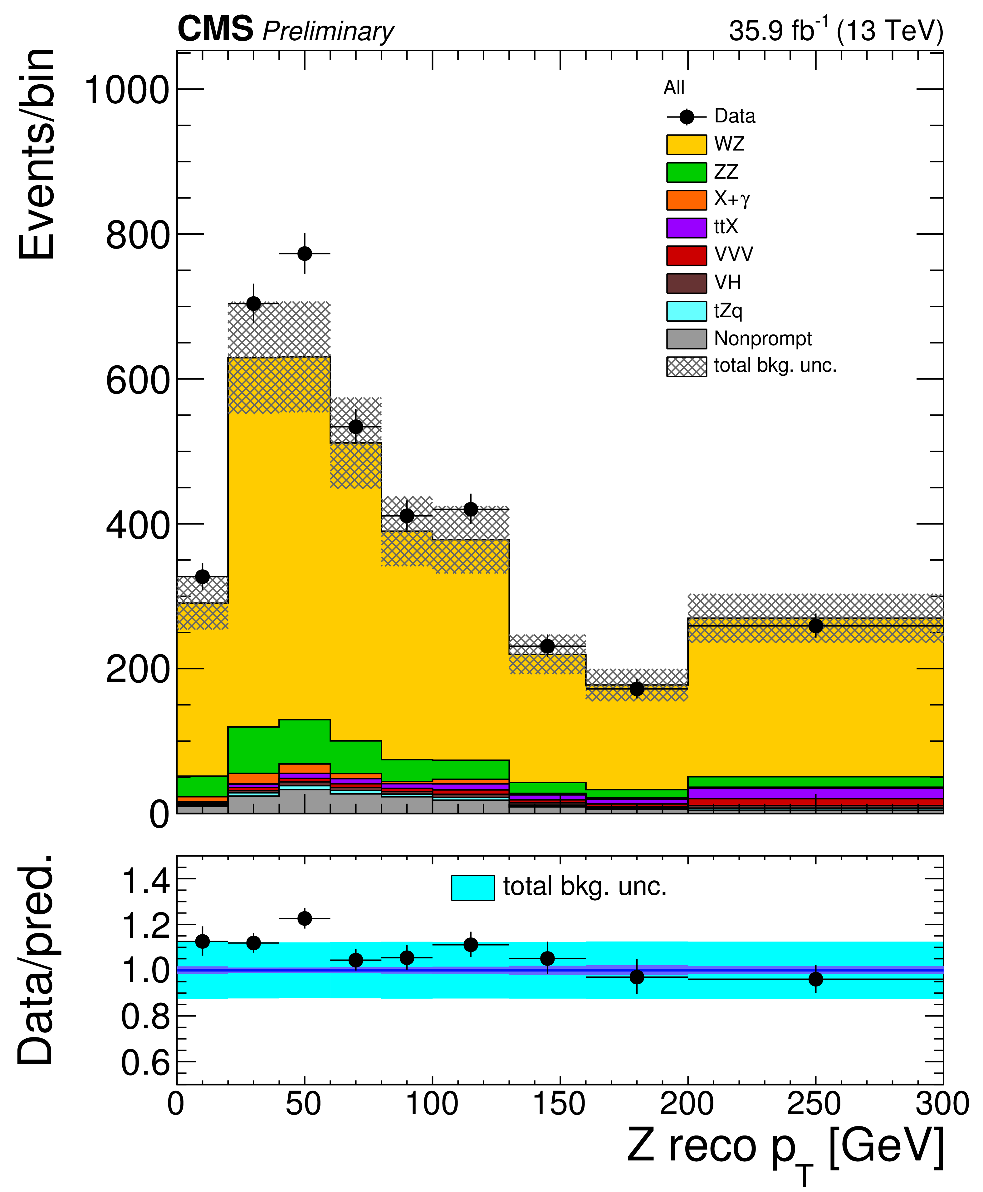
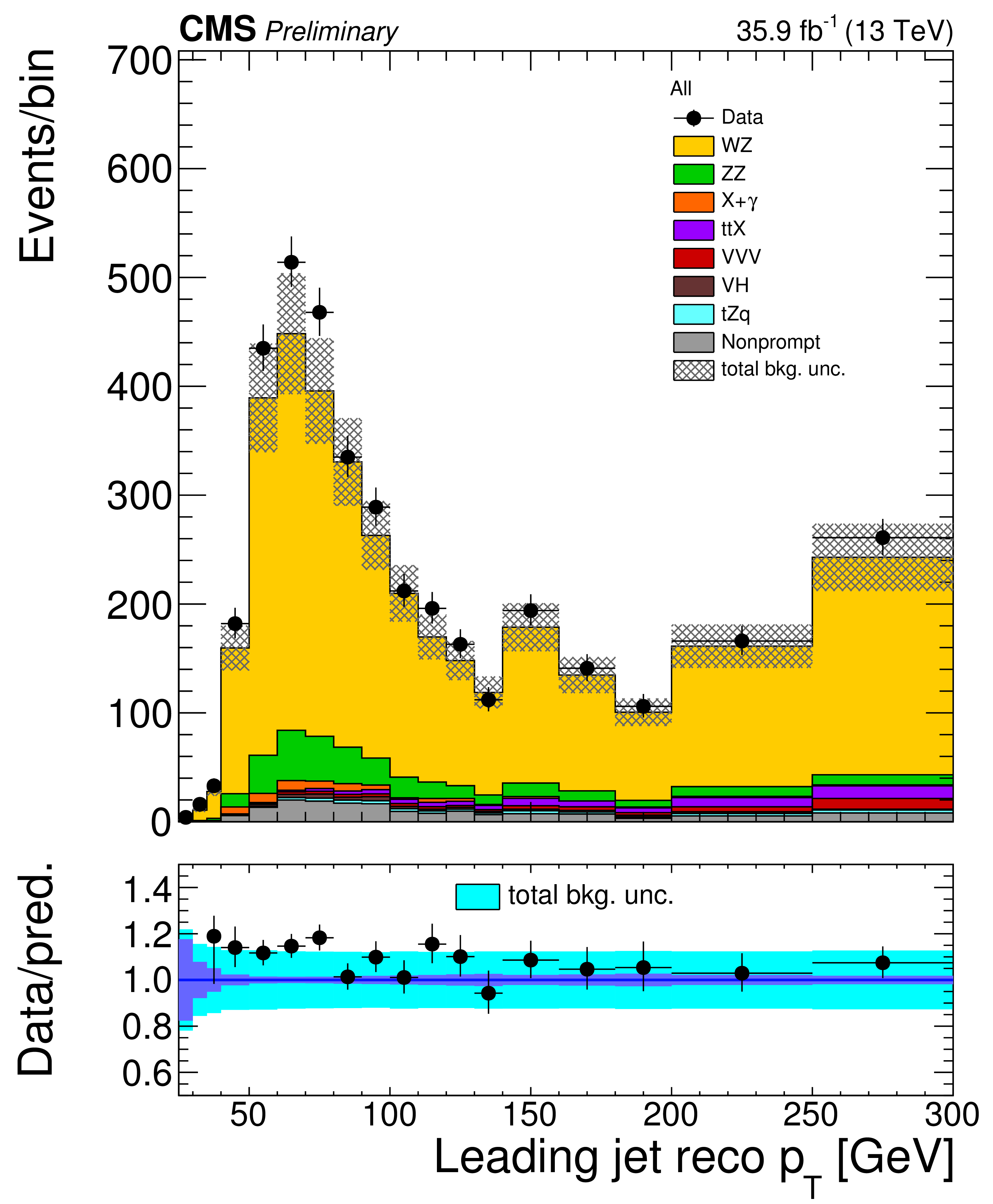
Distributions of key observables in the signal region. The transverse momentum of the Z boson, estimated from the two final state leptons assigned to the Z boson, (top left), the transverse momentum of the leading jet (top right), and the mass of the WZ system, estimated as the mass of the trilepton system plus the missing transverse momentum vector (bottom). The last bin contains the overflow. Vertical bars on the data points include their statistical uncertainty and shaded bands over the MC prediction include both the statistical and the systematic uncertainties in the normalization of each of the background processes. An additional 15% uncertainty is assigned to the signal WZ process in the figures to account for the NLO/NNLO normalization differences. |
png pdf |
Figure 8-a:
Distributions of key observables in the signal region. The transverse momentum of the Z boson, estimated from the two final state leptons assigned to the Z boson, (top left), the transverse momentum of the leading jet (top right), and the mass of the WZ system, estimated as the mass of the trilepton system plus the missing transverse momentum vector (bottom). The last bin contains the overflow. Vertical bars on the data points include their statistical uncertainty and shaded bands over the MC prediction include both the statistical and the systematic uncertainties in the normalization of each of the background processes. An additional 15% uncertainty is assigned to the signal WZ process in the figures to account for the NLO/NNLO normalization differences. |
png pdf |
Figure 8-b:
Distributions of key observables in the signal region. The transverse momentum of the Z boson, estimated from the two final state leptons assigned to the Z boson, (top left), the transverse momentum of the leading jet (top right), and the mass of the WZ system, estimated as the mass of the trilepton system plus the missing transverse momentum vector (bottom). The last bin contains the overflow. Vertical bars on the data points include their statistical uncertainty and shaded bands over the MC prediction include both the statistical and the systematic uncertainties in the normalization of each of the background processes. An additional 15% uncertainty is assigned to the signal WZ process in the figures to account for the NLO/NNLO normalization differences. |

png pdf |
Figure 8-c:
Distributions of key observables in the signal region. The transverse momentum of the Z boson, estimated from the two final state leptons assigned to the Z boson, (top left), the transverse momentum of the leading jet (top right), and the mass of the WZ system, estimated as the mass of the trilepton system plus the missing transverse momentum vector (bottom). The last bin contains the overflow. Vertical bars on the data points include their statistical uncertainty and shaded bands over the MC prediction include both the statistical and the systematic uncertainties in the normalization of each of the background processes. An additional 15% uncertainty is assigned to the signal WZ process in the figures to account for the NLO/NNLO normalization differences. |

png pdf |
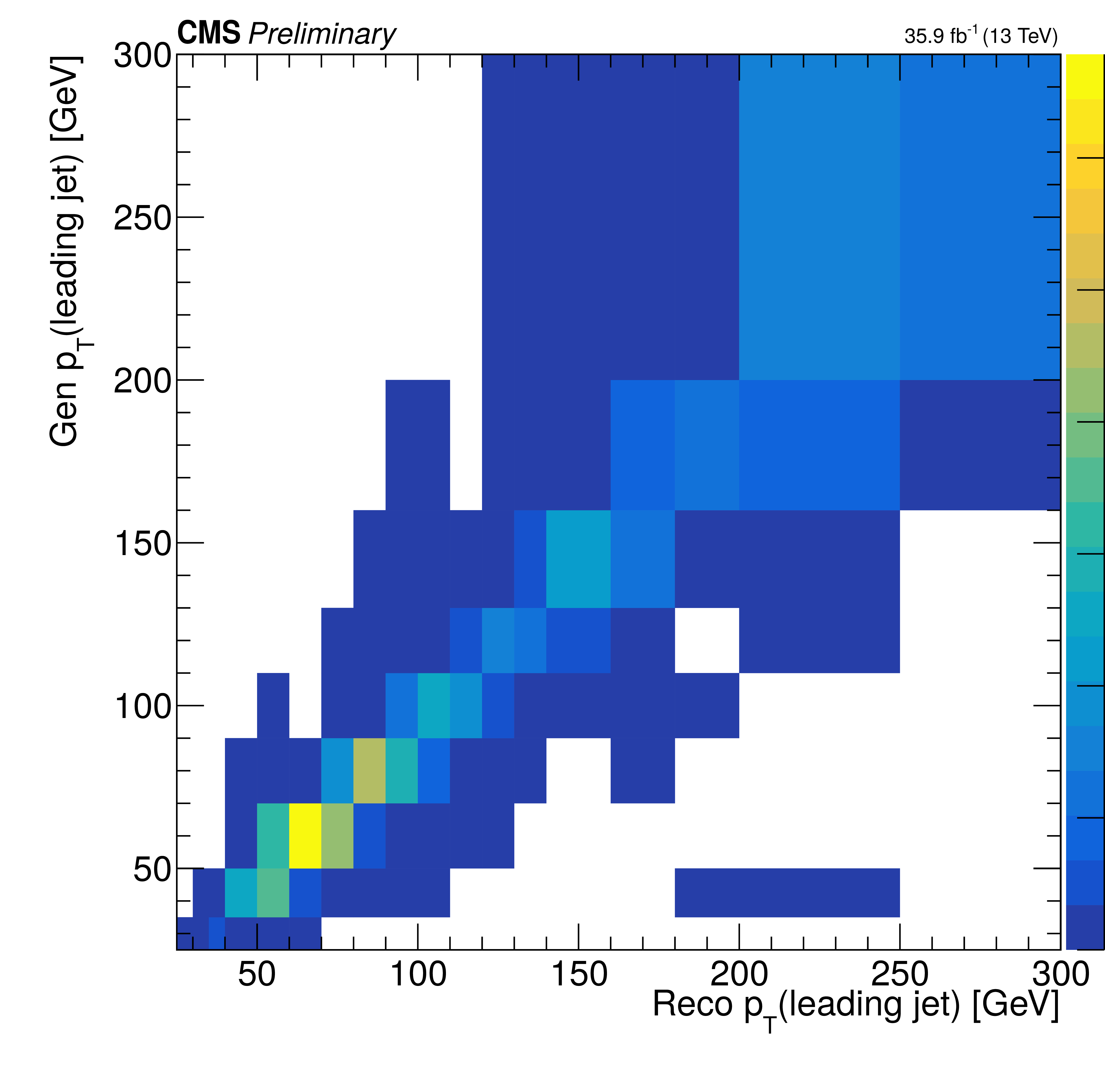
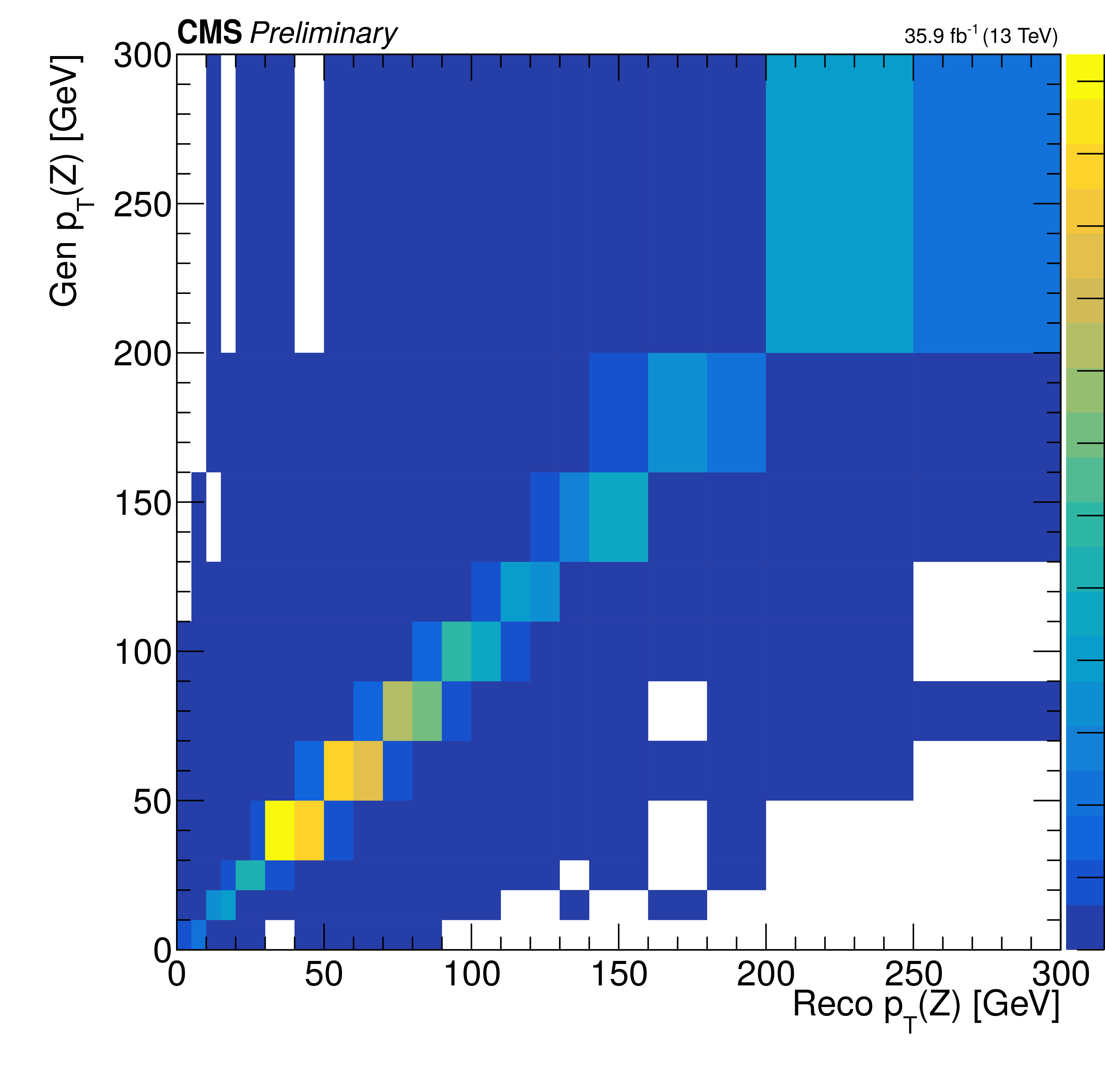
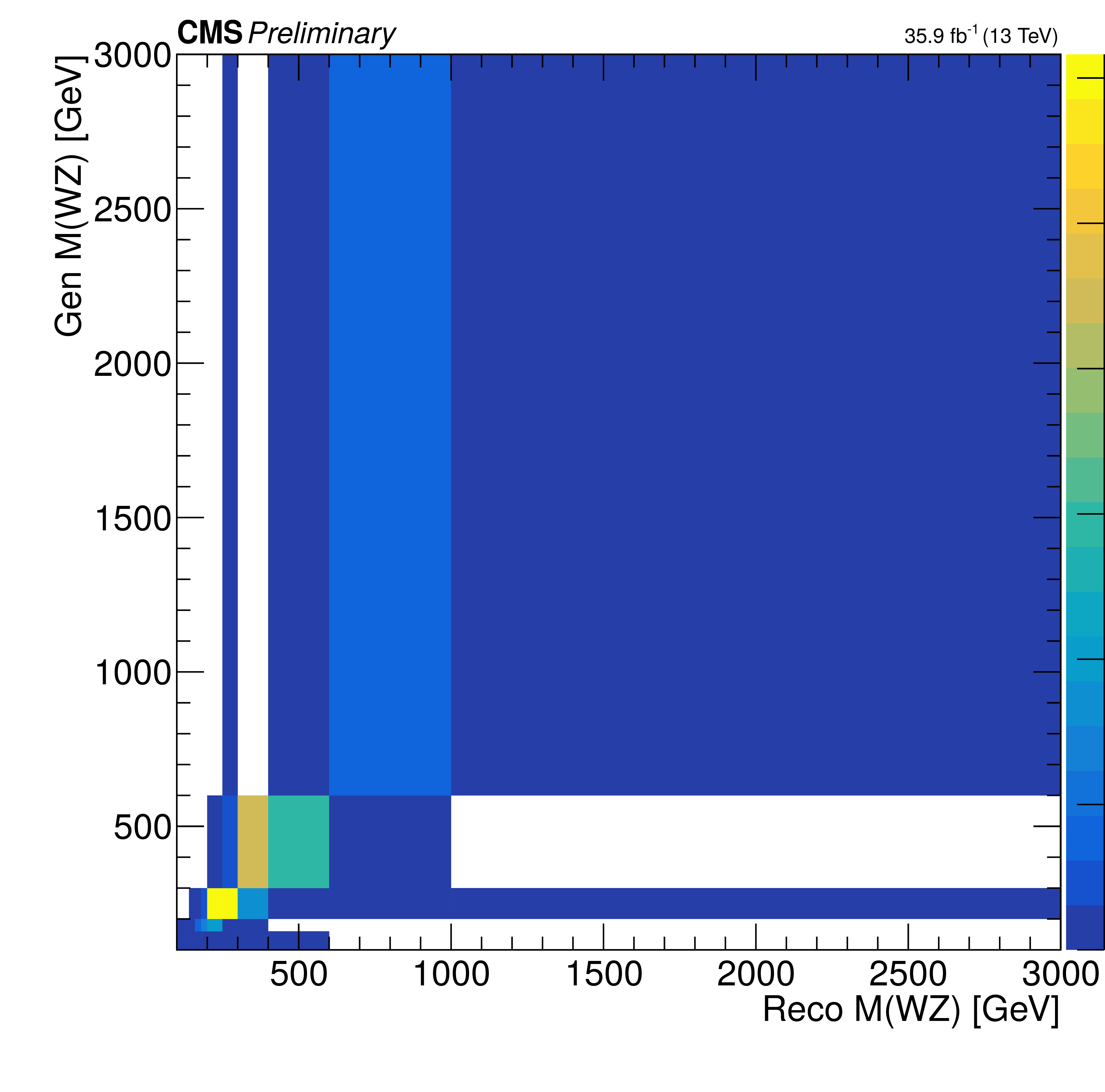
Figure 9:
Response matrices obtained using NLO simulated samples, for the {powheg} generator. The leading jet transverse momentum (top left), the transverse momentum of the Z boson (top right), and the mass of the WZ system (bottom) are shown. |
png pdf |
Figure 9-a:
Response matrices obtained using NLO simulated samples, for the {powheg} generator. The leading jet transverse momentum (top left), the transverse momentum of the Z boson (top right), and the mass of the WZ system (bottom) are shown. |
png pdf |
Figure 9-b:
Response matrices obtained using NLO simulated samples, for the {powheg} generator. The leading jet transverse momentum (top left), the transverse momentum of the Z boson (top right), and the mass of the WZ system (bottom) are shown. |
png pdf |
Figure 9-c:
Response matrices obtained using NLO simulated samples, for the {powheg} generator. The leading jet transverse momentum (top left), the transverse momentum of the Z boson (top right), and the mass of the WZ system (bottom) are shown. |
png pdf |
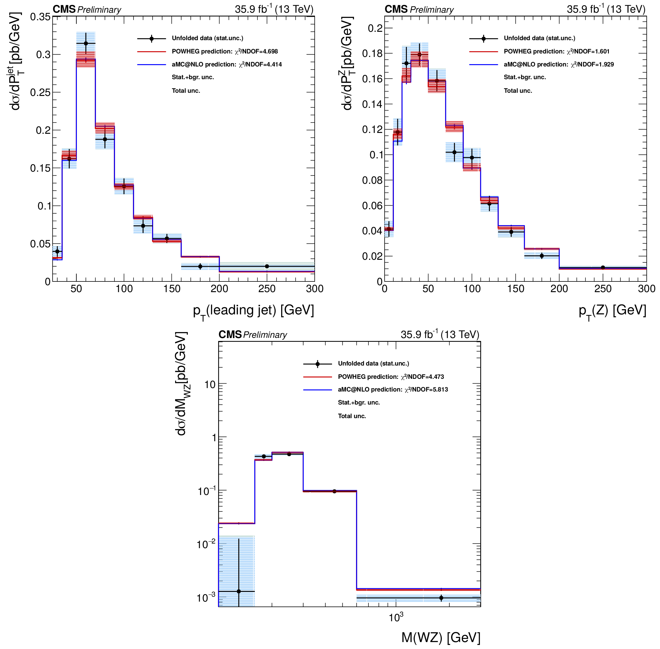
Figure 10:
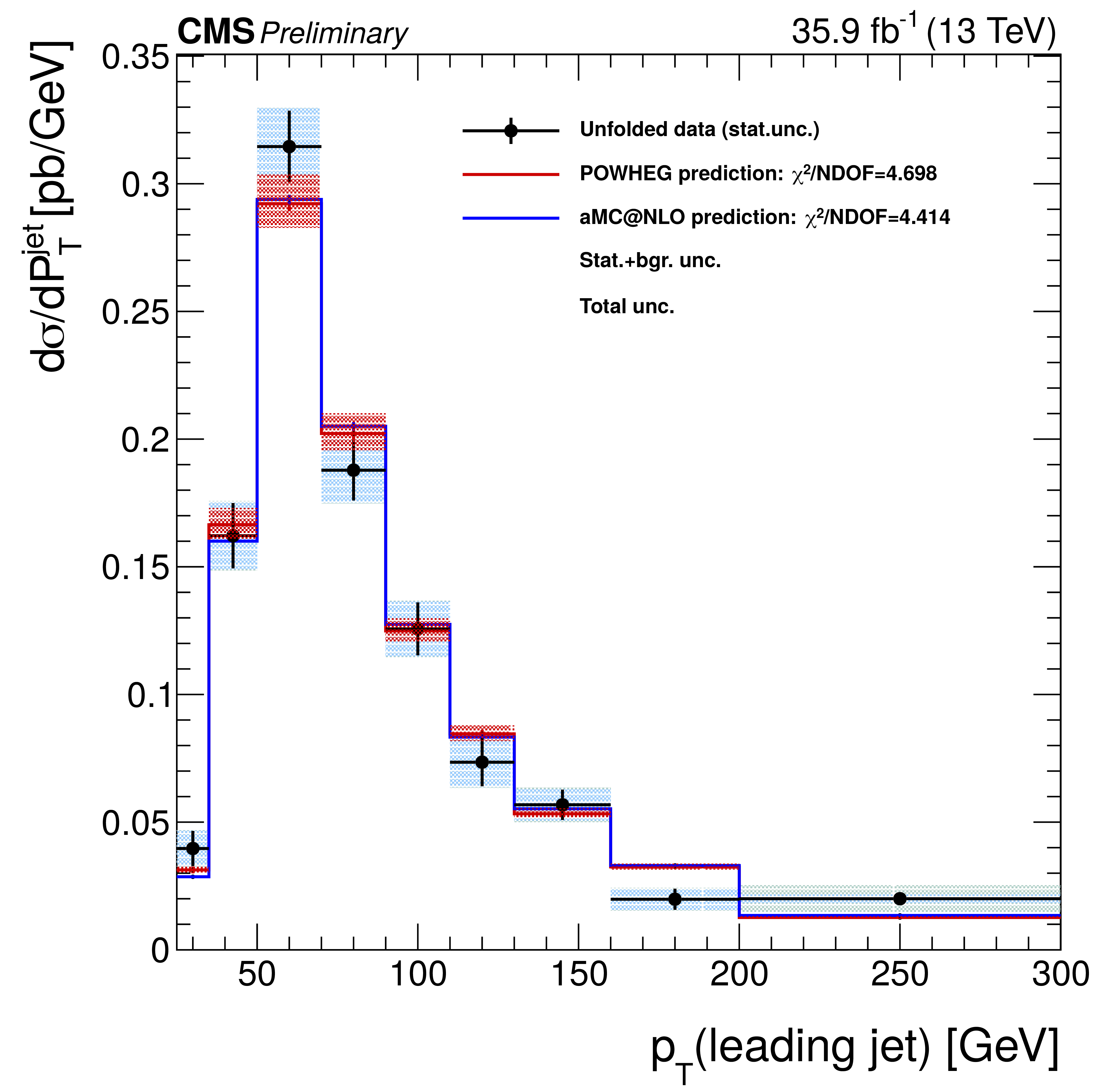
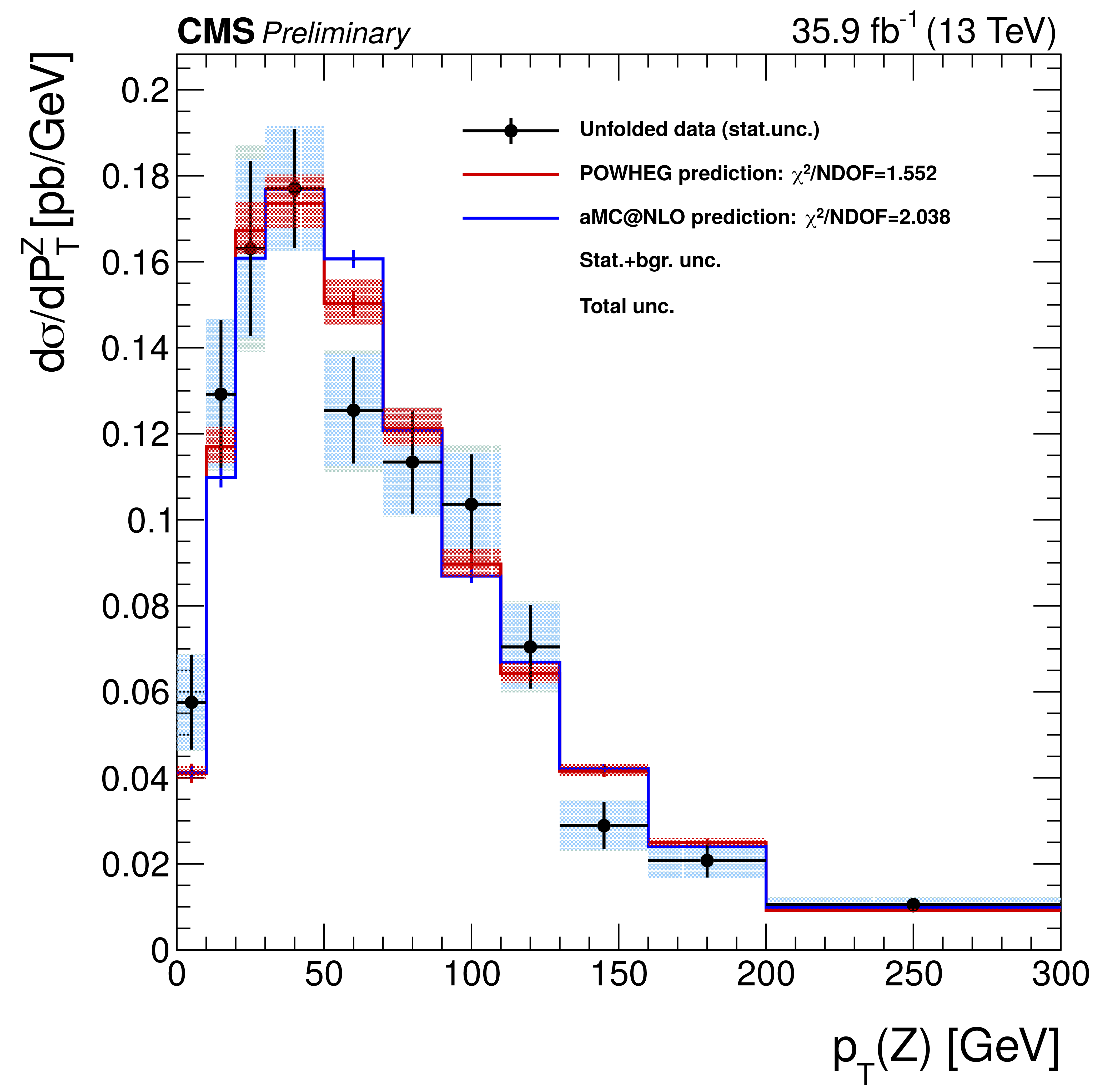
Results for non-regularized unfolding, area constraint, and a bias scale of 1.13. The leading jet ${p_{\mathrm {T}}}$ (top left), Z boson ${p_{\mathrm {T}}}$ (top right), and mass of the WZ system (bottom) data distributions are unfolded at the dressed leptons level and compared with the {powheg}, MadGraph5\_aMC@NLO, and {pythia} predictions. The red band around the {powheg} prediction represents the theory uncertainty on the prediction; the effect on the unfolded data of this uncertainty, through the unfolding matrix, is included in the grey bands described in the legend. The agreement between the normalizations is forced by the choice of bias scale. |
png pdf |
Figure 10-a:
Results for non-regularized unfolding, area constraint, and a bias scale of 1.13. The leading jet ${p_{\mathrm {T}}}$ (top left), Z boson ${p_{\mathrm {T}}}$ (top right), and mass of the WZ system (bottom) data distributions are unfolded at the dressed leptons level and compared with the {powheg}, MadGraph5\_aMC@NLO, and {pythia} predictions. The red band around the {powheg} prediction represents the theory uncertainty on the prediction; the effect on the unfolded data of this uncertainty, through the unfolding matrix, is included in the grey bands described in the legend. The agreement between the normalizations is forced by the choice of bias scale. |

png pdf |
Figure 10-b:
Results for non-regularized unfolding, area constraint, and a bias scale of 1.13. The leading jet ${p_{\mathrm {T}}}$ (top left), Z boson ${p_{\mathrm {T}}}$ (top right), and mass of the WZ system (bottom) data distributions are unfolded at the dressed leptons level and compared with the {powheg}, MadGraph5\_aMC@NLO, and {pythia} predictions. The red band around the {powheg} prediction represents the theory uncertainty on the prediction; the effect on the unfolded data of this uncertainty, through the unfolding matrix, is included in the grey bands described in the legend. The agreement between the normalizations is forced by the choice of bias scale. |

png pdf |
Figure 10-c:
Results for non-regularized unfolding, area constraint, and a bias scale of 1.13. The leading jet ${p_{\mathrm {T}}}$ (top left), Z boson ${p_{\mathrm {T}}}$ (top right), and mass of the WZ system (bottom) data distributions are unfolded at the dressed leptons level and compared with the {powheg}, MadGraph5\_aMC@NLO, and {pythia} predictions. The red band around the {powheg} prediction represents the theory uncertainty on the prediction; the effect on the unfolded data of this uncertainty, through the unfolding matrix, is included in the grey bands described in the legend. The agreement between the normalizations is forced by the choice of bias scale. |
png pdf |
Figure 11:
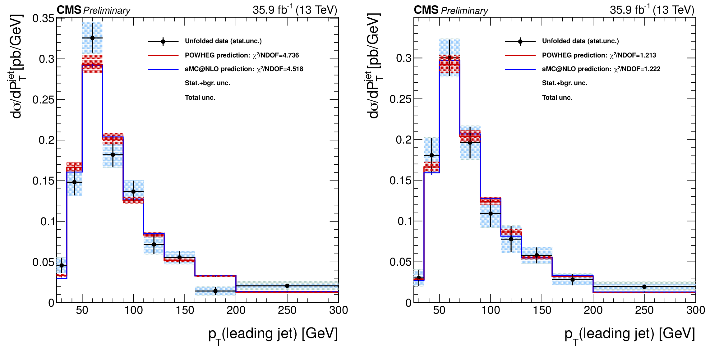
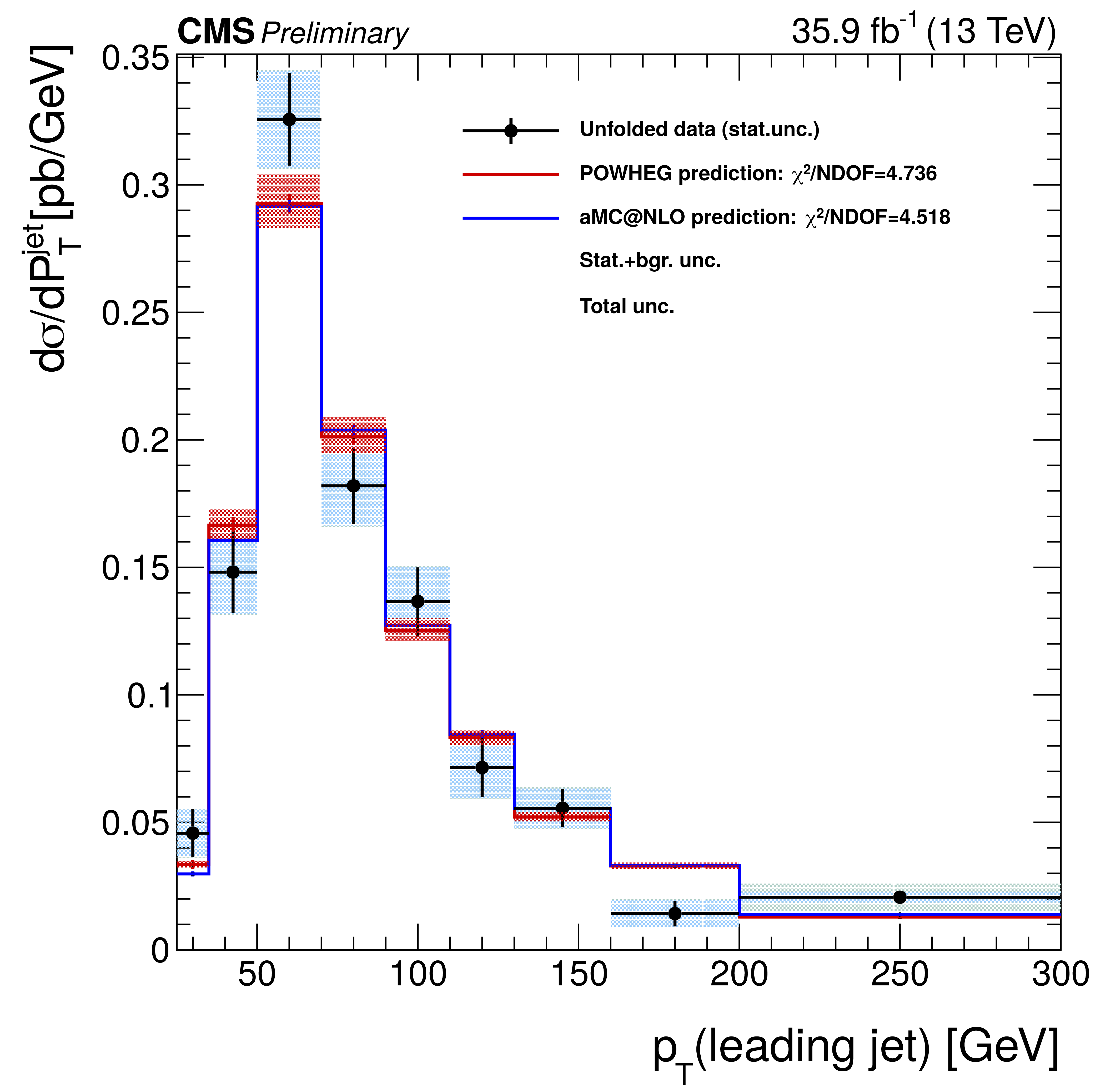
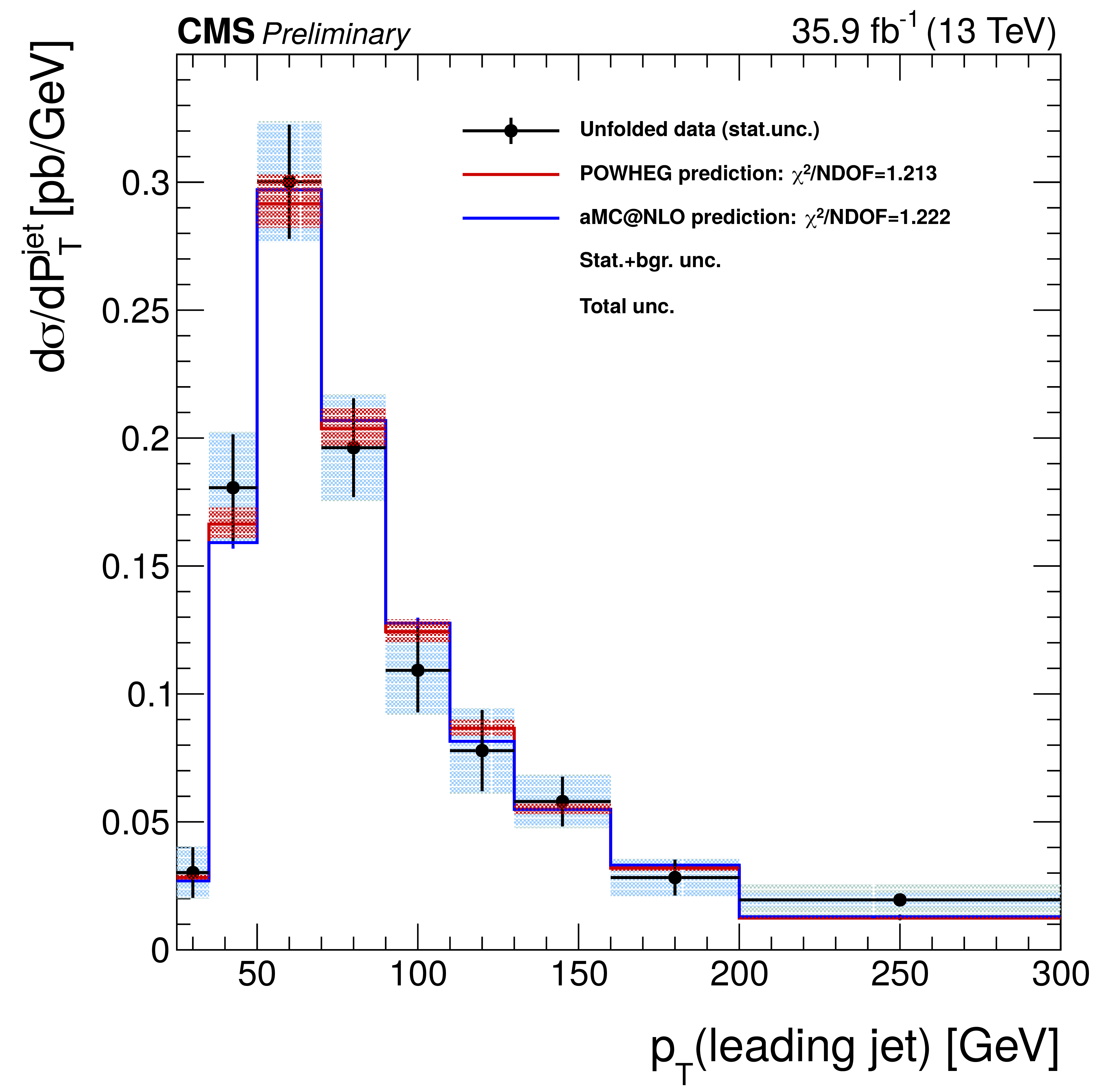
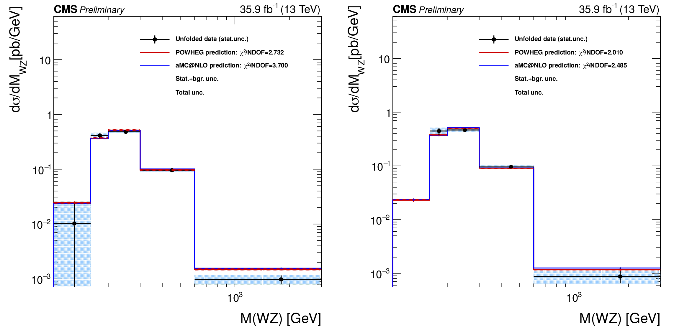
Results for non-regularized unfolding, area constraint, and a bias scale of 1.13 for ${\mathrm {W}}^{+}$ (left) and ${\mathrm {W}}^{-}$ (right), in the full SR. The leading jet transverse momentum is unfolded at the dressed leptons level. The red band around the {powheg} prediction represents the theory uncertainty on the prediction; the effect on the unfolded data of this uncertainty, through the unfolding matrix, is included in the grey bands described in the legend. The agreement between the normalizations is forced by the choice of bias scale. |
png pdf |
Figure 11-a:
Results for non-regularized unfolding, area constraint, and a bias scale of 1.13 for ${\mathrm {W}}^{+}$ (left) and ${\mathrm {W}}^{-}$ (right), in the full SR. The leading jet transverse momentum is unfolded at the dressed leptons level. The red band around the {powheg} prediction represents the theory uncertainty on the prediction; the effect on the unfolded data of this uncertainty, through the unfolding matrix, is included in the grey bands described in the legend. The agreement between the normalizations is forced by the choice of bias scale. |
png pdf |
Figure 11-b:
Results for non-regularized unfolding, area constraint, and a bias scale of 1.13 for ${\mathrm {W}}^{+}$ (left) and ${\mathrm {W}}^{-}$ (right), in the full SR. The leading jet transverse momentum is unfolded at the dressed leptons level. The red band around the {powheg} prediction represents the theory uncertainty on the prediction; the effect on the unfolded data of this uncertainty, through the unfolding matrix, is included in the grey bands described in the legend. The agreement between the normalizations is forced by the choice of bias scale. |

png pdf |
Figure 12:
Results for non-regularized unfolding, area constraint, and a bias scale of 1.13 for ${\mathrm {W}}^{+}$ (left) and ${\mathrm {W}}^{-}$ (right), in the full SR. The transverse momentum of the Z boson is unfolded at the dressed leptons level. The red band around the {powheg} prediction represents the theory uncertainty on the prediction; the effect on the unfolded data of this uncertainty, through the unfolding matrix, is included in the grey bands described in the legend. The agreement between the normalizations is forced by the choice of bias scale. |

png pdf |
Figure 12-a:
Results for non-regularized unfolding, area constraint, and a bias scale of 1.13 for ${\mathrm {W}}^{+}$ (left) and ${\mathrm {W}}^{-}$ (right), in the full SR. The transverse momentum of the Z boson is unfolded at the dressed leptons level. The red band around the {powheg} prediction represents the theory uncertainty on the prediction; the effect on the unfolded data of this uncertainty, through the unfolding matrix, is included in the grey bands described in the legend. The agreement between the normalizations is forced by the choice of bias scale. |
png pdf |
Figure 12-b:
Results for non-regularized unfolding, area constraint, and a bias scale of 1.13 for ${\mathrm {W}}^{+}$ (left) and ${\mathrm {W}}^{-}$ (right), in the full SR. The transverse momentum of the Z boson is unfolded at the dressed leptons level. The red band around the {powheg} prediction represents the theory uncertainty on the prediction; the effect on the unfolded data of this uncertainty, through the unfolding matrix, is included in the grey bands described in the legend. The agreement between the normalizations is forced by the choice of bias scale. |
png pdf |
Figure 13:
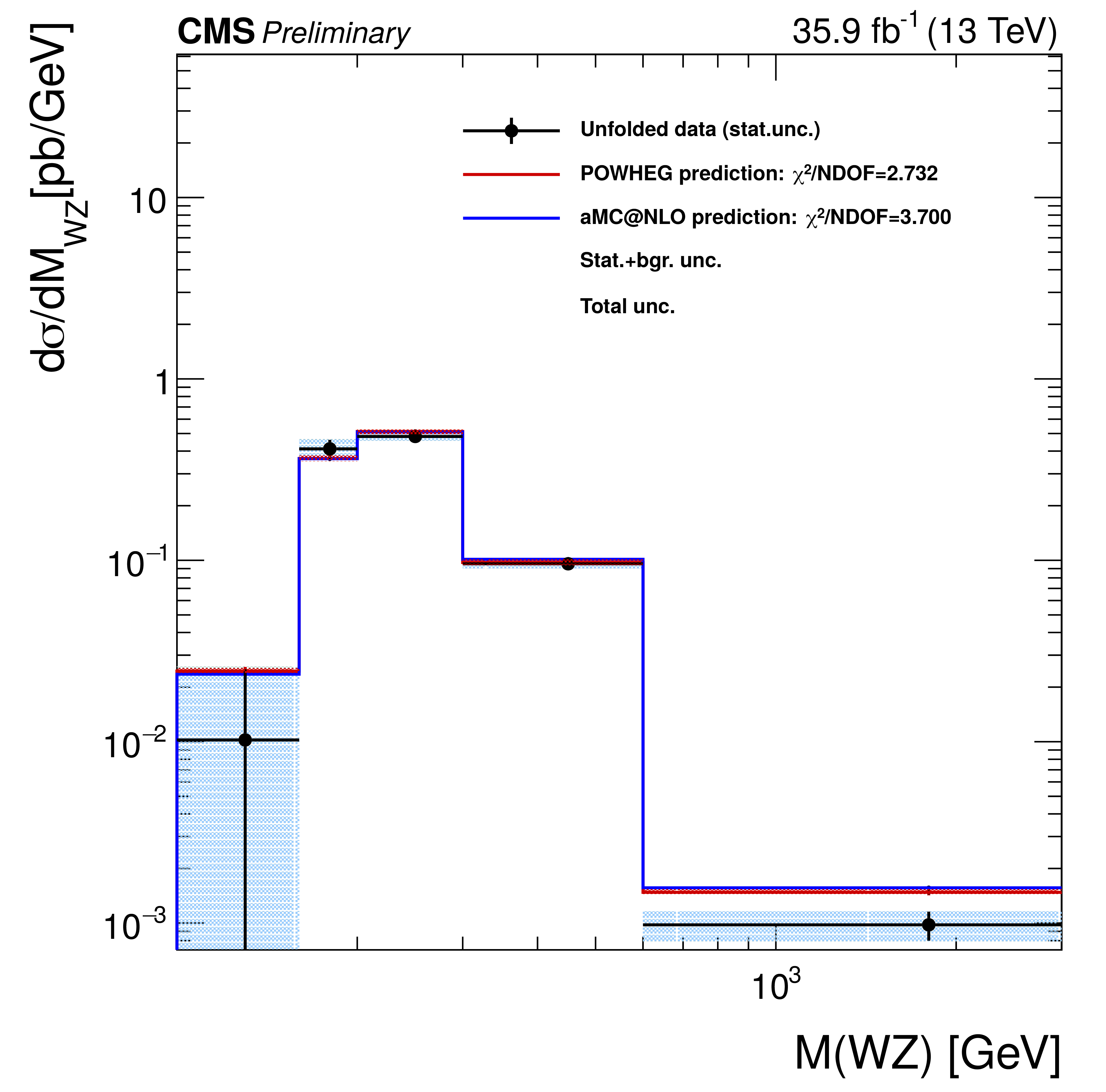
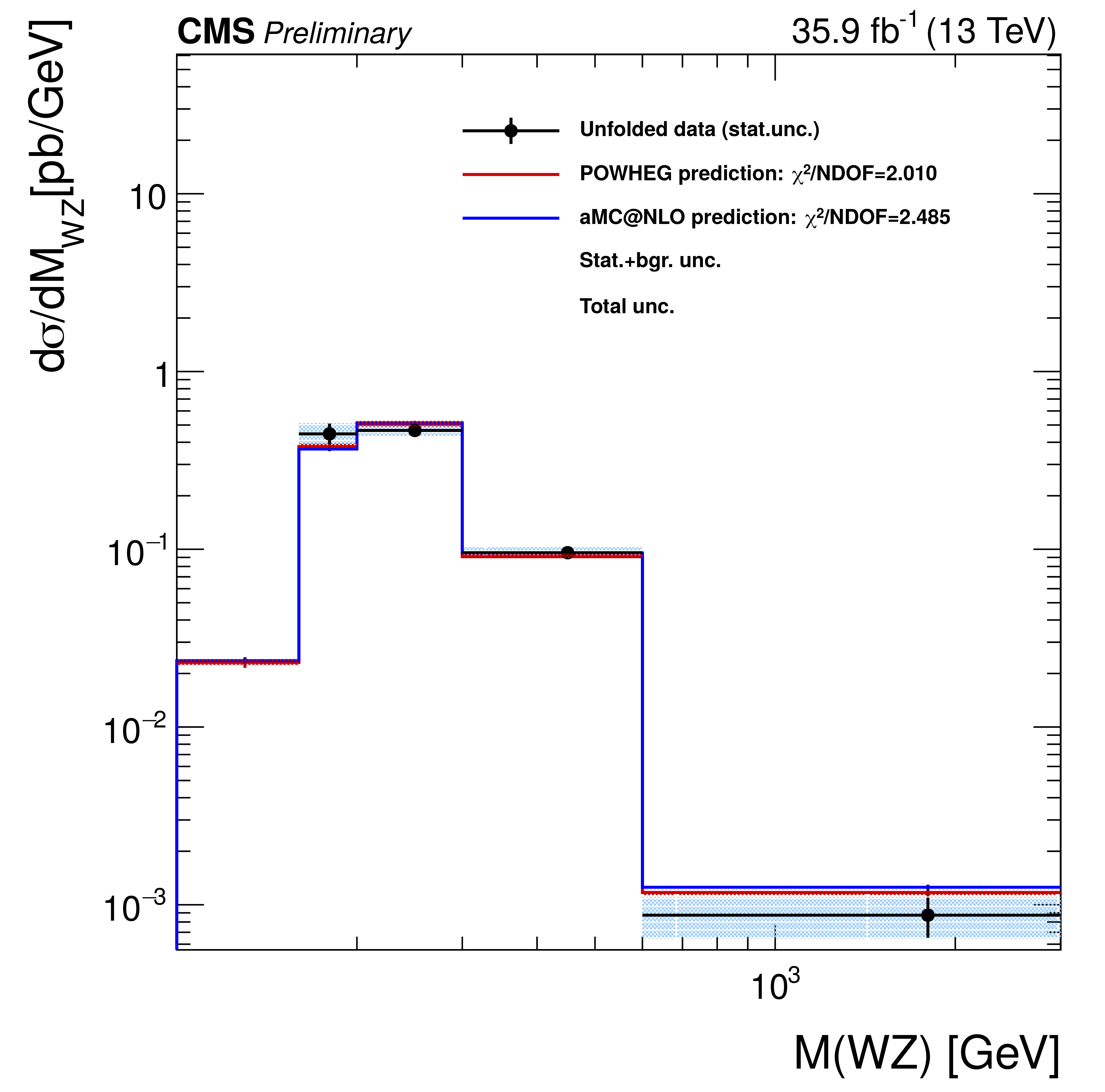
Results for non-regularized unfolding, area constraint, and a bias scale of 1.13 for ${\mathrm {W}}^{+}$ (left) and ${\mathrm {W}}^{-}$ (right), in the full SR. The mass of the WZ system data distribution is unfolded at the dressed leptons level. The red band around the {powheg} prediction represents the theory uncertainty on the prediction; the effect on the unfolded data of this uncertainty, through the unfolding matrix, is included in the grey bands described in the legend. The agreement between the normalizations is forced by the choice of bias scale. |
png pdf |
Figure 13-a:
Results for non-regularized unfolding, area constraint, and a bias scale of 1.13 for ${\mathrm {W}}^{+}$ (left) and ${\mathrm {W}}^{-}$ (right), in the full SR. The mass of the WZ system data distribution is unfolded at the dressed leptons level. The red band around the {powheg} prediction represents the theory uncertainty on the prediction; the effect on the unfolded data of this uncertainty, through the unfolding matrix, is included in the grey bands described in the legend. The agreement between the normalizations is forced by the choice of bias scale. |
png pdf |
Figure 13-b:
Results for non-regularized unfolding, area constraint, and a bias scale of 1.13 for ${\mathrm {W}}^{+}$ (left) and ${\mathrm {W}}^{-}$ (right), in the full SR. The mass of the WZ system data distribution is unfolded at the dressed leptons level. The red band around the {powheg} prediction represents the theory uncertainty on the prediction; the effect on the unfolded data of this uncertainty, through the unfolding matrix, is included in the grey bands described in the legend. The agreement between the normalizations is forced by the choice of bias scale. |
png pdf |
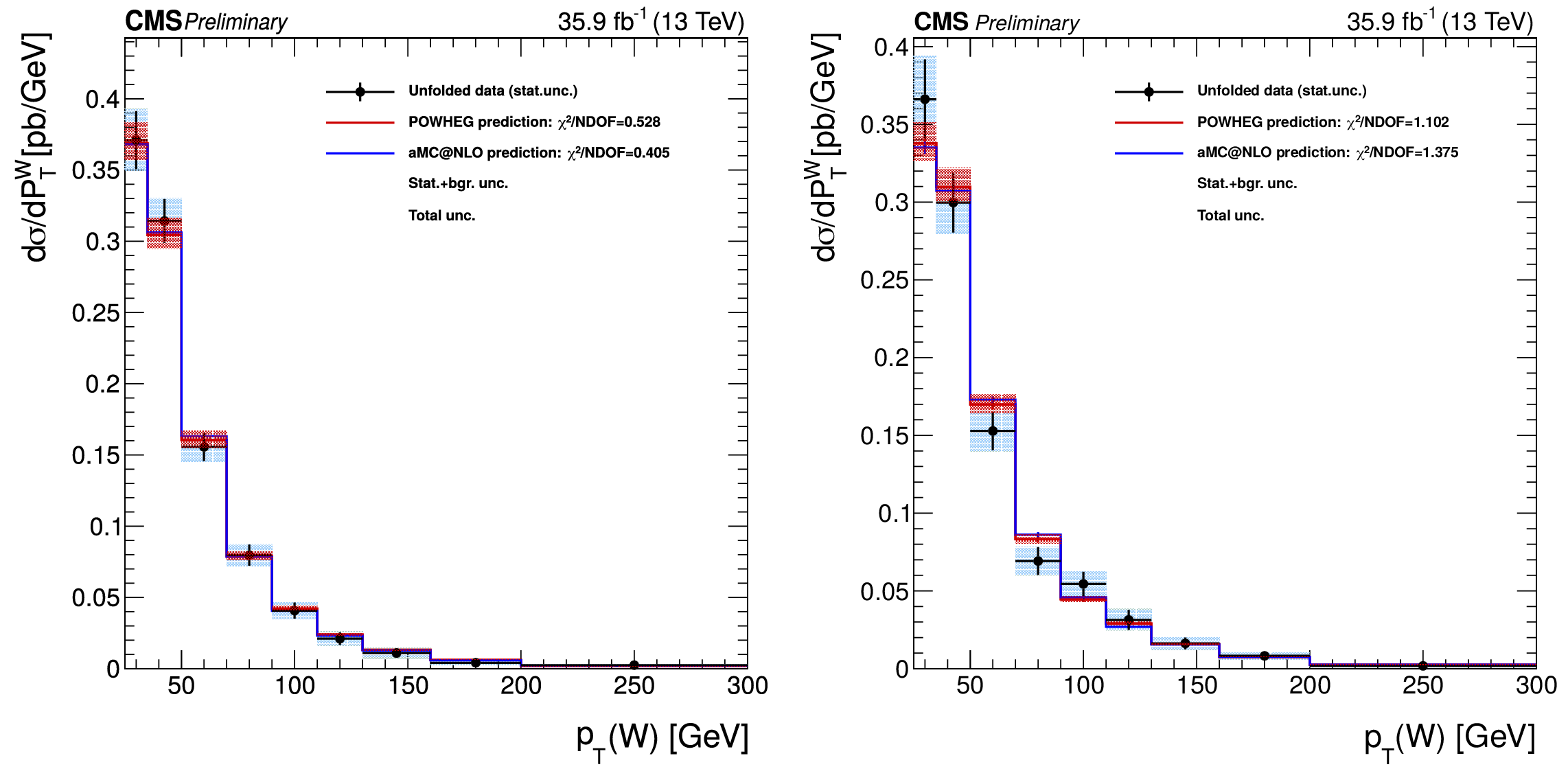
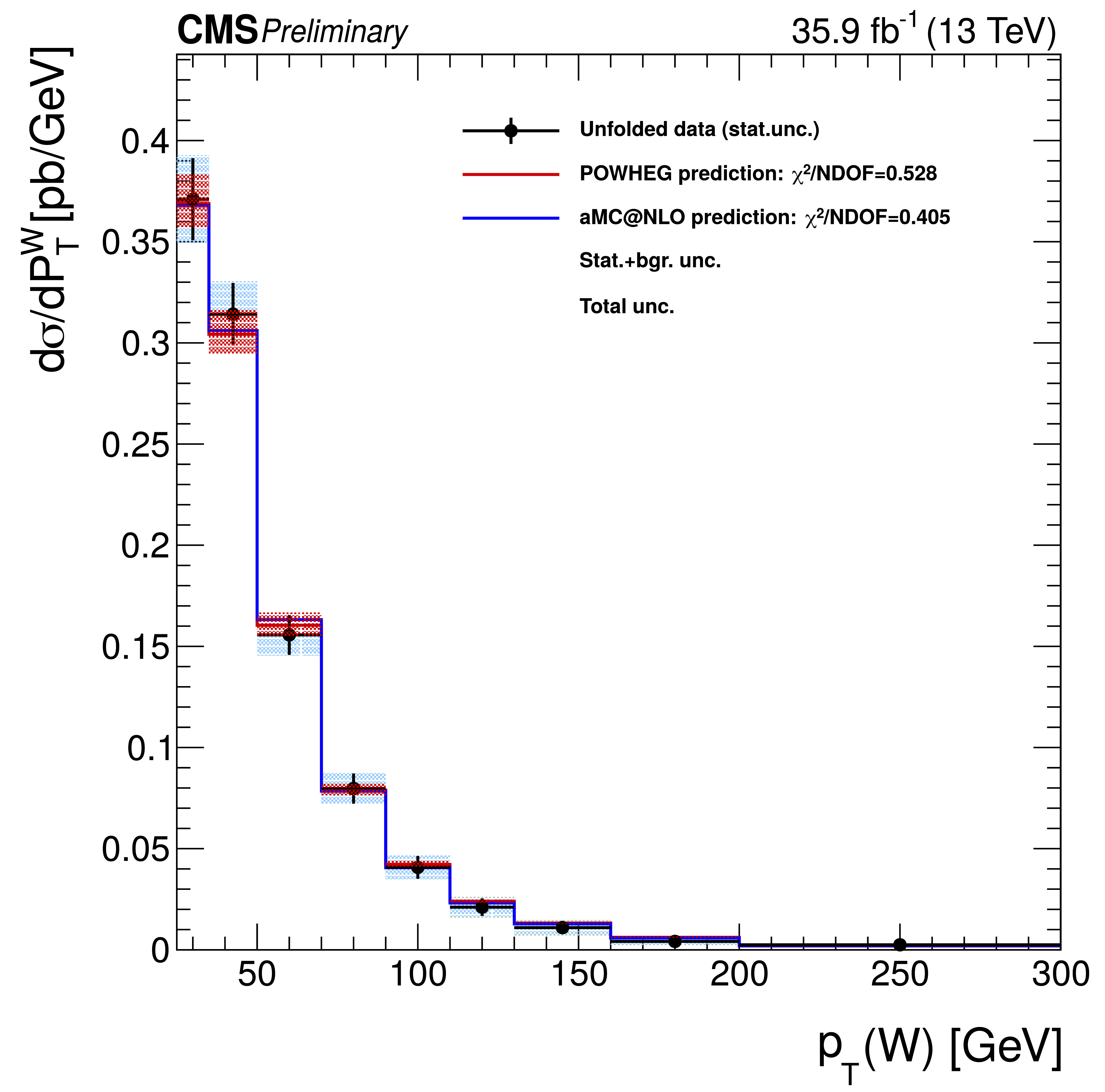
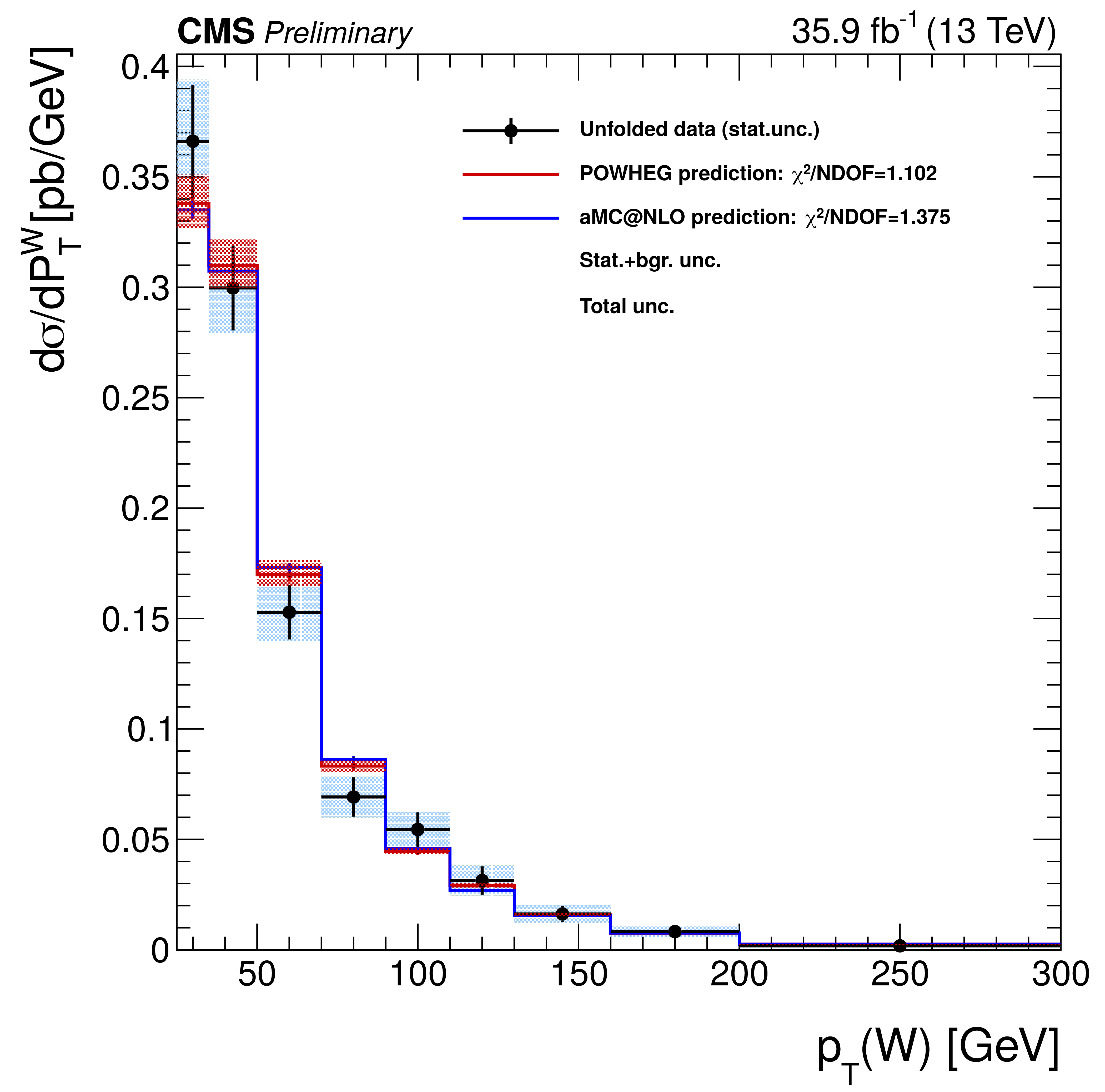
Figure 14:
Results for non-regularized unfolding, area constraint, and a bias scale of 1.13 for ${\mathrm {W}}^{+}$ (left) and ${\mathrm {W}}^{-}$ (right), in the full SR. The W boson transverse momentum is unfolded at the dressed leptons level. The red band around the {powheg} prediction represents the theory uncertainty on the prediction; the effect on the unfolded data of this uncertainty, through the unfolding matrix, is included in the grey bands described in the legend. The agreement between the normalizations is forced by the choice of bias scale. |
png pdf |
Figure 14-a:
Results for non-regularized unfolding, area constraint, and a bias scale of 1.13 for ${\mathrm {W}}^{+}$ (left) and ${\mathrm {W}}^{-}$ (right), in the full SR. The W boson transverse momentum is unfolded at the dressed leptons level. The red band around the {powheg} prediction represents the theory uncertainty on the prediction; the effect on the unfolded data of this uncertainty, through the unfolding matrix, is included in the grey bands described in the legend. The agreement between the normalizations is forced by the choice of bias scale. |
png pdf |
Figure 14-b:
Results for non-regularized unfolding, area constraint, and a bias scale of 1.13 for ${\mathrm {W}}^{+}$ (left) and ${\mathrm {W}}^{-}$ (right), in the full SR. The W boson transverse momentum is unfolded at the dressed leptons level. The red band around the {powheg} prediction represents the theory uncertainty on the prediction; the effect on the unfolded data of this uncertainty, through the unfolding matrix, is included in the grey bands described in the legend. The agreement between the normalizations is forced by the choice of bias scale. |

png pdf |
Figure 15:
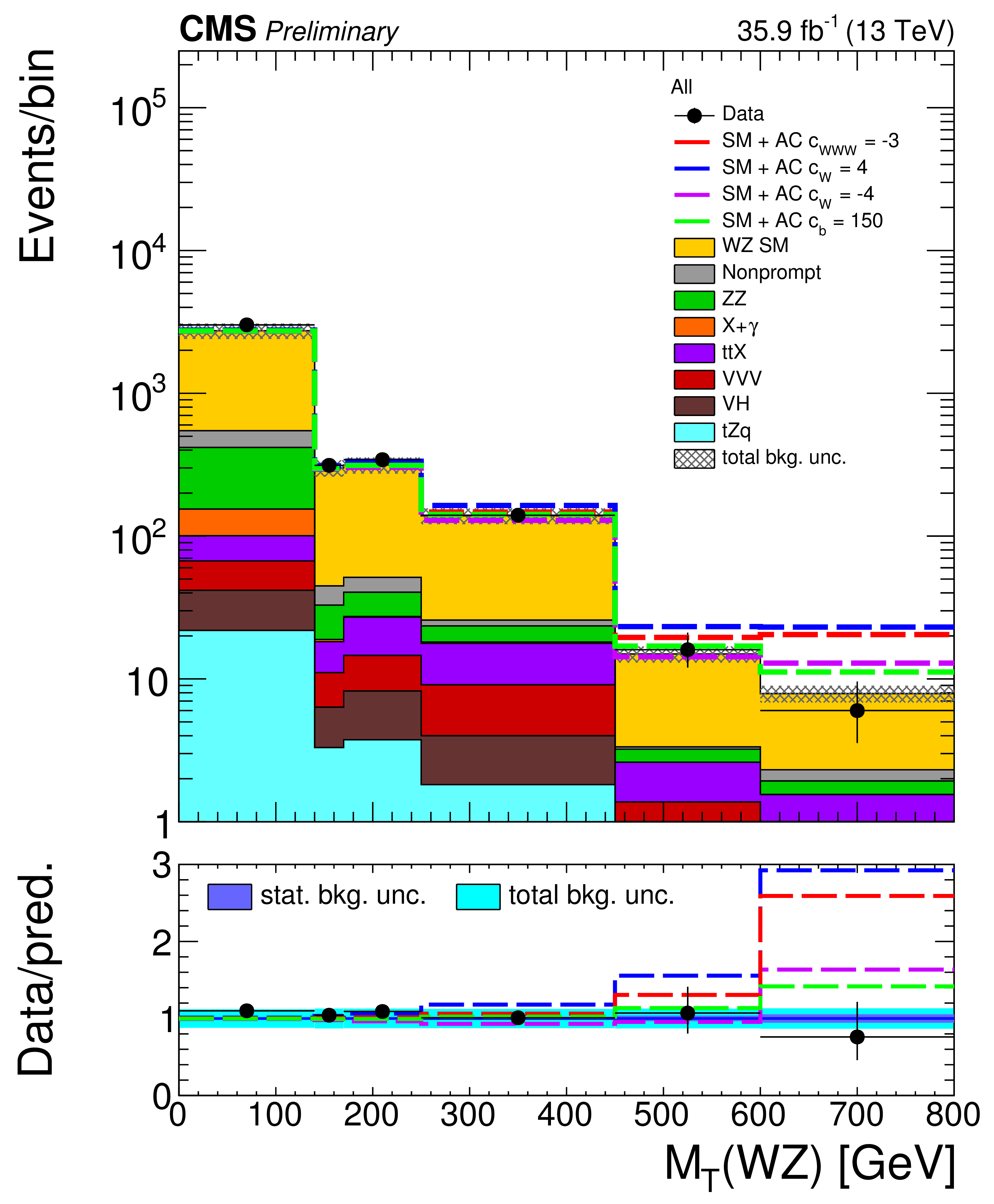
Distributions of discriminant observables in the anomalous couplings searches. The invariant mass of the three lepton plus the missing transverse momentum system (left) and the transverse mass of the same configuration (right). The dashed lines represent the total yields that would be expected from the sum of the SM processes with the total WZ yields modified according to their correspondence to the given values of the associated anomalous coupling parameters. The SM prediction for the WZ process is obtained from the aTGC simulated sample with the anomalous couplings set to $0$. |
png pdf |
Figure 15-a:
Distributions of discriminant observables in the anomalous couplings searches. The invariant mass of the three lepton plus the missing transverse momentum system (left) and the transverse mass of the same configuration (right). The dashed lines represent the total yields that would be expected from the sum of the SM processes with the total WZ yields modified according to their correspondence to the given values of the associated anomalous coupling parameters. The SM prediction for the WZ process is obtained from the aTGC simulated sample with the anomalous couplings set to $0$. |
png pdf |
Figure 15-b:
Distributions of discriminant observables in the anomalous couplings searches. The invariant mass of the three lepton plus the missing transverse momentum system (left) and the transverse mass of the same configuration (right). The dashed lines represent the total yields that would be expected from the sum of the SM processes with the total WZ yields modified according to their correspondence to the given values of the associated anomalous coupling parameters. The SM prediction for the WZ process is obtained from the aTGC simulated sample with the anomalous couplings set to $0$. |

png pdf |
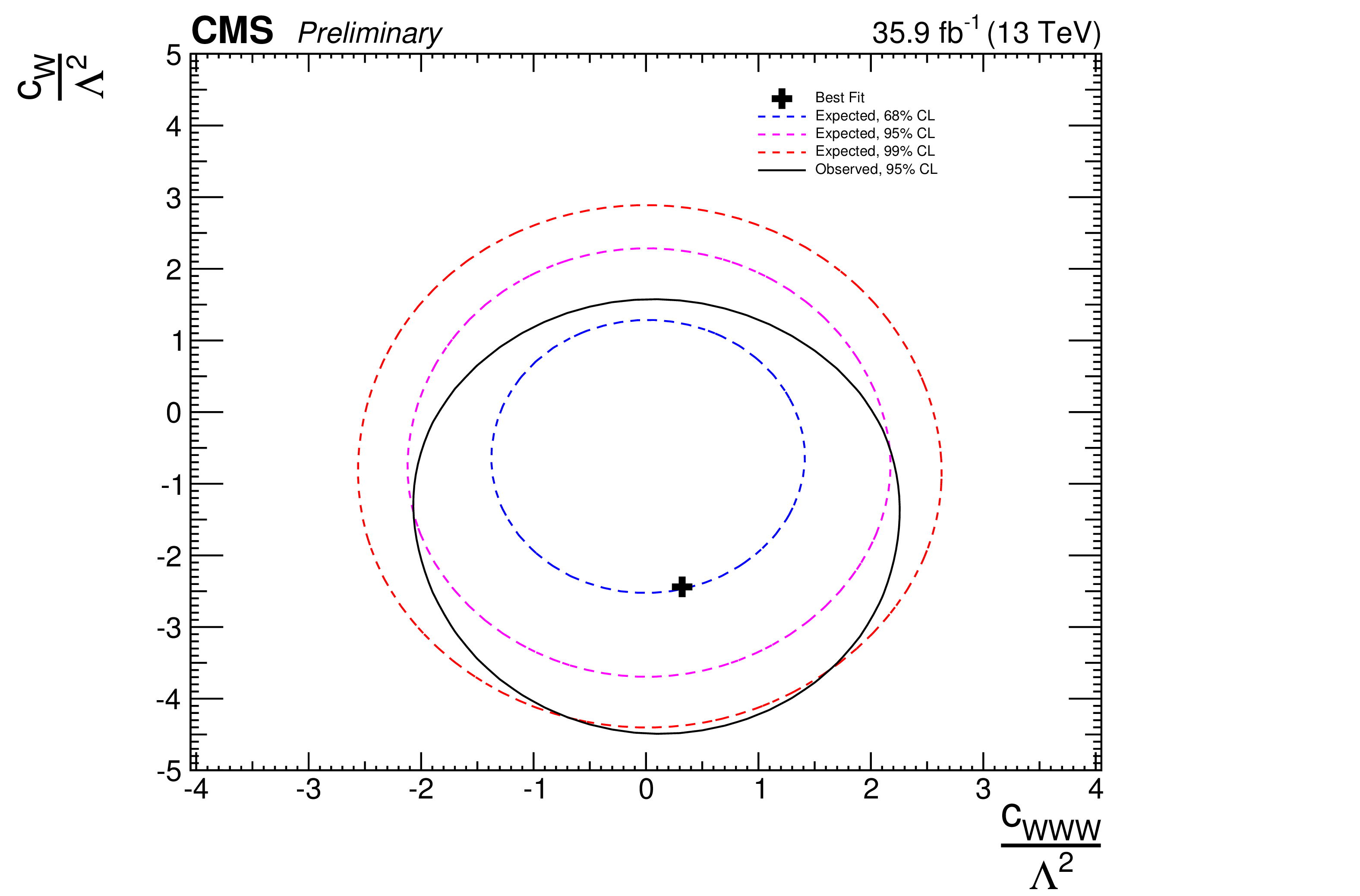
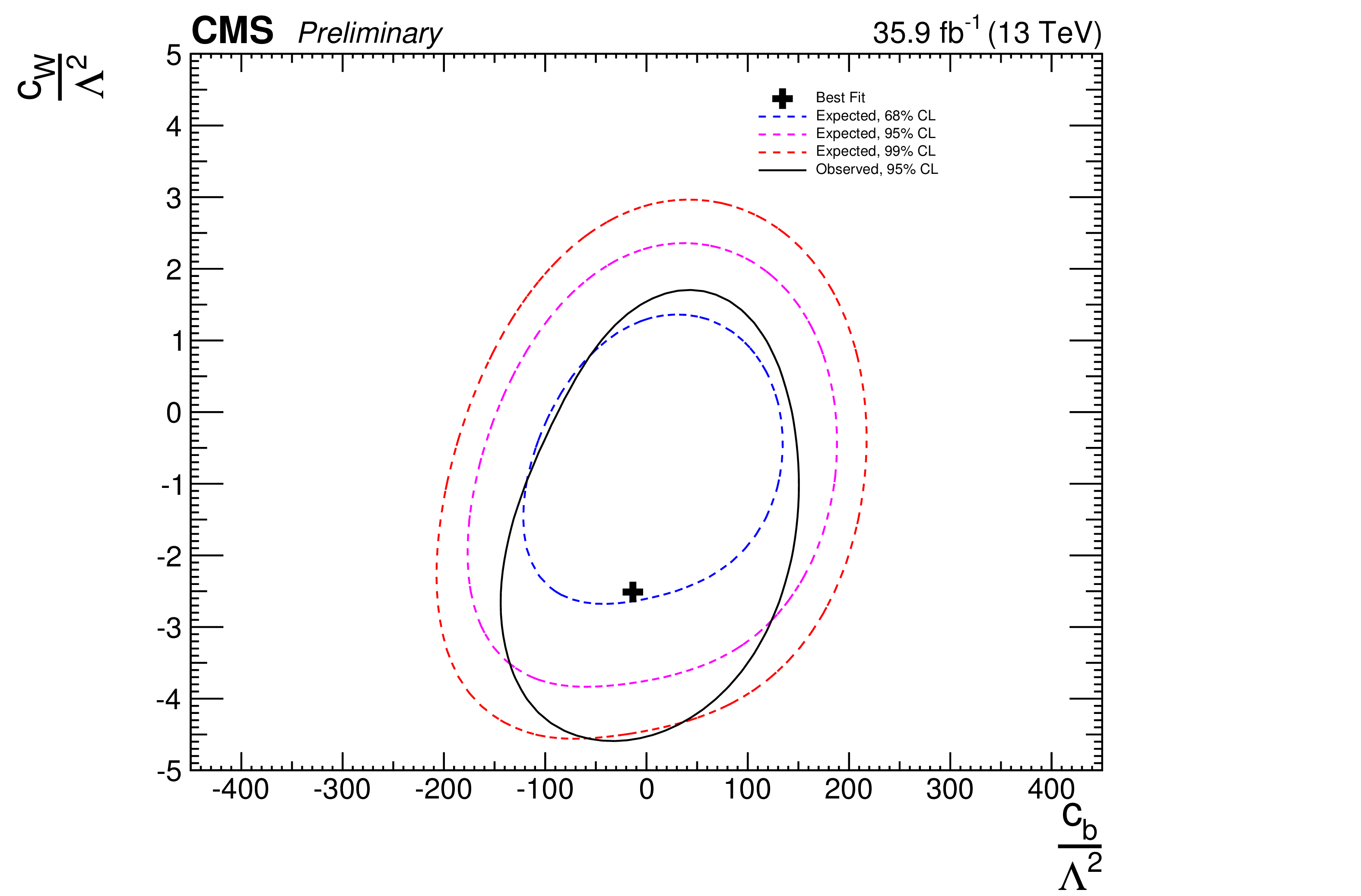
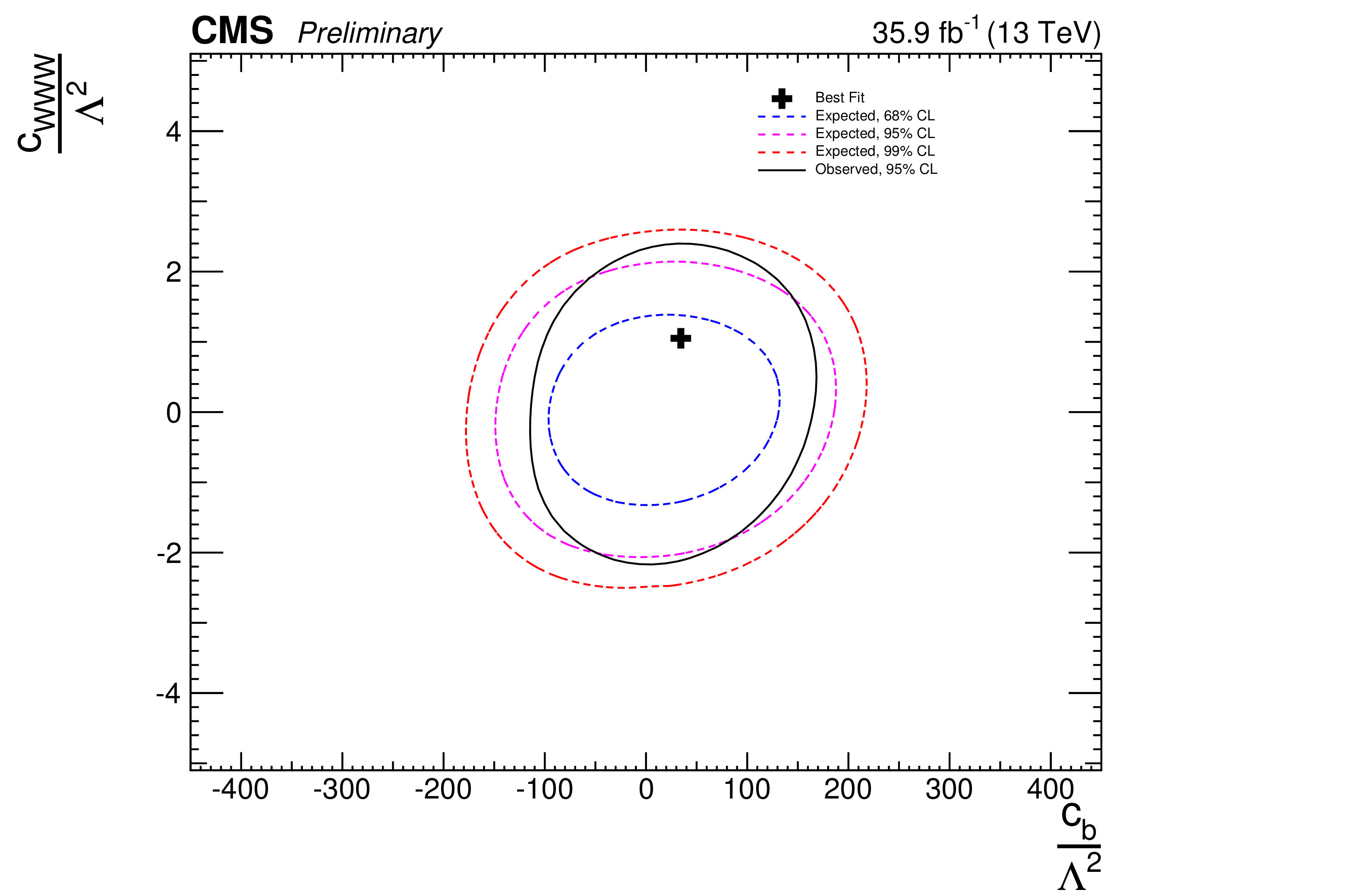
Figure 16:
2D confidence regions for each of the possible combinations of the considered aTGC parameters. The contours of the expected confidence regions for $68%$ and $95%$ confidence level are presented in each case. The parameters considered in each plot are $c_{\text {w}}-c_{\text {www}}$ (top), $c_{\text {w}}-c_{\text {b}}$ (middle) and $c_{\text {www}}-c_{\text {b}}$ (bottom). |
png pdf |
Figure 16-a:
2D confidence regions for each of the possible combinations of the considered aTGC parameters. The contours of the expected confidence regions for $68%$ and $95%$ confidence level are presented in each case. The parameters considered in each plot are $c_{\text {w}}-c_{\text {www}}$ (top), $c_{\text {w}}-c_{\text {b}}$ (middle) and $c_{\text {www}}-c_{\text {b}}$ (bottom). |
png pdf |
Figure 16-b:
2D confidence regions for each of the possible combinations of the considered aTGC parameters. The contours of the expected confidence regions for $68%$ and $95%$ confidence level are presented in each case. The parameters considered in each plot are $c_{\text {w}}-c_{\text {www}}$ (top), $c_{\text {w}}-c_{\text {b}}$ (middle) and $c_{\text {www}}-c_{\text {b}}$ (bottom). |
png pdf |
Figure 16-c:
2D confidence regions for each of the possible combinations of the considered aTGC parameters. The contours of the expected confidence regions for $68%$ and $95%$ confidence level are presented in each case. The parameters considered in each plot are $c_{\text {w}}-c_{\text {www}}$ (top), $c_{\text {w}}-c_{\text {b}}$ (middle) and $c_{\text {www}}-c_{\text {b}}$ (bottom). |

png pdf |
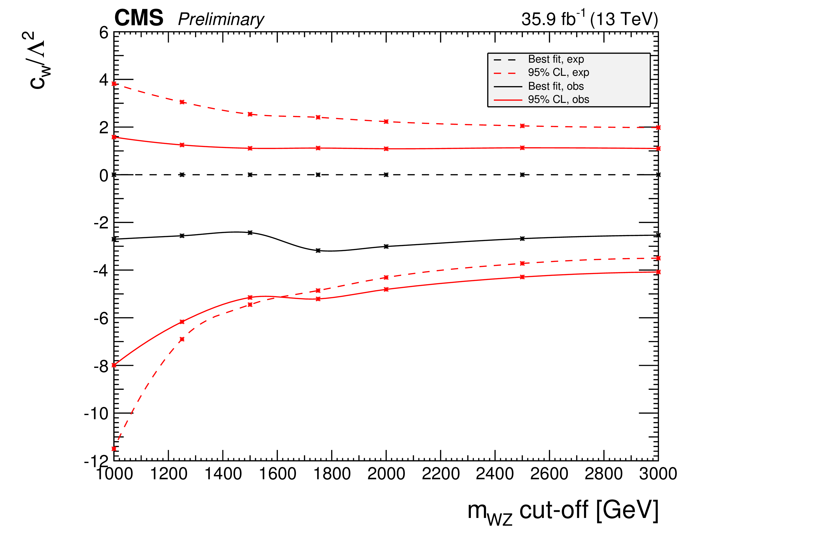
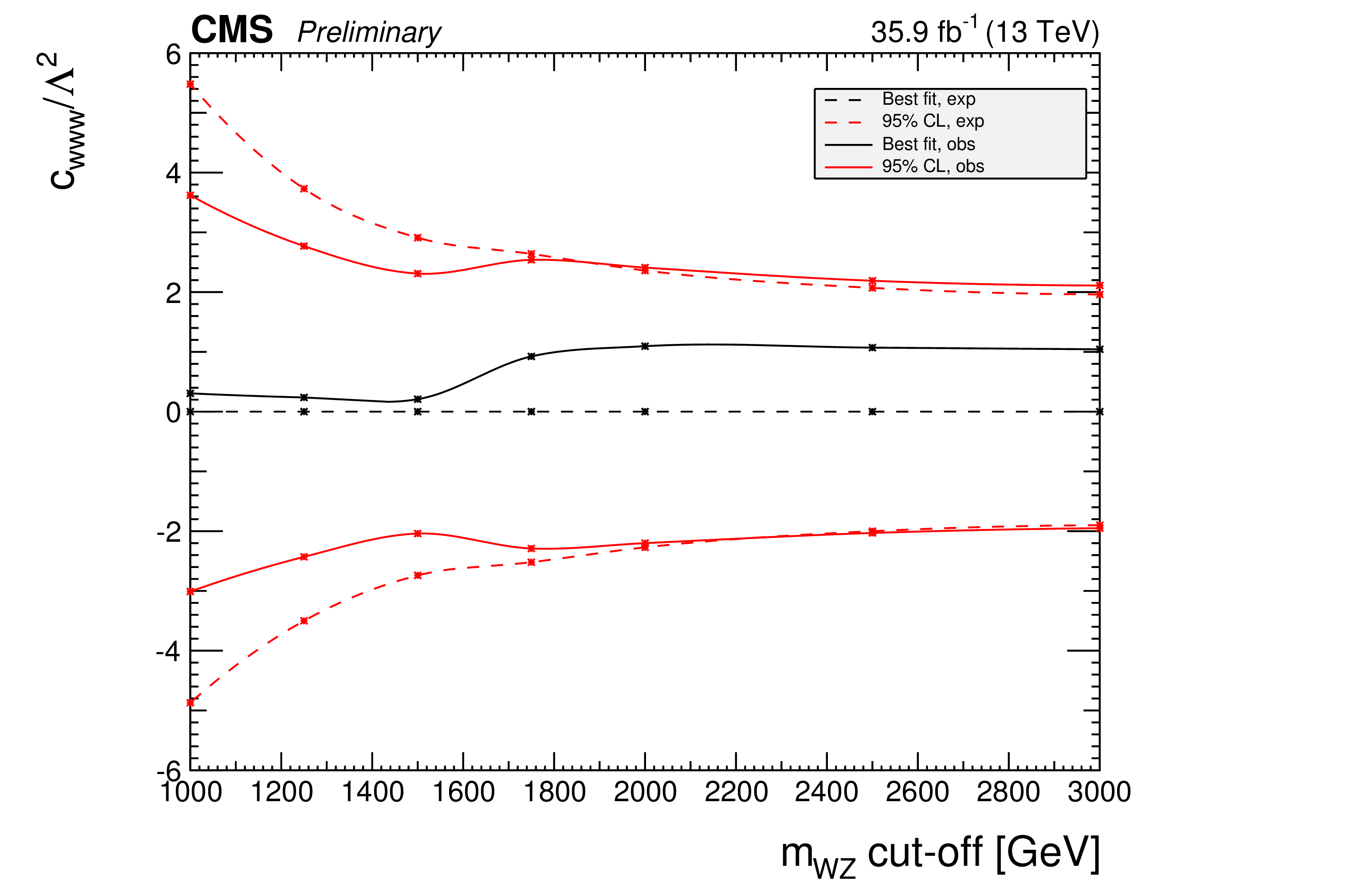
Figure 17:
Evolution of the expected confidence intervals in the EFT anomalous coupling parameters in terms of the cutoff scale given by different restrictions in the $M_{{\mathrm {W}} {\mathrm {Z}}}$ variable. For each point and parameter, the confidence intervals are computed imposing the additional restriction of no anomalous coupling contribution on top of SM prediction over the given value of $M_{{\mathrm {W}} {\mathrm {Z}}}$. Due to the statistical limitations in our simulation the last point is equivalent to no cut-off requirement being imposed. The parameter considered in each plot is: $c_{\textrm {w}}$ (top left), $c_{\textrm {www}}$ (top right) and $c_{\textrm {b}}$ (bottom). |
png pdf |
Figure 17-a:
Evolution of the expected confidence intervals in the EFT anomalous coupling parameters in terms of the cutoff scale given by different restrictions in the $M_{{\mathrm {W}} {\mathrm {Z}}}$ variable. For each point and parameter, the confidence intervals are computed imposing the additional restriction of no anomalous coupling contribution on top of SM prediction over the given value of $M_{{\mathrm {W}} {\mathrm {Z}}}$. Due to the statistical limitations in our simulation the last point is equivalent to no cut-off requirement being imposed. The parameter considered in each plot is: $c_{\textrm {w}}$ (top left), $c_{\textrm {www}}$ (top right) and $c_{\textrm {b}}$ (bottom). |
png pdf |
Figure 17-b:
Evolution of the expected confidence intervals in the EFT anomalous coupling parameters in terms of the cutoff scale given by different restrictions in the $M_{{\mathrm {W}} {\mathrm {Z}}}$ variable. For each point and parameter, the confidence intervals are computed imposing the additional restriction of no anomalous coupling contribution on top of SM prediction over the given value of $M_{{\mathrm {W}} {\mathrm {Z}}}$. Due to the statistical limitations in our simulation the last point is equivalent to no cut-off requirement being imposed. The parameter considered in each plot is: $c_{\textrm {w}}$ (top left), $c_{\textrm {www}}$ (top right) and $c_{\textrm {b}}$ (bottom). |

png pdf |
Figure 17-c:
Evolution of the expected confidence intervals in the EFT anomalous coupling parameters in terms of the cutoff scale given by different restrictions in the $M_{{\mathrm {W}} {\mathrm {Z}}}$ variable. For each point and parameter, the confidence intervals are computed imposing the additional restriction of no anomalous coupling contribution on top of SM prediction over the given value of $M_{{\mathrm {W}} {\mathrm {Z}}}$. Due to the statistical limitations in our simulation the last point is equivalent to no cut-off requirement being imposed. The parameter considered in each plot is: $c_{\textrm {w}}$ (top left), $c_{\textrm {www}}$ (top right) and $c_{\textrm {b}}$ (bottom). |
| Tables | |
png pdf |
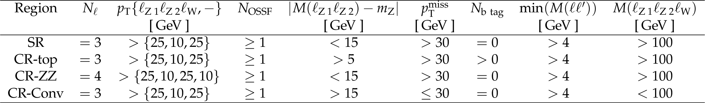
Table 1:
Definition of the complete requirements for the definition of the signal (measurement) region of the analysis and the three different regions designed to control the behaviour of the main background sources. |

png pdf |
Table 2:
Measured fiducial cross sections and their corresponding uncertainties for each of the individual flavour categories as well as for the combination of the four. |
png pdf |
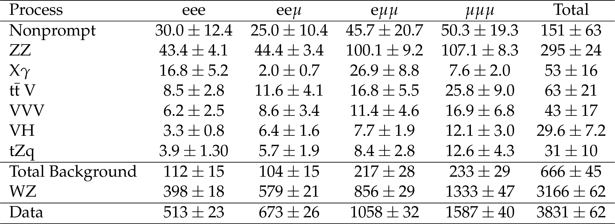
Table 3:
Expected and observed yields for each of the relevant processes and flavour categories. Combined statistical and systematic uncertainties are shown for each case except for the observed data yields for which only statistical uncertainties are shown. All expected yields correspond to quantities estimated after the maximum likelihood fit. Uncertainties are computed taking into account the full correlation matrix between sources of uncertainty, processes, and flavour categories. |
png pdf |
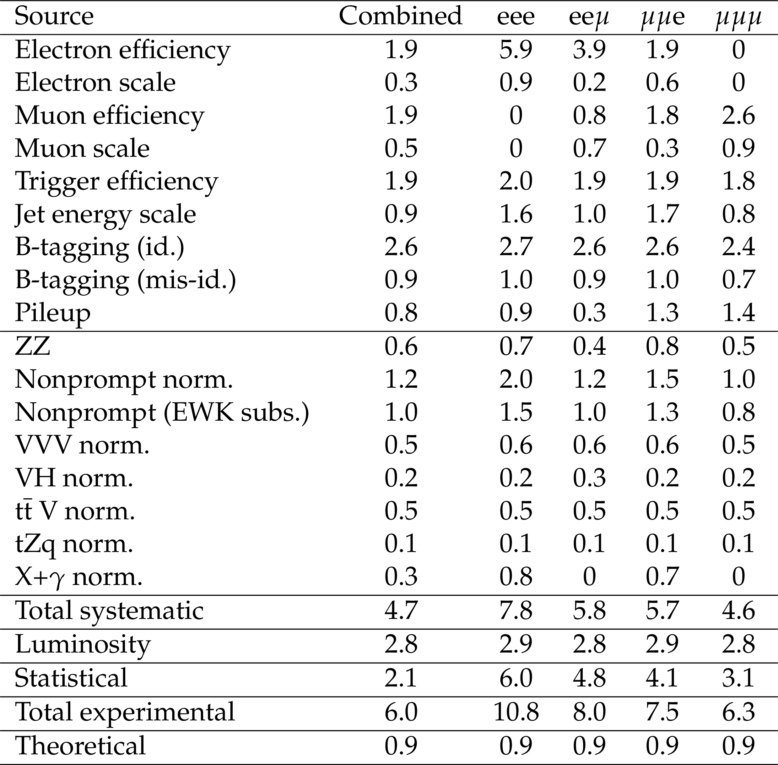
Table 4:
Summary of the total postfit impact of each uncertainty source on the uncertainty of the signal strength measurement for each of the flavour categories and their combination. Theoretical uncertainties are only included in the signal acceptance during the extrapolation to the total phase space so they are not included in the likelihood fit. The values are percentages and correspond to the half-width between the up and down variation of each systematic uncertainty component. |
png pdf |
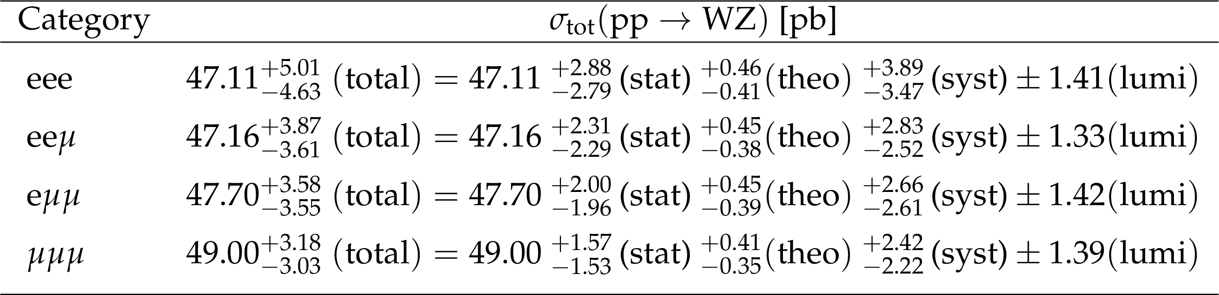
Table 5:
Measured WZ production cross sections computed separately in each of the flavour categories. |
png pdf |
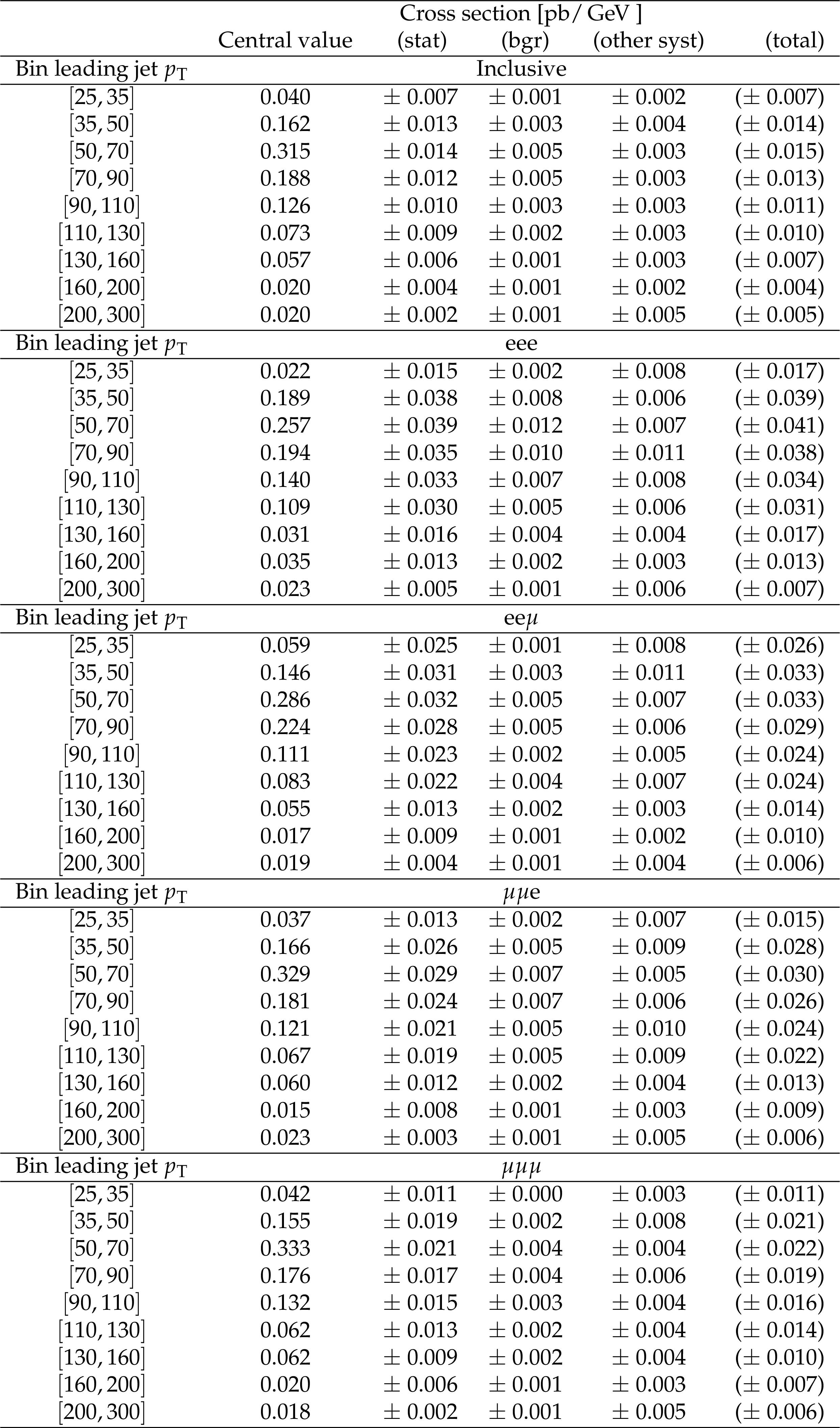
Table 6:
Differential cross section in bins of leading jet ${p_{\mathrm {T}}}$. Values are expressed as fraction of the inclusive cross section. |
png pdf |
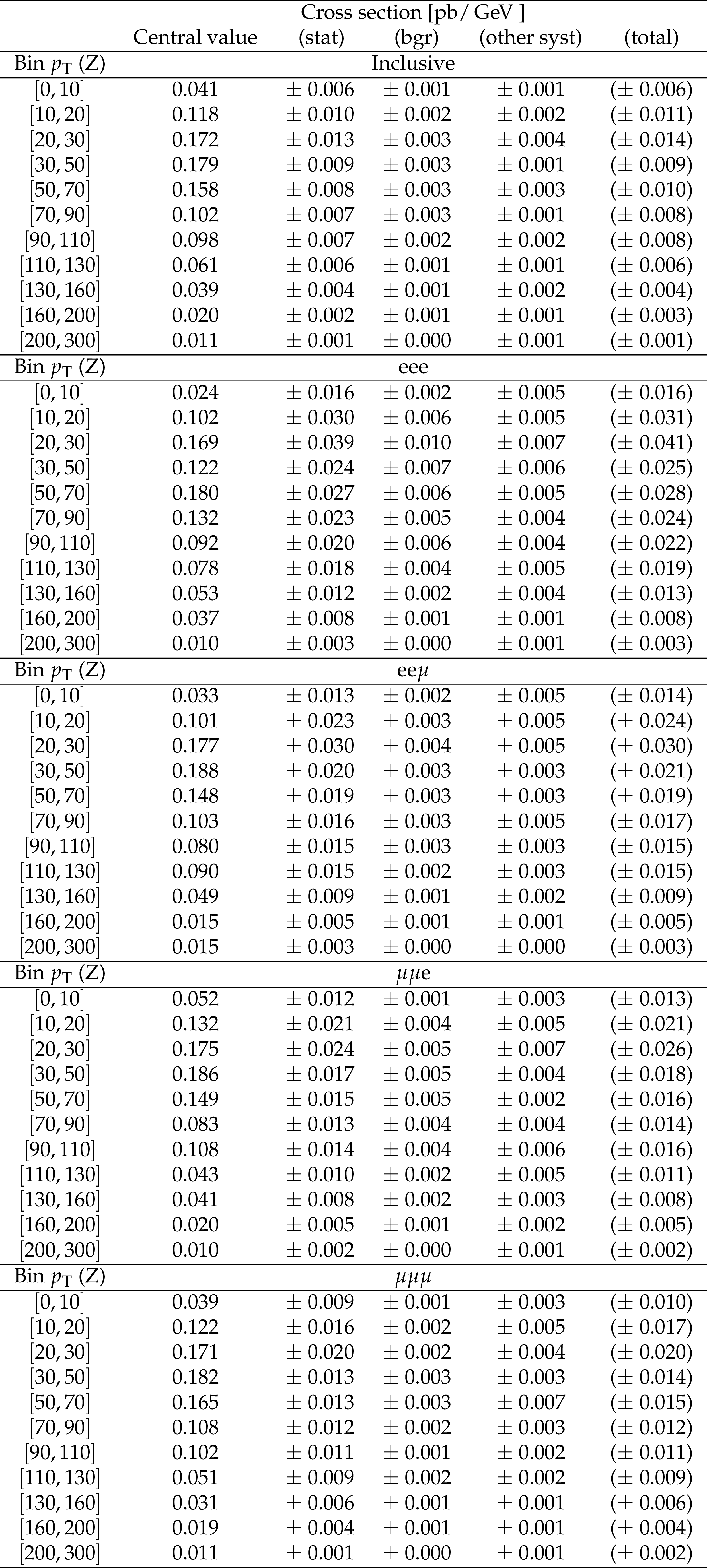
Table 7:
Differential cross section in bins of Z boson ${p_{\mathrm {T}}}$. Values are expressed as fraction of the inclusive cross section. |
png pdf |
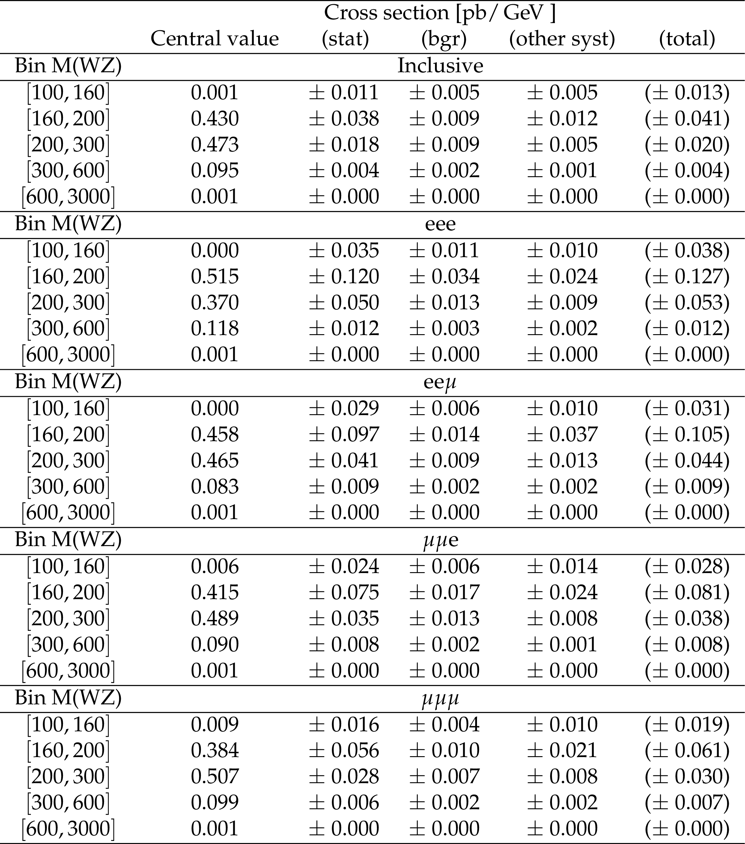
Table 8:
Differential cross section in bins of mass of the WZ system. Values are expressed as fraction of the inclusive cross section. |
png pdf |
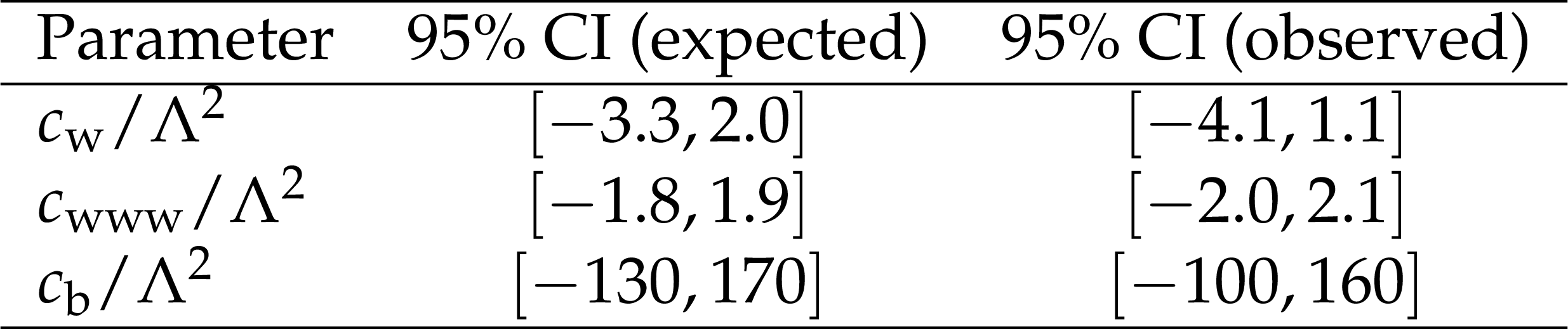
Table 9:
Expected and observed 1-D confidence intervals at 95% confidence level for each of the considered AC parameters. |
| Summary |
|
The production process ${\mathrm{p}}{\mathrm{p}} \to \mathrm{W}\mathrm{Z}$ is studied in the trilepton final state at $\sqrt{s}= $ 13 TeV, using the full 2016 data set with a total integrated luminosity of 35.9 fb$^{-1}$. Fiducial results are obtained in each of the flavour categories and in the combined category, and are extrapolated for 60 $ < M_{\mathrm{W}\mathrm{Z}} < $ 120 GeV to the total WZ production cross section. Differential cross sections are measured as a function of the transverse momentum of the Z boson, of the transverse momentum of the leading jet, and of an estimate of the mass of the WZ system; results are compared with predictions from the POWHEG and MadGraph5\_aMC@NLO generators. Differential cross section are also measured depending on the sign of the W boson as a function of its transverse momentum. Confidence intervals for anomalous triple gauge-boson couplings are extracted for each of the anomalous couplings parameters for all the 1-D and 2-D possible combinations of parameters, using the $M_{\mathrm{W}\mathrm{Z}}$ variable in a maximum likelihood fit. The confidence intervals obtained represent the most stringent results on anomalous triple gauge-boson couplings to date. |
| References | ||||
| 1 | D0 Collaboration | Measurement of the $ \mathrm{WZ}\to \ell\nu\ell\ell $ cross section and limits on anomalous triple gauge couplings in $ \mathrm{p}\bar{\mathrm{p}} $ collisions at $ \sqrt{s} = $ 1.96 ~tev | PLB 695 (2011) 67 | |
| 2 | CDF Collaboration | Observation of WZ production | PRLett 98 (2007) 161801 | |
| 3 | ATLAS Collaboration | Measurement of the WZ production cross section and limits on $ \ $ anomalous triple gauge couplings in proton-proton collisions at $ \sqrt{s} = $ 7 TeV with the ATLAS detector | PLB 709 (2012) 341 | 1111.5570 |
| 4 | CMS Collaboration | Measurement of the WZ production cross section in pp collisions at $ \sqrt{s} = $ 7 and 8 TeV and search for anomalous triple gauge couplings at $ \sqrt{s} = $ 8 TeV | EPJC 77 (2017), no. 4, 236 | CMS-SMP-14-014 1609.05721 |
| 5 | CMS Collaboration | Measurement of the WZ production cross section in pp collisions at $ \sqrt(s) = $ 13 TeV | PLB 766 (2017) 268 | CMS-SMP-16-002 1607.06943 |
| 6 | CMS Collaboration | The CMS experiment at the CERN LHC | JINST 3 (2008) S08004 | CMS-00-001 |
| 7 | T. Melia, P. Nason, R. Rontsch, and G. Zanderighi | $ \mathrm{W}^+ \mathrm{W}^- $, $ \mathrm{W} \mathrm{Z} $ and $ \mathrm{Z} \mathrm{Z} $ production in the POWHEG BOX | JHEP 11 (2011) 078 | 1107.5051 |
| 8 | P. Nason and G. Zanderighi | $ \mathrm{W}^+ \mathrm{W}^- $, $ \mathrm{W} \mathrm{Z} $ and $ \mathrm{Z} \mathrm{Z} $ production in the POWHEG-BOX-V2 | EPJC 74 (2014) 2702 | 1311.1365 |
| 9 | J. Alwall et al. | The automated computation of tree-level and next-to-leading order differential cross sections, and their matching to parton shower simulations | JHEP 07 (2014) 079 | 1405.0301 |
| 10 | R. Frederix and S. Frixione | Merging meets matching in MC@NLO | JHEP 12 (2012) 061 | 1209.6215 |
| 11 | J. Alwall et al. | Comparative study of various algorithms for the merging of parton showers and matrix elements in hadronic collisions | EPJC 53 (2008) 473 | 0706.2569 |
| 12 | O. Mattelaer | On the maximal use of Monte Carlo samples: re-weighting events at NLO accuracy | EPJC 76 (2016) 010 | 1607.00763 |
| 13 | NNPDF Collaboration | Parton distributions for the LHC Run II | JHEP 04 (2015) 040 | 1410.8849 |
| 14 | T. Sjostrand, S. Mrenna, and P. Z. Skands | A brief introduction to PYTHIA 8.1 | CPC 178 (2008) 852 | 0710.3820 |
| 15 | P. Skands, S. Carrazza, and J. Rojo | Tuning PYTHIA 8.1: the Monash 2013 tune | EPJC 74 (2014) 3024 | 1404.5630 |
| 16 | CMS Collaboration | Event generator tunes obtained from underlying event and multiparton scattering measurements | EPJC 76 (2016) 155 | CMS-GEN-14-001 1512.00815 |
| 17 | GEANT4 Collaboration | GEANT4---a simulation toolkit | NIMA 506 (2003) 250 | |
| 18 | CMS Collaboration | Particle-flow reconstruction and global event description with the cms detector | JINST 12 (2017) P10003 | CMS-PRF-14-001 1706.04965 |
| 19 | CMS Collaboration | Performance of CMS muon reconstruction in pp collision events at $ \sqrt{s} = $ 7 TeV | JINST 7 (2012) P10002 | CMS-MUO-10-004 1206.4071 |
| 20 | K. Rehermann and B. Tweedie | Efficient Identification of Boosted Semileptonic Top Quarks at the LHC | JHEP 03 (2011) 059 | 1007.2221 |
| 21 | CMS Collaboration | Search for new physics in same-sign dilepton events in proton-proton collisions at $ \sqrt{s} = $ 13 TeV | EPJC 76 (2016) 439 | CMS-SUS-15-008 1605.03171 |
| 22 | CMS Collaboration | Search for electroweak production of charginos and neutralinos in multilepton final states in proton-proton collisions at $ \sqrt{s}= $ 13 TeV | JHEP 03 (2018) 166 | CMS-SUS-16-039 1709.05406 |
| 23 | CMS Collaboration | Search for Higgs boson production in association with top quarks in multilepton final states at $ \sqrt{s}= $ 13 TeV | ||
| 24 | M. Cacciari, G. P. Salam, and G. Soyez | The anti-$ k_t $ jet clustering algorithm | JHEP 04 (2008) 063 | 0802.1189 |
| 25 | M. Cacciari, G. P. Salam, and G. Soyez | FastJet user manual | EPJC 72 (2012) 1896 | 1111.6097 |
| 26 | CMS Collaboration | Jet energy scale and resolution performances with 13~TeV data | CDS | |
| 27 | CMS Collaboration | Jet energy scale and resolution in the CMS experiment in pp collisions at 8 TeV | JINST 12 (2017) P02014 | CMS-JME-13-004 1607.03663 |
| 28 | CMS Collaboration | Determination of jet energy calibration and transverse momentum resolution in CMS | JINST 6 (2011) 11002 | |
| 29 | CMS Collaboration | Identification of b-quark jets with the CMS experiment | JINST 8 (2013) P04013 | CMS-BTV-12-001 1211.4462 |
| 30 | CMS Collaboration | Performance of the CMS missing transverse momentum reconstruction in pp data at $ \sqrt{s} = $ 8 TeV | JINST 10 (2015) P02006 | CMS-JME-13-003 1411.0511 |
| 31 | CMS Collaboration | Measurements of the $ \mathrm {p}\mathrm {p}\rightarrow \mathrm{Z}\mathrm{Z} $ production cross section and the $ \mathrm{Z}\rightarrow 4\ell $ branching fraction, and constraints on anomalous triple gauge couplings at $ \sqrt{s} = $ 13 TeV | EPJC 78 (2018) 165 | CMS-SMP-16-017 1709.08601 |
| 32 | CMS Collaboration | Measurement of the associated production of a single top quark and a Z boson in pp collisions at $ \sqrt{s} = $ TeV | PLB 779 (2018) 358 | CMS-TOP-16-020 1712.02825 |
| 33 | CMS Collaboration | Measurement of the cross section for top quark pair production in association with a W or Z boson in proton-proton collisions at $ \sqrt{s}= $ 13 TeV | (2017, Submitted to JHEP) | CMS-TOP-17-005 1711.02547 |
| 34 | CMS Collaboration | Performance of electron reconstruction and selection with the CMS detector in proton-proton collisions at $ \sqrt{s} = $ 8 TeV | JINST 10 (2015) P06005 | CMS-EGM-13-001 1502.02701 |
| 35 | C. J. Clopper and E. S. Pearson | The use of confidence or fiducial limits illustrated in the case of the binomial | Biometrika 26 (1934) 404 | |
| 36 | M. Botje et al. | The PDF4LHC Working Group Interim Recommendations | 1101.0538 | |
| 37 | S. Alekhin et al. | The PDF4LHC Working Group Interim Report | 1101.0536 | |
| 38 | CMS Collaboration | CMS Luminosity Measurements for the 2016 Data Taking Period | CMS-PAS-LUM-17-001 | CMS-PAS-LUM-17-001 |
| 39 | Particle Data Group, C. Patrignani et al. | Review of particle physics | CPC 40 (2016) 100001 | |
| 40 | M. Grazzini, S. Kallweit, D. Rathlev, and M. Wiesemann | $ W^{\pm}Z $ production at hadron colliders in NNLO QCD | PLB 761 (2016) 179 | 1604.08576 |
| 41 | R. Barlow | Wiley | ||
| 42 | S. Schmitt | Data Unfolding Methods in High Energy Physics | EPJ Web Conf. 137 (2017) 11008 | 1611.01927 |
| 43 | S. Schmitt | TUnfold: an algorithm for correcting migration effects in high energy physics | JINST 7 (2012) T10003 | 1205.6201 |
| 44 | P. C. Hansen | The l-curve and its use in the numerical treatment of inverse problems | in Computational Inverse Problems in Electrocardiology, ed. P. Johnston, Advances in Computational Bioengineering, p. 119 WIT Press | |
| 45 | R. D. Cousins, S. J. May, and Y. Sun | Should unfolded histograms be used to test hypotheses? | 1607.07038 | |
| 46 | ATLAS Collaboration | Measurement of total and differential $ W^+W^- $ production cross sections in proton-proton collisions at $ \sqrt{s}= $ 8 TeV with the ATLAS detector and limits on anomalous triple-gauge-boson couplings | JHEP 09 (2016) 029 | 1603.01702 |
| 47 | CMS Collaboration | Search for anomalous couplings in boosted $ \mathrm{WW/WZ}\to\ell\nu\mathrm{q \bar{q}} $ production in proton-proton collisions at $ \sqrt{s} = $ 8 TeV | PLB 772 (2017) 21 | CMS-SMP-13-008 1703.06095 |
|
|
Compact Muon Solenoid LHC, CERN |
|

|

|

|

|

|