

Compact Muon Solenoid
LHC, CERN
| CMS-SUS-16-039 ; CERN-EP-2017-121 | ||
| Search for electroweak production of charginos and neutralinos in multilepton final states in proton-proton collisions at $\sqrt{s} = $ 13 TeV | ||
| CMS Collaboration | ||
| 15 September 2017 | ||
| JHEP 03 (2018) 166 | ||
| Abstract: Results are presented from a search for the direct electroweak production of charginos and neutralinos in signatures with either two or more leptons (electrons or muons) of the same electric charge, or with three or more leptons, which can include up to two hadronically decaying tau leptons. The results are based on a sample of proton-proton collision data collected at $\sqrt{s} = $ 13 TeV, recorded with the CMS detector at the LHC, corresponding to an integrated luminosity of 35.9 fb$^{-1}$. The observed event yields are consistent with the expectations based on the standard model. The results are interpreted in simplified models of supersymmetry describing various scenarios for the production and decay of charginos and neutralinos. Depending on the model parameters chosen, mass values between 180 GeV and 1150 GeV are excluded at 95% CL. These results significantly extend the parameter space probed for these particles in searches at the LHC. In addition, results are presented in a form suitable for alternative theoretical interpretations. | ||
| Links: e-print arXiv:1709.05406 [hep-ex] (PDF) ; CDS record ; inSPIRE record ; CADI line (restricted) ; | ||
| Figures & Tables | Summary | Additional Figures & Tables | References | CMS Publications |
|---|
|
Additional information on efficiencies needed for reinterpretation of these results are available here.
Additional technical material for CMS speakers can be found here |
| Figures | |

png pdf |
Figure 1:
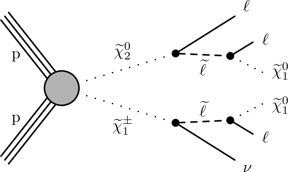
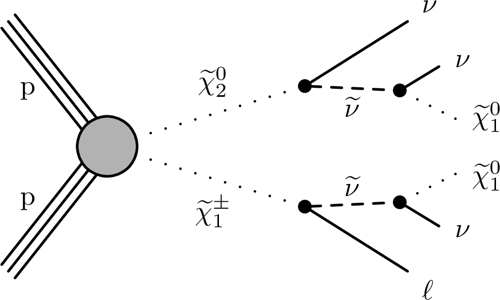
Chargino and neutralino pair production with decays mediated by sleptons and sneutrinos. |
png pdf |
Figure 1-a:
Chargino and neutralino pair production with decays mediated by sleptons. |
png pdf |
Figure 1-b:
Chargino and neutralino pair production with decays mediated by sneutrinos. |

png pdf |
Figure 2:
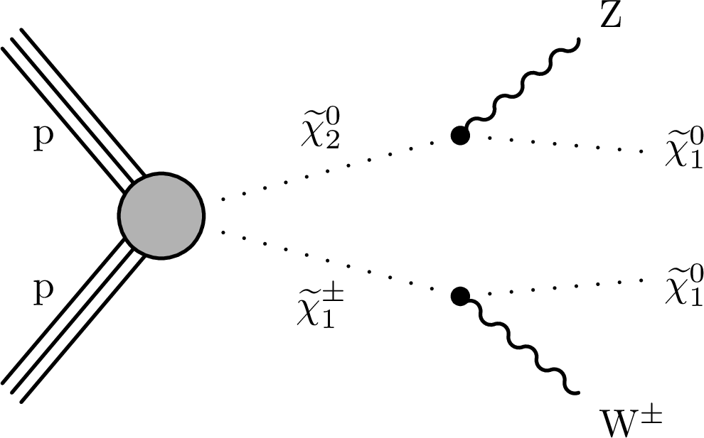
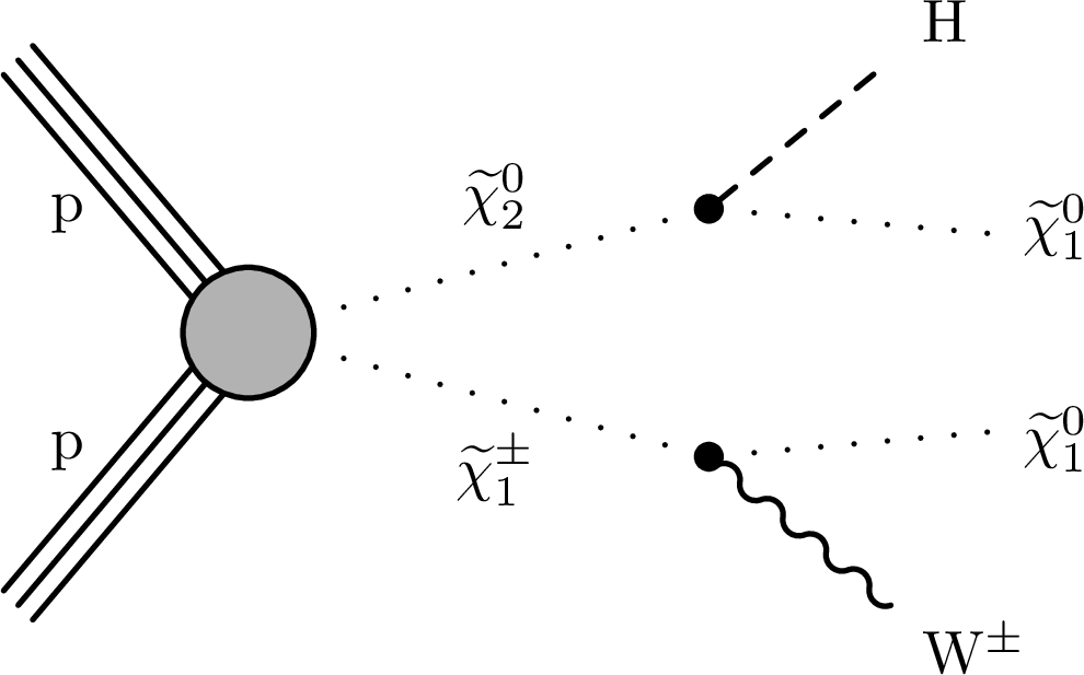
Chargino and neutralino pair production with the chargino decaying to a W boson and the LSP and the neutralino decaying to (left) a Z boson and the LSP or (right) a Higgs boson and the LSP. |
png pdf |
Figure 2-a:
Chargino and neutralino pair production with the chargino decaying to a W boson and the LSP and the neutralino decaying to a Z boson and the LSP. |
png pdf |
Figure 2-b:
Chargino and neutralino pair production with the chargino decaying to a W boson and the LSP and the neutralino decaying to a Higgs boson and the LSP. |

png pdf |
Figure 3:
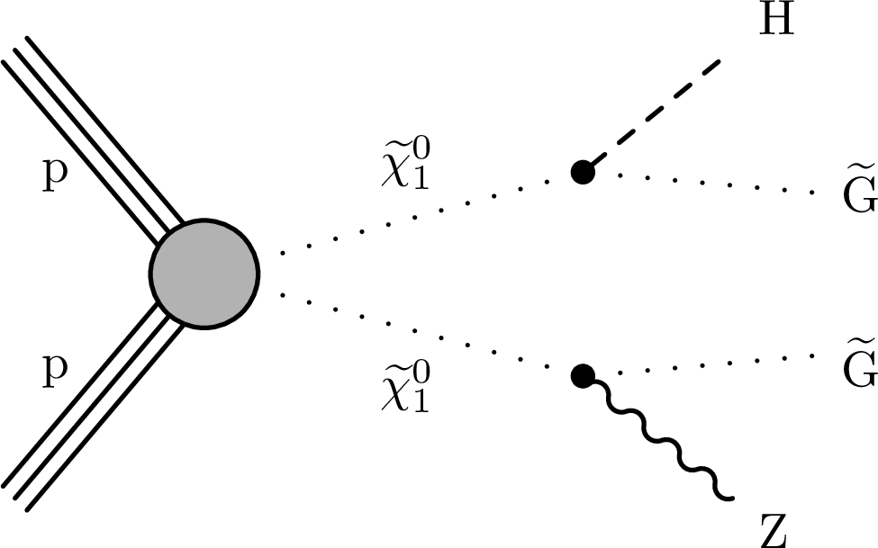
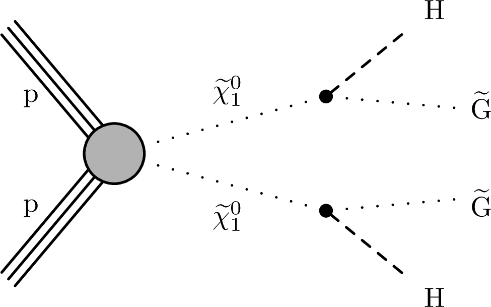
A GMSB model with higgsino pair production. The $\tilde{ \chi }^0_2 $, $\tilde{\chi}^{\pm}_1 $, and $\tilde{\chi}^0_1 $ are nearly mass-degenerate with $\tilde{\chi}^0_1 $ decaying to Z or Higgs bosons and $\tilde{\mathrm{G}} $ LSP. |

png pdf |
Figure 3-a:
A GMSB model with higgsino pair production. The $\tilde{ \chi }^0_2 $, $\tilde{\chi}^{\pm}_1 $, and $\tilde{\chi}^0_1 $ are nearly mass-degenerate with $\tilde{\chi}^0_1 $ decaying to two Z bosons and $\tilde{\mathrm{G}} $ LSP. |
png pdf |
Figure 3-b:
A GMSB model with higgsino pair production. The $\tilde{ \chi }^0_2 $, $\tilde{\chi}^{\pm}_1 $, and $\tilde{\chi}^0_1 $ are nearly mass-degenerate with $\tilde{\chi}^0_1 $ decaying to a Z boson, a Higgs boson and $\tilde{\mathrm{G}} $ LSP. |
png pdf |
Figure 3-c:
A GMSB model with higgsino pair production. The $\tilde{ \chi }^0_2 $, $\tilde{\chi}^{\pm}_1 $, and $\tilde{\chi}^0_1 $ are nearly mass-degenerate with $\tilde{\chi}^0_1 $ decaying to two Higgs bosons and $\tilde{\mathrm{G}} $ LSP. |

png pdf |
Figure 4:
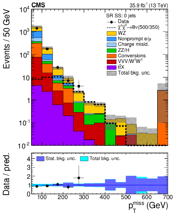
Distribution of $ {{p_{\mathrm {T}}} ^\text {miss}} $ for events with 2 SS leptons and 0 jets (left) or 1 jet (right). An example signal mass point in the flavor-democratic model with mass parameter $x= $ 0.05 is displayed for illustration. The numbers in the parentheses denote the $\tilde{\chi}^{\pm}_1 $ and $\tilde{\chi}^0_1 $ masses, namely $m_{\tilde{\chi}^{\pm}_1}=m_{\tilde{ \chi }^0_2} = $ 500 GeV and $m_{\tilde{\chi}^0_1} = $ 350 GeV. The last bin contains the overflow events. |
png pdf |
Figure 4-a:
Distribution of $ {{p_{\mathrm {T}}} ^\text {miss}} $ for events with 2 SS leptons and no jet. An example signal mass point in the flavor-democratic model with mass parameter $x= $ 0.05 is displayed for illustration. The numbers in the parentheses denote the $\tilde{\chi}^{\pm}_1 $ and $\tilde{\chi}^0_1 $ masses, namely $m_{\tilde{\chi}^{\pm}_1}=m_{\tilde{ \chi }^0_2} = $ 500 GeV and $m_{\tilde{\chi}^0_1} = $ 350 GeV. The last bin contains the overflow events. |

png pdf |
Figure 4-b:
Distribution of $ {{p_{\mathrm {T}}} ^\text {miss}} $ for events with 2 SS leptons and 1 jet. An example signal mass point in the flavor-democratic model with mass parameter $x= $ 0.05 is displayed for illustration. The numbers in the parentheses denote the $\tilde{\chi}^{\pm}_1 $ and $\tilde{\chi}^0_1 $ masses, namely $m_{\tilde{\chi}^{\pm}_1}=m_{\tilde{ \chi }^0_2} = $ 500 GeV and $m_{\tilde{\chi}^0_1} = $ 350 GeV. The last bin contains the overflow events. |
png pdf |
Figure 5:
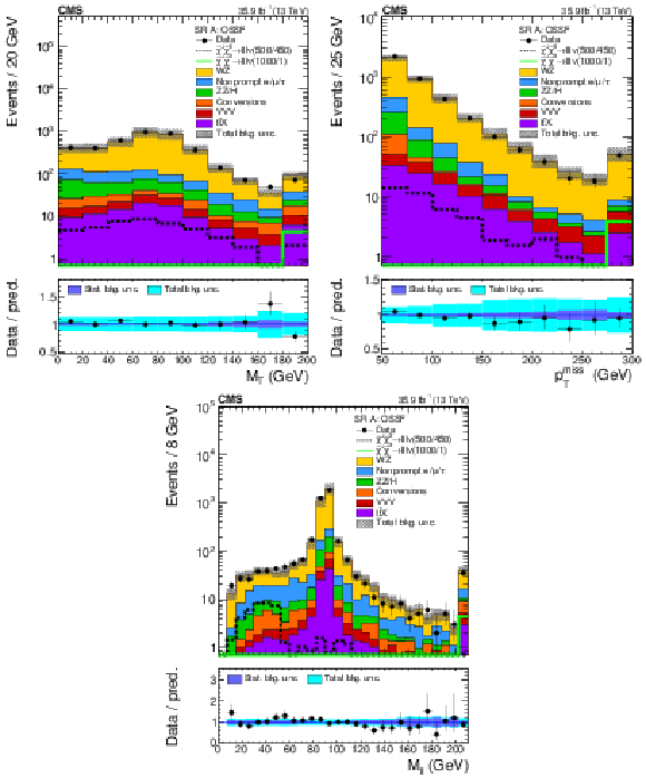
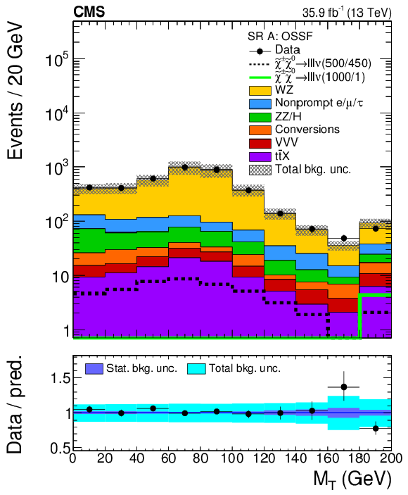
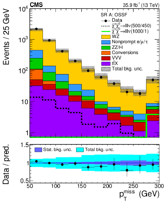
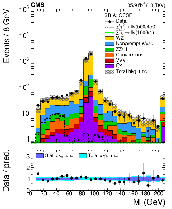
Distribution of kinematical observables used in the event selection for events entering signal regions A: the transverse mass of the third lepton (upper left), the $ {{p_{\mathrm {T}}} ^\text {miss}} $ (upper right) and the $ {M_{\ell \ell}} $ of the OSSF pair (lower). Two signal mass points in the flavor-democratic model with mass parameter $x= $ 0.5 are displayed for illustration. The notation is analogous to that used in Fig. 4. |
png pdf |
Figure 5-a:
Distribution of kinematical observables used in the event selection for events entering signal regions A: the transverse mass of the third lepton. Two signal mass points in the flavor-democratic model with mass parameter $x= $ 0.5 are displayed for illustration. |
png pdf |
Figure 5-b:
Distribution of kinematical observables used in the event selection for events entering signal regions A: the transverse mass of the $ {{p_{\mathrm {T}}} ^\text {miss}} $. Two signal mass points in the flavor-democratic model with mass parameter $x= $ 0.5 are displayed for illustration. |
png pdf |
Figure 5-c:
Distribution of kinematical observables used in the event selection for events entering signal regions A: the transverse mass of the $ {M_{\ell \ell}} $ of the OSSF pair. Two signal mass points in the flavor-democratic model with mass parameter $x= $ 0.5 are displayed for illustration. |

png pdf |
Figure 6:
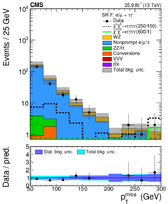
Distributions in the stransverse mass for events with two OSSF light leptons and one $ {\tau _\mathrm {h}} $ (left) and in $ {{p_{\mathrm {T}}} ^\text {miss}} $ for events with one light-flavor lepton and two $ {\tau _\mathrm {h}} $s. Two signal mass points in the $\tau $-enriched (left) and the $\tau $-dominated (right) scenarios with mass parameter $x= $ 0.5 are displayed for illustration. The notation is analogous to that used in Fig. 4. |

png pdf |
Figure 6-a:
Distribution in the stransverse mass for events with two OSSF light leptons and one $ {\tau _\mathrm {h}} $. Two signal mass points in the $\tau $-enriched scenario with mass parameter $x= $ 0.5 are displayed for illustration. |
png pdf |
Figure 6-b:
Distribution in $ {{p_{\mathrm {T}}} ^\text {miss}} $ for events with one light-flavor lepton and two $ {\tau _\mathrm {h}} $s. Two signal mass points in the $\tau $-dominated scenario with mass parameter $x= $ 0.5 are displayed for illustration. |
png pdf |
Figure 7:
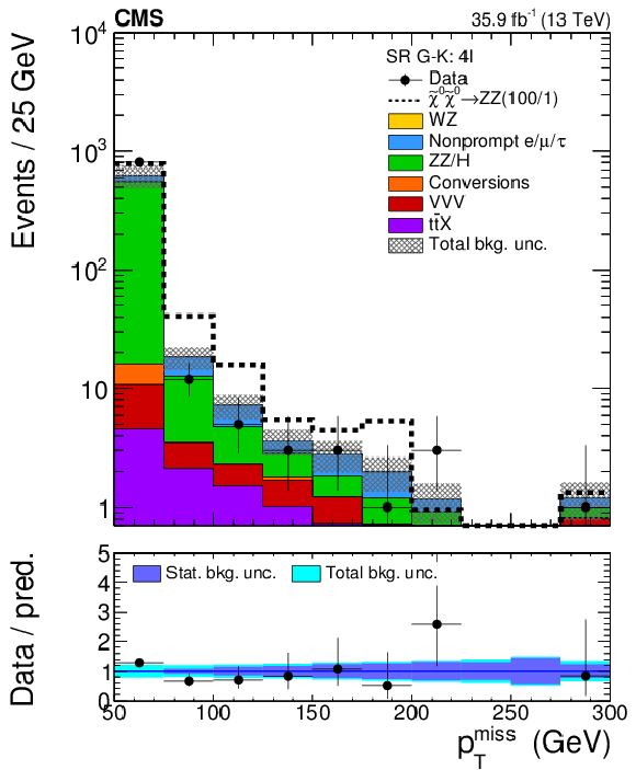
Distribution in $ {{p_{\mathrm {T}}} ^\text {miss}} $ for events with 4 or more leptons entering search categories G-K. An example signal mass point in the $\tilde{\chi}^0_1 \tilde{\chi}^0_1 $ production GMSB model is displayed for illustration. The numbers in the parenthesis denote the $\tilde{\chi}^0_1 $ and $\tilde{\mathrm{G}} $ masses, namely $m_{\tilde{\chi}^0_1} = $ 100 GeV and $m_{\tilde{\mathrm{G}}} = $ 1 GeV. |

png pdf |
Figure 8:
Expected and observed yields comparison in the SS dilepton category. An example signal mass point in the flavor-democratic model with mass parameter $x= $ 0.05 is displayed for illustration. The notation is analogous to that used in Fig. 4. |
png pdf |
Figure 9:
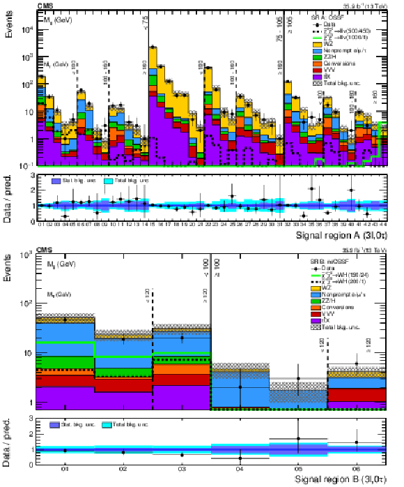
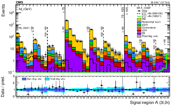
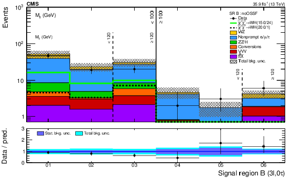
Expected and observed yields comparison in category A (upper) and category B (lower) signal regions, i.e. 3 light flavor leptons including at least one OSSF pair (A) or no OSSF pair (B). SR A15 is replaced by the WZ control region in interpretations of the results. Two signal mass points in the flavor-democratic model with mass parameter $x= $ 0.5 are displayed for illustration. The notation is analogous to that used in Fig. 4. |
png pdf |
Figure 9-a:
Expected and observed yields comparison in category A B signal region, i.e. 3 light flavor leptons including at least one OSSF pair. SR A15 is replaced by the WZ control region in interpretations of the results. Two signal mass points in the flavor-democratic model with mass parameter $x= $ 0.5 are displayed for illustration. |
png pdf |
Figure 9-b:
Expected and observed yields comparison in category A B signal region, i.e. no OSSF pair. Two signal mass points in the flavor-democratic model with mass parameter $x= $ 0.5 are displayed for illustration. |
png pdf |
Figure 10:
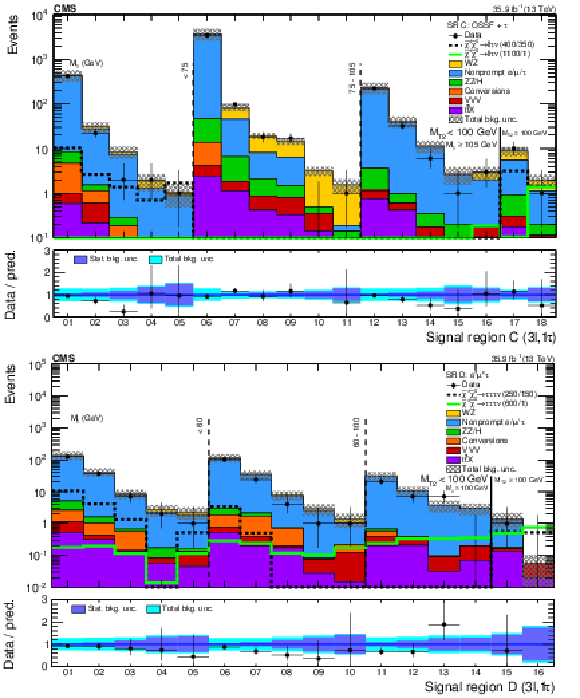
Expected and observed yields comparison in events with one $ {\tau _\mathrm {h}} $: categories C (upper) and D (lower). Two signal mass points in the $\tau $-enriched (upper) and the $\tau $-dominated (lower) scenarios with mass parameter $x= $ 0.5 are displayed for illustration. The notation is analogous to that used in Fig. 4. |
png pdf |
Figure 10-a:
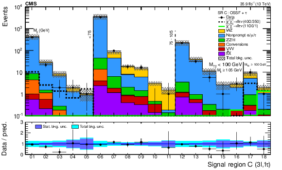
Expected and observed yields comparison in events with one $ {\tau _\mathrm {h}} $: category C. Two signal mass points in the $\tau $-enriched scenario with mass parameter $x= $ 0.5 are displayed for illustration. |
png pdf |
Figure 10-b:
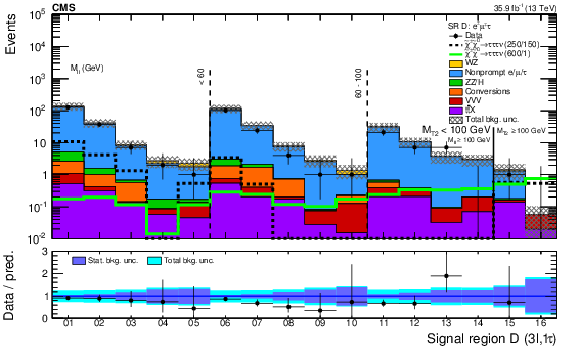
Expected and observed yields comparison in events with one $ {\tau _\mathrm {h}} $: category D. Two signal mass points in the $\tau $-dominated scenario with mass parameter $x= $ 0.5 are displayed for illustration. |
png pdf |
Figure 11:
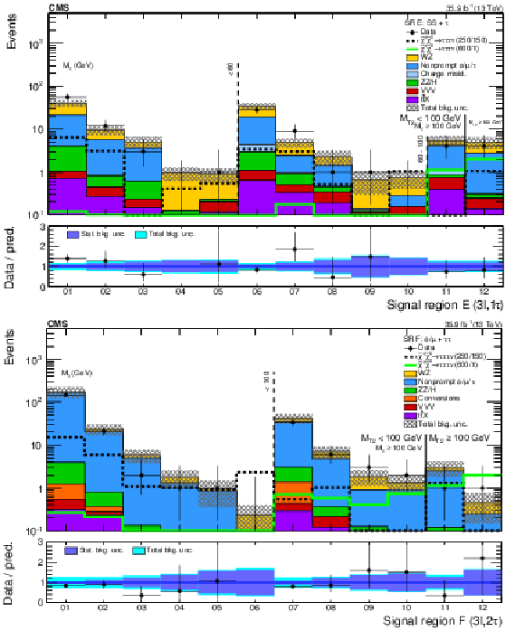
Expected and observed yields comparison in events with one $ {\tau _\mathrm {h}} $: category E (upper); and in events with two $ {\tau _\mathrm {h}} $: category F (lower). Two signal mass points in the $\tau $-dominated model with mass parameter $x= $ 0.5 are displayed for illustration. The notation is analogous to that used in Fig. 4. |
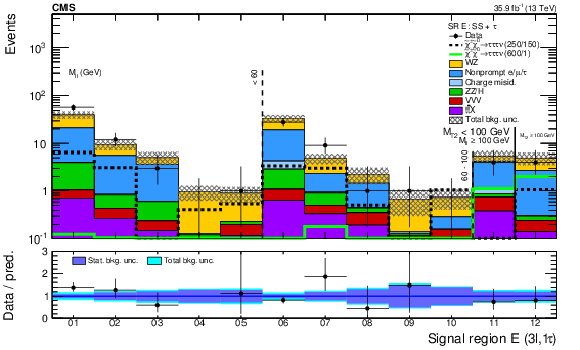
png pdf |
Figure 11-a:
Expected and observed yields comparison in events with one $ {\tau _\mathrm {h}} $: category E. Two signal mass points in the $\tau $-dominated model with mass parameter $x= $ 0.5 are displayed for illustration. |
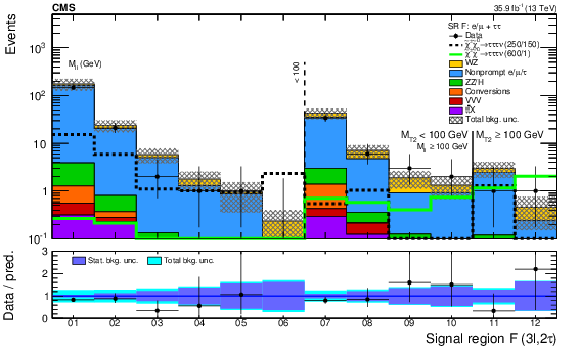
png pdf |
Figure 11-b:
Expected and observed yields comparison in events with two $ {\tau _\mathrm {h}} $: category F. Two signal mass points in the $\tau $-dominated model with mass parameter $x= $ 0.5 are displayed for illustration. |

png pdf |
Figure 12:
Expected and observed yields comparison in signal regions with at least four leptons (categories G-K). An example mass point in the $\tilde{\chi}^0_1 \tilde{\chi}^0_1 $ production GMSB model is displayed for illustration. The notation is analogous to that used in Fig. 7. |
png pdf |
Figure 13:
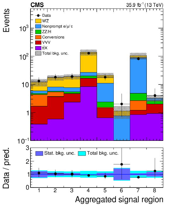
Expected and observed yields comparison in the aggregated signal regions. In this plot, the charge misidentification background prediction from control samples in data (that is only relevant in the first two bins due to the SS dilepton final state) are included in the nonprompt background prediction. |
png pdf root |
Figure 14:
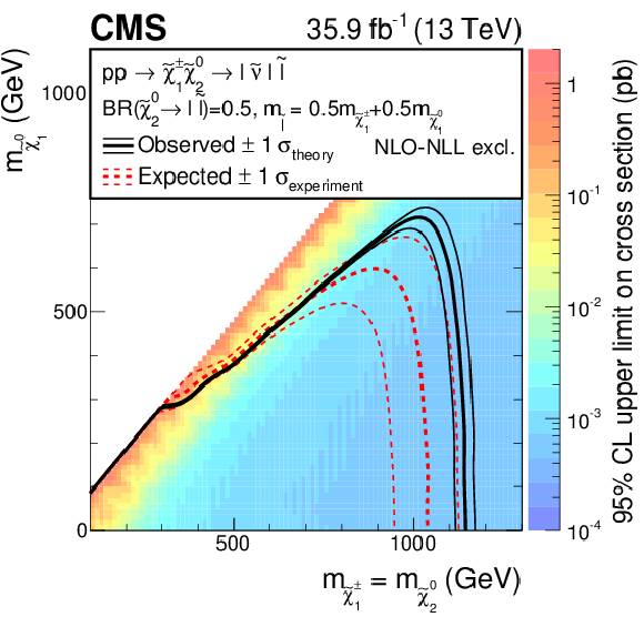
Interpretation of the results in the flavor-democratic model with mass parameter $x= $ 0.5 obtained with events of category A. The shading in the $m_{\tilde{\chi}^0_1}$ versus $m_{\tilde{ \chi }^0_2}$ ($=m_{\tilde{\chi}^{\pm}_1}$) plane indicates the 95% CL upper limit on the chargino-neutralino production cross section. The contours bound the mass regions excluded at 95% CL assuming the NLO+NLL cross sections. The observed, ${\pm}$1$\sigma _{\text {theory}}$ ($\pm $1 standard deviation of the theoretical cross section) observed, median expected, and ${\pm}$1$\sigma _{\text {experiment}}$ expected bounds are shown. |
png pdf |
Figure 15:
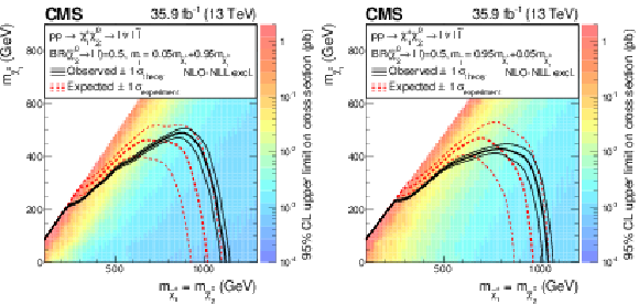
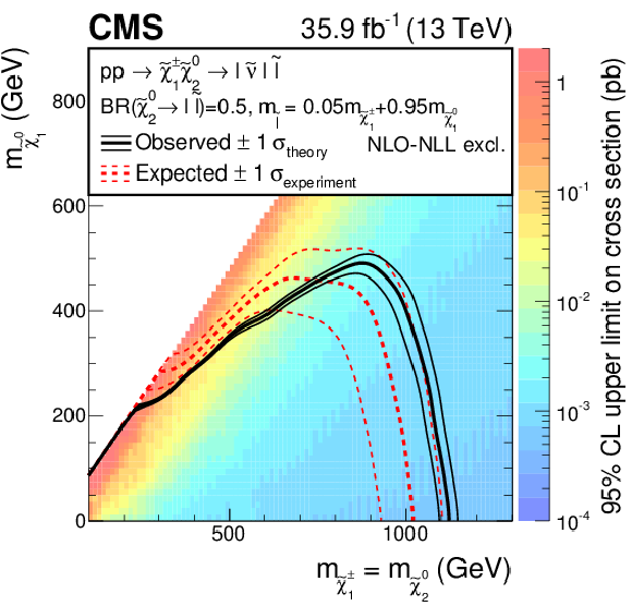
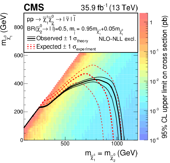
Interpretation of the results in the flavor-democratic model with mass parameter $x= $ 0.05 (left) and $x= $ 0.95 (right) obtained with the combination of the SS dilepton category and category A. The shading in this figure is as described in Fig. 14. |
png pdf root |
Figure 15-a:
Interpretation of the results in the flavor-democratic model with mass parameter $x= $ 0.05 obtained with the combination of the SS dilepton category and category A. |
png pdf root |
Figure 15-b:
Interpretation of the results in the flavor-democratic model with mass parameter $x= $ 0.95 obtained with the combination of the SS dilepton category and category A. |

png pdf |
Figure 16:
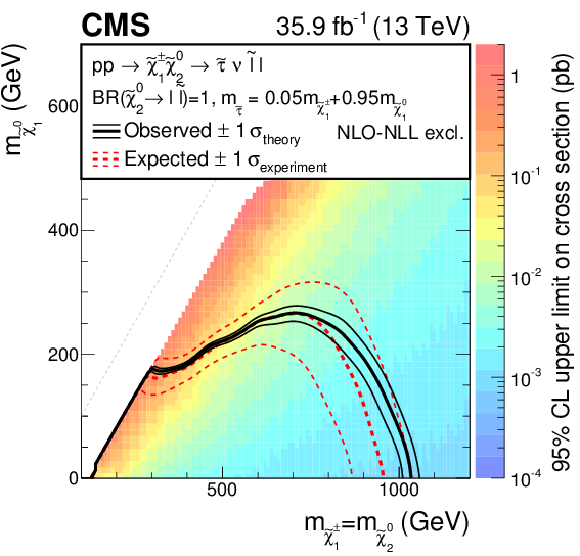
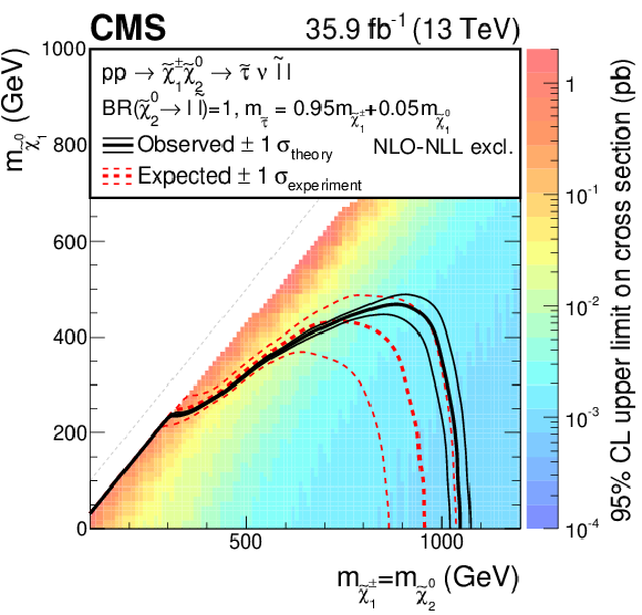
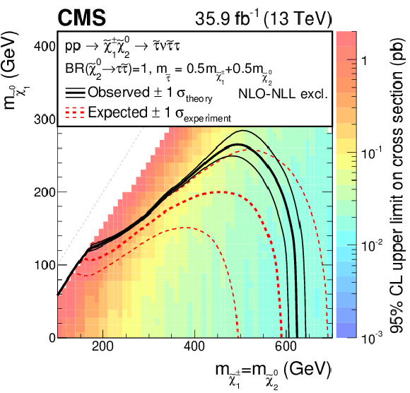
Interpretation of the results in the $\tau $-enriched model with mass parameter $x= $ 0.05 (upper-left), $x= $ 0.95 (upper-right) and $x= $ 0.5 (lower) obtained with events of categories A and C. The shading in this figure is as described in Fig. 14. |
png pdf root |
Figure 16-a:
Interpretation of the results in the $\tau $-enriched model with mass parameter $x= $ 0.05 obtained with events of categories A and C. |
png pdf root |
Figure 16-b:
Interpretation of the results in the $\tau $-enriched model with mass parameter $x= $ 0.95 obtained with events of categories A and C. |

png pdf root |
Figure 16-c:
Interpretation of the results in the $\tau $-enriched model with mass parameter $x= $ 0.5 obtained with events of categories A and C. |
png pdf root |
Figure 17:
Interpretation of the results in the $\tau $-dominated model with mass parameter $x= $ 0.5 obtained with events of category B-F. The shading in this figure is as described in Fig. 14. |
png pdf |
Figure 18:
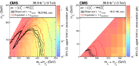
Interpretation of the results in the $\tilde{\chi}^{\pm}_1 \tilde{ \chi }^0_2 \to \mathrm{W} \mathrm{Z} \tilde{\chi}^0_1 \tilde{\chi}^0_1 $ (left) model obtained with events of category A and the $\tilde{\chi}^{\pm}_1 \tilde{ \chi }^0_2 \to \mathrm{W} \mathrm{H} \tilde{\chi}^0_1 \tilde{\chi}^0_1 $ (right) model obtained with events of all categories (SS dilepton, trilepton, and four-lepton). The shading in this figure is as described in Fig. 14. The dashed grey line on the left plot corresponds to a mass difference between the $\tilde{\chi}^{\pm}_1 $ and $\tilde{\chi}^0_1 $ equal to the Z mass. |

png pdf root |
Figure 18-a:
Interpretation of the results in the $\tilde{\chi}^{\pm}_1 \tilde{ \chi }^0_2 \to \mathrm{W} \mathrm{Z} \tilde{\chi}^0_1 \tilde{\chi}^0_1 $ model obtained with events of category A. The dashed grey line corresponds to a mass difference between the $\tilde{\chi}^{\pm}_1 $ and $\tilde{\chi}^0_1 $ equal to the Z mass. |

png pdf root |
Figure 18-b:
Interpretation of the results in the $\tilde{\chi}^{\pm}_1 \tilde{ \chi }^0_2 \to \mathrm{W} \mathrm{H} \tilde{\chi}^0_1 \tilde{\chi}^0_1 $ model obtained with events of all categories (SS dilepton, trilepton, and four-lepton). |
png pdf |
Figure 19:
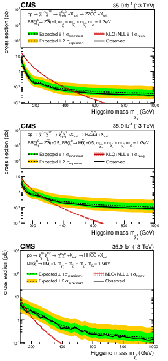
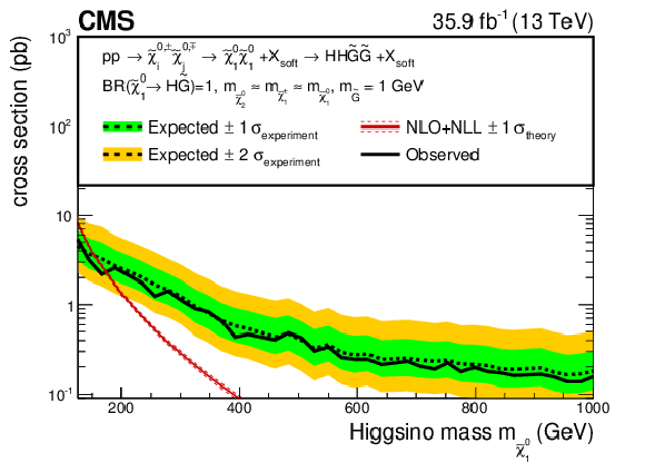
Interpretation of the results in the $\tilde{\chi}^0_1 \tilde{\chi}^0_1 \to \mathrm{Z} \mathrm{Z} \tilde{\mathrm{G}} \tilde{\mathrm{G}} $ model (upper), the $\tilde{\chi}^0_1 \tilde{\chi}^0_1 \to \mathrm{H} \mathrm{Z} \tilde{\mathrm{G}} \tilde{\mathrm{G}} $ model (middle), and the $\tilde{\chi}^0_1 \tilde{\chi}^0_1 \to \mathrm{H} \mathrm{H} \tilde{\mathrm{G}} \tilde{\mathrm{G}} $ model (lower) obtained with events of all trilepton (A-F) and all four-lepton (G-K) categories. The observed, median expected, ${\pm}$1$\sigma _{\text {experiment}}$ expected, and ${\pm}$2$\sigma _{\text {experiment}}$ expected 95% CL upper limit on the neutralino pair production cross section are compared to the NLO+NLL cross sections ${\pm}$1$\sigma _{\text {theory}}$. |

png pdf root |
Figure 19-a:
Interpretation of the results in the $\tilde{\chi}^0_1 \tilde{\chi}^0_1 \to \mathrm{Z} \mathrm{Z} \tilde{\mathrm{G}} \tilde{\mathrm{G}} $ model obtained with events of all trilepton (A-F) and all four-lepton (G-K) categories. The observed, median expected, ${\pm}$1$\sigma _{\text {experiment}}$ expected, and ${\pm}$2$\sigma _{\text {experiment}}$ expected 95% CL upper limit on the neutralino pair production cross section are compared to the NLO+NLL cross sections ${\pm}$1$\sigma _{\text {theory}}$. |

png pdf root |
Figure 19-b:
Interpretation of the results in the $\tilde{\chi}^0_1 \tilde{\chi}^0_1 \to \mathrm{H} \mathrm{Z} \tilde{\mathrm{G}} \tilde{\mathrm{G}} $ model obtained with events of all trilepton (A-F) and all four-lepton (G-K) categories. The observed, median expected, ${\pm}$1$\sigma _{\text {experiment}}$ expected, and ${\pm}$2$\sigma _{\text {experiment}}$ expected 95% CL upper limit on the neutralino pair production cross section are compared to the NLO+NLL cross sections ${\pm}$1$\sigma _{\text {theory}}$. |
png pdf root |
Figure 19-c:
Interpretation of the results in the $\tilde{\chi}^0_1 \tilde{\chi}^0_1 \to \mathrm{H} \mathrm{H} \tilde{\mathrm{G}} \tilde{\mathrm{G}} $ model obtained with events of all trilepton (A-F) and all four-lepton (G-K) categories. The observed, median expected, ${\pm}$1$\sigma _{\text {experiment}}$ expected, and ${\pm}$2$\sigma _{\text {experiment}}$ expected 95% CL upper limit on the neutralino pair production cross section are compared to the NLO+NLL cross sections ${\pm}$1$\sigma _{\text {theory}}$. |
| Tables | |

png pdf |
Table 1:
Search regions for events with two SS light-flavor leptons. |

png pdf |
Table 2:
Search regions corresponding to category A, events with three electrons or muons that form at least one opposite-sign same-flavor (OSSF) pair. Search region A15$^\dagger $ overlaps with the WZ control region of the analysis, and is not used in the interpretation. |

png pdf |
Table 3:
Search regions corresponding to category B, events with three e or $\mu $ that do not form an opposite-sign same-flavor (OSSF) pair. |

png pdf |
Table 4:
Search region definition corresponding to category C, events with two e or $\mu $ forming an opposite-sign same-flavor (OSSF) pair and one $ {\tau _\mathrm {h}} $ candidate. Regions where there is a Z boson candidate are not split into $ {M_{\mathrm {T}2}} $ categories. |

png pdf |
Table 5:
Search region definition corresponding to category D, events with one e and one $\mu $ of OS and one $ {\tau _\mathrm {h}} $ candidate. |

png pdf |
Table 6:
Search region definition corresponding to category E, events with two e or $\mu $ of same sign and one $ {\tau _\mathrm {h}} $ candidate. |
png pdf |
Table 7:
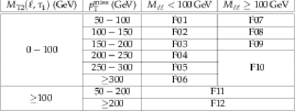
Search region definition corresponding to category F, events with one electron or muon and two $ {\tau _\mathrm {h}} $ candidates. |

png pdf |
Table 8:
Search region definition corresponding to categories G-K, events with four or more leptons. Categorization is made based on the number of OSSF pairs (nOSSF). |

png pdf |
Table 9:
Definition of the aggregated regions for multilepton and two SS dilepton final states. |
png pdf |
Table 10:
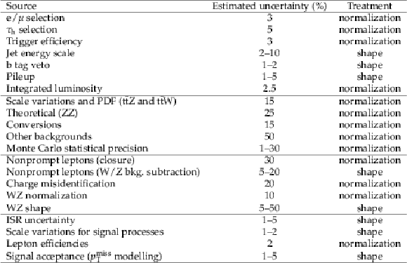
Summary of systematic uncertainties in the event yields in the search regions and their treatment. Uncertainties are allowed to vary only the normalization of all the bins at once, or both the shape and the normalization (allowing for different correlations across the bins). The upper group lists uncertainties related to experimental effects for all processes whose yield is estimated from simulation; the middle group lists uncertainties in these yields related to the event simulation process itself. The third group lists uncertainties for background processes whose yield is estimated from data. Finally, the last group describes uncertainties related to the extraction of the signal acceptance in MC simulation. |

png pdf |
Table 11:
SS dilepton category: Expected and observed yields in events with two SS light-flavor leptons. For each bin, the first number corresponds to the expected yield (exp.) and its uncertainty, and the second denotes the observed yield (obs.). The uncertainty denotes the total uncertainty in the yield. |
png pdf |
Table 12:
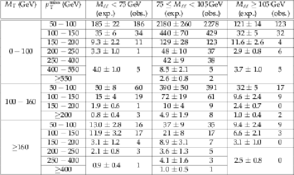
Category A: Expected and observed yields in events with three e or $\mu $ that form at least one OSSF pair. For each bin, the first number corresponds to the expected yield (exp.) and its uncertainty, and the second denotes the observed yield (obs.). The uncertainty denotes the total uncertainty in the yield. |

png pdf |
Table 13:
Category B: Expected and observed yields in events with three e or $\mu $ that do not form an OSSF pair. For each bin, the first number corresponds to the expected yield (exp.) and its uncertainty, and the second denotes the observed yield (obs.). The uncertainty denotes the total uncertainty in the yield. |

png pdf |
Table 14:
Category C: Expected and observed yields in events with two e or $\mu $ forming and OSSF pair and one $ {\tau _\mathrm {h}} $. For each bin, the first number corresponds to the expected yield and its uncertainty, and the second denotes the observed yield. The uncertainty denotes the total uncertainty in the yield. |

png pdf |
Table 15:
Category D: Expected and observed yields in events with an opposite-sign e$ \mu $ pair and one $ {\tau _\mathrm {h}} $. For each bin, the first number corresponds to the expected yield and its uncertainty, and the second denotes the observed yield. The uncertainty denotes the total uncertainty in the yield. |

png pdf |
Table 16:
Category E: Expected and observed yields in events with one SS e or $\mu $ and one $ {\tau _\mathrm {h}} $. For each bin, the first number corresponds to the expected yield and its uncertainty, and the second denotes the observed yield. The uncertainty denotes the total uncertainty in the yield. |

png pdf |
Table 17:
Category F: Expected and observed yields in events with one e or $\mu $ and two $ {\tau _\mathrm {h}} $. For each bin, the first number corresponds to the expected yield and its uncertainty, and the second denotes the observed yield. The uncertainty denotes total uncertainty in the yield. |

png pdf |
Table 18:
Categories G-K: Expected and observed yields in the 4$\ell $ category of the analysis. For each bin, the first number corresponds to the expected yield (exp.) and its uncertainty, and the second denotes the observed yield (obs.). The uncertainty denotes the total uncertainty in the yield. |

png pdf |
Table 19:
Expected and observed yields in the aggregated signal regions defined in Section 5.3. For each bin, the first number corresponds to the expected yield (exp.) and its uncertainty, and the second denotes the observed yield (obs.). The uncertainty denotes the total uncertainty in the yield. |
png pdf |
Table 20:
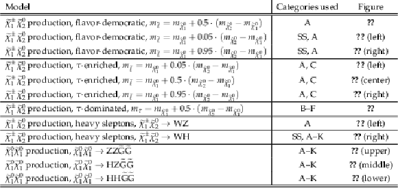
Summary of the interpretations of the results using different models. |
| Summary |
|
Results are presented from a search for new physics in same-sign dilepton, trilepton, and four-lepton events containing up to two hadronically decaying $\tau$ leptons in proton-proton collision data at $\sqrt{s} = $ 13 TeV, recorded with the CMS detector at the LHC and corresponding to an integrated luminosity of 35.9 fb$^{-1}$. The data are categorized based on the number, charge, and flavor of the leptons, and are subdivided into several kinematic regions to be sensitive to a broad range of supersymmetric particles produced via the electroweak interaction. No significant deviation from the standard model expectations is observed. The results are used to set limits on various simplified models of supersymmetry (SUSY) that entail the production of superpartners of electroweak gauge or Higgs bosons (charginos and neutralinos). Specifically, we consider chargino-neutralino pair production, the electroweak process that is expected to have the largest cross section, and higgsino pair production in a gauge-mediated SUSY breaking inspired SUSY scenario. The resulting signal topologies depend on the masses of the lepton superpartners. Models with light left-handed sleptons lead to enhanced branching fractions to final states with three leptons. The results imply limits on the masses of charginos and neutralinos up to 1150 GeV at 95% confidence level for the flavor-democratic scenario, extending the reach of our previous search [21] by about 450 GeV. In these models, searches in the same-sign dilepton final state enhance the sensitivity in the experimentally challenging region with small mass difference between the produced gauginos and the lightest supersymmetric particle (LSP) that is inaccessible with the trilepton signature. Assuming light right-handed sleptons, we consider two scenarios, one in which the chargino decays to $\tau$ leptons while the neutralino decays democratically, and another in which both chargino and neutralino decay to $\tau$ leptons. For the former we exclude masses of charginos and neutralinos up to 1050 GeV, while for the latter masses up to 625 GeV are excluded. We also consider scenarios that involve the direct decay of gauginos to the LSP via W and Z or Higgs bosons. For the models with W and Z bosons, chargino masses up to 475 GeV are excluded, improving the previous reach by 200 GeV. In the case of the neutralino decay via a Higgs boson, masses up to 180 GeV are excluded. In the case of the gauge-mediated SUSY breaking model with four higgsinos and an effectively massless gravitino as the LSP, we exclude higgsino masses up to 450 GeV depending on the assumed next-to-LSP branching fraction to Z or H boson. Finally, results are presented in a form suitable for alternative theoretical interpretations. |
| Additional Figures | |

png pdf root |
Additional Figure 1:
Interpretation of the results in the flavor-democratic model with mass parameter $x= $ 0.05 obtained with events of the same-sign category. |
png pdf root |
Additional Figure 2:
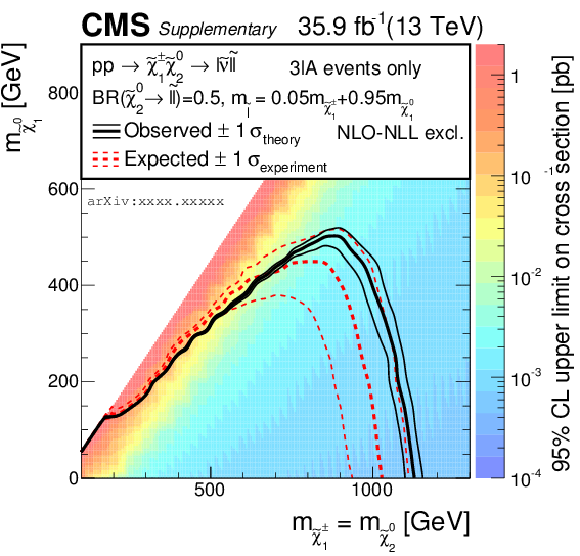
Interpretation of the results in the flavor-democratic model with mass parameter $x= $ 0.05 obtained with events of the 3lA category. |
png pdf root |
Additional Figure 3:
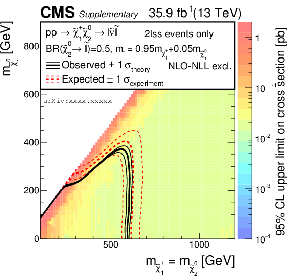
Interpretation of the results in the flavor-democratic model with mass parameter $x= $ 0.95 obtained with events of the same-sign category. |
png pdf root |
Additional Figure 4:
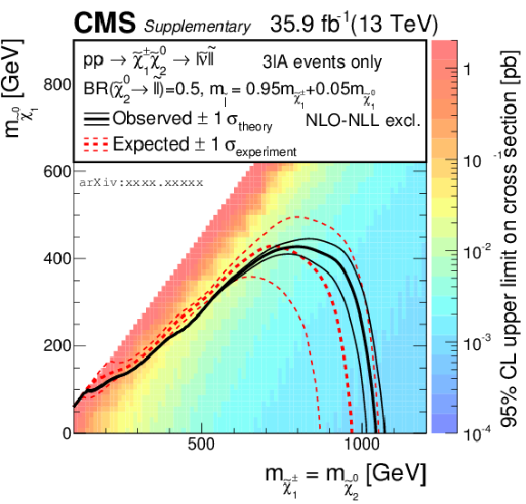
Interpretation of the results in the flavor-democratic model with mass parameter $x= $ 0.95 obtained with events of the 3lA category. |
png pdf root |
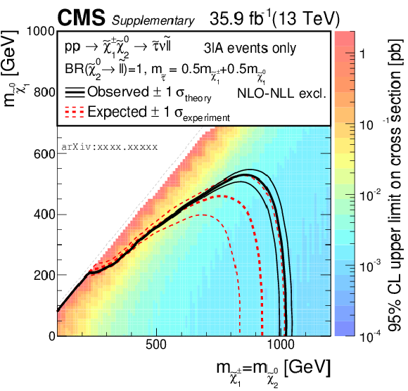
Additional Figure 5:
Interpretation of the results in the tau-enriched model with mass parameter $x= $ 0.5 obtained with events of the 3lA category. |
png pdf root |
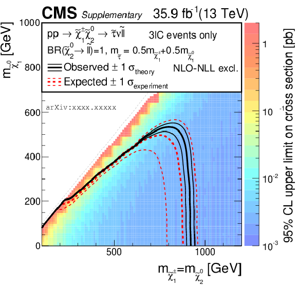
Additional Figure 6:
Interpretation of the results in the tau-enriched model with mass parameter $x= $ 0.5 obtained with events of the 3lC category. |

png pdf root |
Additional Figure 7:
Interpretation of the results in the tau-enriched model with mass parameter $x= $ 0.05 obtained with events of the 3lA category. |
png pdf root |
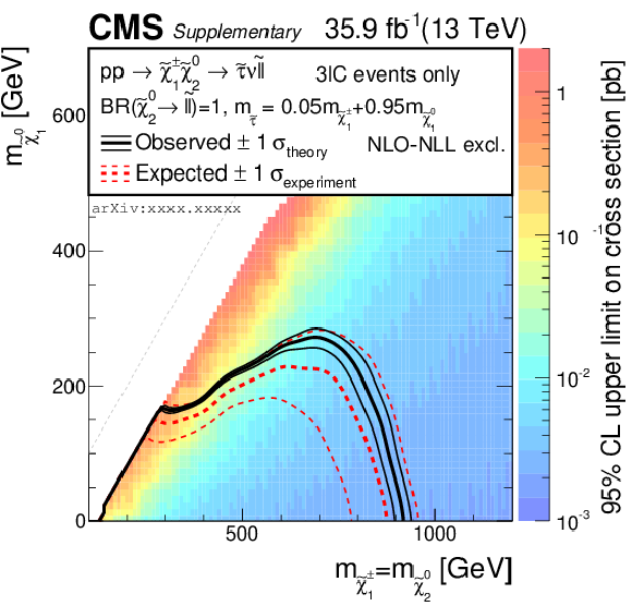
Additional Figure 8:
Interpretation of the results in the tau-enriched model with mass parameter $x= $ 0.05 obtained with events of the 3lC category. |
png pdf root |
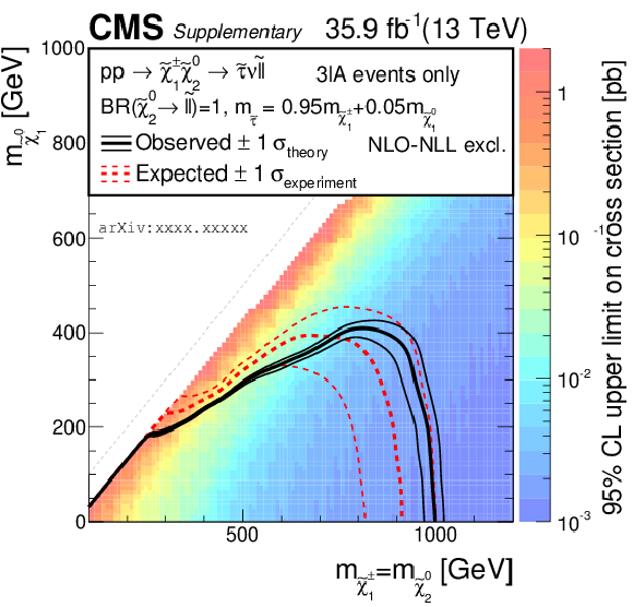
Additional Figure 9:
Interpretation of the results in the tau-enriched model with mass parameter $x= $ 0.95 obtained with events of the 3lA category. |

png pdf root |
Additional Figure 10:
Interpretation of the results in the tau-enriched model with mass parameter $x= $ 0.95 obtained with events of the 3lC category. |

png pdf root |
Additional Figure 11:
Interpretation of the results in the tau-dominated model with mass parameter $x= $ 0.5 obtained with events of the 3lB category. |

png pdf root |
Additional Figure 12:
Interpretation of the results in the tau-dominated model with mass parameter $x= $ 0.5 obtained with events of the 3lC category. |
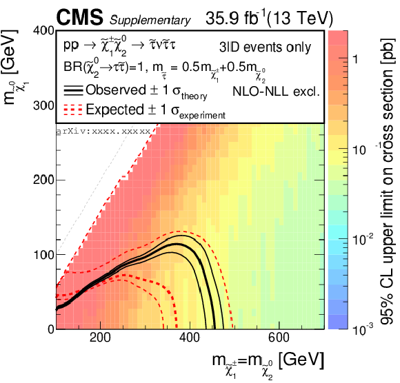
png pdf root |
Additional Figure 13:
Interpretation of the results in the tau-dominated model with mass parameter $x= $ 0.5 obtained with events of the 3lD category. |

png pdf root |
Additional Figure 14:
Interpretation of the results in the tau-dominated model with mass parameter $x= $ 0.5 obtained with events of the 3lE category. |
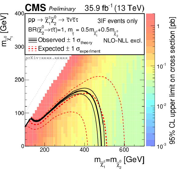
png pdf root |
Additional Figure 15:
Interpretation of the results in the tau-dominated model with mass parameter $x= $ 0.5 obtained with events of the 3lF category. |
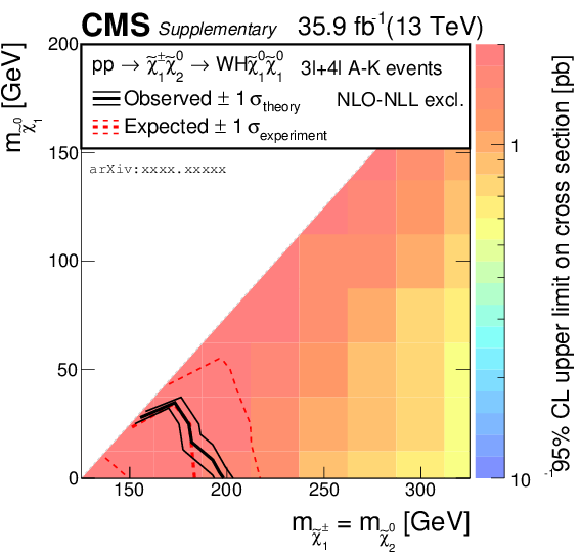
png pdf root |
Additional Figure 16:
Interpretation of the results in the TChiWH model obtained with events of the 3l categories A-F and the 4l categories G-K. |
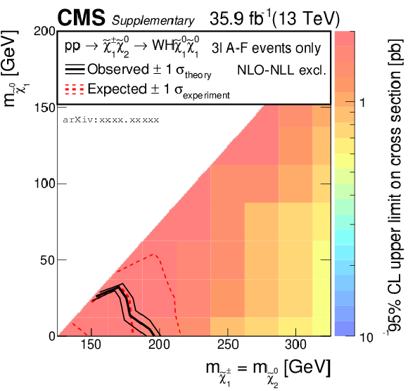
png pdf root |
Additional Figure 17:
Interpretation of the results in the TChiWH model obtained with events of the 3l categories A-F. |
png pdf root |
Additional Figure 18:
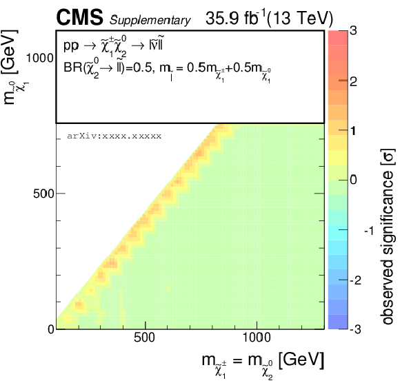
Observed local significance in the flavor-democratic model with mass parameter $x= $ 0.5 obtained with 3lA events. |
png pdf root |
Additional Figure 19:
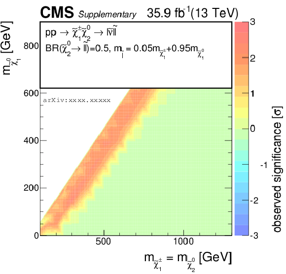
Observed local significance in the flavor-democratic model with mass parameter $x= $ 0.05 obtained with the combination of 2lss and 3lA events. |
png pdf root |
Additional Figure 20:
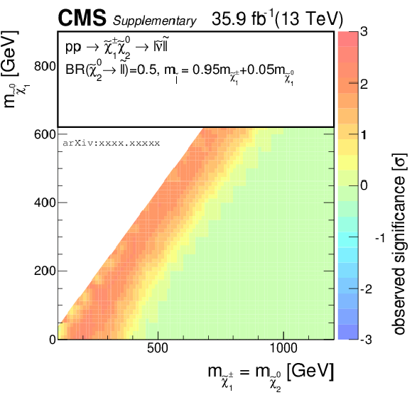
Observed local significance in the flavor-democratic model with mass parameter $x= $ 0.95 obtained with the combination of 2lss and 3lA events. |
png pdf root |
Additional Figure 21:
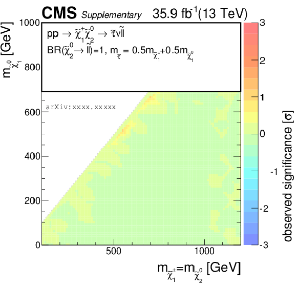
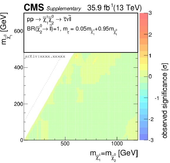
Observed local significance in the tau-enriched model with mass parameter $x= $ 0.5 obtained with the combination of 3lA and 3lC events. |
png pdf root |
Additional Figure 22:
Observed local significance in the tau-enriched model with mass parameter $x= $ 0.05 obtained with the combination of 3lA and 3lC events. |

png pdf root |
Additional Figure 23:
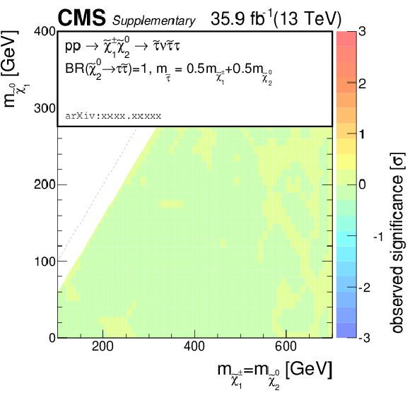
Observed local significance in the tau-enriched model with mass parameter $x= $ 0.95 obtained with the combination of 3lA and 3lC events. |
png pdf root |
Additional Figure 24:
Observed local significance in the tau-dominated model obtained with events of the 3lB, 3lC, 3lD, 3lE and 3lF categories. |

png pdf root |
Additional Figure 25:
Observed local significance in the $ \tilde{\chi}^{\pm} _1 \tilde{\chi}^0_2 \rightarrow \mathrm{W} \mathrm{Z} $ model obtained with events of category 3lA. |

png pdf root |
Additional Figure 26:
Observed local significance in the $ \tilde{\chi}^{\pm} _1 \tilde{\chi}^0_2 \rightarrow \mathrm{W} \mathrm{H} $ model obtained with all events of all categories 2lss, 3lA-3lF and 4lG-4lK. |
png pdf root |
Additional Figure 27:
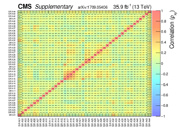
The correlation matrix for the background predictions in the 3lA category signal regions. |
| Additional Tables | |
png pdf |
Additional Table 1:
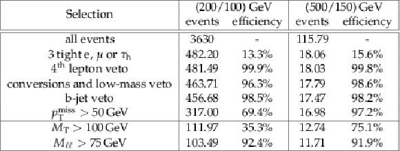
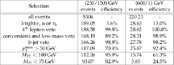
Cut-flow for the trilepton channel for a compressed ($m_{ \tilde{\chi}^0_2} = $ 200 GeV, $m_{ \tilde{\chi}^0 _1} = $ 100 GeV, production cross section 1.8 pb) and an uncompressed mass point ($m_{ \tilde{\chi}^0_2} = $ 500 GeV, $m_{ \tilde{\chi}^0 _1} = $ 150 GeV, production cross section 0.046 pb) for the $ \tilde{\chi}^{\pm} _1 \tilde{\chi}^0_2 \to \mathrm{W} \mathrm{Z} \tilde{\chi}^0_1 \tilde{\chi}^0_1 $ model from which one expects three hard and isolated light flavor leptons in the final state. The yields correspond to the integrated luminosity of 35.9 fb$^{-1}$ and a branching fraction of 0.1 is assumed corresponding to $\mathrm{Z} \to \ell \ell $ decays. |
png pdf |
Additional Table 2:
Cut-flow for the trilepton channel for a compressed ($m_{ \tilde{\chi}^0_2} = $ 250 GeV, $m_{ \tilde{\chi}^0 _1} = $ 150 GeV, production cross section 0.78 pb) and an uncompressed mass point ($m_{ \tilde{\chi}^0_2} = $ 600 GeV, $m_{ \tilde{\chi}^0 _1} = $ 1 GeV, production cross section 0.020 pb) for the $\tau $-dominated model from which one expects three hard and isolated taus in the final state. The yields correspond to the integrated luminosity of 35.9 fb$^{-1}$. |

png pdf |
Additional Table 3:
Cut-flow for the same-sign dilepton channel for a compressed mass point ($m_{ \tilde{\chi}^0_2} = $ 500 GeV, $m_{ \tilde{\chi}^0 _1} = $ 350 GeV, production cross section 0.046 pb) for the flavor-democratic model with mass parameters $x= $ 0.05 and $x= $ 0.5 where $m_{\tilde{\ell}} = m_{ \tilde{\chi}^0 _1} + x (m_{ \tilde{\chi}^0_2} - m_{ \tilde{\chi}^0 _1})$. The yields correspond to the integrated luminosity of 35.9 fb$^{-1}$. A branching fraction penality of 0.5 is assumed given that the $ \tilde{\chi}^0_2 \to \nu \tilde{\nu}$ decays are neglected. |
png pdf |
Additional Table 4:
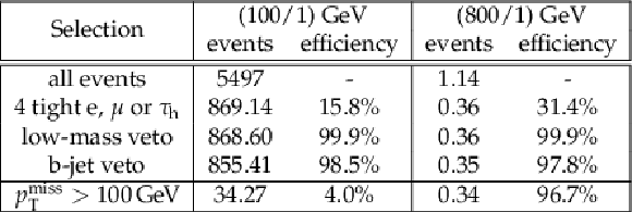
Cut-flow for the four-lepton channel for a compressed ($m_{ \tilde{\chi}^0 _1} = $ 100 GeV, $m_{\tilde{\mathrm{G}}} = $ 1 GeV, production cross section 16.8 pb) and an uncompressed mass point ($m_{ \tilde{\chi}^0 _1} = $ 800 GeV, $m_{\tilde{\mathrm{G}}} = $ 1 GeV, production cross section 0.0035 pb) for the $ { \tilde{\chi}^0_i \tilde{\chi}^0_j}\rightarrow \mathrm{Z} \mathrm{Z} \tilde{\mathrm{G}} \tilde{\mathrm{G}} $ model from which one expects four hard and isolated light flavor leptons in the final state. The yields correspond to the integrated luminosity of 35.9 fb$^{-1}$ and a branching fraction of 0.01 is assumed corresponding to both Z to decay leptonically, $\mathrm{Z} \to \ell \ell $. |
| References | ||||
| 1 | ATLAS Collaboration | Observation of a new particle in the search for the Standard Model Higgs boson with the ATLAS detector at the LHC | PLB 716 (2012) 1 | 1207.7214 |
| 2 | CMS Collaboration | Observation of a new boson at a mass of 125 GeV with the CMS experiment at the LHC | PLB 716 (2012) 30 | CMS-HIG-12-028 1207.7235 |
| 3 | CMS Collaboration | Observation of a new boson with mass near 125 GeV in pp collisions at $ \sqrt{s} = $ 7 and 8 TeV | JHEP 06 (2013) 081 | CMS-HIG-12-036 1303.4571 |
| 4 | R. Barbieri and G. F. Giudice | Upper Bounds on Supersymmetric Particle Masses | NPB 306 (1988) 63 | |
| 5 | E. Witten | Dynamical Breaking of Supersymmetry | NPB 188 (1981) 513 | |
| 6 | S. Dimopoulos and H. Georgi | Softly Broken Supersymmetry and SU(5) | NPB 193 (1981) 150 | |
| 7 | P. Ramond | Dual theory for free fermions | PRD 3 (1971) 2415 | |
| 8 | Y. A. Gol'fand and E. P. Likhtman | Extension of the algebra of Poincare group generators and violation of P invariance | JEPTL 13 (1971)323 | |
| 9 | A. Neveu and J. H. Schwarz | Factorizable dual model of pions | NPB 31 (1971) 86 | |
| 10 | D. V. Volkov and V. P. Akulov | Possible universal neutrino interaction | JEPTL 16 (1972)438 | |
| 11 | J. Wess and B. Zumino | A Lagrangian model invariant under supergauge transformations | PLB 49 (1974) 52 | |
| 12 | J. Wess and B. Zumino | Supergauge transformations in four-dimensions | NPB 70 (1974) 39 | |
| 13 | P. Fayet | Supergauge invariant extension of the Higgs mechanism and a model for the electron and its neutrino | NPB 90 (1975) 104 | |
| 14 | H. P. Nilles | Supersymmetry, supergravity and particle physics | PR 110 (1984) 1 | |
| 15 | S. P. Martin | A supersymmetry primer | Adv. Ser. Direct. High Energy Phys. 18 (1998) 1 | hep-ph/9709356 |
| 16 | CMS Collaboration | Search for physics beyond the standard model in events with two leptons of same sign, missing transverse momentum, and jets in proton-proton collisions at $ \sqrt{s} = $ 13 TeV | Submitted to EPJC | CMS-SUS-16-035 1704.07323 |
| 17 | CMS Collaboration | Search for new phenomena with the $M_{\mathrm{T2}}$ variable in the all-hadronic final state produced in proton-proton collisions at $ \sqrt{s} = $ 13 TeV | Submitted to EPJC | CMS-SUS-16-036 1705.04650 |
| 18 | CMS Collaboration | Search for supersymmetry in multijet events with missing transverse momentum in proton-proton collisions at 13 TeV | Submitted to PRD | CMS-SUS-16-033 1704.07781 |
| 19 | ATLAS Collaboration | Search for new phenomena in a lepton plus high jet multiplicity final state with the ATLAS experiment using $ \sqrt{s} = $ 13 TeV proton-proton collision data | Submitted to JHEP | 1704.08493 |
| 20 | ATLAS Collaboration | Search for new phenomena in events containing a same-flavour opposite-sign dilepton pair, jets, and large missing transverse momentum in $ \sqrt{s} = $ 13 TeV pp collisions with the ATLAS detector | EPJC 77 (2017) 144 | 1611.05791 |
| 21 | CMS Collaboration | Searches for electroweak production of charginos, neutralinos, and sleptons decaying to leptons and W, Z, and Higgs bosons in pp collisions at 8 TeV | EPJC 74 (2014) 3036 | CMS-SUS-13-006 1405.7570 |
| 22 | CMS Collaboration | Searches for electroweak neutralino and chargino production in channels with Higgs, Z, and W bosons in pp collisions at 8 TeV | PRD 90 (2014) 092007 | CMS-SUS-14-002 1409.3168 |
| 23 | ATLAS Collaboration | Search for the electroweak production of supersymmetric particles in $ \sqrt{s}= $ 8 TeV pp collisions with the ATLAS detector | PRD 93 (2016) 052002 | 1509.07152 |
| 24 | CMS Collaboration | Interpretation of searches for supersymmetry with simplified models | PRD 88 (2013) 052017 | CMS-SUS-11-016 1301.2175 |
| 25 | D. Alves et al. | Simplified models for LHC new physics searches | JPG 39 (2012) 105005 | 1105.2838 |
| 26 | Particle Data Group, C. Patrignani et al. | Review of particle physics | CPC 40 (2016) 100001 | |
| 27 | B. Fuks, M. Klasen, D. R. Lamprea, and M. Rothering | Gaugino production in proton-proton collisions at a center-of-mass energy of 8 TeV | JHEP 10 (2012) 081 | 1207.2159 |
| 28 | B. Fuks, M. Klasen, D. R. Lamprea, and M. Rothering | Precision predictions for electroweak superpartner production at hadron colliders with Resummino | EPJC 73 (2013) 2480 | 1304.0790 |
| 29 | K. T. Matchev and S. D. Thomas | Higgs and Z boson signatures of supersymmetry | PRD 62 (2000) 077702 | hep-ph/9908482 |
| 30 | J. T. Ruderman and D. Shih | General Neutralino NLSPs at the Early LHC | JHEP 08 (2012) 159 | 1103.6083 |
| 31 | P. Meade, M. Reece, and D. Shih | Prompt Decays of General Neutralino NLSPs at the Tevatron | JHEP 05 (2010) 105 | 0911.4130 |
| 32 | P. Z. Skands et al. | SUSY Les Houches accord: Interfacing SUSY spectrum calculators, decay packages, and event generators | JHEP 07 (2004) 036 | hep-ph/0311123 |
| 33 | CMS Collaboration | The CMS experiment at the CERN LHC | JINST 3 (2008) S08004 | CMS-00-001 |
| 34 | CMS Collaboration | Particle-flow reconstruction and global event description with the CMS detector | Submitted to JINST | CMS-PRF-14-001 1706.04965 |
| 35 | CMS Collaboration | Performance of electron reconstruction and selection with the CMS detector in proton-proton collisions at $ \sqrt{s} = $ 8 TeV | JINST 10 (2015) P06005 | CMS-EGM-13-001 1502.02701 |
| 36 | CMS Collaboration | Performance of CMS muon reconstruction in pp collision events at $ \sqrt{s} = $ 7 TeV | JINST 7 (2012) P10002 | CMS-MUO-10-004 1206.4071 |
| 37 | K. Rehermann and B. Tweedie | Efficient identification of boosted semileptonic top quarks at the LHC | JHEP 03 (2011) 059 | 1007.2221 |
| 38 | CMS Collaboration | Search for new physics in same-sign dilepton events in proton-proton collisions at $ \sqrt{s} = $ 13 TeV | EPJC 76 (2016) 439 | CMS-SUS-15-008 1605.03171 |
| 39 | B. P. Roe et al. | Boosted decision trees, an alternative to artificial neural networks | NIMA 543 (2005) 577 | physics/0408124 |
| 40 | CMS Collaboration | Search for the associated production of the Higgs boson with a top-quark pair | JHEP 09 (2014) 087 | CMS-HIG-13-029 1408.1682 |
| 41 | CMS Collaboration | Reconstruction and identification of $ \tau $ lepton decays to hadrons and $ \nu_\tau $ at CMS | JINST 11 (2016) P01019 | CMS-TAU-14-001 1510.07488 |
| 42 | CMS Collaboration | Performance of reconstruction and identification of tau leptons in their decays to hadrons and tau neutrino in LHC Run-2 | CMS-PAS-TAU-16-002 | CMS-PAS-TAU-16-002 |
| 43 | M. Cacciari, G. P. Salam, and G. Soyez | The anti-$ k_t $ jet clustering algorithm | JHEP 04 (2008) 063 | 0802.1189 |
| 44 | M. Cacciari, G. P. Salam, and G. Soyez | FastJet User Manual | EPJC 72 (2012) 1896 | 1111.6097 |
| 45 | M. Cacciari and G. P. Salam | Dispelling the $ N^{3} $ myth for the $ k_t $ jet-finder | PLB 641 (2006) 57 | hep-ph/0512210 |
| 46 | CMS Collaboration | Determination of jet energy calibration and transverse momentum resolution in CMS | JINST 6 (2011) P11002 | CMS-JME-10-011 1107.4277 |
| 47 | M. Cacciari and G. P. Salam | Pileup subtraction using jet areas | PLB 659 (2008) 119 | 0707.1378 |
| 48 | CMS Collaboration | Jet energy scale and resolution in the CMS experiment in pp collisions at 8 TeV | JINST 12 (2017) P02014 | CMS-JME-13-004 1607.03663 |
| 49 | CMS Collaboration | Identification of b-quark jets with the CMS experiment | JINST 8 (2013) P04013 | CMS-BTV-12-001 1211.4462 |
| 50 | CMS Collaboration | Identification of b quark jets at the CMS Experiment in the LHC Run 2 | CMS-PAS-BTV-15-001 | CMS-PAS-BTV-15-001 |
| 51 | CMS Collaboration | Performance of the CMS missing transverse momentum reconstruction in pp data at $ \sqrt{s} = $ 8 TeV | JINST 10 (2015) P02006 | CMS-JME-13-003 1411.0511 |
| 52 | J. Alwall et al. | The automated computation of tree-level and next-to-leading order differential cross sections, and their matching to parton shower simulations | JHEP 07 (2014) 079 | 1405.0301 |
| 53 | J. Alwall et al. | Comparative study of various algorithms for the merging of parton showers and matrix elements in hadronic collisions | EPJC 53 (2008) 473 | 0706.2569 |
| 54 | R. Frederix and S. Frixione | Merging meets matching in MC@NLO | JHEP 12 (2012) 061 | 1209.6215 |
| 55 | T. Melia, P. Nason, R. Rontsch, and G. Zanderighi | $ \mathrm{W}^+ \mathrm{W}^- $, $ \mathrm{W} \mathrm{Z} $ and $ \mathrm{Z} \mathrm{Z} $ production in the POWHEG BOX | JHEP 11 (2011) 078 | 1107.5051 |
| 56 | P. Nason and G. Zanderighi | $ \mathrm{W}^+ \mathrm{W}^- $, $ \mathrm{W} \mathrm{Z} $ and $ \mathrm{Z} \mathrm{Z} $ production in the POWHEG-BOX-V2 | EPJC 74 (2014) 2702 | 1311.1365 |
| 57 | NNPDF Collaboration | Parton distributions for the LHC Run II | JHEP 04 (2015) 040 | 1410.8849 |
| 58 | T. Sjostrand, S. Mrenna, and P. Z. Skands | A brief introduction to PYTHIA 8.1 | CPC 178 (2008) 852 | 0710.3820 |
| 59 | P. Skands, S. Carrazza, and J. Rojo | Tuning PYTHIA 8.1: the Monash 2013 tune | EPJC 74 (2014) 3024 | 1404.5630 |
| 60 | CMS Collaboration | Event generator tunes obtained from underlying event and multiparton scattering measurements | EPJC 76 (2016) 155 | CMS-GEN-14-001 1512.00815 |
| 61 | GEANT4 Collaboration | GEANT4 --- a simulation toolkit | NIMA 506 (2003) 250 | |
| 62 | S. Abdullin et al. | The fast simulation of the CMS detector at LHC | J. Phys. Conf. Ser. 331 (2011) 032049 | |
| 63 | C. G. Lester and D. J. Summers | Measuring masses of semiinvisibly decaying particles pair produced at hadron colliders | PLB 463 (1999) 99 | hep-ph/9906349 |
| 64 | A. Barr, C. Lester, and P. Stephens | A variable for measuring masses at hadron colliders when missing energy is expected; $ m_{\text{t}2} $: the truth behind the glamour | JPG 29 (2003) 2343 | hep-ph/0304226 |
| 65 | CMS Collaboration | CMS Luminosity Measurement for the 2016 Data Taking Period | CMS-PAS-LUM-15-001 | CMS-PAS-LUM-15-001 |
| 66 | J. Butterworth et al. | PDF4LHC recommendations for LHC Run II | JPG 43 (2016) 023001 | 1510.03865 |
| 67 | CMS Collaboration | Search for top-squark pair production in the single-lepton final state in pp collisions at $ \sqrt{s} = $ 8 TeV | EPJC 73 (2013) 2677 | CMS-SUS-13-011 1308.1586 |
| 68 | B. Fuks, M. Klasen, D. R. Lamprea, and M. Rothering | Revisiting slepton pair production at the Large Hadron Collider | JHEP 01 (2014) 168 | 1310.2621 |
| 69 | G. Cowan, K. Cranmer, E. Gross, and O. Vitells | Asymptotic formulae for likelihood-based tests of new physics | EPJC 71 (2011) 1554 | 1007.1727 |
| 70 | T. Junk | Confidence level computation for combining searches with small statistics | NIMA 434 (1999) 435 | hep-ex/9902006 |
| 71 | A. L. Read | Presentation of search results: The CL$ _\text{s} $ technique | JPG 28 (2002) 2693 | |
| 72 | ATLAS and CMS Collaborations | Procedure for the LHC higgs boson search combination in summer 2011 | CMS-NOTE-2011-005 | |

|
Compact Muon Solenoid LHC, CERN |

|

|

|

|

|

|