

Compact Muon Solenoid
LHC, CERN
| CMS-PAS-MUO-22-001 | ||
| Identification of prompt and isolated muons using multivariate techniques at the CMS experiment in proton-proton collisions at $ \sqrt{s}= $ 13 TeV | ||
| CMS Collaboration | ||
| 22 May 2023 | ||
| Abstract: Prompt and isolated muons as well as muons from heavy flavour decays represent a key object for many analyses at CMS either to select the signal final states or to reject the background events. In this note we present two multivariate techniques that have been developed to provide a highly efficient identification algorithm for muons with transverse momentum greater than 10 GeV. One has been trained as an alternative to the standard cut-based identification criteria but with higher efficiency working points, and offers a continuous variable which provides more flexibility to pick the desired working points. The second one aims to select prompt and isolated muons by using isolation requirements to reduce the contamination from nonprompt muons arising in heavy flavour hadron decays. Both algorithms are developed using 59.7 fb$ ^{-1} $ of data produced in proton-proton collisions at a center-of-mass energy of $ \sqrt{s}= $ 13 TeV collected during 2018 with the CMS experiment at CERN LHC. Their performance has been assessed in both data and simulation. The measured efficiencies for the first MVA are similar or better than those achieved by the standard cut-based selection criteria. While the second MVA is key to reduce background contribution from nonprompt muons, which leads to an increase in sensitivity crucial both in precision standard model measurements as well as in beyond standard model searches. | ||
|
Links:
CDS record (PDF) ;
CADI line (restricted) ;
These preliminary results are superseded in this paper, Accepted by JINST. The superseded preliminary plots can be found here. |
||
| Figures | Summary | Additional Figures | References | CMS Publications |
|---|
| Figures | |
png pdf |
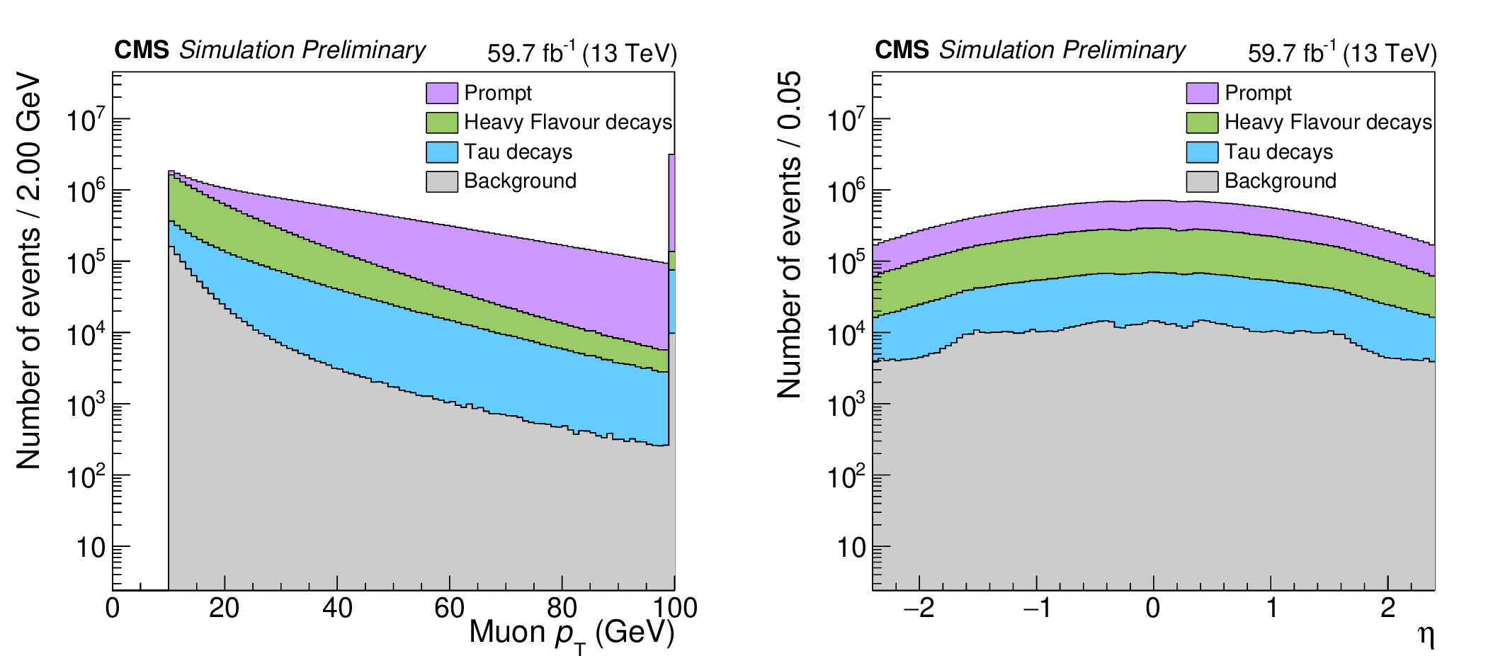
Figure 1:
Composition of the $ \mathrm{t} \bar{\mathrm{t}} $ sample used for training after muon preselection in terms of the muon origing acording to generator information. The composition is shown as a function of $ p_{\mathrm{T}} $ (left) and $ \eta $ (right). |
png pdf |
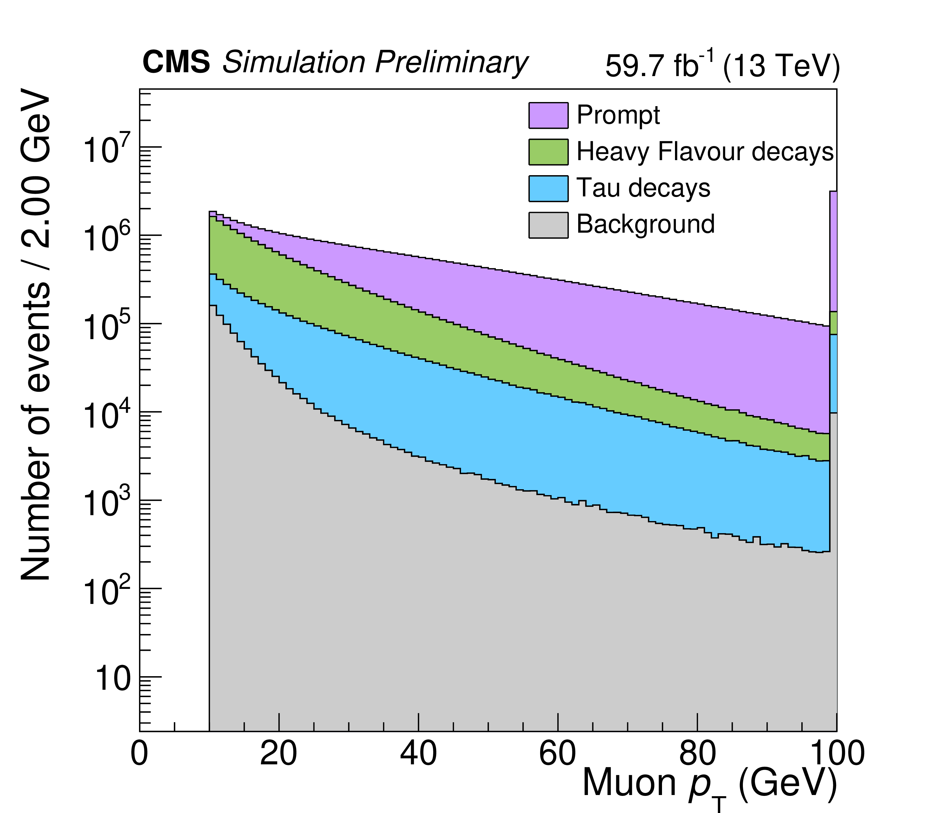
Figure 1-a:
Composition of the $ \mathrm{t} \bar{\mathrm{t}} $ sample used for training after muon preselection in terms of the muon origing acording to generator information. The composition is shown as a function of $ p_{\mathrm{T}} $ (left) and $ \eta $ (right). |
png pdf |
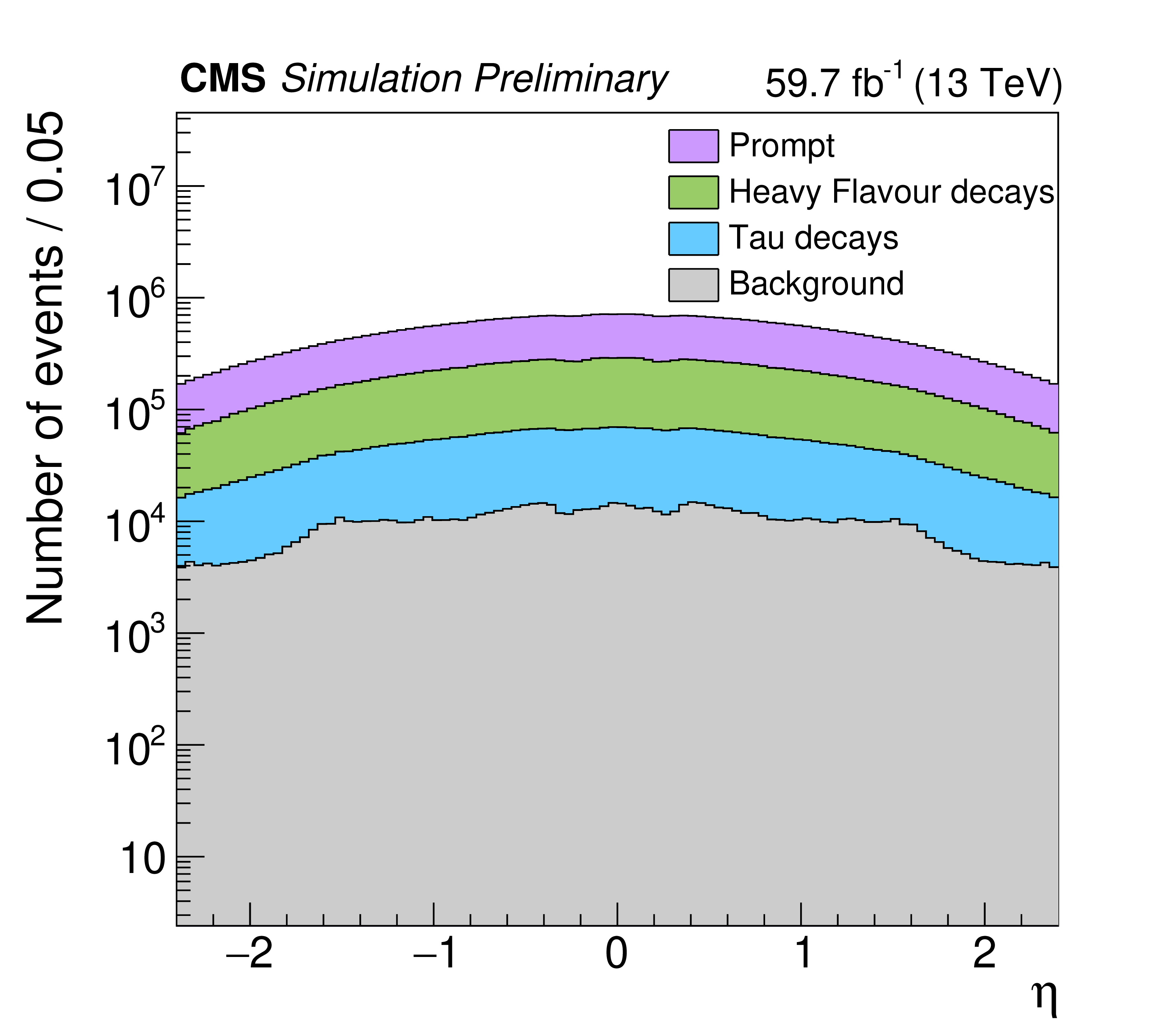
Figure 1-b:
Composition of the $ \mathrm{t} \bar{\mathrm{t}} $ sample used for training after muon preselection in terms of the muon origing acording to generator information. The composition is shown as a function of $ p_{\mathrm{T}} $ (left) and $ \eta $ (right). |
png pdf |
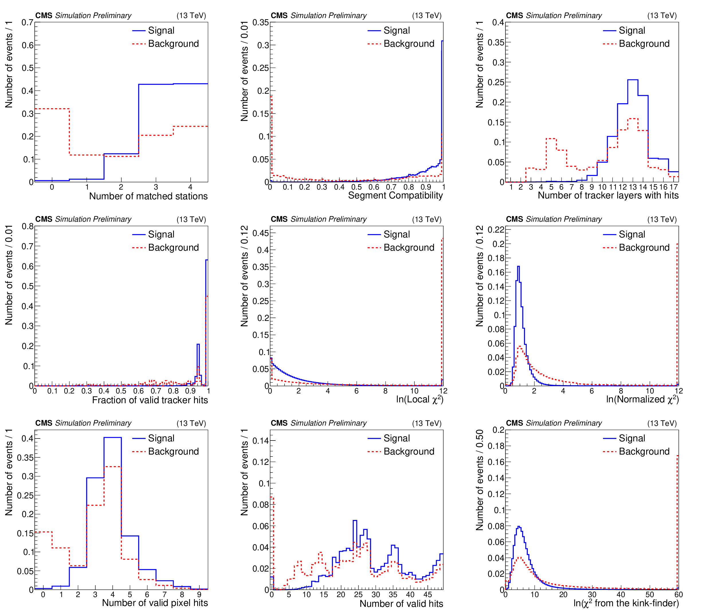
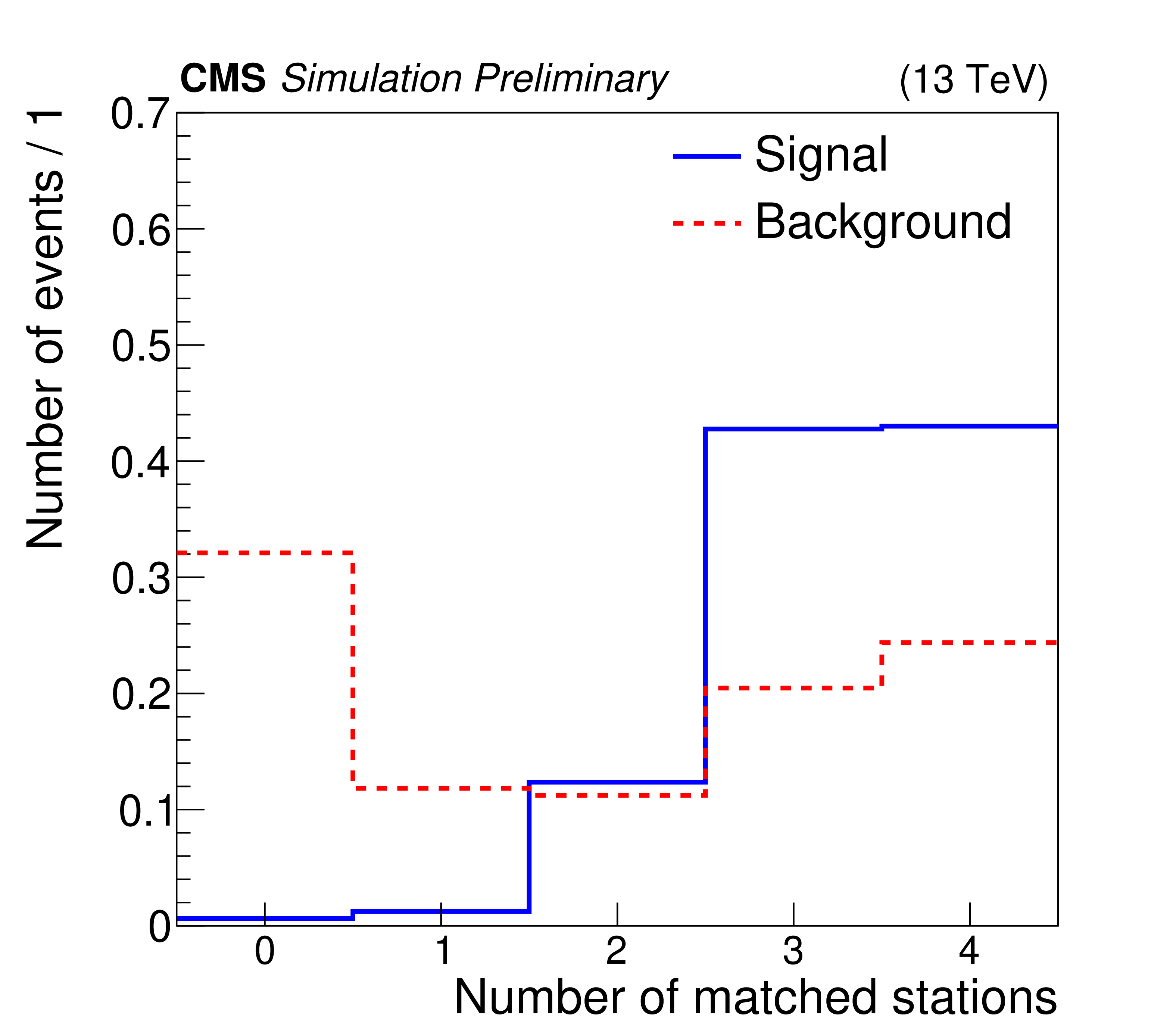
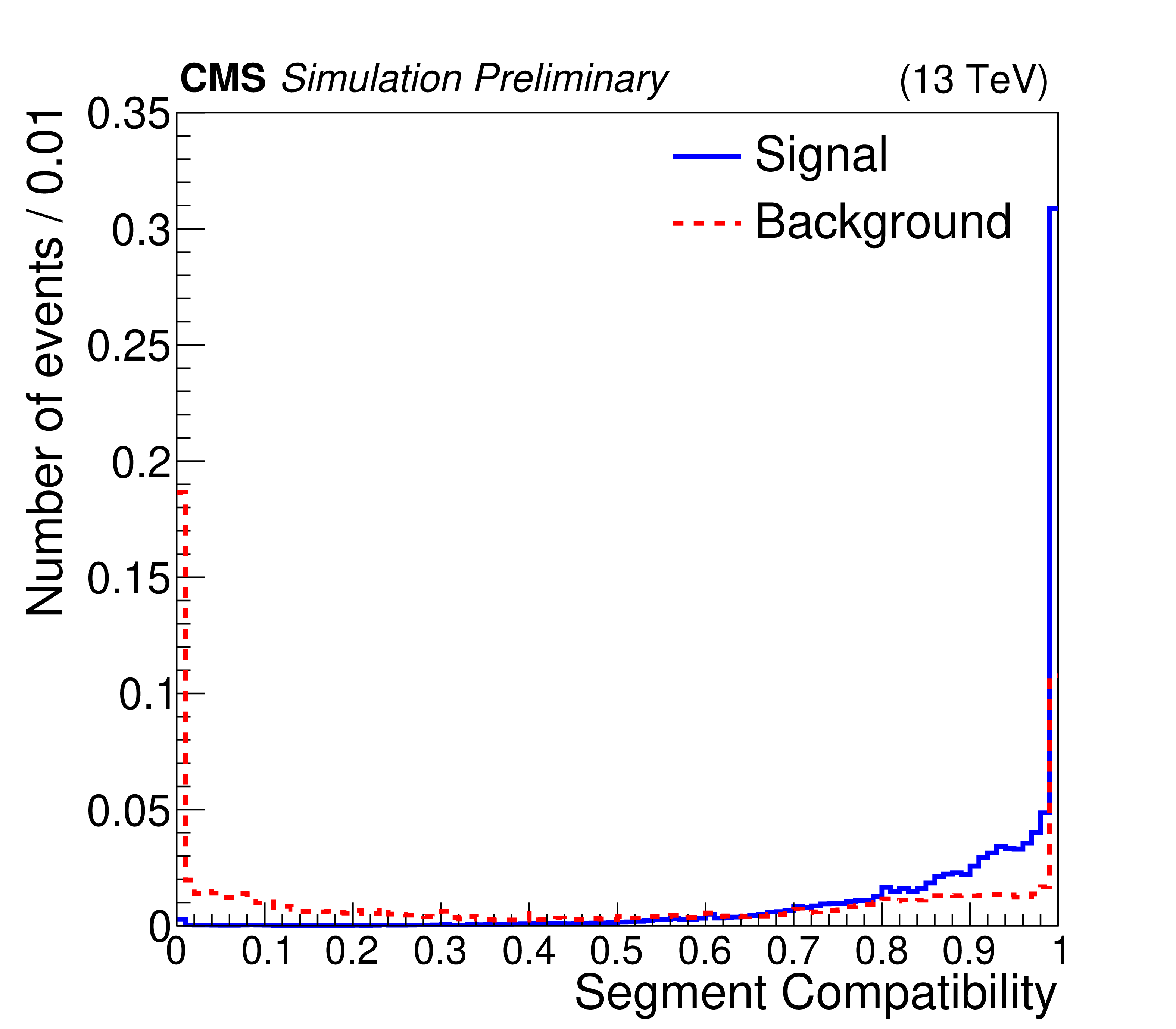
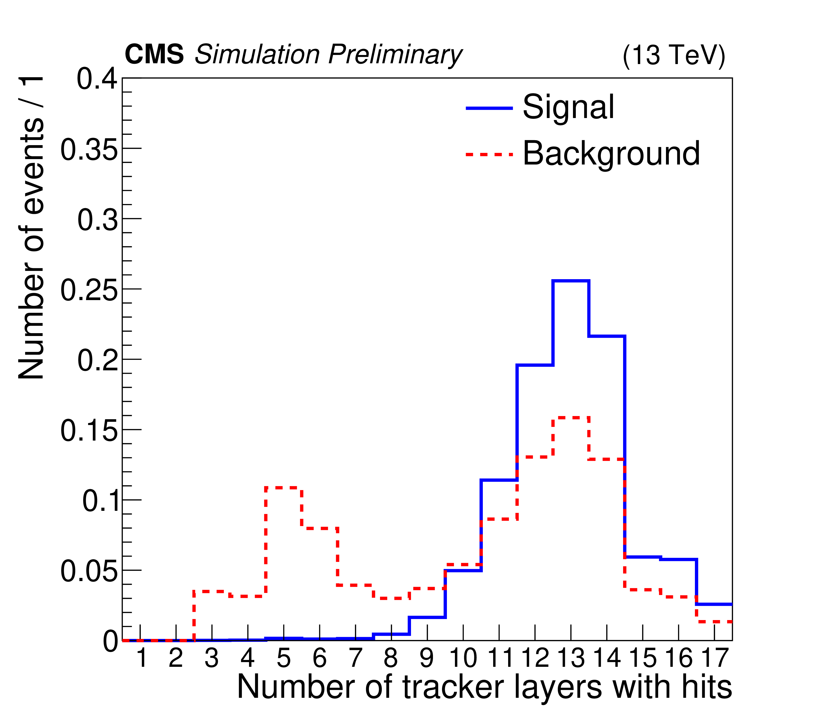
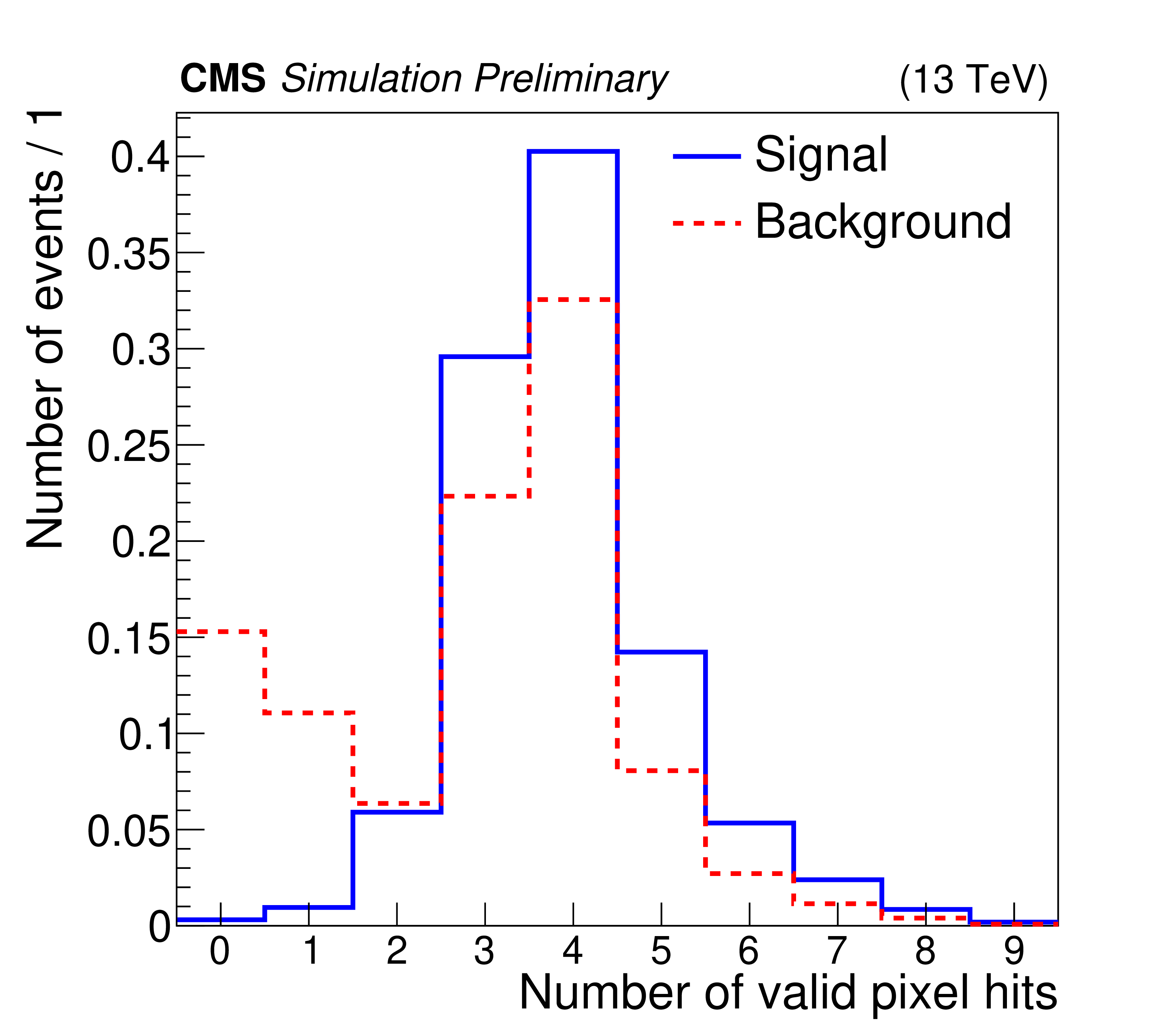
Figure 2:
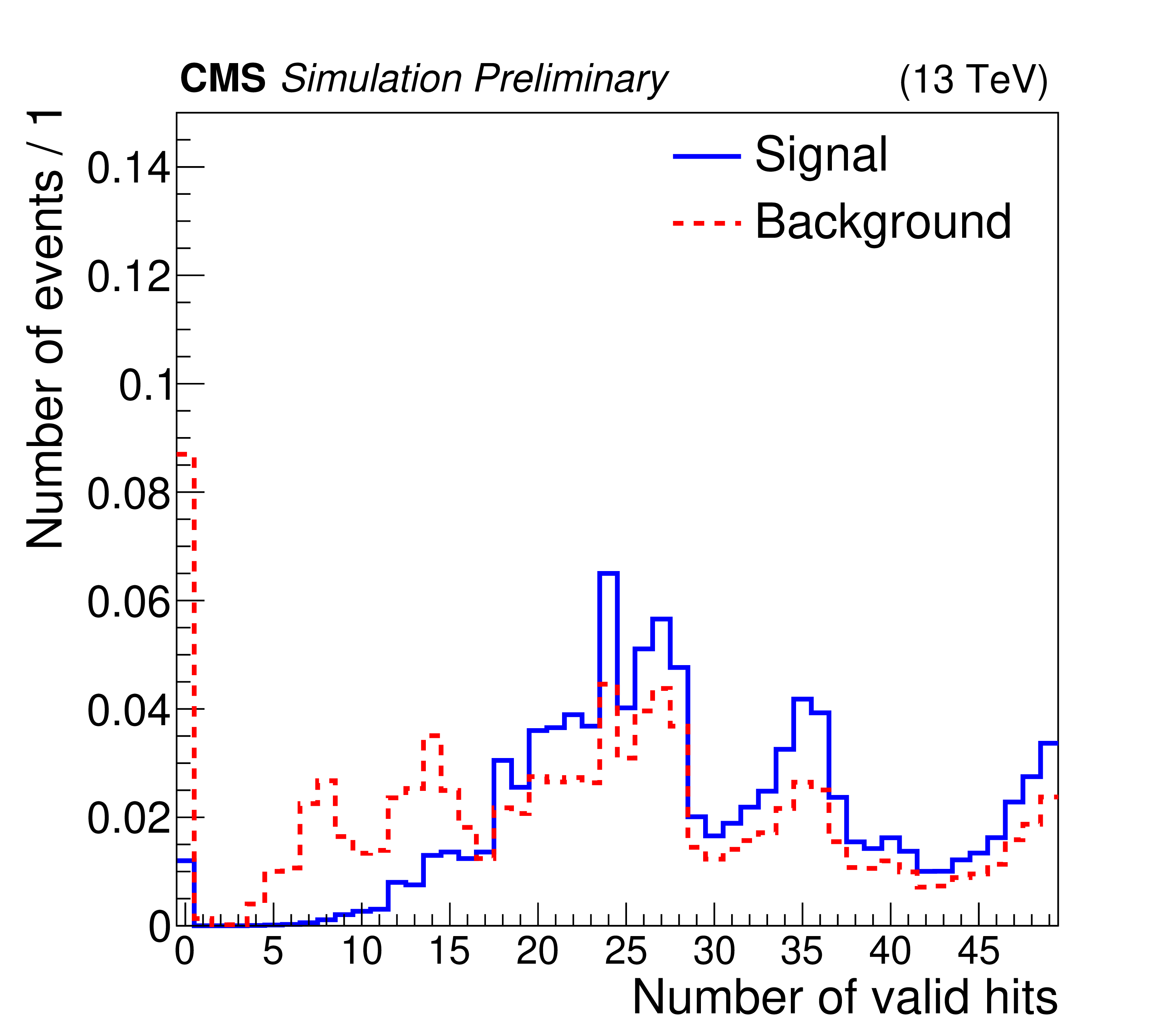
Distribution in the $ \mathrm{t} \bar{\mathrm{t}} $ training sample of the number of matched stations (top left), the segment compatibility (upper central), the number of tracker layers with hits (upper right), the fraction of valid tracker hits (middle left), the inner-standalone matching (middle central) and normalized $ \chi^2 $ of the muon fit (middle right), the number of valid pixel hits (lower left) and the total number of valid hits in the muon detectors (lower central), and the $ \chi^2 $ of the kink-finder algorithm (lower right), divided in signal and background. Signal and background are defined in 5.1. All variables are plotted after the preselection described in Section 5.1. |
png pdf |
Figure 2-a:
Distribution in the $ \mathrm{t} \bar{\mathrm{t}} $ training sample of the number of matched stations (top left), the segment compatibility (upper central), the number of tracker layers with hits (upper right), the fraction of valid tracker hits (middle left), the inner-standalone matching (middle central) and normalized $ \chi^2 $ of the muon fit (middle right), the number of valid pixel hits (lower left) and the total number of valid hits in the muon detectors (lower central), and the $ \chi^2 $ of the kink-finder algorithm (lower right), divided in signal and background. Signal and background are defined in 5.1. All variables are plotted after the preselection described in Section 5.1. |
png pdf |
Figure 2-b:
Distribution in the $ \mathrm{t} \bar{\mathrm{t}} $ training sample of the number of matched stations (top left), the segment compatibility (upper central), the number of tracker layers with hits (upper right), the fraction of valid tracker hits (middle left), the inner-standalone matching (middle central) and normalized $ \chi^2 $ of the muon fit (middle right), the number of valid pixel hits (lower left) and the total number of valid hits in the muon detectors (lower central), and the $ \chi^2 $ of the kink-finder algorithm (lower right), divided in signal and background. Signal and background are defined in 5.1. All variables are plotted after the preselection described in Section 5.1. |
png pdf |
Figure 2-c:
Distribution in the $ \mathrm{t} \bar{\mathrm{t}} $ training sample of the number of matched stations (top left), the segment compatibility (upper central), the number of tracker layers with hits (upper right), the fraction of valid tracker hits (middle left), the inner-standalone matching (middle central) and normalized $ \chi^2 $ of the muon fit (middle right), the number of valid pixel hits (lower left) and the total number of valid hits in the muon detectors (lower central), and the $ \chi^2 $ of the kink-finder algorithm (lower right), divided in signal and background. Signal and background are defined in 5.1. All variables are plotted after the preselection described in Section 5.1. |

png pdf |
Figure 2-d:
Distribution in the $ \mathrm{t} \bar{\mathrm{t}} $ training sample of the number of matched stations (top left), the segment compatibility (upper central), the number of tracker layers with hits (upper right), the fraction of valid tracker hits (middle left), the inner-standalone matching (middle central) and normalized $ \chi^2 $ of the muon fit (middle right), the number of valid pixel hits (lower left) and the total number of valid hits in the muon detectors (lower central), and the $ \chi^2 $ of the kink-finder algorithm (lower right), divided in signal and background. Signal and background are defined in 5.1. All variables are plotted after the preselection described in Section 5.1. |

png pdf |
Figure 2-e:
Distribution in the $ \mathrm{t} \bar{\mathrm{t}} $ training sample of the number of matched stations (top left), the segment compatibility (upper central), the number of tracker layers with hits (upper right), the fraction of valid tracker hits (middle left), the inner-standalone matching (middle central) and normalized $ \chi^2 $ of the muon fit (middle right), the number of valid pixel hits (lower left) and the total number of valid hits in the muon detectors (lower central), and the $ \chi^2 $ of the kink-finder algorithm (lower right), divided in signal and background. Signal and background are defined in 5.1. All variables are plotted after the preselection described in Section 5.1. |

png pdf |
Figure 2-f:
Distribution in the $ \mathrm{t} \bar{\mathrm{t}} $ training sample of the number of matched stations (top left), the segment compatibility (upper central), the number of tracker layers with hits (upper right), the fraction of valid tracker hits (middle left), the inner-standalone matching (middle central) and normalized $ \chi^2 $ of the muon fit (middle right), the number of valid pixel hits (lower left) and the total number of valid hits in the muon detectors (lower central), and the $ \chi^2 $ of the kink-finder algorithm (lower right), divided in signal and background. Signal and background are defined in 5.1. All variables are plotted after the preselection described in Section 5.1. |
png pdf |
Figure 2-g:
Distribution in the $ \mathrm{t} \bar{\mathrm{t}} $ training sample of the number of matched stations (top left), the segment compatibility (upper central), the number of tracker layers with hits (upper right), the fraction of valid tracker hits (middle left), the inner-standalone matching (middle central) and normalized $ \chi^2 $ of the muon fit (middle right), the number of valid pixel hits (lower left) and the total number of valid hits in the muon detectors (lower central), and the $ \chi^2 $ of the kink-finder algorithm (lower right), divided in signal and background. Signal and background are defined in 5.1. All variables are plotted after the preselection described in Section 5.1. |
png pdf |
Figure 2-h:
Distribution in the $ \mathrm{t} \bar{\mathrm{t}} $ training sample of the number of matched stations (top left), the segment compatibility (upper central), the number of tracker layers with hits (upper right), the fraction of valid tracker hits (middle left), the inner-standalone matching (middle central) and normalized $ \chi^2 $ of the muon fit (middle right), the number of valid pixel hits (lower left) and the total number of valid hits in the muon detectors (lower central), and the $ \chi^2 $ of the kink-finder algorithm (lower right), divided in signal and background. Signal and background are defined in 5.1. All variables are plotted after the preselection described in Section 5.1. |

png pdf |
Figure 2-i:
Distribution in the $ \mathrm{t} \bar{\mathrm{t}} $ training sample of the number of matched stations (top left), the segment compatibility (upper central), the number of tracker layers with hits (upper right), the fraction of valid tracker hits (middle left), the inner-standalone matching (middle central) and normalized $ \chi^2 $ of the muon fit (middle right), the number of valid pixel hits (lower left) and the total number of valid hits in the muon detectors (lower central), and the $ \chi^2 $ of the kink-finder algorithm (lower right), divided in signal and background. Signal and background are defined in 5.1. All variables are plotted after the preselection described in Section 5.1. |

png pdf |
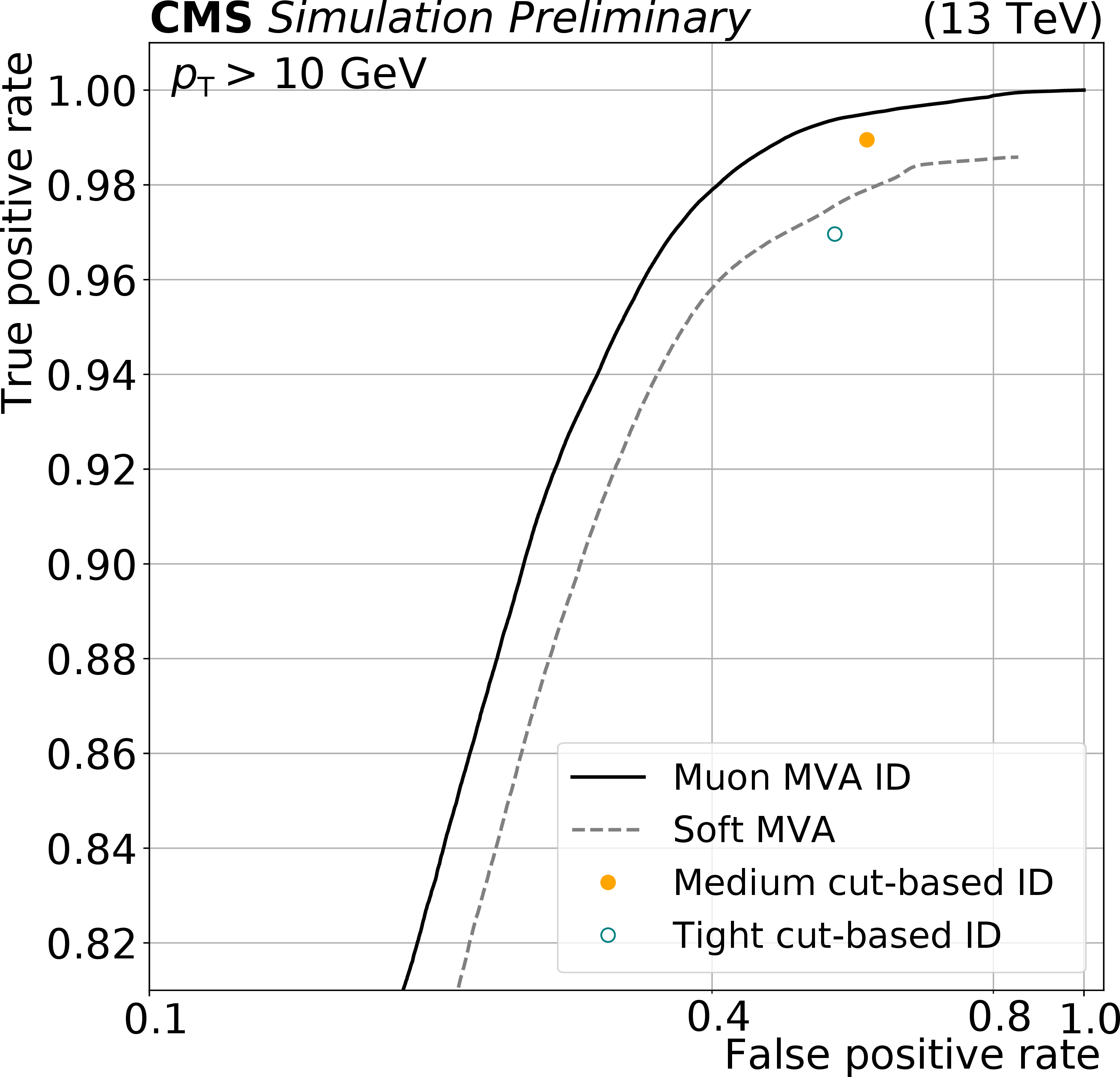
Figure 3:
ROC curve for muons with $ p_{\mathrm{T}} > $ 10 GeV for the developed general muon MVA ID discriminator (black solid line) with the selected medium and tight WPs shown as orange and purple stars, respectively. Orange and blue points show the medium and tight WPs of the cut-based ID. The ROC curve of the soft MVA is shown in gray. |

png pdf |
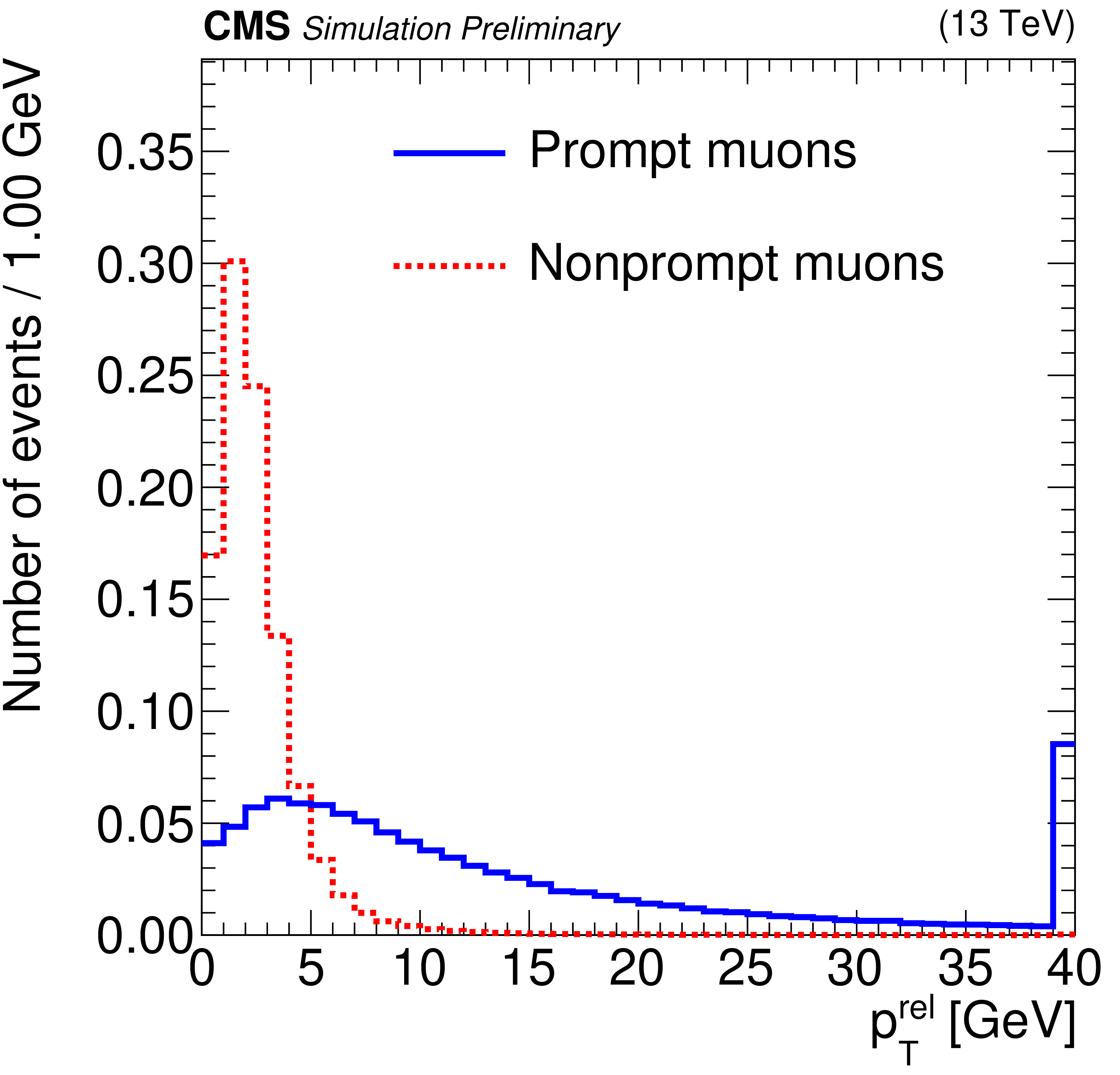
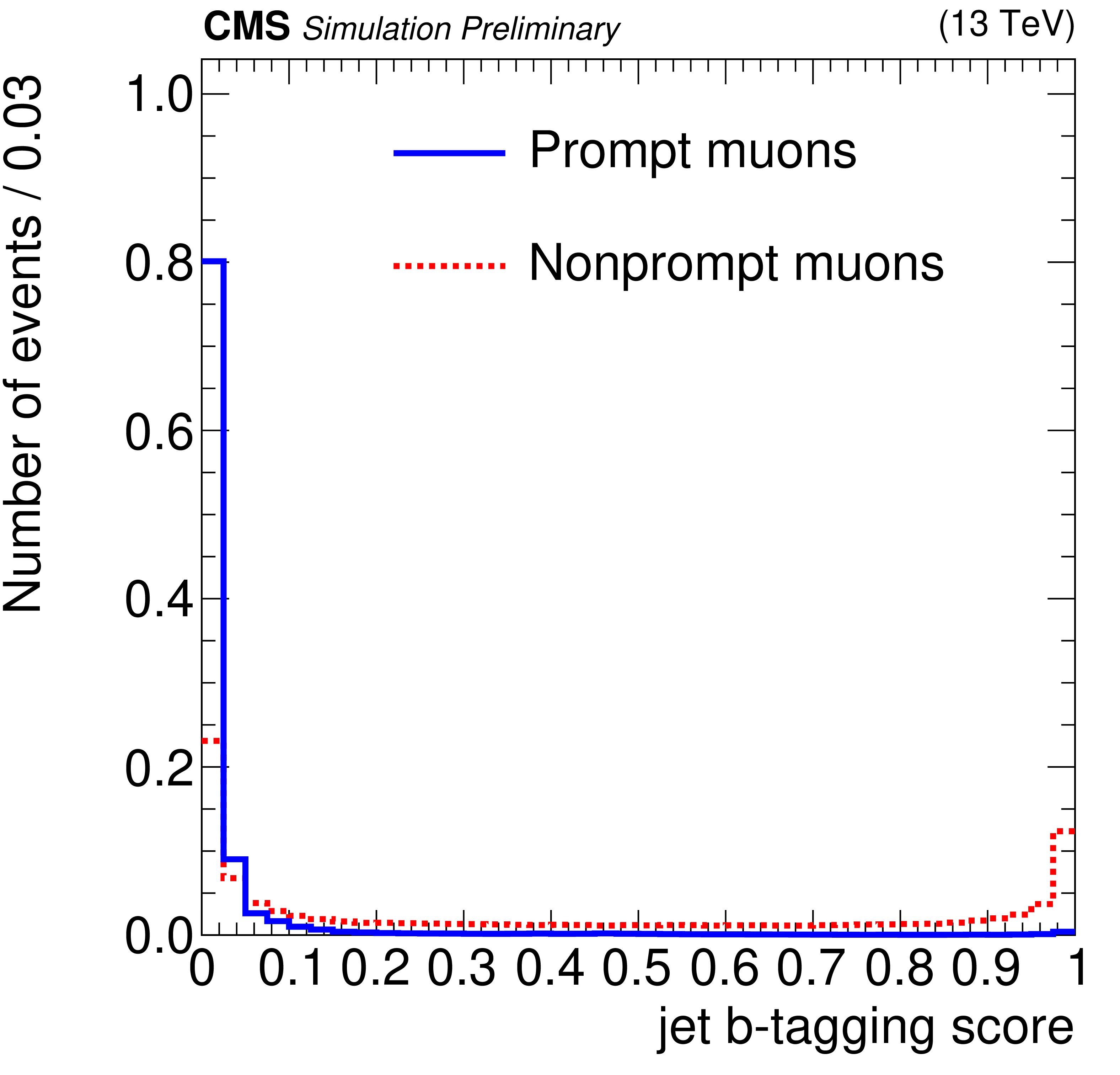
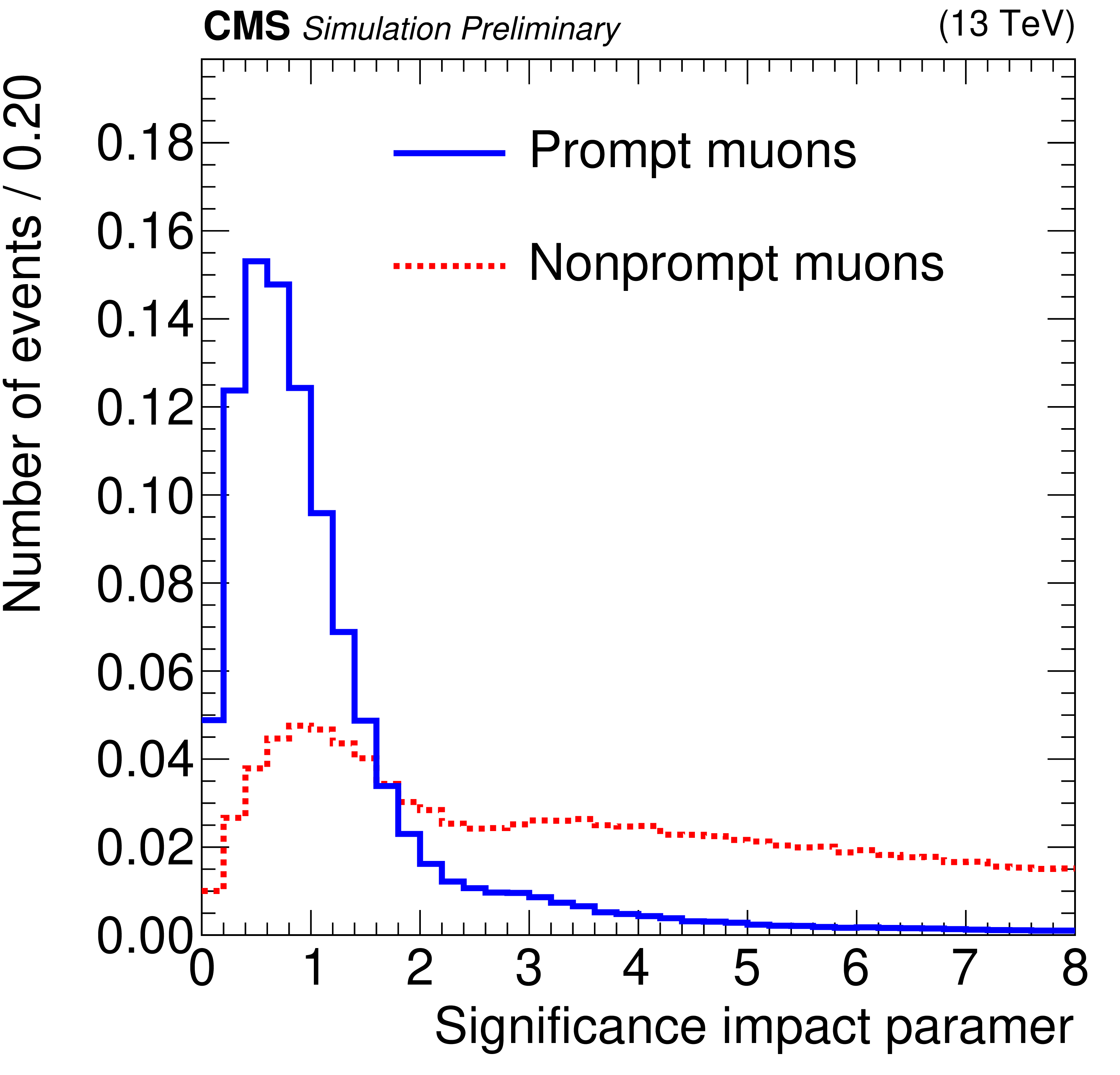
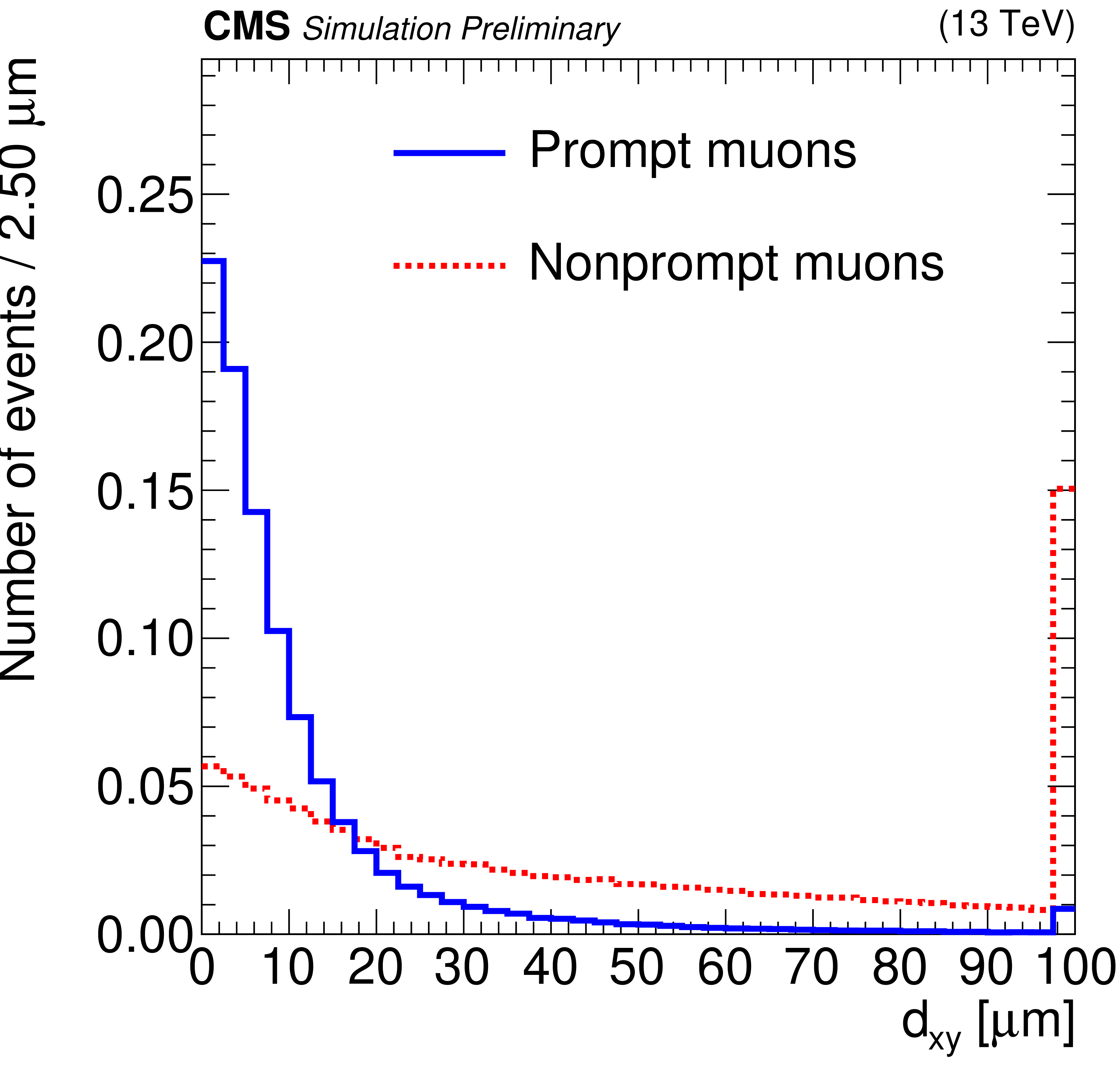
Figure 4:
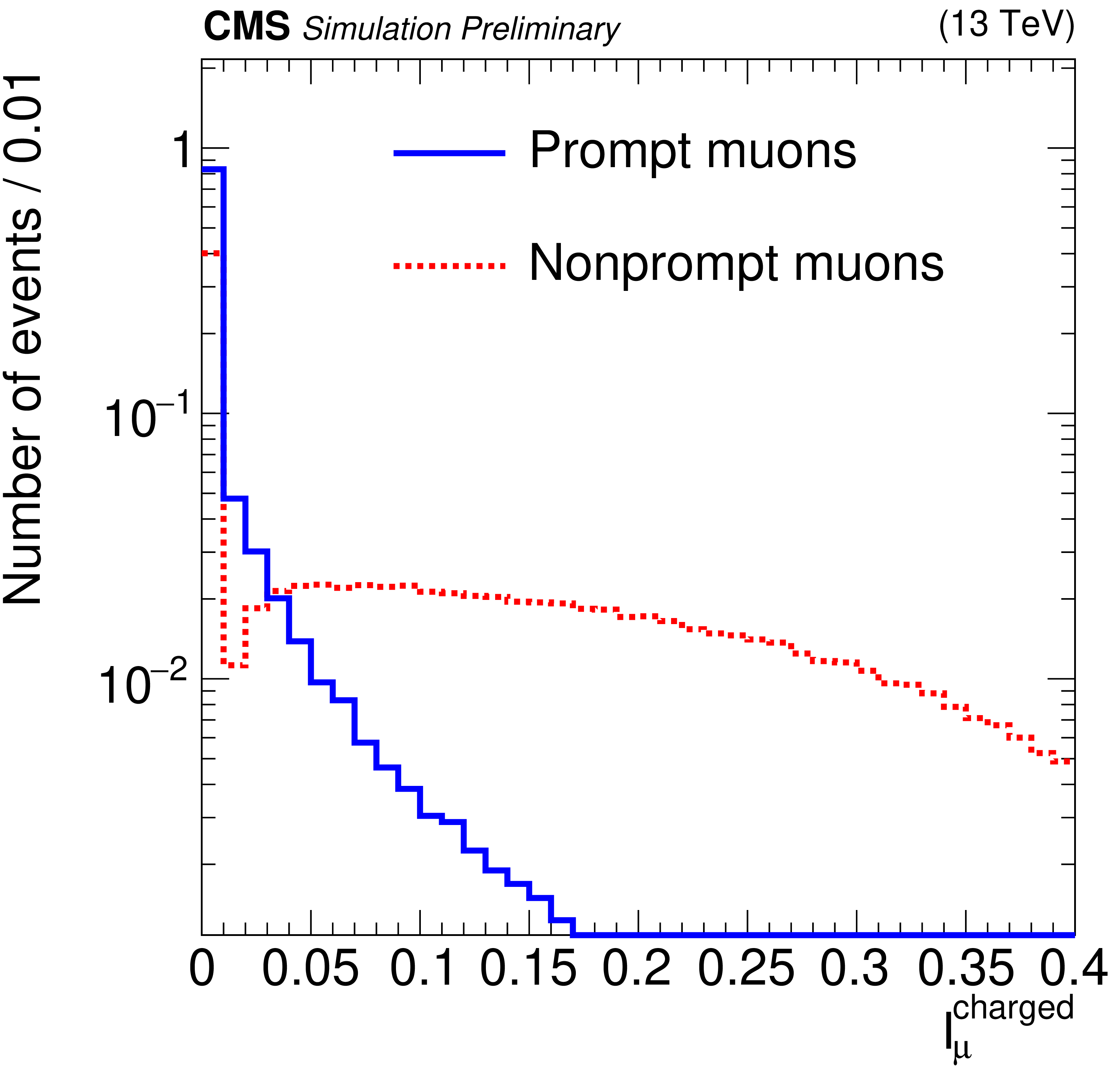
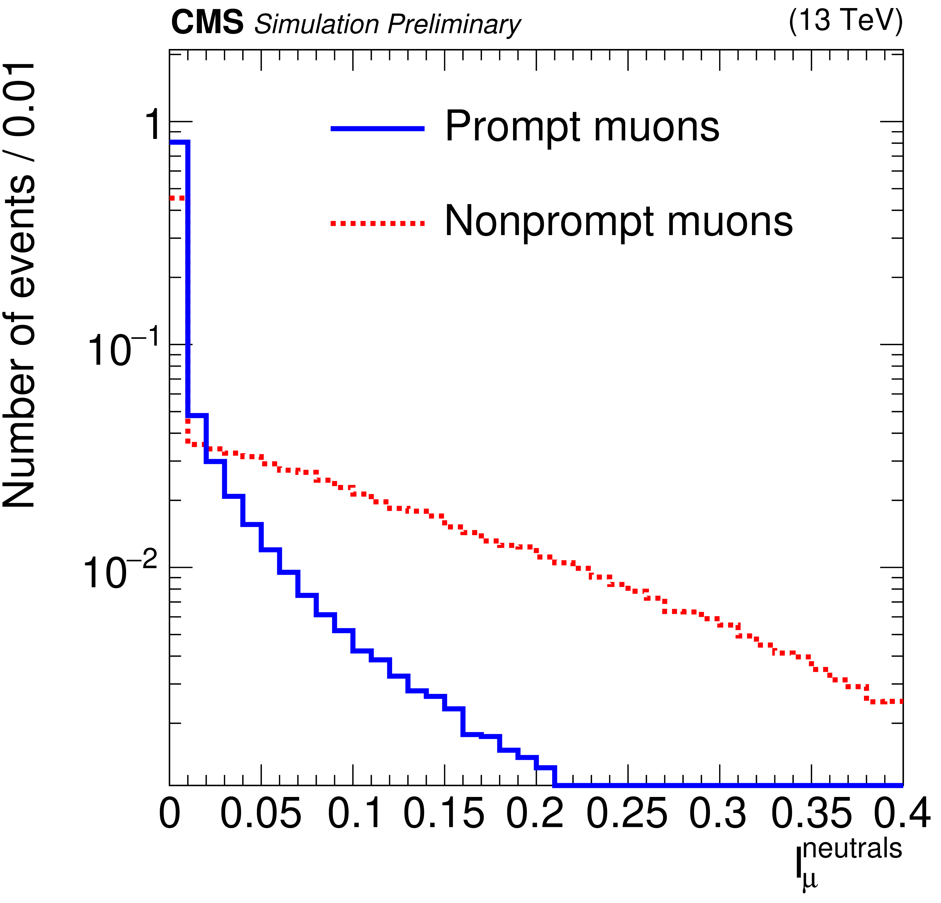
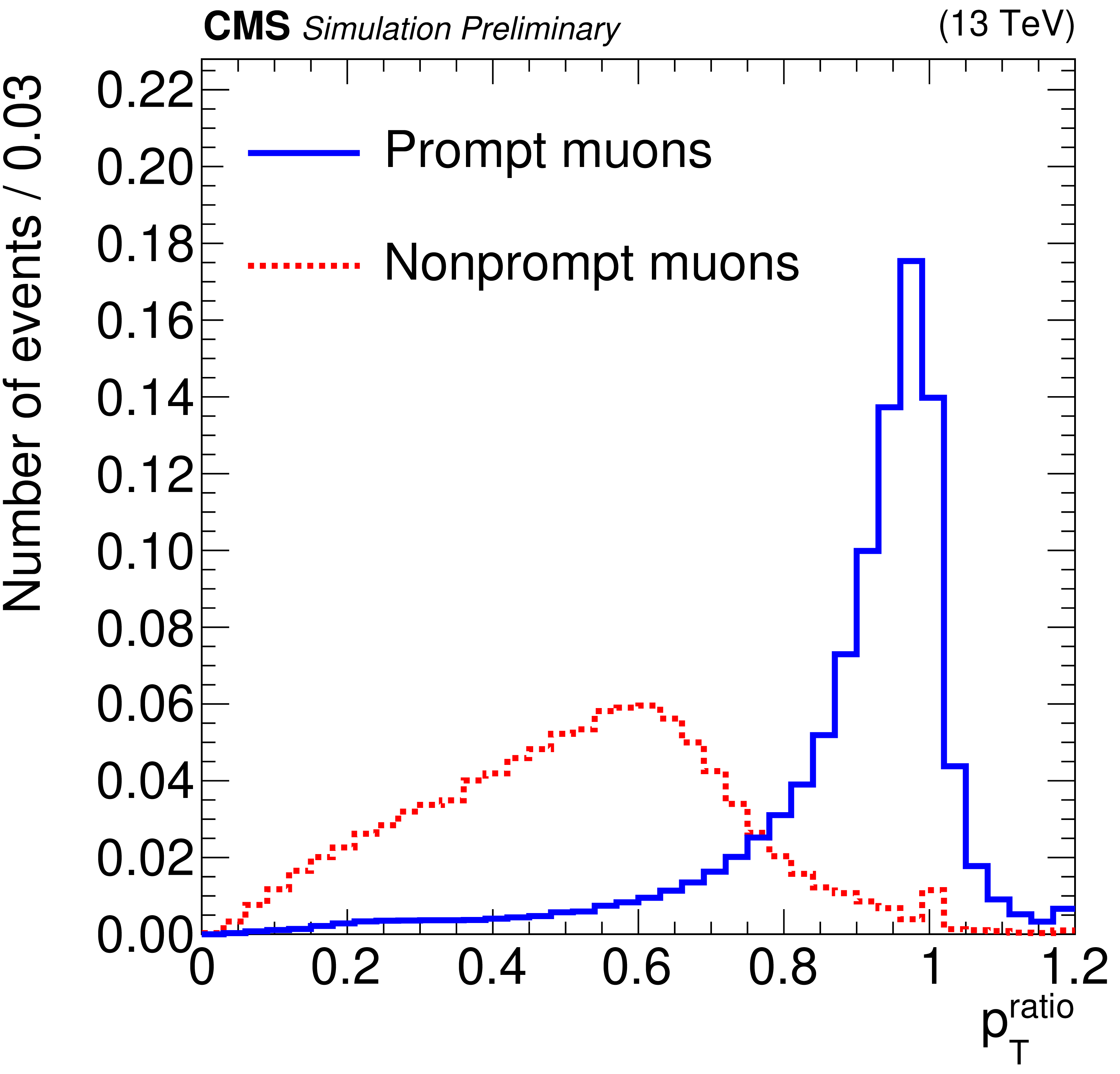
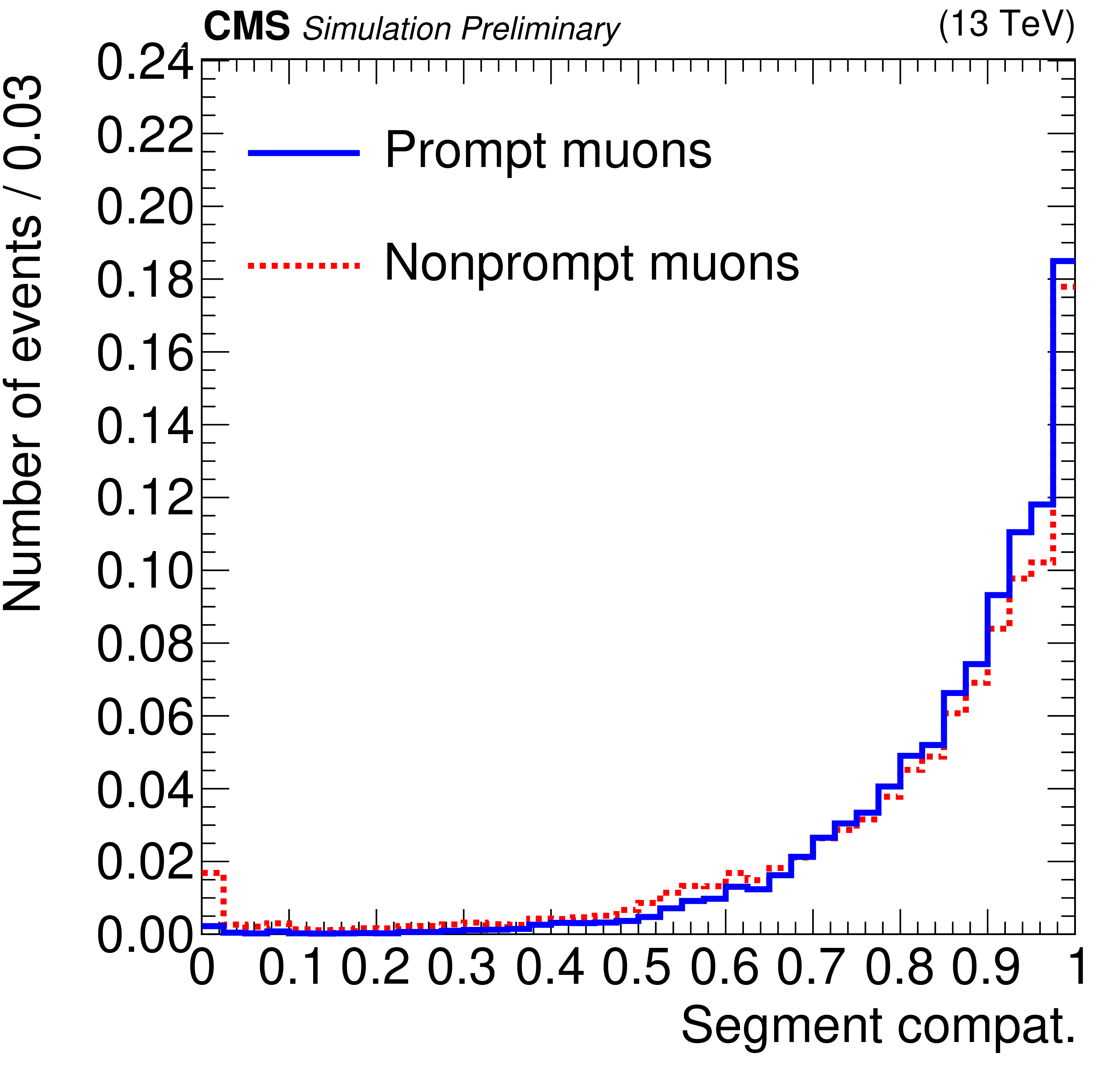
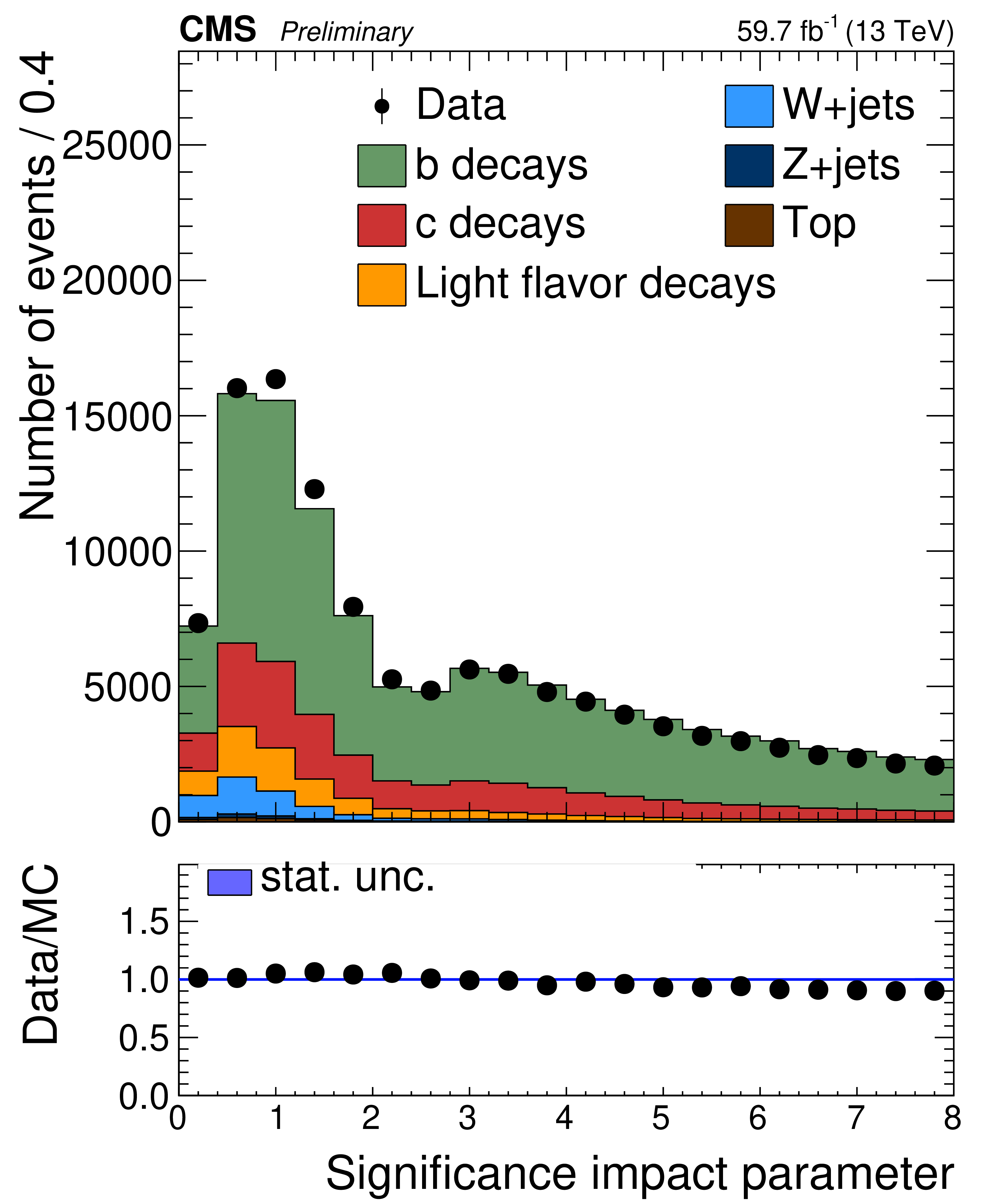
Distribution of the charged component (top left) and the neutral component (top central) of mini-isolation, the jet $ p_{\mathrm{T}} $ ratio (top right), the jet relative $ p_{\mathrm{T}} $ (middle left), the score of the associated deep flavor (middle center), the significance of the impact parameter (middle right), the impact parameter in the transverse (bottom left) and longitudinal (bottom center) direction between the muon and the PV, and the segment compatibility (bottom right). |
png pdf |
Figure 4-a:
Distribution of the charged component (top left) and the neutral component (top central) of mini-isolation, the jet $ p_{\mathrm{T}} $ ratio (top right), the jet relative $ p_{\mathrm{T}} $ (middle left), the score of the associated deep flavor (middle center), the significance of the impact parameter (middle right), the impact parameter in the transverse (bottom left) and longitudinal (bottom center) direction between the muon and the PV, and the segment compatibility (bottom right). |
png pdf |
Figure 4-b:
Distribution of the charged component (top left) and the neutral component (top central) of mini-isolation, the jet $ p_{\mathrm{T}} $ ratio (top right), the jet relative $ p_{\mathrm{T}} $ (middle left), the score of the associated deep flavor (middle center), the significance of the impact parameter (middle right), the impact parameter in the transverse (bottom left) and longitudinal (bottom center) direction between the muon and the PV, and the segment compatibility (bottom right). |
png pdf |
Figure 4-c:
Distribution of the charged component (top left) and the neutral component (top central) of mini-isolation, the jet $ p_{\mathrm{T}} $ ratio (top right), the jet relative $ p_{\mathrm{T}} $ (middle left), the score of the associated deep flavor (middle center), the significance of the impact parameter (middle right), the impact parameter in the transverse (bottom left) and longitudinal (bottom center) direction between the muon and the PV, and the segment compatibility (bottom right). |
png pdf |
Figure 4-d:
Distribution of the charged component (top left) and the neutral component (top central) of mini-isolation, the jet $ p_{\mathrm{T}} $ ratio (top right), the jet relative $ p_{\mathrm{T}} $ (middle left), the score of the associated deep flavor (middle center), the significance of the impact parameter (middle right), the impact parameter in the transverse (bottom left) and longitudinal (bottom center) direction between the muon and the PV, and the segment compatibility (bottom right). |
png pdf |
Figure 4-e:
Distribution of the charged component (top left) and the neutral component (top central) of mini-isolation, the jet $ p_{\mathrm{T}} $ ratio (top right), the jet relative $ p_{\mathrm{T}} $ (middle left), the score of the associated deep flavor (middle center), the significance of the impact parameter (middle right), the impact parameter in the transverse (bottom left) and longitudinal (bottom center) direction between the muon and the PV, and the segment compatibility (bottom right). |
png pdf |
Figure 4-f:
Distribution of the charged component (top left) and the neutral component (top central) of mini-isolation, the jet $ p_{\mathrm{T}} $ ratio (top right), the jet relative $ p_{\mathrm{T}} $ (middle left), the score of the associated deep flavor (middle center), the significance of the impact parameter (middle right), the impact parameter in the transverse (bottom left) and longitudinal (bottom center) direction between the muon and the PV, and the segment compatibility (bottom right). |
png pdf |
Figure 4-g:
Distribution of the charged component (top left) and the neutral component (top central) of mini-isolation, the jet $ p_{\mathrm{T}} $ ratio (top right), the jet relative $ p_{\mathrm{T}} $ (middle left), the score of the associated deep flavor (middle center), the significance of the impact parameter (middle right), the impact parameter in the transverse (bottom left) and longitudinal (bottom center) direction between the muon and the PV, and the segment compatibility (bottom right). |

png pdf |
Figure 4-h:
Distribution of the charged component (top left) and the neutral component (top central) of mini-isolation, the jet $ p_{\mathrm{T}} $ ratio (top right), the jet relative $ p_{\mathrm{T}} $ (middle left), the score of the associated deep flavor (middle center), the significance of the impact parameter (middle right), the impact parameter in the transverse (bottom left) and longitudinal (bottom center) direction between the muon and the PV, and the segment compatibility (bottom right). |
png pdf |
Figure 4-i:
Distribution of the charged component (top left) and the neutral component (top central) of mini-isolation, the jet $ p_{\mathrm{T}} $ ratio (top right), the jet relative $ p_{\mathrm{T}} $ (middle left), the score of the associated deep flavor (middle center), the significance of the impact parameter (middle right), the impact parameter in the transverse (bottom left) and longitudinal (bottom center) direction between the muon and the PV, and the segment compatibility (bottom right). |
png pdf |
Figure 5:
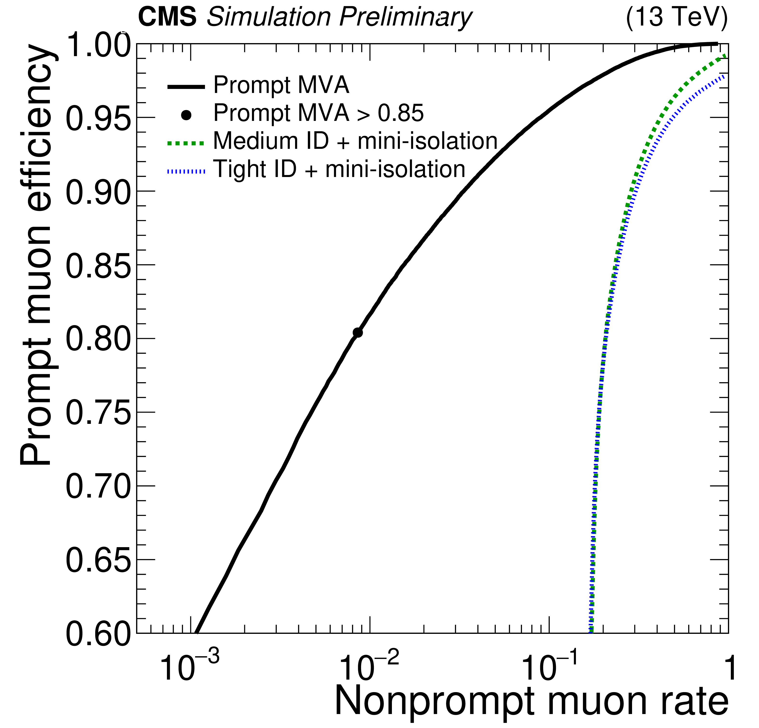
ROC curve for the developed prompt muon MVA discriminator together with requirements on mini-isolation and the tight and medium cut-based criteria. For each working point, the efficiency is shown as a function of proportion of nonprompt muons passing the working point selection. |
png pdf |
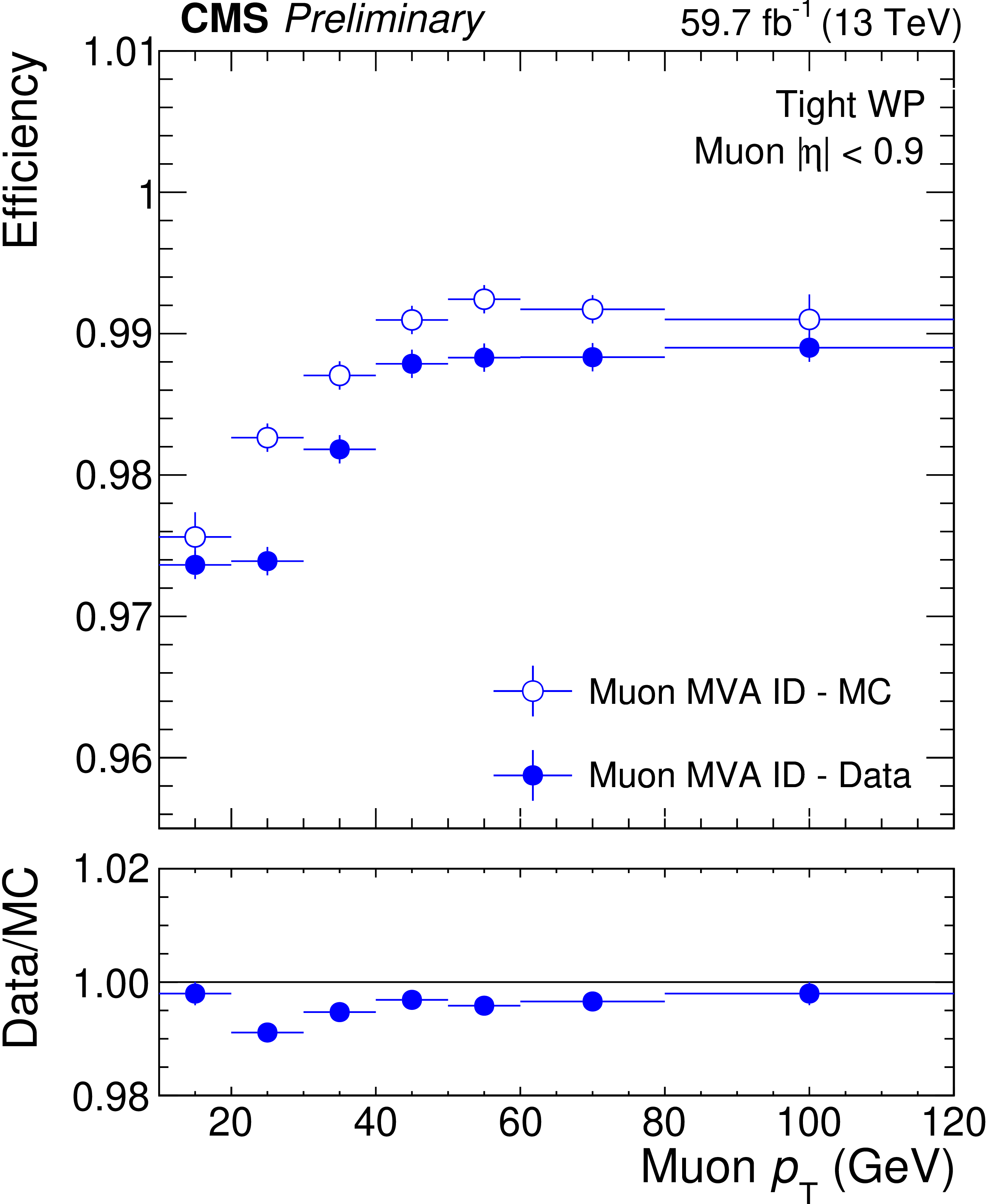
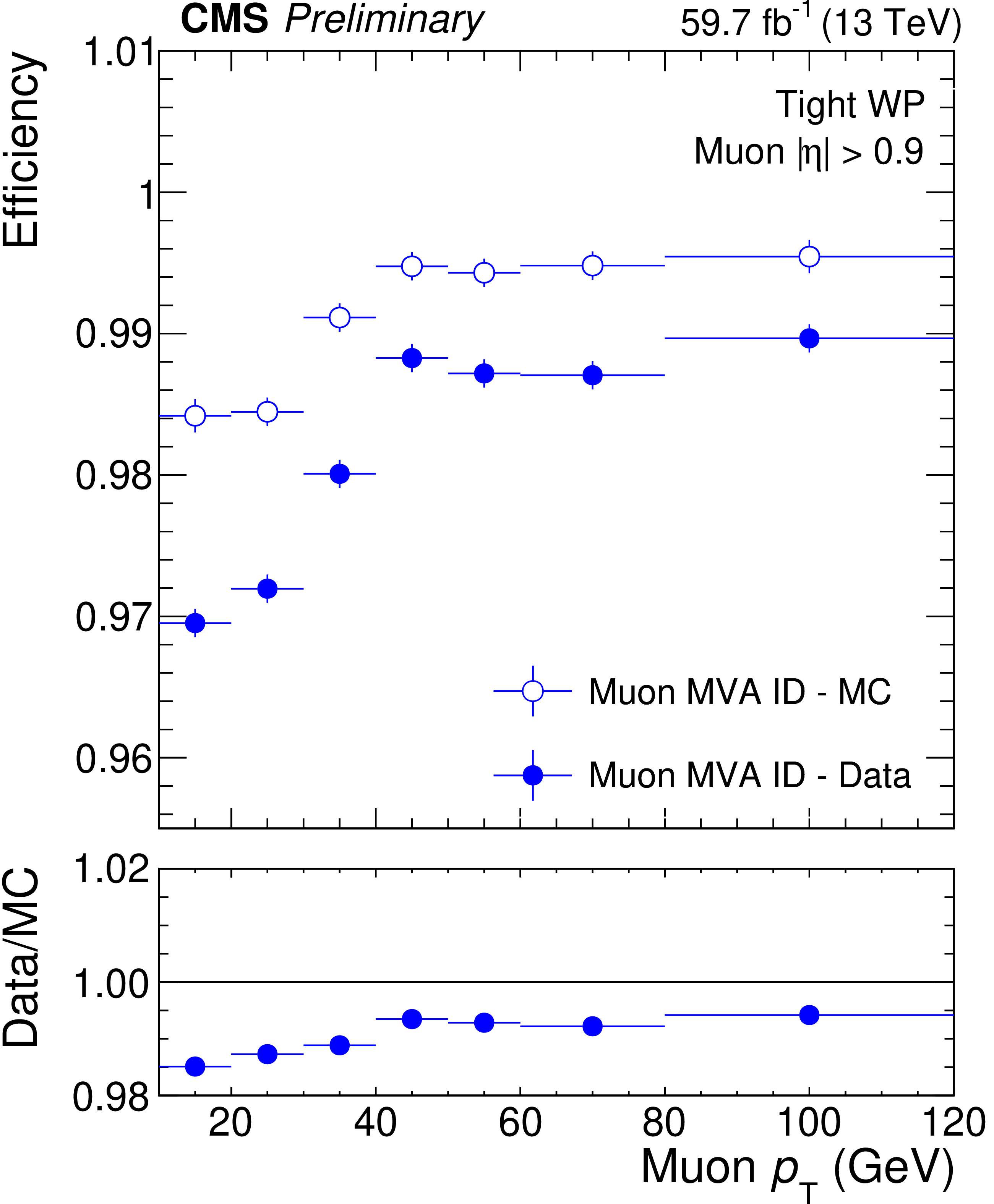
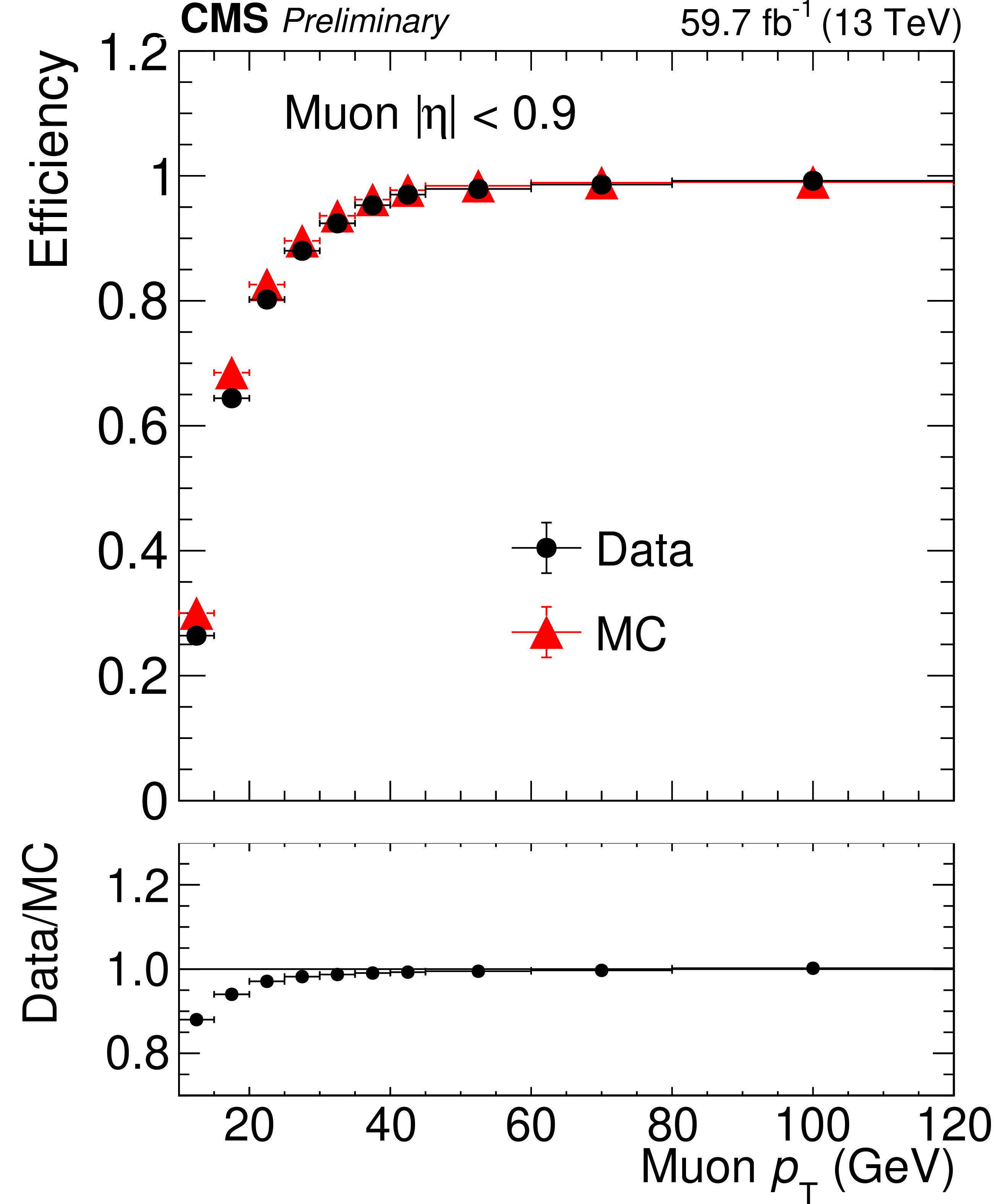
Figure 6:
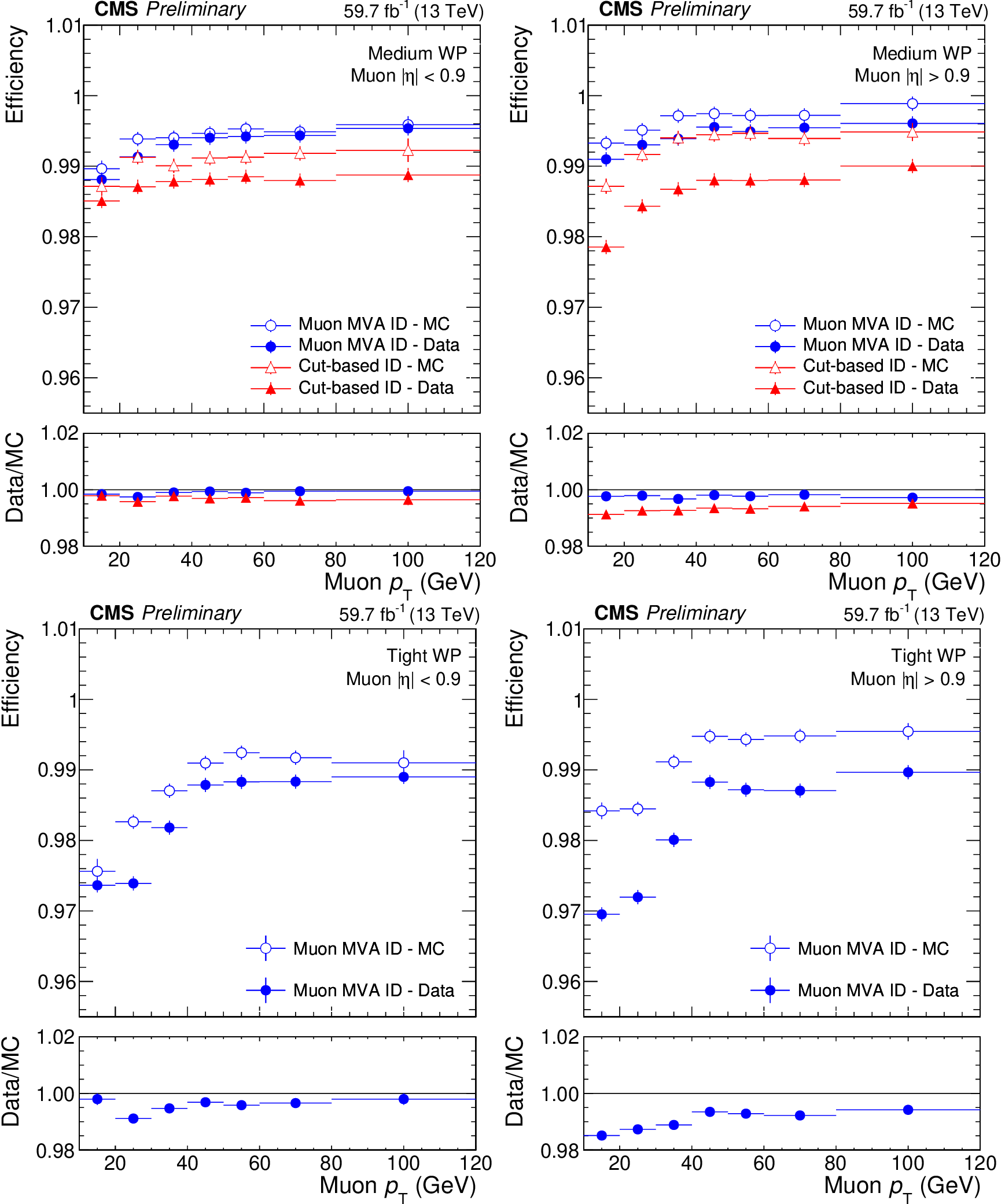
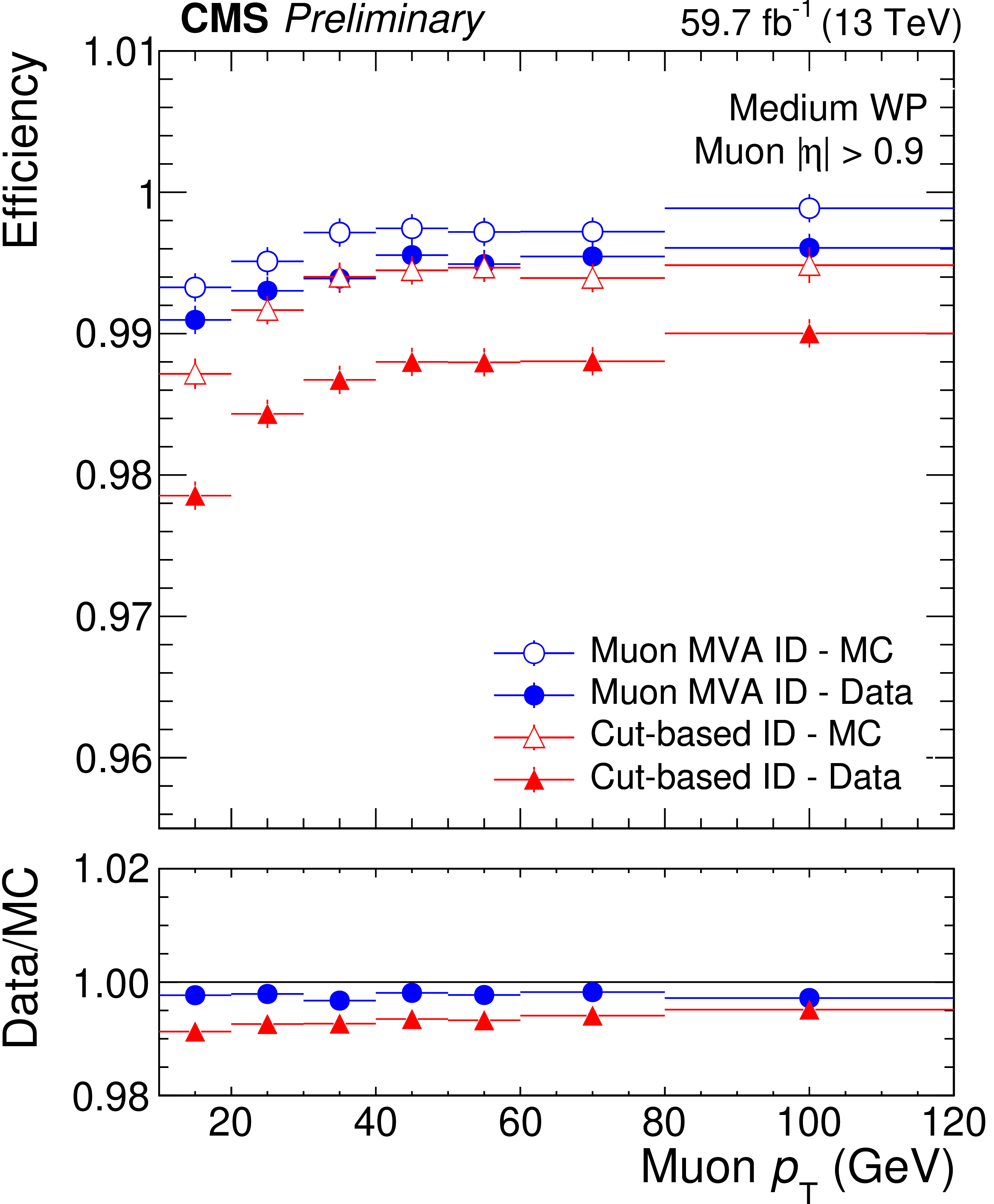
Muon identification efficiency for the medium (top) and tight (bottom) WPs as a function of $ p_{\mathrm{T}} $ for muons with $ |\eta| < $ 0.9 (left) and $ |\eta| > $ 0.9 (right). Blue dots show the muon MVA ID performance both for 2018 dataset and DY while red triangles show the efficiency of the cut-based ID used during Run 2. |

png pdf |
Figure 6-a:
Muon identification efficiency for the medium (top) and tight (bottom) WPs as a function of $ p_{\mathrm{T}} $ for muons with $ |\eta| < $ 0.9 (left) and $ |\eta| > $ 0.9 (right). Blue dots show the muon MVA ID performance both for 2018 dataset and DY while red triangles show the efficiency of the cut-based ID used during Run 2. |
png pdf |
Figure 6-b:
Muon identification efficiency for the medium (top) and tight (bottom) WPs as a function of $ p_{\mathrm{T}} $ for muons with $ |\eta| < $ 0.9 (left) and $ |\eta| > $ 0.9 (right). Blue dots show the muon MVA ID performance both for 2018 dataset and DY while red triangles show the efficiency of the cut-based ID used during Run 2. |
png pdf |
Figure 6-c:
Muon identification efficiency for the medium (top) and tight (bottom) WPs as a function of $ p_{\mathrm{T}} $ for muons with $ |\eta| < $ 0.9 (left) and $ |\eta| > $ 0.9 (right). Blue dots show the muon MVA ID performance both for 2018 dataset and DY while red triangles show the efficiency of the cut-based ID used during Run 2. |
png pdf |
Figure 6-d:
Muon identification efficiency for the medium (top) and tight (bottom) WPs as a function of $ p_{\mathrm{T}} $ for muons with $ |\eta| < $ 0.9 (left) and $ |\eta| > $ 0.9 (right). Blue dots show the muon MVA ID performance both for 2018 dataset and DY while red triangles show the efficiency of the cut-based ID used during Run 2. |
png pdf |
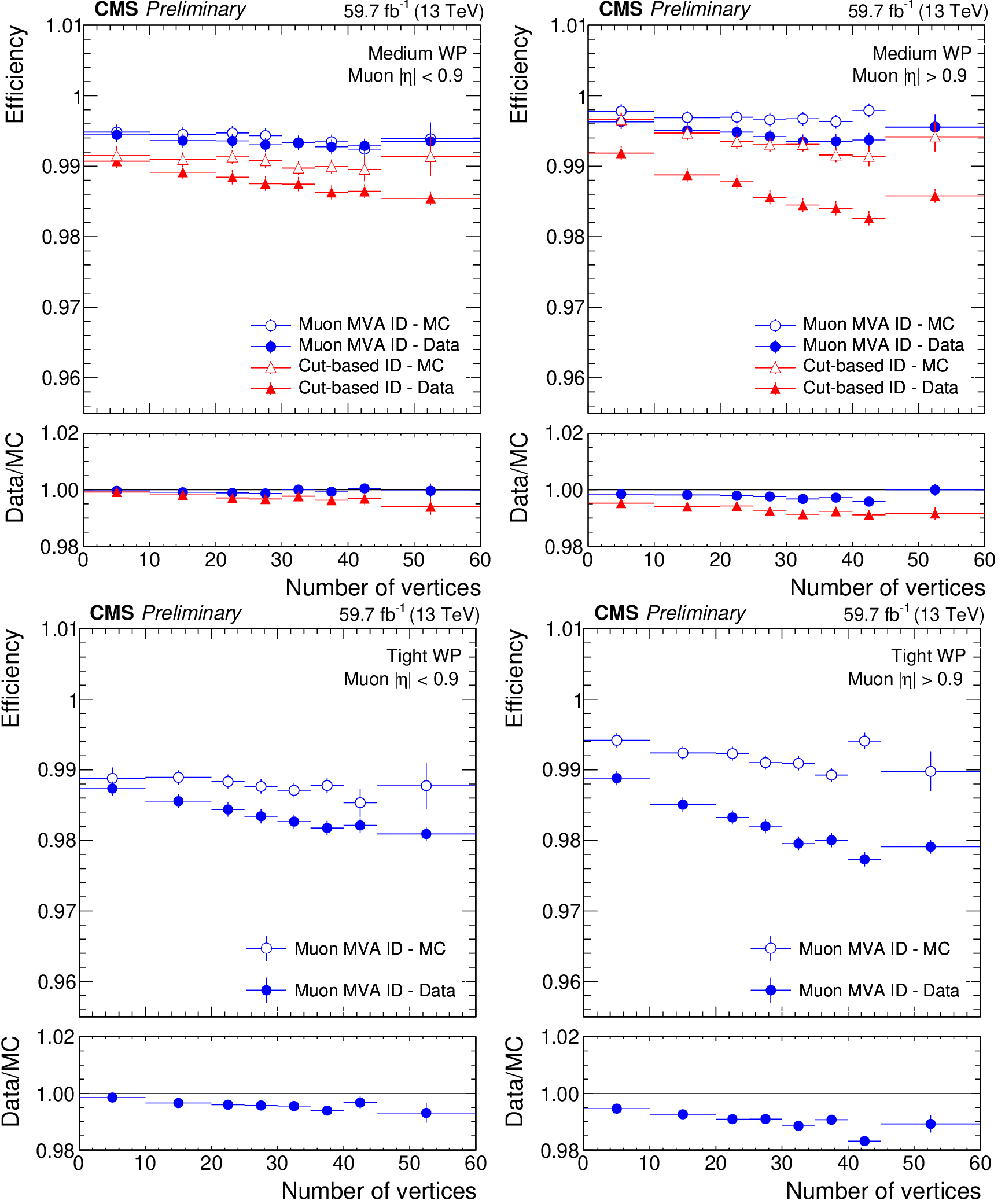
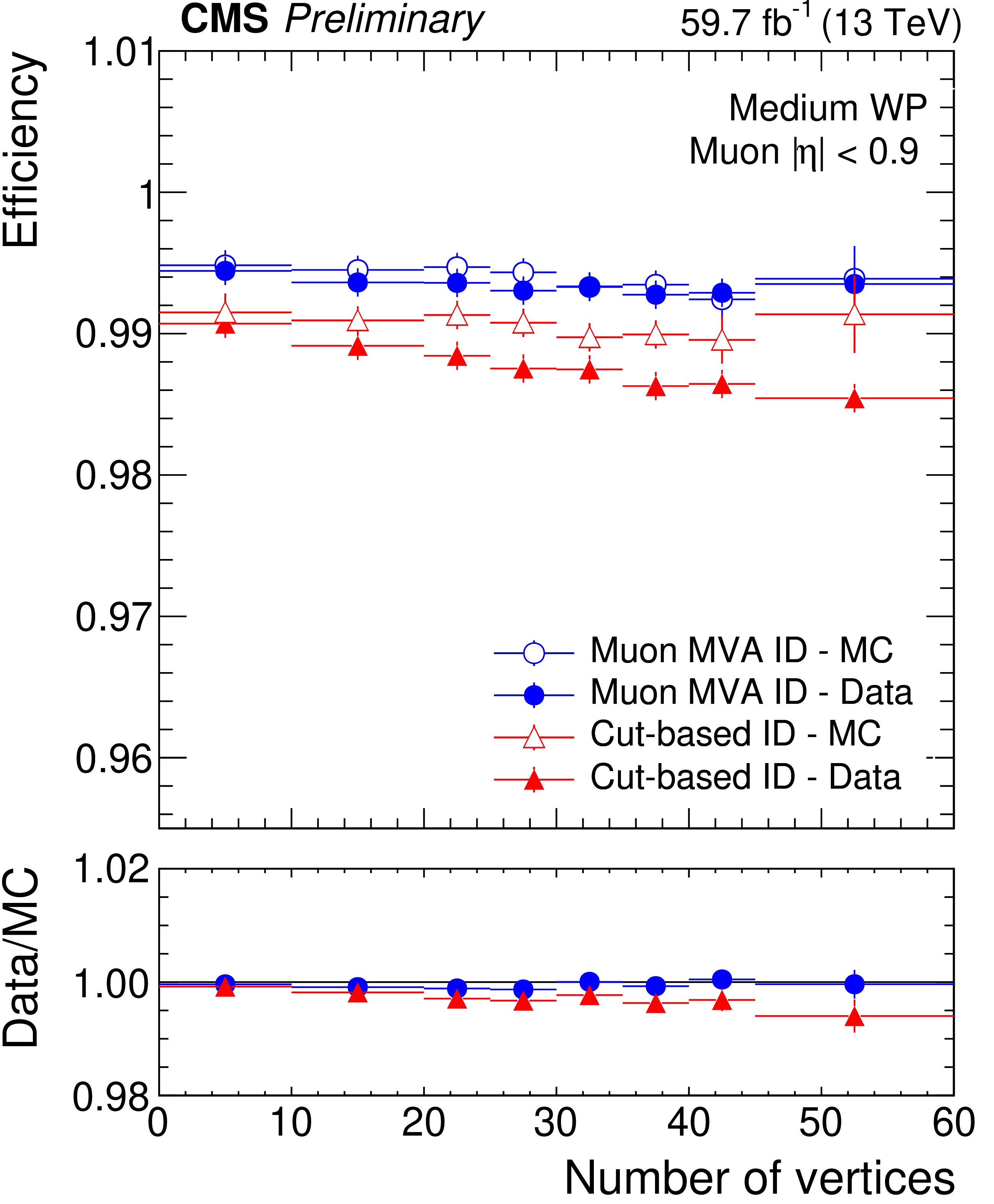
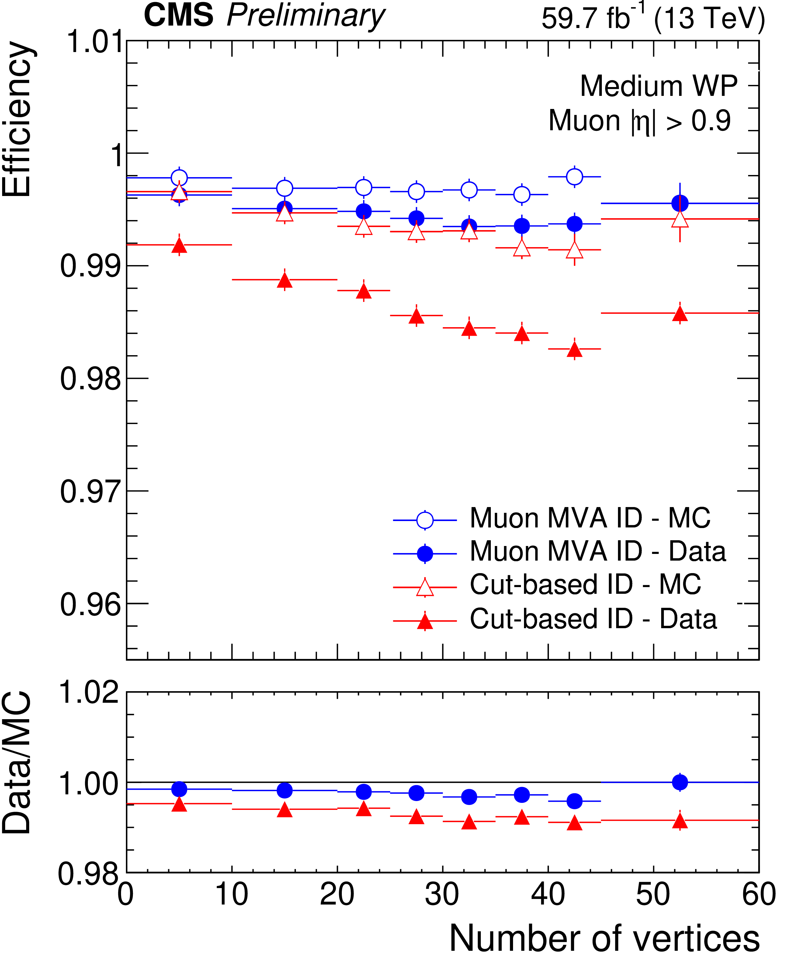
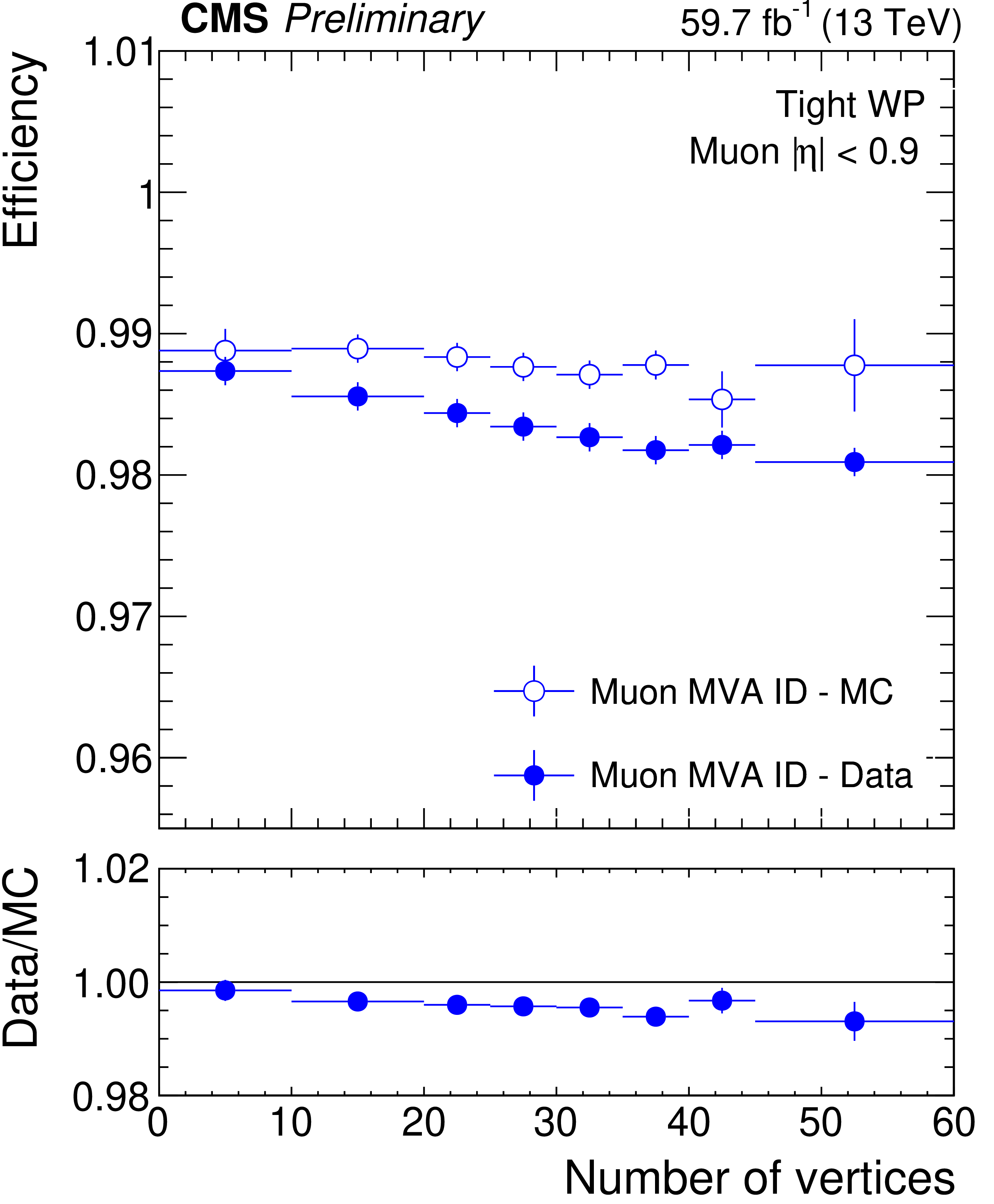
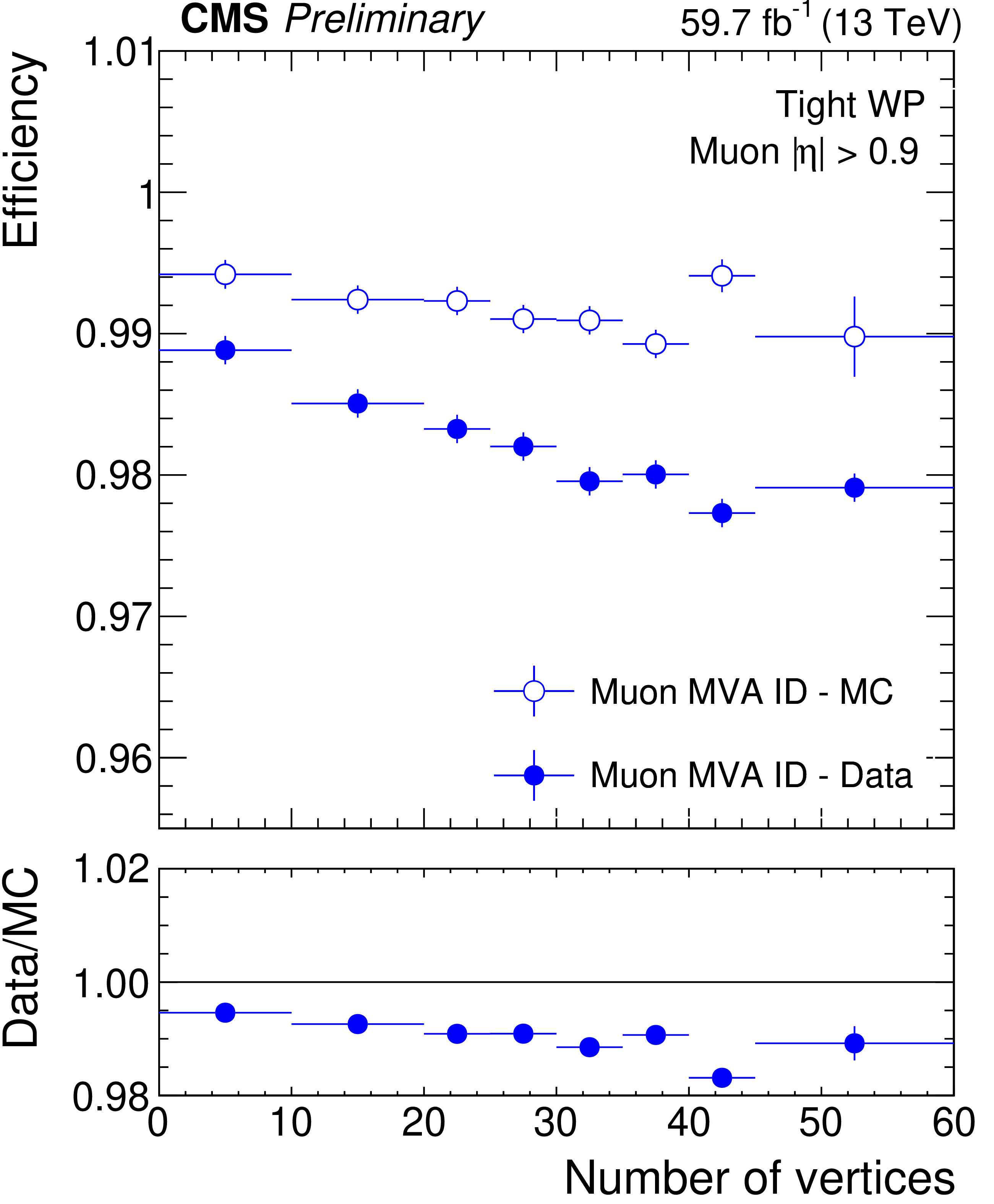
Figure 7:
Muon identification efficiency for the medium (top) and tight (bottom) WPs as a function of PU for muons with $ |\eta| < $ 0.9 (left) and $ |\eta| > $ 0.9 (right). Blue dots show the MVA ID performance both for 2018 dataset and DY while red triangles show the efficiency of the cut-based ID used during Run 2. |
png pdf |
Figure 7-a:
Muon identification efficiency for the medium (top) and tight (bottom) WPs as a function of PU for muons with $ |\eta| < $ 0.9 (left) and $ |\eta| > $ 0.9 (right). Blue dots show the MVA ID performance both for 2018 dataset and DY while red triangles show the efficiency of the cut-based ID used during Run 2. |
png pdf |
Figure 7-b:
Muon identification efficiency for the medium (top) and tight (bottom) WPs as a function of PU for muons with $ |\eta| < $ 0.9 (left) and $ |\eta| > $ 0.9 (right). Blue dots show the MVA ID performance both for 2018 dataset and DY while red triangles show the efficiency of the cut-based ID used during Run 2. |
png pdf |
Figure 7-c:
Muon identification efficiency for the medium (top) and tight (bottom) WPs as a function of PU for muons with $ |\eta| < $ 0.9 (left) and $ |\eta| > $ 0.9 (right). Blue dots show the MVA ID performance both for 2018 dataset and DY while red triangles show the efficiency of the cut-based ID used during Run 2. |
png pdf |
Figure 7-d:
Muon identification efficiency for the medium (top) and tight (bottom) WPs as a function of PU for muons with $ |\eta| < $ 0.9 (left) and $ |\eta| > $ 0.9 (right). Blue dots show the MVA ID performance both for 2018 dataset and DY while red triangles show the efficiency of the cut-based ID used during Run 2. |

png pdf |
Figure 8:
Efficiency of the prompt MVA selection as a function of the muon $ p_{\mathrm{T}} $ for muons with $ |\eta| < $ 0.9 (left) and $ |\eta| > $ 0.9 (right), for 2018 dataset in black and DY events in red. |
png pdf |
Figure 8-a:
Efficiency of the prompt MVA selection as a function of the muon $ p_{\mathrm{T}} $ for muons with $ |\eta| < $ 0.9 (left) and $ |\eta| > $ 0.9 (right), for 2018 dataset in black and DY events in red. |

png pdf |
Figure 8-b:
Efficiency of the prompt MVA selection as a function of the muon $ p_{\mathrm{T}} $ for muons with $ |\eta| < $ 0.9 (left) and $ |\eta| > $ 0.9 (right), for 2018 dataset in black and DY events in red. |
png pdf |
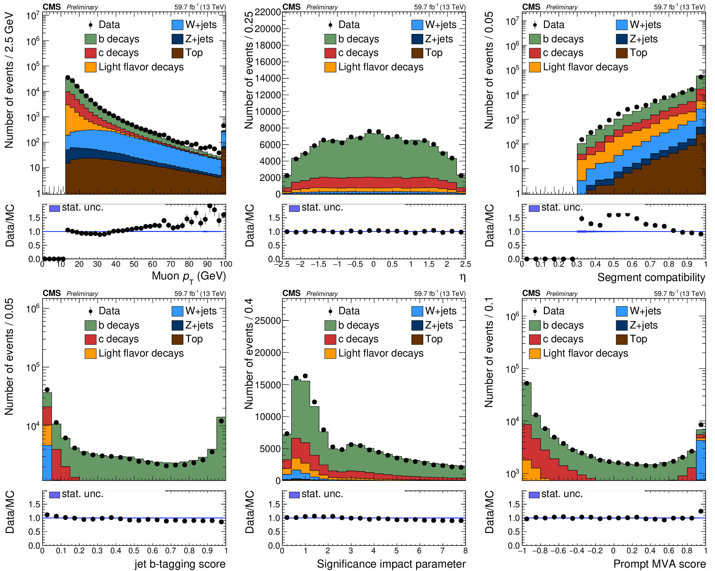
Figure 9:
Distribution of data in the multijet control region as a function of the muon $ p_{\mathrm{T}} $ (top left), $ \eta $ (top right), segment compatibility (middle left), the deep flavor b-tagging of the jet associated to the muon (middle right), the significance of the impact parameter (bottom left) and the prompt MVA score (bottom right). |
png pdf |
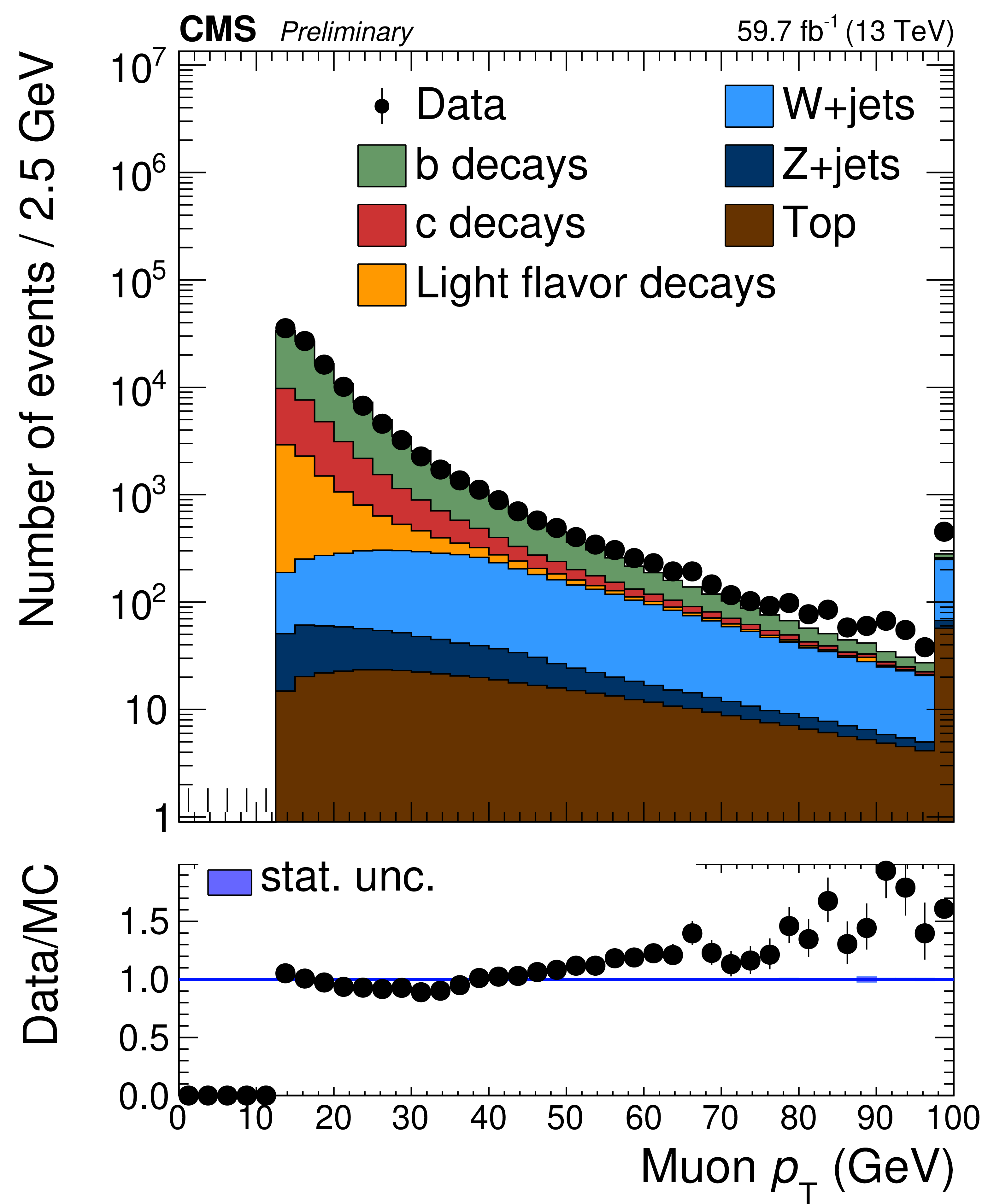
Figure 9-a:
Distribution of data in the multijet control region as a function of the muon $ p_{\mathrm{T}} $ (top left), $ \eta $ (top right), segment compatibility (middle left), the deep flavor b-tagging of the jet associated to the muon (middle right), the significance of the impact parameter (bottom left) and the prompt MVA score (bottom right). |
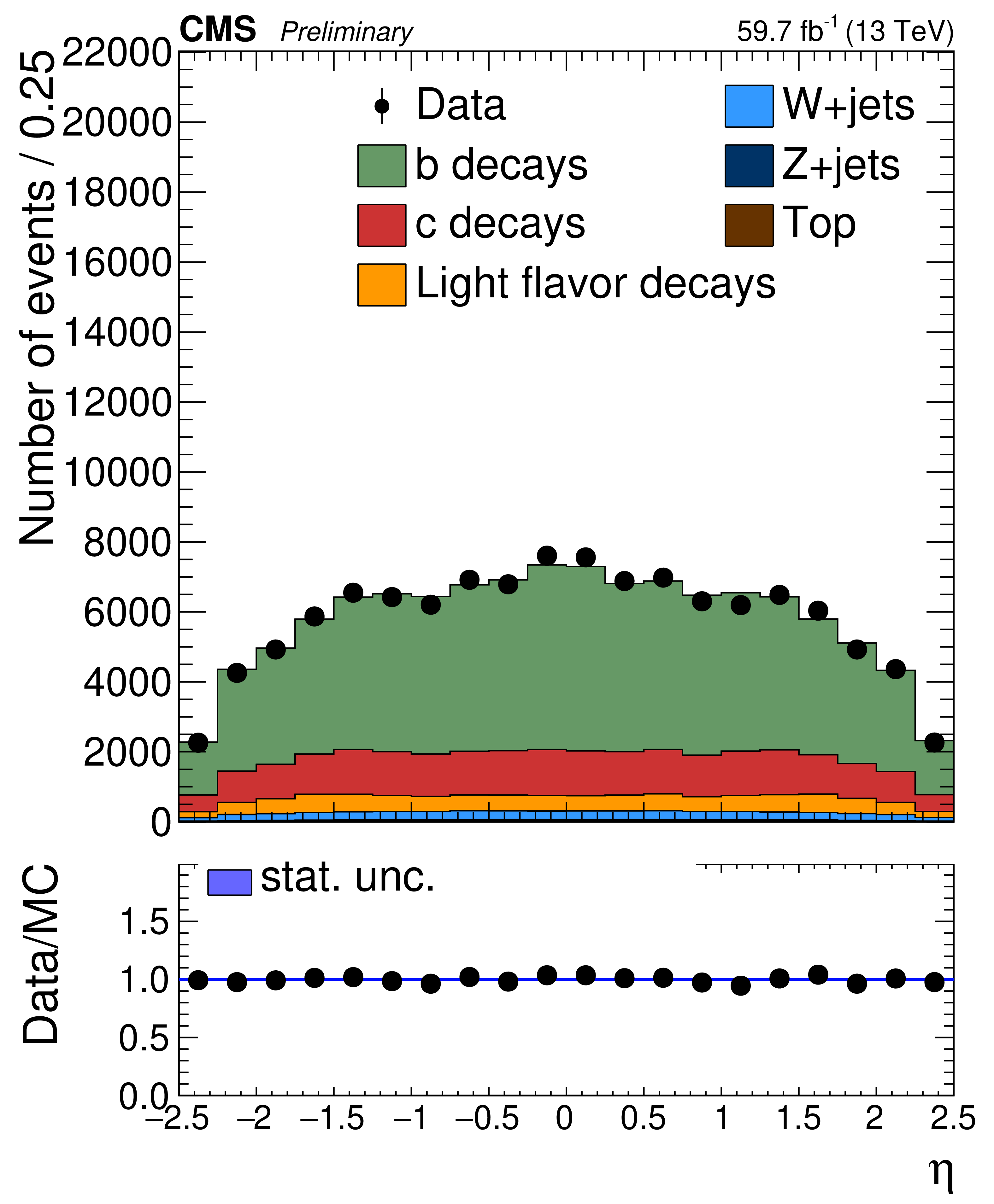
png pdf |
Figure 9-b:
Distribution of data in the multijet control region as a function of the muon $ p_{\mathrm{T}} $ (top left), $ \eta $ (top right), segment compatibility (middle left), the deep flavor b-tagging of the jet associated to the muon (middle right), the significance of the impact parameter (bottom left) and the prompt MVA score (bottom right). |
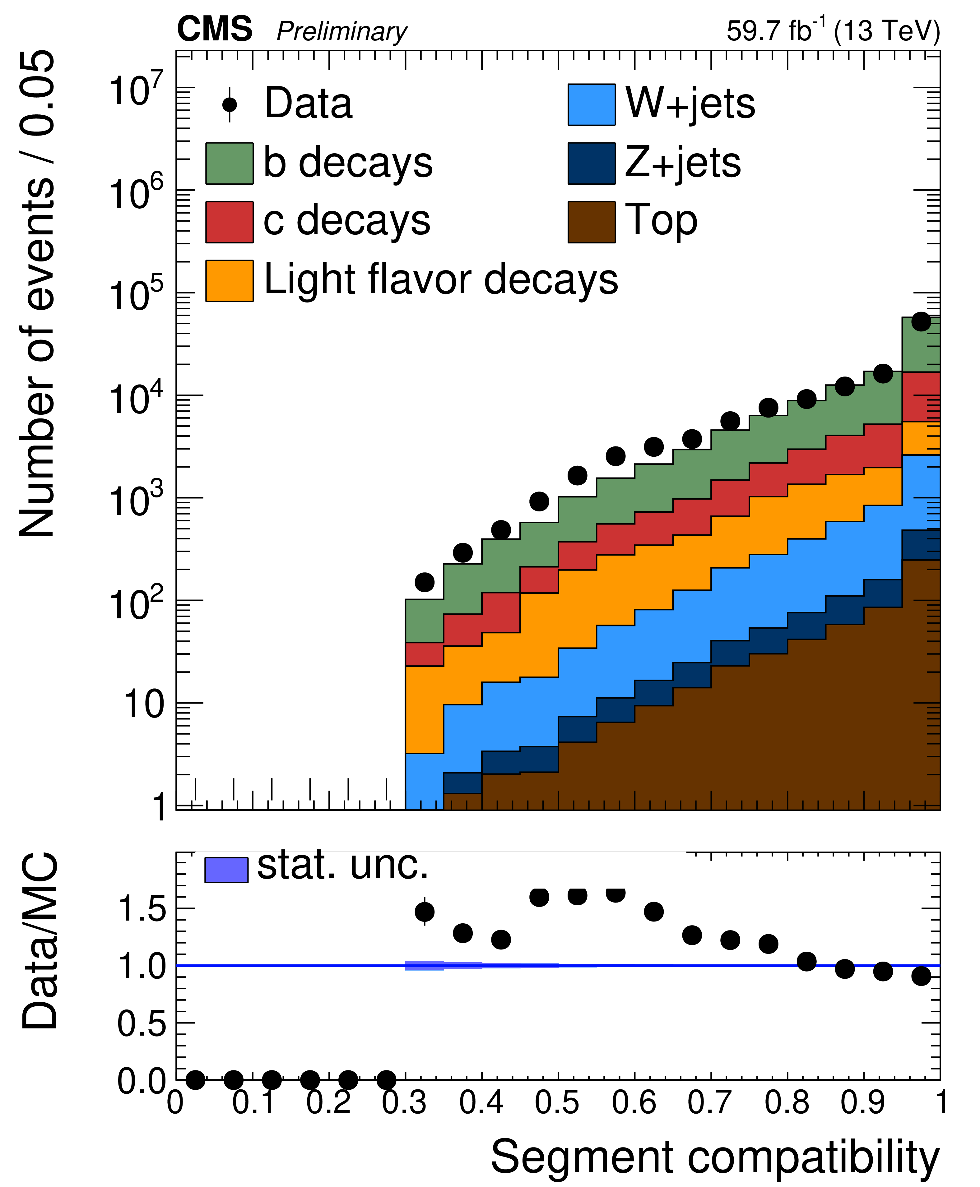
png pdf |
Figure 9-c:
Distribution of data in the multijet control region as a function of the muon $ p_{\mathrm{T}} $ (top left), $ \eta $ (top right), segment compatibility (middle left), the deep flavor b-tagging of the jet associated to the muon (middle right), the significance of the impact parameter (bottom left) and the prompt MVA score (bottom right). |

png pdf |
Figure 9-d:
Distribution of data in the multijet control region as a function of the muon $ p_{\mathrm{T}} $ (top left), $ \eta $ (top right), segment compatibility (middle left), the deep flavor b-tagging of the jet associated to the muon (middle right), the significance of the impact parameter (bottom left) and the prompt MVA score (bottom right). |
png pdf |
Figure 9-e:
Distribution of data in the multijet control region as a function of the muon $ p_{\mathrm{T}} $ (top left), $ \eta $ (top right), segment compatibility (middle left), the deep flavor b-tagging of the jet associated to the muon (middle right), the significance of the impact parameter (bottom left) and the prompt MVA score (bottom right). |

png pdf |
Figure 9-f:
Distribution of data in the multijet control region as a function of the muon $ p_{\mathrm{T}} $ (top left), $ \eta $ (top right), segment compatibility (middle left), the deep flavor b-tagging of the jet associated to the muon (middle right), the significance of the impact parameter (bottom left) and the prompt MVA score (bottom right). |

png pdf |
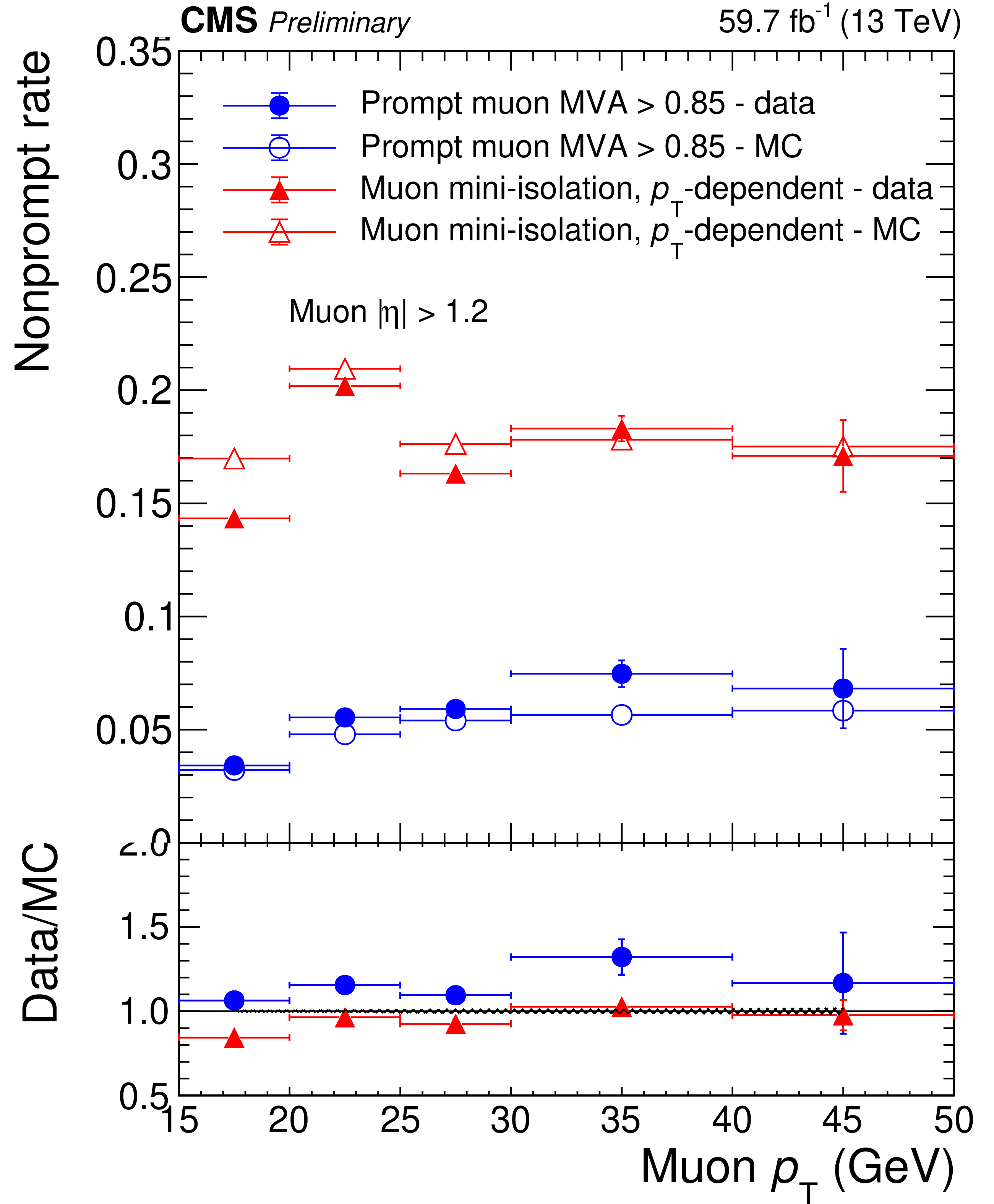
Figure 10:
Measurement of the muon nonprompt rate of a prompt MVA (red) and mini-isolation (blue) selection as a function of $ p_{\mathrm{T}} $ for muons with $ |\eta| < $ 1.2 (left) and $ |\eta| > $ 1.2 (right) for the 2018 dataset and DY events. |

png pdf |
Figure 10-a:
Measurement of the muon nonprompt rate of a prompt MVA (red) and mini-isolation (blue) selection as a function of $ p_{\mathrm{T}} $ for muons with $ |\eta| < $ 1.2 (left) and $ |\eta| > $ 1.2 (right) for the 2018 dataset and DY events. |
png pdf |
Figure 10-b:
Measurement of the muon nonprompt rate of a prompt MVA (red) and mini-isolation (blue) selection as a function of $ p_{\mathrm{T}} $ for muons with $ |\eta| < $ 1.2 (left) and $ |\eta| > $ 1.2 (right) for the 2018 dataset and DY events. |
| Summary |
| The presence of leptons is crucial in many precision measurements and searches for suppressing the otherwise overwhelming background and as an indicator of interesting physical processes. Two multivariate (MVA) techniques have been developed for a highly efficient muon identification and isolation. One, the MVA ID, has been trained to distinguish muons produced promptly in heavy gauge boson decays as well as muons from $ \tau $ lepton and heavy flavour hadron decays, from background muons produced in light hadron decays (pions or kaons) or other spurious signatures in the detector that could be misreconstructed as muons. The discriminator is presented as an alternative to the standard cut-based identification criteria and could be used for high-efficiency working points. The second one, the prompt MVA, aims to select isolated muons from W, Z, H bosons, and $ \tau $ lepton decays to reduce contamination from nonisolated muons arising in heavy flavour hadron decays. Their performance has been measured in proton-proton collisions recorded by the CMS experiment during 2018 and compared to simulation performance. The measured efficiencies are similar to or better than those achieved by the standard cut-based selection criteria. |
| Additional Figures | |
png pdf |
Additional Figure 1:
ROC curve for muons with $ p_{\mathrm{T}} > $ 10 GeV for the developed general muon MVA ID discriminator (black solid line). Orange and blue points show the medium and tight WPs of the cut-based ID. The ROC curve of the soft MVA is also shown (gray dashed line). |
| References | ||||
| 1 | CMS Collaboration | The CMS experiment at the CERN LHC | JINST 3 (2008) S08004 | |
| 2 | CMS Collaboration | Performance of the CMS muon detector and muon reconstruction with proton-proton collisions at $ \sqrt{s}= $ 13 TeV | JINST 13 (2018) P06015 | CMS-MUO-16-001 1804.04528 |
| 3 | CMS Collaboration | Measurement of the Higgs boson production rate in association with top quarks in final states with electrons, muons, and hadronically decaying tau leptons at $ \sqrt{s} = $ 13 TeV | EPJC 81 (2021) 378 | CMS-HIG-19-008 2011.03652 |
| 4 | CMS Collaboration | Evidence for associated production of a Higgs boson with a top quark pair in final states with electrons, muons, and hadronically decaying $ \tau $ leptons at $ \sqrt{s} = $ 13 TeV | JHEP 08 (2018) 066 | CMS-HIG-17-018 1803.05485 |
| 5 | CMS Collaboration | Observation of $ \mathrm{t\overline{t}} $H production | PRL 120 (2018) 231801 | CMS-HIG-17-035 1804.02610 |
| 6 | CMS Collaboration | Measurements of the electroweak diboson production cross sections in proton-proton collisions at $ \sqrt{s} = $ 5.02 TeV using leptonic decays | PRL 127 (2021) 191801 | CMS-SMP-20-012 2107.01137 |
| 7 | CMS Collaboration | Search for electroweak production of charginos and neutralinos in proton-proton collisions at $ \sqrt{s} = $ 13 TeV | JHEP 04 (2022) 147 | CMS-SUS-19-012 2106.14246 |
| 8 | CMS Collaboration | Search for electroweak production of charginos and neutralinos in multilepton final states in proton-proton collisions at $ \sqrt{s}= $ 13 TeV | JHEP 03 (2018) 166 | CMS-SUS-16-039 1709.05406 |
| 9 | CMS Collaboration | Combined search for electroweak production of charginos and neutralinos in proton-proton collisions at $ \sqrt{s} = $ 13 TeV | JHEP 03 (2018) 160 | CMS-SUS-17-004 1801.03957 |
| 10 | CMS Collaboration | Measurement of the inclusive and differential WZ production cross sections, polarization angles, and triple gauge couplings in pp collisions at $ \sqrt{s} $ = 13 TeV | JHEP 07 (2022) 032 | CMS-SMP-20-014 2110.11231 |
| 11 | CMS Collaboration | Measurements of the pp $ \to $ WZ inclusive and differential production cross section and constraints on charged anomalous triple gauge couplings at $ \sqrt{s} = $ 13 TeV | JHEP 04 (2019) 122 | CMS-SMP-18-002 1901.03428 |
| 12 | CMS Collaboration | Observation of Single Top Quark Production in Association with a $ Z $ Boson in Proton-Proton Collisions at $ \sqrt {s} $ =13 TeV | PRL 122 (2019) 132003 | CMS-TOP-18-008 1812.05900 |
| 13 | CMS Collaboration | Measurement of the cross section of top quark-antiquark pair production in association with a W boson in proton-proton collisions at $ \sqrt{s} $ = 13 TeV | Submitted to JHEP, 2022 | CMS-TOP-21-011 2208.06485 |
| 14 | CMS Collaboration | Measurement of top quark pair production in association with a Z boson in proton-proton collisions at $ \sqrt{s}= $ 13 TeV | JHEP 03 (2020) 056 | CMS-TOP-18-009 1907.11270 |
| 15 | CMS Collaboration | Inclusive and differential cross section measurements of single top quark production in association with a Z boson in proton-proton collisions at $ \sqrt{s} $ = 13 TeV | JHEP 02 (2022) 107 | CMS-TOP-20-010 2111.02860 |
| 16 | CMS Collaboration | Measurement of properties of B$ ^0_\mathrm{s}\to\mu^+\mu^- $ decays and search for B$ ^0\to\mu^+\mu^- $ with the CMS experiment | JHEP 04 (2020) 188 | CMS-BPH-16-004 1910.12127 |
| 17 | CMS Collaboration | Performance of the CMS Level-1 trigger in proton-proton collisions at $ \sqrt{s} = $ 13 TeV | JINST 15 (2020) P10017 | CMS-TRG-17-001 2006.10165 |
| 18 | CMS Collaboration | The CMS trigger system | JINST 12 (2017) P01020 | CMS-TRG-12-001 1609.02366 |
| 19 | CMS Collaboration | CMS luminosity measurement for the 2018 data-taking period at $ \sqrt{s} $ = 13 TeV | CMS Physics Analysis Summary, 2019 link |
CMS-PAS-LUM-18-002 |
| 20 | CMS Collaboration | Precision luminosity measurement in proton-proton collisions at $ \sqrt{s}= $ 13 TeV in 2015 and 2016 at CMS | EPJC 81 (2021) 800 | CMS-LUM-17-003 2104.01927 |
| 21 | CMS Collaboration | Performance of the CMS muon trigger system in proton-proton collisions at $ \sqrt{s} = $ 13 TeV | JINST 16 (2021) P07001 | CMS-MUO-19-001 2102.04790 |
| 22 | J. Alwall et al. | The automated computation of tree-level and next-to-leading order differential cross sections, and their matching to parton shower simulations | JHEP 07 (2014) 079 | 1405.0301 |
| 23 | J. Alwall et al. | Comparative study of various algorithms for the merging of parton showers and matrix elements in hadronic collisions | EPJC 53 (2008) 473 | 0706.2569 |
| 24 | S. Alioli, P. Nason, C. Oleari, and E. Re | A general framework for implementing NLO calculations in shower Monte Carlo programs: the POWHEG BOX | JHEP 06 (2010) 043 | 1002.2581 |
| 25 | S. Frixione, P. Nason, and C. Oleari | Matching NLO QCD computations with Parton Shower simulations: the POWHEG method | JHEP 11 (2007) 070 | 0709.2092 |
| 26 | P. Nason | A new method for combining NLO QCD with shower Monte Carlo algorithms | JHEP 11 (2004) 040 | hep-ph/0409146 |
| 27 | NNPDF Collaboration | Parton distributions from high-precision collider data | EPJC 77 (2017) 663 | 1706.00428 |
| 28 | T. Sjöstrand et al. | An introduction to PYTHIA 8.2 | Comput. Phys. Commun. 191 (2015) 159 | 1410.3012 |
| 29 | P. Skands, S. Carrazza, and J. Rojo | Tuning PYTHIA 8.1: the Monash 2013 Tune | EPJC 74 (2014) 3024 | 1404.5630 |
| 30 | CMS Collaboration | Extraction and validation of a new set of CMS PYTHIA8 tunes from underlying-event measurements | EPJC 80 (2020) 4 | CMS-GEN-17-001 1903.12179 |
| 31 | R. Frederix and S. Frixione | Merging meets matching in MC@NLO | JHEP 12 (2012) 061 | 1209.6215 |
| 32 | GEANT4 Collaboration | GEANT4---a simulation toolkit | NIMA 506 (2003) 250 | |
| 33 | R. Frühwirth | Application of Kalman filtering to track and vertex fitting | NIM A 262 (1987) 444 | |
| 34 | CMS Collaboration | Description and performance of track and primary-vertex reconstruction with the CMS tracker | JINST 9 (2014) P10009 | CMS-TRK-11-001 1405.6569 |
| 35 | CMS Collaboration | Performance of the reconstruction and identification of high-momentum muons in proton-proton collisions at $ \sqrt{s} = $ 13 TeV | JINST 15 (2020) P02027 | CMS-MUO-17-001 1912.03516 |
| 36 | CMS Collaboration | Particle-flow reconstruction and global event description with the CMS detector | JINST 12 (2017) P10003 | CMS-PRF-14-001 1706.04965 |
| 37 | M. Cacciari, G. P. Salam, and G. Soyez | The anti-$ k_{\mathrm{T}} $ jet clustering algorithm | JHEP 04 (2008) 063 | 0802.1189 |
| 38 | M. Cacciari, G. P. Salam, and G. Soyez | The catchment area of jets | JHEP 04 (2008) 005 | 0802.1188 |
| 39 | M. Cacciari and G. P. Salam | Pileup subtraction using jet areas | PLB 659 (2008) 119 | 0707.1378 |
| 40 | CMS Collaboration | Jet energy scale and resolution in the CMS experiment in pp collisions at 8 TeV | JINST 12 (2017) P02014 | CMS-JME-13-004 1607.03663 |
| 41 | CMS Collaboration | Performance summary of AK4 jet b tagging with data from proton-proton collisions at 13 TeV with the CMS detector | CMS Detector Performance Note CMS-DP-2023-005, 2023 CDS |
|
| 42 | E. Bols et al. | Jet Flavour Classification Using DeepJet | JINST 15 (2020) P12012 | 2008.10519 |
| 43 | D. Contardo et al. | Technical proposal for the phase-II upgrade of the CMS detector | technical report, Geneva, 2015 link |
|
| 44 | CMS Collaboration | Performance of electron reconstruction and selection with the CMS Detector in proton-proton collisions at $ \sqrt{s} $ = 8 TeV | JINST 10 (2015) P06005 | CMS-EGM-13-001 1502.02701 |
| 45 | CMS Collaboration | Search for supersymmetry in pp collisions at $ \sqrt{s}= $ 13 TeV in the single-lepton final state using the sum of masses of large-radius jets | JHEP 08 (2016) 122 | CMS-SUS-15-007 1605.04608 |
| 46 | A. Prinzie and D. Van den Poel | Random multiclass classification: Generalizing random forests to random MNL and random NB | Database and Expert Systems Applications, Volume 4653 of, 2007 Lecture Notes in Computer Science 4653 (2007) 349 |
|
| 47 | F. Pedregosa et al. | Scikit-learn: Machine learning in Python | link | |
| 48 | A. Höcker et al. | TMVA, the toolkit for multivariate data analysis with ROOT | PoS ACAT 04 (2007) 0 | |
| 49 | CMS Collaboration | Measurements of inclusive W and Z cross sections in pp collisions at $ \sqrt{s}= $ 7 TeV | JHEP 01 (2011) 080 | CMS-EWK-10-002 1012.2466 |
|
|
Compact Muon Solenoid LHC, CERN |
|

|

|

|

|

|