

Compact Muon Solenoid
LHC, CERN
| CMS-PAS-HIG-22-011 | ||
| Search for ZZ and ZH production in the $ \rm{b}\bar{\rm{b}}\rm{b}\bar{\rm{b}} $ final state using proton-proton collisions at $ \sqrt{s}= $ 13 TeV | ||
| CMS Collaboration | ||
| 4 December 2023 | ||
| Abstract: A search for ZZ and ZH production in the $ \mathrm{b}\bar{\mathrm{b}}\mathrm{b}\bar{\mathrm{b}} $ final state is presented. The search uses an event sample of proton-proton collisions corresponding to an integrated luminosity of 133 fb$ ^{-1} $ at a center-of-mass energy of 13 TeV with the CMS detector at the LHC. This analysis introduces several novel techniques for deriving and validating the data-driven background model using synthetic data sets, derived from the hemisphere-mixing technique. A multi-class multivariate classifier customized for the $ \mathrm{b}\bar{\mathrm{b}}\mathrm{b}\bar{\mathrm{b}} $ final state is developed to both extract the signal and derive the background model. The data are found to be consistent, within uncertainties, with the standard model (SM) predictions. The observed (expected) upper limit at 95% confidence level corresponds to 3.8 (3.8) and 5.0 (2.9) times the SM prediction for the ZZ and ZH production cross sections, respectively. The ZZ and ZH $ \rightarrow \mathrm{b}\bar{\mathrm{b}}\mathrm{b}\bar{\mathrm{b}} $ processes share the experimental challenges of the HH $ \rightarrow \mathrm{b}\bar{\mathrm{b}}\mathrm{b}\bar{\mathrm{b}} $ analysis. The novel techniques developed and demonstrated in the ZZ and ZH search are used to analyze the HH $ \rightarrow \mathrm{b}\bar{\mathrm{b}}\mathrm{b}\bar{\mathrm{b}} $ background. The ZZ, ZH, and HH $ \rightarrow \mathrm{b}\bar{\mathrm{b}}\mathrm{b}\bar{\mathrm{b}} $ expected sensitivities are extrapolated to an integrated luminosity of 3000 $ \mathrm{fb}^{-1} $. | ||
|
Links:
CDS record (PDF) ;
CADI line (restricted) ;
These preliminary results are superseded in this paper, Submitted to EPJC. The superseded preliminary plots can be found here. |
||
| Figures & Tables | Summary | Additional Figures | References | CMS Publications |
|---|
| Figures | |
png pdf |
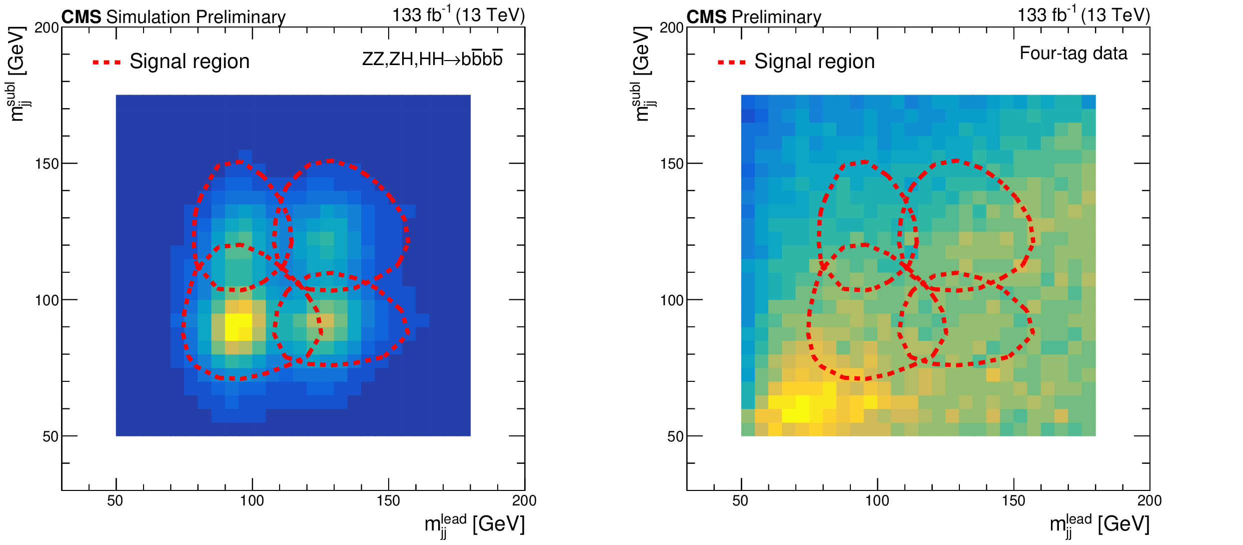
Figure 1:
Signal (left) and four-tag data (right) passing the event selection. The signal region is defined by the union of the red dashed lines. |
png pdf |
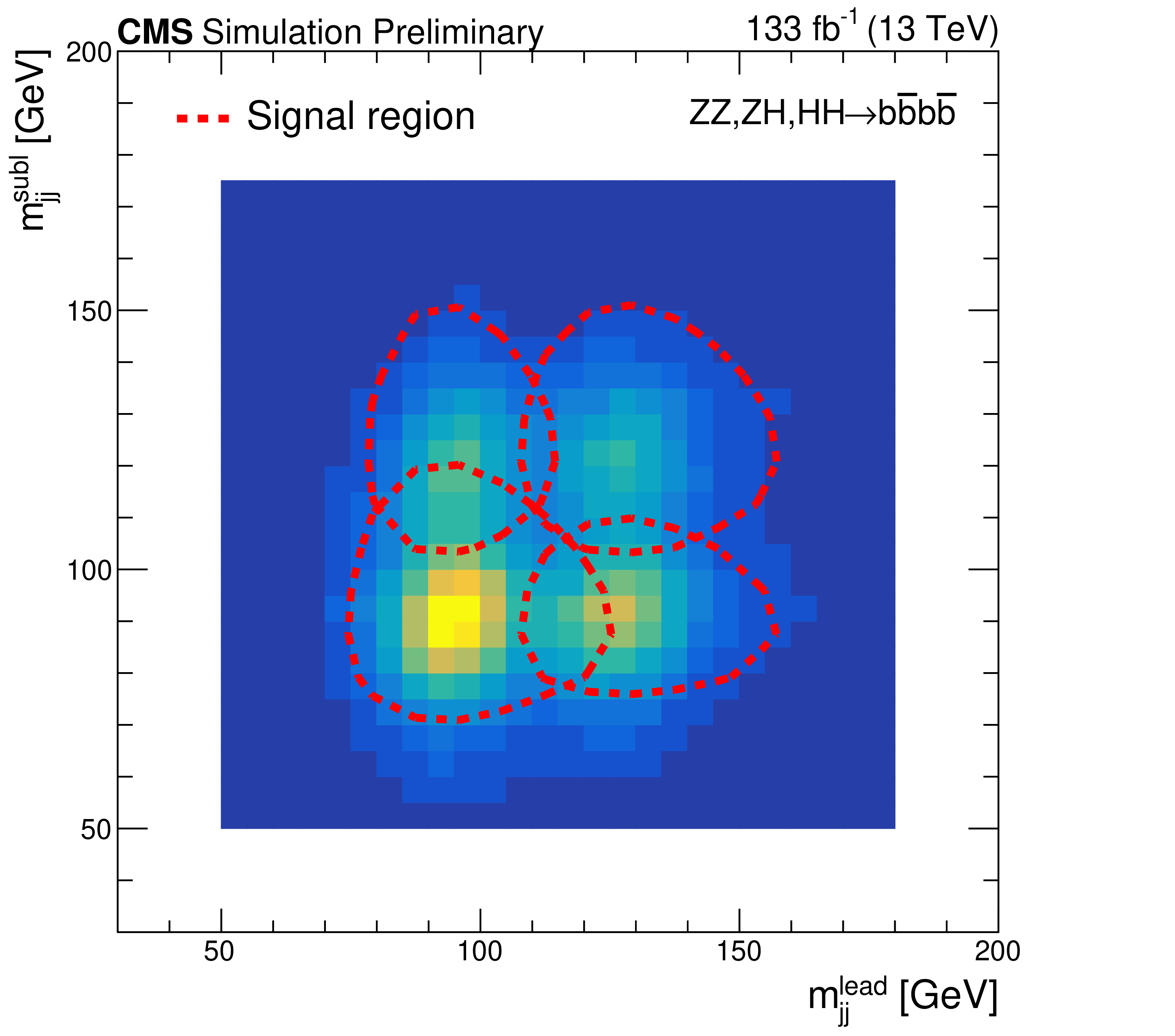
Figure 1-a:
Signal (left) and four-tag data (right) passing the event selection. The signal region is defined by the union of the red dashed lines. |

png pdf |
Figure 1-b:
Signal (left) and four-tag data (right) passing the event selection. The signal region is defined by the union of the red dashed lines. |

png pdf |
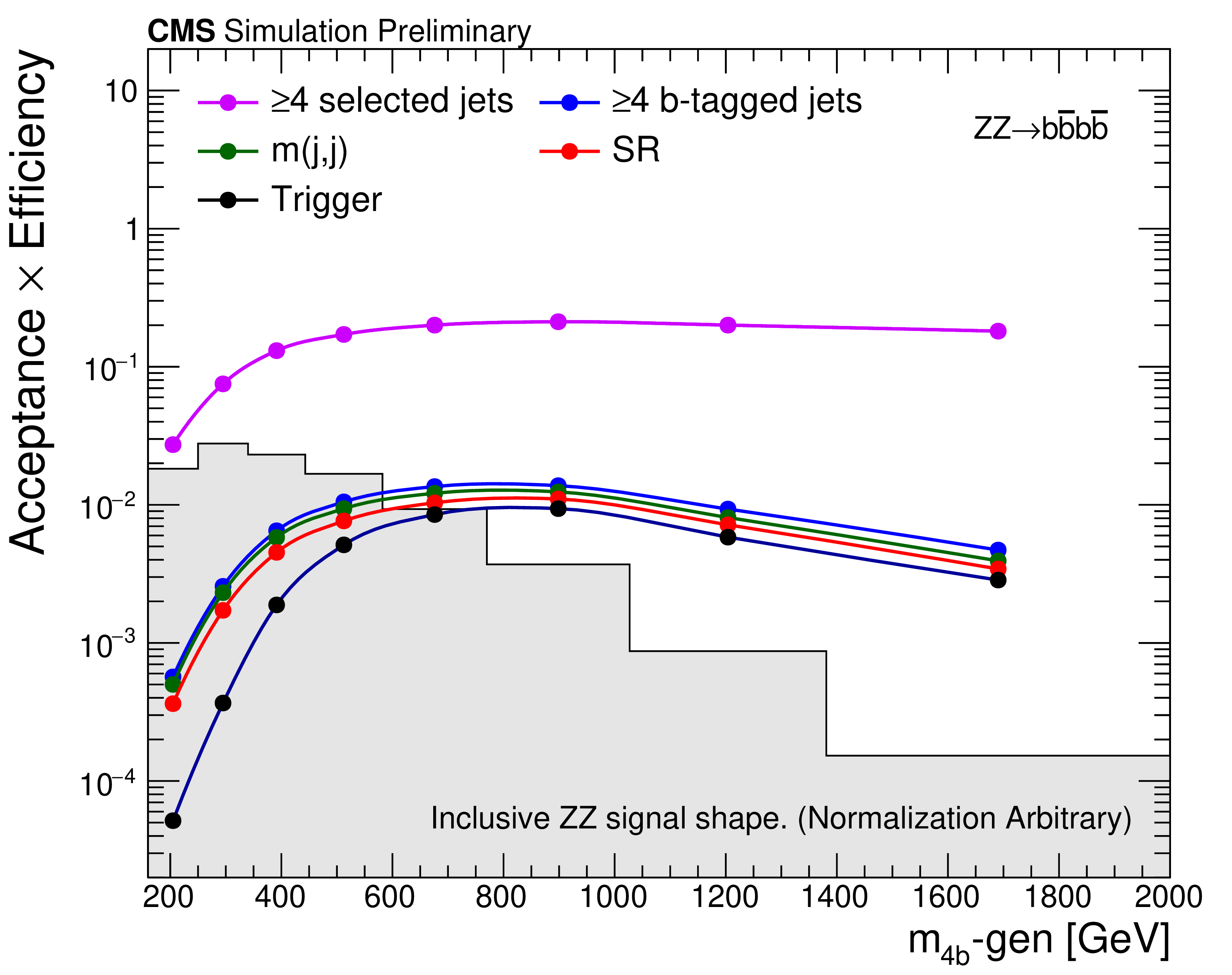
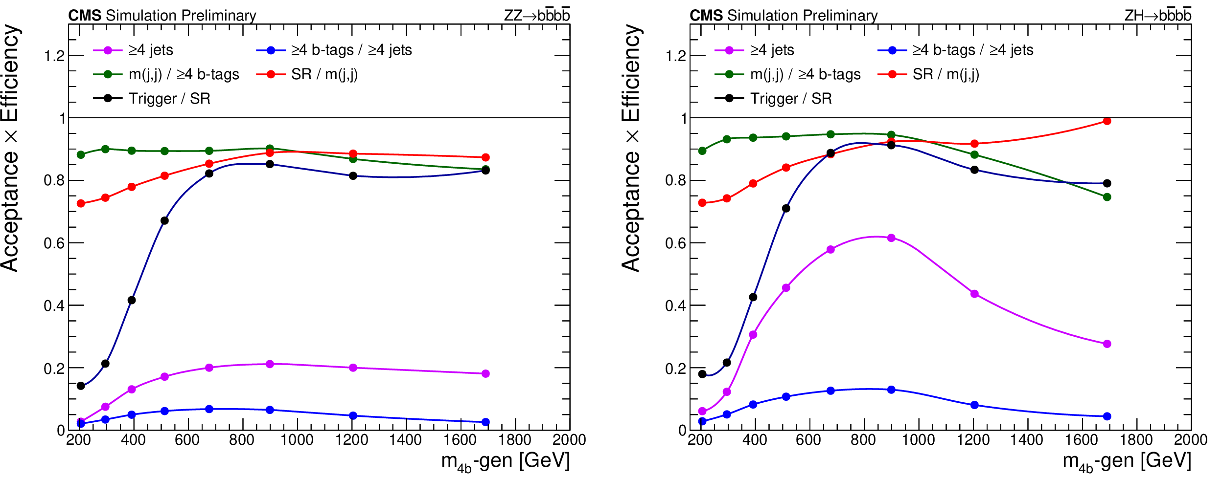
Figure 2:
Event selection acceptance times efficiency as a function of the generated four body mass $ m_{4\mathrm{b}} $-gen for the ZZ (left) and ZH (right) signal. The plots show the cumulative efficiency with respect to the inclusive sample. The expected $ m_{4\mathrm{b}} $-gen distribution of the inclusive ZZ and ZH\ signal is given in gray with arbitrary normalization. |
png pdf |
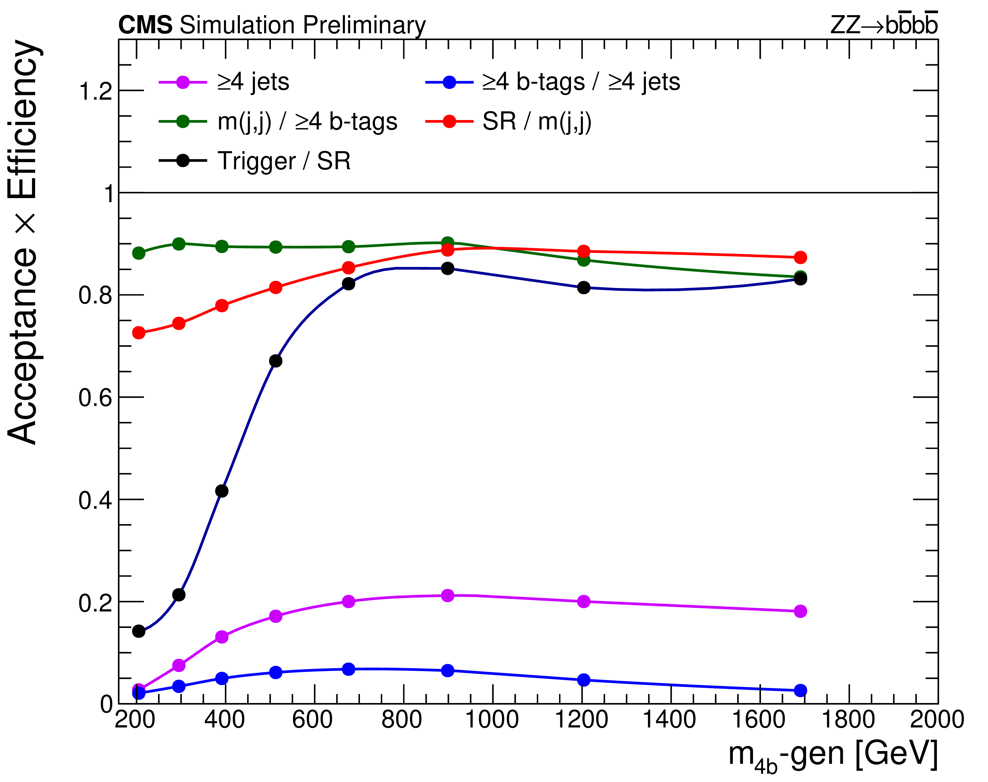
Figure 2-a:
Event selection acceptance times efficiency as a function of the generated four body mass $ m_{4\mathrm{b}} $-gen for the ZZ (left) and ZH (right) signal. The plots show the cumulative efficiency with respect to the inclusive sample. The expected $ m_{4\mathrm{b}} $-gen distribution of the inclusive ZZ and ZH\ signal is given in gray with arbitrary normalization. |

png pdf |
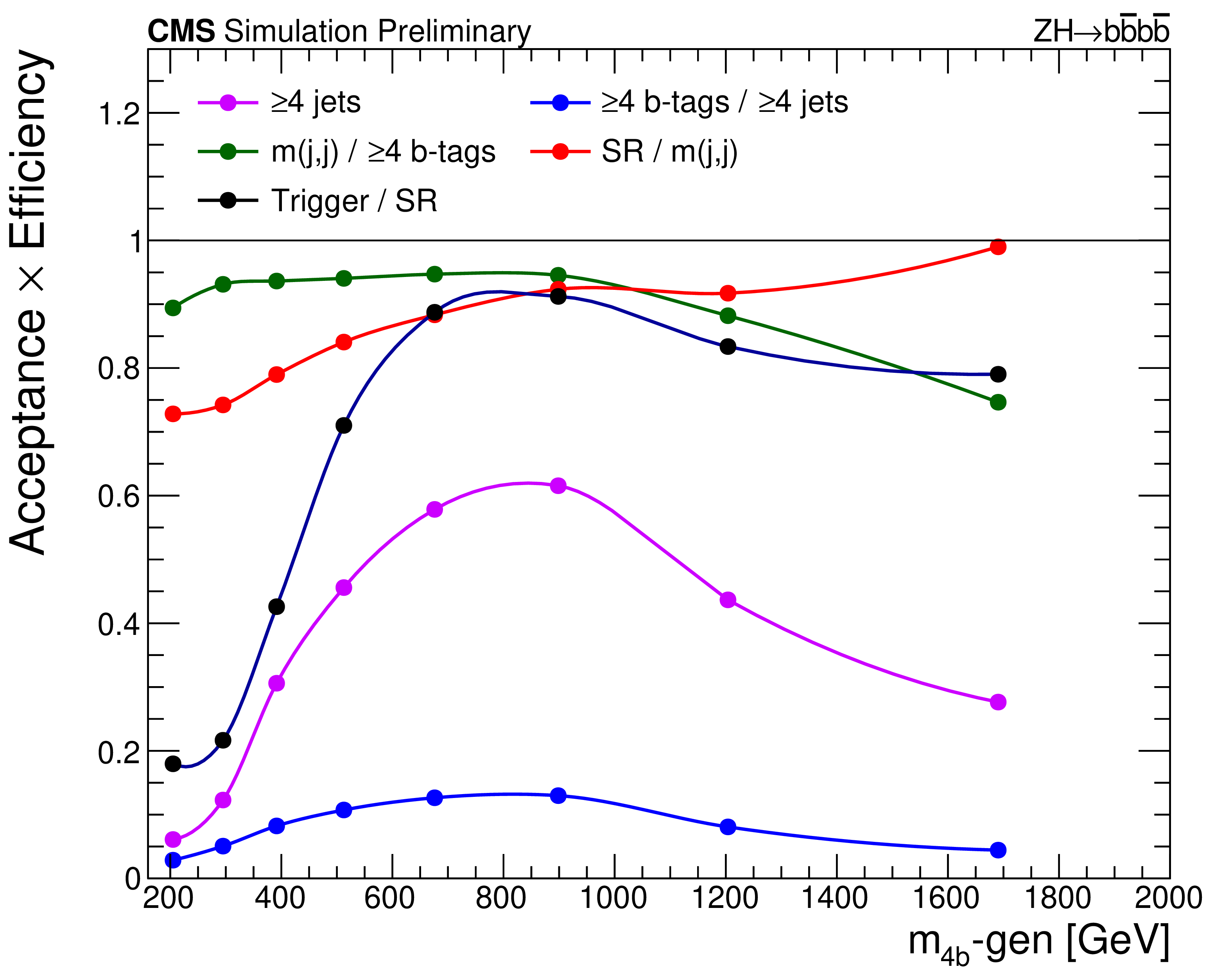
Figure 2-b:
Event selection acceptance times efficiency as a function of the generated four body mass $ m_{4\mathrm{b}} $-gen for the ZZ (left) and ZH (right) signal. The plots show the cumulative efficiency with respect to the inclusive sample. The expected $ m_{4\mathrm{b}} $-gen distribution of the inclusive ZZ and ZH\ signal is given in gray with arbitrary normalization. |
png pdf |
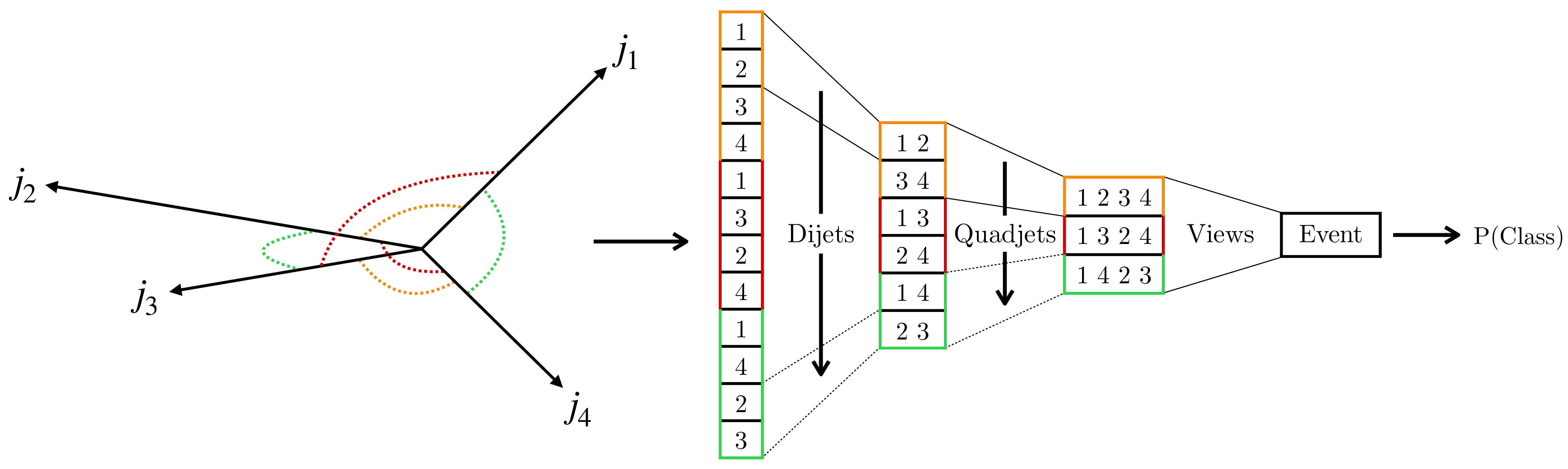
Figure 3:
A high-level sketch of the HCR classifier architecture. Boson-candidate jets are shown on the left with the three possible jet pairings. The HCR architecture is shown in the right. The boxes represent pixels, with the labels indicating which jet, dijet, or quadjet the pixel refers to. The different jet pairings on the left are each represented within the network, as indicated by the color coding. |
png pdf |
Figure 4:
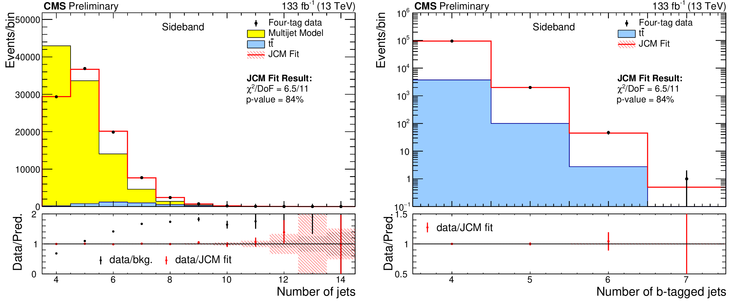
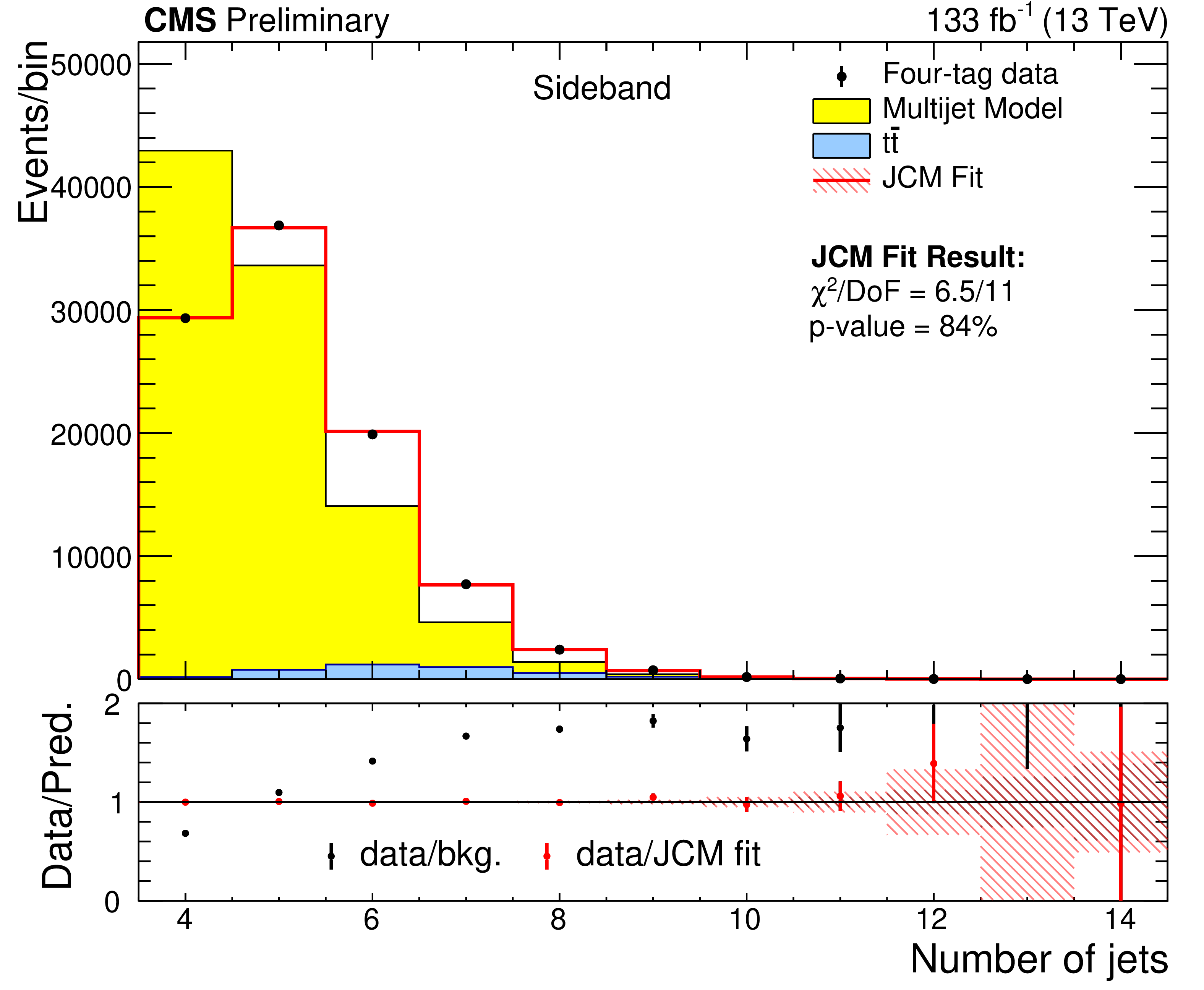
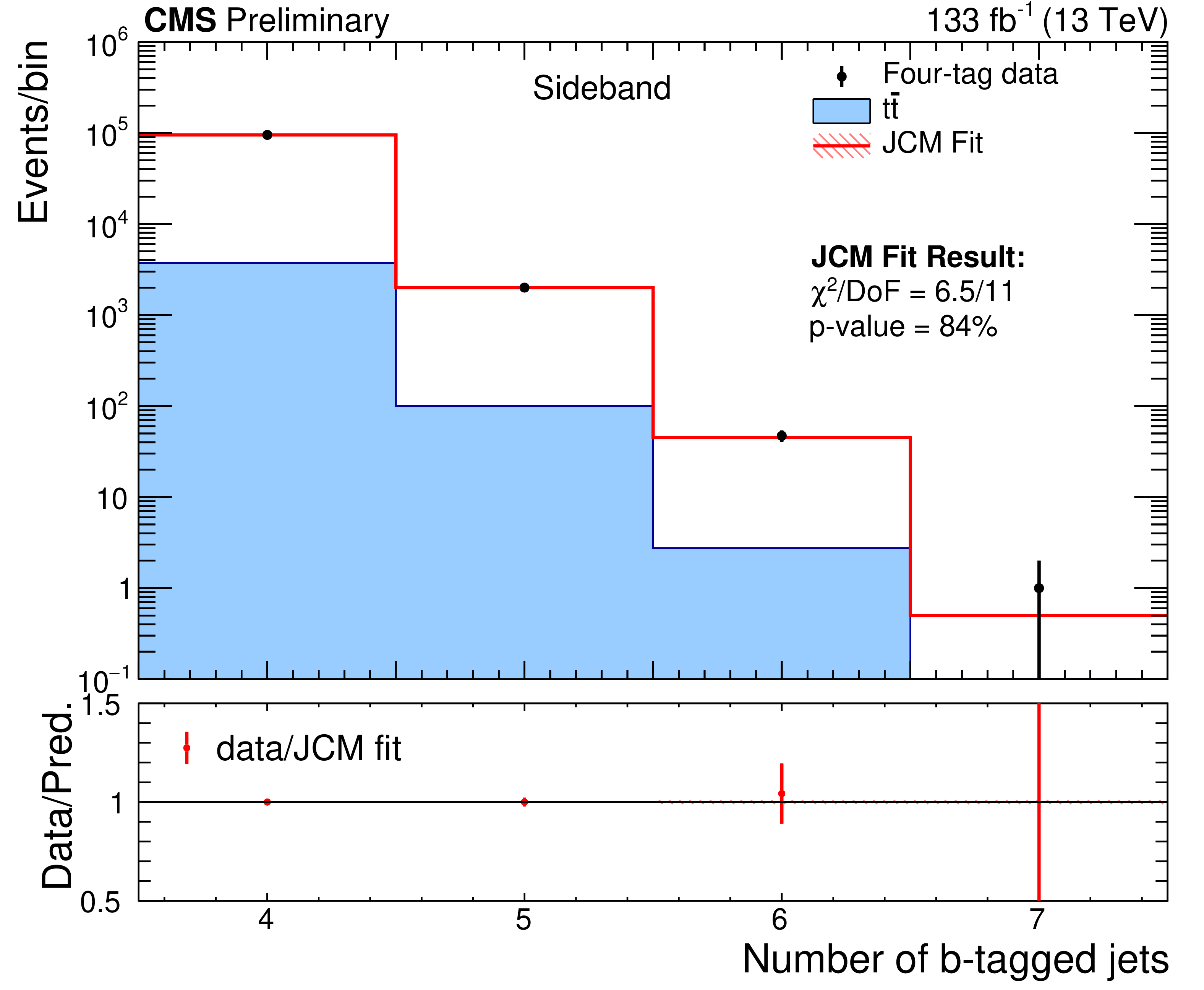
Jet (left) and b-tagged jet (right) multiplicity distributions in the sideband region. The black data points show the observed four-tag data, the blue distribution the $ \mathrm{t} \overline{\mathrm{t}} $ simulation, and the yellow the three-tag multijet prior to the JCM corrections. The red distribution shows the result of the fitted JCM model. |
png pdf |
Figure 4-a:
Jet (left) and b-tagged jet (right) multiplicity distributions in the sideband region. The black data points show the observed four-tag data, the blue distribution the $ \mathrm{t} \overline{\mathrm{t}} $ simulation, and the yellow the three-tag multijet prior to the JCM corrections. The red distribution shows the result of the fitted JCM model. |
png pdf |
Figure 4-b:
Jet (left) and b-tagged jet (right) multiplicity distributions in the sideband region. The black data points show the observed four-tag data, the blue distribution the $ \mathrm{t} \overline{\mathrm{t}} $ simulation, and the yellow the three-tag multijet prior to the JCM corrections. The red distribution shows the result of the fitted JCM model. |

png pdf |
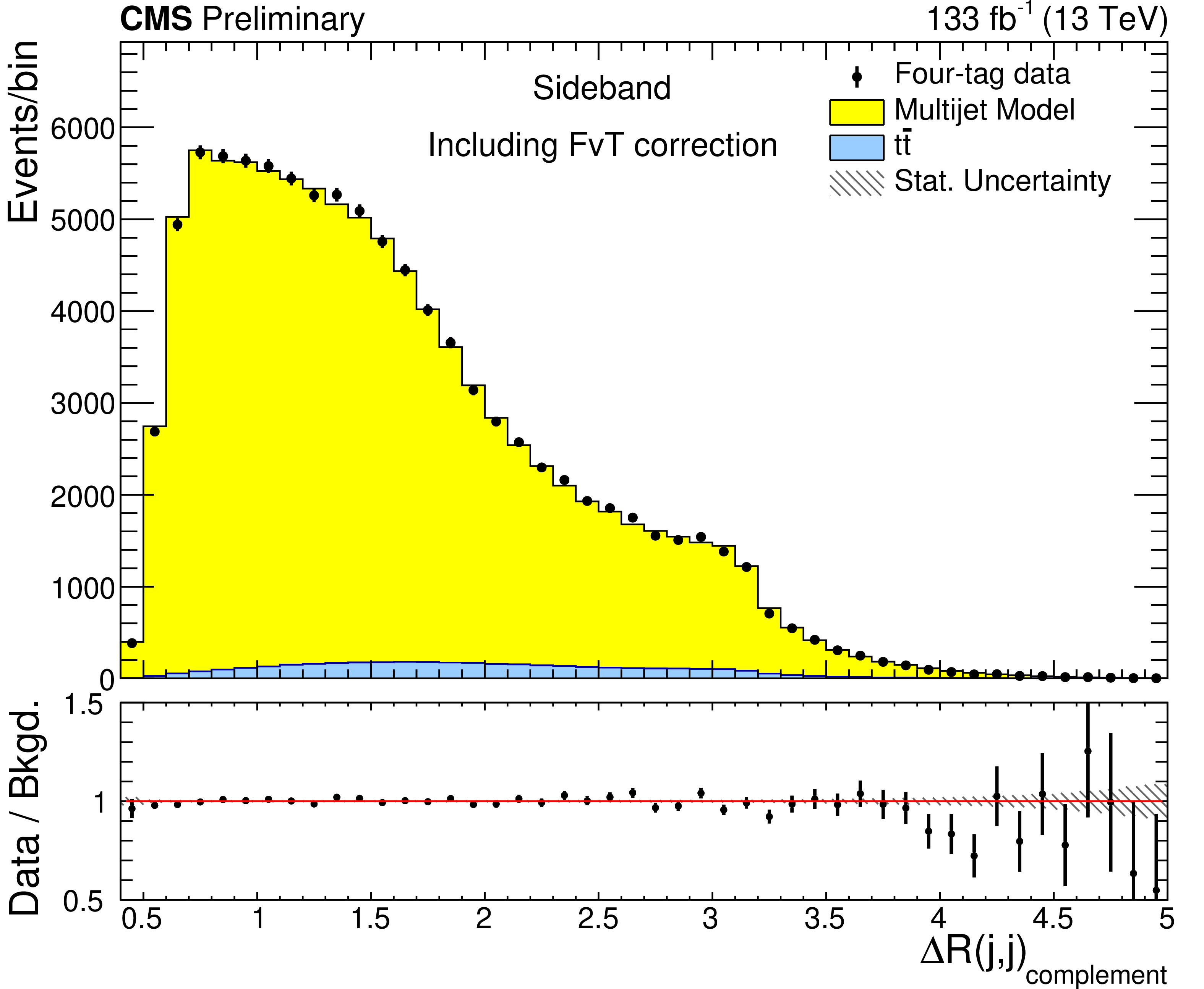
Figure 5:
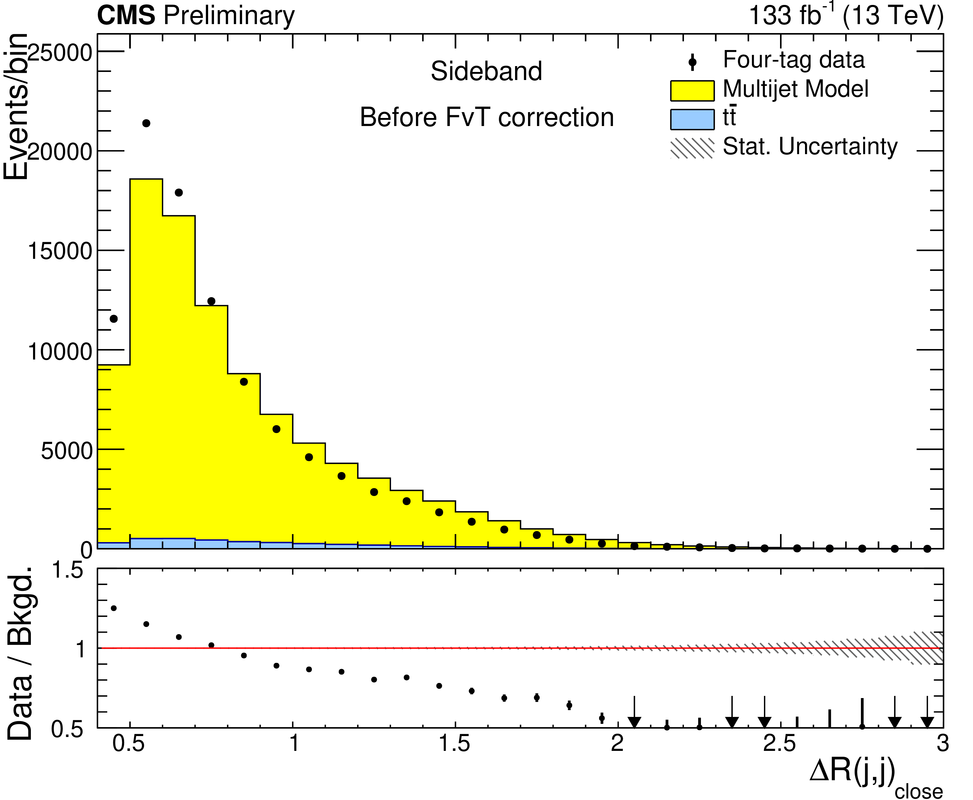
Distributions illustrating one of the key differences between the three- and four-tag samples shown with the JCM correction but before kinematic reweighting. The $ \Delta\text{R}(j,j) $ distribution of the two boson-candidate jets with the smallest angular separation is shown on the left. The $ \Delta\text{R}(j,j) $ distribution of the other two bosons-candidate jets is shown on the right. |
png pdf |
Figure 5-a:
Distributions illustrating one of the key differences between the three- and four-tag samples shown with the JCM correction but before kinematic reweighting. The $ \Delta\text{R}(j,j) $ distribution of the two boson-candidate jets with the smallest angular separation is shown on the left. The $ \Delta\text{R}(j,j) $ distribution of the other two bosons-candidate jets is shown on the right. |

png pdf |
Figure 5-b:
Distributions illustrating one of the key differences between the three- and four-tag samples shown with the JCM correction but before kinematic reweighting. The $ \Delta\text{R}(j,j) $ distribution of the two boson-candidate jets with the smallest angular separation is shown on the left. The $ \Delta\text{R}(j,j) $ distribution of the other two bosons-candidate jets is shown on the right. |

png pdf |
Figure 6:
Signal probabilities for ZZ (left) and ZH (right) events in the sideband with the JCM correction but before kinematic reweighting. |

png pdf |
Figure 6-a:
Signal probabilities for ZZ (left) and ZH (right) events in the sideband with the JCM correction but before kinematic reweighting. |

png pdf |
Figure 6-b:
Signal probabilities for ZZ (left) and ZH (right) events in the sideband with the JCM correction but before kinematic reweighting. |

png pdf |
Figure 7:
The $ \Delta\text{R}(j,j) $ distributions shown in Fig. 5 after including the FvT corrections. |

png pdf |
Figure 7-a:
The $ \Delta\text{R}(j,j) $ distributions shown in Fig. 5 after including the FvT corrections. |
png pdf |
Figure 7-b:
The $ \Delta\text{R}(j,j) $ distributions shown in Fig. 5 after including the FvT corrections. |
png pdf |
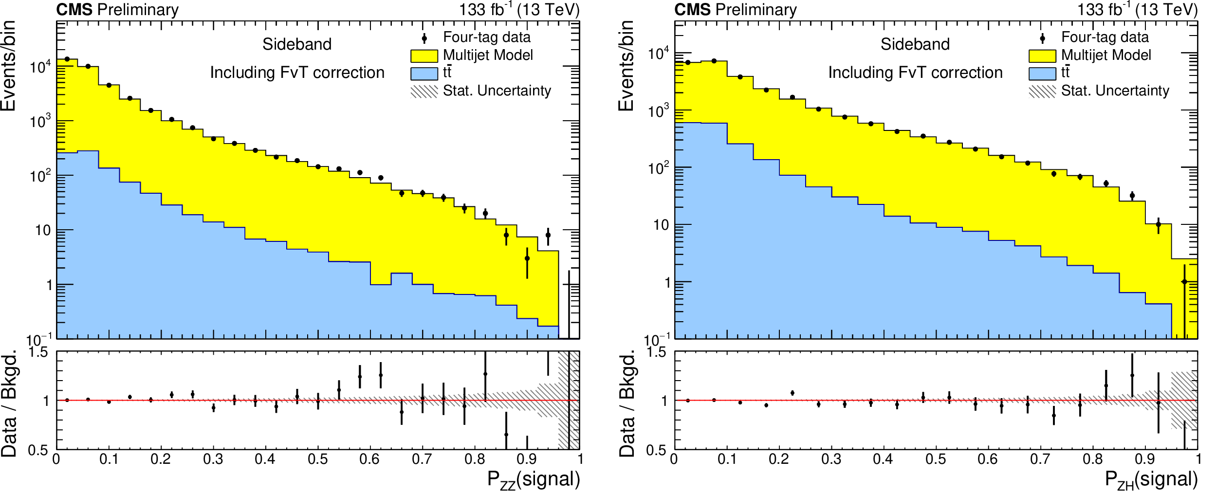
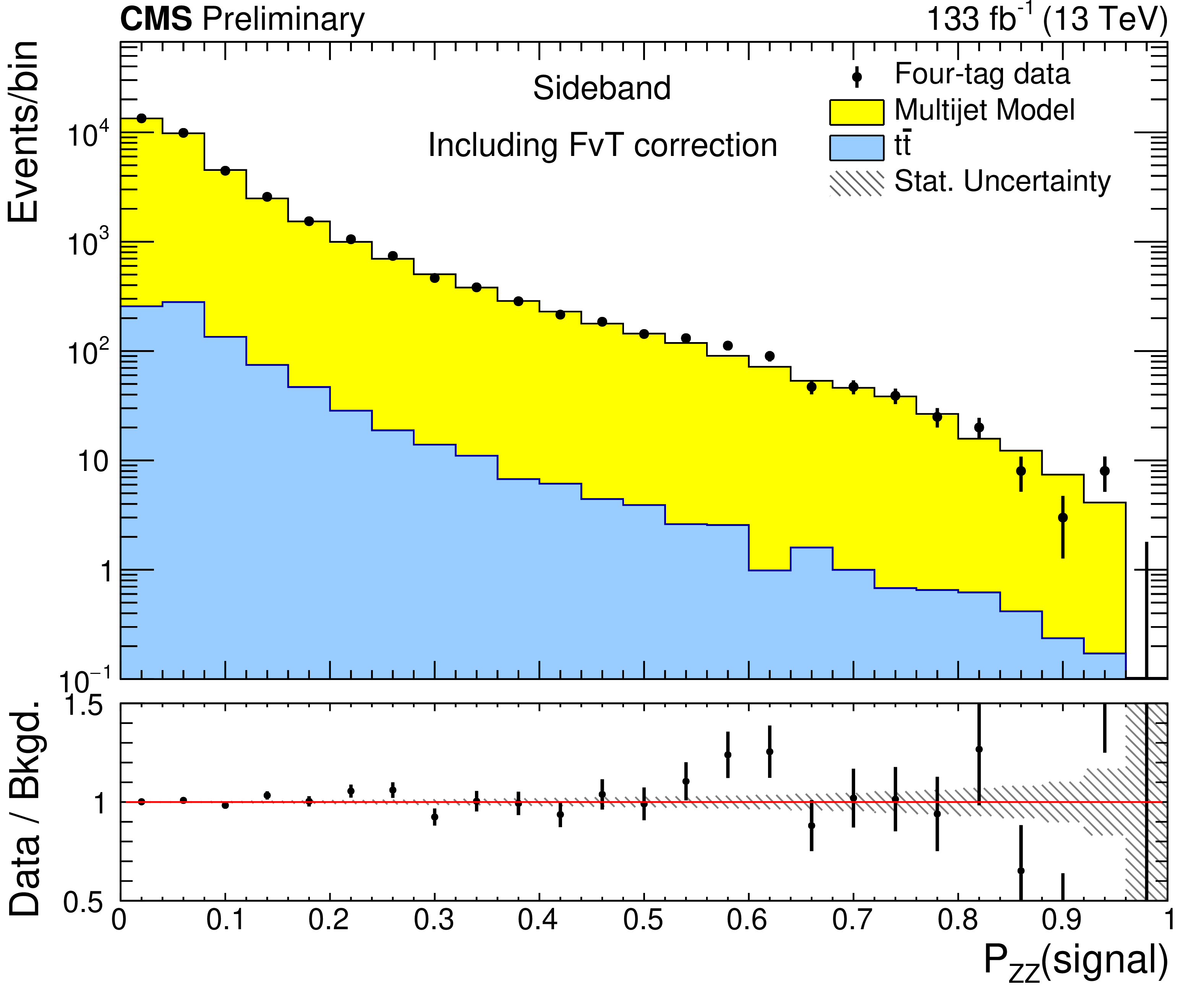
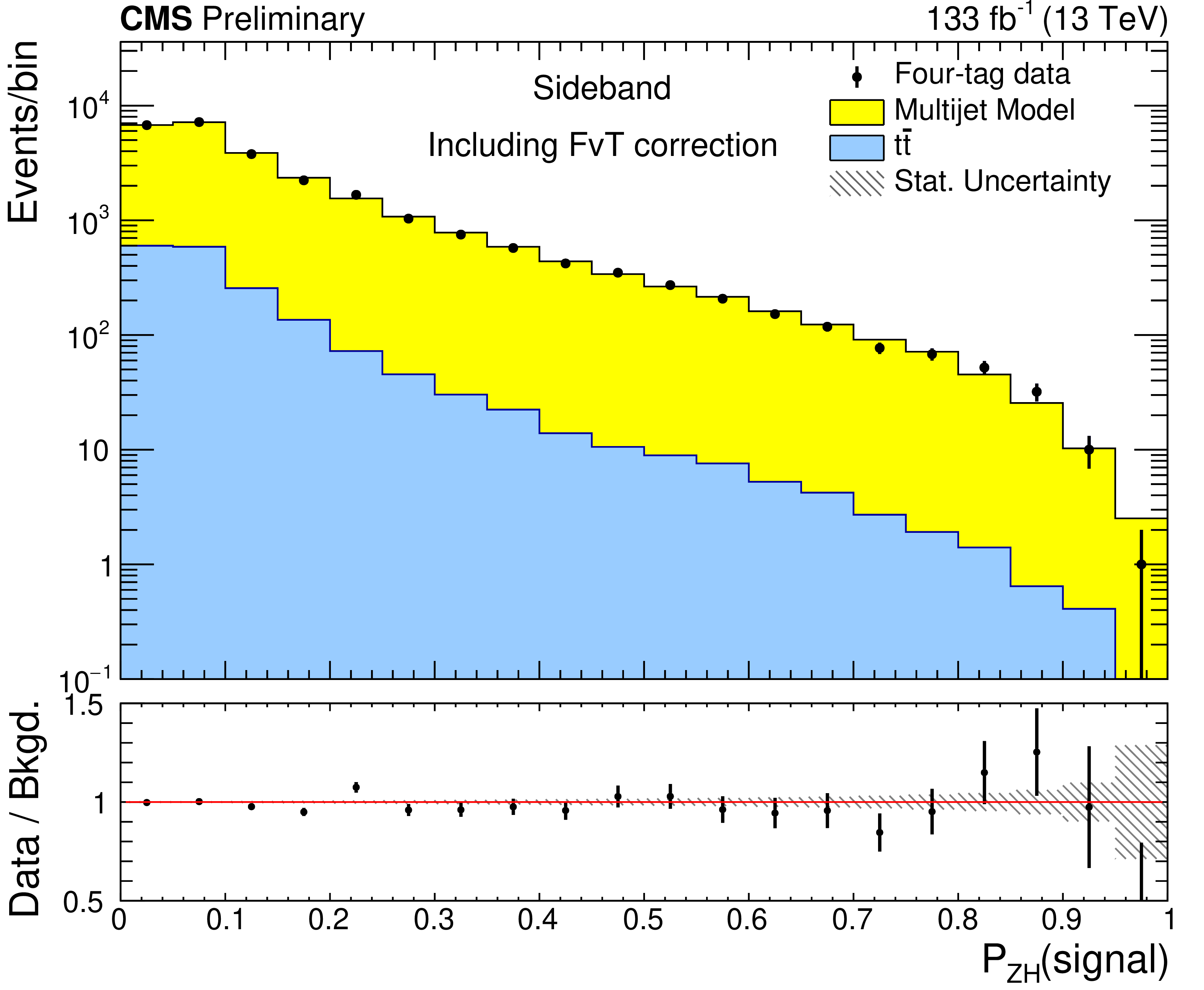
Figure 8:
Signal probabilities for ZZ (left) and ZH (right) events in the sideband after including the FvT corrections. |
png pdf |
Figure 8-a:
Signal probabilities for ZZ (left) and ZH (right) events in the sideband after including the FvT corrections. |
png pdf |
Figure 8-b:
Signal probabilities for ZZ (left) and ZH (right) events in the sideband after including the FvT corrections. |
png pdf |
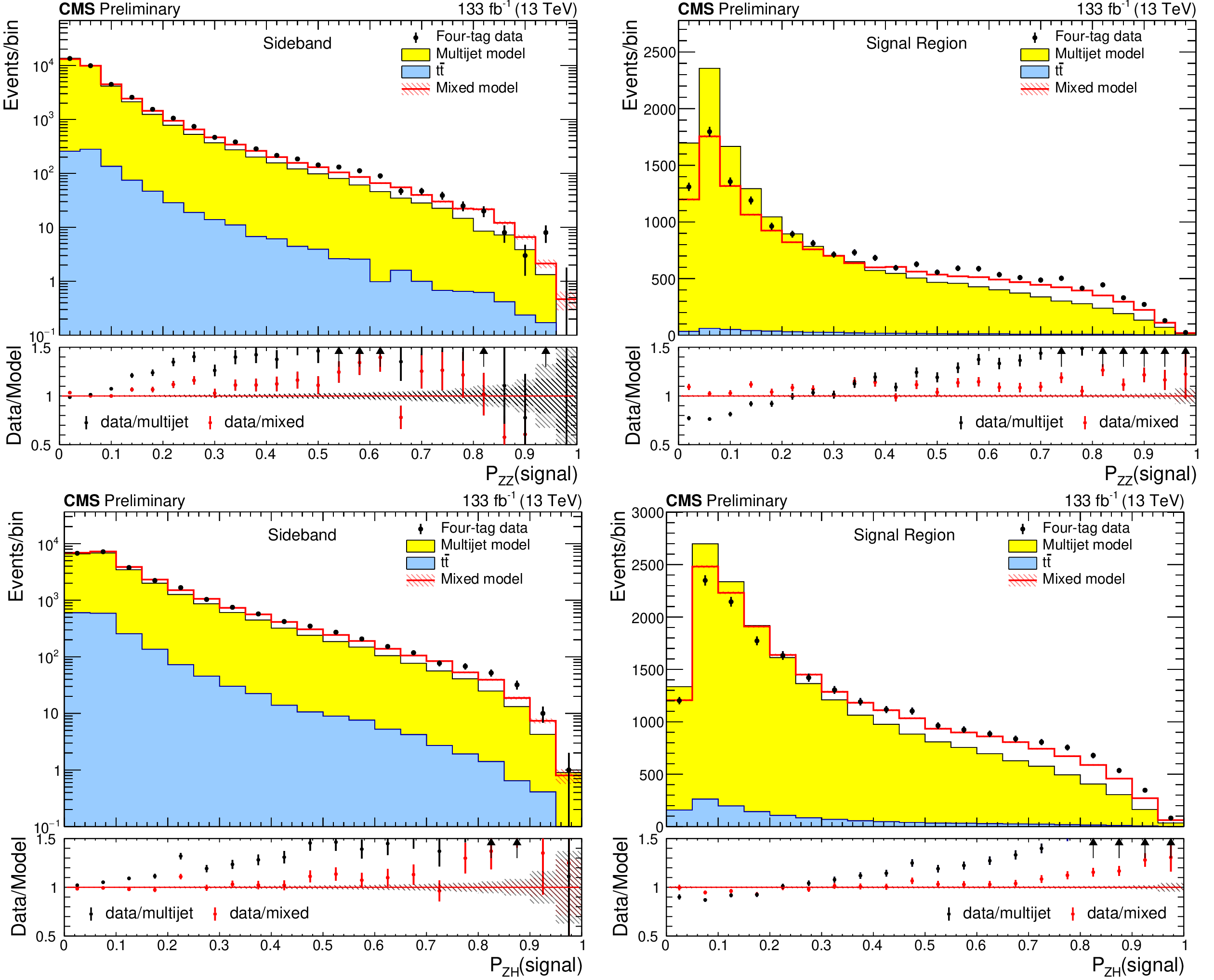
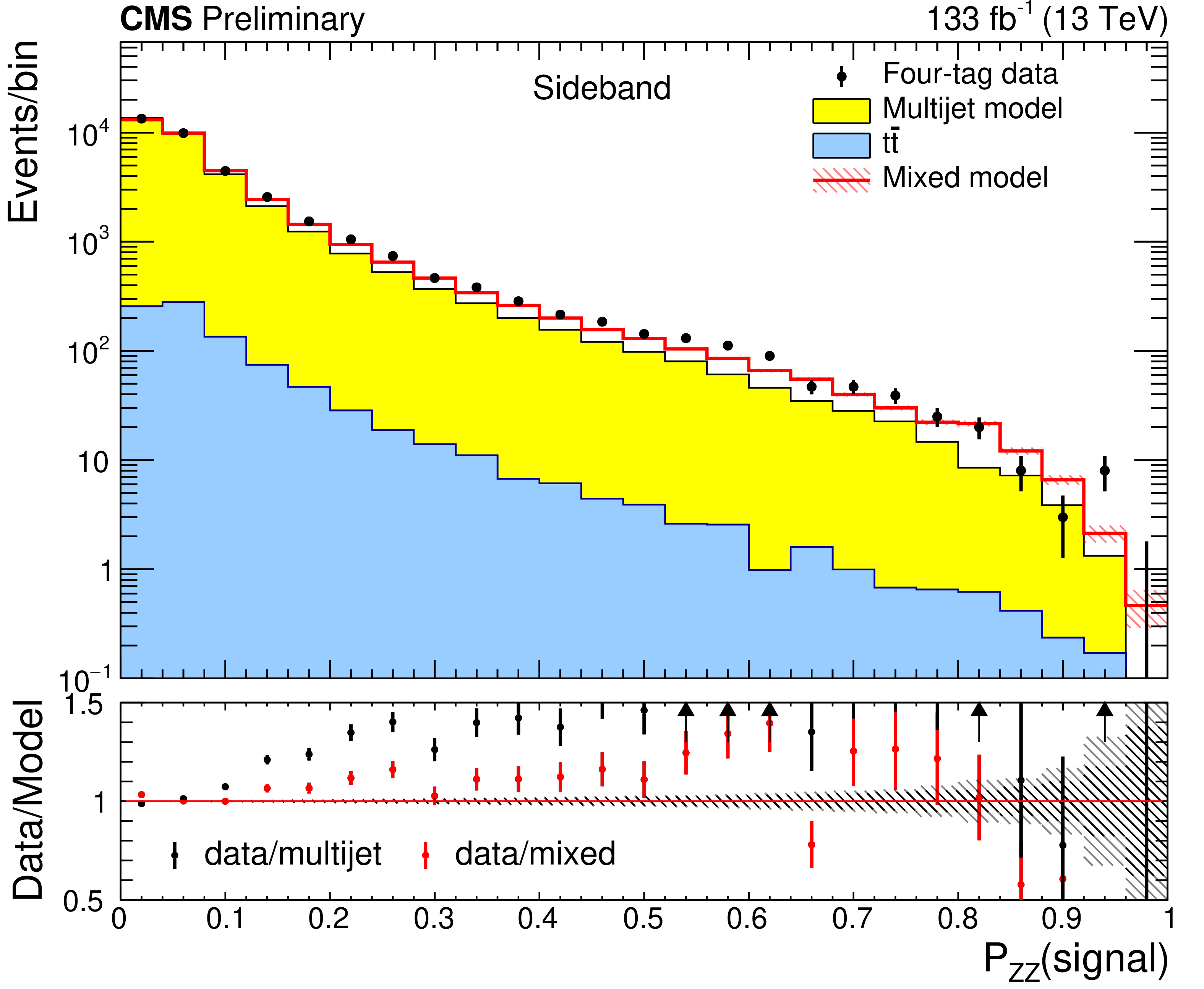
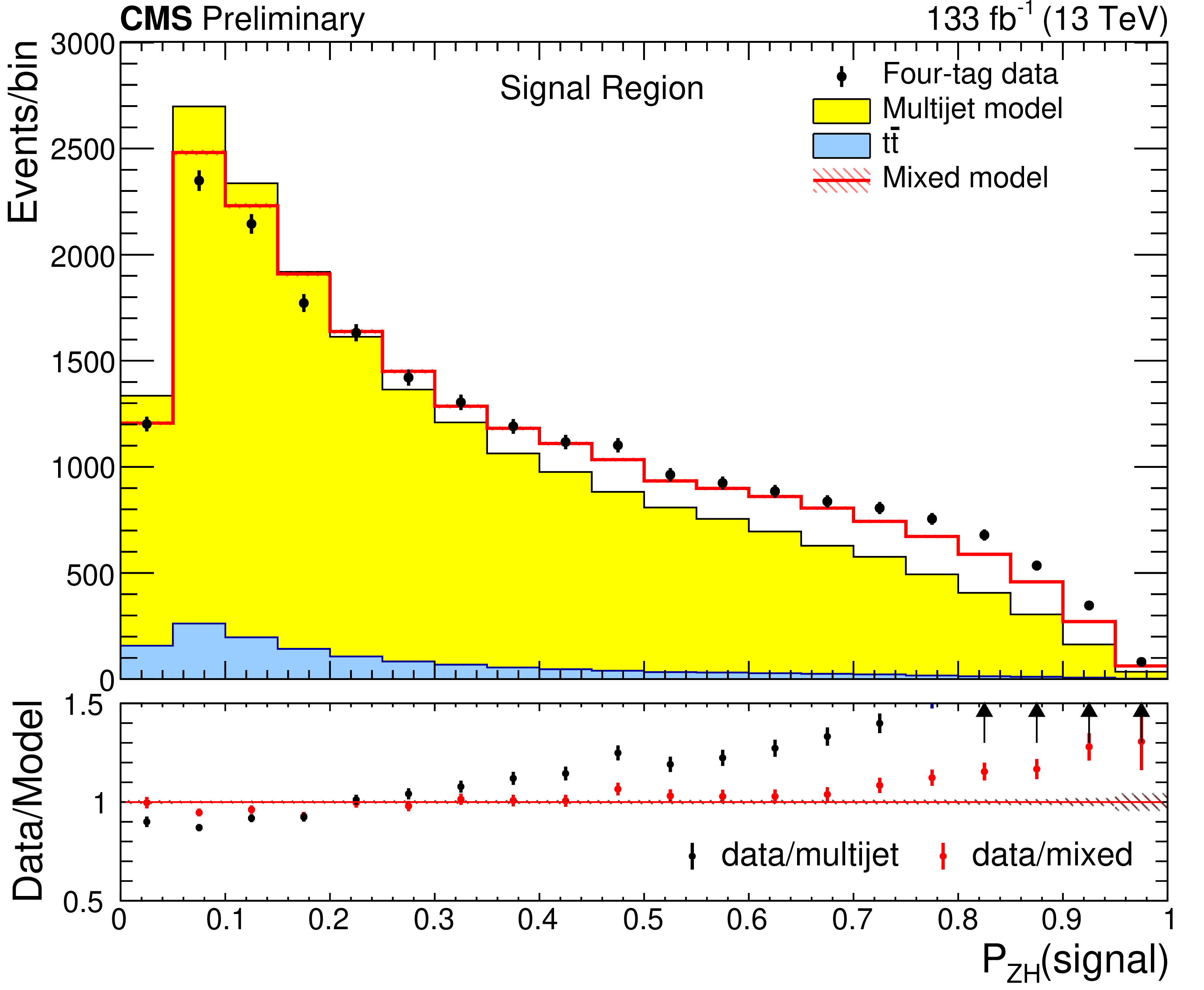
Figure 9:
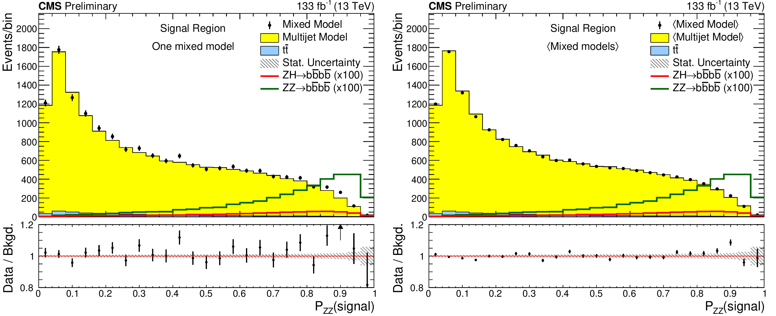
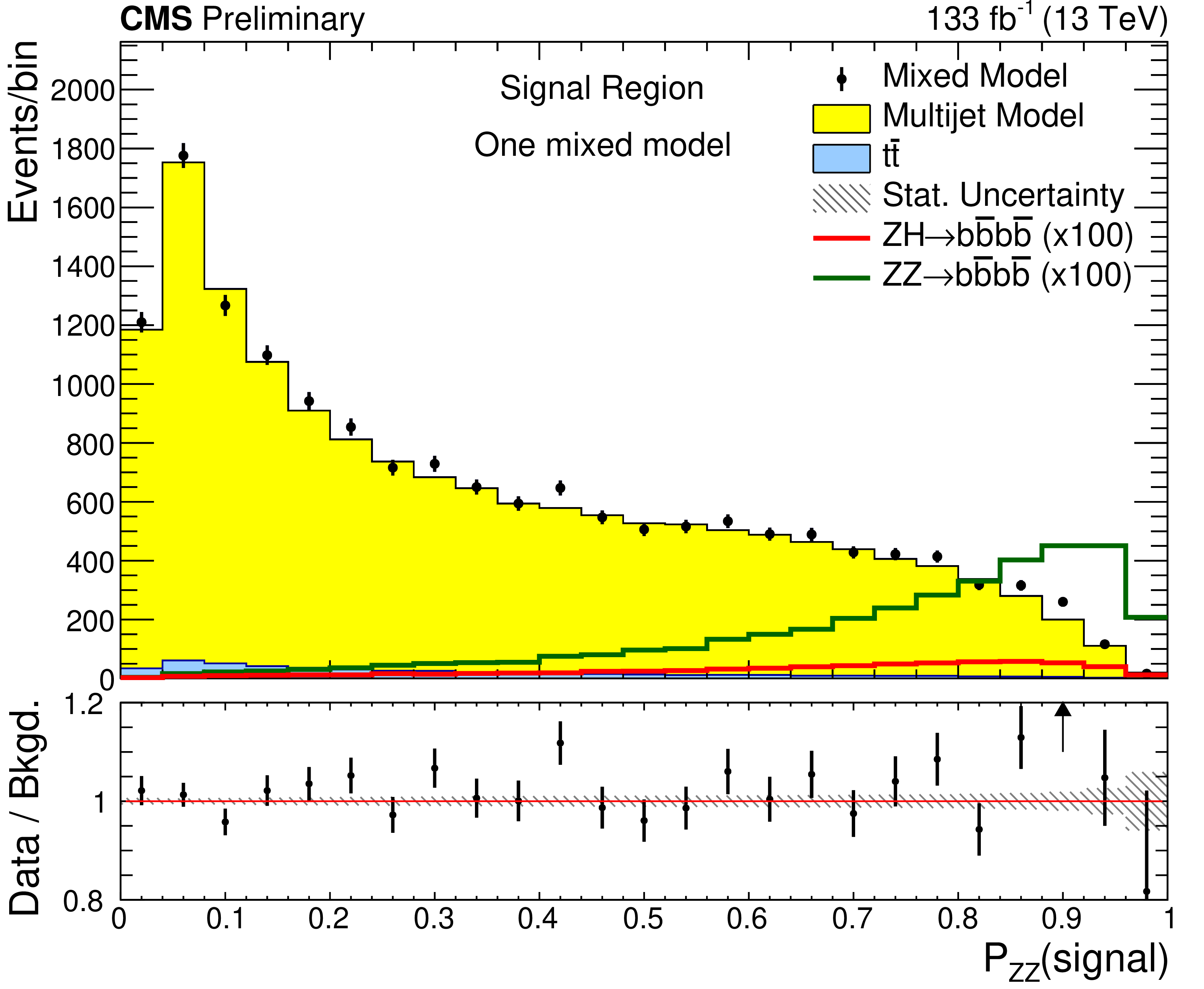
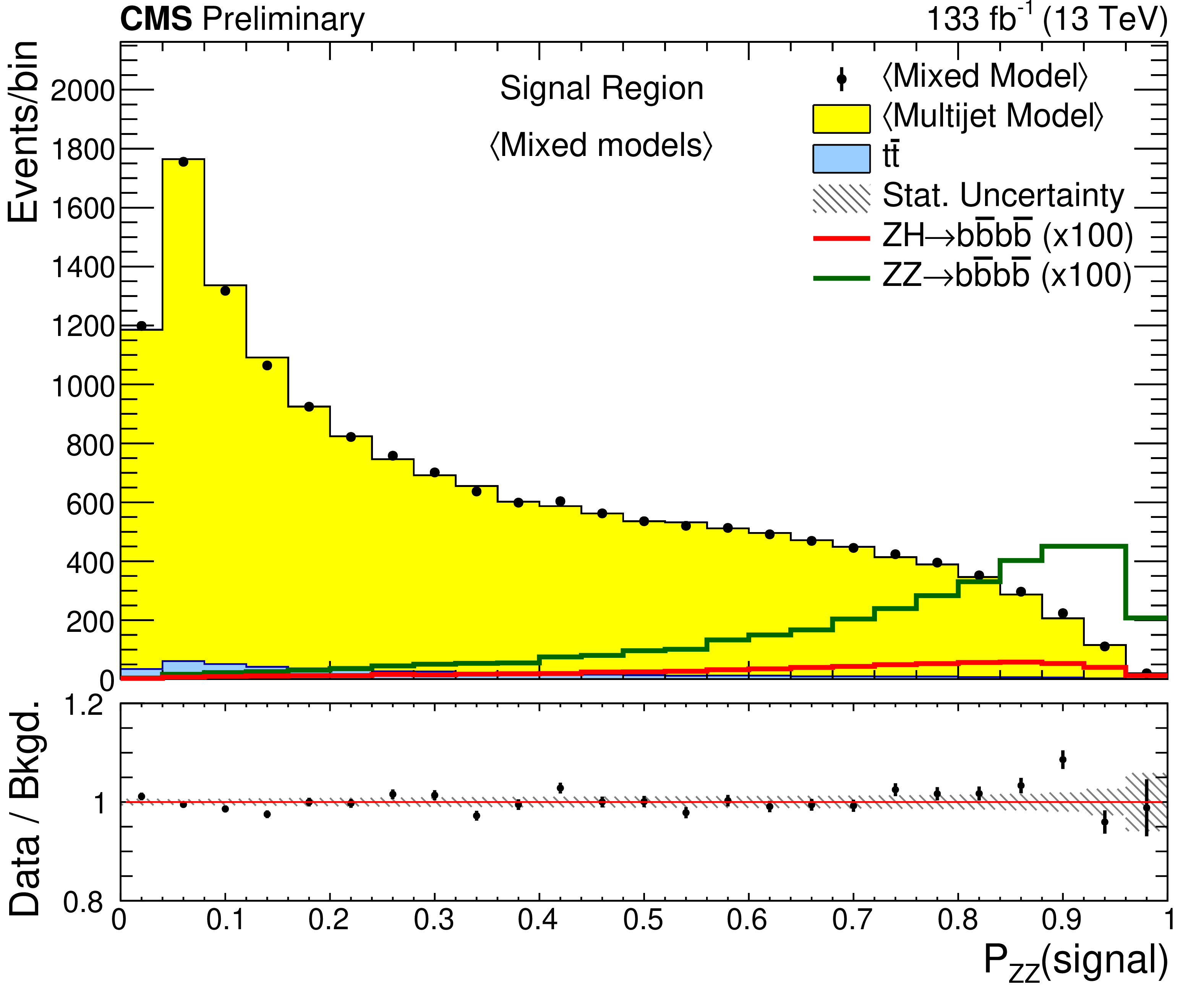
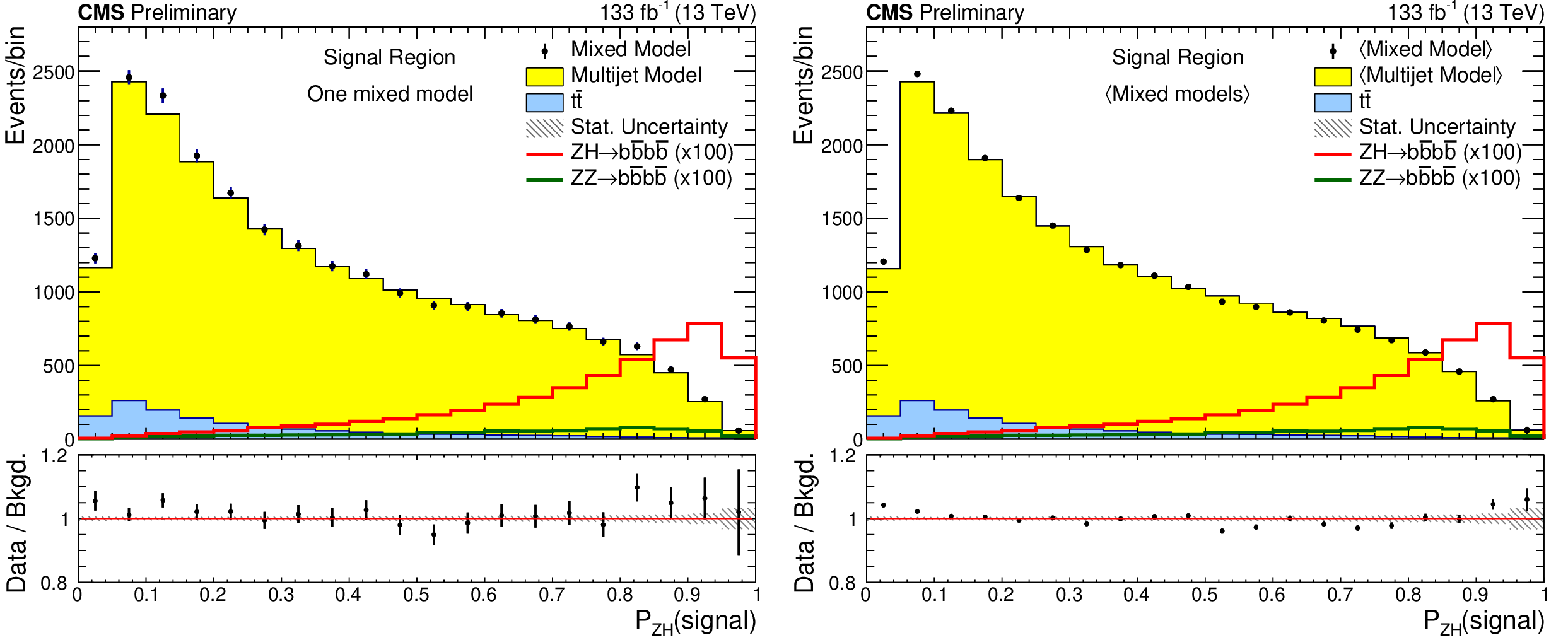
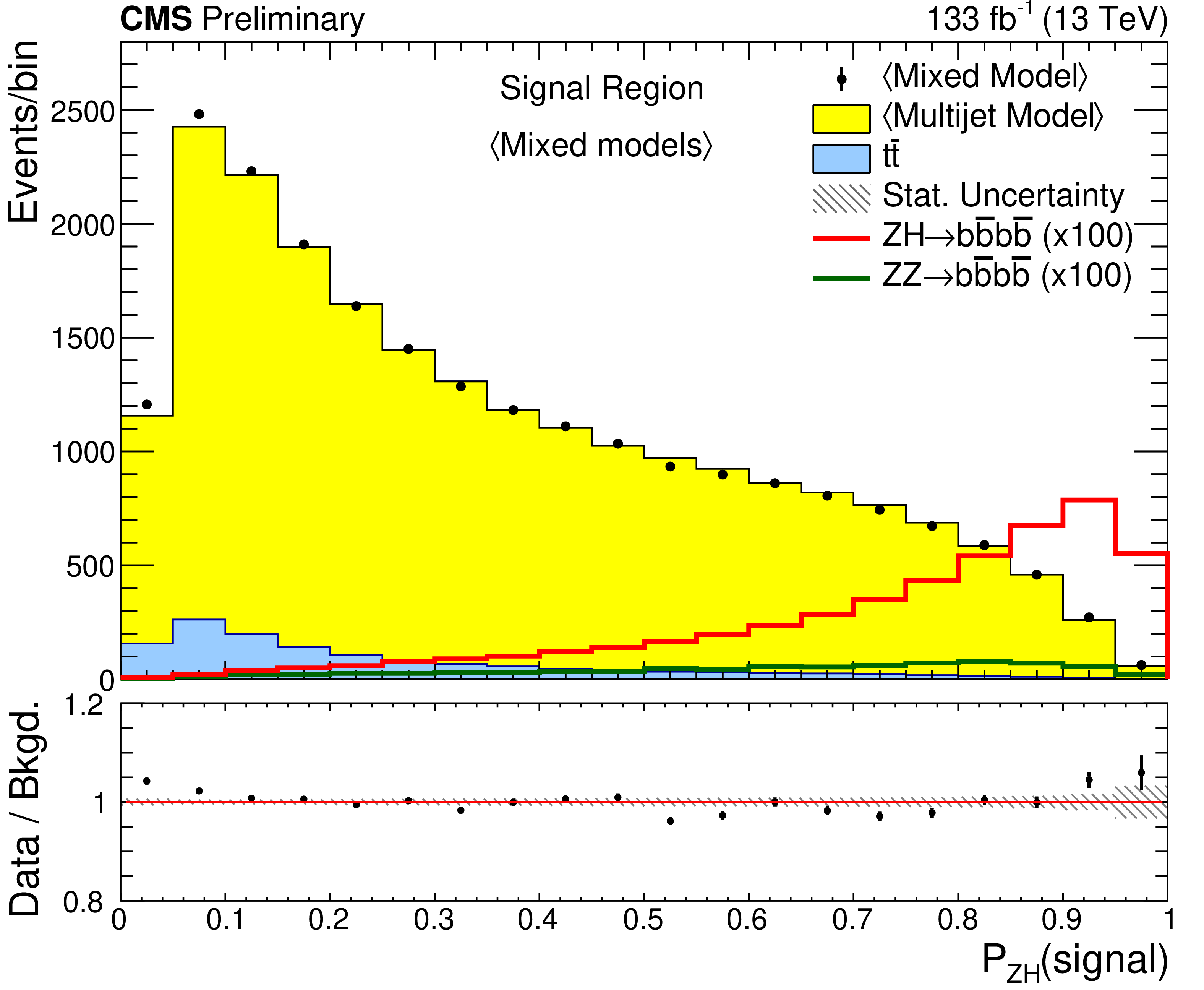
Signal probabilities for ZZ (upper row) and ZH (lower row) events in the sideband (left) and signal region (right). The yellow distributions show the multijet model before applying the FvT corrections. The average of the mixed models (red) provides a high-statistics proxy of the 4b background (black) that allows the extrapolation of the background model to be tested with precision. |
png pdf |
Figure 9-a:
Signal probabilities for ZZ (upper row) and ZH (lower row) events in the sideband (left) and signal region (right). The yellow distributions show the multijet model before applying the FvT corrections. The average of the mixed models (red) provides a high-statistics proxy of the 4b background (black) that allows the extrapolation of the background model to be tested with precision. |

png pdf |
Figure 9-b:
Signal probabilities for ZZ (upper row) and ZH (lower row) events in the sideband (left) and signal region (right). The yellow distributions show the multijet model before applying the FvT corrections. The average of the mixed models (red) provides a high-statistics proxy of the 4b background (black) that allows the extrapolation of the background model to be tested with precision. |

png pdf |
Figure 9-c:
Signal probabilities for ZZ (upper row) and ZH (lower row) events in the sideband (left) and signal region (right). The yellow distributions show the multijet model before applying the FvT corrections. The average of the mixed models (red) provides a high-statistics proxy of the 4b background (black) that allows the extrapolation of the background model to be tested with precision. |
png pdf |
Figure 9-d:
Signal probabilities for ZZ (upper row) and ZH (lower row) events in the sideband (left) and signal region (right). The yellow distributions show the multijet model before applying the FvT corrections. The average of the mixed models (red) provides a high-statistics proxy of the 4b background (black) that allows the extrapolation of the background model to be tested with precision. |
png pdf |
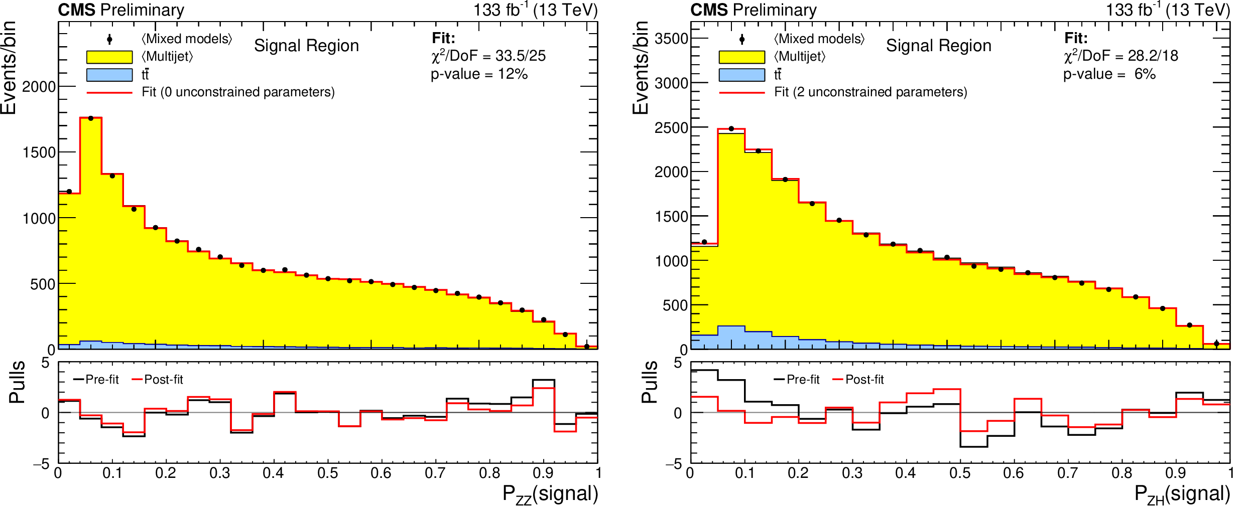
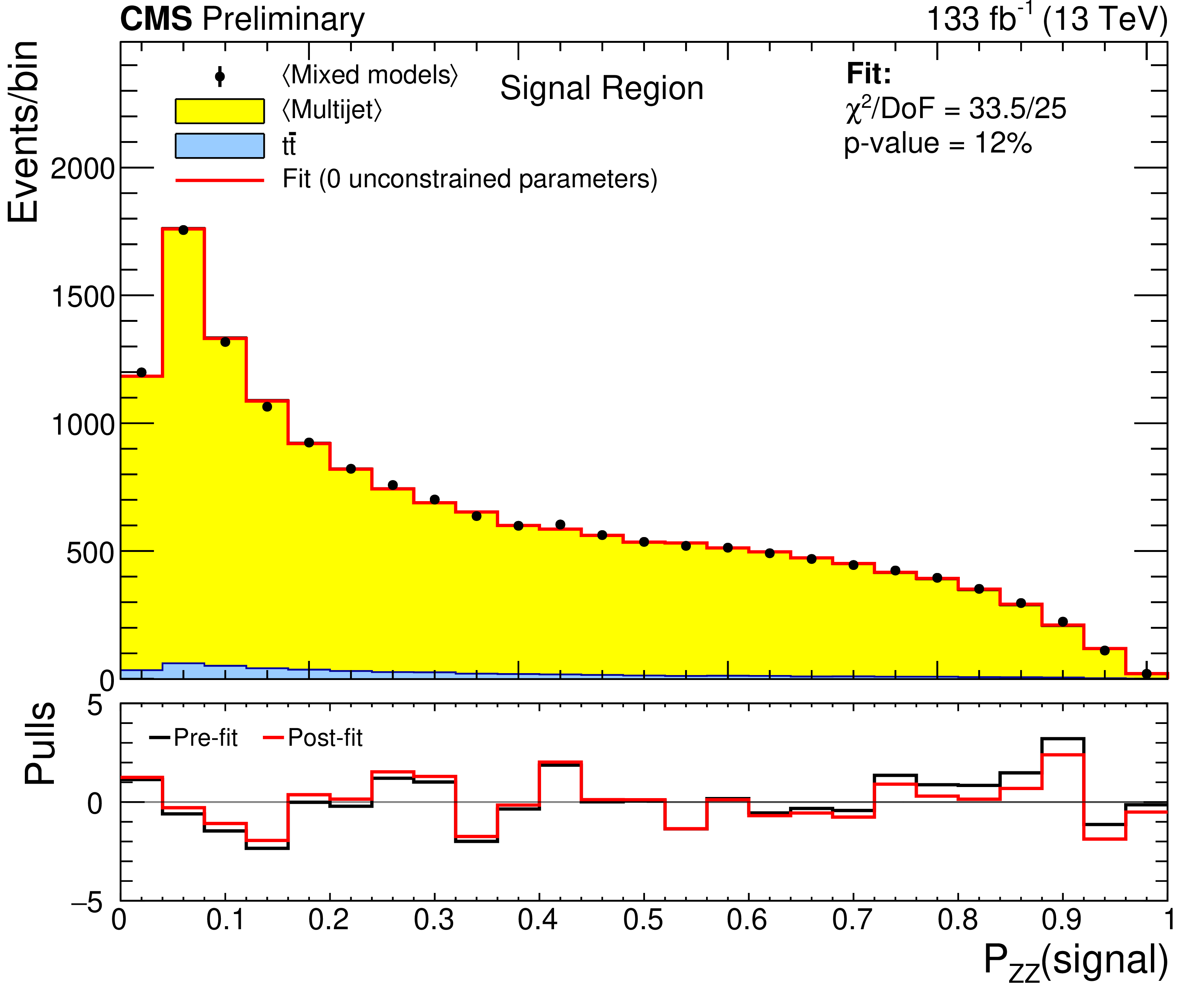
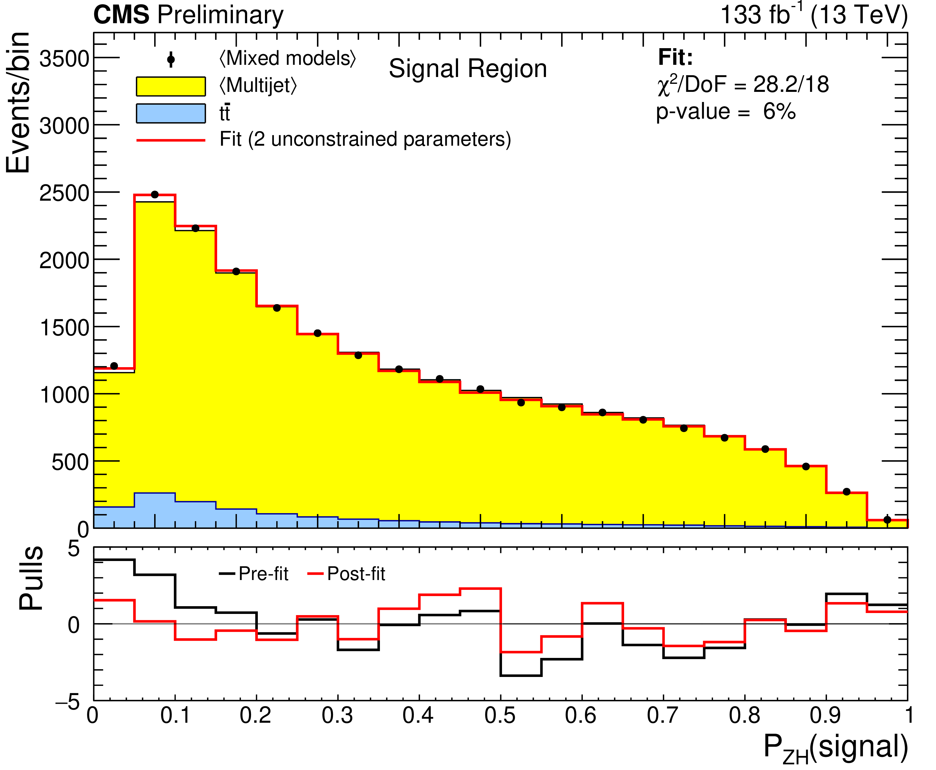
Figure 10:
The ZZ (left) and ZH (right) background models fit to the observed signal-region yield in the mixed models. The black data points show the average of the mixed models, the yellow distributions the average of the multijet models. The red distribution shows the post-fit background model. The lower panels show the pre- and post-fit pulls. The ZZ distribution is fit with all five basis coefficients constrained. The ZH distribution is fit with two of the four basis parameters unconstrained. |
png pdf |
Figure 10-a:
The ZZ (left) and ZH (right) background models fit to the observed signal-region yield in the mixed models. The black data points show the average of the mixed models, the yellow distributions the average of the multijet models. The red distribution shows the post-fit background model. The lower panels show the pre- and post-fit pulls. The ZZ distribution is fit with all five basis coefficients constrained. The ZH distribution is fit with two of the four basis parameters unconstrained. |
png pdf |
Figure 10-b:
The ZZ (left) and ZH (right) background models fit to the observed signal-region yield in the mixed models. The black data points show the average of the mixed models, the yellow distributions the average of the multijet models. The red distribution shows the post-fit background model. The lower panels show the pre- and post-fit pulls. The ZZ distribution is fit with all five basis coefficients constrained. The ZH distribution is fit with two of the four basis parameters unconstrained. |
png pdf |
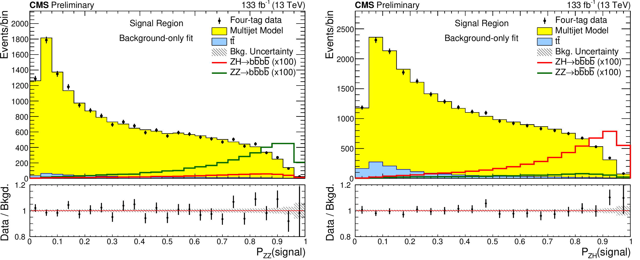
Figure 11:
Post-fit background-only SvB signal probability distributions in the ZZ region (left) and the ZH region (right). |

png pdf |
Figure 11-a:
Post-fit background-only SvB signal probability distributions in the ZZ region (left) and the ZH region (right). |

png pdf |
Figure 11-b:
Post-fit background-only SvB signal probability distributions in the ZZ region (left) and the ZH region (right). |

png pdf |
Figure 12:
Projected ZZ, ZH, and $ \mathrm{H}\mathrm{H} \rightarrow 4\mathrm{b} $ 95% CL exclusion limits up to 3000 fb$ ^{-1} $. The HH projections are shown with four different background uncertainty scaling assumptions. |
| Tables | |
png pdf |
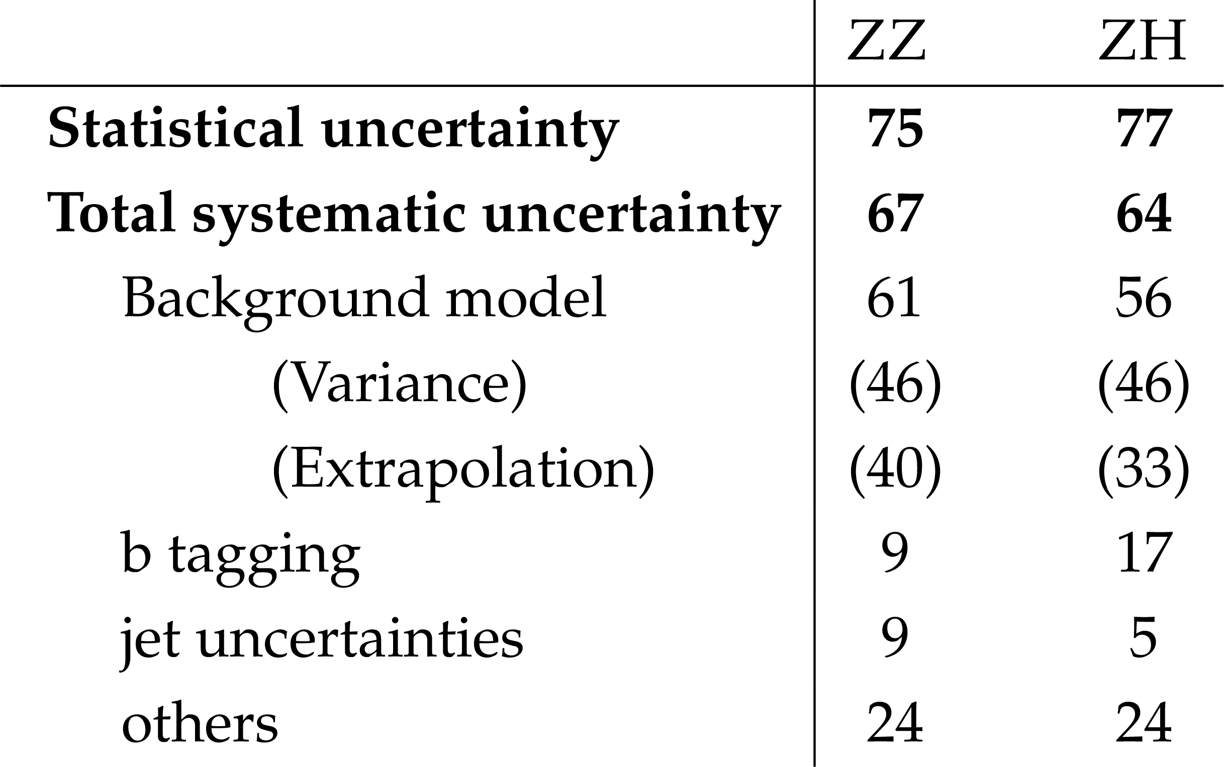
Table 1:
Summary of relative uncertainties on the measured signal strength, expressed in percentage of total uncertainty. The total uncertainties include the effect of correlations. |
png pdf |
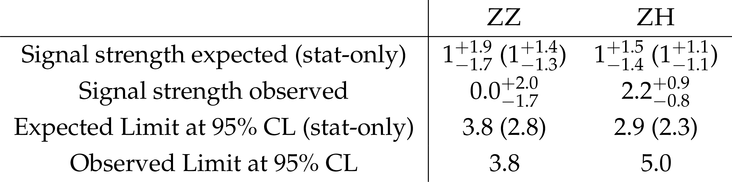
Table 2:
Expected and observed significance and 95% CL limit for ZZ, and ZH signal strengths. The limits are computed under the hypothesis of no $ \mathrm{Z}\mathrm{Z}\rightarrow 4\mathrm{b} $ or $ \mathrm{Z}\mathrm{H}\rightarrow 4\mathrm{b} $ signal. |
| Summary |
| Sensitivity to di-Higgs boson (HH) production is driven by combining the $ \mathrm{b}\overline{\mathrm{b}}\gamma\gamma $, $ \mathrm{b}\overline{\mathrm{b}}\tau\tau $, and $ \mathrm{b}\overline{\mathrm{b}}\mathrm{b}\overline{\mathrm{b}} $ (4b) decay modes. Extracting all available information from the 4b decay mode will require the development and validation of a high-dimensional data-driven background model. The $ \mathrm{Z}\mathrm{Z}\rightarrow 4\mathrm{b} $ and $ \mathrm{Z}\mathrm{H} \rightarrow4\mathrm{b} $ processes provide standard candles that can be used to validate the 4b background model in situ. A search for ZZ and ZH production in the 4b final state was presented. The search uses the full 2016--2018 data set of proton-proton collisions at a center-of-mass energy of 13 TeV recorded with the CMS detector at the LHC, corresponding to an integrated luminosity of 133 fb$ ^{-1} $. This analysis benefits from a multi-class multivariate classifier, which uses convolutions to solve the combinatoric jet-pairing problem, and has been designed with an architecture customized to the 4b final state. The classifier is used both for signal-versus-background discrimination and for the derivation and validation of the background model. A novel technique for assessing background modeling uncertainties, using a synthetic data set derived from hemisphere mixing, allows both the extrapolation uncertainty and variance of the background model to be measured with a precision better than the statistical uncertainties of the four-tag data. The observed (expected) 95% CL upper limits on the $ \mathrm{Z}\mathrm{Z} \rightarrow 4\mathrm{b} $ and $ \mathrm{Z}\mathrm{H} \rightarrow 4\mathrm{b} $ production cross sections correspond to 3.8 (3.8) and 5.0 (2.9) times the standard model prediction, respectively. The results of this analysis, in addition to the expected HH sensitivity, have been extrapolated to 3000 fb$ ^{-1} $. These projections indicate that, using the current analysis strategy, the $ \mathrm{Z}\mathrm{Z} \rightarrow 4\mathrm{b} $ and $ \mathrm{Z}\mathrm{H} \rightarrow 4\mathrm{b} $ signals are within reach of the HL-LHC and that the sensitivity to $ \mathrm{H}\mathrm{H} \rightarrow 4\mathrm{b} $ would be close to the cross section predicted in the standard model. These projections are conservative as they do not consider improvements from the upgraded HL-LHC detectors or from analysis strategies developed with the much larger data sets. |
| Additional Figures | |
png pdf |
Additional Figure 1:
Event selection acceptance times efficiency as a function of the generated four body mass $ m_{4\mathrm{b}} $-gen for the ZZ (left) and ZH (right) signal. The plots show the relative efficiency of each selection requirement. |
png pdf |
Additional Figure 1-a:
Event selection acceptance times efficiency as a function of the generated four body mass $ m_{4\mathrm{b}} $-gen for the ZZ (left) and ZH (right) signal. The plots show the relative efficiency of each selection requirement. |
png pdf |
Additional Figure 1-b:
Event selection acceptance times efficiency as a function of the generated four body mass $ m_{4\mathrm{b}} $-gen for the ZZ (left) and ZH (right) signal. The plots show the relative efficiency of each selection requirement. |
png pdf |
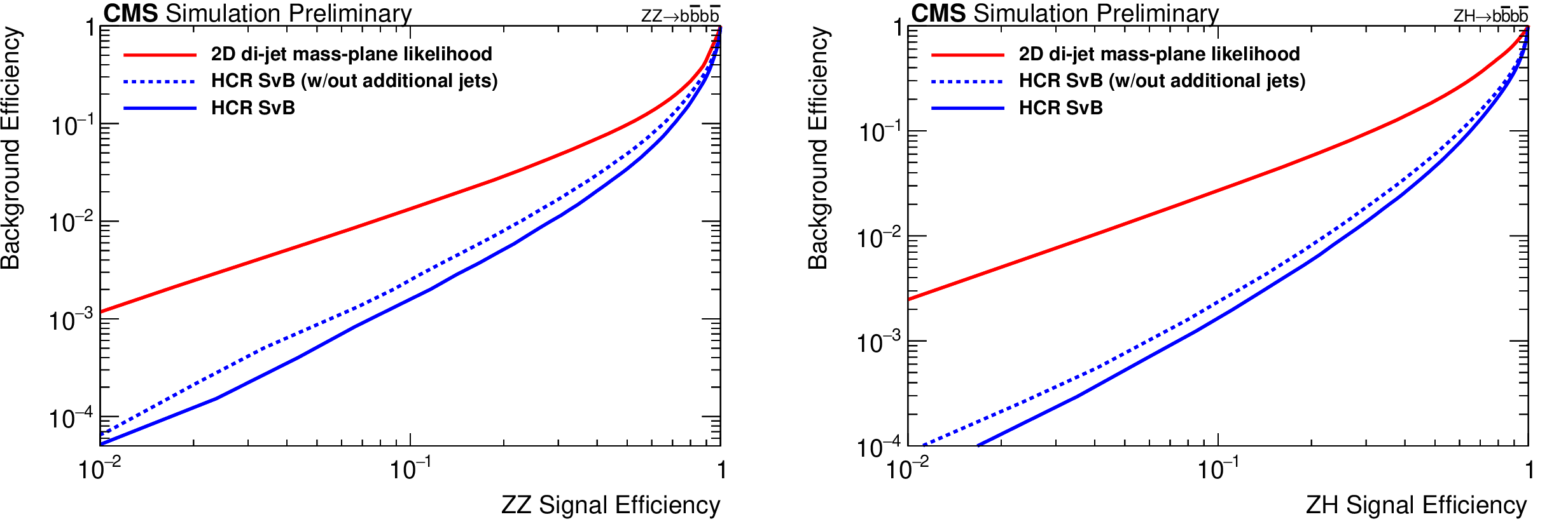
Additional Figure 2:
Comparison of the performance of the nominal HCR SvB to a simpler likelihood-based classifier using the two dijet invariant masses. A comparison is also made to a version of the HCR SvB with out multijet attention block including the kinematics from the additional non-boson-candidate jets. ZZ is shown on the left and ZH on the right. |
png pdf |
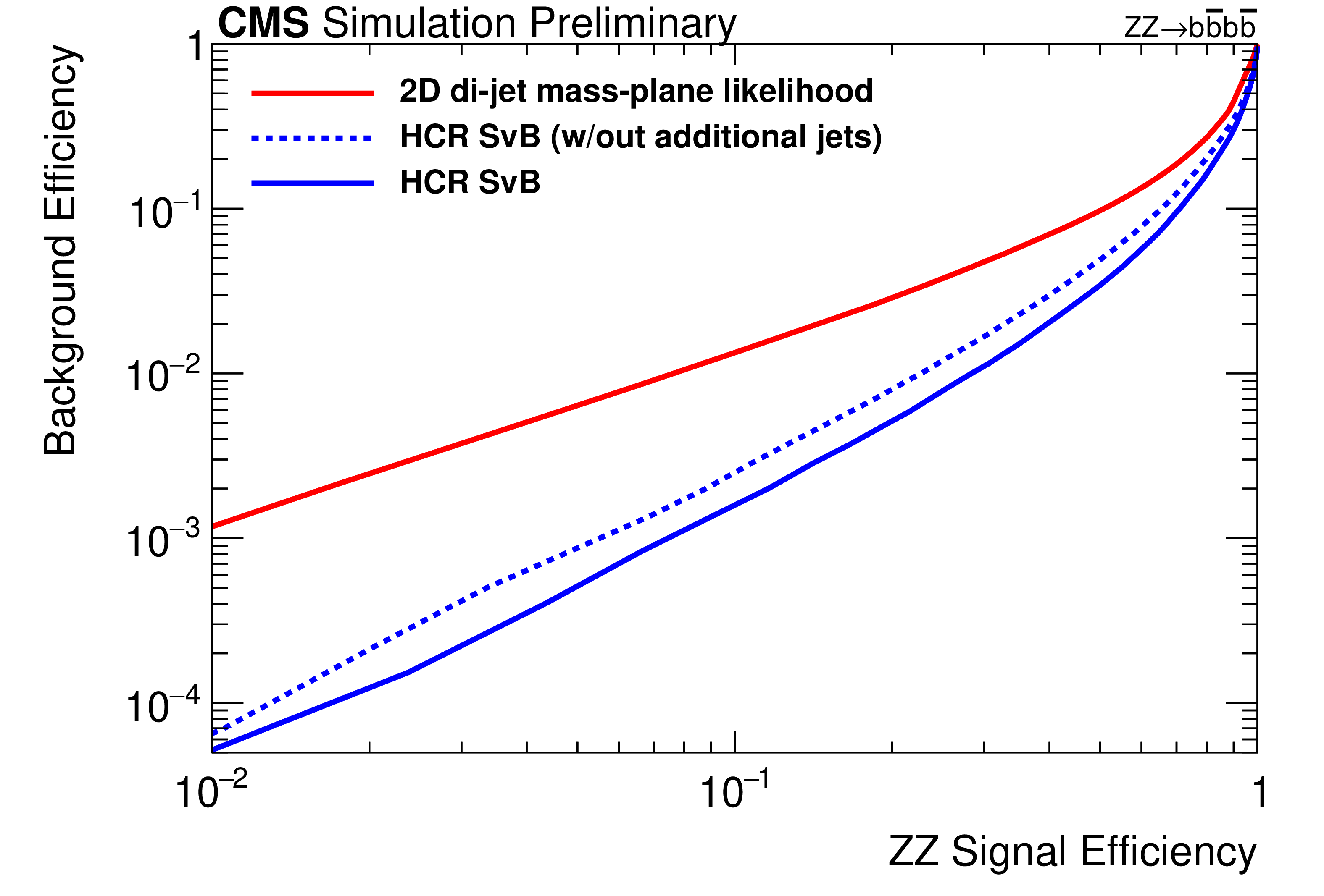
Additional Figure 2-a:
Comparison of the performance of the nominal HCR SvB to a simpler likelihood-based classifier using the two dijet invariant masses. A comparison is also made to a version of the HCR SvB with out multijet attention block including the kinematics from the additional non-boson-candidate jets. ZZ is shown on the left and ZH on the right. |
png pdf |
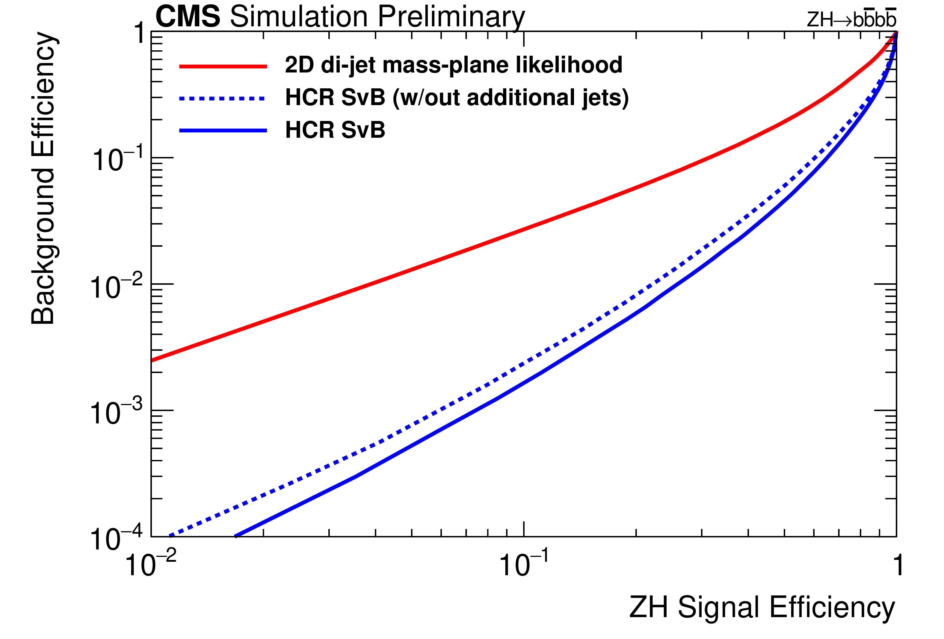
Additional Figure 2-b:
Comparison of the performance of the nominal HCR SvB to a simpler likelihood-based classifier using the two dijet invariant masses. A comparison is also made to a version of the HCR SvB with out multijet attention block including the kinematics from the additional non-boson-candidate jets. ZZ is shown on the left and ZH on the right. |

png pdf |
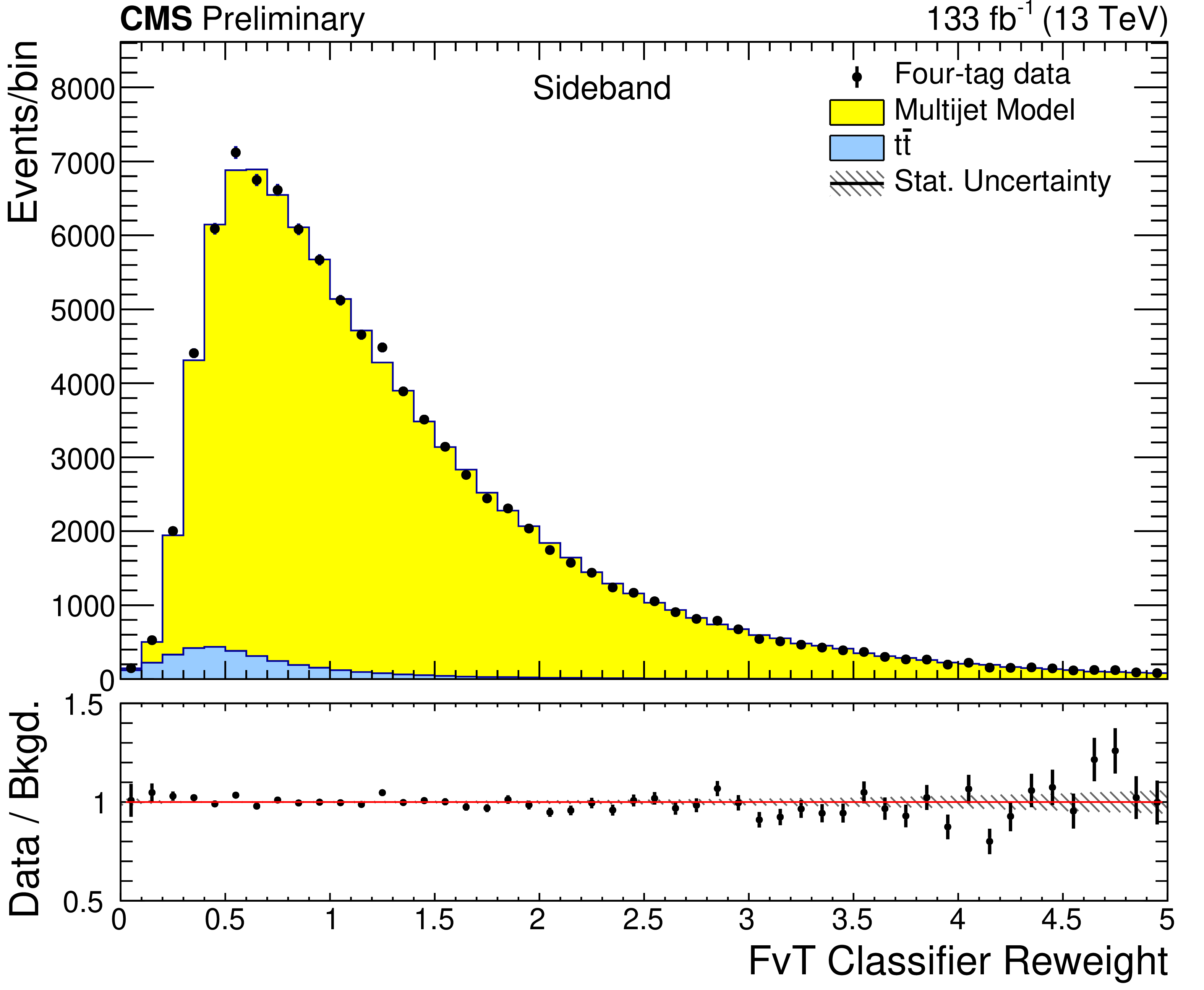
Additional Figure 3:
The FvT classifier reweight distribution before (left) and after (right) applying the FvT corrections. |

png pdf |
Additional Figure 3-a:
The FvT classifier reweight distribution before (left) and after (right) applying the FvT corrections. |
png pdf |
Additional Figure 3-b:
The FvT classifier reweight distribution before (left) and after (right) applying the FvT corrections. |
png pdf |
Additional Figure 4:
The ZZ SvB distribution in the signal region for one of the mixed data sub-samples (left) and after averaging over all fifteen of the mixed sub-samples (right). |
png pdf |
Additional Figure 4-a:
The ZZ SvB distribution in the signal region for one of the mixed data sub-samples (left) and after averaging over all fifteen of the mixed sub-samples (right). |
png pdf |
Additional Figure 4-b:
The ZZ SvB distribution in the signal region for one of the mixed data sub-samples (left) and after averaging over all fifteen of the mixed sub-samples (right). |
png pdf |
Additional Figure 5:
The ZH SvB distribution in the signal region for one of the mixed data sub-samples (left) and after averaging over all fifteen of the mixed sub-samples (right). |

png pdf |
Additional Figure 5-a:
The ZH SvB distribution in the signal region for one of the mixed data sub-samples (left) and after averaging over all fifteen of the mixed sub-samples (right). |
png pdf |
Additional Figure 5-b:
The ZH SvB distribution in the signal region for one of the mixed data sub-samples (left) and after averaging over all fifteen of the mixed sub-samples (right). |

png pdf |
Additional Figure 6:
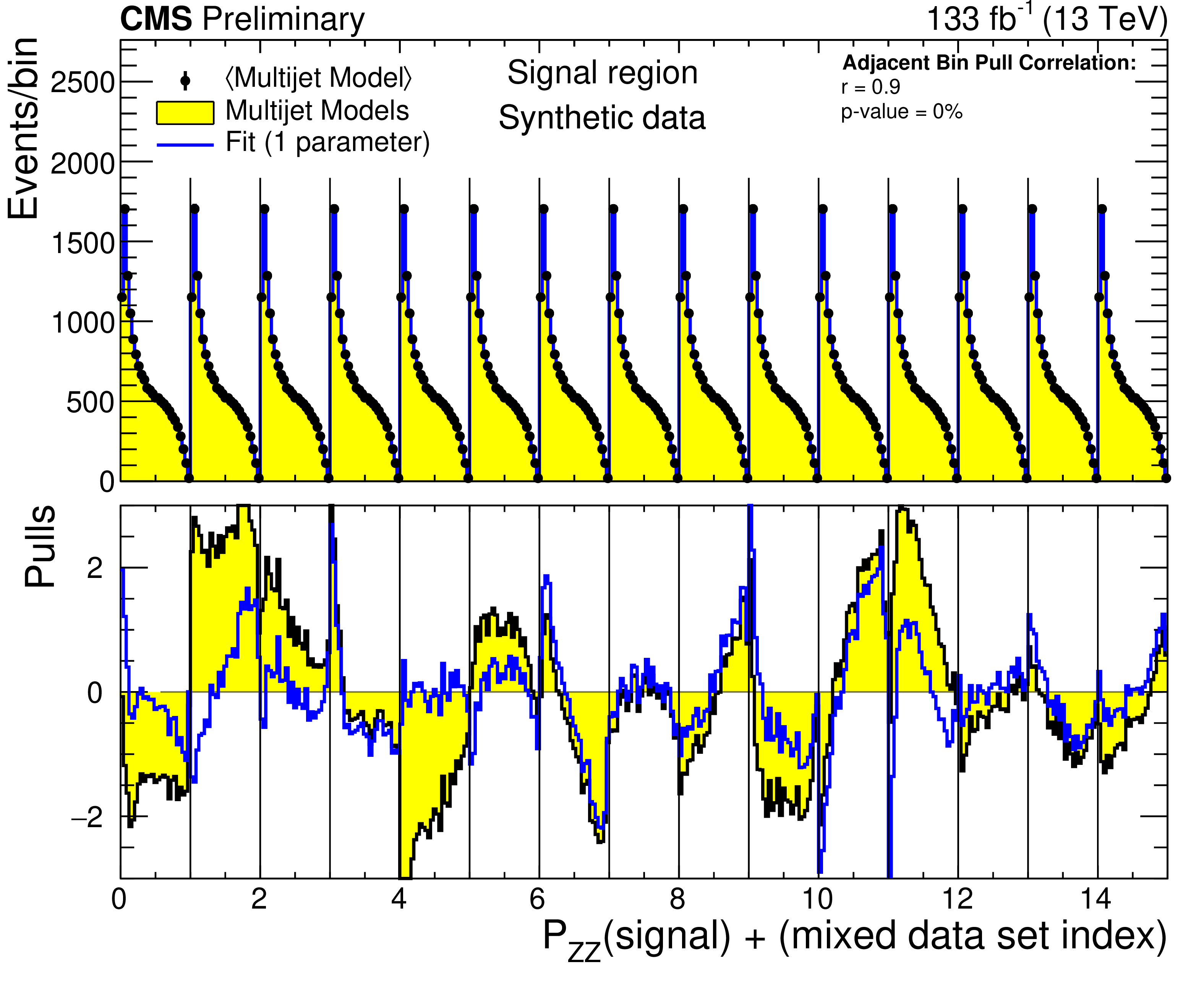
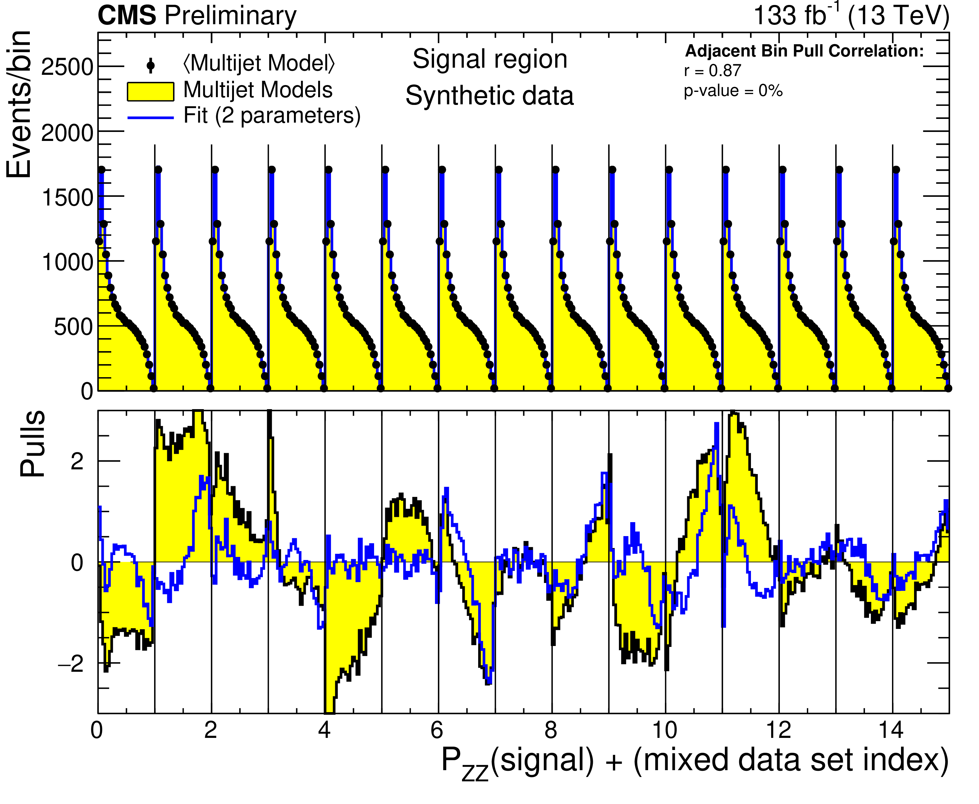
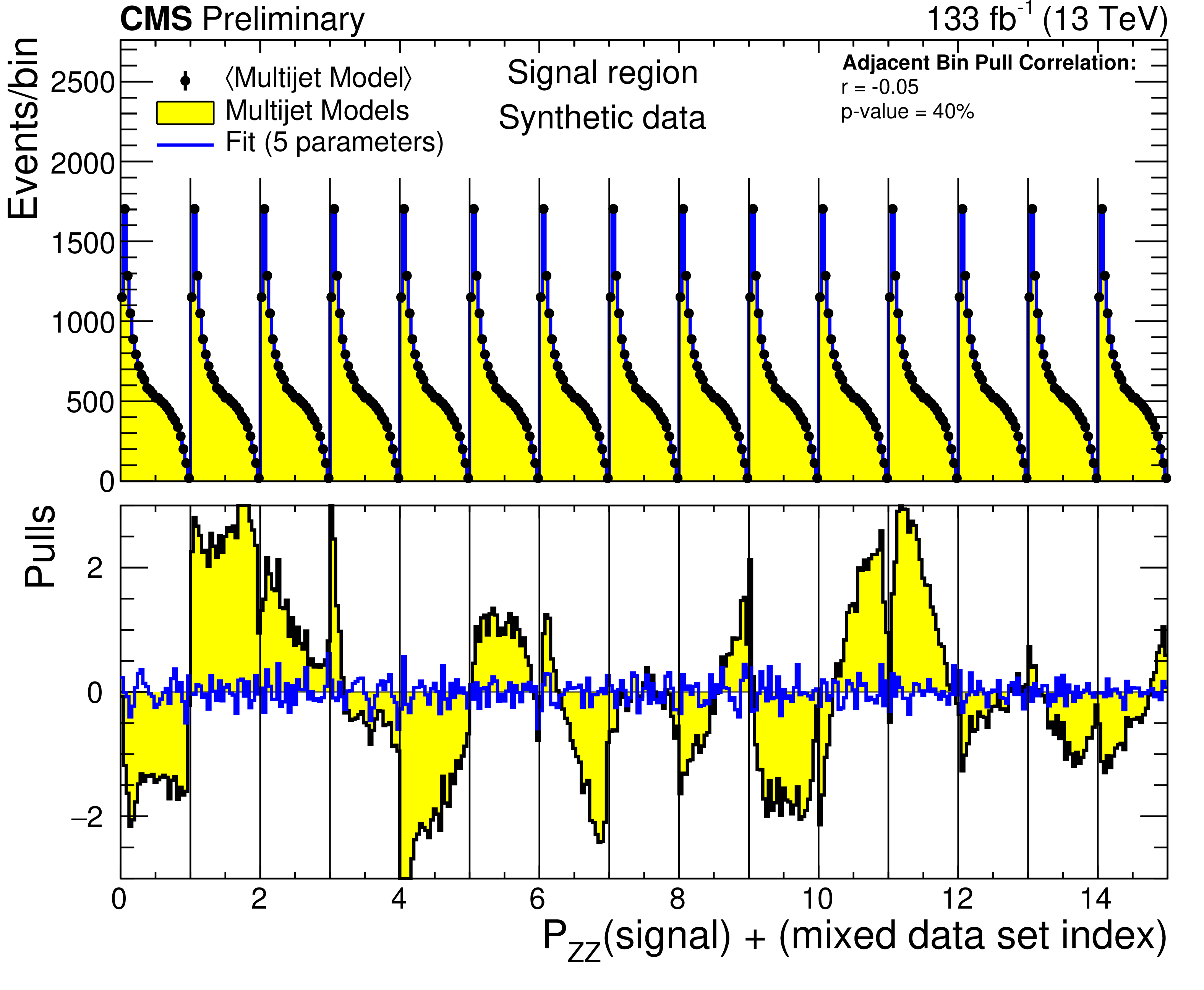
The predicted multijet ZZ SvB distributions in the mixed data signal regions fit to their average. The plots show the results of fitting with an increasing number of basis functions, from one in the upper left figure, to five in the lower row. The predictions from each mixed model are shown separately in yellow by adding the mixed data set index to offset the signal SvB distribution. The black data points show the average of the predictions. The predictions, including the fitted basis corrections, are shown in blue. The lower panels show the pulls before and after adding the basis corrections. The pull of adjacent bins are tested for statistical correlation. The correlation coefficient (r) is reported in the legend along with the p-value used to test for lack of correlation. Basis functions are added until the p-value is above 5%. |
png pdf |
Additional Figure 6-a:
The predicted multijet ZZ SvB distributions in the mixed data signal regions fit to their average. The plots show the results of fitting with an increasing number of basis functions, from one in the upper left figure, to five in the lower row. The predictions from each mixed model are shown separately in yellow by adding the mixed data set index to offset the signal SvB distribution. The black data points show the average of the predictions. The predictions, including the fitted basis corrections, are shown in blue. The lower panels show the pulls before and after adding the basis corrections. The pull of adjacent bins are tested for statistical correlation. The correlation coefficient (r) is reported in the legend along with the p-value used to test for lack of correlation. Basis functions are added until the p-value is above 5%. |
png pdf |
Additional Figure 6-b:
The predicted multijet ZZ SvB distributions in the mixed data signal regions fit to their average. The plots show the results of fitting with an increasing number of basis functions, from one in the upper left figure, to five in the lower row. The predictions from each mixed model are shown separately in yellow by adding the mixed data set index to offset the signal SvB distribution. The black data points show the average of the predictions. The predictions, including the fitted basis corrections, are shown in blue. The lower panels show the pulls before and after adding the basis corrections. The pull of adjacent bins are tested for statistical correlation. The correlation coefficient (r) is reported in the legend along with the p-value used to test for lack of correlation. Basis functions are added until the p-value is above 5%. |

png pdf |
Additional Figure 6-c:
The predicted multijet ZZ SvB distributions in the mixed data signal regions fit to their average. The plots show the results of fitting with an increasing number of basis functions, from one in the upper left figure, to five in the lower row. The predictions from each mixed model are shown separately in yellow by adding the mixed data set index to offset the signal SvB distribution. The black data points show the average of the predictions. The predictions, including the fitted basis corrections, are shown in blue. The lower panels show the pulls before and after adding the basis corrections. The pull of adjacent bins are tested for statistical correlation. The correlation coefficient (r) is reported in the legend along with the p-value used to test for lack of correlation. Basis functions are added until the p-value is above 5%. |

png pdf |
Additional Figure 6-d:
The predicted multijet ZZ SvB distributions in the mixed data signal regions fit to their average. The plots show the results of fitting with an increasing number of basis functions, from one in the upper left figure, to five in the lower row. The predictions from each mixed model are shown separately in yellow by adding the mixed data set index to offset the signal SvB distribution. The black data points show the average of the predictions. The predictions, including the fitted basis corrections, are shown in blue. The lower panels show the pulls before and after adding the basis corrections. The pull of adjacent bins are tested for statistical correlation. The correlation coefficient (r) is reported in the legend along with the p-value used to test for lack of correlation. Basis functions are added until the p-value is above 5%. |
png pdf |
Additional Figure 6-e:
The predicted multijet ZZ SvB distributions in the mixed data signal regions fit to their average. The plots show the results of fitting with an increasing number of basis functions, from one in the upper left figure, to five in the lower row. The predictions from each mixed model are shown separately in yellow by adding the mixed data set index to offset the signal SvB distribution. The black data points show the average of the predictions. The predictions, including the fitted basis corrections, are shown in blue. The lower panels show the pulls before and after adding the basis corrections. The pull of adjacent bins are tested for statistical correlation. The correlation coefficient (r) is reported in the legend along with the p-value used to test for lack of correlation. Basis functions are added until the p-value is above 5%. |
png pdf |
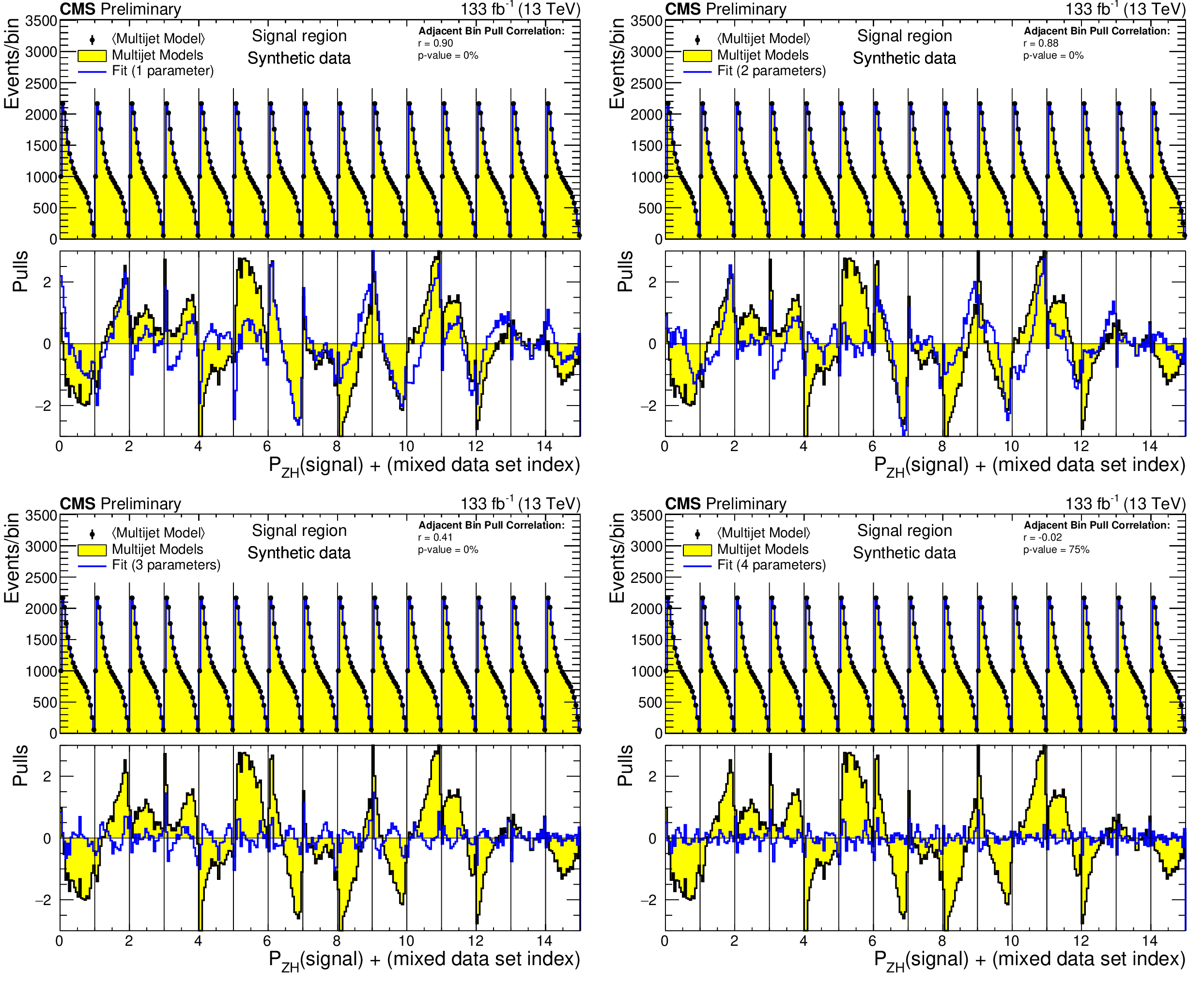
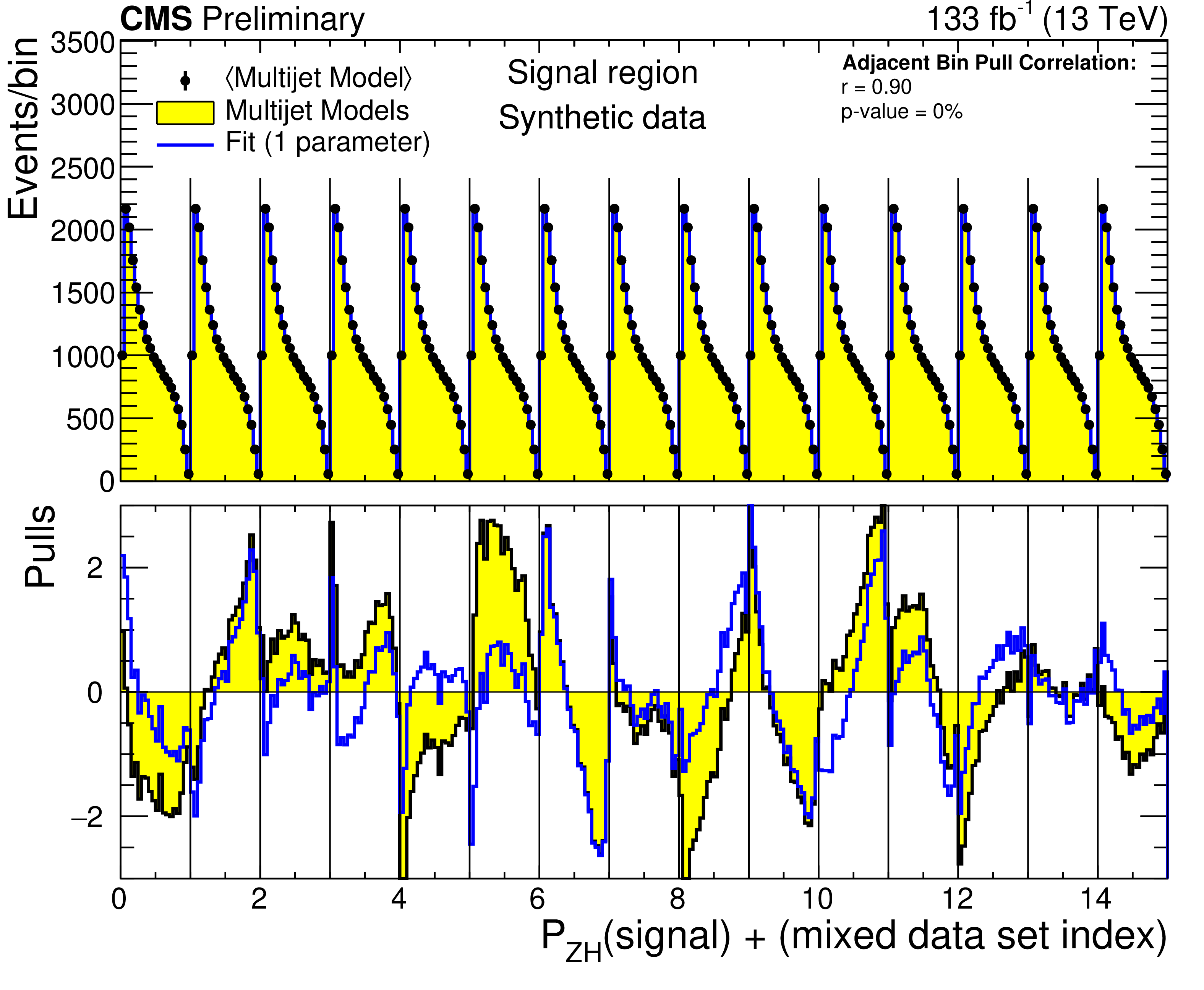
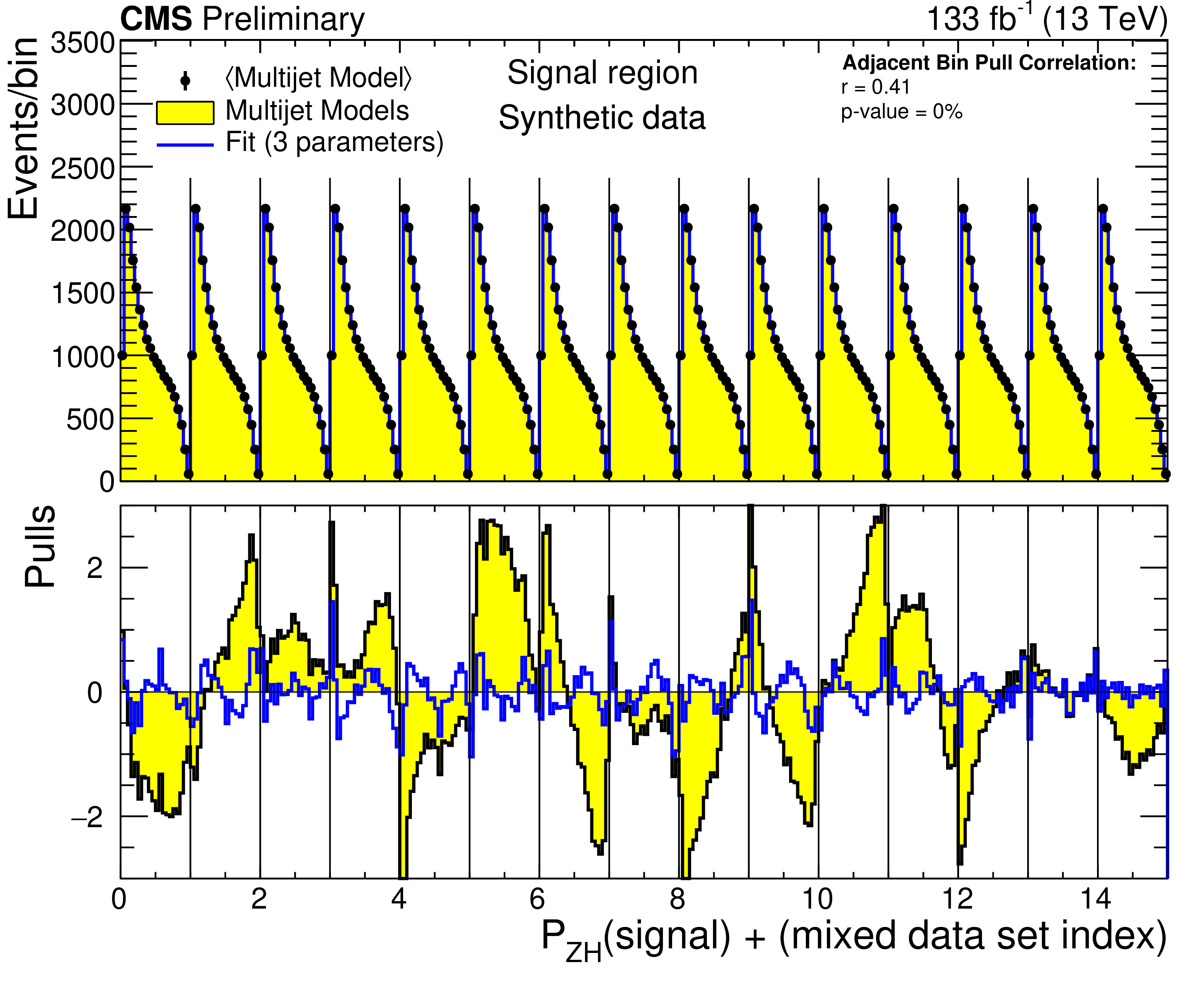
Additional Figure 7:
The predicted multijet ZH SvB distributions in the mixed data signal regions fit to their average. The plots show the results of fitting with an increasing number of basis functions, from one in the upper left figure, to four in the lower right. The predictions from each mixed model are shown separately in yellow by adding the mixed data set index to offset the signal SvB distribution. The black data points show the average of the predictions. The predictions, including the fitted basis corrections, are shown in blue. The lower panels show the pulls before and after adding the basis corrections. The pull of adjacent bins are tested for statistical correlation. The correlation coefficient (r) is reported in the legend along with the p-value used to test for lack of correlation. Basis functions are added until the p-value is above 5%. |
png pdf |
Additional Figure 7-a:
The predicted multijet ZH SvB distributions in the mixed data signal regions fit to their average. The plots show the results of fitting with an increasing number of basis functions, from one in the upper left figure, to four in the lower right. The predictions from each mixed model are shown separately in yellow by adding the mixed data set index to offset the signal SvB distribution. The black data points show the average of the predictions. The predictions, including the fitted basis corrections, are shown in blue. The lower panels show the pulls before and after adding the basis corrections. The pull of adjacent bins are tested for statistical correlation. The correlation coefficient (r) is reported in the legend along with the p-value used to test for lack of correlation. Basis functions are added until the p-value is above 5%. |

png pdf |
Additional Figure 7-b:
The predicted multijet ZH SvB distributions in the mixed data signal regions fit to their average. The plots show the results of fitting with an increasing number of basis functions, from one in the upper left figure, to four in the lower right. The predictions from each mixed model are shown separately in yellow by adding the mixed data set index to offset the signal SvB distribution. The black data points show the average of the predictions. The predictions, including the fitted basis corrections, are shown in blue. The lower panels show the pulls before and after adding the basis corrections. The pull of adjacent bins are tested for statistical correlation. The correlation coefficient (r) is reported in the legend along with the p-value used to test for lack of correlation. Basis functions are added until the p-value is above 5%. |
png pdf |
Additional Figure 7-c:
The predicted multijet ZH SvB distributions in the mixed data signal regions fit to their average. The plots show the results of fitting with an increasing number of basis functions, from one in the upper left figure, to four in the lower right. The predictions from each mixed model are shown separately in yellow by adding the mixed data set index to offset the signal SvB distribution. The black data points show the average of the predictions. The predictions, including the fitted basis corrections, are shown in blue. The lower panels show the pulls before and after adding the basis corrections. The pull of adjacent bins are tested for statistical correlation. The correlation coefficient (r) is reported in the legend along with the p-value used to test for lack of correlation. Basis functions are added until the p-value is above 5%. |

png pdf |
Additional Figure 7-d:
The predicted multijet ZH SvB distributions in the mixed data signal regions fit to their average. The plots show the results of fitting with an increasing number of basis functions, from one in the upper left figure, to four in the lower right. The predictions from each mixed model are shown separately in yellow by adding the mixed data set index to offset the signal SvB distribution. The black data points show the average of the predictions. The predictions, including the fitted basis corrections, are shown in blue. The lower panels show the pulls before and after adding the basis corrections. The pull of adjacent bins are tested for statistical correlation. The correlation coefficient (r) is reported in the legend along with the p-value used to test for lack of correlation. Basis functions are added until the p-value is above 5%. |

png pdf |
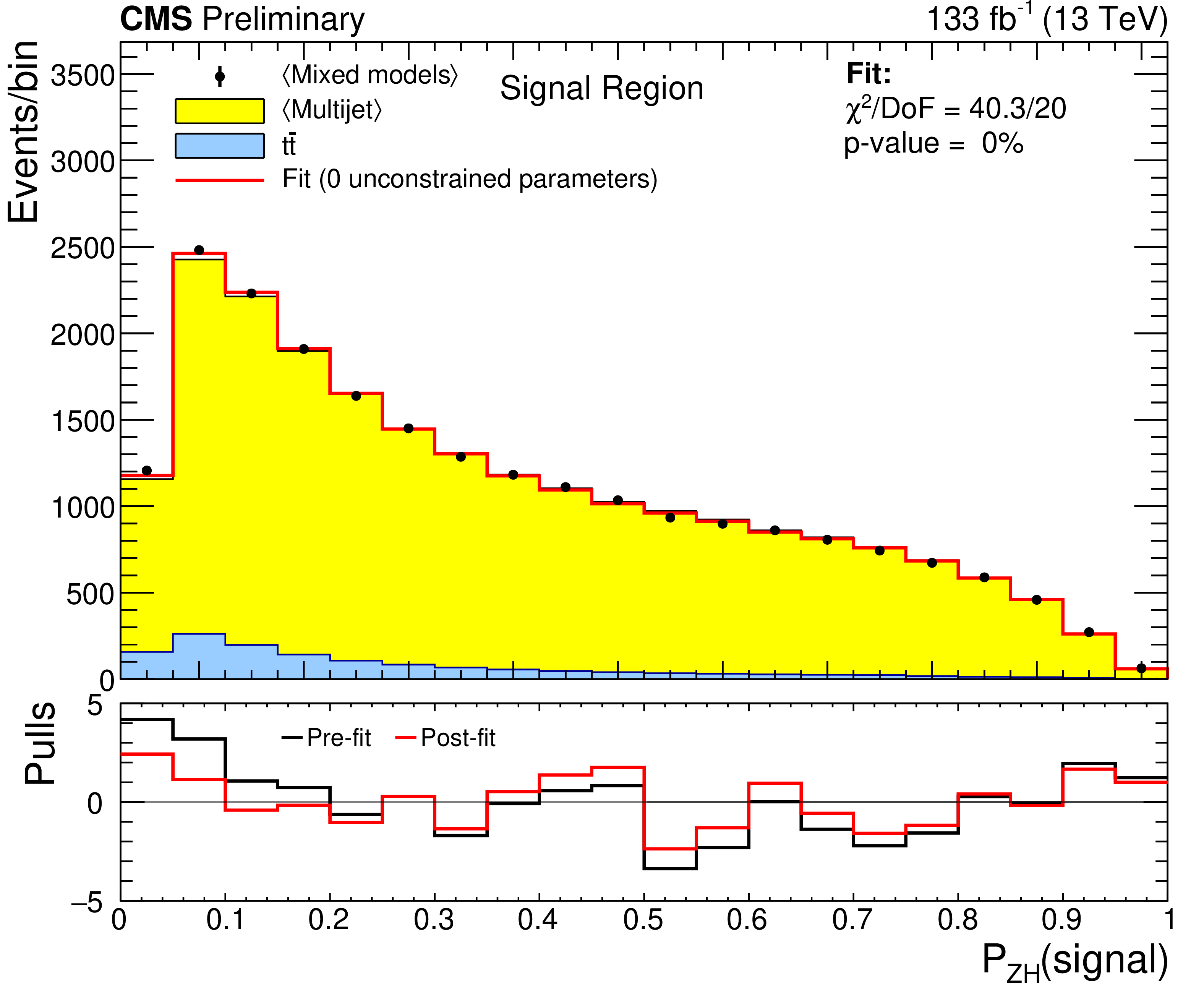
Additional Figure 8:
Fits of the ZH background model to the observed signal-region yield in the mixed models. The black data points show the average of the mixed models, the yellow distributions the average of the multijet models. The lower panels show the pre- and post-fit pulls. The figure on the left (right) shows the fit with zero (one) unconstrained basis parameter(s). |
png pdf |
Additional Figure 8-a:
Fits of the ZH background model to the observed signal-region yield in the mixed models. The black data points show the average of the mixed models, the yellow distributions the average of the multijet models. The lower panels show the pre- and post-fit pulls. The figure on the left (right) shows the fit with zero (one) unconstrained basis parameter(s). |

png pdf |
Additional Figure 8-b:
Fits of the ZH background model to the observed signal-region yield in the mixed models. The black data points show the average of the mixed models, the yellow distributions the average of the multijet models. The lower panels show the pre- and post-fit pulls. The figure on the left (right) shows the fit with zero (one) unconstrained basis parameter(s). |
png pdf |
Additional Figure 9:
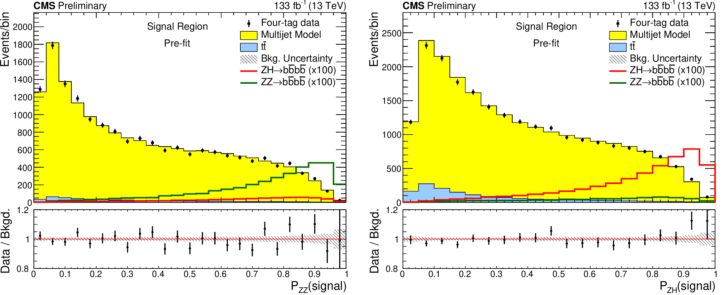
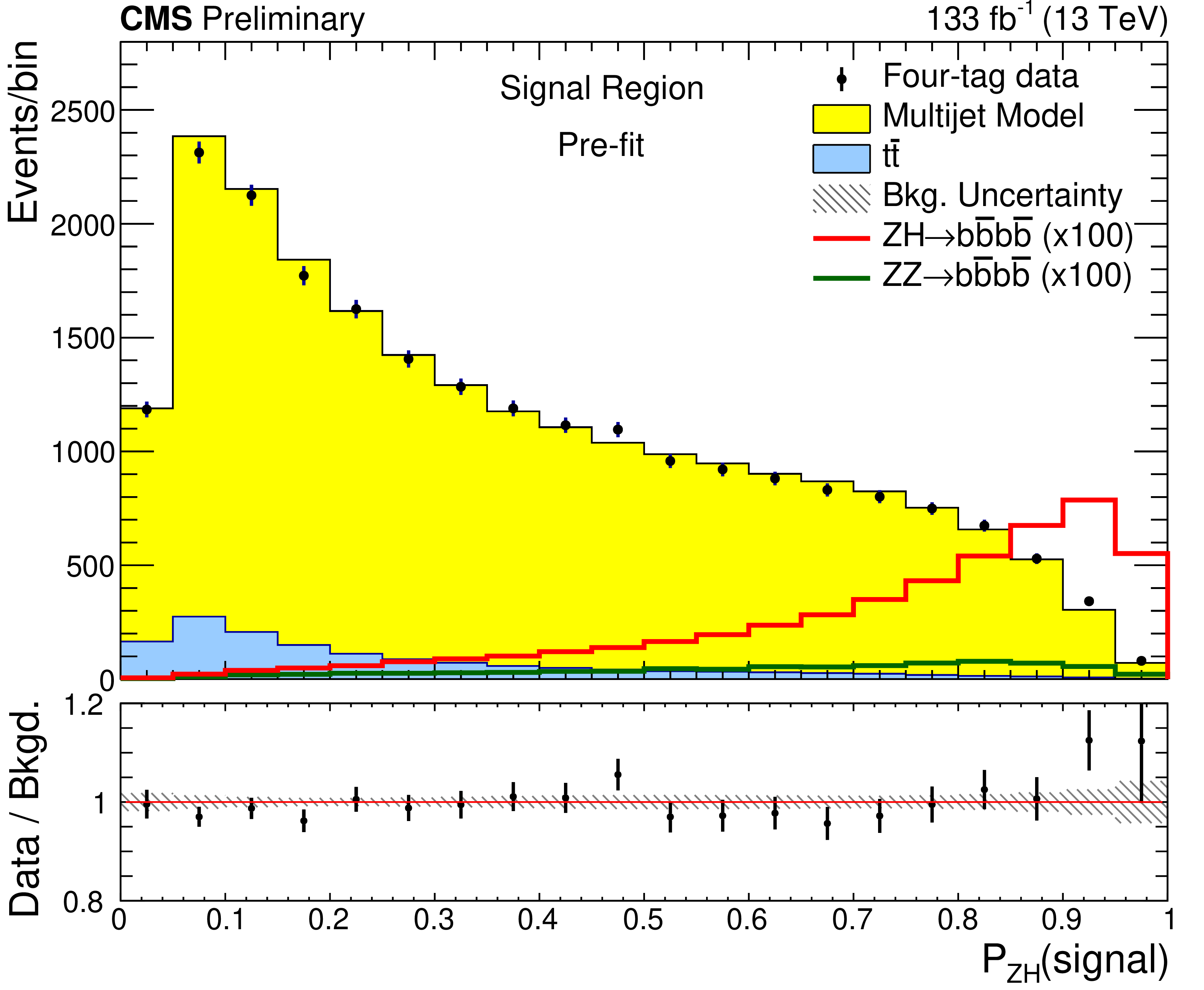
The pre-fit signal SvB signal probability distributions in the ZZ region (left) and the ZH region (right). |

png pdf |
Additional Figure 9-a:
The pre-fit signal SvB signal probability distributions in the ZZ region (left) and the ZH region (right). |
png pdf |
Additional Figure 9-b:
The pre-fit signal SvB signal probability distributions in the ZZ region (left) and the ZH region (right). |
png pdf |
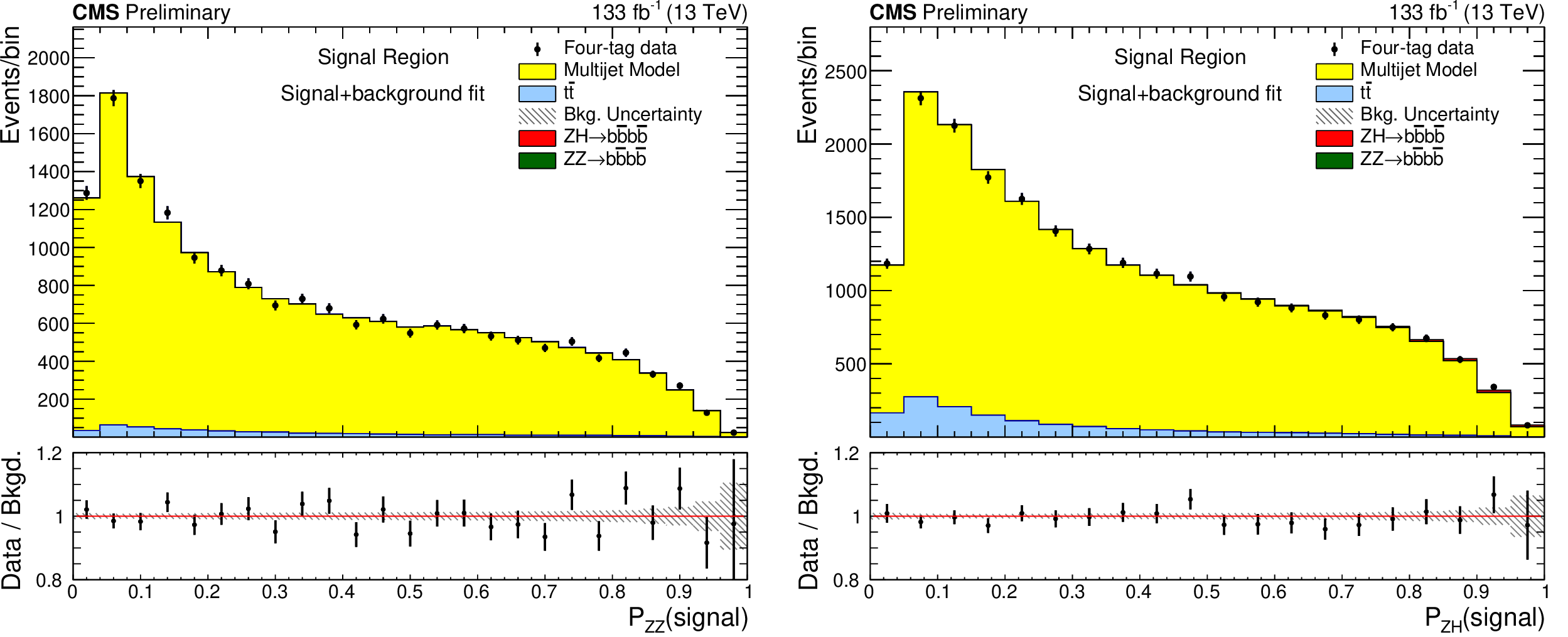
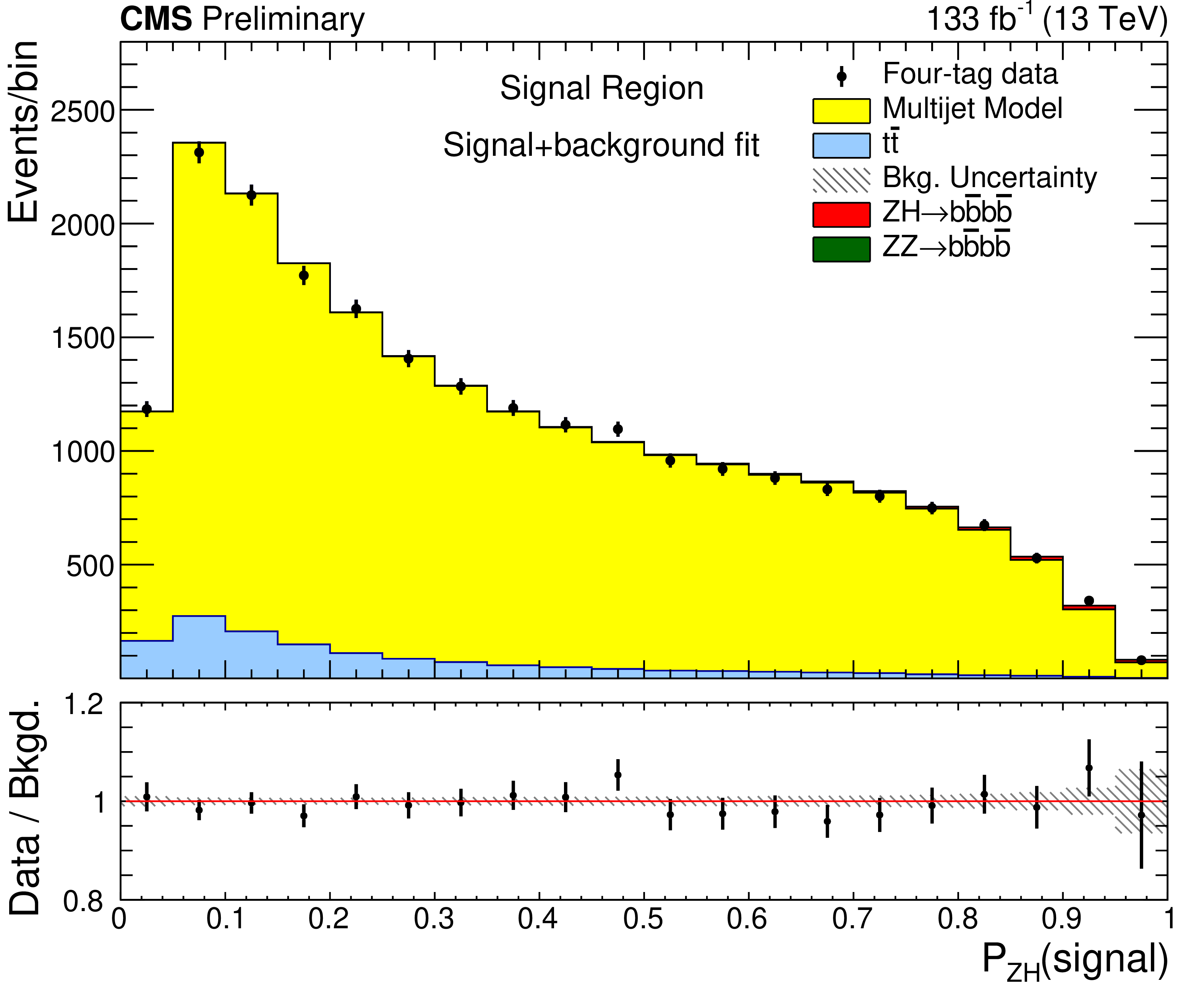
Additional Figure 10:
The post-fit signal plus background SvB signal probability distributions in the ZZ region (left) and the ZH region (right). |

png pdf |
Additional Figure 10-a:
The post-fit signal plus background SvB signal probability distributions in the ZZ region (left) and the ZH region (right). |
png pdf |
Additional Figure 10-b:
The post-fit signal plus background SvB signal probability distributions in the ZZ region (left) and the ZH region (right). |
| References | ||||
| 1 | M. Cepeda et al. | Report from working group 2: Higgs physics at the HL-LHC and HE-LHC | CERN Yellow Rep. Monogr. 7 (2019) 221 | 1902.00134 |
| 2 | B. D. Micco, M. Gouzevitch, J. Mazzitelli, and C. Vernieri | Higgs boson potential at colliders: status and perspectives | Rev. Phys. 5 (2020) 100045 | 1910.00012 |
| 3 | CMS Collaboration | A portrait of the Higgs boson by the CMS experiment ten years after the discovery | Nature 607 (2022) 60 | CMS-HIG-22-001 2207.00043 |
| 4 | CMS Collaboration | Search for Higgs boson pair production in the four b quark final state in proton-proton collisions at $ \sqrt{s}= $ 13 TeV | PRL 129 (2022) 081802 | CMS-HIG-20-005 2202.09617 |
| 5 | ATLAS Collaboration | Search for Higgs boson pair production in the two bottom quarks plus two photons final state in $ pp $ collisions at $ \sqrt{s}= $ 13 TeV with the ATLAS detector | PRD 106 (2022) 052001 | 2112.11876 |
| 6 | CMS Collaboration | Search for nonresonant Higgs boson pair production in final state with two bottom quarks and two tau leptons in proton-proton collisions at $ \sqrt{s} = $ 13 TeV | Submitted to Physics Letters B, 2022 | CMS-HIG-20-010 2206.09401 |
| 7 | ATLAS Collaboration | Search for resonant and non-resonant Higgs boson pair production in the $ b\overline{b}{\tau}^{+}{\tau}^{-} $ decay channel using 13 TeV pp collision data from the ATLAS detector | JHEP 07 (2023) 040 | 2209.10910 |
| 8 | CMS Collaboration | Search for nonresonant Higgs boson pair production in final states with two bottom quarks and two photons in proton-proton collisions at $ \sqrt{s} = $ 13 TeV | JHEP 03 (2021) 257 | CMS-HIG-19-018 2011.12373 |
| 9 | ATLAS Collaboration | Search for nonresonant pair production of Higgs bosons in the $ b\bar{b}b\bar{b} $ final state in pp collisions at $ \sqrt{s}= $ 13 TeV with the ATLAS detector | PRD 108 (2023) 052003 | 2301.03212 |
| 10 | CMS Collaboration | Search for nonresonant pair production of highly energetic Higgs bosons decaying to bottom quarks | (Jul, ) 041803, 2023 PRL 13 (2023) 1 |
2205.06667 |
| 11 | CMS Collaboration | Measurement of the ZZ production cross section and Z $ \to \ell^+\ell^-\ell'^+\ell'^- $ branching fraction in pp collisions at $ \sqrt{s} = $ 13 TeV | PLB 763 (2016) 280 | CMS-SMP-16-001 1607.08834 |
| 12 | LHC Higgs Cross Section Working Group | Handbook of LHC Higgs cross sections: 4. Deciphering the nature of the Higgs sector | CERN Report CERN-2017-002-M, 2016 link |
1610.07922 |
| 13 | CMS Collaboration | Measurements of $ {\mathrm{p}} {\mathrm{p}} \rightarrow {\mathrm{Z}} {\mathrm{Z}} $ production cross sections and constraints on anomalous triple gauge couplings at $ \sqrt{s} = $ 13 TeV | EPJC 81 (2021) 200 | CMS-SMP-19-001 2009.01186 |
| 14 | ATLAS Collaboration | $ ZZ \to \ell^{+}\ell^{-}\ell^{\prime +}\ell^{\prime -} $ cross-section measurements and search for anomalous triple gauge couplings in 13 TeV $ pp $ collisions with the ATLAS detector | PRD 97 (2018) 032005 | 1709.07703 |
| 15 | CMS Collaboration | Observation of Higgs boson decay to bottom quarks | PRL 121 (2018) 121801 | CMS-HIG-18-016 1808.08242 |
| 16 | ATLAS Collaboration | Observation of $ H \rightarrow b\bar{b} $ decays and $ VH $ production with the ATLAS detector | PLB 786 (2018) 59 | 1808.08238 |
| 17 | ATLAS Collaboration | Search for pair production of Higgs bosons in the $ b\bar{b}b\bar{b} $ final state using proton-proton collisions at $ \sqrt{s} = $ 13 TeV with the ATLAS detector | JHEP 01 (2019) 030 | 1804.06174 |
| 18 | CMS Collaboration | Search for resonant pair production of Higgs bosons decaying to bottom quark-antiquark pairs in proton-proton collisions at 13 TeV | JHEP 08 (2018) 152 | CMS-HIG-17-009 1806.03548 |
| 19 | ATLAS Collaboration | Search for pair production of Higgs bosons in the $ b\bar{b}b\bar{b} $ final state using proton--proton collisions at $ \sqrt{s} = $ 13 TeV with the ATLAS detector | PRD 94 (2016) 052002 | 1606.04782 |
| 20 | ATLAS Collaboration | Search for Higgs boson pair production in the $ b\bar{b}b\bar{b} $ final state from pp collisions at $ \sqrt{s} = $ 8 TeV with the ATLAS detector | EPJC 75 (2015) 412 | 1506.00285 |
| 21 | CMS Collaboration | Search for resonant pair production of Higgs bosons decaying to two bottom quark-antiquark pairs in proton-proton collisions at 8 TeV | PLB 749 (2015) 560 | CMS-HIG-14-013 1503.04114 |
| 22 | F. Lincoln | Calculating Waterfowl Abundance on the Basis of Banding Returns | Circular (United States. Department of Agriculture). U.S. Department of Agriculture, 1930 | |
| 23 | CDF Collaboration | Measurement of $ \sigma \times \mathcal{B}(W\rightarrow e\nu) $ and $ \sigma \times \mathcal{B}({Z}^{0}\rightarrow {e}^{+}{e}^{-}) $ in $ \overline{p}p $ collisions at $ \sqrt{s}= $ 1800 GeV | PRD 44 (1991) 29 | |
| 24 | O. Behnke, K. Kröninger, G. Schott, and T. Schörner-Sadenius | Data analysis in high energy physics: a practical guide to statistical methods | Wiley-VCH, Weinheim, 2013 link |
|
| 25 | P. De Castro Manzano et al. | Hemisphere mixing: a fully data-driven model of QCD multijet Backgrounds for LHC searches | PoS EPS-HEP 370, 2017 link |
1712.02538 |
| 26 | CMS Collaboration | Search for nonresonant Higgs boson pair production in the $ b\overline{b}b\overline{b} $ final state at $ \sqrt{s} = $ 13 TeV | JHEP 04 (2019) 112 | CMS-HIG-17-017 1810.11854 |
| 27 | CMS Collaboration | The CMS experiment at the CERN LHC | JINST 3 (2008) S08004 | |
| 28 | CMS Collaboration | Development of the CMS detector for the CERN LHC Run 3 | CMS-PRF-21-001 2309.05466 |
|
| 29 | CMS Collaboration | Performance of the CMS Level-1 trigger in proton-proton collisions at $ \sqrt{s} = $ 13\,TeV | JINST 15 (2020) P10017 | CMS-TRG-17-001 2006.10165 |
| 30 | CMS Collaboration | The CMS trigger system | JINST 12 (2017) P01020 | CMS-TRG-12-001 1609.02366 |
| 31 | CMS Collaboration | Electron and photon reconstruction and identification with the CMS experiment at the CERN LHC | JINST 16 (2021) P05014 | CMS-EGM-17-001 2012.06888 |
| 32 | CMS Collaboration | Performance of the CMS muon detector and muon reconstruction with proton-proton collisions at $ \sqrt{s}= $ 13 TeV | JINST 13 (2018) P06015 | CMS-MUO-16-001 1804.04528 |
| 33 | CMS Collaboration | Description and performance of track and primary-vertex reconstruction with the CMS tracker | JINST 9 (2014) P10009 | CMS-TRK-11-001 1405.6569 |
| 34 | CMS Collaboration | The CMS experiment at the CERN LHC | JINST 3 (2008) S08004 | |
| 35 | CMS Collaboration | Performance of the CMS Level-1 trigger in proton-proton collisions at $ \sqrt{s} = $ 13 TeV | JINST 15 (2020) P10017 | CMS-TRG-17-001 2006.10165 |
| 36 | CMS Collaboration | The CMS trigger system | JINST 12 (2017) P01020 | CMS-TRG-12-001 1609.02366 |
| 37 | CMS Collaboration | Particle-flow reconstruction and global event description with the CMS detector | JINST 12 (2017) P10003 | CMS-PRF-14-001 1706.04965 |
| 38 | CMS Collaboration | Technical proposal for the Phase-II upgrade of the Compact Muon Solenoid | CMS Technical Proposal CERN-LHCC-2015-010, CMS-TDR-15-02, CERN, 2015 CDS |
|
| 39 | M. Cacciari, G. P. Salam, and G. Soyez | The anti-$ k_{\mathrm{T}} $ jet clustering algorithm | JHEP 04 (2008) 063 | 0802.1189 |
| 40 | M. Cacciari, G. P. Salam, and G. Soyez | FastJet user manual | EPJC 72 (2012) 1896 | 1111.6097 |
| 41 | CMS Collaboration | Pileup mitigation at CMS in $ \sqrt{s}= $ 13 TeV data | JINST 15 (2020) P09018 | CMS-JME-18-001 2003.00503 |
| 42 | CMS Collaboration | Jet energy scale and resolution in the CMS experiment in proton-proton collisions at $ \sqrt{s}= $ 8 TeV | JINST 12 (2017) P02014 | CMS-JME-13-004 1607.03663 |
| 43 | CMS Collaboration | Jet energy scale and resolution measurement with Run-2 legacy data collected by CMS at $ \sqrt{s}= $ 13 TeV | CMS Detector Performance Summary CMS-DP-2021-033, CERN, 2021 CDS |
|
| 44 | E. Bols et al. | Jet flavour classification using DeepJet | JINST 15 (2020) P12012 | 2008.10519 |
| 45 | CMS Collaboration | Precision luminosity measurement in proton-proton collisions at $ \sqrt{s} = $ 13 TeV in 2015 and 2016 at CMS | EPJC 81 (2021) 800 | CMS-LUM-17-003 2104.01927 |
| 46 | CMS Collaboration | CMS luminosity measurement for the 2017 data-taking period at $ \sqrt{s} = $ 13 TeV | CMS Physics Analysis Summary , CERN, 2017 CMS-PAS-LUM-17-004 |
CMS-PAS-LUM-17-004 |
| 47 | CMS Collaboration | CMS luminosity measurement for the 2018 data-taking period at $ \sqrt{s} = $ 13 TeV | CMS Physics Analysis Summary , CERN, 2019 CMS-PAS-LUM-18-002 |
CMS-PAS-LUM-18-002 |
| 48 | CMS Collaboration | Identification of heavy-flavour jets with the cms detector in pp collisions at 13 TeV | JINST 13 (2018) P05011 | CMS-BTV-16-002 1712.07158 |
| 49 | S. Frixione, P. Nason, and G. Ridolfi | A positive-weight next-to-leading-order Monte Carlo for heavy flavour hadroproduction | JHEP 09 (2007) 126 | 0707.3088 |
| 50 | S. Frixione, P. Nason, and C. Oleari | Matching NLO QCD computations with parton shower simulations: the POWHEG method | JHEP 11 (2007) 070 | 0709.2092 |
| 51 | J. M. Campbell, R. K. Ellis, P. Nason, and E. Re | Top-pair production and decay at NLO matched with parton showers | JHEP 04 (2015) 114 | 1412.1828 |
| 52 | J. Alwall et al. | The automated computation of tree-level and next-to-leading order differential cross sections, and their matching to parton shower simulations | JHEP 07 (2014) 79 | 1405.0301 |
| 53 | R. Frederix and S. Frixione | Merging meets matching in MC@NLO | JHEP 12 (2012) 061 | 1209.6215 |
| 54 | K. Mimasu, V. Sanz, and C. Williams | Higher Order QCD predictions for Associated Higgs production with anomalous couplings to gauge bosons | JHEP 08 (2016) 039 | 1512.02572 |
| 55 | K. Hamilton, P. Nason, and G. Zanderighi | MINLO: Multi-scale improved NLO | JHEP 10 (2012) 155 | 1206.3572 |
| 56 | G. Luisoni, P. Nason, C. Oleari, and F. Tramontano | HW/HZ + 0 and 1 jet at NLO with the POWHEG BOX interfaced to GoSam and their merging within MiNLO | JHEP 10 (2013) 083 | 1306.2542 |
| 57 | S. Dawson, S. Dittmaier, and M. Spira | Neutral Higgs boson pair production at hadron colliders: QCD corrections | PRD 58 (1998) 115012 | hep-ph/9805244 |
| 58 | S. Borowka et al. | Higgs boson pair production in gluon fusion at next-to-leading order with full top-quark mass dependence | PRL 117 (2016) 012001 | 1604.06447 |
| 59 | J. Baglio et al. | Gluon fusion into Higgs pairs at NLO QCD and the top mass scheme | EPJC 79 (2019) 459 | 1811.05692 |
| 60 | D. de Florian and J. Mazzitelli | Higgs boson pair production at next-to-next-to-leading order in QCD | PRL 111 (2013) 201801 | 1309.6594 |
| 61 | D. Y. Shao, C. S. Li, H. T. Li, and J. Wang | Threshold resummation effects in Higgs boson pair production at the LHC | JHEP 07 (2013) 169 | 1301.1245 |
| 62 | D. de Florian and J. Mazzitelli | Higgs pair production at next-to-next-to-leading logarithmic accuracy at the LHC | JHEP 09 (2015) 053 | 1505.07122 |
| 63 | M. Grazzini et al. | Higgs boson pair production at NNLO with top quark mass effects | JHEP 05 (2018) 059 | 1803.02463 |
| 64 | J. Baglio et al. | $ \mathrm{g}\mathrm{g}\to \mathrm{H}\mathrm{H} $: Combined uncertainties | PRD 103 (2021) 056002 | 2008.11626 |
| 65 | G. Heinrich et al. | NLO predictions for Higgs boson pair production with full top quark mass dependence matched to parton showers | JHEP 08 (2017) 088 | 1703.09252 |
| 66 | A. Djouadi, J. Kalinowski, and M. Spira | HDECAY: A program for Higgs boson decays in the standard model and its supersymmetric extension | Comput. Phys. Commun. 108 (1998) 56 | hep-ph/9704448 |
| 67 | Particle Data Group Collaboration | Review of particle physics | Prog. Theor. Exp. Phys. 2022 (2022) 083C01 | |
| 68 | T. Sjöstrand et al. | An introduction to PYTHIA 8.2 | Comp. Phys. Commun. 191 (2015) 159 | 1410.3012 |
| 69 | CMS Collaboration | Extraction and validation of a new set of CMS PYTHIA8 tunes from underlying-event measurements | EPJC 80 (2020) 4 | CMS-GEN-17-001 1903.12179 |
| 70 | CMS Collaboration | Event generator tunes obtained from underlying event and multiparton scattering measurements | EPJC 76 (2016) 155 | CMS-GEN-14-001 1512.00815 |
| 71 | NNPDF Collaboration | Parton distributions for the LHC Run II | JHEP 04 (2015) 040 | 1410.8849 |
| 72 | R. D. Ball et al. | Parton distributions from high-precision collider data | EPJC 77 (2017) 663 | 1706.00428 |
| 73 | GEANT4 Collaboration | GEANT4---a simulation toolkit | NIM A 506 (2003) 250 | |
| 74 | CMS Collaboration | Evidence for the Higgs boson decay to a bottom quark-antiquark pair | PLB 780 (2018) 501 | CMS-HIG-16-044 1709.07497 |
| 75 | W. Shang, K. Sohn, D. Almeida, and H. Lee | Understanding and improving convolutional neural networks via concatenated rectified linear units | in 33rd International Conference on Machine Learning, volume 48 of Proceedings of Machine Learning Research, PMLR, 2016 link |
1603.05201 |
| 76 | K. He, X. Zhang, S. Ren, and J. Sun | Deep residual learning for image recognition | in IEEE Conference on Computer Vision and Pattern Recognition (CVPR), 2016 link |
1512.03385 |
| 77 | A. Vaswani et al. | Attention is all you need | in Advances in Neural Information Processing Systems, volume 30. Curran Associates, Inc, 2017 link |
1706.03762 |
| 78 | A. L. Read | Presentation of search results: The CL$ _{\text{s}} $ technique | JPG 28 (2002) 2693 | |
| 79 | T. Junk | Confidence level computation for combining searches with small statistics | NIM A 434 (1999) 435 | hep-ex/9902006 |
|
|
Compact Muon Solenoid LHC, CERN |
|

|

|

|

|

|