

Compact Muon Solenoid
LHC, CERN
| CMS-PAS-HIG-19-008 | ||
| Higgs boson production in association with top quarks in final states with electrons, muons, and hadronically decaying tau leptons at $\sqrt{s} = $ 13 TeV | ||
| CMS Collaboration | ||
| July 2020 | ||
| Abstract: The rate for Higgs (H) bosons production in association with either one ($\mathrm{t}\mathrm{H}$) or two ($\mathrm{t}\bar{\mathrm{t}}\mathrm{H}$) top quarks is measured in final states with multiple electrons, muons, and hadronically decaying $\tau$ leptons, using proton-proton collision data recorded at a center-of-mass energy of 13 TeV by the CMS experiment. The analyzed data set corresponds to an integrated luminosity of 137 fb$^{-1}$. The analysis targets events where the H boson decays via $\mathrm{H} \to \mathrm{W}\mathrm{W}$, $\mathrm{H} \to \tau\tau$, or $\mathrm{H} \to \mathrm{Z}\mathrm{Z}$ and the top quark(s) decay either leptonically or hadronically. The signal yield is maximized by including ten different signatures in the analysis depending on the lepton multiplicity. The separation of the H boson signal from backgrounds is enhanced by machine learning techniques and matrix element methods. The measured production rates for the $\mathrm{t}\bar{\mathrm{t}}\mathrm{H}$ and $\mathrm{t}\mathrm{H}$ signals amount to 0.92 $\pm$ 0.19 (stat) $^{+0.17}_{-0.13}$ (syst) and 5.7 $\pm$ 2.7 (stat) $\pm$ 3.0 (syst) times their respective standard model (SM) expectations. Assuming that the H boson coupling to the $\tau$ lepton is equal in strength to the values expected in the SM, the coupling $y_{\mathrm{t}}$ of the H boson to the top quark is constrained, at 95% confidence level, to be within $-0.9 < y_{\mathrm{t}} < -0.7$ or $ 0.7 < y_{\mathrm{t}} < 1.1$ times the SM expectation for this coupling. | ||
|
Links:
CDS record (PDF) ;
CADI line (restricted) ;
These preliminary results are superseded in this paper, EPJC 81 (2021) 378. The superseded preliminary plots can be found here. |
||
| Figures & Tables | Summary | Additional Figures | References | CMS Publications |
|---|
| Figures | |
png pdf |
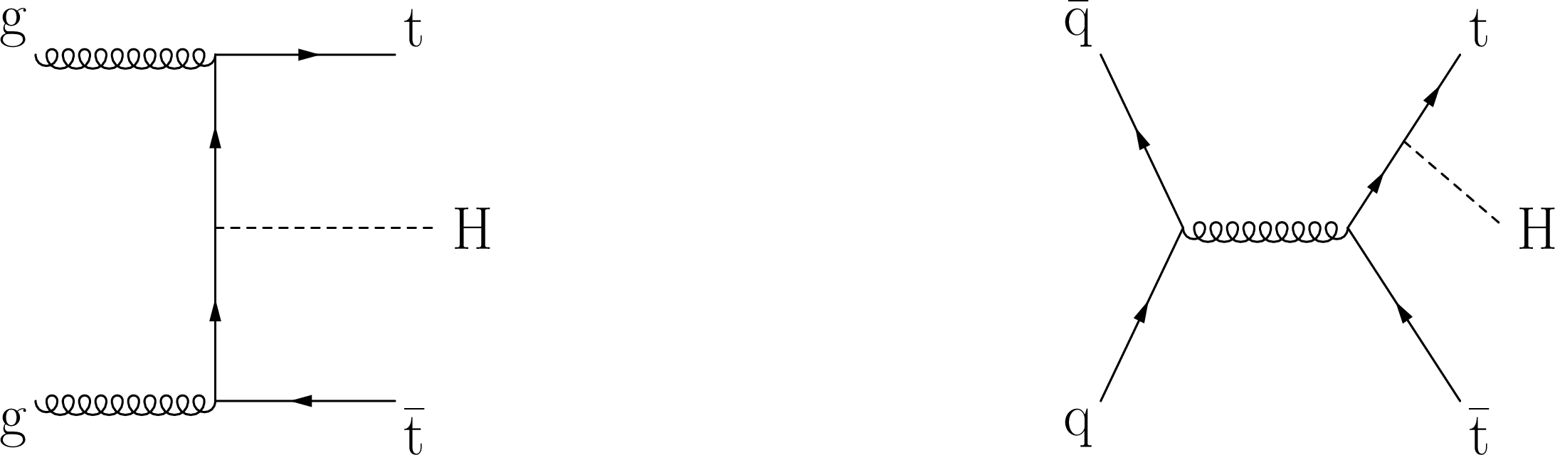
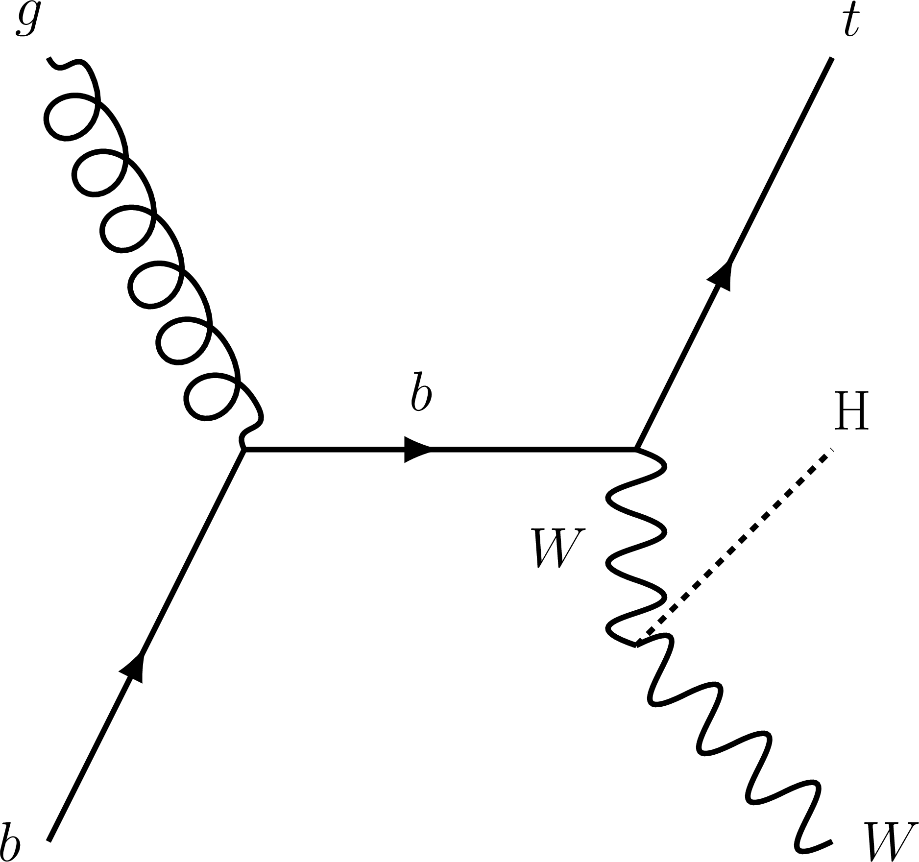
Figure 1:
Feynman diagrams at LO for $ {{\mathrm{t}} {\mathrm{\bar{t}}} {\mathrm{H}}}$ production. |
png pdf |
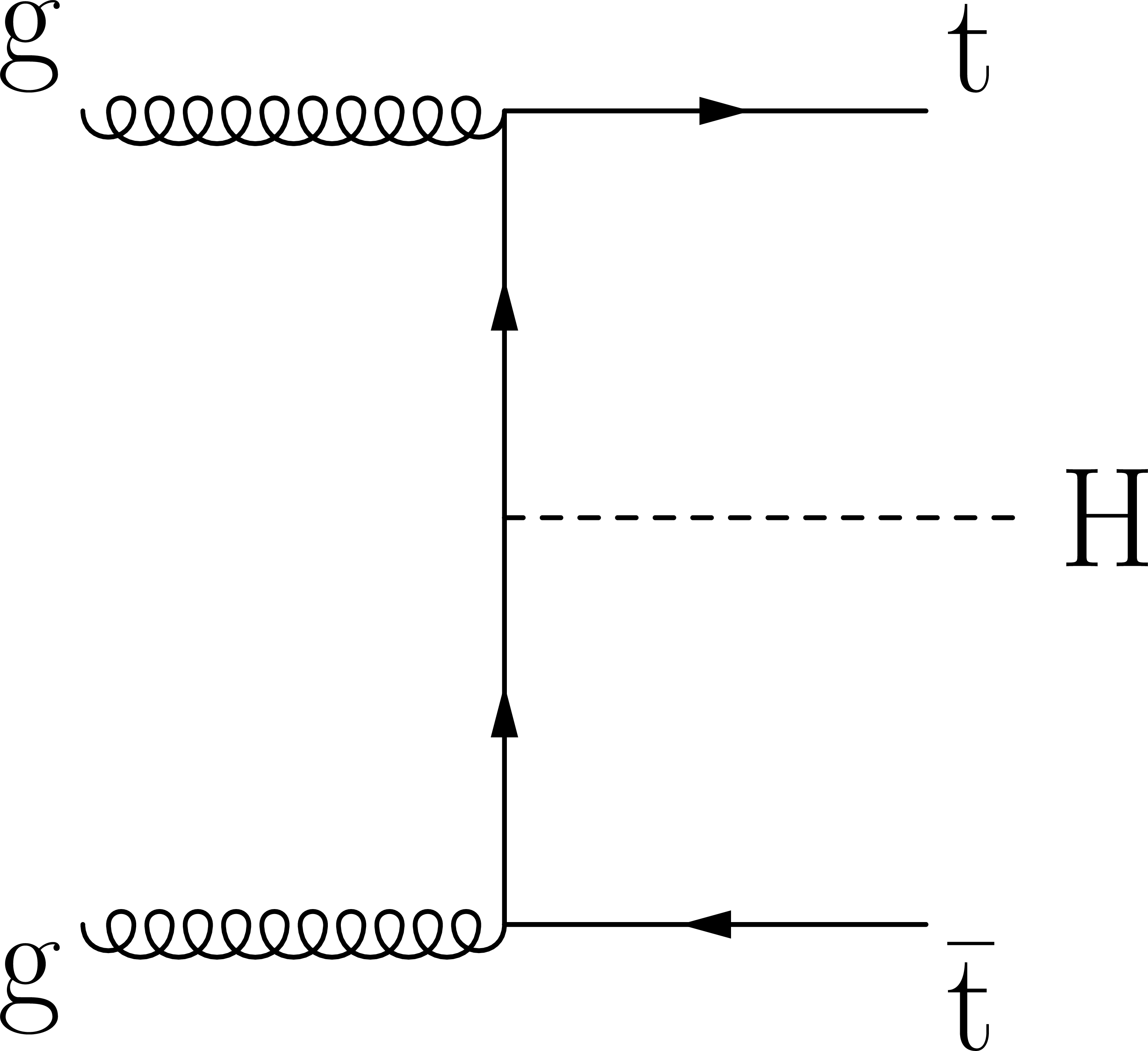
Figure 1-a:
Feynman diagram at LO for $ {{\mathrm{t}} {\mathrm{\bar{t}}} {\mathrm{H}}}$ production. |
png pdf |
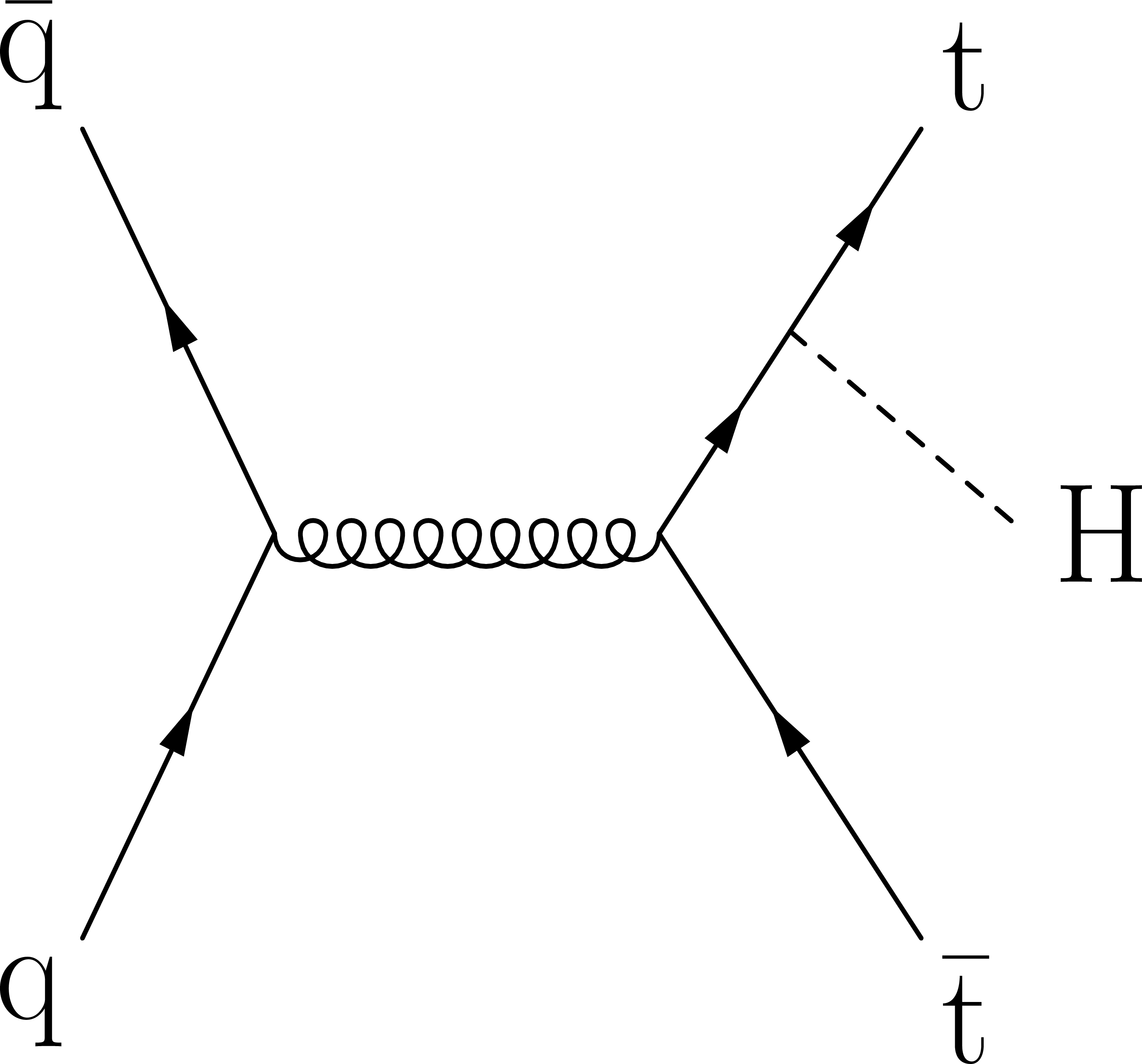
Figure 1-b:
Feynman diagram at LO for $ {{\mathrm{t}} {\mathrm{\bar{t}}} {\mathrm{H}}}$ production. |
png pdf |
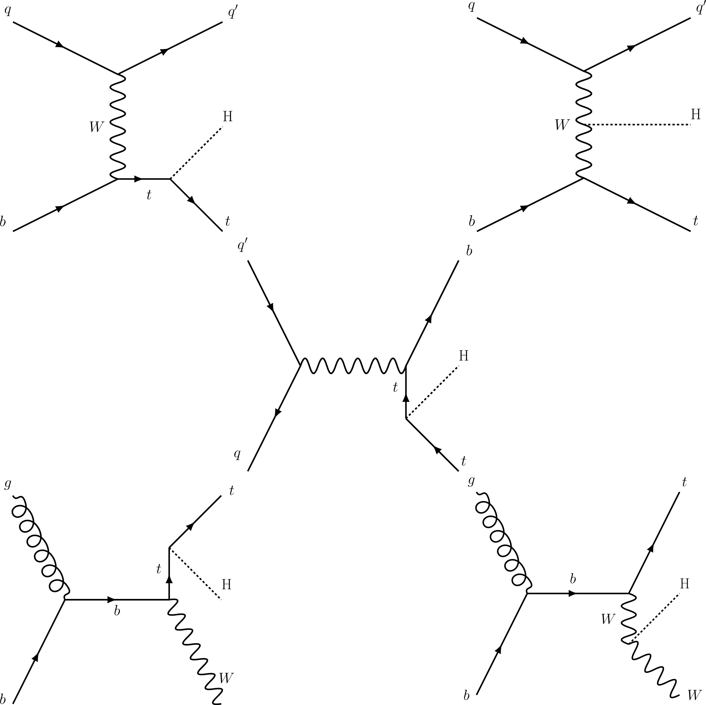
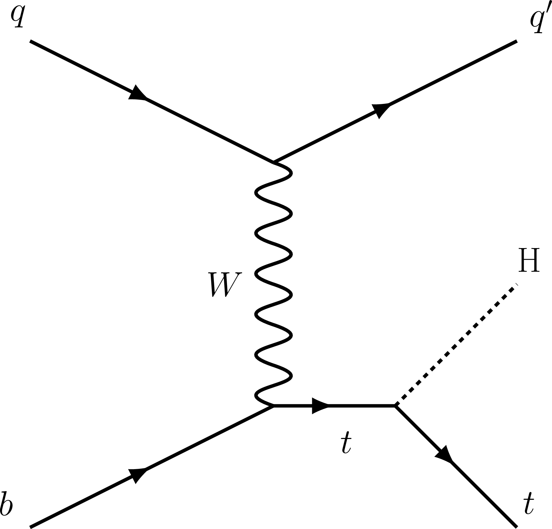
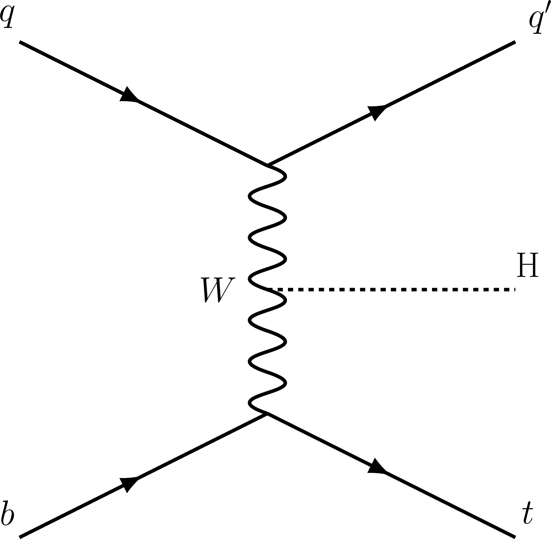
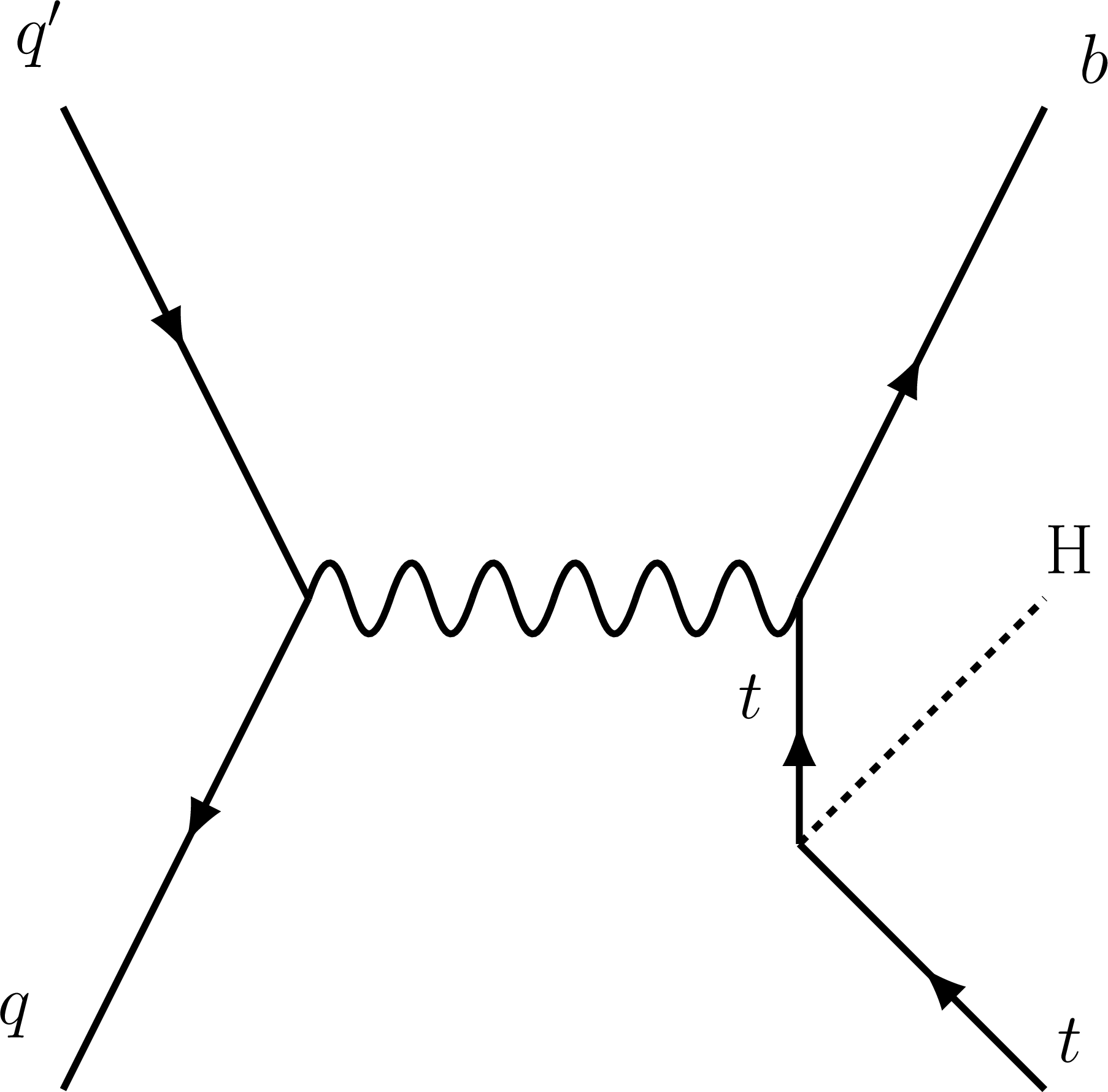
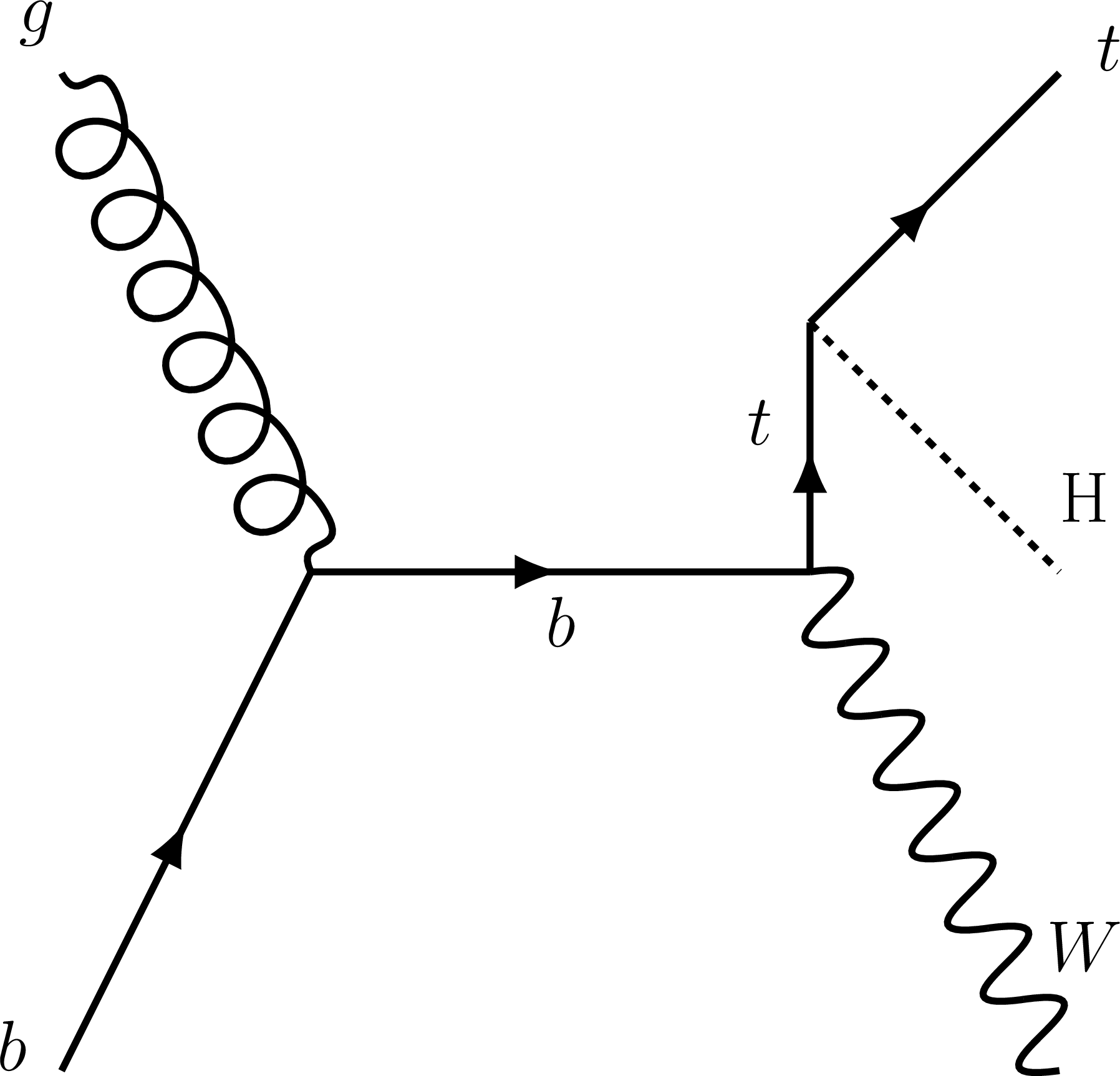
Figure 2:
Feynman diagrams at LO for $ {{\mathrm{t}} {\mathrm{H}}}$ production via the $t$-channel ($ {{{\mathrm{t}} {\mathrm{H}}} {\mathrm{q}}}$; upper left, upper right) and $s$-channel (center) processes and for the associated production of a $ {\mathrm{H}}$ boson with a single top quark and a $\mathrm{W} $ boson ($ {{{\mathrm{t}} {\mathrm{H}}}\mathrm{W}}$; lower left, lower right). The $ {{{\mathrm{t}} {\mathrm{H}}} {\mathrm{q}}}$ and $ {{{\mathrm{t}} {\mathrm{H}}}\mathrm{W}}$ production processes are shown for the 5FS. |
png pdf |
Figure 2-a:
Feynman diagram at LO for $ {{\mathrm{t}} {\mathrm{H}}}$ production via the $t$-channel ($ {{{\mathrm{t}} {\mathrm{H}}} {\mathrm{q}}}$. |
png pdf |
Figure 2-b:
Feynman diagram at LO for $ {{\mathrm{t}} {\mathrm{H}}}$ production via the $t$-channel ($ {{{\mathrm{t}} {\mathrm{H}}} {\mathrm{q}}}$. |
png pdf |
Figure 2-c:
Feynman diagram at LO for $ {{\mathrm{t}} {\mathrm{H}}}$ production via the $s$-channel ($ {{{\mathrm{t}} {\mathrm{H}}} {\mathrm{b}}}$. |
png pdf |
Figure 2-d:
Feynman diagram at LO for the associated production of a $ {\mathrm{H}}$ boson with a single top quark and a $\mathrm{W} $ boson ($ {{{\mathrm{t}} {\mathrm{H}}}\mathrm{W}}$). |
png pdf |
Figure 2-e:
Feynman diagram at LO for the associated production of a $ {\mathrm{H}}$ boson with a single top quark and a $\mathrm{W} $ boson ($ {{{\mathrm{t}} {\mathrm{H}}}\mathrm{W}}$). |
png pdf |
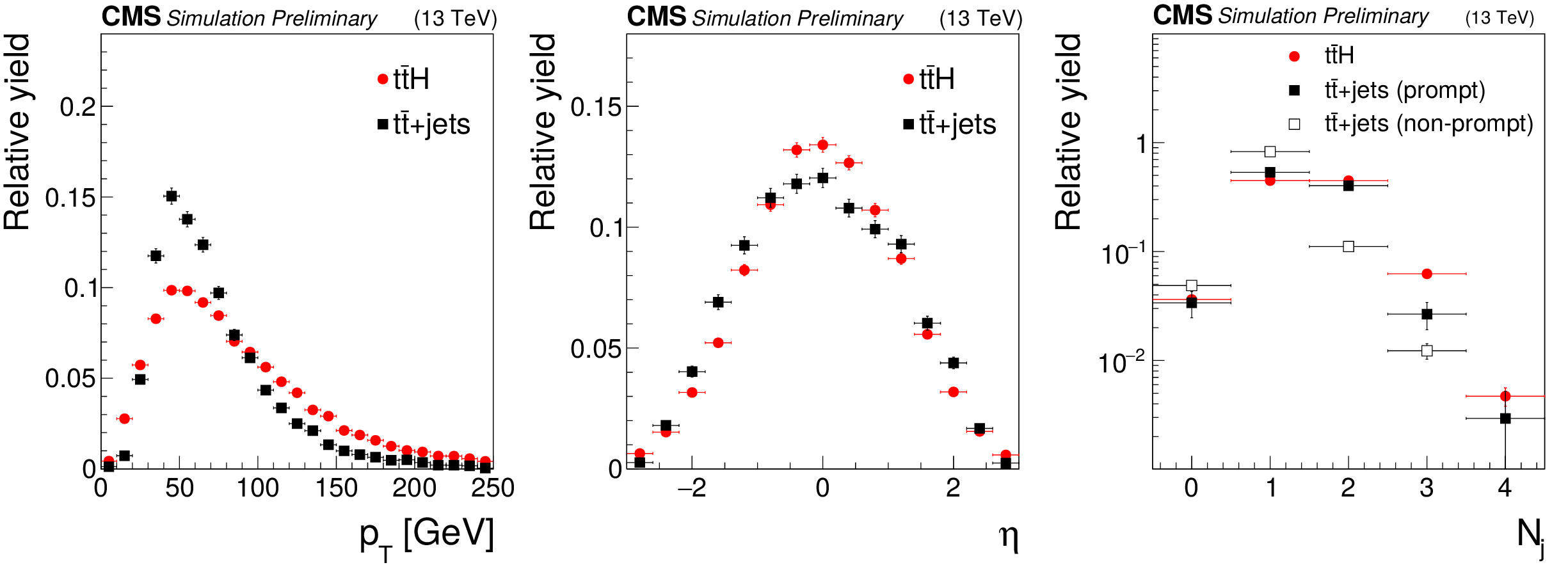
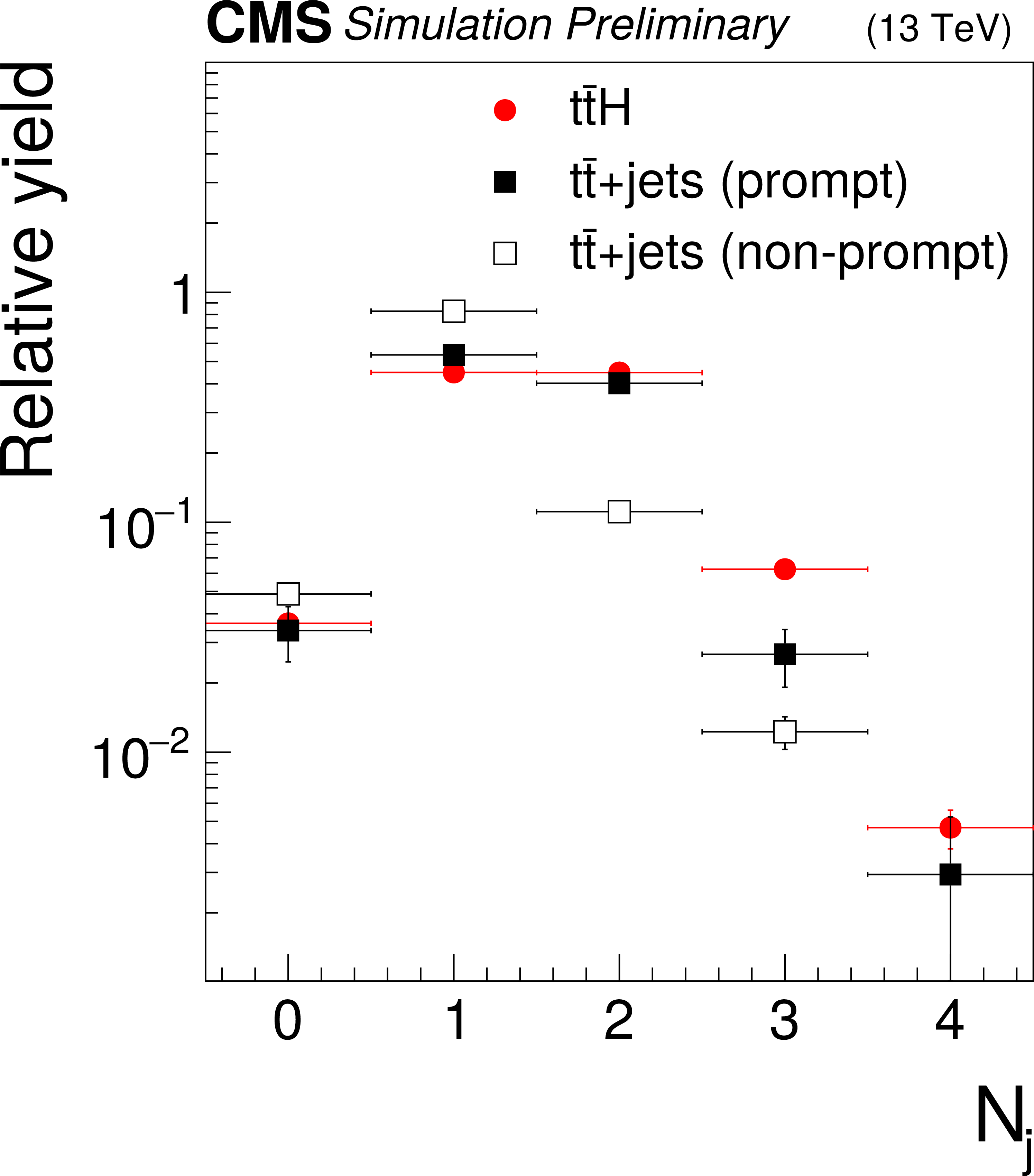
Figure 3:
Transverse momentum (left) and pseudorapidity (center) distribution of bottom quarks in $ {{\mathrm{t}} {\mathrm{\bar{t}}} {\mathrm{H}}}$ signal events compared to $ {{\mathrm{t}} {\mathrm{\bar{t}}}}$+jets background events, and multiplicity of jets passing tight b jet identification criteria (right). The latter distribution is shown separately for $ {{\mathrm{t}} {\mathrm{\bar{t}}}}$+jets background events in which a non-prompt lepton is misidentified as a prompt lepton and for those background events in which all reconstructed leptons are prompt leptons. The events are selected in the 2${\ell}$+0${\tau _{\mathrm {h}}}$ channel. |
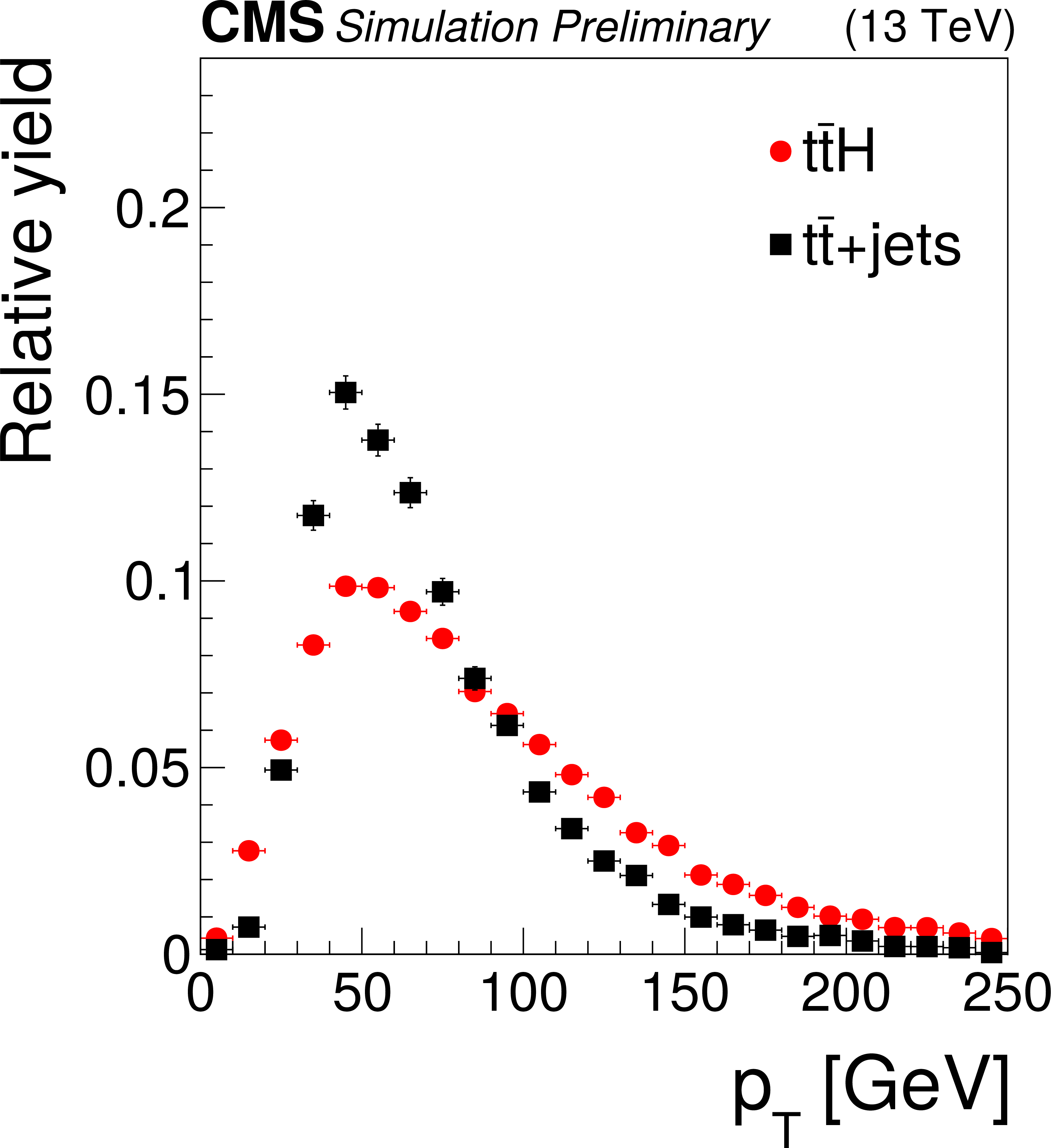
png pdf |
Figure 3-a:
Transverse momentum distribution of bottom quarks in $ {{\mathrm{t}} {\mathrm{\bar{t}}} {\mathrm{H}}}$ signal events compared to $ {{\mathrm{t}} {\mathrm{\bar{t}}}}$+jets background events. The events are selected in the 2${\ell}$+0${\tau _{\mathrm {h}}}$ channel. |
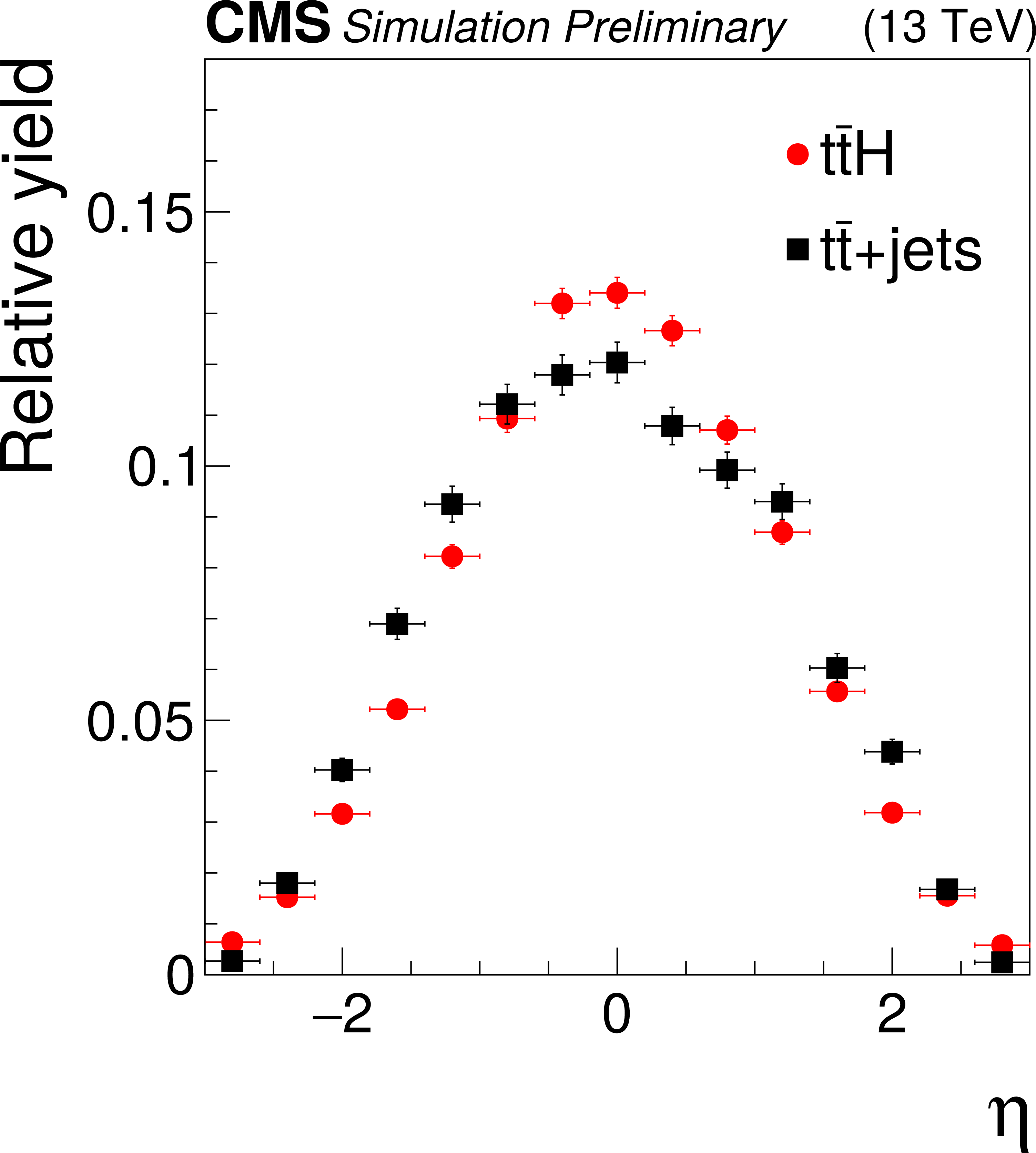
png pdf |
Figure 3-b:
Pseudorapidity distribution of bottom quarks in $ {{\mathrm{t}} {\mathrm{\bar{t}}} {\mathrm{H}}}$ signal events compared to $ {{\mathrm{t}} {\mathrm{\bar{t}}}}$+jets background events. The events are selected in the 2${\ell}$+0${\tau _{\mathrm {h}}}$ channel. |
png pdf |
Figure 3-c:
Multiplicity of jets passing tight b jet identification criteria. The distribution is shown separately for $ {{\mathrm{t}} {\mathrm{\bar{t}}}}$+jets background events in which a non-prompt lepton is misidentified as a prompt lepton and for those background events in which all reconstructed leptons are prompt leptons. The events are selected in the 2${\ell}$+0${\tau _{\mathrm {h}}}$ channel. |
png pdf |
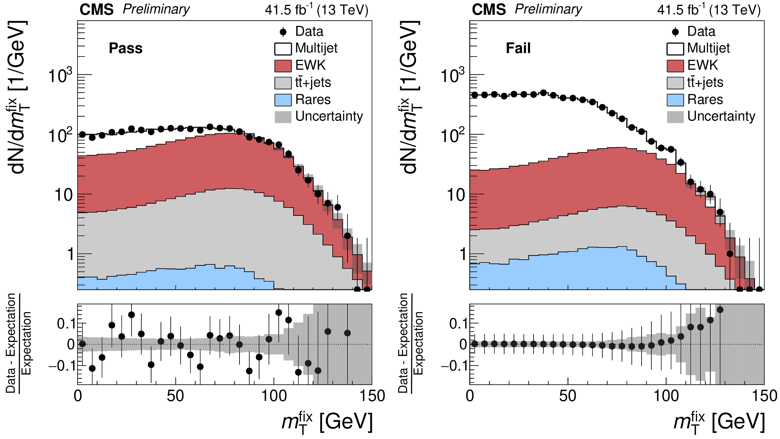
Figure 4:
Distributions in $ {{m_{\mathrm {T}}} ^{{\text {fix}}}}$ for events containing an electron candidate of 25 $ < {p_{\mathrm {T}}} < $ 35 GeV in the ECAL barrel, which (left) passes the nominal selection and (right) passes the relaxed, but fails the nominal selection. The "electroweak'' (EWK) background refers to the sum of W+jets, DY and diboson production. The "rare'' background is defined in the text. The data in the fail sample agrees with the sum of multijet, EWK, $ {{\mathrm{t}} {\mathrm{\bar{t}}}}$+jets, and "rare'' backgrounds by construction, as the number of multijet events in the fail sample is computed by the subtracting the sum of EWK, $ {{\mathrm{t}} {\mathrm{\bar{t}}}}$+jets, and "rare'' background contributions from the data. The FF contribution is derived separately for each era: this figure shows, as an example, the results obtained with the 2017 data set. The uncertainty band represents the uncertainty after the fit has been performed. |
png pdf |
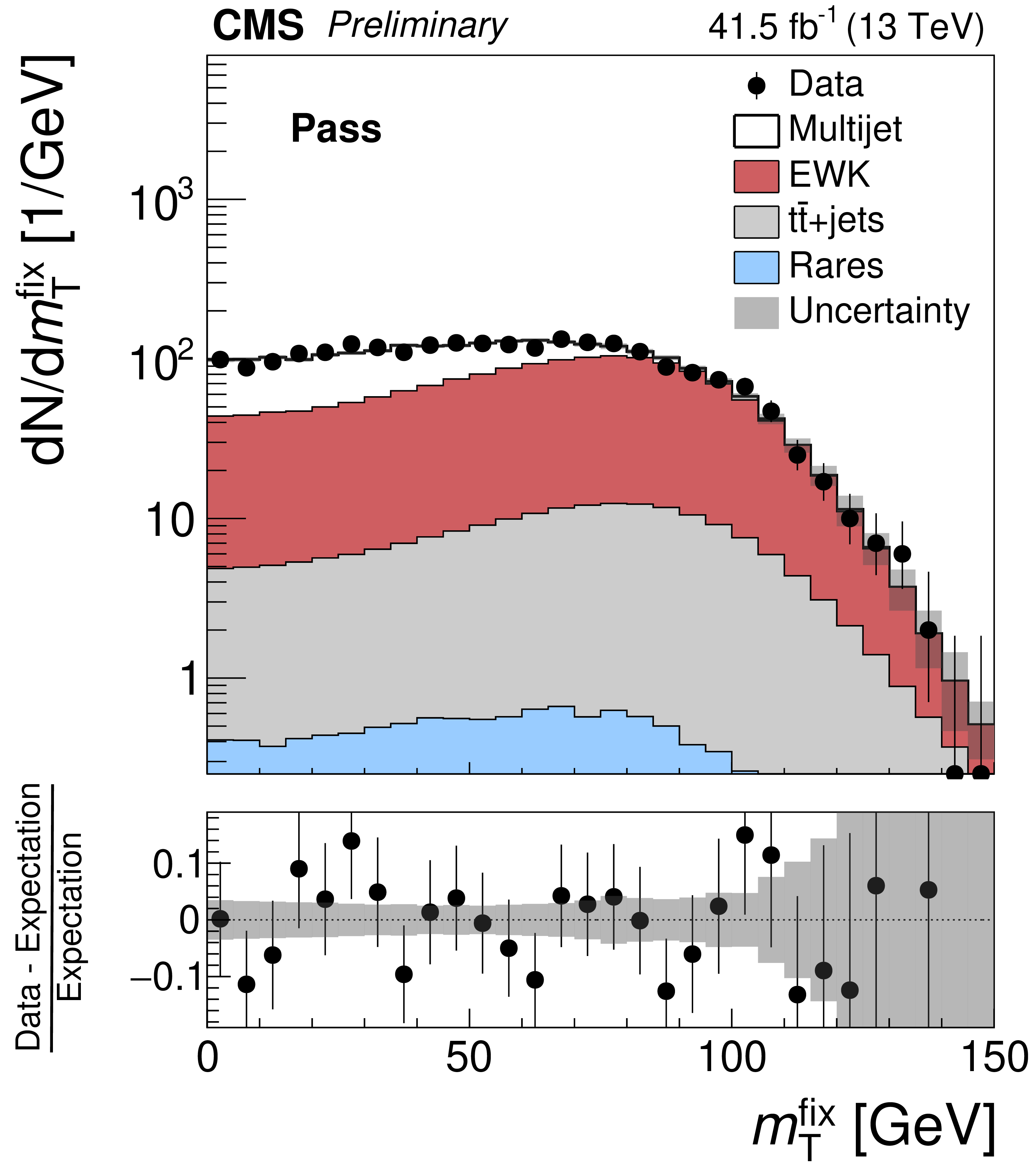
Figure 4-a:
Distribution in $ {{m_{\mathrm {T}}} ^{{\text {fix}}}}$ for events containing an electron candidate of 25 $ < {p_{\mathrm {T}}} < $ 35 GeV in the ECAL barrel, which passes the nominal selection. The "electroweak'' (EWK) background refers to the sum of W+jets, DY and diboson production. The "rare'' background is defined in the text. The data in the fail sample agrees with the sum of multijet, EWK, $ {{\mathrm{t}} {\mathrm{\bar{t}}}}$+jets, and "rare'' backgrounds by construction, as the number of multijet events in the fail sample is computed by the subtracting the sum of EWK, $ {{\mathrm{t}} {\mathrm{\bar{t}}}}$+jets, and "rare'' background contributions from the data. The FF contribution is derived separately for each era: this figure shows, as an example, the results obtained with the 2017 data set. The uncertainty band represents the uncertainty after the fit has been performed. |
png pdf |
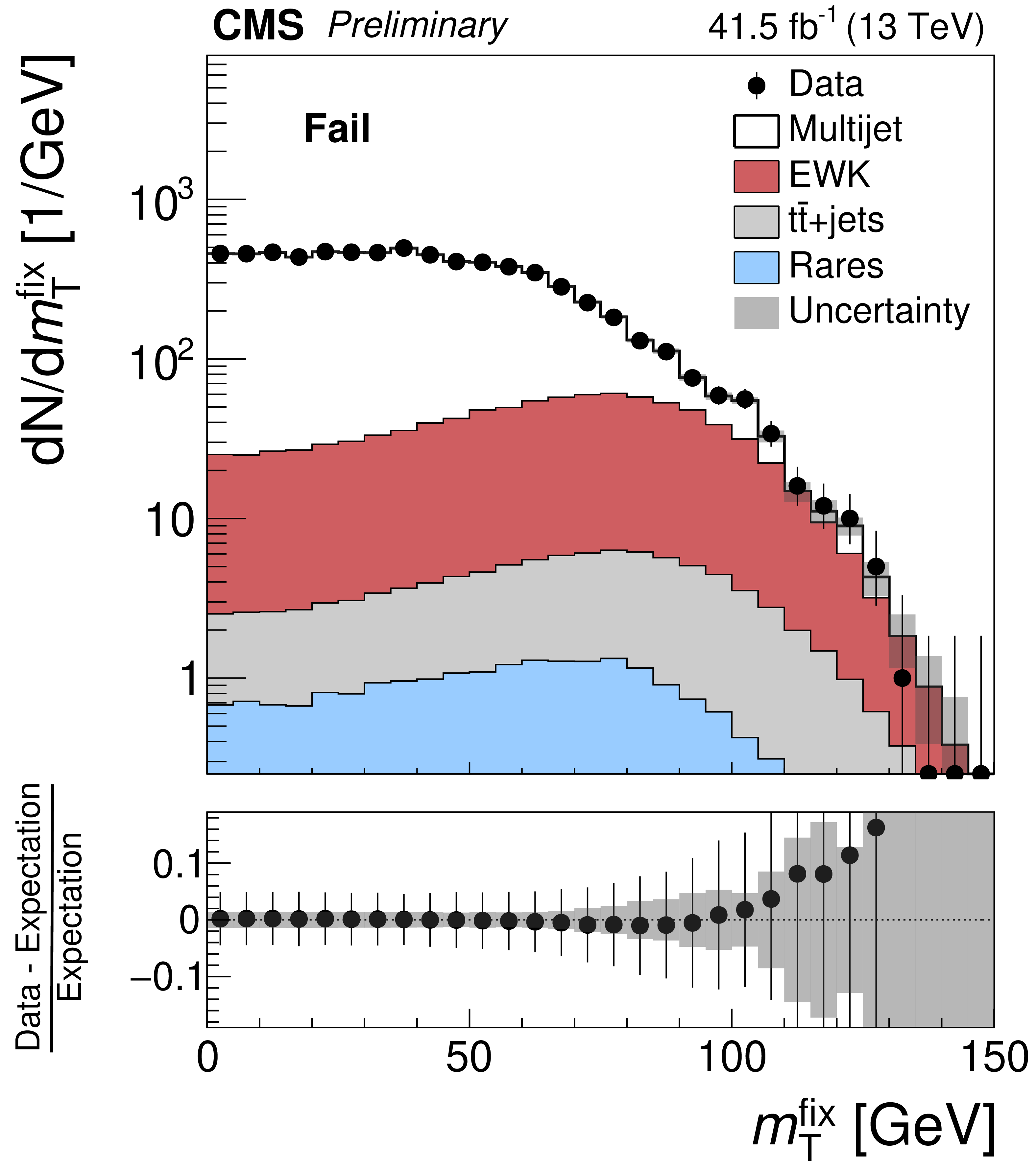
Figure 4-b:
Distribution in $ {{m_{\mathrm {T}}} ^{{\text {fix}}}}$ for events containing an electron candidate of 25 $ < {p_{\mathrm {T}}} < $ 35 GeV in the ECAL barrel, which passes the relaxed, but fails the nominal selection. The "electroweak'' (EWK) background refers to the sum of W+jets, DY and diboson production. The "rare'' background is defined in the text. The data in the fail sample agrees with the sum of multijet, EWK, $ {{\mathrm{t}} {\mathrm{\bar{t}}}}$+jets, and "rare'' backgrounds by construction, as the number of multijet events in the fail sample is computed by the subtracting the sum of EWK, $ {{\mathrm{t}} {\mathrm{\bar{t}}}}$+jets, and "rare'' background contributions from the data. The FF contribution is derived separately for each era: this figure shows, as an example, the results obtained with the 2017 data set. The uncertainty band represents the uncertainty after the fit has been performed. |
png pdf |
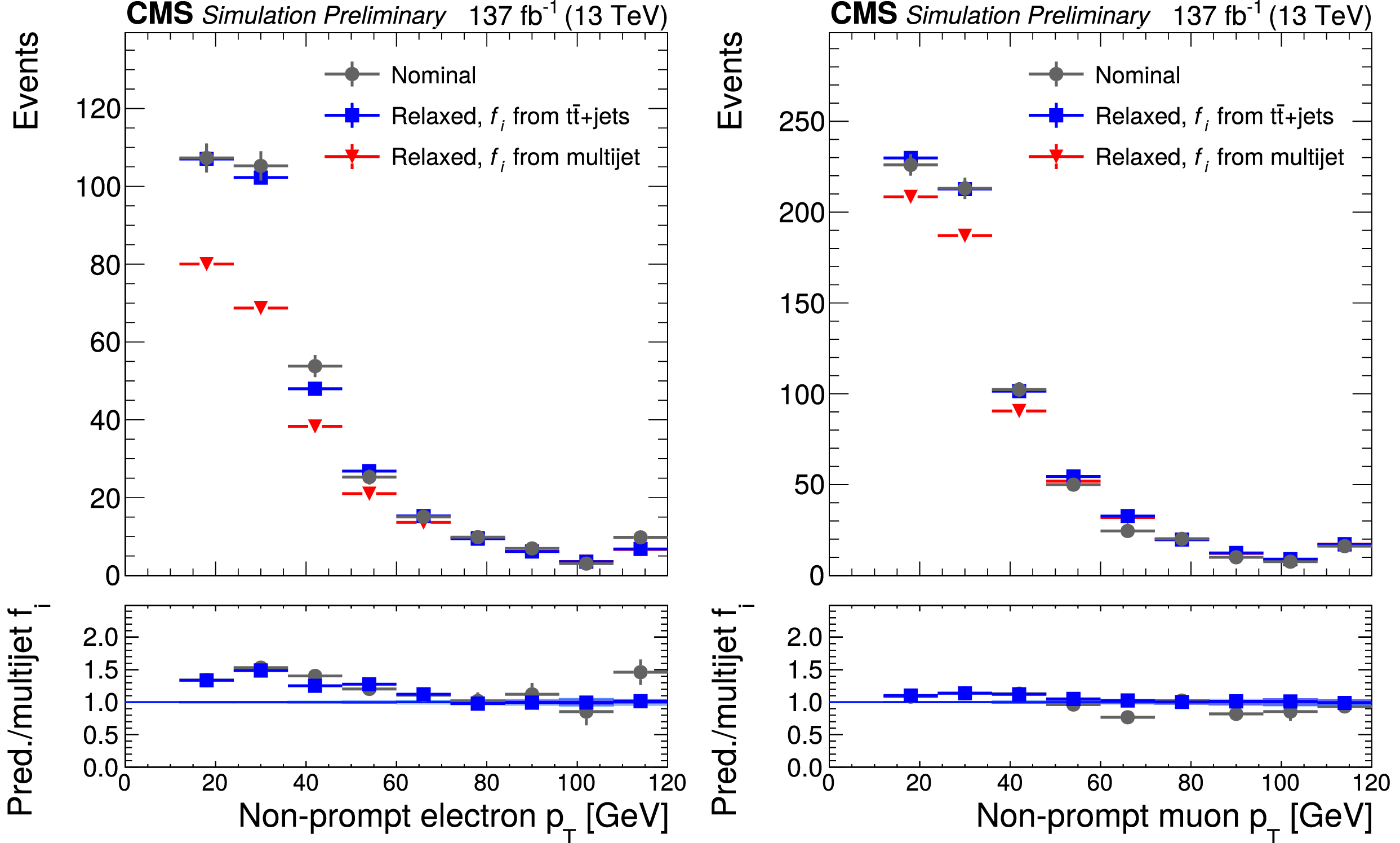
Figure 5:
Distributions in ${p_{\mathrm {T}}}$ of non-prompt (left) electrons and (right) muons in simulated $ {{\mathrm{t}} {\mathrm{\bar{t}}}}$+jets events, for the three cases "nominal'', "relaxed, $f_{i}$ from $ {{\mathrm{t}} {\mathrm{\bar{t}}}}$+jets'', and "relaxed, $f_{i}$ from multijet'' discussed in text. The figure illustrates that a non-closure correction needs to be applied to the probabilities $f_{i}$ measured for electrons in data, while no such correction is needed for muons. |

png pdf |
Figure 5-a:
Distribution in ${p_{\mathrm {T}}}$ of non-prompt electrons in simulated $ {{\mathrm{t}} {\mathrm{\bar{t}}}}$+jets events, for the three cases "nominal'', "relaxed, $f_{i}$ from $ {{\mathrm{t}} {\mathrm{\bar{t}}}}$+jets'', and "relaxed, $f_{i}$ from multijet'' discussed in text. The figure illustrates that a non-closure correction needs to be applied to the probabilities $f_{i}$ measured for electrons in data, while no such correction is needed for muons. |

png pdf |
Figure 5-b:
Distribution in ${p_{\mathrm {T}}}$ of non-prompt muons in simulated $ {{\mathrm{t}} {\mathrm{\bar{t}}}}$+jets events, for the three cases "nominal'', "relaxed, $f_{i}$ from $ {{\mathrm{t}} {\mathrm{\bar{t}}}}$+jets'', and "relaxed, $f_{i}$ from multijet'' discussed in text. The figure illustrates that a non-closure correction needs to be applied to the probabilities $f_{i}$ measured for electrons in data, while no such correction is needed for muons. |
png pdf |
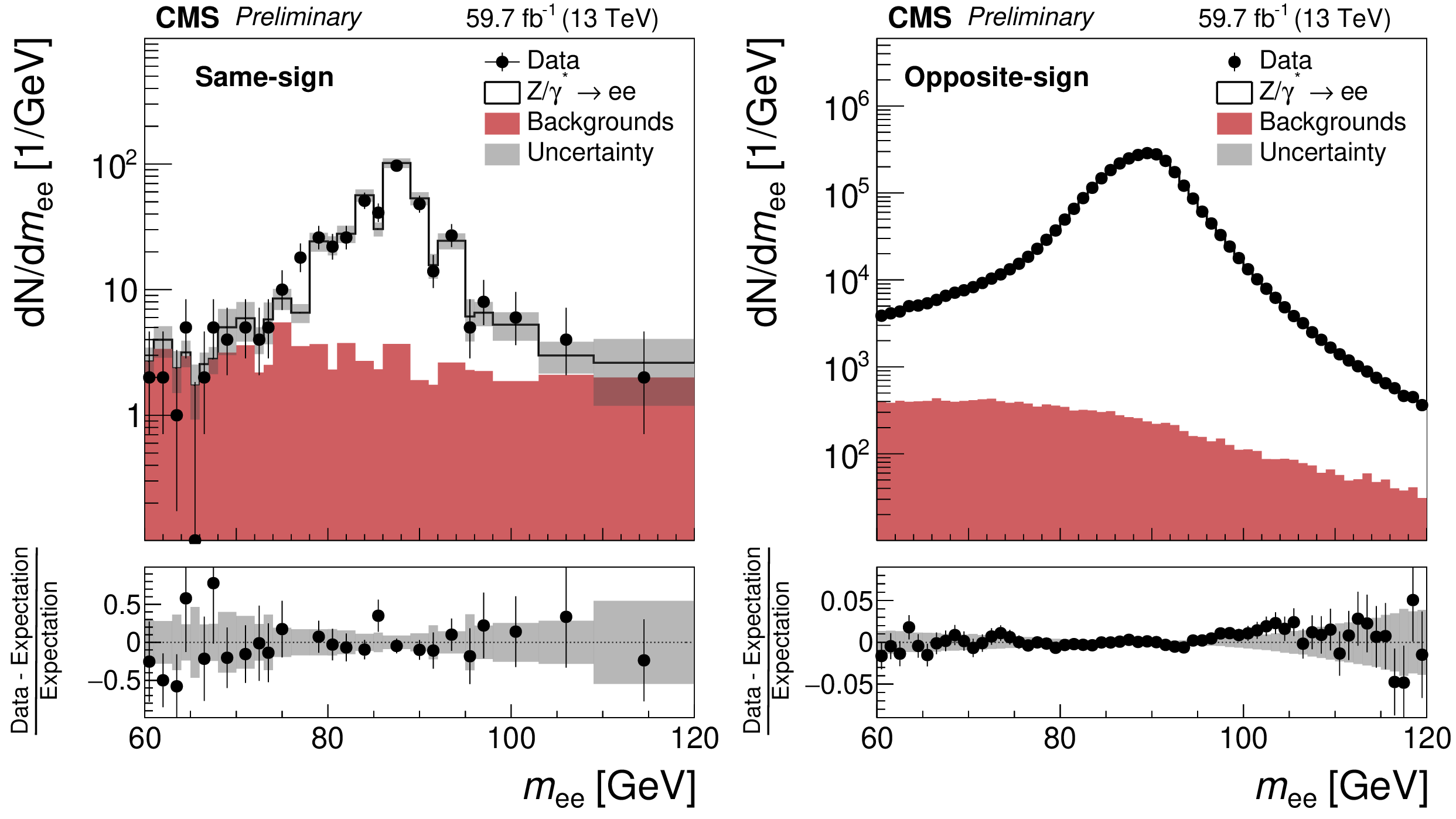
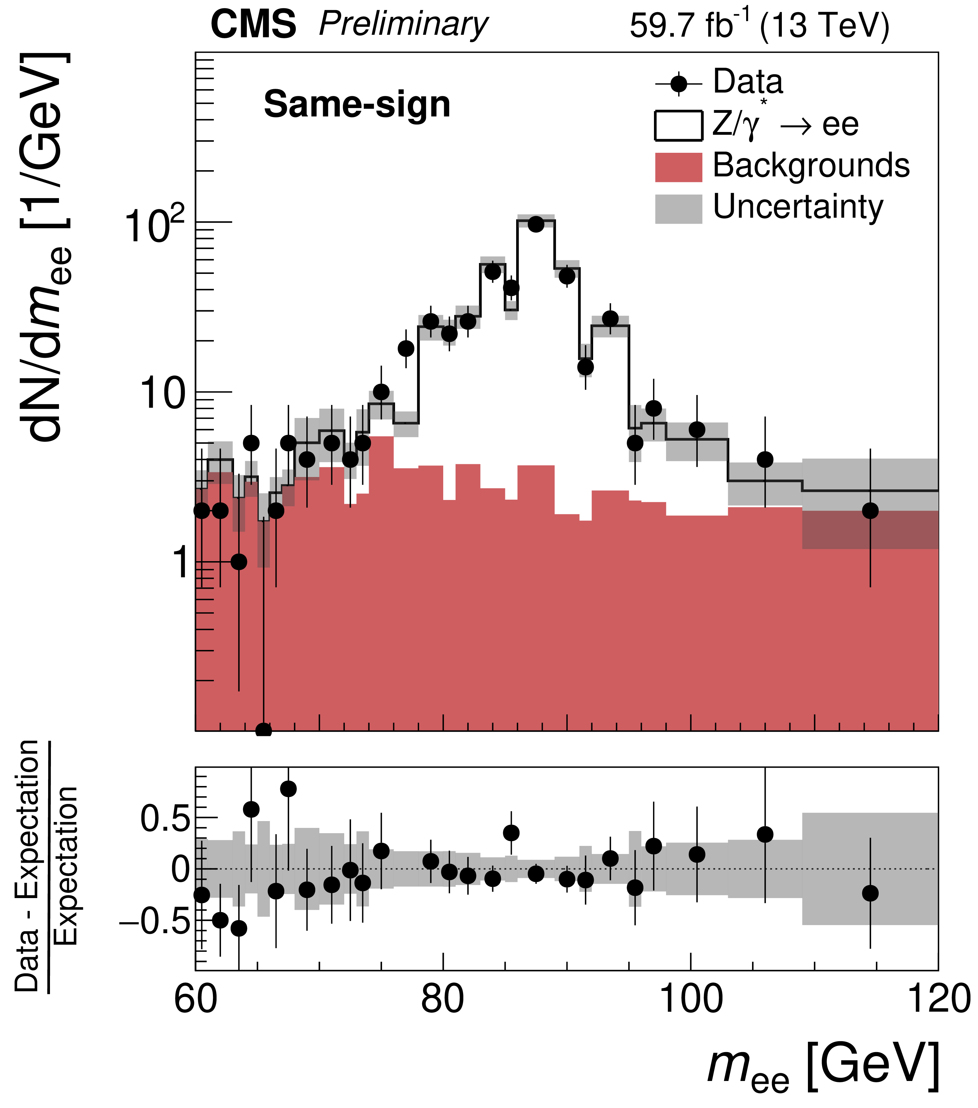
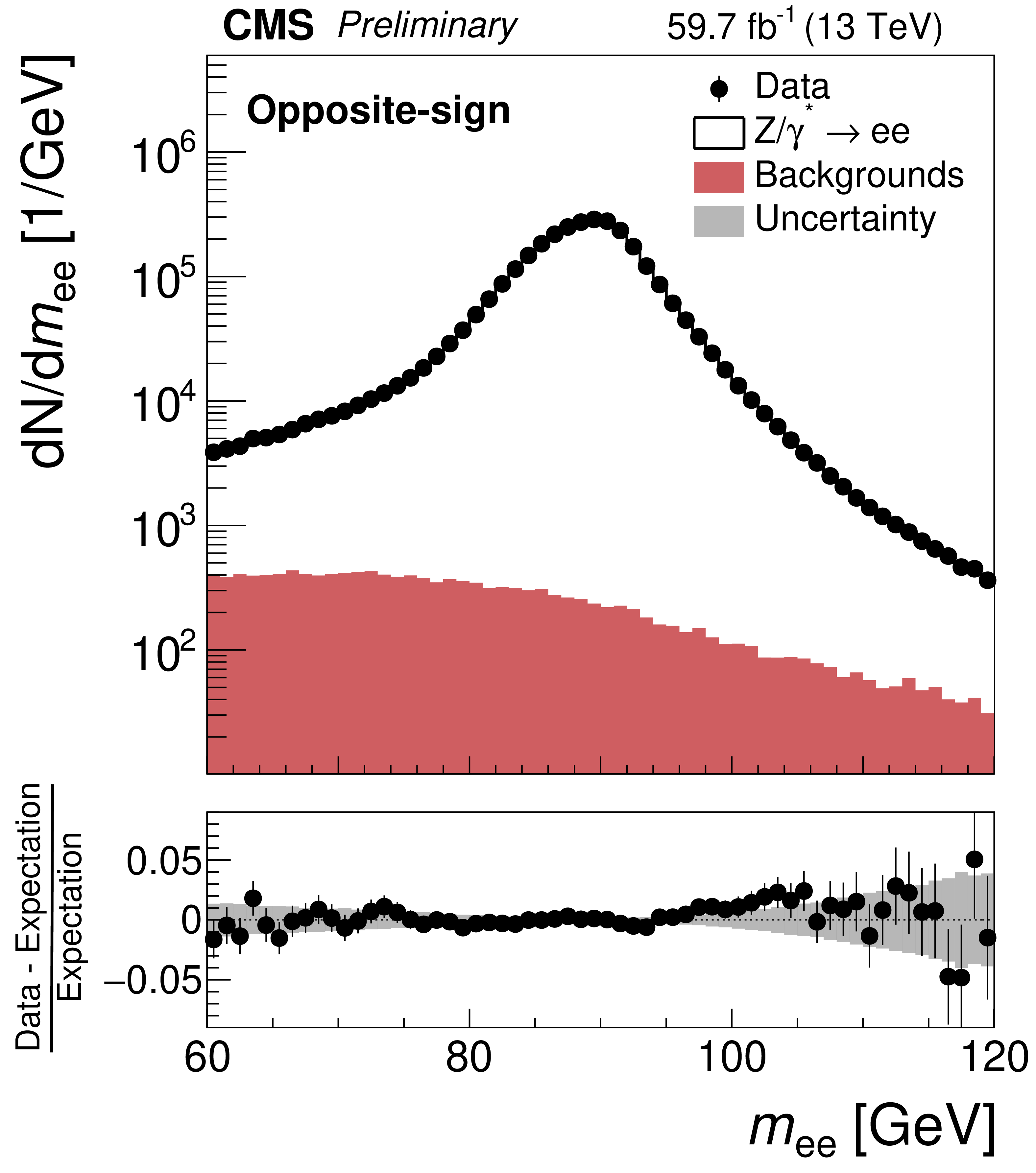
Figure 6:
Distributions in $m_{\mathrm{e} \mathrm{e}}$ for electron pairs of (left) SS and (right) OS charge in $ {{\mathrm{Z} /\gamma ^{*}} \to \mathrm{e} \mathrm{e}}$ candidate events in which both electrons are in the ECAL barrel and have transverse momenta within the range 25 $ < {p_{\mathrm {T}}} < $ 50 GeV, for data recorded in 2018 compared to the expectation. Uncertainties shown include statistical uncertainties. |
png pdf |
Figure 6-a:
Distribution in $m_{\mathrm{e} \mathrm{e}}$ for electron pairs of SS charge in $ {{\mathrm{Z} /\gamma ^{*}} \to \mathrm{e} \mathrm{e}}$ candidate events in which both electrons are in the ECAL barrel and have transverse momenta within the range 25 $ < {p_{\mathrm {T}}} < $ 50 GeV, for data recorded in 2018 compared to the expectation. Uncertainties shown include statistical uncertainties. |
png pdf |
Figure 6-b:
Distribution in $m_{\mathrm{e} \mathrm{e}}$ for electron pairs of OS charge in $ {{\mathrm{Z} /\gamma ^{*}} \to \mathrm{e} \mathrm{e}}$ candidate events in which both electrons are in the ECAL barrel and have transverse momenta within the range 25 $ < {p_{\mathrm {T}}} < $ 50 GeV, for data recorded in 2018 compared to the expectation. Uncertainties shown include statistical uncertainties. |
png pdf |
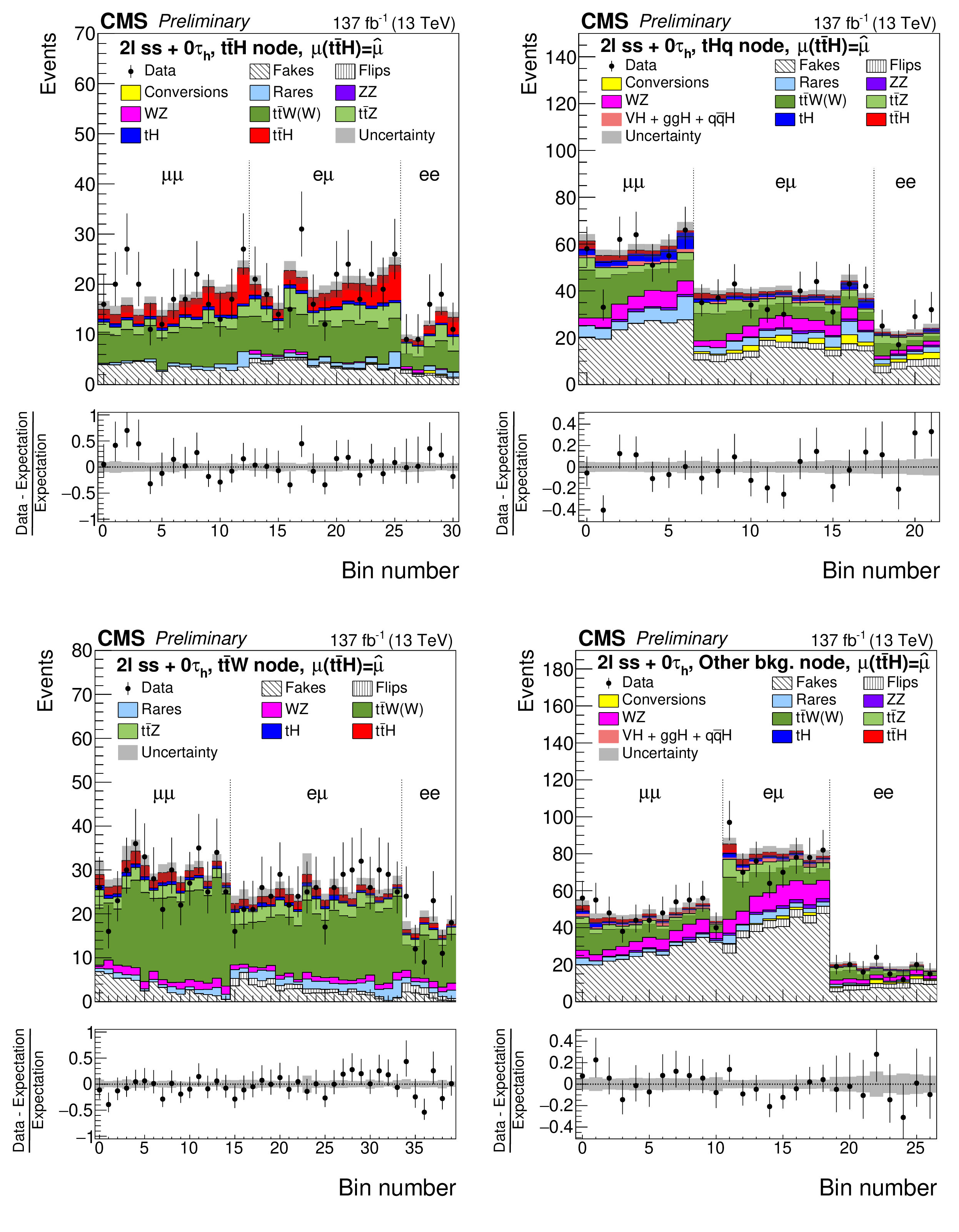
Figure 7:
Distributions in the activation value of the ANN output node with the highest activation value for events selected in the 2${\ell}$+0${\tau _{\mathrm {h}}}$ channel and classified as $ {{\mathrm{t}} {\mathrm{\bar{t}}} {\mathrm{H}}}$ signal (upper left), $ {{\mathrm{t}} {\mathrm{H}}}$ signal (upper right), $ {{\mathrm{t}} {\mathrm{\bar{t}}}\mathrm{W}}$ background (lower left), and other background (lower right). The distributions expected for the $ {{\mathrm{t}} {\mathrm{\bar{t}}} {\mathrm{H}}}$ and $ {{\mathrm{t}} {\mathrm{H}}}$ signals and for background processes are shown for the values of the POI and of the nuisance parameters obtained from the ML fit. The best-fit value of the $ {{\mathrm{t}} {\mathrm{\bar{t}}} {\mathrm{H}}}$ and $ {{\mathrm{t}} {\mathrm{H}}}$ production rates amounts to $ {\hat{\mu}}_{{{\mathrm{t}} {\mathrm{\bar{t}}} {\mathrm{H}}}} = $ 0.92 and $ {\hat{\mu}}_{{{\mathrm{t}} {\mathrm{H}}}} = $ 5.7 times the rates expected in the SM. |
png pdf |
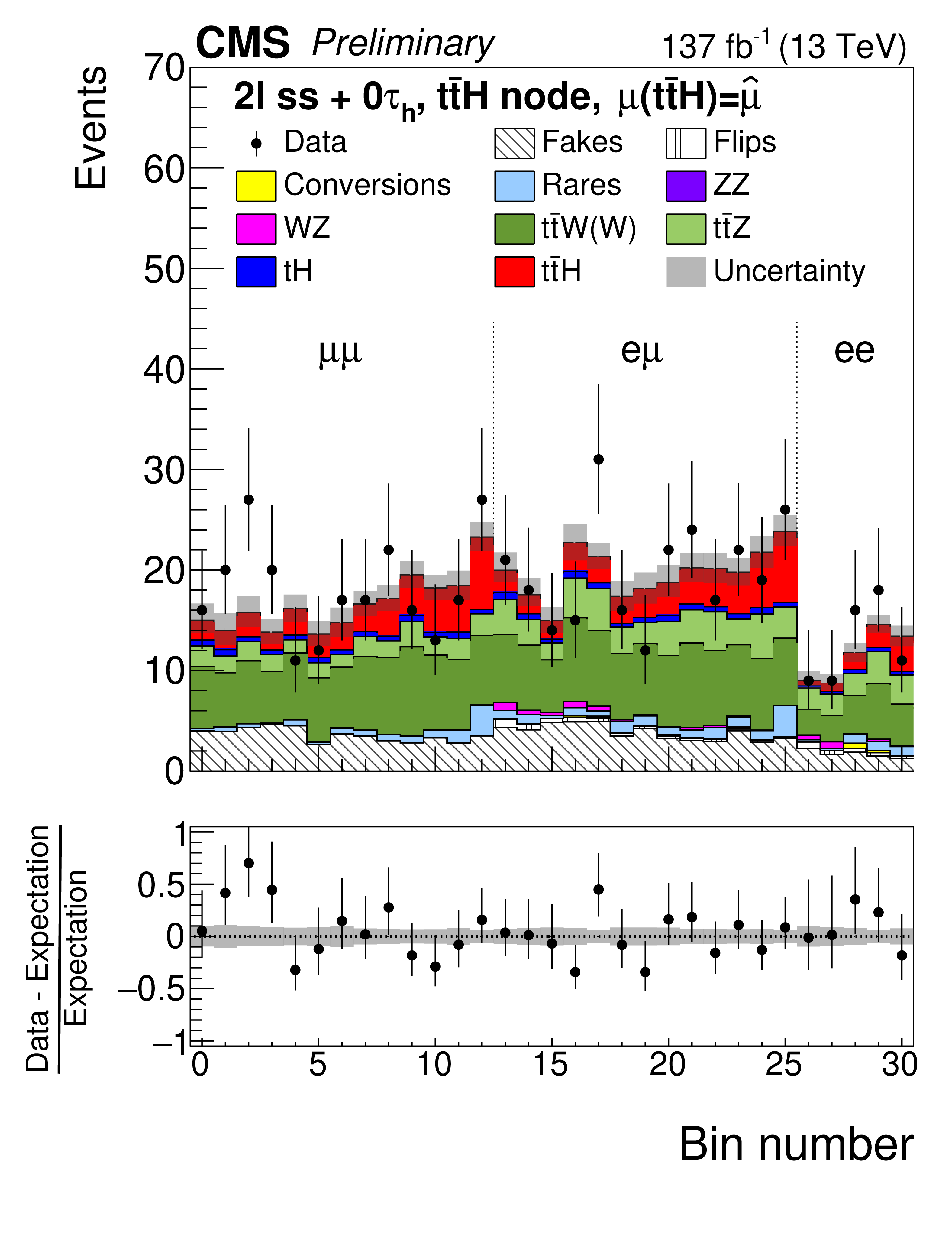
Figure 7-a:
Distribution in the activation value of the ANN output node with the highest activation value for events selected in the 2${\ell}$+0${\tau _{\mathrm {h}}}$ channel and classified as $ {{\mathrm{t}} {\mathrm{\bar{t}}} {\mathrm{H}}}$ signal. The distributions expected for the $ {{\mathrm{t}} {\mathrm{\bar{t}}} {\mathrm{H}}}$ and $ {{\mathrm{t}} {\mathrm{H}}}$ signals and for background processes are shown for the values of the POI and of the nuisance parameters obtained from the ML fit. The best-fit value of the $ {{\mathrm{t}} {\mathrm{\bar{t}}} {\mathrm{H}}}$ and $ {{\mathrm{t}} {\mathrm{H}}}$ production rates amounts to $ {\hat{\mu}}_{{{\mathrm{t}} {\mathrm{\bar{t}}} {\mathrm{H}}}} = $ 0.92 and $ {\hat{\mu}}_{{{\mathrm{t}} {\mathrm{H}}}} = $ 5.7 times the rates expected in the SM. |
png pdf |
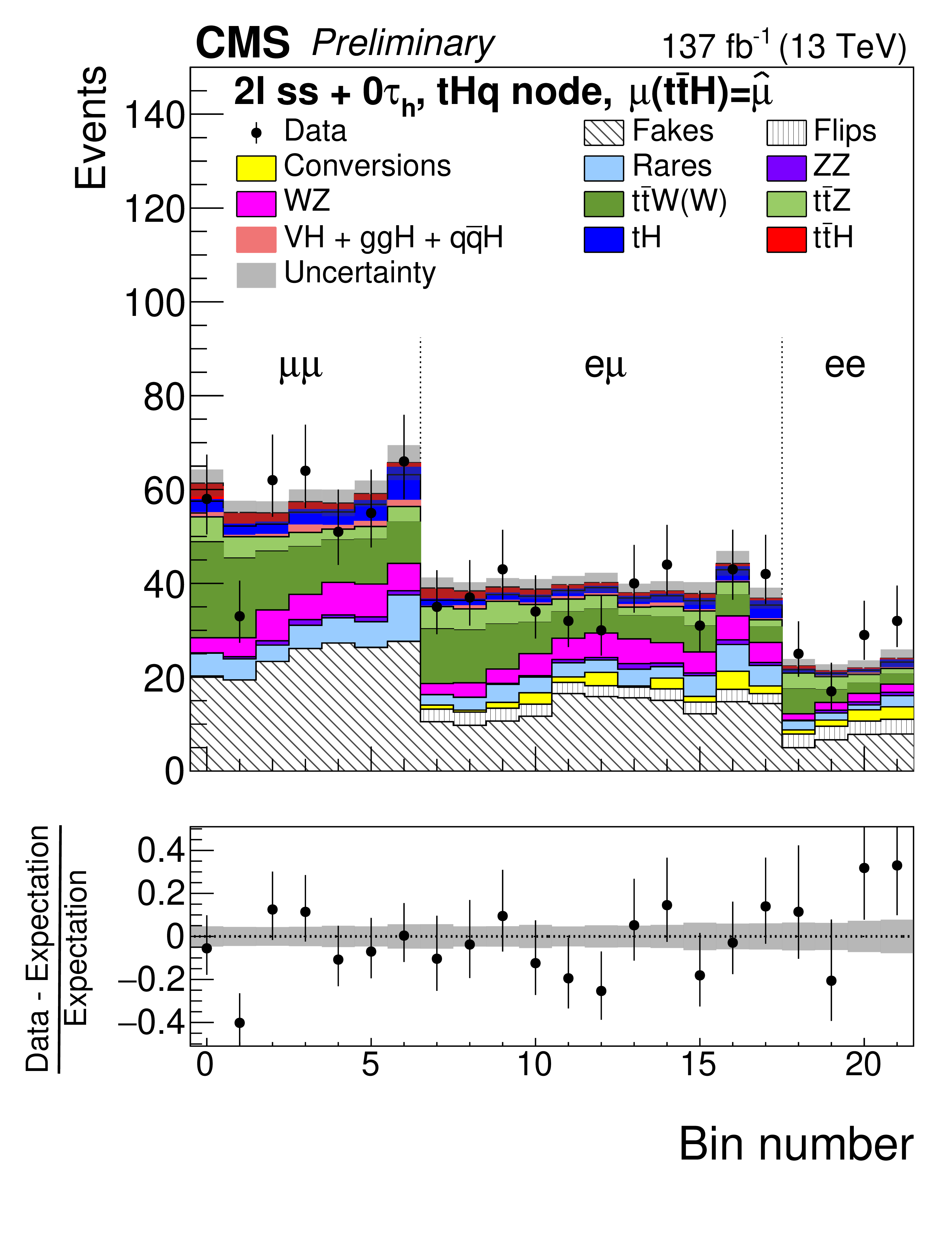
Figure 7-b:
Distribution in the activation value of the ANN output node with the highest activation value for events selected in the 2${\ell}$+0${\tau _{\mathrm {h}}}$ channel and classified as $ {{\mathrm{t}} {\mathrm{H}}}$ signal. The distributions expected for the $ {{\mathrm{t}} {\mathrm{\bar{t}}} {\mathrm{H}}}$ and $ {{\mathrm{t}} {\mathrm{H}}}$ signals and for background processes are shown for the values of the POI and of the nuisance parameters obtained from the ML fit. The best-fit value of the $ {{\mathrm{t}} {\mathrm{\bar{t}}} {\mathrm{H}}}$ and $ {{\mathrm{t}} {\mathrm{H}}}$ production rates amounts to $ {\hat{\mu}}_{{{\mathrm{t}} {\mathrm{\bar{t}}} {\mathrm{H}}}} = $ 0.92 and $ {\hat{\mu}}_{{{\mathrm{t}} {\mathrm{H}}}} = $ 5.7 times the rates expected in the SM. |
png pdf |
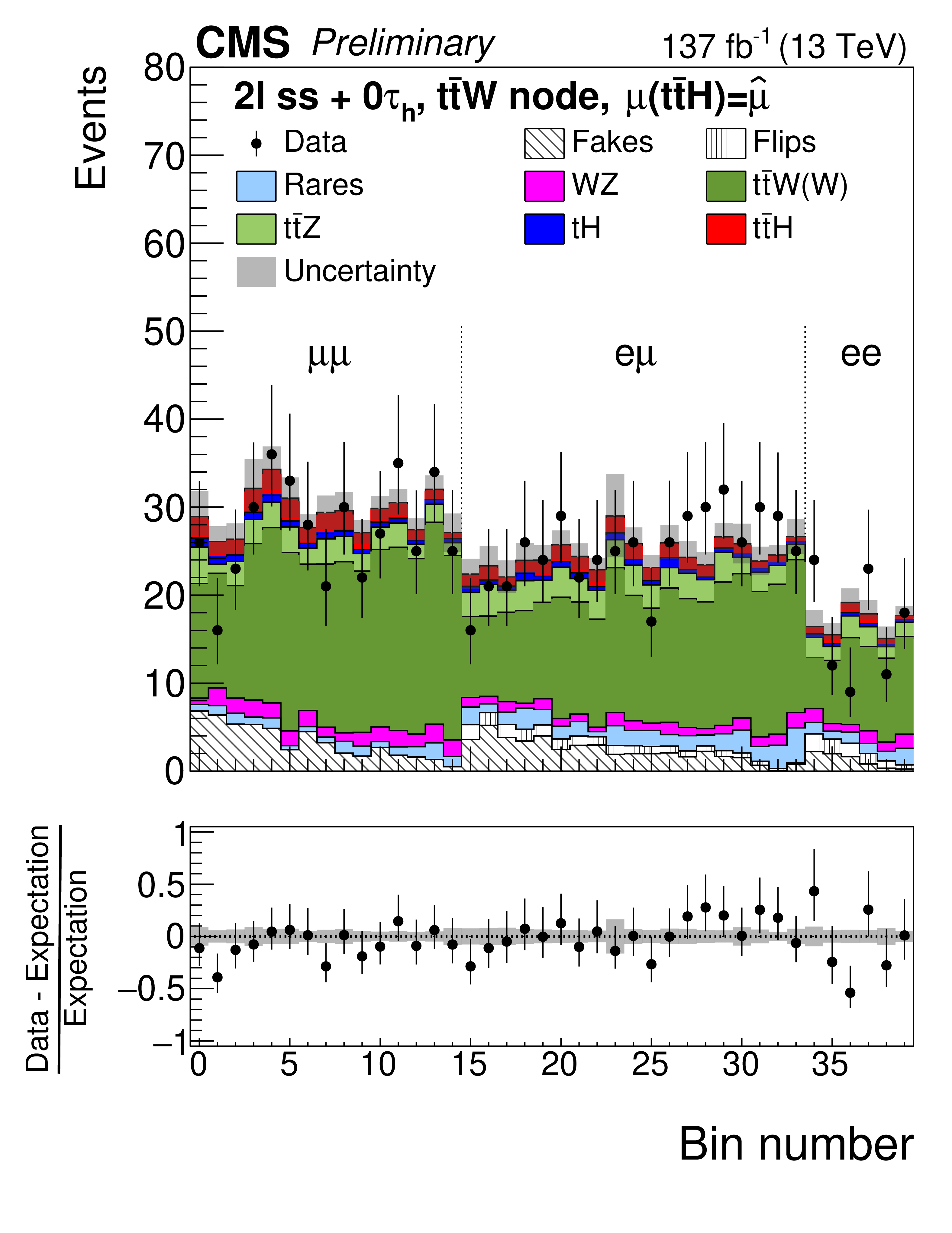
Figure 7-c:
Distribution in the activation value of the ANN output node with the highest activation value for events selected in the 2${\ell}$+0${\tau _{\mathrm {h}}}$ channel and classified as $ {{\mathrm{t}} {\mathrm{\bar{t}}}\mathrm{W}}$ background. The distributions expected for the $ {{\mathrm{t}} {\mathrm{\bar{t}}} {\mathrm{H}}}$ and $ {{\mathrm{t}} {\mathrm{H}}}$ signals and for background processes are shown for the values of the POI and of the nuisance parameters obtained from the ML fit. The best-fit value of the $ {{\mathrm{t}} {\mathrm{\bar{t}}} {\mathrm{H}}}$ and $ {{\mathrm{t}} {\mathrm{H}}}$ production rates amounts to $ {\hat{\mu}}_{{{\mathrm{t}} {\mathrm{\bar{t}}} {\mathrm{H}}}} = $ 0.92 and $ {\hat{\mu}}_{{{\mathrm{t}} {\mathrm{H}}}} = $ 5.7 times the rates expected in the SM. |
png pdf |
Figure 7-d:
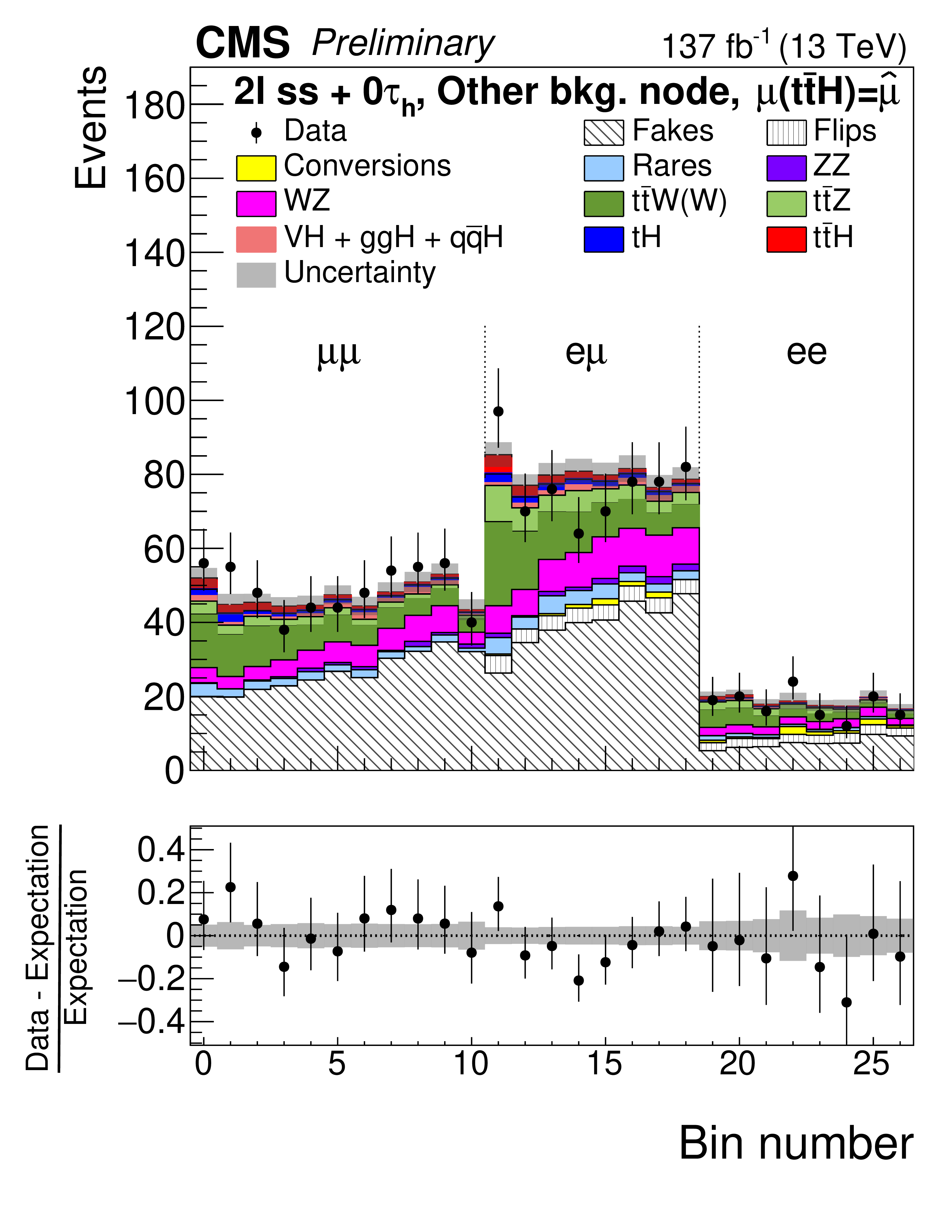
Distribution in the activation value of the ANN output node with the highest activation value for events selected in the 2${\ell}$+0${\tau _{\mathrm {h}}}$ channel and classified as other backgrounds. The distributions expected for the $ {{\mathrm{t}} {\mathrm{\bar{t}}} {\mathrm{H}}}$ and $ {{\mathrm{t}} {\mathrm{H}}}$ signals and for background processes are shown for the values of the POI and of the nuisance parameters obtained from the ML fit. The best-fit value of the $ {{\mathrm{t}} {\mathrm{\bar{t}}} {\mathrm{H}}}$ and $ {{\mathrm{t}} {\mathrm{H}}}$ production rates amounts to $ {\hat{\mu}}_{{{\mathrm{t}} {\mathrm{\bar{t}}} {\mathrm{H}}}} = $ 0.92 and $ {\hat{\mu}}_{{{\mathrm{t}} {\mathrm{H}}}} = $ 5.7 times the rates expected in the SM. |
png pdf |
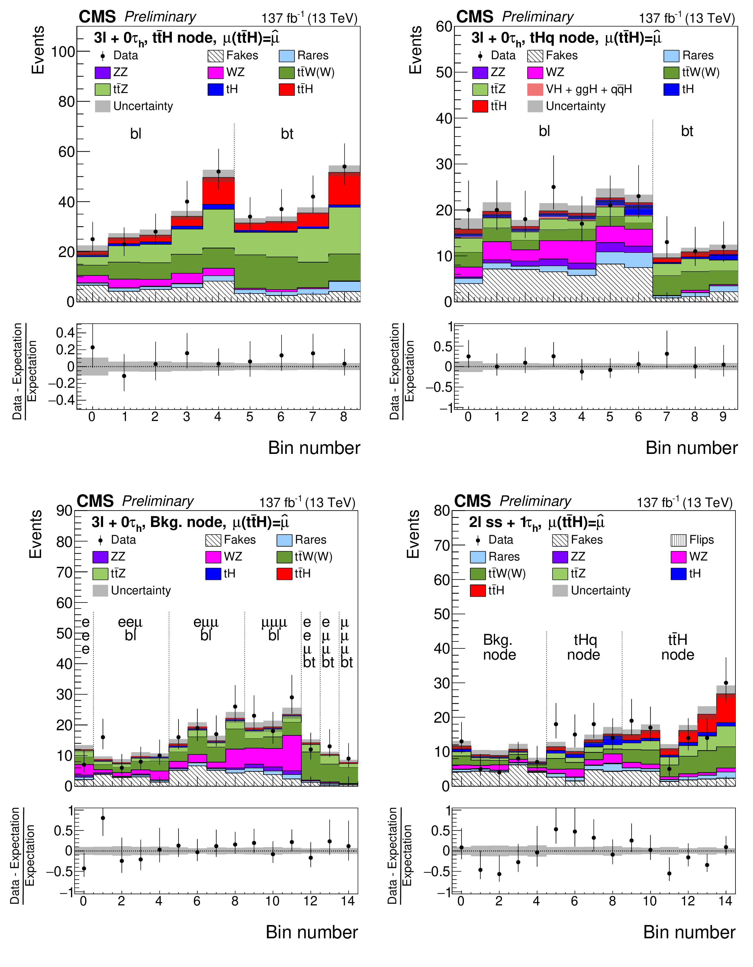
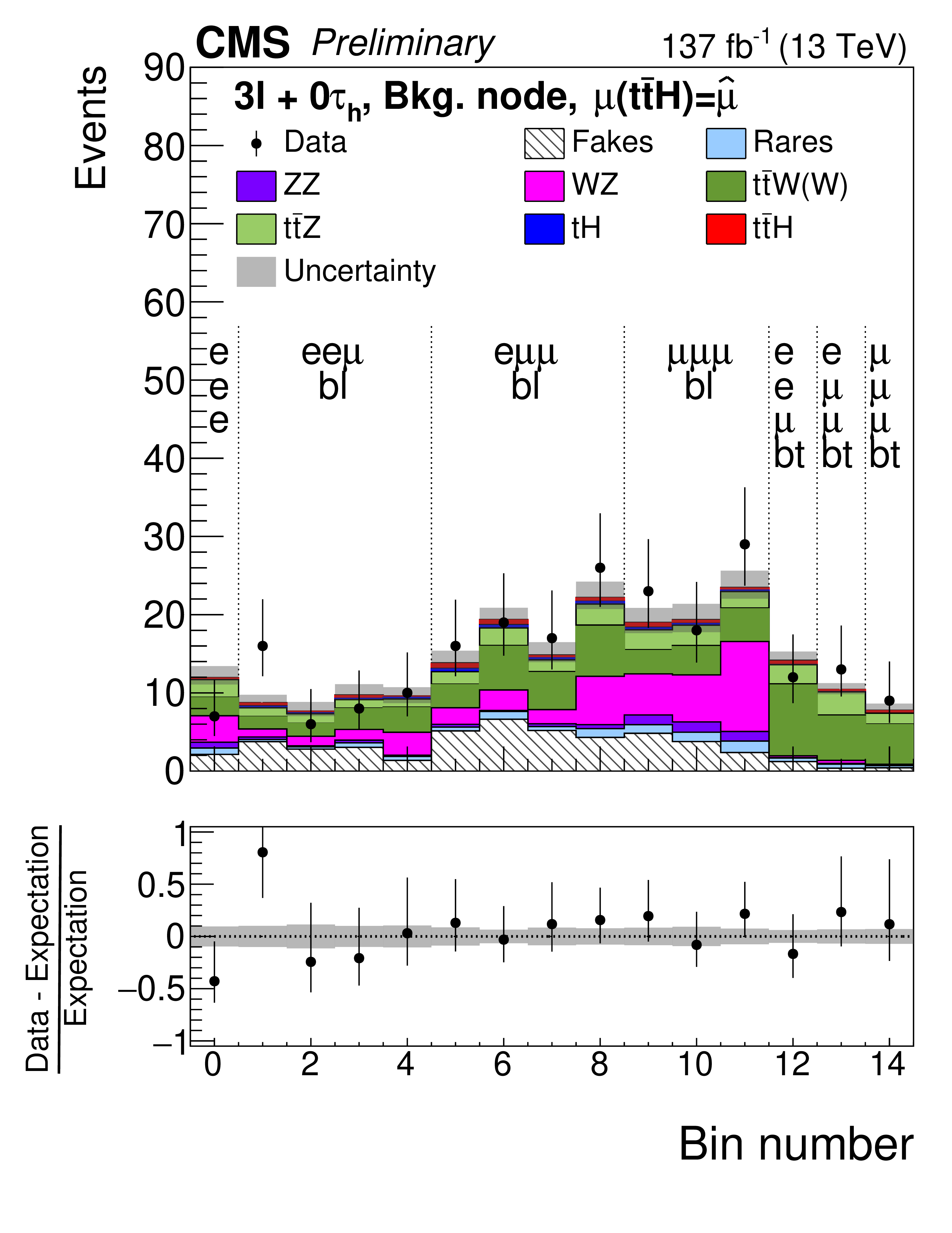
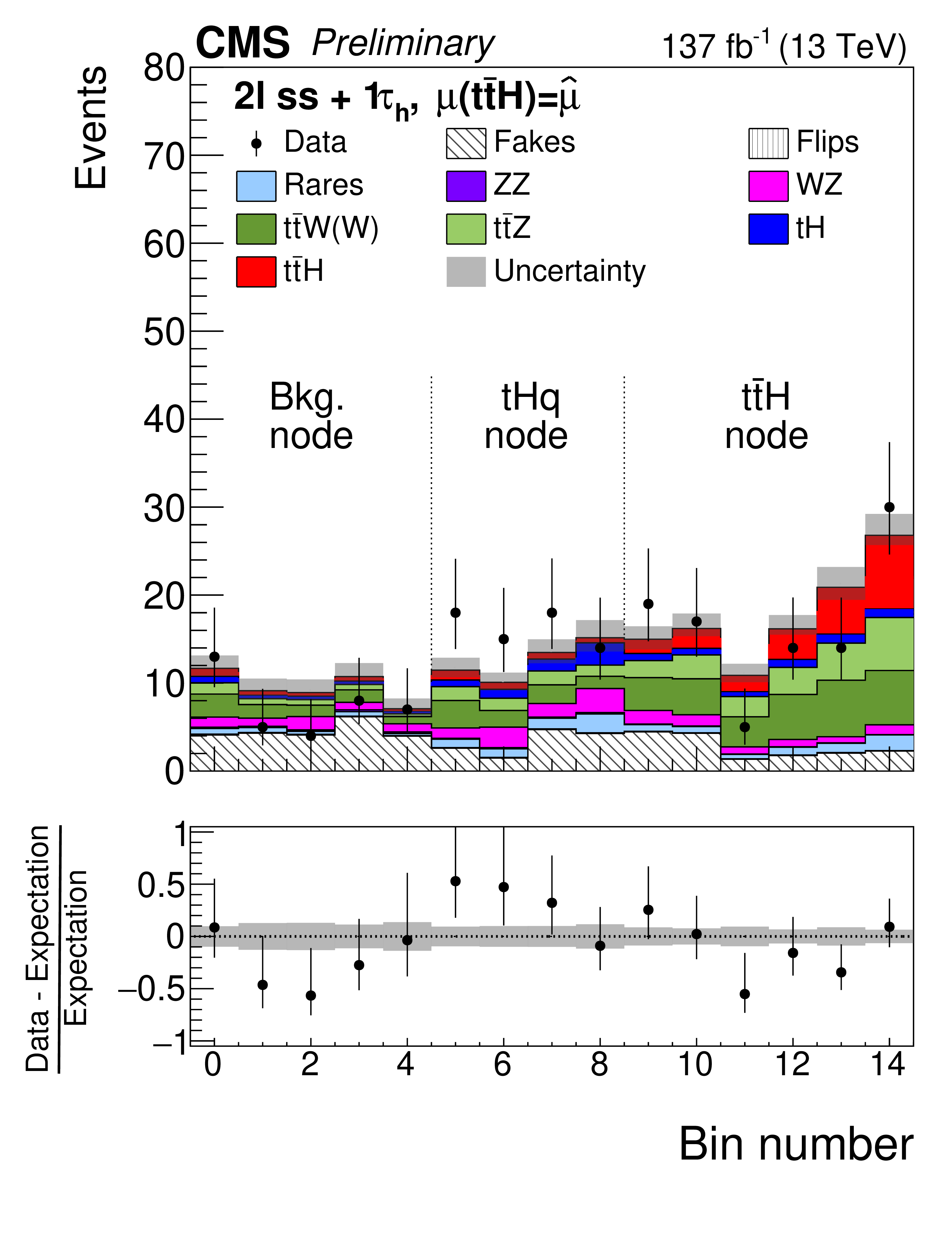
Figure 8:
Distributions in the activation value of the ANN output node with the highest activation value for events selected in the 3${\ell}$+0${\tau _{\mathrm {h}}}$ channel and classified as $ {{\mathrm{t}} {\mathrm{\bar{t}}} {\mathrm{H}}}$ signal (upper left), $ {{\mathrm{t}} {\mathrm{H}}}$ signal (upper right), and background (lower left), and for events selected in the 2${\ell}$ ss+1${\tau _{\mathrm {h}}}$ channel (lower right). In case of the 2${\ell}$ ss+1${\tau _{\mathrm {h}}}$ channel, the activation value of the ANN output nodes for $ {{\mathrm{t}} {\mathrm{\bar{t}}} {\mathrm{H}}}$ signal, $ {{\mathrm{t}} {\mathrm{H}}}$ signal, and background are shown together in a single histogram, concatenating histogram bins as appropriate and enumerating the bins by a monotonously increasing number. The distributions expected for the $ {{\mathrm{t}} {\mathrm{\bar{t}}} {\mathrm{H}}}$ and $ {{\mathrm{t}} {\mathrm{H}}}$ signals and for background processes are shown for the values of the POI and of the nuisance parameters obtained from the ML fit. The best-fit value of the $ {{\mathrm{t}} {\mathrm{\bar{t}}} {\mathrm{H}}}$ and $ {{\mathrm{t}} {\mathrm{H}}}$ production rates amounts to $ {\hat{\mu}}_{{{\mathrm{t}} {\mathrm{\bar{t}}} {\mathrm{H}}}} = $ 0.92 and $ {\hat{\mu}}_{{{\mathrm{t}} {\mathrm{H}}}} = $ 5.7 times the rates expected in the SM. |
png pdf |
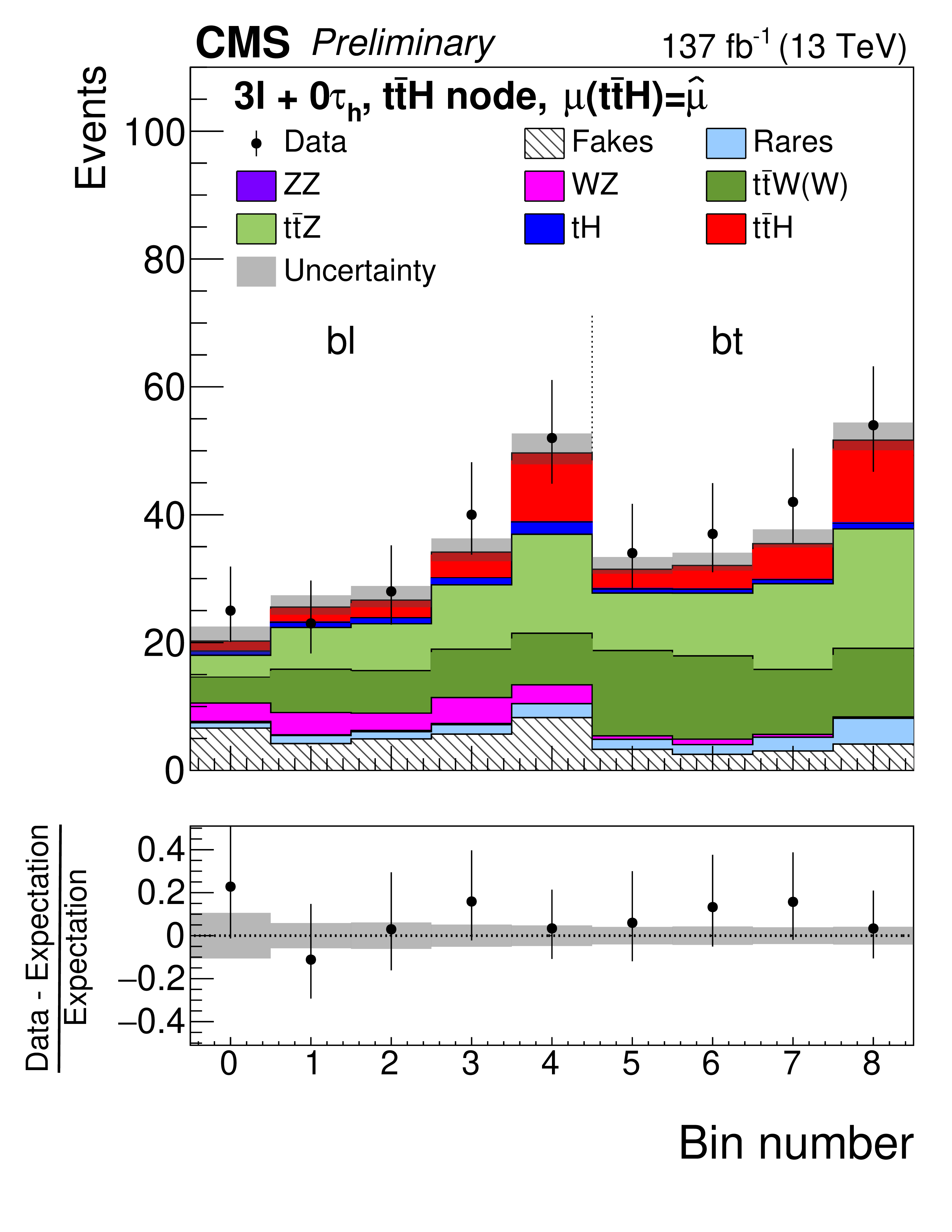
Figure 8-a:
Distribution in the activation value of the ANN output node with the highest activation value for events selected in the 3${\ell}$+0${\tau _{\mathrm {h}}}$ channel and classified as $ {{\mathrm{t}} {\mathrm{\bar{t}}} {\mathrm{H}}}$ signal. The distributions expected for the $ {{\mathrm{t}} {\mathrm{\bar{t}}} {\mathrm{H}}}$ and $ {{\mathrm{t}} {\mathrm{H}}}$ signals and for background processes are shown for the values of the POI and of the nuisance parameters obtained from the ML fit. The best-fit value of the $ {{\mathrm{t}} {\mathrm{\bar{t}}} {\mathrm{H}}}$ and $ {{\mathrm{t}} {\mathrm{H}}}$ production rates amounts to $ {\hat{\mu}}_{{{\mathrm{t}} {\mathrm{\bar{t}}} {\mathrm{H}}}} = $ 0.92 and $ {\hat{\mu}}_{{{\mathrm{t}} {\mathrm{H}}}} = $ 5.7 times the rates expected in the SM. |
png pdf |
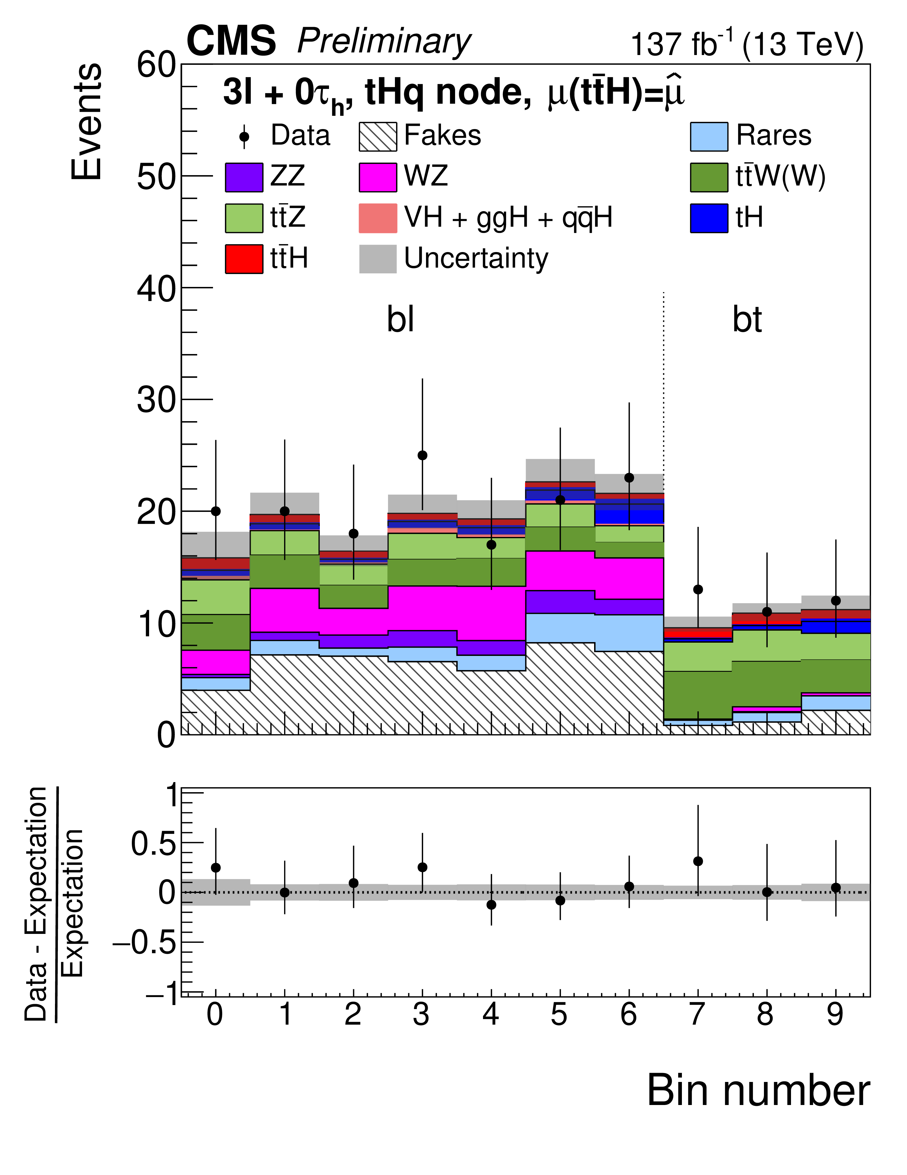
Figure 8-b:
Distribution in the activation value of the ANN output node with the highest activation value for events selected in the 3${\ell}$+0${\tau _{\mathrm {h}}}$ channel and classified as $ {{\mathrm{t}} {\mathrm{H}}}$ signal. The distributions expected for the $ {{\mathrm{t}} {\mathrm{\bar{t}}} {\mathrm{H}}}$ and $ {{\mathrm{t}} {\mathrm{H}}}$ signals and for background processes are shown for the values of the POI and of the nuisance parameters obtained from the ML fit. The best-fit value of the $ {{\mathrm{t}} {\mathrm{\bar{t}}} {\mathrm{H}}}$ and $ {{\mathrm{t}} {\mathrm{H}}}$ production rates amounts to $ {\hat{\mu}}_{{{\mathrm{t}} {\mathrm{\bar{t}}} {\mathrm{H}}}} = $ 0.92 and $ {\hat{\mu}}_{{{\mathrm{t}} {\mathrm{H}}}} = $ 5.7 times the rates expected in the SM. |
png pdf |
Figure 8-c:
Distribution in the activation value of the ANN output node with the highest activation value for events selected in the 3${\ell}$+0${\tau _{\mathrm {h}}}$ channel $ {{\mathrm{t}} {\mathrm{H}}}$ background. The distributions expected for the $ {{\mathrm{t}} {\mathrm{\bar{t}}} {\mathrm{H}}}$ and $ {{\mathrm{t}} {\mathrm{H}}}$ signals and for background processes are shown for the values of the POI and of the nuisance parameters obtained from the ML fit. The best-fit value of the $ {{\mathrm{t}} {\mathrm{\bar{t}}} {\mathrm{H}}}$ and $ {{\mathrm{t}} {\mathrm{H}}}$ production rates amounts to $ {\hat{\mu}}_{{{\mathrm{t}} {\mathrm{\bar{t}}} {\mathrm{H}}}} = $ 0.92 and $ {\hat{\mu}}_{{{\mathrm{t}} {\mathrm{H}}}} = $ 5.7 times the rates expected in the SM. |
png pdf |
Figure 8-d:
Distribution in the activation value of the ANN output node with the highest activation value for events selected in the 2${\ell}$ ss+1${\tau _{\mathrm {h}}}$ channel. The activation value of the ANN output nodes for $ {{\mathrm{t}} {\mathrm{\bar{t}}} {\mathrm{H}}}$ signal, $ {{\mathrm{t}} {\mathrm{H}}}$ signal, and background are shown together in a single histogram, concatenating histogram bins as appropriate and enumerating the bins by a monotonously increasing number. The distributions expected for the $ {{\mathrm{t}} {\mathrm{\bar{t}}} {\mathrm{H}}}$ and $ {{\mathrm{t}} {\mathrm{H}}}$ signals and for background processes are shown for the values of the POI and of the nuisance parameters obtained from the ML fit. The best-fit value of the $ {{\mathrm{t}} {\mathrm{\bar{t}}} {\mathrm{H}}}$ and $ {{\mathrm{t}} {\mathrm{H}}}$ production rates amounts to $ {\hat{\mu}}_{{{\mathrm{t}} {\mathrm{\bar{t}}} {\mathrm{H}}}} = $ 0.92 and $ {\hat{\mu}}_{{{\mathrm{t}} {\mathrm{H}}}} = $ 5.7 times the rates expected in the SM. |
png pdf |
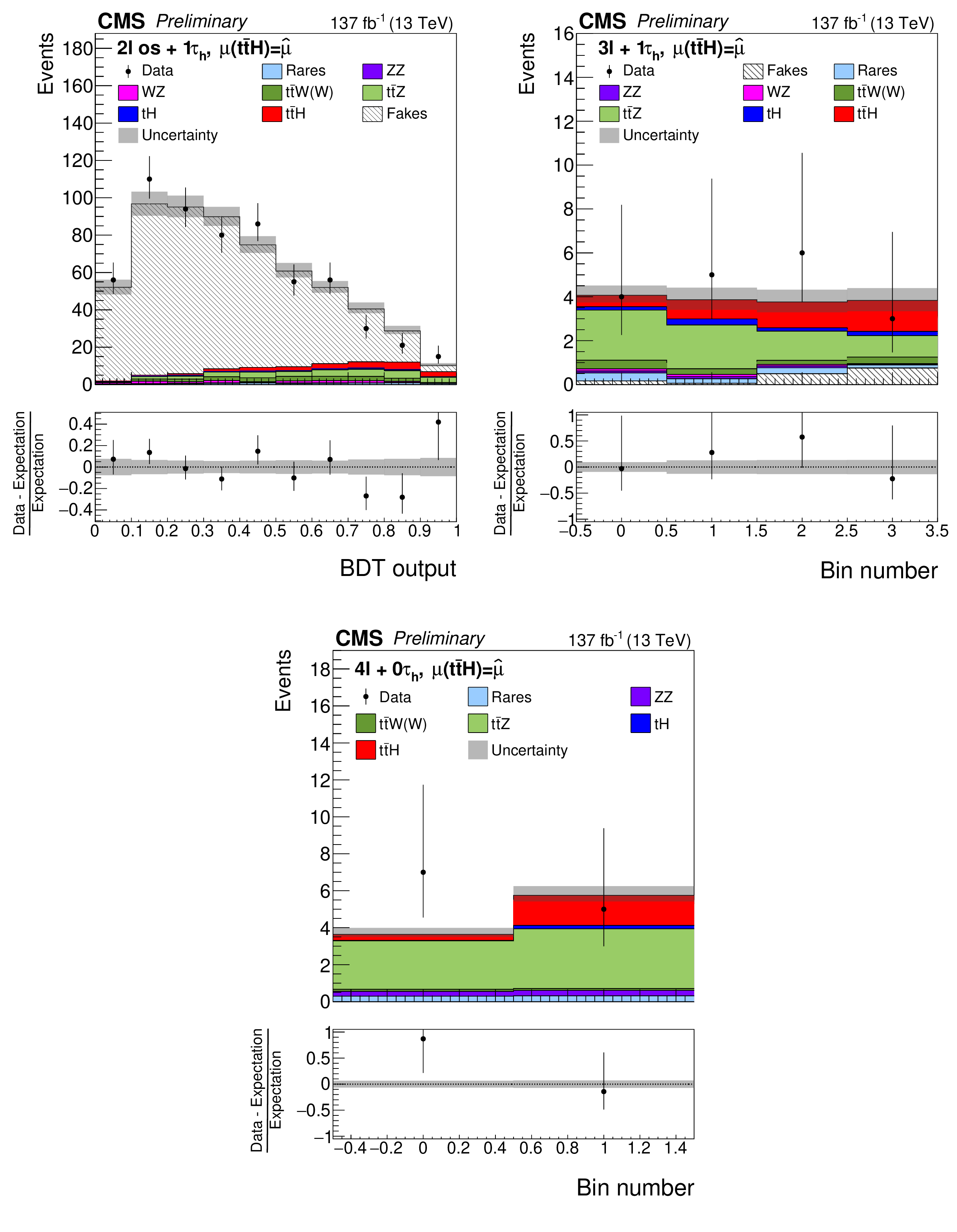
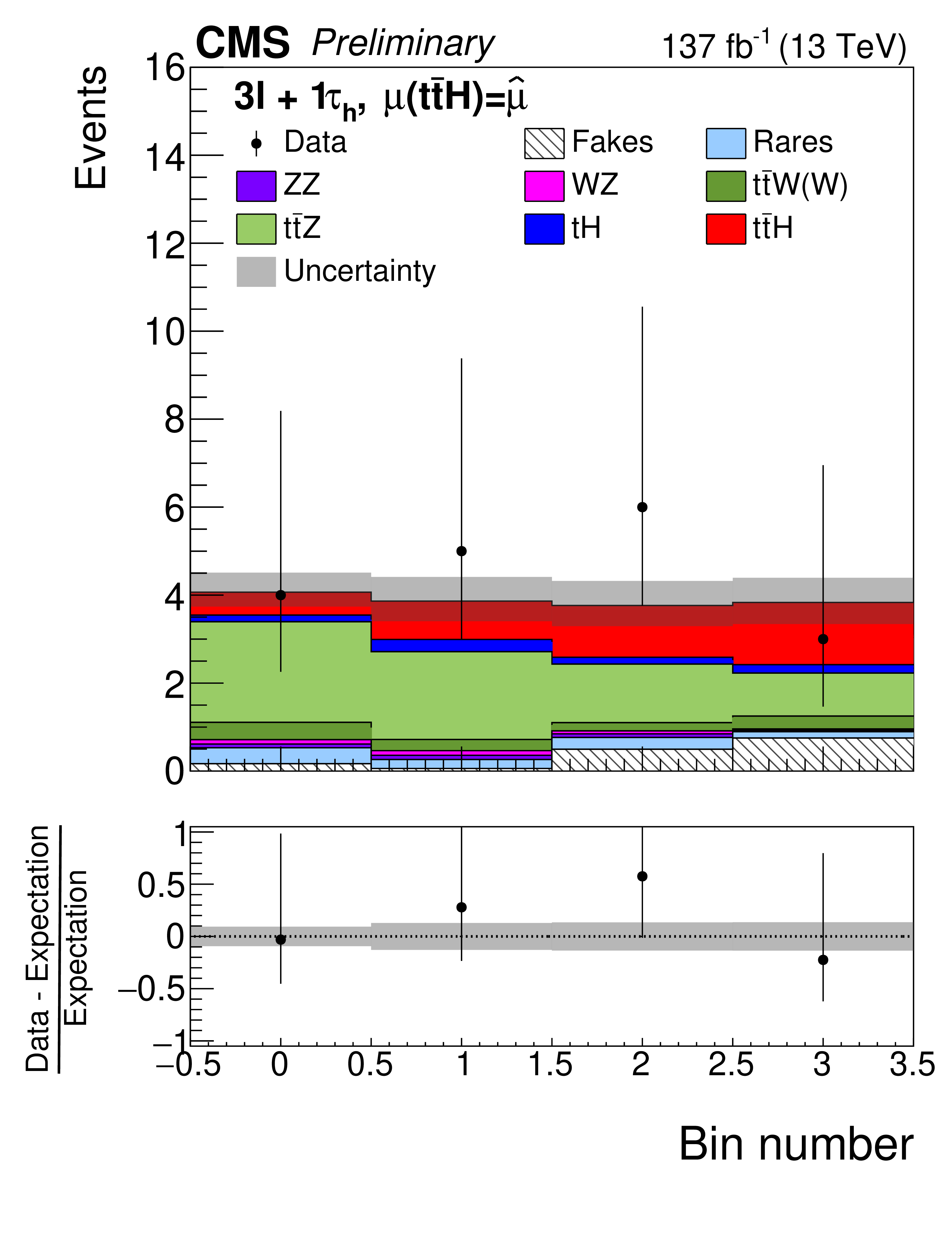
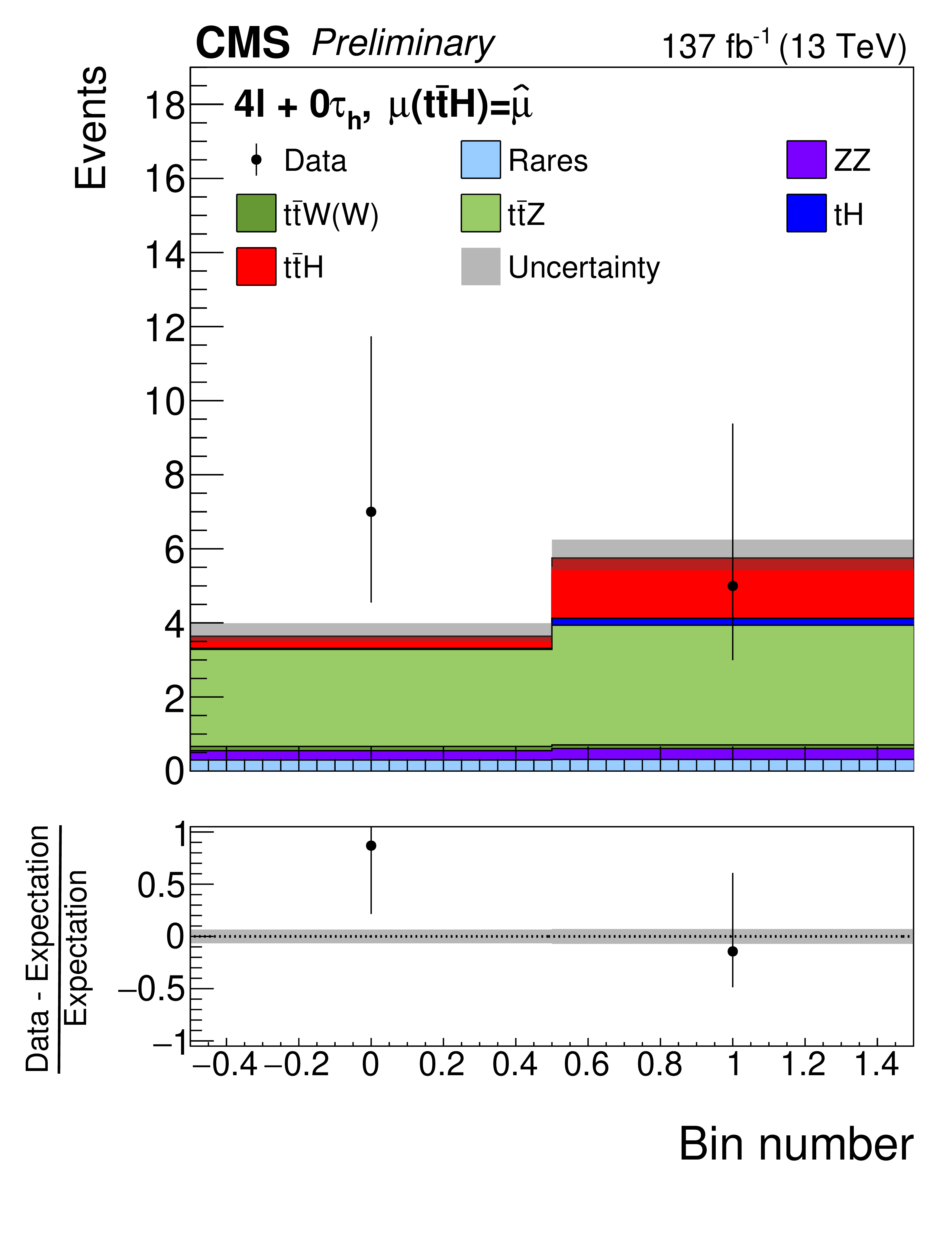
Figure 9:
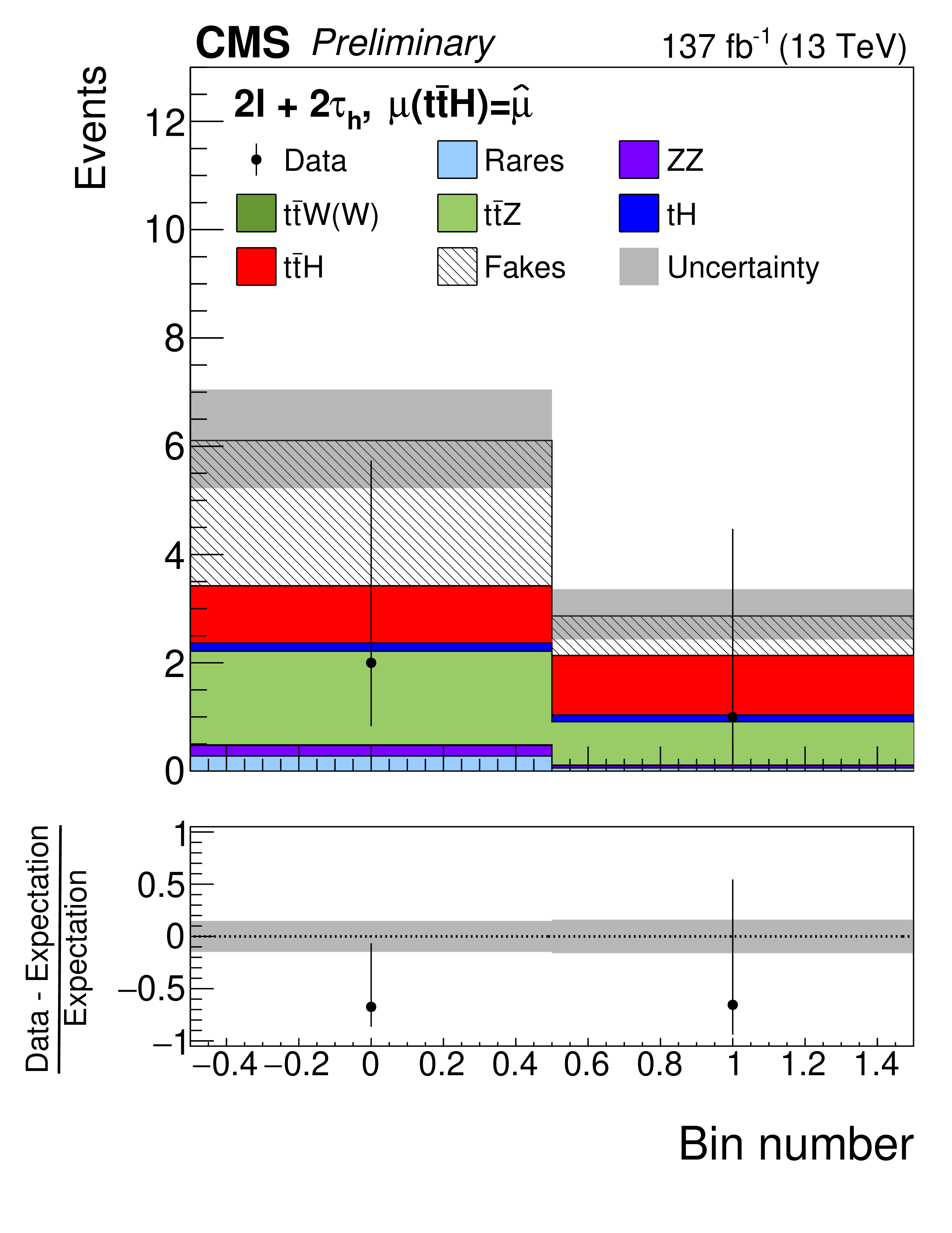
Distributions in BDT output for events selected in the 2${\ell}$ os+1${\tau _{\mathrm {h}}}$ (upper left), 3${\ell}$+1${\tau _{\mathrm {h}}}$ (upper right), and 4${\ell}$+0${\tau _{\mathrm {h}}}$ (lower) channels. The distributions expected for the $ {{\mathrm{t}} {\mathrm{\bar{t}}} {\mathrm{H}}}$ and $ {{\mathrm{t}} {\mathrm{H}}}$ signals and for background processes are shown for the values of the POI and of the nuisance parameters obtained from the ML fit. The best-fit value of the $ {{\mathrm{t}} {\mathrm{\bar{t}}} {\mathrm{H}}}$ and $ {{\mathrm{t}} {\mathrm{H}}}$ production rates amounts to $ {\hat{\mu}}_{{{\mathrm{t}} {\mathrm{\bar{t}}} {\mathrm{H}}}} = $ 0.92 and $ {\hat{\mu}}_{{{\mathrm{t}} {\mathrm{H}}}} = $ 5.7 times the rates expected in the SM. |
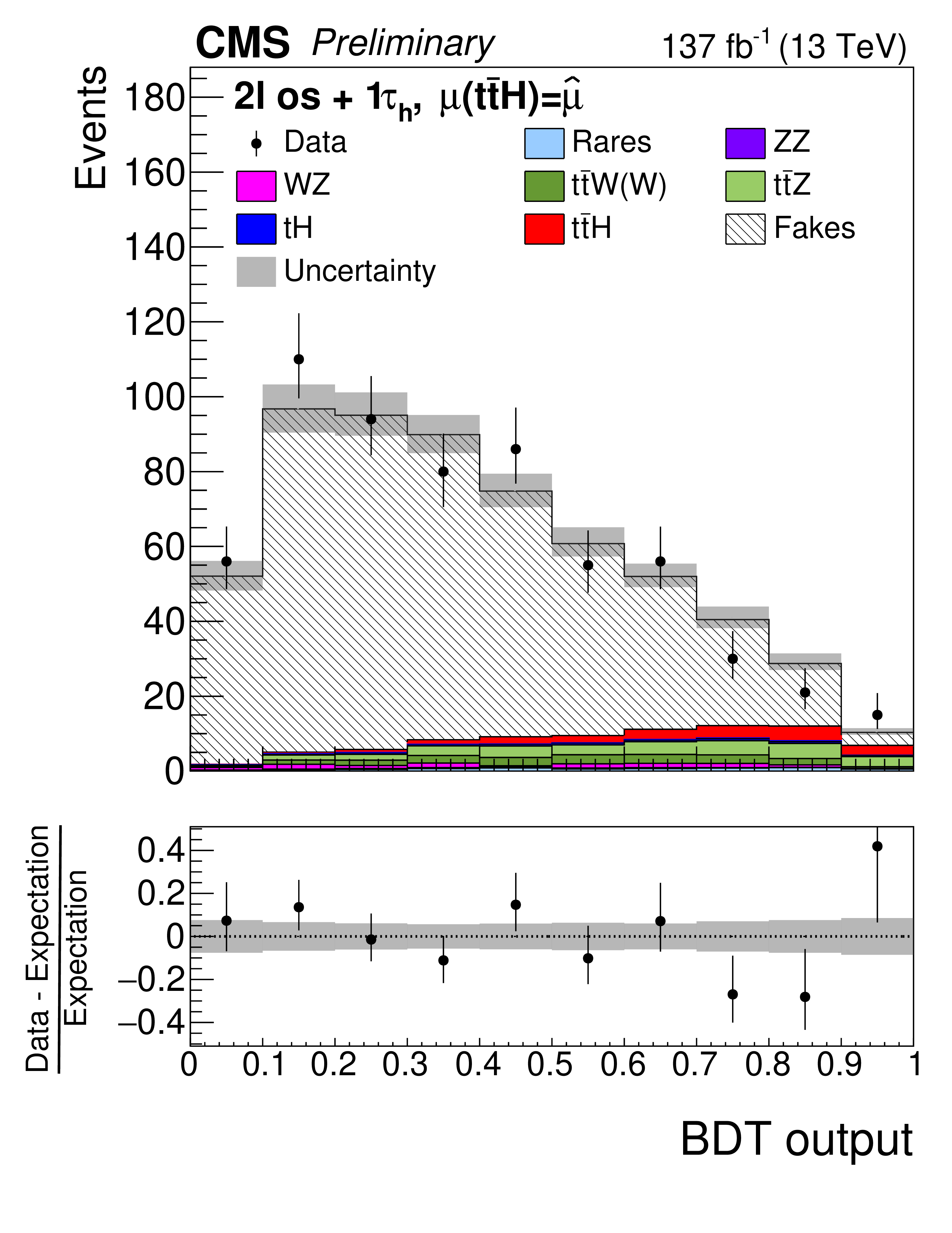
png pdf |
Figure 9-a:
Distribution in BDT output for events selected in the 2${\ell}$ os+1${\tau _{\mathrm {h}}}$ channel. The distributions expected for the $ {{\mathrm{t}} {\mathrm{\bar{t}}} {\mathrm{H}}}$ and $ {{\mathrm{t}} {\mathrm{H}}}$ signals and for background processes are shown for the values of the POI and of the nuisance parameters obtained from the ML fit. The best-fit value of the $ {{\mathrm{t}} {\mathrm{\bar{t}}} {\mathrm{H}}}$ and $ {{\mathrm{t}} {\mathrm{H}}}$ production rates amounts to $ {\hat{\mu}}_{{{\mathrm{t}} {\mathrm{\bar{t}}} {\mathrm{H}}}} = $ 0.92 and $ {\hat{\mu}}_{{{\mathrm{t}} {\mathrm{H}}}} = $ 5.7 times the rates expected in the SM. |
png pdf |
Figure 9-b:
Distribution in BDT output for events selected in the 3${\ell}$+1${\tau _{\mathrm {h}}}$ channel. The distributions expected for the $ {{\mathrm{t}} {\mathrm{\bar{t}}} {\mathrm{H}}}$ and $ {{\mathrm{t}} {\mathrm{H}}}$ signals and for background processes are shown for the values of the POI and of the nuisance parameters obtained from the ML fit. The best-fit value of the $ {{\mathrm{t}} {\mathrm{\bar{t}}} {\mathrm{H}}}$ and $ {{\mathrm{t}} {\mathrm{H}}}$ production rates amounts to $ {\hat{\mu}}_{{{\mathrm{t}} {\mathrm{\bar{t}}} {\mathrm{H}}}} = $ 0.92 and $ {\hat{\mu}}_{{{\mathrm{t}} {\mathrm{H}}}} = $ 5.7 times the rates expected in the SM. |
png pdf |
Figure 9-c:
Distribution in BDT output for events selected in the 4${\ell}$+0${\tau _{\mathrm {h}}}$ channel. The distributions expected for the $ {{\mathrm{t}} {\mathrm{\bar{t}}} {\mathrm{H}}}$ and $ {{\mathrm{t}} {\mathrm{H}}}$ signals and for background processes are shown for the values of the POI and of the nuisance parameters obtained from the ML fit. The best-fit value of the $ {{\mathrm{t}} {\mathrm{\bar{t}}} {\mathrm{H}}}$ and $ {{\mathrm{t}} {\mathrm{H}}}$ production rates amounts to $ {\hat{\mu}}_{{{\mathrm{t}} {\mathrm{\bar{t}}} {\mathrm{H}}}} = $ 0.92 and $ {\hat{\mu}}_{{{\mathrm{t}} {\mathrm{H}}}} = $ 5.7 times the rates expected in the SM. |
png pdf |
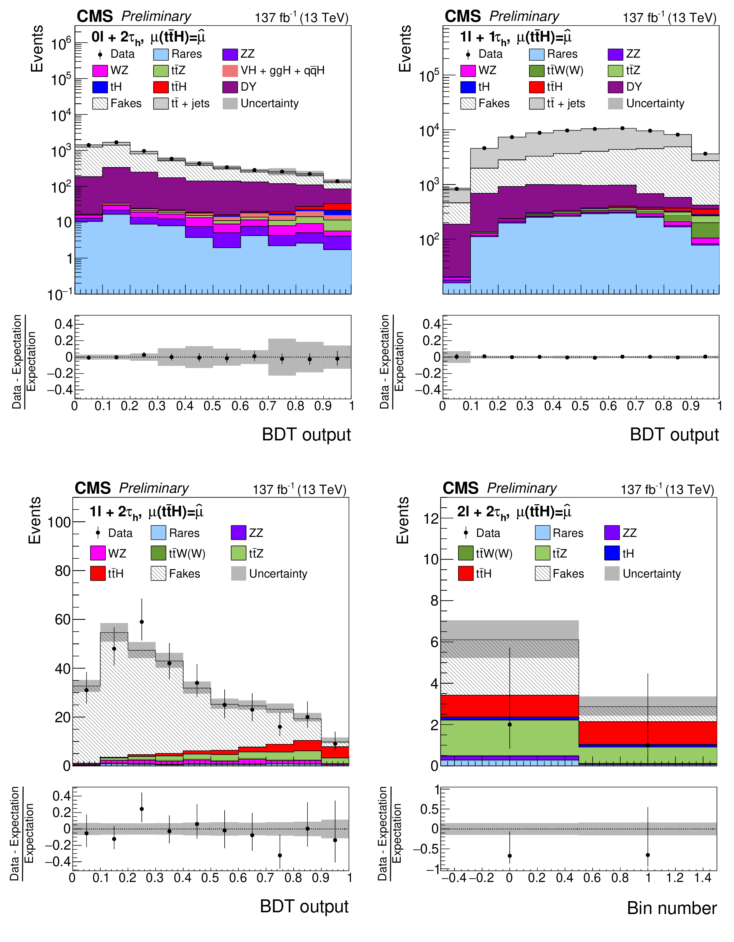
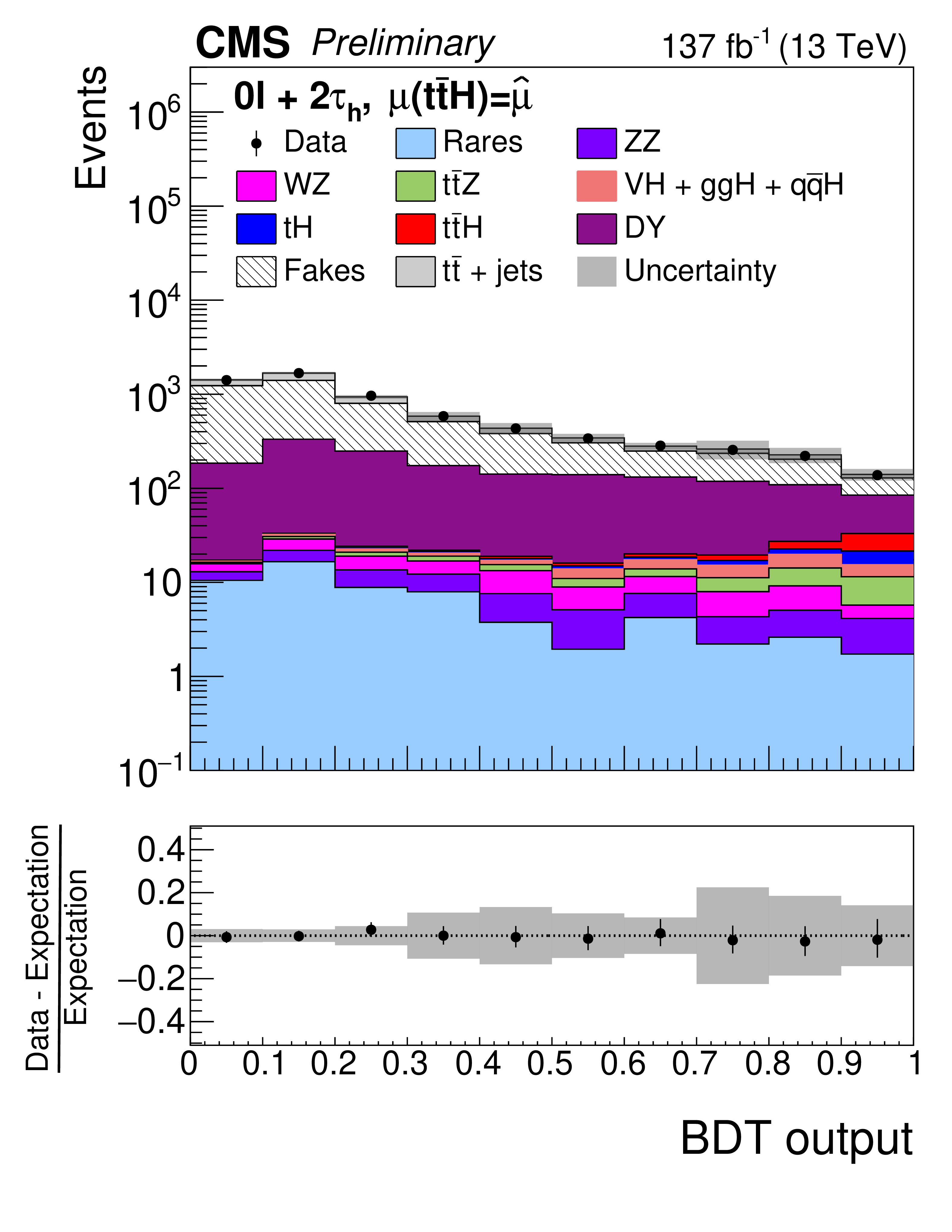
Figure 10:
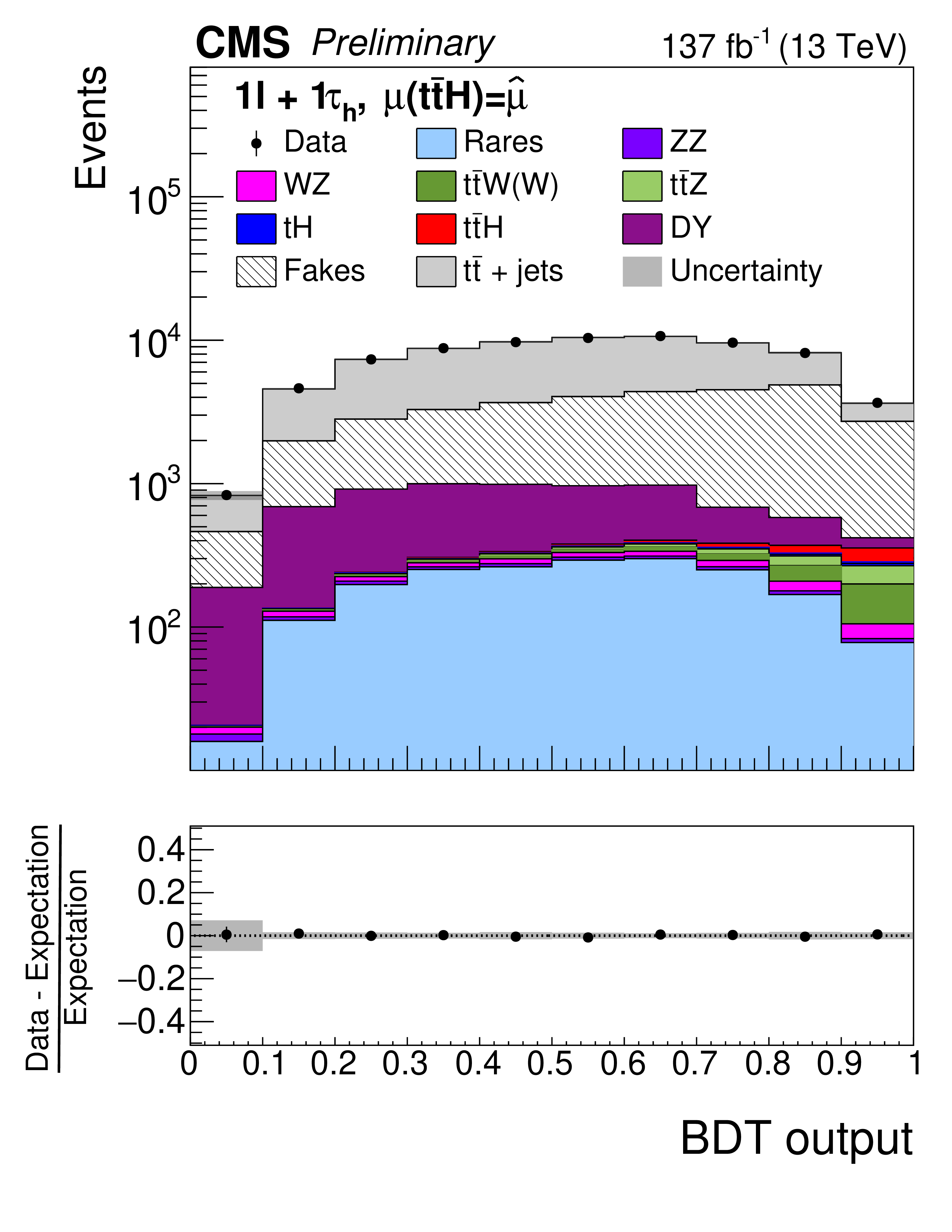
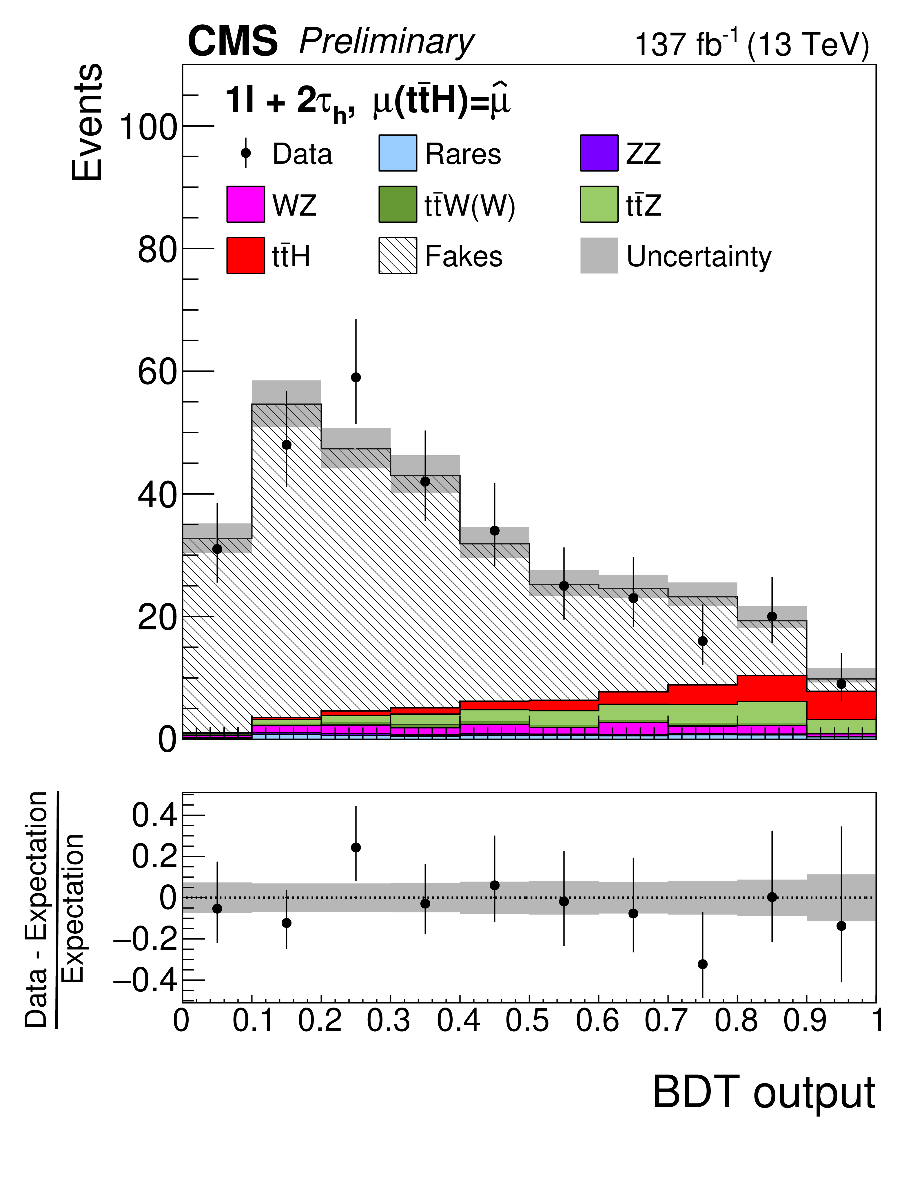
Distributions in BDT output used for the signal extraction in the 0${\ell}$+2${\tau _{\mathrm {h}}}$ (upper left), 1${\ell}$+1${\tau _{\mathrm {h}}}$ (upper right), 1${\ell}$+2${\tau _{\mathrm {h}}}$ (lower left), and 2${\ell}$+2${\tau _{\mathrm {h}}}$ (lower right) channels. The distributions expected for the $ {{\mathrm{t}} {\mathrm{\bar{t}}} {\mathrm{H}}}$ and $ {{\mathrm{t}} {\mathrm{H}}}$ signals and for background processes are shown for the values of the POI and of the nuisance parameters obtained from the ML fit. The best-fit value of the $ {{\mathrm{t}} {\mathrm{\bar{t}}} {\mathrm{H}}}$ and $ {{\mathrm{t}} {\mathrm{H}}}$ production rates amounts to $ {\hat{\mu}}_{{{\mathrm{t}} {\mathrm{\bar{t}}} {\mathrm{H}}}} = $ 0.92 and $ {\hat{\mu}}_{{{\mathrm{t}} {\mathrm{H}}}} = $ 5.7 times the rates expected in the SM. |
png pdf |
Figure 10-a:
Distribution in BDT output used for the signal extraction in the 0${\ell}$+2${\tau _{\mathrm {h}}}$ channel. The distributions expected for the $ {{\mathrm{t}} {\mathrm{\bar{t}}} {\mathrm{H}}}$ and $ {{\mathrm{t}} {\mathrm{H}}}$ signals and for background processes are shown for the values of the POI and of the nuisance parameters obtained from the ML fit. The best-fit value of the $ {{\mathrm{t}} {\mathrm{\bar{t}}} {\mathrm{H}}}$ and $ {{\mathrm{t}} {\mathrm{H}}}$ production rates amounts to $ {\hat{\mu}}_{{{\mathrm{t}} {\mathrm{\bar{t}}} {\mathrm{H}}}} = $ 0.92 and $ {\hat{\mu}}_{{{\mathrm{t}} {\mathrm{H}}}} = $ 5.7 times the rates expected in the SM. |
png pdf |
Figure 10-b:
Distribution in BDT output used for the signal extraction in the 1${\ell}$+1${\tau _{\mathrm {h}}}$ channel. The distributions expected for the $ {{\mathrm{t}} {\mathrm{\bar{t}}} {\mathrm{H}}}$ and $ {{\mathrm{t}} {\mathrm{H}}}$ signals and for background processes are shown for the values of the POI and of the nuisance parameters obtained from the ML fit. The best-fit value of the $ {{\mathrm{t}} {\mathrm{\bar{t}}} {\mathrm{H}}}$ and $ {{\mathrm{t}} {\mathrm{H}}}$ production rates amounts to $ {\hat{\mu}}_{{{\mathrm{t}} {\mathrm{\bar{t}}} {\mathrm{H}}}} = $ 0.92 and $ {\hat{\mu}}_{{{\mathrm{t}} {\mathrm{H}}}} = $ 5.7 times the rates expected in the SM. |
png pdf |
Figure 10-c:
Distribution in BDT output used for the signal extraction in the 1${\ell}$+2${\tau _{\mathrm {h}}}$ channel. The distributions expected for the $ {{\mathrm{t}} {\mathrm{\bar{t}}} {\mathrm{H}}}$ and $ {{\mathrm{t}} {\mathrm{H}}}$ signals and for background processes are shown for the values of the POI and of the nuisance parameters obtained from the ML fit. The best-fit value of the $ {{\mathrm{t}} {\mathrm{\bar{t}}} {\mathrm{H}}}$ and $ {{\mathrm{t}} {\mathrm{H}}}$ production rates amounts to $ {\hat{\mu}}_{{{\mathrm{t}} {\mathrm{\bar{t}}} {\mathrm{H}}}} = $ 0.92 and $ {\hat{\mu}}_{{{\mathrm{t}} {\mathrm{H}}}} = $ 5.7 times the rates expected in the SM. |
png pdf |
Figure 10-d:
Distribution in BDT output used for the signal extraction in the 2${\ell}$+2${\tau _{\mathrm {h}}}$ channel. The distributions expected for the $ {{\mathrm{t}} {\mathrm{\bar{t}}} {\mathrm{H}}}$ and $ {{\mathrm{t}} {\mathrm{H}}}$ signals and for background processes are shown for the values of the POI and of the nuisance parameters obtained from the ML fit. The best-fit value of the $ {{\mathrm{t}} {\mathrm{\bar{t}}} {\mathrm{H}}}$ and $ {{\mathrm{t}} {\mathrm{H}}}$ production rates amounts to $ {\hat{\mu}}_{{{\mathrm{t}} {\mathrm{\bar{t}}} {\mathrm{H}}}} = $ 0.92 and $ {\hat{\mu}}_{{{\mathrm{t}} {\mathrm{H}}}} = $ 5.7 times the rates expected in the SM. |
png pdf |
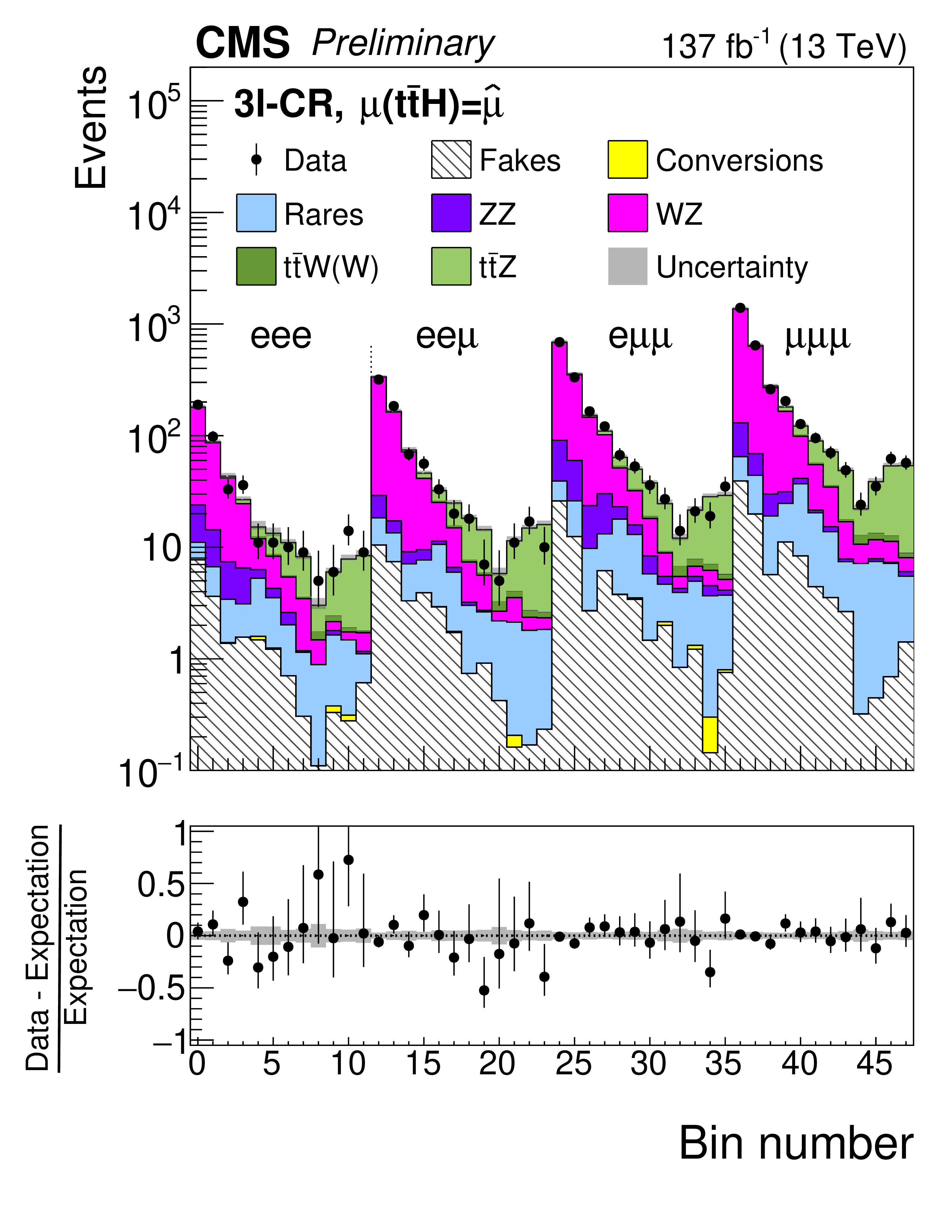
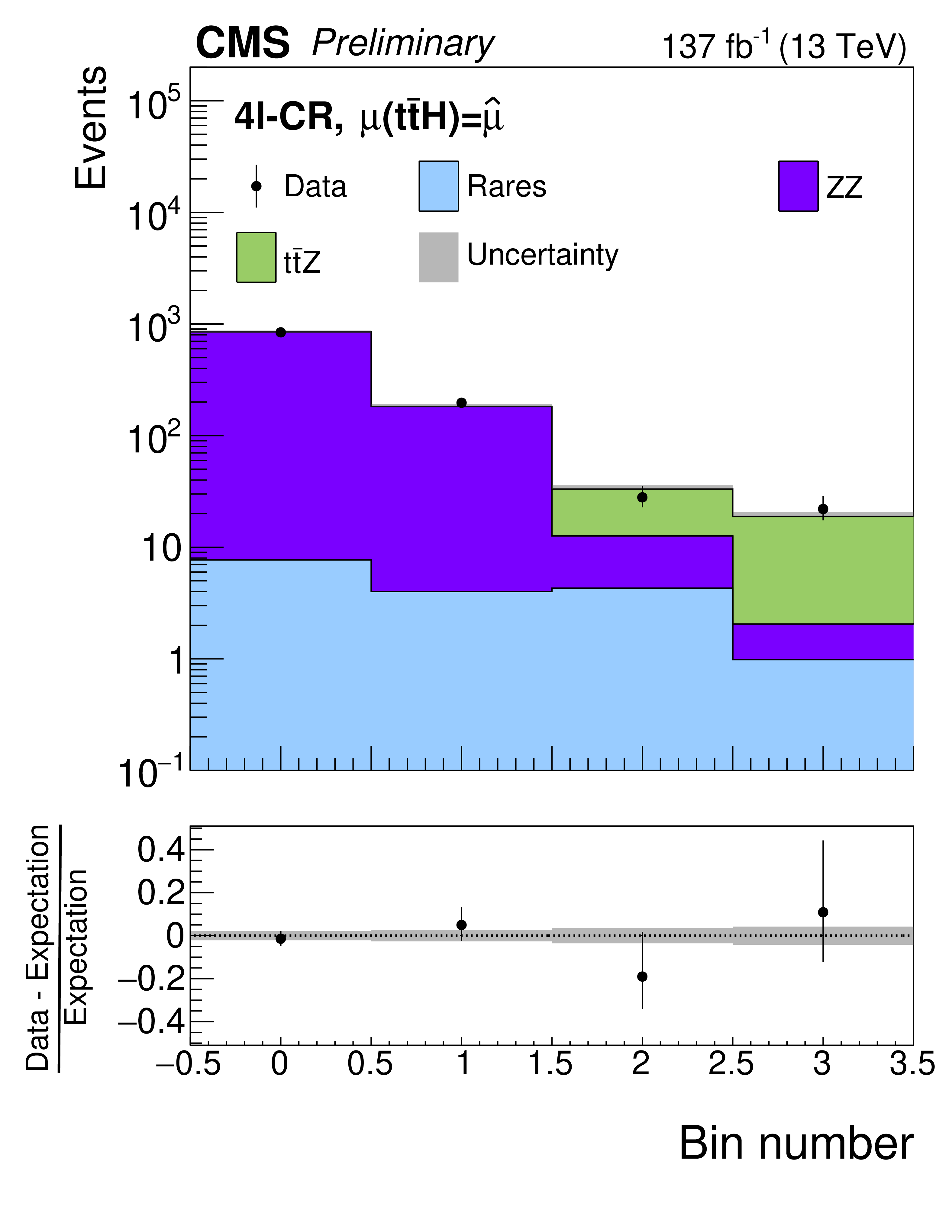
Figure 11:
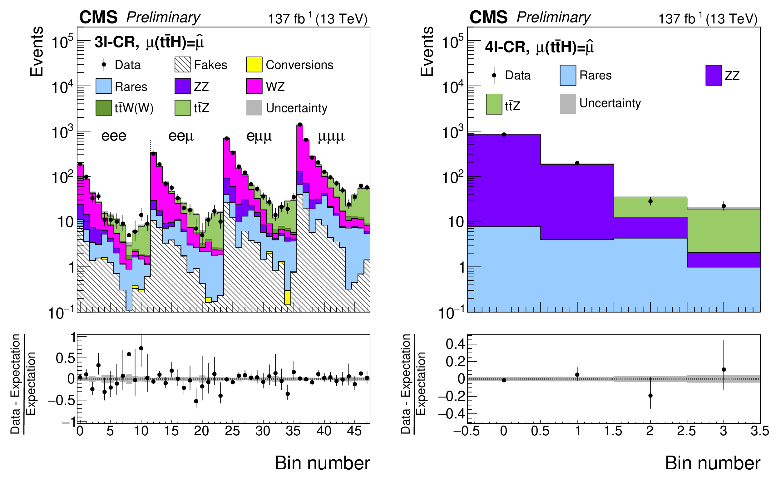
Distributions in discriminating observables in the 3${\ell}$+0${\tau _{\mathrm {h}}}$ (left) and 4${\ell}$+0${\tau _{\mathrm {h}}}$ (right) control region. The distributions expected for the $ {{\mathrm{t}} {\mathrm{\bar{t}}} {\mathrm{H}}}$ and $ {{\mathrm{t}} {\mathrm{H}}}$ signals and for background processes are shown for the values of the POI and of the nuisance parameters obtained from the ML fit. The best-fit value of the $ {{\mathrm{t}} {\mathrm{\bar{t}}} {\mathrm{H}}}$ and $ {{\mathrm{t}} {\mathrm{H}}}$ production rates amounts to $ {\hat{\mu}}_{{{\mathrm{t}} {\mathrm{\bar{t}}} {\mathrm{H}}}} = $ 0.92 and $ {\hat{\mu}}_{{{\mathrm{t}} {\mathrm{H}}}} = $ 5.7 times the rates expected in the SM. |
png pdf |
Figure 11-a:
Distribution in discriminating observables in the 3${\ell}$+0${\tau _{\mathrm {h}}}$ control region. The distributions expected for the $ {{\mathrm{t}} {\mathrm{\bar{t}}} {\mathrm{H}}}$ and $ {{\mathrm{t}} {\mathrm{H}}}$ signals and for background processes are shown for the values of the POI and of the nuisance parameters obtained from the ML fit. The best-fit value of the $ {{\mathrm{t}} {\mathrm{\bar{t}}} {\mathrm{H}}}$ and $ {{\mathrm{t}} {\mathrm{H}}}$ production rates amounts to $ {\hat{\mu}}_{{{\mathrm{t}} {\mathrm{\bar{t}}} {\mathrm{H}}}} = $ 0.92 and $ {\hat{\mu}}_{{{\mathrm{t}} {\mathrm{H}}}} = $ 5.7 times the rates expected in the SM. |
png pdf |
Figure 11-b:
Distribution in discriminating observables in the 4${\ell}$+0${\tau _{\mathrm {h}}}$ control region. The distributions expected for the $ {{\mathrm{t}} {\mathrm{\bar{t}}} {\mathrm{H}}}$ and $ {{\mathrm{t}} {\mathrm{H}}}$ signals and for background processes are shown for the values of the POI and of the nuisance parameters obtained from the ML fit. The best-fit value of the $ {{\mathrm{t}} {\mathrm{\bar{t}}} {\mathrm{H}}}$ and $ {{\mathrm{t}} {\mathrm{H}}}$ production rates amounts to $ {\hat{\mu}}_{{{\mathrm{t}} {\mathrm{\bar{t}}} {\mathrm{H}}}} = $ 0.92 and $ {\hat{\mu}}_{{{\mathrm{t}} {\mathrm{H}}}} = $ 5.7 times the rates expected in the SM. |
png pdf |
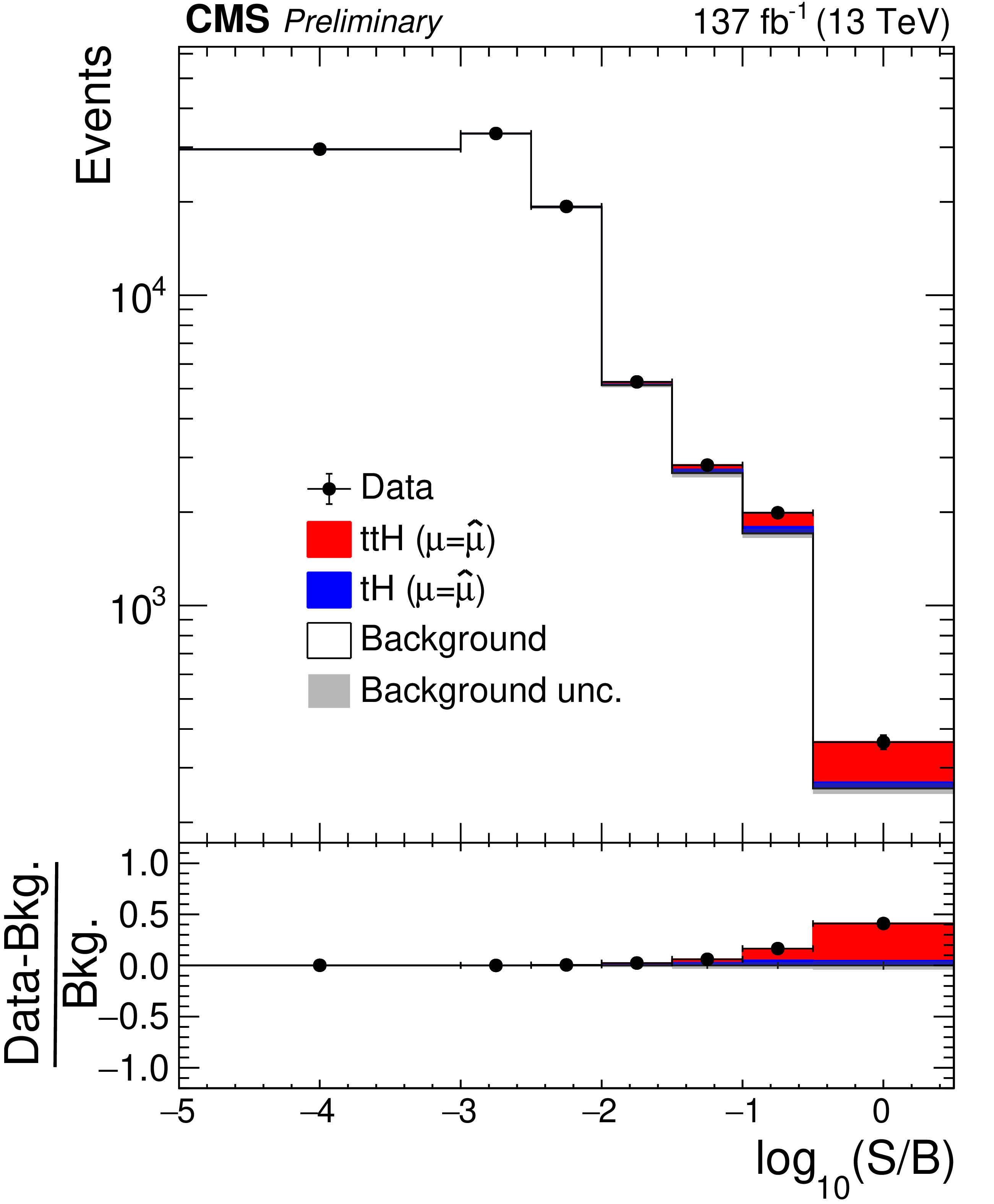
Figure 12:
Distribution in the decimal logarithm of the ratio between the expected $ {{\mathrm{t}} {\mathrm{\bar{t}}} {\mathrm{H}}}+ {{\mathrm{t}} {\mathrm{H}}}$ signal and the expected sum of background contributions in each bin of the $105$ distributions that are included in the ML fit used for the signal extraction. The distributions expected for signal and background processes are computed for $ {\hat{\mu}}_{{{\mathrm{t}} {\mathrm{\bar{t}}} {\mathrm{H}}}} = $ 0.92, $ {\hat{\mu}}_{{{\mathrm{t}} {\mathrm{H}}}} = $ 5.7, and the values of nuisance parameters obtained from the ML fit. |
png pdf |
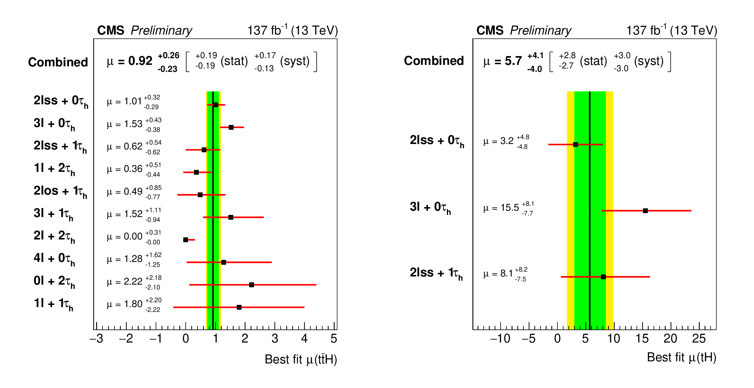
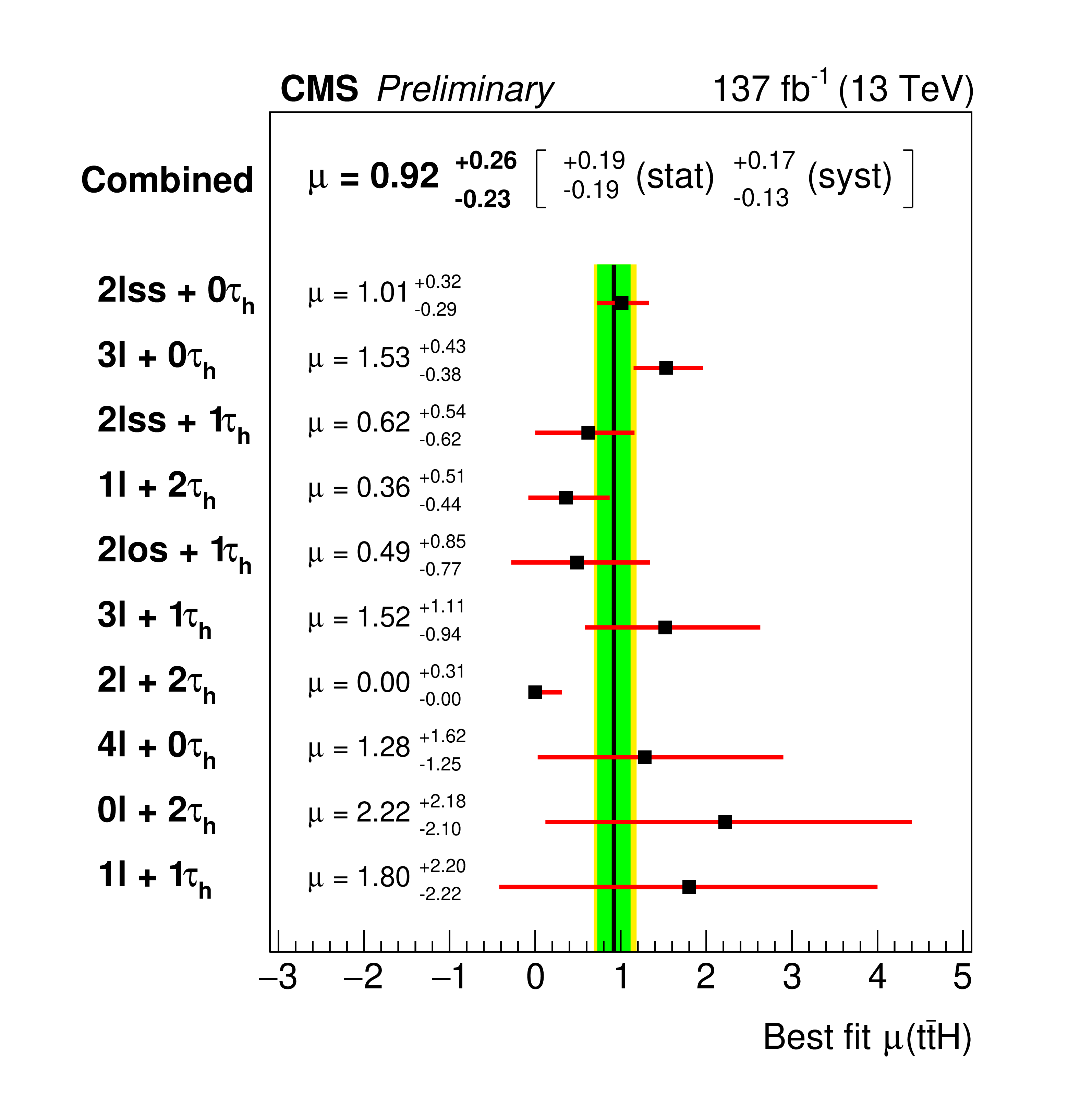
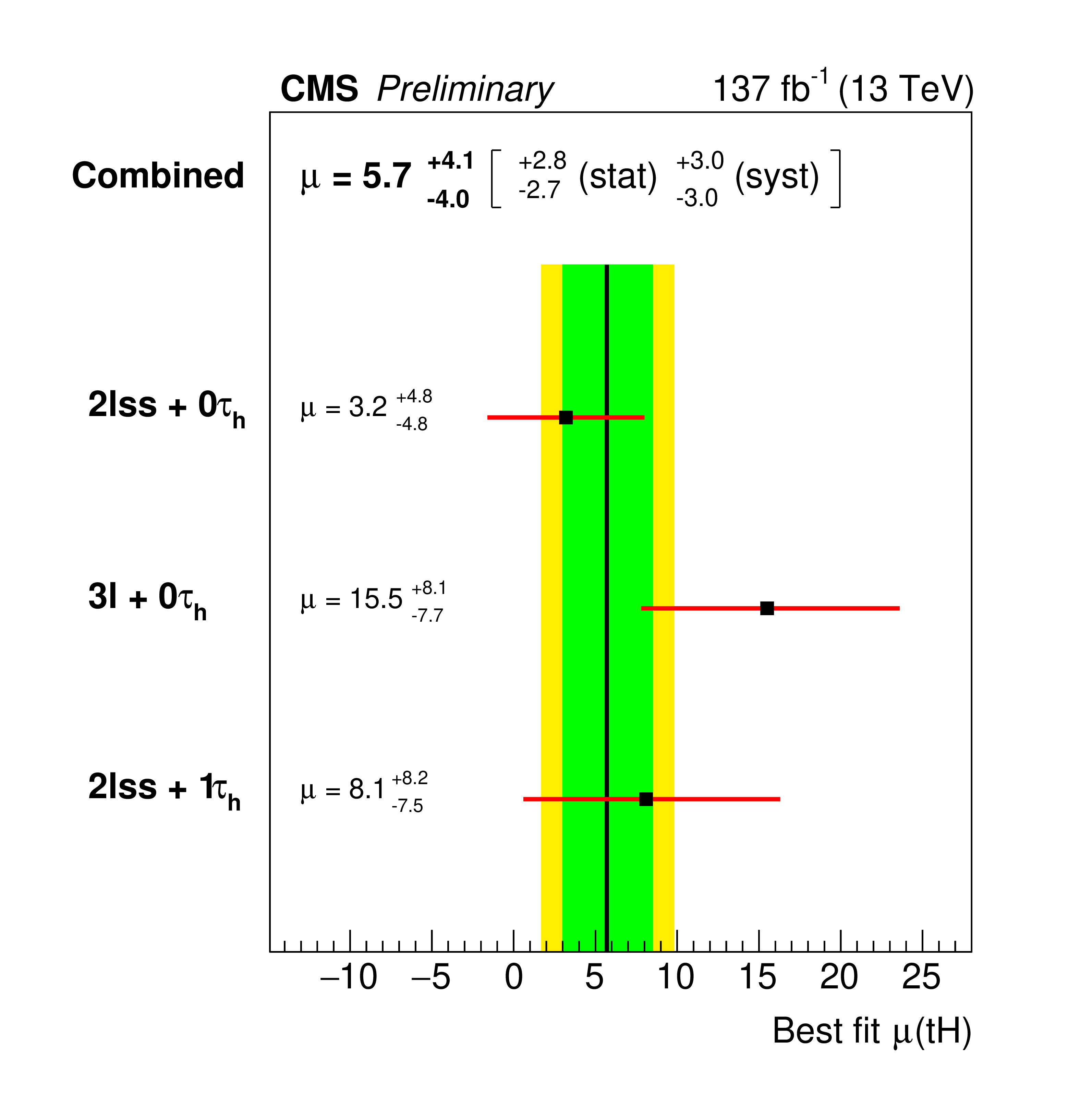
Figure 13:
Production rate $ {\hat{\mu}}_{{{\mathrm{t}} {\mathrm{\bar{t}}} {\mathrm{H}}}}$ of the $ {{\mathrm{t}} {\mathrm{\bar{t}}} {\mathrm{H}}}$ signal (left) and $ {\hat{\mu}}_{{{\mathrm{t}} {\mathrm{H}}}}$ of $ {{\mathrm{t}} {\mathrm{H}}}$ signal (right), in units of their rate of production expected in the SM, measured in each of the ten channels individually and for the combination of all channels. The signal strength in the 2${\ell}$+2$\tau_{\mathrm{h}}$ is constrained to be greater than zero. |
png pdf |
Figure 13-a:
Production rate $ {\hat{\mu}}_{{{\mathrm{t}} {\mathrm{\bar{t}}} {\mathrm{H}}}}$ of the $ {{\mathrm{t}} {\mathrm{\bar{t}}} {\mathrm{H}}}$ signal, in units of their rate of production expected in the SM, measured in each of the ten channels individually and for the combination of all channels. The signal strength in the 2${\ell}$+2$\tau_{\mathrm{h}}$ is constrained to be greater than zero. |
png pdf |
Figure 13-b:
Production rate $ {\hat{\mu}}_{{{\mathrm{t}} {\mathrm{\bar{t}}} {\mathrm{H}}}}$ of the $ {\hat{\mu}}_{{{\mathrm{t}} {\mathrm{H}}}}$ of $ {{\mathrm{t}} {\mathrm{H}}}$ signal, in units of their rate of production expected in the SM, measured in each of the ten channels individually and for the combination of all channels. The signal strength in the 2${\ell}$+2$\tau_{\mathrm{h}}$ is constrained to be greater than zero. |

png pdf |
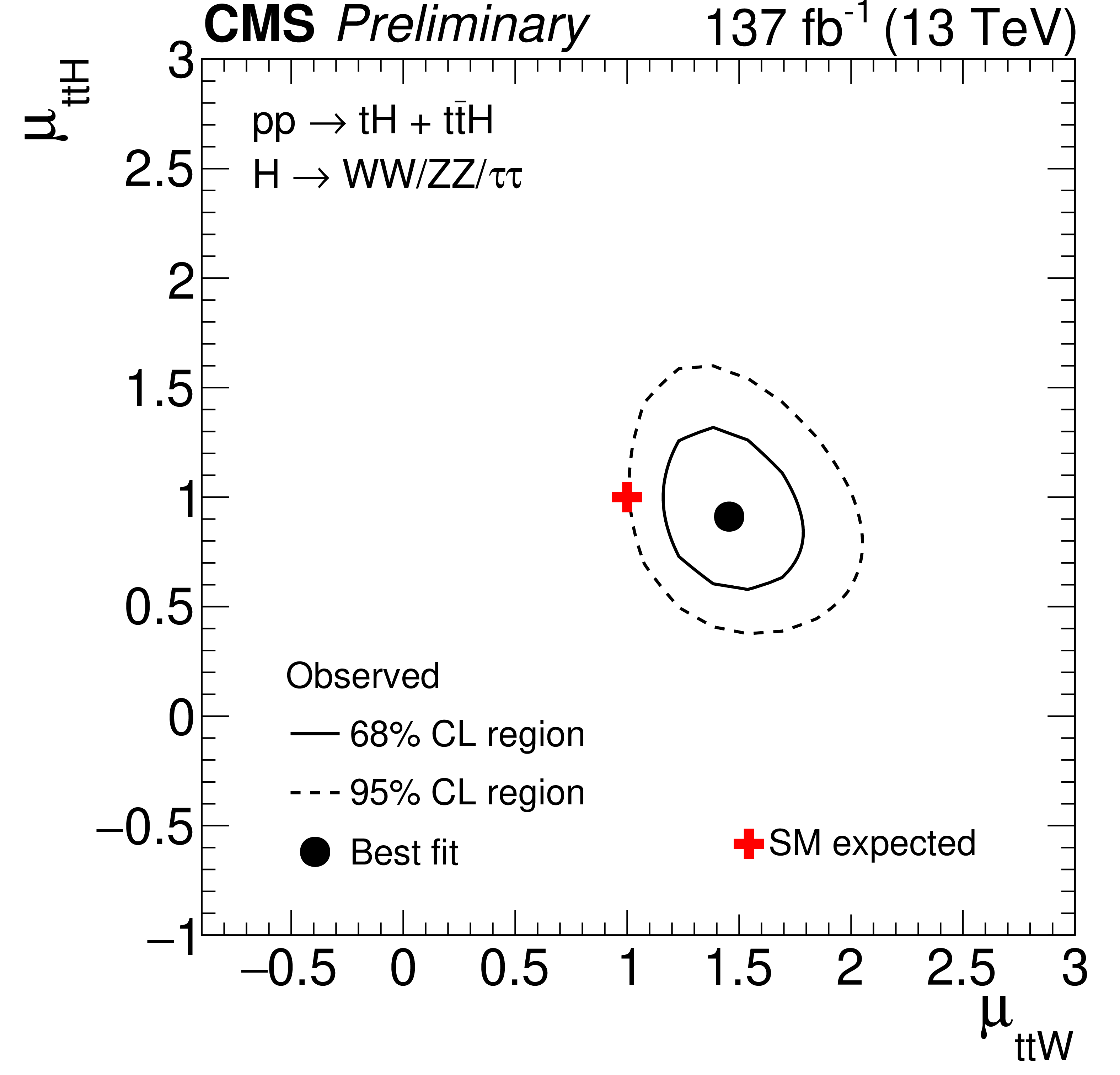
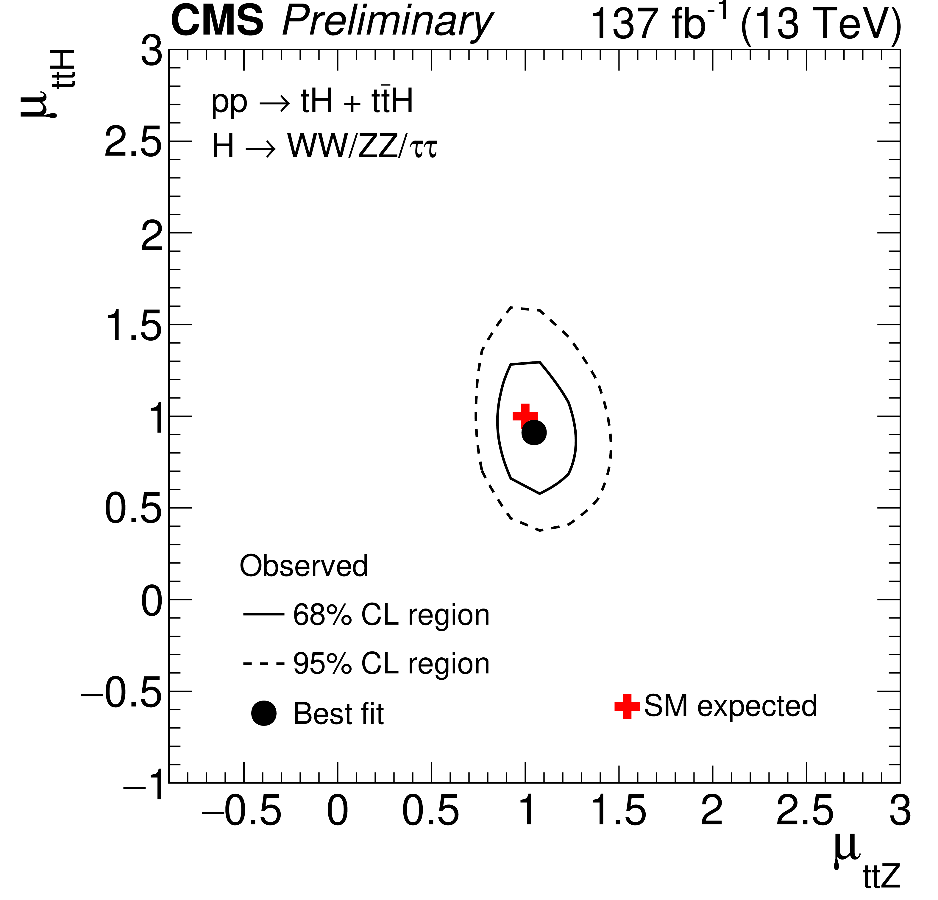
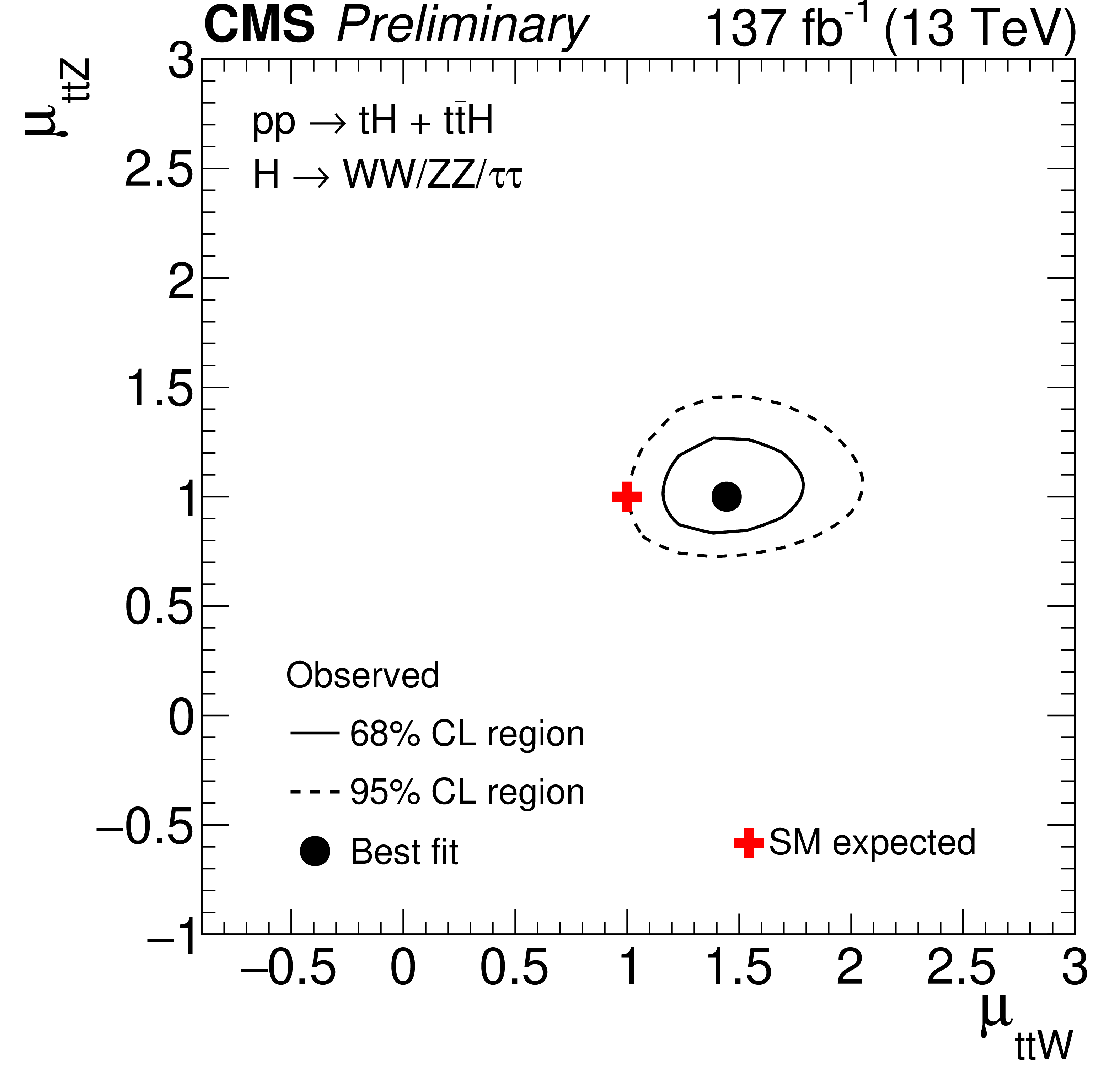
Figure 14:
Two-dimensional contours of the likelihood function $\mathcal {L}$, given by Eq. (3), as a function of the production rates of the $ {{\mathrm{t}} {\mathrm{\bar{t}}} {\mathrm{H}}}$ and $ {{\mathrm{t}} {\mathrm{H}}}$ signals ($ {\hat{\mu}}_{{{\mathrm{t}} {\mathrm{\bar{t}}} {\mathrm{H}}}}$ and $ {\hat{\mu}}_{{{\mathrm{t}} {\mathrm{H}}}}$) and of the $ {{\mathrm{t}} {\mathrm{\bar{t}}}\mathrm{Z}}$ and $ {{\mathrm{t}} {\mathrm{\bar{t}}}\mathrm{W}}$ backgrounds ($\theta _{{{\mathrm{t}} {\mathrm{\bar{t}}}\mathrm{Z}}}$ and $\theta _{{{\mathrm{t}} {\mathrm{\bar{t}}}\mathrm{W}}}$). The two production rates that are not shown on either the $x$ or the $y$ axis are profiled such that the function $\mathcal {L}$ attains its minimum at each point in the $x$-$y$ plane. |

png pdf |
Figure 14-a:
Two-dimensional contour of the likelihood function $\mathcal {L}$, given by Eq. (3), as a function of the production rates of the |
png pdf |
Figure 14-b:
Two-dimensional contour of the likelihood function $\mathcal {L}$, given by Eq. (3), as a function of the production rates of the |
png pdf |
Figure 14-c:
Two-dimensional contour of the likelihood function $\mathcal {L}$, given by Eq. (3), as a function of the production rates of the |
png pdf |
Figure 14-d:
Two-dimensional contour of the likelihood function $\mathcal {L}$, given by Eq. (3), as a function of the production rates of the |
png pdf |
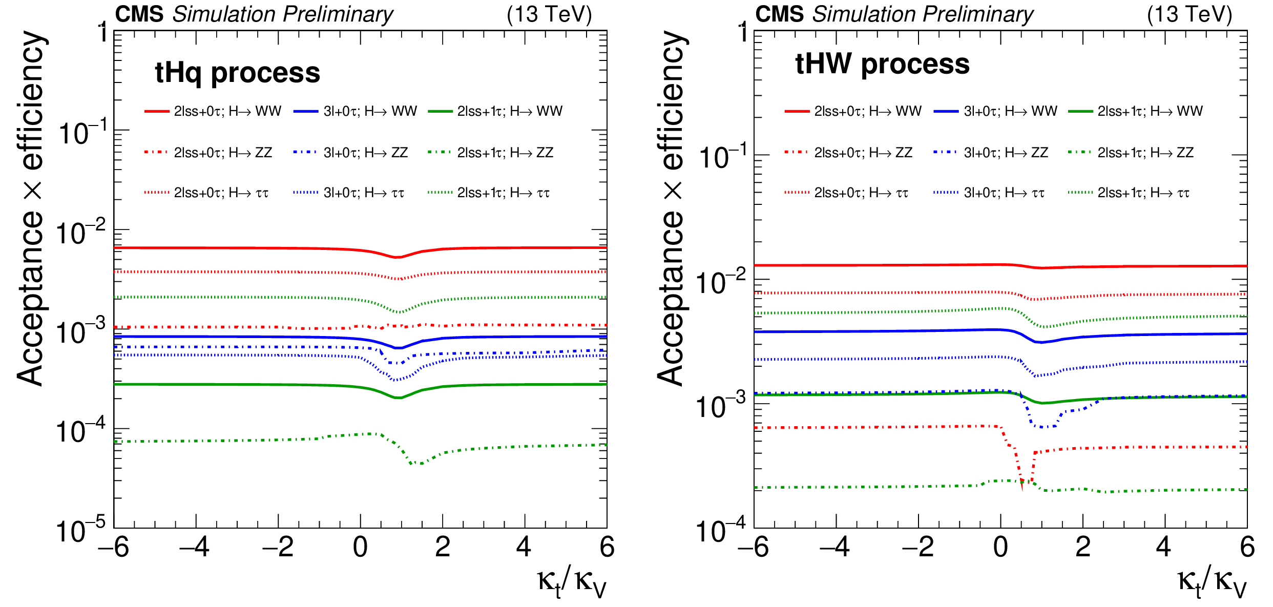
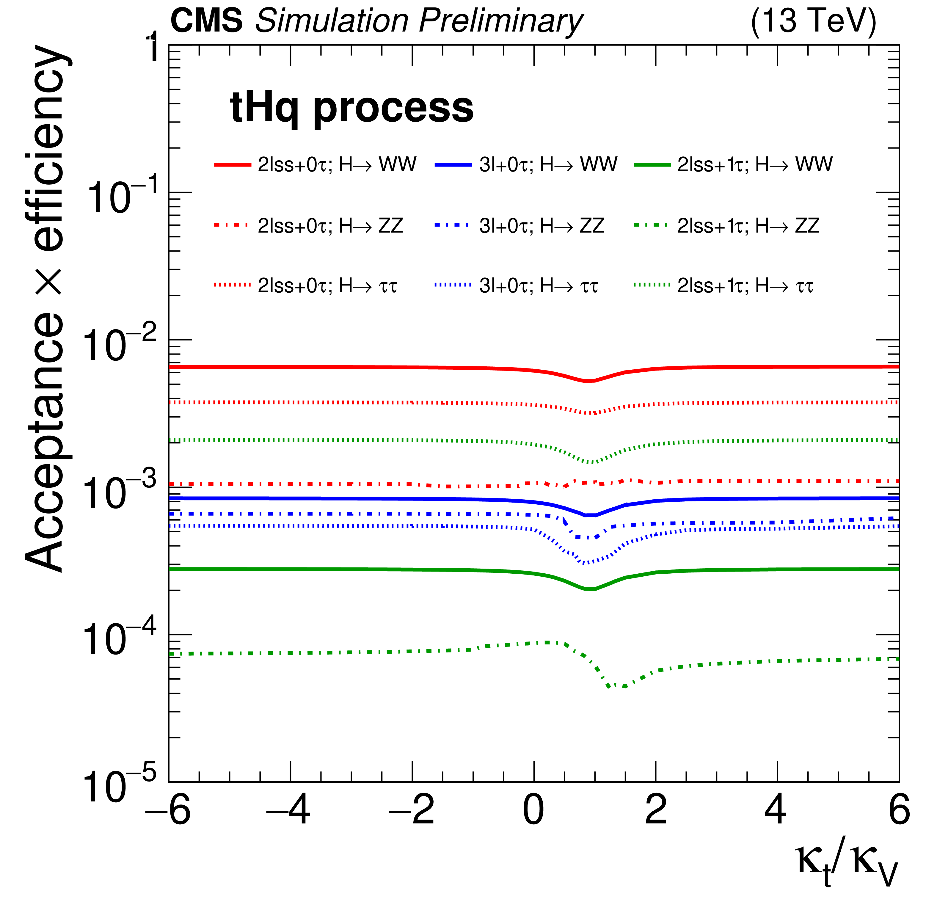
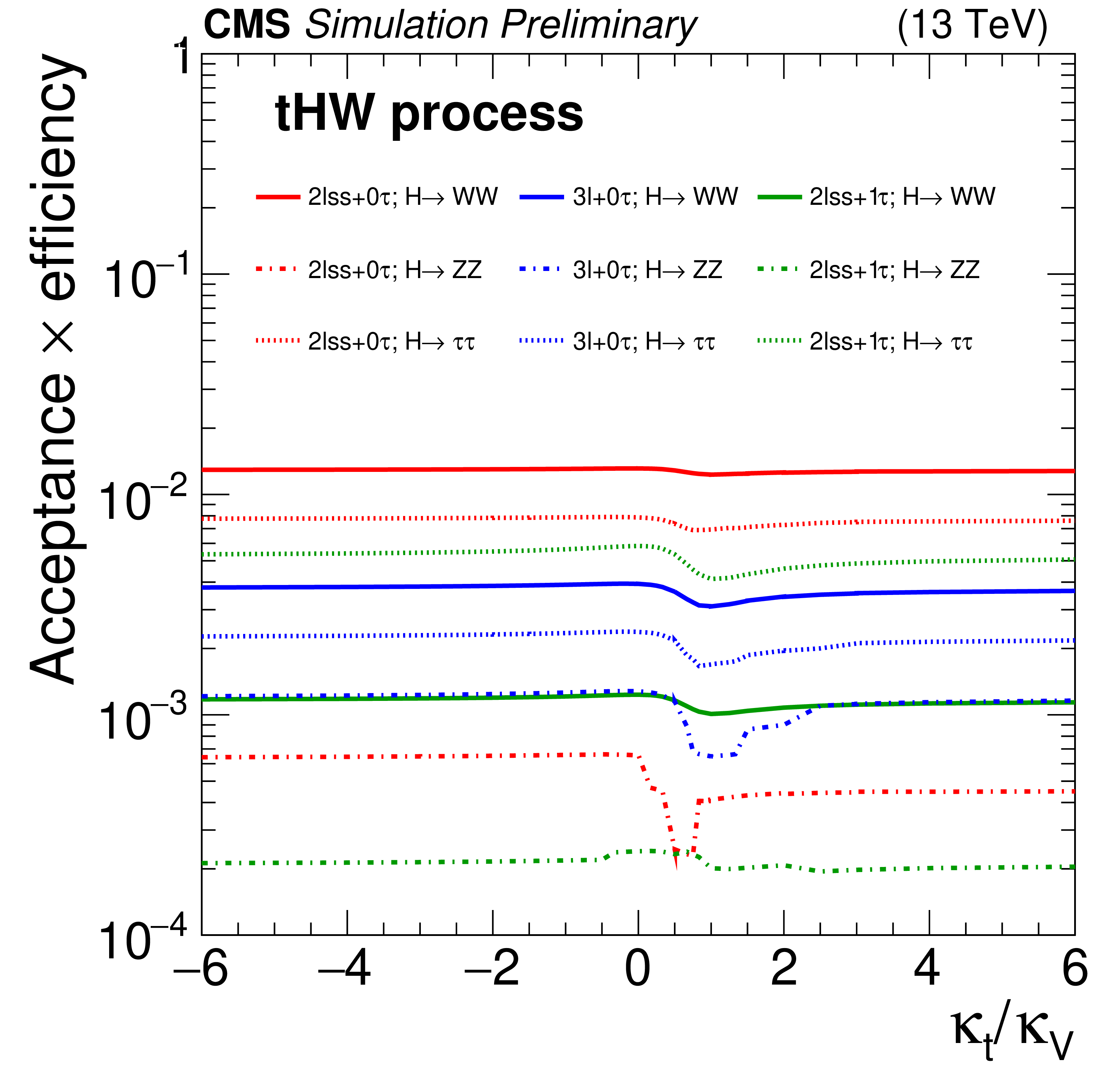
Figure 15:
Probability for $ {{\mathrm{t}} {\mathrm{H}}}$ signal events produced by the $ {{{\mathrm{t}} {\mathrm{H}}} {\mathrm{q}}}$ (left) and $ {{{\mathrm{t}} {\mathrm{H}}}\mathrm{W}}$ (right) production process to pass the event selection criteria for the 2${\ell}$+0${\tau _{\mathrm {h}}}$, 3${\ell}$+0${\tau _{\mathrm {h}}}$, and 2${\ell}$+1${\tau _{\mathrm {h}}}$ channels in each of the $ {\mathrm{H}}$ boson decay modes as a function of the ratio $ {\kappa _{{\mathrm{t}}}}/ {\kappa _{\mathrm {V}}}$ of the $ {\mathrm{H}}$ boson couplings to the top quark and to the $\mathrm{W} $ boson. |
png pdf |
Figure 15-a:
Probability for $ {{\mathrm{t}} {\mathrm{H}}}$ signal events produced by the $ {{{\mathrm{t}} {\mathrm{H}}} {\mathrm{q}}}$ production process to pass the event selection criteria for the 2${\ell}$+0${\tau _{\mathrm {h}}}$, 3${\ell}$+0${\tau _{\mathrm {h}}}$, and 2${\ell}$+1${\tau _{\mathrm {h}}}$ channels in each of the $ {\mathrm{H}}$ boson decay modes as a function of the ratio $ {\kappa _{{\mathrm{t}}}}/ {\kappa _{\mathrm {V}}}$ of the $ {\mathrm{H}}$ boson couplings to the top quark and to the $\mathrm{W} $ boson. |
png pdf |
Figure 15-b:
Probability for $ {{\mathrm{t}} {\mathrm{H}}}$ signal events produced by the $ {{{\mathrm{t}} {\mathrm{H}}}\mathrm{W}}$ production process to pass the event selection criteria for the 2${\ell}$+0${\tau _{\mathrm {h}}}$, 3${\ell}$+0${\tau _{\mathrm {h}}}$, and 2${\ell}$+1${\tau _{\mathrm {h}}}$ channels in each of the $ {\mathrm{H}}$ boson decay modes as a function of the ratio $ {\kappa _{{\mathrm{t}}}}/ {\kappa _{\mathrm {V}}}$ of the $ {\mathrm{H}}$ boson couplings to the top quark and to the $\mathrm{W} $ boson. |
png pdf |
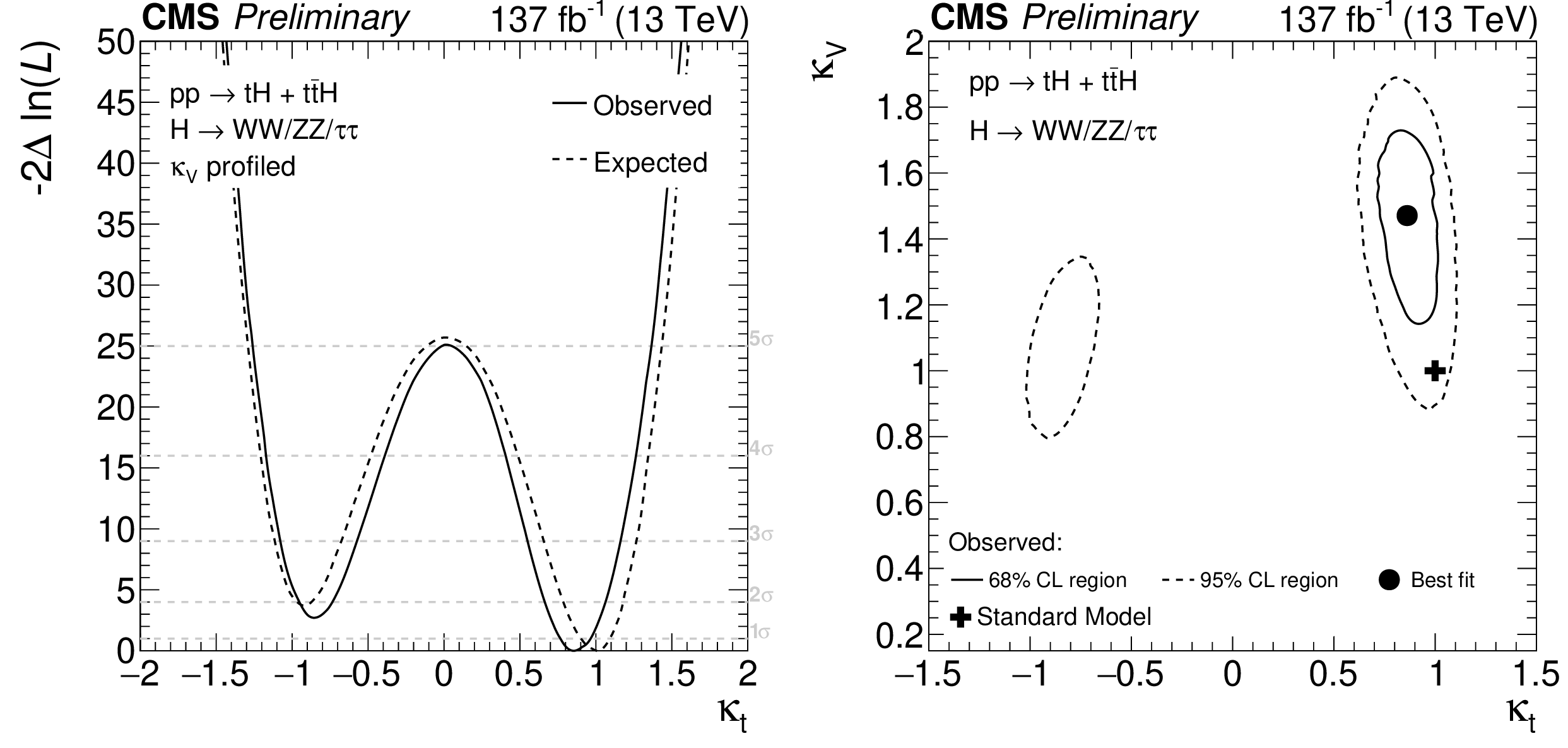
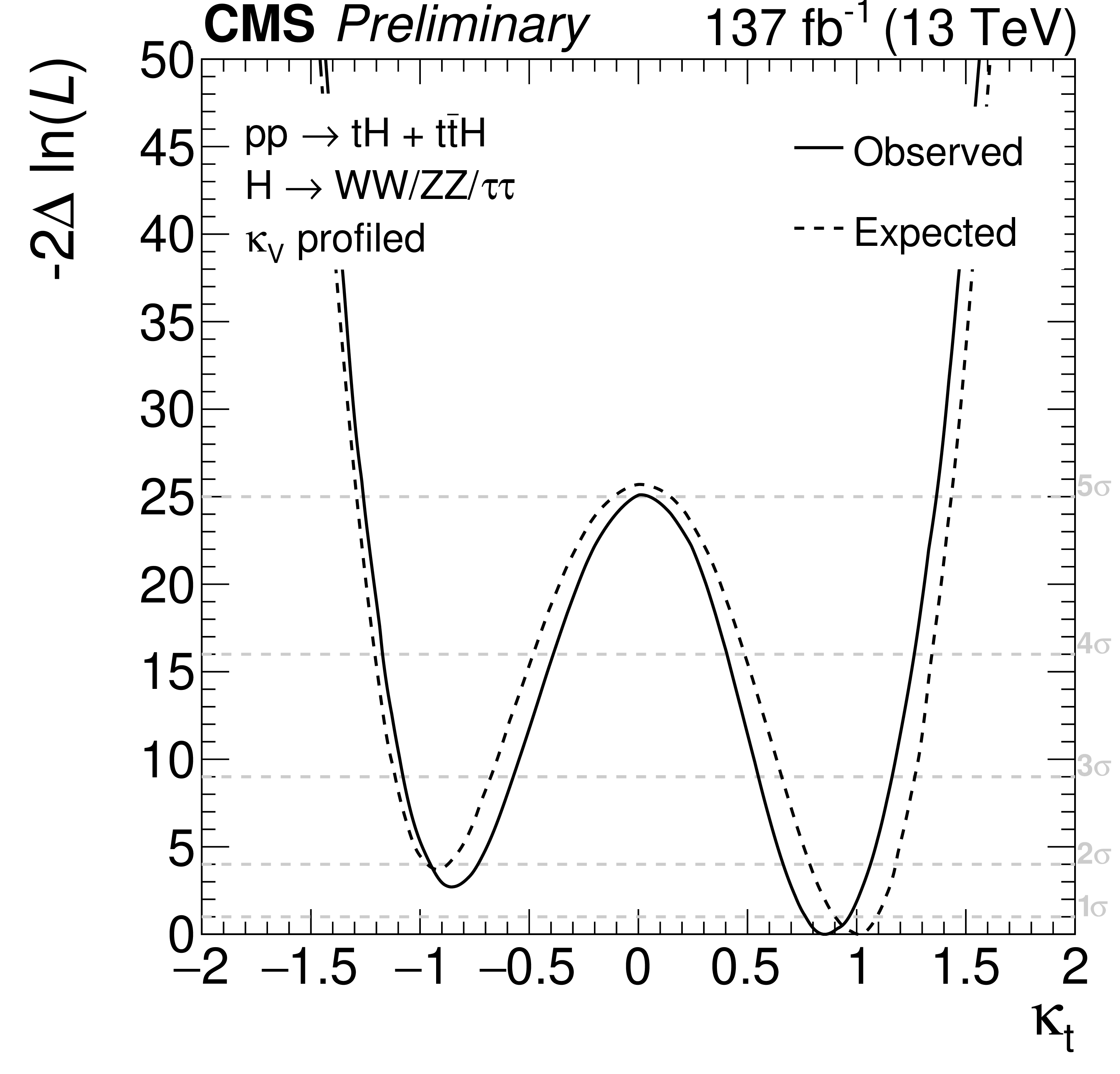
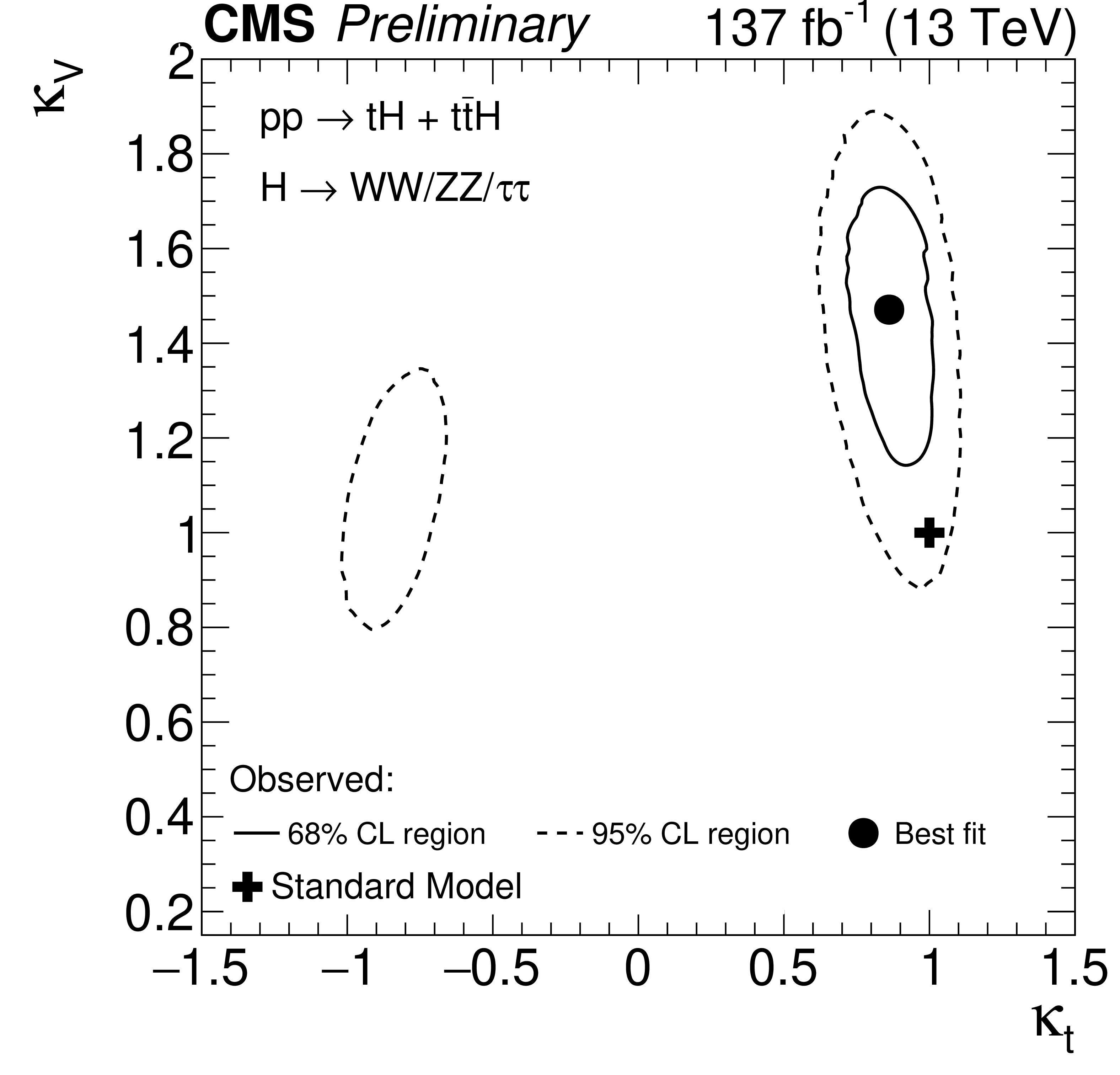
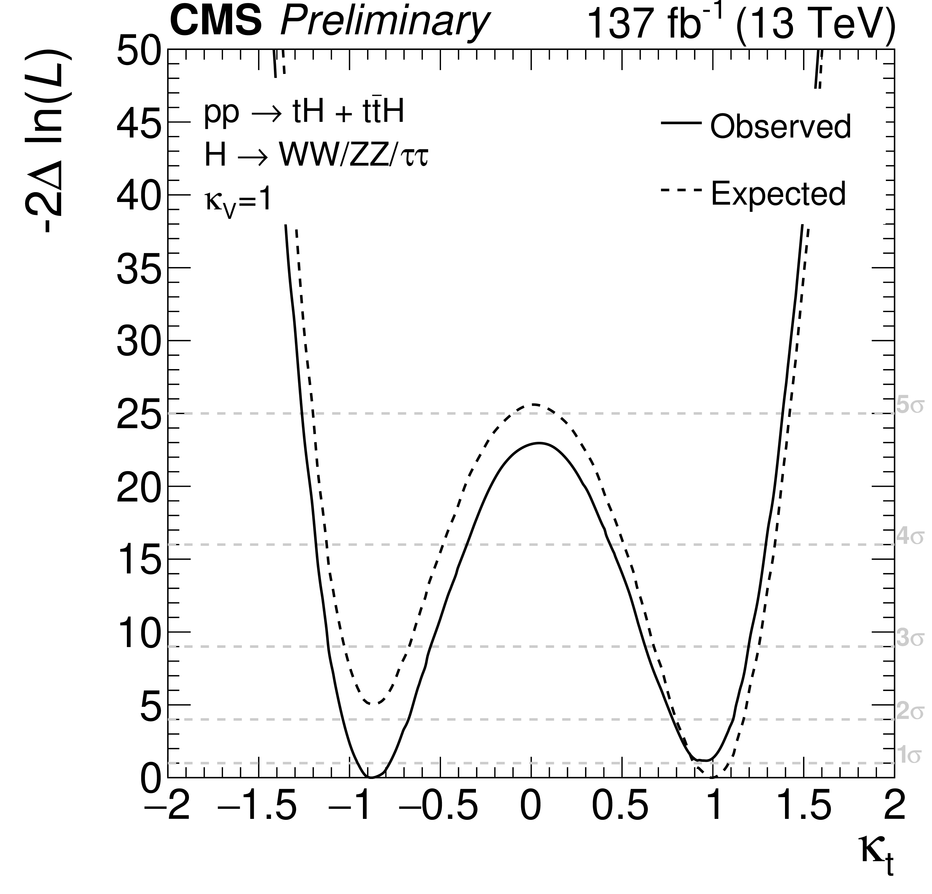
Figure 16:
Variation of the likelihood function $\mathcal {L}$, given by Eq. (3), as a function of $ {\kappa _{{\mathrm{t}}}}$, profiling over $ {\kappa _{\mathrm {V}}}$ (left), and as a function of $ {\kappa _{{\mathrm{t}}}}$ and $ {\kappa _{\mathrm {V}}}$ (right). |
png pdf |
Figure 16-a:
Variation of the likelihood function $\mathcal {L}$, given by Eq. (3), as a function of $ {\kappa _{{\mathrm{t}}}}$, profiling over $ {\kappa _{\mathrm {V}}}$. |
png pdf |
Figure 16-b:
Variation of the likelihood function $\mathcal {L}$, given by Eq. (3), as a function of $ {\kappa _{{\mathrm{t}}}}$ and $ {\kappa _{\mathrm {V}}}$. |
| Tables | |
png pdf |
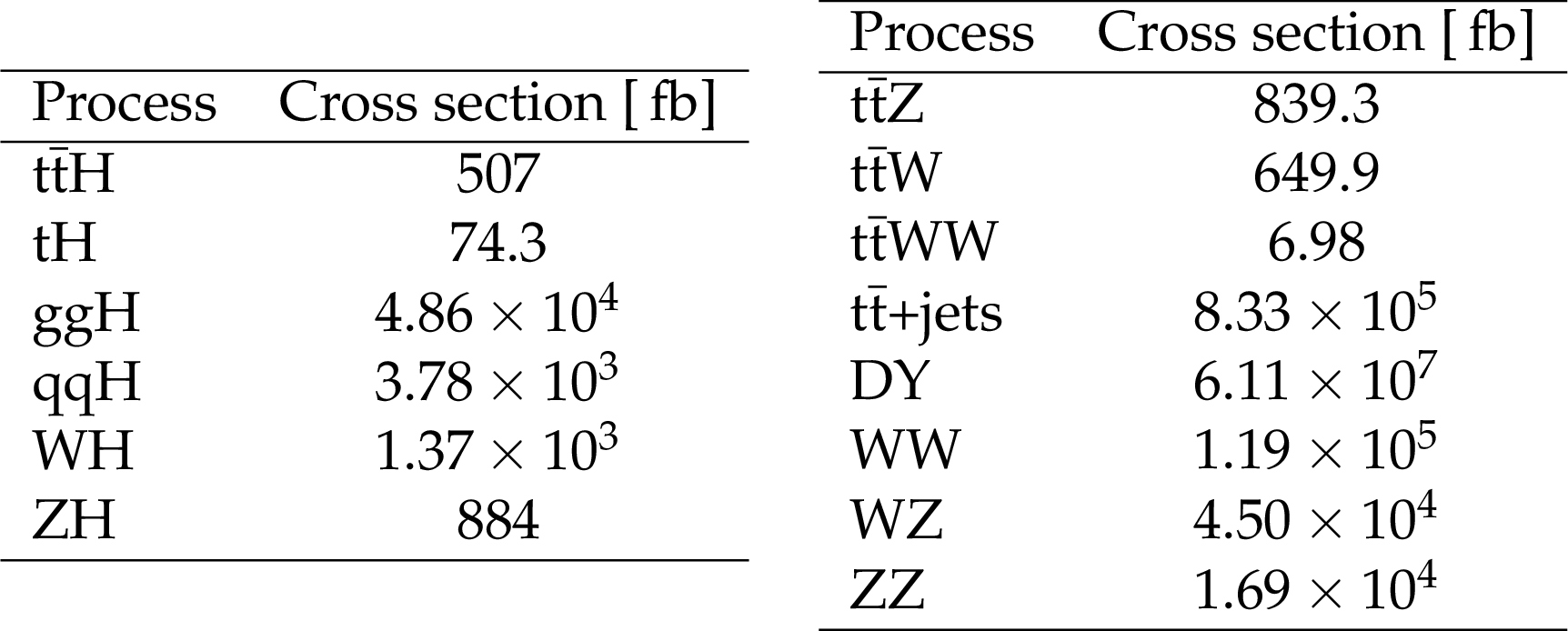
Table 1:
Standard model cross sections for the $ {{\mathrm{t}} {\mathrm{\bar{t}}} {\mathrm{H}}}$ and $ {{\mathrm{t}} {\mathrm{H}}}$ signals as well as for the most relevant background processes. The cross sections are quoted for ${\mathrm{p}} {\mathrm{p}} $ collisions at $\sqrt {s} = $ 13 TeV. The quoted value for DY production includes a generator-level requirement of $m_{\mathrm{Z} /\gamma ^*} > $ 50 GeV. |
png pdf |
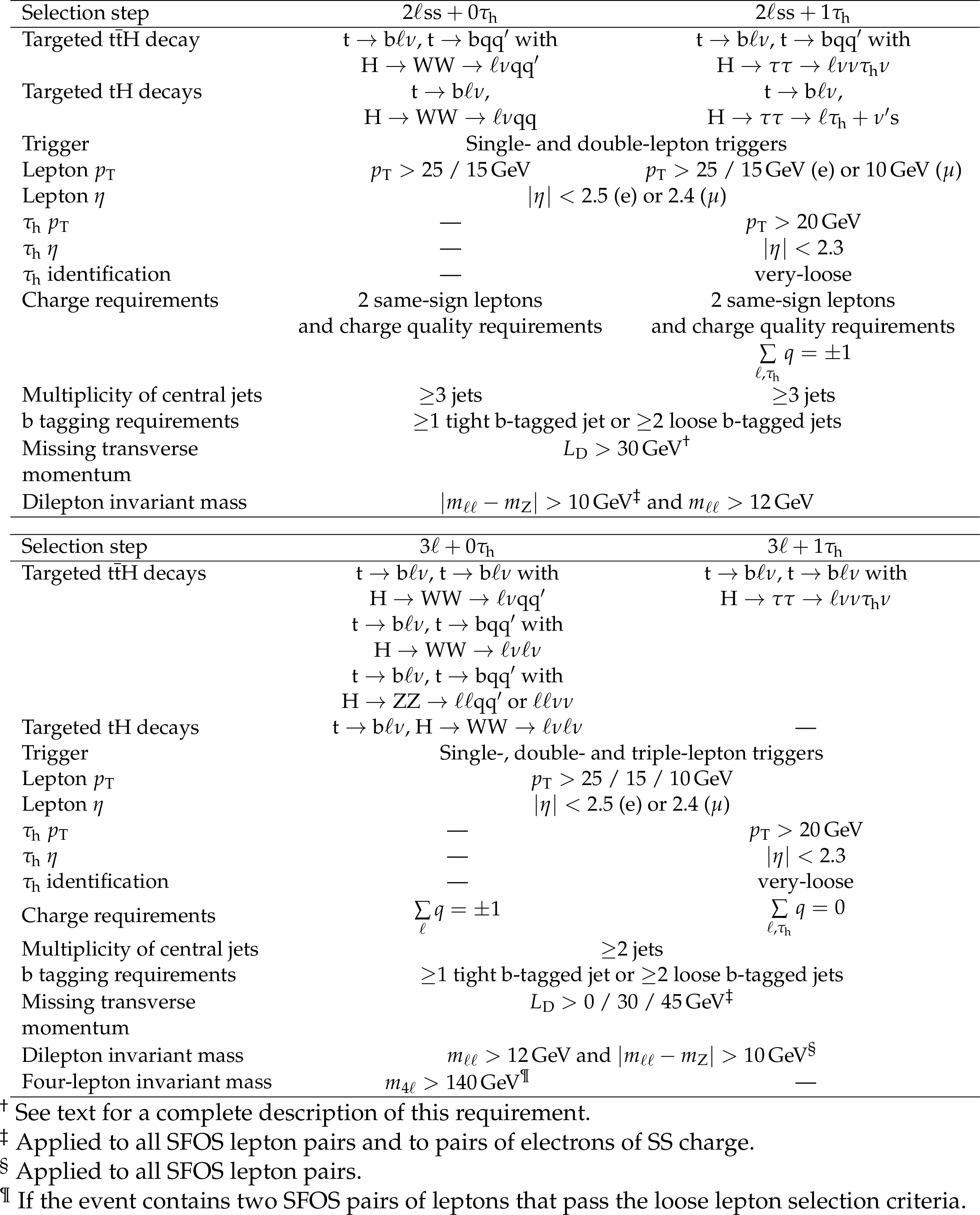
Table 2:
Event selections applied in the 2${\ell}$+0${\tau _{\mathrm {h}}}$, 2${\ell}$+1${\tau _{\mathrm {h}}}$, 3${\ell}$+0${\tau _{\mathrm {h}}}$, and 3${\ell}$+1${\tau _{\mathrm {h}}}$ channels. The ${p_{\mathrm {T}}}$ thresholds applied to the lepton of highest, second highest, and third highest ${p_{\mathrm {T}}}$ are separated by slashes. The symbol "---'' indicates that no requirement is applied on the feature. |
png pdf |
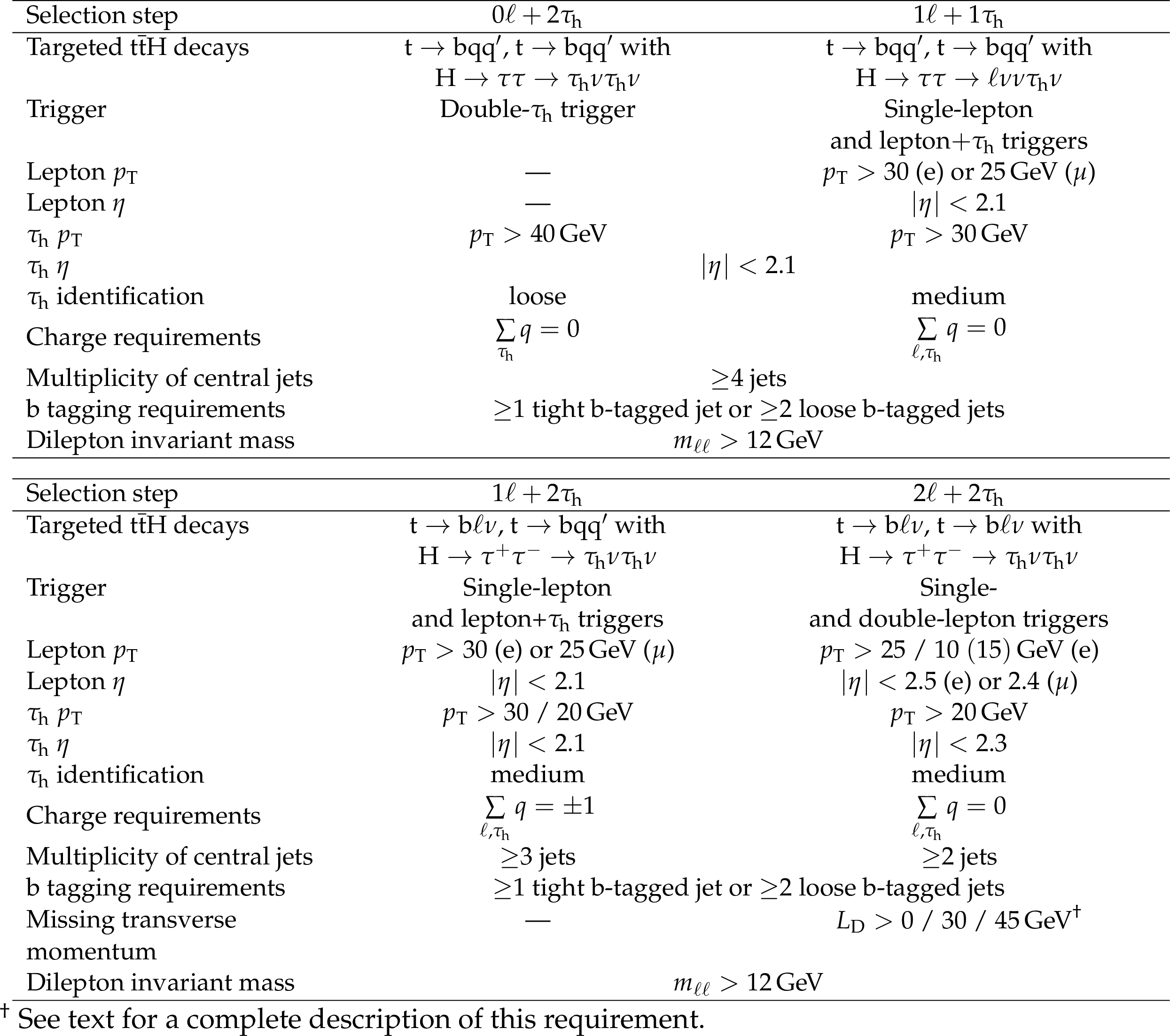
Table 3:
Event selections applied in the 0${\ell}$+2${\tau _{\mathrm {h}}}$, 1${\ell}$+1${\tau _{\mathrm {h}}}$, 1${\ell}$+2${\tau _{\mathrm {h}}}$, and 2${\ell}$+2${\tau _{\mathrm {h}}}$ channels. The ${p_{\mathrm {T}}}$ thresholds applied to the lepton and to the $ {\tau _\mathrm {h}} $ of highest and second highest ${p_{\mathrm {T}}}$ are separated by slashes. The symbol "---'' indicates that no requirement is applied on the feature. |
png pdf |
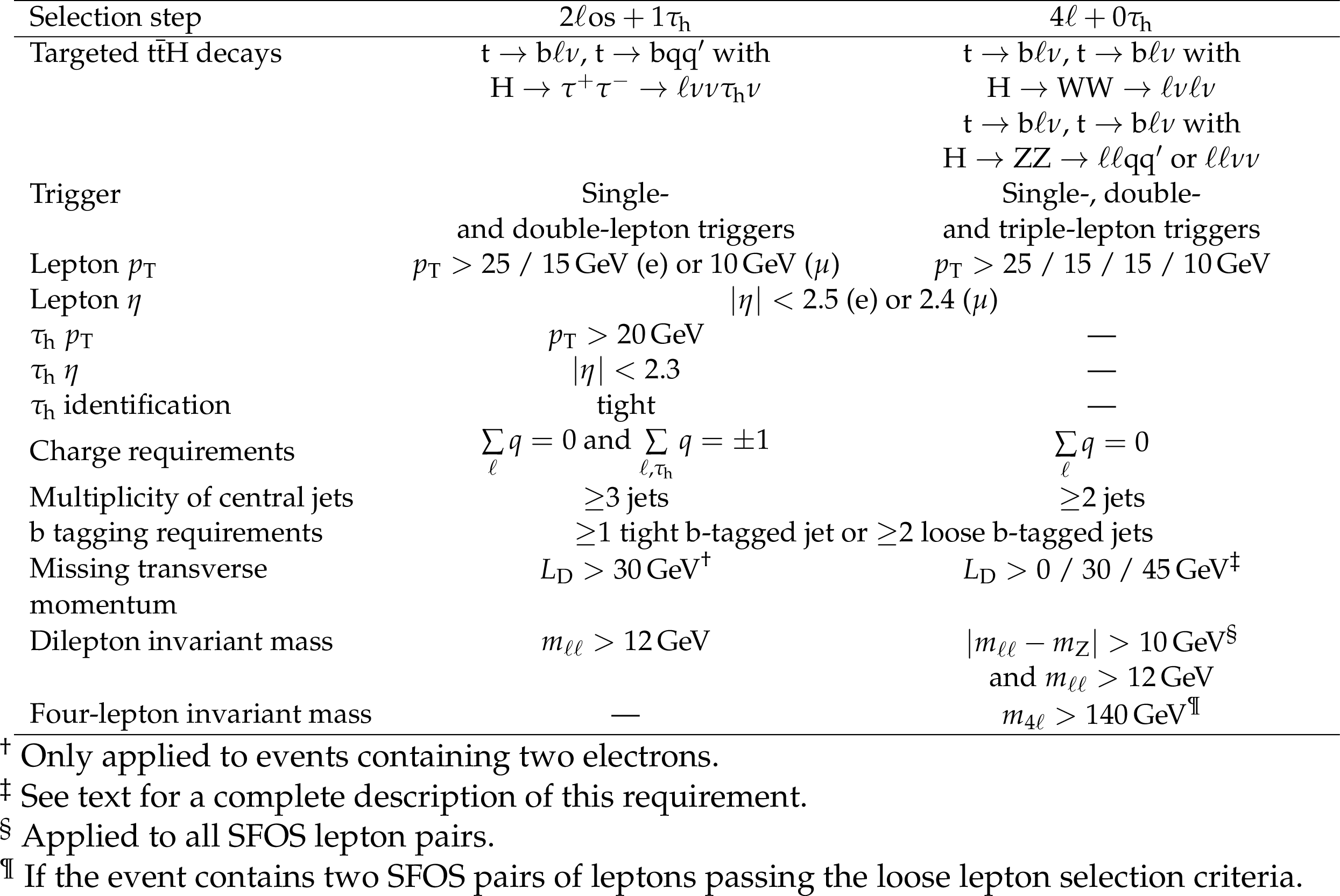
Table 4:
Event selections applied in the 2${\ell}$+1${\tau _{\mathrm {h}}}$ and 4${\ell}$+0${\tau _{\mathrm {h}}}$ channels. The symbol "---'' indicates that no requirement is applied on the feature. |

png pdf |
Table 5:
Input variables to the multivariant discriminants in each of the ten analysis channels. The symbol "---'' indicates that the variable is not considered. |
png pdf |
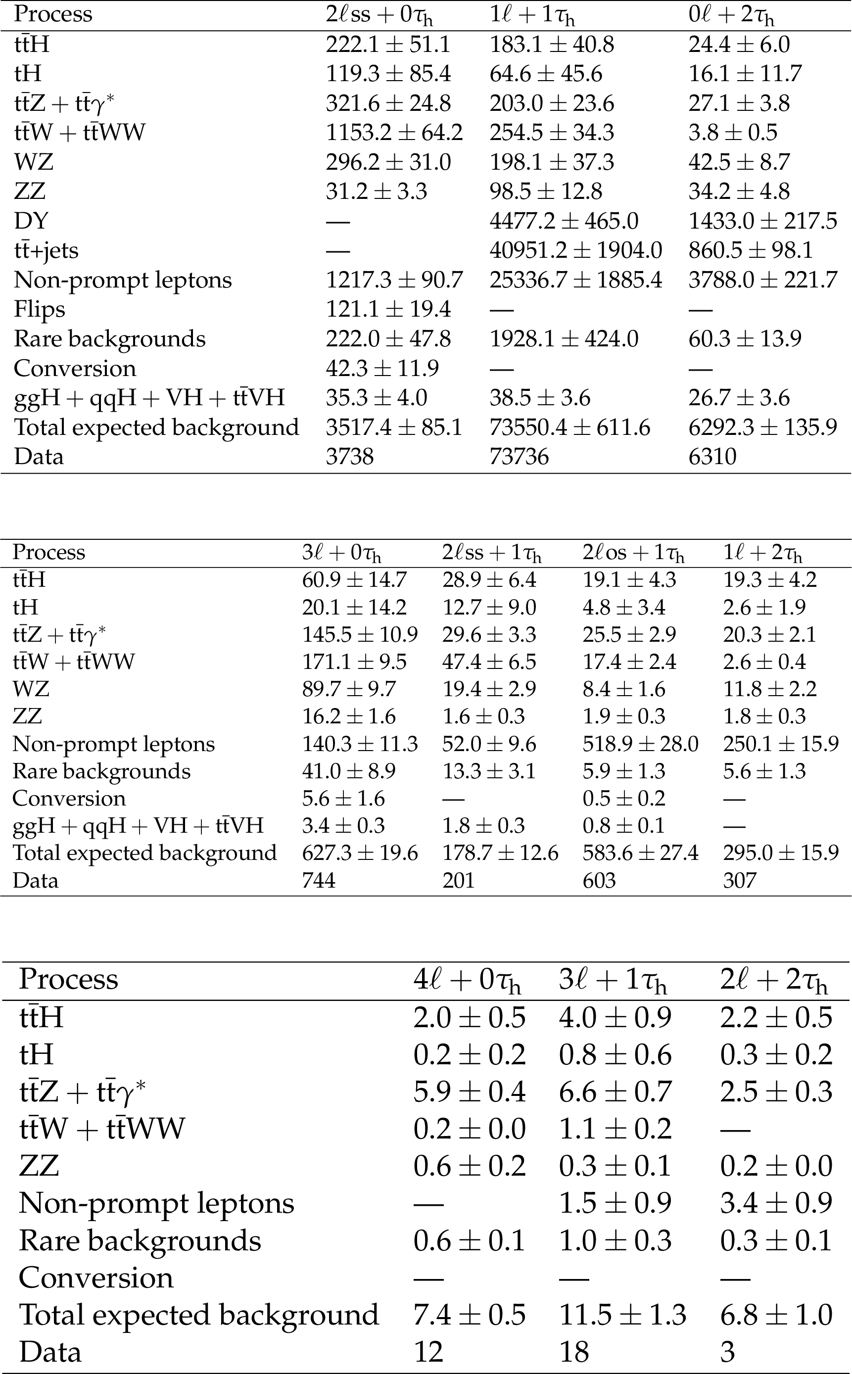
Table 6:
Number of events selected in the 3${\ell}$- and 4${\ell}$-CRs and in the CR for the $ {{\mathrm{t}} {\mathrm{\bar{t}}}\mathrm{W} (\mathrm{W})}$ background, compared to the event yields expected from different types of background and from the $ {{\mathrm{t}} {\mathrm{\bar{t}}} {\mathrm{H}}}$ and $ {{\mathrm{t}} {\mathrm{H}}}$ signals, after the fit to data is performed as described in 9. Uncertainties shown include all systematic components. |
png pdf |
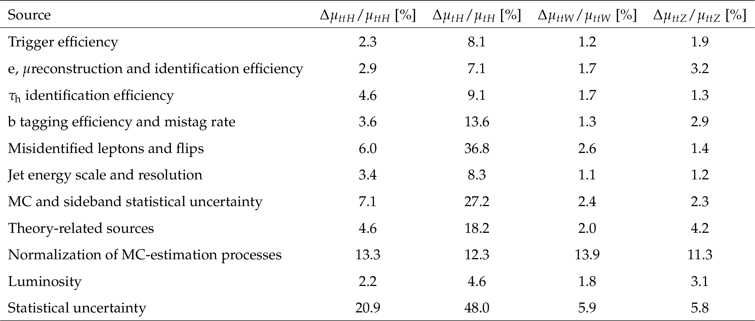
Table 7:
Summary of the main sources of systematic uncertainty and their impact on the measurement of the $ {{\mathrm{t}} {\mathrm{\bar{t}}} {\mathrm{H}}}$ plus $ {{\mathrm{t}} {\mathrm{H}}}$ signal rate $ {\mu}_{{{\mathrm{t}} {\mathrm{\bar{t}}} {\mathrm{H}}}+ {{\mathrm{t}} {\mathrm{H}}}}$ and the measured value of the unconstrained nuisance parameters. The quantity $\Delta {\mu}_{x}/ {\mu}_{x}$ corresponds to the change in uncertainty when fixing the nuisance parameters associated to that uncertainty in the fit. Under the label "MC and sideband statistical uncertainty'' are the uncertainties associated to the limited number of simulated MC events and the amount of data events in the application region of the FF method. |
| Summary |
| The rate for Higgs boson production in association with either one or two top quarks has been measured in events containing multiple electrons, muons, and hadronically decaying tau leptons, using data recorded by the CMS experiment in pp collisions at $\sqrt{s} = $ 13 TeV in 2016, 2017, and 2018. The analyzed data set corresponds to an integrated luminosity of 137 fb$^{-1}$. Ten different experimental signatures are considered in the analysis, differing by the multiplicity of e, $\mu$, and ${\tau_\mathrm{h}}$ and targeting events in which the Higgs boson decays via $\mathrm{H} \to \mathrm{W}\mathrm{W}$, $\mathrm{H} \to \tau\tau$, or $\mathrm{H} \to \mathrm{Z}\mathrm{Z}$, while the top quark(s) decay either leptonically or hadronically. The measured production rates for the ${\mathrm{t}}{\mathrm{\bar{t}}}\mathrm{H}$ and ${\mathrm{t}}\mathrm{H}$ signals amount to 0.92 $\pm$ 0.19 (stat) $^{+0.17}_{-0.13}$ (syst) and 5.7 $\pm$ 2.7 (stat) $\pm$ 3.0 (syst) times their respective standard model (SM) expectations. Assuming that the H boson coupling to the $\tau$ lepton is equal in strength to the values expected in the SM, the coupling $y_{{\mathrm{t}}}$ of the H boson to the top quark is constrained, at 95% confidence level, to be within $-0.9 < y_{{\mathrm{t}}} < -0.7$ or $ 0.7 < y_{{\mathrm{t}}} < 1.1$ times the SM expectation for this coupling. |
| Additional Figures | |
png pdf |
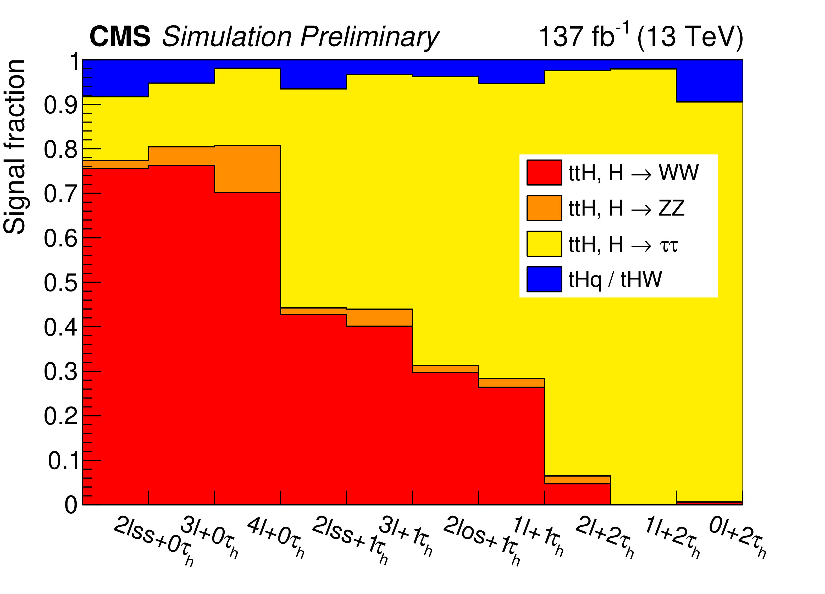
Additional Figure 1:
Relative contribution from signal production and decay mode to each of the signal regions. |
png pdf |
Additional Figure 2:
Variation of the likelihood function $\mathcal {L}$ as a function of $\kappa _{{\mathrm {t}}}$, after fixing $\kappa _{\mathrm{V}}$ to its SM value. |
png pdf |
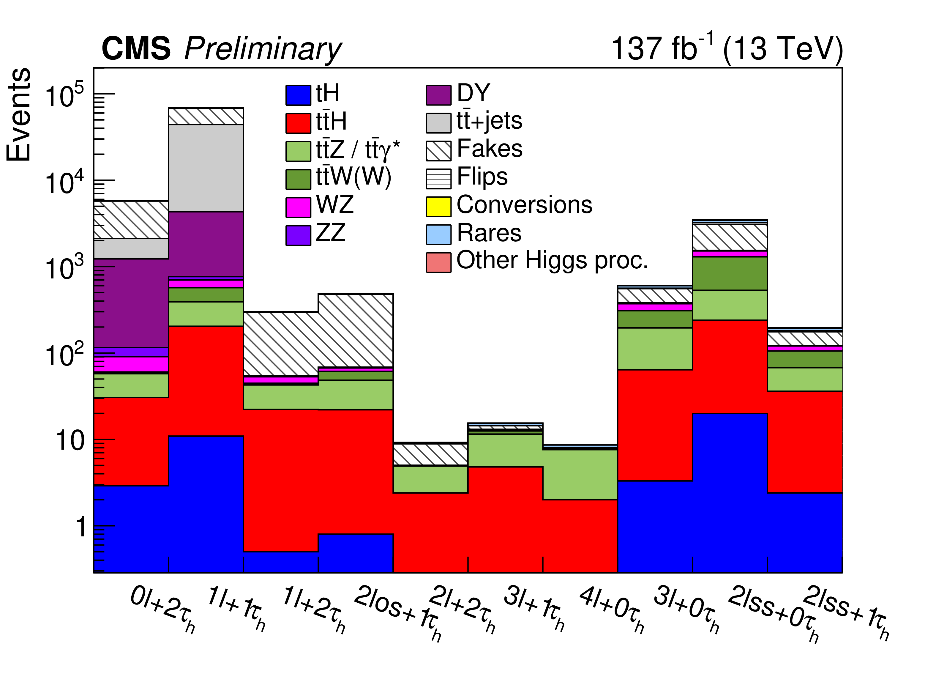
Additional Figure 3:
Number of expected signal and background events in each one of the analysis categories. |
png pdf |
Additional Figure 4:
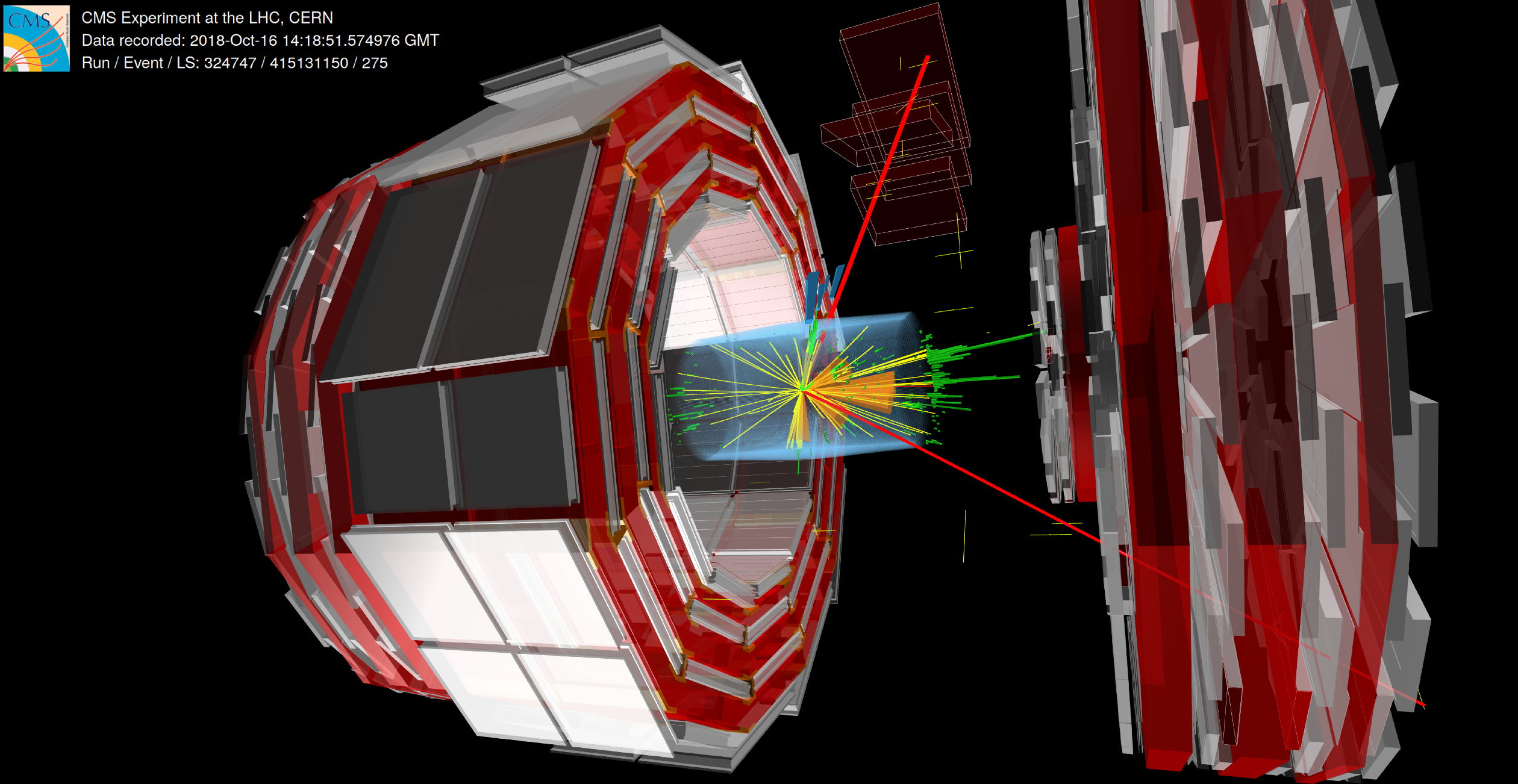
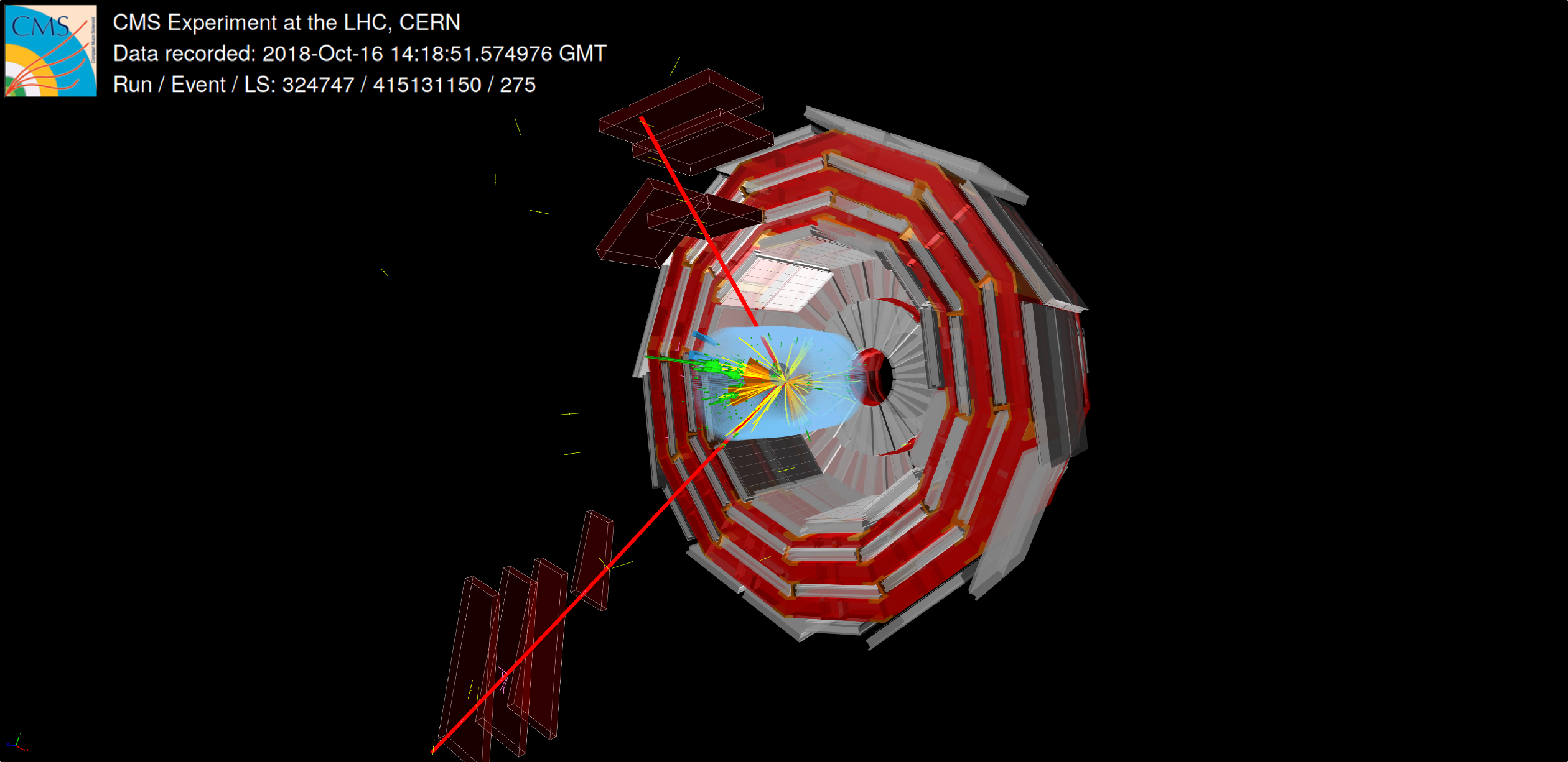
Display of a $ {\mathrm {t}} {\overline {\mathrm {t}}} {\mathrm {H}} $ candidate event in the 2$\ell$+0${{\tau} _\mathrm {h}} $ region. The event features two negative-sign charge muons, six jets and no additional ${{\tau} _\mathrm {h}}$. |
png pdf |
Additional Figure 5:
Display of a $ {\mathrm {t}} {\overline {\mathrm {t}}} {\mathrm {H}} $ candidate event in the 2$\ell$+0${{\tau} _\mathrm {h}} $ region. The event features two negative-sign charge muons, six jets and no additional ${{\tau} _\mathrm {h}}$. |
| References | ||||
| 1 | ATLAS Collaboration | Observation of a new particle in the search for the standard model Higgs boson with the ATLAS detector at the LHC | PLB 716 (2012) 1 | 1207.7214 |
| 2 | CMS Collaboration | Observation of a new boson at a mass of 125 GeV with the CMS experiment at the LHC | PLB 716 (2012) 30 | CMS-HIG-12-028 1207.7235 |
| 3 | CMS Collaboration | Observation of a new boson with mass near 125 GeV in pp collisions at $ \sqrt{s}= $ 7 and 8 TeV | JHEP 06 (2013) 081 | CMS-HIG-12-036 1303.4571 |
| 4 | Particle Data Group Collaboration | Review of particle physics | PRD 98 (2018) 030001 | |
| 5 | B. A. Dobrescu and C. T. Hill | Electroweak symmetry breaking via top condensation seesaw | PRL 81 (1998) 2634 | hep-ph/9712319 |
| 6 | R. S. Chivukula, B. A. Dobrescu, H. Georgi, and C. T. Hill | Top quark seesaw theory of electroweak symmetry breaking | PRD 59 (1999) 075003 | hep-ph/9809470 |
| 7 | D. Delepine, J. M. Gerard, and R. Gonzalez Felipe | Is the standard Higgs scalar elementary? | PLB 372 (1996) 271 | hep-ph/9512339 |
| 8 | F. Maltoni, G. Ridolfi, and M. Ubiali | b-initiated processes at the LHC: a reappraisal | JHEP 07 (2012) 022 | 1203.6393 |
| 9 | LHC Higgs Cross Section Working Group Collaboration | Handbook of LHC Higgs cross sections: 4. Deciphering the nature of the Higgs sector | CERN Yellow Report | 1610.07922 |
| 10 | F. Demartin, F. Maltoni, K. Mawatari, and M. Zaro | Higgs production in association with a single top quark at the LHC | EPJC 75 (2015) 267 | 1504.00611 |
| 11 | F. Demartin et al. | $ \mathrm{t}\mathrm{W}\mathrm{H} $ associated production at the LHC | EPJC 77 (2017) 34 | 1607.05862 |
| 12 | ATLAS, CMS Collaboration | Measurements of the Higgs boson production and decay rates and constraints on its couplings from a combined ATLAS and CMS analysis of the LHC pp collision data at $ \sqrt{s} = $ 7 and 8 TeV | JHEP 08 (2016) 045 | 1606.02266 |
| 13 | S. Biswas, E. Gabrielli, F. Margaroli, and B. Mele | Direct constraints on the top-Higgs coupling from the 8 TeV LHC data | JHEP 07 (2013) 073 | 1304.1822 |
| 14 | B. Hespel, F. Maltoni, and E. Vryonidou | Higgs and Z boson associated production via gluon fusion in the SM and the 2HDM | JHEP 06 (2015) 065 | 1503.01656 |
| 15 | CMS Collaboration | Search for the associated production of the Higgs boson with a top quark pair | JHEP 09 (2014) 087 | CMS-HIG-13-029 1408.1682 |
| 16 | ATLAS Collaboration | Search for $ \mathrm{H}\to\gamma\gamma $ produced in association with top quarks and constraints on the Yukawa coupling between the top quark and the Higgs boson using data taken at 7 TeV and 8 TeV with the ATLAS detector | PLB 740 (2015) 222 | 1409.3122 |
| 17 | ATLAS Collaboration | Search for the standard model Higgs boson produced in association with top quarks and decaying into $ \mathrm{b\bar{b}} $ in pp collisions at $ \sqrt{s} = $ 8 TeV with the ATLAS detector | EPJC 75 (2015) 349 | 1503.05066 |
| 18 | ATLAS Collaboration | Search for the associated production of the Higgs boson with a top quark pair in multilepton final states with the ATLAS detector | PLB 749 (2015) 519 | 1506.05988 |
| 19 | ATLAS Collaboration | Search for the standard model Higgs boson decaying into $ \mathrm{b\bar{b}} $ produced in association with top quarks decaying hadronically in pp collisions at $ \sqrt{s} = $ 8 TeV with the ATLAS detector | JHEP 05 (2016) 160 | 1604.03812 |
| 20 | CMS Collaboration | Measurements of properties of the Higgs boson decaying into the four-lepton final state in pp collisions at $ \sqrt{s} = $ 13 TeV | JHEP 11 (2017) 047 | CMS-HIG-16-041 1706.09936 |
| 21 | ATLAS Collaboration | Evidence for the associated production of the Higgs boson and a top quark pair with the ATLAS detector | PRD 97 (2018) 072003 | 1712.08891 |
| 22 | ATLAS Collaboration | Search for the standard model Higgs boson produced in association with top quarks and decaying into a $ \mathrm{b\bar{b}} $ pair in pp collisions at $ \sqrt{s} = $ 13 TeV with the ATLAS detector | PRD 97 (2018) 072016 | 1712.08895 |
| 23 | CMS Collaboration | Evidence for associated production of a Higgs boson with a top quark pair in final states with electrons, muons, and hadronically decaying $ \tau $ leptons at $ \sqrt{s} = $ 13 TeV | JHEP 08 (2018) 066 | CMS-HIG-17-018 1803.05485 |
| 24 | CMS Collaboration | Search for ttH production in the all-jet final state in proton-proton collisions at $ \sqrt{s} = $ 13 TeV | JHEP 06 (2018) 101 | CMS-HIG-17-022 1803.06986 |
| 25 | CMS Collaboration | Measurements of Higgs boson properties in the diphoton decay channel in proton-proton collisions at $ \sqrt{s} = $ 13 TeV | JHEP 11 (2018) 185 | CMS-HIG-16-040 1804.02716 |
| 26 | CMS Collaboration | Search for ttH production in the $ \mathrm{H} \to \mathrm{b\bar{b}} $ decay channel with leptonic $ \mathrm{t\bar{t}} $ decays in proton-proton collisions at $ \sqrt{s} = $ 13 TeV | JHEP 03 (2019) 026 | CMS-HIG-17-026 1804.03682 |
| 27 | CMS Collaboration | Observation of ttH production | PRL 120 (2018) 231801 | CMS-HIG-17-035 1804.02610 |
| 28 | ATLAS Collaboration | Observation of Higgs boson production in association with a top quark pair at the LHC with the ATLAS detector | PLB 784 (2018) 173 | 1806.00425 |
| 29 | CMS Collaboration | Search for the associated production of a Higgs boson with a single top quark in proton-proton collisions at $ \sqrt{s} = $ 8 TeV | JHEP 06 (2016) 177 | CMS-HIG-14-027 1509.08159 |
| 30 | CMS Collaboration | Search for associated production of a Higgs boson and a single top quark in proton-proton collisions at $ \sqrt{s} = $ 13 TeV | PRD 99 (2019) 092005 | CMS-HIG-18-009 1811.09696 |
| 31 | A. Hocker et al. | TMVA - toolkit for multivariate data analysis | PoS ACAT (2007) 040 | physics/0703039 |
| 32 | T. Chen and C. Guestrin | XGBoost: a scalable tree boosting system | in Proceedings of the 22nd ACM SIGKDD International Conference on Knowledge Discovery and Data Mining 2016 | |
| 33 | F. Pedregosa et al. | Scikit-learn: machine learning in python | JMLR 12 (2011) 2825 | |
| 34 | K. Kondo | Dynamical likelihood method for reconstruction of events with missing momentum. 1: method and toy models | J. Phys. Soc. Jap. 57 (1988) 4126 | |
| 35 | K. Kondo | Dynamical likelihood method for reconstruction of events with missing momentum. 2: mass spectra for 2$ \to $2 processes | J. Phys. Soc. Jap. 60 (1991) 836 | |
| 36 | CMS Collaboration | The CMS trigger system | JINST 12 (2017) P01020 | CMS-TRG-12-001 1609.02366 |
| 37 | CMS Collaboration | The CMS experiment at the CERN LHC | JINST 3 (2008) S08004 | CMS-00-001 |
| 38 | CMS Collaboration | CMS luminosity measurements for the 2016 data-taking period | ||
| 39 | CMS Collaboration | CMS luminosity measurement for the 2017 data-taking period at $ \sqrt{s} = $ 13 TeV | ||
| 40 | CMS Collaboration | CMS luminosity measurement for the 2018 data-taking period at $ \sqrt{s} = $ 13 TeV | ||
| 41 | J. Alwall et al. | Comparative study of various algorithms for the merging of parton showers and matrix elements in hadronic collisions | EPJC 53 (2008) 473 | 0706.2569 |
| 42 | P. Artoisenet, R. Frederix, O. Mattelaer, and R. Rietkerk | Automatic spin-entangled decays of heavy resonances in Monte Carlo simulations | JHEP 03 (2013) 015 | 1212.3460 |
| 43 | R. Frederix and S. Frixione | Merging meets matching in MC@NLO | JHEP 12 (2012) 061 | 1209.6215 |
| 44 | J. Alwall et al. | The automated computation of tree-level and next-to-leading order differential cross sections, and their matching to parton shower simulations | JHEP 07 (2014) 079 | 1405.0301 |
| 45 | R. Frederix and I. Tsinikos | Subleading EW corrections and spin-correlation effects in ttW multi-lepton signatures | 2004.09552 | |
| 46 | P. Nason | A new method for combining NLO QCD with shower Monte Carlo algorithms | JHEP 11 (2004) 040 | hep-ph/0409146 |
| 47 | S. Frixione, P. Nason, and C. Oleari | Matching NLO QCD computations with parton shower simulations: the POWHEG method | JHEP 11 (2007) 070 | 0709.2092 |
| 48 | S. Alioli, P. Nason, C. Oleari, and E. Re | A general framework for implementing NLO calculations in shower Monte Carlo programs: the POWHEG box | JHEP 06 (2010) 043 | 1002.2581 |
| 49 | T. Sjostrand et al. | An introduction to $ PYTHIA 8.2 $ | CPC 191 (2015) 159 | 1410.3012 |
| 50 | NNPDF Collaboration | Unbiased global determination of parton distributions and their uncertainties at NNLO and at LO | NPB 855 (2012) 153 | 1107.2652 |
| 51 | NNPDF Collaboration | Parton distributions with QED corrections | NPB 877 (2013) 290 | 1308.0598 |
| 52 | NNPDF Collaboration | Parton distributions for the LHC Run 2 | JHEP 04 (2015) 040 | 1410.8849 |
| 53 | CMS Collaboration | Extraction and validation of a new set of CMS PYTHIA 8 tunes from underlying-event measurements | EPJC 80 (2020) 4 | CMS-GEN-17-001 1903.12179 |
| 54 | CMS Collaboration | Investigations of the impact of the parton shower tuning in $ PYTHIA $ 8 in the modelling of $ \mathrm{t\bar{t}} $ at $ \sqrt{s}= $ 8 and 13 TeV | CMS-PAS-TOP-16-021 | CMS-PAS-TOP-16-021 |
| 55 | CMS Collaboration | Event generator tunes obtained from underlying event and multiparton scattering measurements | EPJC 76 (2016) 155 | CMS-GEN-14-001 1512.00815 |
| 56 | J. M. Campbell, R. K. Ellis, and C. Williams | Vector boson pair production at the LHC | JHEP 07 (2011) 018 | 1105.0020 |
| 57 | M. Czakon and A. Mitov | Top++ a program for the calculation of the top-pair cross section at hadron colliders | CPC 185 (2014) 2930 | 1112.5675 |
| 58 | Y. Li and F. Petriello | Combining QCD and electroweak corrections to dilepton production in FEWZ | PRD 86 (2012) 094034 | 1208.5967 |
| 59 | GEANT4 Collaboration | $ GEANT4: $ a simulation toolkit | NIMA 506 (2003) 250 | |
| 60 | CMS Collaboration | Measurements of inclusive W and Z cross sections in pp collisions at $ \sqrt{s} = $ 7 TeV | JHEP 01 (2011) 080 | CMS-EWK-10-002 1012.2466 |
| 61 | CMS Collaboration | Jet energy scale and resolution in the CMS experiment in pp collisions at 8 TeV | JINST 12 (2017) P02014 | CMS-JME-13-004 1607.03663 |
| 62 | CMS Collaboration | Identification of heavy-flavour jets with the CMS detector in pp collisions at 13 TeV | JINST 13 (2018) P05011 | CMS-BTV-16-002 1712.07158 |
| 63 | CMS Collaboration | Performance of reconstruction and identification of $ \tau $ leptons decaying to hadrons and $ \nu_{\tau} $ in pp collisions at $ \sqrt{s} = $ 13 TeV | JINST 13 (2018) P10005 | CMS-TAU-16-003 1809.02816 |
| 64 | CMS Collaboration | Performance of missing transverse momentum reconstruction in proton-proton collisions at $ \sqrt{s} = $ 13 TeV using the CMS detector | JINST 14 (2019) P07004 | CMS-JME-17-001 1903.06078 |
| 65 | CMS Collaboration | Particle-flow reconstruction and global event description with the CMS detector | JINST 12 (2017) P10003 | CMS-PRF-14-001 1706.04965 |
| 66 | CMS Collaboration | Performance of electron reconstruction and selection with the CMS detector in proton-proton collisions at $ \sqrt{s} = $ 8 TeV | JINST 10 (2015) P06005 | CMS-EGM-13-001 1502.02701 |
| 67 | CMS Collaboration | Performance of CMS muon reconstruction in pp collision events at $ \sqrt{s} = $ 7 TeV | JINST 7 (2012) P10002 | CMS-MUO-10-004 1206.4071 |
| 68 | K. Rehermann and B. Tweedie | Efficient identification of boosted semileptonic top quarks at the LHC | JHEP 03 (2011) 059 | 1007.2221 |
| 69 | CMS Collaboration | Search for new physics in same-sign dilepton events in proton-proton collisions at $ \sqrt{s} = $ 13 TeV | EPJC 76 (2016) 439 | CMS-SUS-15-008 1605.03171 |
| 70 | M. Cacciari, G. P. Salam, and G. Soyez | The anti-$ {k_{\mathrm{T}}} $ jet clustering algorithm | JHEP 04 (2008) 063 | 0802.1189 |
| 71 | M. Cacciari, G. P. Salam, and G. Soyez | FastJet user manual | EPJC 72 (2012) 1896 | 1111.6097 |
| 72 | M. Cacciari, G. P. Salam, and G. Soyez | The catchment area of jets | JHEP 04 (2008) 005 | 0802.1188 |
| 73 | M. Cacciari and G. P. Salam | Pileup subtraction using jet areas | PLB 659 (2008) 119 | 0707.1378 |
| 74 | CMS Collaboration | Jet algorithms performance in 13 TeV data | CMS-PAS-JME-16-003 | CMS-PAS-JME-16-003 |
| 75 | CMS Collaboration | CMS Phase 1 heavy flavour identification performance and developments | CMS-DP-2017-013 | |
| 76 | Y. Lecun | Generalization and network design strategies | of the University of Toronto, CRG-TR-89-4 | |
| 77 | CMS Collaboration | Measurements of properties of the Higgs boson in the four-lepton final state in proton-proton collisions at $ \sqrt{s} = $ 13 TeV | CMS-PAS-HIG-19-001 | CMS-PAS-HIG-19-001 |
| 78 | L. Bianchini et al. | Reconstruction of the Higgs mass in events with Higgs bosons decaying into a pair of $ \tau $ leptons using matrix element techniques | NIMA 862 (2017) 54 | 1603.05910 |
| 79 | J. S. Bridle | Training stochastic model recognition algorithms as networks can lead to maximum mutual information estimation of parameters | in Proceedings, conference on advances in neural information processing systems 2 (NIPS 1989), p. 211 1990 | |
| 80 | X. Glorot, A. Bordes, and Y. Bengio | Deep sparse rectifier neural networks | in Proceedings, 14th international conference on artificial intelligence and statistics (AISTATS 2011), volume 15, p. 315 2011 | |
| 81 | M. Abadi et al. | TensorFlow: large-scale machine learning on heterogeneous distributed systems | 1603.04467 | |
| 82 | F. Chollet et al. | keras | GitHub | |
| 83 | I. Goodfellow, Y. Bengio, and A. Courville | Deep Learning Book | MIT Press | |
| 84 | A. N. Tikhonov | Solution of incorrectly formulated problems and the regularization method | Soviet Math. Dokl. 4 (1963) 1035 | |
| 85 | N. Srivastava et al. | Dropout: a simple way to prevent neural networks from overfitting | JMLR 15 (2014) 1929 | |
| 86 | M. Cacciari et al. | The $ \mathrm{t\bar{t}} $ cross-section at 1.8 TeV and 1.96 TeV: a study of the systematics due to parton densities and scale dependence | JHEP 04 (2004) 068 | hep-ph/0303085 |
| 87 | S. Catani, D. de Florian, M. Grazzini, and P. Nason | Soft gluon resummation for Higgs boson production at hadron colliders | JHEP 07 (2003) 028 | hep-ph/0306211 |
| 88 | R. Frederix et al. | Four-lepton production at hadron colliders: MadGraph5+MC@NLO predictions with theoretical uncertainties | JHEP 02 (2012) 099 | 1110.4738 |
| 89 | J. Butterworth et al. | PDF4LHC recommendations for LHC Run 2 | JPG 43 (2016) 023001 | 1510.03865 |
| 90 | R. Gavin, Y. Li, F. Petriello, and S. Quackenbush | FEWZ 2.0: a code for hadronic Z production at next-to-next-to-leading order | CPC 182 (2011) 2388 | 1011.3540 |
| 91 | M. Czakon et al. | Top-pair production at the LHC through NNLO QCD and NLO EW | JHEP 10 (2017) 186 | 1705.04105 |
| 92 | J. S. Conway | Incorporating nuisance parameters in likelihoods for multisource spectra | in Proceedings, workshop on statistical issues related to discovery claims in search experiments and unfolding (PHYSTAT 2011), p. 115 2011 | 1103.0354 |
| 93 | R. J. Barlow and C. Beeston | Fitting using finite Monte Carlo samples | CPC 77 (1993) 219 | |
| 94 | ATLAS and CMS Collaborations and LHC Higgs Combination Group | Procedure for the LHC Higgs boson search combination in summer 2011 | technical report | |
| 95 | CMS Collaboration | Combined results of searches for the standard model Higgs boson in pp collisions at $ \sqrt{s} = $ 7 TeV | PLB 710 (2012) 26 | CMS-HIG-11-032 1202.1488 |
| 96 | J. Neyman | Outline of a theory of statistical estimation based on the classical theory of probability | Phil. Trans. Roy. Soc. Lond. A 236 (1937) 333 | |
|
|
Compact Muon Solenoid LHC, CERN |
|

|

|

|

|

|