

Compact Muon Solenoid
LHC, CERN
| CMS-SUS-24-001 ; CERN-EP-2024-335 | ||
| Search for bosons of an extended Higgs sector in b quark final states in proton-proton collisions at $ \sqrt{s} = $ 13 TeV | ||
| CMS Collaboration | ||
| 10 February 2025 | ||
| JHEP 06 (2025) 144 | ||
| Abstract: A search for beyond-the-standard-model neutral Higgs bosons decaying to a pair of bottom quarks, and produced in association with at least one additional bottom quark, is performed with the CMS detector. The data were recorded in proton-proton collisions at a centre-of-mass energy of 13 TeV at the CERN LHC and correspond to an integrated luminosity of 36.7-126.9 fb$ ^{-1} $, depending on the probed mass range. No signal above the standard model background expectation is observed. Upper limits on the production cross section times branching fraction are set for Higgs bosons in the mass range of 125-1800 GeV. The results are interpreted in benchmark scenarios of the minimal supersymmetric standard model, as well as suitable classes of two-Higgs-doublet models. | ||
| Links: e-print arXiv:2502.06568 [hep-ex] (PDF) ; CDS record ; inSPIRE record ; HepData record ; Physics Briefing ; CADI line (restricted) ; | ||
| Figures & Tables | Summary | Additional Figures | References | CMS Publications |
|---|
| Figures | |
png pdf |
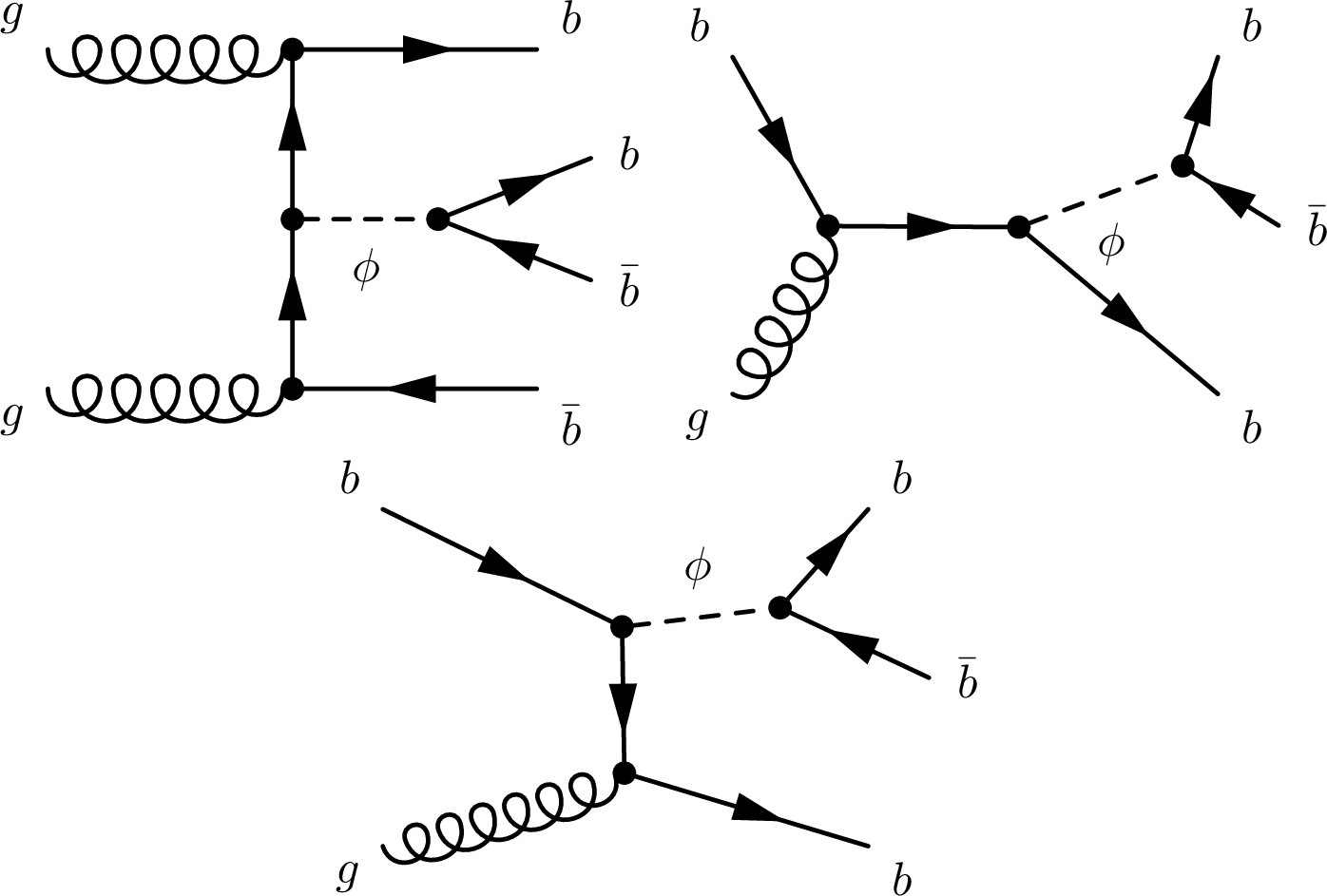
Figure 1:
Example Feynman diagrams for the signal processes. |
png pdf |
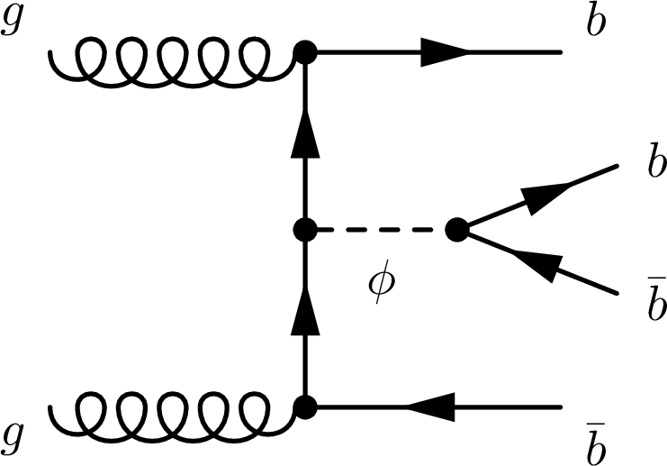
Figure 1-a:
Example Feynman diagrams for the signal processes. |
png pdf |
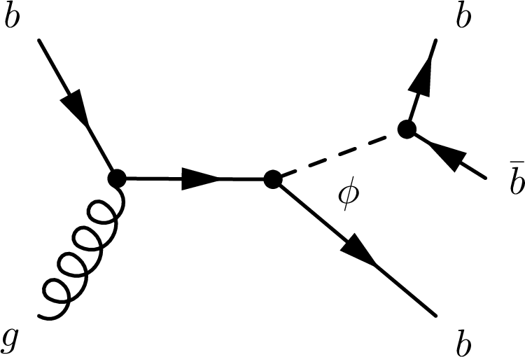
Figure 1-b:
Example Feynman diagrams for the signal processes. |
png pdf |
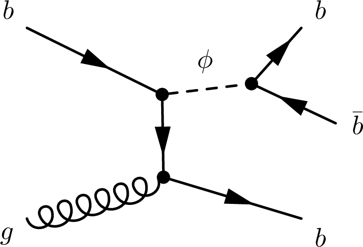
Figure 1-c:
Example Feynman diagrams for the signal processes. |
png pdf |
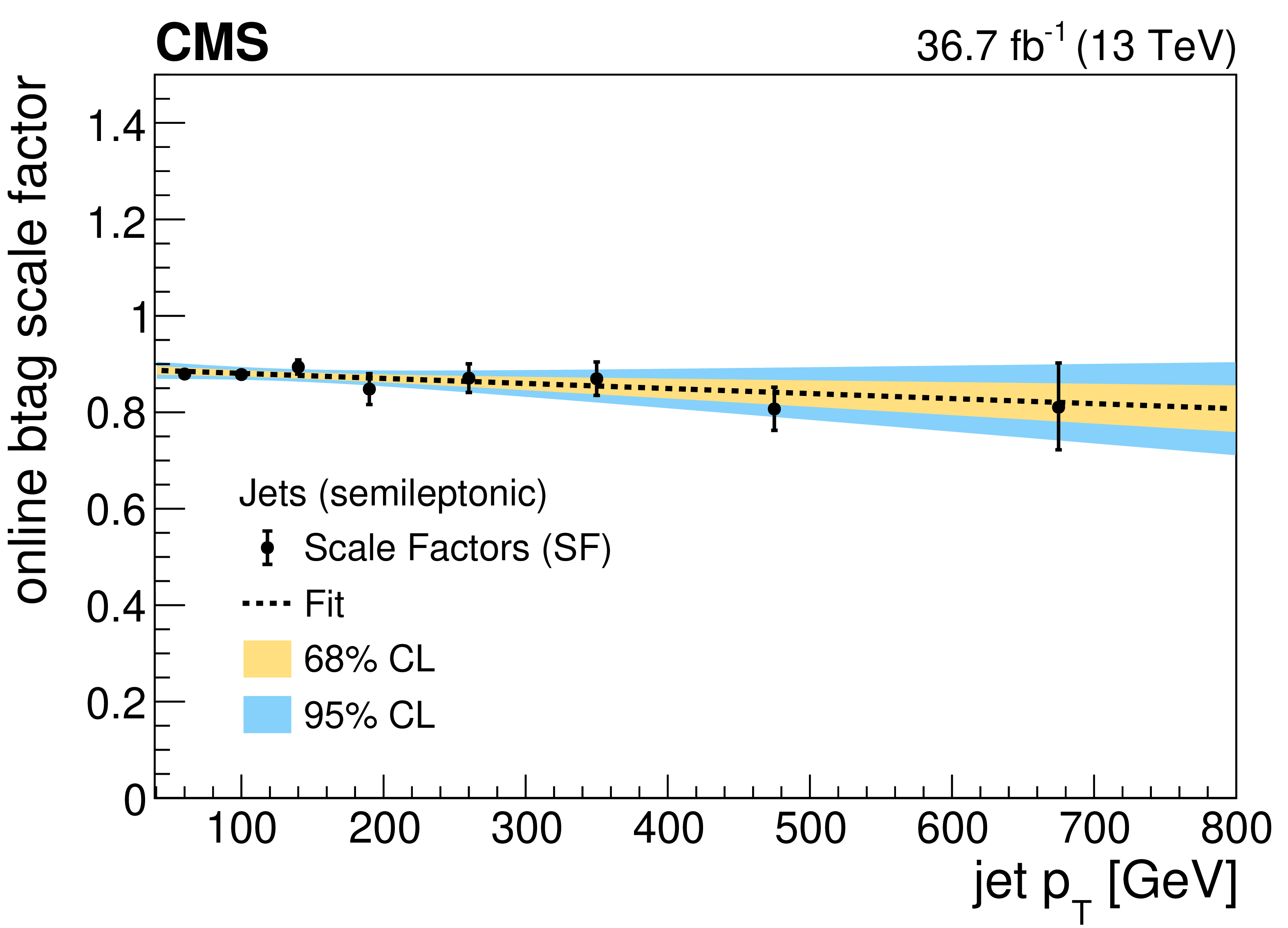
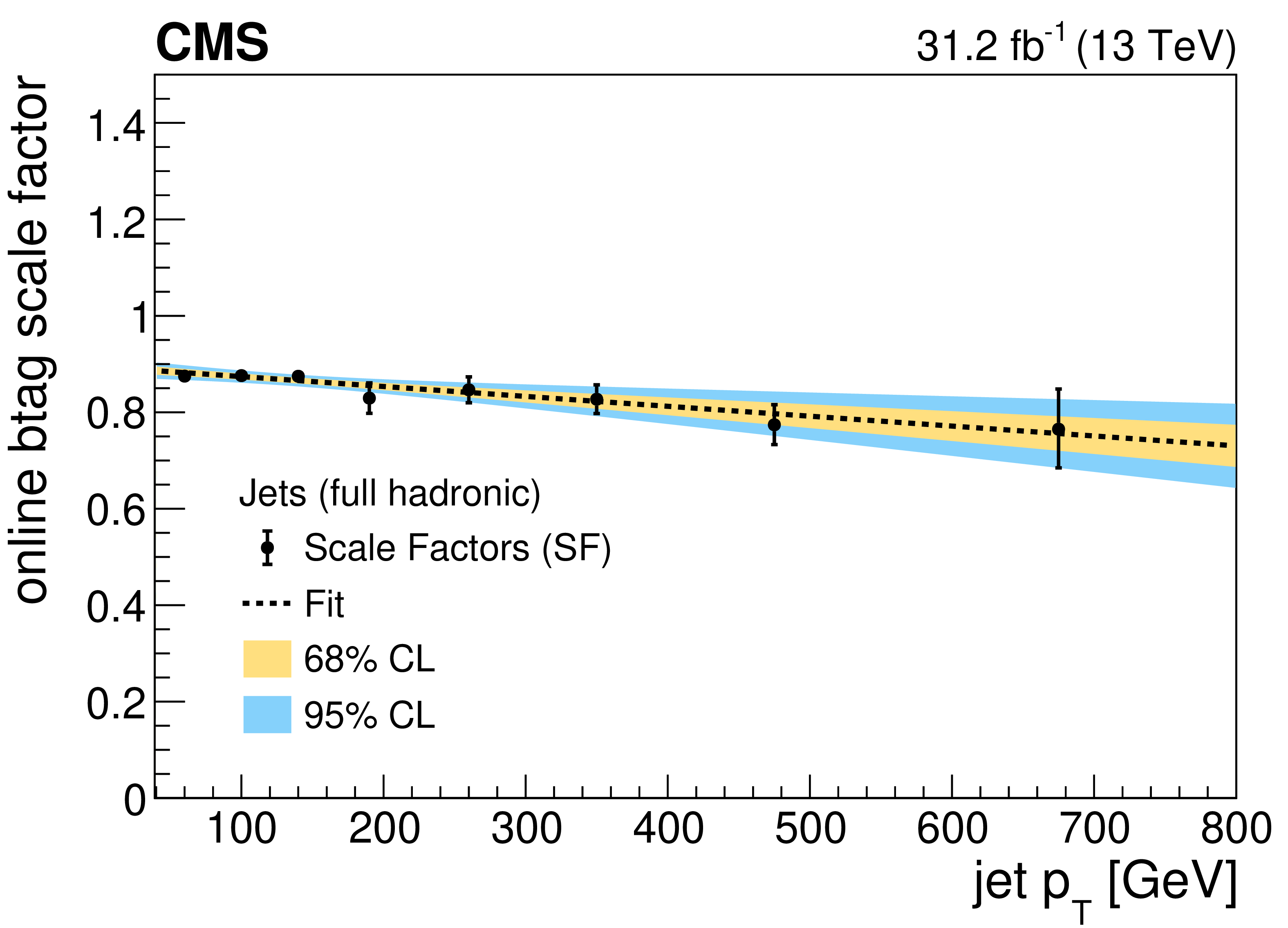
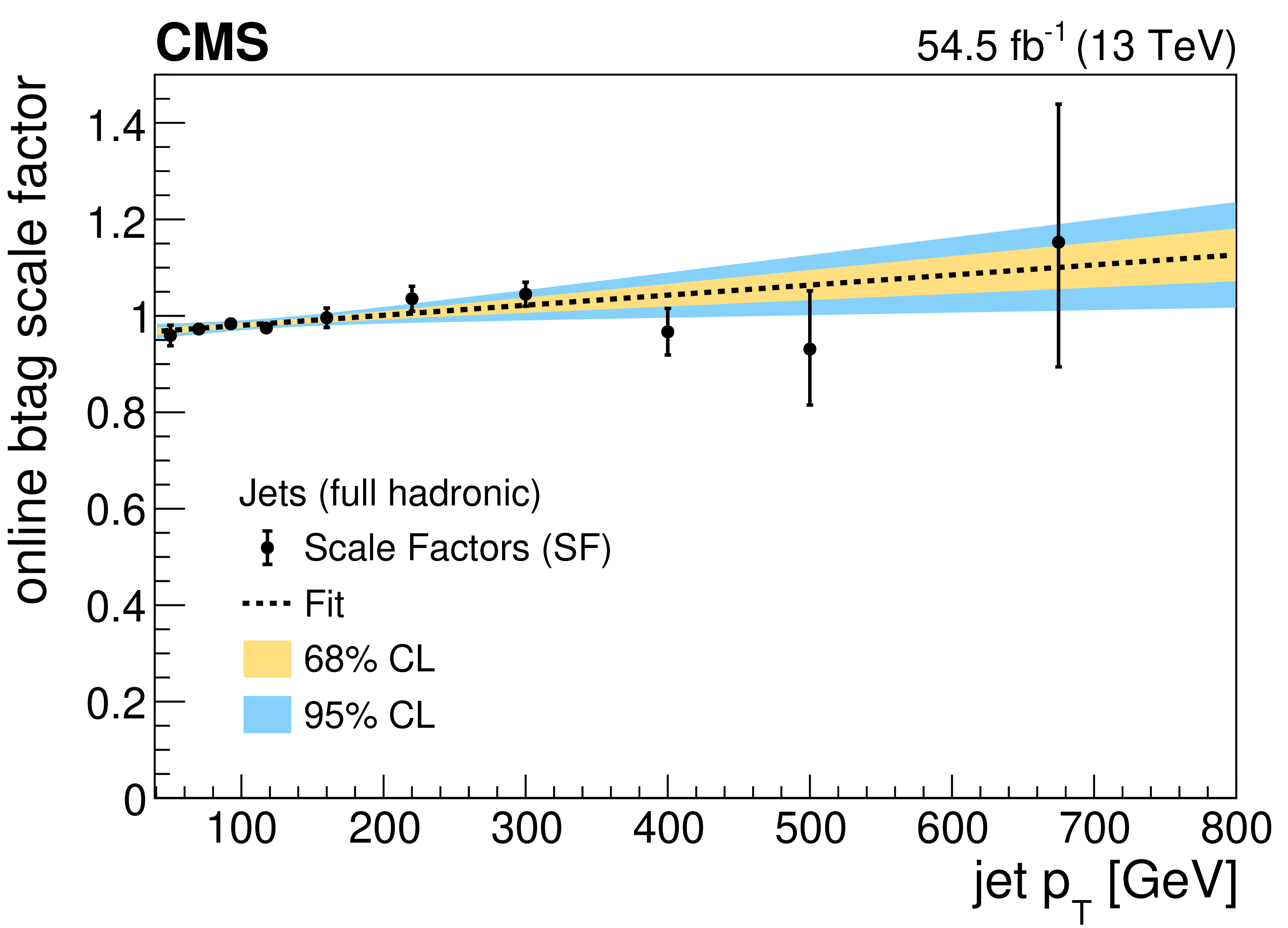
Figure 2:
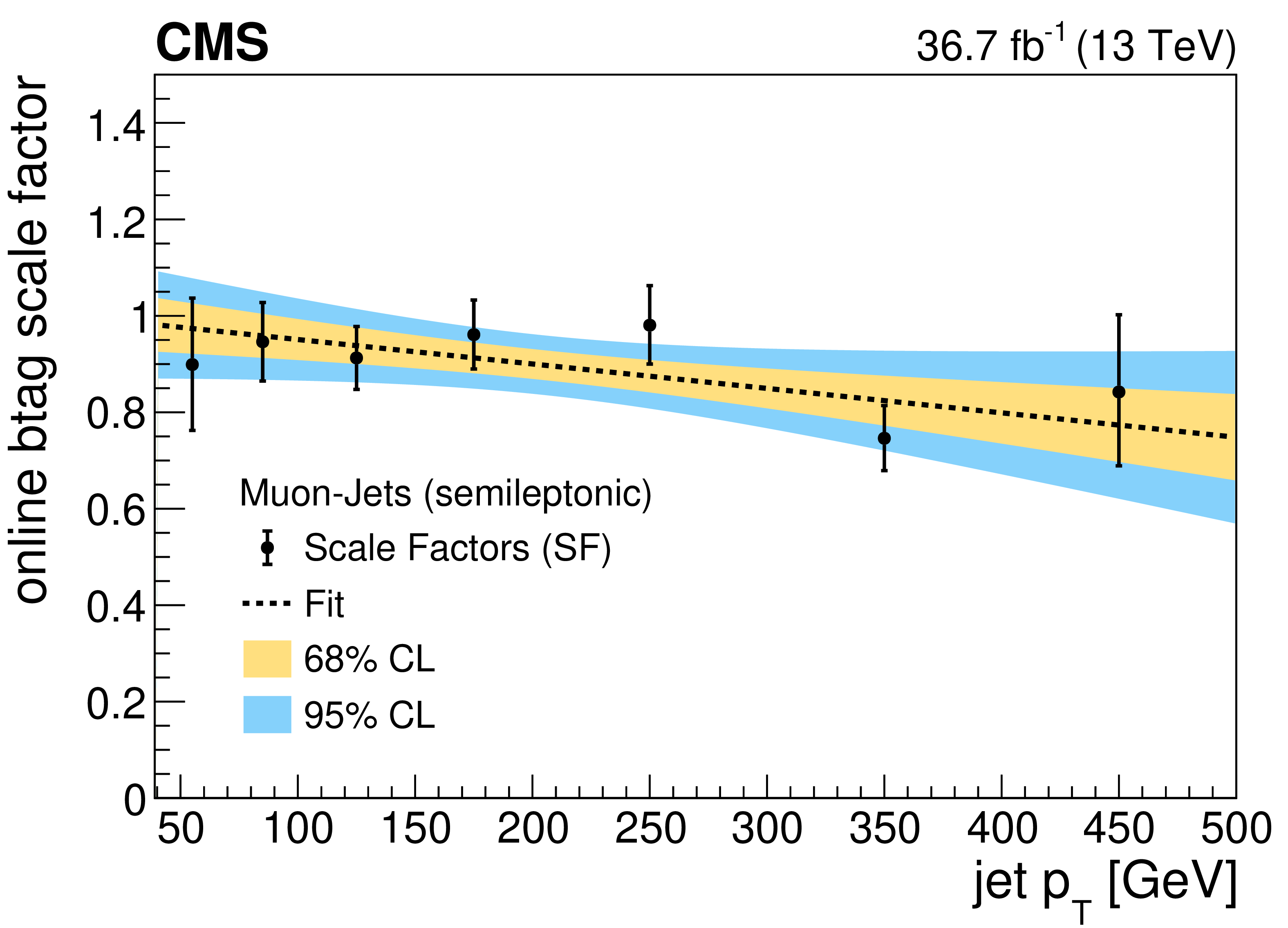
Online b tagging scale factors for b jets in the 2017 SL (upper left), 2017 FH (upper right) and 2018 FH (lower left) analyses, and for b jets with muons in the 2017 SL analysis (lower right). The results of linear fits are also shown, together with $ {\pm}1\sigma $ and $ {\pm}2\sigma $ uncertainty bands. |
png pdf |
Figure 2-a:
Online b tagging scale factors for b jets in the 2017 SL (upper left), 2017 FH (upper right) and 2018 FH (lower left) analyses, and for b jets with muons in the 2017 SL analysis (lower right). The results of linear fits are also shown, together with $ {\pm}1\sigma $ and $ {\pm}2\sigma $ uncertainty bands. |
png pdf |
Figure 2-b:
Online b tagging scale factors for b jets in the 2017 SL (upper left), 2017 FH (upper right) and 2018 FH (lower left) analyses, and for b jets with muons in the 2017 SL analysis (lower right). The results of linear fits are also shown, together with $ {\pm}1\sigma $ and $ {\pm}2\sigma $ uncertainty bands. |
png pdf |
Figure 2-c:
Online b tagging scale factors for b jets in the 2017 SL (upper left), 2017 FH (upper right) and 2018 FH (lower left) analyses, and for b jets with muons in the 2017 SL analysis (lower right). The results of linear fits are also shown, together with $ {\pm}1\sigma $ and $ {\pm}2\sigma $ uncertainty bands. |
png pdf |
Figure 2-d:
Online b tagging scale factors for b jets in the 2017 SL (upper left), 2017 FH (upper right) and 2018 FH (lower left) analyses, and for b jets with muons in the 2017 SL analysis (lower right). The results of linear fits are also shown, together with $ {\pm}1\sigma $ and $ {\pm}2\sigma $ uncertainty bands. |
png pdf |
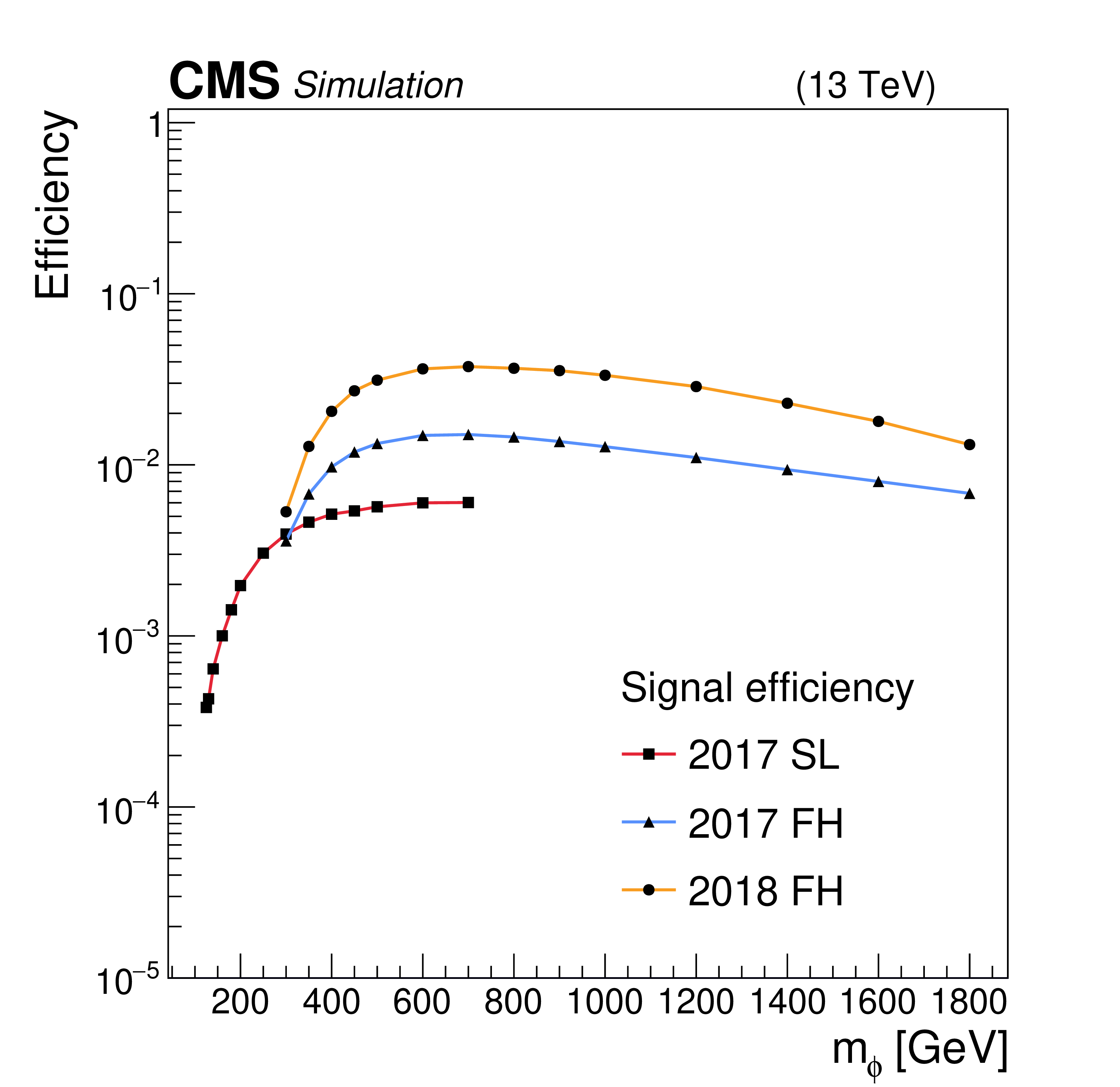
Figure 3:
Signal efficiency as a function of the mass $ m_{\phi} $ after triple b tag selection for 2017 SL (squares), 2017 FH (triangles), and 2018 FH (circles) channels. |
png pdf |
Figure 3-a:
Signal efficiency as a function of the mass $ m_{\phi} $ after triple b tag selection for 2017 SL (squares), 2017 FH (triangles), and 2018 FH (circles) channels. |
png pdf |
Figure 3-b:
Signal efficiency as a function of the mass $ m_{\phi} $ after triple b tag selection for 2017 SL (squares), 2017 FH (triangles), and 2018 FH (circles) channels. |
png pdf |
Figure 3-c:
Signal efficiency as a function of the mass $ m_{\phi} $ after triple b tag selection for 2017 SL (squares), 2017 FH (triangles), and 2018 FH (circles) channels. |
png pdf |
Figure 4:
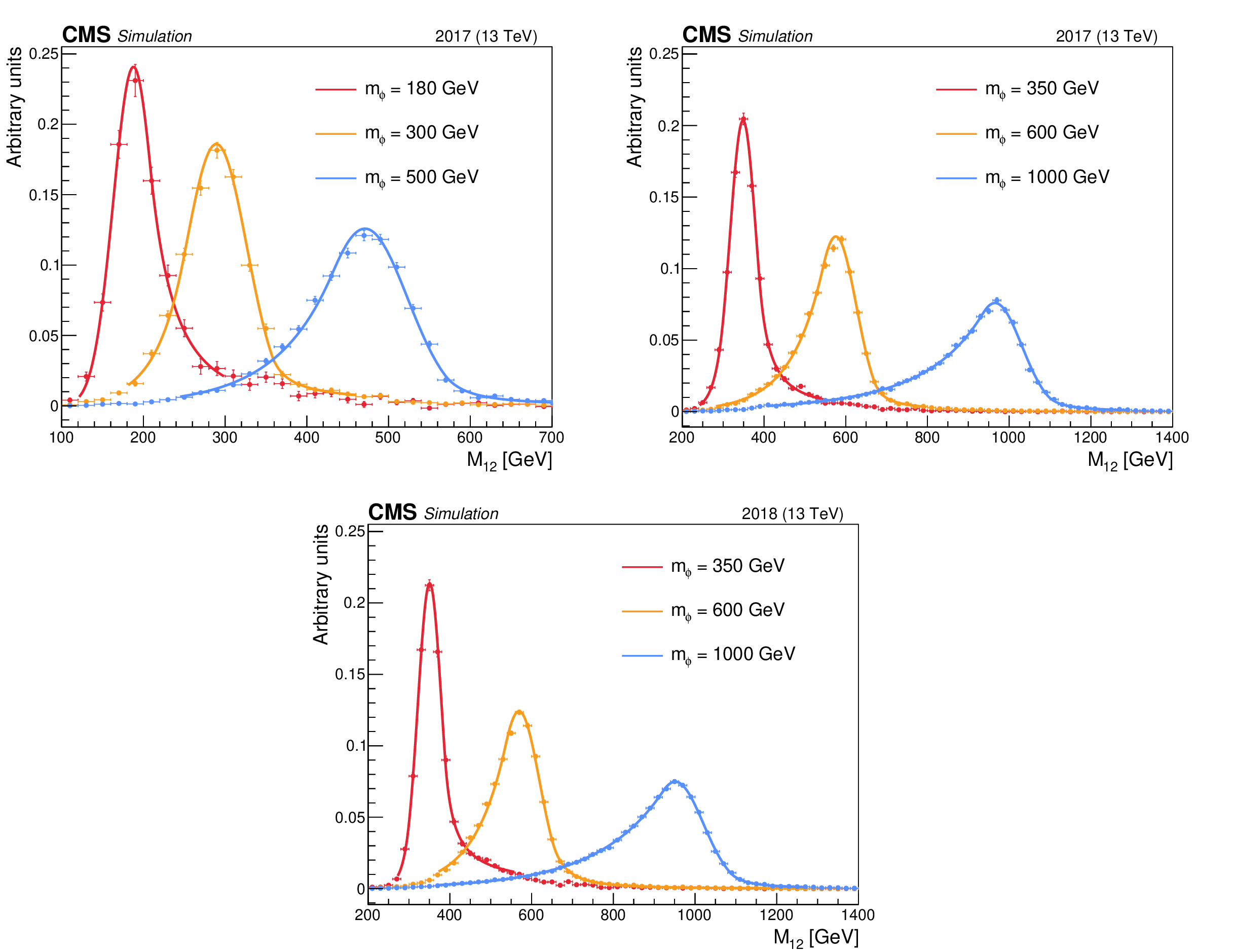
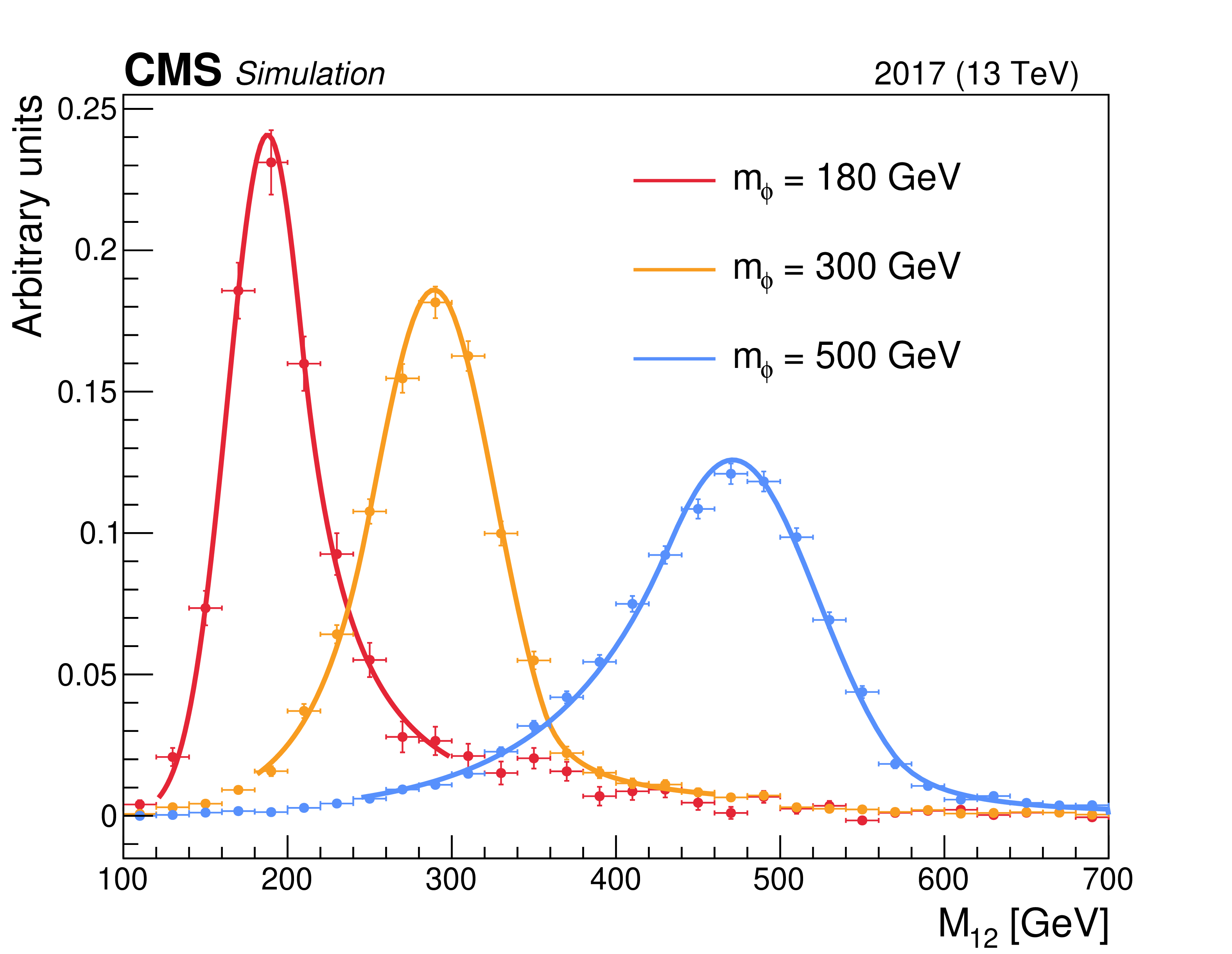
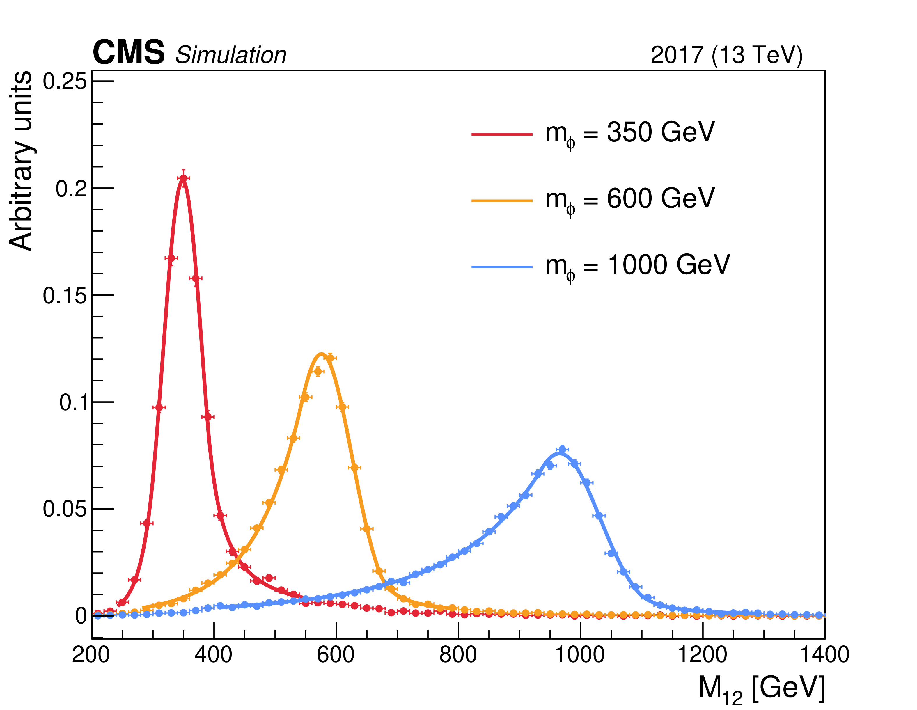
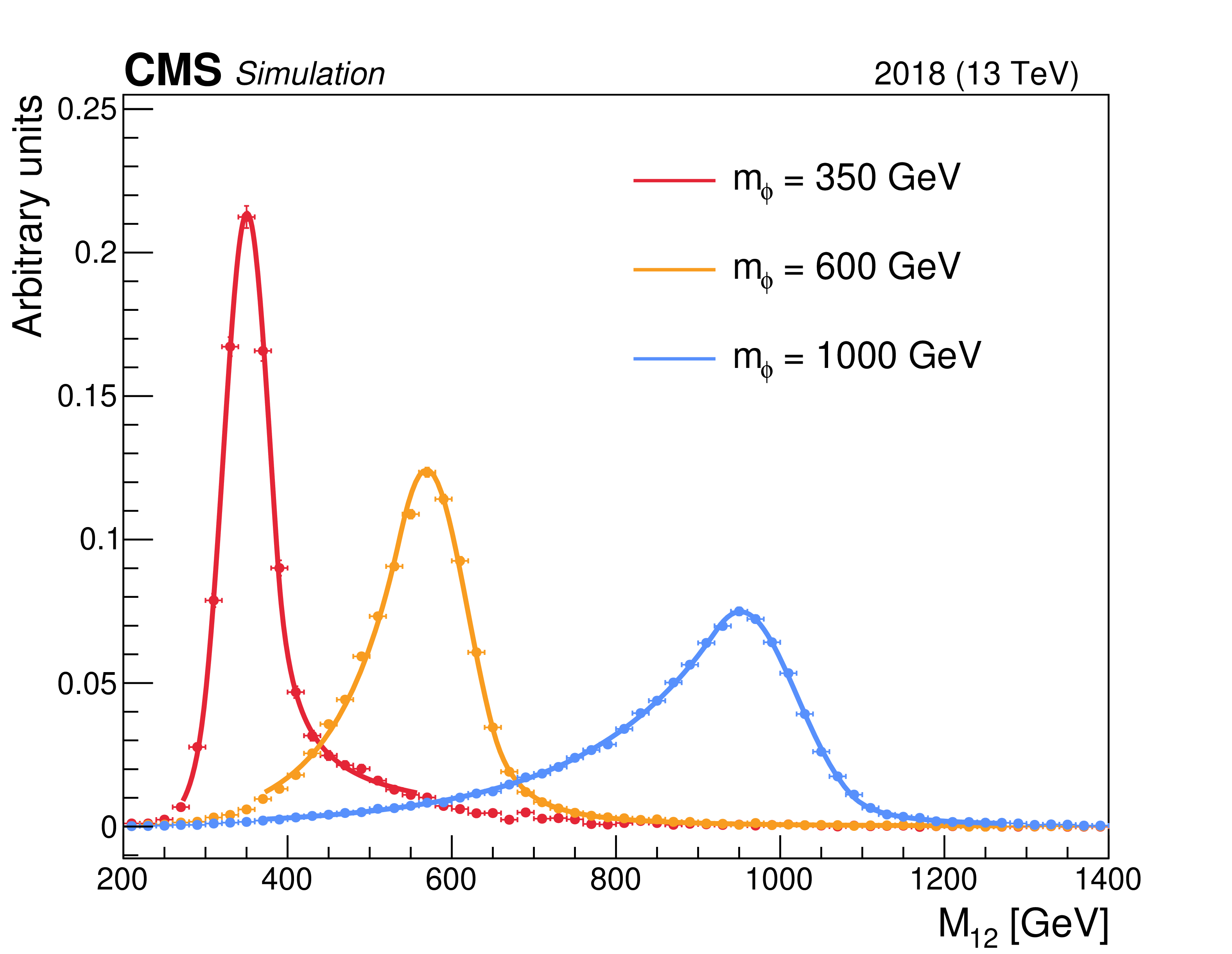
Simulated signal yields normalized to unit area for three representative values of the Higgs boson mass $ m_{\phi} $ in the 2017 SL (upper left), 2017 FH (upper right), and 2018 FH (lower) channels. The solid curves show the signal parameterisations by double-sided Crystal Ball probability density functions. |
png pdf |
Figure 4-a:
Simulated signal yields normalized to unit area for three representative values of the Higgs boson mass $ m_{\phi} $ in the 2017 SL (upper left), 2017 FH (upper right), and 2018 FH (lower) channels. The solid curves show the signal parameterisations by double-sided Crystal Ball probability density functions. |
png pdf |
Figure 4-b:
Simulated signal yields normalized to unit area for three representative values of the Higgs boson mass $ m_{\phi} $ in the 2017 SL (upper left), 2017 FH (upper right), and 2018 FH (lower) channels. The solid curves show the signal parameterisations by double-sided Crystal Ball probability density functions. |
png pdf |
Figure 4-c:
Simulated signal yields normalized to unit area for three representative values of the Higgs boson mass $ m_{\phi} $ in the 2017 SL (upper left), 2017 FH (upper right), and 2018 FH (lower) channels. The solid curves show the signal parameterisations by double-sided Crystal Ball probability density functions. |
png pdf |
Figure 5:
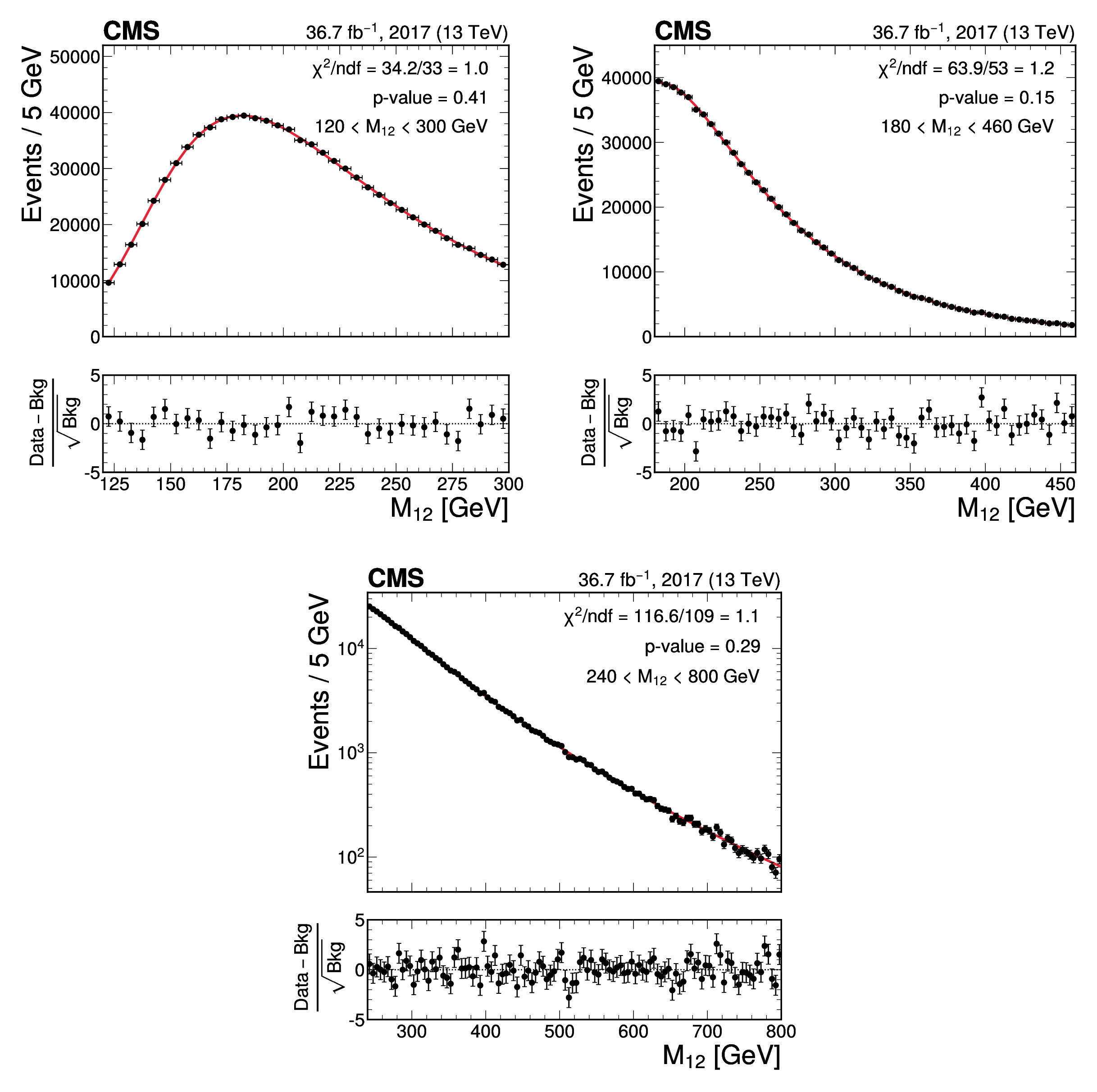
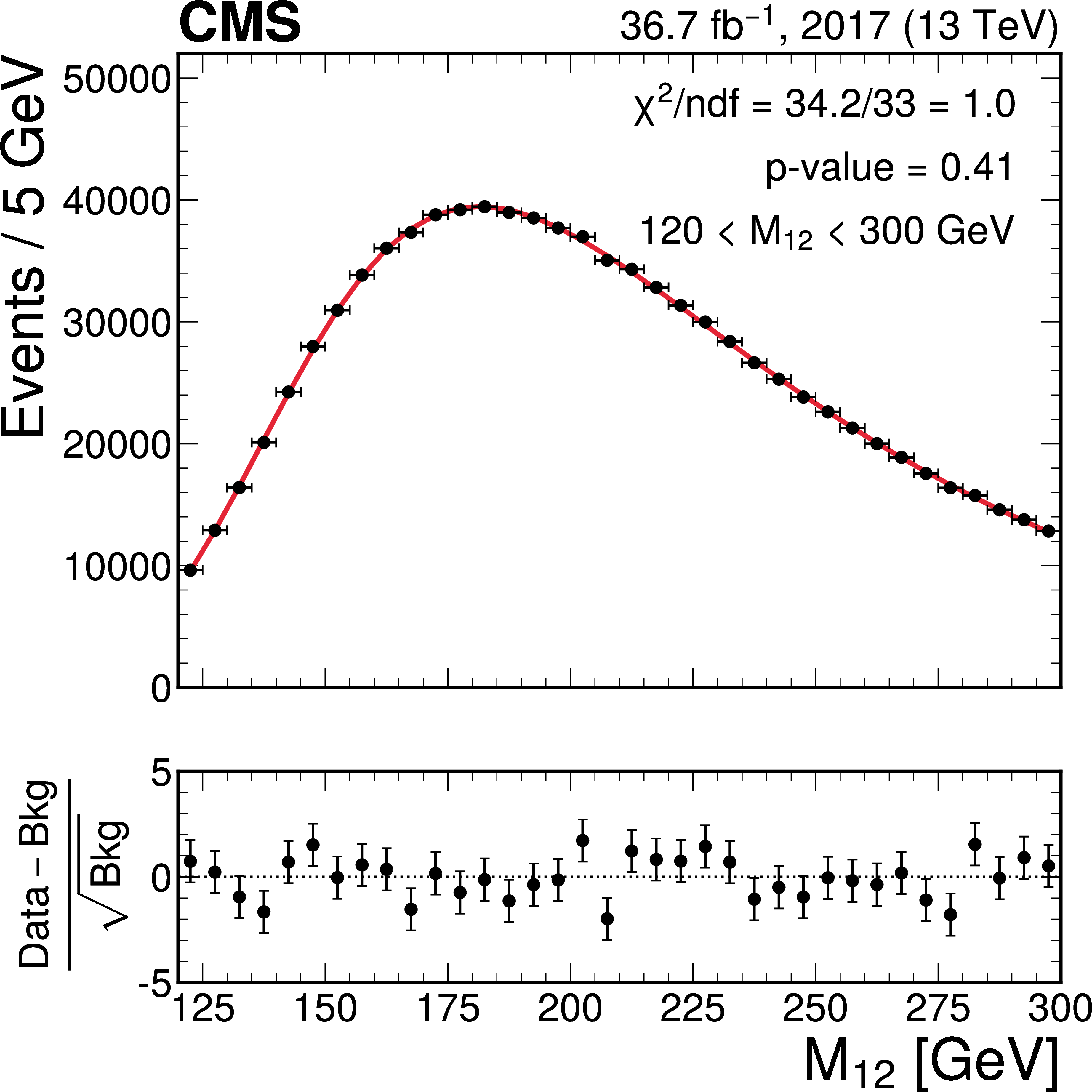
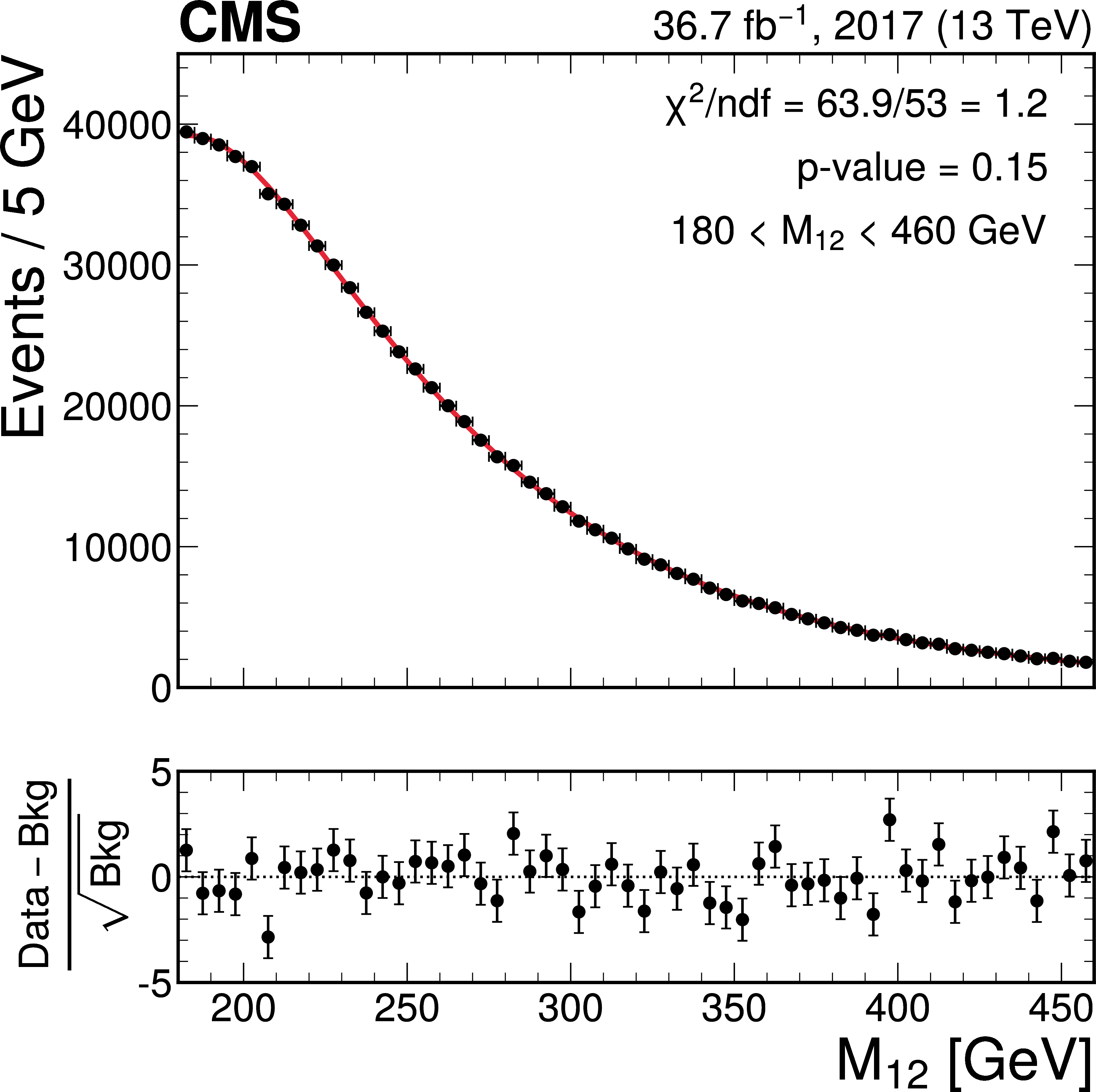
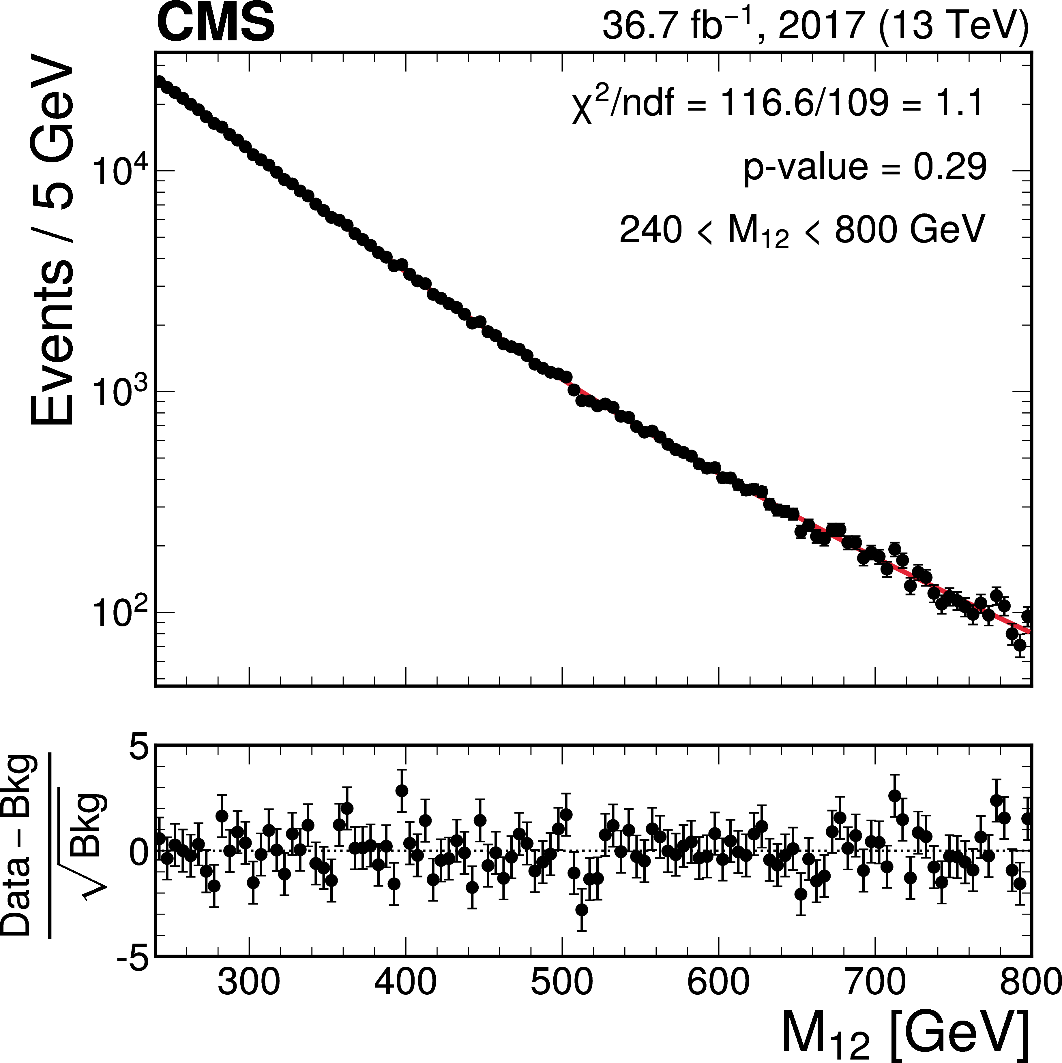
Invariant mass distributions of the three fit ranges in the b tag veto CR for the 2017 SL channel, overlaid with the fitted functions. The distributions are fitted in the $ M_{12} $ ranges of 120-300 GeV (upper left), 180-460 GeV (upper right), and 240-800 GeV (lower). The $ \chi^2 $ and the corresponding p-value obtained from the goodness-of-fit test are displayed on each plot. The lower panels show the difference between the data and the fitted function, divided by the estimated statistical uncertainty for each bin. Good agreement between the fitted functions and the data is achieved. |
png pdf |
Figure 5-a:
Invariant mass distributions of the three fit ranges in the b tag veto CR for the 2017 SL channel, overlaid with the fitted functions. The distributions are fitted in the $ M_{12} $ ranges of 120-300 GeV (upper left), 180-460 GeV (upper right), and 240-800 GeV (lower). The $ \chi^2 $ and the corresponding p-value obtained from the goodness-of-fit test are displayed on each plot. The lower panels show the difference between the data and the fitted function, divided by the estimated statistical uncertainty for each bin. Good agreement between the fitted functions and the data is achieved. |
png pdf |
Figure 5-b:
Invariant mass distributions of the three fit ranges in the b tag veto CR for the 2017 SL channel, overlaid with the fitted functions. The distributions are fitted in the $ M_{12} $ ranges of 120-300 GeV (upper left), 180-460 GeV (upper right), and 240-800 GeV (lower). The $ \chi^2 $ and the corresponding p-value obtained from the goodness-of-fit test are displayed on each plot. The lower panels show the difference between the data and the fitted function, divided by the estimated statistical uncertainty for each bin. Good agreement between the fitted functions and the data is achieved. |
png pdf |
Figure 5-c:
Invariant mass distributions of the three fit ranges in the b tag veto CR for the 2017 SL channel, overlaid with the fitted functions. The distributions are fitted in the $ M_{12} $ ranges of 120-300 GeV (upper left), 180-460 GeV (upper right), and 240-800 GeV (lower). The $ \chi^2 $ and the corresponding p-value obtained from the goodness-of-fit test are displayed on each plot. The lower panels show the difference between the data and the fitted function, divided by the estimated statistical uncertainty for each bin. Good agreement between the fitted functions and the data is achieved. |
png pdf |
Figure 5-d:
Invariant mass distributions of the three fit ranges in the b tag veto CR for the 2017 SL channel, overlaid with the fitted functions. The distributions are fitted in the $ M_{12} $ ranges of 120-300 GeV (upper left), 180-460 GeV (upper right), and 240-800 GeV (lower). The $ \chi^2 $ and the corresponding p-value obtained from the goodness-of-fit test are displayed on each plot. The lower panels show the difference between the data and the fitted function, divided by the estimated statistical uncertainty for each bin. Good agreement between the fitted functions and the data is achieved. |
png pdf |
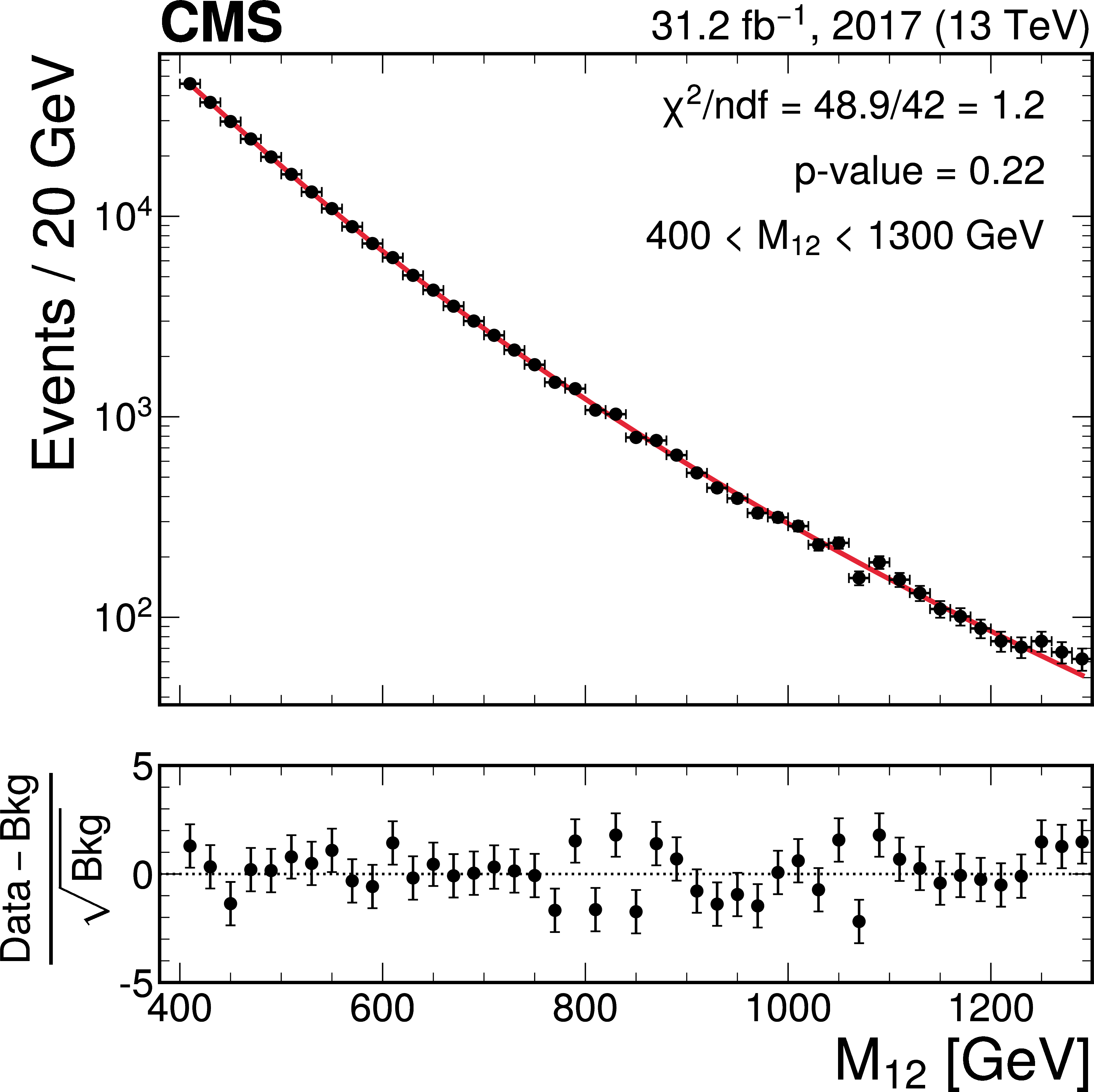
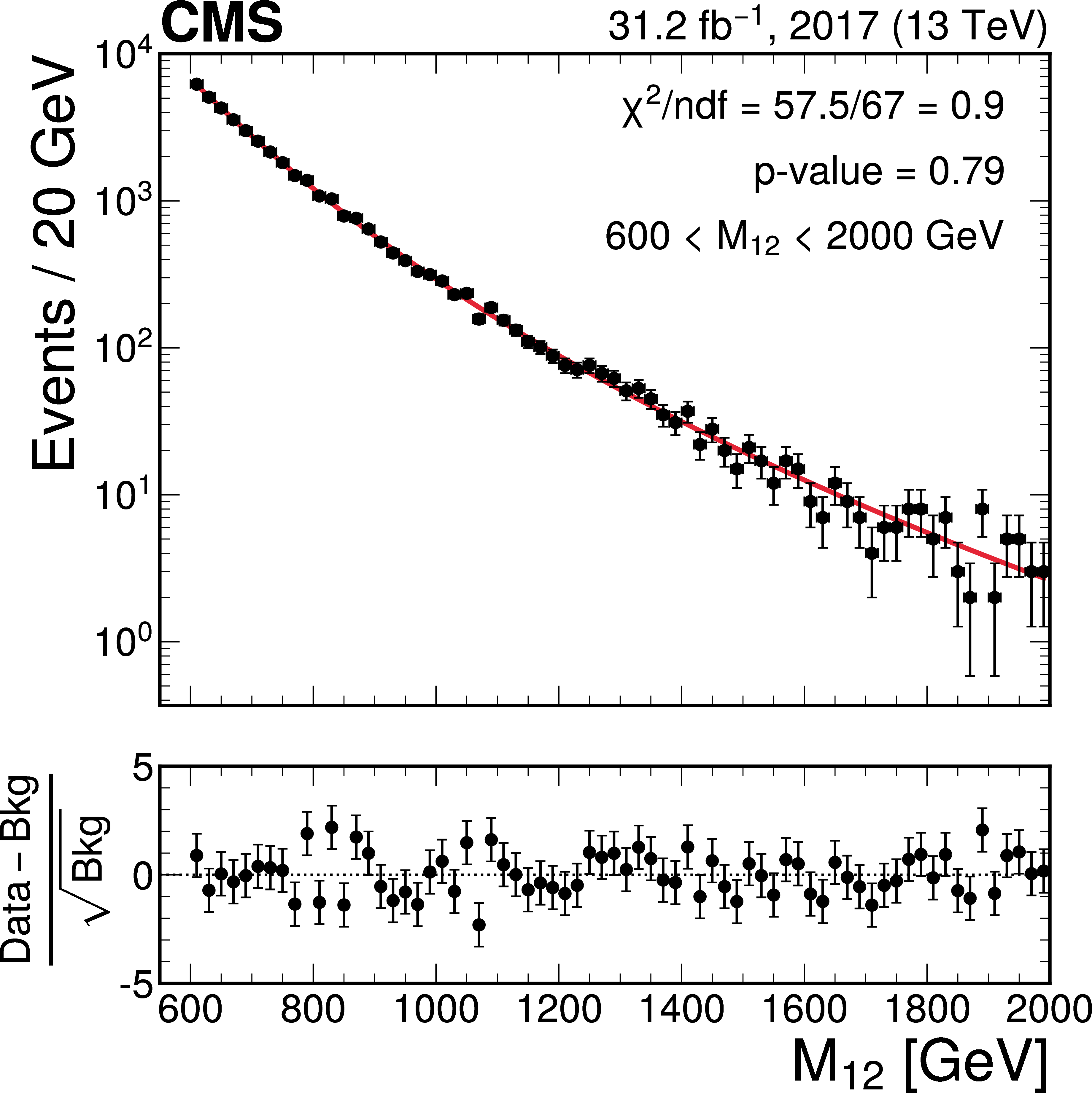
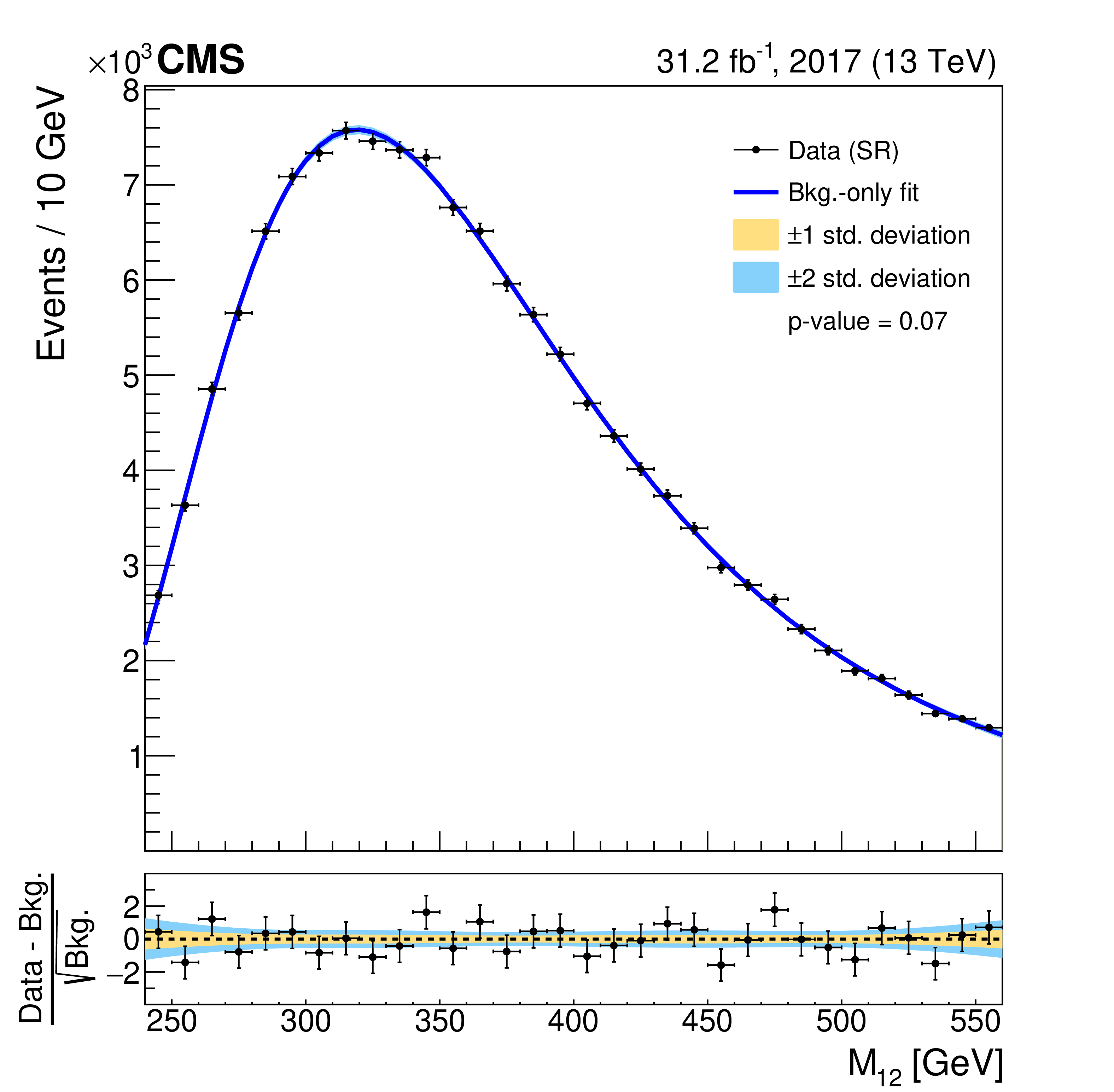
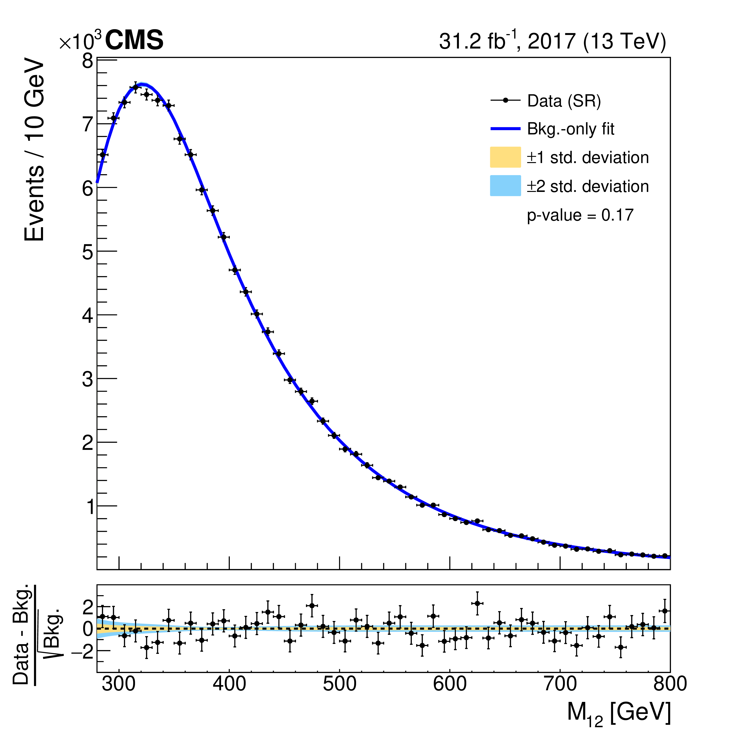
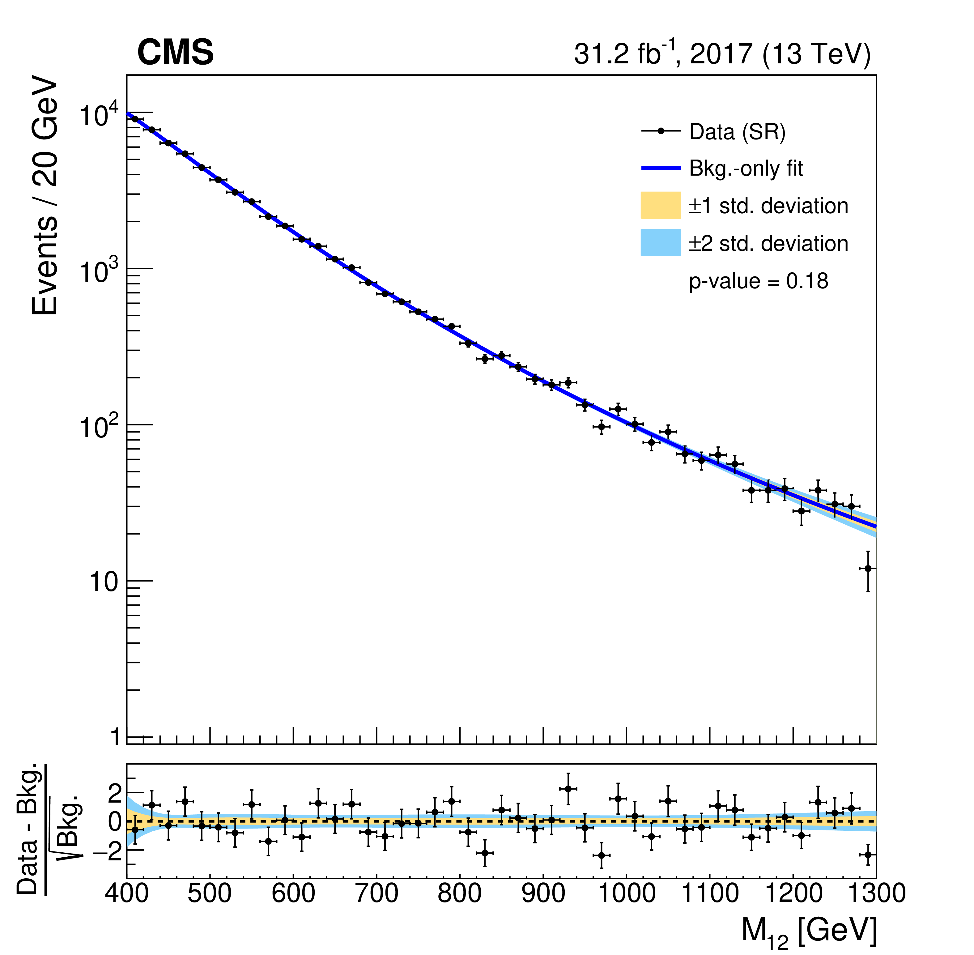
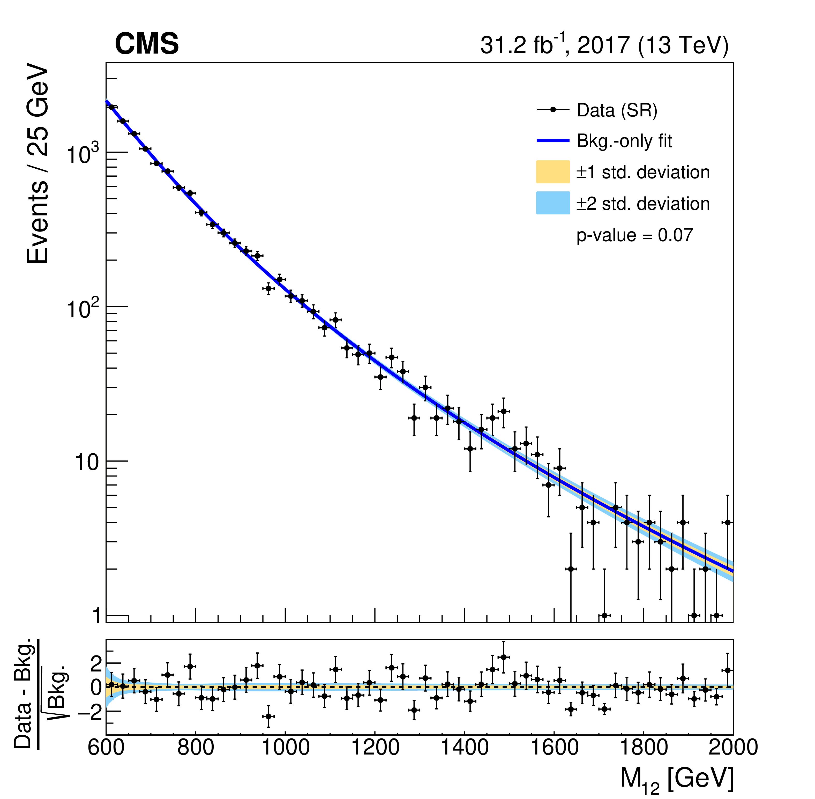
Figure 6:
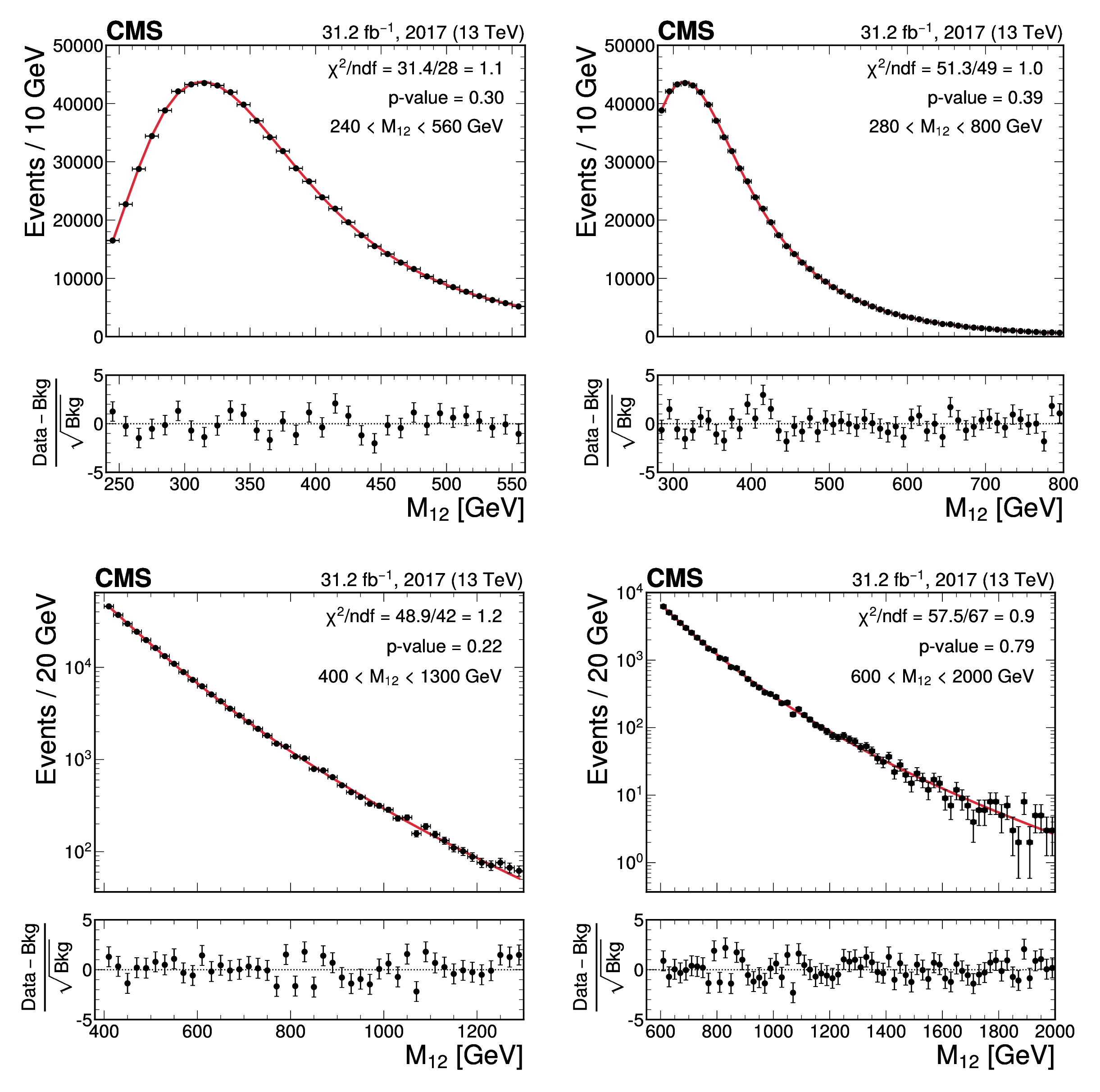
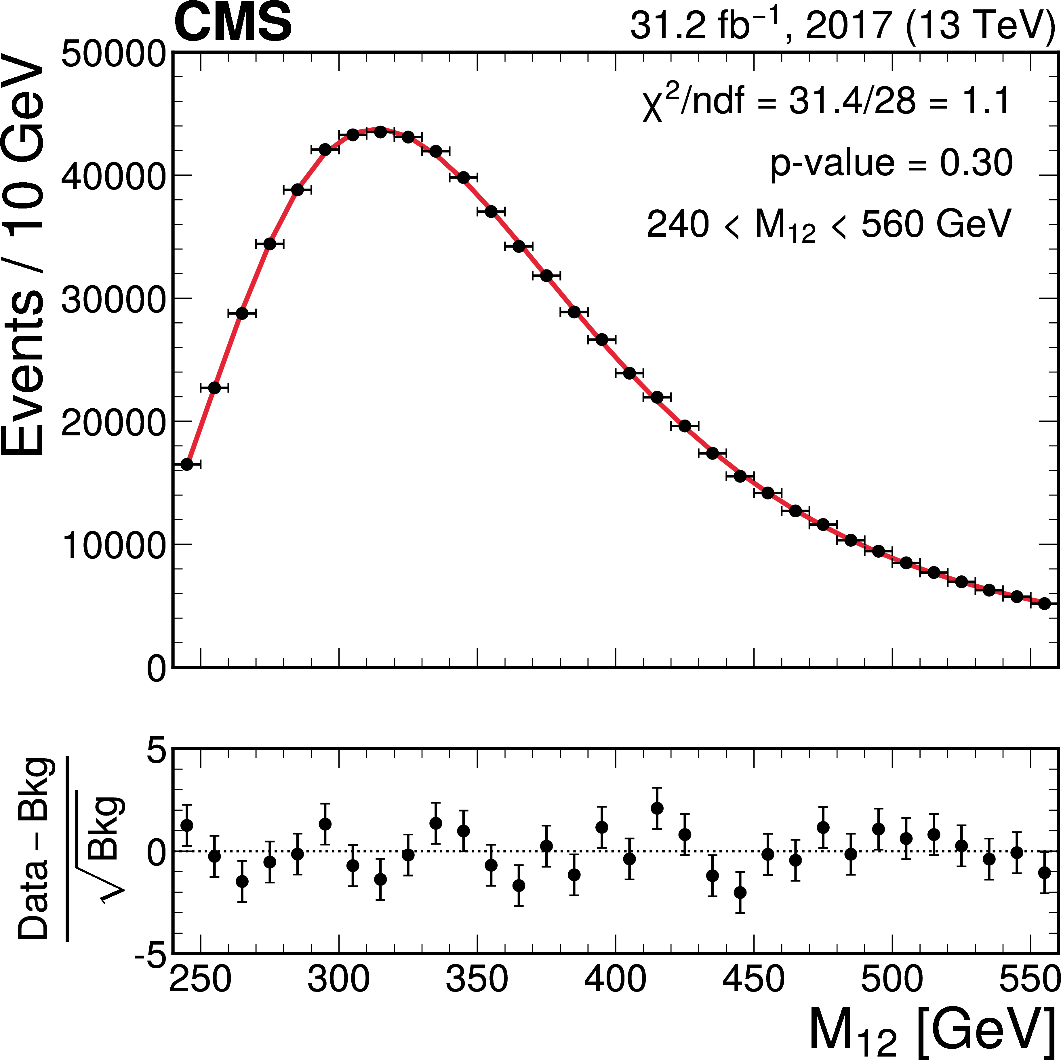
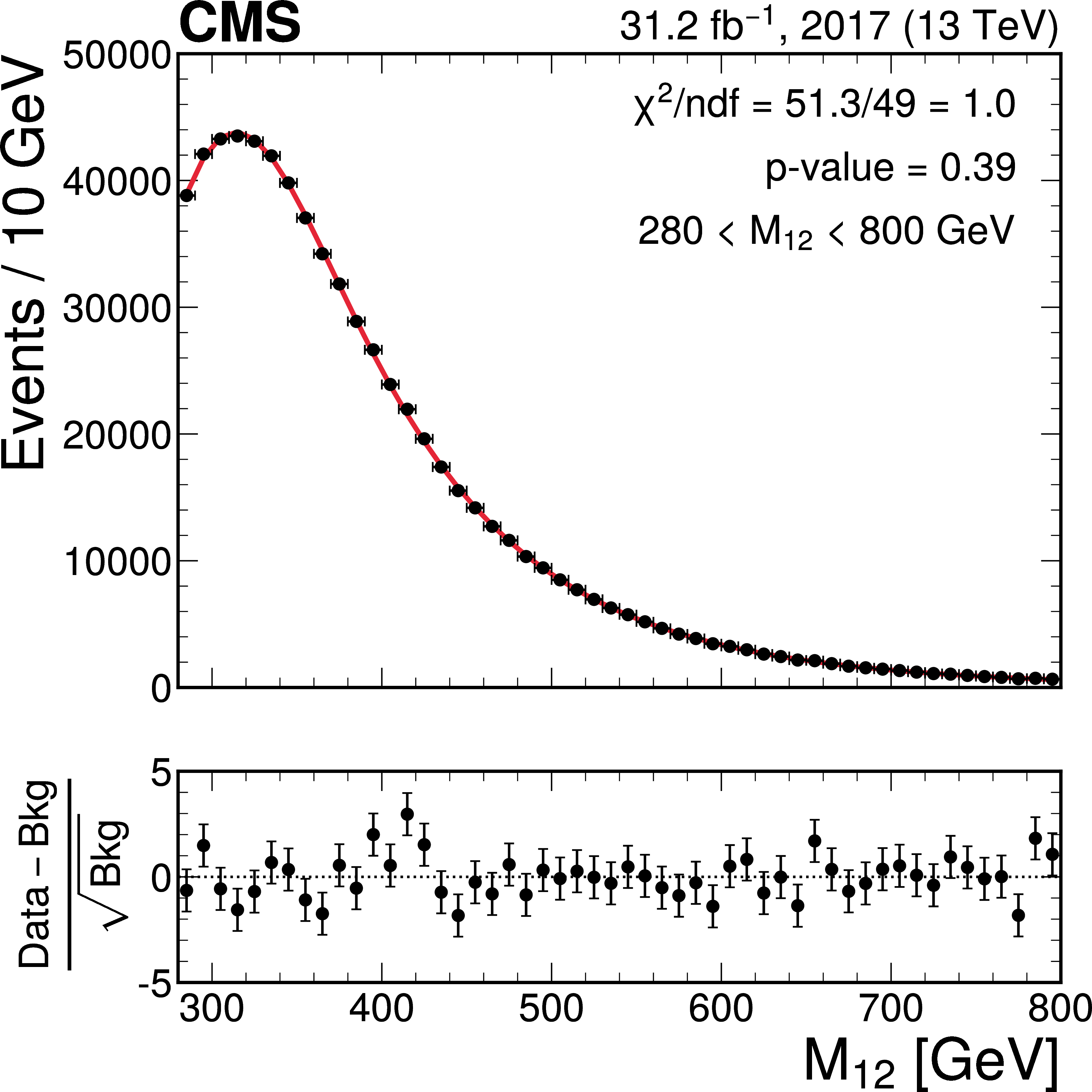
Invariant mass distributions of the four fit ranges in the b tag veto CR for the 2017 FH channel, overlaid with the fitted functions. The distributions are fitted in the $ M_{12} $ ranges of 240-560 GeV (upper left), 280-800 GeV (upper right), 400-1300 GeV (lower left), and 600-2000 GeV (lower right). The $ \chi^2 $ goodness-of-fit test and corresponding p-value are indicated in each plot. The lower panels show the difference between the data and the fitted function, divided by the estimated statistical uncertainty for each bin. Good agreement between the fitted functions and the data is achieved. |
png pdf |
Figure 6-a:
Invariant mass distributions of the four fit ranges in the b tag veto CR for the 2017 FH channel, overlaid with the fitted functions. The distributions are fitted in the $ M_{12} $ ranges of 240-560 GeV (upper left), 280-800 GeV (upper right), 400-1300 GeV (lower left), and 600-2000 GeV (lower right). The $ \chi^2 $ goodness-of-fit test and corresponding p-value are indicated in each plot. The lower panels show the difference between the data and the fitted function, divided by the estimated statistical uncertainty for each bin. Good agreement between the fitted functions and the data is achieved. |
png pdf |
Figure 6-b:
Invariant mass distributions of the four fit ranges in the b tag veto CR for the 2017 FH channel, overlaid with the fitted functions. The distributions are fitted in the $ M_{12} $ ranges of 240-560 GeV (upper left), 280-800 GeV (upper right), 400-1300 GeV (lower left), and 600-2000 GeV (lower right). The $ \chi^2 $ goodness-of-fit test and corresponding p-value are indicated in each plot. The lower panels show the difference between the data and the fitted function, divided by the estimated statistical uncertainty for each bin. Good agreement between the fitted functions and the data is achieved. |
png pdf |
Figure 6-c:
Invariant mass distributions of the four fit ranges in the b tag veto CR for the 2017 FH channel, overlaid with the fitted functions. The distributions are fitted in the $ M_{12} $ ranges of 240-560 GeV (upper left), 280-800 GeV (upper right), 400-1300 GeV (lower left), and 600-2000 GeV (lower right). The $ \chi^2 $ goodness-of-fit test and corresponding p-value are indicated in each plot. The lower panels show the difference between the data and the fitted function, divided by the estimated statistical uncertainty for each bin. Good agreement between the fitted functions and the data is achieved. |

png pdf |
Figure 6-d:
Invariant mass distributions of the four fit ranges in the b tag veto CR for the 2017 FH channel, overlaid with the fitted functions. The distributions are fitted in the $ M_{12} $ ranges of 240-560 GeV (upper left), 280-800 GeV (upper right), 400-1300 GeV (lower left), and 600-2000 GeV (lower right). The $ \chi^2 $ goodness-of-fit test and corresponding p-value are indicated in each plot. The lower panels show the difference between the data and the fitted function, divided by the estimated statistical uncertainty for each bin. Good agreement between the fitted functions and the data is achieved. |
png pdf |
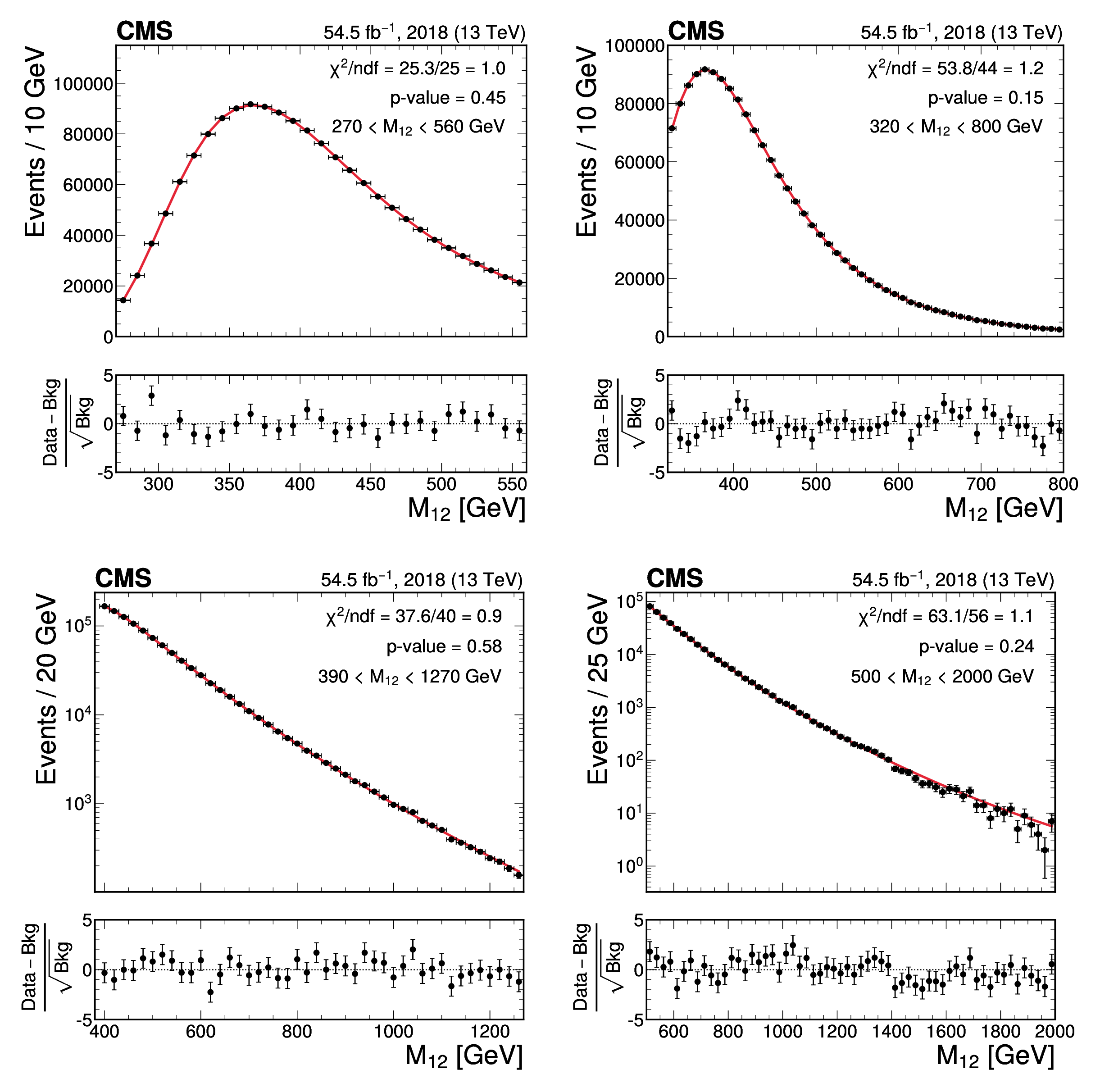
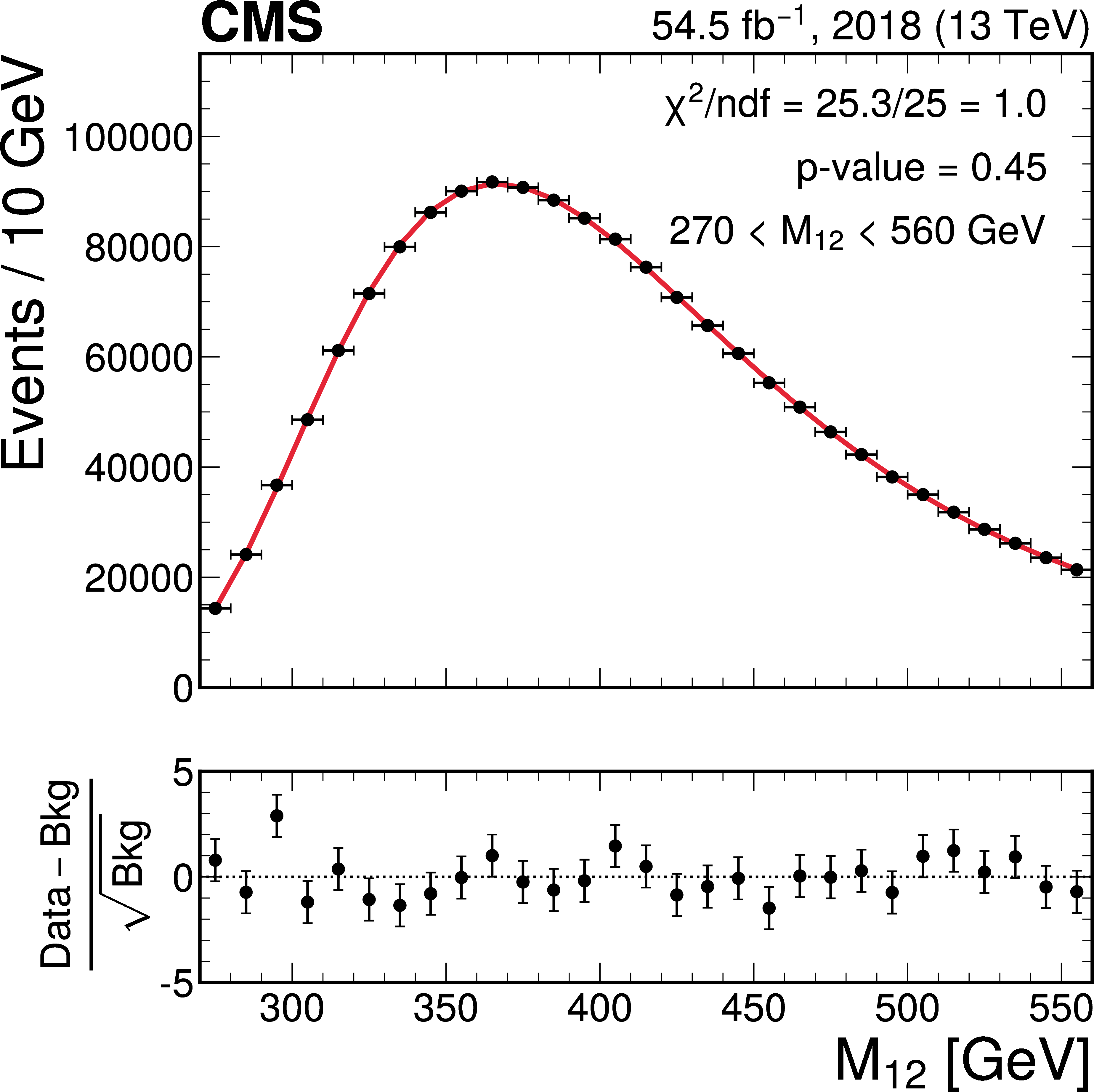
Figure 7:
Invariant mass distributions of the four fit ranges in the b tag veto CR for the 2018 FH channel, overlaid with the fitted functions. The distributions are fitted in the $ M_{12} $ ranges of 270-560 GeV (upper left), 320-800 GeV (upper right), 390-1270 GeV (lower left), and 500-2000 GeV (lower right). The $ \chi^2 $ goodness-of-fit test and corresponding p-value are indicated in each plot. The lower panels show the difference between the data and the fitted function, divided by the estimated statistical uncertainty for each bin. Good agreement between the fitted functions and the data is achieved. |
png pdf |
Figure 7-a:
Invariant mass distributions of the four fit ranges in the b tag veto CR for the 2018 FH channel, overlaid with the fitted functions. The distributions are fitted in the $ M_{12} $ ranges of 270-560 GeV (upper left), 320-800 GeV (upper right), 390-1270 GeV (lower left), and 500-2000 GeV (lower right). The $ \chi^2 $ goodness-of-fit test and corresponding p-value are indicated in each plot. The lower panels show the difference between the data and the fitted function, divided by the estimated statistical uncertainty for each bin. Good agreement between the fitted functions and the data is achieved. |
png pdf |
Figure 7-b:
Invariant mass distributions of the four fit ranges in the b tag veto CR for the 2018 FH channel, overlaid with the fitted functions. The distributions are fitted in the $ M_{12} $ ranges of 270-560 GeV (upper left), 320-800 GeV (upper right), 390-1270 GeV (lower left), and 500-2000 GeV (lower right). The $ \chi^2 $ goodness-of-fit test and corresponding p-value are indicated in each plot. The lower panels show the difference between the data and the fitted function, divided by the estimated statistical uncertainty for each bin. Good agreement between the fitted functions and the data is achieved. |
png pdf |
Figure 7-c:
Invariant mass distributions of the four fit ranges in the b tag veto CR for the 2018 FH channel, overlaid with the fitted functions. The distributions are fitted in the $ M_{12} $ ranges of 270-560 GeV (upper left), 320-800 GeV (upper right), 390-1270 GeV (lower left), and 500-2000 GeV (lower right). The $ \chi^2 $ goodness-of-fit test and corresponding p-value are indicated in each plot. The lower panels show the difference between the data and the fitted function, divided by the estimated statistical uncertainty for each bin. Good agreement between the fitted functions and the data is achieved. |
png pdf |
Figure 7-d:
Invariant mass distributions of the four fit ranges in the b tag veto CR for the 2018 FH channel, overlaid with the fitted functions. The distributions are fitted in the $ M_{12} $ ranges of 270-560 GeV (upper left), 320-800 GeV (upper right), 390-1270 GeV (lower left), and 500-2000 GeV (lower right). The $ \chi^2 $ goodness-of-fit test and corresponding p-value are indicated in each plot. The lower panels show the difference between the data and the fitted function, divided by the estimated statistical uncertainty for each bin. Good agreement between the fitted functions and the data is achieved. |
png pdf |
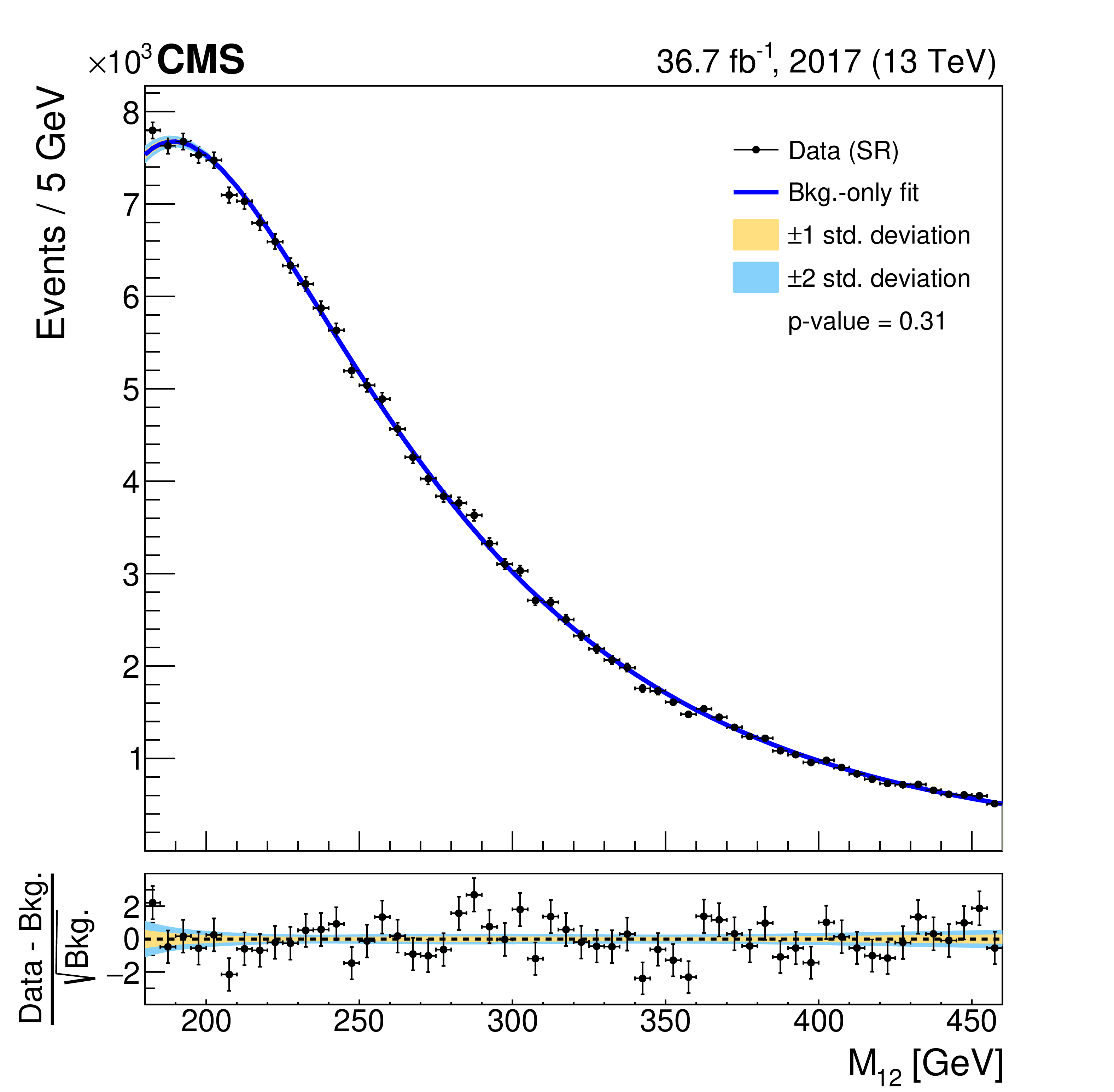
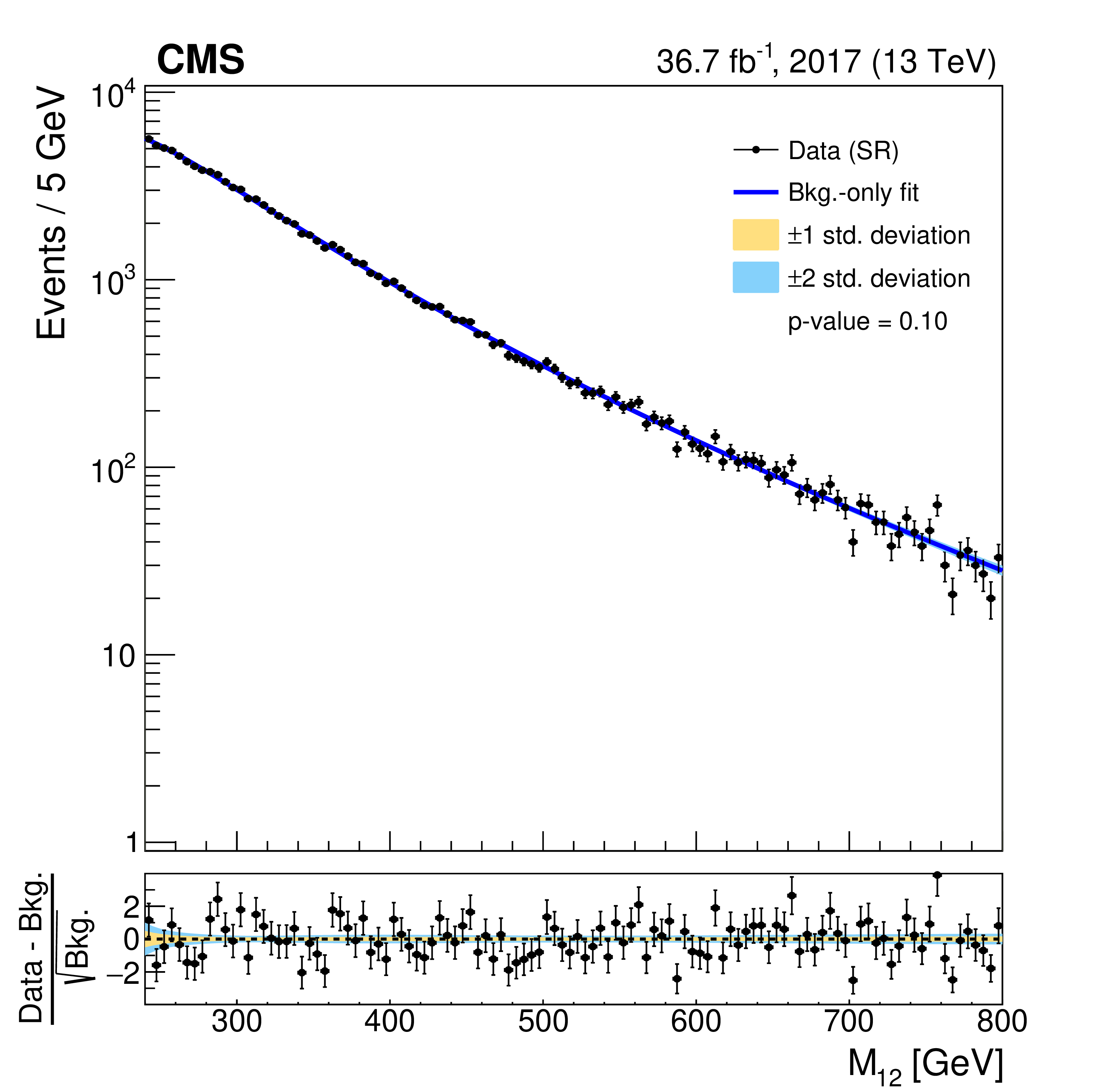
Figure 8:
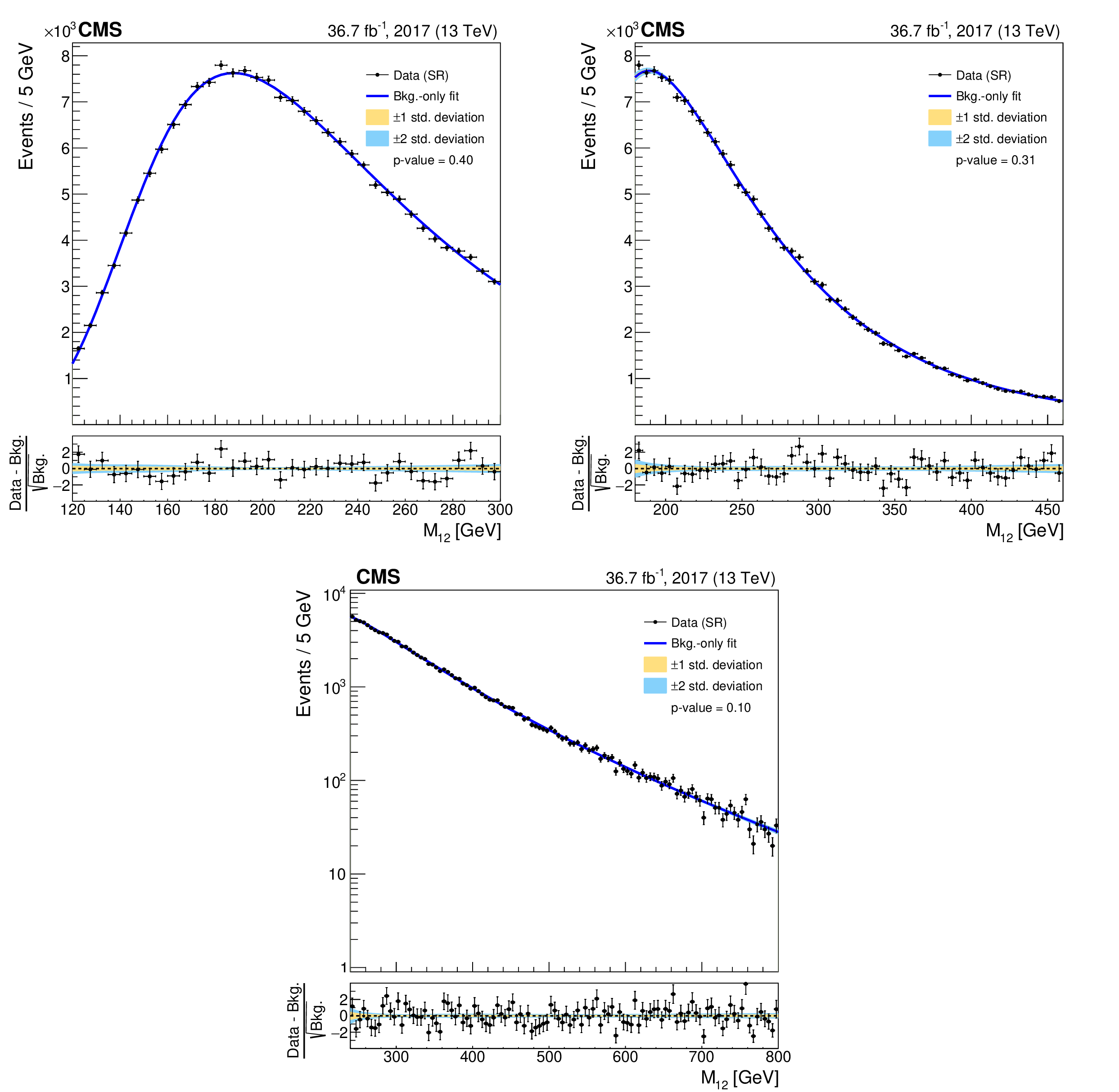
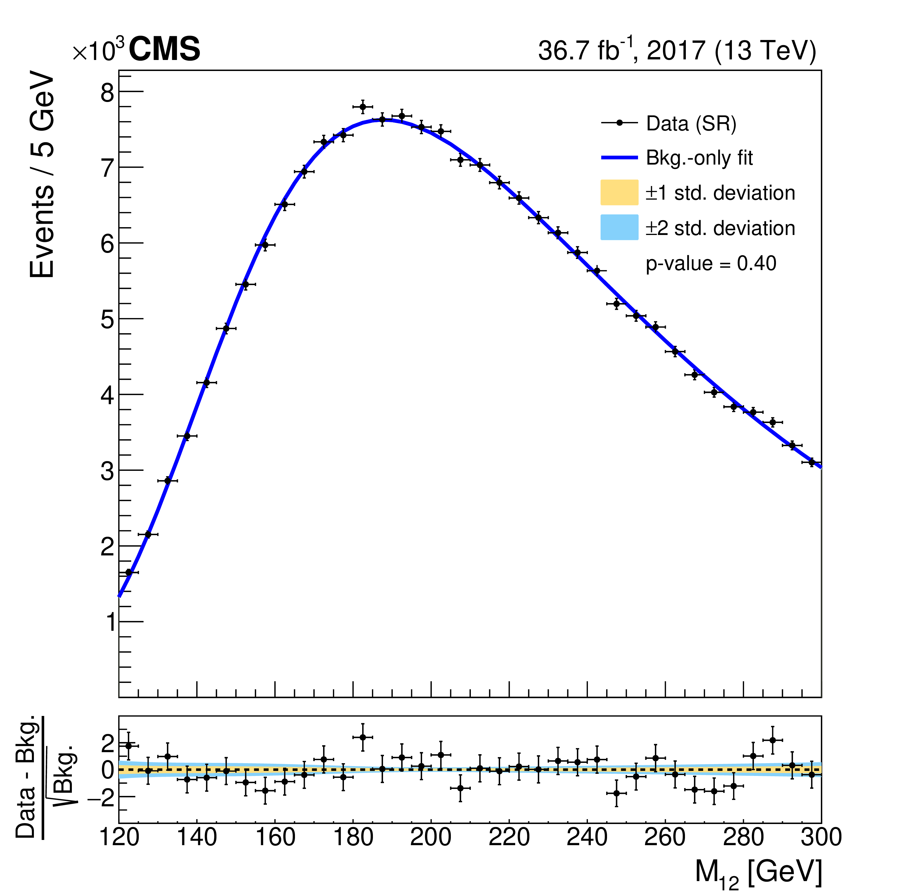
Background-only fits to the $ M_{12} $ distribution in each fit range of the 2017 analysis in the SL category, shown together with $ {\pm}1\sigma $ and $ {\pm}2\sigma $ uncertainty bands extracted from the fit in the upper panels. The lower panels show the difference between data and fitted background, divided by the statistical uncertainty of the latter. The distributions are fitted in the $ M_{12} $ ranges of 120-300 GeV (upper left), 180-460 GeV (upper right), and 240-800 GeV (lower). |
png pdf |
Figure 8-a:
Background-only fits to the $ M_{12} $ distribution in each fit range of the 2017 analysis in the SL category, shown together with $ {\pm}1\sigma $ and $ {\pm}2\sigma $ uncertainty bands extracted from the fit in the upper panels. The lower panels show the difference between data and fitted background, divided by the statistical uncertainty of the latter. The distributions are fitted in the $ M_{12} $ ranges of 120-300 GeV (upper left), 180-460 GeV (upper right), and 240-800 GeV (lower). |
png pdf |
Figure 8-b:
Background-only fits to the $ M_{12} $ distribution in each fit range of the 2017 analysis in the SL category, shown together with $ {\pm}1\sigma $ and $ {\pm}2\sigma $ uncertainty bands extracted from the fit in the upper panels. The lower panels show the difference between data and fitted background, divided by the statistical uncertainty of the latter. The distributions are fitted in the $ M_{12} $ ranges of 120-300 GeV (upper left), 180-460 GeV (upper right), and 240-800 GeV (lower). |
png pdf |
Figure 8-c:
Background-only fits to the $ M_{12} $ distribution in each fit range of the 2017 analysis in the SL category, shown together with $ {\pm}1\sigma $ and $ {\pm}2\sigma $ uncertainty bands extracted from the fit in the upper panels. The lower panels show the difference between data and fitted background, divided by the statistical uncertainty of the latter. The distributions are fitted in the $ M_{12} $ ranges of 120-300 GeV (upper left), 180-460 GeV (upper right), and 240-800 GeV (lower). |
png pdf |
Figure 8-d:
Background-only fits to the $ M_{12} $ distribution in each fit range of the 2017 analysis in the SL category, shown together with $ {\pm}1\sigma $ and $ {\pm}2\sigma $ uncertainty bands extracted from the fit in the upper panels. The lower panels show the difference between data and fitted background, divided by the statistical uncertainty of the latter. The distributions are fitted in the $ M_{12} $ ranges of 120-300 GeV (upper left), 180-460 GeV (upper right), and 240-800 GeV (lower). |
png pdf |
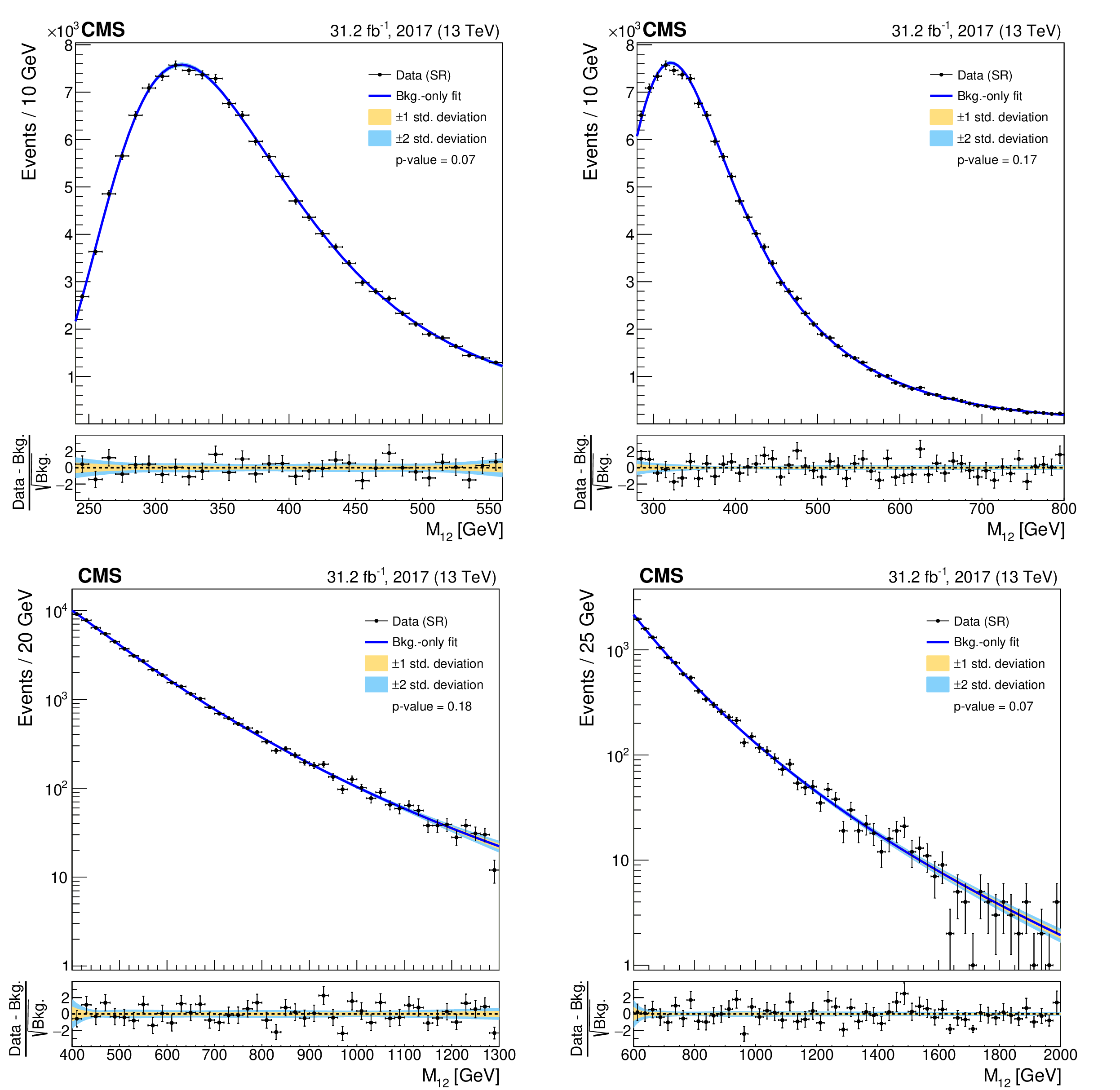
Figure 9:
Background-only fits to the $ M_{12} $ distribution in each fit range of the 2017 analysis in the FH category, shown together with $ {\pm}1\sigma $ and $ {\pm}2\sigma $ uncertainty bands extracted from the fit in the upper panels. The lower panels show the difference between data and fitted background, divided by the statistical uncertainty of the latter. The distributions are fitted in the $ M_{12} $ ranges of 240-560 GeV (upper left), 280-800 GeV (upper right), 400-1300 GeV (lower left), and 600-2000 GeV (lower right). |
png pdf |
Figure 9-a:
Background-only fits to the $ M_{12} $ distribution in each fit range of the 2017 analysis in the FH category, shown together with $ {\pm}1\sigma $ and $ {\pm}2\sigma $ uncertainty bands extracted from the fit in the upper panels. The lower panels show the difference between data and fitted background, divided by the statistical uncertainty of the latter. The distributions are fitted in the $ M_{12} $ ranges of 240-560 GeV (upper left), 280-800 GeV (upper right), 400-1300 GeV (lower left), and 600-2000 GeV (lower right). |

png pdf |
Figure 9-b:
Background-only fits to the $ M_{12} $ distribution in each fit range of the 2017 analysis in the FH category, shown together with $ {\pm}1\sigma $ and $ {\pm}2\sigma $ uncertainty bands extracted from the fit in the upper panels. The lower panels show the difference between data and fitted background, divided by the statistical uncertainty of the latter. The distributions are fitted in the $ M_{12} $ ranges of 240-560 GeV (upper left), 280-800 GeV (upper right), 400-1300 GeV (lower left), and 600-2000 GeV (lower right). |

png pdf |
Figure 9-c:
Background-only fits to the $ M_{12} $ distribution in each fit range of the 2017 analysis in the FH category, shown together with $ {\pm}1\sigma $ and $ {\pm}2\sigma $ uncertainty bands extracted from the fit in the upper panels. The lower panels show the difference between data and fitted background, divided by the statistical uncertainty of the latter. The distributions are fitted in the $ M_{12} $ ranges of 240-560 GeV (upper left), 280-800 GeV (upper right), 400-1300 GeV (lower left), and 600-2000 GeV (lower right). |
png pdf |
Figure 9-d:
Background-only fits to the $ M_{12} $ distribution in each fit range of the 2017 analysis in the FH category, shown together with $ {\pm}1\sigma $ and $ {\pm}2\sigma $ uncertainty bands extracted from the fit in the upper panels. The lower panels show the difference between data and fitted background, divided by the statistical uncertainty of the latter. The distributions are fitted in the $ M_{12} $ ranges of 240-560 GeV (upper left), 280-800 GeV (upper right), 400-1300 GeV (lower left), and 600-2000 GeV (lower right). |
png pdf |
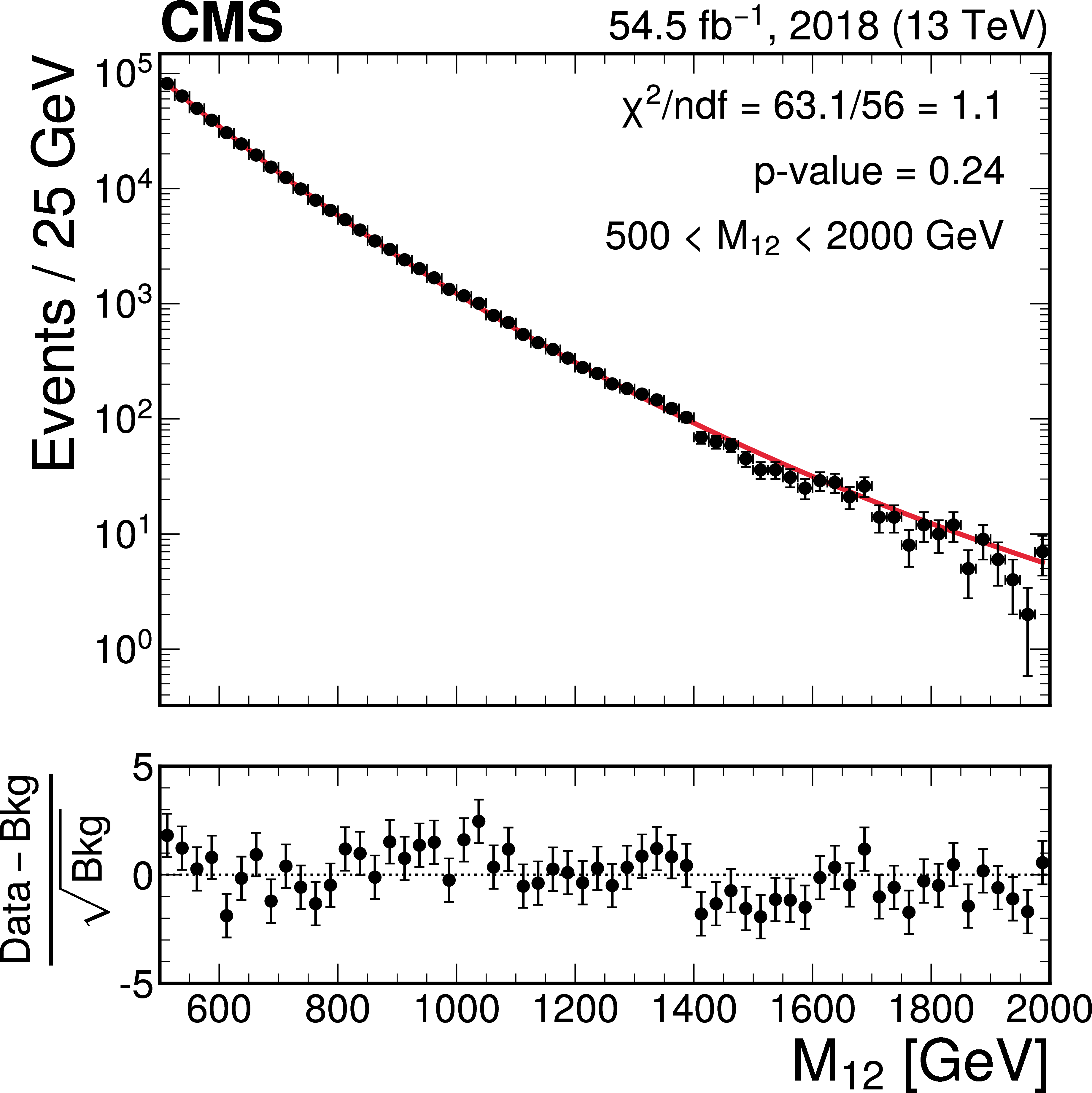
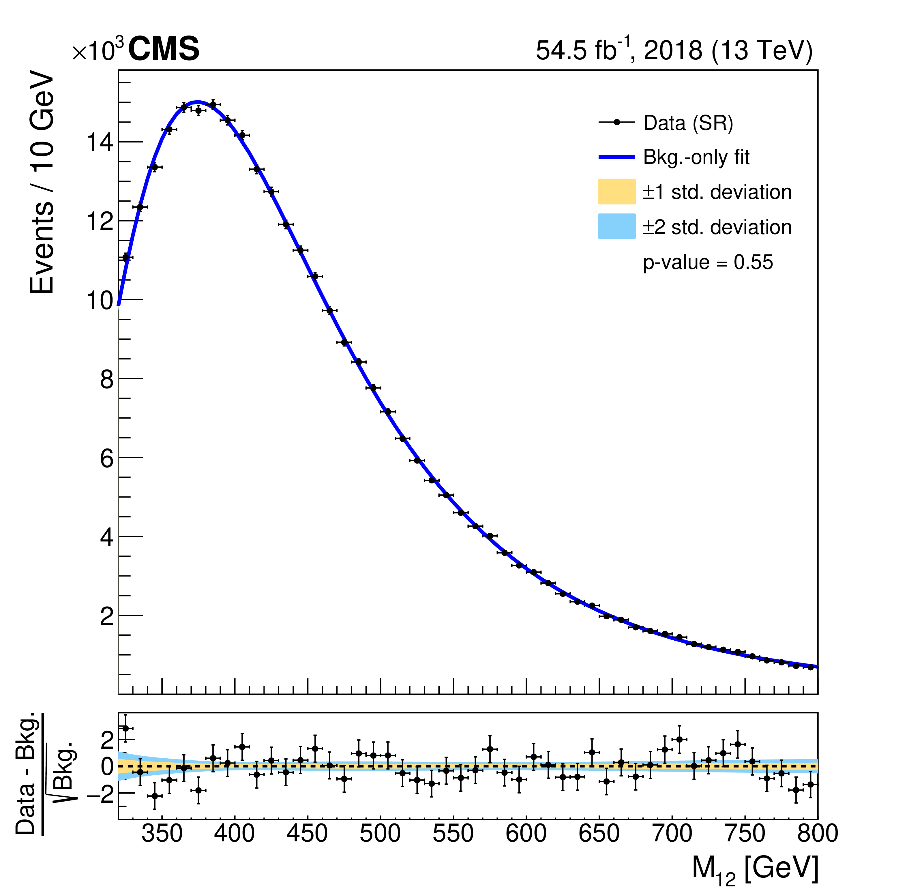
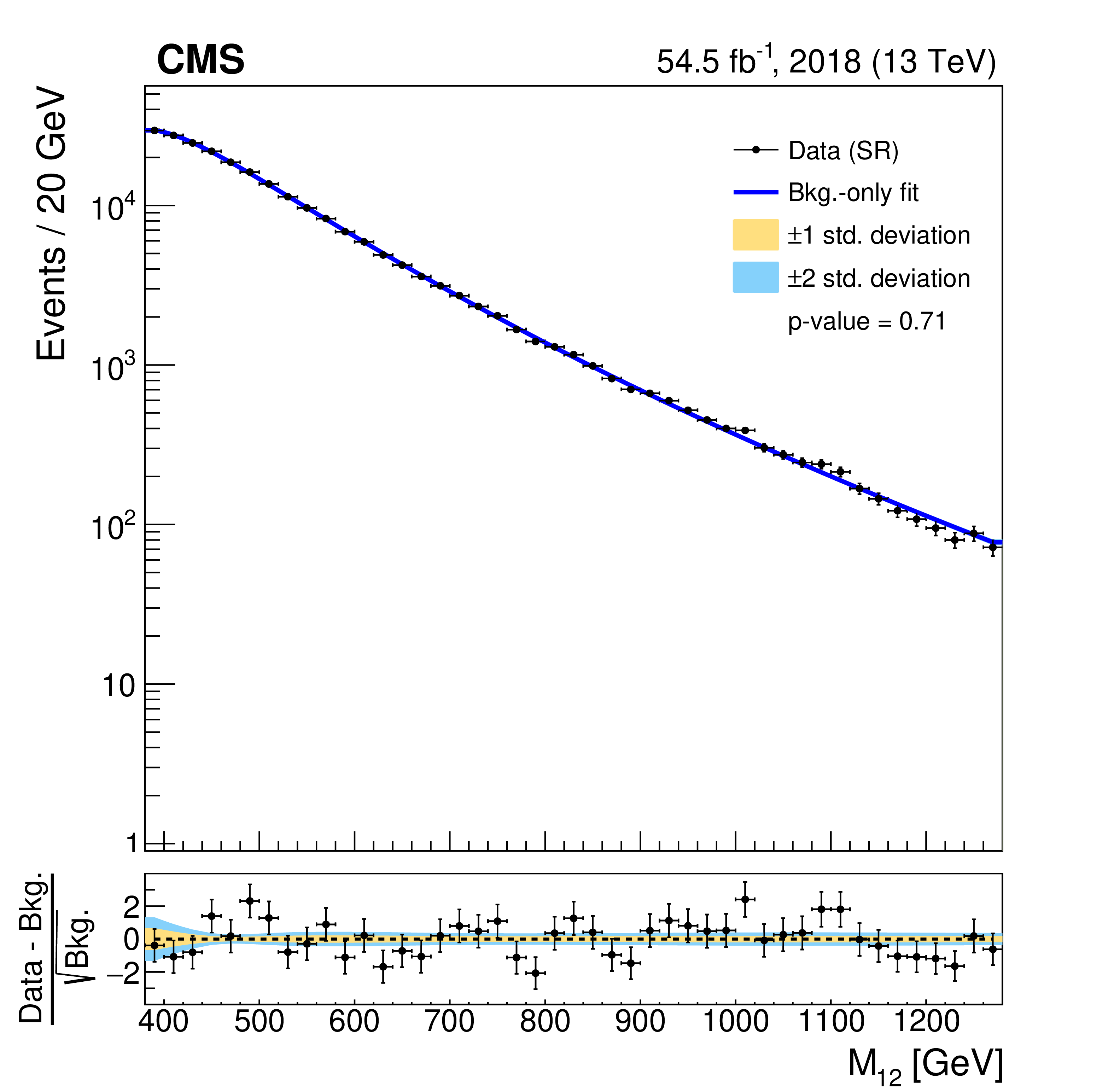
Figure 10:
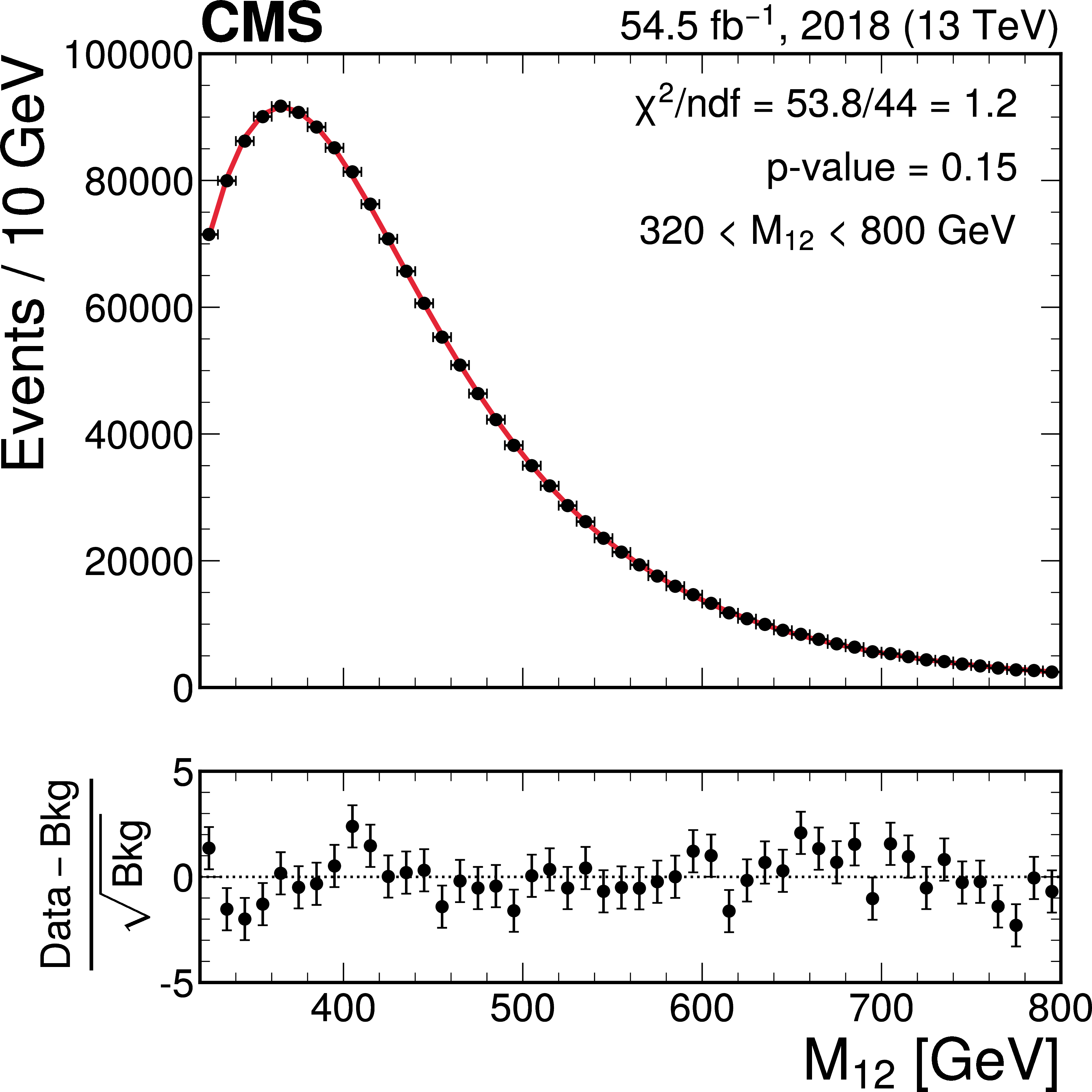
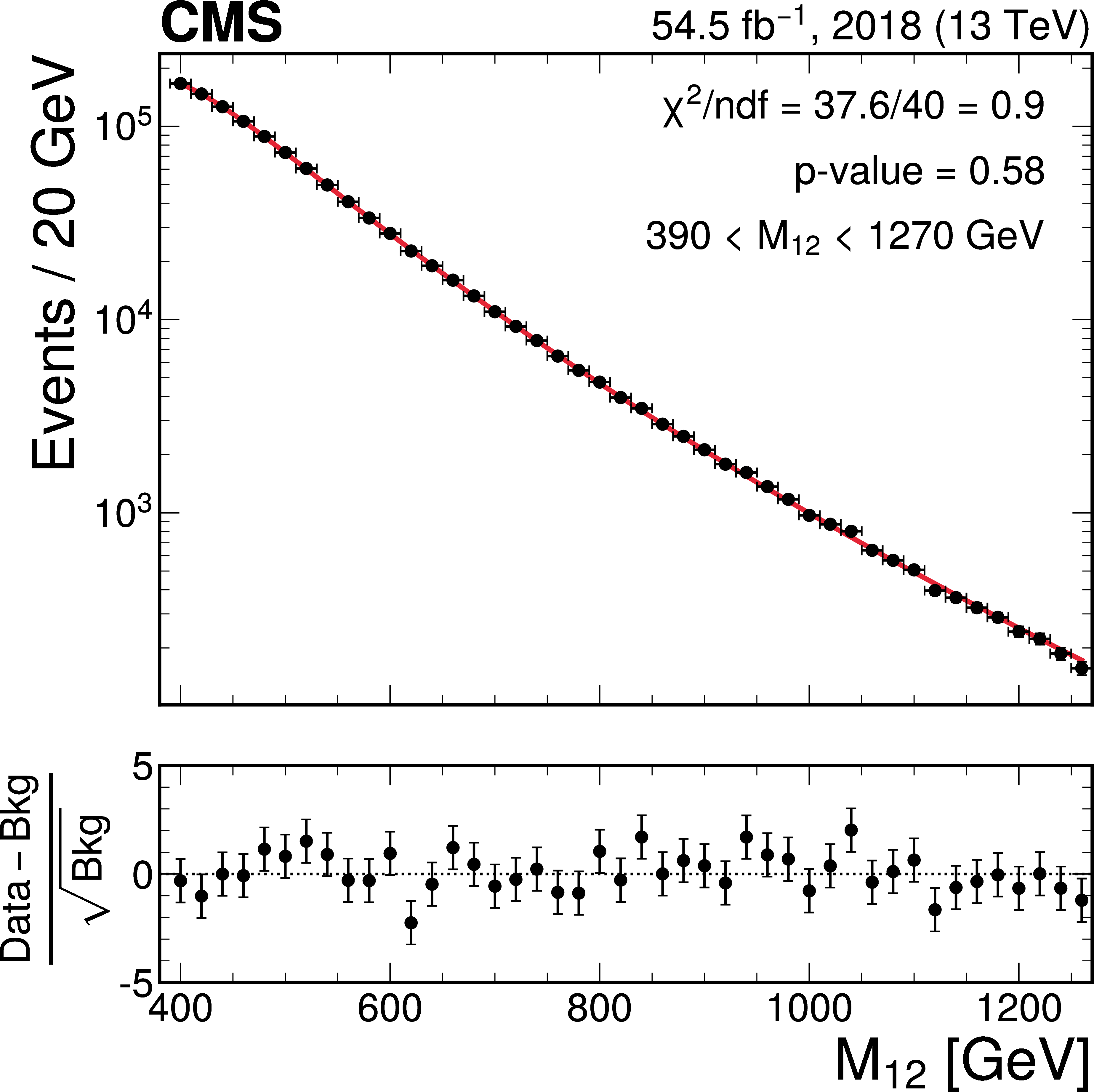
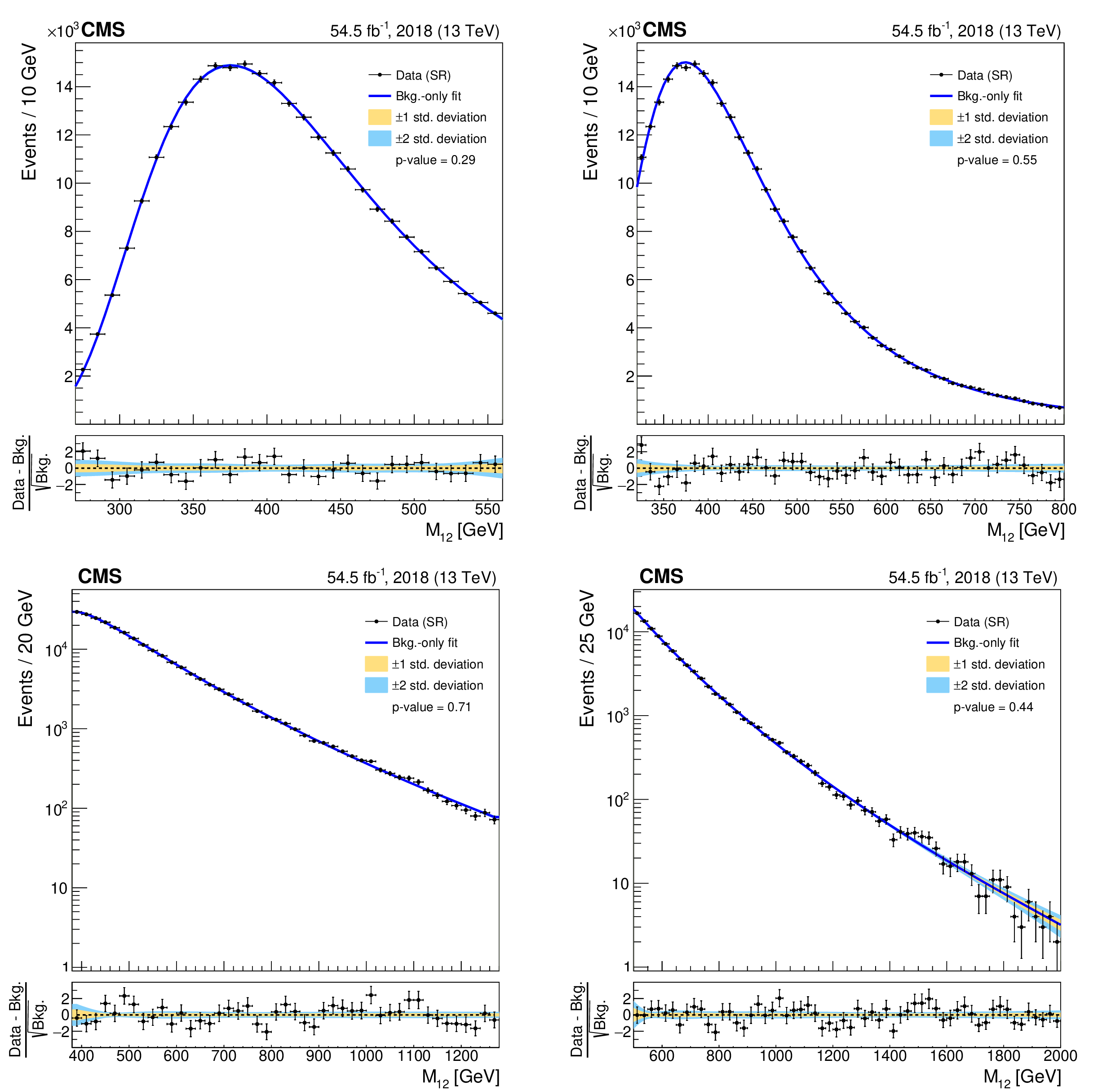
Background-only fits to the $ M_{12} $ distribution in each fit range of the 2018 analysis in the FH category, shown together with $ {\pm}1\sigma $ and $ {\pm}2\sigma $ uncertainty bands extracted from the fit in the upper panels. The lower panels show the difference between data and fitted background, divided by the statistical uncertainty of the latter. The distributions are fitted in the $ M_{12} $ ranges of 270-560 GeV (upper left), 320-800 GeV (upper right), 390-1270 GeV (lower left), and 500-2000 GeV (lower right). |

png pdf |
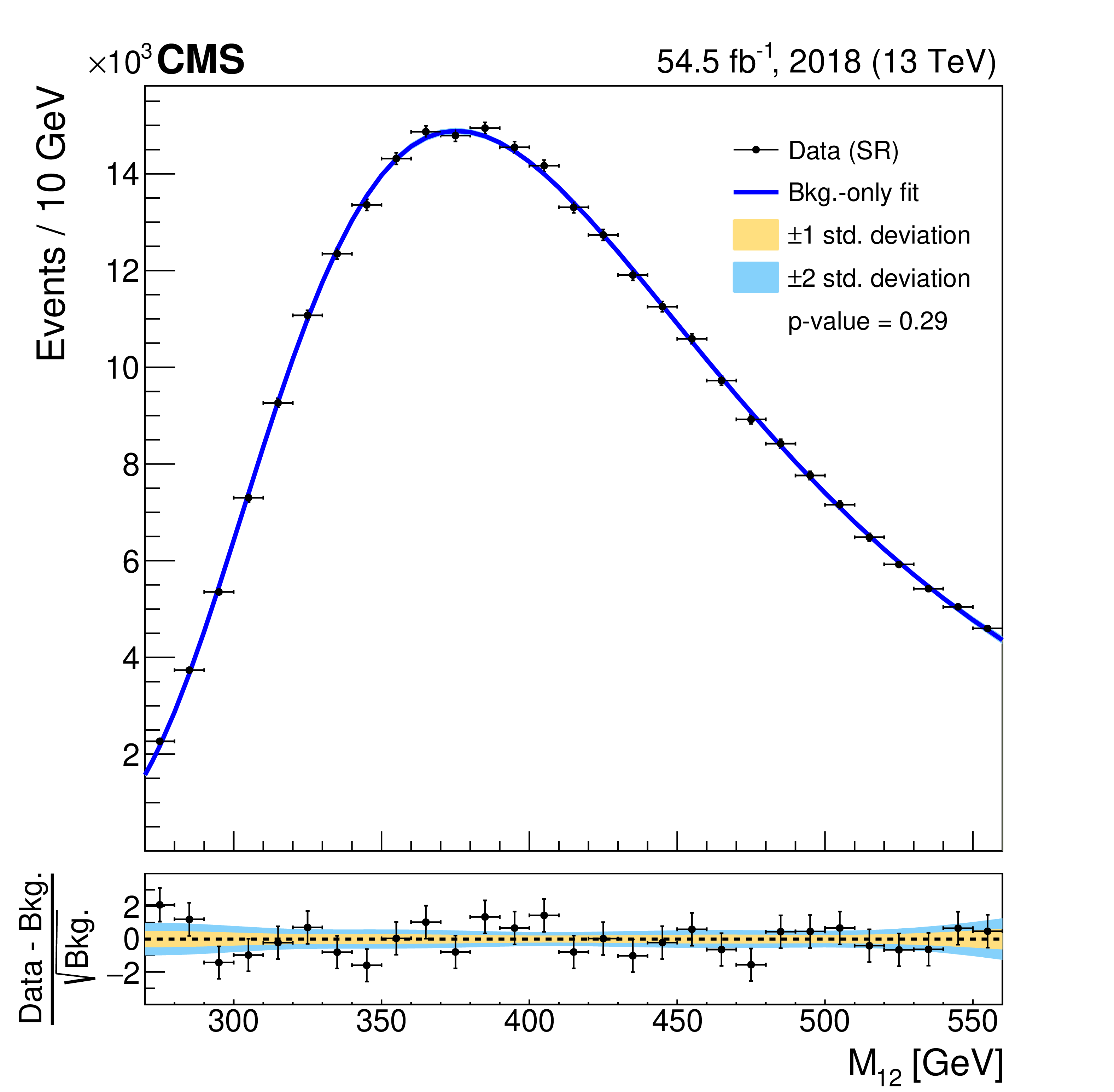
Figure 10-a:
Background-only fits to the $ M_{12} $ distribution in each fit range of the 2018 analysis in the FH category, shown together with $ {\pm}1\sigma $ and $ {\pm}2\sigma $ uncertainty bands extracted from the fit in the upper panels. The lower panels show the difference between data and fitted background, divided by the statistical uncertainty of the latter. The distributions are fitted in the $ M_{12} $ ranges of 270-560 GeV (upper left), 320-800 GeV (upper right), 390-1270 GeV (lower left), and 500-2000 GeV (lower right). |
png pdf |
Figure 10-b:
Background-only fits to the $ M_{12} $ distribution in each fit range of the 2018 analysis in the FH category, shown together with $ {\pm}1\sigma $ and $ {\pm}2\sigma $ uncertainty bands extracted from the fit in the upper panels. The lower panels show the difference between data and fitted background, divided by the statistical uncertainty of the latter. The distributions are fitted in the $ M_{12} $ ranges of 270-560 GeV (upper left), 320-800 GeV (upper right), 390-1270 GeV (lower left), and 500-2000 GeV (lower right). |
png pdf |
Figure 10-c:
Background-only fits to the $ M_{12} $ distribution in each fit range of the 2018 analysis in the FH category, shown together with $ {\pm}1\sigma $ and $ {\pm}2\sigma $ uncertainty bands extracted from the fit in the upper panels. The lower panels show the difference between data and fitted background, divided by the statistical uncertainty of the latter. The distributions are fitted in the $ M_{12} $ ranges of 270-560 GeV (upper left), 320-800 GeV (upper right), 390-1270 GeV (lower left), and 500-2000 GeV (lower right). |

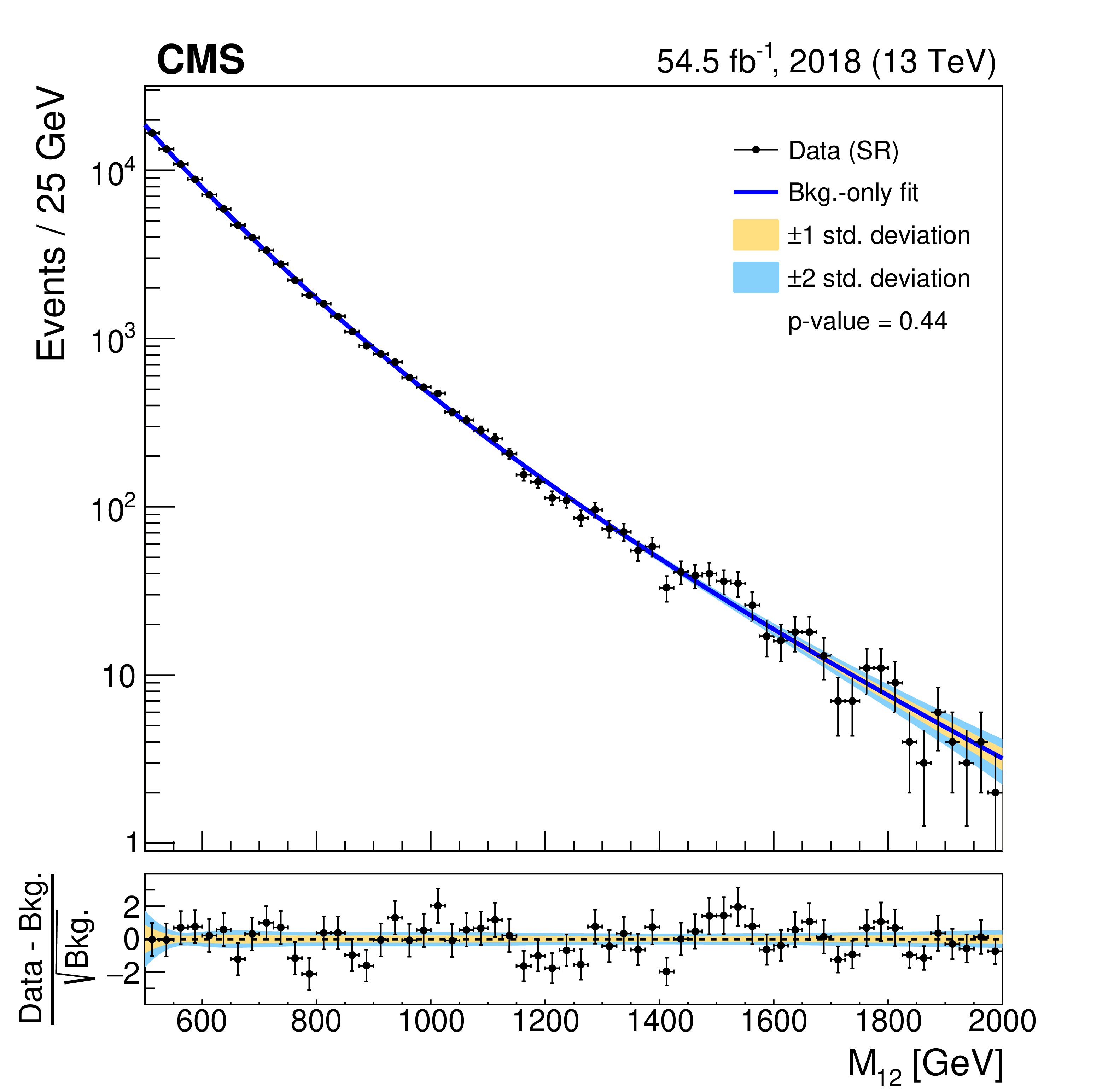
png pdf |
Figure 10-d:
Background-only fits to the $ M_{12} $ distribution in each fit range of the 2018 analysis in the FH category, shown together with $ {\pm}1\sigma $ and $ {\pm}2\sigma $ uncertainty bands extracted from the fit in the upper panels. The lower panels show the difference between data and fitted background, divided by the statistical uncertainty of the latter. The distributions are fitted in the $ M_{12} $ ranges of 270-560 GeV (upper left), 320-800 GeV (upper right), 390-1270 GeV (lower left), and 500-2000 GeV (lower right). |
png pdf |
Figure 11:
Expected and observed upper limits for the b-quark-associated Higgs boson production cross section times branching fraction of the decay into a b quark pair at 95% CL as functions of $ m_{\phi} $ for the 2017 SL category. The vertical dashed lines indicate the boundaries of usage of the different fit ranges, as reflected in the rightmost column of Table 2. |
png pdf |
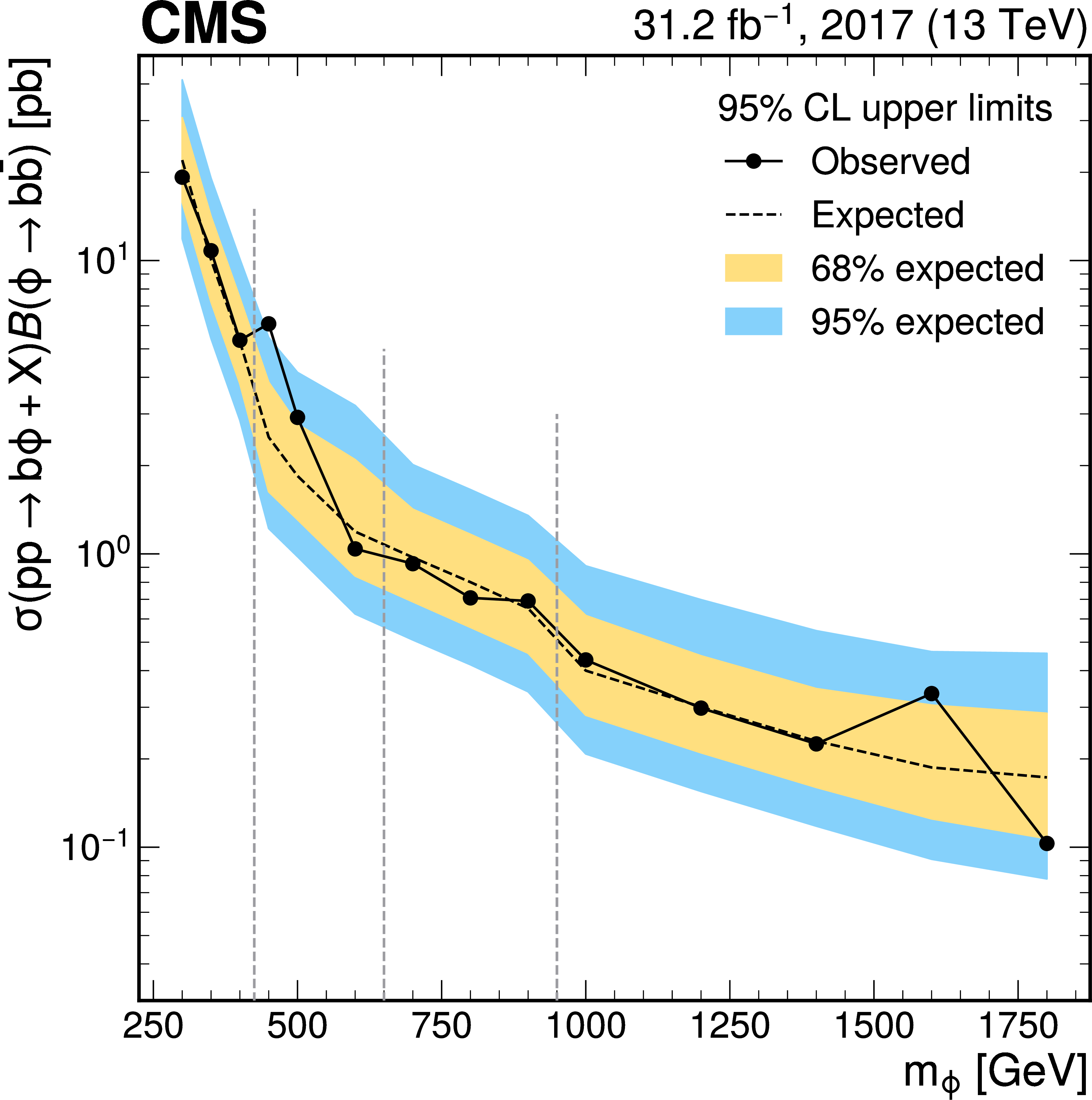
Figure 12:
Expected and observed upper limits for the b-quark-associated Higgs boson production cross section times branching fraction of the decay into a b quark pair at 95% CL as functions of $ m_{\phi} $ for the 2017 FH category. The vertical dashed lines indicate the boundaries of usage of the different fit ranges, as reflected in the rightmost column of Table 2. |
png pdf |
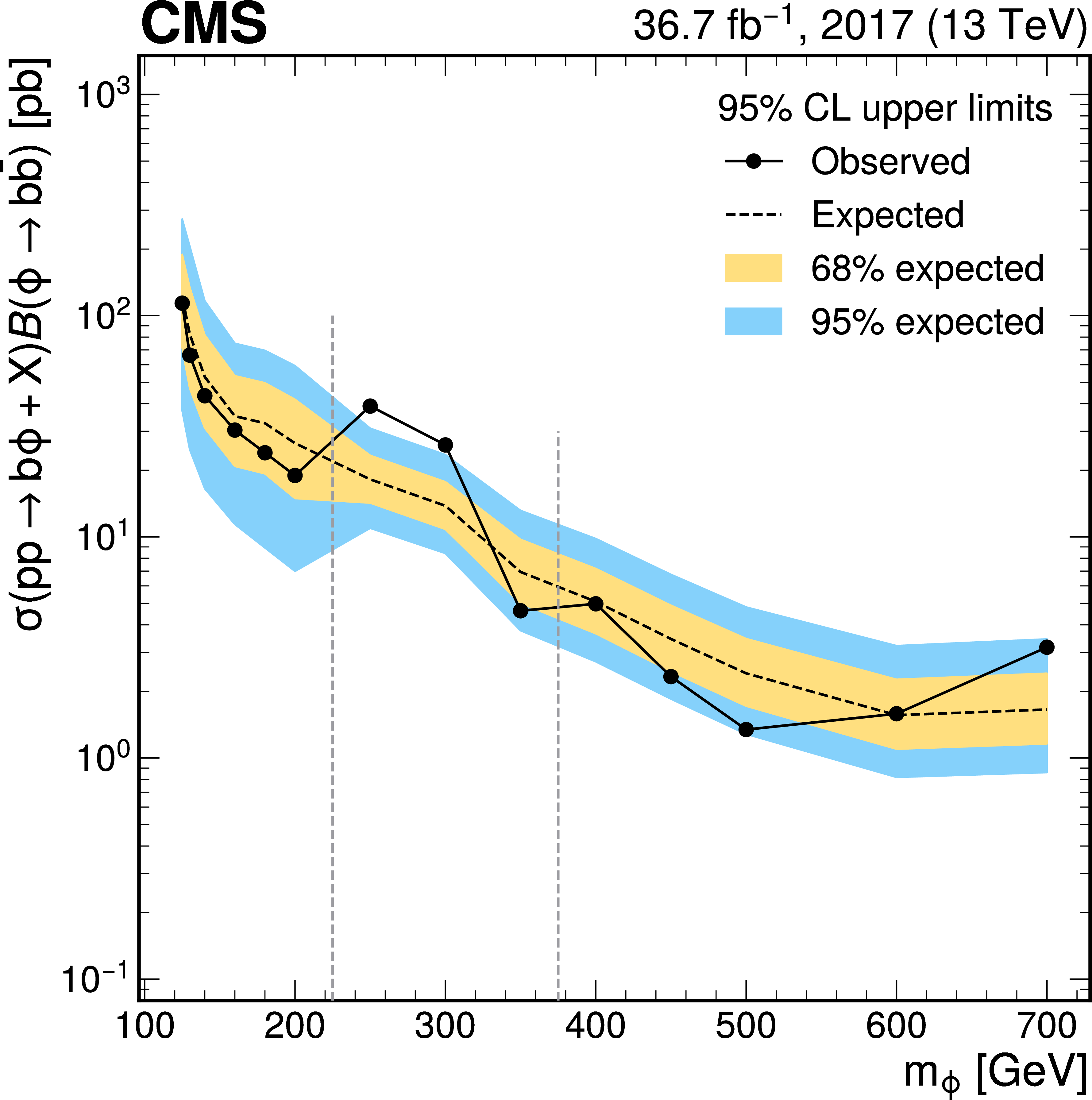
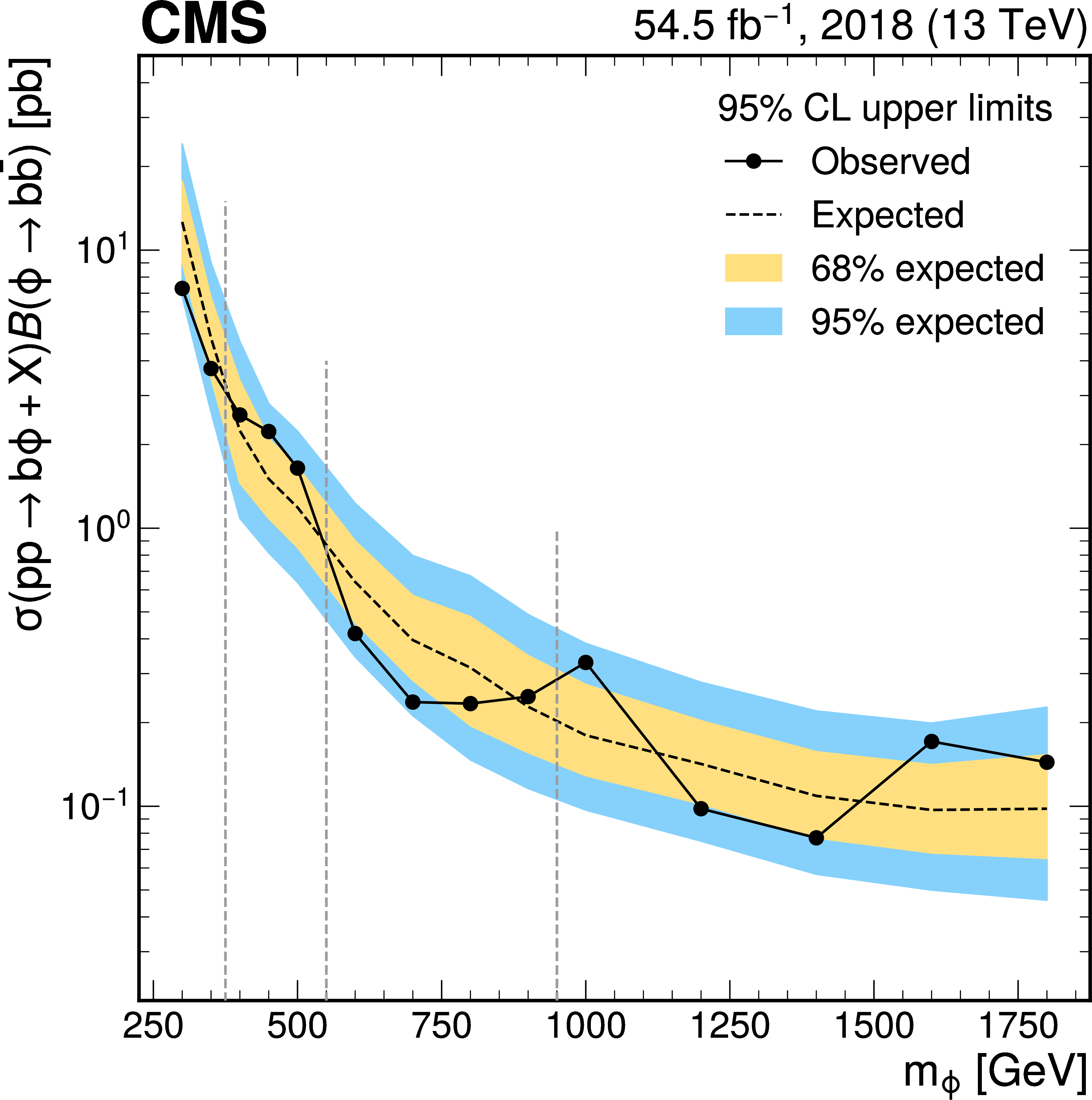
Figure 13:
Expected and observed upper limits for the b-quark-associated Higgs boson production cross section times branching fraction of the decay into a b quark pair at 95% CL as functions of $ m_{\phi} $ for the 2018 FH category. The vertical dashed lines indicate the boundaries of usage of the different fit ranges, as reflected in the rightmost column of Table 2. |
png pdf |
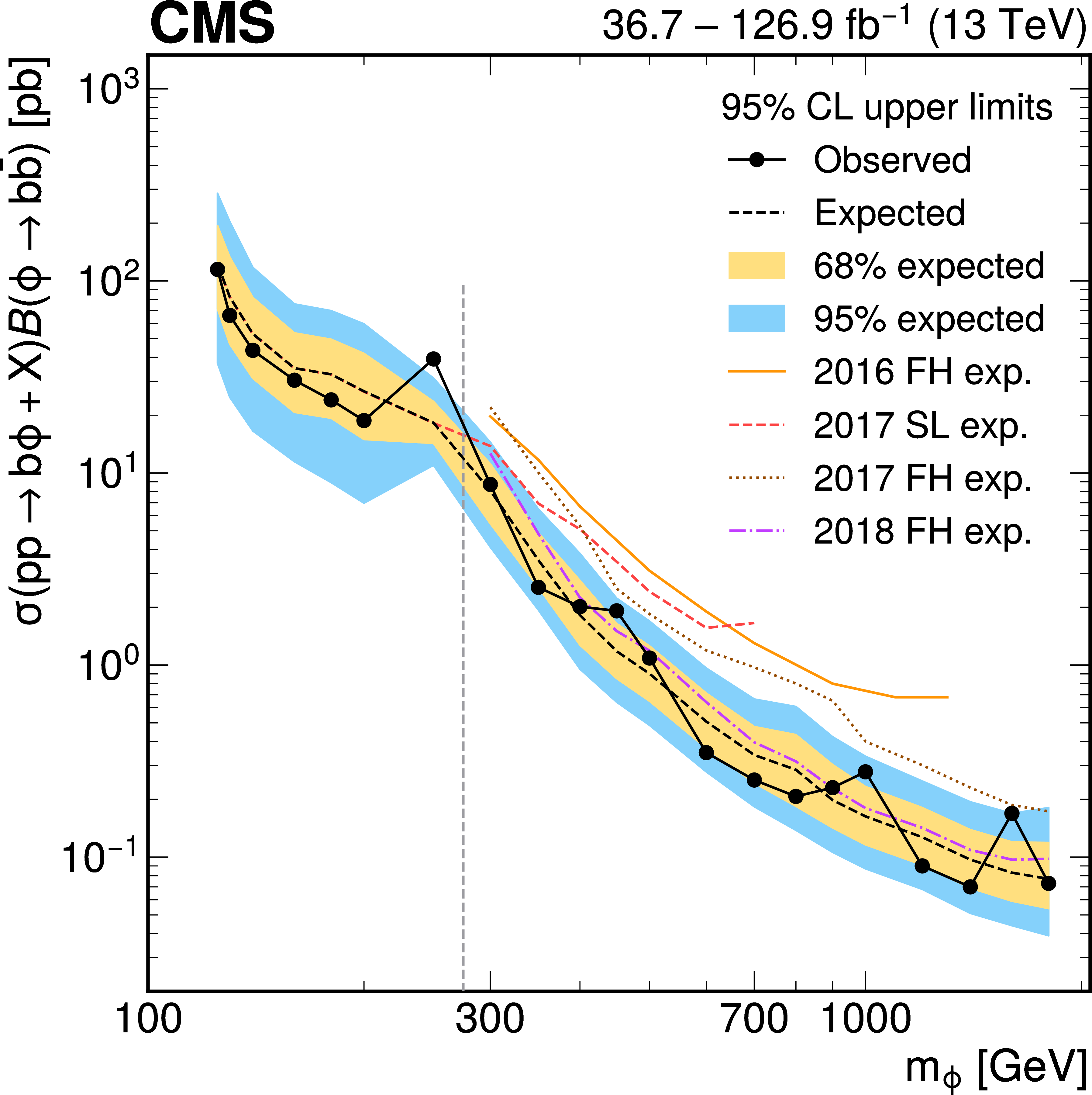
Figure 14:
Expected and observed upper limits for the b-quark-associated Higgs boson production cross section times branching fraction of the decay into a b quark pair at 95% CL as functions of $ m_{\phi} $, corresponding to the combination with the 2016 data. The vertical dashed line separates the mass range where only the 2017 SL category contributes on its left, from the region where also the 2017 FH and 2018 FH categories contribute on its right. The expected limits from the 2017 SL, 2017 FH, and 2018 FH data sets as well as from the previously published result based on the 2016 data set are also shown as colored lines. |
png pdf |
Figure 15:
Ratio of $ M_{12} $ distributions in SR and CR of the 2017 analysis in the SL category, for data (filled circles), fitted with a sum of Chebyshev polynomials up to the second degree (solid line). The ratio is shown in the $ M_{12} $ ranges of 120-300 GeV (upper left), 180-460 GeV (upper right), and 240-800 GeV (lower). The p value resulting from each fit is also quoted. The result of a similar fit based on QCD multijet simulation is superimposed (dashed line) with $ \pm 1\sigma $ and $ \pm 2\sigma $ bands of statistical uncertainty extracted from the fit. |
png pdf |
Figure 15-a:
Ratio of $ M_{12} $ distributions in SR and CR of the 2017 analysis in the SL category, for data (filled circles), fitted with a sum of Chebyshev polynomials up to the second degree (solid line). The ratio is shown in the $ M_{12} $ ranges of 120-300 GeV (upper left), 180-460 GeV (upper right), and 240-800 GeV (lower). The p value resulting from each fit is also quoted. The result of a similar fit based on QCD multijet simulation is superimposed (dashed line) with $ \pm 1\sigma $ and $ \pm 2\sigma $ bands of statistical uncertainty extracted from the fit. |
png pdf |
Figure 15-b:
Ratio of $ M_{12} $ distributions in SR and CR of the 2017 analysis in the SL category, for data (filled circles), fitted with a sum of Chebyshev polynomials up to the second degree (solid line). The ratio is shown in the $ M_{12} $ ranges of 120-300 GeV (upper left), 180-460 GeV (upper right), and 240-800 GeV (lower). The p value resulting from each fit is also quoted. The result of a similar fit based on QCD multijet simulation is superimposed (dashed line) with $ \pm 1\sigma $ and $ \pm 2\sigma $ bands of statistical uncertainty extracted from the fit. |
png pdf |
Figure 15-c:
Ratio of $ M_{12} $ distributions in SR and CR of the 2017 analysis in the SL category, for data (filled circles), fitted with a sum of Chebyshev polynomials up to the second degree (solid line). The ratio is shown in the $ M_{12} $ ranges of 120-300 GeV (upper left), 180-460 GeV (upper right), and 240-800 GeV (lower). The p value resulting from each fit is also quoted. The result of a similar fit based on QCD multijet simulation is superimposed (dashed line) with $ \pm 1\sigma $ and $ \pm 2\sigma $ bands of statistical uncertainty extracted from the fit. |
png pdf |
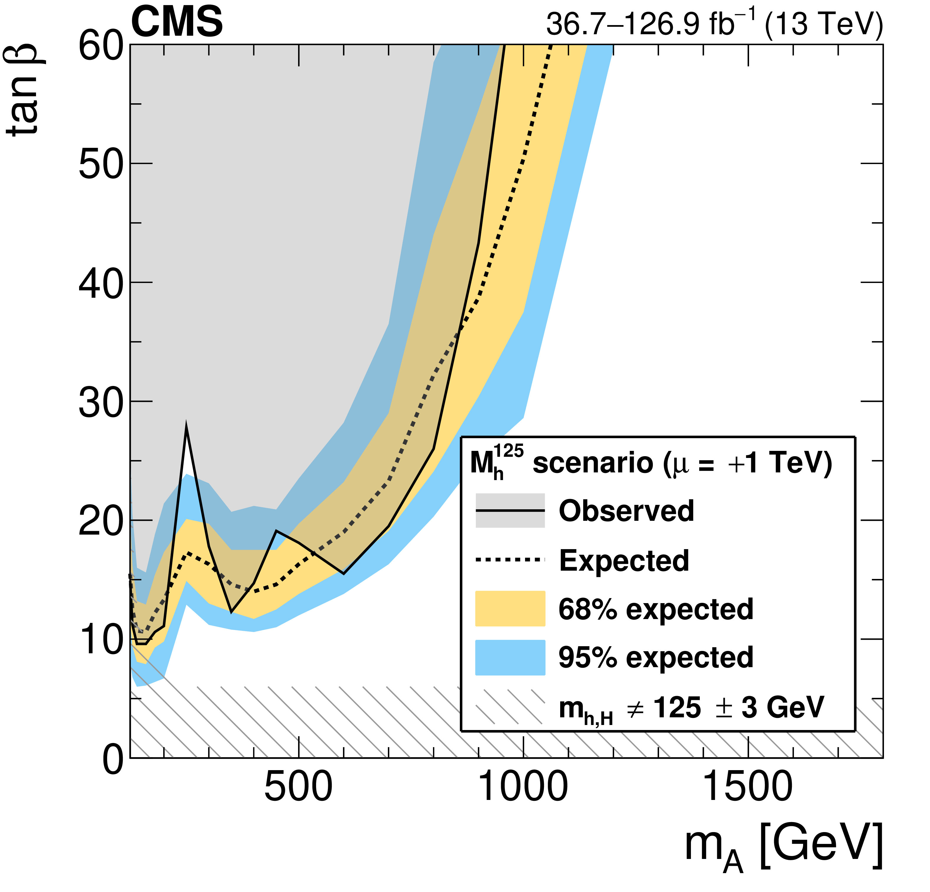
Figure 16:
Interpretation in the $ M_{\mathrm{h}}^{125} $ scenario of the MSSM: observed and expected upper limits at 95% CL on the parameter $ \tan\beta $ as functions of the mass $ m_{\mathrm{A}} $ of the $ CP $-odd Higgs boson. The higgsino mass parameter has been set to $ \mu = + $1 TeV. The hashed area indicates the parameter region in which the mass of the lightest MSSM Higgs boson does not coincide with 125 GeV within a margin of 3 GeV. |
png pdf |
Figure 16-a:
Interpretation in the $ M_{\mathrm{h}}^{125} $ scenario of the MSSM: observed and expected upper limits at 95% CL on the parameter $ \tan\beta $ as functions of the mass $ m_{\mathrm{A}} $ of the $ CP $-odd Higgs boson. The higgsino mass parameter has been set to $ \mu = + $1 TeV. The hashed area indicates the parameter region in which the mass of the lightest MSSM Higgs boson does not coincide with 125 GeV within a margin of 3 GeV. |
png pdf |
Figure 16-b:
Interpretation in the $ M_{\mathrm{h}}^{125} $ scenario of the MSSM: observed and expected upper limits at 95% CL on the parameter $ \tan\beta $ as functions of the mass $ m_{\mathrm{A}} $ of the $ CP $-odd Higgs boson. The higgsino mass parameter has been set to $ \mu = + $1 TeV. The hashed area indicates the parameter region in which the mass of the lightest MSSM Higgs boson does not coincide with 125 GeV within a margin of 3 GeV. |

png pdf |
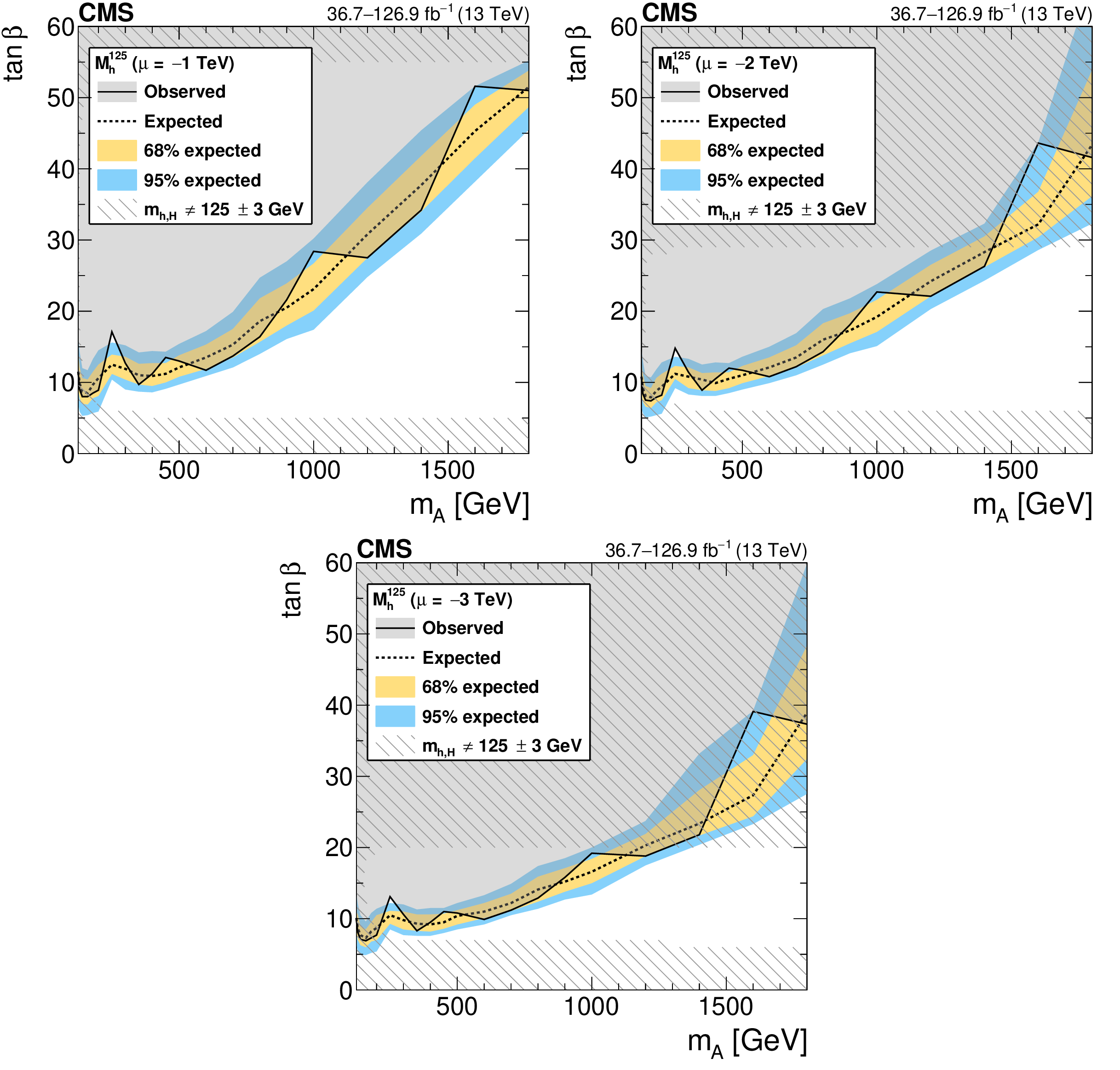
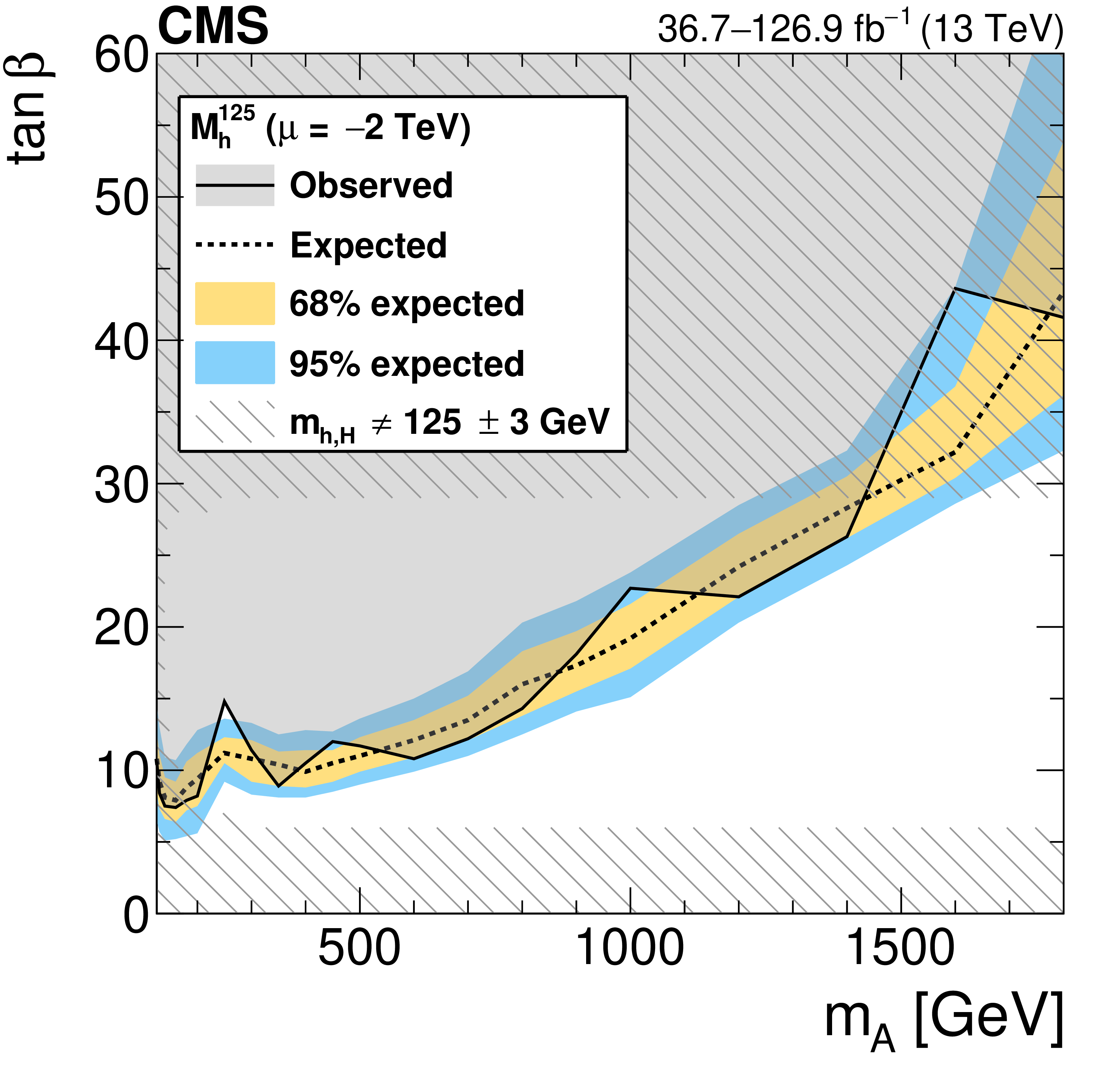
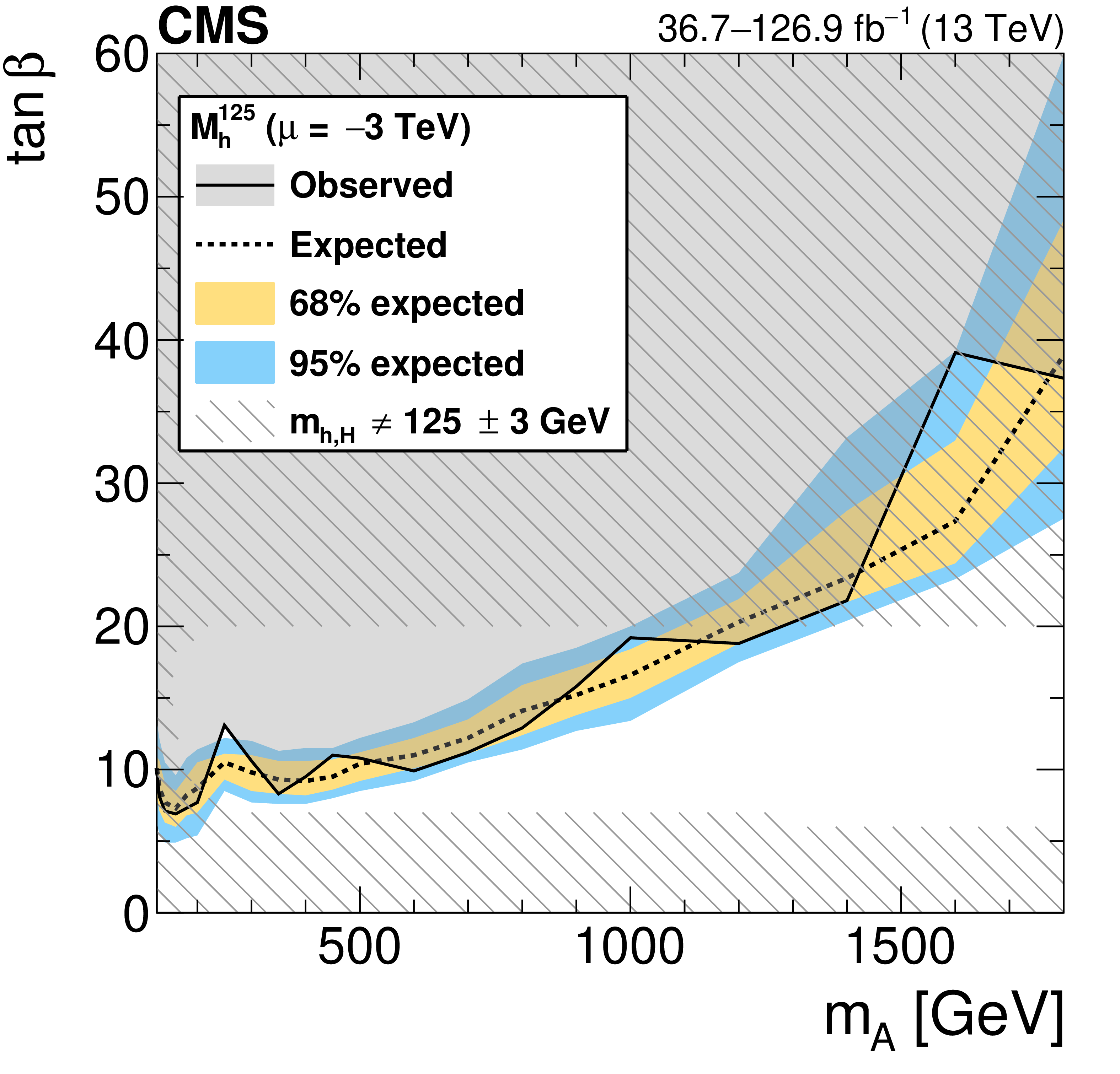
Figure 17:
Interpretation in the $ M_{\mathrm{h}}^{125} $ scenario of the MSSM: observed and expected upper limits at 95% CL on the parameter $ \tan\beta $ as functions of the mass $ m_{\mathrm{A}} $ of the $ CP $-odd Higgs boson. The higgsino mass parameter has been set to $ \mu = - $1 TeV (upper left), $ \mu = - $2 TeV (upper right), and $ \mu = - $3 TeV (lower). The hashed area indicates the parameter region in which the mass of the lightest MSSM Higgs boson does not coincide with 125 GeV within a margin of 3 GeV. |

png pdf |
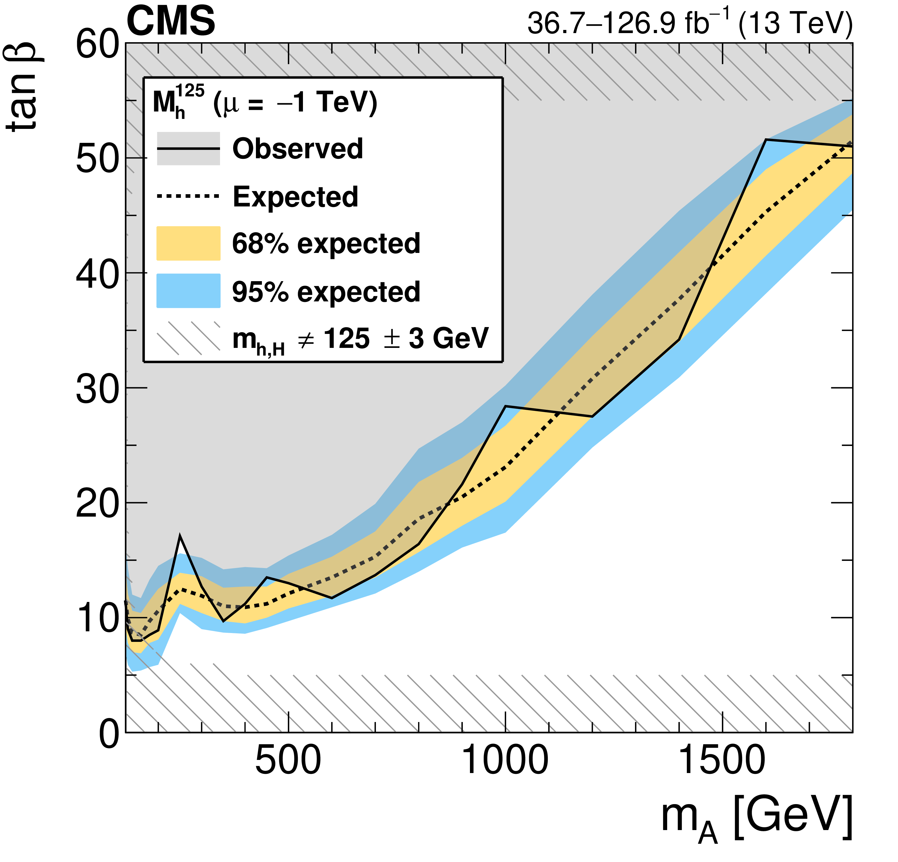
Figure 17-a:
Interpretation in the $ M_{\mathrm{h}}^{125} $ scenario of the MSSM: observed and expected upper limits at 95% CL on the parameter $ \tan\beta $ as functions of the mass $ m_{\mathrm{A}} $ of the $ CP $-odd Higgs boson. The higgsino mass parameter has been set to $ \mu = - $1 TeV (upper left), $ \mu = - $2 TeV (upper right), and $ \mu = - $3 TeV (lower). The hashed area indicates the parameter region in which the mass of the lightest MSSM Higgs boson does not coincide with 125 GeV within a margin of 3 GeV. |
png pdf |
Figure 17-b:
Interpretation in the $ M_{\mathrm{h}}^{125} $ scenario of the MSSM: observed and expected upper limits at 95% CL on the parameter $ \tan\beta $ as functions of the mass $ m_{\mathrm{A}} $ of the $ CP $-odd Higgs boson. The higgsino mass parameter has been set to $ \mu = - $1 TeV (upper left), $ \mu = - $2 TeV (upper right), and $ \mu = - $3 TeV (lower). The hashed area indicates the parameter region in which the mass of the lightest MSSM Higgs boson does not coincide with 125 GeV within a margin of 3 GeV. |
png pdf |
Figure 17-c:
Interpretation in the $ M_{\mathrm{h}}^{125} $ scenario of the MSSM: observed and expected upper limits at 95% CL on the parameter $ \tan\beta $ as functions of the mass $ m_{\mathrm{A}} $ of the $ CP $-odd Higgs boson. The higgsino mass parameter has been set to $ \mu = - $1 TeV (upper left), $ \mu = - $2 TeV (upper right), and $ \mu = - $3 TeV (lower). The hashed area indicates the parameter region in which the mass of the lightest MSSM Higgs boson does not coincide with 125 GeV within a margin of 3 GeV. |
png pdf |
Figure 17-d:
Interpretation in the $ M_{\mathrm{h}}^{125} $ scenario of the MSSM: observed and expected upper limits at 95% CL on the parameter $ \tan\beta $ as functions of the mass $ m_{\mathrm{A}} $ of the $ CP $-odd Higgs boson. The higgsino mass parameter has been set to $ \mu = - $1 TeV (upper left), $ \mu = - $2 TeV (upper right), and $ \mu = - $3 TeV (lower). The hashed area indicates the parameter region in which the mass of the lightest MSSM Higgs boson does not coincide with 125 GeV within a margin of 3 GeV. |

png pdf |
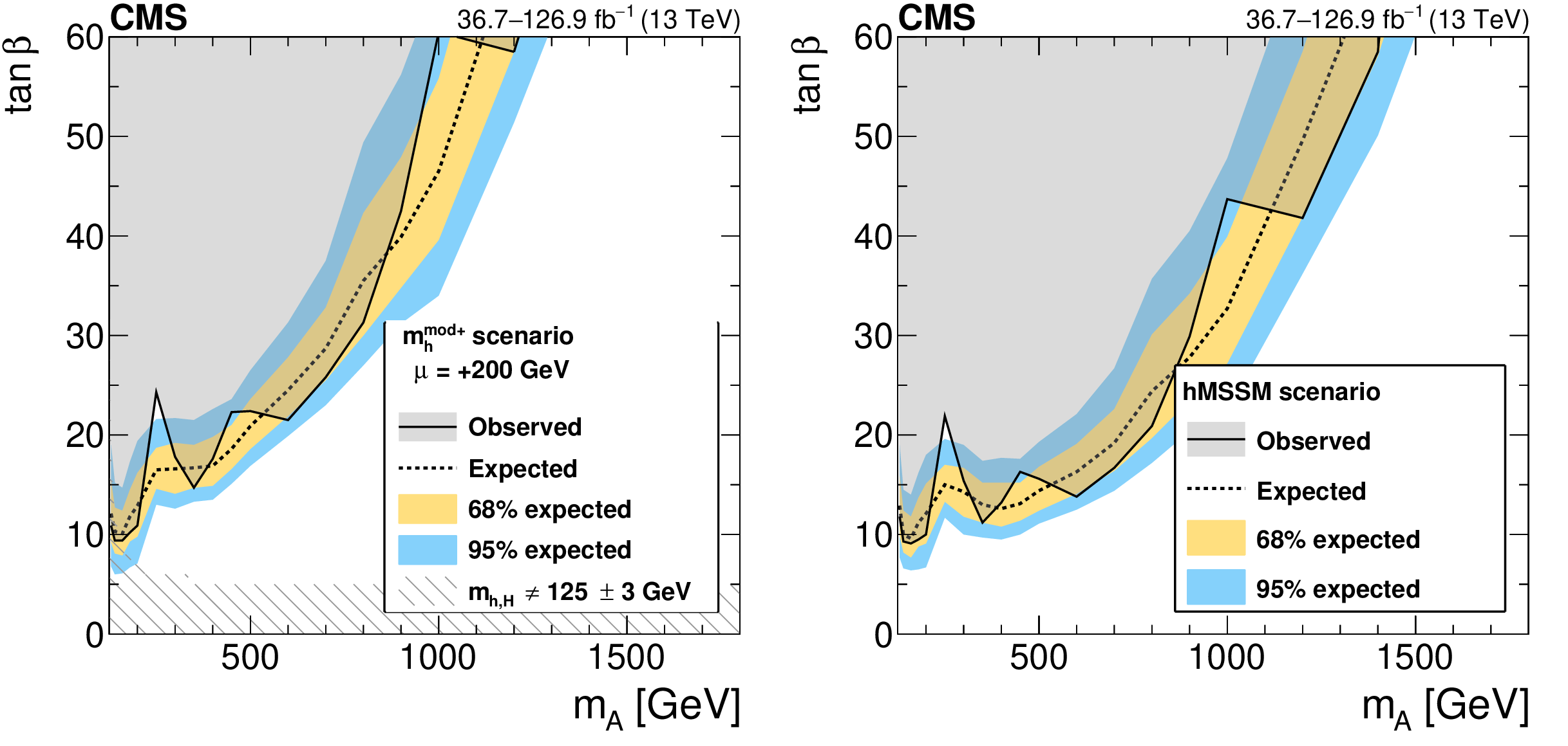
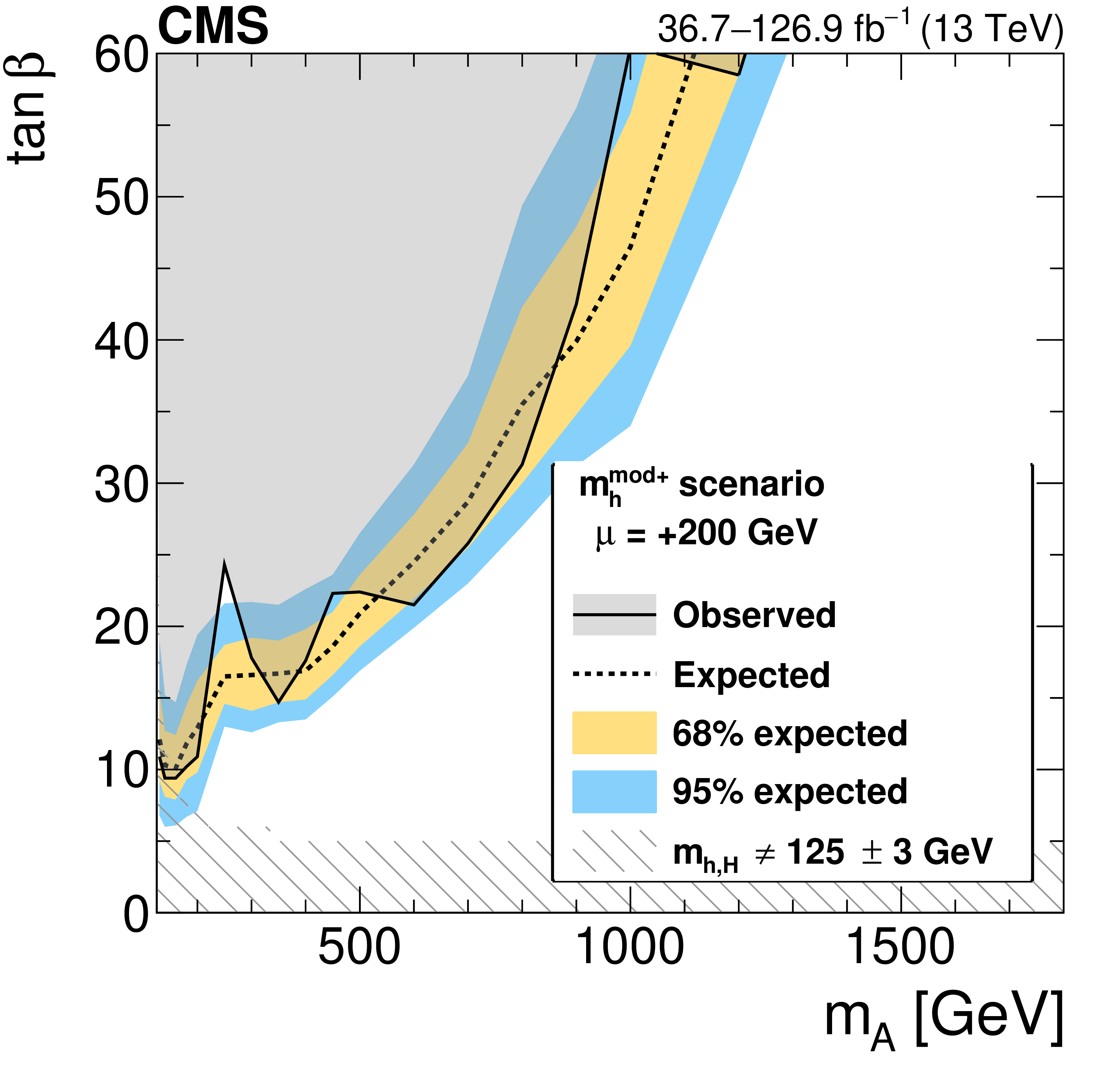
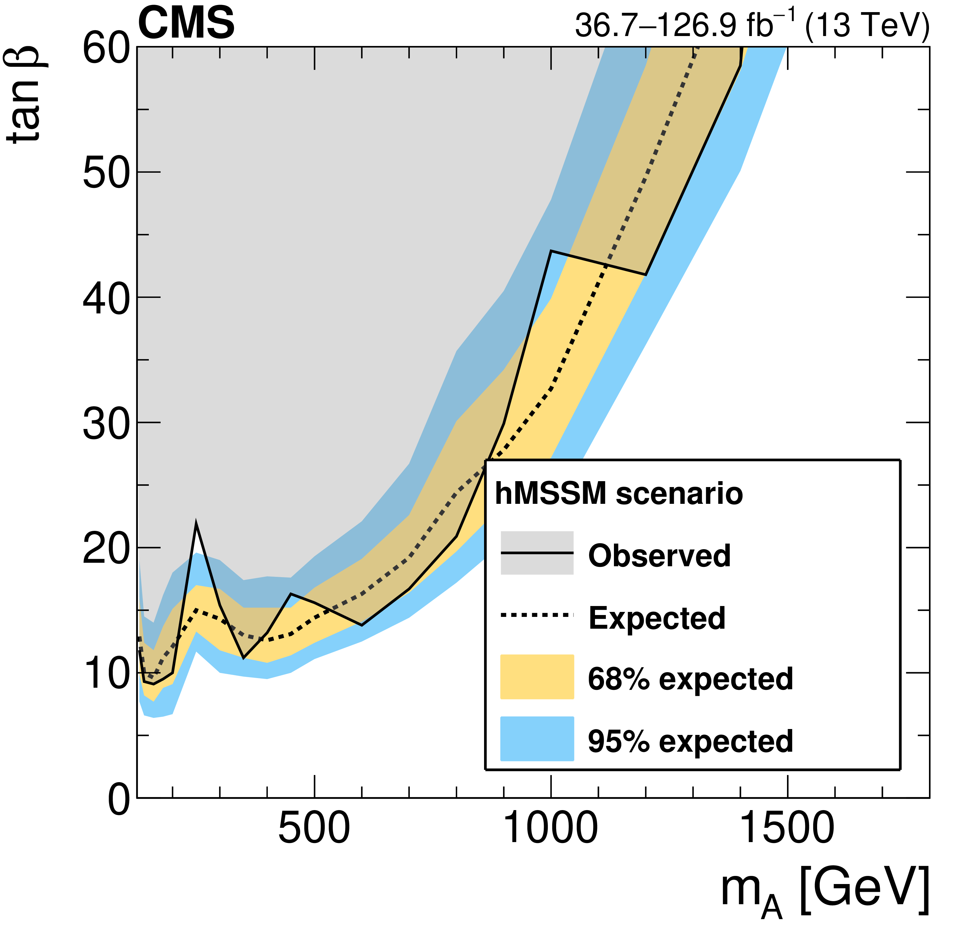
Figure 18:
Interpretation in the $ m_{\mathrm{h}}^{\text{mod+}} $ (left) and hMSSM (right) scenarios of the MSSM: observed and expected upper limits at 95% CL on the parameter $ \tan\beta $ as functions of the mass $ m_{\mathrm{A}} $ of the $ CP $-odd Higgs boson. In the left plot, the hashed area indicates the parameter region in which the mass of the lightest MSSM Higgs boson does not coincide with 125 GeV within a margin of 3 GeV. |
png pdf |
Figure 18-a:
Interpretation in the $ m_{\mathrm{h}}^{\text{mod+}} $ (left) and hMSSM (right) scenarios of the MSSM: observed and expected upper limits at 95% CL on the parameter $ \tan\beta $ as functions of the mass $ m_{\mathrm{A}} $ of the $ CP $-odd Higgs boson. In the left plot, the hashed area indicates the parameter region in which the mass of the lightest MSSM Higgs boson does not coincide with 125 GeV within a margin of 3 GeV. |
png pdf |
Figure 18-b:
Interpretation in the $ m_{\mathrm{h}}^{\text{mod+}} $ (left) and hMSSM (right) scenarios of the MSSM: observed and expected upper limits at 95% CL on the parameter $ \tan\beta $ as functions of the mass $ m_{\mathrm{A}} $ of the $ CP $-odd Higgs boson. In the left plot, the hashed area indicates the parameter region in which the mass of the lightest MSSM Higgs boson does not coincide with 125 GeV within a margin of 3 GeV. |

png pdf |
Figure 18-c:
Interpretation in the $ m_{\mathrm{h}}^{\text{mod+}} $ (left) and hMSSM (right) scenarios of the MSSM: observed and expected upper limits at 95% CL on the parameter $ \tan\beta $ as functions of the mass $ m_{\mathrm{A}} $ of the $ CP $-odd Higgs boson. In the left plot, the hashed area indicates the parameter region in which the mass of the lightest MSSM Higgs boson does not coincide with 125 GeV within a margin of 3 GeV. |

png pdf |
Figure 18-d:
Interpretation in the $ m_{\mathrm{h}}^{\text{mod+}} $ (left) and hMSSM (right) scenarios of the MSSM: observed and expected upper limits at 95% CL on the parameter $ \tan\beta $ as functions of the mass $ m_{\mathrm{A}} $ of the $ CP $-odd Higgs boson. In the left plot, the hashed area indicates the parameter region in which the mass of the lightest MSSM Higgs boson does not coincide with 125 GeV within a margin of 3 GeV. |
png pdf |
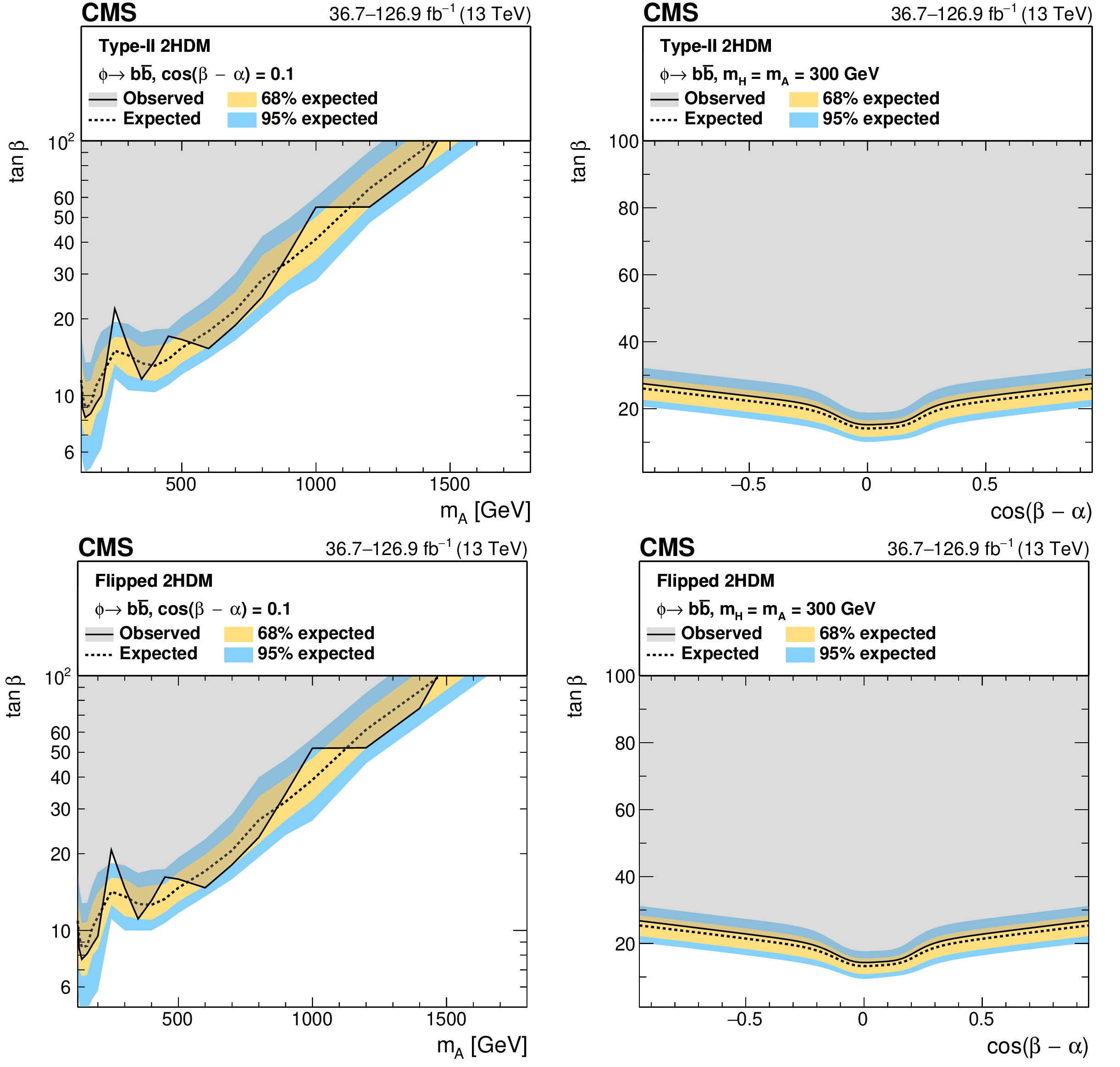
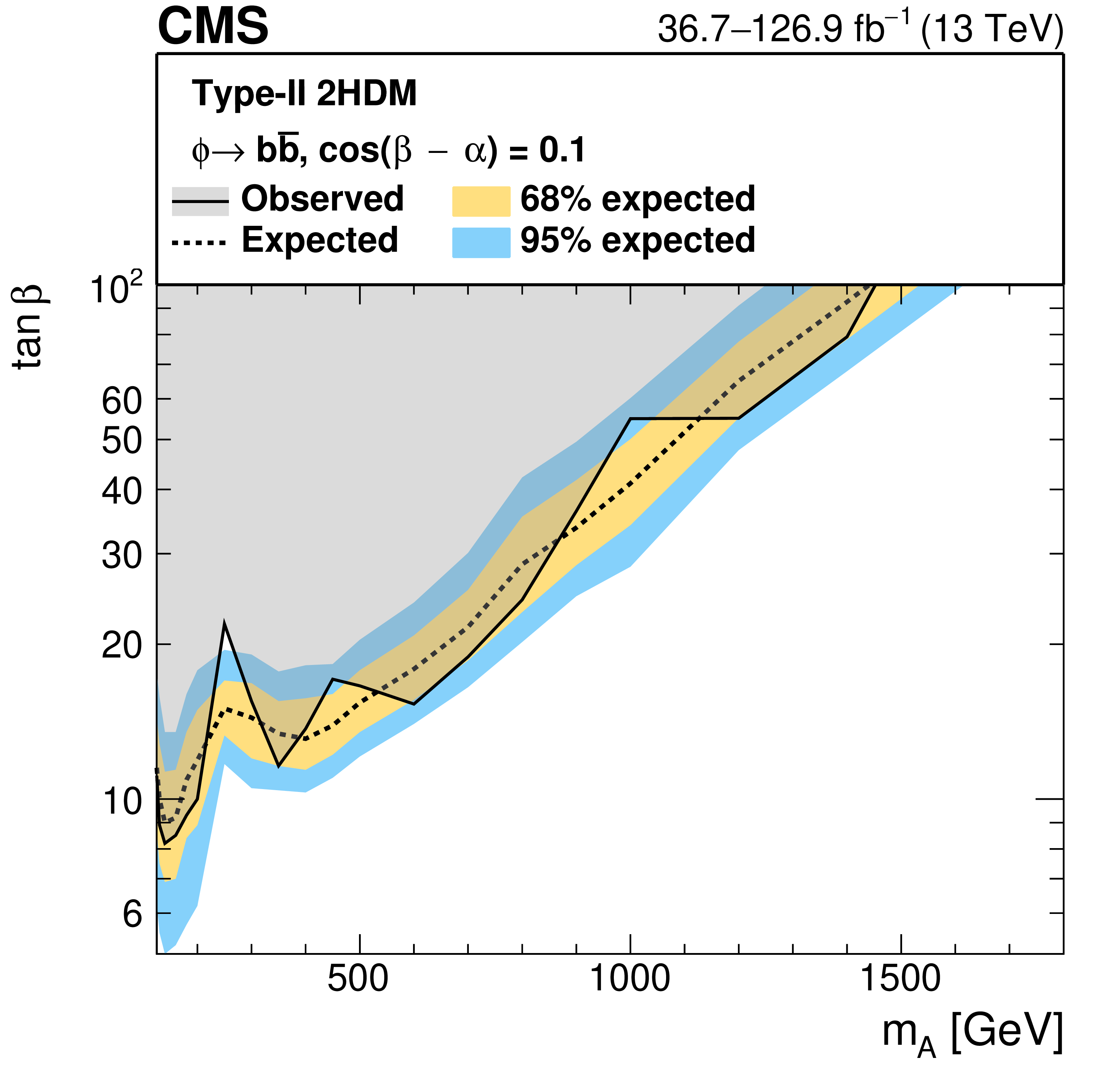
Figure 19:
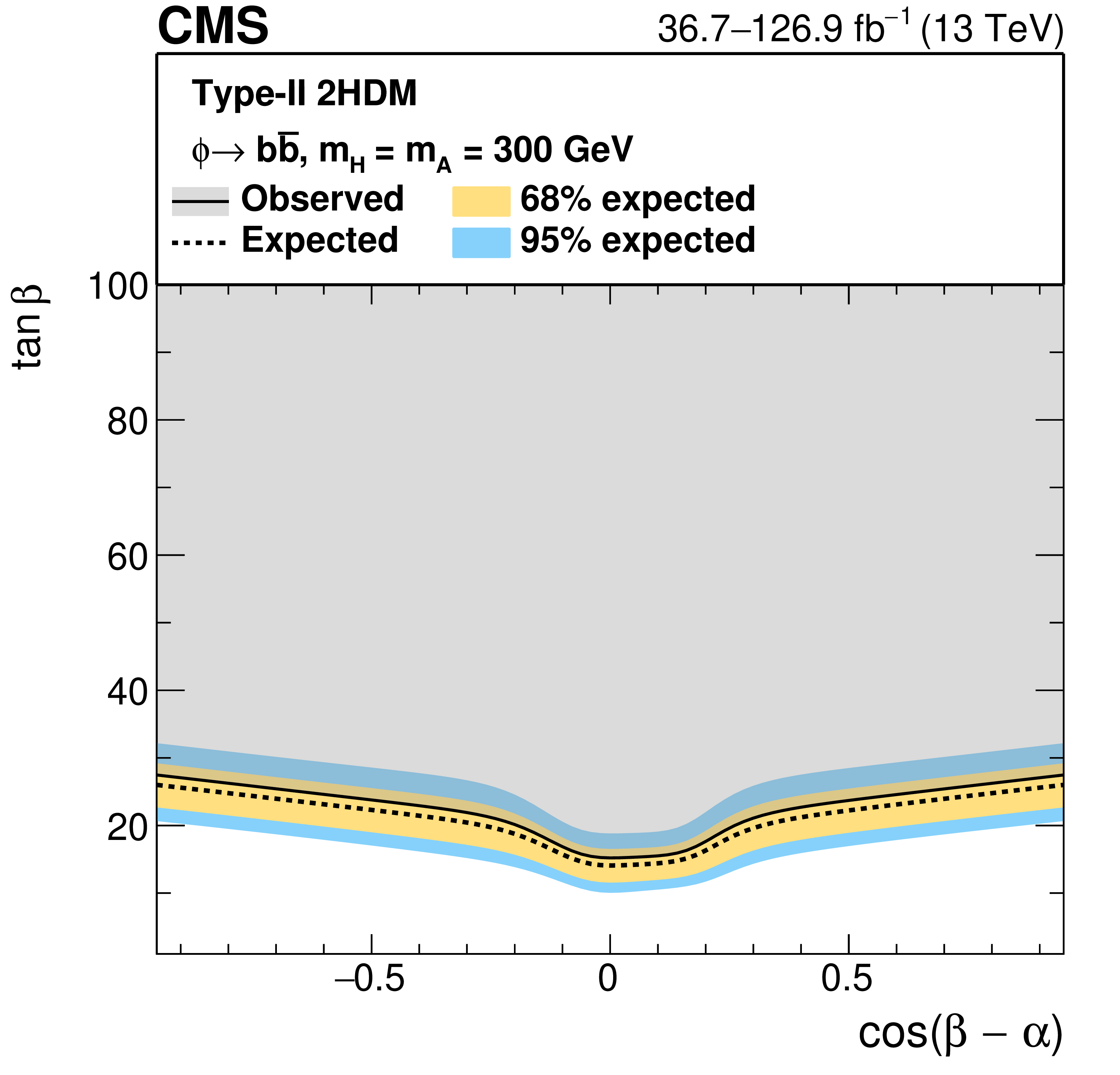
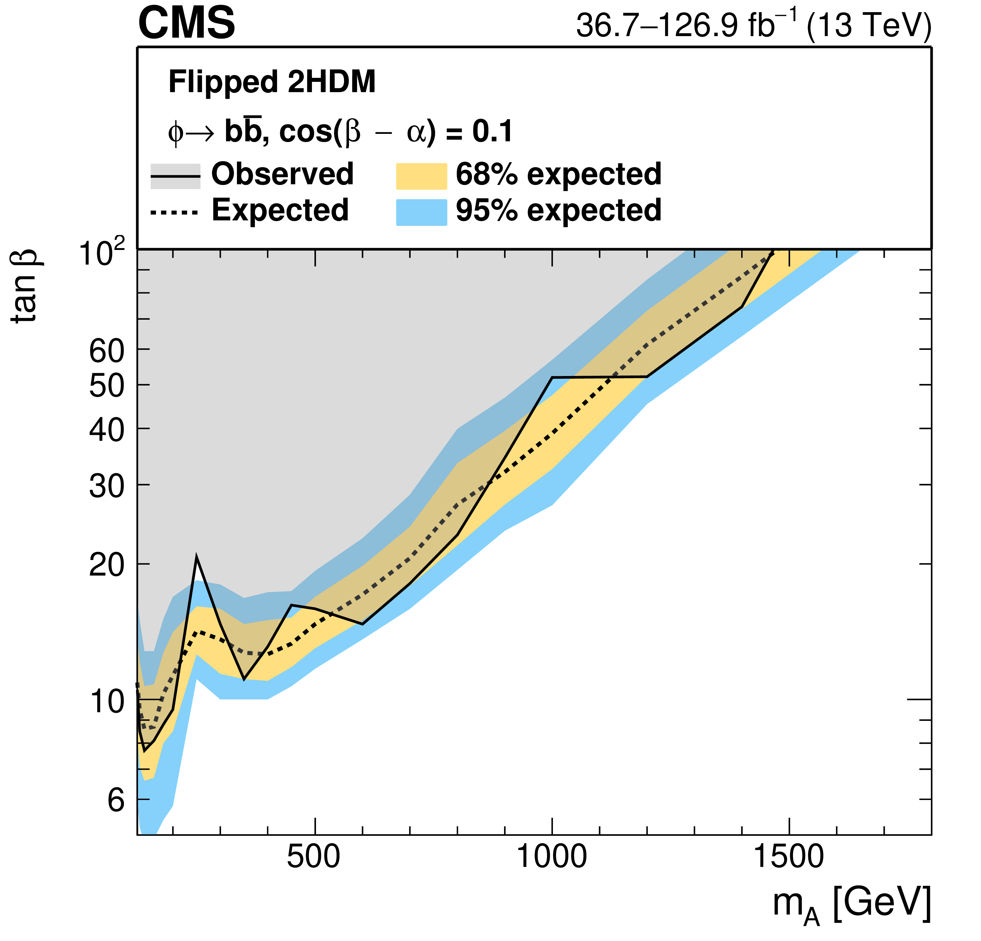
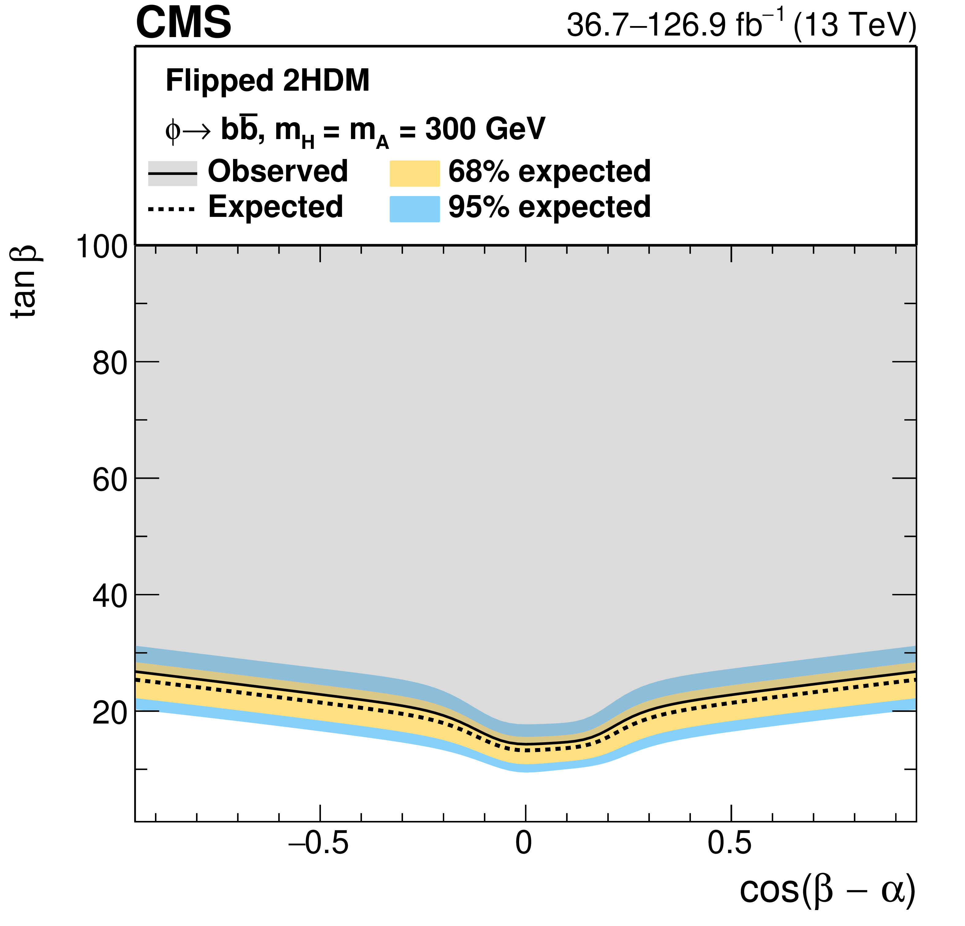
Interpretation in 2HDM scenarios: observed and expected upper limits at 95% CL on the parameter $ \tan\beta $ as a function of $ m_{\mathrm{A},\mathrm{H}} $ for $ \cos(\beta-\alpha)= $ 0.1 (left), and as functions of $ \cos(\beta-\alpha) $ for masses of $ m_{\mathrm{A}} = m_{\mathrm{H}} = $ 300 GeV (right), for the 2HDM Type-II scenario (upper), and the 2HDM Flipped scenario (lower). |
png pdf |
Figure 19-a:
Interpretation in 2HDM scenarios: observed and expected upper limits at 95% CL on the parameter $ \tan\beta $ as a function of $ m_{\mathrm{A},\mathrm{H}} $ for $ \cos(\beta-\alpha)= $ 0.1 (left), and as functions of $ \cos(\beta-\alpha) $ for masses of $ m_{\mathrm{A}} = m_{\mathrm{H}} = $ 300 GeV (right), for the 2HDM Type-II scenario (upper), and the 2HDM Flipped scenario (lower). |

png pdf |
Figure 19-b:
Interpretation in 2HDM scenarios: observed and expected upper limits at 95% CL on the parameter $ \tan\beta $ as a function of $ m_{\mathrm{A},\mathrm{H}} $ for $ \cos(\beta-\alpha)= $ 0.1 (left), and as functions of $ \cos(\beta-\alpha) $ for masses of $ m_{\mathrm{A}} = m_{\mathrm{H}} = $ 300 GeV (right), for the 2HDM Type-II scenario (upper), and the 2HDM Flipped scenario (lower). |

png pdf |
Figure 19-c:
Interpretation in 2HDM scenarios: observed and expected upper limits at 95% CL on the parameter $ \tan\beta $ as a function of $ m_{\mathrm{A},\mathrm{H}} $ for $ \cos(\beta-\alpha)= $ 0.1 (left), and as functions of $ \cos(\beta-\alpha) $ for masses of $ m_{\mathrm{A}} = m_{\mathrm{H}} = $ 300 GeV (right), for the 2HDM Type-II scenario (upper), and the 2HDM Flipped scenario (lower). |

png pdf |
Figure 19-d:
Interpretation in 2HDM scenarios: observed and expected upper limits at 95% CL on the parameter $ \tan\beta $ as a function of $ m_{\mathrm{A},\mathrm{H}} $ for $ \cos(\beta-\alpha)= $ 0.1 (left), and as functions of $ \cos(\beta-\alpha) $ for masses of $ m_{\mathrm{A}} = m_{\mathrm{H}} = $ 300 GeV (right), for the 2HDM Type-II scenario (upper), and the 2HDM Flipped scenario (lower). |
png pdf |
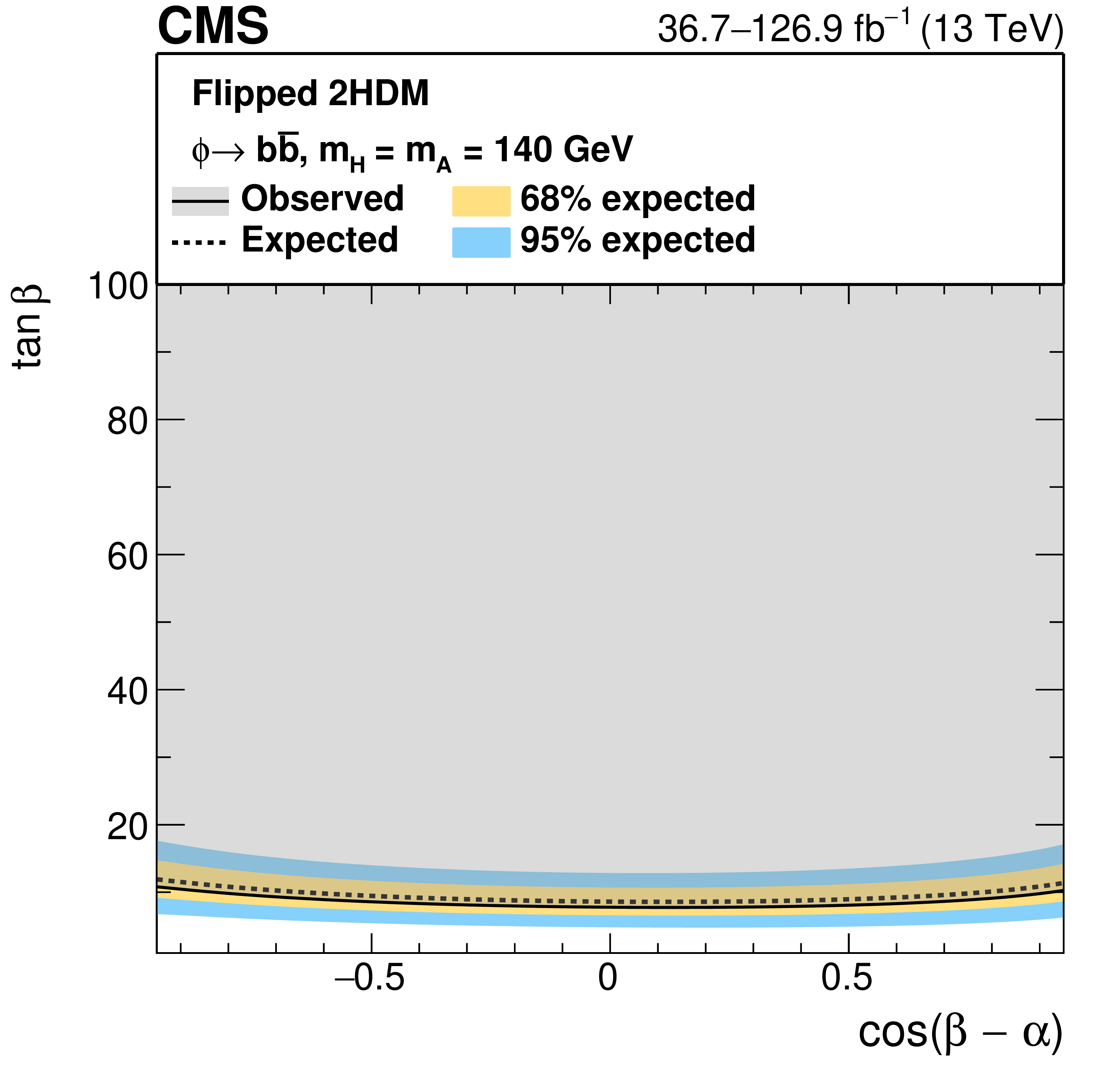
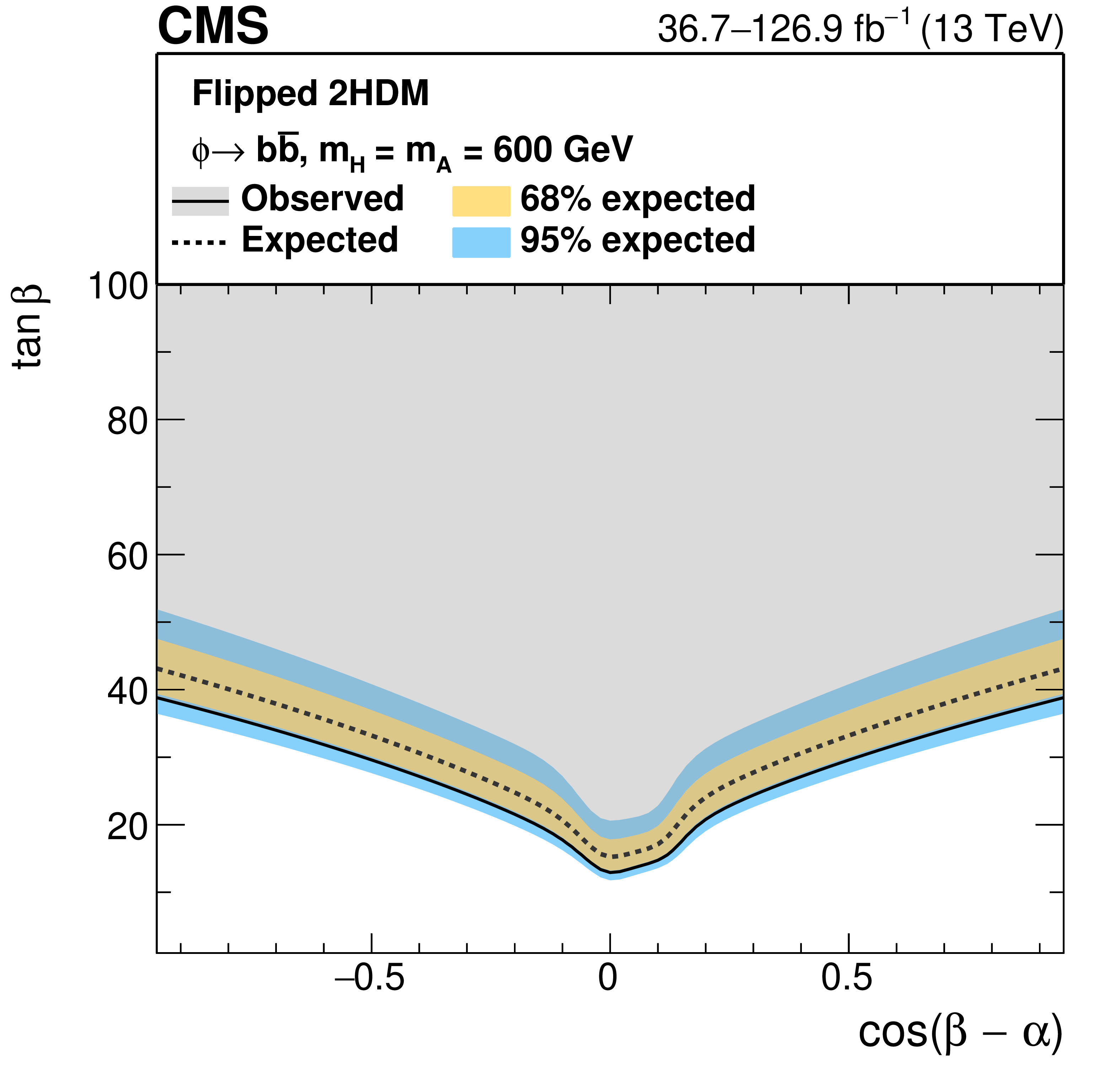
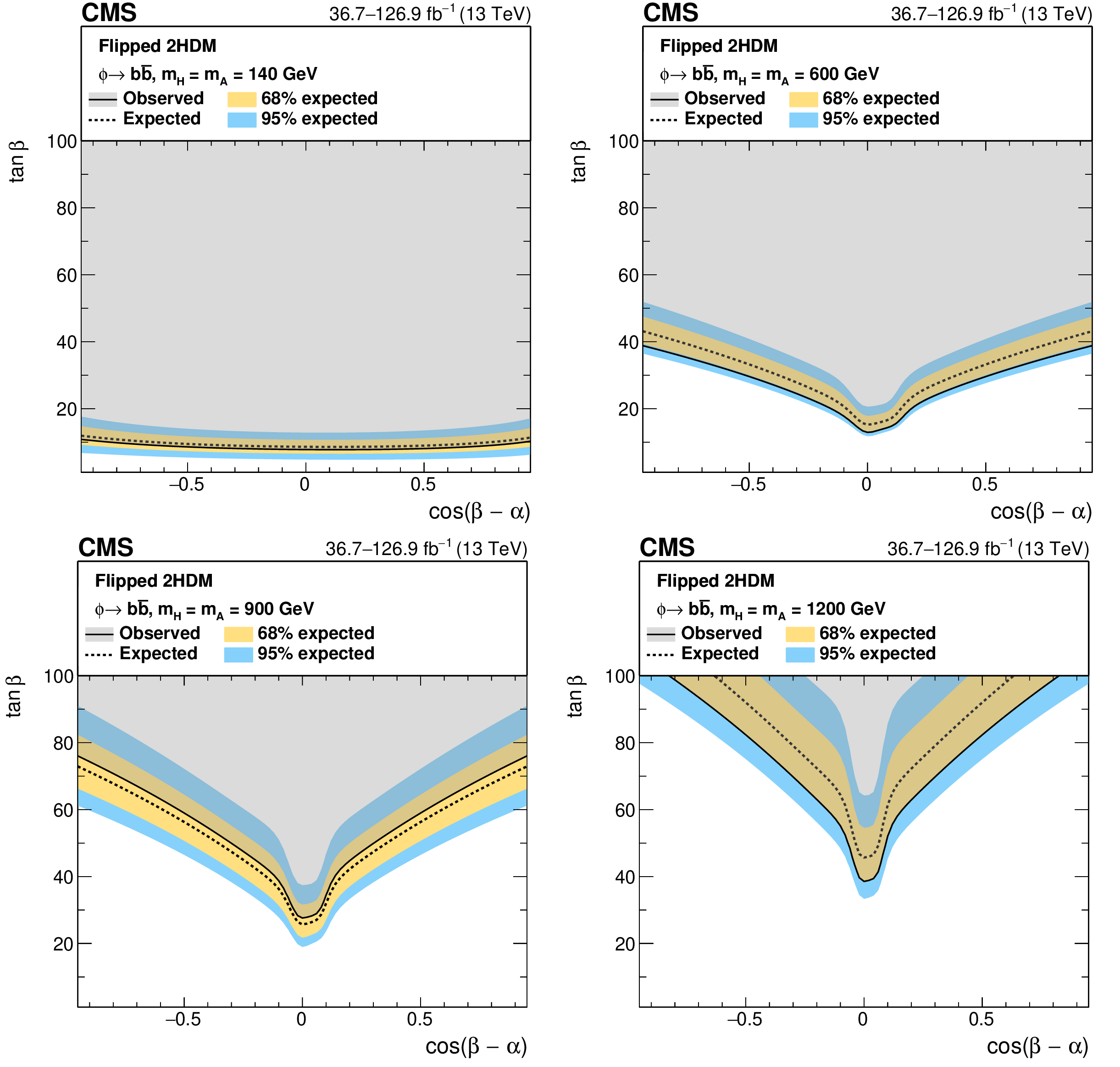
Figure 20:
Interpretation in the 2HDM flipped scenario: observed and expected upper limits at 95% CL on the parameter $ \tan\beta $ as functions of $ \cos(\beta-\alpha) $ for masses of $ m_{\mathrm{A}} = m_{\mathrm{H}} = $ 140, 600, 900, and 1200 GeV. |

png pdf |
Figure 20-a:
Interpretation in the 2HDM flipped scenario: observed and expected upper limits at 95% CL on the parameter $ \tan\beta $ as functions of $ \cos(\beta-\alpha) $ for masses of $ m_{\mathrm{A}} = m_{\mathrm{H}} = $ 140, 600, 900, and 1200 GeV. |

png pdf |
Figure 20-b:
Interpretation in the 2HDM flipped scenario: observed and expected upper limits at 95% CL on the parameter $ \tan\beta $ as functions of $ \cos(\beta-\alpha) $ for masses of $ m_{\mathrm{A}} = m_{\mathrm{H}} = $ 140, 600, 900, and 1200 GeV. |
png pdf |
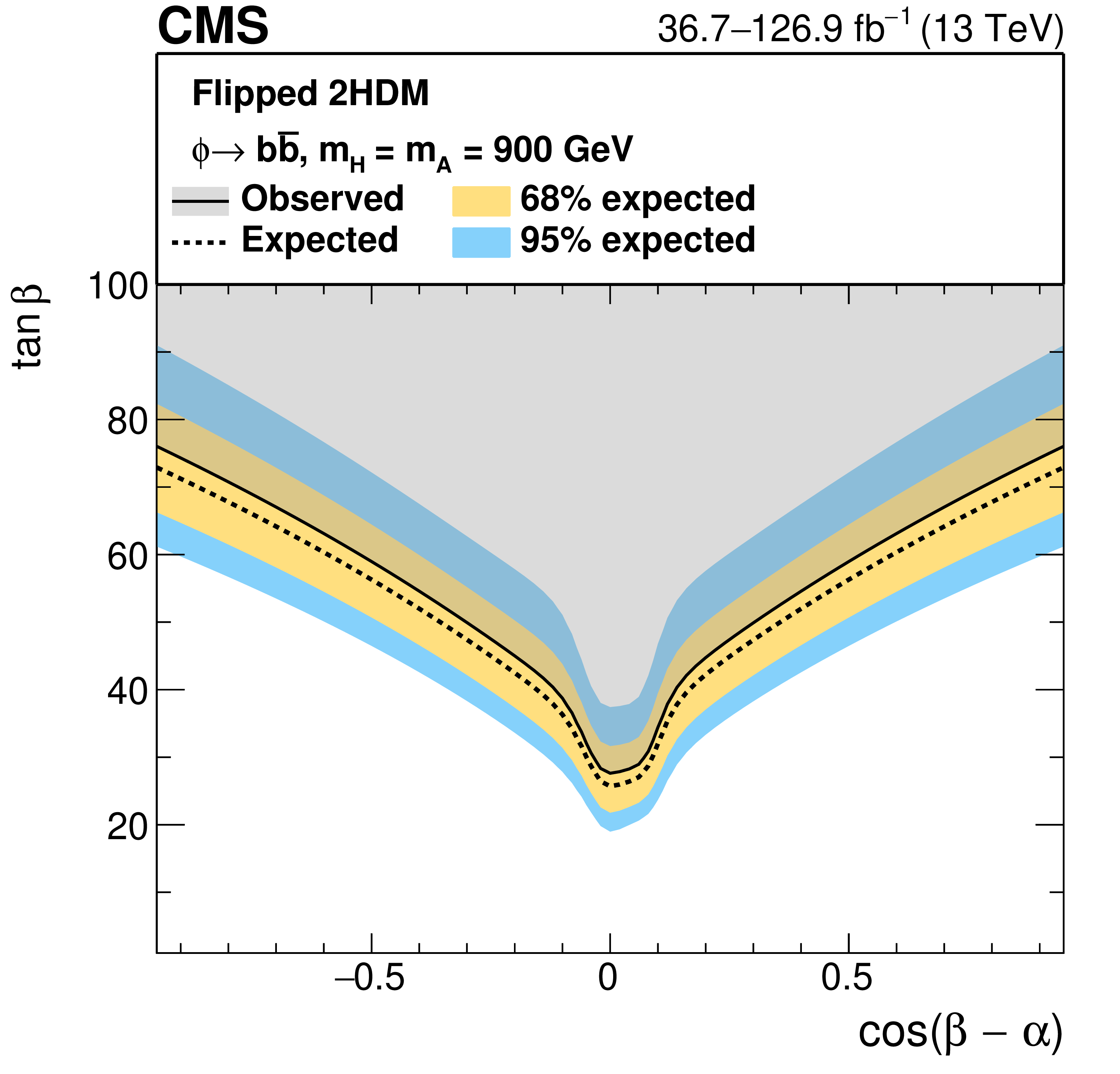
Figure 20-c:
Interpretation in the 2HDM flipped scenario: observed and expected upper limits at 95% CL on the parameter $ \tan\beta $ as functions of $ \cos(\beta-\alpha) $ for masses of $ m_{\mathrm{A}} = m_{\mathrm{H}} = $ 140, 600, 900, and 1200 GeV. |
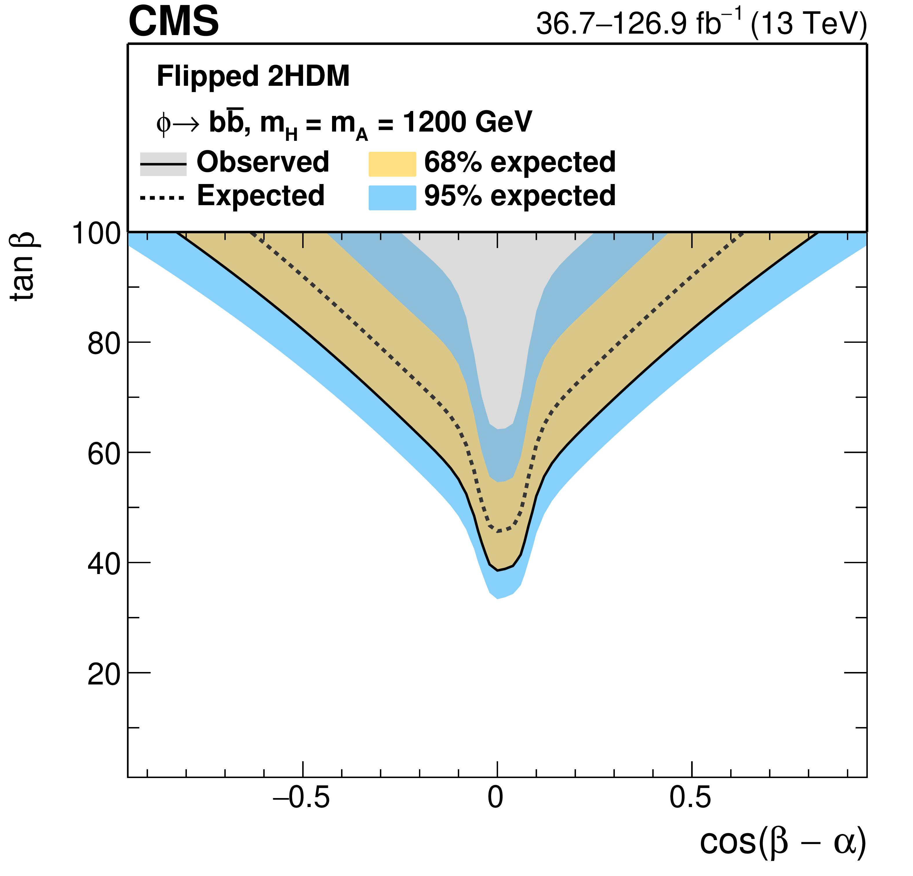
png pdf |
Figure 20-d:
Interpretation in the 2HDM flipped scenario: observed and expected upper limits at 95% CL on the parameter $ \tan\beta $ as functions of $ \cos(\beta-\alpha) $ for masses of $ m_{\mathrm{A}} = m_{\mathrm{H}} = $ 140, 600, 900, and 1200 GeV. |
| Tables | |
png pdf |
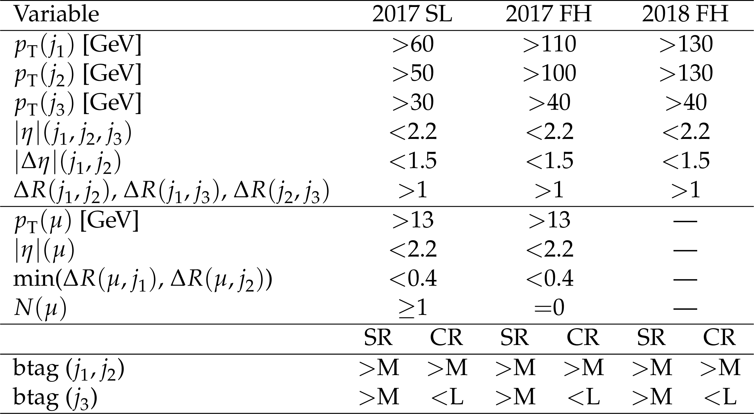
Table 1:
Summary of the main parameters of the offline selection for the three data sets 2017 SL, 2017 FH, and 2018 FH, where $ j_1 $, $ j_2 $, $ j_3 $ indicate the first three leading jets. Entries denoted by ``$ \text{---} $'' indicate that the selection is not applied. Signal region (SR) and control region (CR) only differ in the b\ tag selection, shown in the bottom rows, where ``$ > $M'' (``$ < $L'') indicate that the respective jet should pass (fail) the requirement of the medium (loose) working point, respectively. |
png pdf |
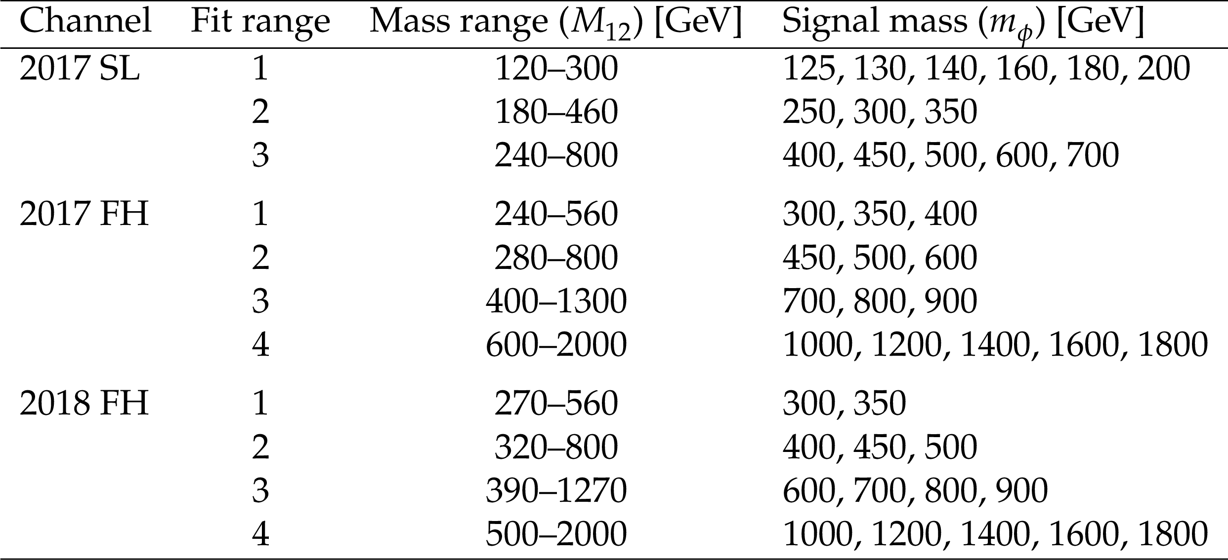
Table 2:
Definition of fit ranges for the 2017 SL, 2017 FH, and 2018 FH channels in terms of $ M_{12} $ and the associated values of the nominal Higgs boson mass, $ m_{\phi} $, which are probed in this fit range. |
| Summary |
| A search for beyond-the-standard-model neutral Higgs bosons, $ \phi $, produced in association with b quarks and decaying into a pair of b quarks is presented using a CMS data set of 13 TeV proton-proton collisions, based on an integrated luminosity of 36.7-126.9 fb$ ^{-1} $. The multi b quark final state is selected with requirements targeting both fully hadronic and semileptonic b quark decays, allowing for a sensitivity in the mass range extending from 125 to 1800 GeV. No significant excess of events above the expected SM background is observed. Exclusion limits at 95% confidence level on the production cross section times branching fraction are obtained. The results are also interpreted as constraints in the parameter space of MSSM and 2HDM scenarios to which this search is sensitive. These results represent the most stringent limits to date in the high-mass regime with this final state. |
| Additional Figures | |
png pdf |
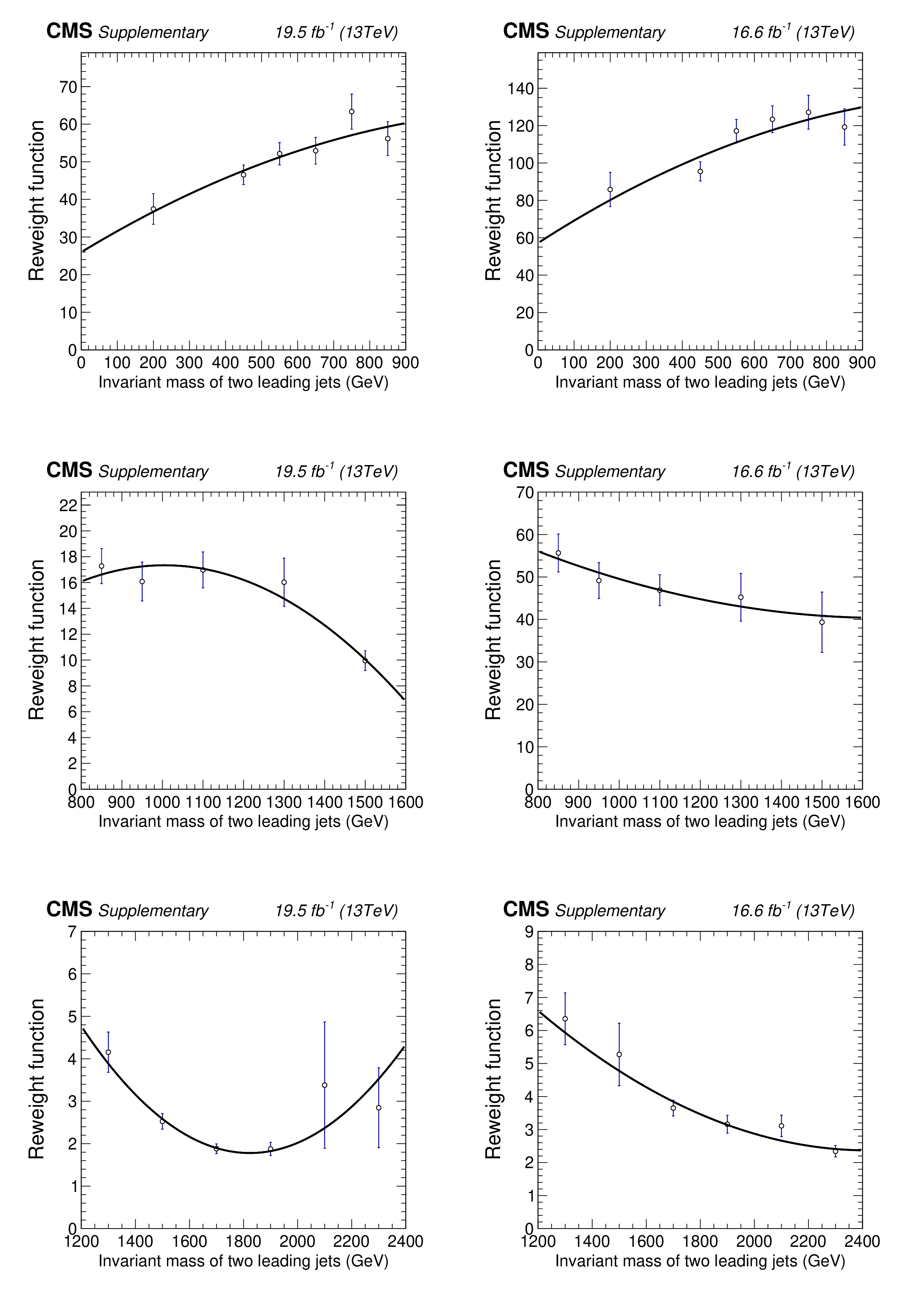
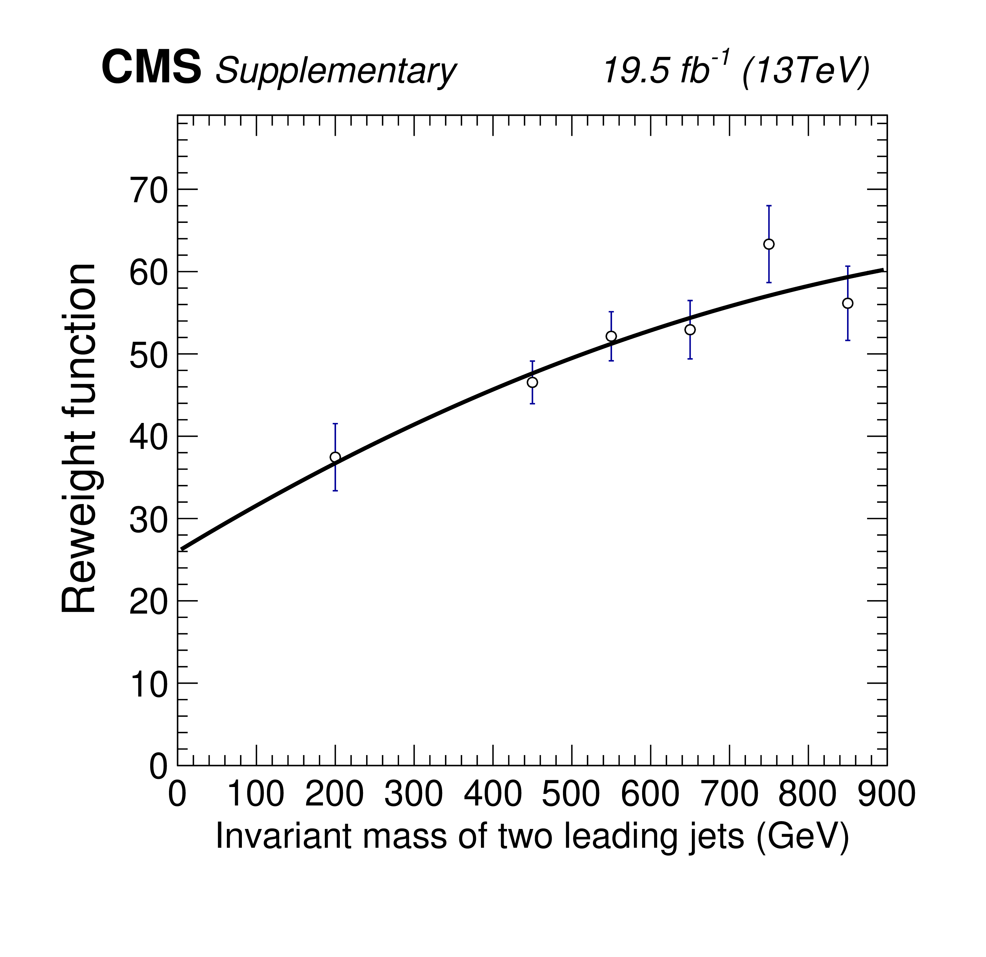
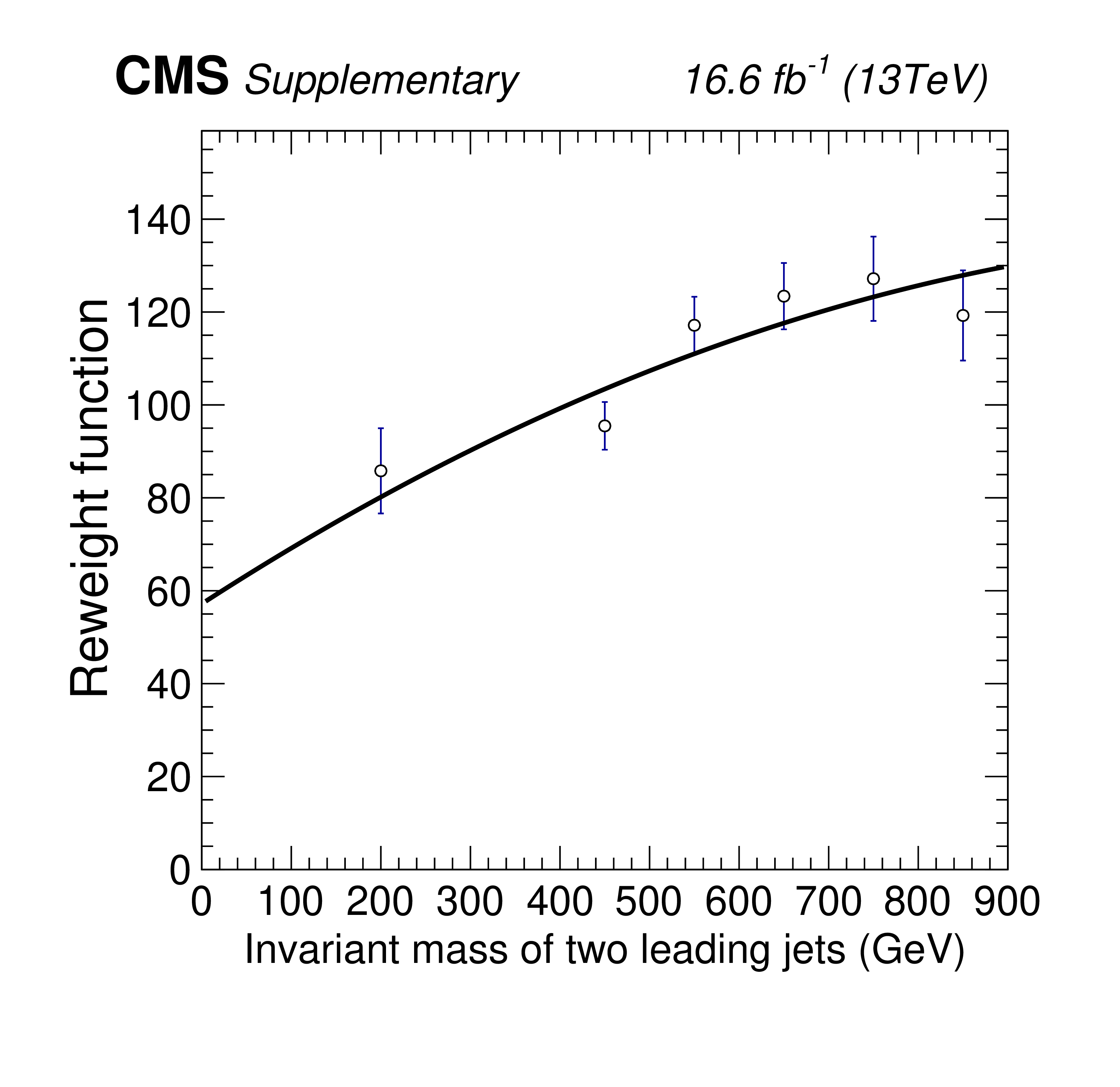
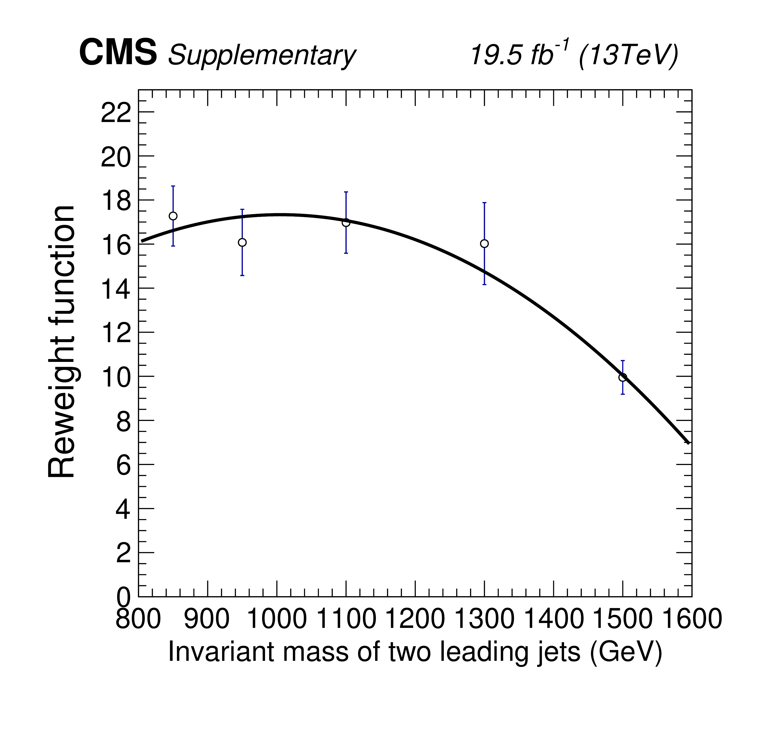
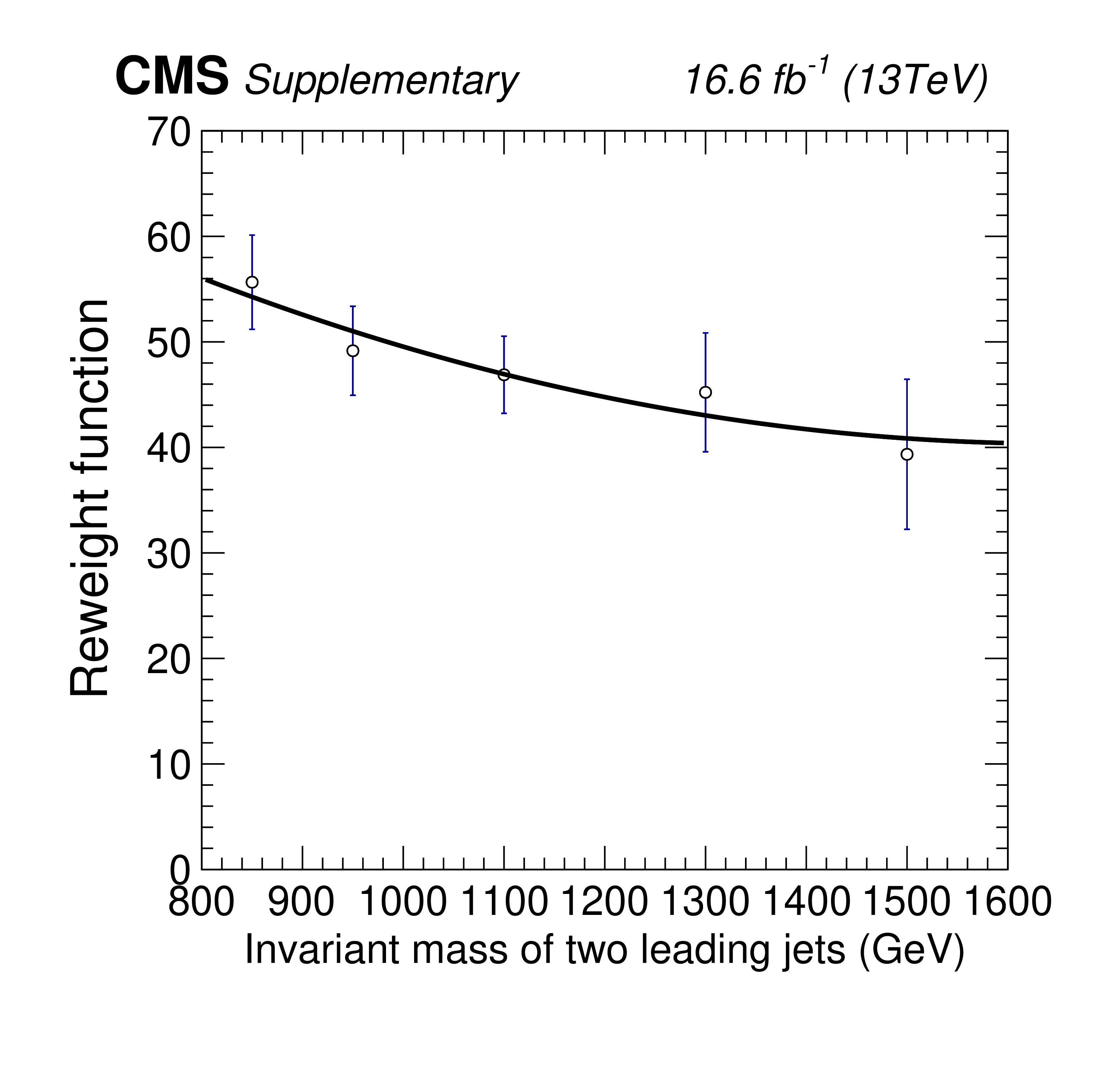
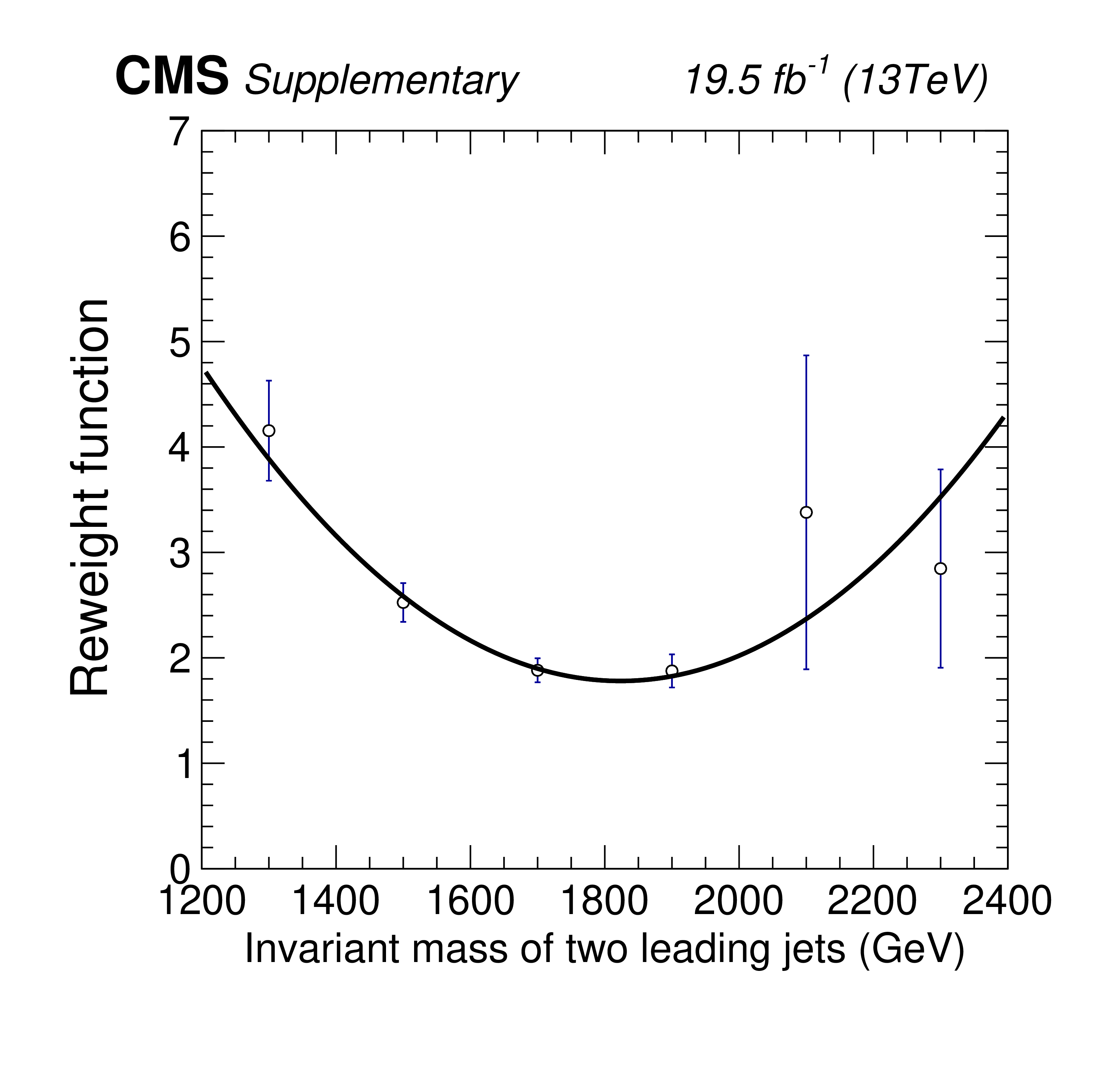
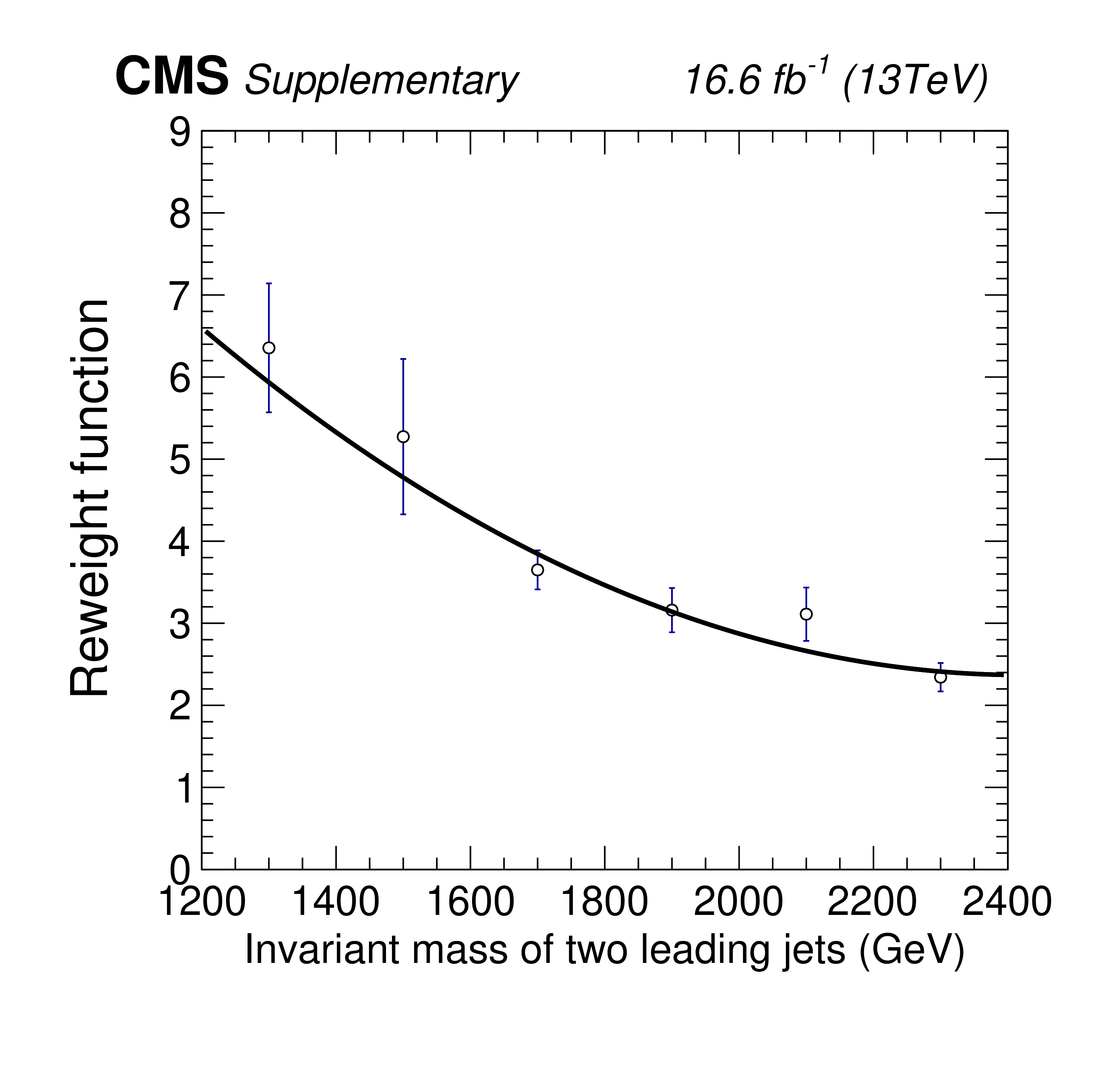
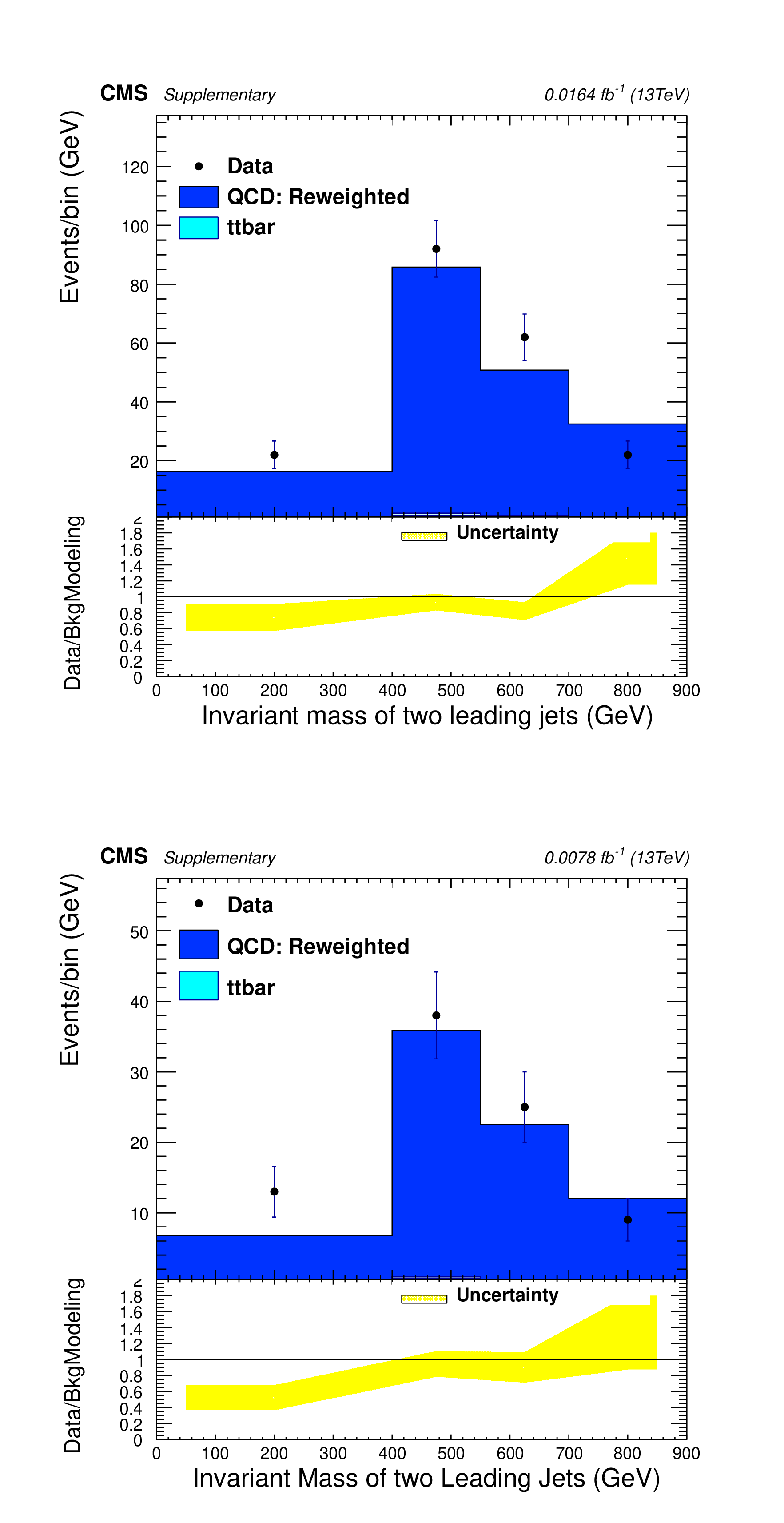
Additional Figure 1:
In the context of a parallel analysis, weights are applied to the data in a control region to estimate the QCD multijet background in the signal region. The weights are derived from simulated samples, separately for data taken in the first (left) or second (right) half of the 2016 data taking, in events with a low (top) or high (right) invariant mass of the two leading jets. The signal region contains events passing a trigger requiring two b tagged jets with $ p_T $ above 160 GeV and including offline at least 3 b tagged jets. The control region is composed of events passing rescaled triggers with lower thresholds, with 2 b-tagged jets and a third jet failing the b-tagging criteria. |
png pdf |
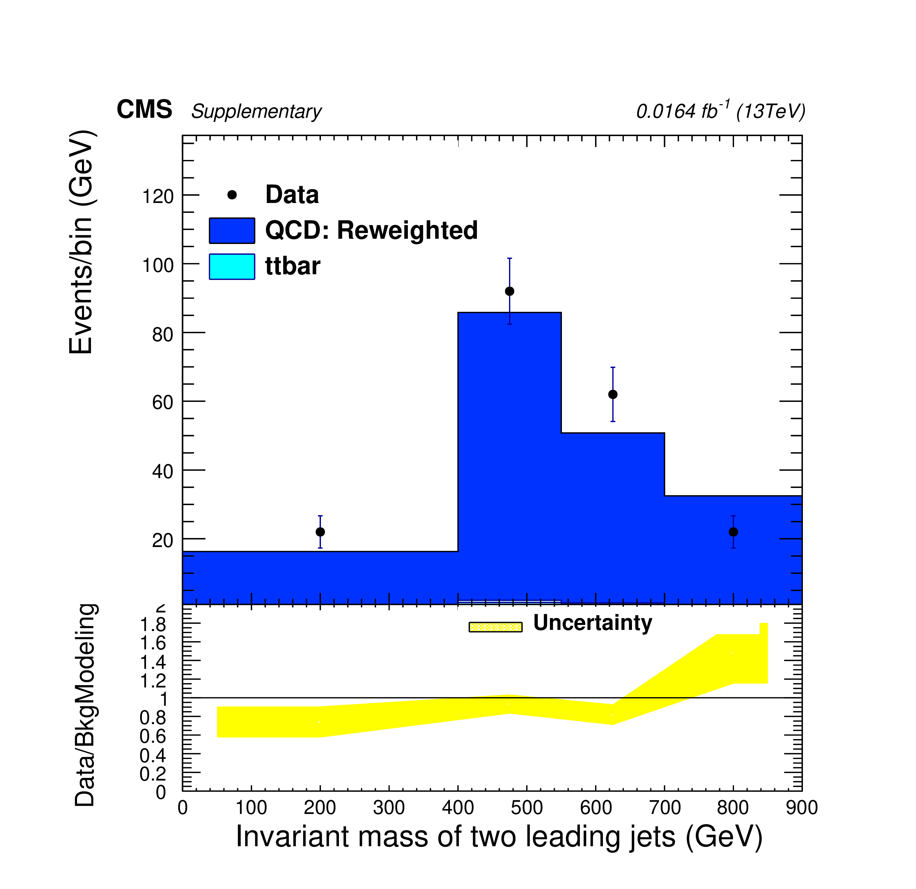
Additional Figure 1-a:
In the context of a parallel analysis, weights are applied to the data in a control region to estimate the QCD multijet background in the signal region. The weights are derived from simulated samples, separately for data taken in the first (left) or second (right) half of the 2016 data taking, in events with a low (top) or high (right) invariant mass of the two leading jets. The signal region contains events passing a trigger requiring two b tagged jets with $ p_T $ above 160 GeV and including offline at least 3 b tagged jets. The control region is composed of events passing rescaled triggers with lower thresholds, with 2 b-tagged jets and a third jet failing the b-tagging criteria. |
png pdf |
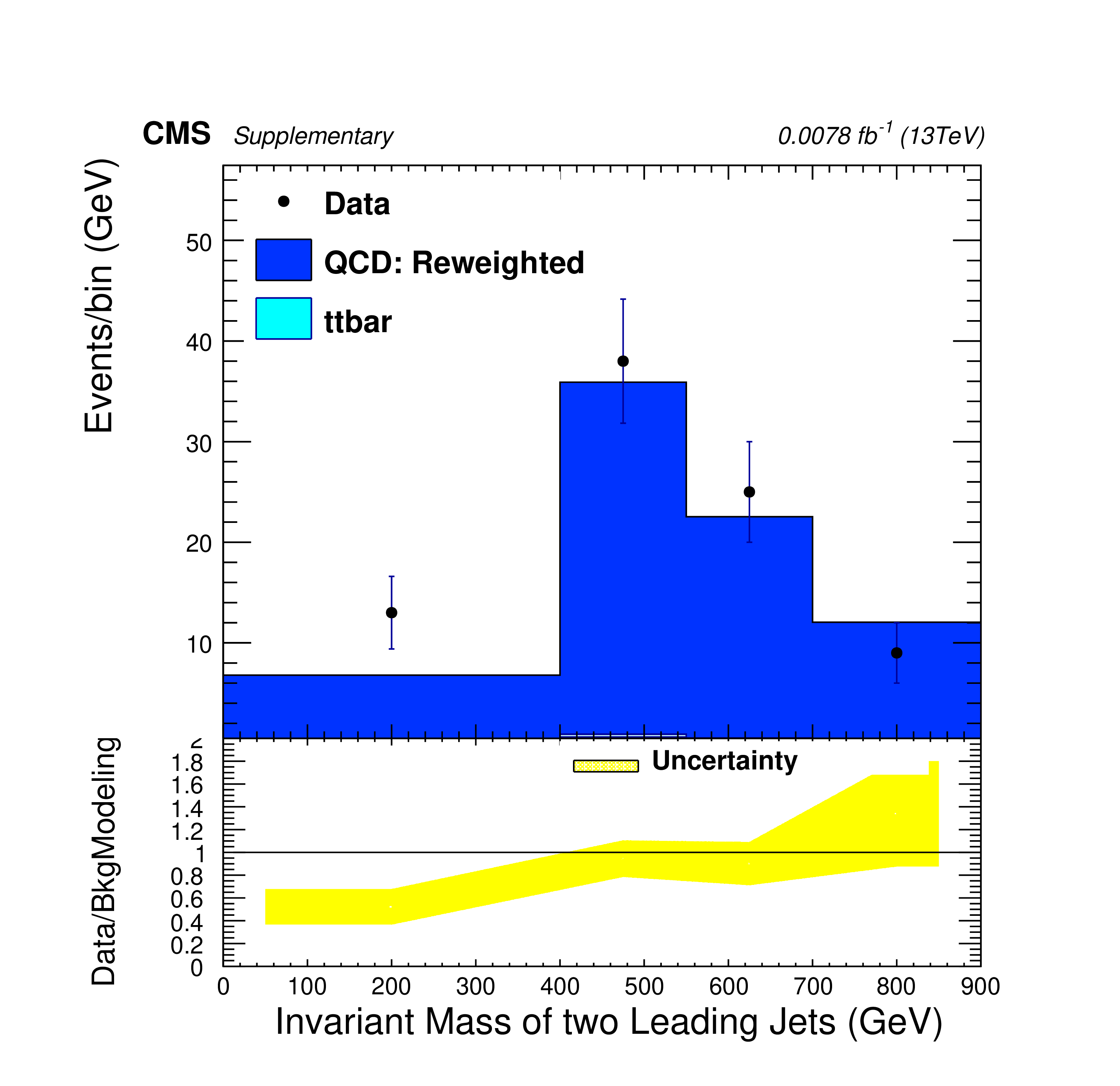
Additional Figure 1-b:
In the context of a parallel analysis, weights are applied to the data in a control region to estimate the QCD multijet background in the signal region. The weights are derived from simulated samples, separately for data taken in the first (left) or second (right) half of the 2016 data taking, in events with a low (top) or high (right) invariant mass of the two leading jets. The signal region contains events passing a trigger requiring two b tagged jets with $ p_T $ above 160 GeV and including offline at least 3 b tagged jets. The control region is composed of events passing rescaled triggers with lower thresholds, with 2 b-tagged jets and a third jet failing the b-tagging criteria. |
png pdf |
Additional Figure 1-c:
In the context of a parallel analysis, weights are applied to the data in a control region to estimate the QCD multijet background in the signal region. The weights are derived from simulated samples, separately for data taken in the first (left) or second (right) half of the 2016 data taking, in events with a low (top) or high (right) invariant mass of the two leading jets. The signal region contains events passing a trigger requiring two b tagged jets with $ p_T $ above 160 GeV and including offline at least 3 b tagged jets. The control region is composed of events passing rescaled triggers with lower thresholds, with 2 b-tagged jets and a third jet failing the b-tagging criteria. |
png pdf |
Additional Figure 1-d:
In the context of a parallel analysis, weights are applied to the data in a control region to estimate the QCD multijet background in the signal region. The weights are derived from simulated samples, separately for data taken in the first (left) or second (right) half of the 2016 data taking, in events with a low (top) or high (right) invariant mass of the two leading jets. The signal region contains events passing a trigger requiring two b tagged jets with $ p_T $ above 160 GeV and including offline at least 3 b tagged jets. The control region is composed of events passing rescaled triggers with lower thresholds, with 2 b-tagged jets and a third jet failing the b-tagging criteria. |
png pdf |
Additional Figure 1-e:
In the context of a parallel analysis, weights are applied to the data in a control region to estimate the QCD multijet background in the signal region. The weights are derived from simulated samples, separately for data taken in the first (left) or second (right) half of the 2016 data taking, in events with a low (top) or high (right) invariant mass of the two leading jets. The signal region contains events passing a trigger requiring two b tagged jets with $ p_T $ above 160 GeV and including offline at least 3 b tagged jets. The control region is composed of events passing rescaled triggers with lower thresholds, with 2 b-tagged jets and a third jet failing the b-tagging criteria. |
png pdf |
Additional Figure 1-f:
In the context of a parallel analysis, weights are applied to the data in a control region to estimate the QCD multijet background in the signal region. The weights are derived from simulated samples, separately for data taken in the first (left) or second (right) half of the 2016 data taking, in events with a low (top) or high (right) invariant mass of the two leading jets. The signal region contains events passing a trigger requiring two b tagged jets with $ p_T $ above 160 GeV and including offline at least 3 b tagged jets. The control region is composed of events passing rescaled triggers with lower thresholds, with 2 b-tagged jets and a third jet failing the b-tagging criteria. |
png pdf |
Additional Figure 2:
In the context of the parallel analysis, the QCD multijet background estimated was validated in a region, containing events selected with a trigger requiring a jet with $ p_T $ above 140 GeV and including offline three b-tagged jets. The QCD multijet prediction is compared to the observed data collected in the first (upper) or second (lower) half of 2016. |
png pdf |
Additional Figure 2-a:
In the context of the parallel analysis, the QCD multijet background estimated was validated in a region, containing events selected with a trigger requiring a jet with $ p_T $ above 140 GeV and including offline three b-tagged jets. The QCD multijet prediction is compared to the observed data collected in the first (upper) or second (lower) half of 2016. |
png pdf |
Additional Figure 2-b:
In the context of the parallel analysis, the QCD multijet background estimated was validated in a region, containing events selected with a trigger requiring a jet with $ p_T $ above 140 GeV and including offline three b-tagged jets. The QCD multijet prediction is compared to the observed data collected in the first (upper) or second (lower) half of 2016. |
png pdf |
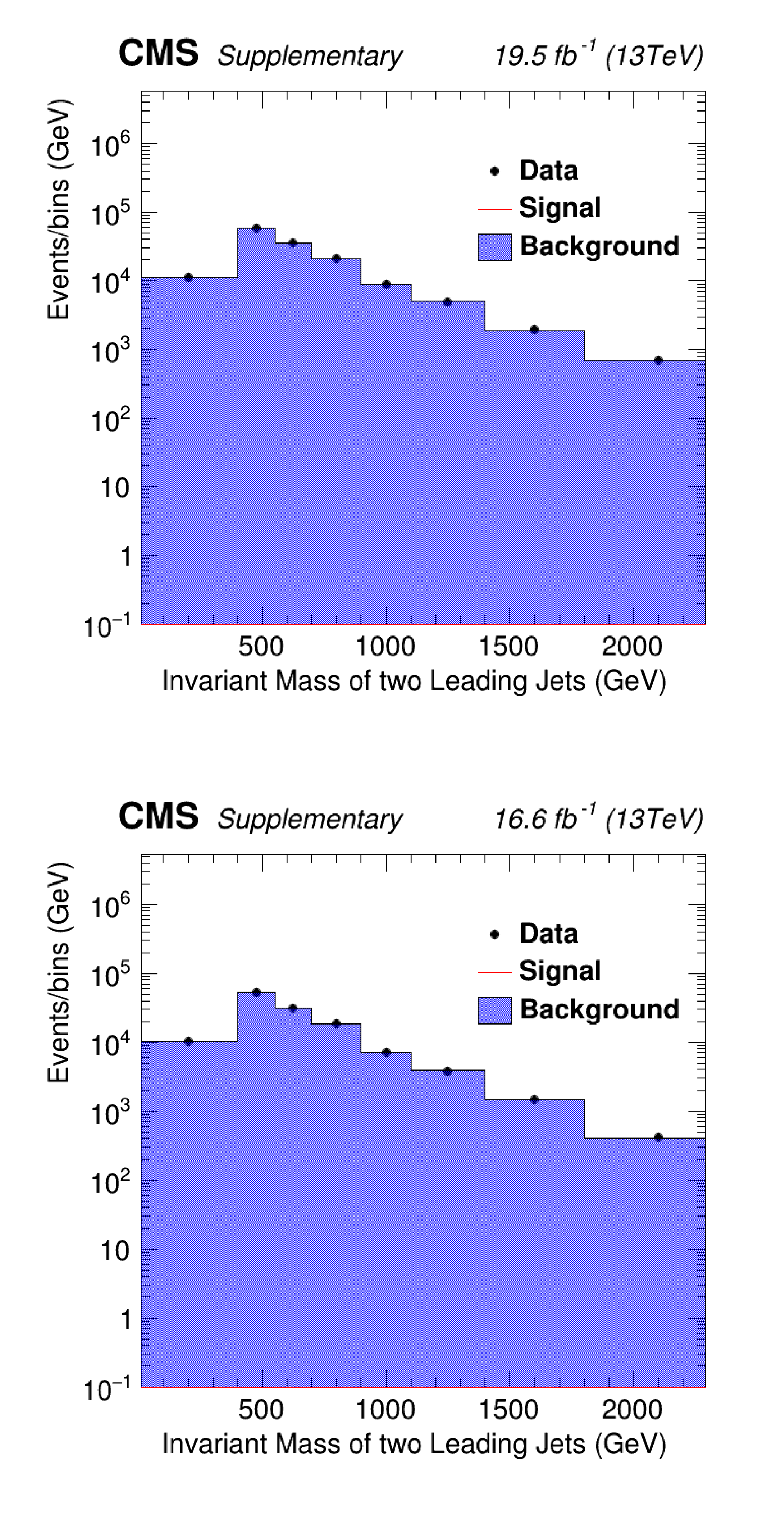
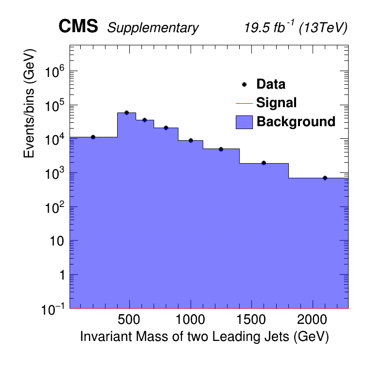
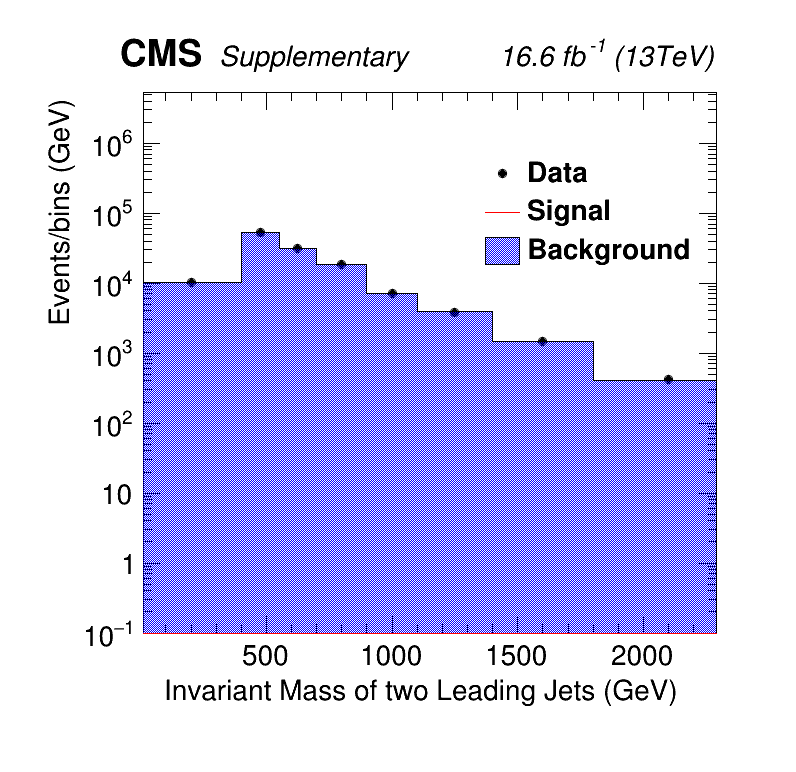
Additional Figure 3:
Observed and predicted distributions of the invariant mass of the two leading jets in the parallel analysis of data collected in the first (upper) or second (lower) half of 2016. The predicted distribution is the result of a maximum likelihood fit performed for a signal with $ m_A = $ 1 TeV. |
png |
Additional Figure 3-a:
Observed and predicted distributions of the invariant mass of the two leading jets in the parallel analysis of data collected in the first (upper) or second (lower) half of 2016. The predicted distribution is the result of a maximum likelihood fit performed for a signal with $ m_A = $ 1 TeV. |
png |
Additional Figure 3-b:
Observed and predicted distributions of the invariant mass of the two leading jets in the parallel analysis of data collected in the first (upper) or second (lower) half of 2016. The predicted distribution is the result of a maximum likelihood fit performed for a signal with $ m_A = $ 1 TeV. |
png pdf |
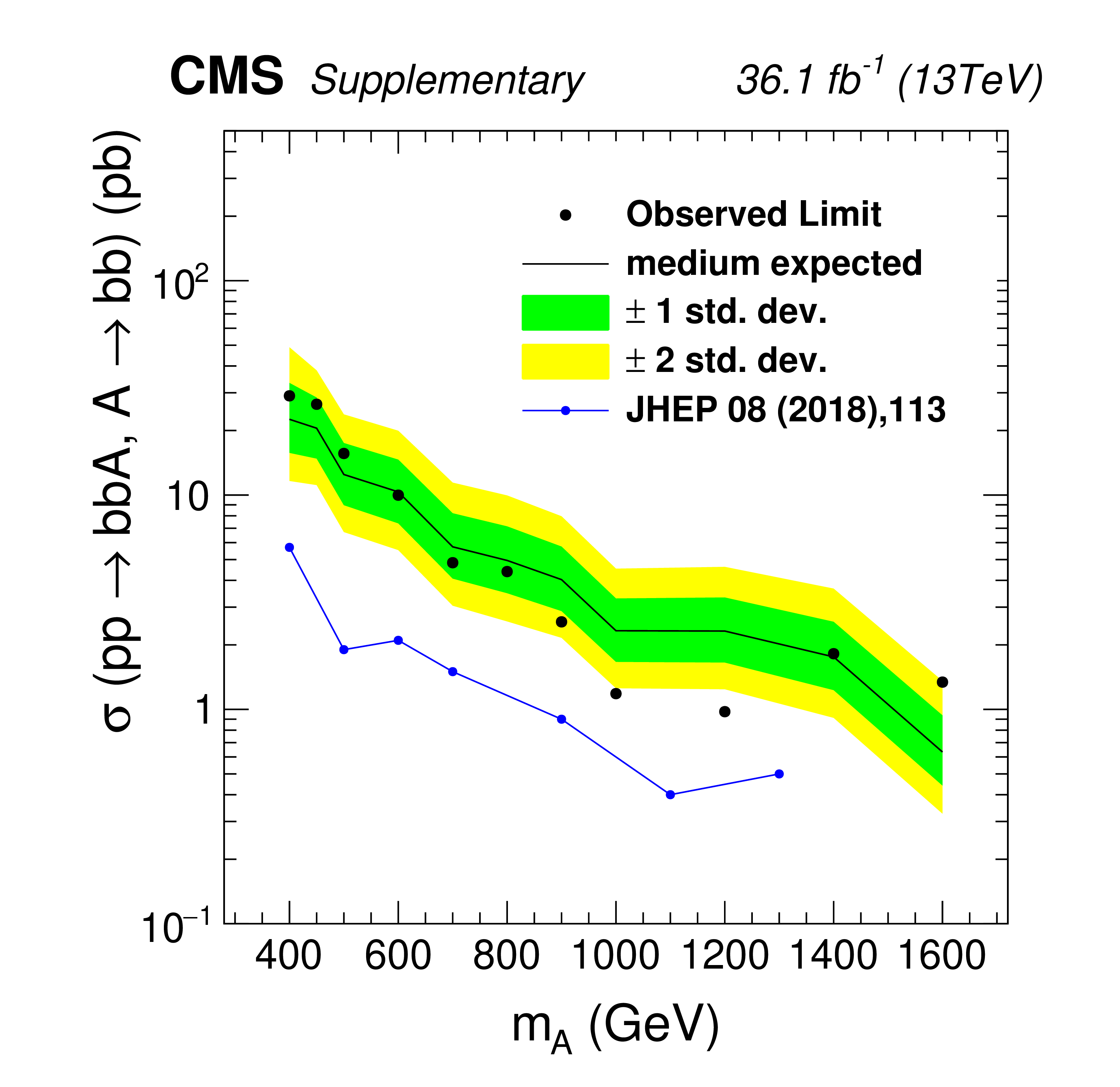
Additional Figure 4:
Expected and observed upper limits for the Higgs b-associated production cross-section times branching fraction of the decay into a b-quark pair at 95% CL, obtained with 2016 data in the context of the parallel analysis. The corresponding observed limit obtained by the nominal analysis using the same data set is shown in blue. |
| References | ||||
| 1 | ATLAS Collaboration | Observation of a new particle in the search for the standard model Higgs boson with the ATLAS detector at the LHC | PLB 716 (2012) 1 | 1207.7214 |
| 2 | CMS Collaboration | Observation of a new boson at a mass of 125 GeV with the CMS experiment at the LHC | PLB 716 (2012) 30 | CMS-HIG-12-028 1207.7235 |
| 3 | CMS Collaboration | Observation of a new boson with mass near 125 GeV in pp collisions at $ \sqrt{s} $ = 7 and 8 TeV | JHEP 06 (2013) 081 | CMS-HIG-12-036 1303.4571 |
| 4 | ATLAS Collaboration | A detailed map of Higgs boson interactions by the ATLAS experiment ten years after the discovery | Nature 607 (2022) 52 | 2207.00092 |
| 5 | CMS Collaboration | A portrait of the Higgs boson by the CMS experiment ten years after the discovery | Nature 607 (2022) 60 | CMS-HIG-22-001 2207.00043 |
| 6 | CMS Collaboration | Search for bottom quark associated production of the standard model Higgs boson in final states with leptons in proton-proton collisions at $ \sqrt{s} = $ 13 TeV | PLB 860 (2025) 139173 | CMS-HIG-23-003 2408.01344 |
| 7 | CMS Collaboration | Evidence for Higgs boson decay to a pair of muons | JHEP 01 (2021) 148 | CMS-HIG-19-006 2009.04363 |
| 8 | ATLAS Collaboration | Direct constraint on the Higgs-charm coupling from a search for Higgs boson decays into charm quarks with the ATLAS detector | EPJC 82 (2022) 717 | 2201.11428 |
| 9 | CMS Collaboration | Search for Higgs boson decay to a charm quark-antiquark pair in proton-proton collisions at $ \sqrt{s} = $ 13 TeV | PRL 131 (2023) 061801 | CMS-HIG-21-008 2205.05550 |
| 10 | ATLAS Collaboration | Combined measurements of Higgs boson production and decay using up to 80 fb$ ^{-1} $ of proton-proton collision data at $ \sqrt{s}= $ 13 TeV collected with the ATLAS experiment | PRD 101 (2020) 012002 | 1909.02845 |
| 11 | CMS Collaboration | Combined measurements of Higgs boson couplings in proton-proton collisions at $ \sqrt{s}= $ 13 TeV | EPJC 79 (2019) 421 | CMS-HIG-17-031 1809.10733 |
| 12 | J. Steggemann | Extended scalar sectors | Ann. Rev. Nucl. Part. Sci. 70 (2020) 197 | |
| 13 | G. C. Branco et al. | Theory and phenomenology of two-higgs-doublet models | Phys. Rep. 516 (2012) 1 | 1106.0034 |
| 14 | H. P. Nilles | Supersymmetry, supergravity and particle physics | Phys. Rep. 110 (1984) 1 | |
| 15 | P. Drechsel, G. Moortgat-Pick, and G. Weiglein | Prospects for direct searches for light Higgs bosons at the ILC with 250 GeV | EPJC 80 (2020) 922 | 1801.09662 |
| 16 | M. Carena et al. | MSSM Higgs boson searches at the LHC: benchmark scenarios after the discovery of a Higgs-like particle | EPJC 73 (2013) 2552 | 1302.7033 |
| 17 | M. S. Carena, S. Heinemeyer, C. E. M. Wagner, and G. Weiglein | MSSM Higgs boson searches at the Tevatron and the LHC: Impact of different benchmark scenarios | EPJC 45 (2006) 797 | hep-ph/0511023 |
| 18 | E. Bagnaschi et al. | MSSM Higgs boson searches at the LHC: benchmark scenarios for Run 2 and beyond | EPJC 79 (2019) 617 | 1808.07542 |
| 19 | H. Bahl et al. | HL-LHC and ILC sensitivities in the hunt for heavy Higgs bosons | EPJC 80 (2020) 916 | 2005.14536 |
| 20 | L. Maiani, A. D. Polosa, and V. Riquer | Bounds to the Higgs sector masses in minimal supersymmetry from LHC data | PLB 724 (2013) 274 | 1305.2172 |
| 21 | A. Djouadi et al. | The post-Higgs MSSM scenario: Habemus MSSM? | EPJC 73 (2013) 2650 | 1307.5205 |
| 22 | A. Djouadi et al. | Fully covering the MSSM Higgs sector at the LHC | JHEP 06 (2015) 168 | 1502.05653 |
| 23 | H. E. Haber and O. Stral | New LHC benchmarks for the $ \mathcal{CP} $ -conserving two-higgs-doublet model | EPJC 75 (2015) 491 | 1507.04281 |
| 24 | LHC Higgs Cross Section Working Group | Handbook of LHC Higgs cross sections: 3. Higgs properties | CERN, 2013 link |
1307.1347 |
| 25 | ALEPH, DELPHI, L3, and OPAL Collaborations, LEP Working Group for Higgs Boson Searches | Search for neutral MSSM Higgs bosons at LEP | EPJC 47 (2006) 547 | hep-ex/0602042 |
| 26 | CDF and D0 Collaborations | Search for neutral Higgs bosons in events with multiple bottom quarks at the Tevatron | PRD 86 (2012) 091101 | 1207.2757 |
| 27 | CMS Collaboration | Search for a Higgs boson decaying into a b-quark pair and produced in association with b quarks in proton-proton collisions at 7 TeV | PLB 722 (2013) 207 | CMS-HIG-12-033 1302.2892 |
| 28 | CMS Collaboration | Search for neutral MSSM Higgs bosons decaying into a pair of bottom quarks | JHEP 11 (2015) 071 | CMS-HIG-14-017 1506.08329 |
| 29 | ATLAS Collaboration | Search for heavy neutral Higgs bosons produced in association with b-quarks and decaying into b-quarks at $ \sqrt{s}= $ 13 TeV with the ATLAS detector | PRD 102 (2020) 032004 | 1907.02749 |
| 30 | CMS Collaboration | Search for beyond the standard model Higgs bosons decaying into a $ \mathrm{b\overline{b}} $ pair in pp collisions at $ \sqrt{s} = $ 13 TeV | JHEP 08 (2018) 113 | CMS-HIG-16-018 1805.12191 |
| 31 | E. Bols et al. | Jet flavour classification using DeepJet | JINST 15 (2020) P12012 | 2008.10519 |
| 32 | CMS Tracker Group Collaboration | The CMS phase-1 pixel detector upgrade | JINST 16 (2021) P02027 | 2012.14304 |
| 33 | CMS Collaboration | HEPData record for this analysis | link | |
| 34 | CMS Collaboration | The CMS experiment at the CERN LHC | JINST 3 (2008) S08004 | |
| 35 | CMS Collaboration | Development of the CMS detector for the CERN LHC Run 3 | JINST 19 (2024) P05064 | CMS-PRF-21-001 2309.05466 |
| 36 | CMS Collaboration | Performance of the CMS level-1 trigger in proton-proton collisions at $ \sqrt{s} = $ 13 TeV | JINST 15 (2020) P10017 | CMS-TRG-17-001 2006.10165 |
| 37 | CMS Collaboration | The CMS trigger system | JINST 12 (2017) P01020 | CMS-TRG-12-001 1609.02366 |
| 38 | CMS Collaboration | Performance of the CMS high-level trigger during LHC Run 2 | JINST 19 (2024) P11021 | CMS-TRG-19-001 2410.17038 |
| 39 | CMS Collaboration | Particle-flow reconstruction and global event description with the CMS detector | JINST 12 (2017) P10003 | CMS-PRF-14-001 1706.04965 |
| 40 | CMS Collaboration | Technical proposal for the phase-II upgrade of the Compact Muon Solenoid | CMS Technical Proposal CERN-LHCC-2015-010, CMS-TDR-15-02, 2015 CDS |
|
| 41 | M. Cacciari, G. P. Salam, and G. Soyez | The anti-$ k_{\mathrm{T}} $ jet clustering algorithm | JHEP 04 (2008) 063 | 0802.1189 |
| 42 | M. Cacciari, G. P. Salam, and G. Soyez | Fastjet user manual | EPJC 72 (2012) 1896 | 1111.6097 |
| 43 | CMS Collaboration | Jet energy scale and resolution in the CMS experiment in pp collisions at 8 TeV | JINST 12 (2017) P02014 | CMS-JME-13-004 1607.03663 |
| 44 | CMS Collaboration | Pileup mitigation at CMS in 13 TeV data | JINST 15 (2020) P09018 | CMS-JME-18-001 2003.00503 |
| 45 | CMS Collaboration | Identification of heavy-flavour jets with the CMS detector in pp collisions at 13 TeV | JINST 13 (2018) P05011 | CMS-BTV-16-002 1712.07158 |
| 46 | CMS Collaboration | Performance of the DeepJet b tagging algorithm using 41.9 fb$ ^{-1} $ of data from proton-proton collisions at 13 TeV with phase 1 CMS detector | CMS Detector Performance Note CMS-DP-2018-058, 2018 CDS |
|
| 47 | CMS Collaboration | B-tagging performance of the CMS legacy dataset 2018 | CMS Detector Performance Note CMS-DP-2021-004, 2021 CDS |
|
| 48 | CMS Collaboration | Performance of the CMS muon detector and muon reconstruction with proton-proton collisions at $ \sqrt{s}= $ 13 TeV | JINST 13 (2018) P06015 | CMS-MUO-16-001 1804.04528 |
| 49 | CMS Collaboration | Performance of missing transverse momentum reconstruction in proton-proton collisions at $ \sqrt{s} = $ 13 TeV using the CMS detector | JINST 14 (2019) P07004 | CMS-JME-17-001 1903.06078 |
| 50 | P. Nason | A new method for combining NLO QCD with shower Monte Carlo algorithms | JHEP 11 (2004) 040 | hep-ph/0409146 |
| 51 | S. Frixione, P. Nason, and C. Oleari | Matching NLO QCD computations with parton shower simulations: the POWHEG method | JHEP 11 (2007) 070 | 0709.2092 |
| 52 | S. Alioli, P. Nason, C. Oleari, and E. Re | A general framework for implementing NLO calculations in shower Monte Carlo programs: the POWHEG BOX | JHEP 06 (2010) 043 | 1002.2581 |
| 53 | B. Jager, L. Reina, and D. Wackeroth | Higgs boson production in association with b jets in the POWHEG BOX | PRD 93 (2016) 014030 | 1509.05843 |
| 54 | F. Maltoni, G. Ridolfi, and M. Ubiali | b-initiated processes at the LHC: a reappraisal | JHEP 07 (2012) 022 | 1203.6393 |
| 55 | J. Alwall et al. | MadGraph 5: Going beyond | JHEP 06 (2011) 128 | 1106.0522 |
| 56 | J. Alwall et al. | The automated computation of tree-level and next-to-leading order differential cross sections, and their matching to parton shower simulations | JHEP 07 (2014) 079 | 1405.0301 |
| 57 | S. Frixione and B. R. Webber | Matching NLO QCD computations and parton shower simulations | JHEP 06 (2002) 029 | hep-ph/0204244 |
| 58 | J. Alwall et al. | Comparative study of various algorithms for the merging of parton showers and matrix elements in hadronic collisions | EPJC 53 (2008) 473 | 0706.2569 |
| 59 | J. Butterworth et al. | PDF4LHC recommendations for LHC Run II | JPG 43 (2016) 023001 | 1510.03865 |
| 60 | NNPDF Collaboration | Parton distributions from high-precision collider data | EPJC 77 (2017) 663 | 1706.00428 |
| 61 | CMS Collaboration | Extraction and validation of a new set of CMS PYTHIA8 tunes from underlying-event measurements | EPJC 80 (2020) 4 | CMS-GEN-17-001 1903.12179 |
| 62 | T. Sjöstrand et al. | An introduction to PYTHIA 8.2 | Comput. Phys. Commun. 191 (2015) 159 | 1410.3012 |
| 63 | GEANT4 Collaboration | GEANT 4---a simulation toolkit | NIM A 506 (2003) 250 | |
| 64 | CMS Collaboration | Measurement of inclusive W and Z boson production cross sections in pp collisions at $ \sqrt{s} = $ 8 TeV | PRL 112 (2014) 191802 | CMS-SMP-12-011 1402.0923 |
| 65 | CMS Collaboration | A deep neural network for simultaneous estimation of b jet energy and resolution | Comput. Softw. Big Sci. 4 (2020) 10 | CMS-HIG-18-027 1912.06046 |
| 66 | J. Gaiser et al. | Charmonium spectroscopy from inclusive $ \psi' $ and J/$ \psi $ radiative decays | PRD 34 (1986) 711 | |
| 67 | A. Vagnerini | Search for Higgs bosons in the final state with b-quarks in the semi-leptonic channel with the CMS 2017 data | PhD thesis, Hamburg U., Hamburg, 2020 link |
|
| 68 | P. Asmuss | Search for high-mass bosons of an extended Higgs sector in b quark final states using the 2017 data set of the CMS experiment | PhD thesis, Hamburg U., Hamburg, 2021 link |
|
| 69 | Belle Collaboration | A detailed test of the CsI(Tl) calorimeter for BELLE with photon beams of energy between 20 MeV and 5.4 GeV | NIM A 441 (2000) 401 | |
| 70 | P. D. Dauncey, M. Kenzie, N. Wardle, and G. J. Davies | Handling uncertainties in background shapes: the discrete profiling method | JINST 10 (2015) P04015 | 1408.6865 |
| 71 | CMS Collaboration | The CMS statistical analysis and combination tool: \textsccombine | Comp. Softw. Big Sci. 8 (2024) 19 | CMS-CAT-23-001 2404.06614 |
| 72 | CMS Collaboration | CMS luminosity measurement for the 2017 data-taking period at $ \sqrt{s} $ = 13 TeV | CMS Physics Analysis Summary, 2018 link |
CMS-PAS-LUM-17-004 |
| 73 | CMS Collaboration | CMS luminosity measurement for the 2018 data-taking period at $ \sqrt{s} $ = 13 TeV | CMS Physics Analysis Summary, 2019 link |
CMS-PAS-LUM-18-002 |
| 74 | CMS Collaboration | Measurement of the inelastic proton-proton cross section at $ \sqrt{s} = $ 13 TeV | JHEP 07 (2018) 161 | CMS-FSQ-15-005 1802.02613 |
| 75 | CMS Collaboration | Performance of the CMS electromagnetic calorimeter in pp collisions at $ \sqrt{s} = $ 13 TeV | JINST 19 (2024) P09004 | CMS-EGM-18-002 2403.15518 |
| 76 | LHC Higgs Cross Section Working Group Collaboration | Handbook of LHC Higgs cross sections: 4. Deciphering the nature of the Higgs sector | CERN Yellow Reports: Monographs 2, 2017 link |
1610.07922 |
| 77 | T. Junk | Confidence level computation for combining searches with small statistics | NIM A 434 (1999) 435 | hep-ex/9902006 |
| 78 | A. L. Read | Presentation of search results: The $ CL_s $ technique | JPG 28 (2002) 2693 | |
| 79 | G. Cowan, K. Cranmer, E. Gross, and O. Vitells | Asymptotic formulae for likelihood-based tests of new physics | EPJC 71 (2011) 1554 | 1007.1727 |
| 80 | E. Gross and O. Vitells | Trial factors for the look elsewhere effect in high energy physics | EPJC 70 (2010) 525 | 1005.1891 |
| 81 | S. Dawson, C. B. Jackson, L. Reina, and D. Wackeroth | Exclusive Higgs boson production with bottom quarks at hadron colliders | PRD 69 (2004) 074027 | hep-ph/0311067 |
| 82 | S. Dittmaier, M. Krämer, and M. Spira | Higgs radiation off bottom quarks at the Tevatron and the CERN LHC | PRD 70 (2004) 074010 | hep-ph/0309204 |
| 83 | R. V. Harlander and W. B. Kilgore | Higgs boson production in bottom quark fusion at next-to-next-to leading order | PRD 68 (2003) 013001 | hep-ph/0304035 |
| 84 | R. Harlander, M. Kramer, and M. Schumacher | Bottom-quark associated Higgs-boson production: reconciling the four- and five-flavour scheme approach | 1112.3478 | |
| 85 | S. Forte, D. Napoletano, and M. Ubiali | Higgs production in bottom-quark fusion in a matched scheme | PLB 751 (2015) 331 | 1508.01529 |
| 86 | S. Forte, D. Napoletano, and M. Ubiali | Higgs production in bottom-quark fusion: matching beyond leading order | PLB 763 (2016) 190 | 1607.00389 |
| 87 | G. Degrassi et al. | Towards high precision predictions for the MSSM Higgs sector | EPJC 28 (2003) 133 | hep-ph/0212020 |
| 88 | S. Heinemeyer, W. Hollik, and G. Weiglein | FeynHiggs: A program for the calculation of the masses of the neutral CP even Higgs bosons in the MSSM | Comput. Phys. Commun. 124 (2000) 76 | hep-ph/9812320 |
| 89 | M. Frank et al. | The Higgs boson masses and mixings of the complex MSSM in the Feynman-diagrammatic approach | JHEP 02 (2007) 047 | hep-ph/0611326 |
| 90 | T. Hahn et al. | High-precision predictions for the light CP-even Higgs boson mass of the minimal supersymmetric standard model | PRL 112 (2014) 141801 | 1312.4937 |
| 91 | H. Bahl and W. Hollik | Precise prediction for the light MSSM Higgs boson mass combining effective field theory and fixed-order calculations | EPJC 76 (2016) 499 | 1608.01880 |
| 92 | H. Bahl, S. Heinemeyer, W. Hollik, and G. Weiglein | Reconciling EFT and hybrid calculations of the light MSSM Higgs-boson mass | EPJC 78 (2018) 57 | 1706.00346 |
| 93 | H. Bahl et al. | Precision calculations in the MSSM Higgs-boson sector with FeynHiggs 2.14 | Comput. Phys. Commun. 249 (2020) 107099 | 1811.09073 |
| 94 | A. Djouadi, J. Kalinowski, and M. Spira | HDECAY: A program for Higgs boson decays in the standard model and its supersymmetric extension | Comput. Phys. Commun. 108 (1998) 56 | hep-ph/9704448 |
| 95 | A. Djouadi, J. Kalinowski, M. Mühlleitner, and M. Spira | HDECAY: Twenty++ years after | Comput. Phys. Commun. 238 (2019) 214 | 1801.09506 |
| 96 | R. V. Harlander, S. Liebler, and H. Mantler | SusHi: A program for the calculation of Higgs production in gluon fusion and bottom-quark annihilation in the standard model and the MSSM | Comput. Phys. Commun. 184 (2013) 1605 | 1212.3249 |
| 97 | R. V. Harlander, S. Liebler, and H. Mantler | SusHi bento: Beyond NNLO and the heavy-top limit | Comput. Phys. Commun. 212 (2017) 239 | 1605.03190 |
| 98 | D. Eriksson, J. Rathsman, and O. Stral | 2HDMC: Two-Higgs-doublet model calculator physics and manual | Comput. Phys. Commun. 181 (2010) 189 | 0902.0851 |
| 99 | A. Buckley et al. | LHAPDF6: parton density access in the LHC precision era | EPJC 75 (2015) 132 | 1412.7420 |
|
|
Compact Muon Solenoid LHC, CERN |
|

|

|

|

|

|