

Compact Muon Solenoid
LHC, CERN
| CMS-SUS-23-003 ; CERN-EP-2025-154 | ||
| A general search for supersymmetric particles in scenarios with compressed mass spectra using proton-proton collisions at $ \sqrt{s}= $ 13 TeV | ||
| CMS Collaboration | ||
| 19 August 2025 | ||
| Phys. Rev. D 112 (2025) 11, 112023 | ||
| Abstract: A general search is presented for supersymmetric particles (sparticles) in scenarios featuring compressed mass spectra using proton-proton collisions at a center-of-mass energy of 13 TeV, recorded with the CMS detector at the LHC. The analyzed data sample corresponds to an integrated luminosity of 138 fb$ ^{-1} $. A wide range of potential sparticle signatures are targeted, including pair production of electroweakinos, sleptons, and top squarks. The search focuses on events with a high transverse momentum system from initial-state-radiation jets recoiling against a potential sparticle system with significant missing transverse momentum. Events are categorized based on their lepton multiplicity, jet multiplicity, number of b-tagged jets, and kinematic variables sensitive to the sparticle masses and mass splittings. The sensitivity extends to higher parent sparticle masses than previously probed at the LHC for production of pairs of electroweakinos, sleptons, and top squarks with mass spectra featuring small mass splittings (compressed mass spectra). The observed results demonstrate agreement with the predictions of the background-only model. Lower mass limits are set at 95% confidence level on production of pairs of electroweakinos, sleptons, and top squarks that extend to 325, 275, and 780 GeV, respectively, for the most favorable compressed mass regime cases. | ||
| Links: e-print arXiv:2508.13900 [hep-ex] (PDF) ; CDS record ; inSPIRE record ; HepData record ; CADI line (restricted) ; | ||
| Figures | |
png pdf |
Figure 1:
Diagrams for top squark pair production. The left panel shows the T2tt model with decay via top quarks and the right panel illustrates the four-body phase space used in modeling the most compressed region. |
png pdf |
Figure 1-a:
Diagrams for top squark pair production. The left panel shows the T2tt model with decay via top quarks and the right panel illustrates the four-body phase space used in modeling the most compressed region. |
png pdf |
Figure 1-b:
Diagrams for top squark pair production. The left panel shows the T2tt model with decay via top quarks and the right panel illustrates the four-body phase space used in modeling the most compressed region. |
png pdf |
Figure 2:
Diagrams for top squark pair production. The left panel shows the T2bW model with decay via an intermediate mass chargino and the right panel shows the T2cc model with decay via charm quarks. |
png pdf |
Figure 2-a:
Diagrams for top squark pair production. The left panel shows the T2bW model with decay via an intermediate mass chargino and the right panel shows the T2cc model with decay via charm quarks. |

png pdf |
Figure 2-b:
Diagrams for top squark pair production. The left panel shows the T2bW model with decay via an intermediate mass chargino and the right panel shows the T2cc model with decay via charm quarks. |
png pdf |
Figure 3:
Diagrams for electroweakino production. The left panel shows associated production of the lightest chargino and second-lightest neutralino ($ \tilde{\chi}_{1}^{\pm}\tilde{\chi}_{2}^{0} $) in the TChiWZ model and the right panel shows pair production of the lightest chargino ($ \tilde{\chi}_{1}^{+}\tilde{\chi}_{1}^{-} $) in the TChiWW model. |
png pdf |
Figure 3-a:
Diagrams for electroweakino production. The left panel shows associated production of the lightest chargino and second-lightest neutralino ($ \tilde{\chi}_{1}^{\pm}\tilde{\chi}_{2}^{0} $) in the TChiWZ model and the right panel shows pair production of the lightest chargino ($ \tilde{\chi}_{1}^{+}\tilde{\chi}_{1}^{-} $) in the TChiWW model. |
png pdf |
Figure 3-b:
Diagrams for electroweakino production. The left panel shows associated production of the lightest chargino and second-lightest neutralino ($ \tilde{\chi}_{1}^{\pm}\tilde{\chi}_{2}^{0} $) in the TChiWZ model and the right panel shows pair production of the lightest chargino ($ \tilde{\chi}_{1}^{+}\tilde{\chi}_{1}^{-} $) in the TChiWW model. |
png pdf |
Figure 4:
Diagrams for pair production of charged sleptons with subsequent decay to $ \ell^{\pm}\tilde{\chi}_{1}^{0} $ where $ \ell = \mathrm{e},\mu $. |
png pdf |
Figure 4-a:
Diagrams for pair production of charged sleptons with subsequent decay to $ \ell^{\pm}\tilde{\chi}_{1}^{0} $ where $ \ell = \mathrm{e},\mu $. |
png pdf |
Figure 4-b:
Diagrams for pair production of charged sleptons with subsequent decay to $ \ell^{\pm}\tilde{\chi}_{1}^{0} $ where $ \ell = \mathrm{e},\mu $. |
png pdf |
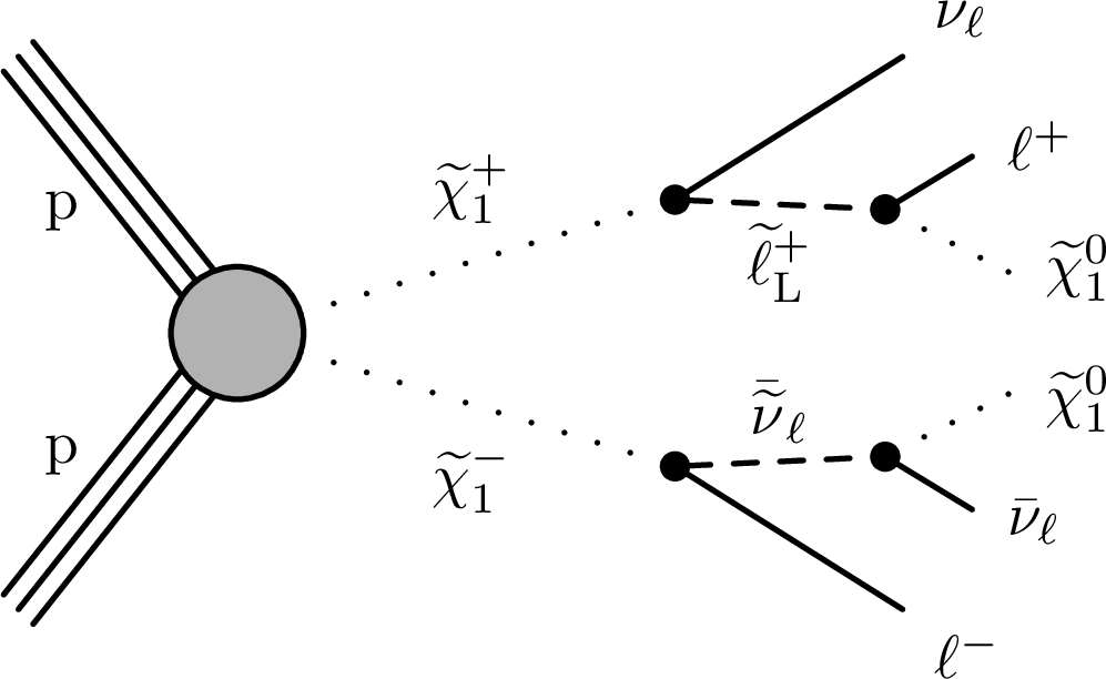
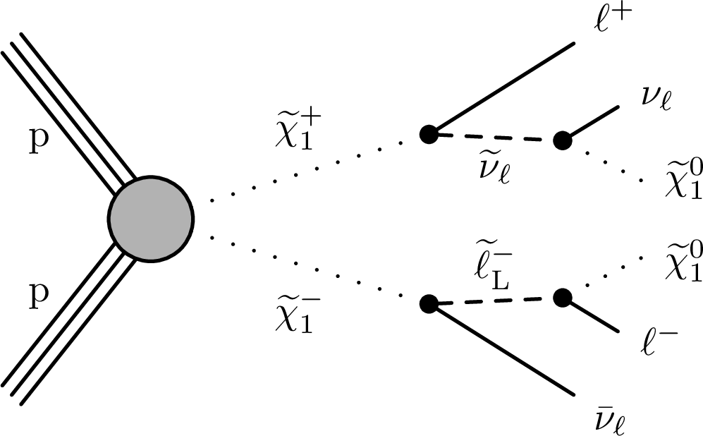
Figure 5:
Diagrams for pair production of the lightest chargino with subsequent leptonic decays via an intermediate mass charged slepton or sneutrino, where $ \ell = \mathrm{e},\mu,\tau $. In addition to the illustrated diagrams, the other two combinations where either both charginos decay to an intermediate charged slepton or both charginos decay to an intermediate sneutrino are also included in this TChiSlepSnu model. |
png pdf |
Figure 5-a:
Diagrams for pair production of the lightest chargino with subsequent leptonic decays via an intermediate mass charged slepton or sneutrino, where $ \ell = \mathrm{e},\mu,\tau $. In addition to the illustrated diagrams, the other two combinations where either both charginos decay to an intermediate charged slepton or both charginos decay to an intermediate sneutrino are also included in this TChiSlepSnu model. |
png pdf |
Figure 5-b:
Diagrams for pair production of the lightest chargino with subsequent leptonic decays via an intermediate mass charged slepton or sneutrino, where $ \ell = \mathrm{e},\mu,\tau $. In addition to the illustrated diagrams, the other two combinations where either both charginos decay to an intermediate charged slepton or both charginos decay to an intermediate sneutrino are also included in this TChiSlepSnu model. |
png pdf |
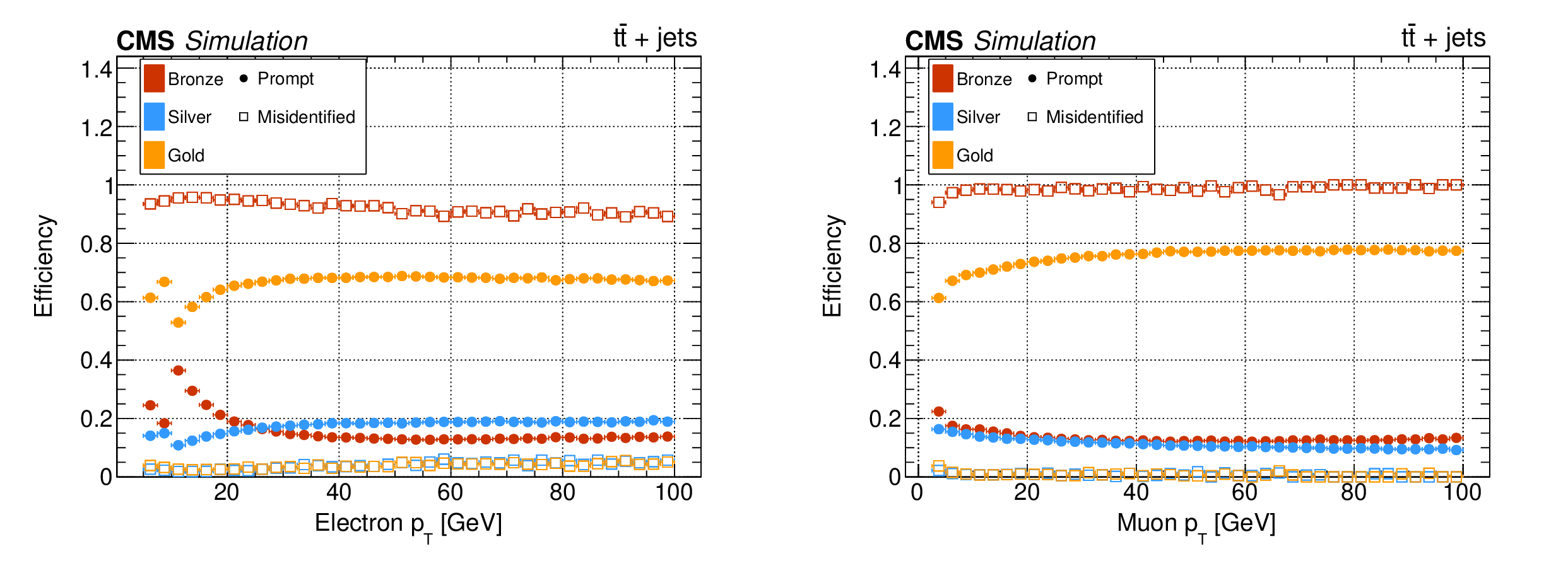
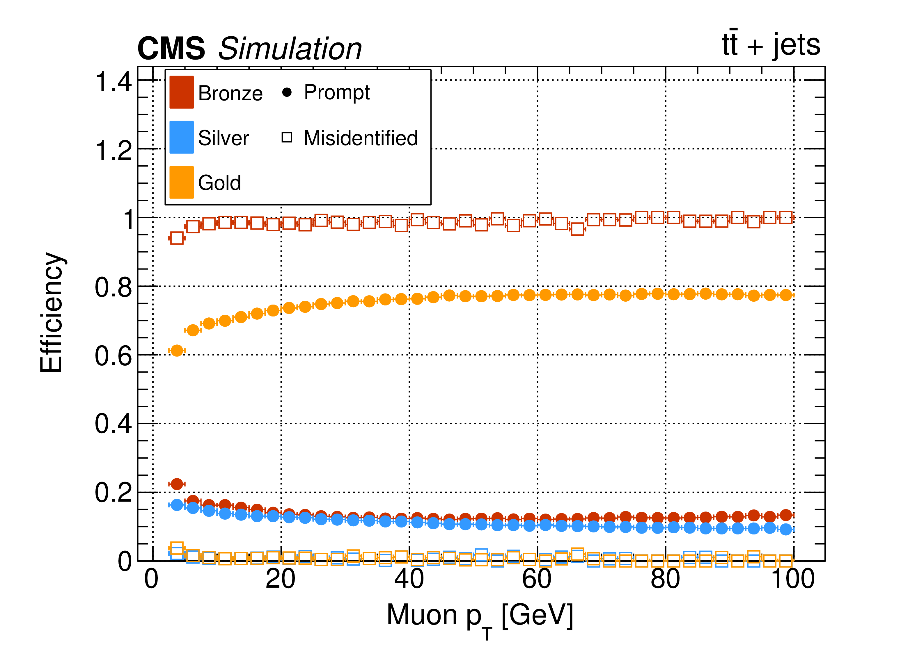
Figure 6:
Efficiencies of lepton candidates satisfying baseline requirements to be identified in the gold, silver, and bronze categories for prompt leptons (solid circles) and misidentified leptons (open squares), evaluated in simulated $ {\mathrm{t}\overline{\mathrm{t}}}+\text{jets} $ events. Electrons (muons) are shown in the left (right) panel. As the three categories are mutually exclusive and exhaustive for baseline leptons, these efficiencies sum to one for each source in each lepton $ p_{\mathrm{T}} $ bin. |
png pdf |
Figure 6-a:
Efficiencies of lepton candidates satisfying baseline requirements to be identified in the gold, silver, and bronze categories for prompt leptons (solid circles) and misidentified leptons (open squares), evaluated in simulated $ {\mathrm{t}\overline{\mathrm{t}}}+\text{jets} $ events. Electrons (muons) are shown in the left (right) panel. As the three categories are mutually exclusive and exhaustive for baseline leptons, these efficiencies sum to one for each source in each lepton $ p_{\mathrm{T}} $ bin. |
png pdf |
Figure 6-b:
Efficiencies of lepton candidates satisfying baseline requirements to be identified in the gold, silver, and bronze categories for prompt leptons (solid circles) and misidentified leptons (open squares), evaluated in simulated $ {\mathrm{t}\overline{\mathrm{t}}}+\text{jets} $ events. Electrons (muons) are shown in the left (right) panel. As the three categories are mutually exclusive and exhaustive for baseline leptons, these efficiencies sum to one for each source in each lepton $ p_{\mathrm{T}} $ bin. |
png pdf |
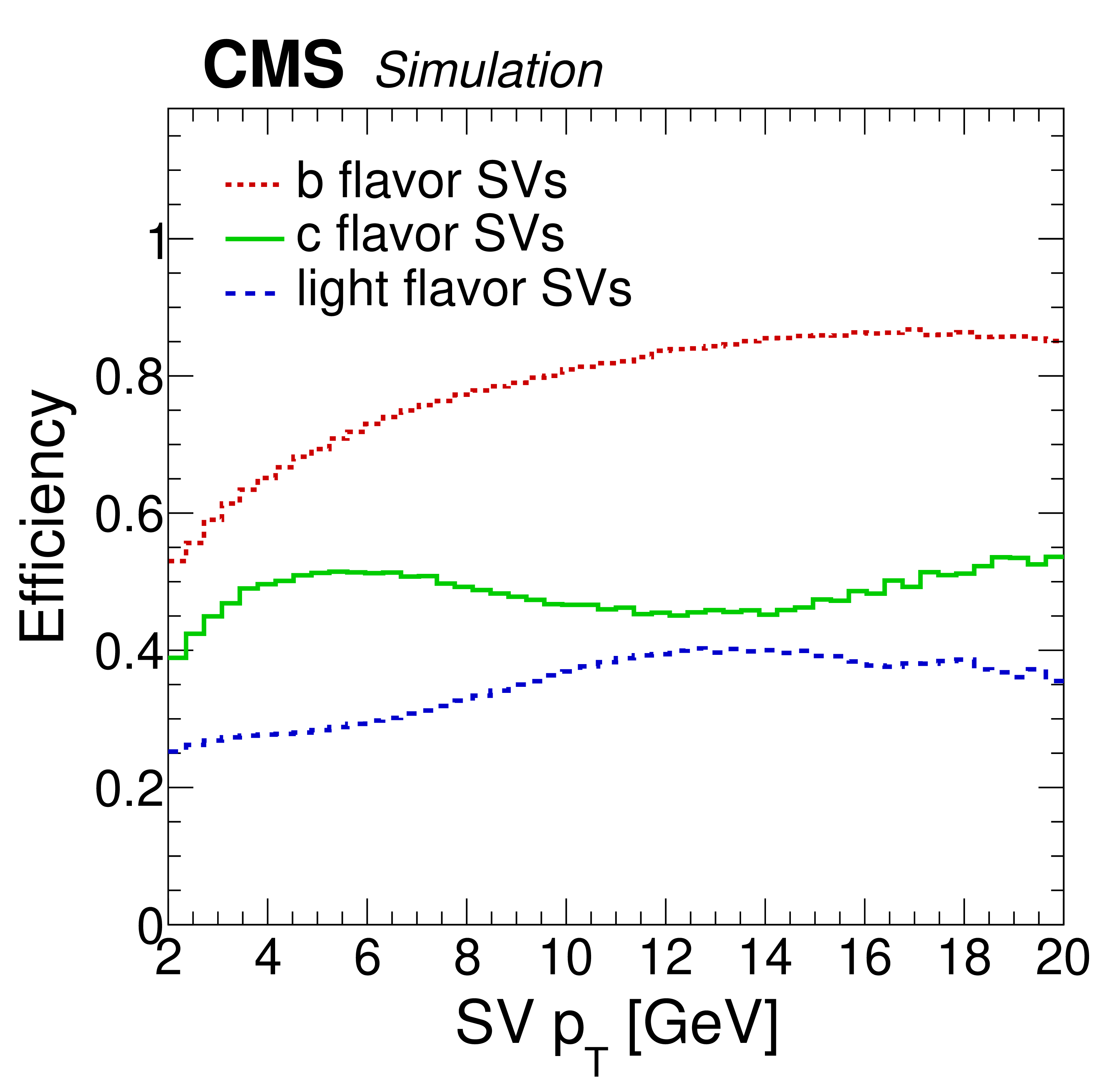
Figure 7:
Distributions of the b, c, and light-quark SV tagging efficiencies, as functions of the SV candidate $ p_{\mathrm{T}} $, for the chosen working point. The SV flavor identities are determined from the generator-level flavor information and $ \Delta R $ matching to SV candidates. |
png pdf |
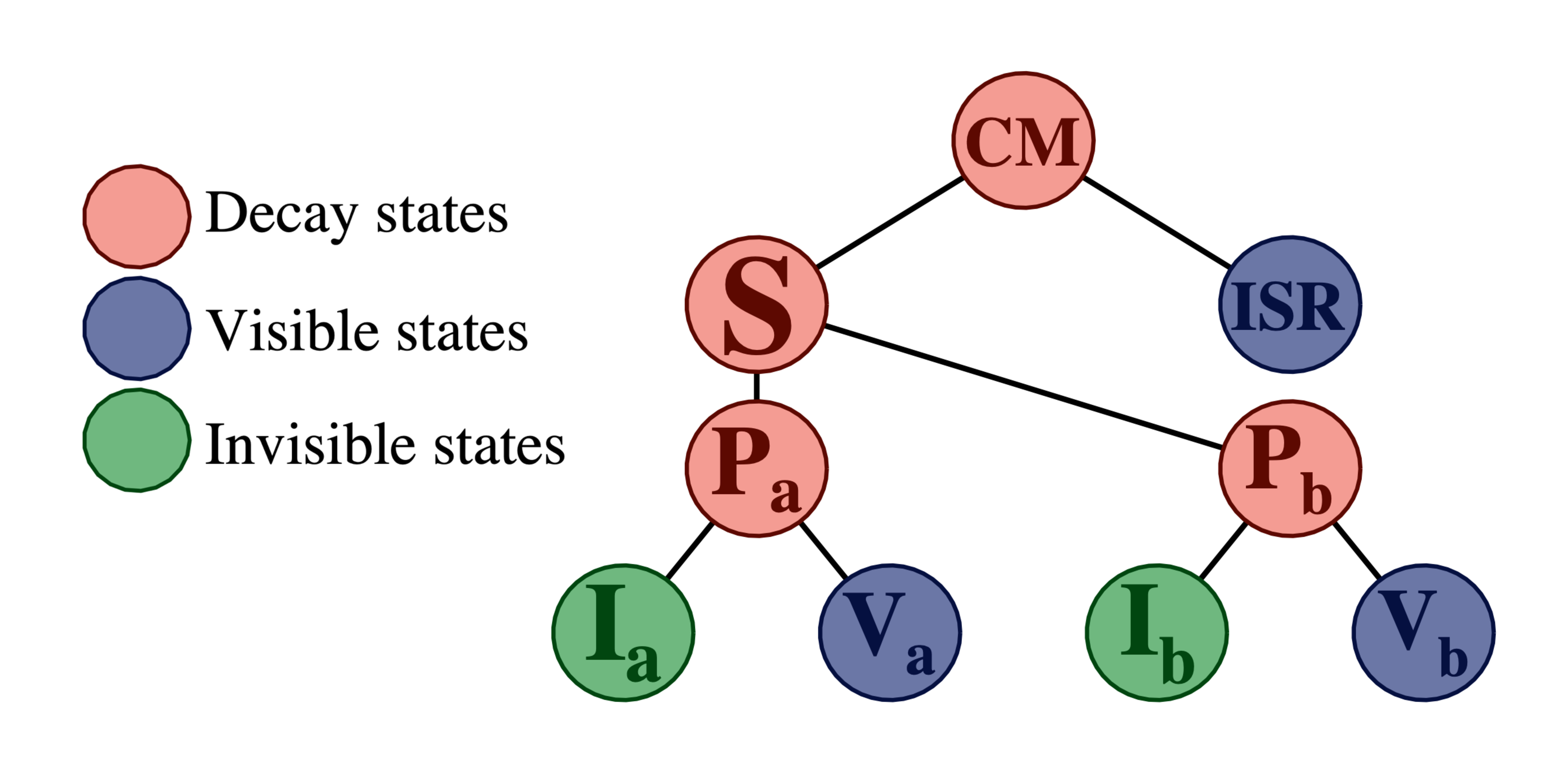
Figure 8:
Decay tree diagram used to analyze events. Here S represents the total system of candidate sparticles, with P$_{\mathrm{a/b}}$ representing pair-produced SUSY parent particles; I$_{\mathrm{a/b}}$ and V$_{\mathrm{a/b}}$ represent the systems of invisible and visible sparticle decay products, respectively. The S system, along with the recoiling ISR system, are viewed as decay products of the entire center-of-mass (CM) system of the colliding partons with constituent center-of-mass energy, $ \sqrt{\hat{s}} $. |
png pdf |
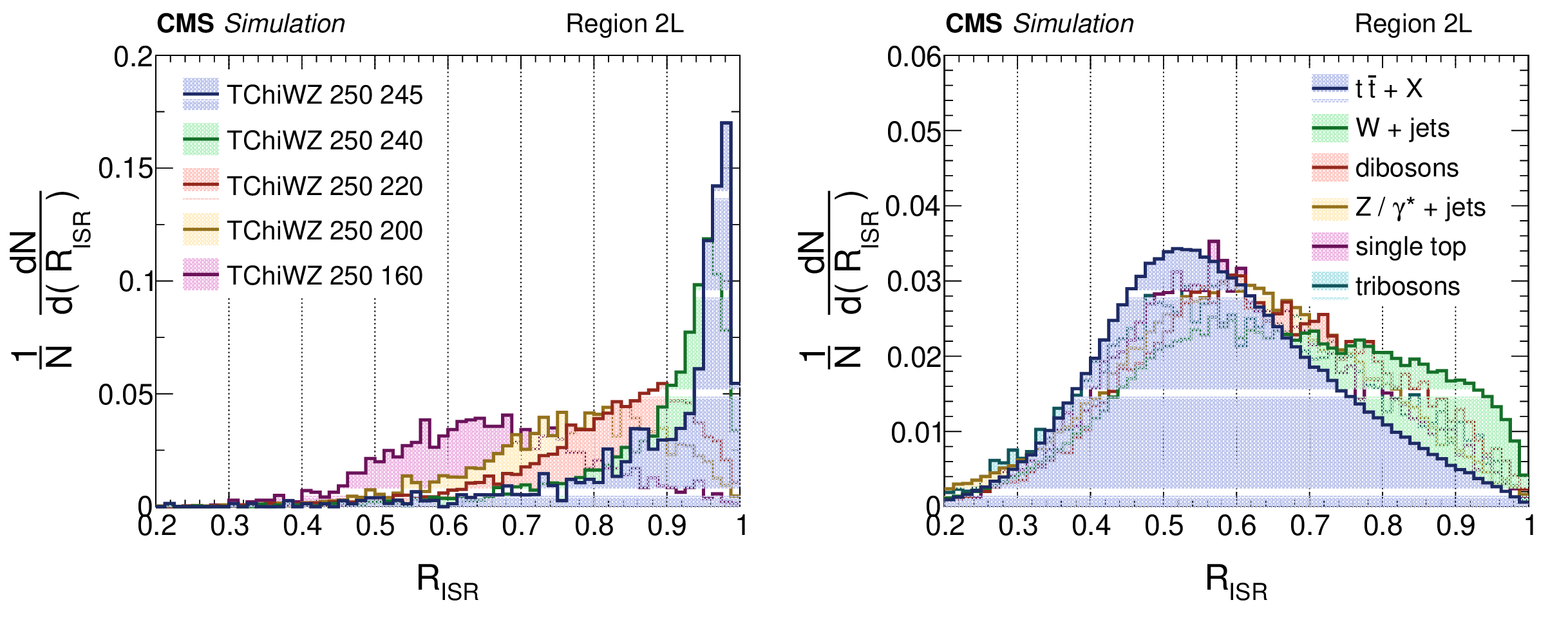
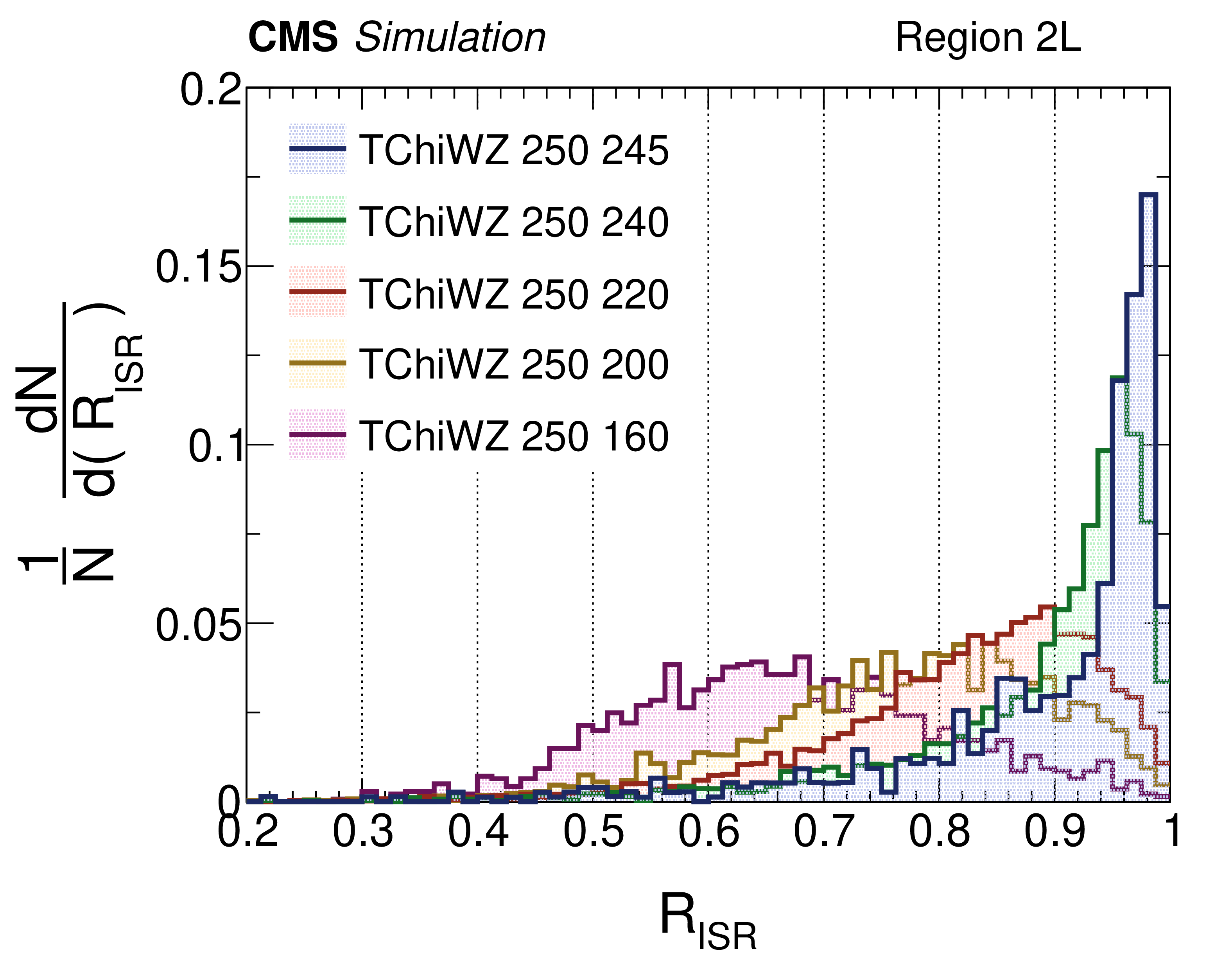
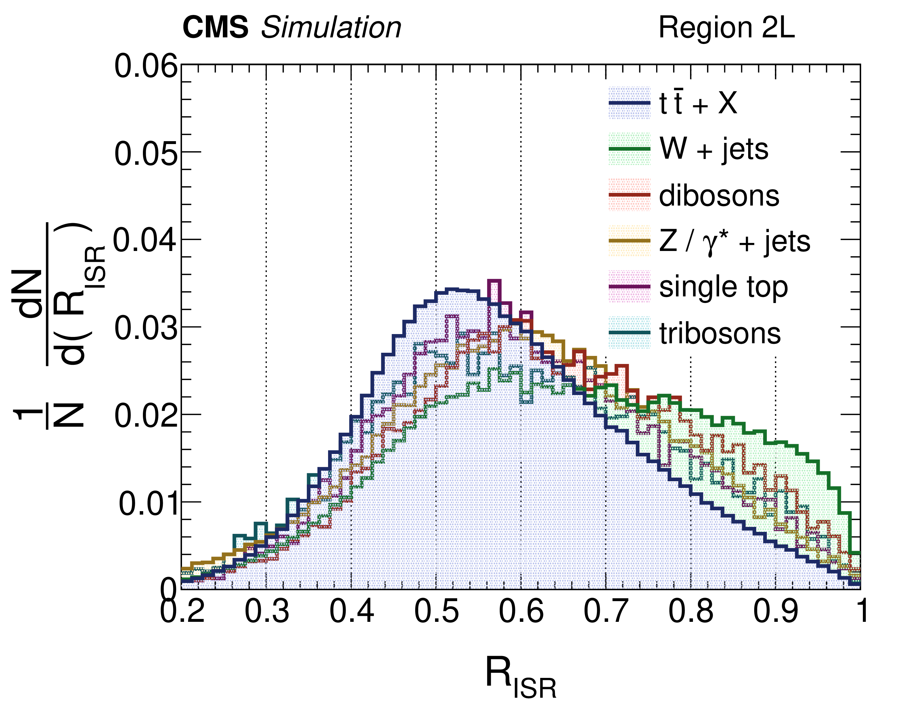
Figure 9:
Distributions of $ R_{\mathrm{ISR}} $ for simulated events in the 2 lepton final state for TChiWZ signal models with 250 GeV parent mass and various LSP masses ranging from 160 to 245 GeV (left) and the SM backgrounds (right). |
png pdf |
Figure 9-a:
Distributions of $ R_{\mathrm{ISR}} $ for simulated events in the 2 lepton final state for TChiWZ signal models with 250 GeV parent mass and various LSP masses ranging from 160 to 245 GeV (left) and the SM backgrounds (right). |
png pdf |
Figure 9-b:
Distributions of $ R_{\mathrm{ISR}} $ for simulated events in the 2 lepton final state for TChiWZ signal models with 250 GeV parent mass and various LSP masses ranging from 160 to 245 GeV (left) and the SM backgrounds (right). |
png pdf |
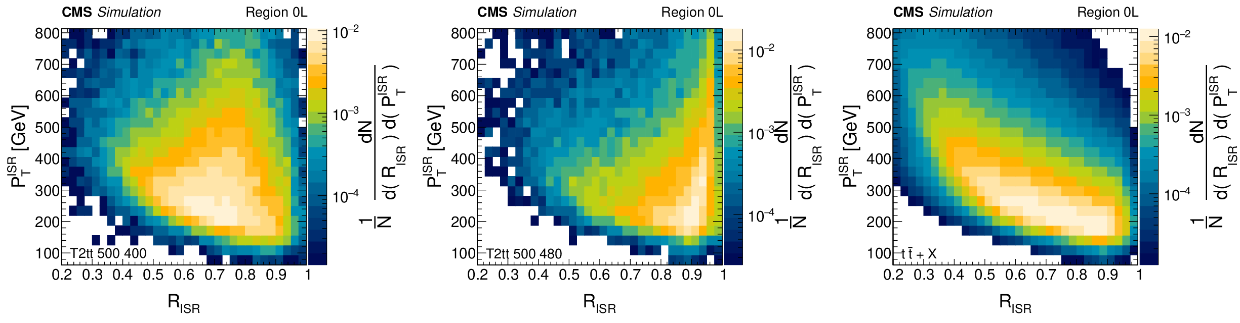
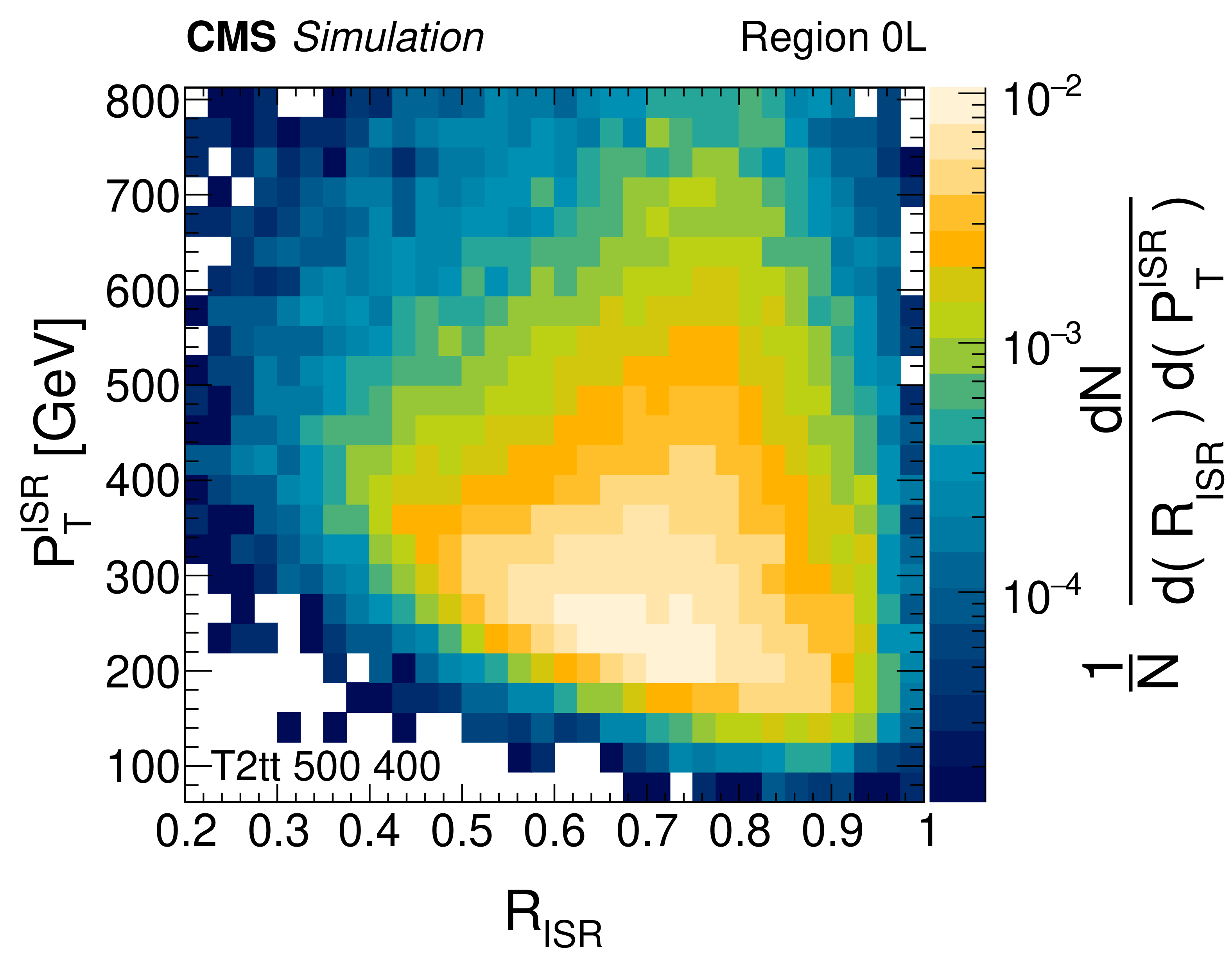
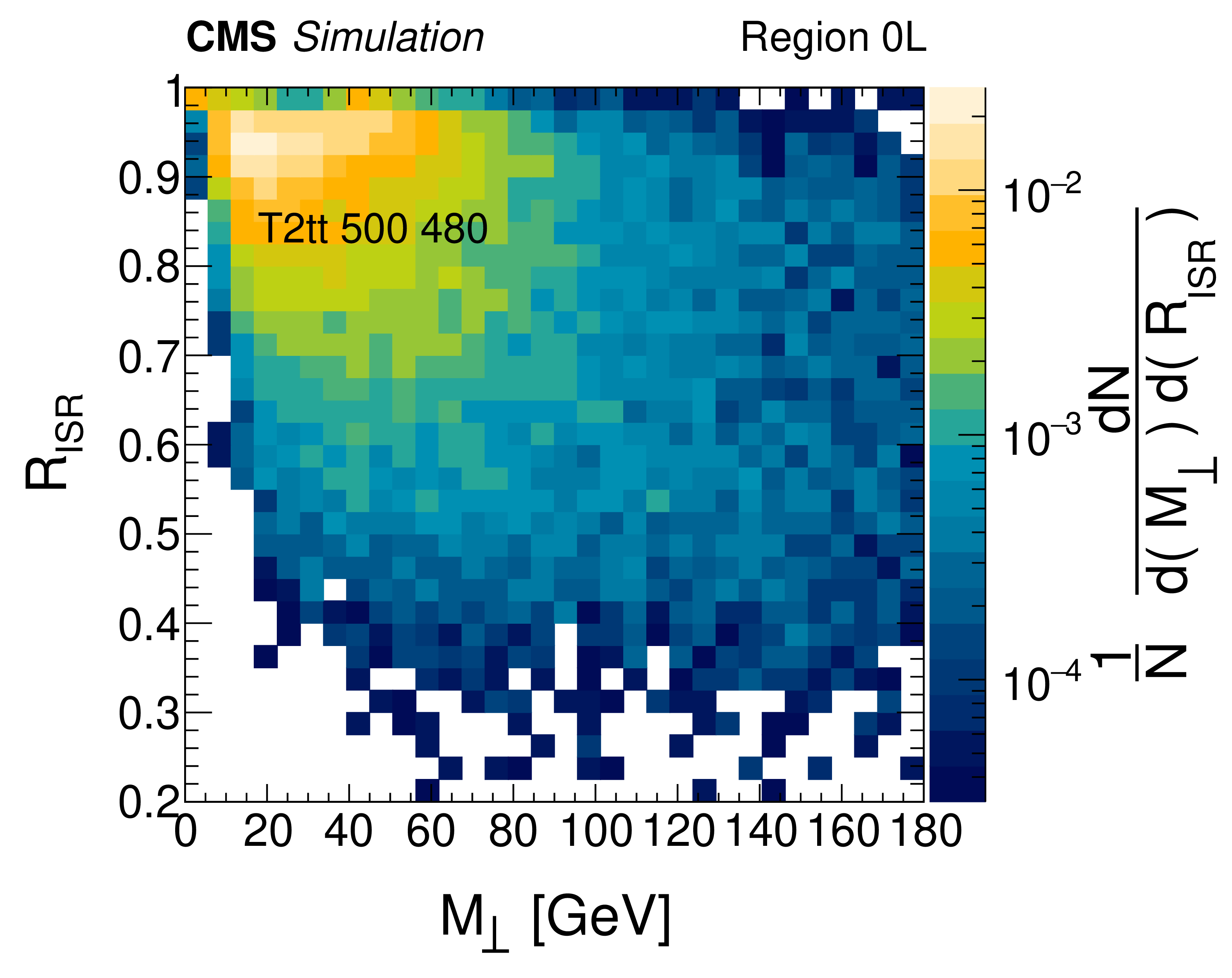
Figure 10:
Distributions of $ p_{\mathrm{T}}^{\mkern3mu\mathrm{ISR}} $ vs. $ R_{\mathrm{ISR}} $ in events with 0 leptons for simulated top squark signals in the T2tt model with parent mass of 500 GeV and a LSP mass of 400 GeV (left), LSP mass of 480 GeV (center), and $ {\mathrm{t}\overline{\mathrm{t}}}+\text{jets} $ background (right). |
png pdf |
Figure 10-a:
Distributions of $ p_{\mathrm{T}}^{\mkern3mu\mathrm{ISR}} $ vs. $ R_{\mathrm{ISR}} $ in events with 0 leptons for simulated top squark signals in the T2tt model with parent mass of 500 GeV and a LSP mass of 400 GeV (left), LSP mass of 480 GeV (center), and $ {\mathrm{t}\overline{\mathrm{t}}}+\text{jets} $ background (right). |
png pdf |
Figure 10-b:
Distributions of $ p_{\mathrm{T}}^{\mkern3mu\mathrm{ISR}} $ vs. $ R_{\mathrm{ISR}} $ in events with 0 leptons for simulated top squark signals in the T2tt model with parent mass of 500 GeV and a LSP mass of 400 GeV (left), LSP mass of 480 GeV (center), and $ {\mathrm{t}\overline{\mathrm{t}}}+\text{jets} $ background (right). |
png pdf |
Figure 10-c:
Distributions of $ p_{\mathrm{T}}^{\mkern3mu\mathrm{ISR}} $ vs. $ R_{\mathrm{ISR}} $ in events with 0 leptons for simulated top squark signals in the T2tt model with parent mass of 500 GeV and a LSP mass of 400 GeV (left), LSP mass of 480 GeV (center), and $ {\mathrm{t}\overline{\mathrm{t}}}+\text{jets} $ background (right). |
png pdf |
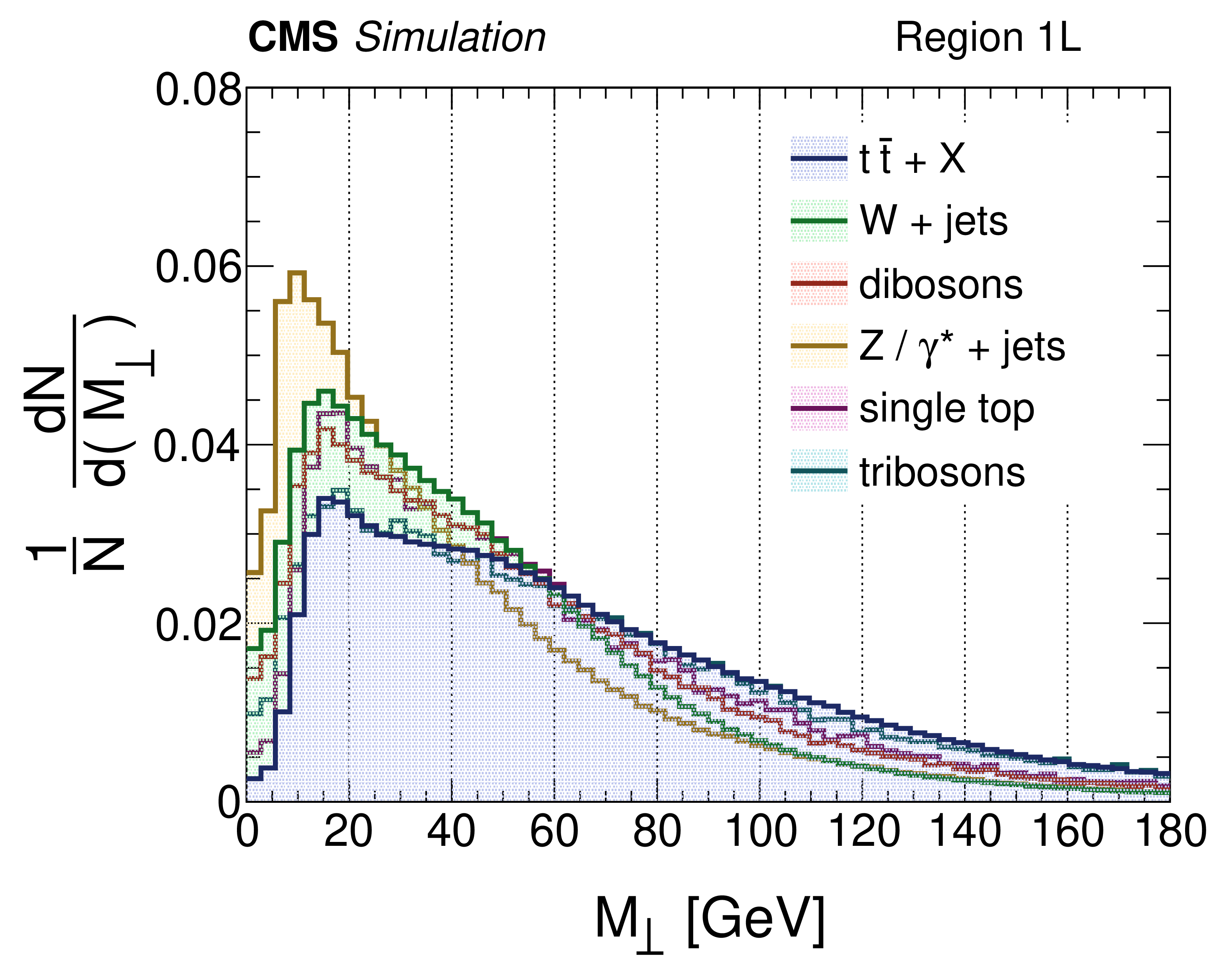
Figure 11:
Distributions of $ M_{\perp} $ in one lepton final states for simulated events: compressed T2tt signal events with a parent top squark mass of 500 GeV and LSP masses ranging from 325 to 480 GeV (left) and the SM backgrounds (right). |
png pdf |
Figure 11-a:
Distributions of $ M_{\perp} $ in one lepton final states for simulated events: compressed T2tt signal events with a parent top squark mass of 500 GeV and LSP masses ranging from 325 to 480 GeV (left) and the SM backgrounds (right). |
png pdf |
Figure 11-b:
Distributions of $ M_{\perp} $ in one lepton final states for simulated events: compressed T2tt signal events with a parent top squark mass of 500 GeV and LSP masses ranging from 325 to 480 GeV (left) and the SM backgrounds (right). |
png pdf |
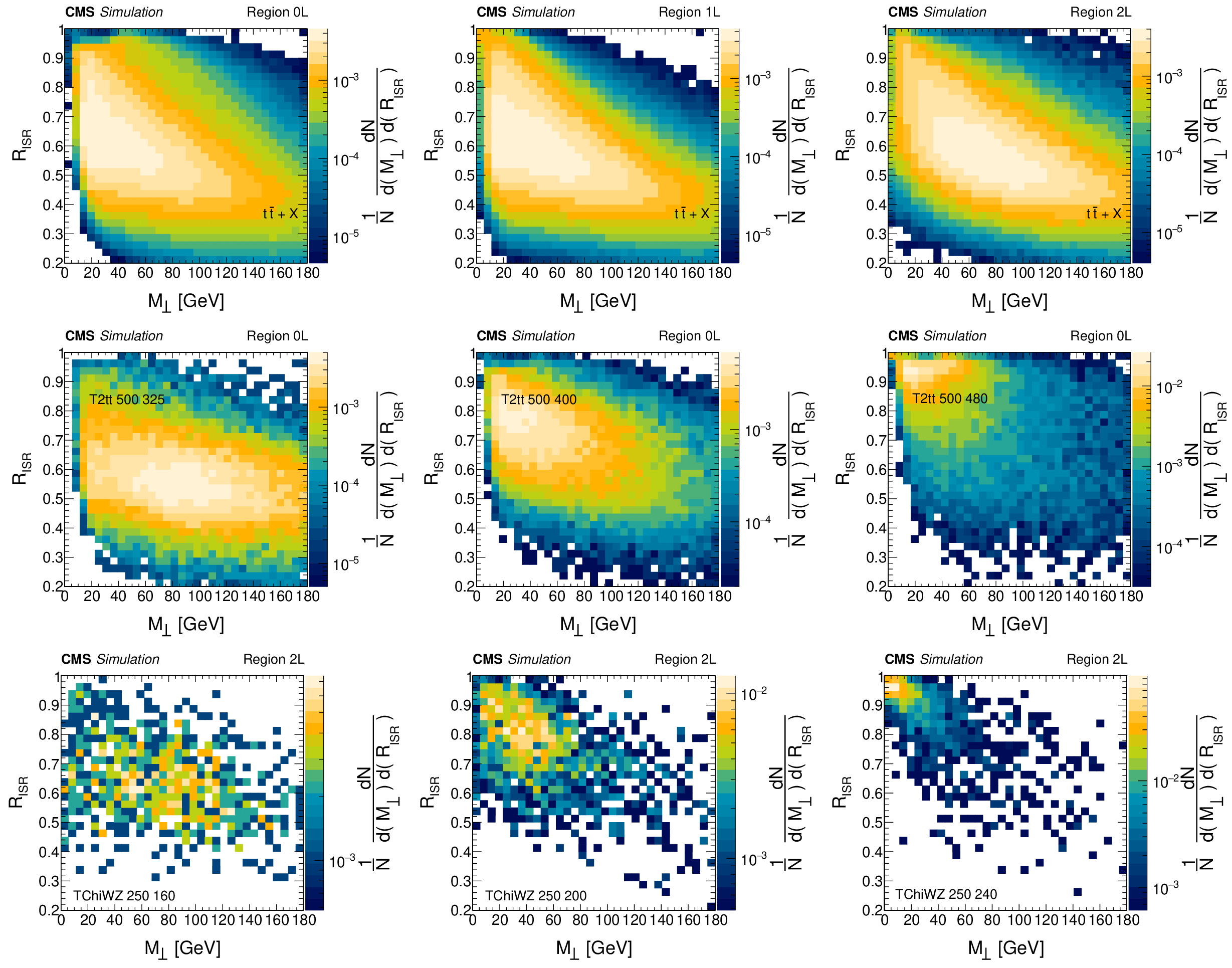
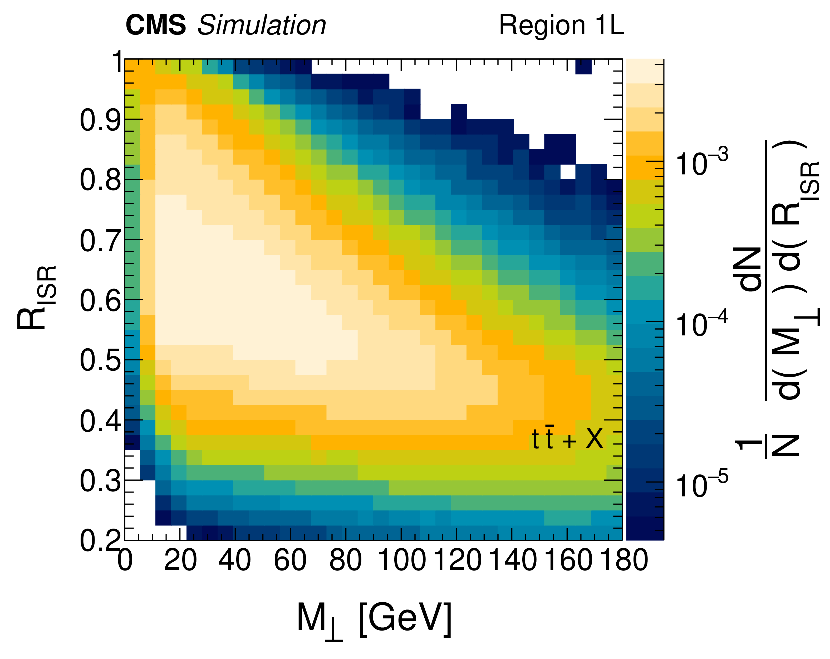
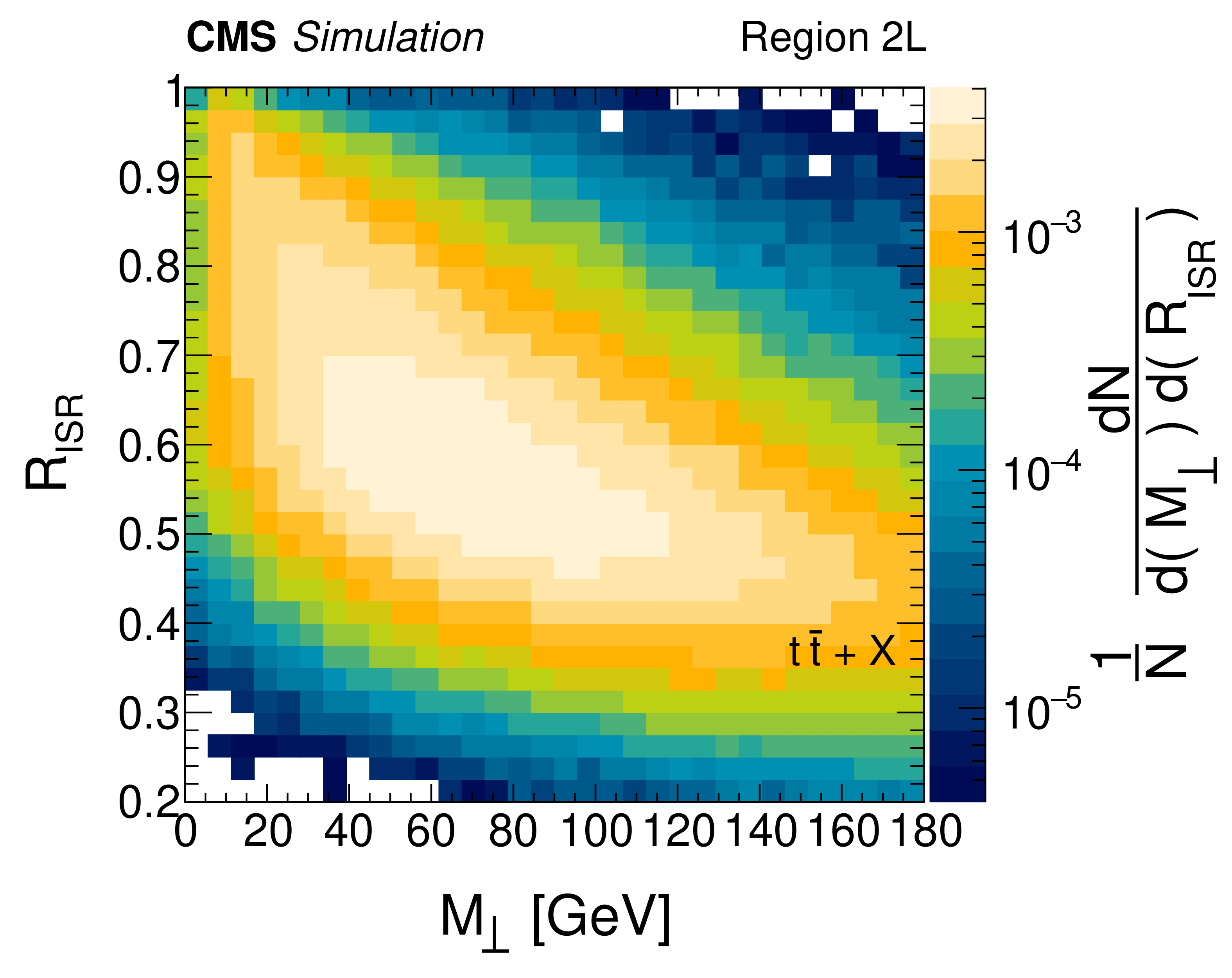
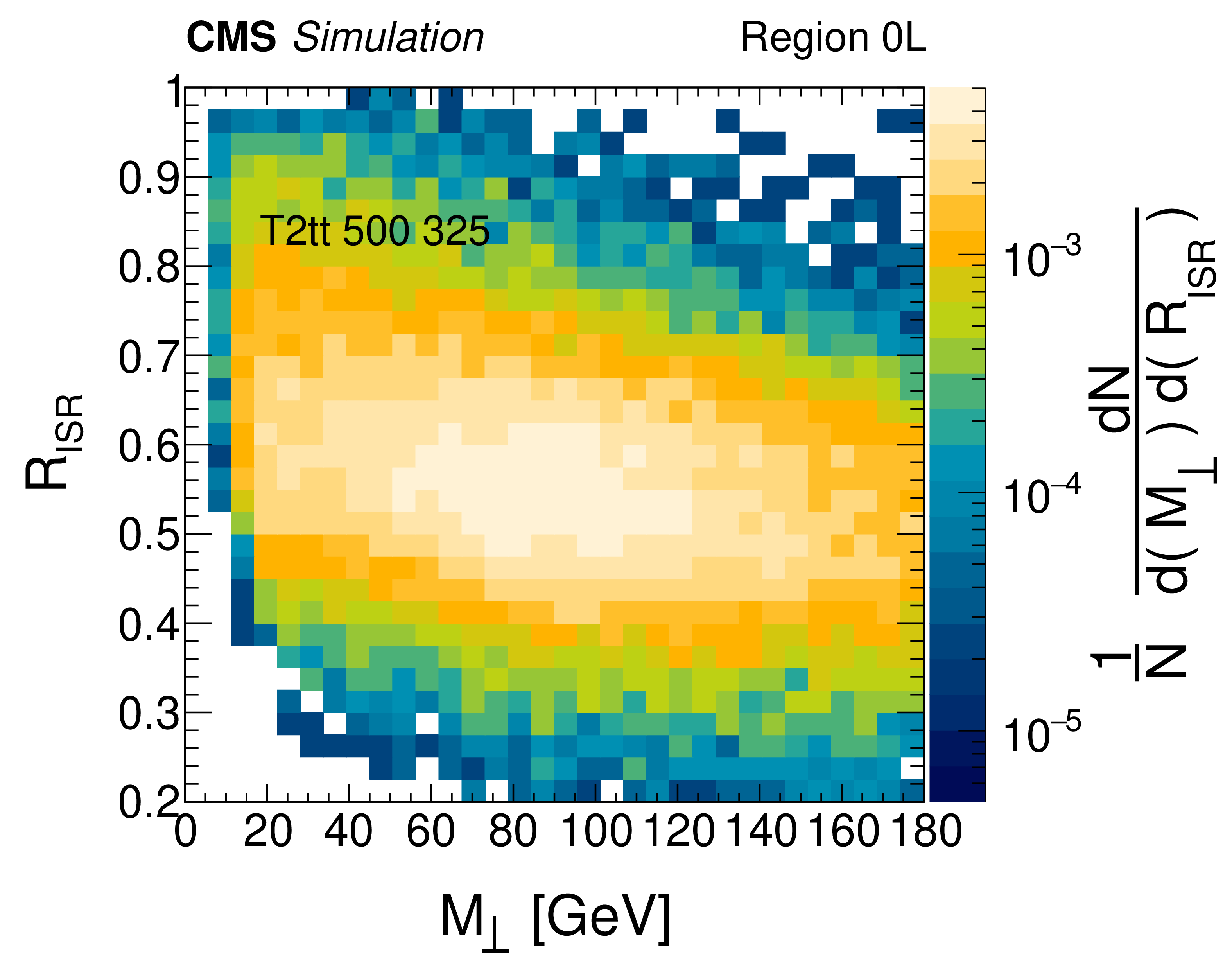
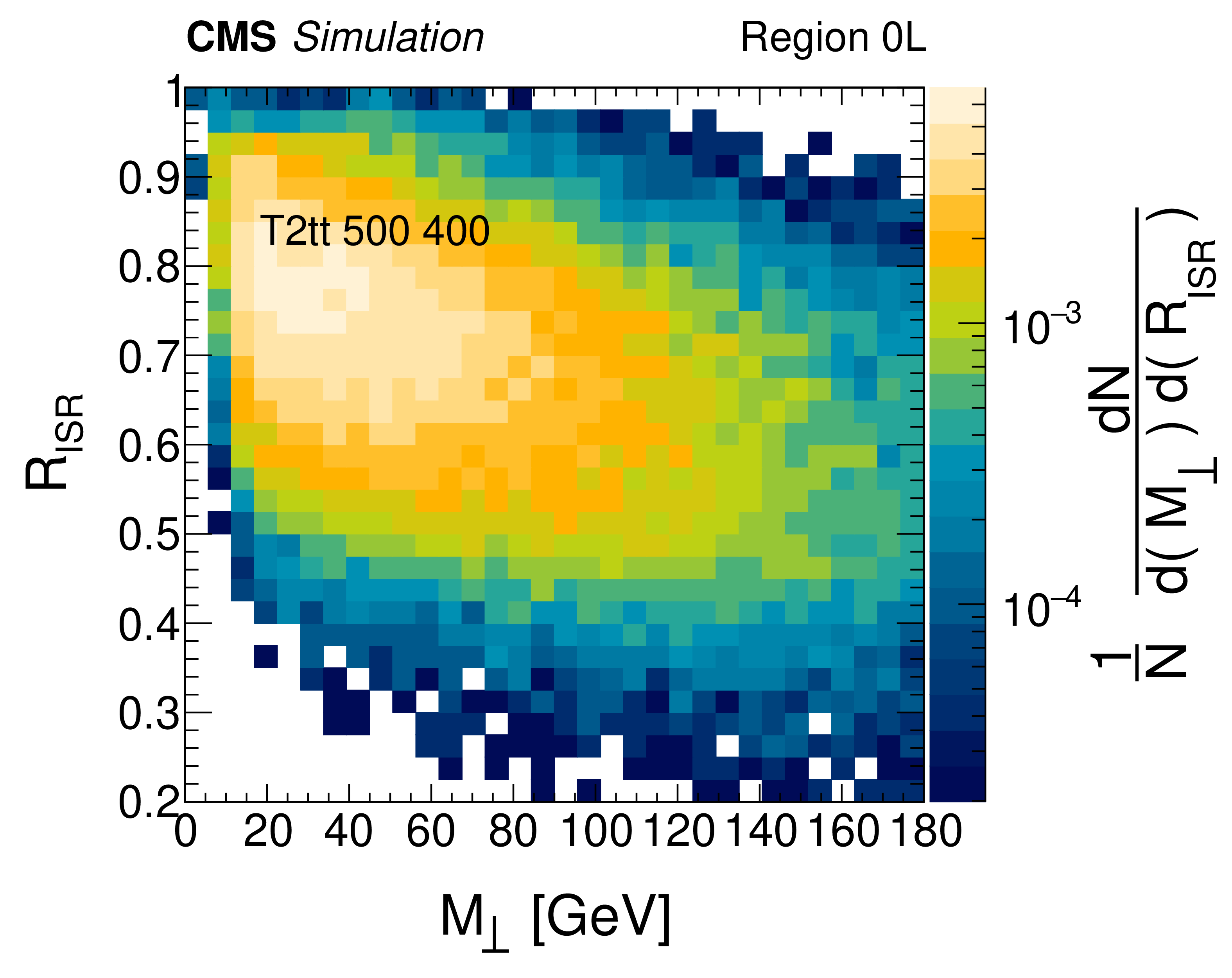
Figure 12:
Distributions of $ R_{\mathrm{ISR}} $ vs. $ M_{\perp} $ for simulated events in multiple final states. (Upper row) $ {\mathrm{t}\overline{\mathrm{t}}}+\text{jets} $ background events in 0 lepton (0L), one lepton (1L), and two lepton (2L) final states. (Middle row) T2tt signals in 0L final states and (lower row) TChiWZ signals in 2L final states for various sparticle mass combinations. |
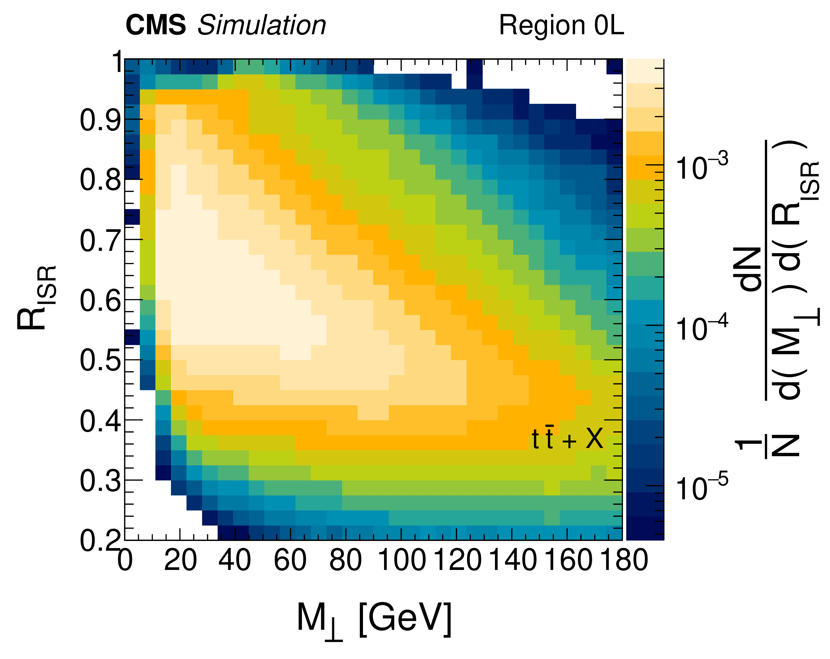
png pdf |
Figure 12-a:
Distributions of $ R_{\mathrm{ISR}} $ vs. $ M_{\perp} $ for simulated events in multiple final states. (Upper row) $ {\mathrm{t}\overline{\mathrm{t}}}+\text{jets} $ background events in 0 lepton (0L), one lepton (1L), and two lepton (2L) final states. (Middle row) T2tt signals in 0L final states and (lower row) TChiWZ signals in 2L final states for various sparticle mass combinations. |
png pdf |
Figure 12-b:
Distributions of $ R_{\mathrm{ISR}} $ vs. $ M_{\perp} $ for simulated events in multiple final states. (Upper row) $ {\mathrm{t}\overline{\mathrm{t}}}+\text{jets} $ background events in 0 lepton (0L), one lepton (1L), and two lepton (2L) final states. (Middle row) T2tt signals in 0L final states and (lower row) TChiWZ signals in 2L final states for various sparticle mass combinations. |
png pdf |
Figure 12-c:
Distributions of $ R_{\mathrm{ISR}} $ vs. $ M_{\perp} $ for simulated events in multiple final states. (Upper row) $ {\mathrm{t}\overline{\mathrm{t}}}+\text{jets} $ background events in 0 lepton (0L), one lepton (1L), and two lepton (2L) final states. (Middle row) T2tt signals in 0L final states and (lower row) TChiWZ signals in 2L final states for various sparticle mass combinations. |
png pdf |
Figure 12-d:
Distributions of $ R_{\mathrm{ISR}} $ vs. $ M_{\perp} $ for simulated events in multiple final states. (Upper row) $ {\mathrm{t}\overline{\mathrm{t}}}+\text{jets} $ background events in 0 lepton (0L), one lepton (1L), and two lepton (2L) final states. (Middle row) T2tt signals in 0L final states and (lower row) TChiWZ signals in 2L final states for various sparticle mass combinations. |
png pdf |
Figure 12-e:
Distributions of $ R_{\mathrm{ISR}} $ vs. $ M_{\perp} $ for simulated events in multiple final states. (Upper row) $ {\mathrm{t}\overline{\mathrm{t}}}+\text{jets} $ background events in 0 lepton (0L), one lepton (1L), and two lepton (2L) final states. (Middle row) T2tt signals in 0L final states and (lower row) TChiWZ signals in 2L final states for various sparticle mass combinations. |
png pdf |
Figure 12-f:
Distributions of $ R_{\mathrm{ISR}} $ vs. $ M_{\perp} $ for simulated events in multiple final states. (Upper row) $ {\mathrm{t}\overline{\mathrm{t}}}+\text{jets} $ background events in 0 lepton (0L), one lepton (1L), and two lepton (2L) final states. (Middle row) T2tt signals in 0L final states and (lower row) TChiWZ signals in 2L final states for various sparticle mass combinations. |
png pdf |
Figure 12-g:
Distributions of $ R_{\mathrm{ISR}} $ vs. $ M_{\perp} $ for simulated events in multiple final states. (Upper row) $ {\mathrm{t}\overline{\mathrm{t}}}+\text{jets} $ background events in 0 lepton (0L), one lepton (1L), and two lepton (2L) final states. (Middle row) T2tt signals in 0L final states and (lower row) TChiWZ signals in 2L final states for various sparticle mass combinations. |
png pdf |
Figure 12-h:
Distributions of $ R_{\mathrm{ISR}} $ vs. $ M_{\perp} $ for simulated events in multiple final states. (Upper row) $ {\mathrm{t}\overline{\mathrm{t}}}+\text{jets} $ background events in 0 lepton (0L), one lepton (1L), and two lepton (2L) final states. (Middle row) T2tt signals in 0L final states and (lower row) TChiWZ signals in 2L final states for various sparticle mass combinations. |
png pdf |
Figure 12-i:
Distributions of $ R_{\mathrm{ISR}} $ vs. $ M_{\perp} $ for simulated events in multiple final states. (Upper row) $ {\mathrm{t}\overline{\mathrm{t}}}+\text{jets} $ background events in 0 lepton (0L), one lepton (1L), and two lepton (2L) final states. (Middle row) T2tt signals in 0L final states and (lower row) TChiWZ signals in 2L final states for various sparticle mass combinations. |
png pdf |
Figure 13:
Distributions of $ \text{max} \: |\eta_{\mathrm{SV}}^{\mathrm{S}}| $ in final states with 0 leptons and $ {\geq} $ 1 SVs associated with the S system, for simulated SM background events (left) and various top squark signal models (right). |
png pdf |
Figure 13-a:
Distributions of $ \text{max} \: |\eta_{\mathrm{SV}}^{\mathrm{S}}| $ in final states with 0 leptons and $ {\geq} $ 1 SVs associated with the S system, for simulated SM background events (left) and various top squark signal models (right). |
png pdf |
Figure 13-b:
Distributions of $ \text{max} \: |\eta_{\mathrm{SV}}^{\mathrm{S}}| $ in final states with 0 leptons and $ {\geq} $ 1 SVs associated with the S system, for simulated SM background events (left) and various top squark signal models (right). |
png pdf |
Figure 14:
Distributions of $ R_{\mathrm{ISR}} $ vs. $ M_{\perp} $ for a TChiWZ signal sample with a parent mass of 300 GeV and a LSP mass of 290 GeV (left) and the corresponding total SM background (right) for the 2L, 0 S-jet category. The dashed lines show the bin edges for this particular jet multiplicity. |
png pdf |
Figure 14-a:
Distributions of $ R_{\mathrm{ISR}} $ vs. $ M_{\perp} $ for a TChiWZ signal sample with a parent mass of 300 GeV and a LSP mass of 290 GeV (left) and the corresponding total SM background (right) for the 2L, 0 S-jet category. The dashed lines show the bin edges for this particular jet multiplicity. |
png pdf |
Figure 14-b:
Distributions of $ R_{\mathrm{ISR}} $ vs. $ M_{\perp} $ for a TChiWZ signal sample with a parent mass of 300 GeV and a LSP mass of 290 GeV (left) and the corresponding total SM background (right) for the 2L, 0 S-jet category. The dashed lines show the bin edges for this particular jet multiplicity. |
png pdf |
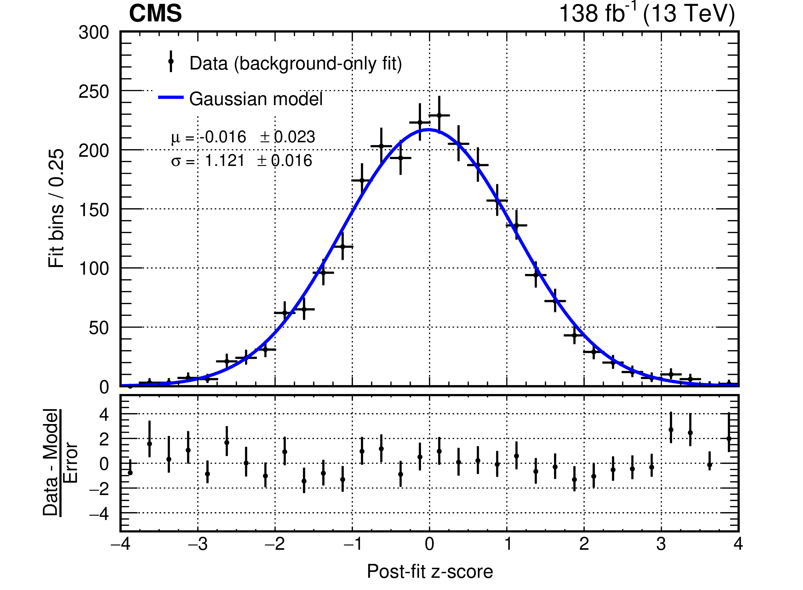
Figure 15:
Distribution of post-fit z-scores for the full data set background-only fit. The superimposed Gaussian model uses the observed mean and standard deviation. |
png pdf |
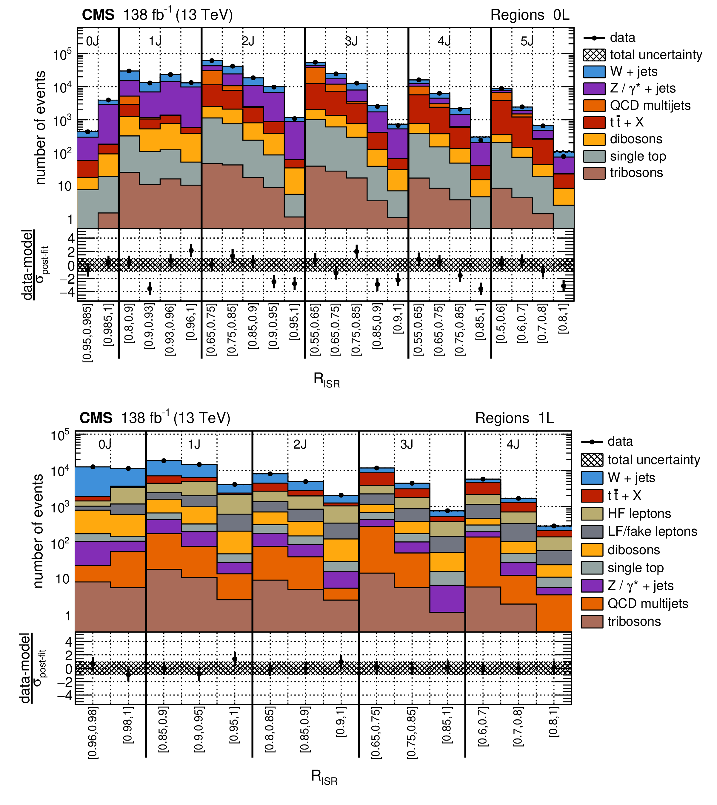
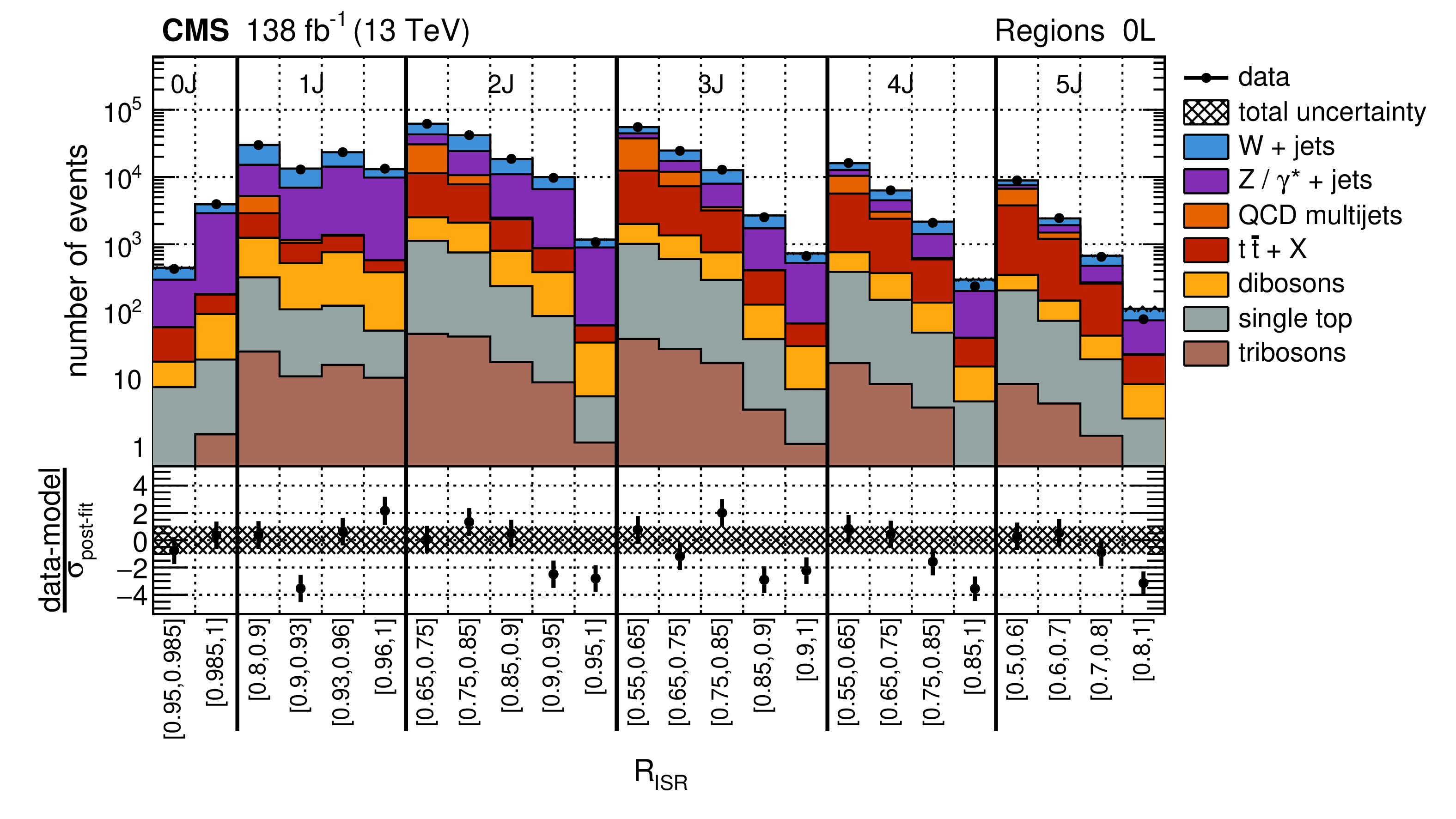
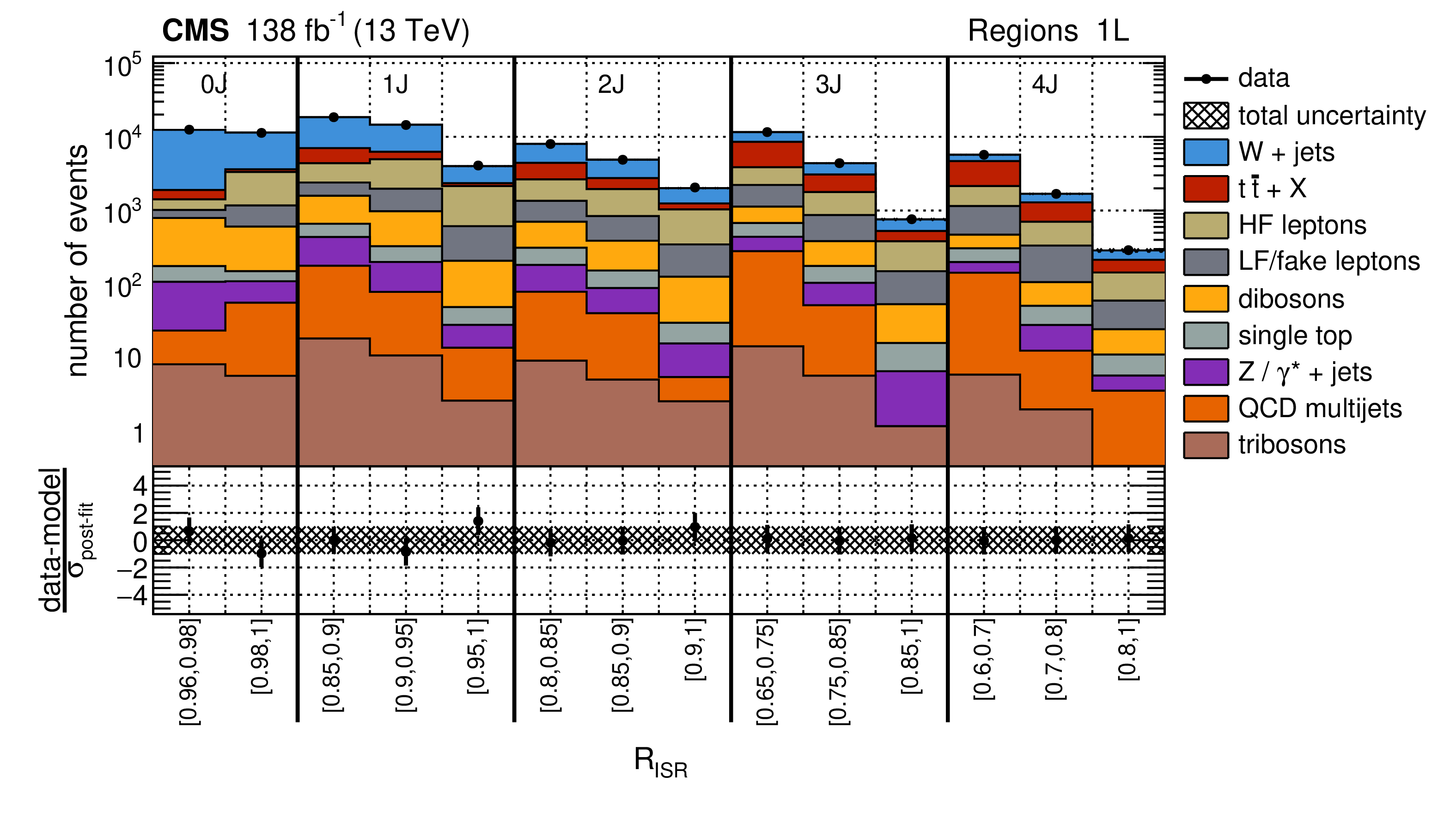
Figure 16:
Post-fit distributions of data with the background-only fit model for the full data set in the 0L region (upper) and 1L region (lower). Bins are split by $ R_{\mathrm{ISR}} $ along with $ N_{\text{jet}}^{\mathrm{S}} $. Yields are integrated over all other sub-categorizations and $ M_{\perp} $. The sub-panels below the panels show the data minus fit model scaled by the post-fit model uncertainty. |
png pdf |
Figure 16-a:
Post-fit distributions of data with the background-only fit model for the full data set in the 0L region (upper) and 1L region (lower). Bins are split by $ R_{\mathrm{ISR}} $ along with $ N_{\text{jet}}^{\mathrm{S}} $. Yields are integrated over all other sub-categorizations and $ M_{\perp} $. The sub-panels below the panels show the data minus fit model scaled by the post-fit model uncertainty. |
png pdf |
Figure 16-b:
Post-fit distributions of data with the background-only fit model for the full data set in the 0L region (upper) and 1L region (lower). Bins are split by $ R_{\mathrm{ISR}} $ along with $ N_{\text{jet}}^{\mathrm{S}} $. Yields are integrated over all other sub-categorizations and $ M_{\perp} $. The sub-panels below the panels show the data minus fit model scaled by the post-fit model uncertainty. |
png pdf |
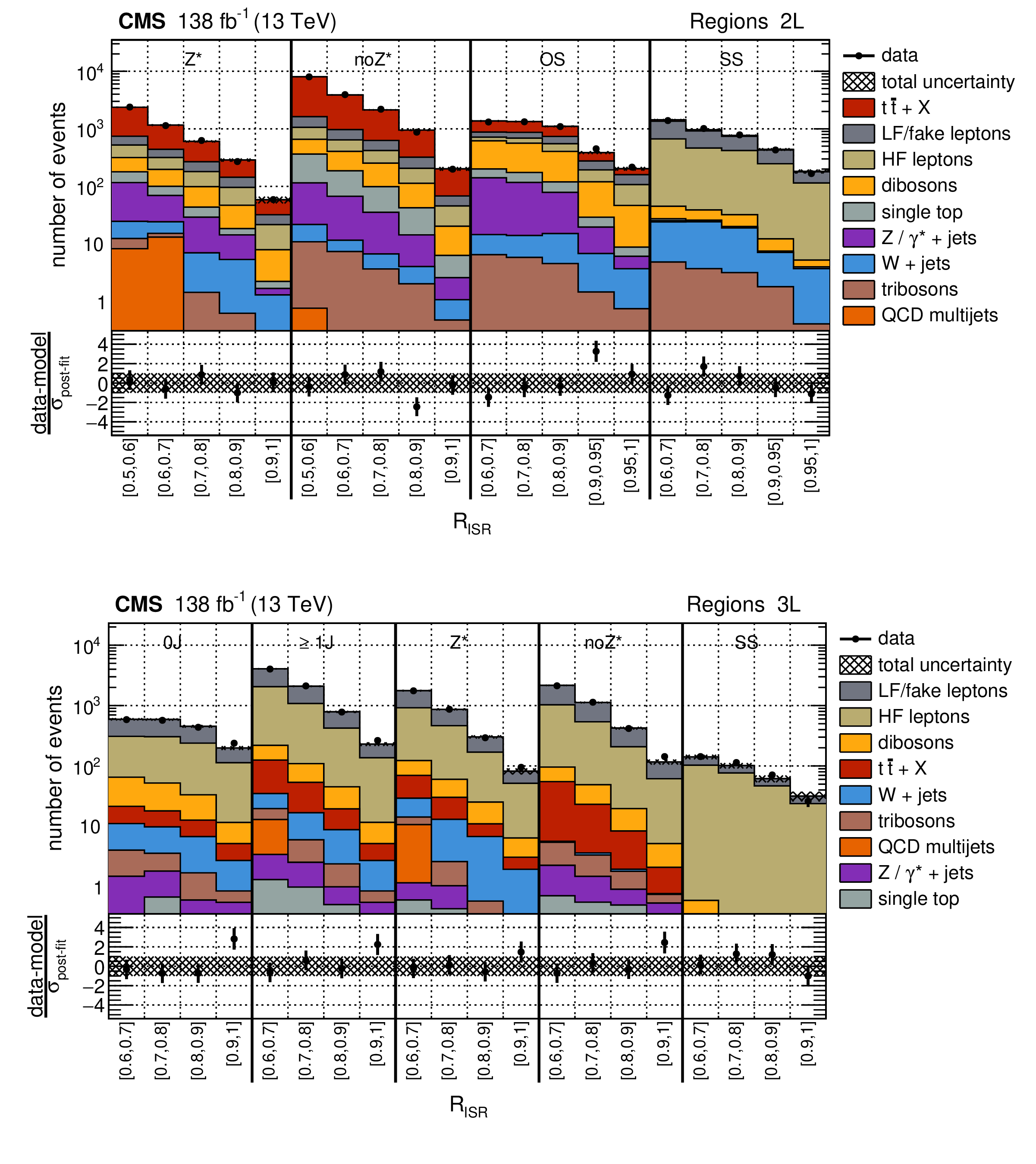
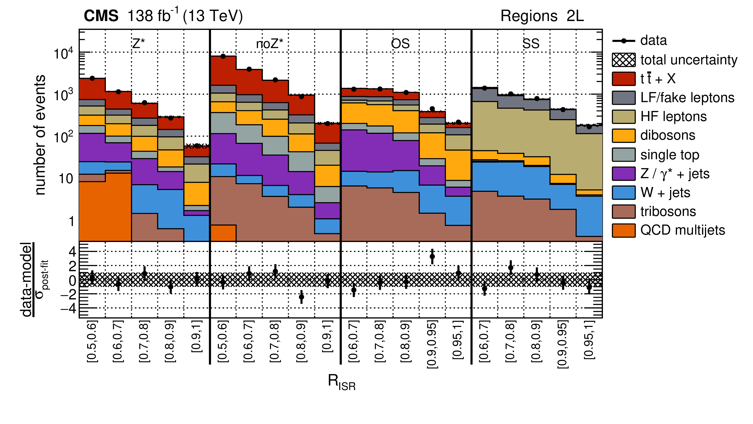
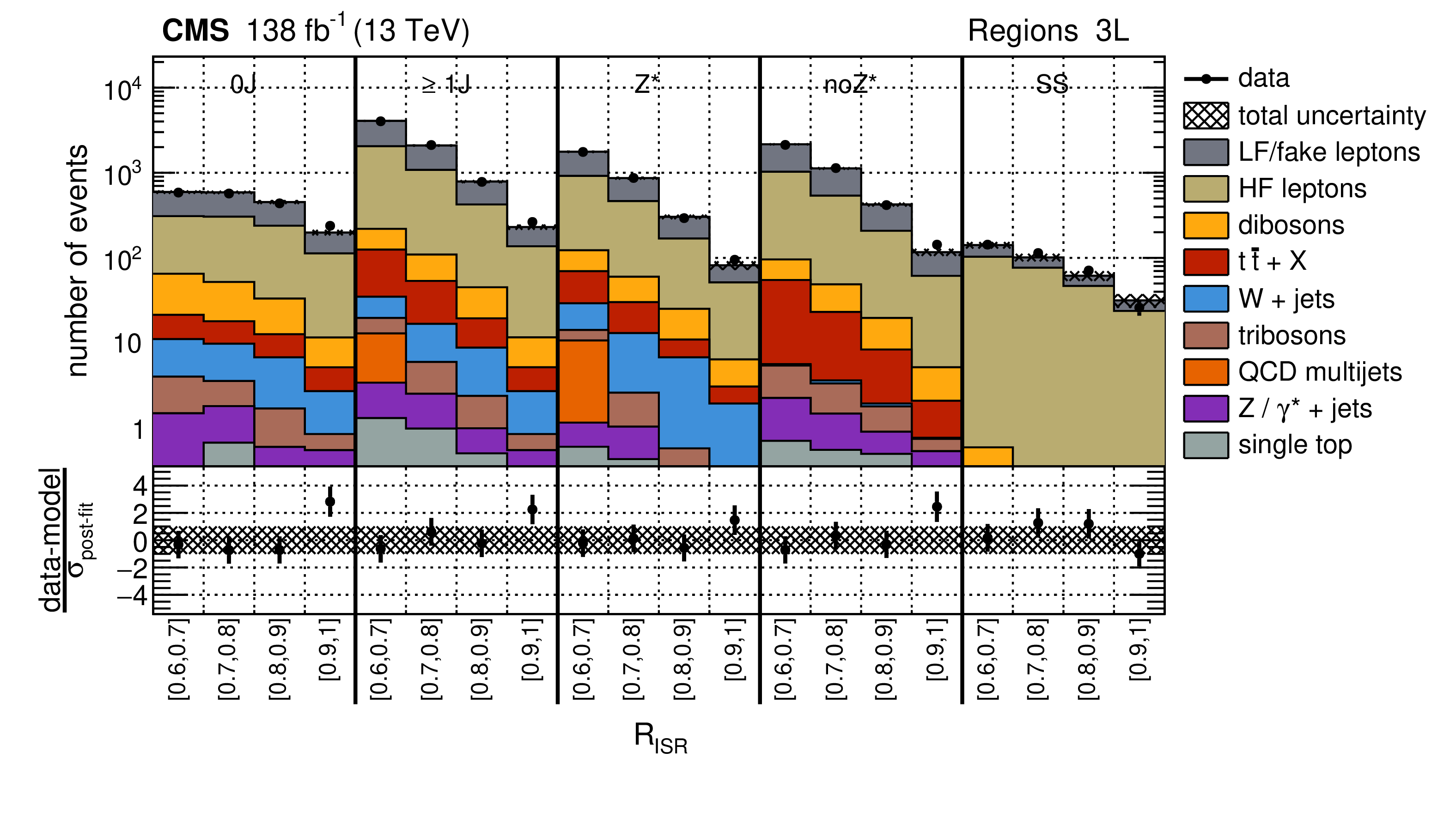
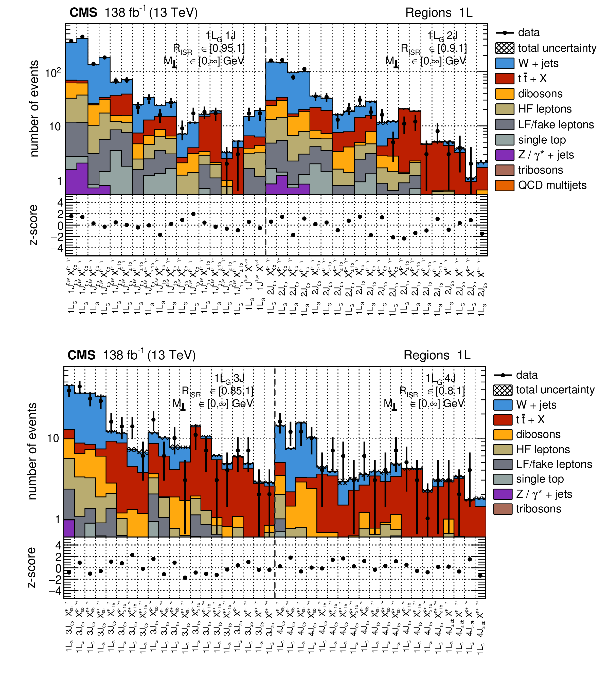
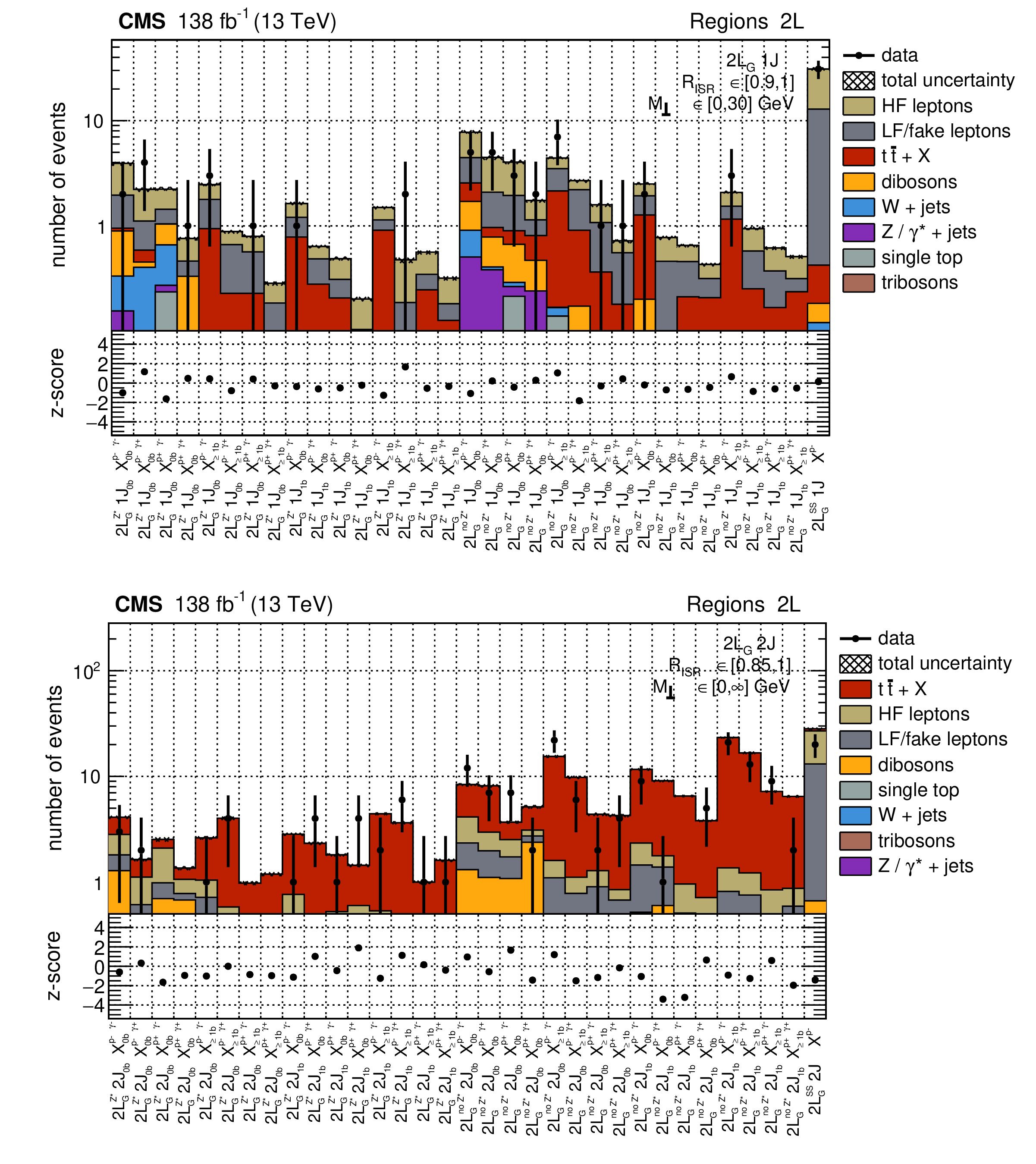
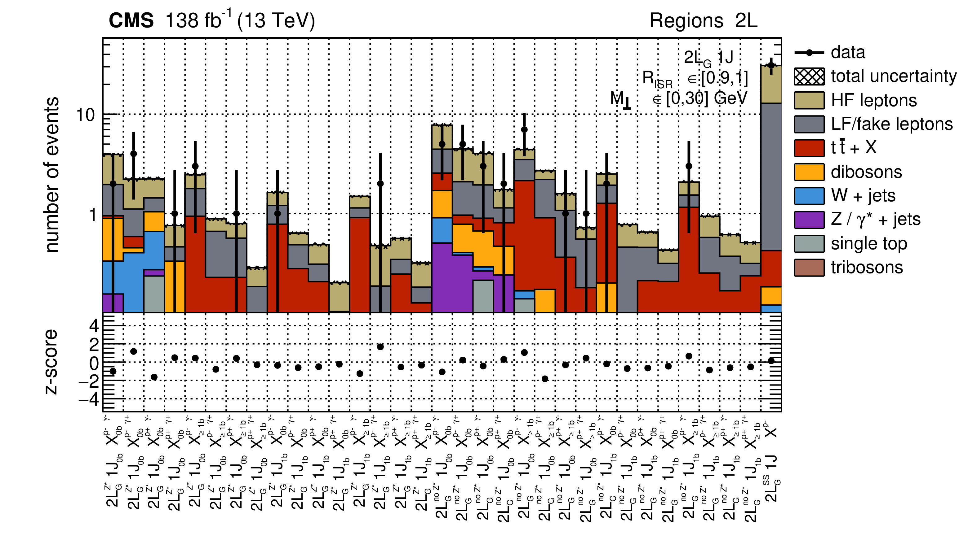
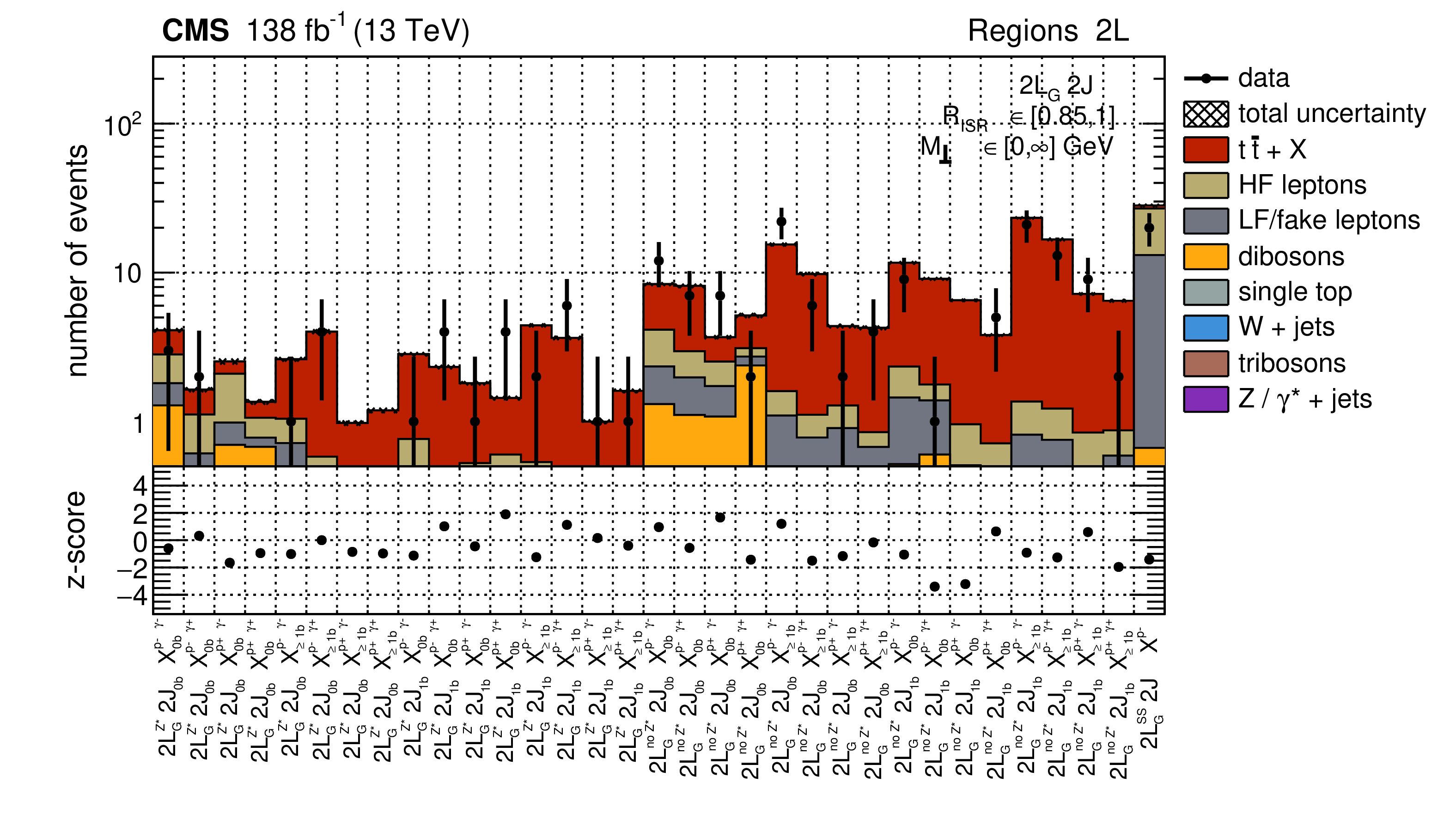
Figure 17:
Post-fit distributions of data with the background-only fit model for the full data set in the 2L region (upper) and 3L region (lower). Bins are split by $ R_{\mathrm{ISR}} $ along with lepton categorization. Yields are integrated over all other sub-categorizations and $ M_{\perp} $. The sub-panels below the panels show the data minus fit model scaled by the post-fit model uncertainty. |
png pdf |
Figure 17-a:
Post-fit distributions of data with the background-only fit model for the full data set in the 2L region (upper) and 3L region (lower). Bins are split by $ R_{\mathrm{ISR}} $ along with lepton categorization. Yields are integrated over all other sub-categorizations and $ M_{\perp} $. The sub-panels below the panels show the data minus fit model scaled by the post-fit model uncertainty. |
png pdf |
Figure 17-b:
Post-fit distributions of data with the background-only fit model for the full data set in the 2L region (upper) and 3L region (lower). Bins are split by $ R_{\mathrm{ISR}} $ along with lepton categorization. Yields are integrated over all other sub-categorizations and $ M_{\perp} $. The sub-panels below the panels show the data minus fit model scaled by the post-fit model uncertainty. |
png pdf |
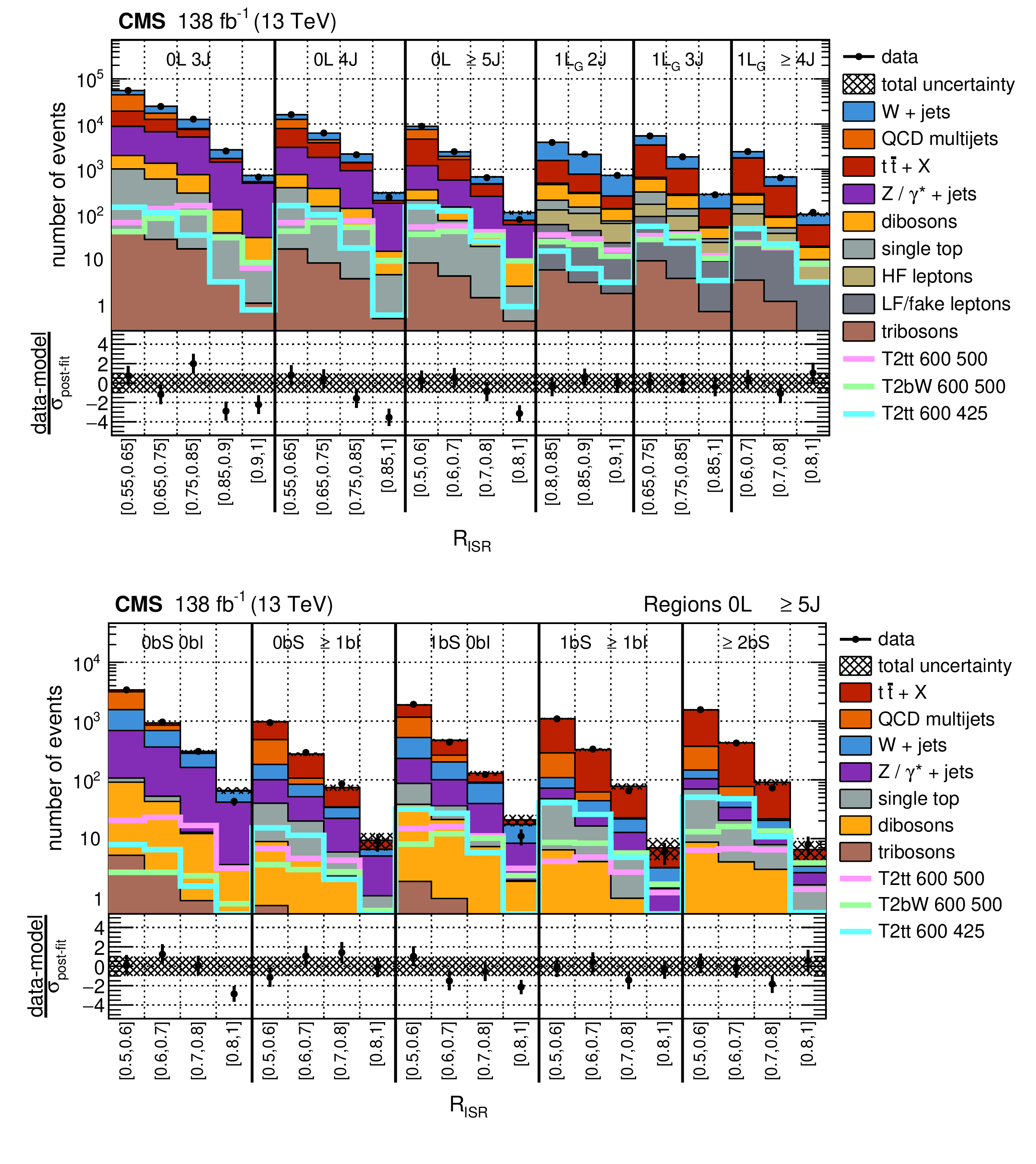
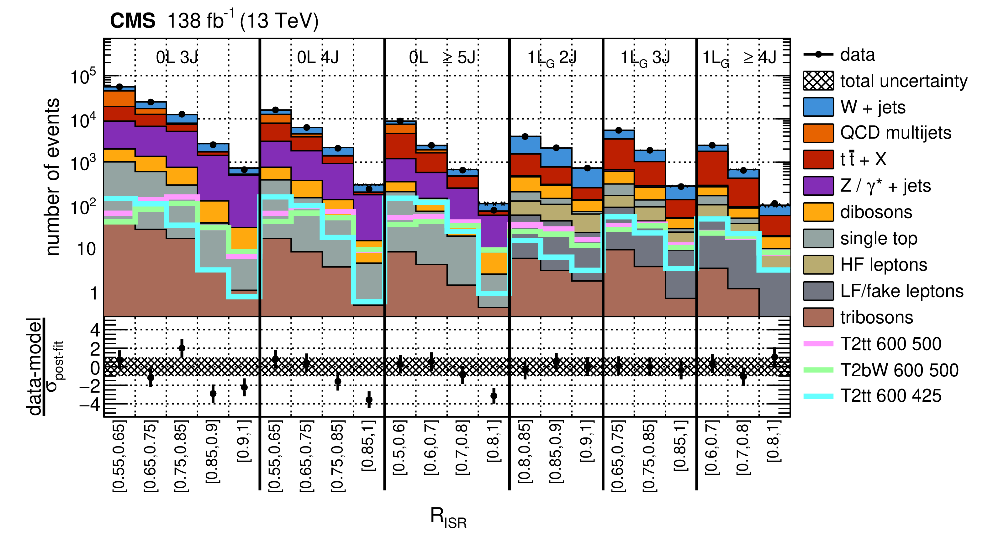
Figure 18:
Post-fit distributions of data with the background-only fit model for the full data set. (Upper) 0L and 1L gold regions with larger jet multiplicities. (Lower) 0L 5J regions separated by $ b $-tagged jet multiplicities in the S and ISR systems. Bins are split by $ R_{\mathrm{ISR}} $ with yields integrated over all other sub-categorizations and $ M_{\perp} $. The sub-panels below the panels show the data minus fit model scaled by the post-fit model uncertainty. Expected yields for example signal models are superimposed. |
png pdf |
Figure 18-a:
Post-fit distributions of data with the background-only fit model for the full data set. (Upper) 0L and 1L gold regions with larger jet multiplicities. (Lower) 0L 5J regions separated by $ b $-tagged jet multiplicities in the S and ISR systems. Bins are split by $ R_{\mathrm{ISR}} $ with yields integrated over all other sub-categorizations and $ M_{\perp} $. The sub-panels below the panels show the data minus fit model scaled by the post-fit model uncertainty. Expected yields for example signal models are superimposed. |
png pdf |
Figure 18-b:
Post-fit distributions of data with the background-only fit model for the full data set. (Upper) 0L and 1L gold regions with larger jet multiplicities. (Lower) 0L 5J regions separated by $ b $-tagged jet multiplicities in the S and ISR systems. Bins are split by $ R_{\mathrm{ISR}} $ with yields integrated over all other sub-categorizations and $ M_{\perp} $. The sub-panels below the panels show the data minus fit model scaled by the post-fit model uncertainty. Expected yields for example signal models are superimposed. |
png pdf |
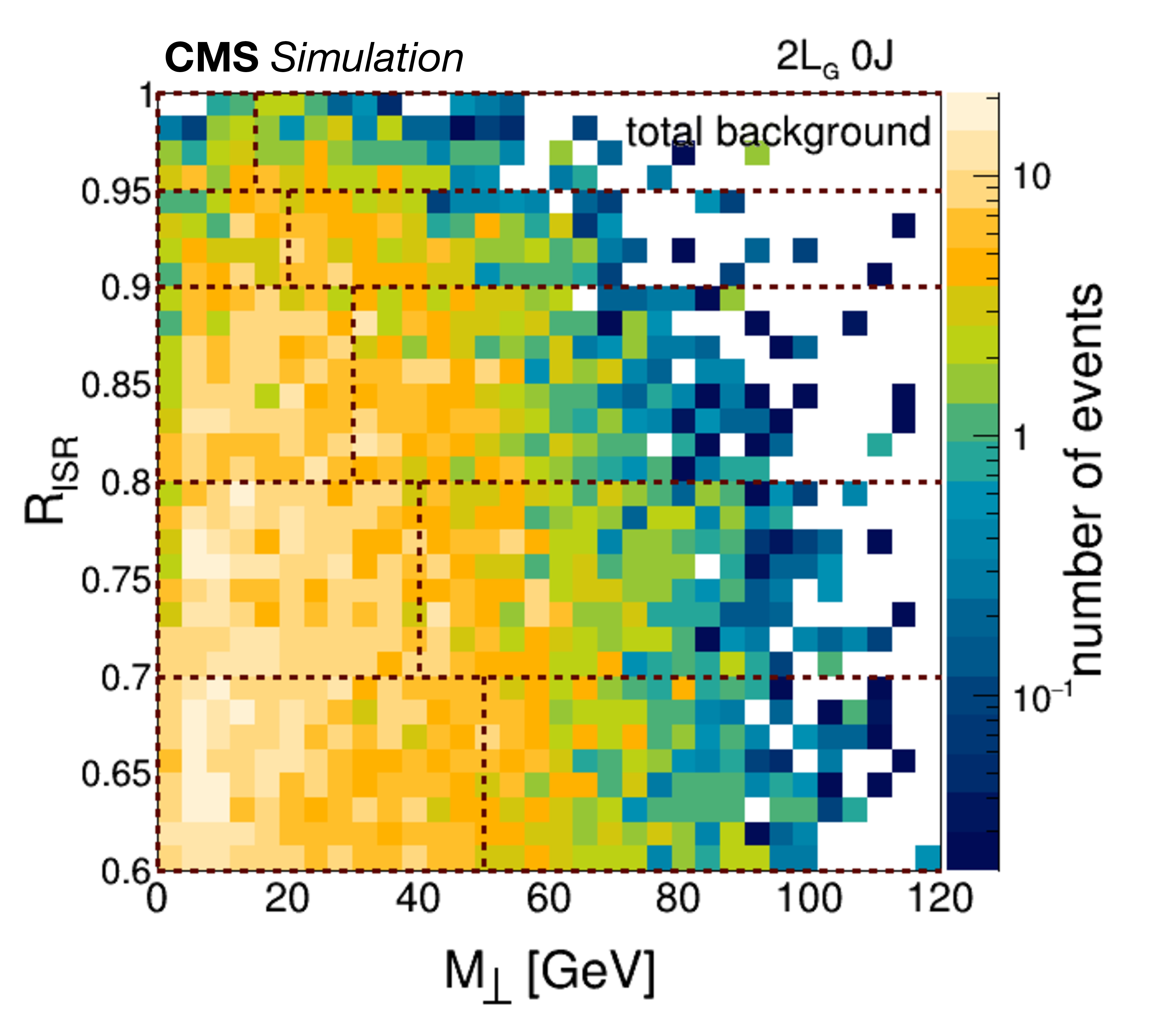
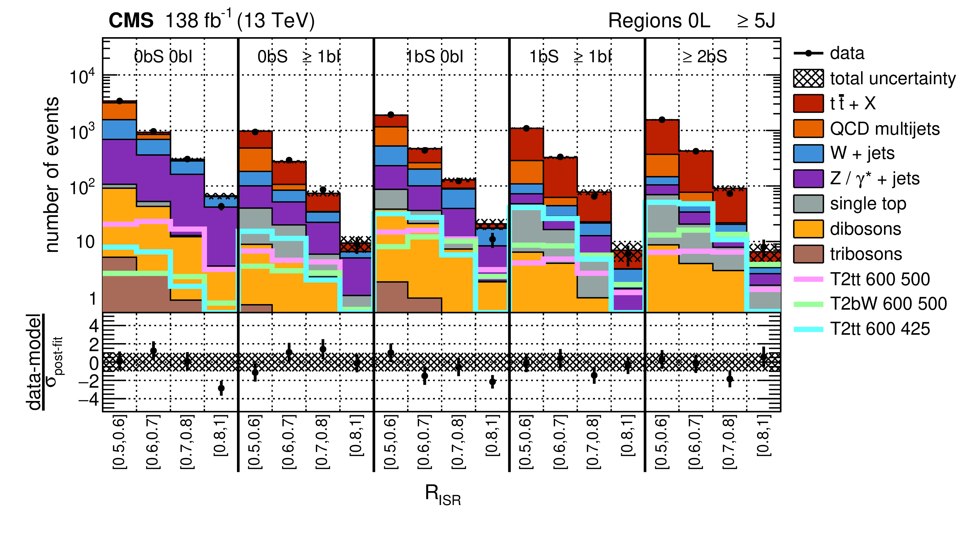
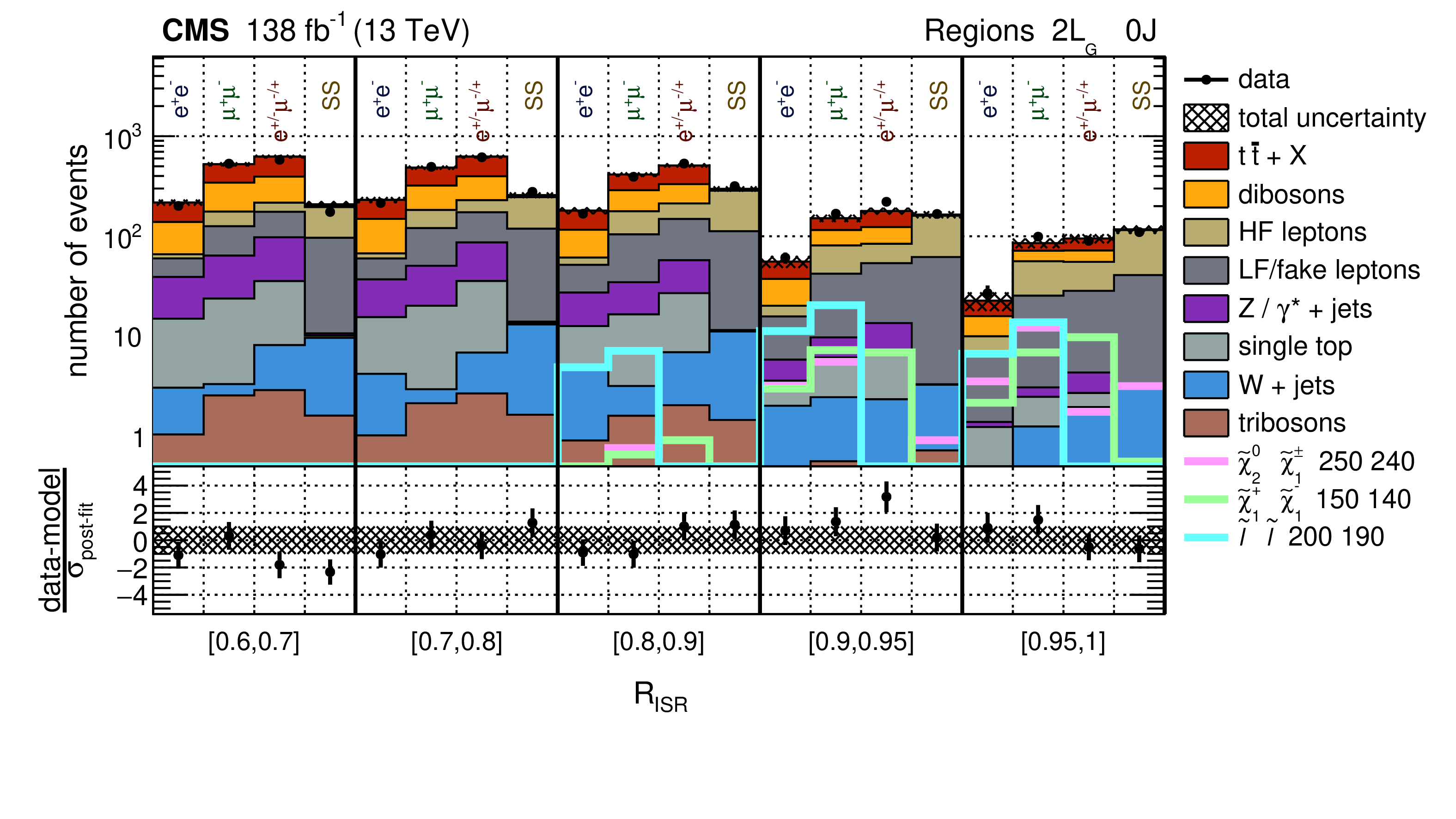
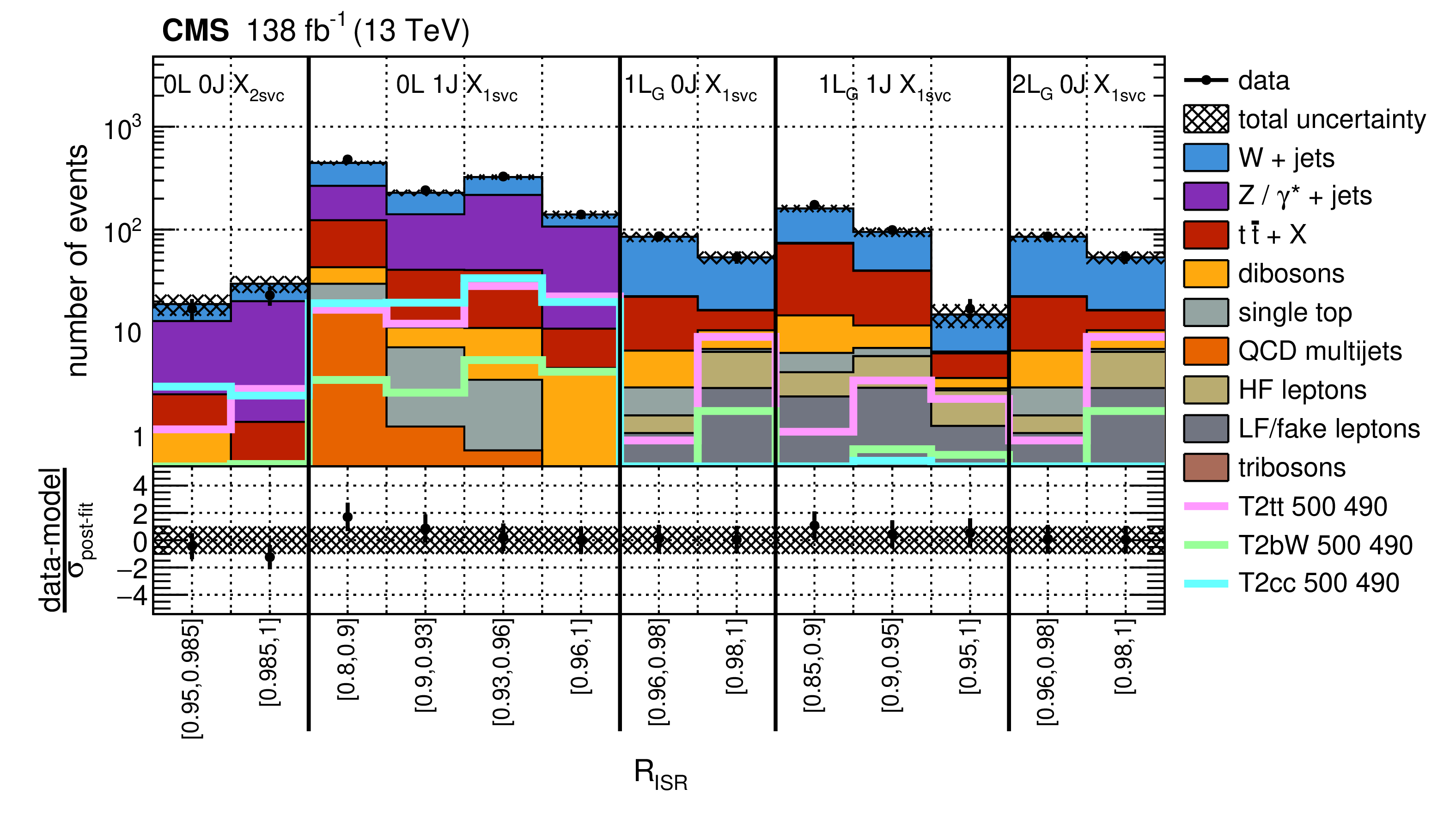
Figure 19:
Post-fit distributions of data with the background-only model for the full data set. (Upper) 2L 0J gold regions separated by lepton flavor and charge. (Lower) Central b-tagged SV regions in 0L, 1L, and 2L final states. Bins are split by $ R_{\mathrm{ISR}} $ with yields integrated over all other sub-categorizations and $ M_{\perp} $. The sub-panels below the panels show the data minus fit model scaled by the post-fit model uncertainty. Expected yields for example signal models are superimposed. |
png pdf |
Figure 19-a:
Post-fit distributions of data with the background-only model for the full data set. (Upper) 2L 0J gold regions separated by lepton flavor and charge. (Lower) Central b-tagged SV regions in 0L, 1L, and 2L final states. Bins are split by $ R_{\mathrm{ISR}} $ with yields integrated over all other sub-categorizations and $ M_{\perp} $. The sub-panels below the panels show the data minus fit model scaled by the post-fit model uncertainty. Expected yields for example signal models are superimposed. |
png pdf |
Figure 19-b:
Post-fit distributions of data with the background-only model for the full data set. (Upper) 2L 0J gold regions separated by lepton flavor and charge. (Lower) Central b-tagged SV regions in 0L, 1L, and 2L final states. Bins are split by $ R_{\mathrm{ISR}} $ with yields integrated over all other sub-categorizations and $ M_{\perp} $. The sub-panels below the panels show the data minus fit model scaled by the post-fit model uncertainty. Expected yields for example signal models are superimposed. |
png pdf |
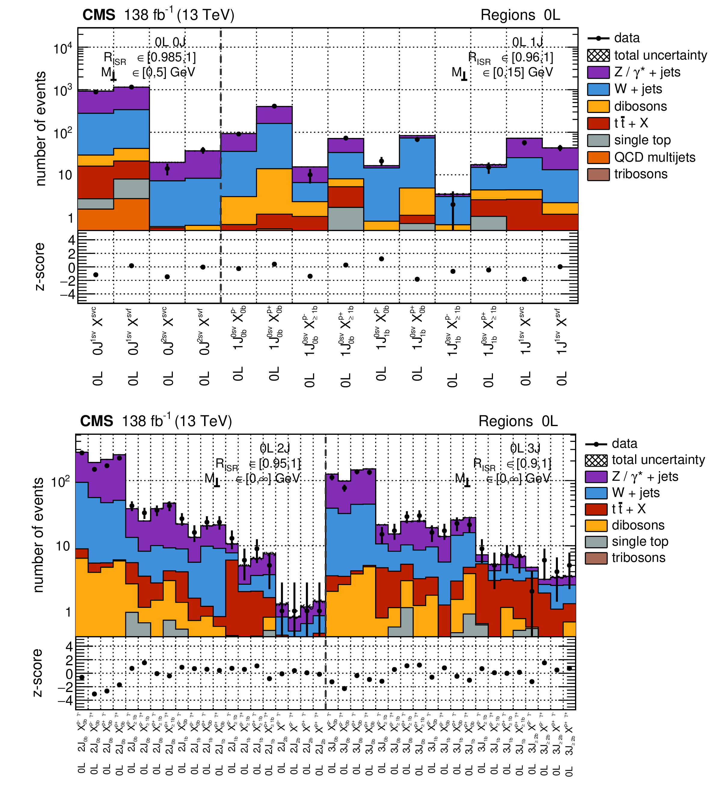
Figure 20:
Post-fit distributions of data with the background-only model for the full data set for the highest $ R_{\mathrm{ISR}} $ bin in each analysis category. (Upper) 0L 0J and 1J regions. (Lower) 0L 2J and 3J regions. The sub-panels below the panels indicate the post-fit z-score for each bin. |
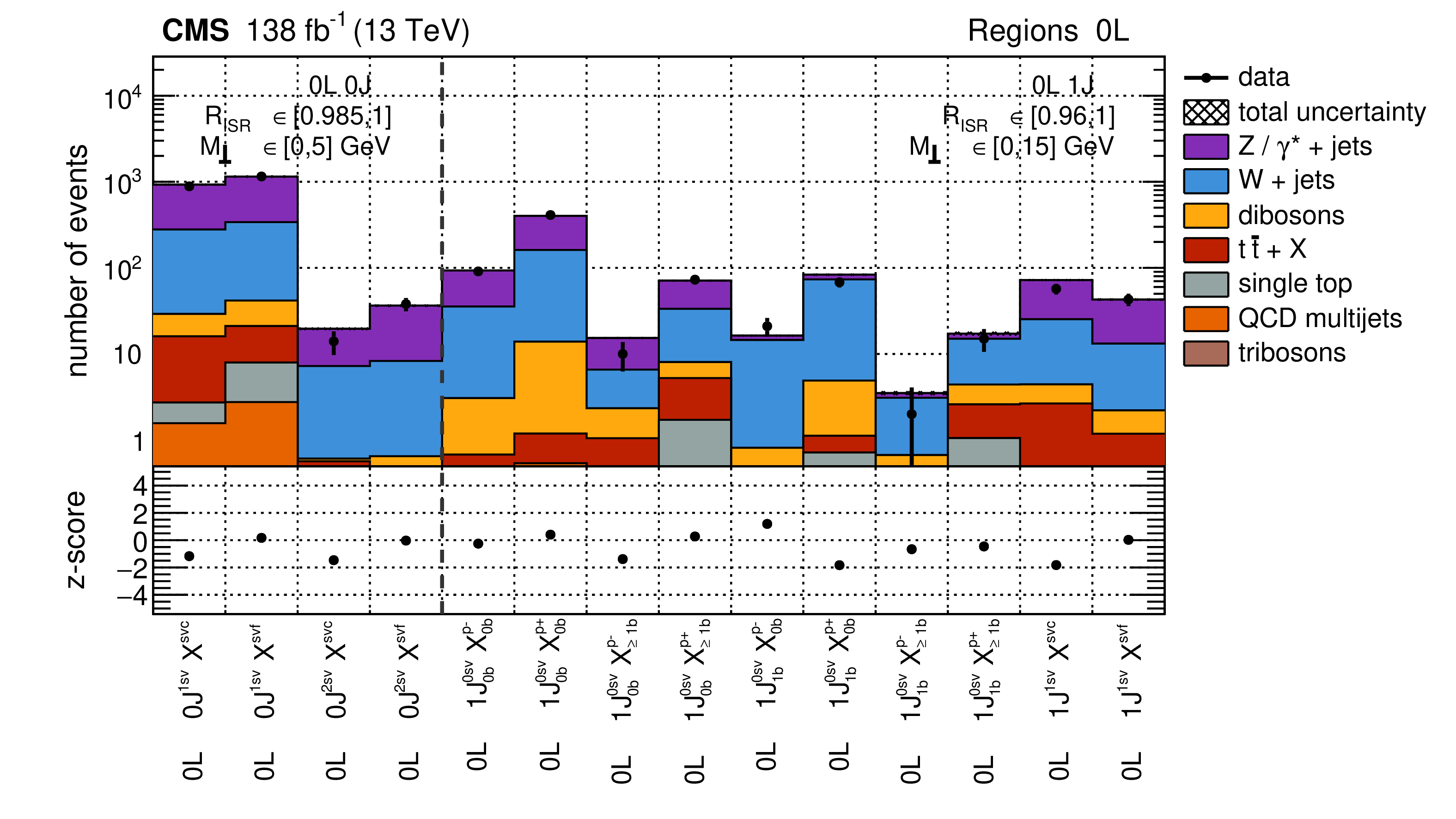
png pdf |
Figure 20-a:
Post-fit distributions of data with the background-only model for the full data set for the highest $ R_{\mathrm{ISR}} $ bin in each analysis category. (Upper) 0L 0J and 1J regions. (Lower) 0L 2J and 3J regions. The sub-panels below the panels indicate the post-fit z-score for each bin. |
png pdf |
Figure 20-b:
Post-fit distributions of data with the background-only model for the full data set for the highest $ R_{\mathrm{ISR}} $ bin in each analysis category. (Upper) 0L 0J and 1J regions. (Lower) 0L 2J and 3J regions. The sub-panels below the panels indicate the post-fit z-score for each bin. |
png pdf |
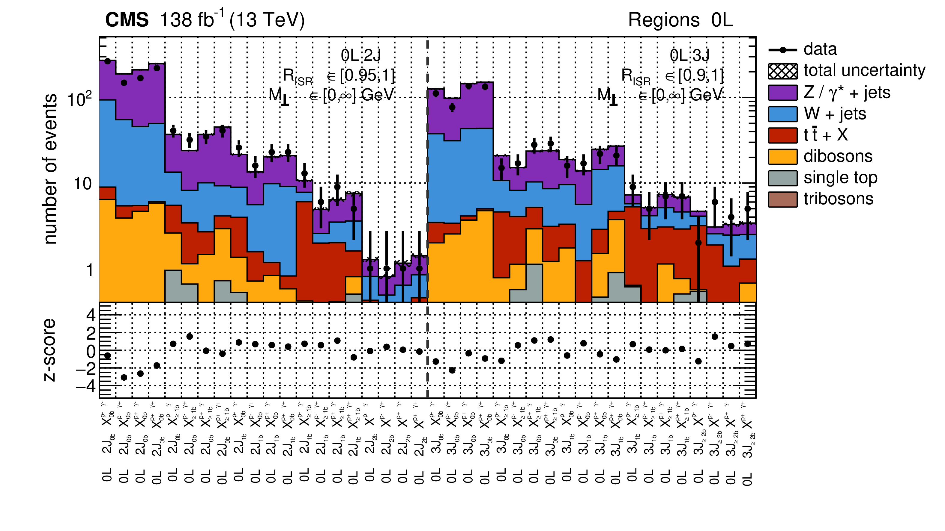
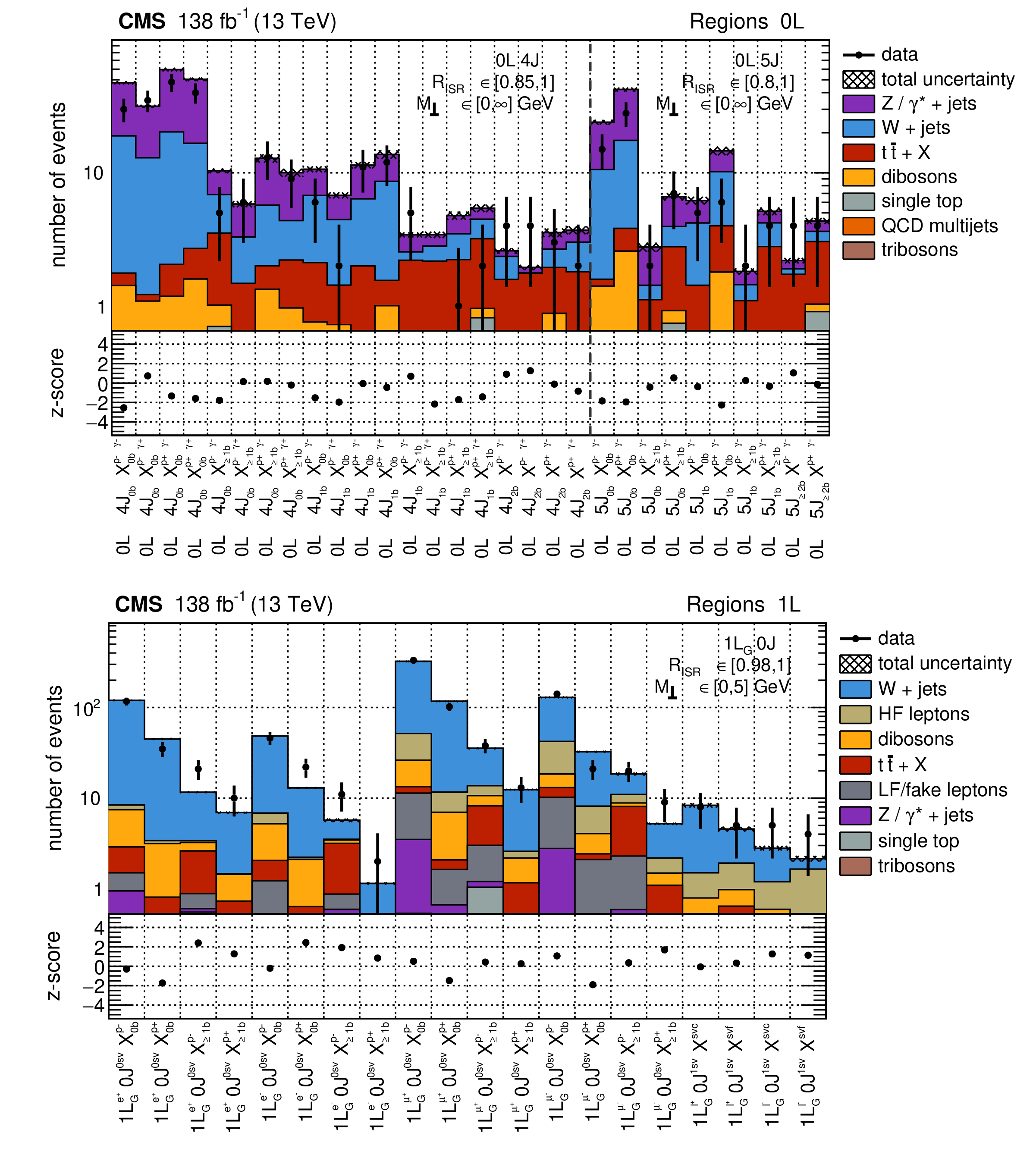
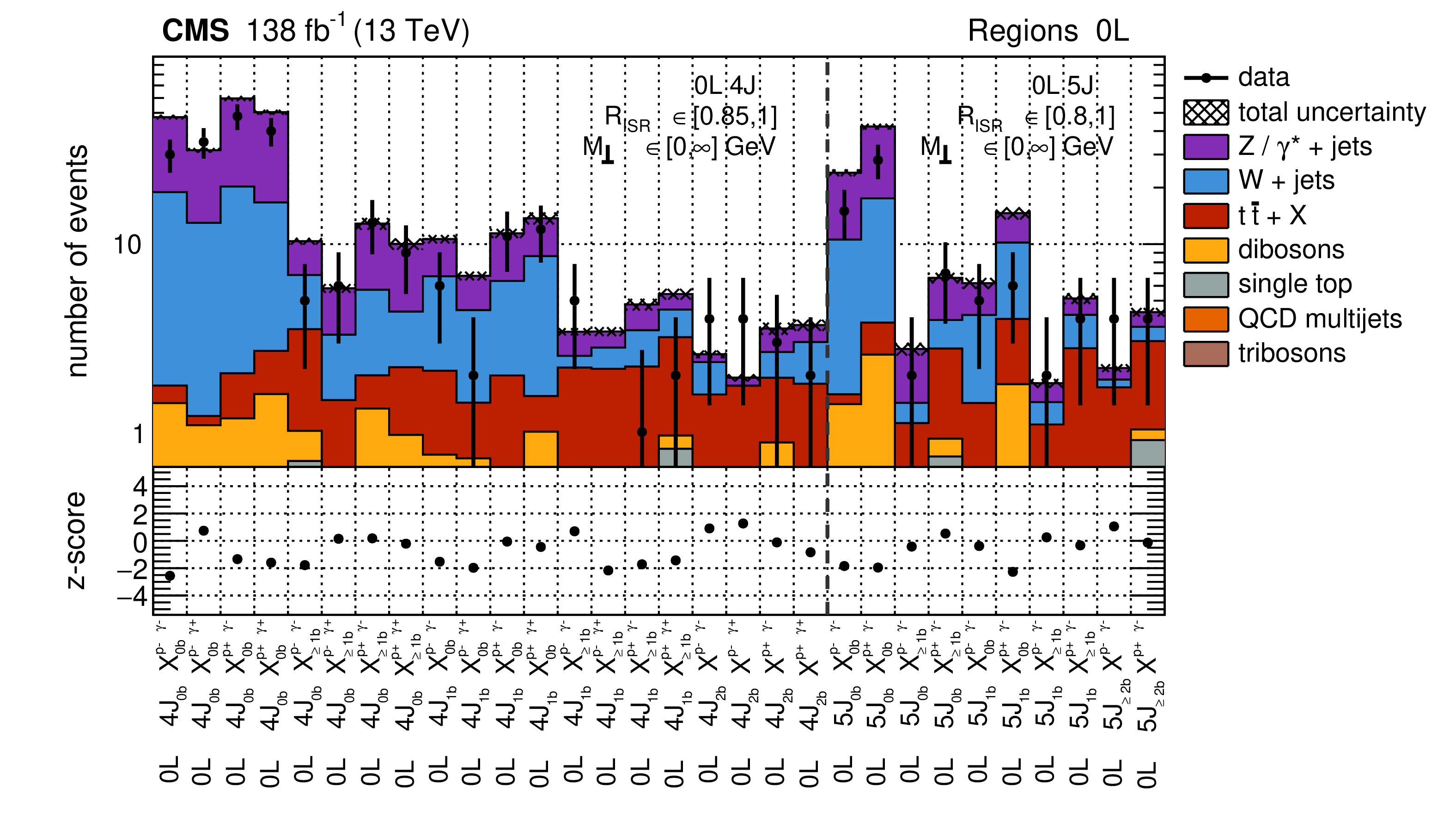
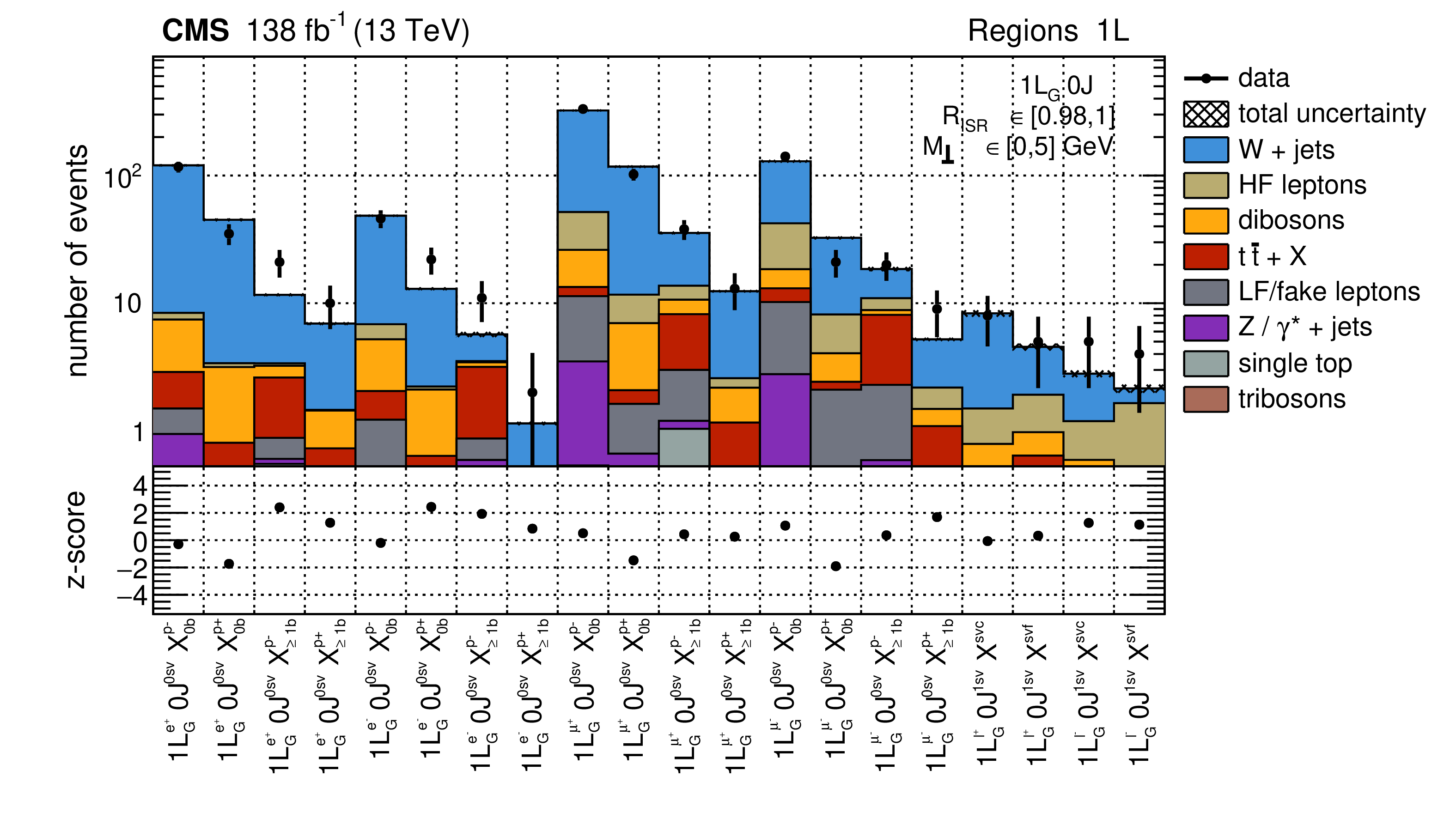
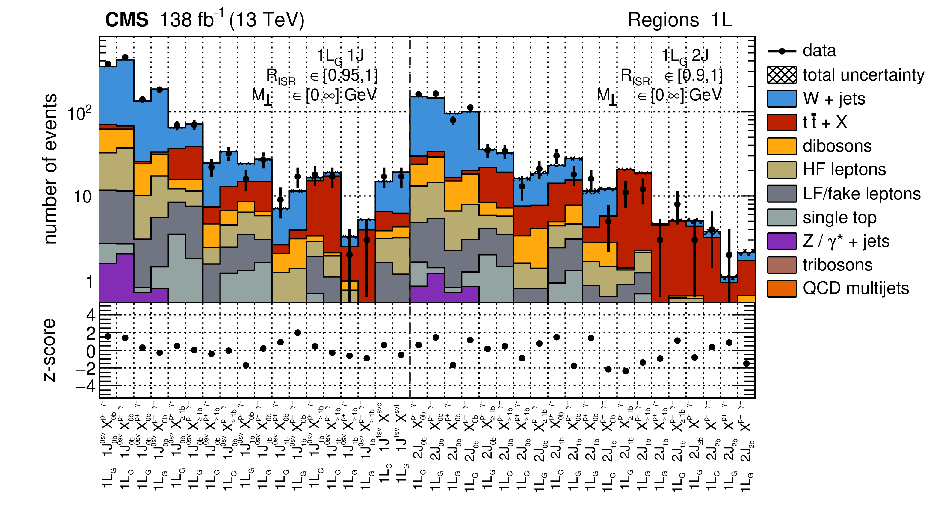
Figure 21:
Post-fit distributions of data with the background-only model for the full data set for the highest $ R_{\mathrm{ISR}} $ bin in each analysis category. (Upper) 0L 4J and $ \ge $5J regions. (Lower) 1L 0J regions with a gold lepton. The sub-panels below the panels indicate the post-fit z-score for each bin. |
png pdf |
Figure 21-a:
Post-fit distributions of data with the background-only model for the full data set for the highest $ R_{\mathrm{ISR}} $ bin in each analysis category. (Upper) 0L 4J and $ \ge $5J regions. (Lower) 1L 0J regions with a gold lepton. The sub-panels below the panels indicate the post-fit z-score for each bin. |
png pdf |
Figure 21-b:
Post-fit distributions of data with the background-only model for the full data set for the highest $ R_{\mathrm{ISR}} $ bin in each analysis category. (Upper) 0L 4J and $ \ge $5J regions. (Lower) 1L 0J regions with a gold lepton. The sub-panels below the panels indicate the post-fit z-score for each bin. |
png pdf |
Figure 22:
Post-fit distributions of data with the background-only model for the full data set for the highest $ R_{\mathrm{ISR}} $ bin in each analysis category. (Upper) 1L 1J and 2J regions with a gold lepton. (Lower) 1L 3J and $ \ge $4J regions with a gold lepton. The sub-panels below the panels indicate the post-fit z-score for each bin. |
png pdf |
Figure 22-a:
Post-fit distributions of data with the background-only model for the full data set for the highest $ R_{\mathrm{ISR}} $ bin in each analysis category. (Upper) 1L 1J and 2J regions with a gold lepton. (Lower) 1L 3J and $ \ge $4J regions with a gold lepton. The sub-panels below the panels indicate the post-fit z-score for each bin. |
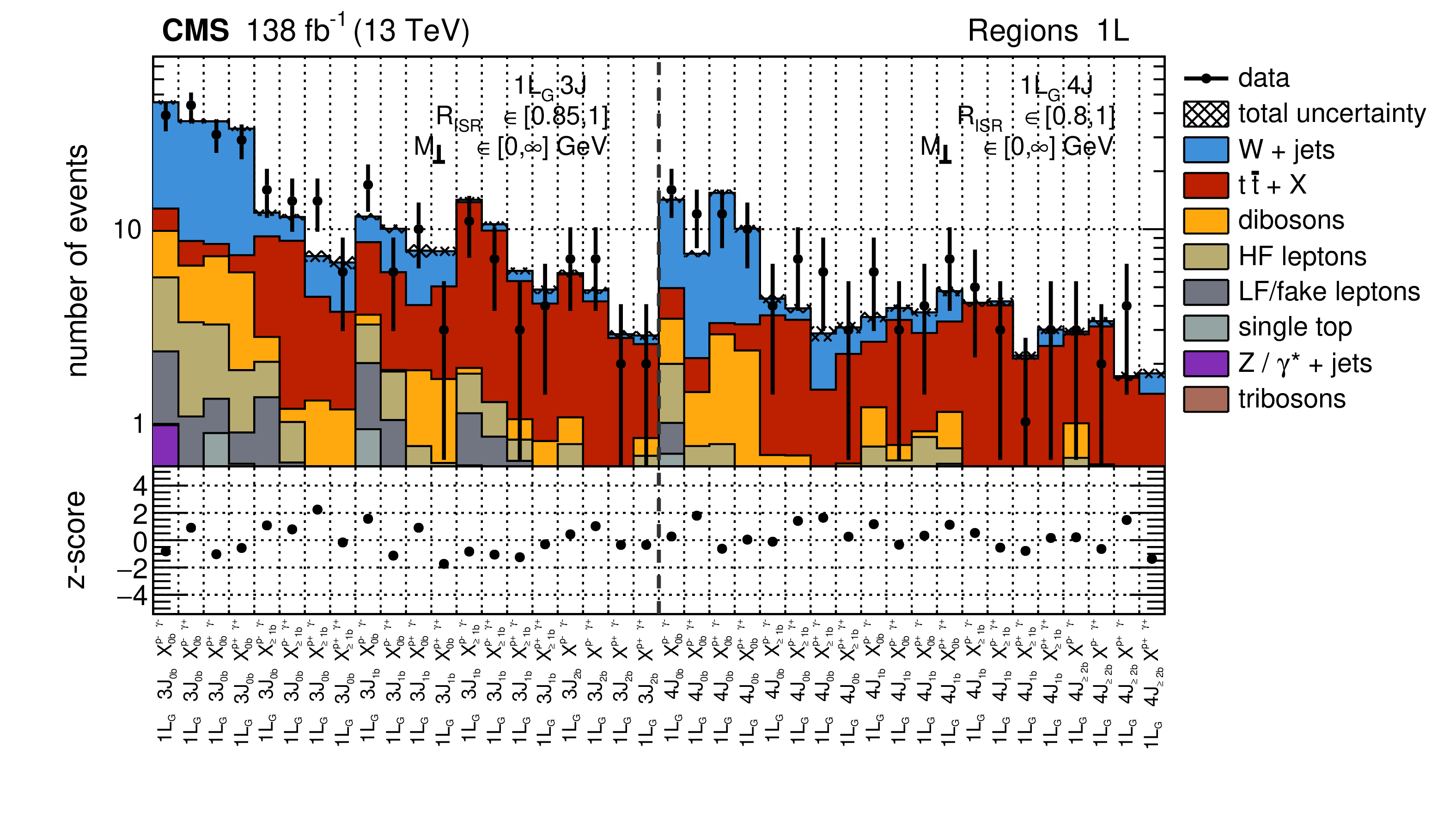
png pdf |
Figure 22-b:
Post-fit distributions of data with the background-only model for the full data set for the highest $ R_{\mathrm{ISR}} $ bin in each analysis category. (Upper) 1L 1J and 2J regions with a gold lepton. (Lower) 1L 3J and $ \ge $4J regions with a gold lepton. The sub-panels below the panels indicate the post-fit z-score for each bin. |
png pdf |
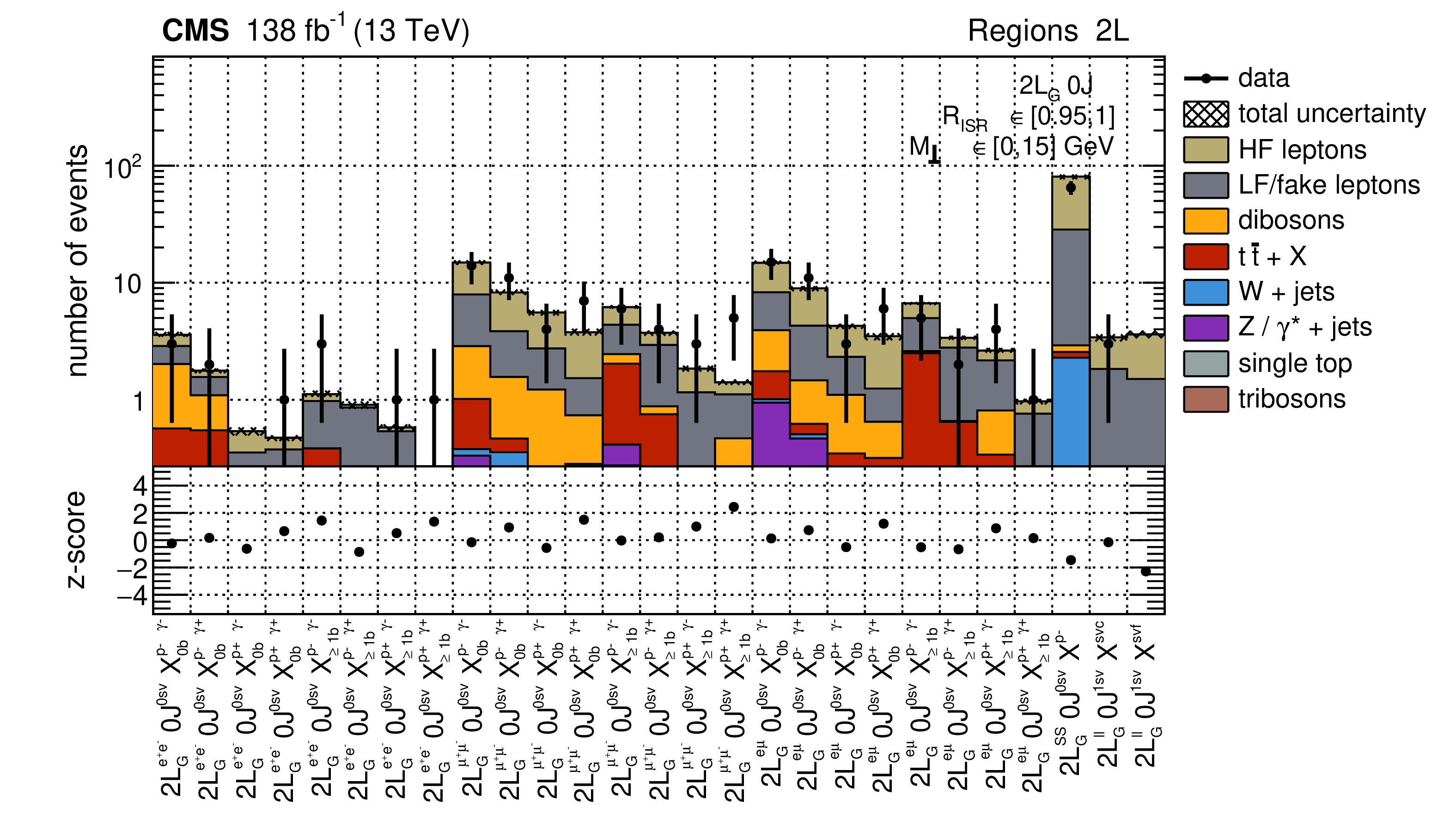
Figure 23:
Post-fit distributions of data with the background-only model for the full data set for the highest $ R_{\mathrm{ISR}} $ bin in each analysis category of the 2L 0J regions with gold leptons. The sub-panels below the panels indicate the post-fit z-score for each bin. |
png pdf |
Figure 24:
Post-fit distributions of data with the background-only model for the full data set for the highest $ R_{\mathrm{ISR}} $ bin in each analysis category. (Upper) 2L 1J regions with gold leptons. (Lower) 2L $ \ge $2J regions with gold leptons. The sub-panels below the panels indicate the post-fit z-score for each bin. |
png pdf |
Figure 24-a:
Post-fit distributions of data with the background-only model for the full data set for the highest $ R_{\mathrm{ISR}} $ bin in each analysis category. (Upper) 2L 1J regions with gold leptons. (Lower) 2L $ \ge $2J regions with gold leptons. The sub-panels below the panels indicate the post-fit z-score for each bin. |
png pdf |
Figure 24-b:
Post-fit distributions of data with the background-only model for the full data set for the highest $ R_{\mathrm{ISR}} $ bin in each analysis category. (Upper) 2L 1J regions with gold leptons. (Lower) 2L $ \ge $2J regions with gold leptons. The sub-panels below the panels indicate the post-fit z-score for each bin. |
png pdf |
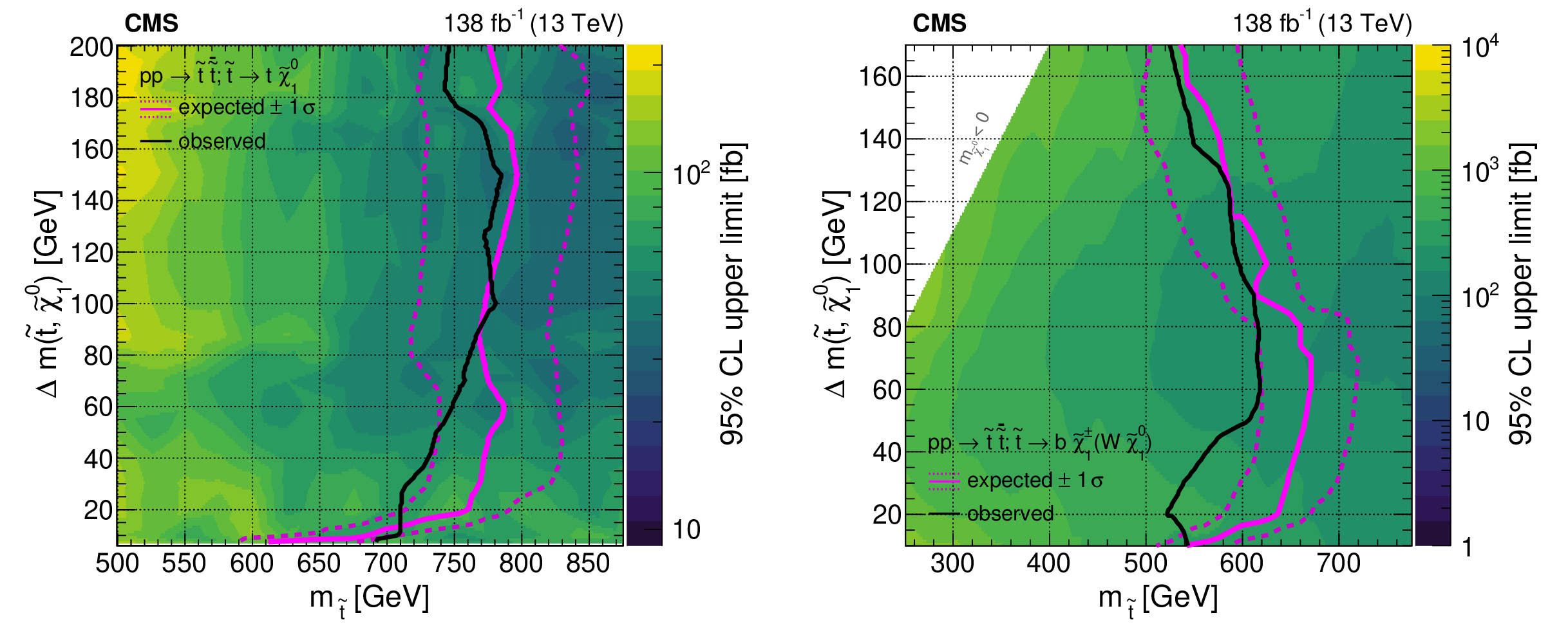
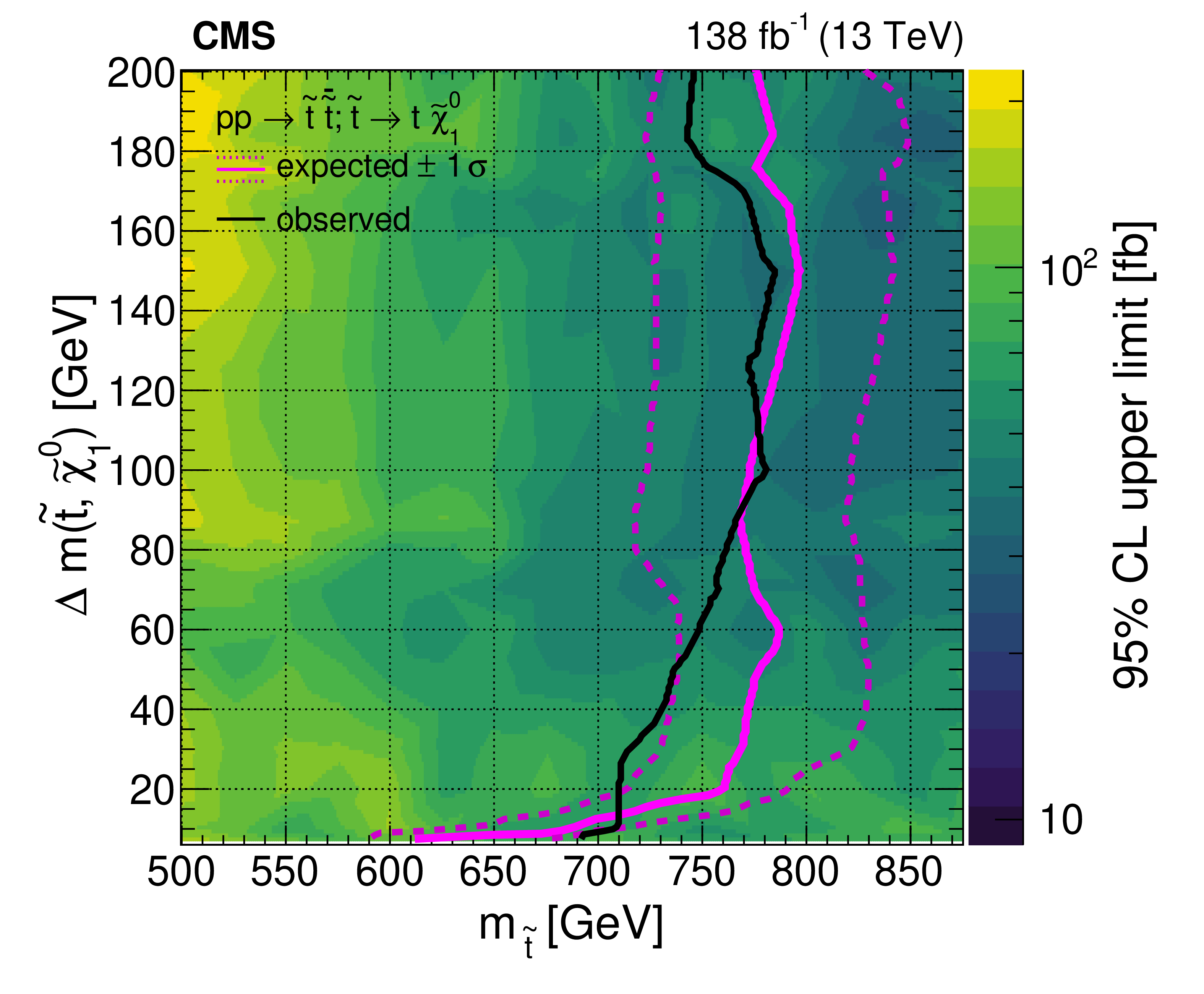
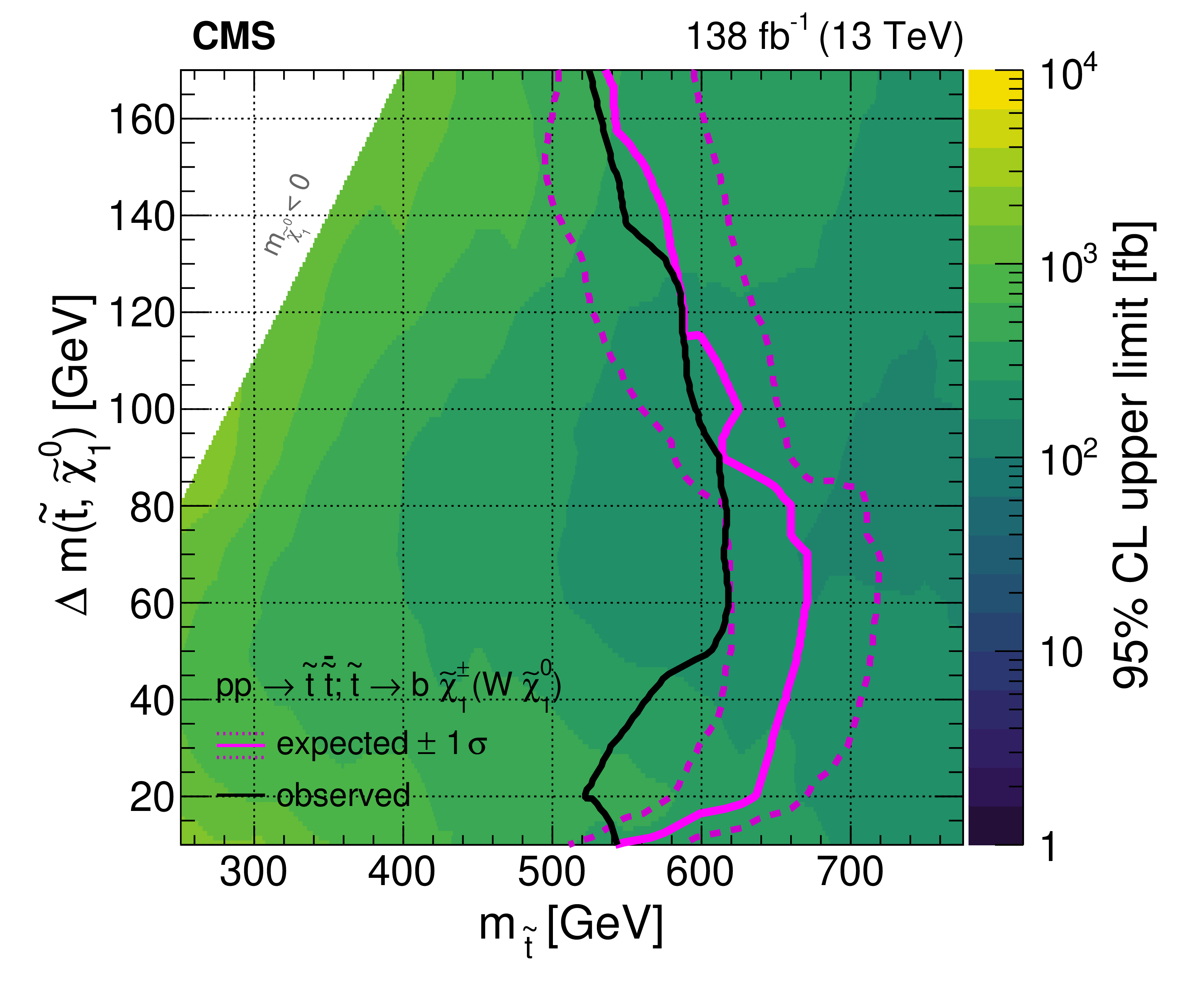
Figure 25:
Top squark pair production. Observed upper limits at 95% CL on the product of the cross section and relevant branching fractions are shown using the color scale where the $ \tilde{\mathrm{t}} $ mass is on the $ x $-axis and the mass difference between the $ \tilde{\mathrm{t}} $ and the LSP is on the $ y $-axis. The expected lower mass limits (magenta line) together with their $ \pm 1\sigma $ uncertainties (magenta dashed lines) and the observed lower mass limits (black line) are indicated for 100% branching fractions. The left panel shows the results for the T2tt model with limits on $ \sigma (\tilde{\mathrm{t}} \overline{\tilde{\mathrm{t}}}) \mathcal{B}^{2} (\tilde{\mathrm{t}} \to \mathrm{t} \tilde{\chi}_{1}^{0}) $. The right panel shows the results for the T2bW model with limits on $ \sigma (\tilde{\mathrm{t}} \overline{\tilde{\mathrm{t}}}) \mathcal{B}^{2} (\tilde{\mathrm{t}} \to \mathrm{b} \tilde{\chi}_{1}^{+}) \mathcal{B}^{2} ( \tilde{\chi}_{1}^{+}\to\mathrm{W^+} \tilde{\chi}_{1}^{0} ) $. |
png pdf |
Figure 25-a:
Top squark pair production. Observed upper limits at 95% CL on the product of the cross section and relevant branching fractions are shown using the color scale where the $ \tilde{\mathrm{t}} $ mass is on the $ x $-axis and the mass difference between the $ \tilde{\mathrm{t}} $ and the LSP is on the $ y $-axis. The expected lower mass limits (magenta line) together with their $ \pm 1\sigma $ uncertainties (magenta dashed lines) and the observed lower mass limits (black line) are indicated for 100% branching fractions. The left panel shows the results for the T2tt model with limits on $ \sigma (\tilde{\mathrm{t}} \overline{\tilde{\mathrm{t}}}) \mathcal{B}^{2} (\tilde{\mathrm{t}} \to \mathrm{t} \tilde{\chi}_{1}^{0}) $. The right panel shows the results for the T2bW model with limits on $ \sigma (\tilde{\mathrm{t}} \overline{\tilde{\mathrm{t}}}) \mathcal{B}^{2} (\tilde{\mathrm{t}} \to \mathrm{b} \tilde{\chi}_{1}^{+}) \mathcal{B}^{2} ( \tilde{\chi}_{1}^{+}\to\mathrm{W^+} \tilde{\chi}_{1}^{0} ) $. |
png pdf |
Figure 25-b:
Top squark pair production. Observed upper limits at 95% CL on the product of the cross section and relevant branching fractions are shown using the color scale where the $ \tilde{\mathrm{t}} $ mass is on the $ x $-axis and the mass difference between the $ \tilde{\mathrm{t}} $ and the LSP is on the $ y $-axis. The expected lower mass limits (magenta line) together with their $ \pm 1\sigma $ uncertainties (magenta dashed lines) and the observed lower mass limits (black line) are indicated for 100% branching fractions. The left panel shows the results for the T2tt model with limits on $ \sigma (\tilde{\mathrm{t}} \overline{\tilde{\mathrm{t}}}) \mathcal{B}^{2} (\tilde{\mathrm{t}} \to \mathrm{t} \tilde{\chi}_{1}^{0}) $. The right panel shows the results for the T2bW model with limits on $ \sigma (\tilde{\mathrm{t}} \overline{\tilde{\mathrm{t}}}) \mathcal{B}^{2} (\tilde{\mathrm{t}} \to \mathrm{b} \tilde{\chi}_{1}^{+}) \mathcal{B}^{2} ( \tilde{\chi}_{1}^{+}\to\mathrm{W^+} \tilde{\chi}_{1}^{0} ) $. |
png pdf |
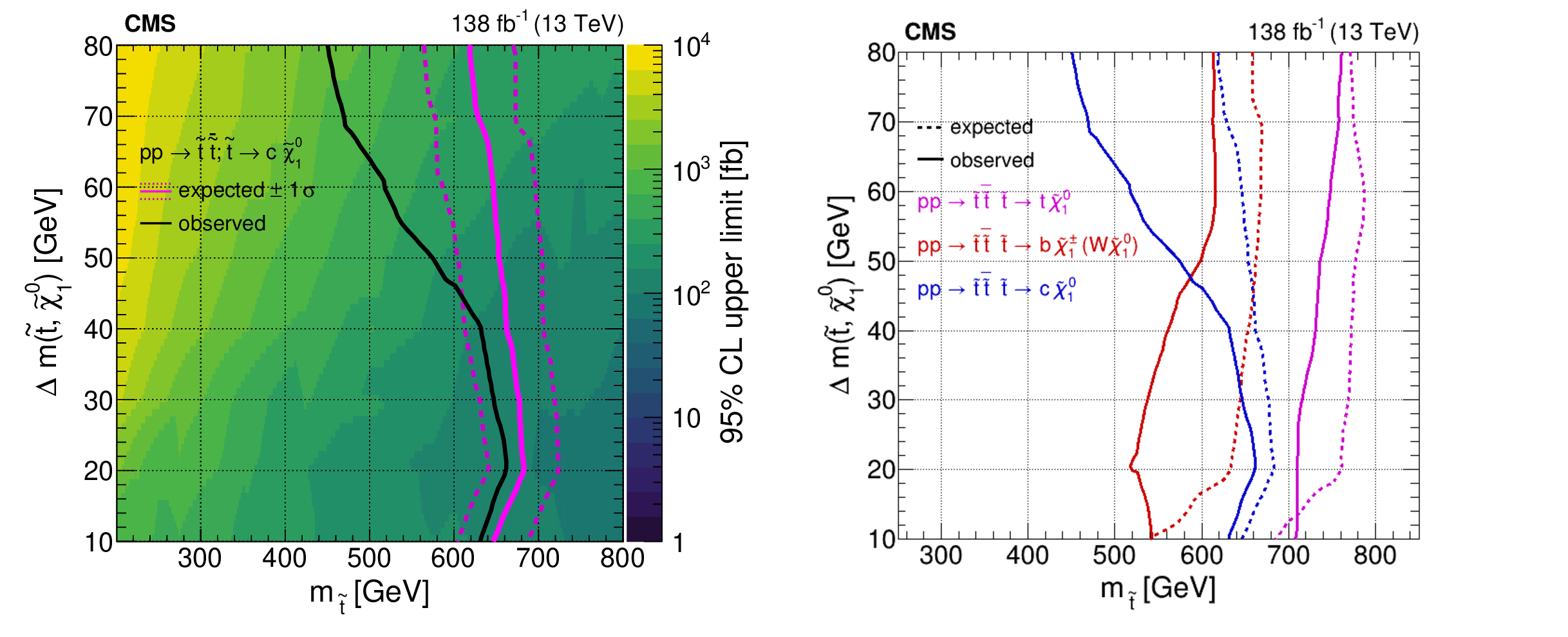
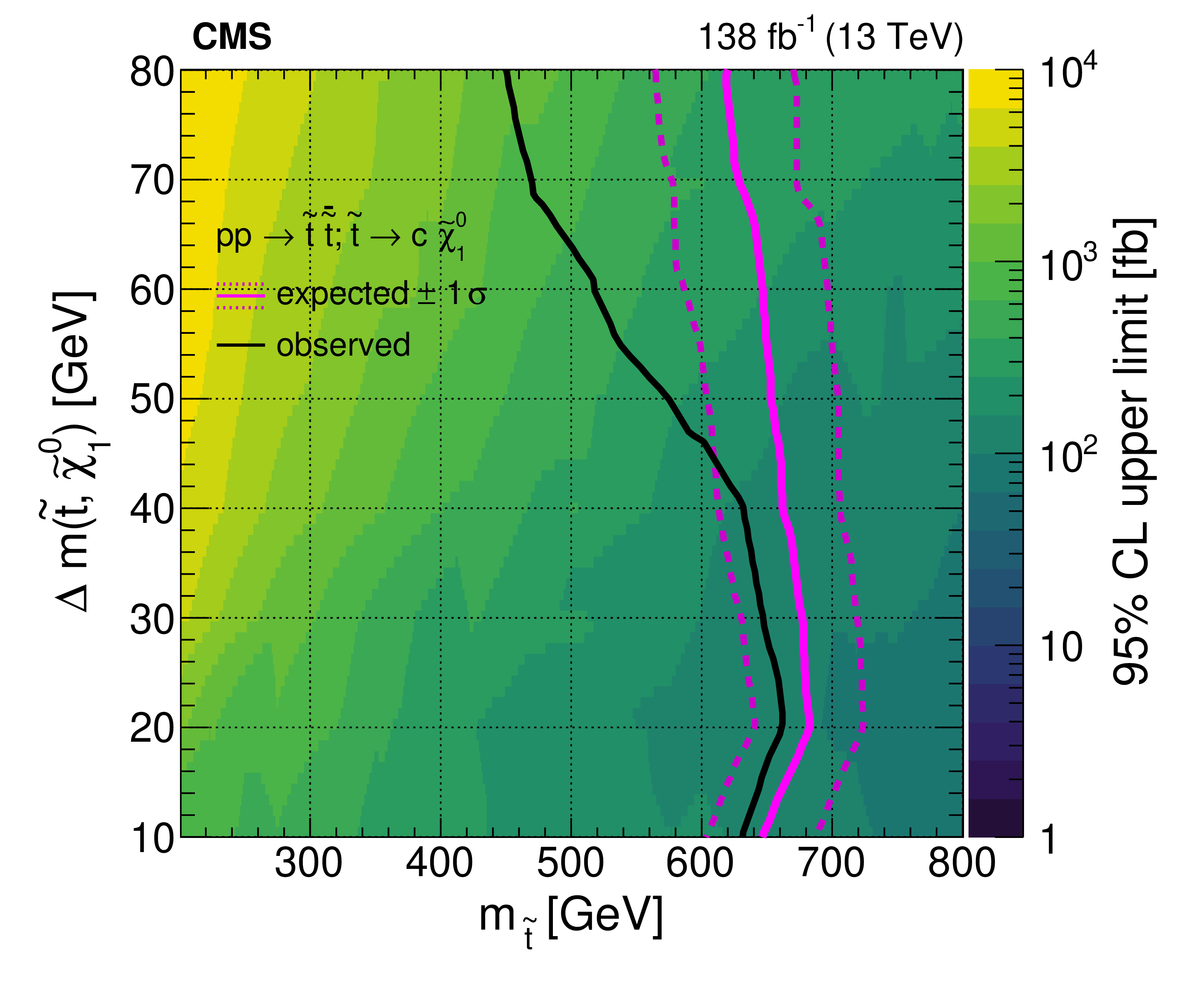
Figure 26:
Top squark pair production. Observed upper limits at 95% CL on the product of the cross section and branching fraction squared, $ \sigma (\tilde{\mathrm{t}} \overline{\tilde{\mathrm{t}}}) \mathcal{B}^{2} (\tilde{\mathrm{t}}\to\mathrm{c} \tilde{\chi}_{1}^{0} ) $ (left), are shown using the color scale where the $ \tilde{\mathrm{t}} $ mass is on the $ x $-axis and the mass difference between the $ \tilde{\mathrm{t}} $ and the LSP is on the $ y $-axis. The expected lower mass limits (magenta line) together with their $ \pm 1\sigma $ uncertainties (magenta dashed lines) and the observed lower mass limits (black line) are indicated for 100% branching fractions. Observed and median expected limits for top squark pair production at 95% CL (right) for the three decay modes investigated. |
png pdf |
Figure 26-a:
Top squark pair production. Observed upper limits at 95% CL on the product of the cross section and branching fraction squared, $ \sigma (\tilde{\mathrm{t}} \overline{\tilde{\mathrm{t}}}) \mathcal{B}^{2} (\tilde{\mathrm{t}}\to\mathrm{c} \tilde{\chi}_{1}^{0} ) $ (left), are shown using the color scale where the $ \tilde{\mathrm{t}} $ mass is on the $ x $-axis and the mass difference between the $ \tilde{\mathrm{t}} $ and the LSP is on the $ y $-axis. The expected lower mass limits (magenta line) together with their $ \pm 1\sigma $ uncertainties (magenta dashed lines) and the observed lower mass limits (black line) are indicated for 100% branching fractions. Observed and median expected limits for top squark pair production at 95% CL (right) for the three decay modes investigated. |
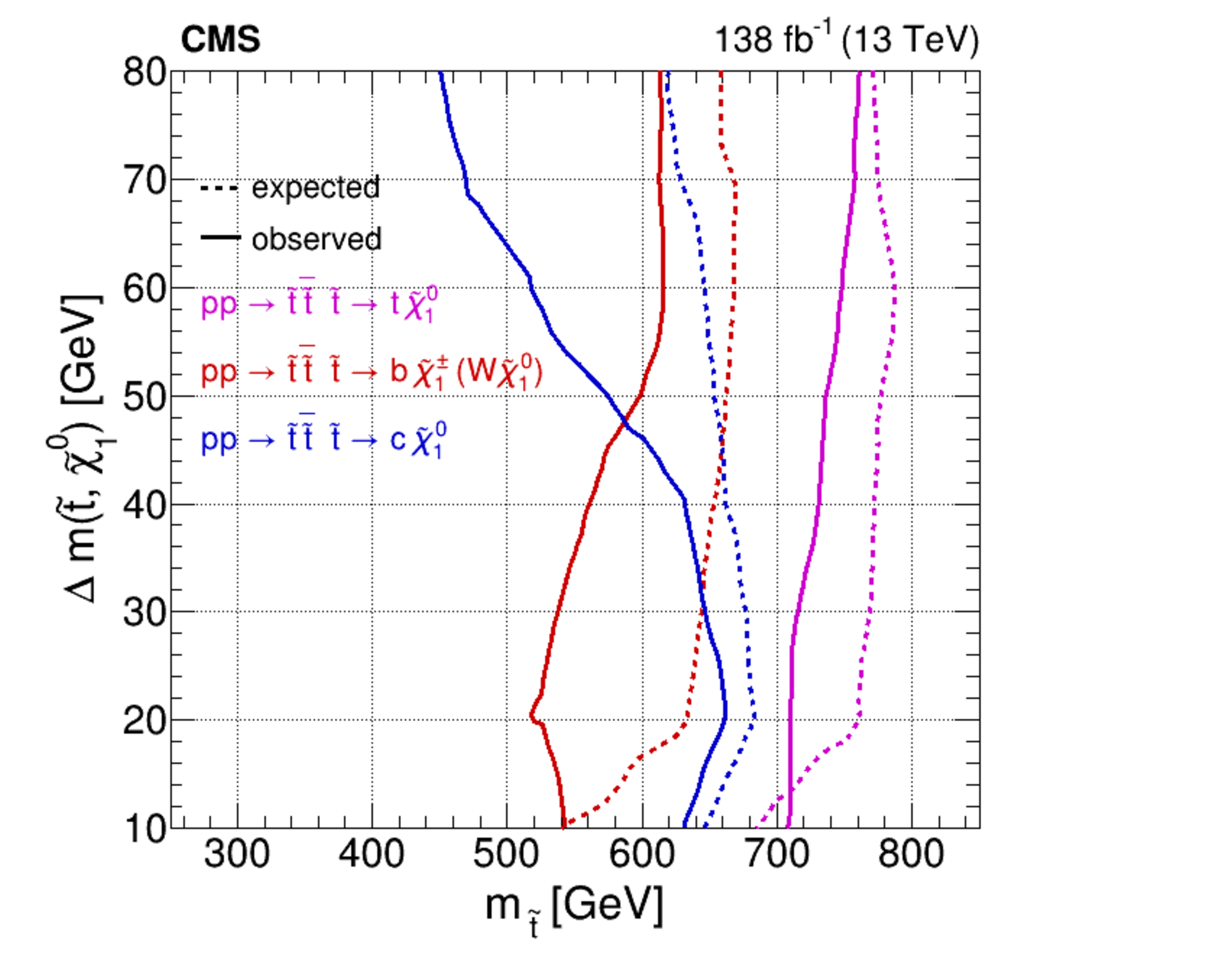
png pdf |
Figure 26-b:
Top squark pair production. Observed upper limits at 95% CL on the product of the cross section and branching fraction squared, $ \sigma (\tilde{\mathrm{t}} \overline{\tilde{\mathrm{t}}}) \mathcal{B}^{2} (\tilde{\mathrm{t}}\to\mathrm{c} \tilde{\chi}_{1}^{0} ) $ (left), are shown using the color scale where the $ \tilde{\mathrm{t}} $ mass is on the $ x $-axis and the mass difference between the $ \tilde{\mathrm{t}} $ and the LSP is on the $ y $-axis. The expected lower mass limits (magenta line) together with their $ \pm 1\sigma $ uncertainties (magenta dashed lines) and the observed lower mass limits (black line) are indicated for 100% branching fractions. Observed and median expected limits for top squark pair production at 95% CL (right) for the three decay modes investigated. |
png pdf |
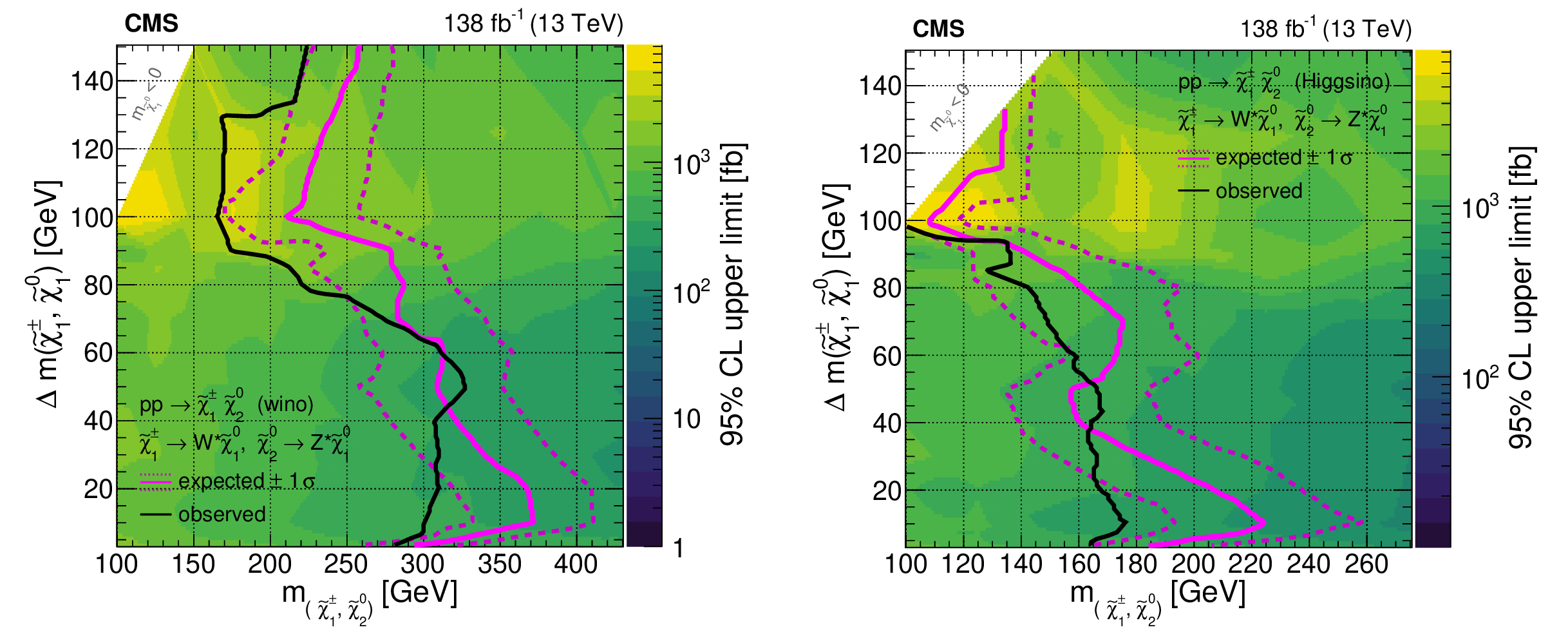
Figure 27:
Chargino-neutralino production. Observed upper limits at 95% CL on the product of the cross section and the two branching fractions, $ \sigma (\tilde{\chi}_{1}^{\pm} \tilde{\chi}_{2}^{0}) \mathcal{B} ( \tilde{\chi}_{1}^{\pm} \to \mathrm{W}^{\pm} \tilde{\chi}_{1}^{0} ) \mathcal{B} ( \tilde{\chi}_{2}^{0} \to \mathrm{Z} \tilde{\chi}_{1}^{0} ) $, are shown using the color scale where the $ \tilde{\chi}_{1}^{\pm}/\tilde{\chi}_{2}^{0} $ mass is on the $ x $-axis and the mass difference between the $ \tilde{\chi}_{1}^{\pm}/\tilde{\chi}_{2}^{0} $ and the LSP is on the $ y $-axis. For these results, based on the TChiWZ simplified model, the $ \tilde{\chi}_{1}^{\pm} $ and $ \tilde{\chi}_{2}^{0} $ masses are set equal. The expected lower mass limits (magenta line) together with their $ \pm 1\sigma $ uncertainties (magenta dashed lines) and the observed lower mass limits (black line) are indicated for 100% branching fractions for wino-like cross-sections (left) and for higgsino-like cross-sections (right). |
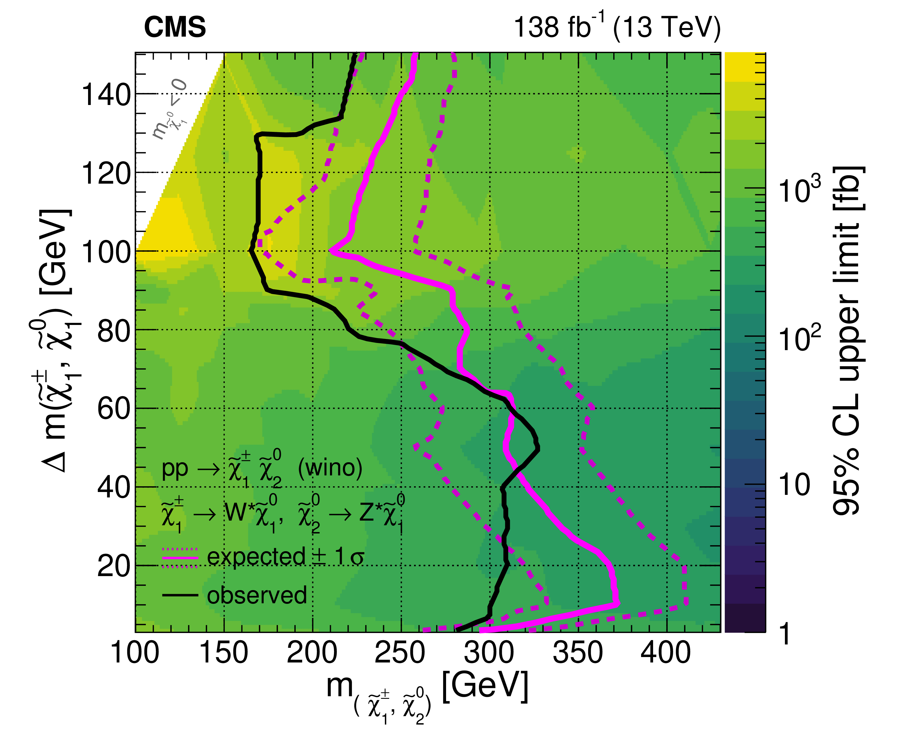
png pdf |
Figure 27-a:
Chargino-neutralino production. Observed upper limits at 95% CL on the product of the cross section and the two branching fractions, $ \sigma (\tilde{\chi}_{1}^{\pm} \tilde{\chi}_{2}^{0}) \mathcal{B} ( \tilde{\chi}_{1}^{\pm} \to \mathrm{W}^{\pm} \tilde{\chi}_{1}^{0} ) \mathcal{B} ( \tilde{\chi}_{2}^{0} \to \mathrm{Z} \tilde{\chi}_{1}^{0} ) $, are shown using the color scale where the $ \tilde{\chi}_{1}^{\pm}/\tilde{\chi}_{2}^{0} $ mass is on the $ x $-axis and the mass difference between the $ \tilde{\chi}_{1}^{\pm}/\tilde{\chi}_{2}^{0} $ and the LSP is on the $ y $-axis. For these results, based on the TChiWZ simplified model, the $ \tilde{\chi}_{1}^{\pm} $ and $ \tilde{\chi}_{2}^{0} $ masses are set equal. The expected lower mass limits (magenta line) together with their $ \pm 1\sigma $ uncertainties (magenta dashed lines) and the observed lower mass limits (black line) are indicated for 100% branching fractions for wino-like cross-sections (left) and for higgsino-like cross-sections (right). |
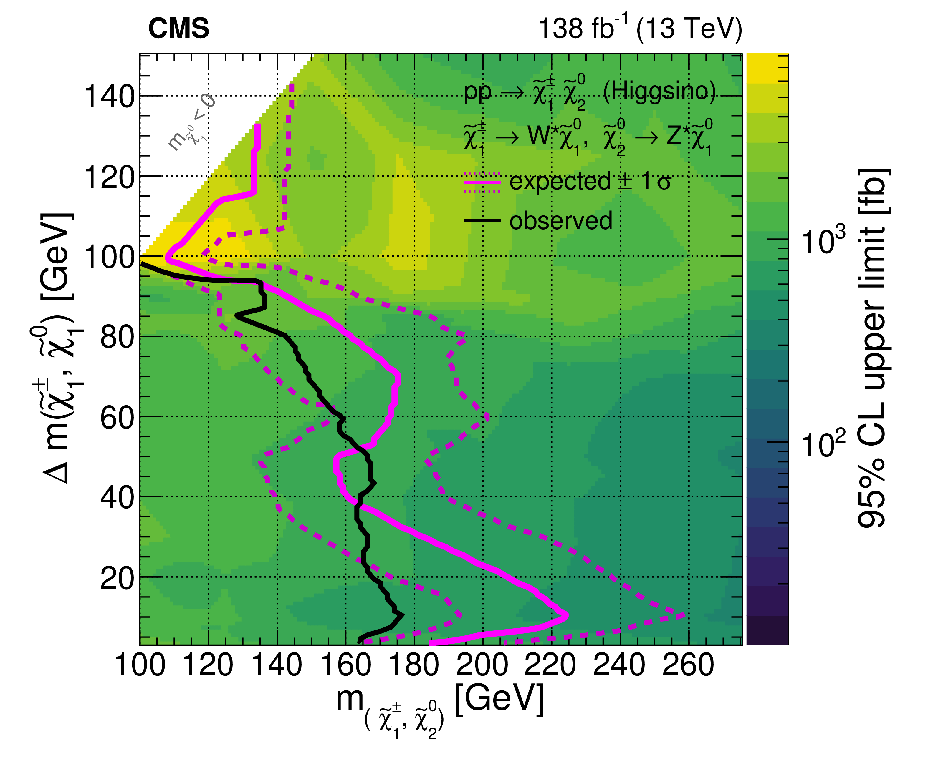
png pdf |
Figure 27-b:
Chargino-neutralino production. Observed upper limits at 95% CL on the product of the cross section and the two branching fractions, $ \sigma (\tilde{\chi}_{1}^{\pm} \tilde{\chi}_{2}^{0}) \mathcal{B} ( \tilde{\chi}_{1}^{\pm} \to \mathrm{W}^{\pm} \tilde{\chi}_{1}^{0} ) \mathcal{B} ( \tilde{\chi}_{2}^{0} \to \mathrm{Z} \tilde{\chi}_{1}^{0} ) $, are shown using the color scale where the $ \tilde{\chi}_{1}^{\pm}/\tilde{\chi}_{2}^{0} $ mass is on the $ x $-axis and the mass difference between the $ \tilde{\chi}_{1}^{\pm}/\tilde{\chi}_{2}^{0} $ and the LSP is on the $ y $-axis. For these results, based on the TChiWZ simplified model, the $ \tilde{\chi}_{1}^{\pm} $ and $ \tilde{\chi}_{2}^{0} $ masses are set equal. The expected lower mass limits (magenta line) together with their $ \pm 1\sigma $ uncertainties (magenta dashed lines) and the observed lower mass limits (black line) are indicated for 100% branching fractions for wino-like cross-sections (left) and for higgsino-like cross-sections (right). |
png pdf |
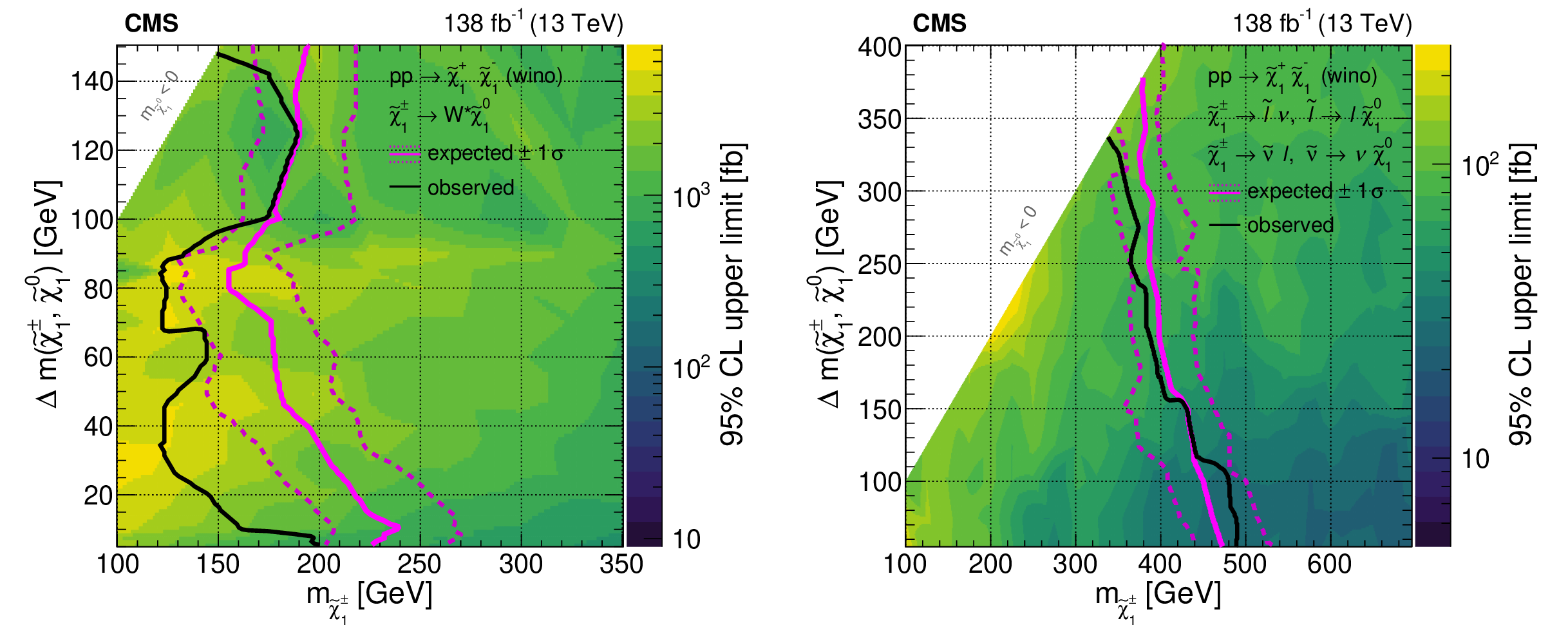
Figure 28:
Chargino pair production. The left panel shows the observed upper limits at 95% CL on the product of the cross section and the branching fraction squared, $ \sigma (\tilde{\chi}_{1}^{+} \tilde{\chi}_{1}^{-}) \mathcal{B}^{2} ( \tilde{\chi}_{1}^{\pm} \to \mathrm{W}^{\pm} \tilde{\chi}_{1}^{0} ) $ are shown using the color scale where the $ \tilde{\chi}_{1}^{\pm} $ mass is on the $ x $-axis and the mass difference between the $ \tilde{\chi}_{1}^{\pm} $ and the LSP is on the $ y $-axis. The expected lower mass limits (magenta line) together with their $ {\pm}1\sigma $ uncertainties (magenta dashed lines) and the observed lower mass limits (black line) are indicated for 100% branching fractions for wino-like cross-sections. The right panel shows the results for chargino pair production with decays as in the TChiSlepSnu model with democratic decay via an intermediate sneutrino or charged slepton ({\HepSusyParticle\ellL\pm} ) with mass halfway between the chargino and the lightest neutralino. These model predictions also assume wino-like cross sections. |
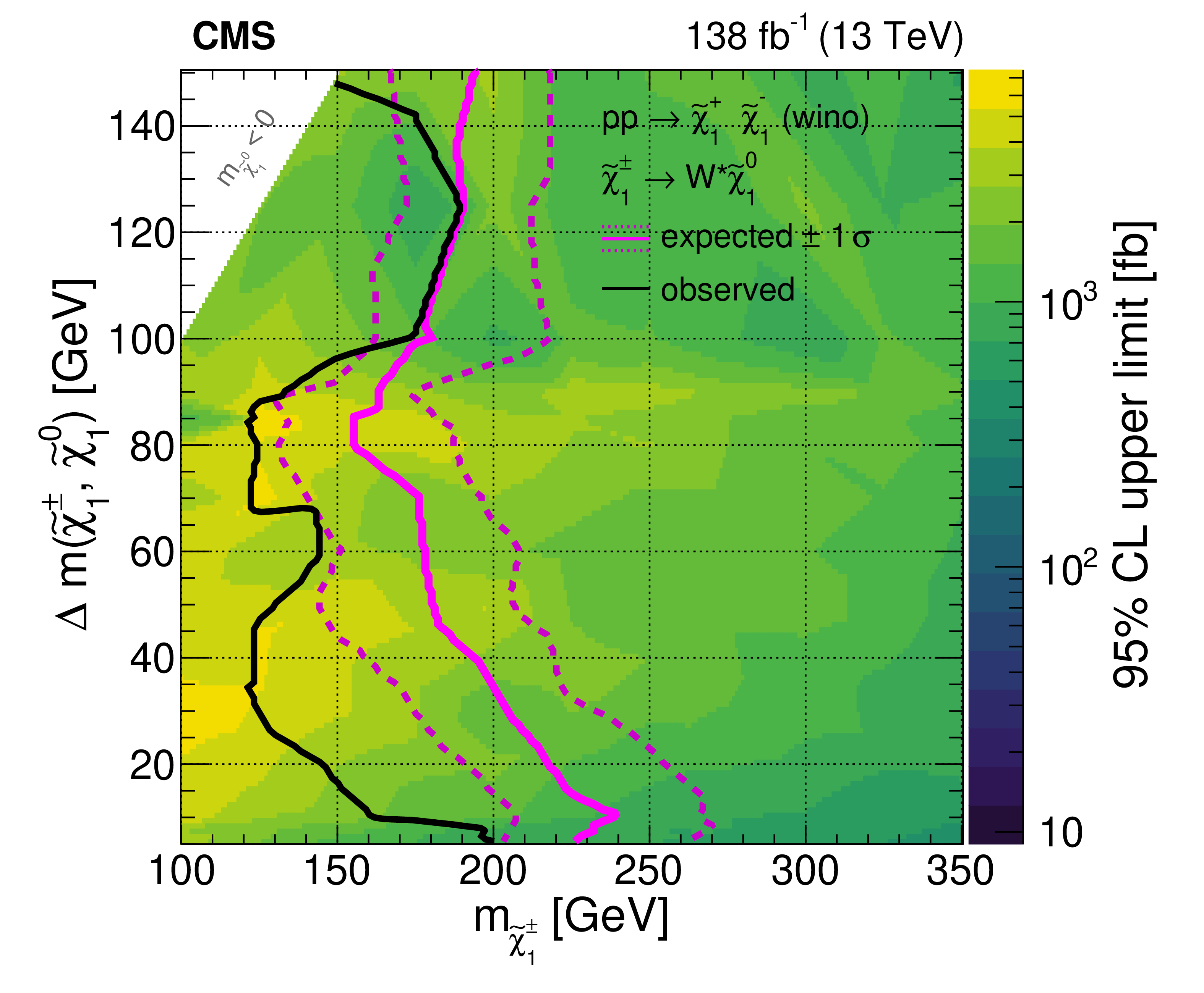
png pdf |
Figure 28-a:
Chargino pair production. The left panel shows the observed upper limits at 95% CL on the product of the cross section and the branching fraction squared, $ \sigma (\tilde{\chi}_{1}^{+} \tilde{\chi}_{1}^{-}) \mathcal{B}^{2} ( \tilde{\chi}_{1}^{\pm} \to \mathrm{W}^{\pm} \tilde{\chi}_{1}^{0} ) $ are shown using the color scale where the $ \tilde{\chi}_{1}^{\pm} $ mass is on the $ x $-axis and the mass difference between the $ \tilde{\chi}_{1}^{\pm} $ and the LSP is on the $ y $-axis. The expected lower mass limits (magenta line) together with their $ {\pm}1\sigma $ uncertainties (magenta dashed lines) and the observed lower mass limits (black line) are indicated for 100% branching fractions for wino-like cross-sections. The right panel shows the results for chargino pair production with decays as in the TChiSlepSnu model with democratic decay via an intermediate sneutrino or charged slepton ({\HepSusyParticle\ellL\pm} ) with mass halfway between the chargino and the lightest neutralino. These model predictions also assume wino-like cross sections. |
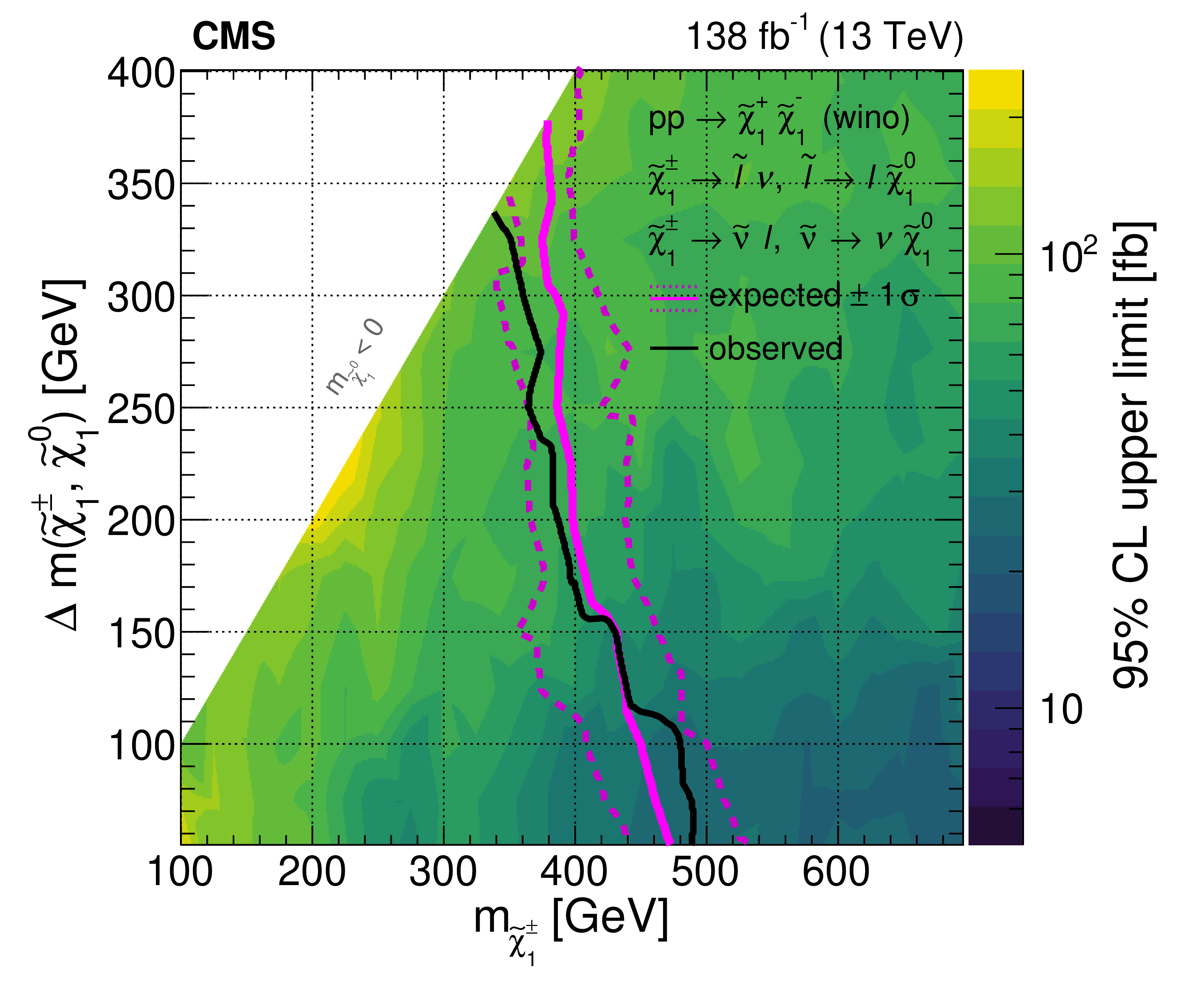
png pdf |
Figure 28-b:
Chargino pair production. The left panel shows the observed upper limits at 95% CL on the product of the cross section and the branching fraction squared, $ \sigma (\tilde{\chi}_{1}^{+} \tilde{\chi}_{1}^{-}) \mathcal{B}^{2} ( \tilde{\chi}_{1}^{\pm} \to \mathrm{W}^{\pm} \tilde{\chi}_{1}^{0} ) $ are shown using the color scale where the $ \tilde{\chi}_{1}^{\pm} $ mass is on the $ x $-axis and the mass difference between the $ \tilde{\chi}_{1}^{\pm} $ and the LSP is on the $ y $-axis. The expected lower mass limits (magenta line) together with their $ {\pm}1\sigma $ uncertainties (magenta dashed lines) and the observed lower mass limits (black line) are indicated for 100% branching fractions for wino-like cross-sections. The right panel shows the results for chargino pair production with decays as in the TChiSlepSnu model with democratic decay via an intermediate sneutrino or charged slepton ({\HepSusyParticle\ellL\pm} ) with mass halfway between the chargino and the lightest neutralino. These model predictions also assume wino-like cross sections. |
png pdf |
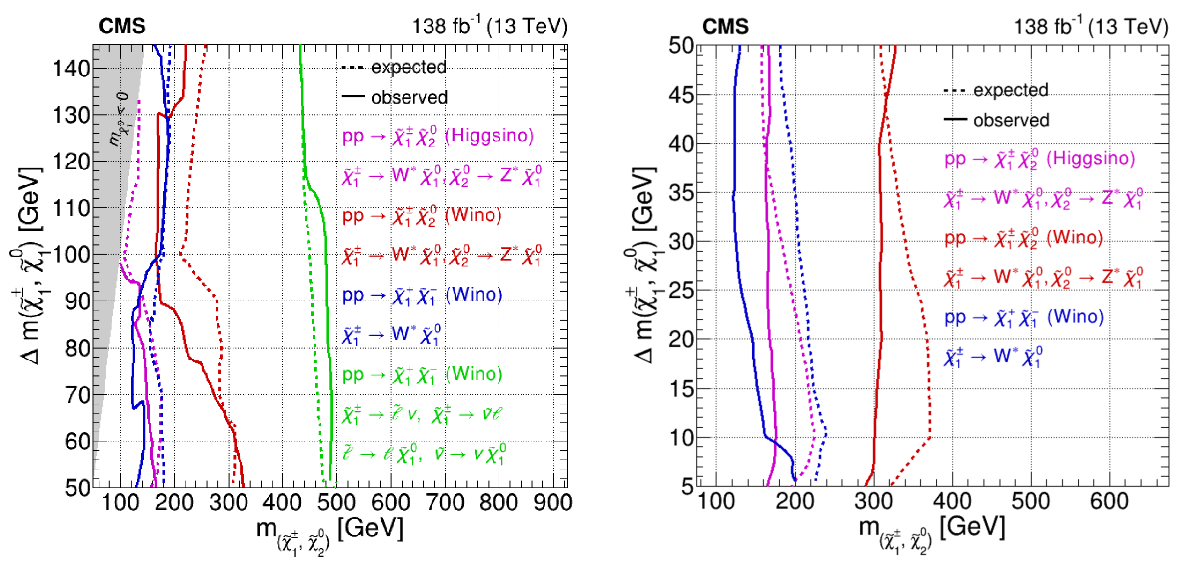
Figure 29:
Summary of the model exclusion results on chargino-neutralino production and chargino pair production. Solid lines are 95% CL observed limits and dashed lines are the corresponding median expected limits. The left panel shows the results for mass differences exceeding 50 GeV and the right panel for mass differences below 50 GeV. |
png pdf |
Figure 29-a:
Summary of the model exclusion results on chargino-neutralino production and chargino pair production. Solid lines are 95% CL observed limits and dashed lines are the corresponding median expected limits. The left panel shows the results for mass differences exceeding 50 GeV and the right panel for mass differences below 50 GeV. |
png pdf |
Figure 29-b:
Summary of the model exclusion results on chargino-neutralino production and chargino pair production. Solid lines are 95% CL observed limits and dashed lines are the corresponding median expected limits. The left panel shows the results for mass differences exceeding 50 GeV and the right panel for mass differences below 50 GeV. |
png pdf |
Figure 30:
Slepton pair production. Observed 95% CL upper limits on the product of the cross section and branching fraction squared for direct slepton pair production followed by decay of both sleptons to the corresponding lepton and neutralino (color scale). Slepton $ \tilde{\ell}_{\mathrm{L}/\mathrm{R}} $ indicates the scalar supersymmetric partner of left- and right-handed electrons and muons. The limit is shown as a function of the slepton mass and the mass difference between the slepton and the lightest neutralino. The regions to the left of the lines denote the regions excluded for a branching fraction of 100%. The median expected exclusion regions for 100% branching fraction are delimited by the dashed lines. |
png pdf |
Figure 31:
Slepton pair production. Observed 95% CL upper limits on the cross section times branching fraction squared for direct selectron pair production (left) and smuon pair production (right) followed by decay of both sleptons to the corresponding lepton and neutralino (color scale). The limits are shown as a function of the slepton mass and the mass difference between the slepton and the lightest neutralino for the three different simplified possibilities of only RR, only LL, and both RR and LL where it is assumed that the R and L masses are identical. The regions to the left of the lines denote the regions excluded for a branching fraction of 100%. Median expected limits for 100% branching fraction are delimited by the dashed lines. |
png pdf |
Figure 31-a:
Slepton pair production. Observed 95% CL upper limits on the cross section times branching fraction squared for direct selectron pair production (left) and smuon pair production (right) followed by decay of both sleptons to the corresponding lepton and neutralino (color scale). The limits are shown as a function of the slepton mass and the mass difference between the slepton and the lightest neutralino for the three different simplified possibilities of only RR, only LL, and both RR and LL where it is assumed that the R and L masses are identical. The regions to the left of the lines denote the regions excluded for a branching fraction of 100%. Median expected limits for 100% branching fraction are delimited by the dashed lines. |
png pdf |
Figure 31-b:
Slepton pair production. Observed 95% CL upper limits on the cross section times branching fraction squared for direct selectron pair production (left) and smuon pair production (right) followed by decay of both sleptons to the corresponding lepton and neutralino (color scale). The limits are shown as a function of the slepton mass and the mass difference between the slepton and the lightest neutralino for the three different simplified possibilities of only RR, only LL, and both RR and LL where it is assumed that the R and L masses are identical. The regions to the left of the lines denote the regions excluded for a branching fraction of 100%. Median expected limits for 100% branching fraction are delimited by the dashed lines. |
png pdf |
Figure 32:
Slepton pair production. Observed and median expected limits for direct slepton pair production at 95% CL. Slepton $ \tilde{\ell}_{\mathrm{L}/\mathrm{R}} $ indicates the scalar supersymmetric partner of left- and right-handed electrons and muons. The limit is shown as a function of the slepton mass and the mass difference between the slepton and the lightest neutralino. The corresponding selectron only and smuon only results of Fig. 31 are shown too assuming a 100% branching fraction. |
png pdf |
Figure 33:
Slepton pair production. Observed 95% CL exclusion regions for direct pair production of the superpartners of the left-handed leptons (left) and direct pair production of the superpartners of the right-handed leptons (right) followed by decay of both sleptons to the corresponding lepton and neutralino with 100% branching fraction. The limits are shown as a function of the slepton mass and the mass difference between the slepton and the lightest neutralino. The regions to the left of the lines denote the excluded regions. Median expected limits are displayed with dashed lines. |
png pdf |
Figure 33-a:
Slepton pair production. Observed 95% CL exclusion regions for direct pair production of the superpartners of the left-handed leptons (left) and direct pair production of the superpartners of the right-handed leptons (right) followed by decay of both sleptons to the corresponding lepton and neutralino with 100% branching fraction. The limits are shown as a function of the slepton mass and the mass difference between the slepton and the lightest neutralino. The regions to the left of the lines denote the excluded regions. Median expected limits are displayed with dashed lines. |
png pdf |
Figure 33-b:
Slepton pair production. Observed 95% CL exclusion regions for direct pair production of the superpartners of the left-handed leptons (left) and direct pair production of the superpartners of the right-handed leptons (right) followed by decay of both sleptons to the corresponding lepton and neutralino with 100% branching fraction. The limits are shown as a function of the slepton mass and the mass difference between the slepton and the lightest neutralino. The regions to the left of the lines denote the excluded regions. Median expected limits are displayed with dashed lines. |
| Tables | |
png pdf |
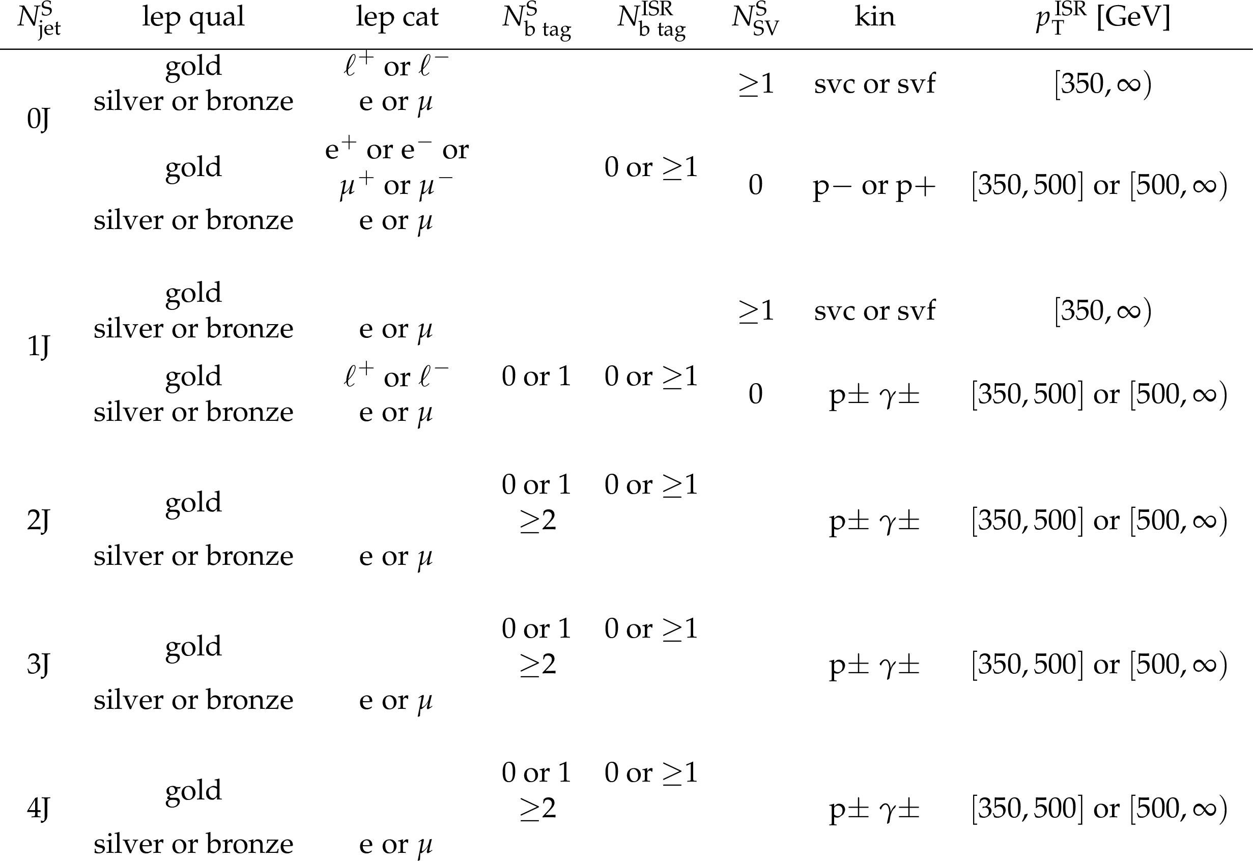
Table 1:
Category definitions for 0L regions for each $ N_{\text{jet}}^{\mathrm{S}} $ multiplicity. The highest (5J) is inclusive ($ N_{\text{jet}}^{\mathrm{S}} \geq $ 5). There are 84 exclusive categories in total for the 0L regions. |
png pdf |
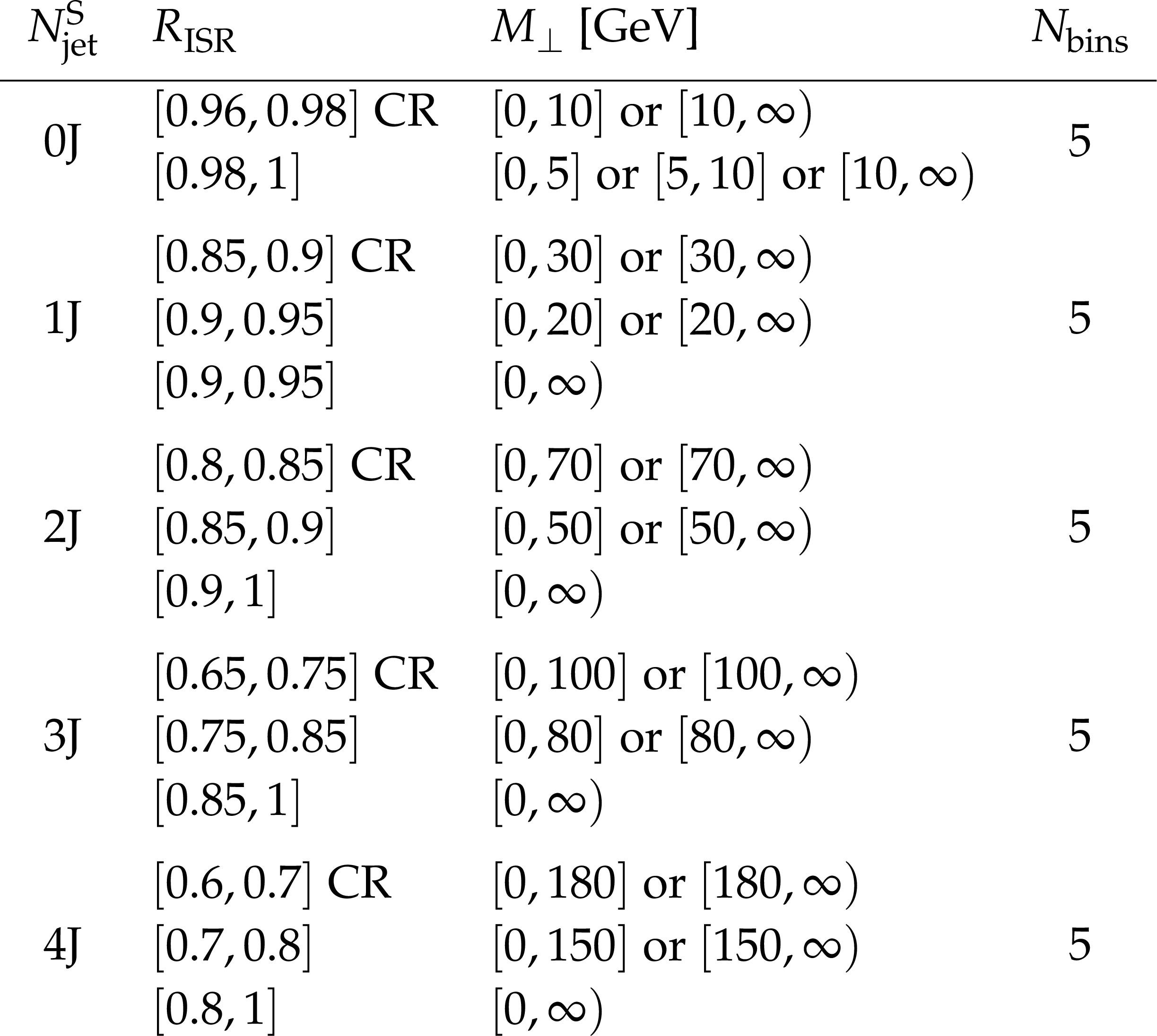
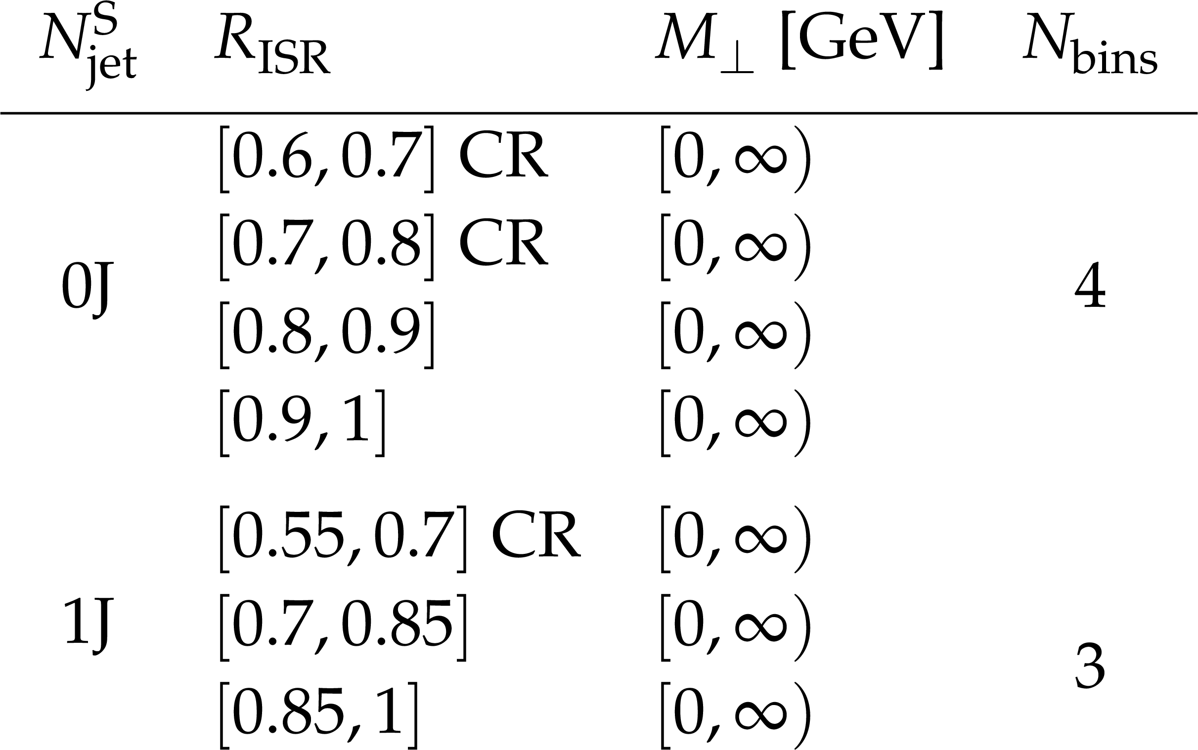
Table 2:
The $ R_{\mathrm{ISR}} $ and $ M_{\perp} $ bin definitions for 0L regions for each $ N_{\text{jet}}^{\mathrm{S}} $ multiplicity. The highest (5J) is inclusive ($ N_{\text{jet}}^{\mathrm{S}} \geq $ 5). The lower $ R_{\mathrm{ISR}} $ bins denoted as "CR" are used as control regions. |
png pdf |
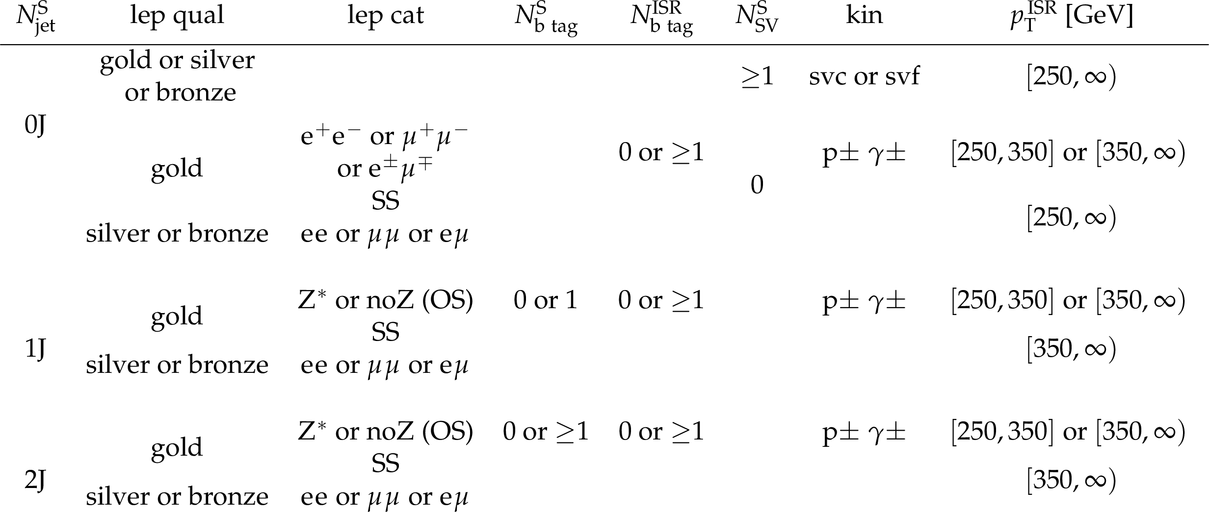
Table 3:
Category definitions for 1L regions for each $ N_{\text{jet}}^{\mathrm{S}} $ multiplicity. The highest (4J) is inclusive ($ N_{\text{jet}}^{\mathrm{S}} \geq $ 4). There are a total of 178 categories for the 1L regions. |
png pdf |
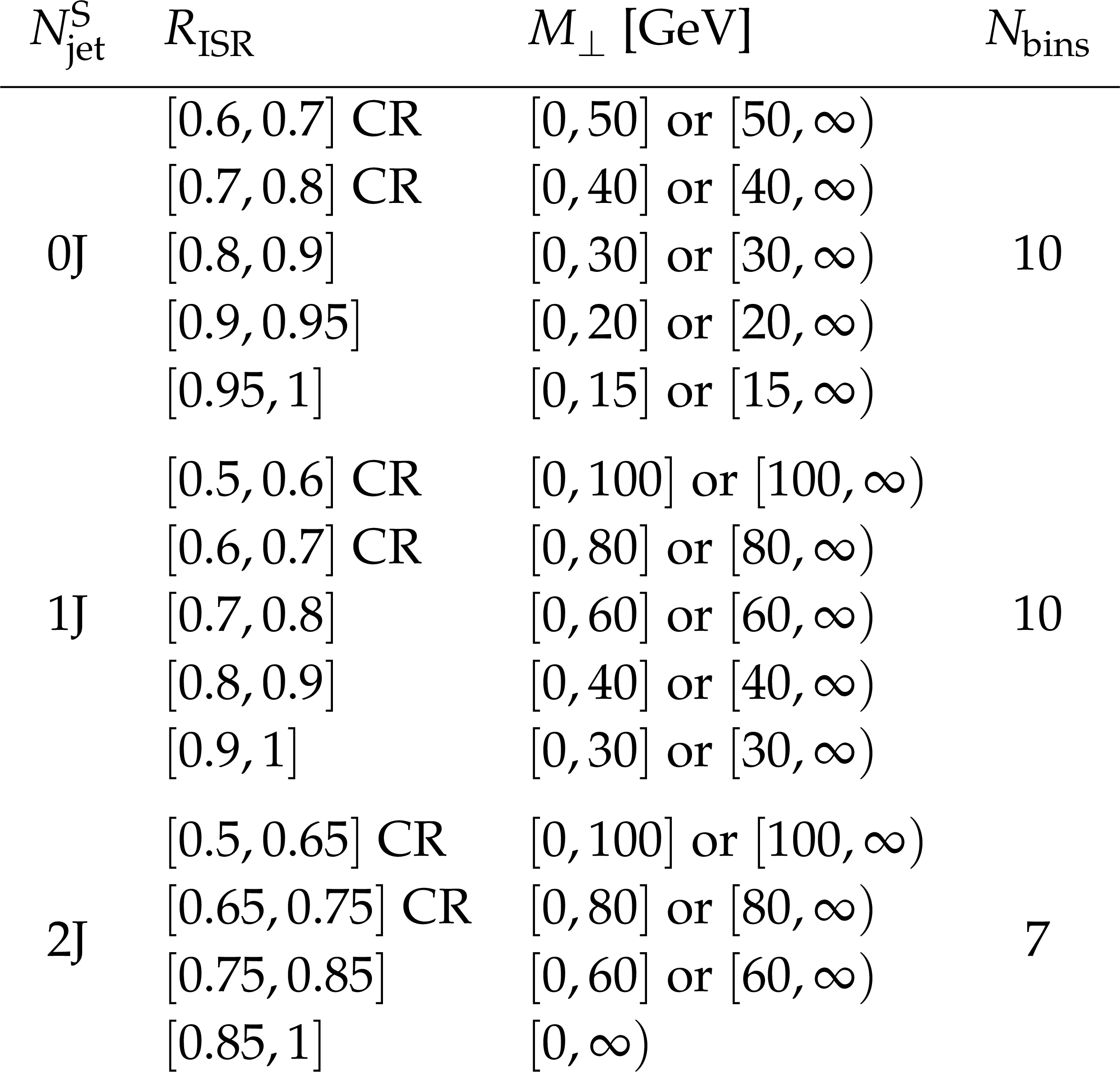
Table 4:
The $ R_{\mathrm{ISR}} $ and $ M_{\perp} $ bin definitions for 1L regions for each $ N_{\text{jet}}^{\mathrm{S}} $ multiplicity. The highest (4J) is inclusive ($ N_{\text{jet}}^{\mathrm{S}} \geq $ 4). The lower $ R_{\mathrm{ISR}} $ bins denoted as "CR" are used as control regions. |
png pdf |
Table 5:
Category definitions for 2L regions for each $ N_{\text{jet}}^{\mathrm{S}} $ multiplicity. The highest (2J) is inclusive ($ N_{\text{jet}}^{\mathrm{S}} \geq $ 2). There is a total of 115 exclusive 2L categories. |
png pdf |
Table 6:
The $ R_{\mathrm{ISR}} $ and $ M_{\perp} $ bin definitions for 2L regions for each $ N_{\text{jet}}^{\mathrm{S}} $ multiplicity. The highest (2J) is inclusive ($ N_{\text{jet}}^{\mathrm{S}} \geq $ 2). The lower $ R_{\mathrm{ISR}} $ bins denoted as "CR" are used as control regions. |

png pdf |
Table 7:
Category definitions for the 3L regions for each $ N_{\text{jet}}^{\mathrm{S}} $ multiplicity. The highest (1J) is inclusive ($ N_{\text{jet}}^{\mathrm{S}} \geq $ 1). There is a total of 15 exclusive 3L categories. |
png pdf |
Table 8:
The $ R_{\mathrm{ISR}} $ and $ M_{\perp} $ bin definitions for 3L regions for each $ N_{\text{jet}}^{\mathrm{S}} $ multiplicity. The highest (1J) is inclusive ($ N_{\text{jet}}^{\mathrm{S}} \geq $ 1). The lower $ R_{\mathrm{ISR}} $ bins denoted as "CR" are used as control regions. An additional control region with 0.5 $ \leq R_{\mathrm{ISR}} < $ 0.6 is also used with the 0 S-jet region. |
png pdf |
Table 9:
List of categories and $ M_{\perp} $/$ R_{\mathrm{ISR}} $ bins corresponding to each model-independent superbin. |
png pdf |
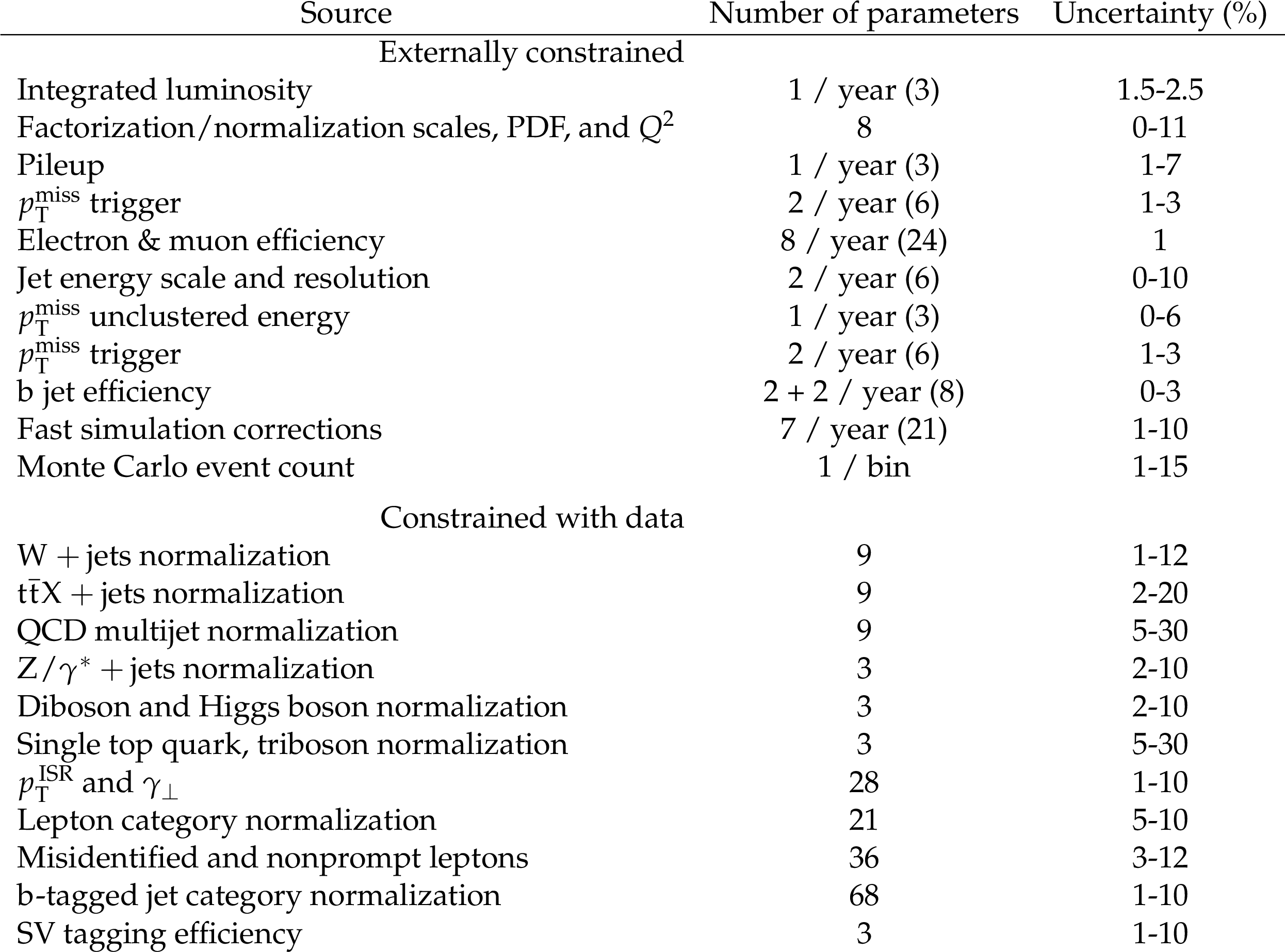
Table 10:
Summary of systematic uncertainties for the full fit. The number of nuisance parameters is listed, with details as to how they are partitioned by data-taking period. The range of the parameter impact variation post-fit is given in the final column. |
png pdf |
Table 11:
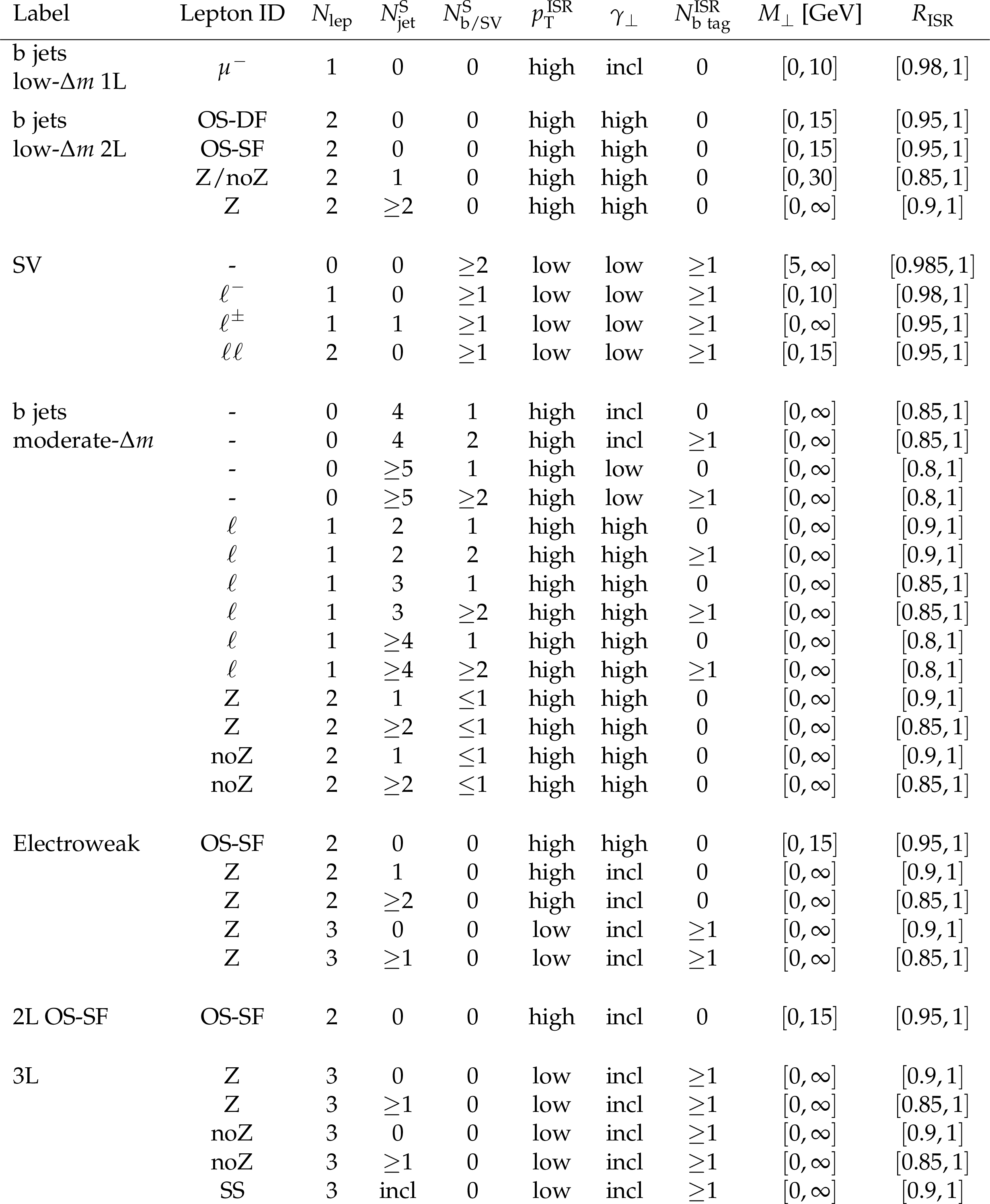
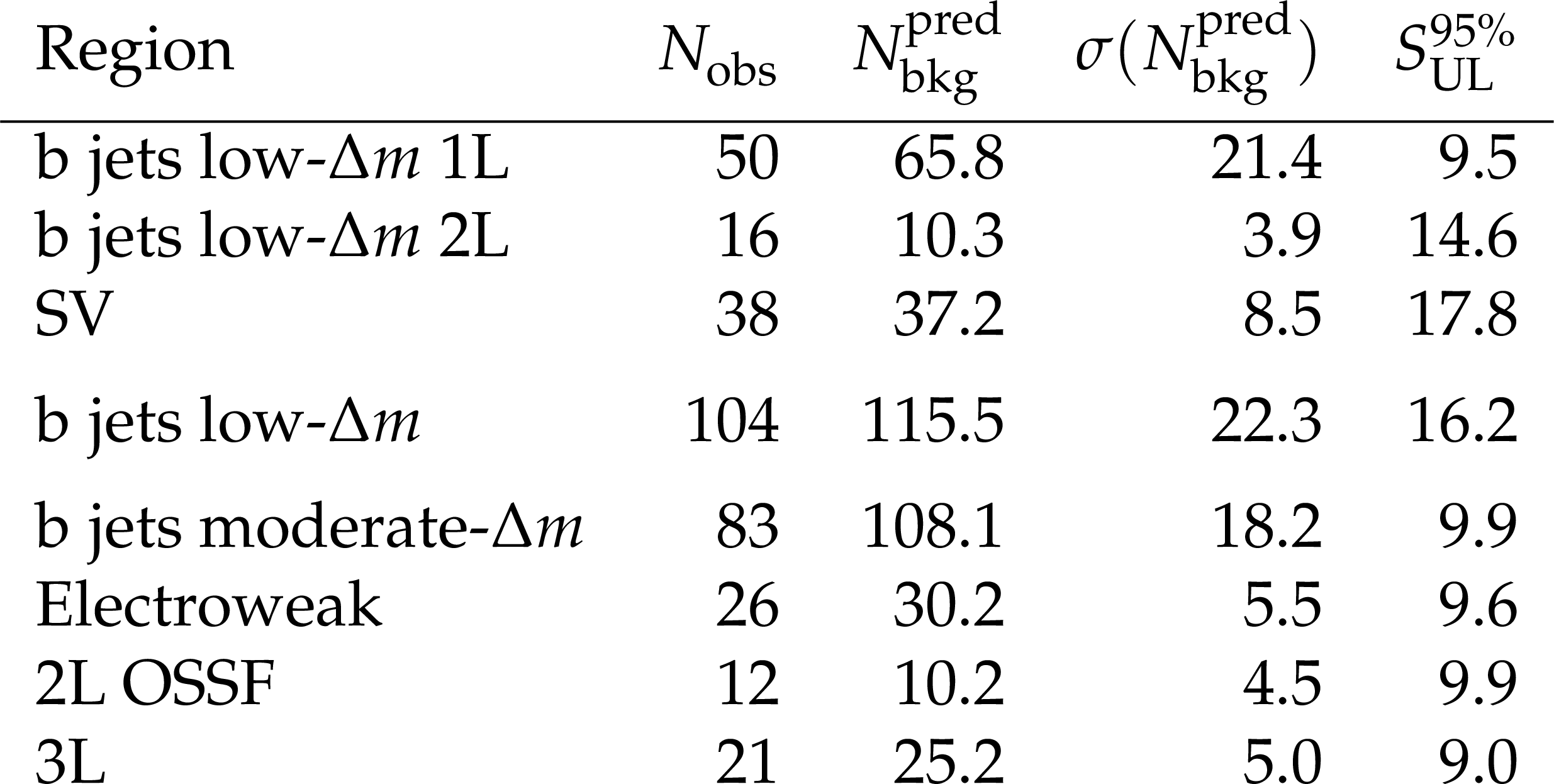
Event counts observed in data, $ N_{\text{obs}} $, in each of the model-independent bins, compared with predictions from the CR fit, $ N^{\text{pred}}_{\text{bkg}} $, their corresponding uncertainties, $ \sigma(N^{\text{pred}}_{\text{bkg}}) $, and the upper limits at 95% CL on the signal strength ($ S_{\mathrm{UL}}^{95%} $) in event counts. All superbins are mutually exclusive except the b jets low-$ \Delta m $ case which aggregates the b jets low-$ \Delta m $ 1L, b jets low-$ Delta m $ 2L, and SV superbins. |
| Summary |
| A general search has been presented for supersymmetric particles (sparticles) in proton-proton collisions at a center-of-mass energy of 13 TeV with the CMS detector at the LHC using a data sample corresponding to an integrated luminosity of 138 fb$ ^{-1} $. A wide range of potential sparticle signatures are targeted including production of pairs of electroweakinos, sleptons, and top squarks. The search is focused on events with a high transverse momentum system from initial-state-radiation jets recoiling against a potential sparticle system with significant missing transverse momentum. Events are categorized based on their lepton multiplicity, jet multiplicity, b tags, and kinematic variables sensitive to the sparticle masses and mass splittings. The sensitivity extends to higher parent sparticle masses than previously probed at the LHC for production of pairs of electroweakinos, sleptons, and top squarks for compressed mass spectra. The results on pair production of charginos and sleptons in the compressed mass regime extend well beyond the canonical 100 GeV sparticle mass scale previously explored at LEP. The observed results demonstrate reasonable agreement with the predictions of the background-only model and model-independent event count upper limits for seven mutually exclusive event selections are reported. Competitive 95% confidence level (CL) lower mass limits are set on sparticle pair production, especially in the compressed mass regime, with mass differences between the lightest and parent sparticle as low as 3 GeV being tested. Top squark mass limits for three decay models are presented in the plane of the top squark mass and the mass difference. Limits on the decay via a top quark extend to 780 GeV with a mass of 750 GeV excluded at 95% CL or higher for mass differences between 60 and 175 GeV; the most stringent exclusion is at a mass difference of 150 GeV. Limits on the decay via a bottom quark and an intermediate chargino extend to 620 GeV with a mass of 550 GeV excluded at 95% CL or higher for mass differences between 35 and 140 GeV; the most stringent exclusion is at mass differences of between 50 and 90 GeV. Limits on the decay via a charm quark extend to 660 GeV with a mass of 520 GeV excluded at 95% CL or higher for mass differences between 10 and 60 GeV; the most stringent exclusion is at a mass difference of 20 GeV. The 95% CL lower mass limits on chargino-neutralino production assuming heavy sleptons extend to 325 (175) GeV for wino (higgsino) cross sections, where the most stringent mass limits are set for mass differences of 50 (10) GeV. The limits with wino cross sections exceed 300 GeV for the broad range of mass differences between 8 and 65 GeV, while the limits with the higgsino cross section assumption exceed 163 GeV for mass differences between 3 and 50 GeV. For chargino pair production, 95% CL lower mass limits are obtained for wino cross sections and decay via a W boson. These extend to 200 GeV with the most stringent mass limit set for a mass difference of 5 GeV while masses exceeding 120 GeV are excluded for all mass differences above 5 GeV. Related chargino pair production limits for the case of decays via sleptons and sneutrinos and with wino cross sections extend to 490 GeV for a mass difference of 55 GeV. The 95% CL lower mass limits on pair production of charged sleptons extend to 168 GeV (slepton partner of right-handed lepton only), 240 GeV (slepton partner of left-handed lepton only), and 270 GeV (both sleptons mass degenerate) for the most favorable mass splitting of around 5 GeV for the case of mass-degenerate first- and second-generation sleptons. Slepton masses exceeding 110, 175, and 200 GeV for all mass splittings ranging from 3 to 80 GeV are excluded at 95% CL or higher for the same three cases respectively. Similar results are also presented separately for selectrons and smuons assuming that the other slepton is not produced. For selectrons (smuons), the most stringent 95% CL lower mass limits are set at 160, 230, 250 GeV (145, 195, 240 GeV) for mass differences around 5 GeV for the three cases and with sensitivity to a broad range of mass differences from 3 to 100 GeV. |
| References | ||||
| 1 | ATLAS Collaboration | Observation of a new particle in the search for the standard model Higgs boson with the ATLAS detector at the LHC | PLB 716 (2012) 1 | 1207.7214 |
| 2 | CMS Collaboration | Observation of a new boson at a mass of 125 GeV with the CMS experiment at the LHC | PLB 716 (2012) 30 | CMS-HIG-12-028 1207.7235 |
| 3 | Particle Data Group and Navas, S. and others Collaboration | Review of particle physics | PRD 110 (2024) 030001 | |
| 4 | G. Jungman, M. Kamionkowski, and K. Griest | Supersymmetric dark matter | Phys. Rept. 267 (1996) 195 | hep-ph/9506380 |
| 5 | M. Drees, R. Godbole, and P. Roy | Theory and phenomenology of sparticles: An account of four-dimensional N$ = $1 supersymmetry in high energy physics | World Scientific Publishing, 2004 | |
| 6 | H. Baer and X. Tata | Weak scale supersymmetry: From superfields to scattering events | Cambridge University Press, 2006 | |
| 7 | S. P. Martin | A supersymmetry primer | Adv. Ser. Direct. High Energy Phys. 21 (2010) 1 | hep-ph/9709356 |
| 8 | ATLAS Collaboration | Search for electroweak production of supersymmetric states in scenarios with compressed mass spectra at $ \sqrt{s}= $ 13 TeV with the ATLAS detector | PRD 97 (2018) 052010 | 1712.08119 |
| 9 | CMS Collaboration | Search for supersymmetry with a compressed mass spectrum in events with a soft $ \tau $ lepton, a highly energetic jet, and large missing transverse momentum in proton-proton collisions at $ \sqrt{s}= $ 13 TeV | PRL 124 (2020) 041803 | CMS-SUS-19-002 1910.01185 |
| 10 | CMS Collaboration | Search for supersymmetry with a compressed mass spectrum in the vector boson fusion topology with 1-lepton and 0-lepton final states in proton-proton collisions at $ \sqrt{s}= $ 13 TeV | JHEP 08 (2019) 150 | CMS-SUS-17-007 1905.13059 |
| 11 | ATLAS Collaboration | Searches for electroweak production of supersymmetric particles with compressed mass spectra in $ \sqrt{s}= $ 13 TeV pp collisions with the ATLAS detector | PRD 101 (2020) 052005 | 1911.12606 |
| 12 | CMS Collaboration | Search for supersymmetry in final states with two oppositely charged same-flavor leptons and missing transverse momentum in proton-proton collisions at $ \sqrt{s}= $ 13 TeV | JHEP 04 (2021) 123 | CMS-SUS-20-001 2012.08600 |
| 13 | CMS Collaboration | Search for top squark pair production using dilepton final states in pp collision data collected at $ \sqrt{s}= $ 13 TeV | EPJC 81 (2021) 3 | CMS-SUS-19-011 2008.05936 |
| 14 | ATLAS Collaboration | Search for direct production of electroweakinos in final states with one lepton, missing transverse momentum and a Higgs boson decaying into two b-jets in pp collisions at $ \sqrt{s}= $ 13 TeV with the ATLAS detector | EPJC 80 (2020) 691 | 1909.09226 |
| 15 | ATLAS Collaboration | Search for chargino-neutralino production with mass splittings near the electroweak scale in three-lepton final states in $ \sqrt{s} = $ 13 TeV pp collisions with the ATLAS detector | PRD 101 (2020) 072001 | 1912.08479 |
| 16 | ATLAS Collaboration | Search for squarks and gluinos in final states with one isolated lepton, jets, and missing transverse momentum at $ \sqrt{s}= $ 13 TeV with the ATLAS detector | EPJC 81 (2021) 600 | 2101.01629 |
| 17 | CMS Collaboration | Search for supersymmetry in final states with two or three soft leptons and missing transverse momentum in proton-proton collisions at $ \sqrt{s}= $ 13 TeV | JHEP 04 (2022) 091 | CMS-SUS-18-004 2111.06296 |
| 18 | CMS Collaboration | Search for top squark production in fully hadronic final states in proton-proton collisions at $ \sqrt{s}= $ 13 TeV | PRD 104 (2021) 052001 | CMS-SUS-19-010 2103.01290 |
| 19 | ATLAS Collaboration | Search for a scalar partner of the top quark in the all-hadronic $ \mathrm{t} \overline{\mathrm{t}} $ plus missing transverse momentum final state at $ \sqrt{s}= $ 13 TeV with the ATLAS detector | EPJC 80 (2020) 737 | 2004.14060 |
| 20 | ATLAS Collaboration | Search for new phenomena with top quark pairs in final states with one lepton, jets, and missing transverse momentum in pp collisions at $ \sqrt{s}= $ 13 TeV with the ATLAS detector | JHEP 04 (2021) 174 | 2012.103799 |
| 21 | ATLAS Collaboration | Search for new phenomena in events with an energetic jet and missing transverse momentum in pp collisions at $ \sqrt{s}= $ 13 TeV with the ATLAS detector | PRD 103 (2021) 112006 | 2102.10874 |
| 22 | ATLAS Collaboration | The quest to discover supersymmetry at the ATLAS experiment | Phys. Rept. 1116 (2025) 261 | 2403.02455 |
| 23 | ATLAS Collaboration | Search for electroweak production of charginos and sleptons decaying into final states with two leptons and missing transverse momentum in $ \sqrt{s}= $ 13 TeV pp collisions using the ATLAS detector | EPJC 80 (2020) 123 | 1908.08215 |
| 24 | ATLAS Collaboration | Search for chargino--neutralino pair production in final states with three leptons and missing transverse momentum in $ \sqrt{s} = $ 13 TeV pp collisions with the ATLAS detector | EPJC 81 (2021) 1118 | 2106.01676 |
| 25 | ATLAS Collaboration | Search for charginos and neutralinos in final states with two boosted hadronically decaying bosons and missing transverse momentum in pp collisions at $ \sqrt{s} = $ 13 TeV with the ATLAS detector | PRD 104 (2021) 112010 | 2108.07586 |
| 26 | ATLAS Collaboration | Searches for new phenomena in events with two leptons, jets, and missing transverse momentum in 139 fb$^{-1}$ of $ \sqrt{s}= $ 13 TeV pp collisions with the ATLAS detector | EPJC 83 (2023) 515 | 2204.13072 |
| 27 | ATLAS Collaboration | Search for direct pair production of sleptons and charginos decaying to two leptons and neutralinos with mass splittings near the W-boson mass in $ \sqrt{s} = $ 13 TeV pp collisions with the ATLAS detector | JHEP 06 (2023) 031 | 2209.13935 |
| 28 | ATLAS Collaboration | Search for direct production of electroweakinos in final states with one lepton, jets and missing transverse momentum in pp collisions at $ \sqrt{s} = $ 13 TeV with the ATLAS detector | JHEP 12 (2023) 167 | 2310.08171 |
| 29 | ATLAS Collaboration | Search for electroweak production of supersymmetric particles in final states with two $ \tau $-leptons in $ \sqrt{s} = $ 13 TeV pp collisions with the ATLAS detector | JHEP 05 (2024) 150 | 2402.00603 |
| 30 | ATLAS Collaboration | Statistical combination of ATLAS Run 2 searches for charginos and neutralinos at the LHC | PRL 133 (2024) 031802 | 2402.08347 |
| 31 | CMS Collaboration | Search for electroweak production of charginos and neutralinos in proton-proton collisions at $ \sqrt{s} = $ 13 TeV | JHEP 04 (2022) 147 | CMS-SUS-19-012 2106.14246 |
| 32 | CMS Collaboration | Search for chargino-neutralino production in events with Higgs and W bosons using 137 fb$^{-1}$ of proton-proton collisions at $ \sqrt{s} = $ 13 TeV | JHEP 10 (2021) 045 | CMS-SUS-20-003 2107.12553 |
| 33 | CMS Collaboration | Search for higgsinos decaying to two Higgs bosons and missing transverse momentum in proton-proton collisions at $ \sqrt{s} = $ 13 TeV | JHEP 05 (2022) 014 | CMS-SUS-20-004 2201.04206 |
| 34 | CMS Collaboration | Search for electroweak production of charginos and neutralinos at $ \sqrt{s}= $ 13 TeV in final states containing hadronic decays of WW, WZ, or WH and missing transverse momentum | PLB 842 (2023) 137460 | CMS-SUS-21-002 2205.09597 |
| 35 | CMS Collaboration | Combined search for electroweak production of winos, binos, higgsinos, and sleptons in proton-proton collisions at $ \sqrt{s}= $ 13 TeV | PRD 109 (2024) 112001 | CMS-SUS-21-008 2402.01888 |
| 36 | ATLAS Collaboration | Searches for direct slepton production in the compressed-mass corridor in $ \sqrt{s}= $ 13 TeV pp collisions with the ATLAS detector | Submitted to JHEP, 2025 | 2503.17186 |
| 37 | ATLAS Collaboration | Search for cascade decays of charged sleptons and sneutrinos in final states with three leptons and missing transverse momentum in pp collisions at $ \sqrt{s}= $ 13 TeV with the ATLAS detector | PRD 112 (2025) 012005 | 2503.13135 |
| 38 | Z. Han, G. D. Kribs, A. Martin, and A. Menon | Hunting quasidegenerate higgsinos | PRD 89 (2014) 075007 | 1401.1235 |
| 39 | A. Canepa, T. Han, and X. Wang | The search for electroweakinos | Ann. Rev. Nucl. Part. Sci. 70 (2020) 425 | 2003.05450 |
| 40 | H. Baer et al. | The LHC higgsino discovery plane for present and future SUSY searches | PLB 810 (2020) 135777 | 2007.09252 |
| 41 | Muon g-2 Collaboration | Final report of the E821 muon anomalous magnetic moment measurement at BNL | PRD 73 (2006) 072003 | hep-ex/0602035 |
| 42 | Muon g-2 Collaboration | Measurement of the positive muon anomalous magnetic moment to 0.20\unitppm | PRL 131 (2023) 161802 | 2308.06230 |
| 43 | Muon g-2 Collaboration | Measurement of the positive muon anomalous magnetic moment to 127\unitppb | Submitted to Phys. Rev. Lett, 2025 | 2506.03069 |
| 44 | T. Moroi | The muon anomalous magnetic dipole moment in the minimal supersymmetric standard model | PRD 53 (1996) 6565 | hep-ph/9512396 |
| 45 | S. P. Martin and J. D. Wells | Muon anomalous magnetic dipole moment in supersymmetric theories | PRD 64 (2001) 035003 | hep-ph/0103067 |
| 46 | D. Stockinger | The muon magnetic moment and supersymmetry | JPG 34 (2007) R45 | hep-ph/0609168 |
| 47 | G. R. Farrar and P. Fayet | Phenomenology of the production, decay, and detection of new hadronic states associated with supersymmetry | PLB 76 (1978) 575 | |
| 48 | CMS Collaboration | HEPData record for this analysis | link | |
| 49 | CMS Collaboration | The CMS experiment at the CERN LHC | JINST 3 (2008) S08004 | |
| 50 | CMS Collaboration | Development of the CMS detector for the CERN LHC Run 3 | JINST 19 (2024) P05064 | CMS-PRF-21-001 2309.05466 |
| 51 | CMS Collaboration | Particle-flow reconstruction and global event description with the CMS detector | JINST 12 (2017) P10003 | CMS-PRF-14-001 1706.04965 |
| 52 | M. Cacciari, G. P. Salam, and G. Soyez | The anti-$ k_{\mathrm{T}} $ jet clustering algorithm | JHEP 04 (2008) 063 | 0802.1189 |
| 53 | M. Cacciari, G. P. Salam, and G. Soyez | FastJet user manual | EPJC 72 (2012) 1896 | 1111.6097 |
| 54 | CMS Collaboration | Jet energy scale and resolution in the CMS experiment in pp collisions at 8 TeV | JINST 12 (2017) P02014 | CMS-JME-13-004 1607.03663 |
| 55 | CMS Collaboration | Performance of electron reconstruction and selection with the CMS detector in proton-proton collisions at $ \sqrt{s} = $ 8 TeV | JINST 10 (2015) P06005 | CMS-EGM-13-001 1502.02701 |
| 56 | CMS Collaboration | Electron and photon reconstruction and identification with the CMS experiment at the CERN LHC | JINST 16 (2021) P05014 | CMS-EGM-17-001 2012.06888 |
| 57 | CMS Collaboration | Performance of CMS muon reconstruction in pp collision events at $ \sqrt{s} = $ 7 TeV | JINST 7 (2012) P10002 | CMS-MUO-10-004 1206.4071 |
| 58 | CMS Collaboration | Performance of missing transverse momentum reconstruction in proton-proton collisions at $ \sqrt{s}= $ 13 TeV using the CMS detector | JINST 14 (2019) P07004 | CMS-JME-17-001 1903.06078 |
| 59 | E. Chabanat and N. Estre | Deterministic annealing for vertex finding at CMS | Proc. Int. Conf. on Computing in High Energy Physics and Nuclear Physics 2004 (2005) 287 | |
| 60 | CMS Collaboration | Technical proposal for the Phase-II upgrade of the Compact Muon Solenoid | CMS Technical Proposal CERN-LHCC-2015-010, CMS-TDR-15-02, 2015 CDS |
|
| 61 | CMS Collaboration | The CMS trigger system | JINST 12 (2017) P01020 | CMS-TRG-12-001 1609.02366 |
| 62 | CMS Collaboration | Performance of the CMS high-level trigger during LHC Run 2 | JINST 19 (2024) P11021 | CMS-TRG-19-001 2410.17038 |
| 63 | J. Alwall, P. Schuster, and N. Toro | Simplified models for a first characterization of new physics at the LHC | PRD 79 (2009) 075020 | 0810.3921 |
| 64 | J. Alwall, M.-P. Le, M. Lisanti, and J. G. Wacker | Model-independent jets plus missing energy searches | PRD 79 (2009) 015005 | 0809.3264 |
| 65 | LHC New Physics Working Group Collaboration | Simplified models for LHC new physics searches | JPG 39 (2012) 105005 | 1105.2838 |
| 66 | NNPDF Collaboration | Parton distributions for the LHC Run II | JHEP 04 (2015) 040 | 1410.8849 |
| 67 | NNPDF Collaboration | Parton distributions from high-precision collider data | EPJC 77 (2017) 663 | 1706.00428 |
| 68 | T. Sjöstrand et al. | An introduction to PYTHIA 8.2 | Comput. Phys. Commun. 191 (2015) 159 | 1410.3012 |
| 69 | CMS Collaboration | Extraction and validation of a new set of CMS PYTHIA8 tunes from underlying-event measurements | EPJC 80 (2020) 4 | CMS-GEN-17-001 1903.12179 |
| 70 | GEANT4 Collaboration | GEANT 4---a simulation toolkit | NIM A 506 (2003) 250 | |
| 71 | S. Abdullin et al. | The fast simulation of the CMS detector at LHC | J. Phys. Conf. Ser. 331 (2011) 032049 | |
| 72 | A. Giammanco | The fast simulation of the CMS experiment | J. Phys. Conf. Ser. 513 (2014) 022012 | |
| 73 | J. Alwall et al. | The automated computation of tree-level and next-to-leading order differential cross sections, and their matching to parton shower simulations | JHEP 07 (2014) 079 | 1405.0301 |
| 74 | B. Fuks, M. Klasen, D. R. Lamprea, and M. Rothering | Gaugino production in proton-proton collisions at a center-of-mass energy of 8 TeV | JHEP 10 (2012) 081 | 1207.2159 |
| 75 | B. Fuks, M. Klasen, D. R. Lamprea, and M. Rothering | Precision predictions for electroweak superpartner production at hadron colliders with RESUMMINO | EPJC 10 (2013) 2480 | 1304.0790 |
| 76 | W. Beenakker, R. Höpker, and M. Spira | PROSPINO: A program for the production of supersymmetric particles in next-to-leading order QCD | hep-ph/9611232 | |
| 77 | C. Borschensky et al. | Squark and gluino production cross sections in pp collisions at $ \sqrt{s}= $ 13, 14, 33 and 100 TeV | EPJC 74 (2014) 3174 | 1407.5066 |
| 78 | W. Beenakker et al. | Production of charginos, neutralinos, and sleptons at hadron colliders | PRL 83 (1999) 3780 | hep-ph/9906298 |
| 79 | W. Beenakker et al. | Stop production at hadron colliders | NPB 515 (1998) 3 | hep-ph/9710451 |
| 80 | W. Beenakker et al. | Supersymmetric top and bottom squark production at hadron colliders | JHEP 08 (2010) 098 | 1006.4771 |
| 81 | W. Beenakker et al. | NNLL resummation for stop pair-production at the LHC | JHEP 05 (2016) 153 | 1601.02954 |
| 82 | S. Alioli, P. Nason, C. Oleari, and E. Re | A general framework for implementing NLO calculations in shower Monte Carlo programs: the POWHEG BOX | JHEP 06 (2010) 043 | 1002.2581 |
| 83 | E. Re | Single-top $ \mathrm{W}\mathrm{t} $-channel production matched with parton showers using the POWHEG method | EPJC 71 (2011) 1547 | 1009.2450 |
| 84 | P. Nason | A new method for combining NLO QCD with shower Monte Carlo algorithms | JHEP 11 (2004) 040 | hep-ph/0409146 |
| 85 | S. Frixione, P. Nason, and C. Oleari | Matching NLO QCD computations with parton shower simulations: the POWHEG method | JHEP 11 (2007) 070 | 0709.2092 |
| 86 | R. Frederix and S. Frixione | Merging meets matching in MC@NLO | JHEP 12 (2012) 061 | 1209.6215 |
| 87 | T. Melia, P. Nason, R. Röntsch, and G. Zanderighi | $ \mathrm{W^+}\mathrm{W^-} $, WZ, and ZZ production in the POWHEG-BOX | JHEP 11 (2011) 078 | 1107.5051 |
| 88 | P. Nason and G. Zanderighi | $ \mathrm{W^+}\mathrm{W^-} $, WZ, and ZZ production in the POWHEG-BOX-V2 | EPJC 74 (2014) 2702 | 1311.1365 |
| 89 | CMS Collaboration | Performance of the CMS muon detector and muon reconstruction with proton-proton collisions at $ \sqrt{s}= $ 13 TeV | JINST 13 (2018) P06015 | CMS-MUO-16-001 1804.04528 |
| 90 | M. Cacciari, G. P. Salam, and G. Soyez | The catchment area of jets | JHEP 04 (2008) 005 | 0802.1188 |
| 91 | CMS Collaboration | Jet algorithms performance in 13 TeV data | CMS Physics Analysis Summary, 2017 link |
CMS-PAS-JME-16-003 |
| 92 | E. Bols et al. | Jet Flavour Classification Using DeepJet | JINST 15 (2020) P12012 | 2008.10519 |
| 93 | CMS Collaboration | Performance of the DEEPJET b tagging algorithm using 41.9 fb$^{-1}$ of data from proton-proton collisions at 13 TeV with Phase 1 CMS detector | CMS Detector Performance Note CMS-DP-2018-058, 2018 CDS |
|
| 94 | CMS Collaboration | Measurement of $ {\mathrm{B}}\overline{\mathrm{B}} $ angular correlations based on secondary vertex reconstruction at $ \sqrt{s}= $ 7 TeV | JHEP 03 (2011) 136 | CMS-BPH-10-010 1102.3194 |
| 95 | S. S. Mehta | DeepJet: a portable ML environment for HEP | in 2nd IML Machine Learning Workshop. April, 2018 | |
| 96 | J. Kieseler et al. | DeepJetCore (2.0) | Zenodo, 2020 link |
|
| 97 | CMS Collaboration | Identification of heavy-flavour jets with the CMS detector in pp collisions at 13 TeV | JINST 13 (2018) P05011 | CMS-BTV-16-002 1712.07158 |
| 98 | M. R. Buckley, J. D. Lykken, C. Rogan, and M. Spiropulu | Super-razor and searches for sleptons and charginos at the LHC | PRD 89 (2014) 055020 | 1310.4827 |
| 99 | P. Jackson, C. Rogan, and M. Santoni | Sparticles in motion: Analyzing compressed SUSY scenarios with a new method of event reconstruction | PRD 95 (2017) 035031 | 1607.08307 |
| 100 | P. Jackson and C. Rogan | Recursive jigsaw reconstruction: HEP event analysis in the presence of kinematic and combinatoric ambiguities | PRD 96 (2017) 112007 | 1705.10733 |
| 101 | CMS Collaboration | The CMS statistical analysis and combination tool: COMBINE | Comput. Softw. Big Sci. 8 (2024) 19 | CMS-CAT-23-001 2404.06614 |
| 102 | W. Verkerke and D. P. Kirkby | The RooFit toolkit for data modeling | in Proceedings of the 13th International Conference for Computing in High-Energy and Nuclear Physics (CHEP03), 2003 link |
physics/0306116 |
| 103 | L. Moneta et al. | The RooStats Project | in PoS, T. Speer et al., eds., volume ACAT, 2010 link |
1009.1003 |
| 104 | CMS Collaboration | Precision luminosity measurement in proton-proton collisions at $ \sqrt{s}= $ 13 TeV in 2015 and 2016 at CMS | EPJC 81 (2021) 800 | CMS-LUM-17-003 2104.01927 |
| 105 | CMS Collaboration | CMS luminosity measurement for the 2017 data-taking period at $ \sqrt{s}= $ 13 TeV | CMS Physics Analysis Summary, 2018 CMS-PAS-LUM-17-004 |
CMS-PAS-LUM-17-004 |
| 106 | CMS Collaboration | CMS luminosity measurement for the 2018 data-taking period at $ \sqrt{s}= $ 13 TeV | CMS Physics Analysis Summary, 2019 CMS-PAS-LUM-18-002 |
CMS-PAS-LUM-18-002 |
| 107 | S. Catani, D. de Florian, M. Grazzini, and P. Nason | Soft-gluon resummation for Higgs boson production at hadron colliders | JHEP 07 (2003) 028 | hep-ph/0306211 |
| 108 | M. Cacciari et al. | The $ {\mathrm{t}\overline{\mathrm{t}}} $ cross-section at 1.8 and 1.96 TeV: a study of the systematics due to parton densities and scale dependence | JHEP 04 (2004) 068 | hep-ph/0303085 |
| 109 | J. Butterworth et al. | PDF4LHC recommendations for LHC Run II | JPG 43 (2016) 023001 | 1510.03865 |
| 110 | CMS Collaboration | Measurement of the inelastic proton-proton cross section at $ \sqrt{s}= $ 13 TeV | JHEP 07 (2018) 161 | CMS-FSQ-15-005 1802.02613 |
| 111 | CMS Collaboration | Measurement of the cross section for top quark pair production in association with a W or Z boson in proton-proton collisions at $ \sqrt{s}= $ 13 TeV | JHEP 08 (2018) 011 | CMS-TOP-17-005 1711.02547 |
| 112 | W. S. Cleveland | Robust locally weighted regression and smoothing scatterplots | J. Am. Stat. Assoc. 74 (1979) 829 | |
| 113 | W. S. Cleveland | Locally weighted regression: An approach to regression analysis by local fitting | J. Am. Stat. Assoc. 83 (1988) 596 | |
| 114 | R. D. Cousins, J. T. Linnemann, and J. Tucker | Evaluation of three methods for calculating statistical significance when incorporating a systematic uncertainty into a test of the background-only hypothesis for a Poisson process | NIM A 595 (2008) 480 | physics/0702156 |
| 115 | T. Junk | Confidence level computation for combining searches with small statistics | NIM A 434 (1999) 435 | hep-ex/9902006 |
| 116 | A. L. Read | Presentation of search results: The $ \text{CL}_\text{s} $ technique | JPG 28 (2002) 2693 | |
| 117 | G. Cowan, K. Cranmer, E. Gross, and O. Vitells | Asymptotic formulae for likelihood-based tests of new physics | EPJC 71 (2011) 1554 | 1007.1727 |
| 118 | ALEPH Collaboration | Absolute mass lower limit for the lightest neutralino of the MSSM from $ \mathrm{e}^+\mathrm{e}^- $ data at $ \sqrt{s} $ up to 209 GeV | PLB 583 (2004) 247 | |
| 119 | DELPHI Collaboration | Searches for supersymmetric particles in $ \mathrm{e}^+\mathrm{e}^- $ collisions up to 208 GeV and interpretation of the results within the MSSM | EPJC 31 (2003) 421 | hep-ex/0311019 |
| 120 | L3 Collaboration | Search for charginos and neutralinos in $ \mathrm{e}^+\mathrm{e}^- $ collisions at $ \sqrt{s} = $ 189 GeV | PLB 472 (2000) 420 | hep-ex/9910007 |
| 121 | OPAL Collaboration | Search for chargino and neutralino production at $ \sqrt{s}= $ 192 to 209 GeV at LEP | EPJC 35 (2004) 1 | hep-ex/0401026 |
| 122 | CMS Collaboration | Searches for pair production of charginos and top squarks in final states with two oppositely charged leptons in proton-proton collisions at $ \sqrt{s}= $ 13 TeV | JHEP 11 (2018) 079 | CMS-SUS-17-010 1807.07799 |
| 123 | ALEPH Collaboration | Search for scalar leptons in $ \mathrm{e}^+\mathrm{e}^- $ collisions at center-of-mass energies up to 209 GeV | PLB 526 (2002) 206 | hep-ex/0112011 |
| 124 | L3 Collaboration | Search for scalar leptons and scalar quarks at LEP | PLB 580 (2004) 37 | hep-ex/0310007 |
| 125 | OPAL Collaboration | Search for anomalous production of dilepton events with missing transverse momentum in $ \mathrm{e}^+\mathrm{e}^- $ collisions at $ \sqrt{s}= $ 183 -- 209 GeV | EPJC 32 (2004) 453 | hep-ex/0309014 |
|
|
Compact Muon Solenoid LHC, CERN |
|

|

|

|

|

|