

Compact Muon Solenoid
LHC, CERN
| CMS-SUS-23-001 ; CERN-EP-2025-017 | ||
| Search for top squarks in final states with many light-flavor jets and 0, 1, or 2 charged leptons in proton-proton collisions at $ \sqrt{s}= $ 13 TeV | ||
| CMS Collaboration | ||
| 10 June 2025 | ||
| JHEP 10 (2025) 236 | ||
| Abstract: Several new physics models including versions of supersymmetry (SUSY) characterized by $ R $-parity violation (RPV) or with additional hidden sectors predict the production of events with top quarks, low missing transverse momentum, and many additional quarks or gluons. The results of a search for top squarks decaying to two top quarks and six additional light-flavor quarks or gluons are reported. The search employs a novel machine learning method for background estimation from control samples in data using decorrelated discriminators. The search is performed using events with 0, 1, or 2 electrons or muons in conjunction with at least six jets. No requirement is placed on the magnitude of the missing transverse momentum. The result is based on a sample of proton-proton collisions at $ \sqrt{s} = $ 13 TeV corresponding to 138 fb$ ^{-1} $ of integrated luminosity collected with the CMS detector at the LHC in 2016-2018. The data are used to determine upper limits on the top squark pair production cross section in the frameworks of RPV and stealth SUSY. Models with top squark masses less than 700 (930) GeV are excluded at 95% confidence level for RPV (stealth) SUSY scenarios. | ||
| Links: e-print arXiv:2506.08825 [hep-ex] (PDF) ; CDS record ; inSPIRE record ; CADI line (restricted) ; | ||
| Figures | |
png pdf |
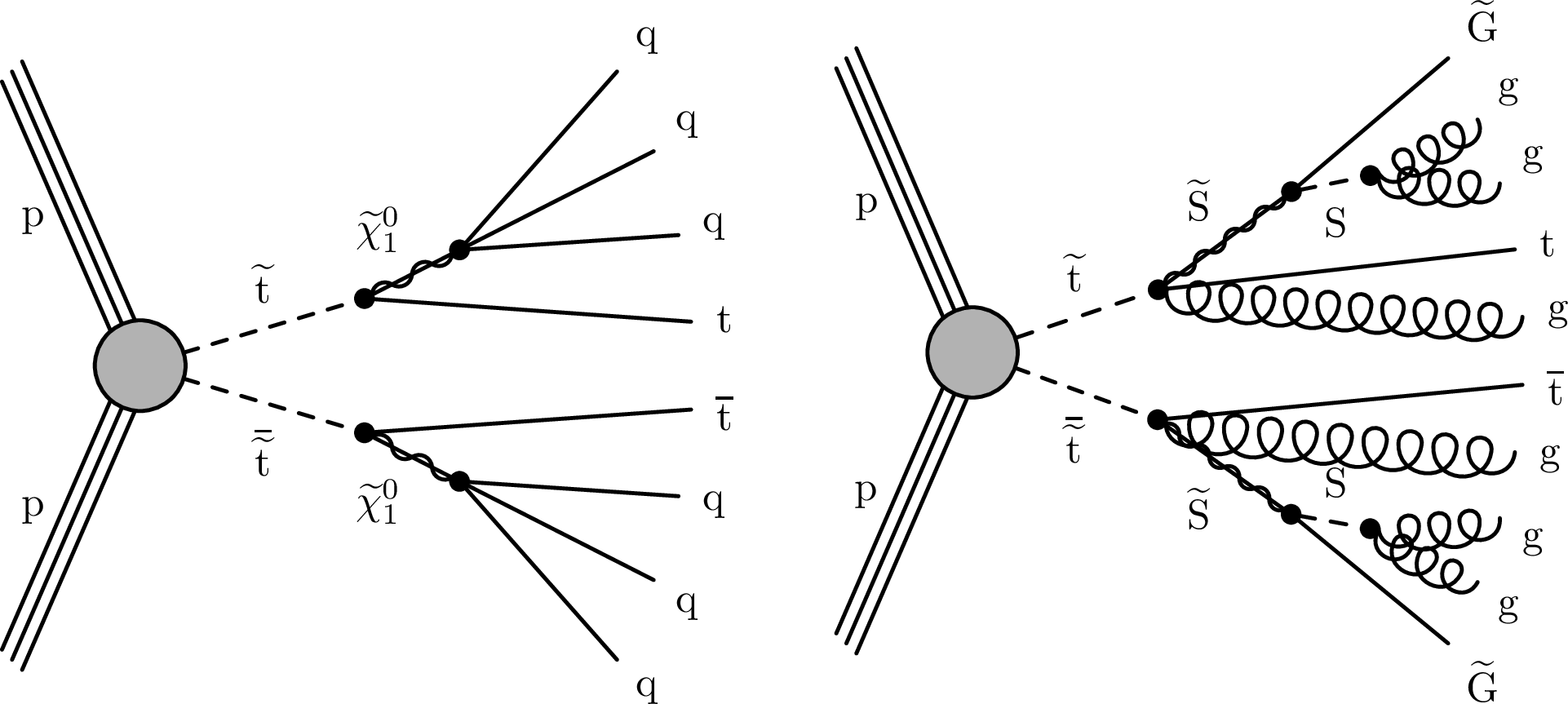
Figure 1:
Diagrams of top squark pair production with each squark decaying to a top quark and additional light-flavor quarks for the RPV SUSY model (left) and with each squark decaying to a top quark, gluons, and a gravitino for the stealth $ \mathrm{S}\mathrm{Y} \overline{\mathrm{Y}} $ model (right). |
png pdf |
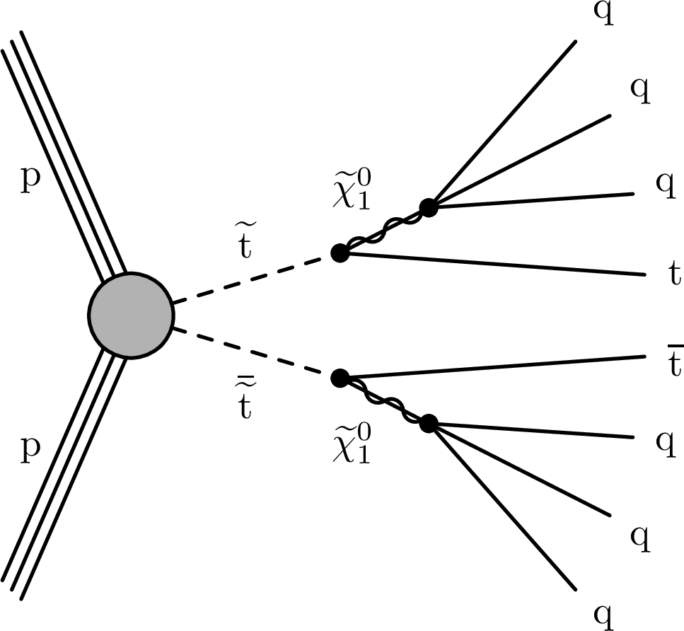
Figure 1-a:
Diagrams of top squark pair production with each squark decaying to a top quark and additional light-flavor quarks for the RPV SUSY model (left) and with each squark decaying to a top quark, gluons, and a gravitino for the stealth $ \mathrm{S}\mathrm{Y} \overline{\mathrm{Y}} $ model (right). |
png pdf |
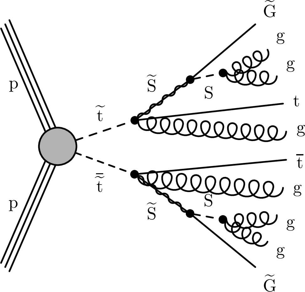
Figure 1-b:
Diagrams of top squark pair production with each squark decaying to a top quark and additional light-flavor quarks for the RPV SUSY model (left) and with each squark decaying to a top quark, gluons, and a gravitino for the stealth $ \mathrm{S}\mathrm{Y} \overline{\mathrm{Y}} $ model (right). |
png pdf |
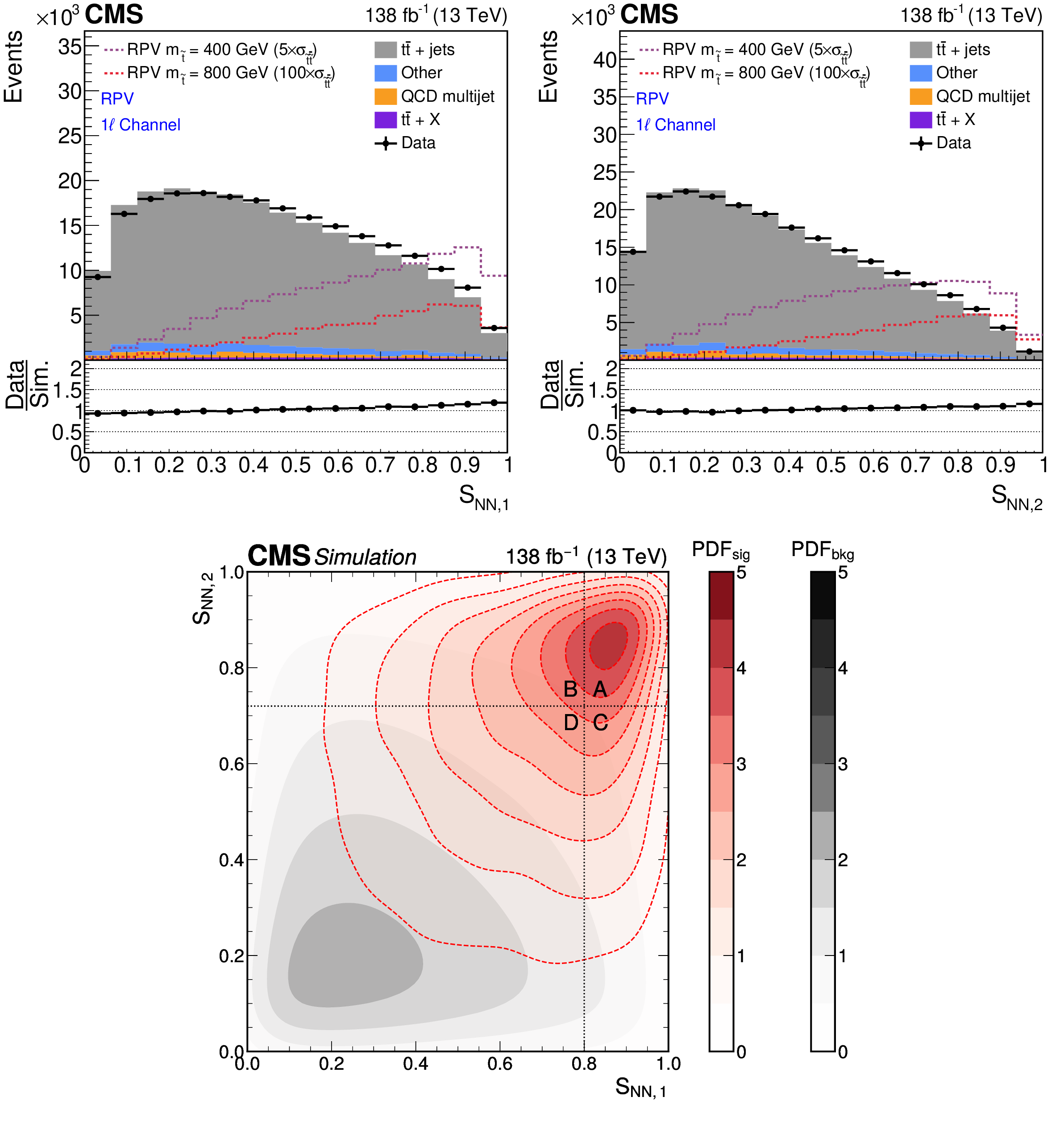
Figure 2:
For the RPV signal model and all $ N_\text{jets} $ categories of the 1$ \ell $ channel, distributions of $S_{\mathrm{NN,1}}$ (upper left) and $S_{\mathrm{NN,2}}$ (upper right) for data (black solid line), pre-fit simulated SM backgrounds (stacked filled histograms), and two RPV signal models with $ m_{\tilde{\mathrm{t}}}= $ 400 and 800 GeV (dashed lines) are shown. The lower panel shows the two-dimensional probability density function distribution of $S_{\mathrm{NN,1}}$ and $S_{\mathrm{NN,2}}$ for simulated $ {\mathrm{t}\overline{\mathrm{t}}} + \text{jets} $ events (solid gray) and the RPV signal model with $ m_{\tilde{\mathrm{t}}}= $ 800 GeV (dashed red). The ABCD bin boundaries for this signal model in the 1$ \ell $ channel are shown with dashed vertical and horizontal lines. |
png pdf |
Figure 2-a:
For the RPV signal model and all $ N_\text{jets} $ categories of the 1$ \ell $ channel, distributions of $S_{\mathrm{NN,1}}$ (upper left) and $S_{\mathrm{NN,2}}$ (upper right) for data (black solid line), pre-fit simulated SM backgrounds (stacked filled histograms), and two RPV signal models with $ m_{\tilde{\mathrm{t}}}= $ 400 and 800 GeV (dashed lines) are shown. The lower panel shows the two-dimensional probability density function distribution of $S_{\mathrm{NN,1}}$ and $S_{\mathrm{NN,2}}$ for simulated $ {\mathrm{t}\overline{\mathrm{t}}} + \text{jets} $ events (solid gray) and the RPV signal model with $ m_{\tilde{\mathrm{t}}}= $ 800 GeV (dashed red). The ABCD bin boundaries for this signal model in the 1$ \ell $ channel are shown with dashed vertical and horizontal lines. |
png pdf |
Figure 2-b:
For the RPV signal model and all $ N_\text{jets} $ categories of the 1$ \ell $ channel, distributions of $S_{\mathrm{NN,1}}$ (upper left) and $S_{\mathrm{NN,2}}$ (upper right) for data (black solid line), pre-fit simulated SM backgrounds (stacked filled histograms), and two RPV signal models with $ m_{\tilde{\mathrm{t}}}= $ 400 and 800 GeV (dashed lines) are shown. The lower panel shows the two-dimensional probability density function distribution of $S_{\mathrm{NN,1}}$ and $S_{\mathrm{NN,2}}$ for simulated $ {\mathrm{t}\overline{\mathrm{t}}} + \text{jets} $ events (solid gray) and the RPV signal model with $ m_{\tilde{\mathrm{t}}}= $ 800 GeV (dashed red). The ABCD bin boundaries for this signal model in the 1$ \ell $ channel are shown with dashed vertical and horizontal lines. |
png pdf |
Figure 2-c:
For the RPV signal model and all $ N_\text{jets} $ categories of the 1$ \ell $ channel, distributions of $S_{\mathrm{NN,1}}$ (upper left) and $S_{\mathrm{NN,2}}$ (upper right) for data (black solid line), pre-fit simulated SM backgrounds (stacked filled histograms), and two RPV signal models with $ m_{\tilde{\mathrm{t}}}= $ 400 and 800 GeV (dashed lines) are shown. The lower panel shows the two-dimensional probability density function distribution of $S_{\mathrm{NN,1}}$ and $S_{\mathrm{NN,2}}$ for simulated $ {\mathrm{t}\overline{\mathrm{t}}} + \text{jets} $ events (solid gray) and the RPV signal model with $ m_{\tilde{\mathrm{t}}}= $ 800 GeV (dashed red). The ABCD bin boundaries for this signal model in the 1$ \ell $ channel are shown with dashed vertical and horizontal lines. |
png pdf |
Figure 3:
Illustrations of the three validation regions that are created by partitioning the $S_{\mathrm{NN,1}}$-$S_{\mathrm{NN,2}}$ plane. VR I (VR II), shown in the upper (middle) row, is a division of the $ B $ and $ D $ ($ C $ and $ D $) regions. VR III (lower row) is a division of the $ D $ region. Each VR is divided into four subregions (d$ A $, d$ B $, d$ C $, d$ D $) that are used to perform the validation of the nonclosure of the $S_{\mathrm{NN,1}}$-$S_{\mathrm{NN,2}}$ plane. The subregion boundaries shown in the figure are the starting points of the stepping procedure explained in the text. |
png pdf |
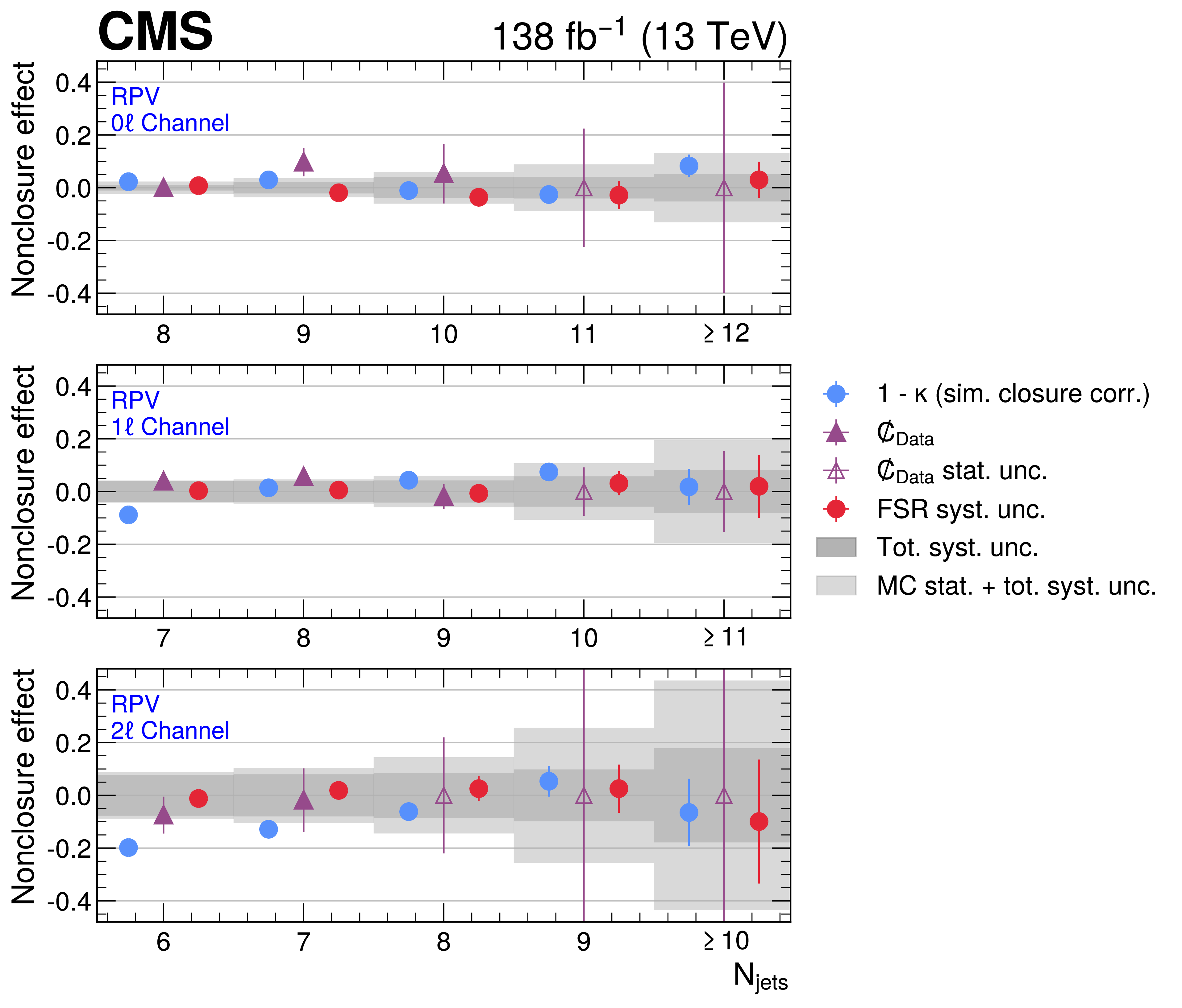
Figure 4:
One minus the simulation-based closure correction $ \kappa $ (blue circle), the residual nonclosure $ {C}\hspace{-0.70em}/\kern 0.0em $ in data (solid purple triangle), and the FSR systematic uncertainty (red circle) are shown for each $ N_\text{jets} $ category for the 0$ \ell $ (upper), 1$ \ell $ (middle), and 2$ \ell $ (lower panel) channels. All values correspond to the low-mass optimization for the RPV signal model. The value of $ {C}\hspace{-0.70em}/\kern 0.0em $ shown is the maximum value of the stepping procedure described in the text. Note the data-based nonclosure systematic uncertainty is defined to be the nonclosure in the lowest $ N_\text{jets} $ bin for each of the channels. Open purple triangles show the statistical uncertainty in $ {C}\hspace{-0.70em}/\kern 0.0em $ in data for categories in which all VR and ABCD boundaries have a signal fraction exceeding 5%. All data-based nonclosure values are calculated after applying the simulation-based closure correction, such that an observed nonclosure of zero signifies identical modeling of the $S_{\mathrm{NN,1}}$-$S_{\mathrm{NN,2}}$ correlation in simulation and data. |
png pdf |
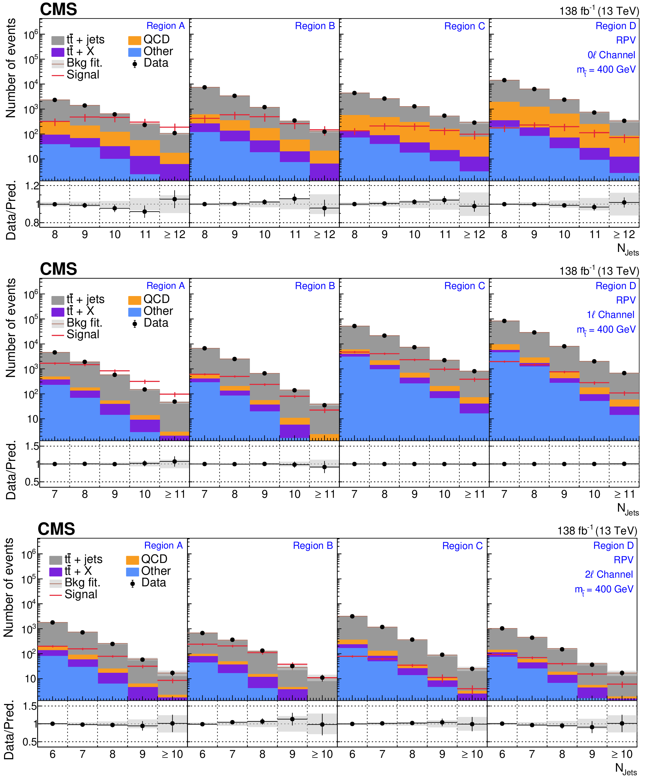
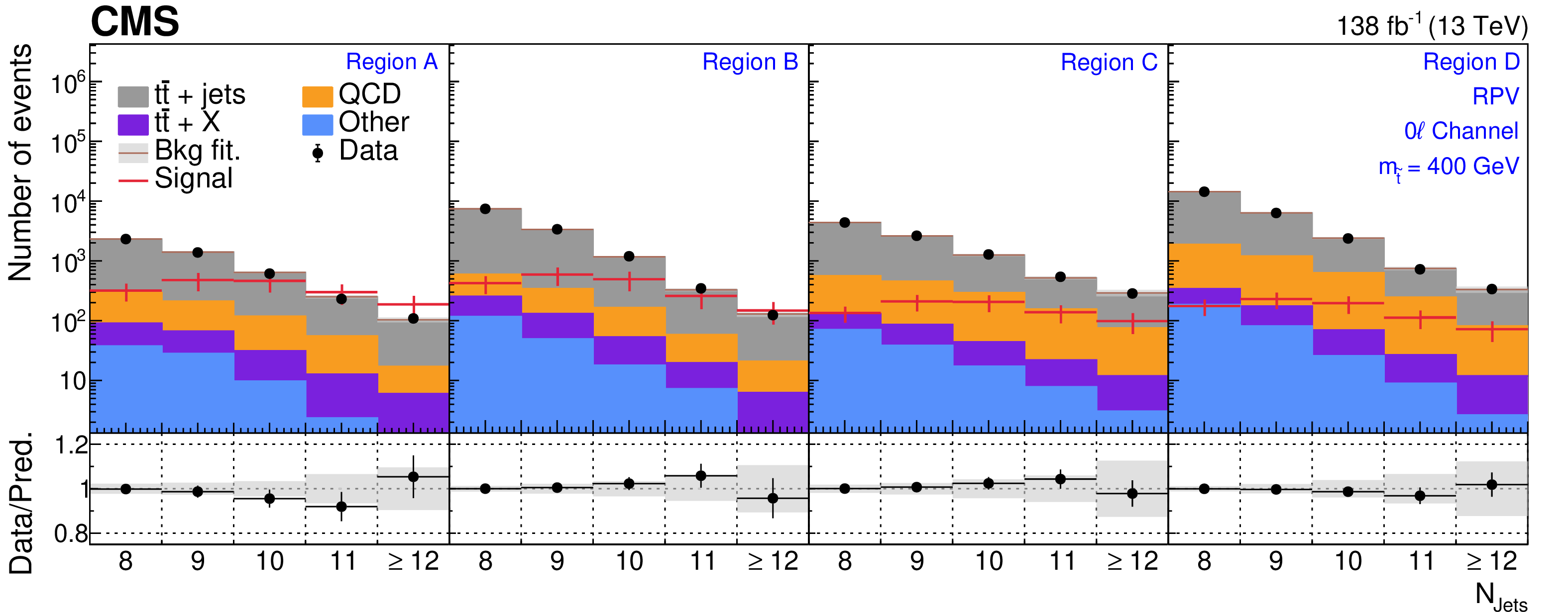
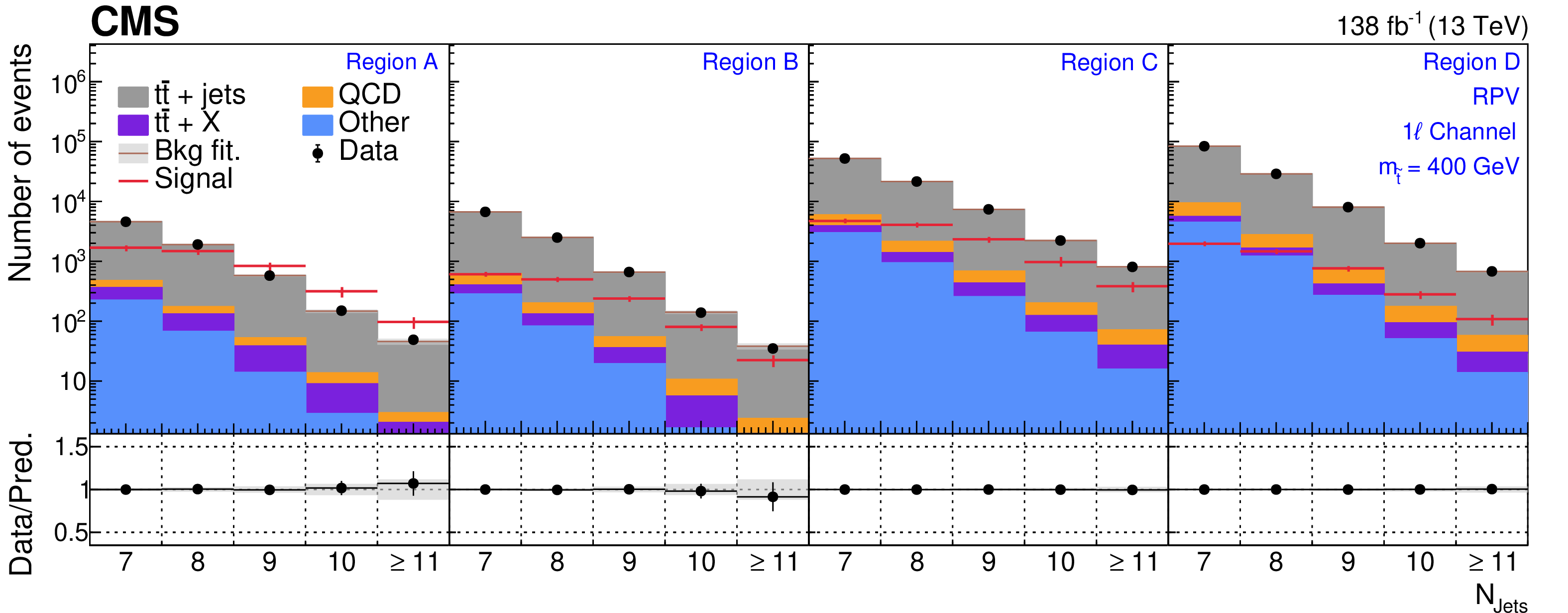
Figure 5:
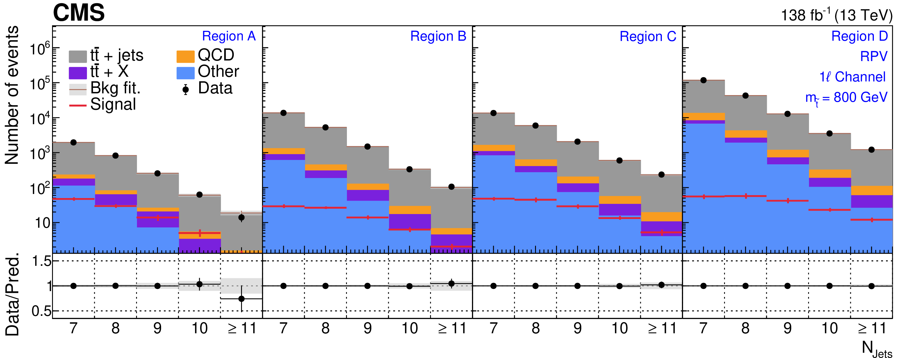
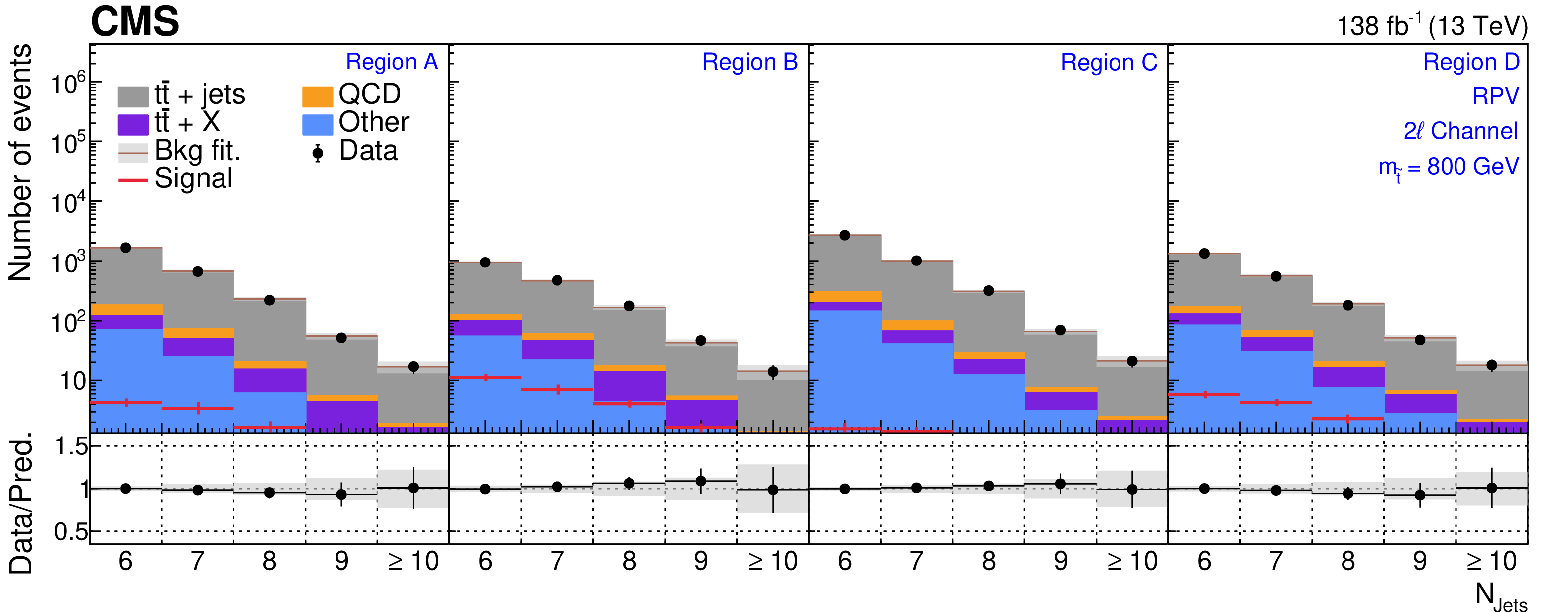
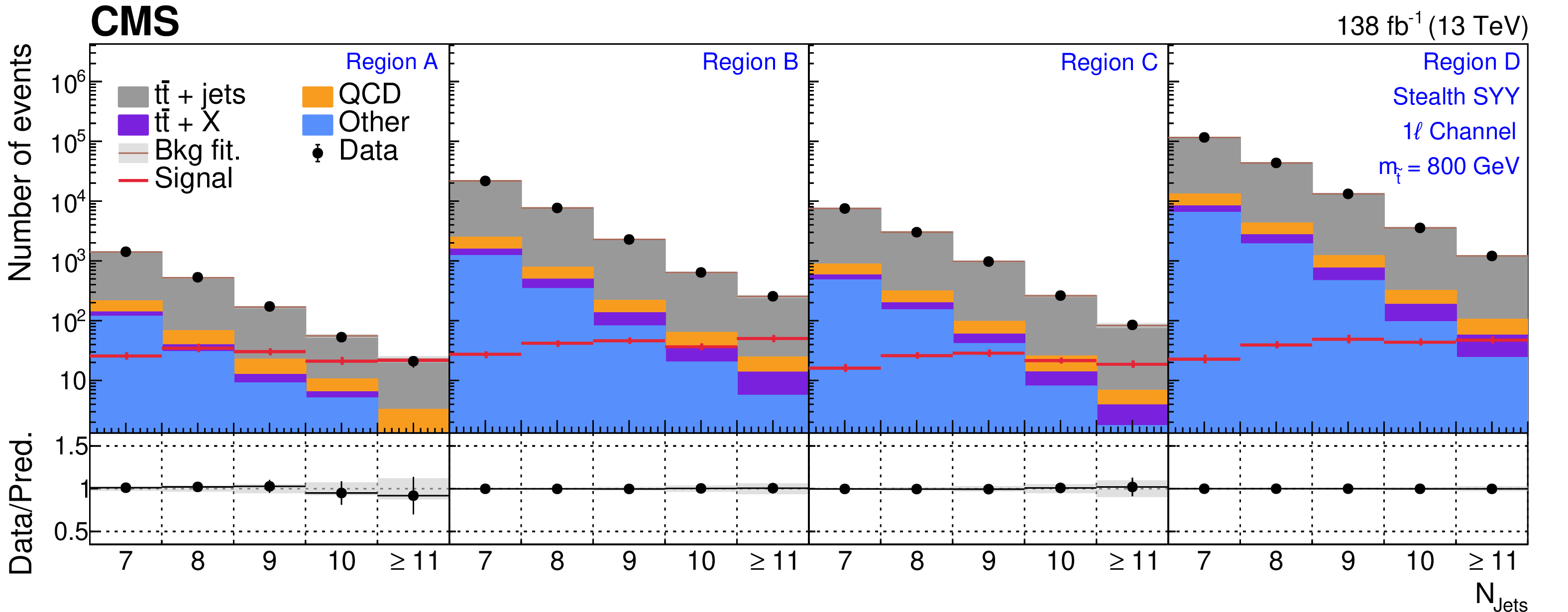
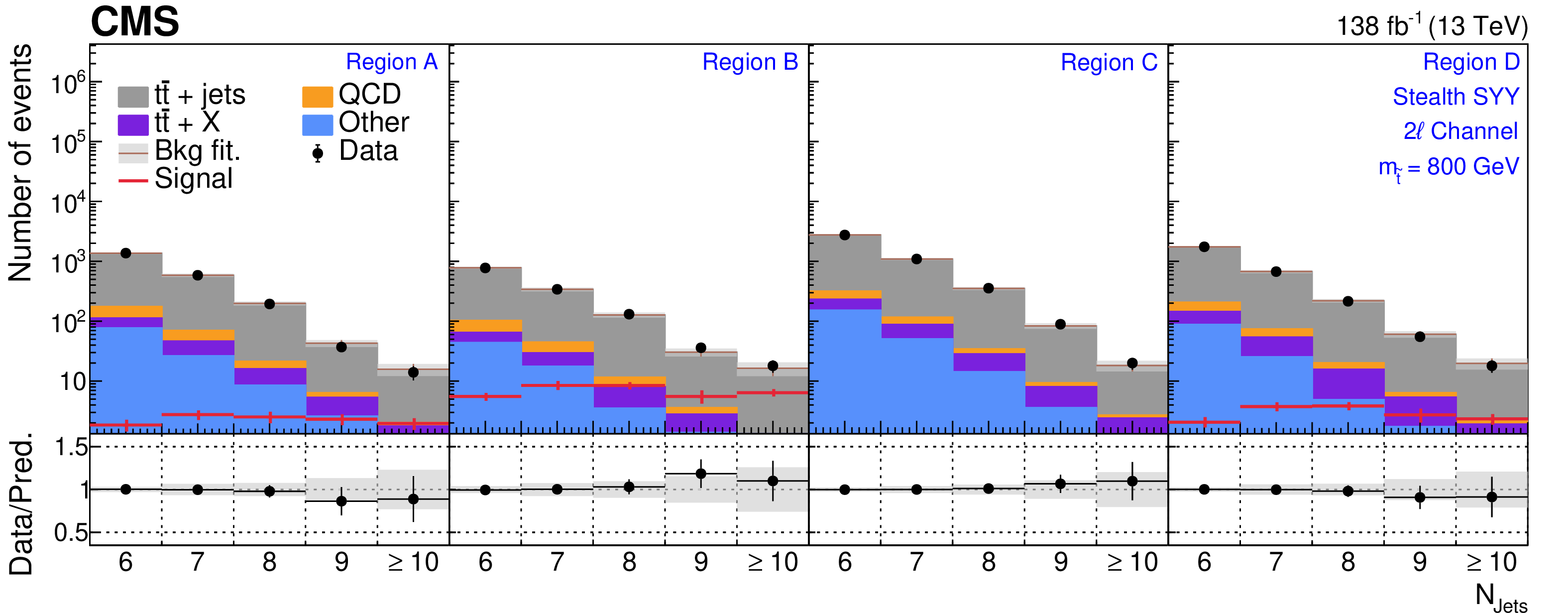
The $ N_\text{jets} $ distributions from the background-only fits to data. Fits are run with the signal strength fixed to zero and all background process event yields are obtained from their fit predictions. The signal distribution overlaid corresponds to the RPV model with $ m_{\tilde{\mathrm{t}}} = $ 400 GeV. The graphs in the upper, middle, and lower rows correspond to the 0$ \ell $, 1$ \ell $, and 2$ \ell $ channels, respectively. The four panels in each row show the $ N_\text{jets} $ distributions for the $ A $, $ B $, $ C $, and $ D $ regions (left to right). The gray error band shows the combined statistical and systematic uncertainty from the background-only fit distributions. |
png pdf |
Figure 5-a:
The $ N_\text{jets} $ distributions from the background-only fits to data. Fits are run with the signal strength fixed to zero and all background process event yields are obtained from their fit predictions. The signal distribution overlaid corresponds to the RPV model with $ m_{\tilde{\mathrm{t}}} = $ 400 GeV. The graphs in the upper, middle, and lower rows correspond to the 0$ \ell $, 1$ \ell $, and 2$ \ell $ channels, respectively. The four panels in each row show the $ N_\text{jets} $ distributions for the $ A $, $ B $, $ C $, and $ D $ regions (left to right). The gray error band shows the combined statistical and systematic uncertainty from the background-only fit distributions. |
png pdf |
Figure 5-b:
The $ N_\text{jets} $ distributions from the background-only fits to data. Fits are run with the signal strength fixed to zero and all background process event yields are obtained from their fit predictions. The signal distribution overlaid corresponds to the RPV model with $ m_{\tilde{\mathrm{t}}} = $ 400 GeV. The graphs in the upper, middle, and lower rows correspond to the 0$ \ell $, 1$ \ell $, and 2$ \ell $ channels, respectively. The four panels in each row show the $ N_\text{jets} $ distributions for the $ A $, $ B $, $ C $, and $ D $ regions (left to right). The gray error band shows the combined statistical and systematic uncertainty from the background-only fit distributions. |
png pdf |
Figure 5-c:
The $ N_\text{jets} $ distributions from the background-only fits to data. Fits are run with the signal strength fixed to zero and all background process event yields are obtained from their fit predictions. The signal distribution overlaid corresponds to the RPV model with $ m_{\tilde{\mathrm{t}}} = $ 400 GeV. The graphs in the upper, middle, and lower rows correspond to the 0$ \ell $, 1$ \ell $, and 2$ \ell $ channels, respectively. The four panels in each row show the $ N_\text{jets} $ distributions for the $ A $, $ B $, $ C $, and $ D $ regions (left to right). The gray error band shows the combined statistical and systematic uncertainty from the background-only fit distributions. |
png pdf |
Figure 6:
The 95% CL upper limit on $ \sigma_{\tilde{\mathrm{t}}\overline{\tilde{\mathrm{t}}}} $ for the RPV (left) and stealth $ \mathrm{S}\mathrm{Y} \overline{\mathrm{Y}} $ (right) SUSY signal models as a function of $ m_{\tilde{\mathrm{t}}} $ for the 0$ \ell $ channel (upper), 1$ \ell $ channel (middle), and 2$ \ell $ channel (lower), assuming 100% branching fraction to the considered $ \tilde{\mathrm{t}} $ squark decay. The median expected limit is shown in the dashed blue line, with the 68 and 95% intervals shown in light-blue and yellow, respectively. The observed limit is shown in black. The vertical dashed line denotes the transition from the low- to high-mass optimization ABCD boundaries. Additionally, the theoretical cross section is shown in red with its uncertainty in light brown. |
png pdf |
Figure 6-a:
The 95% CL upper limit on $ \sigma_{\tilde{\mathrm{t}}\overline{\tilde{\mathrm{t}}}} $ for the RPV (left) and stealth $ \mathrm{S}\mathrm{Y} \overline{\mathrm{Y}} $ (right) SUSY signal models as a function of $ m_{\tilde{\mathrm{t}}} $ for the 0$ \ell $ channel (upper), 1$ \ell $ channel (middle), and 2$ \ell $ channel (lower), assuming 100% branching fraction to the considered $ \tilde{\mathrm{t}} $ squark decay. The median expected limit is shown in the dashed blue line, with the 68 and 95% intervals shown in light-blue and yellow, respectively. The observed limit is shown in black. The vertical dashed line denotes the transition from the low- to high-mass optimization ABCD boundaries. Additionally, the theoretical cross section is shown in red with its uncertainty in light brown. |
png pdf |
Figure 6-b:
The 95% CL upper limit on $ \sigma_{\tilde{\mathrm{t}}\overline{\tilde{\mathrm{t}}}} $ for the RPV (left) and stealth $ \mathrm{S}\mathrm{Y} \overline{\mathrm{Y}} $ (right) SUSY signal models as a function of $ m_{\tilde{\mathrm{t}}} $ for the 0$ \ell $ channel (upper), 1$ \ell $ channel (middle), and 2$ \ell $ channel (lower), assuming 100% branching fraction to the considered $ \tilde{\mathrm{t}} $ squark decay. The median expected limit is shown in the dashed blue line, with the 68 and 95% intervals shown in light-blue and yellow, respectively. The observed limit is shown in black. The vertical dashed line denotes the transition from the low- to high-mass optimization ABCD boundaries. Additionally, the theoretical cross section is shown in red with its uncertainty in light brown. |
png pdf |
Figure 6-c:
The 95% CL upper limit on $ \sigma_{\tilde{\mathrm{t}}\overline{\tilde{\mathrm{t}}}} $ for the RPV (left) and stealth $ \mathrm{S}\mathrm{Y} \overline{\mathrm{Y}} $ (right) SUSY signal models as a function of $ m_{\tilde{\mathrm{t}}} $ for the 0$ \ell $ channel (upper), 1$ \ell $ channel (middle), and 2$ \ell $ channel (lower), assuming 100% branching fraction to the considered $ \tilde{\mathrm{t}} $ squark decay. The median expected limit is shown in the dashed blue line, with the 68 and 95% intervals shown in light-blue and yellow, respectively. The observed limit is shown in black. The vertical dashed line denotes the transition from the low- to high-mass optimization ABCD boundaries. Additionally, the theoretical cross section is shown in red with its uncertainty in light brown. |
png pdf |
Figure 6-d:
The 95% CL upper limit on $ \sigma_{\tilde{\mathrm{t}}\overline{\tilde{\mathrm{t}}}} $ for the RPV (left) and stealth $ \mathrm{S}\mathrm{Y} \overline{\mathrm{Y}} $ (right) SUSY signal models as a function of $ m_{\tilde{\mathrm{t}}} $ for the 0$ \ell $ channel (upper), 1$ \ell $ channel (middle), and 2$ \ell $ channel (lower), assuming 100% branching fraction to the considered $ \tilde{\mathrm{t}} $ squark decay. The median expected limit is shown in the dashed blue line, with the 68 and 95% intervals shown in light-blue and yellow, respectively. The observed limit is shown in black. The vertical dashed line denotes the transition from the low- to high-mass optimization ABCD boundaries. Additionally, the theoretical cross section is shown in red with its uncertainty in light brown. |
png pdf |
Figure 6-e:
The 95% CL upper limit on $ \sigma_{\tilde{\mathrm{t}}\overline{\tilde{\mathrm{t}}}} $ for the RPV (left) and stealth $ \mathrm{S}\mathrm{Y} \overline{\mathrm{Y}} $ (right) SUSY signal models as a function of $ m_{\tilde{\mathrm{t}}} $ for the 0$ \ell $ channel (upper), 1$ \ell $ channel (middle), and 2$ \ell $ channel (lower), assuming 100% branching fraction to the considered $ \tilde{\mathrm{t}} $ squark decay. The median expected limit is shown in the dashed blue line, with the 68 and 95% intervals shown in light-blue and yellow, respectively. The observed limit is shown in black. The vertical dashed line denotes the transition from the low- to high-mass optimization ABCD boundaries. Additionally, the theoretical cross section is shown in red with its uncertainty in light brown. |
png pdf |
Figure 6-f:
The 95% CL upper limit on $ \sigma_{\tilde{\mathrm{t}}\overline{\tilde{\mathrm{t}}}} $ for the RPV (left) and stealth $ \mathrm{S}\mathrm{Y} \overline{\mathrm{Y}} $ (right) SUSY signal models as a function of $ m_{\tilde{\mathrm{t}}} $ for the 0$ \ell $ channel (upper), 1$ \ell $ channel (middle), and 2$ \ell $ channel (lower), assuming 100% branching fraction to the considered $ \tilde{\mathrm{t}} $ squark decay. The median expected limit is shown in the dashed blue line, with the 68 and 95% intervals shown in light-blue and yellow, respectively. The observed limit is shown in black. The vertical dashed line denotes the transition from the low- to high-mass optimization ABCD boundaries. Additionally, the theoretical cross section is shown in red with its uncertainty in light brown. |
png pdf |
Figure 7:
Observed and expected upper limits at 95% CL on $ \sigma_{\tilde{\mathrm{t}}\overline{\tilde{\mathrm{t}}}} $ for the RPV (upper) and stealth $ \mathrm{S}\mathrm{Y} \overline{\mathrm{Y}} $ (lower) SUSY signal models as functions of $ m_{\tilde{\mathrm{t}}} $ for the combination of all three channels, assuming 100% branching fraction to the considered $ \tilde{\mathrm{t}} $ squark decay. The median expected limit is shown in the dashed blue line, with the 68 and 95% intervals shown in light blue and yellow, respectively. The observed limit is shown in black. The vertical dashed line denotes the transition from the low- to high-mass optimization ABCD boundaries. Additionally, the theoretical cross section is shown in red with its uncertainty in light brown. |

png pdf |
Figure 7-a:
Observed and expected upper limits at 95% CL on $ \sigma_{\tilde{\mathrm{t}}\overline{\tilde{\mathrm{t}}}} $ for the RPV (upper) and stealth $ \mathrm{S}\mathrm{Y} \overline{\mathrm{Y}} $ (lower) SUSY signal models as functions of $ m_{\tilde{\mathrm{t}}} $ for the combination of all three channels, assuming 100% branching fraction to the considered $ \tilde{\mathrm{t}} $ squark decay. The median expected limit is shown in the dashed blue line, with the 68 and 95% intervals shown in light blue and yellow, respectively. The observed limit is shown in black. The vertical dashed line denotes the transition from the low- to high-mass optimization ABCD boundaries. Additionally, the theoretical cross section is shown in red with its uncertainty in light brown. |
png pdf |
Figure 7-b:
Observed and expected upper limits at 95% CL on $ \sigma_{\tilde{\mathrm{t}}\overline{\tilde{\mathrm{t}}}} $ for the RPV (upper) and stealth $ \mathrm{S}\mathrm{Y} \overline{\mathrm{Y}} $ (lower) SUSY signal models as functions of $ m_{\tilde{\mathrm{t}}} $ for the combination of all three channels, assuming 100% branching fraction to the considered $ \tilde{\mathrm{t}} $ squark decay. The median expected limit is shown in the dashed blue line, with the 68 and 95% intervals shown in light blue and yellow, respectively. The observed limit is shown in black. The vertical dashed line denotes the transition from the low- to high-mass optimization ABCD boundaries. Additionally, the theoretical cross section is shown in red with its uncertainty in light brown. |
png pdf |
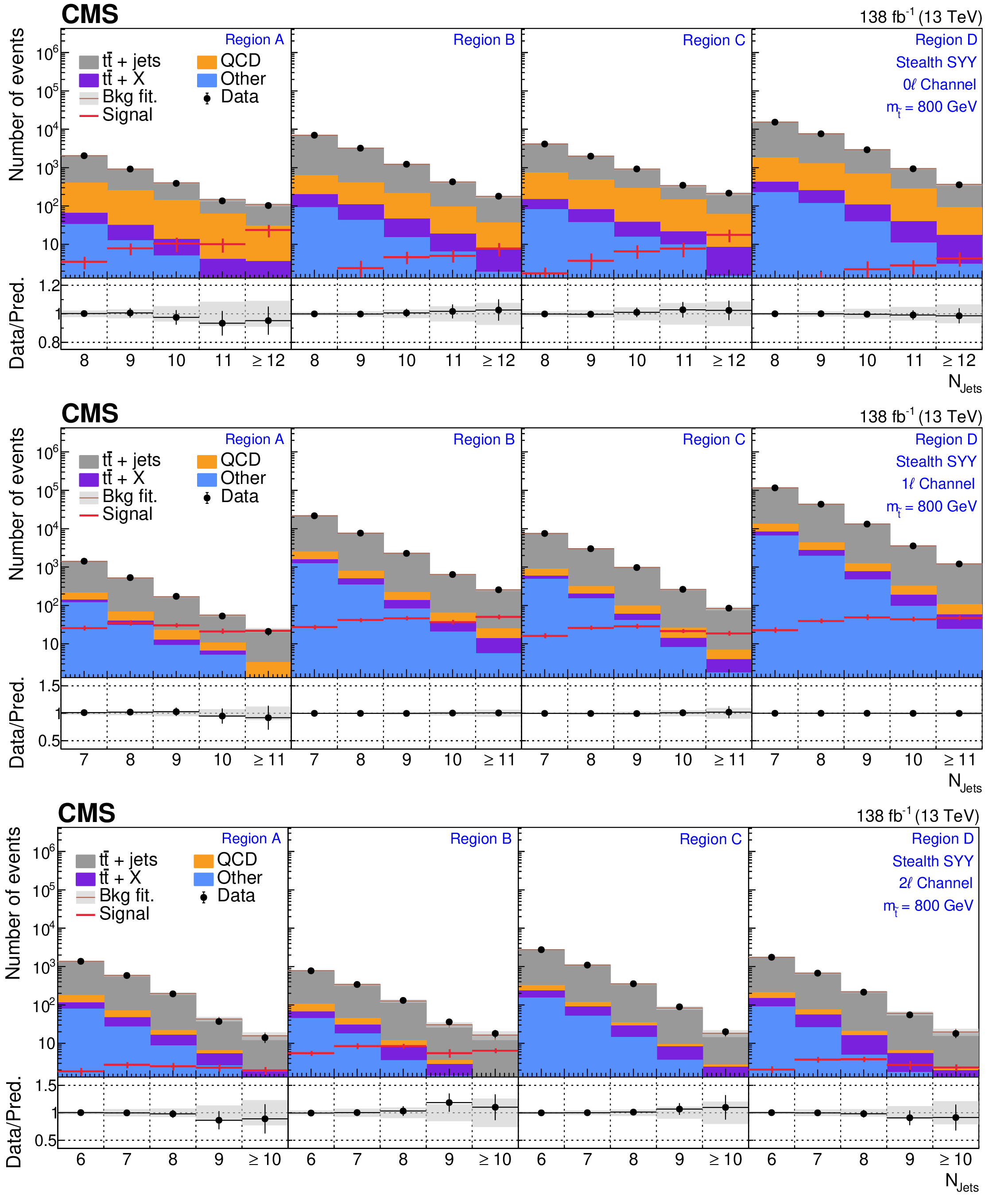
Figure A1:
The $ N_\text{jets} $ distributions from the background-only fits to data. Fits are run with the signal strength fixed to zero and all background process event yields are obtained from their fit predictions. The signal distribution overlaid corresponds to the stealth $ \mathrm{S}\mathrm{Y} \overline{\mathrm{Y}} $ model with $ m_{\tilde{\mathrm{t}}} = $ 400 GeV. The graphs in the upper, middle, and lower rows correspond to the 0$ \ell $, 1$ \ell $, and 2$ \ell $ channels, respectively. The four panels in each row show the $ N_\text{jets} $ distributions for the $ A $, $ B $, $ C $, and $ D $ regions (left to right). The gray error band shows the combined statistical and systematic uncertainty from the background-only fit distributions. |
png pdf |
Figure A1-a:
The $ N_\text{jets} $ distributions from the background-only fits to data. Fits are run with the signal strength fixed to zero and all background process event yields are obtained from their fit predictions. The signal distribution overlaid corresponds to the stealth $ \mathrm{S}\mathrm{Y} \overline{\mathrm{Y}} $ model with $ m_{\tilde{\mathrm{t}}} = $ 400 GeV. The graphs in the upper, middle, and lower rows correspond to the 0$ \ell $, 1$ \ell $, and 2$ \ell $ channels, respectively. The four panels in each row show the $ N_\text{jets} $ distributions for the $ A $, $ B $, $ C $, and $ D $ regions (left to right). The gray error band shows the combined statistical and systematic uncertainty from the background-only fit distributions. |
png pdf |
Figure A1-b:
The $ N_\text{jets} $ distributions from the background-only fits to data. Fits are run with the signal strength fixed to zero and all background process event yields are obtained from their fit predictions. The signal distribution overlaid corresponds to the stealth $ \mathrm{S}\mathrm{Y} \overline{\mathrm{Y}} $ model with $ m_{\tilde{\mathrm{t}}} = $ 400 GeV. The graphs in the upper, middle, and lower rows correspond to the 0$ \ell $, 1$ \ell $, and 2$ \ell $ channels, respectively. The four panels in each row show the $ N_\text{jets} $ distributions for the $ A $, $ B $, $ C $, and $ D $ regions (left to right). The gray error band shows the combined statistical and systematic uncertainty from the background-only fit distributions. |
png pdf |
Figure A1-c:
The $ N_\text{jets} $ distributions from the background-only fits to data. Fits are run with the signal strength fixed to zero and all background process event yields are obtained from their fit predictions. The signal distribution overlaid corresponds to the stealth $ \mathrm{S}\mathrm{Y} \overline{\mathrm{Y}} $ model with $ m_{\tilde{\mathrm{t}}} = $ 400 GeV. The graphs in the upper, middle, and lower rows correspond to the 0$ \ell $, 1$ \ell $, and 2$ \ell $ channels, respectively. The four panels in each row show the $ N_\text{jets} $ distributions for the $ A $, $ B $, $ C $, and $ D $ regions (left to right). The gray error band shows the combined statistical and systematic uncertainty from the background-only fit distributions. |
png pdf |
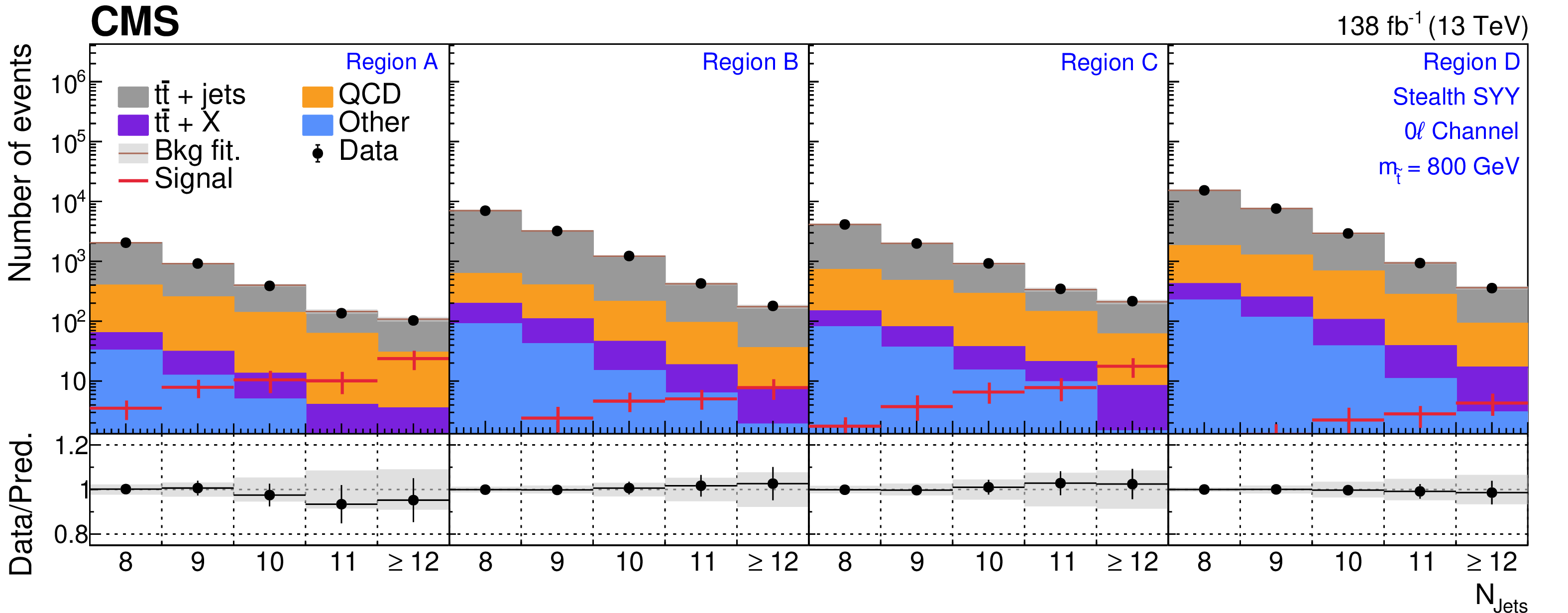
Figure A2:
The $ N_\text{jets} $ distributions from the background-only fits to data. Fits are run with the signal strength fixed to zero and all background process event yields are obtained from their fit predictions. The signal distribution overlaid corresponds to the RPV model with $ m_{\tilde{\mathrm{t}}} = $ 800 GeV. The graphs in the upper, middle, and lower rows correspond to the 0$ \ell $, 1$ \ell $, and 2$ \ell $ channels, respectively. The four panels in each row show the $ N_\text{jets} $ distributions for the $ A $, $ B $, $ C $, and $ D $ regions (left to right). The gray error band shows the combined statistical and systematic uncertainty from the background-only fit distributions. |
png pdf |
Figure A2-a:
The $ N_\text{jets} $ distributions from the background-only fits to data. Fits are run with the signal strength fixed to zero and all background process event yields are obtained from their fit predictions. The signal distribution overlaid corresponds to the RPV model with $ m_{\tilde{\mathrm{t}}} = $ 800 GeV. The graphs in the upper, middle, and lower rows correspond to the 0$ \ell $, 1$ \ell $, and 2$ \ell $ channels, respectively. The four panels in each row show the $ N_\text{jets} $ distributions for the $ A $, $ B $, $ C $, and $ D $ regions (left to right). The gray error band shows the combined statistical and systematic uncertainty from the background-only fit distributions. |
png pdf |
Figure A2-b:
The $ N_\text{jets} $ distributions from the background-only fits to data. Fits are run with the signal strength fixed to zero and all background process event yields are obtained from their fit predictions. The signal distribution overlaid corresponds to the RPV model with $ m_{\tilde{\mathrm{t}}} = $ 800 GeV. The graphs in the upper, middle, and lower rows correspond to the 0$ \ell $, 1$ \ell $, and 2$ \ell $ channels, respectively. The four panels in each row show the $ N_\text{jets} $ distributions for the $ A $, $ B $, $ C $, and $ D $ regions (left to right). The gray error band shows the combined statistical and systematic uncertainty from the background-only fit distributions. |
png pdf |
Figure A2-c:
The $ N_\text{jets} $ distributions from the background-only fits to data. Fits are run with the signal strength fixed to zero and all background process event yields are obtained from their fit predictions. The signal distribution overlaid corresponds to the RPV model with $ m_{\tilde{\mathrm{t}}} = $ 800 GeV. The graphs in the upper, middle, and lower rows correspond to the 0$ \ell $, 1$ \ell $, and 2$ \ell $ channels, respectively. The four panels in each row show the $ N_\text{jets} $ distributions for the $ A $, $ B $, $ C $, and $ D $ regions (left to right). The gray error band shows the combined statistical and systematic uncertainty from the background-only fit distributions. |
png pdf |
Figure A3:
The $ N_\text{jets} $ distributions from the background-only fits to data. Fits are run with the signal strength fixed to zero and all background process event yields are obtained from their fit predictions. The signal distribution overlaid corresponds to the stealth $ \mathrm{S}\mathrm{Y} \overline{\mathrm{Y}} $ model with $ m_{\tilde{\mathrm{t}}} = $ 800 GeV. The graphs in the upper, middle, and lower rows correspond to the 0$ \ell $, 1$ \ell $, and 2$ \ell $ channels, respectively. The four panels in each row show the $ N_\text{jets} $ distributions for the $ A $, $ B $, $ C $, and $ D $ regions (left to right). The gray error band shows the combined statistical and systematic uncertainty from the background-only fit distributions. |
png pdf |
Figure A3-a:
The $ N_\text{jets} $ distributions from the background-only fits to data. Fits are run with the signal strength fixed to zero and all background process event yields are obtained from their fit predictions. The signal distribution overlaid corresponds to the stealth $ \mathrm{S}\mathrm{Y} \overline{\mathrm{Y}} $ model with $ m_{\tilde{\mathrm{t}}} = $ 800 GeV. The graphs in the upper, middle, and lower rows correspond to the 0$ \ell $, 1$ \ell $, and 2$ \ell $ channels, respectively. The four panels in each row show the $ N_\text{jets} $ distributions for the $ A $, $ B $, $ C $, and $ D $ regions (left to right). The gray error band shows the combined statistical and systematic uncertainty from the background-only fit distributions. |
png pdf |
Figure A3-b:
The $ N_\text{jets} $ distributions from the background-only fits to data. Fits are run with the signal strength fixed to zero and all background process event yields are obtained from their fit predictions. The signal distribution overlaid corresponds to the stealth $ \mathrm{S}\mathrm{Y} \overline{\mathrm{Y}} $ model with $ m_{\tilde{\mathrm{t}}} = $ 800 GeV. The graphs in the upper, middle, and lower rows correspond to the 0$ \ell $, 1$ \ell $, and 2$ \ell $ channels, respectively. The four panels in each row show the $ N_\text{jets} $ distributions for the $ A $, $ B $, $ C $, and $ D $ regions (left to right). The gray error band shows the combined statistical and systematic uncertainty from the background-only fit distributions. |
png pdf |
Figure A3-c:
The $ N_\text{jets} $ distributions from the background-only fits to data. Fits are run with the signal strength fixed to zero and all background process event yields are obtained from their fit predictions. The signal distribution overlaid corresponds to the stealth $ \mathrm{S}\mathrm{Y} \overline{\mathrm{Y}} $ model with $ m_{\tilde{\mathrm{t}}} = $ 800 GeV. The graphs in the upper, middle, and lower rows correspond to the 0$ \ell $, 1$ \ell $, and 2$ \ell $ channels, respectively. The four panels in each row show the $ N_\text{jets} $ distributions for the $ A $, $ B $, $ C $, and $ D $ regions (left to right). The gray error band shows the combined statistical and systematic uncertainty from the background-only fit distributions. |
| Tables | |
png pdf |
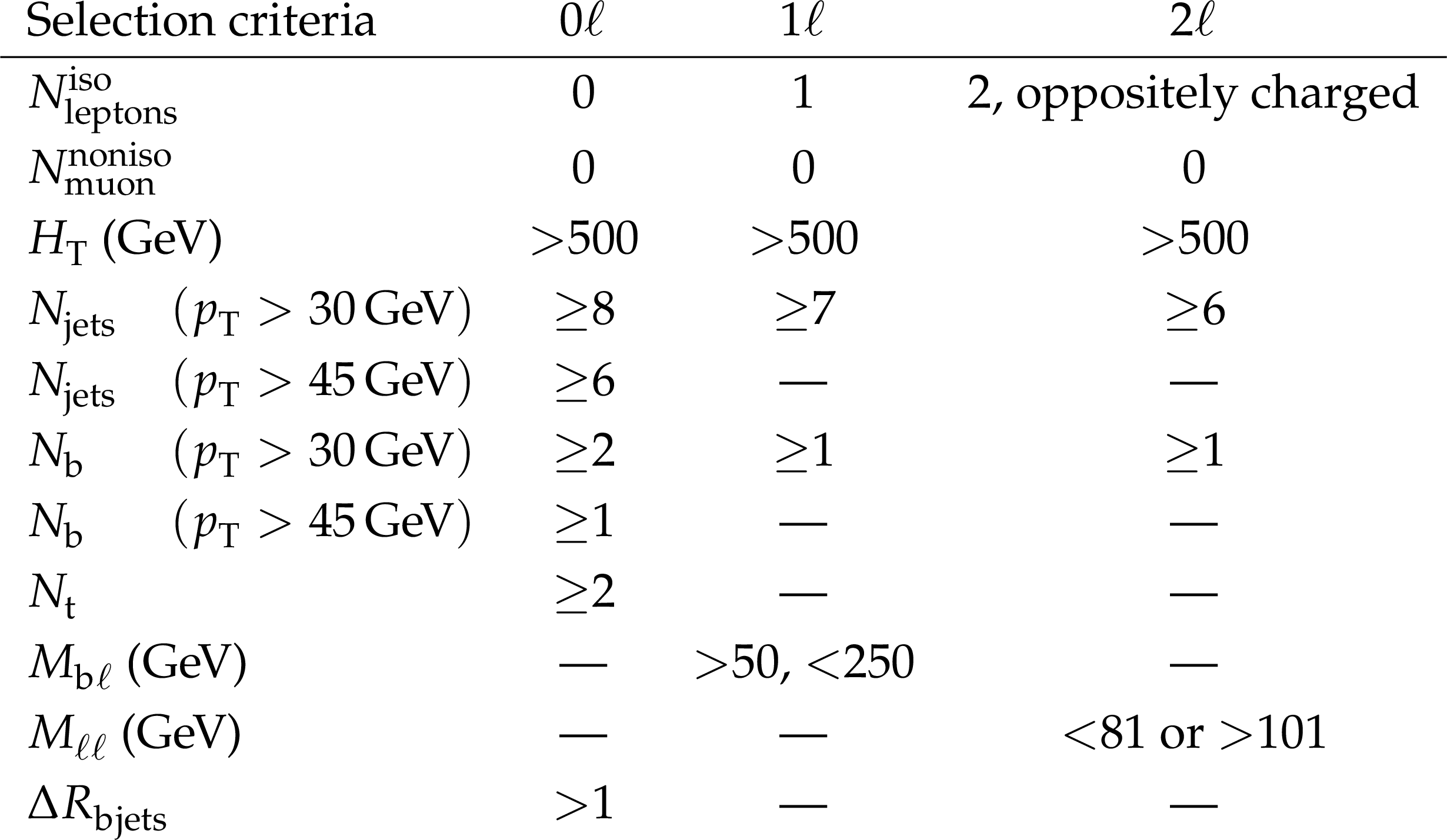
Table 1:
Search region selections for the 0$ \ell $, 1$ \ell $, and 2$ \ell $ channels. The term $ N_{\text{muon}}^{\text{noniso}} $ denotes the number of nonisolated muons. |
png pdf |
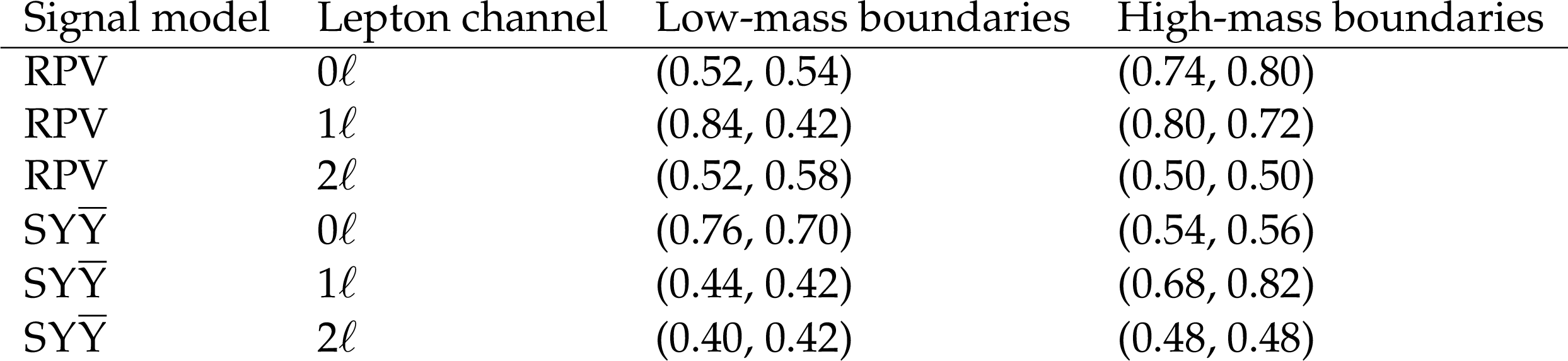
Table 2:
Values of $ (S_{\mathrm{NN,1}},S_{\mathrm{NN,2}}) $ defining the ABCD bin boundaries for the low- and high-mass optimizations for each lepton channel and signal model. |
png pdf |
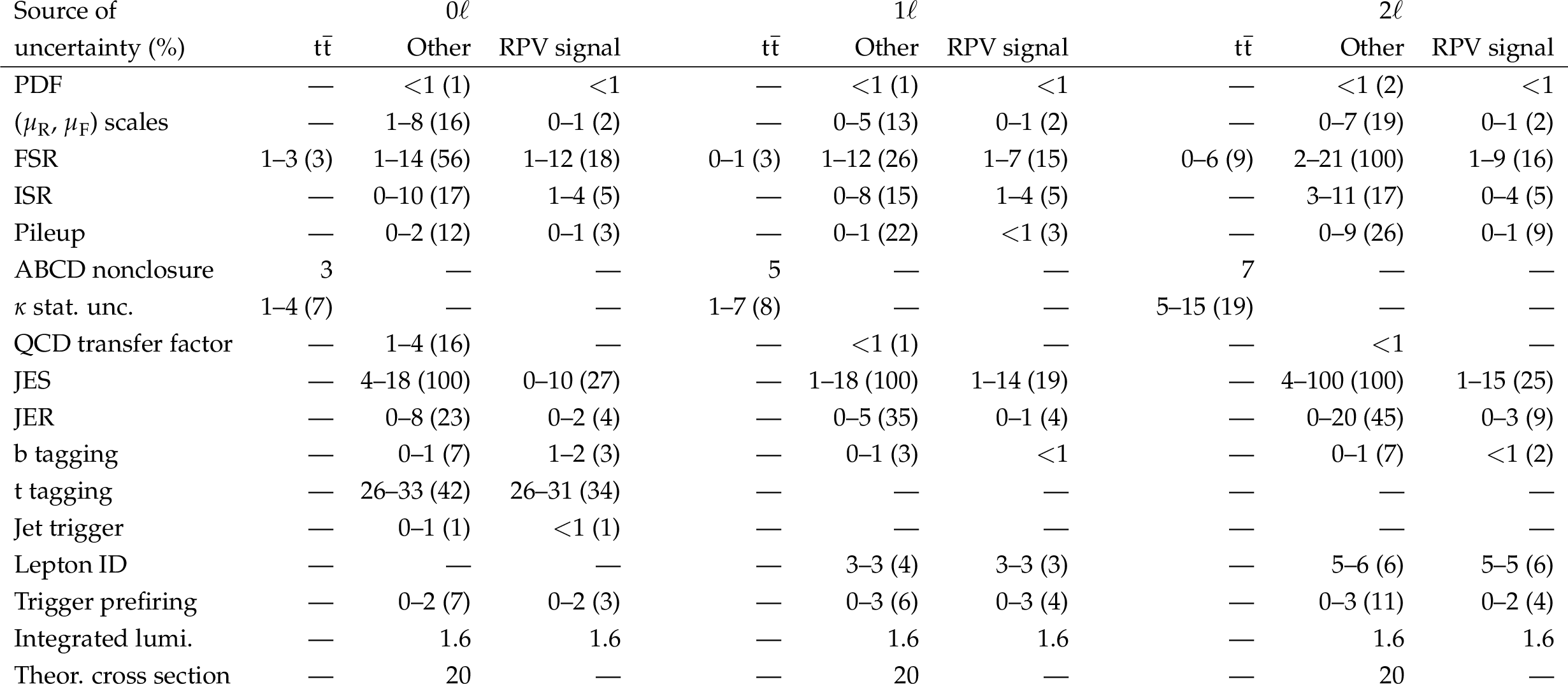
Table 3:
Magnitude of systematic uncertainties for the 0$ \ell $, 1$ \ell $, and 2$ \ell $ channels based on the RPV-trained NN and ABCD bin boundaries optimized for low $ m_{\tilde{\mathrm{t}}} $. Reported values are in units of % and ranges correspond to the 16th and 84th percentile for the value of a systematic uncertainty across all applicable analysis regions (ABCD regions and $ N_\text{jets} $ categories). The maximum value for a given systematic uncertainty across these regions is shown in parentheses. Other backgrounds include the $ \text{QCD multijet} $ and minor background processes. The RPV signal model used assumes $ m_{\tilde{\mathrm{t}}} = $ 550 GeV. The systematic uncertainties based on the RPV-trained model are representative of the values obtained for the stealth $ \mathrm{S}\mathrm{Y} \overline{\mathrm{Y}} $-trained model. |
| Summary |
| A search for the pair production of top squarks with decays to top quarks and six additional gluons or light-flavor quarks via $ R $-parity violating (RPV) or stealth $ \mathrm{S}\mathrm{Y} \overline{\mathrm{Y}} $ supersymmetric decays is presented. The search is performed using proton-proton collision events at $ \sqrt{s} = $ 13 TeV, corresponding to an integrated luminosity of 138 fb$ ^{-1} $, collected by the CMS detector in 2016-2018. Events are selected in three search channels, defined as having at least six jets and zero, one, or two electrons or muons. No requirement is placed on the presence of missing transverse momentum. This analysis is an extension of a previous search for these signatures [16], which observed a deviation with a local significance of 2.8 standard deviations for a top squark mass of 400 GeV for the RPV model. The main improvements of this search are the addition of the zero- and two-lepton channels as well as the inclusion of a novel, neural-network-based background estimation method referred to as ABCDisCoTEC [17]. The key feature of this new method is the creation of two uncorrelated neural network variables that can be used with an ABCD-style background estimation method. The backgrounds are estimated from a simultaneous binned likelihood fit to all search channels in several categories of jet multiplicity, with the contribution from the main $ {\mathrm{t}\overline{\mathrm{t}}} + \text{jets} $ background constrained via the ABCD relationship that encodes the independence between the two neural network variables. This new background estimation method, compared to that of Ref. [16], reduces the dependence of the analysis on uncertainties related to the modeling of the jet multiplicity spectrum. With this alternate background estimation technique, we achieve an improvement in signal sensitivity at low top squark mass. For example, the expected upper limit on the production cross section improves by a factor of 1.53 for a top squark mass of 400 GeV for the RPV model. Overall, good agreement between the data and the background prediction is observed, and the deviation observed previously is not confirmed. The results are interpreted using two top squark decay topologies that generate signatures with low missing transverse momentum: the RPV and stealth $ \mathrm{S}\mathrm{Y} \overline{\mathrm{Y}} $ models. For the RPV model with top squark decays to a top quark and neutralino, with the subsequent decay of the neutralino to three light-flavored quarks, top squark masses up to 700 GeV are excluded at 95% confidence level. Similarly, top squark masses of up to 930 GeV are excluded in the context of the stealth $ \mathrm{S}\mathrm{Y} \overline{\mathrm{Y}} $ model where top squarks decay to a top quark, gluons, and a soft gravitino via a hidden sector. |
| References | ||||
| 1 | P. Fayet and S. Ferrara | Supersymmetry | Phys. Rept. 32 (1977) 249 | |
| 2 | S. P. Martin | A supersymmetry primer | Adv. Ser. Direct. High Energy Phys. 21 (1997) 1 | hep-ph/9709356 |
| 3 | CMS Collaboration | Search for direct top squark pair production in events with one lepton, jets, and missing transverse momentum at 13 TeV with the CMS experiment | JHEP 05 (2020) 032 | CMS-SUS-19-009 1912.08887 |
| 4 | CMS Collaboration | Search for supersymmetry in proton-proton collisions at 13 TeV in final states with jets and missing transverse momentum | JHEP 10 (2019) 244 | CMS-SUS-19-006 1908.04722 |
| 5 | CMS Collaboration | Searches for physics beyond the standard model with the $ M_\mathrm{T2} $ variable in hadronic final states with and without disappearing tracks in proton-proton collisions at $ \sqrt{s}= $ 13 TeV | EPJC 80 (2020) 3 | CMS-SUS-19-005 1909.03460 |
| 6 | CMS Collaboration | Search for top squark production in fully-hadronic final states in proton-proton collisions at $ \sqrt{s} = $ 13 TeV | PRD 104 (2021) 052001 | CMS-SUS-19-010 2103.01290 |
| 7 | ATLAS Collaboration | Search for a scalar partner of the top quark in the all-hadronic $ t{\bar{t}} $ plus missing transverse momentum final state at $ \sqrt{s}= $ 13 TeV with the ATLAS detector | EPJC 80 (2020) 737 | 2004.14060 |
| 8 | ATLAS Collaboration | Search for new phenomena with top quark pairs in final states with one lepton, jets, and missing transverse momentum in $ pp $ collisions at $ \sqrt{s} = $ 13 TeV with the ATLAS detector | JHEP 04 (2021) 174 | 2012.03799 |
| 9 | ATLAS Collaboration | Search for new phenomena in events with two opposite-charge leptons, jets and missing transverse momentum in pp collisions at $ \sqrt{\mathrm{s}} = $ 13 TeV with the ATLAS detector | JHEP 04 (2021) 165 | 2102.01444 |
| 10 | ATLAS Collaboration | Search for new phenomena with top-quark pairs and large missing transverse momentum using 140 fb$ ^{-1} $ of pp collision data at $ \sqrt{s} = $ 13 TeV with the ATLAS detector | JHEP 03 (2024) 139 | 2401.13430 |
| 11 | R. Barbier et al. | $ R $-parity violating supersymmetry | Phys. Rept. 420 (2005) 1 | hep-ph/0406039 |
| 12 | H. K. Dreiner and G. G. Ross | $ R $-parity violation at hadron colliders | NPB 365 (1991) 597 | |
| 13 | J. Fan, M. Reece, and J. T. Ruderman | Stealth supersymmetry | JHEP 11 (2011) 012 | 1105.5135 |
| 14 | J. Fan, M. Reece, and J. T. Ruderman | A stealth supersymmetry sampler | JHEP 07 (2012) 196 | 1201.4875 |
| 15 | J. Fan et al. | Stealth supersymmetry simplified | JHEP 07 (2016) 016 | 1512.05781 |
| 16 | CMS Collaboration | Search for top squarks in final states with two top quarks and several light-flavor jets in proton-proton collisions at $ \sqrt {s} = $ 13 TeV | PRD 104 (2021) 032006 | CMS-SUS-19-004 2102.06976 |
| 17 | CMS Collaboration | Machine learning method for enforcing variable independence in background estimation with LHC data: ABCDisCoTEC | Submitted to MLST, 2025 | CMS-MLG-23-003 2506.08826 |
| 18 | G. Kasieczka, B. Nachman, M. D. Schwartz, and D. Shih | Automating the ABCD method with machine learning | PRD 103 (2021) 035021 | 2007.14400 |
| 19 | CMS Collaboration | HEPData record for this analysis | link | |
| 20 | CMS Collaboration | Precision luminosity measurement in proton-proton collisions at $ \sqrt{s}= $ 13 TeV in 2015 and 2016 at CMS | EPJC 81 (2021) 800 | CMS-LUM-17-003 2104.01927 |
| 21 | CMS Collaboration | CMS luminosity measurement for the 2017 data-taking period at $ \sqrt{s}= $ 13 TeV | CMS Physics Analysis Summary, 2018 CMS-PAS-LUM-17-004 |
CMS-PAS-LUM-17-004 |
| 22 | CMS Collaboration | CMS luminosity measurement for the 2018 data-taking period at $ \sqrt{s}= $ 13 TeV | CMS Physics Analysis Summary, 2019 CMS-PAS-LUM-18-002 |
CMS-PAS-LUM-18-002 |
| 23 | CMS Collaboration | The CMS experiment at the CERN LHC | JINST 3 (2008) S08004 | |
| 24 | CMS Collaboration | Development of the CMS detector for the CERN LHC Run 3 | JINST 19 (2024) P05064 | CMS-PRF-21-001 2309.05466 |
| 25 | CMS Collaboration | Performance of the CMS Level-1 trigger in proton-proton collisions at $ \sqrt{s} = $ 13 TeV | JINST 15 (2020) P10017 | CMS-TRG-17-001 2006.10165 |
| 26 | CMS Collaboration | The CMS trigger system | JINST 12 (2017) P01020 | CMS-TRG-12-001 1609.02366 |
| 27 | CMS Collaboration | Performance of the CMS high-level trigger during LHC Run 2 | JINST 19 (2024) P11021 | CMS-TRG-19-001 2410.17038 |
| 28 | CMS Collaboration | Electron and photon reconstruction and identification with the CMS experiment at the CERN LHC | JINST 16 (2021) P05014 | CMS-EGM-17-001 2012.06888 |
| 29 | CMS Collaboration | Performance of the CMS muon detector and muon reconstruction with proton-proton collisions at $ \sqrt{s}= $ 13 TeV | JINST 13 (2018) P06015 | CMS-MUO-16-001 1804.04528 |
| 30 | CMS Collaboration | Description and performance of track and primary-vertex reconstruction with the CMS tracker | JINST 9 (2014) P10009 | CMS-TRK-11-001 1405.6569 |
| 31 | CMS Collaboration | Technical proposal for the Phase-II upgrade of the Compact Muon Solenoid | CMS Technical Proposal CERN-LHCC-2015-010, CMS-TDR-15-02, 2015 CDS |
|
| 32 | CMS Collaboration | Particle-flow reconstruction and global event description with the CMS detector | JINST 12 (2017) P10003 | CMS-PRF-14-001 1706.04965 |
| 33 | M. Cacciari, G. P. Salam, and G. Soyez | The anti-$ k_{\mathrm{T}} $ jet clustering algorithm | JHEP 04 (2008) 063 | 0802.1189 |
| 34 | M. Cacciari, G. P. Salam, and G. Soyez | FastJet user manual | EPJC 72 (2012) 1896 | 1111.6097 |
| 35 | CMS Collaboration | Pileup mitigation at CMS in 13 TeV data | JINST 15 (2020) P09018 | CMS-JME-18-001 2003.00503 |
| 36 | CMS Collaboration | Jet energy scale and resolution in the CMS experiment in pp collisions at 8 TeV | JINST 12 (2017) P02014 | CMS-JME-13-004 1607.03663 |
| 37 | CMS Collaboration | Identification of heavy-flavour jets with the CMS detector in pp collisions at 13 TeV | JINST 13 (2018) P05011 | CMS-BTV-16-002 1712.07158 |
| 38 | E. Bols et al. | Jet flavour classification using DeepJet | JINST 15 (2020) P12012 | 2008.10519 |
| 39 | CMS Collaboration | Performance of the DeepJet b tagging algorithm using 41.9 fb$ ^{-1} $ of data from proton-proton collisions at 13 TeV with Phase 1 CMS detector | CMS Detector Performance Note CMS-DP-2018-058, 2018 CDS |
|
| 40 | CMS Collaboration | ECAL 2016 refined calibration and Run2 summary plots | CMS Detector Performance Note CMS-DP-2020-021, 2020 CDS |
|
| 41 | K. Rehermann and B. Tweedie | Efficient identification of boosted semileptonic top quarks at the LHC | JHEP 03 (2011) 059 | 1007.2221 |
| 42 | P. Nason | A new method for combining NLO QCD with shower Monte Carlo algorithms | JHEP 11 (2004) 040 | hep-ph/0409146 |
| 43 | S. Frixione, P. Nason, and C. Oleari | Matching NLO QCD computations with parton shower simulations: the POWHEG method | JHEP 11 (2007) 070 | 0709.2092 |
| 44 | S. Alioli, P. Nason, C. Oleari, and E. Re | A general framework for implementing NLO calculations in shower Monte Carlo programs: the POWHEG BOX | JHEP 06 (2010) 043 | 1002.2581 |
| 45 | S. Frixione, P. Nason, and G. Ridolfi | A positive-weight next-to-leading-order Monte Carlo for heavy flavour hadroproduction | JHEP 09 (2007) 126 | 0707.3088 |
| 46 | E. Re | Single-top Wt-channel production matched with parton showers using the POWHEG method | EPJC 71 (2011) 1547 | 1009.2450 |
| 47 | S. Alioli, P. Nason, C. Oleari, and E. Re | NLO single-top production matched with shower in POWHEG: $ s $- and $ t $-channel contributions | JHEP 09 (2009) 111 | 0907.4076 |
| 48 | J. Alwall et al. | The automated computation of tree-level and next-to-leading order differential cross sections, and their matching to parton shower simulations | JHEP 07 (2014) 079 | 1405.0301 |
| 49 | T. Sjöstrand et al. | An introduction to PYTHIA 8.2 | Comput. Phys. Commun. 191 (2015) 159 | 1410.3012 |
| 50 | M. Czakon and A. Mitov | Top++: A program for the calculation of the top-pair cross-section at hadron colliders | Comput. Phys. Commun. 185 (2014) 2930 | 1112.5675 |
| 51 | P. Kant et al. | HATHOR for single top-quark production: Updated predictions and uncertainty estimates for single top-quark production in hadronic collisions | Comput. Phys. Commun. 191 (2015) 74 | 1406.4403 |
| 52 | M. Aliev et al. | HATHOR: HAdronic Top and Heavy quarks crOss section calculatoR | Comput. Phys. Commun. 182 (2011) 1034 | 1007.1327 |
| 53 | T. Gehrmann et al. | W$ ^+ $W$ ^- $ production at hadron colliders in next to next to leading order QCD | PRL 113 (2014) 212001 | 1408.5243 |
| 54 | J. M. Campbell and R. K. Ellis | An update on vector boson pair production at hadron colliders | PRD 60 (1999) 113006 | hep-ph/9905386 |
| 55 | J. M. Campbell, R. K. Ellis, and C. Williams | Vector boson pair production at the LHC | JHEP 07 (2011) 018 | 1105.0020 |
| 56 | Y. Li and F. Petriello | Combining QCD and electroweak corrections to dilepton production in FEWZ | PRD 86 (2012) 094034 | 1208.5967 |
| 57 | C. Borschensky et al. | Squark and gluino production cross sections in pp collisions at $ \sqrt{s}= $ 13, 14, 33 and 100 TeV | EPJC 74 (2014) 3174 | 1407.5066 |
| 58 | W. Beenakker et al. | NNLL-fast: predictions for coloured supersymmetric particle production at the LHC with threshold and Coulomb resummation | JHEP 12 (2016) 133 | 1607.07741 |
| 59 | W. Beenakker et al. | NNLL resummation for stop pair-production at the LHC | JHEP 05 (2016) 153 | 1601.02954 |
| 60 | W. Beenakker et al. | Supersymmetric top and bottom squark production at hadron colliders | JHEP 08 (2010) 098 | 1006.4771 |
| 61 | W. Beenakker et al. | Stop production at hadron colliders | NPB 515 (1998) 3 | hep-ph/9710451 |
| 62 | CMS Collaboration | Extraction and validation of a new set of CMS PYTHIA8 tunes from underlying-event measurements | EPJC 80 (2020) 4 | CMS-GEN-17-001 1903.12179 |
| 63 | CMS Collaboration | CMS PYTHIA 8 colour reconnection tunes based on underlying-event data | EPJC 83 (2023) 587 | CMS-GEN-17-002 2205.02905 |
| 64 | NNPDF Collaboration | Parton distributions from high-precision collider data | EPJC 77 (2017) 663 | 1706.00428 |
| 65 | GEANT4 Collaboration | GEANT 4---a simulation toolkit | NIM A 506 (2003) 250 | |
| 66 | CMS Collaboration | Identification of heavy, energetic, hadronically decaying particles using machine-learning techniques | JINST 15 (2020) P06005 | CMS-JME-18-002 2004.08262 |
| 67 | D0 Collaboration | Search for high mass top quark production in $ p\bar{p} $ collisions at $ \sqrt{s} = $ 1.8 TeV | PRL 74 (1995) 2422 | hep-ex/9411001 |
| 68 | O. Behnke, K. Kröninger, G. Schott, and T. Schörner-Sadenius | Data analysis in high energy physics: a practical guide to statistical methods | Wiley-VCH, 2013 link |
|
| 69 | G. J. Székely and M. L. Rizzo | Partial distance correlation with methods for dissimilarities | Ann. Statist. 42 (2014) 2382 | 1310.2926 |
| 70 | S. Odaka, N. Watanabe, and Y. Kurihara | ME-PS matching in the simulation of multi-jet production in hadron collisions using a subtraction method | PTEP 2015 (2015) 053B04 | 1409.3334 |
| 71 | G. C. Fox and S. Wolfram | Observables for the analysis of event shapes in $ \mathrm{e}^+\mathrm{e}^- $ annihilation and other processes | PRL 41 (1978) 1581 | |
| 72 | J. D. Bjorken and S. J. Brodsky | Statistical model for electron-positron annihilation into hadrons | PRD 1 (1970) 1416 | |
| 73 | CMS Collaboration | Search for supersymmetry in hadronic final states using MT2 in $ pp $ collisions at $ \sqrt{s} = $ 7 TeV | JHEP 10 (2012) 018 | CMS-SUS-12-002 1207.1798 |
| 74 | CMS Collaboration | CMS technical design report, volume II: Physics performance | JPG 34 (2007) 995 | |
| 75 | CMS Collaboration | Determination of jet energy calibration and transverse momentum resolution in CMS | JINST 6 (2011) P11002 | CMS-JME-10-011 1107.4277 |
| 76 | D. Kim et al. | A panoramic study of k-factors for 111 processes at the 14 TeV LHC | J. Korean Phys. Soc. 84 (2024) 914 | 2402.16276 |
| 77 | A. L. Read | Presentation of search results: The $ \text{CL}_\text{s} $ technique | JPG 28 (2002) 2693 | |
| 78 | T. Junk | Confidence level computation for combining searches with small statistics | NIM A 434 (1999) 435 | hep-ex/9902006 |
| 79 | ATLAS and CMS Collaborations, and LHC Higgs Combination Group | Procedure for the LHC Higgs boson search combination in Summer 2011 | Technical Report CMS-NOTE-2011-005, ATL-PHYS-PUB-2011-11, 2011 | |
| 80 | G. Cowan, K. Cranmer, E. Gross, and O. Vitells | Asymptotic formulae for likelihood-based tests of new physics | EPJC 71 (2011) 1554 | 1007.1727 |
| 81 | CMS Collaboration | The CMS statistical analysis and combination tool: Combine | Comput. Softw. Big Sci. 8 (2024) 19 | CMS-CAT-23-001 2404.06614 |
|
|
Compact Muon Solenoid LHC, CERN |
|

|

|

|

|

|