CMS-SUS-19-006

CMS-SUS-19-006 ; CERN-EP-2019-152
Search for supersymmetry in proton-proton collisions at 13 TeV in final states with jets and missing transverse momentum
CMS Collaboration
13 August 2019
JHEP 10 (2019) 244
Abstract: Results are reported from a search for supersymmetric particles in the final state with multiple jets and large missing transverse momentum. The search uses a sample of proton-proton collisions at $\sqrt{s} =$ 13 TeV collected with the CMS detector in 2016-2018, corresponding to an integrated luminosity of 137 fb $^{-1}$ , representing essentially the full LHC Run 2 data sample. The analysis is performed in a four-dimensional search region defined in terms of the number of jets, the number of tagged bottom quark jets, the scalar sum of jet transverse momenta, and the magnitude of the vector sum of jet transverse momenta. No significant excess in the event yield is observed relative to the expected background contributions from standard model processes. Limits on the pair production of gluinos and squarks are obtained in the framework of simplified models for supersymmetric particle production and decay processes. Assuming the lightest supersymmetric particle to be a neutralino, lower limits on the gluino mass as large as 2000 to 2310 GeV are obtained at 95% confidence level, while lower limits on the squark mass as large as 1190 to 1630 GeV are obtained, depending on the production scenario.
Links: e-print arXiv:1908.04722 [hep-ex] (PDF) ; CDS record ; inSPIRE record ; HepData record ; CADI line (restricted) ;

Figures & Tables	Summary	Additional Figures & Tables	References	CMS Publications

Figures
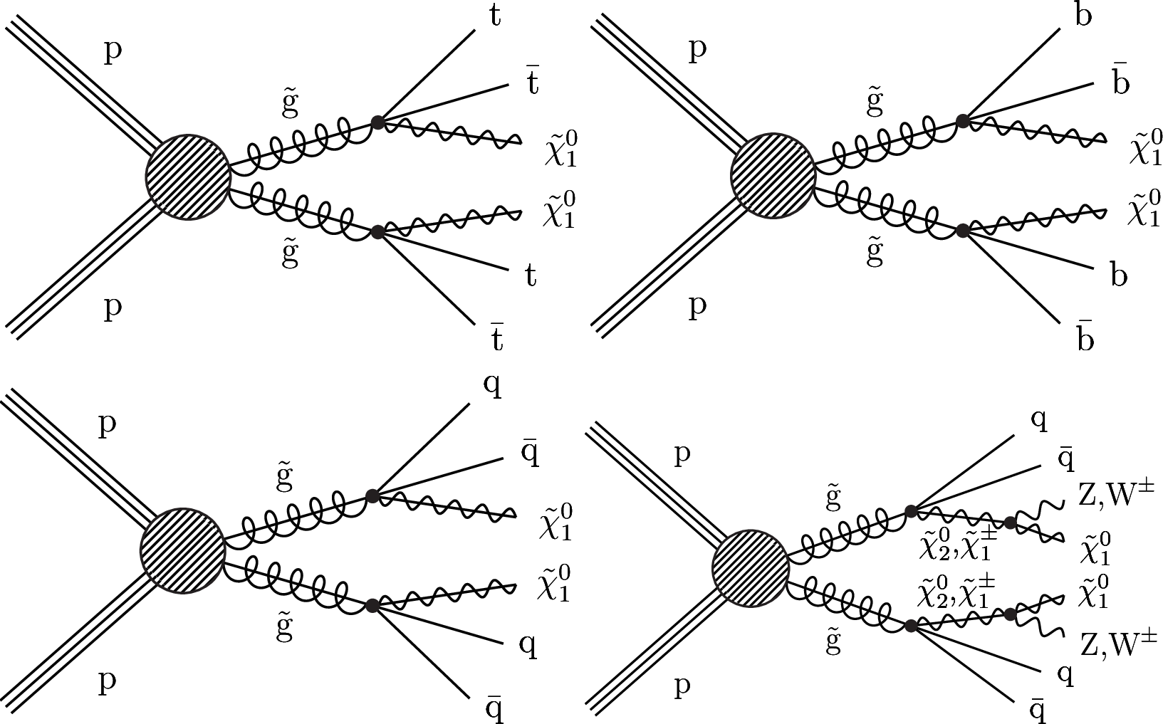
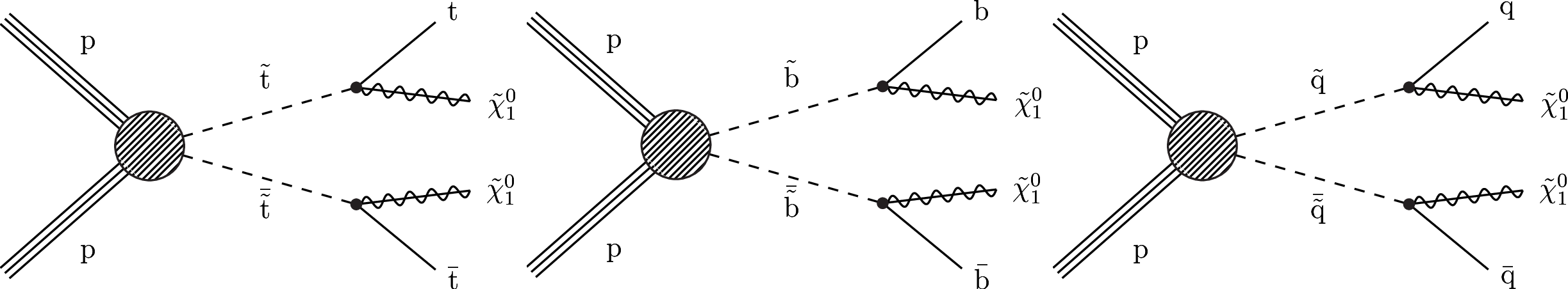
png pdf	Figure 1: Diagrams for the simplified models with direct gluino pair production considered in this study: (upper left) T1tttt, (upper right) T1bbbb, (lower left) T1qqqq, and (lower right) T5qqqqVV.
png pdf	Figure 1-a: Diagram for the T1tttt simplified model of direct gluino pair production.
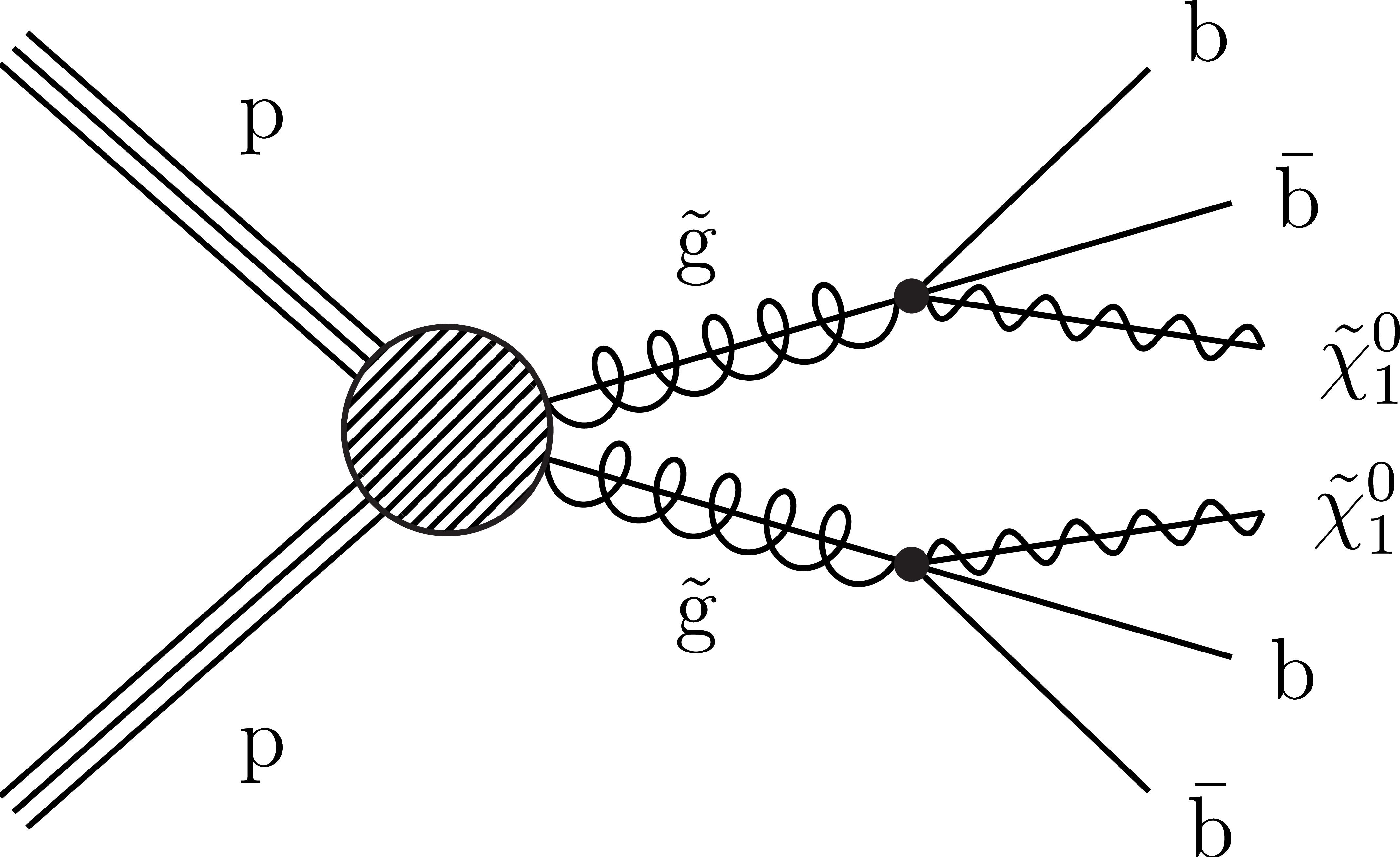
png pdf	Figure 1-b: Diagram for the T1bbbb simplified model of direct gluino pair production.
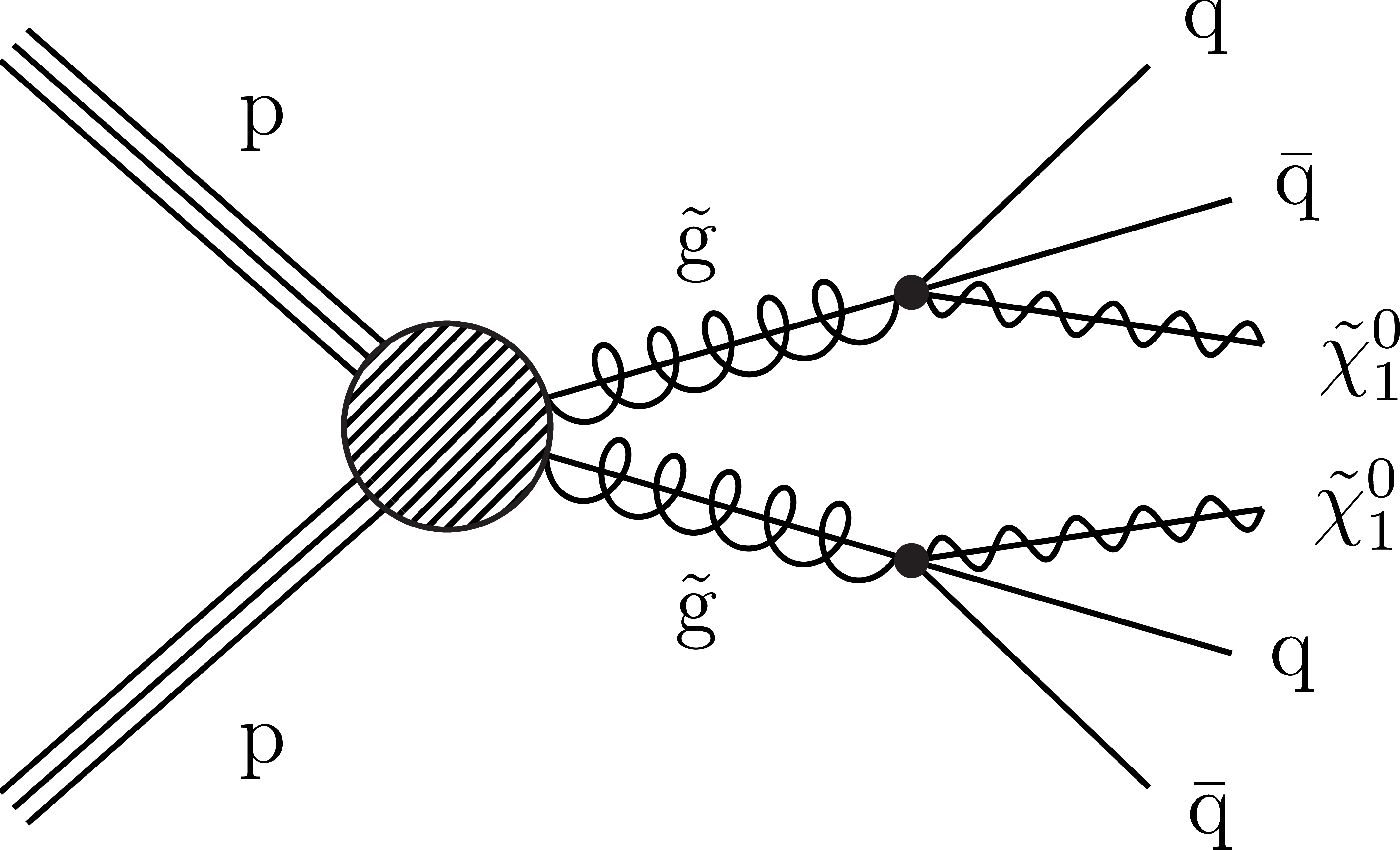
png pdf	Figure 1-c: Diagram for the T1qqqq simplified model of direct gluino pair production.
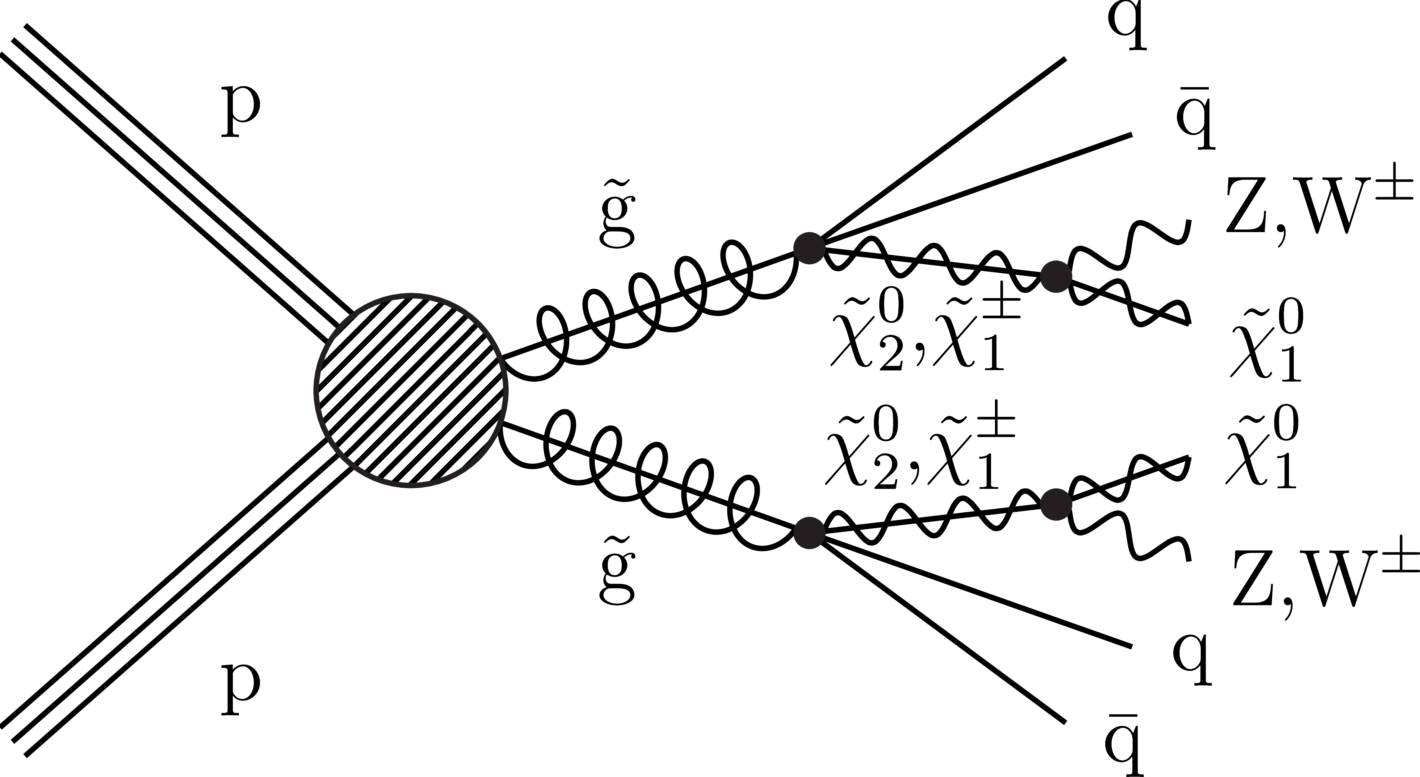
png pdf	Figure 1-d: Diagram for the T5qqqqVV simplified model of direct gluino pair production.
png pdf	Figure 2: Diagrams for the simplified models with direct squark pair production considered in this study: (left) T2tt, (middle) T2bb, and (right) T2qq.
png pdf	Figure 2-a: Diagram for the T2tt simplified model of direct squark pair production.
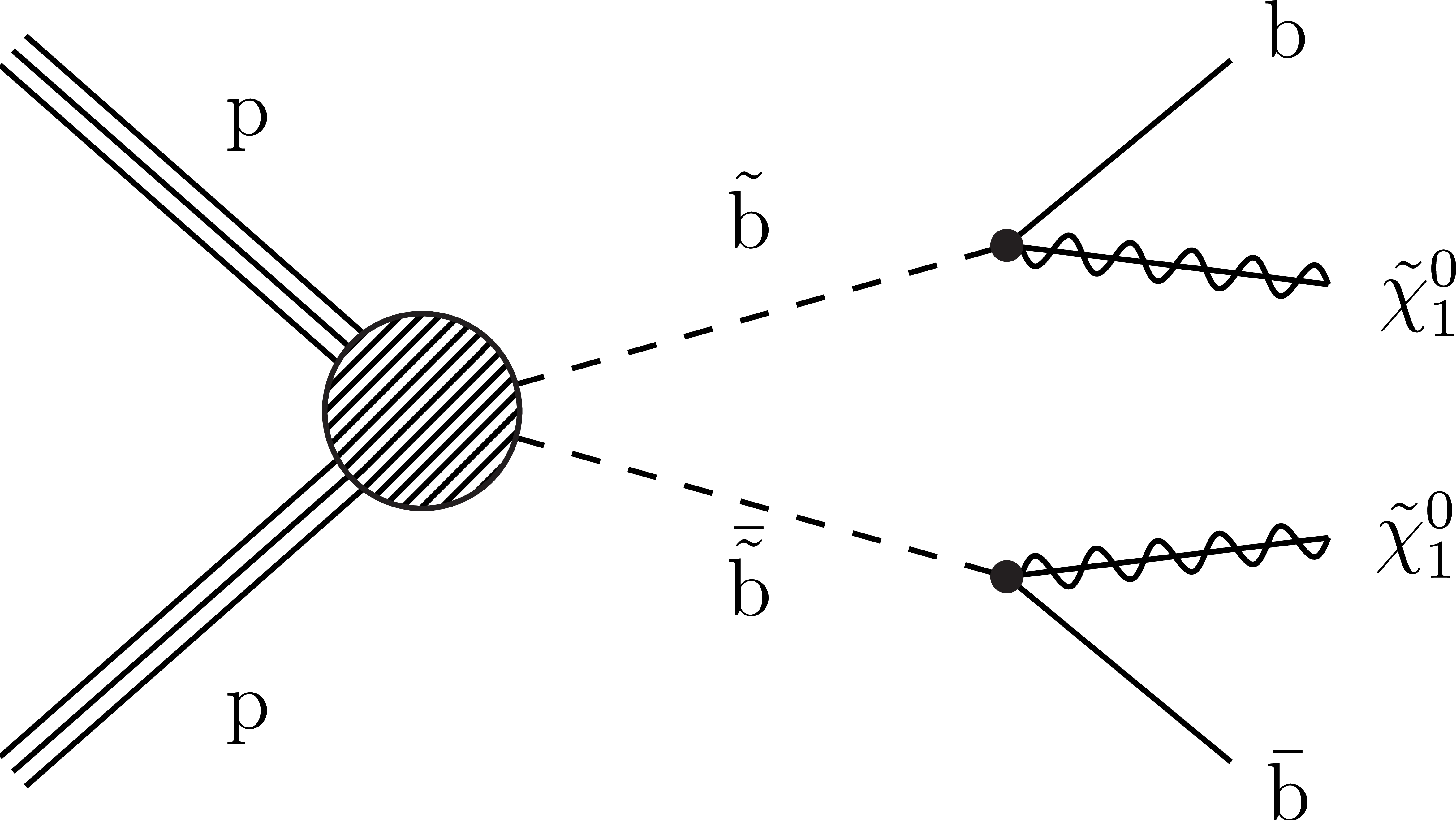
png pdf	Figure 2-b: Diagram for the T2bb simplified model of direct squark pair production.
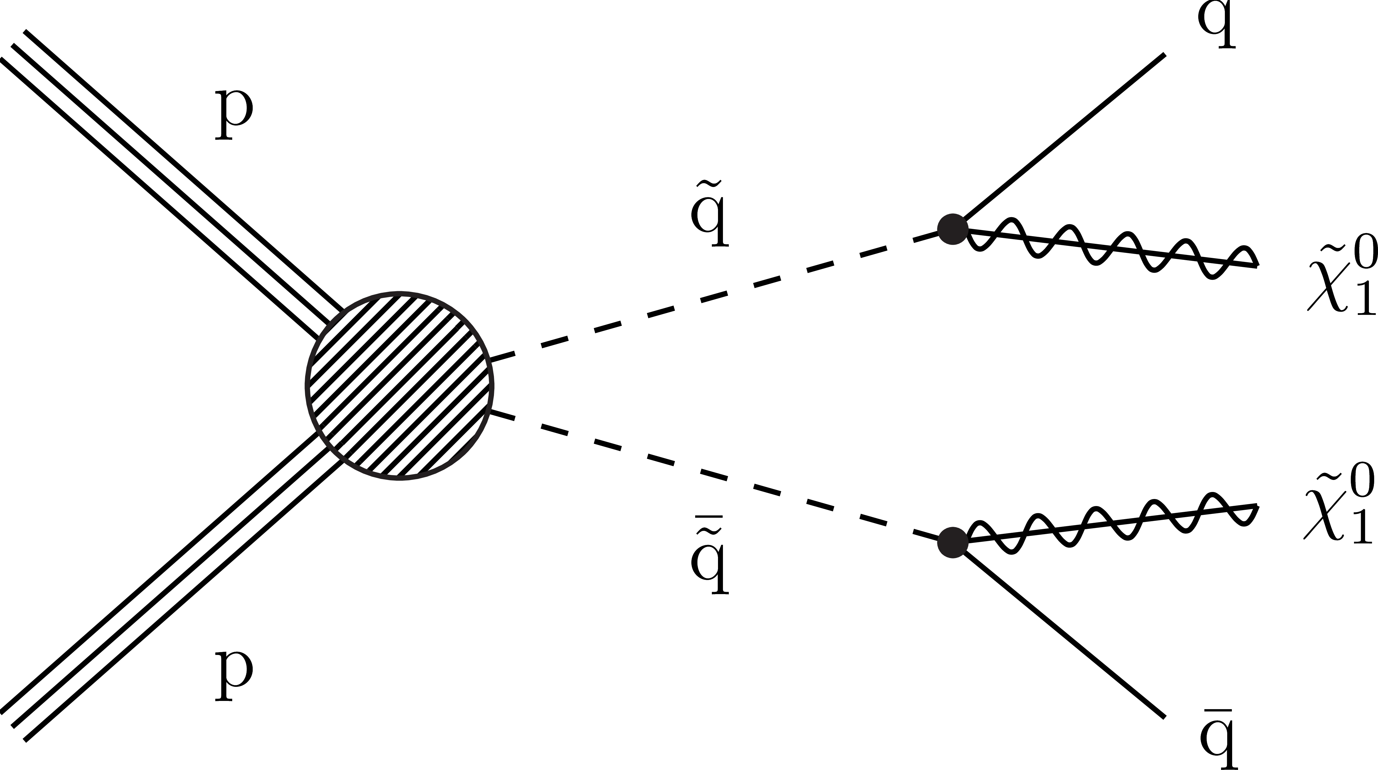
png pdf	Figure 2-c: Diagram for the T2qq simplified model of direct squark pair production.
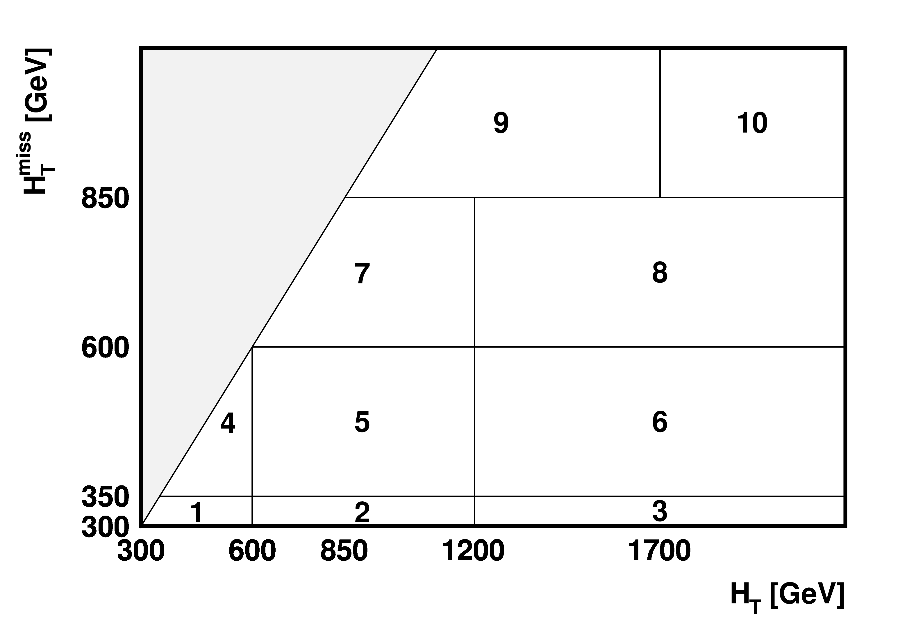
png pdf	Figure 3: Schematic illustration of the 10 kinematic search intervals in the ${H_{\mathrm {T}}^{\text {miss}}}$ versus ${H_{\mathrm {T}}}$ plane. The region above the red dashed line, with ${H_{\mathrm {T}}^{\text {miss}}} > {H_{\mathrm {T}}}$ , is excluded, as are all of regions 1 and 4 for ${N_{\text {jet}}} \geq$ 8. The rightmost and topmost bins are unbounded, extending to ${H_{\mathrm {T}}} =\infty$ and ${H_{\mathrm {T}}^{\text {miss}}} =\infty$ , respectively.
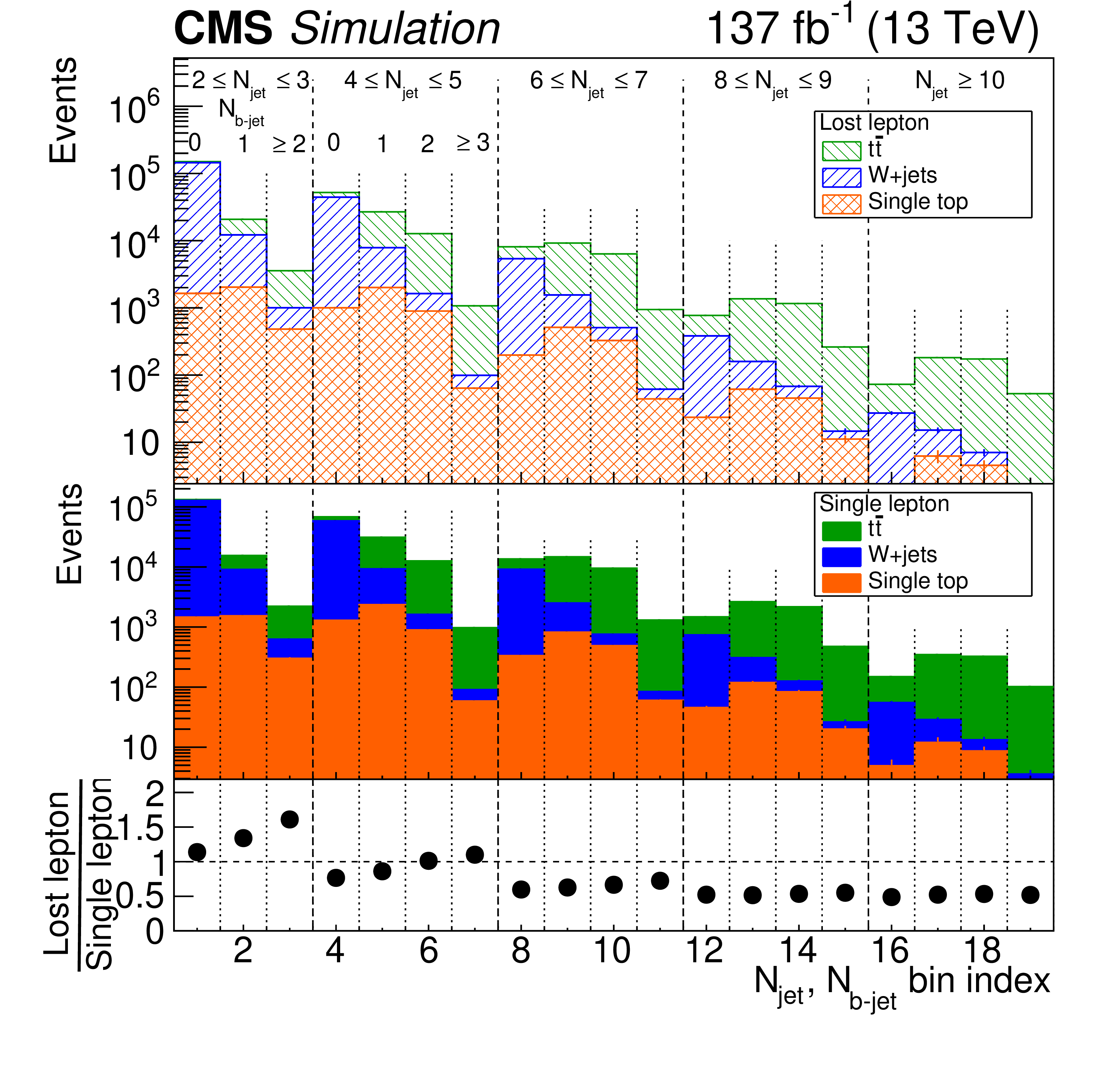
png pdf	Figure 4: (upper) The number of lost-lepton events in simulation, integrated over ${H_{\mathrm {T}}}$ and ${H_{\mathrm {T}}^{\text {miss}}}$ , as a function of ${N_{\text {jet}}}$ and ${N_{{\mathrm{b}}\text {-jet}}}$ . (middle) Corresponding results from simulation for the number of events in the single-lepton control region. (lower) The ratio of the simulated lost-lepton to the single-lepton results, with statistical uncertainties (too small to be visible). These ratios are equivalent to the transfer factors used in the evaluation of the lost-lepton background, except integrated over ${H_{\mathrm {T}}}$ and ${H_{\mathrm {T}}^{\text {miss}}}$ .
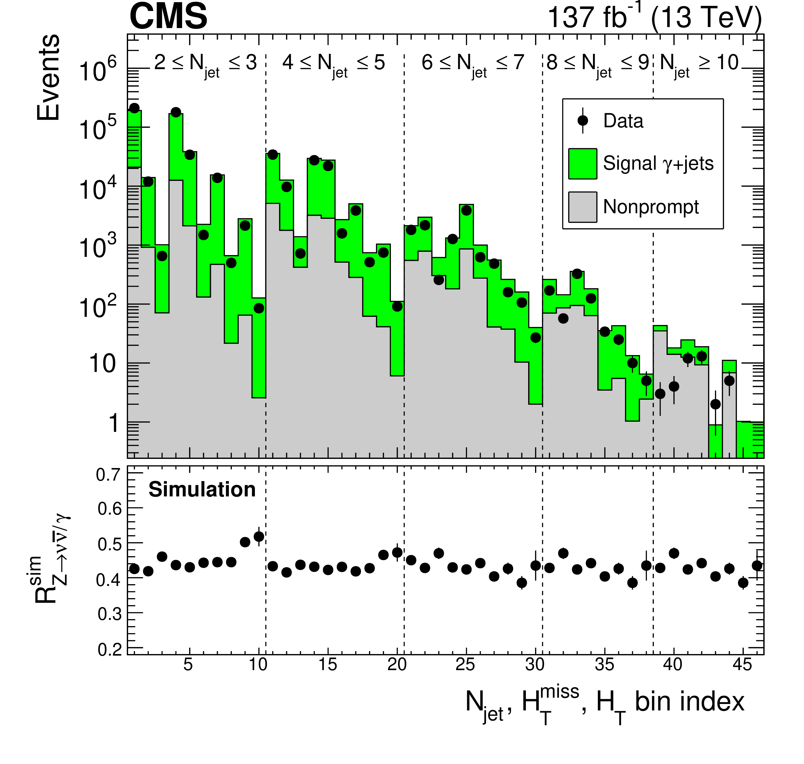
png pdf	Figure 5: The (upper) number of events in the ${\gamma}$ +jets control region for data and simulation and (lower) transfer factors ${\mathcal {R}_{{\mathrm{Z} \to \nu \bar{\nu}} /\gamma}^{\text {sim}}}$ from simulation. The respective results are shown for the 46 search bins with ${N_{{\mathrm{b}}\text {-jet}}} =$ 0. The 10 results (8 for ${N_{\text {jet}}} \geq$ 8) within each region delineated by vertical dashed lines correspond sequentially to the 10 (8) kinematic intervals in ${H_{\mathrm {T}}}$ and ${H_{\mathrm {T}}^{\text {miss}}}$ listed in Table 1 and Fig. 3. The uncertainties are statistical only. For the upper plot, the simulated results show the stacked event rates for the ${\gamma}$ +jets and nonprompt MC event samples, where "nonprompt'' refers to SM MC events other than ${\gamma}$ +jets. The simulated nonprompt results are dominated by events from the QCD sample. Because of limited statistical precision in the simulated event samples at large ${N_{\text {jet}}}$ , the transfer factors determined for the 8 $\leq {N_{\text {jet}}} \leq$ 9 region are also used for the ${N_{\text {jet}}} >$ 10 region.
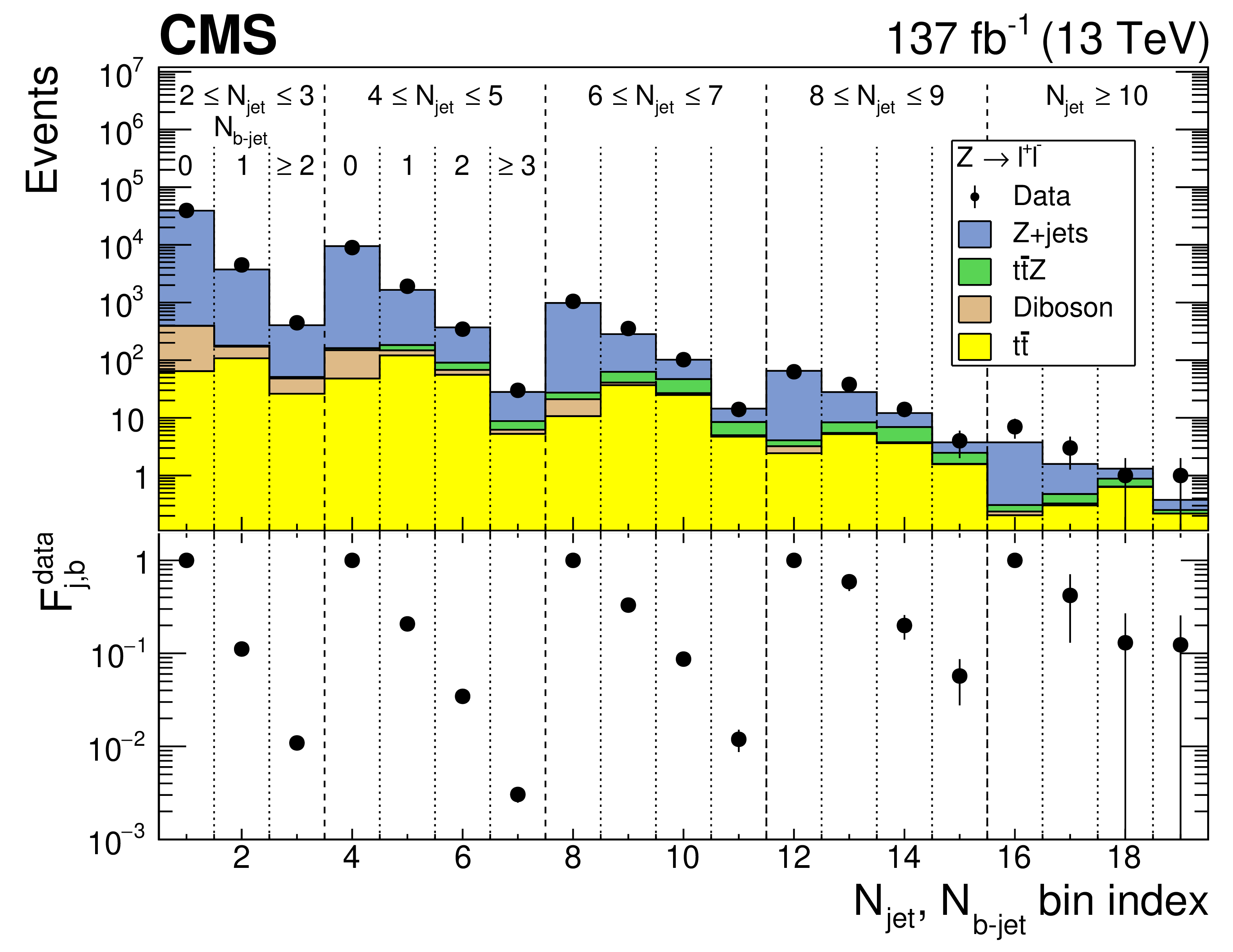
png pdf	Figure 6: (upper) The observed event yield in the ${\mathrm{Z} (\to \ell ^{+}\ell ^{-})}$ +jets control region, integrated over ${H_{\mathrm {T}}}$ and ${H_{\mathrm {T}}^{\text {miss}}}$ , as a function of ${N_{\text {jet}}}$ and ${N_{{\mathrm{b}}\text {-jet}}}$ . The uncertainties are statistical only. The stacked histograms show the corresponding results from simulation. (lower) The extrapolation factors ${\mathcal {F}_{\mathrm {j},\mathrm{b}}^{\text {data}}}$ with their statistical uncertainties.
png pdf	Figure 7: Prediction from simulation for the ${\mathrm{Z} (\to \ell ^{+}\ell ^{-})}$ +jets event yields in the 174 search bins as determined by computing the ${\mathcal {F}_{\mathrm {j},\mathrm{b}}^{\text {data}}}$ factors (Eq. (3)) and the ${N_{{\mathrm{b}}\text {-jet}}} =$ 0 event yields in the same manner as for data, in comparison to the corresponding direct ${\mathrm{Z} (\to \ell ^{+}\ell ^{-})}$ +jets prediction from simulation. The 10 results (8 for ${N_{\text {jet}}} \geq$ 8) within each region delineated by vertical dashed lines correspond sequentially to the 10 (8) kinematic intervals in ${H_{\mathrm {T}}}$ and ${H_{\mathrm {T}}^{\text {miss}}}$ listed in Table 1 and Fig. 3. For bins with ${N_{\text {jet}}} \geq$ 10, some points do not appear in the upper panel because they lie below the minimum of the displayed range. In the case that the direct expected yield is zero, there is no result in the lower, ratio panel. The pink bands show the statistical uncertainties in the prediction, scaled to correspond to the integrated luminosity of the data, combined with the systematic uncertainty attributable to the kinematic ( ${H_{\mathrm {T}}}$ and ${H_{\mathrm {T}}^{\text {miss}}}$ ) dependence. The black error bars show the statistical uncertainties in the simulation. For bins corresponding to ${N_{{\mathrm{b}}\text {-jet}}} =$ 0, the agreement is exact by construction.
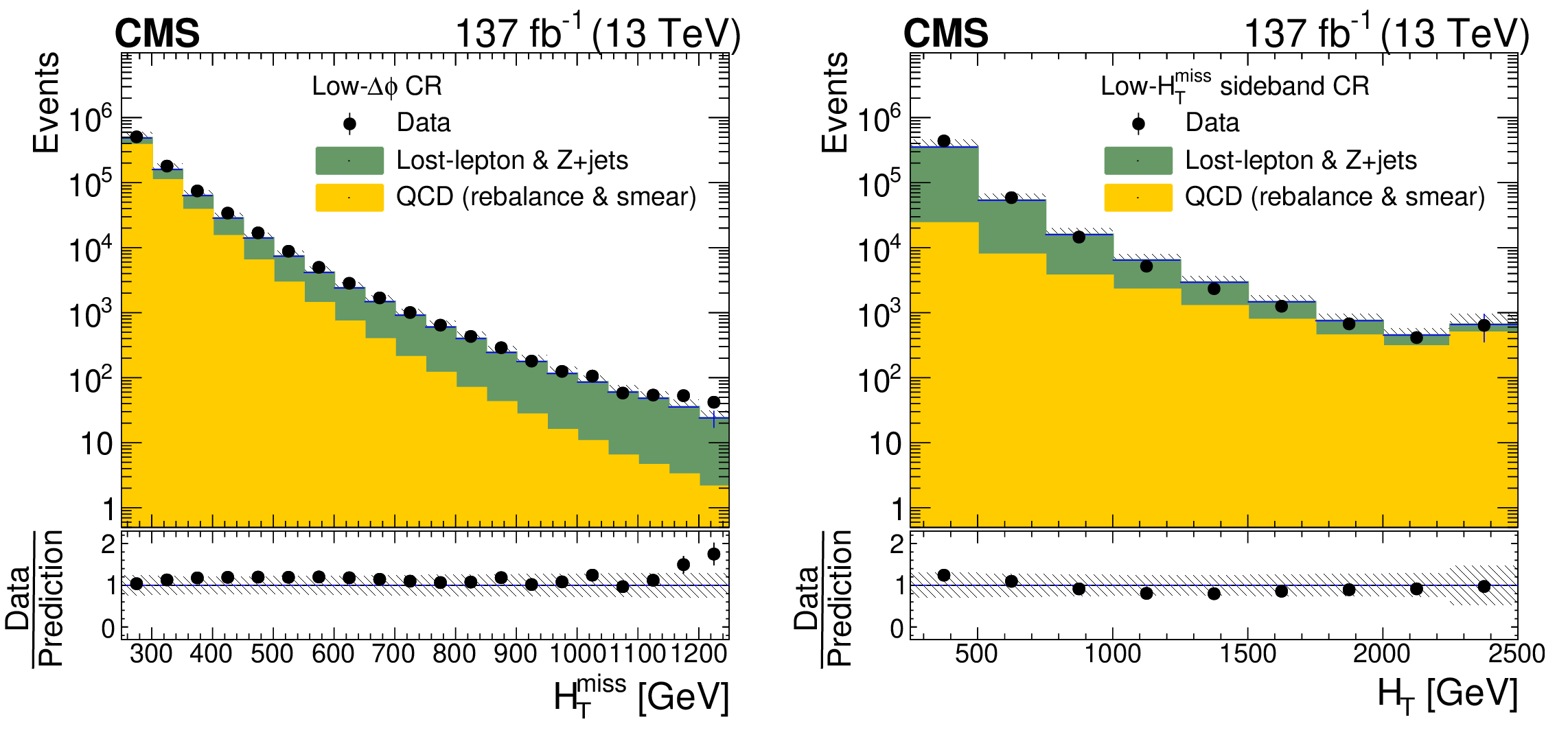
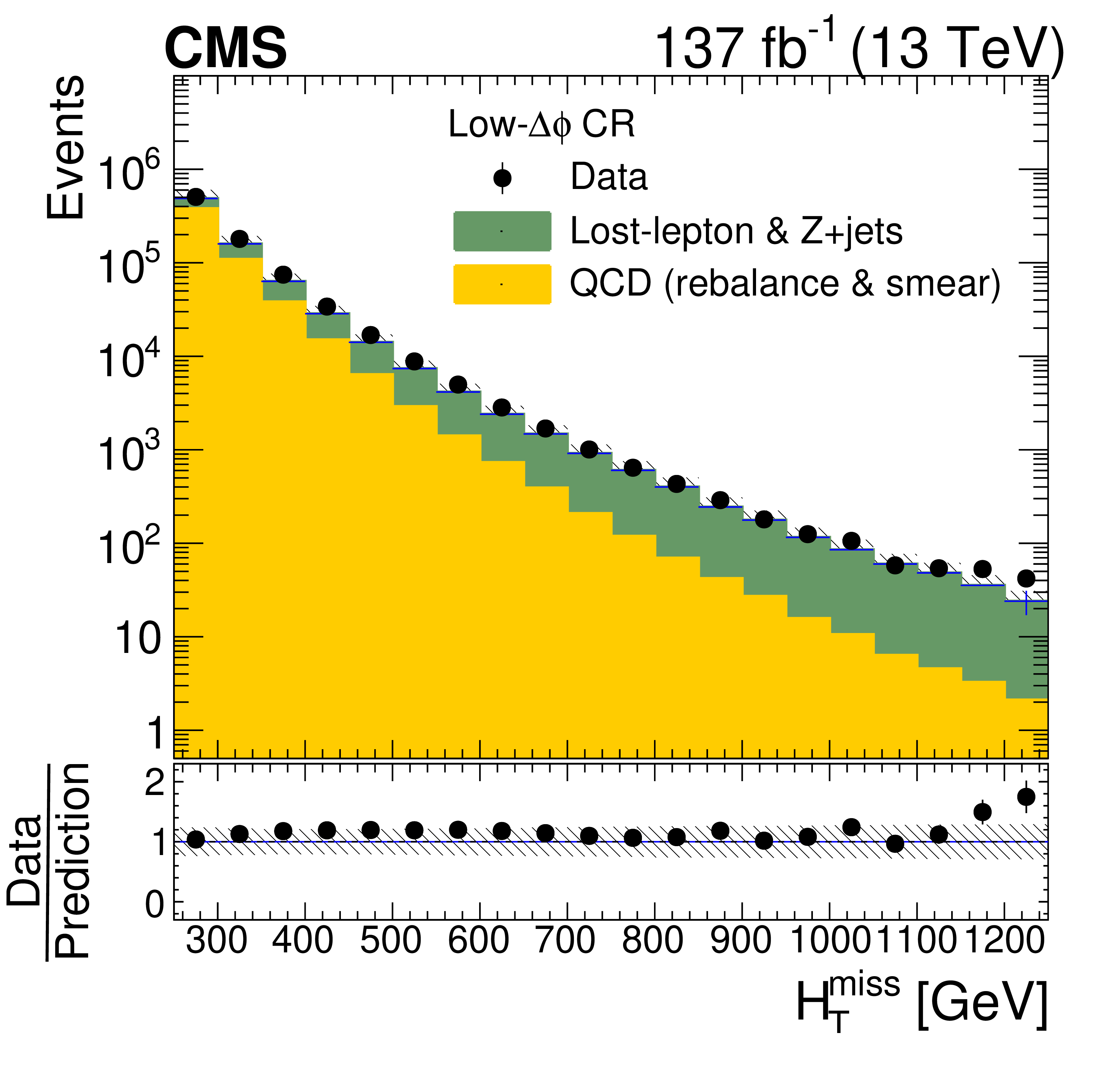
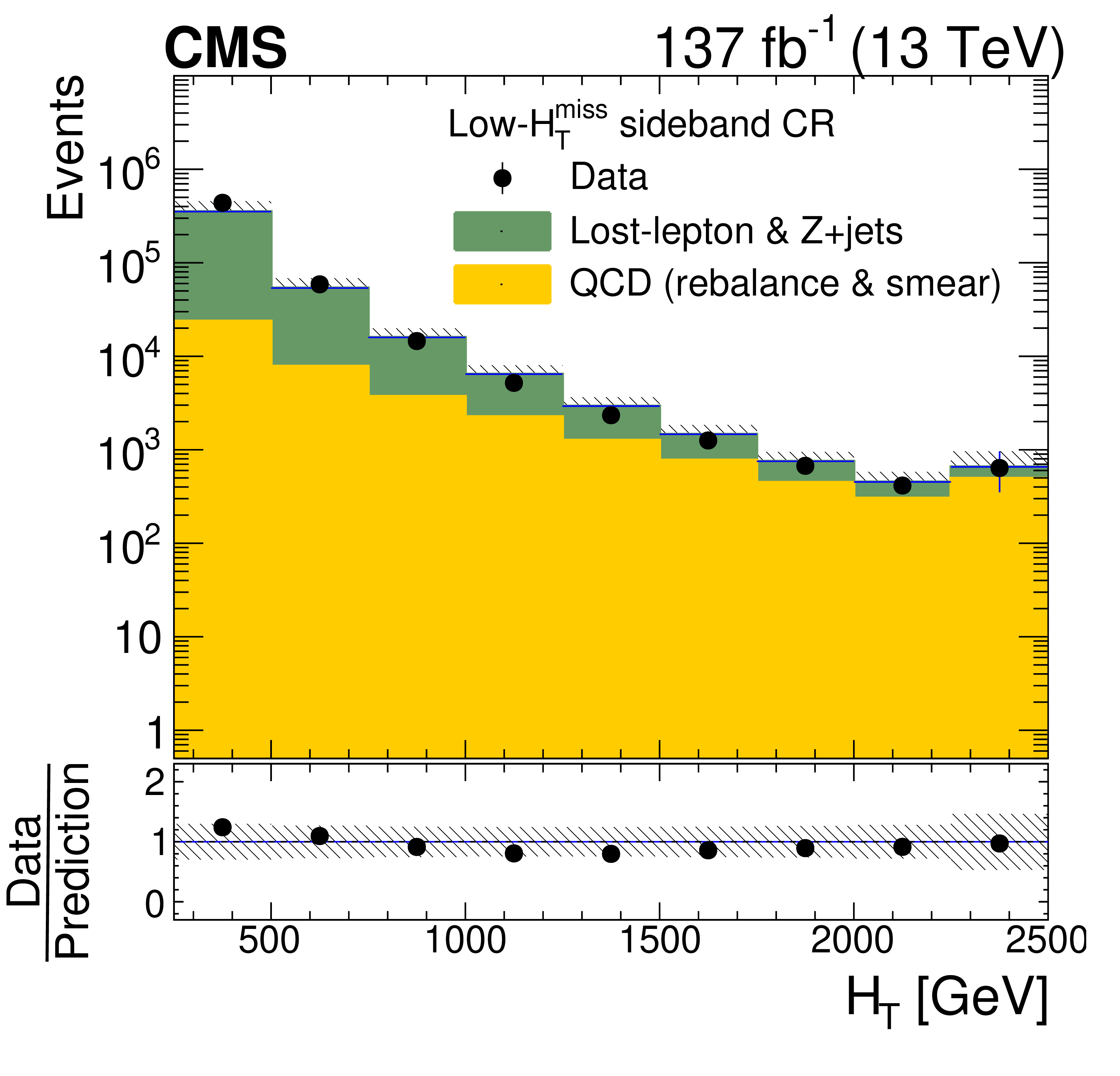
png pdf	Figure 8: The observed and predicted distributions of (left) ${H_{\mathrm {T}}^{\text {miss}}}$ in the inverted- ${\Delta \phi}$ control region and (right) ${H_{\mathrm {T}}}$ in the low- ${H_{\mathrm {T}}^{\text {miss}}}$ sideband. The uncertainties are statistical only. The lower panels show the ratios of the observed to the predicted distributions, with their statistical uncertainties. The hatched regions indicate the total uncertainties in the predictions, with statistical and systematic uncertainties combined in quadrature.
png pdf	Figure 8-a: The observed and predicted distributions of ${H_{\mathrm {T}}^{\text {miss}}}$ in the inverted- ${\Delta \phi}$ control region. The uncertainties are statistical only. The lower panel shows the ratio of the observed to the predicted distributions, with their statistical uncertainties. The hatched regions indicate the total uncertainties in the predictions, with statistical and systematic uncertainties combined in quadrature.
png pdf	Figure 8-b: The observed and predicted distributions of ${H_{\mathrm {T}}}$ in the low- ${H_{\mathrm {T}}^{\text {miss}}}$ sideband. The uncertainties are statistical only. The lower panel shows the ratio of the observed to the predicted distributions, with their statistical uncertainties. The hatched regions indicate the total uncertainties in the predictions, with statistical and systematic uncertainties combined in quadrature.
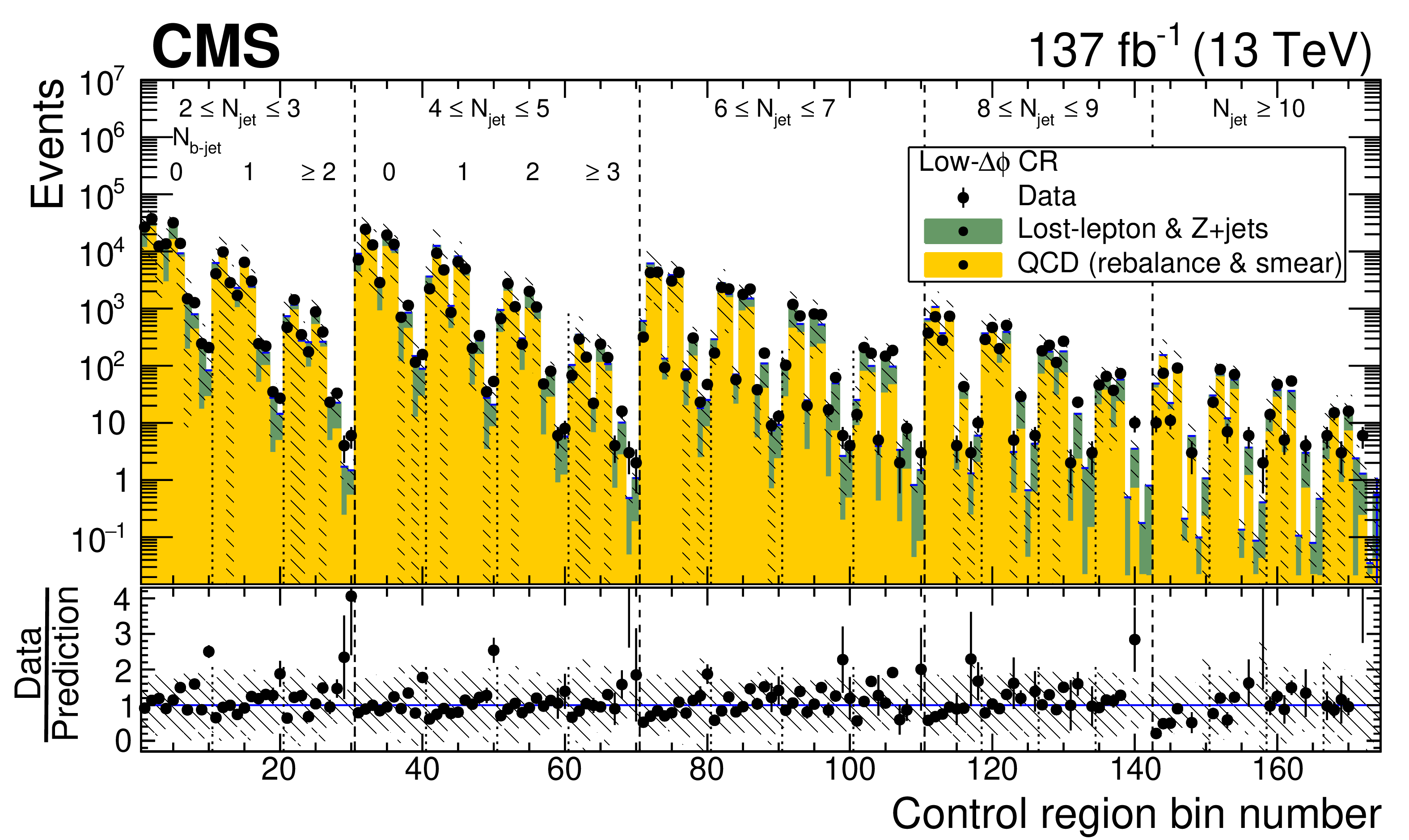
png pdf	Figure 9: Distribution of observed and predicted event yields in the inverted- ${\Delta \phi}$ control region analysis bins. The uncertainties are statistical only. The labeling of the bin numbers is the same as in Fig. 7. The lower panel shows the ratio of the observed to the predicted event yields, with their statistical uncertainties. The hatched region indicates the total uncertainty in the prediction, with statistical and systematic uncertainties combined in quadrature.
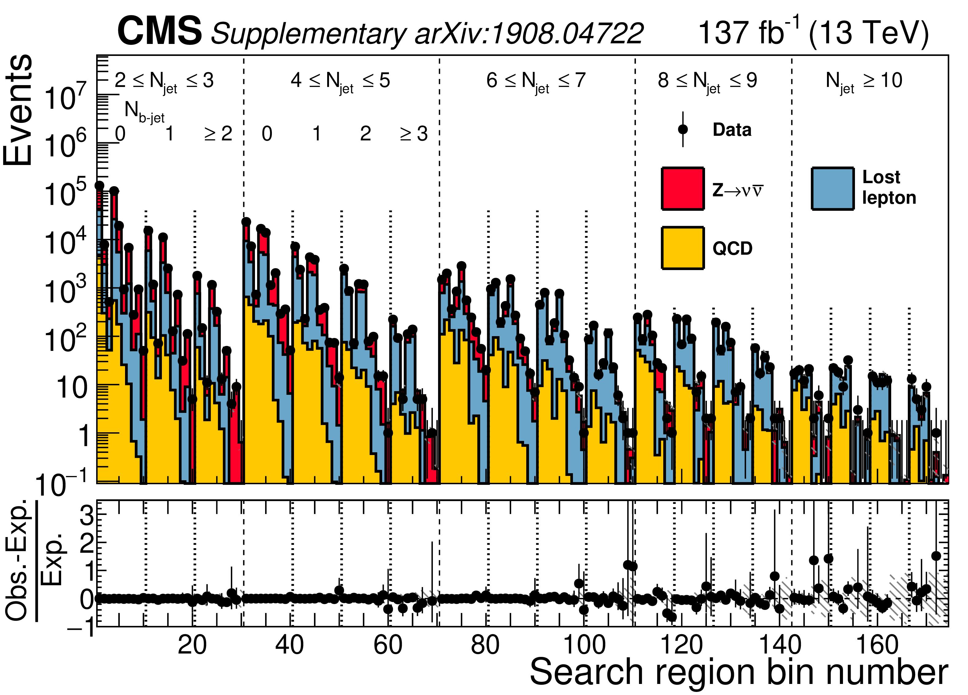
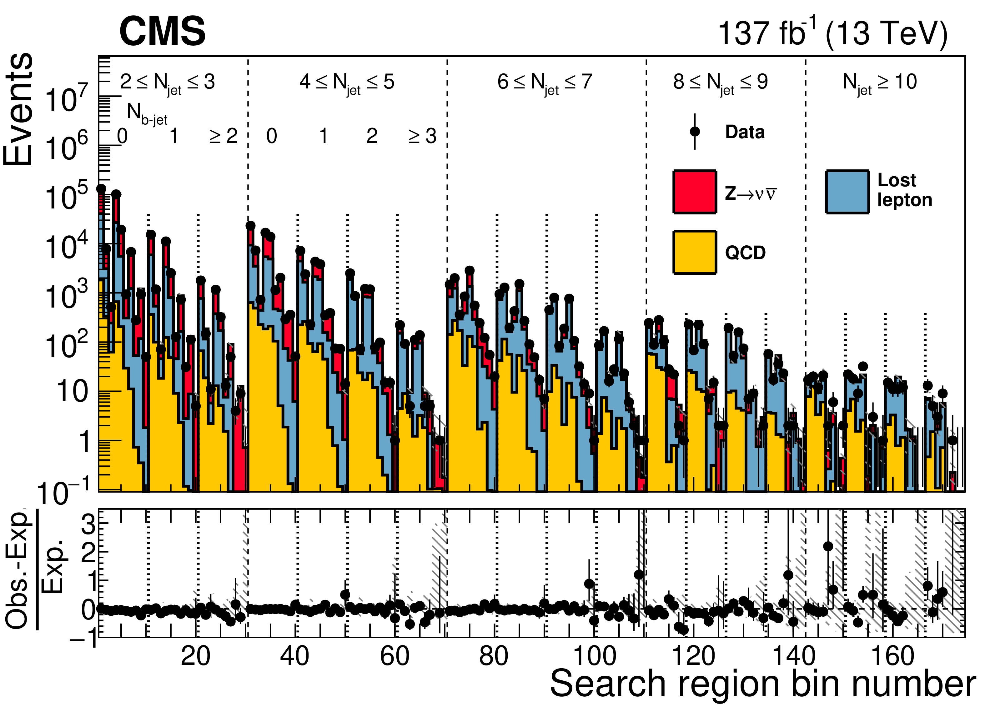
png pdf	Figure 10: The observed numbers of events and pre-fit SM background predictions in the 174 search bins of the analysis, where "pre-fit'' means there is no constraint from the likelihood fit. The labeling of the bin numbers is the same as in Fig. 7. Numerical values are given in Appendix A. The hatching indicates the total uncertainty in the background predictions. The lower panel displays the fractional differences between the data and SM predictions.
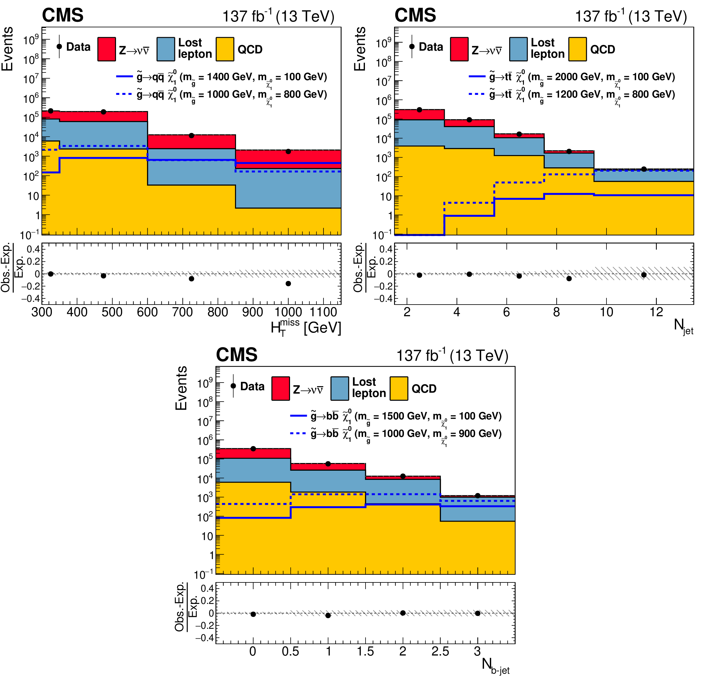
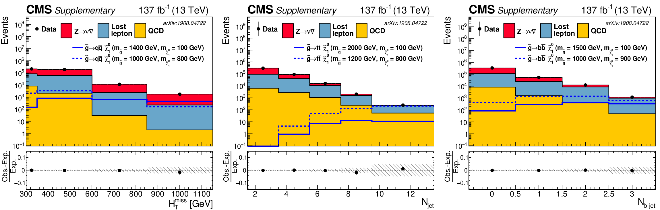
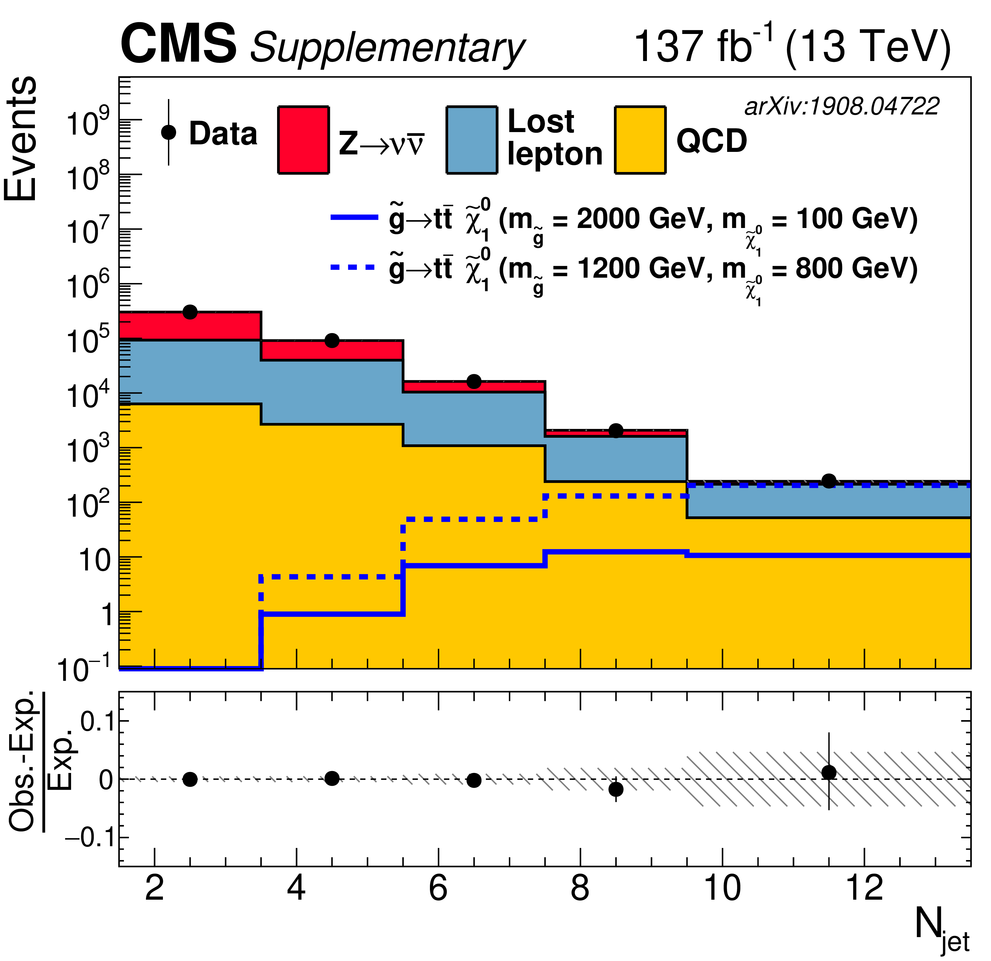
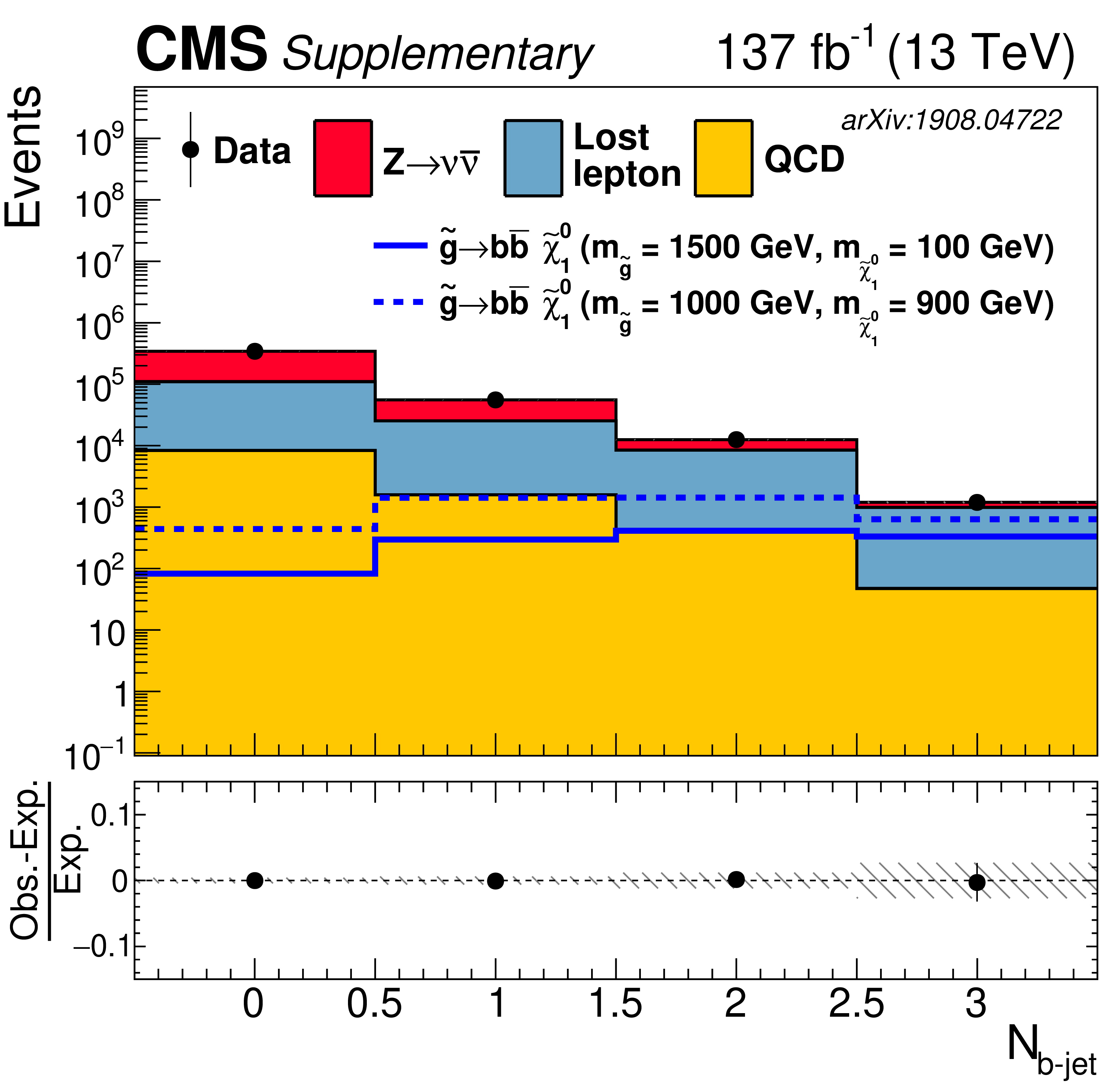
png pdf	Figure 11: One-dimensional projections of the data and pre-fit SM predictions in ${H_{\mathrm {T}}^{\text {miss}}}$ , ${N_{\text {jet}}}$ , and ${N_{{\mathrm{b}}\text {-jet}}}$ . The hatched regions indicate the total uncertainties in the background predictions. The (unstacked) results for two example signal scenarios are shown in each instance, one with ${\Delta m} \gg$ 0 and the other with ${\Delta m} \approx$ 0, where ${\Delta m}$ is the difference between the gluino or squark mass and the sum of the masses of the particles into which it decays.
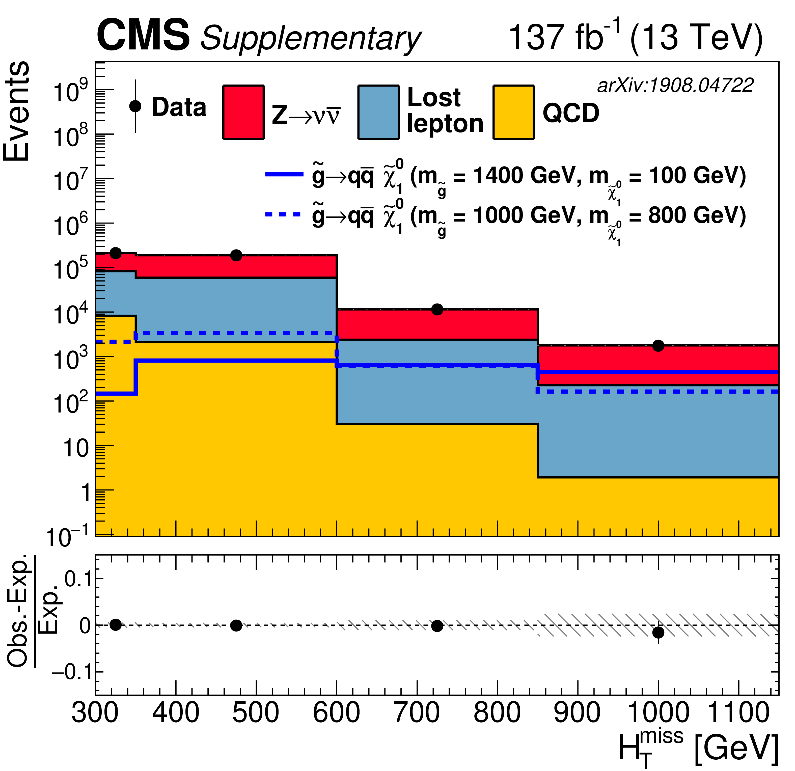
png pdf	Figure 11-a: One-dimensional projection of the data and pre-fit SM predictions in ${H_{\mathrm {T}}^{\text {miss}}}$ . The hatched regions indicate the total uncertainties in the background predictions. The (unstacked) results for two example signal scenarios are shown in each instance, one with ${\Delta m} \gg$ 0 and the other with ${\Delta m} \approx$ 0, where ${\Delta m}$ is the difference between the gluino or squark mass and the sum of the masses of the particles into which it decays.
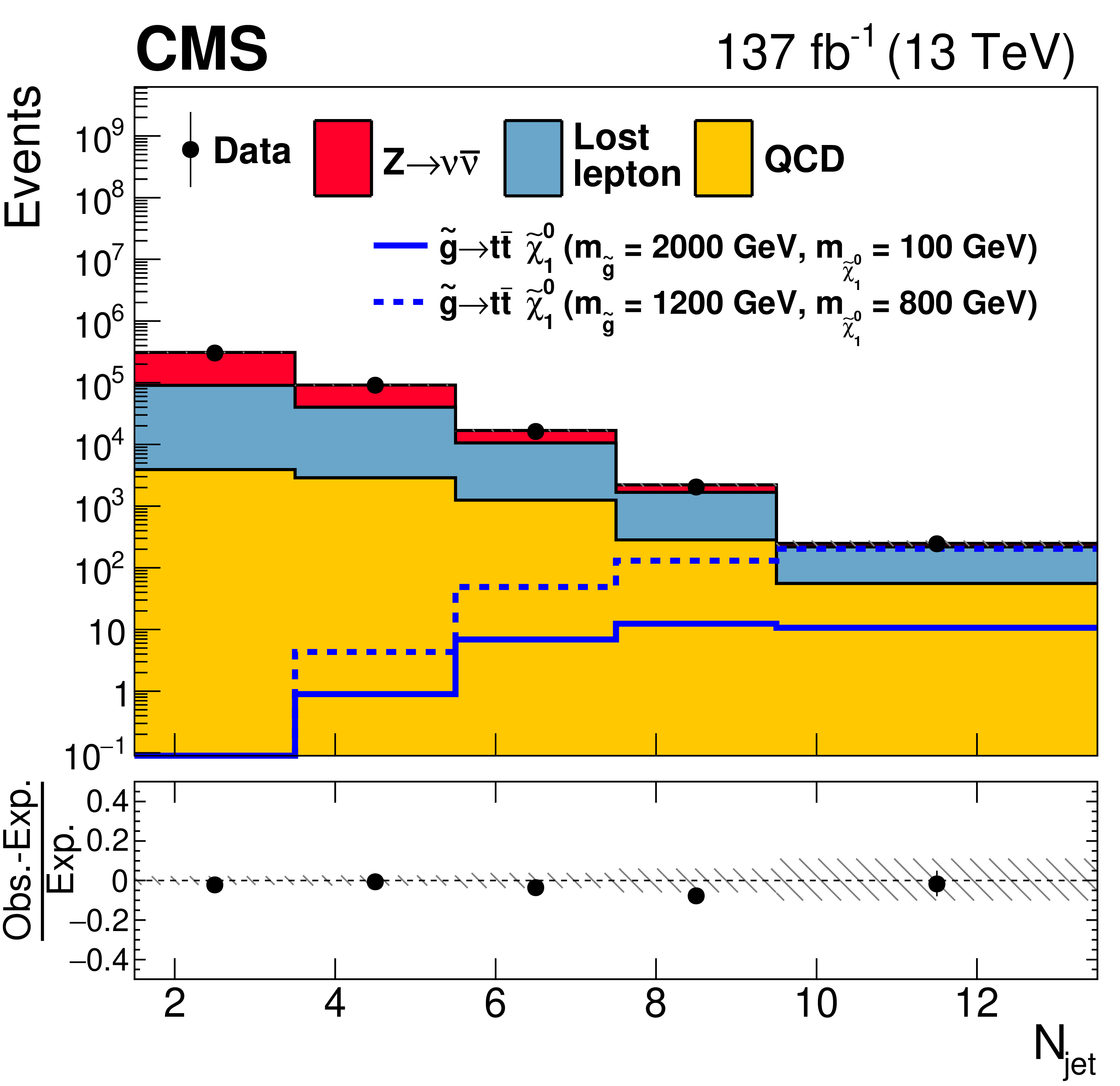
png pdf	Figure 11-b: One-dimensional projection of the data and pre-fit SM predictions in ${N_{\text {jet}}}$ . The hatched regions indicate the total uncertainties in the background predictions. The (unstacked) results for two example signal scenarios are shown in each instance, one with ${\Delta m} \gg$ 0 and the other with ${\Delta m} \approx$ 0, where ${\Delta m}$ is the difference between the gluino or squark mass and the sum of the masses of the particles into which it decays.
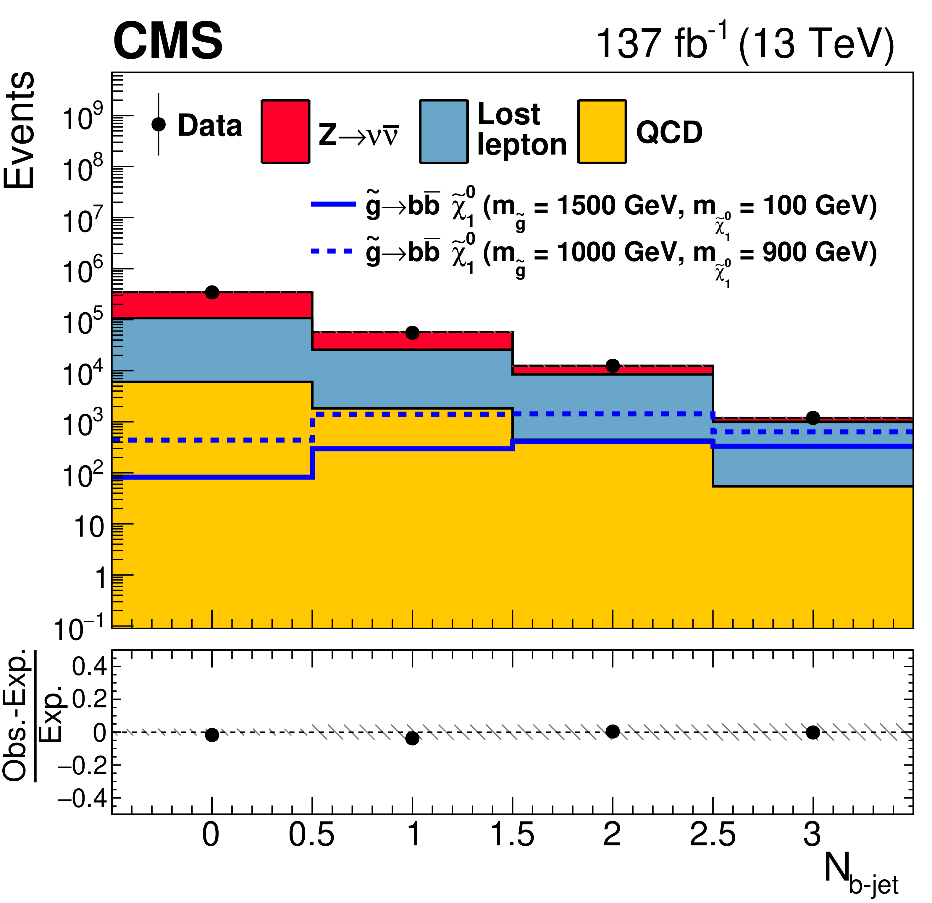
png pdf	Figure 11-c: One-dimensional projection of the data and pre-fit SM predictions in ${N_{{\mathrm{b}}\text {-jet}}}$ . The hatched regions indicate the total uncertainties in the background predictions. The (unstacked) results for two example signal scenarios are shown in each instance, one with ${\Delta m} \gg$ 0 and the other with ${\Delta m} \approx$ 0, where ${\Delta m}$ is the difference between the gluino or squark mass and the sum of the masses of the particles into which it decays.
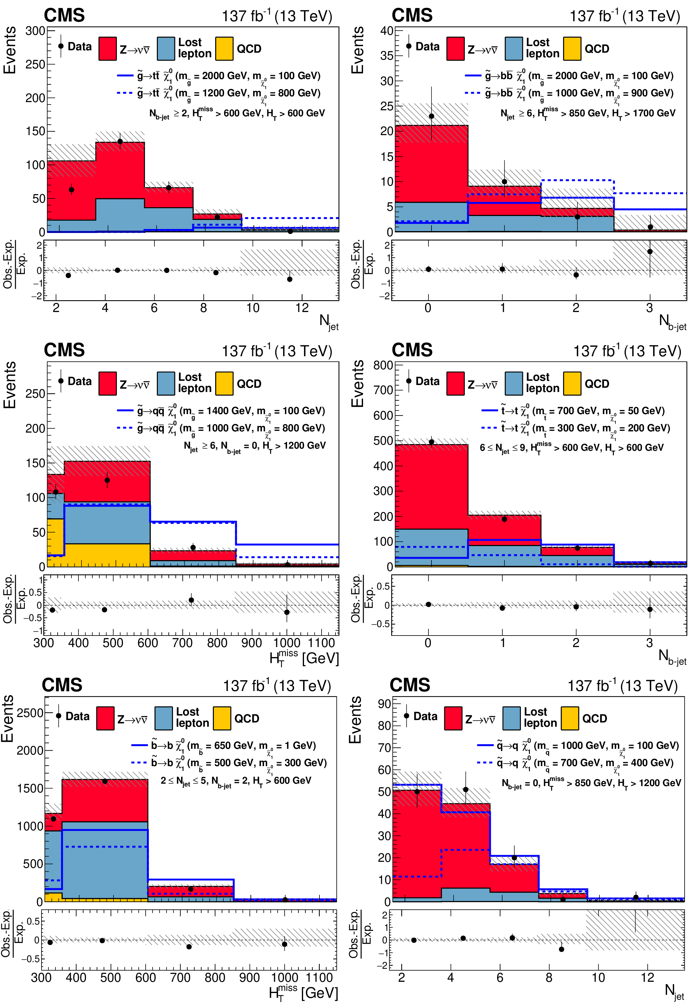
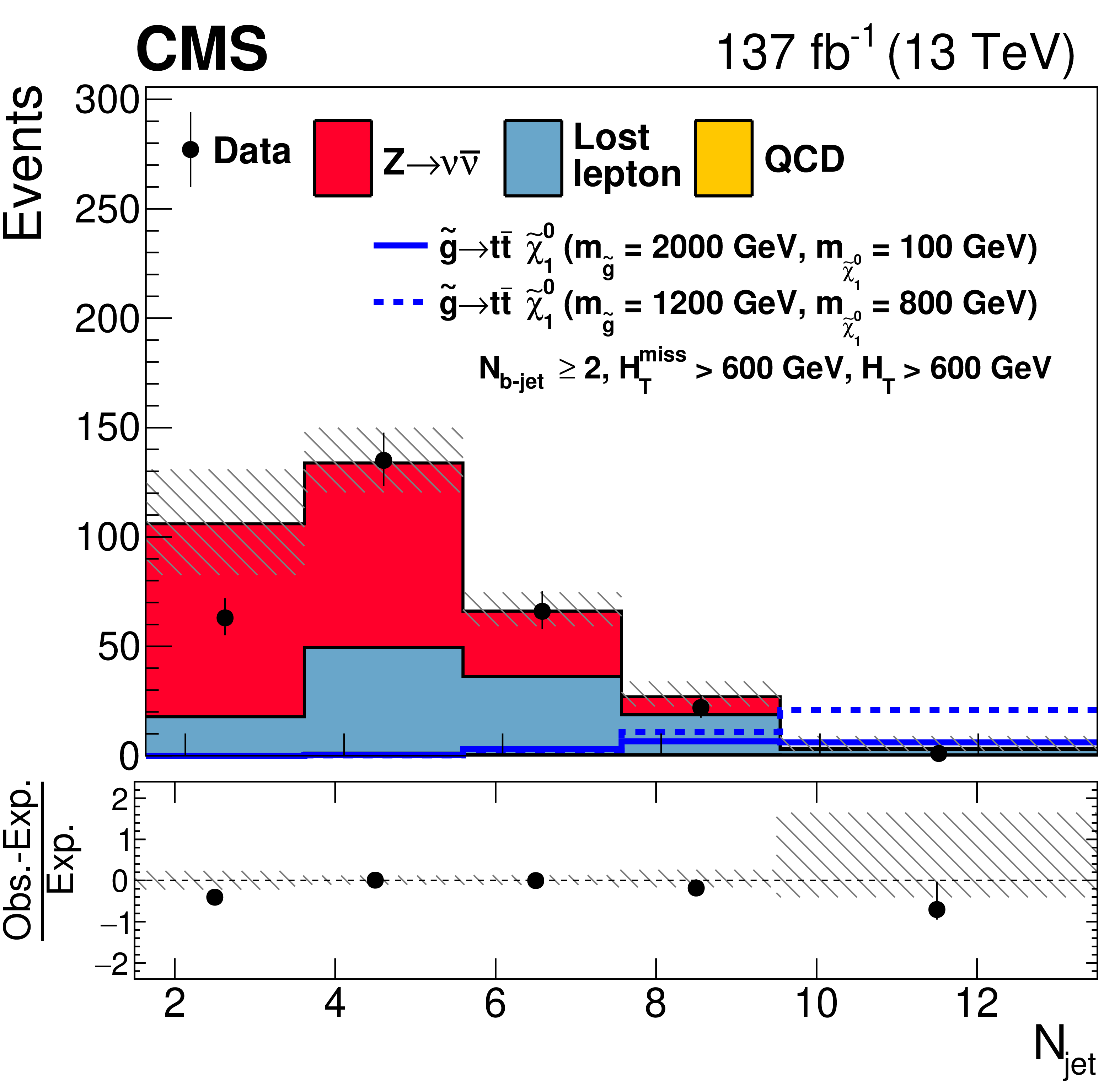
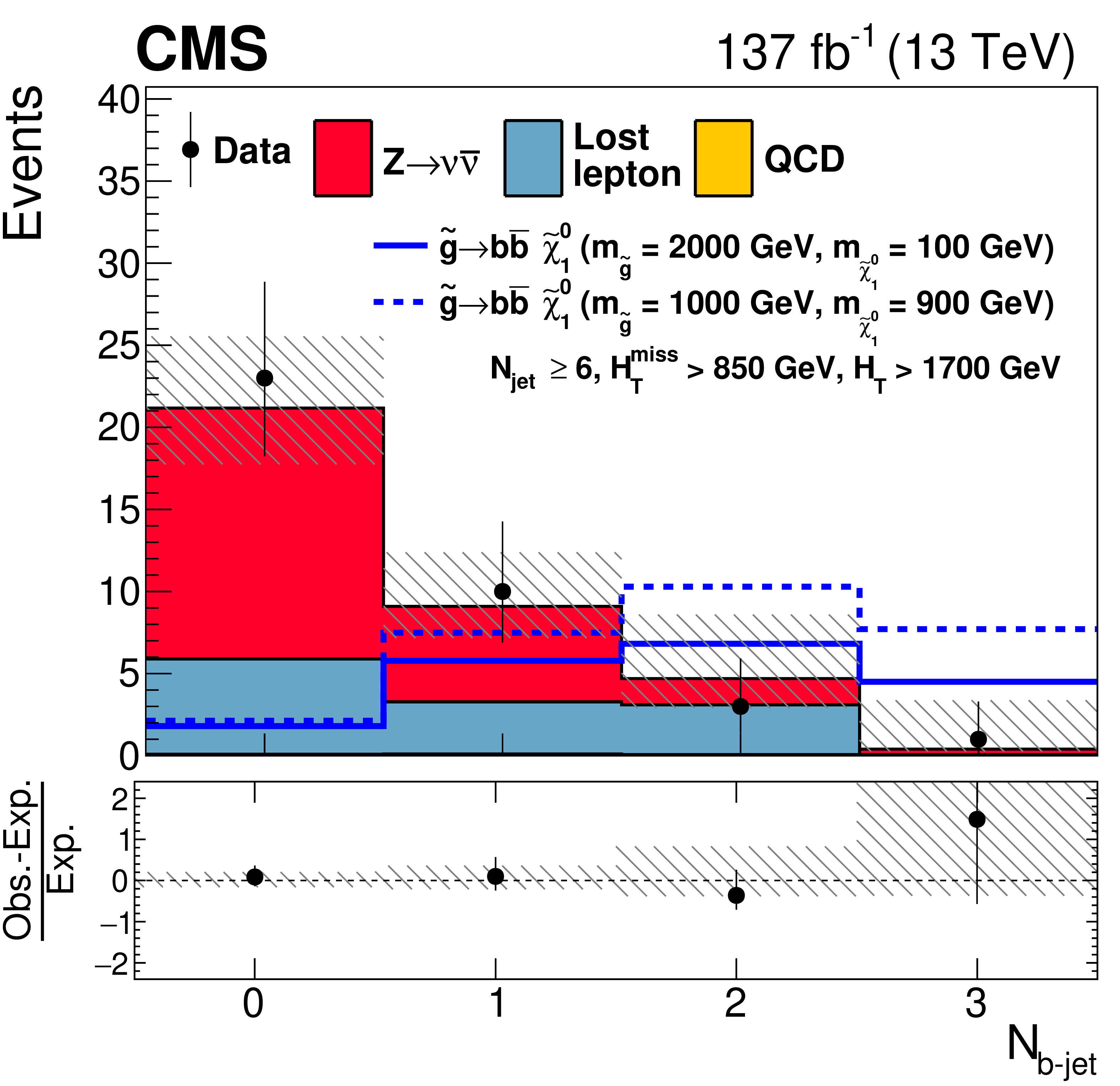
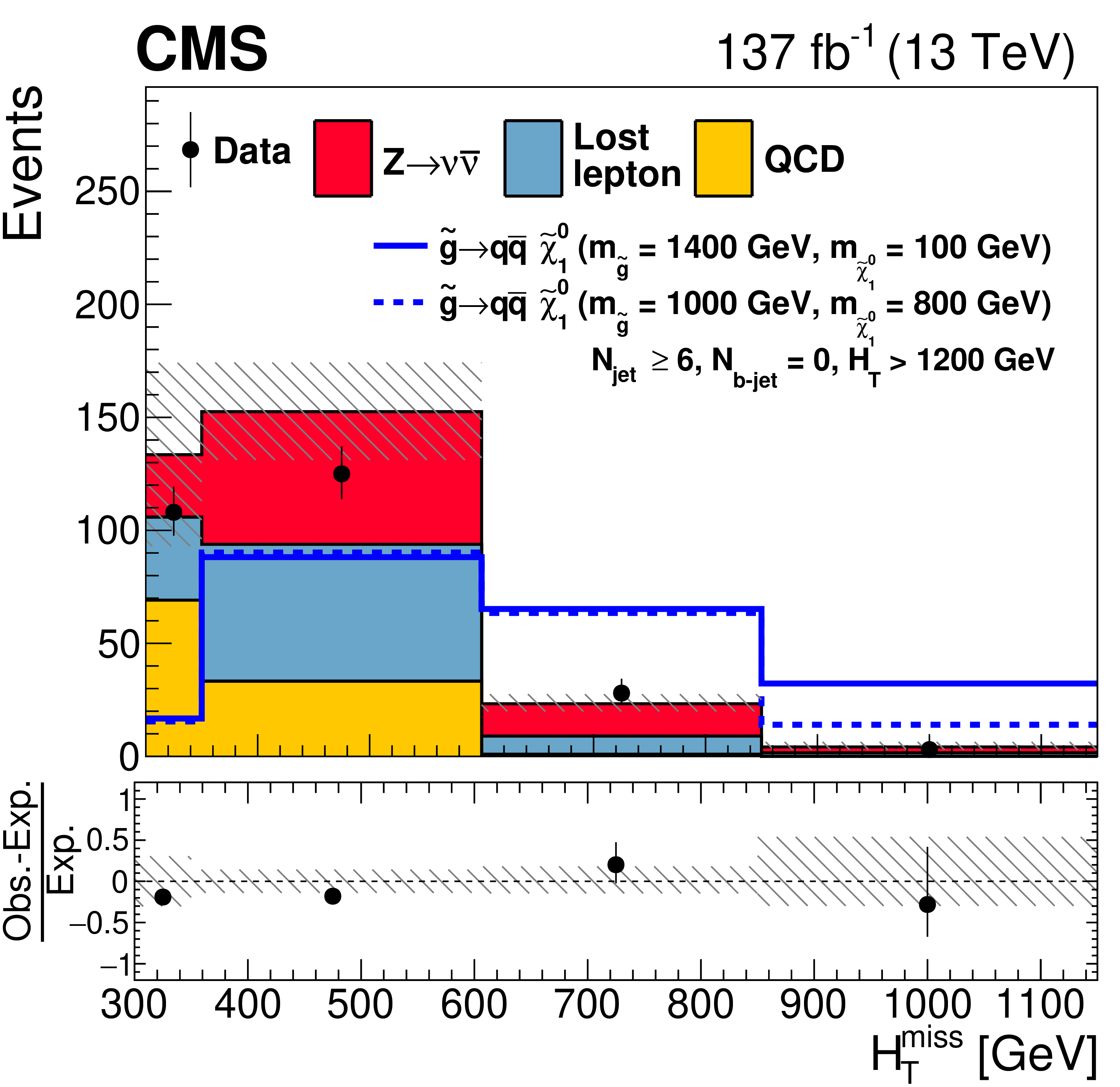
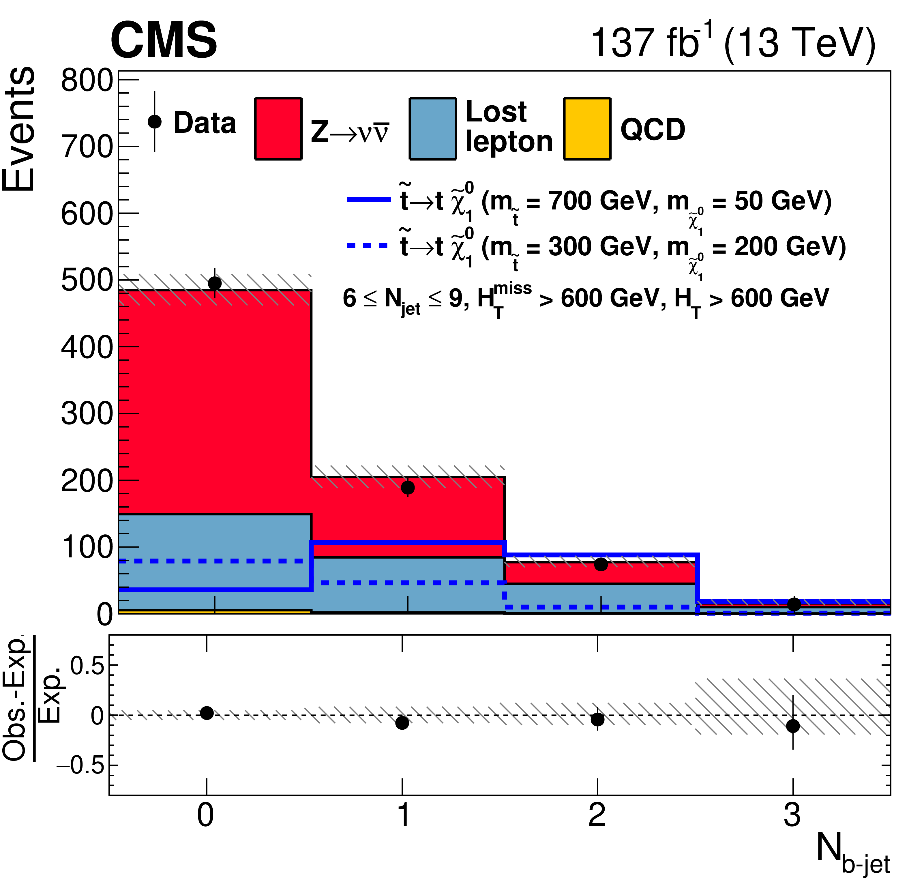
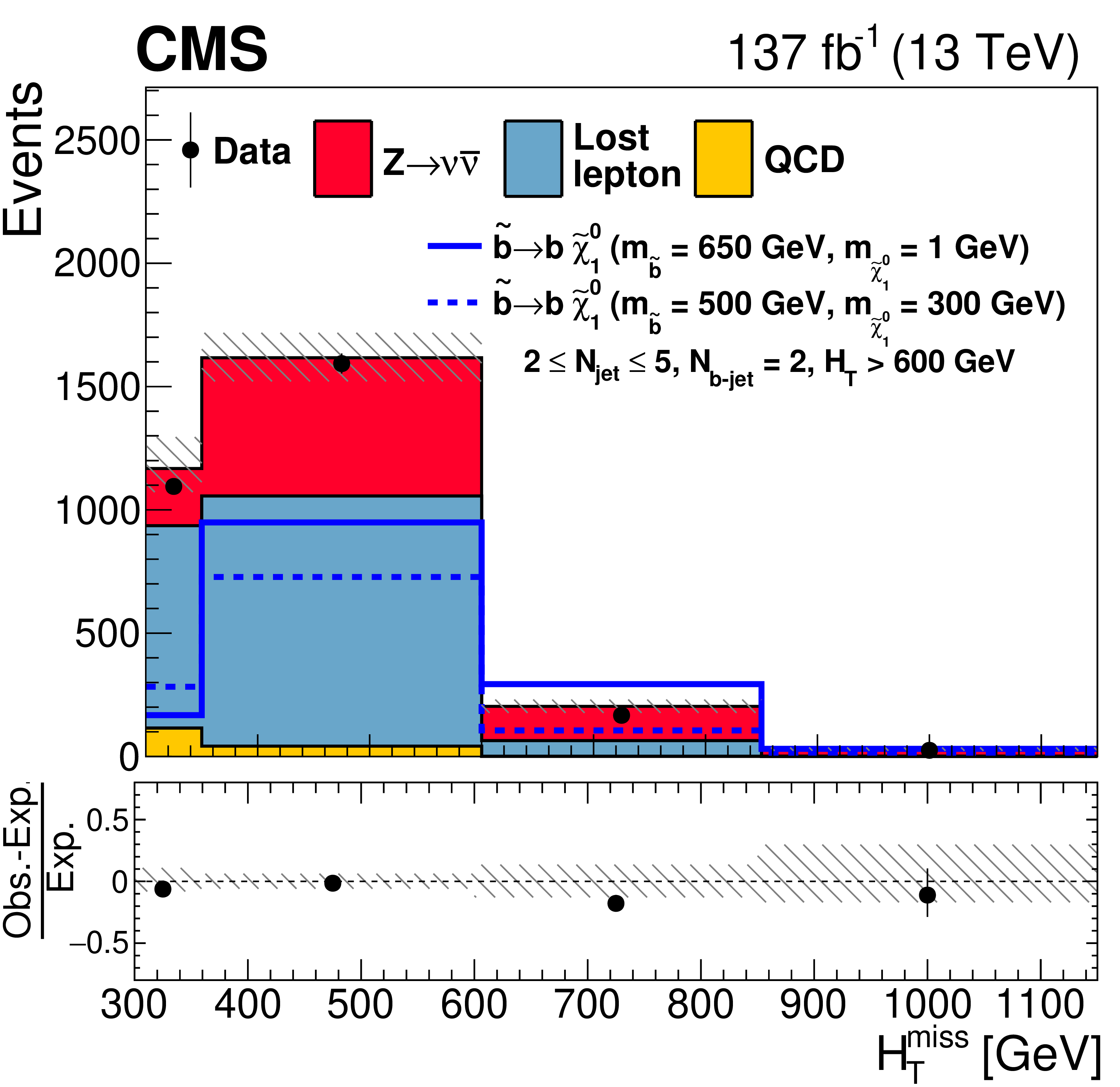
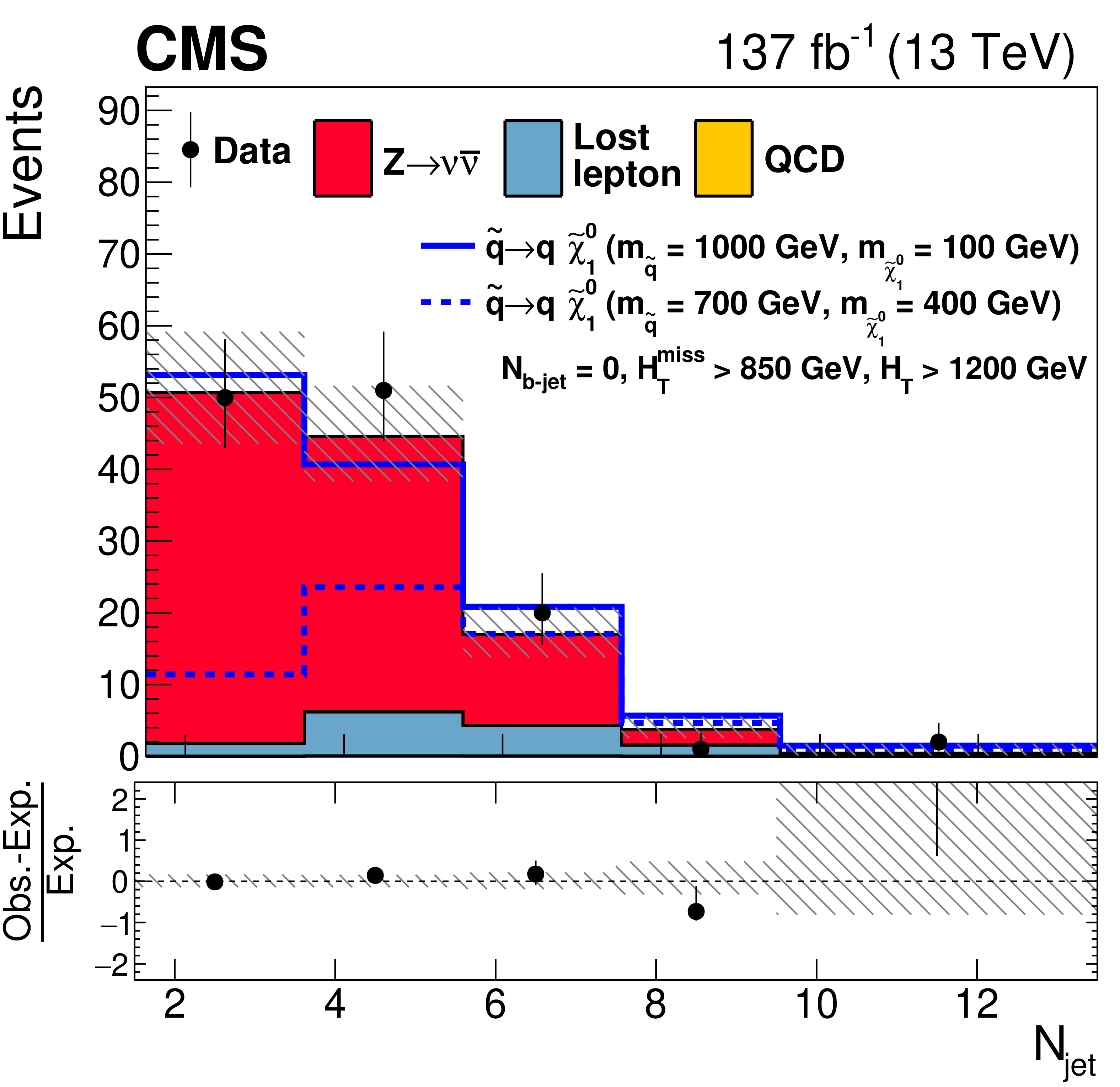
png pdf	Figure 12: One-dimensional projections of the data and pre-fit SM predictions in either ${H_{\mathrm {T}}^{\text {miss}}}$ , ${N_{\text {jet}}}$ , or ${N_{{\mathrm{b}}\text {-jet}}}$ after applying additional selection criteria, given in the figure legends, to enhance the sensitivity to the (upper left) T1tttt, (upper right) T1bbbb, (middle left) T1qqqq, (middle right) T2tt, (lower left) T2bb, and (lower right) T2qq signal processes. The (unstacked) results for two example signal scenarios are shown in each instance, one with ${\Delta m} \gg$ 0 and the other with ${\Delta m} \approx$ 0, where ${\Delta m}$ is the difference between the gluino or squark mass and the sum of the masses of the particles into which it decays.
png pdf	Figure 12-a: One-dimensional projections of the data and pre-fit SM predictions in ${N_{\text {jet}}}$ after applying additional selection criteria, given in the figure legends, to enhance the sensitivity to the T1tttt signal process. The (unstacked) results for two example signal scenarios are shown, one with ${\Delta m} \gg$ 0 and the other with ${\Delta m} \approx$ 0, where ${\Delta m}$ is the difference between the gluino or squark mass and the sum of the masses of the particles into which it decays.
png pdf	Figure 12-b: One-dimensional projections of the data and pre-fit SM predictions in ${N_{{\mathrm{b}}\text {-jet}}}$ after applying additional selection criteria, given in the figure legends, to enhance the sensitivity to the T1bbbb signal process. The (unstacked) results for two example signal scenarios are shown, one with ${\Delta m} \gg$ 0 and the other with ${\Delta m} \approx$ 0, where ${\Delta m}$ is the difference between the gluino or squark mass and the sum of the masses of the particles into which it decays.
png pdf	Figure 12-c: One-dimensional projections of the data and pre-fit SM predictions in ${H_{\mathrm {T}}^{\text {miss}}}$ after applying additional selection criteria, given in the figure legends, to enhance the sensitivity to the T1qqqq signal process. The (unstacked) results for two example signal scenarios are shown, one with ${\Delta m} \gg$ 0 and the other with ${\Delta m} \approx$ 0, where ${\Delta m}$ is the difference between the gluino or squark mass and the sum of the masses of the particles into which it decays.
png pdf	Figure 12-d: One-dimensional projections of the data and pre-fit SM predictions in ${N_{{\mathrm{b}}\text {-jet}}}$ after applying additional selection criteria, given in the figure legends, to enhance the sensitivity to the T2tt signal process. The (unstacked) results for two example signal scenarios are shown, one with ${\Delta m} \gg$ 0 and the other with ${\Delta m} \approx$ 0, where ${\Delta m}$ is the difference between the gluino or squark mass and the sum of the masses of the particles into which it decays.
png pdf	Figure 12-e: One-dimensional projections of the data and pre-fit SM predictions in ${H_{\mathrm {T}}^{\text {miss}}}$ after applying additional selection criteria, given in the figure legends, to enhance the sensitivity to the T2bb signal process. The (unstacked) results for two example signal scenarios are shown, one with ${\Delta m} \gg$ 0 and the other with ${\Delta m} \approx$ 0, where ${\Delta m}$ is the difference between the gluino or squark mass and the sum of the masses of the particles into which it decays.
png pdf	Figure 12-f: One-dimensional projections of the data and pre-fit SM predictions in ${N_{\text {jet}}}$ after applying additional selection criteria, given in the figure legends, to enhance the sensitivity to the T2qq signal process. The (unstacked) results for two example signal scenarios are shown, one with ${\Delta m} \gg$ 0 and the other with ${\Delta m} \approx$ 0, where ${\Delta m}$ is the difference between the gluino or squark mass and the sum of the masses of the particles into which it decays.
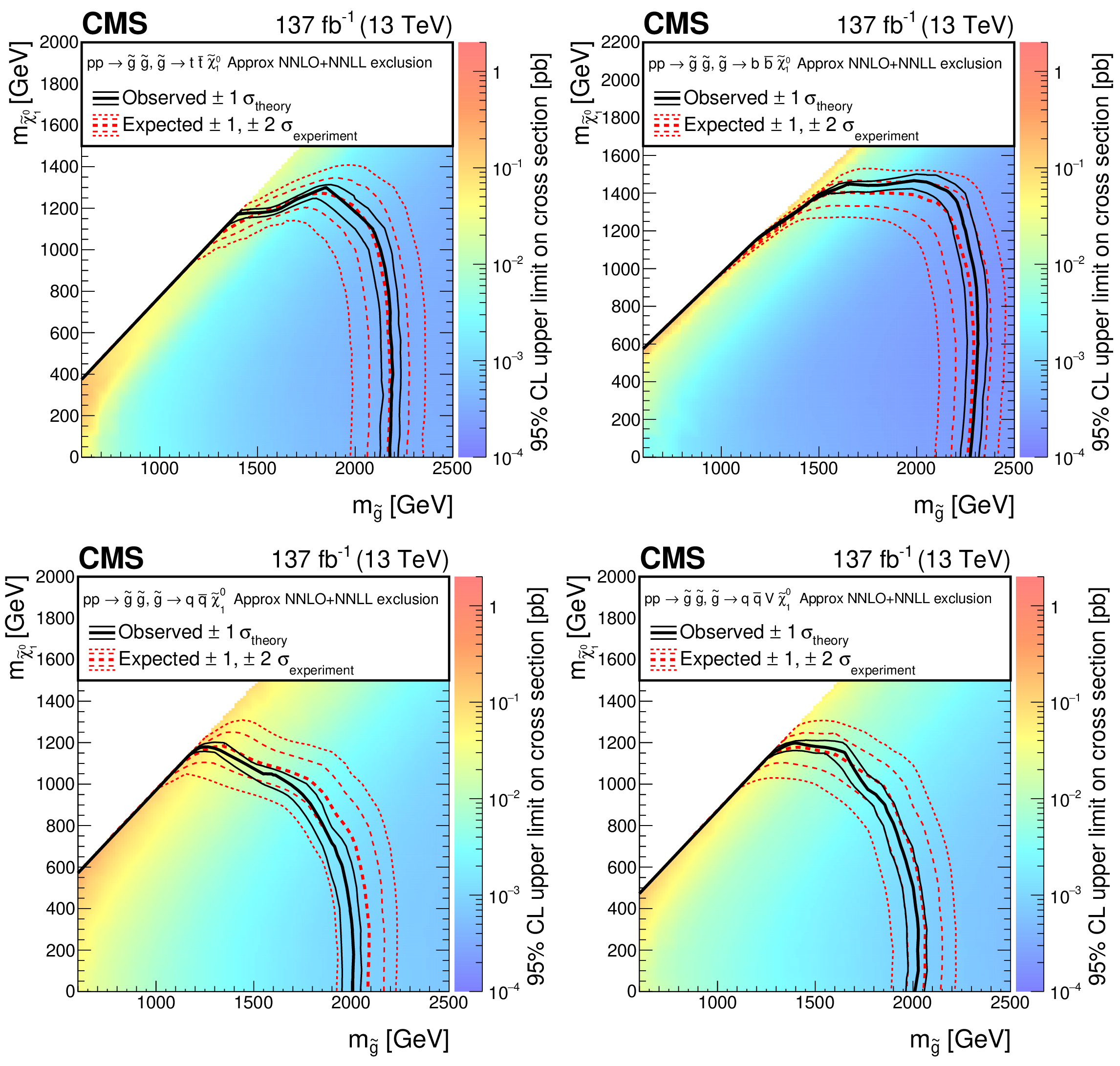
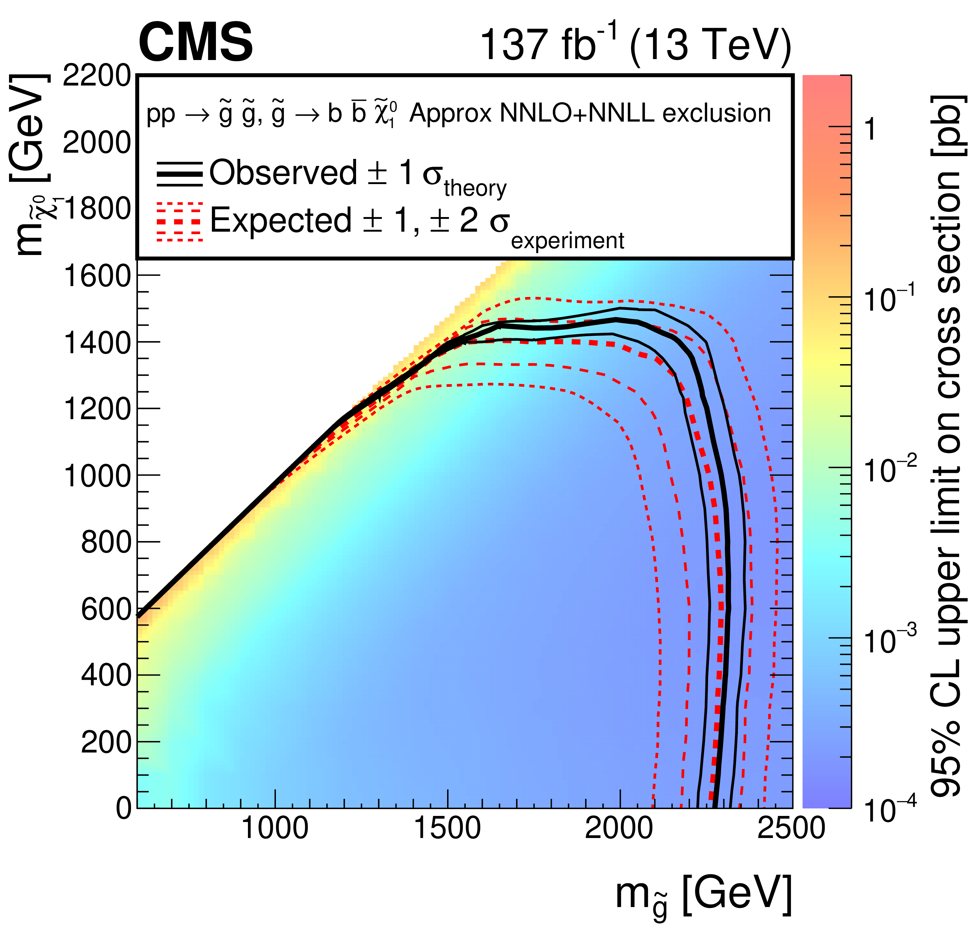
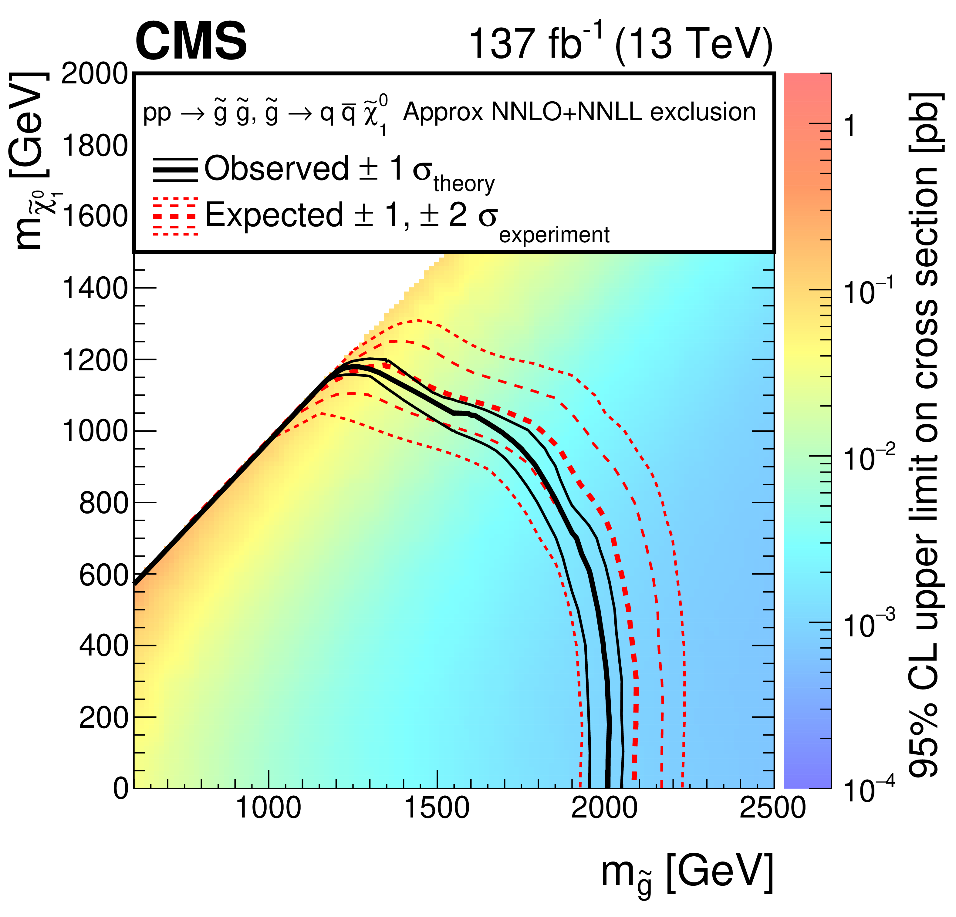
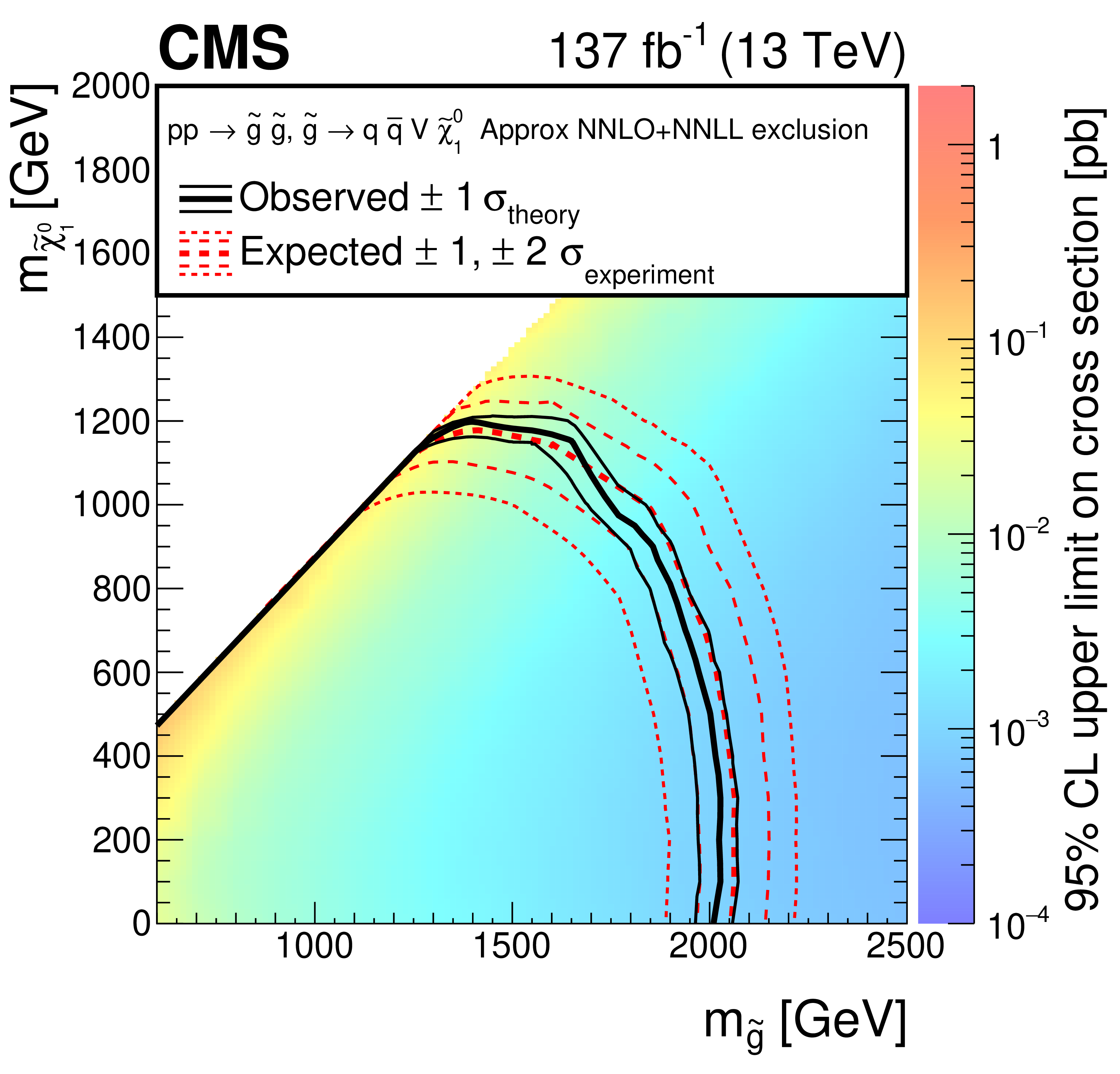
png pdf	Figure 13: The 95% CL upper limits on the production cross sections of the (upper left) T1tttt, (upper right) T1bbbb, (lower left) T1qqqq, and (lower right) T5qqqqVV signal models as a function of the gluino and LSP masses ${m_{{\mathrm{\tilde{g}}}}}$ and ${m_{\tilde{\chi}^0_1}}$ . The thick solid (black) curves show the observed exclusion limits assuming the approximate-NNLO+NNLL cross sections [71,72,73,74,75]. The thin solid (black) curves show the changes in these limits as the signal cross sections are varied by their theoretical uncertainties [93]. The thick dashed (red) curves present the expected limits under the background-only hypothesis, while the two sets of thin dotted (red) curves indicate the region containing 68 and 95% of the distribution of limits expected under this hypothesis.
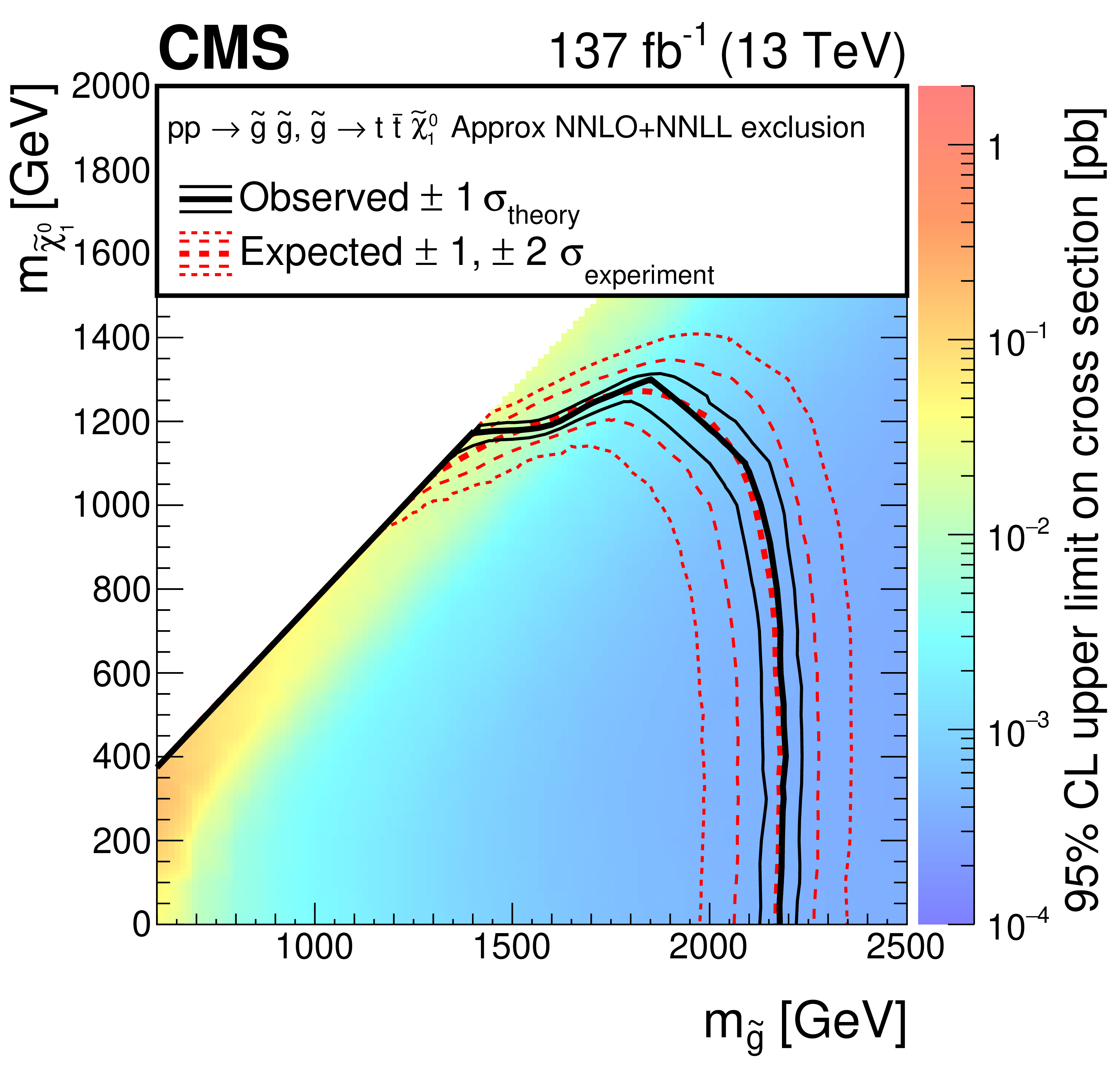
png pdf root	Figure 13-a: The 95% CL upper limits on the production cross sections of the T1tttt signal model as a function of the gluino and LSP masses ${m_{{\mathrm{\tilde{g}}}}}$ and ${m_{\tilde{\chi}^0_1}}$ . The thick solid (black) curves show the observed exclusion limits assuming the approximate-NNLO+NNLL cross sections [71,72,73,74,75]. The thin solid (black) curves show the changes in these limits as the signal cross sections are varied by their theoretical uncertainties [93]. The thick dashed (red) curves present the expected limits under the background-only hypothesis, while the two sets of thin dotted (red) curves indicate the region containing 68 and 95% of the distribution of limits expected under this hypothesis.
png pdf root	Figure 13-b: The 95% CL upper limits on the production cross sections of the T1bbbb signal model as a function of the gluino and LSP masses ${m_{{\mathrm{\tilde{g}}}}}$ and ${m_{\tilde{\chi}^0_1}}$ . The thick solid (black) curves show the observed exclusion limits assuming the approximate-NNLO+NNLL cross sections [71,72,73,74,75]. The thin solid (black) curves show the changes in these limits as the signal cross sections are varied by their theoretical uncertainties [93]. The thick dashed (red) curves present the expected limits under the background-only hypothesis, while the two sets of thin dotted (red) curves indicate the region containing 68 and 95% of the distribution of limits expected under this hypothesis.
png pdf root	Figure 13-c: The 95% CL upper limits on the production cross sections of the T1qqqq signal model as a function of the gluino and LSP masses ${m_{{\mathrm{\tilde{g}}}}}$ and ${m_{\tilde{\chi}^0_1}}$ . The thick solid (black) curves show the observed exclusion limits assuming the approximate-NNLO+NNLL cross sections [71,72,73,74,75]. The thin solid (black) curves show the changes in these limits as the signal cross sections are varied by their theoretical uncertainties [93]. The thick dashed (red) curves present the expected limits under the background-only hypothesis, while the two sets of thin dotted (red) curves indicate the region containing 68 and 95% of the distribution of limits expected under this hypothesis.
png pdf root	Figure 13-d: The 95% CL upper limits on the production cross sections of the T5qqqqVV signal model as a function of the gluino and LSP masses ${m_{{\mathrm{\tilde{g}}}}}$ and ${m_{\tilde{\chi}^0_1}}$ . The thick solid (black) curves show the observed exclusion limits assuming the approximate-NNLO+NNLL cross sections [71,72,73,74,75]. The thin solid (black) curves show the changes in these limits as the signal cross sections are varied by their theoretical uncertainties [93]. The thick dashed (red) curves present the expected limits under the background-only hypothesis, while the two sets of thin dotted (red) curves indicate the region containing 68 and 95% of the distribution of limits expected under this hypothesis.
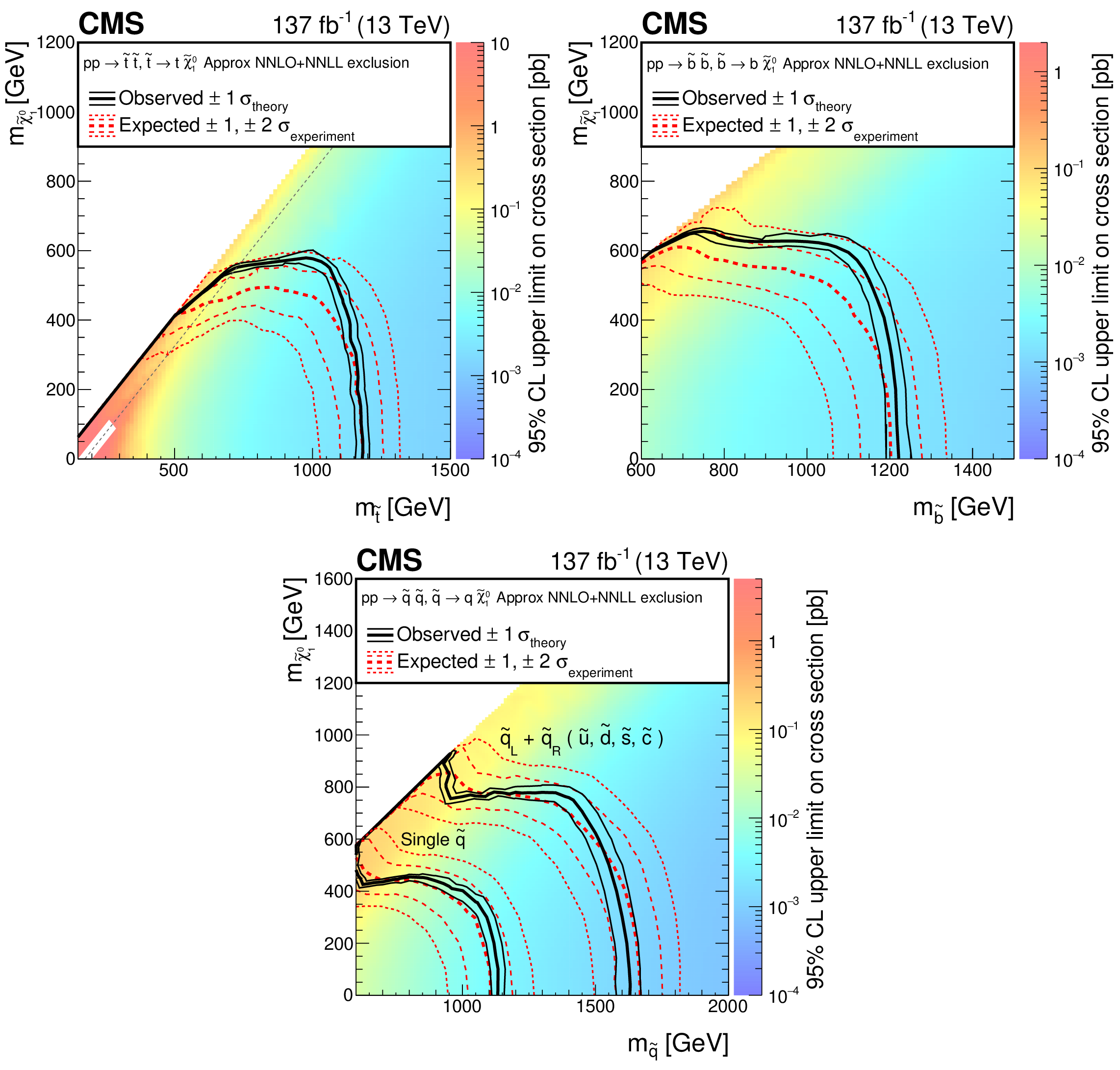
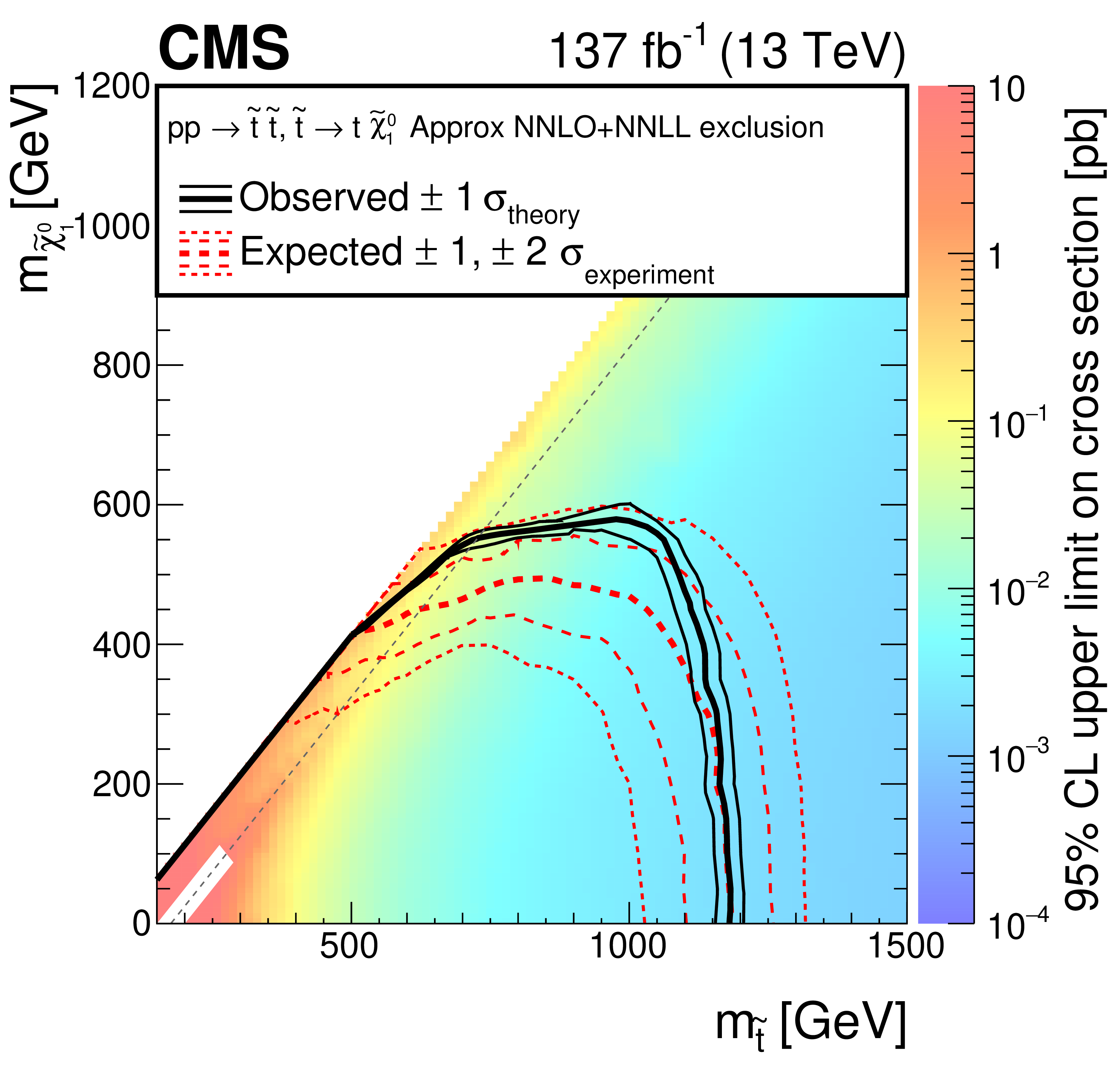
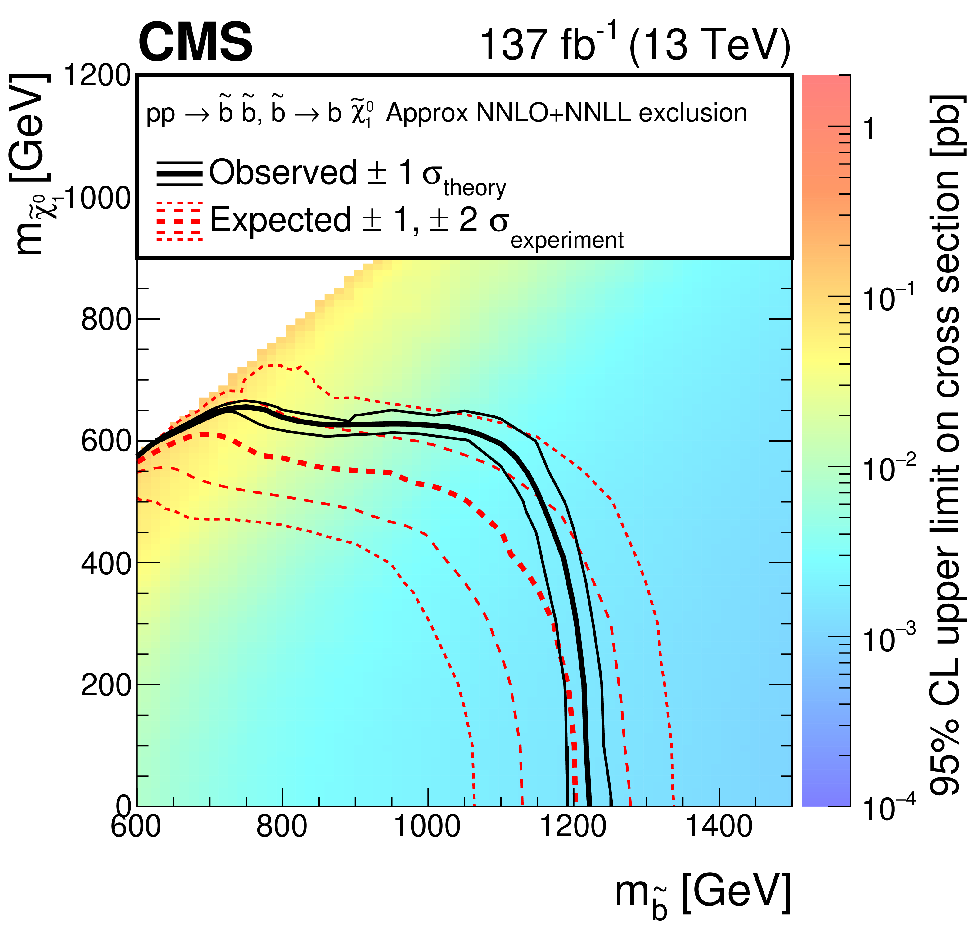
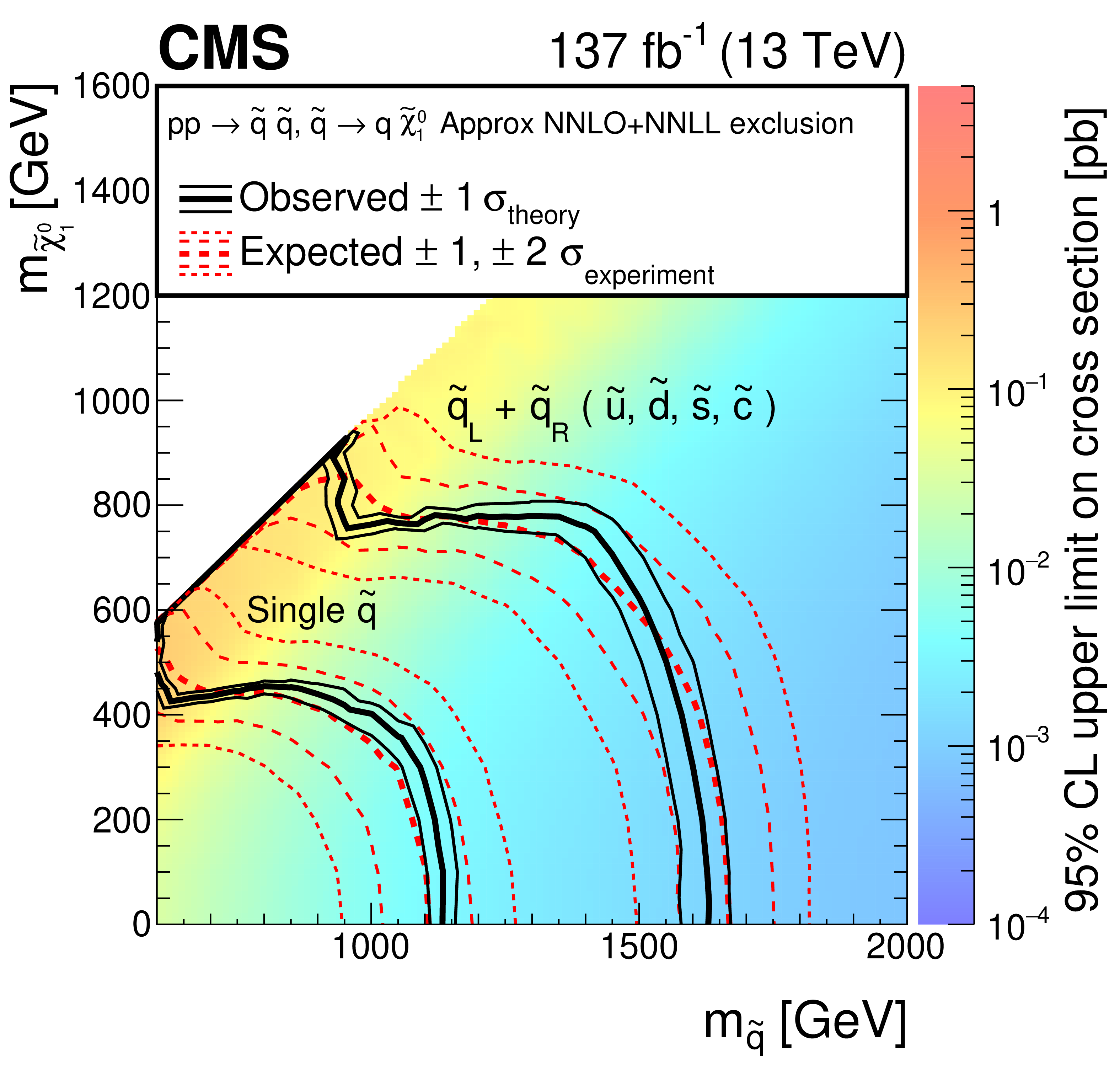
png pdf	Figure 14: The 95% CL upper limits on the production cross sections of the (upper left) T2tt, (upper right) T2bb, and (lower) T2qq signal models as a function of the squark and LSP masses ${m_{\tilde{q}}}$ and ${m_{\tilde{\chi}^0_1}}$ . The meaning of the curves is described in the Fig. 13 caption. For the T2tt model, we do not present cross section upper limits in the unshaded diagonal region at low ${m_{\tilde{\chi}^0_1}}$ for the reason discussed in the text. The diagonal dotted line shown for this model corresponds to ${m_{\tilde{\mathrm{t}}}} - {m_{\tilde{\chi}^0_1}} = {m_{\mathrm{t}}}$ .
png pdf root	Figure 14-a: The 95% CL upper limits on the production cross sections of the T2tt signal models as a function of the squark and LSP masses ${m_{\tilde{q}}}$ and ${m_{\tilde{\chi}^0_1}}$ . The meaning of the curves is described in the Fig. 13 caption. We do not present cross section upper limits in the unshaded diagonal region at low ${m_{\tilde{\chi}^0_1}}$ for the reason discussed in the text. The diagonal dotted line shown for this model corresponds to ${m_{\tilde{\mathrm{t}}}} - {m_{\tilde{\chi}^0_1}} = {m_{\mathrm{t}}}$ .
png pdf root	Figure 14-b: The 95% CL upper limits on the production cross sections of the T2bb signal models as a function of the squark and LSP masses ${m_{\tilde{q}}}$ and ${m_{\tilde{\chi}^0_1}}$ . The meaning of the curves is described in the Fig. 13 caption.
png pdf root	Figure 14-c: The 95% CL upper limits on the production cross sections of the T2qq signal models as a function of the squark and LSP masses ${m_{\tilde{q}}}$ and ${m_{\tilde{\chi}^0_1}}$ . The meaning of the curves is described in the Fig. 13 caption.
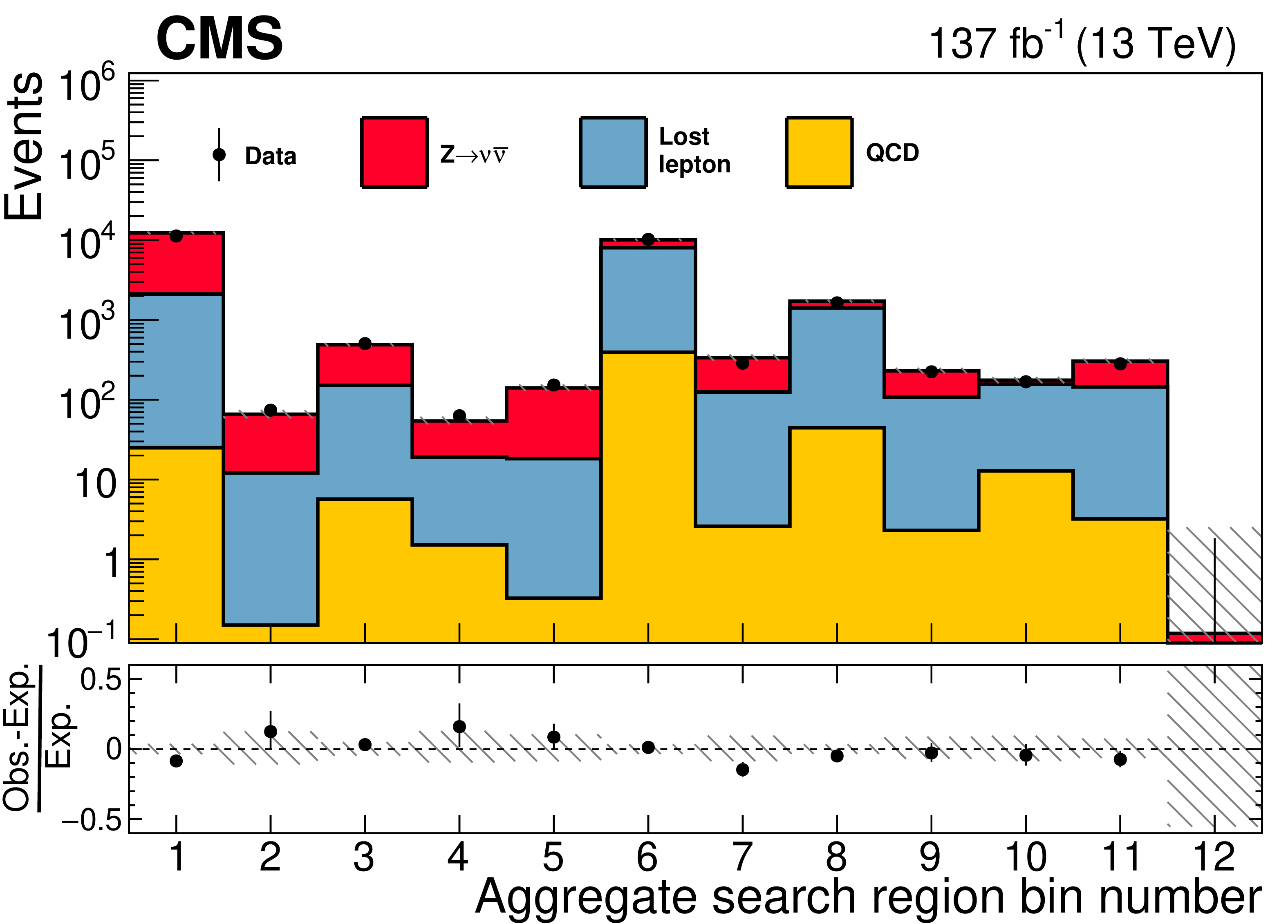
png pdf	Figure 15: The observed numbers of events and pre-fit SM background predictions in the aggregate search bins. The total background uncertainty is shown by the hatched regions. The lower panel displays the fractional differences between the data and the SM predictions.

Tables
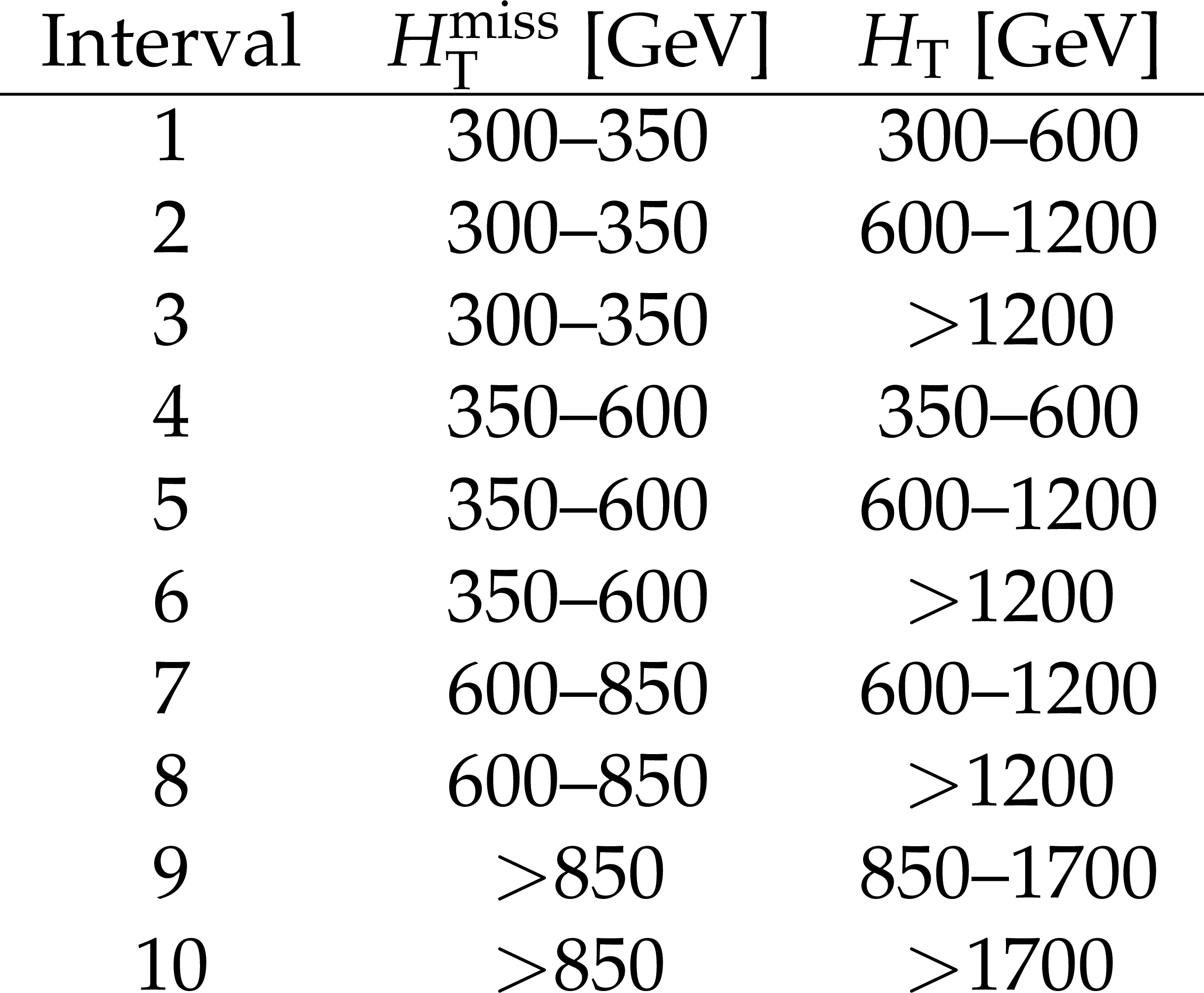
png pdf	Table 1: Definition of the search intervals in the ${H_{\mathrm {T}}^{\text {miss}}}$ and ${H_{\mathrm {T}}}$ variables. Intervals 1 and 4 are discarded for ${N_{\text {jet}}} \geq$ 8. In addition, regions with ${H_{\mathrm {T}}^{\text {miss}}} > {H_{\mathrm {T}}}$ are excluded as illustrated in Fig. 3.
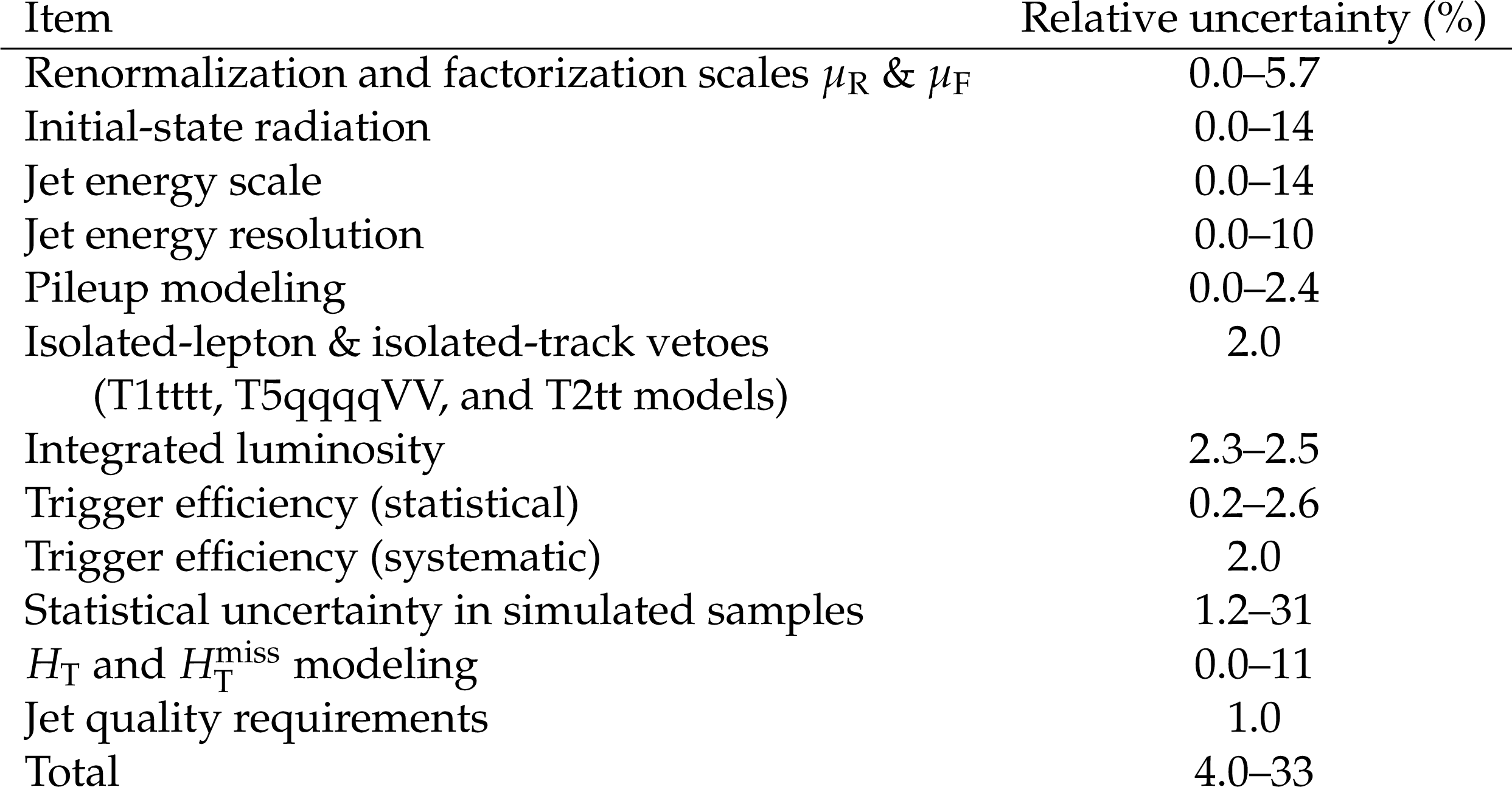
png pdf	Table 2: Systematic uncertainties in the yield of signal events, averaged over all search bins. The variations correspond to different signal models and choices for the SUSY particle masses. Results reported as 0.0 correspond to values less than 0.05%.
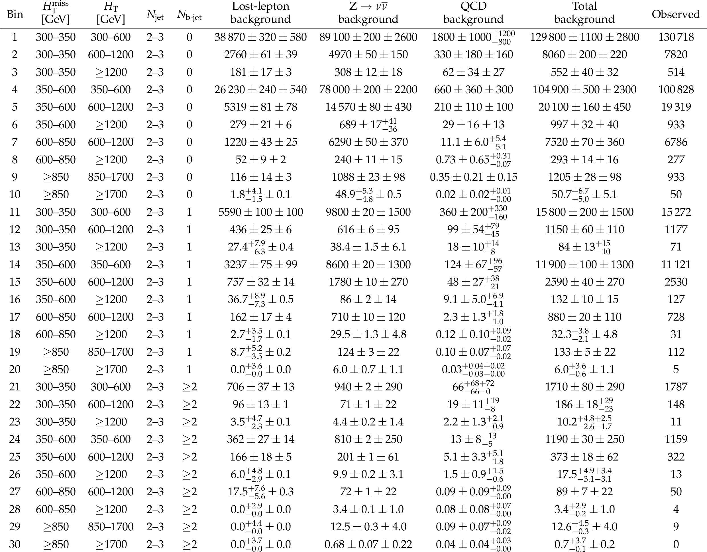
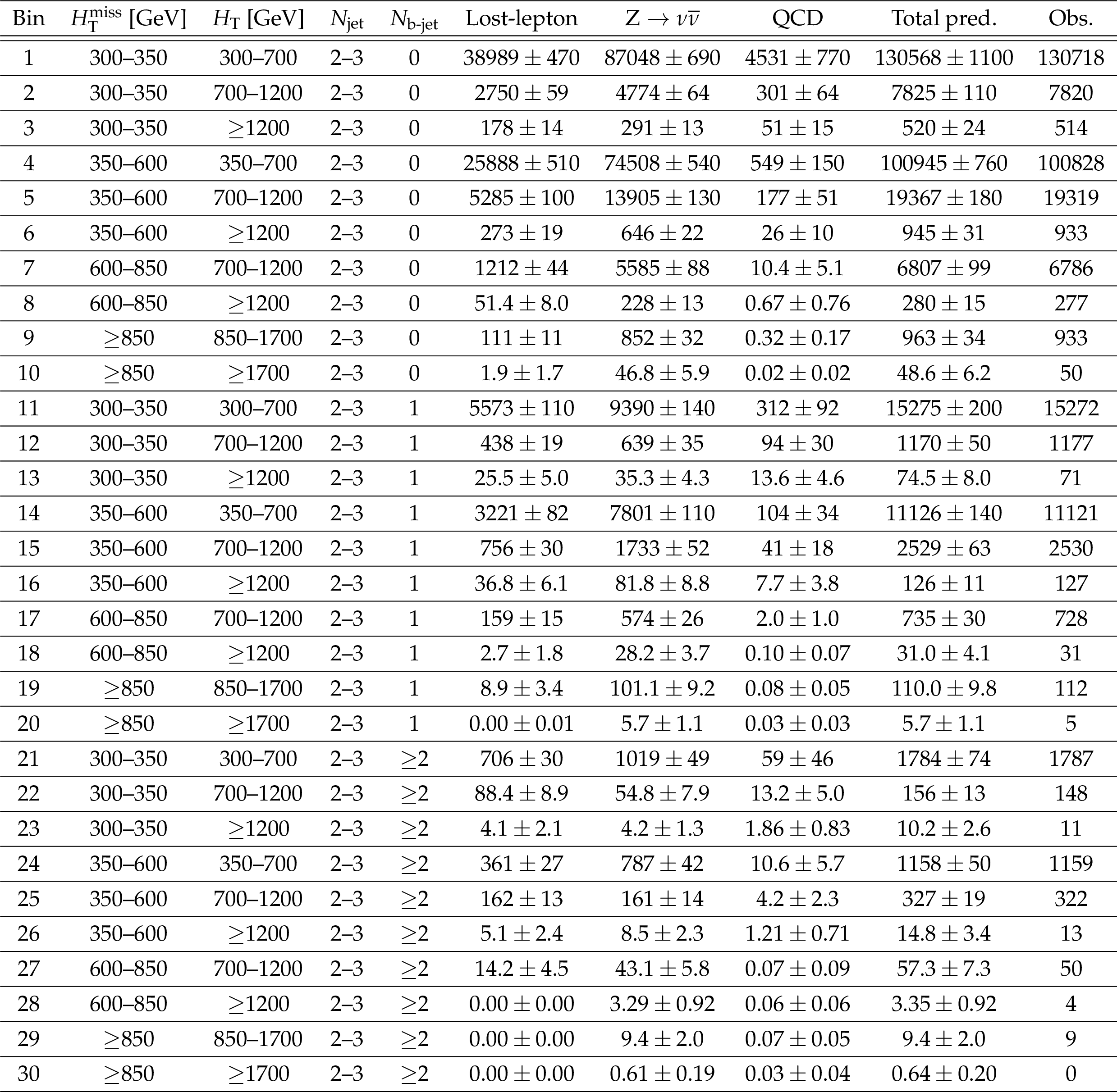
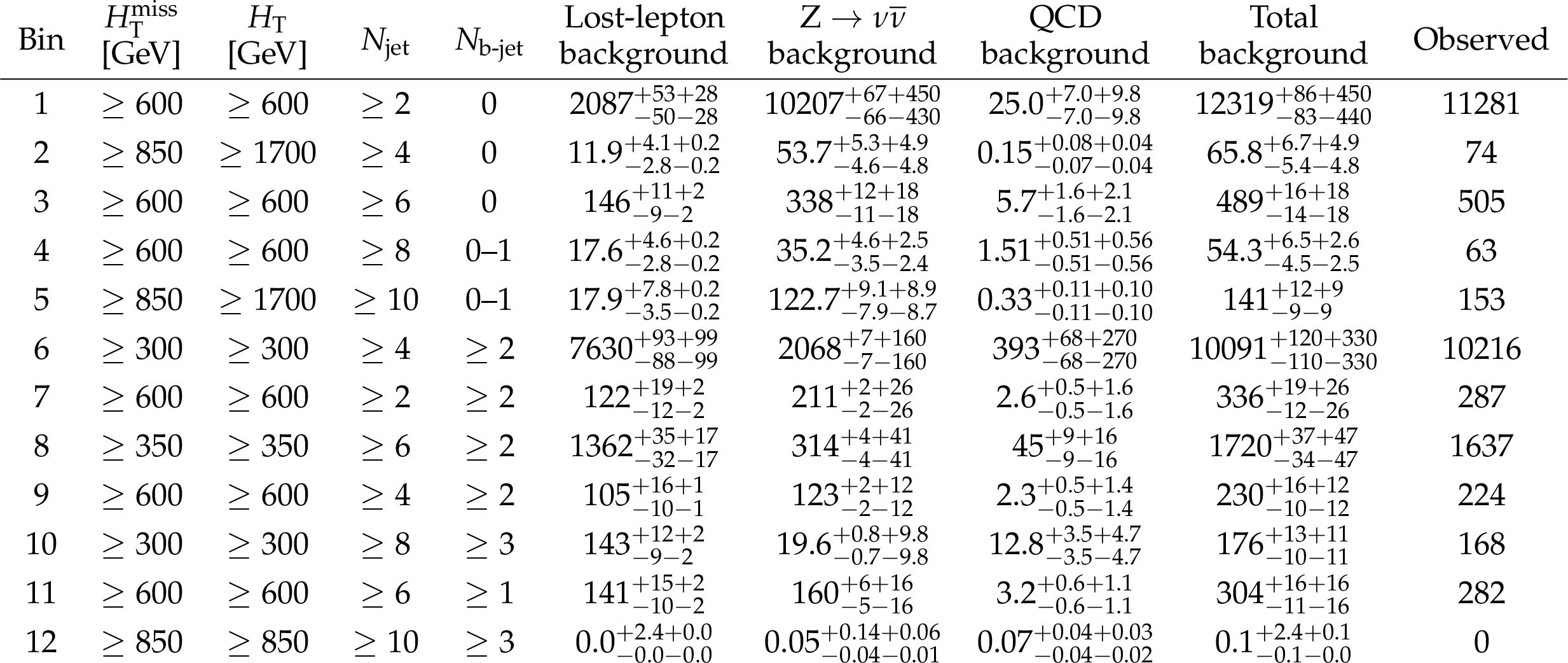
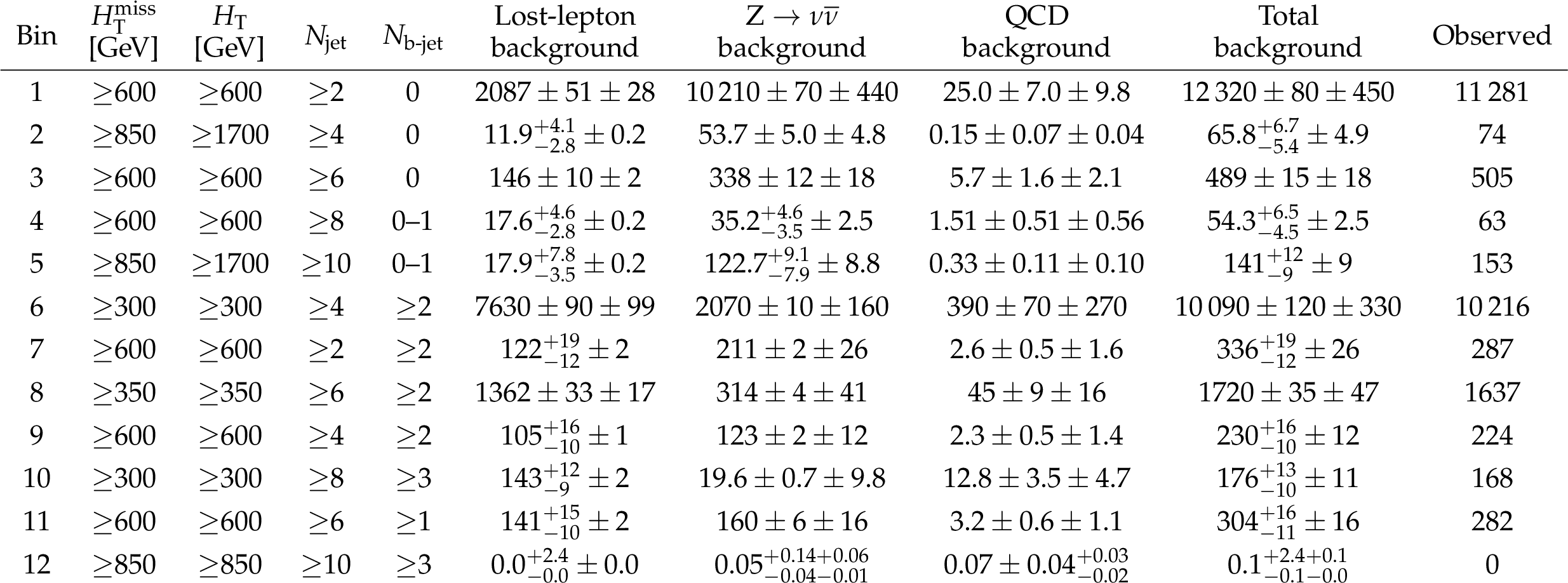
png pdf	Table 3: Observed number of events and pre-fit background predictions in the 2 $\leq {N_{\text {jet}}} \leq$ 3 search bins. For the background predictions, the first uncertainty is statistical and the second systematic.
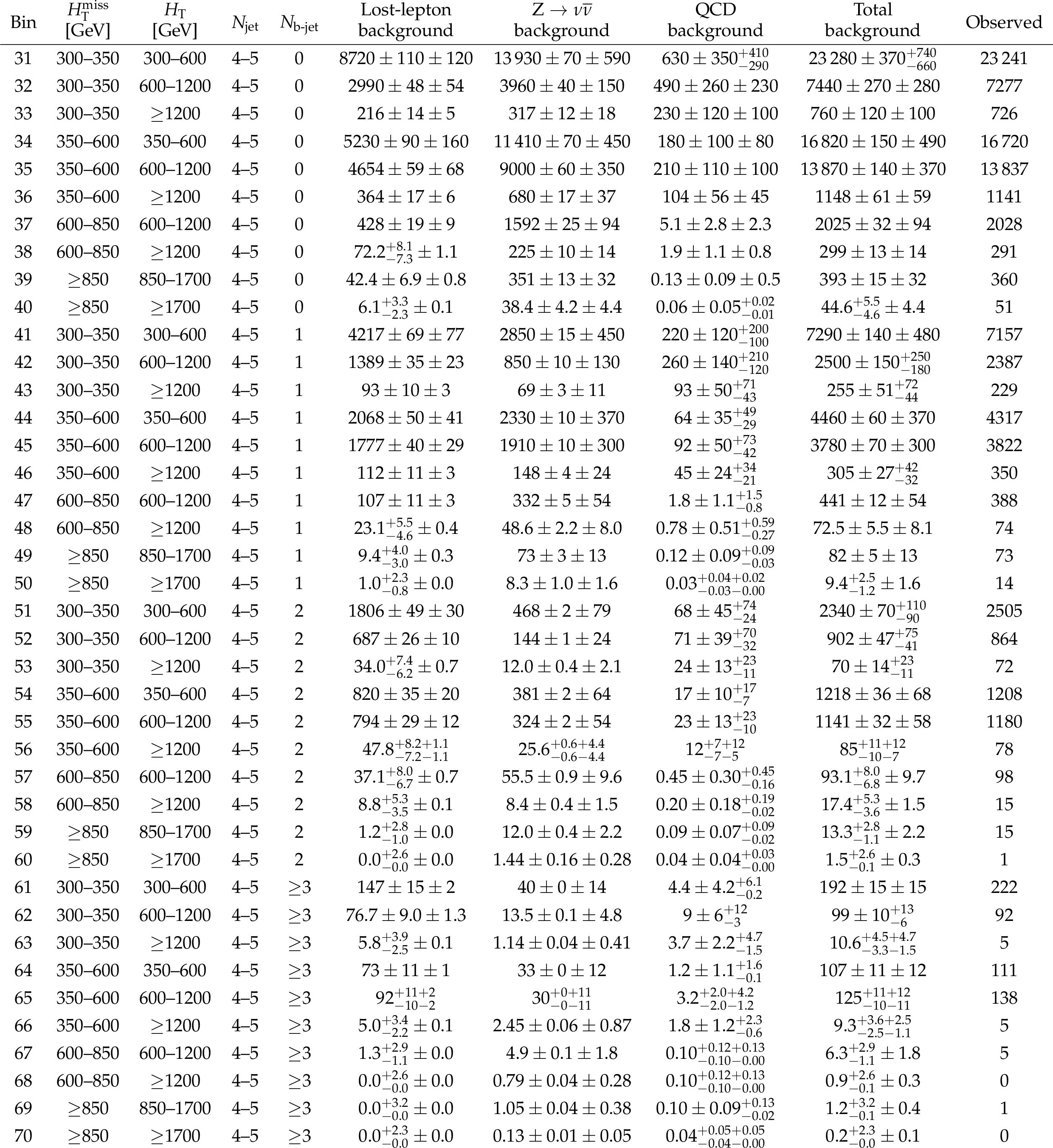
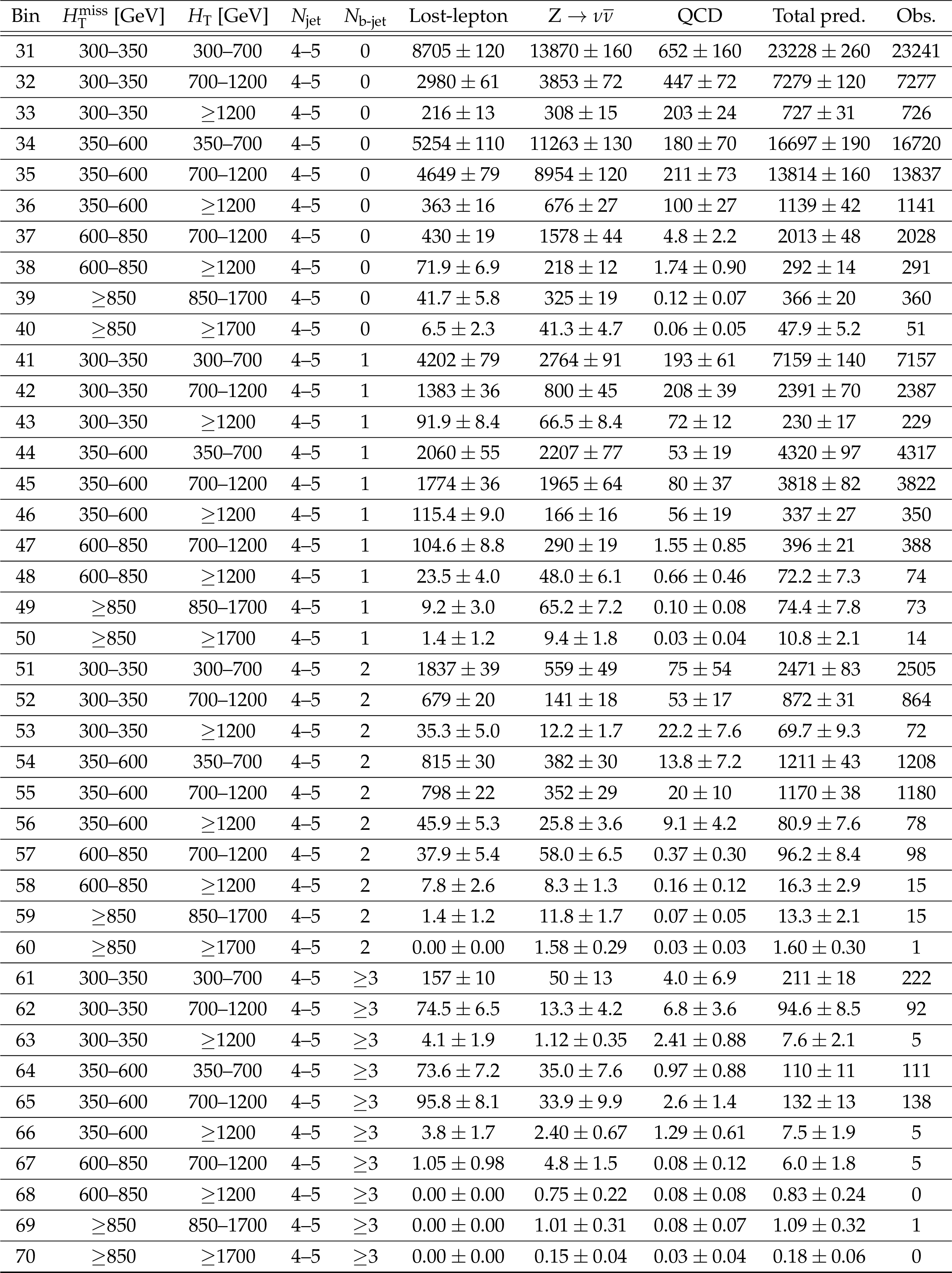
png pdf	Table 4: Observed number of events and pre-fit background predictions in the 4 $\leq {N_{\text {jet}}} \leq$ 5 search bins. For the background predictions, the first uncertainty is statistical and the second systematic.
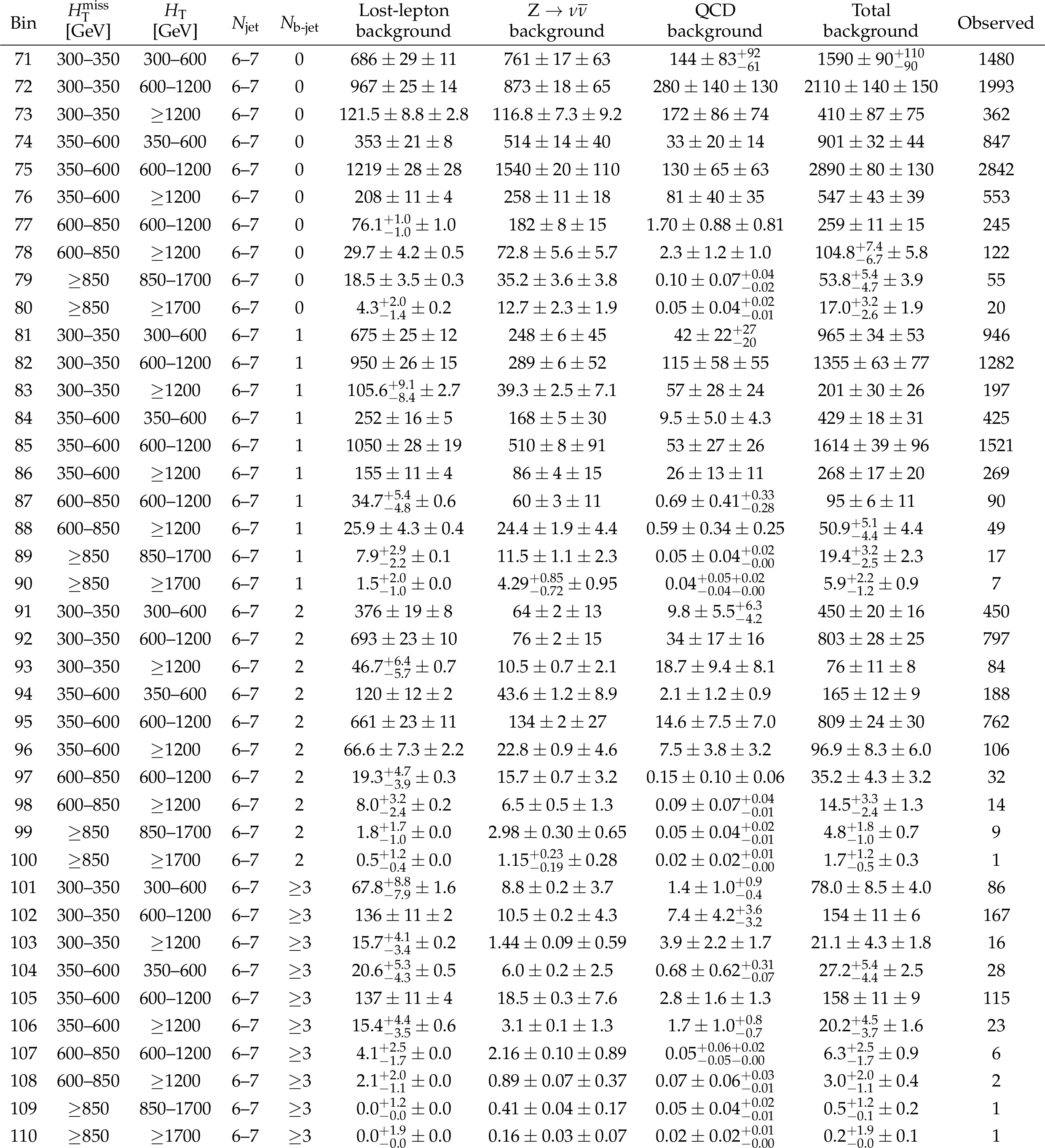
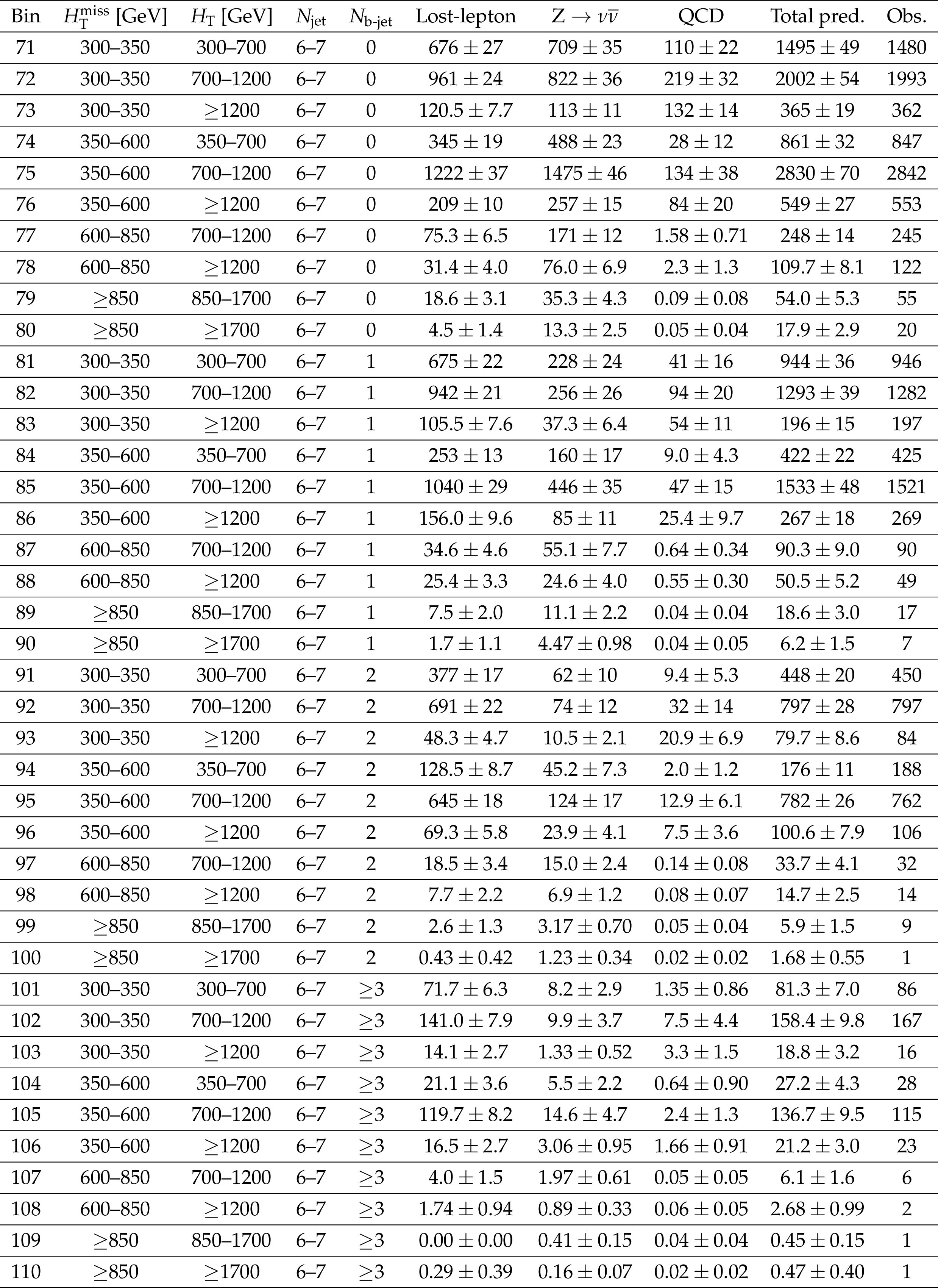
png pdf	Table 5: Observed number of events and pre-fit background predictions in the 6 $\leq {N_{\text {jet}}} \leq$ 7 search bins. For the background predictions, the first uncertainty is statistical and the second systematic.
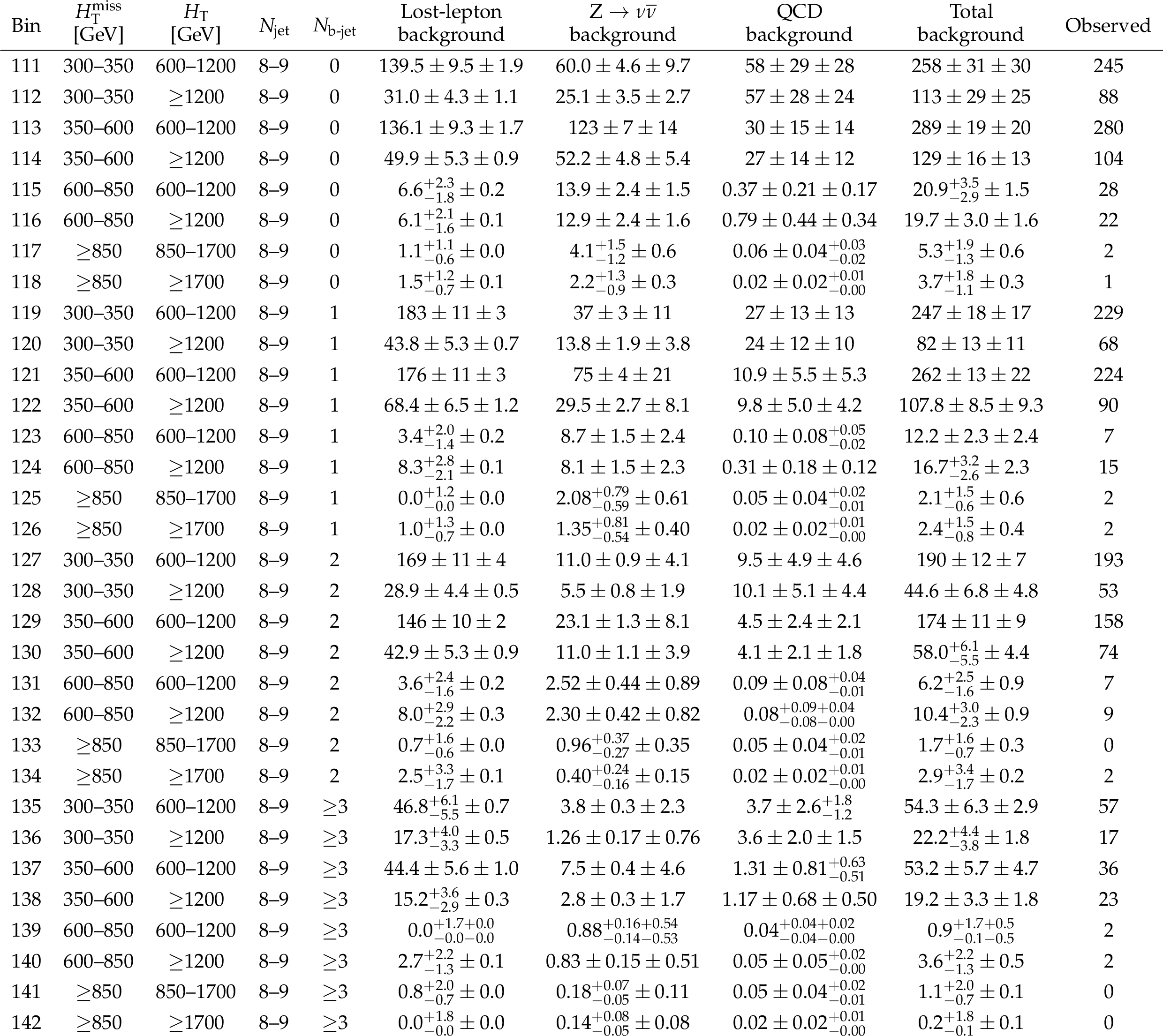
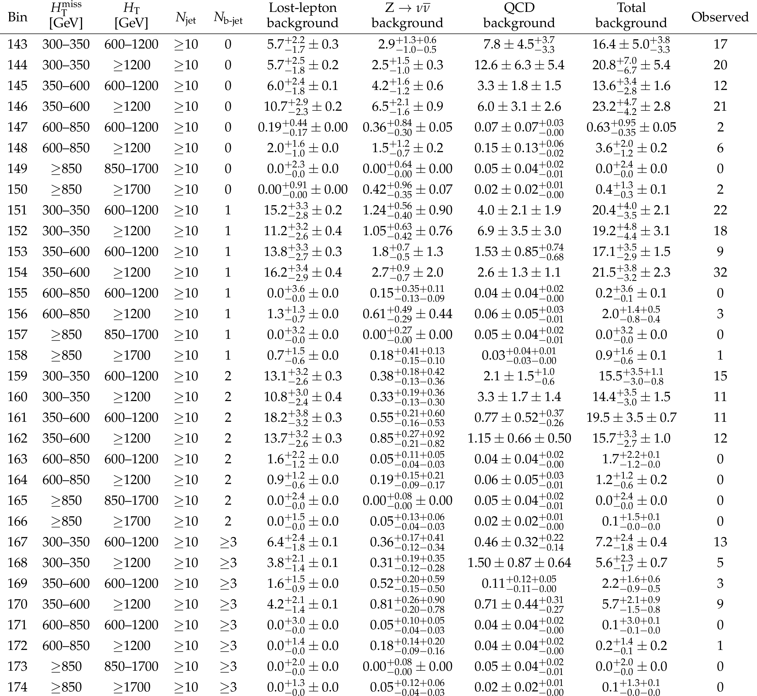
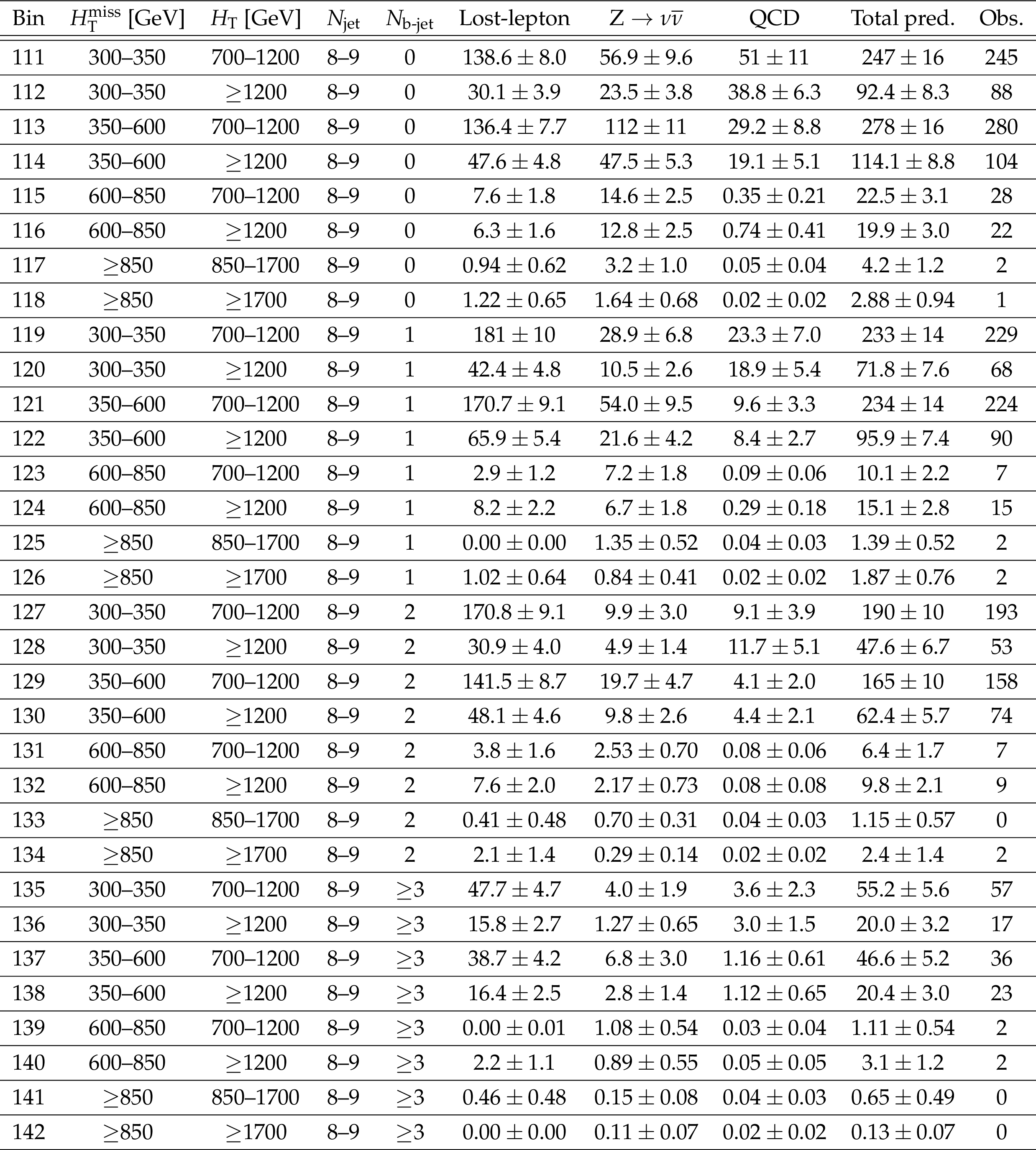
png pdf	Table 6: Observed number of events and pre-fit background predictions in the 8 $\leq {N_{\text {jet}}} \leq$ 9 search bins. For the background predictions, the first uncertainty is statistical and the second systematic.
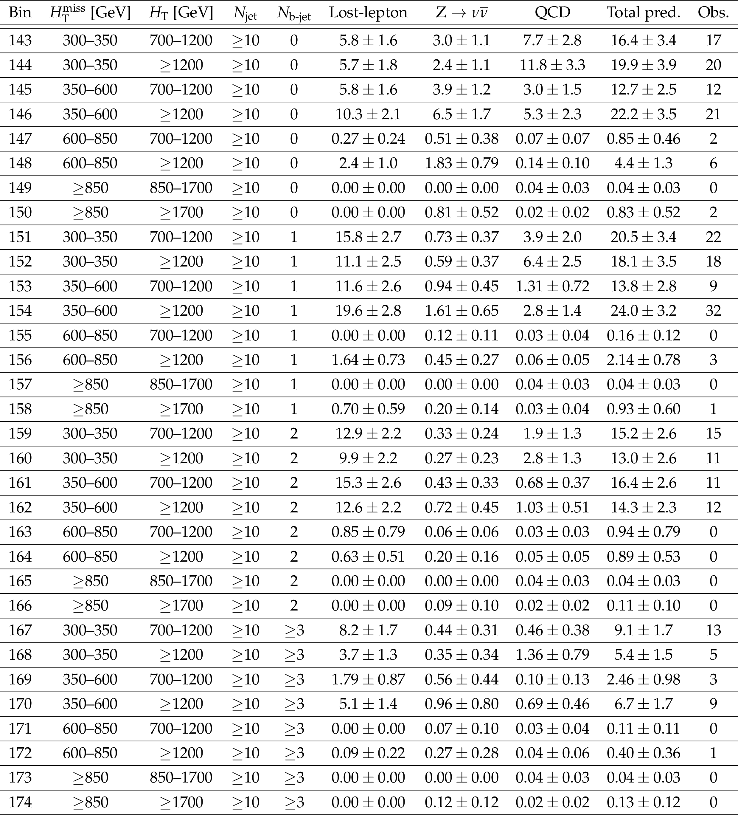
png pdf	Table 7: Observed number of events and pre-fit background predictions in the ${N_{\text {jet}}} \geq$ 10 search bins. For the background predictions, the first uncertainty is statistical and the second systematic.
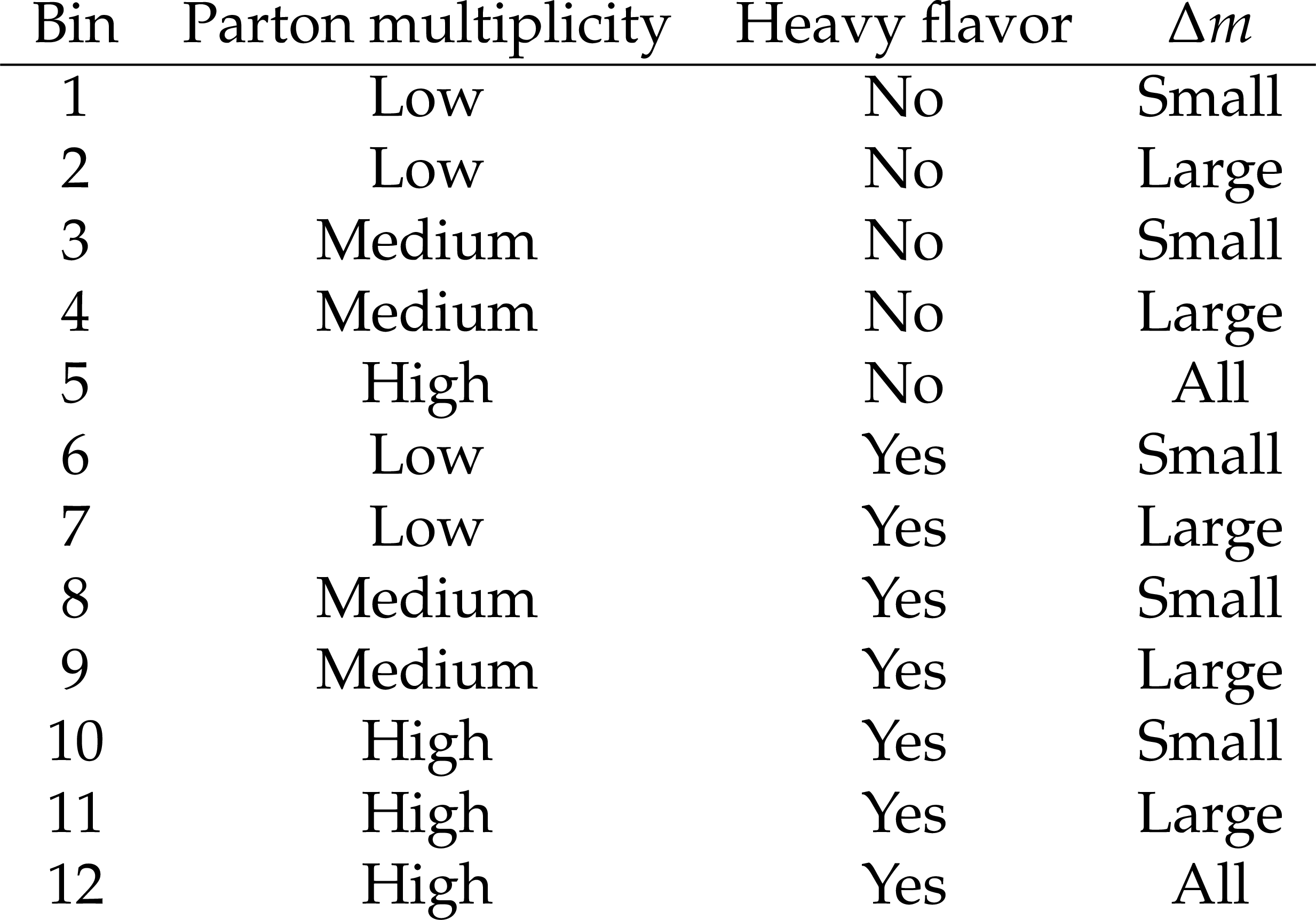
png pdf	Table 8: Targeted event topologies for the 12 aggregate search bins. The variable ${\Delta m}$ states the difference between the gluino or squark mass and the sum of the masses of the particles into which the gluino or squark decays.
png pdf	Table 9: Selection criteria, pre-fit background predictions, and observed number of events for the 12 aggregate search bins. For the background predictions, the first uncertainty is statistical and the second systematic.

Summary

Using essentially the full CMS Run 2 data sample of proton-proton collisions at

$\sqrt{s} =$ 13 TeV, corresponding to an integrated luminosity of 137 fb

$^{-1}$ collected in 2016-2018, a search for supersymmetry has been performed based on events containing multiple jets and large missing transverse momentum. The event yields are measured in 174 nonoverlapping search bins defined in a four-dimensional space of missing transverse momentum (

${H_{\mathrm{T}}^{\text{miss}}}$ ), the scalar sum of jet transverse momenta (

${H_{\mathrm{T}}}$ ), the number of jets, and the number of tagged bottom quark jets. The events are required to satisfy

${H_{\mathrm{T}}^{\text{}}} >$ 300 GeV,

${H_{\mathrm{T}}} >$ 300 GeV, and to have at least two jets with transverse momentum

${p_{\mathrm{T}}} >$ 30 GeV. Events with isolated high

${p_{\mathrm{T}}}$ leptons or photons are vetoed.

The results are compared to the expected number of background events from standard model (SM) processes. The principal backgrounds arise from events with neutrino production or jet mismeasurement. The SM background is evaluated using control regions in data supplemented by information from Monte Carlo event simulation. The observed event yields are found to be consistent with the SM background and no evidence for supersymmetry is obtained.

The results are interpreted in the context of simplified models for gluino and squark pair production. For the gluino models, each of the produced gluinos decays either to a

$\mathrm{t\bar{t}}$ pair and an undetected, stable, lightest supersymmetric particle, assumed to be the

${\tilde{\chi}^0_1}$ neutralino (T1tttt model); to a

$\mathrm{b\bar{b}}$ pair and the

${\tilde{\chi}^0_1}$ (T1bbbb model); to a light-flavored (u, d, s, c)

$\mathrm{q\bar{q}}$ pair and the

${\tilde{\chi}^0_1}$ (T1qqqq model); or to a light-flavored quark and antiquark and either the second-lightest neutralino

$\tilde{\chi}^{0}_{2}$ or the lightest chargino

$\tilde{\chi}_1^{\pm}$ , followed by decay of the

$\tilde{\chi}^{0}_{2}$ (

$\tilde{\chi}_1^{\pm}$ ) to the

$\tilde{\chi}^0_1$ and an on- or off-mass-shell Z (

$\mathrm{W}^\pm$ ) boson (T5qqqqVV model). For the squark models, each of the produced squarks decays either to a top quark and the

${\tilde{\chi}^0_1}$ (T2tt model), to a bottom quark and the

${\tilde{\chi}^0_1}$ (T2bb model), or to a light-flavored quark and the

${\tilde{\chi}^0_1}$ (T2qq model).

Using the predicted cross sections with next-to-leading order plus approximate next-to-leading logarithm accuracy as a reference, gluinos with masses as large as from 2000 to 2310 GeV are excluded at 95% confidence level, depending on the signal model. The corresponding limits on the masses of directly produced squarks range from 1190 for top squarks to 1630 GeV for light-flavored squarks. The results presented here supersede those of Ref. [7], extending the mass limits of this previous study by, typically, 200 GeV or more.

Additional Figures
png pdf root	Additional Figure 1: Observed event yields (solid points with error bars) overlaid with the post-fit background yield (stacked histograms). In each plot the lower panel shows the pull, defined as $(N_{\rm Obs.}-N_{\rm Post.})/\sqrt {N_{\rm Post.}+(\delta N_{\rm Post.})^2}$ , where $\delta N_{\rm Post.}$ is the post-fit uncertainty on the corresponding background.
png pdf	Additional Figure 2: From left-to-right, one-dimensional projections of observed number of events and post-fit background distributions in the search region in ${H_{\mathrm T}^{\text {miss}}}$ , ${N_{\text {jet}}}$ , and ${N_{{{\mathrm {b}}}\text {-jet}}}$ . The events in each distribution are integrated over the other three search variables and uncertainties are taken as fully correlated.
png pdf	Additional Figure 2-a: One-dimensional projection of observed number of events and post-fit background distributions in the search region in ${H_{\mathrm T}^{\text {miss}}}$ . The events in each distribution are integrated over the other three search variables and uncertainties are taken as fully correlated.
png pdf	Additional Figure 2-b: One-dimensional projection of observed number of events and post-fit background distributions in the search region in ${N_{\text {jet}}}$ . The events in each distribution are integrated over the other three search variables and uncertainties are taken as fully correlated.
png pdf	Additional Figure 2-c: One-dimensional projection of observed number of events and post-fit background distributions in the search region in ${N_{{{\mathrm {b}}}\text {-jet}}}$ . The events in each distribution are integrated over the other three search variables and uncertainties are taken as fully correlated.
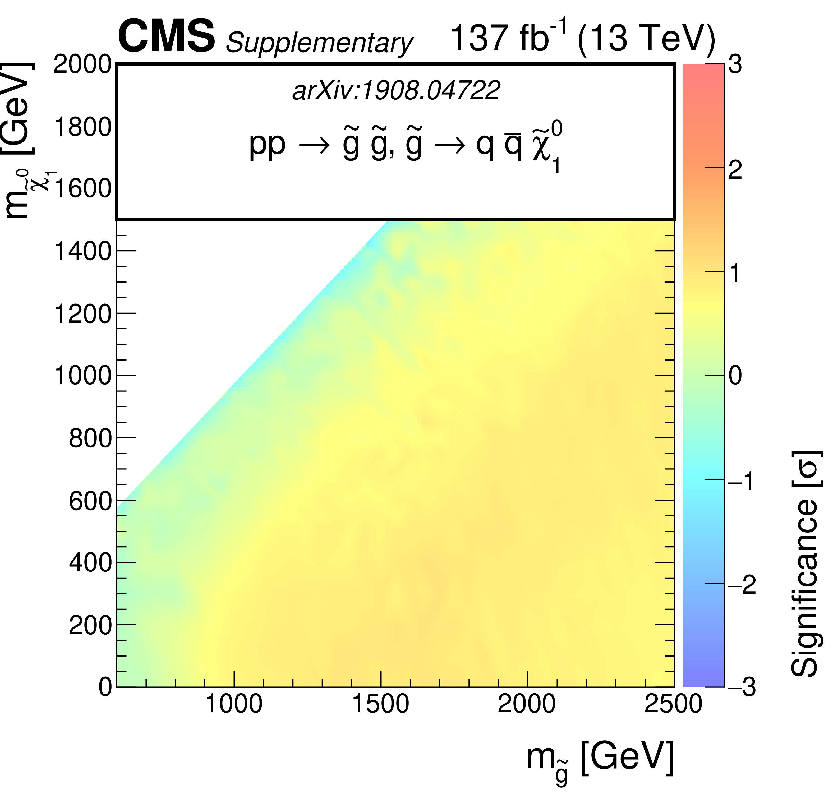
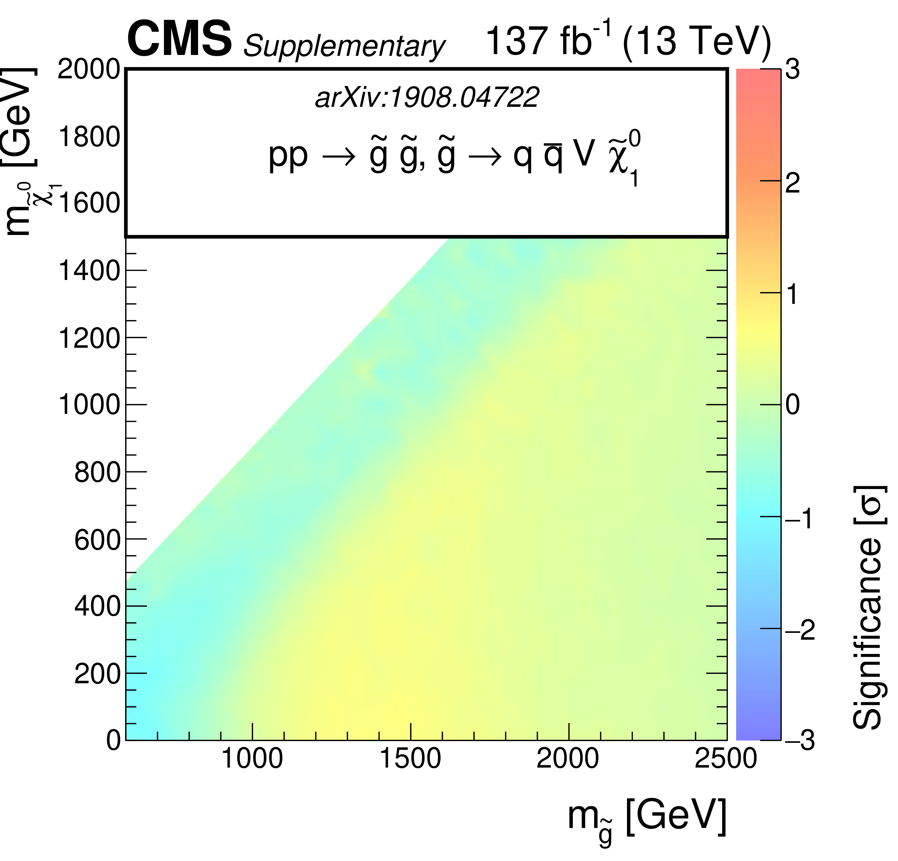
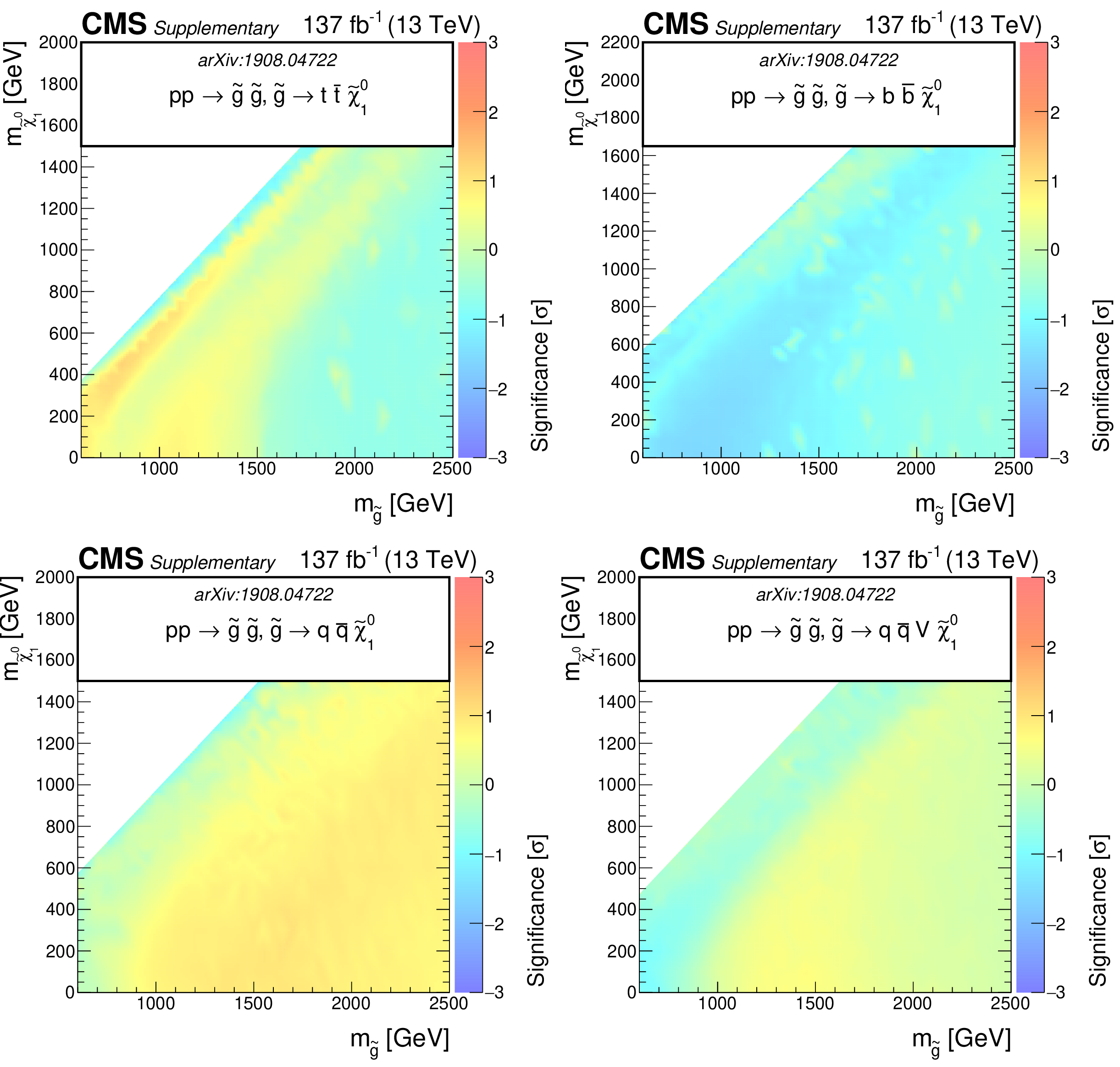
png pdf	Additional Figure 3: The observed significance of the SMS gluino models for T1tttt, T1bbbb, T1qqqq, and T5qqqqVV as function of the gluino and LSP masses.
png pdf root	Additional Figure 3-a: The observed significance of the SMS gluino models for T1tttt as function of the gluino and LSP masses.
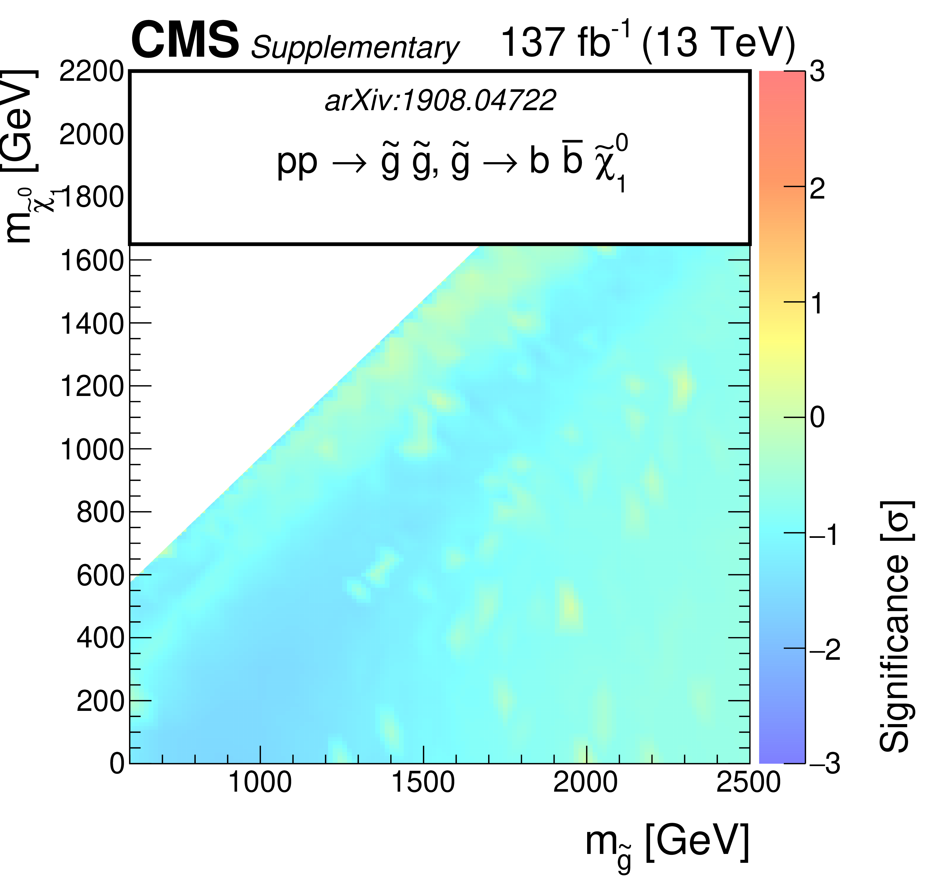
png pdf root	Additional Figure 3-b: The observed significance of the SMS gluino models for T1bbbb as function of the gluino and LSP masses.
png pdf root	Additional Figure 3-c: The observed significance of the SMS gluino models for T1qqqq as function of the gluino and LSP masses.
png pdf root	Additional Figure 3-d: The observed significance of the SMS gluino models for T5qqqqVV as function of the gluino and LSP masses.
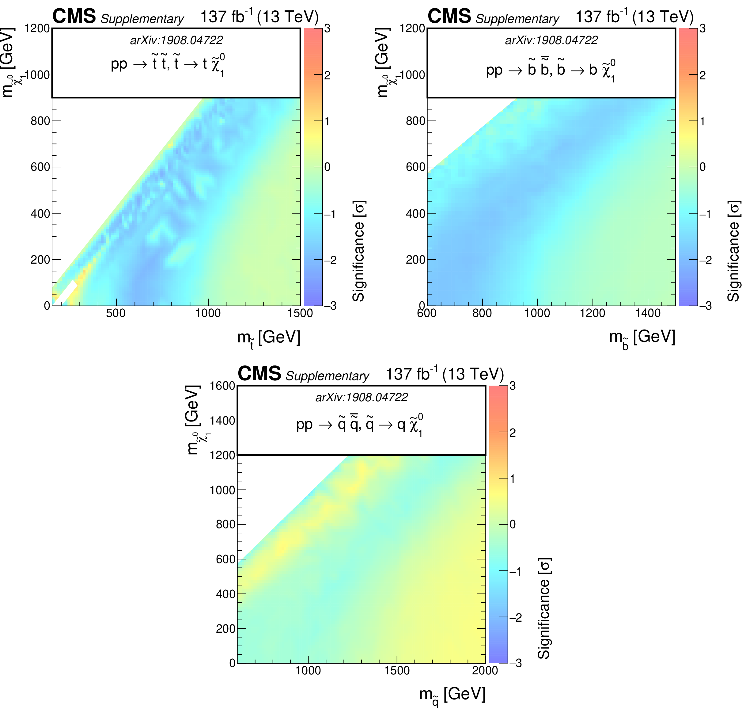
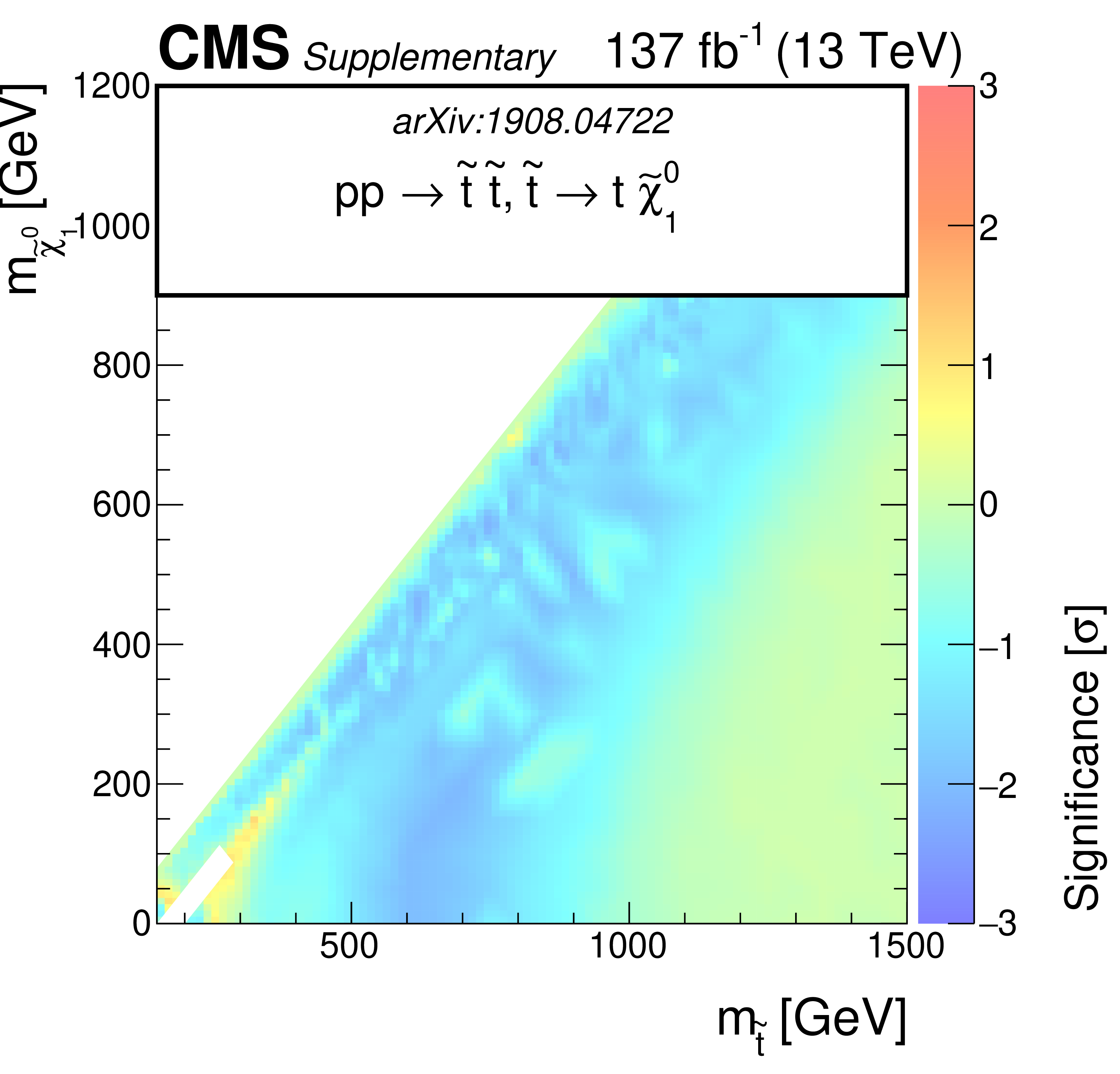
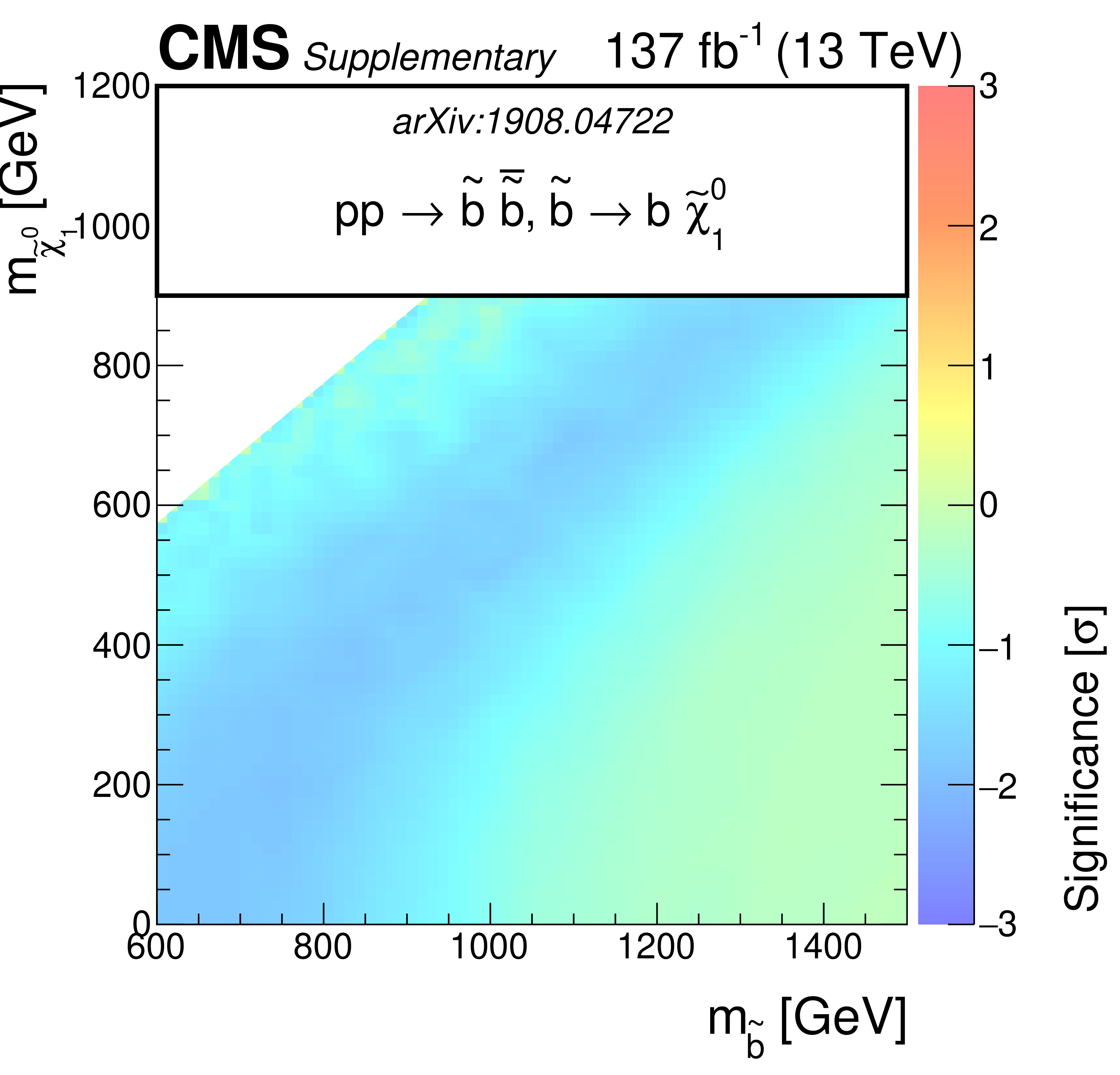
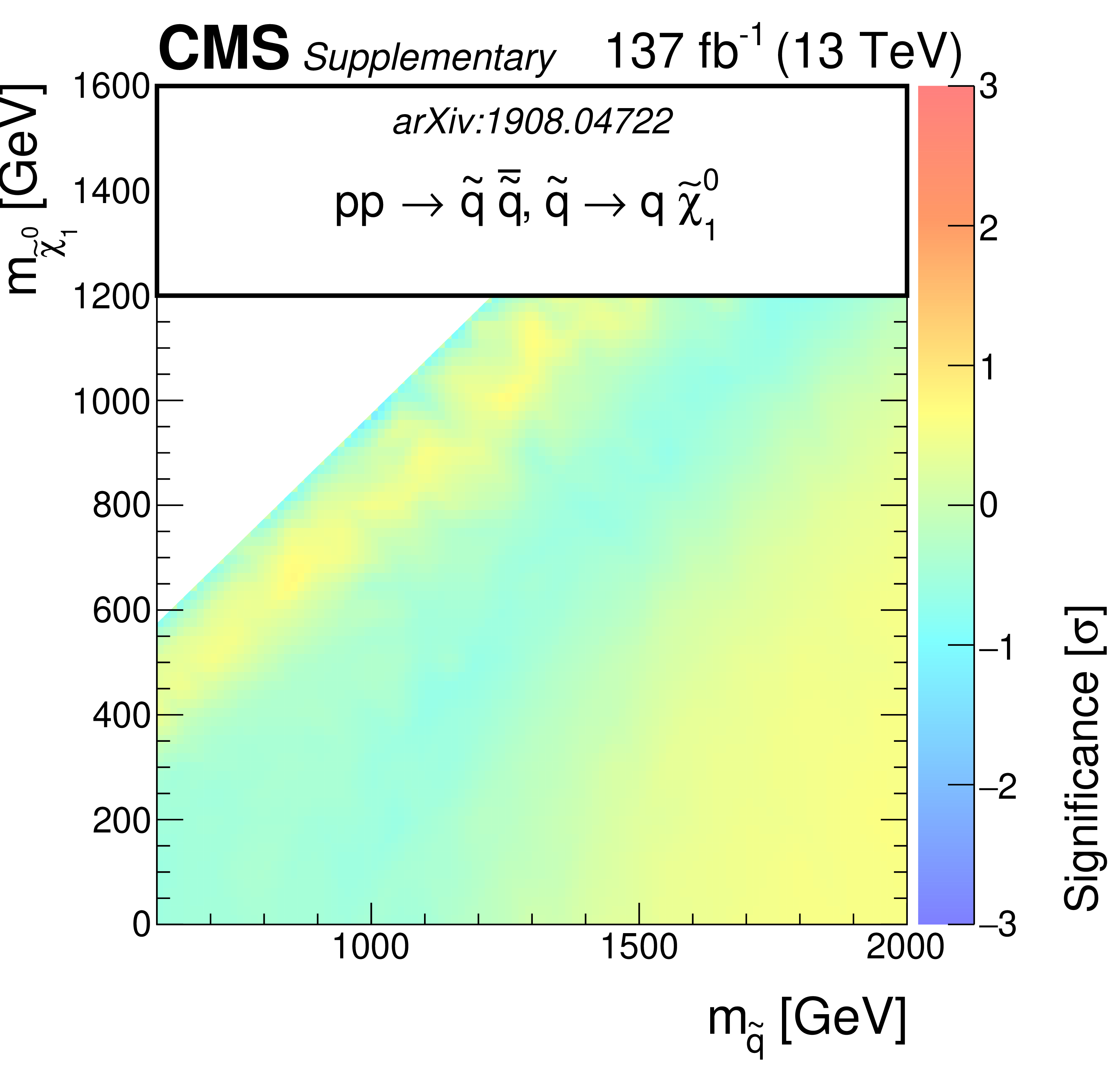
png pdf	Additional Figure 4: The observed significance of the SMS squark models for T2tt, T2bb, and T2qq as function of the squark and LSP masses.
png pdf root	Additional Figure 4-a: The observed significance of the SMS squark models for T2tt as function of the squark and LSP masses.
png pdf root	Additional Figure 4-b: The observed significance of the SMS squark models for T2bb as function of the squark and LSP masses.
png pdf root	Additional Figure 4-c: The observed significance of the SMS squark models for T2qq as function of the squark and LSP masses.
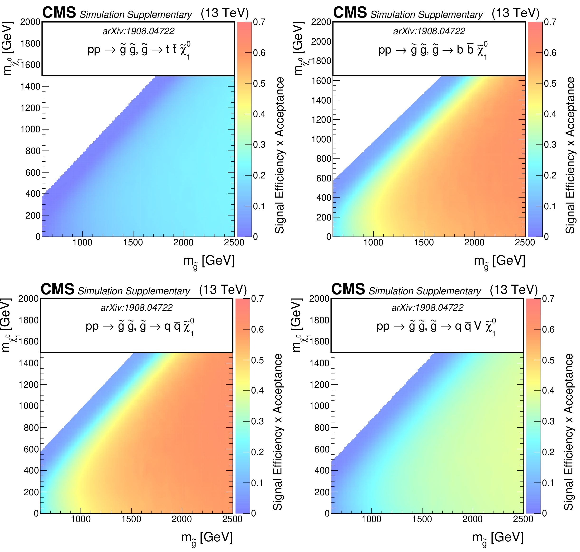
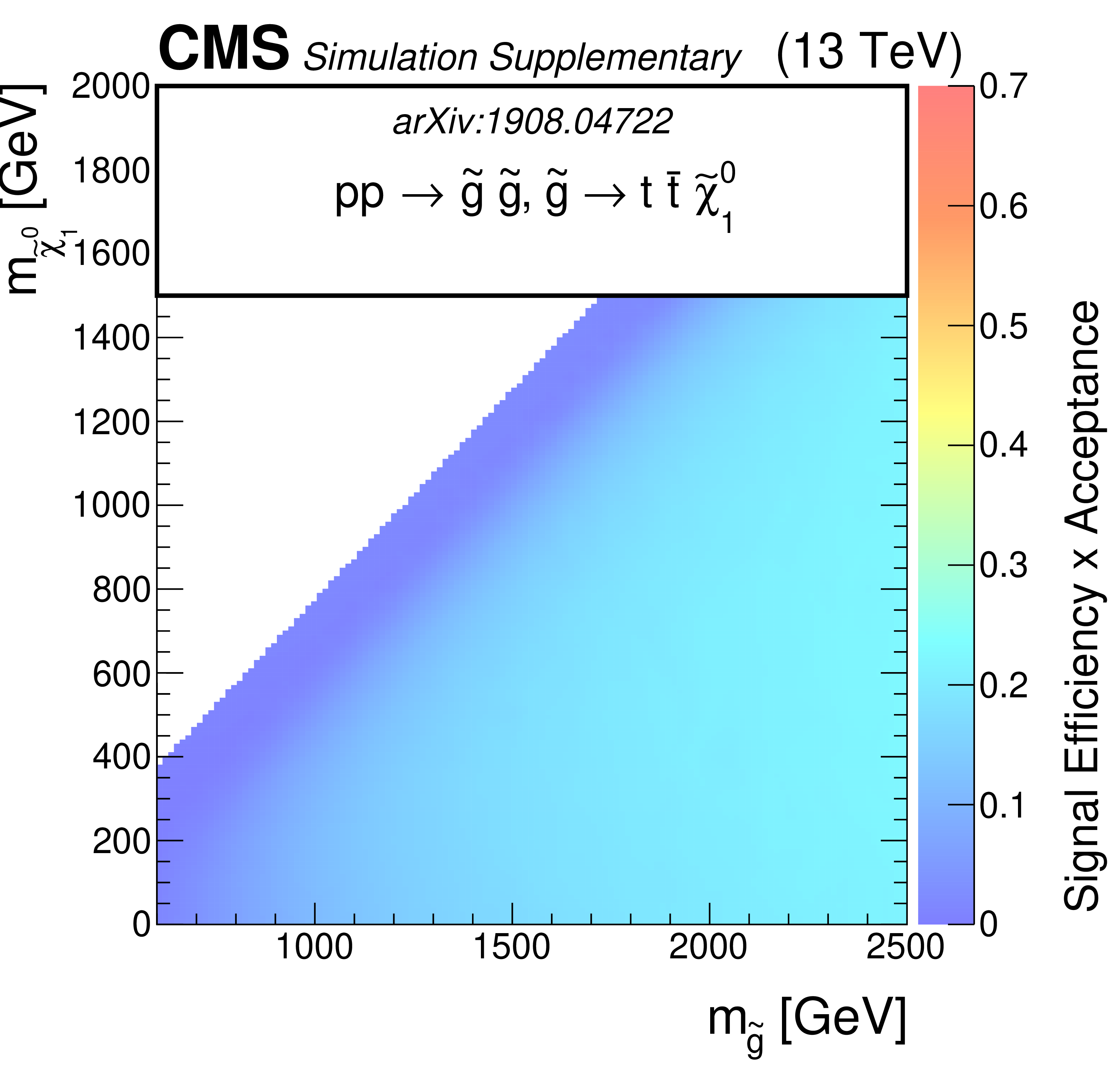
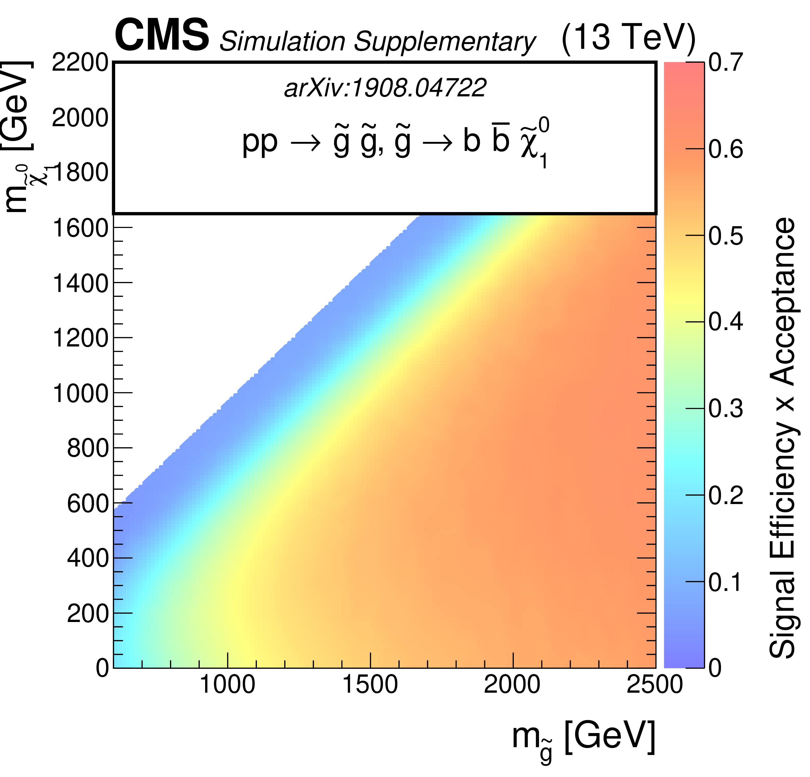
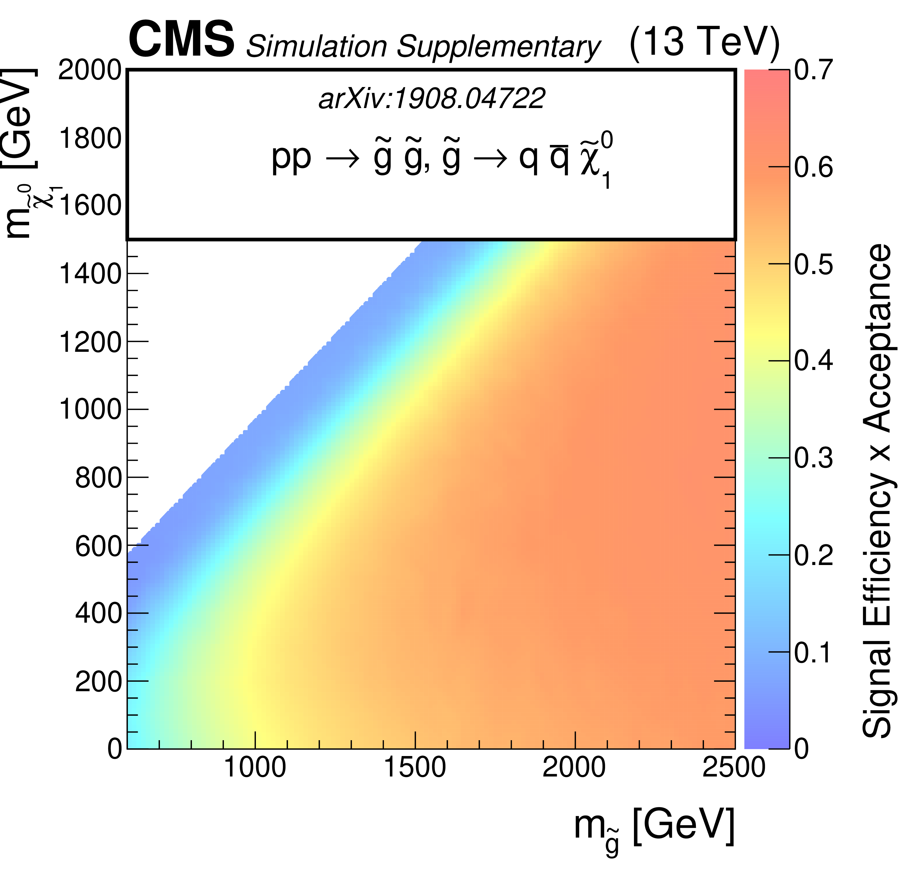
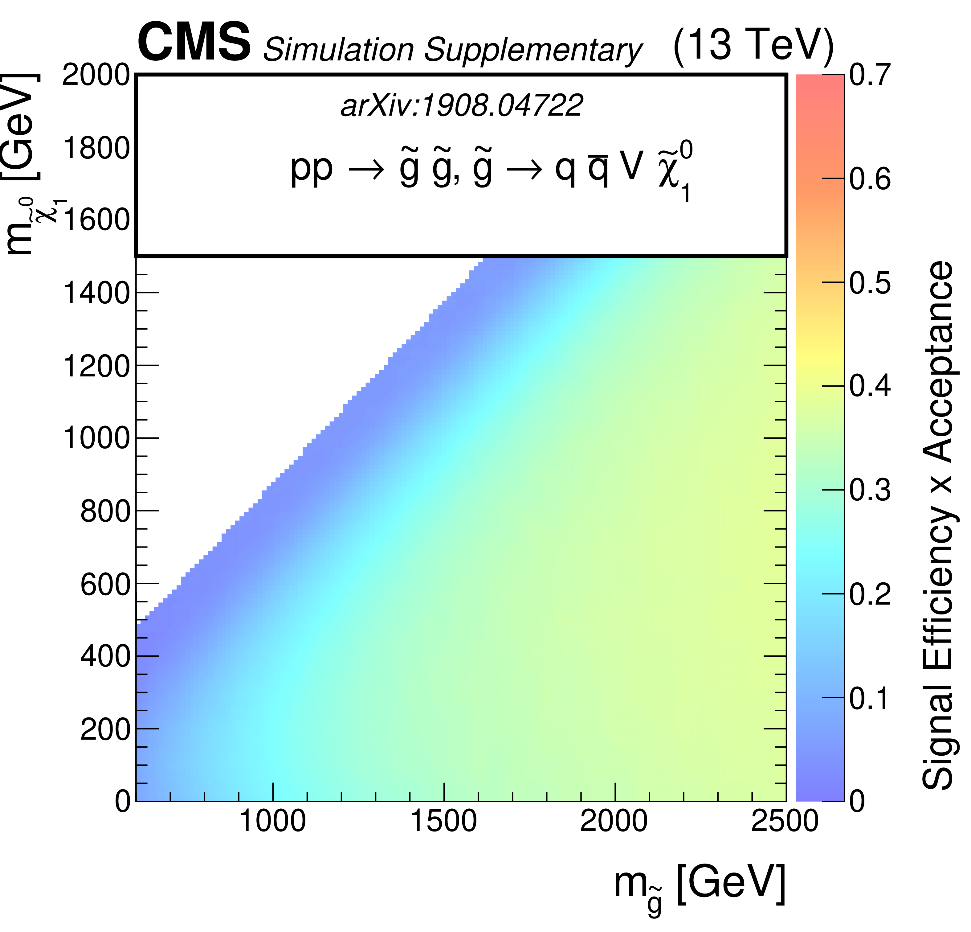
png pdf	Additional Figure 5: The efficiency times acceptance of the SMS gluino models for T1tttt, T1bbbb, T1qqqq, and T5qqqqVV as function of the gluino and LSP masses. The efficiency times acceptance is given for the total signal across the set of 174 search regions.
png pdf root	Additional Figure 5-a: The efficiency times acceptance of the SMS gluino models for T1tttt as function of the gluino and LSP masses. The efficiency times acceptance is given for the total signal across the set of 174 search regions.
png pdf root	Additional Figure 5-b: The efficiency times acceptance of the SMS gluino models for T1bbbb as function of the gluino and LSP masses. The efficiency times acceptance is given for the total signal across the set of 174 search regions.
png pdf root	Additional Figure 5-c: The efficiency times acceptance of the SMS gluino models for T1qqqq as function of the gluino and LSP masses. The efficiency times acceptance is given for the total signal across the set of 174 search regions.
png pdf root	Additional Figure 5-d: The efficiency times acceptance of the SMS gluino models for T5qqqqVV as function of the gluino and LSP masses. The efficiency times acceptance is given for the total signal across the set of 174 search regions.
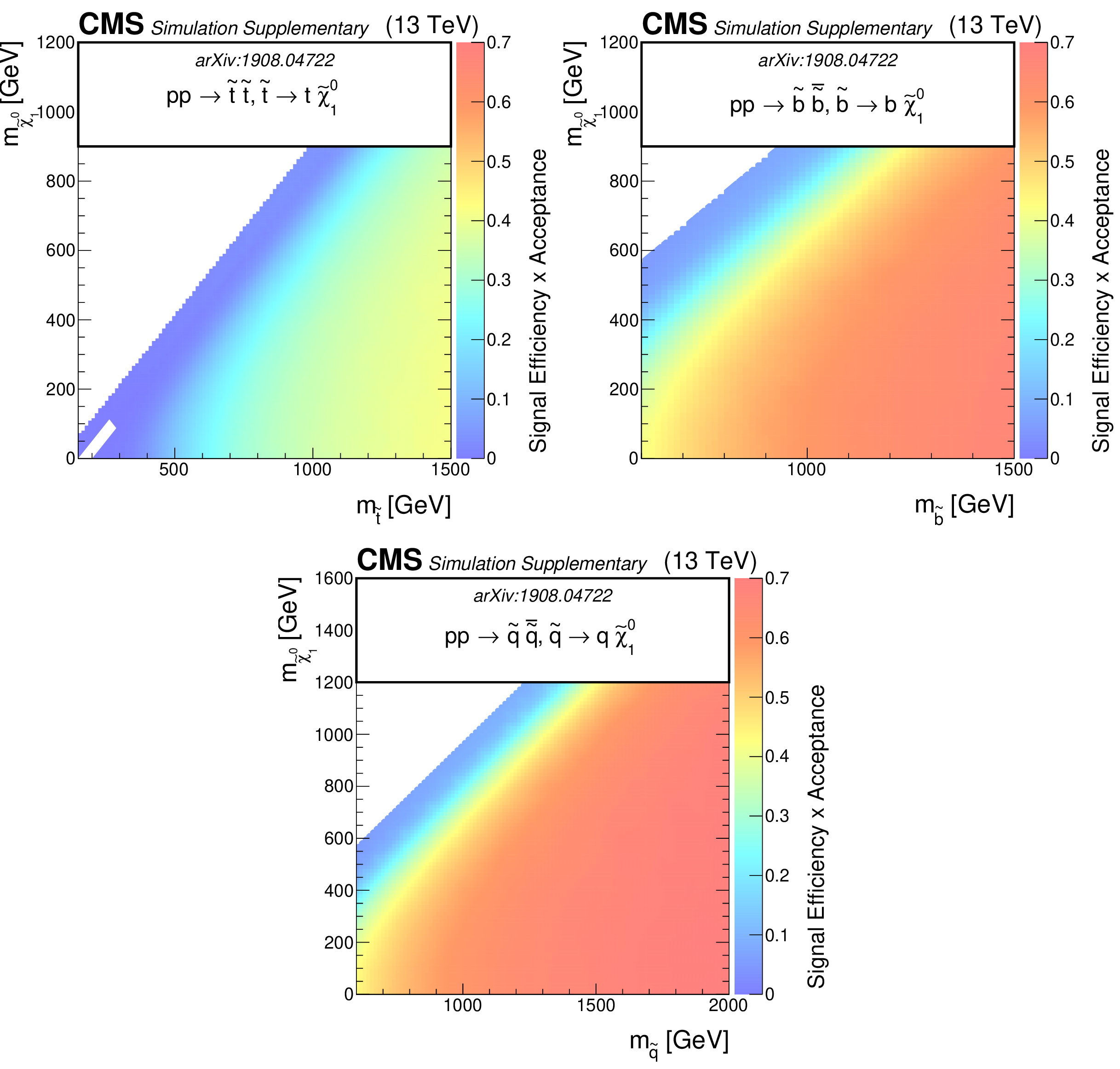
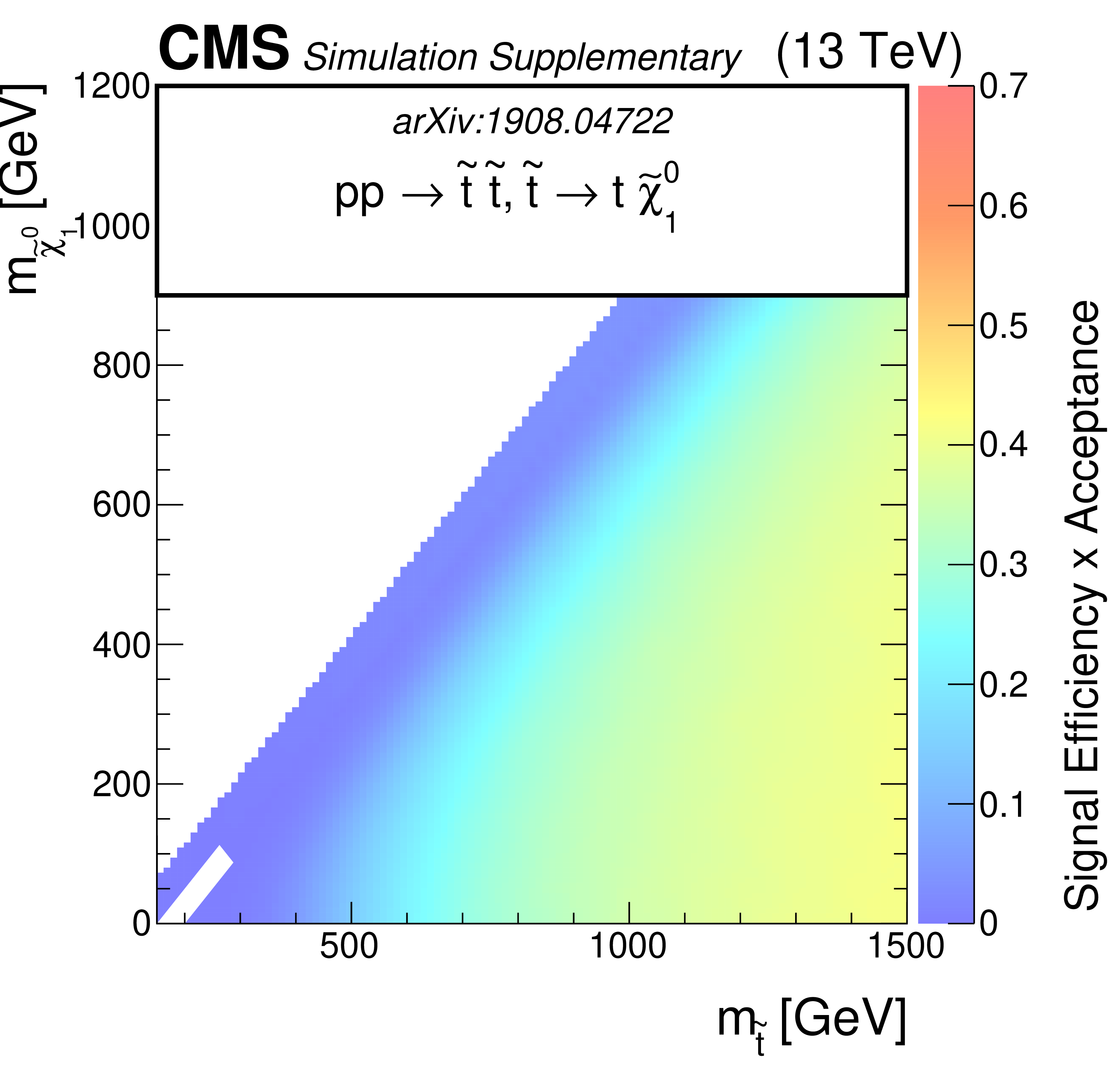
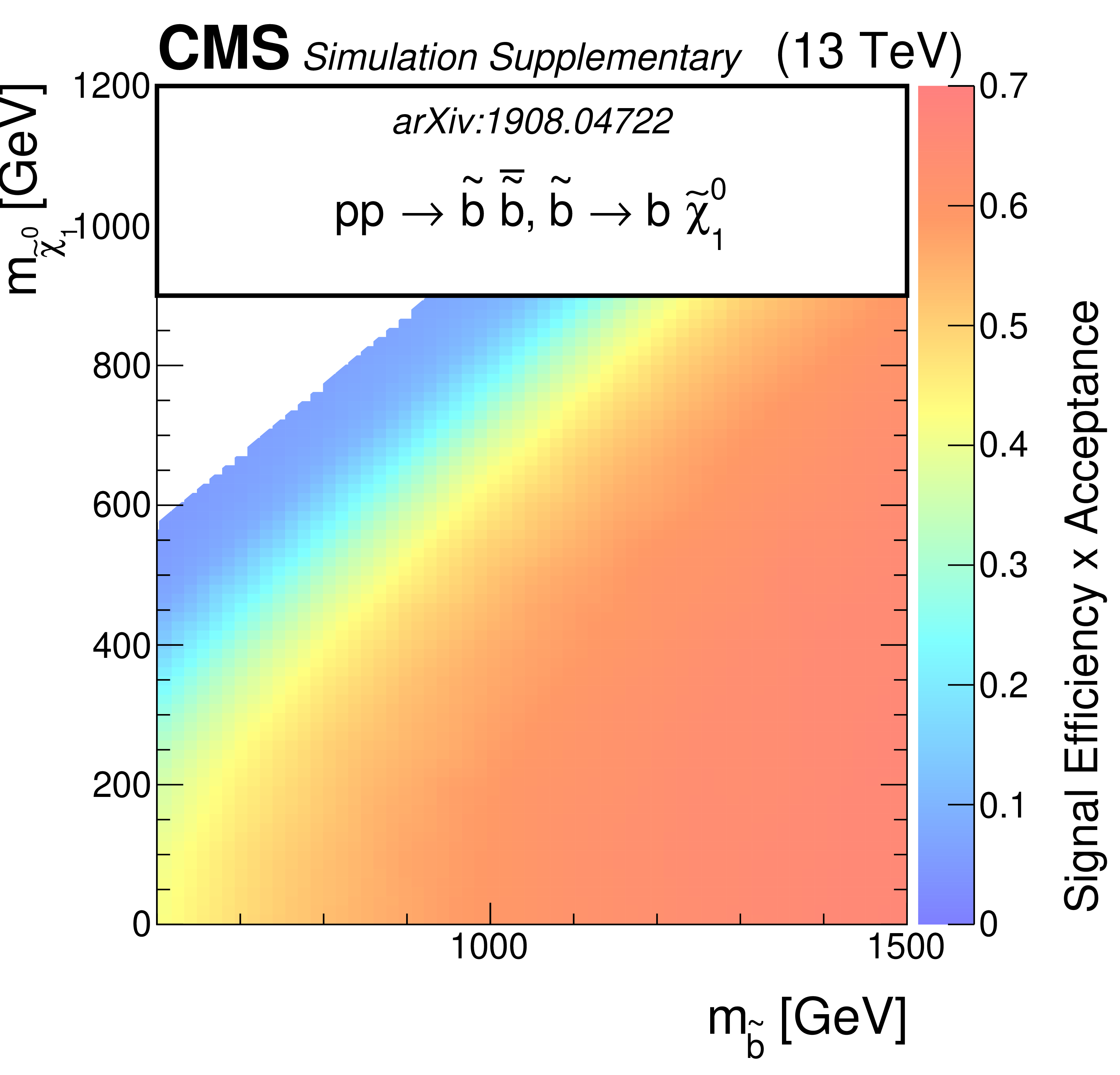
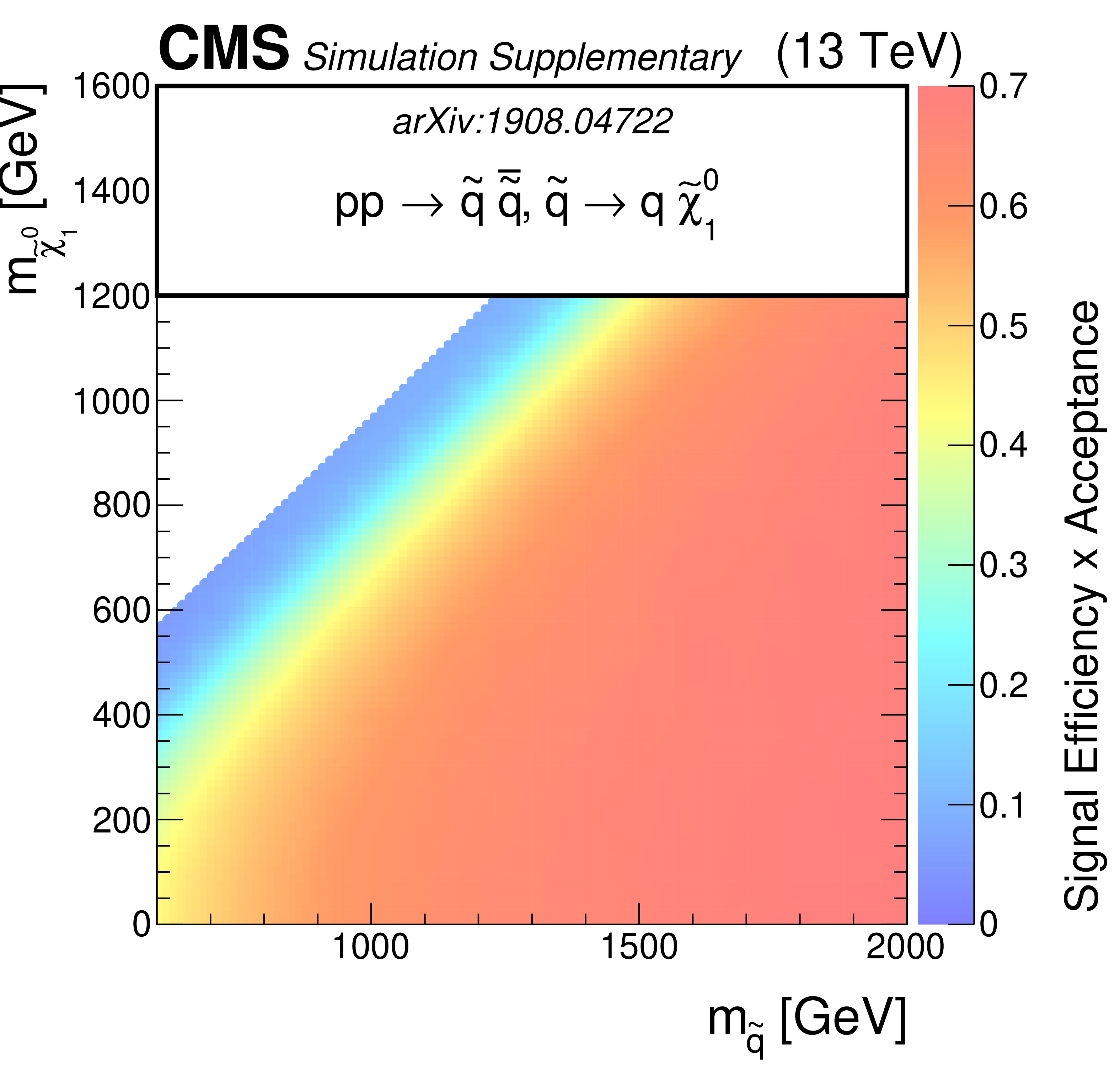
png pdf	Additional Figure 6: The efficiency times acceptance of the SMS squark models for T2tt, T2bb and T2qq as function of the squark and LSP masses. The efficiency times acceptance is given for the total signal across the set of 174 search regions.
png pdf root	Additional Figure 6-a: The efficiency times acceptance of the SMS squark models for T2tt as function of the squark and LSP masses. The efficiency times acceptance is given for the total signal across the set of 174 search regions.
png pdf root	Additional Figure 6-b: The efficiency times acceptance of the SMS squark models for T2bb as function of the squark and LSP masses. The efficiency times acceptance is given for the total signal across the set of 174 search regions.
png pdf root	Additional Figure 6-c: The efficiency times acceptance of the SMS squark models for T2qq as function of the squark and LSP masses. The efficiency times acceptance is given for the total signal across the set of 174 search regions.
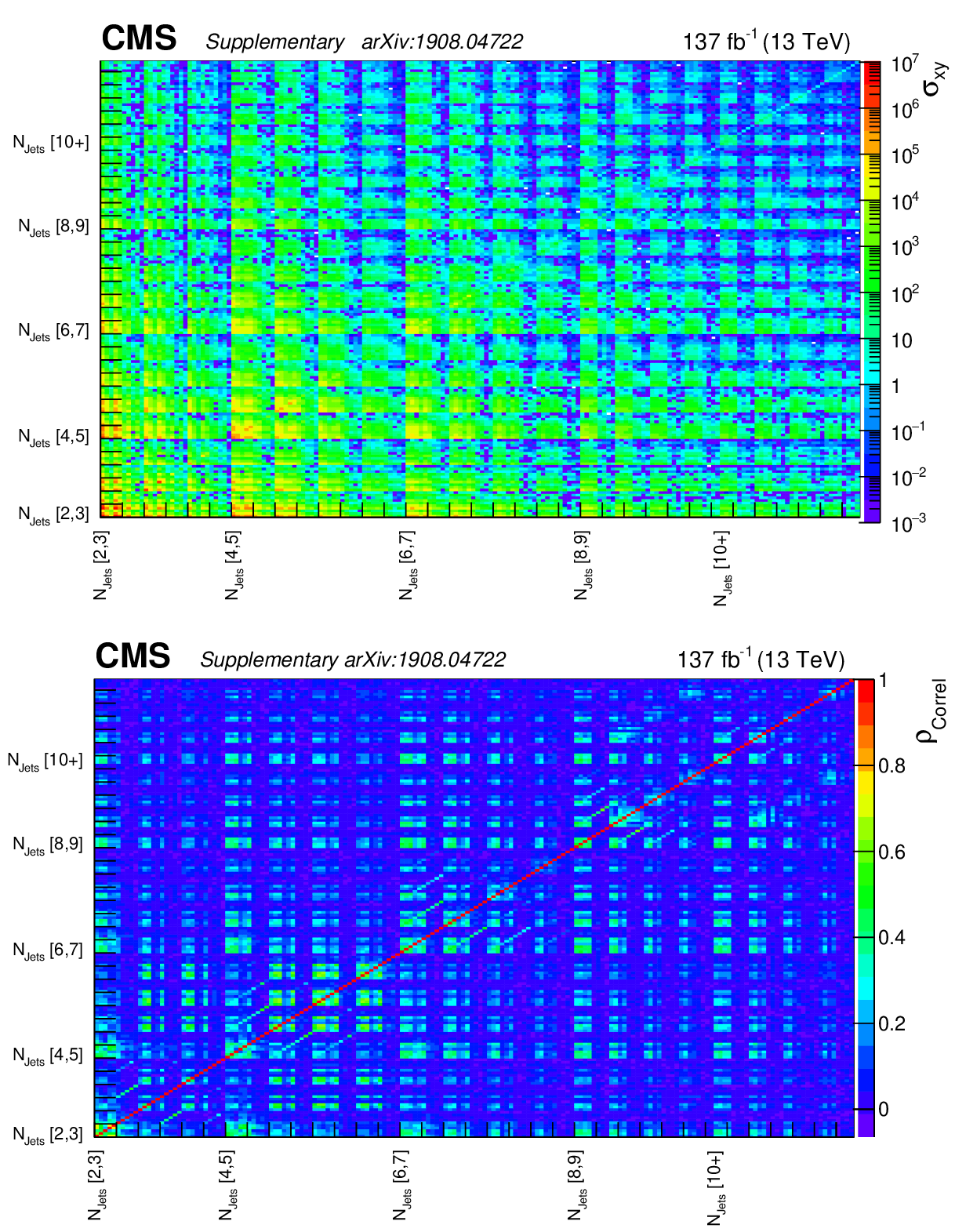
png pdf root	Additional Figure 7: Pre-fit background covariance matrix $\sigma _{xy}$ and correlation matrix $\rho _{correl}$
png pdf root	Additional Figure 7-a: Pre-fit background covariance matrix $\sigma _{xy}$ .
png pdf root	Additional Figure 7-b: Pre-fit background correlation matrix $\rho _{correl}$ .
png pdf	Additional Figure 8: Event displays for a SUSY candidate event with 12 jets in the search region, 273447:179:291867669 in (a) $r-\phi$ view, (b) $r-\phi$ view with a white background, (c) 3D view, and (d) 3D view with a white background. The momenta of the non b-tagged jets are marked and labeled in orange and the momenta of the b-tagged jets are marked in green.
png pdf	Additional Figure 8-a: Event display for a SUSY candidate event with 12 jets in the search region, 273447:179:291867669 in $r-\phi$ view. The momenta of the non b-tagged jets are marked and labeled in orange and the momenta of the b-tagged jets are marked in green.
png pdf	Additional Figure 8-b: Event display for a SUSY candidate event with 12 jets in the search region, 273447:179:291867669 in $r-\phi$ view with a white background. The momenta of the non b-tagged jets are marked and labeled in orange and the momenta of the b-tagged jets are marked in green.
png pdf	Additional Figure 8-c: Event display for a SUSY candidate event with 12 jets in the search region, 273447:179:291867669 in 3D view. The momenta of the non b-tagged jets are marked and labeled in orange and the momenta of the b-tagged jets are marked in green.
png pdf	Additional Figure 8-d: Event display for a SUSY candidate event with 12 jets in the search region, 273447:179:291867669 in 3D view with a white background. The momenta of the non b-tagged jets are marked and labeled in orange and the momenta of the b-tagged jets are marked in green.
png pdf	Additional Figure 9: Event displays for a SUSY candidate event with very high $H_{\rm T}^{\rm miss}$ in the search region, 321219:344:504952772 in (a) $r-\phi$ view, (b) $r-\phi$ view with a white background, (c) 3D view, and (d) 3D view with a white background. The momenta of the two jets are marked and labeled in orange.
png pdf	Additional Figure 9-a: Event display for a SUSY candidate event with very high $H_{\rm T}^{\rm miss}$ in the search region, 321219:344:504952772 in $r-\phi$ view. The momenta of the two jets are marked and labeled in orange.
png pdf	Additional Figure 9-b: Event display for a SUSY candidate event with very high $H_{\rm T}^{\rm miss}$ in the search region, 321219:344:504952772 in $r-\phi$ view with a white background. The momenta of the two jets are marked and labeled in orange.
png pdf	Additional Figure 9-c: Event display for a SUSY candidate event with very high $H_{\rm T}^{\rm miss}$ in the search region, 321219:344:504952772 in 3D view. The momenta of the two jets are marked and labeled in orange.
png pdf	Additional Figure 9-d: Event display for a SUSY candidate event with very high $H_{\rm T}^{\rm miss}$ in the search region, 321219:344:504952772 in 3D view with a white background. The momenta of the two jets are marked and labeled in orange.
png pdf	Additional Figure 10: Event displays for a T1bbbb-like candidate in the search region with exactly 4 jets, all of which are b-tagged, 321295:60:95701713 in (a) $r-\phi$ view, (b) $r-\phi$ view with a white background, (c) 3D view, and (d) 3D view with a white background. The momenta of the four b-tagged jets are marked and labeled in green.
png pdf	Additional Figure 10-a: Event display for a T1bbbb-like candidate in the search region with exactly 4 jets, all of which are b-tagged, 321295:60:95701713 in $r-\phi$ view. The momenta of the four b-tagged jets are marked and labeled in green.
png pdf	Additional Figure 10-b: Event display for a T1bbbb-like candidate in the search region with exactly 4 jets, all of which are b-tagged, 321295:60:95701713 in $r-\phi$ view with a white background. The momenta of the four b-tagged jets are marked and labeled in green.
png pdf	Additional Figure 10-c: Event display for a T1bbbb-like candidate in the search region with exactly 4 jets, all of which are b-tagged, 321295:60:95701713 in 3D view. The momenta of the four b-tagged jets are marked and labeled in green.
png pdf	Additional Figure 10-d: Event display for a T1bbbb-like candidate in the search region with exactly 4 jets, all of which are b-tagged, 321295:60:95701713 in 3D view with a white background. The momenta of the four b-tagged jets are marked and labeled in green.
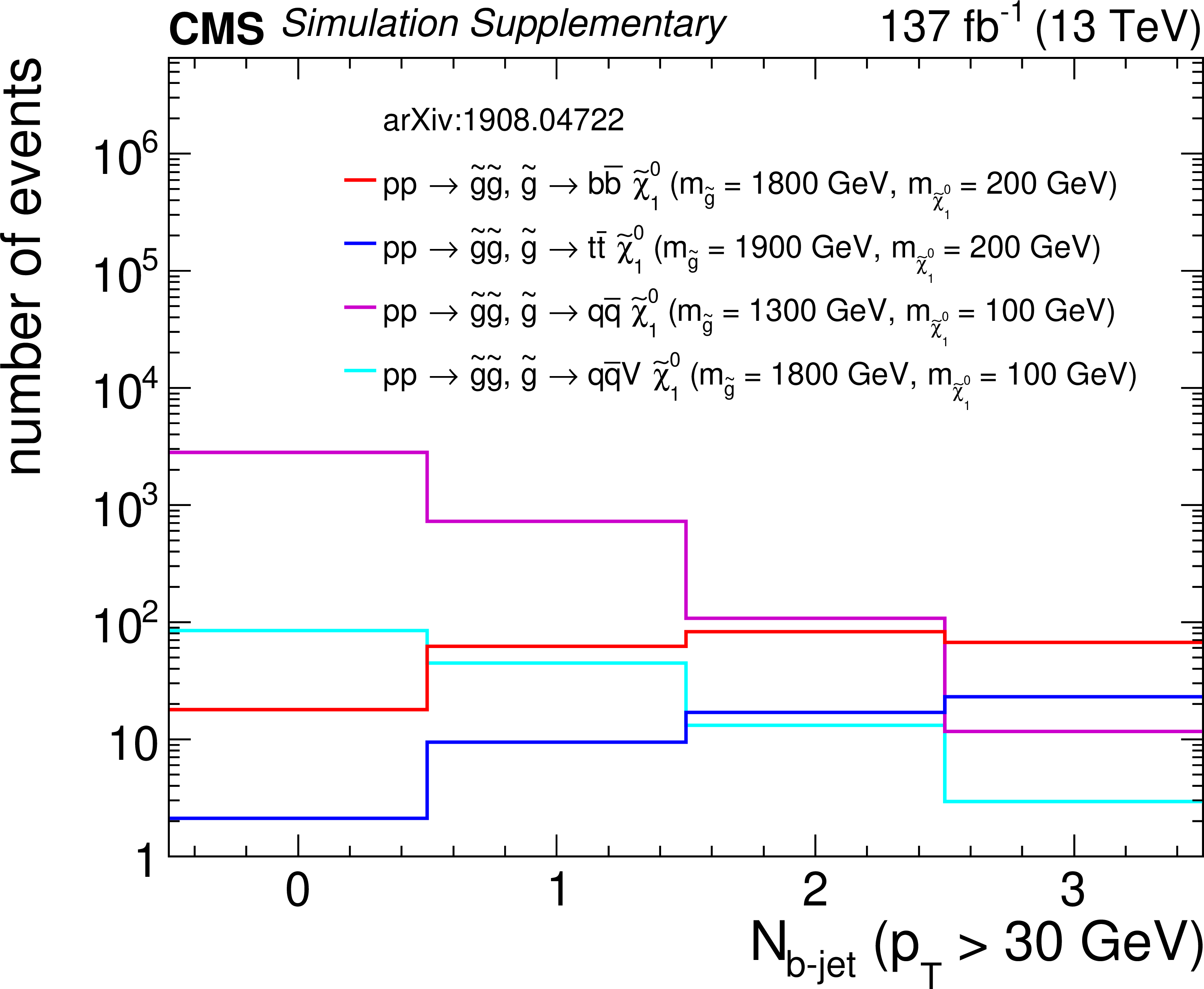
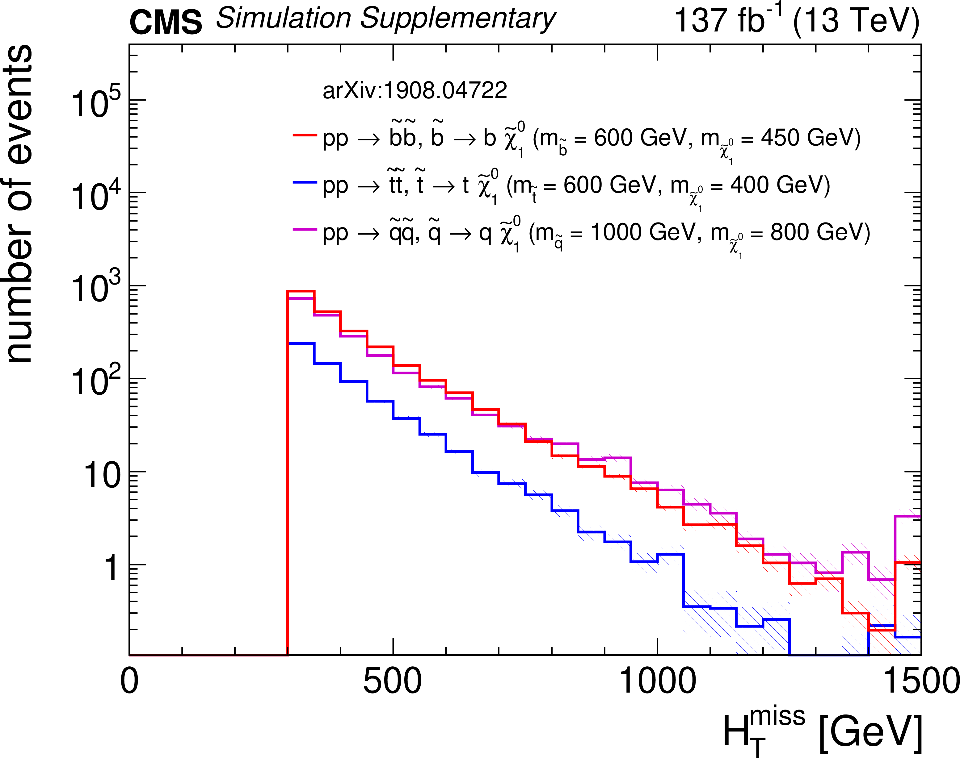
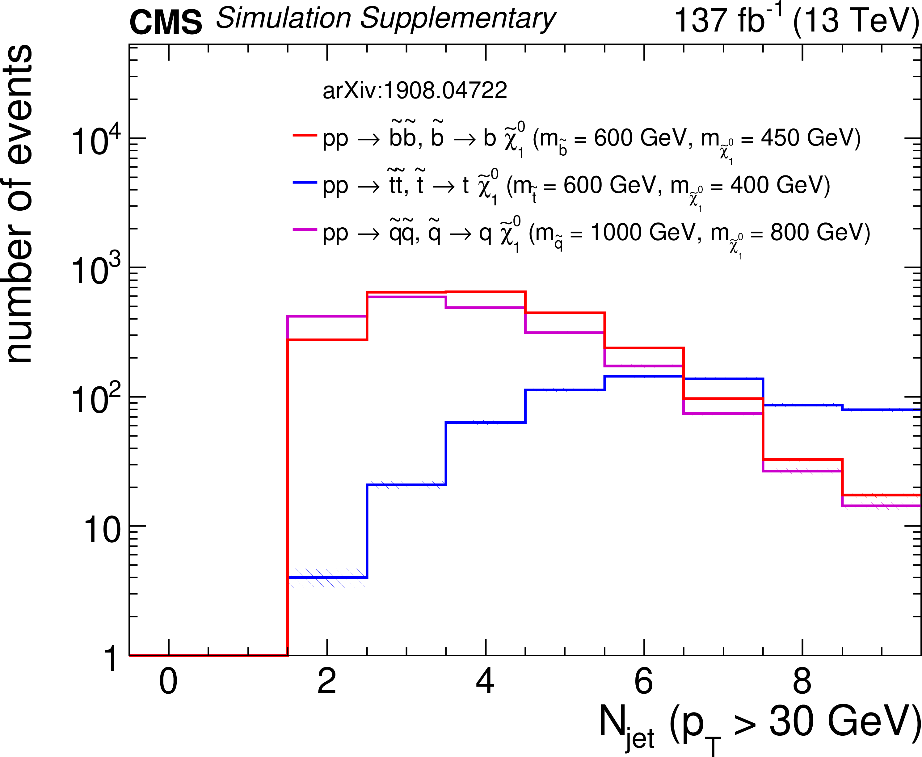
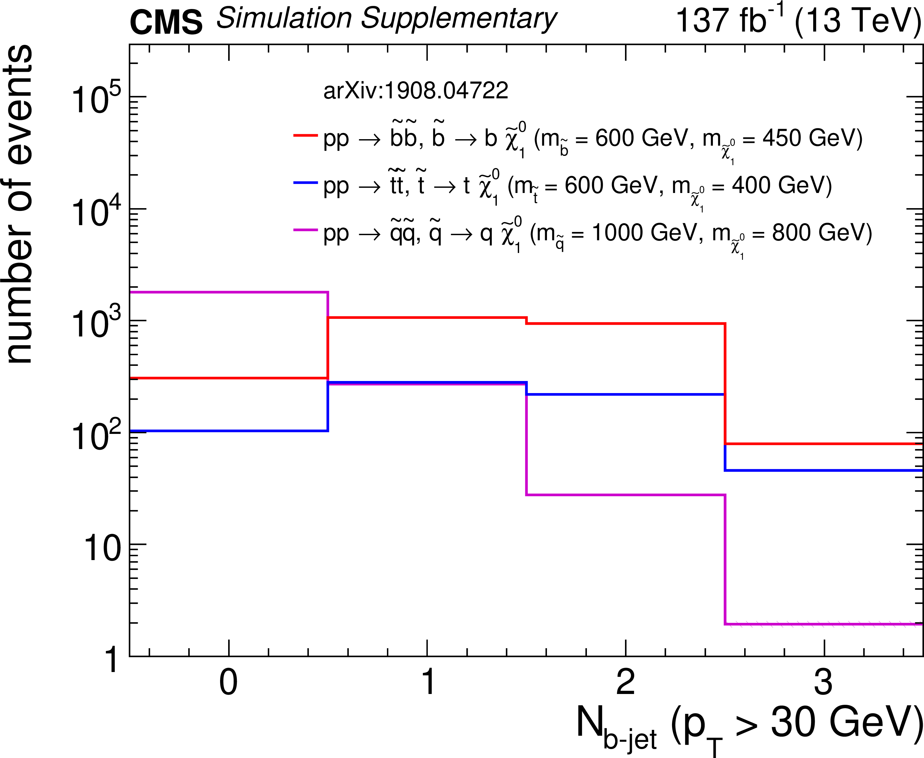
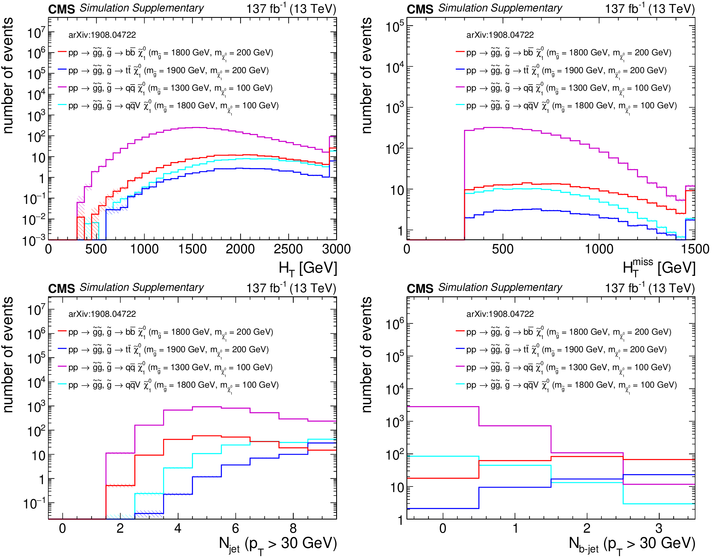
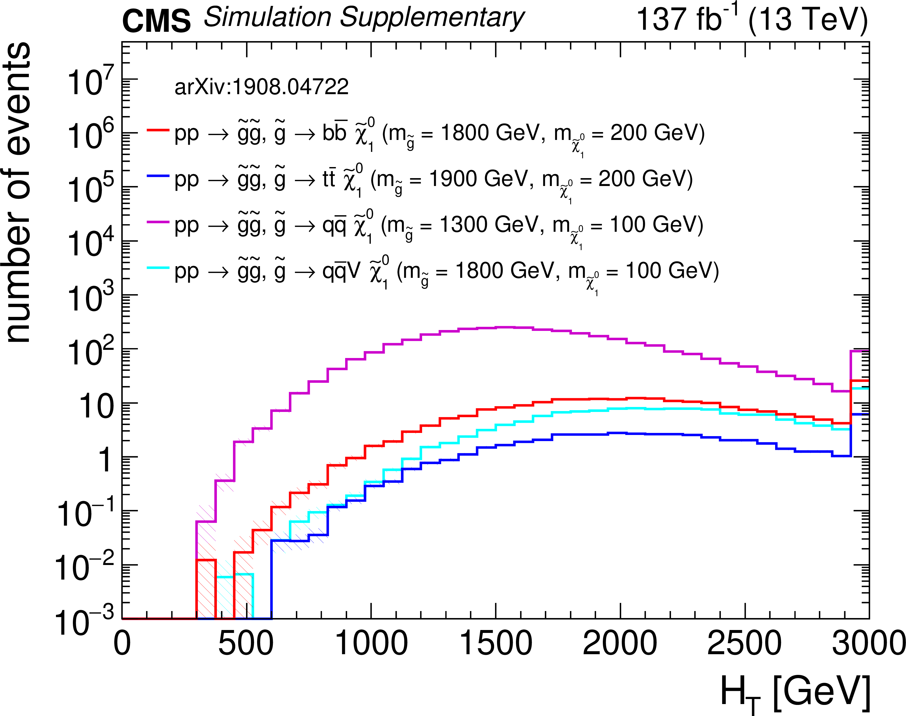
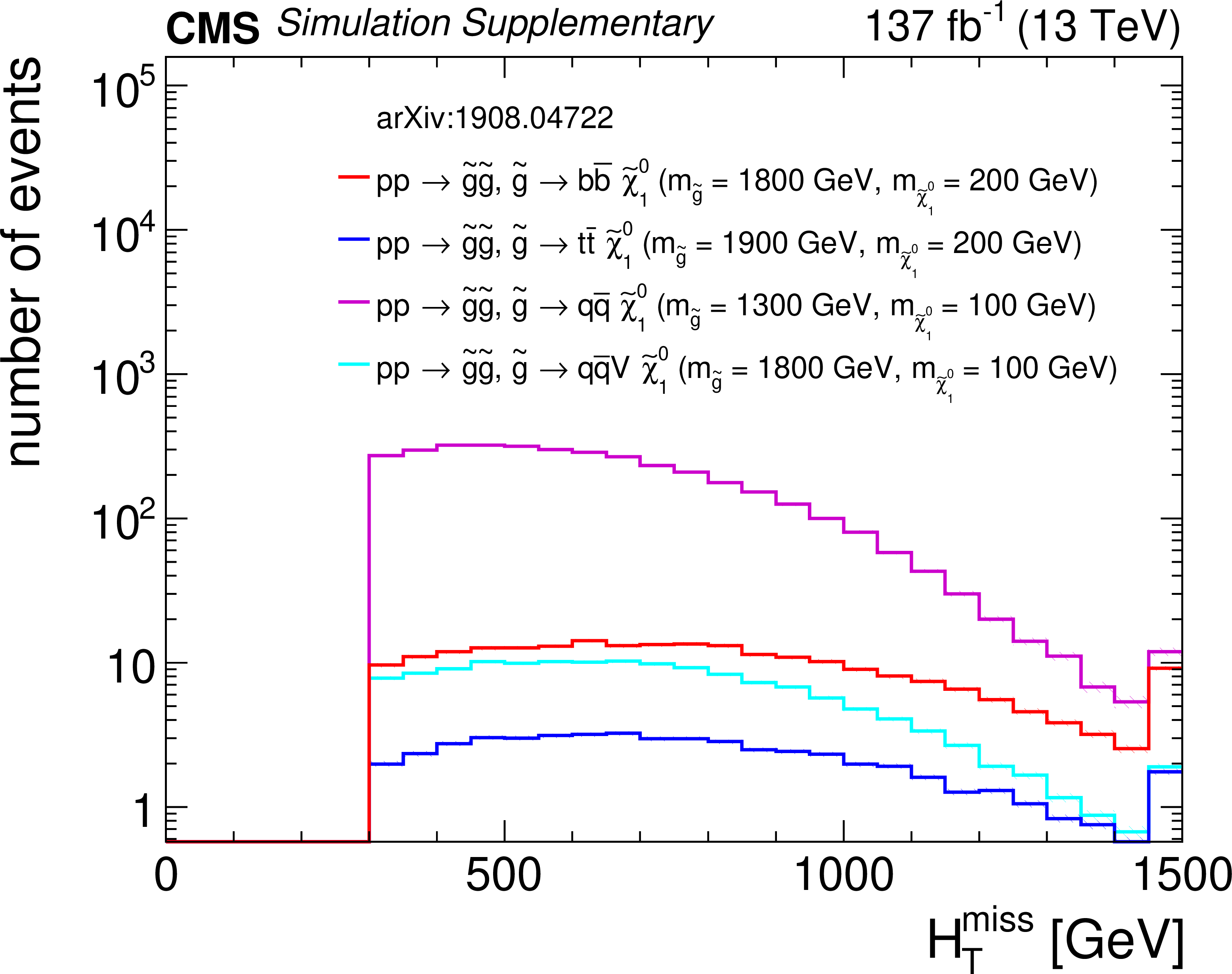
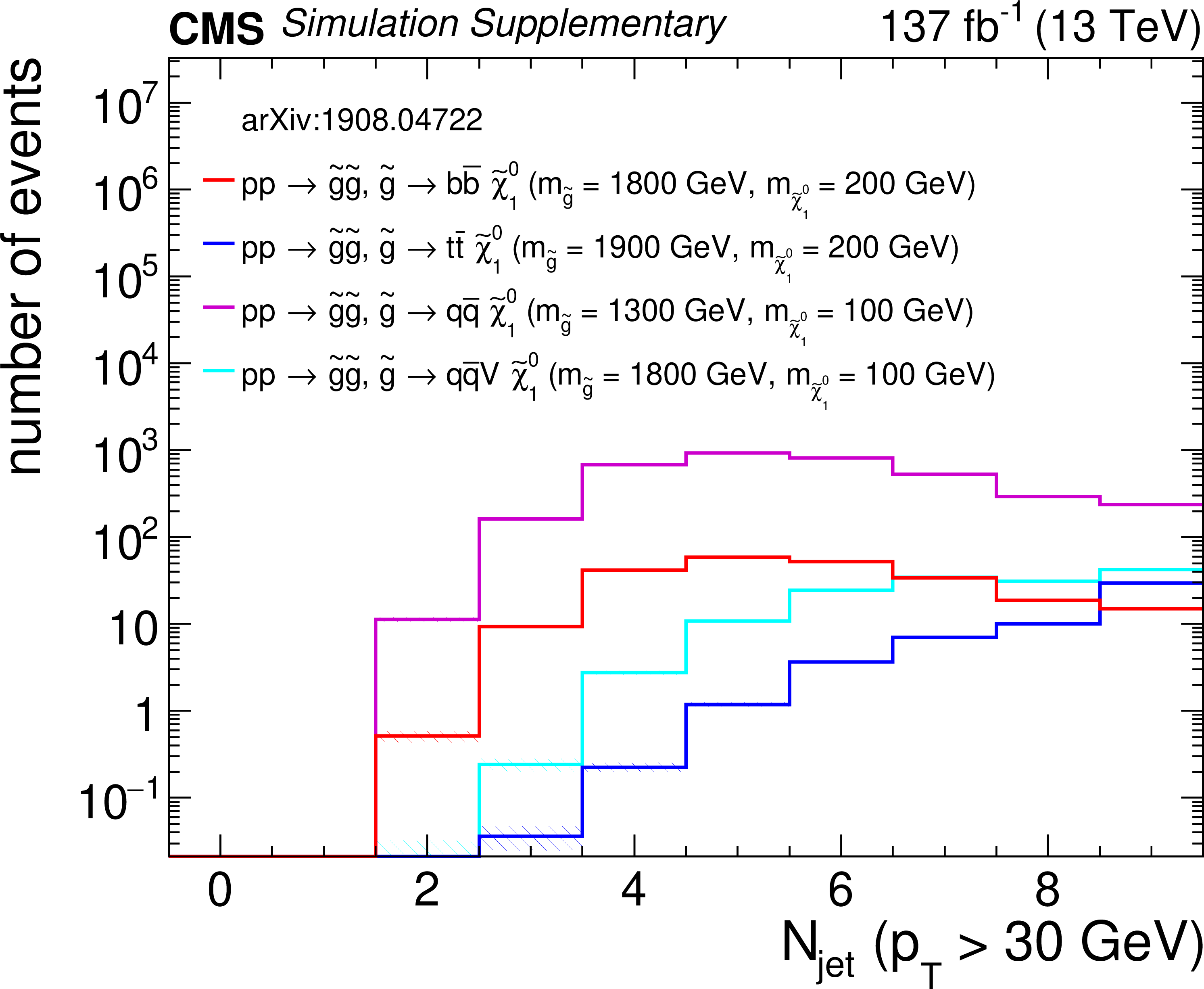
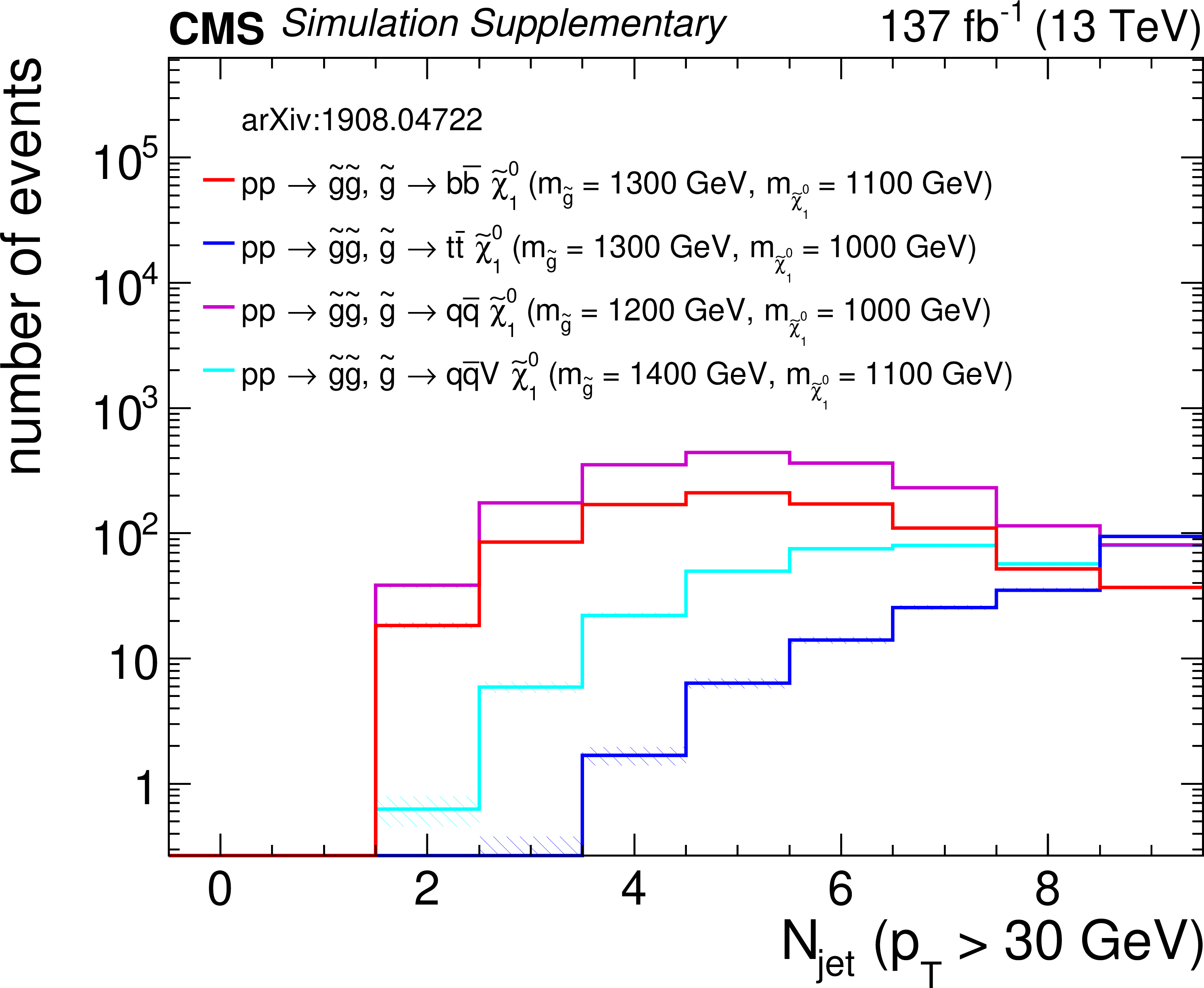
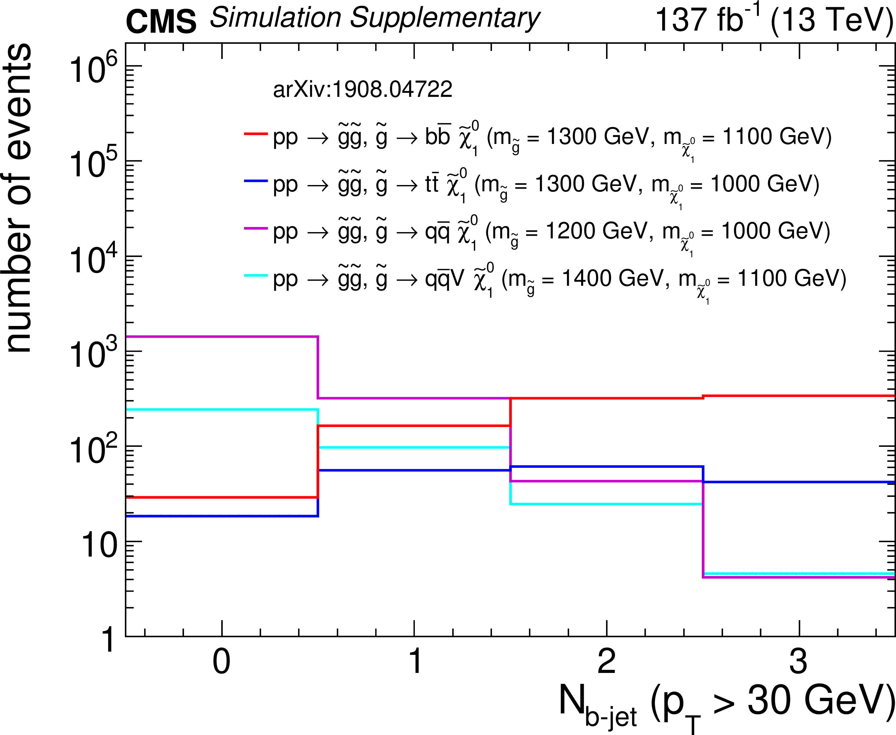
png pdf	Additional Figure 11: Distributions of (a) $H_{\rm T}$ , (b) $H_{\rm T}^{\rm miss}$ , (c) the number of jets, and (d) the number of b-tagged jets from four representative gluino pair production signal models with ${m_{{\mathrm {\tilde{g}}}} \gg m_{{\tilde{\chi}^{0}_{1}}}}$ after the baseline selection. Each plot ignores the baseline requirement (if any) for its respective variable. The last bin in each plot contains the overflow events. Only statistical uncertainties are shown.
png pdf root	Additional Figure 11-a: Distribution of $H_{\rm T}$ from four representative gluino pair production signal models with ${m_{{\mathrm {\tilde{g}}}} \gg m_{{\tilde{\chi}^{0}_{1}}}}$ after the baseline selection. The last bin contains the overflow events. Only statistical uncertainties are shown.
png pdf root	Additional Figure 11-b: Distribution of $H_{\rm T}^{\rm miss}$ from four representative gluino pair production signal models with ${m_{{\mathrm {\tilde{g}}}} \gg m_{{\tilde{\chi}^{0}_{1}}}}$ after the baseline selection. The last bin contains the overflow events. Only statistical uncertainties are shown.
png pdf root	Additional Figure 11-c: Distribution of the number of jets from four representative gluino pair production signal models with ${m_{{\mathrm {\tilde{g}}}} \gg m_{{\tilde{\chi}^{0}_{1}}}}$ after the baseline selection. The last bin contains the overflow events. Only statistical uncertainties are shown.
png pdf root	Additional Figure 11-d: Distribution of the number of b-tagged jets from four representative gluino pair production signal models with ${m_{{\mathrm {\tilde{g}}}} \gg m_{{\tilde{\chi}^{0}_{1}}}}$ after the baseline selection. The last bin contains the overflow events. Only statistical uncertainties are shown.
png pdf	Additional Figure 12: Distributions of (a) $H_{\rm T}$ , (b) $H_{\rm T}^{\rm miss}$ , (c) the number of jets, and (d) the number of b-tagged jets from four representative gluino pair production signal models with ${m_{{\mathrm {\tilde{g}}}} \sim m_{{\tilde{\chi}^{0}_{1}}}}$ after the baseline selection. Each plot ignores the baseline requirement (if any) for its respective variable. The last bin in each plot contains the overflow events. Only statistical uncertainties are shown.
png pdf root	Additional Figure 12-a: Distribution of $H_{\rm T}$ from four representative gluino pair production signal models with ${m_{{\mathrm {\tilde{g}}}} \sim m_{{\tilde{\chi}^{0}_{1}}}}$ after the baseline selection. The last bin contains the overflow events. Only statistical uncertainties are shown.
png pdf root	Additional Figure 12-b: Distribution of $H_{\rm T}^{\rm miss}$ from four representative gluino pair production signal models with ${m_{{\mathrm {\tilde{g}}}} \sim m_{{\tilde{\chi}^{0}_{1}}}}$ after the baseline selection. The last bin contains the overflow events. Only statistical uncertainties are shown.
png pdf root	Additional Figure 12-c: Distribution of the number of jets from four representative gluino pair production signal models with ${m_{{\mathrm {\tilde{g}}}} \sim m_{{\tilde{\chi}^{0}_{1}}}}$ after the baseline selection. The last bin contains the overflow events. Only statistical uncertainties are shown.
png pdf root	Additional Figure 12-d: Distribution of the number of b-tagged jets from four representative gluino pair production signal models with ${m_{{\mathrm {\tilde{g}}}} \sim m_{{\tilde{\chi}^{0}_{1}}}}$ after the baseline selection. The last bin contains the overflow events. Only statistical uncertainties are shown.
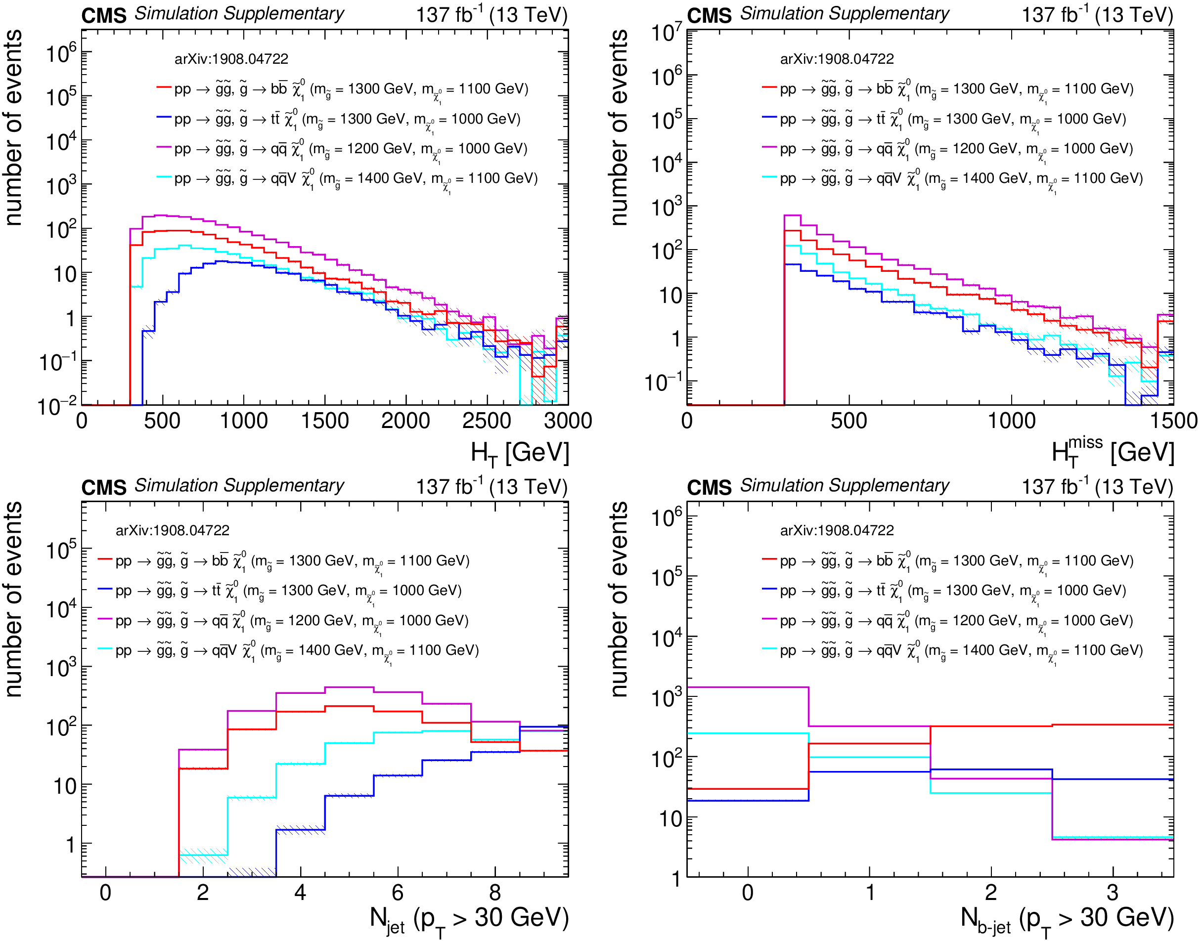
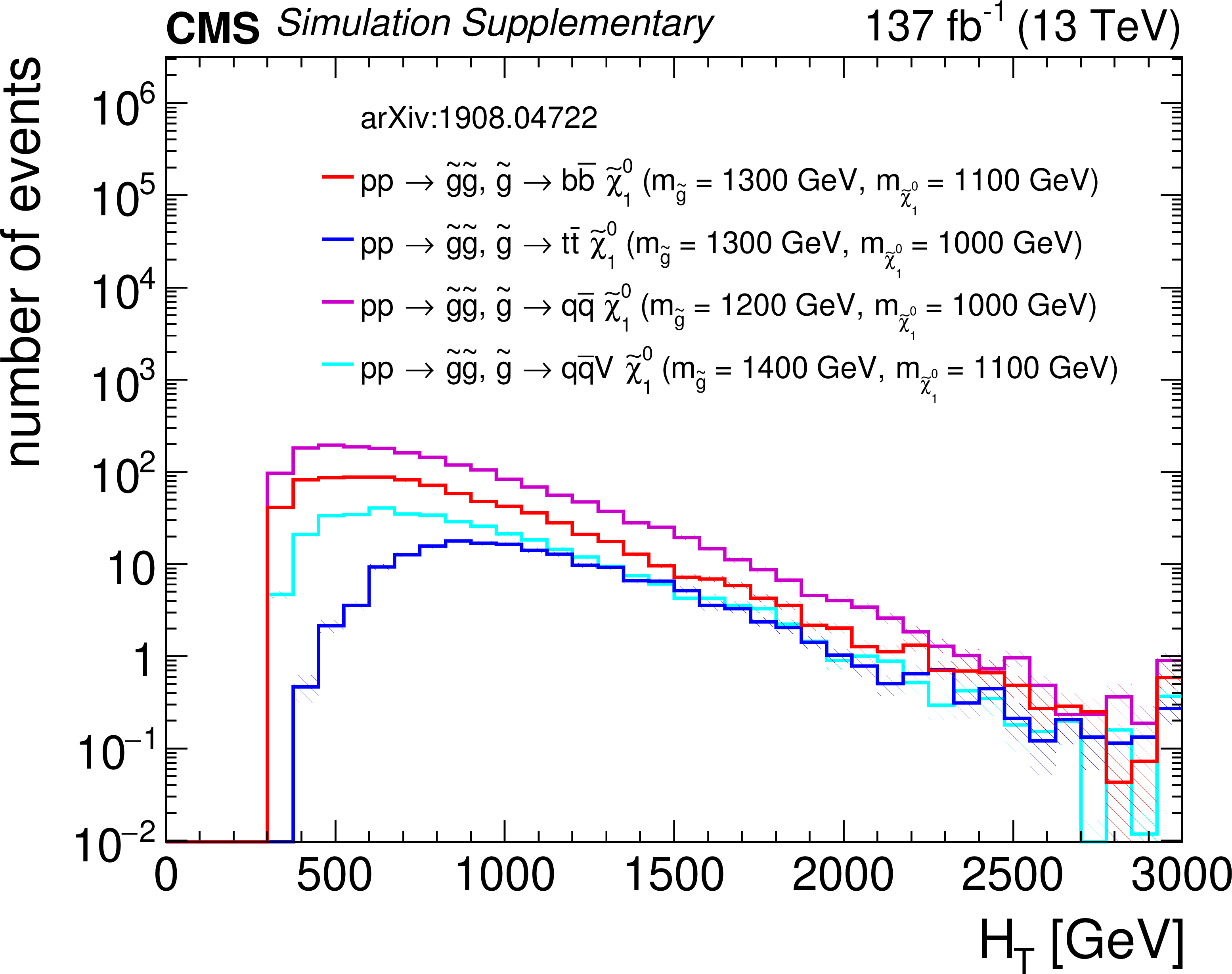
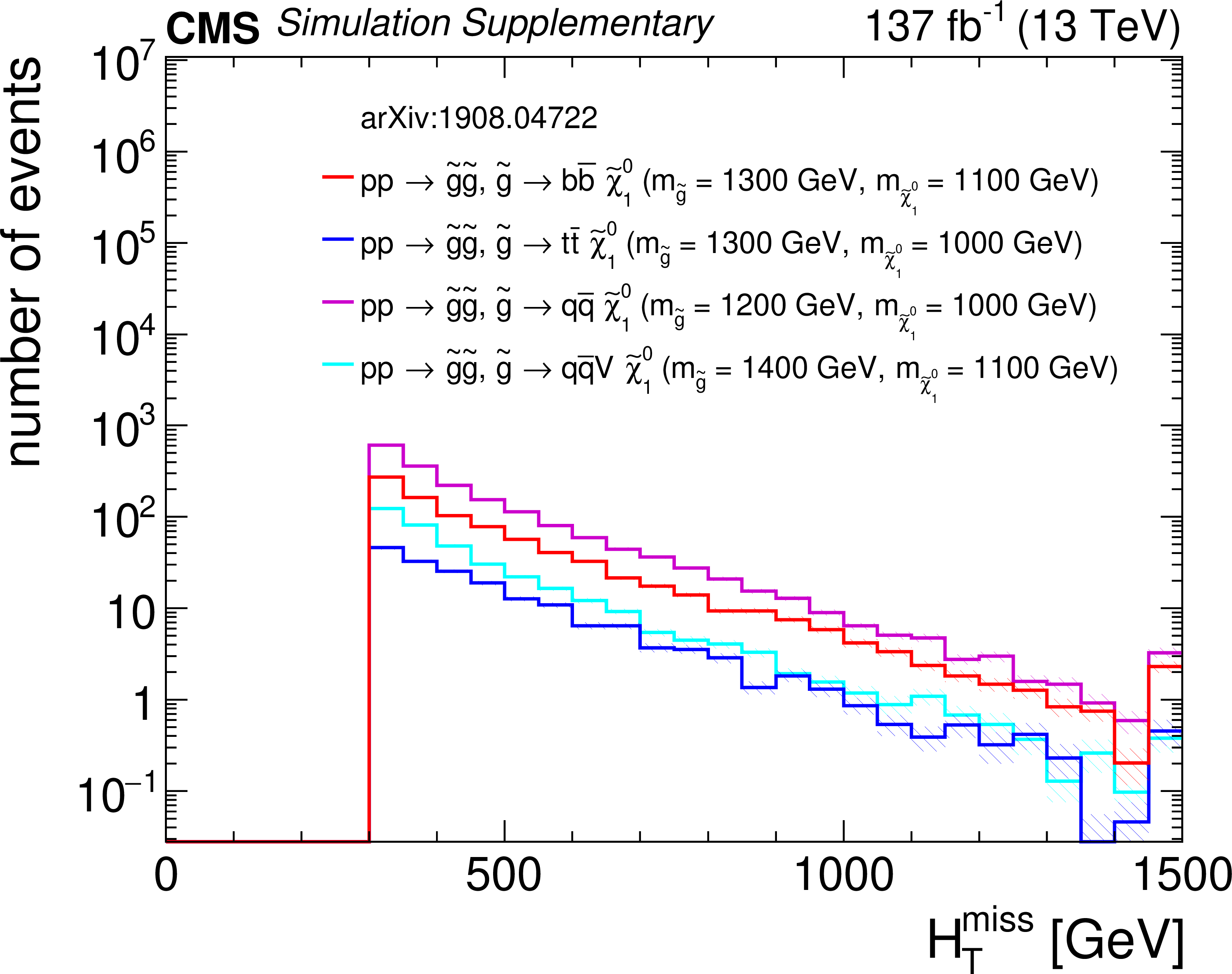
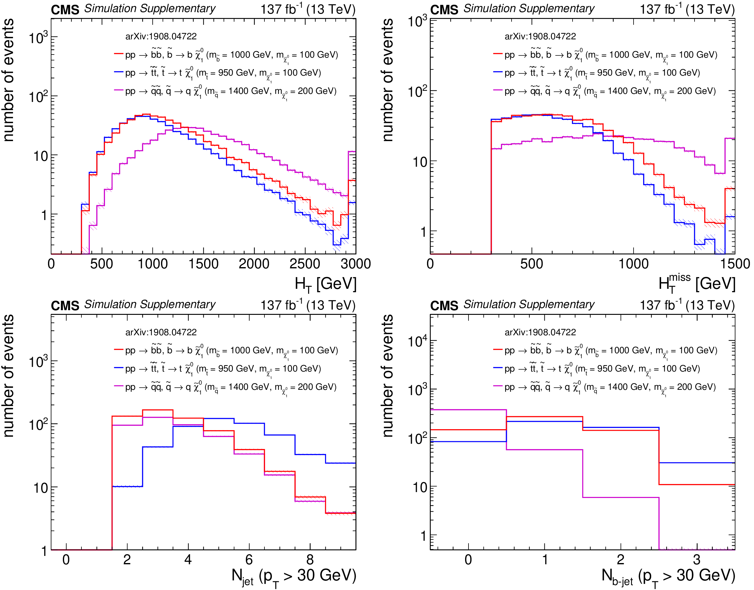
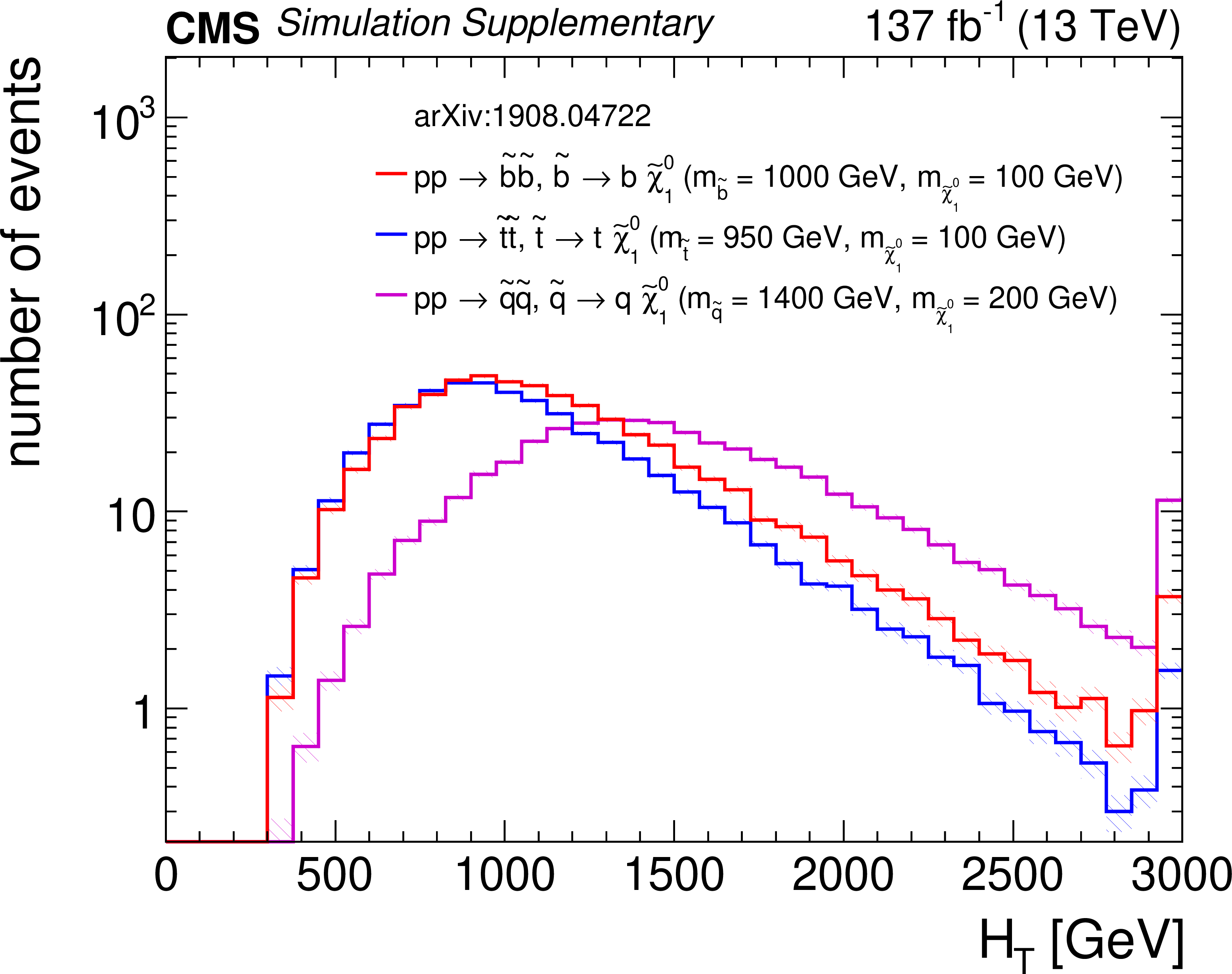
png pdf	Additional Figure 13: Distributions of (a) $H_{\rm T}$ , (b) $H_{\rm T}^{\rm miss}$ , (c) the number of jets, and (d) the number of b-tagged jets from three representative squark pair production signal models with ${m_{{\tilde{\mathrm {q}}}} \gg m_{{\tilde{\chi}^{0}_{1}}}}$ after the baseline selection. Each plot ignores the baseline requirement (if any) for its respective variable. The last bin in each plot contains the overflow events. Only statistical uncertainties are shown.
png pdf root	Additional Figure 13-a: Distribution of $H_{\rm T}$ from three representative squark pair production signal models with ${m_{{\tilde{\mathrm {q}}}} \gg m_{{\tilde{\chi}^{0}_{1}}}}$ after the baseline selection. The last bin contains the overflow events. Only statistical uncertainties are shown.
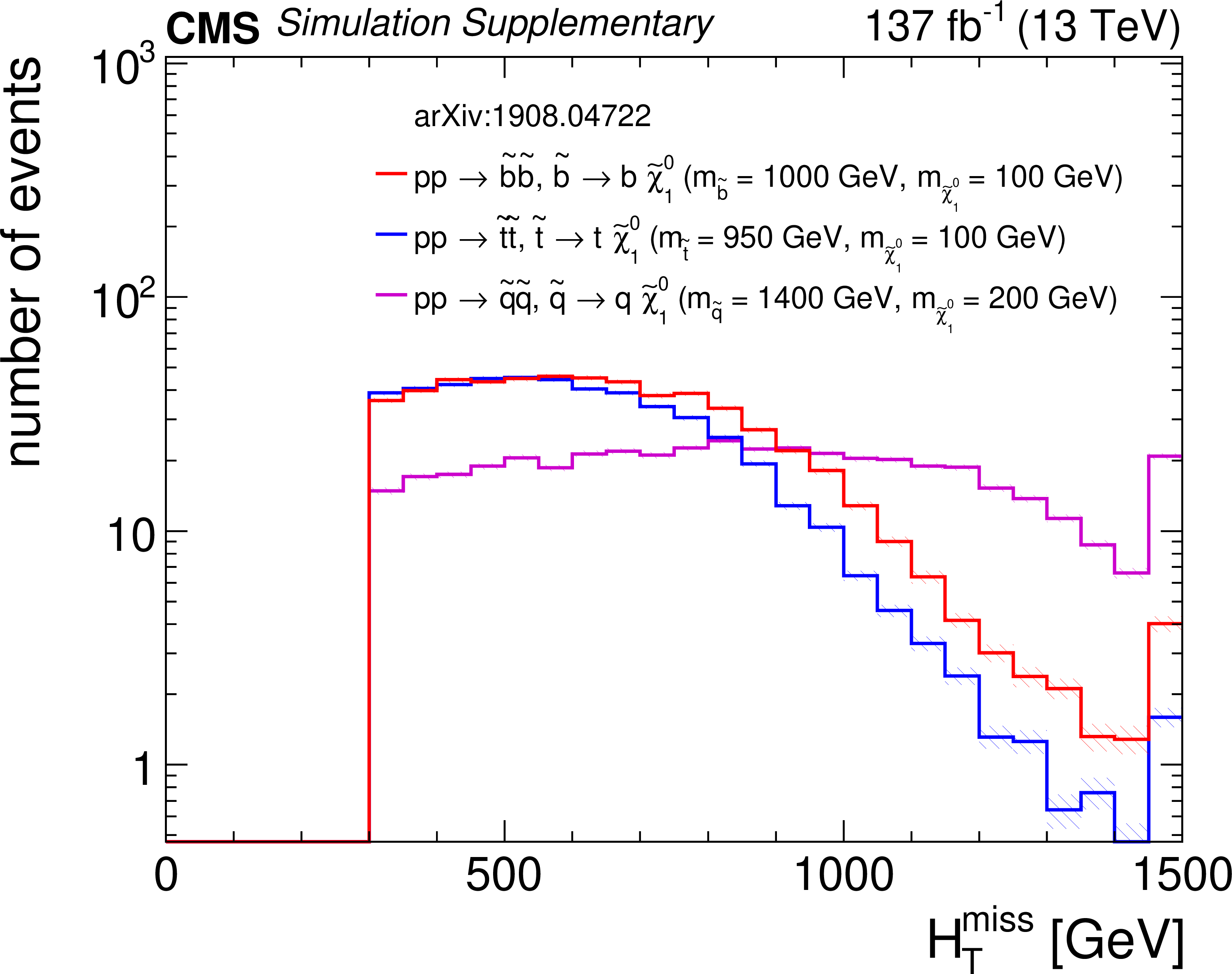
png pdf root	Additional Figure 13-b: Distribution of $H_{\rm T}^{\rm miss}$ from three representative squark pair production signal models with ${m_{{\tilde{\mathrm {q}}}} \gg m_{{\tilde{\chi}^{0}_{1}}}}$ after the baseline selection. The last bin contains the overflow events. Only statistical uncertainties are shown.
png pdf root	Additional Figure 13-c: Distribution of the number of jets from three representative squark pair production signal models with ${m_{{\tilde{\mathrm {q}}}} \gg m_{{\tilde{\chi}^{0}_{1}}}}$ after the baseline selection. The last bin contains the overflow events. Only statistical uncertainties are shown.
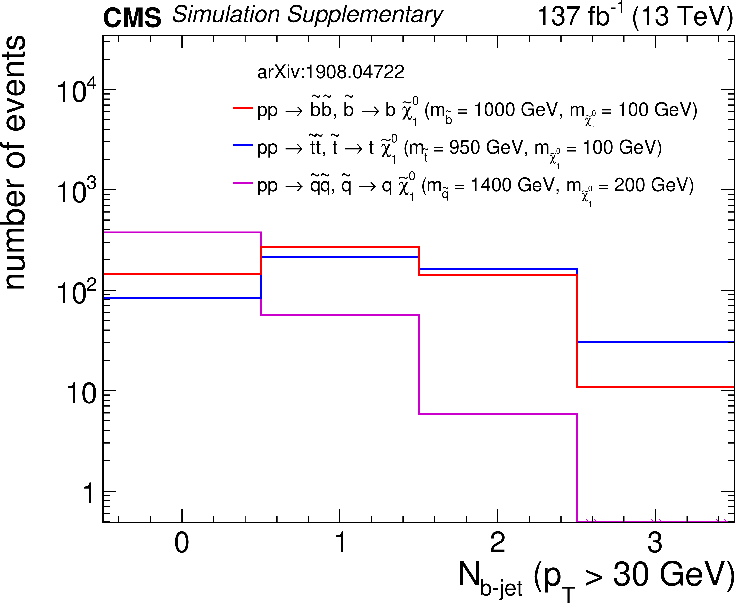
png pdf root	Additional Figure 13-d: Distribution of the number of b-tagged jets from three representative squark pair production signal models with ${m_{{\tilde{\mathrm {q}}}} \gg m_{{\tilde{\chi}^{0}_{1}}}}$ after the baseline selection. The last bin contains the overflow events. Only statistical uncertainties are shown.
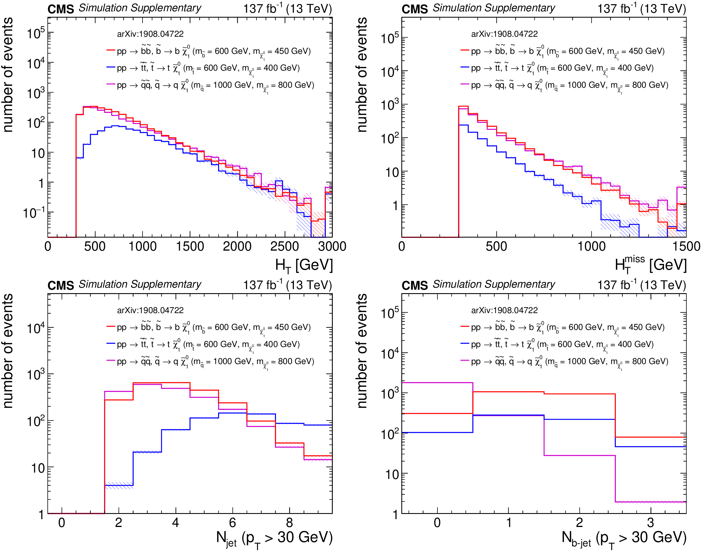
png pdf	Additional Figure 14: Distributions of (a) $H_{\rm T}$ , (b) $H_{\rm T}^{\rm miss}$ , (c) the number of jets, and (d) the number of b-tagged jets from three representative squark pair production signal models with ${m_{{\tilde{\mathrm {q}}}} \sim m_{{\tilde{\chi}^{0}_{1}}}}$ after the baseline selection. Each plot ignores the baseline requirement (if any) for its respective variable. The last bin in each plot contains the overflow events. Only statistical uncertainties are shown.
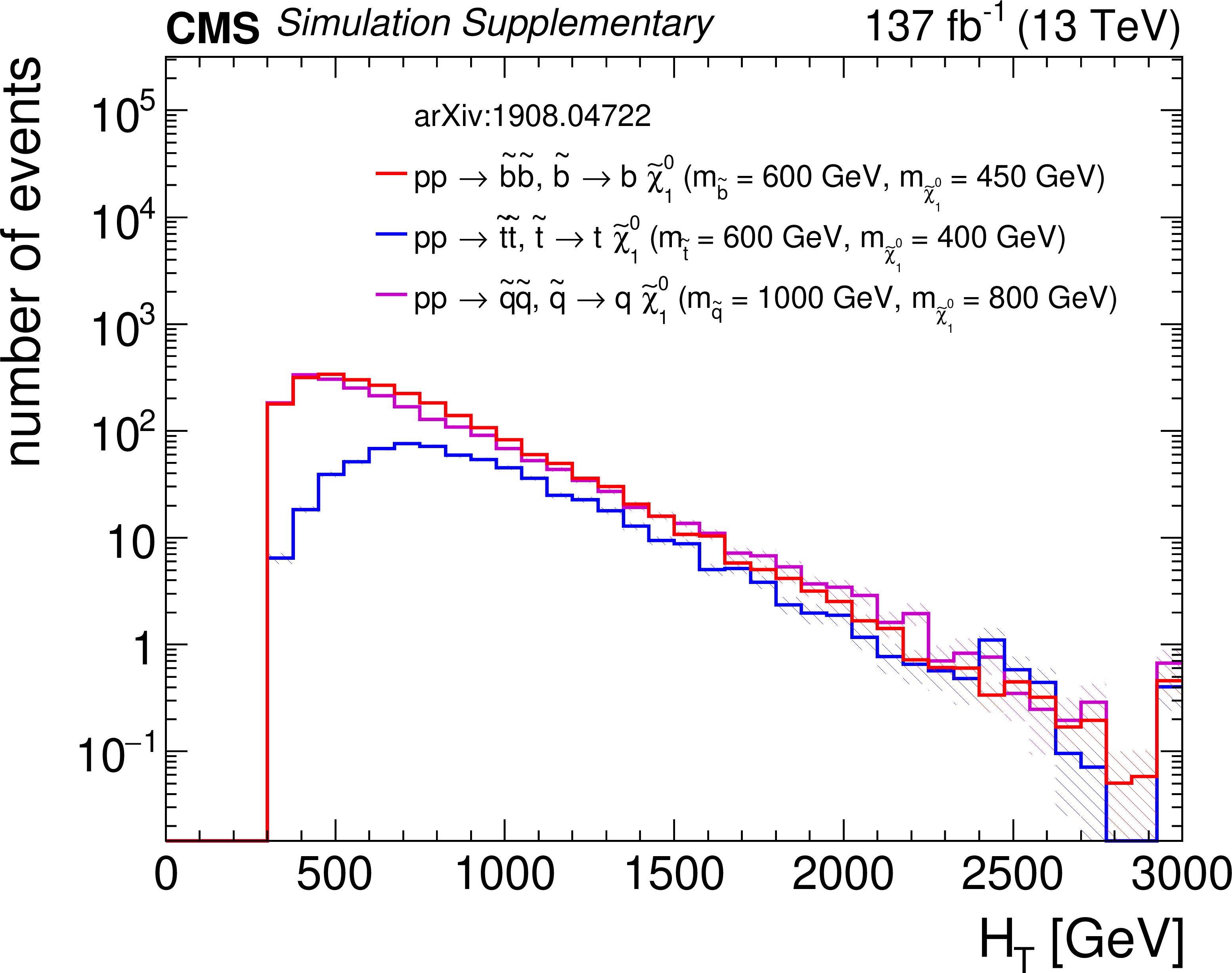
png pdf root	Additional Figure 14-a: Distribution of $H_{\rm T}$ from three representative squark pair production signal models with ${m_{{\tilde{\mathrm {q}}}} \sim m_{{\tilde{\chi}^{0}_{1}}}}$ after the baseline selection. The last bin contains the overflow events. Only statistical uncertainties are shown.
png pdf root	Additional Figure 14-b: Distribution of $H_{\rm T}^{\rm miss}$ from three representative squark pair production signal models with ${m_{{\tilde{\mathrm {q}}}} \sim m_{{\tilde{\chi}^{0}_{1}}}}$ after the baseline selection. The last bin contains the overflow events. Only statistical uncertainties are shown.
png pdf root	Additional Figure 14-c: Distribution of the number of jets from three representative squark pair production signal models with ${m_{{\tilde{\mathrm {q}}}} \sim m_{{\tilde{\chi}^{0}_{1}}}}$ after the baseline selection. The last bin contains the overflow events. Only statistical uncertainties are shown.
png pdf root	Additional Figure 14-d: Distribution of the number of b-tagged jets from three representative squark pair production signal models with ${m_{{\tilde{\mathrm {q}}}} \sim m_{{\tilde{\chi}^{0}_{1}}}}$ after the baseline selection. The last bin contains the overflow events. Only statistical uncertainties are shown.

Additional Tables
png pdf	Additional Table 1: Observed numbers of events and post-fit backgrounds in the 2 $\geq {N_{\text {jet}}} \geq$ 3 search regions.
png pdf	Additional Table 2: Observed numbers of events and post-fit backgrounds in the 4 $\geq {N_{\text {jet}}} \geq$ 5 search regions.
png pdf	Additional Table 3: Observed numbers of events and post-fit backgrounds in the 6 $\geq {N_{\text {jet}}} \geq$ 7 search regions.
png pdf	Additional Table 4: Observed numbers of events and post-fit backgrounds in the 8 $\geq {N_{\text {jet}}} \geq$ 9 search regions.
png pdf	Additional Table 5: Observed numbers of events and post-fit backgrounds in the ${N_{\text {jet}}} \geq$ 10 search regions.
png pdf	Additional Table 6: Observed numbers of events and prefit background predictions in the aggregate search regions. The first uncertainty is statistical and second systematic.
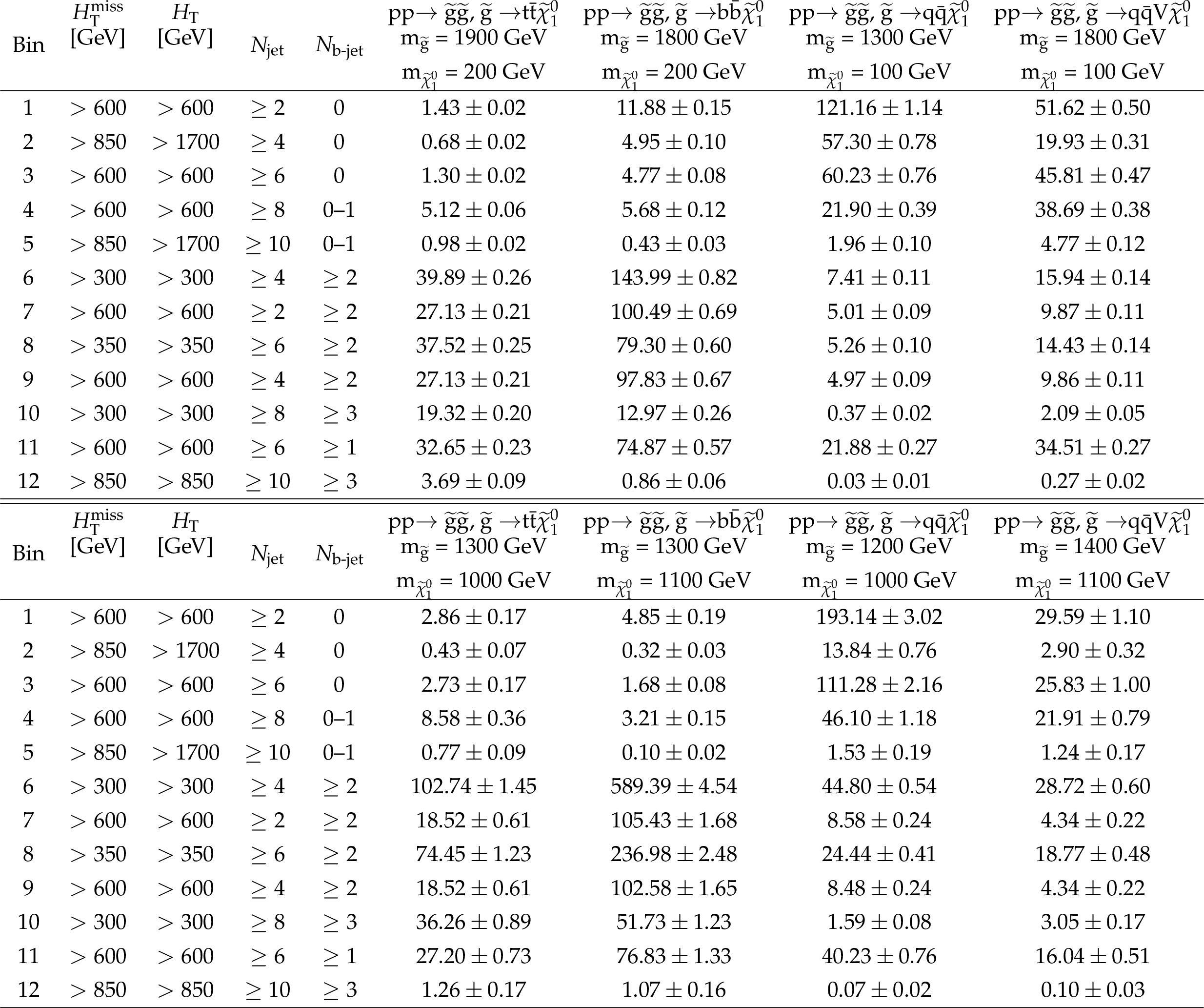
png pdf	Additional Table 7: Signal yields for representative gluino signal model points in the aggregate search regions. The uncertainties shown are statistical.
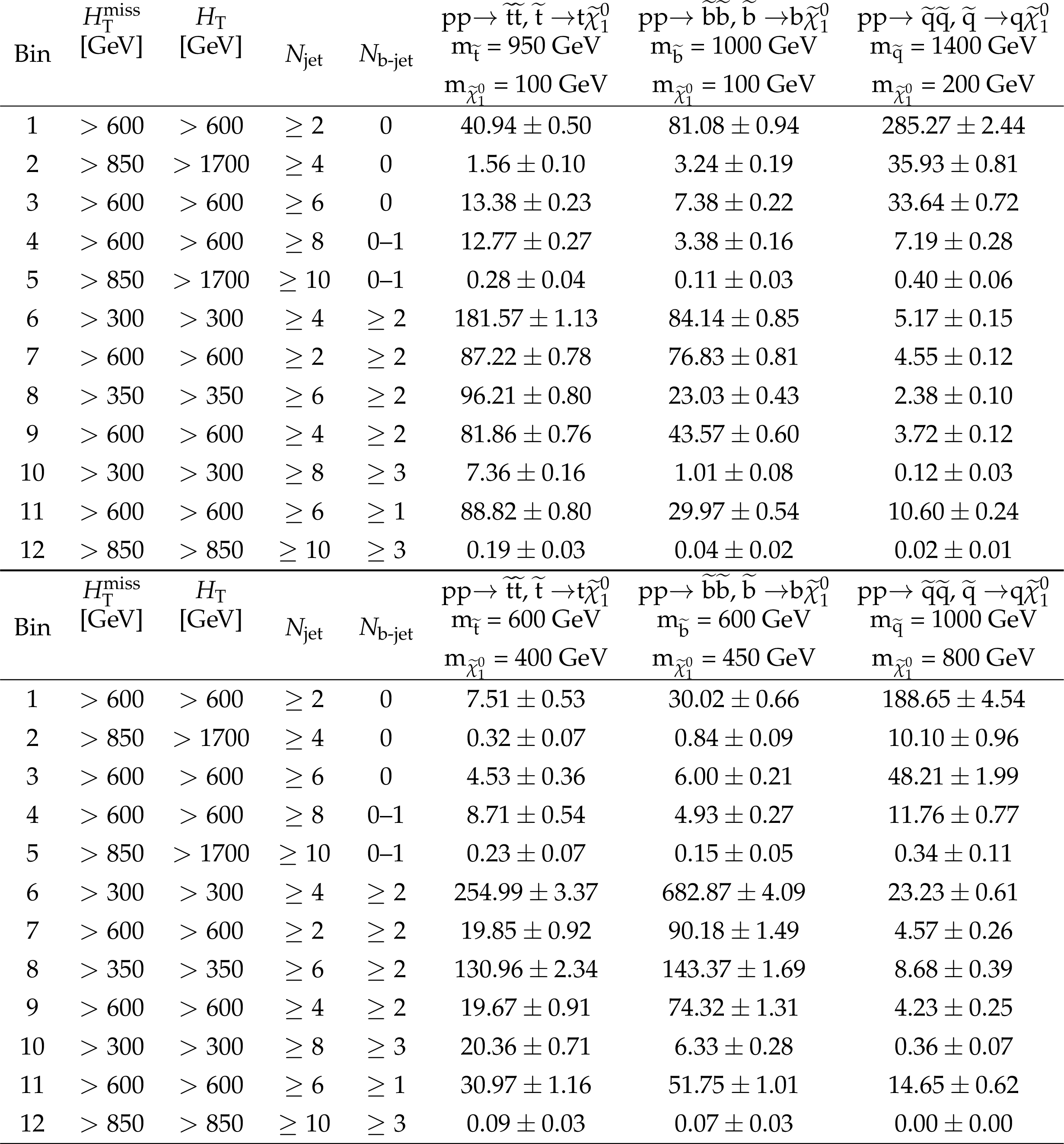
png pdf	Additional Table 8: Signal yields for representative squark signal model points in the aggregate search regions. The uncertainties shown are statistical.
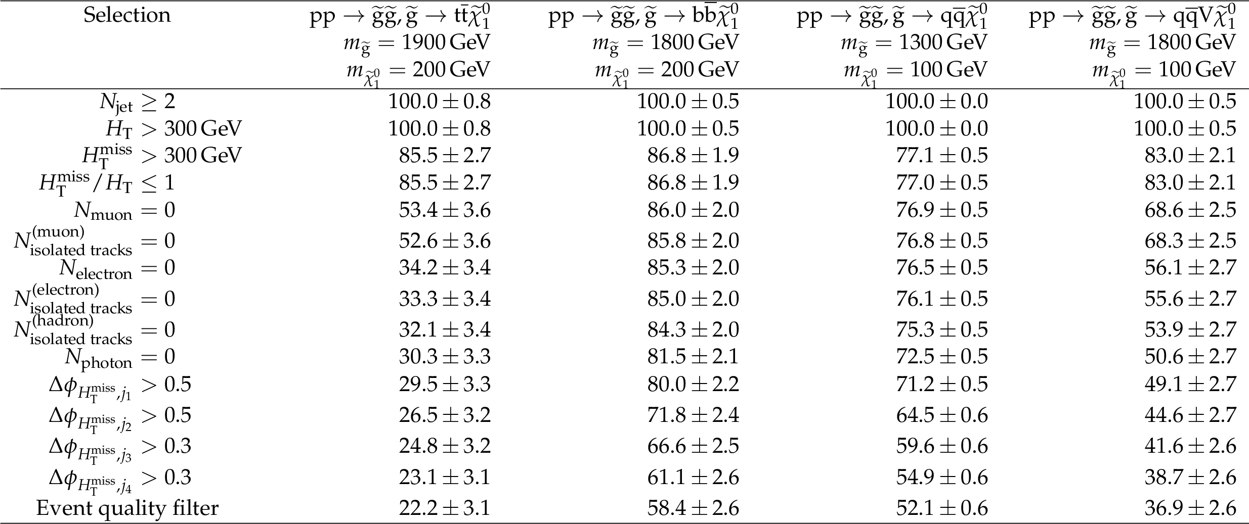
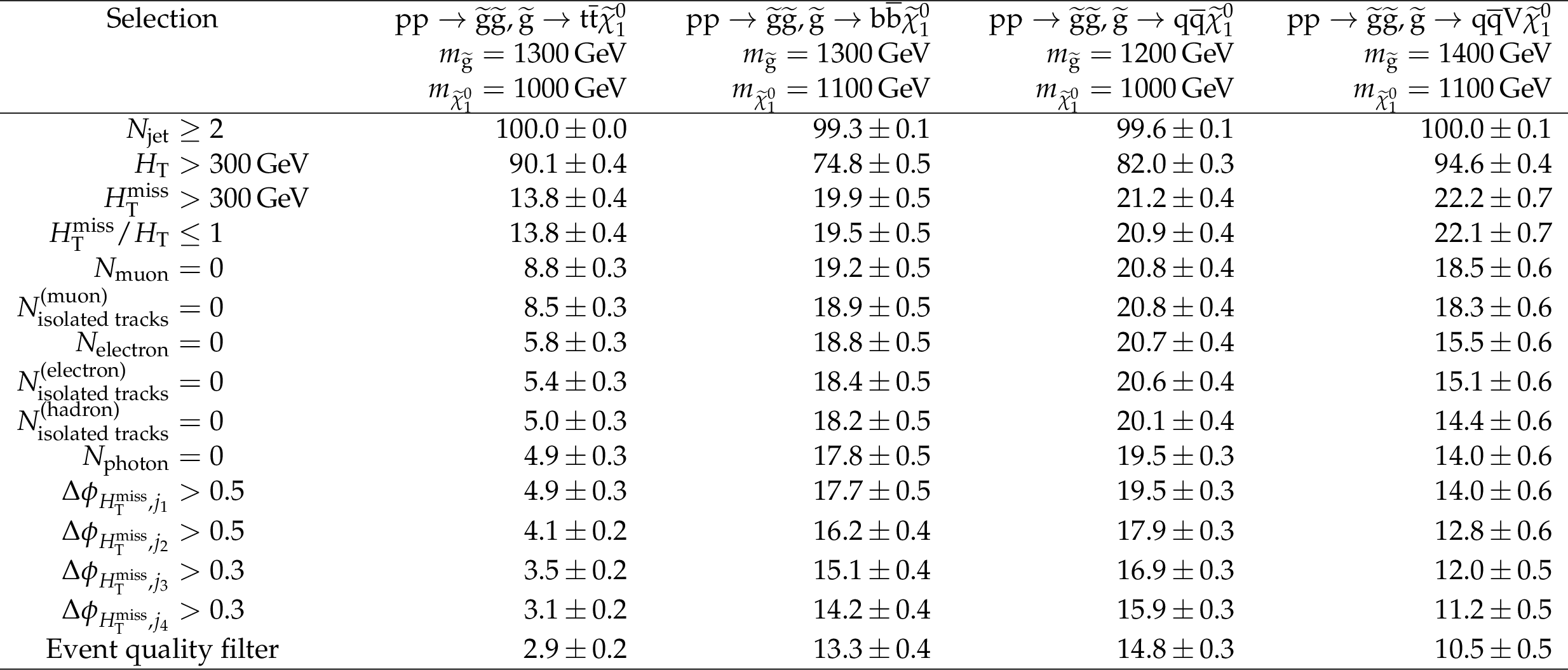
png pdf	Additional Table 9: Absolute cumulative efficiencies in % for each step of the event selection process, listed for four representative gluino pair production signal models with ${m_{{\mathrm {\tilde{g}}}} \gg m_{{\tilde{\chi}^{0}_{1}}}}$ . Only statistical uncertainties are shown.
png pdf	Additional Table 10: Absolute cumulative efficiencies in % for each step of the event selection process, listed for four representative gluino pair production signal models with ${m_{{\mathrm {\tilde{g}}}} \sim m_{{\tilde{\chi}^{0}_{1}}}}$ . Only statistical uncertainties are shown.
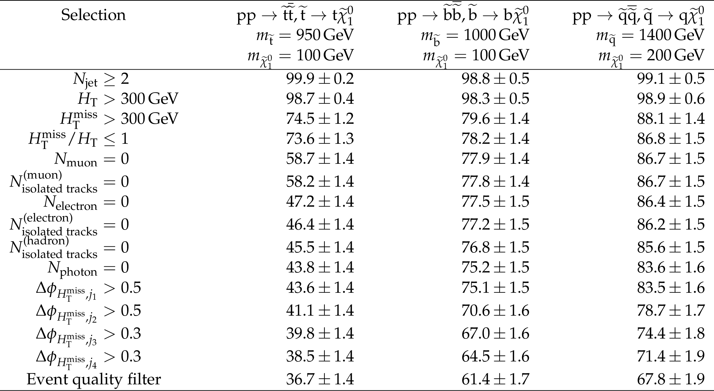
png pdf	Additional Table 11: Absolute cumulative efficiencies in % for each step of the event selection process, listed for three representative squark pair production signal models with ${m_{{\tilde{\mathrm {q}}}} \gg m_{{\tilde{\chi}^{0}_{1}}}}$ . Only statistical uncertainties are shown.
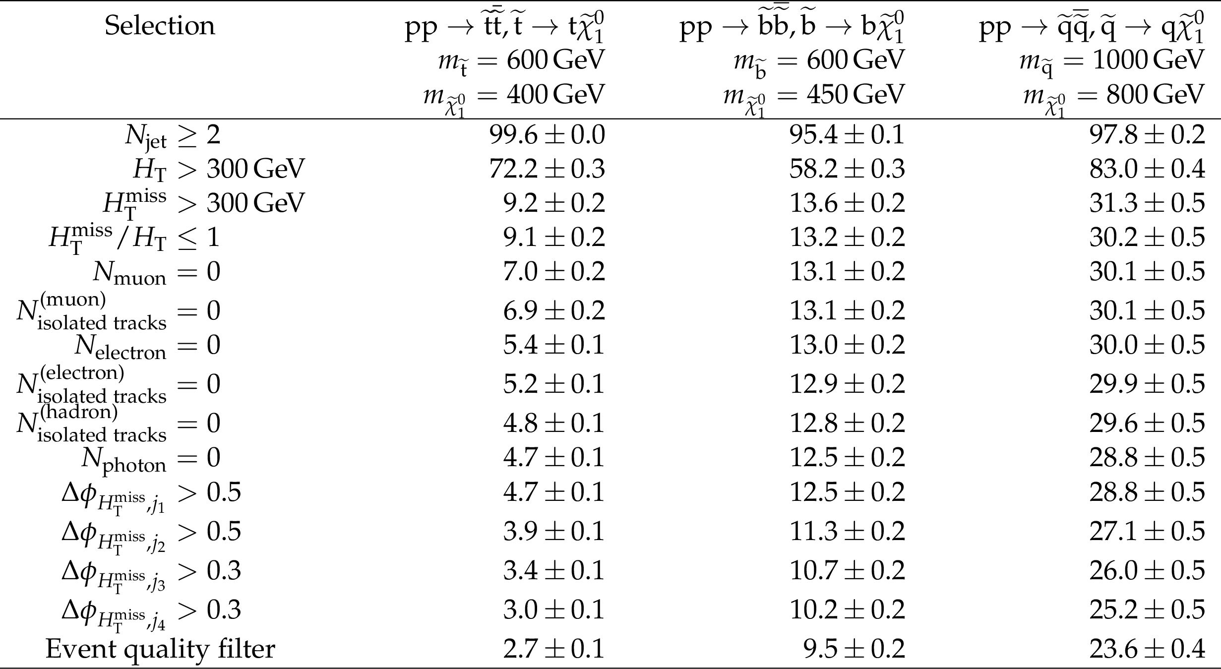
png pdf	Additional Table 12: Absolute cumulative efficiencies in % for each step of the event selection process, listed for three representative squark pair production signal models with ${m_{{\tilde{\mathrm {q}}}} \sim m_{{\tilde{\chi}^{0}_{1}}}}$ . Only statistical uncertainties are shown.

References
1	ATLAS Collaboration	Search for pair production of gluinos decaying via stop and sbottom in events with b-jets and large missing transverse momentum in pp collisions at $\sqrt{s} =$ 13 TeV with the ATLAS detector	PRD 94 (2016) 032003	1605.09318
2	ATLAS Collaboration	Search for squarks and gluinos in final states with jets and missing transverse momentum at $\sqrt{s} =$ 13 TeV with the ATLAS detector	EPJC 76 (2016) 392	1605.03814
3	CMS Collaboration	Search for supersymmetry in the multijet and missing transverse momentum final state in pp collisions at 13 TeV	PLB 758 (2016) 152	CMS-SUS-15-002 1602.06581
4	CMS Collaboration	Search for new physics with the M $_{\text{T2}}$ variable in all-jets final states produced in pp collisions at $\sqrt{s}=$ 13 TeV	JHEP 10 (2016) 006	CMS-SUS-15-003 1603.04053
5	CMS Collaboration	Inclusive search for supersymmetry using razor variables in pp collisions at $\sqrt{s}=$ 13 TeV	PRD 95 (2017) 012003	CMS-SUS-15-004 1609.07658
6	CMS Collaboration	A search for new phenomena in pp collisions at $\sqrt{s}=$ 13 TeV in final states with missing transverse momentum and at least one jet using the ${\alpha_{\text{T}}}$ variable	EPJC 77 (2017) 294	CMS-SUS-15-005 1611.00338
7	CMS Collaboration	Search for supersymmetry in multijet events with missing transverse momentum in proton-proton collisions at 13 TeV	PRD 96 (2017) 032003	CMS-SUS-16-033 1704.07781
8	P. Ramond	Dual theory for free fermions	PRD 3 (1971) 2415
9	Y. A. Golfand and E. P. Likhtman	Extension of the algebra of Poincaré group generators and violation of P invariance	JEPTL 13 (1971)323
10	A. Neveu and J. H. Schwarz	Factorizable dual model of pions	NPB 31 (1971) 86
11	D. V. Volkov and V. P. Akulov	Possible universal neutrino interaction	JEPTL 16 (1972)438
12	J. Wess and B. Zumino	A Lagrangian model invariant under supergauge transformations	PLB 49 (1974) 52
13	J. Wess and B. Zumino	Supergauge transformations in four dimensions	NPB 70 (1974) 39
14	P. Fayet	Supergauge invariant extension of the Higgs mechanism and a model for the electron and its neutrino	NPB 90 (1975) 104
15	P. Fayet and S. Ferrara	Supersymmetry	PR 32 (1977) 249
16	H. P. Nilles	Supersymmetry, supergravity and particle physics	Phys. Rep. 110 (1984) 1
17	S. P. Martin	A supersymmetry primer	Adv. Ser. Direct. High Energy Phys. 21 (2010) 1	hep-ph/9709356
18	B. Gripaios	Composite leptoquarks at the LHC	JHEP 02 (2010) 045	0910.1789
19	S. Dimopoulos	Technicolored signatures	NPB 168 (1980) 69
20	M. Perelstein	Little Higgs models and their phenomenology	Prog. Part. NP 58 (2007) 247	hep-ph/0512128
21	C. Grojean, E. Salvioni, and R. Torre	A weakly constrained W' at the early LHC	JHEP 07 (2011) 002	1103.2761
22	L. Lopez-Honorez, T. Schwetz, and J. Zupan	Higgs portal, fermionic dark matter, and a standard model like Higgs at 125 GeV	PLB 716 (2012) 179	1203.2064
23	J. M. No	Looking through the pseudoscalar portal into dark matter: Novel mono-Higgs and mono-Z signatures at the LHC	PRD 93 (2016) 031701	1509.01110
24	R. Barbieri and G. F. Giudice	Upper bounds on supersymmetric particle masses	NPB 306 (1988) 63
25	S. Dimopoulos and G. F. Giudice	Naturalness constraints in supersymmetric theories with nonuniversal soft terms	PLB 357 (1995) 573	hep-ph/9507282
26	R. Barbieri and D. Pappadopulo	S-particles at their naturalness limits	JHEP 10 (2009) 061	0906.4546
27	M. Papucci, J. T. Ruderman, and A. Weiler	Natural SUSY endures	JHEP 09 (2012) 035	1110.6926
28	G. R. Farrar and P. Fayet	Phenomenology of the production, decay, and detection of new hadronic states associated with supersymmetry	PLB 76 (1978) 575
29	CMS Collaboration	Search for new physics with jets and missing transverse momentum in pp collisions at $\sqrt{s}=$ 7 TeV	JHEP 08 (2011) 155	CMS-SUS-10-005 1106.4503
30	CMS Collaboration	Search for new physics in the multijet and missing transverse momentum final state in proton-proton collisions at $\sqrt{s}=$ 8 TeV	JHEP 06 (2014) 055	CMS-SUS-13-012 1402.4770
31	N. Arkani-Hamed et al.	MARMOSET: The path from LHC data to the new standard model via on-shell effective theories		hep-ph/0703088
32	J. Alwall, M.-P. Le, M. Lisanti, and J. G. Wacker	Model-independent jets plus missing energy searches	PRD 79 (2009) 015005	0809.3264
33	J. Alwall, P. Schuster, and N. Toro	Simplified models for a first characterization of new physics at the LHC	PRD 79 (2009) 075020	0810.3921
34	D. Alves et al.	Simplified models for LHC new physics searches	JPG 39 (2012) 105005	1105.2838
35	CMS Collaboration	Interpretation of searches for supersymmetry with simplified models	PRD 88 (2013) 052017	CMS-SUS-11-016 1301.2175
36	CMS Collaboration	The CMS experiment at the CERN LHC	JINST 3 (2008) S08004	CMS-00-001
37	CMS Collaboration	The CMS trigger system	JINST 12 (2017) P01020	CMS-TRG-12-001 1609.02366
38	CMS Collaboration	Particle-flow reconstruction and global event description with the CMS detector	JINST 12 (2017) P10003	CMS-PRF-14-001 1706.04965
39	CMS Collaboration	Performance of photon reconstruction and identification with the CMS detector in proton-proton collisions at $\sqrt{s} =$ 8 TeV	JINST 10 (2015) P08010	CMS-EGM-14-001 1502.02702
40	CMS Collaboration	Performance of electron reconstruction and selection with the CMS detector in proton-proton collisions at $\sqrt{s} =$ 8 TeV	JINST 10 (2015) P06005	CMS-EGM-13-001 1502.02701
41	CMS Collaboration	Performance of the CMS muon detector and muon reconstruction with proton-proton collisions at $\sqrt{s} =$ 13 TeV	JINST 13 (2018) P06015	CMS-MUO-16-001 1804.04528
42	M. Cacciari, G. P. Salam, and G. Soyez	The anti- ${k_{\mathrm{T}}}$ jet clustering algorithm	JHEP 04 (2008) 063	0802.1189
43	M. Cacciari, G. P. Salam, and G. Soyez	FastJet user manual	EPJC 72 (2012) 1896	1111.6097
44	M. Cacciari and G. P. Salam	Pileup subtraction using jet areas	PLB 659 (2008) 119	0707.1378
45	K. Rehermann and B. Tweedie	Efficient identification of boosted semileptonic top quarks at the LHC	JHEP 03 (2011) 059	1007.2221
46	CMS Collaboration	Jet performance in pp collisions at $\sqrt{s}=$ 7 TeV	CDS
47	CMS Collaboration	Jet algorithms performance in 13 TeV data	CMS-PAS-JME-16-003	CMS-PAS-JME-16-003
48	CMS Collaboration	Jet energy scale and resolution in the CMS experiment in pp collisions at 8 TeV	JINST 12 (2017) P02014	CMS-JME-13-004 1607.03663
49	CMS Collaboration	Identification of heavy-flavour jets with the CMS detector in pp collisions at 13 TeV	JINST 13 (2018) P05011	CMS-BTV-16-002 1712.07158
50	UA1 Collaboration	Experimental observation of isolated large transverse energy electrons with associated missing energy at $\sqrt{s}=$ 540 ~GeV	PLB 122 (1983) 103
51	CMS Collaboration	Performance of missing transverse momentum reconstruction in proton-proton collisions at $\sqrt{s} =$ 13 TeV using the CMS detector	Accepted by JINST	CMS-JME-17-001 1903.06078
52	CMS Collaboration	Search for supersymmetry in events with a photon, jets, b jets, and missing transverse momentum in proton-proton collisions at 13 TeV	EPJC 79 (2019) 444	CMS-SUS-18-002 1901.06726
53	J. Alwall et al.	The automated computation of tree-level and next-to-leading order differential cross sections, and their matching to parton shower simulations	JHEP 07 (2014) 079	1405.0301
54	J. Alwall et al.	Comparative study of various algorithms for the merging of parton showers and matrix elements in hadronic collisions	EPJC 53 (2008) 473	0706.2569
55	R. Frederix and S. Frixione	Merging meets matching in MC@NLO	JHEP 12 (2012) 061	1209.6215
56	P. Nason	A new method for combining NLO QCD with shower Monte Carlo algorithms	JHEP 11 (2004) 040	hep-ph/0409146
57	S. Frixione, P. Nason, and C. Oleari	Matching NLO QCD computations with parton shower simulations: the POWHEG method	JHEP 11 (2007) 070	0709.2092
58	S. Alioli, P. Nason, C. Oleari, and E. Re	A general framework for implementing NLO calculations in shower Monte Carlo programs: the POWHEG BOX	JHEP 06 (2010) 043	1002.2581
59	S. Alioli, P. Nason, C. Oleari, and E. Re	NLO single-top production matched with shower in POWHEG: $s$ - and $t$ -channel contributions	JHEP 09 (2009) 111	0907.4076
60	E. Re	Single-top Wt-channel production matched with parton showers using the POWHEG method	EPJC 71 (2011) 1547	1009.2450
61	GEANT4 Collaboration	GEANT4---a simulation toolkit	NIMA 506 (2003) 250
62	T. Melia, P. Nason, R. Rontsch, and G. Zanderighi	W $^+$ W $^-$ , WZ and ZZ production in the POWHEG BOX	JHEP 11 (2011) 078	1107.5051
63	M. Beneke, P. Falgari, S. Klein, and C. Schwinn	Hadronic top-quark pair production with NNLL threshold resummation	NPB 855 (2012) 695	1109.1536
64	M. Cacciari et al.	Top-pair production at hadron colliders with next-to-next-to-leading logarithmic soft-gluon resummation	PLB 710 (2012) 612	1111.5869
65	P. Barnreuther, M. Czakon, and A. Mitov	Percent level precision physics at the Tevatron: First genuine NNLO QCD corrections to $\mathrm{q\bar{q}}\to\mathrm{t\bar{t}} +X$	PRL 109 (2012) 132001	1204.5201
66	M. Czakon and A. Mitov	NNLO corrections to top-pair production at hadron colliders: the all-fermionic scattering channels	JHEP 12 (2012) 054	1207.0236
67	M. Czakon and A. Mitov	NNLO corrections to top pair production at hadron colliders: the quark-gluon reaction	JHEP 01 (2013) 080	1210.6832
68	M. Czakon, P. Fiedler, and A. Mitov	Total top-quark pair-production cross section at hadron colliders through $O({\alpha_S}^4)$	PRL 110 (2013) 252004	1303.6254
69	R. Gavin, Y. Li, F. Petriello, and S. Quackenbush	W physics at the LHC with FEWZ 2.1	CPC 184 (2013) 208	1201.5896
70	R. Gavin, Y. Li, F. Petriello, and S. Quackenbush	FEWZ 2.0: A code for hadronic Z production at next-to-next-to-leading order	CPC 182 (2011) 2388	1011.3540
71	W. Beenakker, R. Hopker, M. Spira, and P. M. Zerwas	Squark and gluino production at hadron colliders	NPB 492 (1997) 51	hep-ph/9610490
72	A. Kulesza and L. Motyka	Threshold resummation for squark-antisquark and gluino-pair production at the LHC	PRL 102 (2009) 111802	0807.2405
73	A. Kulesza and L. Motyka	Soft gluon resummation for the production of gluino-gluino and squark-antisquark pairs at the LHC	PRD 80 (2009) 095004	0905.4749
74	W. Beenakker et al.	Soft-gluon resummation for squark and gluino hadroproduction	JHEP 12 (2009) 041	0909.4418
75	W. Beenakker et al.	Squark and gluino hadroproduction	Int. J. Mod. Phys. A 26 (2011) 2637	1105.1110
76	T. Sjostrand et al.	An Introduction to PYTHIA 8.2	CPC 191 (2015) 159	1410.3012
77	S. Abdullin et al.	The fast simulation of the CMS detector at LHC	J. Phys. Conf. Ser. 331 (2011) 032049
78	A. Giammanco	The fast simulation of the CMS experiment	J. Phys. Conf. Ser. 513 (2014) 022012
79	CMS Collaboration	Event generator tunes obtained from underlying event and multiparton scattering measurements	EPJC 76 (2016) 155	CMS-GEN-14-001 1512.00815
80	CMS Collaboration	Extraction and validation of a new set of CMS PYTHIA8 tunes from underlying-event measurements	Submitted to EPJC	CMS-GEN-17-001 1903.12179
81	NNPDF Collaboration	Parton distributions with QED corrections	NPB 877 (2013) 290	1308.0598
82	NNPDF Collaboration	Parton distributions from high-precision collider data	EPJC 77 (2017) 663	1706.00428
83	A. Kalogeropoulos and J. Alwall	The SysCalc code: A tool to derive theoretical systematic uncertainties		1801.08401
84	S. Catani, D. de Florian, M. Grazzini, and P. Nason	Soft gluon resummation for Higgs boson production at hadron colliders	JHEP 07 (2003) 028	hep-ph/0306211
85	M. Cacciari et al.	The $\mathrm{t\bar{t}}$ cross-section at 1.8 TeV and 1.96 TeV: a study of the systematics due to parton densities and scale dependence	JHEP 04 (2004) 068	hep-ph/0303085
86	CMS Collaboration	Measurement of the inelastic proton-proton cross section at $\sqrt{s}=$ 13 TeV	JHEP 07 (2018) 161	CMS-FSQ-15-005 1802.02613
87	CMS Collaboration	CMS luminosity measurements for the 2016 data taking period	CMS-PAS-LUM-17-001	CMS-PAS-LUM-17-001
88	CMS Collaboration	CMS luminosity measurement for the 2017 data-taking period at $\sqrt{s} =$ 13 TeV	CMS-PAS-LUM-17-004	CMS-PAS-LUM-17-004
89	CMS Collaboration	CMS luminosity measurement for the 2018 data-taking period at $\sqrt{s}=$ 13 TeV	CMS-PAS-LUM-18-002	CMS-PAS-LUM-18-002
90	G. Cowan, K. Cranmer, E. Gross, and O. Vitells	Asymptotic formulae for likelihood-based tests of new physics	EPJC 71 (2011) 1554	1007.1727
91	T. Junk	Confidence level computation for combining searches with small statistics	NIMA 434 (1999) 435	hep-ex/9902006
92	A. L. Read	Presentation of search results: the CLs technique	JPG 28 (2002) 2693
93	C. Borschensky et al.	Squark and gluino production cross sections in pp collisions at $\sqrt{s} =$ 13, 14, 33 and 100 TeV	EPJC 74 (2014) 3174	1407.5066