

Compact Muon Solenoid
LHC, CERN
| CMS-SMP-23-007 ; CERN-EP-2026-099 | ||
| Measurement of the $ \mathrm{Z} \to \mu^{+}\mu^{-} $ angular coefficients in pp collisions at $ \sqrt{s} = $ 13 TeV as functions of transverse momentum and rapidity | ||
| CMS Collaboration | ||
| 28 April 2026 | ||
| Submitted to Physics Letters B | ||
| Abstract: A measurement of the eight angular polarization coefficients, $ A_0 $ to $ A_7 $, in the cross section for the Drell--Yan production of two muons is presented. The analysis is based on proton-proton (pp) collision data recorded with the CMS detector at the LHC at a center-of-mass energy of $ \sqrt{s}= $ 13 TeV, corresponding to an integrated luminosity of 140 fb$ ^{-1} $. The coefficients are determined double differentially in eight intervals of transverse momentum and two intervals of rapidity of the muon pair $ \mu^{+}\mu^{-} $. The results are presented for the $ \mu^{+}\mu^{-} $ invariant mass range 81--101 GeV and are compared with theoretical predictions calculated at next-to-next-to-leading order in perturbative quantum chromodynamics. The measurement provides relevant information about the underlying partonic dynamics and the Z boson production mechanisms. | ||
| Links: e-print arXiv:2604.25678 [hep-ex] (PDF) ; CDS record ; inSPIRE record ; HepData record ; CADI line (restricted) ; | ||
| Figures | |
png pdf |
Figure 1:
The definition of the CS frame and angles $ \phi^* $ and $ \theta^* $ of the negatively charged lepton produced in the ${\gamma}^{*} /\mathrm{Z} $ decay. The $ p_1 $ and $ p_2 $ vectors indicate the directions of the incoming proton's momenta in the dilepton rest frame and $ \ell $ indicates the momentum of the negatively charged lepton [10]. |
png pdf |
Figure 2:
Distributions of events as functions of $ \cos{\theta^*} $ (left) and $ \phi^* $ (right), averaged over $ p_{\mathrm{T}}^{\mu\mu} $ and $ y^{\mu\mu} $. The measured distributions are represented by the black markers. The simulated contributions (from the signal and background processes) are shown by the colored histograms. The data/MC ratios are presented in the lower panels. The gray bands around unity represent the total systematic uncertainties. |
png pdf |
Figure 2-a:
Distributions of events as functions of $ \cos{\theta^*} $ (left) and $ \phi^* $ (right), averaged over $ p_{\mathrm{T}}^{\mu\mu} $ and $ y^{\mu\mu} $. The measured distributions are represented by the black markers. The simulated contributions (from the signal and background processes) are shown by the colored histograms. The data/MC ratios are presented in the lower panels. The gray bands around unity represent the total systematic uncertainties. |
png pdf |
Figure 2-b:
Distributions of events as functions of $ \cos{\theta^*} $ (left) and $ \phi^* $ (right), averaged over $ p_{\mathrm{T}}^{\mu\mu} $ and $ y^{\mu\mu} $. The measured distributions are represented by the black markers. The simulated contributions (from the signal and background processes) are shown by the colored histograms. The data/MC ratios are presented in the lower panels. The gray bands around unity represent the total systematic uncertainties. |
png pdf |
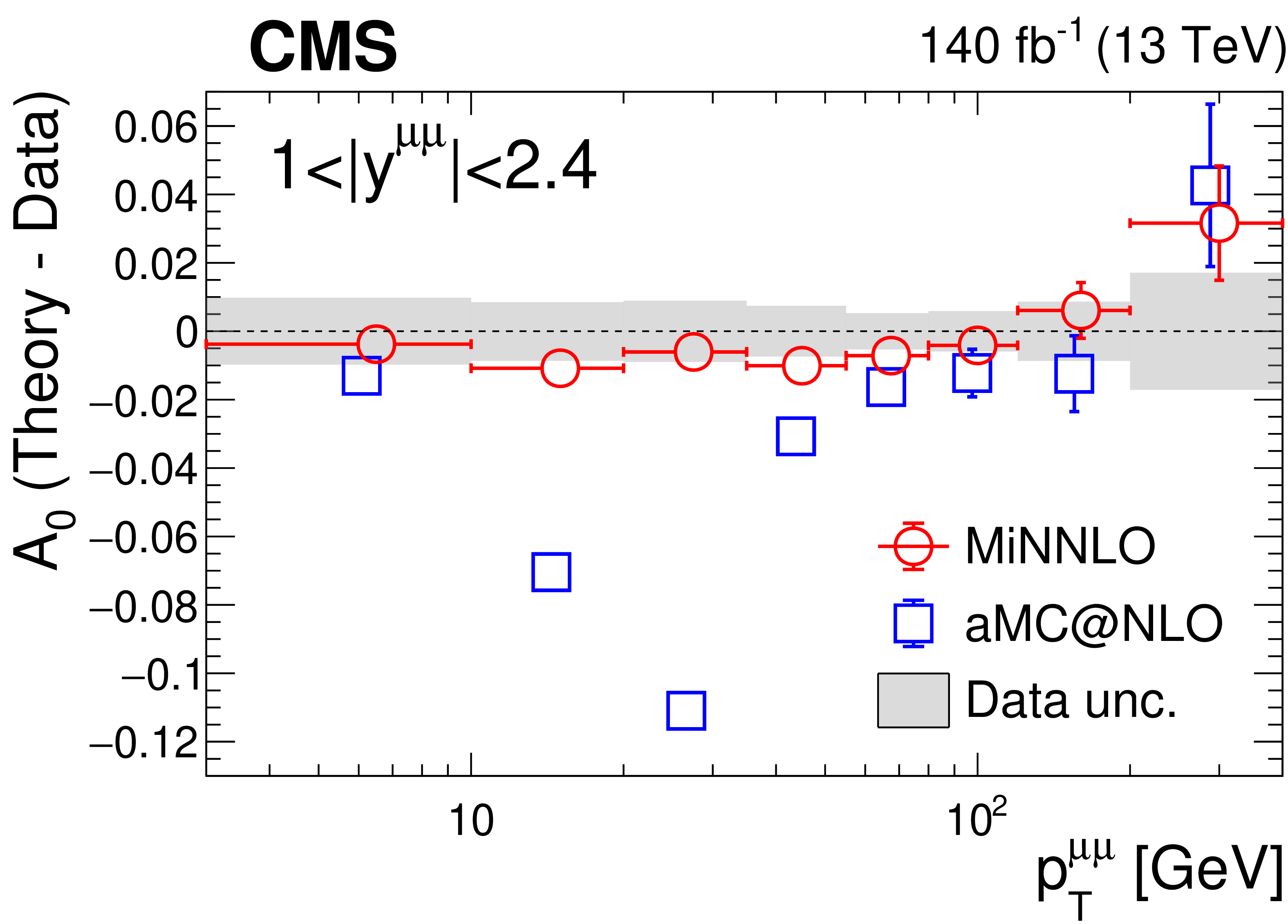
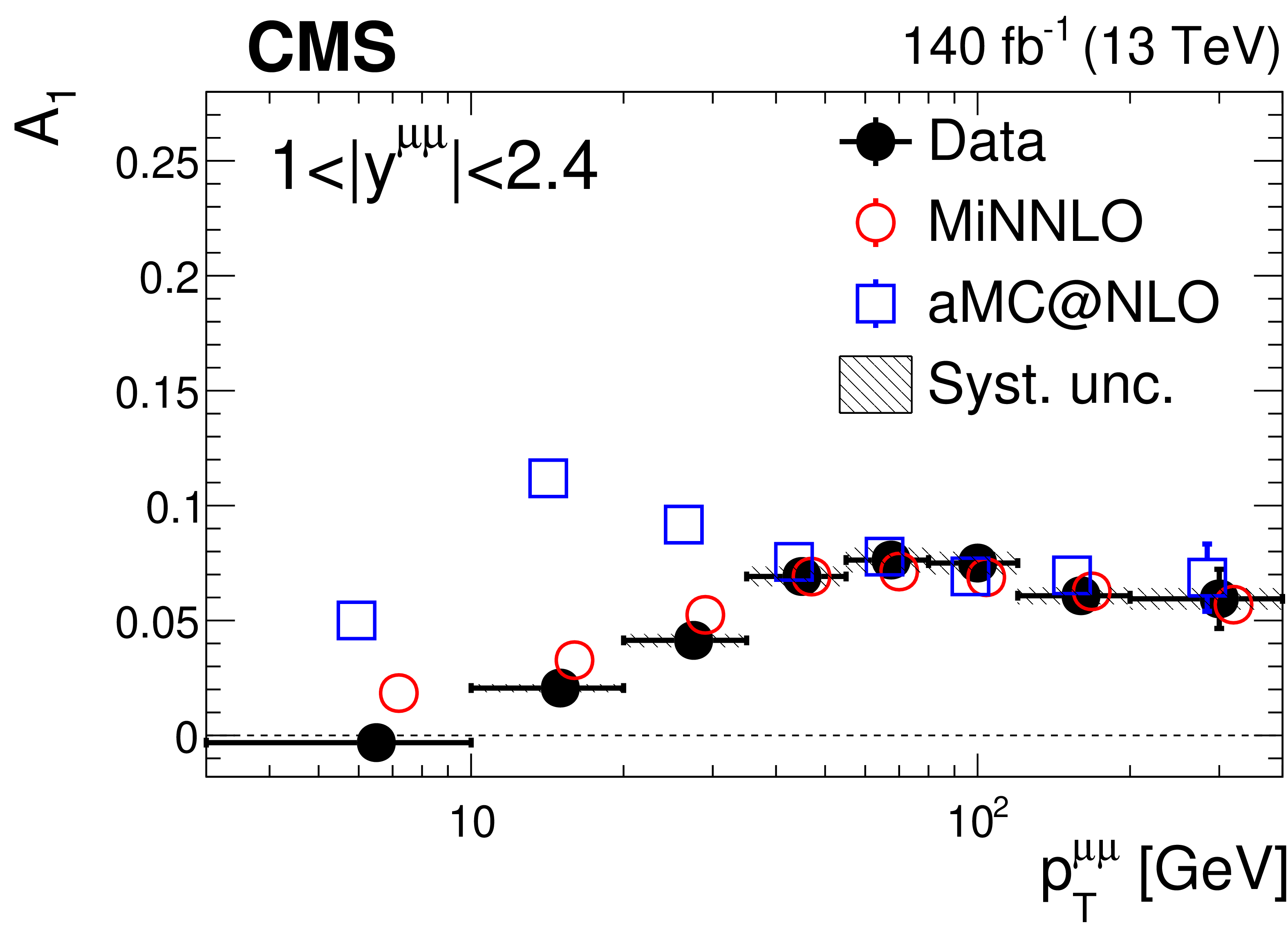
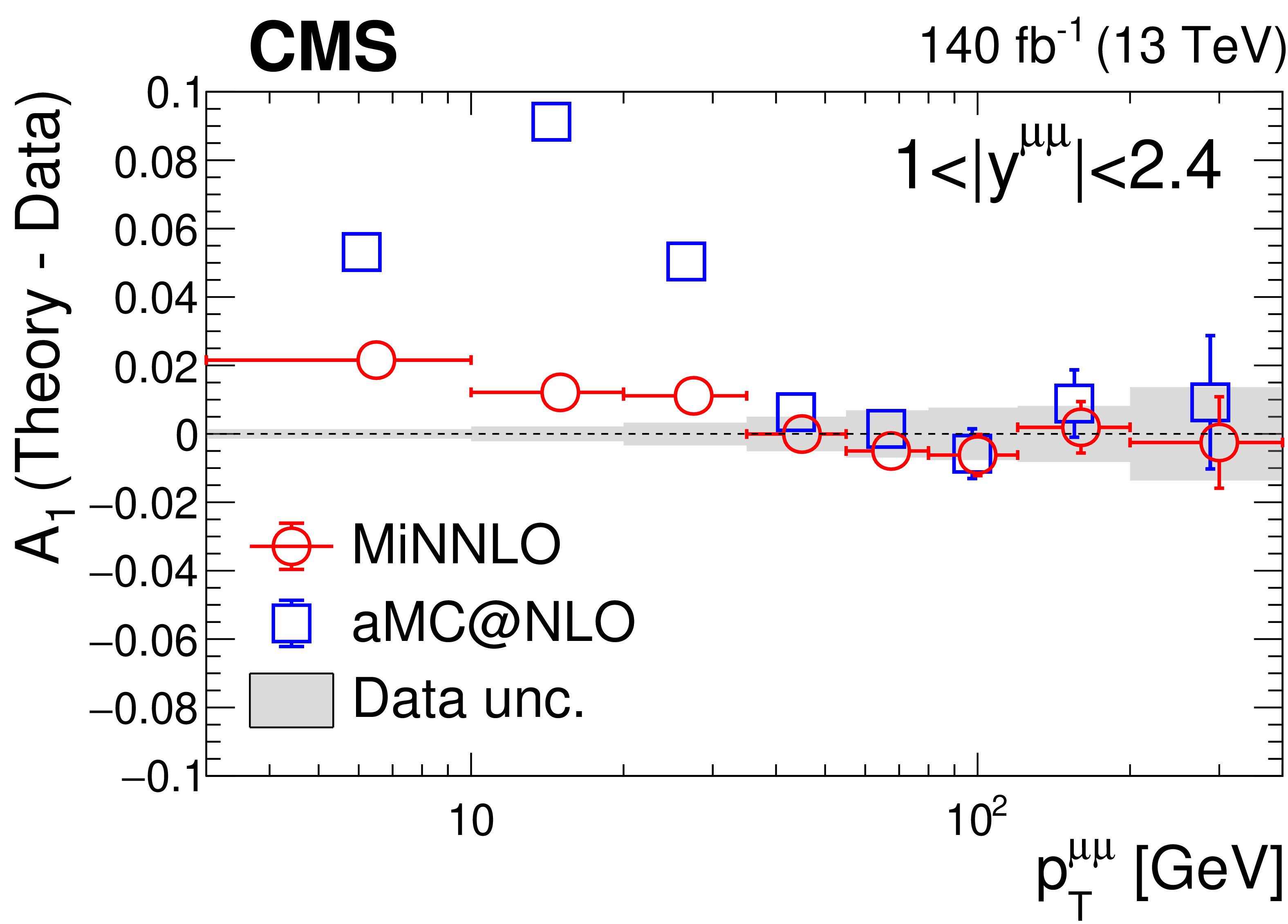
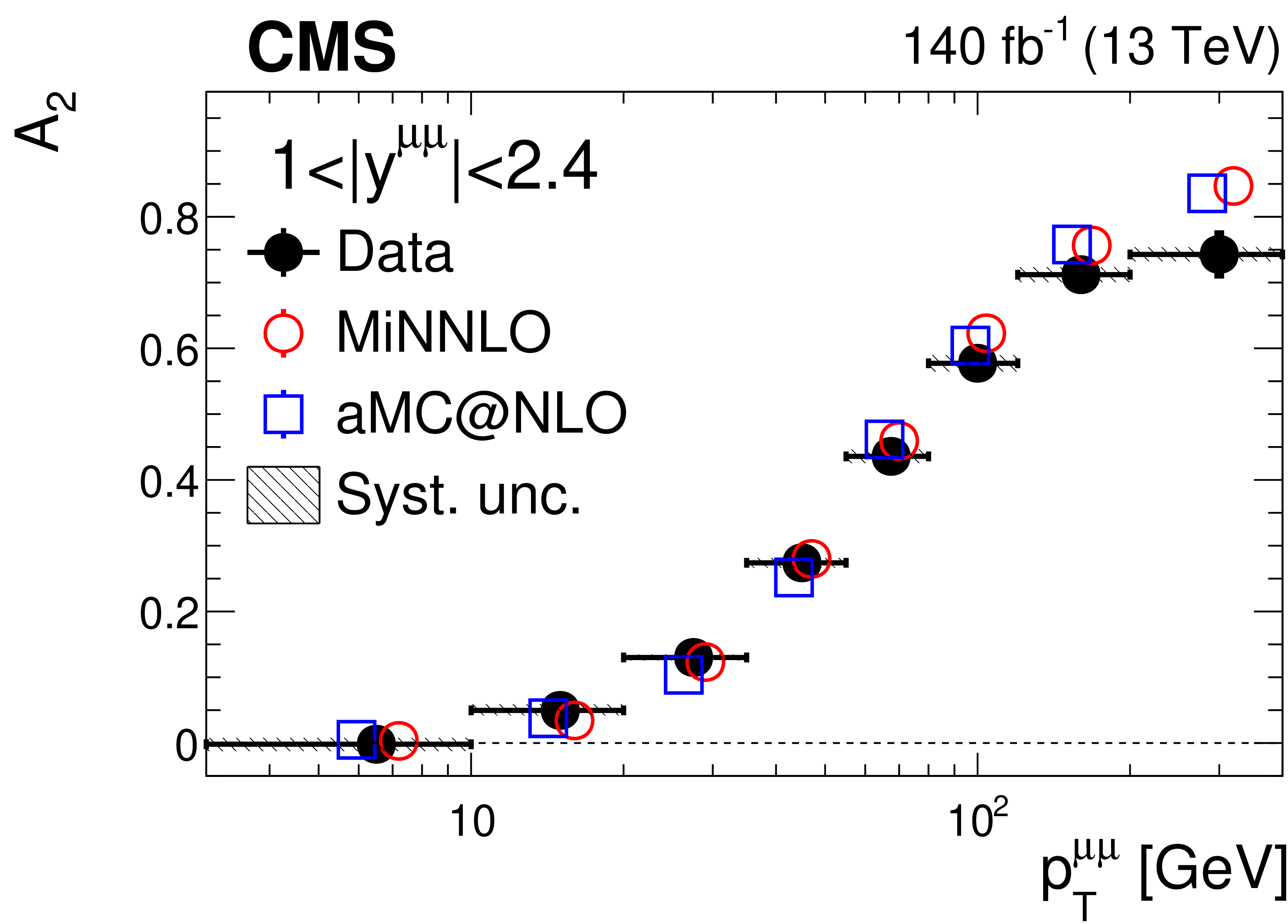
Figure 3:
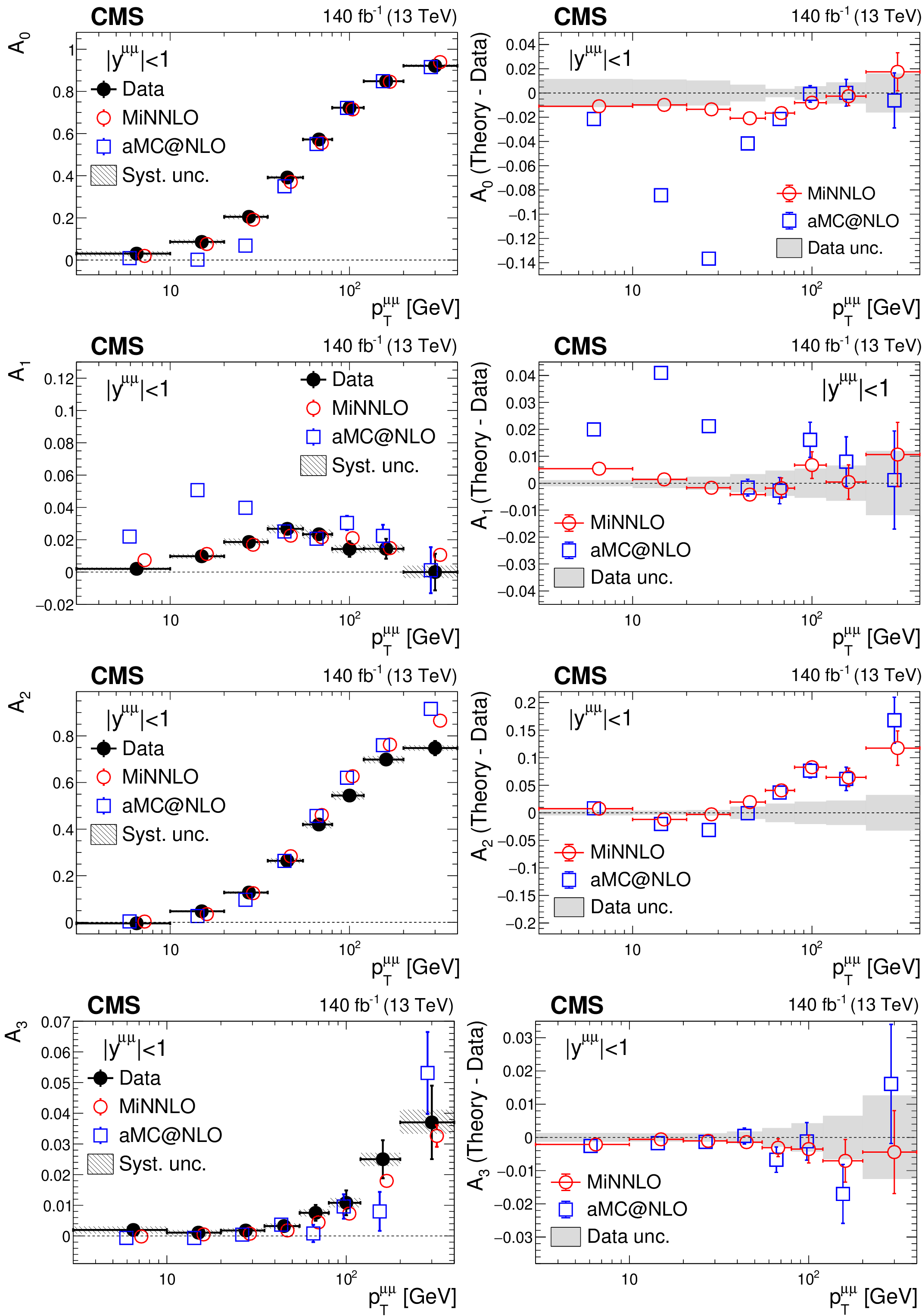
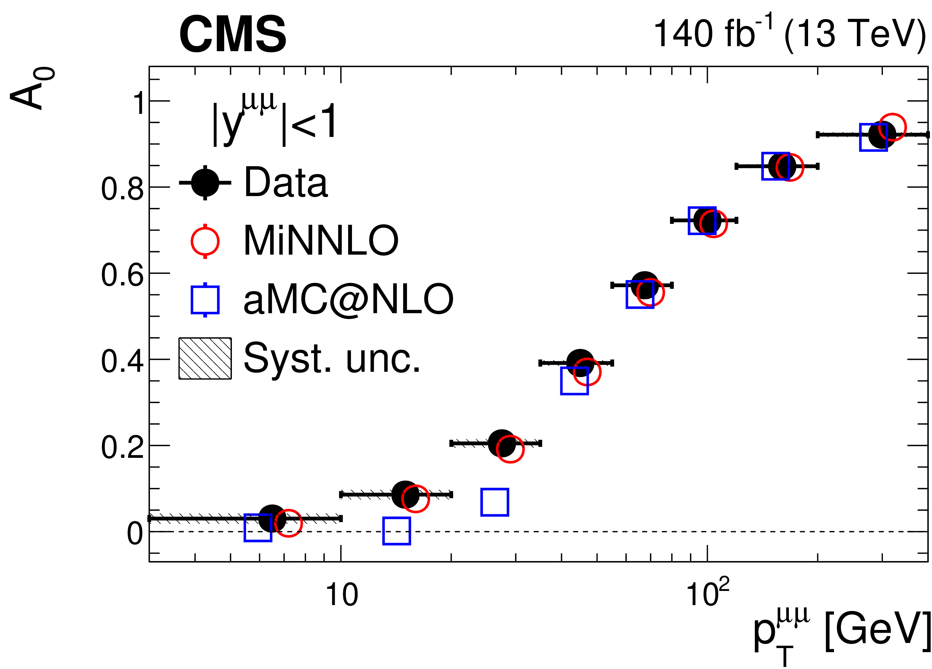
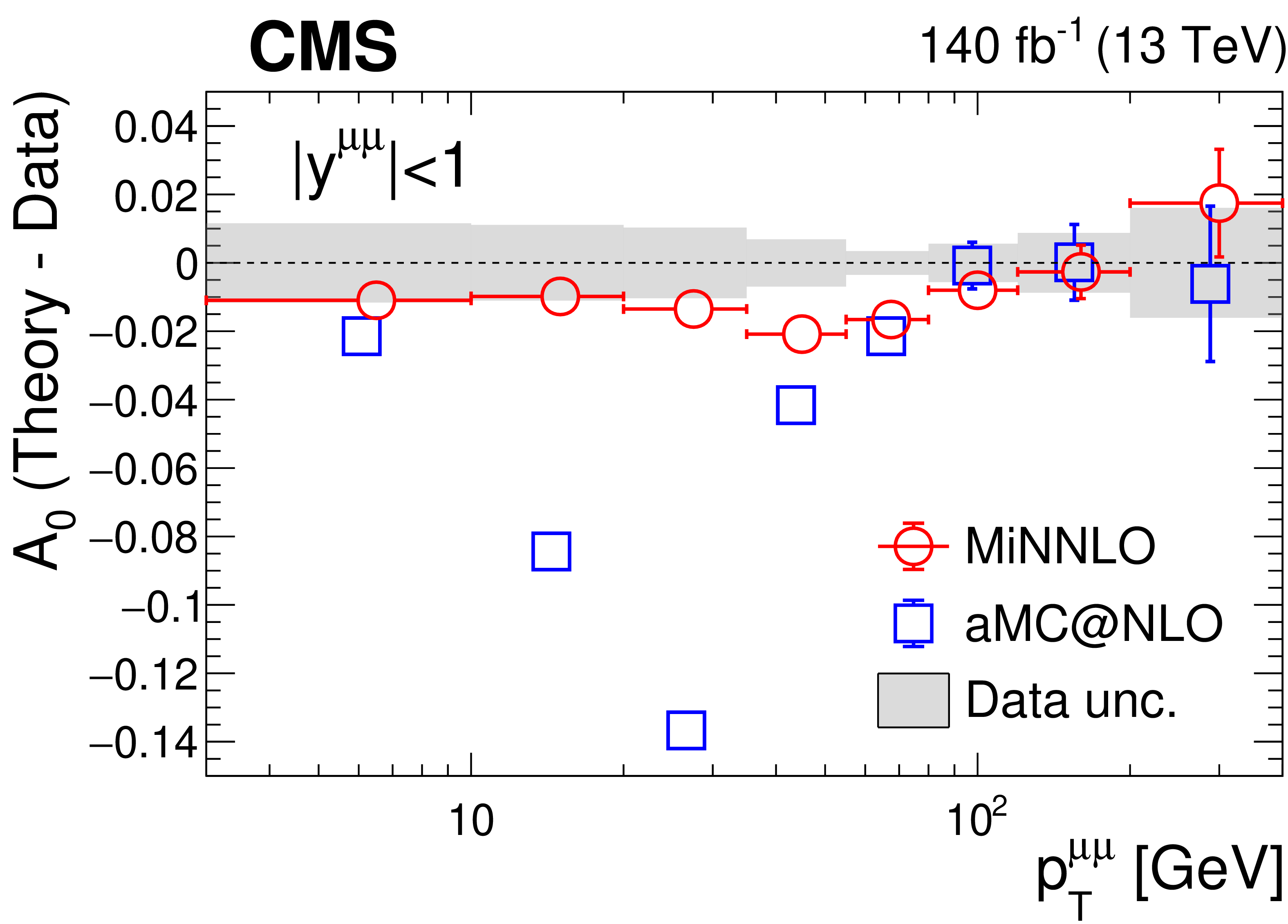
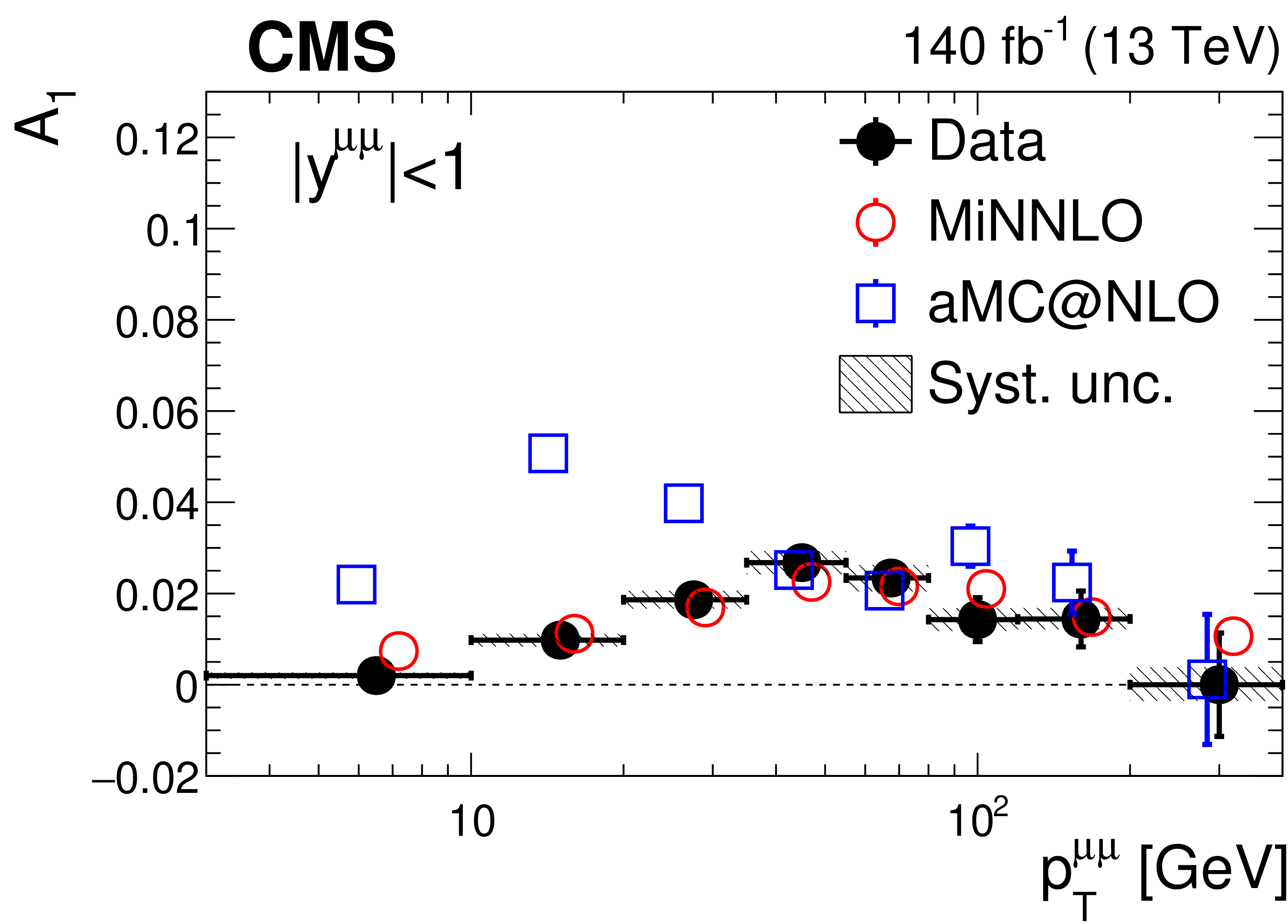
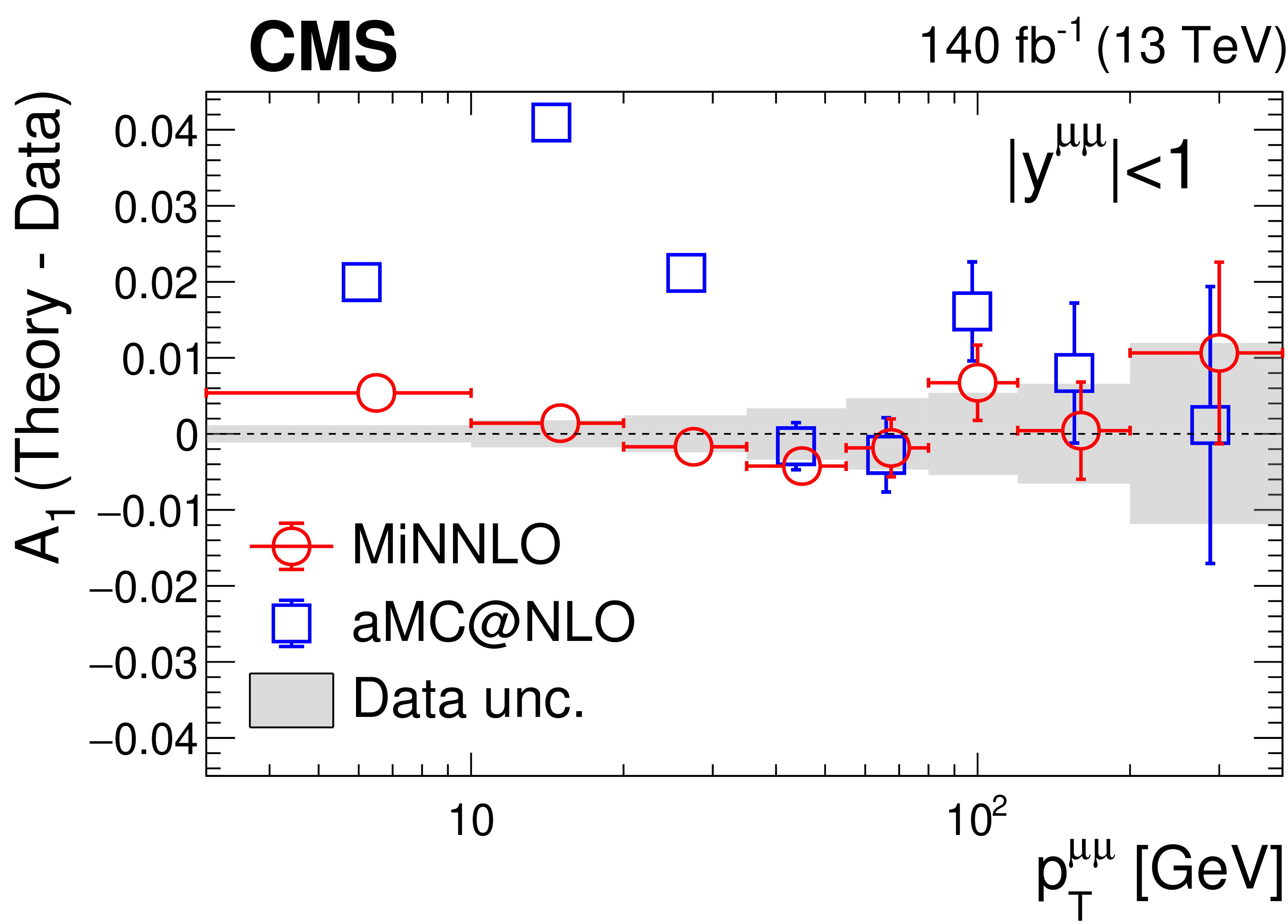
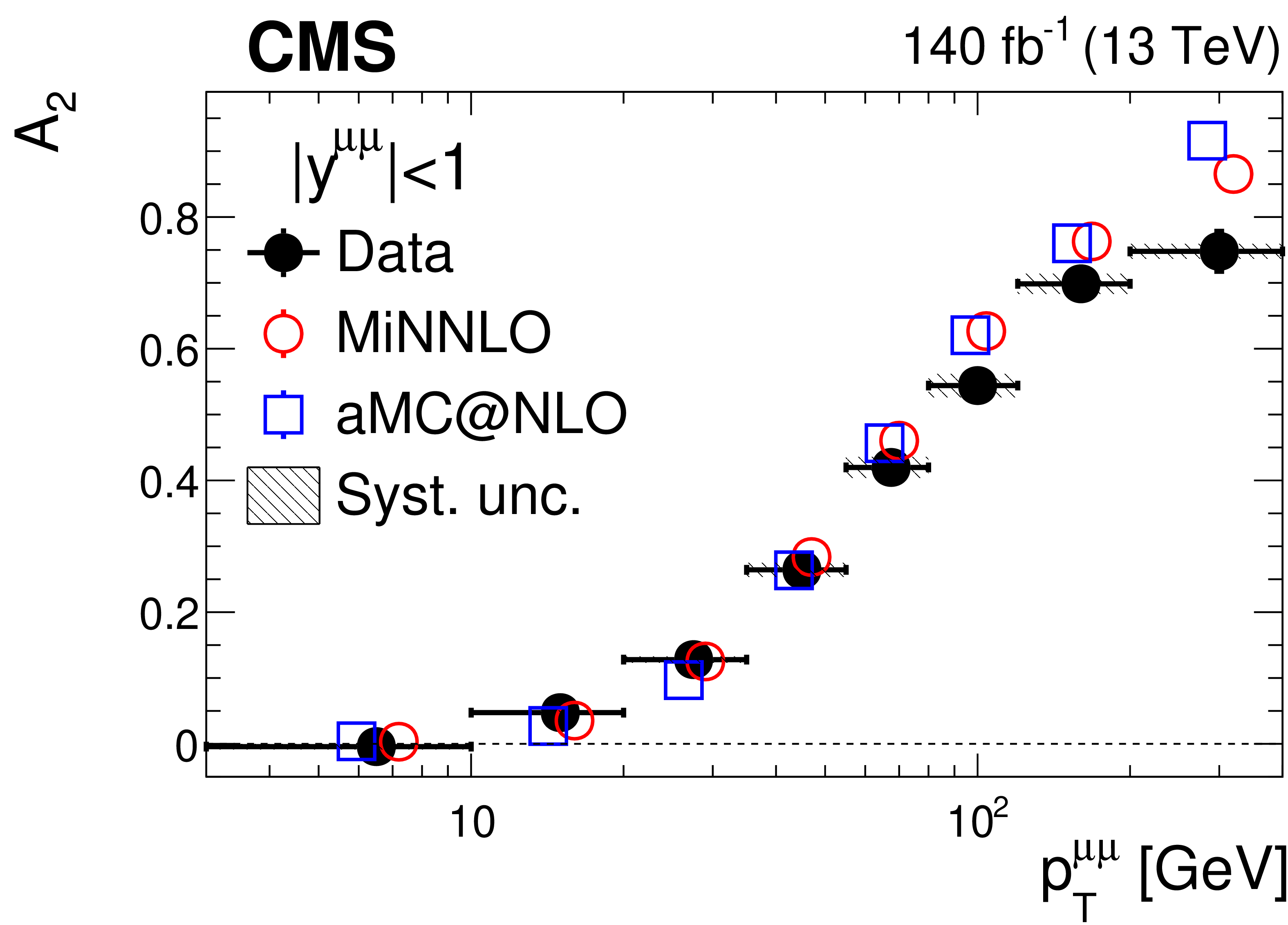
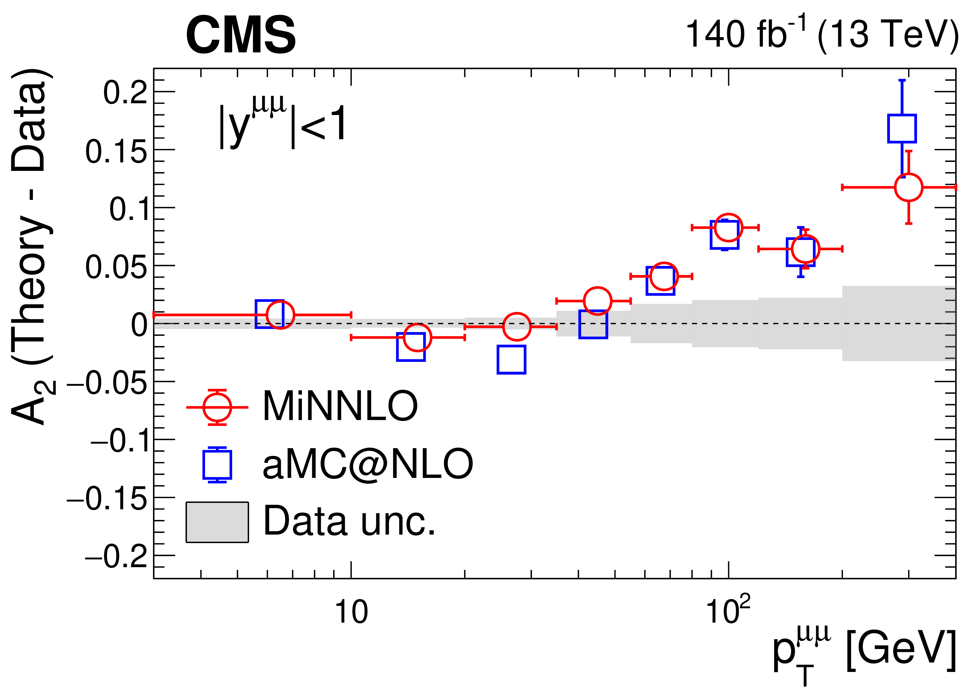
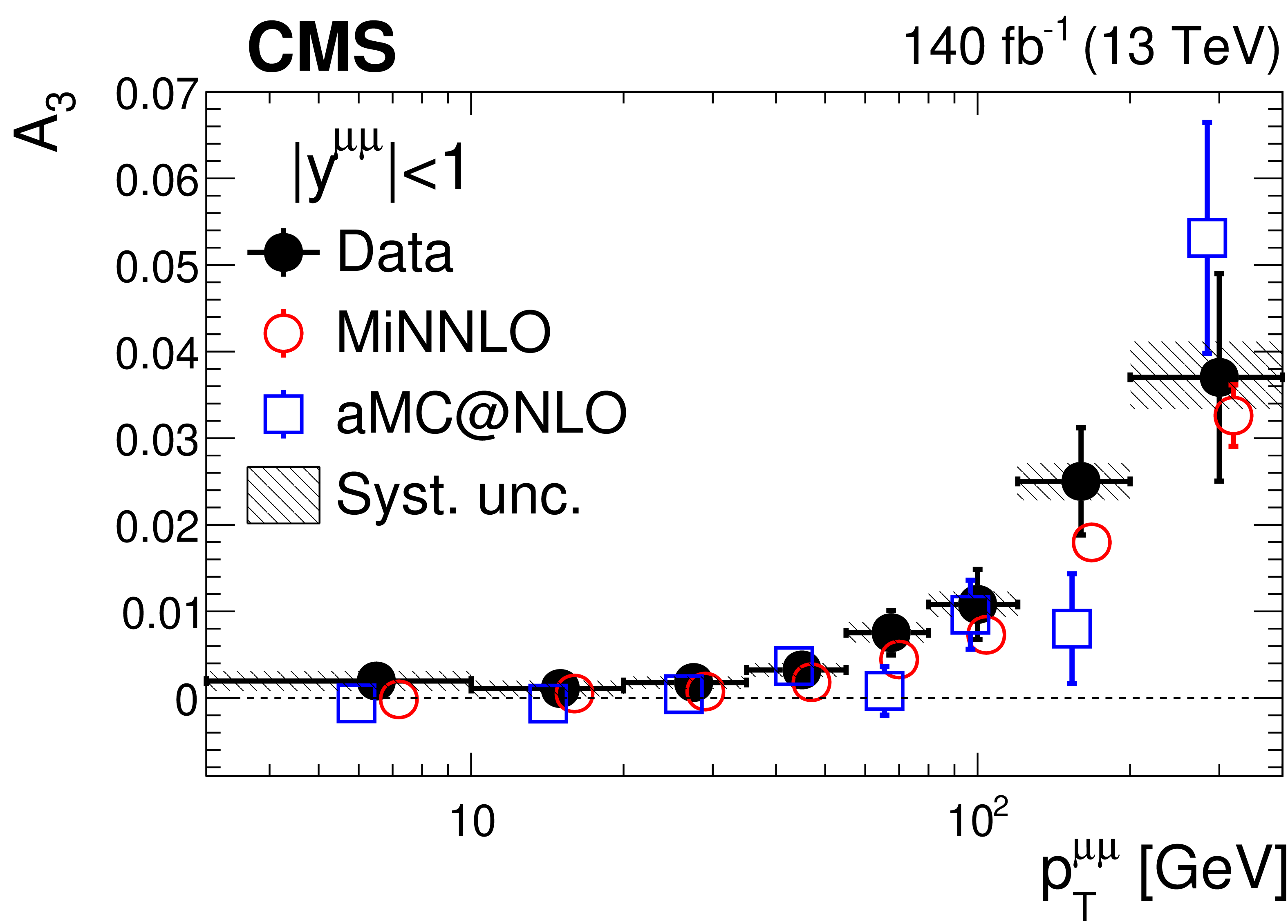
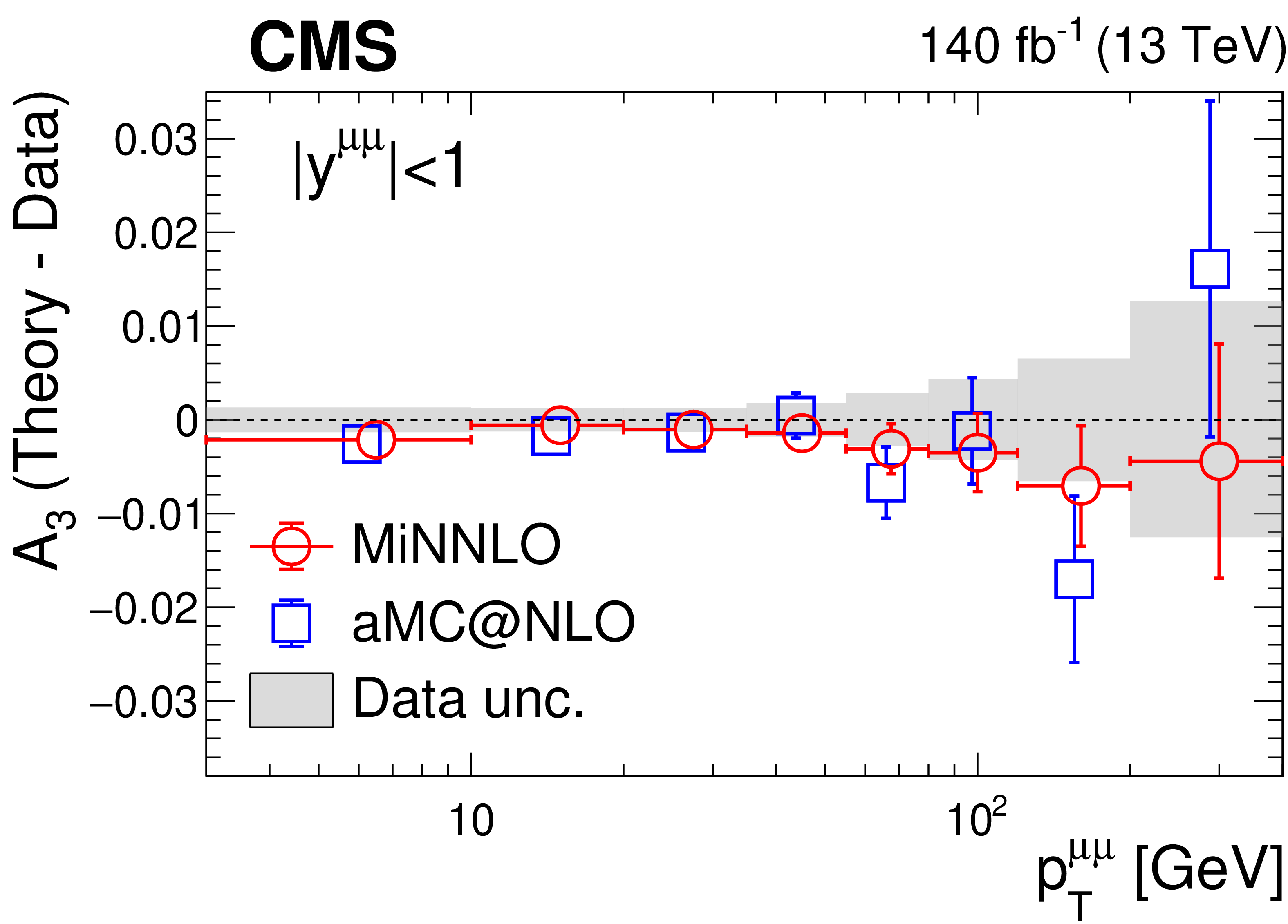
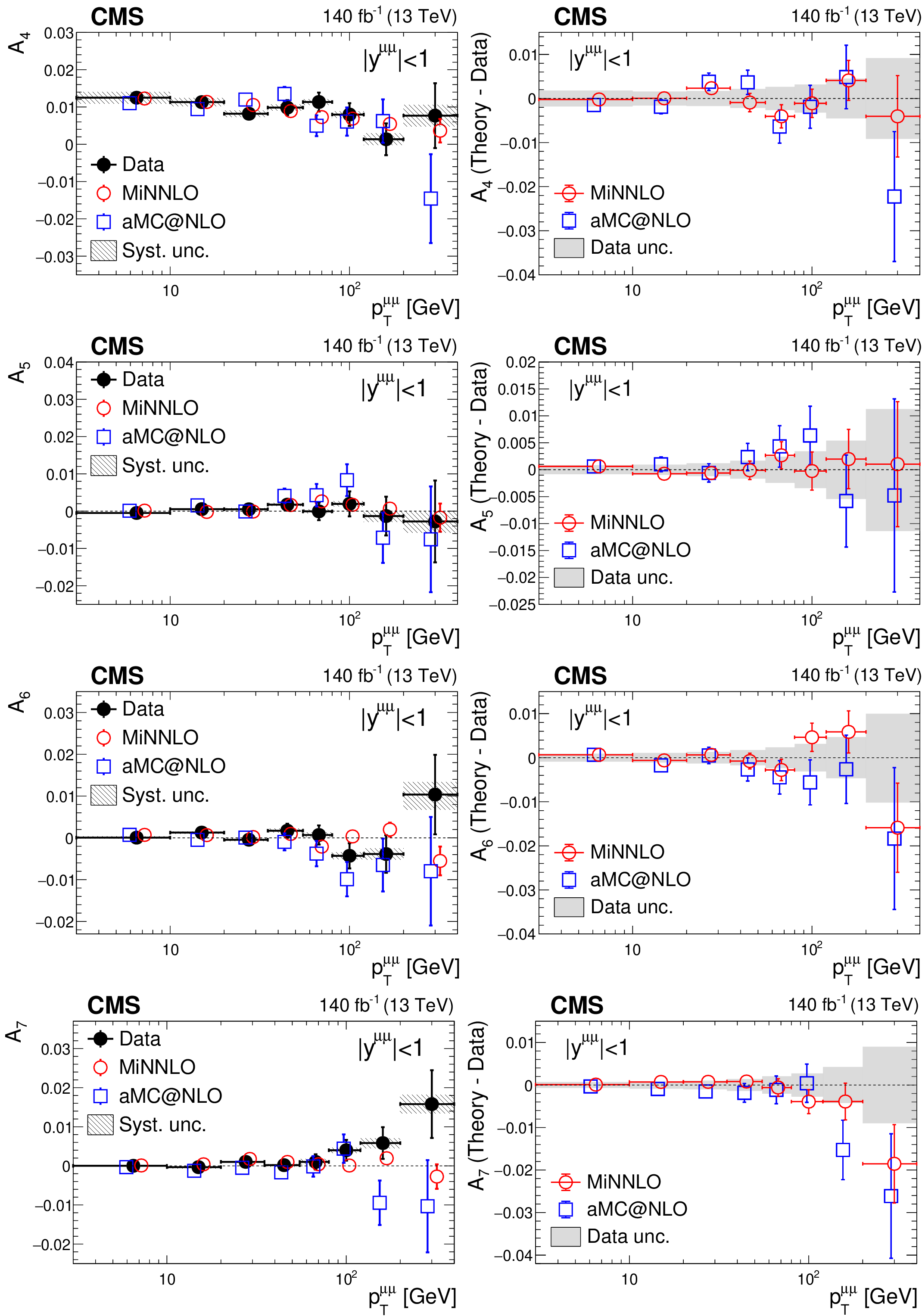
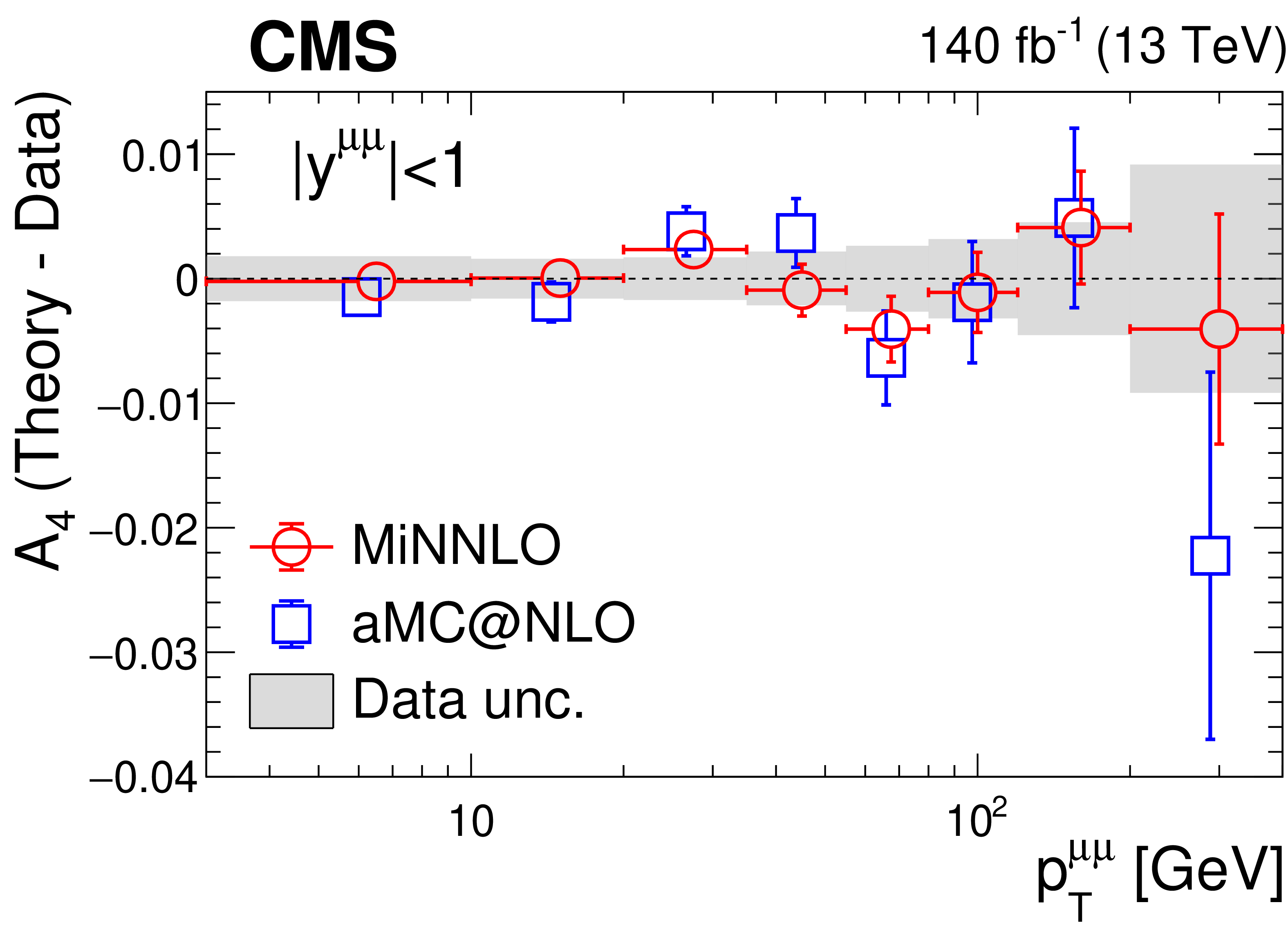
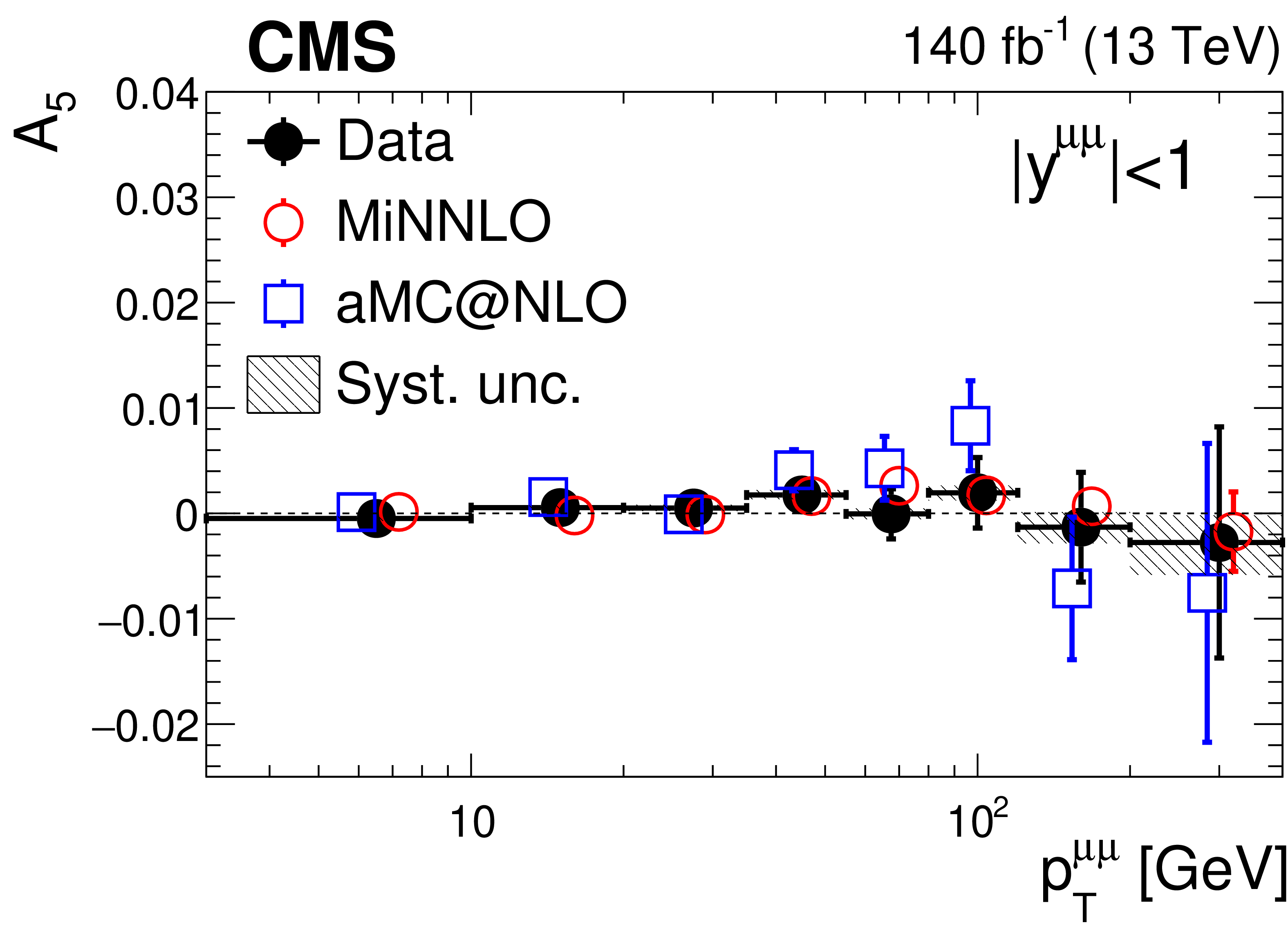
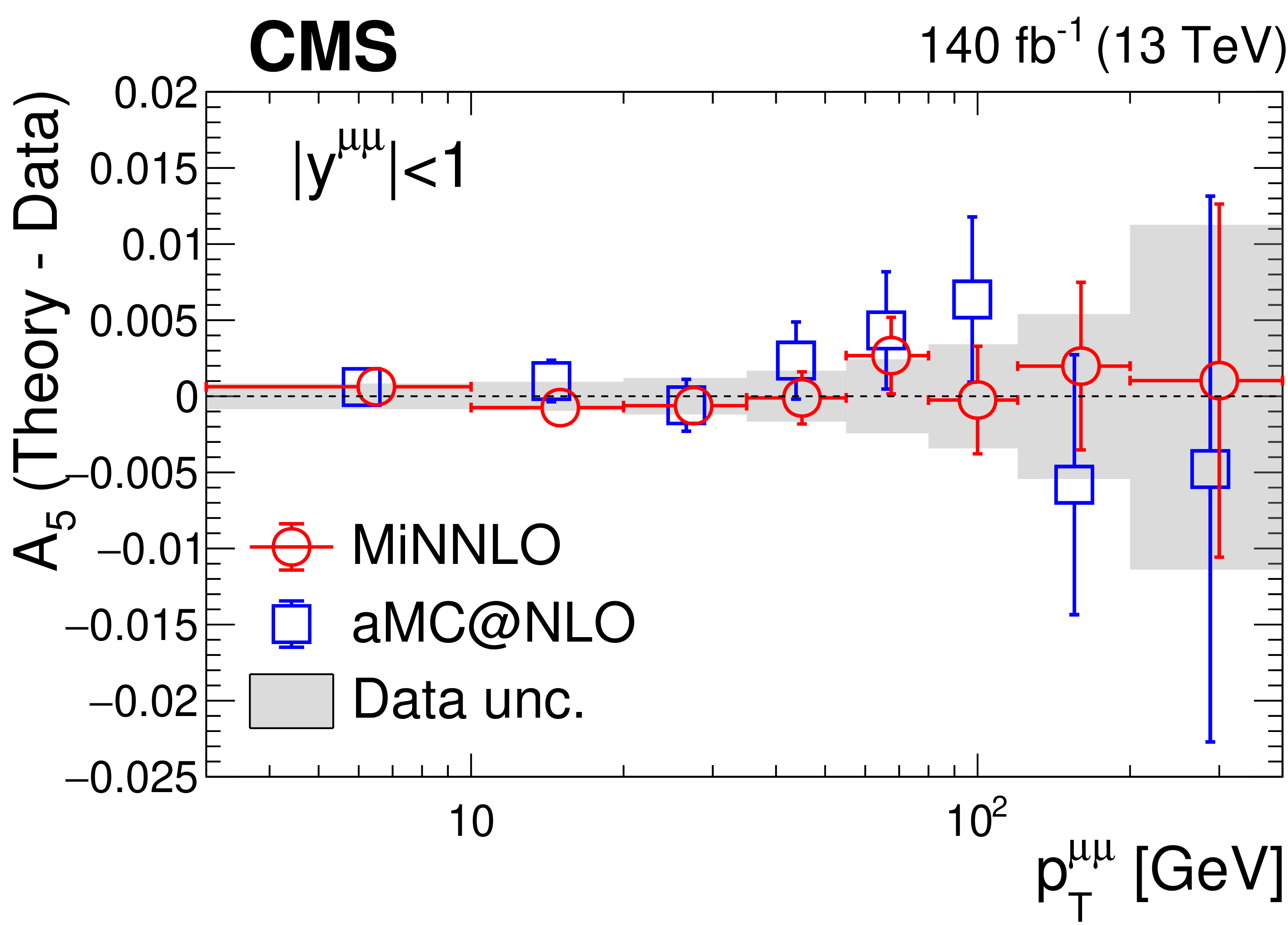
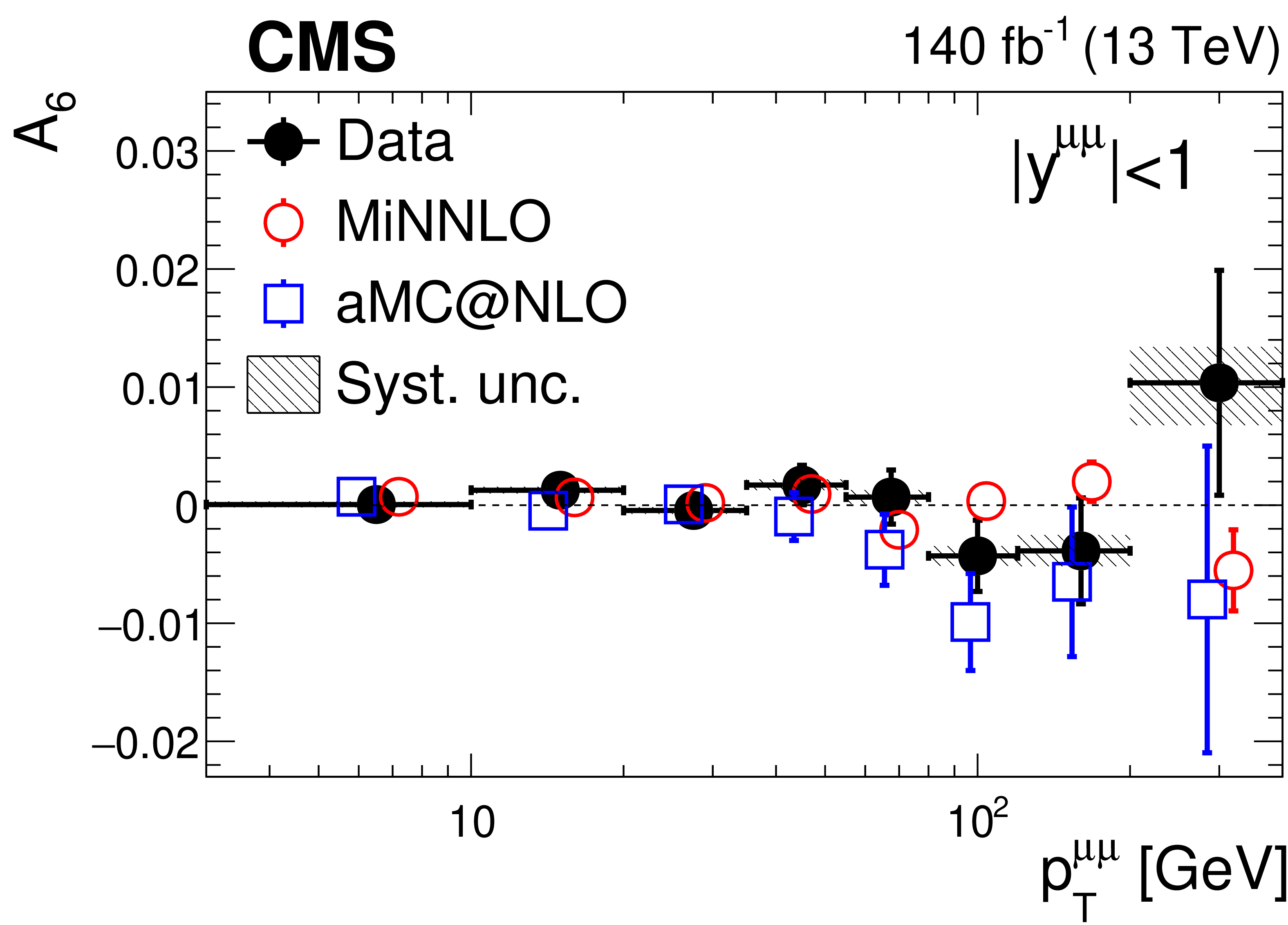
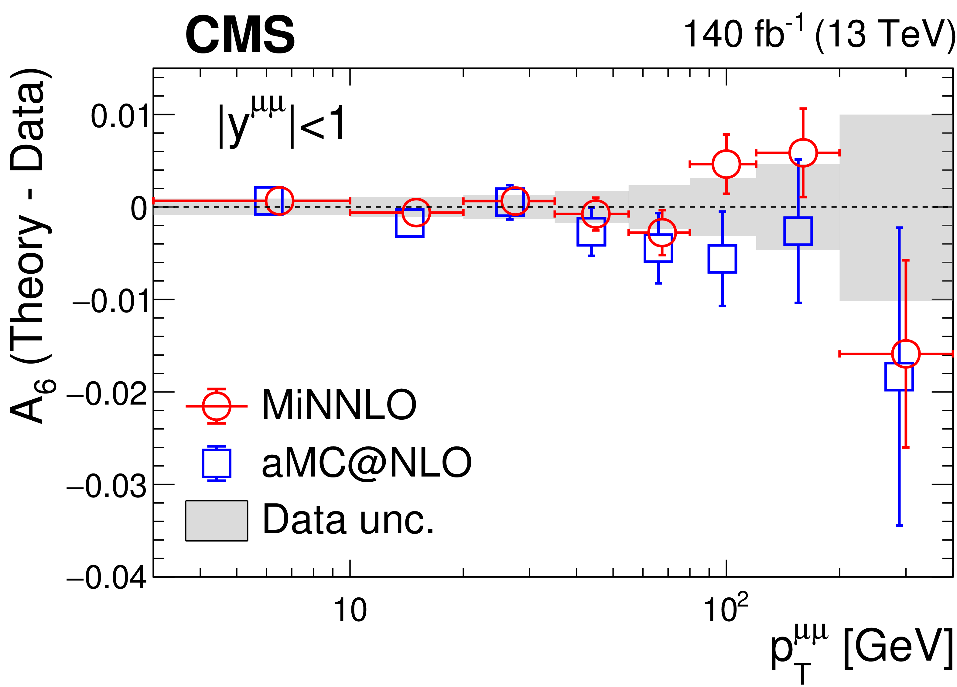
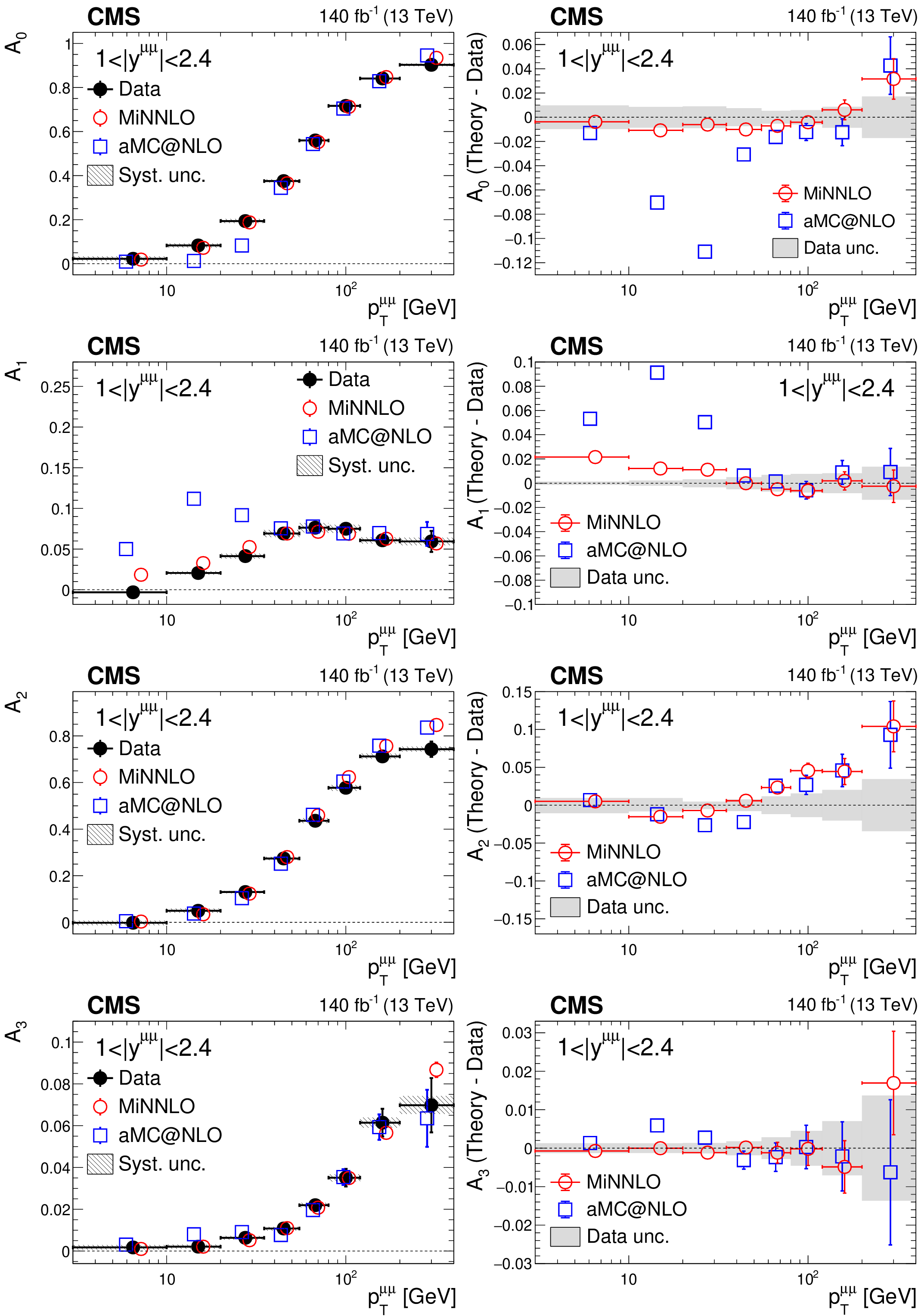
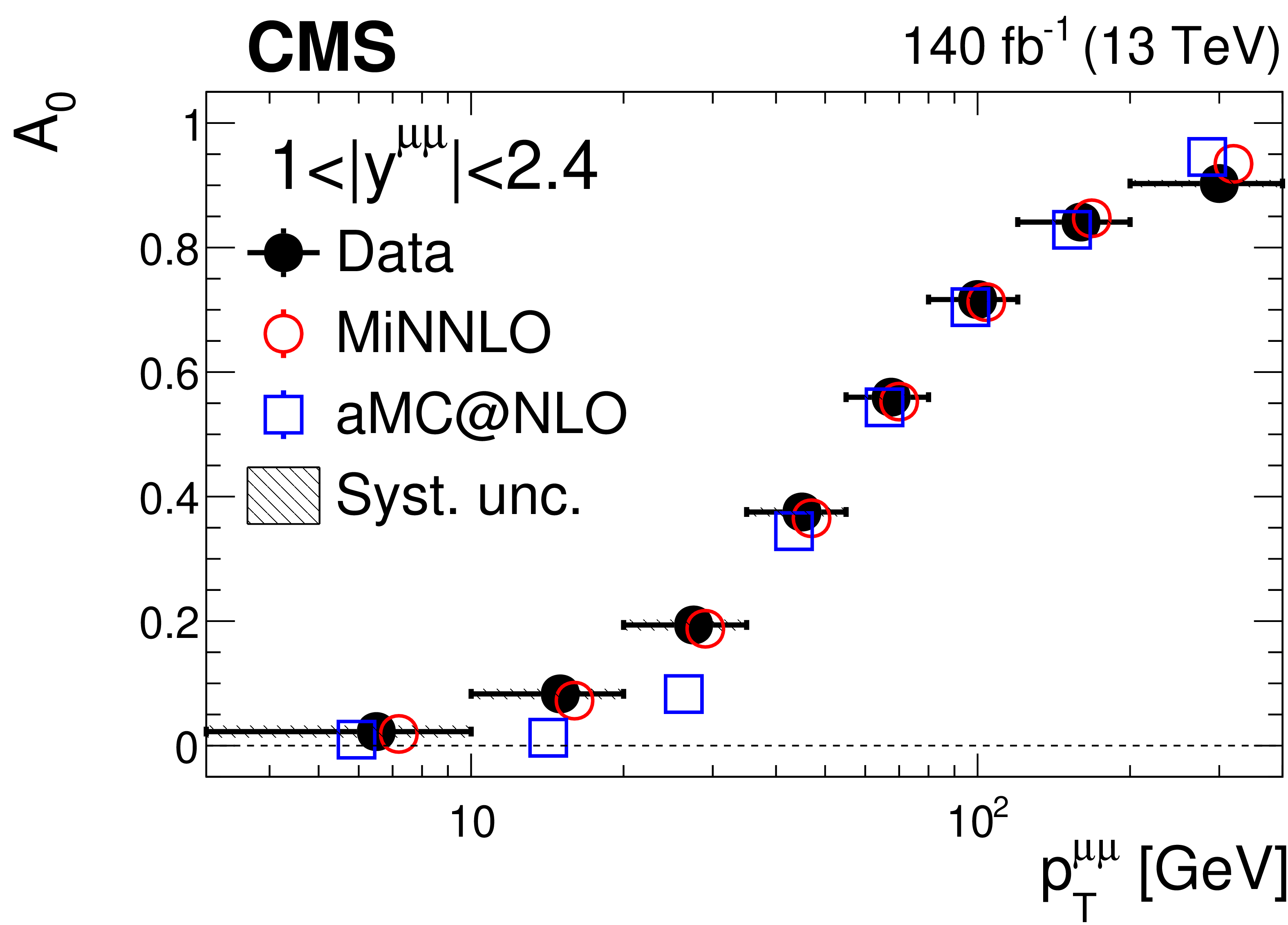
Left: Polarization coefficients $ A_{0} $ to $ A_{3} $ measured in the CS frame in bins of $ p_{\mathrm{T}}^{\mu\mu} $ for $ |y^{\mu\mu}| < $ 1. The data points are shown as black circles. The POWHEG+MINNLO and the MadGraph-5_aMC@NLO predictions are represented by the red circles and blue squares, respectively, slightly displaced horizontally for improved visibility. The vertical bars (hatched boxes) represent the statistical (systematic) uncertainties. Right: Difference between the predicted and measured values. The gray area around zero represents the total uncertainty of the measurement, while the vertical bars represent the statistical uncertainties of the predictions. |
png pdf |
Figure 3-a:
Left: Polarization coefficients $ A_{0} $ to $ A_{3} $ measured in the CS frame in bins of $ p_{\mathrm{T}}^{\mu\mu} $ for $ |y^{\mu\mu}| < $ 1. The data points are shown as black circles. The POWHEG+MINNLO and the MadGraph-5_aMC@NLO predictions are represented by the red circles and blue squares, respectively, slightly displaced horizontally for improved visibility. The vertical bars (hatched boxes) represent the statistical (systematic) uncertainties. Right: Difference between the predicted and measured values. The gray area around zero represents the total uncertainty of the measurement, while the vertical bars represent the statistical uncertainties of the predictions. |
png pdf |
Figure 3-b:
Left: Polarization coefficients $ A_{0} $ to $ A_{3} $ measured in the CS frame in bins of $ p_{\mathrm{T}}^{\mu\mu} $ for $ |y^{\mu\mu}| < $ 1. The data points are shown as black circles. The POWHEG+MINNLO and the MadGraph-5_aMC@NLO predictions are represented by the red circles and blue squares, respectively, slightly displaced horizontally for improved visibility. The vertical bars (hatched boxes) represent the statistical (systematic) uncertainties. Right: Difference between the predicted and measured values. The gray area around zero represents the total uncertainty of the measurement, while the vertical bars represent the statistical uncertainties of the predictions. |
png pdf |
Figure 3-c:
Left: Polarization coefficients $ A_{0} $ to $ A_{3} $ measured in the CS frame in bins of $ p_{\mathrm{T}}^{\mu\mu} $ for $ |y^{\mu\mu}| < $ 1. The data points are shown as black circles. The POWHEG+MINNLO and the MadGraph-5_aMC@NLO predictions are represented by the red circles and blue squares, respectively, slightly displaced horizontally for improved visibility. The vertical bars (hatched boxes) represent the statistical (systematic) uncertainties. Right: Difference between the predicted and measured values. The gray area around zero represents the total uncertainty of the measurement, while the vertical bars represent the statistical uncertainties of the predictions. |
png pdf |
Figure 3-d:
Left: Polarization coefficients $ A_{0} $ to $ A_{3} $ measured in the CS frame in bins of $ p_{\mathrm{T}}^{\mu\mu} $ for $ |y^{\mu\mu}| < $ 1. The data points are shown as black circles. The POWHEG+MINNLO and the MadGraph-5_aMC@NLO predictions are represented by the red circles and blue squares, respectively, slightly displaced horizontally for improved visibility. The vertical bars (hatched boxes) represent the statistical (systematic) uncertainties. Right: Difference between the predicted and measured values. The gray area around zero represents the total uncertainty of the measurement, while the vertical bars represent the statistical uncertainties of the predictions. |
png pdf |
Figure 3-e:
Left: Polarization coefficients $ A_{0} $ to $ A_{3} $ measured in the CS frame in bins of $ p_{\mathrm{T}}^{\mu\mu} $ for $ |y^{\mu\mu}| < $ 1. The data points are shown as black circles. The POWHEG+MINNLO and the MadGraph-5_aMC@NLO predictions are represented by the red circles and blue squares, respectively, slightly displaced horizontally for improved visibility. The vertical bars (hatched boxes) represent the statistical (systematic) uncertainties. Right: Difference between the predicted and measured values. The gray area around zero represents the total uncertainty of the measurement, while the vertical bars represent the statistical uncertainties of the predictions. |
png pdf |
Figure 3-f:
Left: Polarization coefficients $ A_{0} $ to $ A_{3} $ measured in the CS frame in bins of $ p_{\mathrm{T}}^{\mu\mu} $ for $ |y^{\mu\mu}| < $ 1. The data points are shown as black circles. The POWHEG+MINNLO and the MadGraph-5_aMC@NLO predictions are represented by the red circles and blue squares, respectively, slightly displaced horizontally for improved visibility. The vertical bars (hatched boxes) represent the statistical (systematic) uncertainties. Right: Difference between the predicted and measured values. The gray area around zero represents the total uncertainty of the measurement, while the vertical bars represent the statistical uncertainties of the predictions. |
png pdf |
Figure 3-g:
Left: Polarization coefficients $ A_{0} $ to $ A_{3} $ measured in the CS frame in bins of $ p_{\mathrm{T}}^{\mu\mu} $ for $ |y^{\mu\mu}| < $ 1. The data points are shown as black circles. The POWHEG+MINNLO and the MadGraph-5_aMC@NLO predictions are represented by the red circles and blue squares, respectively, slightly displaced horizontally for improved visibility. The vertical bars (hatched boxes) represent the statistical (systematic) uncertainties. Right: Difference between the predicted and measured values. The gray area around zero represents the total uncertainty of the measurement, while the vertical bars represent the statistical uncertainties of the predictions. |
png pdf |
Figure 3-h:
Left: Polarization coefficients $ A_{0} $ to $ A_{3} $ measured in the CS frame in bins of $ p_{\mathrm{T}}^{\mu\mu} $ for $ |y^{\mu\mu}| < $ 1. The data points are shown as black circles. The POWHEG+MINNLO and the MadGraph-5_aMC@NLO predictions are represented by the red circles and blue squares, respectively, slightly displaced horizontally for improved visibility. The vertical bars (hatched boxes) represent the statistical (systematic) uncertainties. Right: Difference between the predicted and measured values. The gray area around zero represents the total uncertainty of the measurement, while the vertical bars represent the statistical uncertainties of the predictions. |
png pdf |
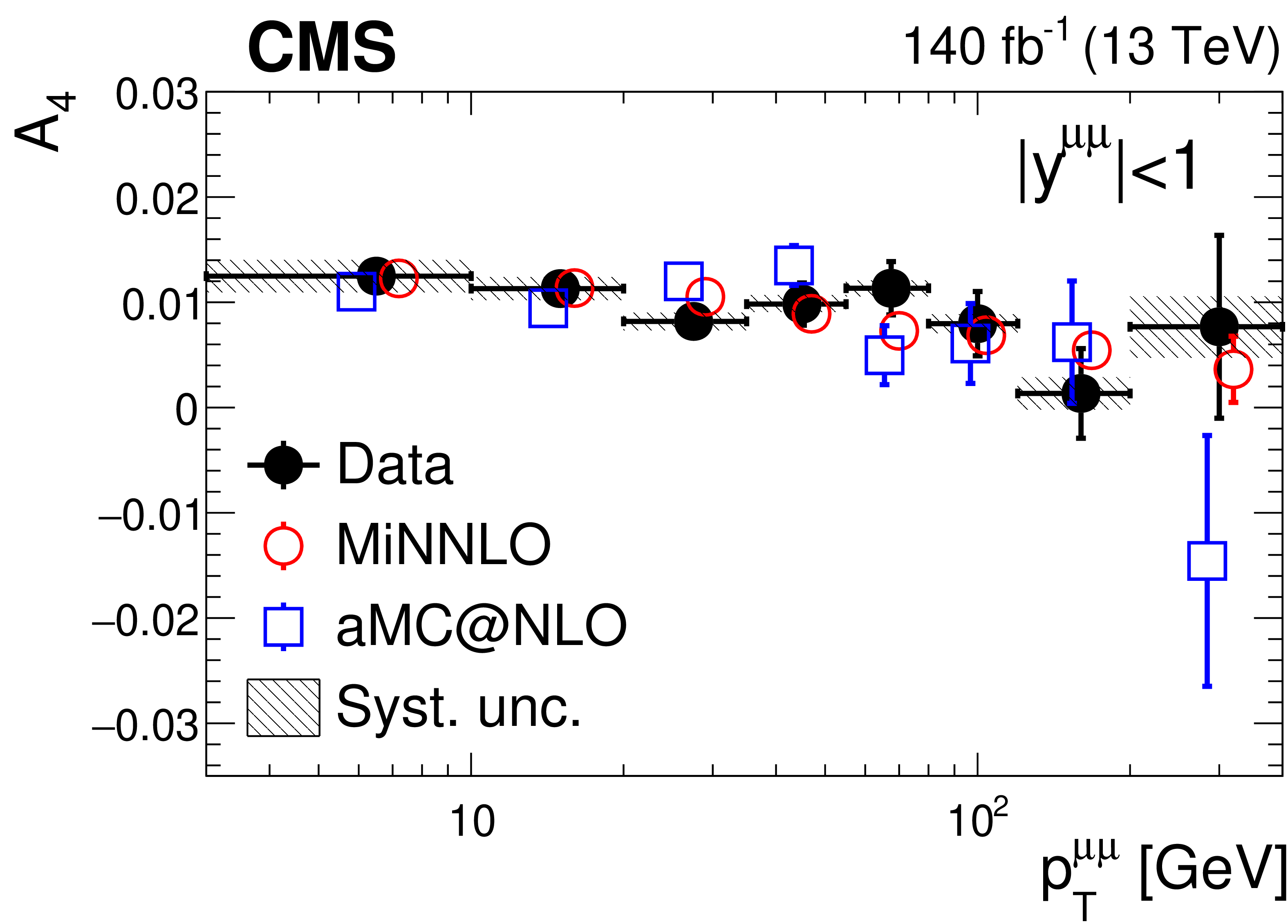
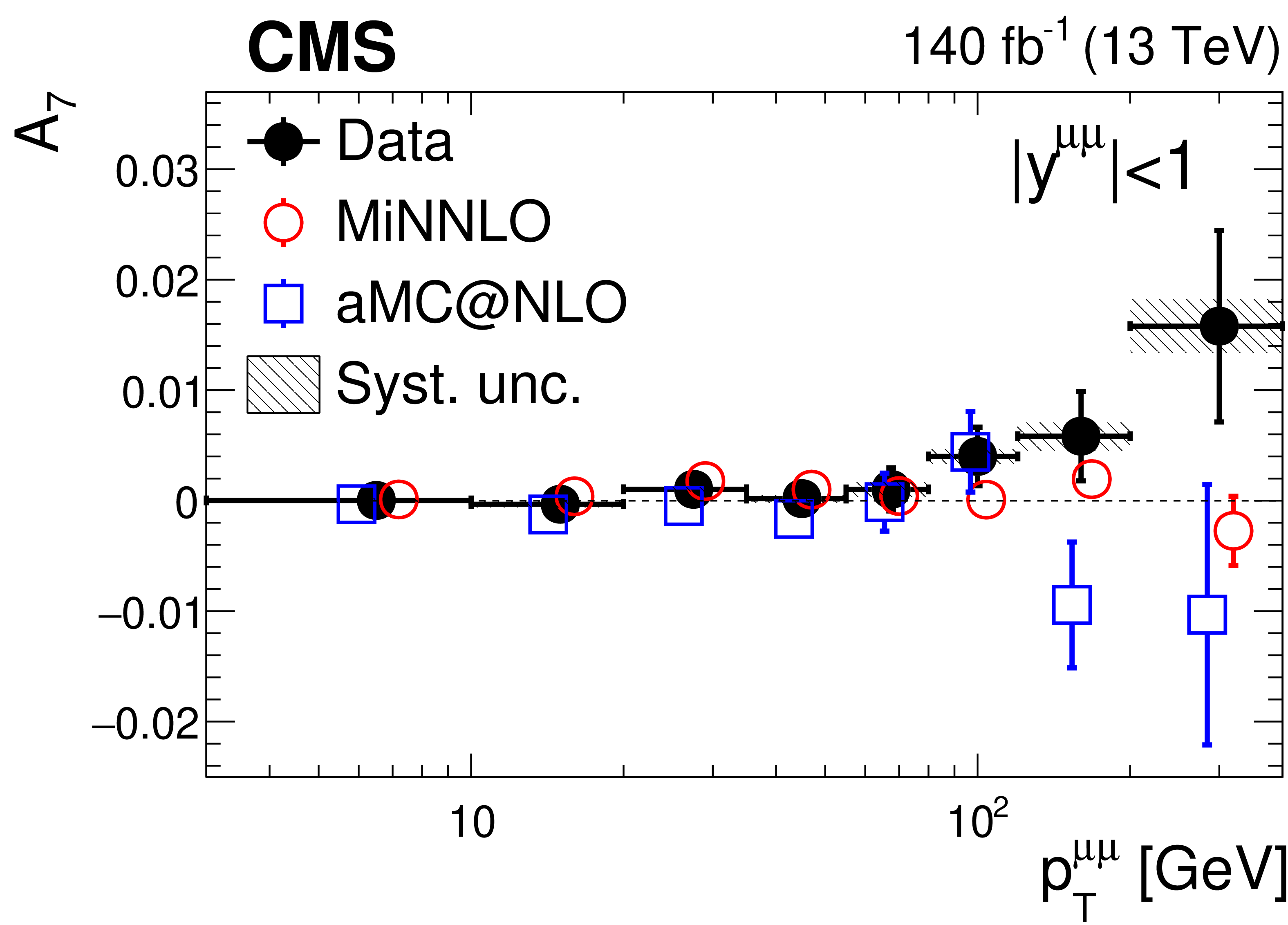
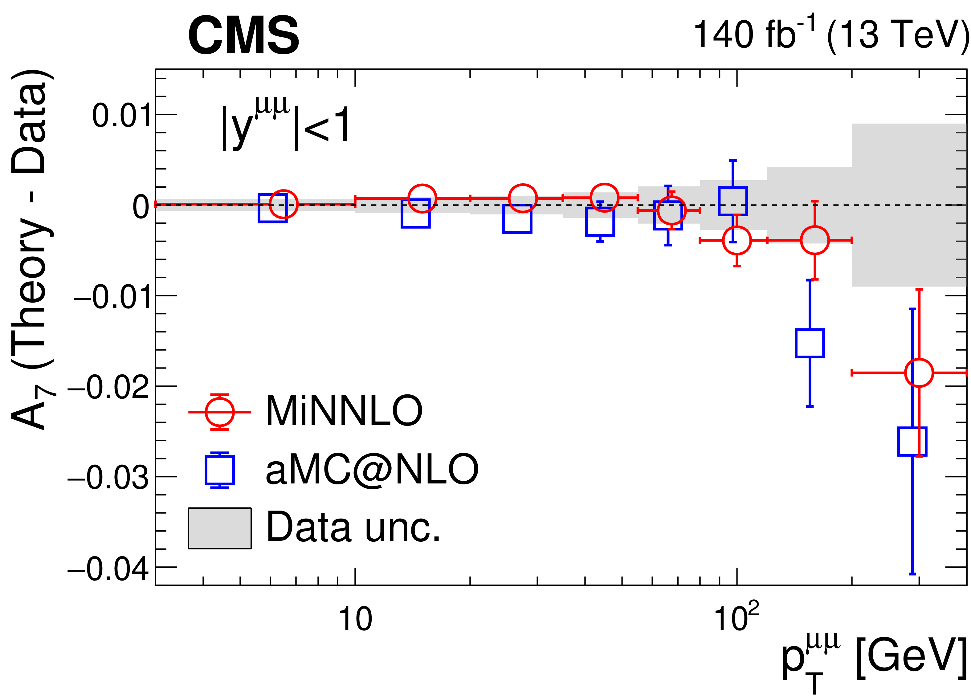
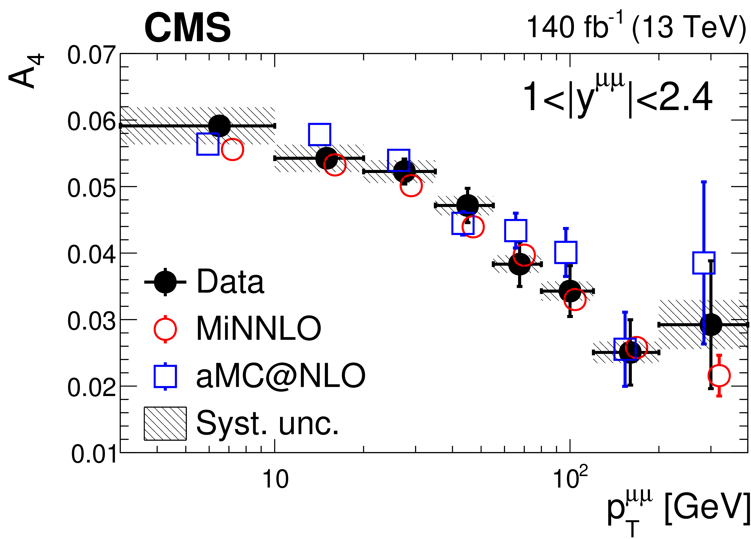
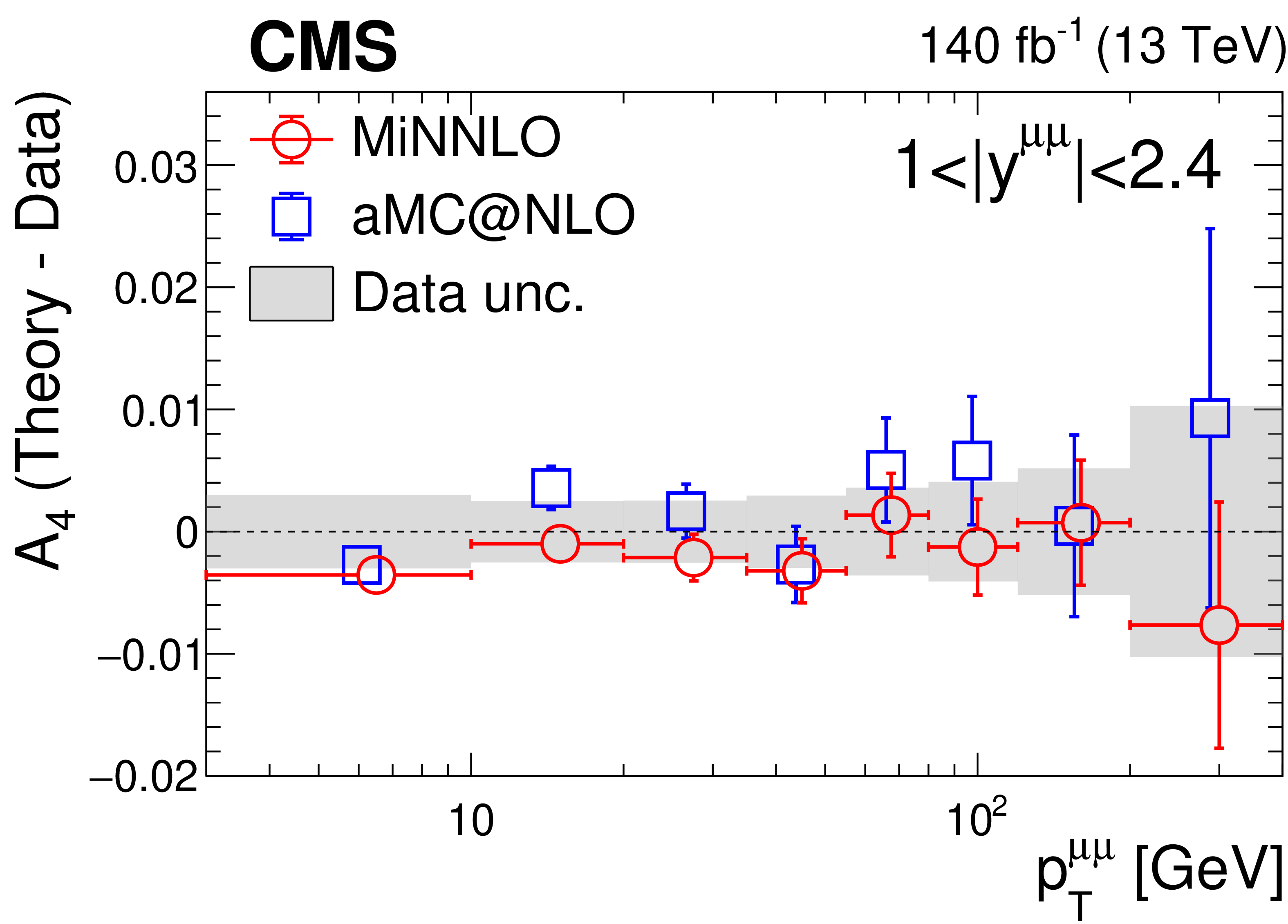
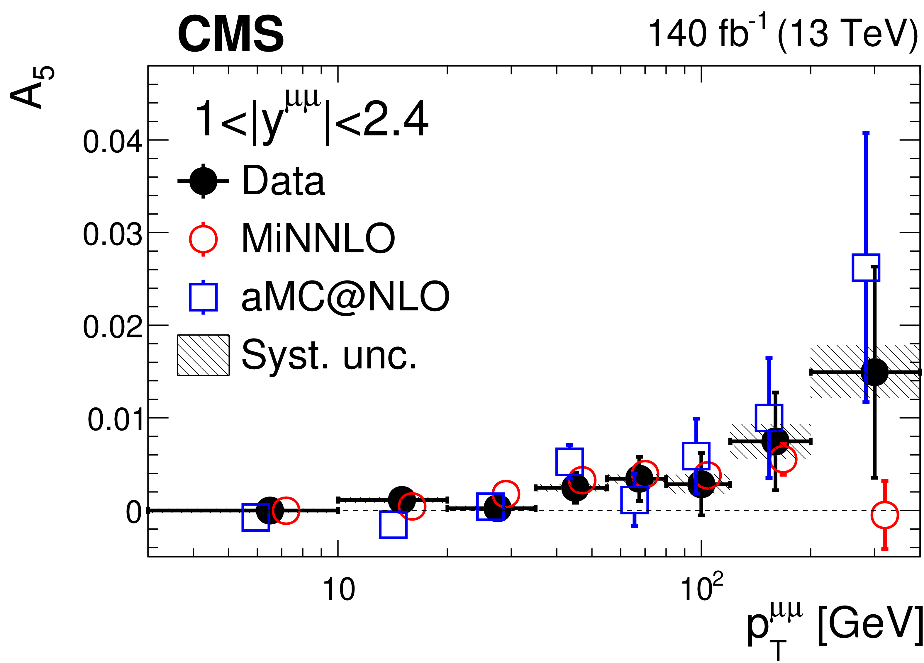
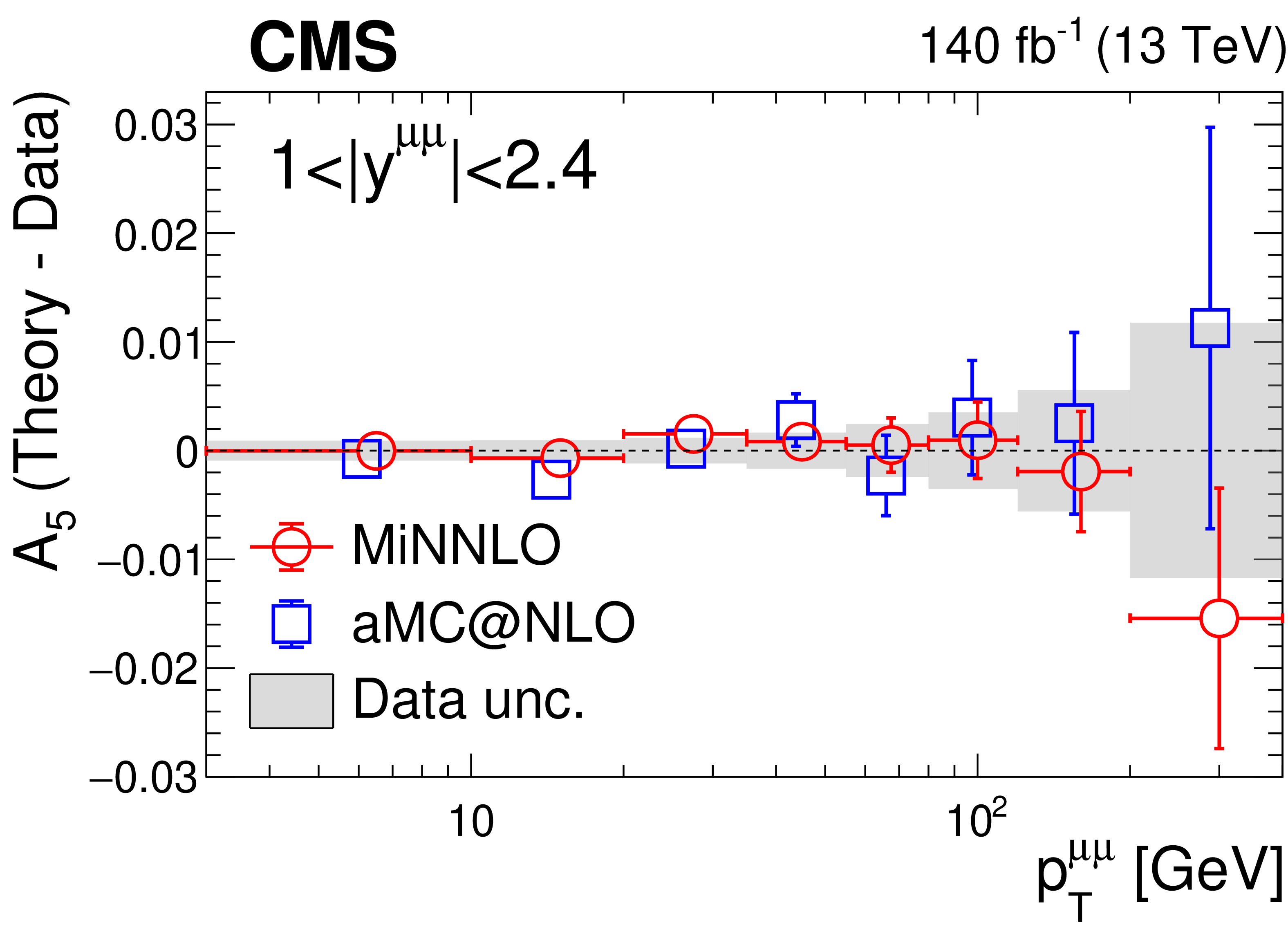
Figure 4:
Same as Fig. 3, for the polarization coefficients $ A_4 $ to $ A_7 $. |
png pdf |
Figure 4-a:
Same as Fig. 3, for the polarization coefficients $ A_4 $ to $ A_7 $. |
png pdf |
Figure 4-b:
Same as Fig. 3, for the polarization coefficients $ A_4 $ to $ A_7 $. |
png pdf |
Figure 4-c:
Same as Fig. 3, for the polarization coefficients $ A_4 $ to $ A_7 $. |
png pdf |
Figure 4-d:
Same as Fig. 3, for the polarization coefficients $ A_4 $ to $ A_7 $. |
png pdf |
Figure 4-e:
Same as Fig. 3, for the polarization coefficients $ A_4 $ to $ A_7 $. |
png pdf |
Figure 4-f:
Same as Fig. 3, for the polarization coefficients $ A_4 $ to $ A_7 $. |
png pdf |
Figure 4-g:
Same as Fig. 3, for the polarization coefficients $ A_4 $ to $ A_7 $. |
png pdf |
Figure 4-h:
Same as Fig. 3, for the polarization coefficients $ A_4 $ to $ A_7 $. |
png pdf |
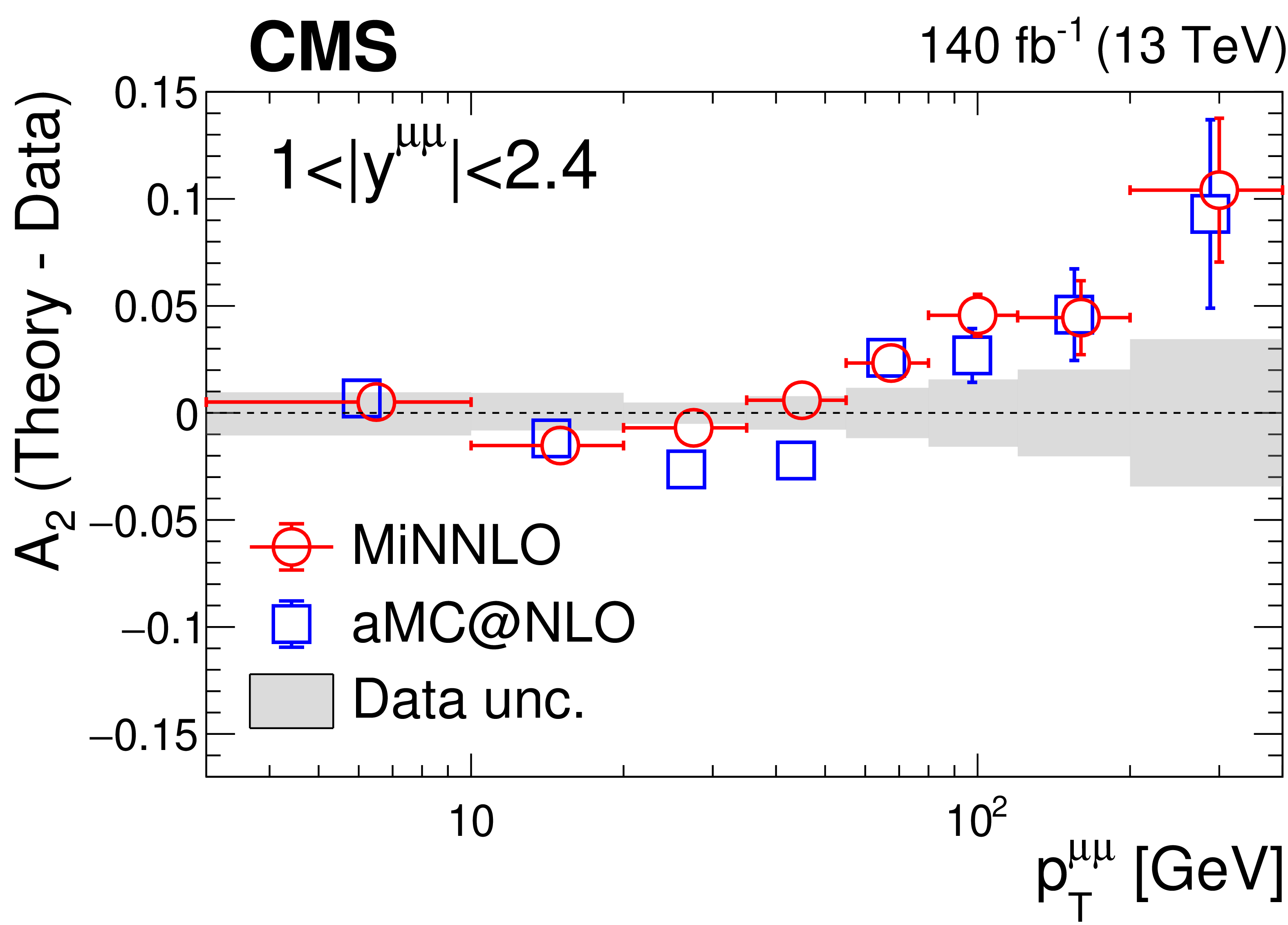
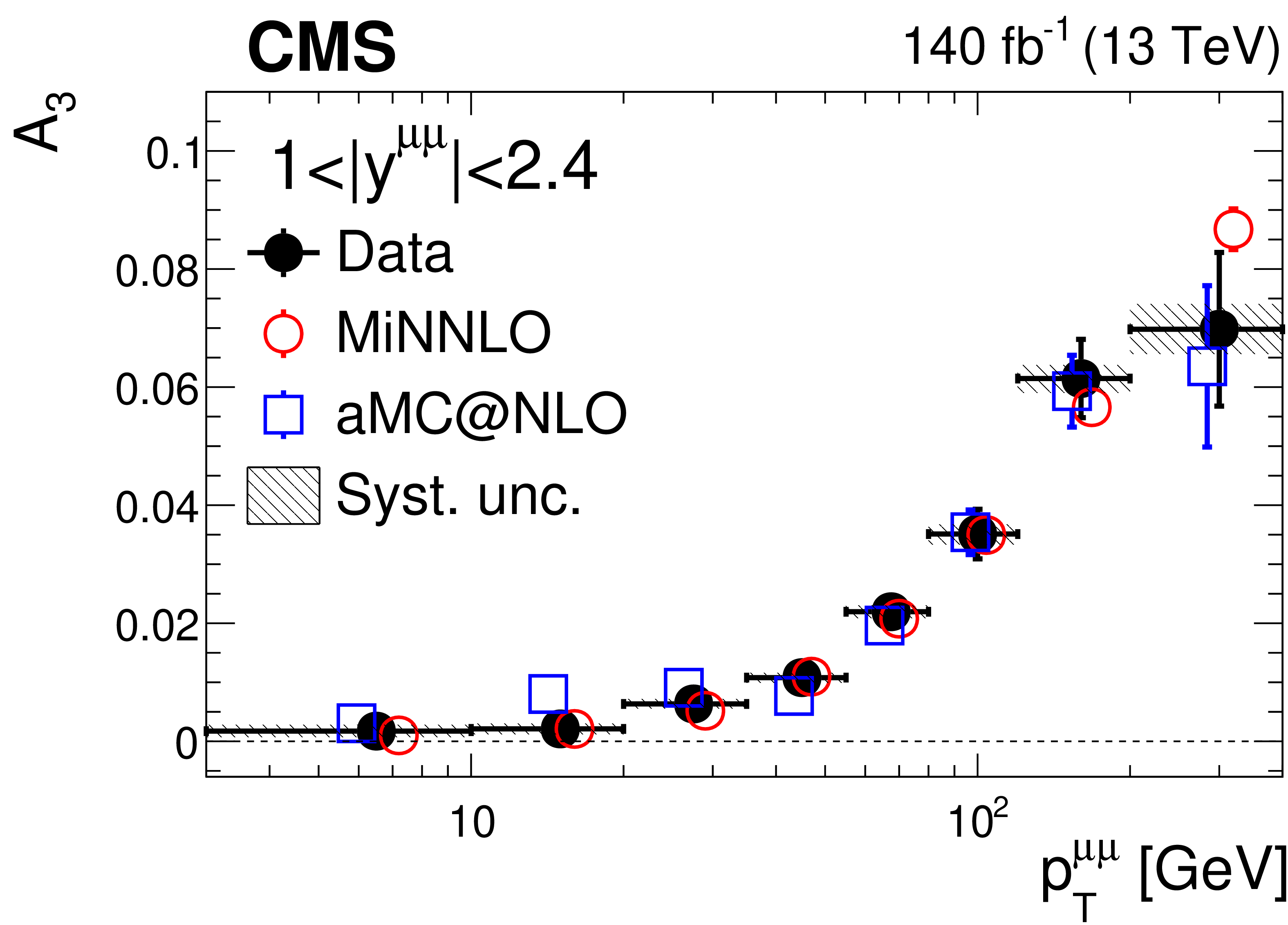
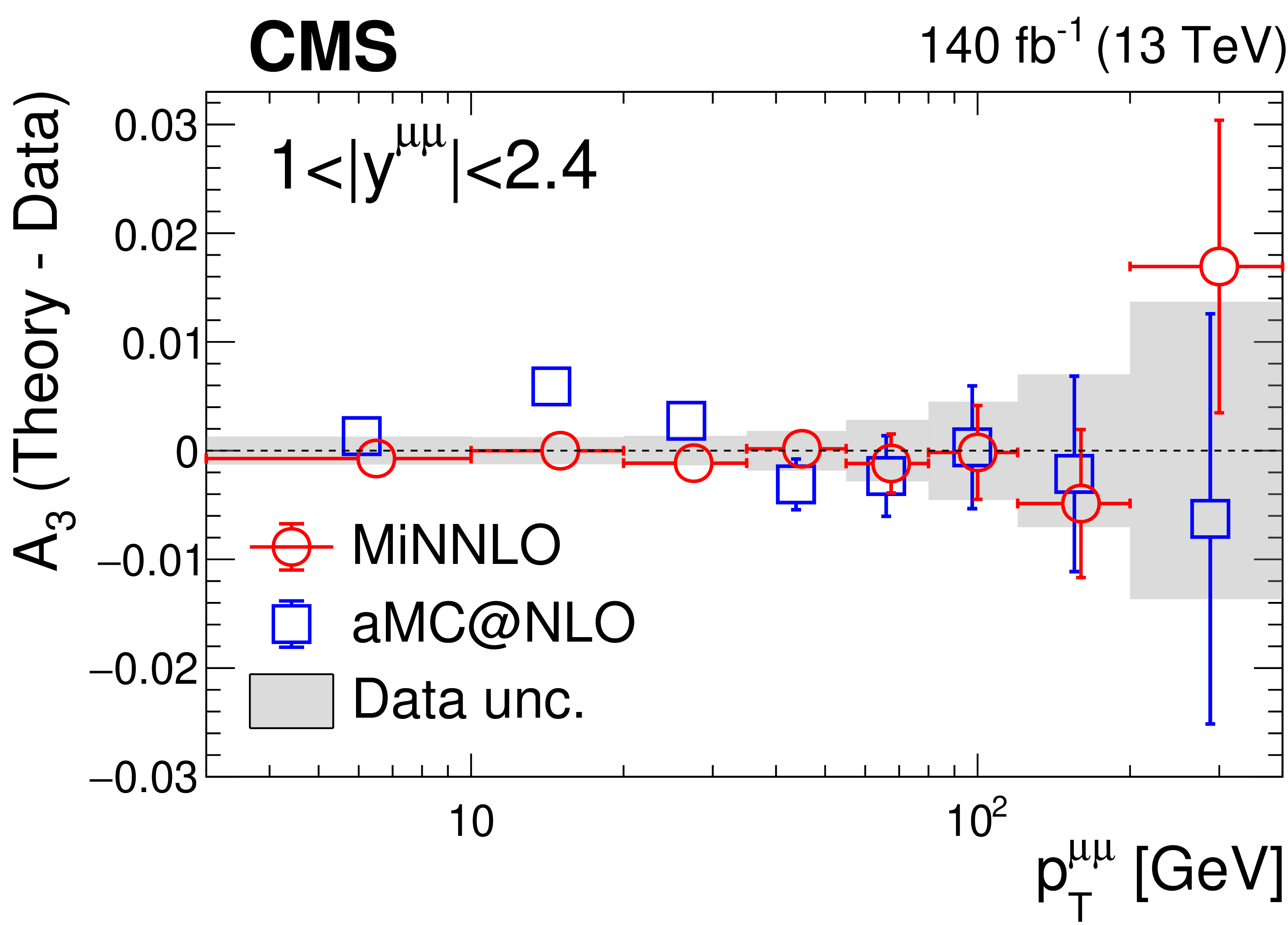
Figure 5:
Same as Fig. 3, for the 1 $ < |y^{\mu\mu}| < $ 2.4 bin. |
png pdf |
Figure 5-a:
Same as Fig. 3, for the 1 $ < |y^{\mu\mu}| < $ 2.4 bin. |
png pdf |
Figure 5-b:
Same as Fig. 3, for the 1 $ < |y^{\mu\mu}| < $ 2.4 bin. |
png pdf |
Figure 5-c:
Same as Fig. 3, for the 1 $ < |y^{\mu\mu}| < $ 2.4 bin. |
png pdf |
Figure 5-d:
Same as Fig. 3, for the 1 $ < |y^{\mu\mu}| < $ 2.4 bin. |
png pdf |
Figure 5-e:
Same as Fig. 3, for the 1 $ < |y^{\mu\mu}| < $ 2.4 bin. |
png pdf |
Figure 5-f:
Same as Fig. 3, for the 1 $ < |y^{\mu\mu}| < $ 2.4 bin. |
png pdf |
Figure 5-g:
Same as Fig. 3, for the 1 $ < |y^{\mu\mu}| < $ 2.4 bin. |
png pdf |
Figure 5-h:
Same as Fig. 3, for the 1 $ < |y^{\mu\mu}| < $ 2.4 bin. |
png pdf |
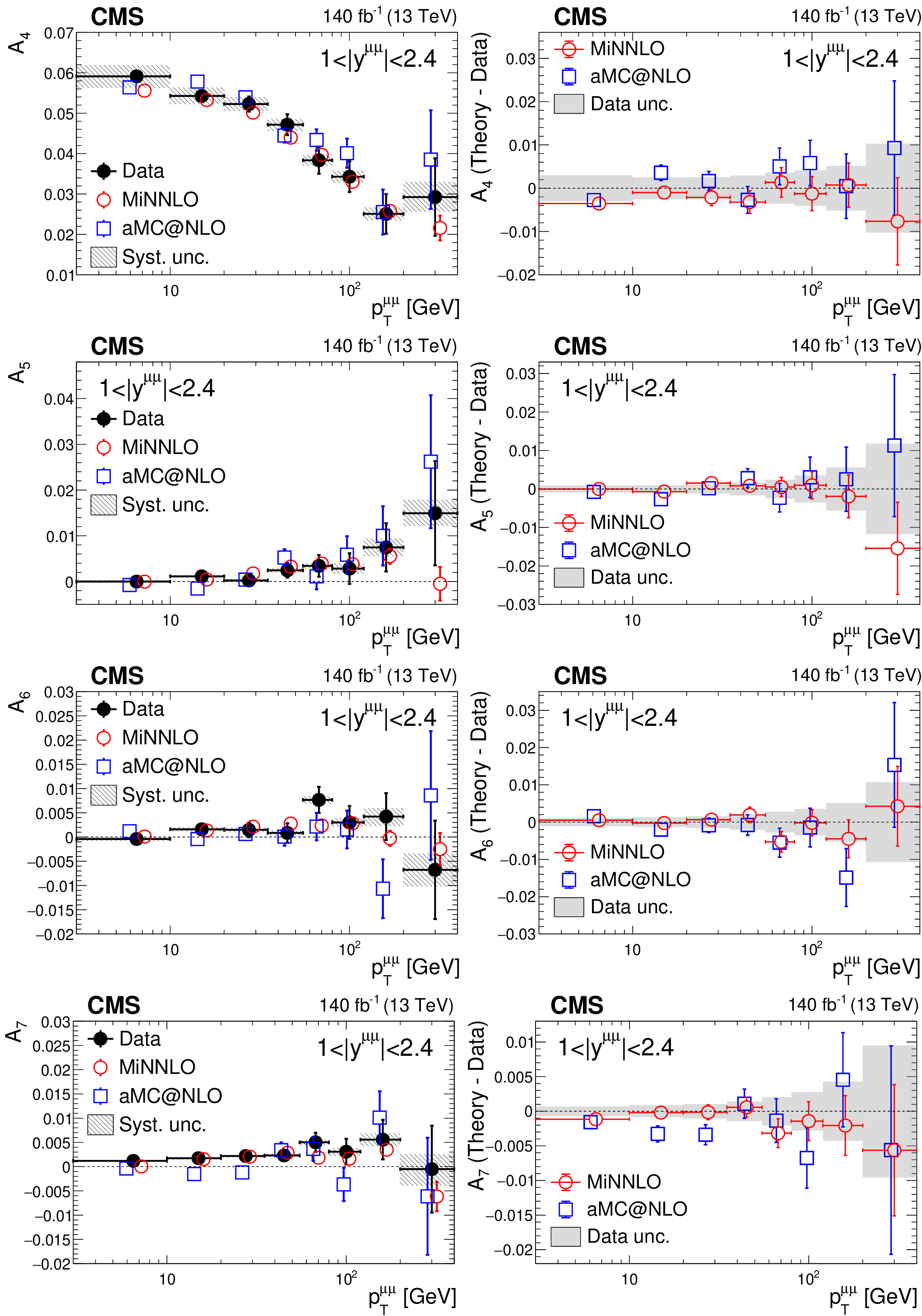
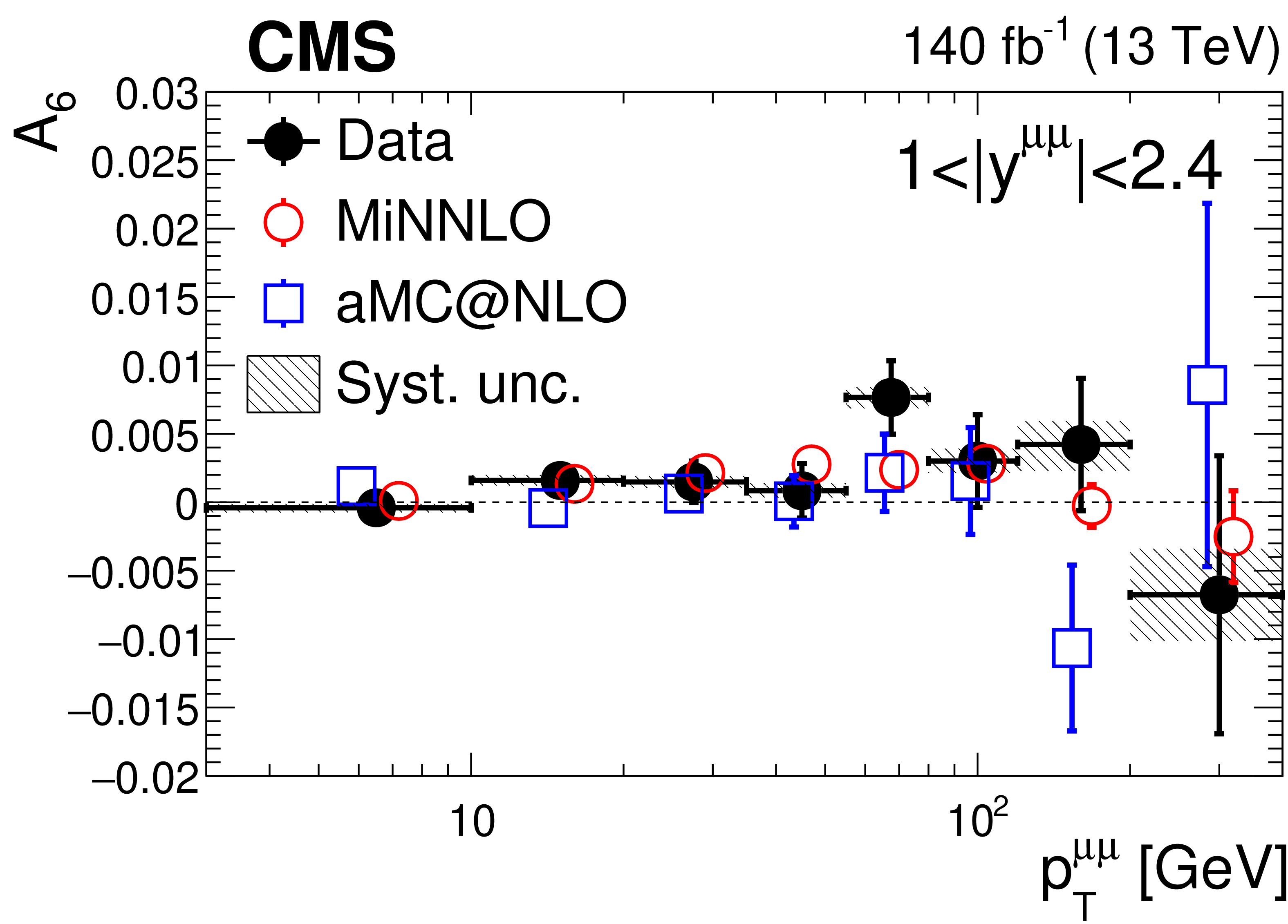
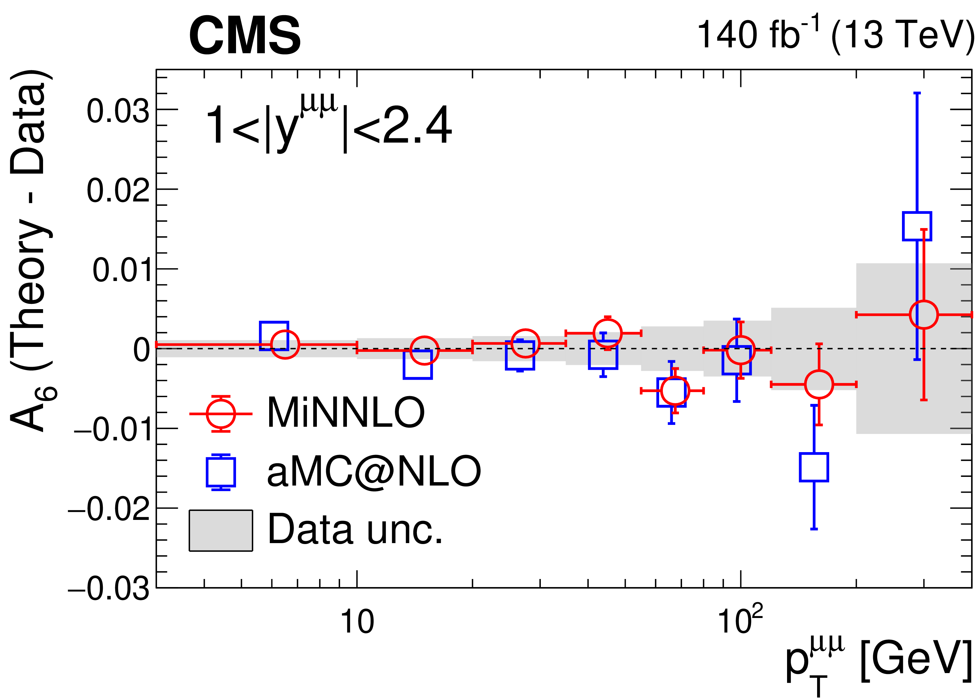
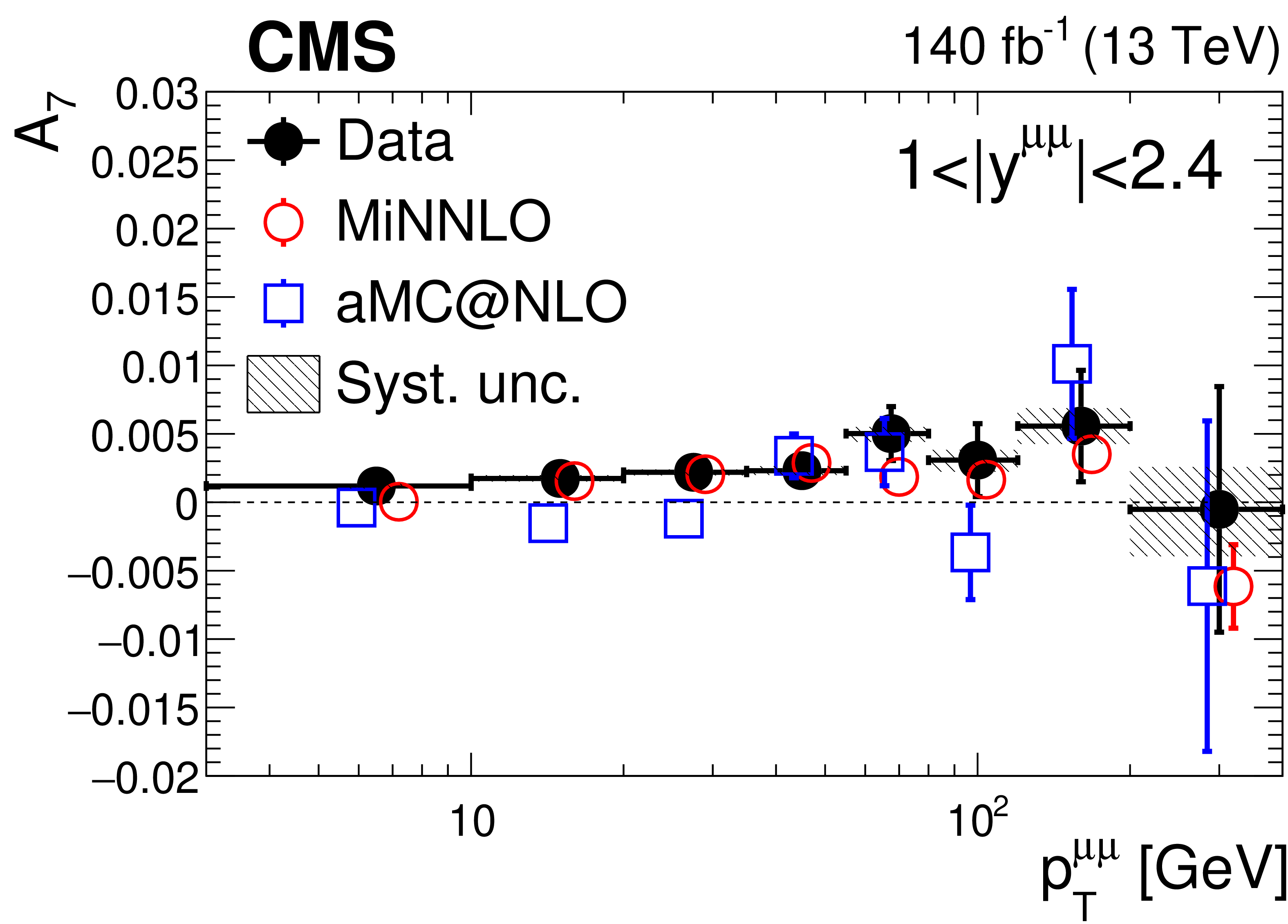
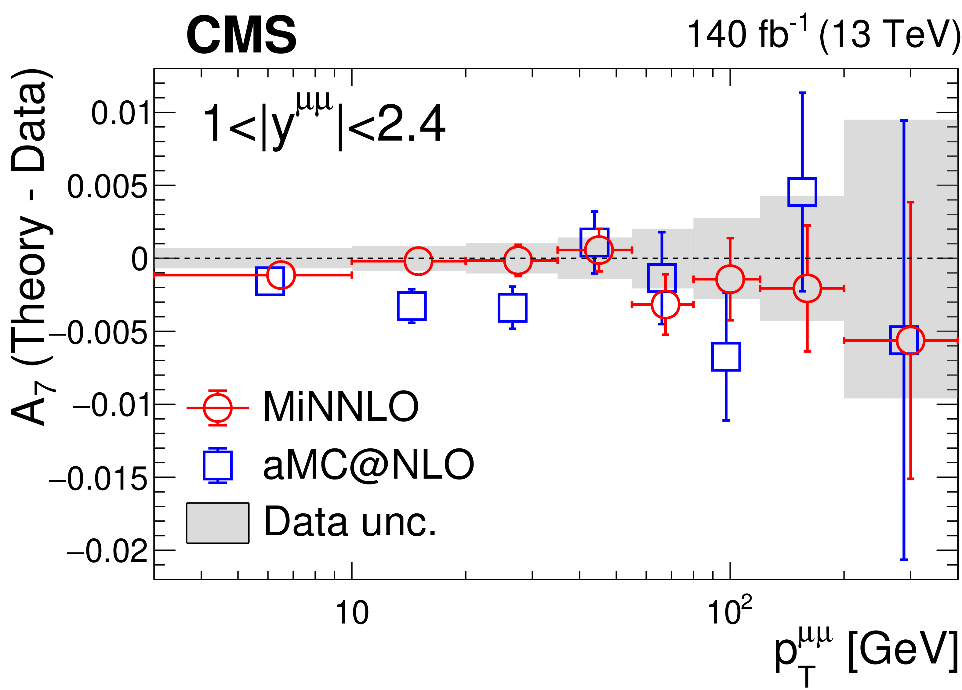
Figure 6:
Same as Fig. 4, for the 1 $ < |y^{\mu\mu}| < $ 2.4 bin. |
png pdf |
Figure 6-a:
Same as Fig. 4, for the 1 $ < |y^{\mu\mu}| < $ 2.4 bin. |
png pdf |
Figure 6-b:
Same as Fig. 4, for the 1 $ < |y^{\mu\mu}| < $ 2.4 bin. |
png pdf |
Figure 6-c:
Same as Fig. 4, for the 1 $ < |y^{\mu\mu}| < $ 2.4 bin. |
png pdf |
Figure 6-d:
Same as Fig. 4, for the 1 $ < |y^{\mu\mu}| < $ 2.4 bin. |
png pdf |
Figure 6-e:
Same as Fig. 4, for the 1 $ < |y^{\mu\mu}| < $ 2.4 bin. |
png pdf |
Figure 6-f:
Same as Fig. 4, for the 1 $ < |y^{\mu\mu}| < $ 2.4 bin. |
png pdf |
Figure 6-g:
Same as Fig. 4, for the 1 $ < |y^{\mu\mu}| < $ 2.4 bin. |
png pdf |
Figure 6-h:
Same as Fig. 4, for the 1 $ < |y^{\mu\mu}| < $ 2.4 bin. |
png pdf |
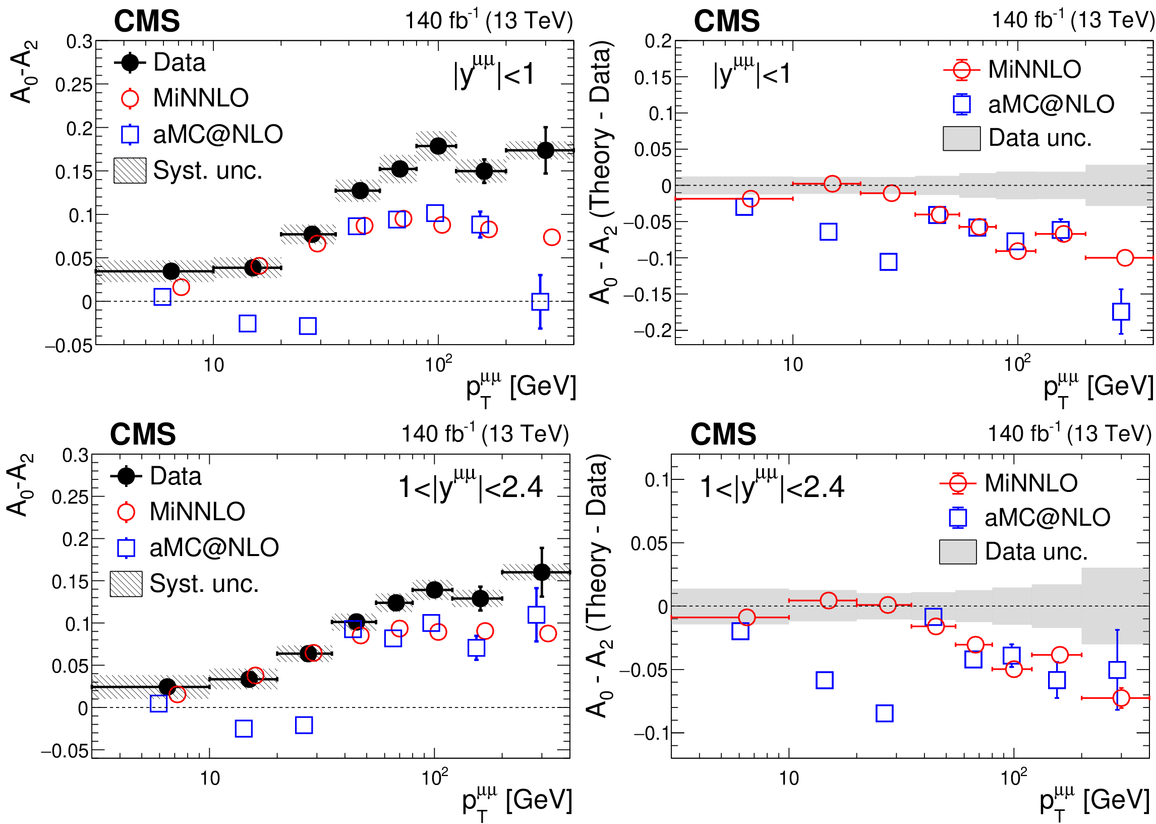
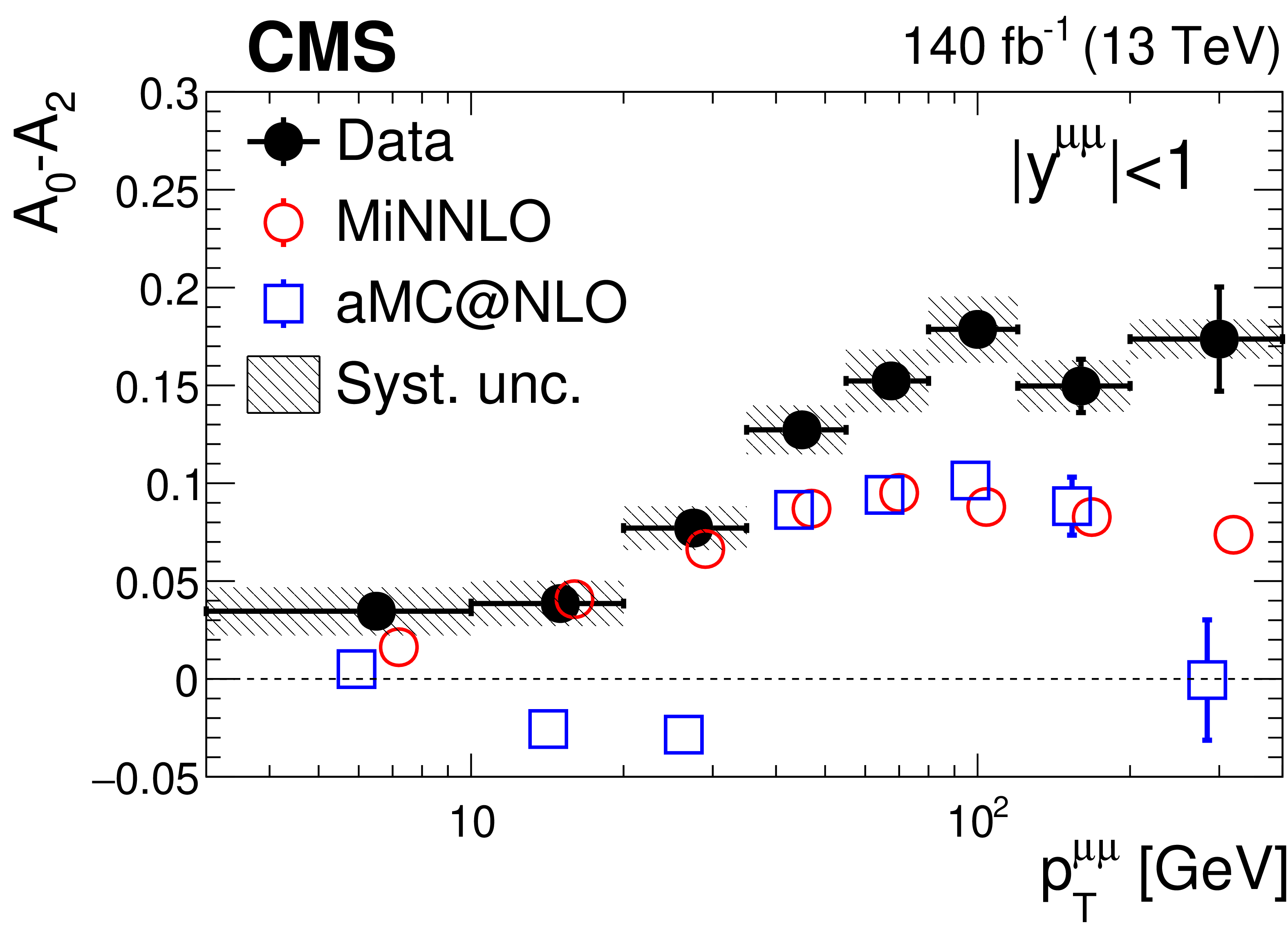
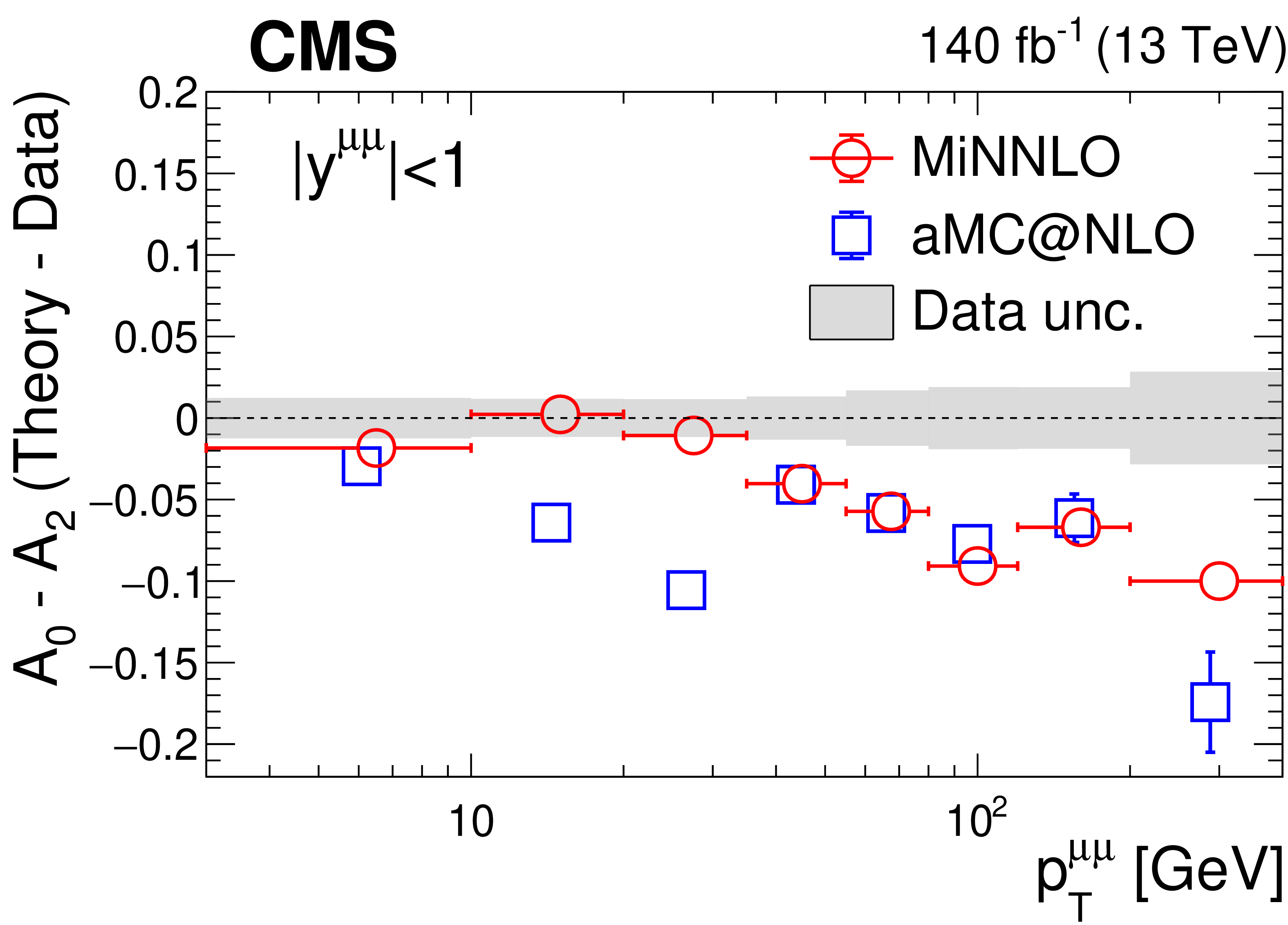
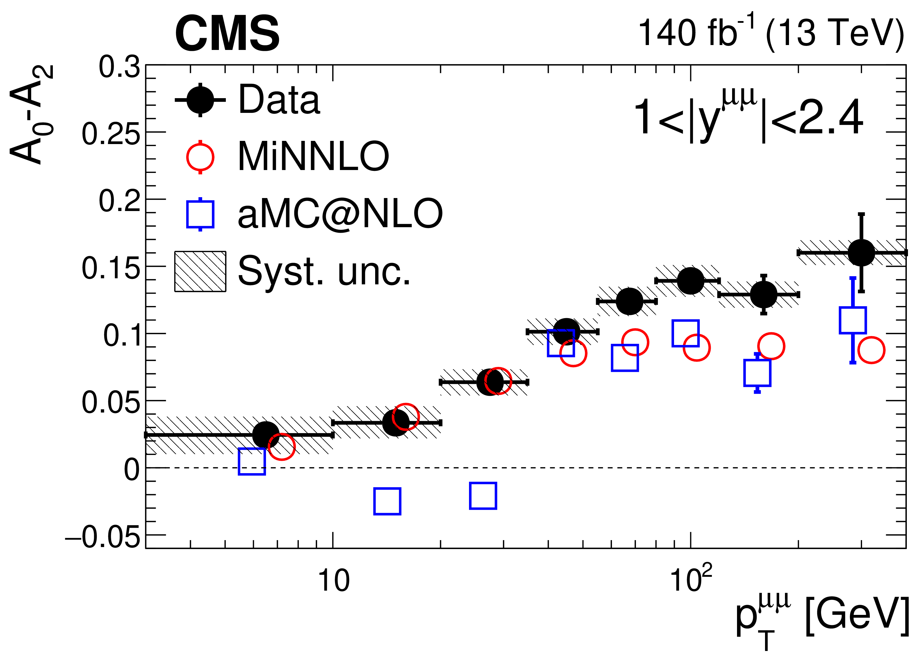
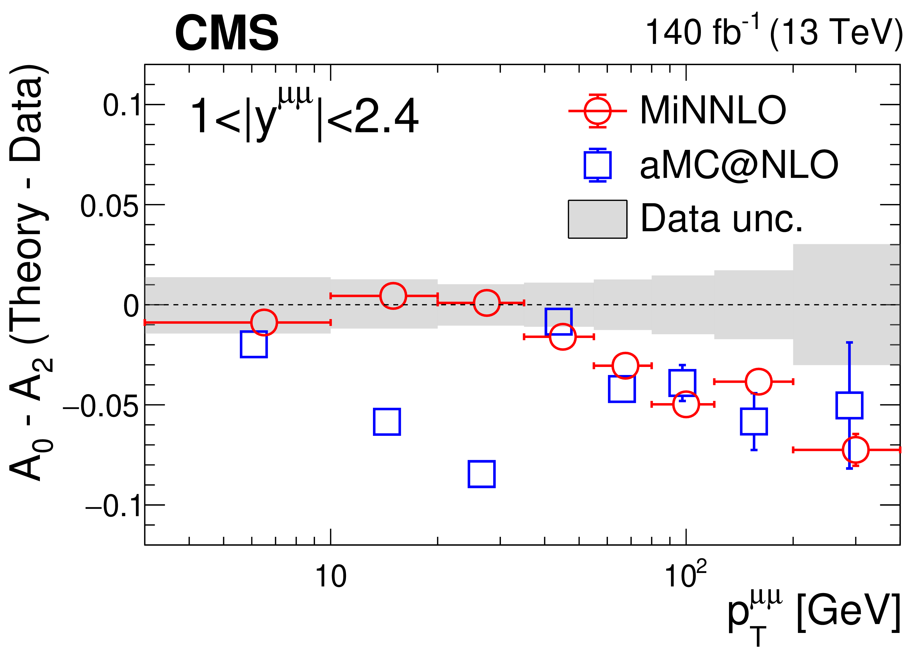
Figure 7:
Left: Difference $ A_0-A_2 $ measured in the CS frame in bins of $ p_{\mathrm{T}}^{\mu\mu} $ for $ |y^{\mu\mu}| < $ 1 (upper) and 1 $ < |y^{\mu\mu}| < $ 2.4 (lower). Right: Corresponding differences between the predicted and measured values. |
png pdf |
Figure 7-a:
Left: Difference $ A_0-A_2 $ measured in the CS frame in bins of $ p_{\mathrm{T}}^{\mu\mu} $ for $ |y^{\mu\mu}| < $ 1 (upper) and 1 $ < |y^{\mu\mu}| < $ 2.4 (lower). Right: Corresponding differences between the predicted and measured values. |
png pdf |
Figure 7-b:
Left: Difference $ A_0-A_2 $ measured in the CS frame in bins of $ p_{\mathrm{T}}^{\mu\mu} $ for $ |y^{\mu\mu}| < $ 1 (upper) and 1 $ < |y^{\mu\mu}| < $ 2.4 (lower). Right: Corresponding differences between the predicted and measured values. |
png pdf |
Figure 7-c:
Left: Difference $ A_0-A_2 $ measured in the CS frame in bins of $ p_{\mathrm{T}}^{\mu\mu} $ for $ |y^{\mu\mu}| < $ 1 (upper) and 1 $ < |y^{\mu\mu}| < $ 2.4 (lower). Right: Corresponding differences between the predicted and measured values. |
png pdf |
Figure 7-d:
Left: Difference $ A_0-A_2 $ measured in the CS frame in bins of $ p_{\mathrm{T}}^{\mu\mu} $ for $ |y^{\mu\mu}| < $ 1 (upper) and 1 $ < |y^{\mu\mu}| < $ 2.4 (lower). Right: Corresponding differences between the predicted and measured values. |
| Tables | |
png pdf |
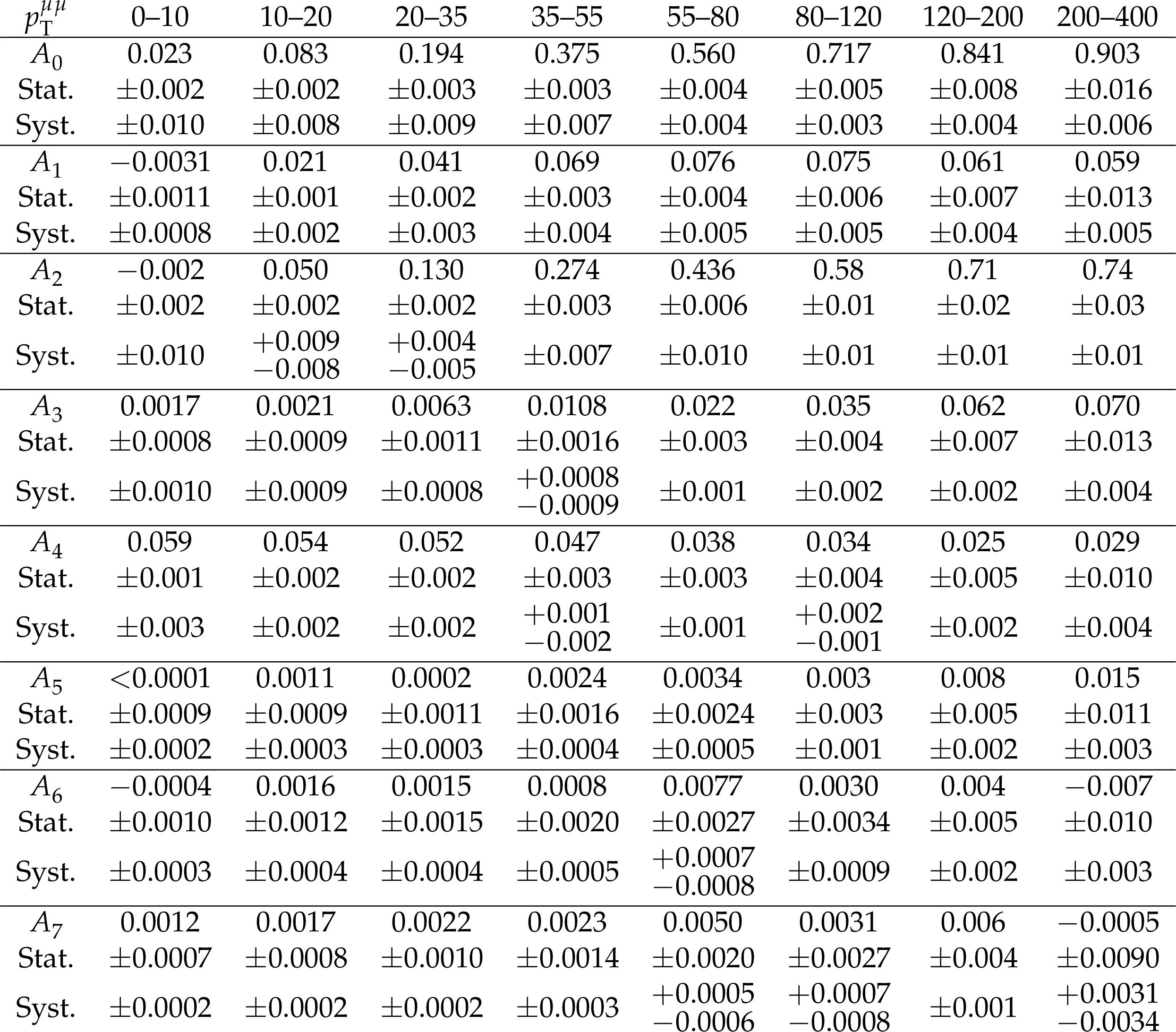
Table A1:
Measured angular coefficients, in bins of $ p_{\mathrm{T}}^{\mu\mu} $ (in GeV), for $ |y^{\mu\mu}| < $ 1. |
png pdf |
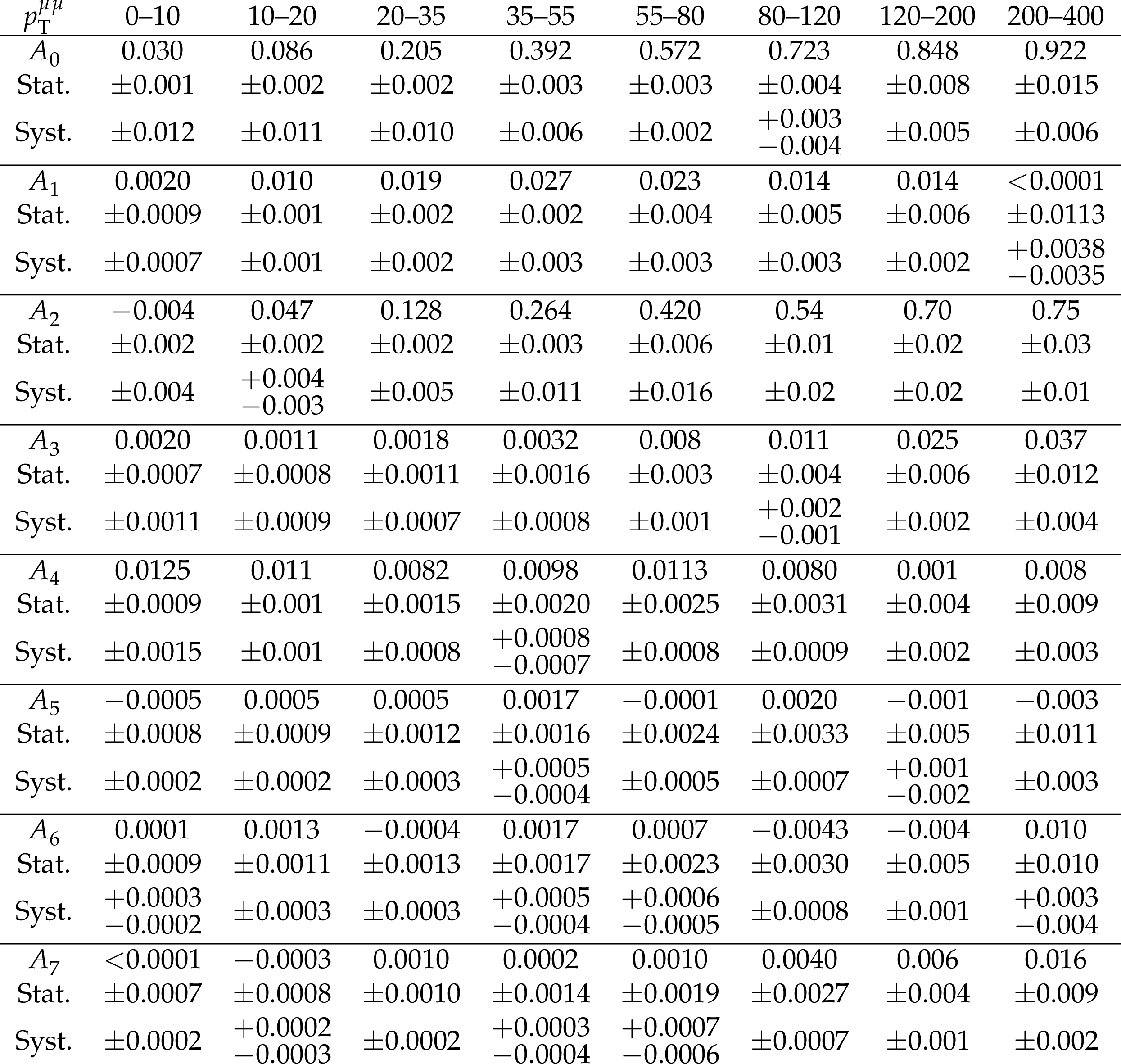
Table A2:
Measured angular coefficients, in bins of $ p_{\mathrm{T}}^{\mu\mu} $ (in GeV), for 1 $ < |y^{\mu\mu}| < $ 2.4. |
png pdf |
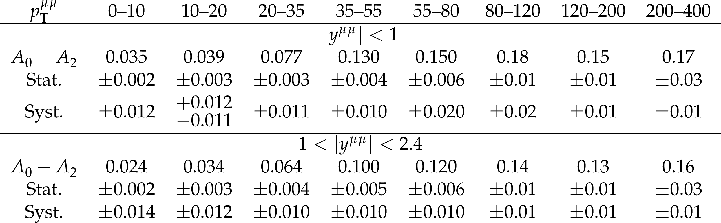
Table A3:
Measured $ A_0-A_2 $ difference in bins of $ p_{\mathrm{T}}^{\mu\mu} $ (in GeV) and $ |y^{\mu\mu}| $. |
| Summary |
| The first measurement of the full set of angular polarization coefficients $ A_0 $--$ A_7 $ in the Drell--Yan dimuon channel in the central rapidity range 0 $ < |y^{\mu\mu}| < $ 2.4 and $ p_{\mathrm{T}}^{\mu\mu} < $ 400 GeV at $ \sqrt{s}= $ 13 TeV is presented. The coefficients were determined double differentially in bins of transverse momentum and rapidity of the dimuon in the 81--101 GeV invariant mass range. The results are compared with state-of-the-art theoretical predictions at next-to-next-to-leading order in QCD and show consistency within uncertainties in most of the phase space. The presented results provide a comprehensive characterization of the angular structure of dilepton production and offer stringent constraints on theoretical descriptions of electroweak vector boson production mechanisms and underlying partonic dynamics [5,6]. The achieved precision and multidimensional binning establish a valuable benchmark for future phenomenological studies and for testing higher-order calculations [19,20]. With larger data sets and simulated event samples, more precise measurements will be possible in the high transverse momentum region, where the contribution of QCD higher-order effects is still poorly studied. Improved modeling of the detector system response will reduce the systematic uncertainty of the measurement. |
| References | ||||
| 1 | S. D. Drell and T.-M. Yan | Massive lepton pair production in hadron-hadron collisions at high-energies | PRL 25 (1970) 316 | |
| 2 | E. Mirkes and J. Ohnemus | W and Z polarization effects in hadronic collisions | PRD 50 (1994) 5692 | hep-ph/9406381 |
| 3 | E. Mirkes | Angular decay distribution of leptons from W-bosons at NLO in hadronic collisions | NPB 387 (1992) 3 | |
| 4 | A. Bodek, J. Han, A. Khukhunaishvili, and W. Sakumoto | Using Drell-Yan forward-backward asymmetry to reduce PDF uncertainties in the measurement of electroweak parameters | EPJC 76 (2016) 115 | 1507.02470 |
| 5 | B. Zhang, Z. Lu, B.-Q. Ma, and I. Schmidt | Extracting Boer--Mulders functions from p+D Drell--Yan processes | PRD 77 (2008) 054011 | 0803.1692 |
| 6 | S. Piloneta and A. Vladimirov | Angular distributions of Drell--Yan leptons in the TMD factorization approach | JHEP 12 (2024) 059 | 2407.06277 |
| 7 | J. C. Collins and D. E. Soper | Angular distribution of dileptons in high-energy hadron collisions | PRD 16 (1977) 2219 | |
| 8 | CMS Collaboration | Angular coefficients of Z bosons produced in pp collisions at $ \sqrt{s} = 8 \textrm{TeV} $ and decaying to $ \mu^+ \mu^- $ as a function of transverse momentum and rapidity | PLB 750 (2015) 154 | CMS-SMP-13-010 1504.03512 |
| 9 | ATLAS Collaboration | Measurement of the angular coefficients in $ Z $-boson events using electron and muon pairs from data taken at $ \sqrt{s}= $ 8 TeV with the ATLAS detector | JHEP 08 (2016) 159 | 1606.00689 |
| 10 | R. Gauld et al. | Precise predictions for the angular coefficients in Z-boson production at the LHC | JHEP 11 (2017) 003 | 1708.00008 |
| 11 | C. S. Lam and W.-K. Tung | Systematic approach to inclusive lepton pair production in hadronic collisions | PRD 18 (1978) 2447 | |
| 12 | P. Faccioli, C. Louren ç o, and J. Seixas | Rotation-invariant relations in vector meson decays into fermion pairs | PRL 105 (2010) 061601 | 1005.2601 |
| 13 | P. Faccioli and C. Lourenço | Particle polarization in high energy physics: an introduction and case studies on vector particle production at the LHC | Lecture Notes in Physics. Springer, 2022 link |
|
| 14 | J.-C. Peng, W.-C. Chang, R. E. McClellan, and O. Teryaev | Interpretation of angular distributions of Z-boson production at colliders | PLB 758 (2016) 384 | 1511.08932 |
| 15 | D. Boer | Intrinsic transverse momentum and transverse spin asymmetries | Nucl. Phys. B Proc. Suppl. 79 (1999) 638 | hep-ph/9905336 |
| 16 | CDF Collaboration | Indirect measurement of $ \sin^2\theta_{\mathrm{W}}(M_{\mathrm{W}}) $ using $ \mathrm{e}^+\mathrm{e}^- $ pairs in the Z-boson region with $ \mathrm{p}\overline{\mathrm{p}} $ collisions at a center-of-momentum energy of 1.96 TeV | PRD 88 (2013) 072002 | 1307.0770 |
| 17 | CDF Collaboration | First measurement of the angular coefficients of Drell--Yan $ \mathrm{e}^{+}\mathrm{e}^{-} $ pairs in the Z mass region from $ \mathrm{p}\overline{\mathrm{p}} $ collisions at $ \sqrt{s} = $ 1.96 TeV | PRL 106 (2011) 241801 | 1103.5699 |
| 18 | CMS Collaboration | Measurement of the Drell--Yan forward-backward asymmetry and of the effective leptonic weak mixing angle in proton-proton collisions at $ \sqrt{s} = $ 13 TeV | PLB 866 (2025) 139526 | CMS-SMP-22-010 2408.07622 |
| 19 | K. Hagiwara, K.-i. Hikasa, and N. Kai | Time-reversal-odd asymmetry in semi-inclusive lepton production in Quantum Chromodynamics | PRD 27 (1983) 84 | |
| 20 | K. Hagiwara, T. Kuruma, and Y. Yamada | Probing the one-loop Zgg vertex at hadron colliders | NPB 369 (1992) 171 | |
| 21 | LHCb Collaboration | First measurement of the $ \mathrm{Z}\to\mu^{+}\mu^{-} $ angular coefficients in the forward region of pp collisions at $ \sqrt{s}= $ 13 TeV | PRL 129 (2022) 091801 | 2203.01602 |
| 22 | CMS Collaboration | HEPData record for this analysis | link | |
| 23 | CMS Collaboration | The CMS experiment at the CERN LHC | JINST 3 (2008) S08004 | |
| 24 | CMS Collaboration | Performance of the CMS Level-1 trigger in proton-proton collisions at $ \sqrt{s} = $ 13 TeV | JINST 15 (2020) P10017 | CMS-TRG-17-001 2006.10165 |
| 25 | CMS Collaboration | The CMS trigger system | JINST 12 (2017) P01020 | CMS-TRG-12-001 1609.02366 |
| 26 | CMS Collaboration | Electron and photon reconstruction and identification with the CMS experiment at the CERN LHC | JINST 16 (2021) P05014 | CMS-EGM-17-001 2012.06888 |
| 27 | CMS Collaboration | Performance of the CMS muon detector and muon reconstruction with proton-proton collisions at $ \sqrt{s}= $ 13 TeV | JINST 13 (2018) P06015 | CMS-MUO-16-001 1804.04528 |
| 28 | CMS Collaboration | Description and performance of track and primary-vertex reconstruction with the CMS tracker | JINST 9 (2014) P10009 | CMS-TRK-11-001 1405.6569 |
| 29 | CMS Collaboration | Particle-flow reconstruction and global event description with the CMS detector | JINST 12 (2017) P10003 | CMS-PRF-14-001 1706.04965 |
| 30 | CMS Collaboration | Performance of the CMS high-level trigger during LHC Run 2 | JINST 19 (2024) P11021 | CMS-TRG-19-001 2410.17038 |
| 31 | P. F. Monni et al. | MiNNLO$ _{\mathrm{PS}} $: a new method to match NNLO QCD to parton showers | JHEP 05 (2020) 143 | 1908.06987 |
| 32 | S. Frixione, P. Nason, and C. Oleari | Matching NLO QCD computations with Parton Shower simulations: the POWHEG method | JHEP 11 (2007) 070 | 0709.2092 |
| 33 | T. Sjöstrand et al. | An introduction to PYTHIA 8.2 | Comput. Phys. Commun. 191 (2015) 159 | 1410.3012 |
| 34 | N. Davidson, T. Przedzinski, and Z. Was | PHOTOS interface in C++: technical and physics documentation | Comput. Phys. Commun. 199 (2016) 86 | 1011.0937 |
| 35 | NNPDF Collaboration | Parton distributions from high-precision collider data | EPJC 77 (2017) 663 | 1706.00428 |
| 36 | J. Alwall et al. | The automated computation of tree-level and next-to-leading order differential cross sections, and their matching to parton shower simulations | JHEP 07 (2014) 079 | 1405.0301 |
| 37 | R. Frederix and S. Frixione | Merging meets matching in MC@NLO | JHEP 12 (2012) 061 | 1209.6215 |
| 38 | CMS Collaboration | Extraction and validation of a new set of CMS PYTHIA8 tunes from underlying-event measurements | EPJC 80 (2020) 4 | CMS-GEN-17-001 1903.12179 |
| 39 | CMS Collaboration | Measurements of differential Z boson production cross sections in proton-proton collisions at $ \sqrt{s} = $ 13 TeV | JHEP 12 (2019) 061 | CMS-SMP-17-010 1909.04133 |
| 40 | S. Agostinelli et al. | GEANT4--A simulation toolkit | NIM A 506 (2003) 250 | |
| 41 | A. Bodek et al. | Extracting muon momentum scale corrections for hadron collider experiments | EPJC 72 (2012) 2194 | 1208.3710 |
| 42 | CMS Collaboration | Performance of the CMS muon trigger system in proton-proton collisions at $ \sqrt{s} = $ 13 TeV | JINST 16 (2021) P07001 | CMS-MUO-19-001 2102.04790 |
| 43 | F. James | MINUIT function minimization and error analysis: reference manual version 94.1 | Technical report, CERN, 1994 link |
|
| 44 | CMS Collaboration | Precision luminosity measurement in proton-proton collisions at $ \sqrt{s} = $ 13 TeV in 2015 and 2016 at CMS | EPJC 81 (2021) 800 | CMS-LUM-17-003 2104.01927 |
| 45 | CMS Collaboration | Precision luminosity measurement in proton-proton collisions at $ \sqrt{s} = $ 13 TeV with the CMS detector | Technical Report, CERN, 2025 CMS-PAS-LUM-20-001 |
CMS-PAS-LUM-20-001 |
| 46 | J. Butterworth et al. | PDF4LHC recommendations for LHC Run II | JPG 43 (2016) 023001 | 1510.03865 |
|
|
Compact Muon Solenoid LHC, CERN |
|

|

|

|

|

|