CMS-SMP-13-010

CMS-SMP-13-010 ; CERN-PH-EP-2015-046
Angular coefficients of Z bosons produced in pp collisions at $\sqrt{s}$ = 8 TeV and decaying to $\mu^{+}\mu^{-}$ as a function of transverse momentum and rapidity
CMS Collaboration
15 April 2015
Phys. Lett. B 750 (2015) 154
Abstract: Measurements of the five most significant angular coefficients, $A_{0}$ through $A_{4}$ , for Z bosons produced in pp collisions at $\sqrt{s}$ = 8 TeV and decaying to $\mu^{+}\mu^{-}$ are presented as a function of the transverse momentum and rapidity of Z boson. The integrated luminosity of the dataset collected with the CMS detector at the LHC corresponds to 19.7 fb $^{-1}$ . These measurements provide comprehensive information about Z boson production mechanisms, and are compared to QCD predictions at leading order, next-to-leading order, and next-to-next-to-leading order in perturbation theory.
Links: e-print arXiv:1504.03512 [hep-ex] (PDF) ; CDS record ; inSPIRE record ; Public twiki page ; HepData record ; CADI line (restricted) ;

Figures & Tables	Summary	CMS Publications

Figures
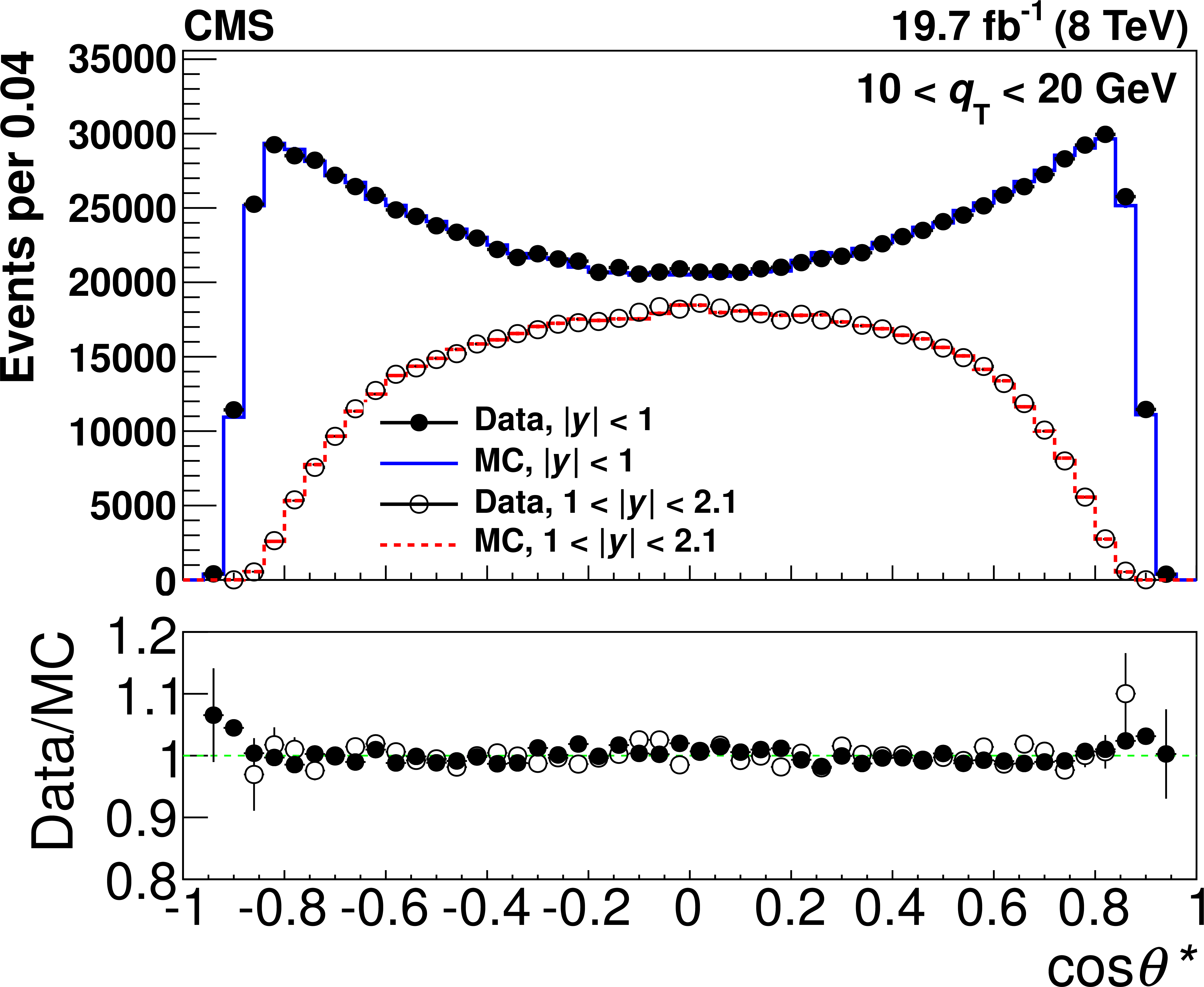
png pdf	Figure 1-a: A few examples of the observed 1D angular distributions in $\cos{ \theta^* }$ (a) and $\| \phi ^{*} \|$ (b) compared to the MC simulation using the best fit values of the angular coefficients. The top (bottom) plots show the distributions for $10 < {q_\mathrm {T}} < 20$ GeV ( $120 < {q_\mathrm {T}} < 200$ GeV ), a region where $A_0$ and $A_2$ are small (large). The background-subtracted data points are shown with filled (open) circles for $\| y \| < 1$ ( $1 < \| y \| < 2.1$ ), whilst the corresponding MC results are shown with the solid (dashed) lines. Vertical bars represent the statistical uncertainties. The lower panels show the data-to-MC ratios.
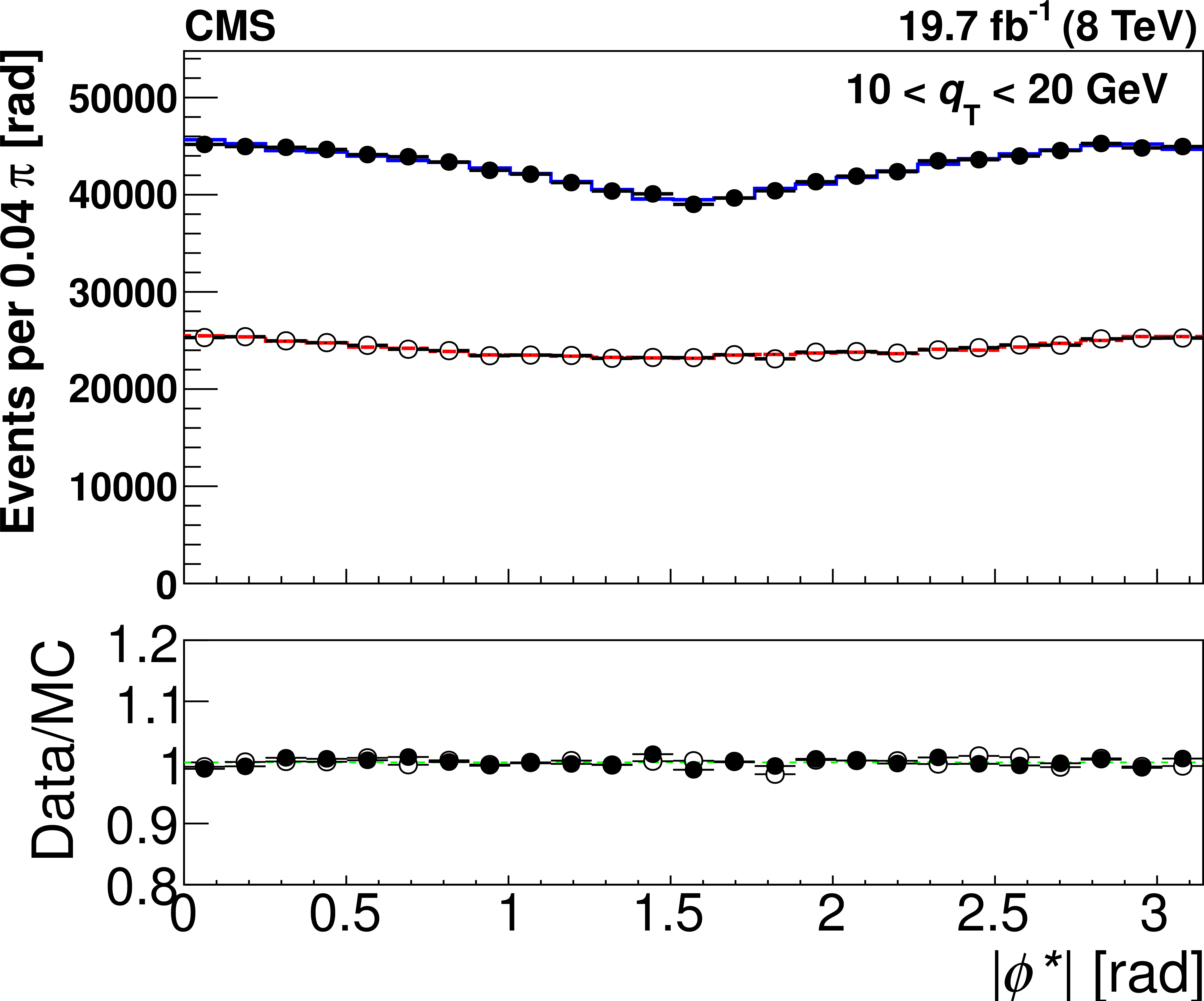
png pdf	Figure 1-b: A few examples of the observed 1D angular distributions in $\cos{ \theta^* }$ (a) and $\| \phi ^{*} \|$ (b) compared to the MC simulation using the best fit values of the angular coefficients. The top (bottom) plots show the distributions for $10 < {q_\mathrm {T}} < 20$ GeV ( $120 < {q_\mathrm {T}} < 200$ GeV ), a region where $A_0$ and $A_2$ are small (large). The background-subtracted data points are shown with filled (open) circles for $\| y \| < 1$ ( $1 < \| y \| < 2.1$ ), whilst the corresponding MC results are shown with the solid (dashed) lines. Vertical bars represent the statistical uncertainties. The lower panels show the data-to-MC ratios.
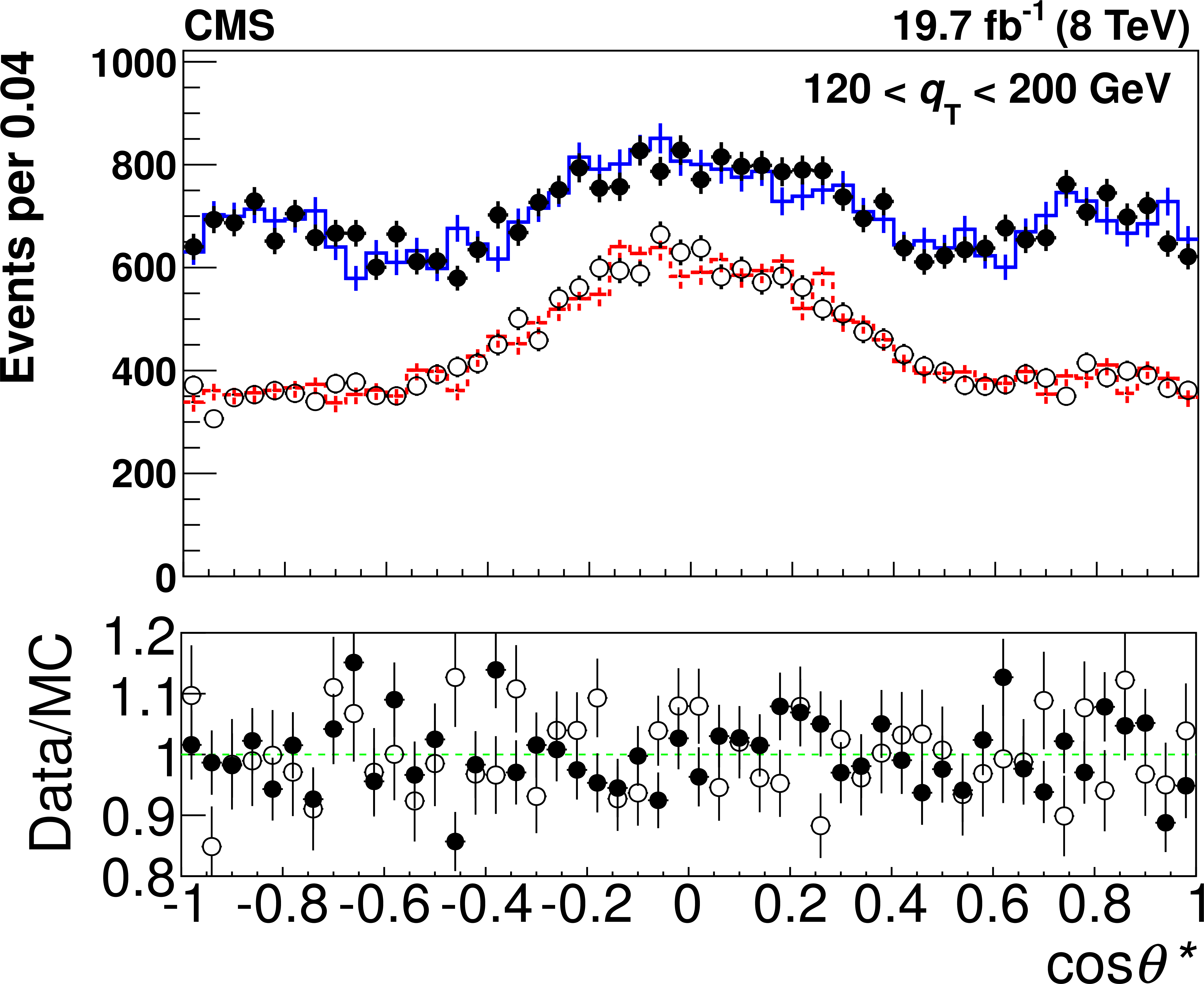
png pdf	Figure 1-c: A few examples of the observed 1D angular distributions in $\cos{ \theta^* }$ (a) and $\| \phi ^{*} \|$ (b) compared to the MC simulation using the best fit values of the angular coefficients. The top (bottom) plots show the distributions for $10 < {q_\mathrm {T}} < 20$ GeV ( $120 < {q_\mathrm {T}} < 200$ GeV ), a region where $A_0$ and $A_2$ are small (large). The background-subtracted data points are shown with filled (open) circles for $\| y \| < 1$ ( $1 < \| y \| < 2.1$ ), whilst the corresponding MC results are shown with the solid (dashed) lines. Vertical bars represent the statistical uncertainties. The lower panels show the data-to-MC ratios.
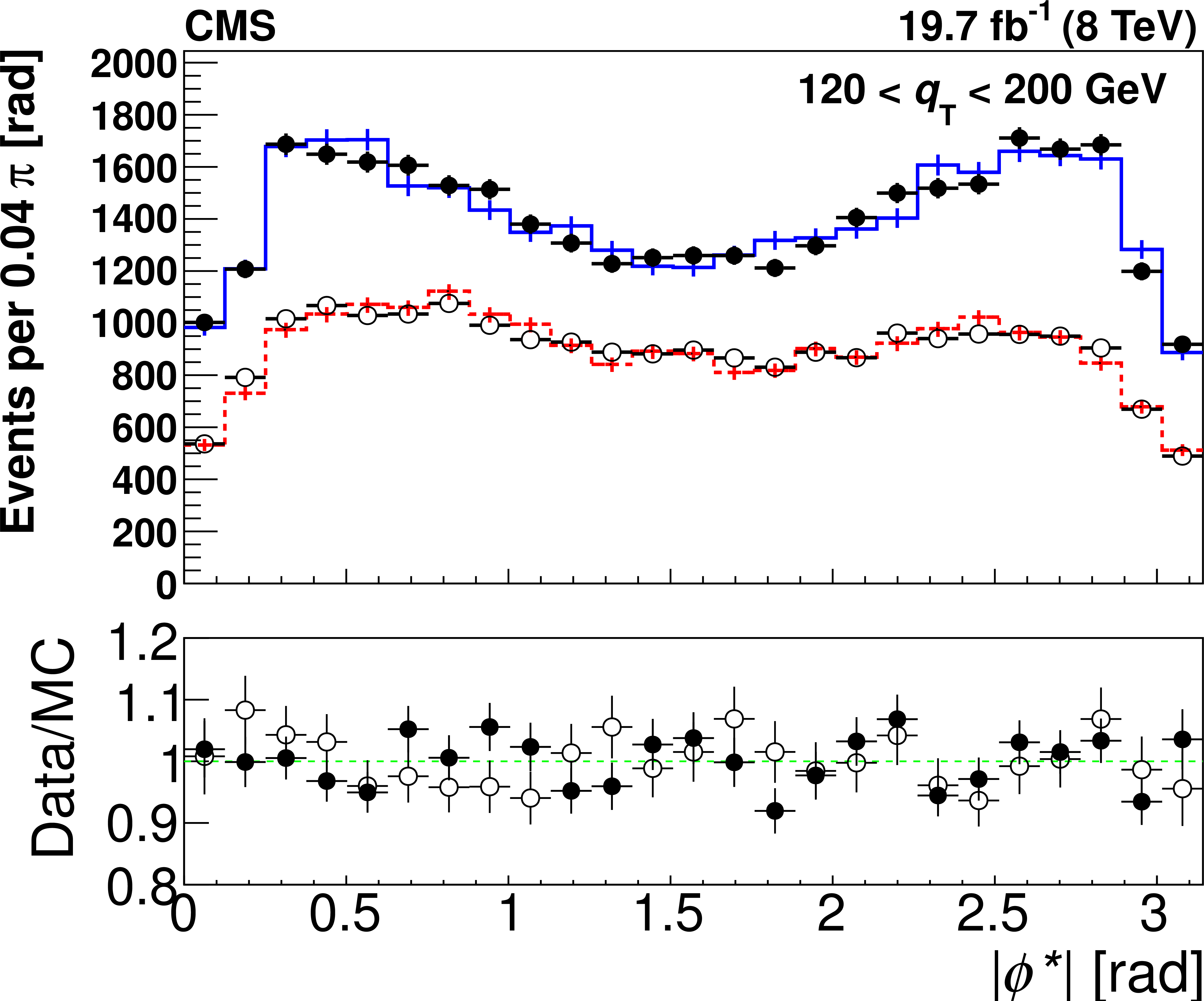
png pdf	Figure 1-d: A few examples of the observed 1D angular distributions in $\cos{ \theta^* }$ (a) and $\| \phi ^{*} \|$ (b) compared to the MC simulation using the best fit values of the angular coefficients. The top (bottom) plots show the distributions for $10 < {q_\mathrm {T}} < 20$ GeV ( $120 < {q_\mathrm {T}} < 200$ GeV ), a region where $A_0$ and $A_2$ are small (large). The background-subtracted data points are shown with filled (open) circles for $\| y \| < 1$ ( $1 < \| y \| < 2.1$ ), whilst the corresponding MC results are shown with the solid (dashed) lines. Vertical bars represent the statistical uncertainties. The lower panels show the data-to-MC ratios.
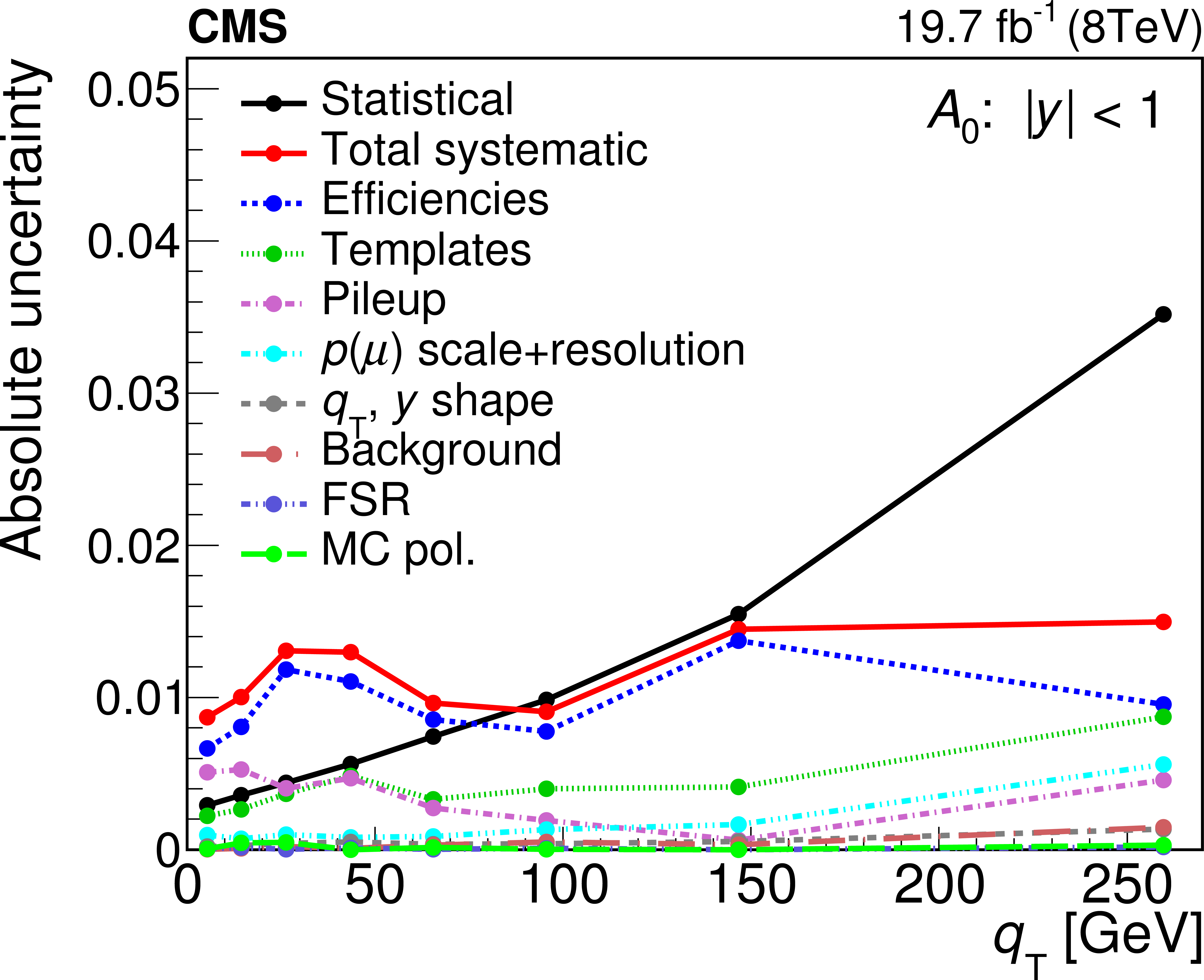
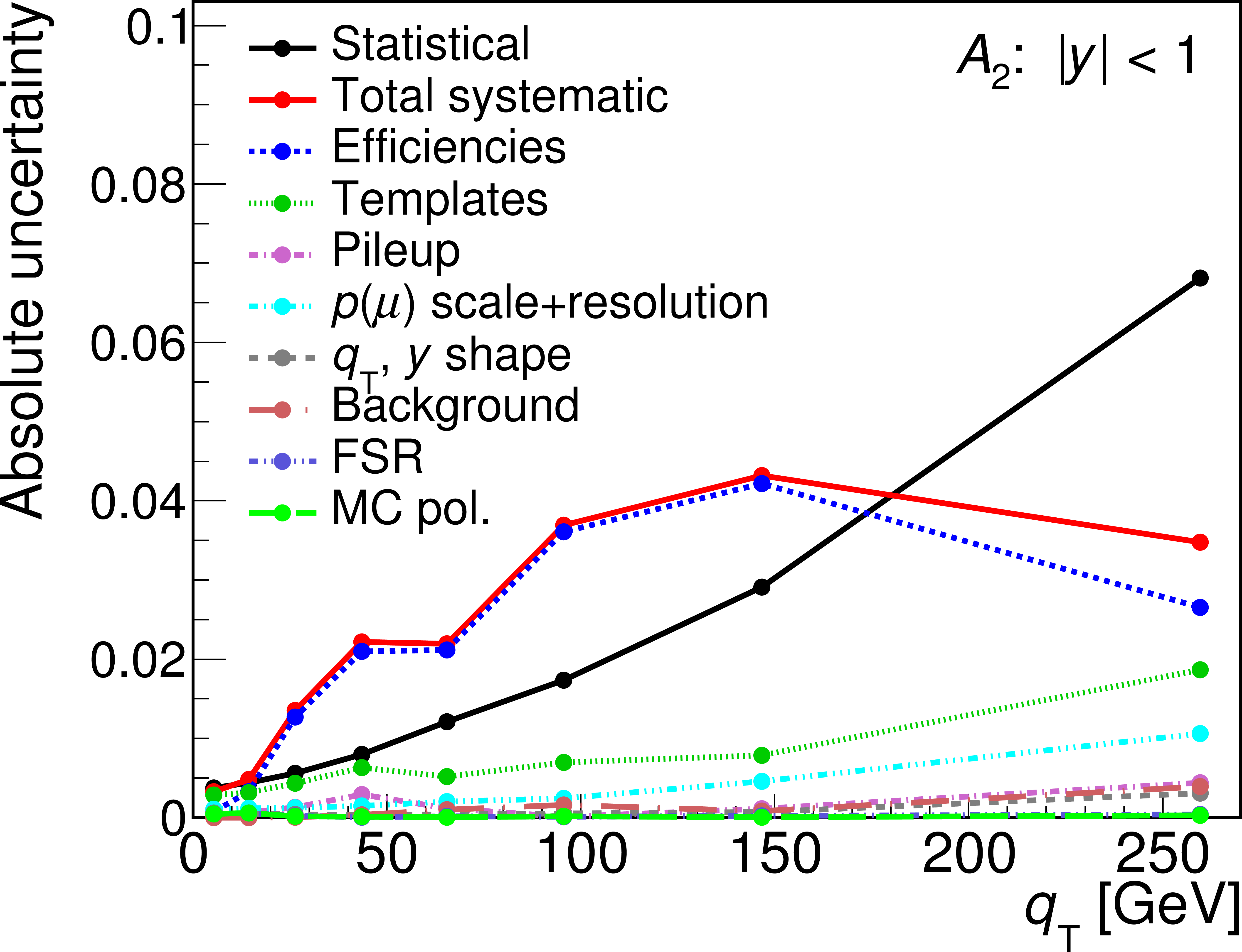
png pdf	Figure 2-a: Absolute uncertainties in the five angular coefficients $A_0$ to $A_4$ . Each figure shows the ${q_\mathrm {T}}$ dependence in the indicated ranges of $\| y \|$ .
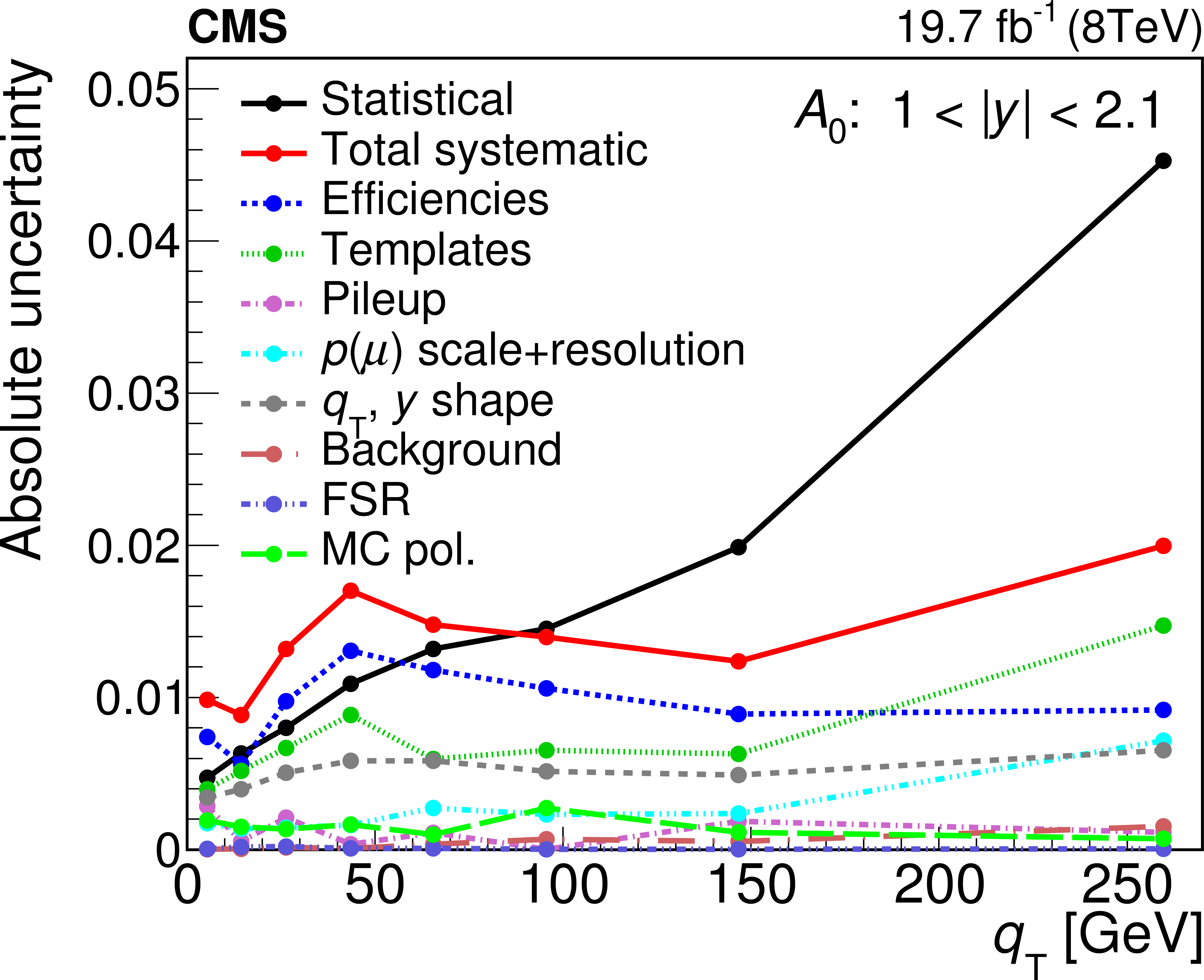
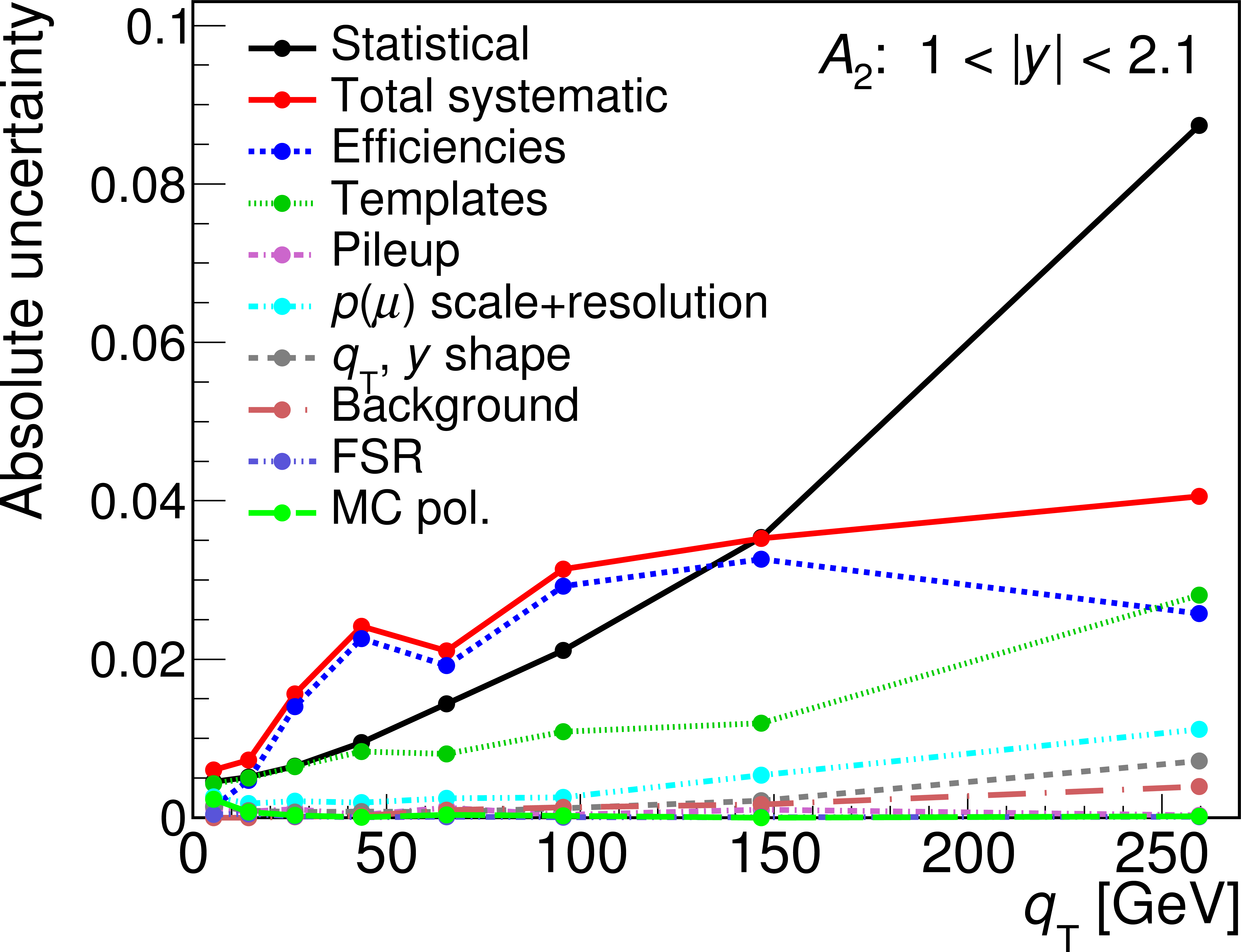
png pdf	Figure 2-b: Absolute uncertainties in the five angular coefficients $A_0$ to $A_4$ . Each figure shows the ${q_\mathrm {T}}$ dependence in the indicated ranges of $\| y \|$ .
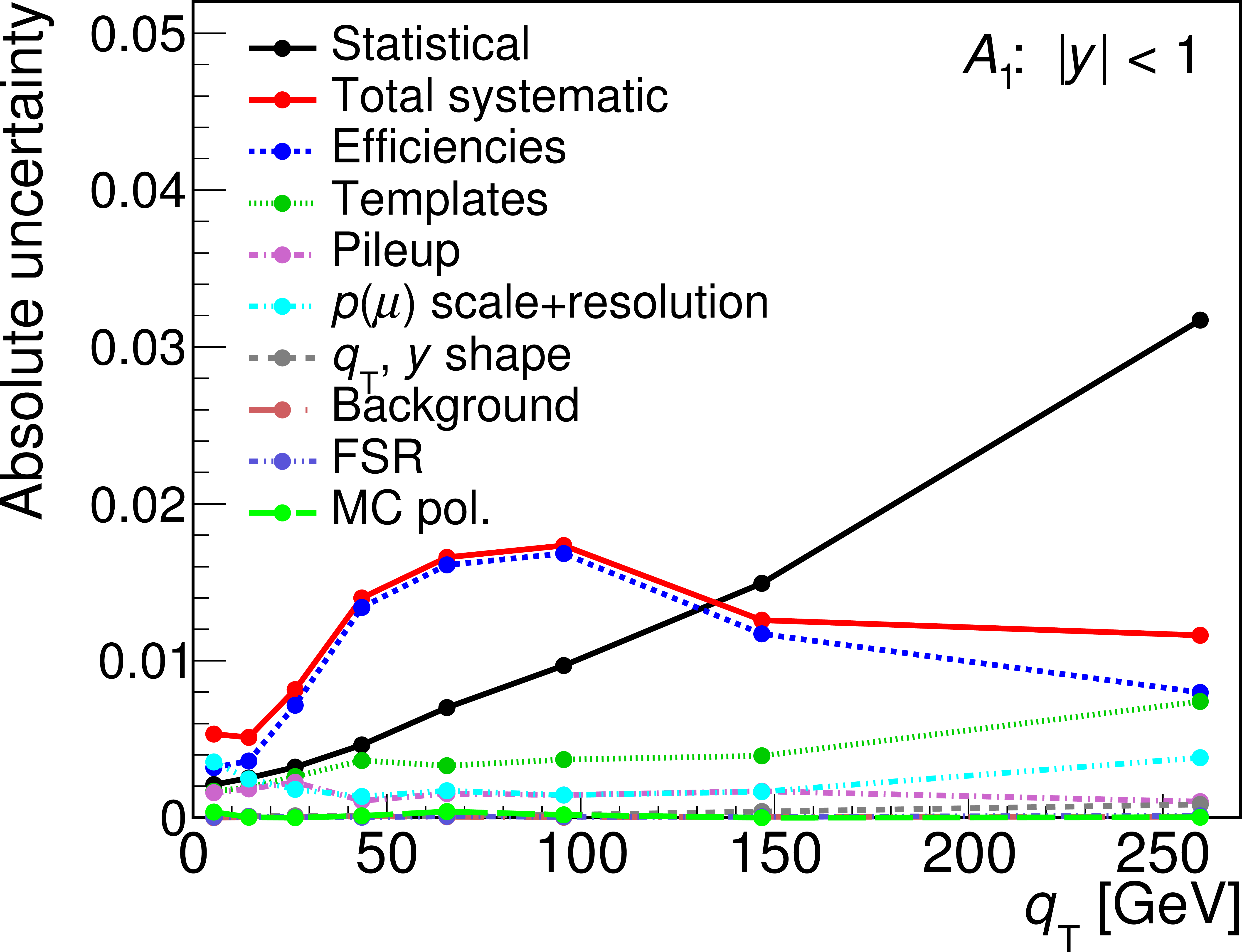
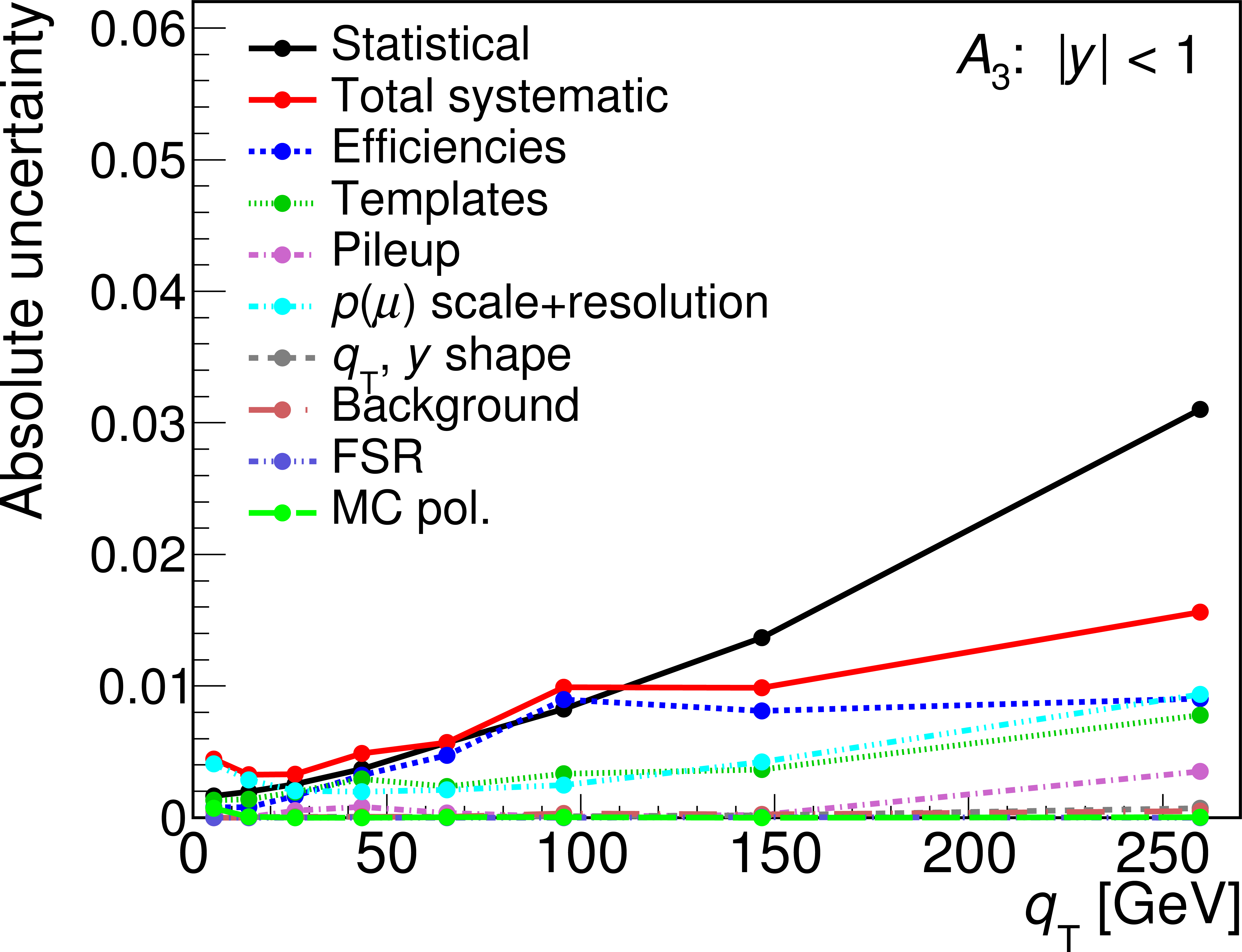
png pdf	Figure 2-c: Absolute uncertainties in the five angular coefficients $A_0$ to $A_4$ . Each figure shows the ${q_\mathrm {T}}$ dependence in the indicated ranges of $\| y \|$ .
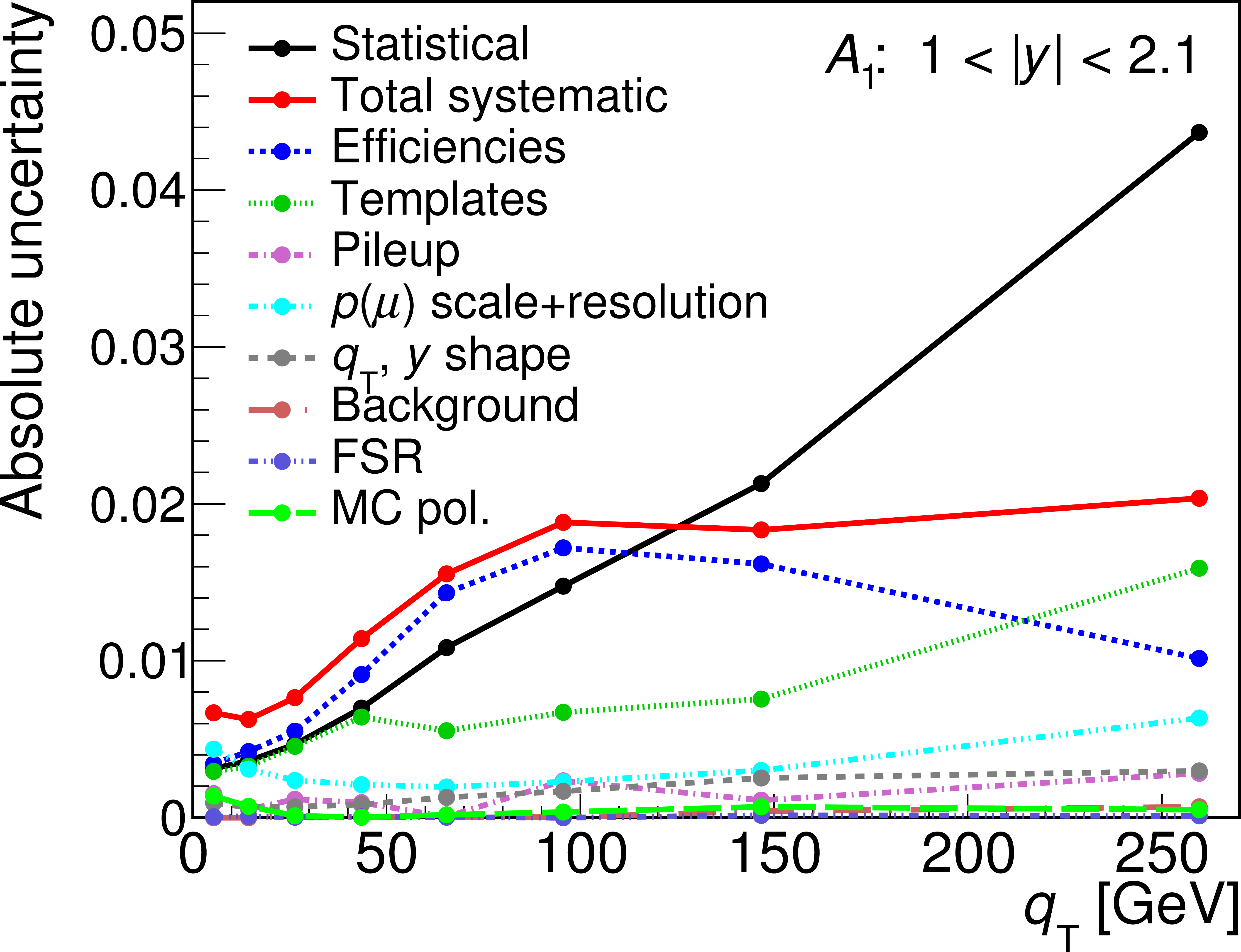
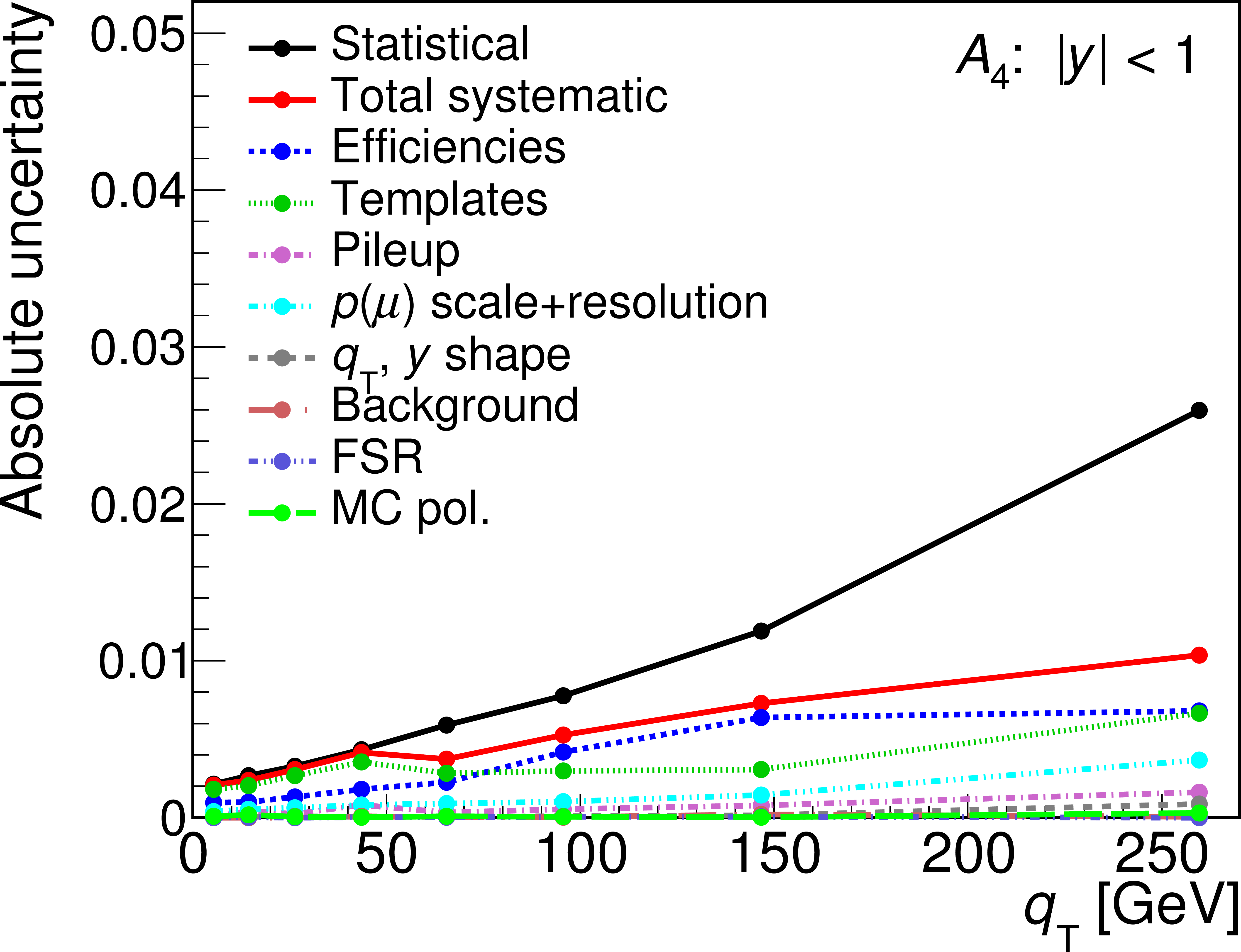
png pdf	Figure 2-d: Absolute uncertainties in the five angular coefficients $A_0$ to $A_4$ . Each figure shows the ${q_\mathrm {T}}$ dependence in the indicated ranges of $\| y \|$ .
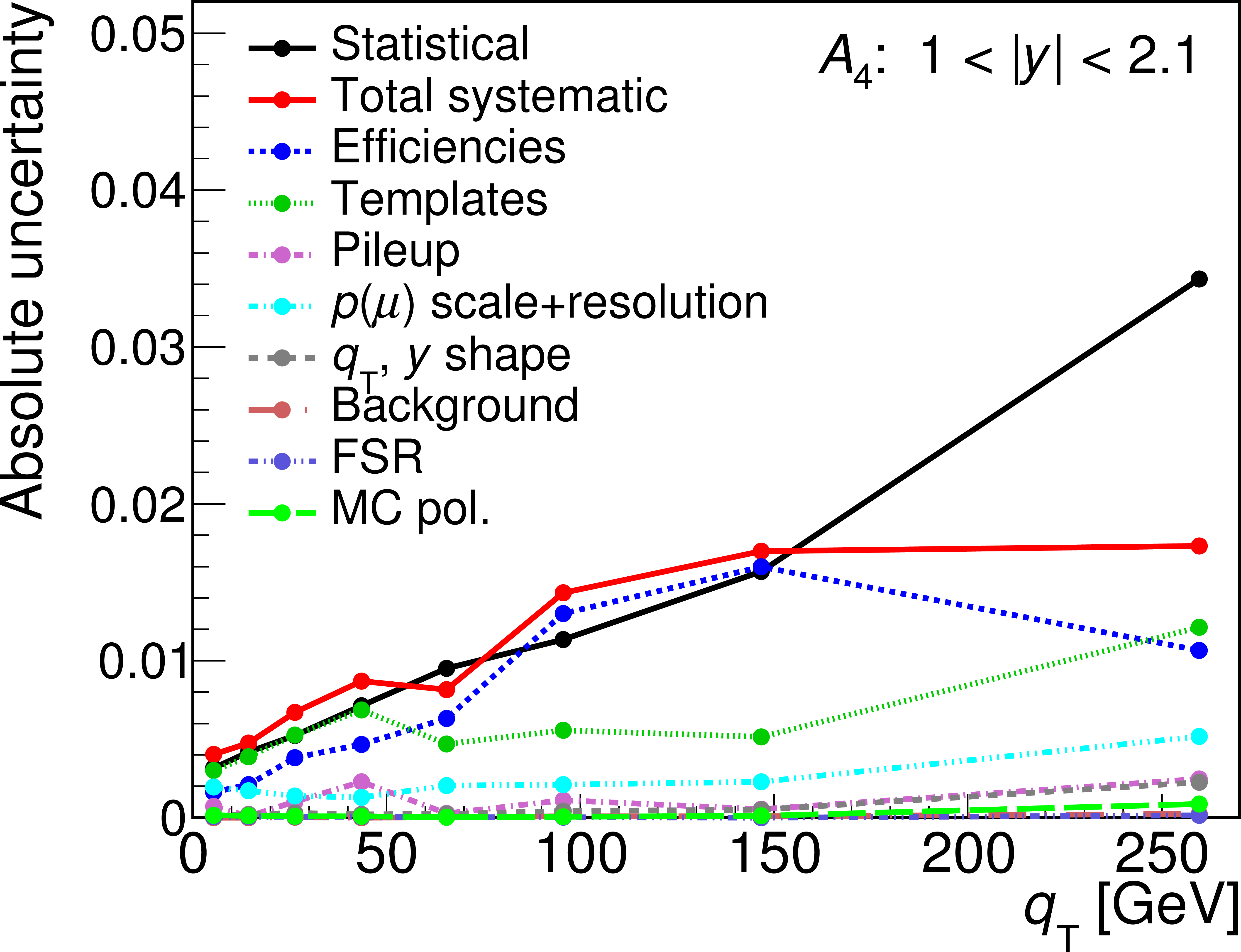
png pdf	Figure 2-e: Absolute uncertainties in the five angular coefficients $A_0$ to $A_4$ . Each figure shows the ${q_\mathrm {T}}$ dependence in the indicated ranges of $\| y \|$ .
png pdf	Figure 2-f: Absolute uncertainties in the five angular coefficients $A_0$ to $A_4$ . Each figure shows the ${q_\mathrm {T}}$ dependence in the indicated ranges of $\| y \|$ .
png pdf	Figure 2-g: Absolute uncertainties in the five angular coefficients $A_0$ to $A_4$ . Each figure shows the ${q_\mathrm {T}}$ dependence in the indicated ranges of $\| y \|$ .
png pdf	Figure 2-h: Absolute uncertainties in the five angular coefficients $A_0$ to $A_4$ . Each figure shows the ${q_\mathrm {T}}$ dependence in the indicated ranges of $\| y \|$ .
png pdf	Figure 2-i: Absolute uncertainties in the five angular coefficients $A_0$ to $A_4$ . Each figure shows the ${q_\mathrm {T}}$ dependence in the indicated ranges of $\| y \|$ .
png pdf	Figure 2-j: Absolute uncertainties in the five angular coefficients $A_0$ to $A_4$ . Each figure shows the ${q_\mathrm {T}}$ dependence in the indicated ranges of $\| y \|$ .
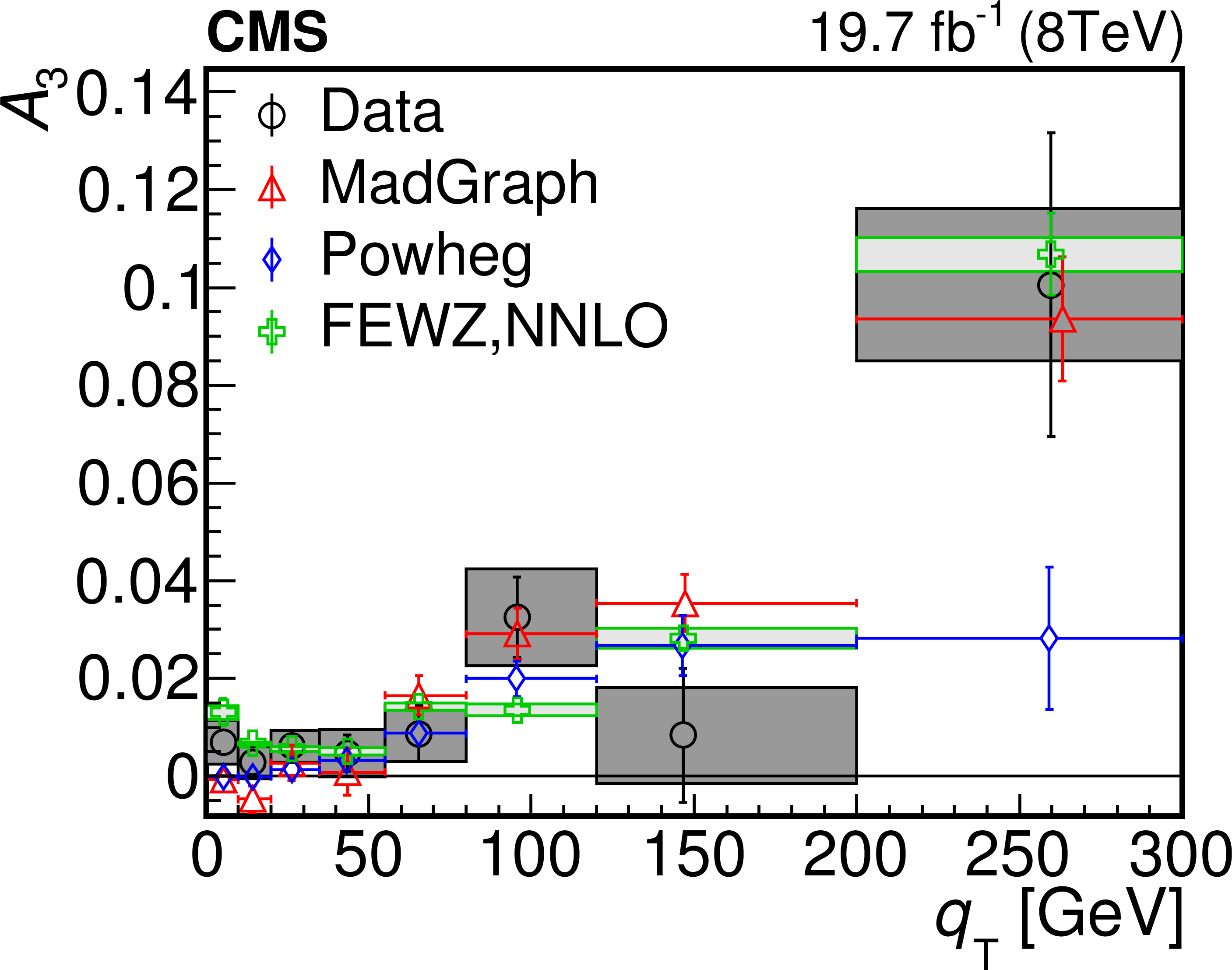
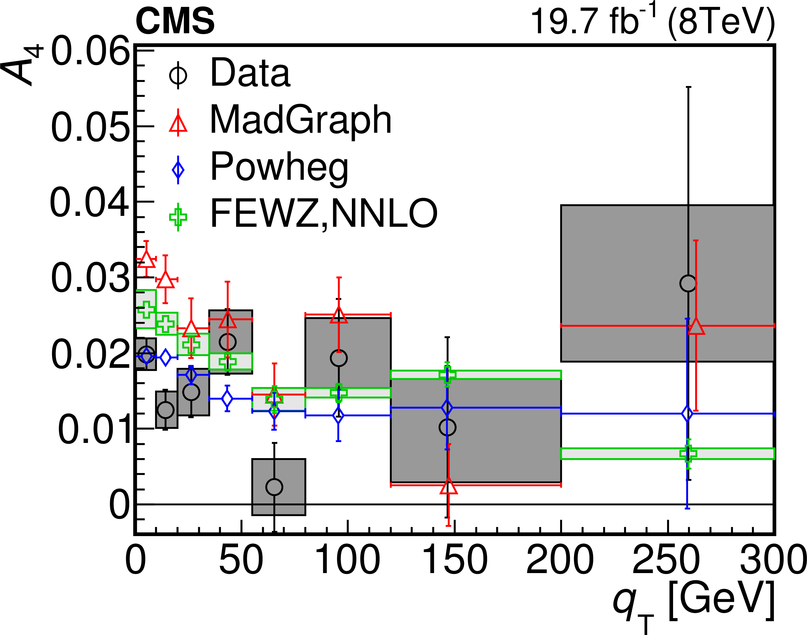
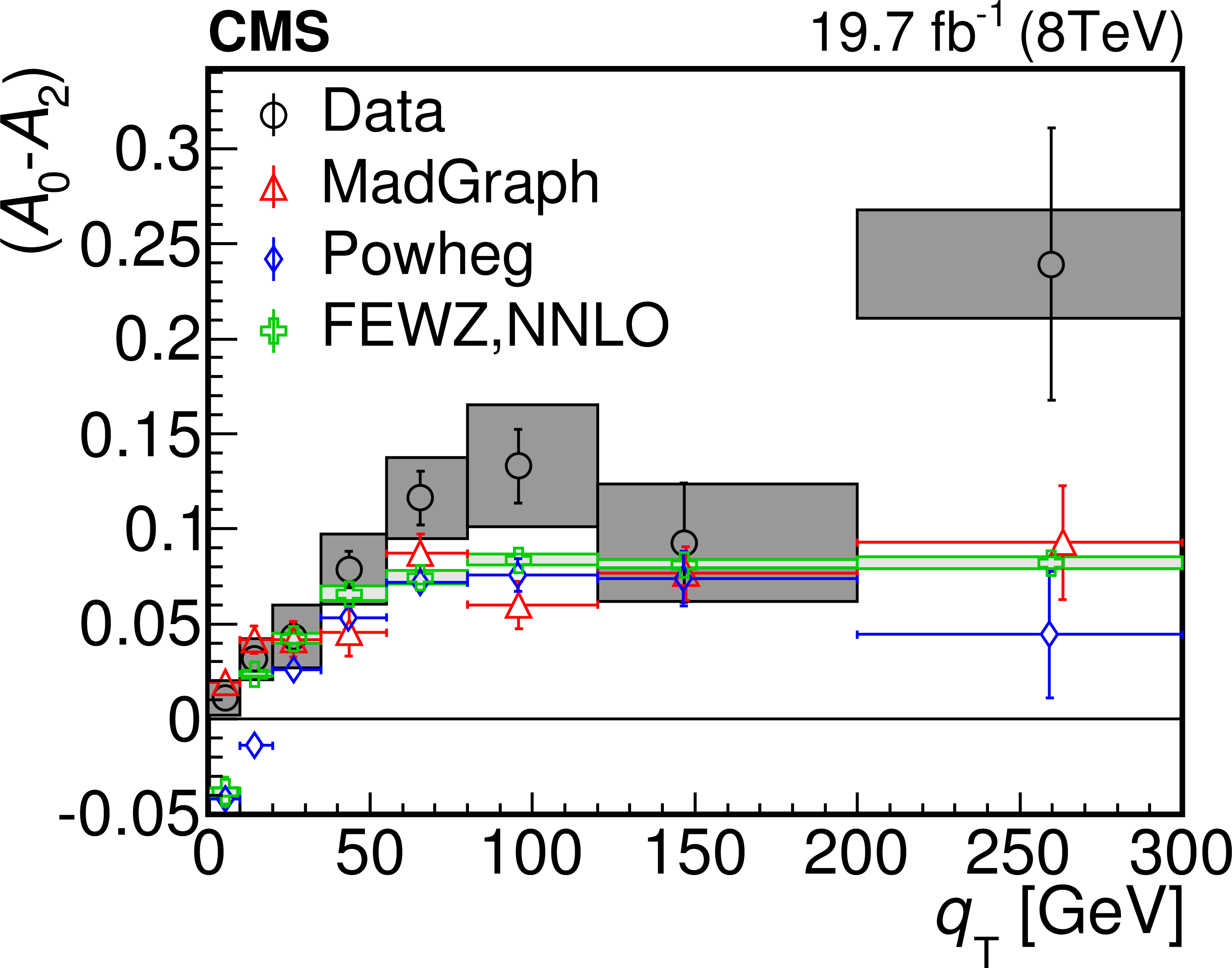
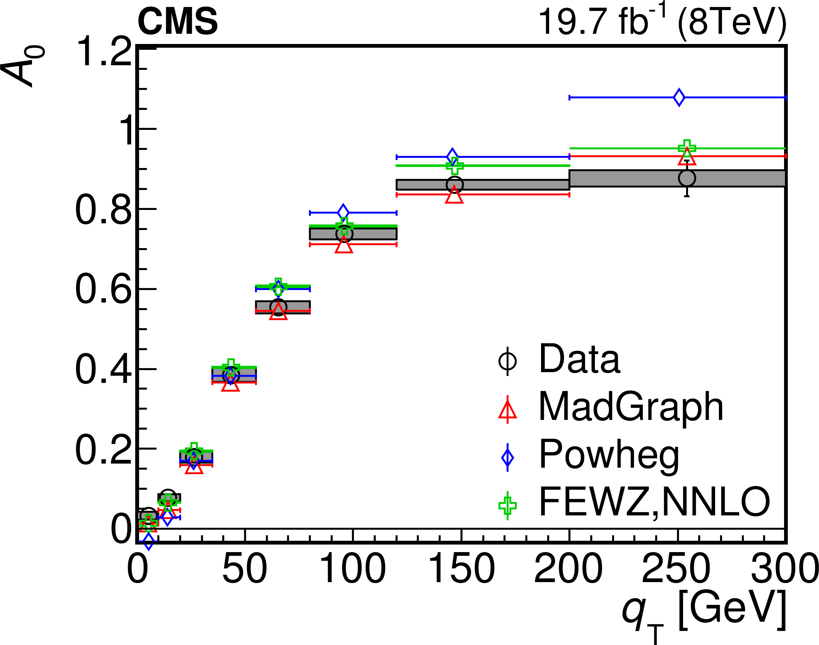
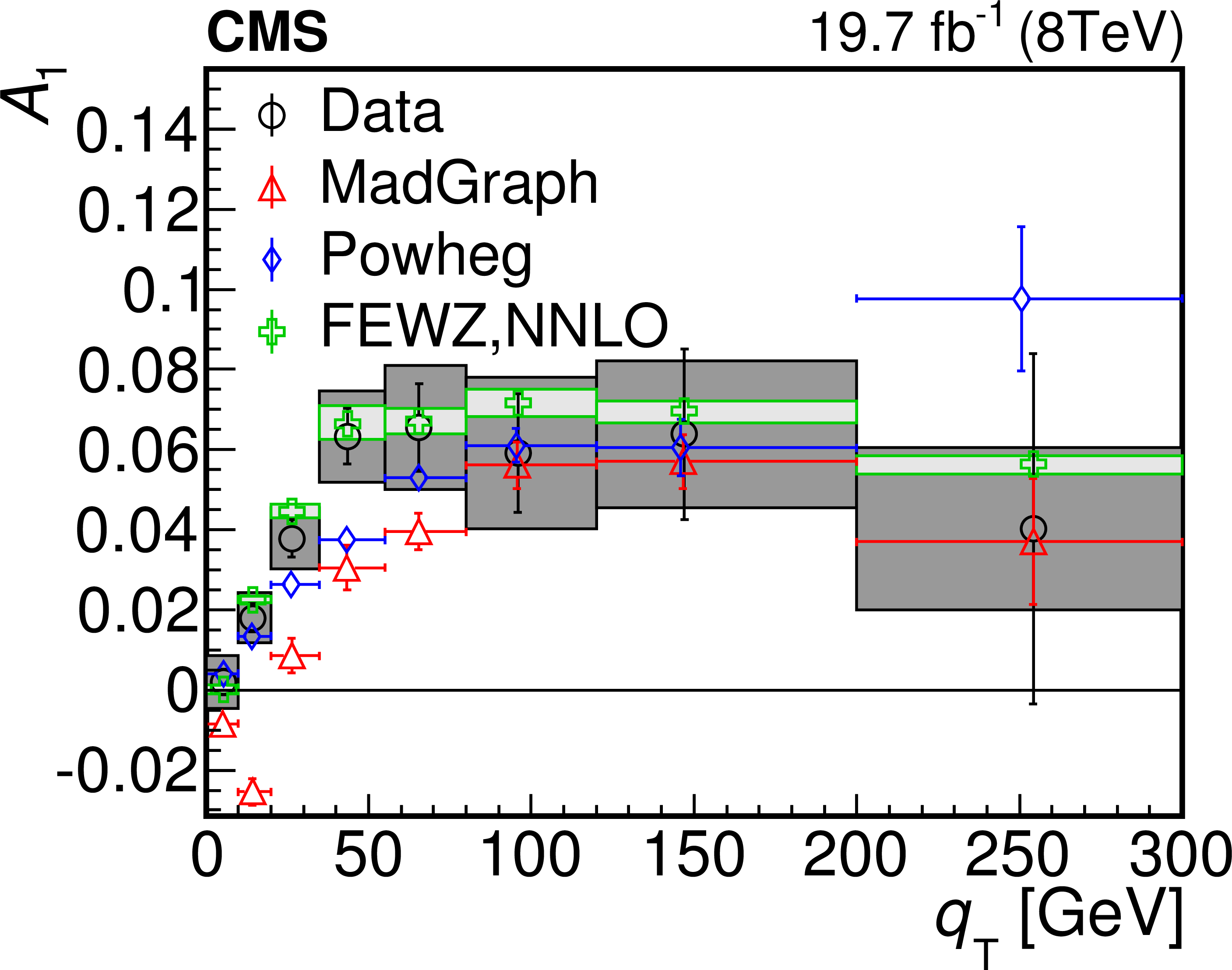
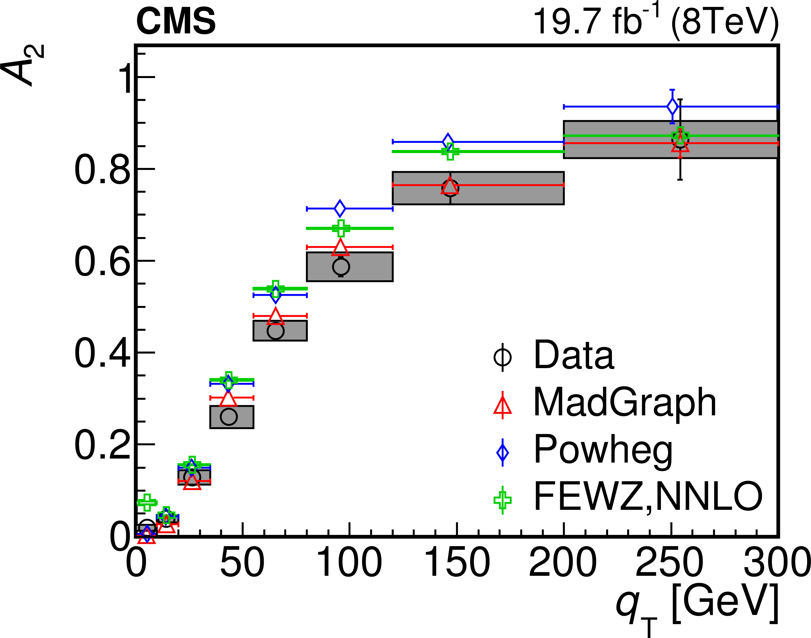
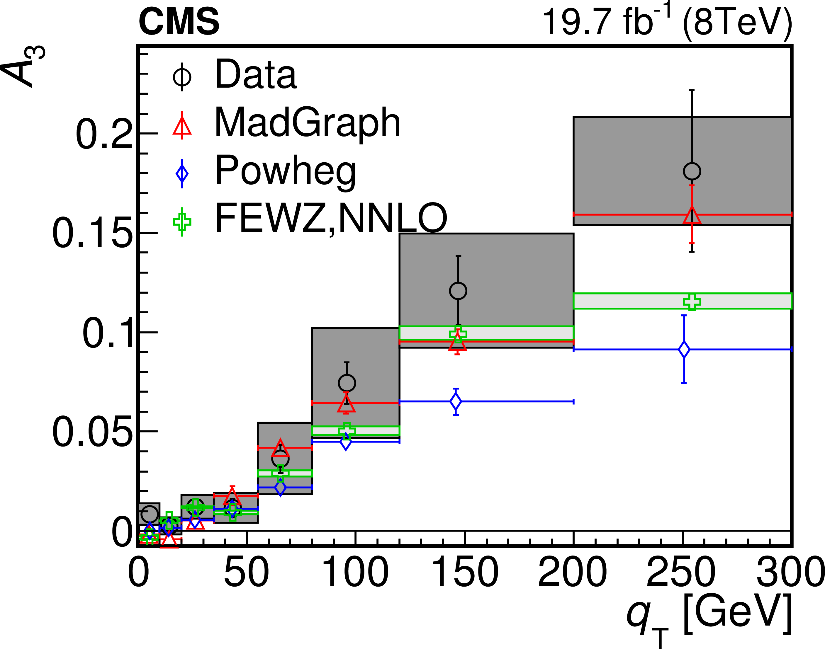
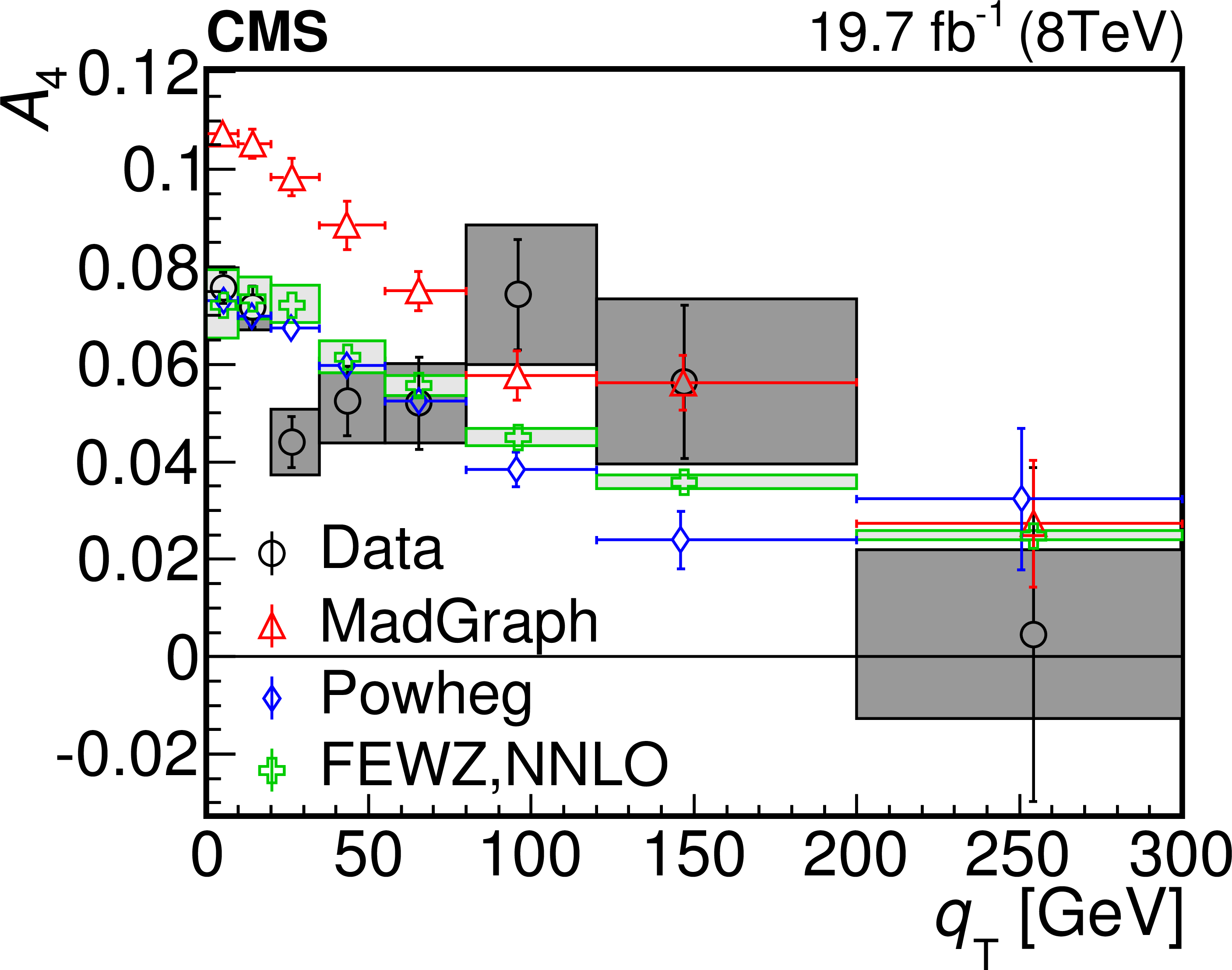
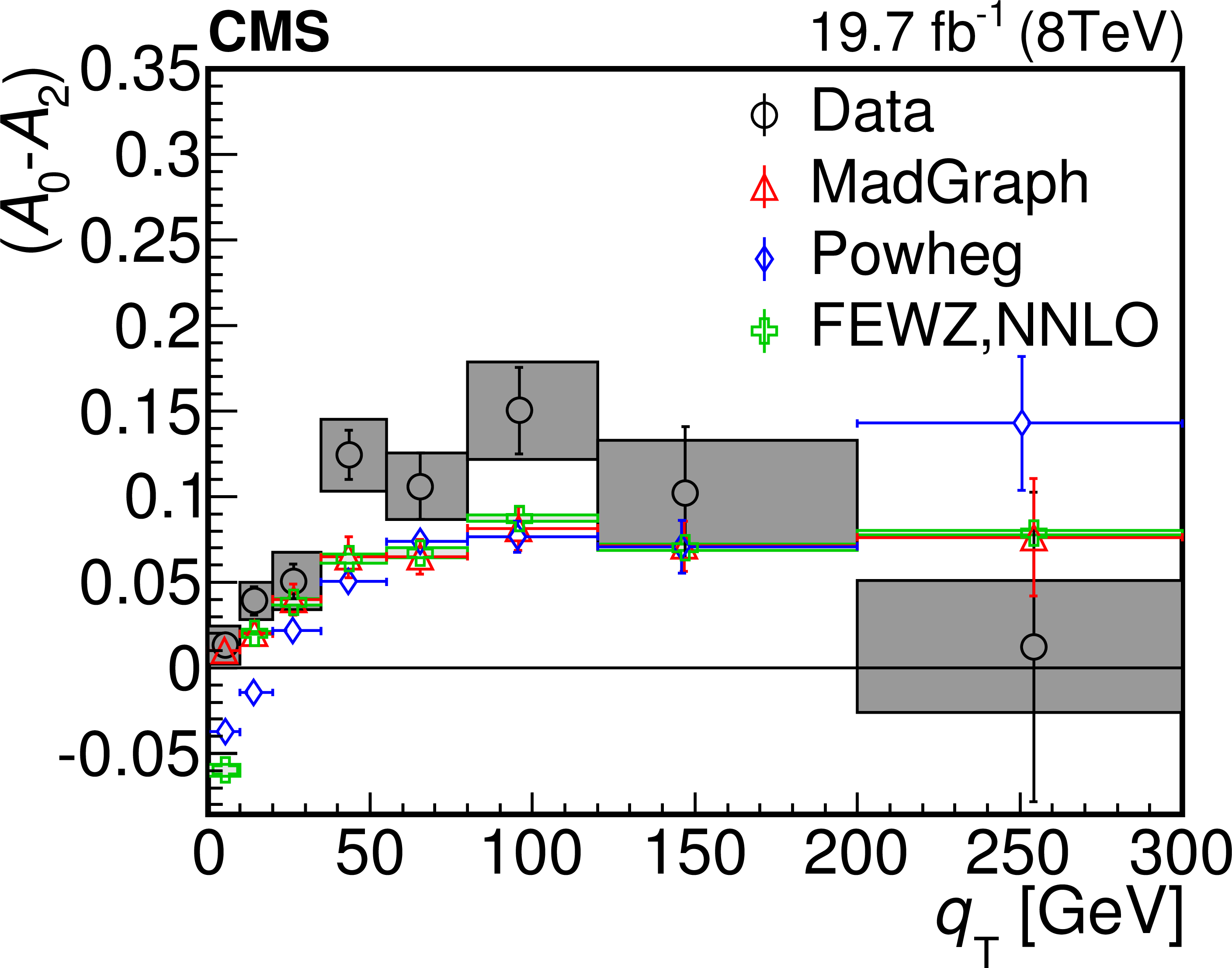
png pdf	Figure 3-a: Comparison of the five angular coefficients $A_i$ and $A_0-A_2$ measured in the Collins--Soper frame in bins of ${q_\mathrm {T}}$ for $\| y \| < 1$ . The circles show the measured results. The vertical bars represent the statistical uncertainties and the boxes the systematic uncertainties of the measurement. The triangles show the predictions from MADGRAPH, the diamonds from POWHEG, and the crosses from FEWZ at NNLO. The boxes at the FEWZ values indicate the PDF uncertainties.
png pdf	Figure 3-b: Comparison of the five angular coefficients $A_i$ and $A_0-A_2$ measured in the Collins--Soper frame in bins of ${q_\mathrm {T}}$ for $\| y \| < 1$ . The circles show the measured results. The vertical bars represent the statistical uncertainties and the boxes the systematic uncertainties of the measurement. The triangles show the predictions from MADGRAPH, the diamonds from POWHEG, and the crosses from FEWZ at NNLO. The boxes at the FEWZ values indicate the PDF uncertainties.
png pdf	Figure 3-c: Comparison of the five angular coefficients $A_i$ and $A_0-A_2$ measured in the Collins--Soper frame in bins of ${q_\mathrm {T}}$ for $\| y \| < 1$ . The circles show the measured results. The vertical bars represent the statistical uncertainties and the boxes the systematic uncertainties of the measurement. The triangles show the predictions from MADGRAPH, the diamonds from POWHEG, and the crosses from FEWZ at NNLO. The boxes at the FEWZ values indicate the PDF uncertainties.
png pdf	Figure 3-d: Comparison of the five angular coefficients $A_i$ and $A_0-A_2$ measured in the Collins--Soper frame in bins of ${q_\mathrm {T}}$ for $\| y \| < 1$ . The circles show the measured results. The vertical bars represent the statistical uncertainties and the boxes the systematic uncertainties of the measurement. The triangles show the predictions from MADGRAPH, the diamonds from POWHEG, and the crosses from FEWZ at NNLO. The boxes at the FEWZ values indicate the PDF uncertainties.
png pdf	Figure 3-e: Comparison of the five angular coefficients $A_i$ and $A_0-A_2$ measured in the Collins--Soper frame in bins of ${q_\mathrm {T}}$ for $\| y \| < 1$ . The circles show the measured results. The vertical bars represent the statistical uncertainties and the boxes the systematic uncertainties of the measurement. The triangles show the predictions from MADGRAPH, the diamonds from POWHEG, and the crosses from FEWZ at NNLO. The boxes at the FEWZ values indicate the PDF uncertainties.
png pdf	Figure 3-f: Comparison of the five angular coefficients $A_i$ and $A_0-A_2$ measured in the Collins--Soper frame in bins of ${q_\mathrm {T}}$ for $\| y \| < 1$ . The circles show the measured results. The vertical bars represent the statistical uncertainties and the boxes the systematic uncertainties of the measurement. The triangles show the predictions from MADGRAPH, the diamonds from POWHEG, and the crosses from FEWZ at NNLO. The boxes at the FEWZ values indicate the PDF uncertainties.
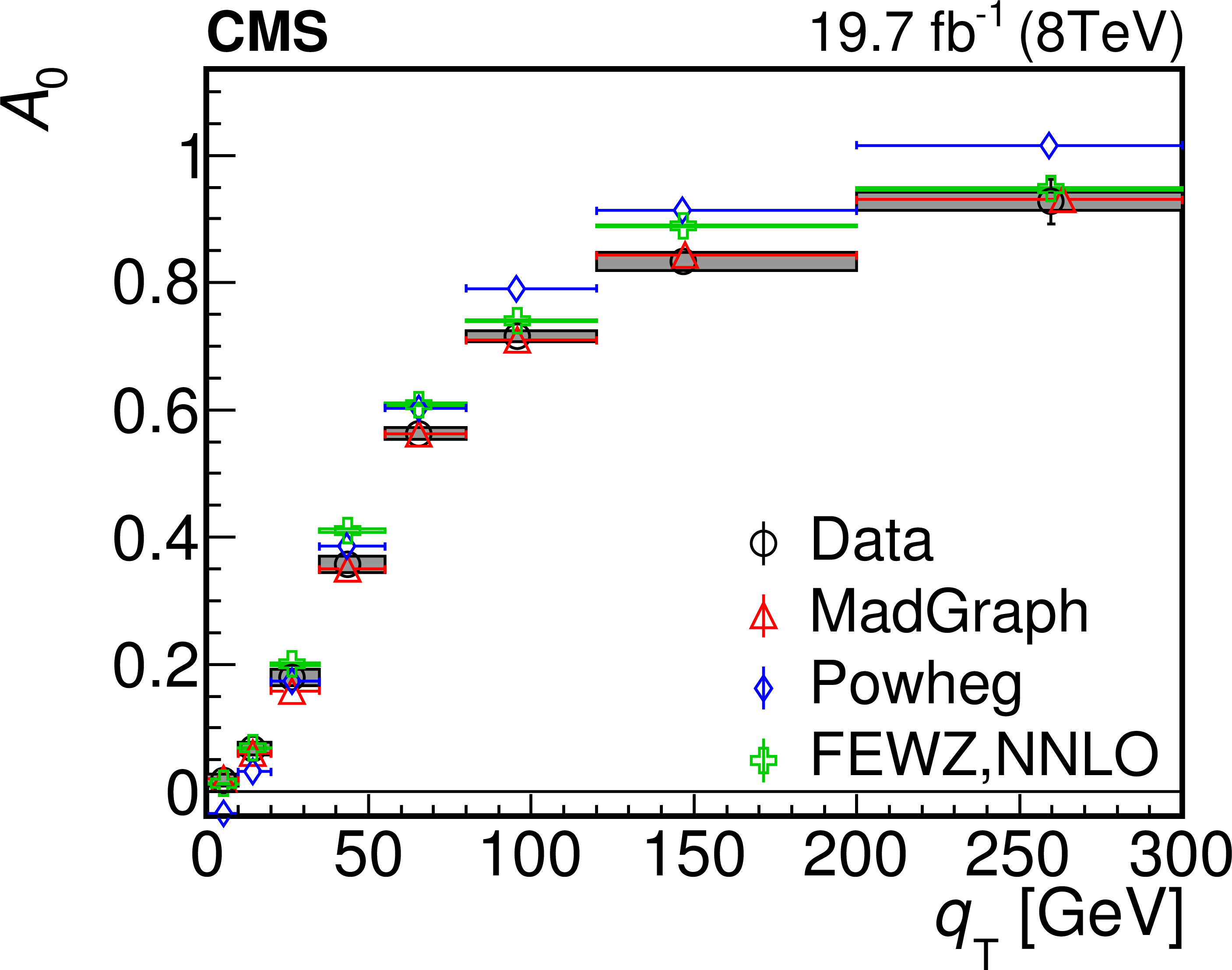
png pdf	Figure 4-a: Comparison of the five angular coefficients and $A_0-A_2$ under the same conditions as Fig. 3, for the rapidity bin $1 < \| y \| < 2.1$ .
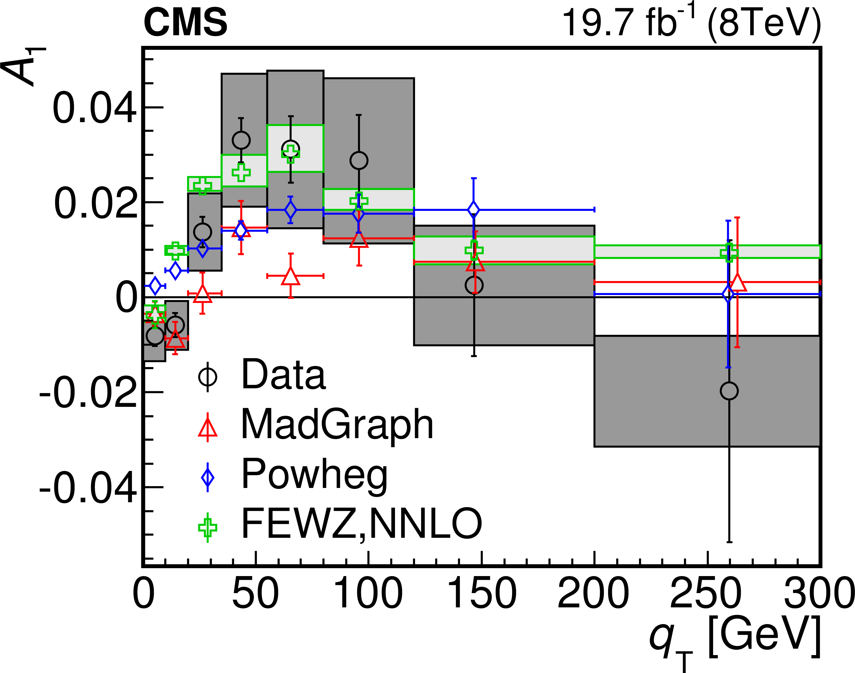
png pdf	Figure 4-b: Comparison of the five angular coefficients and $A_0-A_2$ under the same conditions as Fig. 3, for the rapidity bin $1 < \| y \| < 2.1$ .
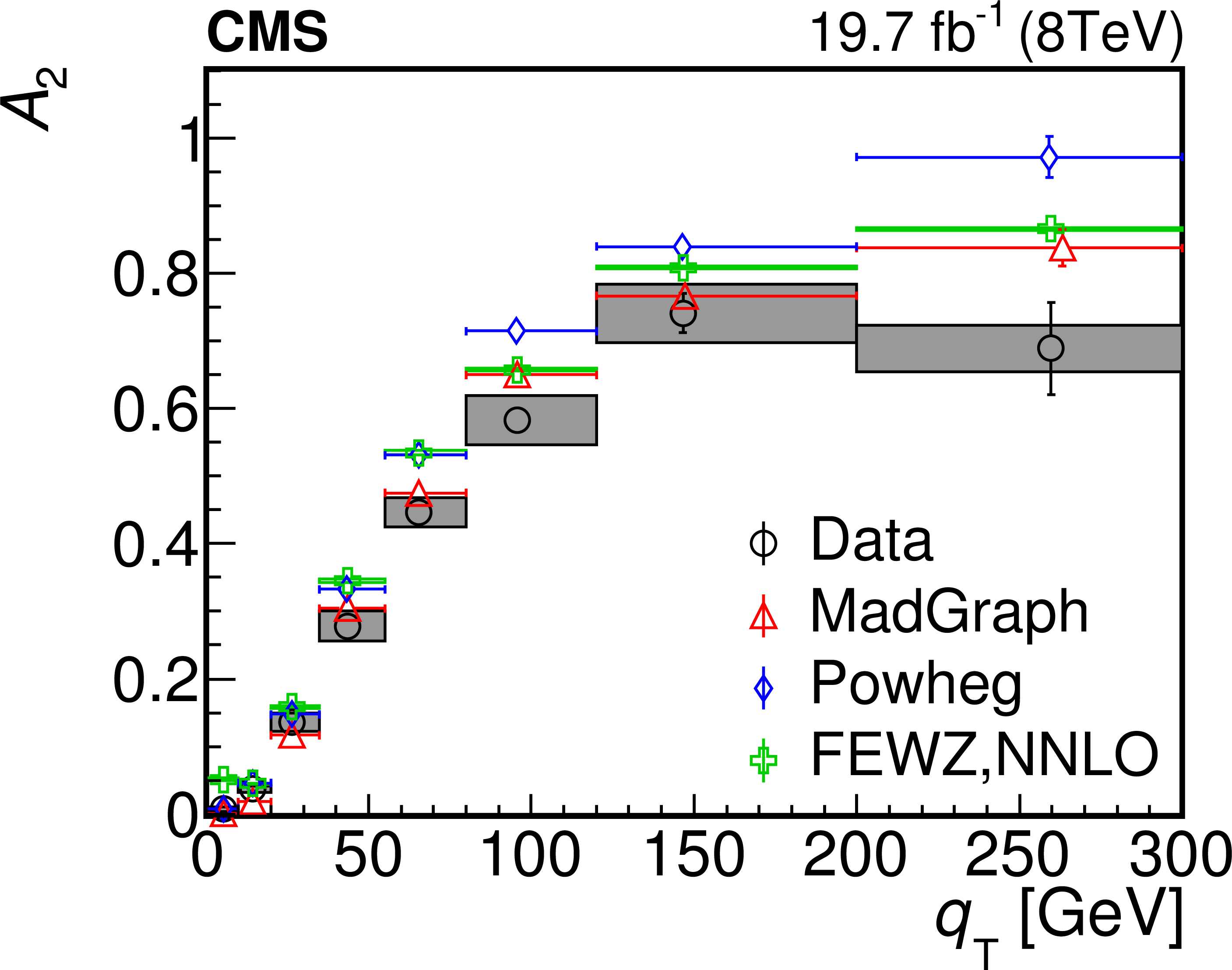
png pdf	Figure 4-c: Comparison of the five angular coefficients and $A_0-A_2$ under the same conditions as Fig. 3, for the rapidity bin $1 < \| y \| < 2.1$ .
png pdf	Figure 4-d: Comparison of the five angular coefficients and $A_0-A_2$ under the same conditions as Fig. 3, for the rapidity bin $1 < \| y \| < 2.1$ .
png pdf	Figure 4-e: Comparison of the five angular coefficients and $A_0-A_2$ under the same conditions as Fig. 3, for the rapidity bin $1 < \| y \| < 2.1$ .
png pdf	Figure 4-f: Comparison of the five angular coefficients and $A_0-A_2$ under the same conditions as Fig. 3, for the rapidity bin $1 < \| y \| < 2.1$ .
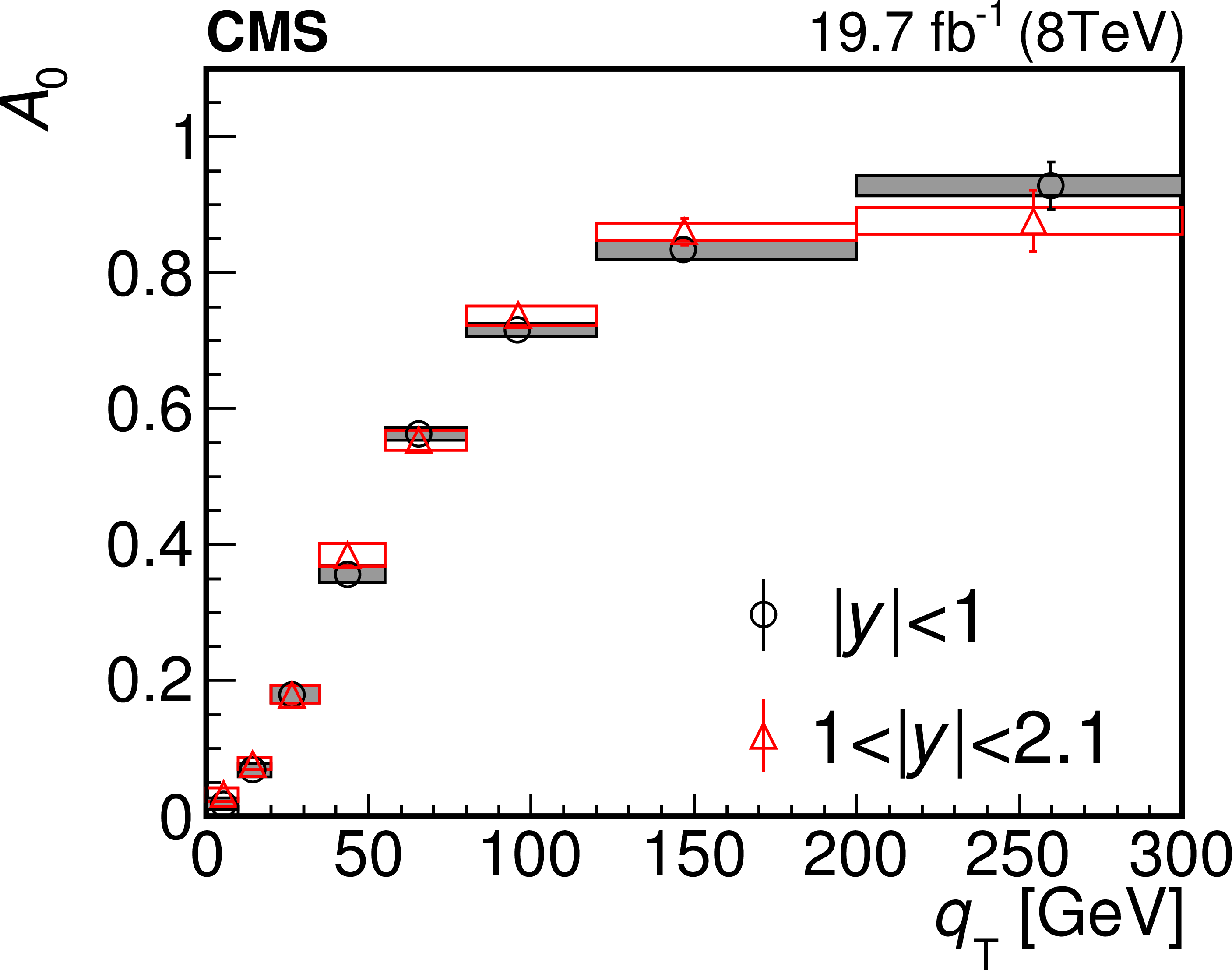
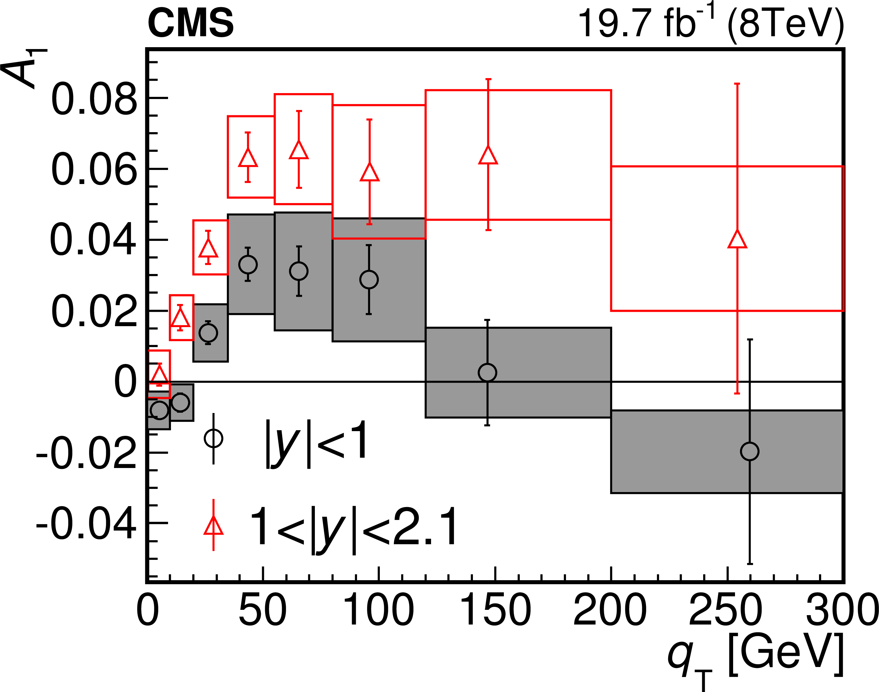
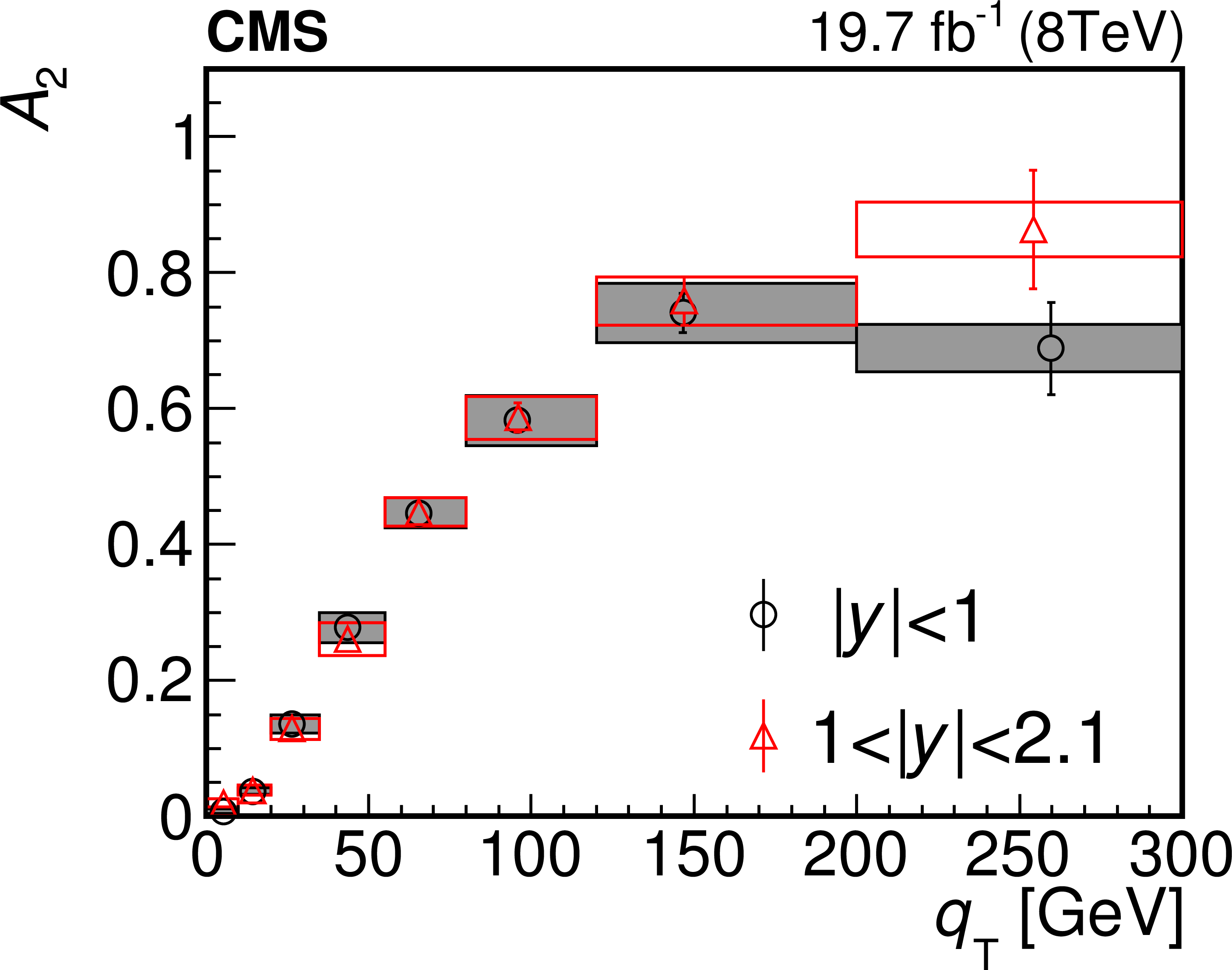
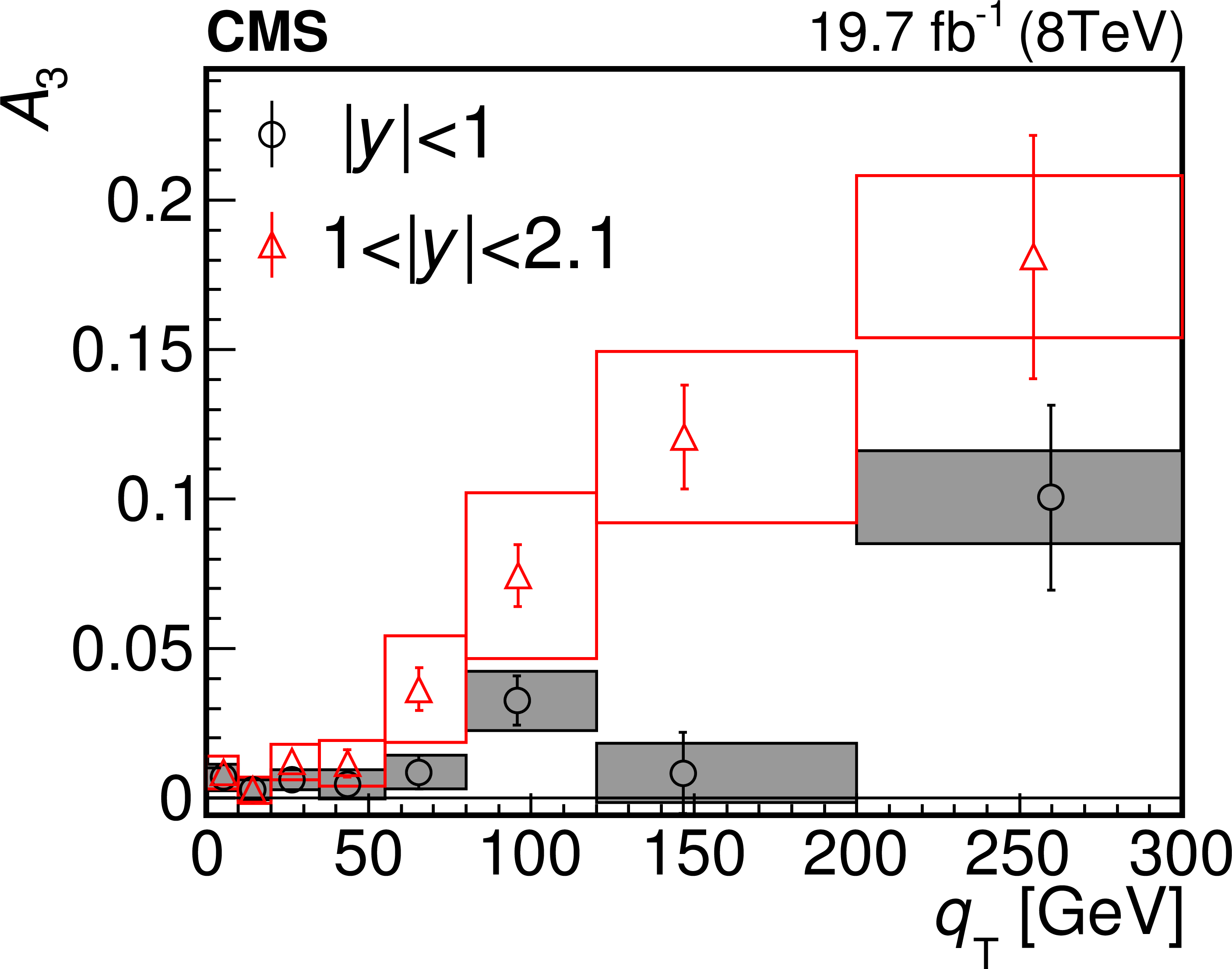
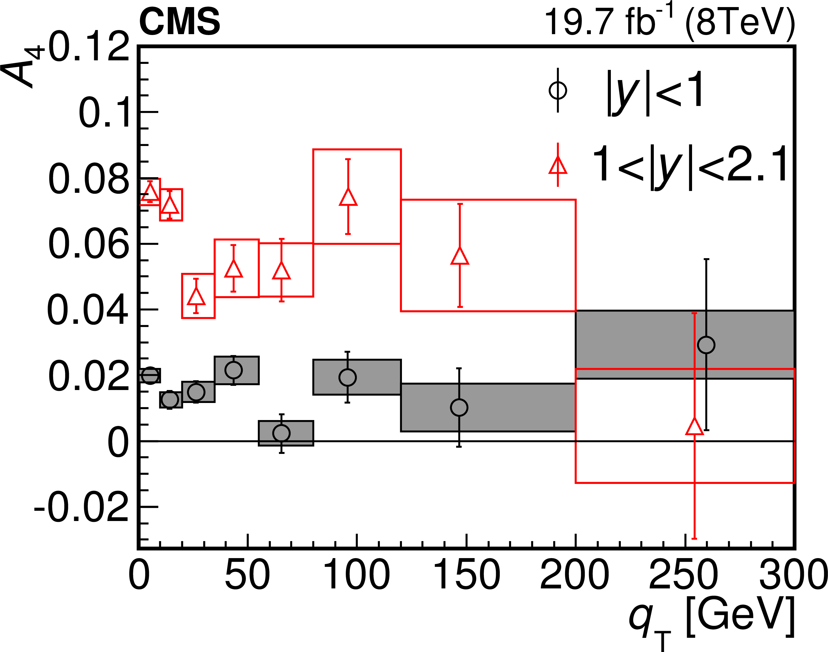
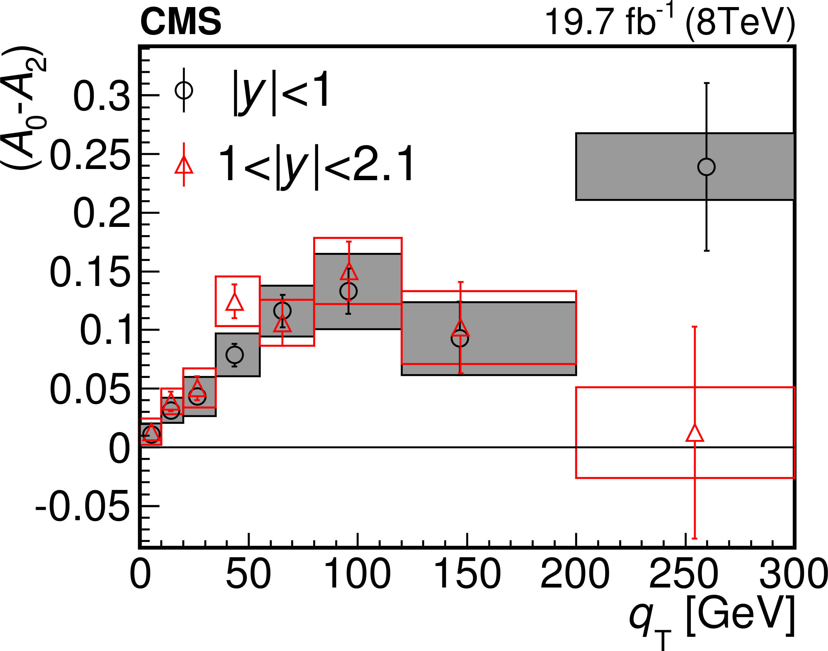
png pdf	Figure 5-a: Comparison of the five angular coefficients $A_i$ and $A_0-A_2$ measured in the Collins--Soper frame in bins of ${q_\mathrm {T}}$ between $\| y \| < 1$ (circles) and $1 < \| y \| < 2.1$ (triangles). The vertical bars represent the statistical uncertainties and the boxes the systematic uncertainties of the measurement.
png pdf	Figure 5-b: Comparison of the five angular coefficients $A_i$ and $A_0-A_2$ measured in the Collins--Soper frame in bins of ${q_\mathrm {T}}$ between $\| y \| < 1$ (circles) and $1 < \| y \| < 2.1$ (triangles). The vertical bars represent the statistical uncertainties and the boxes the systematic uncertainties of the measurement.
png pdf	Figure 5-c: Comparison of the five angular coefficients $A_i$ and $A_0-A_2$ measured in the Collins--Soper frame in bins of ${q_\mathrm {T}}$ between $\| y \| < 1$ (circles) and $1 < \| y \| < 2.1$ (triangles). The vertical bars represent the statistical uncertainties and the boxes the systematic uncertainties of the measurement.
png pdf	Figure 5-d: Comparison of the five angular coefficients $A_i$ and $A_0-A_2$ measured in the Collins--Soper frame in bins of ${q_\mathrm {T}}$ between $\| y \| < 1$ (circles) and $1 < \| y \| < 2.1$ (triangles). The vertical bars represent the statistical uncertainties and the boxes the systematic uncertainties of the measurement.
png pdf	Figure 5-e: Comparison of the five angular coefficients $A_i$ and $A_0-A_2$ measured in the Collins--Soper frame in bins of ${q_\mathrm {T}}$ between $\| y \| < 1$ (circles) and $1 < \| y \| < 2.1$ (triangles). The vertical bars represent the statistical uncertainties and the boxes the systematic uncertainties of the measurement.
png pdf	Figure 5-f: Comparison of the five angular coefficients $A_i$ and $A_0-A_2$ measured in the Collins--Soper frame in bins of ${q_\mathrm {T}}$ between $\| y \| < 1$ (circles) and $1 < \| y \| < 2.1$ (triangles). The vertical bars represent the statistical uncertainties and the boxes the systematic uncertainties of the measurement.

Tables
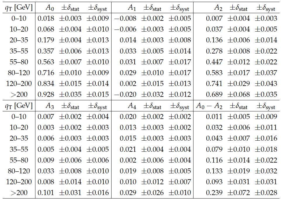
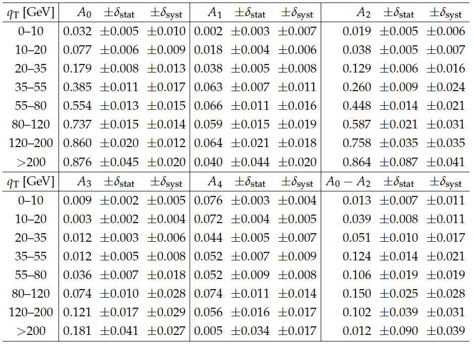
png pdf	Table 1: The five angular coefficients $A_0$ to $A_4$ and $A_0-A_2$ in bins of ${q_\mathrm {T}}$ for ${\| y \| }<$ 1.
png pdf	Table 2: The five angular coefficients $A_0$ to $A_4$ and $A_0-A_2$ in bins of ${q_\mathrm {T}}$ for 1 $< {\| y \| } <$ 2.1.

Summary

In summary, we presented the five major angular coefficients,

$A_0$ through

$A_4$ , for the production of the Z boson decaying to muon pairs as a function of

$q_{\mathrm{T}}$ and

$|y|$ in pp collisions. These results play an important role in future high-precision measurements, such as the measurement of the mass of the W boson and of the electroweak mixing angle. Some theoretical predictions deviate from the measurements in

$q_{\mathrm{T}}$ . Further refinements of the theory are needed to achieve a better agreement with the experimental results.