
Compact Muon Solenoid
LHC, CERN
 Visit us: CMS Public Website, CMS Physics ;
Contact us: CMS Publications Committee
Visit us: CMS Public Website, CMS Physics ;
Contact us: CMS Publications Committee
| CMS-MLG-25-002 ; CERN-EP-2026-222 | ||
| Calibration of electromagnetic shower features in the CMS calorimeter with machine-learning techniques | ||
| CMS Collaboration | ||
| 13 September 2026 | ||
| Submitted to SciPost Physics | ||
| Abstract: Monte Carlo simulations are used extensively in high-energy particle physics analyses. However, an incomplete description of the underlying physics can lead to significant discrepancies between observables measured in simulated and collision data. To mitigate potential biases arising from such mismodelling, it is essential to calibrate simulations to data. This paper presents two novel calibration methods based on machine-learning techniques: a reweighting approach, which employs a classifier to learn the ratio of probability density functions between simulation and data; and a normalising-flow approach, which learns a high-dimensional transformation to map simulation to data. Compared to traditional calibration methods, both approaches offer continuous, unbinned corrections across high-dimensional feature spaces, enabling improved global agreement with data. The techniques are demonstrated in the context of correcting the features of simulated electromagnetic showers in the CMS calorimeters, using proton-proton collision data collected during 2022 at $ \sqrt{s} = $ 13.6 TeV, corresponding to an integrated luminosity of 26.7 fb$ ^{-1} $. The strengths and limitations of the two methods are compared. | ||
| Links: e-print arXiv:2609.15377 [hep-ex] (PDF) ; CDS record ; inSPIRE record ; CADI line (restricted) ; | ||
| Figures | |
png pdf |
Figure 1:
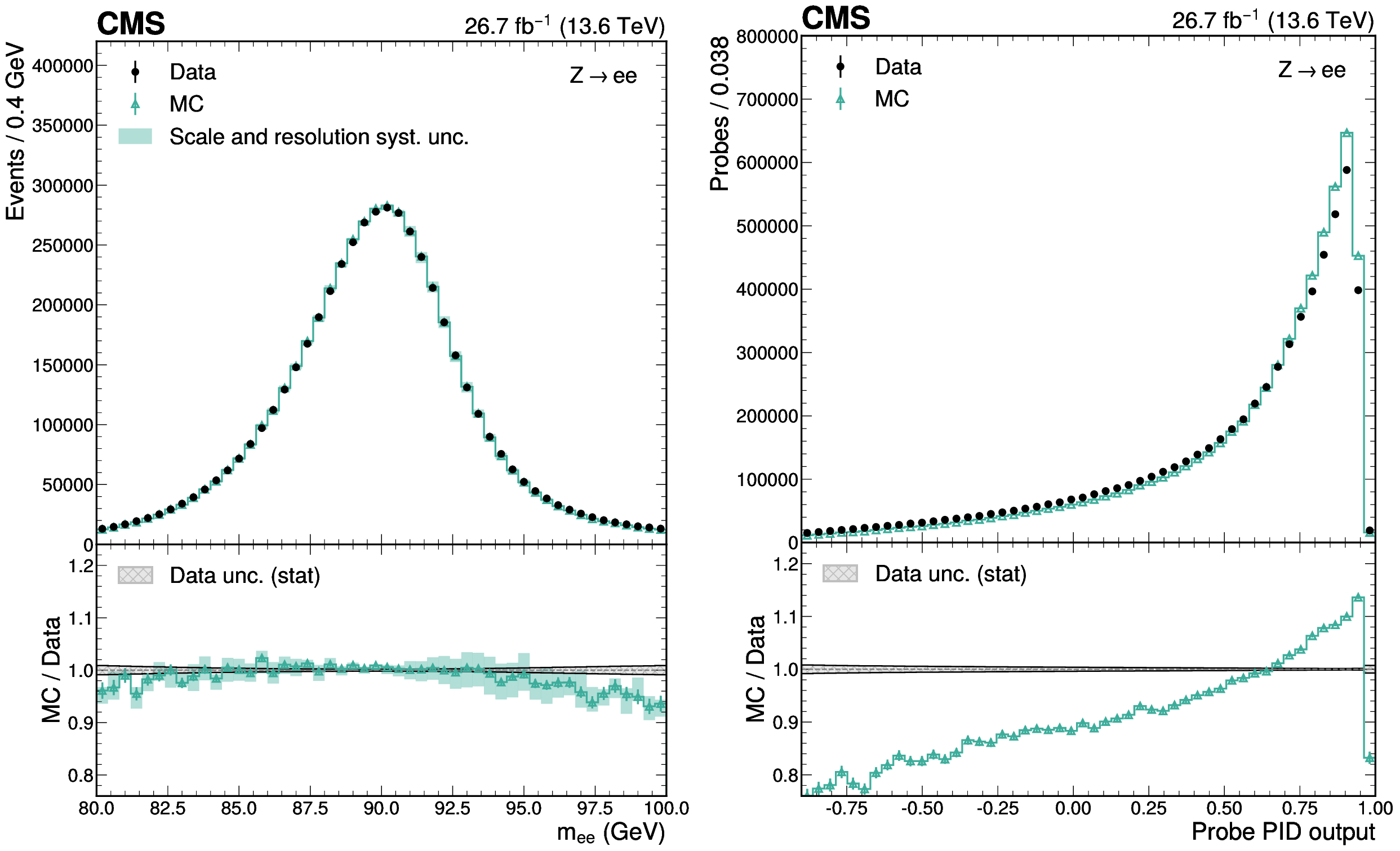
Invariant mass spectrum for tag-and-probe candidates from $ \mathrm{Z}\to\mathrm{e}\mathrm{e} $ events (left) and the PID output distribution for the probe EM showers (right) in data (black points) and simulation (teal histogram with triangular points). The statistical uncertainties in the simulation and data are shown by the error bars on the points. For the left-hand figure, the invariant mass for events in which both electrons pass the tag selection is included only once. The systematic uncertainty arising from the residual energy scale and resolution corrections is shown by the teal band in the left-hand figure. The lower panels show the ratio of simulation to data, where the statistical uncertainty in the data is indicated by the grey hatched band. |
png pdf |
Figure 1-a:
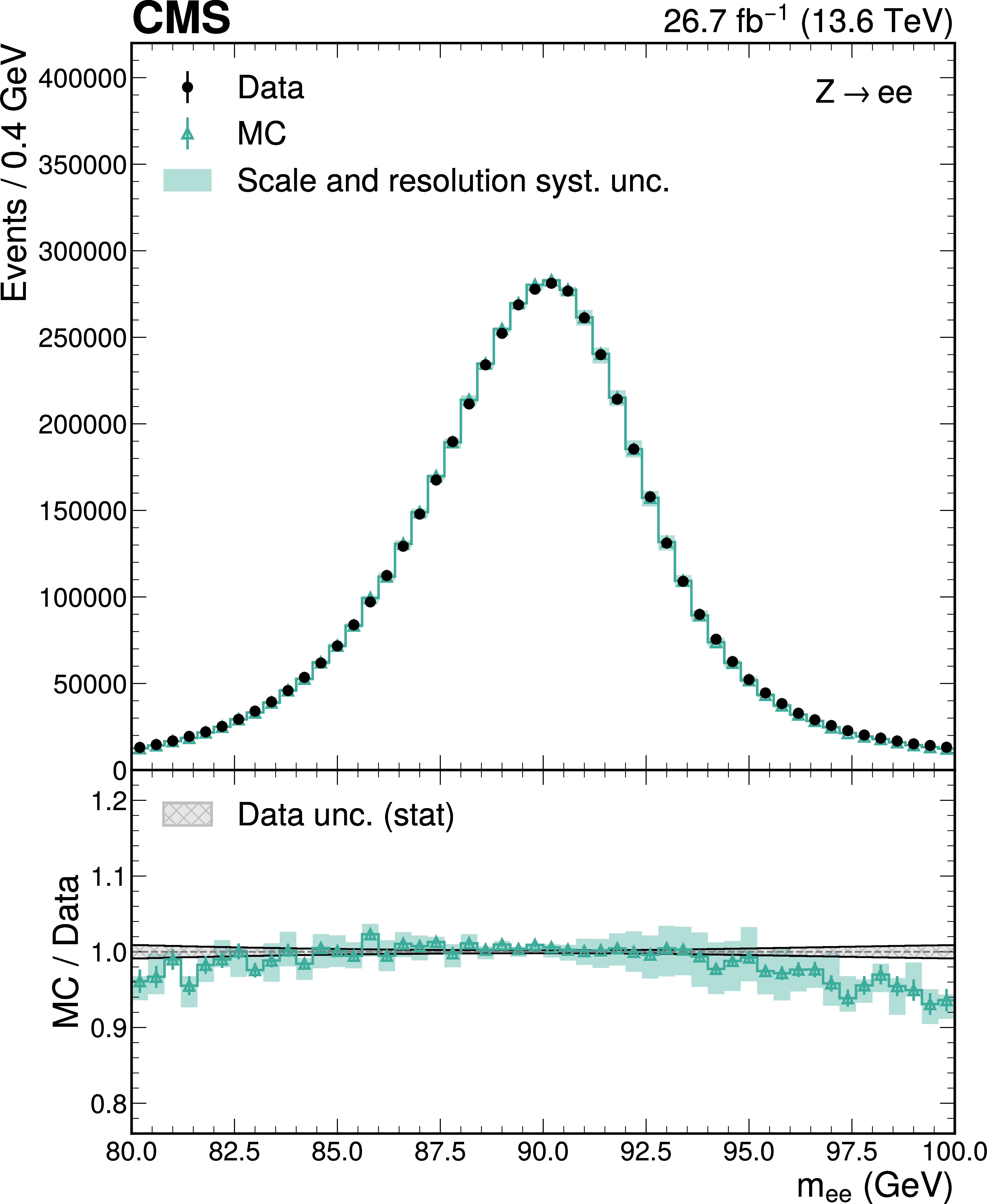
Invariant mass spectrum for tag-and-probe candidates from $ \mathrm{Z}\to\mathrm{e}\mathrm{e} $ events (left) and the PID output distribution for the probe EM showers (right) in data (black points) and simulation (teal histogram with triangular points). The statistical uncertainties in the simulation and data are shown by the error bars on the points. For the left-hand figure, the invariant mass for events in which both electrons pass the tag selection is included only once. The systematic uncertainty arising from the residual energy scale and resolution corrections is shown by the teal band in the left-hand figure. The lower panels show the ratio of simulation to data, where the statistical uncertainty in the data is indicated by the grey hatched band. |
png pdf |
Figure 1-b:
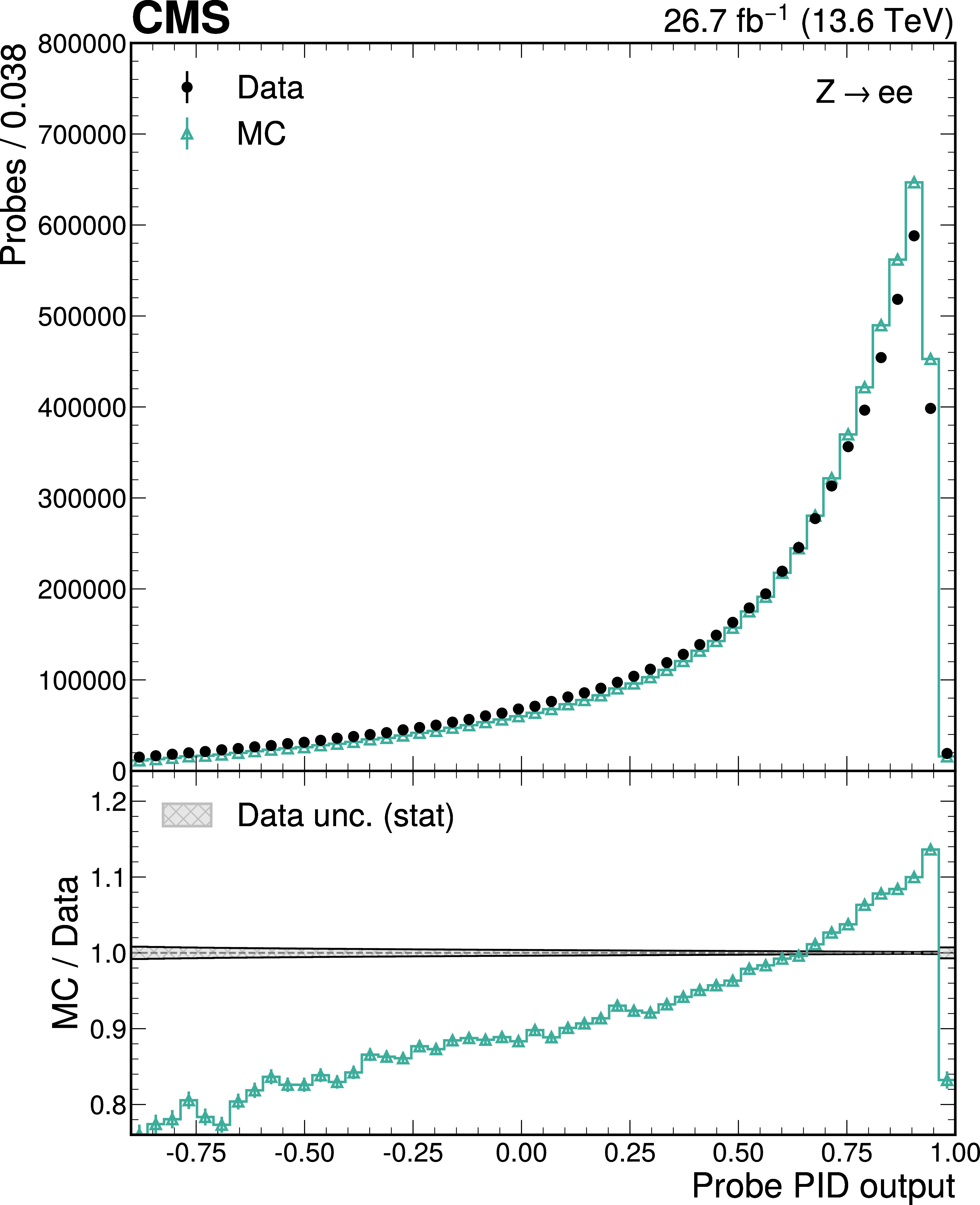
Invariant mass spectrum for tag-and-probe candidates from $ \mathrm{Z}\to\mathrm{e}\mathrm{e} $ events (left) and the PID output distribution for the probe EM showers (right) in data (black points) and simulation (teal histogram with triangular points). The statistical uncertainties in the simulation and data are shown by the error bars on the points. For the left-hand figure, the invariant mass for events in which both electrons pass the tag selection is included only once. The systematic uncertainty arising from the residual energy scale and resolution corrections is shown by the teal band in the left-hand figure. The lower panels show the ratio of simulation to data, where the statistical uncertainty in the data is indicated by the grey hatched band. |
png pdf |
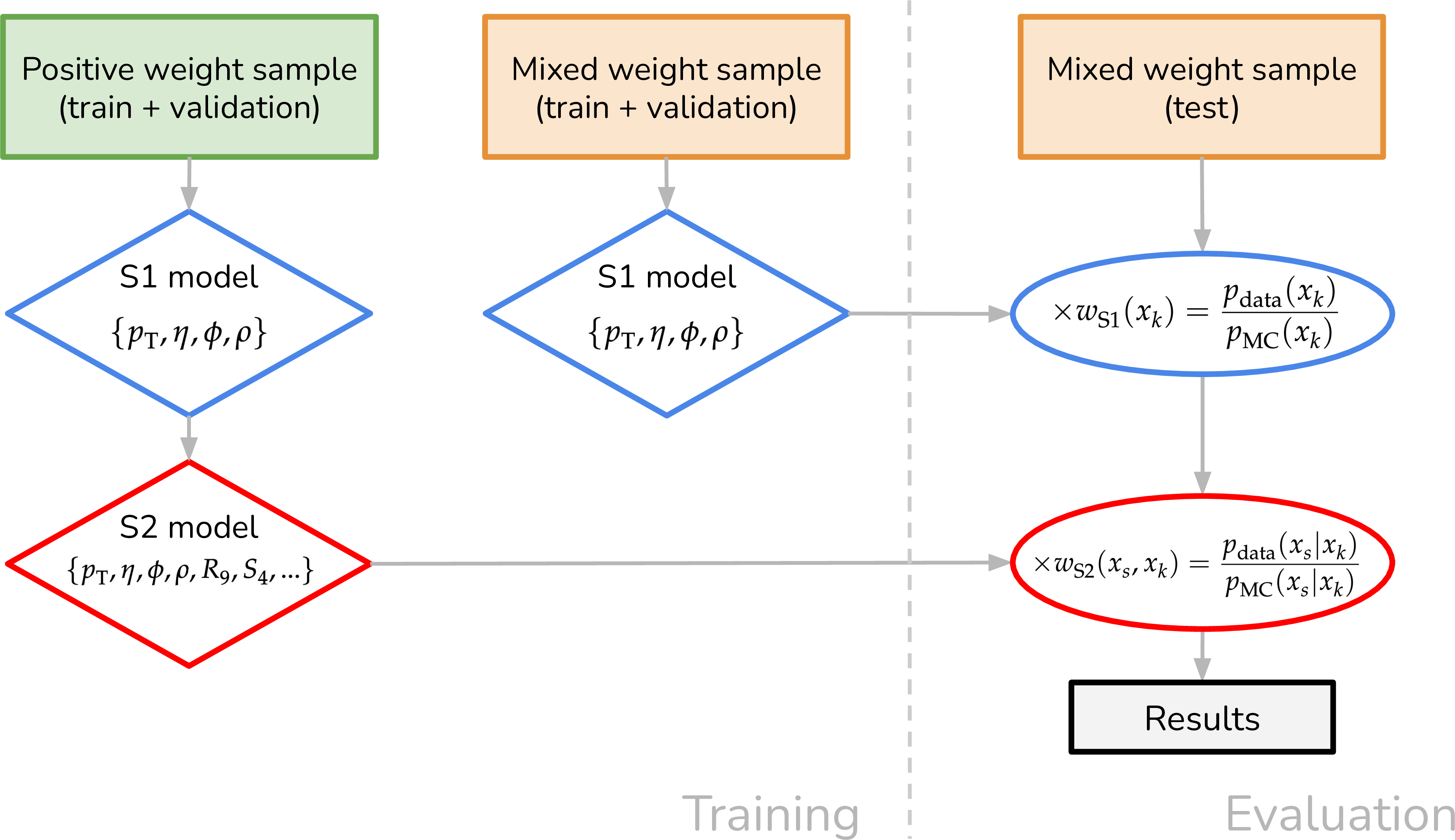
Figure 2:
Schematic diagram of the two-staged model training and evaluation steps. Only positively weighted events are used in the training of the S2 model. This necessitates an S1 model trained using only positively weighted events during the initial training process. For evaluation, a separate S1 model is required that is trained on both positively and negatively weighted events. |
png pdf |
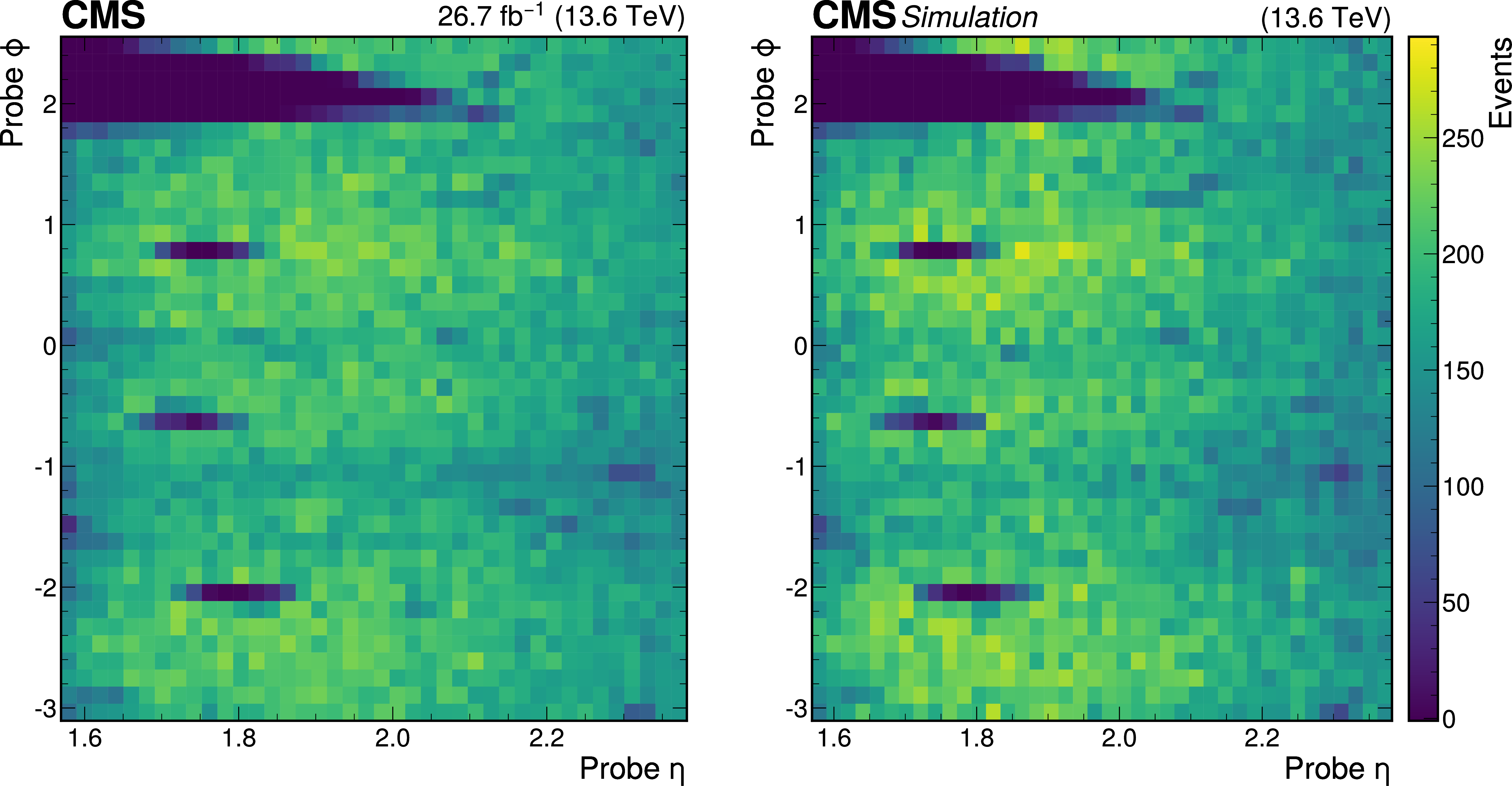
Figure 3:
Heatmap for probes in data (left) and simulation (right) in the $ (\eta,\phi) $ plane for the EE$ + $ subdetector. The hole from the power cooling issue can be seen in the upper-left corner of the plots. The simulation is normalised to have the same yield as data. |
png pdf |
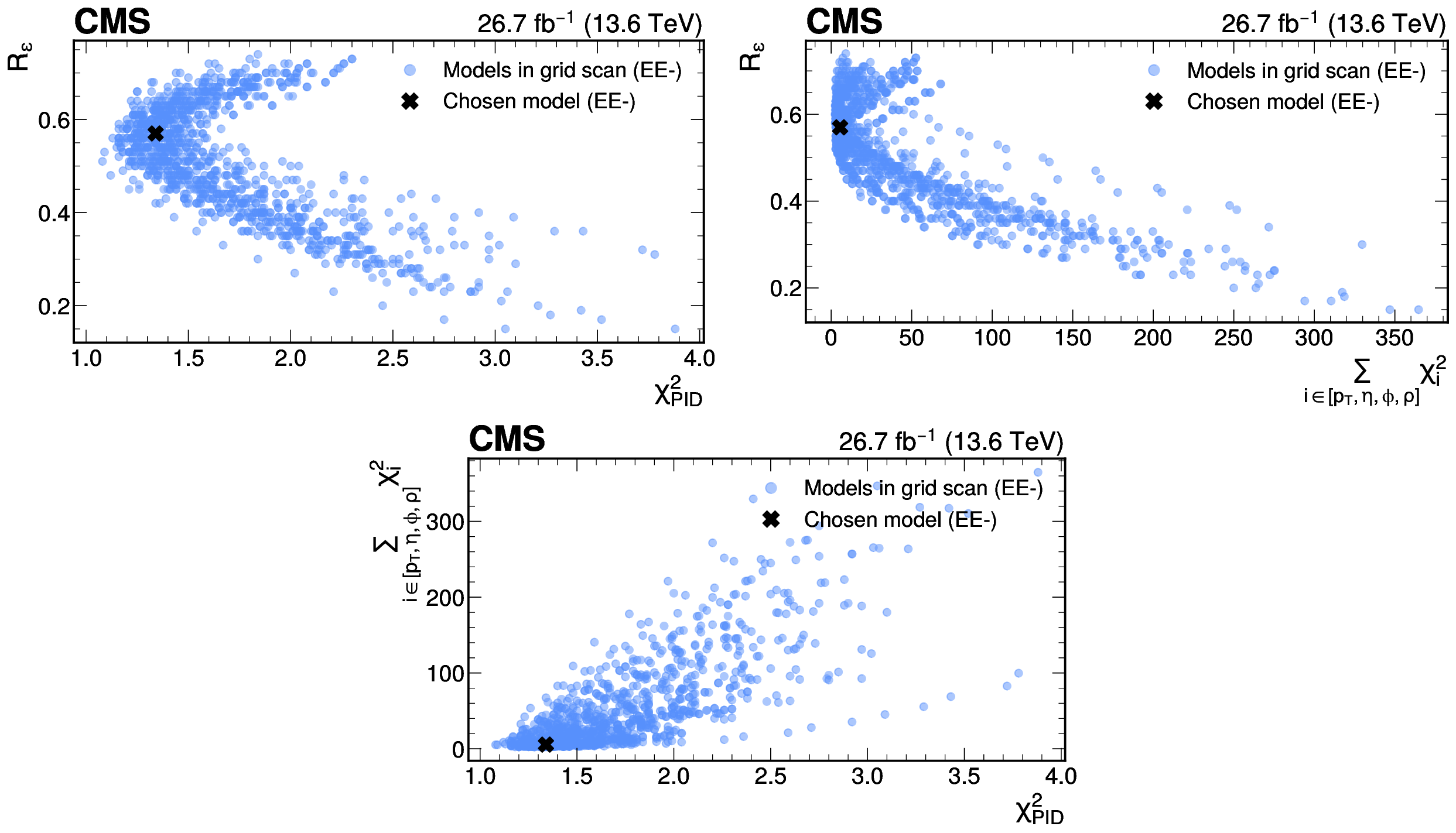
Figure 4:
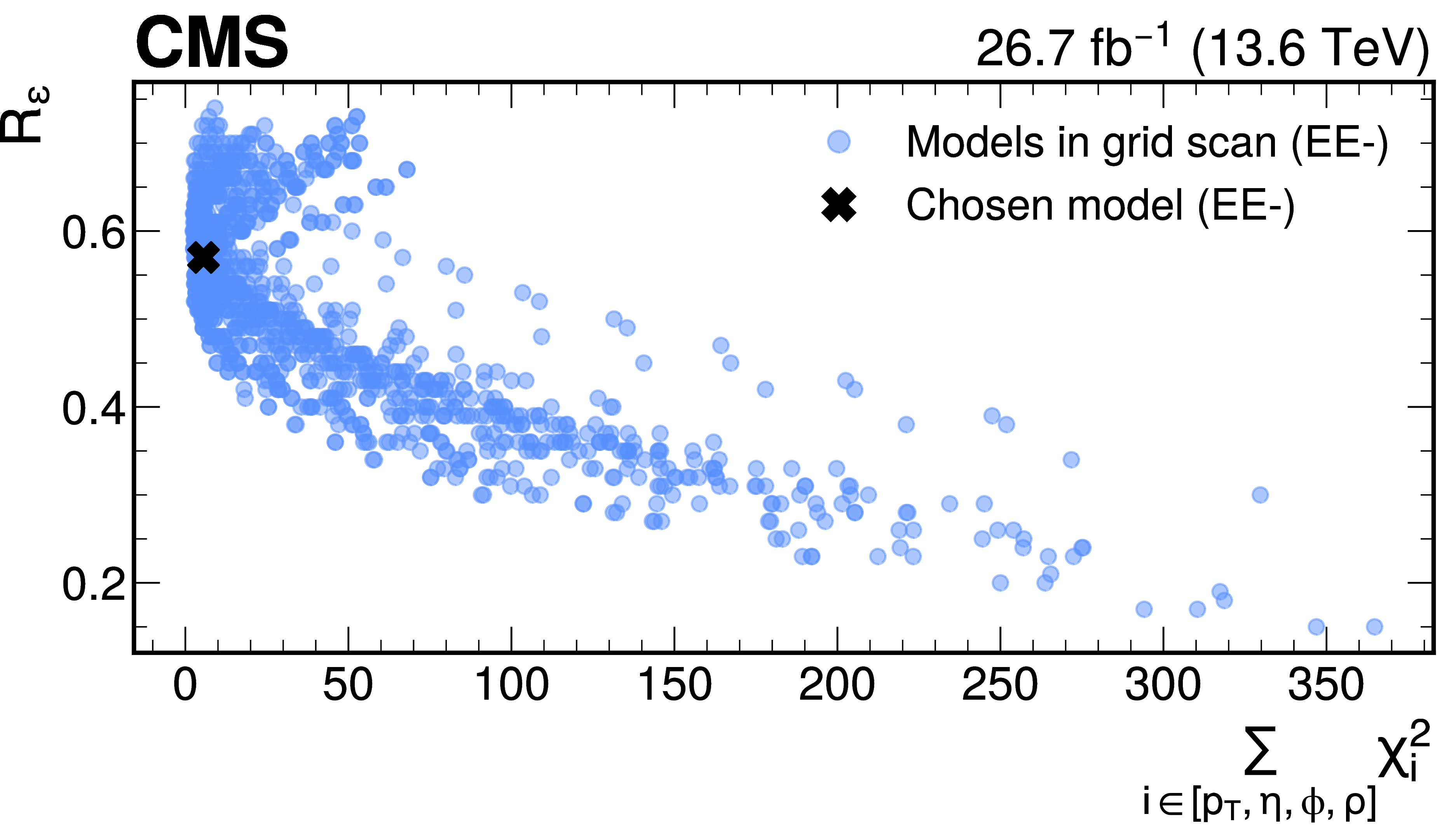
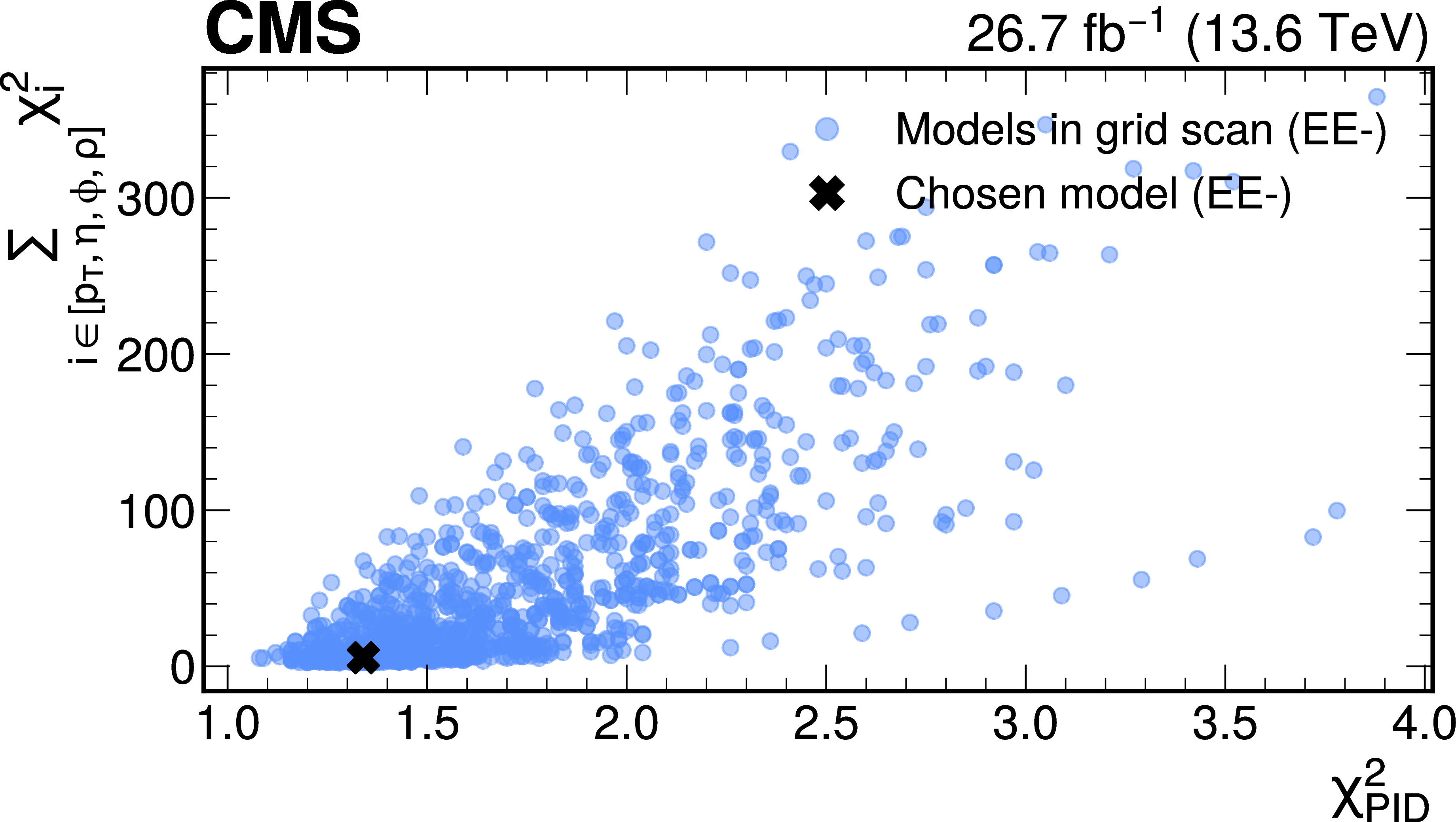
Scatter plots showing the performance of the different S2 EE-models obtained in the grid-scan procedure. The performance is shown for different pairs of the following metrics: the $ \chi^2/n_{\mathrm{dof}} $ for the PID output, the sum of $ \chi^2/n_{\mathrm{dof}} $ values over the $ x_k $ features evaluated between the nominal and corrected simulation, and $ R_\varepsilon $. The black cross indicates the chosen S2 EE-model. |
png pdf |
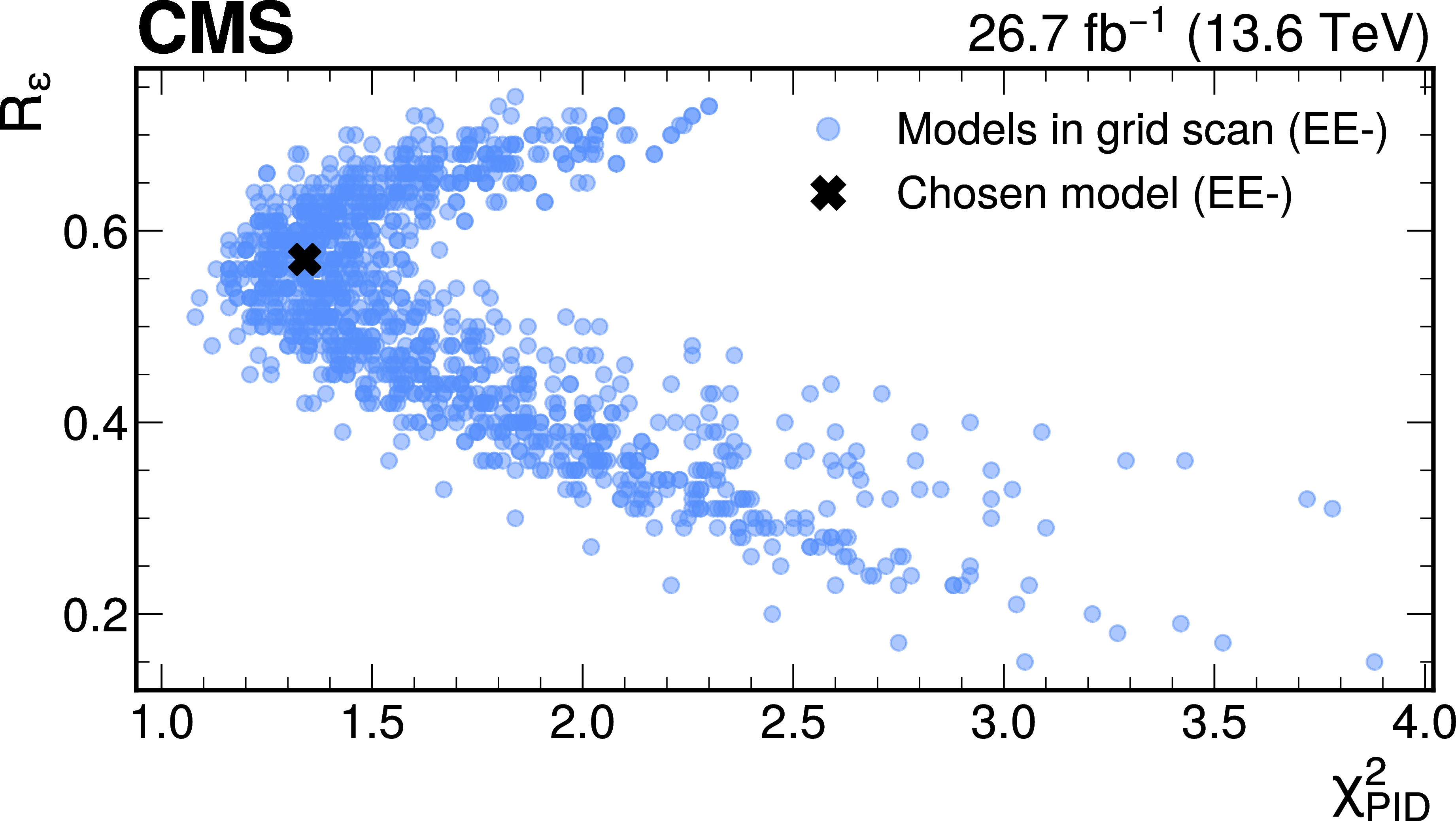
Figure 4-a:
Scatter plots showing the performance of the different S2 EE-models obtained in the grid-scan procedure. The performance is shown for different pairs of the following metrics: the $ \chi^2/n_{\mathrm{dof}} $ for the PID output, the sum of $ \chi^2/n_{\mathrm{dof}} $ values over the $ x_k $ features evaluated between the nominal and corrected simulation, and $ R_\varepsilon $. The black cross indicates the chosen S2 EE-model. |
png pdf |
Figure 4-b:
Scatter plots showing the performance of the different S2 EE-models obtained in the grid-scan procedure. The performance is shown for different pairs of the following metrics: the $ \chi^2/n_{\mathrm{dof}} $ for the PID output, the sum of $ \chi^2/n_{\mathrm{dof}} $ values over the $ x_k $ features evaluated between the nominal and corrected simulation, and $ R_\varepsilon $. The black cross indicates the chosen S2 EE-model. |
png pdf |
Figure 4-c:
Scatter plots showing the performance of the different S2 EE-models obtained in the grid-scan procedure. The performance is shown for different pairs of the following metrics: the $ \chi^2/n_{\mathrm{dof}} $ for the PID output, the sum of $ \chi^2/n_{\mathrm{dof}} $ values over the $ x_k $ features evaluated between the nominal and corrected simulation, and $ R_\varepsilon $. The black cross indicates the chosen S2 EE-model. |
png pdf |
Figure 5:
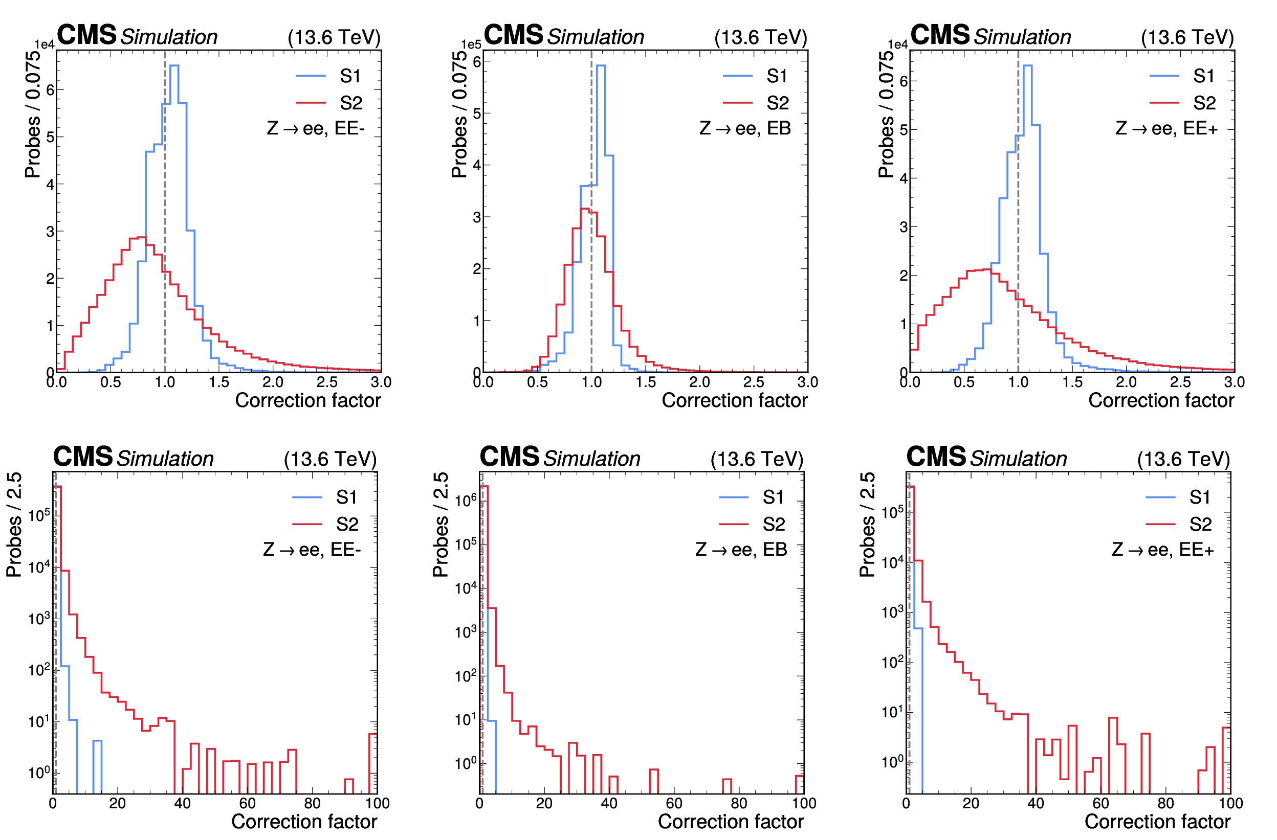
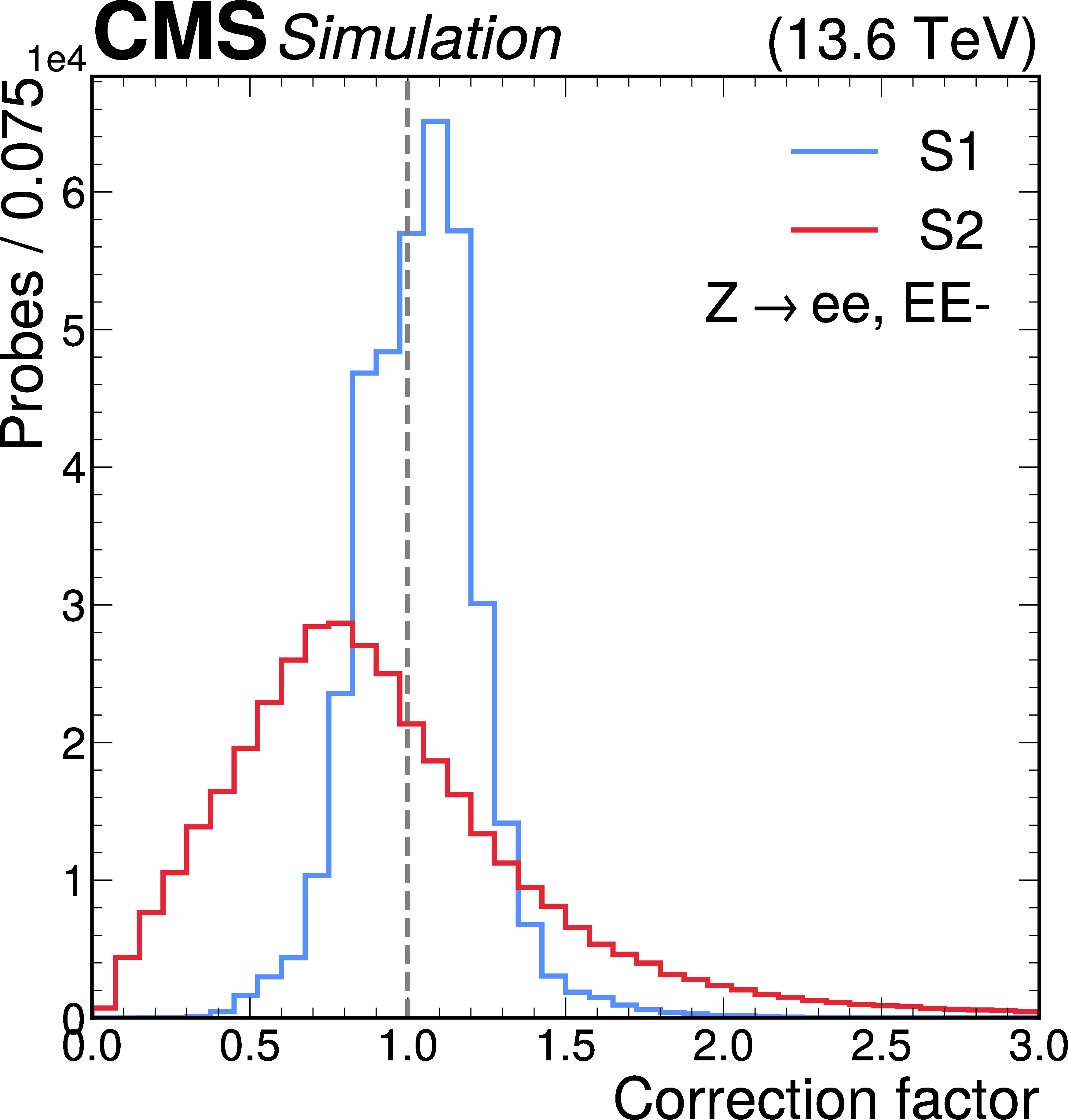
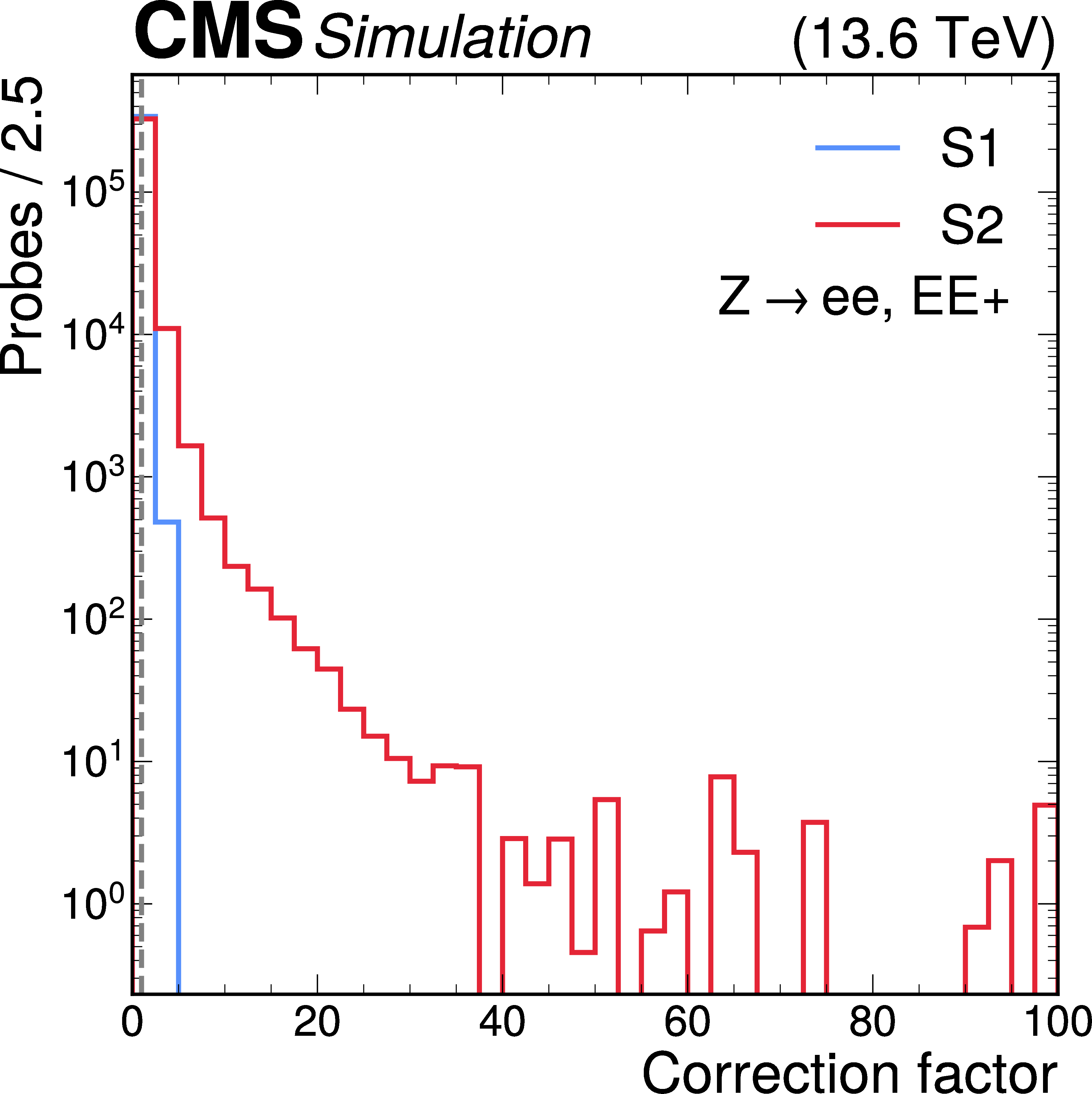
Weight correction distributions for the S1 (blue) and S2 (red) models, shown for the EE-(left), EB (centre), and EE$ + $ (right) subdetector regions. Linear and logarithmic y-scale plots are shown in the upper and lower rows, respectively. The lower plots extend up to $ w_{\text{ceil}} $, used in the weight-clipping procedure. |
png pdf |
Figure 5-a:
Weight correction distributions for the S1 (blue) and S2 (red) models, shown for the EE-(left), EB (centre), and EE$ + $ (right) subdetector regions. Linear and logarithmic y-scale plots are shown in the upper and lower rows, respectively. The lower plots extend up to $ w_{\text{ceil}} $, used in the weight-clipping procedure. |
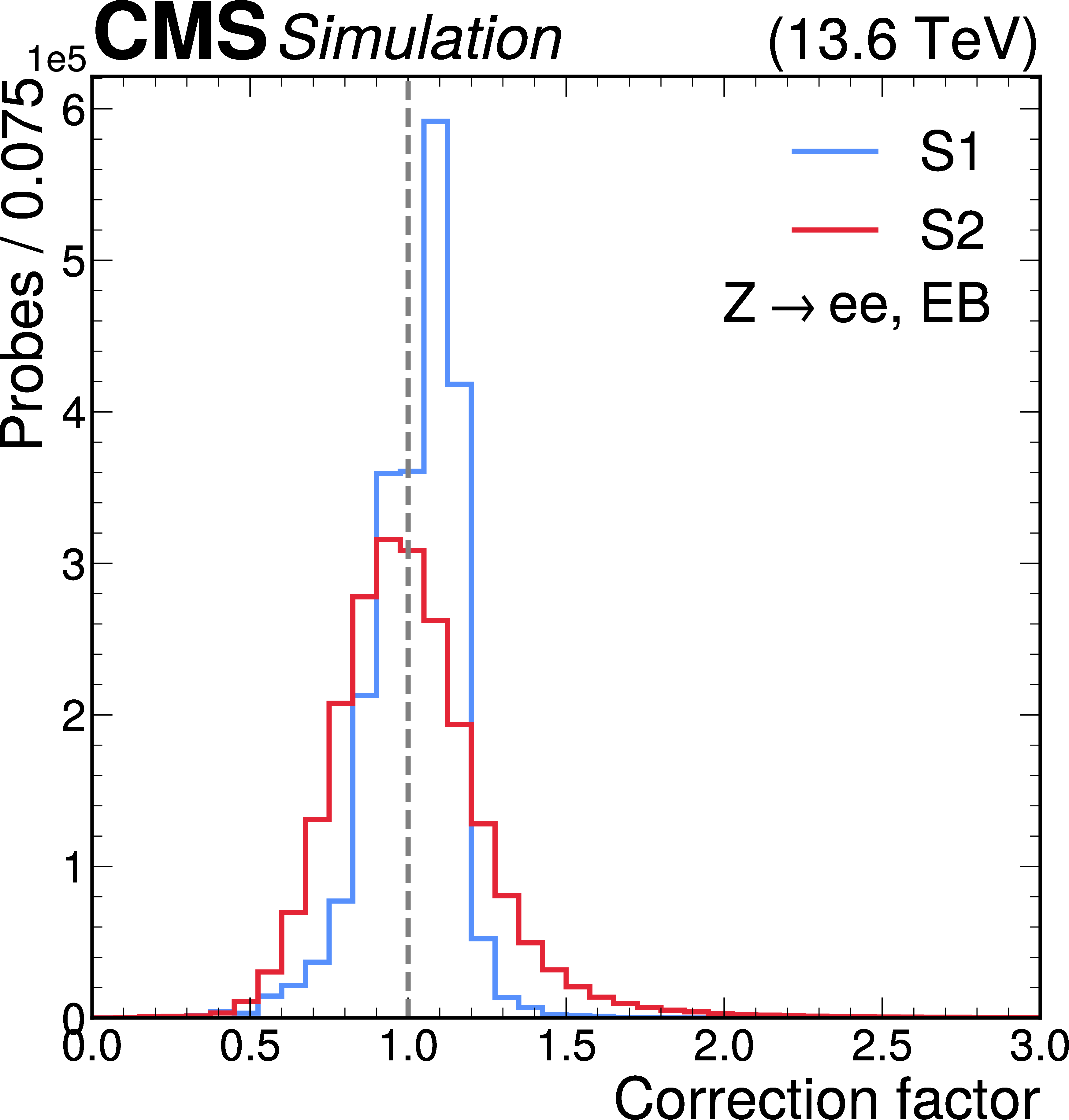
png pdf |
Figure 5-b:
Weight correction distributions for the S1 (blue) and S2 (red) models, shown for the EE-(left), EB (centre), and EE$ + $ (right) subdetector regions. Linear and logarithmic y-scale plots are shown in the upper and lower rows, respectively. The lower plots extend up to $ w_{\text{ceil}} $, used in the weight-clipping procedure. |
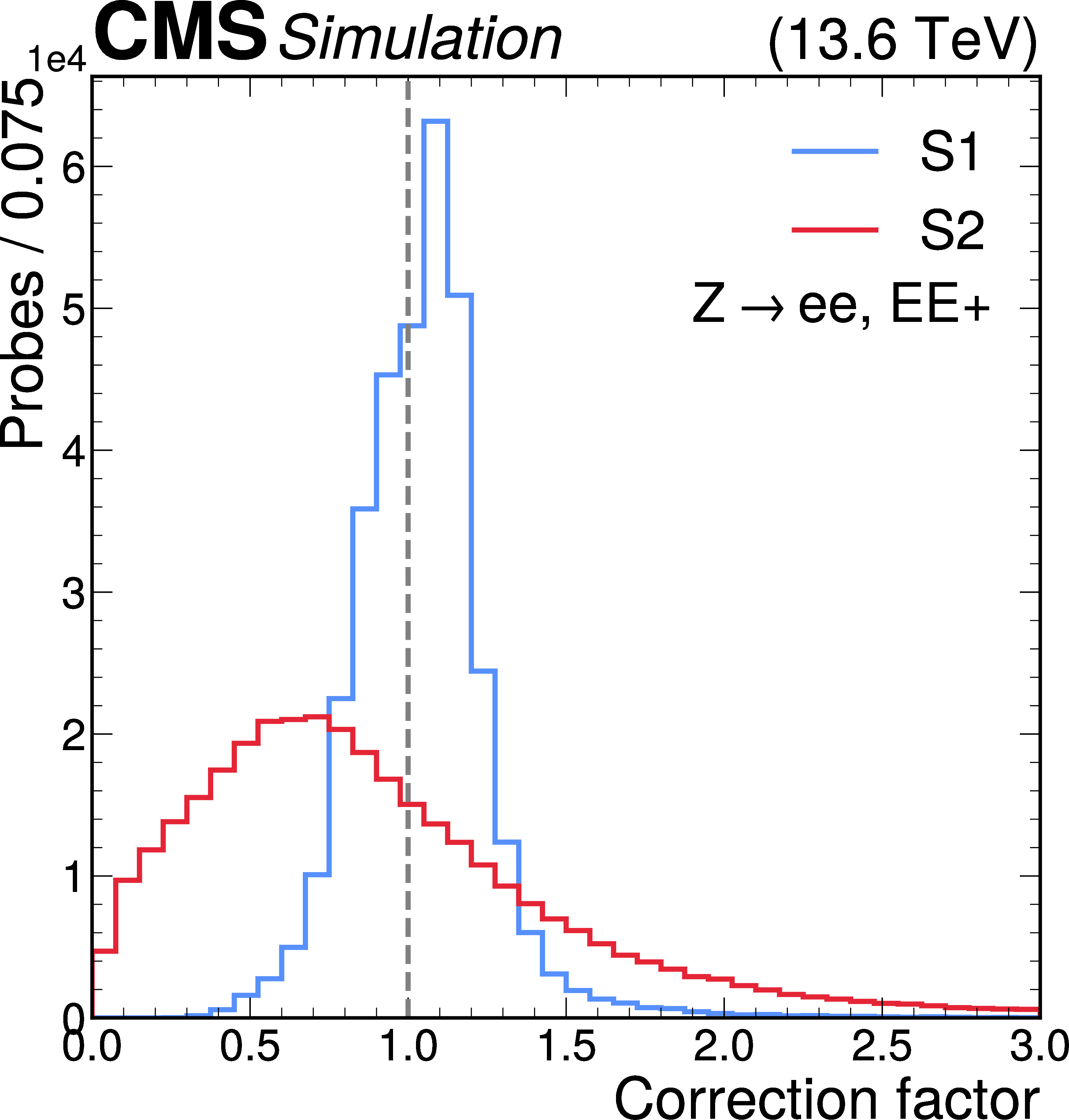
png pdf |
Figure 5-c:
Weight correction distributions for the S1 (blue) and S2 (red) models, shown for the EE-(left), EB (centre), and EE$ + $ (right) subdetector regions. Linear and logarithmic y-scale plots are shown in the upper and lower rows, respectively. The lower plots extend up to $ w_{\text{ceil}} $, used in the weight-clipping procedure. |
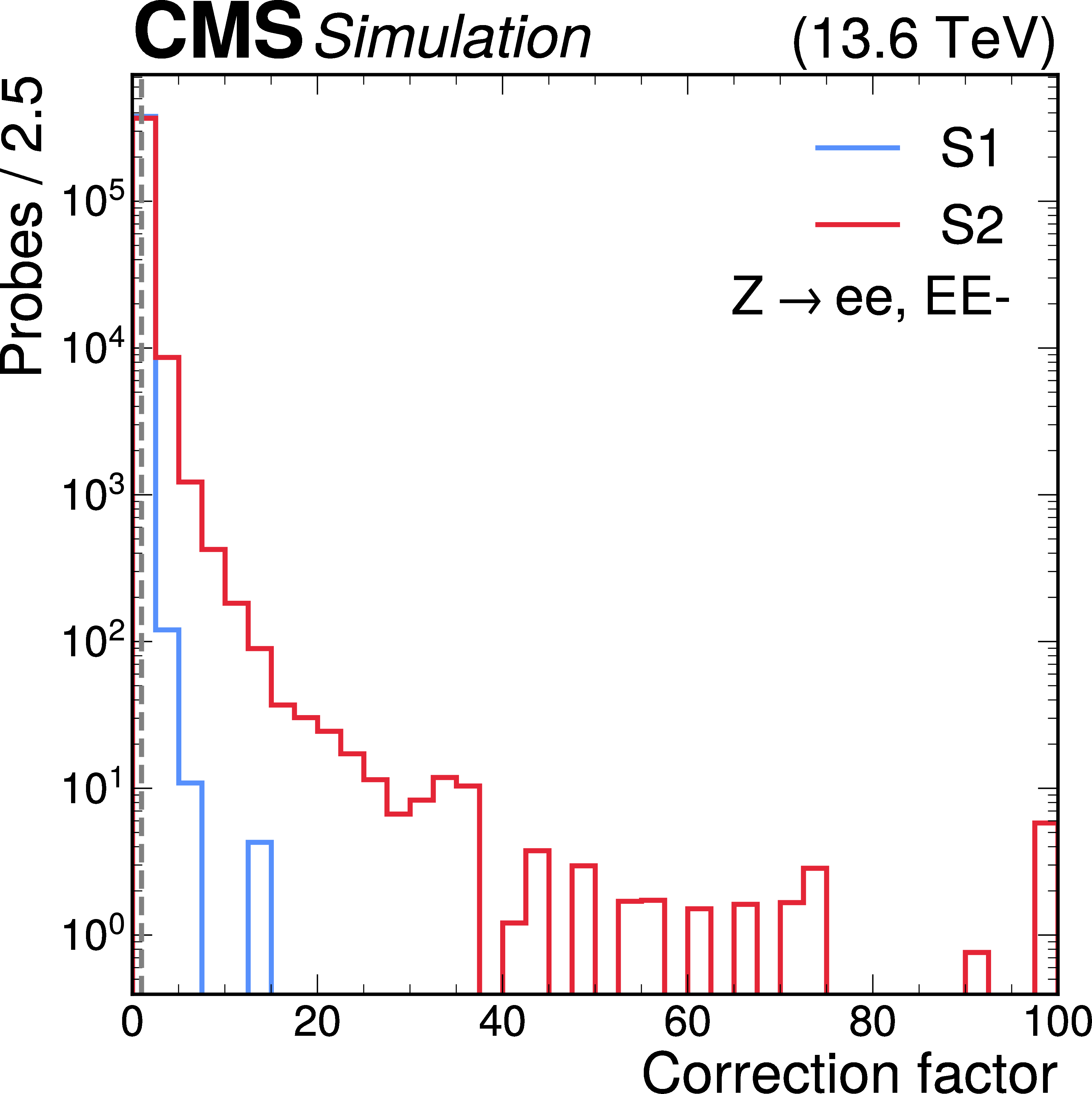
png pdf |
Figure 5-d:
Weight correction distributions for the S1 (blue) and S2 (red) models, shown for the EE-(left), EB (centre), and EE$ + $ (right) subdetector regions. Linear and logarithmic y-scale plots are shown in the upper and lower rows, respectively. The lower plots extend up to $ w_{\text{ceil}} $, used in the weight-clipping procedure. |
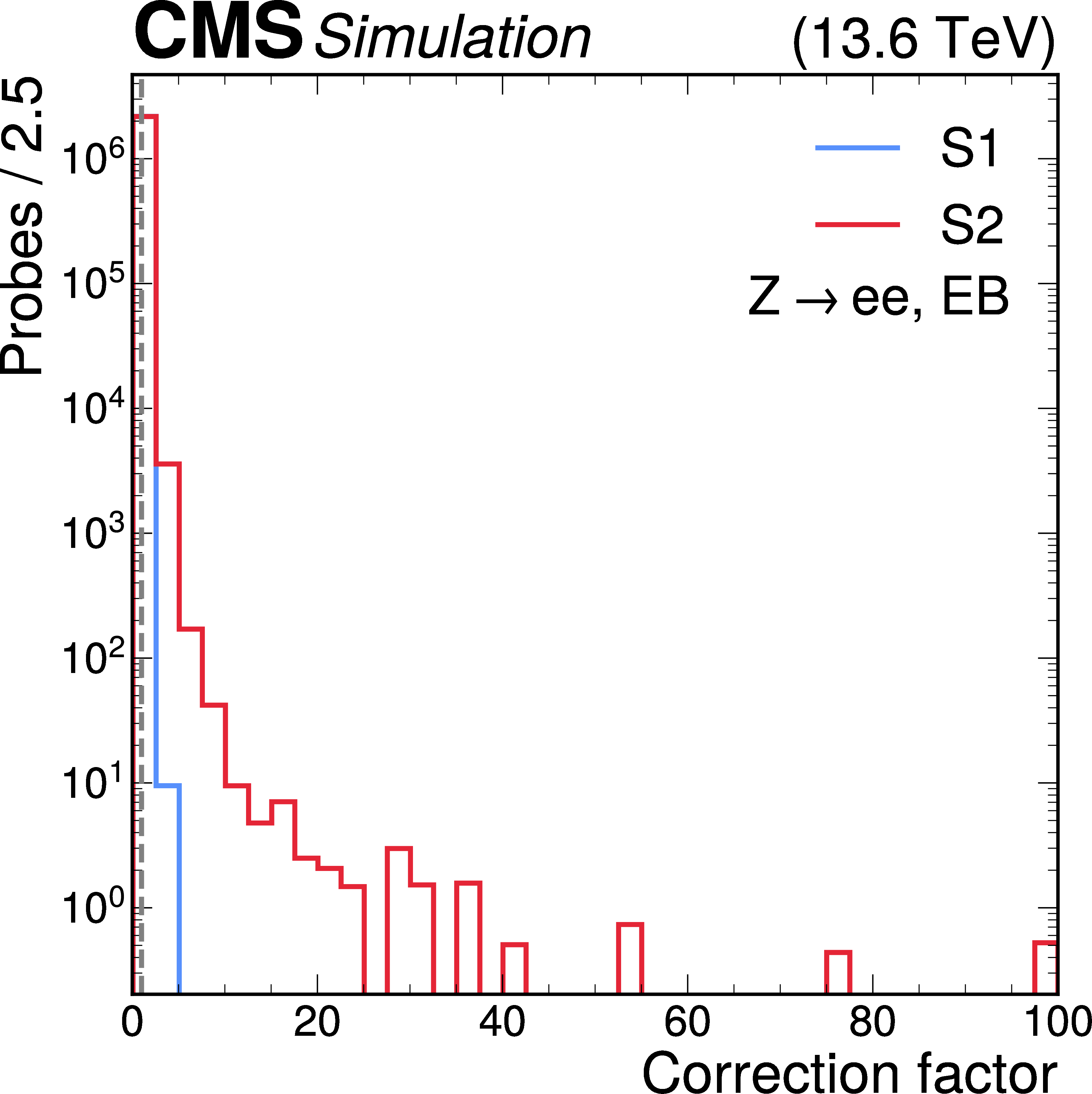
png pdf |
Figure 5-e:
Weight correction distributions for the S1 (blue) and S2 (red) models, shown for the EE-(left), EB (centre), and EE$ + $ (right) subdetector regions. Linear and logarithmic y-scale plots are shown in the upper and lower rows, respectively. The lower plots extend up to $ w_{\text{ceil}} $, used in the weight-clipping procedure. |
png pdf |
Figure 5-f:
Weight correction distributions for the S1 (blue) and S2 (red) models, shown for the EE-(left), EB (centre), and EE$ + $ (right) subdetector regions. Linear and logarithmic y-scale plots are shown in the upper and lower rows, respectively. The lower plots extend up to $ w_{\text{ceil}} $, used in the weight-clipping procedure. |
png pdf |
Figure 6:
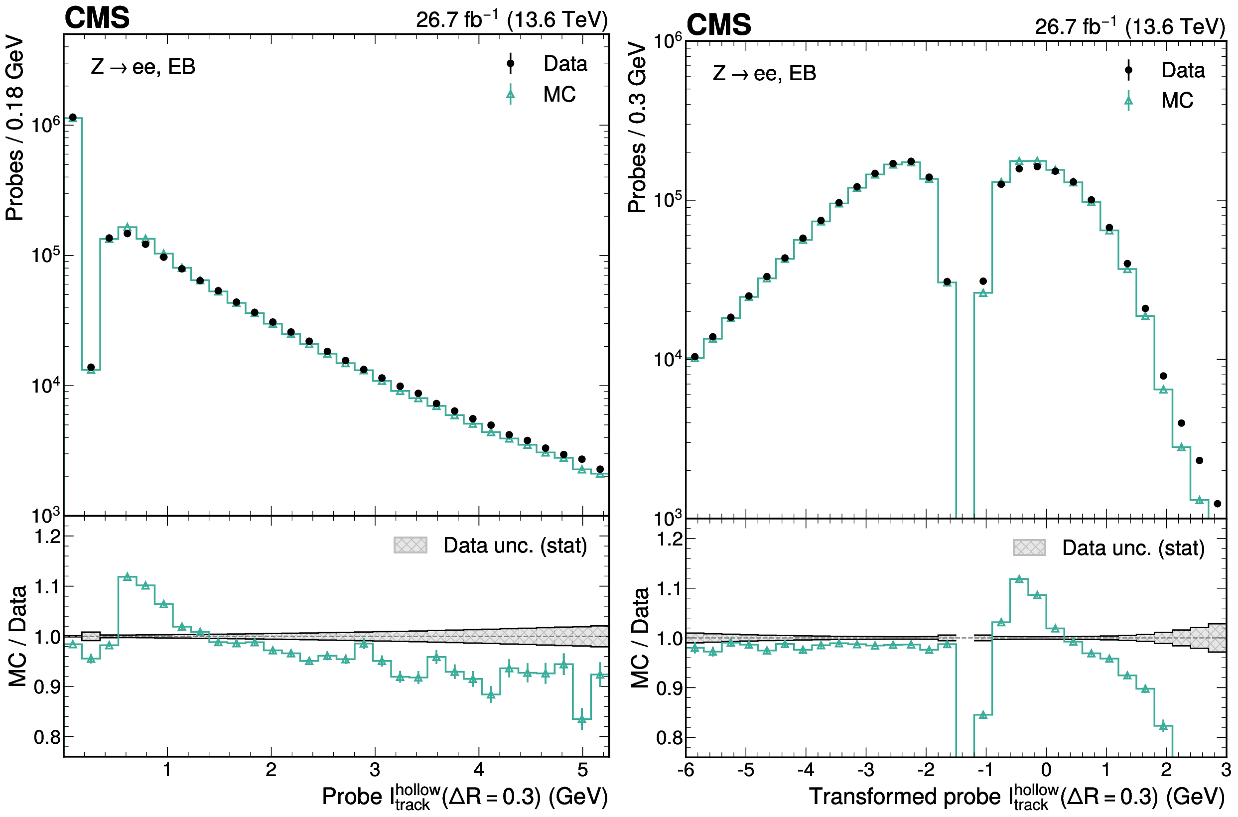
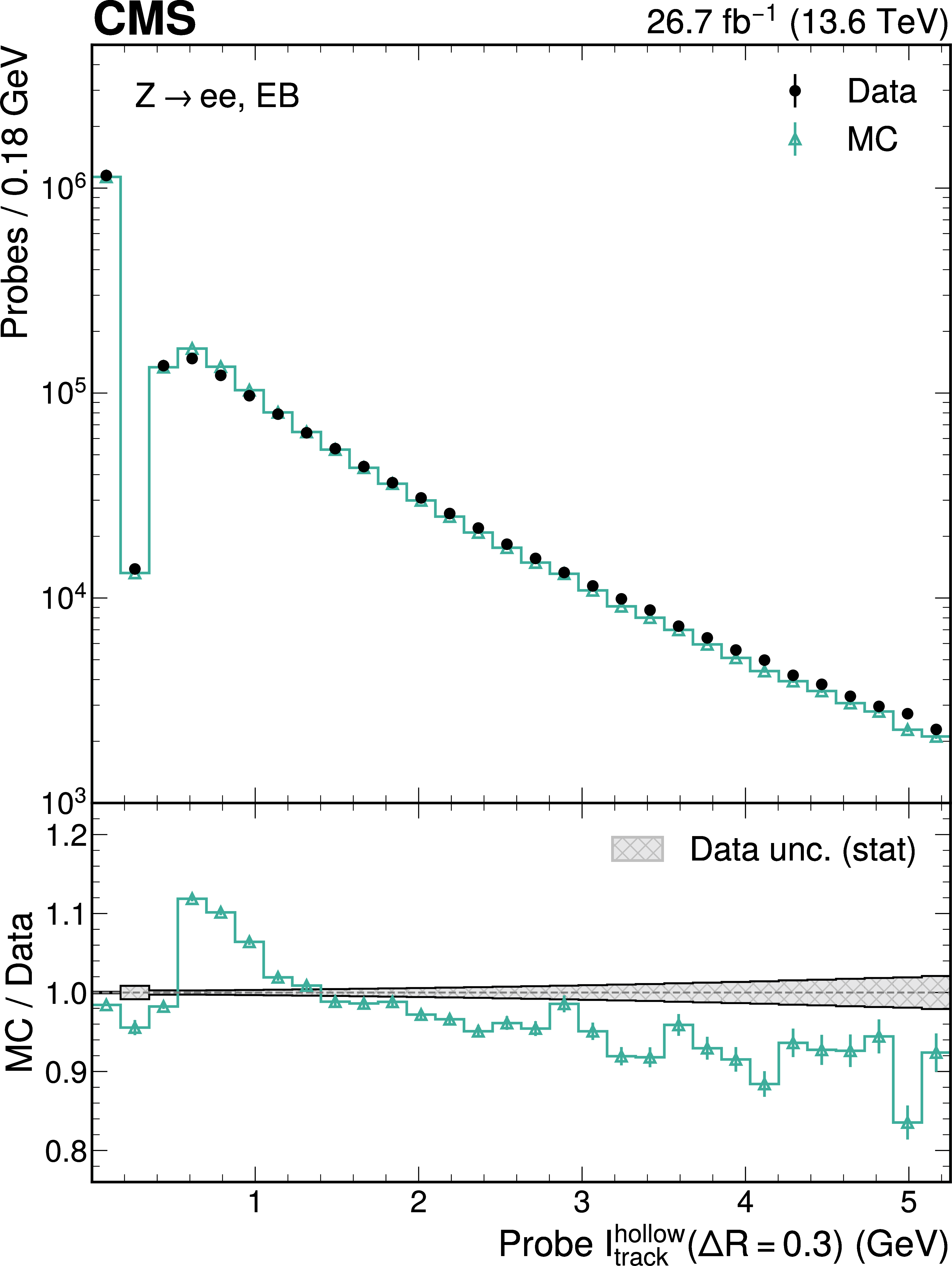
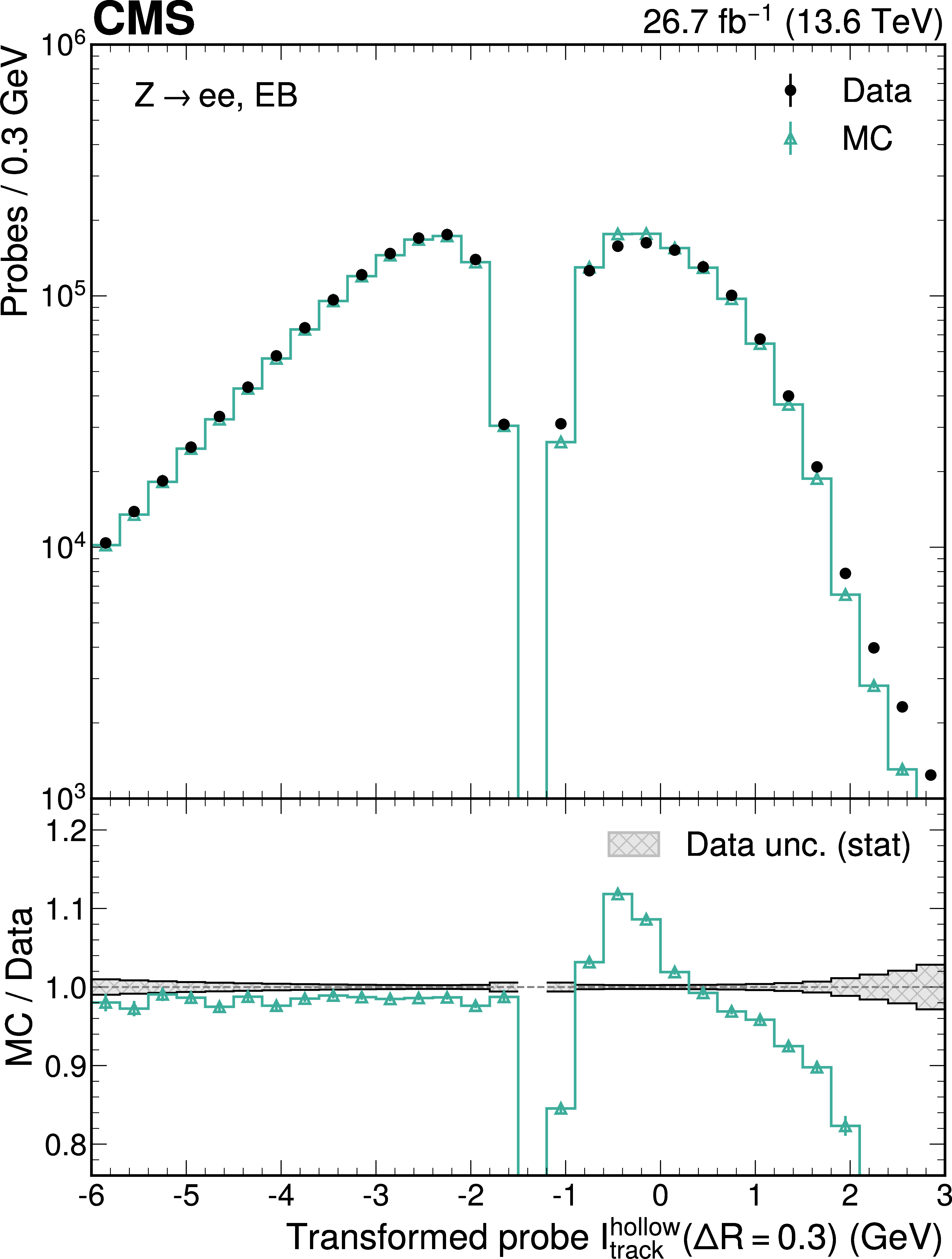
The probe $ \mathcal{I}^{\text{hollow}}_{\text{track}}(\Delta R = 0.3) $ distribution in simulation (teal points) and data (black histogram), before (left) and after (right) the transformation of this isolation-related feature, used in the normalising-flow model. The lower panels show the ratio of simulation to data, where the statistical uncertainties in the simulation and data are shown by the teal error bars and the grey hatched bands, respectively. |
png pdf |
Figure 6-a:
The probe $ \mathcal{I}^{\text{hollow}}_{\text{track}}(\Delta R = 0.3) $ distribution in simulation (teal points) and data (black histogram), before (left) and after (right) the transformation of this isolation-related feature, used in the normalising-flow model. The lower panels show the ratio of simulation to data, where the statistical uncertainties in the simulation and data are shown by the teal error bars and the grey hatched bands, respectively. |
png pdf |
Figure 6-b:
The probe $ \mathcal{I}^{\text{hollow}}_{\text{track}}(\Delta R = 0.3) $ distribution in simulation (teal points) and data (black histogram), before (left) and after (right) the transformation of this isolation-related feature, used in the normalising-flow model. The lower panels show the ratio of simulation to data, where the statistical uncertainties in the simulation and data are shown by the teal error bars and the grey hatched bands, respectively. |
png pdf |
Figure 7:
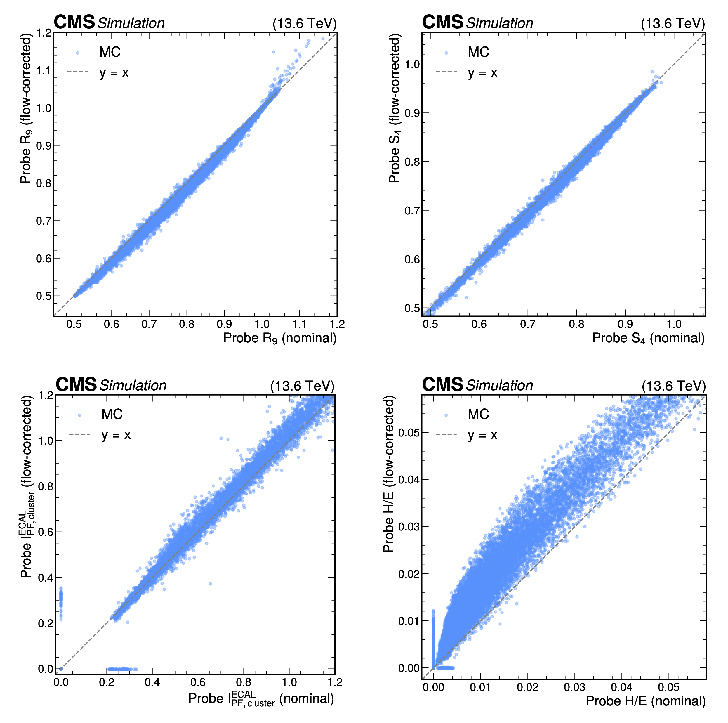
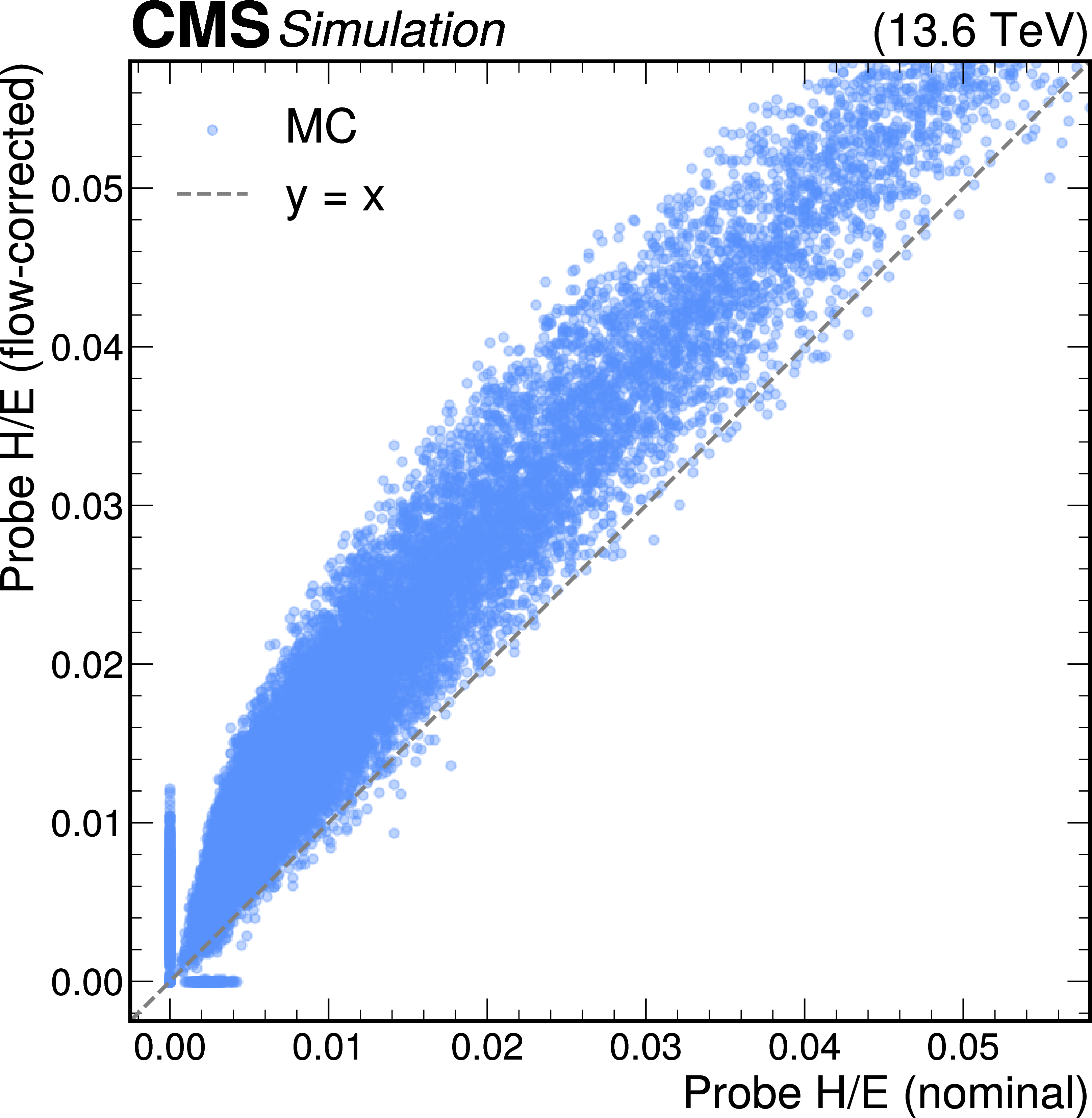
Scatter plots showing the learned high-dimensional mapping projected onto a single dimension: probe $ R_9 $ (upper left), $ S_4 $ (upper right), $ \mathcal{I}^{\mathrm{ECAL}}_{\text{PF, cluster}} $ (lower left) and H/E (lower right). The $ x $ axis shows the nominal values of these features in the simulation sample, while the $ y $ axis shows the flow-corrected features. The dashed line in each panel shows the identity line $ y=x $, where points on the line are unchanged by the flow corrections in this dimension. |
png pdf |
Figure 7-a:
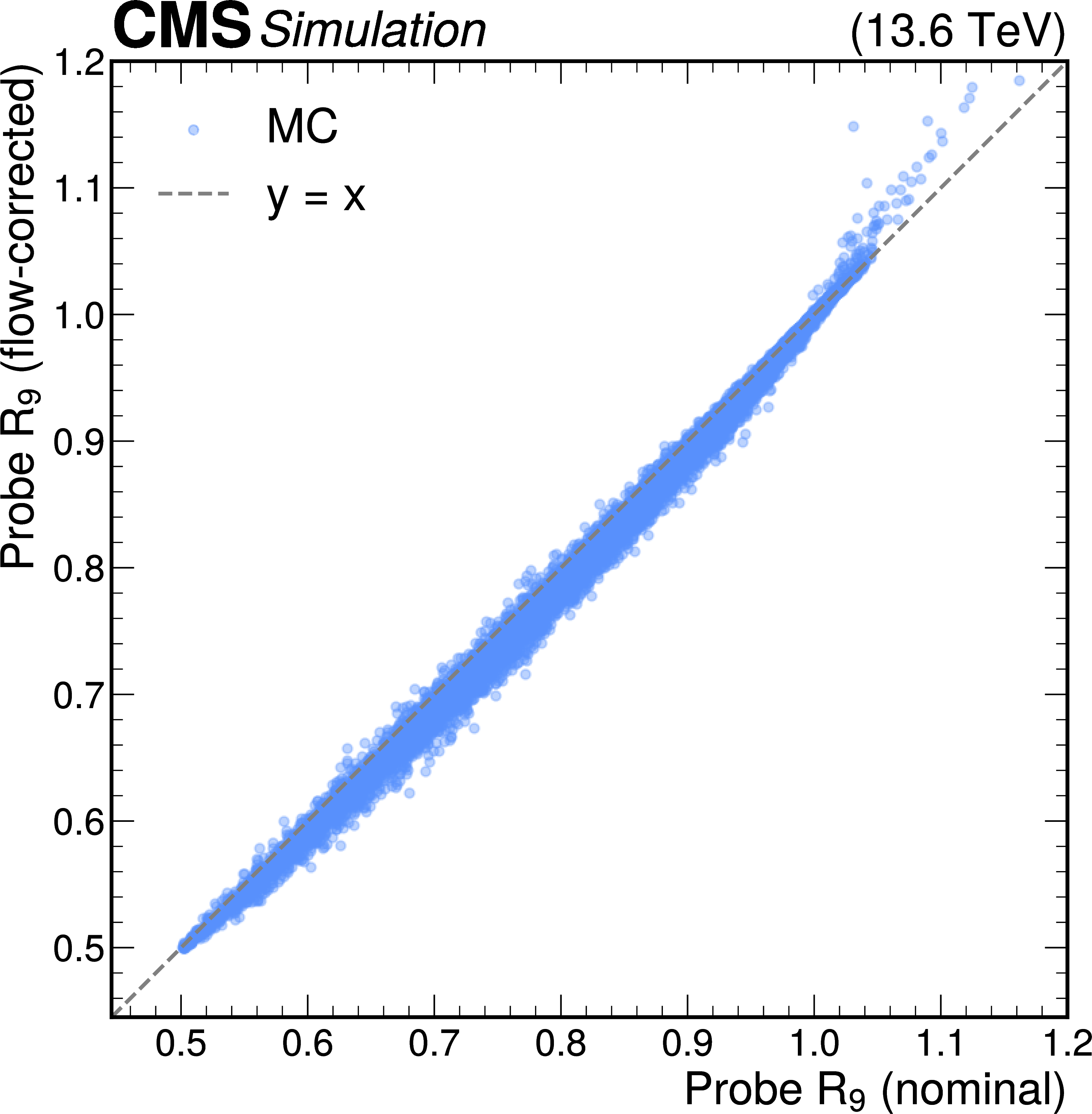
Scatter plots showing the learned high-dimensional mapping projected onto a single dimension: probe $ R_9 $ (upper left), $ S_4 $ (upper right), $ \mathcal{I}^{\mathrm{ECAL}}_{\text{PF, cluster}} $ (lower left) and H/E (lower right). The $ x $ axis shows the nominal values of these features in the simulation sample, while the $ y $ axis shows the flow-corrected features. The dashed line in each panel shows the identity line $ y=x $, where points on the line are unchanged by the flow corrections in this dimension. |
png pdf |
Figure 7-b:
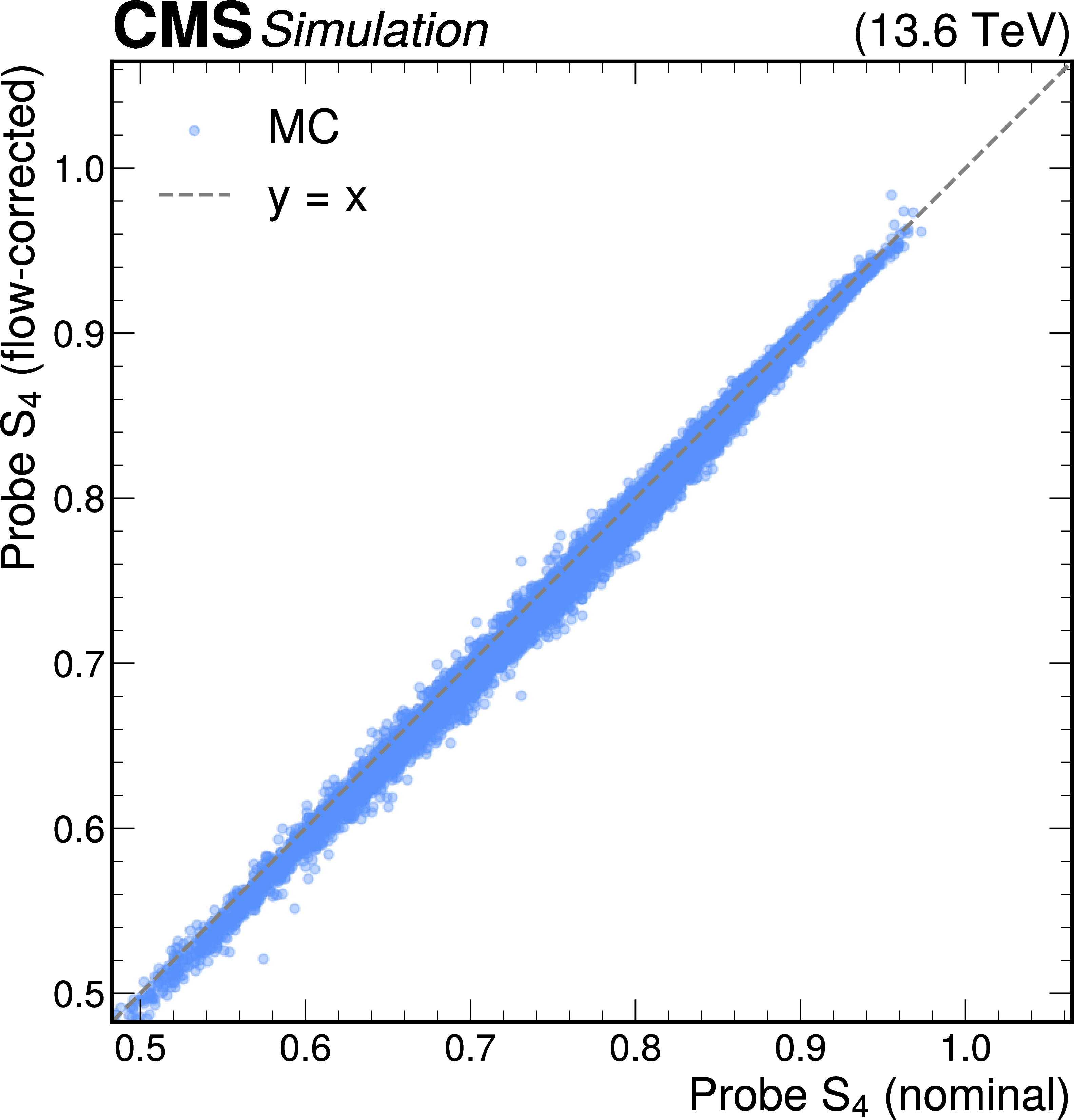
Scatter plots showing the learned high-dimensional mapping projected onto a single dimension: probe $ R_9 $ (upper left), $ S_4 $ (upper right), $ \mathcal{I}^{\mathrm{ECAL}}_{\text{PF, cluster}} $ (lower left) and H/E (lower right). The $ x $ axis shows the nominal values of these features in the simulation sample, while the $ y $ axis shows the flow-corrected features. The dashed line in each panel shows the identity line $ y=x $, where points on the line are unchanged by the flow corrections in this dimension. |
png pdf |
Figure 7-c:
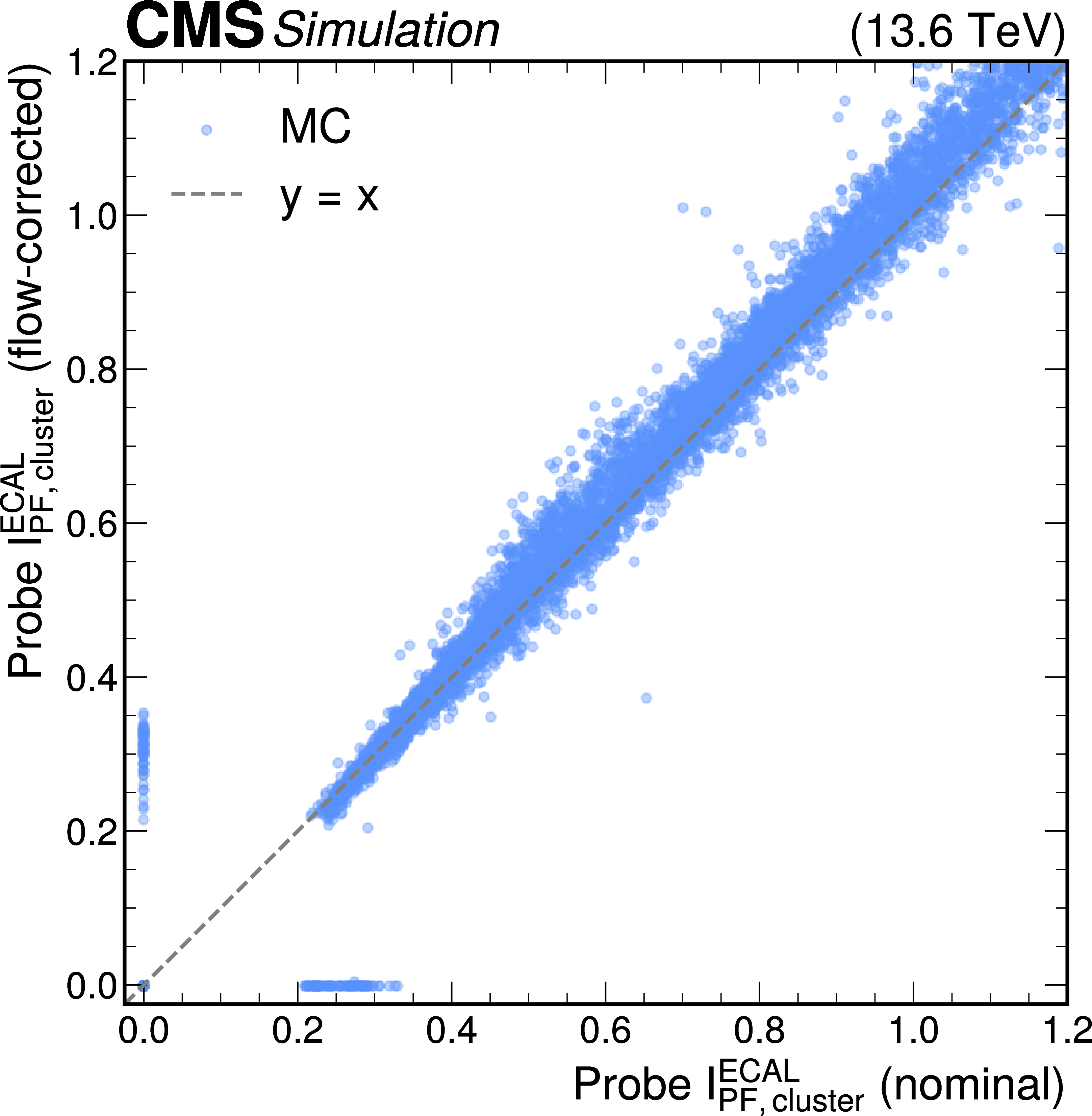
Scatter plots showing the learned high-dimensional mapping projected onto a single dimension: probe $ R_9 $ (upper left), $ S_4 $ (upper right), $ \mathcal{I}^{\mathrm{ECAL}}_{\text{PF, cluster}} $ (lower left) and H/E (lower right). The $ x $ axis shows the nominal values of these features in the simulation sample, while the $ y $ axis shows the flow-corrected features. The dashed line in each panel shows the identity line $ y=x $, where points on the line are unchanged by the flow corrections in this dimension. |
png pdf |
Figure 7-d:
Scatter plots showing the learned high-dimensional mapping projected onto a single dimension: probe $ R_9 $ (upper left), $ S_4 $ (upper right), $ \mathcal{I}^{\mathrm{ECAL}}_{\text{PF, cluster}} $ (lower left) and H/E (lower right). The $ x $ axis shows the nominal values of these features in the simulation sample, while the $ y $ axis shows the flow-corrected features. The dashed line in each panel shows the identity line $ y=x $, where points on the line are unchanged by the flow corrections in this dimension. |
png pdf |
Figure 8:
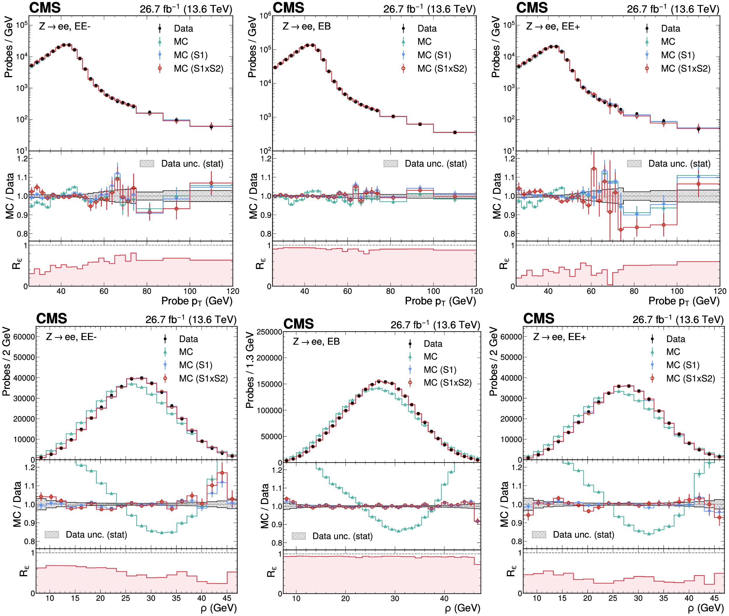
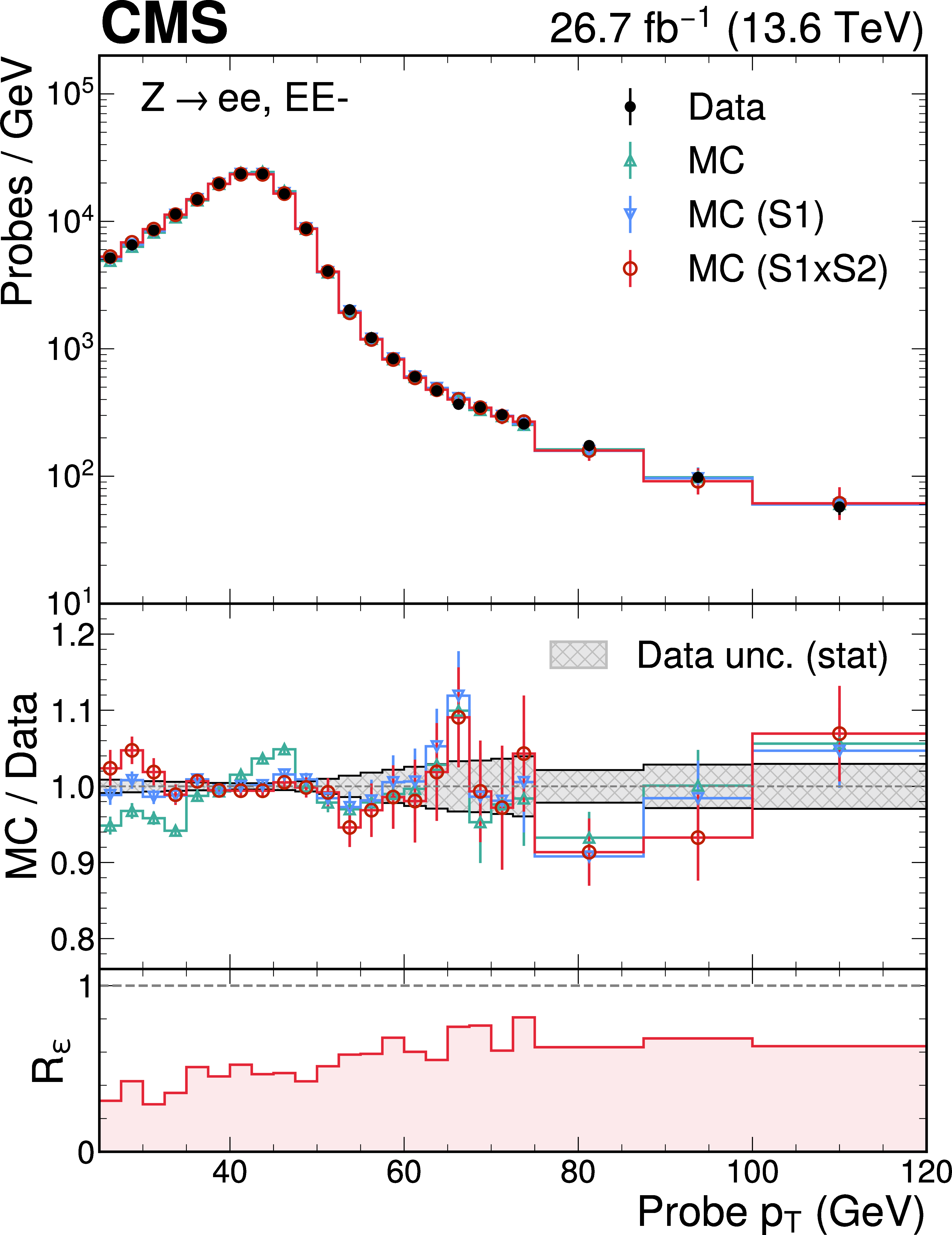
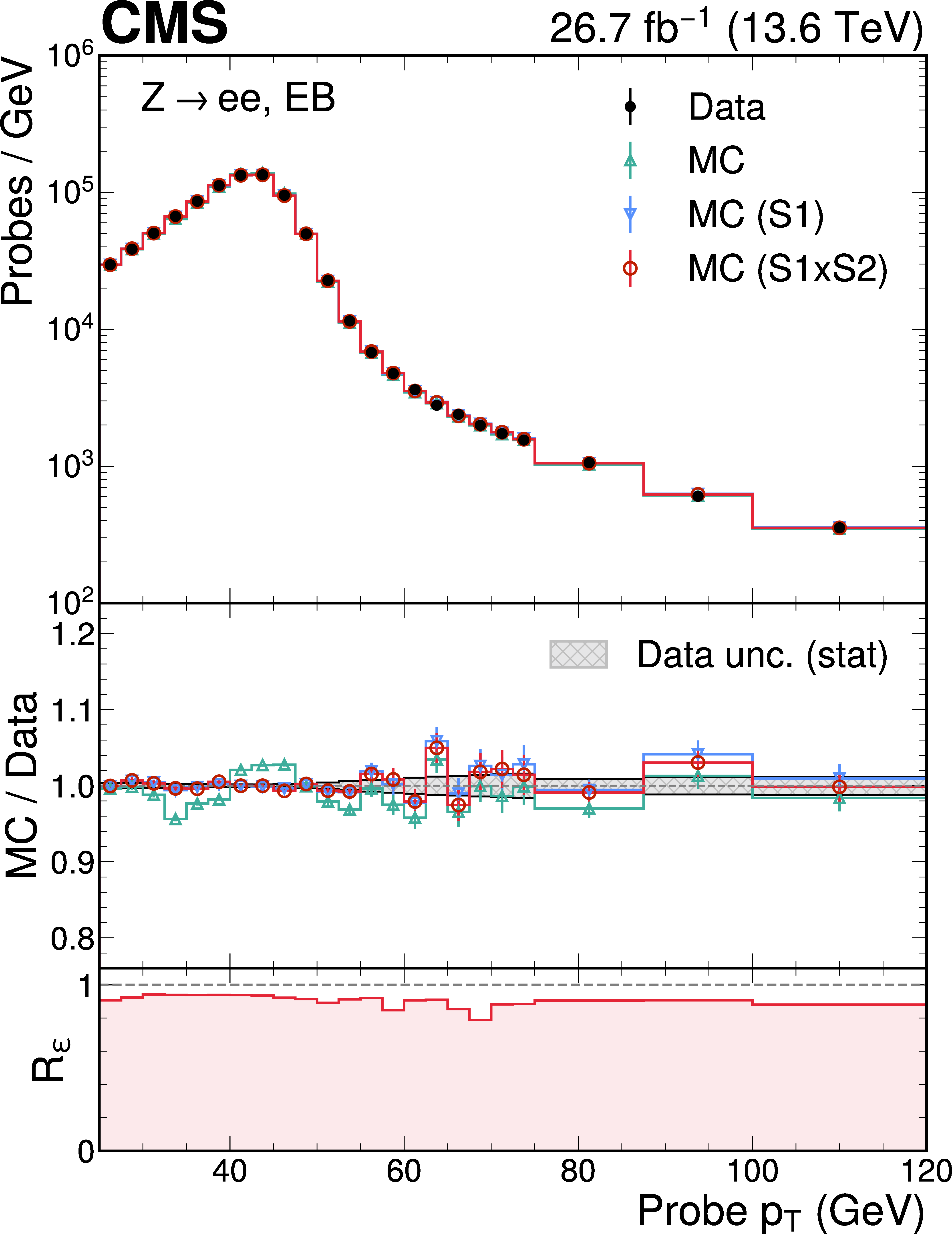
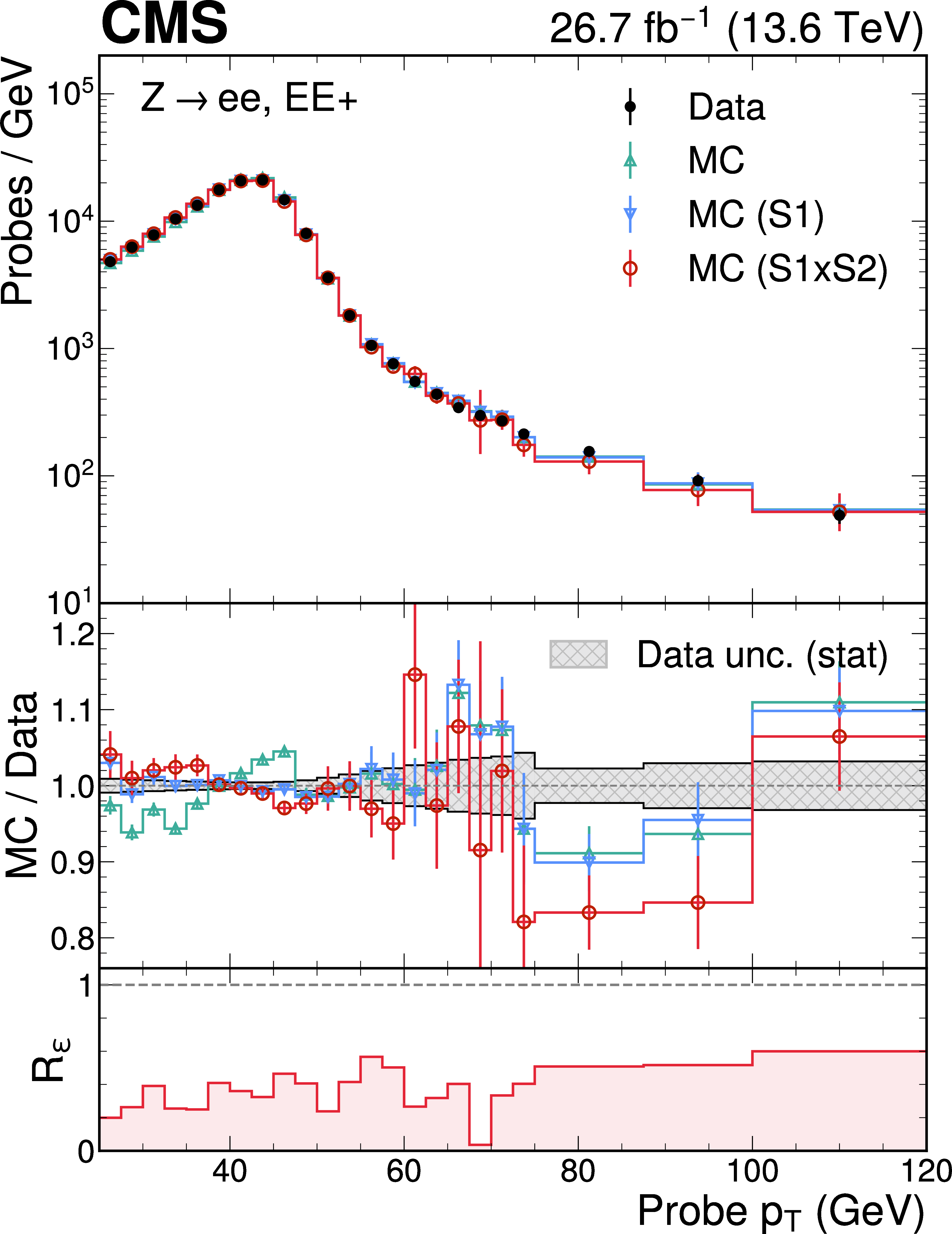
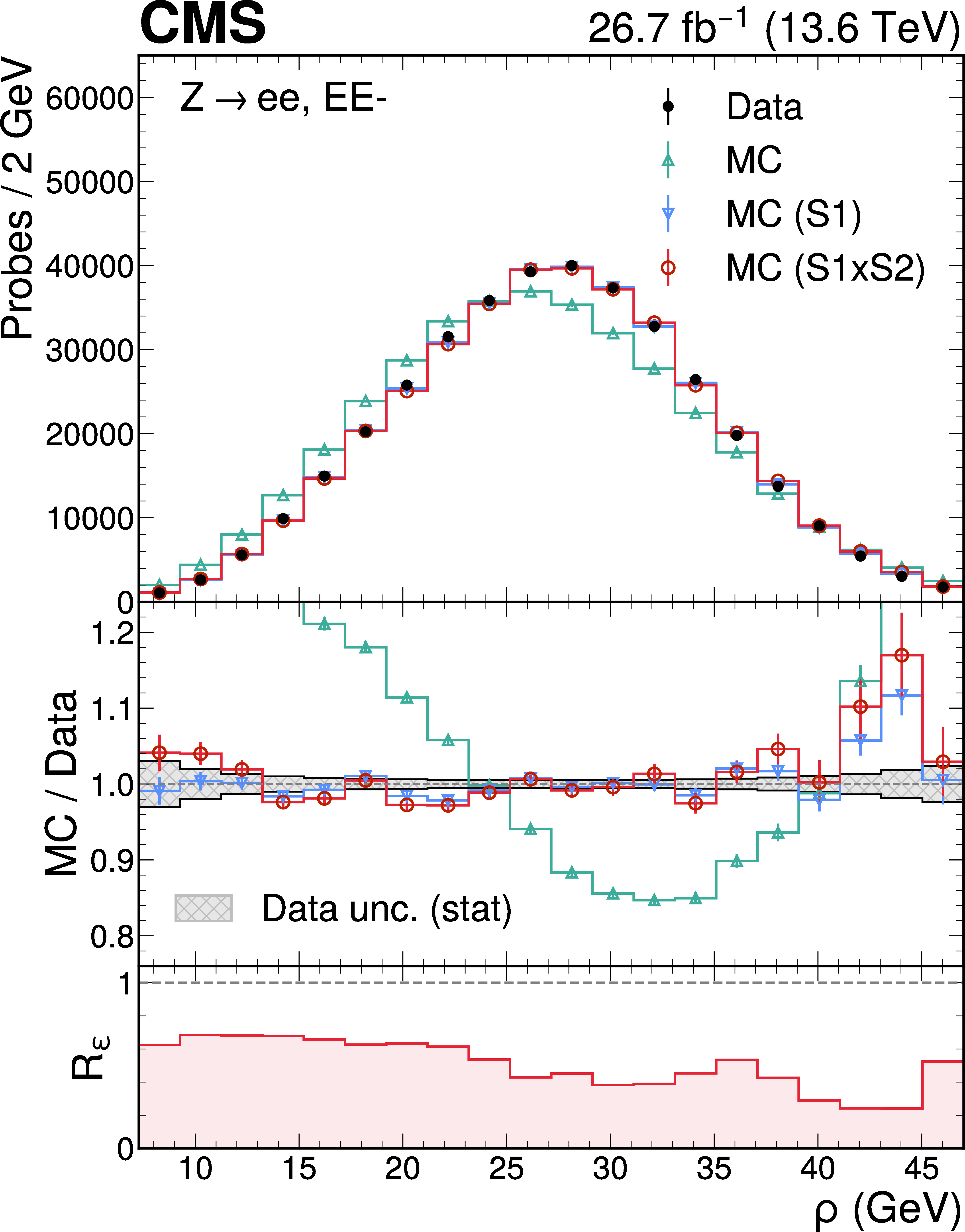
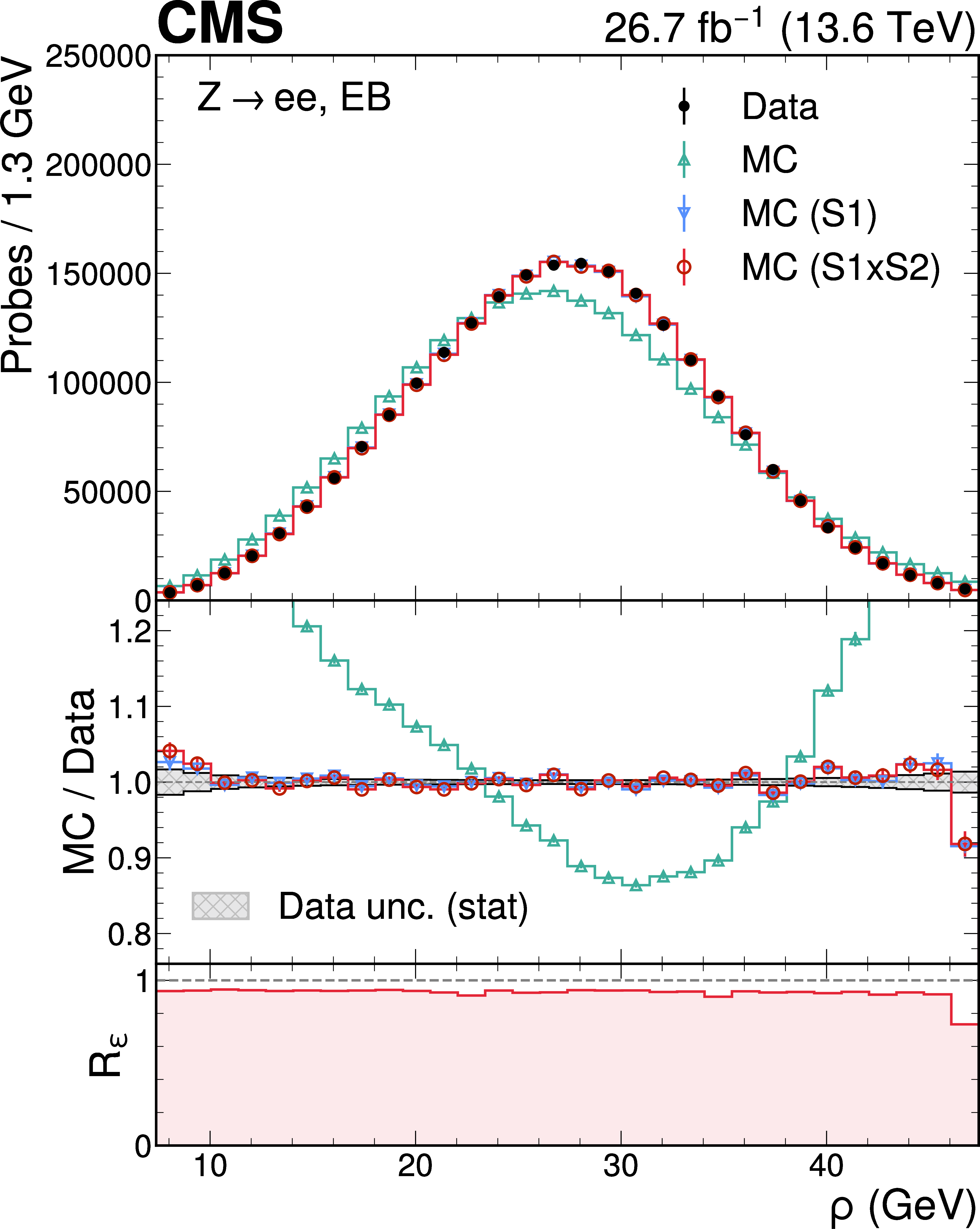
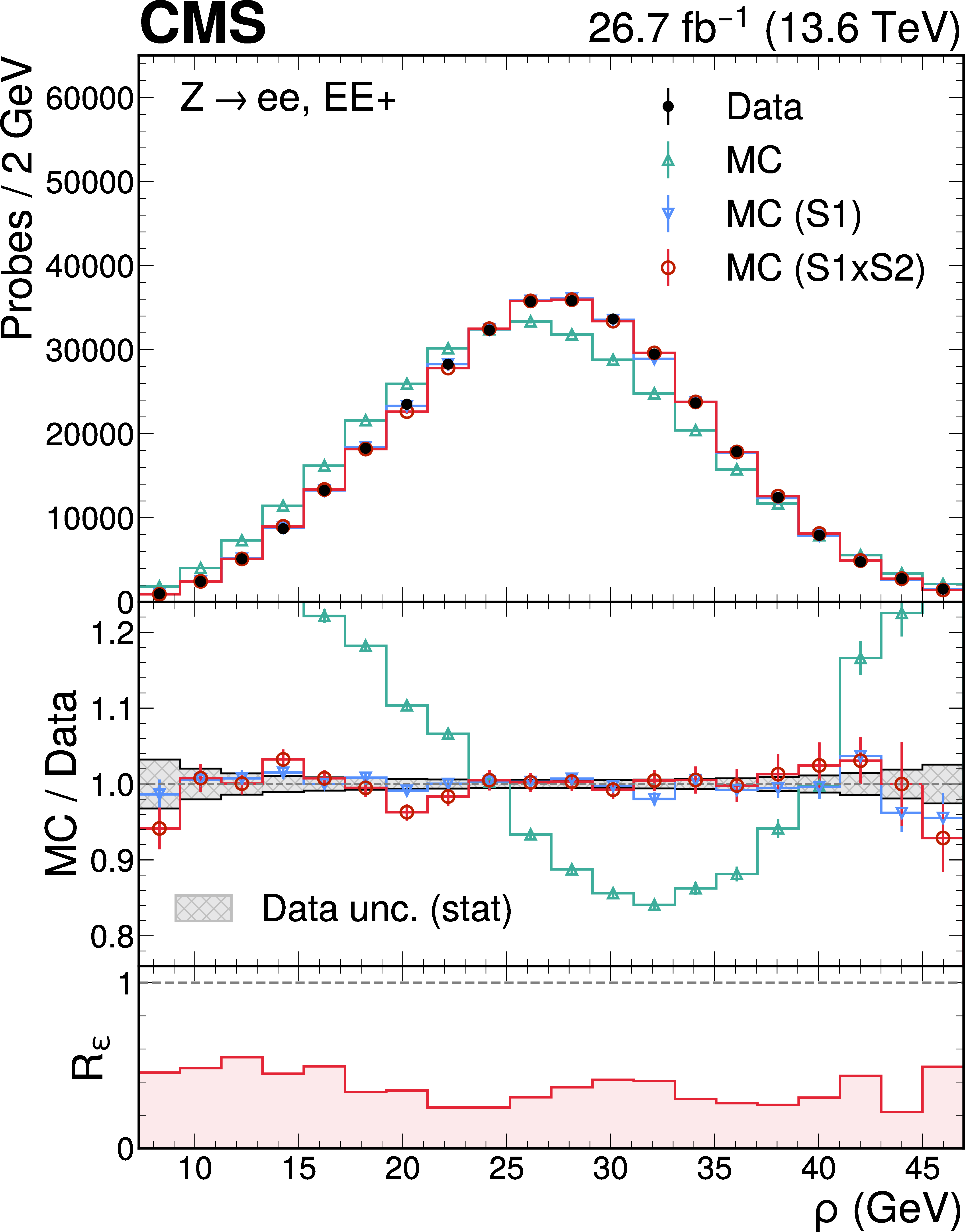
The probe $ p_{\mathrm{T}} $ (upper row) and $ \rho $ (lower row) distributions in data (black points) and simulation (coloured histograms with points), for the EE-(left), EB (centre), and EE$ + $ (right) subdetector regions. The statistical uncertainties in the simulation and data are shown by the error bars on the points. The simulation is shown for three scenarios. The teal histograms show the nominal simulation normalised to the data, the blue histograms show the simulation after S1 reweighting, and the red histograms show the simulation after S2 reweighting. The middle panels show the ratio of simulation to data, where the statistical uncertainty in the data is indicated by the grey hatched band. The lower panels show the reduction in statistical power $ R_\varepsilon $, in bins of each observable, after applying the S2 reweighting. |
png pdf |
Figure 8-a:
The probe $ p_{\mathrm{T}} $ (upper row) and $ \rho $ (lower row) distributions in data (black points) and simulation (coloured histograms with points), for the EE-(left), EB (centre), and EE$ + $ (right) subdetector regions. The statistical uncertainties in the simulation and data are shown by the error bars on the points. The simulation is shown for three scenarios. The teal histograms show the nominal simulation normalised to the data, the blue histograms show the simulation after S1 reweighting, and the red histograms show the simulation after S2 reweighting. The middle panels show the ratio of simulation to data, where the statistical uncertainty in the data is indicated by the grey hatched band. The lower panels show the reduction in statistical power $ R_\varepsilon $, in bins of each observable, after applying the S2 reweighting. |
png pdf |
Figure 8-b:
The probe $ p_{\mathrm{T}} $ (upper row) and $ \rho $ (lower row) distributions in data (black points) and simulation (coloured histograms with points), for the EE-(left), EB (centre), and EE$ + $ (right) subdetector regions. The statistical uncertainties in the simulation and data are shown by the error bars on the points. The simulation is shown for three scenarios. The teal histograms show the nominal simulation normalised to the data, the blue histograms show the simulation after S1 reweighting, and the red histograms show the simulation after S2 reweighting. The middle panels show the ratio of simulation to data, where the statistical uncertainty in the data is indicated by the grey hatched band. The lower panels show the reduction in statistical power $ R_\varepsilon $, in bins of each observable, after applying the S2 reweighting. |
png pdf |
Figure 8-c:
The probe $ p_{\mathrm{T}} $ (upper row) and $ \rho $ (lower row) distributions in data (black points) and simulation (coloured histograms with points), for the EE-(left), EB (centre), and EE$ + $ (right) subdetector regions. The statistical uncertainties in the simulation and data are shown by the error bars on the points. The simulation is shown for three scenarios. The teal histograms show the nominal simulation normalised to the data, the blue histograms show the simulation after S1 reweighting, and the red histograms show the simulation after S2 reweighting. The middle panels show the ratio of simulation to data, where the statistical uncertainty in the data is indicated by the grey hatched band. The lower panels show the reduction in statistical power $ R_\varepsilon $, in bins of each observable, after applying the S2 reweighting. |
png pdf |
Figure 8-d:
The probe $ p_{\mathrm{T}} $ (upper row) and $ \rho $ (lower row) distributions in data (black points) and simulation (coloured histograms with points), for the EE-(left), EB (centre), and EE$ + $ (right) subdetector regions. The statistical uncertainties in the simulation and data are shown by the error bars on the points. The simulation is shown for three scenarios. The teal histograms show the nominal simulation normalised to the data, the blue histograms show the simulation after S1 reweighting, and the red histograms show the simulation after S2 reweighting. The middle panels show the ratio of simulation to data, where the statistical uncertainty in the data is indicated by the grey hatched band. The lower panels show the reduction in statistical power $ R_\varepsilon $, in bins of each observable, after applying the S2 reweighting. |
png pdf |
Figure 8-e:
The probe $ p_{\mathrm{T}} $ (upper row) and $ \rho $ (lower row) distributions in data (black points) and simulation (coloured histograms with points), for the EE-(left), EB (centre), and EE$ + $ (right) subdetector regions. The statistical uncertainties in the simulation and data are shown by the error bars on the points. The simulation is shown for three scenarios. The teal histograms show the nominal simulation normalised to the data, the blue histograms show the simulation after S1 reweighting, and the red histograms show the simulation after S2 reweighting. The middle panels show the ratio of simulation to data, where the statistical uncertainty in the data is indicated by the grey hatched band. The lower panels show the reduction in statistical power $ R_\varepsilon $, in bins of each observable, after applying the S2 reweighting. |
png pdf |
Figure 8-f:
The probe $ p_{\mathrm{T}} $ (upper row) and $ \rho $ (lower row) distributions in data (black points) and simulation (coloured histograms with points), for the EE-(left), EB (centre), and EE$ + $ (right) subdetector regions. The statistical uncertainties in the simulation and data are shown by the error bars on the points. The simulation is shown for three scenarios. The teal histograms show the nominal simulation normalised to the data, the blue histograms show the simulation after S1 reweighting, and the red histograms show the simulation after S2 reweighting. The middle panels show the ratio of simulation to data, where the statistical uncertainty in the data is indicated by the grey hatched band. The lower panels show the reduction in statistical power $ R_\varepsilon $, in bins of each observable, after applying the S2 reweighting. |
png pdf |
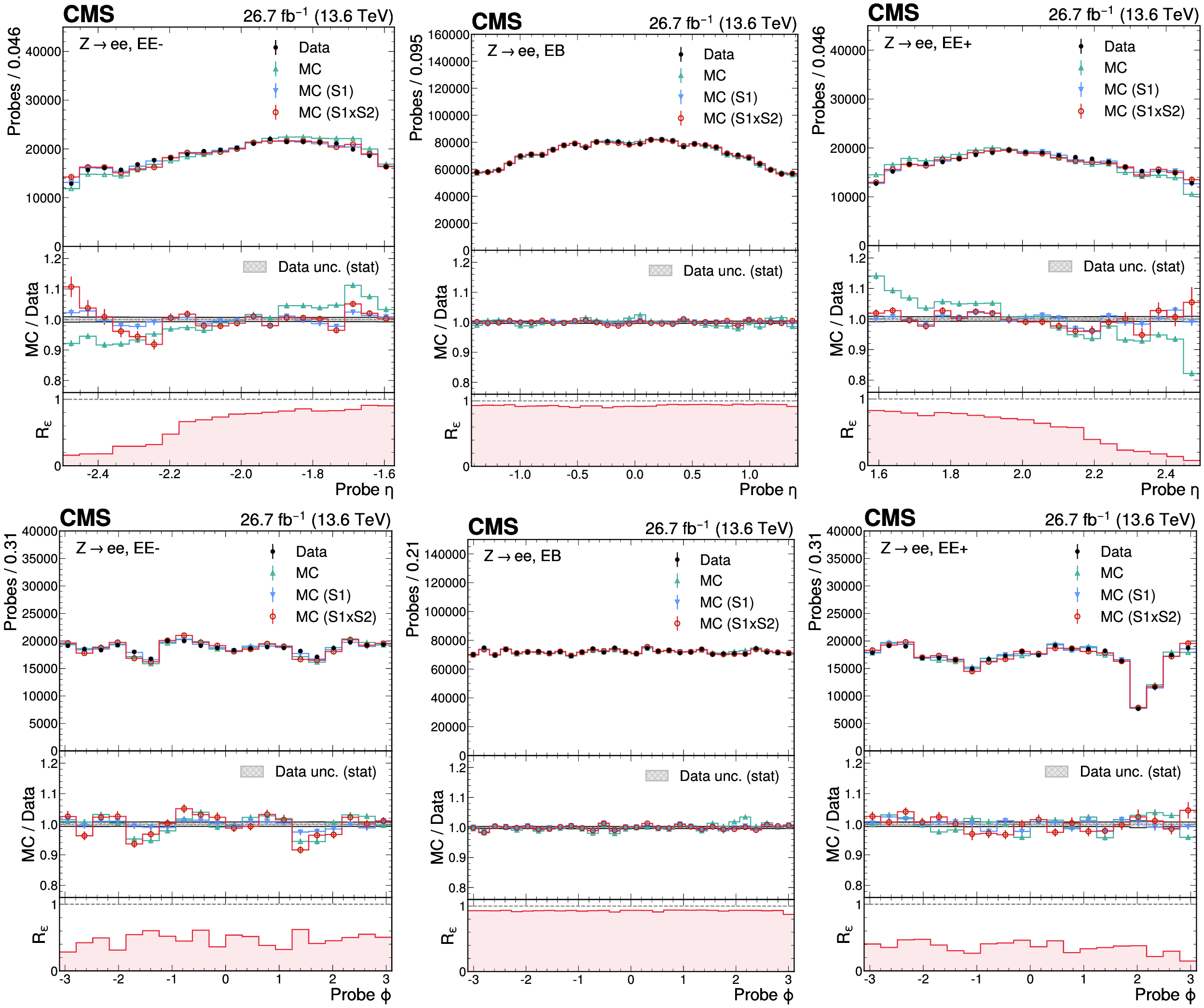
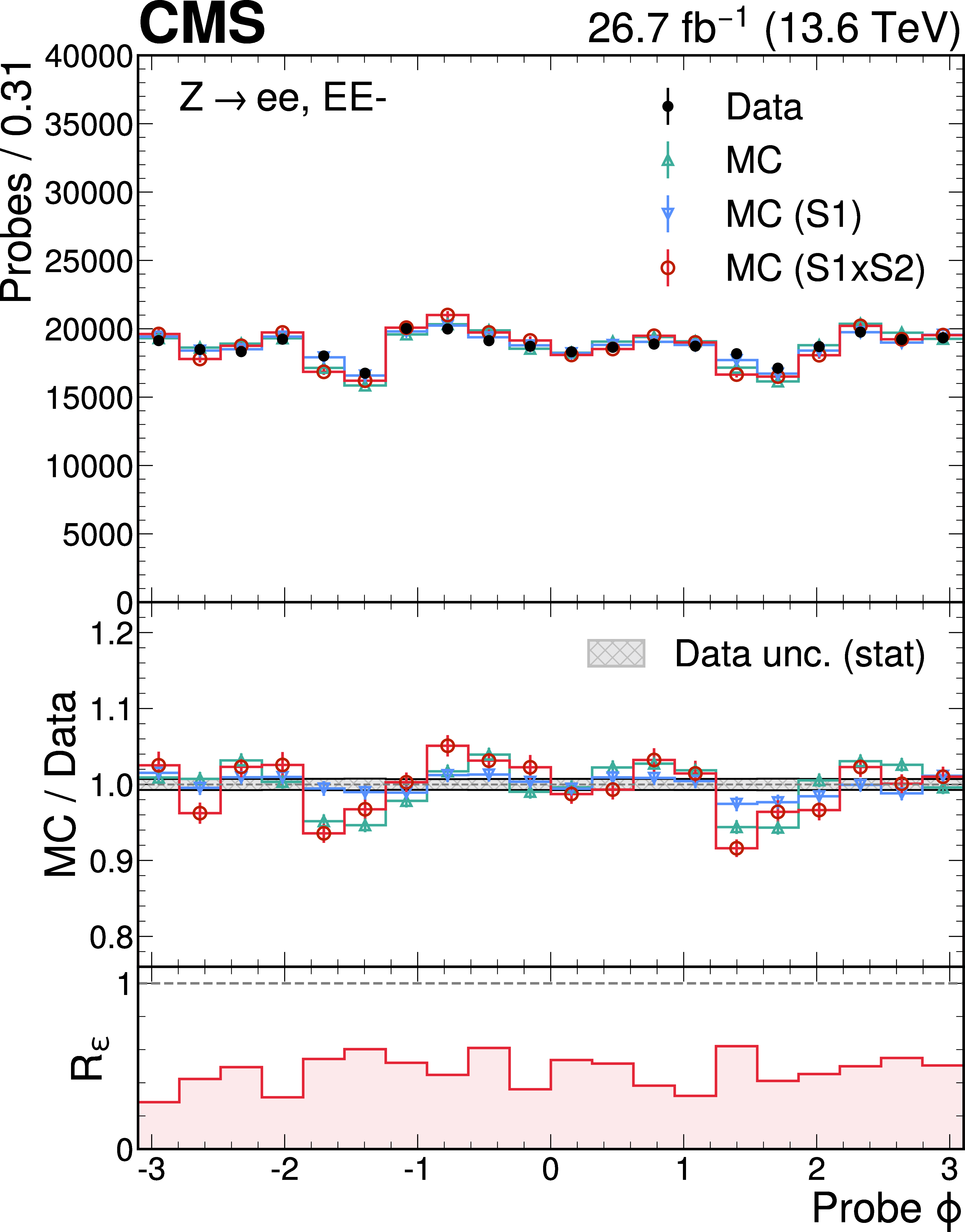
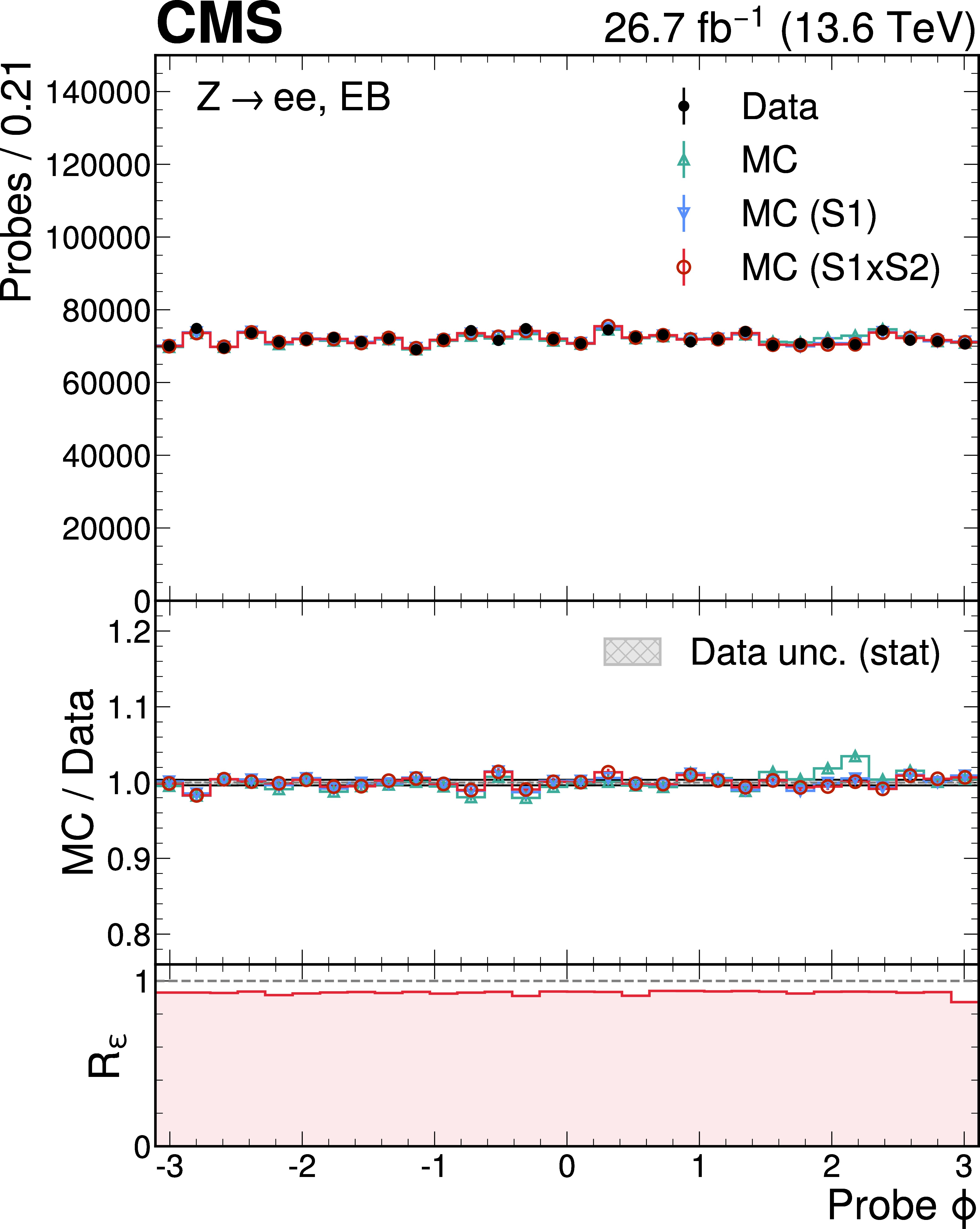
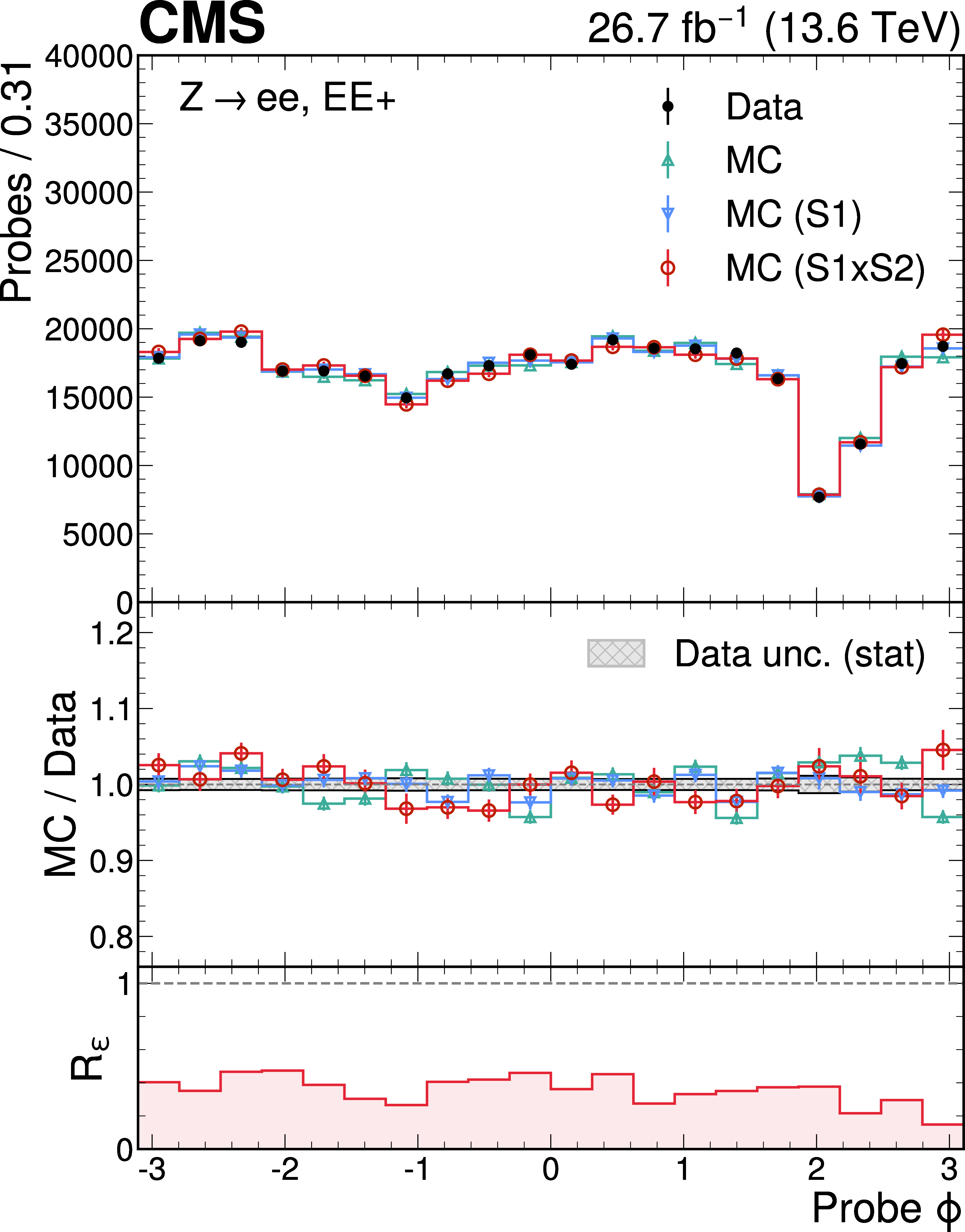
Figure 9:
The probe $ \eta $ (upper row) and $ \phi $ (lower row) distributions in data and simulation, for the EE-(left), EB (centre), and EE$ + $ (right) subdetector regions. The plotting conventions are the same as in Fig. 8. |
png pdf |
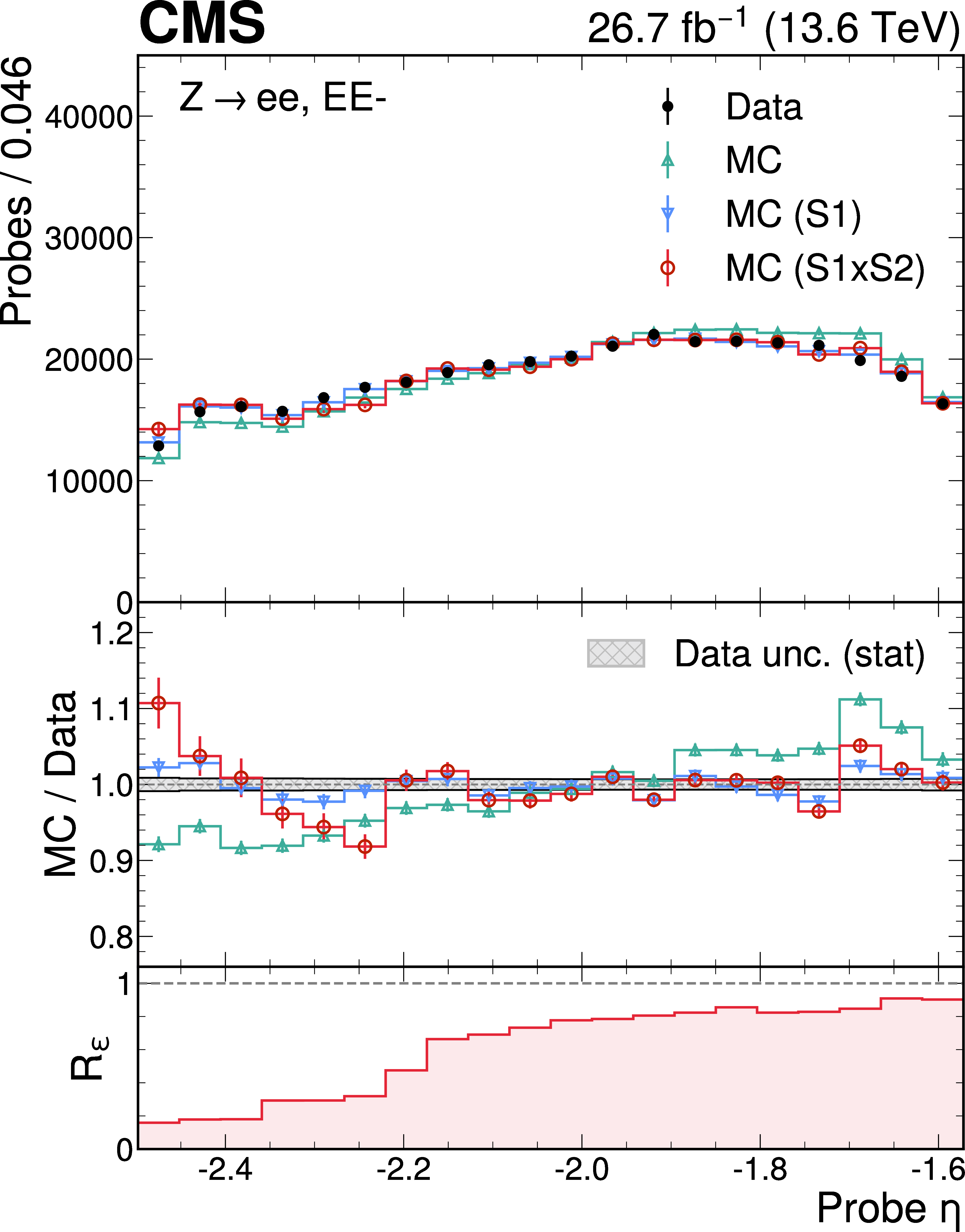
Figure 9-a:
The probe $ \eta $ (upper row) and $ \phi $ (lower row) distributions in data and simulation, for the EE-(left), EB (centre), and EE$ + $ (right) subdetector regions. The plotting conventions are the same as in Fig. 8. |
png pdf |
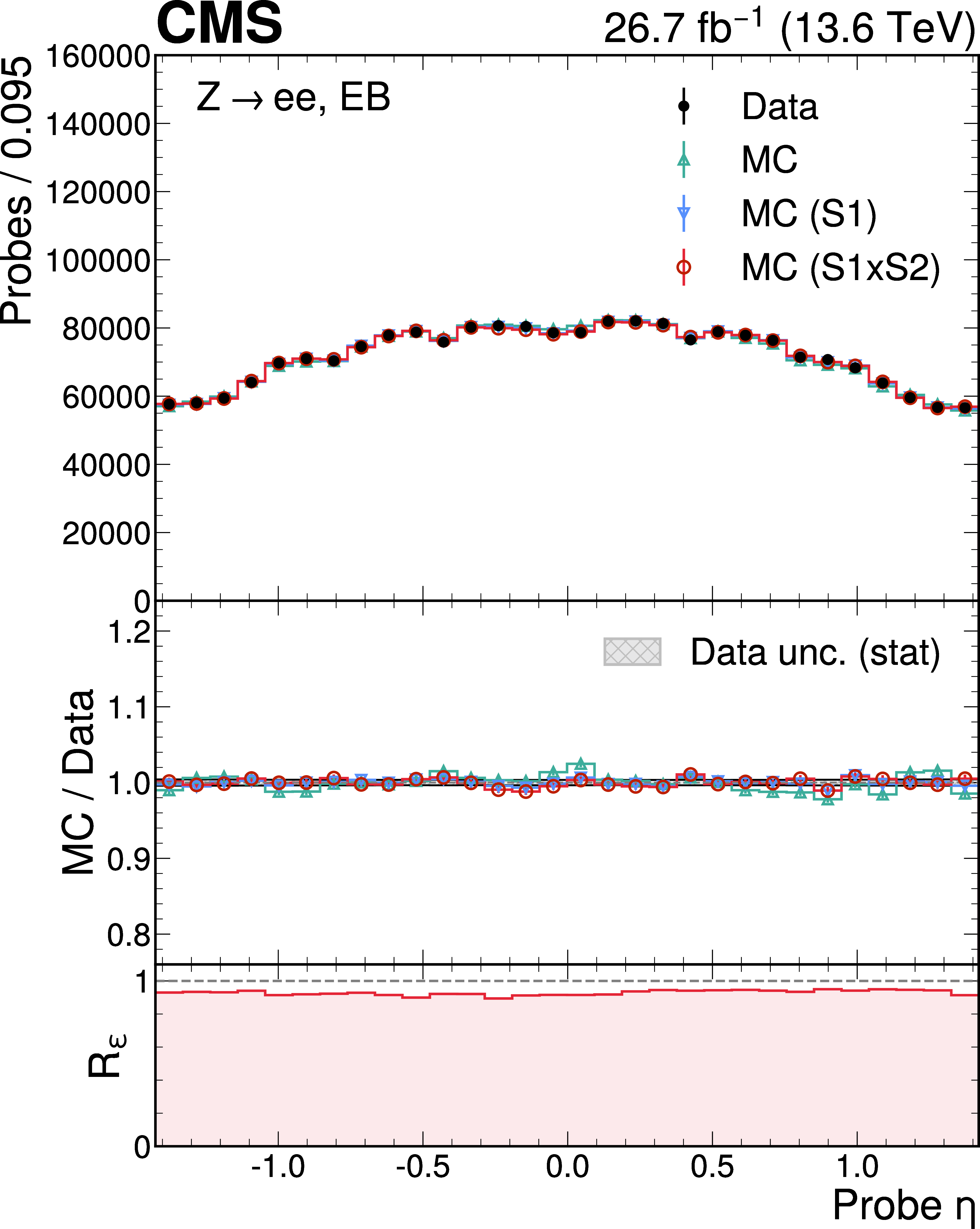
Figure 9-b:
The probe $ \eta $ (upper row) and $ \phi $ (lower row) distributions in data and simulation, for the EE-(left), EB (centre), and EE$ + $ (right) subdetector regions. The plotting conventions are the same as in Fig. 8. |
png pdf |
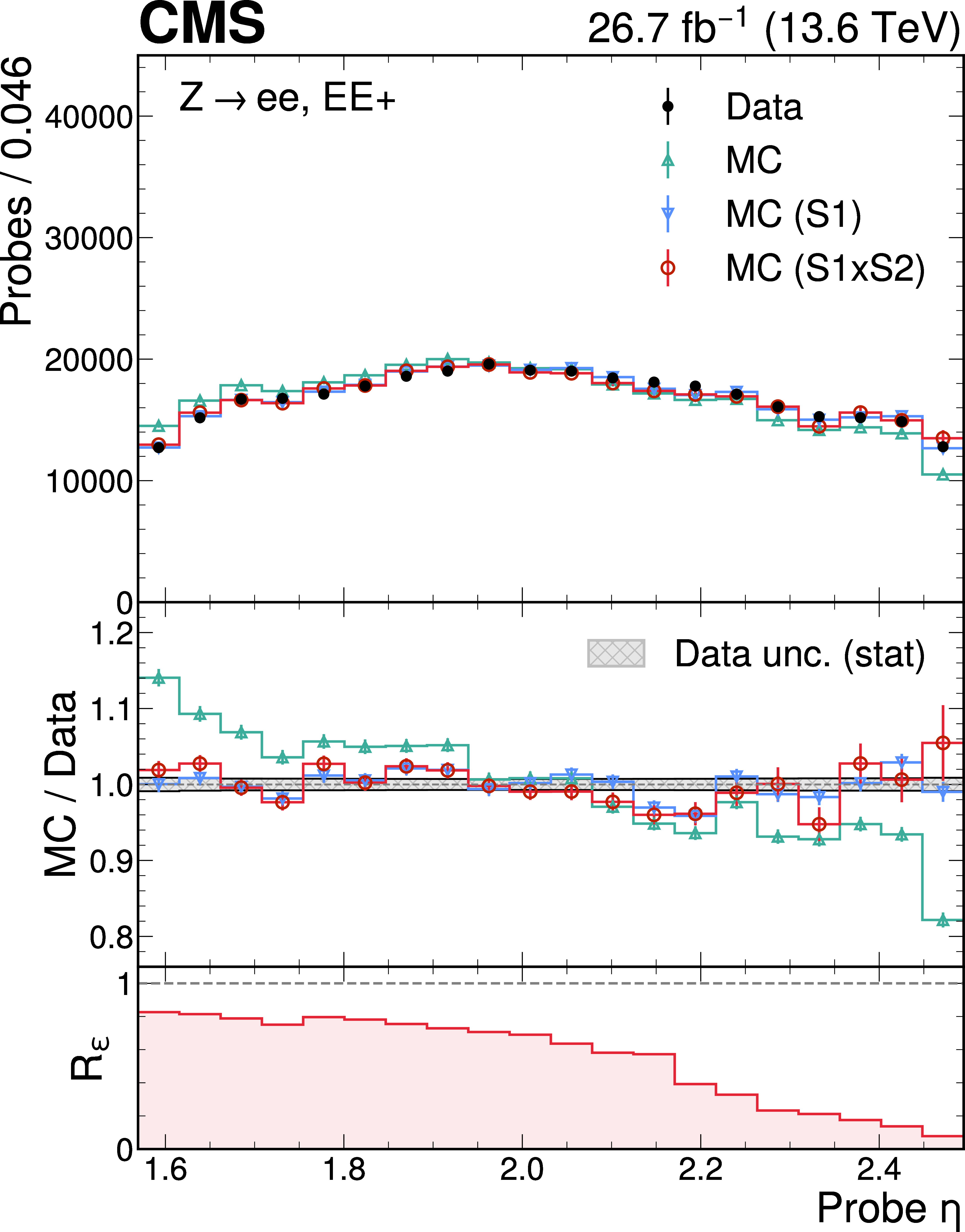
Figure 9-c:
The probe $ \eta $ (upper row) and $ \phi $ (lower row) distributions in data and simulation, for the EE-(left), EB (centre), and EE$ + $ (right) subdetector regions. The plotting conventions are the same as in Fig. 8. |
png pdf |
Figure 9-d:
The probe $ \eta $ (upper row) and $ \phi $ (lower row) distributions in data and simulation, for the EE-(left), EB (centre), and EE$ + $ (right) subdetector regions. The plotting conventions are the same as in Fig. 8. |
png pdf |
Figure 9-e:
The probe $ \eta $ (upper row) and $ \phi $ (lower row) distributions in data and simulation, for the EE-(left), EB (centre), and EE$ + $ (right) subdetector regions. The plotting conventions are the same as in Fig. 8. |
png pdf |
Figure 9-f:
The probe $ \eta $ (upper row) and $ \phi $ (lower row) distributions in data and simulation, for the EE-(left), EB (centre), and EE$ + $ (right) subdetector regions. The plotting conventions are the same as in Fig. 8. |
png pdf |
Figure 10:
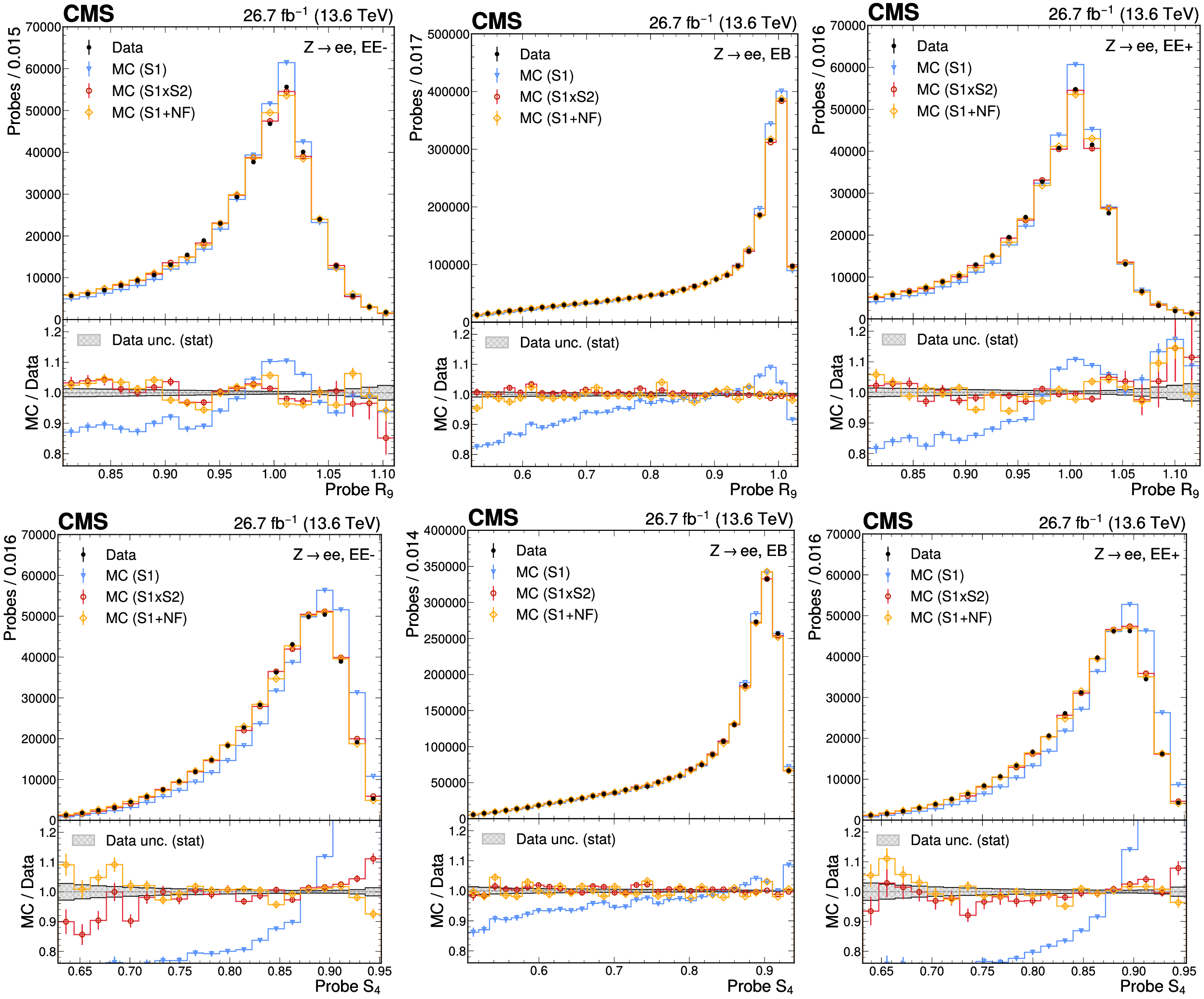
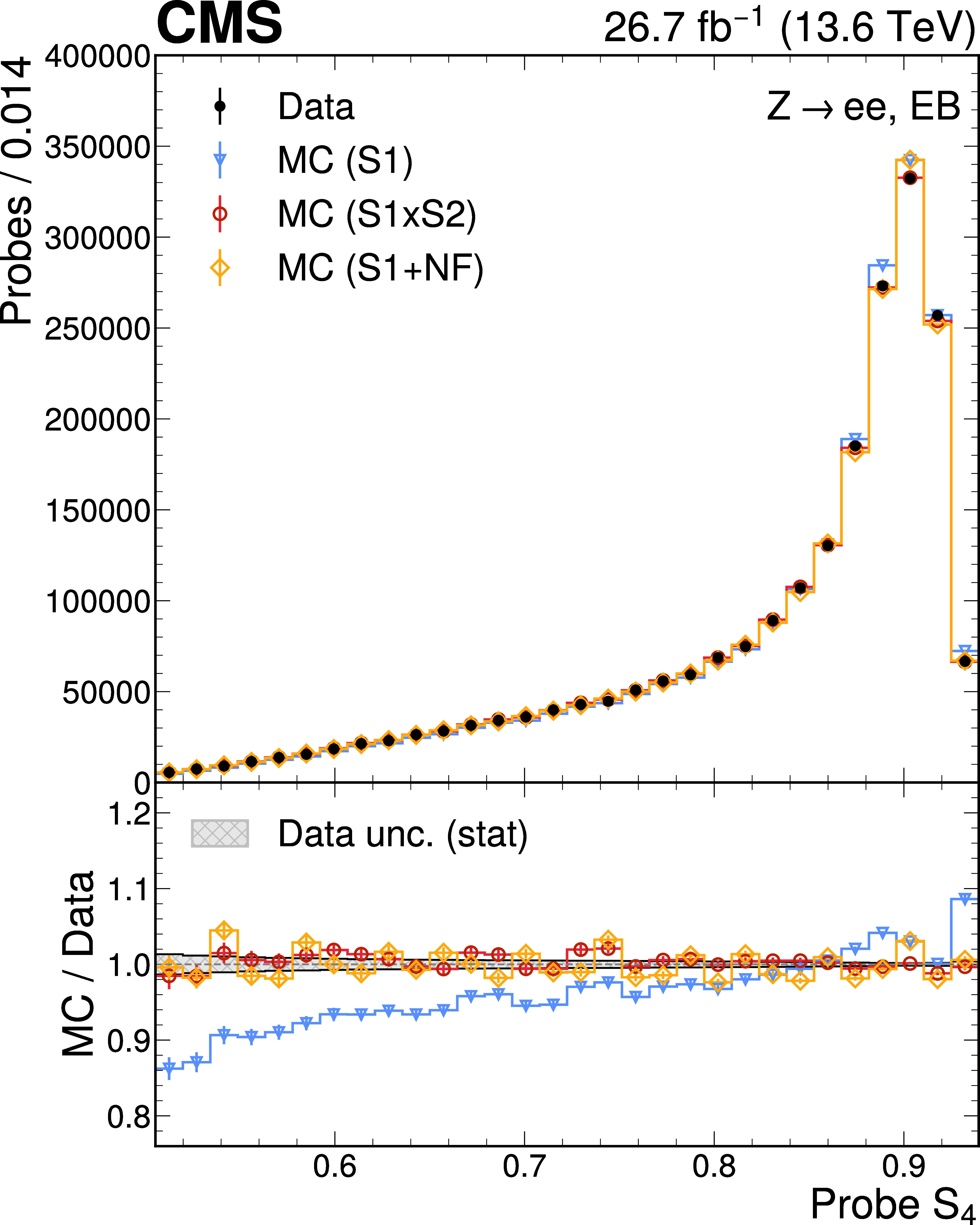
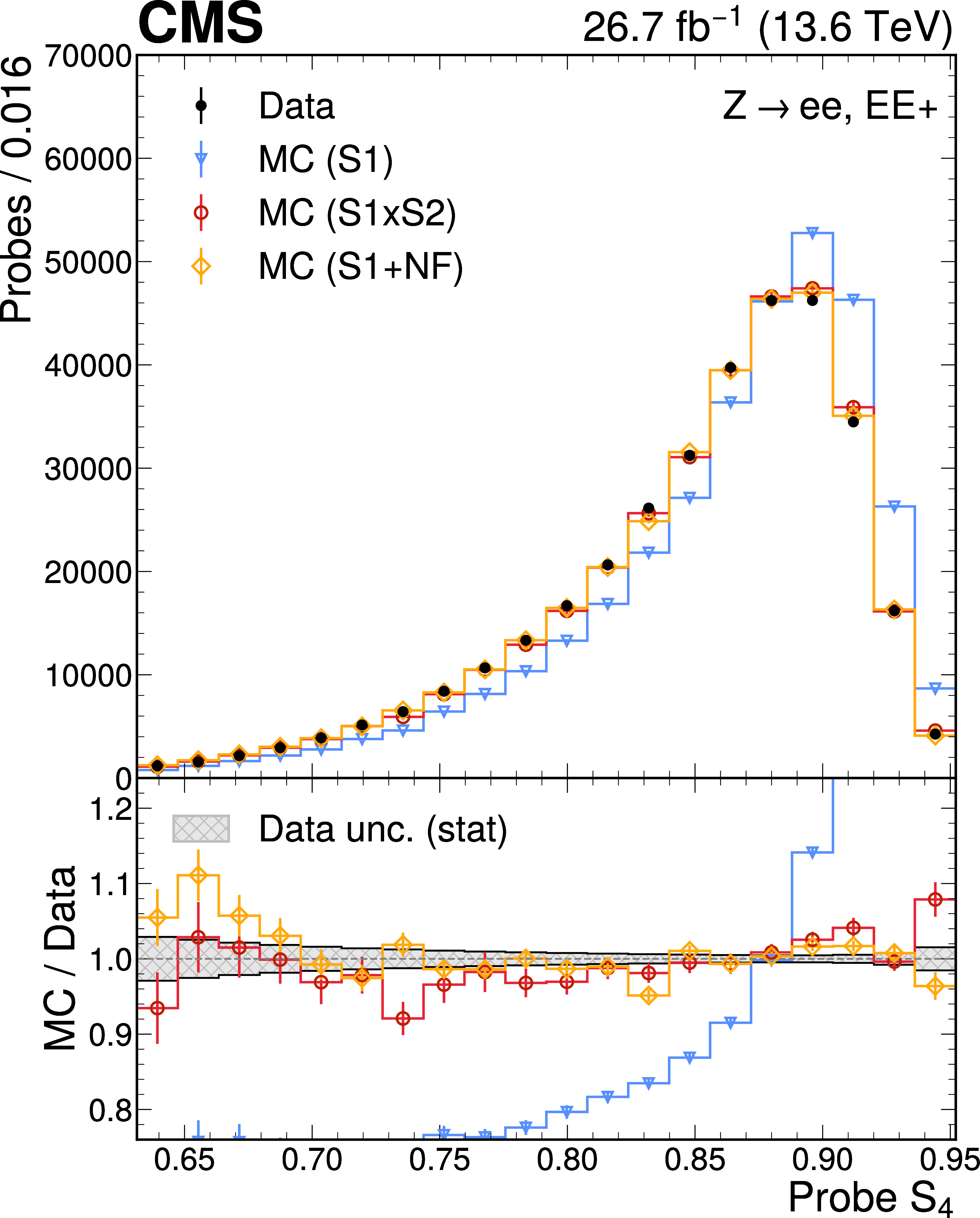
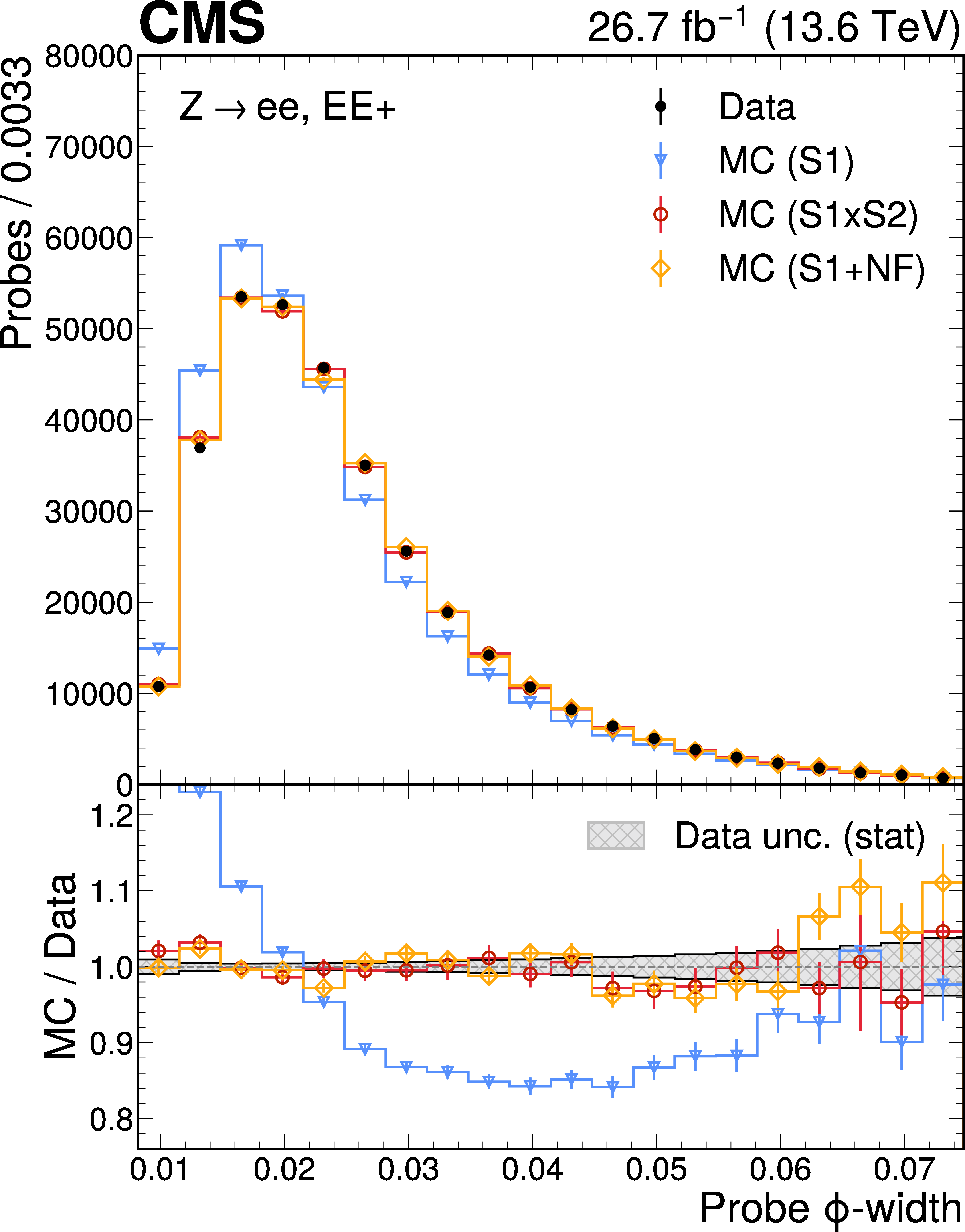
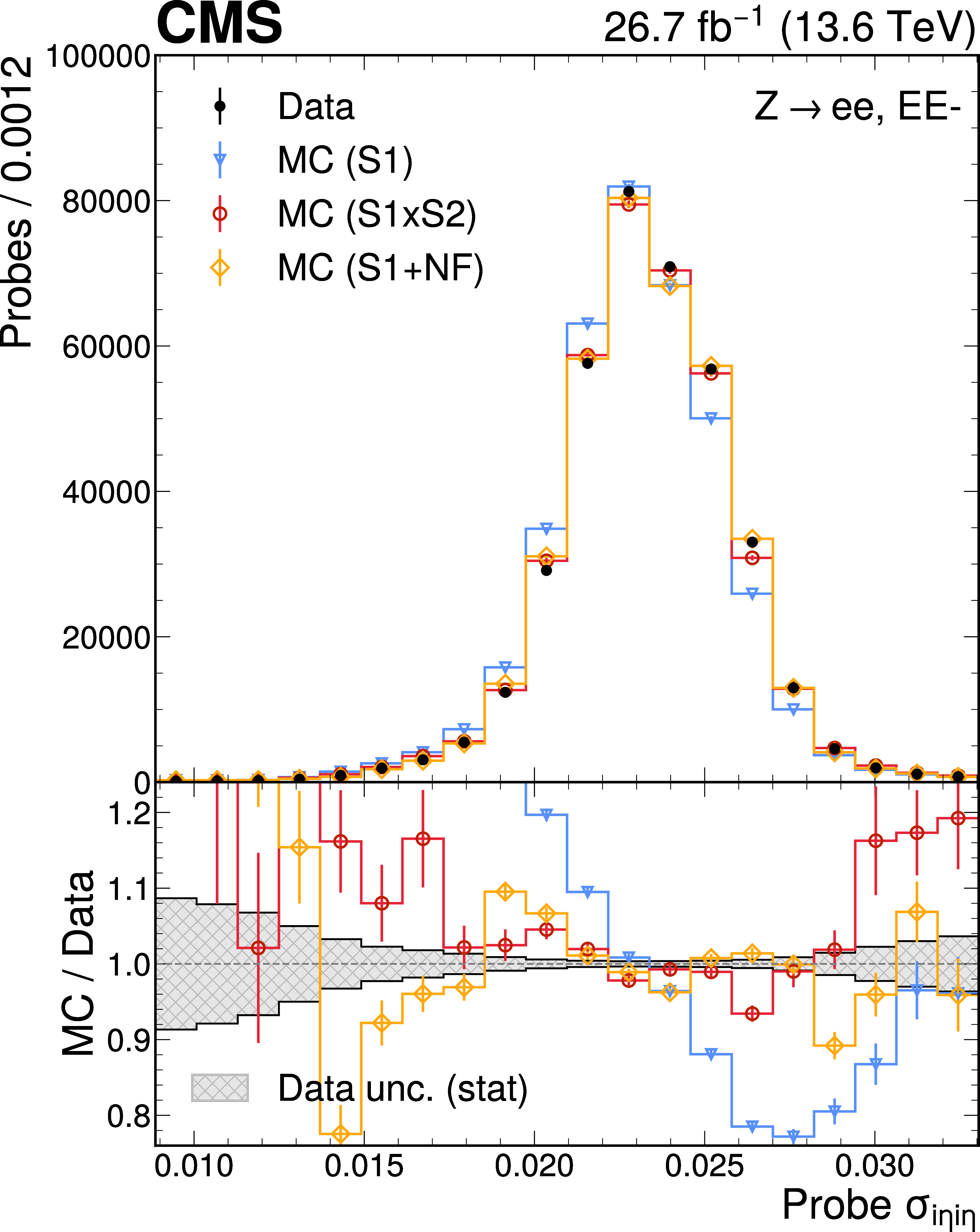
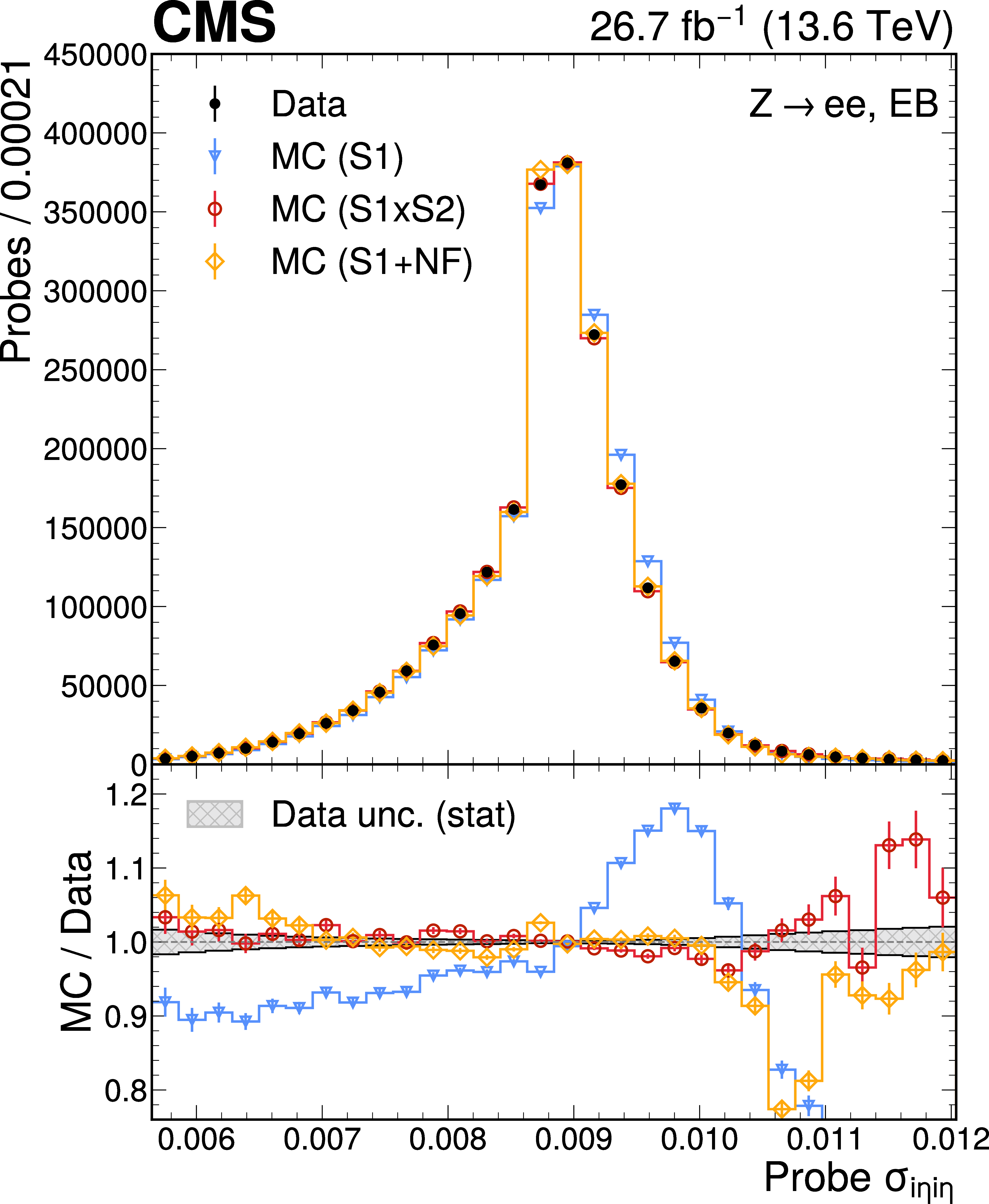
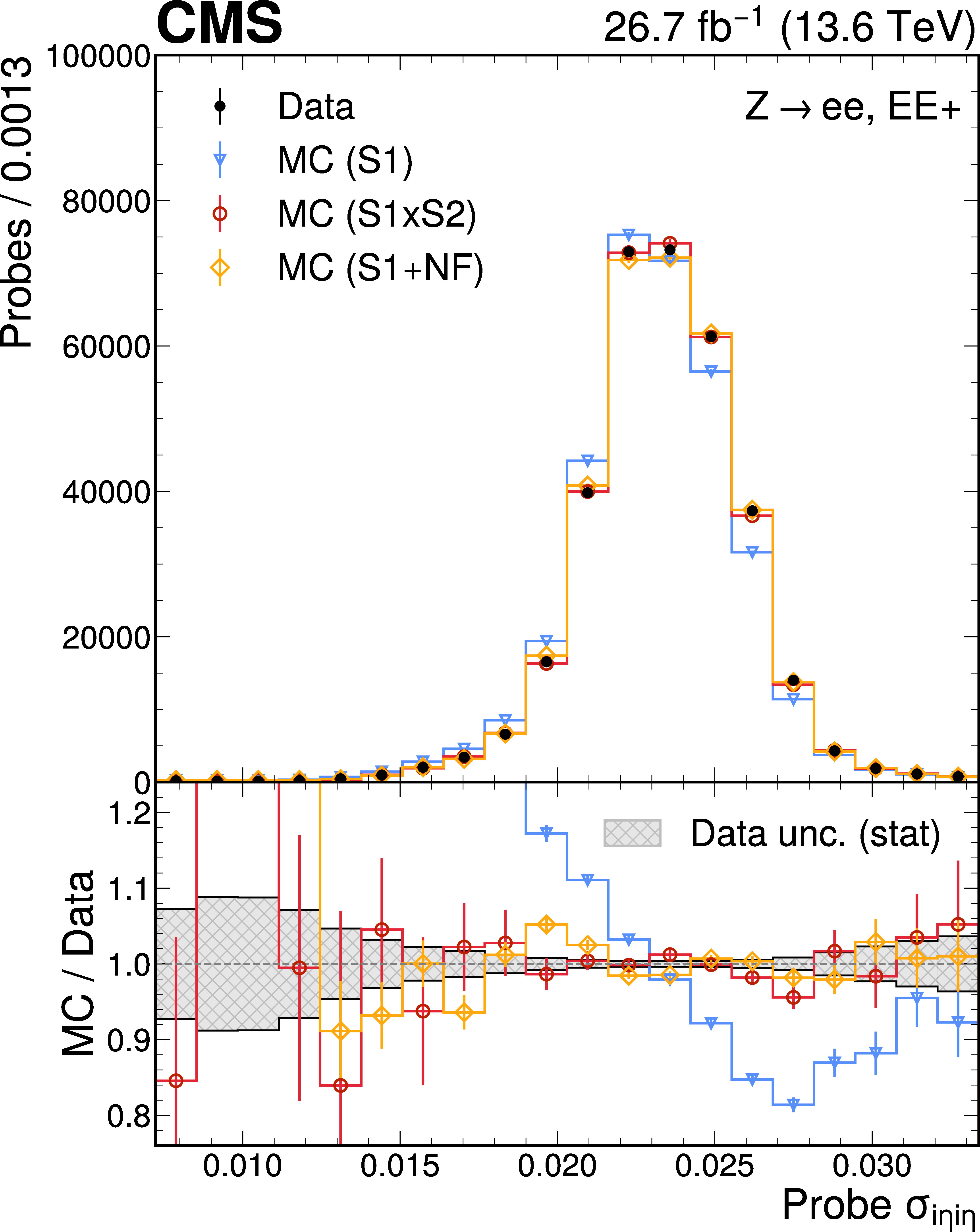
The probe $ R_9 $ (upper row) and $ S_4 $ (lower row) distributions in data (black points) and simulation (coloured histograms with points), for the EE-(left), EB (centre), and EE$ + $ (right) subdetector regions. The statistical uncertainties in the simulation and data are shown by the error bars on the points. The simulation is shown for three scenarios after first normalising the nominal simulation to the data. The blue histograms show the simulation after the S1 reweighting to align the kinematic distributions with data. The red and orange histograms show the calibrated simulation after the S2 reweighting and the flow corrections are applied, respectively. The lower panels show the ratio of simulation to data, where the statistical uncertainty in the data is indicated by the grey hatched band. |
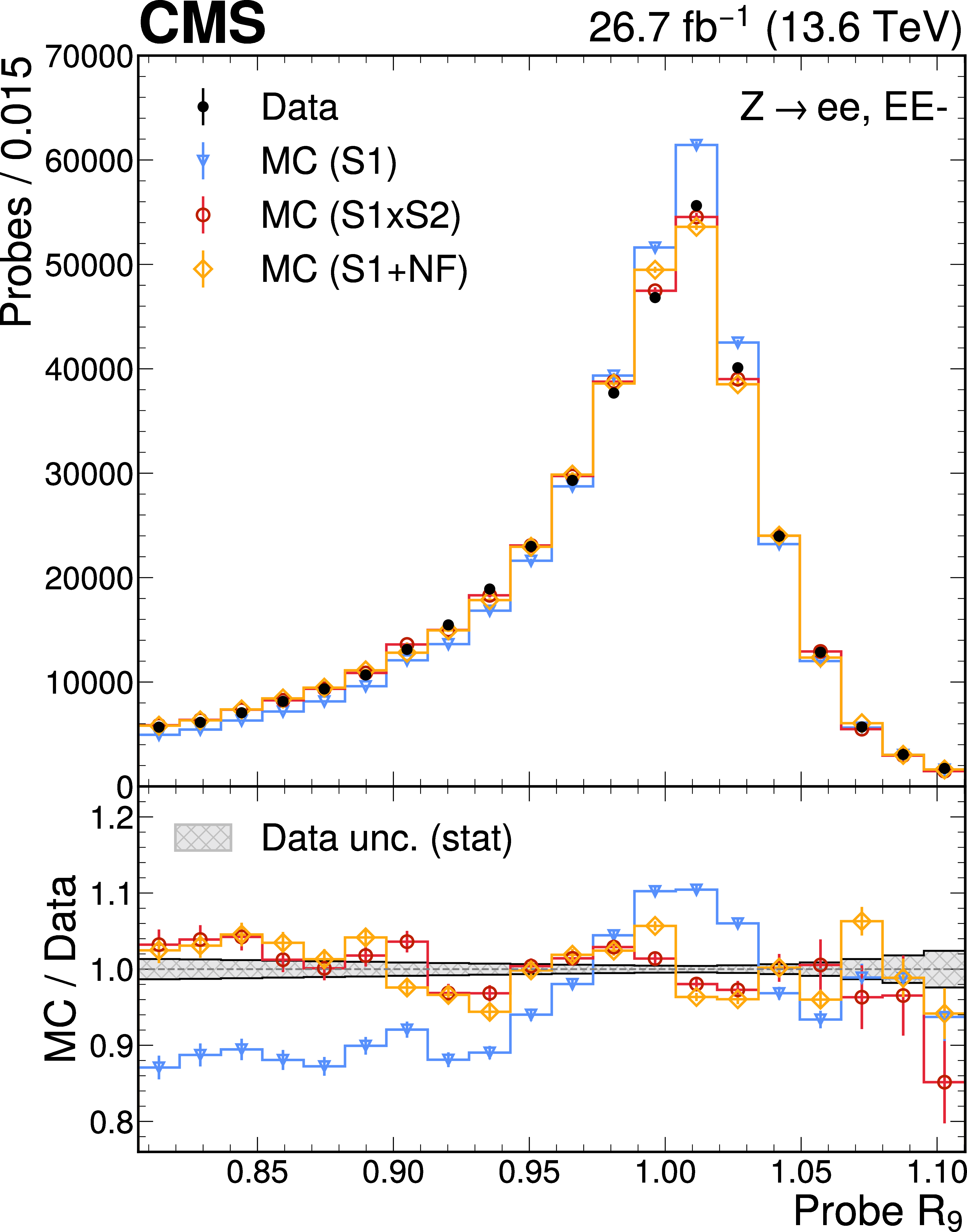
png pdf |
Figure 10-a:
The probe $ R_9 $ (upper row) and $ S_4 $ (lower row) distributions in data (black points) and simulation (coloured histograms with points), for the EE-(left), EB (centre), and EE$ + $ (right) subdetector regions. The statistical uncertainties in the simulation and data are shown by the error bars on the points. The simulation is shown for three scenarios after first normalising the nominal simulation to the data. The blue histograms show the simulation after the S1 reweighting to align the kinematic distributions with data. The red and orange histograms show the calibrated simulation after the S2 reweighting and the flow corrections are applied, respectively. The lower panels show the ratio of simulation to data, where the statistical uncertainty in the data is indicated by the grey hatched band. |
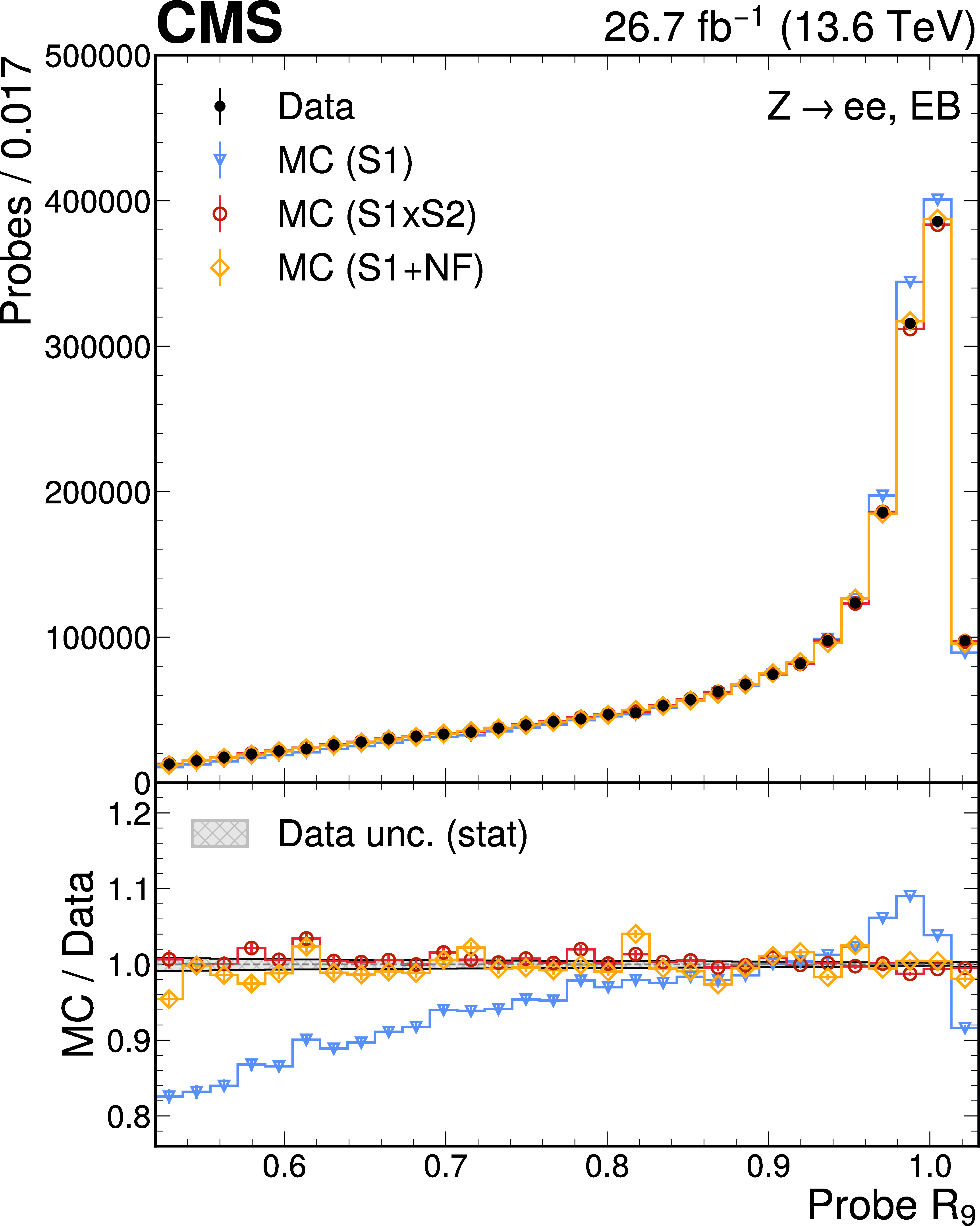
png pdf |
Figure 10-b:
The probe $ R_9 $ (upper row) and $ S_4 $ (lower row) distributions in data (black points) and simulation (coloured histograms with points), for the EE-(left), EB (centre), and EE$ + $ (right) subdetector regions. The statistical uncertainties in the simulation and data are shown by the error bars on the points. The simulation is shown for three scenarios after first normalising the nominal simulation to the data. The blue histograms show the simulation after the S1 reweighting to align the kinematic distributions with data. The red and orange histograms show the calibrated simulation after the S2 reweighting and the flow corrections are applied, respectively. The lower panels show the ratio of simulation to data, where the statistical uncertainty in the data is indicated by the grey hatched band. |
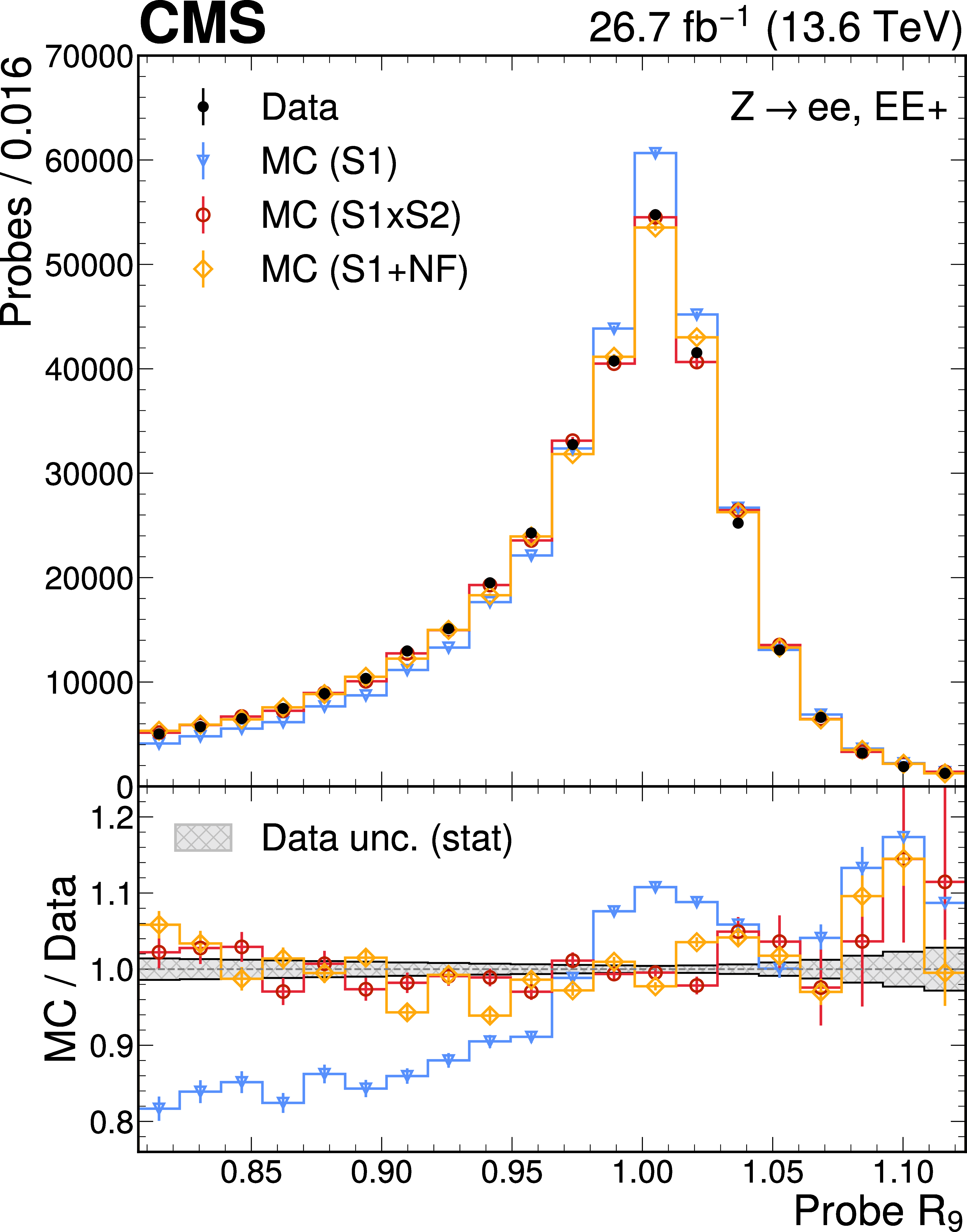
png pdf |
Figure 10-c:
The probe $ R_9 $ (upper row) and $ S_4 $ (lower row) distributions in data (black points) and simulation (coloured histograms with points), for the EE-(left), EB (centre), and EE$ + $ (right) subdetector regions. The statistical uncertainties in the simulation and data are shown by the error bars on the points. The simulation is shown for three scenarios after first normalising the nominal simulation to the data. The blue histograms show the simulation after the S1 reweighting to align the kinematic distributions with data. The red and orange histograms show the calibrated simulation after the S2 reweighting and the flow corrections are applied, respectively. The lower panels show the ratio of simulation to data, where the statistical uncertainty in the data is indicated by the grey hatched band. |
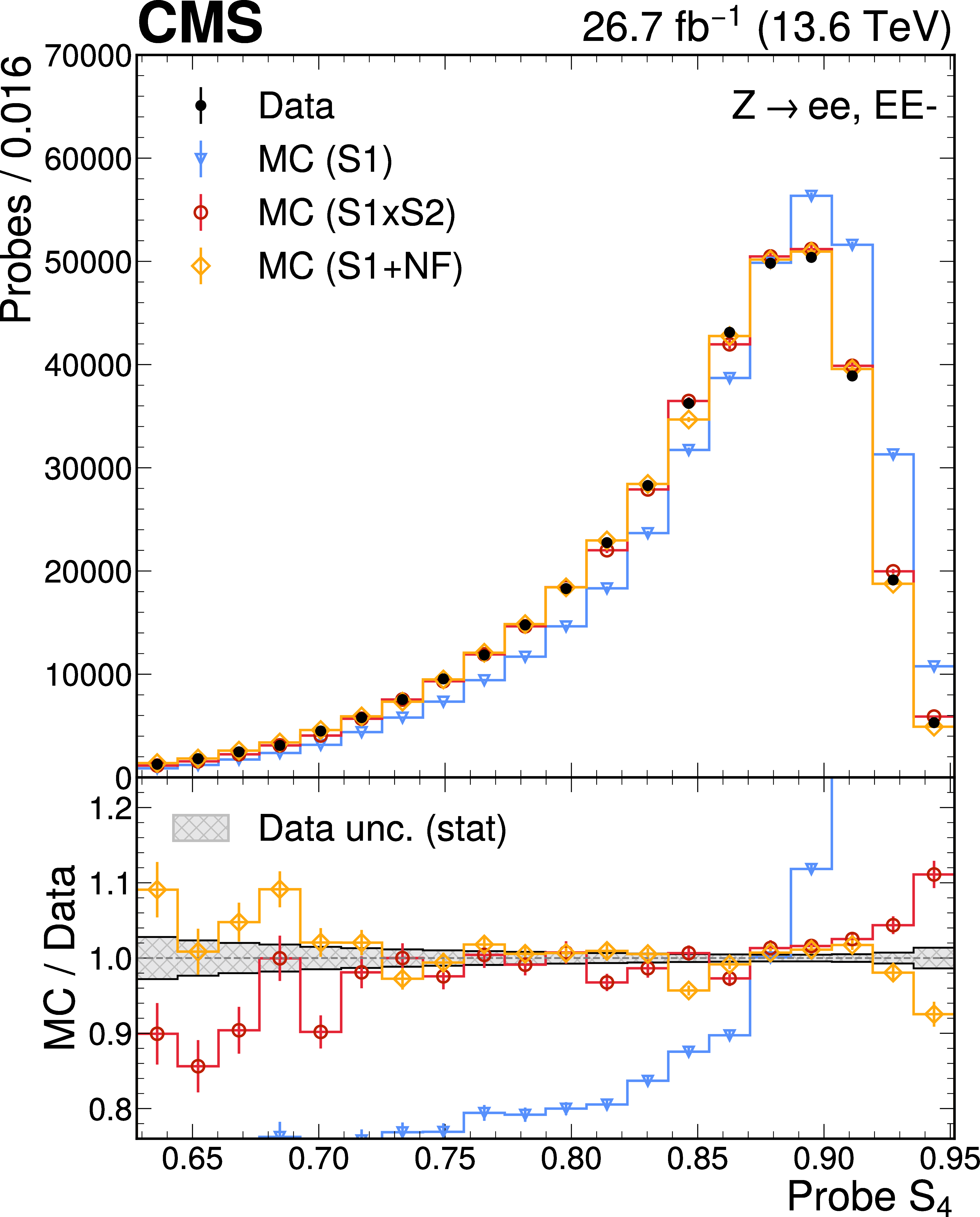
png pdf |
Figure 10-d:
The probe $ R_9 $ (upper row) and $ S_4 $ (lower row) distributions in data (black points) and simulation (coloured histograms with points), for the EE-(left), EB (centre), and EE$ + $ (right) subdetector regions. The statistical uncertainties in the simulation and data are shown by the error bars on the points. The simulation is shown for three scenarios after first normalising the nominal simulation to the data. The blue histograms show the simulation after the S1 reweighting to align the kinematic distributions with data. The red and orange histograms show the calibrated simulation after the S2 reweighting and the flow corrections are applied, respectively. The lower panels show the ratio of simulation to data, where the statistical uncertainty in the data is indicated by the grey hatched band. |
png pdf |
Figure 10-e:
The probe $ R_9 $ (upper row) and $ S_4 $ (lower row) distributions in data (black points) and simulation (coloured histograms with points), for the EE-(left), EB (centre), and EE$ + $ (right) subdetector regions. The statistical uncertainties in the simulation and data are shown by the error bars on the points. The simulation is shown for three scenarios after first normalising the nominal simulation to the data. The blue histograms show the simulation after the S1 reweighting to align the kinematic distributions with data. The red and orange histograms show the calibrated simulation after the S2 reweighting and the flow corrections are applied, respectively. The lower panels show the ratio of simulation to data, where the statistical uncertainty in the data is indicated by the grey hatched band. |
png pdf |
Figure 10-f:
The probe $ R_9 $ (upper row) and $ S_4 $ (lower row) distributions in data (black points) and simulation (coloured histograms with points), for the EE-(left), EB (centre), and EE$ + $ (right) subdetector regions. The statistical uncertainties in the simulation and data are shown by the error bars on the points. The simulation is shown for three scenarios after first normalising the nominal simulation to the data. The blue histograms show the simulation after the S1 reweighting to align the kinematic distributions with data. The red and orange histograms show the calibrated simulation after the S2 reweighting and the flow corrections are applied, respectively. The lower panels show the ratio of simulation to data, where the statistical uncertainty in the data is indicated by the grey hatched band. |
png pdf |
Figure 11:
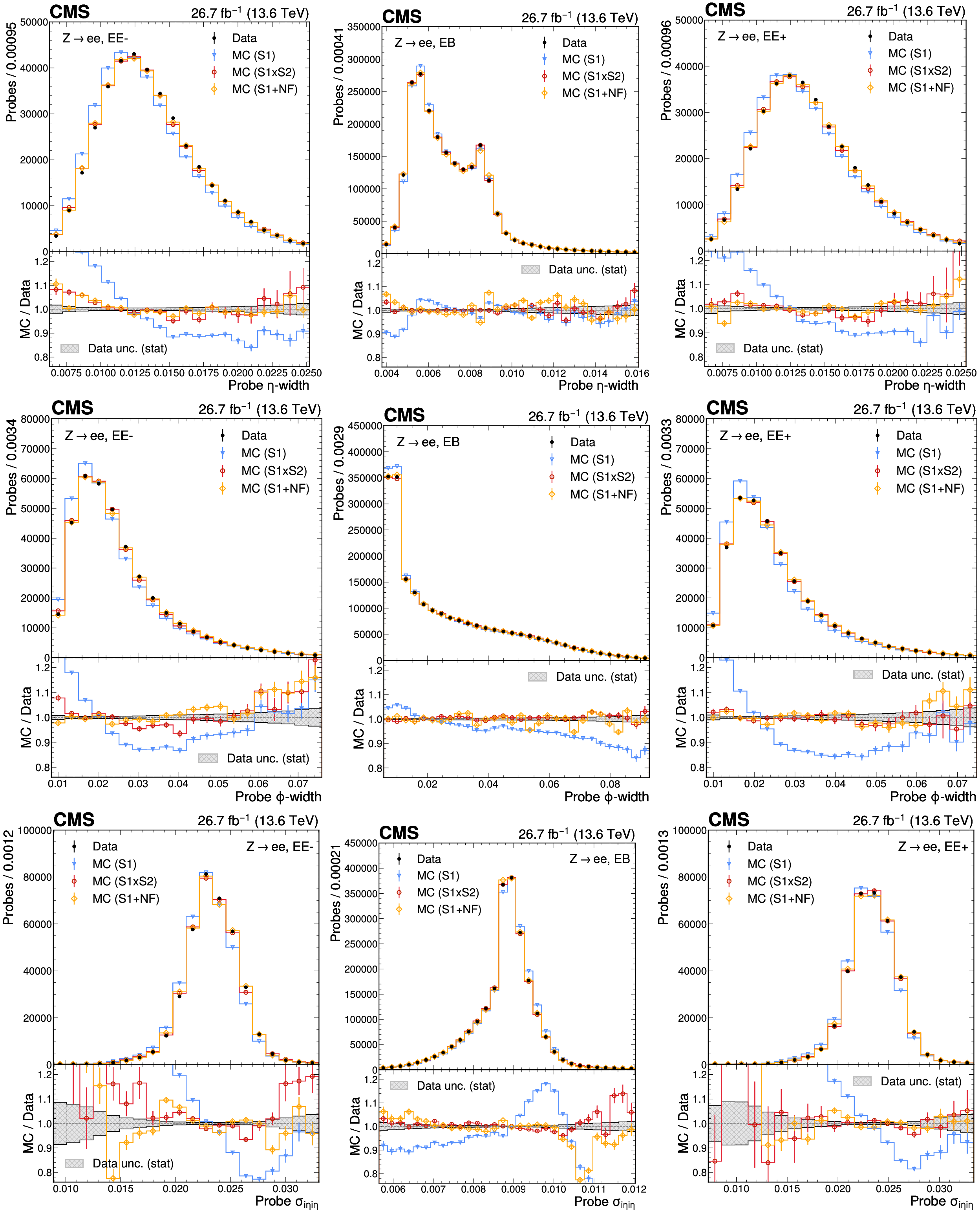
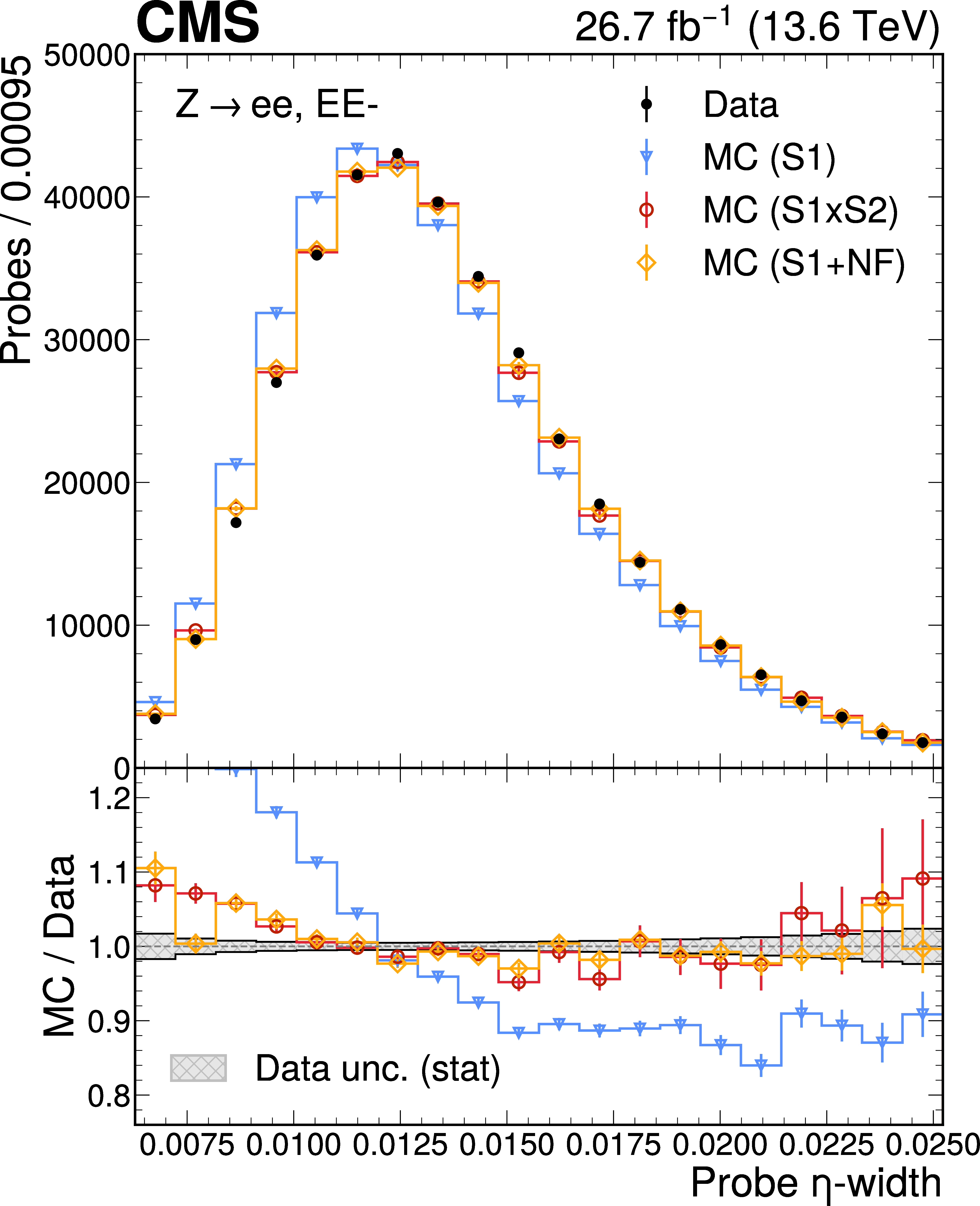
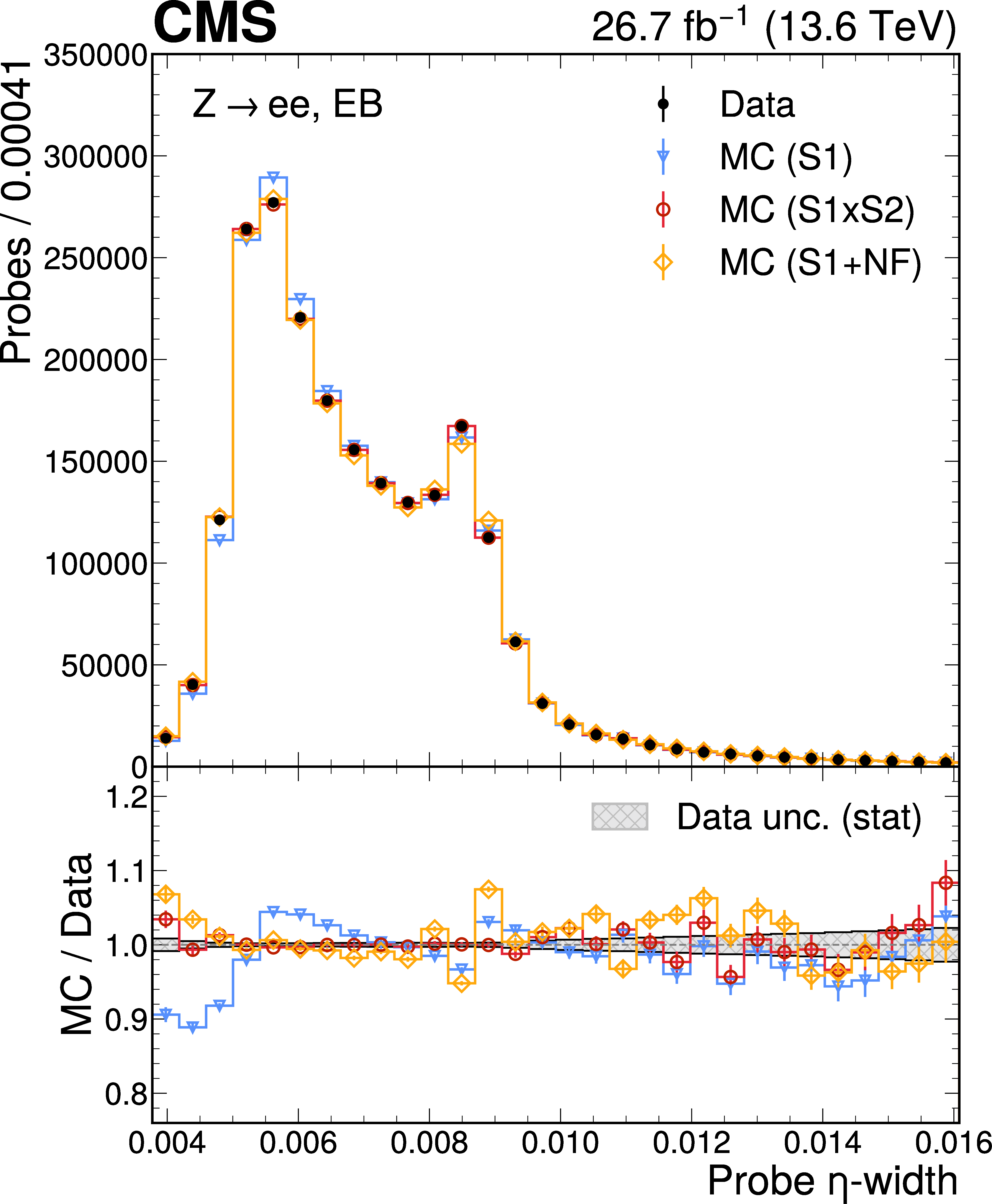
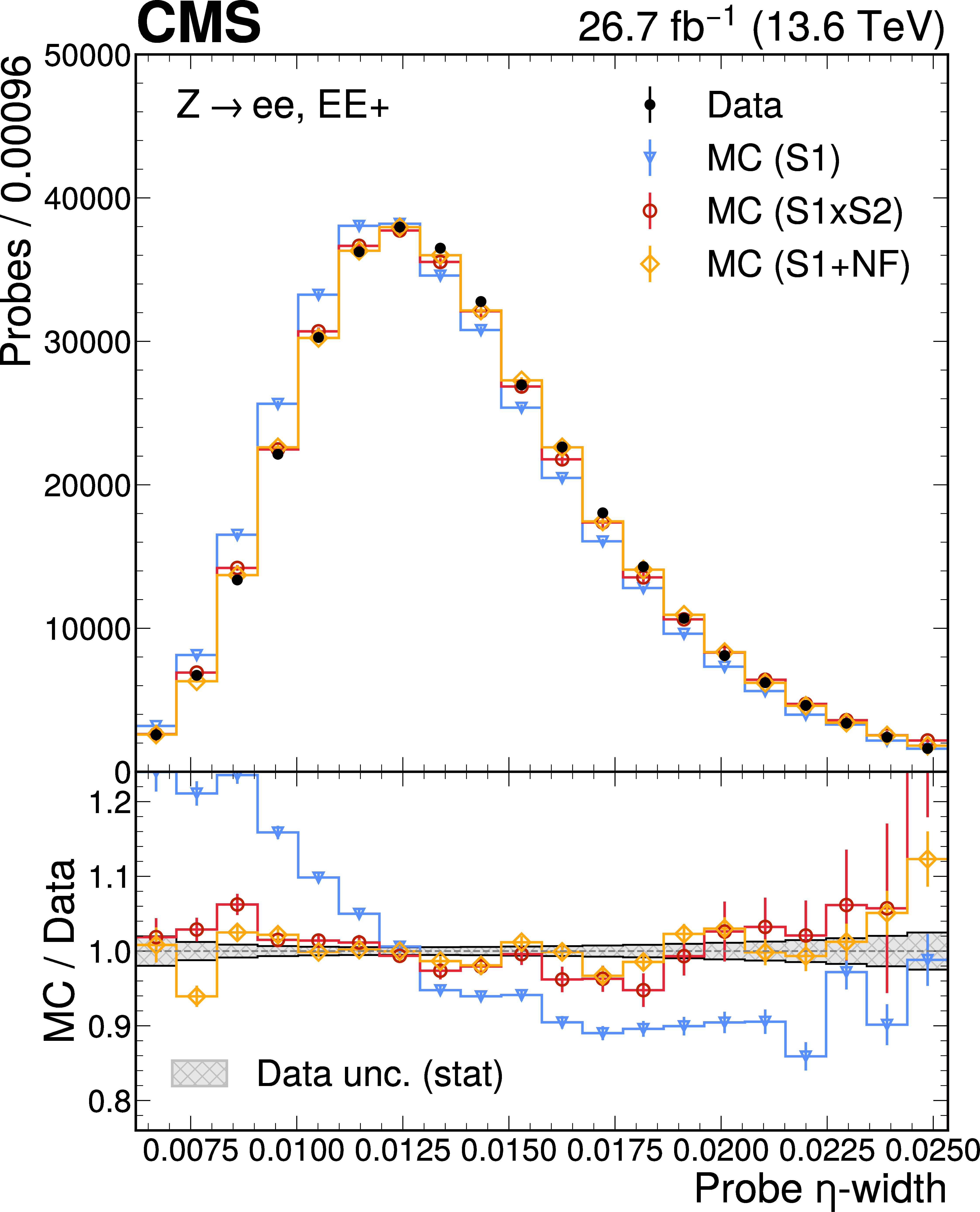
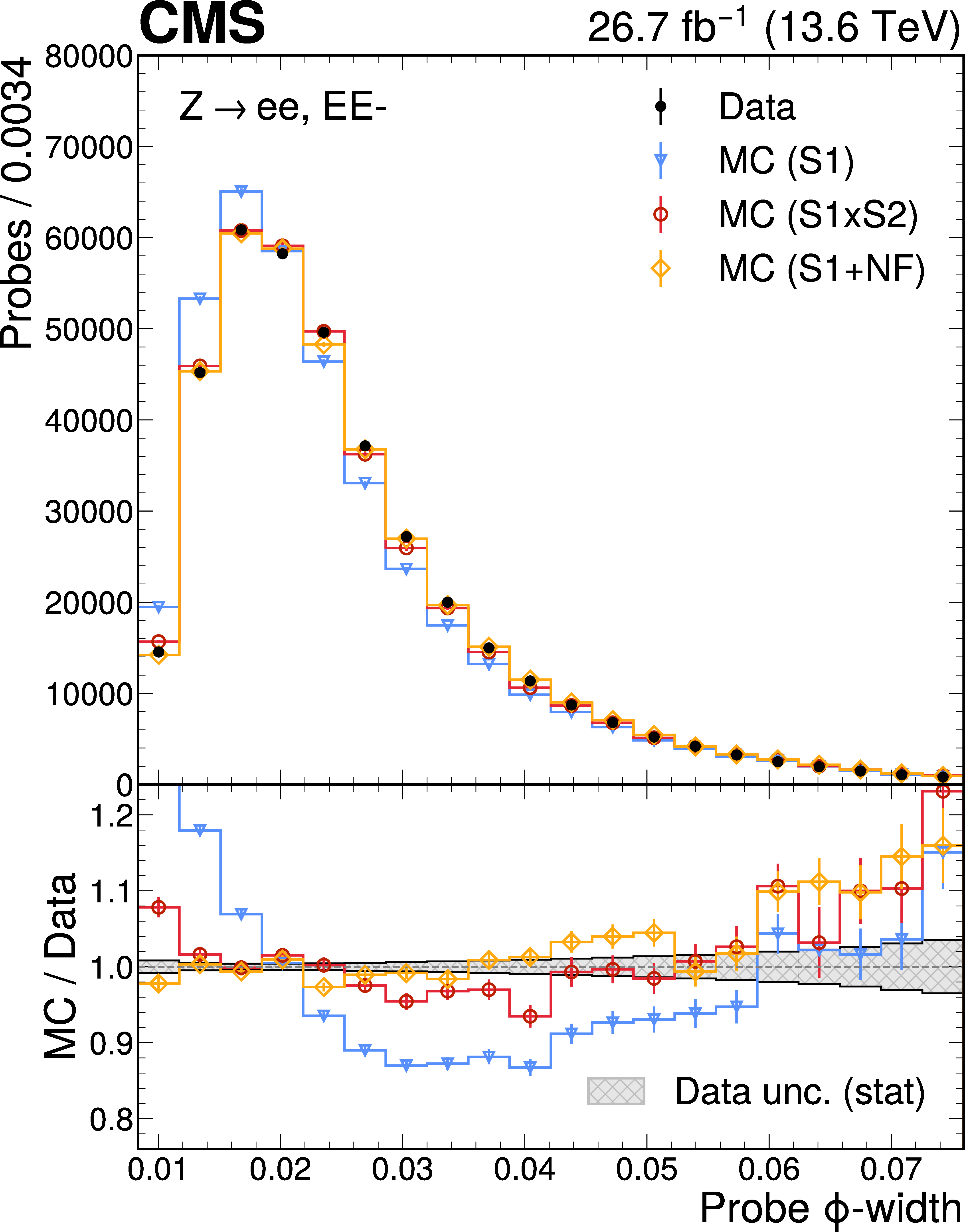
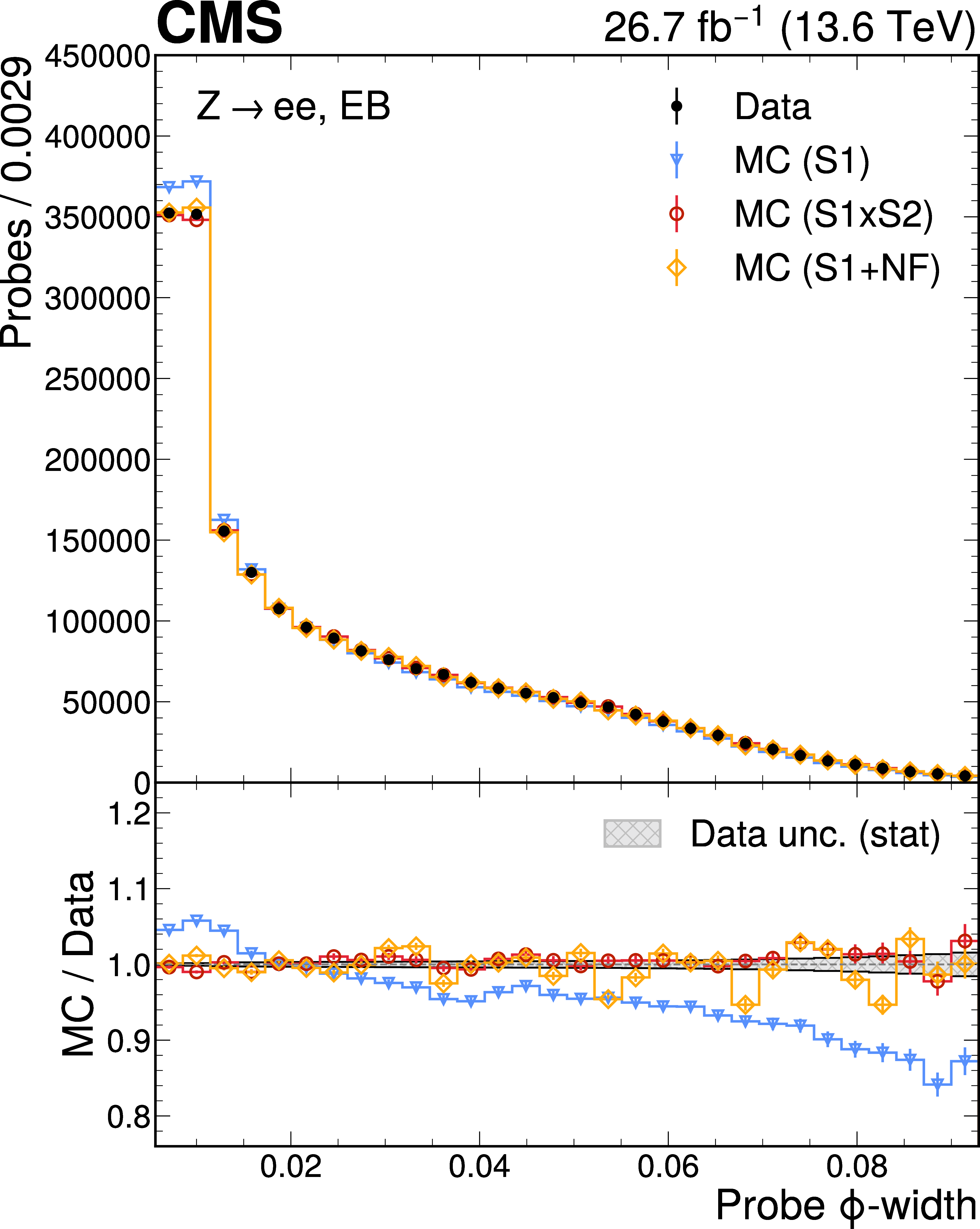
The probe $ \eta $-width (upper row), $ \phi $-width (middle row), and $ \sigma_{i\eta i\eta} $ (lower row) distributions in data and simulation, for the EE-(left), EB (centre), and EE$ + $ (right) subdetector regions. The plotting conventions are the same as in Fig. 10. |
png pdf |
Figure 11-a:
The probe $ \eta $-width (upper row), $ \phi $-width (middle row), and $ \sigma_{i\eta i\eta} $ (lower row) distributions in data and simulation, for the EE-(left), EB (centre), and EE$ + $ (right) subdetector regions. The plotting conventions are the same as in Fig. 10. |
png pdf |
Figure 11-b:
The probe $ \eta $-width (upper row), $ \phi $-width (middle row), and $ \sigma_{i\eta i\eta} $ (lower row) distributions in data and simulation, for the EE-(left), EB (centre), and EE$ + $ (right) subdetector regions. The plotting conventions are the same as in Fig. 10. |
png pdf |
Figure 11-c:
The probe $ \eta $-width (upper row), $ \phi $-width (middle row), and $ \sigma_{i\eta i\eta} $ (lower row) distributions in data and simulation, for the EE-(left), EB (centre), and EE$ + $ (right) subdetector regions. The plotting conventions are the same as in Fig. 10. |
png pdf |
Figure 11-d:
The probe $ \eta $-width (upper row), $ \phi $-width (middle row), and $ \sigma_{i\eta i\eta} $ (lower row) distributions in data and simulation, for the EE-(left), EB (centre), and EE$ + $ (right) subdetector regions. The plotting conventions are the same as in Fig. 10. |
png pdf |
Figure 11-e:
The probe $ \eta $-width (upper row), $ \phi $-width (middle row), and $ \sigma_{i\eta i\eta} $ (lower row) distributions in data and simulation, for the EE-(left), EB (centre), and EE$ + $ (right) subdetector regions. The plotting conventions are the same as in Fig. 10. |
png pdf |
Figure 11-f:
The probe $ \eta $-width (upper row), $ \phi $-width (middle row), and $ \sigma_{i\eta i\eta} $ (lower row) distributions in data and simulation, for the EE-(left), EB (centre), and EE$ + $ (right) subdetector regions. The plotting conventions are the same as in Fig. 10. |
png pdf |
Figure 11-g:
The probe $ \eta $-width (upper row), $ \phi $-width (middle row), and $ \sigma_{i\eta i\eta} $ (lower row) distributions in data and simulation, for the EE-(left), EB (centre), and EE$ + $ (right) subdetector regions. The plotting conventions are the same as in Fig. 10. |
png pdf |
Figure 11-h:
The probe $ \eta $-width (upper row), $ \phi $-width (middle row), and $ \sigma_{i\eta i\eta} $ (lower row) distributions in data and simulation, for the EE-(left), EB (centre), and EE$ + $ (right) subdetector regions. The plotting conventions are the same as in Fig. 10. |
png pdf |
Figure 11-i:
The probe $ \eta $-width (upper row), $ \phi $-width (middle row), and $ \sigma_{i\eta i\eta} $ (lower row) distributions in data and simulation, for the EE-(left), EB (centre), and EE$ + $ (right) subdetector regions. The plotting conventions are the same as in Fig. 10. |
png pdf |
Figure 12:
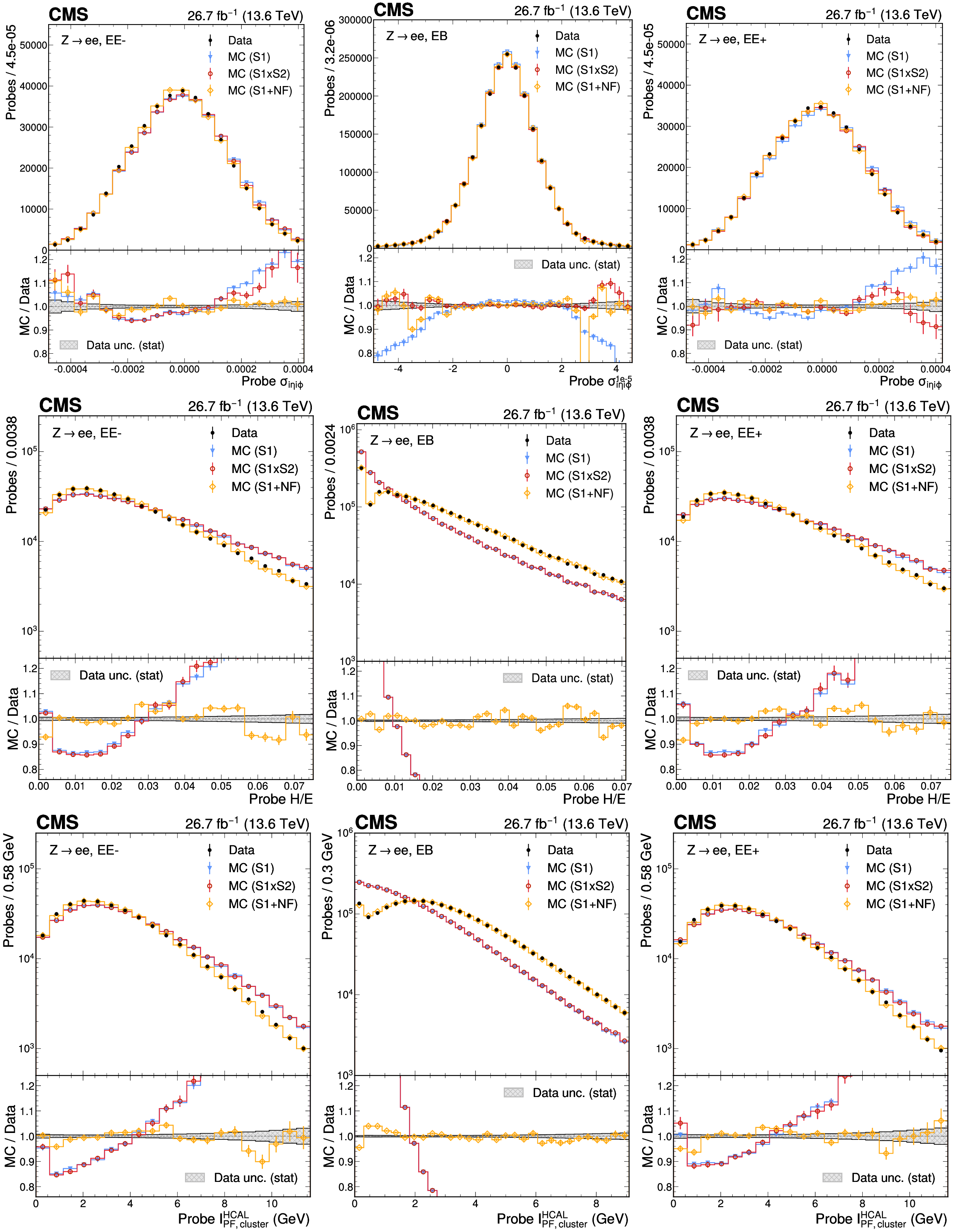
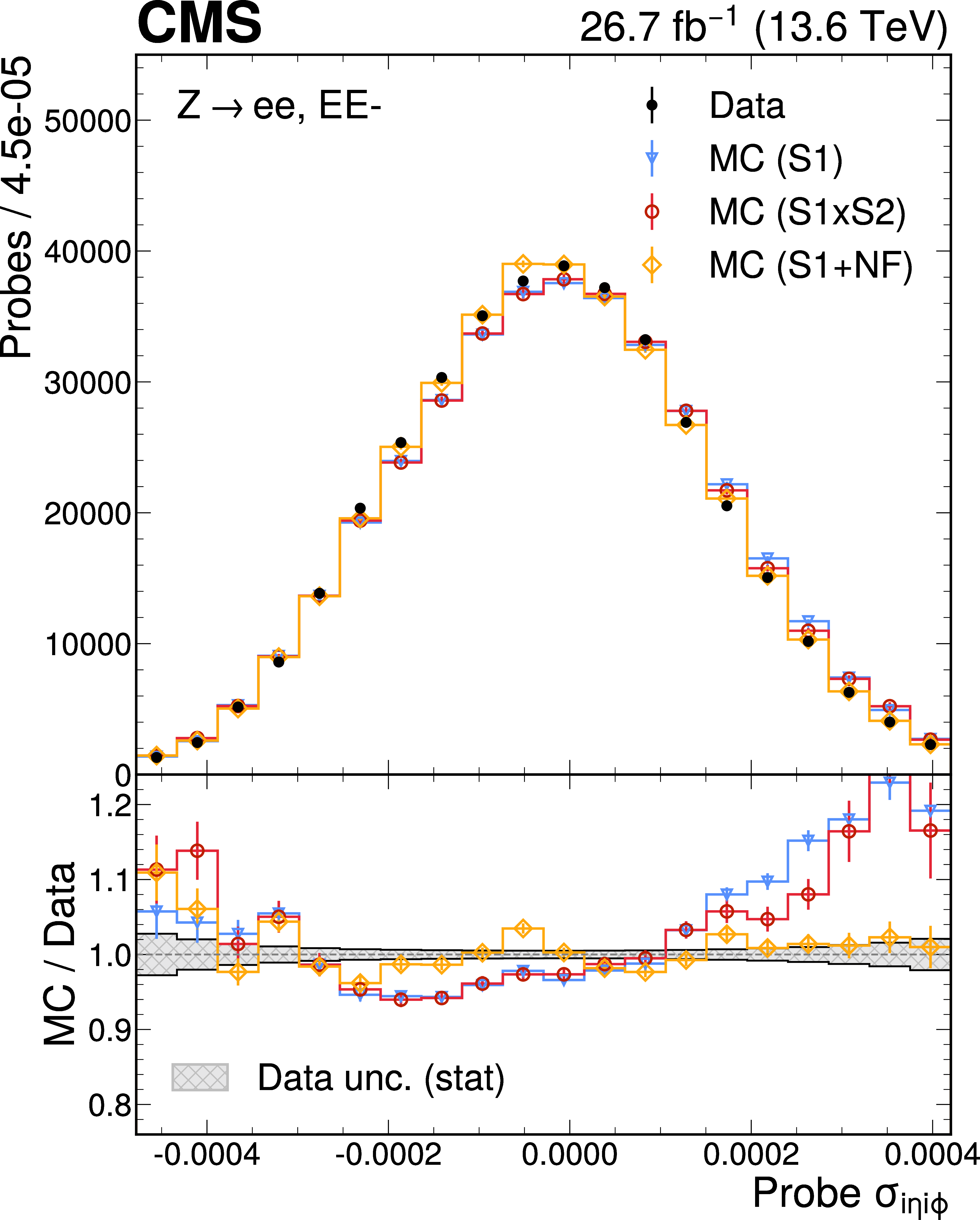
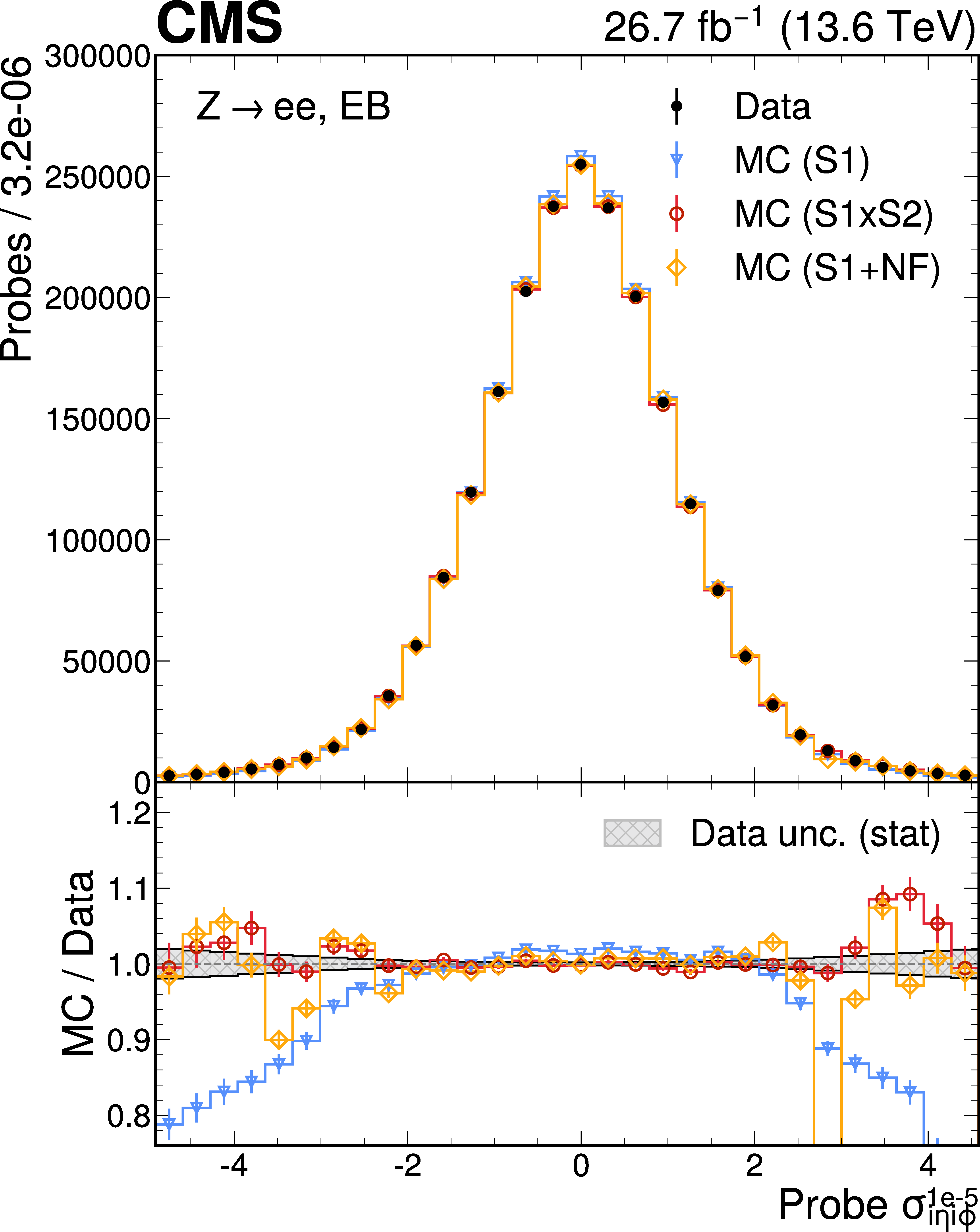
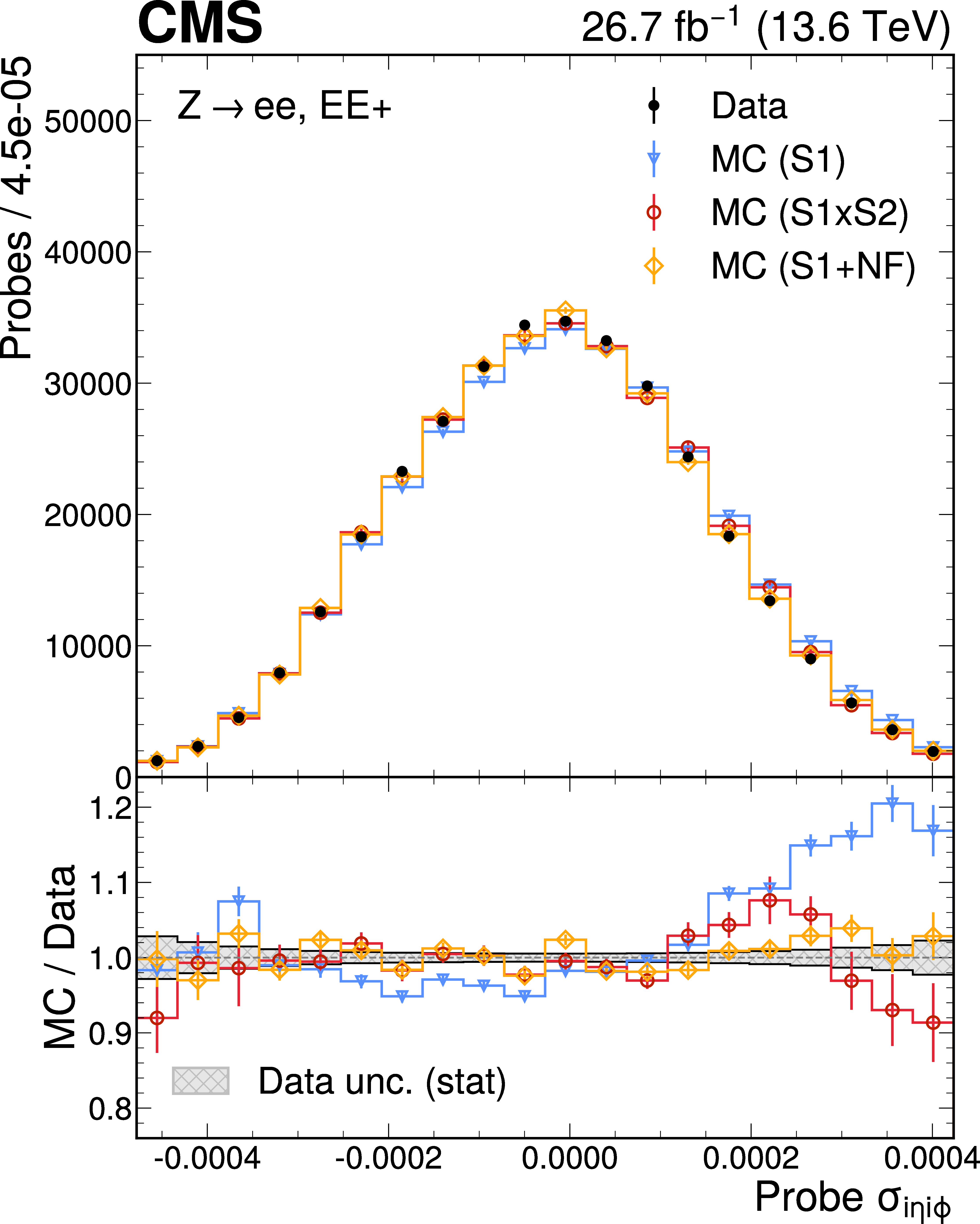
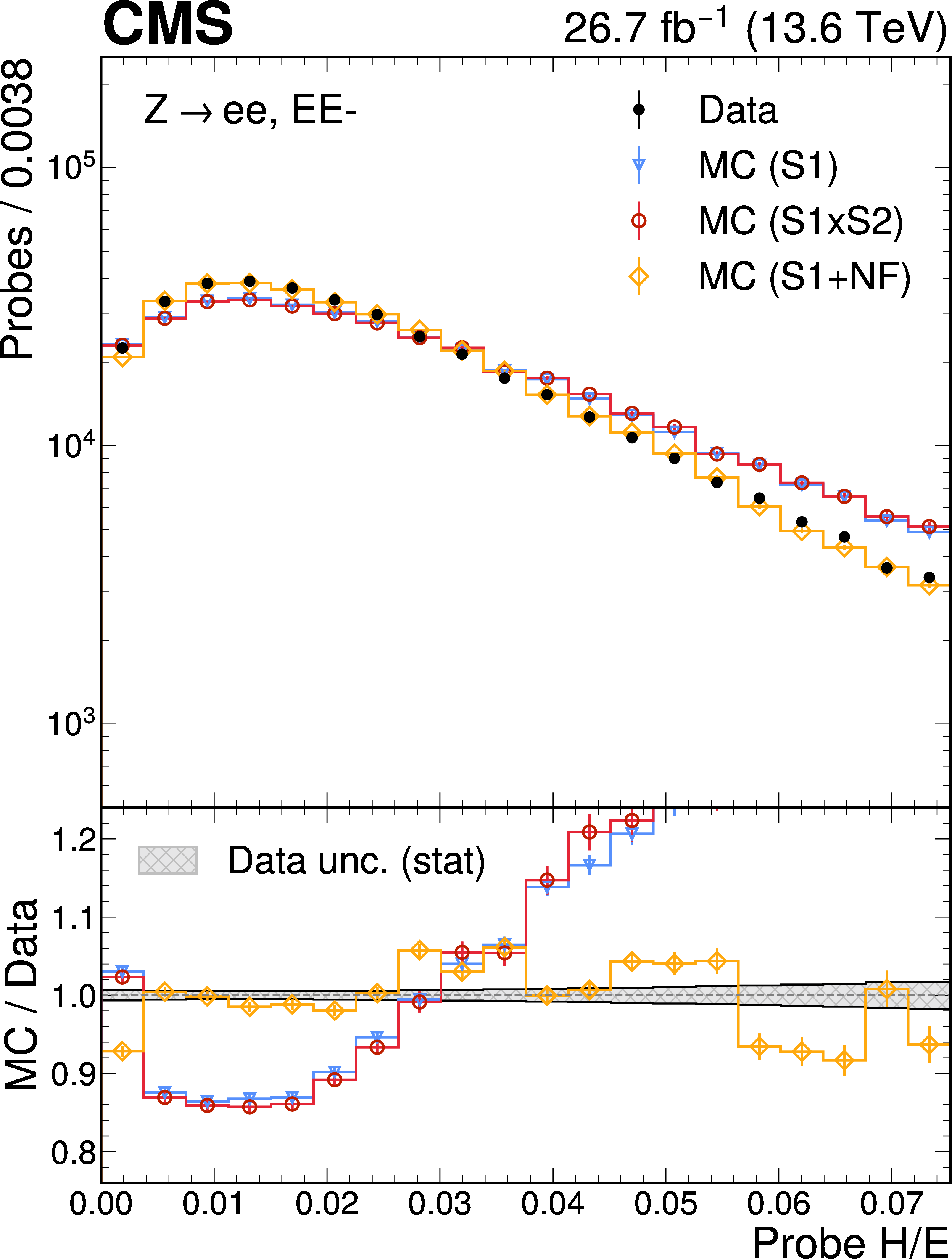
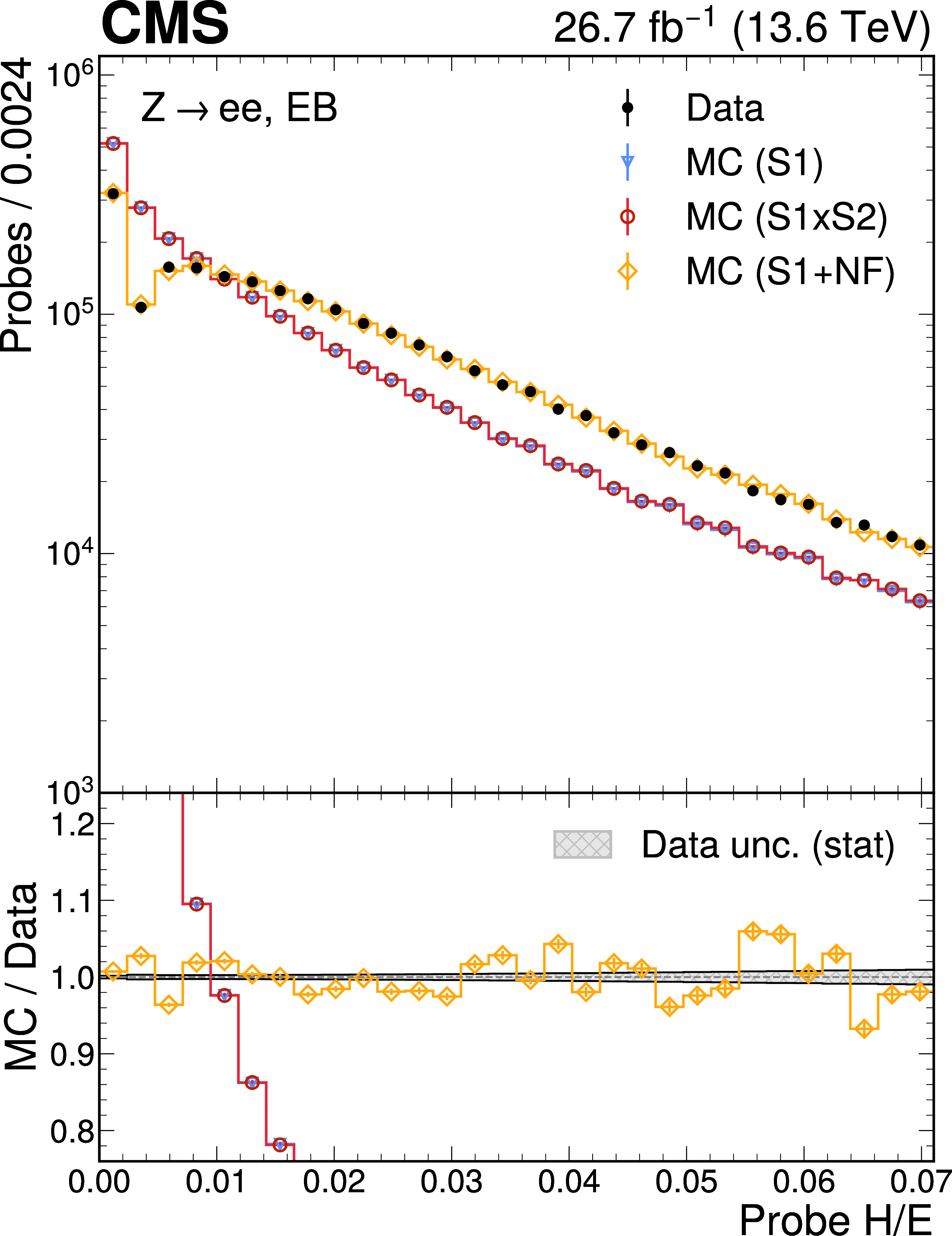
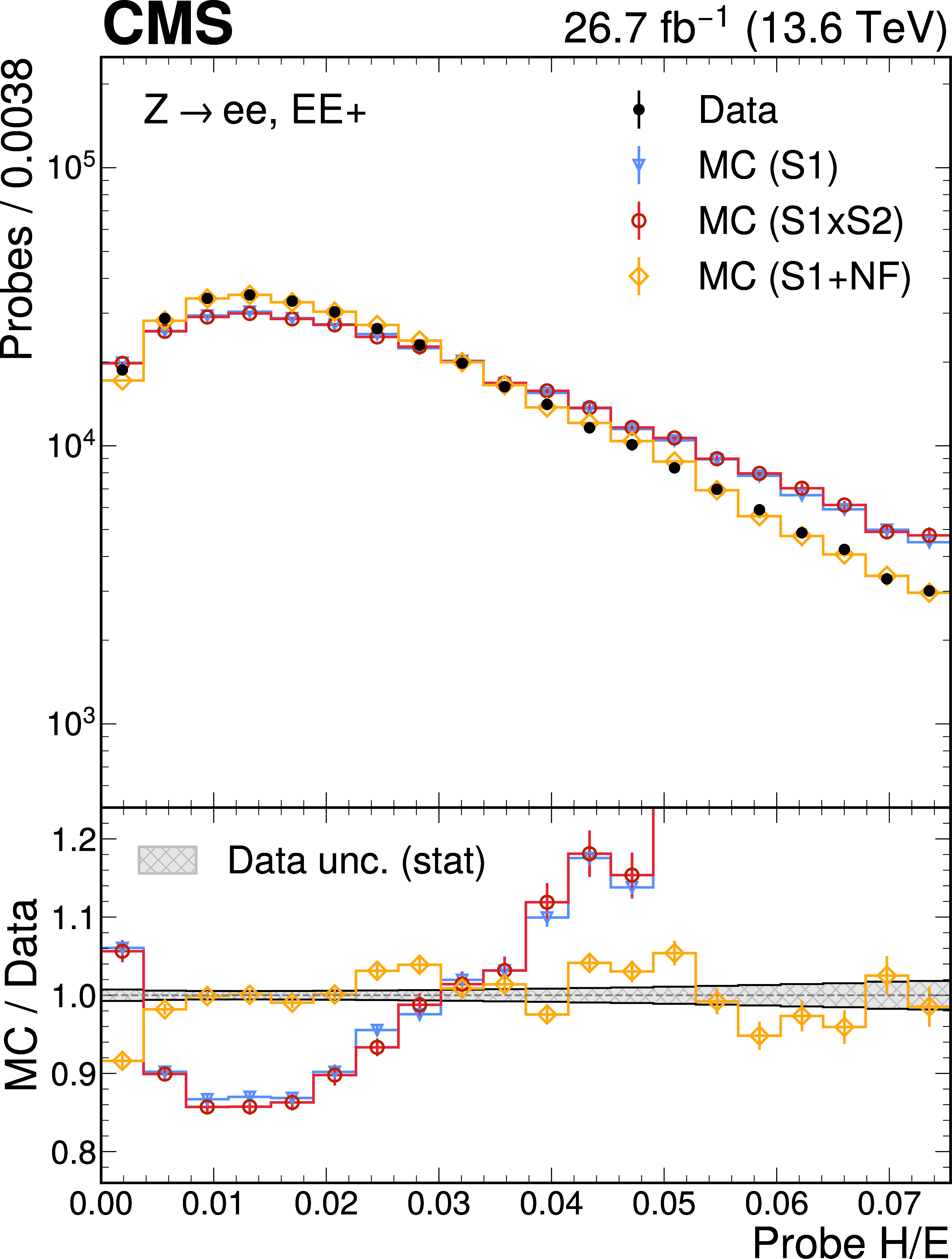
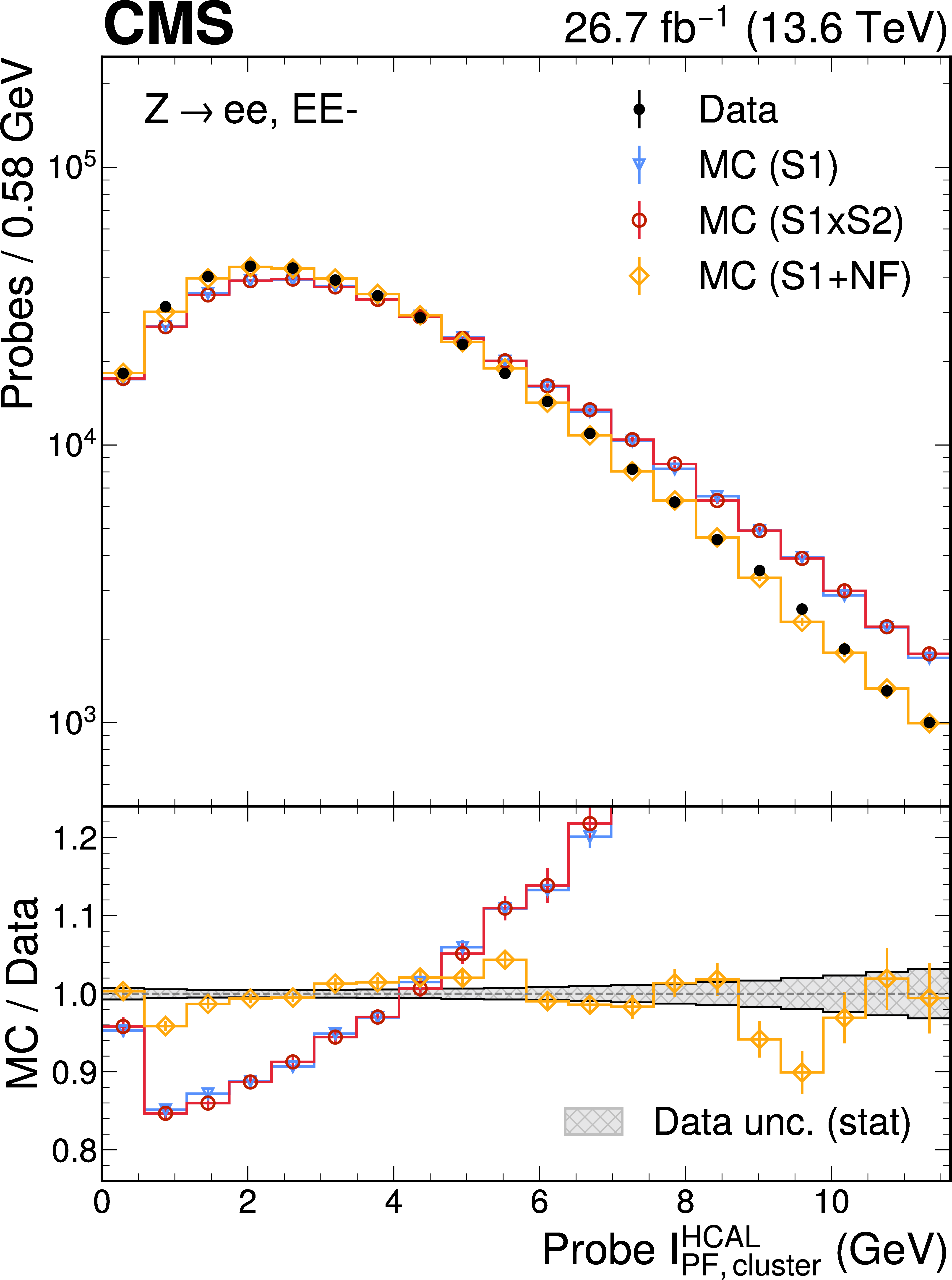
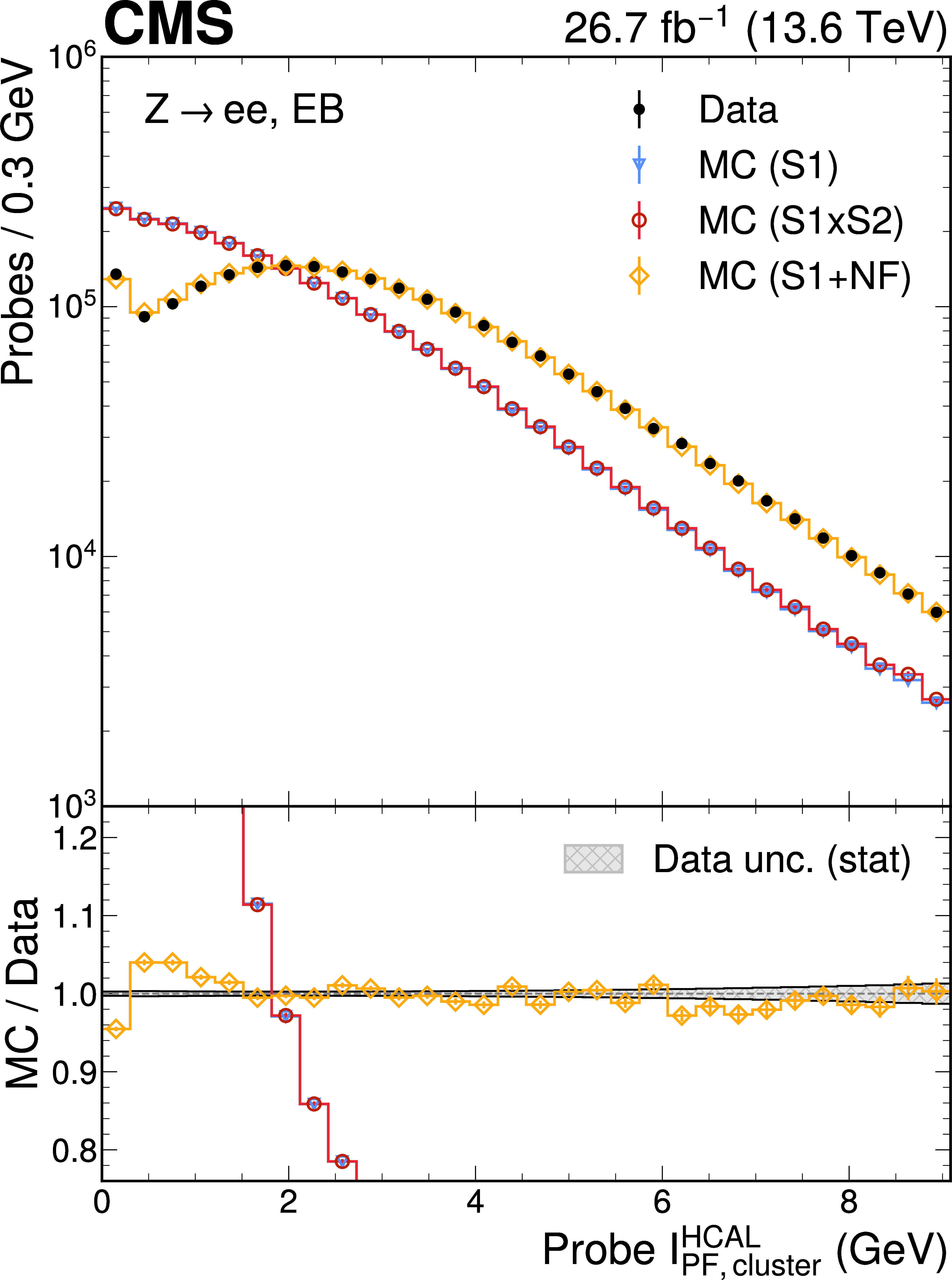
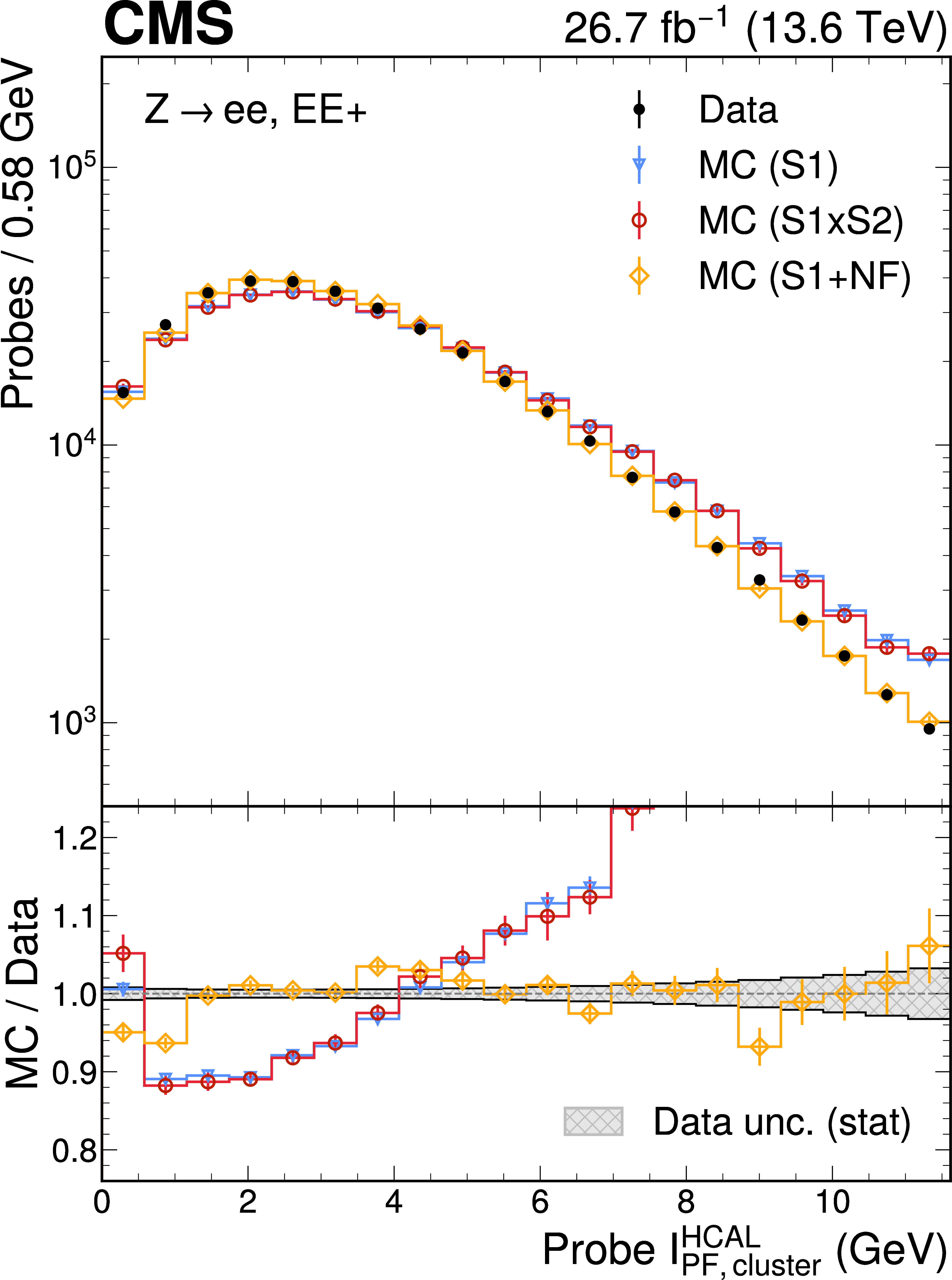
The probe $ \sigma_{i\eta i\phi} $ (upper row), H/E (middle row), and $ \mathcal{I}^{\mathrm{HCAL}}_{\text{PF, cluster}} $ (lower row) distributions in data and simulation, for the EE-(left), EB (centre), and EE$ + $ (right) subdetector regions. The plotting conventions are the same as in Fig. 10. The H/E and $ \mathcal{I}^{\mathrm{HCAL}}_{\text{PF, cluster}} $ features were not included in the S2 reweighting method training, and therefore the S2 reweighting has a negligible effect on the distributions. |
png pdf |
Figure 12-a:
The probe $ \sigma_{i\eta i\phi} $ (upper row), H/E (middle row), and $ \mathcal{I}^{\mathrm{HCAL}}_{\text{PF, cluster}} $ (lower row) distributions in data and simulation, for the EE-(left), EB (centre), and EE$ + $ (right) subdetector regions. The plotting conventions are the same as in Fig. 10. The H/E and $ \mathcal{I}^{\mathrm{HCAL}}_{\text{PF, cluster}} $ features were not included in the S2 reweighting method training, and therefore the S2 reweighting has a negligible effect on the distributions. |
png pdf |
Figure 12-b:
The probe $ \sigma_{i\eta i\phi} $ (upper row), H/E (middle row), and $ \mathcal{I}^{\mathrm{HCAL}}_{\text{PF, cluster}} $ (lower row) distributions in data and simulation, for the EE-(left), EB (centre), and EE$ + $ (right) subdetector regions. The plotting conventions are the same as in Fig. 10. The H/E and $ \mathcal{I}^{\mathrm{HCAL}}_{\text{PF, cluster}} $ features were not included in the S2 reweighting method training, and therefore the S2 reweighting has a negligible effect on the distributions. |
png pdf |
Figure 12-c:
The probe $ \sigma_{i\eta i\phi} $ (upper row), H/E (middle row), and $ \mathcal{I}^{\mathrm{HCAL}}_{\text{PF, cluster}} $ (lower row) distributions in data and simulation, for the EE-(left), EB (centre), and EE$ + $ (right) subdetector regions. The plotting conventions are the same as in Fig. 10. The H/E and $ \mathcal{I}^{\mathrm{HCAL}}_{\text{PF, cluster}} $ features were not included in the S2 reweighting method training, and therefore the S2 reweighting has a negligible effect on the distributions. |
png pdf |
Figure 12-d:
The probe $ \sigma_{i\eta i\phi} $ (upper row), H/E (middle row), and $ \mathcal{I}^{\mathrm{HCAL}}_{\text{PF, cluster}} $ (lower row) distributions in data and simulation, for the EE-(left), EB (centre), and EE$ + $ (right) subdetector regions. The plotting conventions are the same as in Fig. 10. The H/E and $ \mathcal{I}^{\mathrm{HCAL}}_{\text{PF, cluster}} $ features were not included in the S2 reweighting method training, and therefore the S2 reweighting has a negligible effect on the distributions. |
png pdf |
Figure 12-e:
The probe $ \sigma_{i\eta i\phi} $ (upper row), H/E (middle row), and $ \mathcal{I}^{\mathrm{HCAL}}_{\text{PF, cluster}} $ (lower row) distributions in data and simulation, for the EE-(left), EB (centre), and EE$ + $ (right) subdetector regions. The plotting conventions are the same as in Fig. 10. The H/E and $ \mathcal{I}^{\mathrm{HCAL}}_{\text{PF, cluster}} $ features were not included in the S2 reweighting method training, and therefore the S2 reweighting has a negligible effect on the distributions. |
png pdf |
Figure 12-f:
The probe $ \sigma_{i\eta i\phi} $ (upper row), H/E (middle row), and $ \mathcal{I}^{\mathrm{HCAL}}_{\text{PF, cluster}} $ (lower row) distributions in data and simulation, for the EE-(left), EB (centre), and EE$ + $ (right) subdetector regions. The plotting conventions are the same as in Fig. 10. The H/E and $ \mathcal{I}^{\mathrm{HCAL}}_{\text{PF, cluster}} $ features were not included in the S2 reweighting method training, and therefore the S2 reweighting has a negligible effect on the distributions. |
png pdf |
Figure 12-g:
The probe $ \sigma_{i\eta i\phi} $ (upper row), H/E (middle row), and $ \mathcal{I}^{\mathrm{HCAL}}_{\text{PF, cluster}} $ (lower row) distributions in data and simulation, for the EE-(left), EB (centre), and EE$ + $ (right) subdetector regions. The plotting conventions are the same as in Fig. 10. The H/E and $ \mathcal{I}^{\mathrm{HCAL}}_{\text{PF, cluster}} $ features were not included in the S2 reweighting method training, and therefore the S2 reweighting has a negligible effect on the distributions. |
png pdf |
Figure 12-h:
The probe $ \sigma_{i\eta i\phi} $ (upper row), H/E (middle row), and $ \mathcal{I}^{\mathrm{HCAL}}_{\text{PF, cluster}} $ (lower row) distributions in data and simulation, for the EE-(left), EB (centre), and EE$ + $ (right) subdetector regions. The plotting conventions are the same as in Fig. 10. The H/E and $ \mathcal{I}^{\mathrm{HCAL}}_{\text{PF, cluster}} $ features were not included in the S2 reweighting method training, and therefore the S2 reweighting has a negligible effect on the distributions. |
png pdf |
Figure 12-i:
The probe $ \sigma_{i\eta i\phi} $ (upper row), H/E (middle row), and $ \mathcal{I}^{\mathrm{HCAL}}_{\text{PF, cluster}} $ (lower row) distributions in data and simulation, for the EE-(left), EB (centre), and EE$ + $ (right) subdetector regions. The plotting conventions are the same as in Fig. 10. The H/E and $ \mathcal{I}^{\mathrm{HCAL}}_{\text{PF, cluster}} $ features were not included in the S2 reweighting method training, and therefore the S2 reweighting has a negligible effect on the distributions. |
png pdf |
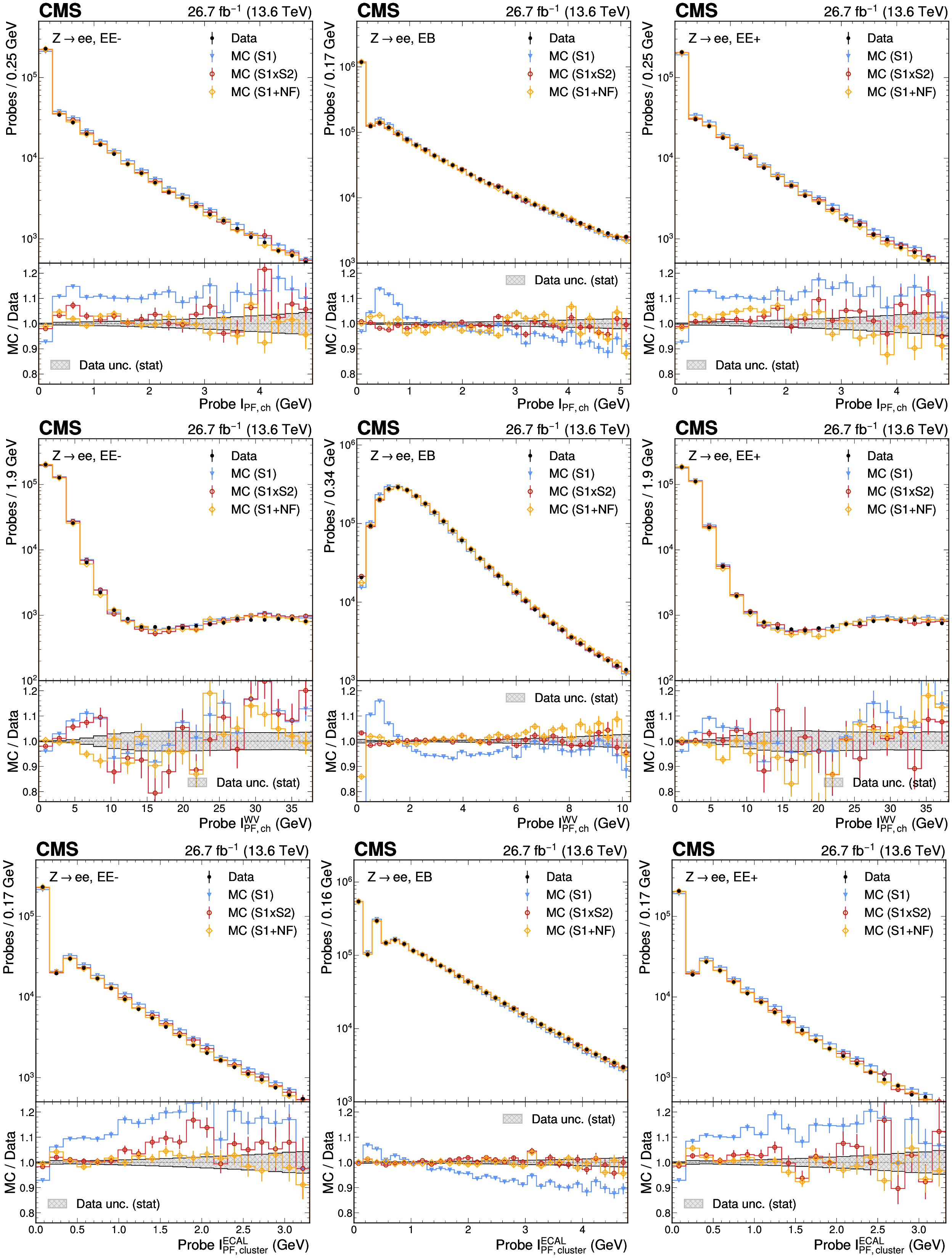
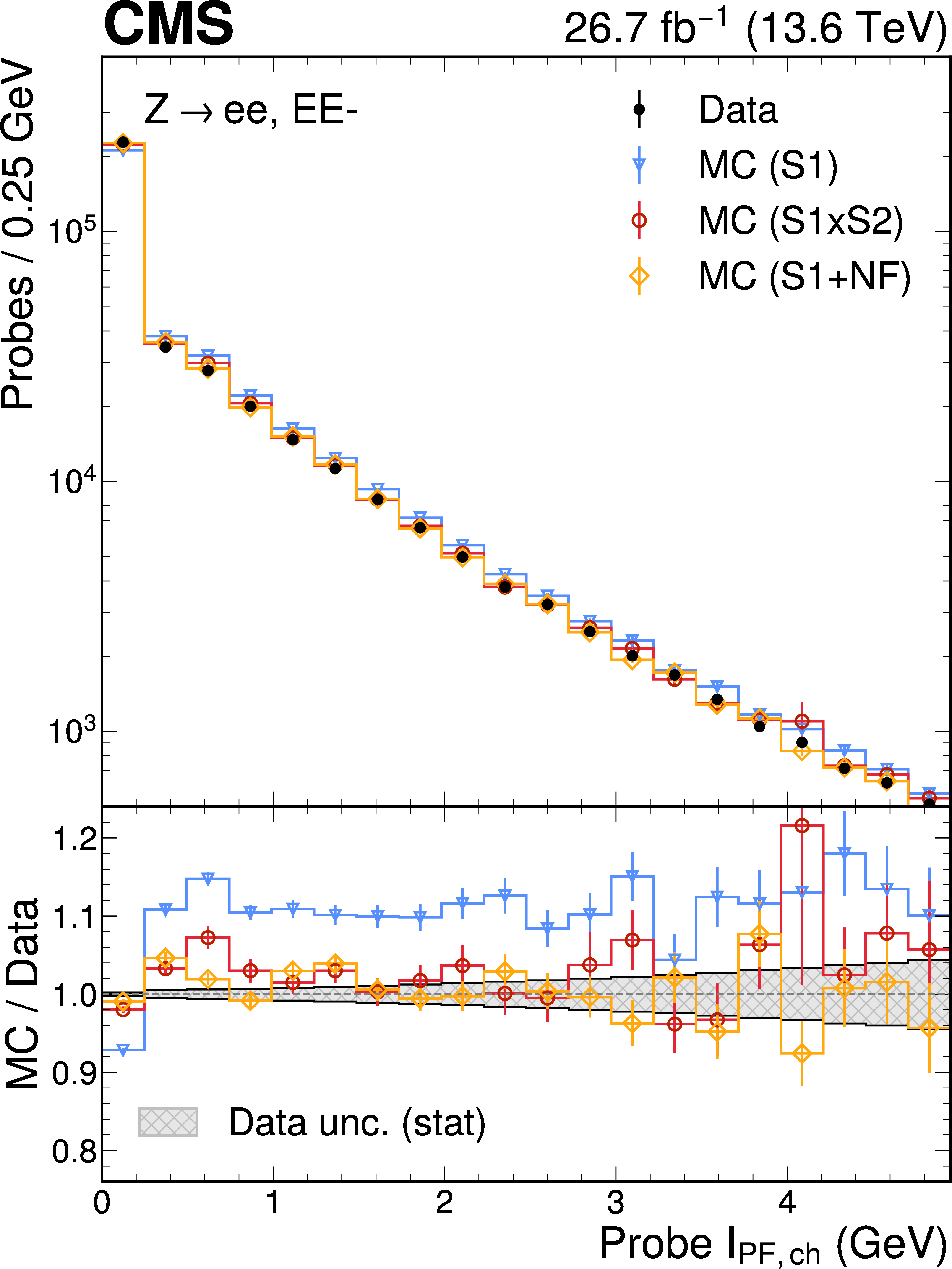
Figure 13:
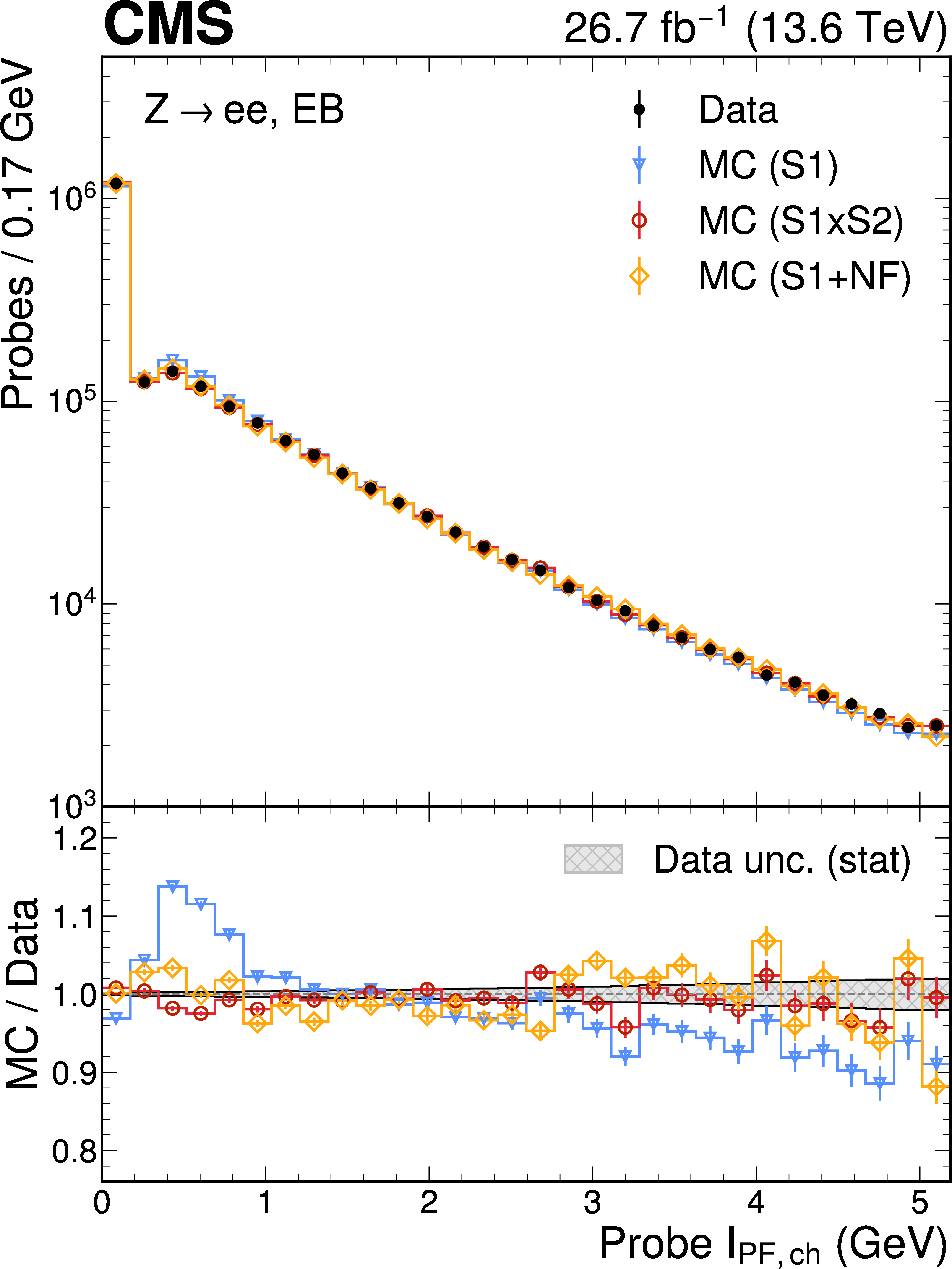
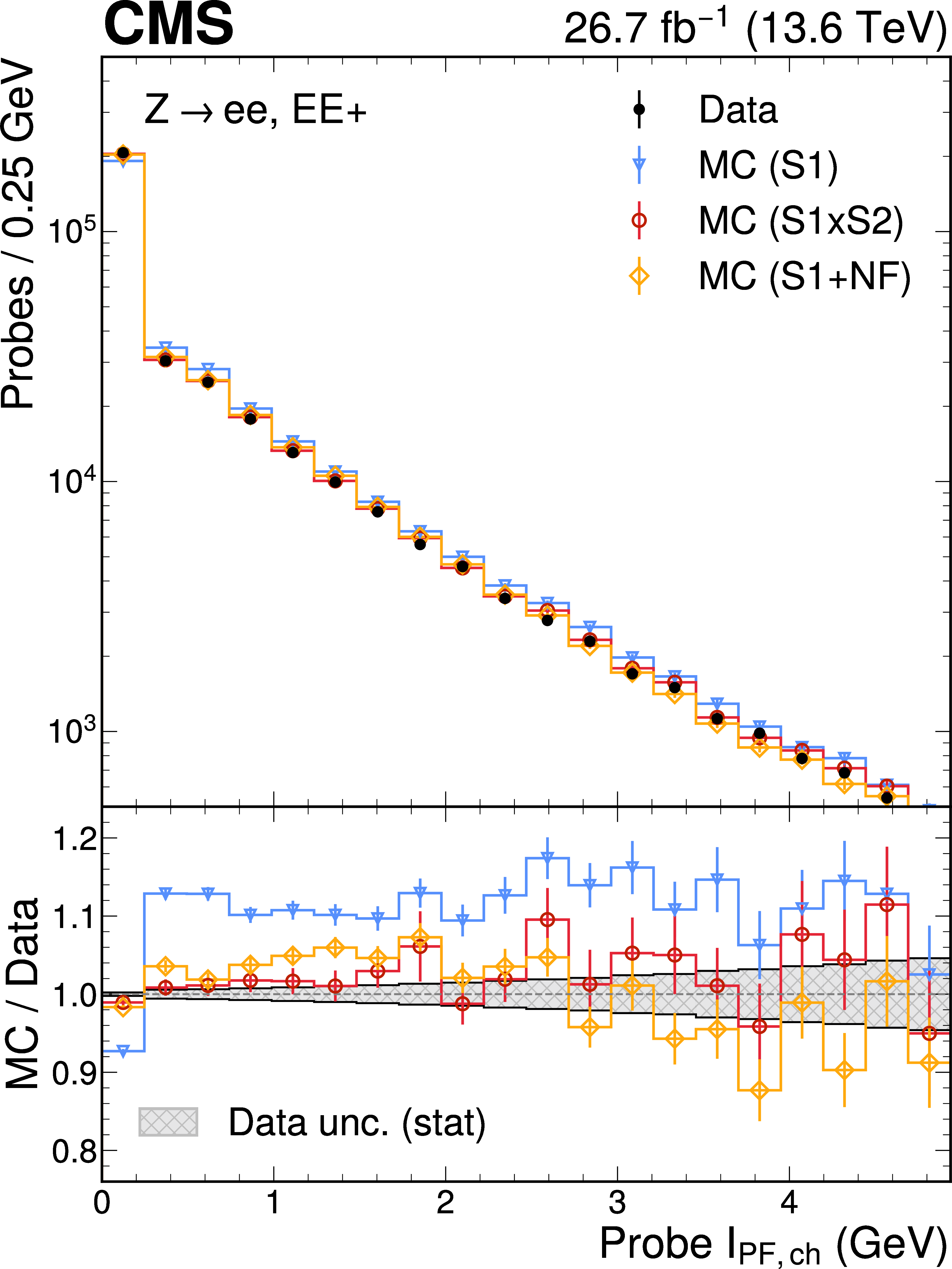
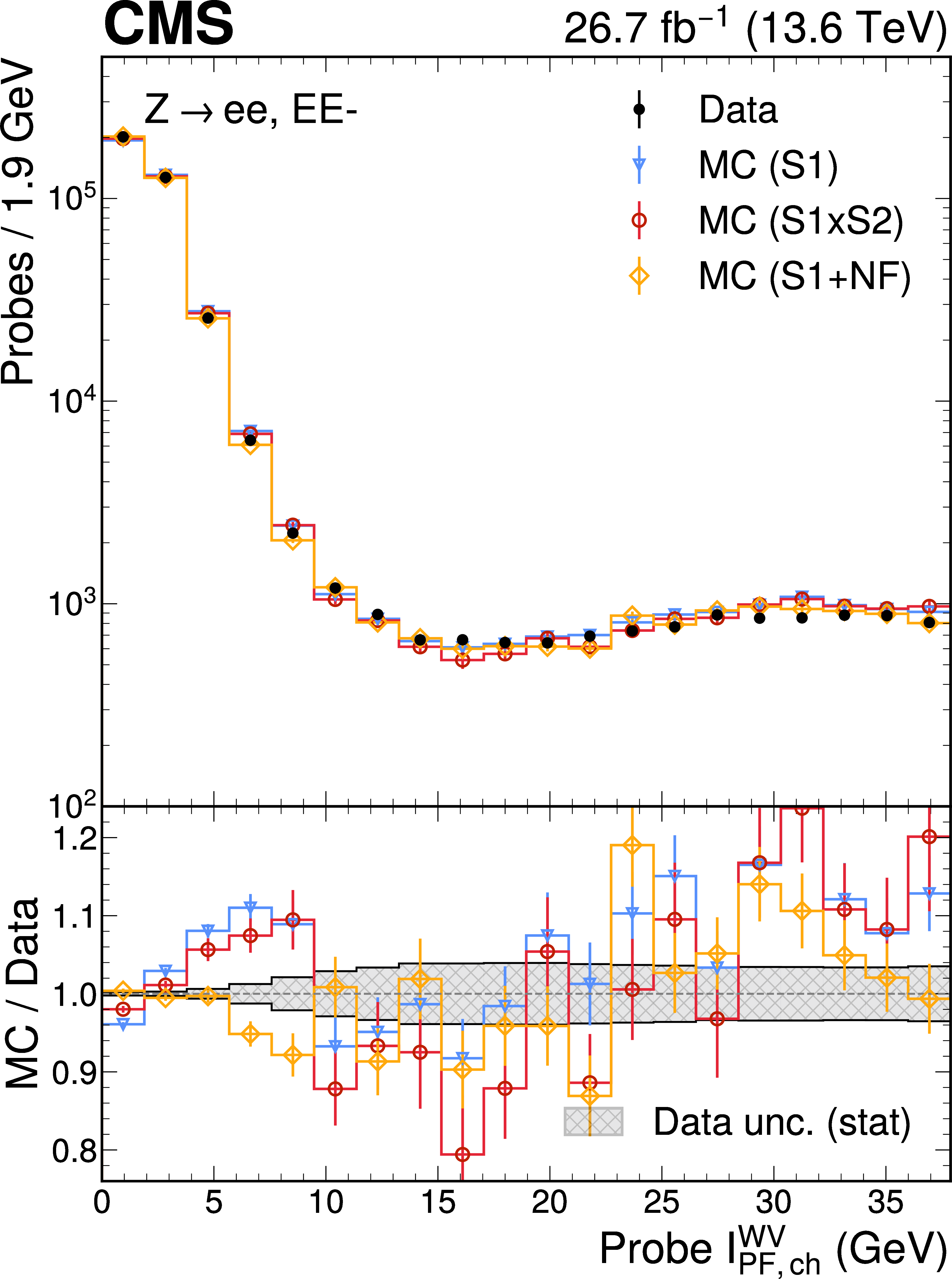
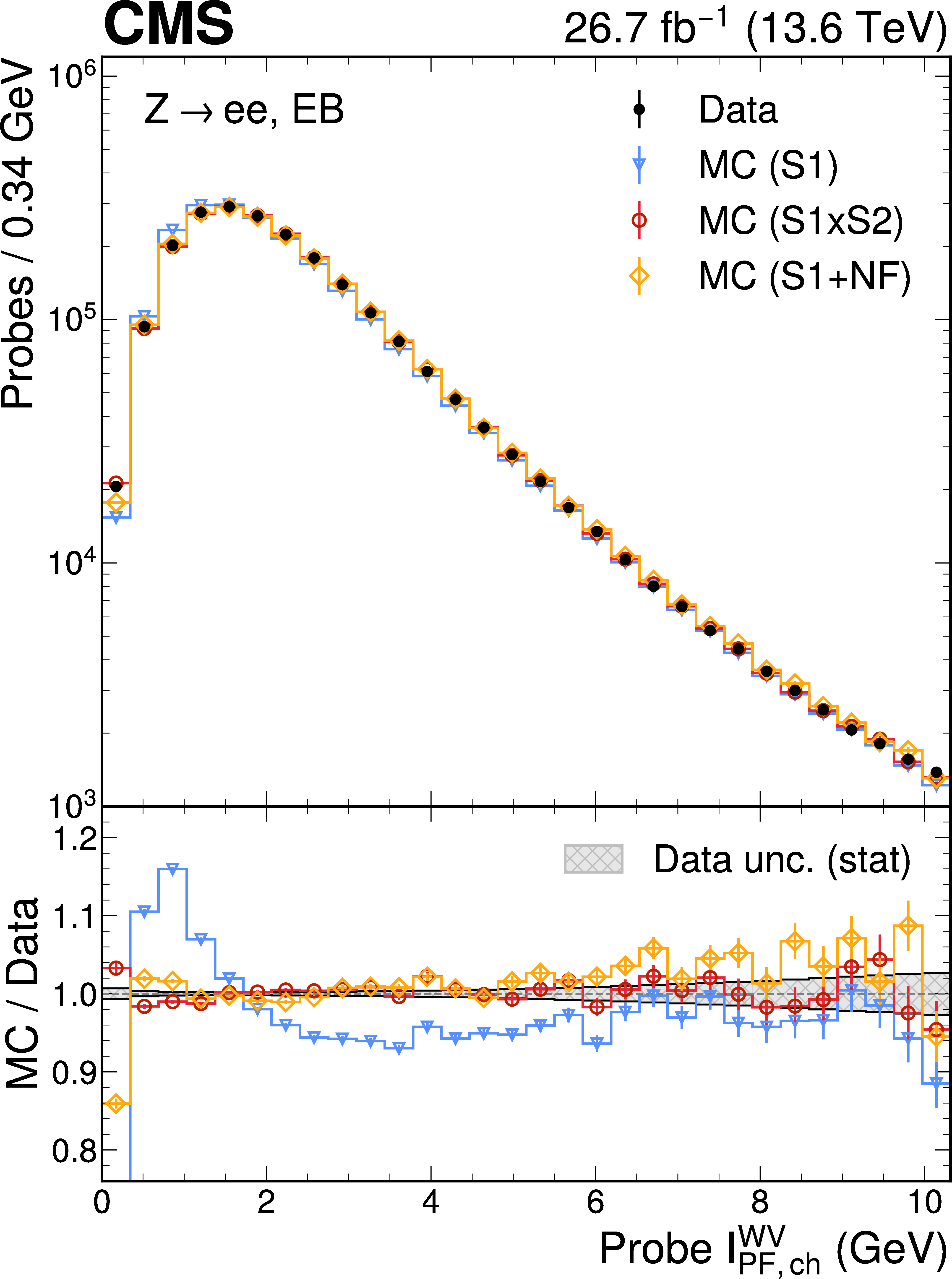
The probe $ \mathcal{I}_{\mathrm{PF,ch}} $ (upper row), $ \mathcal{I}^{\mathrm{WV}}_{\mathrm{PF,ch}} $ (middle row), and $ \mathcal{I}^{\mathrm{ECAL}}_{\text{PF, cluster}} $ (lower row) distributions in data and simulation, for the EE-(left), EB (centre), and EE$ + $ (right) subdetector regions. The plotting conventions are the same as in Fig. 10. |
png pdf |
Figure 13-a:
The probe $ \mathcal{I}_{\mathrm{PF,ch}} $ (upper row), $ \mathcal{I}^{\mathrm{WV}}_{\mathrm{PF,ch}} $ (middle row), and $ \mathcal{I}^{\mathrm{ECAL}}_{\text{PF, cluster}} $ (lower row) distributions in data and simulation, for the EE-(left), EB (centre), and EE$ + $ (right) subdetector regions. The plotting conventions are the same as in Fig. 10. |
png pdf |
Figure 13-b:
The probe $ \mathcal{I}_{\mathrm{PF,ch}} $ (upper row), $ \mathcal{I}^{\mathrm{WV}}_{\mathrm{PF,ch}} $ (middle row), and $ \mathcal{I}^{\mathrm{ECAL}}_{\text{PF, cluster}} $ (lower row) distributions in data and simulation, for the EE-(left), EB (centre), and EE$ + $ (right) subdetector regions. The plotting conventions are the same as in Fig. 10. |
png pdf |
Figure 13-c:
The probe $ \mathcal{I}_{\mathrm{PF,ch}} $ (upper row), $ \mathcal{I}^{\mathrm{WV}}_{\mathrm{PF,ch}} $ (middle row), and $ \mathcal{I}^{\mathrm{ECAL}}_{\text{PF, cluster}} $ (lower row) distributions in data and simulation, for the EE-(left), EB (centre), and EE$ + $ (right) subdetector regions. The plotting conventions are the same as in Fig. 10. |
png pdf |
Figure 13-d:
The probe $ \mathcal{I}_{\mathrm{PF,ch}} $ (upper row), $ \mathcal{I}^{\mathrm{WV}}_{\mathrm{PF,ch}} $ (middle row), and $ \mathcal{I}^{\mathrm{ECAL}}_{\text{PF, cluster}} $ (lower row) distributions in data and simulation, for the EE-(left), EB (centre), and EE$ + $ (right) subdetector regions. The plotting conventions are the same as in Fig. 10. |
png pdf |
Figure 13-e:
The probe $ \mathcal{I}_{\mathrm{PF,ch}} $ (upper row), $ \mathcal{I}^{\mathrm{WV}}_{\mathrm{PF,ch}} $ (middle row), and $ \mathcal{I}^{\mathrm{ECAL}}_{\text{PF, cluster}} $ (lower row) distributions in data and simulation, for the EE-(left), EB (centre), and EE$ + $ (right) subdetector regions. The plotting conventions are the same as in Fig. 10. |
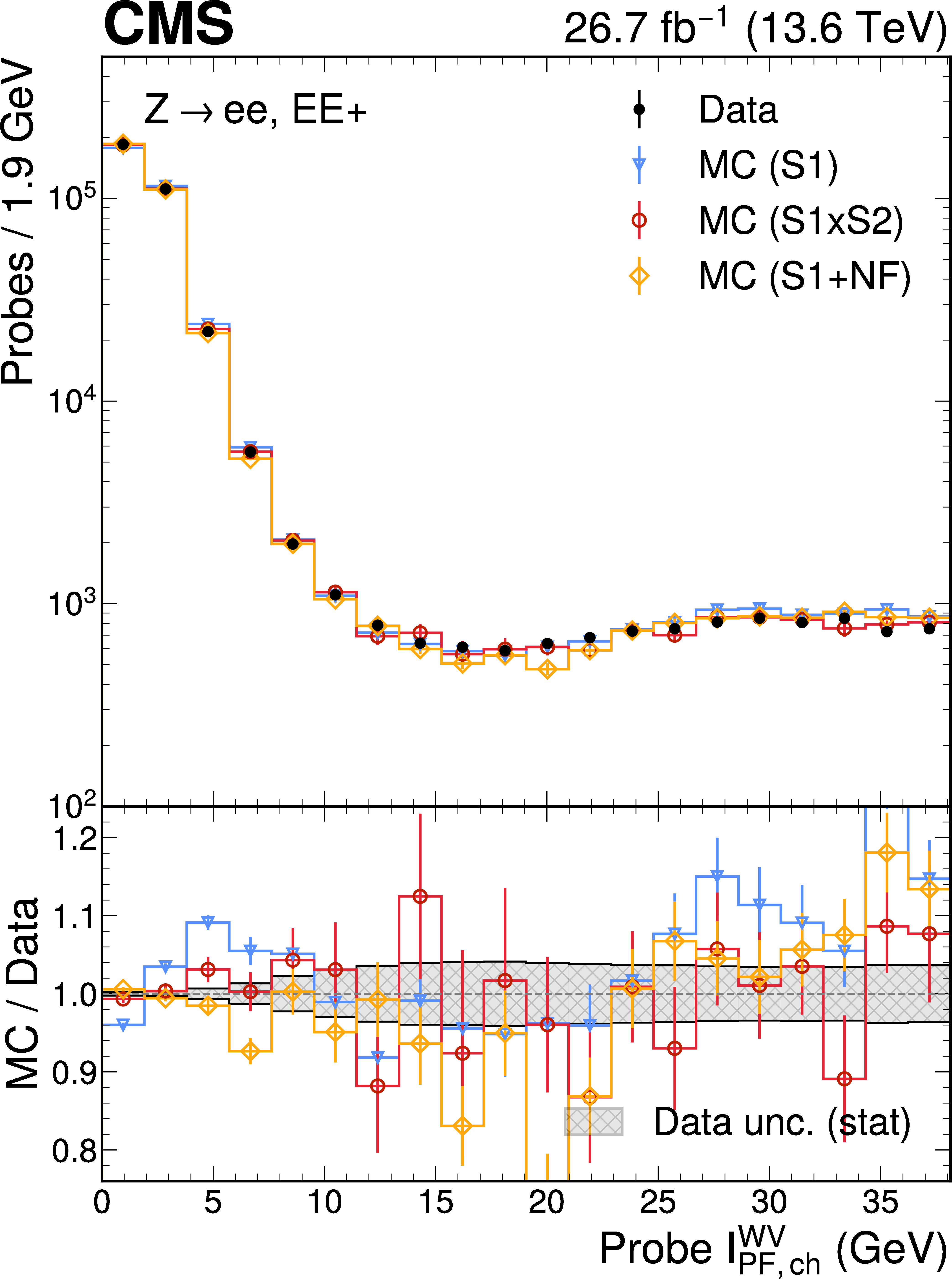
png pdf |
Figure 13-f:
The probe $ \mathcal{I}_{\mathrm{PF,ch}} $ (upper row), $ \mathcal{I}^{\mathrm{WV}}_{\mathrm{PF,ch}} $ (middle row), and $ \mathcal{I}^{\mathrm{ECAL}}_{\text{PF, cluster}} $ (lower row) distributions in data and simulation, for the EE-(left), EB (centre), and EE$ + $ (right) subdetector regions. The plotting conventions are the same as in Fig. 10. |
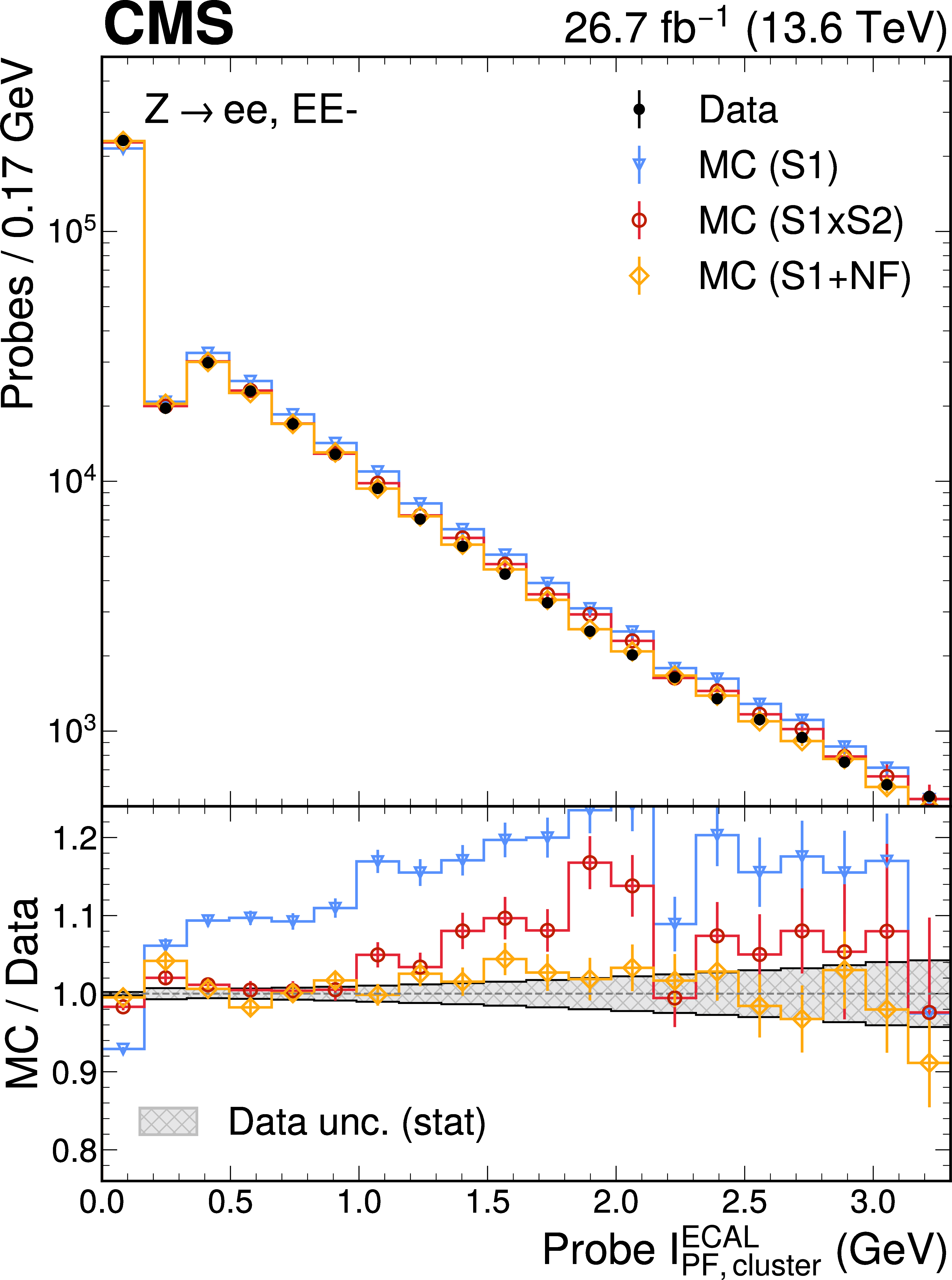
png pdf |
Figure 13-g:
The probe $ \mathcal{I}_{\mathrm{PF,ch}} $ (upper row), $ \mathcal{I}^{\mathrm{WV}}_{\mathrm{PF,ch}} $ (middle row), and $ \mathcal{I}^{\mathrm{ECAL}}_{\text{PF, cluster}} $ (lower row) distributions in data and simulation, for the EE-(left), EB (centre), and EE$ + $ (right) subdetector regions. The plotting conventions are the same as in Fig. 10. |
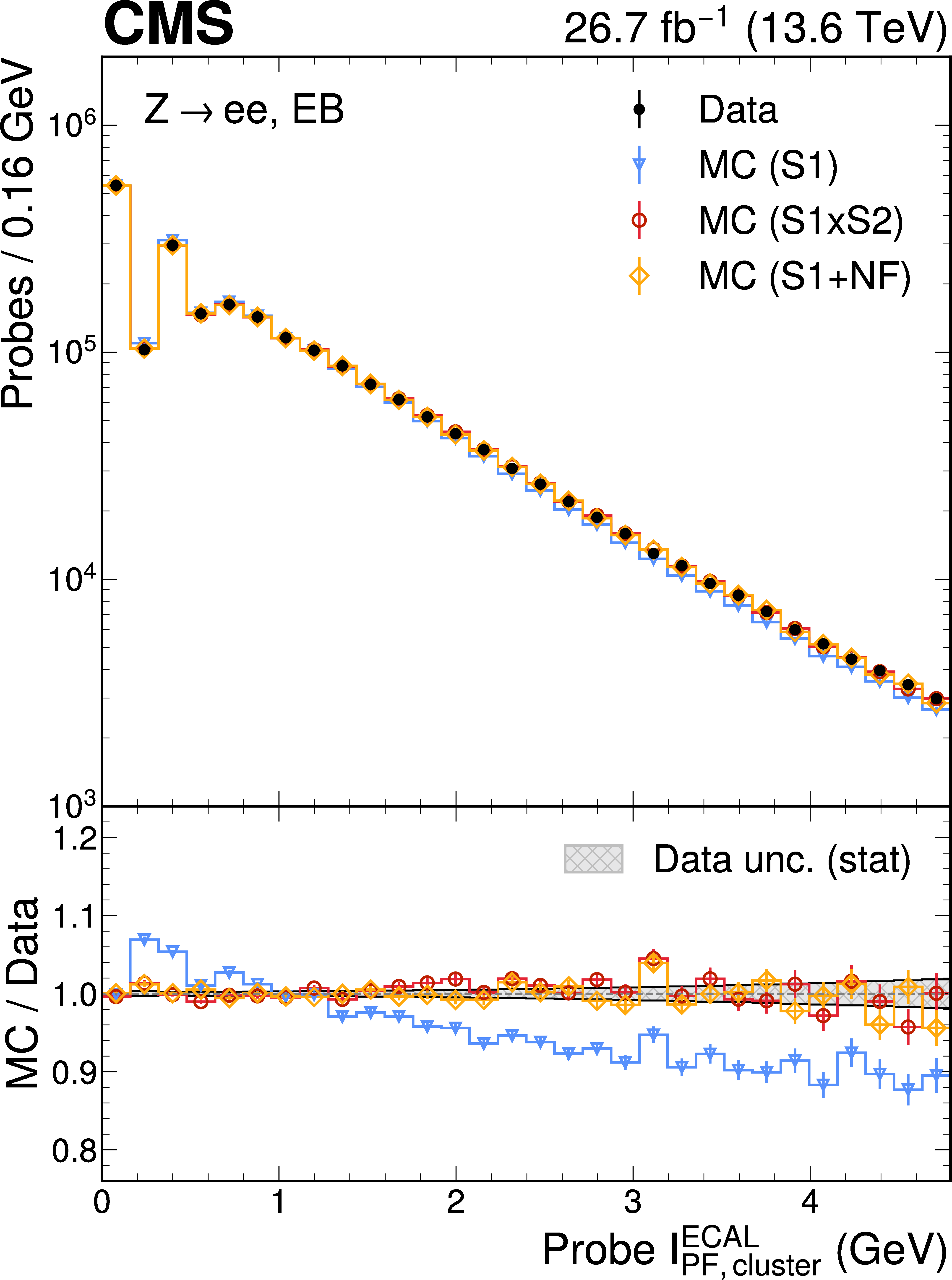
png pdf |
Figure 13-h:
The probe $ \mathcal{I}_{\mathrm{PF,ch}} $ (upper row), $ \mathcal{I}^{\mathrm{WV}}_{\mathrm{PF,ch}} $ (middle row), and $ \mathcal{I}^{\mathrm{ECAL}}_{\text{PF, cluster}} $ (lower row) distributions in data and simulation, for the EE-(left), EB (centre), and EE$ + $ (right) subdetector regions. The plotting conventions are the same as in Fig. 10. |
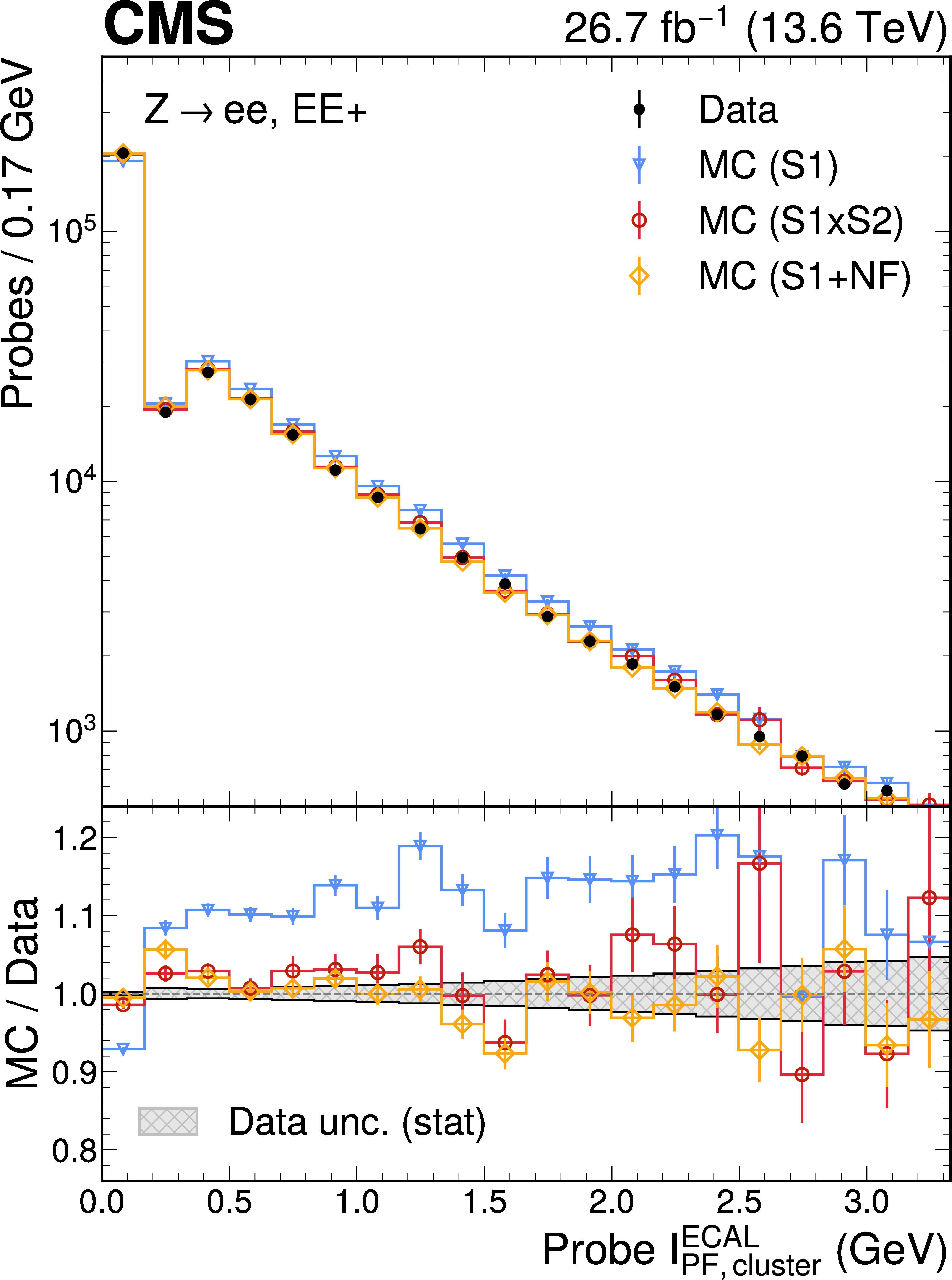
png pdf |
Figure 13-i:
The probe $ \mathcal{I}_{\mathrm{PF,ch}} $ (upper row), $ \mathcal{I}^{\mathrm{WV}}_{\mathrm{PF,ch}} $ (middle row), and $ \mathcal{I}^{\mathrm{ECAL}}_{\text{PF, cluster}} $ (lower row) distributions in data and simulation, for the EE-(left), EB (centre), and EE$ + $ (right) subdetector regions. The plotting conventions are the same as in Fig. 10. |
png pdf |
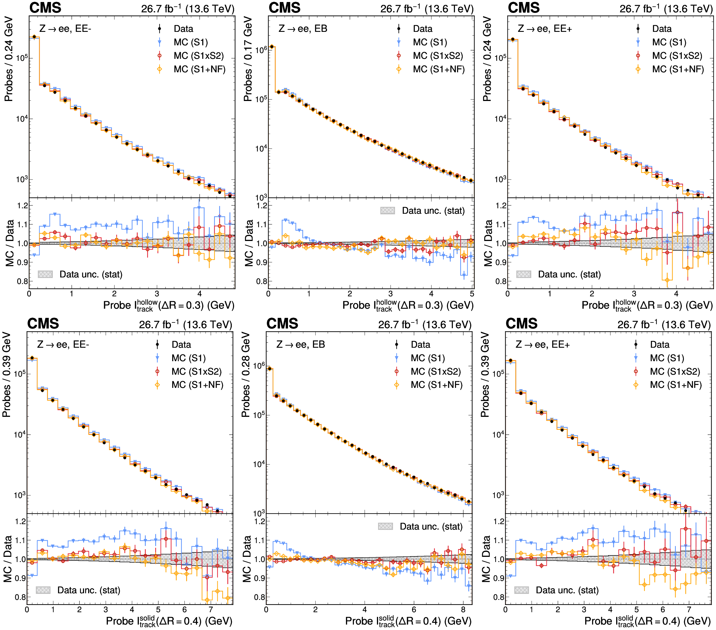
Figure 14:
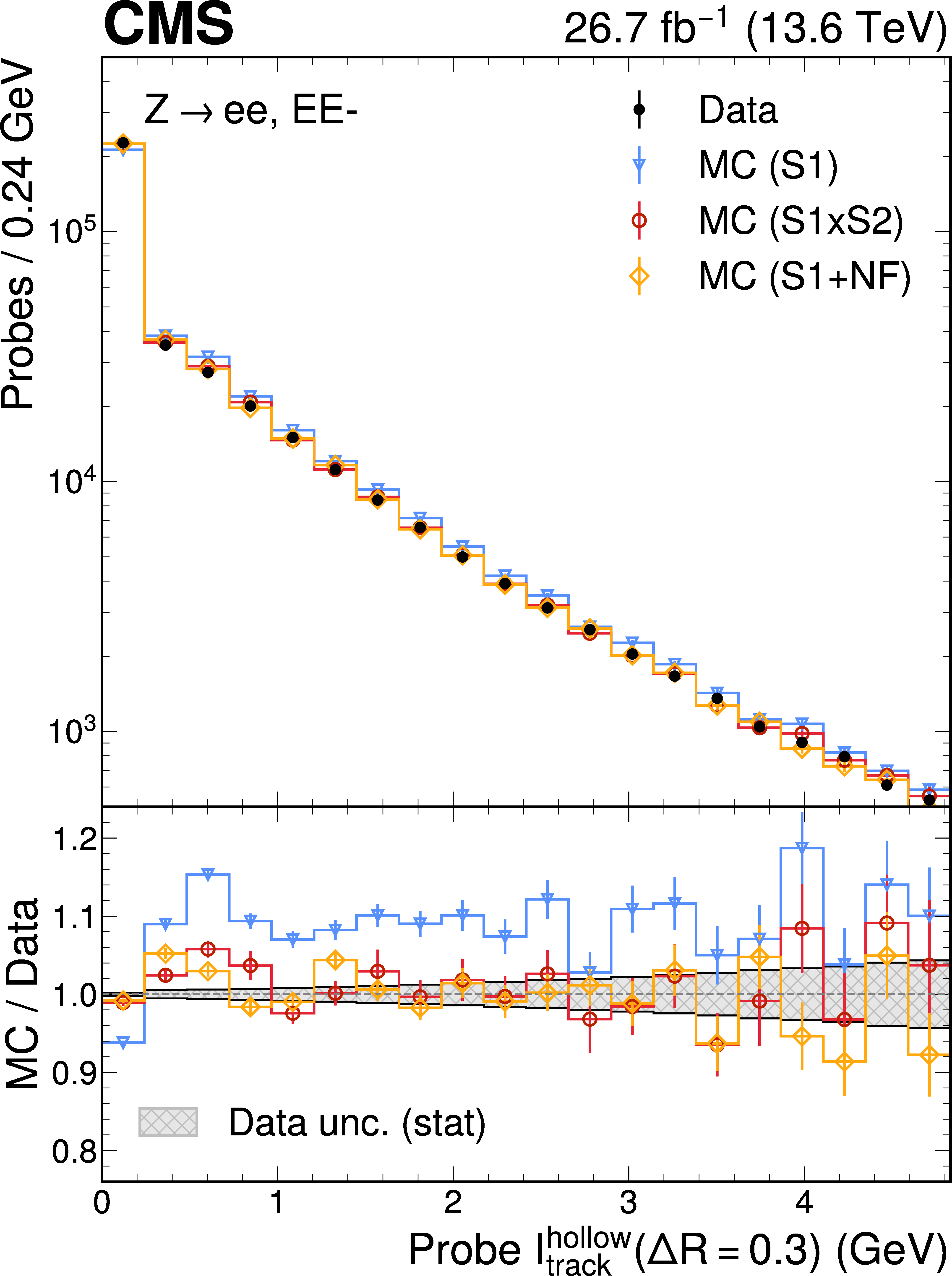
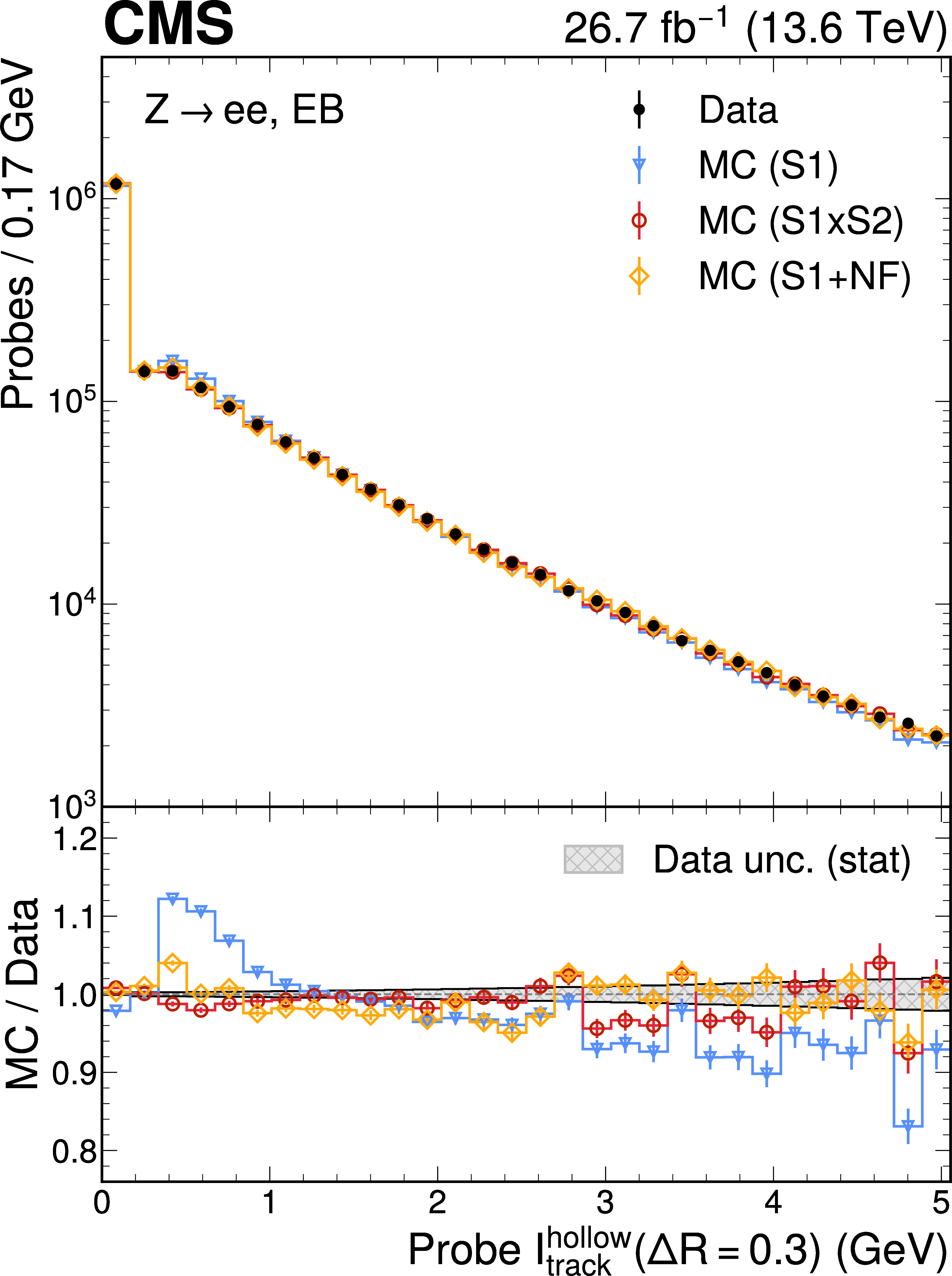
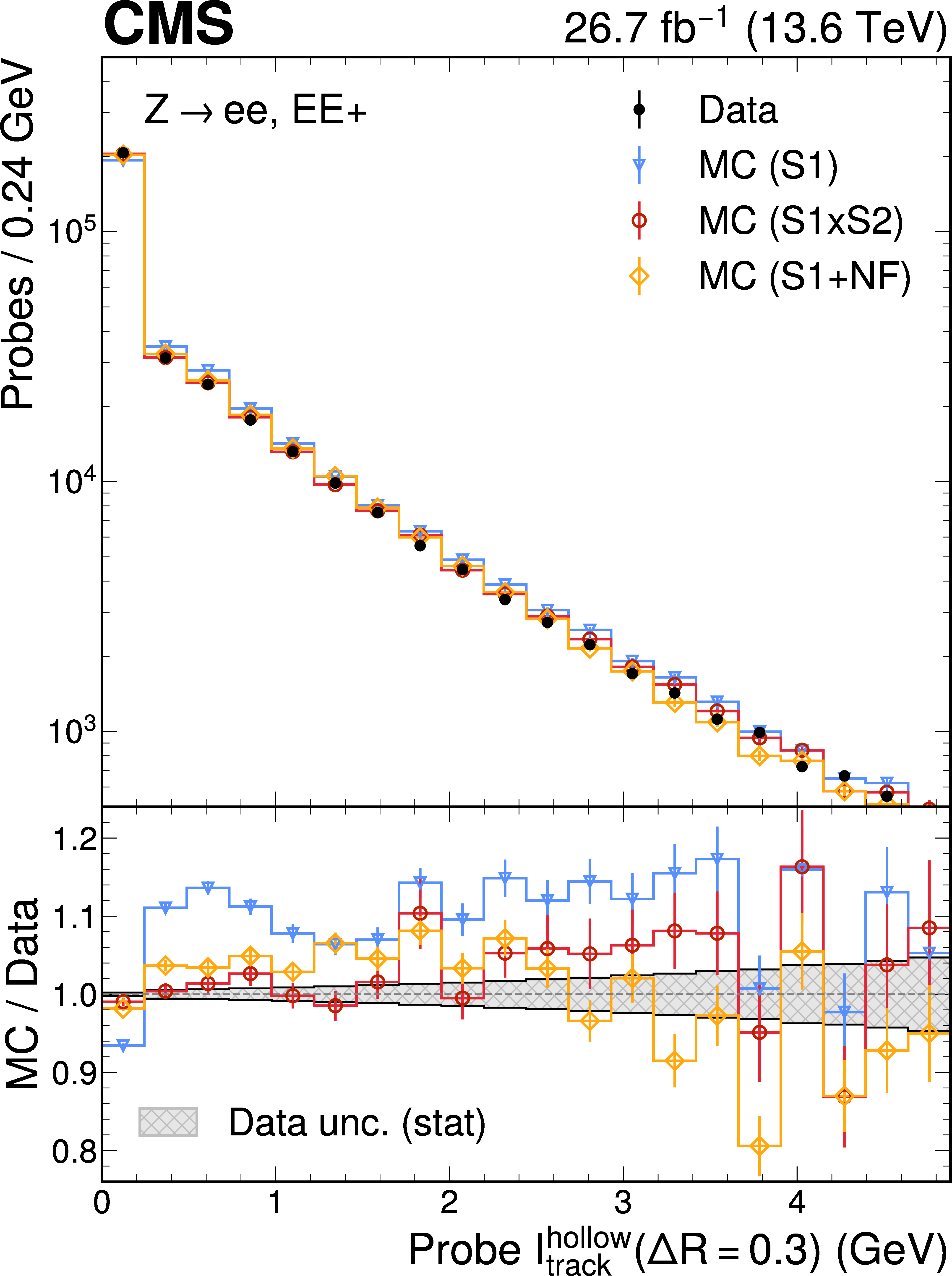
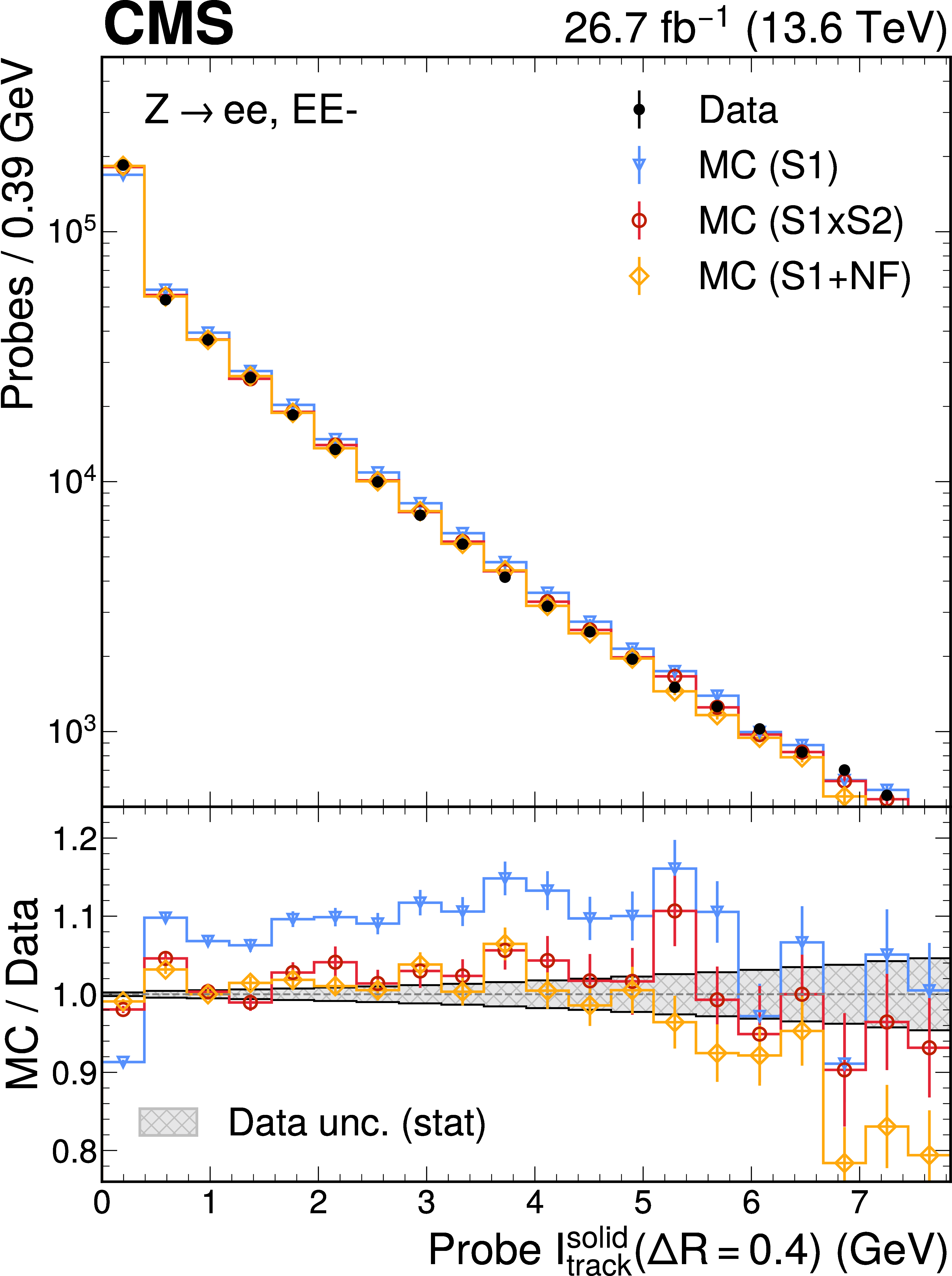
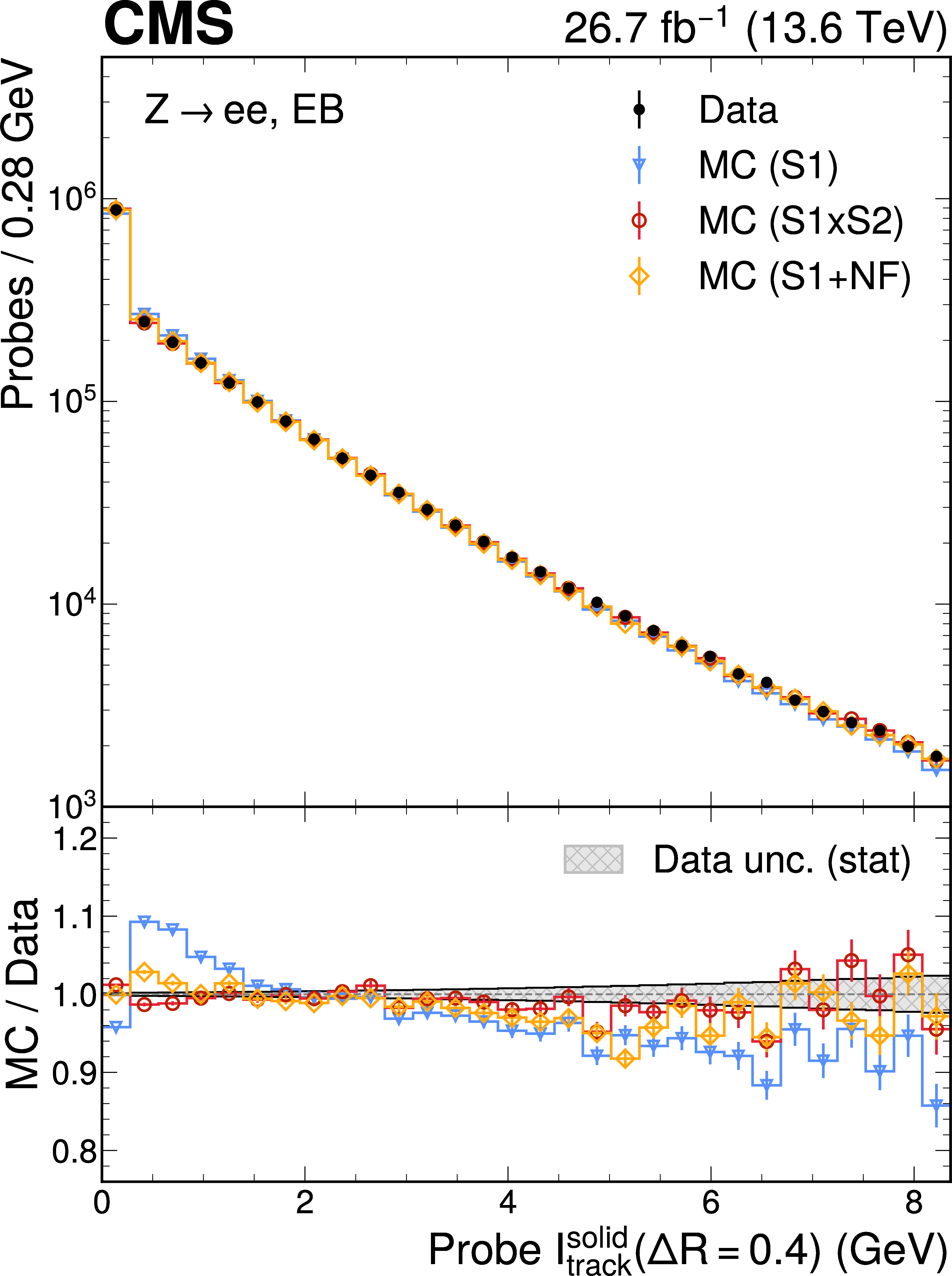
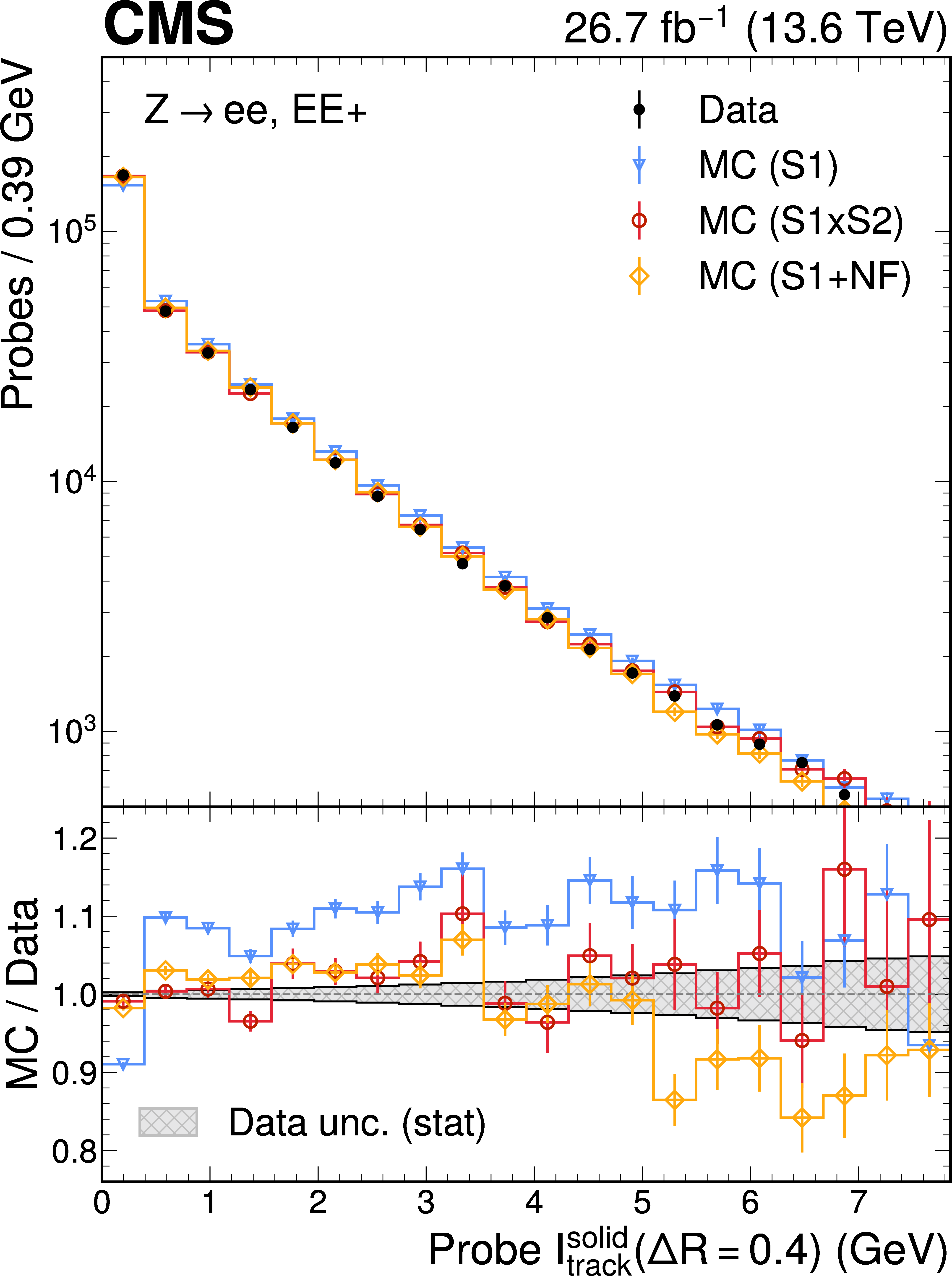
The probe $ \mathcal{I}^{\text{hollow}}_{\text{track}}(\Delta R = 0.3) $ (upper row) and $ \mathcal{I}^{\text{solid}}_{\text{track}}(\Delta R = 0.4) $ (lower row) distributions in data and simulation, for the EE-(left), EB (centre), and EE$ + $ (right) subdetector regions. The plotting conventions are the same as in Fig. 10. |
png pdf |
Figure 14-a:
The probe $ \mathcal{I}^{\text{hollow}}_{\text{track}}(\Delta R = 0.3) $ (upper row) and $ \mathcal{I}^{\text{solid}}_{\text{track}}(\Delta R = 0.4) $ (lower row) distributions in data and simulation, for the EE-(left), EB (centre), and EE$ + $ (right) subdetector regions. The plotting conventions are the same as in Fig. 10. |
png pdf |
Figure 14-b:
The probe $ \mathcal{I}^{\text{hollow}}_{\text{track}}(\Delta R = 0.3) $ (upper row) and $ \mathcal{I}^{\text{solid}}_{\text{track}}(\Delta R = 0.4) $ (lower row) distributions in data and simulation, for the EE-(left), EB (centre), and EE$ + $ (right) subdetector regions. The plotting conventions are the same as in Fig. 10. |
png pdf |
Figure 14-c:
The probe $ \mathcal{I}^{\text{hollow}}_{\text{track}}(\Delta R = 0.3) $ (upper row) and $ \mathcal{I}^{\text{solid}}_{\text{track}}(\Delta R = 0.4) $ (lower row) distributions in data and simulation, for the EE-(left), EB (centre), and EE$ + $ (right) subdetector regions. The plotting conventions are the same as in Fig. 10. |
png pdf |
Figure 14-d:
The probe $ \mathcal{I}^{\text{hollow}}_{\text{track}}(\Delta R = 0.3) $ (upper row) and $ \mathcal{I}^{\text{solid}}_{\text{track}}(\Delta R = 0.4) $ (lower row) distributions in data and simulation, for the EE-(left), EB (centre), and EE$ + $ (right) subdetector regions. The plotting conventions are the same as in Fig. 10. |
png pdf |
Figure 14-e:
The probe $ \mathcal{I}^{\text{hollow}}_{\text{track}}(\Delta R = 0.3) $ (upper row) and $ \mathcal{I}^{\text{solid}}_{\text{track}}(\Delta R = 0.4) $ (lower row) distributions in data and simulation, for the EE-(left), EB (centre), and EE$ + $ (right) subdetector regions. The plotting conventions are the same as in Fig. 10. |
png pdf |
Figure 14-f:
The probe $ \mathcal{I}^{\text{hollow}}_{\text{track}}(\Delta R = 0.3) $ (upper row) and $ \mathcal{I}^{\text{solid}}_{\text{track}}(\Delta R = 0.4) $ (lower row) distributions in data and simulation, for the EE-(left), EB (centre), and EE$ + $ (right) subdetector regions. The plotting conventions are the same as in Fig. 10. |
png pdf |
Figure 15:
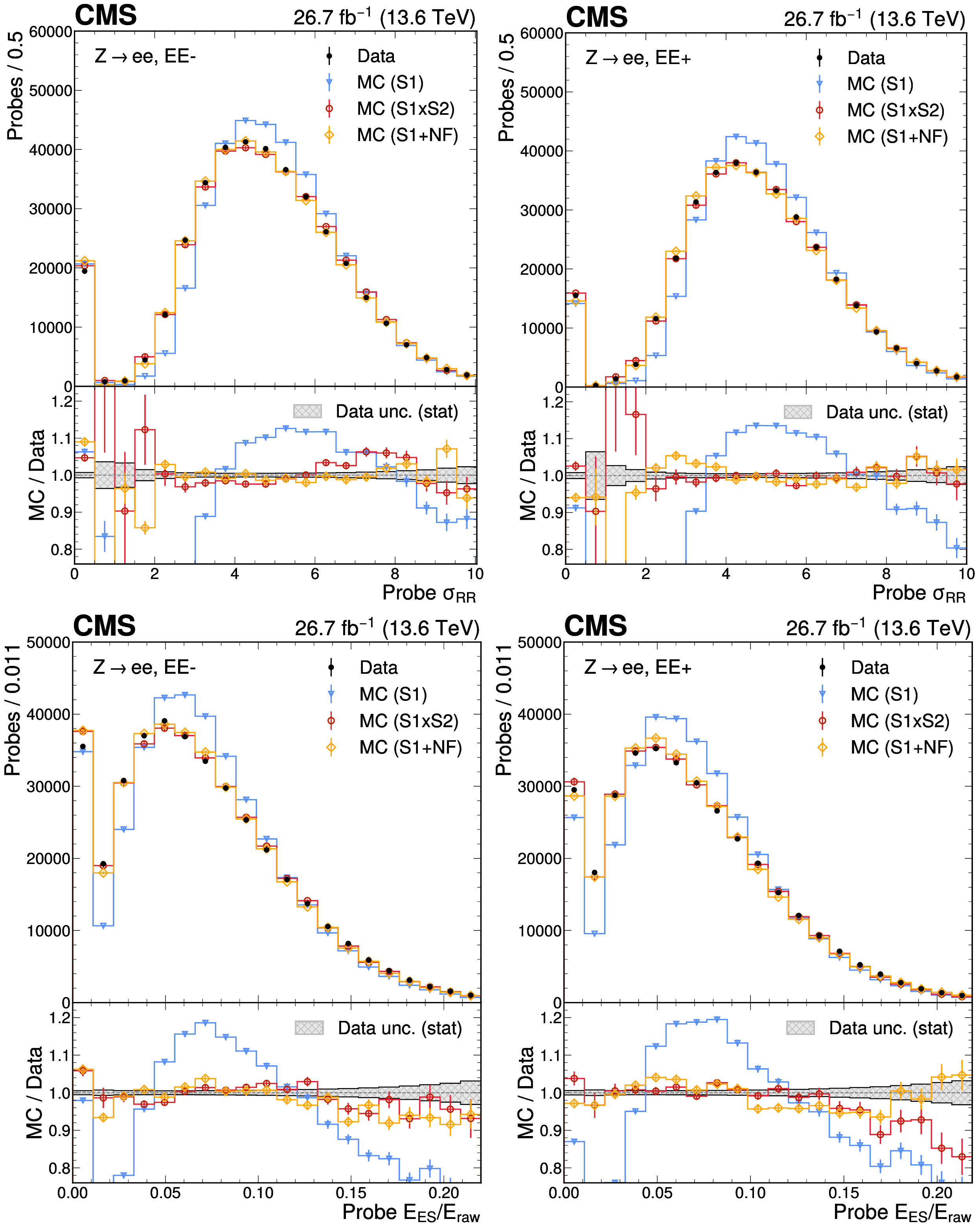
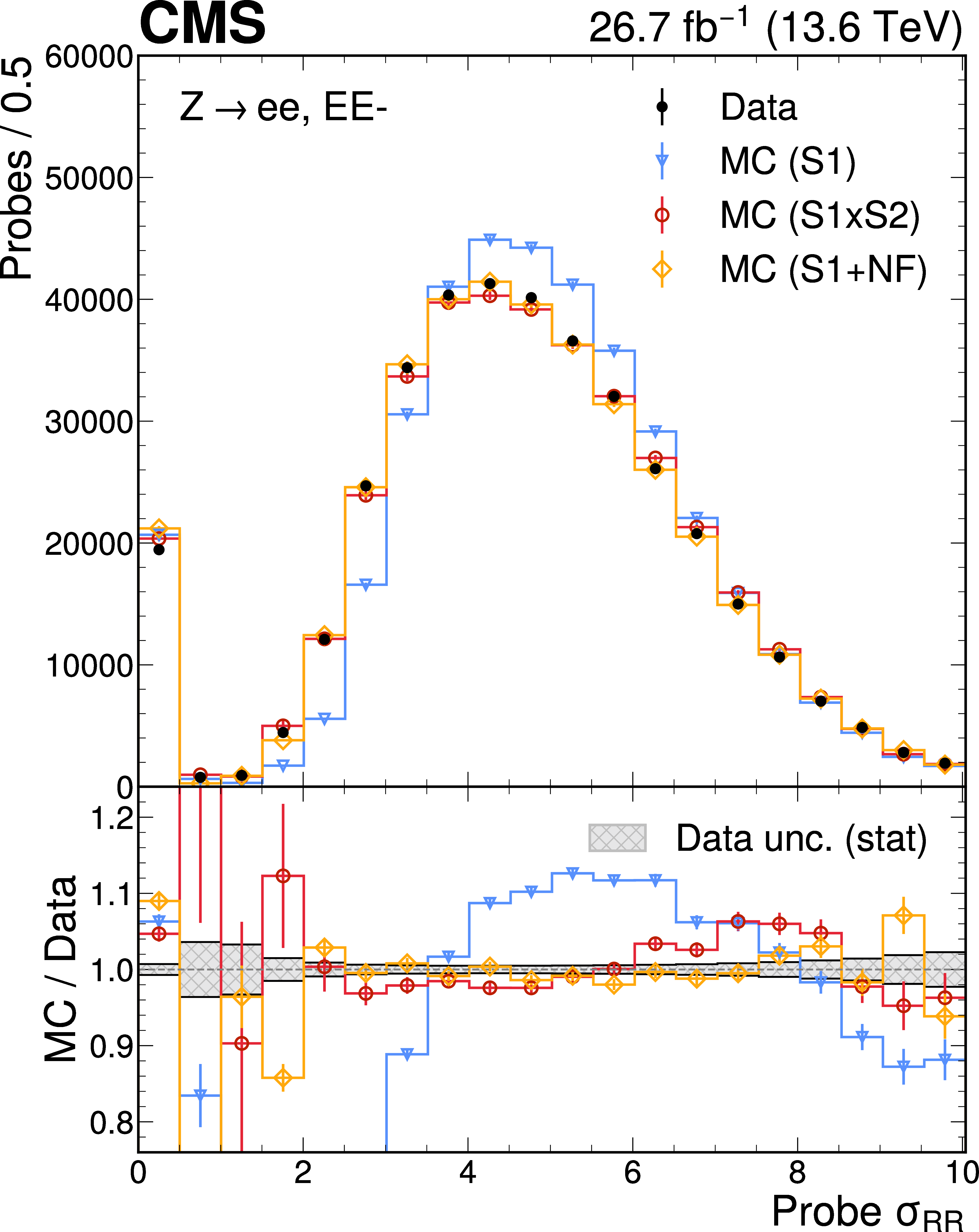
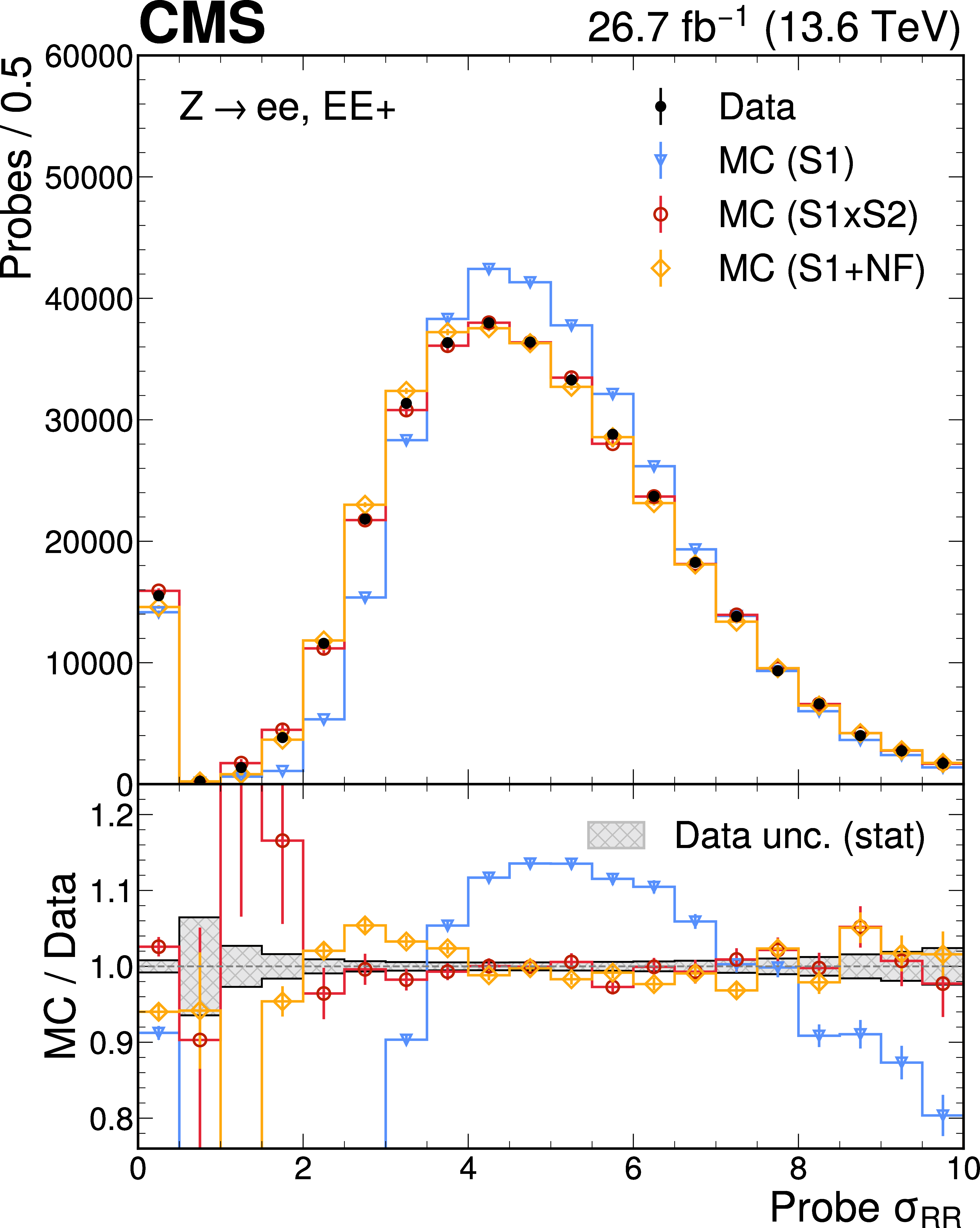
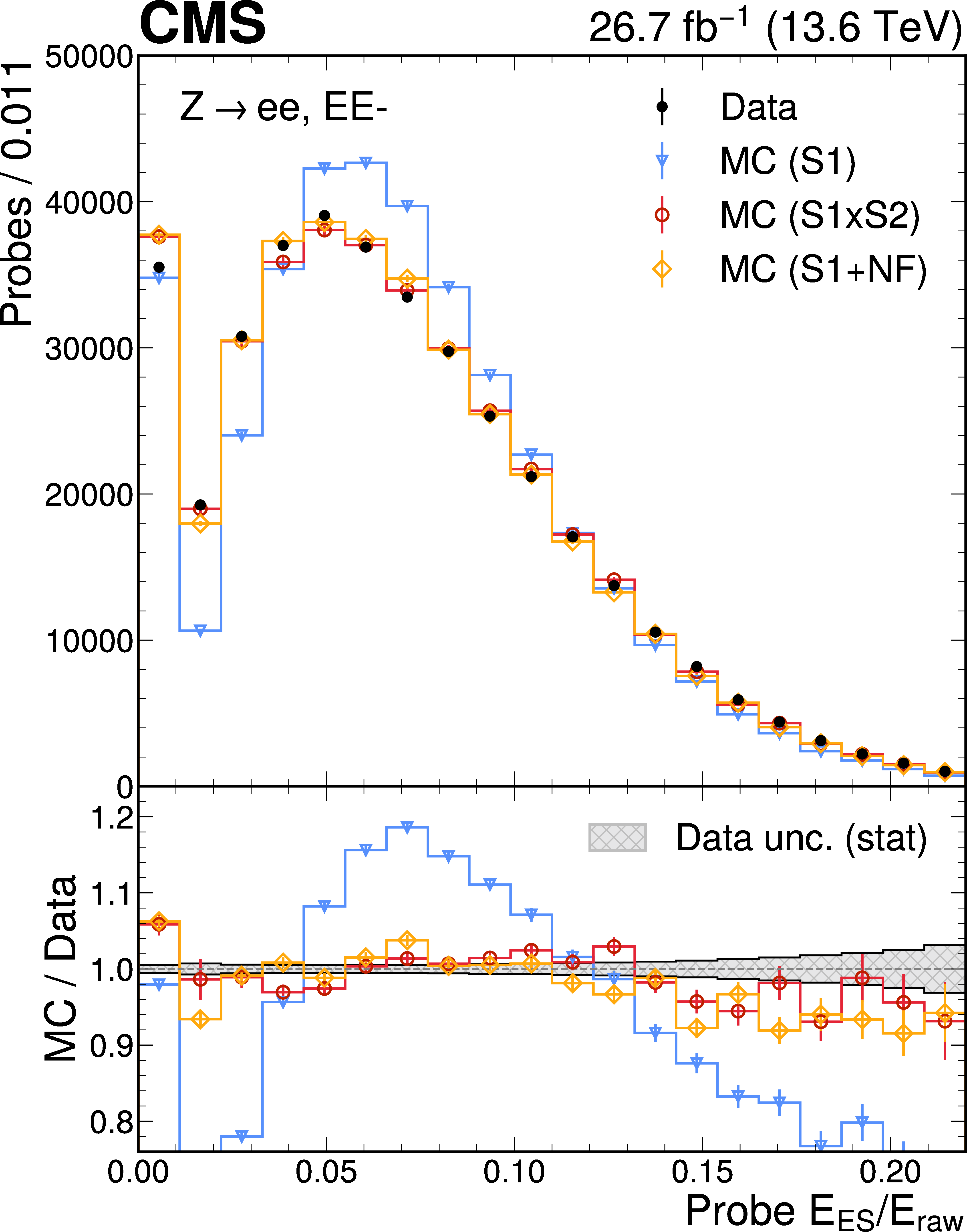
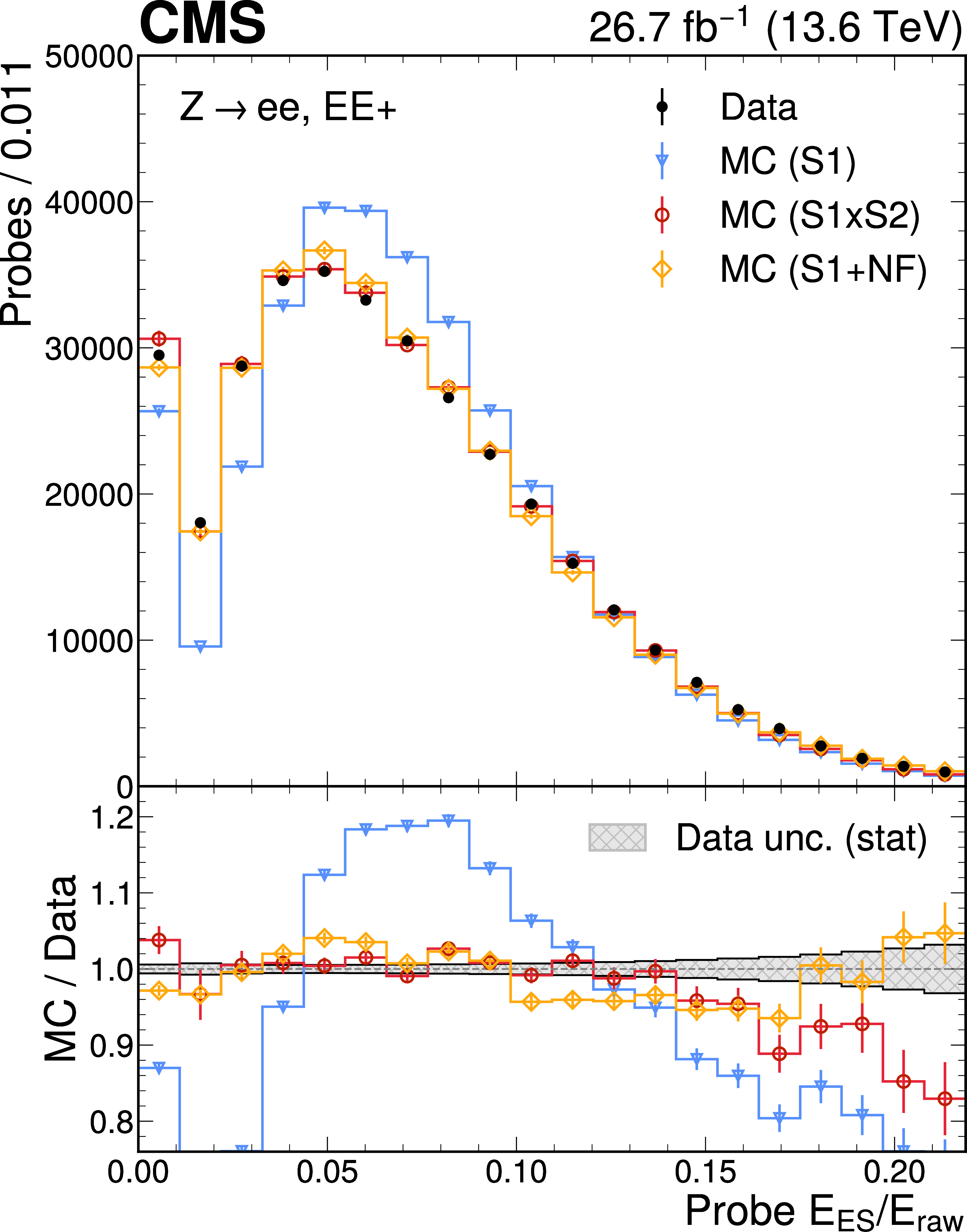
The probe features related to the preshower detector, $ \sigma_{\mathrm{RR}} $ (upper row) and $ E_{\mathrm{ES}}/E_{\text{raw}} $ (lower row), are shown. These variables are only defined for probes in the endcaps, where the preshower detectors are located. The plots show the distributions in data and simulation, for the EE-(left) and EE$ + $ (right) subdetector regions. The plotting conventions are the same as in Fig. 10. |
png pdf |
Figure 15-a:
The probe features related to the preshower detector, $ \sigma_{\mathrm{RR}} $ (upper row) and $ E_{\mathrm{ES}}/E_{\text{raw}} $ (lower row), are shown. These variables are only defined for probes in the endcaps, where the preshower detectors are located. The plots show the distributions in data and simulation, for the EE-(left) and EE$ + $ (right) subdetector regions. The plotting conventions are the same as in Fig. 10. |
png pdf |
Figure 15-b:
The probe features related to the preshower detector, $ \sigma_{\mathrm{RR}} $ (upper row) and $ E_{\mathrm{ES}}/E_{\text{raw}} $ (lower row), are shown. These variables are only defined for probes in the endcaps, where the preshower detectors are located. The plots show the distributions in data and simulation, for the EE-(left) and EE$ + $ (right) subdetector regions. The plotting conventions are the same as in Fig. 10. |
png pdf |
Figure 15-c:
The probe features related to the preshower detector, $ \sigma_{\mathrm{RR}} $ (upper row) and $ E_{\mathrm{ES}}/E_{\text{raw}} $ (lower row), are shown. These variables are only defined for probes in the endcaps, where the preshower detectors are located. The plots show the distributions in data and simulation, for the EE-(left) and EE$ + $ (right) subdetector regions. The plotting conventions are the same as in Fig. 10. |
png pdf |
Figure 15-d:
The probe features related to the preshower detector, $ \sigma_{\mathrm{RR}} $ (upper row) and $ E_{\mathrm{ES}}/E_{\text{raw}} $ (lower row), are shown. These variables are only defined for probes in the endcaps, where the preshower detectors are located. The plots show the distributions in data and simulation, for the EE-(left) and EE$ + $ (right) subdetector regions. The plotting conventions are the same as in Fig. 10. |
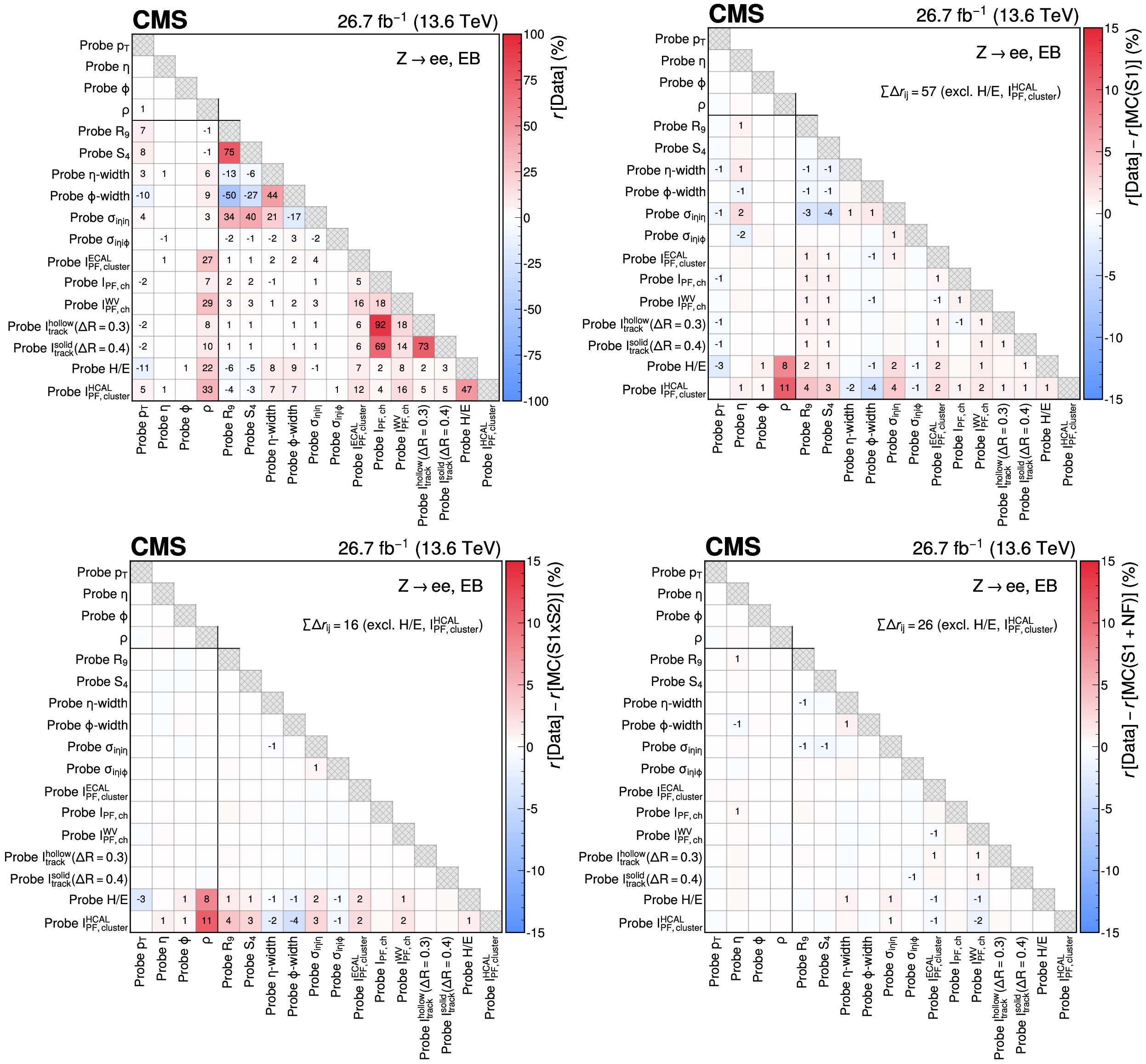
png pdf |
Figure 16:
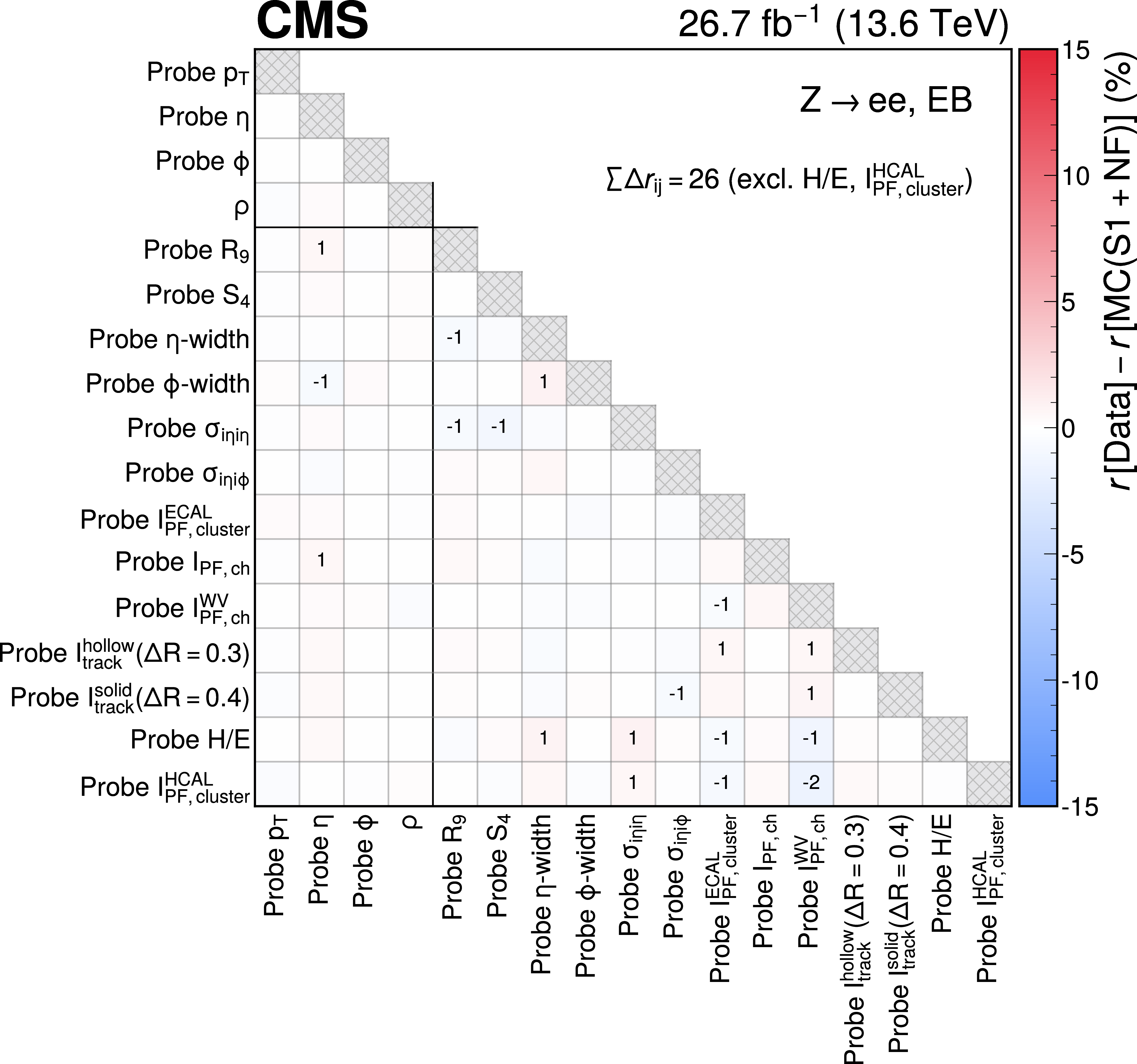
The upper left plot shows the Pearson correlation coefficients $ r_{ij} $, between pairs of features in data for the EB subdetector. The other three plots show the difference in correlation coefficients $ \Delta r_{ij} $ between data and simulation for three scenarios: the upper right plot corresponds to simulation after the initial S1 reweighting to align the kinematic distributions with data, while the lower left and lower right plots show the calibrated simulation after the S2 reweighting and the flow corrections are applied, respectively. All $ r_{ij} $ and $ \Delta r_{ij} $ values are rounded to the nearest percent, and values of absolute size less than 0.5% are not shown. The sum of absolute $ \Delta r_{ij} $ terms are shown in each of the relevant plots, where the sum excludes the probe H/E and $ \mathcal{I}^{\mathrm{HCAL}}_{\text{PF, cluster}} $ features, since these are not included in the reweighting method. A solid line is used to separate the $ x_k $ and $ x_s $ features. |
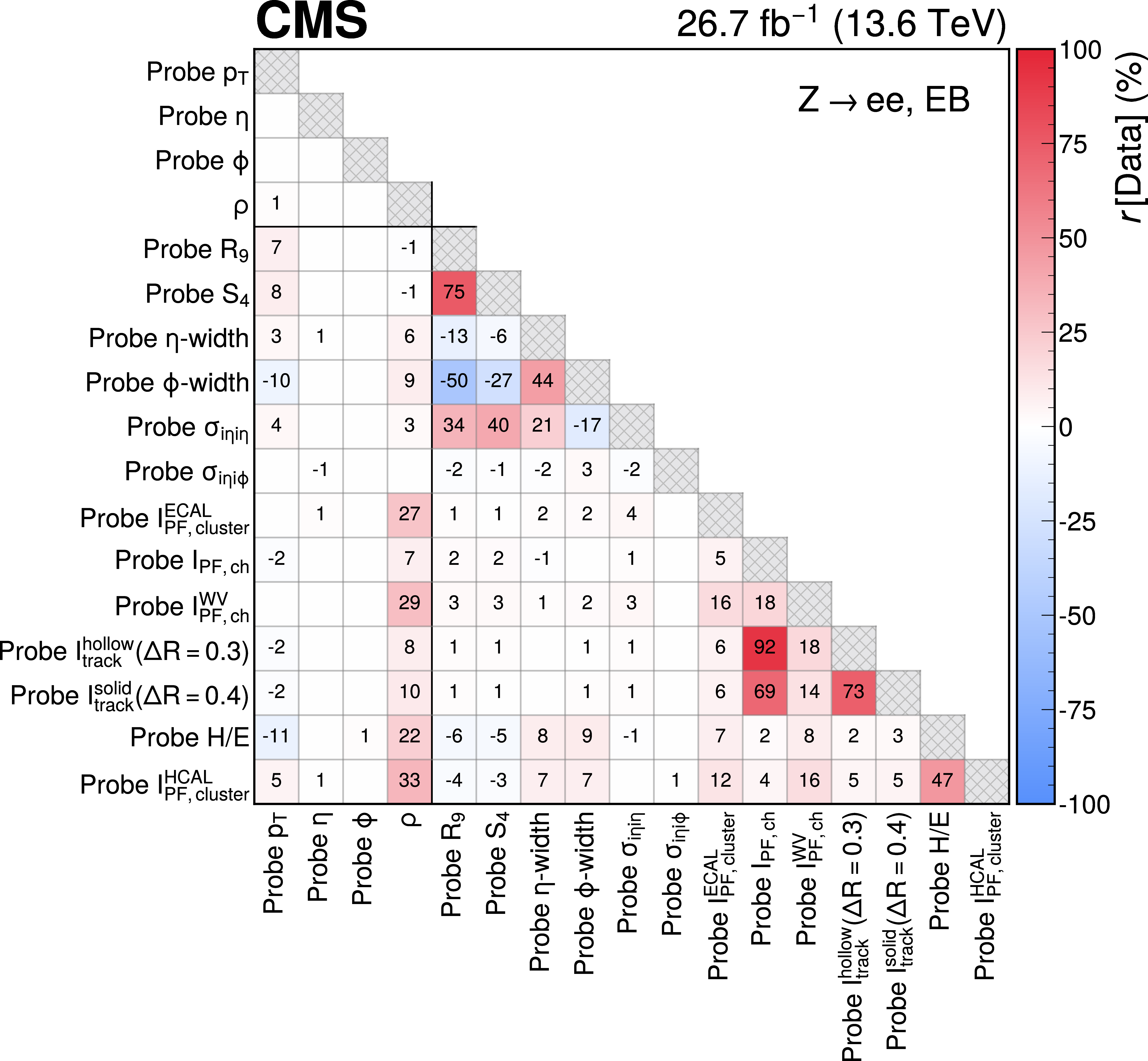
png pdf |
Figure 16-a:
The upper left plot shows the Pearson correlation coefficients $ r_{ij} $, between pairs of features in data for the EB subdetector. The other three plots show the difference in correlation coefficients $ \Delta r_{ij} $ between data and simulation for three scenarios: the upper right plot corresponds to simulation after the initial S1 reweighting to align the kinematic distributions with data, while the lower left and lower right plots show the calibrated simulation after the S2 reweighting and the flow corrections are applied, respectively. All $ r_{ij} $ and $ \Delta r_{ij} $ values are rounded to the nearest percent, and values of absolute size less than 0.5% are not shown. The sum of absolute $ \Delta r_{ij} $ terms are shown in each of the relevant plots, where the sum excludes the probe H/E and $ \mathcal{I}^{\mathrm{HCAL}}_{\text{PF, cluster}} $ features, since these are not included in the reweighting method. A solid line is used to separate the $ x_k $ and $ x_s $ features. |
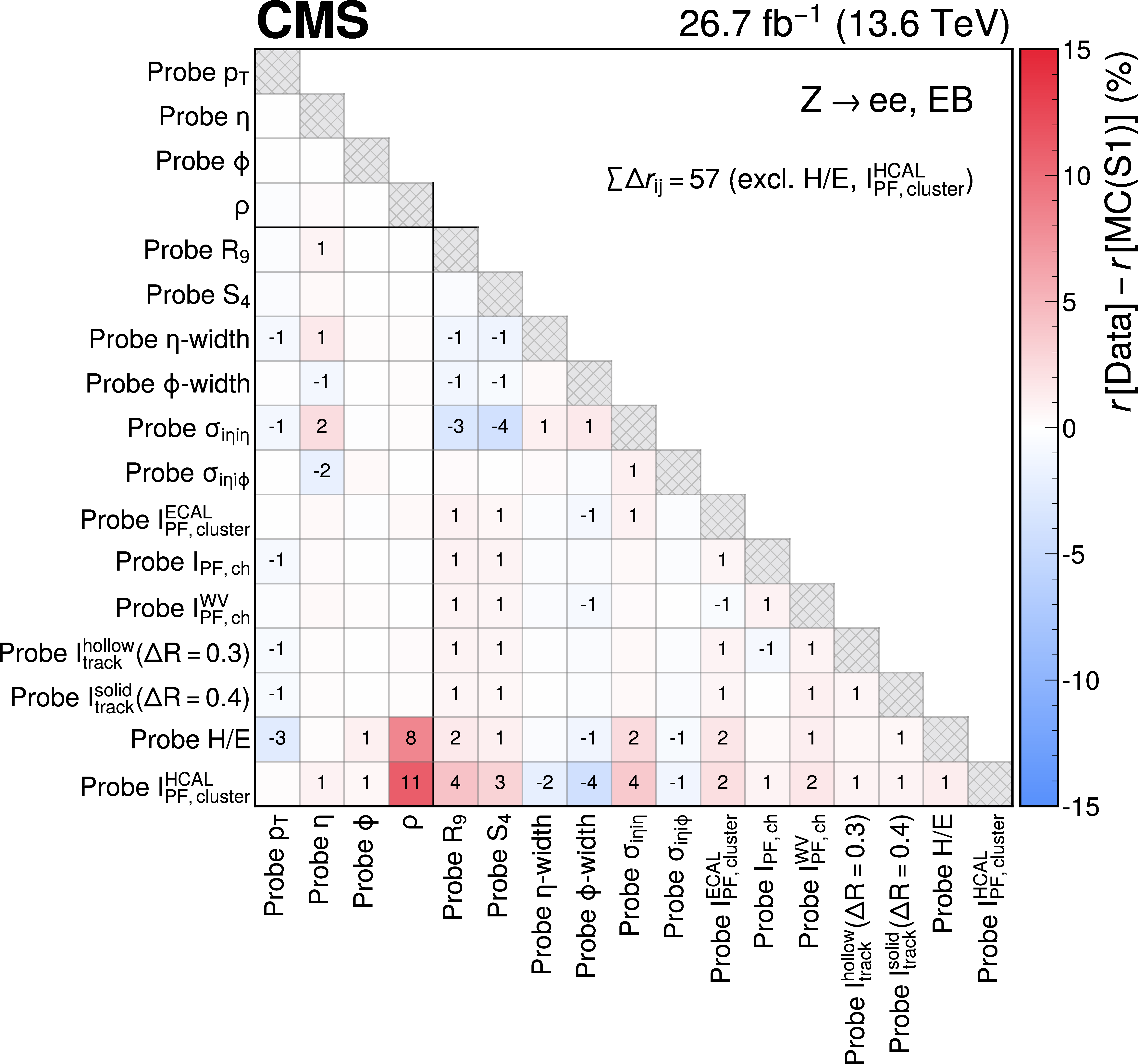
png pdf |
Figure 16-b:
The upper left plot shows the Pearson correlation coefficients $ r_{ij} $, between pairs of features in data for the EB subdetector. The other three plots show the difference in correlation coefficients $ \Delta r_{ij} $ between data and simulation for three scenarios: the upper right plot corresponds to simulation after the initial S1 reweighting to align the kinematic distributions with data, while the lower left and lower right plots show the calibrated simulation after the S2 reweighting and the flow corrections are applied, respectively. All $ r_{ij} $ and $ \Delta r_{ij} $ values are rounded to the nearest percent, and values of absolute size less than 0.5% are not shown. The sum of absolute $ \Delta r_{ij} $ terms are shown in each of the relevant plots, where the sum excludes the probe H/E and $ \mathcal{I}^{\mathrm{HCAL}}_{\text{PF, cluster}} $ features, since these are not included in the reweighting method. A solid line is used to separate the $ x_k $ and $ x_s $ features. |
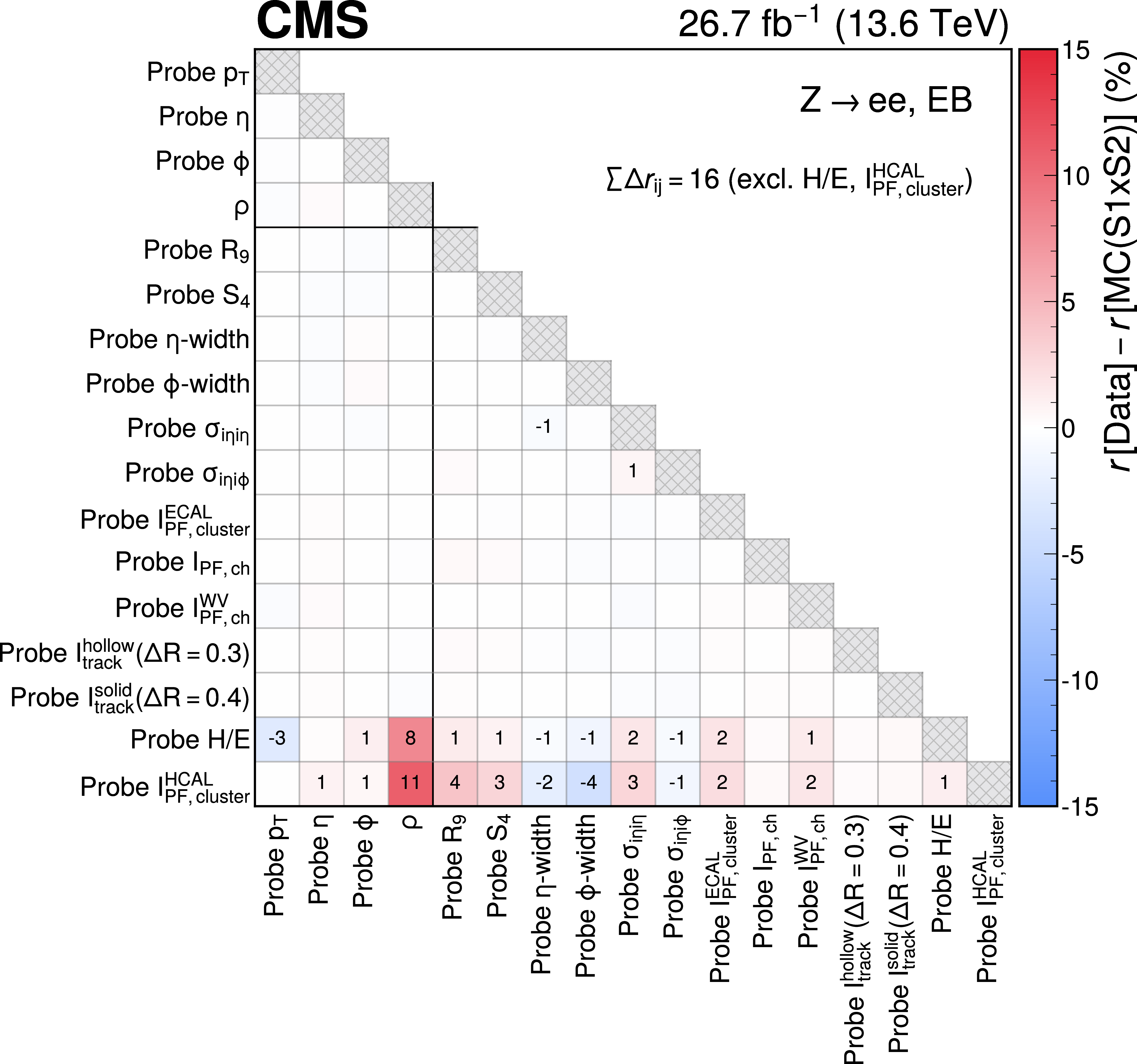
png pdf |
Figure 16-c:
The upper left plot shows the Pearson correlation coefficients $ r_{ij} $, between pairs of features in data for the EB subdetector. The other three plots show the difference in correlation coefficients $ \Delta r_{ij} $ between data and simulation for three scenarios: the upper right plot corresponds to simulation after the initial S1 reweighting to align the kinematic distributions with data, while the lower left and lower right plots show the calibrated simulation after the S2 reweighting and the flow corrections are applied, respectively. All $ r_{ij} $ and $ \Delta r_{ij} $ values are rounded to the nearest percent, and values of absolute size less than 0.5% are not shown. The sum of absolute $ \Delta r_{ij} $ terms are shown in each of the relevant plots, where the sum excludes the probe H/E and $ \mathcal{I}^{\mathrm{HCAL}}_{\text{PF, cluster}} $ features, since these are not included in the reweighting method. A solid line is used to separate the $ x_k $ and $ x_s $ features. |
png pdf |
Figure 16-d:
The upper left plot shows the Pearson correlation coefficients $ r_{ij} $, between pairs of features in data for the EB subdetector. The other three plots show the difference in correlation coefficients $ \Delta r_{ij} $ between data and simulation for three scenarios: the upper right plot corresponds to simulation after the initial S1 reweighting to align the kinematic distributions with data, while the lower left and lower right plots show the calibrated simulation after the S2 reweighting and the flow corrections are applied, respectively. All $ r_{ij} $ and $ \Delta r_{ij} $ values are rounded to the nearest percent, and values of absolute size less than 0.5% are not shown. The sum of absolute $ \Delta r_{ij} $ terms are shown in each of the relevant plots, where the sum excludes the probe H/E and $ \mathcal{I}^{\mathrm{HCAL}}_{\text{PF, cluster}} $ features, since these are not included in the reweighting method. A solid line is used to separate the $ x_k $ and $ x_s $ features. |
png pdf |
Figure 17:
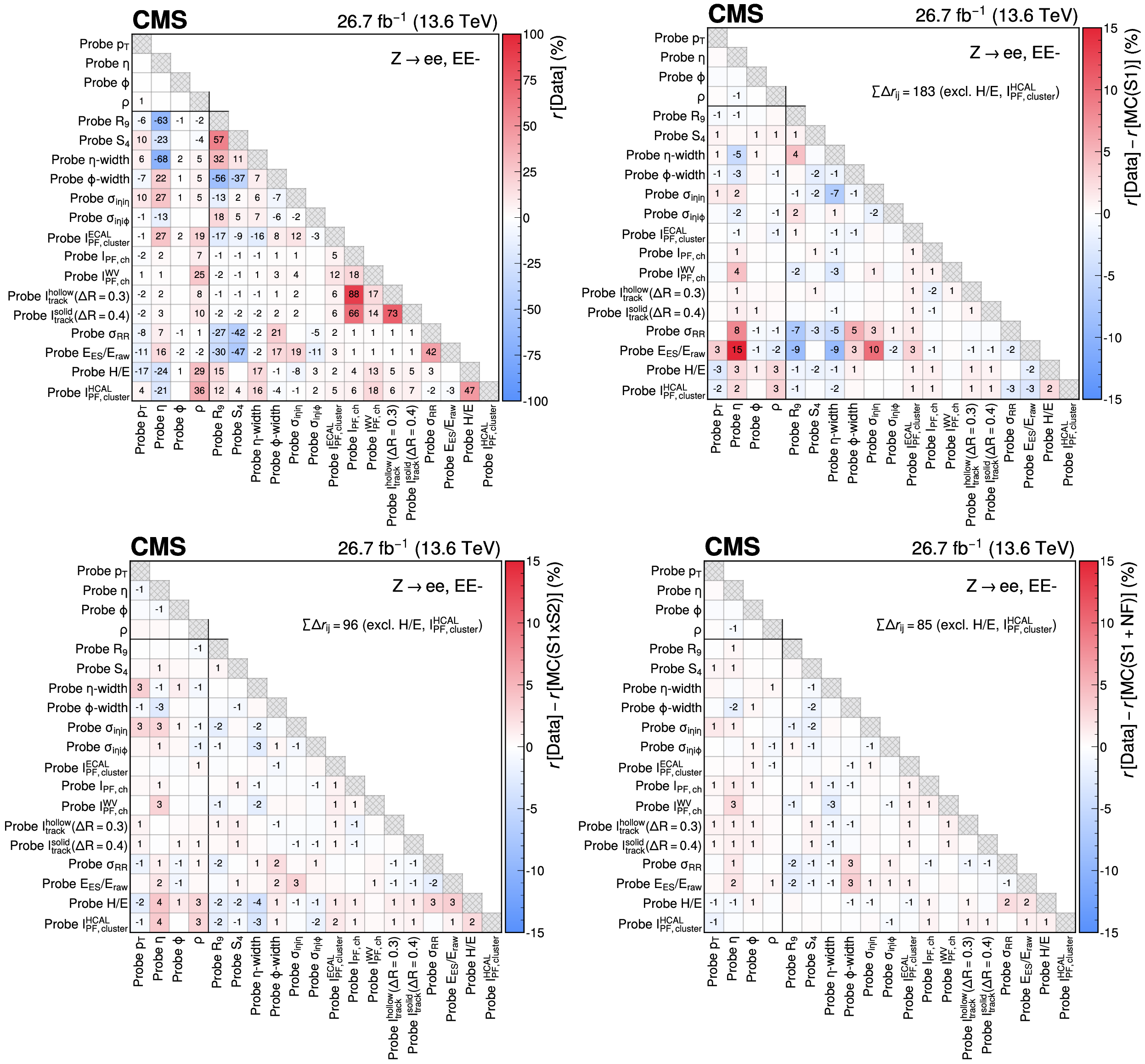
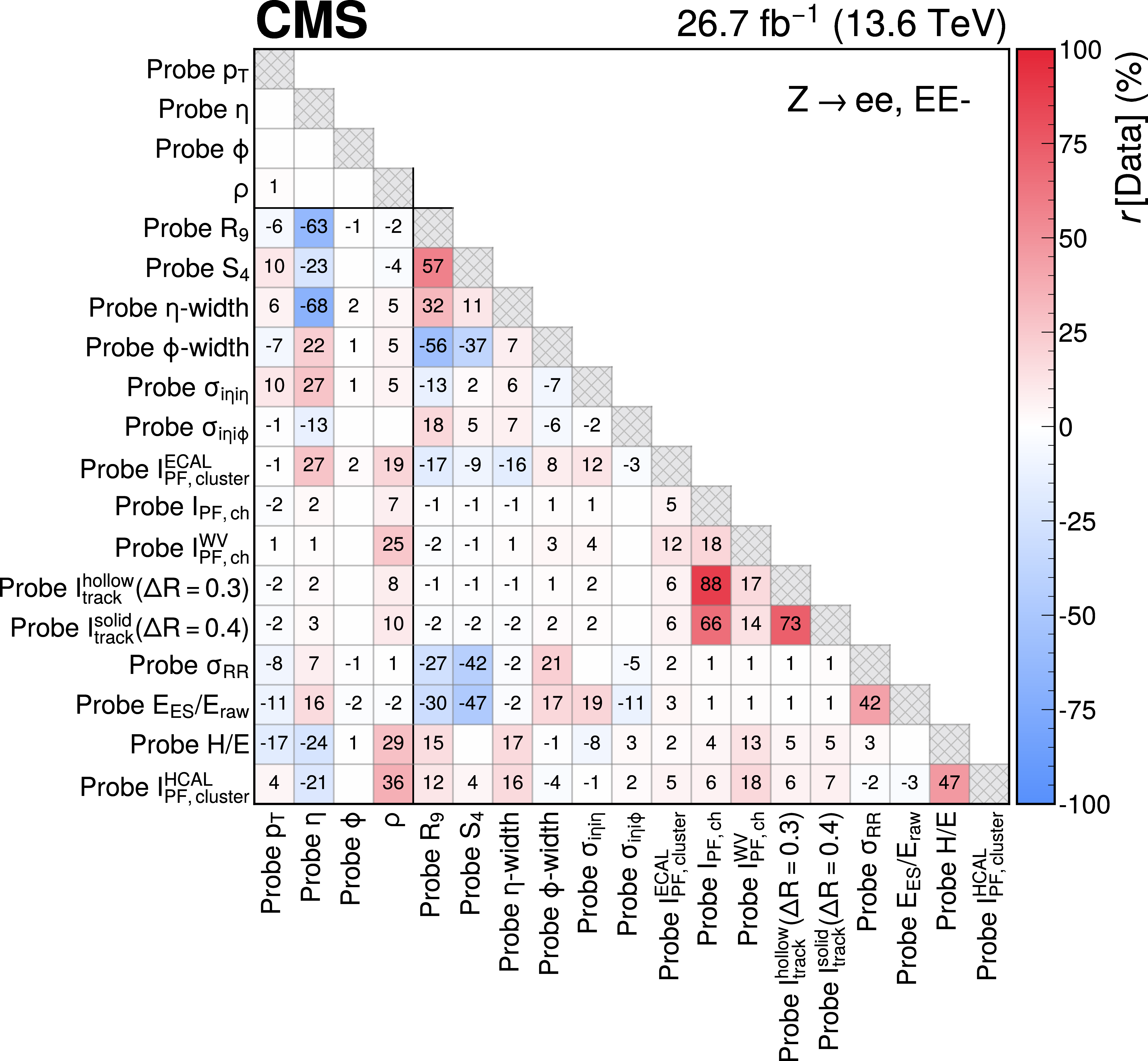
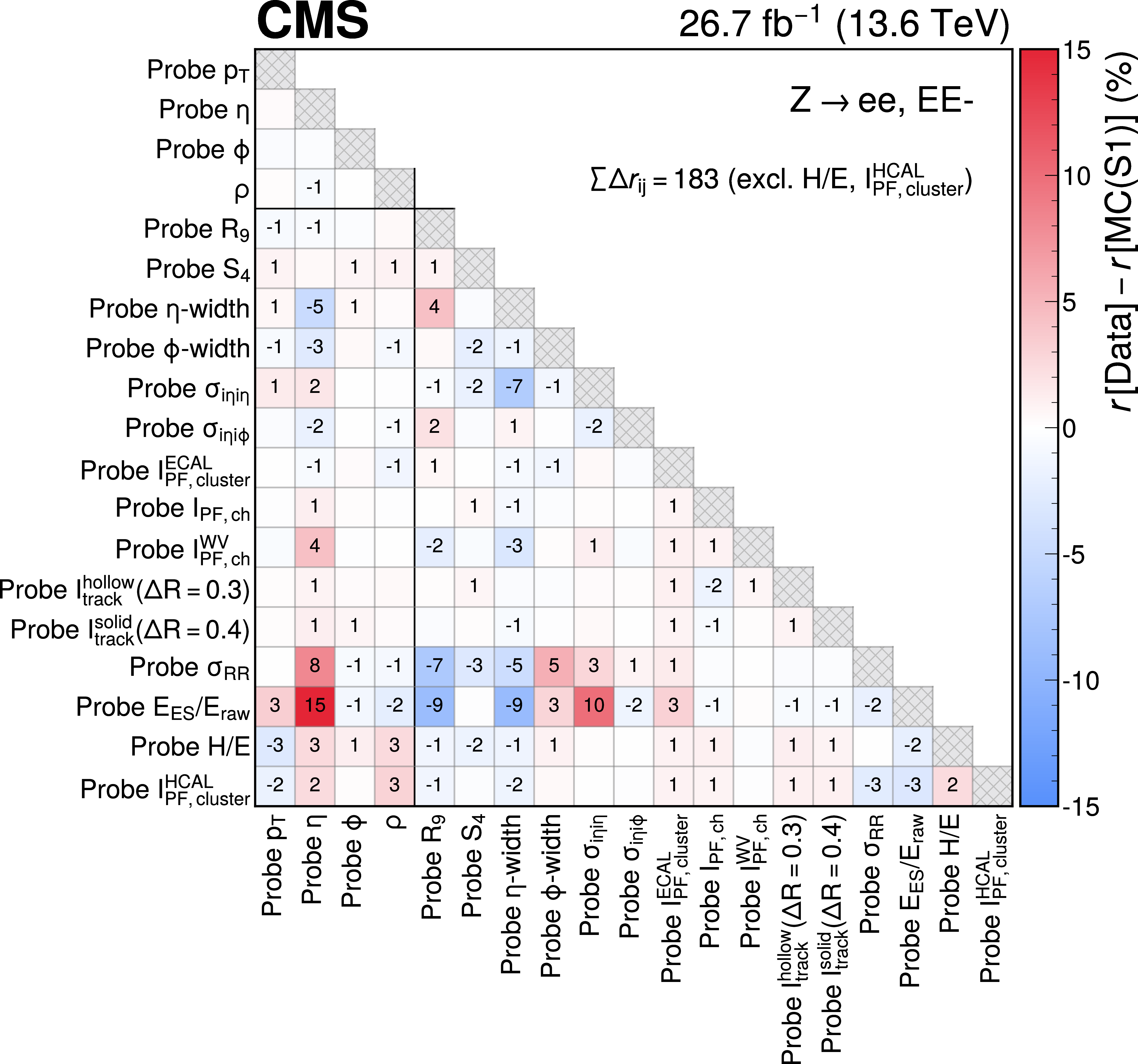
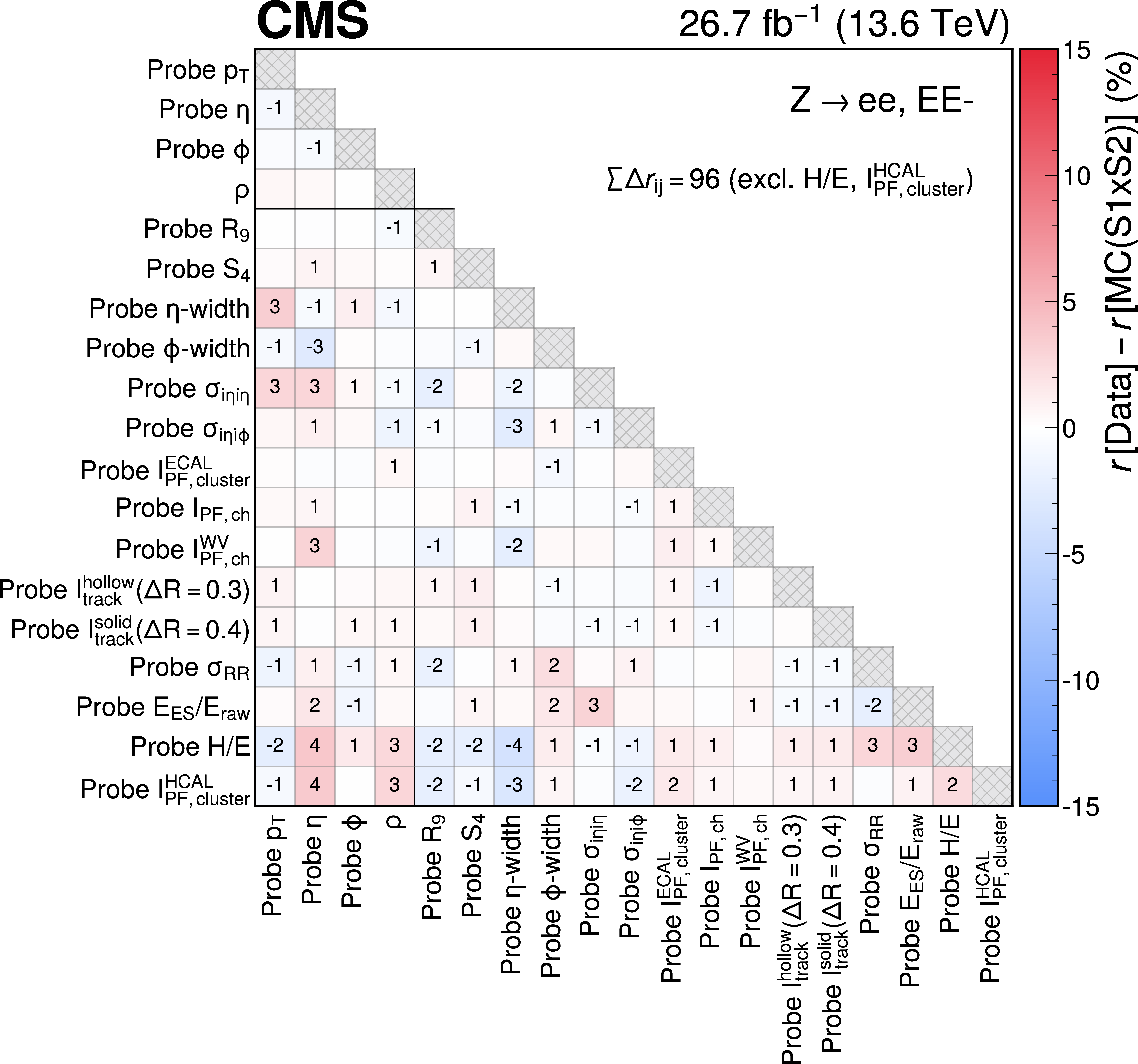
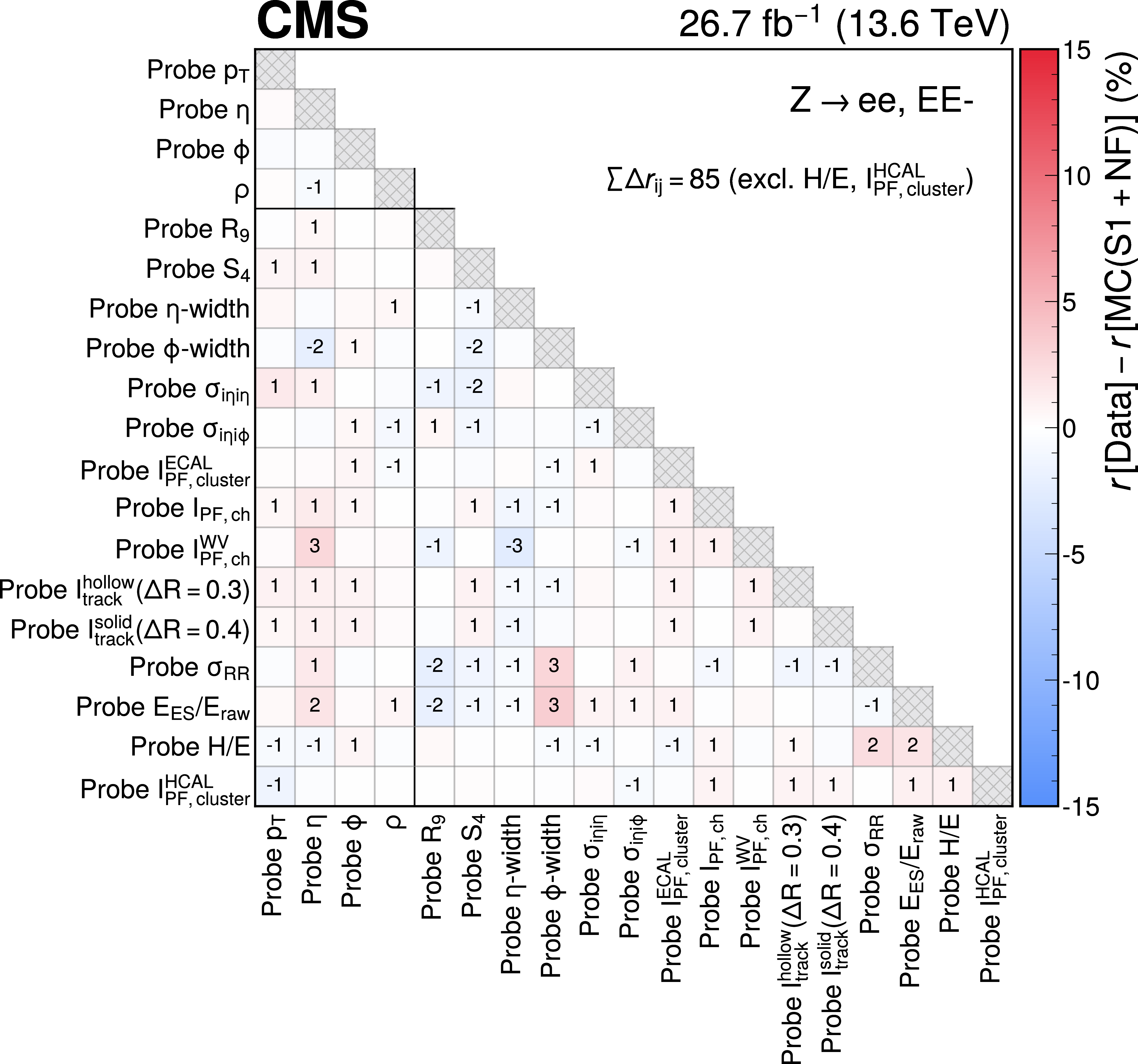
The upper left plot shows the Pearson correlation coefficients $ r_{ij} $, between pairs of features in data for the EE-subdetector. The other three plots show the difference in correlation coefficients $ \Delta r_{ij} $ between data and simulation for three scenarios: the upper right plot corresponds to simulation after the initial S1 reweighting to align the kinematic distributions with data, while the lower left and lower right plots show the calibrated simulation after the S2 reweighting and the flow corrections are applied, respectively. All $ r_{ij} $ and $ \Delta r_{ij} $ values are rounded to the nearest percent, and values of absolute size less than 0.5% are not shown. The sum of absolute $ \Delta r_{ij} $ terms are shown in each of the relevant plots, where the sum excludes the probe H/E and $ \mathcal{I}^{\mathrm{HCAL}}_{\text{PF, cluster}} $ features, since these are not included in the reweighting method. A solid line is used to separate the $ x_k $ and $ x_s $ features. |
png pdf |
Figure 17-a:
The upper left plot shows the Pearson correlation coefficients $ r_{ij} $, between pairs of features in data for the EE-subdetector. The other three plots show the difference in correlation coefficients $ \Delta r_{ij} $ between data and simulation for three scenarios: the upper right plot corresponds to simulation after the initial S1 reweighting to align the kinematic distributions with data, while the lower left and lower right plots show the calibrated simulation after the S2 reweighting and the flow corrections are applied, respectively. All $ r_{ij} $ and $ \Delta r_{ij} $ values are rounded to the nearest percent, and values of absolute size less than 0.5% are not shown. The sum of absolute $ \Delta r_{ij} $ terms are shown in each of the relevant plots, where the sum excludes the probe H/E and $ \mathcal{I}^{\mathrm{HCAL}}_{\text{PF, cluster}} $ features, since these are not included in the reweighting method. A solid line is used to separate the $ x_k $ and $ x_s $ features. |
png pdf |
Figure 17-b:
The upper left plot shows the Pearson correlation coefficients $ r_{ij} $, between pairs of features in data for the EE-subdetector. The other three plots show the difference in correlation coefficients $ \Delta r_{ij} $ between data and simulation for three scenarios: the upper right plot corresponds to simulation after the initial S1 reweighting to align the kinematic distributions with data, while the lower left and lower right plots show the calibrated simulation after the S2 reweighting and the flow corrections are applied, respectively. All $ r_{ij} $ and $ \Delta r_{ij} $ values are rounded to the nearest percent, and values of absolute size less than 0.5% are not shown. The sum of absolute $ \Delta r_{ij} $ terms are shown in each of the relevant plots, where the sum excludes the probe H/E and $ \mathcal{I}^{\mathrm{HCAL}}_{\text{PF, cluster}} $ features, since these are not included in the reweighting method. A solid line is used to separate the $ x_k $ and $ x_s $ features. |
png pdf |
Figure 17-c:
The upper left plot shows the Pearson correlation coefficients $ r_{ij} $, between pairs of features in data for the EE-subdetector. The other three plots show the difference in correlation coefficients $ \Delta r_{ij} $ between data and simulation for three scenarios: the upper right plot corresponds to simulation after the initial S1 reweighting to align the kinematic distributions with data, while the lower left and lower right plots show the calibrated simulation after the S2 reweighting and the flow corrections are applied, respectively. All $ r_{ij} $ and $ \Delta r_{ij} $ values are rounded to the nearest percent, and values of absolute size less than 0.5% are not shown. The sum of absolute $ \Delta r_{ij} $ terms are shown in each of the relevant plots, where the sum excludes the probe H/E and $ \mathcal{I}^{\mathrm{HCAL}}_{\text{PF, cluster}} $ features, since these are not included in the reweighting method. A solid line is used to separate the $ x_k $ and $ x_s $ features. |
png pdf |
Figure 17-d:
The upper left plot shows the Pearson correlation coefficients $ r_{ij} $, between pairs of features in data for the EE-subdetector. The other three plots show the difference in correlation coefficients $ \Delta r_{ij} $ between data and simulation for three scenarios: the upper right plot corresponds to simulation after the initial S1 reweighting to align the kinematic distributions with data, while the lower left and lower right plots show the calibrated simulation after the S2 reweighting and the flow corrections are applied, respectively. All $ r_{ij} $ and $ \Delta r_{ij} $ values are rounded to the nearest percent, and values of absolute size less than 0.5% are not shown. The sum of absolute $ \Delta r_{ij} $ terms are shown in each of the relevant plots, where the sum excludes the probe H/E and $ \mathcal{I}^{\mathrm{HCAL}}_{\text{PF, cluster}} $ features, since these are not included in the reweighting method. A solid line is used to separate the $ x_k $ and $ x_s $ features. |
png pdf |
Figure 18:
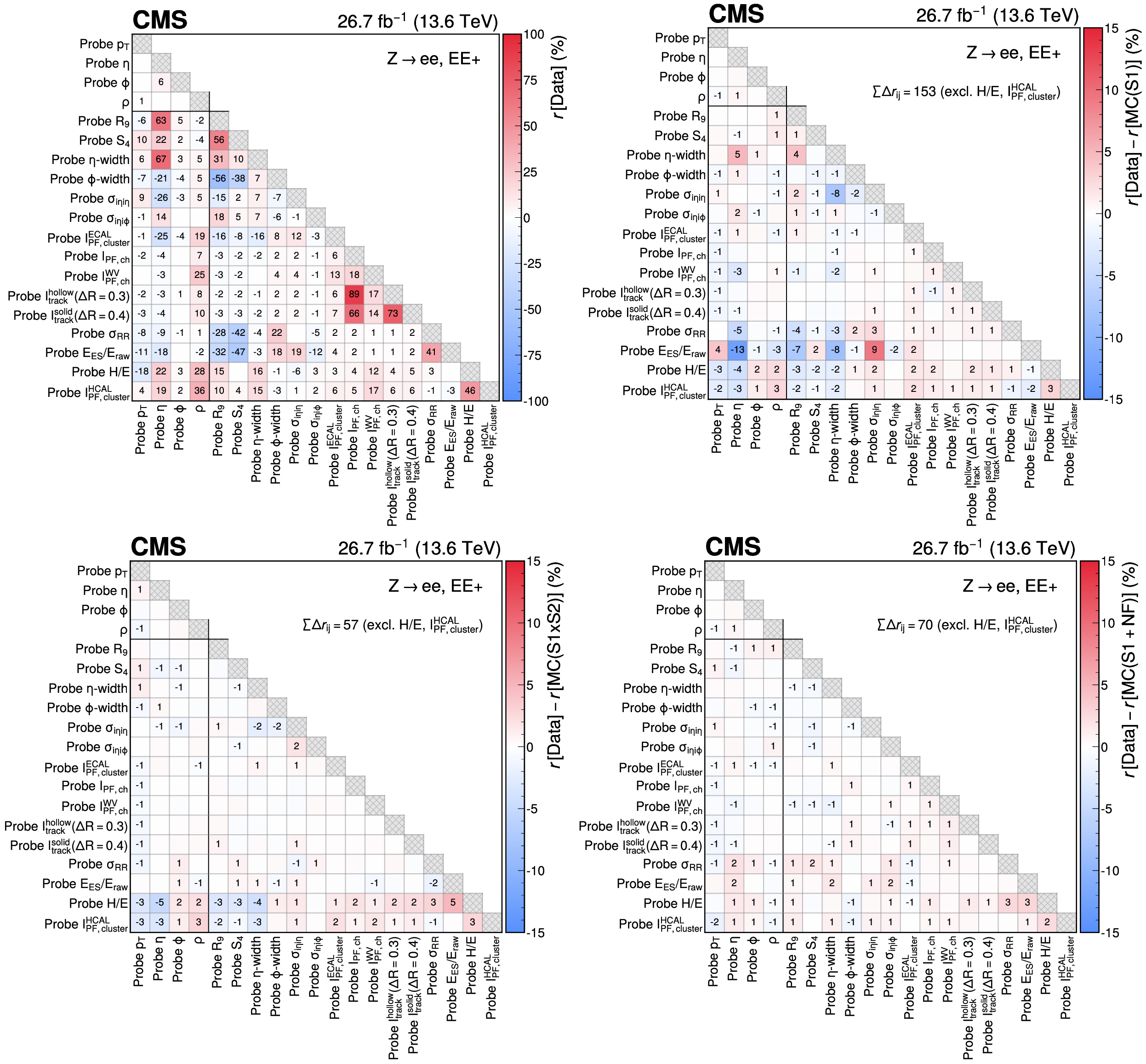
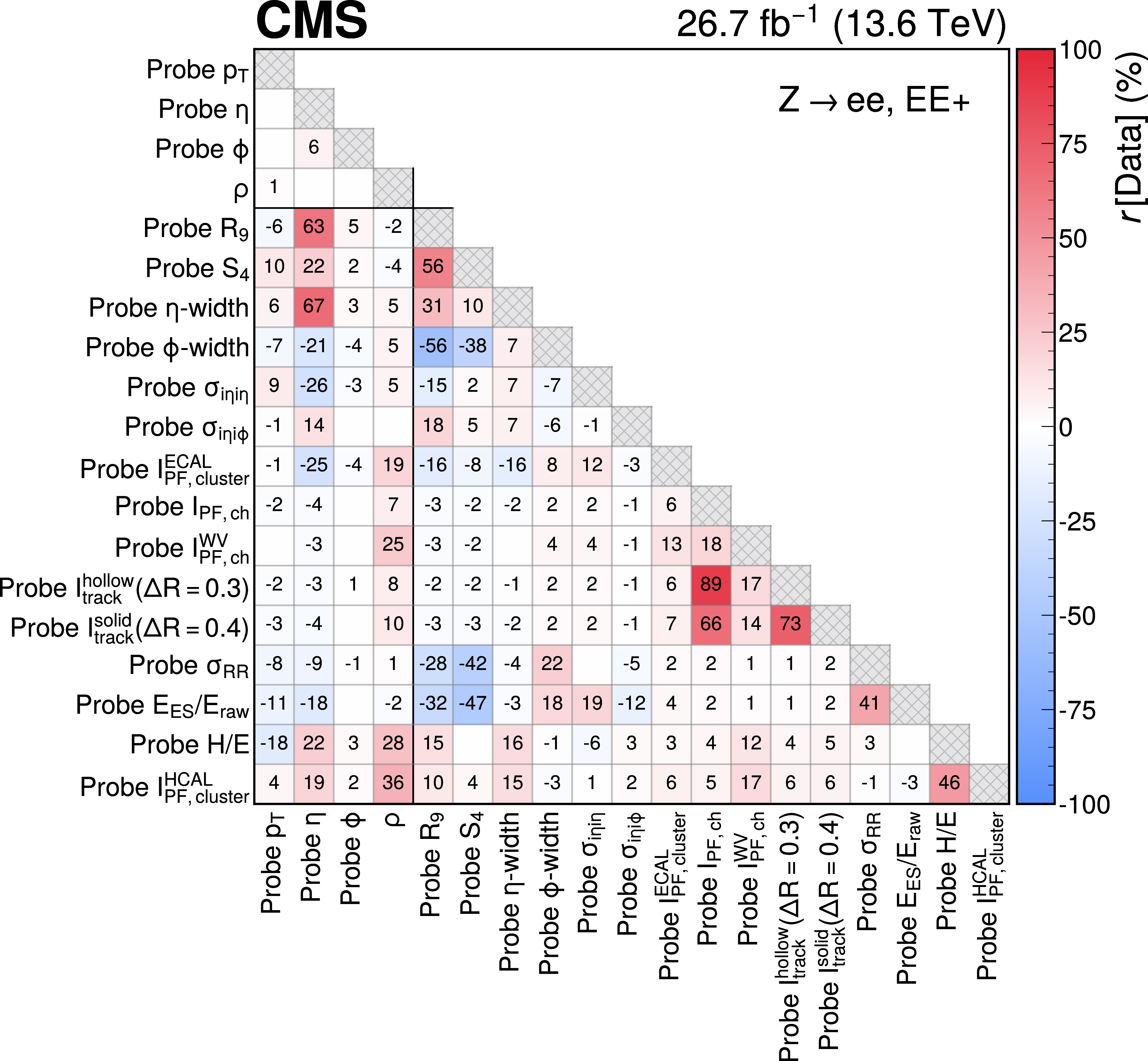
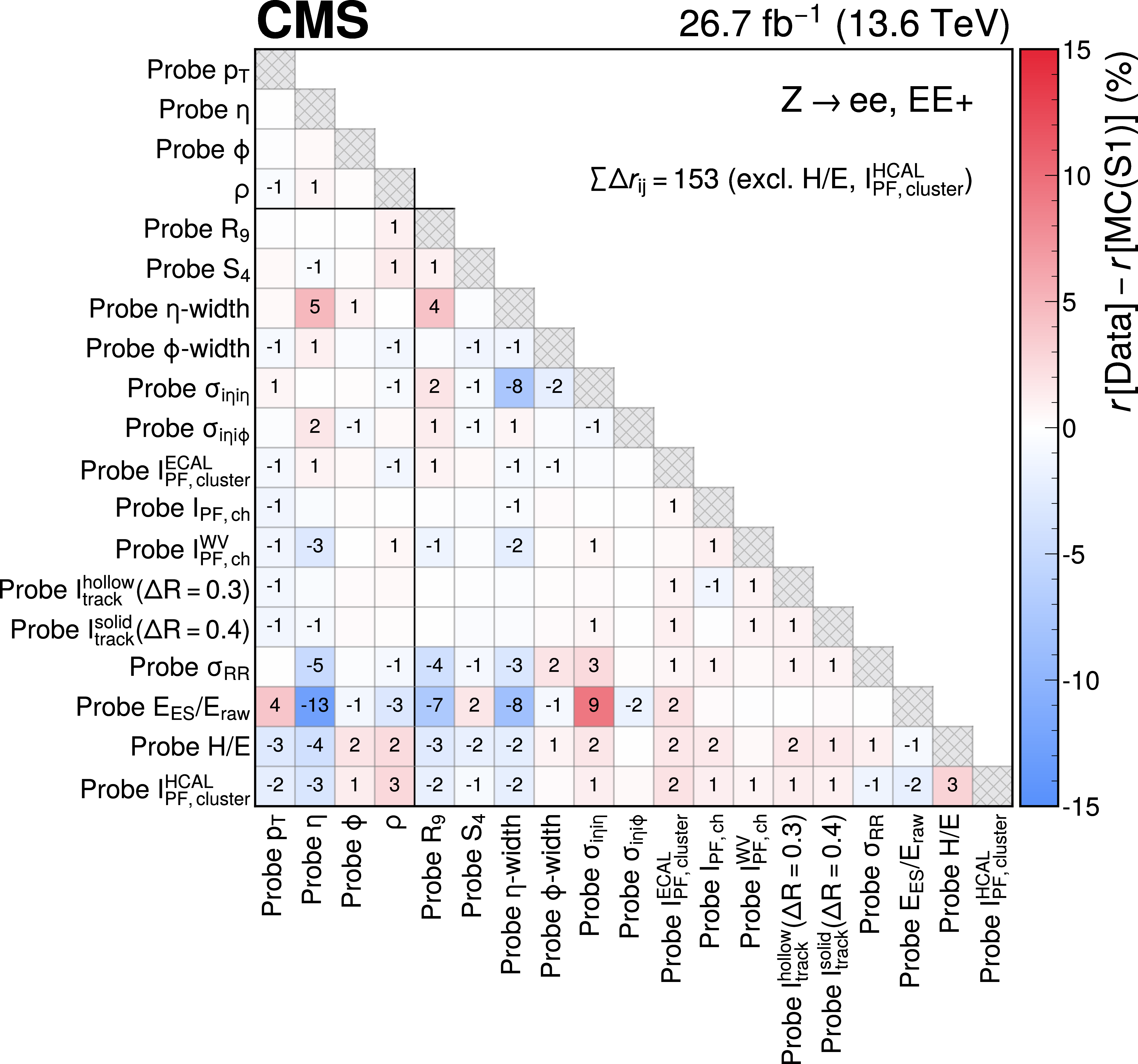
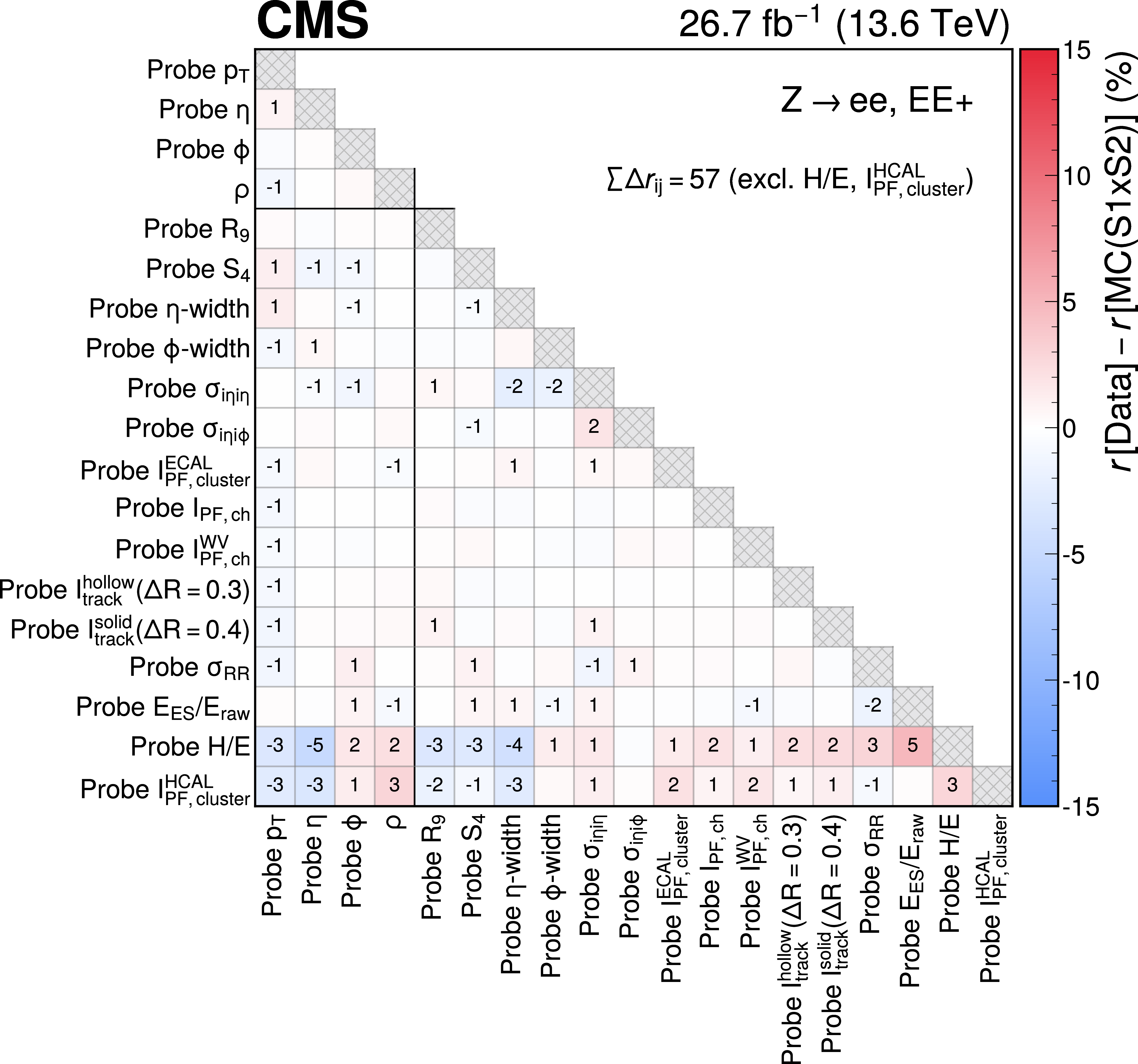
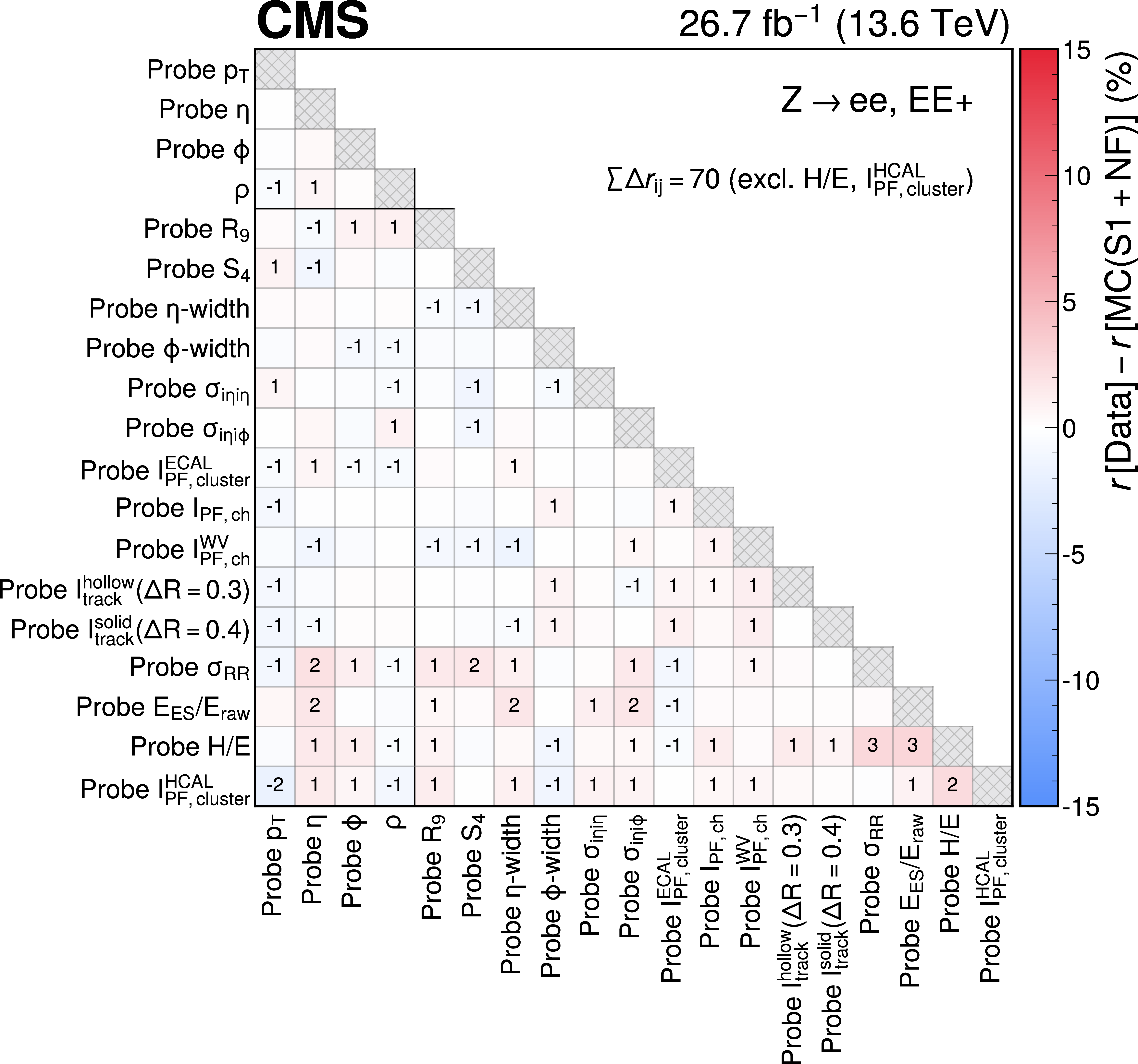
The upper left plot shows the Pearson correlation coefficients $ r_{ij} $, between pairs of features in data for the EE$ + $ subdetector. The other three plots show the difference in correlation coefficients $ \Delta r_{ij} $ between data and simulation for three scenarios: the upper right plot corresponds to simulation after the initial S1 reweighting to align the kinematic distributions with data, while the lower left and lower right plots show the calibrated simulation after the S2 reweighting and the flow corrections are applied, respectively. All $ r_{ij} $ and $ \Delta r_{ij} $ values are rounded to the nearest percent, and values of absolute size less than 0.5% are not shown. The sum of absolute $ \Delta r_{ij} $ terms are shown in each of the relevant plots, where the sum excludes the probe H/E and $ \mathcal{I}^{\mathrm{HCAL}}_{\text{PF, cluster}} $ features, since these are not included in the reweighting method. A solid line is used to separate the $ x_k $ and $ x_s $ features. |
png pdf |
Figure 18-a:
The upper left plot shows the Pearson correlation coefficients $ r_{ij} $, between pairs of features in data for the EE$ + $ subdetector. The other three plots show the difference in correlation coefficients $ \Delta r_{ij} $ between data and simulation for three scenarios: the upper right plot corresponds to simulation after the initial S1 reweighting to align the kinematic distributions with data, while the lower left and lower right plots show the calibrated simulation after the S2 reweighting and the flow corrections are applied, respectively. All $ r_{ij} $ and $ \Delta r_{ij} $ values are rounded to the nearest percent, and values of absolute size less than 0.5% are not shown. The sum of absolute $ \Delta r_{ij} $ terms are shown in each of the relevant plots, where the sum excludes the probe H/E and $ \mathcal{I}^{\mathrm{HCAL}}_{\text{PF, cluster}} $ features, since these are not included in the reweighting method. A solid line is used to separate the $ x_k $ and $ x_s $ features. |
png pdf |
Figure 18-b:
The upper left plot shows the Pearson correlation coefficients $ r_{ij} $, between pairs of features in data for the EE$ + $ subdetector. The other three plots show the difference in correlation coefficients $ \Delta r_{ij} $ between data and simulation for three scenarios: the upper right plot corresponds to simulation after the initial S1 reweighting to align the kinematic distributions with data, while the lower left and lower right plots show the calibrated simulation after the S2 reweighting and the flow corrections are applied, respectively. All $ r_{ij} $ and $ \Delta r_{ij} $ values are rounded to the nearest percent, and values of absolute size less than 0.5% are not shown. The sum of absolute $ \Delta r_{ij} $ terms are shown in each of the relevant plots, where the sum excludes the probe H/E and $ \mathcal{I}^{\mathrm{HCAL}}_{\text{PF, cluster}} $ features, since these are not included in the reweighting method. A solid line is used to separate the $ x_k $ and $ x_s $ features. |
png pdf |
Figure 18-c:
The upper left plot shows the Pearson correlation coefficients $ r_{ij} $, between pairs of features in data for the EE$ + $ subdetector. The other three plots show the difference in correlation coefficients $ \Delta r_{ij} $ between data and simulation for three scenarios: the upper right plot corresponds to simulation after the initial S1 reweighting to align the kinematic distributions with data, while the lower left and lower right plots show the calibrated simulation after the S2 reweighting and the flow corrections are applied, respectively. All $ r_{ij} $ and $ \Delta r_{ij} $ values are rounded to the nearest percent, and values of absolute size less than 0.5% are not shown. The sum of absolute $ \Delta r_{ij} $ terms are shown in each of the relevant plots, where the sum excludes the probe H/E and $ \mathcal{I}^{\mathrm{HCAL}}_{\text{PF, cluster}} $ features, since these are not included in the reweighting method. A solid line is used to separate the $ x_k $ and $ x_s $ features. |
png pdf |
Figure 18-d:
The upper left plot shows the Pearson correlation coefficients $ r_{ij} $, between pairs of features in data for the EE$ + $ subdetector. The other three plots show the difference in correlation coefficients $ \Delta r_{ij} $ between data and simulation for three scenarios: the upper right plot corresponds to simulation after the initial S1 reweighting to align the kinematic distributions with data, while the lower left and lower right plots show the calibrated simulation after the S2 reweighting and the flow corrections are applied, respectively. All $ r_{ij} $ and $ \Delta r_{ij} $ values are rounded to the nearest percent, and values of absolute size less than 0.5% are not shown. The sum of absolute $ \Delta r_{ij} $ terms are shown in each of the relevant plots, where the sum excludes the probe H/E and $ \mathcal{I}^{\mathrm{HCAL}}_{\text{PF, cluster}} $ features, since these are not included in the reweighting method. A solid line is used to separate the $ x_k $ and $ x_s $ features. |
png pdf |
Figure 19:
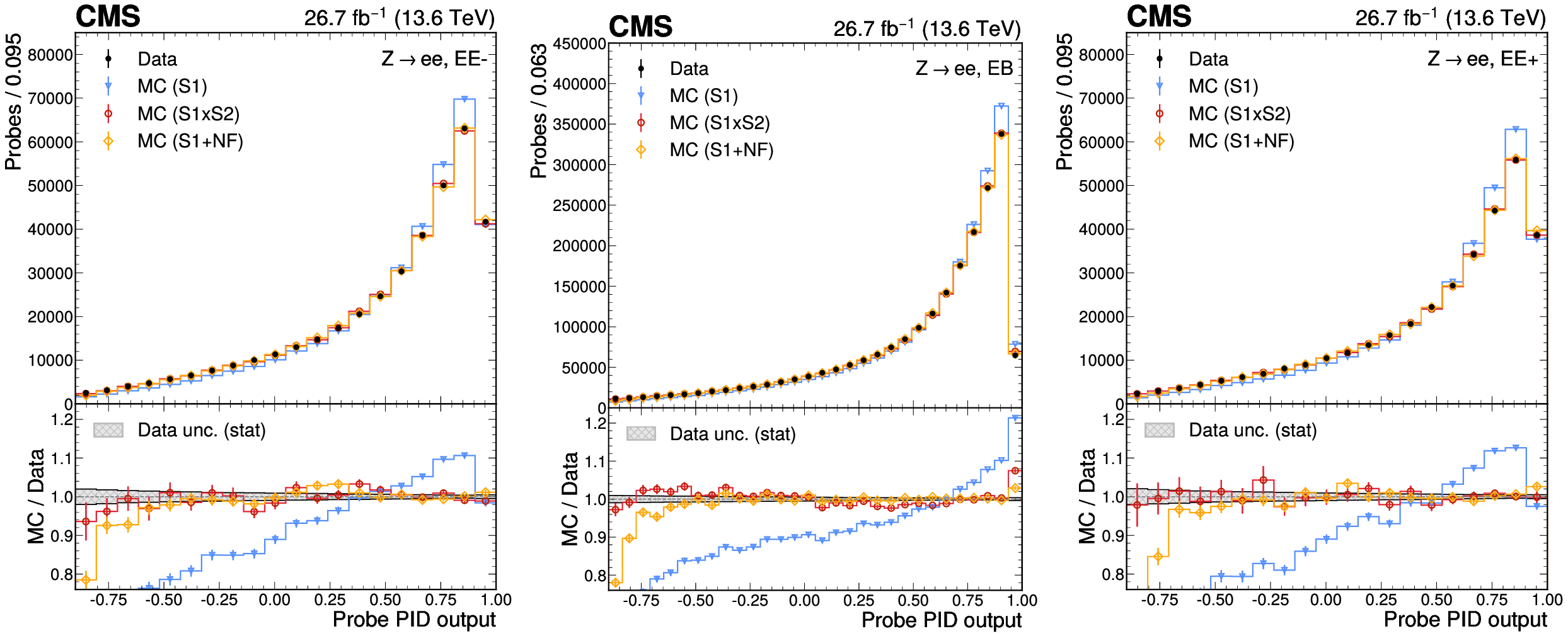
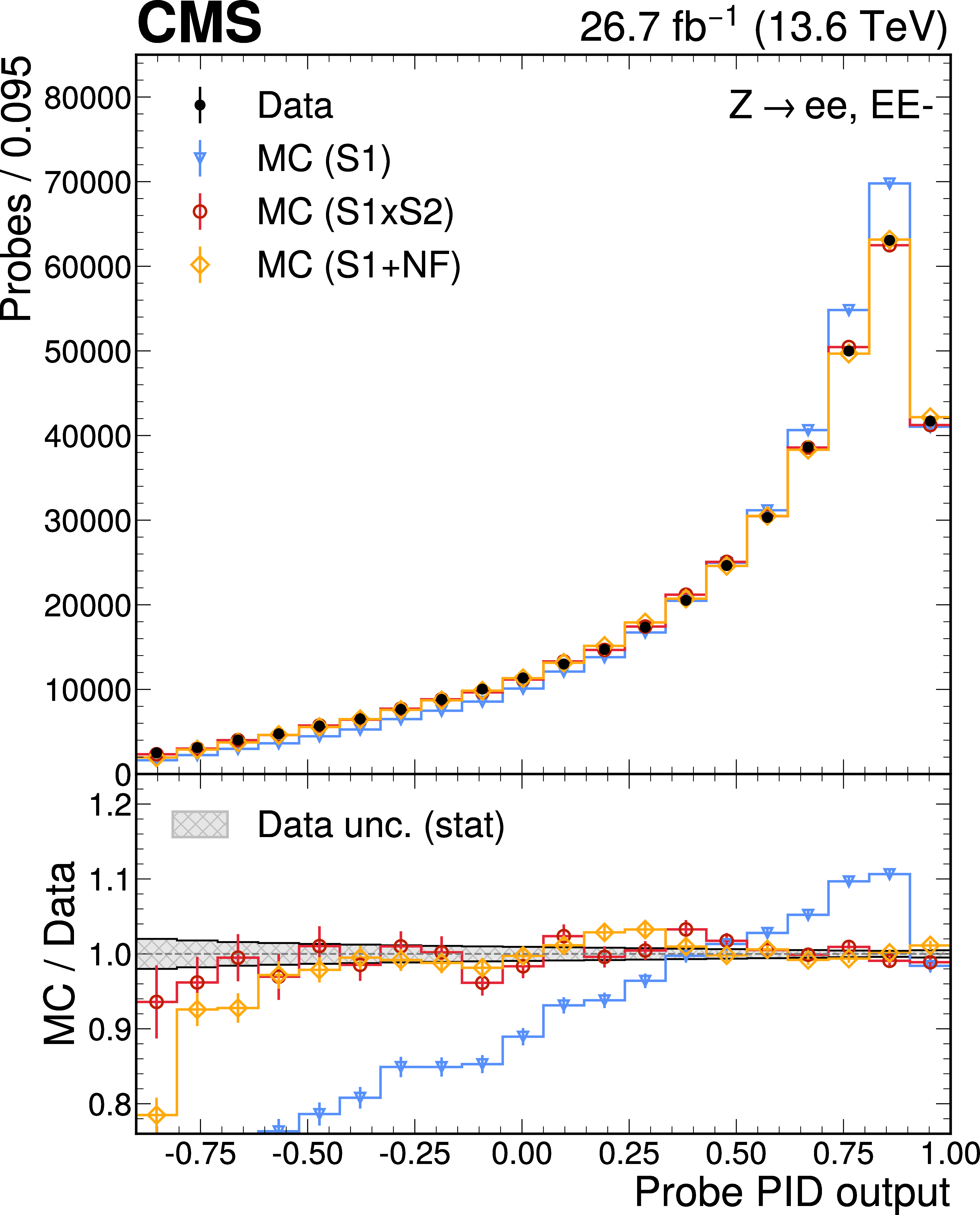
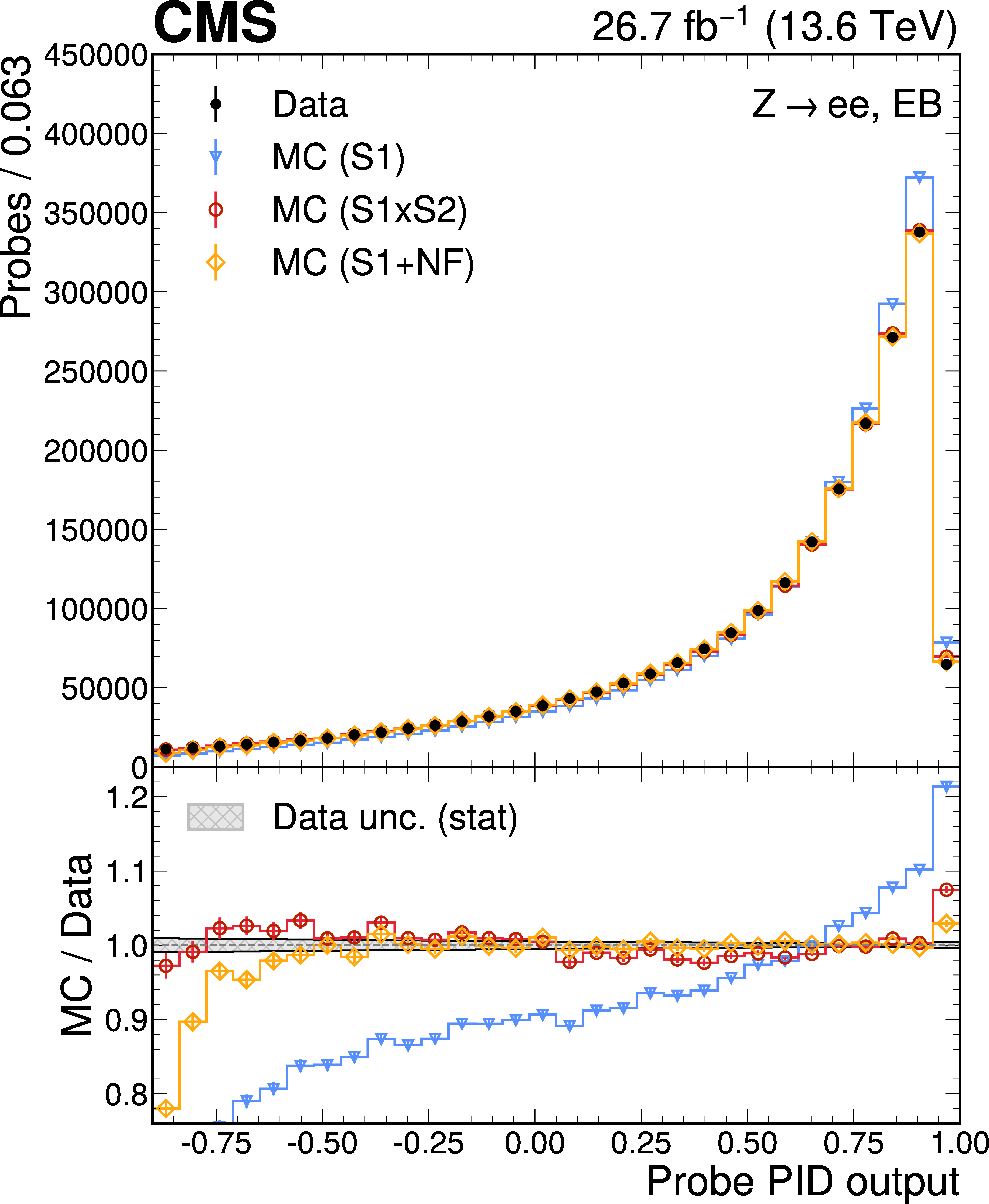
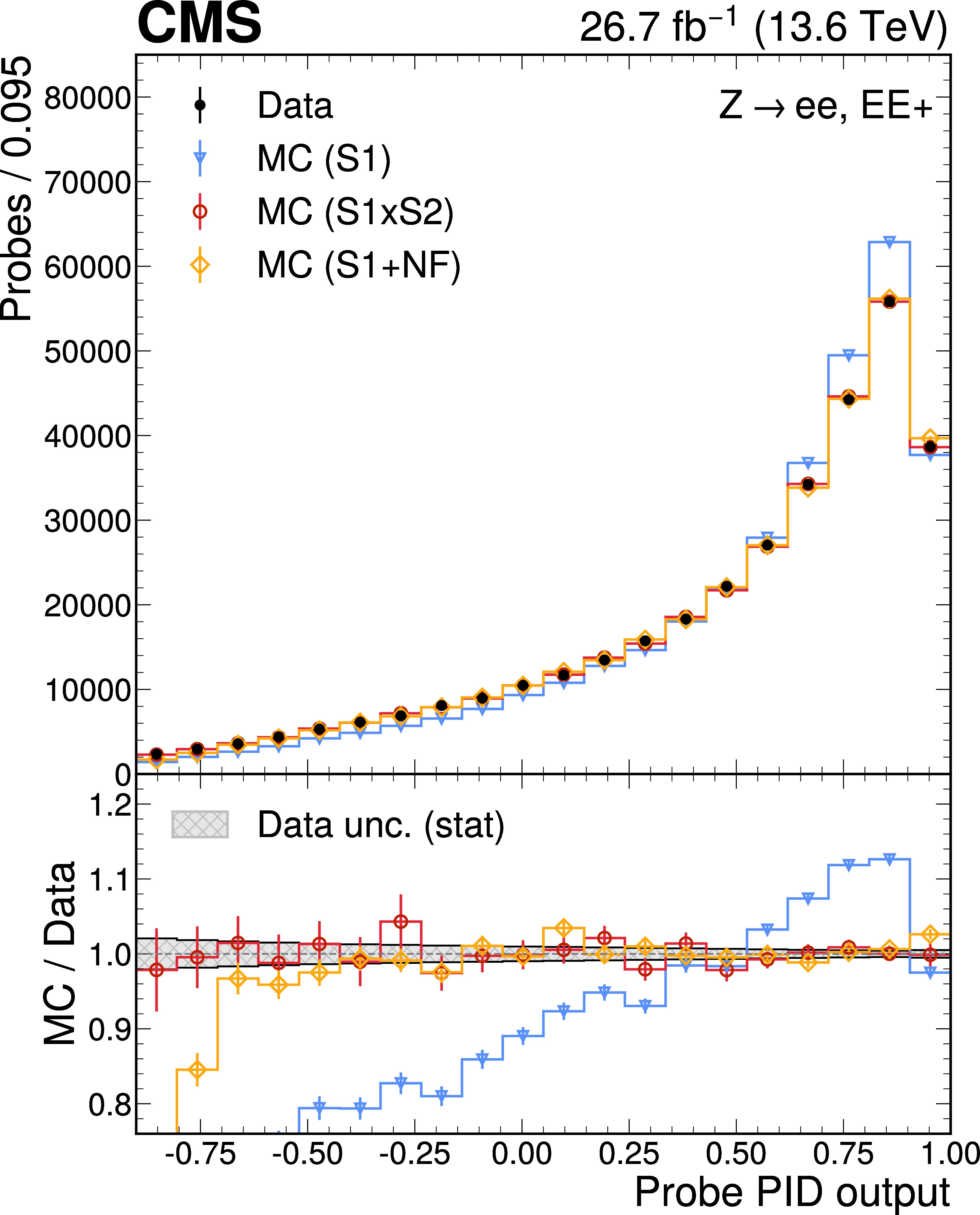
The probe PID output distributions in data (black points) and simulation (coloured histograms with points), for the EE-(left), EB (centre), and EE$ + $ (right) subdetector regions. The statistical uncertainties in the simulation and data are shown by the error bars on the points. The simulation is shown for three scenarios. The blue histograms show the simulation after the initial S1 reweighting to align the kinematic distributions with data. The red and orange histograms show the calibrated simulation after the S2 reweighting and the flow corrections are applied, respectively. The lower panels show the ratio of simulation to data, where the statistical uncertainty in the data is indicated by the grey hatched band. |
png pdf |
Figure 19-a:
The probe PID output distributions in data (black points) and simulation (coloured histograms with points), for the EE-(left), EB (centre), and EE$ + $ (right) subdetector regions. The statistical uncertainties in the simulation and data are shown by the error bars on the points. The simulation is shown for three scenarios. The blue histograms show the simulation after the initial S1 reweighting to align the kinematic distributions with data. The red and orange histograms show the calibrated simulation after the S2 reweighting and the flow corrections are applied, respectively. The lower panels show the ratio of simulation to data, where the statistical uncertainty in the data is indicated by the grey hatched band. |
png pdf |
Figure 19-b:
The probe PID output distributions in data (black points) and simulation (coloured histograms with points), for the EE-(left), EB (centre), and EE$ + $ (right) subdetector regions. The statistical uncertainties in the simulation and data are shown by the error bars on the points. The simulation is shown for three scenarios. The blue histograms show the simulation after the initial S1 reweighting to align the kinematic distributions with data. The red and orange histograms show the calibrated simulation after the S2 reweighting and the flow corrections are applied, respectively. The lower panels show the ratio of simulation to data, where the statistical uncertainty in the data is indicated by the grey hatched band. |
png pdf |
Figure 19-c:
The probe PID output distributions in data (black points) and simulation (coloured histograms with points), for the EE-(left), EB (centre), and EE$ + $ (right) subdetector regions. The statistical uncertainties in the simulation and data are shown by the error bars on the points. The simulation is shown for three scenarios. The blue histograms show the simulation after the initial S1 reweighting to align the kinematic distributions with data. The red and orange histograms show the calibrated simulation after the S2 reweighting and the flow corrections are applied, respectively. The lower panels show the ratio of simulation to data, where the statistical uncertainty in the data is indicated by the grey hatched band. |
png pdf |
Figure 20:
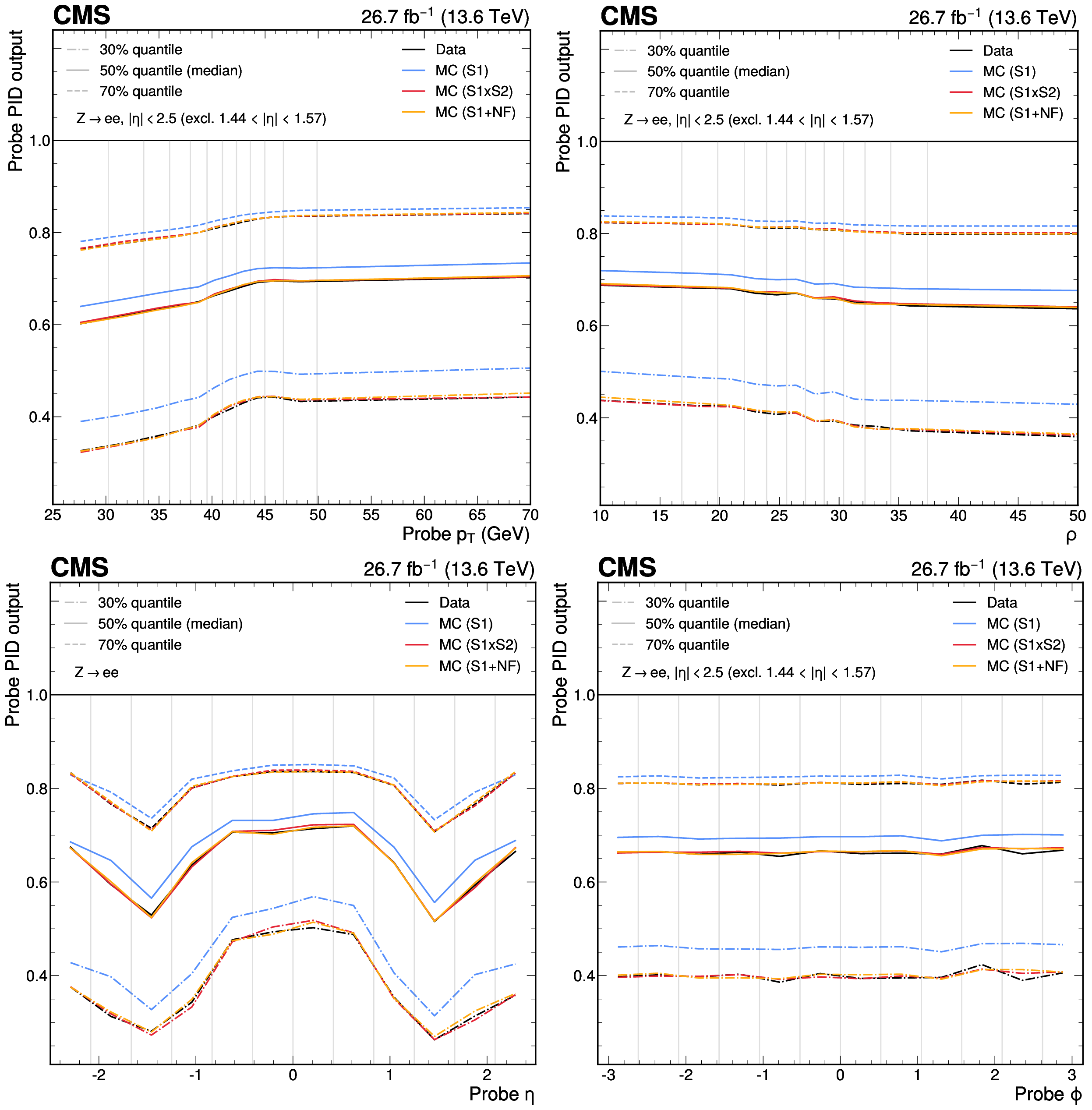
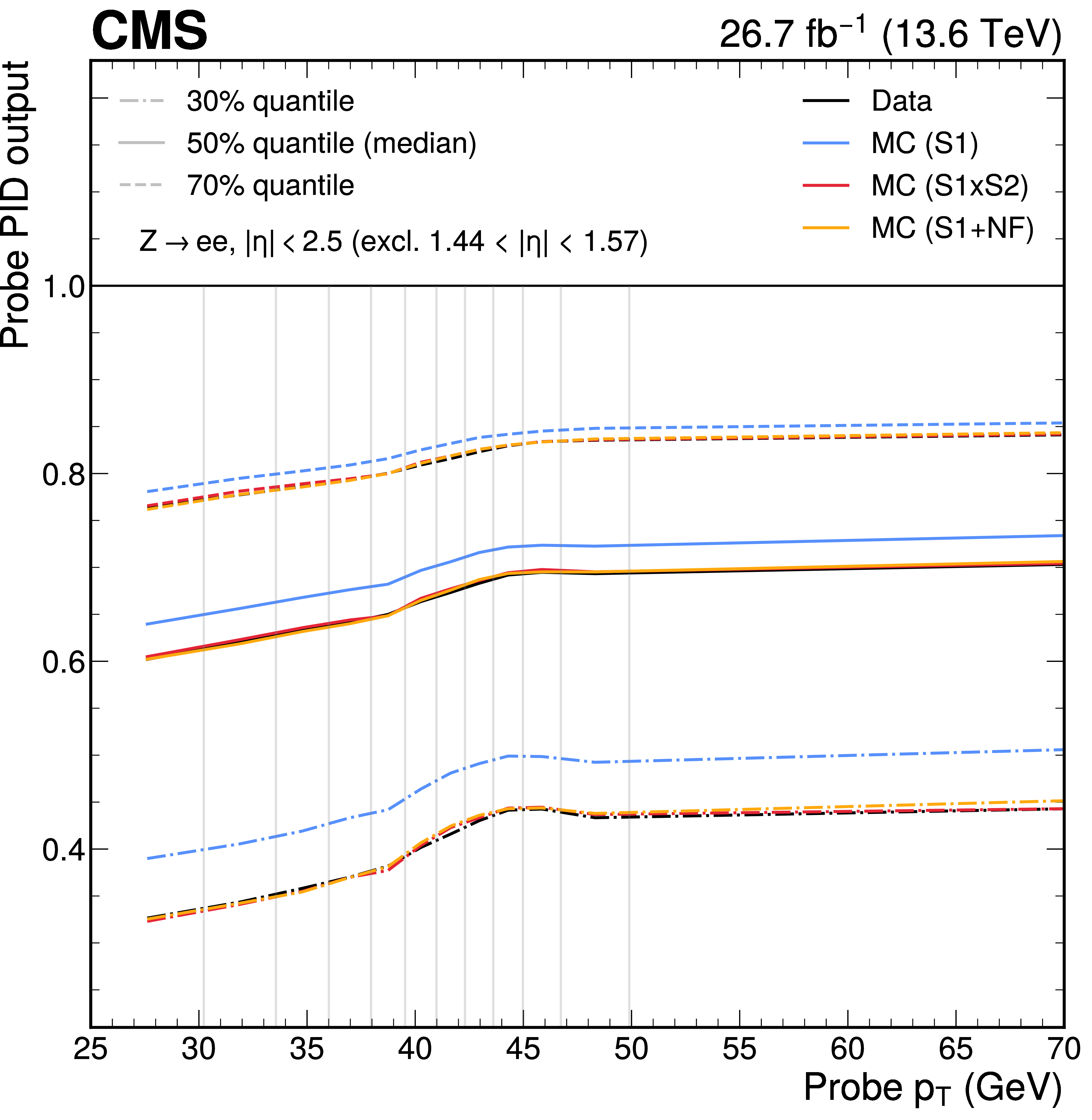
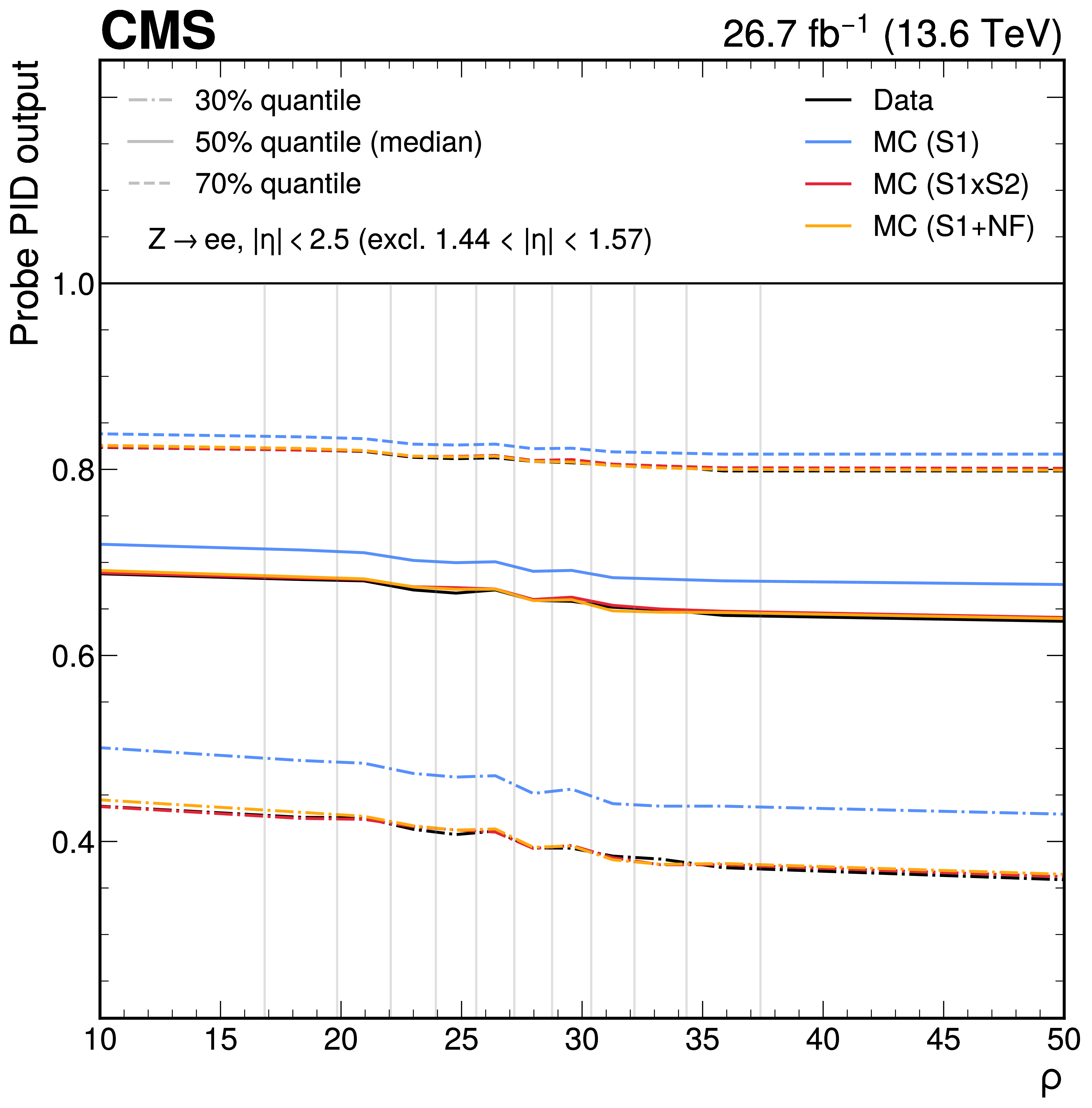
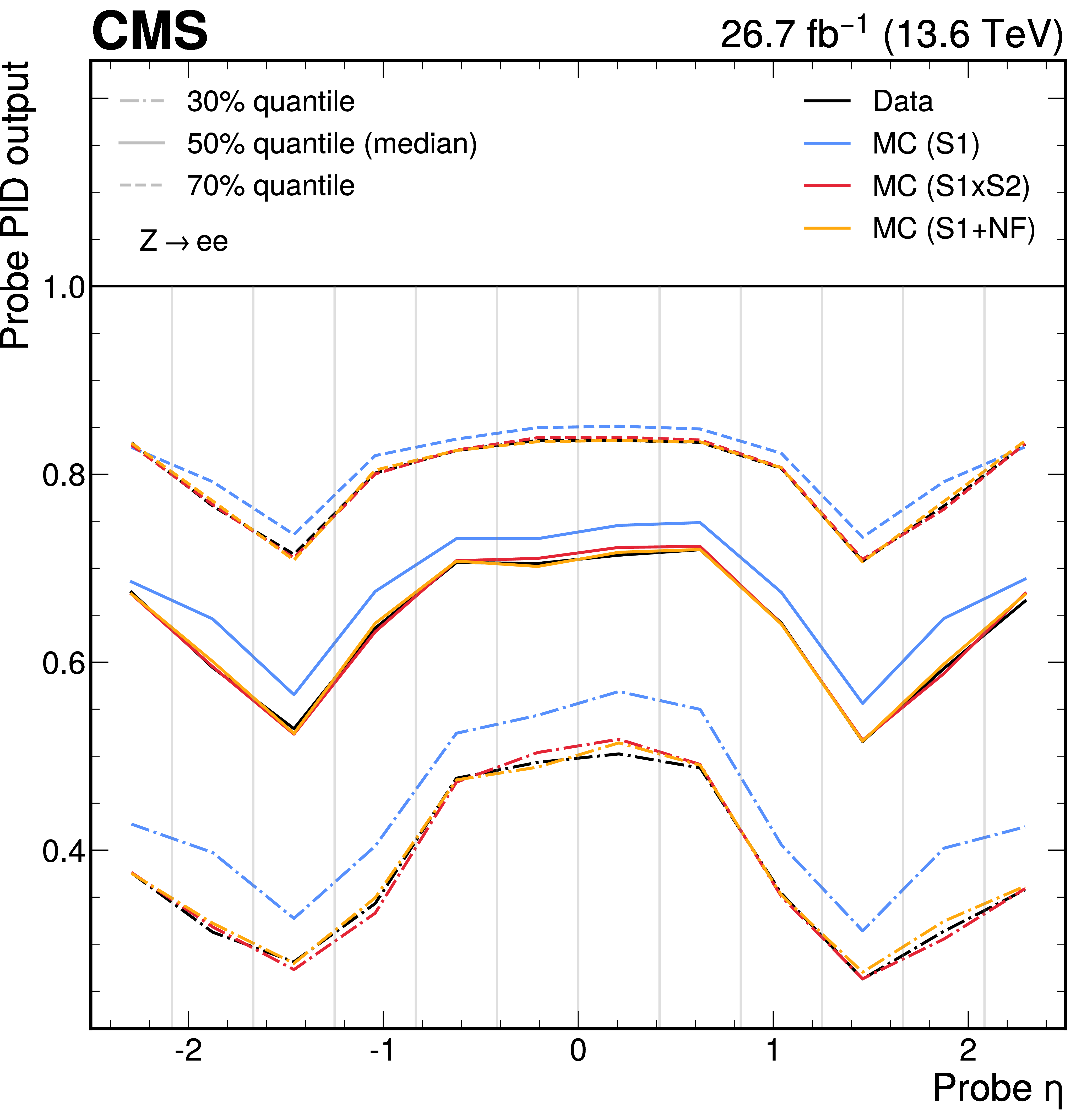
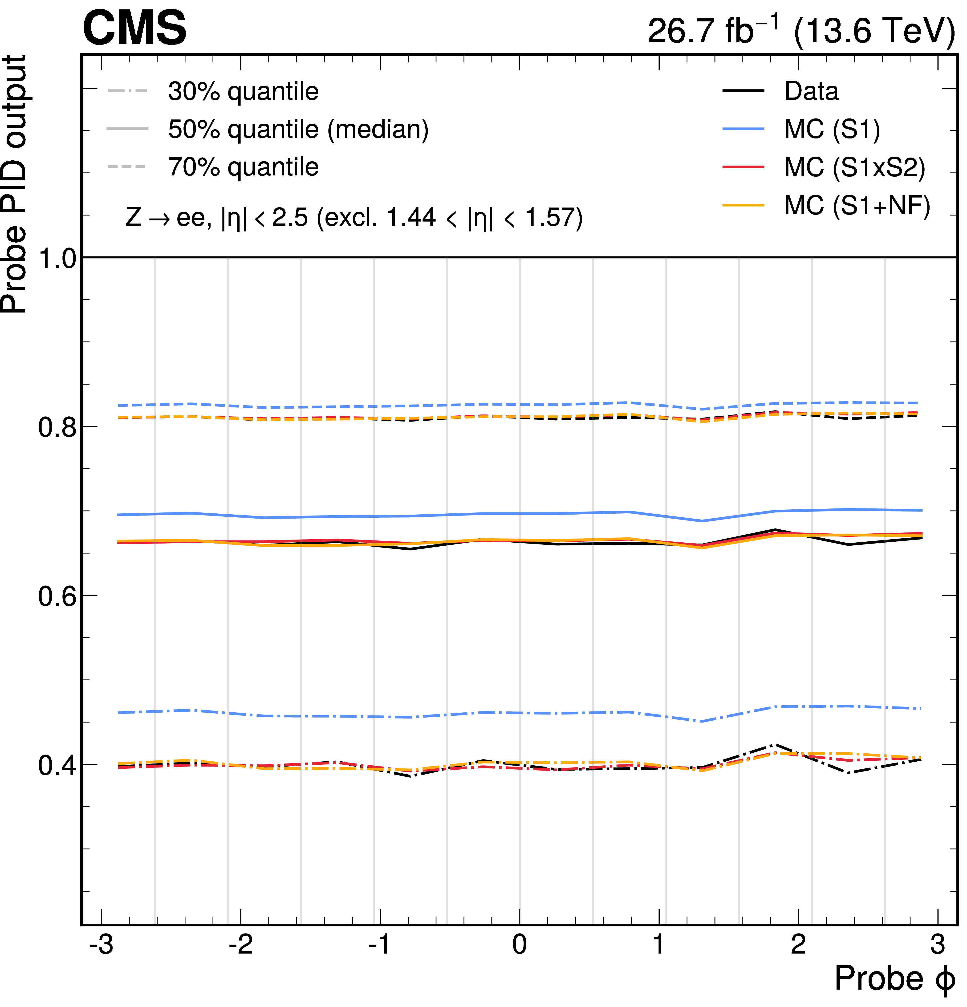
Quantiles of the PID output distribution as a function of the $ x_k $ features: $ p_{\mathrm{T}} $ (upper left), $ \rho $ (upper right), $ \eta $ (lower left), and $ \phi $ (lower right). The probe EM showers are divided into 12 bins for each feature. For $ p_{\mathrm{T}} $ and $ \rho $, bin edges are chosen such that each bin contains an equal number of events in data, while for $ \eta $ and $ \phi $ the bins are linearly spaced. Within each bin, the 30%, 50%, and 70% quantiles of the PID output are shown as dot-dashed, solid, and dashed lines, respectively. The quantiles are shown for data (black), simulation after the initial S1 reweighting (blue), and the calibrated simulation after applying the S2 reweighting (red) or the normalising flow (orange). The quantiles for $ p_{\mathrm{T}} $, $ \rho $, and $ \phi $ are computed inclusively in $ \eta $, across all subdetector regions. |
png pdf |
Figure 20-a:
Quantiles of the PID output distribution as a function of the $ x_k $ features: $ p_{\mathrm{T}} $ (upper left), $ \rho $ (upper right), $ \eta $ (lower left), and $ \phi $ (lower right). The probe EM showers are divided into 12 bins for each feature. For $ p_{\mathrm{T}} $ and $ \rho $, bin edges are chosen such that each bin contains an equal number of events in data, while for $ \eta $ and $ \phi $ the bins are linearly spaced. Within each bin, the 30%, 50%, and 70% quantiles of the PID output are shown as dot-dashed, solid, and dashed lines, respectively. The quantiles are shown for data (black), simulation after the initial S1 reweighting (blue), and the calibrated simulation after applying the S2 reweighting (red) or the normalising flow (orange). The quantiles for $ p_{\mathrm{T}} $, $ \rho $, and $ \phi $ are computed inclusively in $ \eta $, across all subdetector regions. |
png pdf |
Figure 20-b:
Quantiles of the PID output distribution as a function of the $ x_k $ features: $ p_{\mathrm{T}} $ (upper left), $ \rho $ (upper right), $ \eta $ (lower left), and $ \phi $ (lower right). The probe EM showers are divided into 12 bins for each feature. For $ p_{\mathrm{T}} $ and $ \rho $, bin edges are chosen such that each bin contains an equal number of events in data, while for $ \eta $ and $ \phi $ the bins are linearly spaced. Within each bin, the 30%, 50%, and 70% quantiles of the PID output are shown as dot-dashed, solid, and dashed lines, respectively. The quantiles are shown for data (black), simulation after the initial S1 reweighting (blue), and the calibrated simulation after applying the S2 reweighting (red) or the normalising flow (orange). The quantiles for $ p_{\mathrm{T}} $, $ \rho $, and $ \phi $ are computed inclusively in $ \eta $, across all subdetector regions. |
png pdf |
Figure 20-c:
Quantiles of the PID output distribution as a function of the $ x_k $ features: $ p_{\mathrm{T}} $ (upper left), $ \rho $ (upper right), $ \eta $ (lower left), and $ \phi $ (lower right). The probe EM showers are divided into 12 bins for each feature. For $ p_{\mathrm{T}} $ and $ \rho $, bin edges are chosen such that each bin contains an equal number of events in data, while for $ \eta $ and $ \phi $ the bins are linearly spaced. Within each bin, the 30%, 50%, and 70% quantiles of the PID output are shown as dot-dashed, solid, and dashed lines, respectively. The quantiles are shown for data (black), simulation after the initial S1 reweighting (blue), and the calibrated simulation after applying the S2 reweighting (red) or the normalising flow (orange). The quantiles for $ p_{\mathrm{T}} $, $ \rho $, and $ \phi $ are computed inclusively in $ \eta $, across all subdetector regions. |
png pdf |
Figure 20-d:
Quantiles of the PID output distribution as a function of the $ x_k $ features: $ p_{\mathrm{T}} $ (upper left), $ \rho $ (upper right), $ \eta $ (lower left), and $ \phi $ (lower right). The probe EM showers are divided into 12 bins for each feature. For $ p_{\mathrm{T}} $ and $ \rho $, bin edges are chosen such that each bin contains an equal number of events in data, while for $ \eta $ and $ \phi $ the bins are linearly spaced. Within each bin, the 30%, 50%, and 70% quantiles of the PID output are shown as dot-dashed, solid, and dashed lines, respectively. The quantiles are shown for data (black), simulation after the initial S1 reweighting (blue), and the calibrated simulation after applying the S2 reweighting (red) or the normalising flow (orange). The quantiles for $ p_{\mathrm{T}} $, $ \rho $, and $ \phi $ are computed inclusively in $ \eta $, across all subdetector regions. |
| Tables | |
png pdf |
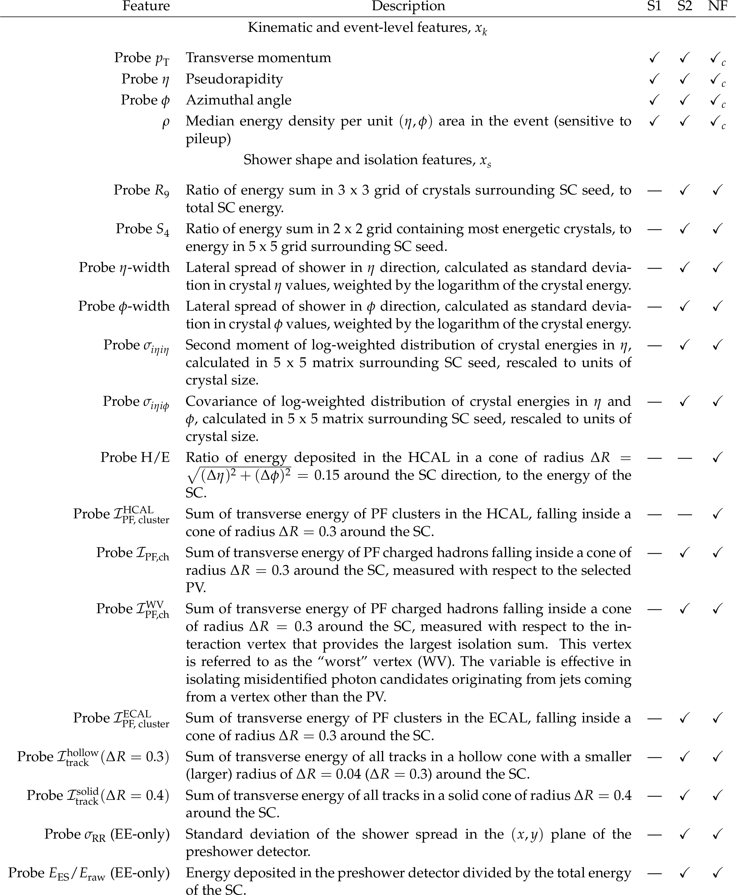
Table 1:
Features used in the calibration algorithms. The features are split into two subsets: kinematic and event-level features, $ x_k $, and shower shape and isolation features, $ x_s $. The final three columns show whether the feature is used as an input for each model, as indicated by a checkmark. The labels S1, S2, and NF refer to the Stage 1 reweighting model, the Stage 2 reweighting model, and the normalising-flow model, respectively, as described in Section 5. The checkmarks with a ``c" subscript highlight the conditional features for the normalising-flow model. A more detailed description of each feature is provided in Refs. [39,none-none-none-none]. |
png pdf |
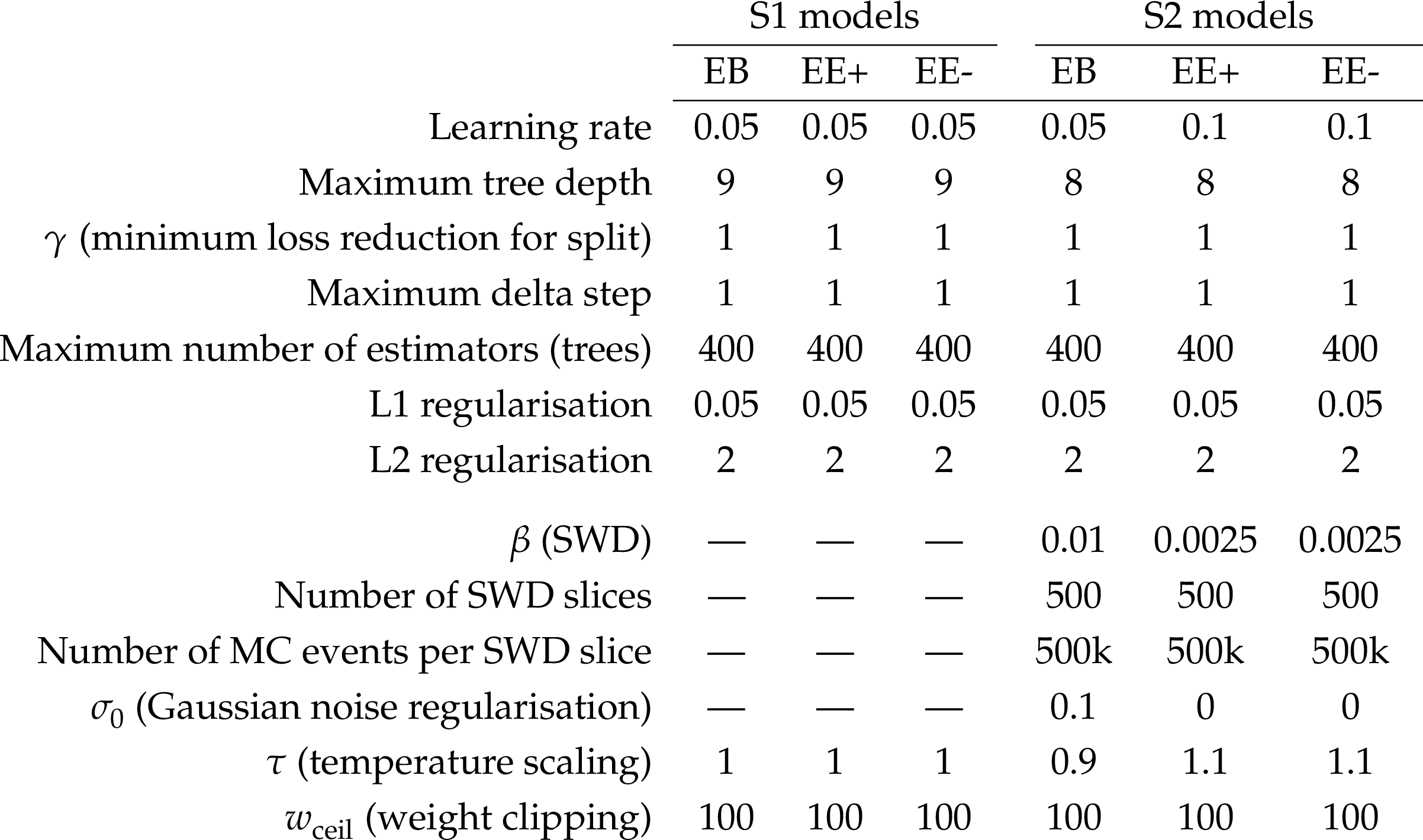
Table 2:
Summary of hyperparameters used in the reweighting models. The first block lists the XGBOOST-specific parameters, where information on the meaning of each parameter can be found in the XGBOOST documentation [none]. The parameters not listed are set to the XGBOOST (v2.1.4) default values. The second block contains additional custom parameters, which are described in the text. |
png pdf |
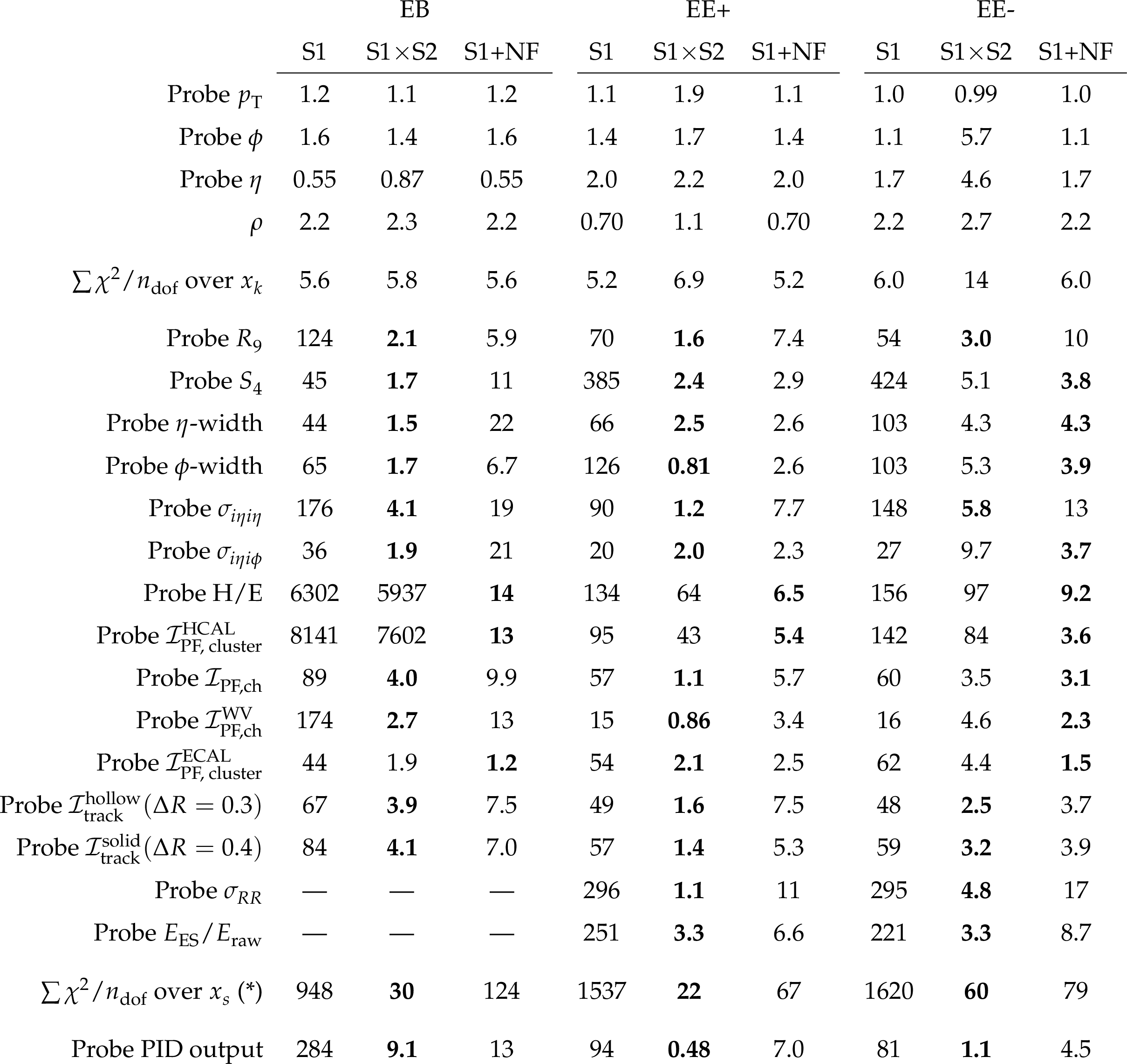
Table 3:
A comparison of the 1D $ \chi^2/n_{\mathrm{dof}} $ metric for the three scenarios: MC (S1), MC (S1$ \times $S2) and MC (S1+NF). The first four rows correspond to the kinematic and event-level features $ x_k $, to highlight the level of kinematic invariance achieved with the S2 reweighting model. The normalising-flow method does not change the $ x_k $ distributions, and therefore the values for S1 and S1+NF are identical. The sum of $ \chi^2/n_{\mathrm{dof}} $ values calculated over the $ x_k $ features are also provided as a global metric for the level of kinematic invariance achieved. The following rows correspond to the shower shape and isolation features $ x_s $, which show the improved agreement after the calibration methods are applied. This is further quantified by the sum of $ \chi^2/n_{\mathrm{dof}} $ values calculated over the $ x_s $ features. The asterisk indicates that H/E and $ \mathcal{I}^{\mathrm{HCAL}}_{\text{PF, cluster}} $ are omitted from the sums, as these features are not used as inputs into the S2 reweighting model. The final row shows the reduction in the 1D $ \chi^2/n_{\mathrm{dof}} $ values for the PID output. Boldface indicates the best performing calibration method for each of the corrected $ x_s $ features, the summed $ x_s $ metric, and the PID output. We note that the $ \chi^2/n_{\mathrm{dof}} $ values for the reweighting method (S1$ \times $S2) include the inflated statistical uncertainties in the simulation, often leading to smaller values than the normalising-flow method (S1+NF). |
png pdf |
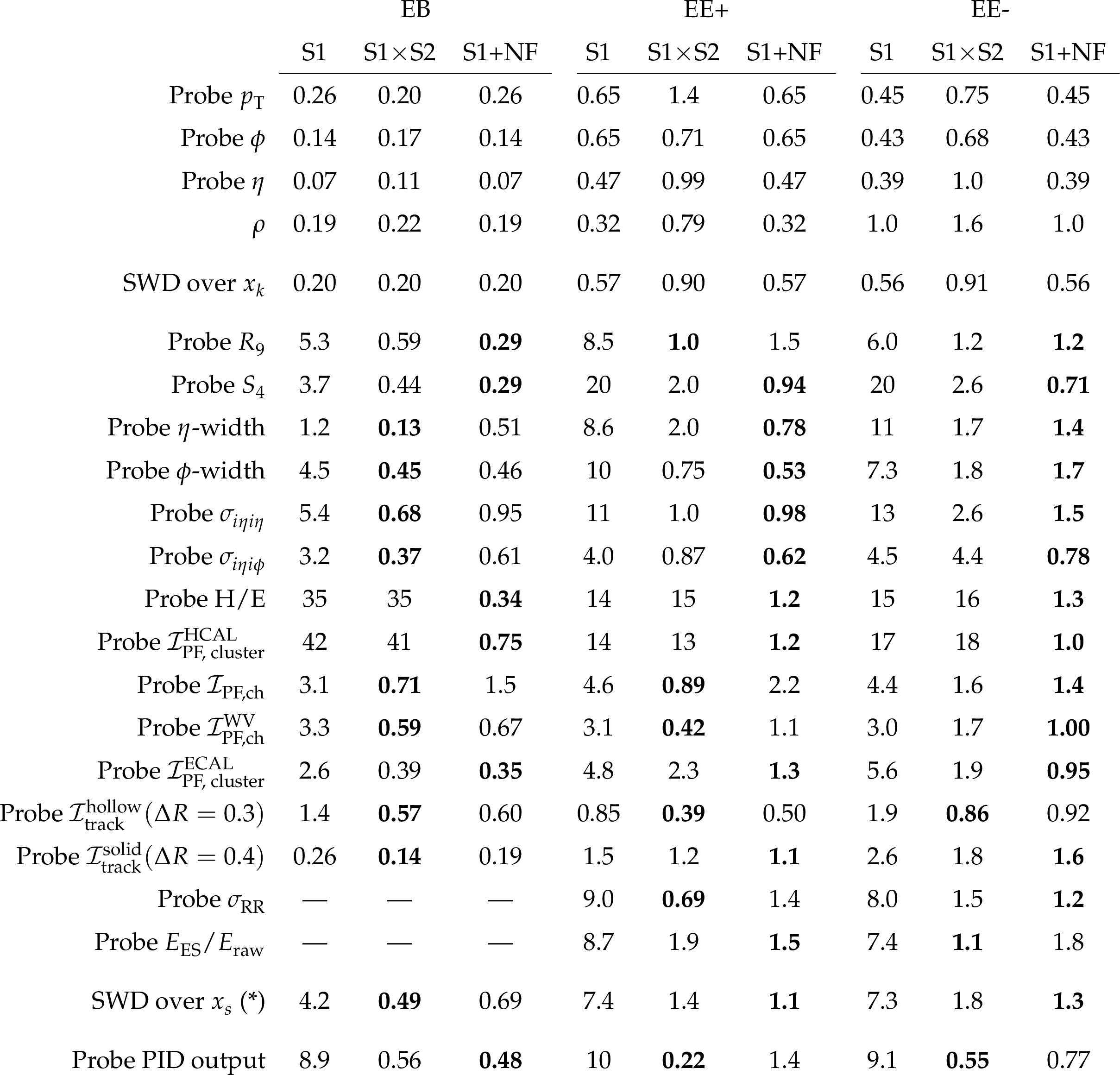
Table 4:
A comparison of the EMD metric for the three scenarios: MC (S1), MC (S1$ \times $S2) and MC (S1+NF). The EMD values are calculated for the normalised feature distributions, and scaled by a factor of 100 for readability. The first four rows correspond to the kinematic and event-level features $ x_k $, to highlight the level of kinematic invariance achieved with the S2 reweighting model. The normalising-flow method does not change the $ x_k $ distributions, and therefore the values for S1 and S1+NF are identical. The SWD values calculated for 500 randomly sampled slices of the $ x_k $ feature space and averaged over are also provided as a global metric for the level of kinematic invariance achieved. The following rows correspond to the shower shape and isolation features $ x_s $, which show the improved agreement after the calibration methods are applied. This is further quantified by the SWD values calculated over the $ x_s $ feature space using the same number of slices as for $ x_k $. The asterisk indicates that H/E and $ \mathcal{I}^{\mathrm{HCAL}}_{\text{PF, cluster}} $ are omitted from the SWD calculations, as these features are not used as inputs into the S2 reweighting model. The final row shows the reduction in the EMD values for the PID output. Boldface indicates the best performing calibration method for each of the corrected $ x_s $ features, the SWD over $ x_s $ metric, and the PID output. |
| Summary |
| Particle physics measurements depend on comparisons between Monte Carlo simulations and data. Discrepancies arising from imperfect simulation can introduce biases, which are accounted for by assigning systematic uncertainties to cover the mismodelling effects. Improving the calibration of simulation can help mitigate these biases, thereby reducing the associated systematic uncertainties and enhancing the precision of measurements and the sensitivity of searches for new physics. In this paper, two machine-learning (ML) based calibration methods are presented. The methods are employed to correct the features of simulated electromagnetic (EM) showers, as measured with the CMS detector. A subset of the proton-proton collision data collected by the CMS experiment in 2022 at $ \sqrt{s}= $ 13.6 TeV is used, corresponding to an integrated luminosity of 26.7 fb$ ^{-1} $. The tag-and-probe technique is applied to $ \mathrm{Z}\to\mathrm{e}\mathrm{e} $ decays to obtain a pure sample of EM showers in both simulation and data. The probe EM showers are then used to train the ML calibration methods to correct a high-dimensional feature space characterising the shower shape and isolation properties. The corrections are conditioned on the kinematic properties of the EM shower, as well as a variable sensitive to the pileup conditions. The final performance is evaluated by comparing the agreement between simulation and data in the output of a particle identification algorithm based on the corrected features. The two methods follow fundamentally different approaches. The reweighting method is an example of vertical morphing. An ML classifier is trained to distinguish between samples drawn from simulation and data, effectively learning the ratio of conditional densities between the two classes. The classifier output is then translated to a weight, which acts as a multiplicative correction to the total event weight. In contrast, the normalising flow method demonstrates horizontal morphing. A high-dimensional transformation is learned that directly modifies the input feature values of the simulation to match the data distribution. Each method offers different advantages and limitations, which are important to consider when applying them in particle physics analyses. Both methods offer a significant advantage over traditional calibration techniques by providing continuous corrections in high-dimensional feature spaces. The ML methods demonstrate excellent performance in correcting the input features, as well as the particle identification output distribution. This work documents the first application of these advanced ML calibration techniques to collision data in CMS, and serves as both motivation and guidance for future applications of these methods in particle physics and related fields. |
| References | ||||
| 1 | CMS Collaboration | Measurements of Higgs boson production cross sections and couplings in the diphoton decay channel at $ \sqrt{\mathrm{s}} = $ 13 TeV | JHEP 07 (2021) 027 | CMS-HIG-19-015 2103.06956 |
| 2 | CMS Collaboration | The CMS experiment at the CERN LHC | JINST 3 (2008) S08004 | |
| 3 | CMS Collaboration | Development of the CMS detector for the CERN LHC Run 3 | JINST 19 (2024) P05064 | |
| 4 | CMS Collaboration | The CMS electromagnetic calorimeter project: Technical Design Report | CERN-LHCC-97-033, 1997 | |
| 5 | CMS Collaboration | Description and performance of track and primary-vertex reconstruction with the CMS tracker | JINST 9 (2014) P10009 | CMS-TRK-11-001 1405.6569 |
| 6 | CMS Collaboration | Measurements of inclusive $ W $ and $ Z $ cross sections in $ pp $ collisions at $ \sqrt{s}= $ 7 TeV | JHEP 01 (2011) 080 | CMS-EWK-10-002 1012.2466 |
| 7 | A. Rogozhnikov | Reweighting with boosted decision trees | J. Phys. Conf. Ser. 762 (2016) 012036 | 1608.05806 |
| 8 | K. Cranmer, J. Pavez, and G. Louppe | Approximating likelihood ratios with calibrated discriminative classifiers | 1506.02169 | |
| 9 | A. Andreassen and B. Nachman | Neural networks for full phase-space reweighting and parameter tuning | PRD 101 (2020) 091901 | 1907.08209 |
| 10 | B. Nachman and J. Thaler | Neural conditional reweighting | PRD 105 (2022) 076015 | 2107.08979 |
| 11 | S. Diefenbacher et al. | DCTRGAN: Improving the precision of generative models with reweighting | JINST 15 (2020) P11004 | 2009.03796 |
| 12 | CMS Collaboration | Reweighting simulated events using machine-learning techniques in the CMS experiment | EPJC 85 (2025) 495 | CMS-MLG-24-001 2411.03023 |
| 13 | C. Pollard and P. Windischhofer | Transport away your problems: Calibrating stochastic simulations with optimal transport | NIM A 1027 (2022) 166119 | 2107.08648 |
| 14 | E. G. Tabak and C. V. Turner | A family of nonparametric density estimation algorithms | Commun. Pure Appl. Math. 66 (2013) 145 | |
| 15 | E. Tabak and E. Vanden-Eijnden | Density estimation by dual ascent of the log-likelihood | Commun. Math. Sci. 8 (2010) 217 | |
| 16 | T. Golling, S. Klein, R. Mastandrea, and B. Nachman | Flow-enhanced transportation for anomaly detection | PRD 107 (2023) 096025 | 2212.11285 |
| 17 | J. A. Raine, S. Klein, D. Sengupta, and T. Golling | CURTAINs for your sliding window: Constructing unobserved regions by transforming adjacent intervals | Front. Big Data 6 (2023) 899345 | 2203.09470 |
| 18 | A. Hallin et al. | Classifying anomalies through outer density estimation | PRD 106 (2022) 055006 | 2109.00546 |
| 19 | M. Algren et al. | Flow away your differences: conditional normalizing flows as an improvement to reweighting | Submitted to SciPost Phys, 2023 | 2304.14963 |
| 20 | S. Bright-Thonney, P. Harris, P. McCormack, and S. Rothman | Chained quantile morphing with normalizing flows | 2309.15912 | |
| 21 | T. Golling et al. | Morphing one dataset into another with maximum likelihood estimation | PRD 108 (2023) 096018 | 2309.06472 |
| 22 | G. Papamakarios et al. | Normalizing flows for probabilistic modeling and inference | J. Mach. Learn. Res. 22 (2021) 1 | 1912.02762 |
| 23 | C. Daumann et al. | One flow to correct them all: Improving simulations in high-energy physics with a single normalising flow and a switch | Comput. Softw. Big Sci. 8 (2024) 15 | 2403.18582 |
| 24 | CMS Collaboration | Measurements of inclusive and differential Higgs boson production cross sections at $ \sqrt{\text{s}}= $ 13.6 TeV in the H \textrightarrow \ensuremath\gamma\ensuremath\gamma decay channel | JHEP 09 (2025) 070 | CMS-HIG-23-014 2504.17755 |
| 25 | B. Amos, L. Xu, and J. Z. Kolter | Input convex neural networks | Proc. Mach. Learn. Res. 70 (2017) 146 | |
| 26 | ATLAS Collaboration | A continuous calibration of the ATLAS flavour-tagging classifiers via optimal transportation maps | Eur. Phys. J. C. 85 (2025) 1272 | 2505.13063 |
| 27 | CMS Collaboration | Measurement of the Higgs boson inclusive and differential fiducial production cross sections in the diphoton decay channel with pp collisions at $ \sqrt{s} = $ 13 TeV | JHEP 07 (2023) 091 | CMS-HIG-19-016 2208.12279 |
| 28 | A. Stein, X. Coubez, S. Mondal et al. | Improving robustness of jet tagging algorithms with adversarial training | Comput. Softw. Big Sci. 6 (2022) 15 | |
| 29 | CMS Collaboration | Identification of tau leptons using a convolutional neural network with domain adaptation | JINST 20 (2025) P12032 | CMS-TAU-24-001 2511.05468 |
| 30 | A. Andreassen et al. | OmniFold: A method to simultaneously unfold all observables | PRL 124 (2020) 182001 | 1911.09107 |
| 31 | ATLAS Collaboration | Simultaneous unbinned differential cross-section measurement of twenty-four Z+jets kinematic observables with the ATLAS detector | PRL 133 (2024) 261803 | 2405.20041 |
| 32 | CMS Collaboration | Measurement of event shapes in minimum-bias events from proton-proton collisions at $ \sqrt{s}= $ 13 TeV | PRD 112 (2025) 112006 | CMS-SMP-23-008 2505.17850 |
| 33 | ATLAS Collaboration | Measurement of off-shell Higgs boson production in the $ H^*\rightarrow ZZ\rightarrow 4\ell $ decay channel using a neural simulation-based inference technique in 13 TeV pp collisions with the ATLAS detector | Rept. Prog. Phys. 88 (2025) 057803 | 2412.01548 |
| 34 | M. Mieskolainen | ICENET: A deep learning library for HEP | link | |
| 35 | C. Daumann and D. Valsecchi | OneFlow-Morphing | link | |
| 36 | CMS Collaboration | Performance of the CMS Level-1 trigger in proton-proton collisions at $ \sqrt{s} = $ 13 TeV | JINST 15 (2020) P10017 | CMS-TRG-17-001 2006.10165 |
| 37 | CMS Collaboration | The CMS trigger system | JINST 12 (2017) P01020 | CMS-TRG-12-001 1609.02366 |
| 38 | CMS Collaboration | Performance of the CMS high-level trigger during LHC Run 2 | JINST 19 (2024) P11021 | CMS-TRG-19-001 2410.17038 |
| 39 | CMS Collaboration | Electron and photon reconstruction and identification with the CMS experiment at the CERN LHC | JINST 16 (2021) P05014 | CMS-EGM-17-001 2012.06888 |
| 40 | CMS Collaboration | Performance of the CMS muon detector and muon reconstruction with proton-proton collisions at $ \sqrt{s}= $ 13 TeV | JINST 13 (2018) P06015 | CMS-MUO-16-001 1804.04528 |
| 41 | CMS Collaboration | Luminosity measurement in proton-proton collisions at 13.6 TeV in 2022 at CMS | CMS-PAS-LUM-22-001 | |
| 42 | CMS Collaboration | Electron and photon reconstruction and identification performance at CMS in 2022 and 2023 | CMS-DP-2024-052, 2024 | |
| 43 | J. Alwall et al. | The automated computation of tree-level and next-to-leading order differential cross sections, and their matching to parton shower simulations | JHEP 07 (2014) 079 | 1405.0301 |
| 44 | C. Bierlich et al. | A comprehensive guide to the physics and usage of PYTHIA 8.3 | SciPost Phys. Codeb. 2022 (2022) 8 | 2203.11601 |
| 45 | CMS Collaboration | Extraction and validation of a new set of CMS PYTHIA8 tunes from underlying-event measurements | EPJC 80 (2020) 4 | CMS-GEN-17-001 1903.12179 |
| 46 | NNPDF Collaboration | Parton distributions from high-precision collider data | EPJC 77 (2017) 663 | 1706.00428 |
| 47 | GEANT4 Collaboration | GEANT 4---a simulation toolkit | NIM A 506 (2003) 250 | |
| 48 | CMS Collaboration | Technical proposal for the Phase-II upgrade of the Compact Muon Solenoid | CMS Technical Proposal CERN-LHCC-2015-010, CMS-TDR-15-02, 2015 CDS |
|
| 49 | CMS Collaboration | Particle-flow reconstruction and global event description with the CMS detector | JINST 12 (2017) P10003 | CMS-PRF-14-001 1706.04965 |
| 50 | T. Chen and C. Guestrin | XGBoost: A Scalable Tree Boosting System | Proc. of the 22nd, 2016 ACM SIGKDD Int. Conf. on Knowledge Discovery and Data Mining 22 (2016) 785 |
|
| 51 | A. Paszke et al. | Pytorch: An imperative style, high-performance deep learning library | Adv. Neural Inf. Process. Syst. 32 (2019) 8024 | |
| 52 | M. F. Hutchinson | A stochastic estimator of the trace of the influence matrix for Laplacian smoothing splines | Simul. Comput. 19 (1990) 433 | |
| 53 | J. Rabin, G. Peyr é , J. Delon, and M. Bernot | Wasserstein barycenter and its application to texture mixing | in Proc. Int. Conf. on Scale Space and Variational Methods in Computer Vision Springer. 201 (1900) 435 |
|
| 54 | N. Bonneel, J. Rabin, G. Peyr é , and H. Pfister | Sliced and radon Wasserstein barycenters of measures | J. Math. Imaging Vis. 51 (2015) 22 | |
| 55 | C. Villani | Optimal Transport: Old and New | Springer, 2009 link |
|
| 56 | B.-H. Tran, G. Franzese, P. Michiardi, and M. Filippone | One-line-of-code data mollification improves optimization of likelihood-based generative models | Adv. Neural Inf. Process. Syst. 36 (2023) 6545 | |
| 57 | J. Bergstra and Y. Bengio | Random search for hyper-parameter optimization | J. Mach. Learn. Res. 13 (2012) 281 | |
| 58 | C. Guo, G. Pleiss, Y. Sun, and K. Q. Weinberger | On calibration of modern neural networks | Proc. Mach. Learn. Res. 70 (2017) 1321 | |
| 59 | T. Hastie, R. Tibshirani, and J. Friedman | The elements of statistical learning: Data mining, inference and prediction | Springer, 2nd ed, 2009 | |
| 60 | CMSnoop | Multiobjective optimization using evolutionary algorithms | \hrefK. Deb, Wiley, New York, 2001 | |
| 61 | I. Kobyzev, S. J. D. Prince, and M. A. Brubaker | Normalizing flows: An introduction and review of current methods | IEEE Transactions on Pattern Analysis and Mach. Intell. 43 (2020) 3964 | |
| 62 | L. Dinh, J. Sohl - Dickstein, and S. Bengio | Density estimation using real NVP | Int. Conf. on Learning Representations, 2017 link |
|
| 63 | D. P. Kingma and P. Dhariwal | Glow: Generative flow with invertible 1x1 convolutions | Adv. Neural Inf. Process. Syst. 31 (2018) 10236 | |
| 64 | C. Durkan, A. Bekasov, I. Murray, and G. Papamakarios | Neural spline flows | Adv. Neural Inf. Process. Syst. 32 (2019) 7511 | |
| 65 | T. M \"u ller et al. | Neural importance sampling | ACM Transactions on Graphics 38 (2018) 1 | |
| 66 | J. Serr \`a , S. Pascual, and C. Segura Perales | Blow: a single-scale hyperconditioned flow for non-parallel raw-audio voice conversion | Adv. Neural Inf. Process. Syst. 32 (2019) 6790 | |
| 67 | F. Rozet et al. | Zuko: Normalizing flows in PyTorch | link | |
| 68 | R. Kansal et al. | Evaluating generative models in high energy physics | PRD 107 (2023) 076017 | 2211.10295 |
| 69 | CMS Collaboration | Performance of reconstruction and identification of $ \tau $ leptons decaying to hadrons and $ \nu_\tau $ in pp collisions at $ \sqrt{s}= $ 13 TeV | JINST 13 (2018) P10005 | CMS-TAU-16-003 1809.02816 |
|
|
Compact Muon Solenoid LHC, CERN |

|
|
|
|
|
|