

Compact Muon Solenoid
LHC, CERN
| CMS-HIG-24-011 ; CERN-EP-2025-279 | ||
| Measurement of the Higgs boson total decay width using the $ \mathrm{H} \to \mathrm{W}\mathrm{W} \to \mathrm{e}\nu\mu\nu $ decay channel in proton-proton collisions at $ \sqrt{s} = $ 13 TeV | ||
| CMS Collaboration | ||
| 8 January 2026 | ||
| Phys. Rev. D 113, 092014 | ||
| Abstract: The Higgs boson (H) decay width is determined from the ratio of off- and on-shell production of $ \mathrm{H} \to \mathrm{W}\mathrm{W} \to \mathrm{e}\nu\mu\nu $ using proton-proton collision data corresponding to an integrated luminosity of 138 fb$ ^{-1} $ collected at $ \sqrt{s}= $ 13 TeV by the CMS experiment at the LHC. The off-shell signal strength is measured as $ \mu_{\text{off-shell} } = $ 1.2 $ ^{+0.8}_{-0.7} $. The Higgs boson total decay width is $ \Gamma_{\mathrm{H}} = $ 3.9 $ ^{+2.7}_{-2.2} $ MeV, in agreement with the standard model prediction. The uncertainty in this result represents a factor of three improvement over the previous CMS result in this decay channel. | ||
| Links: e-print arXiv:2601.05168 [hep-ex] (PDF) ; CDS record ; inSPIRE record ; CADI line (restricted) ; | ||
| Figures | |
png pdf |
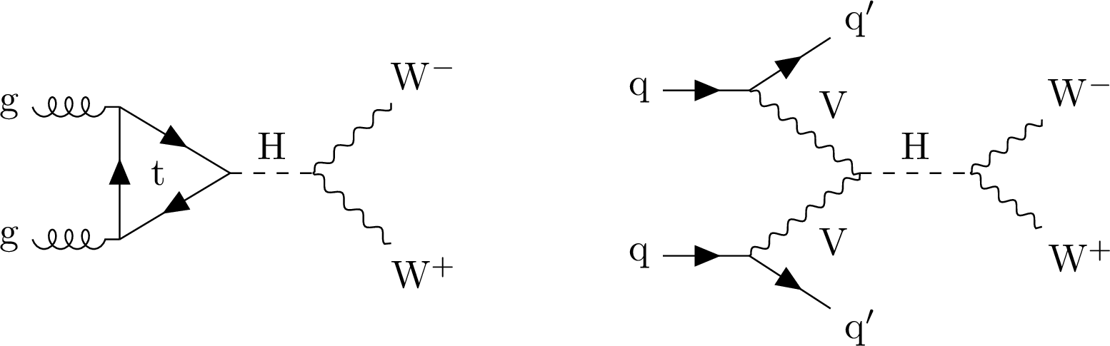
Figure 1:
Feynman diagrams illustrating Higgs boson production and decays to WW in ggF (left) and VBF (right) modes. |
png pdf |
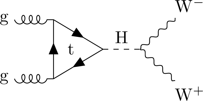
Figure 1-a:
Feynman diagrams illustrating Higgs boson production and decays to WW in ggF (left) and VBF (right) modes. |
png pdf |
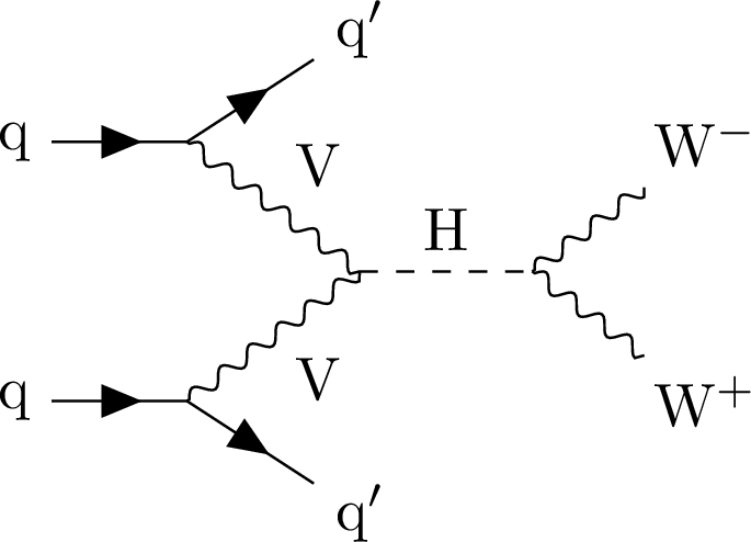
Figure 1-b:
Feynman diagrams illustrating Higgs boson production and decays to WW in ggF (left) and VBF (right) modes. |
png pdf |
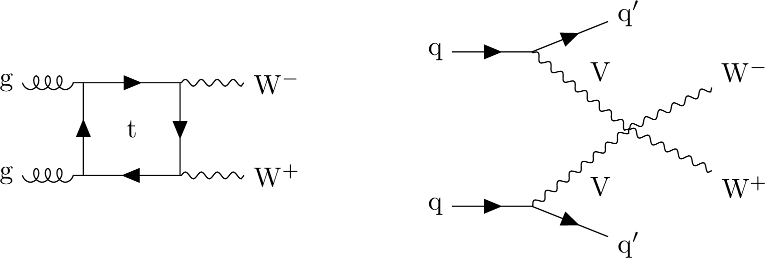
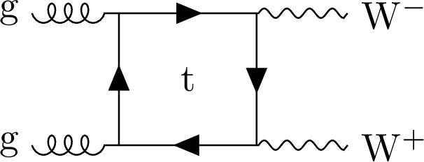
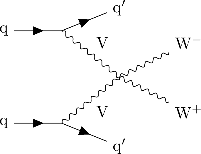
Figure 2:
Feynman diagrams for nonresonant WW production: $ \mathrm{g}\mathrm{g} \to \mathrm{W}\mathrm{W} $ (left) and $ \mathrm{q}\mathrm{q} \to \mathrm{q}\mathrm{q}\mathrm{W}\mathrm{W} $ (right). |
png pdf |
Figure 2-a:
Feynman diagrams for nonresonant WW production: $ \mathrm{g}\mathrm{g} \to \mathrm{W}\mathrm{W} $ (left) and $ \mathrm{q}\mathrm{q} \to \mathrm{q}\mathrm{q}\mathrm{W}\mathrm{W} $ (right). |
png pdf |
Figure 2-b:
Feynman diagrams for nonresonant WW production: $ \mathrm{g}\mathrm{g} \to \mathrm{W}\mathrm{W} $ (left) and $ \mathrm{q}\mathrm{q} \to \mathrm{q}\mathrm{q}\mathrm{W}\mathrm{W} $ (right). |
png pdf |
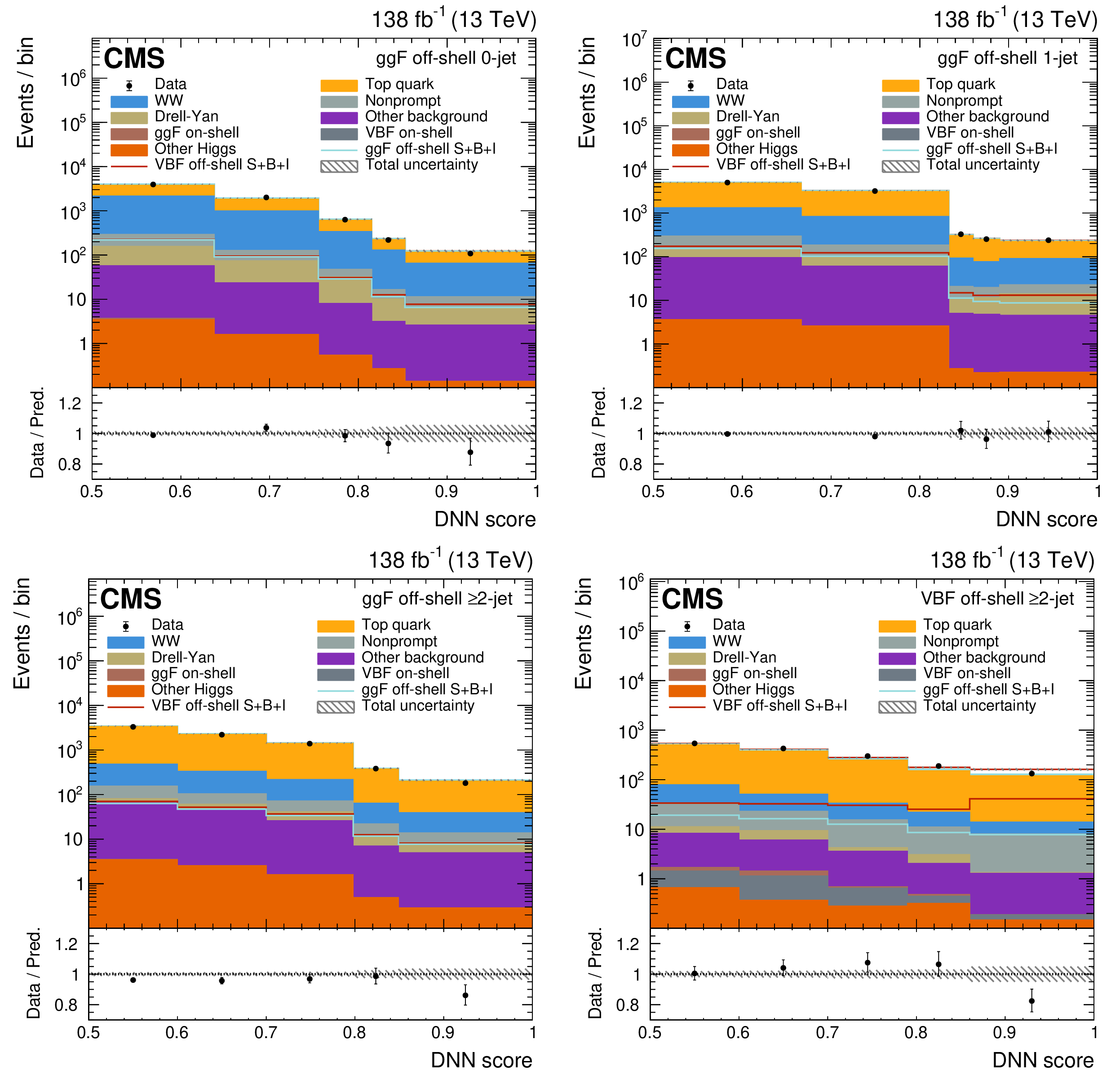
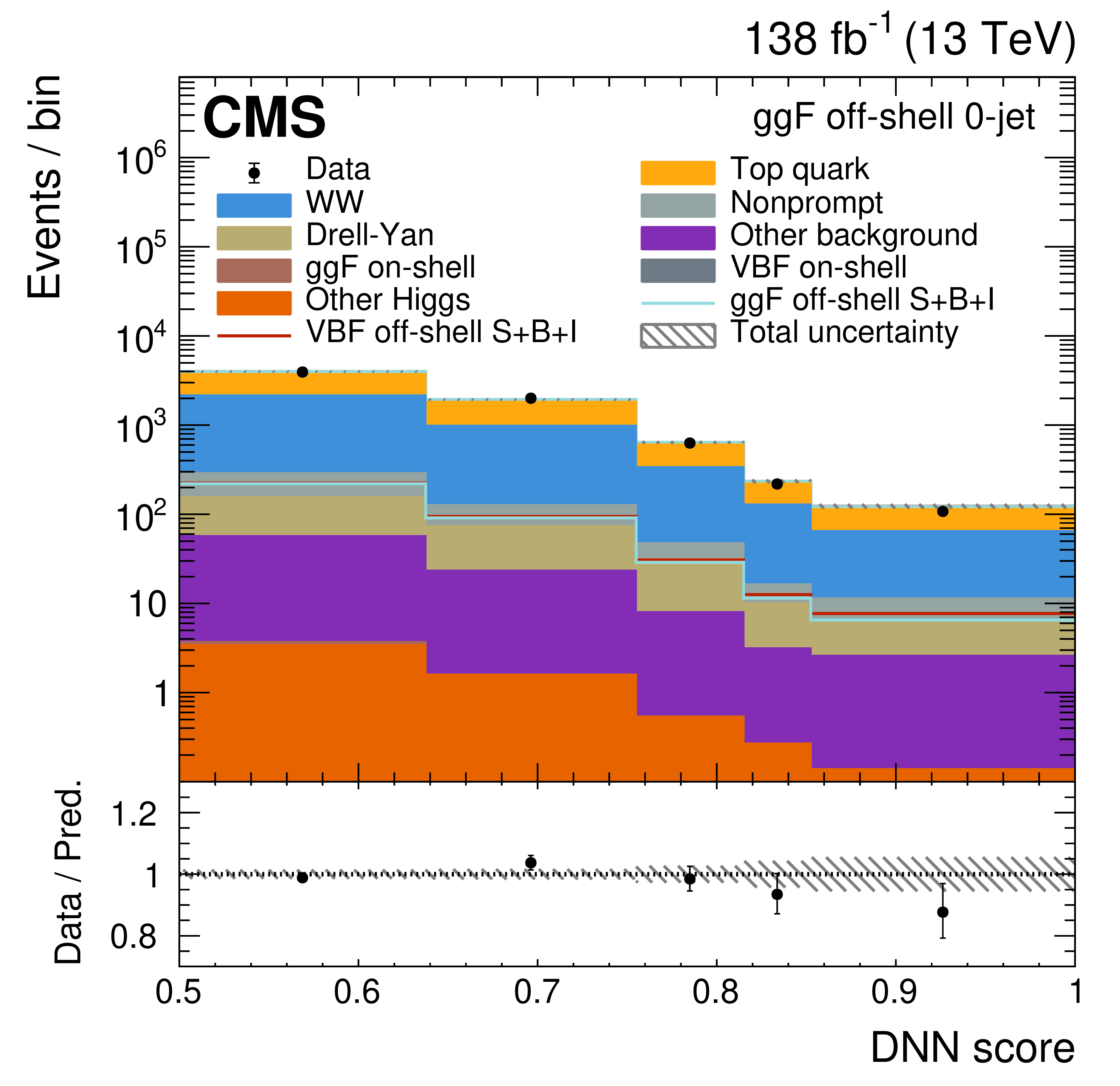
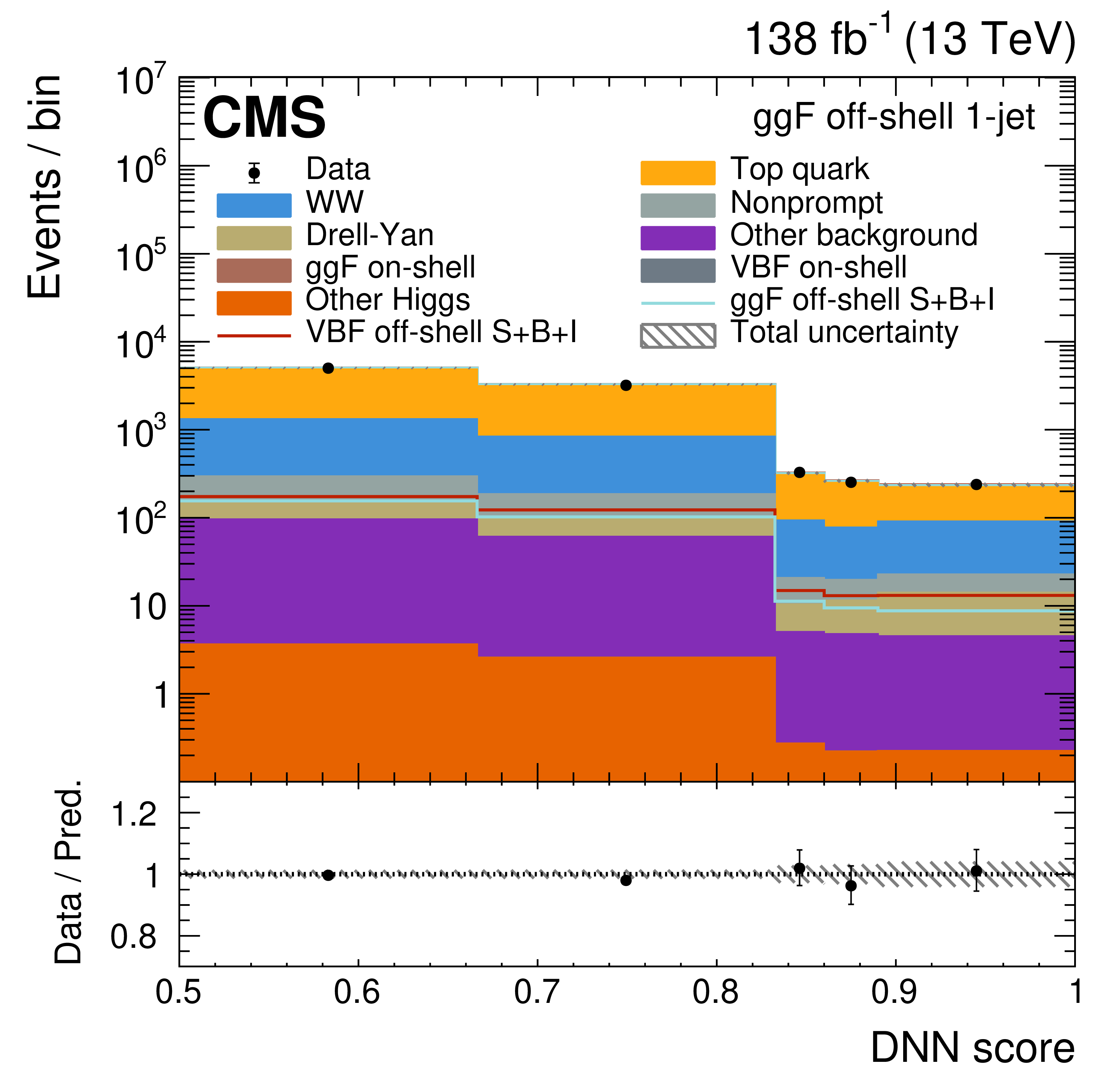
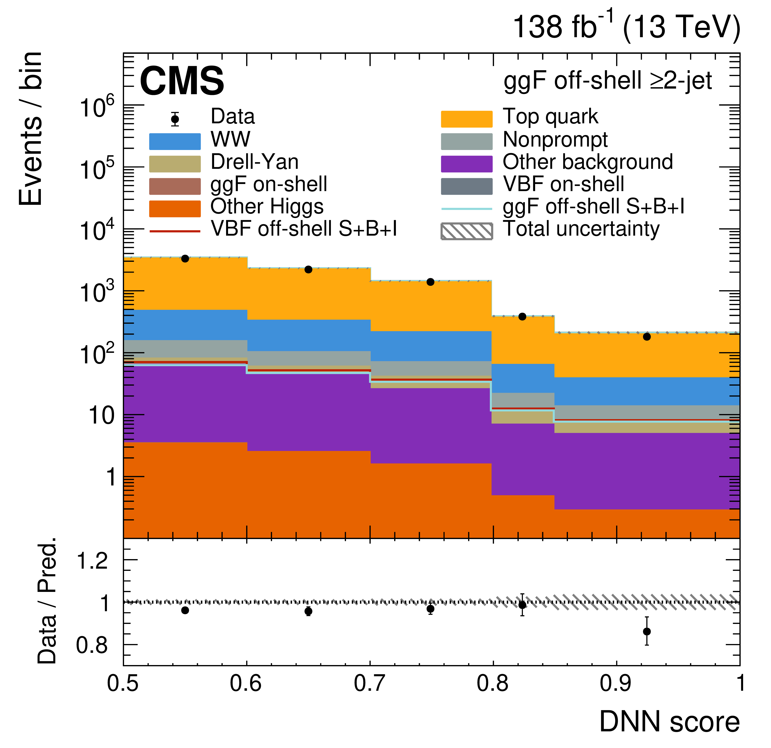
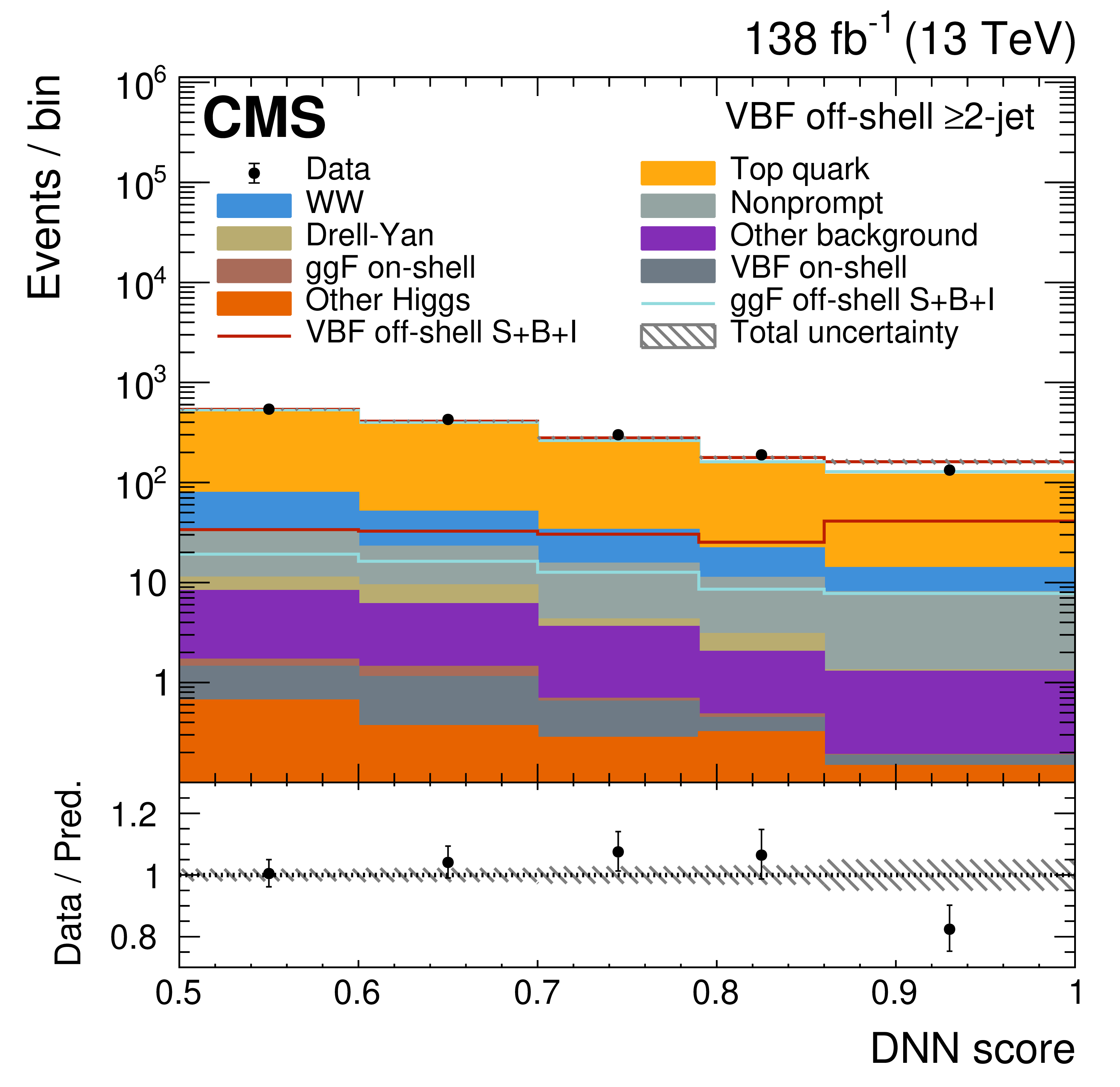
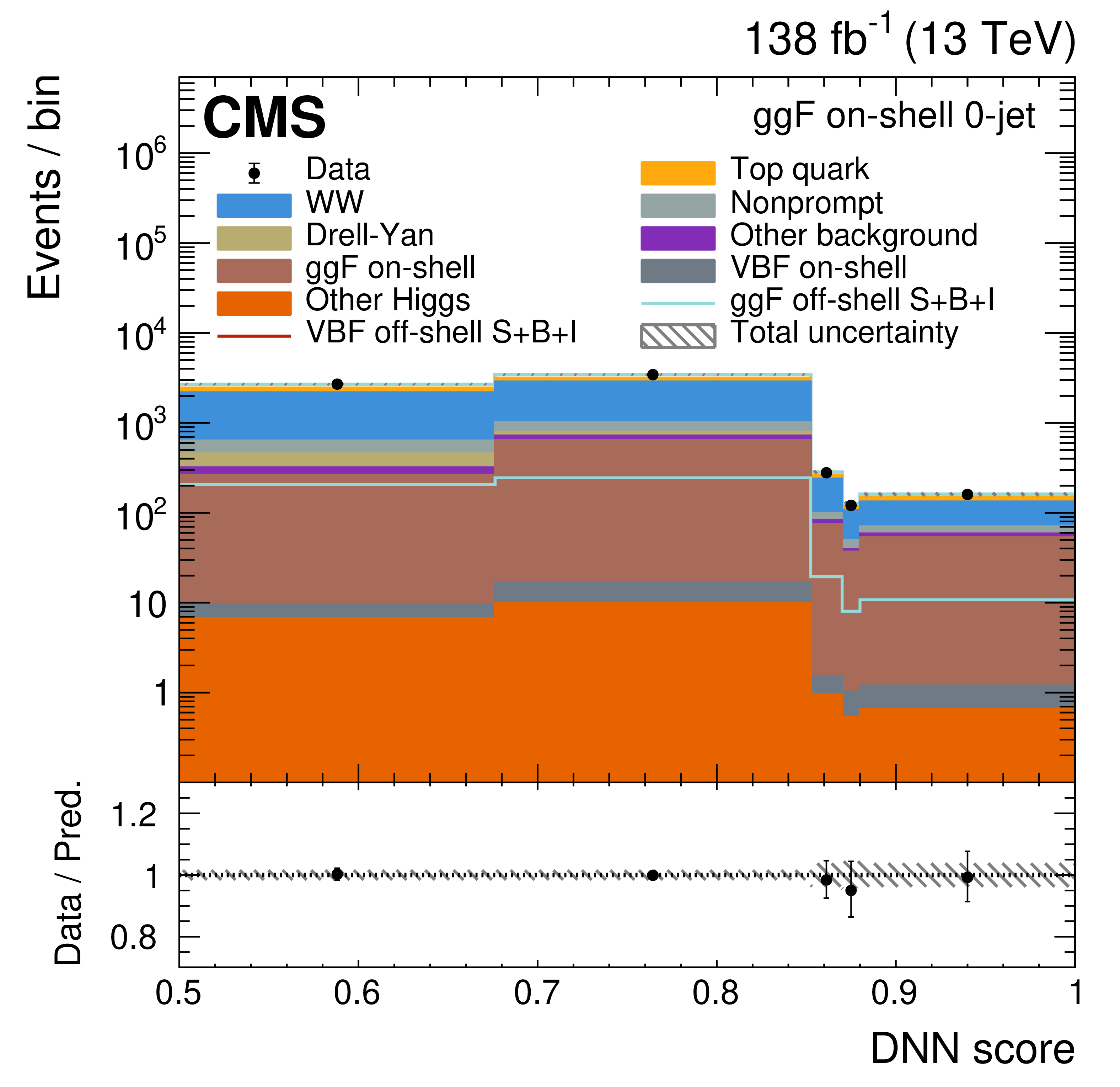
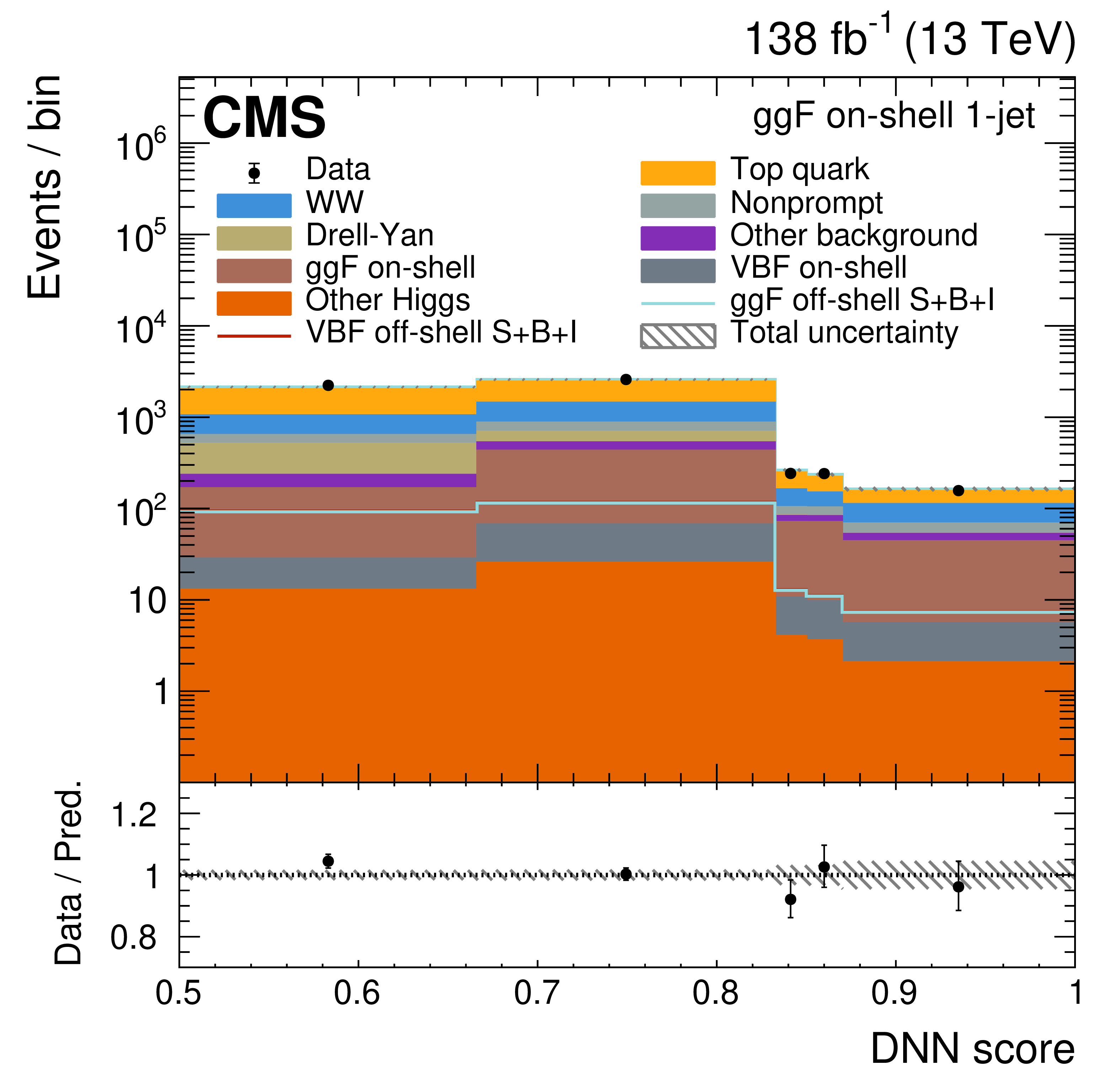
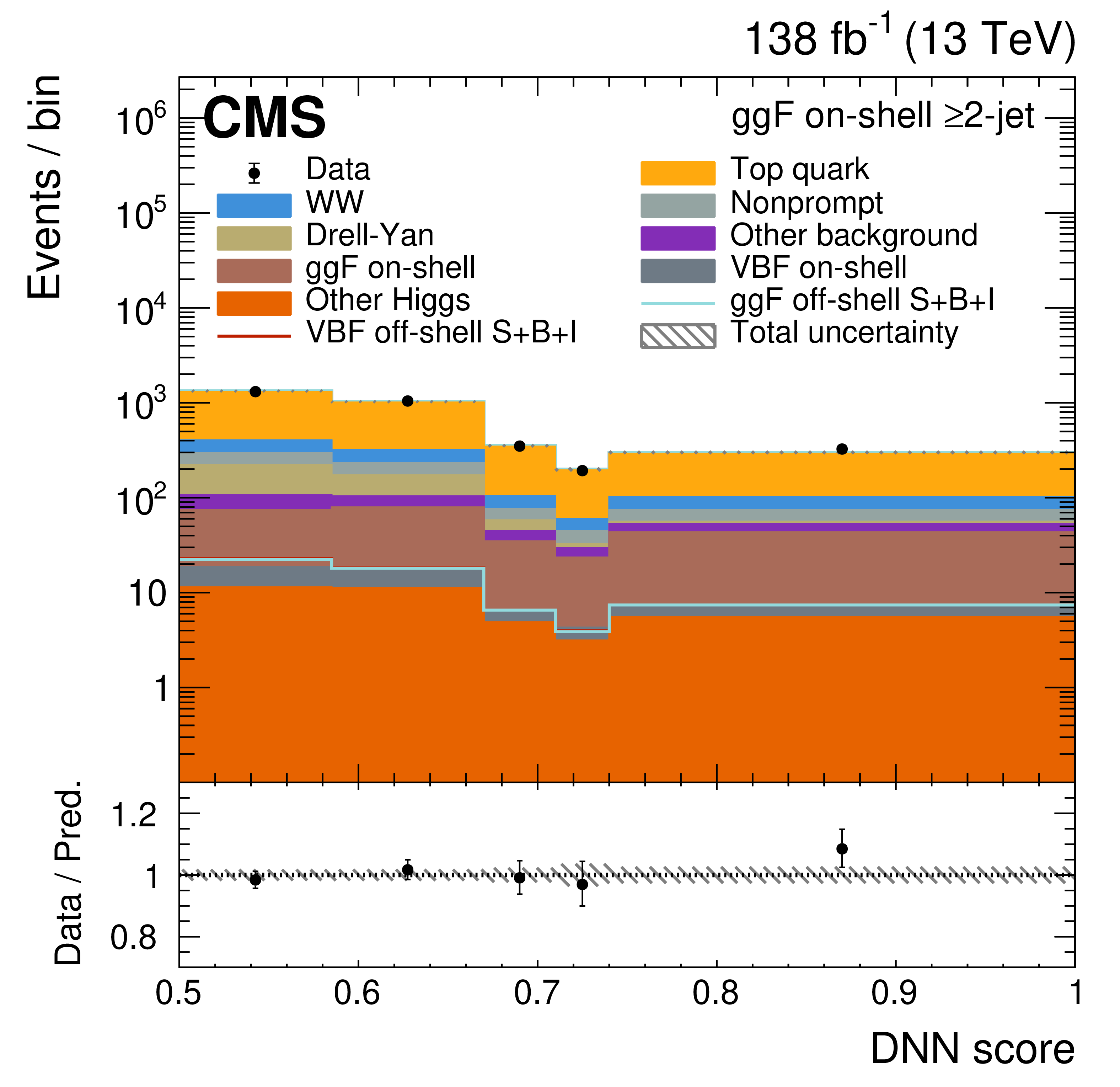
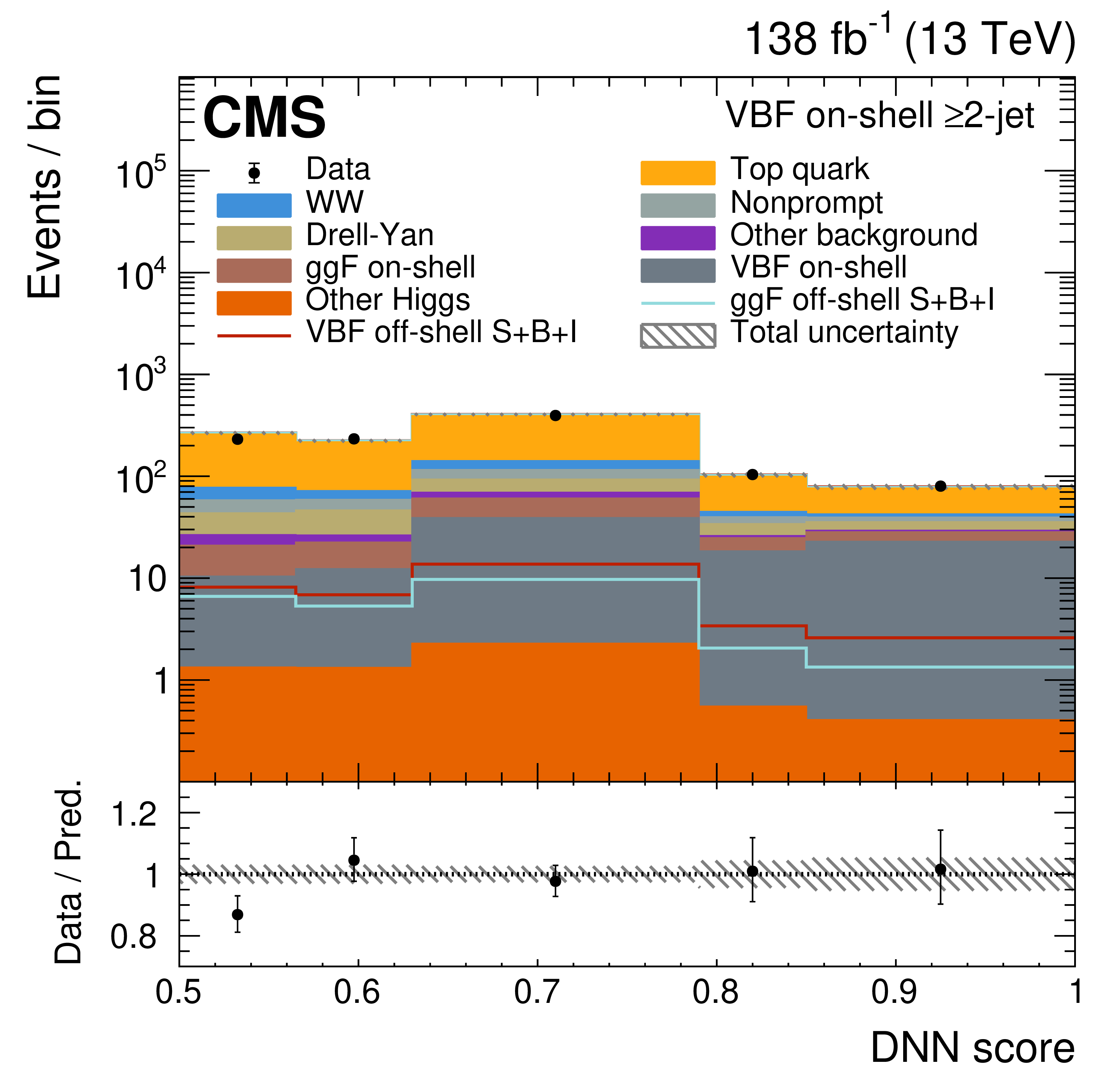
Figure 3:
The off-shell SR post-fit DNN output distributions for the 0-jet (upper left), 1-jet (upper right), and $ \geq $2-jet (lower plots) event categories. The data are shown as the black dots, with the vertical bars representing the statistical uncertainties. The predicted signal and background distributions are shown by the various colored histograms. The predicted signal ggF and VBH off-shell $ S+B+I $ distributions are displayed both as part of the total stacked histograms, along with all the predicted background distributions, and on top of the stacked background distributions for visibility. The lower portion of the plots gives the ratio of the data to the total predicted yields, including the post-fit signal. The hatched area represents the total uncertainty in the ratio. |
png pdf |
Figure 3-a:
The off-shell SR post-fit DNN output distributions for the 0-jet (upper left), 1-jet (upper right), and $ \geq $2-jet (lower plots) event categories. The data are shown as the black dots, with the vertical bars representing the statistical uncertainties. The predicted signal and background distributions are shown by the various colored histograms. The predicted signal ggF and VBH off-shell $ S+B+I $ distributions are displayed both as part of the total stacked histograms, along with all the predicted background distributions, and on top of the stacked background distributions for visibility. The lower portion of the plots gives the ratio of the data to the total predicted yields, including the post-fit signal. The hatched area represents the total uncertainty in the ratio. |
png pdf |
Figure 3-b:
The off-shell SR post-fit DNN output distributions for the 0-jet (upper left), 1-jet (upper right), and $ \geq $2-jet (lower plots) event categories. The data are shown as the black dots, with the vertical bars representing the statistical uncertainties. The predicted signal and background distributions are shown by the various colored histograms. The predicted signal ggF and VBH off-shell $ S+B+I $ distributions are displayed both as part of the total stacked histograms, along with all the predicted background distributions, and on top of the stacked background distributions for visibility. The lower portion of the plots gives the ratio of the data to the total predicted yields, including the post-fit signal. The hatched area represents the total uncertainty in the ratio. |
png pdf |
Figure 3-c:
The off-shell SR post-fit DNN output distributions for the 0-jet (upper left), 1-jet (upper right), and $ \geq $2-jet (lower plots) event categories. The data are shown as the black dots, with the vertical bars representing the statistical uncertainties. The predicted signal and background distributions are shown by the various colored histograms. The predicted signal ggF and VBH off-shell $ S+B+I $ distributions are displayed both as part of the total stacked histograms, along with all the predicted background distributions, and on top of the stacked background distributions for visibility. The lower portion of the plots gives the ratio of the data to the total predicted yields, including the post-fit signal. The hatched area represents the total uncertainty in the ratio. |
png pdf |
Figure 3-d:
The off-shell SR post-fit DNN output distributions for the 0-jet (upper left), 1-jet (upper right), and $ \geq $2-jet (lower plots) event categories. The data are shown as the black dots, with the vertical bars representing the statistical uncertainties. The predicted signal and background distributions are shown by the various colored histograms. The predicted signal ggF and VBH off-shell $ S+B+I $ distributions are displayed both as part of the total stacked histograms, along with all the predicted background distributions, and on top of the stacked background distributions for visibility. The lower portion of the plots gives the ratio of the data to the total predicted yields, including the post-fit signal. The hatched area represents the total uncertainty in the ratio. |
png pdf |
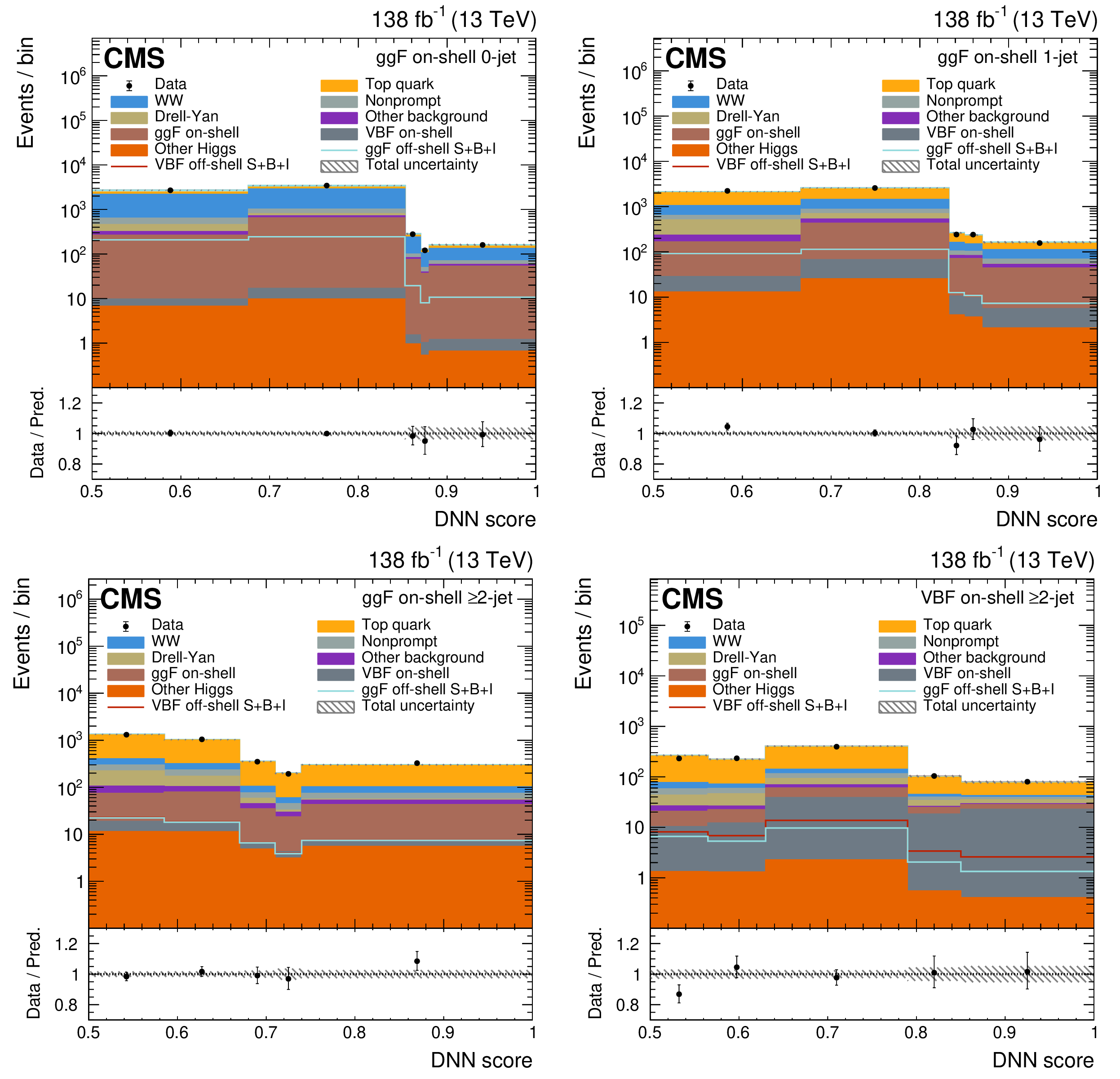
Figure 4:
The on-shell CR post-fit DNN output distributions for the 0-jet (upper left), 1-jet (upper right), and $ \geq $2-jet (lower plots) event categories. The data are shown as the black dots, with the vertical bars representing the statistical uncertainties. The predicted signal and background distributions are shown by the various colored histograms. The predicted signal ggF and VBH off-shell $ S+B+I $ distributions are displayed both as part of the total stacked histograms, along with all the predicted background distributions, and on top of the stacked background distributions for visibility. The lower portion of the plots gives the ratio of the data to the total predicted yields, including the post-fit signal. The hatched area represents the total uncertainty in the ratio. |
png pdf |
Figure 4-a:
The on-shell CR post-fit DNN output distributions for the 0-jet (upper left), 1-jet (upper right), and $ \geq $2-jet (lower plots) event categories. The data are shown as the black dots, with the vertical bars representing the statistical uncertainties. The predicted signal and background distributions are shown by the various colored histograms. The predicted signal ggF and VBH off-shell $ S+B+I $ distributions are displayed both as part of the total stacked histograms, along with all the predicted background distributions, and on top of the stacked background distributions for visibility. The lower portion of the plots gives the ratio of the data to the total predicted yields, including the post-fit signal. The hatched area represents the total uncertainty in the ratio. |
png pdf |
Figure 4-b:
The on-shell CR post-fit DNN output distributions for the 0-jet (upper left), 1-jet (upper right), and $ \geq $2-jet (lower plots) event categories. The data are shown as the black dots, with the vertical bars representing the statistical uncertainties. The predicted signal and background distributions are shown by the various colored histograms. The predicted signal ggF and VBH off-shell $ S+B+I $ distributions are displayed both as part of the total stacked histograms, along with all the predicted background distributions, and on top of the stacked background distributions for visibility. The lower portion of the plots gives the ratio of the data to the total predicted yields, including the post-fit signal. The hatched area represents the total uncertainty in the ratio. |
png pdf |
Figure 4-c:
The on-shell CR post-fit DNN output distributions for the 0-jet (upper left), 1-jet (upper right), and $ \geq $2-jet (lower plots) event categories. The data are shown as the black dots, with the vertical bars representing the statistical uncertainties. The predicted signal and background distributions are shown by the various colored histograms. The predicted signal ggF and VBH off-shell $ S+B+I $ distributions are displayed both as part of the total stacked histograms, along with all the predicted background distributions, and on top of the stacked background distributions for visibility. The lower portion of the plots gives the ratio of the data to the total predicted yields, including the post-fit signal. The hatched area represents the total uncertainty in the ratio. |
png pdf |
Figure 4-d:
The on-shell CR post-fit DNN output distributions for the 0-jet (upper left), 1-jet (upper right), and $ \geq $2-jet (lower plots) event categories. The data are shown as the black dots, with the vertical bars representing the statistical uncertainties. The predicted signal and background distributions are shown by the various colored histograms. The predicted signal ggF and VBH off-shell $ S+B+I $ distributions are displayed both as part of the total stacked histograms, along with all the predicted background distributions, and on top of the stacked background distributions for visibility. The lower portion of the plots gives the ratio of the data to the total predicted yields, including the post-fit signal. The hatched area represents the total uncertainty in the ratio. |
png pdf |
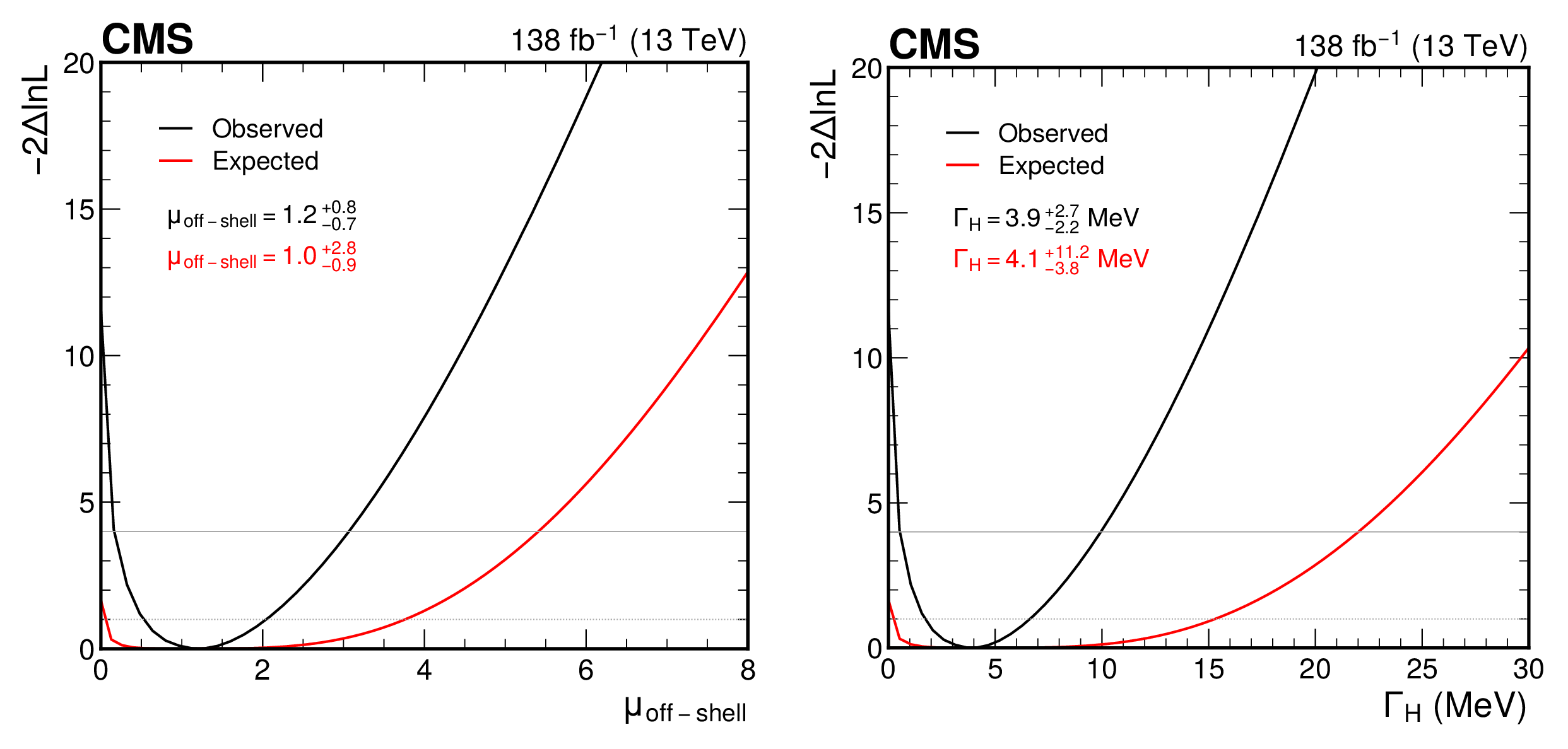
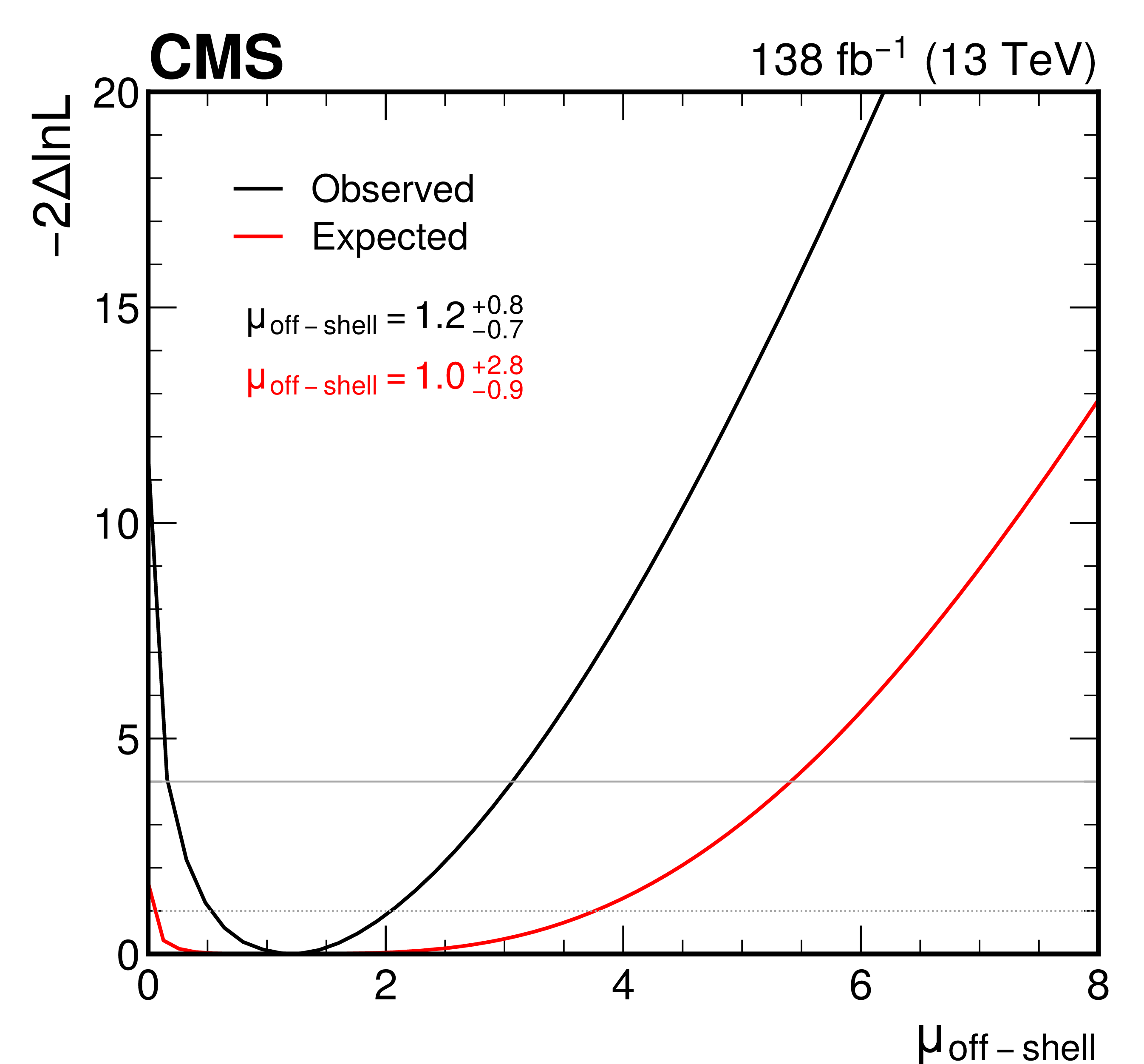
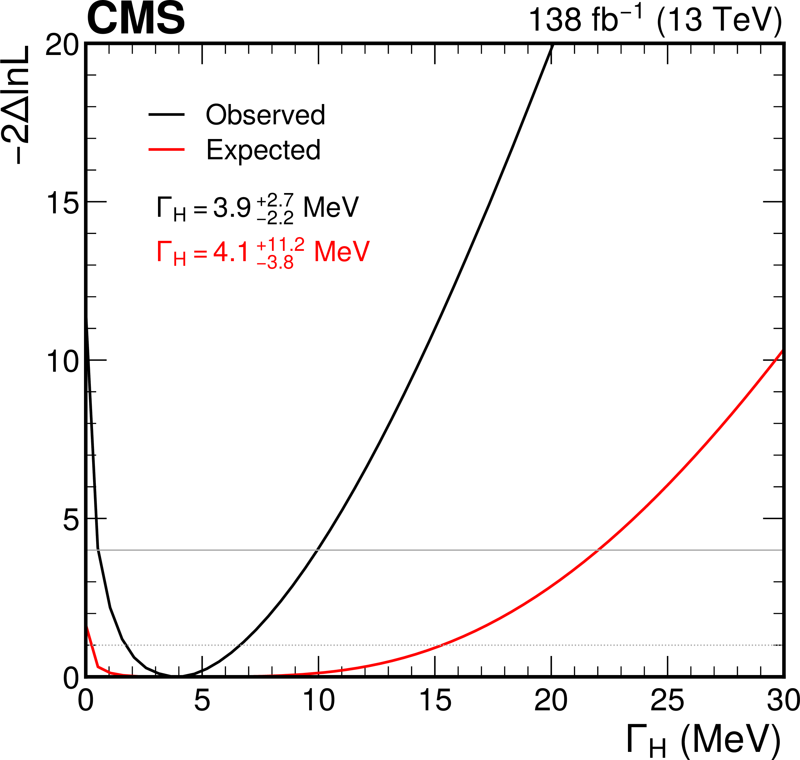
Figure 5:
The observed (black curve) and expected (red curve) likelihood function scans for the off-shell signal strength $ \mu_{\text{off-shell} } $ (left) and the Higgs boson decay width $ \Gamma_{\mathrm{H}} $ (right). The resulting best-fit observed and expected values are also given, along with their uncertainties. The 68 and 95% confidence level intervals are shown by the intersection of the likelihood function curves with the dotted and solid horizontal lines, respectively. |
png pdf |
Figure 5-a:
The observed (black curve) and expected (red curve) likelihood function scans for the off-shell signal strength $ \mu_{\text{off-shell} } $ (left) and the Higgs boson decay width $ \Gamma_{\mathrm{H}} $ (right). The resulting best-fit observed and expected values are also given, along with their uncertainties. The 68 and 95% confidence level intervals are shown by the intersection of the likelihood function curves with the dotted and solid horizontal lines, respectively. |
png pdf |
Figure 5-b:
The observed (black curve) and expected (red curve) likelihood function scans for the off-shell signal strength $ \mu_{\text{off-shell} } $ (left) and the Higgs boson decay width $ \Gamma_{\mathrm{H}} $ (right). The resulting best-fit observed and expected values are also given, along with their uncertainties. The 68 and 95% confidence level intervals are shown by the intersection of the likelihood function curves with the dotted and solid horizontal lines, respectively. |
| Tables | |
png pdf |
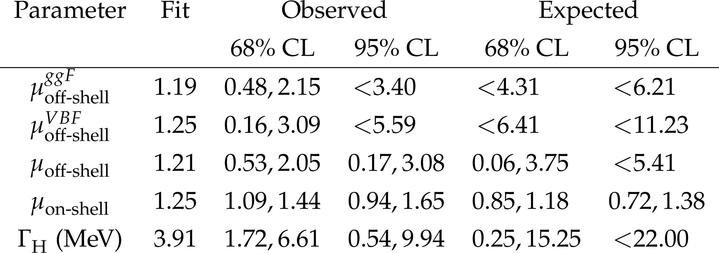
Table 1:
Measurements of the ggF and VBF off-shell signal strengths $ \mu^{ggF}_{\text{off-shell} } $ and $ \mu^{VBF}_{\text{off-shell} } $, the overall off-shell signal strength $ \mu_{\text{off-shell} } $, the on-shell signal strength $ \mu_{\text{on-shell} } $, and the Higgs boson decay width $ \Gamma_{\mathrm{H}} $. The observed best-fit values are given (Fit), as well as the observed and expected 68 and 95% confidence levels (CLs). |
png pdf |
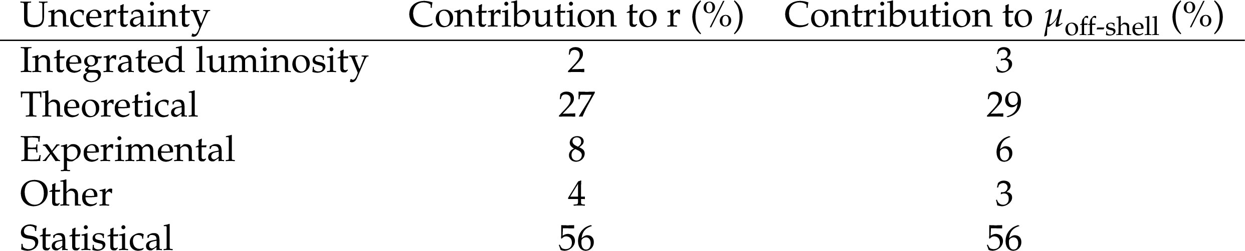
Table 2:
The sources of systematic uncertainty and their contributions to the total uncertainty in the parameter of interest $ \text{r} = \mu_{\text{off-shell} }/\mu_{\text{on-shell} } $. The statistical uncertainty is also shown. The values given are the ratios in percent of each uncertainty, divided by the total uncertainty. The last column shows the similar ratios for the uncertainty in $ \mu_{\text{off-shell} } $. |
| Summary |
| Measurements of the off- and on-shell signal strengths for the Higgs boson have been performed with the gluon-gluon fusion (ggF) and vector boson fusion (VBF) production modes in the $ \mathrm{H} \to \mathrm{W}\mathrm{W} \to \mathrm{e}\nu\mu\nu $ decay channel, using proton-proton collision data at $ \sqrt{s}= $ 13 TeV from the CMS experiment in 2016--2018, corresponding to an integrated luminosity of 138 fb$ ^{-1} $. Specific event selection and background discrimination techniques were applied in order to extract the results from maximum likelihood fits to data. The combined off-shell Higgs boson signal strength from ggF and VBF processes is found to be $ \mu_{\text{off-shell} } = $ 1.2 $ ^{+0.8}_{-0.7} $, which is used to derive the Higgs boson total decay width of $ \Gamma_{\mathrm{H}} = $ 3.9 $ ^{+2.7}_{-2.2} $ MeV, in agreement with the standard model prediction of 4.1 MeV. This measurement represents the first CMS determination of the Higgs boson decay width using the $ \mathrm{H} \to \mathrm{W}\mathrm{W} $ channel at $ \sqrt{s}= $ 13 TeV. This result improves on the analogous CMS analyses at $ \sqrt{s} = $ 7 and 8 TeV limit by a factor of three, while complementing the CMS Higgs boson decay width measurement using the $ \mathrm{H} \to \mathrm{Z}\mathrm{Z} $ channel at $ \sqrt{s}= $ 13 TeV. |
| References | ||||
| 1 | S. Weinberg | A model of leptons | PRL 19 (1967) 1264 | |
| 2 | S. L. Glashow | Partial-symmetries of weak interactions | NP 22 (1961) 579 | |
| 3 | A. Salam | Weak and electromagnetic interactions | Conf. Proc. C 680519 (1968) 367 | |
| 4 | P. W. Higgs | Broken symmetries, massless particles and gauge fields | PLB 12 (1964) 132 | |
| 5 | P. W. Higgs | Spontaneous symmetry breakdown without massless bosons | PR 145 (1966) 1156 | |
| 6 | F. Englert and R. Brout | Broken symmetry and the mass of gauge vector mesons | PRL 13 (1964) 321 | |
| 7 | P. W. Higgs | Broken symmetries and the masses of gauge bosons | PRL 13 (1964) 508 | |
| 8 | ATLAS Collaboration | Observation of a new particle in the search for the standard model Higgs boson with the ATLAS detector at the LHC | PLB 716 (2012) 1 | 1207.7214 |
| 9 | CMS Collaboration | Observation of a new boson at a mass of 125 GeV with the CMS experiment at the LHC | PLB 716 (2012) 30 | CMS-HIG-12-028 1207.7235 |
| 10 | ATLAS Collaboration | A detailed map of Higgs boson interactions by the ATLAS experiment ten years after the discovery | [Erratum: Nature 612, E24 ()], 2022 Nature 607 (2022) 52 |
2207.00092 |
| 11 | CMS Collaboration | A portrait of the Higgs boson by the CMS experiment ten years after the discovery | [Corrigendum: Nature 623, ()], 2022 Nature 607 (2022) 60 |
CMS-HIG-22-001 2207.00043 |
| 12 | D. de Florian et al. | Handbook of LHC Higgs cross sections: 4. Deciphering the nature of the Higgs sector | CERN Yellow Rep. Monogr. 2 (2017) 1 | 1610.07922 |
| 13 | CMS Collaboration | Measurement of the Higgs boson mass and width using the four-lepton final state in proton-proton collisions at $ \sqrt{s}= $ 13 TeV | PRD 111 (2025) 052014 | CMS-HIG-21-019 2409.13663 |
| 14 | ATLAS Collaboration | Measurement of off-shell Higgs boson production in the $ H^*\rightarrow ZZ\rightarrow 4\ell $ decay channel using a neural simulation-based inference technique in 13 TeV pp collisions with the ATLAS detector | Rept. Prog. Phys. 88 (2025) 057803 | 2412.01548 |
| 15 | ATLAS Collaboration | Constraining off-shell Higgs boson production and the Higgs boson total width using $ WW\to \ell\nu\ell\nu $ final states with the ATLAS detector | PLB 870 (2025) 139898 | 2504.07710 |
| 16 | ATLAS Collaboration | Constraint on the total width of the Higgs boson from Higgs boson and four-top-quark measurements in pp collisions at $ \sqrt{s}= $ 13 TeV with the ATLAS detector | PLB 861 (2025) 139277 | 2407.10631 |
| 17 | CMS Collaboration | Search for Higgs boson off-shell production in proton-proton collisions at 7 and 8 TeV and derivation of constraints on its total decay width | JHEP 09 (2016) 051 | CMS-HIG-14-032 1605.02329 |
| 18 | N. Kauer and G. Passarino | Inadequacy of zero-width approximation for a light Higgs boson signal | JHEP 08 (2012) 116 | 1206.4803 |
| 19 | D. A. Dicus and S. S. D. Willenbrock | Photon pair production and the intermediate mass Higgs boson | PRD 37 (1988) 1801 | |
| 20 | L. J. Dixon and Y. Li | Bounding the Higgs boson width through interferometry | PRL 111 (2013) 111802 | 1305.3854 |
| 21 | J. M. Campbell, R. K. Ellis, and C. Williams | Gluon-gluon contributions to $ \text{W}^+ \text{W}^- $ production and Higgs interference effects | JHEP 10 (2011) 005 | 1107.5569 |
| 22 | CMS Collaboration | HEPData record for this analysis | link | |
| 23 | CMS Collaboration | The CMS Experiment at the CERN LHC | JINST 3 (2008) S08004 | |
| 24 | CMS Collaboration | Development of the CMS detector for the CERN LHC Run 3 | JINST 19 (2024) P05064 | CMS-PRF-21-001 2309.05466 |
| 25 | CMS Collaboration | Performance of the CMS Level-1 trigger in proton-proton collisions at $ \sqrt{s} = $ 13 TeV | JINST 15 (2020) P10017 | CMS-TRG-17-001 2006.10165 |
| 26 | CMS Collaboration | The CMS trigger system | JINST 12 (2017) P01020 | CMS-TRG-12-001 1609.02366 |
| 27 | CMS Collaboration | Performance of the CMS high-level trigger during LHC Run 2 | JINST 19 (2024) P11021 | CMS-TRG-19-001 2410.17038 |
| 28 | CMS Collaboration | Electron and photon reconstruction and identification with the CMS experiment at the CERN LHC | JINST 16 (2021) P05014 | |
| 29 | CMS Collaboration | Performance of the CMS muon detector and muon reconstruction with proton-proton collisions at $ \sqrt{s}= $ 13 TeV | JINST 13 (2018) P06015 | CMS-MUO-16-001 1804.04528 |
| 30 | CMS Collaboration | Description and performance of track and primary-vertex reconstruction with the CMS tracker | JINST 9 (2014) P10009 | CMS-TRK-11-001 1405.6569 |
| 31 | CMS Collaboration | Particle-flow reconstruction and global event description with the CMS detector | JINST 12 (2017) P10003 | CMS-PRF-14-001 1706.04965 |
| 32 | CMS Collaboration | Performance of missing transverse momentum reconstruction in proton-proton collisions at $ \sqrt{s}= $ 13 TeV using the CMS detector | JINST 14 (2019) P07004 | CMS-JME-17-001 1903.06078 |
| 33 | CMS Collaboration | Pileup mitigation at CMS in 13 TeV data | CMS Detector Performance Summary, 2020 link |
CMS-PAS-JME-18-001 |
| 34 | M. Cacciari, G. P. Salam, and G. Soyez | The anti-$ k_{\mathrm{T}} $ jet clustering algorithm | JHEP 04 (2008) 063 | 0802.1189 |
| 35 | M. Cacciari, G. P. Salam, and G. Soyez | FastJet user manual | EPJC 72 (2012) 1896 | 1111.6097 |
| 36 | CMS Collaboration | Jet energy scale and resolution in the CMS experiment in pp collisions at 8 TeV | JINST 12 (2017) P02014 | CMS-JME-13-004 1607.03663 |
| 37 | CMS Collaboration | Precision luminosity measurement in proton-proton collisions at $ \sqrt{s} = $ 13 TeV in 2015 and 2016 at CMS | EPJC 81 (2021) 800 | CMS-LUM-17-003 2104.01927 |
| 38 | CMS Collaboration | CMS luminosity measurement for the 2017 data-taking period at $ \sqrt{s} = $ 13 TeV | CMS Physics Analysis Summary, 2018 CMS-PAS-LUM-17-004 |
CMS-PAS-LUM-17-004 |
| 39 | CMS Collaboration | CMS luminosity measurement for the 2018 data-taking period at $ \sqrt{s} = $ 13 TeV | CMS Physics Analysis Summary, 2019 CMS-PAS-LUM-18-002 |
CMS-PAS-LUM-18-002 |
| 40 | CMS Collaboration | Methods for off-shell Higgs boson production simulation used in CMS analyses | CMS Physics Analysis Summary CMS-NOTE-2022-010, 2022 CDS |
|
| 41 | P. Nason | A new method for combining NLO QCD with shower Monte Carlo algorithms | JHEP 11 (2004) 040 | hep-ph/0409146 |
| 42 | S. Frixione, P. Nason, and C. Oleari | Matching NLO QCD computations with parton shower simulations: the POWHEG method | JHEP 11 (2007) 070 | 0709.2092 |
| 43 | S. Alioli, P. Nason, C. Oleari, and E. Re | A general framework for implementing NLO calculations in shower Monte Carlo programs: the POWHEG BOX | JHEP 06 (2010) 043 | 1002.2581 |
| 44 | S. Bolognesi et al. | On the spin and parity of a single-produced resonance at the LHC | PRD 86 (2012) 095031 | 1208.4018 |
| 45 | S. Goria, G. Passarino, and D. Rosco | The Higgs boson lineshape | NPB 864 (2012) 530 | 1112.5517 |
| 46 | A. V. Gritsan, R. Röntsch, M. Schulze, and M. Xiao | Constraining anomalous Higgs boson couplings to the heavy flavor fermions using matrix element techniques | PRD 94 (2016) 055023 | 1606.03107 |
| 47 | A. V. Gritsan et al. | New features in the JHU generator framework: constraining Higgs boson properties from on-shell and off-shell production | PRD 102 (2020) 056022 | 2002.09888 |
| 48 | J. M. Campbell and R. K. Ellis | An update on vector boson pair production at hadron colliders | PRD 60 (1999) 113006 | hep-ph/9905386 |
| 49 | J. M. Campbell, R. K. Ellis, and C. Williams | Vector boson pair production at the LHC | JHEP 07 (2011) 018 | 1105.0020 |
| 50 | J. M. Campbell, R. K. Ellis, and W. T. Giele | A multi-threaded version of MCFM | EPJC 75 (2015) 246 | 1503.06182 |
| 51 | CMS Collaboration | Measurement of the Higgs boson width and evidence of its off-shell contributions to ZZ production | Nature Phys. 18 (2022) 1329 | CMS-HIG-21-013 2202.06923 |
| 52 | C. Anastasiou et al. | High precision determination of the gluon fusion Higgs boson cross-section at the LHC | JHEP 05 (2016) 058 | 1602.00695 |
| 53 | K. Hamilton, P. Nason, E. Re, and G. Zanderighi | NNLOPS simulation of Higgs boson production | JHEP 10 (2013) 222 | 1309.0017 |
| 54 | K. Hamilton, P. Nason, and G. Zanderighi | Finite quark-mass effects in the NNLOPS POWHEG+MiNLO Higgs generator | JHEP 05 (2015) 140 | 1501.04637 |
| 55 | CMS Collaboration | Measurements of the Higgs boson production cross section and couplings in the W boson pair decay channel in proton-proton collisions at $ \sqrt{s}= $ 13 TeV | EPJC 83 (2023) 667 | CMS-HIG-20-013 2206.09466 |
| 56 | J. Alwall et al. | The automated computation of tree-level and next-to-leading order differential cross sections, and their matching to parton shower simulations | JHEP 07 (2014) 079 | 1405.0301 |
| 57 | CMS Collaboration | Review of top quark mass measurements in CMS | Phys. Rept. 1115 (2025) 116 | CMS-TOP-23-003 2403.01313 |
| 58 | M. Czakon et al. | Top-pair production at the LHC through NNLO QCD and NLO EW | JHEP 10 (2017) 186 | 1705.04105 |
| 59 | T. Sjöstrand et al. | An introduction to PYTHIA 8.2 | Comput. Phys. Commun. 191 (2015) 159 | 1410.3012 |
| 60 | CMS Collaboration | Extraction and validation of a new set of CMS PYTHIA8 tunes from underlying-event measurements | EPJC 80 (2020) 4 | CMS-GEN-17-001 1903.12179 |
| 61 | NNPDF Collaboration | Parton distributions from high-precision collider data | EPJC 77 (2017) 663 | 1706.00428 |
| 62 | GEANT4 Collaboration | GEANT 4 -- a simulation toolkit | NIM A 506 (2003) 250 | |
| 63 | CMS Collaboration | Evidence for associated production of a Higgs boson with a top quark pair in final states with electrons, muons, and hadronically decaying $ \tau $ leptons at $ \sqrt{s}= $ 13 TeV | JHEP 08 (2018) 066 | CMS-HIG-17-018 1803.05485 |
| 64 | CMS Collaboration | Identification of heavy-flavour jets with the CMS detector in pp collisions at 13 TeV | JINST 13 (2018) P05011 | CMS-BTV-16-002 1712.07158 |
| 65 | E. Bols et al. | Jet flavour classification using DeepJet | JINST 15 (2020) P12012 | 2008.10519 |
| 66 | CMS Collaboration | Performance summary of AK4 jet b tagging with data from proton-proton collisions at 13 TeV with the CMS detector | CMS Detector Performance Summary CMS-DP-2023-005, 2023 CDS |
|
| 67 | F. Chollet | Deep learning with Python | Manning Publications Co., second edition, ISBN 978161764, 2021 | |
| 68 | D. P. Kingma and J. Ba | Adam: A method for stochastic optimization | link | |
| 69 | W. J. Conover | Practical nonparametric statistics | Wiley, 3. ed edition, ISBN 0471160687, 1999 | |
| 70 | CMS Collaboration | Measurements of properties of the Higgs boson decaying to a W boson pair in pp collisions at $ \sqrt{s}= $ 13 TeV | PLB 791 (2019) 96 | CMS-HIG-16-042 1806.05246 |
| 71 | A. Hayrapetyan, et. al. | The CMS statistical analysis and combination tool: Combine | Comput. Software. Big Science 8 (2024) 18 | |
| 72 | W. Verkerke and D. Kirkby | The RooFit toolkit for data modeling | in th International Conference on Computing in High Energy and Nuclear Physics (CHEP ), p. MOLT007... [eConf C0303241, MOLT007], 2003 Proc. 1 (2003) 3 |
physics/0306116 |
| 73 | L. Moneta et al. | The RooStats project | in th International Workshop on Advanced Computing and Analysis Techniques in Physics Research (ACAT )... [PoS(ACAT)057], 2010 Proc. 1 (2010) 3 |
1009.1003 |
| 74 | R. D. Cousins | Lectures on statistics in theory: Prelude to statistics in practice | 1807.05996 | |
| 75 | E. Gross and O. Vitells | Trial factors for the look elsewhere effect in high energy physics | EPJC 70 (2010) 525 | 1005.1891 |
|
|
Compact Muon Solenoid LHC, CERN |
|

|

|

|

|

|