

Compact Muon Solenoid
LHC, CERN
| CMS-HIG-24-004 ; CERN-EP-2025-173 | ||
| Model-independent measurement of the Higgs boson associated production with two jets and decaying to a pair of W bosons in proton-proton collisions at $ \sqrt{s} = $ 13 TeV | ||
| CMS Collaboration | ||
| 9 September 2025 | ||
| JHEP 03 (2026) 073 | ||
| Abstract: A model-independent measurement of the differential production cross section of the Higgs boson decaying into a pair of W bosons, with a final state including two jets produced in association, is presented. In the analysis, events are selected in which the decay products of the two W bosons consist of an electron, a muon, and missing transverse momentum. The model independence of the measurement is maximized by making use of a discriminating variable that is agnostic to the signal hypothesis developed through machine learning. The analysis is based on proton-proton collision data at $ \sqrt{s}= $ 13 TeV collected with the CMS detector from 2016-2018, corresponding to an integrated luminosity of 138 fb$^{-1}$. The production cross section is measured as a function of the difference in azimuthal angle between the two jets. The differential cross section measurements are used to constrain Higgs boson couplings within the standard model effective field theory framework. | ||
| Links: e-print arXiv:2509.07958 [hep-ex] (PDF) ; CDS record ; inSPIRE record ; HepData record ; CADI line (restricted) ; | ||
| Figures | |
png pdf |
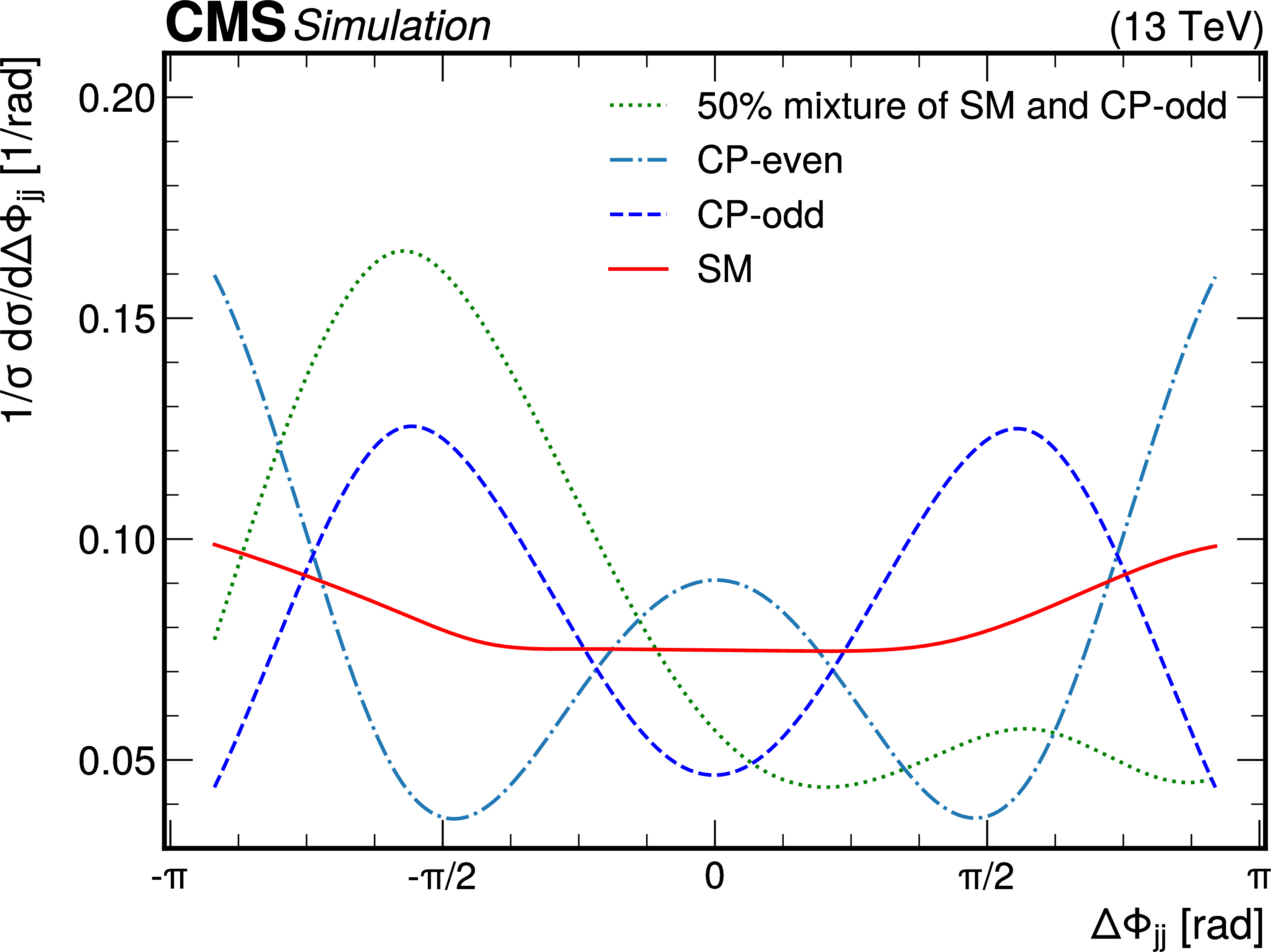
Figure 1:
Normalized VBF differential cross section as a function of the signed azimuthal angle difference between the two jets, with the Higgs boson mass assumed to be 125 GeV. Different hypotheses are superimposed corresponding to a mixed $ CP $ scenario, a pure $ CP $-even AC, a pure $ CP $-odd AC, and an SM coupling in the HVV vertex. |
png pdf |
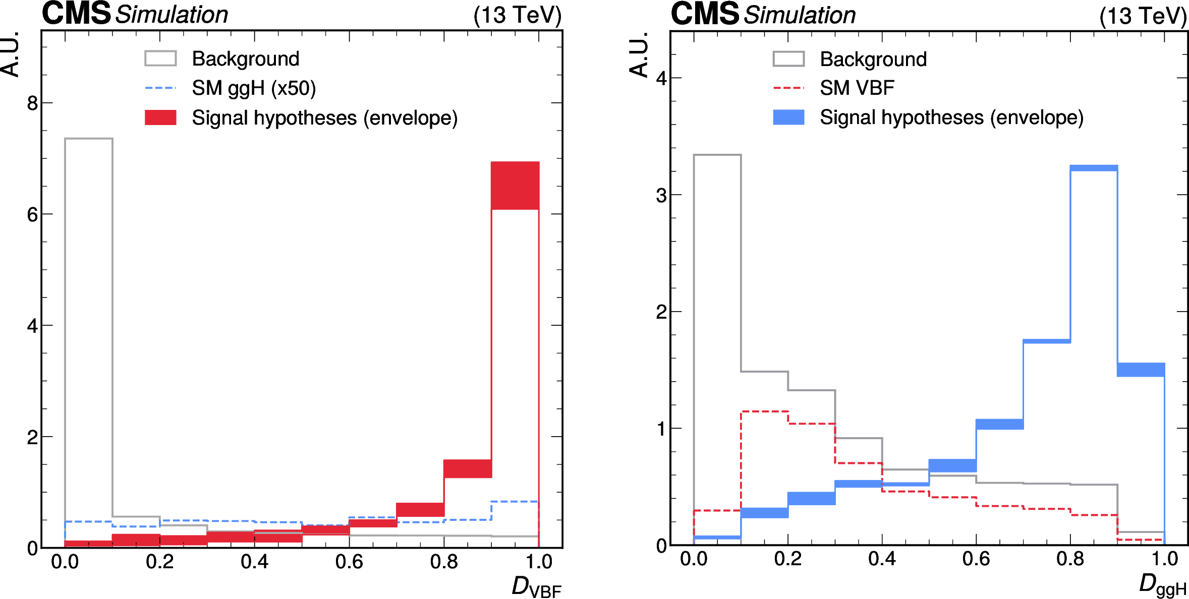
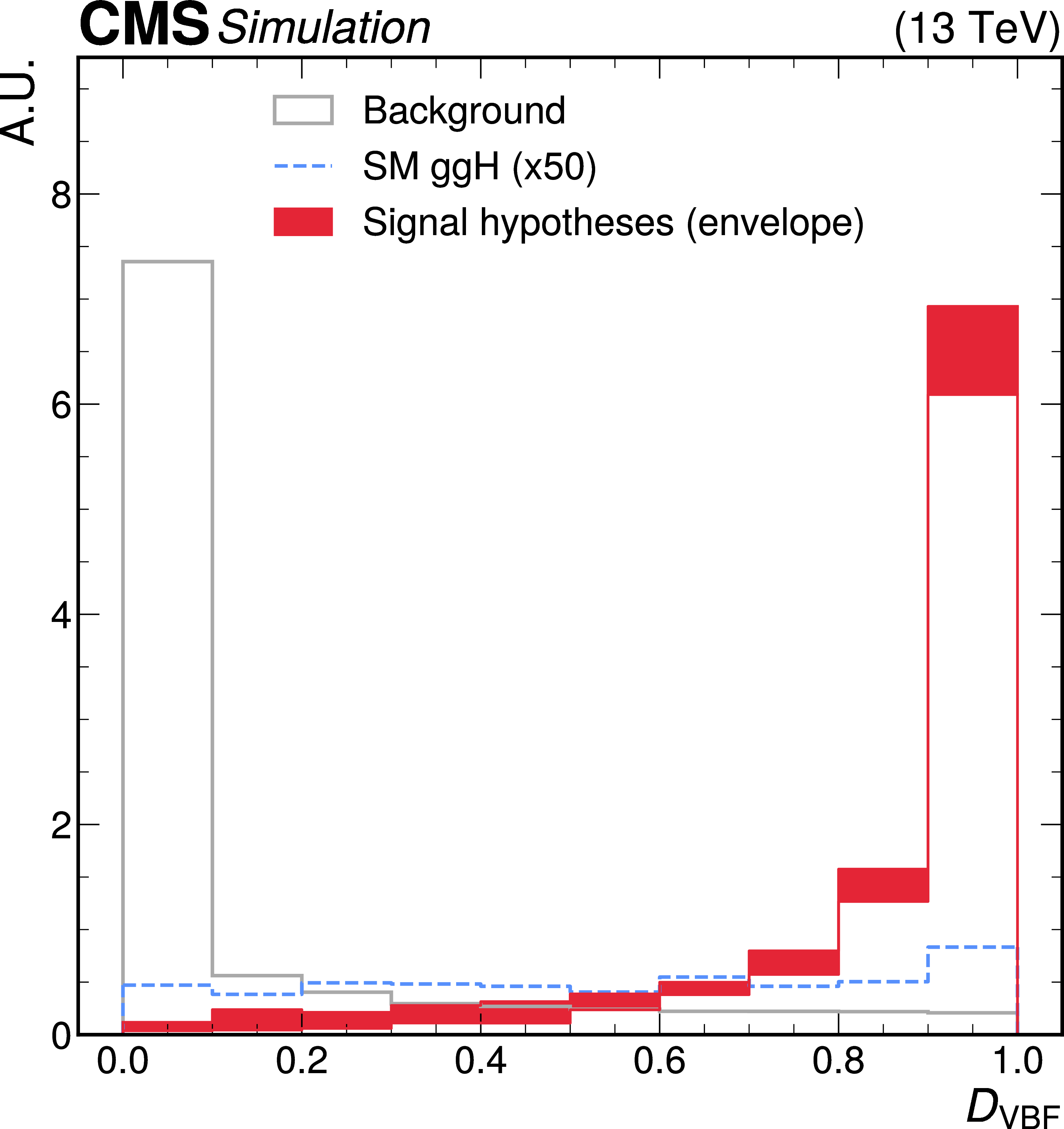
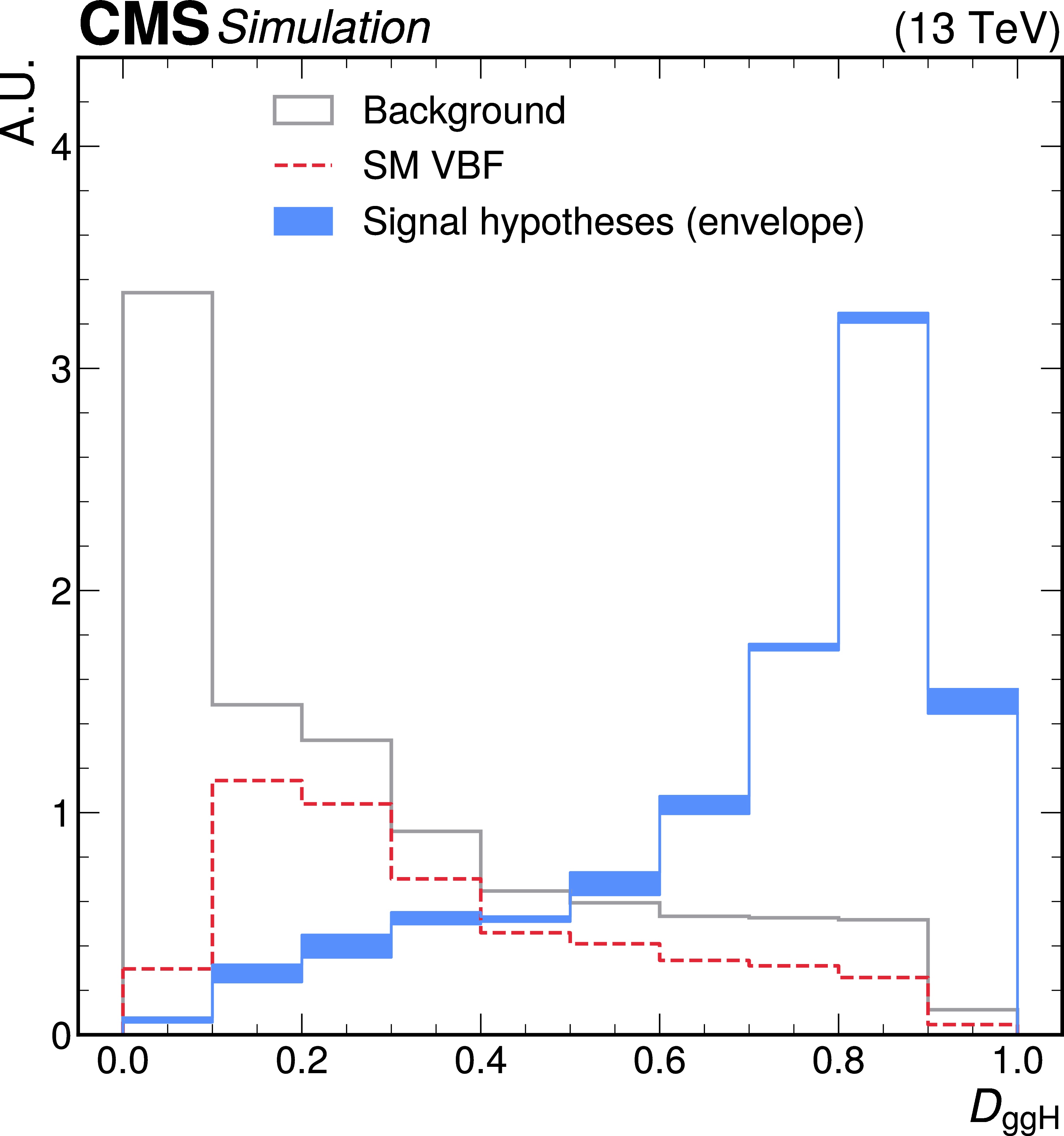
Figure 2:
Normalized distributions of $ \mathcal{D}_\mathrm{VBF} $ (left) and $ \mathcal{D}_\mathrm{ggH} $ (right), evaluated on signal and background events using the ADNNs trained on even-numbered MC events. The signal predictions are displayed as an envelope representing the range of algorithm outputs across all signal hypotheses included in the training. The background class contributions from SM ggH (left) and SM VBF (right) events are highlighted using dashed lines. For $ \mathcal{D}_\mathrm{VBF} $, the background class contains ggH events according to the SM proportion, and the corresponding contribution is rescaled by a factor of 50 to enhance visibility in the plot; for $ \mathcal{D}_\mathrm{ggH} $, the background class contains 50% VBF events. |
png pdf |
Figure 2-a:
Normalized distributions of $ \mathcal{D}_\mathrm{VBF} $ (left) and $ \mathcal{D}_\mathrm{ggH} $ (right), evaluated on signal and background events using the ADNNs trained on even-numbered MC events. The signal predictions are displayed as an envelope representing the range of algorithm outputs across all signal hypotheses included in the training. The background class contributions from SM ggH (left) and SM VBF (right) events are highlighted using dashed lines. For $ \mathcal{D}_\mathrm{VBF} $, the background class contains ggH events according to the SM proportion, and the corresponding contribution is rescaled by a factor of 50 to enhance visibility in the plot; for $ \mathcal{D}_\mathrm{ggH} $, the background class contains 50% VBF events. |
png pdf |
Figure 2-b:
Normalized distributions of $ \mathcal{D}_\mathrm{VBF} $ (left) and $ \mathcal{D}_\mathrm{ggH} $ (right), evaluated on signal and background events using the ADNNs trained on even-numbered MC events. The signal predictions are displayed as an envelope representing the range of algorithm outputs across all signal hypotheses included in the training. The background class contributions from SM ggH (left) and SM VBF (right) events are highlighted using dashed lines. For $ \mathcal{D}_\mathrm{VBF} $, the background class contains ggH events according to the SM proportion, and the corresponding contribution is rescaled by a factor of 50 to enhance visibility in the plot; for $ \mathcal{D}_\mathrm{ggH} $, the background class contains 50% VBF events. |
png pdf |
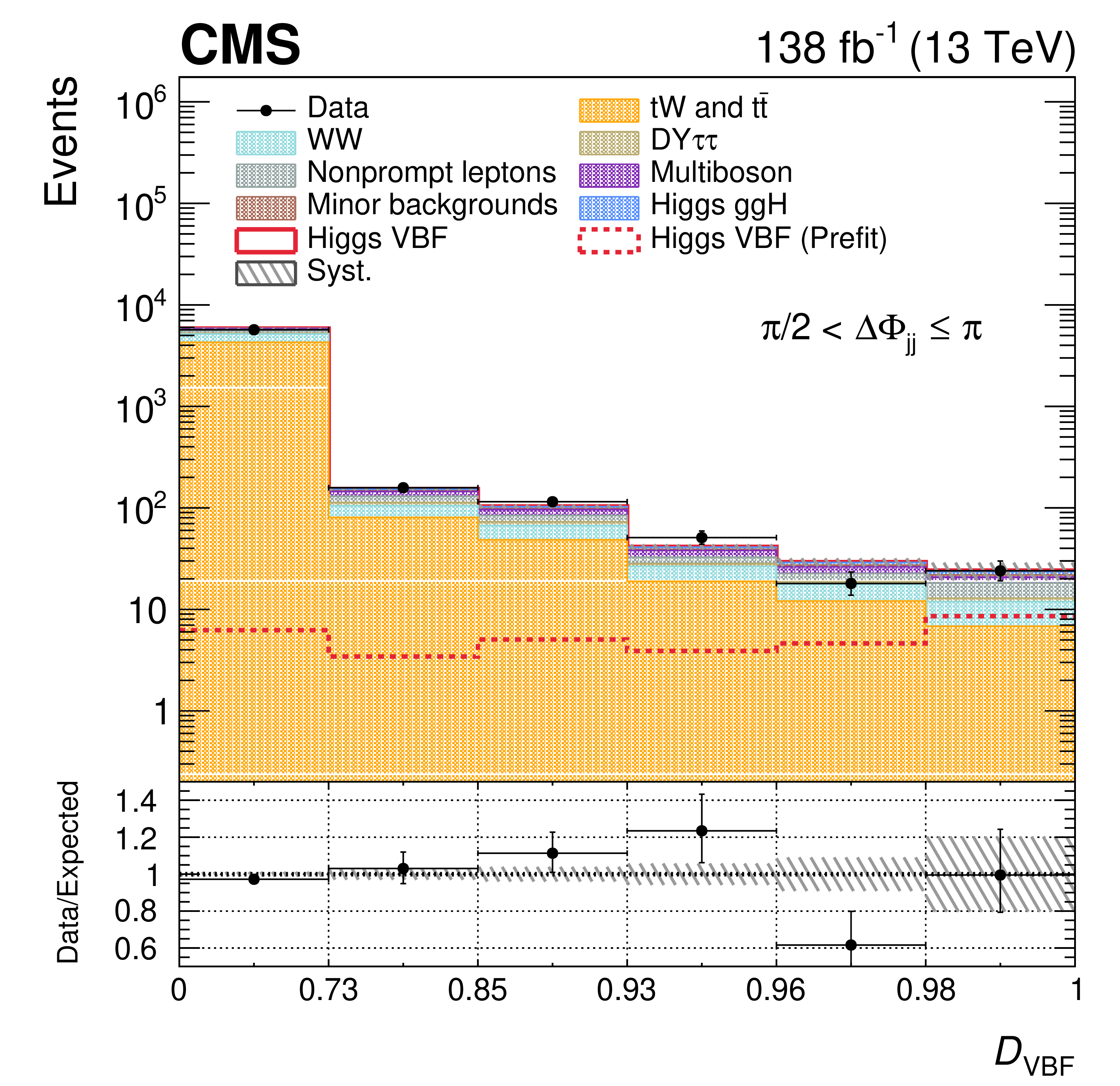
Figure 3:
Post-fit $ \mathcal{D}_\mathrm{VBF} $ distributions in the $ \Delta\Phi_\mathrm{{jj}} $ bins of the SR for the 2016-2018 data set, corresponding to fit configuration 3. Systematic uncertainties are shown as dashed gray bands. The pre-fit signal is shown superimposed as a dotted line, while the post-fit signal is included in the stacked histograms on top of the background templates. A uniform binning is applied for visualization, with the true binning range indicated on the $ x $ axis. The binning scheme optimized for the 2018 data set is used. The lower panel shows the ratio of data to the total expected yield, where the signal contribution is included in the expectation. |
png pdf |
Figure 3-a:
Post-fit $ \mathcal{D}_\mathrm{VBF} $ distributions in the $ \Delta\Phi_\mathrm{{jj}} $ bins of the SR for the 2016-2018 data set, corresponding to fit configuration 3. Systematic uncertainties are shown as dashed gray bands. The pre-fit signal is shown superimposed as a dotted line, while the post-fit signal is included in the stacked histograms on top of the background templates. A uniform binning is applied for visualization, with the true binning range indicated on the $ x $ axis. The binning scheme optimized for the 2018 data set is used. The lower panel shows the ratio of data to the total expected yield, where the signal contribution is included in the expectation. |
png pdf |
Figure 3-b:
Post-fit $ \mathcal{D}_\mathrm{VBF} $ distributions in the $ \Delta\Phi_\mathrm{{jj}} $ bins of the SR for the 2016-2018 data set, corresponding to fit configuration 3. Systematic uncertainties are shown as dashed gray bands. The pre-fit signal is shown superimposed as a dotted line, while the post-fit signal is included in the stacked histograms on top of the background templates. A uniform binning is applied for visualization, with the true binning range indicated on the $ x $ axis. The binning scheme optimized for the 2018 data set is used. The lower panel shows the ratio of data to the total expected yield, where the signal contribution is included in the expectation. |
png pdf |
Figure 3-c:
Post-fit $ \mathcal{D}_\mathrm{VBF} $ distributions in the $ \Delta\Phi_\mathrm{{jj}} $ bins of the SR for the 2016-2018 data set, corresponding to fit configuration 3. Systematic uncertainties are shown as dashed gray bands. The pre-fit signal is shown superimposed as a dotted line, while the post-fit signal is included in the stacked histograms on top of the background templates. A uniform binning is applied for visualization, with the true binning range indicated on the $ x $ axis. The binning scheme optimized for the 2018 data set is used. The lower panel shows the ratio of data to the total expected yield, where the signal contribution is included in the expectation. |
png pdf |
Figure 3-d:
Post-fit $ \mathcal{D}_\mathrm{VBF} $ distributions in the $ \Delta\Phi_\mathrm{{jj}} $ bins of the SR for the 2016-2018 data set, corresponding to fit configuration 3. Systematic uncertainties are shown as dashed gray bands. The pre-fit signal is shown superimposed as a dotted line, while the post-fit signal is included in the stacked histograms on top of the background templates. A uniform binning is applied for visualization, with the true binning range indicated on the $ x $ axis. The binning scheme optimized for the 2018 data set is used. The lower panel shows the ratio of data to the total expected yield, where the signal contribution is included in the expectation. |
png pdf |
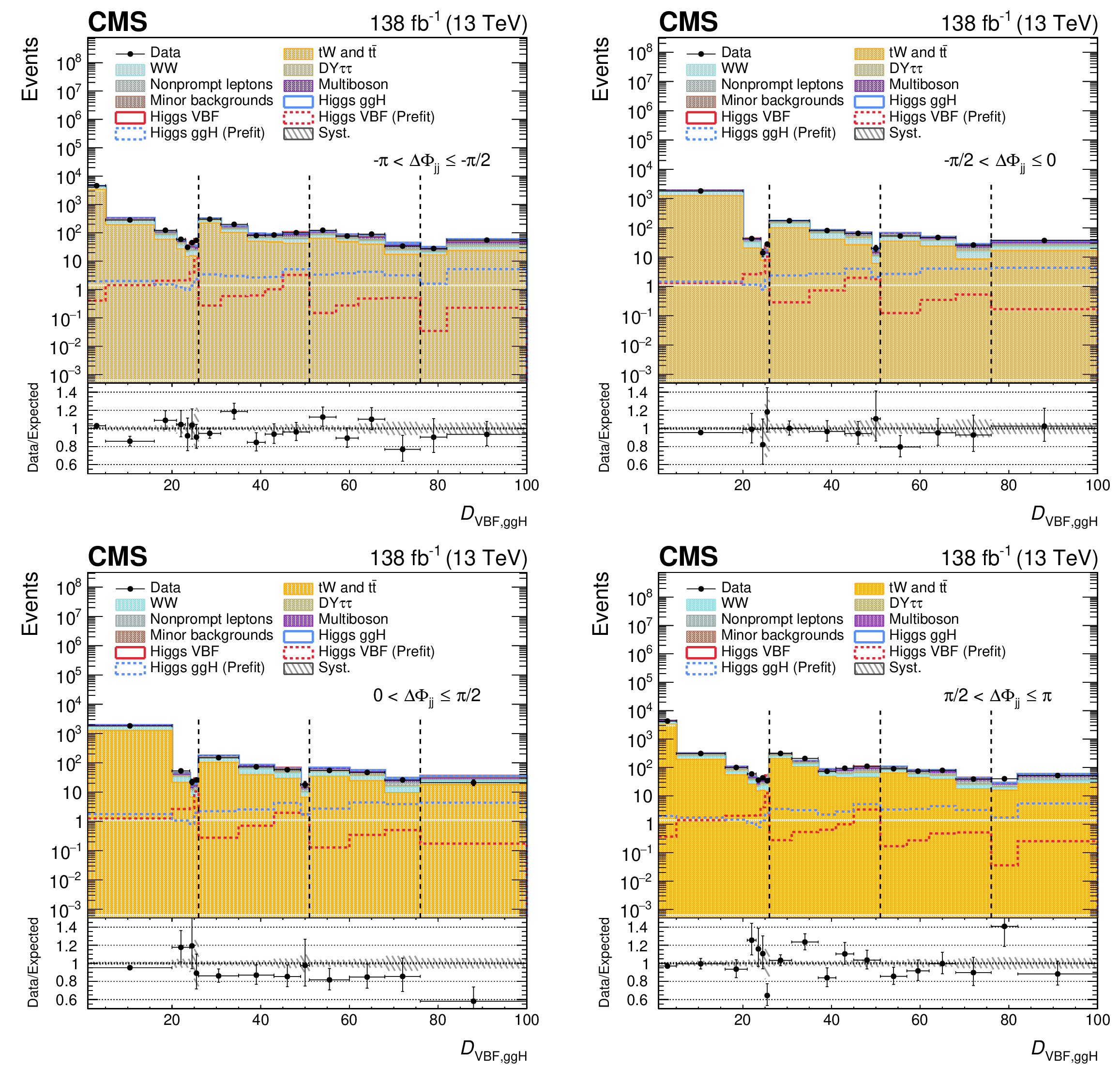
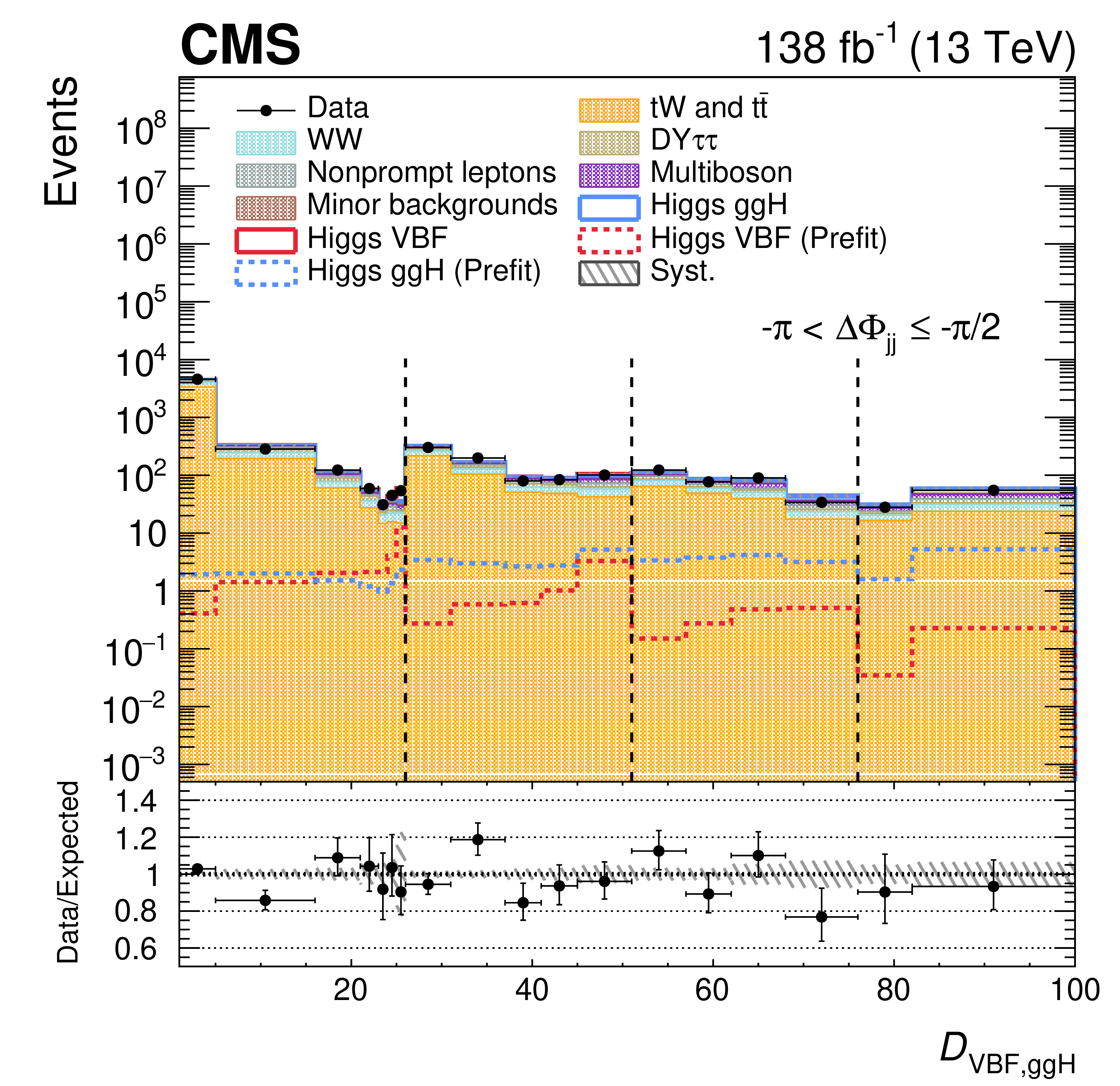
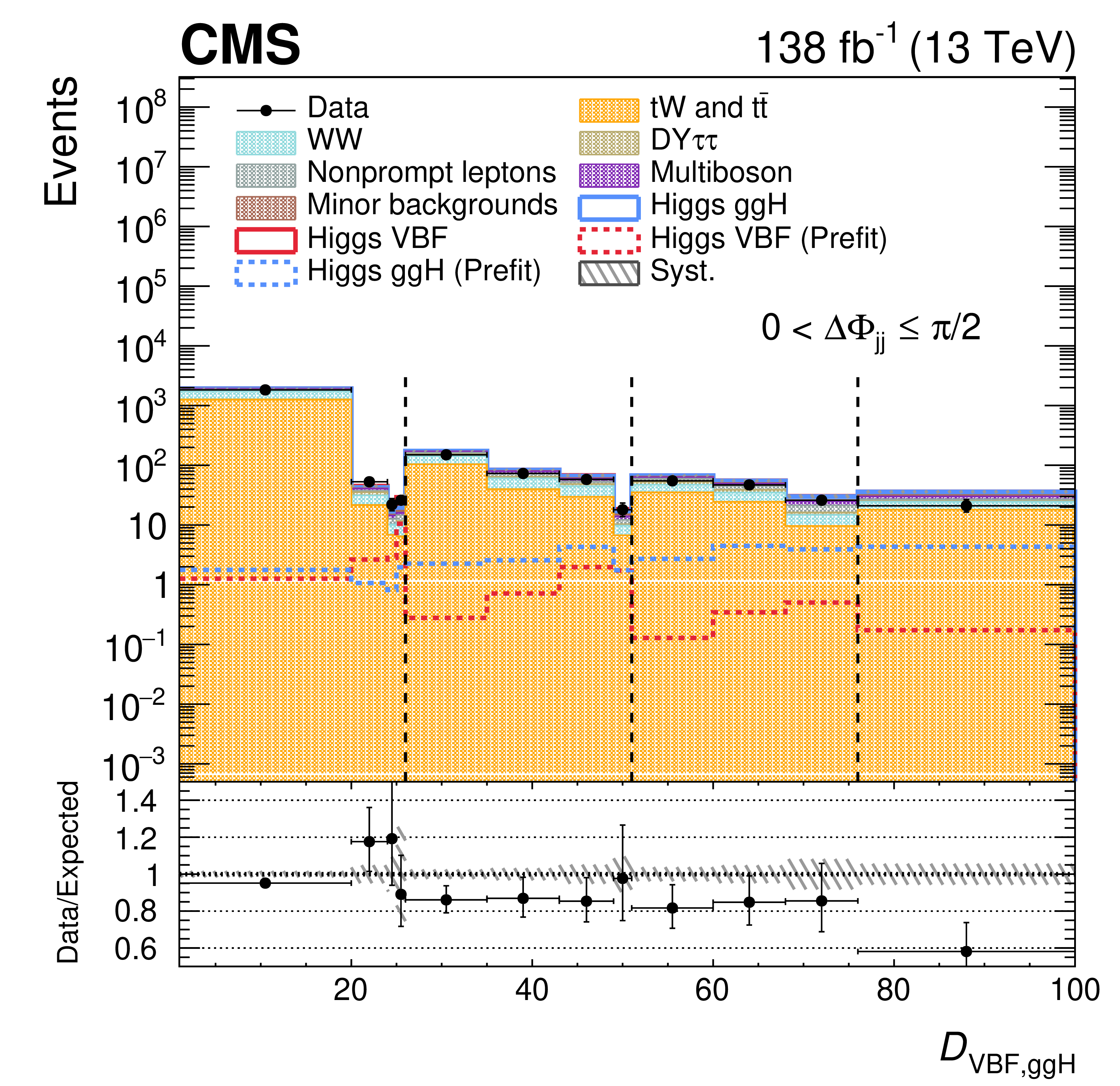
Figure 4:
Post-fit $ \mathcal{D}_\mathrm{VBF,ggH} $ distributions in the $ \Delta\Phi_\mathrm{{jj}} $ bins of the SR for the 2016-2018 data set, corresponding to fit configuration 1. The 2D distribution is unrolled into a 1D histogram, where the $ x $-axis labels correspond to the bin numbering of the original 2D map. Dashed black vertical lines mark the boundaries between $ \mathcal{D}_\mathrm{ggH} $ intervals, within which the binning reflects the $ \mathcal{D}_\mathrm{VBF} $ subdivisions. Systematic uncertainties are shown as dashed gray bands. The pre-fit signal is shown superimposed as a dotted line, while the post-fit signal is included in the stacked histograms on top of the background templates. The binning scheme optimized for the 2018 data set is used. The lower panel shows the ratio of data to the total expected yield, where the signal contribution is included in the expectation. |
png pdf |
Figure 4-a:
Post-fit $ \mathcal{D}_\mathrm{VBF,ggH} $ distributions in the $ \Delta\Phi_\mathrm{{jj}} $ bins of the SR for the 2016-2018 data set, corresponding to fit configuration 1. The 2D distribution is unrolled into a 1D histogram, where the $ x $-axis labels correspond to the bin numbering of the original 2D map. Dashed black vertical lines mark the boundaries between $ \mathcal{D}_\mathrm{ggH} $ intervals, within which the binning reflects the $ \mathcal{D}_\mathrm{VBF} $ subdivisions. Systematic uncertainties are shown as dashed gray bands. The pre-fit signal is shown superimposed as a dotted line, while the post-fit signal is included in the stacked histograms on top of the background templates. The binning scheme optimized for the 2018 data set is used. The lower panel shows the ratio of data to the total expected yield, where the signal contribution is included in the expectation. |

png pdf |
Figure 4-b:
Post-fit $ \mathcal{D}_\mathrm{VBF,ggH} $ distributions in the $ \Delta\Phi_\mathrm{{jj}} $ bins of the SR for the 2016-2018 data set, corresponding to fit configuration 1. The 2D distribution is unrolled into a 1D histogram, where the $ x $-axis labels correspond to the bin numbering of the original 2D map. Dashed black vertical lines mark the boundaries between $ \mathcal{D}_\mathrm{ggH} $ intervals, within which the binning reflects the $ \mathcal{D}_\mathrm{VBF} $ subdivisions. Systematic uncertainties are shown as dashed gray bands. The pre-fit signal is shown superimposed as a dotted line, while the post-fit signal is included in the stacked histograms on top of the background templates. The binning scheme optimized for the 2018 data set is used. The lower panel shows the ratio of data to the total expected yield, where the signal contribution is included in the expectation. |
png pdf |
Figure 4-c:
Post-fit $ \mathcal{D}_\mathrm{VBF,ggH} $ distributions in the $ \Delta\Phi_\mathrm{{jj}} $ bins of the SR for the 2016-2018 data set, corresponding to fit configuration 1. The 2D distribution is unrolled into a 1D histogram, where the $ x $-axis labels correspond to the bin numbering of the original 2D map. Dashed black vertical lines mark the boundaries between $ \mathcal{D}_\mathrm{ggH} $ intervals, within which the binning reflects the $ \mathcal{D}_\mathrm{VBF} $ subdivisions. Systematic uncertainties are shown as dashed gray bands. The pre-fit signal is shown superimposed as a dotted line, while the post-fit signal is included in the stacked histograms on top of the background templates. The binning scheme optimized for the 2018 data set is used. The lower panel shows the ratio of data to the total expected yield, where the signal contribution is included in the expectation. |

png pdf |
Figure 4-d:
Post-fit $ \mathcal{D}_\mathrm{VBF,ggH} $ distributions in the $ \Delta\Phi_\mathrm{{jj}} $ bins of the SR for the 2016-2018 data set, corresponding to fit configuration 1. The 2D distribution is unrolled into a 1D histogram, where the $ x $-axis labels correspond to the bin numbering of the original 2D map. Dashed black vertical lines mark the boundaries between $ \mathcal{D}_\mathrm{ggH} $ intervals, within which the binning reflects the $ \mathcal{D}_\mathrm{VBF} $ subdivisions. Systematic uncertainties are shown as dashed gray bands. The pre-fit signal is shown superimposed as a dotted line, while the post-fit signal is included in the stacked histograms on top of the background templates. The binning scheme optimized for the 2018 data set is used. The lower panel shows the ratio of data to the total expected yield, where the signal contribution is included in the expectation. |
png pdf |
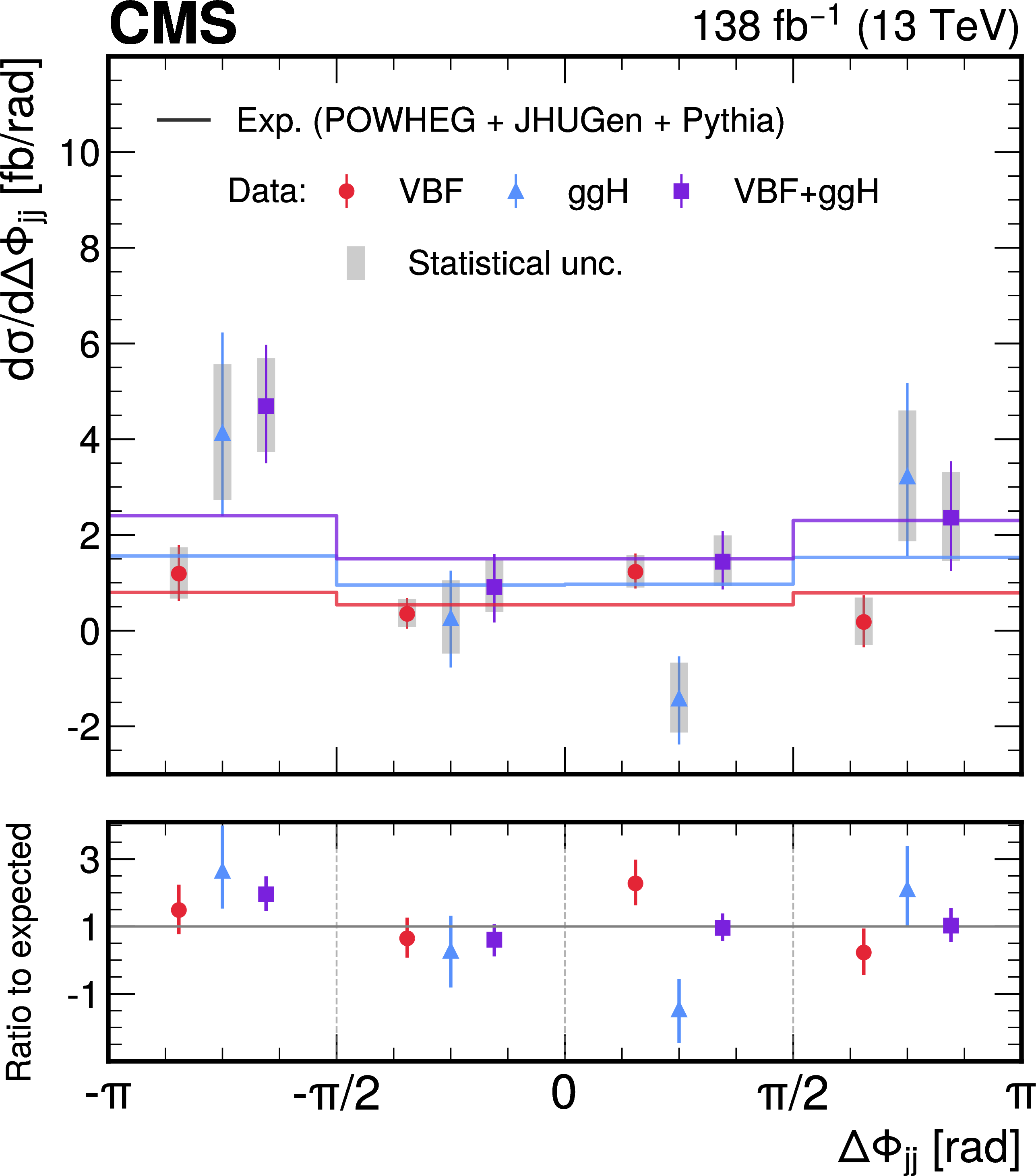
Figure 5:
Measured fiducial cross section of the VBF and ggH production processes. Colored markers represent the extracted cross section values from data, with error bars showing the combined statistical and systematic uncertainties: red for VBF, light blue for ggH, and violet for the sum of VBF + ggH. The gray bands indicate the statistical uncertainties. The colored histogram corresponds to the expected SM prediction, simulated with POWHEG + JHUGEN + PYTHIA generators. The lower panel displays the ratio of the measured values to the SM expectation. |
png pdf |
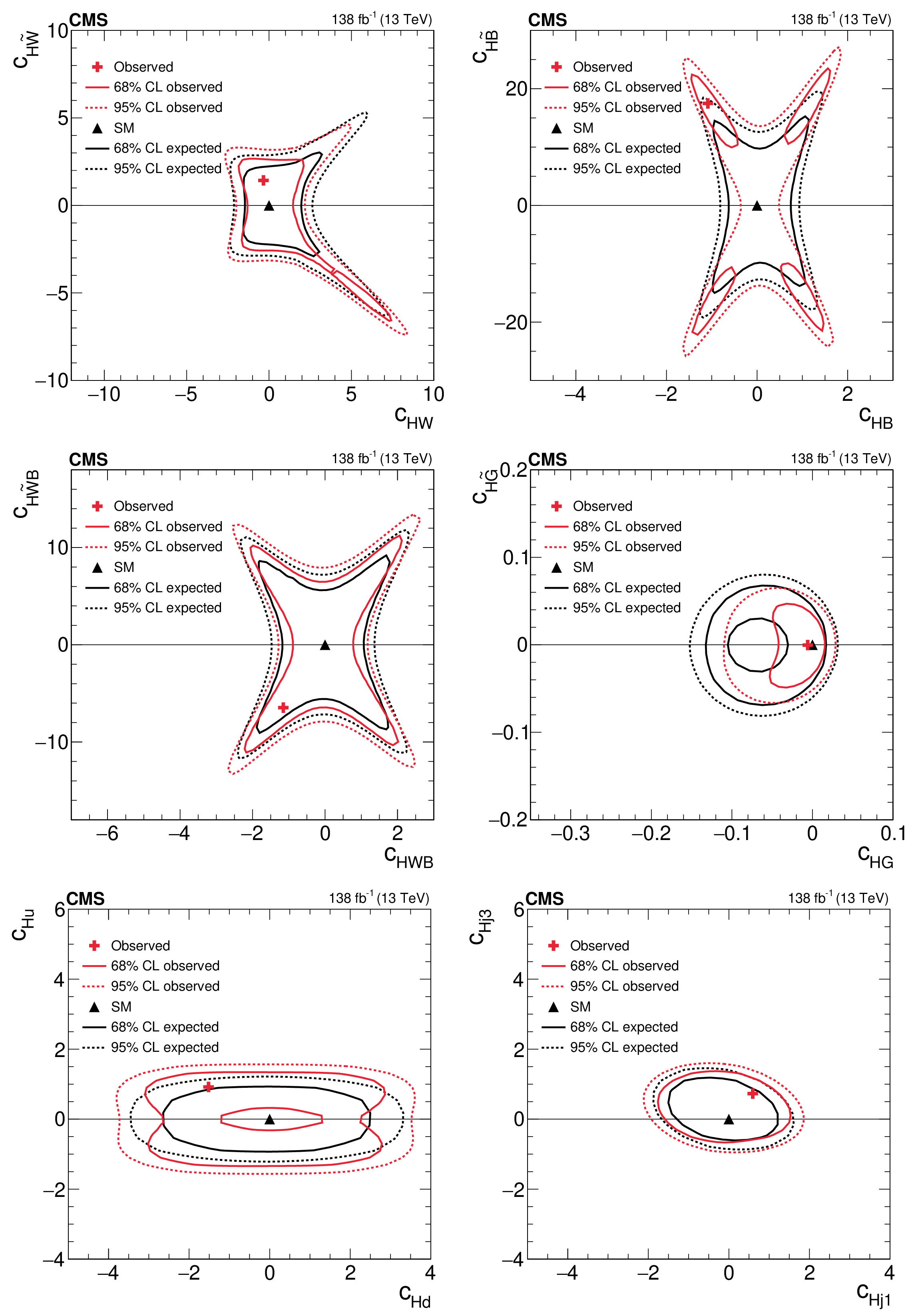
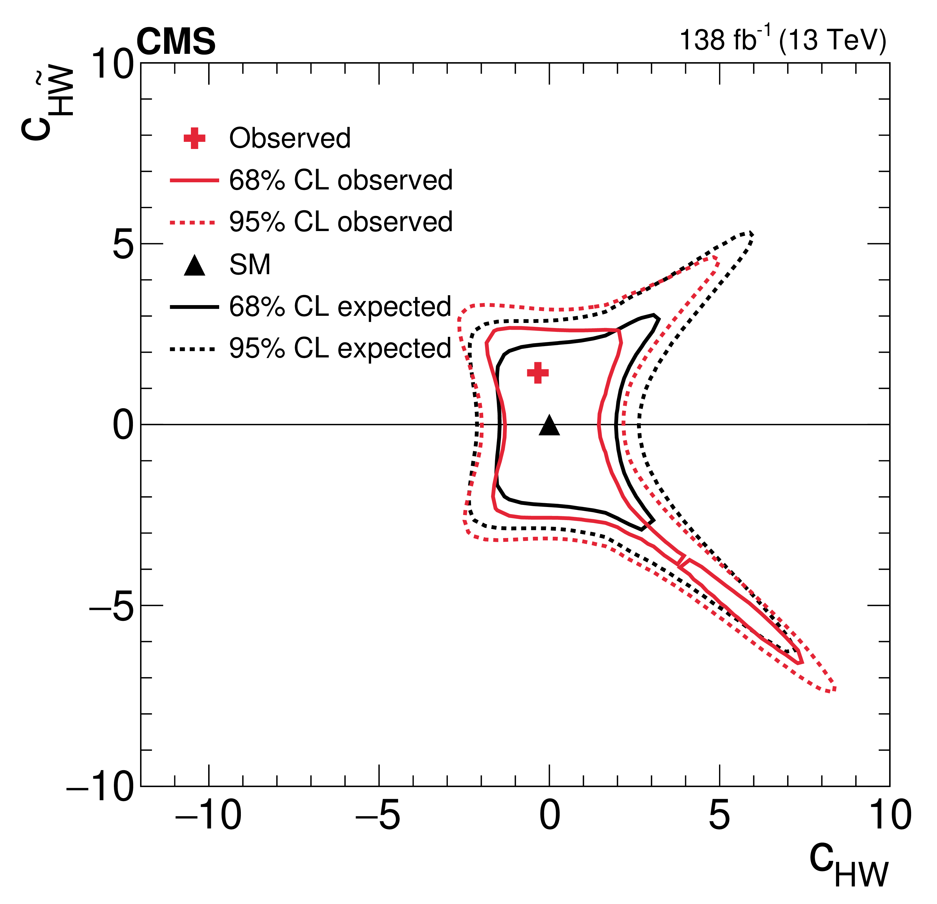
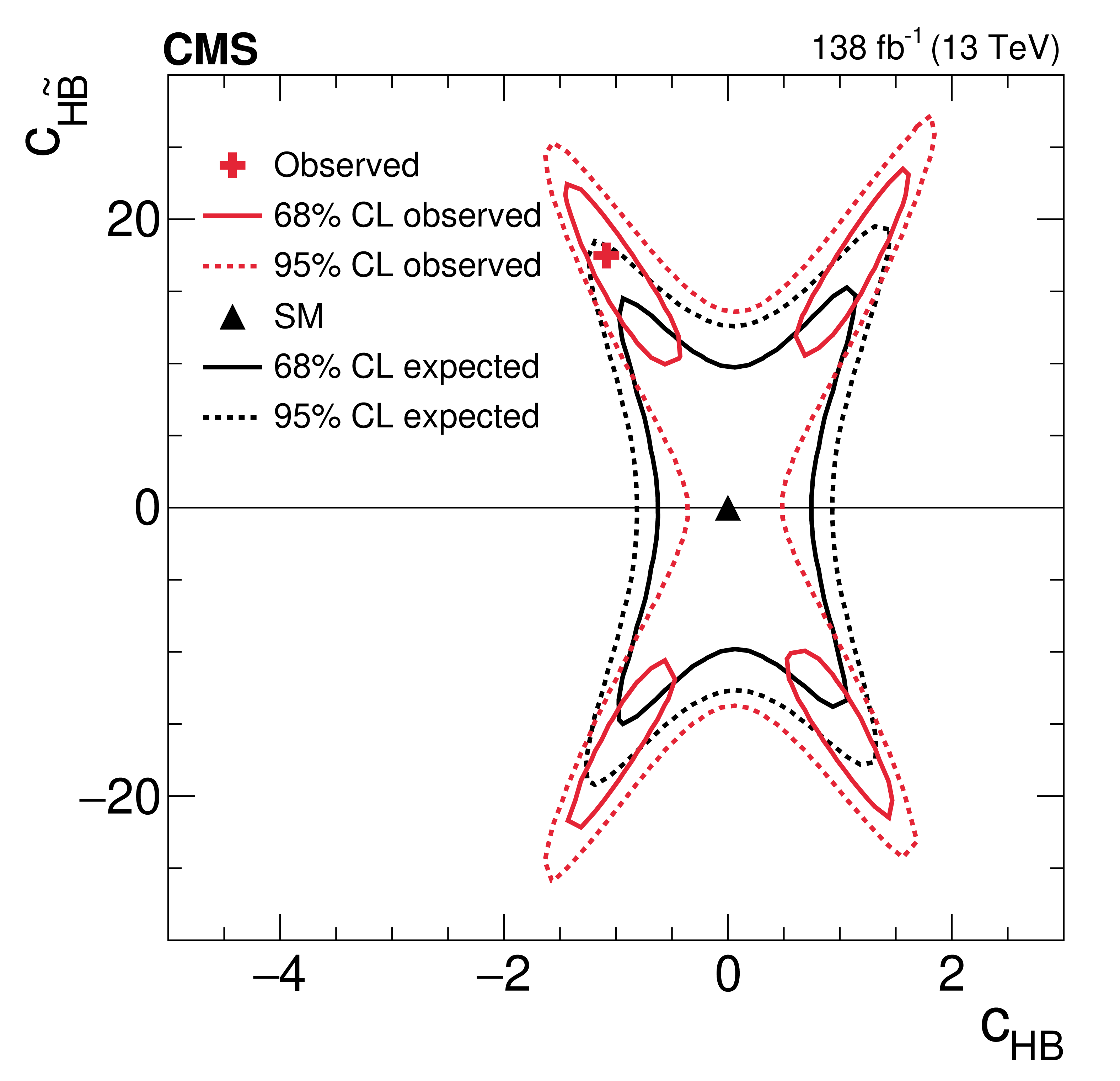
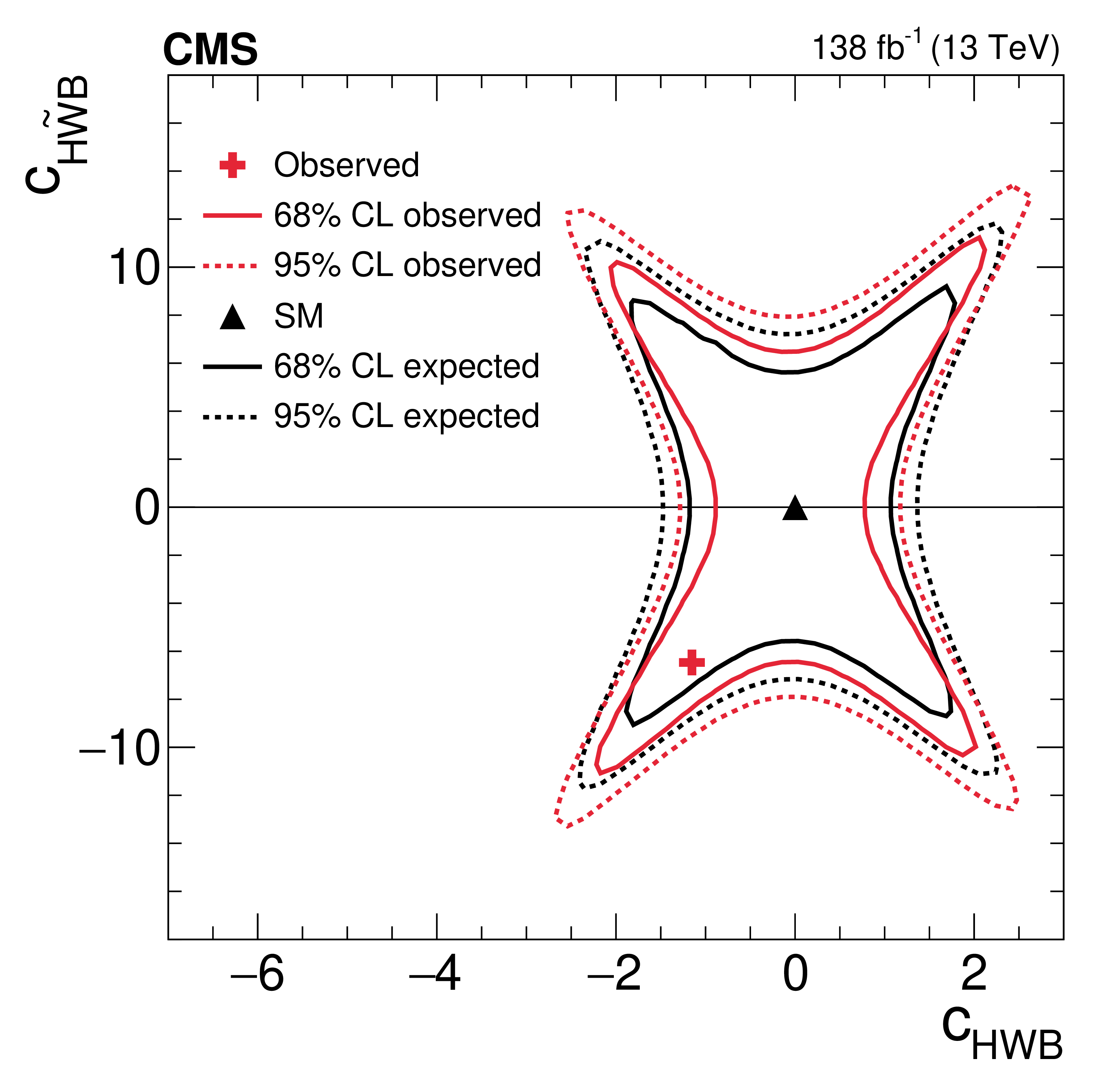
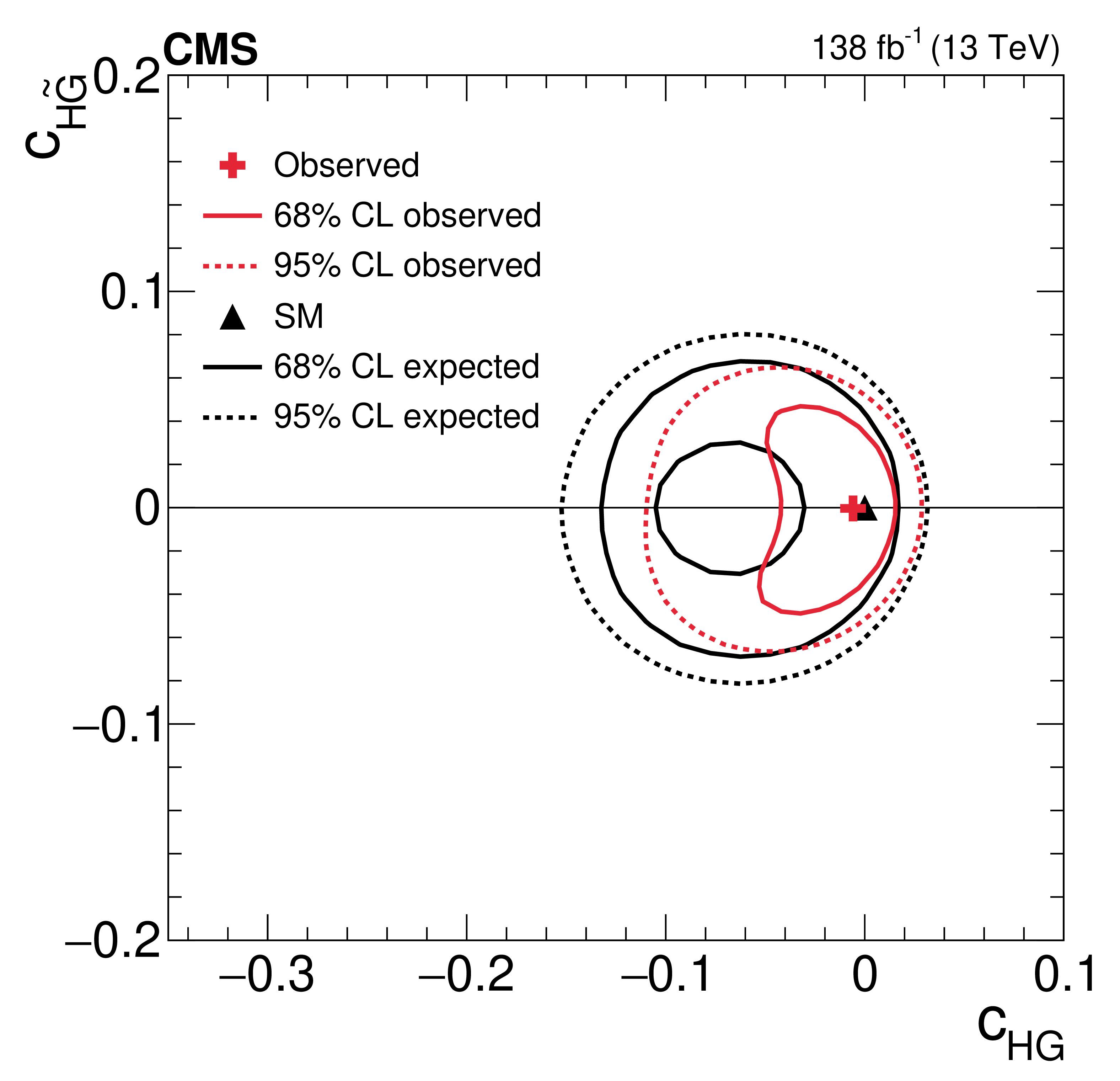
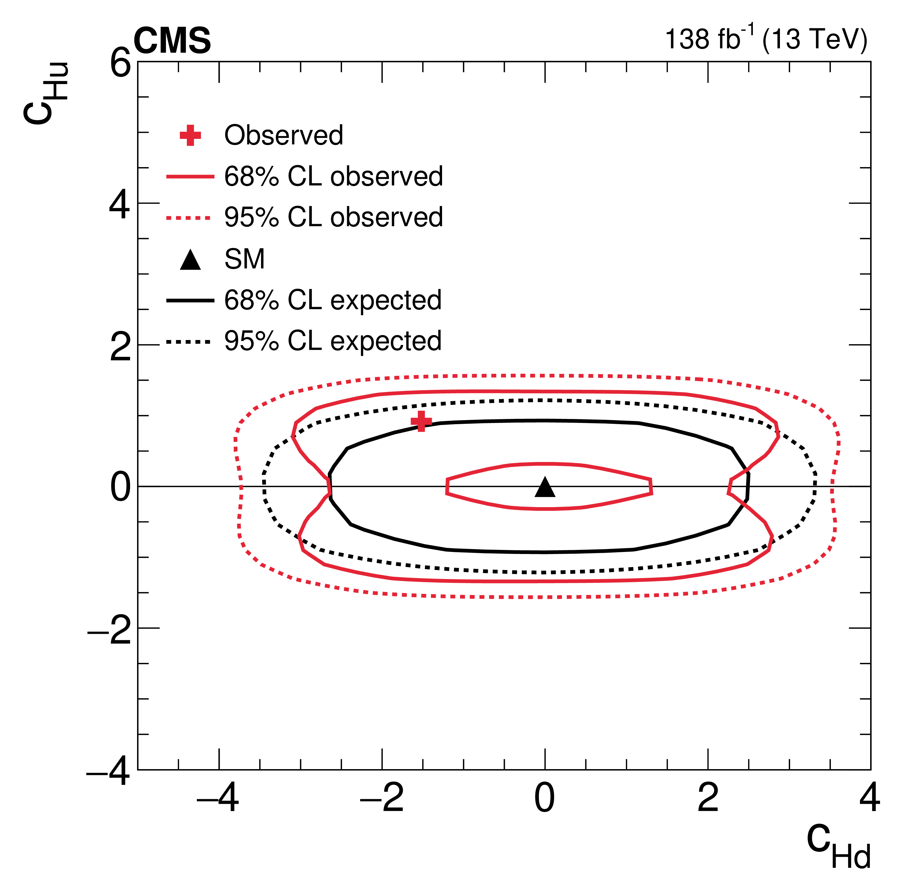
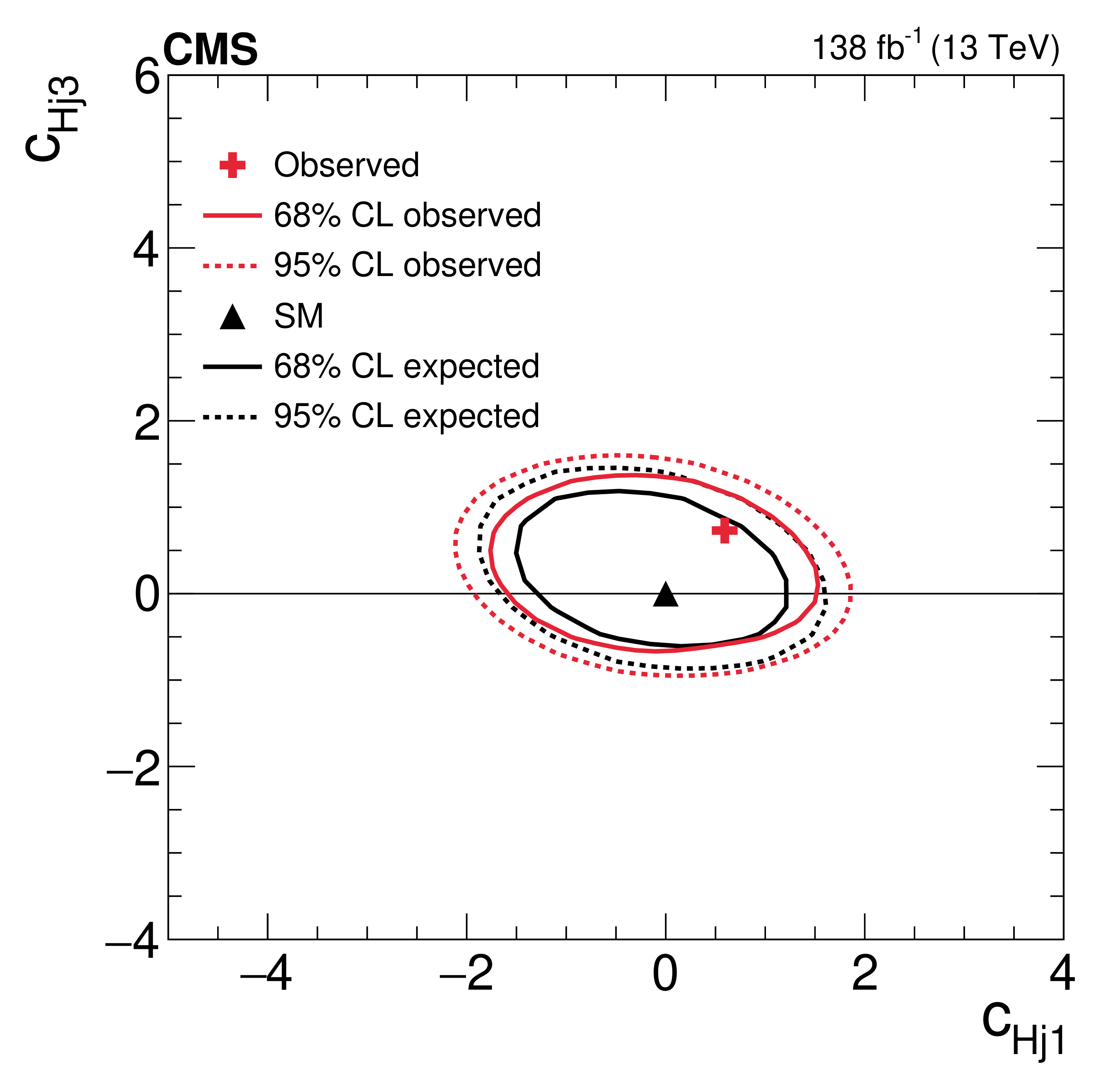
Figure 6:
Two-dimensional expected and observed scans for the pairs of Wilson coefficients $ c_\text{HW} $, $ c_{\text{H}\tilde{\text{W}}} $ (upper left), $ c_\text{HB} $, $ c_{\text{H}\tilde{\text{B}}} $ (upper right), $ c_\text{HWB} $, $ c_{\text{H}\tilde{\text{W}}\text{B}} $ (middle left), $ c_\text{HG} $, $ c_{\text{H}\tilde{\text{G}}} $ (middle right), $ c_{\text{Hu}} $, $ c_{\text{Hd}} $ (lower left) and $ c_{\text{Hj1}} $, $ c_{\text{Hj3}} $ (lower right). Solid (dotted) lines correspond to the 68% (95%) CL contours. |
png pdf |
Figure 6-a:
Two-dimensional expected and observed scans for the pairs of Wilson coefficients $ c_\text{HW} $, $ c_{\text{H}\tilde{\text{W}}} $ (upper left), $ c_\text{HB} $, $ c_{\text{H}\tilde{\text{B}}} $ (upper right), $ c_\text{HWB} $, $ c_{\text{H}\tilde{\text{W}}\text{B}} $ (middle left), $ c_\text{HG} $, $ c_{\text{H}\tilde{\text{G}}} $ (middle right), $ c_{\text{Hu}} $, $ c_{\text{Hd}} $ (lower left) and $ c_{\text{Hj1}} $, $ c_{\text{Hj3}} $ (lower right). Solid (dotted) lines correspond to the 68% (95%) CL contours. |
png pdf |
Figure 6-b:
Two-dimensional expected and observed scans for the pairs of Wilson coefficients $ c_\text{HW} $, $ c_{\text{H}\tilde{\text{W}}} $ (upper left), $ c_\text{HB} $, $ c_{\text{H}\tilde{\text{B}}} $ (upper right), $ c_\text{HWB} $, $ c_{\text{H}\tilde{\text{W}}\text{B}} $ (middle left), $ c_\text{HG} $, $ c_{\text{H}\tilde{\text{G}}} $ (middle right), $ c_{\text{Hu}} $, $ c_{\text{Hd}} $ (lower left) and $ c_{\text{Hj1}} $, $ c_{\text{Hj3}} $ (lower right). Solid (dotted) lines correspond to the 68% (95%) CL contours. |
png pdf |
Figure 6-c:
Two-dimensional expected and observed scans for the pairs of Wilson coefficients $ c_\text{HW} $, $ c_{\text{H}\tilde{\text{W}}} $ (upper left), $ c_\text{HB} $, $ c_{\text{H}\tilde{\text{B}}} $ (upper right), $ c_\text{HWB} $, $ c_{\text{H}\tilde{\text{W}}\text{B}} $ (middle left), $ c_\text{HG} $, $ c_{\text{H}\tilde{\text{G}}} $ (middle right), $ c_{\text{Hu}} $, $ c_{\text{Hd}} $ (lower left) and $ c_{\text{Hj1}} $, $ c_{\text{Hj3}} $ (lower right). Solid (dotted) lines correspond to the 68% (95%) CL contours. |
png pdf |
Figure 6-d:
Two-dimensional expected and observed scans for the pairs of Wilson coefficients $ c_\text{HW} $, $ c_{\text{H}\tilde{\text{W}}} $ (upper left), $ c_\text{HB} $, $ c_{\text{H}\tilde{\text{B}}} $ (upper right), $ c_\text{HWB} $, $ c_{\text{H}\tilde{\text{W}}\text{B}} $ (middle left), $ c_\text{HG} $, $ c_{\text{H}\tilde{\text{G}}} $ (middle right), $ c_{\text{Hu}} $, $ c_{\text{Hd}} $ (lower left) and $ c_{\text{Hj1}} $, $ c_{\text{Hj3}} $ (lower right). Solid (dotted) lines correspond to the 68% (95%) CL contours. |
png pdf |
Figure 6-e:
Two-dimensional expected and observed scans for the pairs of Wilson coefficients $ c_\text{HW} $, $ c_{\text{H}\tilde{\text{W}}} $ (upper left), $ c_\text{HB} $, $ c_{\text{H}\tilde{\text{B}}} $ (upper right), $ c_\text{HWB} $, $ c_{\text{H}\tilde{\text{W}}\text{B}} $ (middle left), $ c_\text{HG} $, $ c_{\text{H}\tilde{\text{G}}} $ (middle right), $ c_{\text{Hu}} $, $ c_{\text{Hd}} $ (lower left) and $ c_{\text{Hj1}} $, $ c_{\text{Hj3}} $ (lower right). Solid (dotted) lines correspond to the 68% (95%) CL contours. |
png pdf |
Figure 6-f:
Two-dimensional expected and observed scans for the pairs of Wilson coefficients $ c_\text{HW} $, $ c_{\text{H}\tilde{\text{W}}} $ (upper left), $ c_\text{HB} $, $ c_{\text{H}\tilde{\text{B}}} $ (upper right), $ c_\text{HWB} $, $ c_{\text{H}\tilde{\text{W}}\text{B}} $ (middle left), $ c_\text{HG} $, $ c_{\text{H}\tilde{\text{G}}} $ (middle right), $ c_{\text{Hu}} $, $ c_{\text{Hd}} $ (lower left) and $ c_{\text{Hj1}} $, $ c_{\text{Hj3}} $ (lower right). Solid (dotted) lines correspond to the 68% (95%) CL contours. |
png pdf |
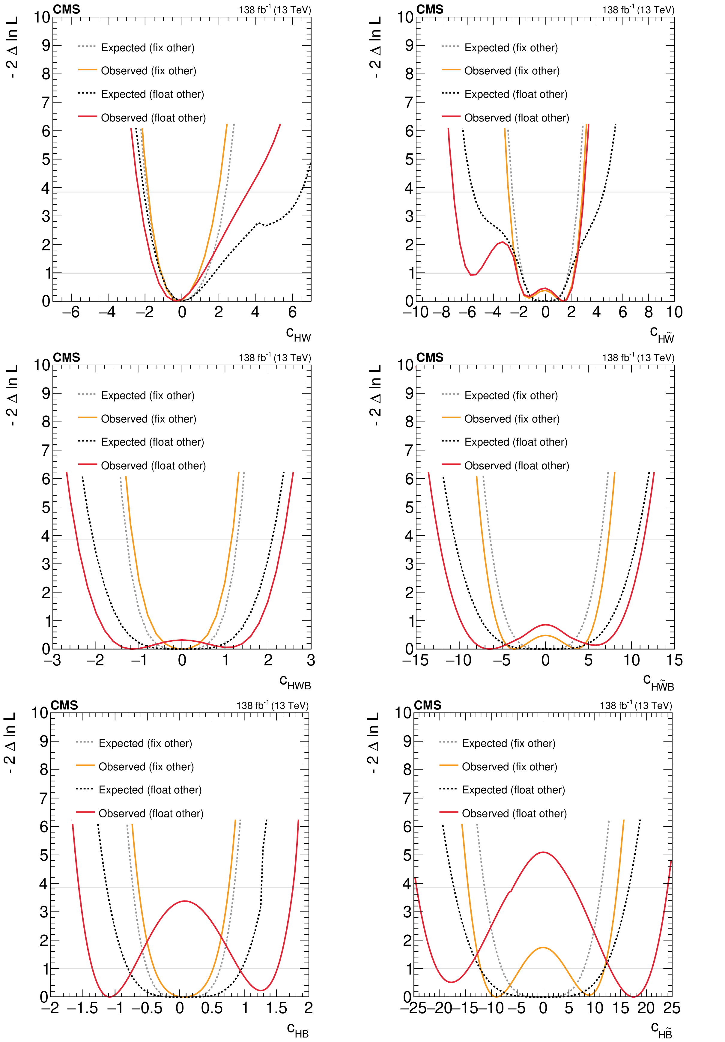
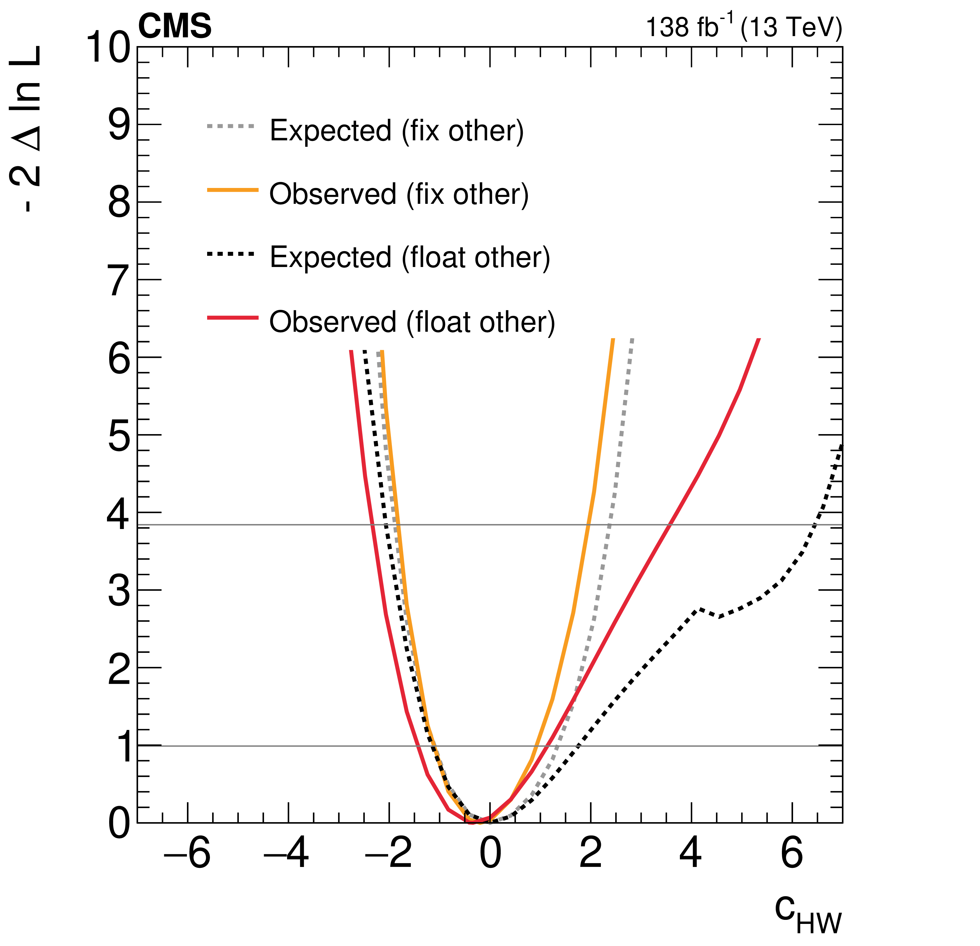
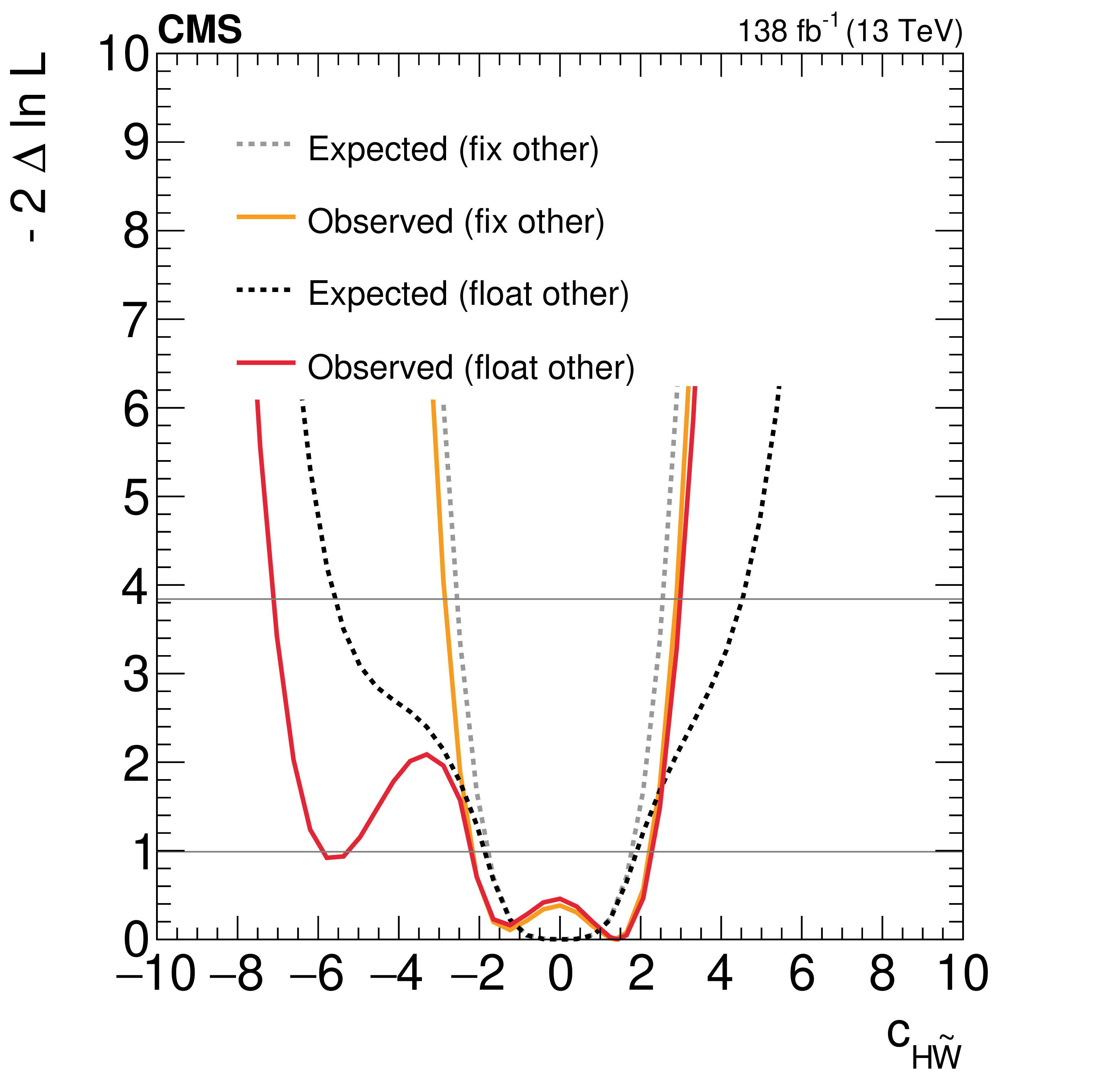
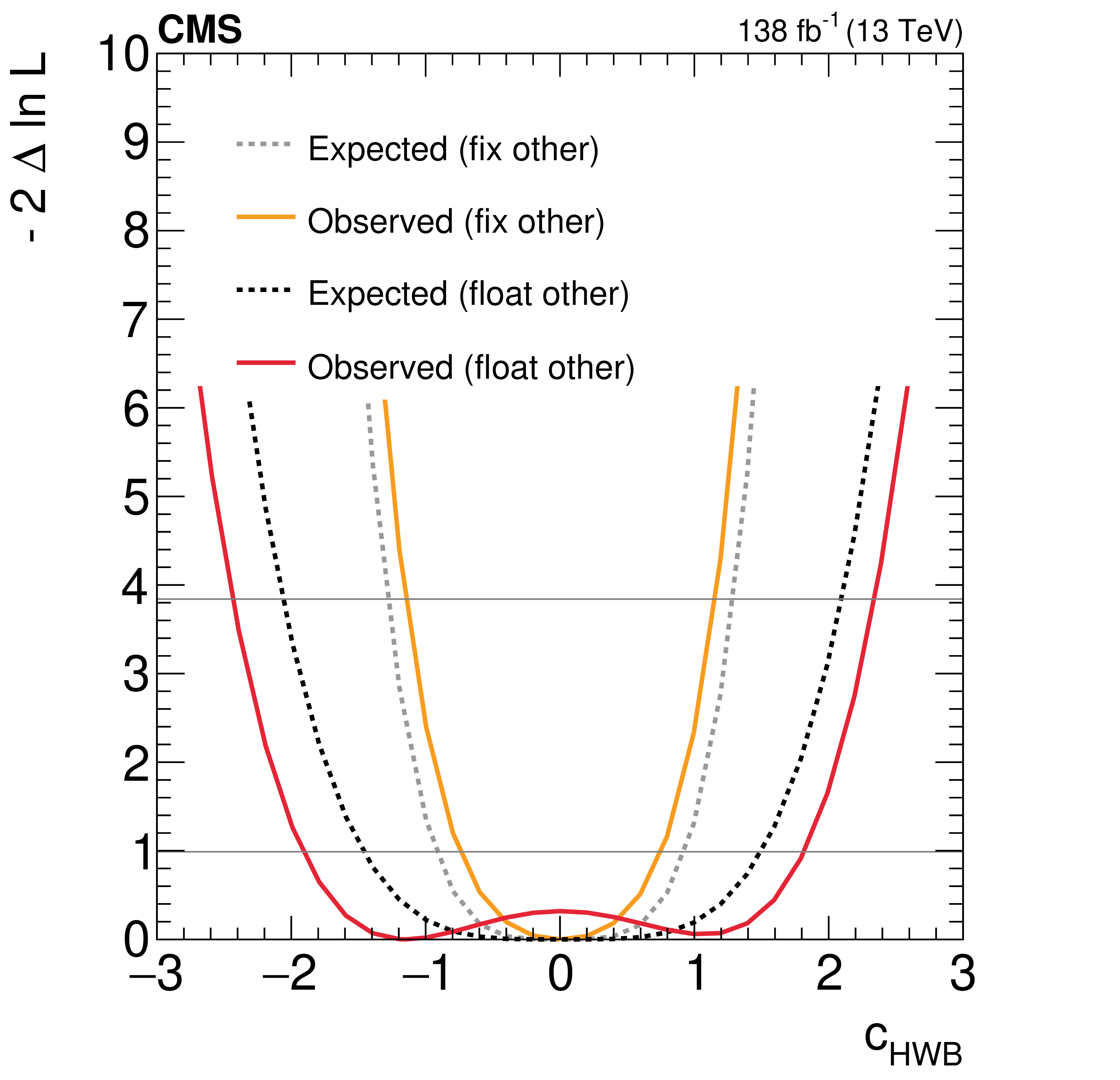
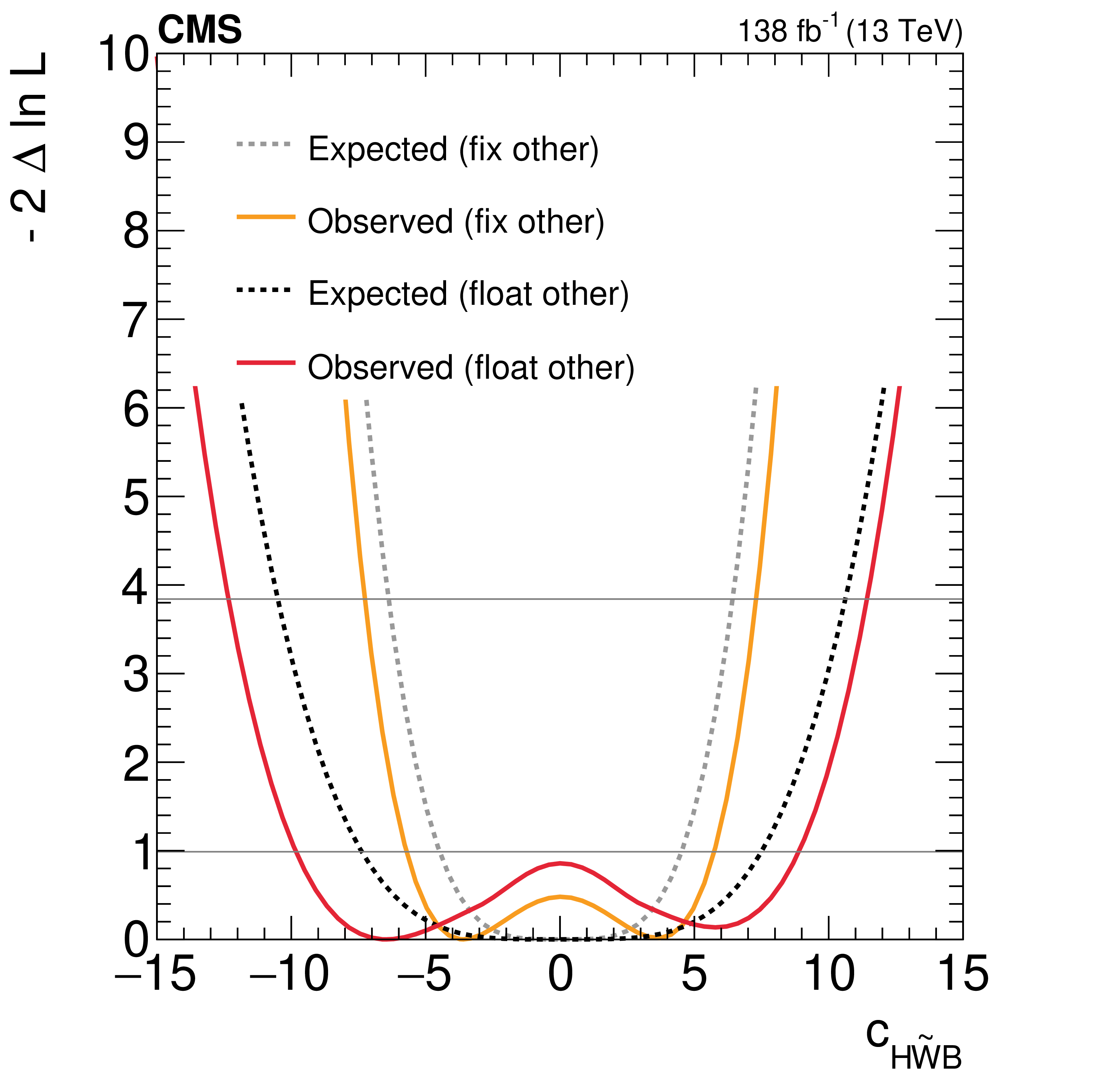
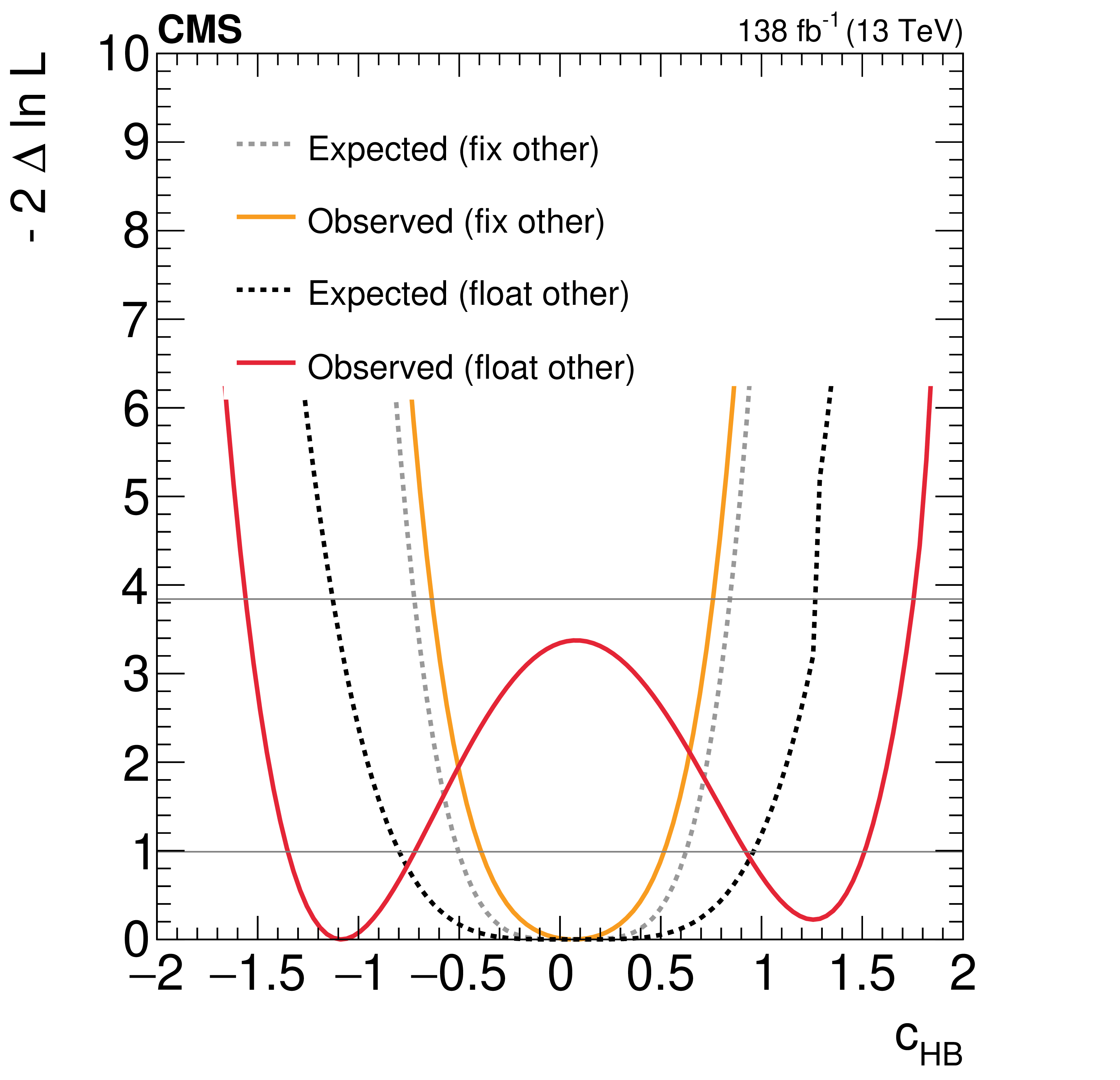
Figure 7:
Expected and observed scans for the Wilson coefficients $ c_\text{HW} $ (upper left), $ c_\text{HWB} $ (middle left), $ c_\text{HB} $ (lower left), $ c_{\text{H}\tilde{\text{W}}} $ (upper right), $ c_{\text{H}\tilde{\text{W}}\text{B}} $ (middle right) and $ c_{\text{H}\tilde{\text{B}}} $ (lower right). The results are presented for two scenarios: one where all other coefficients are fixed to their SM values (grey) and another where the coefficient with opposite $ CP $-parity is allowed to float in the fit (black). Horizontal lines indicate the one-dimensional 68% and 95% CL values. |
png pdf |
Figure 7-a:
Expected and observed scans for the Wilson coefficients $ c_\text{HW} $ (upper left), $ c_\text{HWB} $ (middle left), $ c_\text{HB} $ (lower left), $ c_{\text{H}\tilde{\text{W}}} $ (upper right), $ c_{\text{H}\tilde{\text{W}}\text{B}} $ (middle right) and $ c_{\text{H}\tilde{\text{B}}} $ (lower right). The results are presented for two scenarios: one where all other coefficients are fixed to their SM values (grey) and another where the coefficient with opposite $ CP $-parity is allowed to float in the fit (black). Horizontal lines indicate the one-dimensional 68% and 95% CL values. |
png pdf |
Figure 7-b:
Expected and observed scans for the Wilson coefficients $ c_\text{HW} $ (upper left), $ c_\text{HWB} $ (middle left), $ c_\text{HB} $ (lower left), $ c_{\text{H}\tilde{\text{W}}} $ (upper right), $ c_{\text{H}\tilde{\text{W}}\text{B}} $ (middle right) and $ c_{\text{H}\tilde{\text{B}}} $ (lower right). The results are presented for two scenarios: one where all other coefficients are fixed to their SM values (grey) and another where the coefficient with opposite $ CP $-parity is allowed to float in the fit (black). Horizontal lines indicate the one-dimensional 68% and 95% CL values. |
png pdf |
Figure 7-c:
Expected and observed scans for the Wilson coefficients $ c_\text{HW} $ (upper left), $ c_\text{HWB} $ (middle left), $ c_\text{HB} $ (lower left), $ c_{\text{H}\tilde{\text{W}}} $ (upper right), $ c_{\text{H}\tilde{\text{W}}\text{B}} $ (middle right) and $ c_{\text{H}\tilde{\text{B}}} $ (lower right). The results are presented for two scenarios: one where all other coefficients are fixed to their SM values (grey) and another where the coefficient with opposite $ CP $-parity is allowed to float in the fit (black). Horizontal lines indicate the one-dimensional 68% and 95% CL values. |
png pdf |
Figure 7-d:
Expected and observed scans for the Wilson coefficients $ c_\text{HW} $ (upper left), $ c_\text{HWB} $ (middle left), $ c_\text{HB} $ (lower left), $ c_{\text{H}\tilde{\text{W}}} $ (upper right), $ c_{\text{H}\tilde{\text{W}}\text{B}} $ (middle right) and $ c_{\text{H}\tilde{\text{B}}} $ (lower right). The results are presented for two scenarios: one where all other coefficients are fixed to their SM values (grey) and another where the coefficient with opposite $ CP $-parity is allowed to float in the fit (black). Horizontal lines indicate the one-dimensional 68% and 95% CL values. |
png pdf |
Figure 7-e:
Expected and observed scans for the Wilson coefficients $ c_\text{HW} $ (upper left), $ c_\text{HWB} $ (middle left), $ c_\text{HB} $ (lower left), $ c_{\text{H}\tilde{\text{W}}} $ (upper right), $ c_{\text{H}\tilde{\text{W}}\text{B}} $ (middle right) and $ c_{\text{H}\tilde{\text{B}}} $ (lower right). The results are presented for two scenarios: one where all other coefficients are fixed to their SM values (grey) and another where the coefficient with opposite $ CP $-parity is allowed to float in the fit (black). Horizontal lines indicate the one-dimensional 68% and 95% CL values. |

png pdf |
Figure 7-f:
Expected and observed scans for the Wilson coefficients $ c_\text{HW} $ (upper left), $ c_\text{HWB} $ (middle left), $ c_\text{HB} $ (lower left), $ c_{\text{H}\tilde{\text{W}}} $ (upper right), $ c_{\text{H}\tilde{\text{W}}\text{B}} $ (middle right) and $ c_{\text{H}\tilde{\text{B}}} $ (lower right). The results are presented for two scenarios: one where all other coefficients are fixed to their SM values (grey) and another where the coefficient with opposite $ CP $-parity is allowed to float in the fit (black). Horizontal lines indicate the one-dimensional 68% and 95% CL values. |
png pdf |
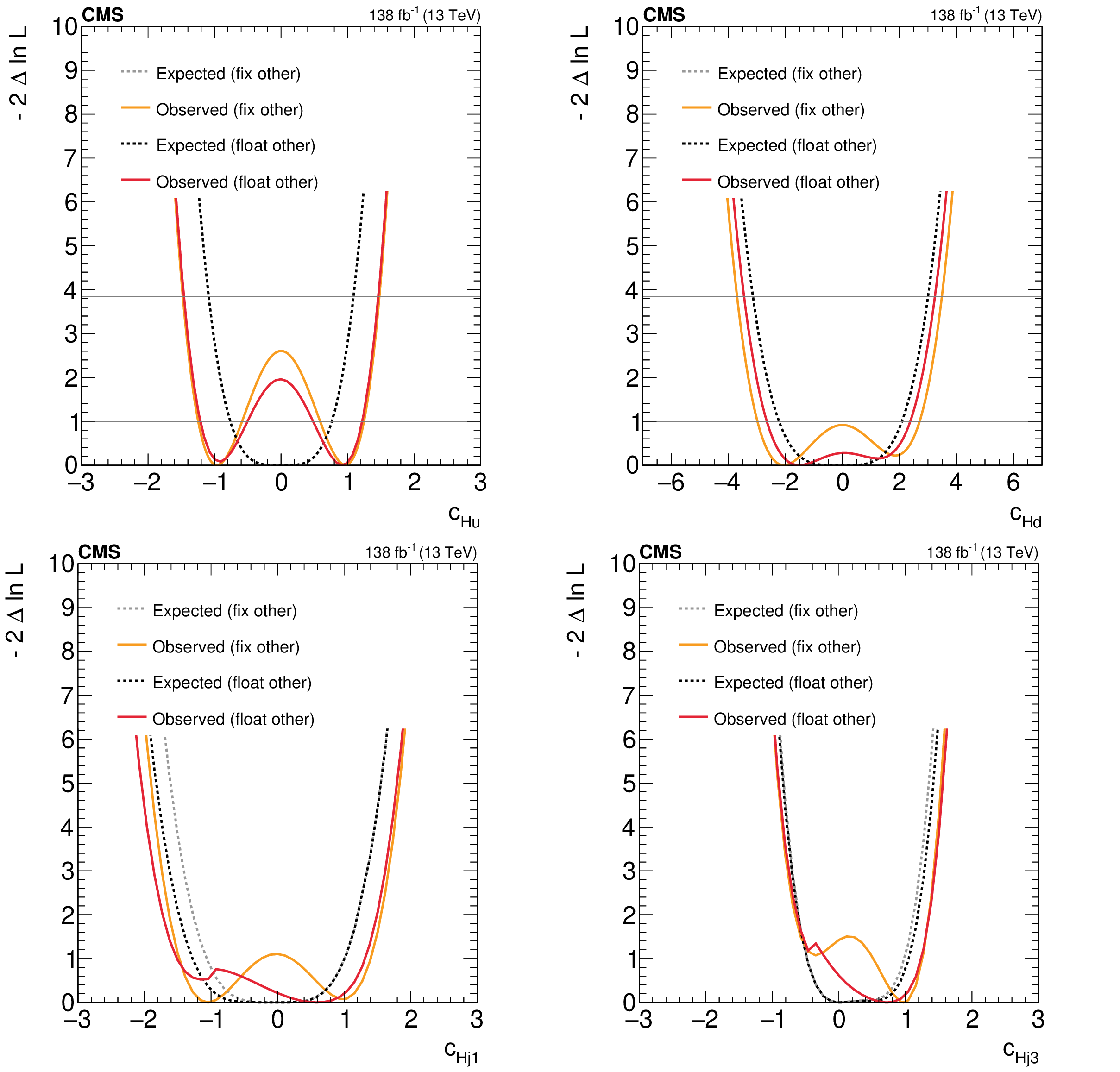
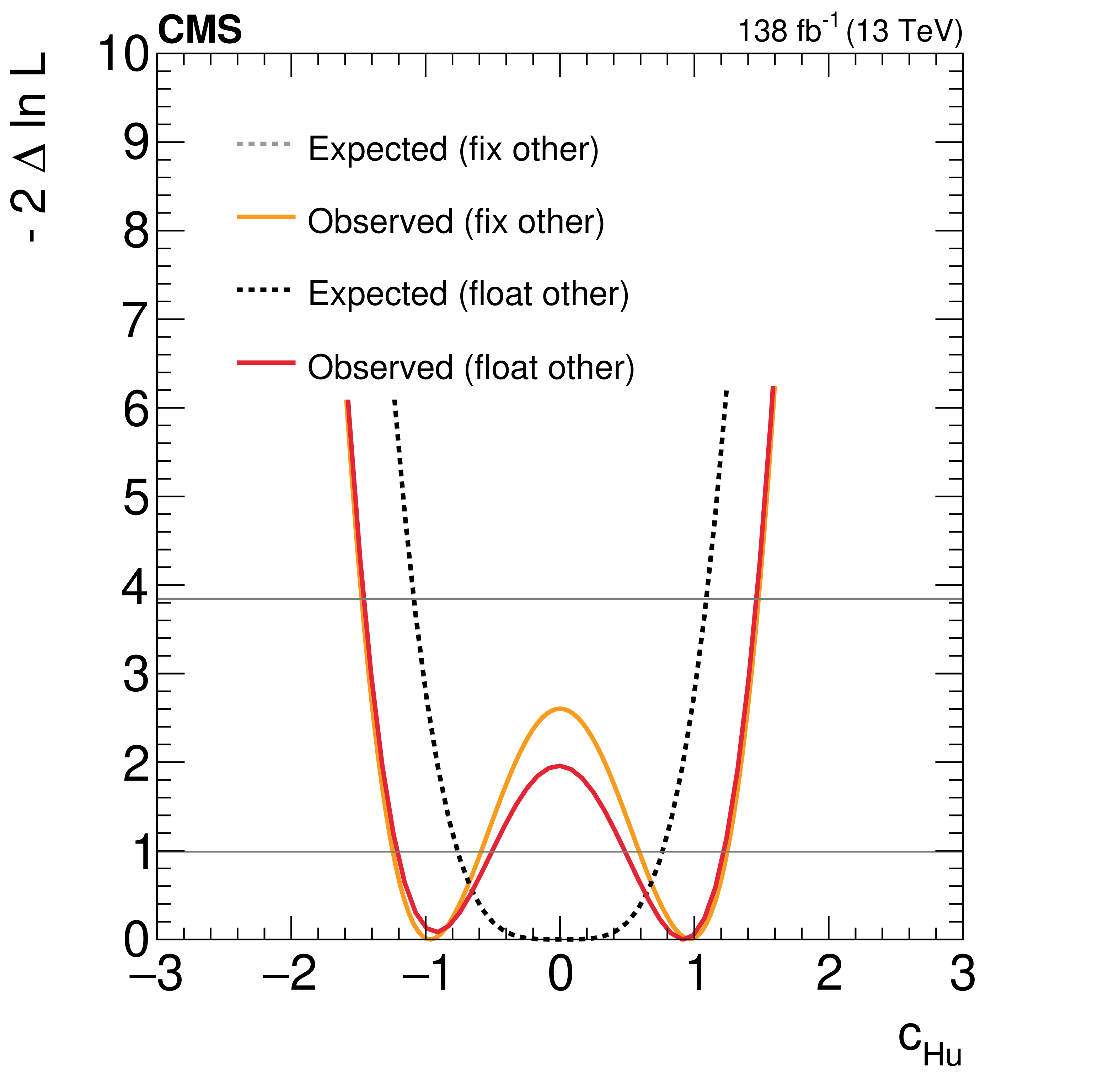
Figure 8:
Expected and observed scans for the Wilson coefficients $ c_\text{Hu} $ (upper left), $ c_{\text{Hd}} $ (upper right), $ c_{\text{Hj1}} $ (lower left) and $ c_{\text{Hj3}} $ (lower right). The results are presented for two scenarios: one where all other coefficients are fixed to their SM values (grey) and another where the other coefficient from the $ (c_\text{Hu},c_{\text{Hd}}) $ and $ (c_\text{Hj1},c_{\text{Hj3}}) $ pairs, respectively, is allowed to float in the fit (black). Horizontal lines indicate the one-dimensional 68% and 95% CL values. |
png pdf |
Figure 8-a:
Expected and observed scans for the Wilson coefficients $ c_\text{Hu} $ (upper left), $ c_{\text{Hd}} $ (upper right), $ c_{\text{Hj1}} $ (lower left) and $ c_{\text{Hj3}} $ (lower right). The results are presented for two scenarios: one where all other coefficients are fixed to their SM values (grey) and another where the other coefficient from the $ (c_\text{Hu},c_{\text{Hd}}) $ and $ (c_\text{Hj1},c_{\text{Hj3}}) $ pairs, respectively, is allowed to float in the fit (black). Horizontal lines indicate the one-dimensional 68% and 95% CL values. |
png pdf |
Figure 8-b:
Expected and observed scans for the Wilson coefficients $ c_\text{Hu} $ (upper left), $ c_{\text{Hd}} $ (upper right), $ c_{\text{Hj1}} $ (lower left) and $ c_{\text{Hj3}} $ (lower right). The results are presented for two scenarios: one where all other coefficients are fixed to their SM values (grey) and another where the other coefficient from the $ (c_\text{Hu},c_{\text{Hd}}) $ and $ (c_\text{Hj1},c_{\text{Hj3}}) $ pairs, respectively, is allowed to float in the fit (black). Horizontal lines indicate the one-dimensional 68% and 95% CL values. |
png pdf |
Figure 8-c:
Expected and observed scans for the Wilson coefficients $ c_\text{Hu} $ (upper left), $ c_{\text{Hd}} $ (upper right), $ c_{\text{Hj1}} $ (lower left) and $ c_{\text{Hj3}} $ (lower right). The results are presented for two scenarios: one where all other coefficients are fixed to their SM values (grey) and another where the other coefficient from the $ (c_\text{Hu},c_{\text{Hd}}) $ and $ (c_\text{Hj1},c_{\text{Hj3}}) $ pairs, respectively, is allowed to float in the fit (black). Horizontal lines indicate the one-dimensional 68% and 95% CL values. |
png pdf |
Figure 8-d:
Expected and observed scans for the Wilson coefficients $ c_\text{Hu} $ (upper left), $ c_{\text{Hd}} $ (upper right), $ c_{\text{Hj1}} $ (lower left) and $ c_{\text{Hj3}} $ (lower right). The results are presented for two scenarios: one where all other coefficients are fixed to their SM values (grey) and another where the other coefficient from the $ (c_\text{Hu},c_{\text{Hd}}) $ and $ (c_\text{Hj1},c_{\text{Hj3}}) $ pairs, respectively, is allowed to float in the fit (black). Horizontal lines indicate the one-dimensional 68% and 95% CL values. |
png pdf |
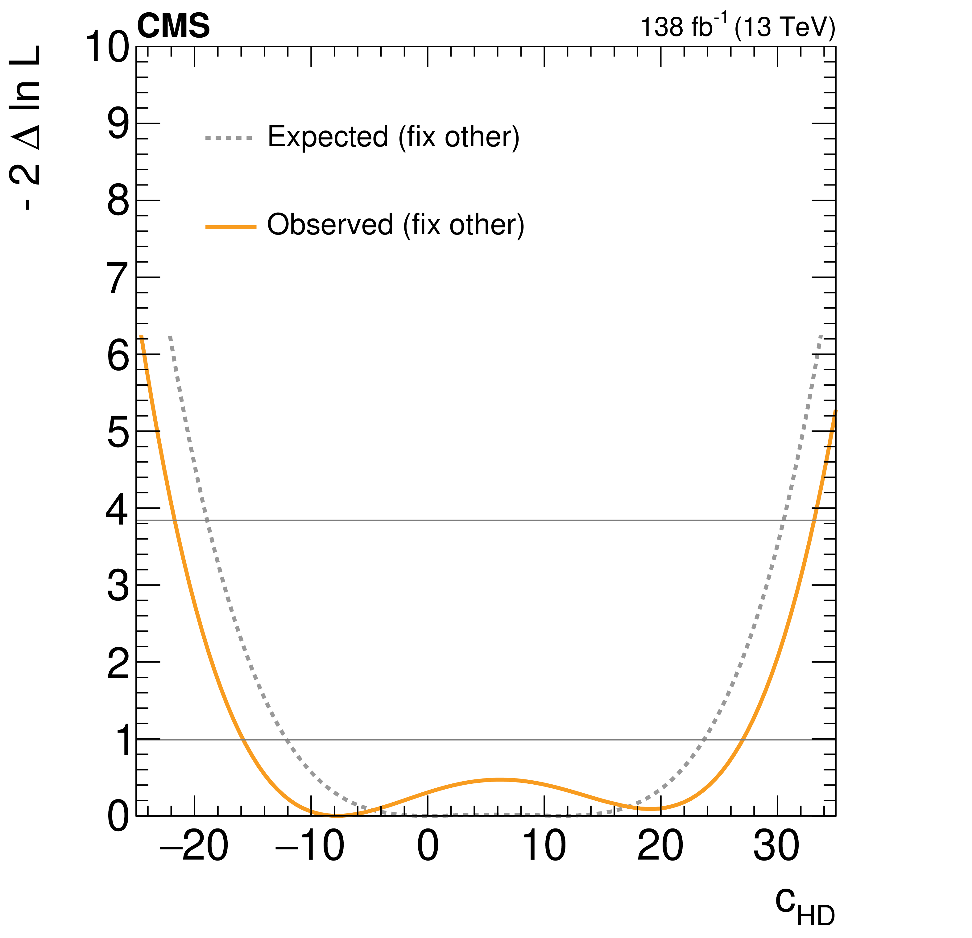
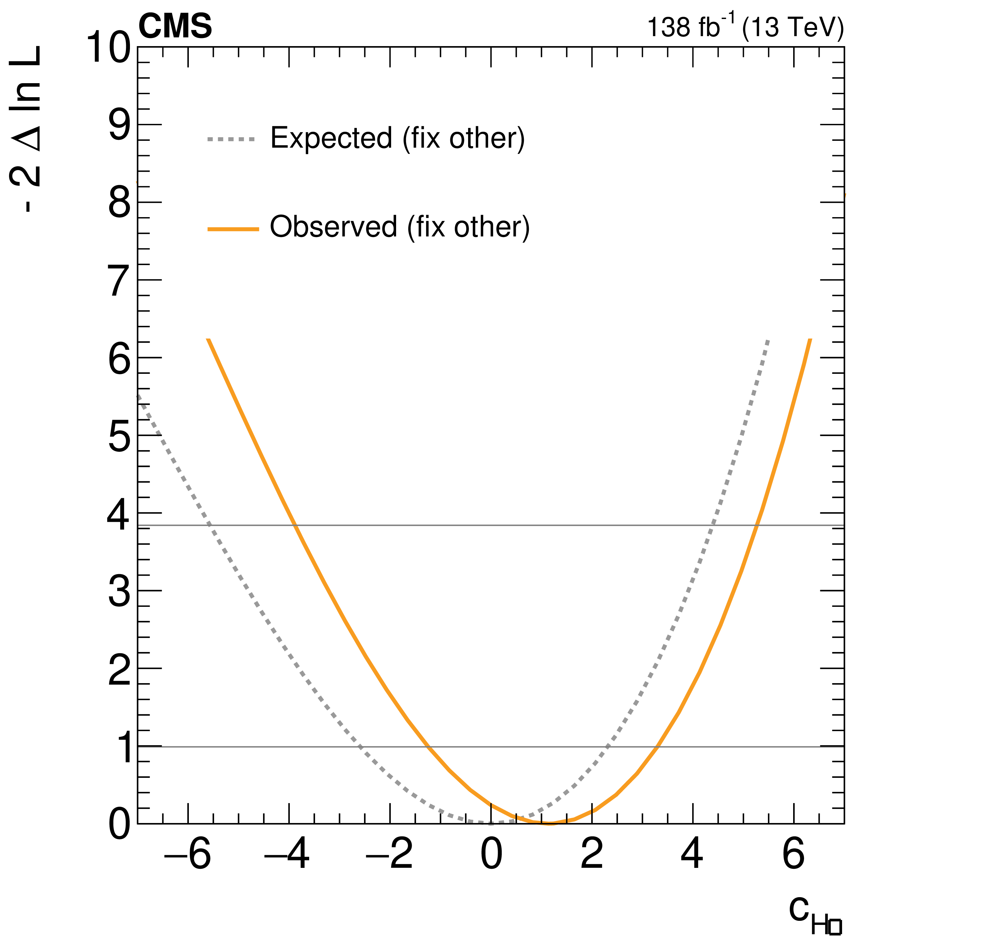
Figure 9:
Expected and observed scans for the Wilson coefficients $ c_\text{HD} $ (left) and $ c_{\text{H}\Box} $ (right). The results are presented for the scenario where all other coefficients are fixed to their SM values. Horizontal lines indicate the one-dimensional 68% and 95% CL values. |
png pdf |
Figure 9-a:
Expected and observed scans for the Wilson coefficients $ c_\text{HD} $ (left) and $ c_{\text{H}\Box} $ (right). The results are presented for the scenario where all other coefficients are fixed to their SM values. Horizontal lines indicate the one-dimensional 68% and 95% CL values. |
png pdf |
Figure 9-b:
Expected and observed scans for the Wilson coefficients $ c_\text{HD} $ (left) and $ c_{\text{H}\Box} $ (right). The results are presented for the scenario where all other coefficients are fixed to their SM values. Horizontal lines indicate the one-dimensional 68% and 95% CL values. |
png pdf |
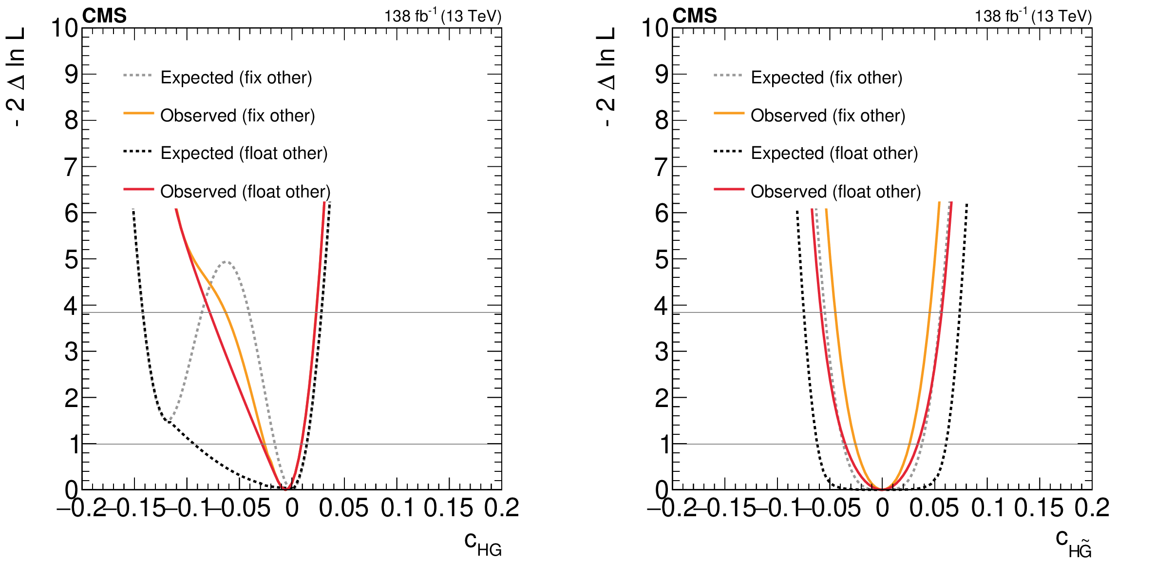
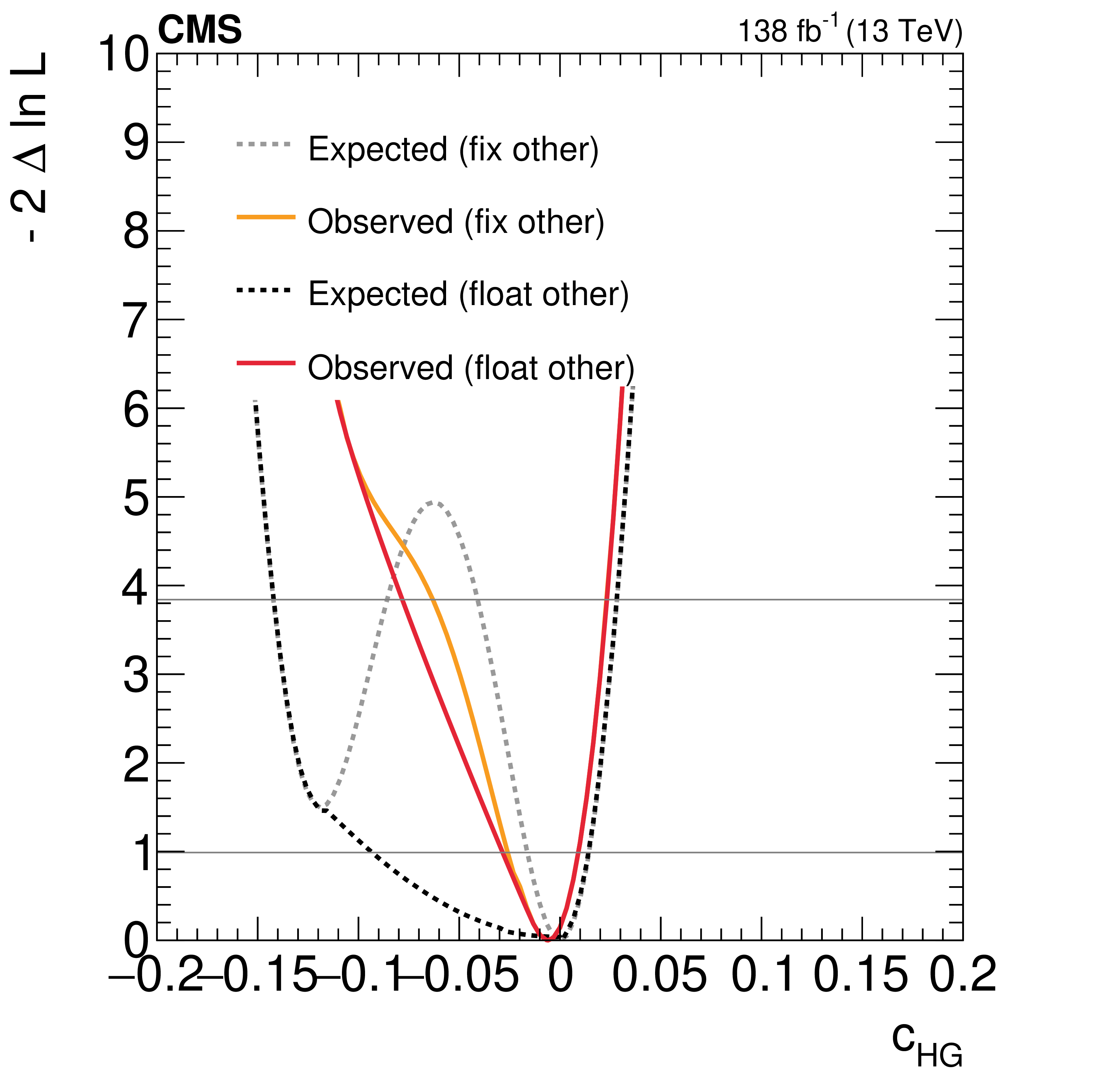
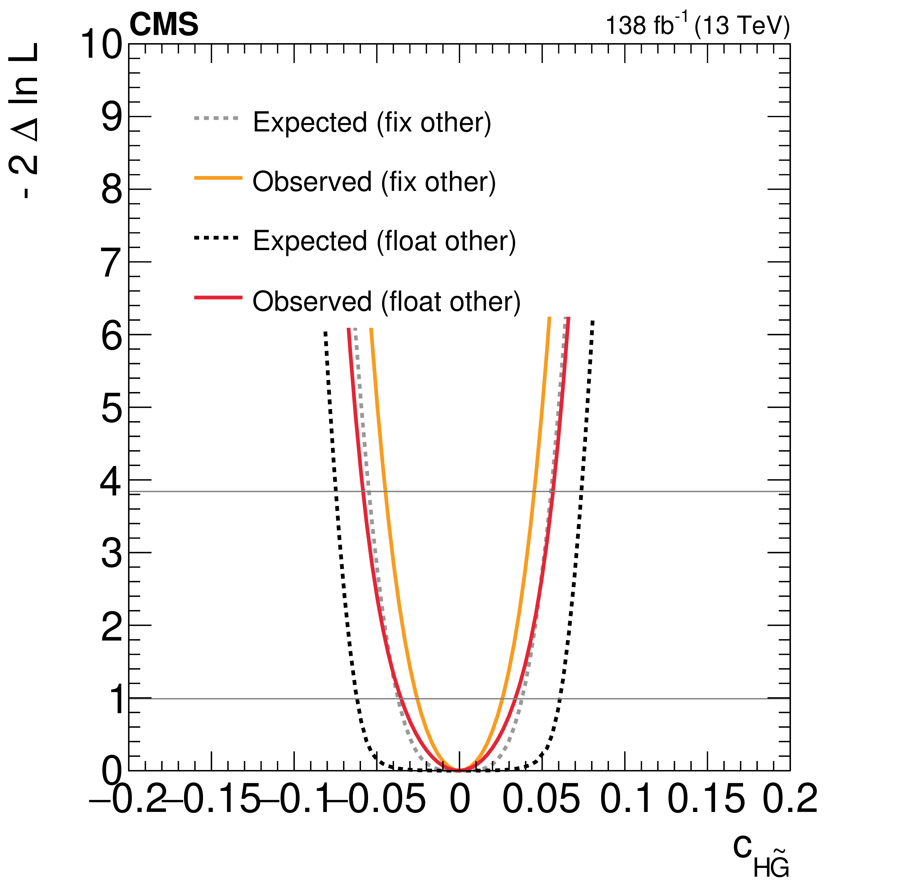
Figure 10:
Expected and observed scans for the Wilson coefficients $ c_\text{HG} $ (left) and $ c_{\text{H}\tilde{\text{G}}} $ (right). The results are presented for two scenarios: one where all other coefficients are fixed to their SM values (grey) and another where the coefficient with opposite $ CP $-parity is allowed to float in the fit (black). Horizontal lines indicate the one-dimensional 68% and 95% CL values. |
png pdf |
Figure 10-a:
Expected and observed scans for the Wilson coefficients $ c_\text{HG} $ (left) and $ c_{\text{H}\tilde{\text{G}}} $ (right). The results are presented for two scenarios: one where all other coefficients are fixed to their SM values (grey) and another where the coefficient with opposite $ CP $-parity is allowed to float in the fit (black). Horizontal lines indicate the one-dimensional 68% and 95% CL values. |
png pdf |
Figure 10-b:
Expected and observed scans for the Wilson coefficients $ c_\text{HG} $ (left) and $ c_{\text{H}\tilde{\text{G}}} $ (right). The results are presented for two scenarios: one where all other coefficients are fixed to their SM values (grey) and another where the coefficient with opposite $ CP $-parity is allowed to float in the fit (black). Horizontal lines indicate the one-dimensional 68% and 95% CL values. |
png pdf |
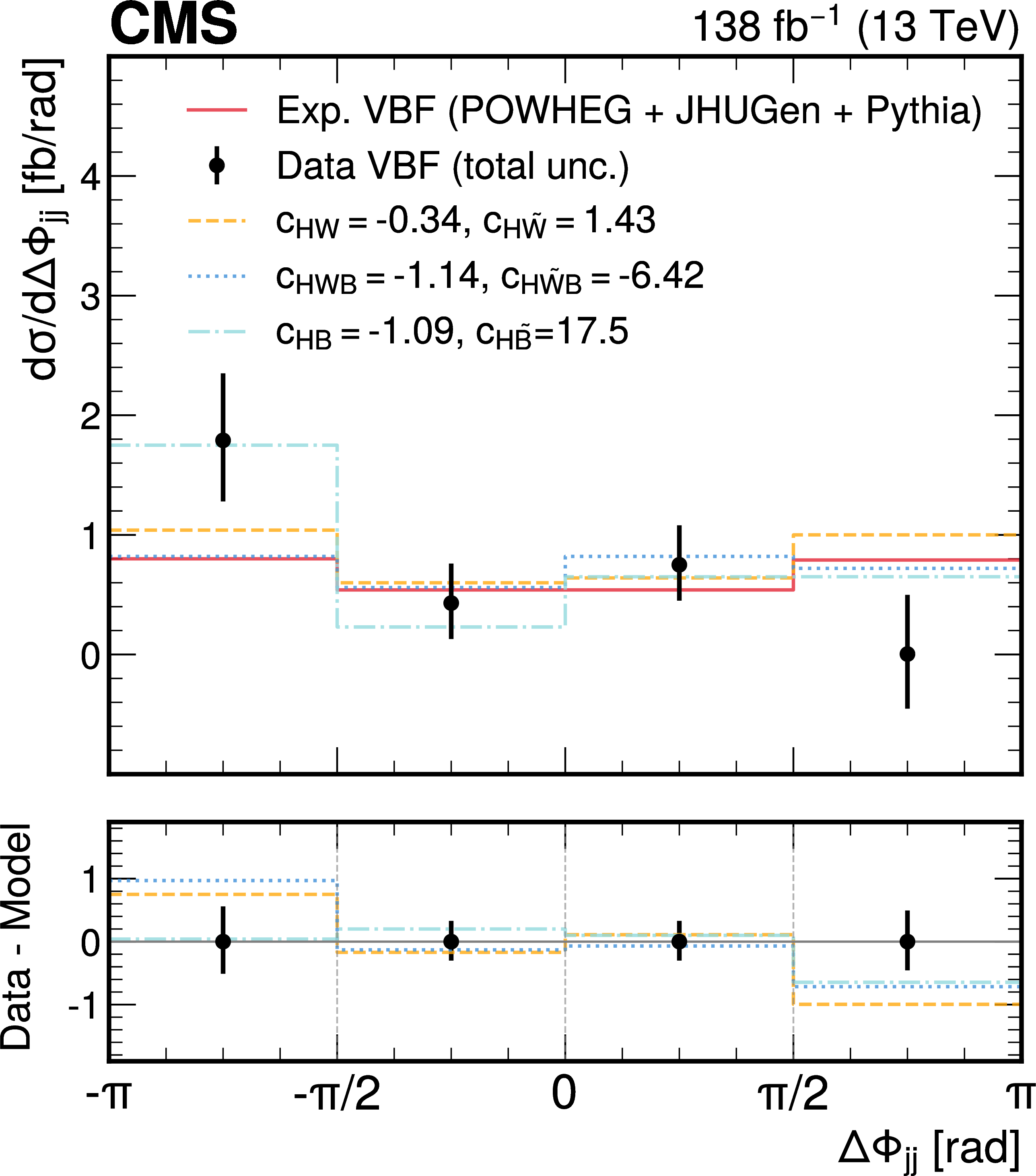
Figure 11:
Measured fiducial cross section for VBF production as a function of $ \Delta\Phi_\mathrm{{jj}} $ (black) compared to various predictions. The cross section predictions include: the SM (red), the ones obtained from the best fit of Wilson coefficients of $ c_\text{HW} $, $ c_{\text{H}\tilde{\text{W}}} $ (yellow), $ c_\text{HWB} $, $ c_{\text{H}\tilde{\text{W}}\text{B}} $ (blue) and $ c_\text{HB} $, $ c_{\text{H}\tilde{\text{B}}} $ (green). The difference between the data and the predictions are displayed in the lower panel. |
png pdf |
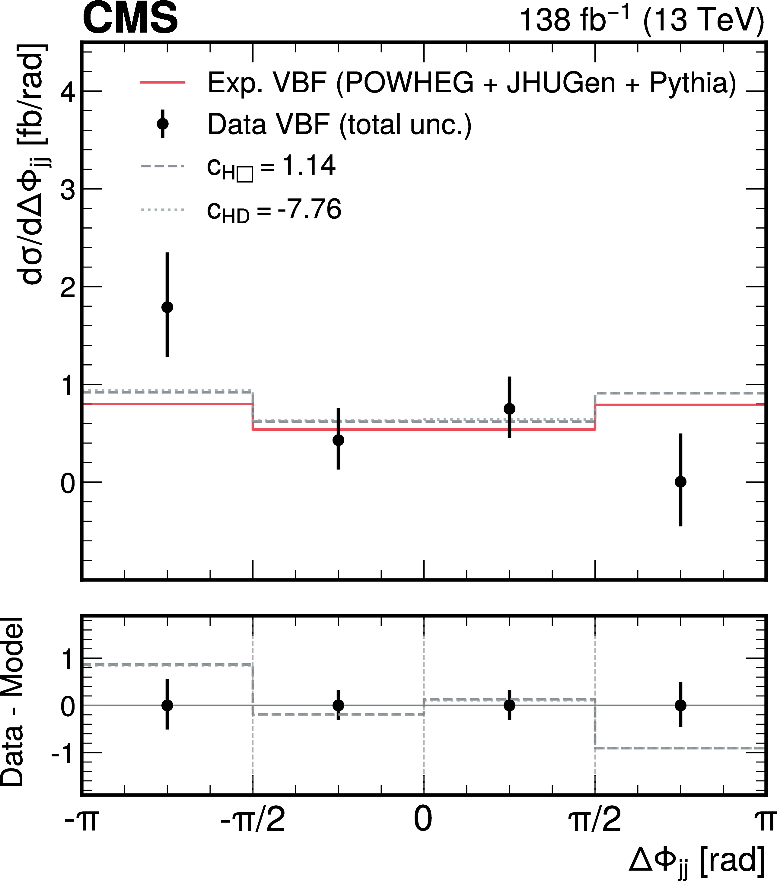
Figure 12:
Measured fiducial cross section for VBF production as a function of $ \Delta\Phi_\mathrm{{jj}} $ (black) compared to various predictions. The cross section predictions include: the SM (red), the ones obtained from the best fit of Wilson coefficients of $ c_{\text{H}\Box} $ (dark grey) and $ c_\text{HD} $ (light grey). The difference between the data and the predictions are displayed in the lower panel. |
png pdf |
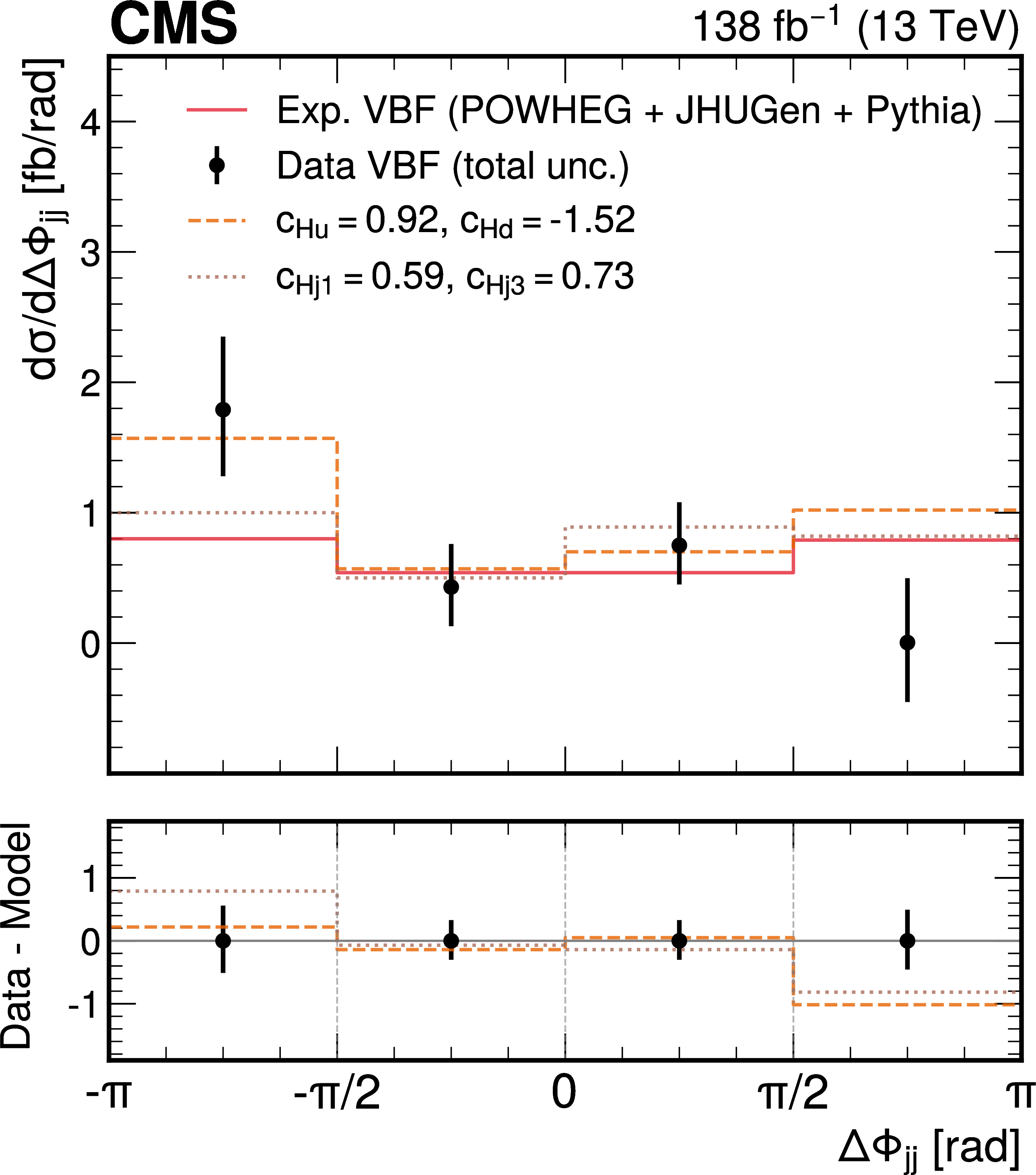
Figure 13:
Measured fiducial cross section for VBF production as a function of $ \Delta\Phi_\mathrm{{jj}} $ (black) compared to various predictions. The cross section predictions include: the SM (red), the ones obtained from the best fit of Wilson coefficients of $ c_{\text{Hu}} $, $ c_{\text{Hd}} $ (light orange) and $ c_\text{Hj1} $, $ c_{\text{Hj3}} $ (dark orange). The difference between the data and the predictions are displayed in the lower panel. |
png pdf |
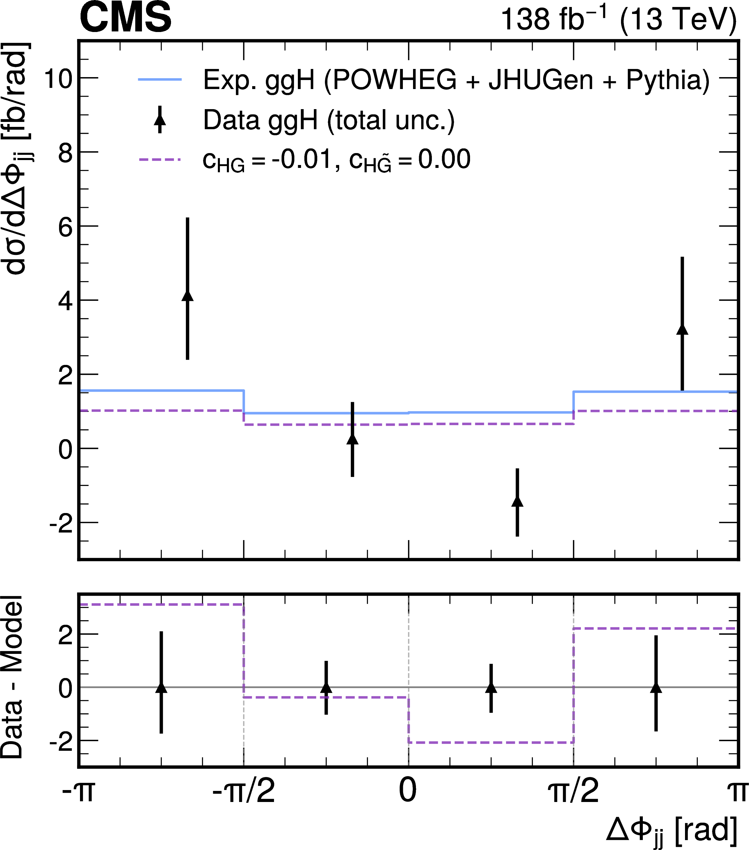
Figure 14:
Measured fiducial cross section for ggH production as a function of $ \Delta\Phi_\mathrm{{jj}} $ (black) compared to various predictions. The cross section predictions include: the SM (blue) and the ones obtained from the best fit of Wilson coefficients of $ c_\text{HG} $, $ c_{\text{H}\tilde{\text{G}}} $ (magenta). The difference between the data and the predictions are displayed in the bottom panel. |
| Tables | |
png pdf |
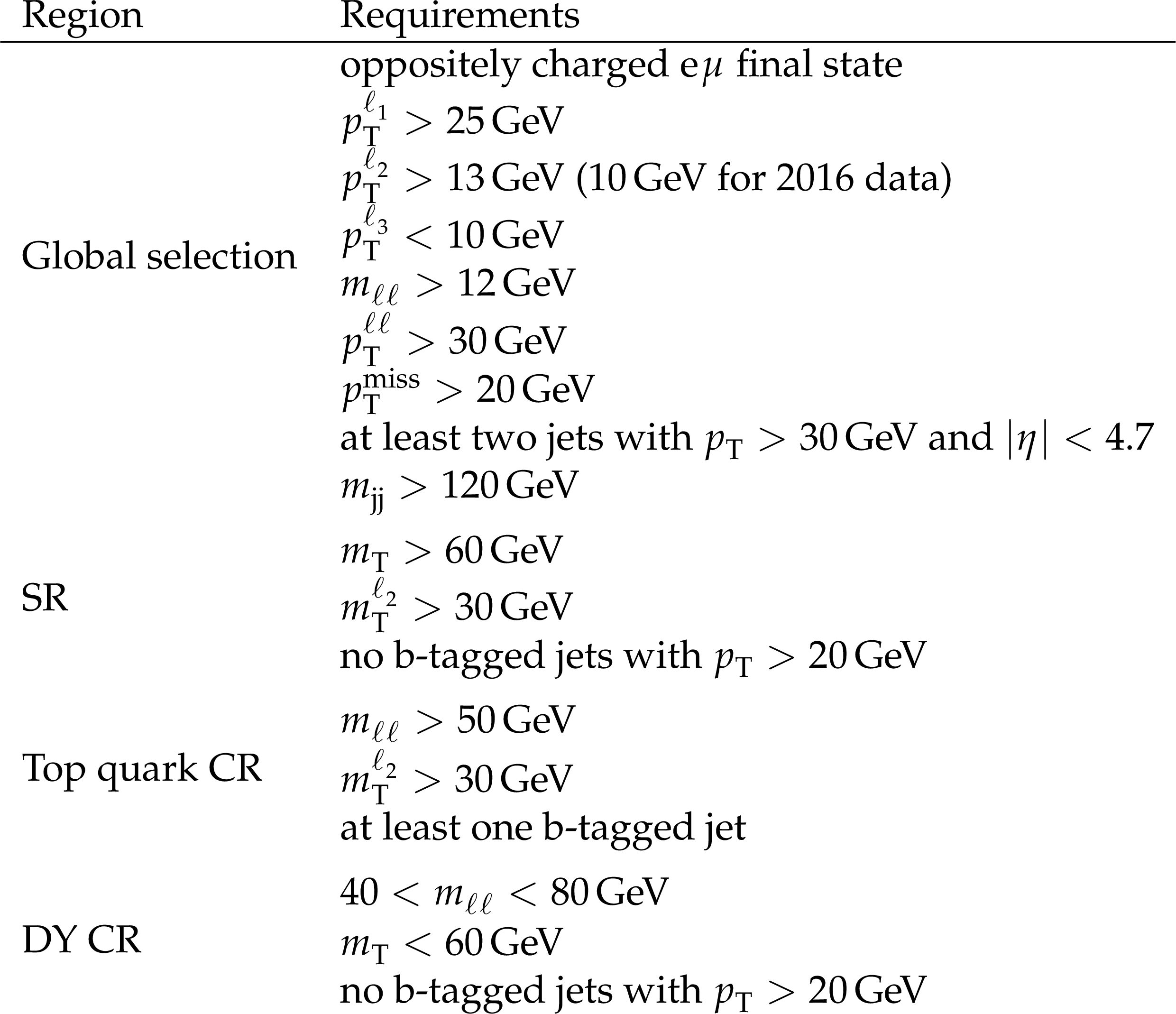
Table 1:
Definition of the analysis phase spaces. |

png pdf |
Table 2:
Definition of the $ \Delta\Phi_\mathrm{{jj}} $ bins. |
png pdf |
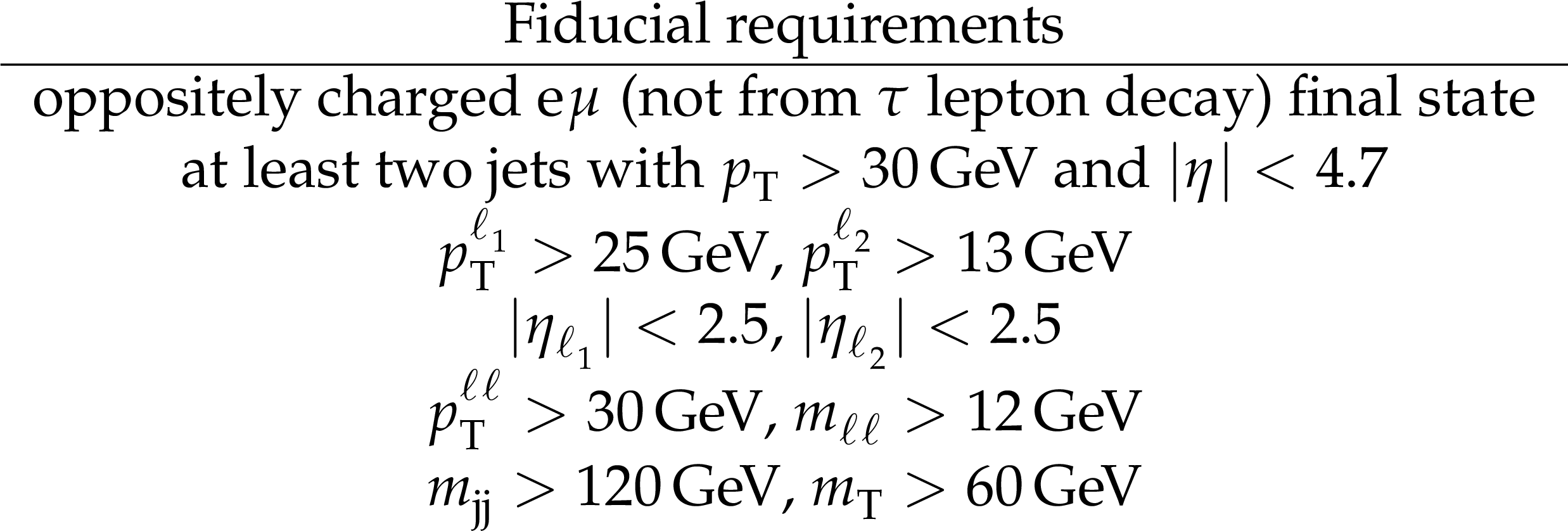
Table 3:
Definition of the fiducial phase space. Observables are defined using generator-level quantities. |
png pdf |
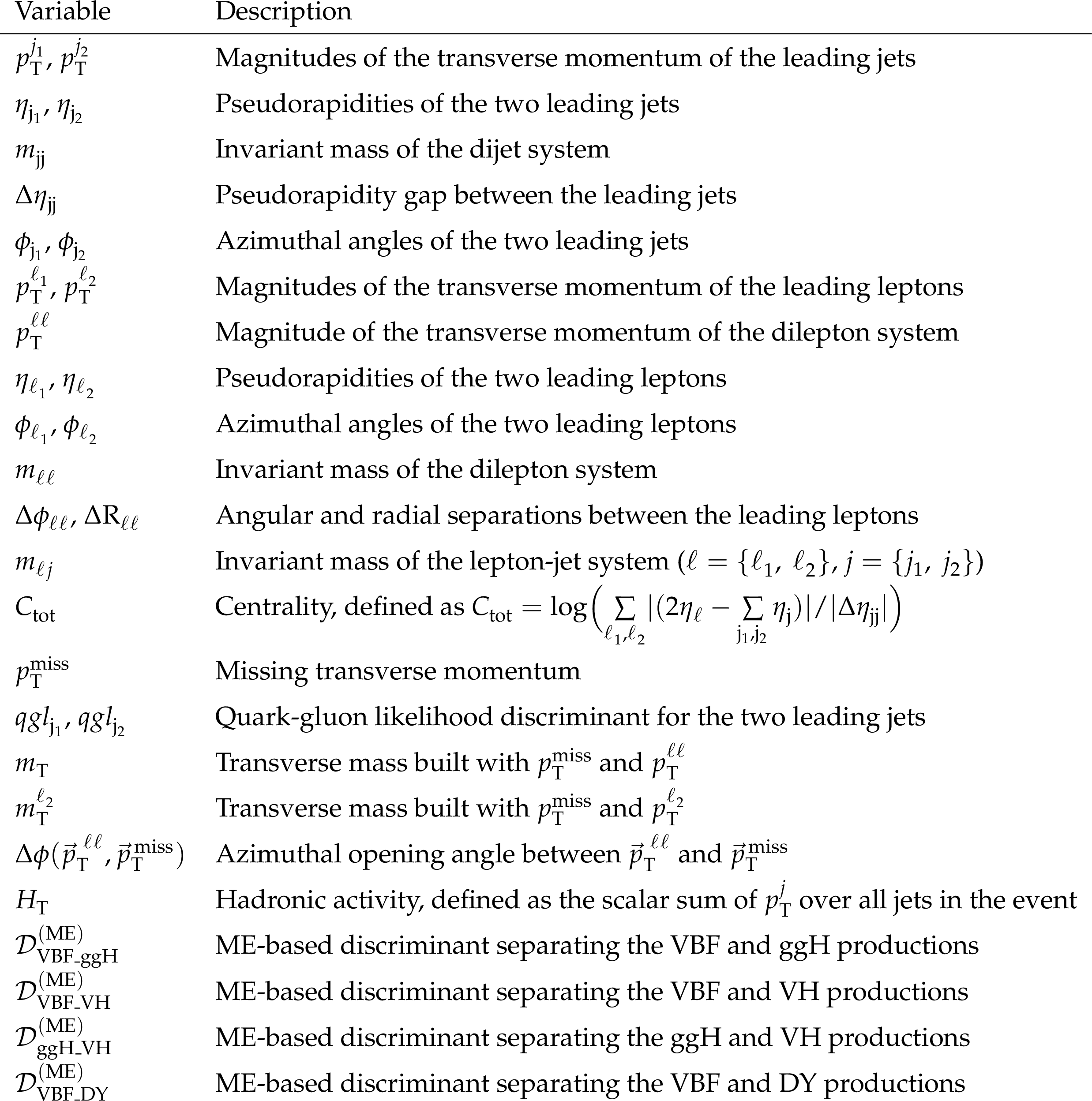
Table 4:
Set of ADNN input features. |
png pdf |
Table 5:
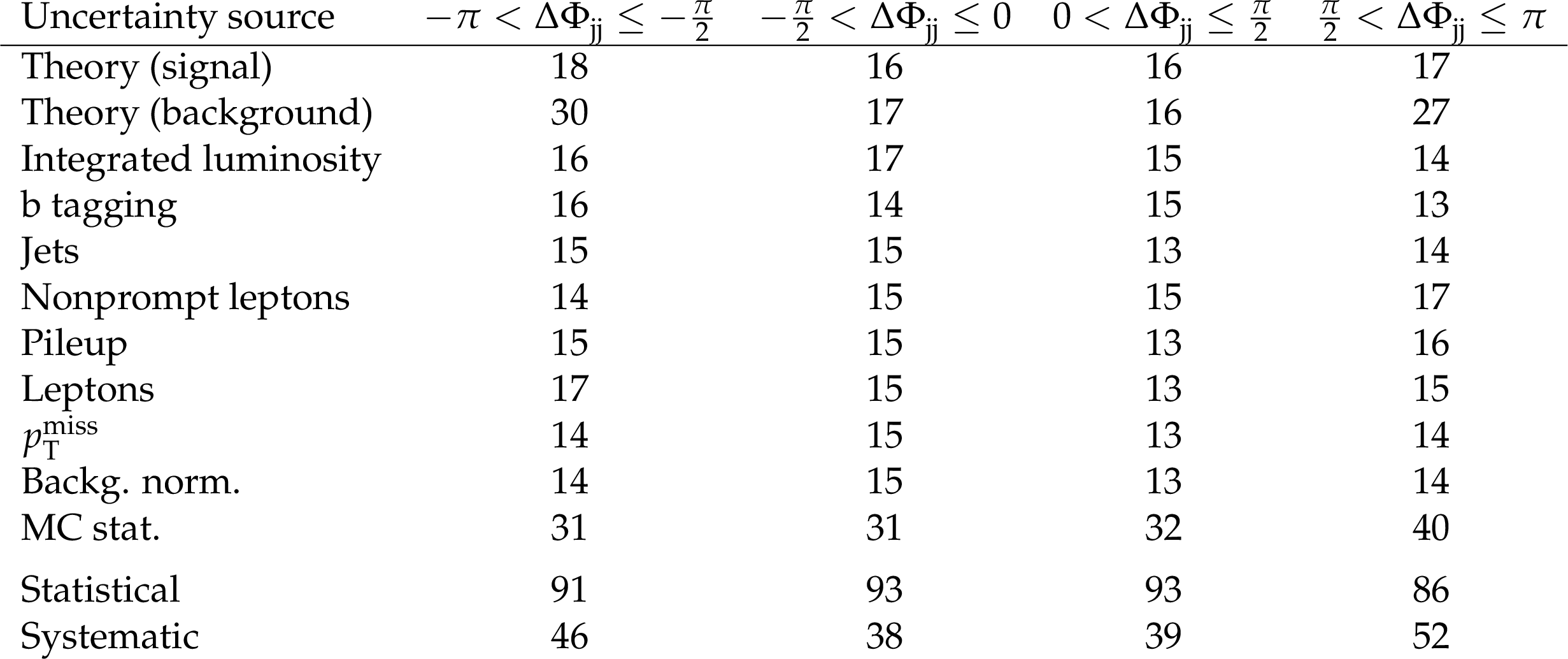
Contributions of different sources of uncertainty in the differential cross section measurement, expressed as a percentage of the total uncertainty ($ \Delta \sigma_i / \Delta \sigma_{\text{tot}} \times $ 100). For asymmetric errors, the largest of the up and down uncertainties is reported. The systematic component includes all sources except for background normalization, which is part of the statistical component. Results are shown for each of the four $ \Delta\Phi_\mathrm{{jj}} $ bins. |
png pdf |
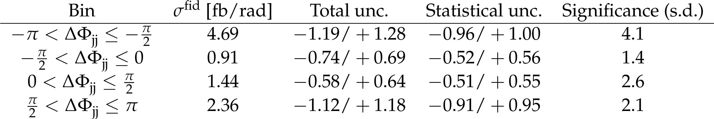
Table 6:
Measured fiducial cross section summing VBF and ggH production processes, corresponding to fit configuration 1. The total (statistical and systematic) and statistical uncertainties corresponding to the 68% CL are shown. The observed significance with respect to the background-only hypothesis is computed accounting for the total uncertainty. |
png pdf |
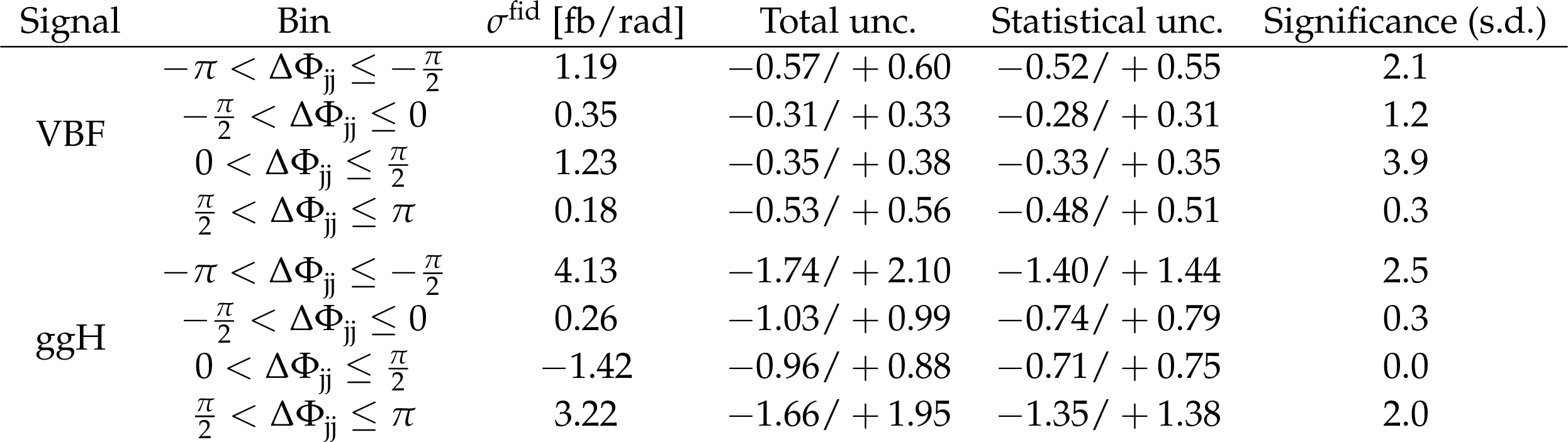
Table 7:
Measured fiducial cross section of VBF and ggH production processes, corresponding to fit configuration 2. The measurement is performed through a simultaneous fit, where the contributions from VBF and ggH production are determined independently in each bin. The observed significance with respect to the background-only hypothesis is computed accounting for the total uncertainty. Negative values or lower uncertainty bounds extending below zero are artifacts of the fit and reflect statistical fluctuations in regions with limited sensitivity. |
png pdf |
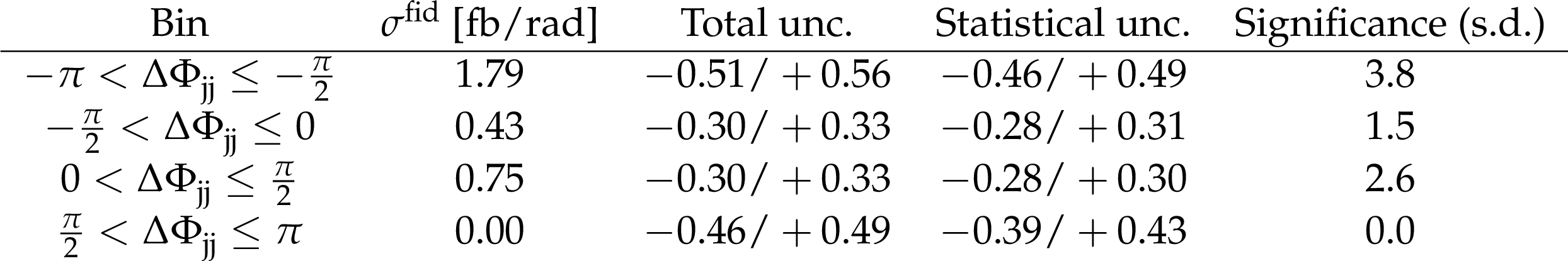
Table 8:
Measured fiducial cross section of VBF production process while fixing the ggH process to the SM prediction, corresponding to fit configuration 3. The total (statistical and systematic) and statistical uncertainties corresponding to the 68% CL are shown. The observed significance with respect to the background only hypothesis is computed accounting for the total uncertainty. Negative values or lower uncertainty bounds extending below zero are artifacts of the fit and reflect statistical fluctuations in regions with limited sensitivity. |
png pdf |
Table 9:
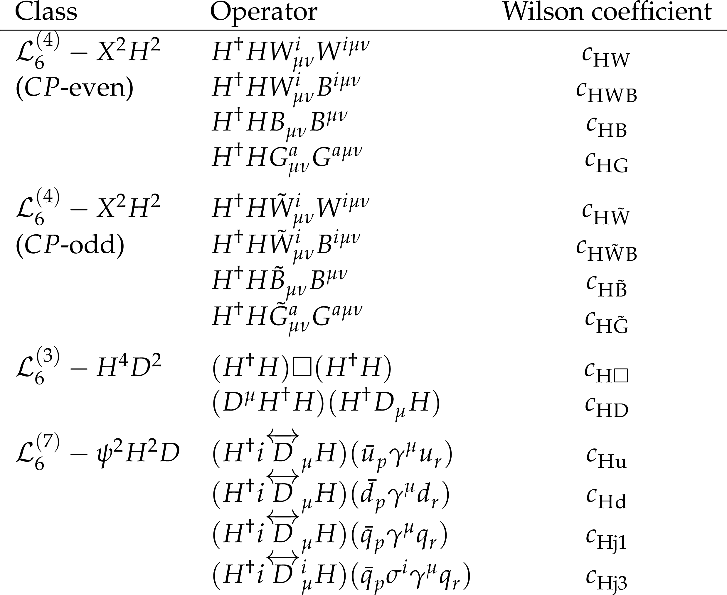
List of $ X^{2}H^{2} $, $ H^{4}D^{2} $, and $ \psi^{2}H^{2}D $ operators and their corresponding Wilson coefficients. |

png pdf |
Table 10:
Summary of the constraints on Wilson coefficients, including best fit values, 68% and 95% CL intervals. The observed significance with respect to the SM scenario is shown in the last column. The constraints on $ c_{\text{H}\Box} $ and $ c_\text{HD} $ were obtained from individual fits with all other coefficients fixed to their SM values. For the remaining coefficients, results were obtained from fits where the corresponding $ CP $-even or $ CP $-odd partner was allowed to float, while all other coefficients were fixed to their SM values. |
| Summary |
| This paper presents a model-independent measurement of the Higgs boson differential production cross section in its decay to a pair of W bosons, with a final state that includes two jets, two different-flavor leptons $ (\mathrm{e}\mu) $, and missing transverse momentum. The model independence of the measurement is maximized by making use of a signal discriminating variable that is agnostic to the signal hypothesis developed through an adversarial deep neural network. The measurement is based on proton-proton collision data recorded with the CMS detector between 2016 and 2018, corresponding to an integrated luminosity of 138 fb$ ^{-1} $ at a center-of-mass energy of 13 TeV. The production cross section is measured as a function of the azimuthal angle difference between the two jets. Three different signal extraction configurations are employed to measure the Higgs boson production cross section in association with two jets via vector boson fusion (VBF) and gluon-gluon fusion (ggH). Differential cross section measurements are further utilized to constrain Wilson coefficients within the standard model effective field theory framework. The most stringent constraints are obtained on the Charge conjugation Parity ($ CP $)-even $ c_\text{HW} $ and $ c_\text{Hj3} $ coefficients from the VBF cross section measurement, and on the $ CP $-even $ c_\text{HG} $ coefficient from the ggH cross section measurement. All results are found to be consistent with the SM expectations. |
| References | ||||
| 1 | ATLAS Collaboration | Observation of a new particle in the search for the standard model Higgs boson with the ATLAS detector at the LHC | PLB 716 (2012) 1 | 1207.7214 |
| 2 | CMS Collaboration | Observation of a new boson at a mass of 125 GeV with the CMS experiment at the LHC | PLB 716 (2012) 30 | CMS-HIG-12-028 1207.7235 |
| 3 | CMS Collaboration | Observation of a new boson with mass near 125 GeV in pp collisions at $ \sqrt{s}= $ 7 and 8 TeV | JHEP 06 (2013) 081 | CMS-HIG-12-036 1303.4571 |
| 4 | ATLAS Collaboration | A detailed map of Higgs boson interactions by the ATLAS experiment ten years after the discovery | Nature 607 (2022) 52 | 2207.00092 |
| 5 | CMS Collaboration | A portrait of the Higgs boson by the CMS experiment ten years after the discovery. | Nature 607 (2022) 60 | CMS-HIG-22-001 2207.00043 |
| 6 | V. Hankele, G. Klamke, D. Zeppenfeld, and T. Figy | Anomalous Higgs boson couplings in vector boson fusion at the CERN LHC | PRD 74 (2006) 095001 | hep-ph/0609075 |
| 7 | B. Grzadkowski, M. Iskrzynski, M. Misiak, and J. Rosiek | Dimension-six terms in the standard model lagrangian | JHEP 10 (2010) 085 | 1008.4884 |
| 8 | LHC Higgs Cross Section Working Group | Handbook of LHC Higgs cross sections: 4. Deciphering the nature of the Higgs sector | CERN Report CERN-2017-002-M, 2016 link |
1610.07922 |
| 9 | CMS Collaboration | HEPData record for this analysis | link | |
| 10 | CMS Collaboration | Constraints on anomalous Higgs boson couplings to vector bosons and fermions in its production and decay using the four-lepton final state | PRD 104 (2021) 052004 | CMS-HIG-19-009 2104.12152 |
| 11 | I. Anderson et al. | Constraining anomalous HVV interactions at proton and lepton colliders | PRD 89 (2014) 035007 | 1309.4819 |
| 12 | A. V. Gritsan et al. | New features in the JHU generator framework: constraining Higgs boson properties from on-shell and off-shell production | PRD 102 (2020) 056022 | 2002.09888 |
| 13 | CMS Collaboration | Constraints on anomalous Higgs boson couplings from its production and decay using the WW channel in proton-proton collisions at $ \sqrt{s} = $ 13 TeV | EPJC 84 (2024) 779 | CMS-HIG-22-008 2403.00657 |
| 14 | CMS Collaboration | The CMS experiment at the CERN LHC | JINST 3 (2008) S08004 | |
| 15 | CMS Collaboration | Development of the CMS detector for the CERN LHC Run 3 | JINST 19 (2024) P05064 | CMS-PRF-21-001 2309.05466 |
| 16 | CMS Collaboration | Performance of electron reconstruction and selection with the CMS detector in proton-proton collisions at $ \sqrt{s} = $ 8 TeV | JINST 10 (2015) P06005 | CMS-EGM-13-001 1502.02701 |
| 17 | CMS Collaboration | Performance of the CMS muon detector and muon reconstruction with proton-proton collisions at $ \sqrt{s}= $ 13 TeV | JINST 13 (2018) P06015 | CMS-MUO-16-001 1804.04528 |
| 18 | CMS Collaboration | Performance of photon reconstruction and identification with the CMS detector in proton-proton collisions at $ \sqrt{s}= $ 8 TeV | JINST 10 (2015) P08010 | CMS-EGM-14-001 1502.02702 |
| 19 | CMS Collaboration | Description and performance of track and primary-vertex reconstruction with the CMS tracker | JINST 9 (2014) P10009 | CMS-TRK-11-001 1405.6569 |
| 20 | CMS Collaboration | Particle-flow reconstruction and global event description with the CMS detector | JINST 12 (2017) P10003 | CMS-PRF-14-001 1706.04965 |
| 21 | CMS Collaboration | Performance of reconstruction and identification of $ \tau $ leptons decaying to hadrons and $ \nu_\tau $ in pp collisions at $ \sqrt{s}= $ 13 TeV | JINST 13 (2018) P10005 | CMS-TAU-16-003 1809.02816 |
| 22 | CMS Collaboration | Jet energy scale and resolution in the CMS experiment in pp collisions at 8 TeV | JINST 12 (2017) P02014 | CMS-JME-13-004 1607.03663 |
| 23 | CMS Collaboration | Performance of missing transverse momentum reconstruction in proton-proton collisions at $ \sqrt{s} = $ 13 TeV using the CMS detector | JINST 14 (2019) P07004 | CMS-JME-17-001 1903.06078 |
| 24 | CMS Collaboration | Performance of the CMS Level-1 trigger in proton-proton collisions at $ \sqrt{s} = $ 13 TeV | JINST 15 (2020) P10017 | CMS-TRG-17-001 2006.10165 |
| 25 | CMS Collaboration | The CMS trigger system | JINST 12 (2017) P01020 | CMS-TRG-12-001 1609.02366 |
| 26 | CMS Collaboration | Performance of the CMS high-level trigger during LHC Run 2 | JINST 19 (2024) P11021 | CMS-TRG-19-001 2410.17038 |
| 27 | CMS Collaboration | Technical proposal for the Phase-II upgrade of the Compact Muon Solenoid | CMS Technical Proposal CERN-LHCC-2015-010, CMS-TDR-15-02, 2015 CDS |
|
| 28 | CMS Collaboration | Electron and photon reconstruction and identification with the CMS experiment at the CERN LHC | JINST 16 (2021) P05014 | CMS-EGM-17-001 2012.06888 |
| 29 | CMS Collaboration | ECAL 2016 refined calibration and Run2 summary plots | CMS Detector Performance Note CMS-DP-2020-021, 2020 CDS |
|
| 30 | M. Cacciari, G. P. Salam, and G. Soyez | The anti-$ k_{\mathrm{T}} $ jet clustering algorithm | JHEP 04 (2008) 063 | 0802.1189 |
| 31 | M. Cacciari, G. P. Salam, and G. Soyez | FastJet user manual | EPJC 72 (2012) 1896 | 1111.6097 |
| 32 | CMS Collaboration | Pileup mitigation at CMS in 13 TeV data | JINST 15 (2020) P09018 | CMS-JME-18-001 2003.00503 |
| 33 | CMS Collaboration | Identification of heavy-flavour jets with the CMS detector in pp collisions at 13 TeV | JINST 13 (2018) P05011 | CMS-BTV-16-002 1712.07158 |
| 34 | E. Bols et al. | Jet Flavour Classification Using DeepJet | JINST 15 (2020) P12012 | 2008.10519 |
| 35 | D. Bertolini, P. Harris, M. Low, and N. Tran | Pileup per particle identification | JHEP 10 (2014) 059 | 1407.6013 |
| 36 | CMS Collaboration | Precision luminosity measurement in proton-proton collisions at $ \sqrt{s} = $ 13 TeV in 2015 and 2016 at CMS | EPJC 81 (2021) 800 | CMS-LUM-17-003 2104.01927 |
| 37 | CMS Collaboration | CMS luminosity measurement for the 2017 data-taking period at $ \sqrt{s} = $ 13 TeV | CMS Physics Analysis Summary, 2018 link |
CMS-PAS-LUM-17-004 |
| 38 | CMS Collaboration | CMS luminosity measurement for the 2018 data-taking period at $ \sqrt{s} = $ 13 TeV | CMS Physics Analysis Summary, 2019 link |
CMS-PAS-LUM-18-002 |
| 39 | NNPDF Collaboration | Parton distributions from high-precision collider data | EPJC 77 (2017) 663 | 1706.00428 |
| 40 | T. Sjöstrand et al. | An introduction to PYTHIA 8.2 | Comput. Phys. Commun. 191 (2015) 159 | 1410.3012 |
| 41 | CMS Collaboration | Extraction and validation of a new set of CMS PYTHIA8 tunes from underlying-event measurements | EPJC 80 (2020) 4 | CMS-GEN-17-001 1903.12179 |
| 42 | P. Nason | A new method for combining NLO QCD with shower Monte Carlo algorithms | JHEP 11 (2004) 040 | hep-ph/0409146 |
| 43 | S. Frixione, P. Nason, and C. Oleari | Matching NLO QCD computations with parton shower simulations: the POWHEG method | JHEP 11 (2007) 070 | 0709.2092 |
| 44 | S. Alioli, P. Nason, C. Oleari, and E. Re | A general framework for implementing NLO calculations in shower Monte Carlo programs: the POWHEG BOX | JHEP 06 (2010) 043 | 1002.2581 |
| 45 | A. Kardos, P. Nason, and C. Oleari | Three-jet production in POWHEG | JHEP 04 (2014) 043 | 1402.4001 |
| 46 | B. Cabouat and T. Sjöstrand | Some dipole shower studies | EPJC 78 (2018) 226 | 1710.00391 |
| 47 | B. Jager et al. | Parton-shower effects in Higgs production via vector-boson fusion | EPJC 80 (2020) 756 | 2003.12435 |
| 48 | S. Bolognesi et al. | On the Spin and Parity of a Single-Produced Resonance at the LHC | PRD 86 (2012) 095031 | 1208.4018 |
| 49 | J. M. Campbell and R. K. Ellis | An update on vector boson pair production at hadron colliders | PRD 60 (1999) 113006 | hep-ph/9905386 |
| 50 | J. M. Campbell, R. K. Ellis, and C. Williams | Vector boson pair production at the LHC | JHEP 07 (2011) 018 | 1105.0020 |
| 51 | J. M. Campbell, R. K. Ellis, and W. T. Giele | A multi-threaded version of MCFM | EPJC 75 (2015) 246 | 1503.06182 |
| 52 | F. Caola et al. | QCD corrections to vector boson pair production in gluon fusion including interference effects with off-shell Higgs at the LHC | JHEP 07 (2016) 087 | 1605.04610 |
| 53 | J. Alwall et al. | The automated computation of tree-level and next-to-leading order differential cross sections, and their matching to parton shower simulations | JHEP 07 (2014) 079 | 1405.0301 |
| 54 | J. Alwall et al. | Comparative study of various algorithms for the merging of parton showers and matrix elements in hadronic collisions | EPJC 53 (2008) 473 | 0706.2569 |
| 55 | R. Frederix and S. Frixione | Merging meets matching in MC@NLO | JHEP 12 (2012) 061 | 1209.6215 |
| 56 | GEANT4 Collaboration | GEANT 4---a simulation toolkit | NIM A 506 (2003) 250 | |
| 57 | CMS Collaboration | Measurements of properties of the Higgs boson decaying to a W boson pair in pp collisions at $ \sqrt{s}= $ 13 TeV | PLB 791 (2019) 96 | CMS-HIG-16-042 1806.05246 |
| 58 | CMS Collaboration | Measurements of inclusive W and Z cross sections in pp collisions at $ \sqrt{s}= $ 7 TeV | JHEP 01 (2011) 080 | CMS-EWK-10-002 1012.2466 |
| 59 | B. Camaiani et al. | Model independent measurements of standard model cross sections with domain adaptation | EPJC 82 (2022) 921 | 2207.09293 |
| 60 | F. Chollet et al. | Keras | link | |
| 61 | M. Abadi et al. | Tensorflow: Large-scale machine learning on heterogeneous distributed systems | 1603.04467 | |
| 62 | D. P. Kingma and J. Ba | Adam: A method for stochastic optimization | 1412.6980 | |
| 63 | CMS Collaboration | Performance of quark/gluon discrimination in 13 TeV data | Technical Report CMS-DP-2016-070, 2016 CDS |
|
| 64 | Y. Gao et al. | Spin determination of single-produced resonances at hadron colliders | PRD 81 (2010) 075022 | 1001.3396 |
| 65 | A. V. Gritsan, R. Röntsch, M. Schulze, and M. Xiao | Constraining anomalous Higgs boson couplings to the heavy-flavor fermions using matrix element techniques | PRD 94 (2016) 055023 | 1606.03107 |
| 66 | T. Martini, R.-Q. Pan, M. Schulze, and M. Xiao | Probing the structure of the top quark Yukawa coupling: Loop sensitivity versus on-shell sensitivity | PRD 104 (2021) 055045 | 2104.04277 |
| 67 | J. Davis et al. | Constraining anomalous Higgs boson couplings to virtual photons | PRD 105 (2022) 096027 | 2109.13363 |
| 68 | S. Brochet et al. | MoMEMta, a modular toolkit for the Matrix Element Method at the LHC | EPJC 79 (2019) 126 | 1805.08555 |
| 69 | J. L. Hodges | The significance probability of the Smirnov two-sample test | Arkiv för Matematik 3(5) 469, 1958 link |
|
| 70 | T. Akiba et al. | Optuna: A next-generation hyperparameter optimization framework | in Proc. 25rd ACM SIGKDD International Conference on Knowledge Discovery and Data Mining. 2019 | 1907.10902 |
| 71 | ATLAS Collaboration | Measurement of the inelastic proton-proton cross section at $ \sqrt{s} = $ 13 TeV with the ATLAS detector at the LHC | PRL 117 (2016) 182002 | 1606.02625 |
| 72 | CMS Collaboration | Measurement of the inelastic proton-proton cross section at $ \sqrt{s}= $ 13 TeV | JHEP 07 (2018) 161 | CMS-FSQ-15-005 1802.02613 |
| 73 | R. Barlow and C. Beeston | Fitting using finite Monte Carlo samples | Comput. Phys. Commun. 77 (1993) 219 | |
| 74 | CMS Collaboration | The CMS statistical analysis and combination tool: Combine | Comput. Softw. Big Sci. 8 (2024) 19 | CMS-CAT-23-001 2404.06614 |
| 75 | W. Verkerke and D. Kirkby | The RooFit toolkit for data modeling | in Proc. 13th International Conference on Computing in High Energy and Nuclear Physics (CHEP 2003): La Jolla CA, United States, March 24--28, 2003 link |
physics/0306116 |
| 76 | L. Moneta et al. | The RooStats project | in Proc. 13th International Workshop on Advanced Computing and Analysis Techniques in Physics Research (ACAT 2010): Jaipur, India, February 22--27, 2010 link |
1009.1003 |
| 77 | G. Brooijmans et al. | Les Houches 2019 Physics at TeV Colliders: New Physics Working Group Report | in 11th Les Houches Workshop on Physics at TeV Colliders: PhysTeV Les Houches. 2, 2020 | 2002.12220 |
| 78 | C. Bierlich et al. | Robust Independent Validation of Experiment and Theory: Rivet version 3 | SciPost Phys. 8 (2020) 026 | 1912.05451 |
|
|
Compact Muon Solenoid LHC, CERN |
|

|

|

|

|

|