

Compact Muon Solenoid
LHC, CERN
| CMS-EXO-24-034 ; CERN-EP-2026-118 | ||
| Search for light scalar particles produced in Higgs boson decays in exclusive final states with two muons and two hadrons in proton-proton collisions at $ \sqrt{s}= $ 13 TeV | ||
| CMS Collaboration | ||
| 27 May 2026 | ||
| Submitted to the Journal of High Energy Physics | ||
| Abstract: A search for new scalar particles of $ \mathcal{O} $ (GeV) mass in exclusive final states with muons and light hadrons is presented. The analysis uses proton-proton collision data produced at a center-of-mass energy of 13 TeV collected by the CMS experiment at the CERN LHC in 2016--2018, corresponding to an integrated luminosity of 138 fb$ ^{-1} $. The search targets exotic decays of the Higgs boson to a pair of prompt or long-lived identical scalar particles with proper decay lengths $ c\tau $ up to 100$ \text{mm} $ and masses within the range of 0.4--2.0 GeV. This mass window corresponds to a unique parameter space where hadronic decays of these particles mostly result in a pair of light hadrons. The considered experimental signature is a collimated pair of muons and another pair of charged kaons or pions, each of which may be prompt or displaced. The analysis improves the sensitivity to very light scalar boson masses and demonstrates a novel approach to probe hadronic decays of light scalar bosons. Upper limits on the branching fraction of the Higgs boson to scalar bosons at the level of $ \mathcal{O}(10^{-4}) $ are obtained for several scalar boson masses between 0.4 and 2.0 GeV, with proper decay lengths of up to $ \sim $1$ \text{mm} $. | ||
| Links: e-print arXiv:2605.27875 [hep-ex] (PDF) ; CDS record ; inSPIRE record ; HepData record ; Physics Briefing ; CADI line (restricted) ; | ||
| Figures | |
png pdf |
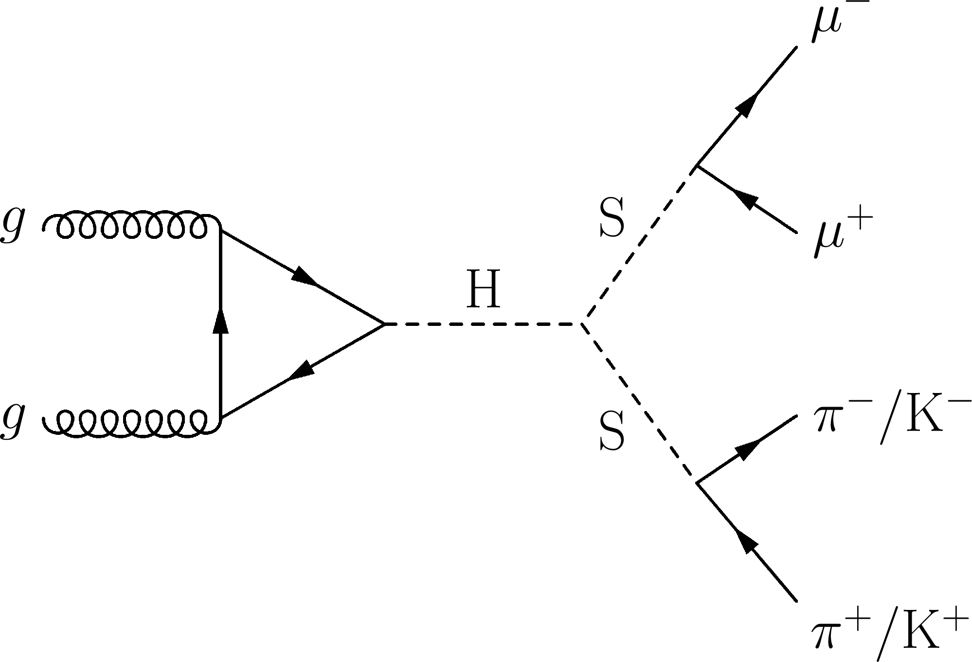
Figure 1:
Feynman diagram illustrating Higgs boson-mediated BSM light scalar boson production in the gluon fusion process in the final state of a pair of muons and a pair of charged hadrons. |
png pdf |
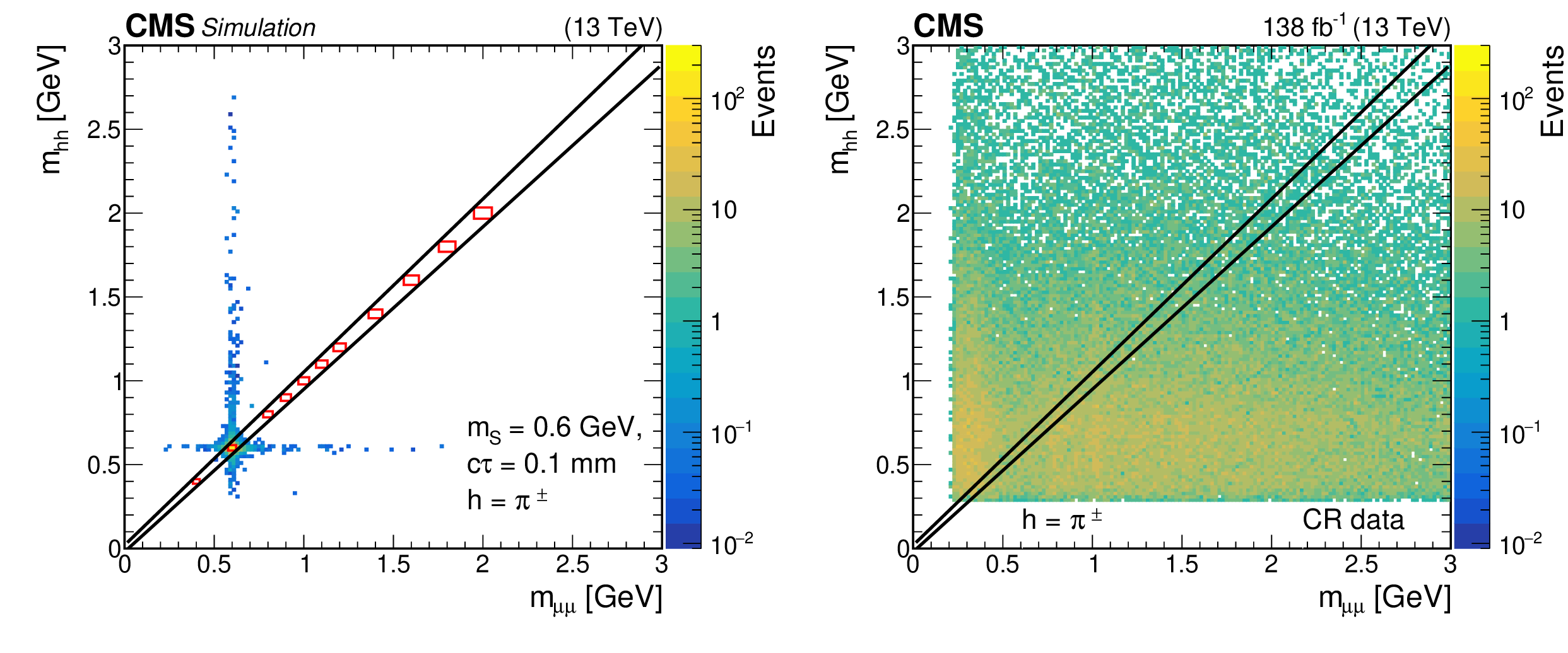
Figure 2:
Two-dimensional distribution of the invariant masses $ m_{\mathrm{h}\mathrm{h}} $ versus $ m_{\mu\mu} $ for a BSM scalar boson of $ m_{\mathrm{S} }= $ 0.6 GeV and proper decay length $ c\tau=0.1 \text{mm} $ (left) and the 2016--2018 data set in the CR (right), after the baseline selection is applied. The red boxes denote the bounding boxes for each BSM scalar boson mass considered, as discussed in Section 4. The black solid lines denote the 2D diagonal mass selection, $ m_{\mathrm{h}\mathrm{h}} \approx m_{\mu\mu} $. The distribution of data in the CR (right) is shown for the final state containing charged pions. The boundaries along the dimuon and dihadron mass correspond to the minimum possible dimuon mass ($ \approx $0.2 GeV) and minimum possible dipion mass ($ \approx $0.3 GeV). For the search targeting charged kaons in the final state, the boundary along the dihadron mass is at the minimum possible dikaon mass ($ \approx $1 GeV). |
png pdf |
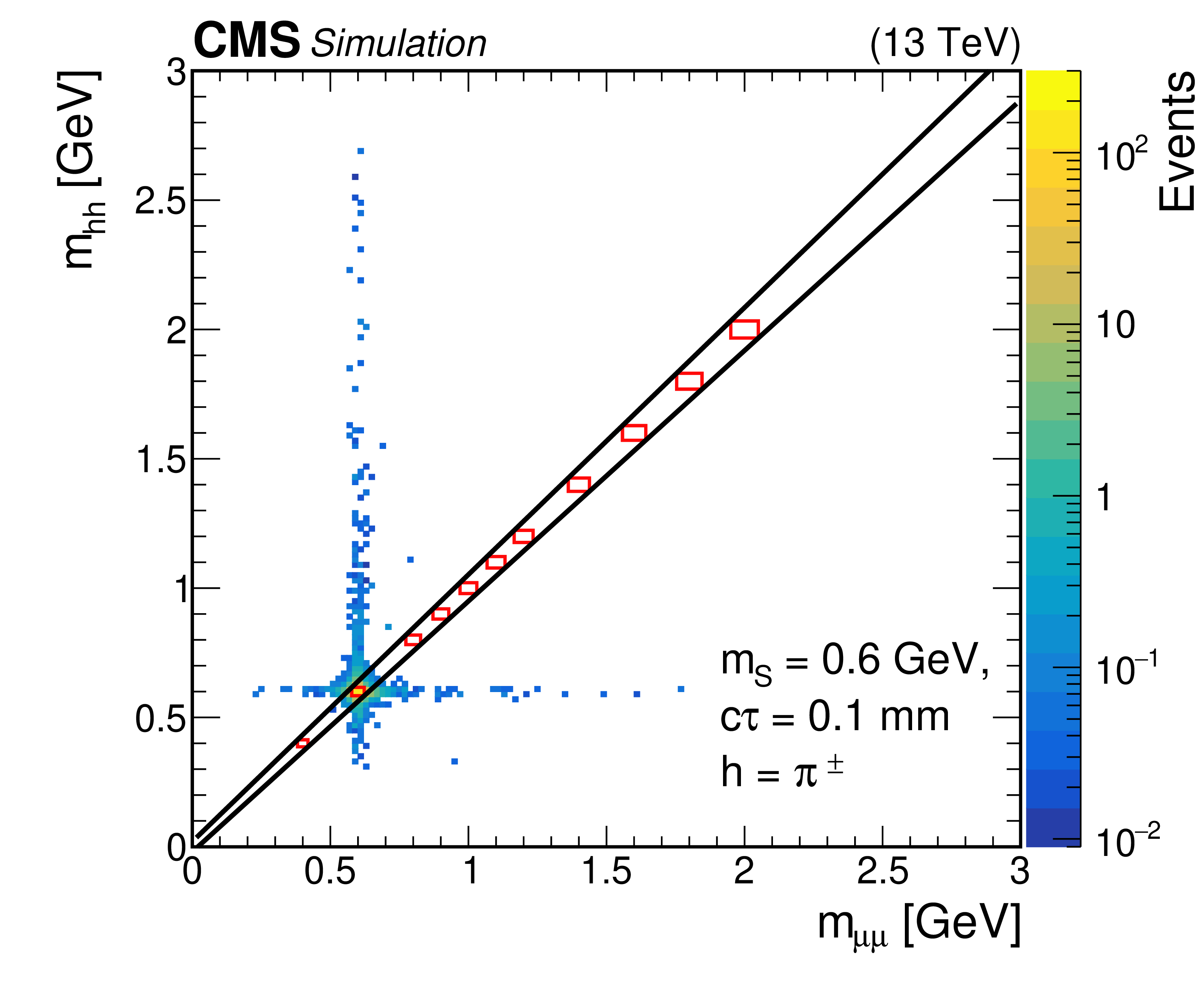
Figure 2-a:
Two-dimensional distribution of the invariant masses $ m_{\mathrm{h}\mathrm{h}} $ versus $ m_{\mu\mu} $ for a BSM scalar boson of $ m_{\mathrm{S} }= $ 0.6 GeV and proper decay length $ c\tau=0.1 \text{mm} $ (left) and the 2016--2018 data set in the CR (right), after the baseline selection is applied. The red boxes denote the bounding boxes for each BSM scalar boson mass considered, as discussed in Section 4. The black solid lines denote the 2D diagonal mass selection, $ m_{\mathrm{h}\mathrm{h}} \approx m_{\mu\mu} $. The distribution of data in the CR (right) is shown for the final state containing charged pions. The boundaries along the dimuon and dihadron mass correspond to the minimum possible dimuon mass ($ \approx $0.2 GeV) and minimum possible dipion mass ($ \approx $0.3 GeV). For the search targeting charged kaons in the final state, the boundary along the dihadron mass is at the minimum possible dikaon mass ($ \approx $1 GeV). |
png pdf |
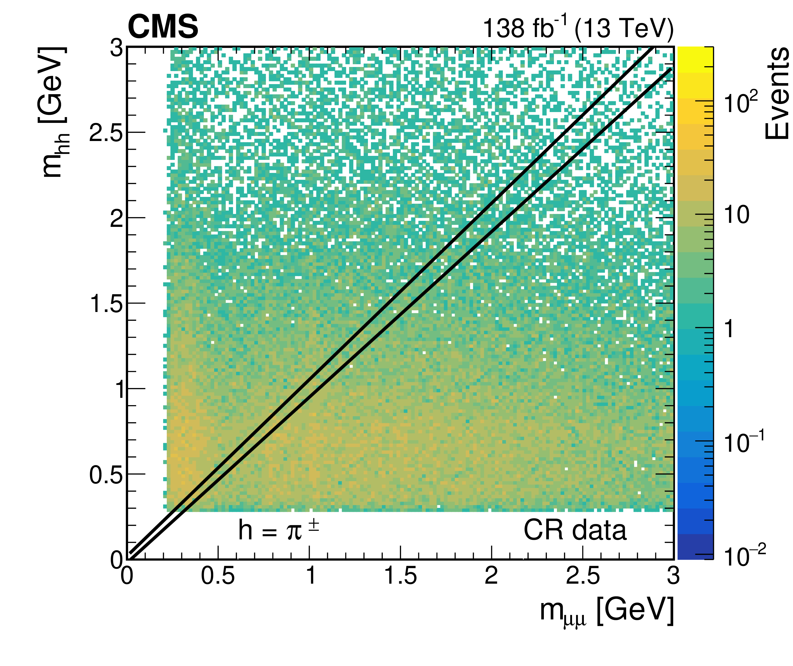
Figure 2-b:
Two-dimensional distribution of the invariant masses $ m_{\mathrm{h}\mathrm{h}} $ versus $ m_{\mu\mu} $ for a BSM scalar boson of $ m_{\mathrm{S} }= $ 0.6 GeV and proper decay length $ c\tau=0.1 \text{mm} $ (left) and the 2016--2018 data set in the CR (right), after the baseline selection is applied. The red boxes denote the bounding boxes for each BSM scalar boson mass considered, as discussed in Section 4. The black solid lines denote the 2D diagonal mass selection, $ m_{\mathrm{h}\mathrm{h}} \approx m_{\mu\mu} $. The distribution of data in the CR (right) is shown for the final state containing charged pions. The boundaries along the dimuon and dihadron mass correspond to the minimum possible dimuon mass ($ \approx $0.2 GeV) and minimum possible dipion mass ($ \approx $0.3 GeV). For the search targeting charged kaons in the final state, the boundary along the dihadron mass is at the minimum possible dikaon mass ($ \approx $1 GeV). |
png pdf |
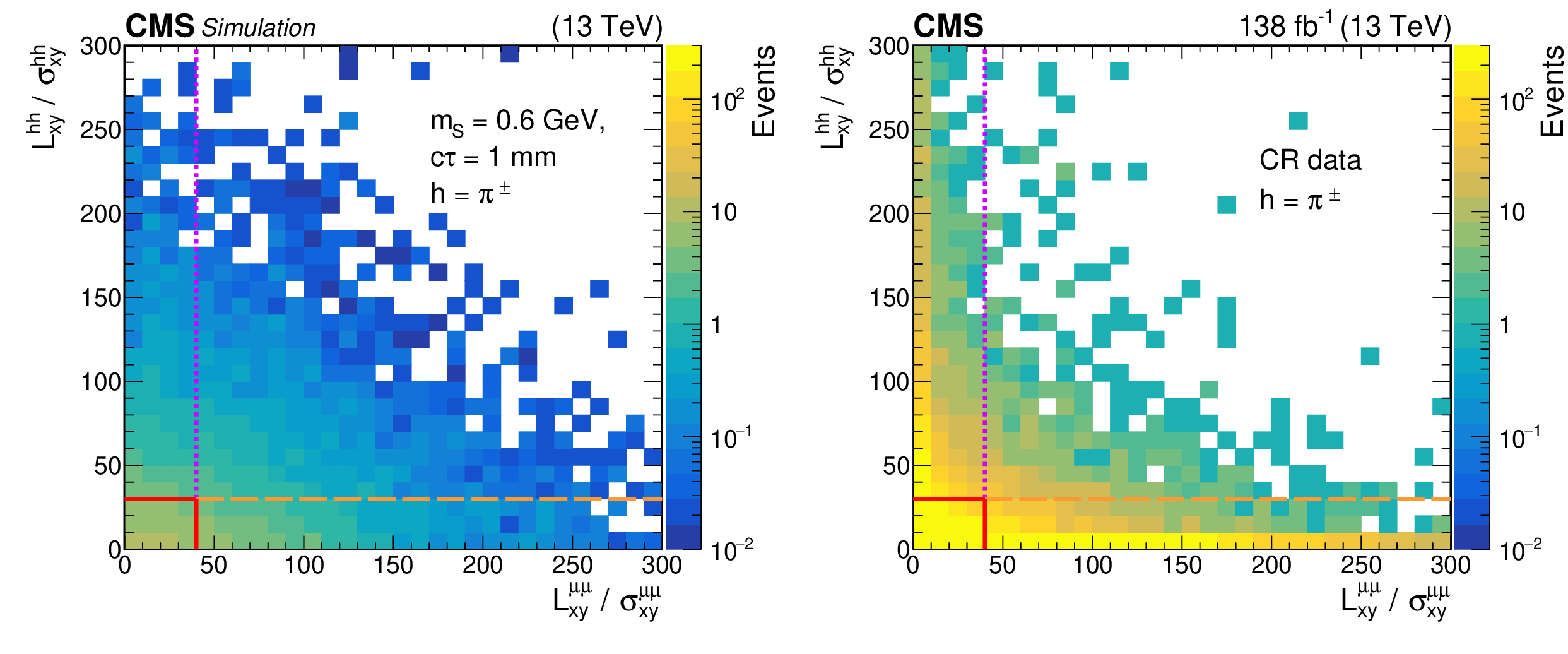
Figure 3:
Two-dimensional distribution of the transverse displacement significance $ L^{\mathrm{h}\mathrm{h}}_{xy}/\sigma^{\mathrm{h}\mathrm{h}}_{xy} $ versus $ L^{\mu\mu}_{xy}/\sigma^{\mu\mu}_{xy} $ for a BSM scalar boson with $ m_{\mathrm{S} }= $ 0.6 GeV and $ c\tau=1 \text{mm} $ (left) and the 2016--2018 data set in the CR (right) after the baseline selection is applied. The lines denote the boundaries for each of the four categories considered: prompt (solid red line), displaced $ \mu\mu $ (dashed orange line), displaced $ \mathrm{h}\mathrm{h} $ (dotted pink line), and displaced (remaining region). The distribution of data in the CR (right) shows that majority of the background is concentrated in the prompt category. |
png pdf |
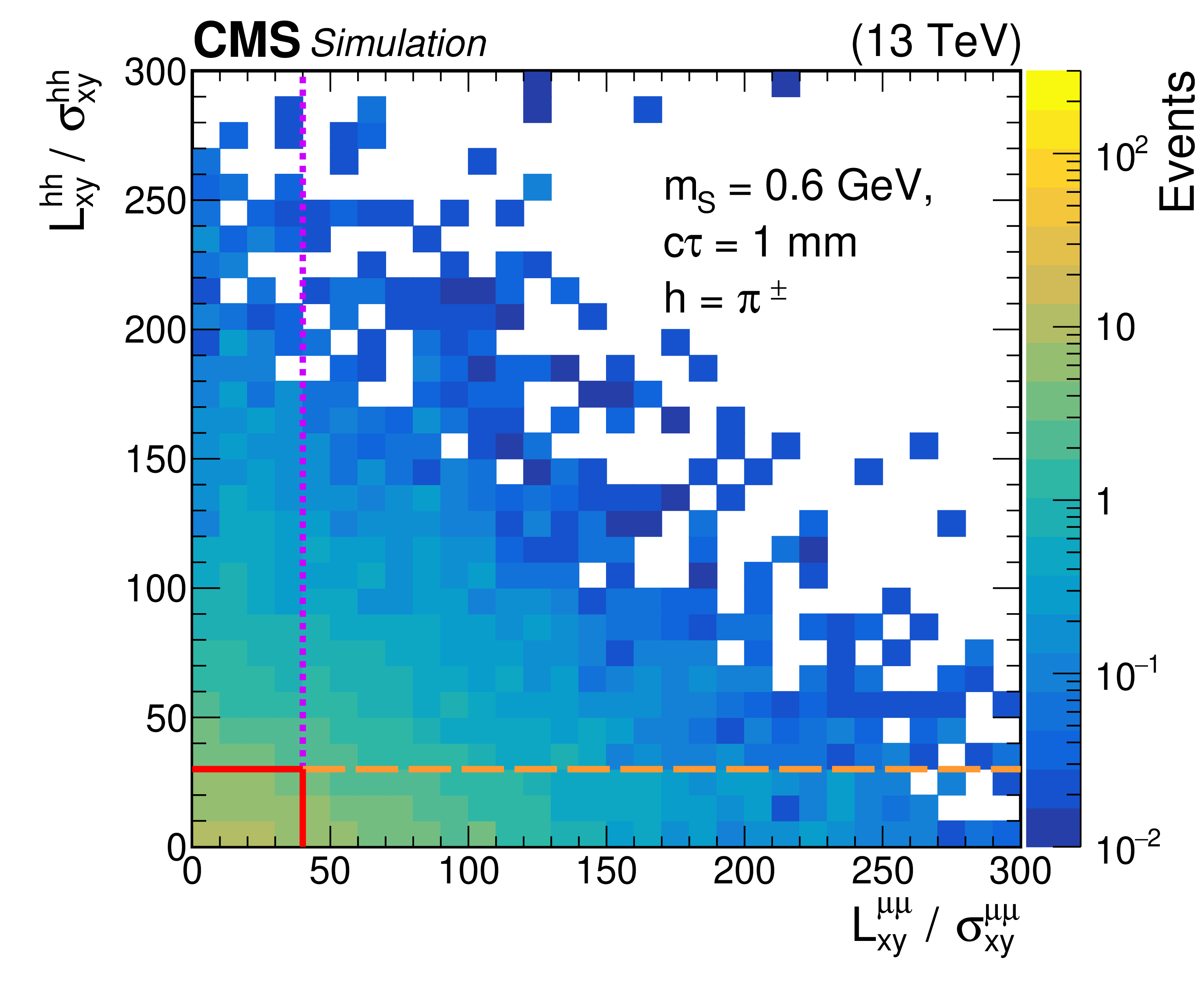
Figure 3-a:
Two-dimensional distribution of the transverse displacement significance $ L^{\mathrm{h}\mathrm{h}}_{xy}/\sigma^{\mathrm{h}\mathrm{h}}_{xy} $ versus $ L^{\mu\mu}_{xy}/\sigma^{\mu\mu}_{xy} $ for a BSM scalar boson with $ m_{\mathrm{S} }= $ 0.6 GeV and $ c\tau=1 \text{mm} $ (left) and the 2016--2018 data set in the CR (right) after the baseline selection is applied. The lines denote the boundaries for each of the four categories considered: prompt (solid red line), displaced $ \mu\mu $ (dashed orange line), displaced $ \mathrm{h}\mathrm{h} $ (dotted pink line), and displaced (remaining region). The distribution of data in the CR (right) shows that majority of the background is concentrated in the prompt category. |
png pdf |
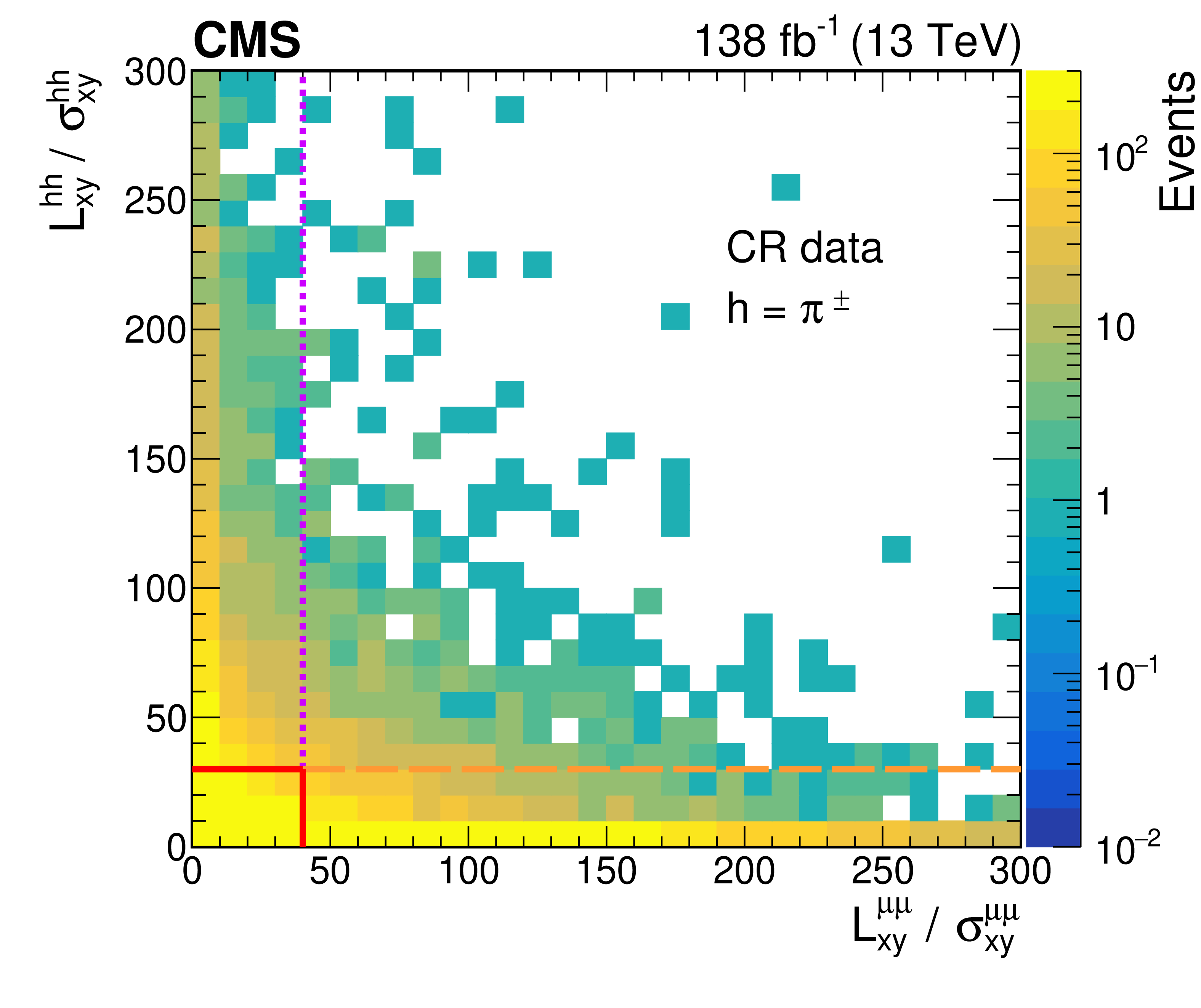
Figure 3-b:
Two-dimensional distribution of the transverse displacement significance $ L^{\mathrm{h}\mathrm{h}}_{xy}/\sigma^{\mathrm{h}\mathrm{h}}_{xy} $ versus $ L^{\mu\mu}_{xy}/\sigma^{\mu\mu}_{xy} $ for a BSM scalar boson with $ m_{\mathrm{S} }= $ 0.6 GeV and $ c\tau=1 \text{mm} $ (left) and the 2016--2018 data set in the CR (right) after the baseline selection is applied. The lines denote the boundaries for each of the four categories considered: prompt (solid red line), displaced $ \mu\mu $ (dashed orange line), displaced $ \mathrm{h}\mathrm{h} $ (dotted pink line), and displaced (remaining region). The distribution of data in the CR (right) shows that majority of the background is concentrated in the prompt category. |
png pdf |
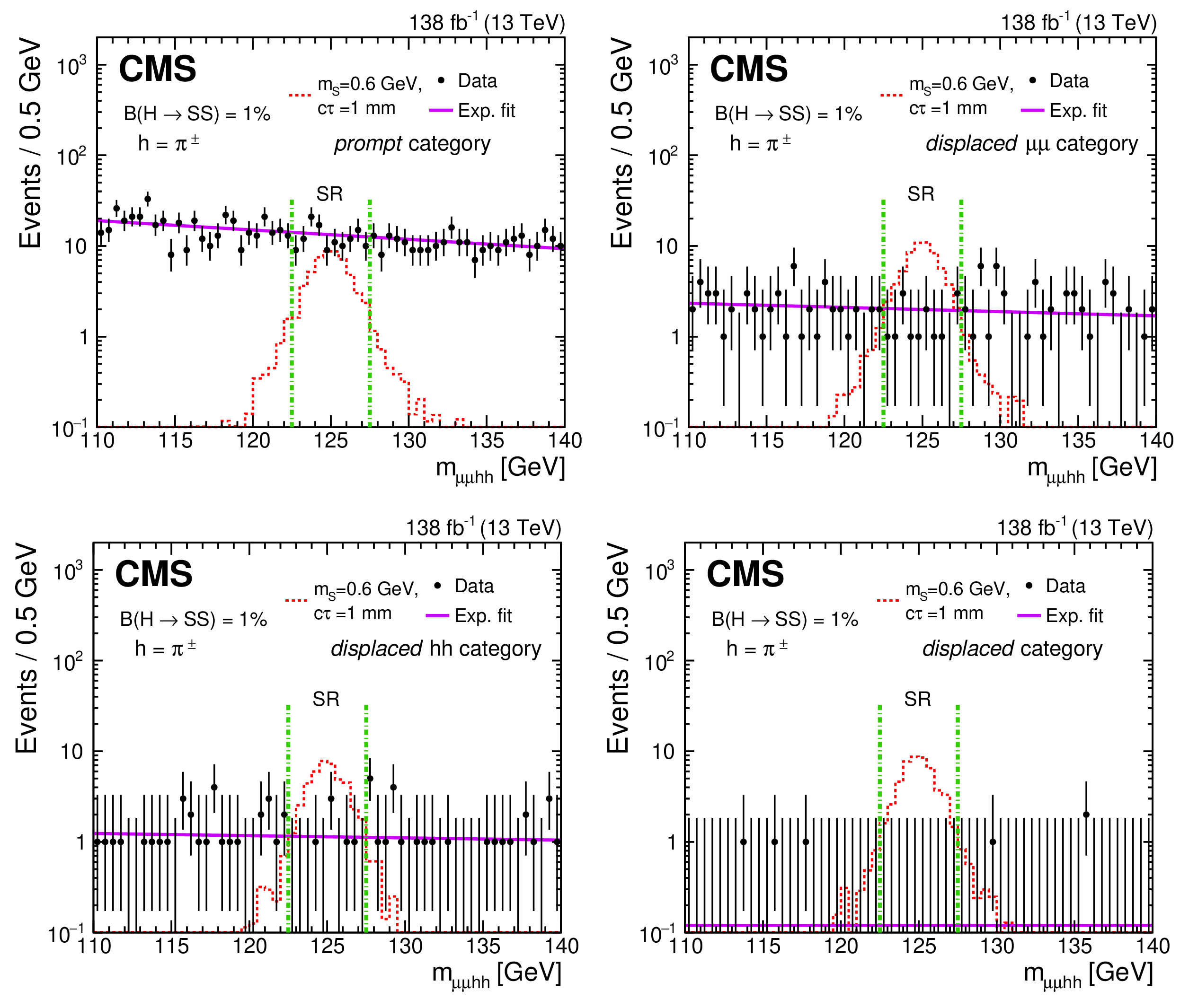
Figure 4:
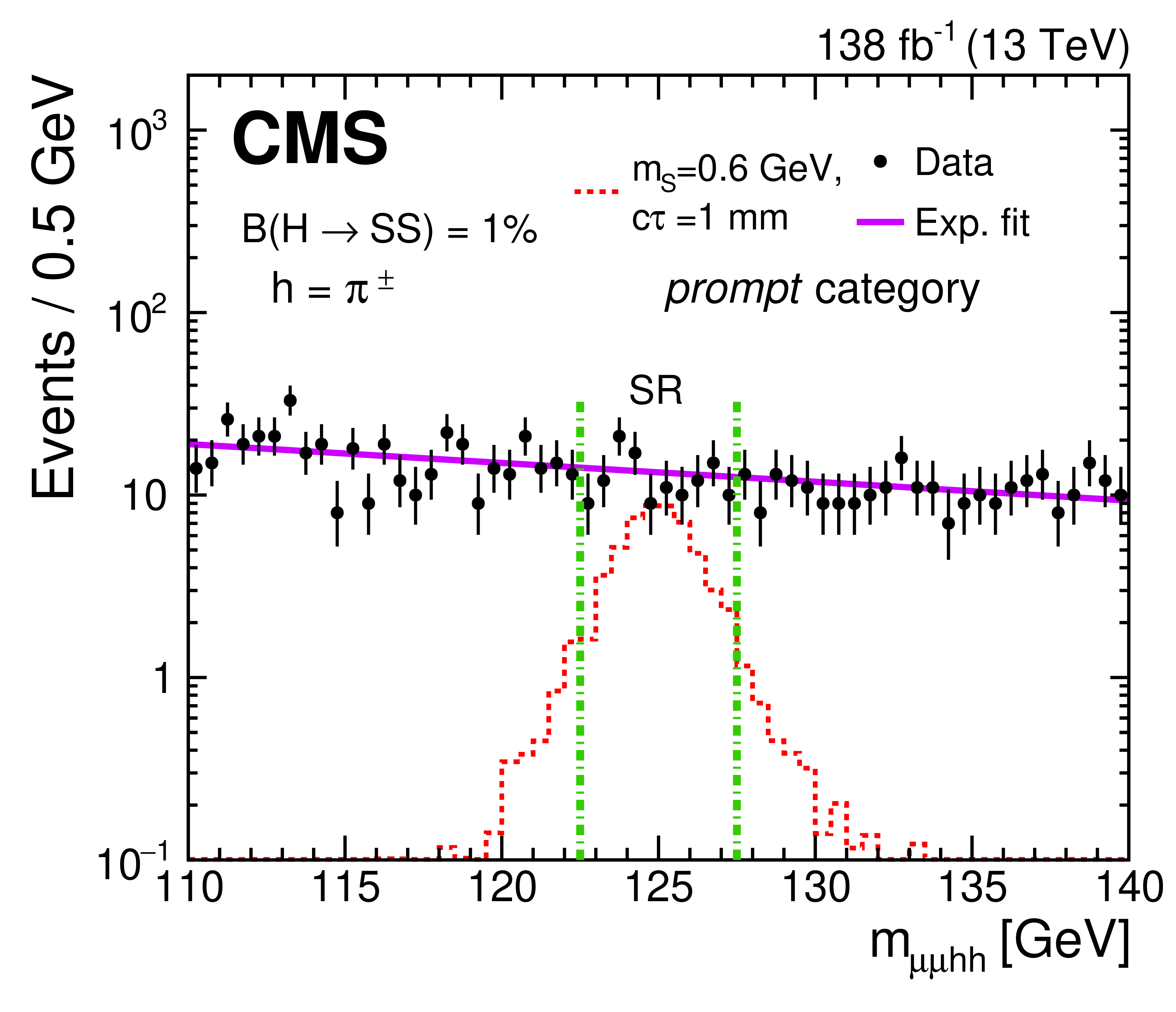
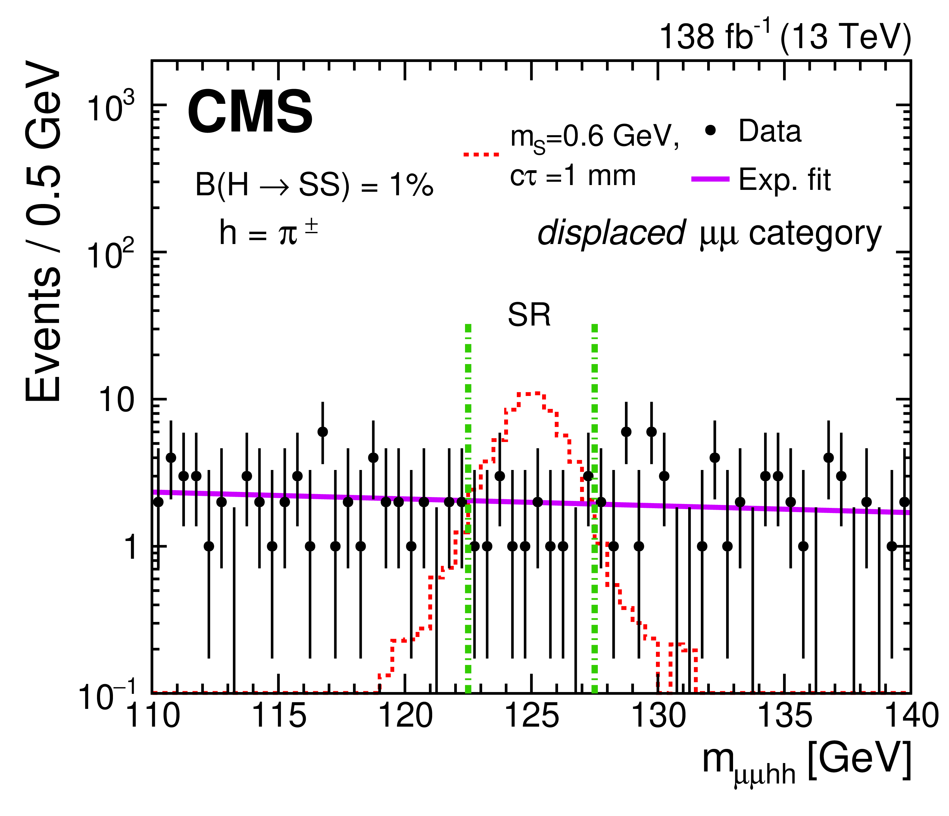
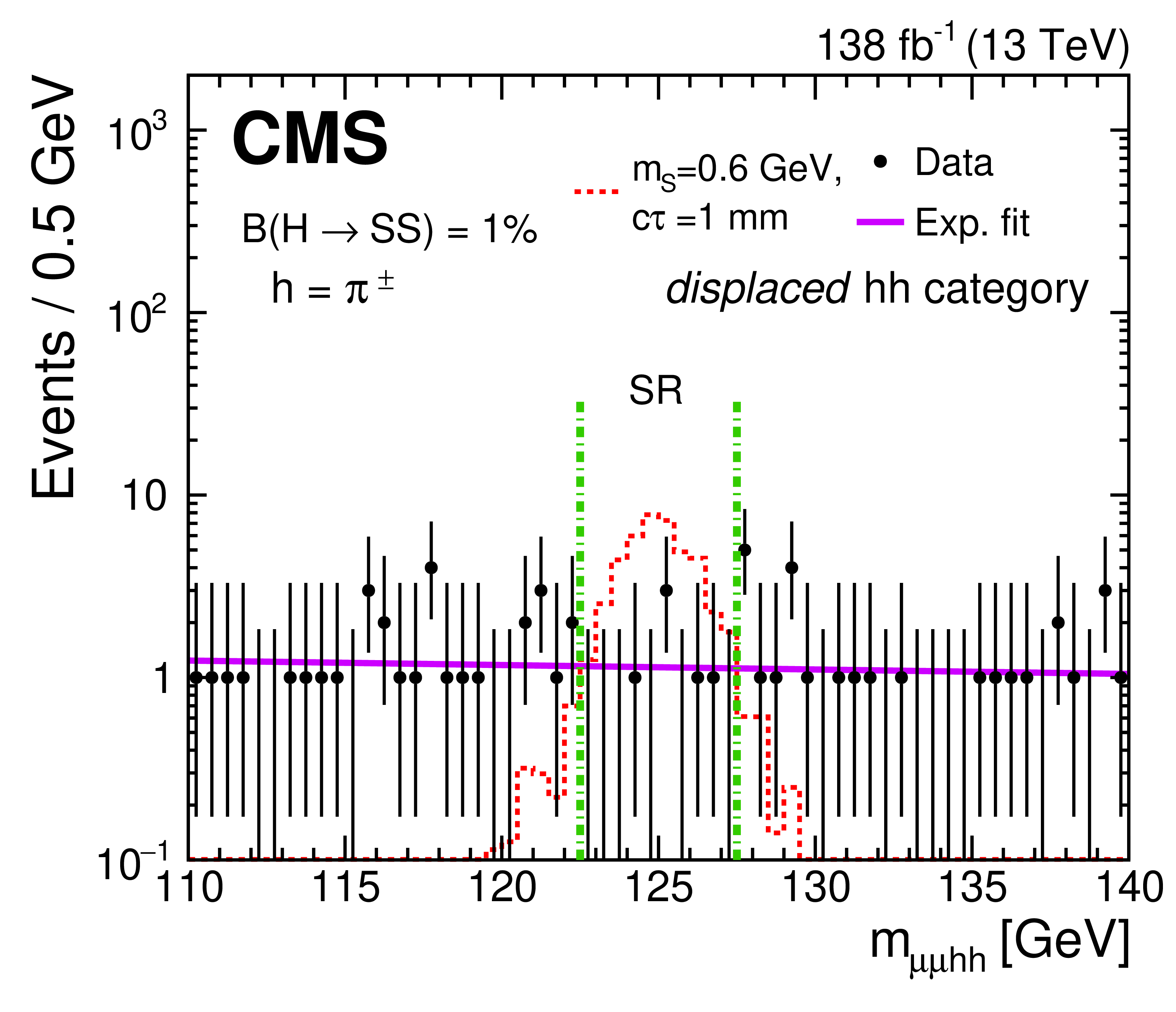
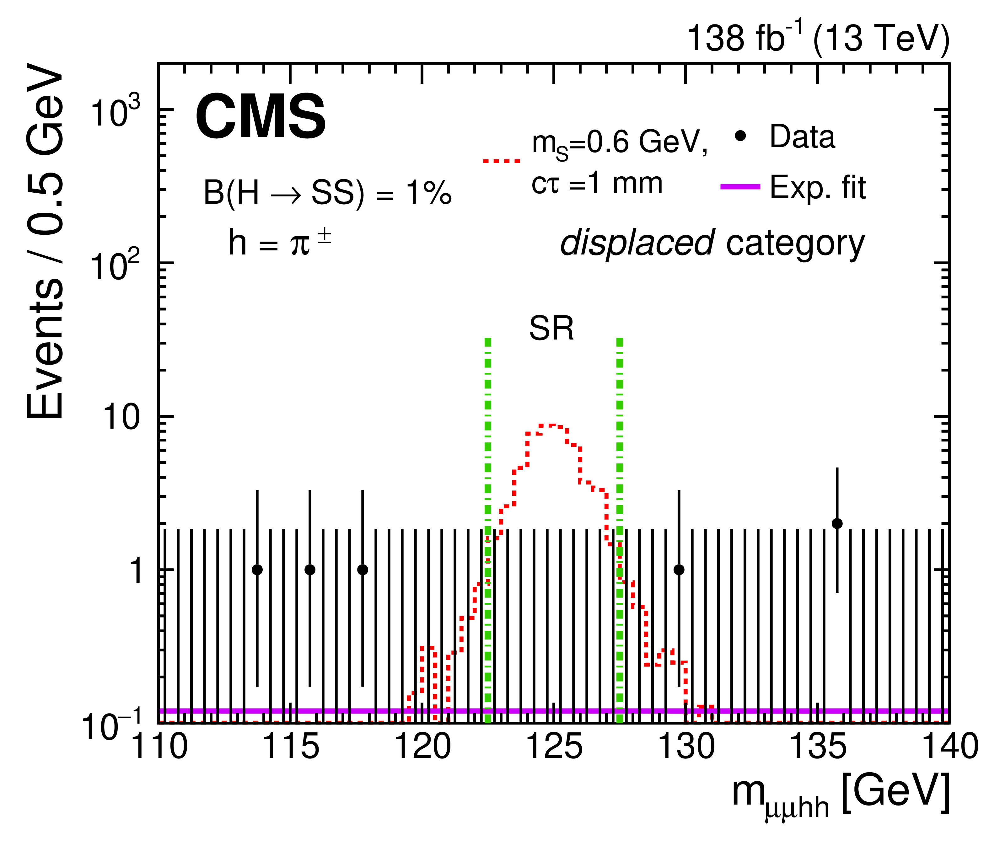
Four-object invariant mass distributions in data (black dots with error bars) and for a BSM scalar boson signal with $ m_{\mathrm{S} }= $ 0.6 GeV and $ c\tau=1 \text{mm} $ (red histogram) for the prompt (upper left), displaced $ \mu\mu $ (upper right), displaced $ \mathrm{h}\mathrm{h} $ (lower left) and the displaced category (lower right). The event selection criteria, as listed in Table 2, have been applied. The signal event yield is scaled to the integrated luminosity, assuming the gluon fusion Higgs boson production cross section [56], $ \mathcal{B}(\mathrm{H}\to\mathrm{S} \mathrm{S} )=1% $, and $ \mathcal{B}(\mathrm{S} \to\mu^{+}\mu^{-}) $, and $ \mathcal{B}(\mathrm{S} \to\pi^{+}\pi^{-}) $ for $ m_{\mathrm{S} }= $ 0.6 GeV, as in Table 1. The green dash-dotted vertical lines delineate the SR. |
png pdf |
Figure 4-a:
Four-object invariant mass distributions in data (black dots with error bars) and for a BSM scalar boson signal with $ m_{\mathrm{S} }= $ 0.6 GeV and $ c\tau=1 \text{mm} $ (red histogram) for the prompt (upper left), displaced $ \mu\mu $ (upper right), displaced $ \mathrm{h}\mathrm{h} $ (lower left) and the displaced category (lower right). The event selection criteria, as listed in Table 2, have been applied. The signal event yield is scaled to the integrated luminosity, assuming the gluon fusion Higgs boson production cross section [56], $ \mathcal{B}(\mathrm{H}\to\mathrm{S} \mathrm{S} )=1% $, and $ \mathcal{B}(\mathrm{S} \to\mu^{+}\mu^{-}) $, and $ \mathcal{B}(\mathrm{S} \to\pi^{+}\pi^{-}) $ for $ m_{\mathrm{S} }= $ 0.6 GeV, as in Table 1. The green dash-dotted vertical lines delineate the SR. |
png pdf |
Figure 4-b:
Four-object invariant mass distributions in data (black dots with error bars) and for a BSM scalar boson signal with $ m_{\mathrm{S} }= $ 0.6 GeV and $ c\tau=1 \text{mm} $ (red histogram) for the prompt (upper left), displaced $ \mu\mu $ (upper right), displaced $ \mathrm{h}\mathrm{h} $ (lower left) and the displaced category (lower right). The event selection criteria, as listed in Table 2, have been applied. The signal event yield is scaled to the integrated luminosity, assuming the gluon fusion Higgs boson production cross section [56], $ \mathcal{B}(\mathrm{H}\to\mathrm{S} \mathrm{S} )=1% $, and $ \mathcal{B}(\mathrm{S} \to\mu^{+}\mu^{-}) $, and $ \mathcal{B}(\mathrm{S} \to\pi^{+}\pi^{-}) $ for $ m_{\mathrm{S} }= $ 0.6 GeV, as in Table 1. The green dash-dotted vertical lines delineate the SR. |
png pdf |
Figure 4-c:
Four-object invariant mass distributions in data (black dots with error bars) and for a BSM scalar boson signal with $ m_{\mathrm{S} }= $ 0.6 GeV and $ c\tau=1 \text{mm} $ (red histogram) for the prompt (upper left), displaced $ \mu\mu $ (upper right), displaced $ \mathrm{h}\mathrm{h} $ (lower left) and the displaced category (lower right). The event selection criteria, as listed in Table 2, have been applied. The signal event yield is scaled to the integrated luminosity, assuming the gluon fusion Higgs boson production cross section [56], $ \mathcal{B}(\mathrm{H}\to\mathrm{S} \mathrm{S} )=1% $, and $ \mathcal{B}(\mathrm{S} \to\mu^{+}\mu^{-}) $, and $ \mathcal{B}(\mathrm{S} \to\pi^{+}\pi^{-}) $ for $ m_{\mathrm{S} }= $ 0.6 GeV, as in Table 1. The green dash-dotted vertical lines delineate the SR. |
png pdf |
Figure 4-d:
Four-object invariant mass distributions in data (black dots with error bars) and for a BSM scalar boson signal with $ m_{\mathrm{S} }= $ 0.6 GeV and $ c\tau=1 \text{mm} $ (red histogram) for the prompt (upper left), displaced $ \mu\mu $ (upper right), displaced $ \mathrm{h}\mathrm{h} $ (lower left) and the displaced category (lower right). The event selection criteria, as listed in Table 2, have been applied. The signal event yield is scaled to the integrated luminosity, assuming the gluon fusion Higgs boson production cross section [56], $ \mathcal{B}(\mathrm{H}\to\mathrm{S} \mathrm{S} )=1% $, and $ \mathcal{B}(\mathrm{S} \to\mu^{+}\mu^{-}) $, and $ \mathcal{B}(\mathrm{S} \to\pi^{+}\pi^{-}) $ for $ m_{\mathrm{S} }= $ 0.6 GeV, as in Table 1. The green dash-dotted vertical lines delineate the SR. |
png pdf |
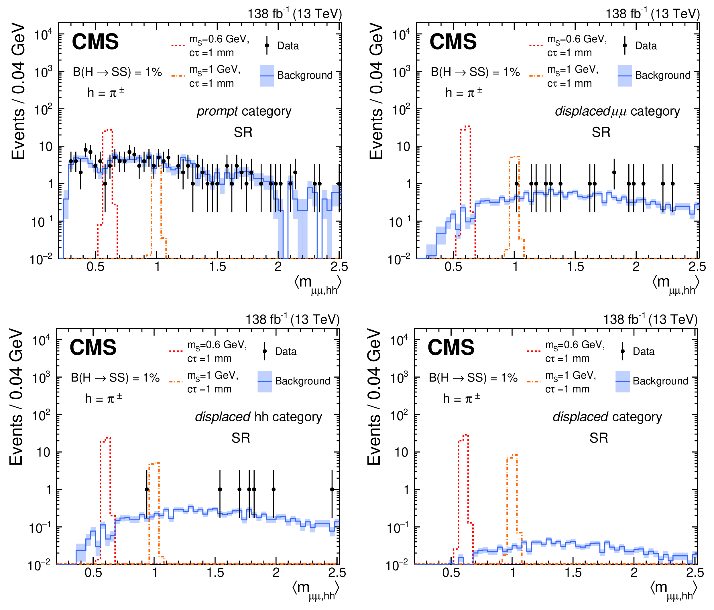
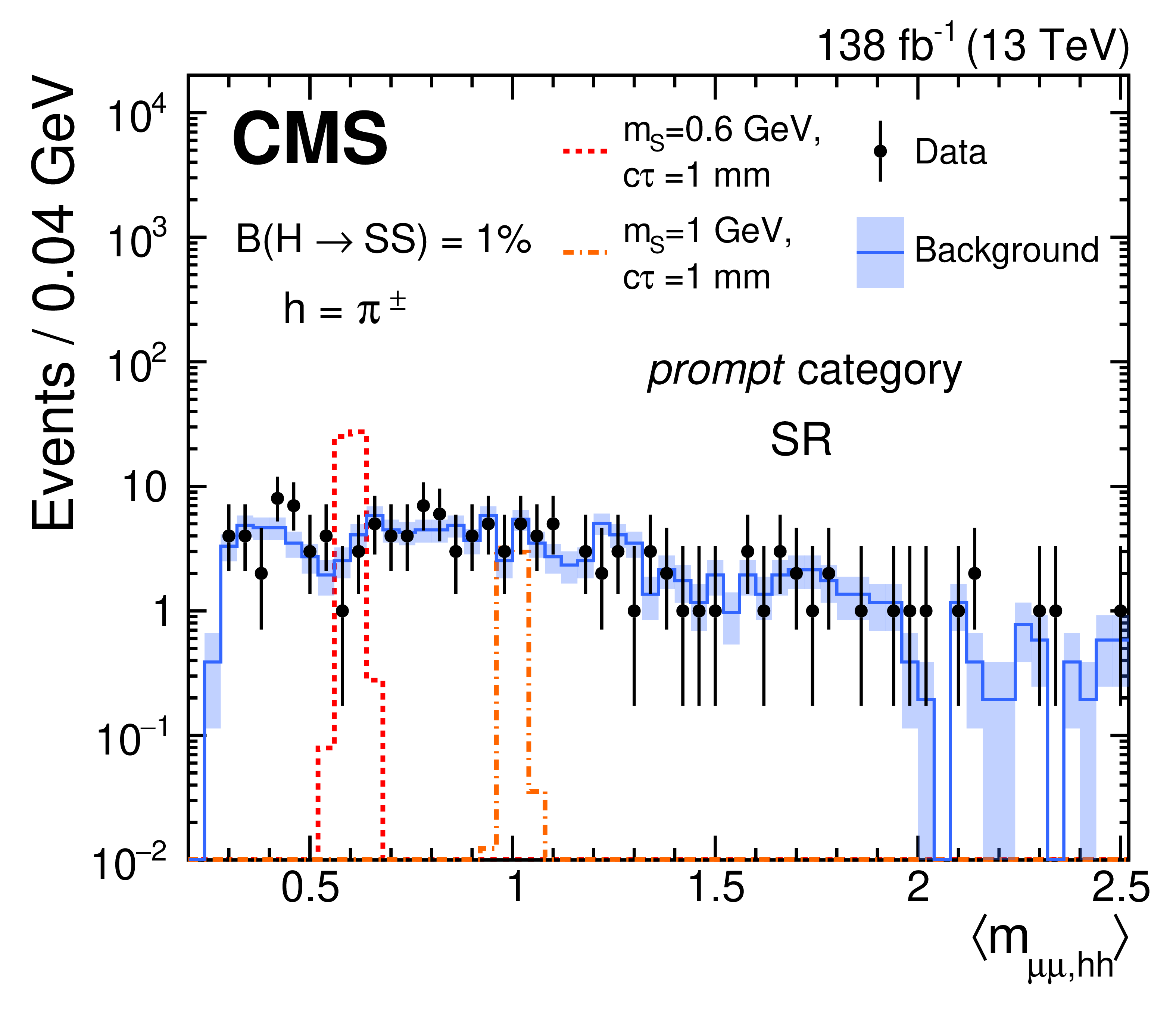
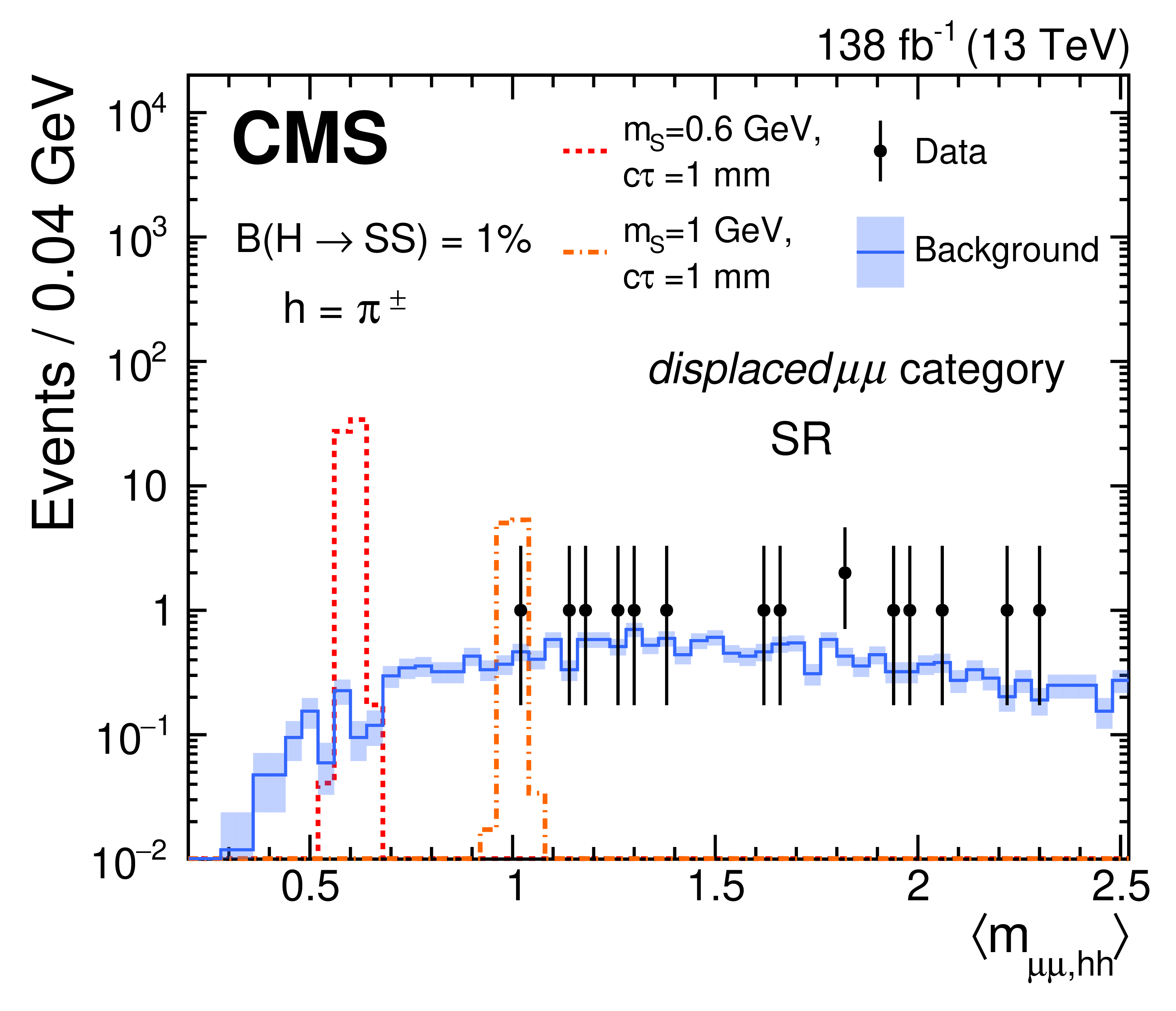
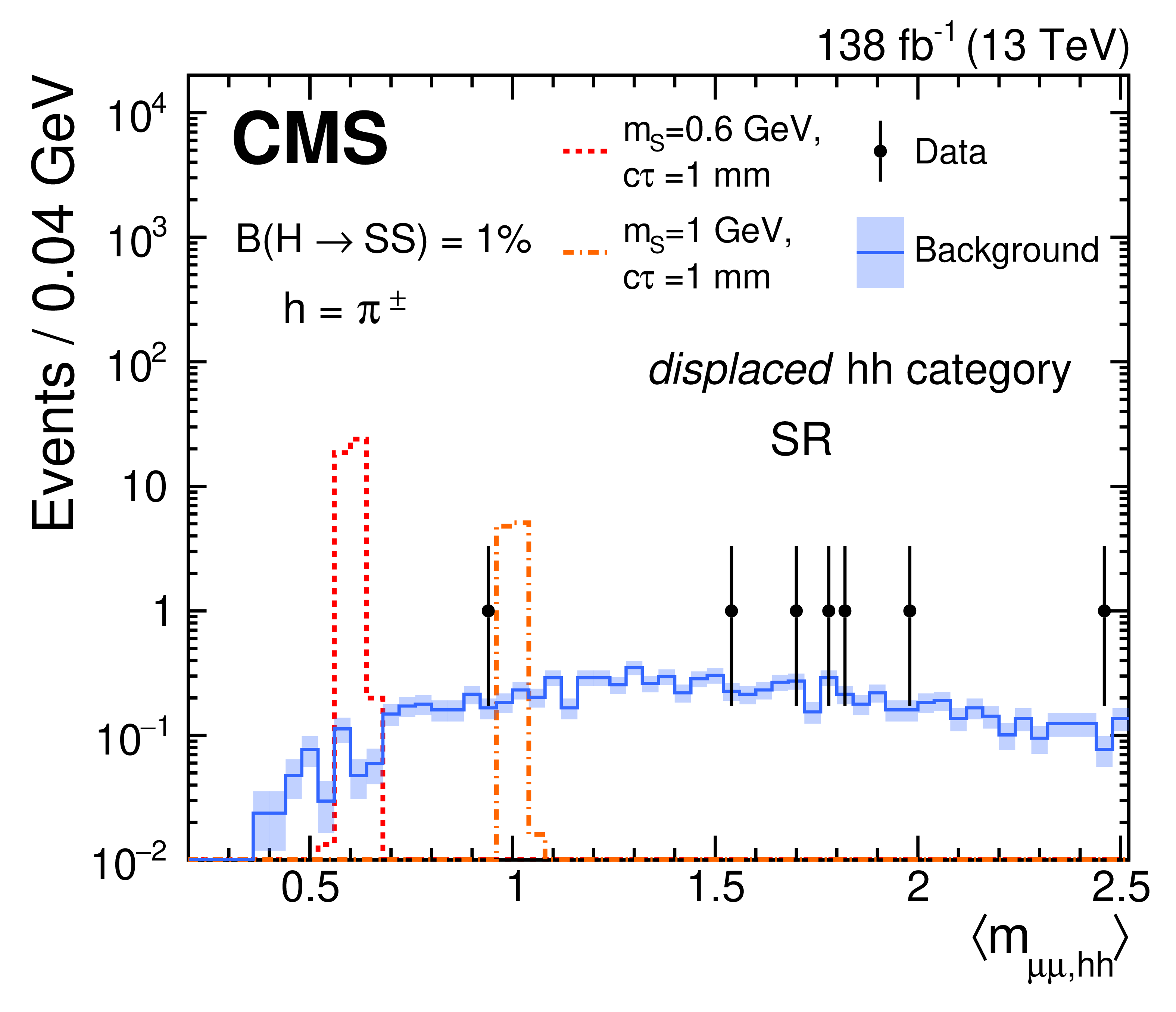
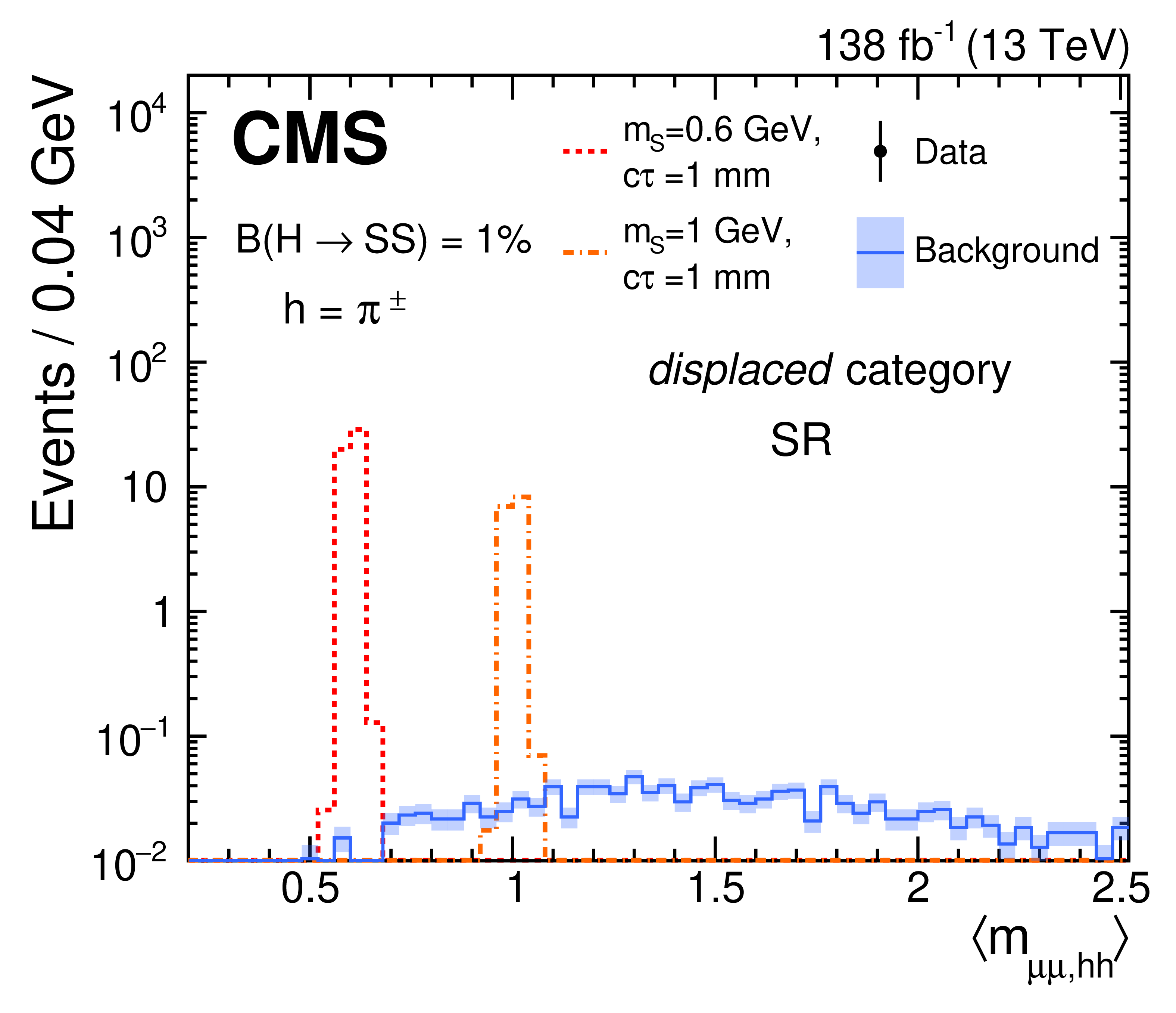
Figure 5:
Average diobject invariant mass distributions in the SR for the prompt (upper left), displaced $ \mu\mu $ (upper right), displaced $ \mathrm{h}\mathrm{h} $ (lower left), and displaced (lower right) categories. The event selection criteria of Table 2 have been applied. The observed number of events in data are shown as black dots with the uncertainty bars and the background prediction (estimated from the events in the CR as explained in Section 5) as blue histograms. Uncertainty bars are not shown for bins with zero entries. Two signal samples are also presented for BSM scalar bosons with $ m_{\mathrm{S} }= $ 0.6 and 1 GeV and $ c\tau=1 \text{mm} $. The signal yield is scaled to the integrated luminosity, assuming the gluon fusion Higgs boson production cross-section [56], $ \mathcal{B}(\mathrm{H}\to\mathrm{S} \mathrm{S} )=1% $, and $ \mathcal{B}(\mathrm{S} \to\mu^{+}\mu^{-}) $, and $ \mathcal{B}(\mathrm{S} \to\pi^{+}\pi^{-}) $ for $ m_{\mathrm{S} }= $ 0.6 and 1 GeV, according to the values listed in Table 1. |
png pdf |
Figure 5-a:
Average diobject invariant mass distributions in the SR for the prompt (upper left), displaced $ \mu\mu $ (upper right), displaced $ \mathrm{h}\mathrm{h} $ (lower left), and displaced (lower right) categories. The event selection criteria of Table 2 have been applied. The observed number of events in data are shown as black dots with the uncertainty bars and the background prediction (estimated from the events in the CR as explained in Section 5) as blue histograms. Uncertainty bars are not shown for bins with zero entries. Two signal samples are also presented for BSM scalar bosons with $ m_{\mathrm{S} }= $ 0.6 and 1 GeV and $ c\tau=1 \text{mm} $. The signal yield is scaled to the integrated luminosity, assuming the gluon fusion Higgs boson production cross-section [56], $ \mathcal{B}(\mathrm{H}\to\mathrm{S} \mathrm{S} )=1% $, and $ \mathcal{B}(\mathrm{S} \to\mu^{+}\mu^{-}) $, and $ \mathcal{B}(\mathrm{S} \to\pi^{+}\pi^{-}) $ for $ m_{\mathrm{S} }= $ 0.6 and 1 GeV, according to the values listed in Table 1. |
png pdf |
Figure 5-b:
Average diobject invariant mass distributions in the SR for the prompt (upper left), displaced $ \mu\mu $ (upper right), displaced $ \mathrm{h}\mathrm{h} $ (lower left), and displaced (lower right) categories. The event selection criteria of Table 2 have been applied. The observed number of events in data are shown as black dots with the uncertainty bars and the background prediction (estimated from the events in the CR as explained in Section 5) as blue histograms. Uncertainty bars are not shown for bins with zero entries. Two signal samples are also presented for BSM scalar bosons with $ m_{\mathrm{S} }= $ 0.6 and 1 GeV and $ c\tau=1 \text{mm} $. The signal yield is scaled to the integrated luminosity, assuming the gluon fusion Higgs boson production cross-section [56], $ \mathcal{B}(\mathrm{H}\to\mathrm{S} \mathrm{S} )=1% $, and $ \mathcal{B}(\mathrm{S} \to\mu^{+}\mu^{-}) $, and $ \mathcal{B}(\mathrm{S} \to\pi^{+}\pi^{-}) $ for $ m_{\mathrm{S} }= $ 0.6 and 1 GeV, according to the values listed in Table 1. |
png pdf |
Figure 5-c:
Average diobject invariant mass distributions in the SR for the prompt (upper left), displaced $ \mu\mu $ (upper right), displaced $ \mathrm{h}\mathrm{h} $ (lower left), and displaced (lower right) categories. The event selection criteria of Table 2 have been applied. The observed number of events in data are shown as black dots with the uncertainty bars and the background prediction (estimated from the events in the CR as explained in Section 5) as blue histograms. Uncertainty bars are not shown for bins with zero entries. Two signal samples are also presented for BSM scalar bosons with $ m_{\mathrm{S} }= $ 0.6 and 1 GeV and $ c\tau=1 \text{mm} $. The signal yield is scaled to the integrated luminosity, assuming the gluon fusion Higgs boson production cross-section [56], $ \mathcal{B}(\mathrm{H}\to\mathrm{S} \mathrm{S} )=1% $, and $ \mathcal{B}(\mathrm{S} \to\mu^{+}\mu^{-}) $, and $ \mathcal{B}(\mathrm{S} \to\pi^{+}\pi^{-}) $ for $ m_{\mathrm{S} }= $ 0.6 and 1 GeV, according to the values listed in Table 1. |
png pdf |
Figure 5-d:
Average diobject invariant mass distributions in the SR for the prompt (upper left), displaced $ \mu\mu $ (upper right), displaced $ \mathrm{h}\mathrm{h} $ (lower left), and displaced (lower right) categories. The event selection criteria of Table 2 have been applied. The observed number of events in data are shown as black dots with the uncertainty bars and the background prediction (estimated from the events in the CR as explained in Section 5) as blue histograms. Uncertainty bars are not shown for bins with zero entries. Two signal samples are also presented for BSM scalar bosons with $ m_{\mathrm{S} }= $ 0.6 and 1 GeV and $ c\tau=1 \text{mm} $. The signal yield is scaled to the integrated luminosity, assuming the gluon fusion Higgs boson production cross-section [56], $ \mathcal{B}(\mathrm{H}\to\mathrm{S} \mathrm{S} )=1% $, and $ \mathcal{B}(\mathrm{S} \to\mu^{+}\mu^{-}) $, and $ \mathcal{B}(\mathrm{S} \to\pi^{+}\pi^{-}) $ for $ m_{\mathrm{S} }= $ 0.6 and 1 GeV, according to the values listed in Table 1. |
png pdf |
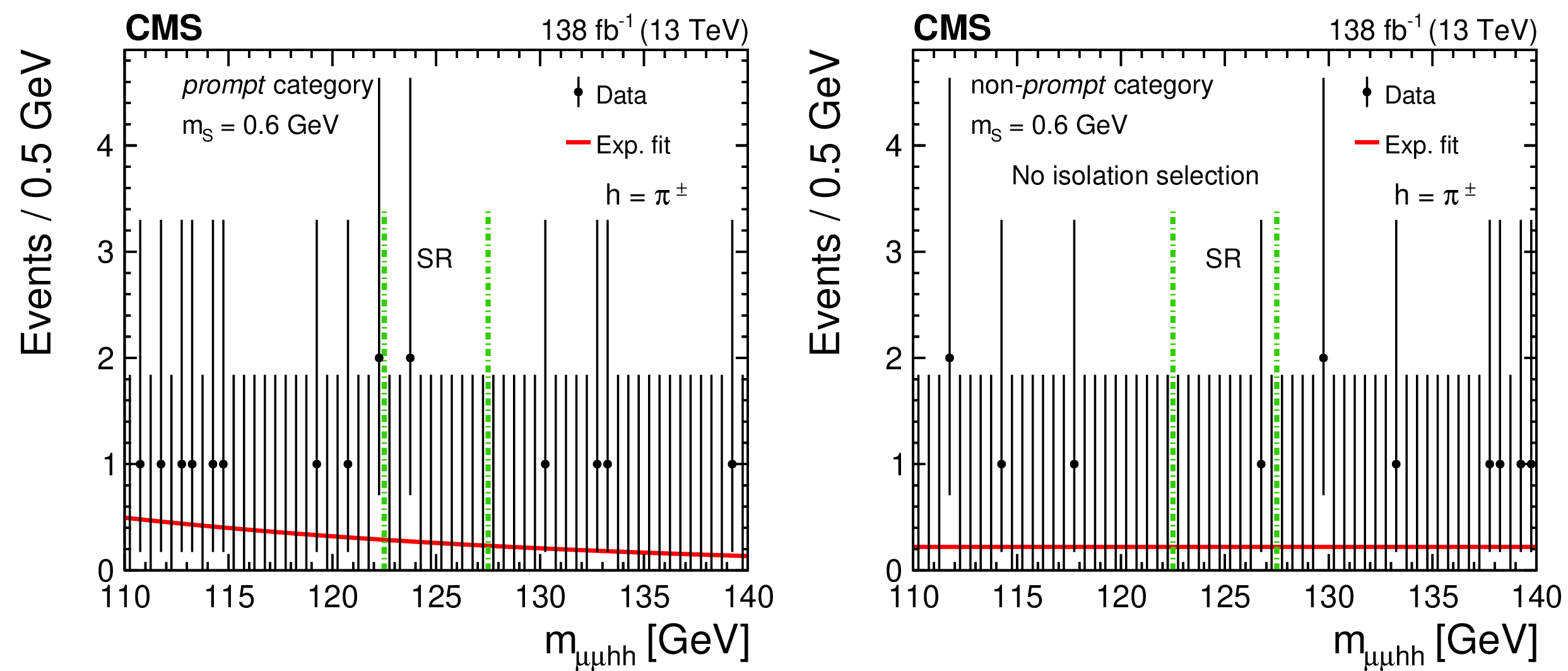
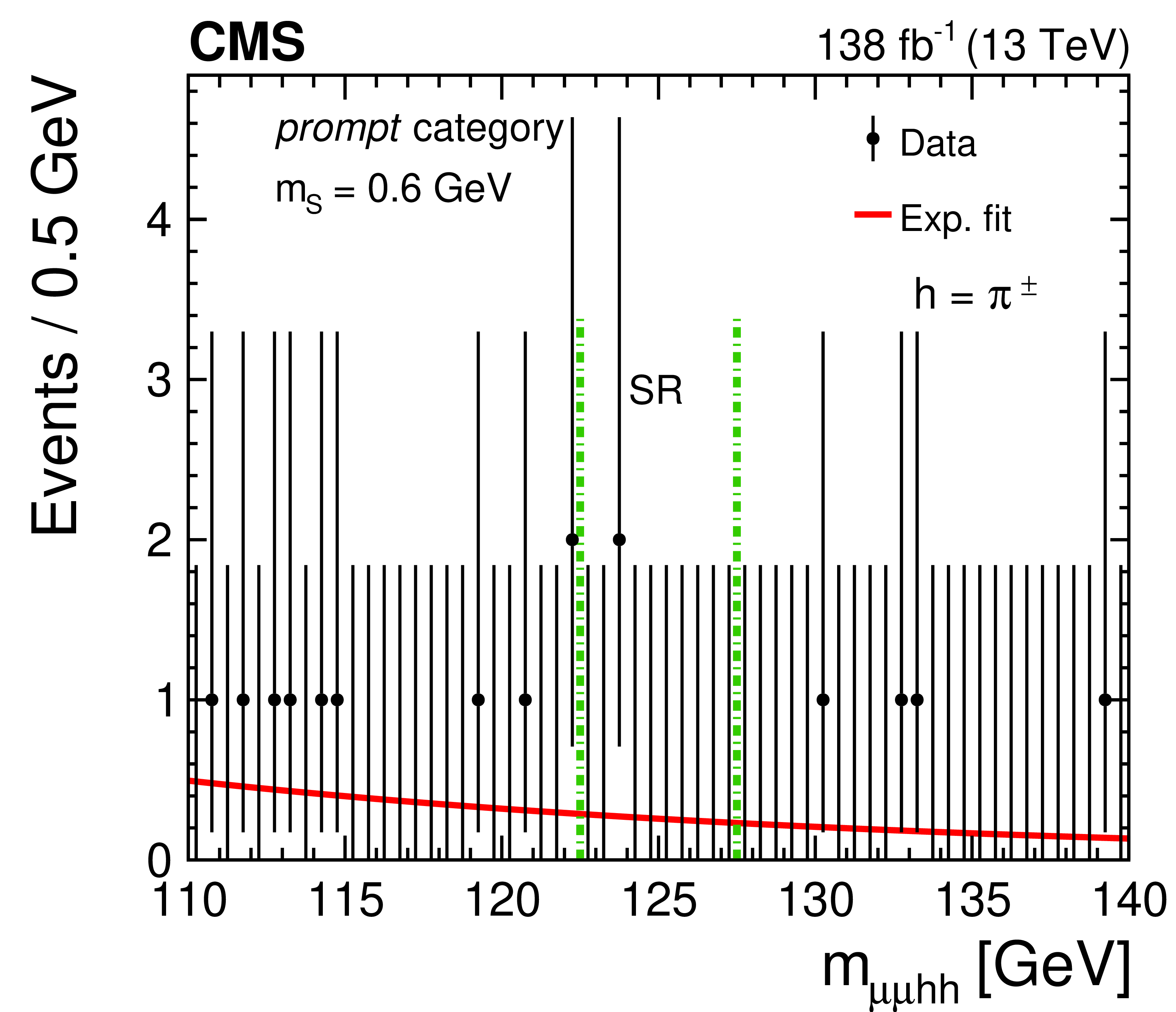
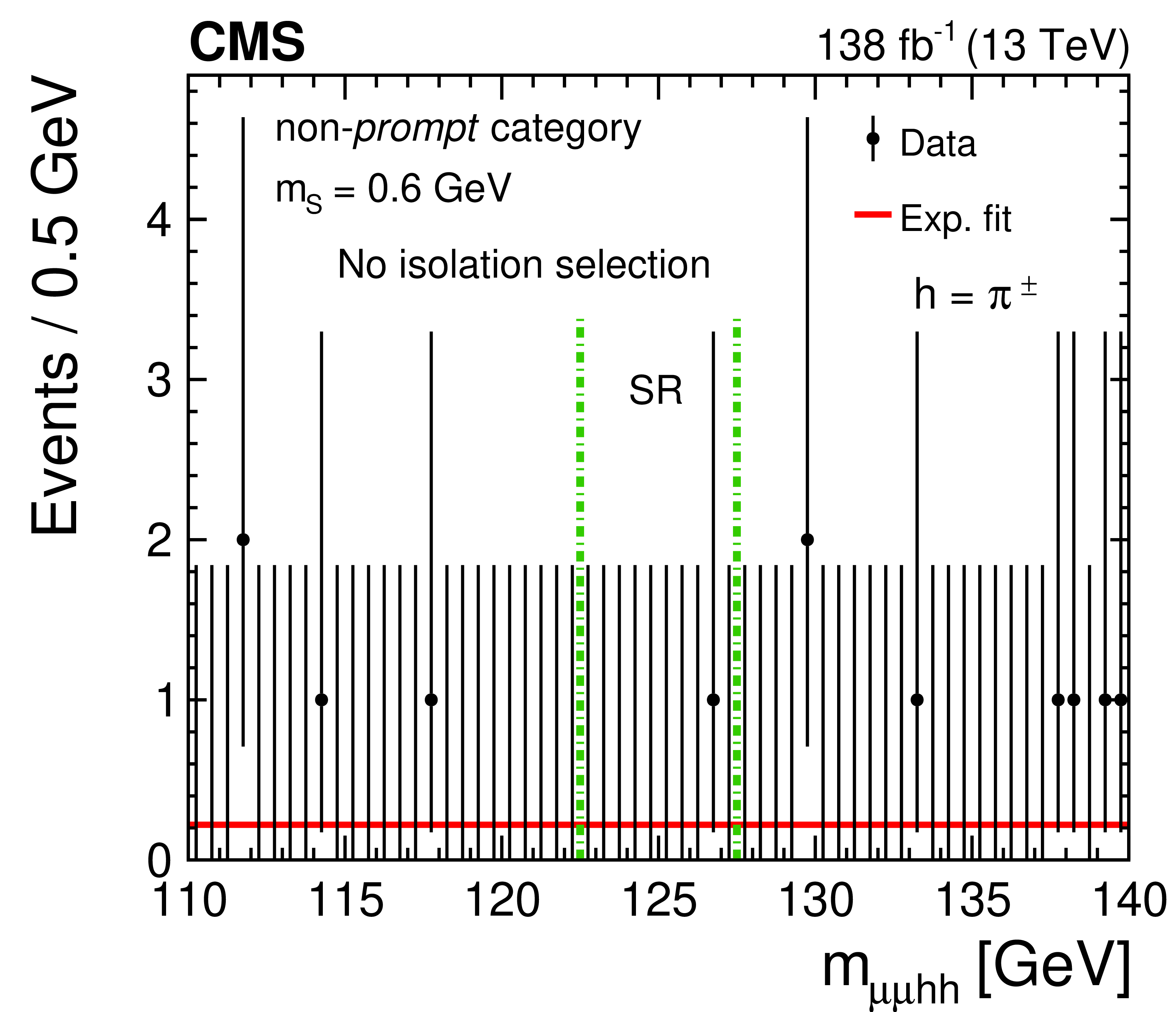
Figure 6:
The four-object invariant mass distribution for the 2016--2018 dataset in the prompt (left) and merged non-prompt (right) categories after the application of the event selection listed in Table 2 and the mass window for $ m_{\mathrm{S} }= $ 0.6 GeV. The dots with uncertainty bars represent the data. The red curve is the result of the exponential fit to the CR. The green dash-dotted vertical lines delineate the SR. The distributions for the merged non-prompt nonisolated category are not weighted by the relevant transfer factors. |
png pdf |
Figure 6-a:
The four-object invariant mass distribution for the 2016--2018 dataset in the prompt (left) and merged non-prompt (right) categories after the application of the event selection listed in Table 2 and the mass window for $ m_{\mathrm{S} }= $ 0.6 GeV. The dots with uncertainty bars represent the data. The red curve is the result of the exponential fit to the CR. The green dash-dotted vertical lines delineate the SR. The distributions for the merged non-prompt nonisolated category are not weighted by the relevant transfer factors. |
png pdf |
Figure 6-b:
The four-object invariant mass distribution for the 2016--2018 dataset in the prompt (left) and merged non-prompt (right) categories after the application of the event selection listed in Table 2 and the mass window for $ m_{\mathrm{S} }= $ 0.6 GeV. The dots with uncertainty bars represent the data. The red curve is the result of the exponential fit to the CR. The green dash-dotted vertical lines delineate the SR. The distributions for the merged non-prompt nonisolated category are not weighted by the relevant transfer factors. |
png pdf |
Figure 7:
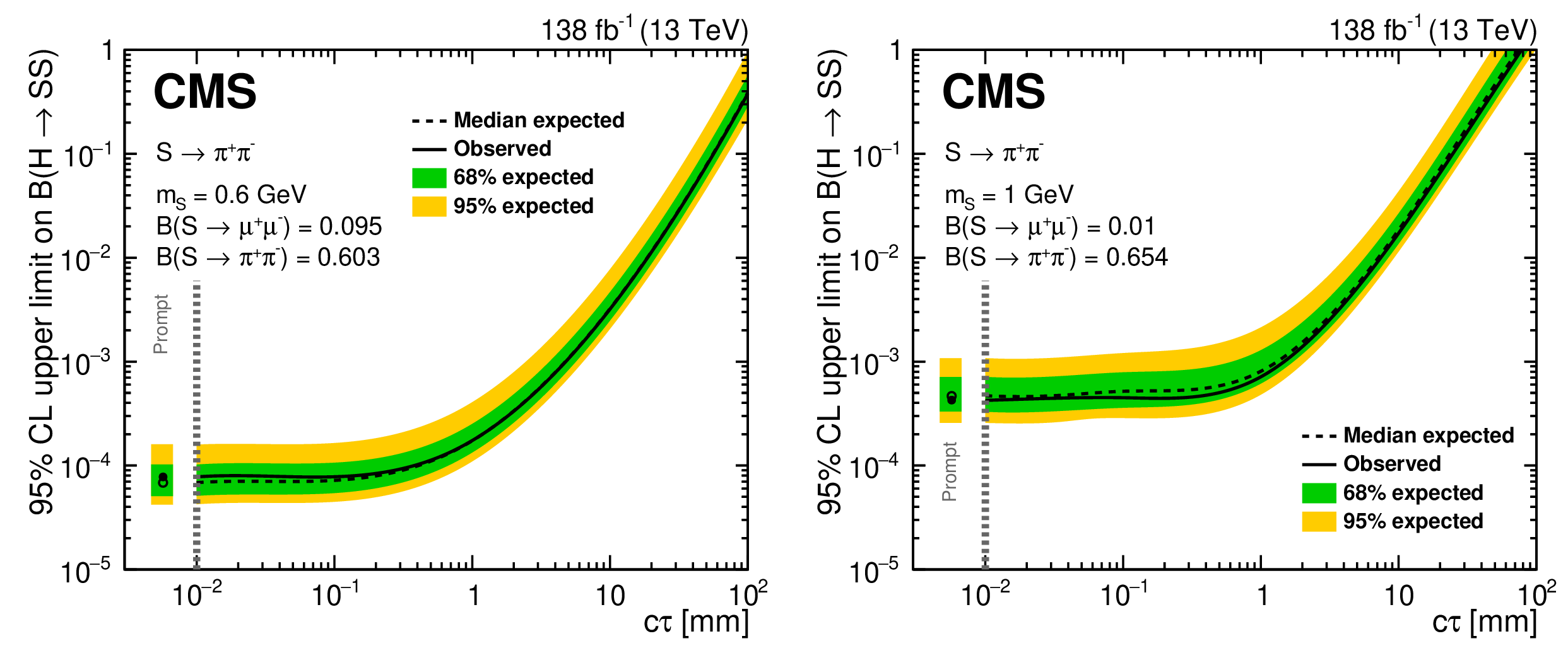
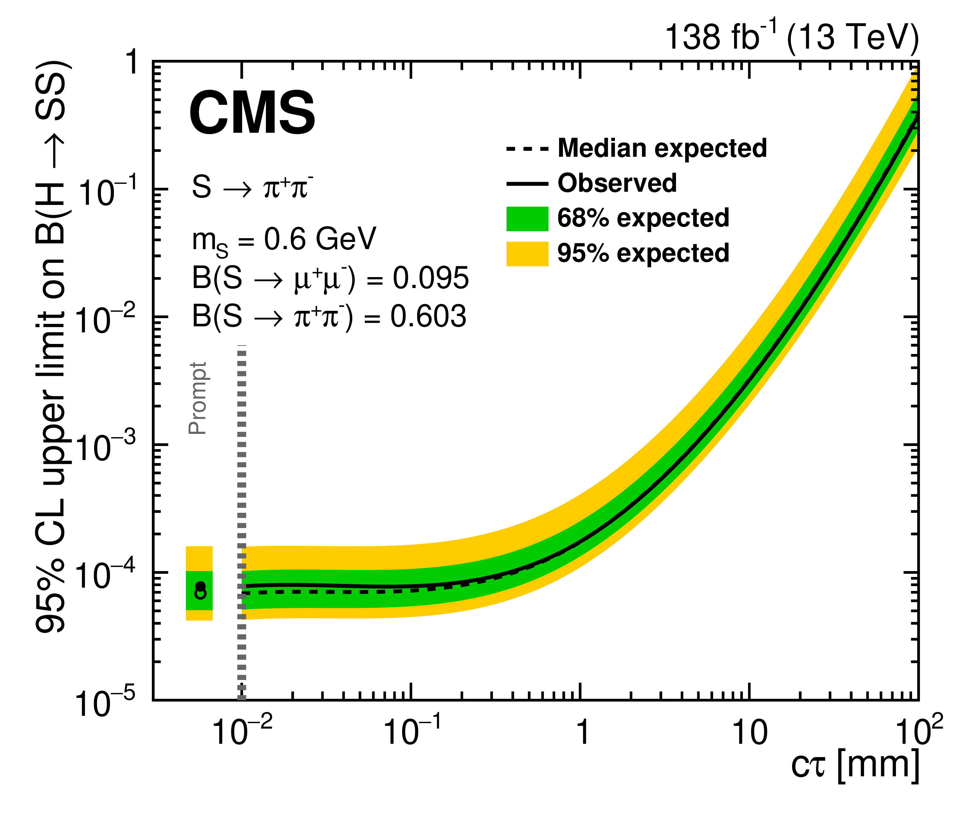
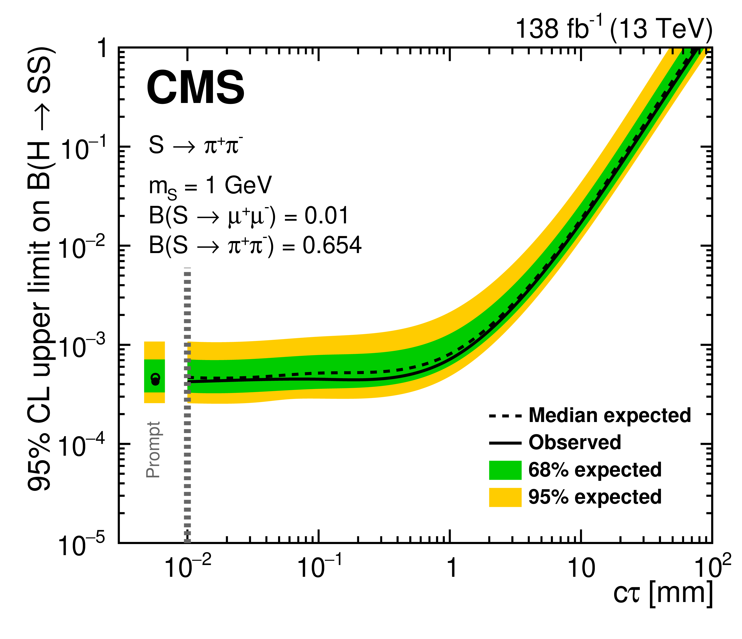
Observed (solid black line) and expected (dashed black line) exclusion limits on the branching fraction $ \mathcal{B}(\mathrm{H}\to\mathrm{S} \mathrm{S} ) $ as functions of signal proper decay length $ c\tau $ for $ m_{\mathrm{S} }= $ 0.6 GeV (left) and 1 GeV (right) for the minimal extension of the SM Higgs sector [12], assuming $ \mathcal{B}(\mathrm{S} \to\mu^{+}\mu^{-}) $ and $ \mathcal{B}(\mathrm{S} \to\pi^{+}\pi^{-}) $, as in Table 1. The inner green (outer yellow) indicates the region containing 68 (95)% of the limits. The limits are obtained using the combination of all data-taking eras and the four different displacement categories. |
png pdf |
Figure 7-a:
Observed (solid black line) and expected (dashed black line) exclusion limits on the branching fraction $ \mathcal{B}(\mathrm{H}\to\mathrm{S} \mathrm{S} ) $ as functions of signal proper decay length $ c\tau $ for $ m_{\mathrm{S} }= $ 0.6 GeV (left) and 1 GeV (right) for the minimal extension of the SM Higgs sector [12], assuming $ \mathcal{B}(\mathrm{S} \to\mu^{+}\mu^{-}) $ and $ \mathcal{B}(\mathrm{S} \to\pi^{+}\pi^{-}) $, as in Table 1. The inner green (outer yellow) indicates the region containing 68 (95)% of the limits. The limits are obtained using the combination of all data-taking eras and the four different displacement categories. |
png pdf |
Figure 7-b:
Observed (solid black line) and expected (dashed black line) exclusion limits on the branching fraction $ \mathcal{B}(\mathrm{H}\to\mathrm{S} \mathrm{S} ) $ as functions of signal proper decay length $ c\tau $ for $ m_{\mathrm{S} }= $ 0.6 GeV (left) and 1 GeV (right) for the minimal extension of the SM Higgs sector [12], assuming $ \mathcal{B}(\mathrm{S} \to\mu^{+}\mu^{-}) $ and $ \mathcal{B}(\mathrm{S} \to\pi^{+}\pi^{-}) $, as in Table 1. The inner green (outer yellow) indicates the region containing 68 (95)% of the limits. The limits are obtained using the combination of all data-taking eras and the four different displacement categories. |
png pdf |
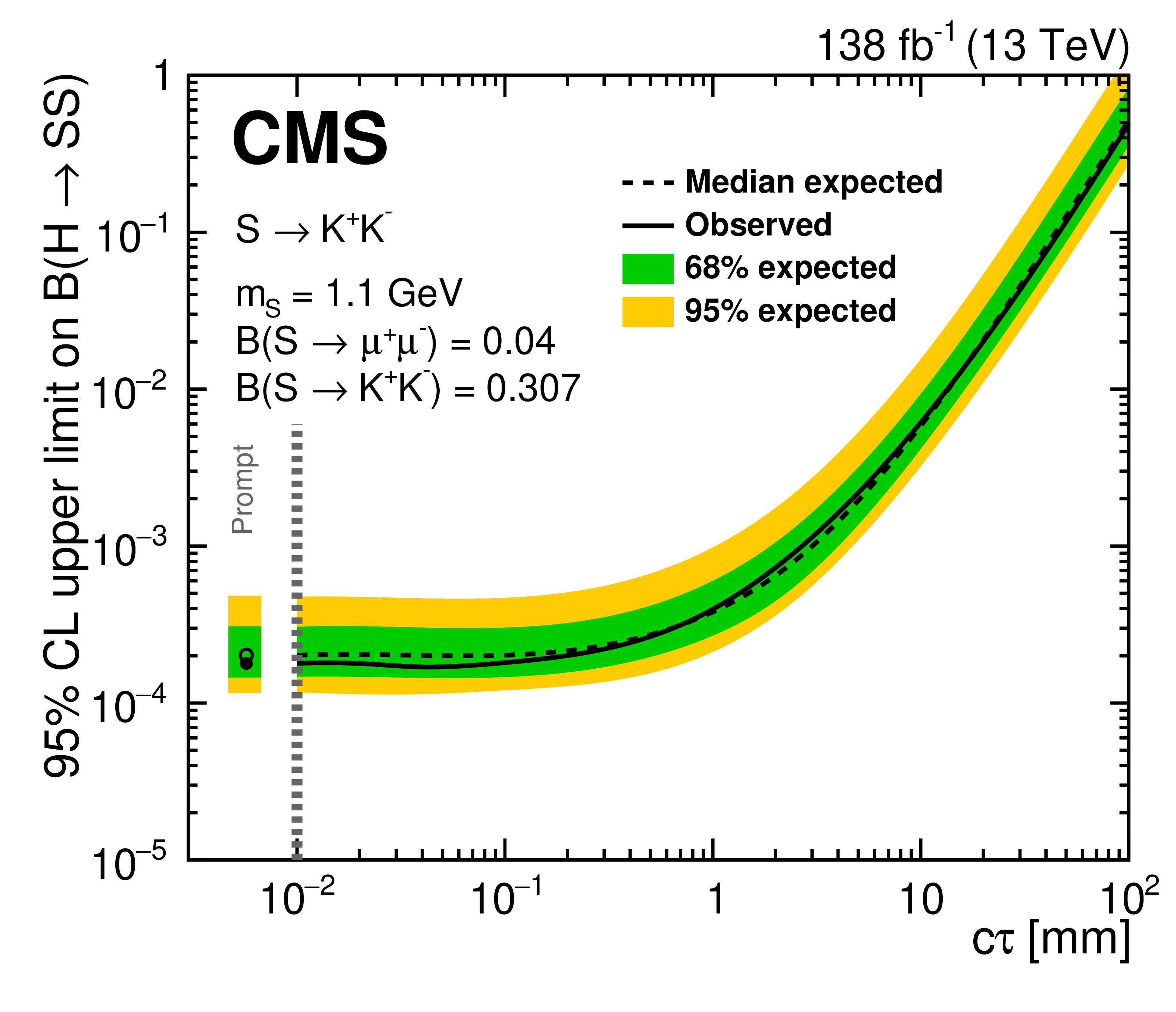
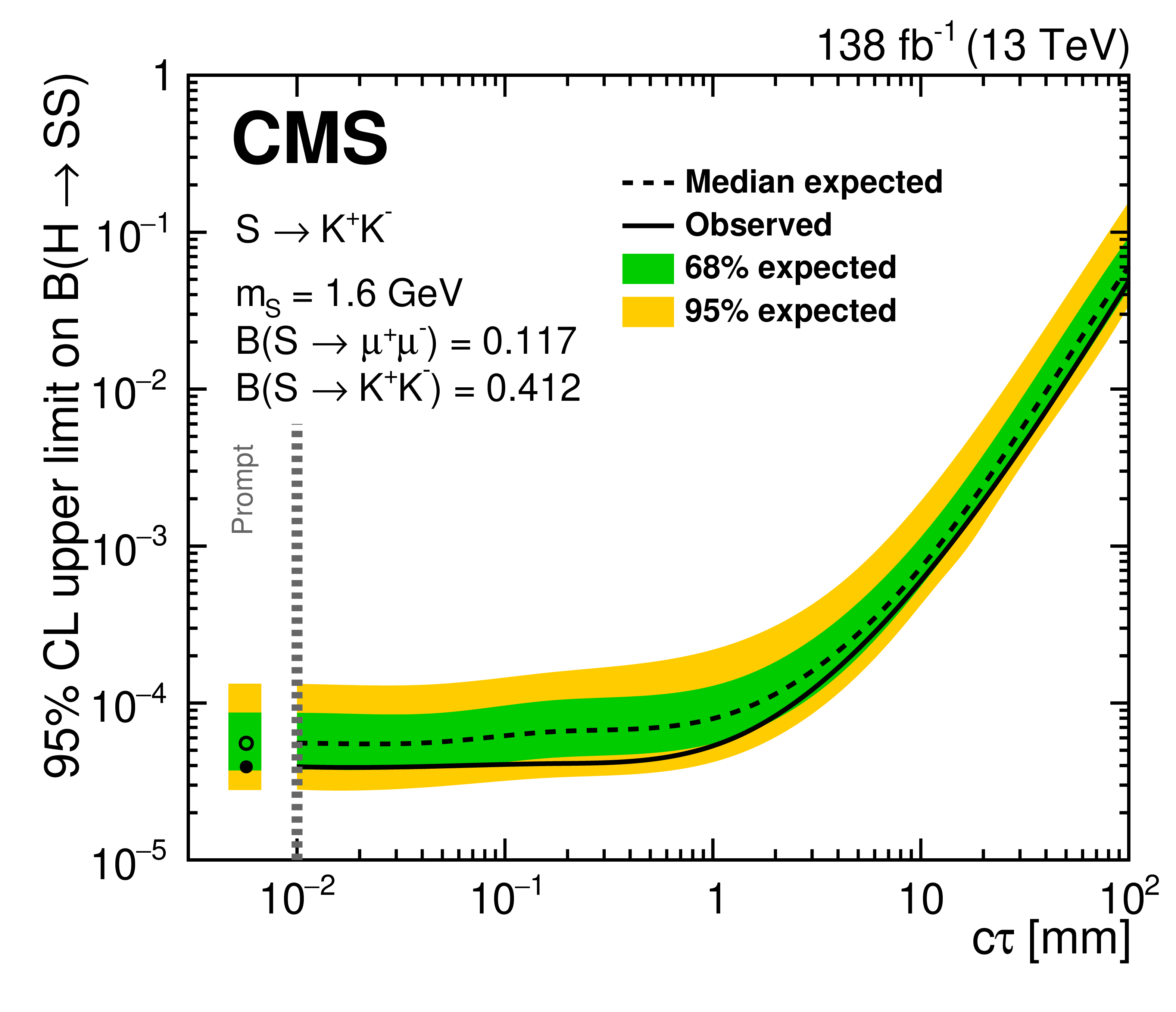
Figure 8:
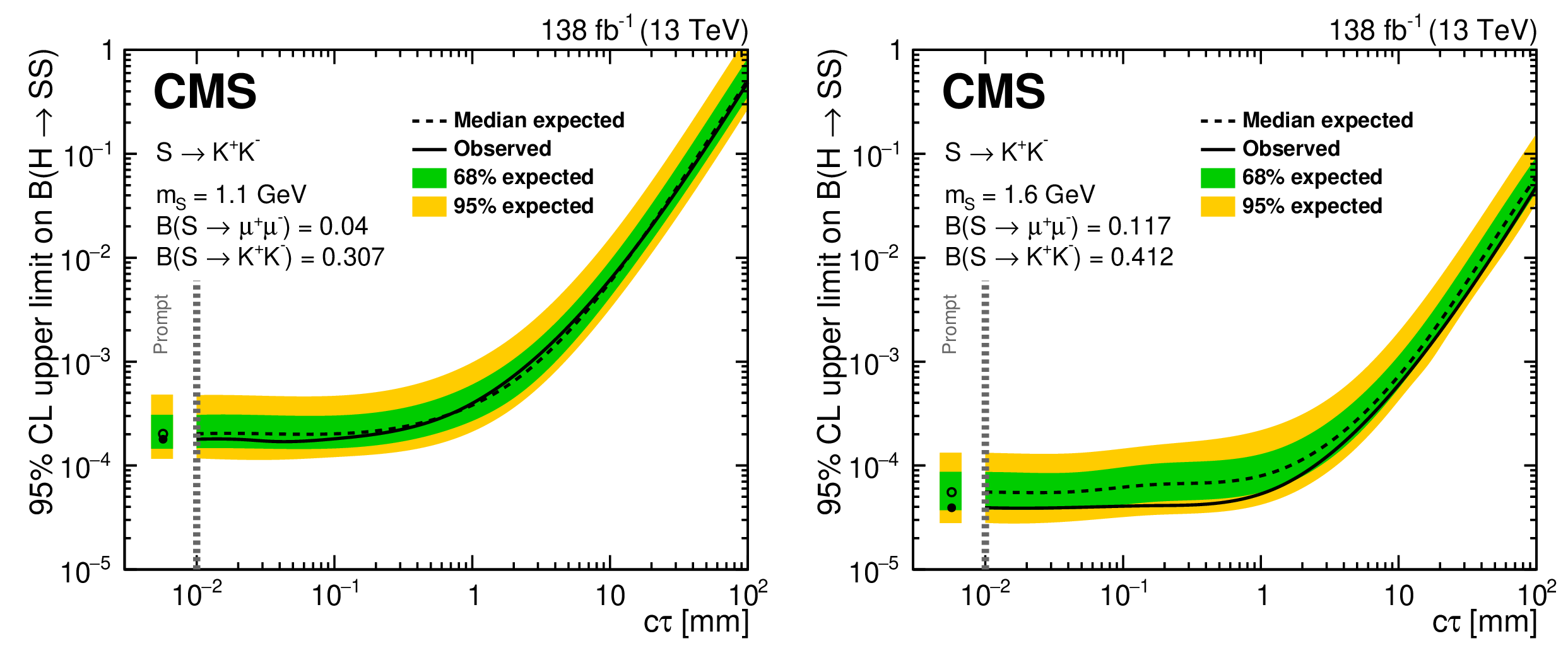
Observed (solid black line) and expected (dashed black line) exclusion limits on the branching fraction $ \mathcal{B}(\mathrm{H}\to\mathrm{S} \mathrm{S} ) $ as functions of signal proper decay length $ c\tau $ for $ m_{\mathrm{S} }= $ 1.1 GeV (left) and 1.6 GeV (right) for the minimal extension of the SM Higgs sector [12], assuming $ \mathcal{B}(\mathrm{S} \to\mu^{+}\mu^{-}) $ and $ \mathcal{B}(\mathrm{S} \to \mathrm{K^+}\mathrm{K^-}) $, as in Table 1. The inner green (outer yellow) indicates the region containing 68 (95)% of the limits. The limits are obtained using the combination of all data-taking eras and the four different displacement categories. |
png pdf |
Figure 8-a:
Observed (solid black line) and expected (dashed black line) exclusion limits on the branching fraction $ \mathcal{B}(\mathrm{H}\to\mathrm{S} \mathrm{S} ) $ as functions of signal proper decay length $ c\tau $ for $ m_{\mathrm{S} }= $ 1.1 GeV (left) and 1.6 GeV (right) for the minimal extension of the SM Higgs sector [12], assuming $ \mathcal{B}(\mathrm{S} \to\mu^{+}\mu^{-}) $ and $ \mathcal{B}(\mathrm{S} \to \mathrm{K^+}\mathrm{K^-}) $, as in Table 1. The inner green (outer yellow) indicates the region containing 68 (95)% of the limits. The limits are obtained using the combination of all data-taking eras and the four different displacement categories. |
png pdf |
Figure 8-b:
Observed (solid black line) and expected (dashed black line) exclusion limits on the branching fraction $ \mathcal{B}(\mathrm{H}\to\mathrm{S} \mathrm{S} ) $ as functions of signal proper decay length $ c\tau $ for $ m_{\mathrm{S} }= $ 1.1 GeV (left) and 1.6 GeV (right) for the minimal extension of the SM Higgs sector [12], assuming $ \mathcal{B}(\mathrm{S} \to\mu^{+}\mu^{-}) $ and $ \mathcal{B}(\mathrm{S} \to \mathrm{K^+}\mathrm{K^-}) $, as in Table 1. The inner green (outer yellow) indicates the region containing 68 (95)% of the limits. The limits are obtained using the combination of all data-taking eras and the four different displacement categories. |
png pdf |
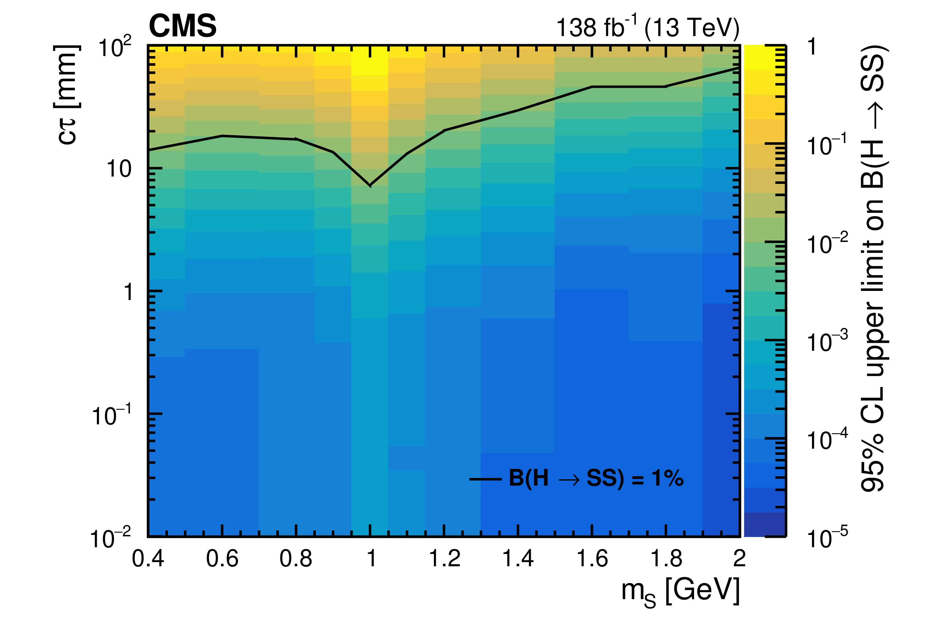
Figure 9:
Observed upper limit on the branching fraction $ \mathcal{B}(\mathrm{H}\to\mathrm{S} \mathrm{S} ) $ as a function of signal mass and proper decay length $ c\tau $ for the minimal extension of the SM Higgs sector [12], assuming $ \mathcal{B}(\mathrm{S} \to\mu^{+}\mu^{-}) $, $ \mathcal{B}(\mathrm{S} \to \mathrm{K^+}\mathrm{K^-}) $, and $ \mathcal{B}(\mathrm{S} \to\pi^{+}\pi^{-}) $, as in Table 1. The area below the solid black line denotes the region where the limits are smaller than 1%. |
| Tables | |
png pdf |
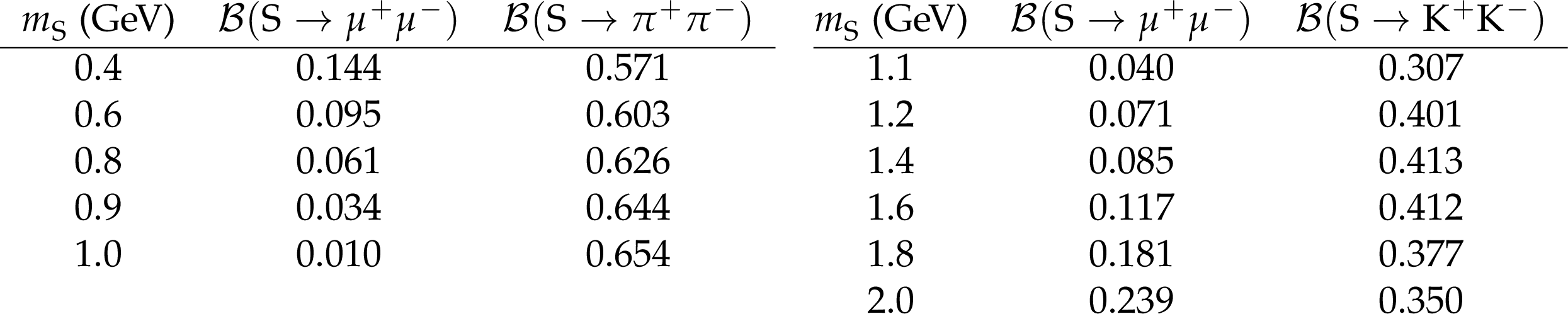
Table 1:
Branching fractions for the BSM scalar boson decays to a muon pair and to a pion or kaon pair [25], in the targeted range of BSM scalar boson masses $ m_{\mathrm{S} } $. For $ m_{\mathrm{S} }\leq $ 1 GeV, the hadronic decay mode to kaons is not allowed because of kinematic constraints. The charged kaon decay mode dominates over the charged pion decay mode for $ m_{\mathrm{S} }\geq $ 1.1 GeV. Subdominant decay modes of the BSM scalar boson have not been included. |
png pdf |
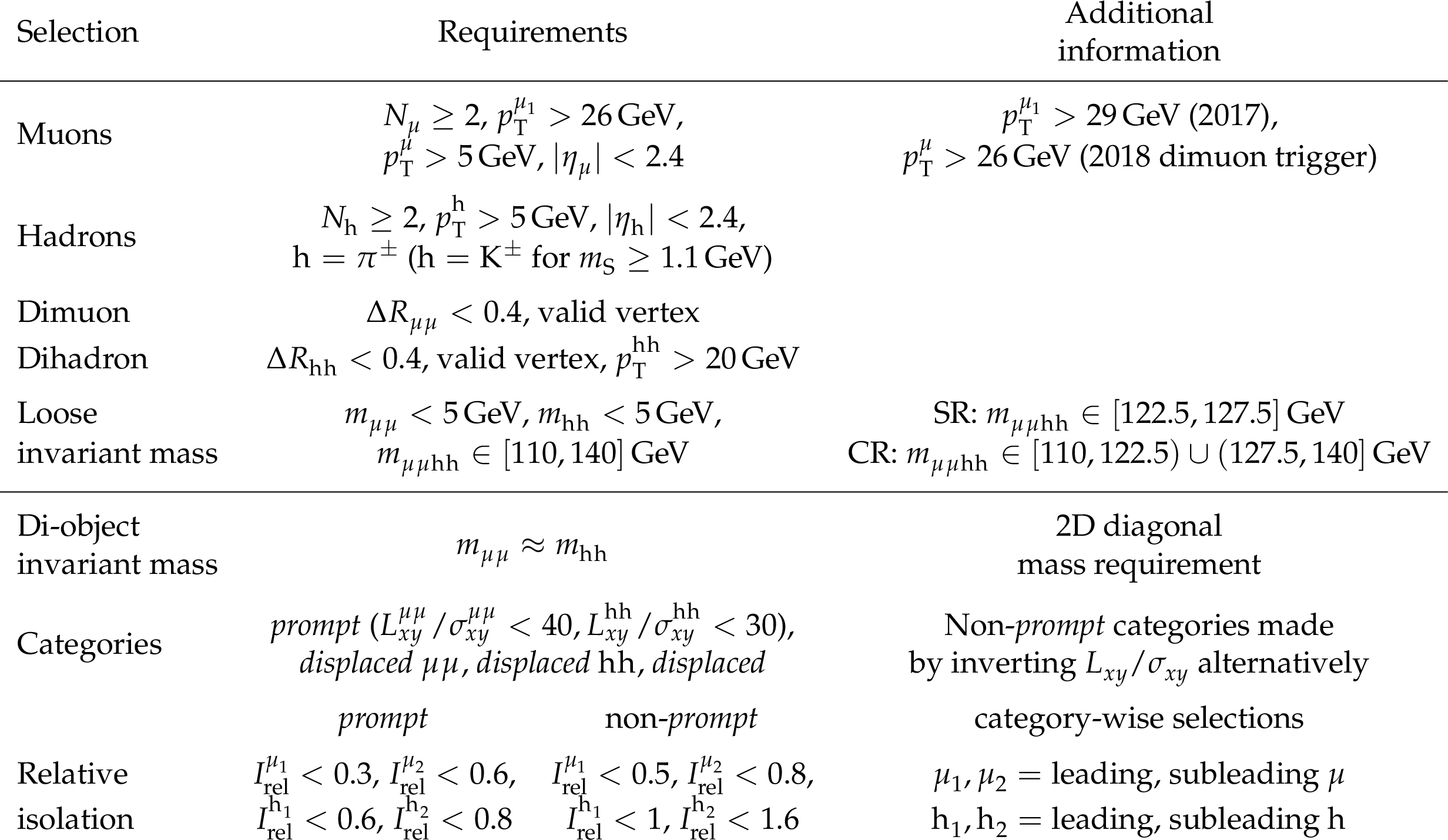
Table 2:
Summary of the event selection requirements for the analysis. The set of criteria up to (and including) the loose invariant mass row defines the baseline selection. The subscripts 1 and 2 refer to the leading and subleading particles, respectively. |

png pdf |
Table 3:
Number of observed events, background predictions for the 2016--2018 dataset in the SR under the BSM scalar mass hypothesis, $ m_{\mathrm{S} }= $ 0.6 GeV (upper) and $ m_{\mathrm{S} }= $ 1.6 GeV (lower), and the expected signal yield assuming $ \mathcal{B}(\mathrm{H}\to \mathrm{S} \mathrm{S} )=1% $. |
png pdf |
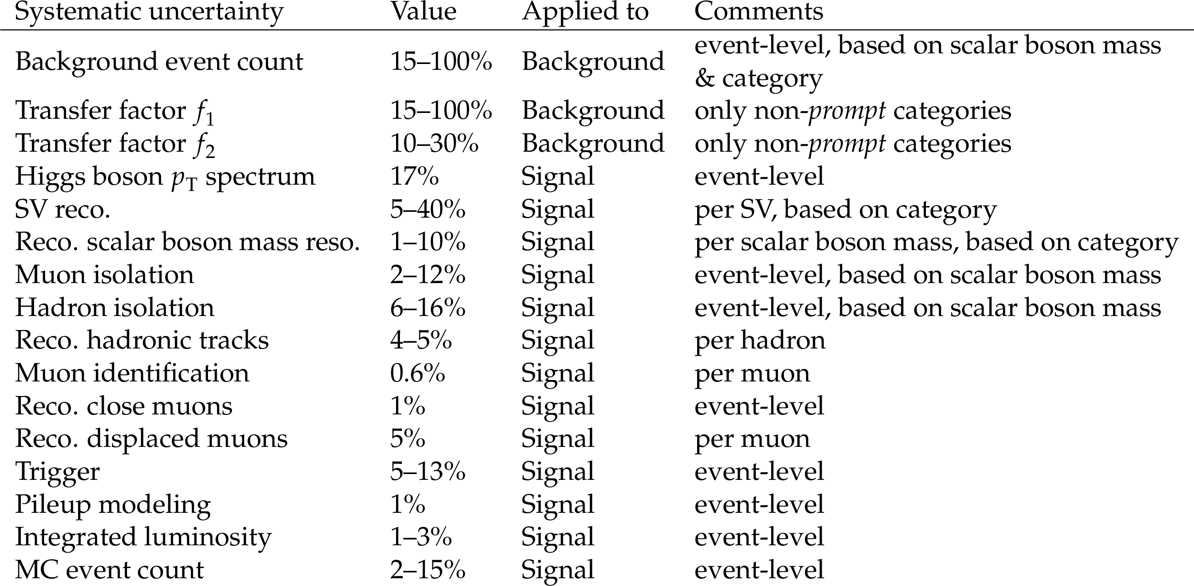
Table 4:
Summary of systematic uncertainties. |
| Summary |
| An exclusive search for light exotic scalar bosons has been presented using proton-proton collision data collected in 2016--2018 at $ \sqrt{s}= $ 13 TeV, and corresponding to an integrated luminosity of 138 fb$ ^{-1} $. The analysis accesses a unique hadronic decay mode where the low mass of the scalar boson restricts hadronization and dominantly allows decays to only a pair of light hadrons. The Higgs boson-mediated production of a pair of light scalar bosons decaying within the CMS trackers is sought in the final state of two muons and two charged hadrons. Scalar boson masses below 2 GeV with a proper decay length $ c\tau $ up to 100$ \text{mm} $ are probed. The boosted topology, the isolation, and mass constraints between the reconstructed dimuon and dihadron resonances are used to reduce the background. Considering the benchmark signal model [25], this search excludes at 95% confidence level branching fractions of the Higgs boson to light scalar bosons greater than $ 10^{-4} $ and covers a largely unexplored parameter space of light long-lived particles. |
| References | ||||
| 1 | ATLAS Collaboration | Observation of a new particle in the search for the Standard Model Higgs boson with the ATLAS detector at the LHC | PLB 716 (2012) 1 | 1207.7214 |
| 2 | CMS Collaboration | Observation of a new boson at a mass of 125 GeV with the CMS Experiment at the LHC | PLB 716 (2012) 30 | CMS-HIG-12-028 1207.7235 |
| 3 | F. Englert and R. Brout | Broken symmetry and the mass of gauge vector mesons | PRL 13 (1964) 321 | |
| 4 | P. W. Higgs | Broken symmetries, massless particles and gauge fields | PL 12 (1964) 132 | |
| 5 | P. W. Higgs | Broken symmetries and the masses of gauge bosons | PRL 13 (1964) 508 | |
| 6 | G. S. Guralnik, C. R. Hagen, and T. W. B. Kibble | Global conservation laws and massless particles | PRL 13 (1964) 585 | |
| 7 | ATLAS Collaboration | A detailed map of Higgs boson interactions by the ATLAS experiment ten years after the discovery | [Erratum: \doi10./s41586-022-05581-5], 2022 Nature 607 (2022) 52 |
2207.00092 |
| 8 | CMS Collaboration | A portrait of the Higgs boson by the CMS experiment ten years after the discovery. | [Erratum: \doi10./s41586-023-06164-8], 2022 Nature 607 (2022) 60 |
CMS-HIG-22-001 2207.00043 |
| 9 | ATLAS Collaboration | Combination of searches for invisible decays of the Higgs boson using 139 fb$ ^{-1} $ of proton-proton collision data at $ \sqrt{s} = 13 \text {Te}\hspace{-.08em}\text {V} $ collected with the ATLAS experiment | PLB 842 (2023) 137963 | 2301.10731 |
| 10 | CMS Collaboration | A search for decays of the Higgs boson to invisible particles in events with a top-antitop quark pair or a vector boson in proton-proton collisions at $ \sqrt{s} = 13 \text {Te}\hspace{-.08em}\text {V} $ | EPJC 83 (2023) 933 | CMS-HIG-21-007 2303.01214 |
| 11 | J. D. Clarke, R. Foot, and R. R. Volkas | Phenomenology of a very light scalar (100 MeV \ensuremath< $ m_{\rm h} $ \ensuremath< 10 GeV) mixing with the SM Higgs | JHEP 02 (2014) 123 | 1310.8042 |
| 12 | M. W. Winkler | Decay and detection of a light scalar boson mixing with the Higgs boson | PRD 99 (2019) 015018 | 1809.01876 |
| 13 | I. Boiarska et al. | Phenomenology of GeV-scale scalar portal | JHEP 11 (2019) 162 | 1904.10447 |
| 14 | M. Shaposhnikov and I. Tkachev | The nuMSM, inflation, and dark matter | PLB 639 (2006) 414 | hep-ph/0604236 |
| 15 | F. Bezrukov and D. Gorbunov | Light inflaton hunter's guide | JHEP 05 (2010) 010 | 0912.0390 |
| 16 | F. Bezrukov and D. Gorbunov | Light inflaton after LHC8 and WMAP9 results | JHEP 07 (2013) 140 | 1303.4395 |
| 17 | P. Fayet | Supergauge invariant extension of the Higgs mechanism and a model for the electron and its neutrino | NPB 90 (1975) 104 | |
| 18 | U. Ellwanger, C. Hugonie, and A. M. Teixeira | The Next-to-Minimal Supersymmetric Standard Model | Phys. Rept. 496 (2010) 1 | 0910.1785 |
| 19 | M. Pospelov, A. Ritz, and M. B. Voloshin | Secluded WIMP Dark Matter | PLB 662 (2008) 53 | 0711.4866 |
| 20 | G. Krnjaic | Probing light thermal dark matter with a Higgs portal mediator | PRD 94 (2016) 073009 | |
| 21 | P. W. Graham, D. E. Kaplan, and S. Rajendran | Cosmological relaxation of the electroweak scale | PRL 115 (2015) 221801 | |
| 22 | T. Ferber, A. Grohsjean, and F. Kahlhoefer | Dark Higgs bosons at colliders | Prog. Part. Nucl. Phys. 136 (2024) 104105 | 2305.16169 |
| 23 | CMS Collaboration | Dark sector searches with the CMS experiment | Phys. Rept. 1115 (2025) 448 | CMS-EXO-23-005 2405.13778 |
| 24 | X. Cid Vidal, Y. Tsai, and J. Zurita | Exclusive displaced hadronic signatures in the LHC forward region | JHEP 01 (2020) 115 | 1910.05225 |
| 25 | Y. Gershtein, S. Knapen, and D. Redigolo | Probing naturally light singlets with a displaced vertex trigger | PLB 823 (2021) 136758 | 2012.07864 |
| 26 | CMS Collaboration | Search for long-lived particles decaying into muon pairs in proton-proton collisions at $ \sqrt{s} = $ 13 TeV collected with a dedicated high-rate data stream | JHEP 04 (2022) 062 | CMS-EXO-20-014 2112.13769 |
| 27 | CMS Collaboration | Model-independent search for pair production of new bosons decaying into muons in proton-proton collisions at $ \sqrt{s} = $ 13 TeV | JHEP 12 (2024) 172 | CMS-HIG-21-004 2407.20425 |
| 28 | CMS Collaboration | Search for long-lived particles decaying in the CMS muon detectors in proton-proton collisions at $ \sqrt{s} = $ 13 TeV | PRD 110 (2024) 032007 | CMS-EXO-21-008 2402.01898 |
| 29 | ATLAS Collaboration | Search for light long-lived neutral particles that decay to collimated pairs of leptons or light hadrons in pp collisions at $ \sqrt{s} = $ 13 TeV with the ATLAS detector | JHEP 06 (2023) 153 | 2206.12181 |
| 30 | ATLAS Collaboration | Search for light long-lived neutral particles from Higgs boson decays via vector-boson-fusion production from pp collisions at $ \sqrt{s}= $ 13 TeV with the ATLAS detector | EPJC 84 (2024) 719 | 2311.18298 |
| 31 | LHCb Collaboration | Search for hidden-sector bosons in $ B^0 \!\to K^{*0}\mu^+\mu^- $ decays | PRL 115 (2015) 161802 | 1508.04094 |
| 32 | LHCb Collaboration | Search for long-lived scalar particles in $ B^+ \to K^+ \chi (\mu^+\mu^-) $ decays | PRD 95 (2017) 071101 | 1612.07818 |
| 33 | CMS Collaboration | HEPData record for this analysis | link | |
| 34 | CMS Collaboration | The CMS experiment at the CERN LHC | JINST 3 (2008) S08004 | |
| 35 | CMS Collaboration | Development of the CMS detector for the CERN LHC Run 3 | JINST 19 (2024) P05064 | |
| 36 | CMS Collaboration | Performance of the CMS Level-1 trigger in proton-proton collisions at $ \sqrt{s} = $ 13 TeV | JINST 15 (2020) P10017 | CMS-TRG-17-001 2006.10165 |
| 37 | CMS Collaboration | The CMS trigger system | JINST 12 (2017) P01020 | CMS-TRG-12-001 1609.02366 |
| 38 | CMS Collaboration | Performance of the CMS high-level trigger during LHC Run 2 | JINST 19 (2024) P11021 | CMS-TRG-19-001 2410.17038 |
| 39 | CMS Collaboration | Electron and photon reconstruction and identification with the CMS experiment at the CERN LHC | JINST 16 (2021) P05014 | CMS-EGM-17-001 2012.06888 |
| 40 | CMS Collaboration | Performance of the CMS muon detector and muon reconstruction with proton-proton collisions at $ \sqrt{s}= $ 13 TeV | JINST 13 (2018) P06015 | CMS-MUO-16-001 1804.04528 |
| 41 | CMS Collaboration | Description and performance of track and primary-vertex reconstruction with the CMS tracker | JINST 9 (2014) P10009 | CMS-TRK-11-001 1405.6569 |
| 42 | CMS Tracker Group Collaboration | The CMS phase-1 pixel detector upgrade | JINST 16 (2021) P02027 | 2012.14304 |
| 43 | CMS Collaboration | Track impact parameter resolution for the full pseudorapidity coverage in the 2017 dataset with the CMS phase-1 pixel detector | CMS Detector Performance Summary CMS-DP-2020-049, 2020 CDS |
|
| 44 | CMS Collaboration | 2017 tracking performance plots | CMS Detector Performance Summary CMS-DP-2017-015, 2017 CDS |
|
| 45 | CMS Collaboration | Particle-flow reconstruction and global event description with the CMS detector | JINST 12 (2017) P10003 | CMS-PRF-14-001 1706.04965 |
| 46 | CMS Collaboration | Technical proposal for the Phase-II upgrade of the Compact Muon Solenoid | CMS Technical Proposal CMS-TDR-15-02, 2015 CDS |
|
| 47 | P. Nason | A new method for combining NLO QCD with shower Monte Carlo algorithms | JHEP 11 (2004) 040 | hep-ph/0409146 |
| 48 | S. Frixione, P. Nason, and C. Oleari | Matching NLO QCD computations with Parton Shower simulations: the POWHEG method | JHEP 11 (2007) 070 | 0709.2092 |
| 49 | S. Alioli, P. Nason, C. Oleari, and E. Re | A general framework for implementing NLO calculations in shower Monte Carlo programs: the POWHEG BOX | JHEP 06 (2010) 043 | 1002.2581 |
| 50 | E. Bagnaschi, G. Degrassi, P. Slavich, and A. Vicini | Higgs production via gluon fusion in the POWHEG approach in the SM and in the MSSM | JHEP 02 (2012) 088 | 1111.2854 |
| 51 | T. Sjöstrand et al. | An introduction to PYTHIA 8.2 | Comput. Phys. Commun. 191 (2015) 159 | 1410.3012 |
| 52 | CMS Collaboration | Extraction and validation of a new set of CMS PYTHIA8 tunes from underlying-event measurements | EPJC 80 (2020) 4 | CMS-GEN-17-001 1903.12179 |
| 53 | NNPDF Collaboration | Parton distributions from high-precision collider data | EPJC 77 (2017) 663 | 1706.00428 |
| 54 | GEANT4 Collaboration | GEANT 4---a simulation toolkit | NIM A 506 (2003) 250 | |
| 55 | CMS Collaboration | Simulation of the Silicon Strip Tracker pre-amplifier in early 2016 data | CMS Detector Performance Summary CMS-DP-2020-045, 2020 CDS |
|
| 56 | LHC Higgs Cross Section Working Group | Handbook of LHC Higgs cross sections: 4. Deciphering the nature of the Higgs sector | CERN Report CERN-2017-002-M, 2016 link |
1610.07922 |
| 57 | CMS Collaboration | Displaced tracking and vertexing calibration using neutral K mesons | CMS Detector Performance Summary CMS-DP-2024-010, 2024 CDS |
|
| 58 | CMS Collaboration | Tracking performances for charged pions with Run2 Legacy data | CMS Detector Performance Summary CMS-DP-2022-012, 2022 CDS |
|
| 59 | CMS Collaboration | Search for long-lived particles decaying to a pair of muons in proton-proton collisions at $ \sqrt{s} = $ 13 TeV | JHEP 05 (2023) 228 | CMS-EXO-21-006 2205.08582 |
| 60 | CMS Collaboration | Measurements of Inclusive $ W $ and $ Z $ Cross Sections in $ pp $ Collisions at $ \sqrt{s}= $ 7 TeV | JHEP 01 (2011) 080 | CMS-EWK-10-002 1012.2466 |
| 61 | CMS Collaboration | Precision luminosity measurement in proton-proton collisions at $ \sqrt{s} = $ 13 TeV in 2015 and 2016 at CMS | EPJC 81 (2021) 800 | CMS-LUM-17-003 2104.01927 |
| 62 | CMS Collaboration | CMS luminosity measurement for the 2017 data-taking period at $ \sqrt{s} = $ 13 TeV | CMS Physics Analysis Summary, 2018 link |
CMS-PAS-LUM-17-004 |
| 63 | CMS Collaboration | CMS luminosity measurement for the 2018 data-taking period at $ \sqrt{s} = $ 13 TeV | CMS Physics Analysis Summary, 2019 link |
CMS-PAS-LUM-18-002 |
| 64 | T. Junk | Confidence level computation for combining searches with small statistics | NIM A 434 (1999) 435 | hep-ex/9902006 |
| 65 | CMS Collaboration | Precise determination of the mass of the Higgs boson and tests of compatibility of its couplings with the standard model predictions using proton collisions at 7 and 8 $ \text {TeV} $ | EPJC 75 (2015) 212 | CMS-HIG-14-009 1412.8662 |
| 66 | CMS Collaboration | The CMS statistical analysis and combination tool: Combine | Comput. Softw. Big Sci. 8 (2024) 19 | CMS-CAT-23-001 2404.06614 |
| 67 | W. Verkerke and D. Kirkby | The RooFit toolkit for data modeling | in th International Conference on Computing in High Energy and Nuclear Physics (CHEP )... [eConf C0303241, MOLT007], 2003 Proc. 1 (2003) 3 |
physics/0306116 |
| 68 | L. Moneta et al. | The RooStats project | PoS ACAT 057, 2010 link |
1009.1003 |
|
|
Compact Muon Solenoid LHC, CERN |
|

|

|

|

|

|