

Compact Muon Solenoid
LHC, CERN
| CMS-B2G-24-015 ; CERN-EP-2025-190 | ||
| Search for resonances decaying to an anomalous jet and a Higgs boson in proton-proton collisions at $ \sqrt{s}= $ 13 TeV | ||
| CMS Collaboration | ||
| 16 September 2025 | ||
| Eur. Phys. J. C 86 (2026) 137 | ||
| Abstract: This paper presents a search for new physics through the process where a massive particle, X, decays into a Higgs boson and a second particle, Y. The Higgs boson subsequently decays into a bottom quark-antiquark pair, which is reconstructed as a single large-radius jet. The decay products of Y are also assumed to produce a single large-radius jet. The identification of the Y particle is enhanced by computing the anomaly score of its candidate jet using an autoencoder, which measures deviations from typical quark- or gluon-induced jets. This allows a simultaneous search for multiple Y decay scenarios within a single analysis. In the main benchmark process, Y is a scalar particle that decays into a W boson pair. Two other scalar Y decay processes are also considered as benchmarks: decays to a light quark-antiquark pair, and decays to a top quark-antiquark pair. A fourth benchmark process considers Y as a hadronically decaying top quark, arising from the decay of a vector-like quark into a top quark and a Higgs boson. Data recorded by the CMS experiment at a center-of-mass energy of 13 TeV in 2016-2018, corresponding to an integrated luminosity of 138 fb$^{-1}$, are analyzed. No significant excess above the standard model background expectation is observed. The most stringent upper limits to date are placed on benchmark signal cross sections for various masses of X and Y particles. | ||
| Links: e-print arXiv:2509.13635 [hep-ex] (PDF) ; CDS record ; inSPIRE record ; HepData record ; CADI line (restricted) ; | ||
| Figures | |
png pdf |
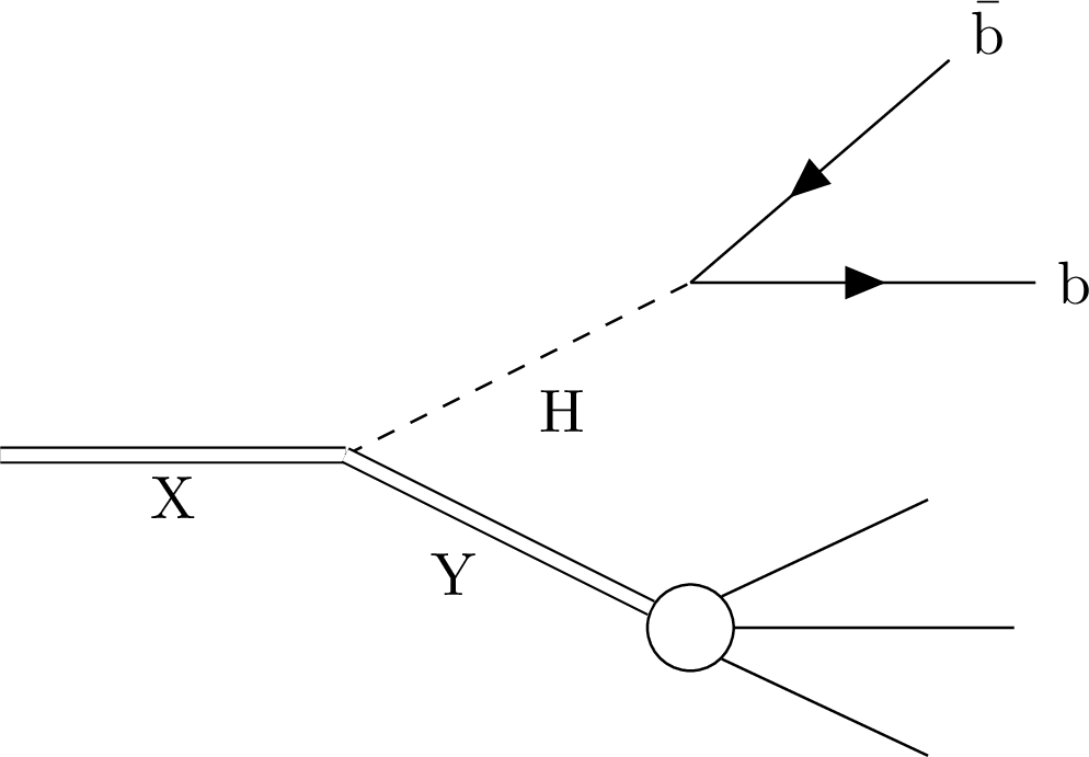
Figure 1:
An illustration showing the signal targeted by this analysis. The final state consists of a large-radius jet originating from H decaying to $ \mathrm{b}\overline{\mathrm{b}} $ and another large-radius jet originating from the decay of a second particle, Y. |
png pdf |
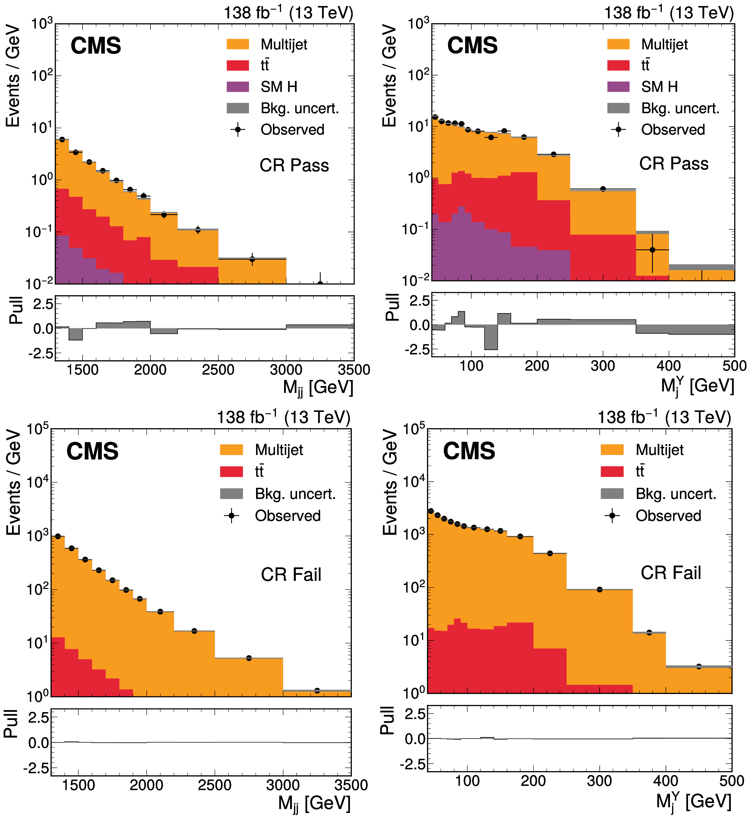
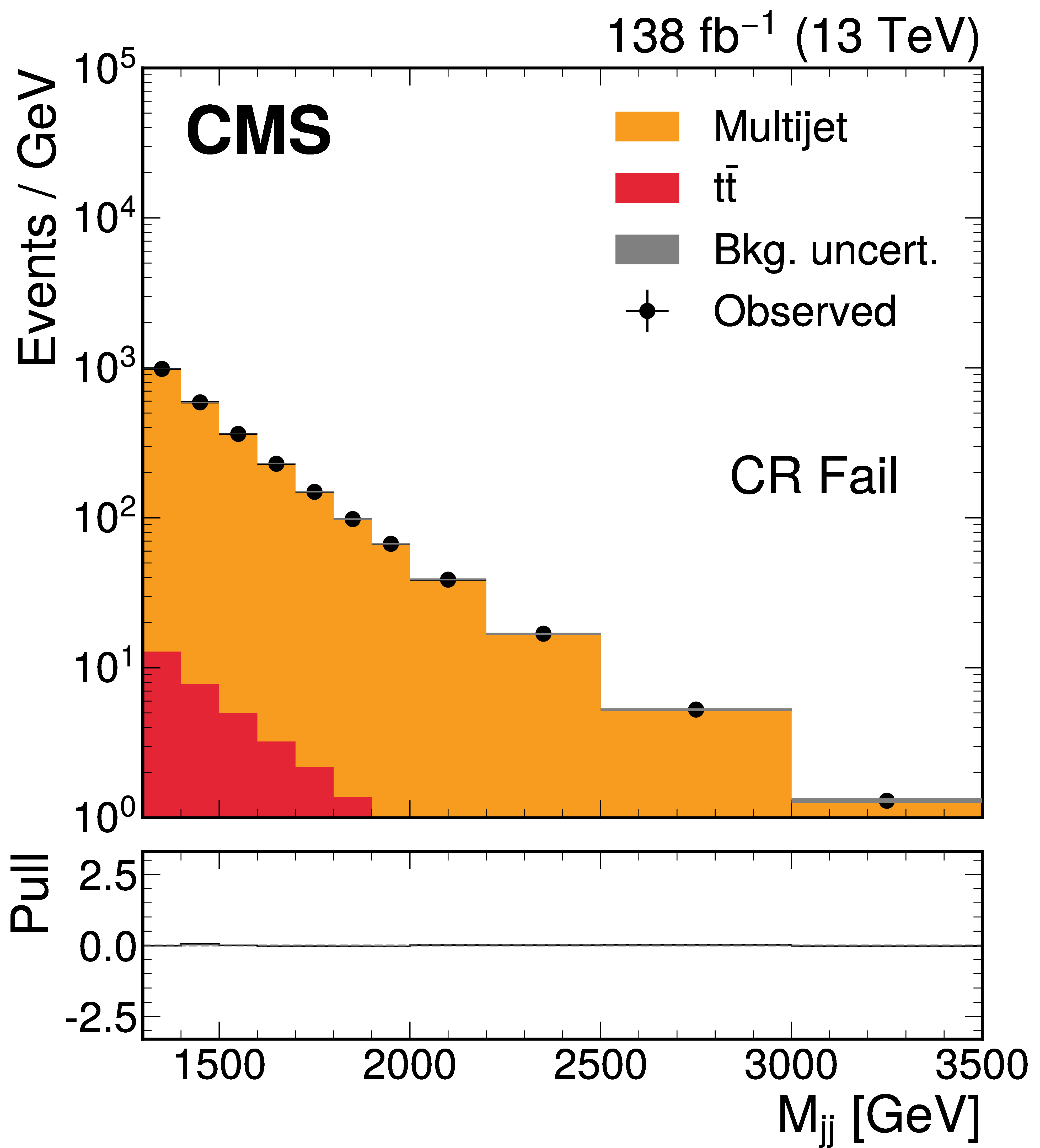
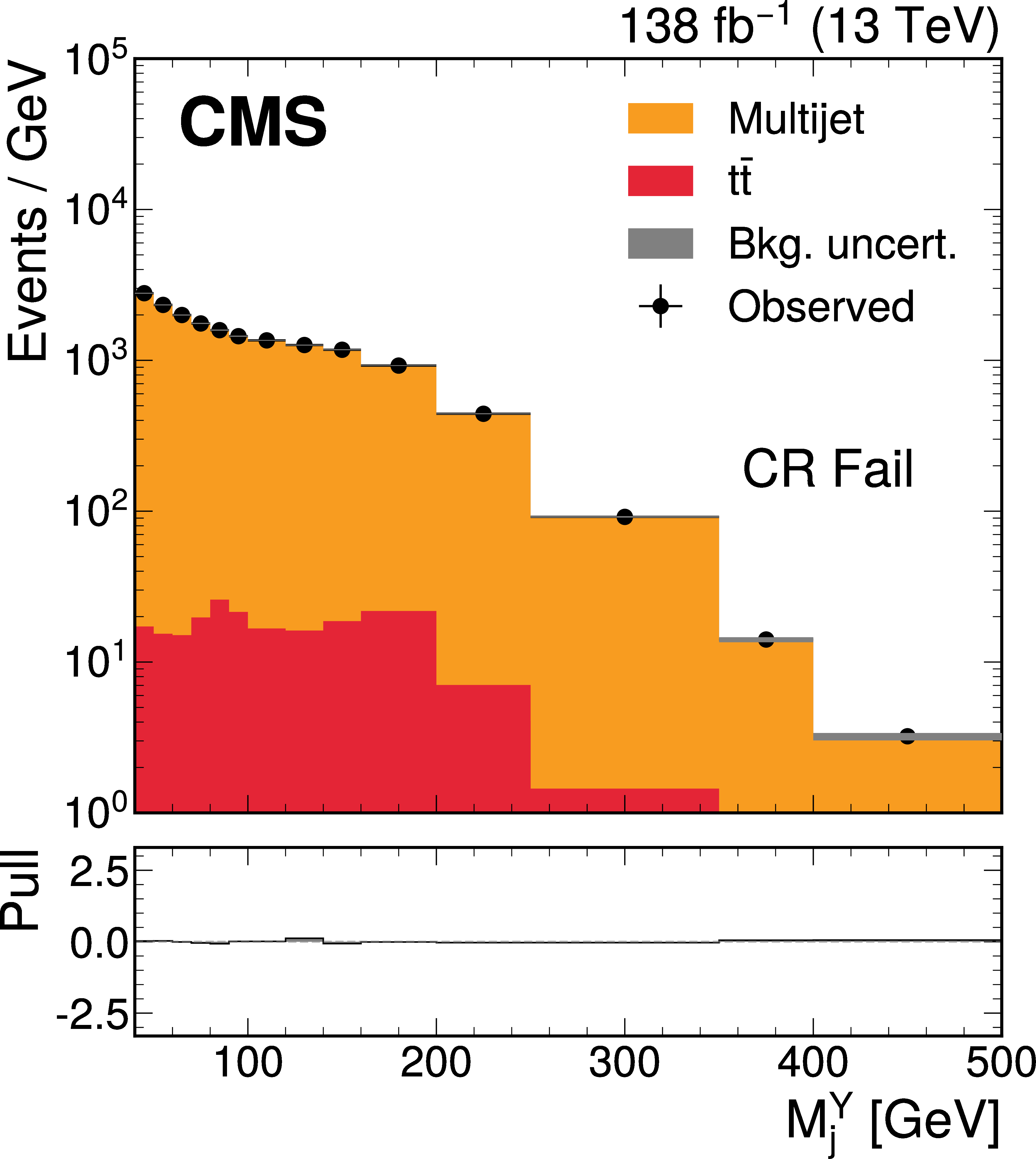
Figure 2:
The $ M_\mathrm{jj} $ (left) and $ M_\mathrm{j}^{\mathrm{Y}} $ (right) projections showing the number of observed events per GeV (black markers) compared with the backgrounds estimated in the fit to the data (filled histograms) in the CR. Pass (upper) and Fail (lower) categories are shown. The high level of agreement between the model and the data in the Fail region is due to the nature of the background estimate. The lower panels show the ``Pull'' defined as (observed events}-\text{expected events) $ /\sqrt{\smash[b]{\sigma_{\text{obs}}^{2} + \sigma_{\text{bkg}}^{2}}} $, where $ \sigma_{\text{obs}} $ and $ \sigma_{\text{bkg}} $ are the total uncertainties in the observation and the background estimation, respectively. |
png pdf |
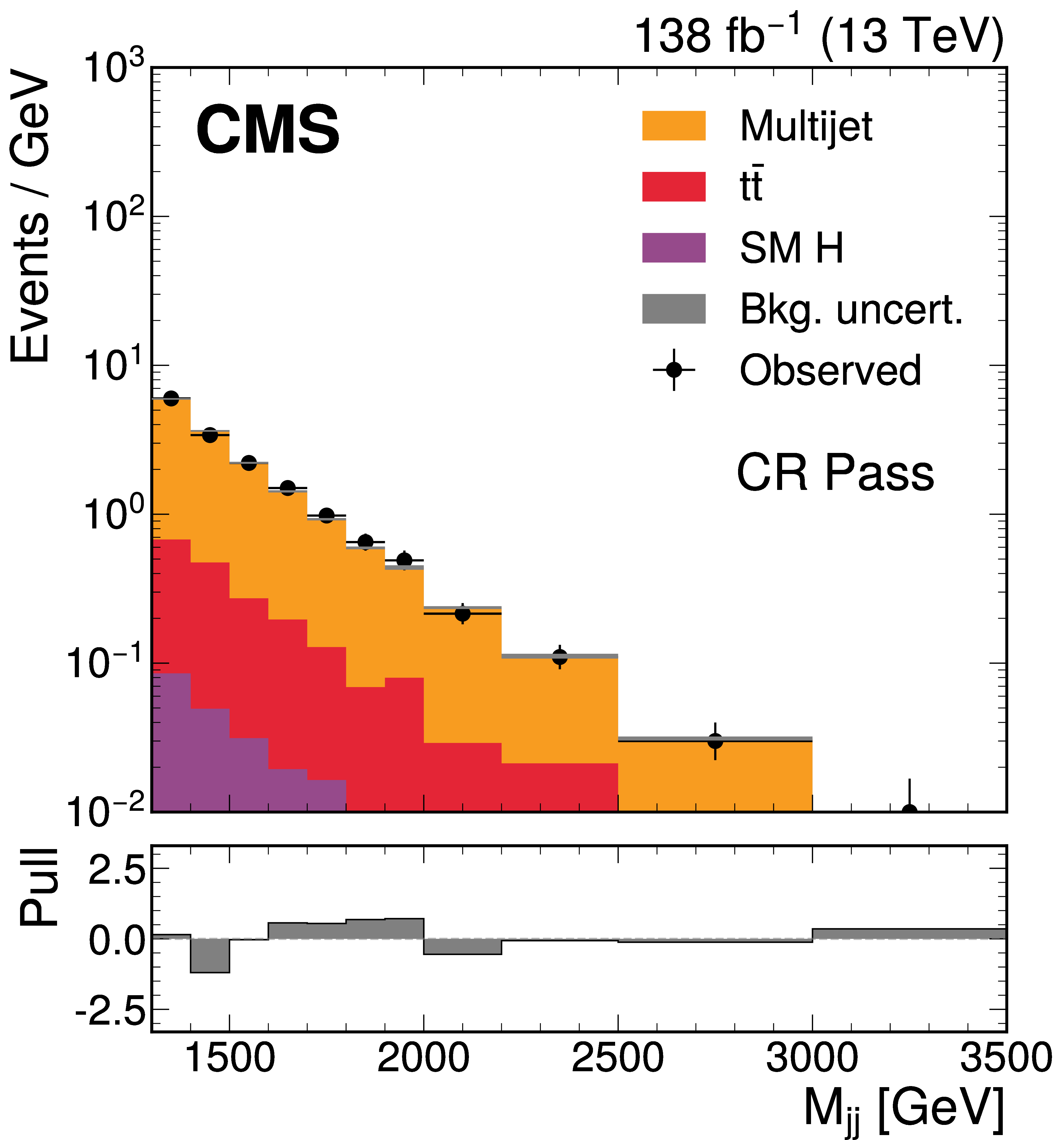
Figure 2-a:
The $ M_\mathrm{jj} $ (left) and $ M_\mathrm{j}^{\mathrm{Y}} $ (right) projections showing the number of observed events per GeV (black markers) compared with the backgrounds estimated in the fit to the data (filled histograms) in the CR. Pass (upper) and Fail (lower) categories are shown. The high level of agreement between the model and the data in the Fail region is due to the nature of the background estimate. The lower panels show the ``Pull'' defined as (observed events}-\text{expected events) $ /\sqrt{\smash[b]{\sigma_{\text{obs}}^{2} + \sigma_{\text{bkg}}^{2}}} $, where $ \sigma_{\text{obs}} $ and $ \sigma_{\text{bkg}} $ are the total uncertainties in the observation and the background estimation, respectively. |
png pdf |
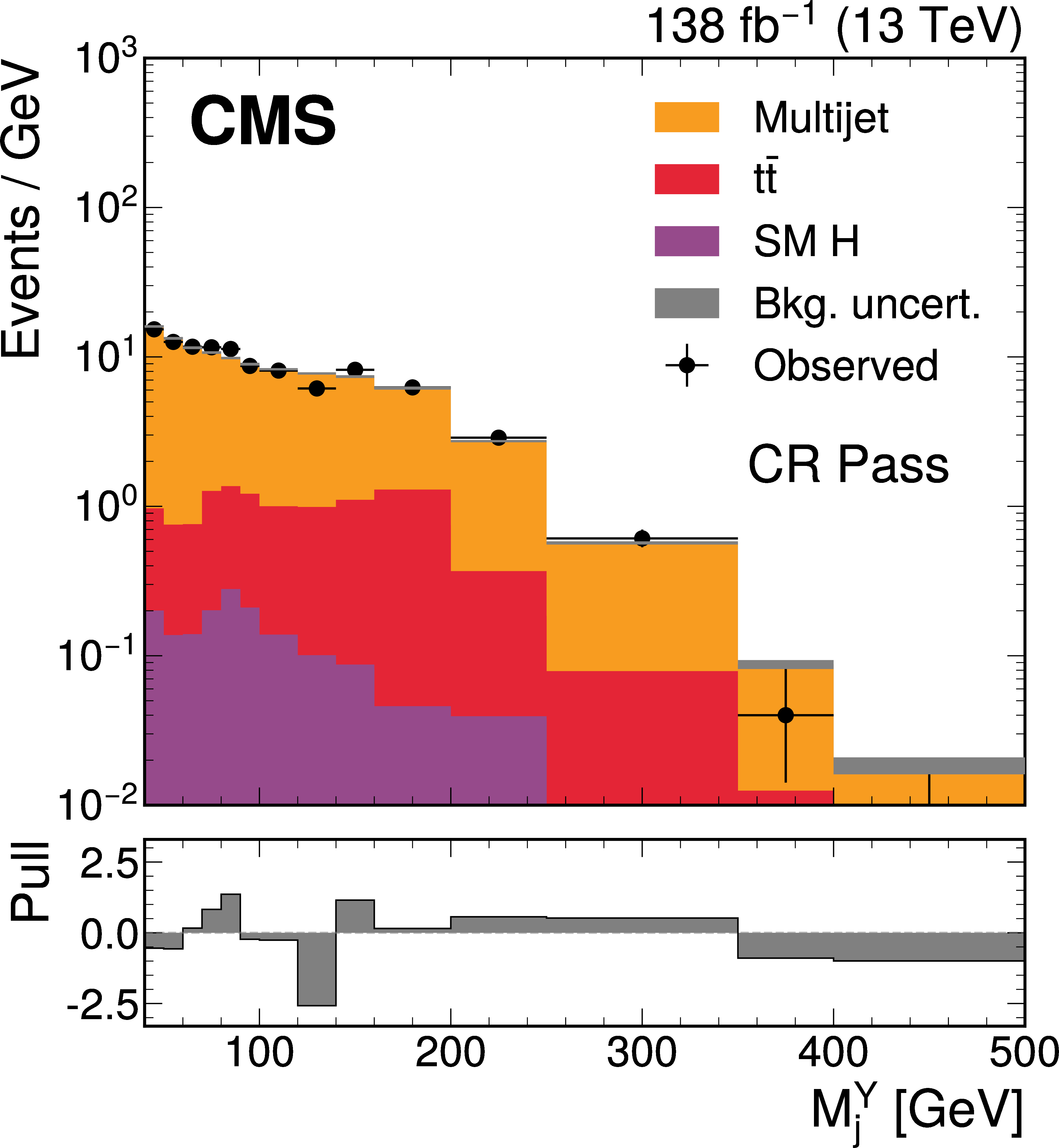
Figure 2-b:
The $ M_\mathrm{jj} $ (left) and $ M_\mathrm{j}^{\mathrm{Y}} $ (right) projections showing the number of observed events per GeV (black markers) compared with the backgrounds estimated in the fit to the data (filled histograms) in the CR. Pass (upper) and Fail (lower) categories are shown. The high level of agreement between the model and the data in the Fail region is due to the nature of the background estimate. The lower panels show the ``Pull'' defined as (observed events}-\text{expected events) $ /\sqrt{\smash[b]{\sigma_{\text{obs}}^{2} + \sigma_{\text{bkg}}^{2}}} $, where $ \sigma_{\text{obs}} $ and $ \sigma_{\text{bkg}} $ are the total uncertainties in the observation and the background estimation, respectively. |
png pdf |
Figure 2-c:
The $ M_\mathrm{jj} $ (left) and $ M_\mathrm{j}^{\mathrm{Y}} $ (right) projections showing the number of observed events per GeV (black markers) compared with the backgrounds estimated in the fit to the data (filled histograms) in the CR. Pass (upper) and Fail (lower) categories are shown. The high level of agreement between the model and the data in the Fail region is due to the nature of the background estimate. The lower panels show the ``Pull'' defined as (observed events}-\text{expected events) $ /\sqrt{\smash[b]{\sigma_{\text{obs}}^{2} + \sigma_{\text{bkg}}^{2}}} $, where $ \sigma_{\text{obs}} $ and $ \sigma_{\text{bkg}} $ are the total uncertainties in the observation and the background estimation, respectively. |
png pdf |
Figure 2-d:
The $ M_\mathrm{jj} $ (left) and $ M_\mathrm{j}^{\mathrm{Y}} $ (right) projections showing the number of observed events per GeV (black markers) compared with the backgrounds estimated in the fit to the data (filled histograms) in the CR. Pass (upper) and Fail (lower) categories are shown. The high level of agreement between the model and the data in the Fail region is due to the nature of the background estimate. The lower panels show the ``Pull'' defined as (observed events}-\text{expected events) $ /\sqrt{\smash[b]{\sigma_{\text{obs}}^{2} + \sigma_{\text{bkg}}^{2}}} $, where $ \sigma_{\text{obs}} $ and $ \sigma_{\text{bkg}} $ are the total uncertainties in the observation and the background estimation, respectively. |
png pdf |
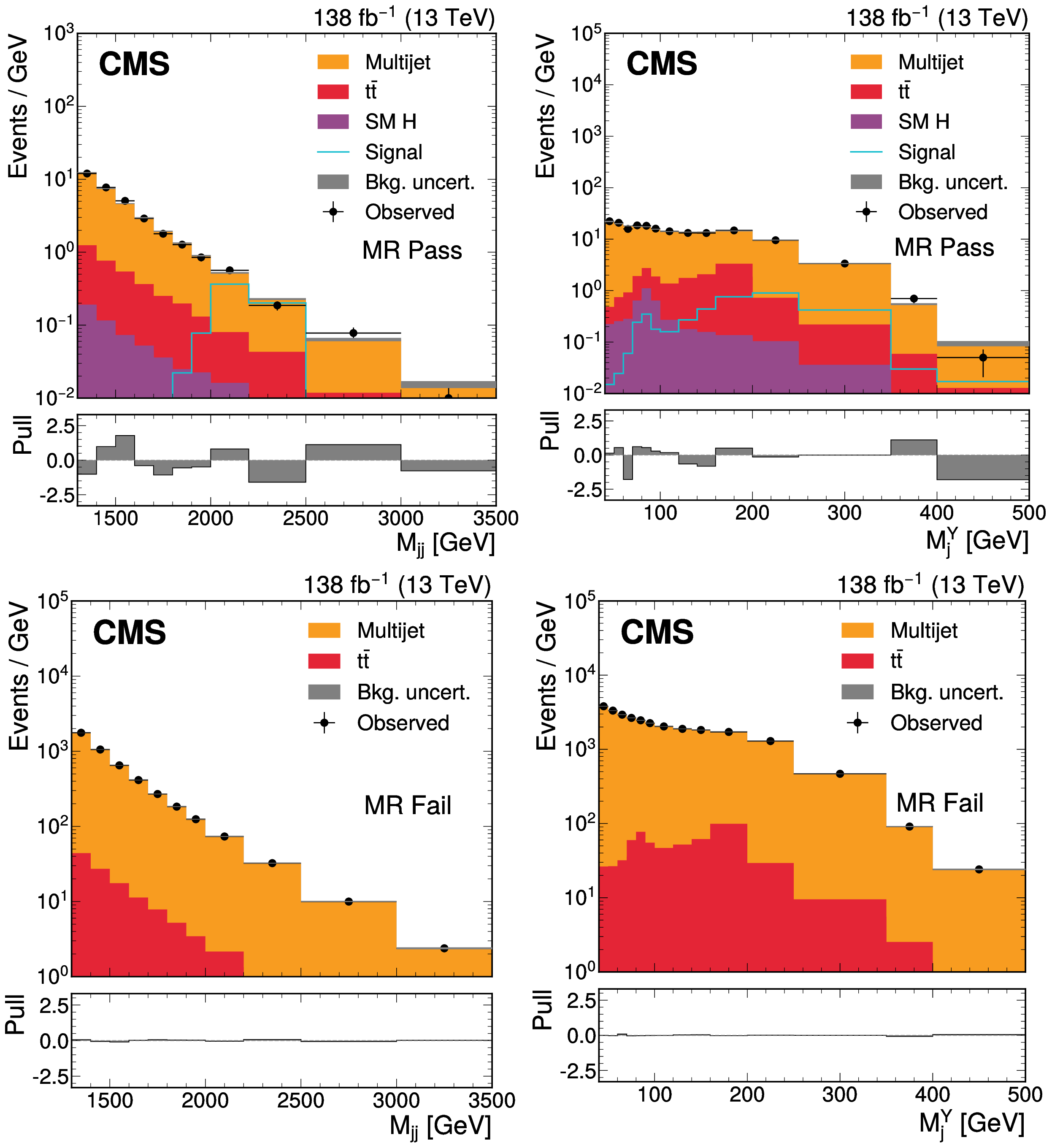
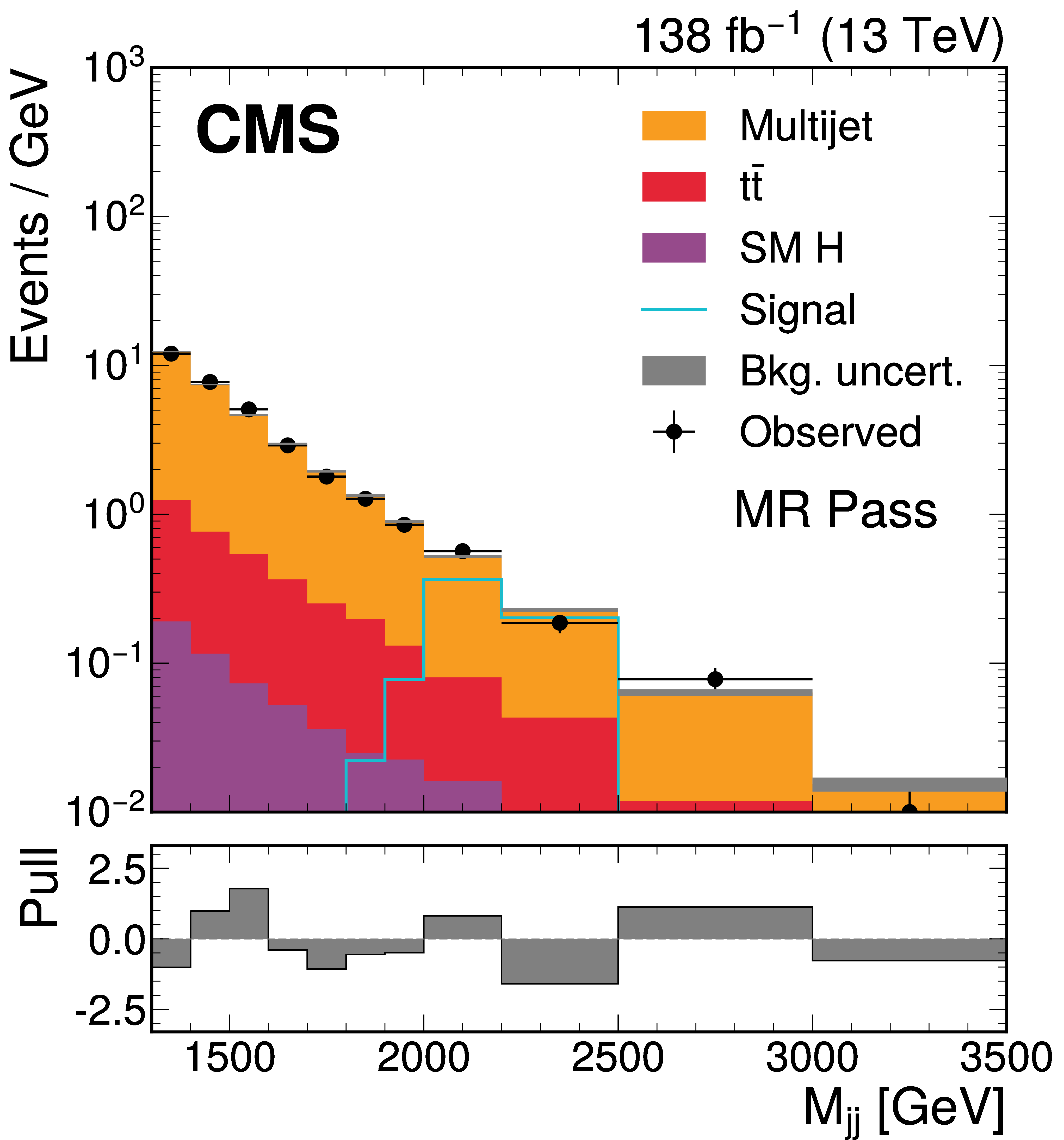
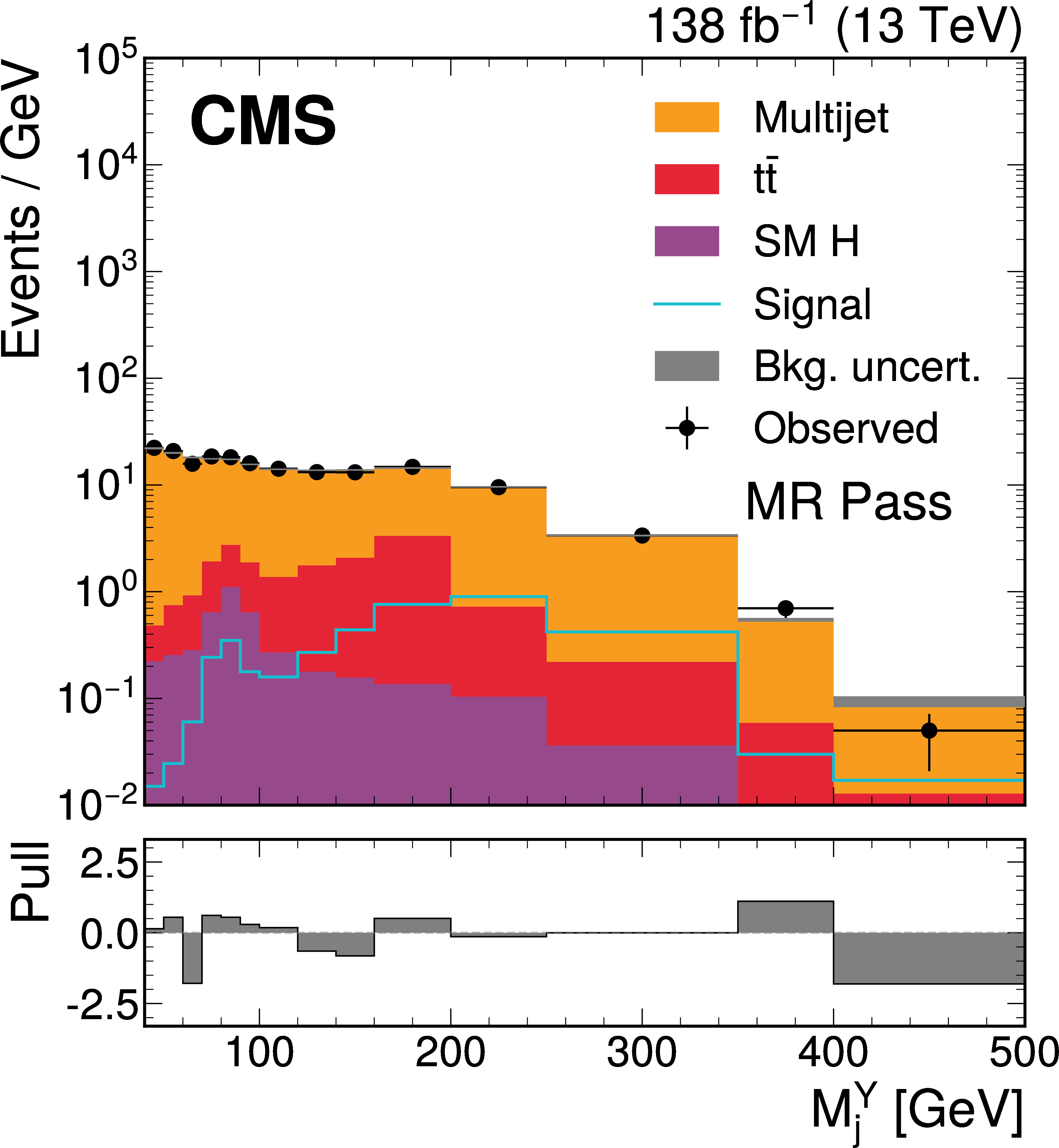
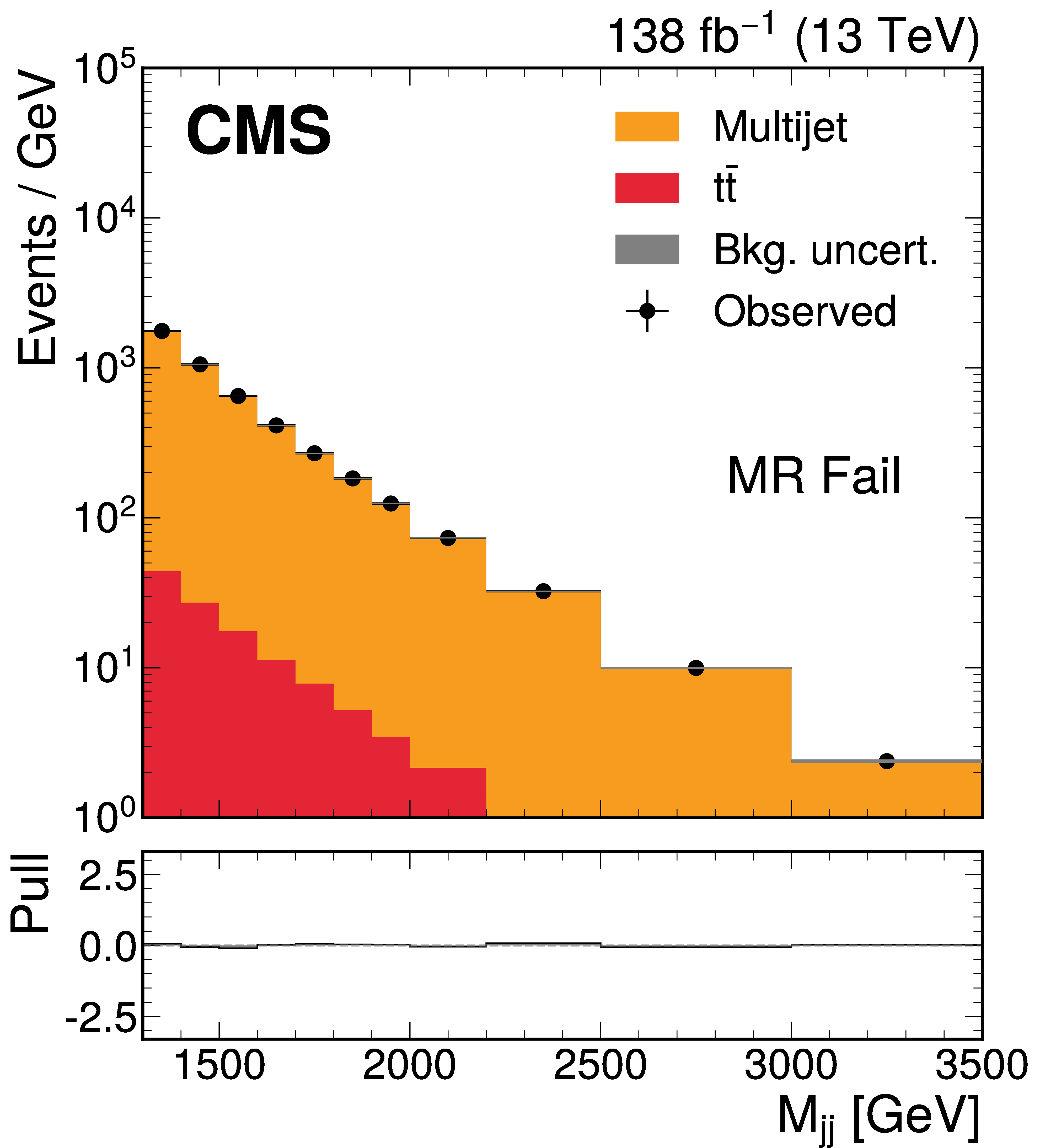
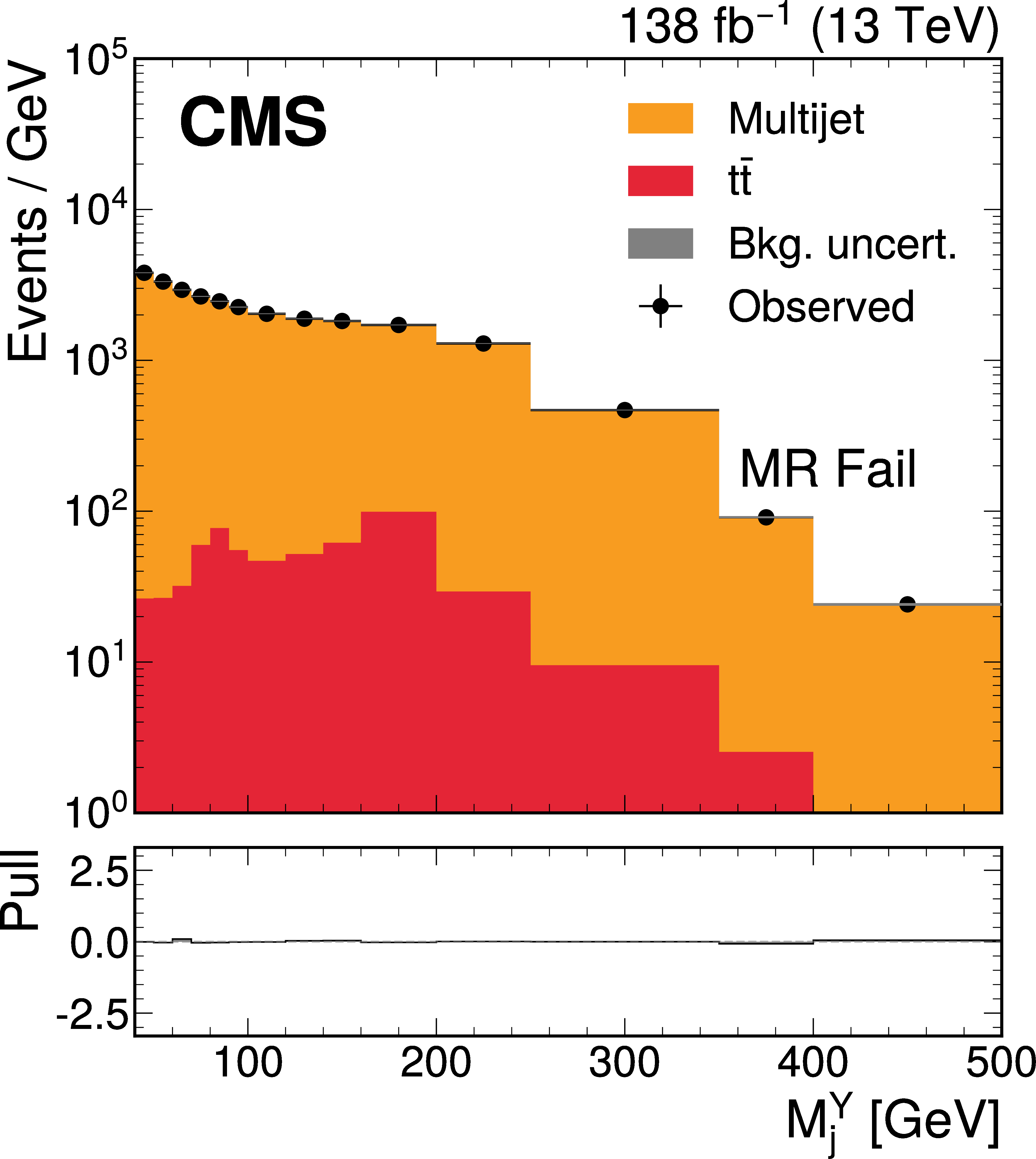
Figure 3:
The $ M_\mathrm{jj} $ (left) and $ M_\mathrm{j}^{\mathrm{Y}} $ (right) projections showing the number of observed events per GeV (black markers) compared with the backgrounds estimated in the fit to the data (filled histograms) in the MR. Pass (upper) and Fail (lower) categories are shown. The expected contribution from the signal benchmark with $ M_{\mathrm{X}} = $ 2200 GeV and $ M_{\mathrm{Y}} = $ 250 GeV is overlaid in the MR Pass, assuming a production cross section of 5\unitfb. The high level of agreement between the model and the data in the Fail region is due to the nature of the background estimate. The lower panels show the ``Pull'' defined as (observed events}-\text{expected events) $ /\sqrt{\smash[b]{\sigma_{\text{obs}}^{2} + \sigma_{\text{bkg}}^{2}}} $, where $ \sigma_{\text{obs}} $ and $ \sigma_{\text{bkg}} $ are the total uncertainties in the observation and the background estimation, respectively. |
png pdf |
Figure 3-a:
The $ M_\mathrm{jj} $ (left) and $ M_\mathrm{j}^{\mathrm{Y}} $ (right) projections showing the number of observed events per GeV (black markers) compared with the backgrounds estimated in the fit to the data (filled histograms) in the MR. Pass (upper) and Fail (lower) categories are shown. The expected contribution from the signal benchmark with $ M_{\mathrm{X}} = $ 2200 GeV and $ M_{\mathrm{Y}} = $ 250 GeV is overlaid in the MR Pass, assuming a production cross section of 5\unitfb. The high level of agreement between the model and the data in the Fail region is due to the nature of the background estimate. The lower panels show the ``Pull'' defined as (observed events}-\text{expected events) $ /\sqrt{\smash[b]{\sigma_{\text{obs}}^{2} + \sigma_{\text{bkg}}^{2}}} $, where $ \sigma_{\text{obs}} $ and $ \sigma_{\text{bkg}} $ are the total uncertainties in the observation and the background estimation, respectively. |
png pdf |
Figure 3-b:
The $ M_\mathrm{jj} $ (left) and $ M_\mathrm{j}^{\mathrm{Y}} $ (right) projections showing the number of observed events per GeV (black markers) compared with the backgrounds estimated in the fit to the data (filled histograms) in the MR. Pass (upper) and Fail (lower) categories are shown. The expected contribution from the signal benchmark with $ M_{\mathrm{X}} = $ 2200 GeV and $ M_{\mathrm{Y}} = $ 250 GeV is overlaid in the MR Pass, assuming a production cross section of 5\unitfb. The high level of agreement between the model and the data in the Fail region is due to the nature of the background estimate. The lower panels show the ``Pull'' defined as (observed events}-\text{expected events) $ /\sqrt{\smash[b]{\sigma_{\text{obs}}^{2} + \sigma_{\text{bkg}}^{2}}} $, where $ \sigma_{\text{obs}} $ and $ \sigma_{\text{bkg}} $ are the total uncertainties in the observation and the background estimation, respectively. |
png pdf |
Figure 3-c:
The $ M_\mathrm{jj} $ (left) and $ M_\mathrm{j}^{\mathrm{Y}} $ (right) projections showing the number of observed events per GeV (black markers) compared with the backgrounds estimated in the fit to the data (filled histograms) in the MR. Pass (upper) and Fail (lower) categories are shown. The expected contribution from the signal benchmark with $ M_{\mathrm{X}} = $ 2200 GeV and $ M_{\mathrm{Y}} = $ 250 GeV is overlaid in the MR Pass, assuming a production cross section of 5\unitfb. The high level of agreement between the model and the data in the Fail region is due to the nature of the background estimate. The lower panels show the ``Pull'' defined as (observed events}-\text{expected events) $ /\sqrt{\smash[b]{\sigma_{\text{obs}}^{2} + \sigma_{\text{bkg}}^{2}}} $, where $ \sigma_{\text{obs}} $ and $ \sigma_{\text{bkg}} $ are the total uncertainties in the observation and the background estimation, respectively. |
png pdf |
Figure 3-d:
The $ M_\mathrm{jj} $ (left) and $ M_\mathrm{j}^{\mathrm{Y}} $ (right) projections showing the number of observed events per GeV (black markers) compared with the backgrounds estimated in the fit to the data (filled histograms) in the MR. Pass (upper) and Fail (lower) categories are shown. The expected contribution from the signal benchmark with $ M_{\mathrm{X}} = $ 2200 GeV and $ M_{\mathrm{Y}} = $ 250 GeV is overlaid in the MR Pass, assuming a production cross section of 5\unitfb. The high level of agreement between the model and the data in the Fail region is due to the nature of the background estimate. The lower panels show the ``Pull'' defined as (observed events}-\text{expected events) $ /\sqrt{\smash[b]{\sigma_{\text{obs}}^{2} + \sigma_{\text{bkg}}^{2}}} $, where $ \sigma_{\text{obs}} $ and $ \sigma_{\text{bkg}} $ are the total uncertainties in the observation and the background estimation, respectively. |
png pdf |
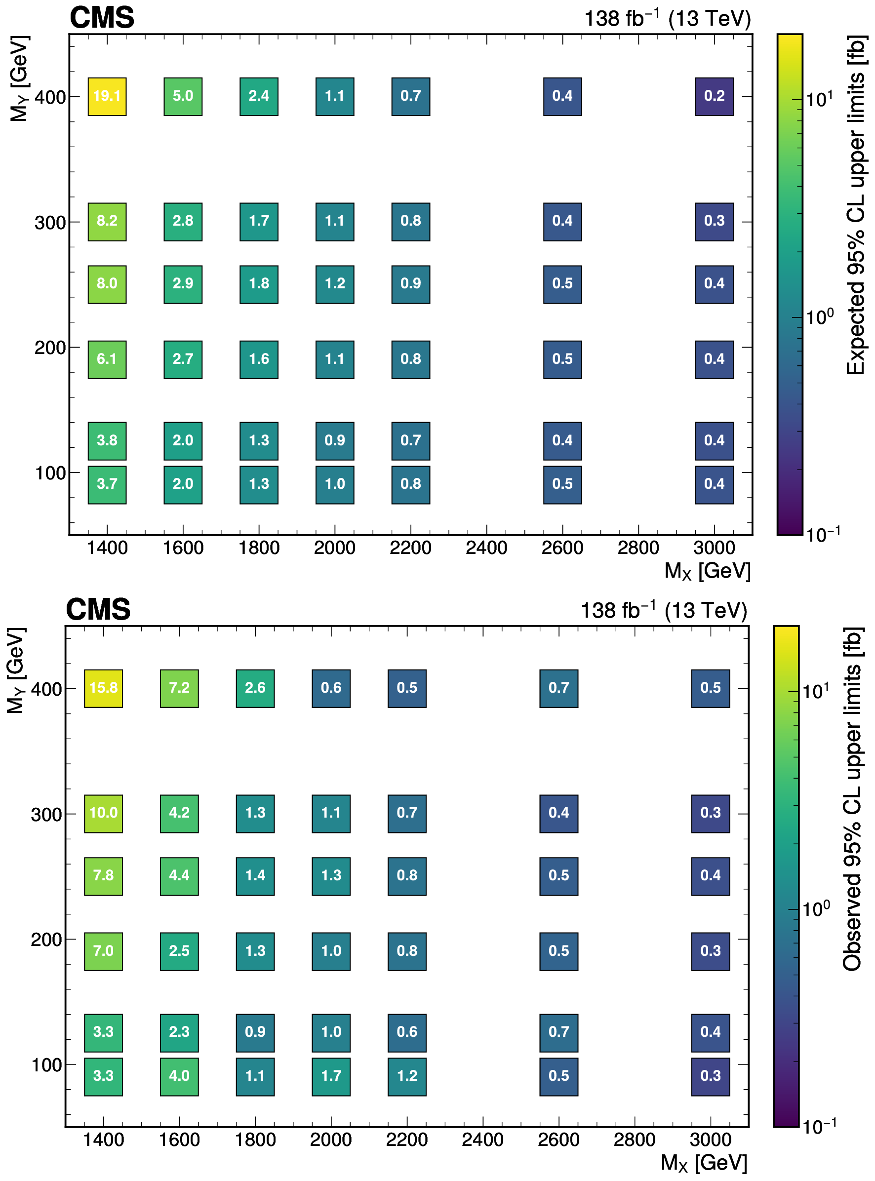
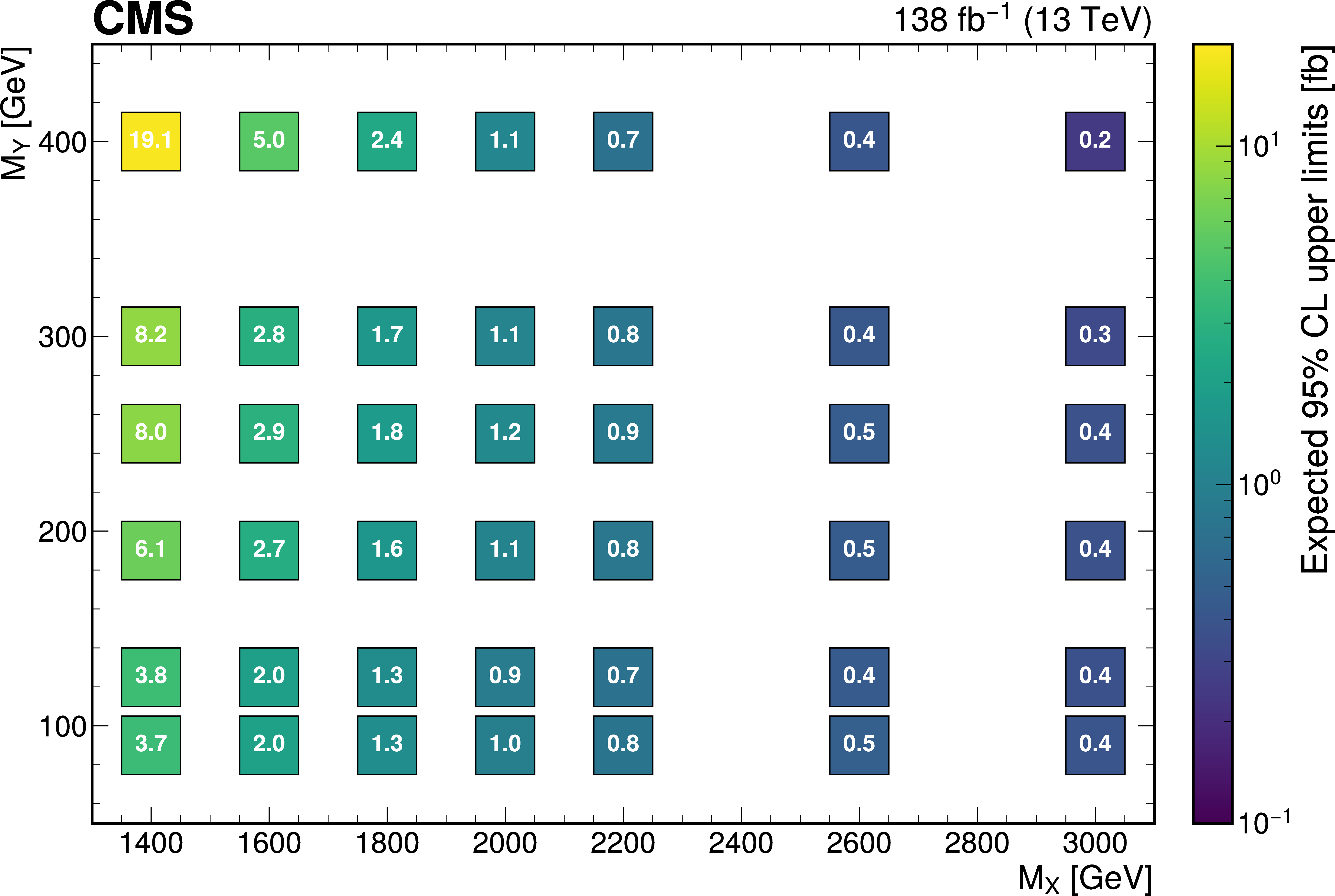
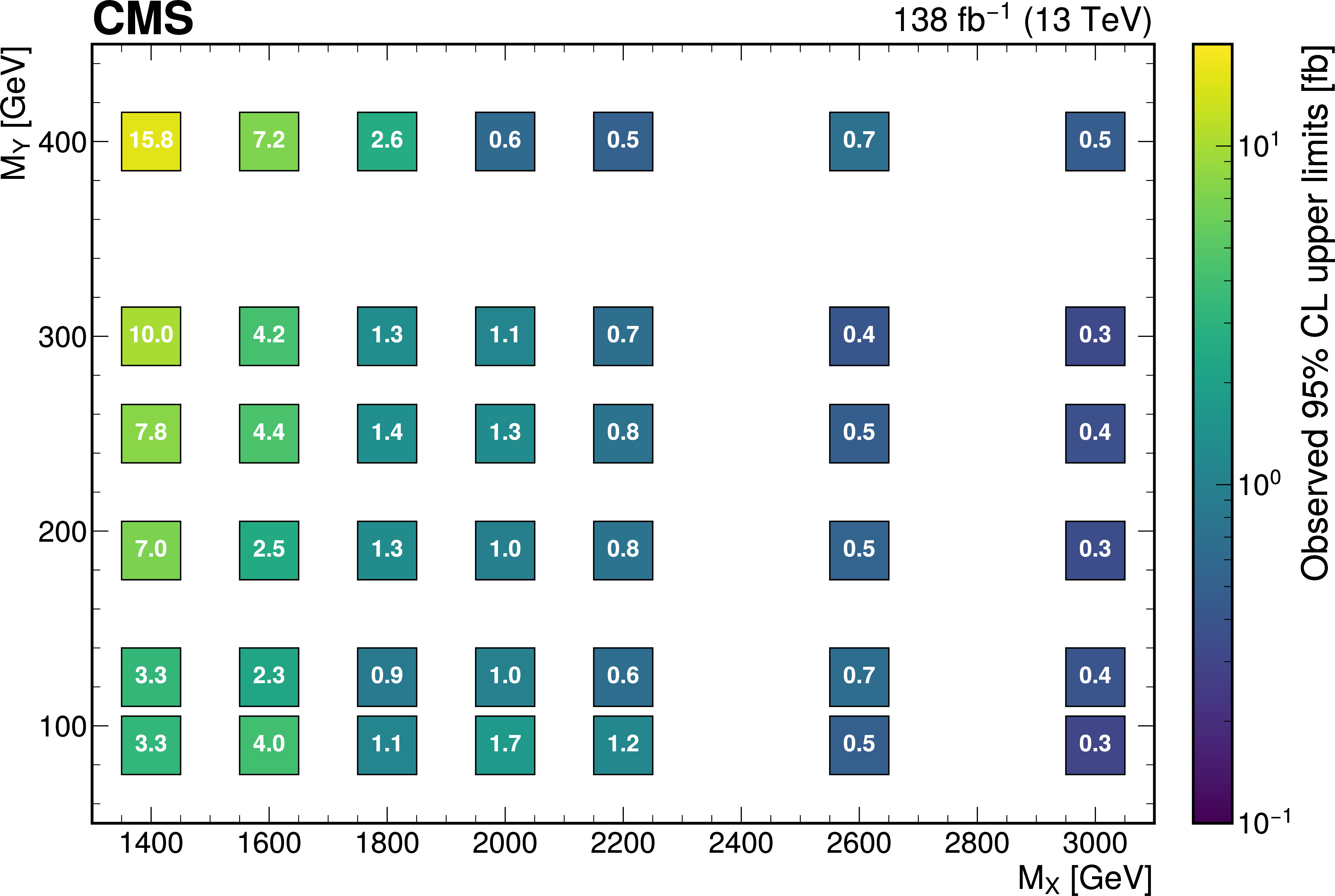
Figure 4:
The expected (upper) and observed (lower) 95% confidence level upper limits on $ \sigma(\mathrm{p} \to \mathrm{X} \to \mathrm{H} \mathrm{Y})\mathcal{B}(\mathrm{H}\to\mathrm{b}\overline{\mathrm{b}})\mathcal{B}(\mathrm{Y}\to\mathrm{W}\mathrm{W}\to2\mathrm{q} 2\overline{\mathrm{q}}^\prime) $ for different values of $ M_{\mathrm{X}} $ and $ M_{\mathrm{Y}} $. The limits have been evaluated in discrete steps corresponding to the centers of the boxes. The numbers in the boxes are given in fb. |
png pdf |
Figure 4-a:
The expected (upper) and observed (lower) 95% confidence level upper limits on $ \sigma(\mathrm{p} \to \mathrm{X} \to \mathrm{H} \mathrm{Y})\mathcal{B}(\mathrm{H}\to\mathrm{b}\overline{\mathrm{b}})\mathcal{B}(\mathrm{Y}\to\mathrm{W}\mathrm{W}\to2\mathrm{q} 2\overline{\mathrm{q}}^\prime) $ for different values of $ M_{\mathrm{X}} $ and $ M_{\mathrm{Y}} $. The limits have been evaluated in discrete steps corresponding to the centers of the boxes. The numbers in the boxes are given in fb. |
png pdf |
Figure 4-b:
The expected (upper) and observed (lower) 95% confidence level upper limits on $ \sigma(\mathrm{p} \to \mathrm{X} \to \mathrm{H} \mathrm{Y})\mathcal{B}(\mathrm{H}\to\mathrm{b}\overline{\mathrm{b}})\mathcal{B}(\mathrm{Y}\to\mathrm{W}\mathrm{W}\to2\mathrm{q} 2\overline{\mathrm{q}}^\prime) $ for different values of $ M_{\mathrm{X}} $ and $ M_{\mathrm{Y}} $. The limits have been evaluated in discrete steps corresponding to the centers of the boxes. The numbers in the boxes are given in fb. |
png pdf |
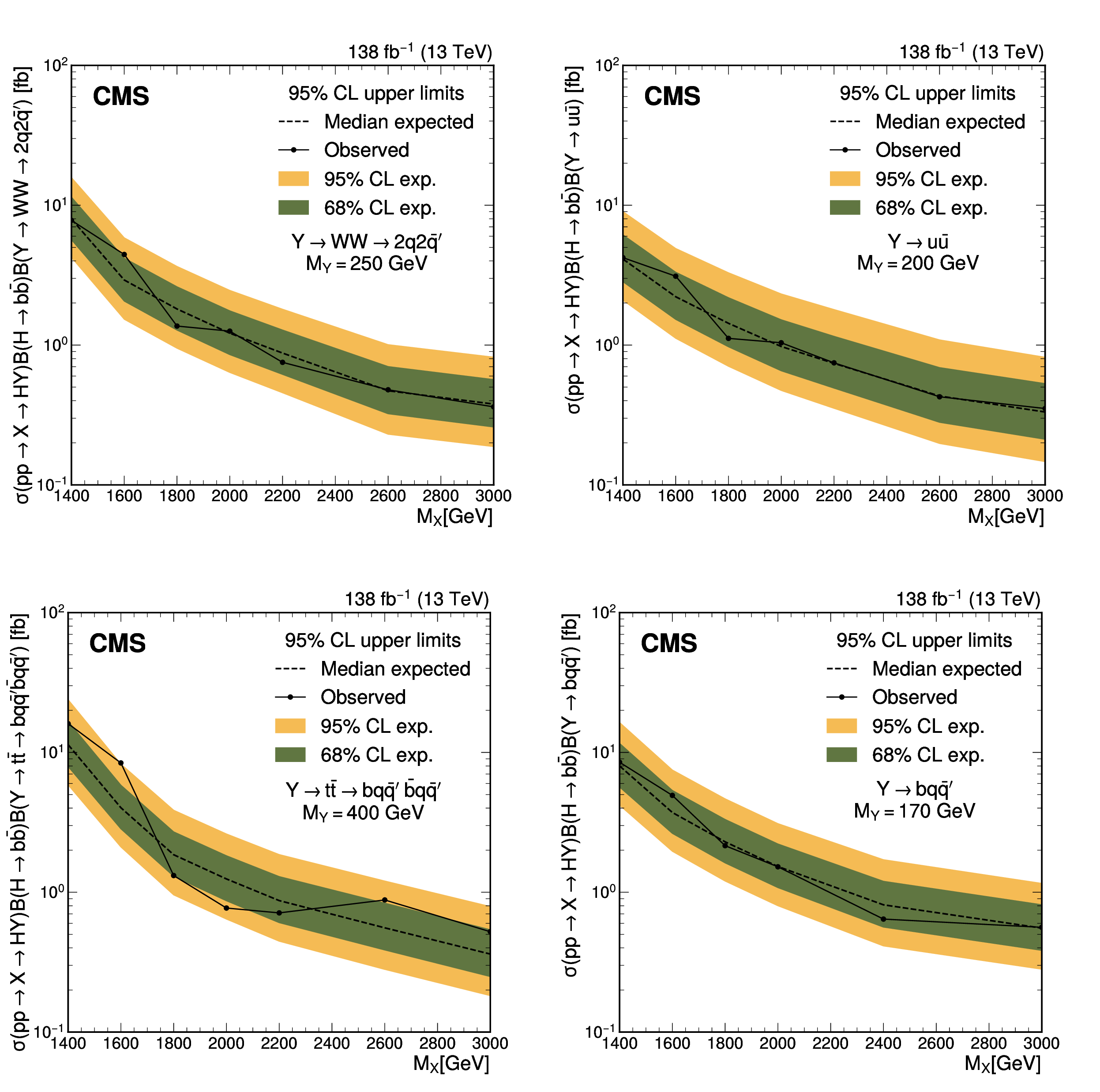
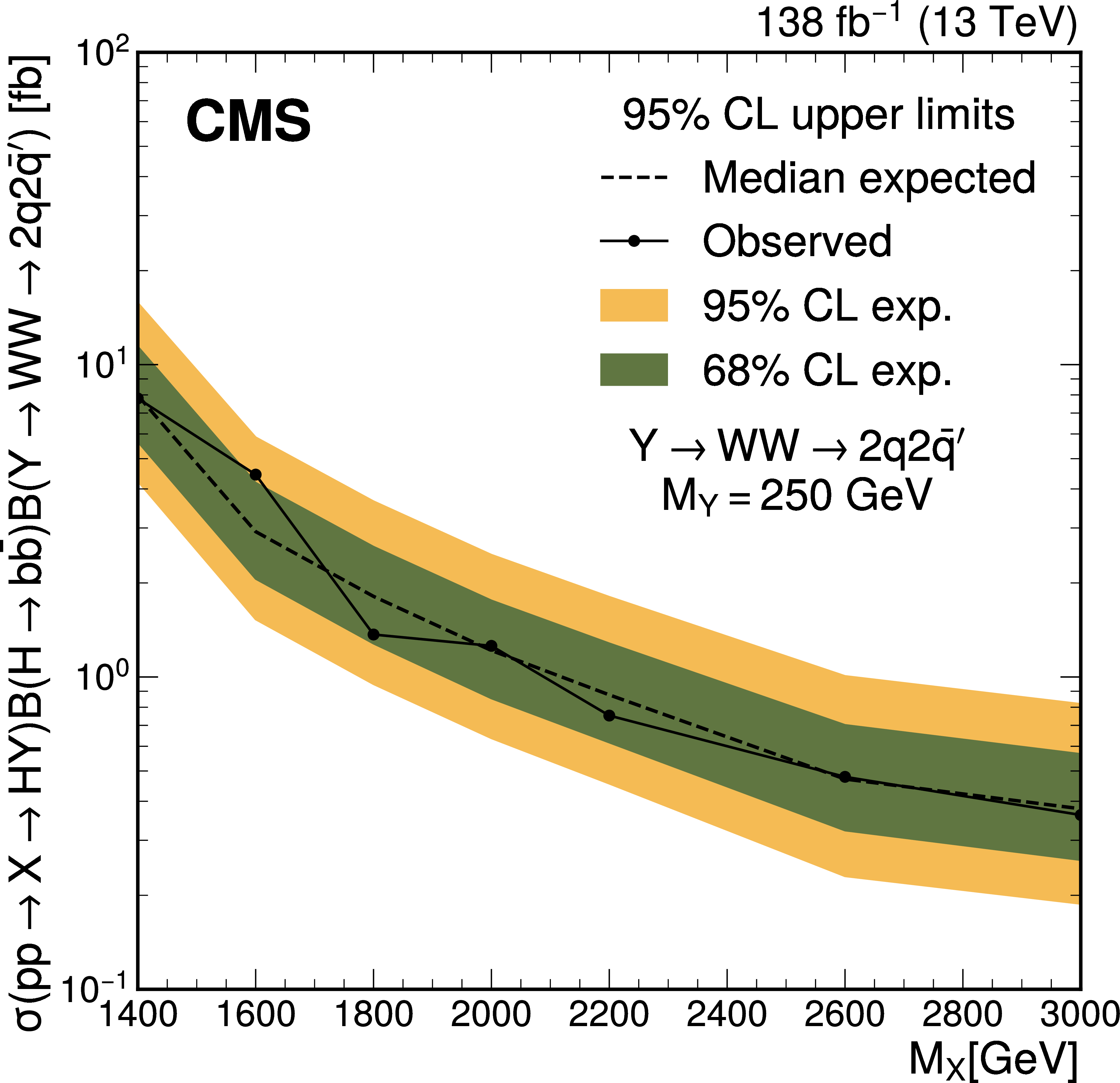
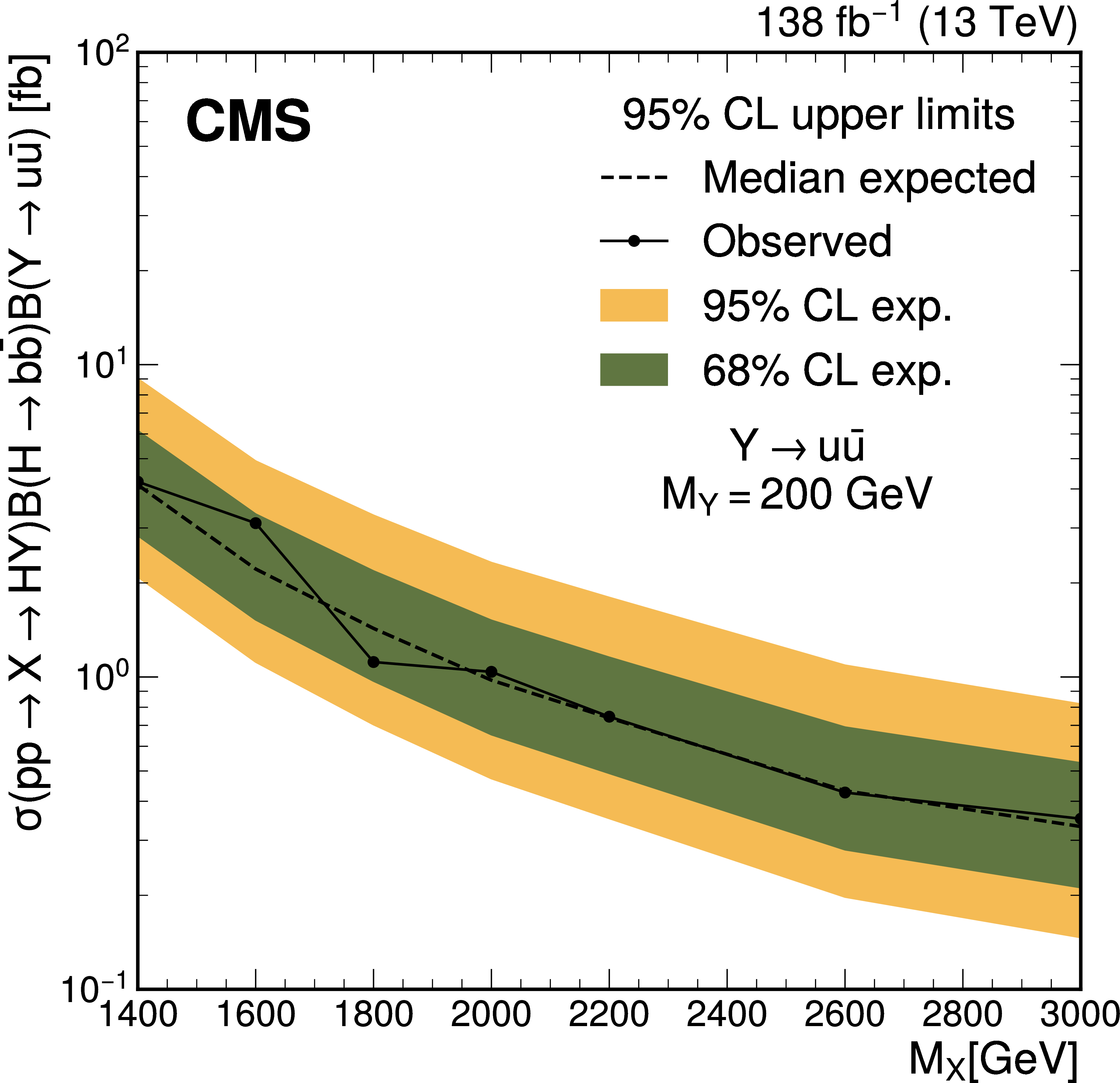
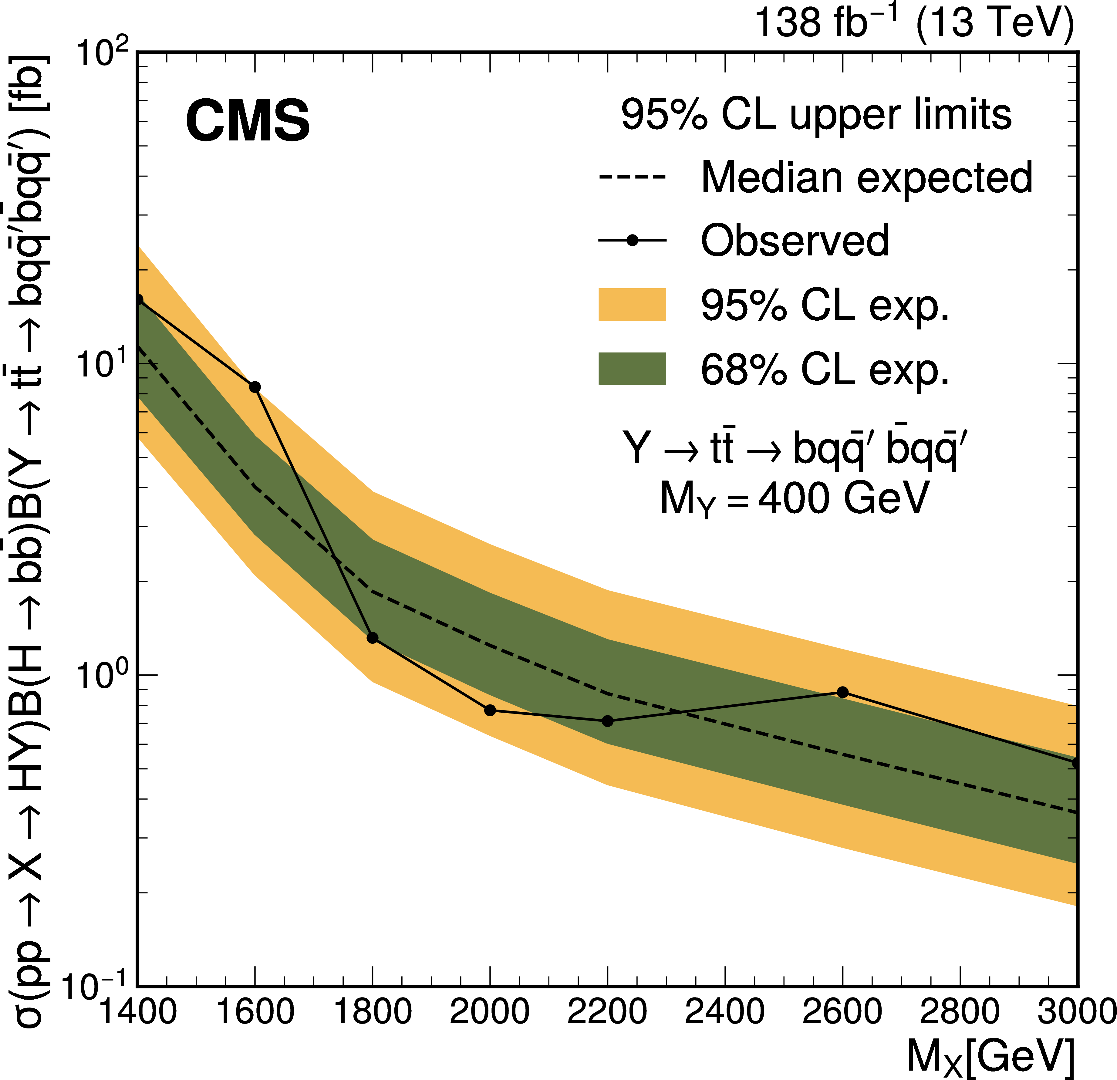
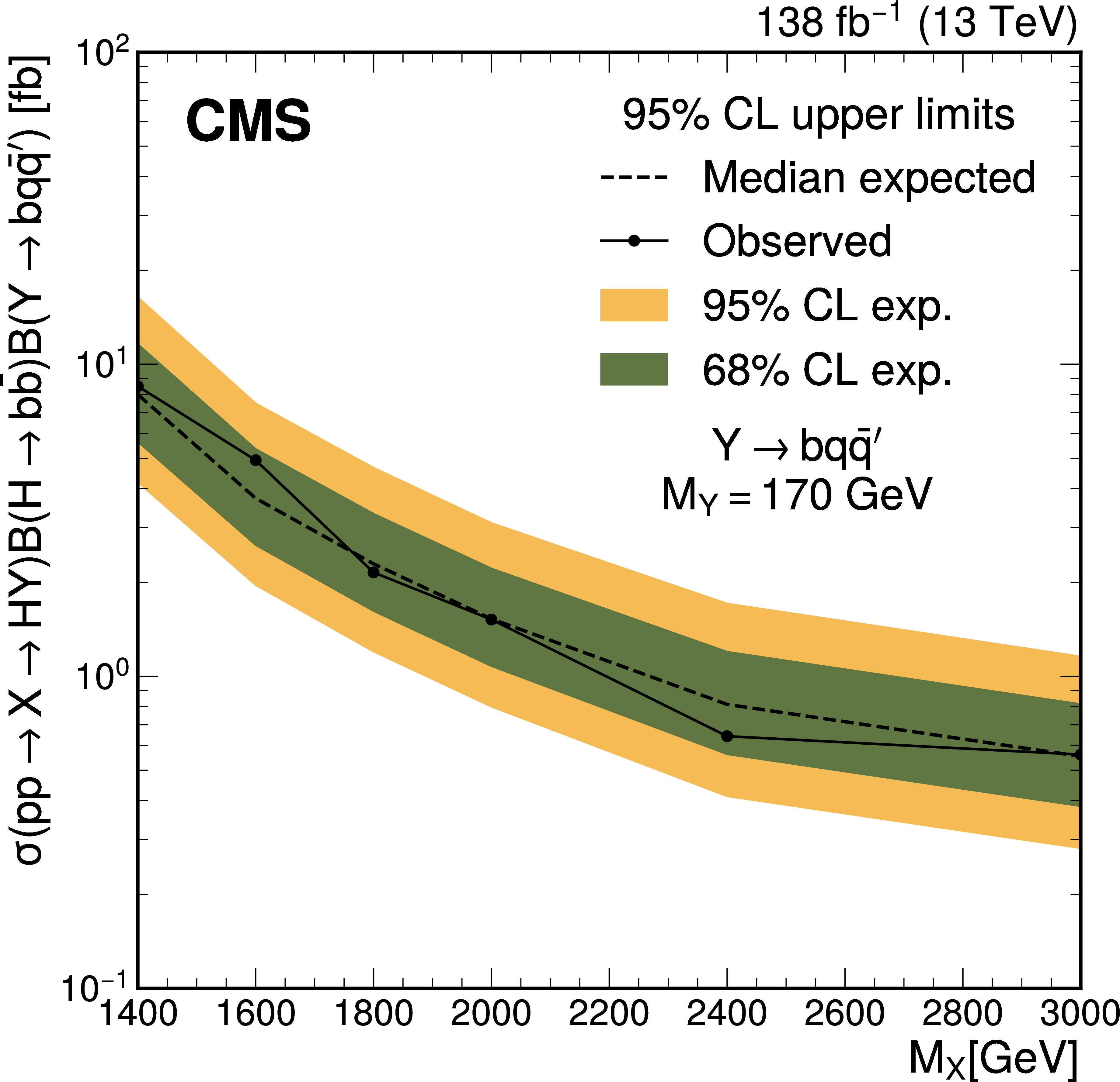
Figure 5:
The median expected (dashed line) and observed (solid line) 95% confidence level upper limits on the main and three alternative signal scenarios as a function of $ M_{\mathrm{X}} $. The inner (green) band and outer (yellow) band represent the regions containing 68% and 95%, respectively, of the distribution of limits expected under the background-only hypothesis. |
png pdf |
Figure 5-a:
The median expected (dashed line) and observed (solid line) 95% confidence level upper limits on the main and three alternative signal scenarios as a function of $ M_{\mathrm{X}} $. The inner (green) band and outer (yellow) band represent the regions containing 68% and 95%, respectively, of the distribution of limits expected under the background-only hypothesis. |
png pdf |
Figure 5-b:
The median expected (dashed line) and observed (solid line) 95% confidence level upper limits on the main and three alternative signal scenarios as a function of $ M_{\mathrm{X}} $. The inner (green) band and outer (yellow) band represent the regions containing 68% and 95%, respectively, of the distribution of limits expected under the background-only hypothesis. |
png pdf |
Figure 5-c:
The median expected (dashed line) and observed (solid line) 95% confidence level upper limits on the main and three alternative signal scenarios as a function of $ M_{\mathrm{X}} $. The inner (green) band and outer (yellow) band represent the regions containing 68% and 95%, respectively, of the distribution of limits expected under the background-only hypothesis. |
png pdf |
Figure 5-d:
The median expected (dashed line) and observed (solid line) 95% confidence level upper limits on the main and three alternative signal scenarios as a function of $ M_{\mathrm{X}} $. The inner (green) band and outer (yellow) band represent the regions containing 68% and 95%, respectively, of the distribution of limits expected under the background-only hypothesis. |
| Summary |
| A search for beyond the standard model physics through the process where a resonant particle decays into a Higgs boson, H, and an additional particle Y has been presented. The H subsequently decays into a bottom quark-antiquark pair, $ \mathrm{b}\overline{\mathrm{b}} $, reconstructed as a large-radius jet in the Lorentz-boosted regime. The H candidate jets are tagged using the ParticleNet algorithm that is designed to recognize jets originating from a decay of a massive particle into $ \mathrm{b}\overline{\mathrm{b}} $. The identification of the second particle, Y, is performed by computing the anomaly score of its candidate jet using an autoencoder, allowing the simultaneous search for multiple Y decay modes within a single analysis. This approach combines the targeted identification of H decays with model-independent anomaly detection technique, enabling a broad search for new physics. By combining the strong discrimination power of the H decay to $ \mathrm{b}\overline{\mathrm{b}} $ with a model-independent anomaly detection for the second particle, this analysis achieves both enhanced sensitivity and broad applicability to diverse new-physics scenarios. The analysis considers four benchmark models. The main benchmark assumes $ \mathrm{Y} \to \mathrm{W^+}\mathrm{W^-} $, with further hadronic decays of the W bosons. It is simulated for $ M_{\mathrm{X}} $ values within 1400-3000 GeV and $ M_{\mathrm{Y}} $ values within 90-400 GeV, covering 42 signal hypotheses. No significant excess above the standard model background expectations is observed. Upper limits on benchmark signal cross sections at 95% confidence level are set on the main benchmark model in the 0.3-15.8\unitfb range. Additionally, exclusion limits are calculated for three alternative benchmark models, assuming $ \mathrm{Y} \to \mathrm{u} \overline{\mathrm{u}} $, $ \mathrm{Y} \to {\mathrm{t}\overline{\mathrm{t}}} $, or $ \mathrm{Y} \to \mathrm{b} \mathrm{q} \overline{\mathrm{q}}^\prime $ decay modes, for which the most stringent limits to date are achieved. |
| References | ||||
| 1 | S. L. Glashow | Partial-symmetries of weak interactions | NP 22 (1961) 579 | |
| 2 | S. Weinberg | A model of leptons | PRL 19 (1967) 1264 | |
| 3 | A. Salam | Weak and electromagnetic interactions | in Elementary particle physics: relativistic groups and analyticity, N. Svartholm, ed., p. 367. Almqvist \& Wiksell, Stockholm, 1968 | |
| 4 | Planck Collaboration | Planck 2018 results: I. Overview and the cosmological legacy of Planck | Astron. Astrophys. 641 (2020) A1 | 1807.06205 |
| 5 | J. de Vries , M. Postma, and J. van de Vis | The role of leptons in electroweak baryogenesis | JHEP 04 (2019) 024 | 1811.11104 |
| 6 | P. Fayet | Supergauge invariant extension of the Higgs mechanism and a model for the electron and its neutrino | NPB 90 (1975) 104 | |
| 7 | P. Fayet | Spontaneously broken supersymmetric theories of weak, electromagnetic and strong interactions | PLB 69 (1977) 489 | |
| 8 | N. Arkani-Hamed, S. Dimopoulos, and G. Dvali | The hierarchy problem and new dimensions at a millimeter | PLB 429 (1998) 263 | hep-ph/9803315 |
| 9 | L. Randall and R. Sundrum | A large mass hierarchy from a small extra dimension | PRL 83 (1999) 3370 | hep-ph/9905221 |
| 10 | L. Randall and R. Sundrum | An alternative to compactification | PRL 83 (1999) 4690 | hep-th/9906064 |
| 11 | T. Robens, T. Stefaniak, and J. Wittbrodt | Two-real-scalar-singlet extension of the SM: LHC phenomenology and benchmark scenarios | EPJC 80 (2020) 151 | 1908.08554 |
| 12 | G. Kasieczka et al. | The LHC Olympics: a community challenge for anomaly detection in high energy physics | Rep. Prog. Phys. 84 (2021) 124201 | 2101.08320 |
| 13 | G. Arcadi, A. Djouadi, and M. Kado | The Higgs-portal for dark matter: effective field theories versus concrete realizations | EPJC 81 (2021) 653 | 2101.02507 |
| 14 | M. Cacciari, G. P. Salam, and G. Soyez | The anti-$ k_{\mathrm{T}} $ jet clustering algorithm | JHEP 04 (2008) 063 | 0802.1189 |
| 15 | M. Cacciari, G. P. Salam, and G. Soyez | FastJet user manual | EPJC 72 (2012) 1896 | 1111.6097 |
| 16 | U. Ellwanger, C. Hugonie, and A. M. Teixeira | The next-to-minimal supersymmetric standard model | Phys. Rep. 496 (2010) 1 | 0910.1785 |
| 17 | CMS Collaboration | Searches for Higgs boson production through decays of heavy resonances | Phys. Rep. 1115 (2025) 368 | 2403.16926 |
| 18 | A. Carvalho et al. | Single production of vectorlike quarks with large width at the Large Hadron Collider | PRD 98 (2018) 015029 | 1805.06402 |
| 19 | CMS Collaboration | Model-agnostic search for dijet resonances with anomalous jet substructure in proton-proton collisions at $ \sqrt{s} = $ 13 TeV | Rep. Prog. Phys. 88 (2025) 067802 | CMS-EXO-22-026 2412.03747 |
| 20 | H. Qu and L. Gouskos | ParticleNet: Jet tagging via particle clouds | PRD 101 (2020) 056019 | 1902.08570 |
| 21 | CMS Collaboration | The CMS experiment at the CERN LHC | JINST 3 (2008) S08004 | |
| 22 | CMS Collaboration | Performance of the CMS Level-1 trigger in proton-proton collisions at $ \sqrt{s} = $ 13 TeV | JINST 15 (2020) P10017 | CMS-TRG-17-001 2006.10165 |
| 23 | CMS Collaboration | The CMS trigger system | JINST 12 (2017) P01020 | CMS-TRG-12-001 1609.02366 |
| 24 | CMS Collaboration | Performance of the CMS high-level trigger during LHC Run 2 | JINST 19 (2024) P11021 | CMS-TRG-19-001 2410.17038 |
| 25 | CMS Collaboration | Electron and photon reconstruction and identification with the CMS experiment at the CERN LHC | JINST 16 (2021) P05014 | CMS-EGM-17-001 2012.06888 |
| 26 | CMS Collaboration | Performance of the CMS muon detector and muon reconstruction with proton-proton collisions at $ \sqrt{s}= $ 13 TeV | JINST 13 (2018) P06015 | CMS-MUO-16-001 1804.04528 |
| 27 | CMS Collaboration | Description and performance of track and primary-vertex reconstruction with the CMS tracker | JINST 9 (2014) P10009 | CMS-TRK-11-001 1405.6569 |
| 28 | CMS Collaboration | Development of the CMS detector for the CERN LHC Run 3 | JINST 19 (2024) P05064 | CMS-PRF-21-001 2309.05466 |
| 29 | CMS Collaboration | Particle-flow reconstruction and global event description with the CMS detector | JINST 12 (2017) P10003 | CMS-PRF-14-001 1706.04965 |
| 30 | CMS Collaboration | Pileup mitigation at CMS in 13 TeV data | JINST 15 (2020) P09018 | CMS-JME-18-001 2003.00503 |
| 31 | D. Bertolini, P. Harris, M. Low, and N. Tran | Pileup per particle identification | JHEP 10 (2014) 059 | 1407.6013 |
| 32 | G. P. Salam | Towards jetography | EPJC 67 (2010) 637 | 0906.1833 |
| 33 | D. Krohn, J. Thaler, and L.-T. Wang | Jet trimming | JHEP 02 (2010) 084 | 0912.1342 |
| 34 | Y. L. Dokshitzer, G. D. Leder, S. Moretti, and B. R. Webber | Better jet clustering algorithms | JHEP 08 (1997) 001 | hep-ph/9707323 |
| 35 | M. Wobisch and T. Wengler | Hadronization corrections to jet cross-sections in deep inelastic scattering | in Proceedings of the Workshop on Monte Carlo Generators for HERA Physics. 1998 link |
hep-ph/9907280 |
| 36 | M. Dasgupta, A. Fregoso, S. Marzani, and G. P. Salam | Towards an understanding of jet substructure | JHEP 09 (2013) 029 | 1307.0007 |
| 37 | J. M. Butterworth, A. R. Davison, M. Rubin, and G. P. Salam | Jet substructure as a new Higgs search channel at the LHC | PRL 100 (2008) 242001 | 0802.2470 |
| 38 | A. J. Larkoski, S. Marzani, G. Soyez, and J. Thaler | Soft drop | JHEP 05 (2014) 146 | 1402.2657 |
| 39 | J. Alwall et al. | The automated computation of tree-level and next-to-leading order differential cross sections, and their matching to parton shower simulations | JHEP 07 (2014) 079 | 1405.0301 |
| 40 | D. Curtin et al. | Exotic decays of the 125 GeV Higgs boson | PRD 90 (2014) 075004 | 1312.4992 |
| 41 | A. Alloul et al. | FeynRules 2.0 --- a complete toolbox for tree-level phenomenology | Comput. Phys. Commun. 185 (2014) 2250 | 1310.1921 |
| 42 | S. Frixione, G. Ridolfi, and P. Nason | A positive-weight next-to-leading-order Monte Carlo for heavy flavour hadroproduction | JHEP 09 (2007) 126 | 0707.3088 |
| 43 | S. Frixione, P. Nason, and C. Oleari | Matching NLO QCD computations with parton shower simulations: the POWHEG method | JHEP 11 (2007) 070 | 0709.2092 |
| 44 | S. Alioli, P. Nason, C. Oleari, and E. Re | A general framework for implementing NLO calculations in shower Monte Carlo programs: the POWHEG BOX | JHEP 06 (2010) 043 | 1002.2581 |
| 45 | P. Nason | A new method for combining NLO QCD with shower Monte Carlo algorithms | JHEP 11 (2004) 040 | hep-ph/0409146 |
| 46 | M. Czakon and A. Mitov | Top++: A program for the calculation of the top-pair cross-section at hadron colliders | Comput. Phys. Commun. 185 (2014) 2930 | 1112.5675 |
| 47 | K. Hamilton, P. Nason, E. Re, and G. Zanderighi | NNLOPS simulation of Higgs boson production | JHEP 10 (2013) 222 | |
| 48 | P. Nason and C. Oleari | NLO Higgs boson production via vector-boson fusion matched with shower in POWHEG | JHEP 02 (2010) 037 | 0911.5299 |
| 49 | G. Luisoni, P. Nason, C. Oleari, and F. Tramontano | $ \mathrm{H}\mathrm{W}^{\pm} $/HZ+0 and 1 jet at NLO with the POWHEG BOX interfaced to GoSam and their merging within MiNLO | JHEP 10 (2013) 083 | 1306.2542 |
| 50 | NNPDF Collaboration | Parton distributions from high-precision collider data | EPJC 77 (2017) 663 | 1706.00428 |
| 51 | A. Buckley et al. | LHAPDF6: parton density access in the LHC precision era | EPJC 75 (2015) 132 | 1412.7420 |
| 52 | T. Sjöstrand et al. | An introduction to PYTHIA 8.2 | Comput. Phys. Commun. 191 (2015) 159 | 1410.3012 |
| 53 | CMS Collaboration | Extraction and validation of a new set of CMS PYTHIA8 tunes from underlying-event measurements | EPJC 80 (2020) 4 | CMS-GEN-17-001 1903.12179 |
| 54 | GEANT4 Collaboration | GEANT 4---a simulation toolkit | NIM A 506 (2003) 250 | |
| 55 | CMS Collaboration | Measurement of the inelastic proton-proton cross section at $ \sqrt{s} = $ 13 TeV | JHEP 07 (2018) 161 | CMS-FSQ-15-005 1802.02613 |
| 56 | CMS Collaboration | Identification of highly Lorentz-boosted heavy particles using graph neural networks and new mass decorrelation techniques | CMS Detector Performance Summary CMS-DP-2020-002, 2020 CDS |
|
| 57 | CMS Collaboration | Calibration of the mass-decorrelated ParticleNet tagger for boosted $ \mathrm{b}\overline{\mathrm{b}} $ and $ \mathrm{c}\overline{\mathrm{c}} $ jets using LHC Run 2 data | CMS Detector Performance Summary CMS-DP-2022-005, 2022 CDS |
|
| 58 | G. E. Hinton and R. R. Salakhutdinov | Reducing the dimensionality of data with neural networks | Science 313 (2006) 504 | |
| 59 | S. Macaluso and D. Shih | Pulling out all the tops with computer vision and deep learning | JHEP 10 (2018) 121 | 1803.00107 |
| 60 | CMS Collaboration | Performance of heavy-flavour jet identification in boosted topologies in proton-proton collisions at $ \sqrt{s}= $ 13 TeV | CMS Physics Analysis Summary, 2023 CMS-PAS-BTV-22-001 |
CMS-PAS-BTV-22-001 |
| 61 | CMS Collaboration | A method for correcting the substructure of multiprong jets using the Lund jet plane | Submitted to JHEP, 2025 link |
CMS-JME-23-001 2507.07775 |
| 62 | R. A. Fisher | On the interpretation of $ \chi^{2} $ from contingency tables, and the calculation of P | J. R. Stat. Soc. 85 (1922) 87 | |
| 63 | CMS Collaboration | The CMS statistical analysis and combination tool: COMBINE | Comput. Softw. Big Sci. 8 (2024) 19 | CMS-CAT-23-001 2404.06614 |
| 64 | CMS Collaboration | Precision luminosity measurement in proton-proton collisions at $ \sqrt{s}= $ 13 TeV in 2015 and 2016 at CMS | EPJC 81 (2021) 800 | CMS-LUM-17-003 2104.01927 |
| 65 | CMS Collaboration | CMS luminosity measurement for the 2017 data-taking period at $ \sqrt{s} = $ 13 TeV | CMS Physics Analysis Summary, 2018 link |
CMS-PAS-LUM-17-004 |
| 66 | CMS Collaboration | CMS luminosity measurement for the 2018 data-taking period at $ \sqrt{s} = $ 13 TeV | CMS Physics Analysis Summary, 2019 link |
CMS-PAS-LUM-18-002 |
| 67 | R. D. Cousins | Lectures on statistics in theory: Prelude to statistics in practice | 1807.05996 | |
| 68 | E. Gross and O. Vitells | Trial factors for the look elsewhere effect in high energy physics | EPJC 70 (2010) 525 | 1005.1891 |
| 69 | T. Junk | Confidence level computation for combining searches with small statistics | NIM A 434 (1999) 435 | hep-ex/9902006 |
| 70 | A. L. Read | Presentation of search results: the CL$ _s $ technique | JPG 28 (2002) 2693 | |
| 71 | G. Cowan, K. Cranmer, E. Gross, and O. Vitells | Asymptotic formulae for likelihood-based tests of new physics | EPJC 71 (2011) 1554 | 1007.1727 |
| 72 | K. Agashe, P. Du, S. Hong, and R. Sundrum | Flavor universal resonances and warped gravity | JHEP 01 (2017) 016 | 1608.00526 |
| 73 | K. Agashe et al. | Dedicated strategies for triboson signals from cascade decays of vector resonances | PRD 99 (2019) 075016 | 1711.09920 |
| 74 | CMS Collaboration | HEPData record for this analysis | link | |
|
|
Compact Muon Solenoid LHC, CERN |
|

|

|

|

|

|