

Compact Muon Solenoid
LHC, CERN
| CMS-B2G-24-013 ; CERN-EP-2026-137 | ||
| Search for single production of a vector-like $ {\mathrm{B}}^{\prime}$ quark decaying to a top quark and a W boson in the single-lepton final state in proton-proton collisions at $ \sqrt{s}= $ 13 TeV | ||
| CMS Collaboration | ||
| 31 May 2026 | ||
| Submitted to Physical Review D | ||
| Abstract: A search is presented for the single production of a narrow-width vector-like $ {\mathrm{B}}^{\prime}$ quark that decays to a t quark and a W boson, with one of the decay products yielding an electron or muon. The data were collected from 2016 to 2018 by the CMS experiment at the LHC in proton-proton collisions at $ \sqrt{s}= $ 13 TeV, corresponding to an integrated luminosity of 138 fb$ ^{-1} $. The search is performed in a single-lepton final state, where the $ {\mathrm{B}}^{\prime}$ quark candidate is reconstructed from an electron or muon, missing transverse momentum, one large-radius jet, and one small-radius jet if the t quark decays leptonically. The originating particles of large-radius jets are identified using a neural-network-based tagger, and the dominant background contributions are modeled from data using a neural autoregressive flow network. This search is the most sensitive to date to the single production of narrow-width $ {\mathrm{B}}^{\prime}$ quarks, excluding singlet $ {\mathrm{B}}^{\prime}$ quarks with $ \Gamma/m_{{\mathrm{B}}^{\prime}} =5% $ for masses between 0.8 and 1.23 TeV. Limits are also placed on the production cross section of single $ {\mathrm{B}}^{\prime}$ quarks produced in association with t quarks, and on the coupling factor of the $ {\mathrm{B}}^{\prime}$ quark to electroweak bosons. | ||
| Links: e-print arXiv:2606.01423 [hep-ex] (PDF) ; CDS record ; inSPIRE record ; HepData record ; CADI line (restricted) ; | ||
| Figures & Tables | Summary | Additional Figures | References | CMS Publications |
|---|
| Figures | |
png pdf |
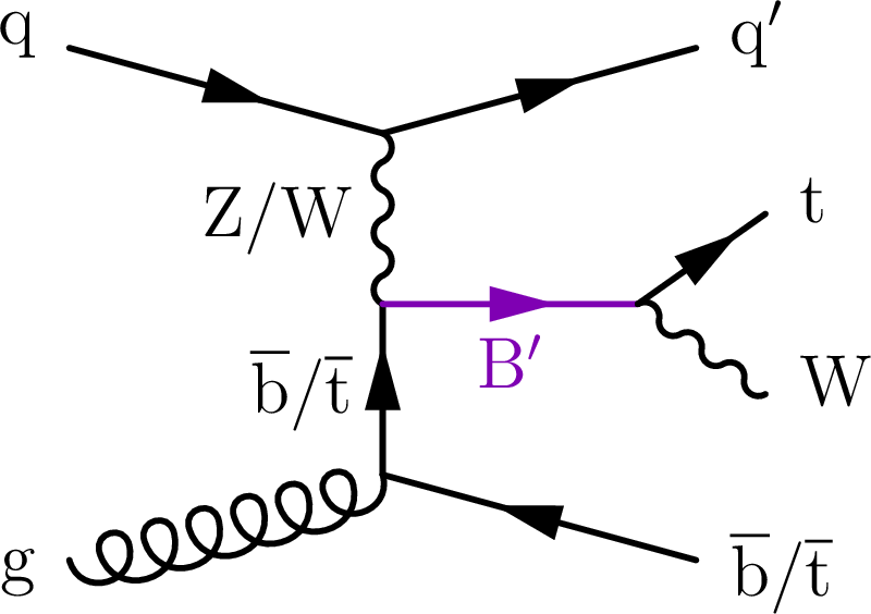
Figure 1:
Tree-level Feynman diagram showing the single production of a $ {\mathrm{B}}^{\prime}$ quark in association with an SM b quark or t quark, decaying in the $ \mathrm{t}\mathrm{W} $ channel. |
png pdf |
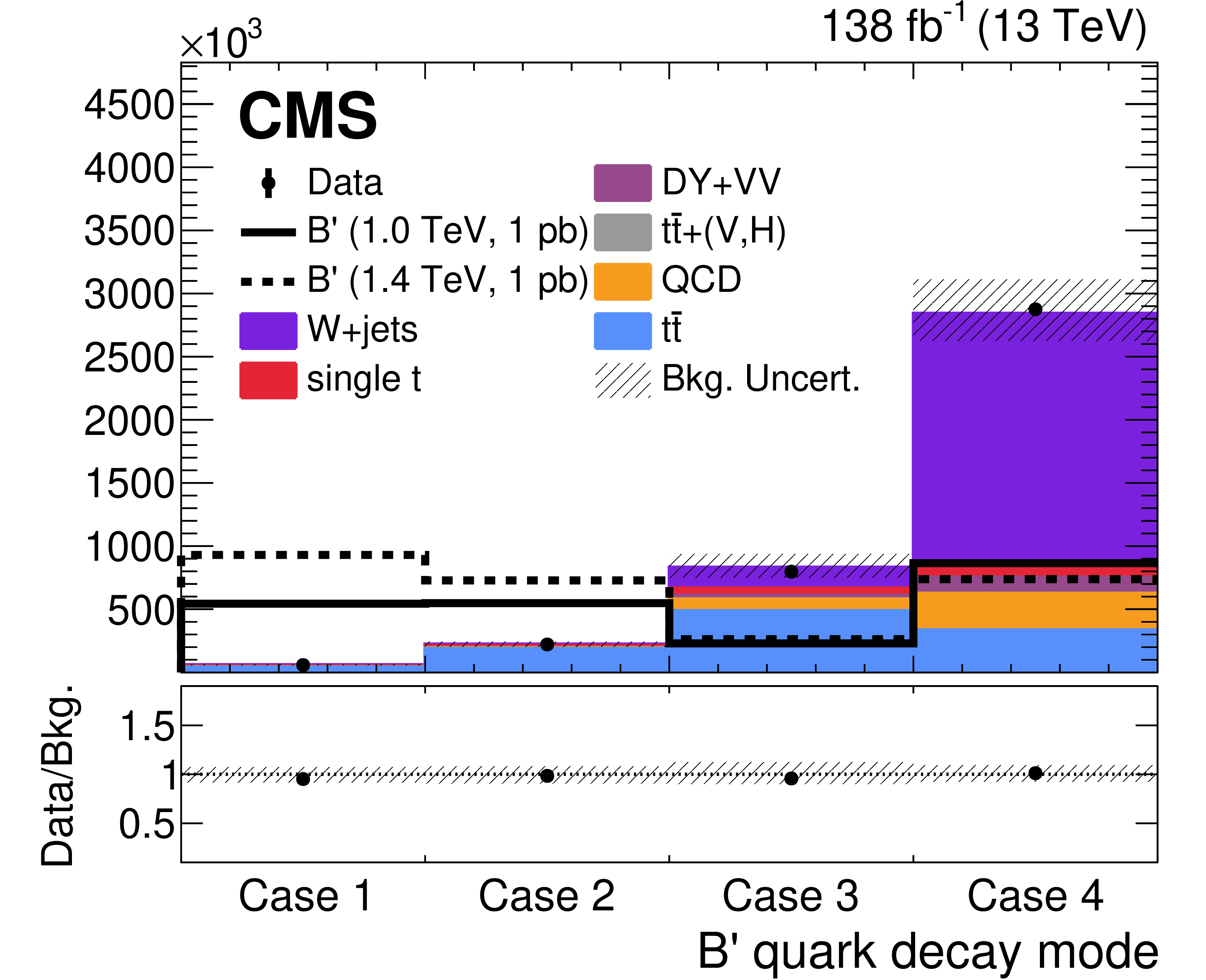
Figure 2:
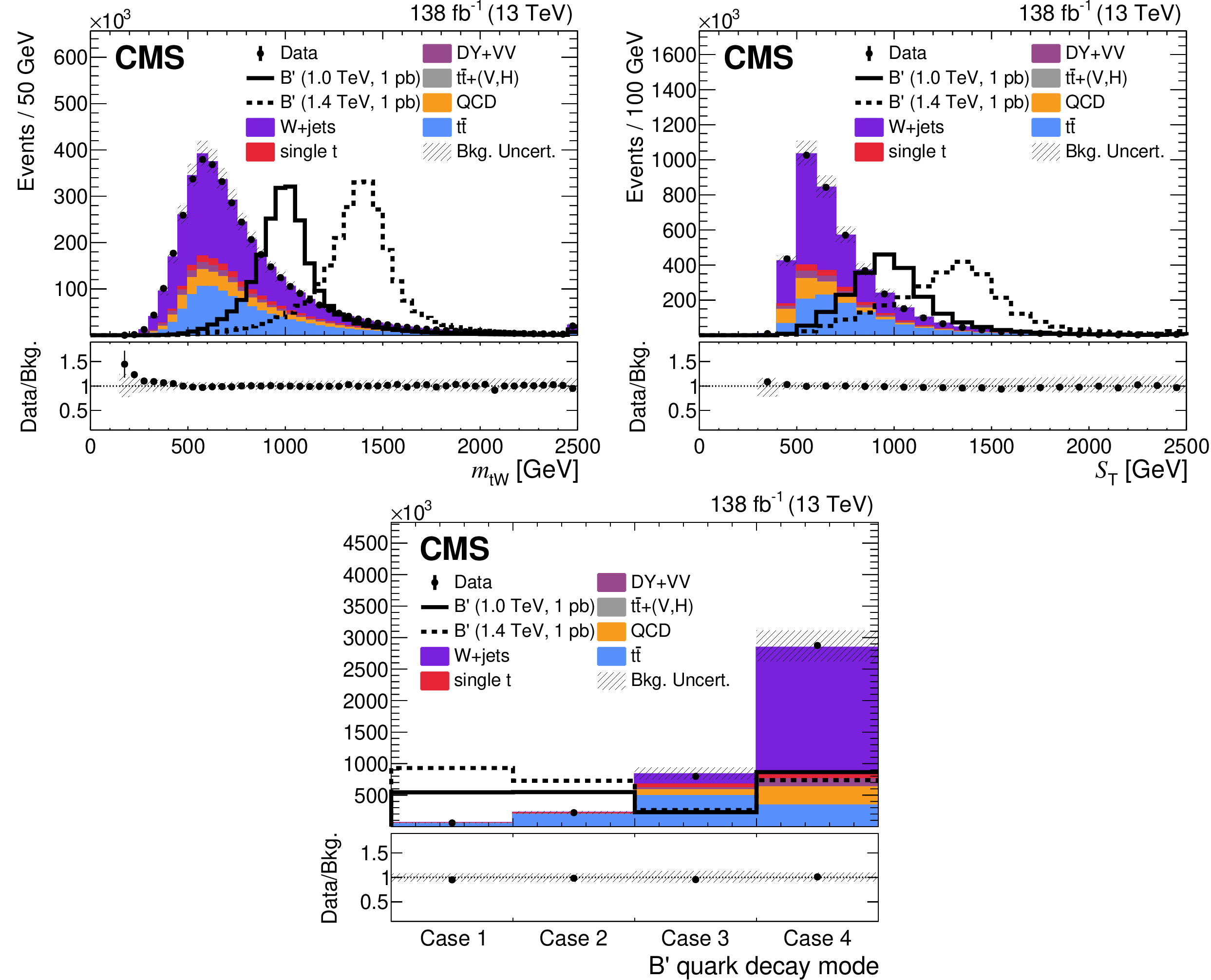
Distributions of the reconstructed $ {\mathrm{B}}^{\prime}$ quark mass, $ m_{\mathrm{t}\mathrm{W}} $ (upper left), the scalar $ p_{\mathrm{T}} $ sum ($ S_\mathrm{T} $) of small-radius jets, lepton, and $ p_{\mathrm{T}}^\text{miss} $ (upper right), and the reconstruction case (lower) for all selected events. The observed data are shown as black markers. Predicted $ \mathrm{b}\mathrm{q}{\mathrm{B}}^{\prime} $ quark signals with masses of 1.0 and 1.4 TeV are shown as solid and dashed lines, respectively, normalized to a cross section of 1 pb for visualization. Simulated background estimates are displayed as filled histograms. The lower panels show the ratio of the data to the background prediction. Statistical and systematic uncertainties in the background estimate are indicated by hatched bands. |
png pdf |
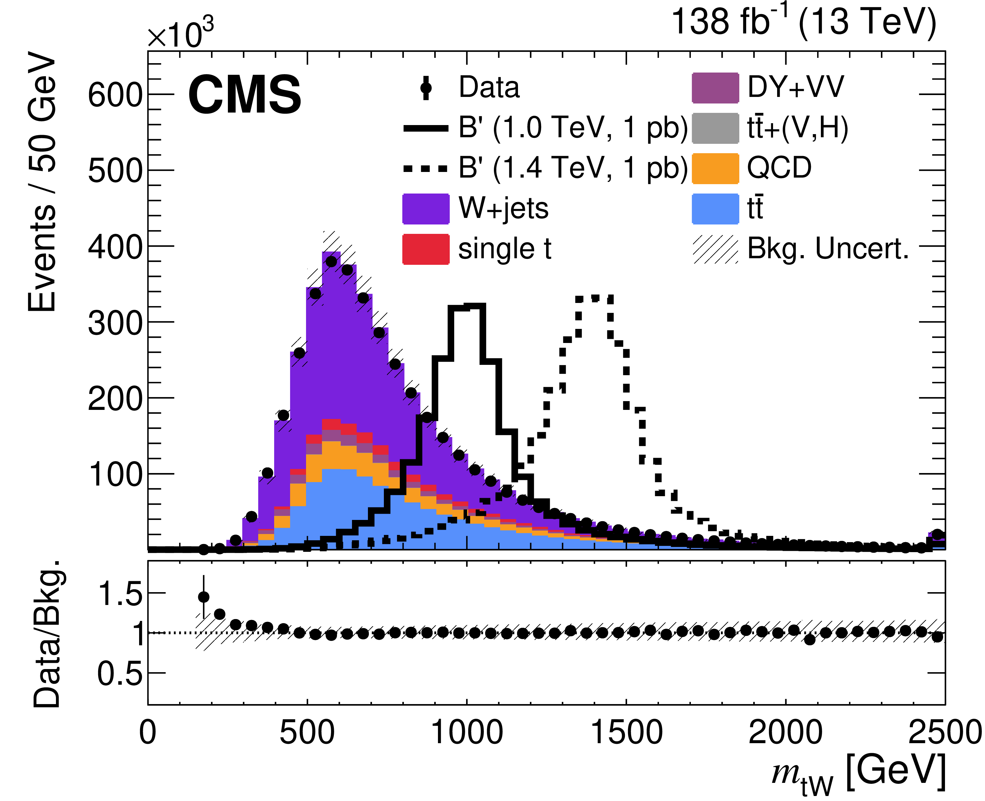
Figure 2-a:
Distributions of the reconstructed $ {\mathrm{B}}^{\prime}$ quark mass, $ m_{\mathrm{t}\mathrm{W}} $ (upper left), the scalar $ p_{\mathrm{T}} $ sum ($ S_\mathrm{T} $) of small-radius jets, lepton, and $ p_{\mathrm{T}}^\text{miss} $ (upper right), and the reconstruction case (lower) for all selected events. The observed data are shown as black markers. Predicted $ \mathrm{b}\mathrm{q}{\mathrm{B}}^{\prime} $ quark signals with masses of 1.0 and 1.4 TeV are shown as solid and dashed lines, respectively, normalized to a cross section of 1 pb for visualization. Simulated background estimates are displayed as filled histograms. The lower panels show the ratio of the data to the background prediction. Statistical and systematic uncertainties in the background estimate are indicated by hatched bands. |
png pdf |
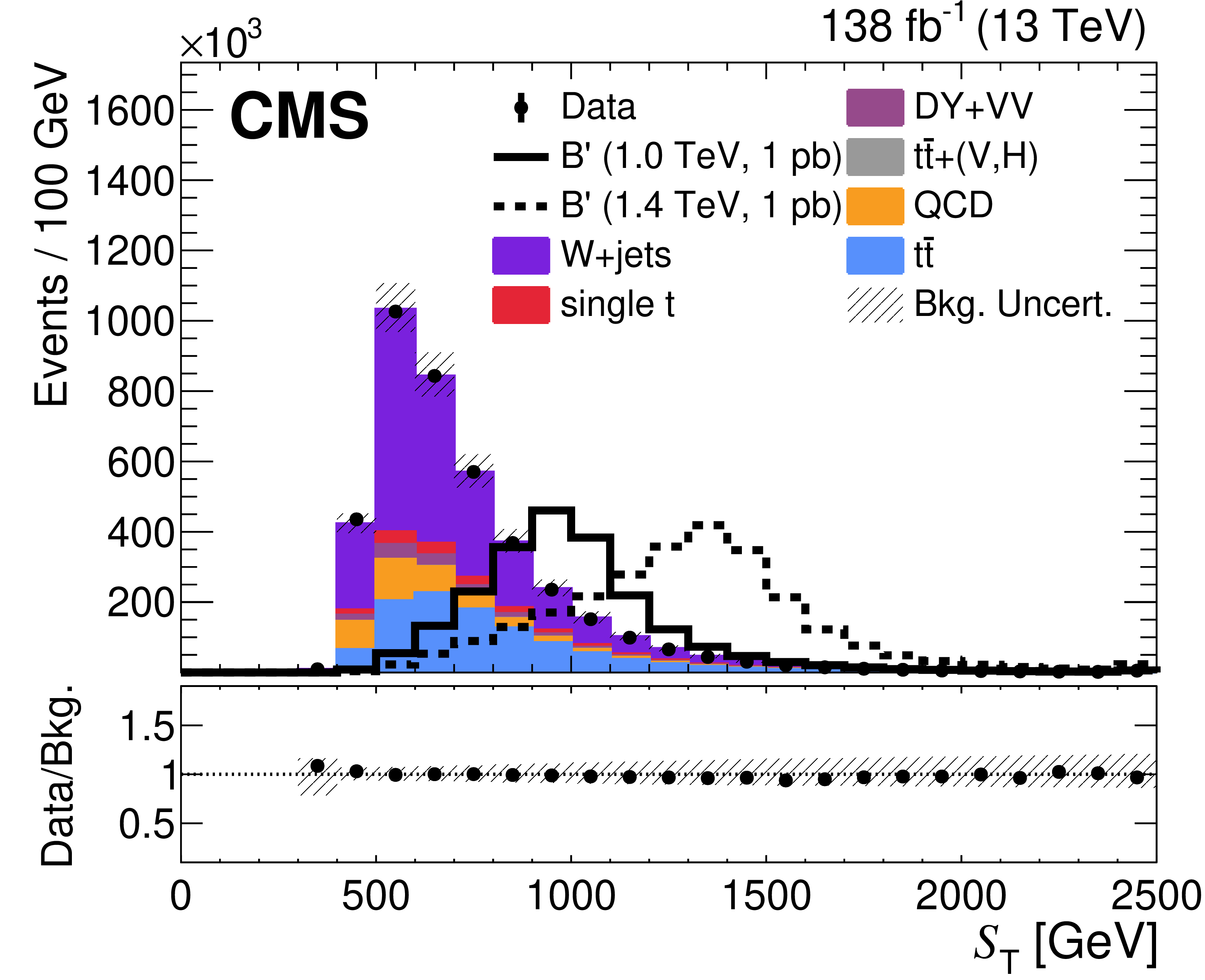
Figure 2-b:
Distributions of the reconstructed $ {\mathrm{B}}^{\prime}$ quark mass, $ m_{\mathrm{t}\mathrm{W}} $ (upper left), the scalar $ p_{\mathrm{T}} $ sum ($ S_\mathrm{T} $) of small-radius jets, lepton, and $ p_{\mathrm{T}}^\text{miss} $ (upper right), and the reconstruction case (lower) for all selected events. The observed data are shown as black markers. Predicted $ \mathrm{b}\mathrm{q}{\mathrm{B}}^{\prime} $ quark signals with masses of 1.0 and 1.4 TeV are shown as solid and dashed lines, respectively, normalized to a cross section of 1 pb for visualization. Simulated background estimates are displayed as filled histograms. The lower panels show the ratio of the data to the background prediction. Statistical and systematic uncertainties in the background estimate are indicated by hatched bands. |
png pdf |
Figure 2-c:
Distributions of the reconstructed $ {\mathrm{B}}^{\prime}$ quark mass, $ m_{\mathrm{t}\mathrm{W}} $ (upper left), the scalar $ p_{\mathrm{T}} $ sum ($ S_\mathrm{T} $) of small-radius jets, lepton, and $ p_{\mathrm{T}}^\text{miss} $ (upper right), and the reconstruction case (lower) for all selected events. The observed data are shown as black markers. Predicted $ \mathrm{b}\mathrm{q}{\mathrm{B}}^{\prime} $ quark signals with masses of 1.0 and 1.4 TeV are shown as solid and dashed lines, respectively, normalized to a cross section of 1 pb for visualization. Simulated background estimates are displayed as filled histograms. The lower panels show the ratio of the data to the background prediction. Statistical and systematic uncertainties in the background estimate are indicated by hatched bands. |
png pdf |
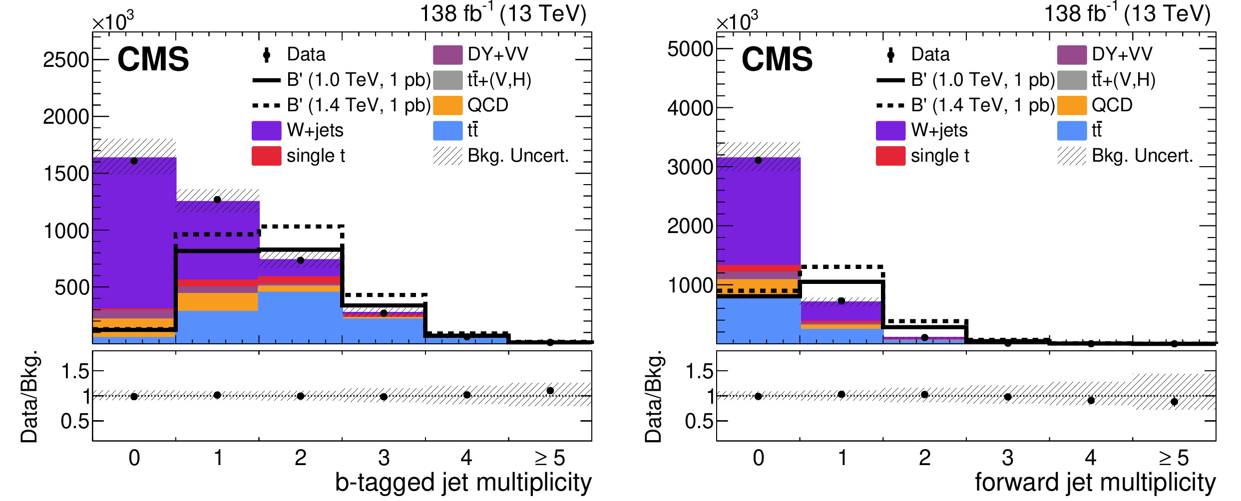
Figure 3:
Distributions of b-tagged jet multiplicity (left) and forward jet multiplicity (right) for all selected events. The observed data are shown as black markers. Predicted $ \mathrm{b}\mathrm{q}{\mathrm{B}}^{\prime} $ quark signals with masses of 1.0 and 1.4 TeV are shown as solid and dashed lines, respectively, normalized to a cross section of 1 pb for visualization. Simulated background estimates are displayed as filled histograms. The lower panels show the ratio of the data to the background prediction. Statistical and systematic uncertainties in the background estimate are indicated by hatched bands. |
png pdf |
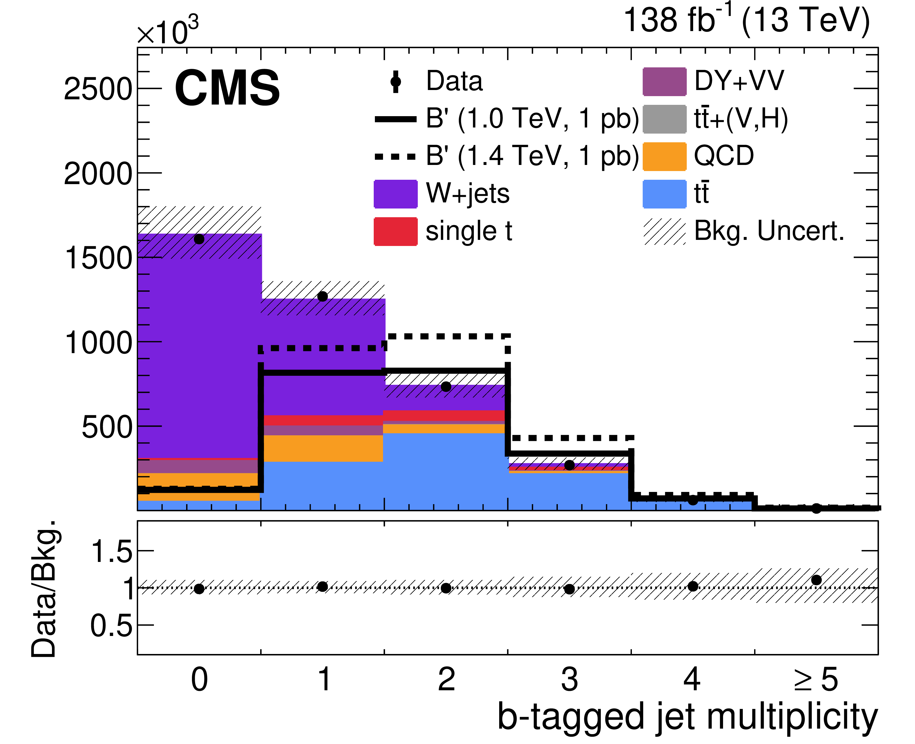
Figure 3-a:
Distributions of b-tagged jet multiplicity (left) and forward jet multiplicity (right) for all selected events. The observed data are shown as black markers. Predicted $ \mathrm{b}\mathrm{q}{\mathrm{B}}^{\prime} $ quark signals with masses of 1.0 and 1.4 TeV are shown as solid and dashed lines, respectively, normalized to a cross section of 1 pb for visualization. Simulated background estimates are displayed as filled histograms. The lower panels show the ratio of the data to the background prediction. Statistical and systematic uncertainties in the background estimate are indicated by hatched bands. |
png pdf |
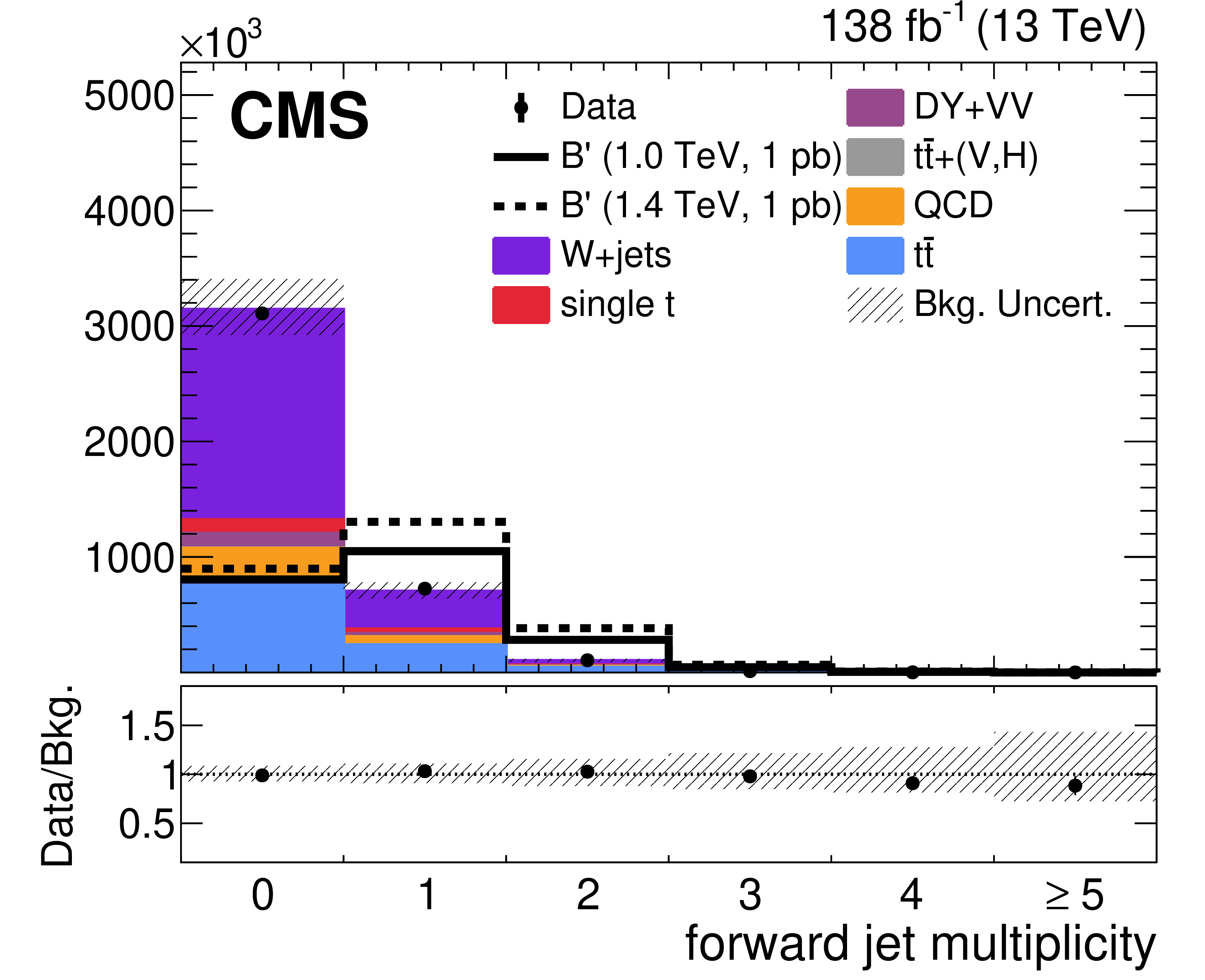
Figure 3-b:
Distributions of b-tagged jet multiplicity (left) and forward jet multiplicity (right) for all selected events. The observed data are shown as black markers. Predicted $ \mathrm{b}\mathrm{q}{\mathrm{B}}^{\prime} $ quark signals with masses of 1.0 and 1.4 TeV are shown as solid and dashed lines, respectively, normalized to a cross section of 1 pb for visualization. Simulated background estimates are displayed as filled histograms. The lower panels show the ratio of the data to the background prediction. Statistical and systematic uncertainties in the background estimate are indicated by hatched bands. |
png pdf |
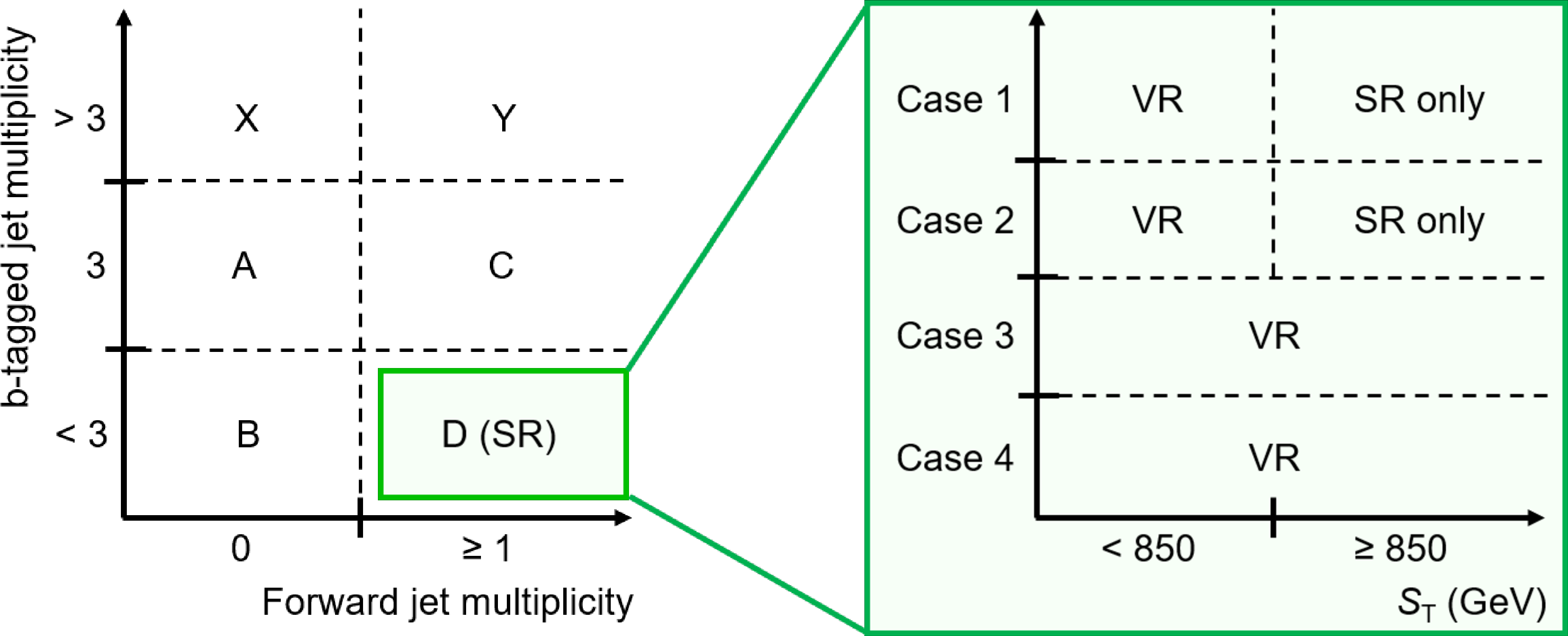
Figure 4:
Diagrams illustrating the definitions and labels of the CRs and SR (left), and the subsets of the SR used for validation (right). |
png pdf |
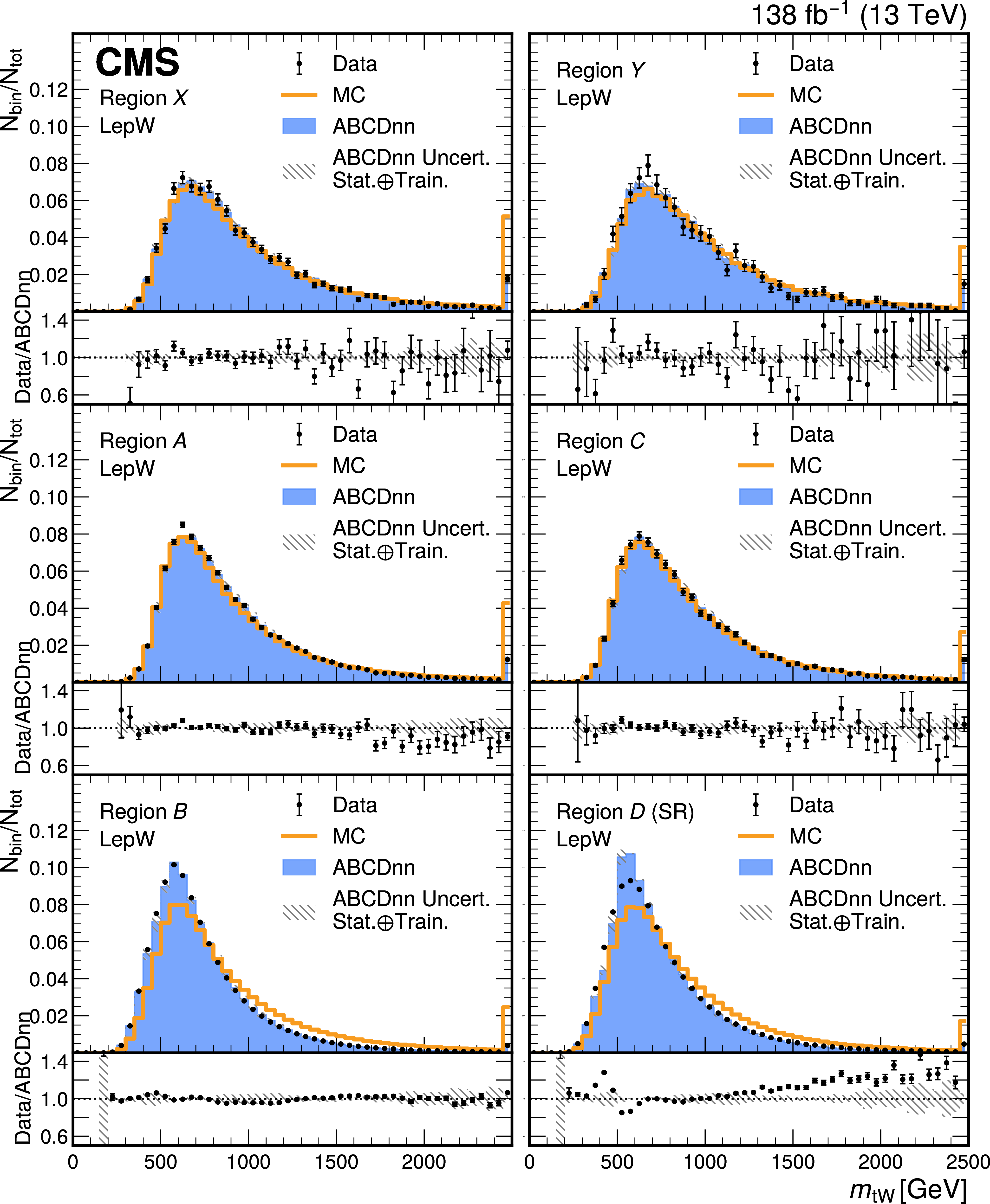
Figure 5:
Distributions of $ m_{\mathrm{t}\mathrm{W}} $ in the SR and CRs for the lepW ABCDnn model, normalized to unity. Observed data are shown as black markers with statistical uncertainties. Major background distributions from simulation are shown as orange solid lines with statistical uncertainties and are labeled ``MC''. The ABCDnn predictions are shown as blue filled histograms. The lower panels show the ratio of the data to the ABCDnn prediction. Statistical and training uncertainties in the ABCDnn predictions are indicated by hatched bands, though they are too small to be visible in the upper panels. |
png pdf |
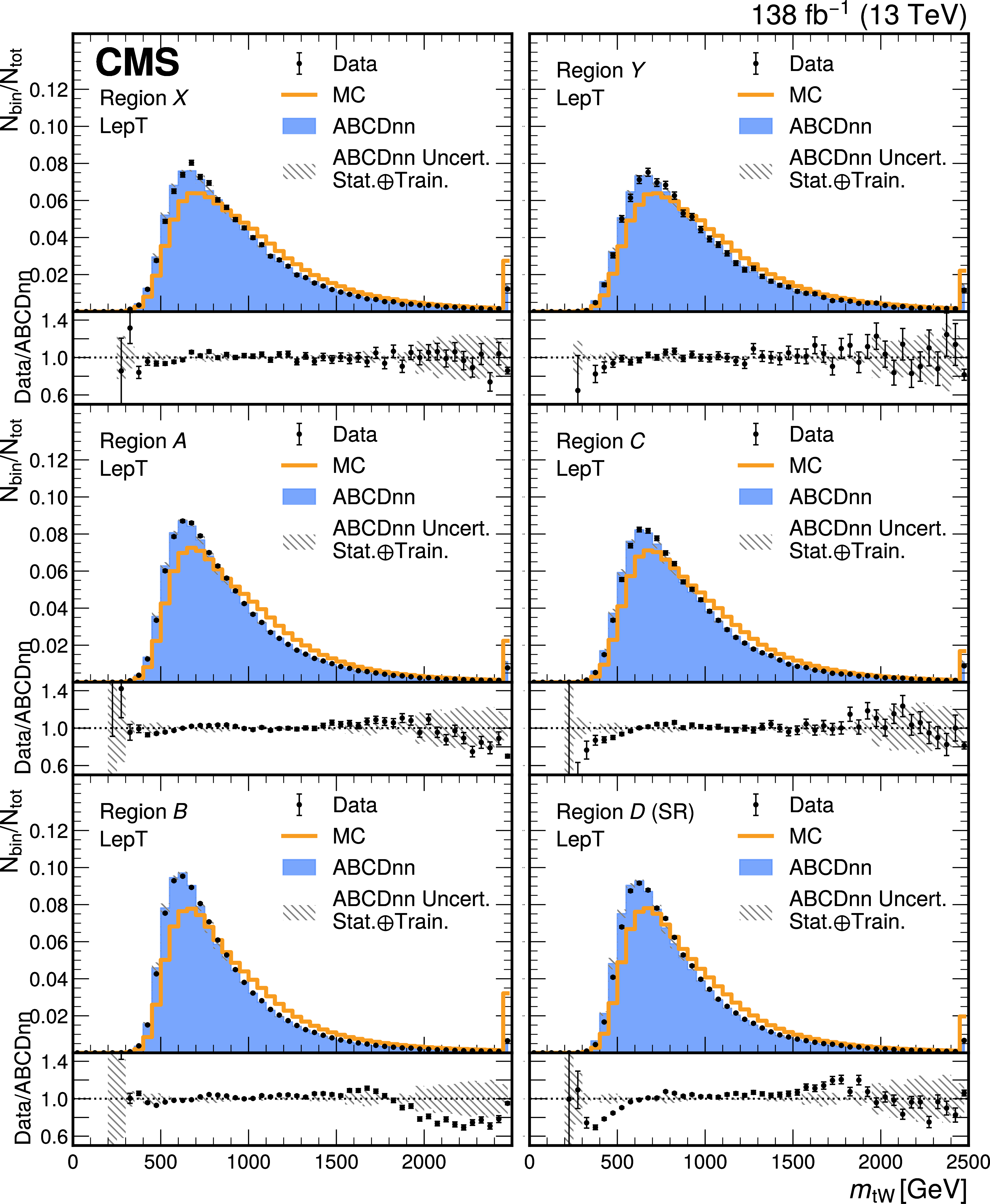
Figure 6:
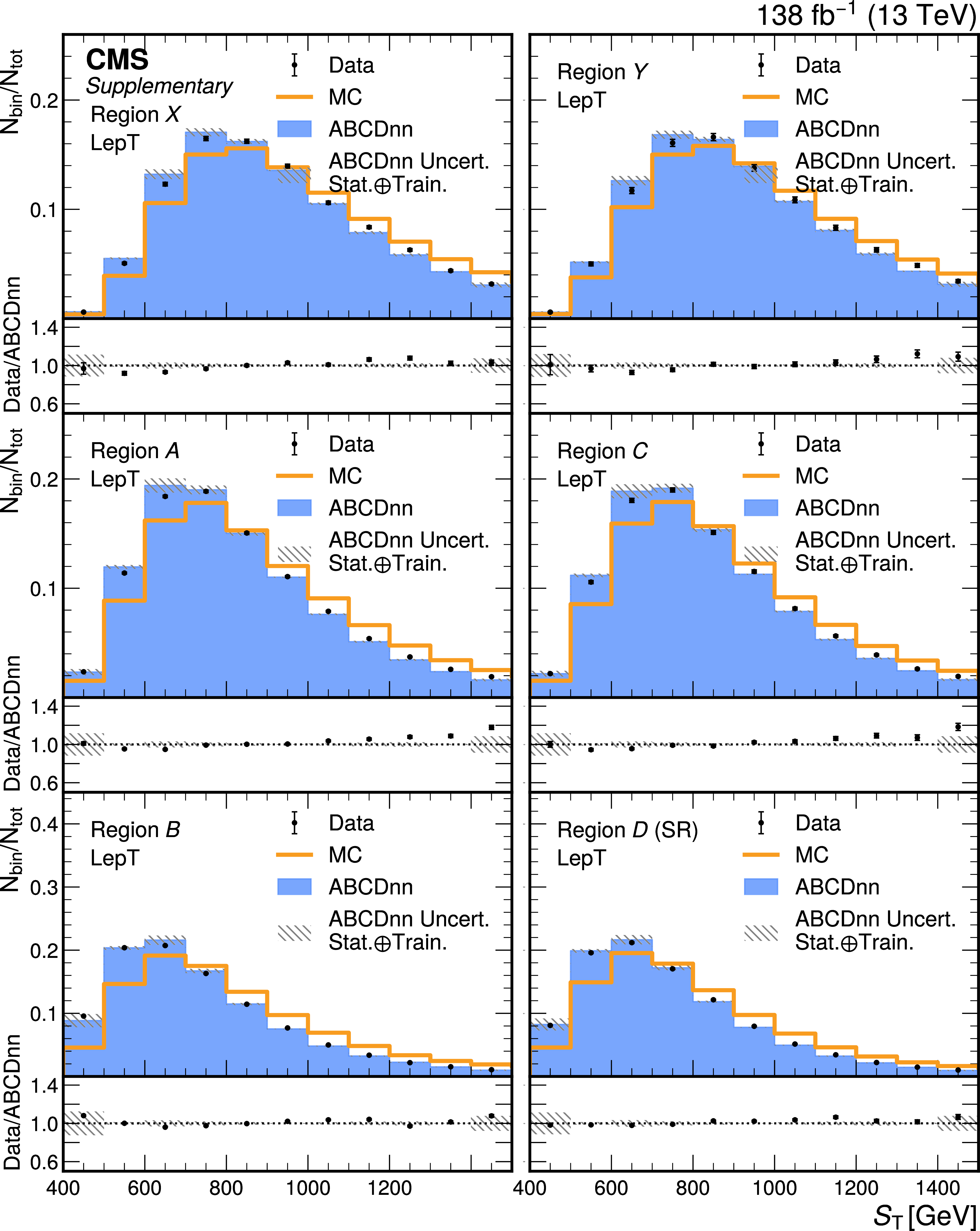
Distributions of $ m_{\mathrm{t}\mathrm{W}} $ in the SR and CRs for the lepT ABCDnn model, normalized to unity. Observed data are shown as black markers with statistical uncertainties. Major background distributions from simulation are shown as orange solid lines with statistical uncertainties and are labeled ``MC''. The ABCDnn predictions are shown as blue filled histograms. The lower panels show the ratio of the data to the ABCDnn prediction. Statistical and training uncertainties in the ABCDnn predictions are indicated by hatched bands, though they are too small to be visible in the upper panels. |
png pdf |
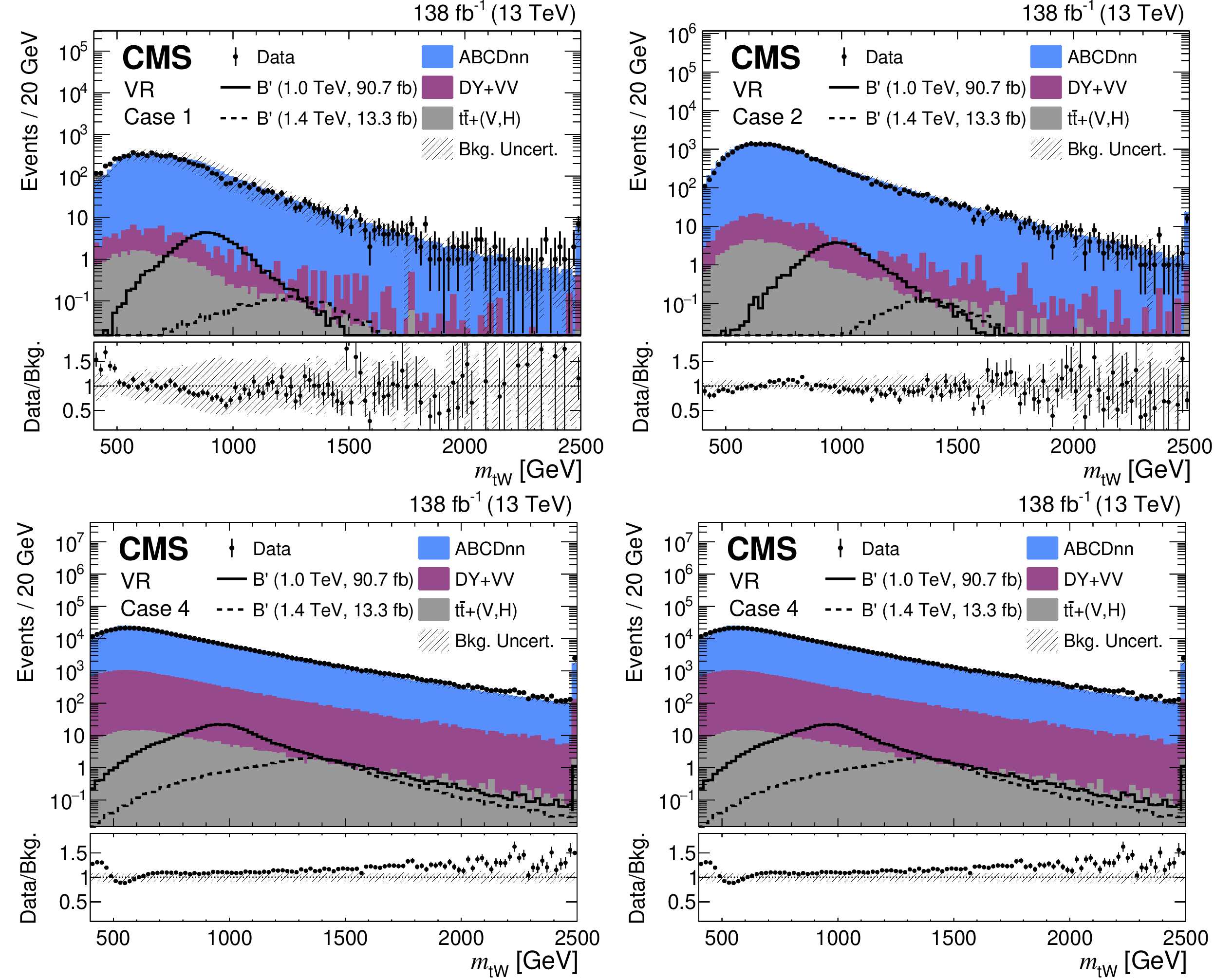
Figure 7:
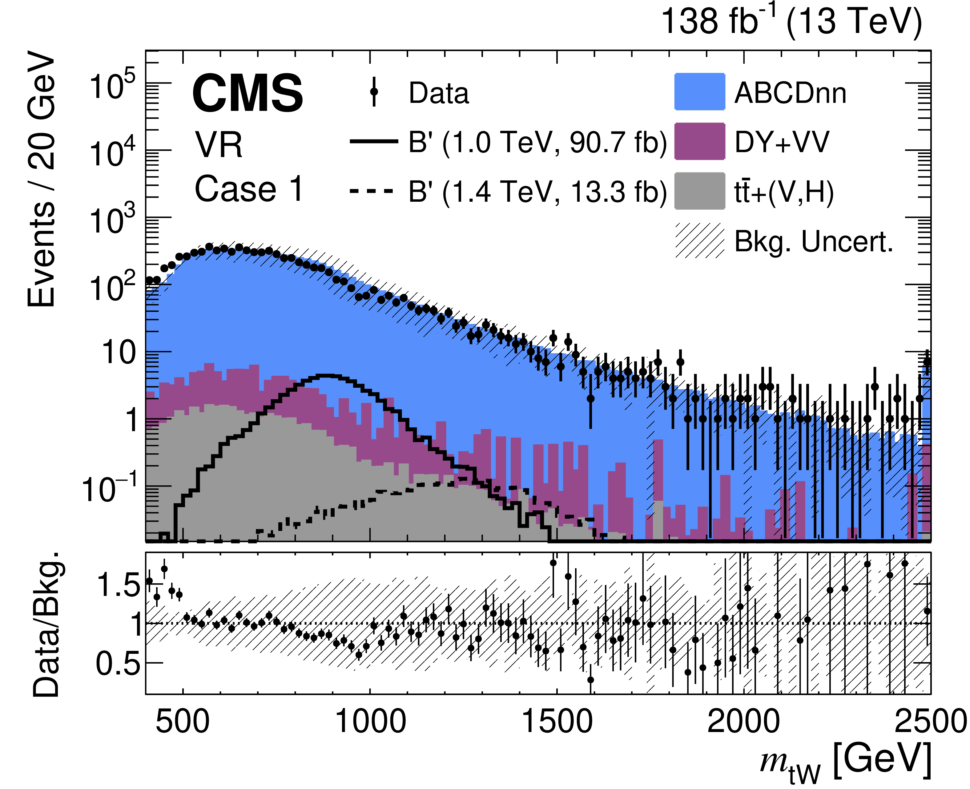
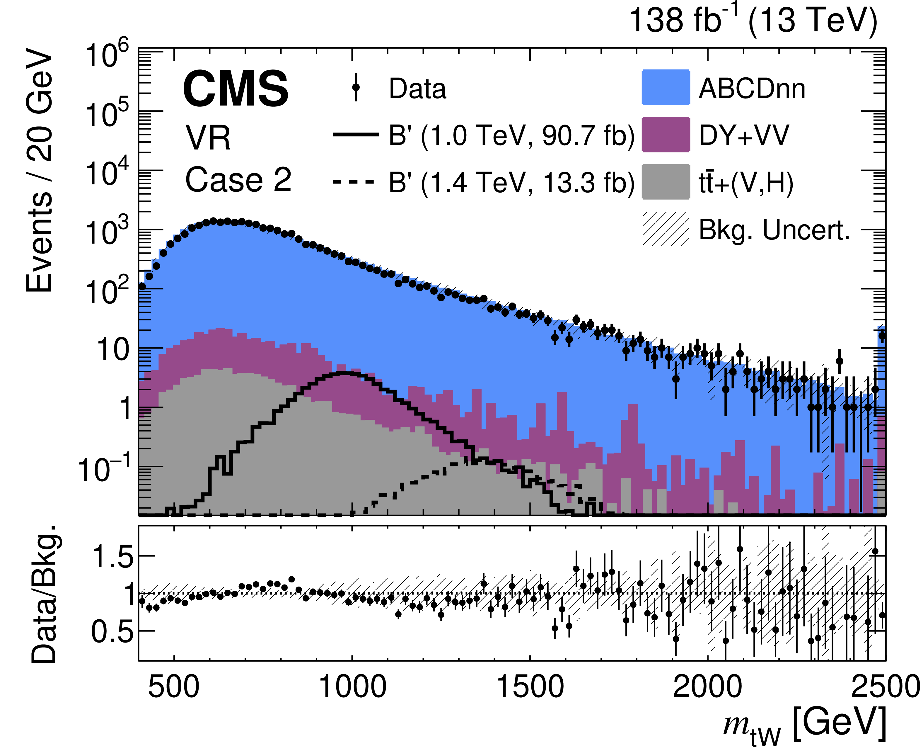
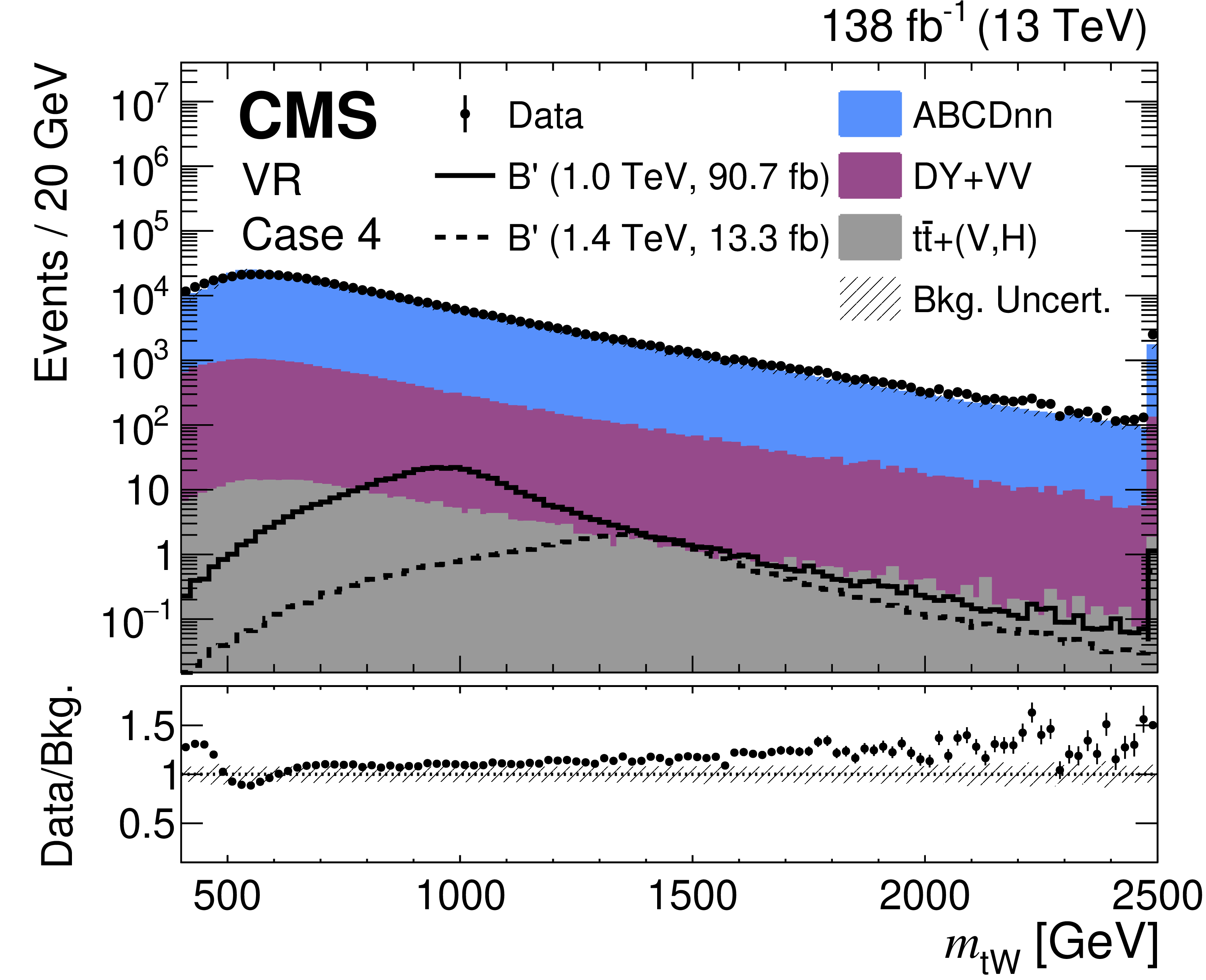
Distributions of $ m_{\mathrm{t}\mathrm{W}} $ for VR events in Case 1 (upper left) through Case 4 (lower right). Observed data are shown as black markers. Predicted $ \mathrm{b}\mathrm{q}{\mathrm{B}}^{\prime} $ quark signals with masses of 1.0 and 1.4 TeV are shown as solid and dashed lines, respectively, normalized to the predicted cross section for singlet $ \mathrm{b}\mathrm{q}{\mathrm{B}}^{\prime} $ production with $ \Gamma/m_{{\mathrm{B}}^{\prime}} =5% $. Background estimates are displayed as filled histograms, with the ABCDnn prediction shown prior to application of the closure correction. The lower panels show the ratio of the data to the background prediction. Statistical and systematic uncertainties in the background estimate are indicated by hatched bands. |
png pdf |
Figure 7-a:
Distributions of $ m_{\mathrm{t}\mathrm{W}} $ for VR events in Case 1 (upper left) through Case 4 (lower right). Observed data are shown as black markers. Predicted $ \mathrm{b}\mathrm{q}{\mathrm{B}}^{\prime} $ quark signals with masses of 1.0 and 1.4 TeV are shown as solid and dashed lines, respectively, normalized to the predicted cross section for singlet $ \mathrm{b}\mathrm{q}{\mathrm{B}}^{\prime} $ production with $ \Gamma/m_{{\mathrm{B}}^{\prime}} =5% $. Background estimates are displayed as filled histograms, with the ABCDnn prediction shown prior to application of the closure correction. The lower panels show the ratio of the data to the background prediction. Statistical and systematic uncertainties in the background estimate are indicated by hatched bands. |
png pdf |
Figure 7-b:
Distributions of $ m_{\mathrm{t}\mathrm{W}} $ for VR events in Case 1 (upper left) through Case 4 (lower right). Observed data are shown as black markers. Predicted $ \mathrm{b}\mathrm{q}{\mathrm{B}}^{\prime} $ quark signals with masses of 1.0 and 1.4 TeV are shown as solid and dashed lines, respectively, normalized to the predicted cross section for singlet $ \mathrm{b}\mathrm{q}{\mathrm{B}}^{\prime} $ production with $ \Gamma/m_{{\mathrm{B}}^{\prime}} =5% $. Background estimates are displayed as filled histograms, with the ABCDnn prediction shown prior to application of the closure correction. The lower panels show the ratio of the data to the background prediction. Statistical and systematic uncertainties in the background estimate are indicated by hatched bands. |

png pdf |
Figure 7-c:
Distributions of $ m_{\mathrm{t}\mathrm{W}} $ for VR events in Case 1 (upper left) through Case 4 (lower right). Observed data are shown as black markers. Predicted $ \mathrm{b}\mathrm{q}{\mathrm{B}}^{\prime} $ quark signals with masses of 1.0 and 1.4 TeV are shown as solid and dashed lines, respectively, normalized to the predicted cross section for singlet $ \mathrm{b}\mathrm{q}{\mathrm{B}}^{\prime} $ production with $ \Gamma/m_{{\mathrm{B}}^{\prime}} =5% $. Background estimates are displayed as filled histograms, with the ABCDnn prediction shown prior to application of the closure correction. The lower panels show the ratio of the data to the background prediction. Statistical and systematic uncertainties in the background estimate are indicated by hatched bands. |
png pdf |
Figure 7-d:
Distributions of $ m_{\mathrm{t}\mathrm{W}} $ for VR events in Case 1 (upper left) through Case 4 (lower right). Observed data are shown as black markers. Predicted $ \mathrm{b}\mathrm{q}{\mathrm{B}}^{\prime} $ quark signals with masses of 1.0 and 1.4 TeV are shown as solid and dashed lines, respectively, normalized to the predicted cross section for singlet $ \mathrm{b}\mathrm{q}{\mathrm{B}}^{\prime} $ production with $ \Gamma/m_{{\mathrm{B}}^{\prime}} =5% $. Background estimates are displayed as filled histograms, with the ABCDnn prediction shown prior to application of the closure correction. The lower panels show the ratio of the data to the background prediction. Statistical and systematic uncertainties in the background estimate are indicated by hatched bands. |
png pdf |
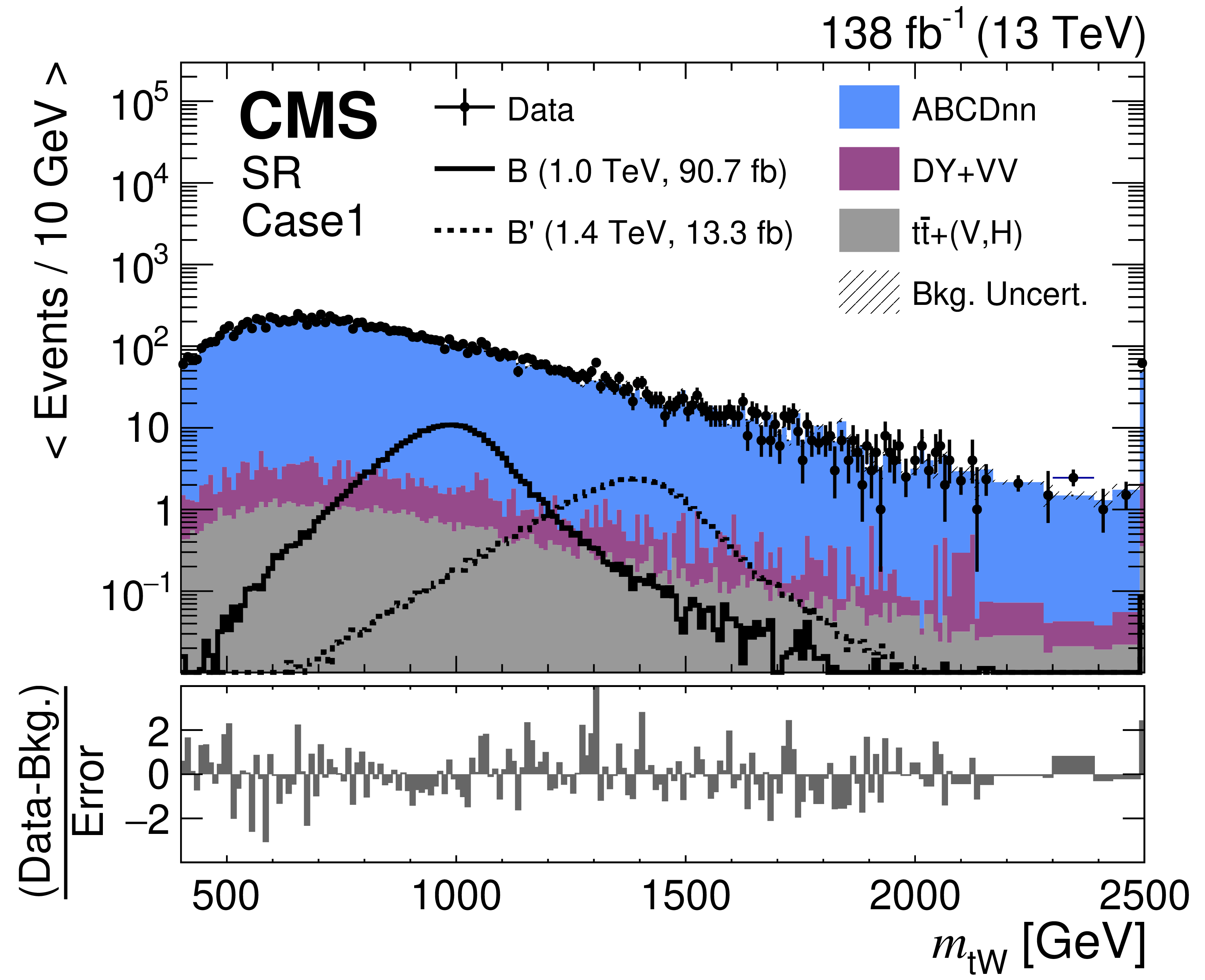
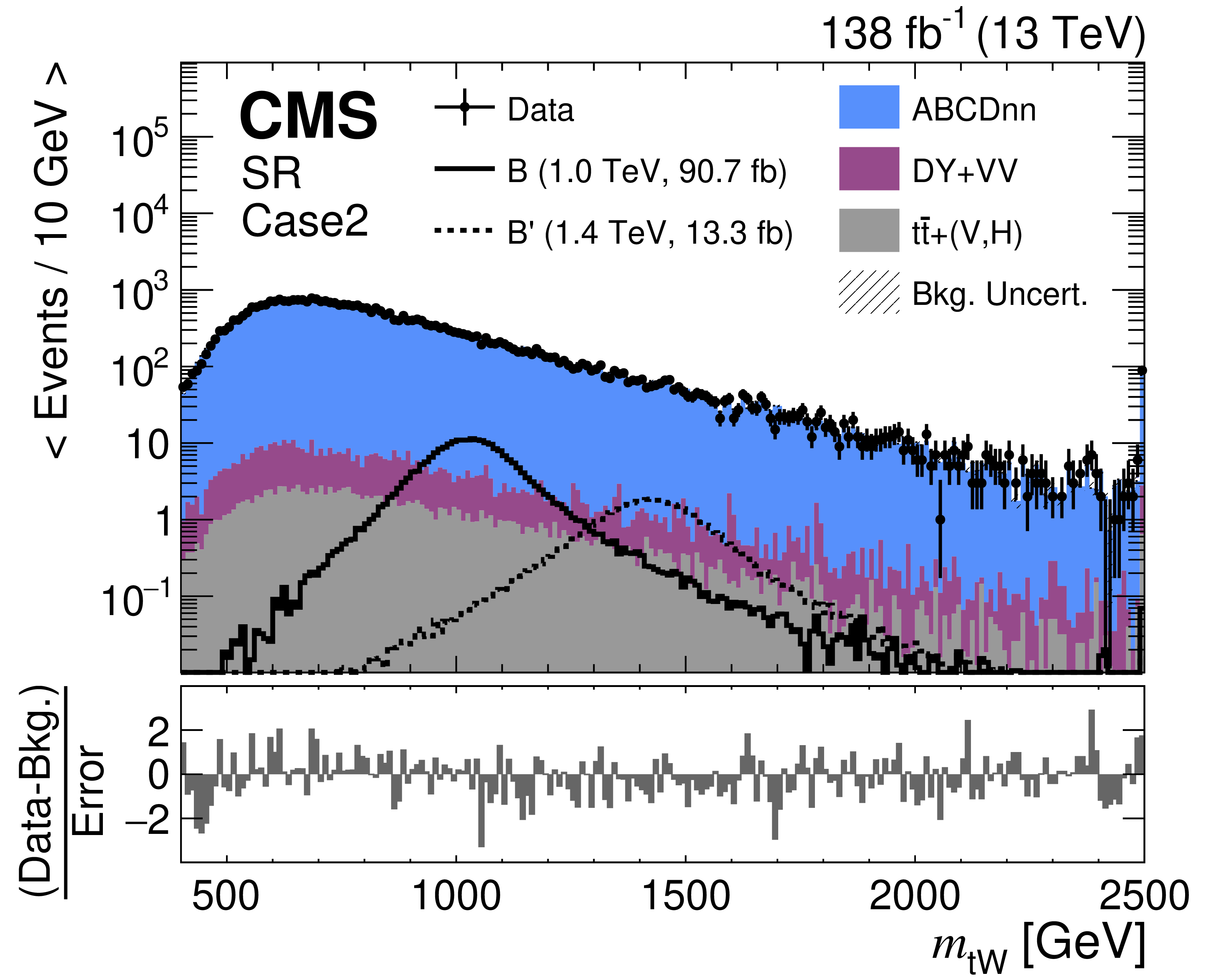
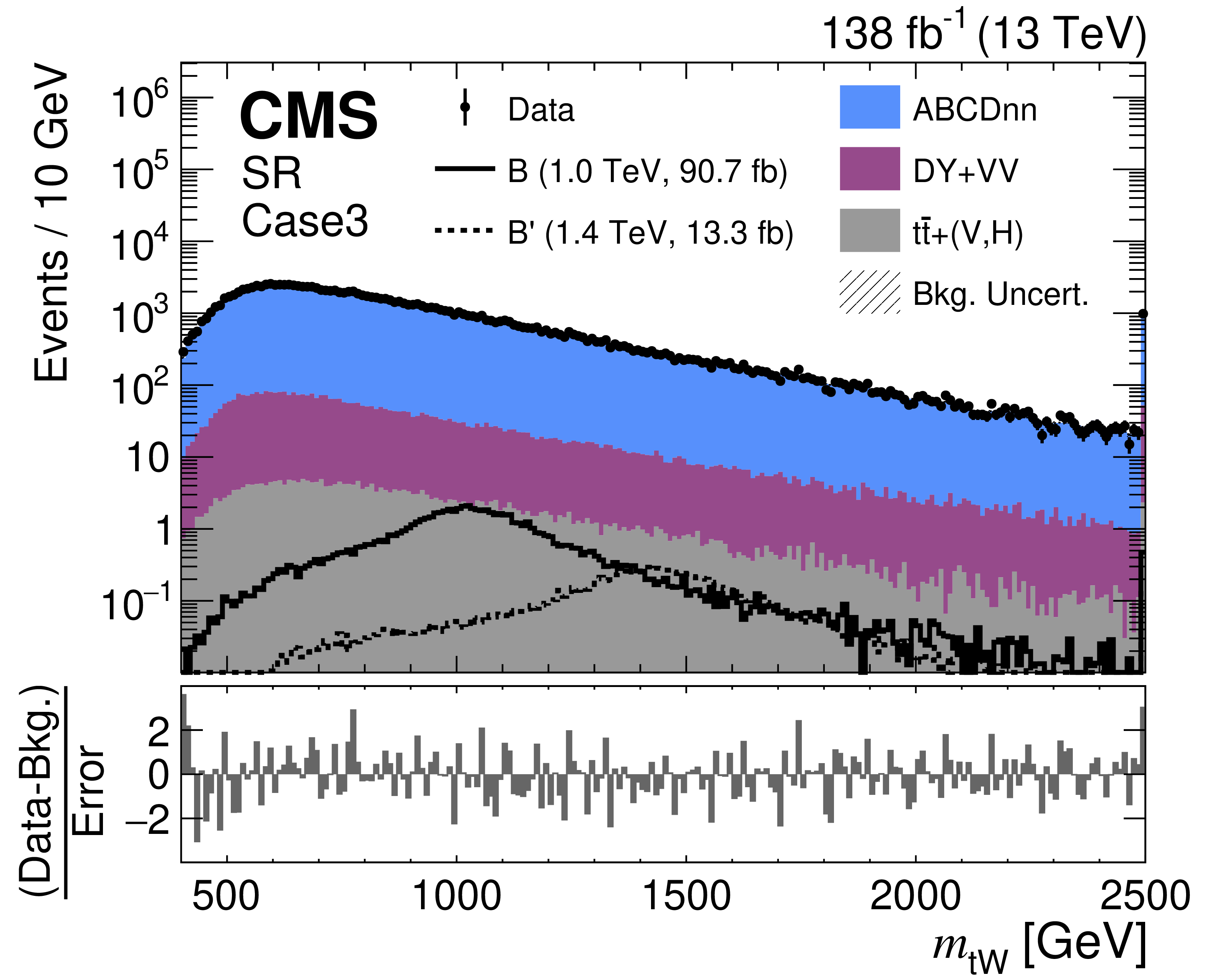
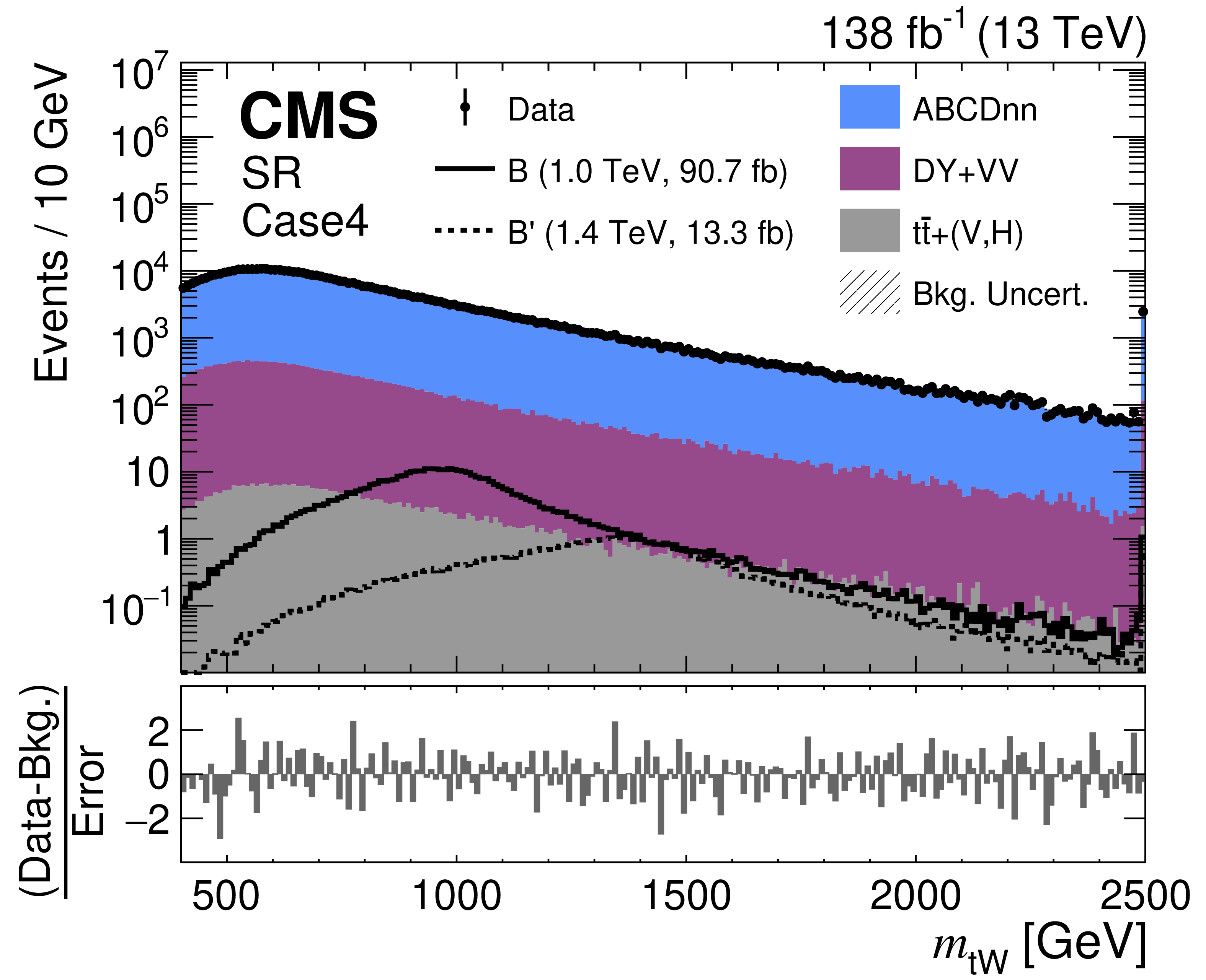
Figure 8:
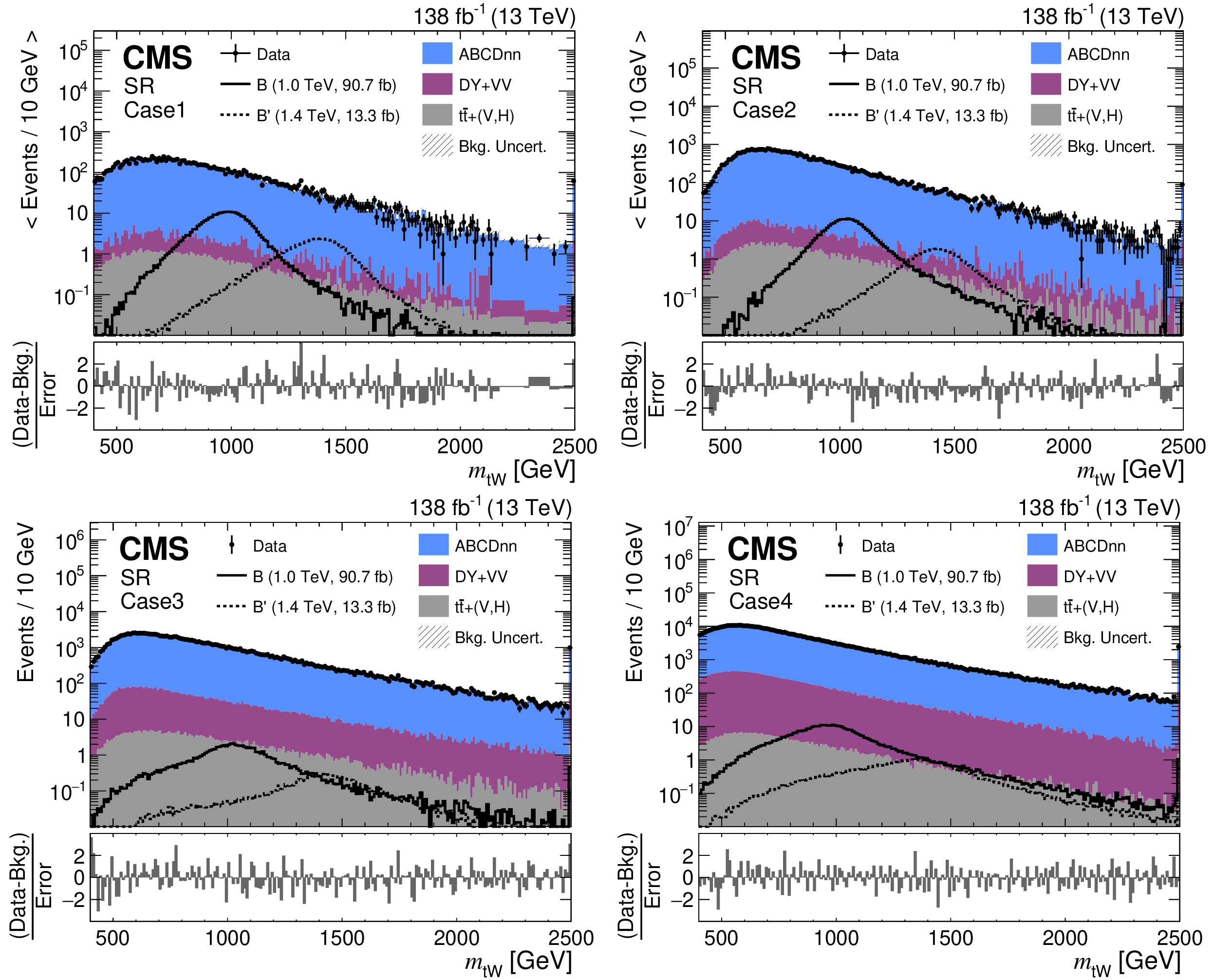
Distributions of $ m_{\mathrm{t}\mathrm{W}} $ for events in the SR in Case 1 (upper left) through Case 4 (lower right). The observed data are shown as black markers. Predicted $ \mathrm{b}\mathrm{q}{\mathrm{B}}^{\prime} $ quark signals with masses of 1.0 and 1.4 TeV are shown as the solid and dashed lines, respectively, normalized to the predicted cross section for singlet $ \mathrm{b}\mathrm{q}{\mathrm{B}}^{\prime} $ production with $ \Gamma/m_{{\mathrm{B}}^{\prime}} =5% $. The best-fit background prediction from a background-only fit to data is shown as the filled histograms. The lower panels show the difference between the data and the background prediction, divided by the total uncertainty in the background estimate. |
png pdf |
Figure 8-a:
Distributions of $ m_{\mathrm{t}\mathrm{W}} $ for events in the SR in Case 1 (upper left) through Case 4 (lower right). The observed data are shown as black markers. Predicted $ \mathrm{b}\mathrm{q}{\mathrm{B}}^{\prime} $ quark signals with masses of 1.0 and 1.4 TeV are shown as the solid and dashed lines, respectively, normalized to the predicted cross section for singlet $ \mathrm{b}\mathrm{q}{\mathrm{B}}^{\prime} $ production with $ \Gamma/m_{{\mathrm{B}}^{\prime}} =5% $. The best-fit background prediction from a background-only fit to data is shown as the filled histograms. The lower panels show the difference between the data and the background prediction, divided by the total uncertainty in the background estimate. |
png pdf |
Figure 8-b:
Distributions of $ m_{\mathrm{t}\mathrm{W}} $ for events in the SR in Case 1 (upper left) through Case 4 (lower right). The observed data are shown as black markers. Predicted $ \mathrm{b}\mathrm{q}{\mathrm{B}}^{\prime} $ quark signals with masses of 1.0 and 1.4 TeV are shown as the solid and dashed lines, respectively, normalized to the predicted cross section for singlet $ \mathrm{b}\mathrm{q}{\mathrm{B}}^{\prime} $ production with $ \Gamma/m_{{\mathrm{B}}^{\prime}} =5% $. The best-fit background prediction from a background-only fit to data is shown as the filled histograms. The lower panels show the difference between the data and the background prediction, divided by the total uncertainty in the background estimate. |
png pdf |
Figure 8-c:
Distributions of $ m_{\mathrm{t}\mathrm{W}} $ for events in the SR in Case 1 (upper left) through Case 4 (lower right). The observed data are shown as black markers. Predicted $ \mathrm{b}\mathrm{q}{\mathrm{B}}^{\prime} $ quark signals with masses of 1.0 and 1.4 TeV are shown as the solid and dashed lines, respectively, normalized to the predicted cross section for singlet $ \mathrm{b}\mathrm{q}{\mathrm{B}}^{\prime} $ production with $ \Gamma/m_{{\mathrm{B}}^{\prime}} =5% $. The best-fit background prediction from a background-only fit to data is shown as the filled histograms. The lower panels show the difference between the data and the background prediction, divided by the total uncertainty in the background estimate. |
png pdf |
Figure 8-d:
Distributions of $ m_{\mathrm{t}\mathrm{W}} $ for events in the SR in Case 1 (upper left) through Case 4 (lower right). The observed data are shown as black markers. Predicted $ \mathrm{b}\mathrm{q}{\mathrm{B}}^{\prime} $ quark signals with masses of 1.0 and 1.4 TeV are shown as the solid and dashed lines, respectively, normalized to the predicted cross section for singlet $ \mathrm{b}\mathrm{q}{\mathrm{B}}^{\prime} $ production with $ \Gamma/m_{{\mathrm{B}}^{\prime}} =5% $. The best-fit background prediction from a background-only fit to data is shown as the filled histograms. The lower panels show the difference between the data and the background prediction, divided by the total uncertainty in the background estimate. |
png pdf |
Figure 9:
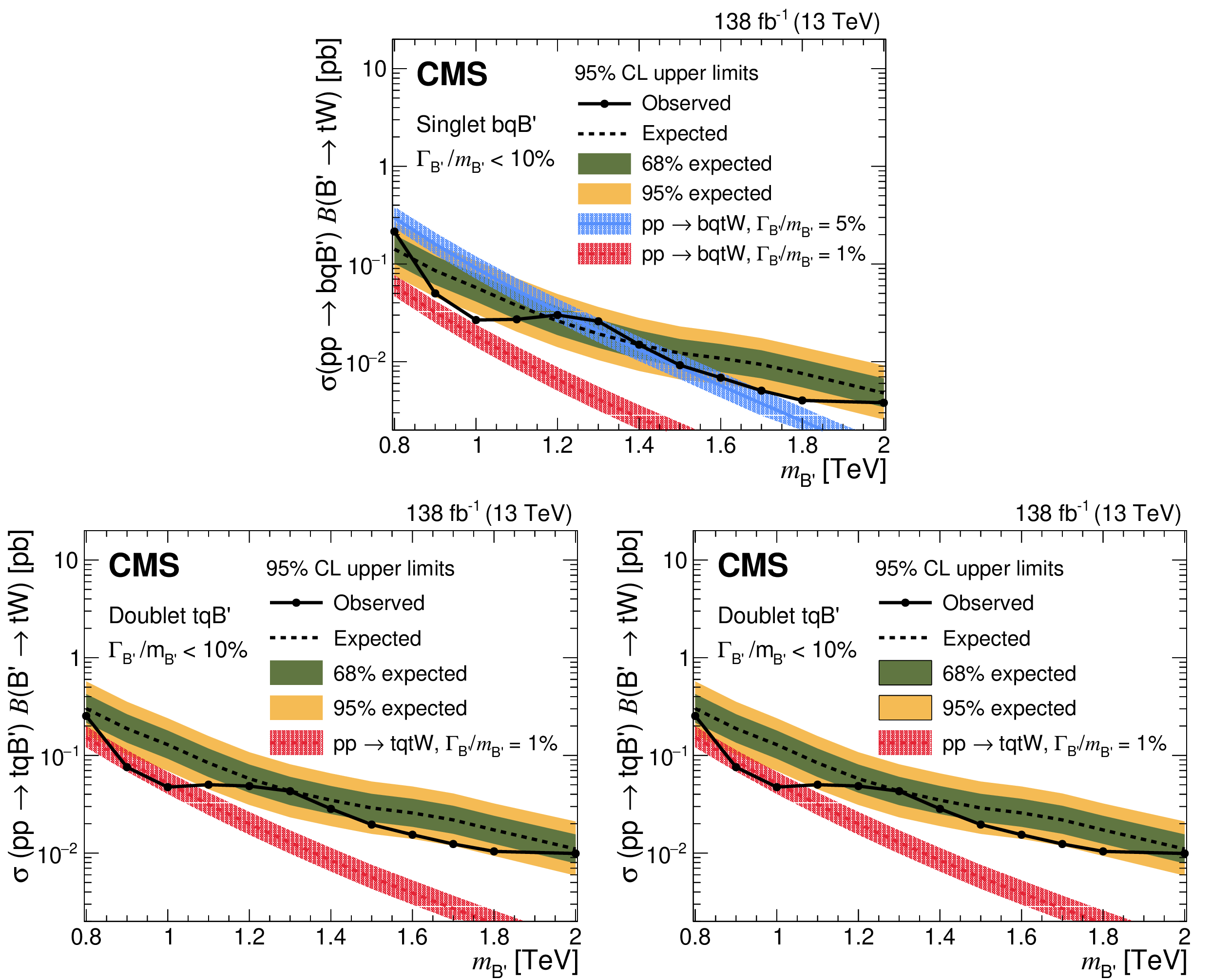
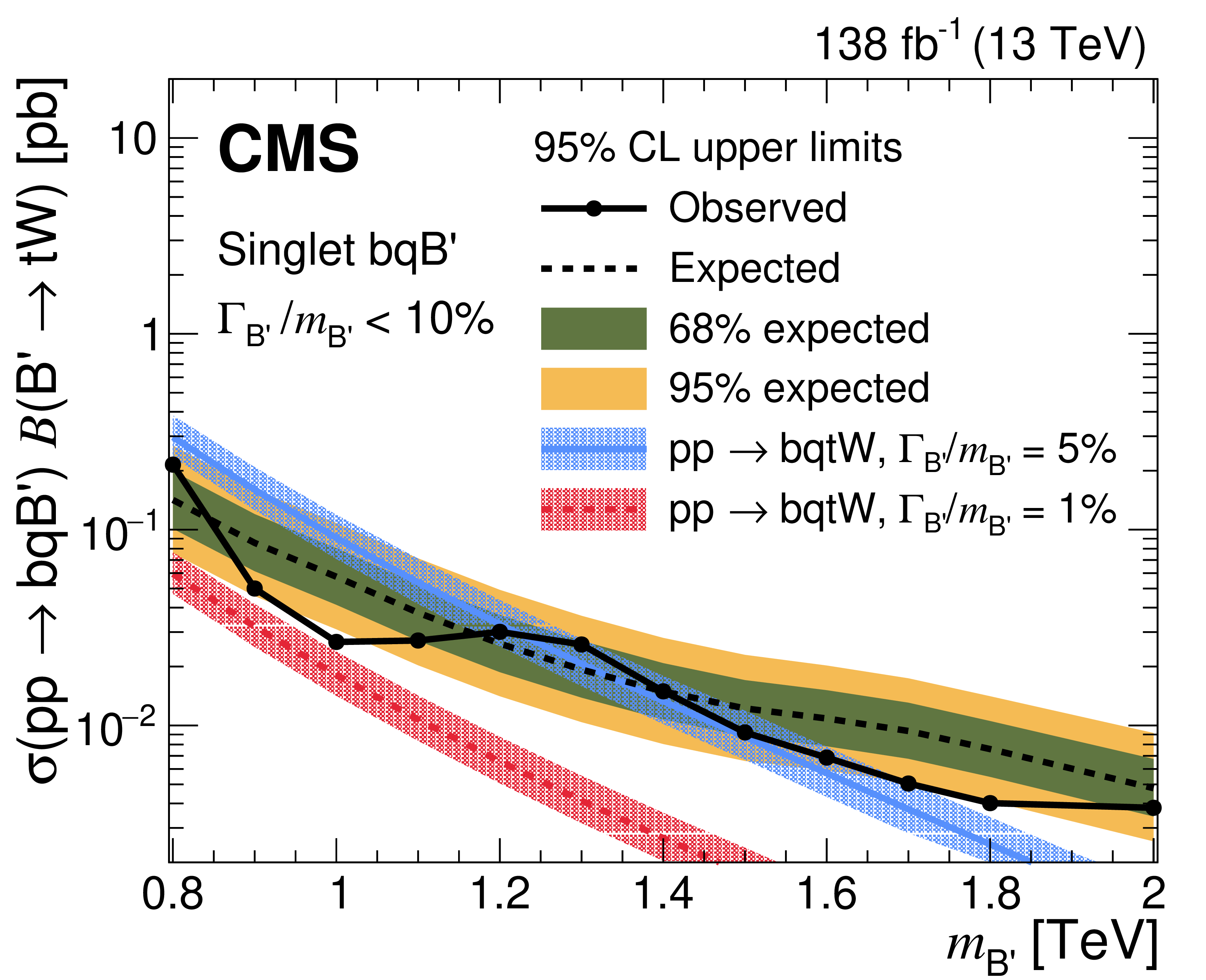
Observed (solid black lines) and expected (dashed lines) 95% CL upper limits on the product of the production cross section and branching fraction $ \mathcal{B}(\mathrm{t}\mathrm{W}) $ for singlet $ \mathrm{b}\mathrm{q}{\mathrm{B}}^{\prime} $ production (upper), singlet $ \mathrm{t}\mathrm{q}{\mathrm{B}}^{\prime} $ production (lower left), and up-type doublet $ \mathrm{t}\mathrm{q}{\mathrm{B}}^{\prime} $ production (lower right), as functions of $ m_{{\mathrm{B}}^{\prime}} $. Predicted cross sections for various $ {\mathrm{B}}^{\prime}$ quark relative widths are shown as dashed red and solid blue lines. The bands around the predicted cross sections represent the associated energy scale and PDF uncertainties. |
png pdf |
Figure 9-a:
Observed (solid black lines) and expected (dashed lines) 95% CL upper limits on the product of the production cross section and branching fraction $ \mathcal{B}(\mathrm{t}\mathrm{W}) $ for singlet $ \mathrm{b}\mathrm{q}{\mathrm{B}}^{\prime} $ production (upper), singlet $ \mathrm{t}\mathrm{q}{\mathrm{B}}^{\prime} $ production (lower left), and up-type doublet $ \mathrm{t}\mathrm{q}{\mathrm{B}}^{\prime} $ production (lower right), as functions of $ m_{{\mathrm{B}}^{\prime}} $. Predicted cross sections for various $ {\mathrm{B}}^{\prime}$ quark relative widths are shown as dashed red and solid blue lines. The bands around the predicted cross sections represent the associated energy scale and PDF uncertainties. |
png pdf |
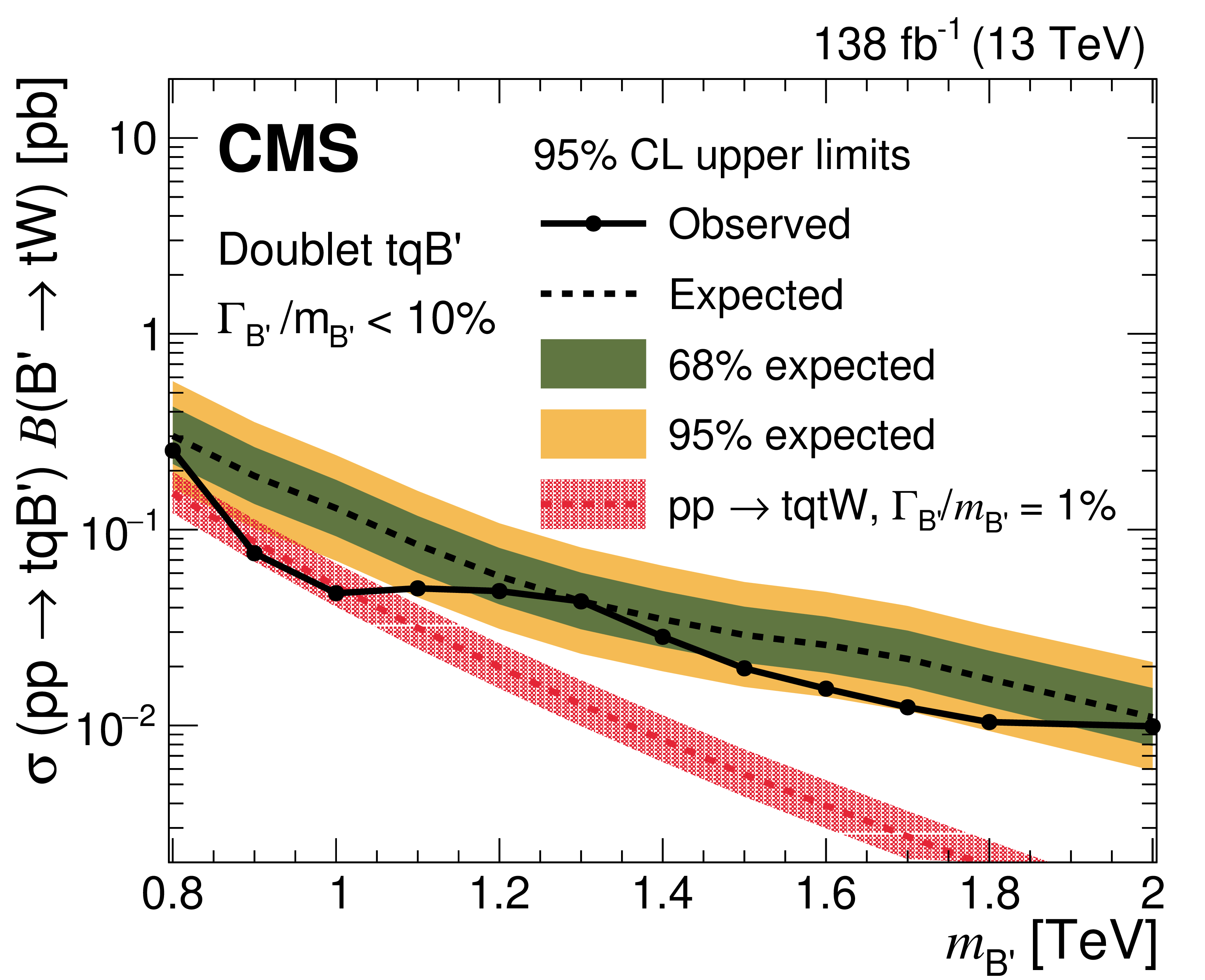
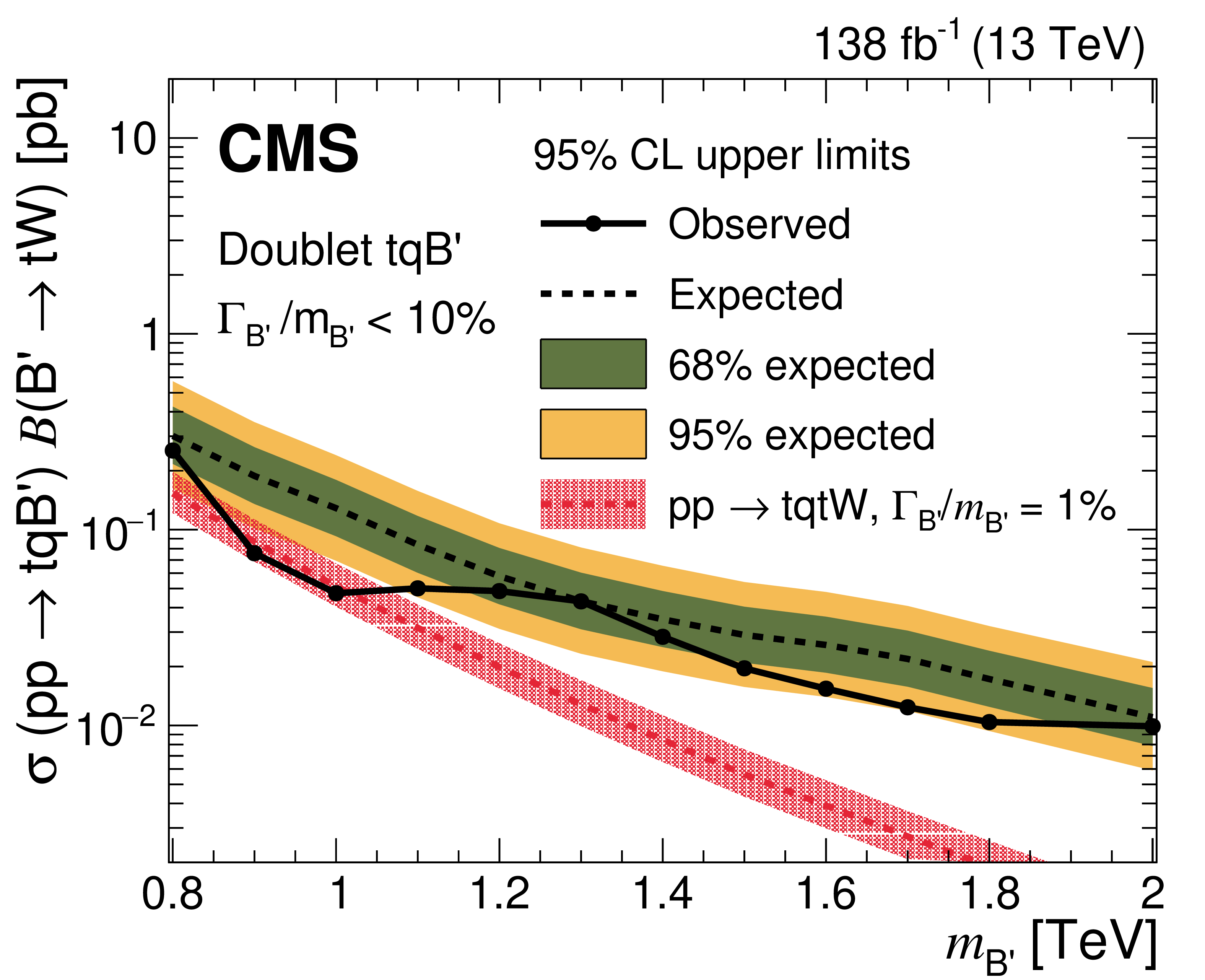
Figure 9-b:
Observed (solid black lines) and expected (dashed lines) 95% CL upper limits on the product of the production cross section and branching fraction $ \mathcal{B}(\mathrm{t}\mathrm{W}) $ for singlet $ \mathrm{b}\mathrm{q}{\mathrm{B}}^{\prime} $ production (upper), singlet $ \mathrm{t}\mathrm{q}{\mathrm{B}}^{\prime} $ production (lower left), and up-type doublet $ \mathrm{t}\mathrm{q}{\mathrm{B}}^{\prime} $ production (lower right), as functions of $ m_{{\mathrm{B}}^{\prime}} $. Predicted cross sections for various $ {\mathrm{B}}^{\prime}$ quark relative widths are shown as dashed red and solid blue lines. The bands around the predicted cross sections represent the associated energy scale and PDF uncertainties. |
png pdf |
Figure 9-c:
Observed (solid black lines) and expected (dashed lines) 95% CL upper limits on the product of the production cross section and branching fraction $ \mathcal{B}(\mathrm{t}\mathrm{W}) $ for singlet $ \mathrm{b}\mathrm{q}{\mathrm{B}}^{\prime} $ production (upper), singlet $ \mathrm{t}\mathrm{q}{\mathrm{B}}^{\prime} $ production (lower left), and up-type doublet $ \mathrm{t}\mathrm{q}{\mathrm{B}}^{\prime} $ production (lower right), as functions of $ m_{{\mathrm{B}}^{\prime}} $. Predicted cross sections for various $ {\mathrm{B}}^{\prime}$ quark relative widths are shown as dashed red and solid blue lines. The bands around the predicted cross sections represent the associated energy scale and PDF uncertainties. |
png pdf |
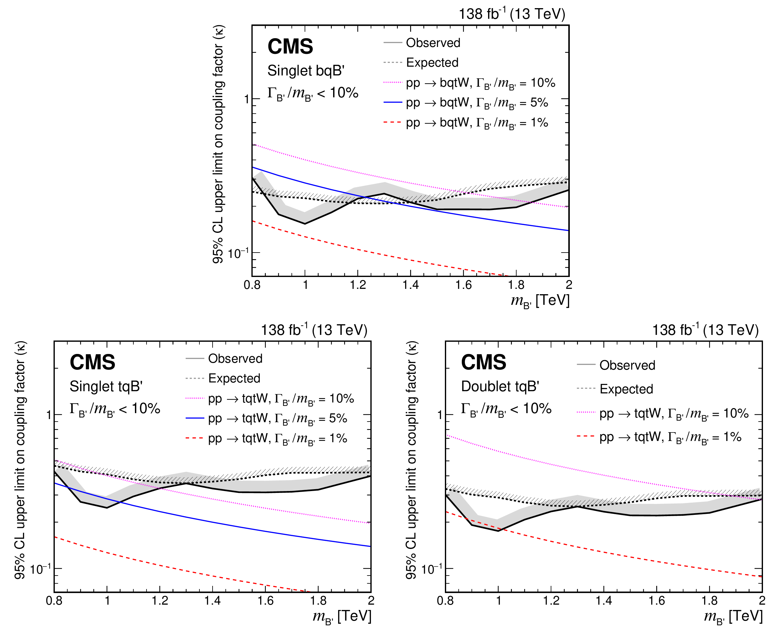
Figure 10:
Observed (solid black lines) and expected (dashed lines) 95% CL upper limits on the coupling factor $ \kappa $ for singlet $ \mathrm{b}\mathrm{q}{\mathrm{B}}^{\prime} $ production (upper), singlet $ \mathrm{t}\mathrm{q}{\mathrm{B}}^{\prime} $ production (lower left), and up-type doublet $ \mathrm{t}\mathrm{q}{\mathrm{B}}^{\prime} $ production (lower right), as functions of $ m_{{\mathrm{B}}^{\prime}} $. The hatched and shaded regions indicate that the limits are upper bounds on the coupling factor. Predicted coupling values for various $ {\mathrm{B}}^{\prime}$ quark relative widths are shown as dashed red, solid blue, and dotted magenta lines. |
png pdf |
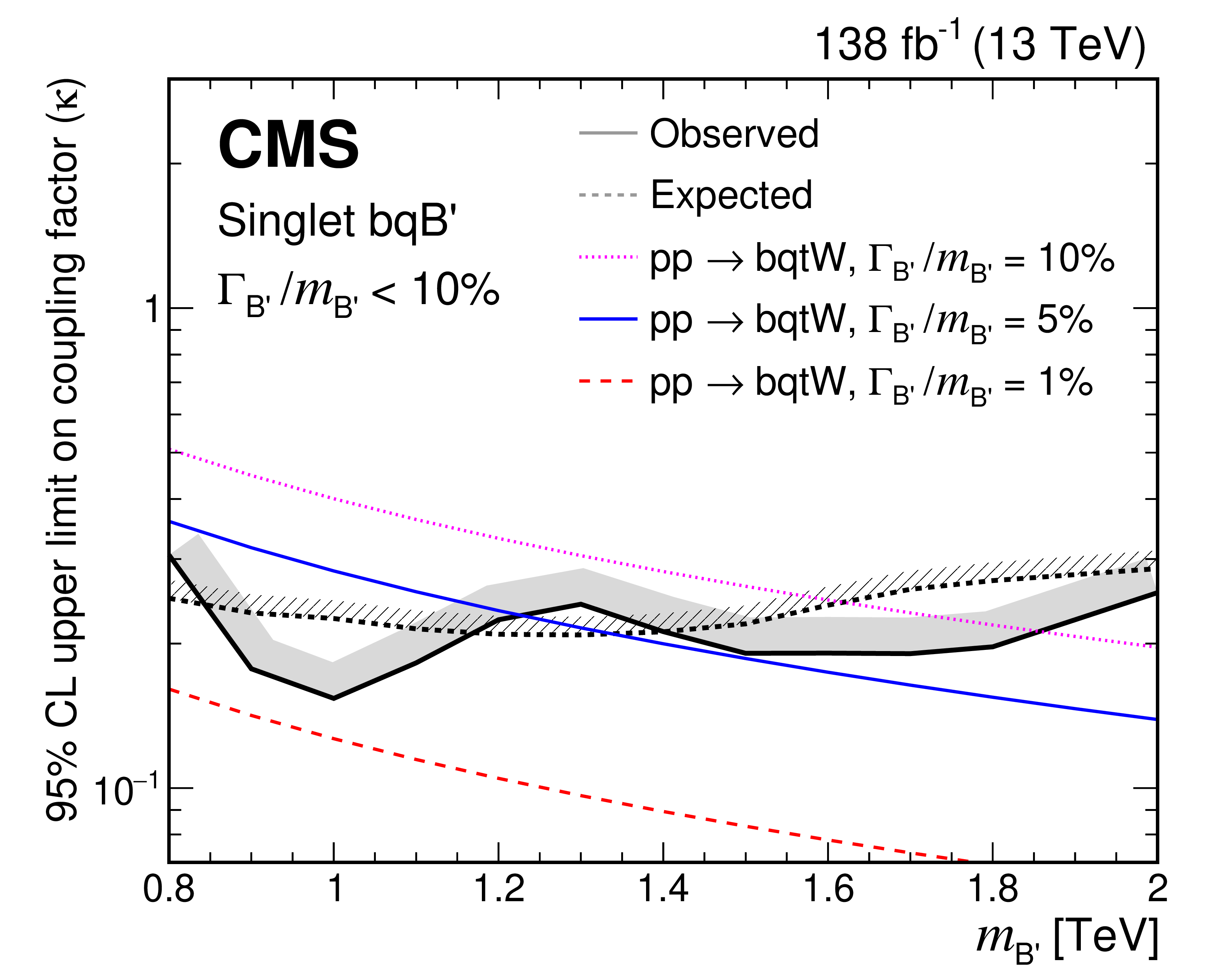
Figure 10-a:
Observed (solid black lines) and expected (dashed lines) 95% CL upper limits on the coupling factor $ \kappa $ for singlet $ \mathrm{b}\mathrm{q}{\mathrm{B}}^{\prime} $ production (upper), singlet $ \mathrm{t}\mathrm{q}{\mathrm{B}}^{\prime} $ production (lower left), and up-type doublet $ \mathrm{t}\mathrm{q}{\mathrm{B}}^{\prime} $ production (lower right), as functions of $ m_{{\mathrm{B}}^{\prime}} $. The hatched and shaded regions indicate that the limits are upper bounds on the coupling factor. Predicted coupling values for various $ {\mathrm{B}}^{\prime}$ quark relative widths are shown as dashed red, solid blue, and dotted magenta lines. |
png pdf |
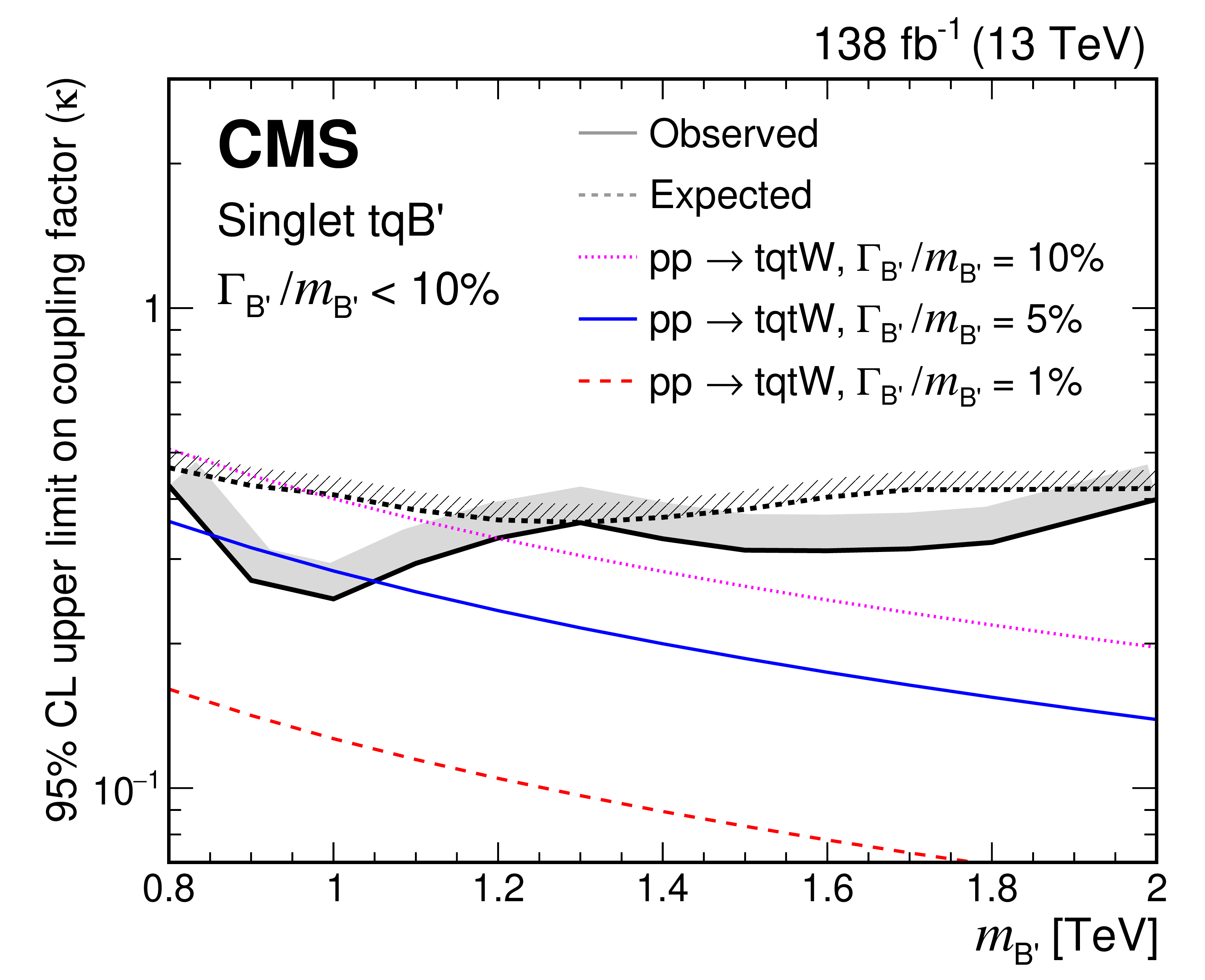
Figure 10-b:
Observed (solid black lines) and expected (dashed lines) 95% CL upper limits on the coupling factor $ \kappa $ for singlet $ \mathrm{b}\mathrm{q}{\mathrm{B}}^{\prime} $ production (upper), singlet $ \mathrm{t}\mathrm{q}{\mathrm{B}}^{\prime} $ production (lower left), and up-type doublet $ \mathrm{t}\mathrm{q}{\mathrm{B}}^{\prime} $ production (lower right), as functions of $ m_{{\mathrm{B}}^{\prime}} $. The hatched and shaded regions indicate that the limits are upper bounds on the coupling factor. Predicted coupling values for various $ {\mathrm{B}}^{\prime}$ quark relative widths are shown as dashed red, solid blue, and dotted magenta lines. |
png pdf |
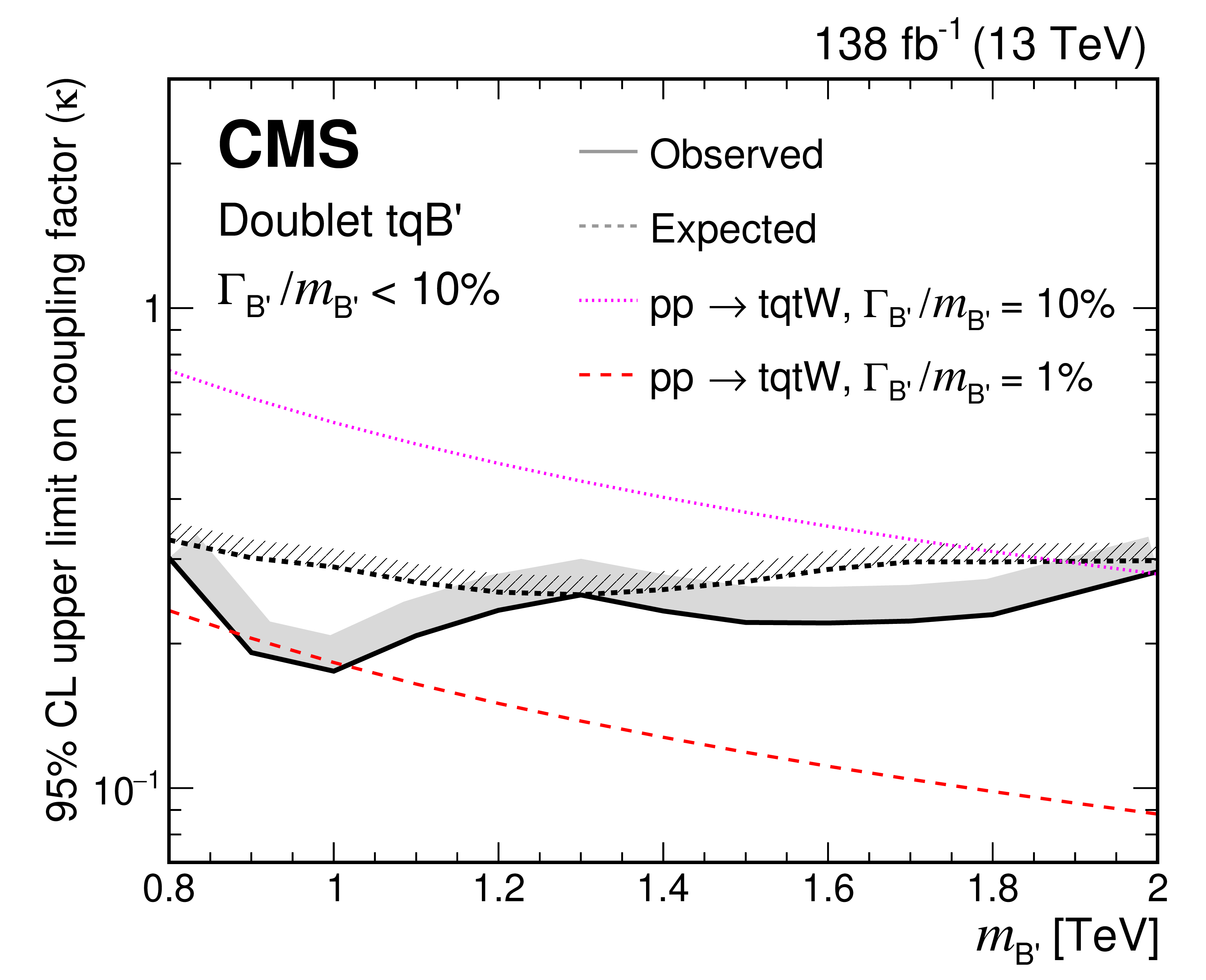
Figure 10-c:
Observed (solid black lines) and expected (dashed lines) 95% CL upper limits on the coupling factor $ \kappa $ for singlet $ \mathrm{b}\mathrm{q}{\mathrm{B}}^{\prime} $ production (upper), singlet $ \mathrm{t}\mathrm{q}{\mathrm{B}}^{\prime} $ production (lower left), and up-type doublet $ \mathrm{t}\mathrm{q}{\mathrm{B}}^{\prime} $ production (lower right), as functions of $ m_{{\mathrm{B}}^{\prime}} $. The hatched and shaded regions indicate that the limits are upper bounds on the coupling factor. Predicted coupling values for various $ {\mathrm{B}}^{\prime}$ quark relative widths are shown as dashed red, solid blue, and dotted magenta lines. |
| Tables | |
png pdf |
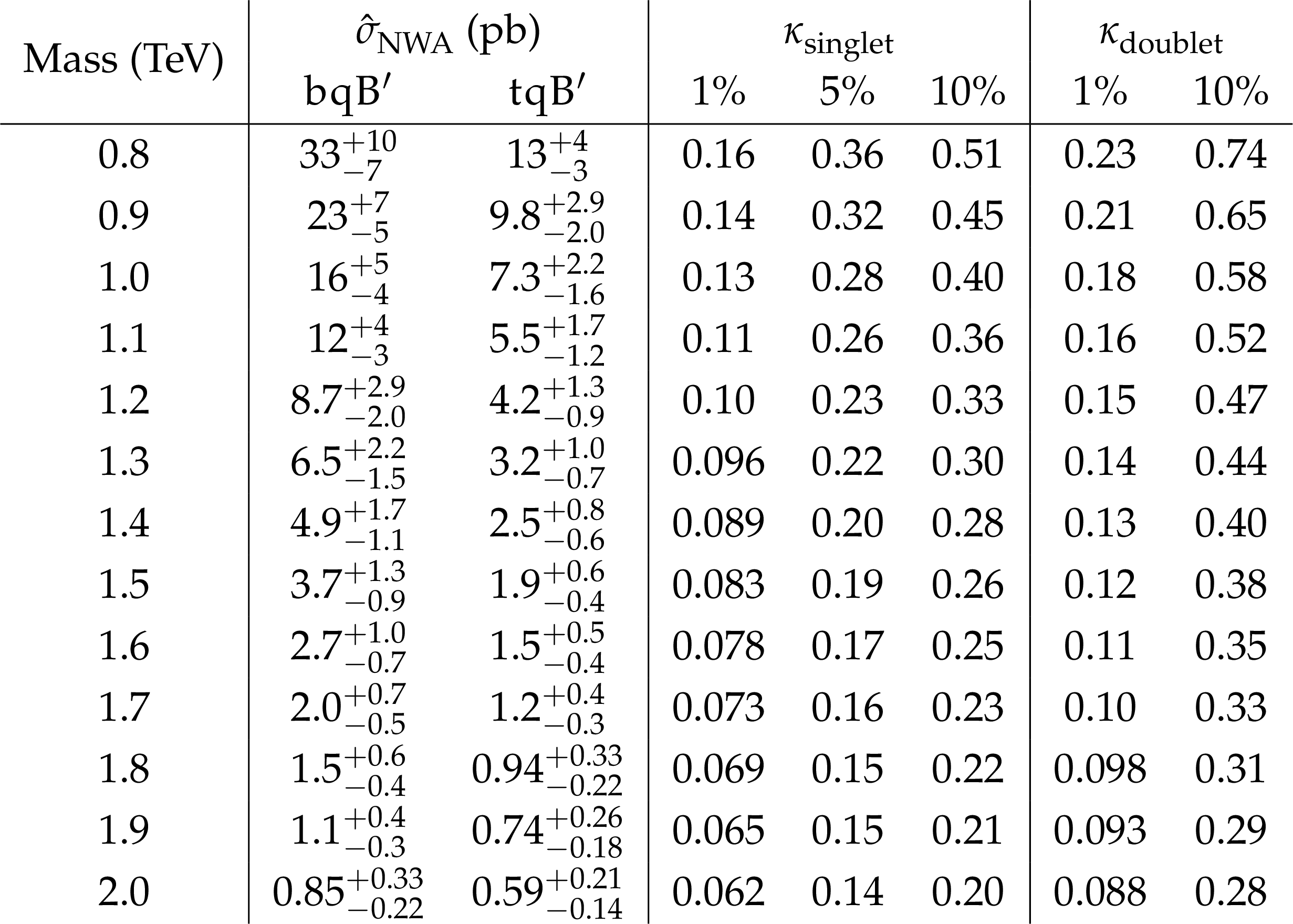
Table 1:
Values of $ \hat{\sigma}_{\mathrm{NWA}} $ and $ \kappa $ used to compute the cross sections for the production of a $ {\mathrm{B}}^{\prime}$ quark that is either a singlet or a member of a (\HepParticle{\HepParticleT} {\prime},\HepParticle $ {\mathrm{B}}^{\prime}$ ) doublet, based on the calculations described in Refs. [none-none-none,35]. The value of $ \hat{\sigma}_{\mathrm{NWA}} $ depends on the $ {\mathrm{B}}^{\prime}$ quark mass and production mode. The value of $ \kappa $ depends on the $ {\mathrm{B}}^{\prime}$ quark mass, width, and multiplet structure. All numerical values are rounded to two significant figures, and uncertainties due to renormalization and factorization scales are provided for $ \hat{\sigma}_{\mathrm{NWA}} $. |
png pdf |
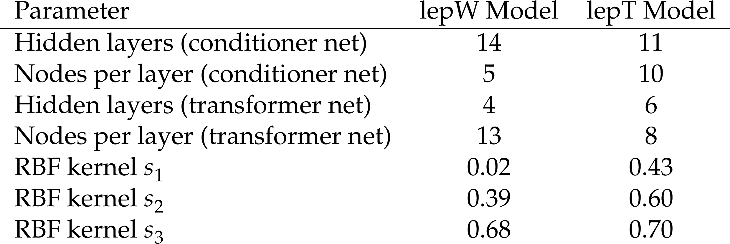
Table 2:
The ABCDnn architectures and RBF kernel sizes for the lepW and lepT models. The lepW model is trained on events in reconstruction Cases 1 and 4, and the lepT model is trained on events in reconstruction Cases 2 and 3. |
png pdf |
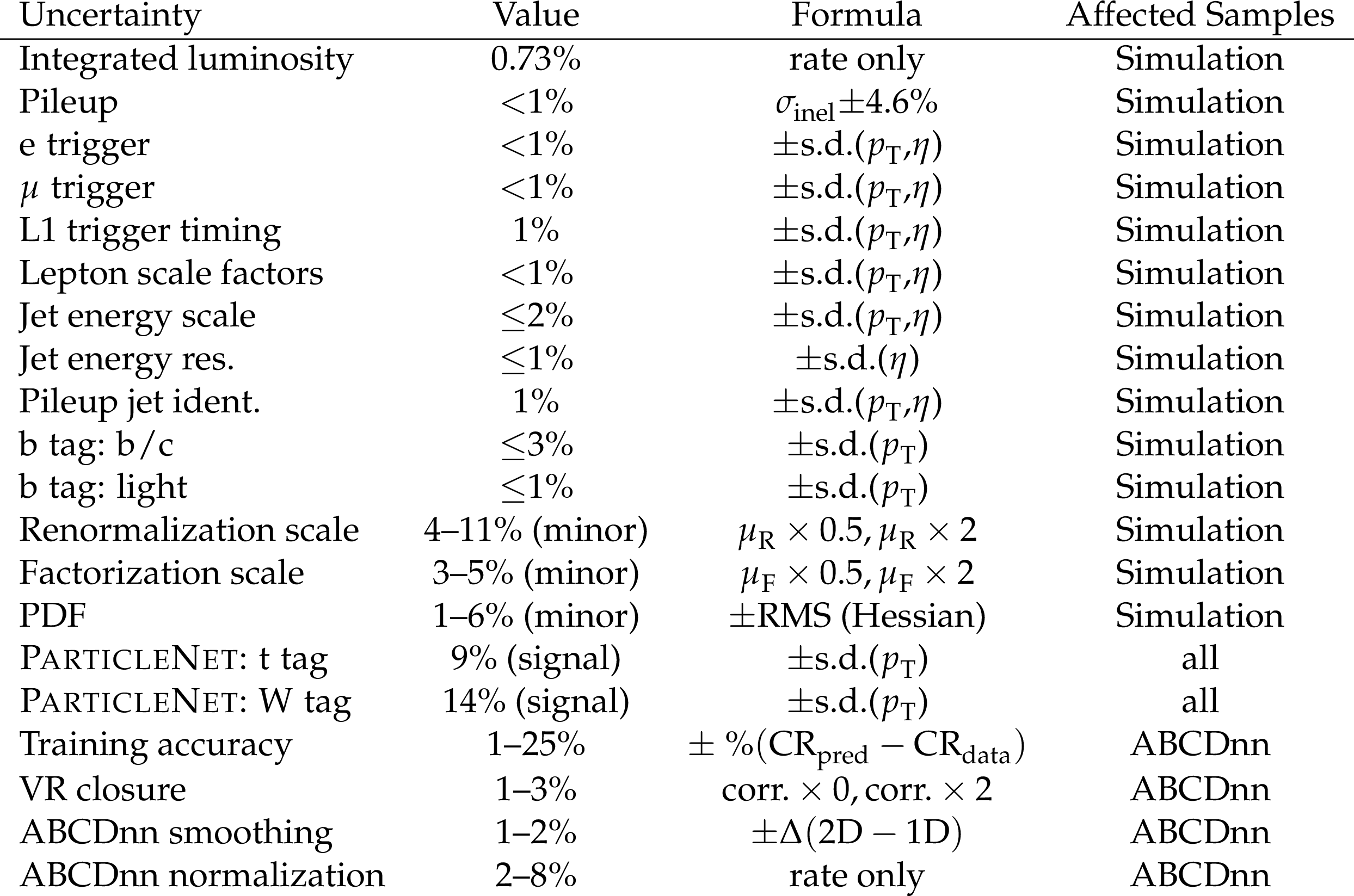
Table 3:
A summary of the systematic uncertainties impacting the analysis. Unless otherwise specified, all uncertainties are implemented as rate and shape variations using alternate template histograms. The numerical values represent the prefit rate impact and are given as ranges across the four reconstruction cases for either the 1.4 TeV signal or the ABCDnn background prediction, unless otherwise specified. The functional form in the third column indicates the quantities on which the uncertainty magnitude depends, where $ \textrm{s.d.} $ denotes one standard deviation. The final column indicates the affected predictions: simulated samples (including signal), ``minor'' refers to simulated minor background processes, and ``ABCDnn'' refers to the major background predicted using the ABCDnn method. |
| Summary |
| A search has been presented for the single production of a vector-like $ {\mathrm{B}}^{\prime}$ quark that decays to a t quark and a W boson via the electroweak interaction. Proton-proton collision data collected with the CMS detector at a center-of-mass energy of 13 TeV are used, corresponding to an integrated luminosity of 138 fb$ ^{-1} $. Events are selected with one electron or muon, missing transverse momentum, and at least one large-radius jet well separated from the charged lepton. A $ {\mathrm{B}}^{\prime}$ quark candidate is reconstructed and categorized according to the PARTICLENET identification of the large-radius jet. Minor background processes are modeled using simulation, while the major background contribution in the signal region is modeled from data in five control regions using a neural autoregressive flow network, referred to as ABCDnn. For $ \mathrm{b}\mathrm{q}{\mathrm{B}}^{\prime} $ production, singlet $ {\mathrm{B}}^{\prime}$ quarks with a 5% relative decay width and masses between 0.8 and 1.23 TeV are excluded at 95% confidence level (CL). Limits are also set on the product of the single production cross section and the ${{\mathrm{B}}}{\prime} \to\mathrm{t}\mathrm{W} $ branching fraction for $ \mathrm{t}\mathrm{q}{\mathrm{B}}^{\prime} $ production, excluding the 0.9 and 1.0 TeV mass hypotheses at 95% CL for both the 5%-width singlet and 1%-width doublet scenarios. For singlet $ \mathrm{b}\mathrm{q}{\mathrm{B}}^{\prime} $ production, coupling factor values above 0.30 are excluded for $ {\mathrm{B}}^{\prime}$ quark masses in the range 0.8--1.8 TeV. For $ \mathrm{t}\mathrm{q}{\mathrm{B}}^{\prime} $ production, coupling factor values above 0.41 are excluded at 95% CL for singlet $ {\mathrm{B}}^{\prime}$ quark masses in the range 0.8--1.2 TeV, and values above 0.29 are excluded at 95% CL for doublet $ {\mathrm{B}}^{\prime}$ quark masses in the range 0.8--2.0 TeV. These limits are the most stringent to date for the single production cross section and coupling factors of narrow-width $ {\mathrm{B}}^{\prime}$ quarks. |
| Additional Figures | |
png pdf |
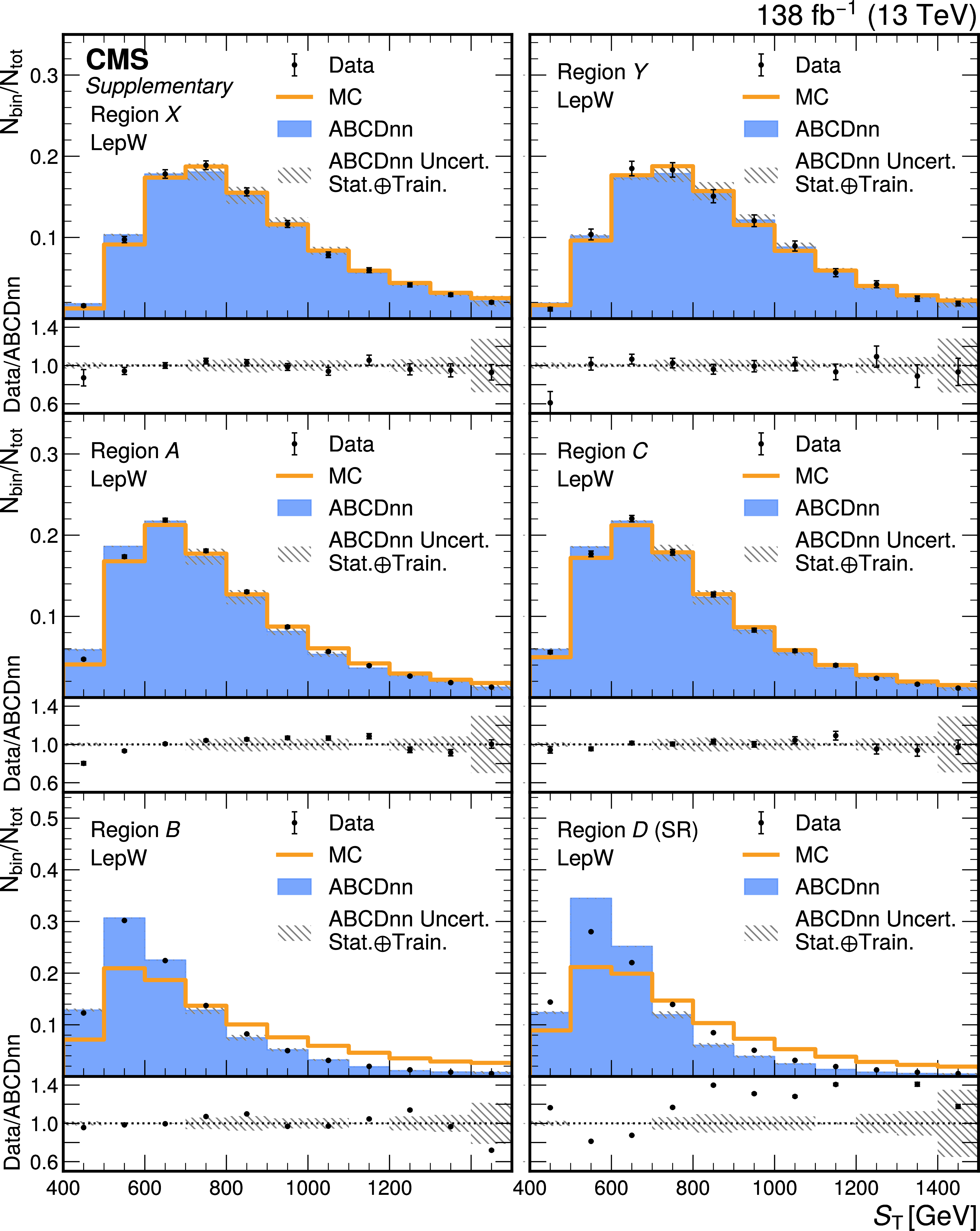
Additional Figure 1:
Distributions of $S_\mathrm{T}$ in the SR and CRs for the lepW ABCDnn model, normalized to unity. The last bins are overflow bins with all the contributions from bins with $S_\mathrm{T}>1500$ GeV. Observed data are shown as black markers with statistical uncertainties. Major background distributions from simulation are shown as orange solid lines with statistical uncertainties and are labeled ``MC''. ABCDnn predictions are shown as blue filled histograms. Statistical and training uncertainties in the ABCDnn predictions are indicated by hatched bands, though they are too small to be visible in the upper panels. The lower panels show the ratio of the data to the ABCDnn prediction. The disagreement between data and predicted shapes is generally within 20% in the CRs and is greater in the SR. |
png pdf |
Additional Figure 2:
Distributions of $S_\mathrm{T}$ in the SR and CRs for the lepT ABCDnn model, normalized to unity. The last bins are overflow bins with all the contributions from bins with $S_\mathrm{T}>1500$ GeV. Observed data are shown as black markers with statistical uncertainties. Major background distributions from simulation are shown as orange solid lines with statistical uncertainties and are labeled ``MC''. ABCDnn predictions are shown as blue filled histograms. Statistical and training uncertainties in the ABCDnn predictions are indicated by hatched bands, though they are too small to be visible in the upper panels. The lower panels show the ratio of the data to the ABCDnn prediction. Disagreement between data and predicted distributions is within 10% for most of the range that is relevant to the analysis in all regions. The largest deviations are around 20% and mainly occur in the tails of some CRs, where the statistics are low. The performance is stable across the training regions (CRs) and the application region (SR). |
png pdf |
Additional Figure 3:
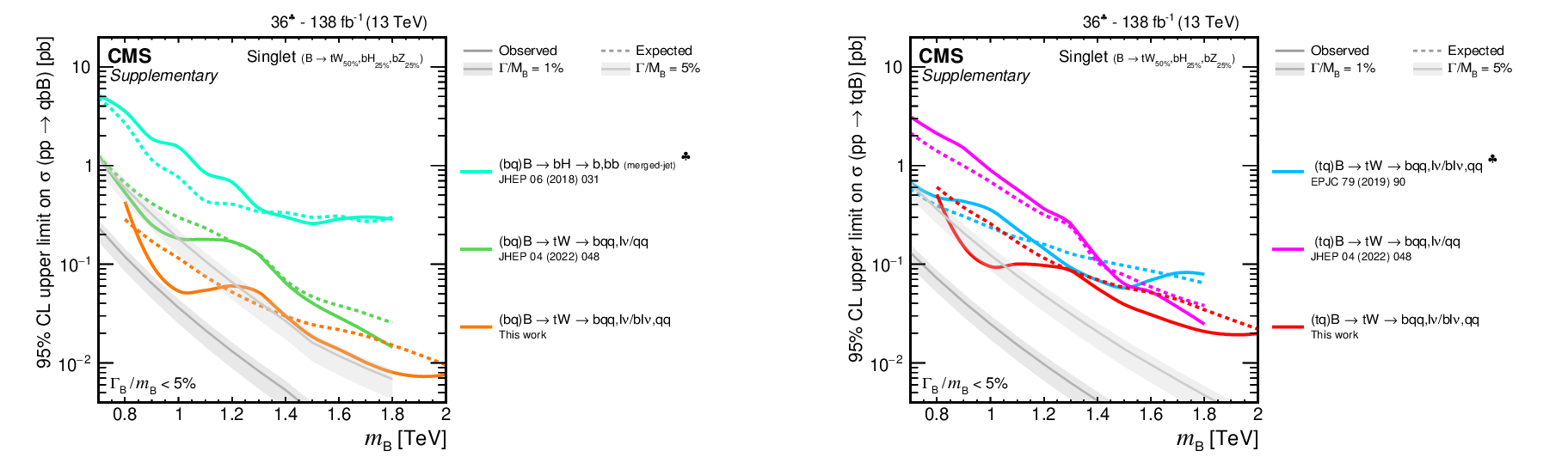
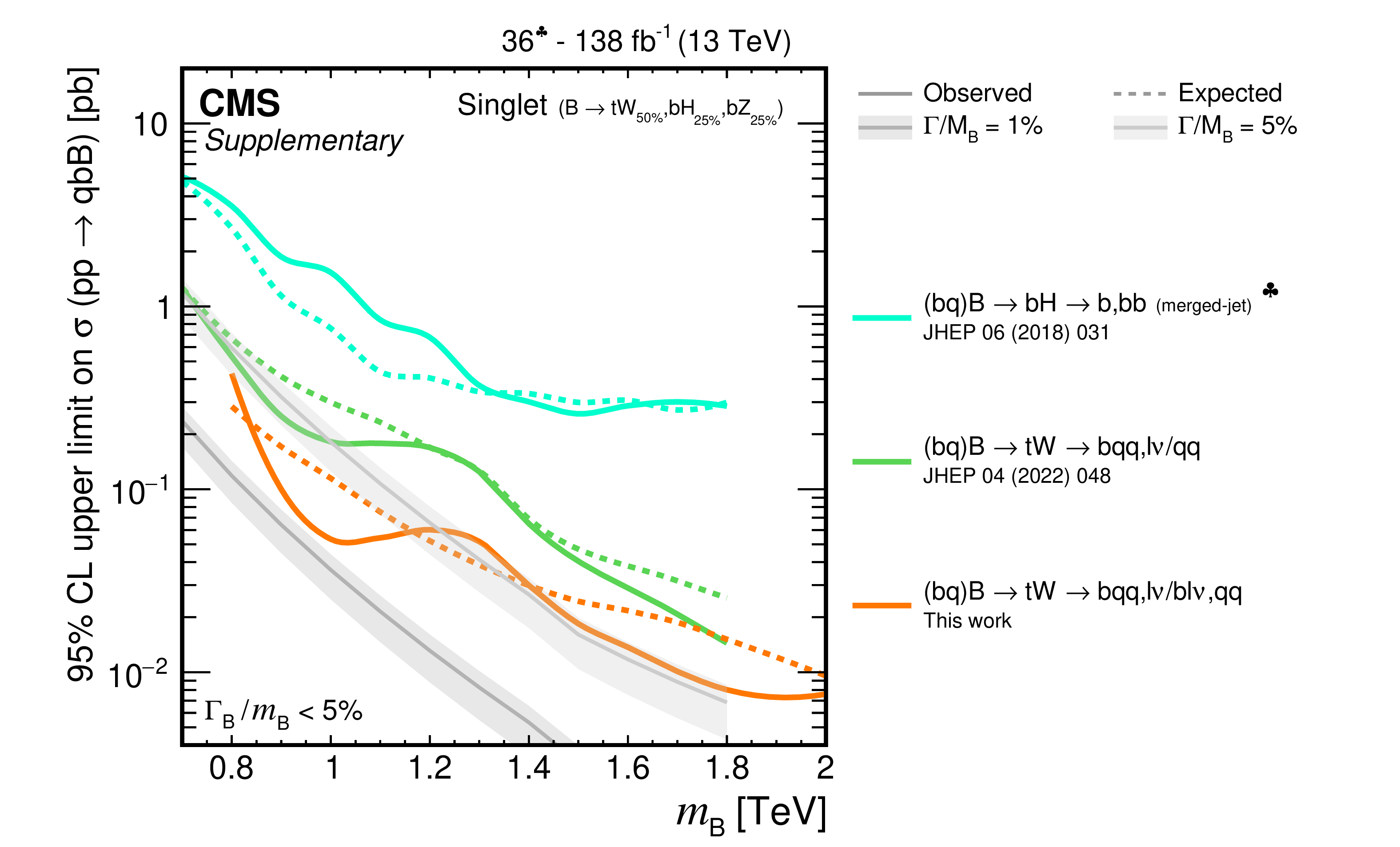
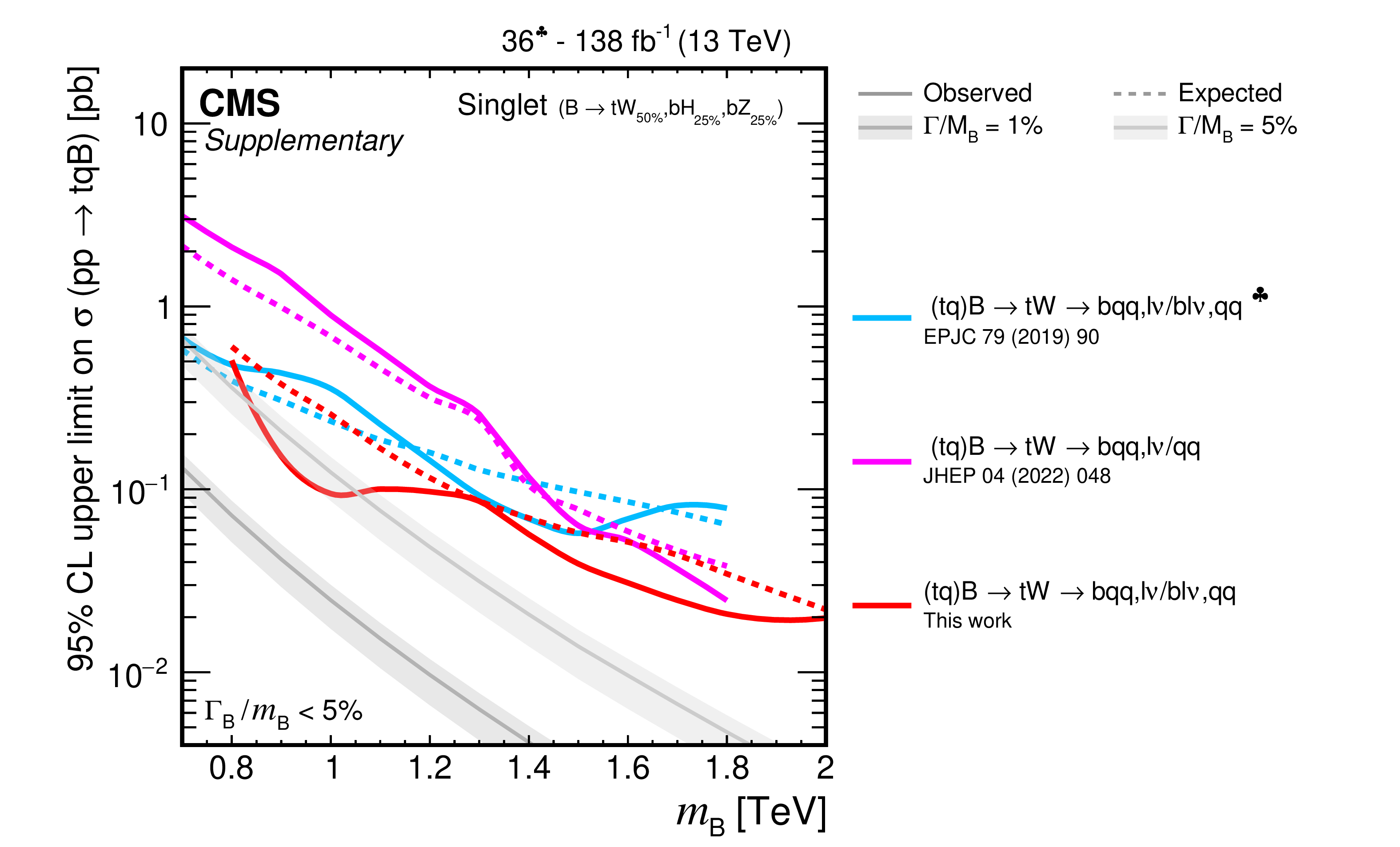
Upper limits at 95% CL on the single production cross section of singlet B quarks that are produced in association with a b quark (upper) or a t quark (lower), as a function of the B quark mass. Expected limits are shown in dashed lines and observed limits in solid lines. Theoretical predictions for B quarks with relative widths of 1% and 5% are overlaid in gray solid lines. The limits are obtained in searches by CMS with integrated luminosities of 36 fb$ ^{-1} $(denoted by the clubs symbol) and 138 fb$ ^{-1} $ Final states and publication references are noted in the legends. |
png pdf |
Additional Figure 3-a:
Upper limits at 95% CL on the single production cross section of singlet B quarks that are produced in association with a b quark (upper) or a t quark (lower), as a function of the B quark mass. Expected limits are shown in dashed lines and observed limits in solid lines. Theoretical predictions for B quarks with relative widths of 1% and 5% are overlaid in gray solid lines. The limits are obtained in searches by CMS with integrated luminosities of 36 fb$ ^{-1} $(denoted by the clubs symbol) and 138 fb$ ^{-1} $ Final states and publication references are noted in the legends. |
png pdf |
Additional Figure 3-b:
Upper limits at 95% CL on the single production cross section of singlet B quarks that are produced in association with a b quark (upper) or a t quark (lower), as a function of the B quark mass. Expected limits are shown in dashed lines and observed limits in solid lines. Theoretical predictions for B quarks with relative widths of 1% and 5% are overlaid in gray solid lines. The limits are obtained in searches by CMS with integrated luminosities of 36 fb$ ^{-1} $(denoted by the clubs symbol) and 138 fb$ ^{-1} $ Final states and publication references are noted in the legends. |
| References | ||||
| 1 | R. Contino, L. Da Rold, and A. Pomarol | Light custodians in natural composite Higgs models | PRD 7 (2007) 5 | hep-ph/0612048 |
| 2 | R. Contino, T. Kramer, M. Son, and R. Sundrum | Warped/composite phenomenology simplified | JHEP 05 (2007) 074 | hep-ph/0612180 |
| 3 | J. A. Aguilar-Saavedra, R. Benbrik, S. Heinemeyer, and M. P é rez-Victoria | Handbook of vectorlike quarks: Mixing and single production | PRD 88 (2013) 094010 | 1306.0572 |
| 4 | A. De Simone, O. Matsedonskyi, R. Rattazzi, and A. Wulzer | A first top partner hunter's guide | JHEP 04 (2013) 004 | |
| 5 | CMS Collaboration | Search for single production of vector-like quarks decaying to a top quark and a W boson in proton-proton collisions at $ \sqrt{s}= $ 13 TeV | EPJC 79 (2019) 90 | 1809.08597 |
| 6 | CMS Collaboration | Search for single production of vector-like quarks decaying to a b quark and a Higgs boson | JHEP 06 (2018) 031 | 1802.01486 |
| 7 | CMS Collaboration | Search for a heavy resonance decaying into a top quark and a W boson in the lepton+jets final state at $ \sqrt{s}= $ 13 TeV | JHEP 04 (2022) 048 | 2111.10216 |
| 8 | CMS Collaboration | Review of searches for vector-like quarks, vector-like leptons, and heavy neutral leptons in proton-proton collisions at $ \sqrt{s}= $ 13 TeVat the CMS experiment | Phys. Rept. 1115 (2025) 570 | CMS-EXO-23-006 2405.17605 |
| 9 | ATLAS Collaboration | Search for the production of single vector-like and excited quarks in the $ {W}t $ final state in $ pp $ collisions at $ \sqrt{s}= $ 8 TeV with the ATLAS detector | JHEP 02 (2016) 110 | 1510.02664 |
| 10 | ATLAS Collaboration | Search for single vector-like $ {B} $ quark production and decay via $ {B}\rightarrow b{H}(b\bar{b}) $ in $ pp $ collisions at $ \sqrt{s}= $ 13 TeV with the atlas detector | JHEP 11 (2023) 168 | 2308.02595 |
| 11 | CMS Collaboration | HEPData record for this analysis | link | |
| 12 | CMS Collaboration | The CMS experiment at the CERN LHC | JINST 3 (2008) S08004 | |
| 13 | CMS Collaboration | Performance of the CMS Level-1 trigger in proton-proton collisions at $ \sqrt{s}= $ 13 TeV | JINST 15 (2020) P10017 | CMS-TRG-17-001 2006.10165 |
| 14 | CMS Collaboration | The CMS trigger system | JINST 12 (2017) P01020 | CMS-TRG-12-001 1609.02366 |
| 15 | CMS Collaboration | Performance of the CMS high-level trigger during LHC run 2 | JINST 19 (2024) P11021 | CMS-TRG-19-001 2410.17038 |
| 16 | CMS Collaboration | Electron and photon reconstruction and identification with the CMS experiment at the CERN LHC | JINST 16 (2021) P05014 | CMS-EGM-17-001 2012.06888 |
| 17 | CMS Collaboration | Performance of the CMS muon detector and muon reconstruction with proton-proton collisions at $ \sqrt{s}= $ 13 TeV | JINST 13 (2018) P06015 | CMS-MUO-16-001 1804.04528 |
| 18 | CMS Collaboration | Description and performance of track and primary-vertex reconstruction with the CMS tracker | JINST 9 (2014) P10009 | CMS-TRK-11-001 1405.6569 |
| 19 | CMS Collaboration | Development of the CMS detector for the CERN LHC Run 3 | JINST 19 (2024) P05064 | CMS-PRF-21-001 2309.05466 |
| 20 | CMS Collaboration | Technical proposal for the Phase-II upgrade of the Compact Muon Solenoid | CMS Technical Proposal CERN-LHCC-2015-010, CMS-TDR-15-02, 2015 CDS |
|
| 21 | CMS Collaboration | Particle-flow reconstruction and global event description with the CMS detector | JINST 12 (2017) P10003 | CMS-PRF-14-001 1706.04965 |
| 22 | M. Cacciari, G. P. Salam, and G. Soyez | The anti-$ k_{\mathrm{T}} $ jet clustering algorithm | JHEP 04 (2008) 063 | 0802.1189 |
| 23 | M. Cacciari, G. P. Salam, and G. Soyez | FastJet user manual | EPJC 72 (2012) 1896 | 1111.6097 |
| 24 | CMS Collaboration | Pileup mitigation at CMS in 13 TeV data | JINST 15 (2020) P09018 | CMS-JME-18-001 2003.00503 |
| 25 | D. Bertolini, P. Harris, M. Low, and N. Tran | Pileup per particle identification | JHEP 10 (2014) 059 | 1407.6013 |
| 26 | CMS Collaboration | Jet energy scale and resolution in the CMS experiment in pp collisions at 8 TeV | JINST 12 (2017) P02014 | CMS-JME-13-004 1607.03663 |
| 27 | CMS Collaboration | Precision luminosity measurement in proton-proton collisions at $ \sqrt{s}= $ 13 TeV in 2015 and 2016 at CMS | EPJC 81 (2021) 800 | CMS-LUM-17-003 2104.01927 |
| 28 | CMS Collaboration | CMS luminosity measurement for the 2017 data-taking period at $ \sqrt{s}= $ 13 TeV | CMS Physics Analysis Summary, 2018 link |
CMS-PAS-LUM-17-004 |
| 29 | CMS Collaboration | CMS luminosity measurement for the 2018 data-taking period at $ \sqrt{s}= $ 13 TeV | CMS Physics Analysis Summary, 2019 link |
CMS-PAS-LUM-18-002 |
| 30 | CMS Collaboration | Precision luminosity measurement in proton-proton collisions at $ \sqrt{s}= $ 13 TeV with the CMS detector | CMS Physics Analysis Summary, 2025 CMS-PAS-LUM-20-001 |
CMS-PAS-LUM-20-001 |
| 31 | J. Alwall et al. | The automated computation of tree-level and next-to-leading order differential cross sections, and their matching to parton shower simulations | JHEP 07 (2014) 079 | 1405.0301 |
| 32 | B. Fuks and H.-S. Shao | QCD next-to-leading-order predictions matched to parton showers for vector-like quark models | EPJC 77 (2017) 135 | 1610.04622 |
| 33 | A. Deandrea et al. | Single production of vector-like quarks: the effects of large width, interference and NLO corrections | JHEP 08 (2021) 107 | 2105.08745 |
| 34 | P. Artoisenet, R. Frederix, O. Mattelaer, and R. Rietkerk | Automatic spin-entangled decays of heavy resonances in Monte Carlo simulations | JHEP 03 (2013) 015 | 1212.3460 |
| 35 | A. Carvalho et al. | Single production of vectorlike quarks with large width at the Large Hadron Collider | PRD 98 (2018) 1 | 1805.06402 |
| 36 | S. Hoeche et al. | Matching parton showers and matrix elements | in HERA and the LHC: A Workshop on the Implications of HERA for LHC Physics, 2005 link |
hep-ph/0602031 |
| 37 | R. Frederix and S. Frixione | Merging meets matching in MC@NLO | JHEP 12 (2012) 061 | 1209.6215 |
| 38 | S. Frixione, G. Ridolfi, and P. Nason | A positive-weight next-to-leading-order Monte Carlo for heavy flavour hadroproduction | JHEP 09 (2007) 126 | 0707.3088 |
| 39 | S. Alioli, P. Nason, C. Oleari, and E. Re | NLO single-top production matched with shower in POWHEG: $ s $- and $ t $-channel contributions | JHEP 09 (2009) 111 | 0907.4076 |
| 40 | E. Re | Single-top $ {\mathrm{W}\mathrm{t}} $-channel production matched with parton showers using the POWHEG method | EPJC 71 (2011) 1547 | 1009.2450 |
| 41 | T. Sjöstrand et al. | An introduction to PYTHIA 8.2 | Comput. Phys. Commun. 191 (2015) 159 | 1410.3012 |
| 42 | NNPDF Collaboration | Parton distributions from high-precision collider data | EPJC 77 (2017) 663 | 1706.00428 |
| 43 | CMS Collaboration | Extraction and validation of a new set of CMS PYTHIA8 tunes from underlying-event measurements | EPJC 80 (2020) 4 | CMS-GEN-17-001 1903.12179 |
| 44 | GEANT4 Collaboration | GEANT 4---a simulation toolkit | NIM A 506 (2003) 250 | |
| 45 | CMS Collaboration | Search for supersymmetry in pp collisions at $ \sqrt{s}= $ 13 TeV in the single-lepton final state using the sum of masses of large-radius jets | JHEP 08 (2016) 122 | CMS-SUS-15-007 1605.04608 |
| 46 | M. Cacciari, G. P. Salam, and G. Soyez | The catchment area of jets | JHEP 04 (2008) 005 | 0802.1188 |
| 47 | E. Bols et al. | Jet flavour classification using DeepJet | JINST 15 (2020) P12012 | 2008.10519 |
| 48 | CMS Collaboration | Performance of the DeepJet b tagging algorithm using 41.9/fb of data from proton-proton collisions at 13 TeV with Phase 1 CMS detector | CMS Detector Performance Summary CMS-DP-2018-058, 2018 CDS |
|
| 49 | H. Qu and L. Gouskos | ParticleNet: Jet tagging via particle clouds | PRD 101 (2020) 056019 | 1902.08570 |
| 50 | CMS Collaboration | Performance of missing transverse momentum reconstruction in proton-proton collisions at $ \sqrt{s}= $ 13 TeV using the CMS detector | JINST 14 (2019) P07004 | CMS-JME-17-001 1903.06078 |
| 51 | S. Choi, J. Lim, and H. Oh | Data-driven estimation of background distribution through neural autoregressive flows | 2008.03636 | |
| 52 | CMS Collaboration | Evidence for four-top quark production in proton-proton collisions at $ \sqrt{s}= $ 13 TeV | PLB 844 (2023) 138076 | CMS-TOP-21-005 2303.03864 |
| 53 | S. Choi and H. Oh | Improved extrapolation methods of data-driven background estimations in high energy physics | EPJC 81 (2021) 643 | 1906.10831 |
| 54 | C.-W. Huang, D. Krueger, A. Lacoste, and A. C. Courville | Neural autoregressive flows | in International Conference on Machine Learning. 201 (1900) 8 |
|
| 55 | V. Nair and G. E. Hinton | Rectified linear units improve restricted boltzmann machines | in the International Conference on Machine Learning, 2010 Proceedings of the 2 (2010) 7 |
|
| 56 | I. Goodfellow, Y. Bengio, and A. Courville | Deep Learning | MIT Press, 2016 | |
| 57 | Gretton J. et al. | A kernel two-sample test | Mach. Learn. Res. 13 (2012) 723 | |
| 58 | W. S. Cleveland | Robust locally weighted regression and smoothing scatterplots | J. Am. Stat. Assoc. 74 (1979) 829 | |
| 59 | W. S. Cleveland and S. J. Devlin | Locally weighted regression: An approach to regression analysis by local fitting | J. Am. Stat. Assoc. 83 (1988) 596 | |
| 60 | CMS Collaboration | Measurement of the inelastic proton-proton cross section at $ \sqrt{s}= $ 13 TeV | JHEP 07 (2018) 161 | CMS-FSQ-15-005 1802.02613 |
| 61 | J. E. Gaiser | Charmonium Spectroscopy from Radiative Decays of the $ {J}/\psi $ and $ \psi\prime $ | PhD thesis, 1982 | |
| 62 | CMS Collaboration | The CMS statistical analysis and combination tool: COMBINE | Comput. Softw. Big Sci. 8 (2024) 19 | CMS-CAT-23-001 2404.06614 |
| 63 | W. Verkerke and D. Kirkby | The RooFit toolkit for data modeling | in the International Conference on Computing in High Energy and Nuclear Physics (CHEP ): La Jolla CA, United States, March 24--28, 2003 Proc. 1 (2003) 3 |
physics/0306116 |
| 64 | L. Moneta et al. | The RooStats project | in the International Workshop on Advanced Computing and Analysis Techniques in Physics Research (ACAT ): Jaipur, India, February 22--27, 2010 Proc. 1 (2010) 3 |
1009.1003 |
| 65 | R. Barlow and C. Beeston | Fitting using finite Monte Carlo samples | Comput. Phys. Commun. 77 (1993) 219 | |
| 66 | J. S. Conway | Incorporating nuisance parameters in likelihoods for multisource spectra | PHYSTAT 201 (2011) 115 | 1103.0354 |
| 67 | G. Cowan, K. Cranmer, E. Gross, and O. Vitells | Asymptotic formulae for likelihood-based tests of new physics | EPJC 71 (2011) 1554 | 1007.1727 |
| 68 | T. Junk | Confidence level computation for combining searches with small statistics | NIM A 434 (1999) 435 | hep-ex/9902006 |
| 69 | A. L. Read | Presentation of search results: The $ \text{CL}_\text{s} $ technique | JPG 28 (2002) 2693 | |
|
|
Compact Muon Solenoid LHC, CERN |
|

|

|

|

|

|