

Compact Muon Solenoid
LHC, CERN
| CMS-B2G-24-001 ; CERN-EP-2025-160 | ||
| Search for a new scalar resonance decaying to a Higgs boson and another new scalar particle in the final state with two bottom quarks and two photons in proton-proton collisions at $ \sqrt{s}= $ 13 TeV | ||
| CMS Collaboration | ||
| 15 August 2025 | ||
| JHEP 12 (2025) 178 | ||
| Abstract: A search is presented for a new scalar resonance, X, decaying to a standard model Higgs boson and another new scalar particle, Y, in the final state where the Higgs boson decays to a $ \mathrm{b}\overline{\mathrm{b}} $ pair, while the Y particle decays to a pair of photons. The search is performed in the mass range 240-1000 GeV for the resonance X, and in the mass range 70-800 GeV for the particle Y, using proton-proton collision data collected by the CMS experiment at $ \sqrt{s}= $ 13 TeV, corresponding to an integrated luminosity of 132 fb$ ^{-1} $. In general, the data are found to be compatible with the standard model expectation. Observed (expected) upper limits at 95% confidence level on the product of the production cross section and the relevant branching fraction are extracted for the $ \mathrm{X}\to{\mathrm{Y}} \mathrm{H} $ process, and are found to be within the range of 0.05-2.69 (0.08-1.94) fb, depending on $ m_\mathrm{X} $ and $ m_{\mathrm{Y}} $. The most significant deviation from the background-only hypothesis is observed for X and Y masses of 300 and 77 GeV, respectively, with a local (global) significance of 3.33 (0.65) standard deviations. | ||
| Links: e-print arXiv:2508.11494 [hep-ex] (PDF) ; CDS record ; inSPIRE record ; HepData record ; CADI line (restricted) ; | ||
| Figures | |
png pdf |
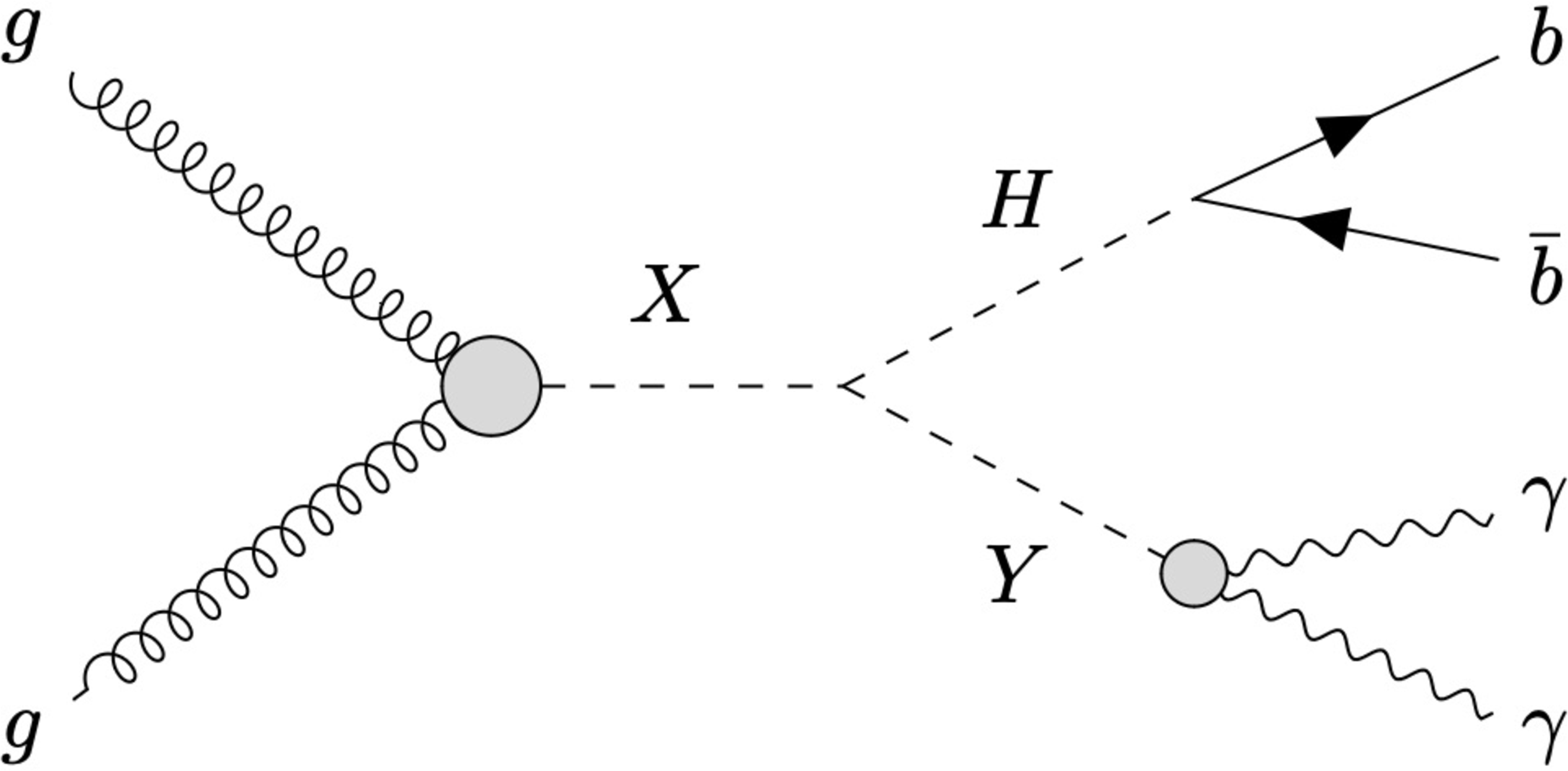
Figure 1:
Feynman diagram for the production of the BSM resonance X and its subsequent decay to two scalars, one SM Higgs boson and one BSM scalar Y, with $ \mathrm{H}\to\mathrm{b}\overline{\mathrm{b}} $ and $ {\mathrm{Y}} \to\gamma\gamma $. |
png pdf |
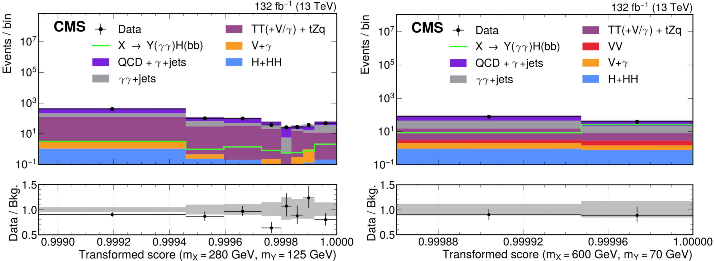
Figure 2:
Distributions of the transformed PNN score for the signal hypotheses of $ m_\mathrm{X}= $ 280 GeV, $ m_{\mathrm{Y}} = $ 125 GeV (left) and $ m_\mathrm{X}= $ 600 GeV, $ m_{\mathrm{Y}} = $ 70 GeV (right) in their corresponding SRs. The bin boundaries correspond to the SR boundaries of each mass point. The distributions are inclusive in the $ m_{\gamma\gamma} $ distribution. The gray bands in the lower panels show the statistical uncertainty in the background estimation. |
png pdf |
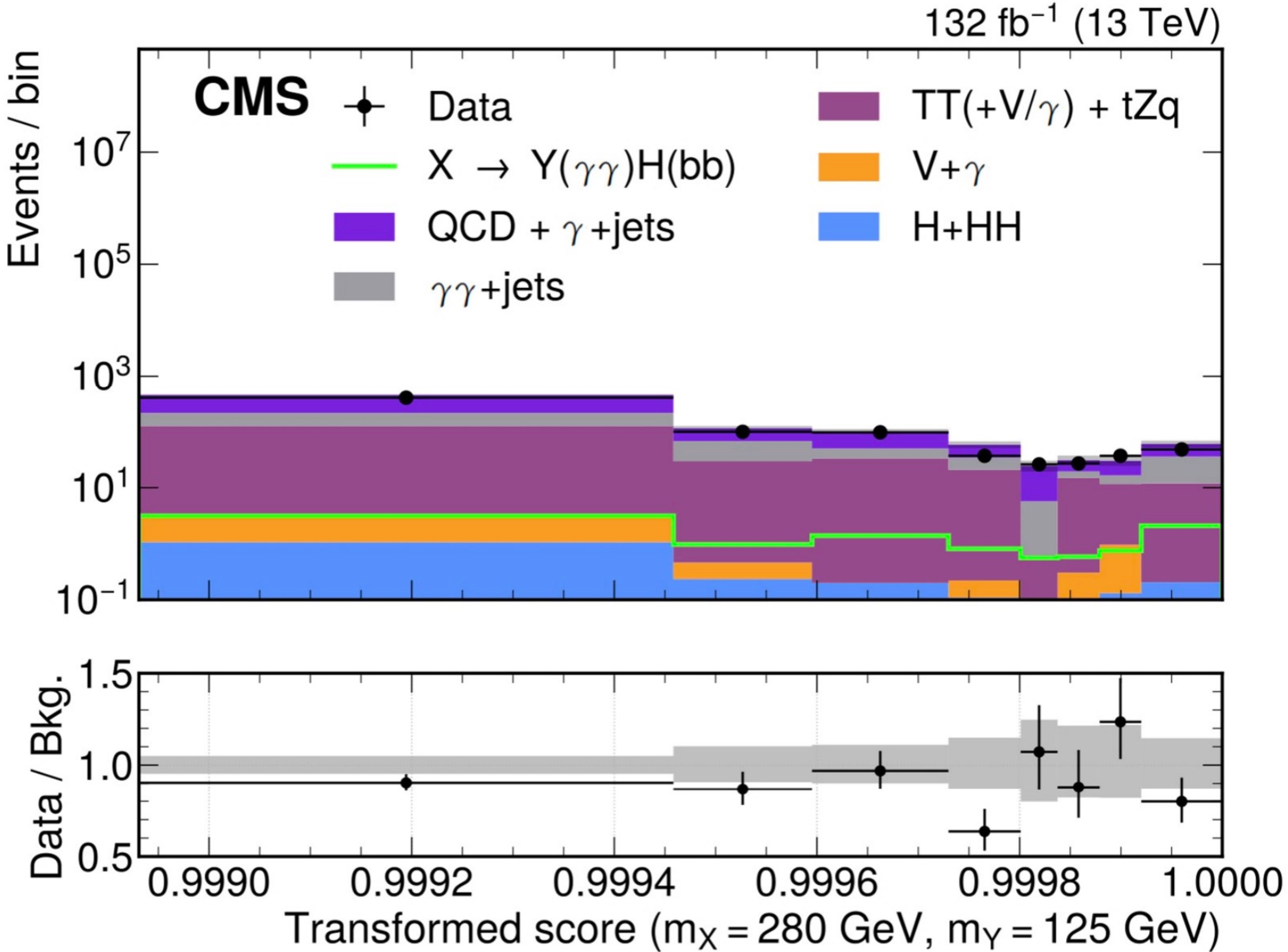
Figure 2-a:
Distributions of the transformed PNN score for the signal hypotheses of $ m_\mathrm{X}= $ 280 GeV, $ m_{\mathrm{Y}} = $ 125 GeV (left) and $ m_\mathrm{X}= $ 600 GeV, $ m_{\mathrm{Y}} = $ 70 GeV (right) in their corresponding SRs. The bin boundaries correspond to the SR boundaries of each mass point. The distributions are inclusive in the $ m_{\gamma\gamma} $ distribution. The gray bands in the lower panels show the statistical uncertainty in the background estimation. |
png pdf |
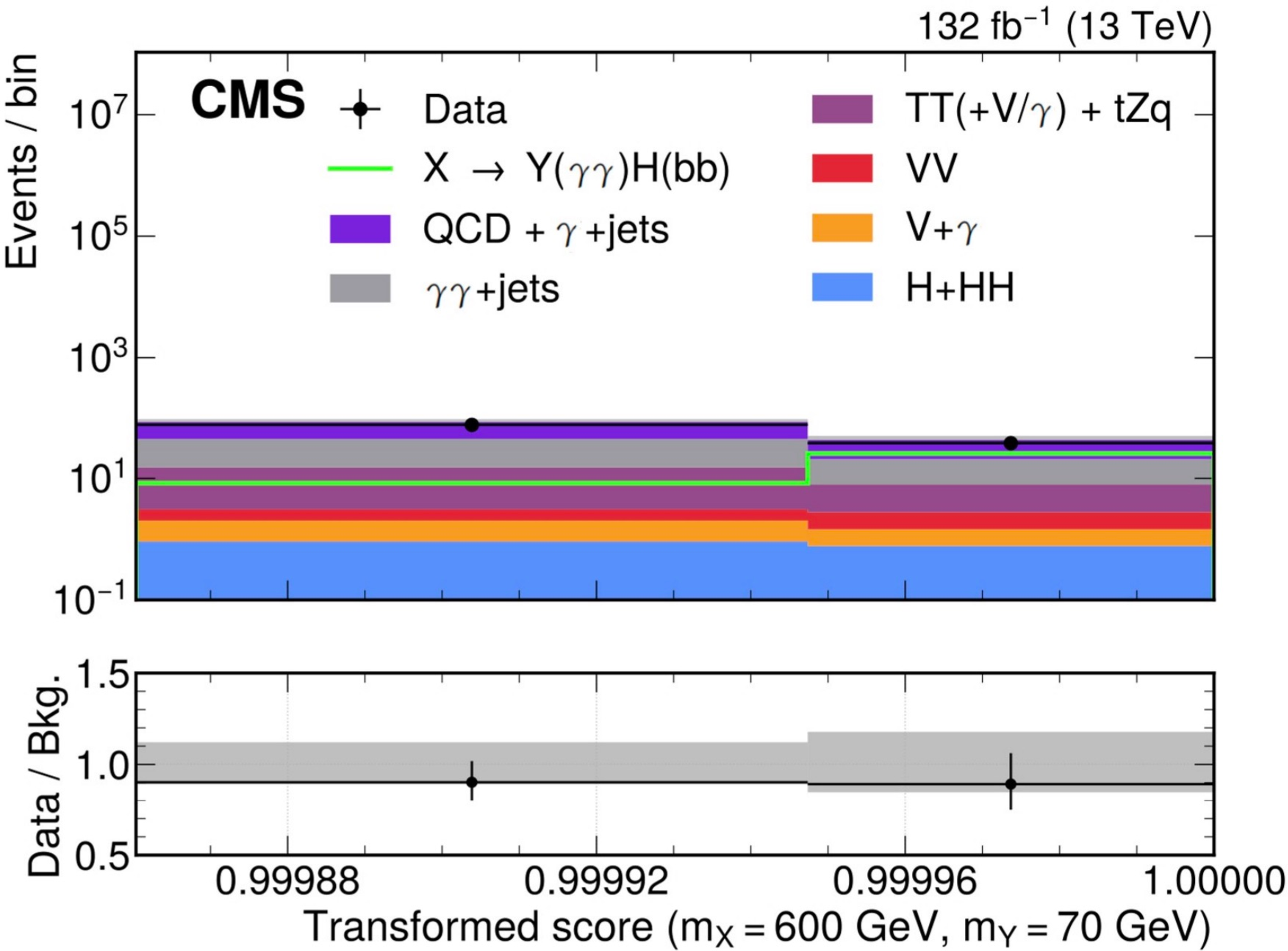
Figure 2-b:
Distributions of the transformed PNN score for the signal hypotheses of $ m_\mathrm{X}= $ 280 GeV, $ m_{\mathrm{Y}} = $ 125 GeV (left) and $ m_\mathrm{X}= $ 600 GeV, $ m_{\mathrm{Y}} = $ 70 GeV (right) in their corresponding SRs. The bin boundaries correspond to the SR boundaries of each mass point. The distributions are inclusive in the $ m_{\gamma\gamma} $ distribution. The gray bands in the lower panels show the statistical uncertainty in the background estimation. |
png pdf |
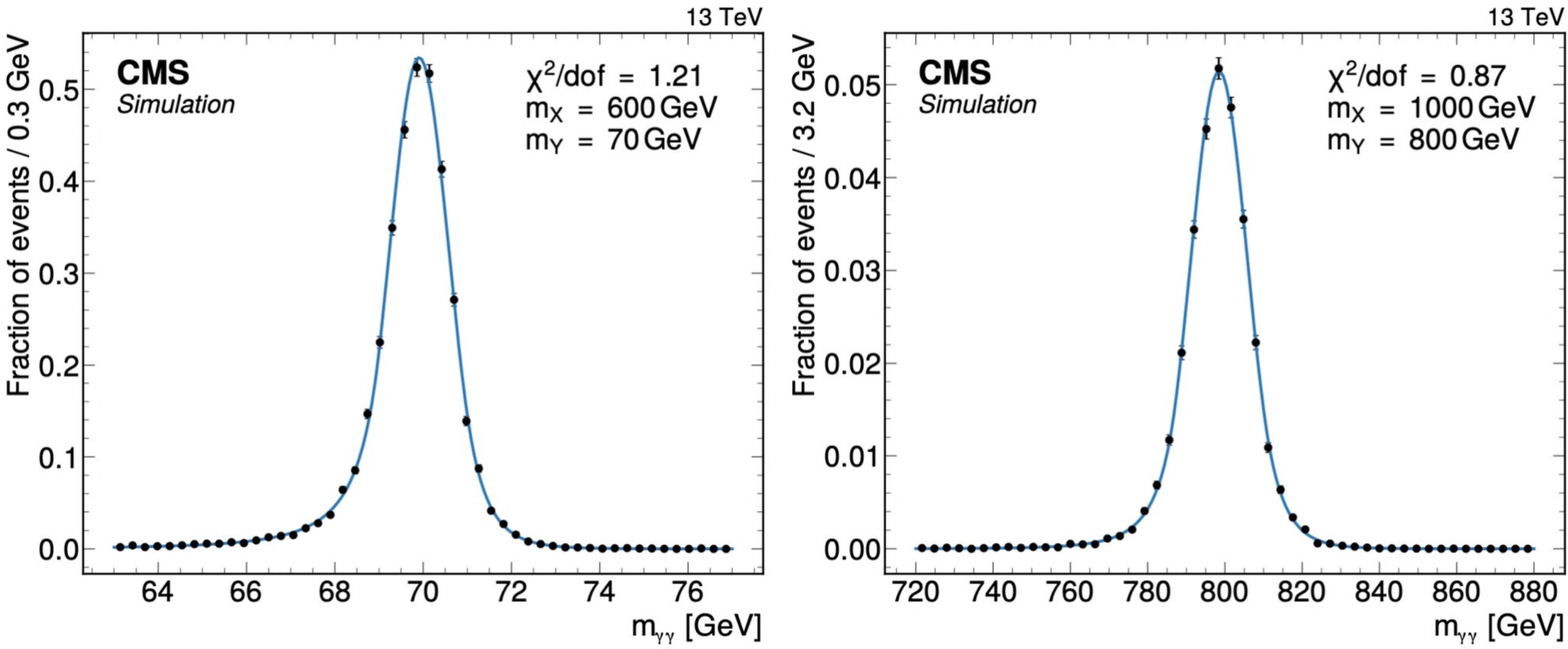
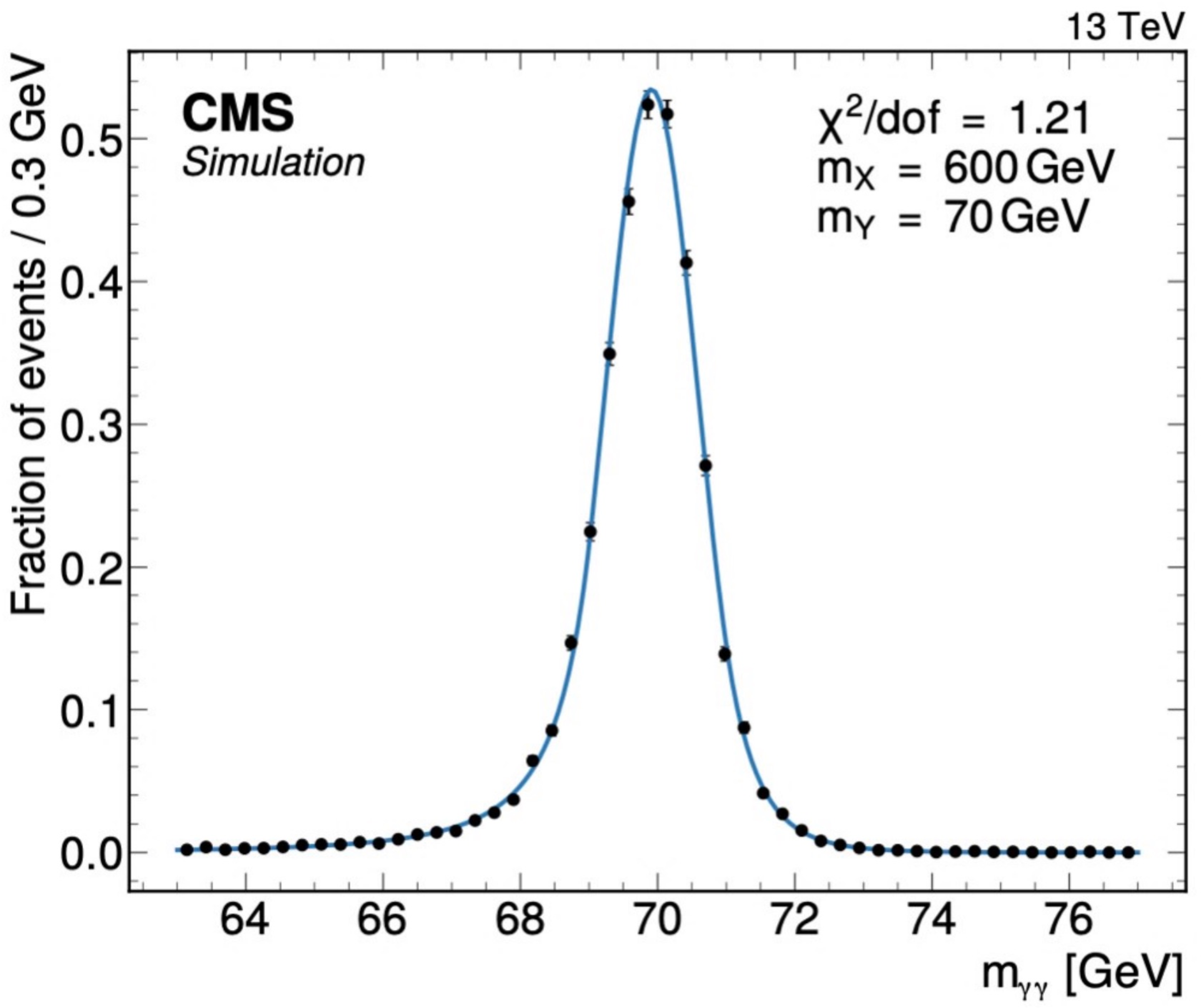
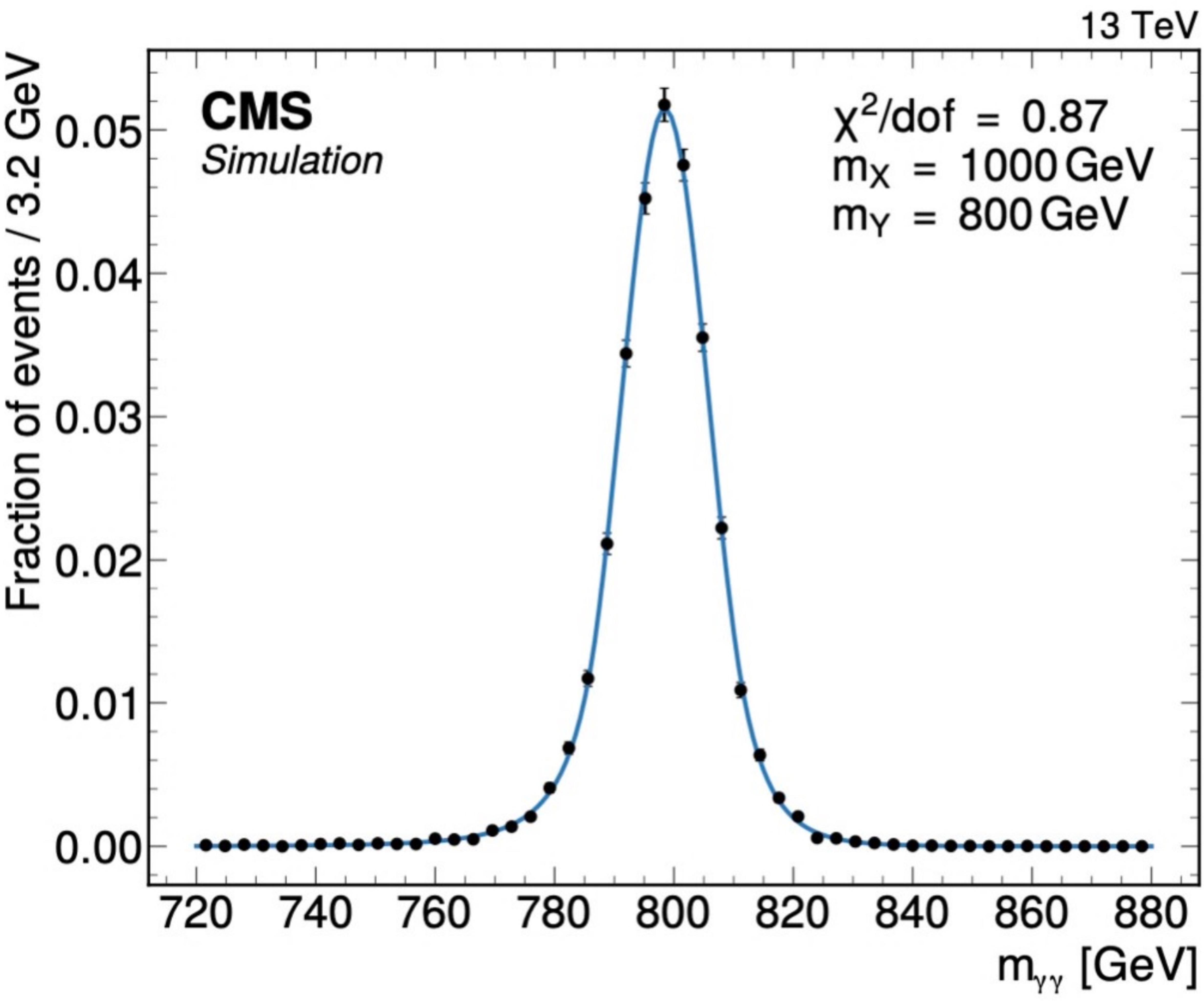
Figure 3:
Parametric models of the signal process for $ m_\mathrm{X}= $ 600 GeV, $ m_{\mathrm{Y}} = $ 70 GeV (left), and for $ m_\mathrm{X}= $ 1000 GeV, $ m_{\mathrm{Y}} = $ 800 GeV (right) in their most sensitive SR. The histograms are normalized to unity. The acronym ``dof" stands for the number of degrees of freedom of the parametric model. |
png pdf |
Figure 3-a:
Parametric models of the signal process for $ m_\mathrm{X}= $ 600 GeV, $ m_{\mathrm{Y}} = $ 70 GeV (left), and for $ m_\mathrm{X}= $ 1000 GeV, $ m_{\mathrm{Y}} = $ 800 GeV (right) in their most sensitive SR. The histograms are normalized to unity. The acronym ``dof" stands for the number of degrees of freedom of the parametric model. |
png pdf |
Figure 3-b:
Parametric models of the signal process for $ m_\mathrm{X}= $ 600 GeV, $ m_{\mathrm{Y}} = $ 70 GeV (left), and for $ m_\mathrm{X}= $ 1000 GeV, $ m_{\mathrm{Y}} = $ 800 GeV (right) in their most sensitive SR. The histograms are normalized to unity. The acronym ``dof" stands for the number of degrees of freedom of the parametric model. |
png pdf |
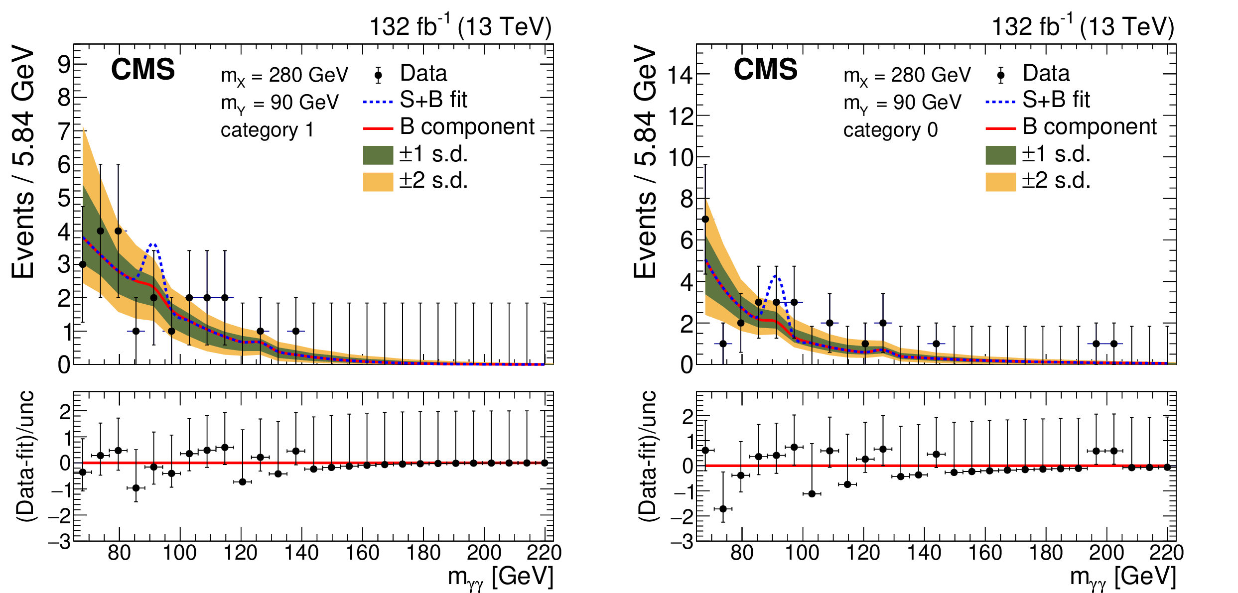
Figure 4:
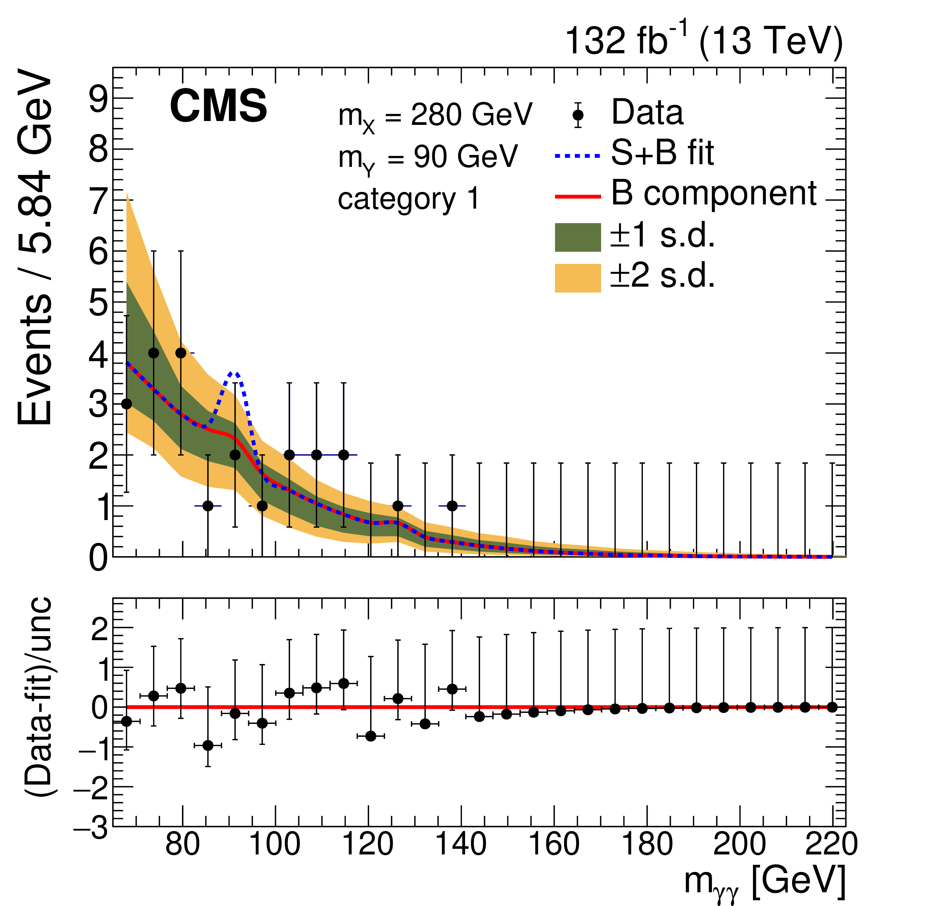
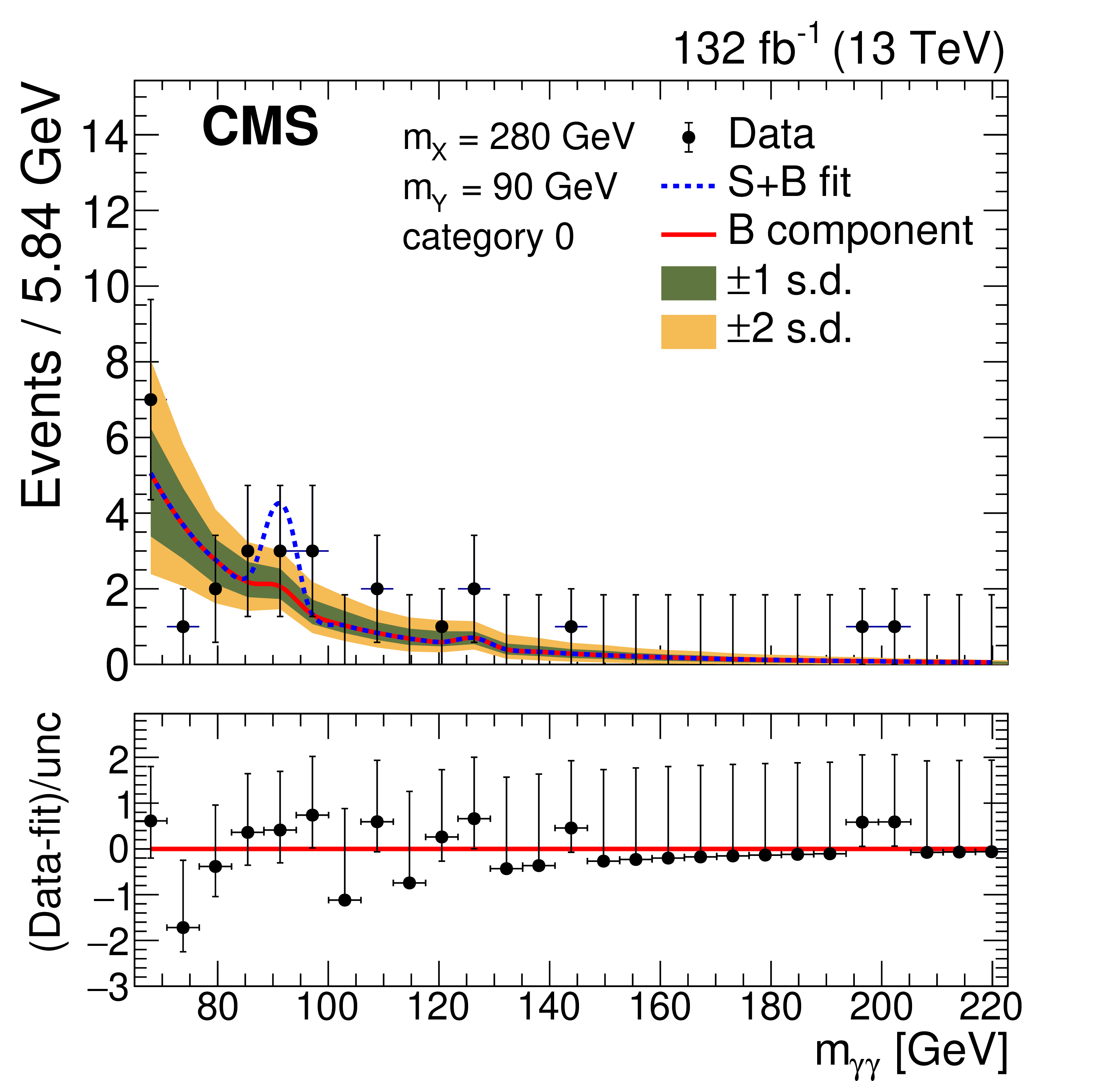
Background-only fit (solid red line) and signal+background fit (dashed blue line) for the mass point hypothesis of $ m_\mathrm{X}= $ 280 GeV, $ m_{\mathrm{Y}} = $ 90 GeV, shown for the most sensitive SR (left) and the second most sensitive SR (right). The points in the lower panel show the difference between the data and the background-only fit, divided by the average uncertainty in the data. The red line in the lower panel shows the background-only fit, which is by definition zero, and it is added as a visual aid. From left to right, the first and second most sensitive SRs are shown. The choice of the background functional form is determined by the maximum likelihood fit. |
png pdf |
Figure 4-a:
Background-only fit (solid red line) and signal+background fit (dashed blue line) for the mass point hypothesis of $ m_\mathrm{X}= $ 280 GeV, $ m_{\mathrm{Y}} = $ 90 GeV, shown for the most sensitive SR (left) and the second most sensitive SR (right). The points in the lower panel show the difference between the data and the background-only fit, divided by the average uncertainty in the data. The red line in the lower panel shows the background-only fit, which is by definition zero, and it is added as a visual aid. From left to right, the first and second most sensitive SRs are shown. The choice of the background functional form is determined by the maximum likelihood fit. |
png pdf |
Figure 4-b:
Background-only fit (solid red line) and signal+background fit (dashed blue line) for the mass point hypothesis of $ m_\mathrm{X}= $ 280 GeV, $ m_{\mathrm{Y}} = $ 90 GeV, shown for the most sensitive SR (left) and the second most sensitive SR (right). The points in the lower panel show the difference between the data and the background-only fit, divided by the average uncertainty in the data. The red line in the lower panel shows the background-only fit, which is by definition zero, and it is added as a visual aid. From left to right, the first and second most sensitive SRs are shown. The choice of the background functional form is determined by the maximum likelihood fit. |
png pdf |
Figure 5:
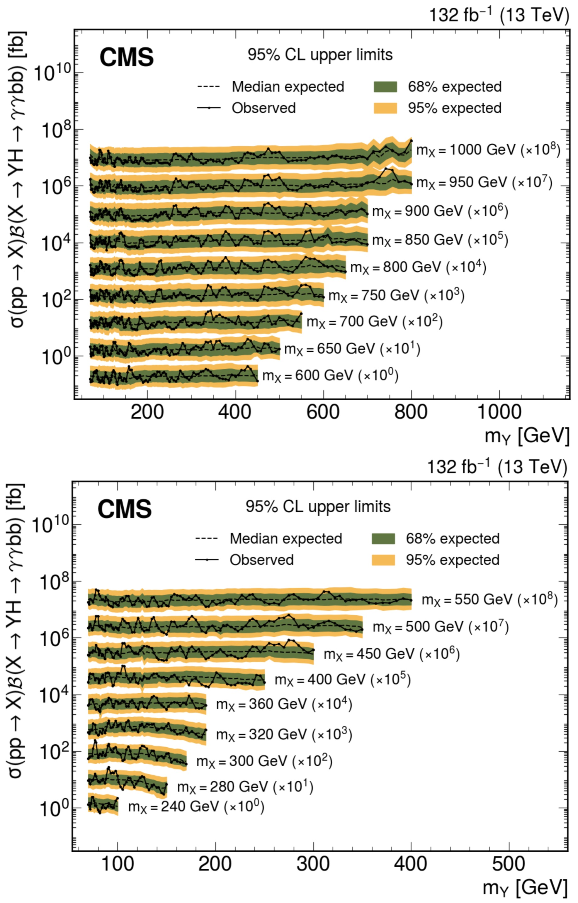
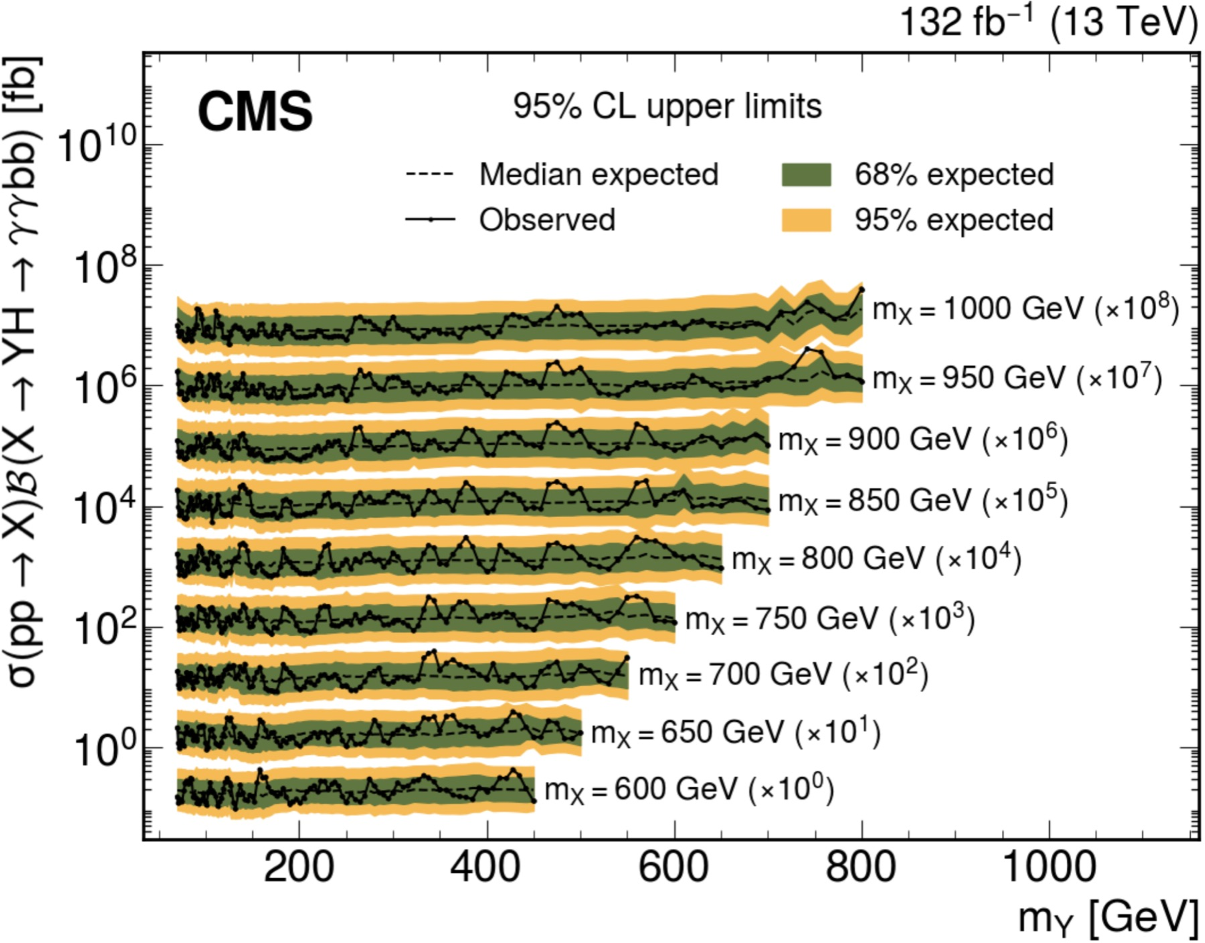
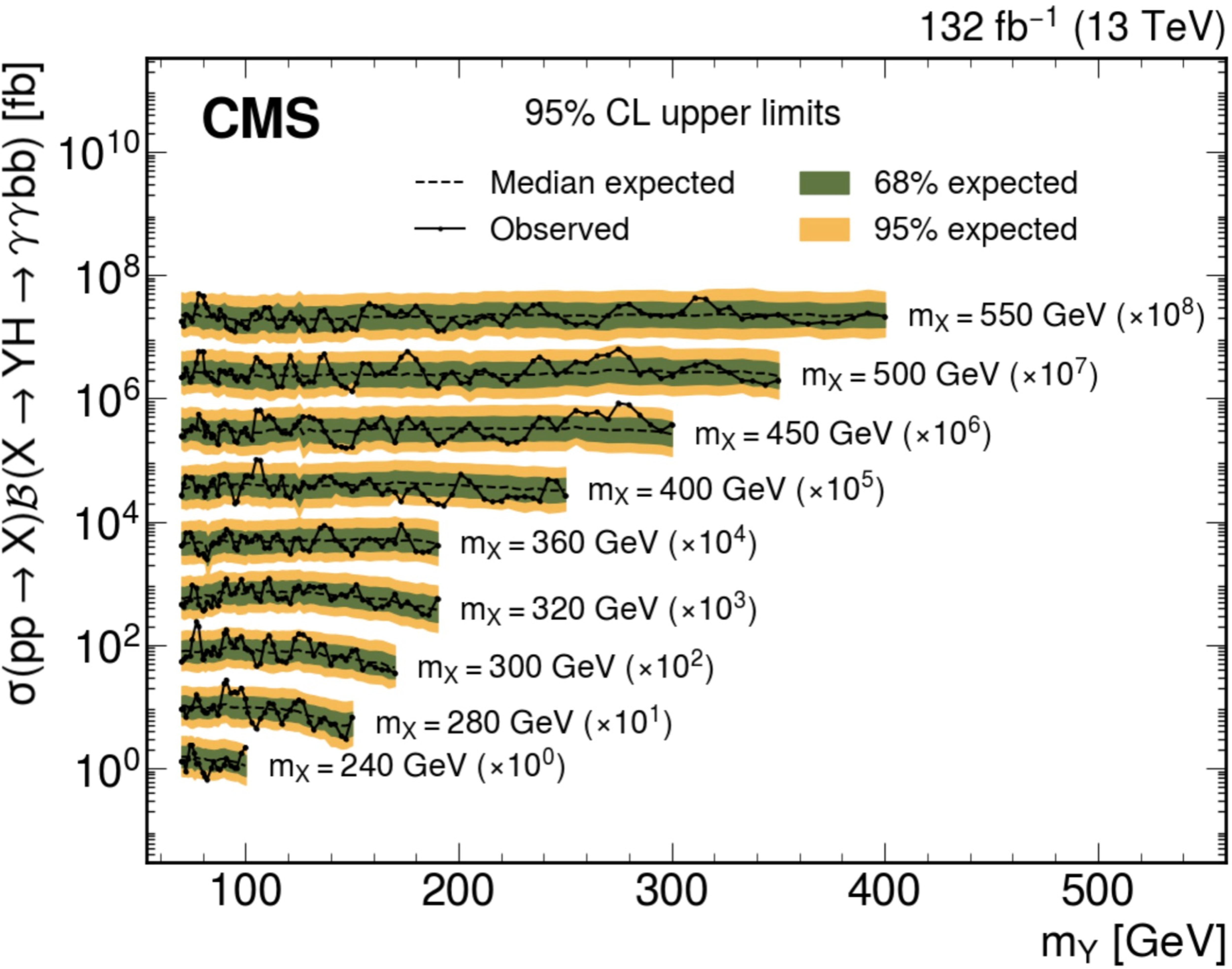
Observed (expected) upper limits on $ \sigma\mathcal{B} $ for the $ \mathrm{X}\to{\mathrm{Y}} (\gamma\gamma)\mathrm{H}(\mathrm{b}\overline{\mathrm{b}}) $ signal with the different mass hypotheses are shown with solid (dashed) lines, for mass points with $ m_\mathrm{X} $ ranging from 600 to 1000 GeV (upper) and from 240 to 550 GeV (lower). The green and the yellow bands define the $ \pm $68% and $ \pm $95% uncertainty bands, respectively. For visualization purposes, the upper limits for mass points with different $ m_\mathrm{X} $ have been multiplied with a constant factor quoted on the right of each band. |
png pdf |
Figure 5-a:
Observed (expected) upper limits on $ \sigma\mathcal{B} $ for the $ \mathrm{X}\to{\mathrm{Y}} (\gamma\gamma)\mathrm{H}(\mathrm{b}\overline{\mathrm{b}}) $ signal with the different mass hypotheses are shown with solid (dashed) lines, for mass points with $ m_\mathrm{X} $ ranging from 600 to 1000 GeV (upper) and from 240 to 550 GeV (lower). The green and the yellow bands define the $ \pm $68% and $ \pm $95% uncertainty bands, respectively. For visualization purposes, the upper limits for mass points with different $ m_\mathrm{X} $ have been multiplied with a constant factor quoted on the right of each band. |
png pdf |
Figure 5-b:
Observed (expected) upper limits on $ \sigma\mathcal{B} $ for the $ \mathrm{X}\to{\mathrm{Y}} (\gamma\gamma)\mathrm{H}(\mathrm{b}\overline{\mathrm{b}}) $ signal with the different mass hypotheses are shown with solid (dashed) lines, for mass points with $ m_\mathrm{X} $ ranging from 600 to 1000 GeV (upper) and from 240 to 550 GeV (lower). The green and the yellow bands define the $ \pm $68% and $ \pm $95% uncertainty bands, respectively. For visualization purposes, the upper limits for mass points with different $ m_\mathrm{X} $ have been multiplied with a constant factor quoted on the right of each band. |
png pdf |
Figure 6:
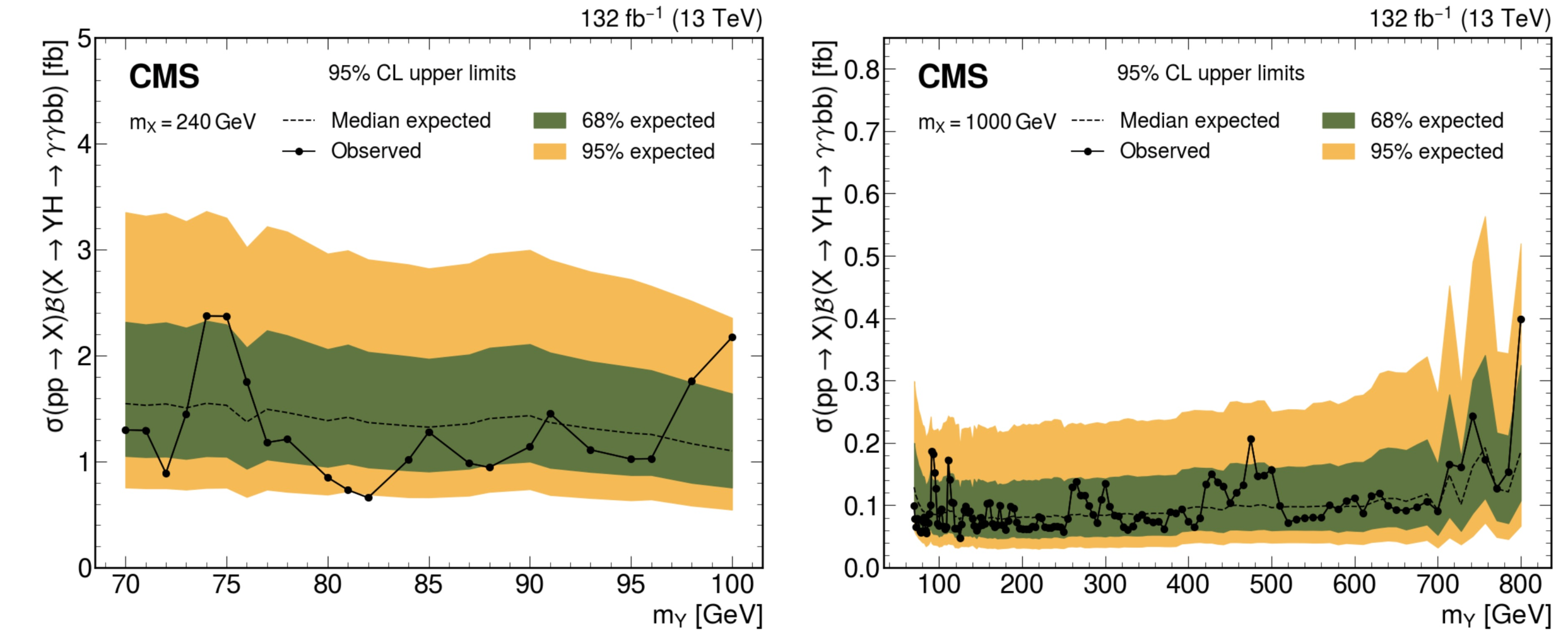
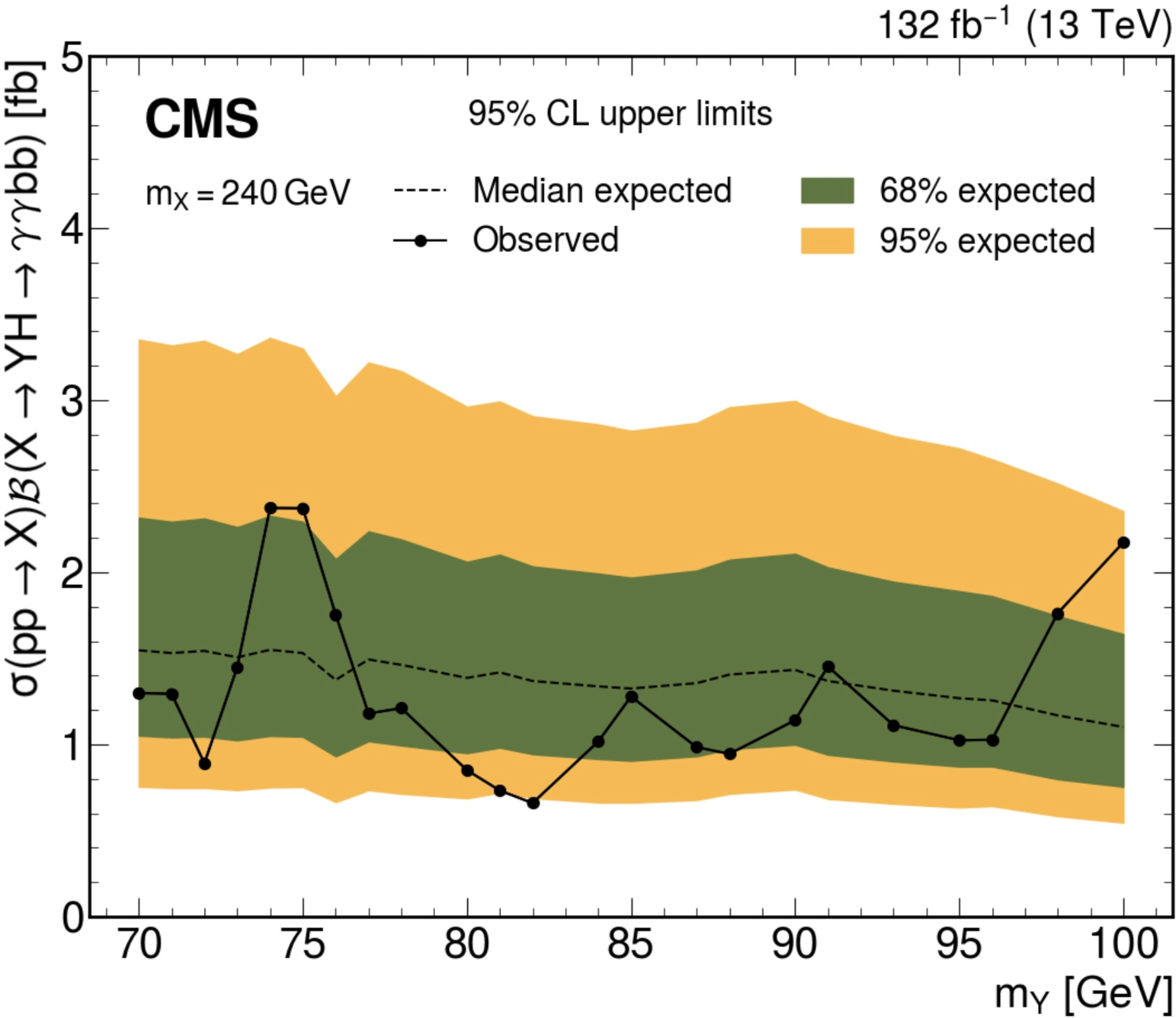
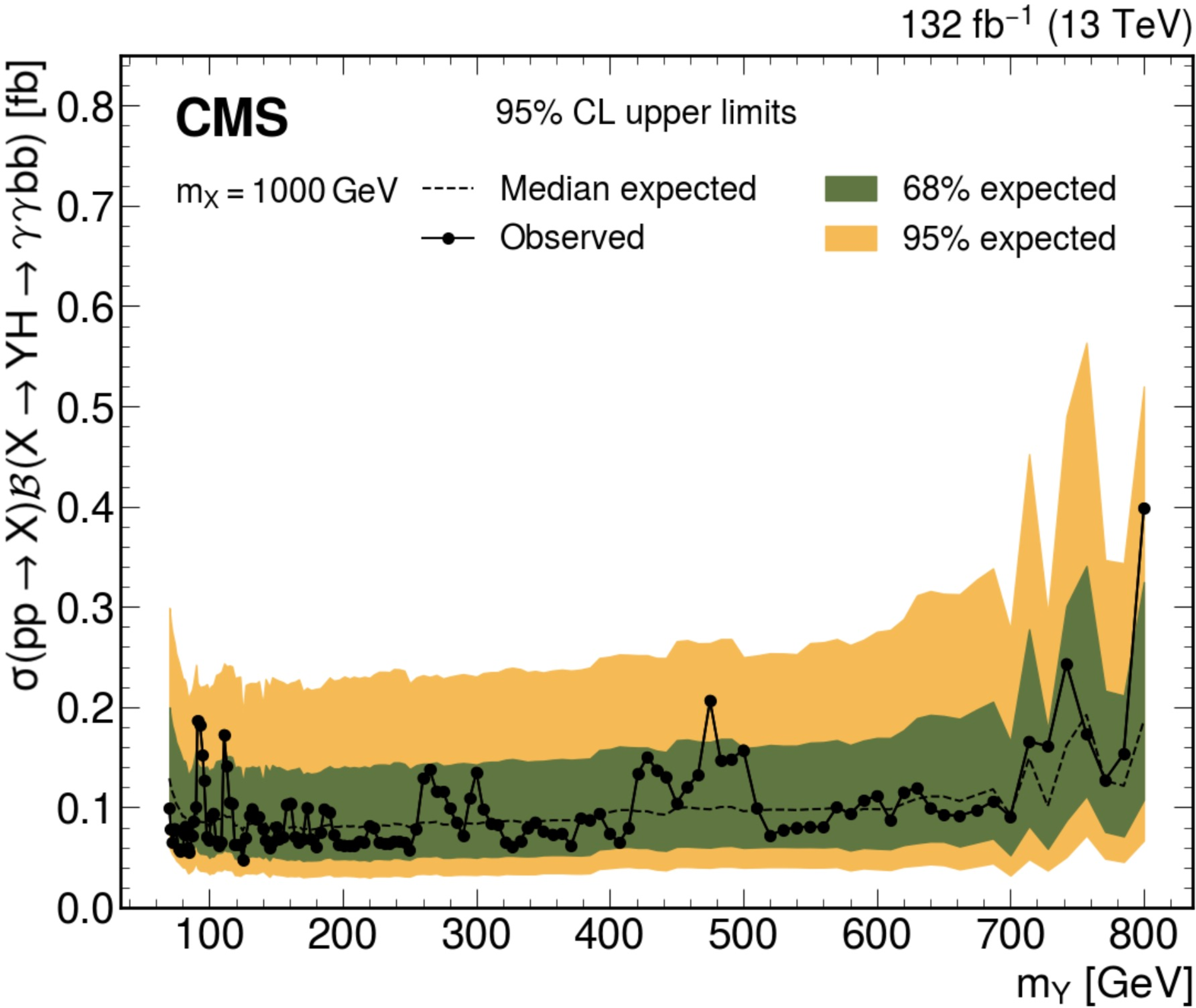
Observed (expected) upper limits on $ \sigma\mathcal{B} $ for the $ \mathrm{X}\to{\mathrm{Y}} (\gamma\gamma)\mathrm{H}(\mathrm{b}\overline{\mathrm{b}}) $ signal with the different $ m_{\mathrm{Y}} $ hypotheses are shown with solid (dashed) lines, shown for the lowest $ m_\mathrm{X} $ = 240 GeV (left) and for the highest $ m_\mathrm{X} $ = 1000 GeV (right). The inner (green) band and the outer (yellow) band indicate the regions containing 68% and 95%, respectively, of the distribution of limits expected under the background-only hypothesis. |
png pdf |
Figure 6-a:
Observed (expected) upper limits on $ \sigma\mathcal{B} $ for the $ \mathrm{X}\to{\mathrm{Y}} (\gamma\gamma)\mathrm{H}(\mathrm{b}\overline{\mathrm{b}}) $ signal with the different $ m_{\mathrm{Y}} $ hypotheses are shown with solid (dashed) lines, shown for the lowest $ m_\mathrm{X} $ = 240 GeV (left) and for the highest $ m_\mathrm{X} $ = 1000 GeV (right). The inner (green) band and the outer (yellow) band indicate the regions containing 68% and 95%, respectively, of the distribution of limits expected under the background-only hypothesis. |
png pdf |
Figure 6-b:
Observed (expected) upper limits on $ \sigma\mathcal{B} $ for the $ \mathrm{X}\to{\mathrm{Y}} (\gamma\gamma)\mathrm{H}(\mathrm{b}\overline{\mathrm{b}}) $ signal with the different $ m_{\mathrm{Y}} $ hypotheses are shown with solid (dashed) lines, shown for the lowest $ m_\mathrm{X} $ = 240 GeV (left) and for the highest $ m_\mathrm{X} $ = 1000 GeV (right). The inner (green) band and the outer (yellow) band indicate the regions containing 68% and 95%, respectively, of the distribution of limits expected under the background-only hypothesis. |
| Tables | |
png pdf |
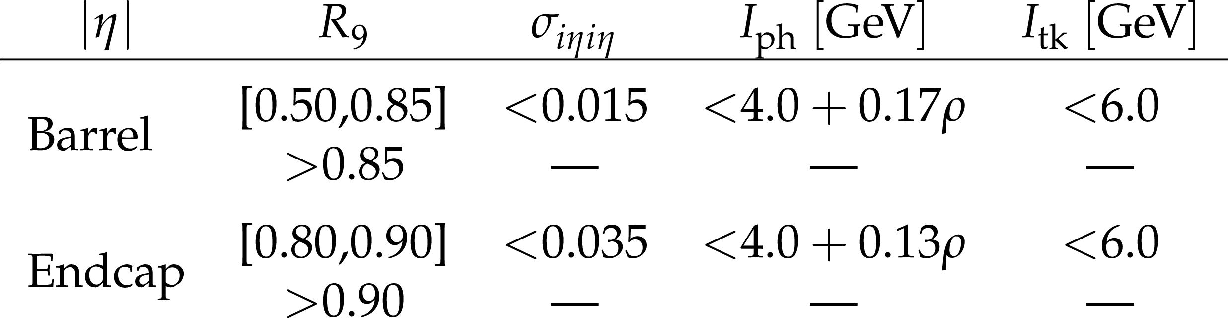
Table 1:
Additional photon requirements, as functions of $ |\eta| $ and $ R_{9} $. The variable $ \rho $ is the median of the transverse energy density per unit area in the event. |
png pdf |
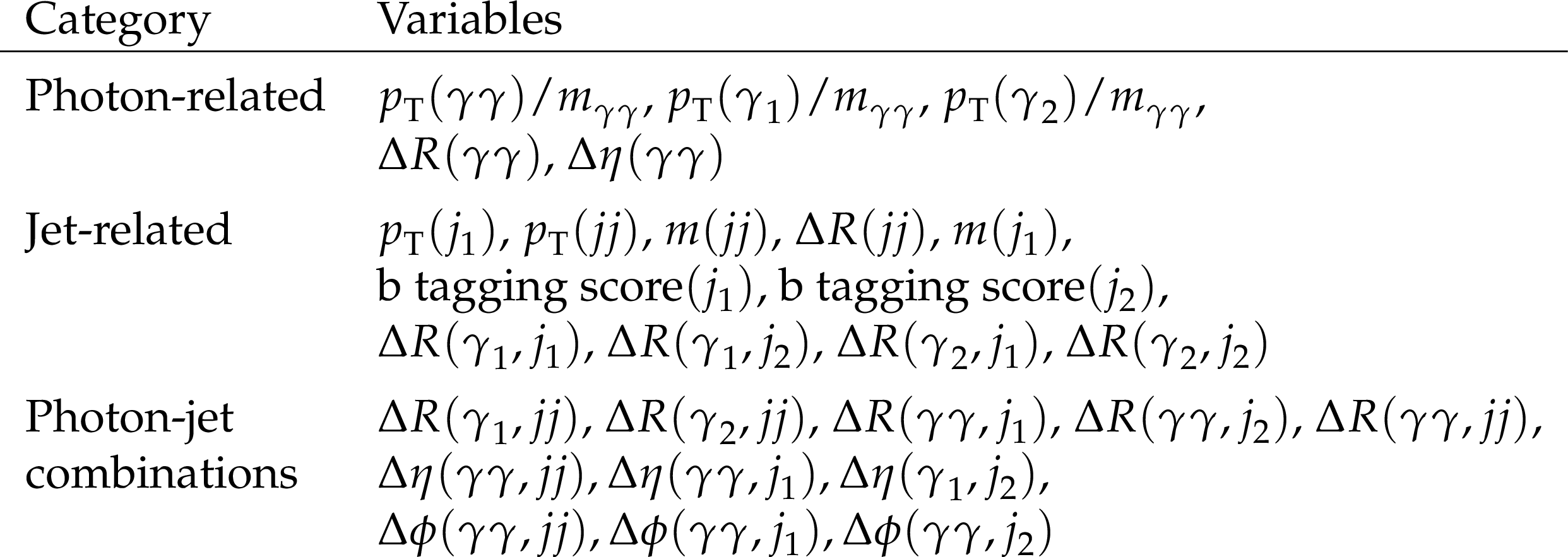
Table 2:
The training variables included as input to the PNN used for the final selection of this search. The symbols $ \gamma_1 $, $ \gamma_2 $ denote the leading and subleading photons, while $ j_1 $ and $ j_2 $ denote the leading and subleading jets. |
| Summary |
| A search has been presented for the production of a new scalar resonance, X, decaying to a standard model Higgs boson and a new scalar resonance, Y, with the final state including a $ \mathrm{b}\overline{\mathrm{b}} $ pair from the Higgs boson decay and a pair of photons from the Y particle decay. This search is the first targeting this final state combination. The analysis probes the mass range 240-1000 GeV for the resonance X and 70-800 GeV for the particle Y, and uses proton-proton collision data collected by the CMS experiment at $ \sqrt{s} = $ 13 TeV, corresponding to an integrated luminosity of 132 fb$ ^{-1} $. In general, the data are found to be compatible with the background-only expectation. As a result, upper limits on the product of the production cross section of X and the branching fraction to the $ \mathrm{b}\overline{\mathrm{b}}\gamma\gamma $ final state are derived at 95% confidence level as functions of the masses of the X and the Y particles. The observed (expected) upper limits are found to be between 0.05-2.69 (0.08-1.94) fb, depending on the assumed specific signal masses. A local (global) significance of 3.33 (0.65) standard deviations is observed for the most significant deviation from the background-only hypothesis, corresponding to $ m_\mathrm{X}= $ 300 GeV and $ m_{\mathrm{Y}} = $ 77 GeV. |
| References | ||||
| 1 | ATLAS Collaboration | Observation of a new particle in the search for the standard model Higgs boson with the detector at the LHC | PLB 716 (2012) 1 | 1207.7214 |
| 2 | CMS Collaboration | Observation of a new boson at a mass of 125 GeV with the CMS experiment at the LHC | PLB 716 (2012) 30 | CMS-HIG-12-028 1207.7235 |
| 3 | CMS Collaboration | Observation of a new boson with mass near 125 GeV in pp collisions at $ \sqrt{s} = $ 7 and 8 TeV | JHEP 06 (2013) 081 | CMS-HIG-12-036 1303.4571 |
| 4 | ATLAS Collaboration | A detailed map of Higgs boson interactions by the ATLAS experiment ten years after the discovery | Nature 607 (2022) 52 | 2207.00092 |
| 5 | CMS Collaboration | A portrait of the Higgs boson by the CMS experiment ten years after the discovery | Nature 607 (2022) 60 | CMS-HIG-22-001 2207.00043 |
| 6 | P. Ramond | Dual theory for free fermions | PRD 3 (1971) 2415 | |
| 7 | Y. A. Golfand and E. P. Likhtman | Extension of the algebra of Poincaré group generators and violation of $ p $ invariance | JETP Lett. 13 (1971) 323 | |
| 8 | A. Neveu and J. H. Schwarz | Factorizable dual model of pions | NPB 31 (1971) 86 | |
| 9 | D. V. Volkov and V. P. Akulov | Possible universal neutrino interaction | JETP Lett. 16 (1972) 438 | |
| 10 | J. Wess and B. Zumino | A Lagrangian model invariant under supergauge transformations | PLB 49 (1974) 52 | |
| 11 | J. Wess and B. Zumino | Supergauge transformations in four dimensions | NPB 70 (1974) 39 | |
| 12 | P. Fayet | Supergauge invariant extension of the Higgs mechanism and a model for the electron and its neutrino | NPB 90 (1975) 104 | |
| 13 | H. P. Nilles | Supersymmetry, supergravity and particle physics | Phys. Rep. 110 (1984) 1 | |
| 14 | A. Djouadi et al. | The minimal supersymmetric standard model: Group summary report | MSSM Working Group Collaboration, in GDR (Groupement De Recherche) Supersymetrie, 1998 | hep-ph/9901246 |
| 15 | U. Ellwanger, C. Hugonie, and A. M. Teixeira | The Next-to-Minimal Supersymmetric Standard Model | Phys. Rept. 496 (2010) 1 | 0910.1785 |
| 16 | T. Robens, T. Stefaniak, and J. Wittbrodt | Two-real-scalar-singlet extension of the SM: LHC phenomenology and benchmark scenarios | EPJC 80 (2020) 151 | 1908.08554 |
| 17 | H. Abouabid et al. | Benchmarking di-Higgs production in various extended Higgs sector models | JHEP 09 (2022) 011 | 2112.12515 |
| 18 | CMS Collaboration | Search for a massive scalar resonance decaying to a light scalar and a Higgs boson in the four b quarks final state with boosted topology | PLB 842 (2023) 137392 | 2204.12413 |
| 19 | CMS Collaboration | Search for a heavy Higgs boson decaying into two lighter Higgs bosons in the $ \tau\tau $bb final state at 13 TeV | JHEP 11 (2021) 057 | CMS-HIG-20-014 2106.10361 |
| 20 | CMS Collaboration | Search for the nonresonant and resonant production of a higgs boson in association with an additional scalar boson in the $ \gamma\gamma\tau\tau $ final state in proton-proton collisions at $ \sqrt{s} = $ 13 tev | Submitted to JHEP, 2025 link |
CMS-HIG-22-012 2506.23012 |
| 21 | CMS Collaboration | Search for a new resonance decaying into two spin-0 bosons in a final state with two photons and two bottom quarks in proton-proton collisions at $ \sqrt{s} = $ 13 TeV | JHEP 05 (2024) 316 | CMS-HIG-21-011 2310.01643 |
| 22 | CMS Collaboration | Search for a standard model-like Higgs boson in the mass range between 70 and 110 GeV in the diphoton final state in proton-proton collisions at $ \sqrt{s}= $ 13 TeV | PLB 860 (2025) 139067 | CMS-HIG-20-002 2405.18149 |
| 23 | CMS Collaboration | HEPData record for this analysis | link | |
| 24 | CMS Collaboration | The CMS experiment at the CERN LHC | JINST 3 (2008) S08004 | |
| 25 | CMS Collaboration | Development of the CMS detector for the CERN LHC Run 3 | JINST 19 (2024) P05064 | CMS-PRF-21-001 2309.05466 |
| 26 | CMS Collaboration | Performance of the CMS Level-1 trigger in proton-proton collisions at $ \sqrt{s} = $ 13 TeV | JINST 15 (2020) P10017 | CMS-TRG-17-001 2006.10165 |
| 27 | CMS Collaboration | The CMS trigger system | JINST 12 (2017) P01020 | CMS-TRG-12-001 1609.02366 |
| 28 | CMS Collaboration | Performance of the CMS high-level trigger during LHC Run 2 | JINST 19 (2024) P11021 | CMS-TRG-19-001 2410.17038 |
| 29 | CMS Collaboration | Technical proposal for the Phase-II upgrade of the Compact Muon Solenoid | CMS Technical Proposal CERN-LHCC-2015-010, CMS-TDR-15-02, 2015 CDS |
|
| 30 | CMS Collaboration | Particle-flow reconstruction and global event description with the CMS detector | JINST 12 (2017) P10003 | CMS-PRF-14-001 1706.04965 |
| 31 | CMS Collaboration | Performance of photon reconstruction and identification with the CMS detector in proton-proton collisions at sqrt(s) = 8 TeV | JINST 10 (2015) P08010 | CMS-EGM-14-001 1502.02702 |
| 32 | CMS Collaboration | A measurement of the Higgs boson mass in the diphoton decay channel | PLB 805 (2020) 135425 | CMS-HIG-19-004 2002.06398 |
| 33 | CMS Collaboration | Electron and photon reconstruction and identification with the CMS experiment at the CERN LHC | JINST 16 (2021) P05014 | CMS-EGM-17-001 2012.06888 |
| 34 | CMS Collaboration | ECAL 2016 refined calibration and Run2 summary plots | CMS Detector Performance Summary CMS-DP-2020-021, 2020 CDS |
|
| 35 | CMS Collaboration | Performance of CMS muon reconstruction in pp collision events at $ \sqrt{s} = $ 7 TeV | JINST 7 (2012) P10002 | CMS-MUO-10-004 1206.4071 |
| 36 | M. Cacciari, G. P. Salam, and G. Soyez | The anti-$ k_{\mathrm{T}} $ jet clustering algorithm | JHEP 04 (2008) 063 | 0802.1189 |
| 37 | M. Cacciari, G. P. Salam, and G. Soyez | Fastjet user manual | EPJC 72 (2012) 1896 | 1111.6097 |
| 38 | CMS Collaboration | Pileup mitigation at CMS in 13 TeV data | JINST 15 (2020) P09018 | CMS-JME-18-001 2003.00503 |
| 39 | CMS Collaboration | Jet energy scale and resolution in the CMS experiment in pp collisions at 8 TeV | JINST 12 (2017) P02014 | CMS-JME-13-004 1607.03663 |
| 40 | E. Bols et al. | Jet flavour classification using DeepJet | JINST 15 (2020) P12012 | 2008.10519 |
| 41 | CMS Collaboration | Performance of the DeepJet b tagging algorithm using 41.9 fb of data from proton-proton collisions at 13 TeV with Phase 1 CMS detector | CMS Detector Performance Summary CMS-DP-2018-058, 2018 CDS |
|
| 42 | J. Alwall et al. | The automated computation of tree-level and next-to-leading order differential cross sections, and their matching to parton shower simulations | JHEP 07 (2014) 079 | 1405.0301 |
| 43 | R. Frederix et al. | The automation of next-to-leading order electroweak calculations | JHEP 07 (2018) 185 | 1804.10017 |
| 44 | D. de Florian et al. | Handbook of LHC Higgs cross sections: 4. Deciphering the nature of the Higgs sector | CERN Report CERN-2017-002-M, 2016 link |
1610.07922 |
| 45 | S. Frixione, P. Nason, and C. Oleari | Matching NLO QCD computations with parton shower simulations: the POWHEG method | JHEP 11 (2007) 070 | 0709.2092 |
| 46 | S. Alioli, P. Nason, C. Oleari, and E. Re | NLO single-top production matched with shower in POWHEG: $ s $- and $ t $-channel contributions | JHEP 09 (2009) 111 | 0907.4076 |
| 47 | T. Melia, P. Nason, R. Rontsch, and G. Zanderighi | $ W^+ W^- $, $ W Z $ and $ Z Z $ production in the POWHEG BOX | JHEP 11 (2011) 078 | 1107.5051 |
| 48 | P. Nason and G. Zanderighi | $ W^+ W^- $, $ W Z $ and $ Z Z $ production in the POWHEG-BOX-V2 | EPJC 74 (2014) 2702 | 1311.1365 |
| 49 | E. Bagnaschi, G. Degrassi, P. Slavich, and A. Vicini | Higgs production via gluon fusion in the POWHEG approach in the SM and in the MSSM | JHEP 02 (2012) 088 | 1111.2854 |
| 50 | G. Heinrich, S. P. Jones, M. Kerner, and L. Scyboz | A non-linear EFT description of $ gg\to hh $ at NLO interfaced to POWHEG | JHEP 10 (2020) 021 | 2006.16877 |
| 51 | G. Heinrich et al. | Probing the trilinear Higgs boson coupling in di-Higgs production at NLO QCD including parton shower effects | JHEP 06 (2019) 066 | 1903.08137 |
| 52 | S. Jones and S. Kuttimalai | Parton shower and NLO-matching uncertainties in Higgs boson pair production | JHEP 02 (2018) 176 | 1711.03319 |
| 53 | G. Heinrich et al. | NLO predictions for Higgs boson pair production with full top quark mass dependence matched to parton showers | JHEP 08 (2017) 088 | 1703.09252 |
| 54 | G. Buchalla et al. | Higgs boson pair production in non-linear effective field theory with full $ m_t $-dependence at NLO QCD | JHEP 09 (2018) 057 | 1806.05162 |
| 55 | T. Gleisberg et al. | Event generation with SHERPA 1.1 | JHEP 02 (2009) 007 | 0811.4622 |
| 56 | T. Sjöstrand et al. | An introduction to PYTHIA 8.2 | Comput. Phys. Commun. 191 (2015) 159 | 1410.3012 |
| 57 | CMS Collaboration | Event generator tunes obtained from underlying event and multiparton scattering measurements | EPJC 76 (2016) 155 | CMS-GEN-14-001 1512.00815 |
| 58 | CMS Collaboration | Extraction and validation of a new set of CMS PYTHIA8 tunes from underlying-event measurements | EPJC 80 (2020) 4 | CMS-GEN-17-001 1903.12179 |
| 59 | NNPDF Collaboration | Parton distributions from high-precision collider data | EPJC 77 (2017) 663 | 1706.00428 |
| 60 | GEANT 4 Collaboration | GEANT 4 --- a simulation toolkit | NIM A 506 (2003) 250 | |
| 61 | CMS Collaboration | Performance of the CMS muon detector and muon reconstruction with proton-proton collisions at $ \sqrt{s}= $ 13 TeV | JINST 13 (2018) P06015 | CMS-MUO-16-001 1804.04528 |
| 62 | CMS Collaboration | Performance of missing transverse momentum reconstruction in proton-proton collisions at $ \sqrt{s} = $ 13 TeV using the CMS detector | JINST 14 (2019) P07004 | CMS-JME-17-001 1903.06078 |
| 63 | CMS Collaboration | Measurements of $ t\overline{t}H $ production and the $ CP $ structure of the Yukawa interaction between the Higgs boson and top quark in the diphoton decay channel | PRL 125 (2020) 061801 | CMS-HIG-19-013 2003.10866 |
| 64 | P. Baldi et al. | Parameterized neural networks for high-energy physics | EPJC 76 (2016) | 1601.07913 |
| 65 | M. J. Oreglia | A study of the reactions $ \psi^\prime \to \gamma \gamma \psi $ | PhD thesis, Stanford University, SLAC Report SLAC-R-236, see Appendix D, 1980 link |
|
| 66 | J. E. Gaiser | Charmonium spectroscopy from radiative decays of the $ J/\psi $ and $ \psi^\prime $ | PhD thesis, Stanford University, SLAC Report SLAC-R-255, 1982 link |
|
| 67 | S. Choi and H. Oh | Improved extrapolation methods of data-driven background estimations in high energy physics | EPJC 81 (2021) | |
| 68 | R. A. Fisher | On the interpretation of $ \chi^{2} $ from contingency tables, and the calculation of P | J. R. Stat. Soc. 85 (1922) 87 | |
| 69 | P. D. Dauncey, M. Kenzie, N. Wardle, and G. J. Davies | Handling uncertainties in background shapes | JINST 10 (2015) P04015 | 1408.6865 |
| 70 | J. Butterworth et al. | PDF4LHC recommendations for LHC Run II | JPG 43 (2016) 023001 | 1510.03865 |
| 71 | J. Baglio et al. | $ \mathrm{g}\mathrm{g} \rightarrow \mathrm{H}\mathrm{H} $: Combined uncertainties | PRD 103 (2021) 056002 | 2008.11626 |
| 72 | S. Heinemeyer at al. | Handbook of LHC Higgs cross sections: 3. Higgs properties | CERN Yellow Reports: Monographs, 2013 link |
|
| 73 | CMS Collaboration | Precision luminosity measurement in proton-proton collisions at $ \sqrt{s} = $ 13 TeV in 2015 and 2016 at CMS | EPJC 81 (2021) 800 | CMS-LUM-17-003 2104.01927 |
| 74 | CMS Collaboration | CMS luminosity measurement for the 2017 data-taking period at $ \sqrt{s} = $ 13 TeV | CMS Physics Analysis Summary, 2018 link |
CMS-PAS-LUM-17-004 |
| 75 | CMS Collaboration | CMS luminosity measurement for the 2018 data-taking period at $ \sqrt{s} = $ 13 TeV | CMS Physics Analysis Summary, 2019 link |
CMS-PAS-LUM-18-002 |
| 76 | CMS Collaboration | Measurement of the inelastic proton-proton cross section at $ \sqrt{s}= $ 13 TeV | JHEP 07 (2018) 161 | CMS-FSQ-15-005 1802.02613 |
| 77 | CMS Collaboration | Measurement of the inclusive $ W $ and $ Z $ production cross sections in $ pp $ collisions at $ \sqrt{s}= $ 7 TeV | JHEP 10 (2011) 132 | CMS-EWK-10-005 1107.4789 |
| 78 | CMS Collaboration | Identification of heavy-flavour jets with the CMS detector in pp collisions at 13 TeV | JINST 13 (2018) P05011 | CMS-BTV-16-002 1712.07158 |
| 79 | CMS Collaboration | The CMS statistical analysis and combination tool: Combine | Comput. Softw. Big Sci. 8 (2024) 19 | CMS-CAT-23-001 2404.06614 |
| 80 | W. Verkerke and D. Kirkby | The RooFit toolkit for data modeling | in Proc. 13th International Conference on Computing in High Energy and Nuclear Physics (CHEP ): La Jolla CA, United States, 2003 link |
physics/0306116 |
| 81 | L. Moneta et al. | The RooStats project | in Proc. 13th International Workshop on Advanced Computing and Analysis Techniques in Physics Research (ACAT ): Jaipur, India, 2010 link |
1009.1003 |
| 82 | E. Gross and O. Vitells | Trial factors for the look elsewhere effect in high energy physics | EPJC 70 (2010) | 1005.1891 |
|
|
Compact Muon Solenoid LHC, CERN |
|

|

|

|

|

|