

Compact Muon Solenoid
LHC, CERN
| CMS-PAS-SMP-25-001 | ||
| Search for anomalous couplings in WW and WZ production with single-lepton final states at $ \sqrt{s}= $ 13 TeV | ||
| CMS Collaboration | ||
| 2026-05-18 | ||
| Abstract: A search for deviations from the standard model in a generic manner using an effective field theory (EFT) approach is carried out using the proton-proton collision dataset recorded by the CMS experiment at the LHC at a center-of-mass energy of 13 TeV, corresponding to an integrated luminosity of 138 fb$ ^{-1} $. In this study we constrain Wilson coefficients (WCs) corresponding to dimension six EFT operators that would lead to anomalous gauge boson self and vector boson to quark couplings. We consider diboson (WW and WZ) production processes with one W boson decaying to (anti-)lepton plus anti-neutrino (neutrino) and the second W or Z boson decaying hadronically. Since the contribution from anomalous couplings is expected to be most visible at high energy scales, we focus on final states where the hadronic decays from the W and Z bosons merge into a single large-radius jet. A dedicated machine-learning based classifier is employed to separate such jets from vector boson decays to those from background processes. We report the most stringent constraints to date on the WCs of operators corresponding to anomalous triple gauge boson couplings. The bounds set on vector bosons' to quark couplings are competitive to those from previous inclusive jet measurements. | ||
| Links: CDS record (PDF) ; CADI line (restricted) ; | ||
| Figures | |
png pdf |
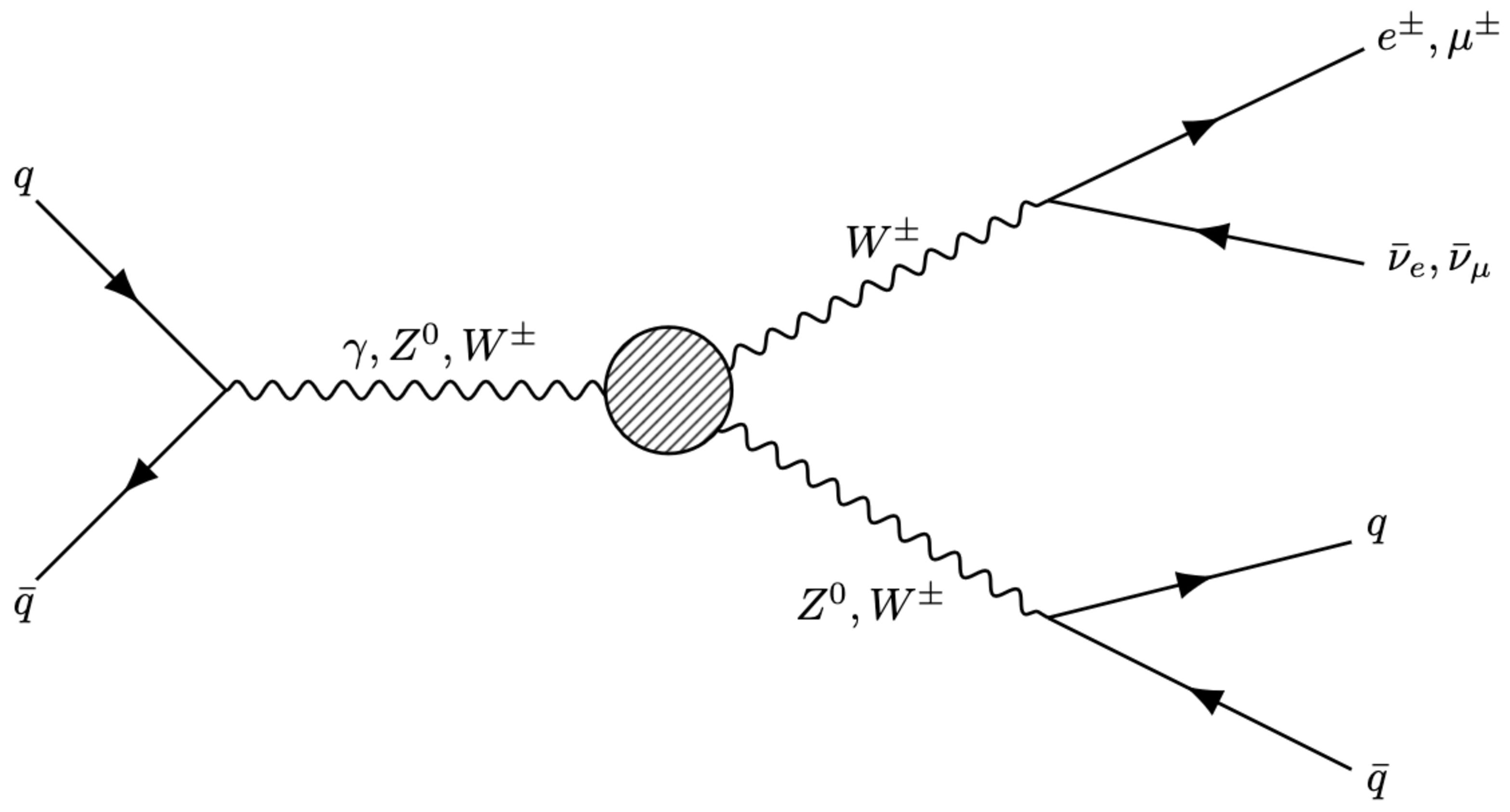
Figure 1:
The LO Feynman diagram for the process studied in this analysis, with an anomalous triple gauge coupling vertex, where one W boson decays to a lepton and a neutrino and another W (Z) boson decays to quarks. |
png pdf |
Figure 2:
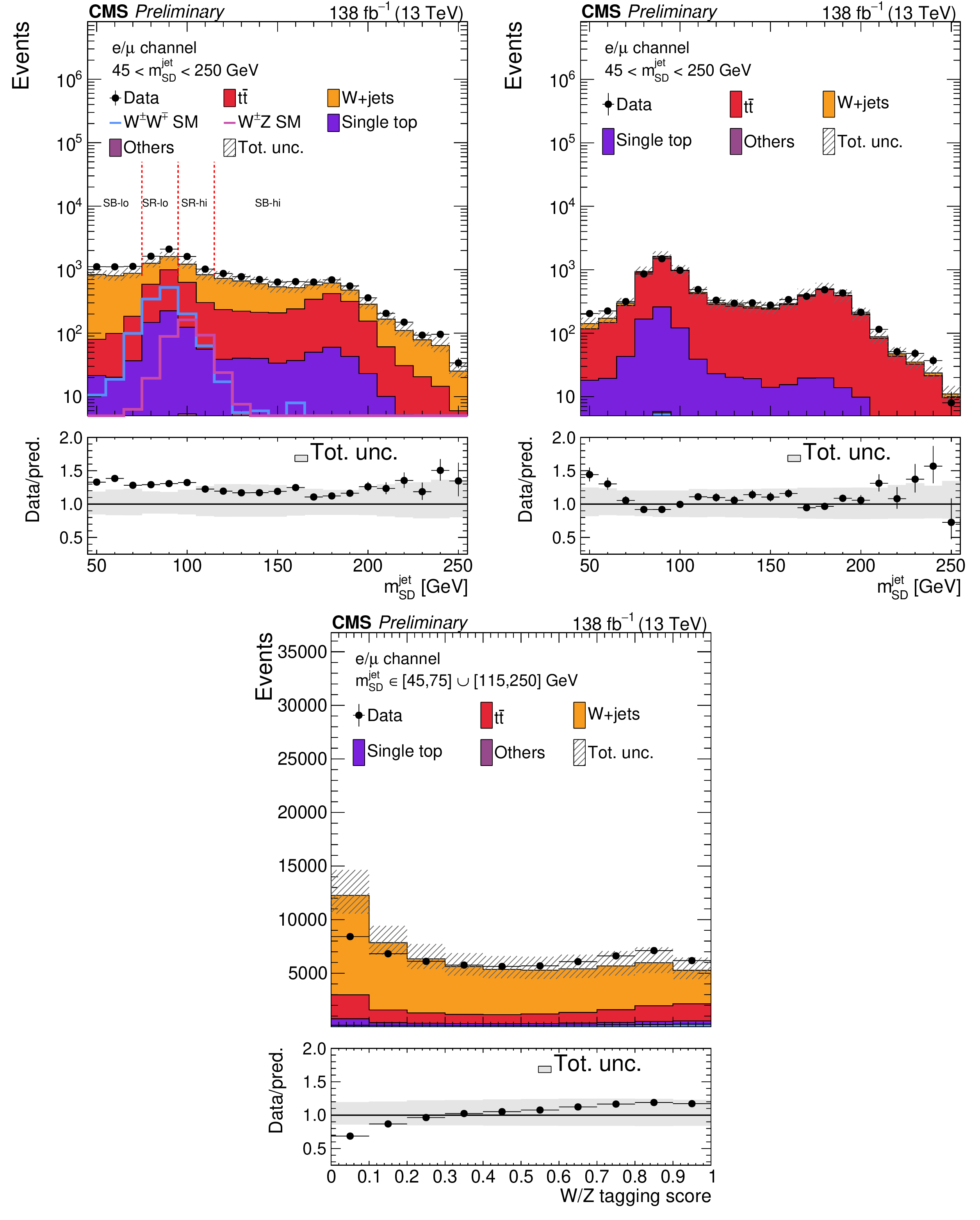
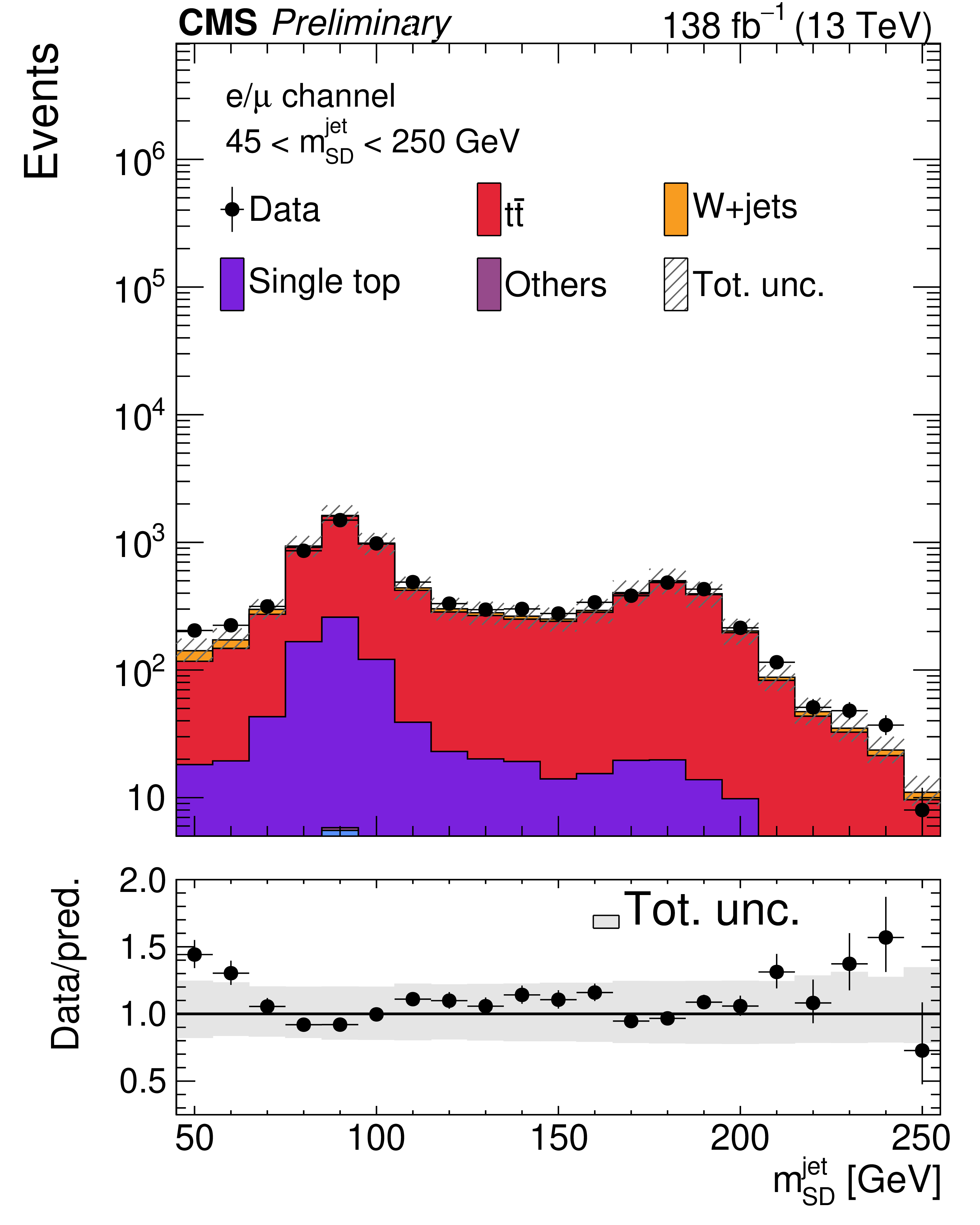
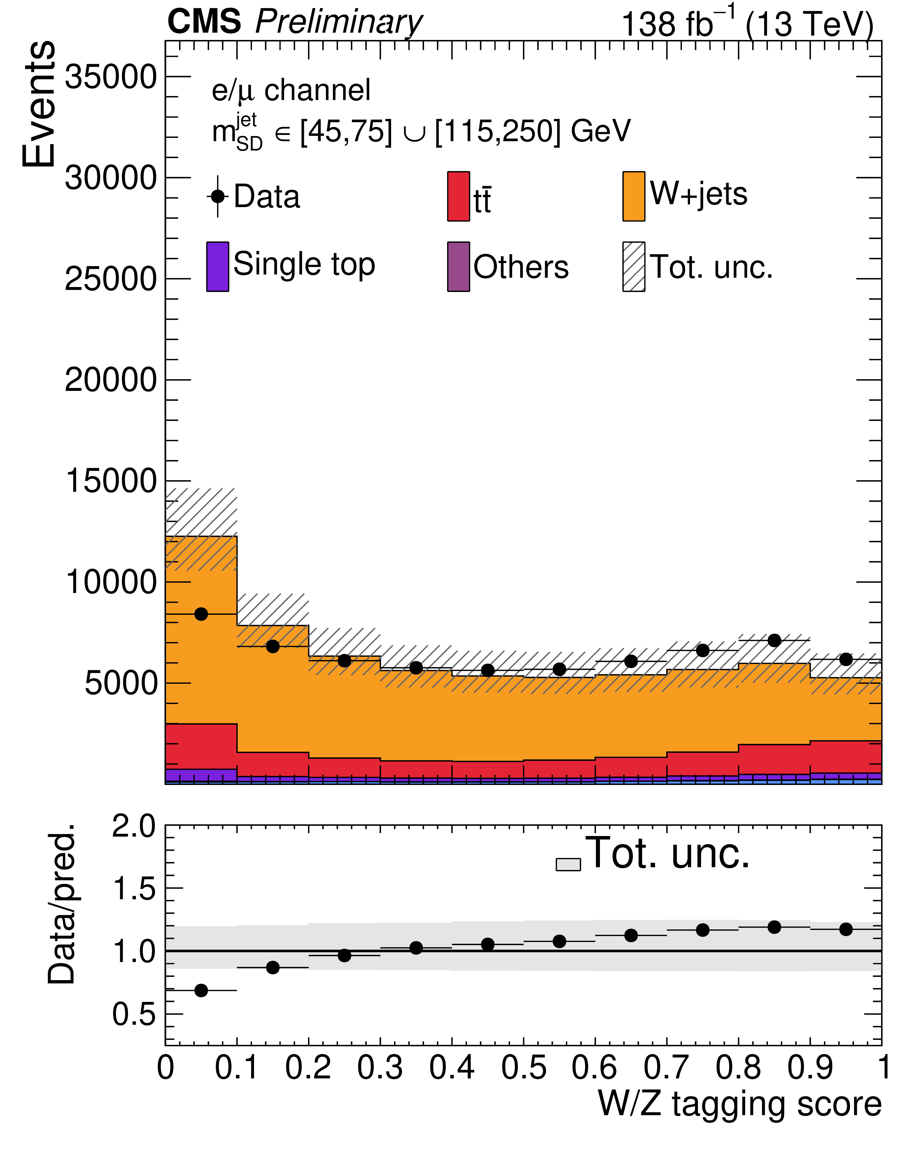
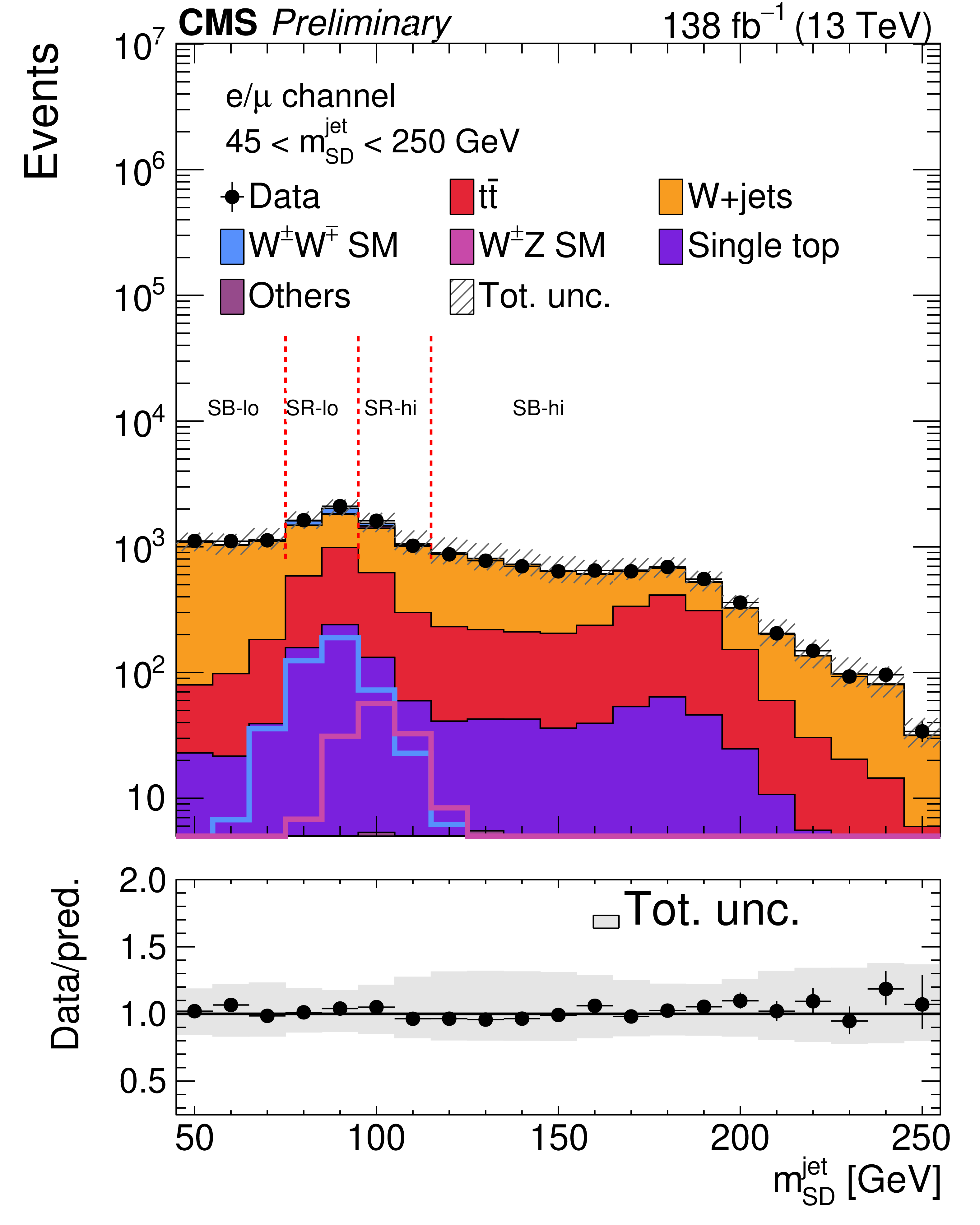
Large-R jet $ m_{\text{SD}}^{\text{jet}} $ in the combined $ \mathrm{W}{\text{+jets}} $ CR and the signal region (top left) and in the $ {\mathrm{t}\overline{\mathrm{t}}} $ control region (top right) after applying the tagger. The $ \mathrm{W}/\mathrm{Z} $ tagging score in the $ \mathrm{W}{\text{+jets}} $ CR without tagger requirement is shown in the bottom row. These prefit distributions are obtained after combining the electron and muon channels and correspond to the full Run 2 data statistics. The uncertainty band shown in the ratio plot contains both statistical and systematic components. |
png pdf |
Figure 2-a:
Large-R jet $ m_{\text{SD}}^{\text{jet}} $ in the combined $ \mathrm{W}{\text{+jets}} $ CR and the signal region (top left) and in the $ {\mathrm{t}\overline{\mathrm{t}}} $ control region (top right) after applying the tagger. The $ \mathrm{W}/\mathrm{Z} $ tagging score in the $ \mathrm{W}{\text{+jets}} $ CR without tagger requirement is shown in the bottom row. These prefit distributions are obtained after combining the electron and muon channels and correspond to the full Run 2 data statistics. The uncertainty band shown in the ratio plot contains both statistical and systematic components. |
png pdf |
Figure 2-b:
Large-R jet $ m_{\text{SD}}^{\text{jet}} $ in the combined $ \mathrm{W}{\text{+jets}} $ CR and the signal region (top left) and in the $ {\mathrm{t}\overline{\mathrm{t}}} $ control region (top right) after applying the tagger. The $ \mathrm{W}/\mathrm{Z} $ tagging score in the $ \mathrm{W}{\text{+jets}} $ CR without tagger requirement is shown in the bottom row. These prefit distributions are obtained after combining the electron and muon channels and correspond to the full Run 2 data statistics. The uncertainty band shown in the ratio plot contains both statistical and systematic components. |
png pdf |
Figure 2-c:
Large-R jet $ m_{\text{SD}}^{\text{jet}} $ in the combined $ \mathrm{W}{\text{+jets}} $ CR and the signal region (top left) and in the $ {\mathrm{t}\overline{\mathrm{t}}} $ control region (top right) after applying the tagger. The $ \mathrm{W}/\mathrm{Z} $ tagging score in the $ \mathrm{W}{\text{+jets}} $ CR without tagger requirement is shown in the bottom row. These prefit distributions are obtained after combining the electron and muon channels and correspond to the full Run 2 data statistics. The uncertainty band shown in the ratio plot contains both statistical and systematic components. |
png pdf |
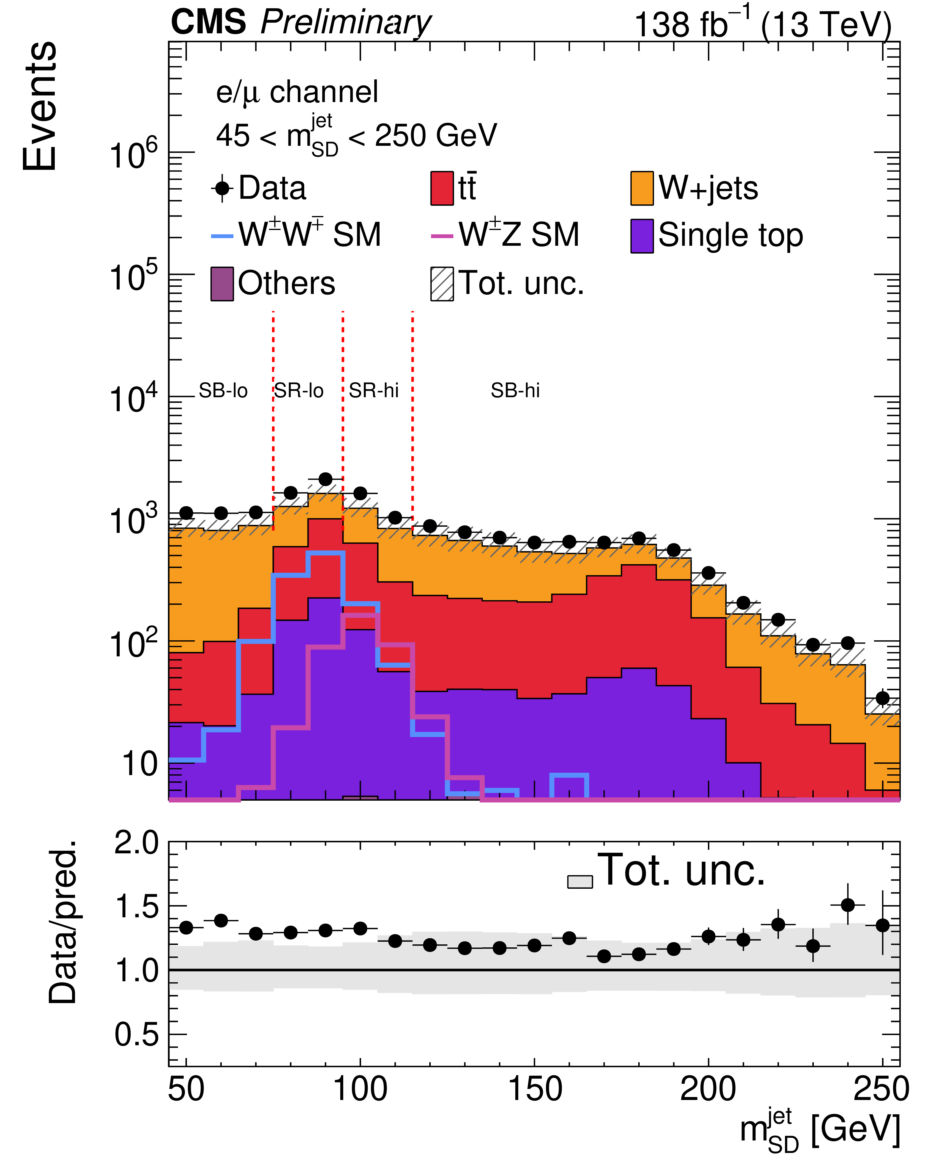
Figure 3:
Large-R jet $ m_{\text{SD}}^{\text{jet}} $ in the $ \mathrm{W}{\text{+jets}} $ CR and the signal region for the combined electron and muon channels with full Run 2 statistics after the ML fit. The uncertainty band shown on the ratio plot contains both statistical and systematic components on the predictions before the ML fit. The SM WW and WZ processes are shown with filled areas contributing to the total background prediction. In addition both processes are overlaid as lines to show more clearly their shape. |
png pdf |
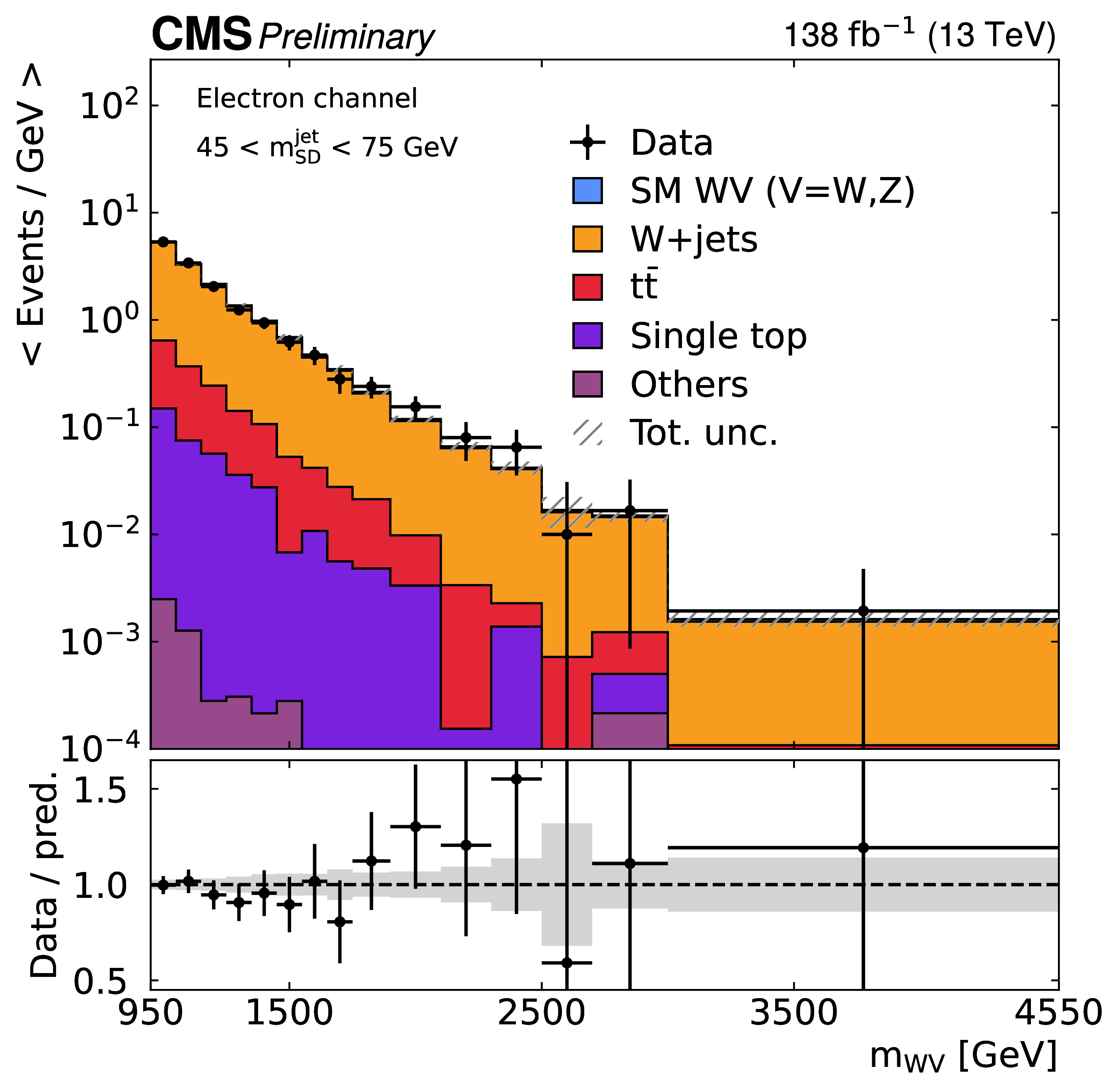
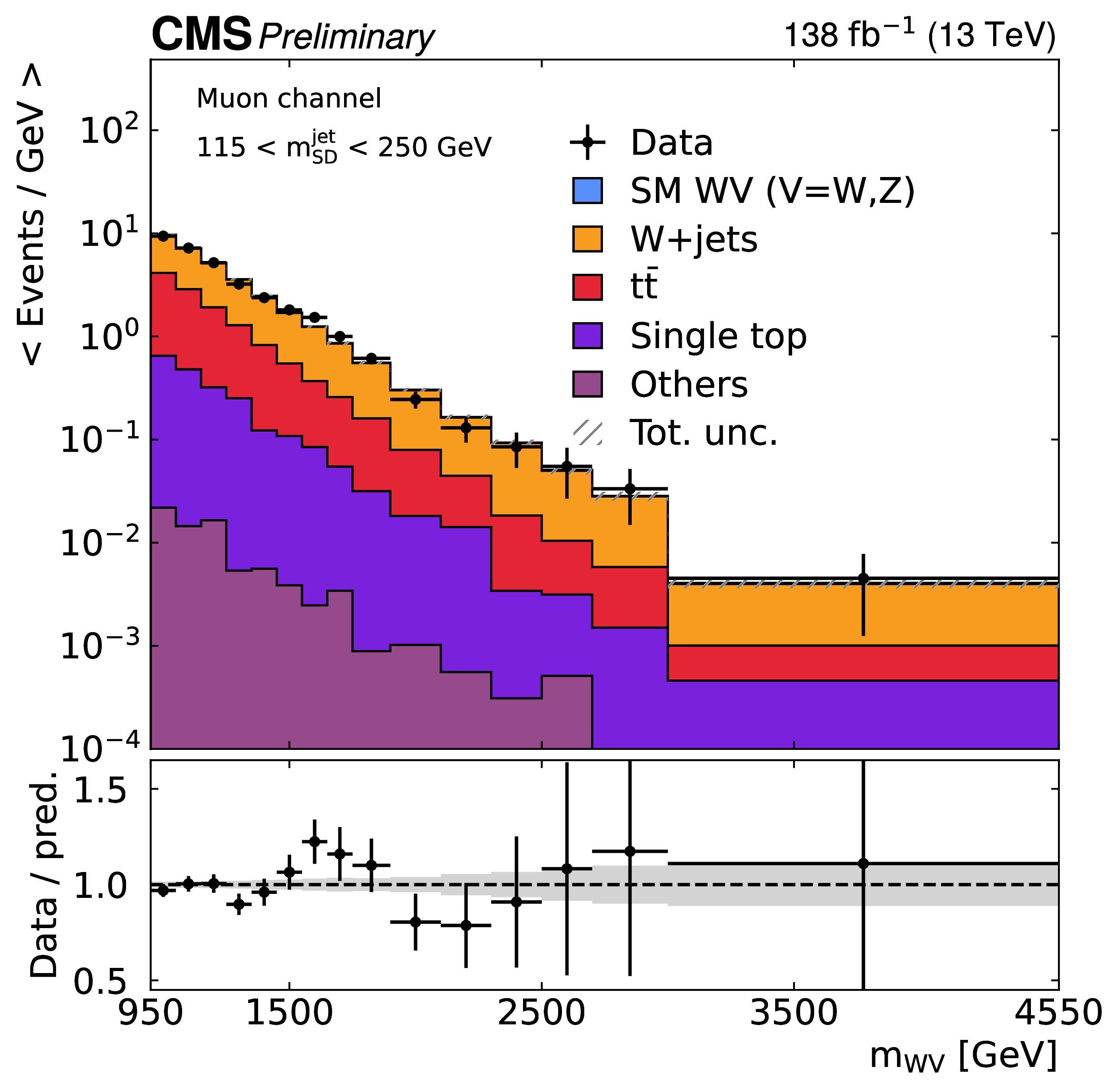
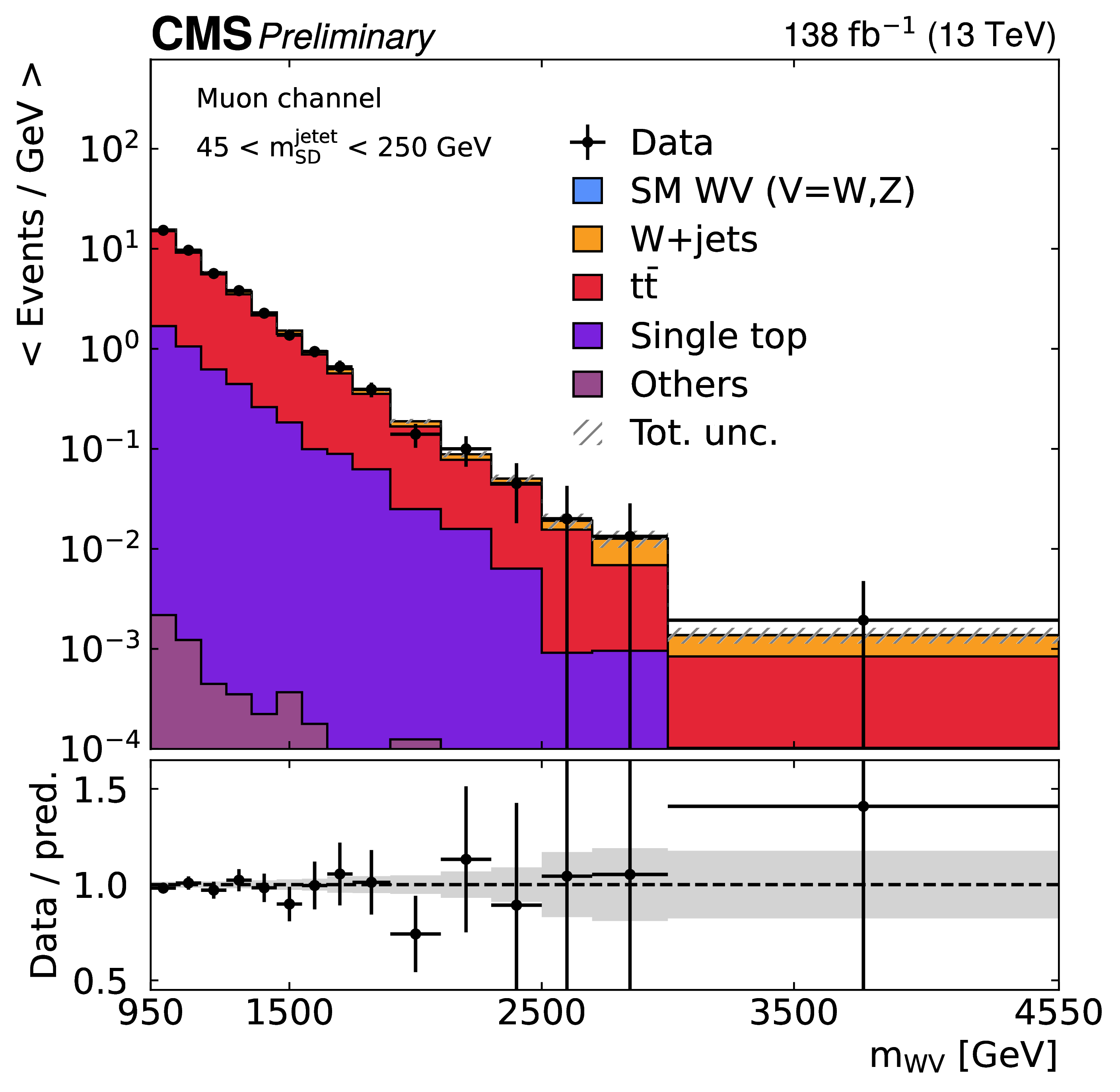
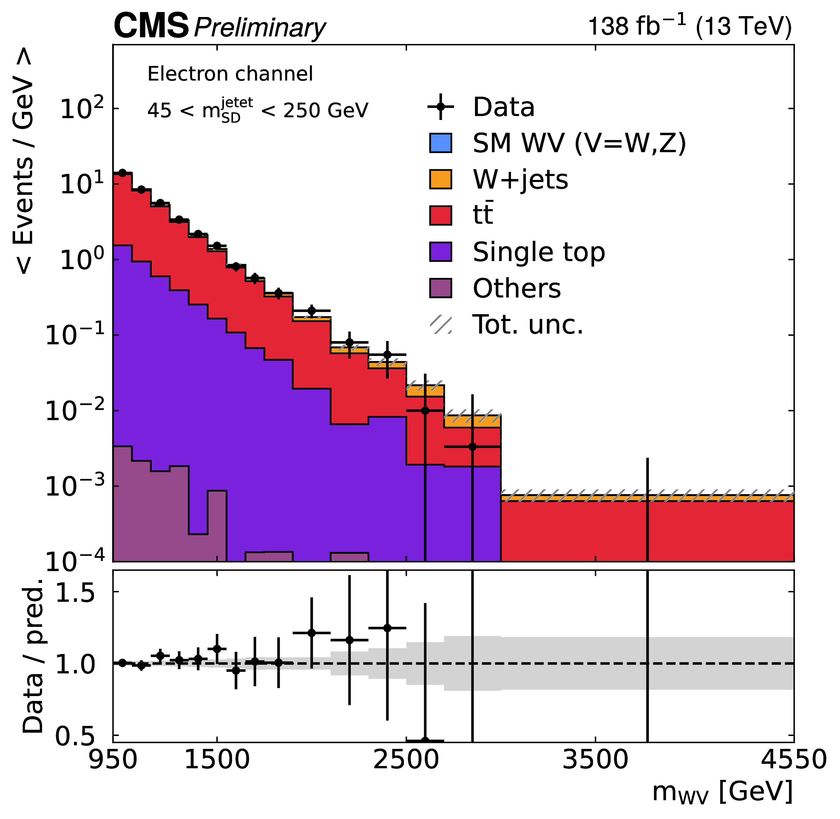
Figure 4:
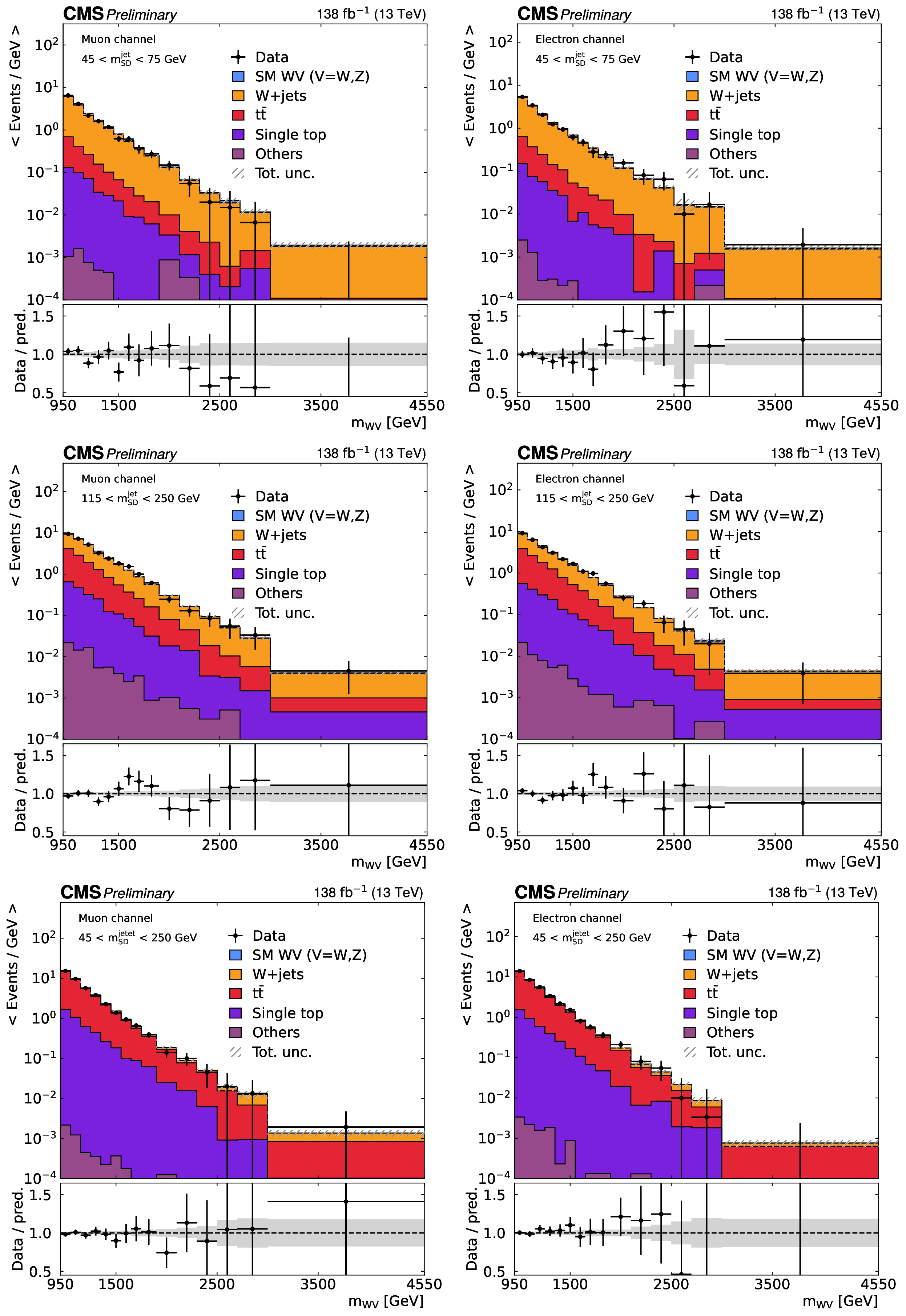
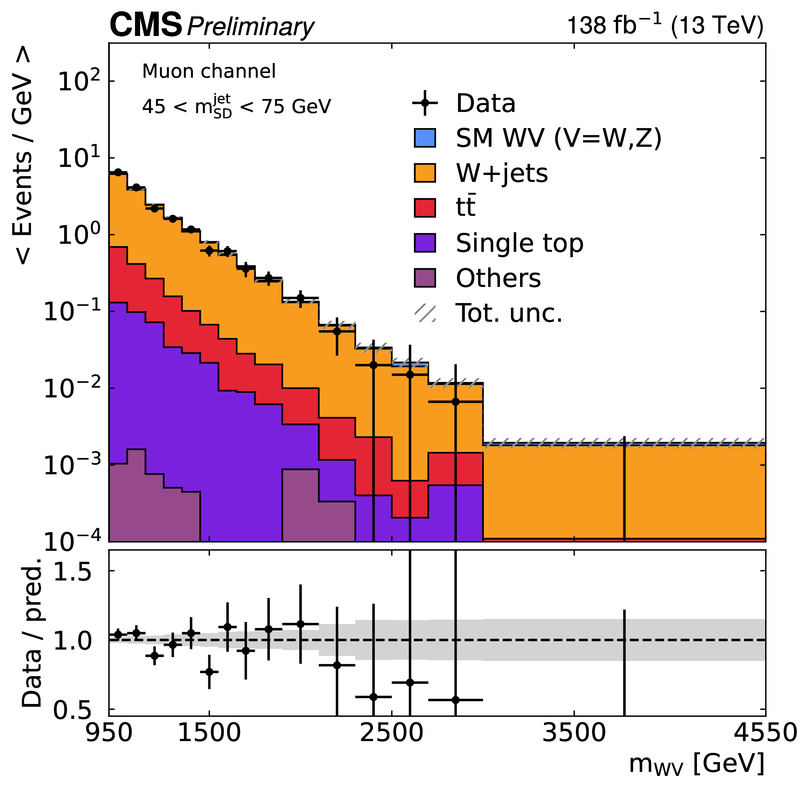
The $ m_{\mathrm{W}\mathrm{V}} $ distribution in the $ \mathrm{W}{\text{+jets}} $ low (upper) and high (middle) sidebands and $ {\mathrm{t}\overline{\mathrm{t}}} $ (lower) control regions in the muon (left) and electron (right) channels after the ML fit considering the WC $ c_{\mathrm{W}} $ as signal. The lower panels show the ratio of the data to the postfit signal plus background prediction. The uncertainty band shown in the ratio plot contains both statistical and systematic components. |
png pdf |
Figure 4-a:
The $ m_{\mathrm{W}\mathrm{V}} $ distribution in the $ \mathrm{W}{\text{+jets}} $ low (upper) and high (middle) sidebands and $ {\mathrm{t}\overline{\mathrm{t}}} $ (lower) control regions in the muon (left) and electron (right) channels after the ML fit considering the WC $ c_{\mathrm{W}} $ as signal. The lower panels show the ratio of the data to the postfit signal plus background prediction. The uncertainty band shown in the ratio plot contains both statistical and systematic components. |
png pdf |
Figure 4-b:
The $ m_{\mathrm{W}\mathrm{V}} $ distribution in the $ \mathrm{W}{\text{+jets}} $ low (upper) and high (middle) sidebands and $ {\mathrm{t}\overline{\mathrm{t}}} $ (lower) control regions in the muon (left) and electron (right) channels after the ML fit considering the WC $ c_{\mathrm{W}} $ as signal. The lower panels show the ratio of the data to the postfit signal plus background prediction. The uncertainty band shown in the ratio plot contains both statistical and systematic components. |
png pdf |
Figure 4-c:
The $ m_{\mathrm{W}\mathrm{V}} $ distribution in the $ \mathrm{W}{\text{+jets}} $ low (upper) and high (middle) sidebands and $ {\mathrm{t}\overline{\mathrm{t}}} $ (lower) control regions in the muon (left) and electron (right) channels after the ML fit considering the WC $ c_{\mathrm{W}} $ as signal. The lower panels show the ratio of the data to the postfit signal plus background prediction. The uncertainty band shown in the ratio plot contains both statistical and systematic components. |

png pdf |
Figure 4-d:
The $ m_{\mathrm{W}\mathrm{V}} $ distribution in the $ \mathrm{W}{\text{+jets}} $ low (upper) and high (middle) sidebands and $ {\mathrm{t}\overline{\mathrm{t}}} $ (lower) control regions in the muon (left) and electron (right) channels after the ML fit considering the WC $ c_{\mathrm{W}} $ as signal. The lower panels show the ratio of the data to the postfit signal plus background prediction. The uncertainty band shown in the ratio plot contains both statistical and systematic components. |
png pdf |
Figure 4-e:
The $ m_{\mathrm{W}\mathrm{V}} $ distribution in the $ \mathrm{W}{\text{+jets}} $ low (upper) and high (middle) sidebands and $ {\mathrm{t}\overline{\mathrm{t}}} $ (lower) control regions in the muon (left) and electron (right) channels after the ML fit considering the WC $ c_{\mathrm{W}} $ as signal. The lower panels show the ratio of the data to the postfit signal plus background prediction. The uncertainty band shown in the ratio plot contains both statistical and systematic components. |
png pdf |
Figure 4-f:
The $ m_{\mathrm{W}\mathrm{V}} $ distribution in the $ \mathrm{W}{\text{+jets}} $ low (upper) and high (middle) sidebands and $ {\mathrm{t}\overline{\mathrm{t}}} $ (lower) control regions in the muon (left) and electron (right) channels after the ML fit considering the WC $ c_{\mathrm{W}} $ as signal. The lower panels show the ratio of the data to the postfit signal plus background prediction. The uncertainty band shown in the ratio plot contains both statistical and systematic components. |
png pdf |
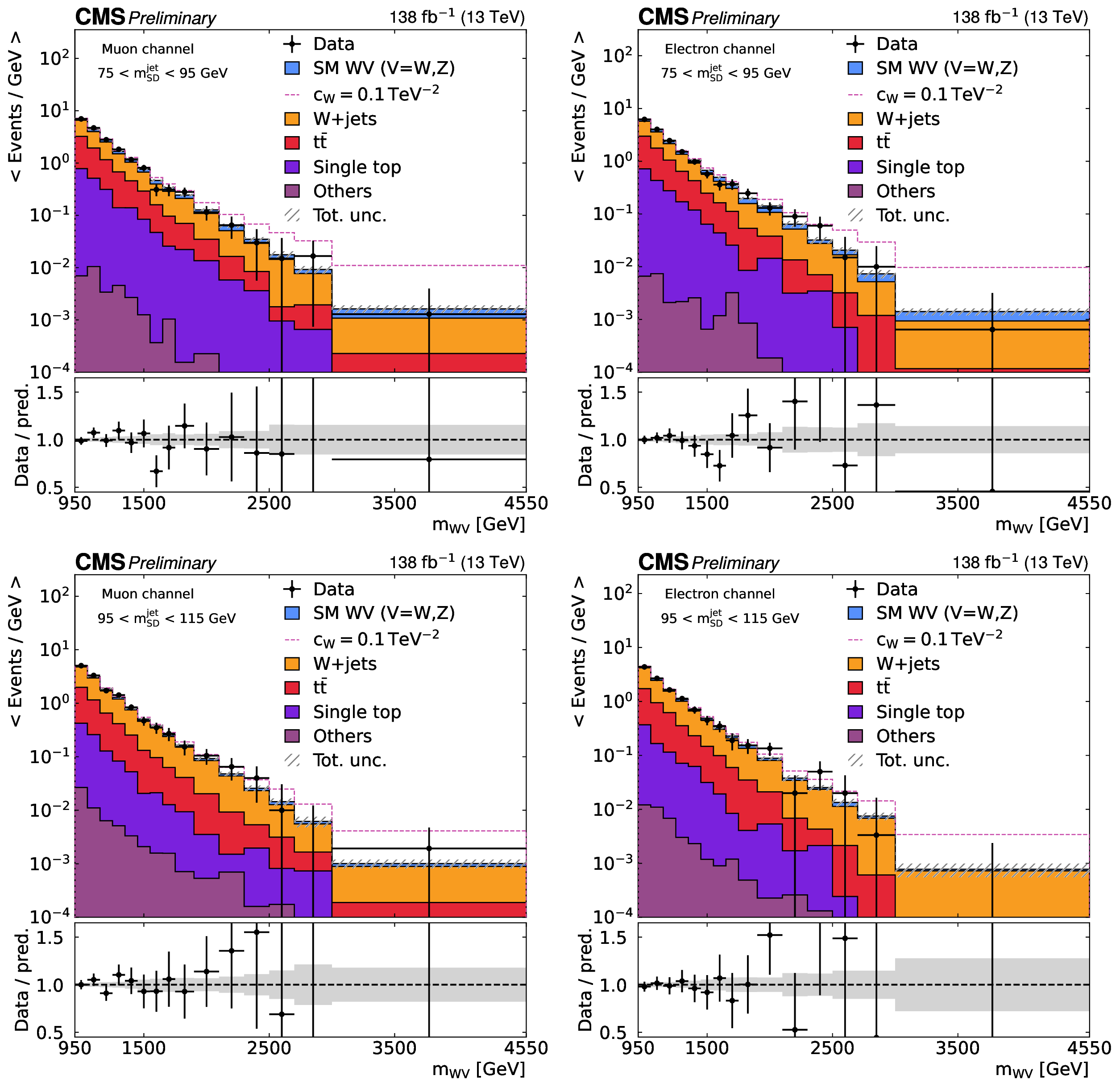
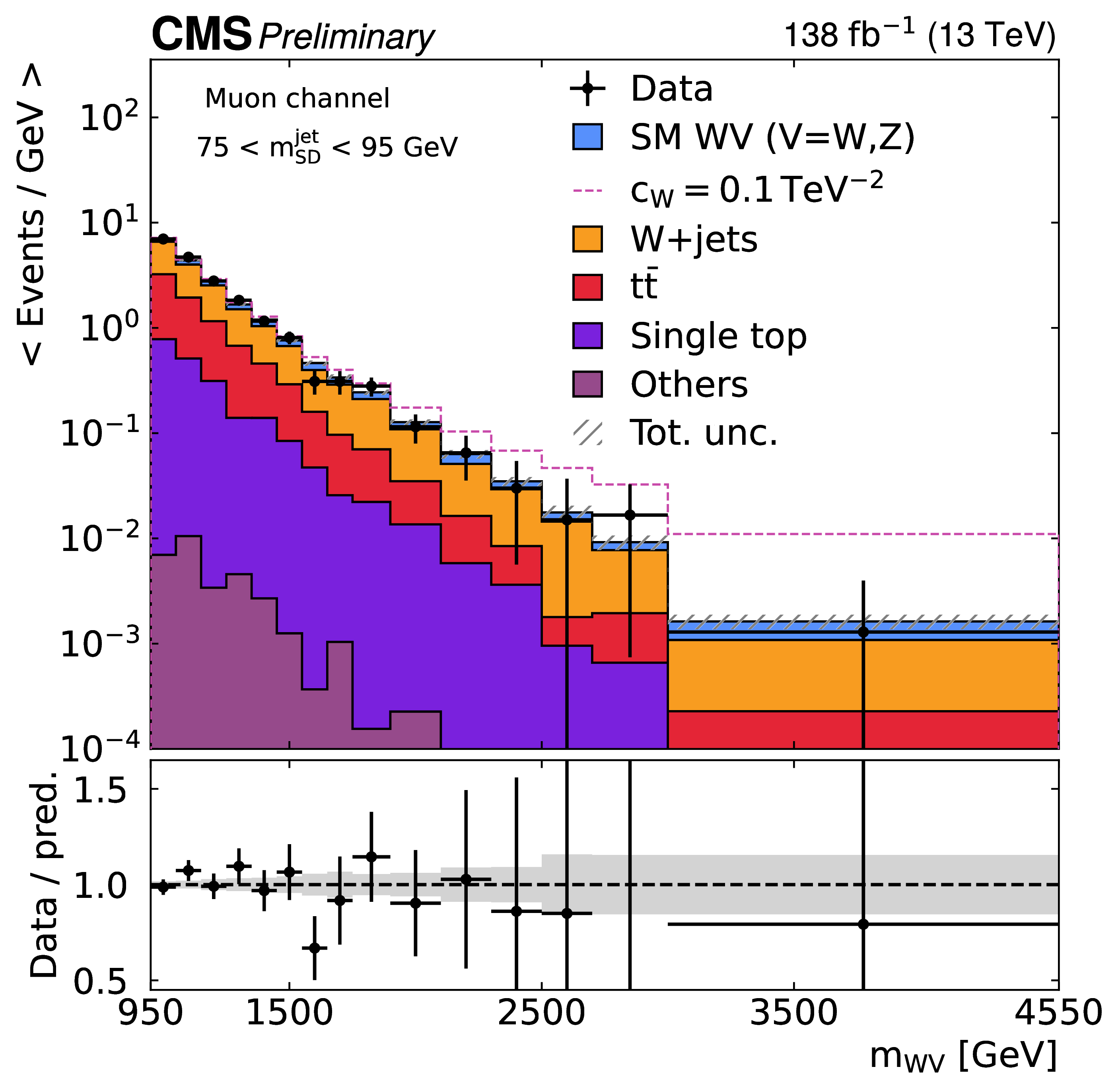
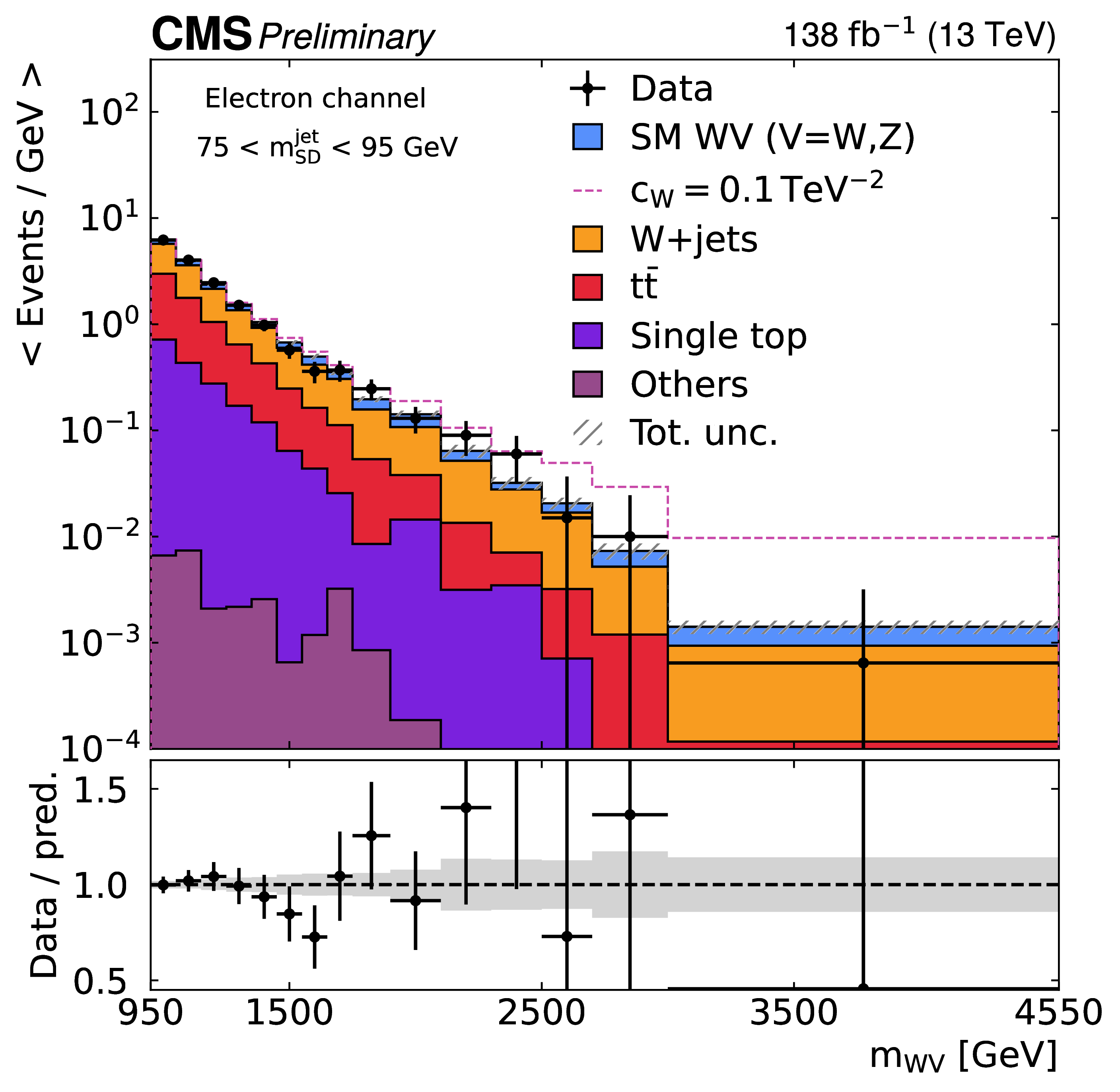
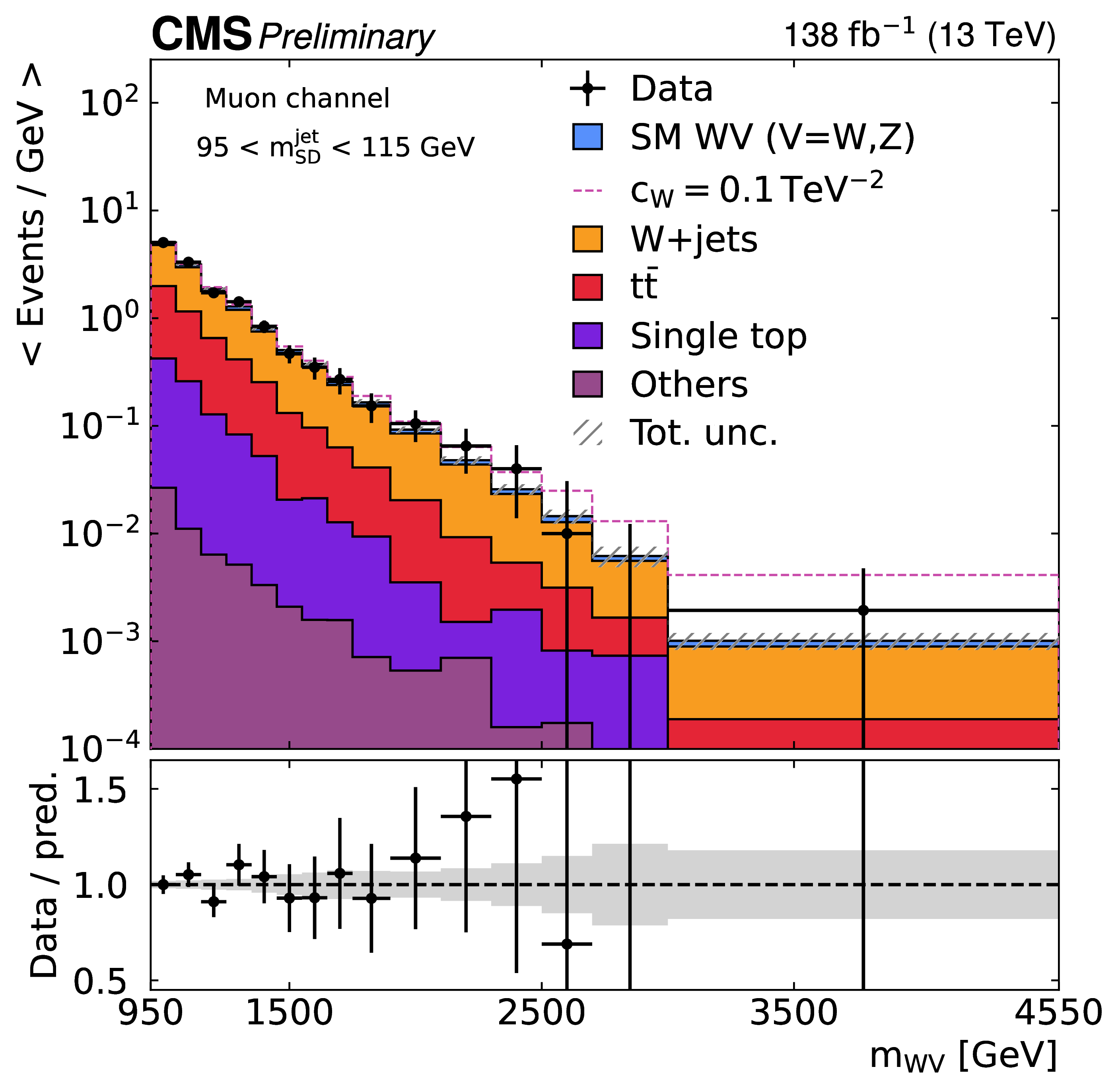
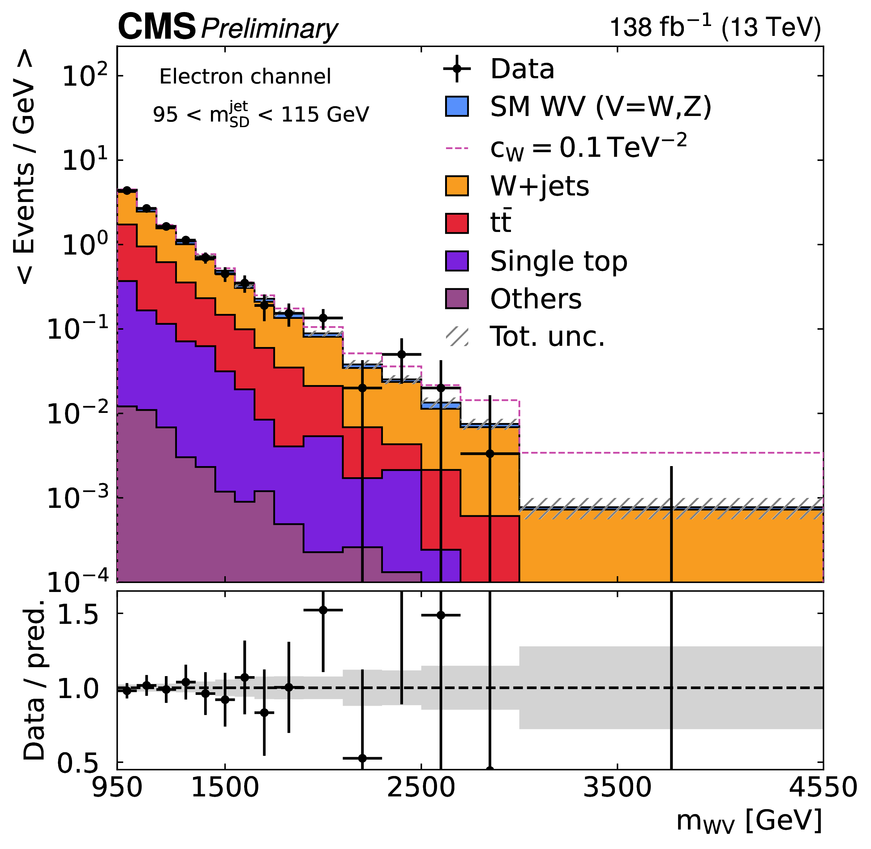
Figure 5:
The $ m_{\mathrm{W}\mathrm{V}} $ distribution in the signal region low (upper) and high (lower) in the muon (left) and electron (right) channels after the ML fit assuming no signal. The prefit signal contribution from the summed linear and quadratic terms corresponding to $ c_{\mathrm{W}} = 0.1 \text{TeV}^{-2} $ are also shown. The lower panels show the ratio of the data to the postfit background prediction. The uncertainty band shown in the ratio plot contains both statistical and systematic components. |
png pdf |
Figure 5-a:
The $ m_{\mathrm{W}\mathrm{V}} $ distribution in the signal region low (upper) and high (lower) in the muon (left) and electron (right) channels after the ML fit assuming no signal. The prefit signal contribution from the summed linear and quadratic terms corresponding to $ c_{\mathrm{W}} = 0.1 \text{TeV}^{-2} $ are also shown. The lower panels show the ratio of the data to the postfit background prediction. The uncertainty band shown in the ratio plot contains both statistical and systematic components. |
png pdf |
Figure 5-b:
The $ m_{\mathrm{W}\mathrm{V}} $ distribution in the signal region low (upper) and high (lower) in the muon (left) and electron (right) channels after the ML fit assuming no signal. The prefit signal contribution from the summed linear and quadratic terms corresponding to $ c_{\mathrm{W}} = 0.1 \text{TeV}^{-2} $ are also shown. The lower panels show the ratio of the data to the postfit background prediction. The uncertainty band shown in the ratio plot contains both statistical and systematic components. |
png pdf |
Figure 5-c:
The $ m_{\mathrm{W}\mathrm{V}} $ distribution in the signal region low (upper) and high (lower) in the muon (left) and electron (right) channels after the ML fit assuming no signal. The prefit signal contribution from the summed linear and quadratic terms corresponding to $ c_{\mathrm{W}} = 0.1 \text{TeV}^{-2} $ are also shown. The lower panels show the ratio of the data to the postfit background prediction. The uncertainty band shown in the ratio plot contains both statistical and systematic components. |
png pdf |
Figure 5-d:
The $ m_{\mathrm{W}\mathrm{V}} $ distribution in the signal region low (upper) and high (lower) in the muon (left) and electron (right) channels after the ML fit assuming no signal. The prefit signal contribution from the summed linear and quadratic terms corresponding to $ c_{\mathrm{W}} = 0.1 \text{TeV}^{-2} $ are also shown. The lower panels show the ratio of the data to the postfit background prediction. The uncertainty band shown in the ratio plot contains both statistical and systematic components. |
png pdf |
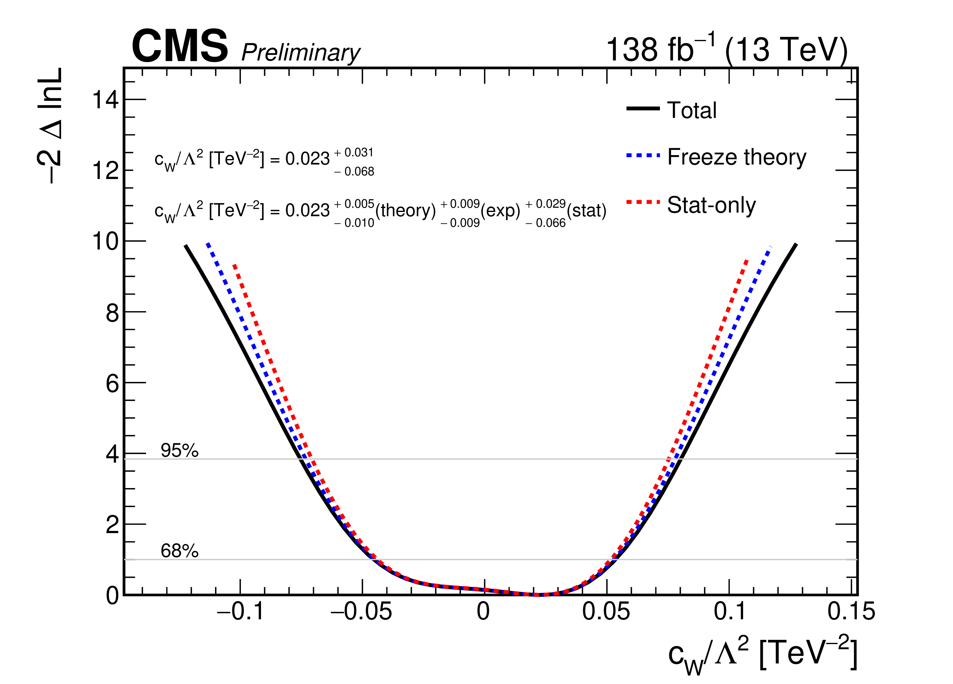
Figure 6:
Profile likelihood scan of the WC $ c_{\mathrm{W}} $ obtained from a simultaneous fit to data in the SRs and background CRs for the case when all other WCs are fixed to 0. Both linear and quadratic contributions in the EFT expansion are included in the fit. The horizontal dashed lines correspond to the 68% and 95% confidence levels. Different profile likelihood curves correspond to cases when: both statistical and systematic uncertainties are included in the fit, theory uncertainties are frozen, and only statistical uncertainties are included. |
png pdf |
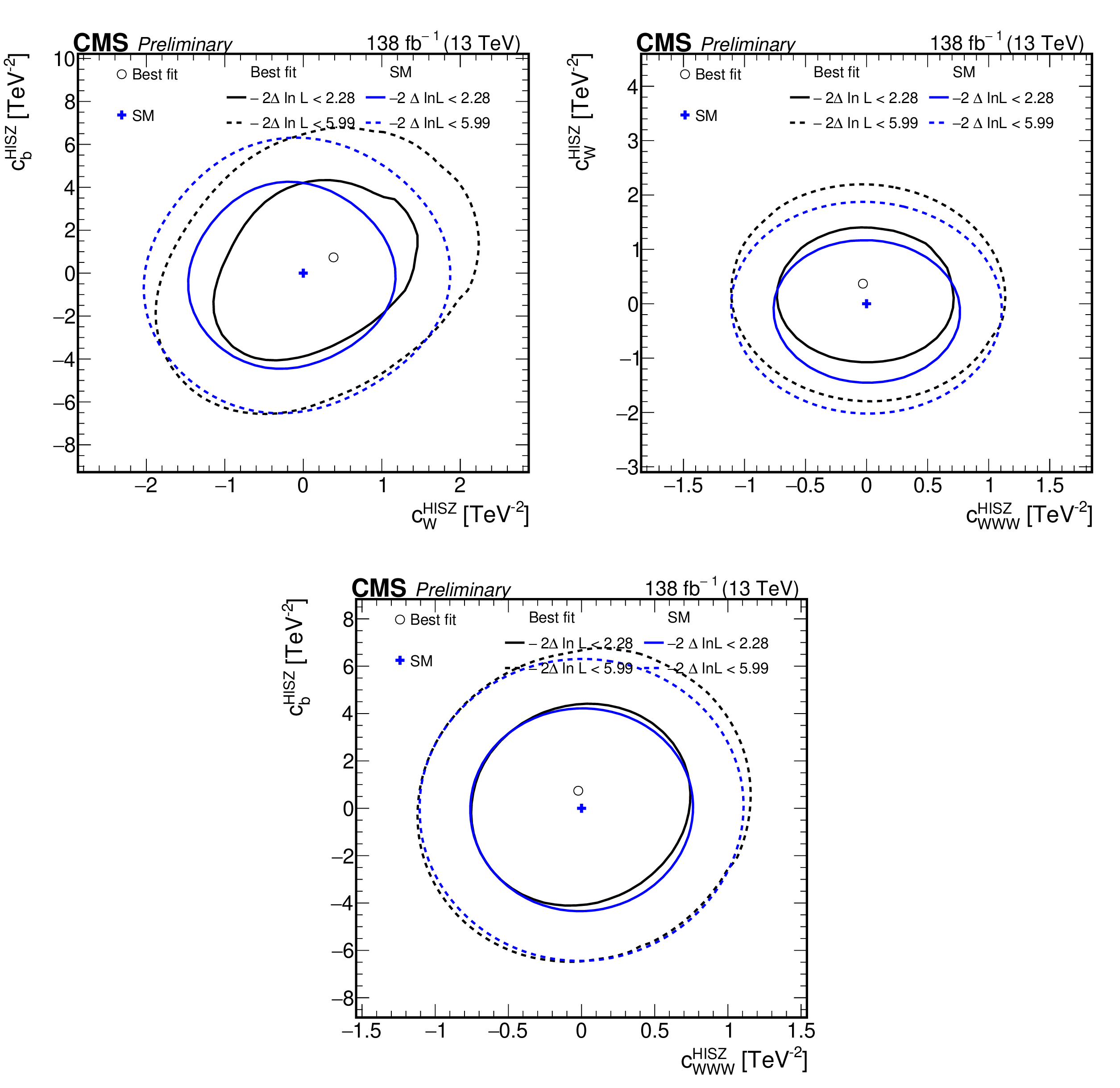
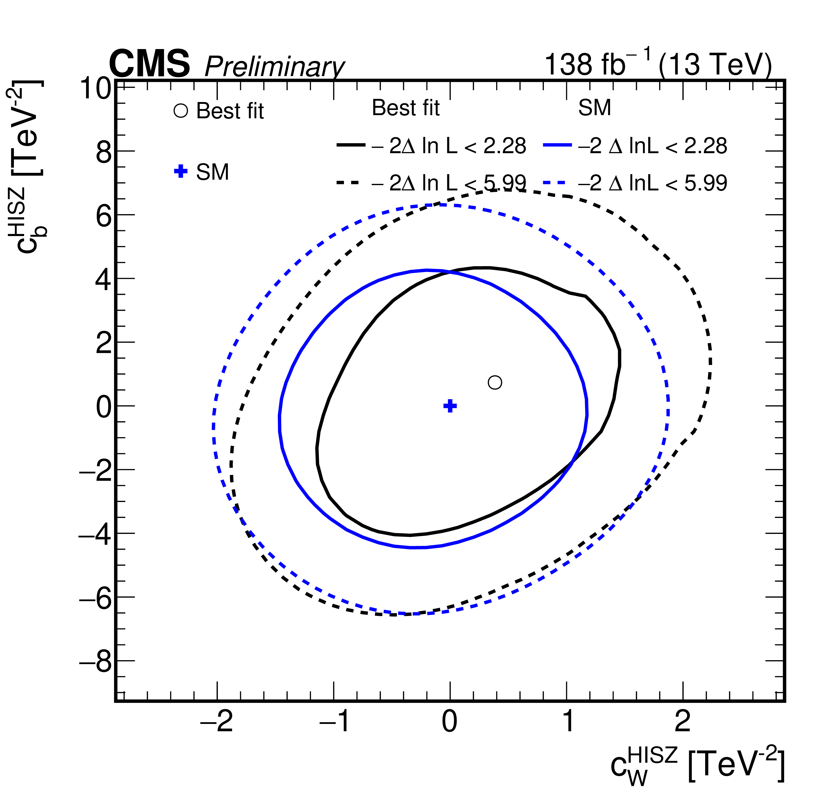
Figure 7:
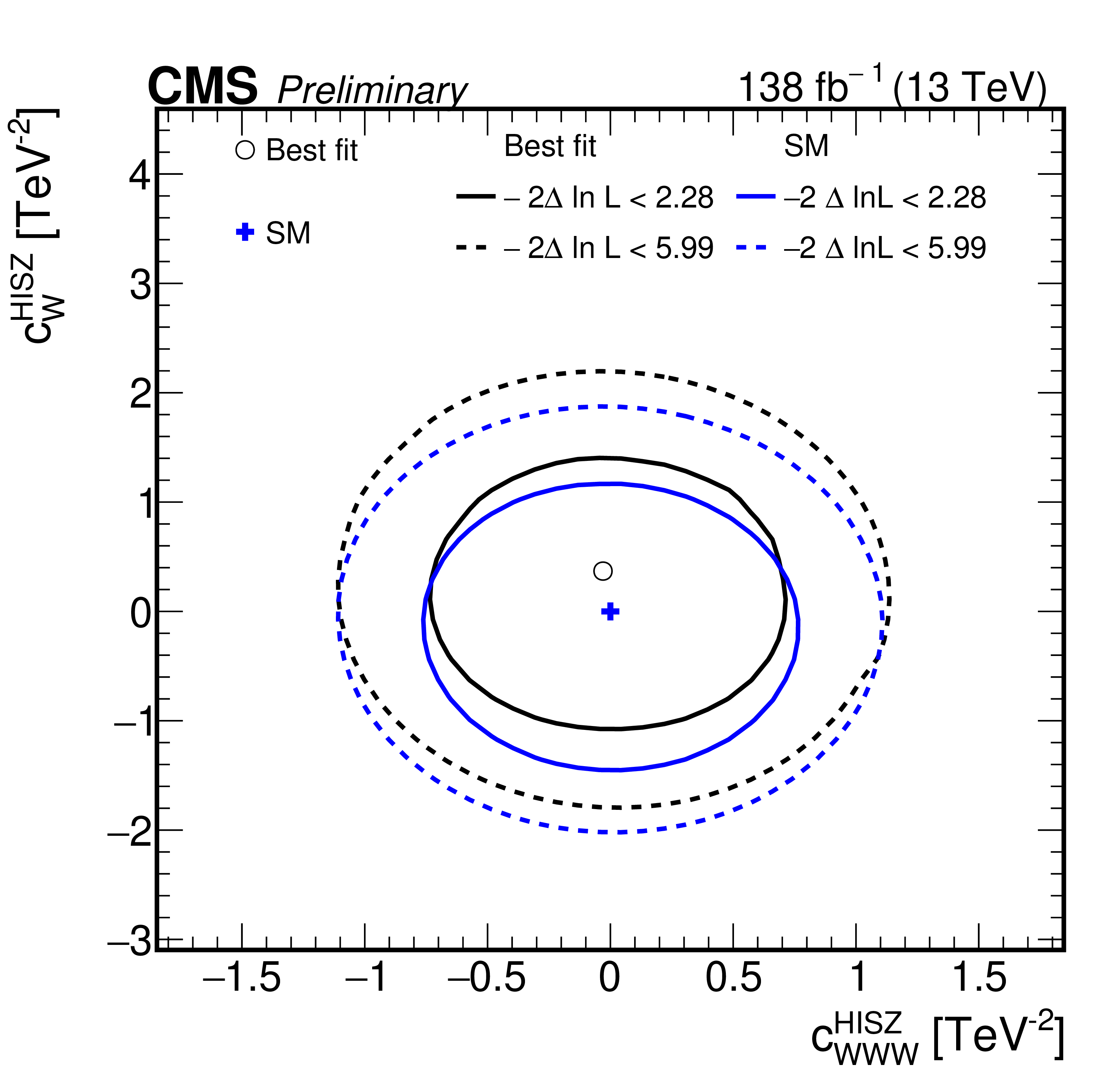
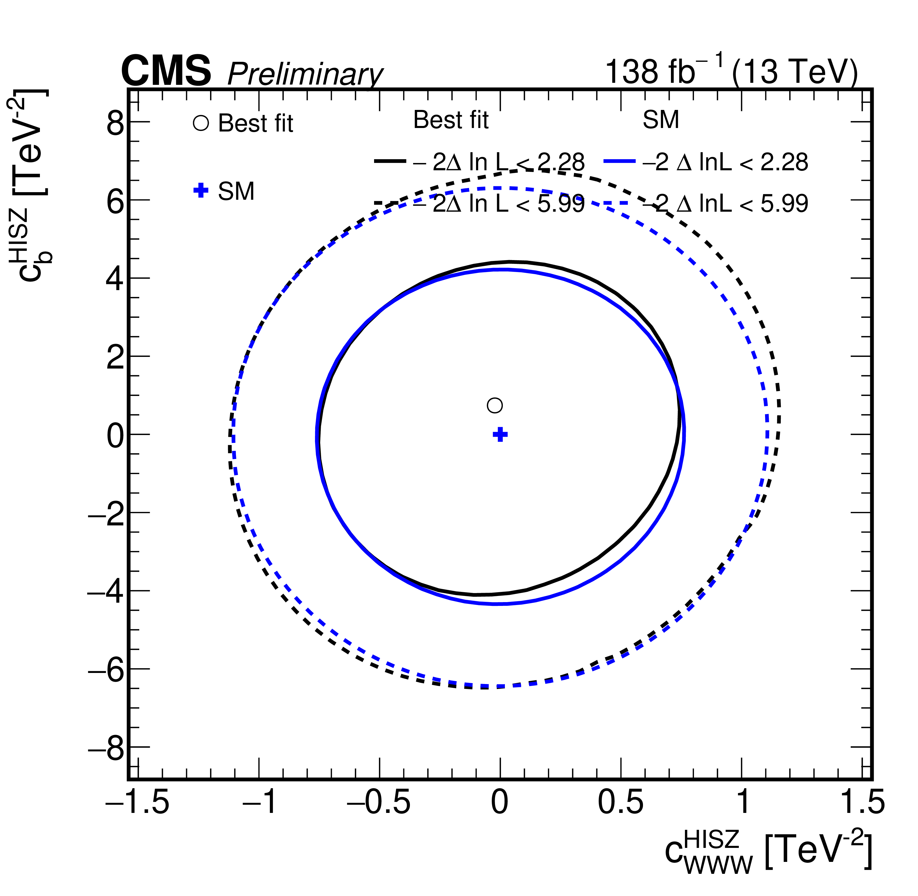
Likelihood as a function of the pairs of WCs from HISZ model: $ c_{\mathrm{W}} $ and $ c_{{\mathrm{B}}} $ (upper left), $ c_{\mathrm{W}\mathrm{W}\mathrm{W}} $ and $ c_{\mathrm{W}} $ (upper right), and $ c_{\mathrm{W}\mathrm{W}\mathrm{W}} $ and $ c_{{\mathrm{B}}} $ (lower). All WCs that are not scanned are fixed to zero. The best fit value is shown with a marker and the dotted lines correspond to the crossing points of $ -2\Delta\ln L $ at 2.28 and 5.99, which correspond to the 68% and 95% confidence levels in the asymptotic approximation. |
png pdf |
Figure 7-a:
Likelihood as a function of the pairs of WCs from HISZ model: $ c_{\mathrm{W}} $ and $ c_{{\mathrm{B}}} $ (upper left), $ c_{\mathrm{W}\mathrm{W}\mathrm{W}} $ and $ c_{\mathrm{W}} $ (upper right), and $ c_{\mathrm{W}\mathrm{W}\mathrm{W}} $ and $ c_{{\mathrm{B}}} $ (lower). All WCs that are not scanned are fixed to zero. The best fit value is shown with a marker and the dotted lines correspond to the crossing points of $ -2\Delta\ln L $ at 2.28 and 5.99, which correspond to the 68% and 95% confidence levels in the asymptotic approximation. |
png pdf |
Figure 7-b:
Likelihood as a function of the pairs of WCs from HISZ model: $ c_{\mathrm{W}} $ and $ c_{{\mathrm{B}}} $ (upper left), $ c_{\mathrm{W}\mathrm{W}\mathrm{W}} $ and $ c_{\mathrm{W}} $ (upper right), and $ c_{\mathrm{W}\mathrm{W}\mathrm{W}} $ and $ c_{{\mathrm{B}}} $ (lower). All WCs that are not scanned are fixed to zero. The best fit value is shown with a marker and the dotted lines correspond to the crossing points of $ -2\Delta\ln L $ at 2.28 and 5.99, which correspond to the 68% and 95% confidence levels in the asymptotic approximation. |
png pdf |
Figure 7-c:
Likelihood as a function of the pairs of WCs from HISZ model: $ c_{\mathrm{W}} $ and $ c_{{\mathrm{B}}} $ (upper left), $ c_{\mathrm{W}\mathrm{W}\mathrm{W}} $ and $ c_{\mathrm{W}} $ (upper right), and $ c_{\mathrm{W}\mathrm{W}\mathrm{W}} $ and $ c_{{\mathrm{B}}} $ (lower). All WCs that are not scanned are fixed to zero. The best fit value is shown with a marker and the dotted lines correspond to the crossing points of $ -2\Delta\ln L $ at 2.28 and 5.99, which correspond to the 68% and 95% confidence levels in the asymptotic approximation. |
png pdf |
Figure 8:
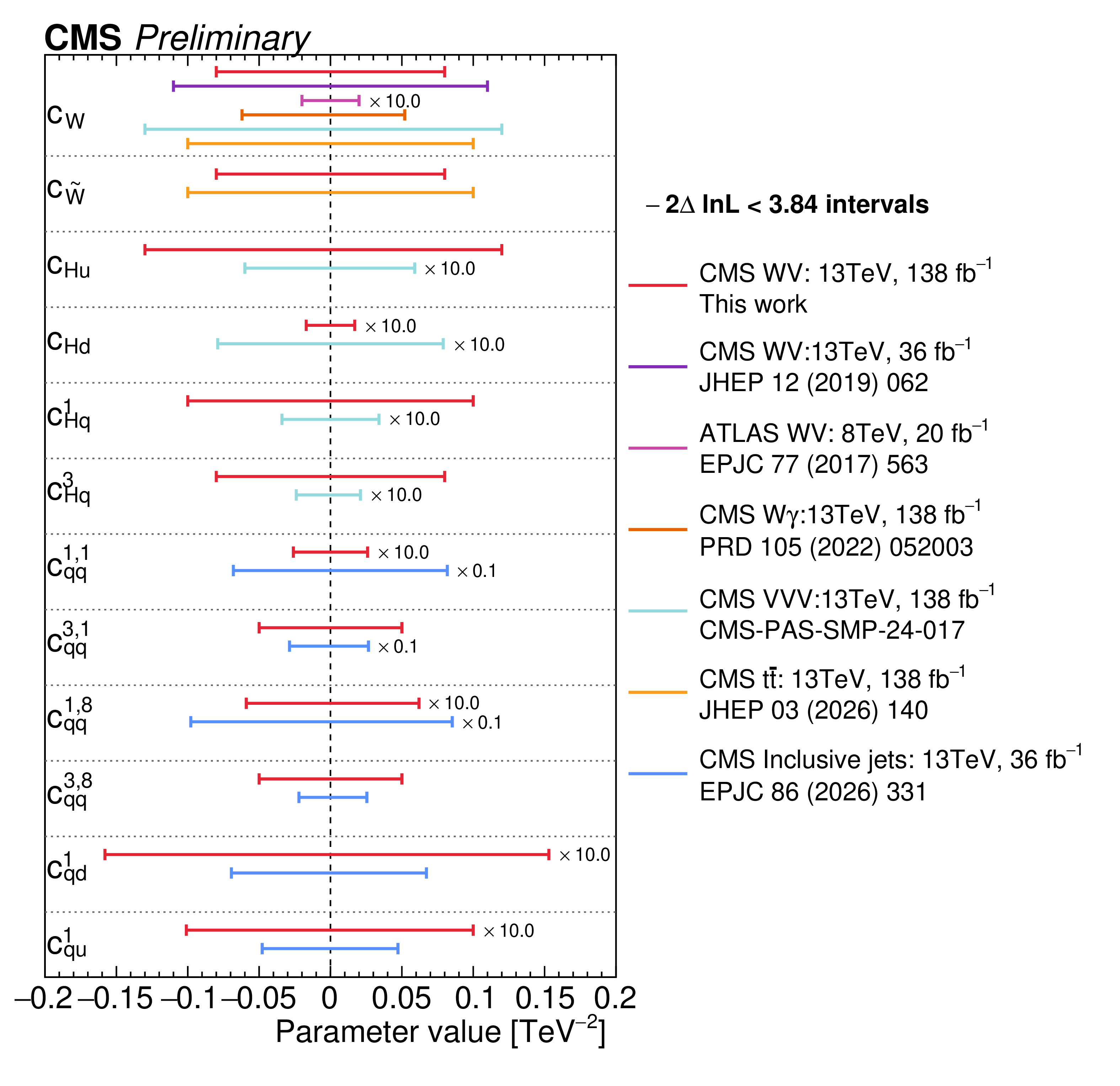
Comparison of limits on different WCs at 95% confidence level with existing analyses at different center-of-mass energies and different final states [94,95,96,25,31]. The limits from some of the analyses are scaled down or up so as to fit on the same scale as for the best constraints. The corresponding scale factor is mentioned, next to the limits, which should be multiplied with the plotted limits to to extract the actual constraints. |
png pdf |
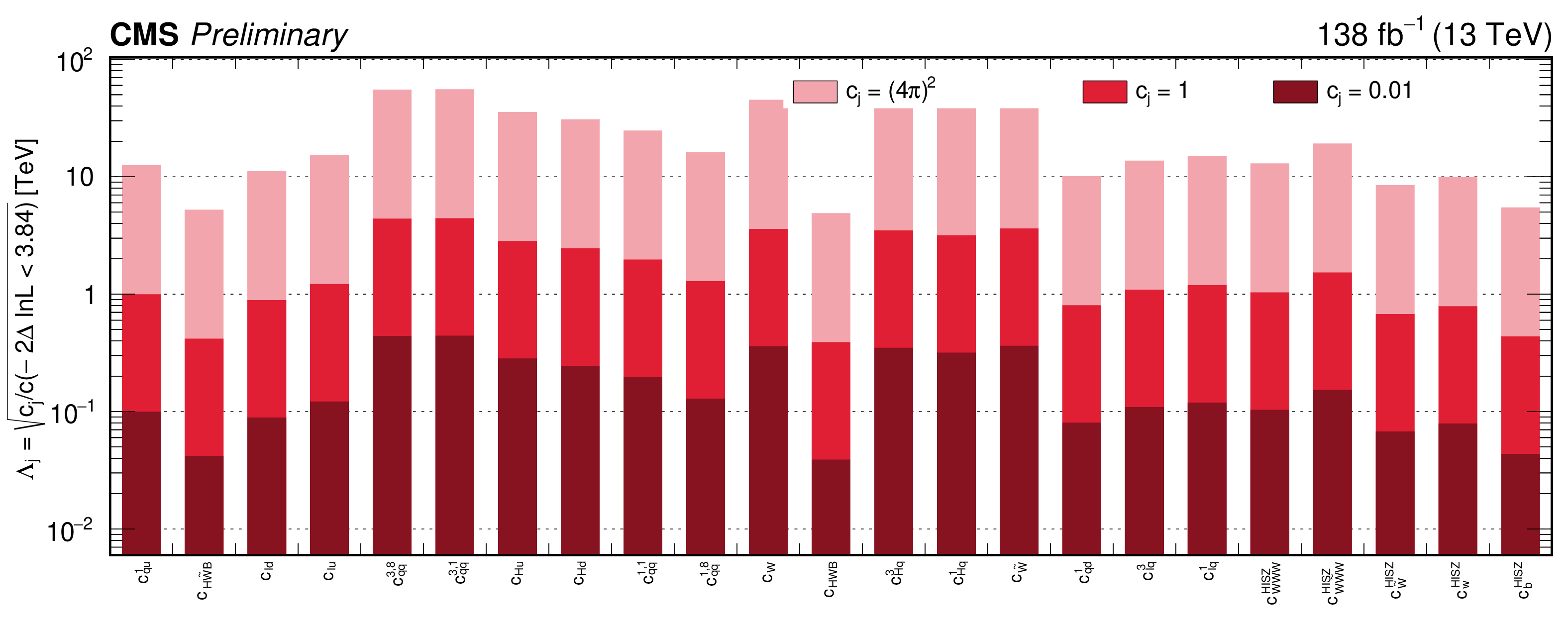
Figure 9:
Summary of the lower limits on the energy scales $ \Lambda_{j} $ at 95% confidence interval for the indicated values of the WCs $ c_{j} $. |
png pdf |
Figure 10:
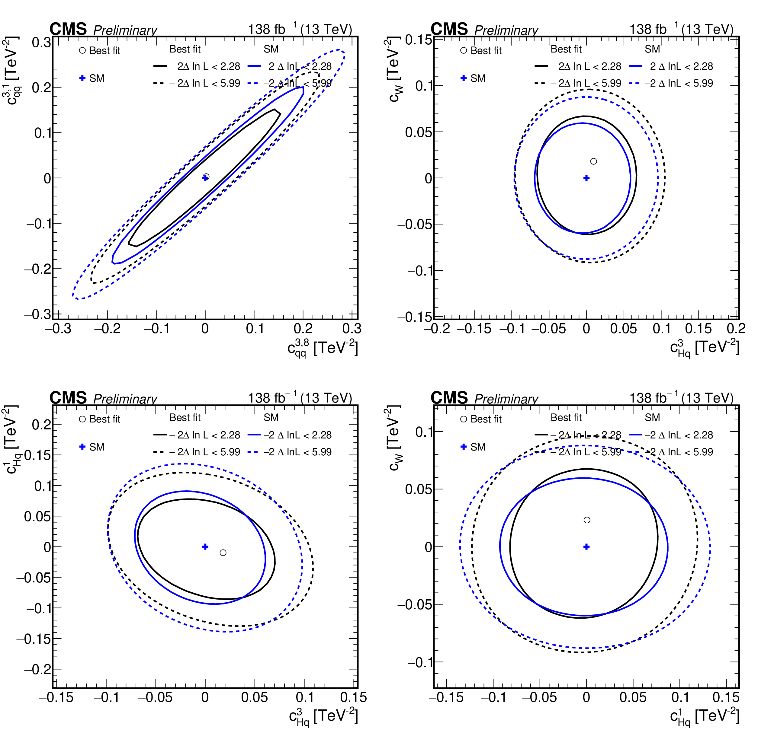
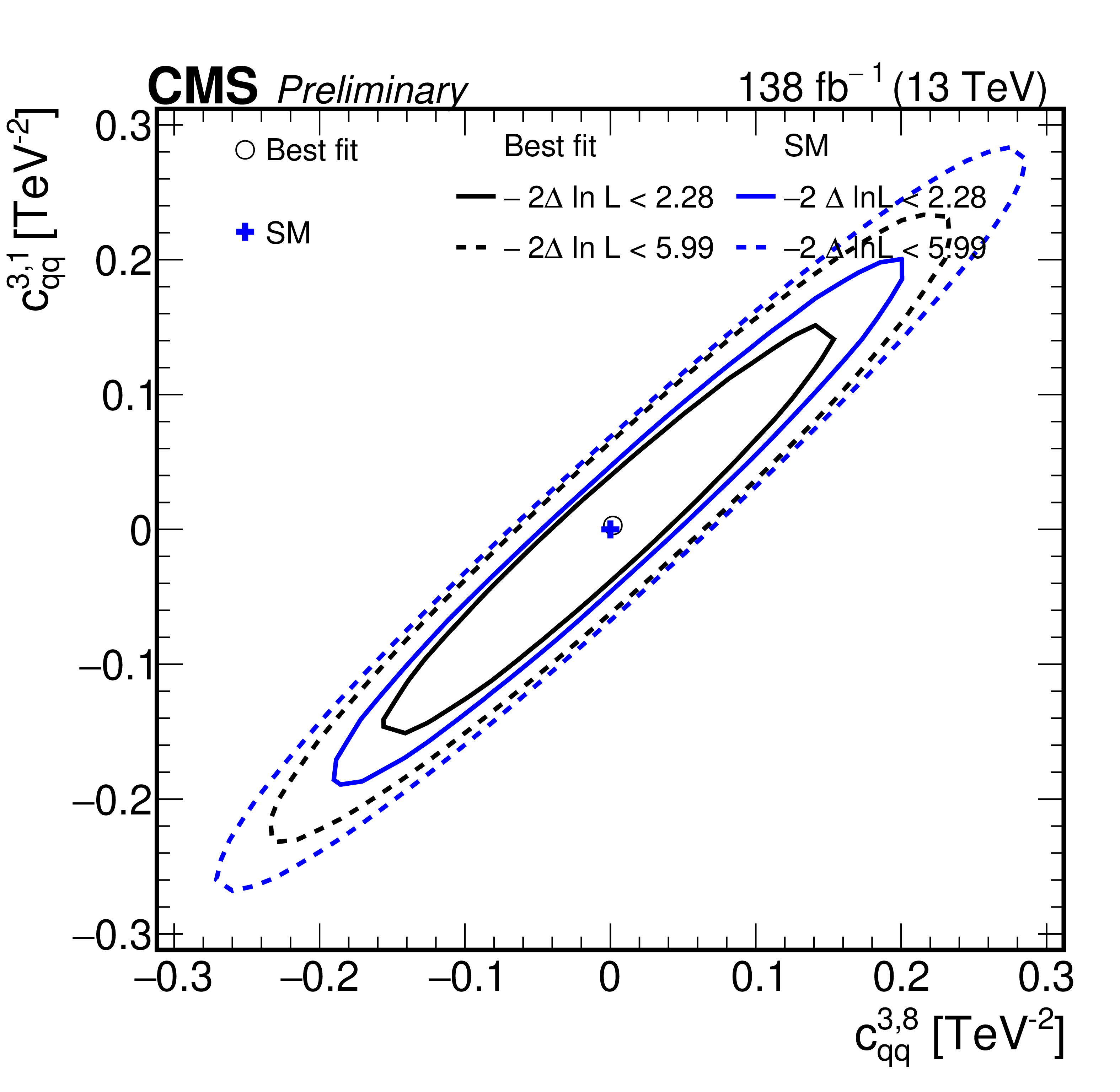
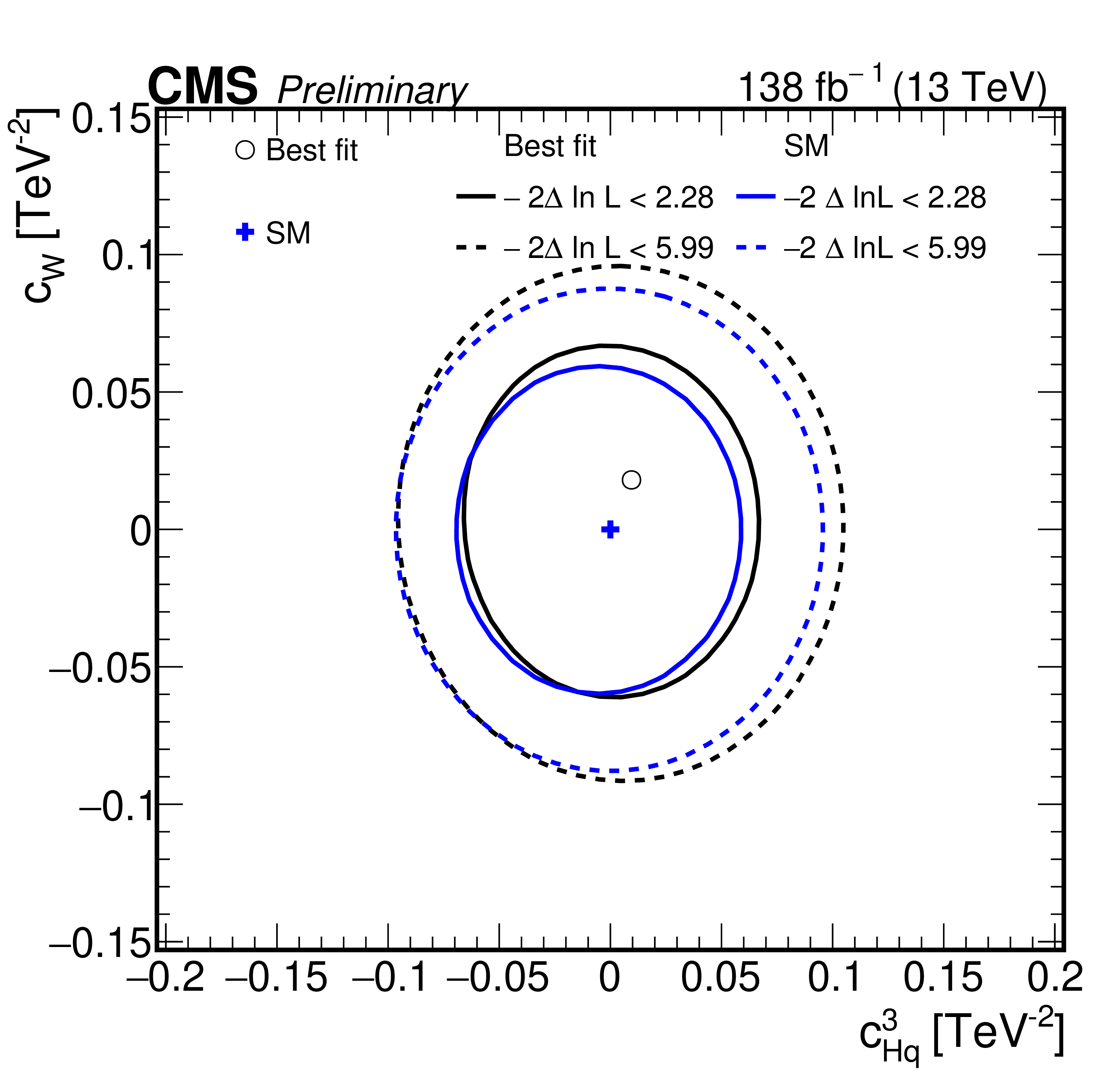
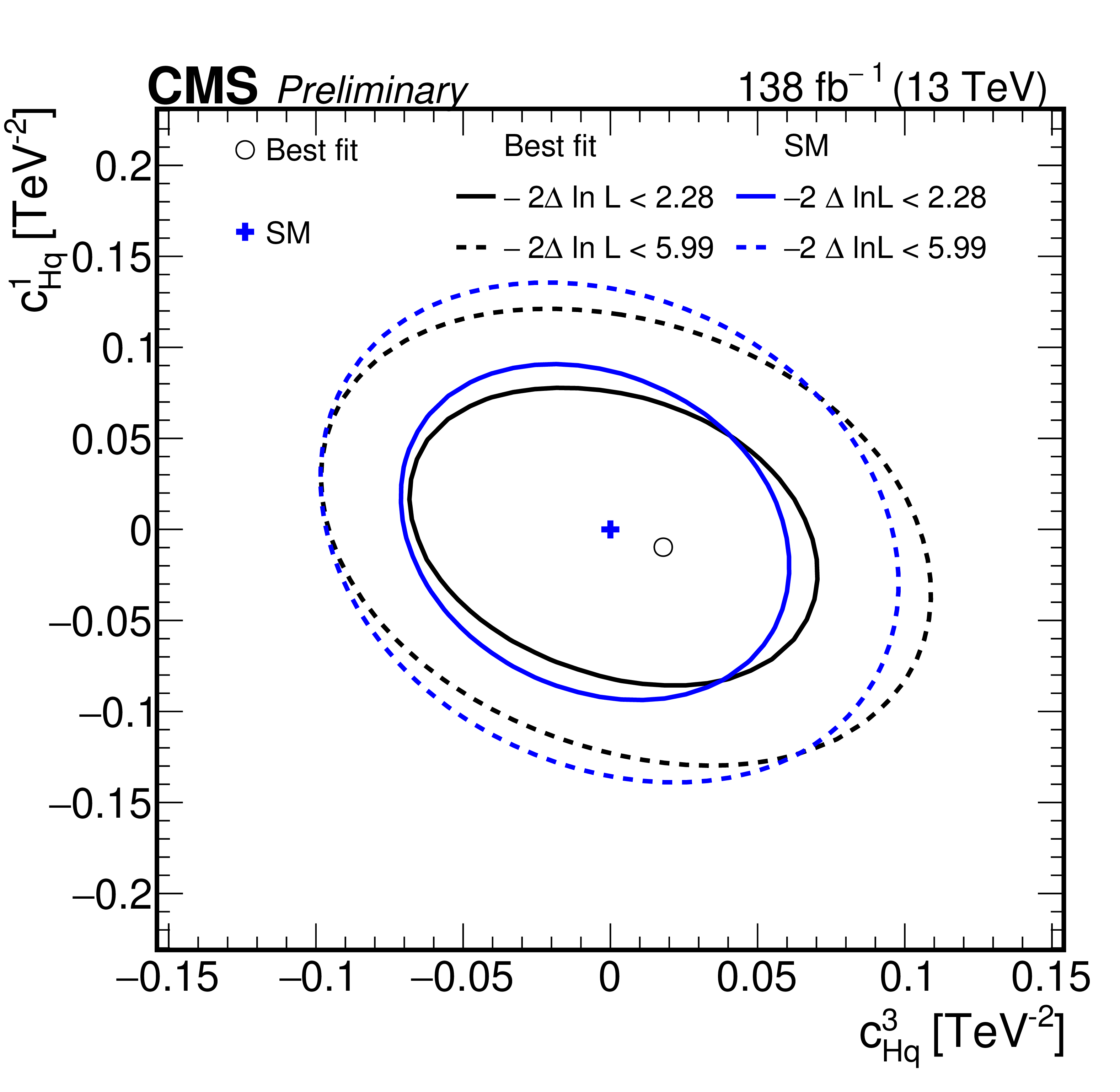
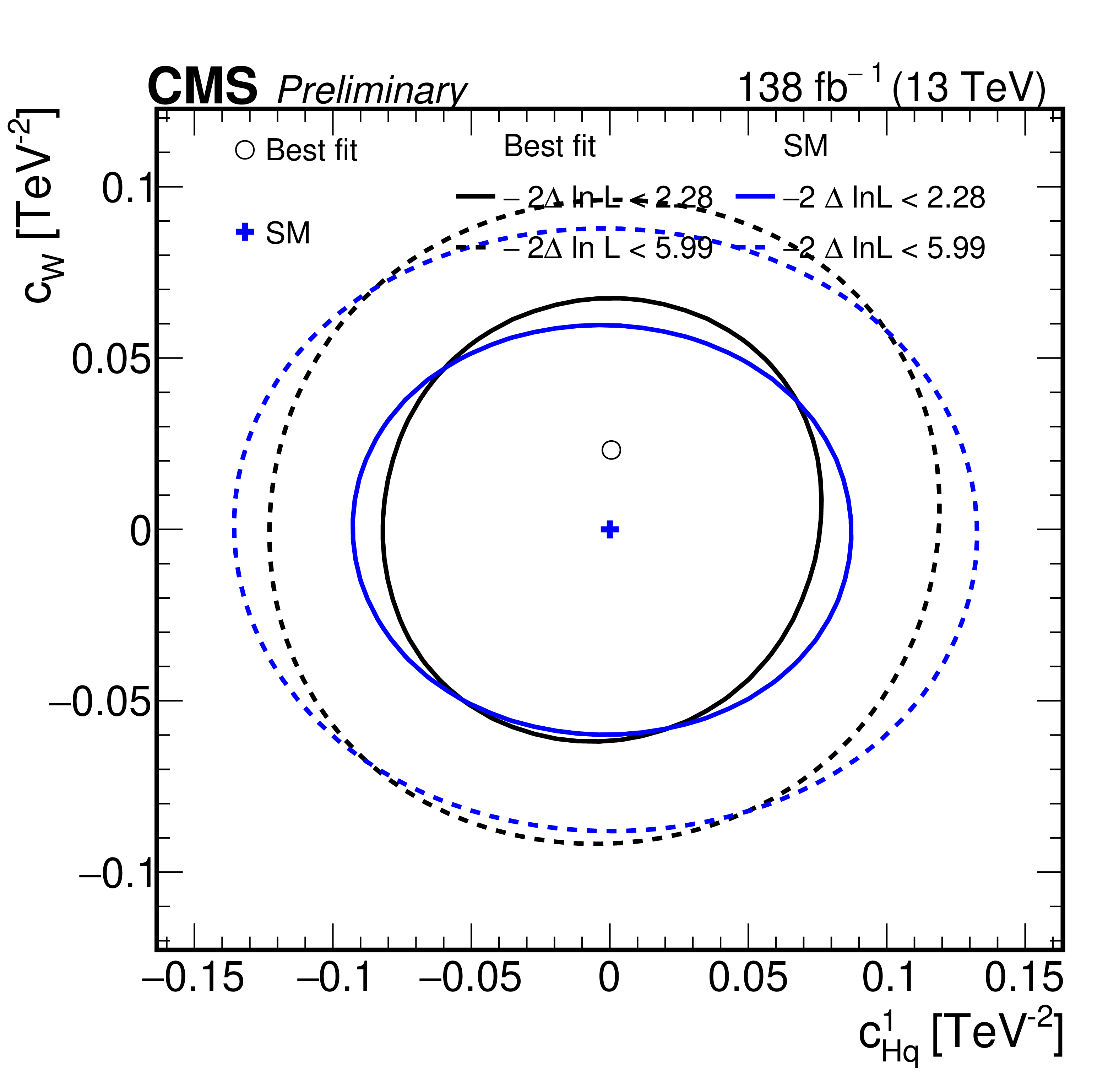
Likelihood scans as a function of the pairs of WCs from SMEFT model: $c_{qq}^{(3,8)}$ and $c_{qq}^{(3,1)}$ (upper left), $c_{Hq}^{(3)} $ and $ c_{\mathrm{W}} $ (upper right), $c_{Hq}^{(3)} $ and $c_{Hq}^{(1)} $(lower left), and $c_{Hq}^{(1)} $ and $ c_{\mathrm{W}} $ (lower right). All WCs that are not scanned are fixed to zero. The best fit value is shown with a marker and the coloured lines correspond to the crossing points of $ -2\Delta\ln L $ at 2.28 and 5.99. |
png pdf |
Figure 10-a:
Likelihood scans as a function of the pairs of WCs from SMEFT model: $c_{qq}^{(3,8)}$ and $c_{qq}^{(3,1)}$ (upper left), $c_{Hq}^{(3)} $ and $ c_{\mathrm{W}} $ (upper right), $c_{Hq}^{(3)} $ and $c_{Hq}^{(1)} $(lower left), and $c_{Hq}^{(1)} $ and $ c_{\mathrm{W}} $ (lower right). All WCs that are not scanned are fixed to zero. The best fit value is shown with a marker and the coloured lines correspond to the crossing points of $ -2\Delta\ln L $ at 2.28 and 5.99. |
png pdf |
Figure 10-b:
Likelihood scans as a function of the pairs of WCs from SMEFT model: $c_{qq}^{(3,8)}$ and $c_{qq}^{(3,1)}$ (upper left), $c_{Hq}^{(3)} $ and $ c_{\mathrm{W}} $ (upper right), $c_{Hq}^{(3)} $ and $c_{Hq}^{(1)} $(lower left), and $c_{Hq}^{(1)} $ and $ c_{\mathrm{W}} $ (lower right). All WCs that are not scanned are fixed to zero. The best fit value is shown with a marker and the coloured lines correspond to the crossing points of $ -2\Delta\ln L $ at 2.28 and 5.99. |
png pdf |
Figure 10-c:
Likelihood scans as a function of the pairs of WCs from SMEFT model: $c_{qq}^{(3,8)}$ and $c_{qq}^{(3,1)}$ (upper left), $c_{Hq}^{(3)} $ and $ c_{\mathrm{W}} $ (upper right), $c_{Hq}^{(3)} $ and $c_{Hq}^{(1)} $(lower left), and $c_{Hq}^{(1)} $ and $ c_{\mathrm{W}} $ (lower right). All WCs that are not scanned are fixed to zero. The best fit value is shown with a marker and the coloured lines correspond to the crossing points of $ -2\Delta\ln L $ at 2.28 and 5.99. |
png pdf |
Figure 10-d:
Likelihood scans as a function of the pairs of WCs from SMEFT model: $c_{qq}^{(3,8)}$ and $c_{qq}^{(3,1)}$ (upper left), $c_{Hq}^{(3)} $ and $ c_{\mathrm{W}} $ (upper right), $c_{Hq}^{(3)} $ and $c_{Hq}^{(1)} $(lower left), and $c_{Hq}^{(1)} $ and $ c_{\mathrm{W}} $ (lower right). All WCs that are not scanned are fixed to zero. The best fit value is shown with a marker and the coloured lines correspond to the crossing points of $ -2\Delta\ln L $ at 2.28 and 5.99. |
| Tables | |
png pdf |
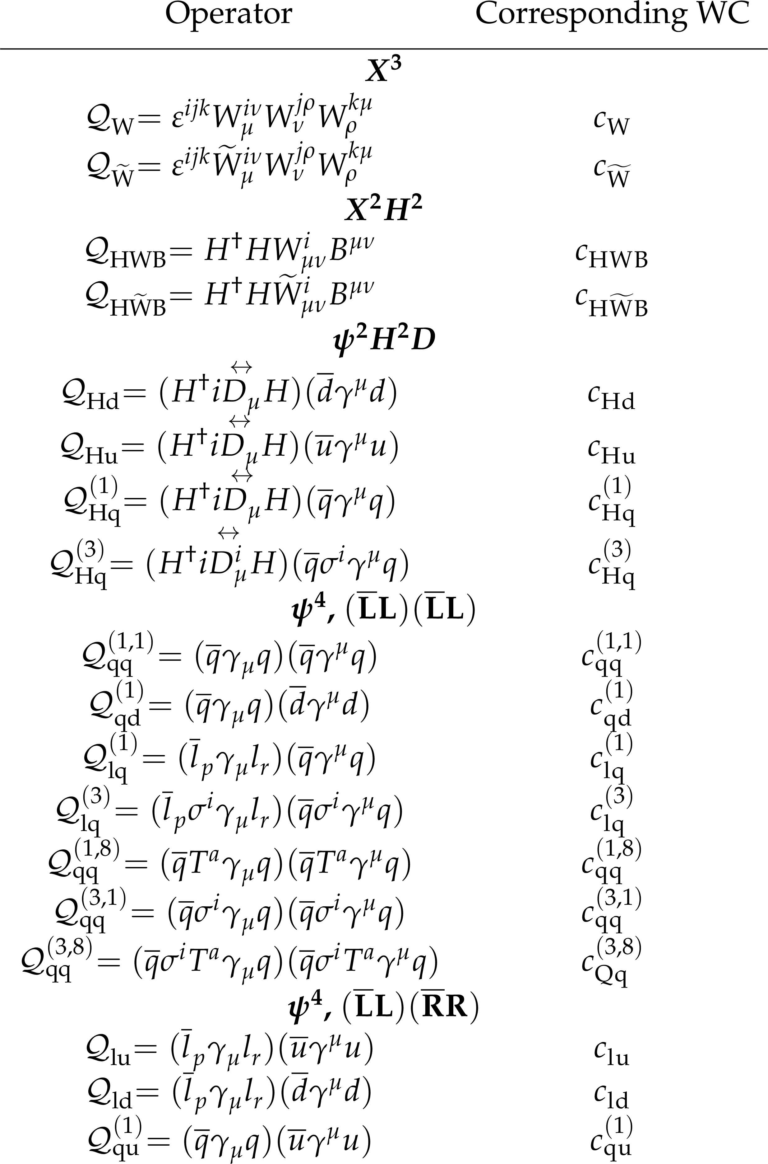
Table 1:
The dimension six SMEFT operators studied in this analysis, following the definitions of Ref. [12,6], where $ \varepsilon $ is the Levi-Civita symbol, $ (q,u,d) $ denote quark fields of the first two generations and $ (l,e,\nu) $ lepton fields of all three generations. The Higgs doublet field is indicated by $ H $; $ D $ represents a covariant derivative; $ X = G, W, B $ denotes a vector boson field strength tensor; $ p,r $ are flavor indices. Fermion fields are represented by $ \psi $, with $ L $ and $ R $ indicating left- and right-handed fermion fields. |
png pdf |
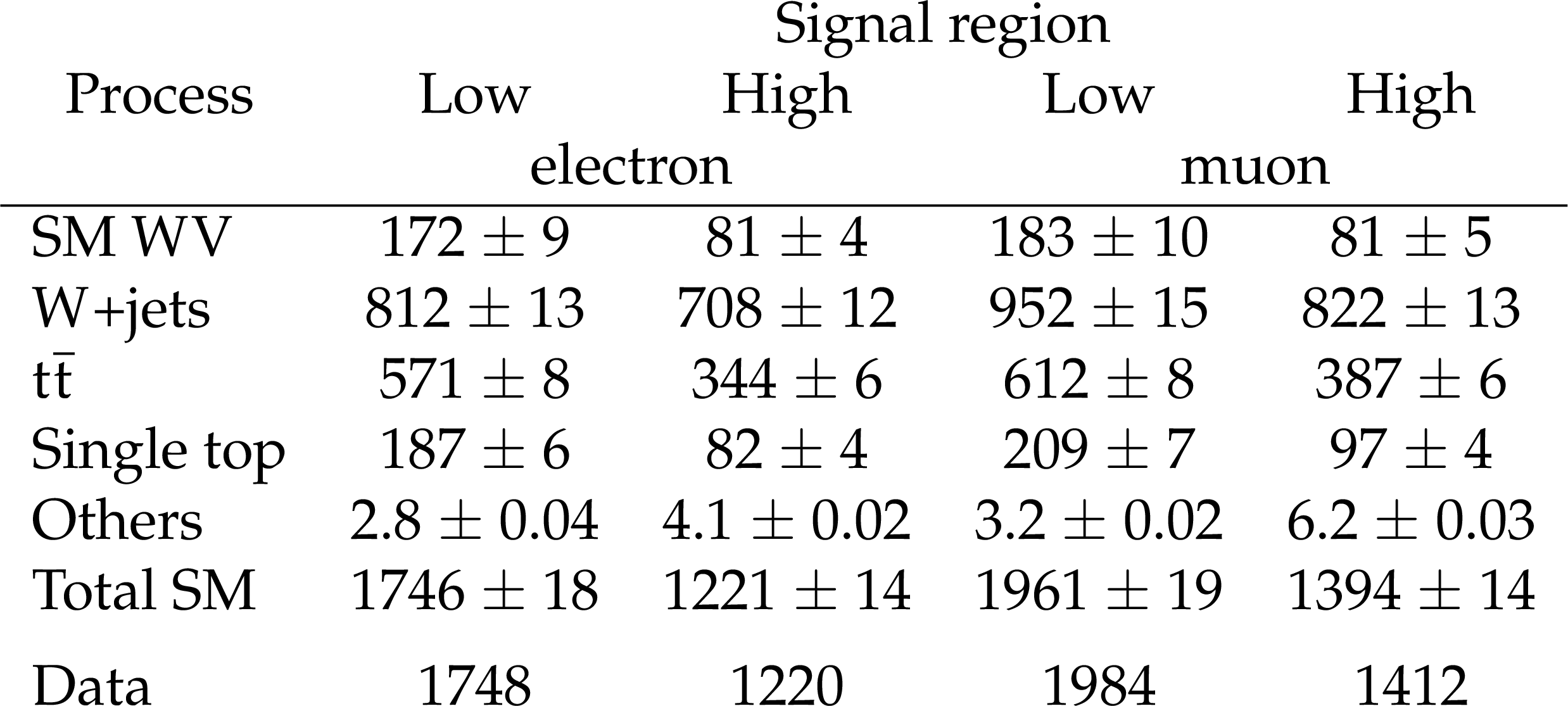
Table 2:
Event yields from SM processes and observed data events in the low and high SRs for the electron and muon channels. The combination of the statistical and systematic uncertainties is indicated. The event yields are shown with their best fit (postfit) normalizations from the simultaneous fit to the data, assuming no signal i.e., for the SM case. The contributions from SM WW and WZ processes are grouped under the SM WV category. |
png pdf |
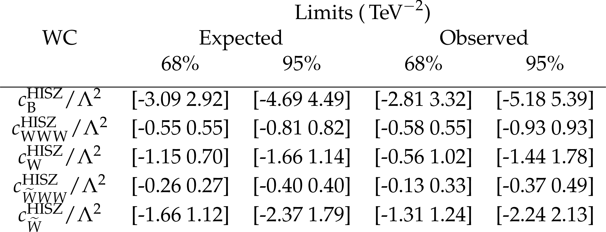
Table 3:
Expected and observed individual limits on the WCs, from HISZ basis at 68% and 95% confidence intervals. |
png pdf |
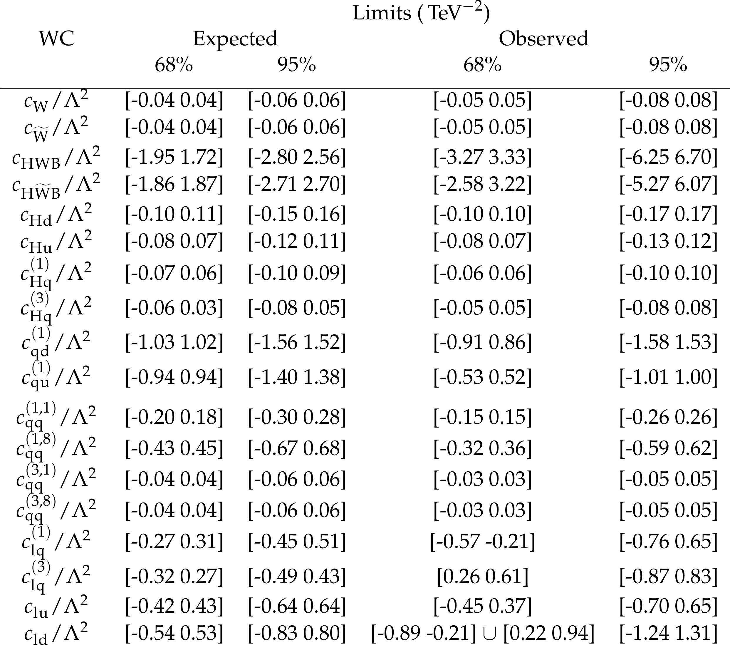
Table 4:
Expected and observed individual limits on WCs in SMEFT scenarios at 68% and 95% confidence intervals. |
| Summary |
| A search for deviations from the standard model using an effective field theory (EFT) approach is presented in the diboson (WW and WZ) production processes with one W boson decaying to (anti-)lepton plus anti-neutrino (neutrino) and the second W or Z boson decaying hadronically. The results are based on data recorded in proton-proton collisions at $ \sqrt{s} = $ 13 TeV with the CMS detector at the CERN LHC, corresponding to an integrated luminosity of 138 fb$ ^{-1} $. In this study we constrain Wilson coefficients (WCs) corresponding to dimension six EFT operators that would lead to anomalous gauge boson self and vector boson to quark couplings. Since the contribution from anomalous couplings is expected to be most visible at high energy scales, we focus on final states where the hadronic decays from the W and Z bosons merge into a single large-radius jet. A dedicated machine-learning based classifier is employed to separate such jets from vector boson decays to those from background processes. We report the most stringent constraints to date on the WCs of operators corresponding to anomalous triple gauge boson couplings. The bounds set on vector bosons' to quark couplings are competitive to those from previous inclusive jet measurements. |
| References | ||||
| 1 | A. Helset and A. Kobach | Baryon number, lepton number, and operator dimension in the SMEFT with flavor symmetries | Phys. Lett. B 800 135132, 2020 | 1909.05853 |
| 2 | W. Buchmuller and D. Wyler | Effective Lagrangian Analysis of New Interactions and Flavor Conservation | NPB 268 (1986) 621 | |
| 3 | C. Degrande et al. | Effective field theory: A modern approach to anomalous couplings | Annals Phys. 335 (2013) 21 | 1205.4231 |
| 4 | K. Hagiwara, S. Ishihara, R. Szalapski, and D. Zeppenfeld | Low energy effects of new interactions in the electroweak boson sector | PRD 48 (1993) 2182 | hep-ph/9706542 |
| 5 | C. Grojean, W. Skiba, and J. Terning | Disguising the oblique parameters | PRD 73 (2006) 075008 | hep-ph/0602154 |
| 6 | I. Brivio | SMEFTsim 3.0 \textemdash a practical guide | JHEP 04 (2021) 073 | 2012.11343 |
| 7 | I. Brivio and M. Trott | The Standard Model as an Effective Field Theory | Phys. Rept. 793 (2019) 1 | 1706.08945 |
| 8 | G. Passarino | XEFT, the challenging path up the hill: dim = 6 and dim = 8 | 1901.04177 | |
| 9 | A. David and G. Passarino | Use and reuse of SMEFT | 2009.00127 | |
| 10 | E. da Silva Almeida et al. | Electroweak Sector Under Scrutiny: A Combined Analysis of LHC and Electroweak Precision Data | PRD 99 (2019) 033001 | 1812.01009 |
| 11 | B. Grzadkowski, M. Iskrzynski, M. Misiak, and J. Rosiek | Dimension-Six Terms in the Standard Model Lagrangian | JHEP 10 (2010) 085 | 1008.4884 |
| 12 | I. Brivio, Y. Jiang, and M. Trott | The SMEFTsim package, theory and tools | JHEP 12 (2017) 070 | 1709.06492 |
| 13 | CMS Collaboration | Measurement of the $ ZZ $ production cross section and search for anomalous couplings in 2 $ \ell2\ell' $ final states in pp collisions at $ \sqrt{s}= $ 7 TeV | JHEP 01 (2013) 063 | CMS-SMP-12-007 1211.4890 |
| 14 | CMS Collaboration | Measurement of the $ \mathrm{W}^+\mathrm{W}^- $ cross section in pp collisions at $ \sqrt{s} = $ 7 TeV and limits on anomalous $ \mathrm{W}\mathrm{W}\gamma $ and $ \mathrm{W}\mathrm{W}\mathrm{Z} $ couplings | EPJC 73 (2013) 2610 | CMS-SMP-12-005 1306.1126 |
| 15 | CMS Collaboration | Measurement of the $ \mathrm{p}\mathrm{p} \to ZZ $ production cross section and constraints on anomalous triple gauge couplings in four-lepton final states at $ \sqrt s= $8 TeV | PLB 740 (2015) 250 | CMS-SMP-13-005 1406.0113 |
| 16 | CMS Collaboration | Measurement of the $ {{\mathrm{W} }^{+} }\mathrm{W}^{-} $ cross section in pp collisions at $ \sqrt{s} = $ 8 TeV and limits on anomalous gauge couplings | EPJC 76 (2016) 401 | CMS-SMP-14-016 1507.03268 |
| 17 | CMS Collaboration | Measurement of the WZ production cross section in pp collisions at $ \sqrt{s} = $ 7 and 8 $ \text{TeV} $ and search for anomalous triple gauge couplings at $ \sqrt{s} = $ 8 TeV | EPJC 77 (2017) 236 | CMS-SMP-14-014 1609.05721 |
| 18 | CMS Collaboration | Measurements of the $ \mathrm {p}\mathrm {p}\rightarrow \mathrm{Z}\mathrm{Z} $ production cross section and the $ \mathrm{Z}\rightarrow 4\ell $ branching fraction, and constraints on anomalous triple gauge couplings at $ \sqrt{s} = 13 \text {TeV} $ | EPJC 78 (2018) 165 | CMS-SMP-16-017 1709.08601 |
| 19 | ATLAS Collaboration | Measurement of the $ W^\pm Z $ production cross section and limits on anomalous triple gauge couplings in proton-proton collisions at $ \sqrt{s}= $ 7 TeV with the ATLAS detector | PLB 709 (2012) 341 | 1111.5570 |
| 20 | ATLAS Collaboration | Measurement of the $ Z Z $ production cross section and limits on anomalous neutral triple gauge couplings in proton-proton collisions at $ \sqrt{s}= $ 7 TeV with the ATLAS detector | PRL 108 (2012) 041804 | 1110.5016 |
| 21 | ATLAS Collaboration | Measurement of the $ W W $ cross section in $ \sqrt{s}= $ 7 TeV pp collisions with the ATLAS detector and limits on anomalous gauge couplings | PLB 712 (2012) 289 | 1203.6232 |
| 22 | ATLAS Collaboration | Measurement of $ WZ $ production in proton-proton collisions at $ \sqrt{s}= $ 7 TeV with the ATLAS detector | EPJC 72 (2012) 2173 | 1208.1390 |
| 23 | ATLAS Collaboration | Measurement of $ W^+W^- $ production in pp collisions at $ \sqrt{s} = $ 7 TeV with the ATLAS detector and limits on anomalous WWZ and WW$ \gamma $ couplings | PRD 87 (2013) 112001 | 1210.2979 |
| 24 | ATLAS Collaboration | Measurement of $ ZZ $ production in pp collisions at $ \sqrt{s}= $ 7 TeV and limits on anomalous $ ZZZ $ and $ ZZ\gamma $ couplings with the ATLAS detector | JHEP 03 (2013) 128 | 1211.6096 |
| 25 | ATLAS Collaboration | Measurement of total and differential $ W^+W^- $ production cross sections in proton-proton collisions at $ \sqrt{s}= $ 8 TeV with the ATLAS detector and limits on anomalous triple-gauge-boson couplings | JHEP 09 (2016) 029 | 1603.01702 |
| 26 | ATLAS Collaboration | Measurements of $ W^\pm Z $ production cross sections in pp collisions at $ \sqrt{s} = $ 8 TeV with the ATLAS detector and limits on anomalous gauge boson self-couplings | PRD 93 (2016) 092004 | 1603.02151 |
| 27 | ATLAS Collaboration | Measurement of the $ ZZ $ production cross section in proton-proton collisions at $ \sqrt s = $ 8 TeV using the $ ZZ\to\ell^{-}\ell^{+}\ell^{\prime -}\ell^{\prime +} $ and $ ZZ\to\ell^{-}\ell^{+}\nu\bar{\nu} $ channels with the ATLAS detector | JHEP 01 (2017) 099 | 1610.07585 |
| 28 | ATLAS Collaboration | $ ZZ \to \ell^{+}\ell^{-}\ell^{\prime +}\ell^{\prime -} $ cross-section measurements and search for anomalous triple gauge couplings in 13 TeV pp collisions with the ATLAS detector | PRD 97 (2018) 032005 | 1709.07703 |
| 29 | CMS Collaboration | Measurements of the pp$ \to $WZ inclusive and differential production cross section and constraints on charged anomalous triple gauge couplings at $ \sqrt{s} = $ 13 TeV | Submitted to JHEP, 2019 | CMS-SMP-18-002 1901.03428 |
| 30 | CMS Collaboration | Measurement of the sum of $ W W $ and $ WZ $ production with $ W+ $dijet events in pp collisions at $ \sqrt{s}= $ 7 TeV | EPJC 73 (2013) 2283 | CMS-SMP-12-015 1210.7544 |
| 31 | CMS Collaboration | Search for anomalous couplings in boosted $ \mathrm{ WW/WZ }\to\ell\nu\mathrm{ q \bar{q} } $ production in proton-proton collisions at $ \sqrt{s} = $ 8 TeV | PLB 772 (2017) 21 | CMS-SMP-13-008 1703.06095 |
| 32 | ATLAS Collaboration | Measurement of the $ WW+WZ $ cross section and limits on anomalous triple gauge couplings using final states with one lepton, missing transverse momentum, and two jets with the ATLAS detector at $ \sqrt{\rm{s}} = $ 7 TeV | JHEP 01 (2015) 049 | 1410.7238 |
| 33 | ATLAS Collaboration | Measurement of $ WW/WZ \to \ell \nu q q^{\prime} $ production with the hadronically decaying boson reconstructed as one or two jets in pp collisions at $ \sqrt{s}= $ 8 TeV with ATLAS, and constraints on anomalous gauge couplings | EPJC 77 (2017) 563 | 1706.01702 |
| 34 | CMS Collaboration | Search for anomalous triple gauge couplings in WW and WZ production in lepton + jet events in proton-proton collisions at $ \sqrt{s} = $ 13 TeV | JHEP 12 (2019) 062 | CMS-SMP-18-008 1907.08354 |
| 35 | H. Qu and L. Gouskos | ParticleNet: Jet Tagging via Particle Clouds | PRD 101 (2020) 5, 056019 | 1902.08570 |
| 36 | CMS Collaboration | The CMS Experiment at the CERN LHC | JINST 3 (2008) S08004 | |
| 37 | CMS Collaboration | Development of the CMS detector for the CERN LHC Run 3 | JINST 19 (2024) P05064 | CMS-PRF-21-001 2309.05466 |
| 38 | CMS Collaboration | The CMS trigger system | JINST 12 (2017) P01020 | CMS-TRG-12-001 1609.02366 |
| 39 | CMS Collaboration | Performance of the CMS Level-1 trigger in proton-proton collisions at $ \sqrt{s} = $ 13 TeV | JINST 15 (2020) P10017 | CMS-TRG-17-001 2006.10165 |
| 40 | J. Alwall et al. | The automated computation of tree-level and next-to-leading order differential cross sections, and their matching to parton shower simulations | JHEP 07 (2014) 079 | 1405.0301 |
| 41 | S. Frixione, P. Nason, and C. Oleari | Matching NLO QCD computations with parton shower simulations: the POWHEG method | JHEP 11 (2007) 070 | 0709.2092 |
| 42 | S. Alioli, P. Nason, C. Oleari, and E. Re | A general framework for implementing NLO calculations in shower Monte Carlo programs: the POWHEG BOX | JHEP 06 (2010) 043 | 1002.2581 |
| 43 | O. Mattelaer | On the maximal use of Monte Carlo samples: Re-weighting events at NLO accuracy | EPJC 76 (2016) 674 | 1607.00763 |
| 44 | T. Sjöstrand et al. | An introduction to PYTHIA 8.2 | Comput. Phys. Commun. 191 (2015) 159 | 1410.3012 |
| 45 | CMS Collaboration | Extraction and validation of a new set of CMS PYTHIA 8 tunes from underlying-event measurements | EPJC 80 (2020) 4 | CMS-GEN-17-001 1903.12179 |
| 46 | R. Frederix and S. Frixione | Merging meets matching in MC@NLO | JHEP 12 (2012) 061 | 1209.6215 |
| 47 | J. Alwall et al. | Comparative study of various algorithms for the merging of parton showers and matrix elements in hadronic collisions | EPJC 53 (2008) 473 | 0706.2569 |
| 48 | NNPDF Collaboration | Parton distributions from high-precision collider data | EPJC 77 (2017) 10, 663 | 1706.00428 |
| 49 | GEANT4 Collaboration | GEANT4--a simulation toolkit | NIM A 506 (2003) 250 | |
| 50 | Y. Li and F. Petriello | Combining QCD and electroweak corrections to dilepton production in FEWZ | PRD 86 (2012) 094034 | 1208.5967 |
| 51 | M. Czakon and A. Mitov | NNLO+NNLL top-quark-pair cross sections. ATLAS-CMS recommended predictions for top-quark-pair cross sections using the Top++v2.0 program | https://twiki.cern.ch/twiki/bin/view/LHCPhysics/TtbarNNLO link |
|
| 52 | T. Gehrmann et al. | $ W^+W^- $ Production at Hadron Colliders in Next to Next to Leading Order QCD | PRL 113 (2014) 21 | 1408.5243 |
| 53 | M. Grazzini, S. Kallweit, D. Rathlev, and M. Wiesemann | $ W^{\pm}Z $ production at hadron colliders in NNLO QCD | PLB 761 (2016) 179 | 1604.08576 |
| 54 | M. Aliev et al. | HATHOR: HAdronic Top and Heavy quarks crOss section calculatoR | Comput. Phys. Commun. 182 (2011) 1034 | 1007.1327 |
| 55 | CMS Collaboration | Measurement of normalized differential $ t\bar{t} $ cross sections in the dilepton channel from pp collisions at $ \sqrt{s}= $ 13 TeV | JHEP 04 (2018) 060 | CMS-TOP-16-007 1708.07638 |
| 56 | CMS Collaboration | Measurement of differential cross sections for top quark pair production using the lepton + jets final state in proton-proton collisions at 13 TeV | PRD 95 (2017) 092001 | CMS-TOP-16-008 1610.04191 |
| 57 | CMS Collaboration | Particle-flow reconstruction and global event description with the CMS detector | JINST 12 (2017) P10003 | CMS-PRF-14-001 1706.04965 |
| 58 | CMS Collaboration | Technical proposal for the Phase-II upgrade of the Compact Muon Solenoid | CMS Technical Proposal CERN-LHCC-2015-010, CMS-TDR-15-02, 2015 CDS |
|
| 59 | M. Cacciari, G. P. Salam, and G. Soyez | The anti-$ k_t $ jet clustering algorithm | JHEP 04 (2008) 063 | 0802.1189 |
| 60 | M. Cacciari, G. P. Salam, and G. Soyez | FastJet User Manual | EPJC 72 (2012) 1896 | 1111.6097 |
| 61 | CMS Collaboration | Pileup mitigation at CMS in 13 TeV data | JINST 15 (2020) P09018 | CMS-JME-18-001 2003.00503 |
| 62 | D. Bertolini, P. Harris, M. Low, and N. Tran | Pileup Per Particle Identification | JHEP 10 (2014) 059 | 1407.6013 |
| 63 | CMS Collaboration | Jet energy scale and resolution in the CMS experiment in pp collisions at 8 TeV | JINST 12 (2017) 02 | CMS-JME-13-004 1607.03663 |
| 64 | CMS Collaboration | Identification of heavy-flavour jets with the CMS detector in $ {\mathrm{p}\mathrm{p}} $ collisions at 13 TeV | JINST 13 (2018) P05011 | CMS-BTV-16-002 1712.07158 |
| 65 | E. Bols et al. | Jet flavour classification using DeepJet | link | |
| 66 | Y. L. Dokshitzer, G. D. Leder, S. Moretti, and B. R. Webber | Better jet clustering algorithms | JHEP 08 (1997) 001 | hep-ph/9707323 |
| 67 | M. Dasgupta, A. Fregoso, S. Marzani, and G. P. Salam | Towards an understanding of jet substructure | JHEP 09 (2013) 029 | 1307.0007 |
| 68 | J. M. Butterworth, A. R. Davison, M. Rubin, and G. P. Salam | Jet substructure as a new Higgs search channel at the LHC | PRL 100 (2008) 242001 | 0802.2470 |
| 69 | A. J. Larkoski, S. Marzani, G. Soyez, and J. Thaler | Soft Drop | JHEP 05 (2014) 146 | 1402.2657 |
| 70 | Particle Data Group , S. Navas et al. | Review of particle physics | PRD 110 (2024) 030001 | |
| 71 | CMS Collaboration | Performance of electron reconstruction and selection with the CMS detector in proton-proton collisions at $ \sqrt{s} = $ 8 TeV | JINST 10 (2015) P06005 | CMS-EGM-13-001 1502.02701 |
| 72 | CMS Collaboration | ECAL 2016 refined calibration and Run2 summary plots | CMS Detector Performance Summary CDS |
|
| 73 | CMS Collaboration | Performance of the CMS muon detector and muon reconstruction with proton-proton collisions at $ \sqrt{s}= $ 13 TeV | JINST 13 (2018) P06015 | CMS-MUO-16-001 1804.04528 |
| 74 | CMS Collaboration | Measurements of properties of the Higgs boson decaying to a W boson pair in pp collisions at $ \sqrt{s}= $ 13 TeV | PLB 791 (2019) 96 | CMS-HIG-16-042 1806.05246 |
| 75 | CMS Collaboration | Performance of missing transverse momentum reconstruction in proton-proton collisions at $ \sqrt{s} = $ 13 TeV using the CMS detector | JINST 14 (2019) P07004 | CMS-JME-17-001 1903.06078 |
| 76 | CMS Collaboration | Identification of heavy, energetic, hadronically decaying particles using machine-learning techniques | no. 06, P06005, 2020 JINST 15 (2020) |
CMS-JME-18-002 2004.08262 |
| 77 | CMS Collaboration | Precision luminosity measurement in proton-proton collisions at $ \sqrt{s} = $ 13 TeV in 2015 and 2016 at CMS | EPJC 81 (2021) 800 | CMS-LUM-17-003 2104.01927 |
| 78 | CMS Collaboration | CMS luminosity measurement for the 2017 data-taking period at $ \sqrt{s}= $ 13 TeV | CMS Physics Analysis Summary, 2018 CMS-PAS-LUM-17-004 |
CMS-PAS-LUM-17-004 |
| 79 | CMS Collaboration | CMS luminosity measurement for the 2018 data-taking period at $ \sqrt{s}= $ 13 TeV | CMS Physics Analysis Summary, 2019 CMS-PAS-LUM-18-002 |
CMS-PAS-LUM-18-002 |
| 80 | CMS Collaboration | Measurements of differential Z boson production cross sections in proton-proton collisions at $ \sqrt{s} = $ 13 TeV | JHEP 12 (2019) 061 | CMS-SMP-17-010 1909.04133 |
| 81 | CMS Collaboration | Performance of the CMS electromagnetic calorimeter in pp collisions at $ \sqrt{s}= $ 13 TeV | JINST 19 (2024) P09004 | CMS-EGM-18-002 2403.15518 |
| 82 | A. Kalogeropoulos and J. Alwall | The SysCalc code: A tool to derive theoretical systematic uncertainties | 1801.08401 | |
| 83 | J. Butterworth et al. | PDF4LHC recommendations for LHC Run II | JPG 43 (2016) 023001 | 1510.03865 |
| 84 | M. Czakon et al. | Top-pair production at the LHC through NNLO QCD and NLO EW | JHEP 10 (2017) 186 | 1705.04105 |
| 85 | R. Barlow and C. Beeston | Fitting using finite Monte Carlo samples | Comput. Phys. Commun. 77 (1993) 219 | |
| 86 | J. S. Conway | Incorporating Nuisance Parameters in Likelihoods for Multisource Spectra | PHYSTAT 201 (2011) 115 | 1103.0354 |
| 87 | CMS Collaboration | The CMS statistical analysis and combination tool: Combine | Comput. Softw. Big Sci. 8 (2024) 19 | CMS-CAT-23-001 2404.06614 |
| 88 | W. Verkerke and D. Kirkby | The RooFit toolkit for data modeling | in the International Conference on Computing in High Energy and Nuclear Physics (CHEP ): La Jolla CA, United States, March 24--28,, 2003 Proc. 1 (2003) 3 |
physics/0306116 |
| 89 | L. Moneta et al. | The RooStats Project | PoS ACAT 057, 2010 link |
1009.1003 |
| 90 | G. Cowan, K. Cranmer, E. Gross, and O. Vitells | Asymptotic formulae for likelihood-based tests of new physics | EPJC 71 (2011) 1554 | 1007.1727 |
| 91 | ATLAS and CMS Collaborations, and the LHC Higgs Combination Group | Procedure for the LHC Higgs boson search combination in summer 2011 | Technical Report CMS-NOTE-2011-005, ATL-PHYS-PUB-2011-11, 2011 | |
| 92 | T. Junk | Confidence level computation for combining searches with small statistics | NIM A 434 (1999) 435 | hep-ex/9902006 |
| 93 | A. L. Read | Presentation of search results: The $ {CL}_{s} $ technique | JPG 28 (2002) 2693 | |
| 94 | C. Collaboration | Probing the flavour structure of dimension-6 eft operators in multilepton final states in proton-proton collisions at $ \sqrt{s} = $ 13 tev | link | |
| 95 | C. Collaboration | Combined effective field theory interpretation of higgs boson, electroweak vector boson, top quark, and multi-jet measurements | link | |
| 96 | CMS Collaboration | Search for new physics in triple boson production at 13 TeV using the effective field theory approach | technical report, CERN, Geneva, 2025 CDS |
|
| 97 | J. Ellis et al. | Top, Higgs, diboson and electroweak fit to the standard model effective field theory | JHEP 04 (2021) 279 | 2012.02779 |
|
|
Compact Muon Solenoid LHC, CERN |
|

|

|

|

|

|