CMS-PAS-SMP-24-013

CMS-PAS-SMP-24-013
Combination of vector boson scattering measurements with fully- and semi-leptonic final states in proton-proton collisionsat $\sqrt{s} =$ 13 TeV
CMS Collaboration
2 April 2025

Abstract: A statistical combination of vector boson scattering measurements is presented, incorporating fully leptonic and semileptonic decay channels from proton-proton collisions at $\sqrt{s} =$ 13 TeV. The analysis is based on a dataset corresponding to an integrated luminosity of 138 fb $^{-1}$ , collected with the CMS detector between 2016 and 2018. All selected events feature at least two jets with a high invariant mass, large pseudorapidity separation, and at least one heavy vector boson decaying leptonically. A combined measurement of the signal strengths is performed for the production of two same-sign W bosons, two opposite-sign W bosons, two Z bosons, and a WZ final state, comparing the results to Standard Model predictions. Additionally, the measurement is reported separately for different W boson charge states.
Links: CDS record (PDF) ; Physics Briefing ; CADI line (restricted) ;

Figures & Tables	Summary	References	CMS Publications

Figures
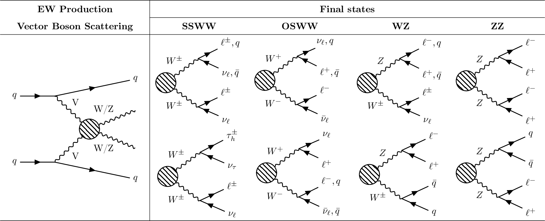
png pdf	Figure 1: The left side shows a representative Feynman diagram for the EW-induced production of VBS involving massive vector bosons. The dashed circle encapsulates different contributions leading to the same final state, including triple and quartic gauge couplings as well as Higgs-boson exchange. On the right, the considered decay channels are categorized into same-sign WW (SSWW), opposite-sign WW (OSWW), WZ, and ZZ pairs, covering both leptonic and semileptonic modes. In all cases, at least one vector boson is required to decay leptonically.
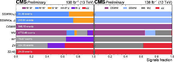
png pdf	Figure 2: The signal fractions for each analysis contributing to the combination are presented. Rows correspond to the names of the analyses, while the x-axis indicates the signal fraction. Different colors, as shown in the legend, represent the distinct signal parameters targeted for measurement. The left half of the figure displays the signal fractions for the six components, separated by the electric charge of the W bosons. The right half of the figure provides the equivalent information for the four components. All signal yields are computed before the combined fit to the signal strengths and including all analyses regions.
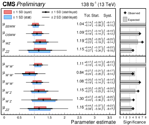
png pdf	Figure 3: Measurement of the vector boson scattering (VBS) signal strength modifiers ( $\mu_{i}$ ) and comparison with Standard Model (SM) predictions. The top (bottom) panel presents results considering four (six) independent signal strengths. In each panel, the left side shows the measured signal strengths, with thick (thin) black lines representing the 1 (2) standard deviation confidence intervals. The red and blue bands within the 1 standard deviation interval illustrate the systematic and statistical uncertainties, respectively. The right side displays the observed (black crosses) and expected (filled grey bars) statistical significance of the electroweak VBS signal relative to the SM background.
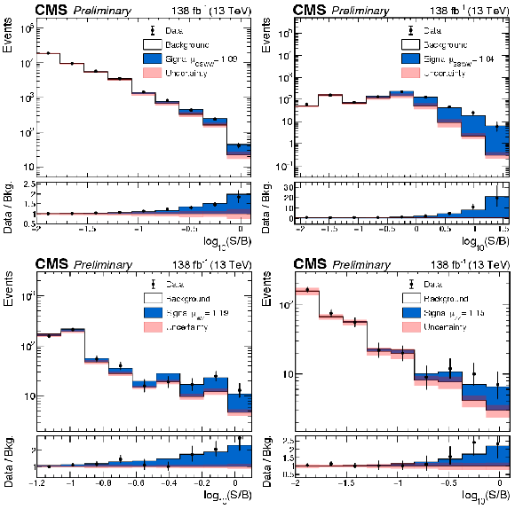
png pdf	Figure 4: Observed $\log[S(\mu_i=1)/B]$ distributions for the VBS SM combination and four parameters model. From left to right, the filled white histograms represent the overall background contributions while the blue histograms represent the signal yields for $\mu_{OSWW}$ , $\mu_{SSWW}$ , $\mu_{WZ}$ and $\mu_{ZZ}$ . The post-fit 68% uncertainty band on the overall background template is shown in pink. The distribution is binned as a function of the prefit value of $\log[S(\mu_i=1)/B]$ and is filled with the post-fit yields of signal and backgrounds. The latter are assigned to the dominant signal contribution in a specific bin of the input templates.
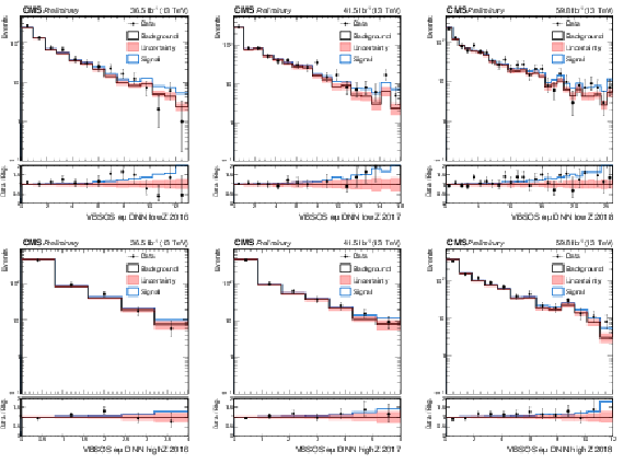
png pdf	Figure 5: Distributions of the DNN scores for the OSWW analysis in the signal $e\mu$ region after the combined fit. The signal region is divided into two sub-regions based on the Zeppenfeld variable ( $Z_{\ell\ell}$ ), with values either greater or smaller than one. The top and bottom rows show the distributions for $Z_{\ell\ell} <$ 1 and $Z_{\ell\ell} >$ 1, respectively. From left to right, the plots correspond to the 2016, 2017, and 2018 data-taking periods.
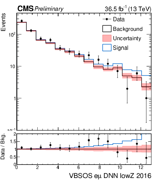
png pdf	Figure 5-a: Distributions of the DNN scores for the OSWW analysis in the signal $e\mu$ region after the combined fit. The signal region is divided into two sub-regions based on the Zeppenfeld variable ( $Z_{\ell\ell}$ ), with values either greater or smaller than one. The top and bottom rows show the distributions for $Z_{\ell\ell} <$ 1 and $Z_{\ell\ell} >$ 1, respectively. From left to right, the plots correspond to the 2016, 2017, and 2018 data-taking periods.
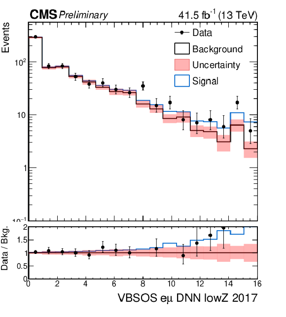
png pdf	Figure 5-b: Distributions of the DNN scores for the OSWW analysis in the signal $e\mu$ region after the combined fit. The signal region is divided into two sub-regions based on the Zeppenfeld variable ( $Z_{\ell\ell}$ ), with values either greater or smaller than one. The top and bottom rows show the distributions for $Z_{\ell\ell} <$ 1 and $Z_{\ell\ell} >$ 1, respectively. From left to right, the plots correspond to the 2016, 2017, and 2018 data-taking periods.
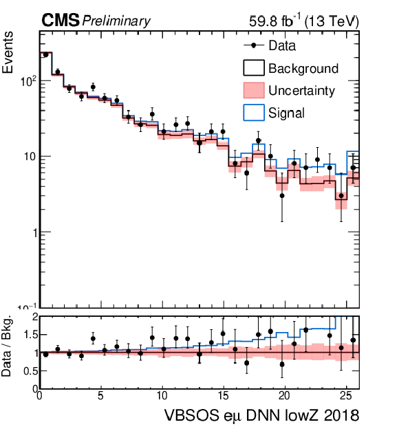
png pdf	Figure 5-c: Distributions of the DNN scores for the OSWW analysis in the signal $e\mu$ region after the combined fit. The signal region is divided into two sub-regions based on the Zeppenfeld variable ( $Z_{\ell\ell}$ ), with values either greater or smaller than one. The top and bottom rows show the distributions for $Z_{\ell\ell} <$ 1 and $Z_{\ell\ell} >$ 1, respectively. From left to right, the plots correspond to the 2016, 2017, and 2018 data-taking periods.
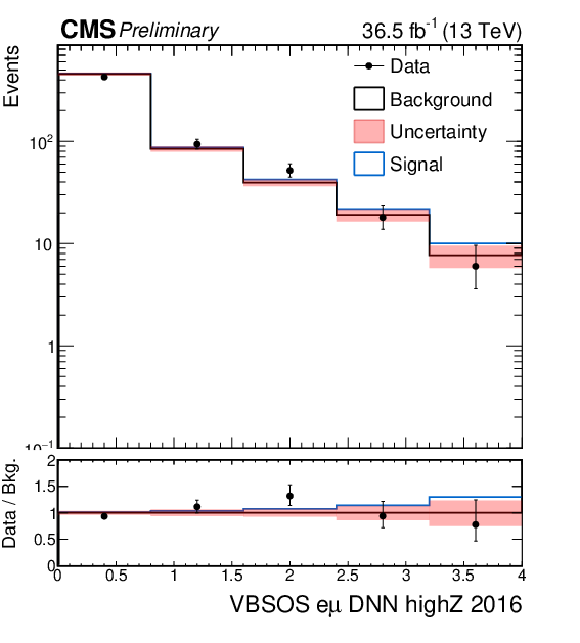
png pdf	Figure 5-d: Distributions of the DNN scores for the OSWW analysis in the signal $e\mu$ region after the combined fit. The signal region is divided into two sub-regions based on the Zeppenfeld variable ( $Z_{\ell\ell}$ ), with values either greater or smaller than one. The top and bottom rows show the distributions for $Z_{\ell\ell} <$ 1 and $Z_{\ell\ell} >$ 1, respectively. From left to right, the plots correspond to the 2016, 2017, and 2018 data-taking periods.
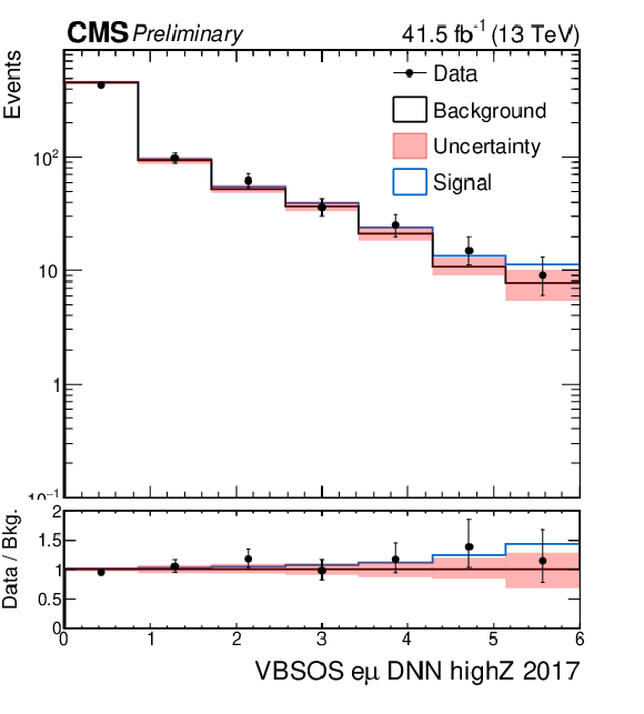
png pdf	Figure 5-e: Distributions of the DNN scores for the OSWW analysis in the signal $e\mu$ region after the combined fit. The signal region is divided into two sub-regions based on the Zeppenfeld variable ( $Z_{\ell\ell}$ ), with values either greater or smaller than one. The top and bottom rows show the distributions for $Z_{\ell\ell} <$ 1 and $Z_{\ell\ell} >$ 1, respectively. From left to right, the plots correspond to the 2016, 2017, and 2018 data-taking periods.
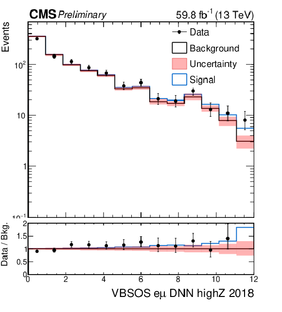
png pdf	Figure 5-f: Distributions of the DNN scores for the OSWW analysis in the signal $e\mu$ region after the combined fit. The signal region is divided into two sub-regions based on the Zeppenfeld variable ( $Z_{\ell\ell}$ ), with values either greater or smaller than one. The top and bottom rows show the distributions for $Z_{\ell\ell} <$ 1 and $Z_{\ell\ell} >$ 1, respectively. From left to right, the plots correspond to the 2016, 2017, and 2018 data-taking periods.
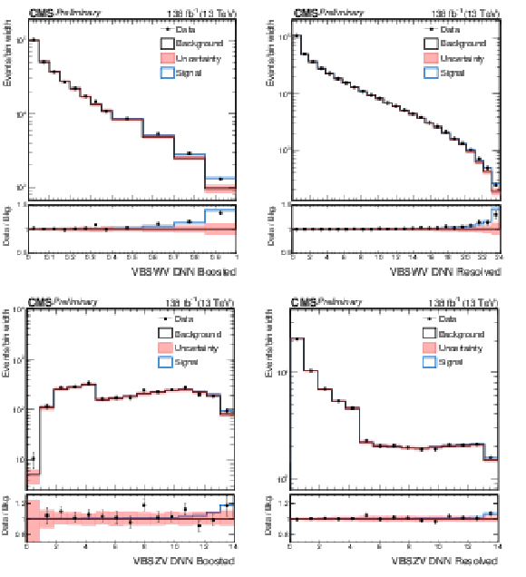
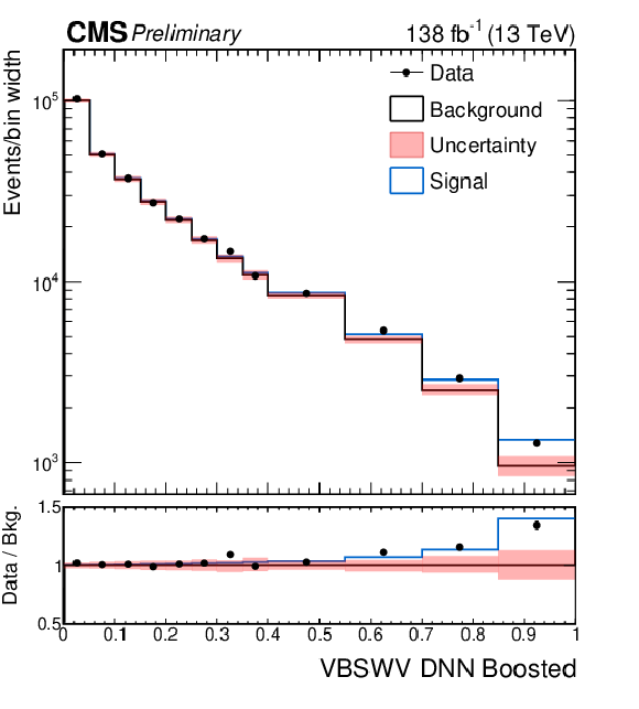
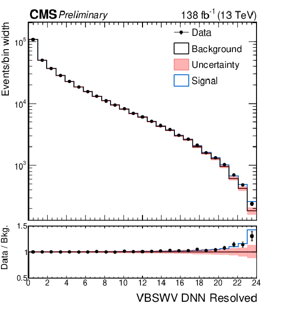
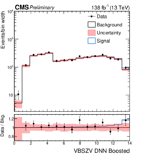
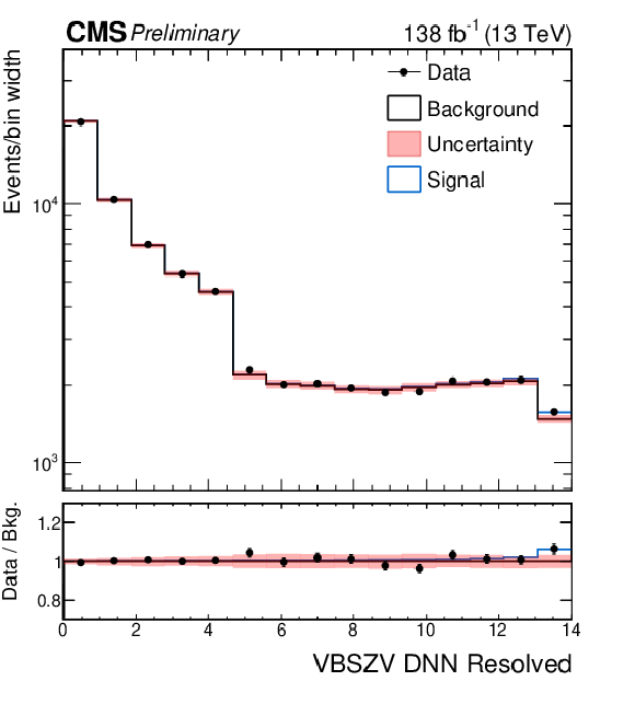
png pdf	Figure 6: Distributions for the signal regions of the semileptonic VBS analyses after the combined fit. The top row shows the DNN spectra of the WV analysis merged for the electron and muon cateogries in the boosted signal region (left) and in the resolved signal region (right). The bottom row shows the DNN spectra of the ZV analysis in the boosted signal region (left) and in the resolved signal region (right).
png pdf	Figure 6-a: Distributions for the signal regions of the semileptonic VBS analyses after the combined fit. The top row shows the DNN spectra of the WV analysis merged for the electron and muon cateogries in the boosted signal region (left) and in the resolved signal region (right). The bottom row shows the DNN spectra of the ZV analysis in the boosted signal region (left) and in the resolved signal region (right).
png pdf	Figure 6-b: Distributions for the signal regions of the semileptonic VBS analyses after the combined fit. The top row shows the DNN spectra of the WV analysis merged for the electron and muon cateogries in the boosted signal region (left) and in the resolved signal region (right). The bottom row shows the DNN spectra of the ZV analysis in the boosted signal region (left) and in the resolved signal region (right).
png pdf	Figure 6-c: Distributions for the signal regions of the semileptonic VBS analyses after the combined fit. The top row shows the DNN spectra of the WV analysis merged for the electron and muon cateogries in the boosted signal region (left) and in the resolved signal region (right). The bottom row shows the DNN spectra of the ZV analysis in the boosted signal region (left) and in the resolved signal region (right).
png pdf	Figure 6-d: Distributions for the signal regions of the semileptonic VBS analyses after the combined fit. The top row shows the DNN spectra of the WV analysis merged for the electron and muon cateogries in the boosted signal region (left) and in the resolved signal region (right). The bottom row shows the DNN spectra of the ZV analysis in the boosted signal region (left) and in the resolved signal region (right).
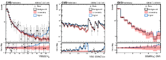
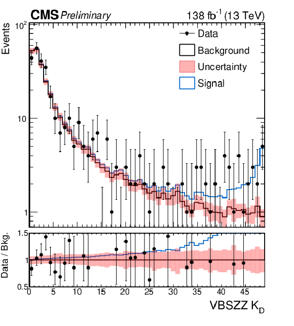
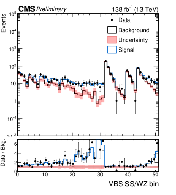
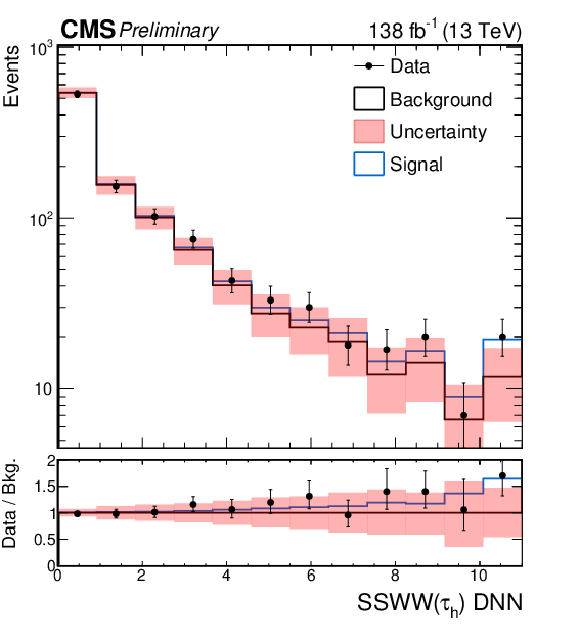
png pdf	Figure 7: The left figure shows the distribution of the $K_{D}$ discriminant used to separate the VBS EW ZZ production from the QCD-induced one in the VBS-ZZ(4 $\ell$ ) signal region. The central figure presents the distribution of the SSWW and WZ analyses in all signal and control regions entering in the combined fit. The right figure shows the distribution fo the DNN score used to separate the SSWW signal from the backgrounds in the SSWW( $\tau_h$ ) signal region. All distributions are shown after the combined fit.
png pdf	Figure 7-a: The left figure shows the distribution of the $K_{D}$ discriminant used to separate the VBS EW ZZ production from the QCD-induced one in the VBS-ZZ(4 $\ell$ ) signal region. The central figure presents the distribution of the SSWW and WZ analyses in all signal and control regions entering in the combined fit. The right figure shows the distribution fo the DNN score used to separate the SSWW signal from the backgrounds in the SSWW( $\tau_h$ ) signal region. All distributions are shown after the combined fit.
png pdf	Figure 7-b: The left figure shows the distribution of the $K_{D}$ discriminant used to separate the VBS EW ZZ production from the QCD-induced one in the VBS-ZZ(4 $\ell$ ) signal region. The central figure presents the distribution of the SSWW and WZ analyses in all signal and control regions entering in the combined fit. The right figure shows the distribution fo the DNN score used to separate the SSWW signal from the backgrounds in the SSWW( $\tau_h$ ) signal region. All distributions are shown after the combined fit.
png pdf	Figure 7-c: The left figure shows the distribution of the $K_{D}$ discriminant used to separate the VBS EW ZZ production from the QCD-induced one in the VBS-ZZ(4 $\ell$ ) signal region. The central figure presents the distribution of the SSWW and WZ analyses in all signal and control regions entering in the combined fit. The right figure shows the distribution fo the DNN score used to separate the SSWW signal from the backgrounds in the SSWW( $\tau_h$ ) signal region. All distributions are shown after the combined fit.
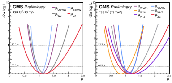
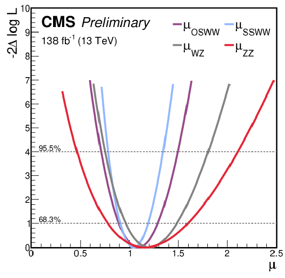
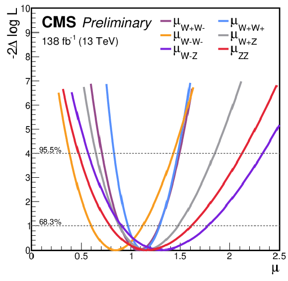
png pdf	Figure 8: The two figures show the likelihood profiles from the combined fit for the various POIs. The left figure shows the $-2\Delta \log L$ profiles for the 4-POIs model while the right one shows the same profiles in the 6-POIs fit.
png pdf	Figure 8-a: The two figures show the likelihood profiles from the combined fit for the various POIs. The left figure shows the $-2\Delta \log L$ profiles for the 4-POIs model while the right one shows the same profiles in the 6-POIs fit.
png pdf	Figure 8-b: The two figures show the likelihood profiles from the combined fit for the various POIs. The left figure shows the $-2\Delta \log L$ profiles for the 4-POIs model while the right one shows the same profiles in the 6-POIs fit.
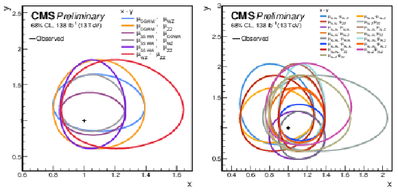
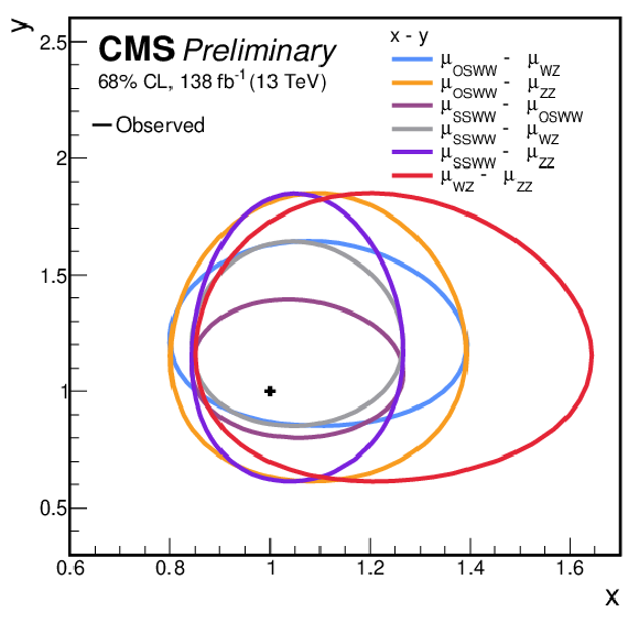
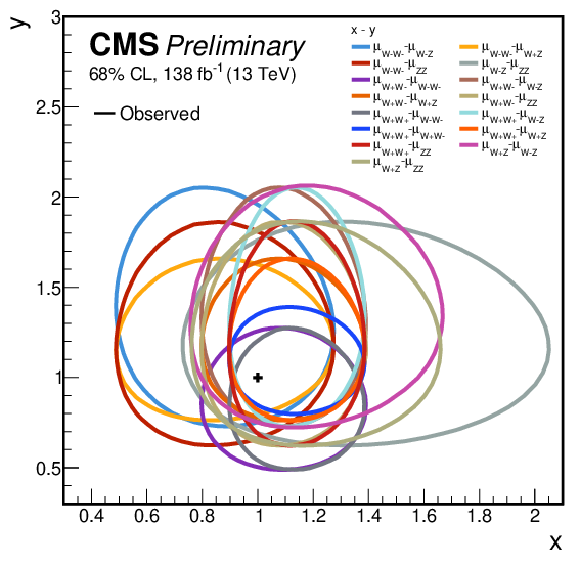
png pdf	Figure 9: Summary plots of the two-dimensional fits are presented. The left plot displays the 68% confidence level intervals for all pairs of parameters of interest in the 4-POIs model, with the legend listing the POI on the x-axis first, followed by the POI on the y-axis. The right plot provides the corresponding intervals for the 6-POIs model. In all cases, all parameters of interest except the two under study are profiled in the maximum likelihood fit along with the nuisance parameters.
png pdf	Figure 9-a: Summary plots of the two-dimensional fits are presented. The left plot displays the 68% confidence level intervals for all pairs of parameters of interest in the 4-POIs model, with the legend listing the POI on the x-axis first, followed by the POI on the y-axis. The right plot provides the corresponding intervals for the 6-POIs model. In all cases, all parameters of interest except the two under study are profiled in the maximum likelihood fit along with the nuisance parameters.
png pdf	Figure 9-b: Summary plots of the two-dimensional fits are presented. The left plot displays the 68% confidence level intervals for all pairs of parameters of interest in the 4-POIs model, with the legend listing the POI on the x-axis first, followed by the POI on the y-axis. The right plot provides the corresponding intervals for the 6-POIs model. In all cases, all parameters of interest except the two under study are profiled in the maximum likelihood fit along with the nuisance parameters.

Tables
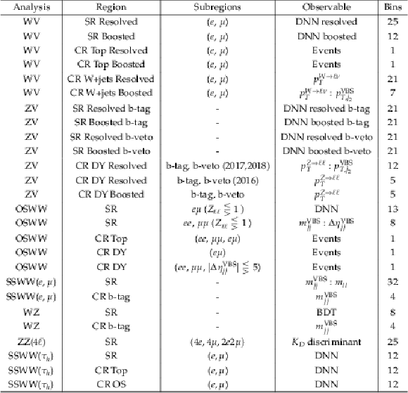
png pdf	Table 1: Summary of the analyses considered in the combination. $\ell$ denotes either an electron or muon, $\tau_h$ an hadronicaly decaying $\tau$ lepton and $j$ is the shorthand notation for a parton.
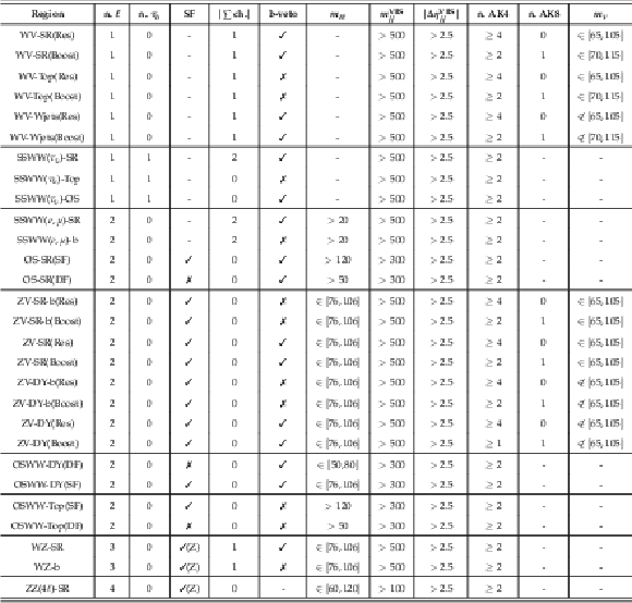
png pdf	Table 2: Summary of the signal and control regions defined in the analyses entering the combination, including the requirements ensuring their orthogonality. The second column is the number of light leptons ( $\ell = e, \mu$ ), and the third column is the number of hadronically decaying tau leptons. The same-flavor requirement for charged leptons is denoted as SF. A check mark indicates that the SF condition is applied, a cross means it is inverted (different-flavour), and no symbol signifies no restriction on lepton flavors. $\|\sum$ ch. $\|$ is the sum of the electrical charges for leptons in the final state. The b-veto column uses check mark to indicate regions that veto b-jets, a cross for regions requiring at least one b-jet, and no symbol for no restriction on b-jets. $m_{\ell\ell}$ denotes the invariant mass of a charged dilepton pair and is defined in GeV. In WZ and ZZ cases, $m_{\ell\ell}$ and SF refer respectively to the invariant mass and same flavour requirements of the Z boson decay candidates. The next two columns are the invariant mass, in units of GeV, of the two VBS jets and the $\eta$ separation between them. The table finally presents the number of small-radius (AK4) and large-radius (AK8) jets, along with the invariant mass, in GeV, of the hadronically decaying vector boson candidate (W or Z).
png pdf	Table 3: Phase space regions included in the combined fit, along with the corresponding observables and the number of bins. Bidimensional observables are represented with a colon separating the two components. For each subregion, a template is defined based on the specified observable and the number of bins. If the data-taking year is not explicitly specified in the subregion column, an independent template is included for each individual year of data-taking.
png pdf	Table 4: Observed values of the signal strengths $\mu^i = \sigma^i/\sigma^i_{\text{SM}}$ and statistical significance ( $\sigma^i$ ) from the VBS combination. The top row reports the results for the model with four signal strengths while the bottom row reports the same results but splitting the signal strengths for the W boson electrical charge. The expected results are reported within brackets. For the expected signal strengths, only the $\pm$ 1 standard deviation uncertainty is reported as the central value is assumed to be 1.

Summary

This study presents the most comprehensive statistical combination of vector boson scattering (VBS) processes to date, integrating results from seven analyses. The fully leptonic final states are SSWW(

$e,\mu$ ),

$pp \rightarrow W^\pm W^\pm jj \rightarrow 2\ell^\pm 2\nu jj$ ; SSWW(

$\tau_h$ ),

$pp \rightarrow W^\pm W^\pm jj \rightarrow \ell^\pm \tau_h^{\pm} 2\nu jj$ ; OSWW,

$pp \rightarrow W^+ W^{-} jj \rightarrow \ell^+ \ell^{-} 2\nu jj$ ; WZ,

$pp \rightarrow W^\pm Z jj \rightarrow 3\ell \nu jj$ ; and ZZ(4

$\ell$ ),

$pp \rightarrow ZZ jj \rightarrow 4\ell jj$ , where

$\ell = e, \mu$ . The semileptonic final states are WV (

$pp \rightarrow W^\pm V jj \rightarrow \ell \nu jjjj$ ) and ZV (

$pp \rightarrow Z V jj \rightarrow 2\ell jjjj$ ) where

$V$ (W,Z) denotes an hadronically decaying vector boson

$V\rightarrow jj$ . Electroweak (EW) VBS production signal strengths are measured in two configurations: one merging W boson electric charges with four free parameters (

$\mu_{\text{SSWW}}$ ,

$\mu_{\text{OSWW}}$ ,

$\mu_{\text{WZ}}$ ,

$\mu_{\text{ZZ}}$ ) and another splitting W boson charges with six parameters (

$\mu_{W^+W^+}$ ,

$\mu_{W^{-}W^{-}}$ ,

$\mu_{W^+W^{-}}$ ,

$\mu_{W^+Z}$ ,

$\mu_{W^{-}Z}$ ,

$\mu_{ZZ}$ ). The EW signal strengths are measured based on a simultaneous fit of the seven channels. Interference effects between QCD and EW diboson production are negligible in all channels except SSWW(

$e,\mu$ ) and ZZ, where they are treated as part of the EW signal. The results for the four-parameter model are

$\mu_{\text{SSWW}} =$ 1.04

$^{+0.14}_{-0.14}$ ,

$\mu_{\text{OSWW}} =$ 1.09

$^{+0.21}_{-0.18}$ ,

$\mu_{\text{WZ}} =$ 1.19

$^{+0.28}_{-0.23}$ , and

$\mu_{\text{ZZ}} =$ 1.15

$^{+0.44}_{-0.37}$ . For the six-parameter model the results are

$\mu_{W^+W^+} =$ 1.11

$^{+0.17}_{-0.15}$ ,

$\mu_{W^{-}W^{-}} =$ 0.84

$^{+0.27}_{-0.24}$ ,

$\mu_{W^+W^{-}} =$ 1.08

$^{+0.20}_{-0.19}$ ,

$\mu_{W^+Z} =$ 1.15

$^{+0.32}_{-0.27}$ ,

$\mu_{W^{-}Z} =$ 1.30

$^{+0.47}_{-0.40}$ , and

$\mu_{ZZ} =$ 1.16

$^{+0.44}_{-0.38}$ . Simultaneous two-dimensional fits were performed for all VBS EW production components. The compatibility between the observed data and the Standard Model (SM) predictions was evaluated differentially using the

$\log(S/B)$ observable. Overall, all one-dimensional and two-dimensional measurements are found to be consistent with SM predictions at the 68% confidence level.

References
1	ATLAS Collaboration	Observation of a new particle in the search for the Standard Model Higgs boson with the ATLAS detector at the LHC	PLB 716 (2012) 1	1207.7214
2	CMS Collaboration	Observation of a New Boson at a Mass of 125 GeV with the CMS Experiment at the LHC	PLB 716 (2012) 30	CMS-HIG-12-028 1207.7235
3	CMS Collaboration	Observation of a New Boson with Mass Near 125 GeV in $pp$ Collisions at $\sqrt{s}$ = 7 and 8 TeV	JHEP 06 (2013) 081	CMS-HIG-12-036 1303.4571
4	CMS Collaboration	A portrait of the Higgs boson by the CMS experiment ten years after the discovery	Nature 607 (2022)	CMS-HIG-22-001 2207.00043
5	ATLAS Collaboration	A detailed map of Higgs boson interactions by the ATLAS experiment ten years after the discovery	Nature 607 (2022)	2207.00092
6	F. Englert and R. Brout	Broken Symmetry and the Mass of Gauge Vector Mesons	PRL 13 (1964) 321
7	P. W. Higgs	Broken symmetries, massless particles and gauge fields	PL 12 (1964) 132
8	P. W. Higgs	Broken Symmetries and the Masses of Gauge Bosons	PRL 13 (1964) 508
9	G. S. Guralnik, C. R. Hagen, and T. W. B. Kibble	Global Conservation Laws and Massless Particles	PRL 13 (1964) 585
10	P. W. Higgs	Spontaneous Symmetry Breakdown without Massless Bosons	PR 145 (1966) 1156
11	T. W. B. Kibble	Symmetry breaking in nonAbelian gauge theories	PR 155 (1967) 1554
12	H. G. J. Veltman	The Equivalence Theorem	PRD 41 (1990) 2294
13	H.-J. He, Y.-P. Kuang, and X.-y. Li	On the precise formulation of equivalence theorem	PRL 69 (1992) 2619
14	B. W. Lee, C. Quigg, and H. B. Thacker	Weak interactions at very high energies: The role of the higgs-boson mass	PRD 1 (1977) 6
15	B. W. Lee, C. Quigg, and H. B. Thacker	Strength of weak interactions at very high energies and the higgs boson mass	PRL 3 (1977) 8
16	D. Espriu and B. Yencho	Longitudinal WW scattering in light of the \textquotedblleftHiggs boson\textquotedblright discovery	PRD 87 (2013)	1212.4158
17	J. Chang, K. Cheung, C.-T. Lu, and T.-C. Yuan	WW scattering in the era of post-Higgs-boson discovery	PRD 87 (2013) 093005	1303.6335
18	O. J. P. Eboli, M. C. Gonzalez-Garcia, and J. K. Mizukoshi	p p ---\ensuremath> j j e+- mu+- nu nu and j j e+- mu-+ nu nu at O( alpha(em)6) and O(alpha(em)4 alpha(s)**2) for the study of the quartic electroweak gauge boson vertex at CERN LHC	PRD 74 (2006) 073005	hep-ph/0606118
19	CMS Collaboration	Precision luminosity measurement in proton-proton collisions at $\sqrt{s} =$ 13 TeV in 2015 and 2016 at CMS	EPJC 81 (2021)	CMS-LUM-17-003 2104.01927
20	CMS Collaboration	CMS luminosity measurement for the 2017 data-taking period at $\sqrt{s}=$ 13 TeV	CMS Physics Analysis Summary, 2018 CMS-PAS-LUM-17-004	CMS-PAS-LUM-17-004
21	CMS Collaboration	CMS luminosity measurement for the 2018 data-taking period at $\sqrt{s}=$ 13 TeV	CMS Physics Analysis Summary, 2019 CMS-PAS-LUM-18-002	CMS-PAS-LUM-18-002
22	CMS Collaboration	The CMS Experiment at the CERN LHC	JINST 3 (2008) S08004
23	CMS Collaboration	Measurements of production cross sections of WZ and same-sign WW boson pairs in association with two jets in proton-proton collisions at $\sqrt{s} =$ 13 TeV	PLB 809 (2020) 135710	CMS-SMP-19-012 2005.01173
24	CMS Collaboration	Study of same-sign W boson scattering and anomalous couplings in events with one tau lepton from pp collisions at $\sqrt{s}$ = 13 TeV		CMS-SMP-22-008 2410.04210
25	CMS Collaboration	Observation of electroweak W+W\ensuremath- pair production in association with two jets in proton-proton collisions at s=13TeV	PLB 841 (2023) 137495	CMS-SMP-21-001 2205.05711
26	CMS Collaboration	Evidence for electroweak production of four charged leptons and two jets in proton-proton collisions at $\sqrt {s}$ = 13 TeV	PLB 812 (2021) 135992	CMS-SMP-20-001 2008.07013
27	CMS Collaboration	Evidence for WW/WZ vector boson scattering in the decay channel \ensuremath\ell\ensuremath\nuqq produced in association with two jets in proton-proton collisions at s=13 TeV	PLB 834 (2022) 137438	CMS-SMP-20-013 2112.05259
28	CMS Collaboration	Study of semileptonic vector boson scattering and anomalous quartic gauge coupling from proton-proton collisions at 13 TeV	CMS Physics Analysis Summary, 2025 CMS-PAS-SMP-22-011	CMS-PAS-SMP-22-011
29	CMS Collaboration	Measurement of the electroweak production of W $\gamma$ in association with two jets in proton-proton collisions at $\sqrt{s}$ = 13 TeV	PRD 108 (2023)	CMS-SMP-21-011 2212.12592
30	CMS Collaboration	Measurement of the electroweak production of Z $\gamma$ and two jets in proton-proton collisions at $\sqrt{s} =$ 13 TeV and constraints on anomalous quartic gauge couplings	PRD 104 (2021) 072001	CMS-SMP-20-016 2106.11082
31	CMS Collaboration	Particle-flow reconstruction and global event description with the CMS detector	JINST 12 (2017)	CMS-PRF-14-001 1706.04965
32	CMS Collaboration	Performance of the CMS Level-1 trigger in proton-proton collisions at $\sqrt{s} =$ 13 TeV	JINST 15 (2020)	CMS-TRG-17-001 2006.10165
33	CMS Collaboration	The CMS trigger system	JINST 12 (2017)	CMS-TRG-12-001 1609.02366
34	J. Alwall et al.	The automated computation of tree-level and next-to-leading order differential cross sections, and their matching to parton shower simulations	JHEP 07 (2014) 079	1405.0301
35	J. Alwall et al.	Comparative study of various algorithms for the merging of parton showers and matrix elements in hadronic collisions	EPJC 53 (2008) 473	0706.2569
36	P. Artoisenet, R. Frederix, O. Mattelaer, and R. Rietkerk	Automatic spin-entangled decays of heavy resonances in Monte Carlo simulations	JHEP 03 (2013) 015	1212.3460
37	P. Nason	A New method for combining NLO QCD with shower Monte Carlo algorithms	JHEP 11 (2004) 040	hep-ph/0409146
38	S. Frixione and B. R. Webber	Matching NLO QCD computations and parton shower simulations	JHEP 06 (2002) 029	hep-ph/0204244
39	S. Frixione, P. Nason, and C. Oleari	Matching NLO QCD computations with Parton Shower simulations: the POWHEG method	JHEP 11 (2007) 070	0709.2092
40	S. Alioli, P. Nason, C. Oleari, and E. Re	NLO vector-boson production matched with shower in POWHEG	JHEP 07 (2008) 060	0805.4802
41	S. Alioli, P. Nason, C. Oleari, and E. Re	A general framework for implementing NLO calculations in shower Monte Carlo programs: the POWHEG BOX	JHEP 06 (2010) 043	1002.2581
42	J. M. Campbell, R. K. Ellis, and W. T. Giele	A Multi-Threaded Version of MCFM	EPJC 75 (2015)	1503.06182
43	J. M. Campbell, R. K. Ellis, and C. Williams	Vector Boson Pair Production at the LHC	JHEP 07 (2011) 018	1105.0020
44	J. M. Campbell and R. K. Ellis	An Update on vector boson pair production at hadron colliders	PRD 60 (1999) 113006	hep-ph/9905386
45	J. Campbell and T. Neumann	Precision Phenomenology with MCFM	JHEP 12 (2019) 034	1909.09117
46	K. Hamilton, P. Nason, and G. Zanderighi	Finite quark-mass effects in the NNLOPS POWHEG+MiNLO Higgs generator	JHEP 05 (2015) 140	1501.04637
47	S. Bolognesi et al.	On the Spin and Parity of a Single-Produced Resonance at the LHC	PRD 86 (2012) 095031	1208.4018
48	T. Sjöstrand et al.	An introduction to PYTHIA 8.2	Comput. Phys. Commun. 191 (2015) 159	1410.3012
49	NNPDF Collaboration	Parton distributions for the LHC Run II	JHEP 04 (2015) 040	1410.8849
50	NNPDF Collaboration	Parton distributions from high-precision collider data	EPJC 77 (2017)	1706.00428
51	P. Skands, S. Carrazza, and J. Rojo	Tuning PYTHIA 8.1: the Monash 2013 Tune	EPJC 74 (2014)	1404.5630
52	CMS Collaboration	Event generator tunes obtained from underlying event and multiparton scattering measurements	EPJC 76 (2016)	CMS-GEN-14-001 1512.00815
53	CMS Collaboration	Extraction and validation of a new set of CMS PYTHIA8 tunes from underlying-event measurements	EPJC 80 (2020)	CMS-GEN-17-001 1903.12179
54	A. Ballestrero et al.	Precise predictions for same-sign W-boson scattering at the LHC	EPJC 78 (2018)	1803.07943
55	B. J ä ger et al.	Parton-shower effects in Higgs production via Vector-Boson Fusion	EPJC 80 (2020)	2003.12435
56	R. Covarelli, M. Pellen, and M. Zaro	Vector-Boson scattering at the LHC: Unraveling the electroweak sector	Int. J. Mod. Phys. A 36 (2021)	2102.10991
57	C. Bierlich et al.	A comprehensive guide to the physics and usage of PYTHIA 8.3	SciPost Phys. Codeb. 2022 (2022) 8	2203.11601
58	GEANT4 Collaboration	GEANT4 - A Simulation Toolkit	NIM A 506 (2003) 250
59	CMS Collaboration	Identification of heavy-flavour jets with the CMS detector in pp collisions at 13 TeV	JINST 13 (2018)	CMS-BTV-16-002 1712.07158
60	Particle Data Group Collaboration	Review of Particle Physics	PTEP 2022 (2022) 083C01
61	D. L. Rainwater, R. Szalapski, and D. Zeppenfeld	Probing color singlet exchange in $Z$ + two jet events at the CERN LHC	PRD 54 (1996) 6680	hep-ph/9605444
62	E. Bols et al.	Jet Flavour Classification Using DeepJet	JINST 15 (2020)	2008.10519
63	CMS Collaboration	Measurement of the single top quark and antiquark production cross sections in the $t$ channel and their ratio in proton-proton collisions at $\sqrt{s}=$ 13 TeV	PLB 800 (2020) 135042	CMS-TOP-17-011 1812.10514
64	CMS Collaboration	Measurement of Higgs Boson Production and Properties in the WW Decay Channel with Leptonic Final States	JHEP 01 (2014) 096	CMS-HIG-13-023 1312.1129
65	Y. Gao et al.	Spin Determination of Single-Produced Resonances at Hadron Colliders	PRD 81 (2010) 075022	1001.3396
66	I. Anderson et al.	Constraining Anomalous HVV Interactions at Proton and Lepton Colliders	PRD 89 (2014)	1309.4819
67	A. V. Gritsan, R. Röntsch, M. Schulze, and M. Xiao	Constraining anomalous Higgs boson couplings to the heavy flavor fermions using matrix element techniques	PRD 94 (2016)	1606.03107
68	The ATLAS Collaboration, The CMS Collaboration, The LHC Higgs Combination Group	Procedure for the LHC Higgs boson search combination in Summer 2011	Technical Report CMS-NOTE-2011-005, ATL-PHYS-PUB-2011-11, 2011
69	ATLAS and CMS Collaborations	Measurements of the Higgs boson production and decay rates and constraints on its couplings from a combined ATLAS and CMS analysis of the LHC pp collision data at $\sqrt{s}=$ 7 and 8 TeV	JHEP 08 (2016) 045	1606.02266
70	CMS Collaboration	The CMS statistical analysis and combination tool: \textscCombine	Comput. Softw. Big Sci. 8 (2024) 19	CMS-CAT-23-001 2404.06614
71	G. Cowan, K. Cranmer, E. Gross, and O. Vitells	Asymptotic formulae for likelihood-based tests of new physics	EPJC 71 (2011) 1554	1007.1727
72	CMS Collaboration	Jet energy scale and resolution in the CMS experiment in pp collisions at 8 TeV	JINST 12 (2017)	CMS-JME-13-004 1607.03663
73	CMS Collaboration	Measurement of the inelastic proton-proton cross section at $\sqrt{s}=$ 13 TeV	JHEP 07 (2018) 161	CMS-FSQ-15-005 1802.02613
74	J. Butterworth et al.	PDF4LHC recommendations for LHC Run II	JPG 43 (2016) 023001	1510.03865
75	R. J. Barlow and C. Beeston	Fitting using finite Monte Carlo samples	Comput. Phys. Commun. 77 (1993) 219
76	J. S. Conway	Incorporating Nuisance Parameters in Likelihoods for Multisource Spectra	PHYSTAT 201 (2011) 115	1103.0354