
Compact Muon Solenoid
LHC, CERN
 Visit us: CMS Public Website, CMS Physics ;
Contact us: CMS Publications Committee
Visit us: CMS Public Website, CMS Physics ;
Contact us: CMS Publications Committee
| CMS-PAS-MLG-25-001 | ||
| Unsupervised anomaly detection for real-time data acquisition in the CMS experiment at the Large Hadron Collider | ||
| CMS Collaboration | ||
| 2026-08-03 | ||
| Abstract: This note presents the first deployment of unsupervised anomaly detection algorithms for real-time data selection at the CERN LHC, establishing a new paradigm for collider data acquisition. Two complementary algorithms, AXOL1TL and CICADA, operate within the CMS trigger system to identify rare and anomalous collisions without reference to predefined signal hypotheses, thus preserving sensitivity to physics signatures not anticipated by existing models. During 2024 proton-proton collisions at $ \sqrt{s}= $ 13.6 TeV, these models selected more than four billion collision events for permanent storage and analysis. Operating directly on FPGAs at the full 40 $ \mathrm{MHz} $ LHC collision rate, they achieve deterministic sub-100 $ \mathrm{ns} $ inference latency. The hardware-aware design and firmware implementation strategy of the algorithms is described in detail, and their performance is evaluated using both simulated benchmark signals and collision data. These results provide a foundation for online model-agnostic data selection through machine-learning algorithms, broadening the discovery reach beyond the limitations of conventional strategies. | ||
| Links: CDS record (PDF) ; CADI line (restricted) ; | ||
| Figures | |
png pdf |
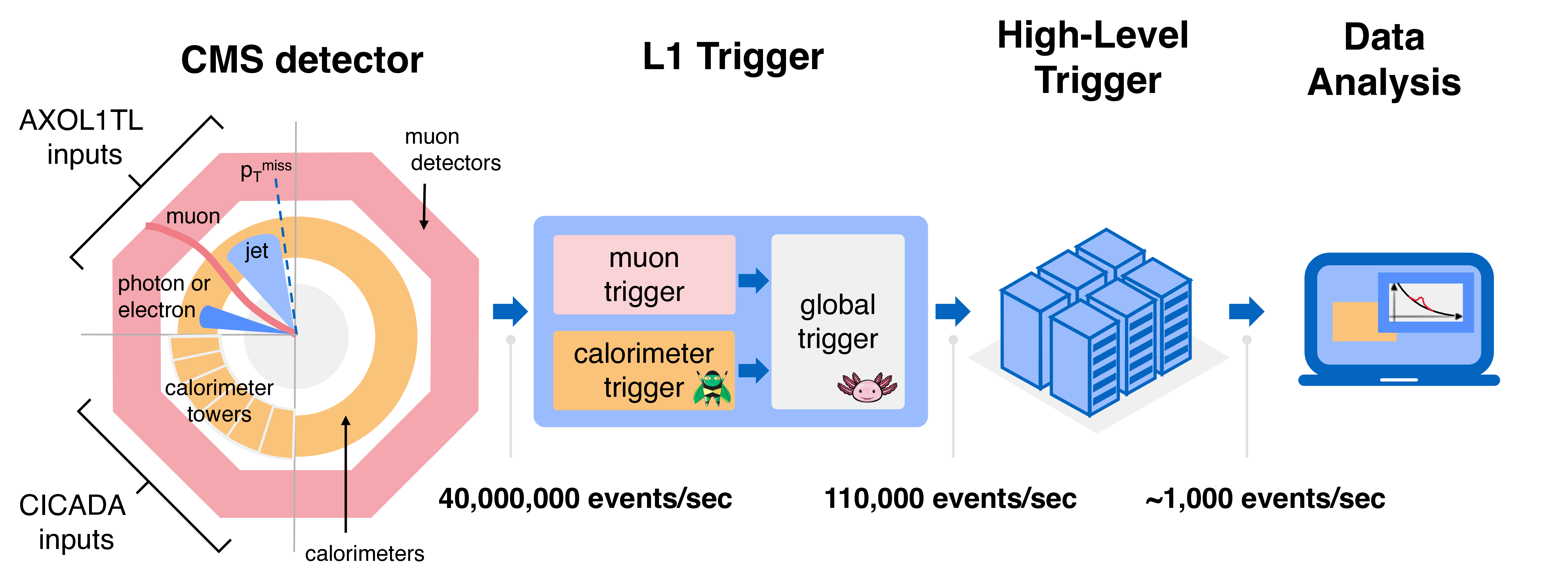
Figure 1:
Diagram of the operation of the CMS detector, trigger, and a typical analysis workflow. The CMS detector diagram (left) shows the different subdetectors and physics objects captured or reconstructed by CMS such as calorimeter towers, photons, electrons, muons, and jets. The L1 trigger diagram (second from left) shows the component pieces of the L1 trigger. The calorimeter trigger, which takes calorimeter inputs, houses the CICADA algorithm, and the global trigger, which takes fast reconstructions of objects as input, houses the AXOL1TL algorithm. The high-level trigger (second from right) analyzes the full detector readout of events that are selected by the L1 trigger and its outputs are permanently saved for further data analysis (right). |
png pdf |
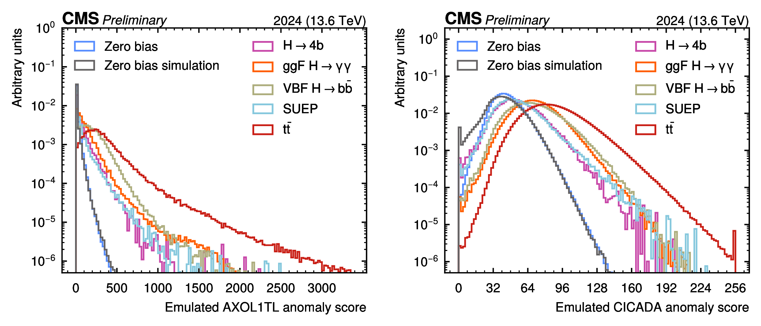
Figure 2:
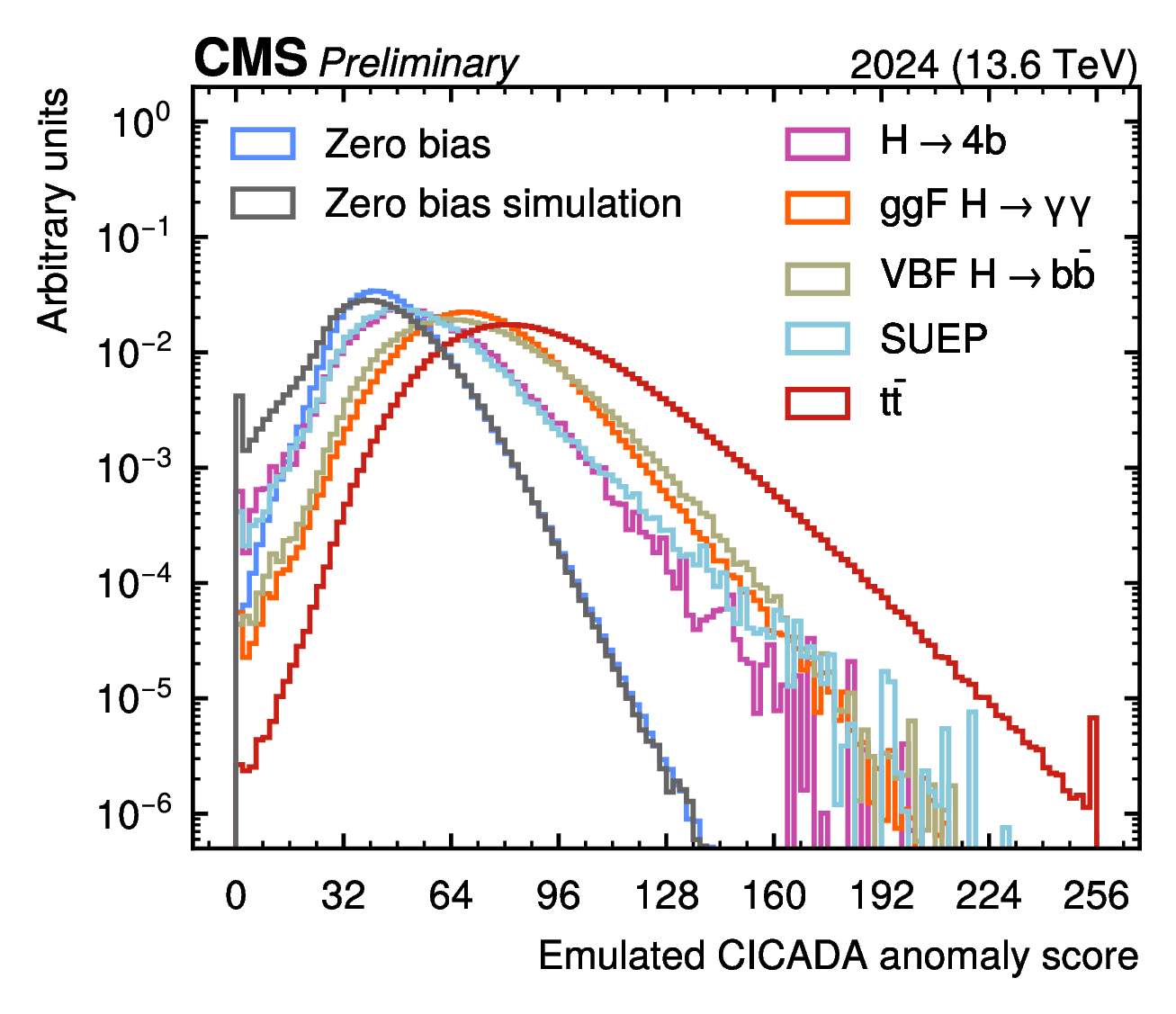
The anomaly score distributions for AXOL1TL (left) and CICADA (right) evaluated on simulated benchmark signals and zero bias background. The distributions are normalized to unit integral. Emulated scores are computed in software that reproduces the firmware output. |
png pdf |
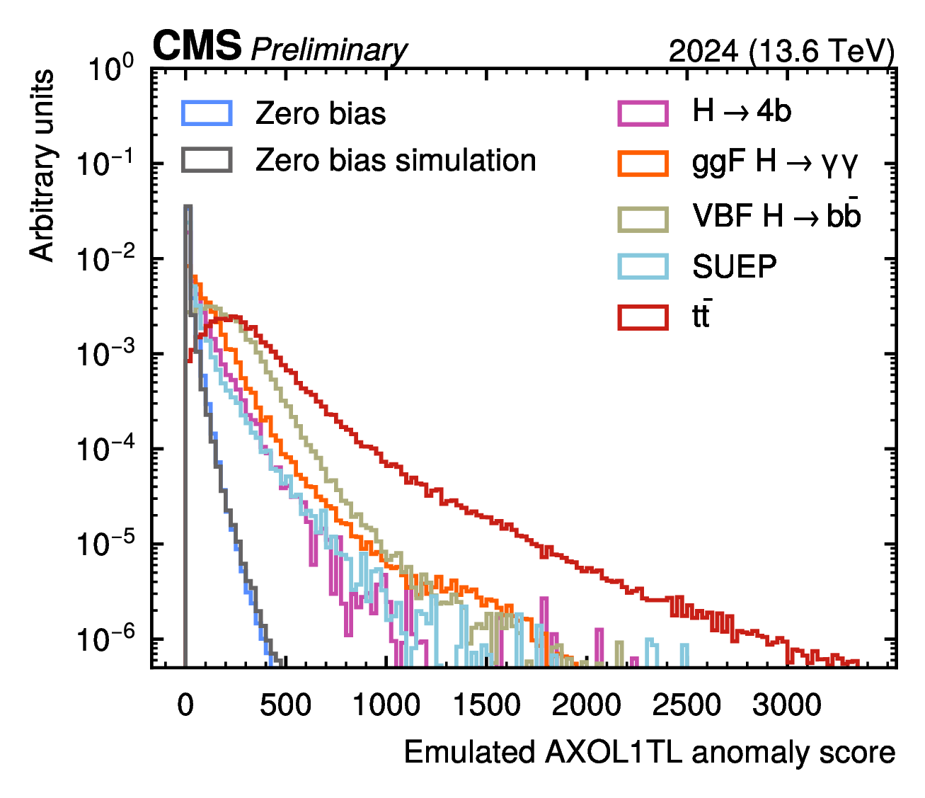
Figure 2-a:
The anomaly score distributions for AXOL1TL (left) and CICADA (right) evaluated on simulated benchmark signals and zero bias background. The distributions are normalized to unit integral. Emulated scores are computed in software that reproduces the firmware output. |
png pdf |
Figure 2-b:
The anomaly score distributions for AXOL1TL (left) and CICADA (right) evaluated on simulated benchmark signals and zero bias background. The distributions are normalized to unit integral. Emulated scores are computed in software that reproduces the firmware output. |
png pdf |
Figure 3:
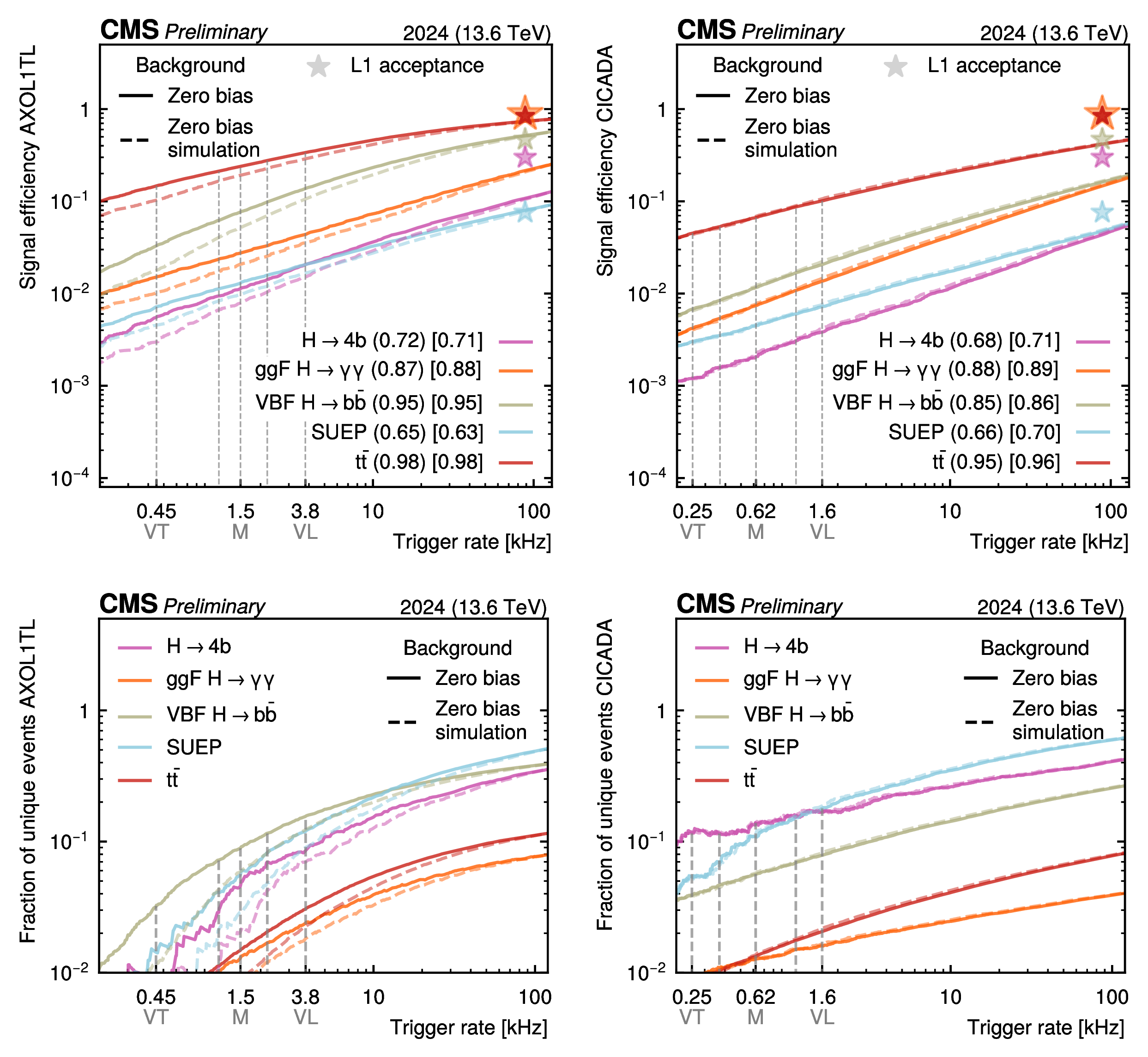
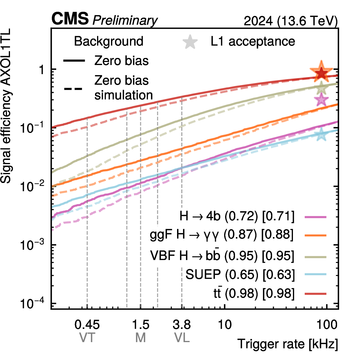
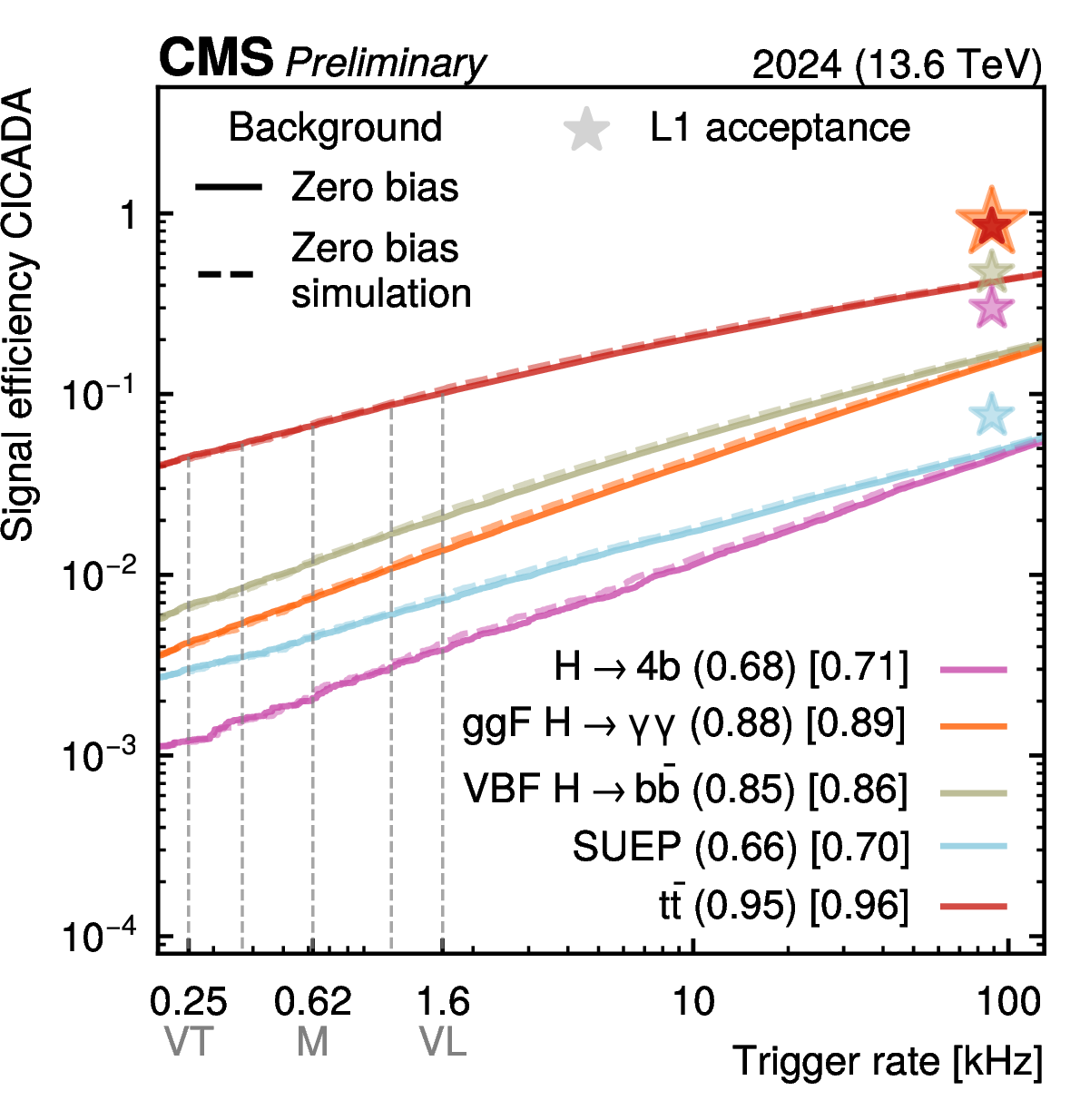
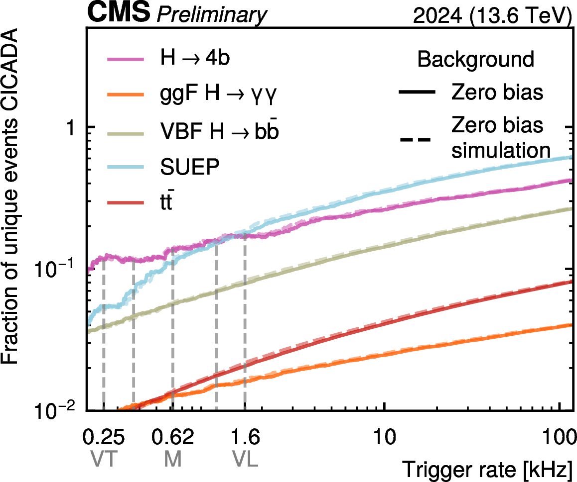
Upper: the receiver operating characteristic (ROC) curves for AXOL1TL (left) and CICADA (right) evaluated on benchmark signal samples. The area under the ROC curve (AUC) is reported for zero bias data in parentheses and zero bias simulation in brackets to reflect the differences between data and simulation. The stars indicate the L1 working point (WP), which corresponds to the trigger rate and signal efficiency of the existing L1 system---a logical OR of 141 purpose-built trigger algorithms. The vertical dashed lines from left to right indicate the very tight (VT), tight, medium (M), loose, and very loose (VL) thresholds at which AXOL1TL and CICADA operate during data taking. Lower: the fraction of unique events recorded by AXOL1TL (left) or CICADA (right), respectively. Unique events are events where no other L1 trigger algorithm selected the event. |
png pdf |
Figure 3-a:
Upper: the receiver operating characteristic (ROC) curves for AXOL1TL (left) and CICADA (right) evaluated on benchmark signal samples. The area under the ROC curve (AUC) is reported for zero bias data in parentheses and zero bias simulation in brackets to reflect the differences between data and simulation. The stars indicate the L1 working point (WP), which corresponds to the trigger rate and signal efficiency of the existing L1 system---a logical OR of 141 purpose-built trigger algorithms. The vertical dashed lines from left to right indicate the very tight (VT), tight, medium (M), loose, and very loose (VL) thresholds at which AXOL1TL and CICADA operate during data taking. Lower: the fraction of unique events recorded by AXOL1TL (left) or CICADA (right), respectively. Unique events are events where no other L1 trigger algorithm selected the event. |
png pdf |
Figure 3-b:
Upper: the receiver operating characteristic (ROC) curves for AXOL1TL (left) and CICADA (right) evaluated on benchmark signal samples. The area under the ROC curve (AUC) is reported for zero bias data in parentheses and zero bias simulation in brackets to reflect the differences between data and simulation. The stars indicate the L1 working point (WP), which corresponds to the trigger rate and signal efficiency of the existing L1 system---a logical OR of 141 purpose-built trigger algorithms. The vertical dashed lines from left to right indicate the very tight (VT), tight, medium (M), loose, and very loose (VL) thresholds at which AXOL1TL and CICADA operate during data taking. Lower: the fraction of unique events recorded by AXOL1TL (left) or CICADA (right), respectively. Unique events are events where no other L1 trigger algorithm selected the event. |
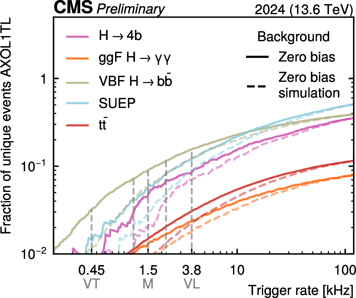
png pdf |
Figure 3-c:
Upper: the receiver operating characteristic (ROC) curves for AXOL1TL (left) and CICADA (right) evaluated on benchmark signal samples. The area under the ROC curve (AUC) is reported for zero bias data in parentheses and zero bias simulation in brackets to reflect the differences between data and simulation. The stars indicate the L1 working point (WP), which corresponds to the trigger rate and signal efficiency of the existing L1 system---a logical OR of 141 purpose-built trigger algorithms. The vertical dashed lines from left to right indicate the very tight (VT), tight, medium (M), loose, and very loose (VL) thresholds at which AXOL1TL and CICADA operate during data taking. Lower: the fraction of unique events recorded by AXOL1TL (left) or CICADA (right), respectively. Unique events are events where no other L1 trigger algorithm selected the event. |
png pdf |
Figure 3-d:
Upper: the receiver operating characteristic (ROC) curves for AXOL1TL (left) and CICADA (right) evaluated on benchmark signal samples. The area under the ROC curve (AUC) is reported for zero bias data in parentheses and zero bias simulation in brackets to reflect the differences between data and simulation. The stars indicate the L1 working point (WP), which corresponds to the trigger rate and signal efficiency of the existing L1 system---a logical OR of 141 purpose-built trigger algorithms. The vertical dashed lines from left to right indicate the very tight (VT), tight, medium (M), loose, and very loose (VL) thresholds at which AXOL1TL and CICADA operate during data taking. Lower: the fraction of unique events recorded by AXOL1TL (left) or CICADA (right), respectively. Unique events are events where no other L1 trigger algorithm selected the event. |
png pdf |
Figure 4:
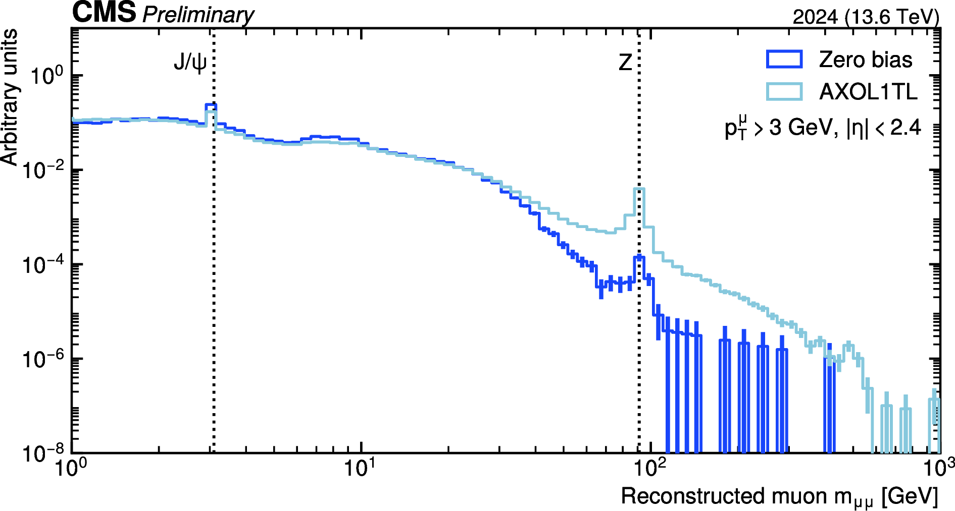
The dimuon invariant mass spectrum for the AXOL1TL trigger compared to zero bias, demonstrating that AXOL1TL selects the $ \mathrm{J}/\psi $ and Z boson standard model resonances without any model assumptions. The Z boson, with its lower cross section and higher mass, is more anomalous than the $ \mathrm{J}/\psi $ and is thus selected more effectively by AXOL1TL compared to zero bias. The distributions are normalized to unit area. The muon reconstruction method is explained further in Section 4.2. This distribution demonstrates sensitivity to known resonances and is not intended as a search. Dedicated statistical analysis would be required for any beyond the standard model interpretation. |
png pdf |
Figure 5:
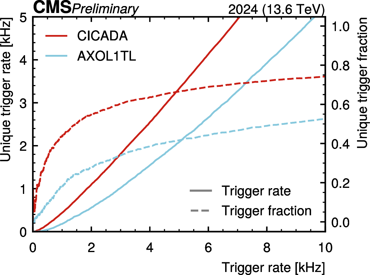
The unique L1 trigger rates for AXOL1TL and CICADA compared to the overall L1 trigger rate in zero bias data. The fraction of the L1 trigger rate that is unique is also shown. Unique events are events where no other L1 trigger algorithm selected the event. |
png pdf |
Figure 6:
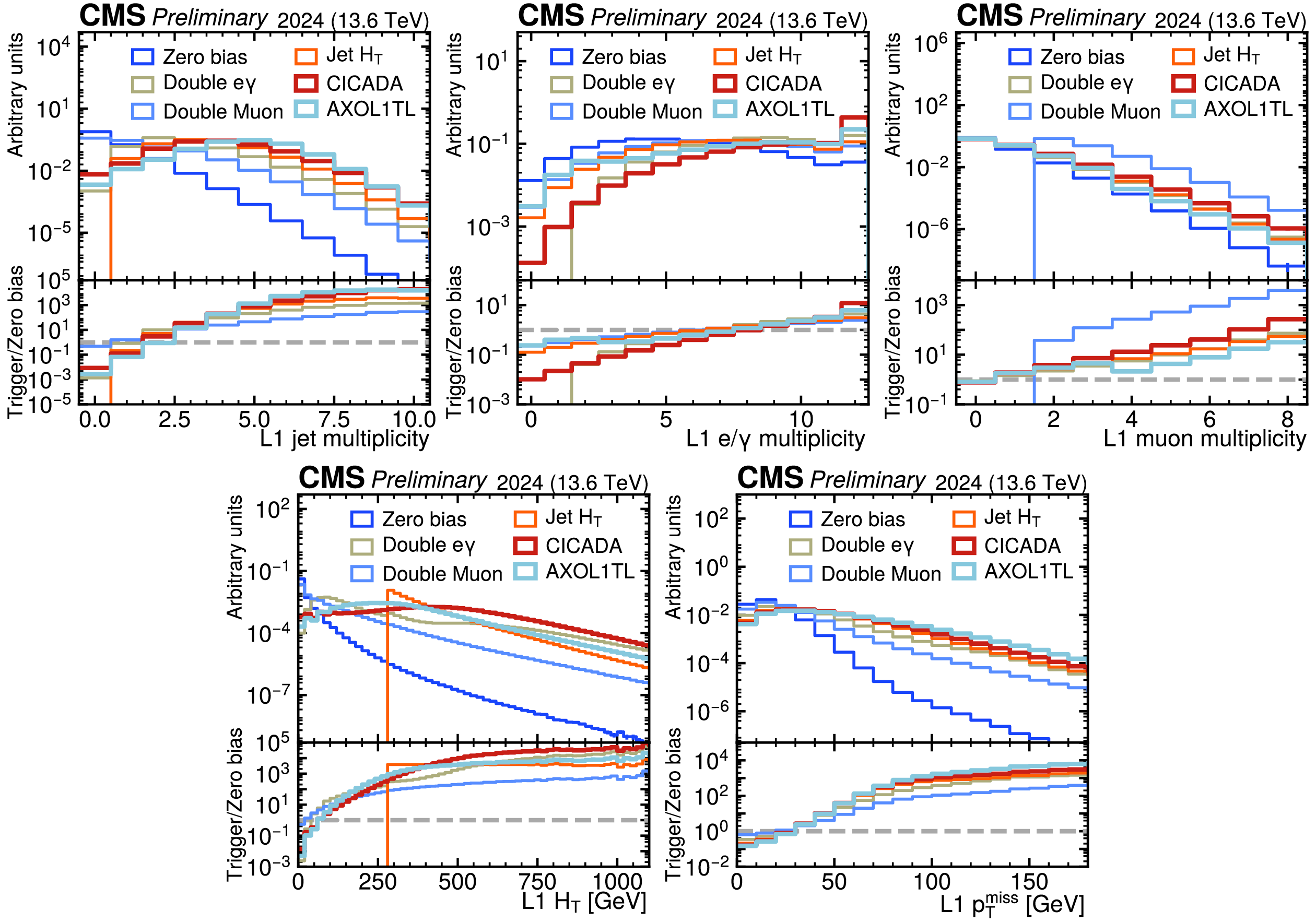
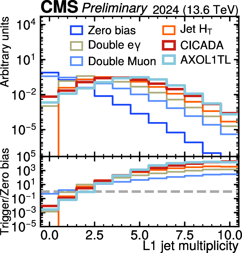
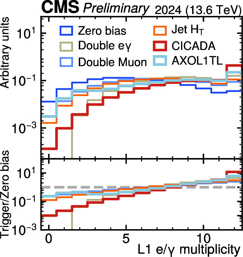
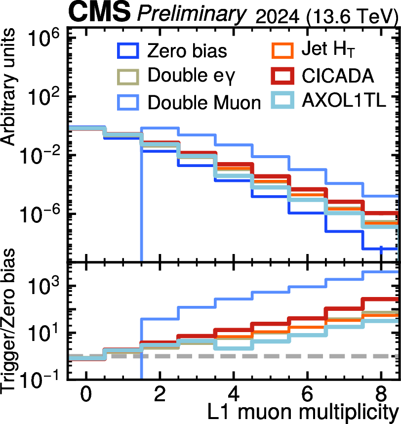
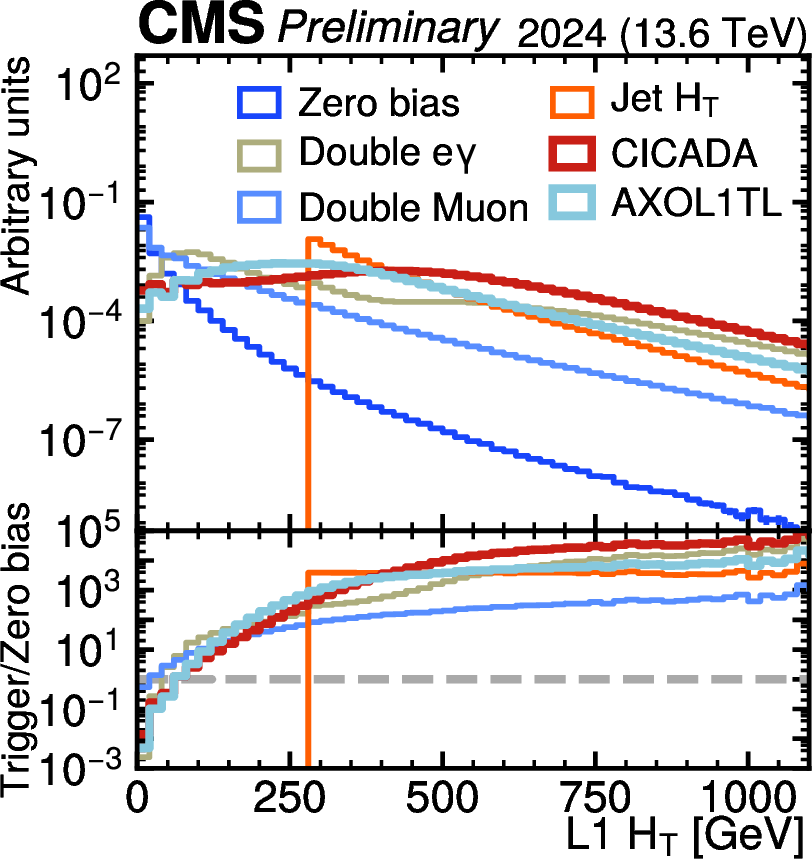
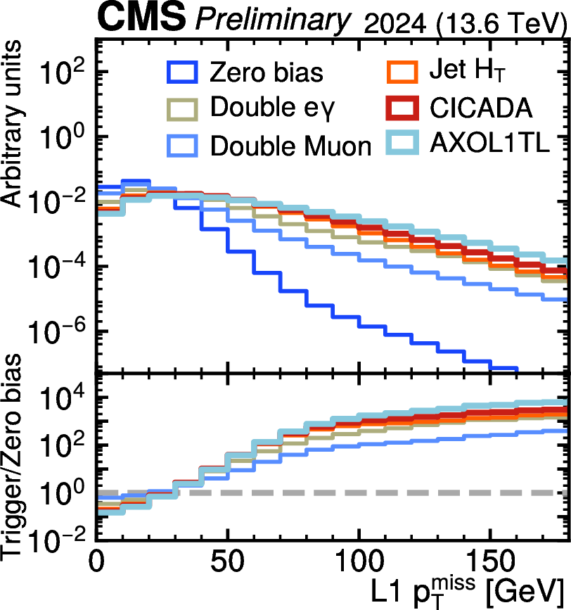
Upper: distributions of the number of L1 trigger objects for events triggered by AXOL1TL and CICADA. Lower: distributions of L1 $ H_{\mathrm{T}} $ and $ p_{\mathrm{T}}^\text{miss} $ for events triggered by AXOL1TL and CICADA. The distributions are normalized to unit integral. The AXOL1TL and CICADA triggers have similar properties to standard triggers designed to target various objects. This highlights that AXOL1TL and CICADA have broad physics reach despite being single algorithms. Below each distribution is a panel showing the ratio of each trigger to zero bias as a baseline. Data collected in 2024 are shown. |
png pdf |
Figure 6-a:
Upper: distributions of the number of L1 trigger objects for events triggered by AXOL1TL and CICADA. Lower: distributions of L1 $ H_{\mathrm{T}} $ and $ p_{\mathrm{T}}^\text{miss} $ for events triggered by AXOL1TL and CICADA. The distributions are normalized to unit integral. The AXOL1TL and CICADA triggers have similar properties to standard triggers designed to target various objects. This highlights that AXOL1TL and CICADA have broad physics reach despite being single algorithms. Below each distribution is a panel showing the ratio of each trigger to zero bias as a baseline. Data collected in 2024 are shown. |
png pdf |
Figure 6-b:
Upper: distributions of the number of L1 trigger objects for events triggered by AXOL1TL and CICADA. Lower: distributions of L1 $ H_{\mathrm{T}} $ and $ p_{\mathrm{T}}^\text{miss} $ for events triggered by AXOL1TL and CICADA. The distributions are normalized to unit integral. The AXOL1TL and CICADA triggers have similar properties to standard triggers designed to target various objects. This highlights that AXOL1TL and CICADA have broad physics reach despite being single algorithms. Below each distribution is a panel showing the ratio of each trigger to zero bias as a baseline. Data collected in 2024 are shown. |
png pdf |
Figure 6-c:
Upper: distributions of the number of L1 trigger objects for events triggered by AXOL1TL and CICADA. Lower: distributions of L1 $ H_{\mathrm{T}} $ and $ p_{\mathrm{T}}^\text{miss} $ for events triggered by AXOL1TL and CICADA. The distributions are normalized to unit integral. The AXOL1TL and CICADA triggers have similar properties to standard triggers designed to target various objects. This highlights that AXOL1TL and CICADA have broad physics reach despite being single algorithms. Below each distribution is a panel showing the ratio of each trigger to zero bias as a baseline. Data collected in 2024 are shown. |
png pdf |
Figure 6-d:
Upper: distributions of the number of L1 trigger objects for events triggered by AXOL1TL and CICADA. Lower: distributions of L1 $ H_{\mathrm{T}} $ and $ p_{\mathrm{T}}^\text{miss} $ for events triggered by AXOL1TL and CICADA. The distributions are normalized to unit integral. The AXOL1TL and CICADA triggers have similar properties to standard triggers designed to target various objects. This highlights that AXOL1TL and CICADA have broad physics reach despite being single algorithms. Below each distribution is a panel showing the ratio of each trigger to zero bias as a baseline. Data collected in 2024 are shown. |
png pdf |
Figure 6-e:
Upper: distributions of the number of L1 trigger objects for events triggered by AXOL1TL and CICADA. Lower: distributions of L1 $ H_{\mathrm{T}} $ and $ p_{\mathrm{T}}^\text{miss} $ for events triggered by AXOL1TL and CICADA. The distributions are normalized to unit integral. The AXOL1TL and CICADA triggers have similar properties to standard triggers designed to target various objects. This highlights that AXOL1TL and CICADA have broad physics reach despite being single algorithms. Below each distribution is a panel showing the ratio of each trigger to zero bias as a baseline. Data collected in 2024 are shown. |
png pdf |
Figure 7:
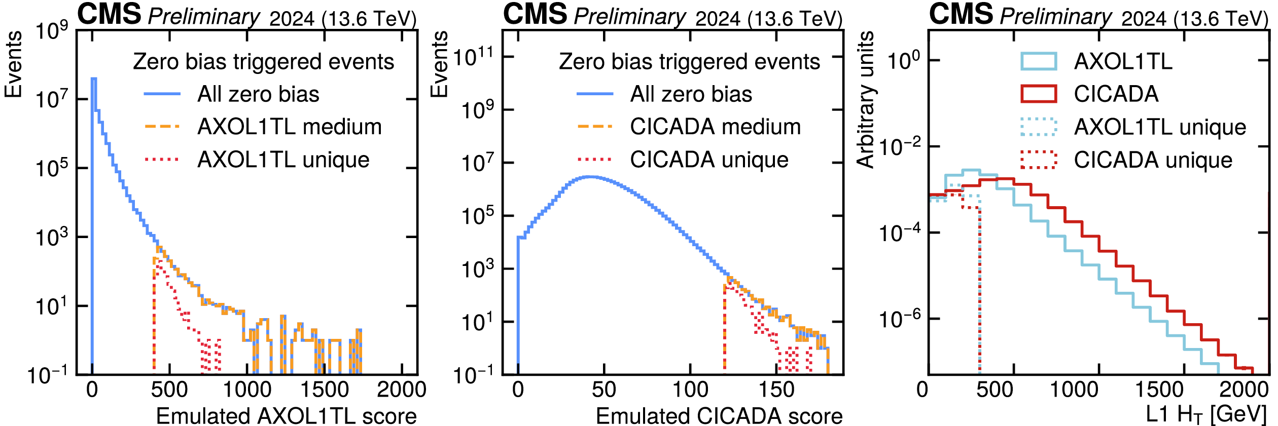
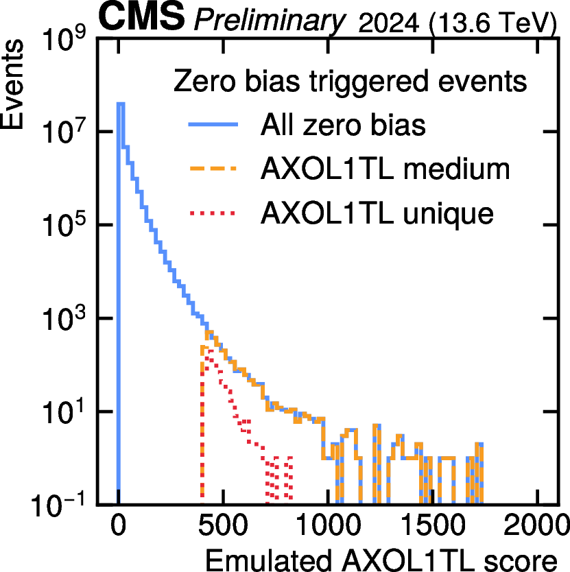
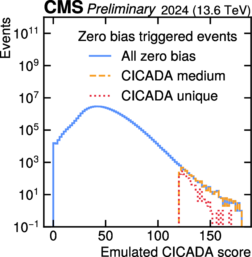
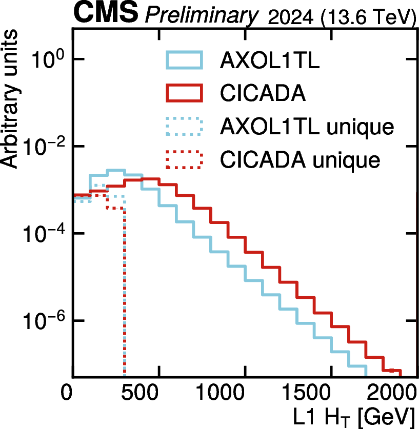
Anomaly score distributions for AXOL1TL (left) and CICADA (middle) evaluated on data collected with the Zero Bias trigger. The normalized distributions of L1 $ H_{\mathrm{T}} $ are shown for all events collected by AXOL1TL and CICADA triggers (right), along with the distribution of unique events with respect to all other L1 triggers. The sharp cutoff is due to an existing L1 trigger algorithm that collects all events above an $ H_{\mathrm{T}} $ threshold. Data collected in 2024 are shown. |
png pdf |
Figure 7-a:
Anomaly score distributions for AXOL1TL (left) and CICADA (middle) evaluated on data collected with the Zero Bias trigger. The normalized distributions of L1 $ H_{\mathrm{T}} $ are shown for all events collected by AXOL1TL and CICADA triggers (right), along with the distribution of unique events with respect to all other L1 triggers. The sharp cutoff is due to an existing L1 trigger algorithm that collects all events above an $ H_{\mathrm{T}} $ threshold. Data collected in 2024 are shown. |
png pdf |
Figure 7-b:
Anomaly score distributions for AXOL1TL (left) and CICADA (middle) evaluated on data collected with the Zero Bias trigger. The normalized distributions of L1 $ H_{\mathrm{T}} $ are shown for all events collected by AXOL1TL and CICADA triggers (right), along with the distribution of unique events with respect to all other L1 triggers. The sharp cutoff is due to an existing L1 trigger algorithm that collects all events above an $ H_{\mathrm{T}} $ threshold. Data collected in 2024 are shown. |
png pdf |
Figure 7-c:
Anomaly score distributions for AXOL1TL (left) and CICADA (middle) evaluated on data collected with the Zero Bias trigger. The normalized distributions of L1 $ H_{\mathrm{T}} $ are shown for all events collected by AXOL1TL and CICADA triggers (right), along with the distribution of unique events with respect to all other L1 triggers. The sharp cutoff is due to an existing L1 trigger algorithm that collects all events above an $ H_{\mathrm{T}} $ threshold. Data collected in 2024 are shown. |
png pdf |
Figure 8:
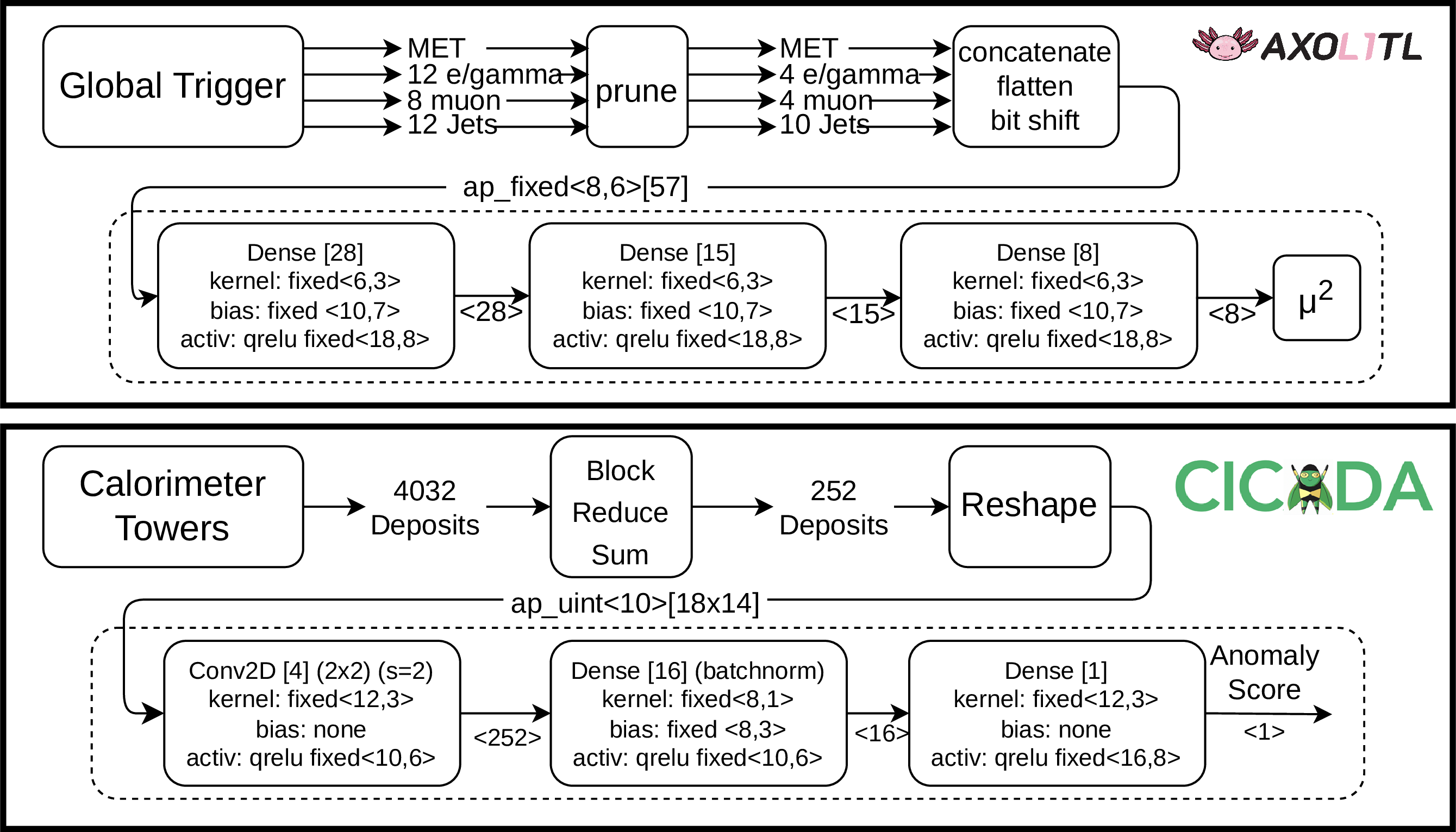
Data flow, model architecture, and quantization for the deployed AXOL1TL encoder and CICADA student models. The AXOL1TL model takes clustered L1 trigger inputs, selects a subset, then uses the $ \mu^2 $ term of the KL divergence as an output score. The CICADA model clusters 4 032 calorimeter towers, and the distilled model outputs a single score output. The number of nodes per layer is defined in square brackets, and the fixed point arithmetic is denoted as $ \langle a, b \rangle $ where the total bit width is $ a $ and the number of integers is $ b $. |
png pdf |
Figure 9:
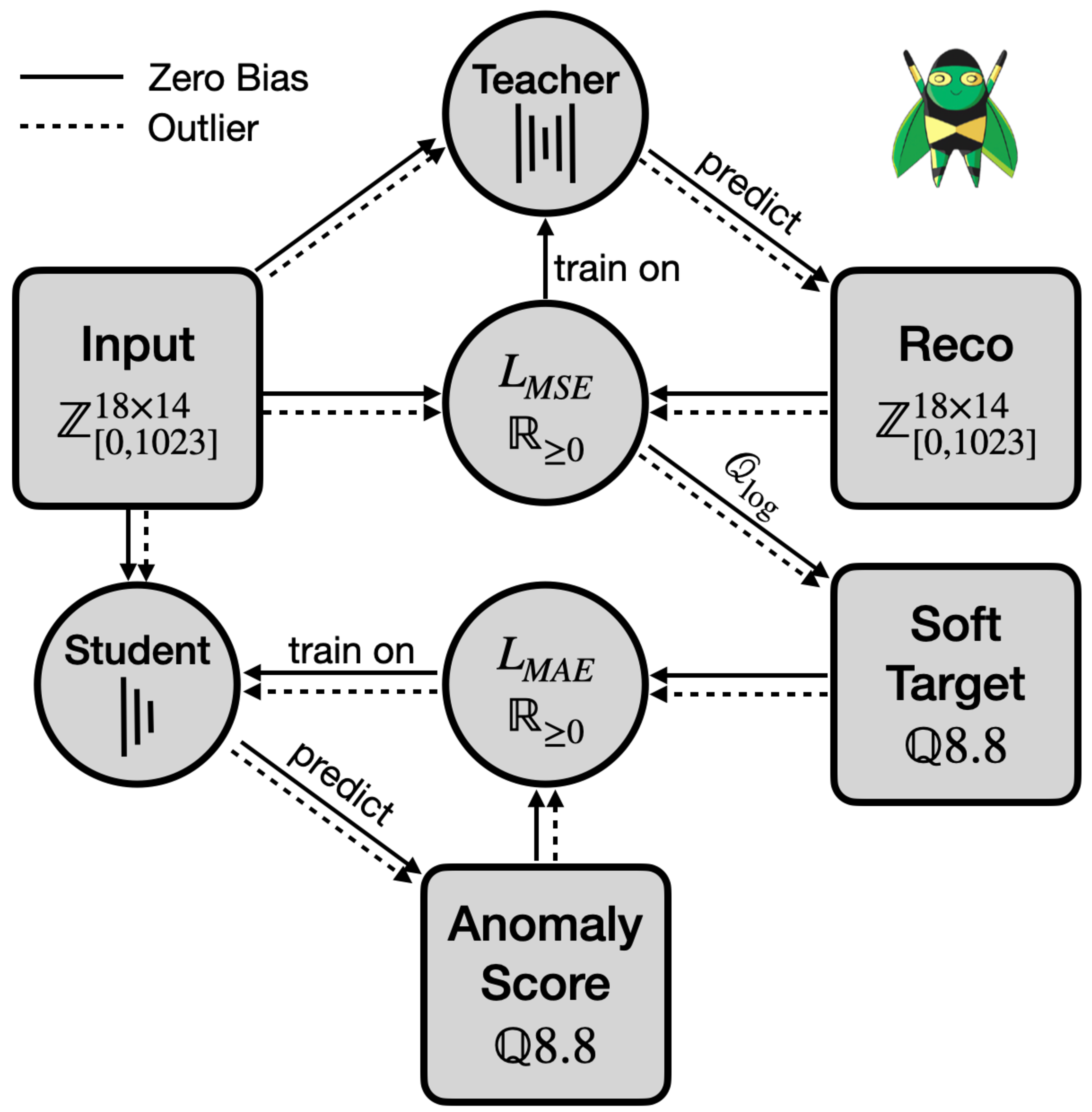
The knowledge distillation process for CICADA. A teacher model (the original autoencoder) is first trained, then used to produce soft target labels on which the student is trained. |
| Tables | |
png pdf |
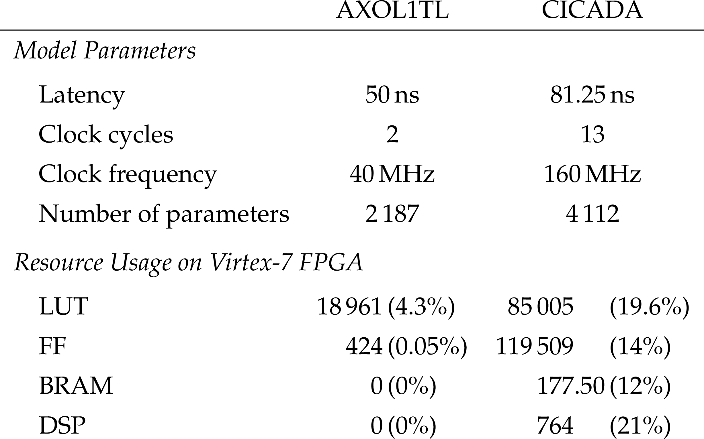
Table 1:
The full FPGA resource utilization of the anomaly detection models. Resources include look-up tables (LUTs) for general-purpose logic, flip-flop (FF) registers, digital signal processors (DSPs) for multiplication, and block RAMs (BRAMs), which are small high-speed memories. |
png pdf |
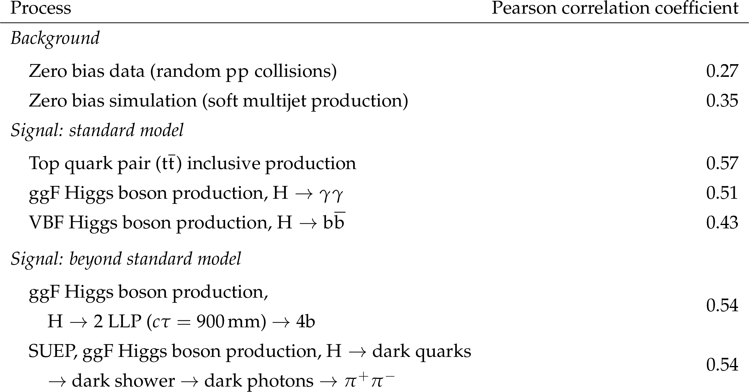
Table 2:
The Pearson correlation coefficients of emulated AXOL1TL and CICADA scores on zero bias, simulated zero bias, and benchmark signal samples. |
png pdf |
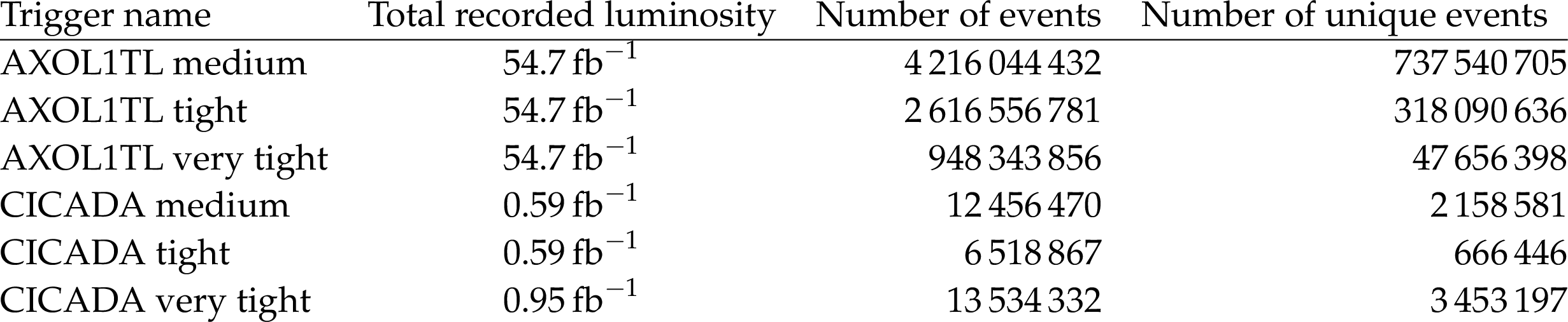
Table 3:
Recorded luminosity and event counts for data collected with the anomaly triggers during 2024. The differences in the amount of data collected correspond to differences in deployment times for each of the triggers. |
| Summary |
| This work demonstrates the first sustained operation of unsupervised anomaly detection in the real-time data selection stream of the CMS experiment at the LHC, where irreversible decisions must be made at 40 $ \mathrm{MHz} $ under fixed latency and FPGA resource constraints. During 2024, the two algorithms selected more than four billion collisions, including almost 740 million events that no other L1 trigger algorithm would have recorded and would otherwise have been permanently lost. Inference latencies of 50--80 $ \mathrm{ns} $ achieved on a continuous terabit-per-second data stream, place these deployments at an extreme point in the design space of real-time machine learning inference. Both algorithms are implemented through hardware-aware workflows that translate trained models into FPGA firmware via HLSML [25,26] pipelines and employ compression techniques such as using only the encoder portion of the network or using knowledge distillation to reduce the model size. These approaches enable sub-microsecond end-to-end integration in the L1 trigger chain while model inference stays well within the overall trigger latency budget. The continued development of such tools could allow larger, more expressive algorithms with ultra-fast inference to be integrated in the L1 trigger in the future. Beyond establishing feasibility, a central insight is that anomaly detection at different levels of feature representation in streaming physics data can be complementary. The AXOL1TL model scores a compact, fixed-length feature vector produced by the existing L1 reconstruction. By contrast, CICADA scores an earlier, image-like calorimeter representation before object formation. Together, the two implementations illustrate a transferable design tradeoff for high-rate systems: anomaly detection with engineered features can be simpler to integrate, monitor, and operate, while anomaly detection with early representations can provide broader coverage at the cost of a larger inference and integration footprint. In the future, anomaly detection algorithms at additional levels of feature representation may preserve sensitivity to an even wider variety of signatures. The physics content of the selected data demonstrates that the anomaly scores are physically meaningful; the triggers both reproduce sensitivity to known signatures and recover events inaccessible to conventional selections. Without any resonance hypothesis or explicit mass reconstruction, the AXOL1TL selection recovers the $ \mathrm{J}/\psi $ and Z boson resonances in the dimuon invariant-mass spectrum (Fig. 4), with the rarer, more anomalous Z boson enhanced relative to zero bias. Moreover, the unique events recovered by both algorithms populate the region below the minimum L1 trigger thresholds (Fig. 7), demonstrating that the anomaly triggers extend coverage into phase space inaccessible even to minimally biased conventional selections. The resulting sample of uniquely triggered events therefore constitutes a novel dataset, unavailable through any previous trigger strategy, that can seed new searches in downstream data analyses. Several limitations qualify these results. Because both models are trained on zero bias data collected under specific accelerator and detector conditions, shifts in pileup or detector response can alter the score distributions. This requires continuous monitoring and periodic retraining. In practice, deployment in a live detector was viable because of the safeguards provided by the rate-controlled working points shown in Table 3. In addition to the operational challenges, the choices of training dataset, input representation, and model architecture each introduce some bias despite the model-agnostic design goal. This is illustrated by the preference towards high-multiplicity, high-HT, and high-$ p_{\mathrm{T}}^\text{miss} $ topologies, which typically are already collected by the L1 trigger algorithms. Finally, further analysis of the novel dataset collected by the anomaly detection triggers will be required to draw meaningful physics conclusions. Because particle physics processes are inherently quantum mechanical, conclusions are drawn from rigorous statistical analysis of large event samples rather than from individual events. This type of analysis will be needed to establish whether the collected data contains evidence of physics beyond the standard model. These algorithms serve as a blueprint for future ML trigger algorithms in collider experiments. At the High-Luminosity LHC, expected to begin taking data in 2030, there will be increases in collision rates and event complexity and therefore a much broader adoption of ML trigger algorithms. The codesign methodology demonstrated here, jointly optimizing representation, architecture, quantization, and firmware, provides a template for deploying such algorithms at the High-Luminosity LHC. This work has opened up new methodology for using unsupervised models in streaming instrumentation across scientific and industrial edge systems, where decisions are irreversible and latency budgets are absolute. |
| References | ||||
| 1 | CMS Collaboration | The CMS experiment at the CERN LHC | JINST 3 (2008) S08004 | |
| 2 | K. Hoffpauir et al. | A survey on edge intelligence and lightweight machine learning support for future applications and services | J. Data and Information Quality 15 (2023) 1 | |
| 3 | C. Zheng et al. | In-network machine learning using programmable network devices: A survey | IEEE Communications Surveys, 2024 Tutorials 26 (2024) 1171 |
|
| 4 | A. T.-J. Akem, M. Gucciardo, and M. Fiore | Flowrest: Practical flow-level inference in programmable switches with random forests | IEEE Conference on Computer Communications, 2023 IEEE INFOCOM 202 (2023) 1 |
|
| 5 | J. Ahn et al. | Federated learning for predictive maintenance and anomaly detection using time series data distribution shifts in manufacturing processes | Sensors 23 (2023) 7331 | |
| 6 | K. Cosmas and A. Kenichi | Utilization of FPGA for onboard inference of landmark localization in CNN-based spacecraft pose estimation | Aerospace 7 (2020) 159 | |
| 7 | R. D. Prete et al. | Optimizing deep learning models for on-orbit deployment through neural architecture search (NAS) | Sci. Rep. 15 (2025) 37783 | |
| 8 | L. Evans and P. Bryant | LHC Machine | JINST 3 (2008) S08001 | |
| 9 | CMS Collaboration | Performance of the CMS Level-1 trigger in proton-proton collisions at $ \sqrt{s} = $ 13 TeV | JINST 15 (2020) P10017 | CMS-TRG-17-001 2006.10165 |
| 10 | CMS Collaboration | The CMS trigger system | JINST 12 (2017) P01020 | CMS-TRG-12-001 1609.02366 |
| 11 | CMS Collaboration | Performance of the CMS high-level trigger during LHC Run 2 | JINST 19 (2024) P11021 | CMS-TRG-19-001 2410.17038 |
| 12 | CMS Collaboration | CMS TriDAS project: Technical design report, volume 1: The trigger systems | CMS Technical Design Report CMS-TDR-6-1, 2000 CDS |
|
| 13 | CMS Collaboration | CMS technical design report for the level-1 trigger upgrade | CMS Technical Design Report CMS-TDR-12, 2013 CDS |
|
| 14 | CMS Collaboration | Observation of a new boson at a mass of 125 GeV with the CMS experiment at the LHC | PLB 716 (2012) 30 | CMS-HIG-12-028 1207.7235 |
| 15 | ATLAS Collaboration | Observation of a new particle in the search for the standard model Higgs boson with the ATLAS detector at the LHC | PLB 716 (2012) 1 | 1207.7214 |
| 16 | G. Kasieczka, B. Nachman, and D. Shih | New methods and datasets for group anomaly detection from fundamental physics | in Conference on Knowledge Discovery and Data Mining. July, 2021 | 2107.02821 |
| 17 | G. Kasieczka et al. | The LHC Olympics 2020 a community challenge for anomaly detection in high energy physics | Rept. Prog. Phys. 84 (2021) 124201 | 2101.08320 |
| 18 | T. Aarrestad et al. | The dark machines anomaly score challenge: Benchmark data and model independent event classification for the Large Hadron Collider | SciPost Phys. 12 (2022) 043 | 2105.14027 |
| 19 | ATLAS Collaboration | Search for new phenomena in two-body invariant mass distributions using unsupervised machine learning for anomaly detection at $ \sqrt{s}= $ 13 TeV with the ATLAS detector | PRL 132 (2024) 081801 | 2307.01612 |
| 20 | ATLAS Collaboration | Anomaly detection search for new resonances decaying into a Higgs boson and a generic new particle $ X $ in hadronic final states using $ \sqrt{s} = $ 13 TeV $ pp $ collisions with the ATLAS detector | PRD 108 (2023) 052009 | 2306.03637 |
| 21 | CMS Collaboration | Model-agnostic search for dijet resonances with anomalous jet substructure in proton-proton collisions at $ \sqrt{s} = $ 13 TeV | Rept. Prog. Phys. 88 (2025) 067802 | CMS-EXO-22-026 2412.03747 |
| 22 | E. Govorkova et al. | LHC physics dataset for unsupervised new physics detection at 40 MHz | Sci. Data 9 (2022) 118 | 2107.02157 |
| 23 | E. Govorkova et al. | Autoencoders on field-programmable gate arrays for real-time, unsupervised new physics detection at 40 MHz at the Large Hadron Collider | Nature Mach. Intell. 4 (2022) 154 | 2108.03986 |
| 24 | CMS Collaboration | Boosted decision trees in the CMS level-1 endcap muon trigger | PoS TWEPP-17 143, 2017 link |
|
| 25 | J. Duarte et al. | Fast inference of deep neural networks in FPGAs for particle physics | JINST 13 (2018) P07027 | 1804.06913 |
| 26 | J.-F. Schulte et al. | hls4ml: A flexible, open-source platform for deep learning acceleration on reconfigurable hardware | ACM Trans. Reconfigurable Technol. Syst. 19 (2026) 19 | 2512.01463 |
| 27 | D. P. Kingma and M. Welling | Auto-encoding variational Bayes | International Conference on Learning Representations. 201 (1900) 4 | 1312.6114 |
| 28 | A. A. Pol et al. | Knowledge Distillation for Anomaly Detection | 2310.06047 | |
| 29 | S. Knapen, S. Pagan Griso, M. Papucci, and D. J. Robinson | Triggering soft bombs at the LHC | JHEP 08 (2017) 076 | 1612.00850 |
| 30 | CMS Collaboration | Development of the CMS detector for the CERN LHC Run 3 | JINST 19 (2024) P05064 | CMS-PRF-21-001 2309.05466 |
| 31 | CMS Collaboration | Electron and photon reconstruction and identification with the CMS experiment at the CERN LHC | JINST 16 (2021) P05014 | CMS-EGM-17-001 2012.06888 |
| 32 | CMS Collaboration | Performance of the CMS muon detector and muon reconstruction with proton-proton collisions at $ \sqrt{s}= $ 13 TeV | JINST 13 (2018) P06015 | CMS-MUO-16-001 1804.04528 |
| 33 | CMS Collaboration | Description and performance of track and primary-vertex reconstruction with the CMS tracker | JINST 9 (2014) P10009 | CMS-TRK-11-001 1405.6569 |
| 34 | CMS Collaboration | Particle-flow reconstruction and global event description with the CMS detector | JINST 12 (2017) P10003 | CMS-PRF-14-001 1706.04965 |
| 35 | CMS Collaboration | Performance of reconstruction and identification of $ \tau $ leptons decaying to hadrons and $ \nu_\tau $ in pp collisions at $ \sqrt{s}= $ 13 TeV | JINST 13 (2018) P10005 | CMS-TAU-16-003 1809.02816 |
| 36 | CMS Collaboration | Jet energy scale and resolution in the CMS experiment in pp collisions at 8 TeV | JINST 12 (2017) P02014 | CMS-JME-13-004 1607.03663 |
| 37 | CMS Collaboration | Performance of missing transverse momentum reconstruction in proton-proton collisions at $ \sqrt{s} = $ 13 TeV using the CMS detector | JINST 14 (2019) P07004 | CMS-JME-17-001 1903.06078 |
| 38 | M. Cacciari, G. P. Salam, and G. Soyez | The anti-$ k_{\mathrm{T}} $ jet clustering algorithm | JHEP 04 (2008) 063 | 0802.1189 |
| 39 | M. Cacciari, G. P. Salam, and G. Soyez | FastJet user manual | EPJC 72 (2012) 1896 | 1111.6097 |
| 40 | T. Sjöstrand et al. | An introduction to PYTHIA 8.2 | Comput. Phys. Commun. 191 (2015) 159 | 1410.3012 |
| 41 | CMS Collaboration | Extraction and validation of a new set of CMS PYTHIA8 tunes from underlying-event measurements | EPJC 80 (2020) 4 | CMS-GEN-17-001 1903.12179 |
| 42 | GEANT4 Collaboration | GEANT 4---a simulation toolkit | NIM A 506 (2003) 250 | |
| 43 | CMS Collaboration | Observation of Higgs boson decay to bottom quarks | PRL 121 (2018) 121801 | CMS-HIG-18-016 1808.08242 |
| 44 | A. Karlberg et al. | Ad interim recommendations for the Higgs boson production cross sections at $ \sqrt{s} = $ 13.6 TeV | 2402.09955 | |
| 45 | LHC Higgs Cross Section Working Group Collaboration | Handbook of LHC Higgs cross sections: 4. deciphering the nature of the Higgs sector | CERN Yellow Rep. Monogr. 2 (2017) 1 | 1610.07922 |
| 46 | CMS Collaboration | Measurement of the top quark pair production cross section in dilepton final states containing one $ \tau $ lepton in pp collisions at $ \sqrt{s}= $ 13 TeV | JHEP 02 (2020) 191 | CMS-TOP-18-005 1911.13204 |
| 47 | M. Czakon and A. Mitov | Top++: A program for the calculation of the top-pair cross-section at hadron colliders | Comput. Phys. Commun. 185 (2014) 2930 | 1112.5675 |
| 48 | M. Czakon, P. Fiedler, and A. Mitov | Total top-quark pair-production cross section at hadron colliders through $ o(\alpha^4_s) $ | PRL 110 (2013) 252004 | 1303.6254 |
| 49 | PDF4LHC Working Group Collaboration | The PDF4LHC21 combination of global PDF fits for the LHC Run III | JPG 49 (2022) 080501 | 2203.05506 |
| 50 | P. Nason | A new method for combining NLO QCD with shower Monte Carlo algorithms | JHEP 11 (2004) 040 | hep-ph/0409146 |
| 51 | S. Frixione, P. Nason, and C. Oleari | Matching NLO QCD computations with parton shower simulations: the POWHEG method | JHEP 11 (2007) 070 | 0709.2092 |
| 52 | S. Alioli, P. Nason, C. Oleari, and E. Re | A general framework for implementing NLO calculations in shower Monte Carlo programs: the POWHEG BOX | JHEP 06 (2010) 043 | 1002.2581 |
| 53 | NNPDF Collaboration | Parton distributions from high-precision collider data | EPJC 77 (2017) 663 | 1706.00428 |
| 54 | CMS Collaboration | Search for soft unclustered energy patterns in proton-proton collisions at 13 TeV | PRL 133 (2024) 191902 | CMS-EXO-23-002 2403.05311 |
| 55 | CMS Collaboration | Enriching the physics program of the CMS experiment via data scouting and data parking | Phys. Rept. 1115 (2025) 678 | CMS-EXO-23-007 2403.16134 |
| 56 | C. N. Coelho et al. | Automatic heterogeneous quantization of deep neural networks for low-latency inference on the edge for particle detectors | Nature Mach. Intell. 3 (2021) 675 | 2006.10159 |
| 57 | G. Hinton, O. Vinyals, and J. Dean | Distilling the knowledge in a neural network | 1503.02531 | |
| 58 | D. Hendrycks, M. Mazeika, and T. Dietterich | Deep anomaly detection with outlier exposure | 1812.04606 | |
| 59 | CMS Collaboration | 2020 CMS data preservation, re-use and open access policy | CERN Open Data Portal link |
|
|
|
Compact Muon Solenoid LHC, CERN |

|
|
|
|
|
|