
Compact Muon Solenoid
LHC, CERN
 Visit us: CMS Public Website, CMS Physics ;
Contact us: CMS Publications Committee
Visit us: CMS Public Website, CMS Physics ;
Contact us: CMS Publications Committee
| CMS-PAS-HIG-24-016 | ||
| Search for nonresonant $ \mathrm{t\bar{t}HH} $ production in the final state with four bottom quarks and one lepton in proton-proton collisions at $ \sqrt{s} = $ 13 TeV | ||
| CMS Collaboration | ||
| 2026-08-20 | ||
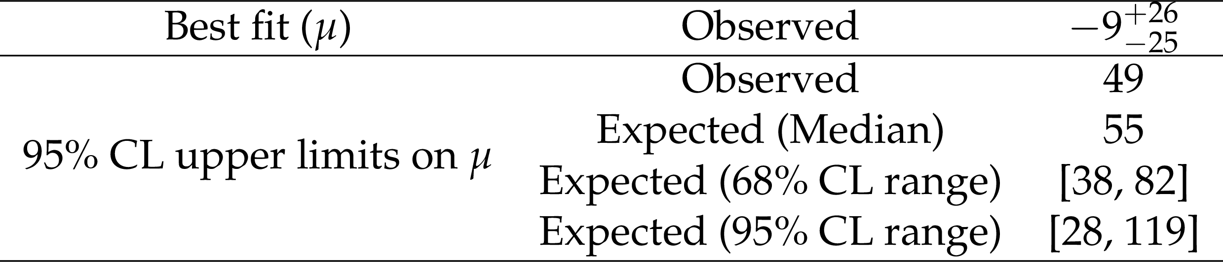
| Abstract: We present the first direct search at the CMS experiment for nonresonant associated production of a Higgs boson (H) pair, where each H decays into a bottom quark-antiquark pair, with a top quark-antiquark pair ($ {\mathrm{t\bar{t}HH}} $), which decays into a single lepton final state. The analysis is performed using proton-proton collision data recorded with the CMS detector at a centre of mass energy of $ \sqrt{s}= $ 13 TeV, corresponding to an integrated luminosity of 138 fb$ ^{-1} $. A method based on neural networks is used for categorizing the events and extracting the signal. A simultaneous fit is performed in the signal and background enriched regions on the neural network discriminant output distribution. The observed signal strength relative to the standard model expectation is $ \mu=- $ 9 $ ^{+26}_{-25} $. The observed (expected) upper limit on the $ {\mathrm{t\bar{t}HH}} $ production cross section is 49 (55) times the standard model prediction and corresponds to an observed (expected) cross section upper limit of 37 (42) fb at 95$ % $ confidence level (CL). The $ {\mathrm{t\bar{t}HH}} $ results are further interpreted within the Higgs Effective Field Theory framework, leading to a 95$ % $ CL interval on the $ {\mathrm{t\bar{t}HH}} $ quartic interaction parameter, $ c_{\mathrm{t\bar{t}HH}} $, of $ -6.6 < c_{\mathrm{t\bar{t}HH}} < $ 6.4. | ||
| Links: CDS record (PDF) ; CADI line (restricted) ; | ||
| Figures | |
png pdf |
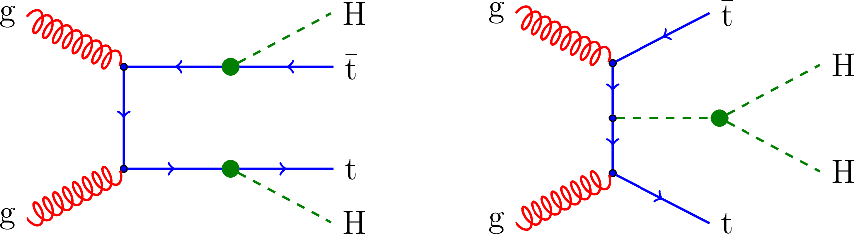
Figure 1:
Representative leading order SM diagrams for $ \mathrm{t\bar{t}HH} $ production, illustrating the two distinct physical subprocesses: (left) the top-Yukawa vertex and (right) the Higgs trilinear self-coupling. |
png pdf |
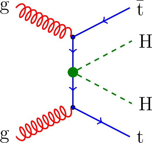
Figure 2:
BSM $ \mathrm{t\bar{t}HH} $ production diagram via the HEFT ttHH $ c_2 $ coupling. |
png pdf |
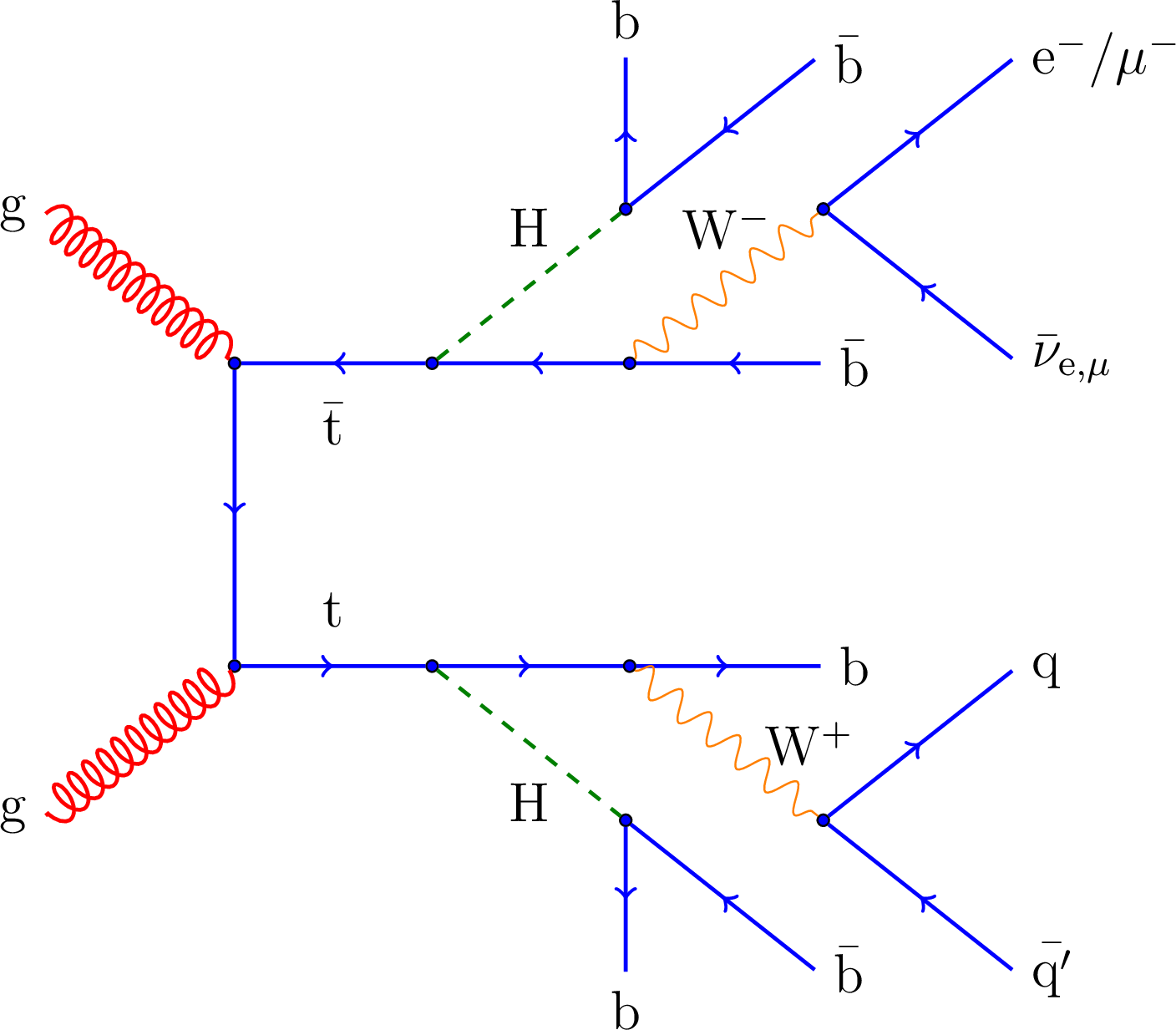
Figure 3:
Feynman diagram of the $ \mathrm{t\overline{t}HH} $ production process in the single lepton channel. |
png pdf |
Figure 4:
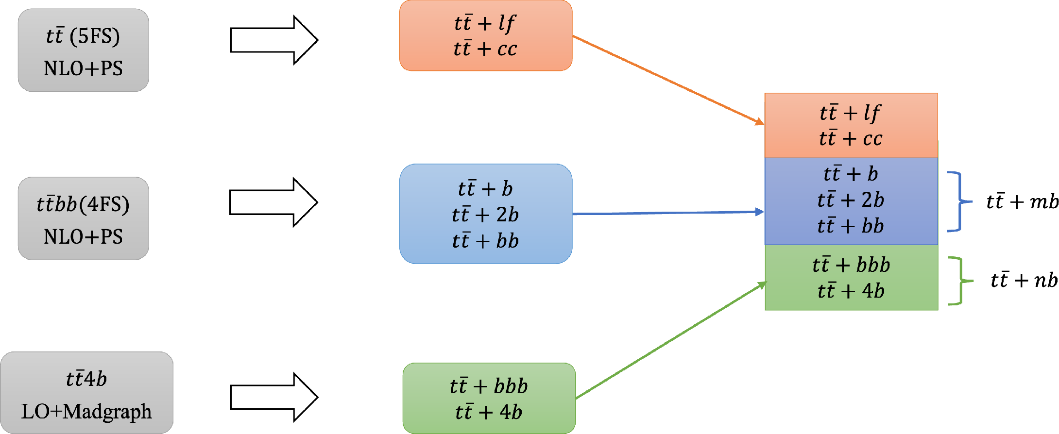
Schematic of the sample--parton correspondence. The large arrows indicate generator-level matching. |
png pdf |
Figure 5:
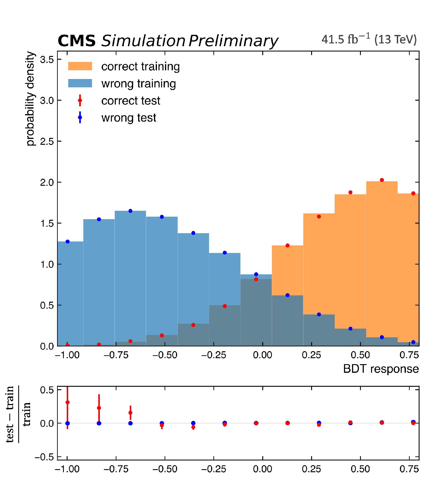
Distributions of the JABDT output score for correct and incorrect jet-to-parton assignments, evaluated on both training (shaded histograms) and testing (red dots) samples. Correct assignments are defined by geometric matching of jets to Monte Carlo generator-level partons with minimum sum of $ \Delta $R, while incorrect assignments refer to the remaining permutations of jets assignments. The BDT is trained on $ \mathrm{t\bar{t}HH} $, and $ \mathrm{t\bar{t}} $ simulations to construct discriminative features for the target events against others considered in this analysis, such as $ \mathrm{t\bar{t}H} $, $ \mathrm{t\bar{t}ZH} $ and $ \mathrm{t\bar{t}ZZ} $, etc. The excellent agreement in shape between the training and testing distributions indicates the absence of overtraining. Samples are split into even event number (shown) and odd (not shown) subsets for validation on each other. The test and training sample are matching in shape, so no overtraining is visible. |
png pdf |
Figure 6:
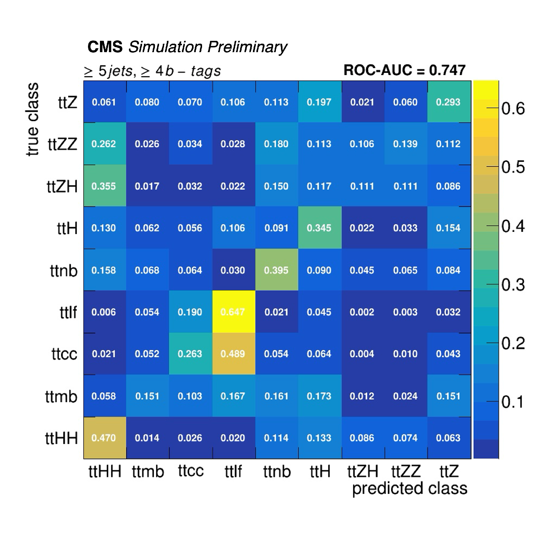
Confusion matrix of the DNN categorization of events in the 2018 dataset. |
png pdf |
Figure 7:
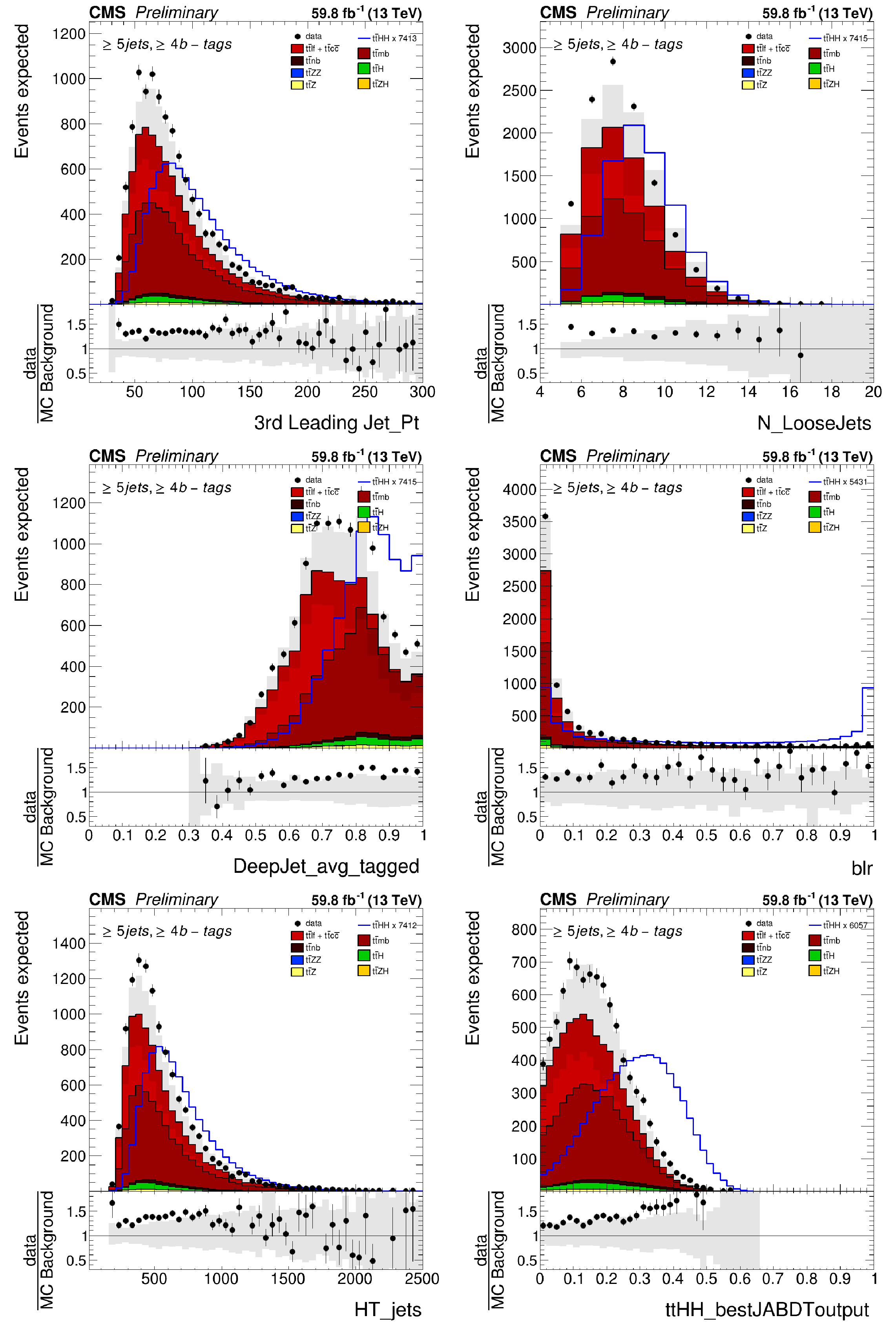
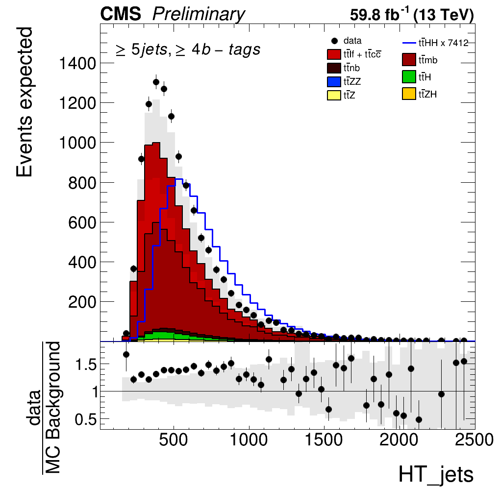
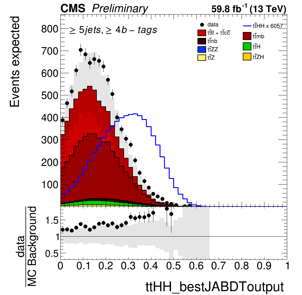
Data/MC comparison of selected DNN input features for the 2018 dataset in the signal region ($ \geq $ 5 jets and $ \geq $ 4 b-tagged jets). The distributions show: $ p_\mathrm{T} $ of the third leading jet (top left), loose jet multiplicity, where loose jets satisfy relaxed kinematic cuts of $ p_{\mathrm{T}} > 20\text{ GeV} $ and $ |\eta| < $ 4.0, while all other selection criteria follow the standard jet reconstruction described in Section 5 (top right), mean DeepJet score of $ b $-tagged jets (middle left), $ b $-tagging likelihood ratio discriminant (middle right), scalar sum of jet $ p_\mathrm{T} $ ($ H_\mathrm{T} $) (bottom left), and the best-fit $ t\bar{t}HH $ JABDT output score (bottom right). |
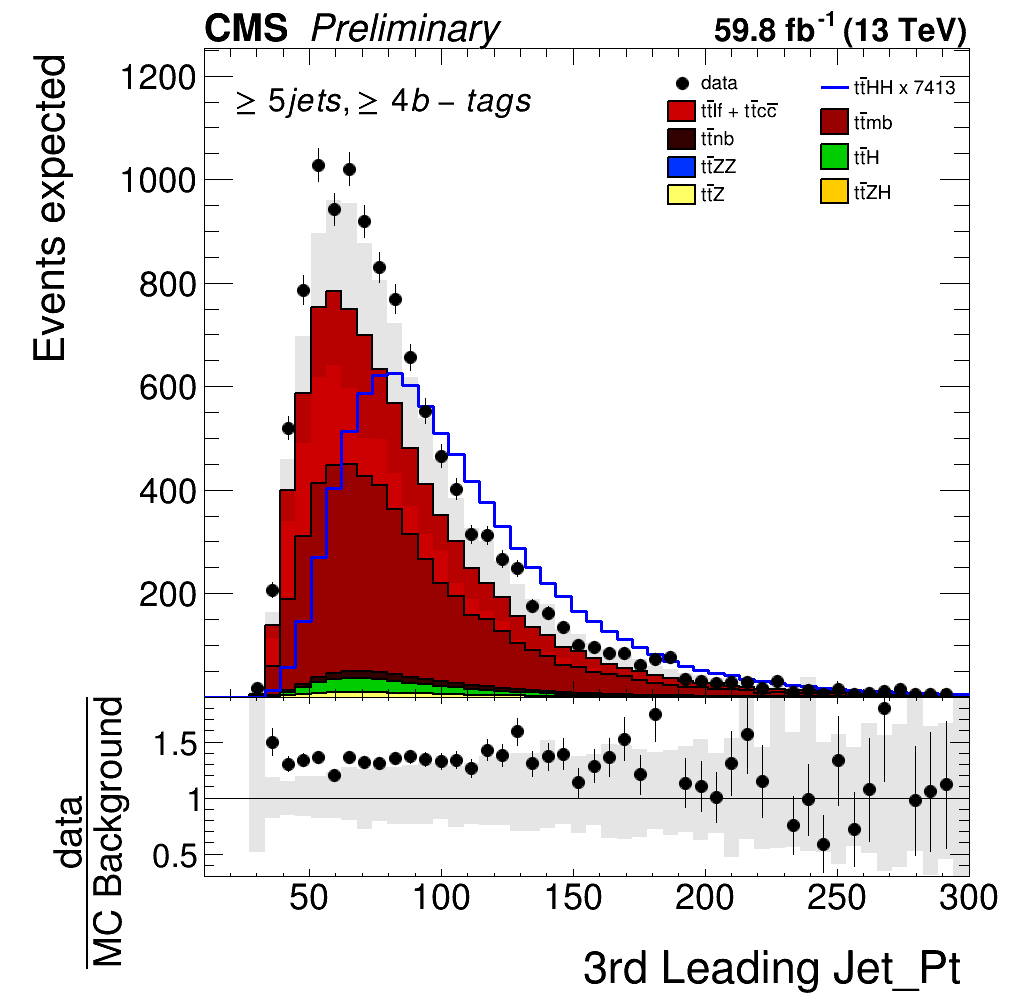
png |
Figure 7-a:
Data/MC comparison of selected DNN input features for the 2018 dataset in the signal region ($ \geq $ 5 jets and $ \geq $ 4 b-tagged jets). The distributions show: $ p_\mathrm{T} $ of the third leading jet (top left), loose jet multiplicity, where loose jets satisfy relaxed kinematic cuts of $ p_{\mathrm{T}} > 20\text{ GeV} $ and $ |\eta| < $ 4.0, while all other selection criteria follow the standard jet reconstruction described in Section 5 (top right), mean DeepJet score of $ b $-tagged jets (middle left), $ b $-tagging likelihood ratio discriminant (middle right), scalar sum of jet $ p_\mathrm{T} $ ($ H_\mathrm{T} $) (bottom left), and the best-fit $ t\bar{t}HH $ JABDT output score (bottom right). |
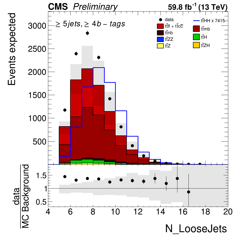
png |
Figure 7-b:
Data/MC comparison of selected DNN input features for the 2018 dataset in the signal region ($ \geq $ 5 jets and $ \geq $ 4 b-tagged jets). The distributions show: $ p_\mathrm{T} $ of the third leading jet (top left), loose jet multiplicity, where loose jets satisfy relaxed kinematic cuts of $ p_{\mathrm{T}} > 20\text{ GeV} $ and $ |\eta| < $ 4.0, while all other selection criteria follow the standard jet reconstruction described in Section 5 (top right), mean DeepJet score of $ b $-tagged jets (middle left), $ b $-tagging likelihood ratio discriminant (middle right), scalar sum of jet $ p_\mathrm{T} $ ($ H_\mathrm{T} $) (bottom left), and the best-fit $ t\bar{t}HH $ JABDT output score (bottom right). |
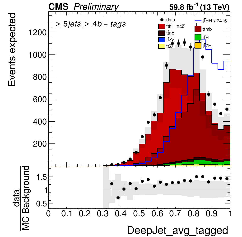
png |
Figure 7-c:
Data/MC comparison of selected DNN input features for the 2018 dataset in the signal region ($ \geq $ 5 jets and $ \geq $ 4 b-tagged jets). The distributions show: $ p_\mathrm{T} $ of the third leading jet (top left), loose jet multiplicity, where loose jets satisfy relaxed kinematic cuts of $ p_{\mathrm{T}} > 20\text{ GeV} $ and $ |\eta| < $ 4.0, while all other selection criteria follow the standard jet reconstruction described in Section 5 (top right), mean DeepJet score of $ b $-tagged jets (middle left), $ b $-tagging likelihood ratio discriminant (middle right), scalar sum of jet $ p_\mathrm{T} $ ($ H_\mathrm{T} $) (bottom left), and the best-fit $ t\bar{t}HH $ JABDT output score (bottom right). |
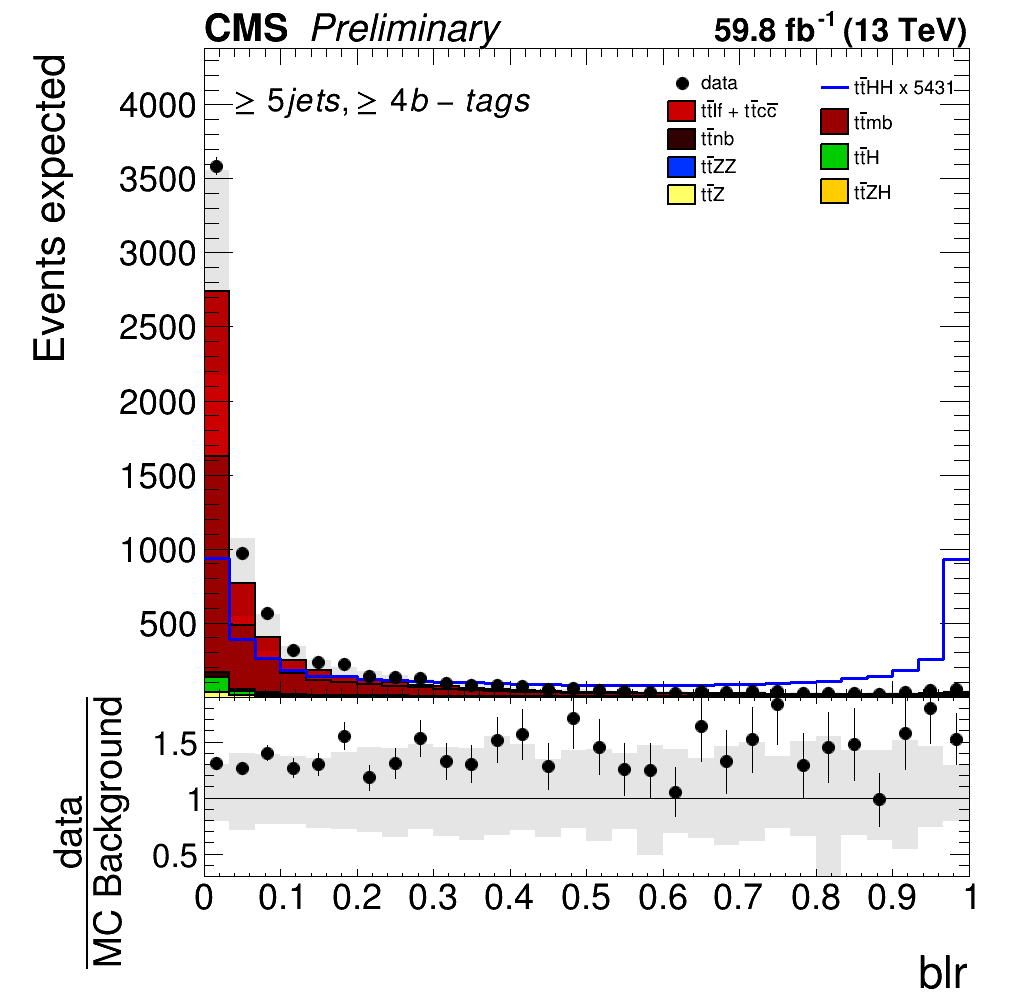
png |
Figure 7-d:
Data/MC comparison of selected DNN input features for the 2018 dataset in the signal region ($ \geq $ 5 jets and $ \geq $ 4 b-tagged jets). The distributions show: $ p_\mathrm{T} $ of the third leading jet (top left), loose jet multiplicity, where loose jets satisfy relaxed kinematic cuts of $ p_{\mathrm{T}} > 20\text{ GeV} $ and $ |\eta| < $ 4.0, while all other selection criteria follow the standard jet reconstruction described in Section 5 (top right), mean DeepJet score of $ b $-tagged jets (middle left), $ b $-tagging likelihood ratio discriminant (middle right), scalar sum of jet $ p_\mathrm{T} $ ($ H_\mathrm{T} $) (bottom left), and the best-fit $ t\bar{t}HH $ JABDT output score (bottom right). |
png |
Figure 7-e:
Data/MC comparison of selected DNN input features for the 2018 dataset in the signal region ($ \geq $ 5 jets and $ \geq $ 4 b-tagged jets). The distributions show: $ p_\mathrm{T} $ of the third leading jet (top left), loose jet multiplicity, where loose jets satisfy relaxed kinematic cuts of $ p_{\mathrm{T}} > 20\text{ GeV} $ and $ |\eta| < $ 4.0, while all other selection criteria follow the standard jet reconstruction described in Section 5 (top right), mean DeepJet score of $ b $-tagged jets (middle left), $ b $-tagging likelihood ratio discriminant (middle right), scalar sum of jet $ p_\mathrm{T} $ ($ H_\mathrm{T} $) (bottom left), and the best-fit $ t\bar{t}HH $ JABDT output score (bottom right). |
png |
Figure 7-f:
Data/MC comparison of selected DNN input features for the 2018 dataset in the signal region ($ \geq $ 5 jets and $ \geq $ 4 b-tagged jets). The distributions show: $ p_\mathrm{T} $ of the third leading jet (top left), loose jet multiplicity, where loose jets satisfy relaxed kinematic cuts of $ p_{\mathrm{T}} > 20\text{ GeV} $ and $ |\eta| < $ 4.0, while all other selection criteria follow the standard jet reconstruction described in Section 5 (top right), mean DeepJet score of $ b $-tagged jets (middle left), $ b $-tagging likelihood ratio discriminant (middle right), scalar sum of jet $ p_\mathrm{T} $ ($ H_\mathrm{T} $) (bottom left), and the best-fit $ t\bar{t}HH $ JABDT output score (bottom right). |
png pdf |
Figure 8:
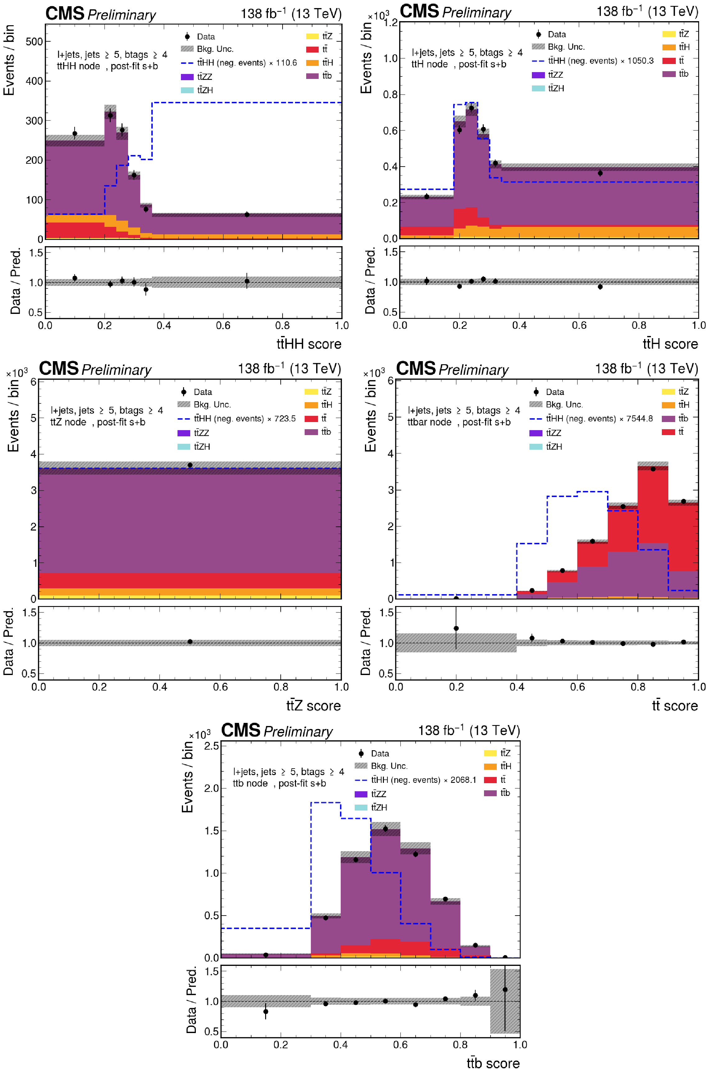
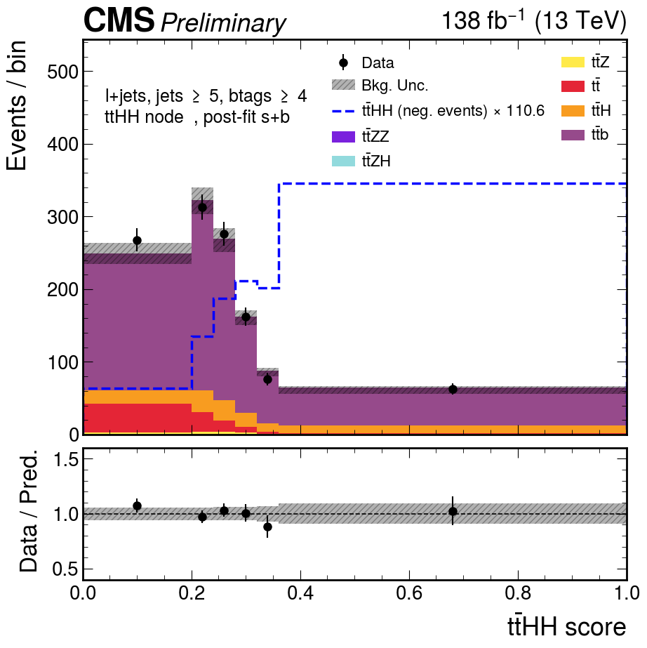
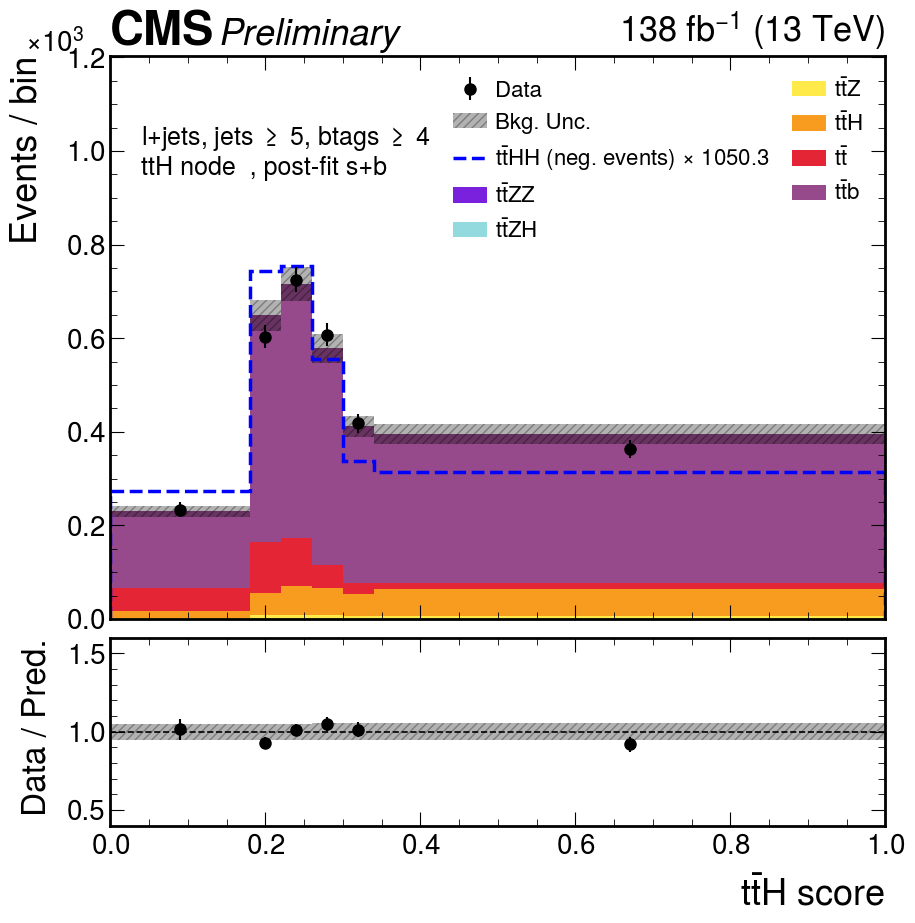
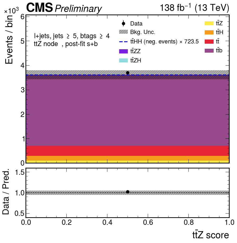
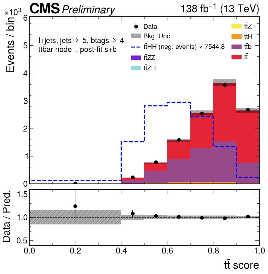
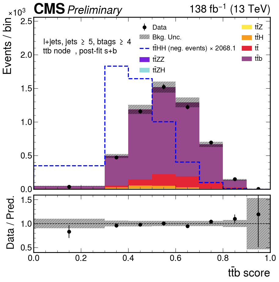
Final discriminant distributions for Run2 for the $ \mathrm{t\bar{t}HH} $ signal node, and for the background nodes $ \mathrm{t\bar{t}H} $, $ \mathrm{t\bar{t}Z} $, where Z stands for: Z $ \to $ bb, ZZ $ \to $ 4b and ZH $ \to $ 4b, $ \mathrm{t} \overline{\mathrm{t}} $ stands: for $ \mathrm{t\bar{t}} $+lf and $ \mathrm{t\bar{t}} $+cc, $ \mathrm{t\bar{t}} $ b stands for $ \mathrm{t\bar{t}} $+mb and $ \mathrm{t\bar{t}} $+nb. In each panel, the SM $ \mathrm{t\bar{t}HH} $ prediction is overlaid, scaled for visibility. |
png |
Figure 8-a:
Final discriminant distributions for Run2 for the $ \mathrm{t\bar{t}HH} $ signal node, and for the background nodes $ \mathrm{t\bar{t}H} $, $ \mathrm{t\bar{t}Z} $, where Z stands for: Z $ \to $ bb, ZZ $ \to $ 4b and ZH $ \to $ 4b, $ \mathrm{t} \overline{\mathrm{t}} $ stands: for $ \mathrm{t\bar{t}} $+lf and $ \mathrm{t\bar{t}} $+cc, $ \mathrm{t\bar{t}} $ b stands for $ \mathrm{t\bar{t}} $+mb and $ \mathrm{t\bar{t}} $+nb. In each panel, the SM $ \mathrm{t\bar{t}HH} $ prediction is overlaid, scaled for visibility. |
png |
Figure 8-b:
Final discriminant distributions for Run2 for the $ \mathrm{t\bar{t}HH} $ signal node, and for the background nodes $ \mathrm{t\bar{t}H} $, $ \mathrm{t\bar{t}Z} $, where Z stands for: Z $ \to $ bb, ZZ $ \to $ 4b and ZH $ \to $ 4b, $ \mathrm{t} \overline{\mathrm{t}} $ stands: for $ \mathrm{t\bar{t}} $+lf and $ \mathrm{t\bar{t}} $+cc, $ \mathrm{t\bar{t}} $ b stands for $ \mathrm{t\bar{t}} $+mb and $ \mathrm{t\bar{t}} $+nb. In each panel, the SM $ \mathrm{t\bar{t}HH} $ prediction is overlaid, scaled for visibility. |
png |
Figure 8-c:
Final discriminant distributions for Run2 for the $ \mathrm{t\bar{t}HH} $ signal node, and for the background nodes $ \mathrm{t\bar{t}H} $, $ \mathrm{t\bar{t}Z} $, where Z stands for: Z $ \to $ bb, ZZ $ \to $ 4b and ZH $ \to $ 4b, $ \mathrm{t} \overline{\mathrm{t}} $ stands: for $ \mathrm{t\bar{t}} $+lf and $ \mathrm{t\bar{t}} $+cc, $ \mathrm{t\bar{t}} $ b stands for $ \mathrm{t\bar{t}} $+mb and $ \mathrm{t\bar{t}} $+nb. In each panel, the SM $ \mathrm{t\bar{t}HH} $ prediction is overlaid, scaled for visibility. |
png |
Figure 8-d:
Final discriminant distributions for Run2 for the $ \mathrm{t\bar{t}HH} $ signal node, and for the background nodes $ \mathrm{t\bar{t}H} $, $ \mathrm{t\bar{t}Z} $, where Z stands for: Z $ \to $ bb, ZZ $ \to $ 4b and ZH $ \to $ 4b, $ \mathrm{t} \overline{\mathrm{t}} $ stands: for $ \mathrm{t\bar{t}} $+lf and $ \mathrm{t\bar{t}} $+cc, $ \mathrm{t\bar{t}} $ b stands for $ \mathrm{t\bar{t}} $+mb and $ \mathrm{t\bar{t}} $+nb. In each panel, the SM $ \mathrm{t\bar{t}HH} $ prediction is overlaid, scaled for visibility. |
png |
Figure 8-e:
Final discriminant distributions for Run2 for the $ \mathrm{t\bar{t}HH} $ signal node, and for the background nodes $ \mathrm{t\bar{t}H} $, $ \mathrm{t\bar{t}Z} $, where Z stands for: Z $ \to $ bb, ZZ $ \to $ 4b and ZH $ \to $ 4b, $ \mathrm{t} \overline{\mathrm{t}} $ stands: for $ \mathrm{t\bar{t}} $+lf and $ \mathrm{t\bar{t}} $+cc, $ \mathrm{t\bar{t}} $ b stands for $ \mathrm{t\bar{t}} $+mb and $ \mathrm{t\bar{t}} $+nb. In each panel, the SM $ \mathrm{t\bar{t}HH} $ prediction is overlaid, scaled for visibility. |
png pdf |
Figure 9:
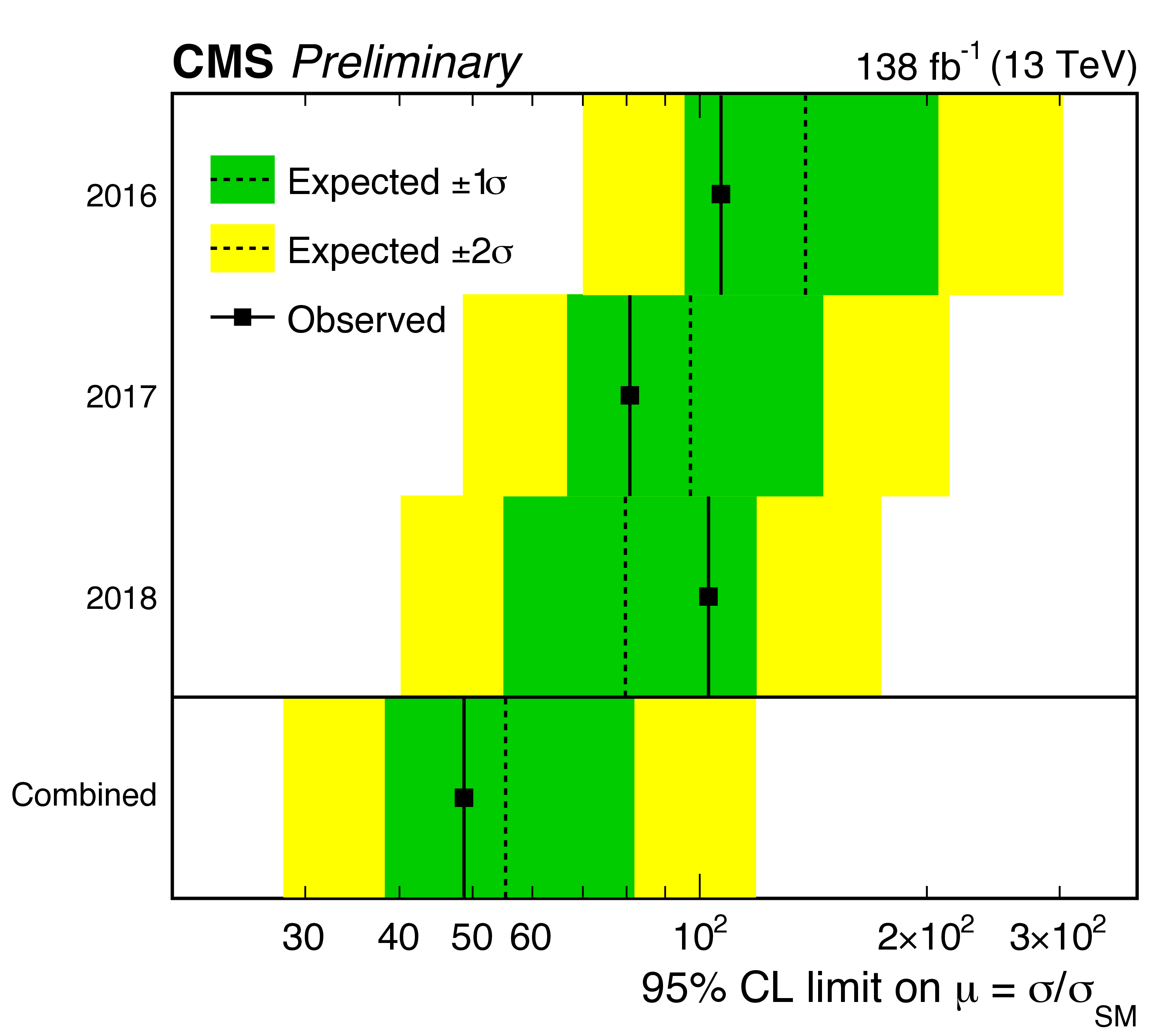
The expected (dashed vertical line) upper 95% CL limit on the $ \mathrm{t\bar{t}HH} $ signal strength modifier $ \mu = \sigma / \sigma_{\mathrm SM} $ for different years and their combination for the SL channel. The green (yellow) areas indicate the one (two) standard deviation confidence intervals on the expected limit. |
png pdf |
Figure 10:
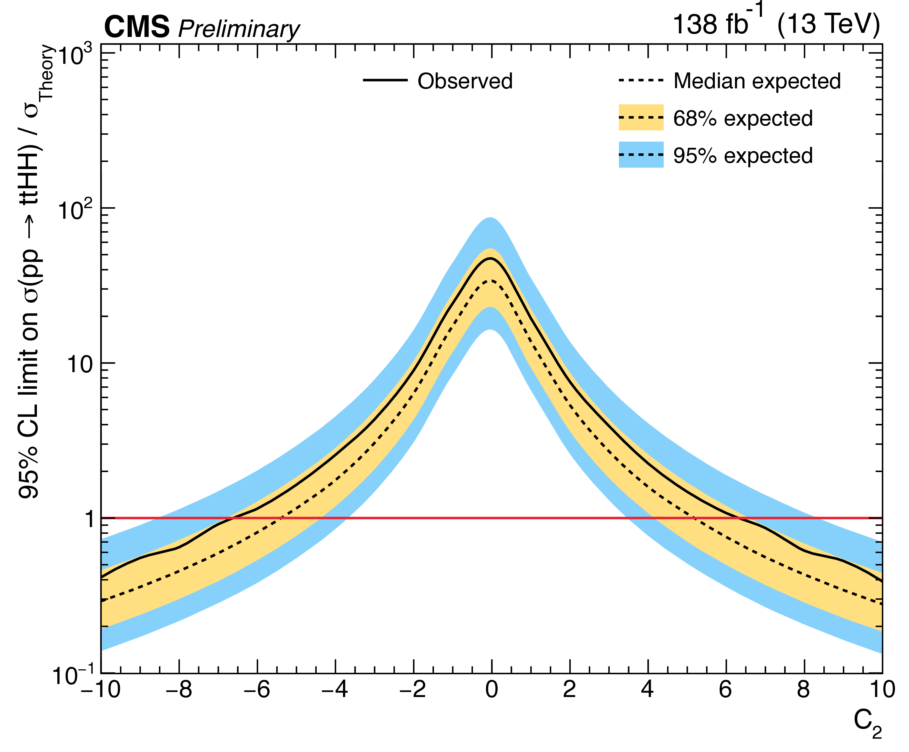
The 95% CL upper limits on the signal strength as a function of $ c_2 $. The yellow and blue bands indicate the one and two standard deviation of the median expected limit (dashed black line), respectively. The red line corresponds to the theoretical prediction for the $ \mathrm{t\bar{t}HH} $ production cross section. |
png pdf |
Figure 11:
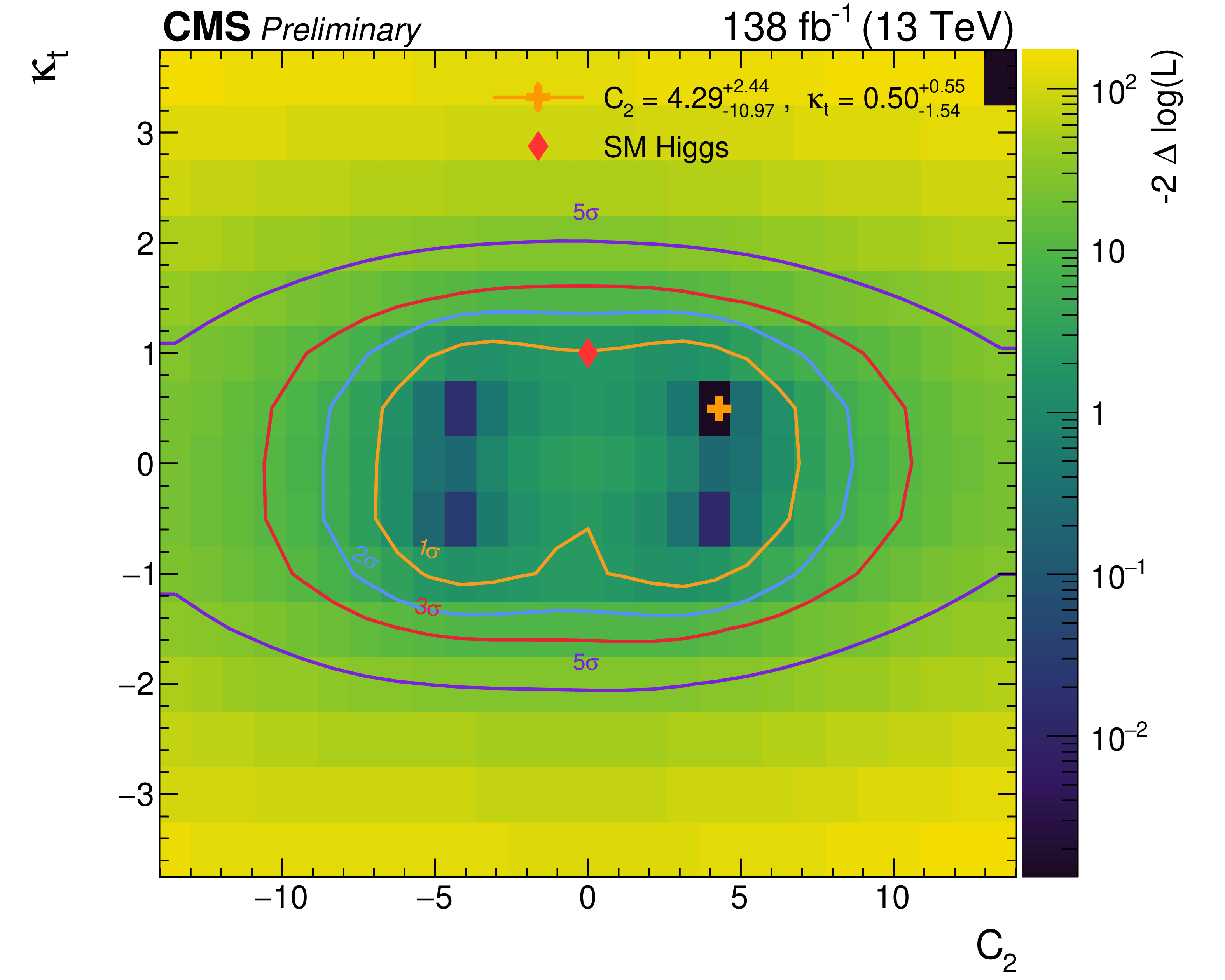
The 68% and 95% CL likehood contours in the ($ c_2 $, $ \kappa_{\mathrm{t}} $) plane. The yellow (blue) lines indicate the one (two) standard deviation contours, along with the 3$ \sigma $ (in red) and 5$ \sigma $ (purple) contours. The yellow cross shows the observed best fit value. The red diamond shows the SM expectation. |
| Tables | |
png pdf |
Table 1:
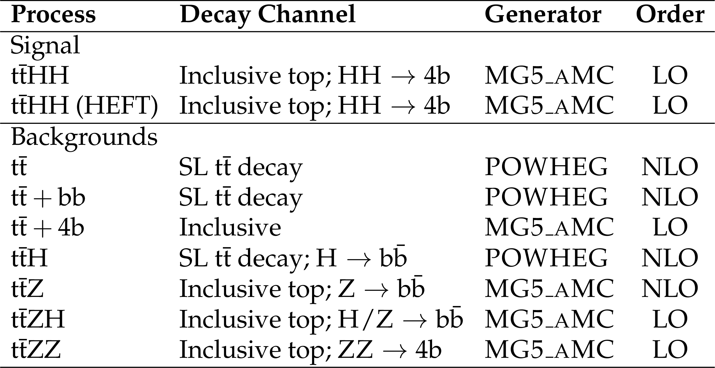
Summary of simulated signal and background MC samples. |
png pdf |
Table 2:
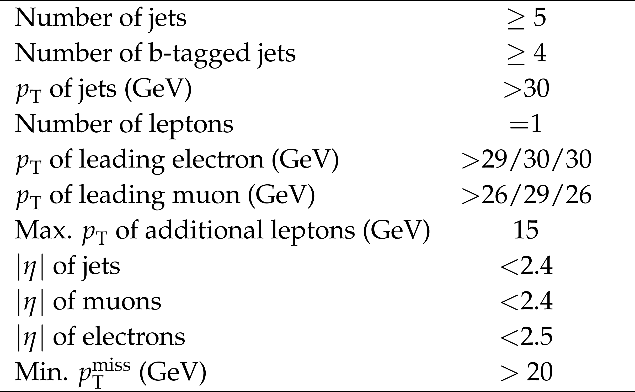
Baseline selection criteria. Leptons and jets are ordered in $ p_{\mathrm{T}} $. Where the criteria differ per year of data taking, they are quoted as three values, corresponding to 2016/2017/2018, respectively. |
png pdf |
Table 3:
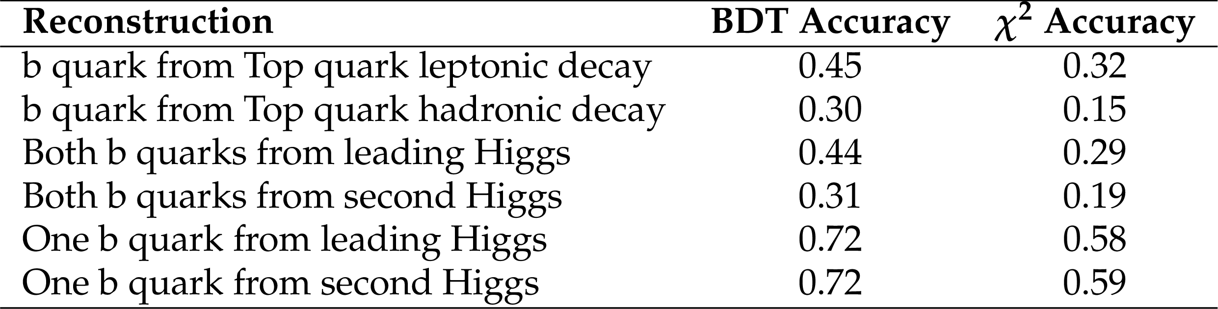
Reconstruction accuracies of the JABDT method and $ \chi^2 $ method, evaluated on $ \mathrm{t\bar{t}HH} $ simulated events. |
png pdf |
Table 4:
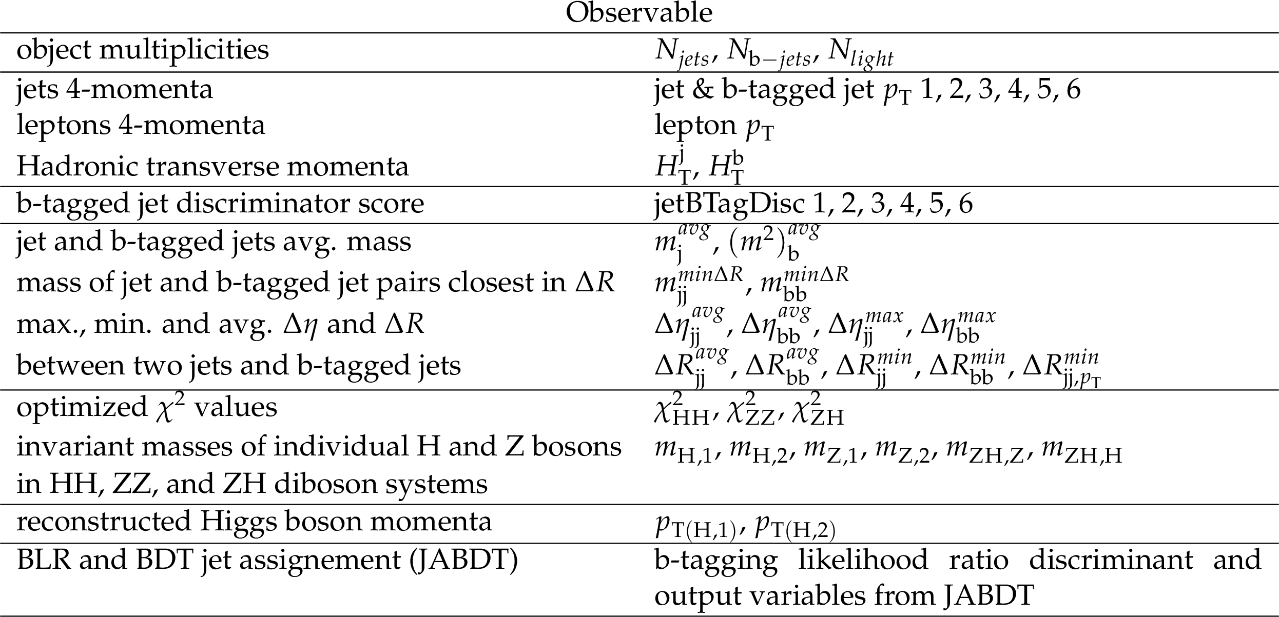
Observables used as input variables to the DNN. |
png pdf |
Table 5:
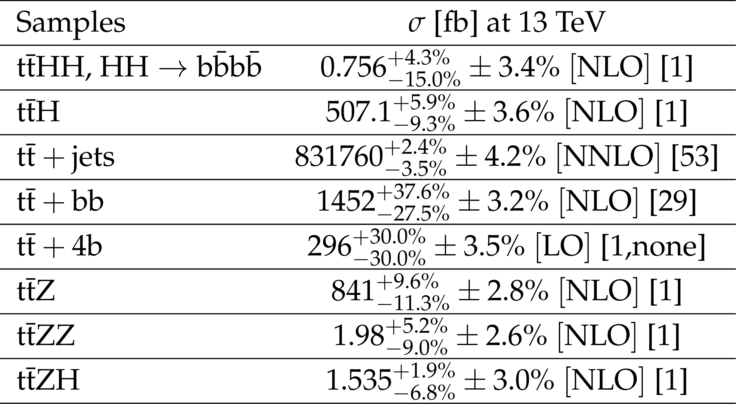
Cross sections at 13 TeV with the uncertainties $ \pm $QCD Scale (%) and $ \pm $(PDF$ +\alpha_s $) (%) for the signal and all the considered backgrounds. |
png pdf |
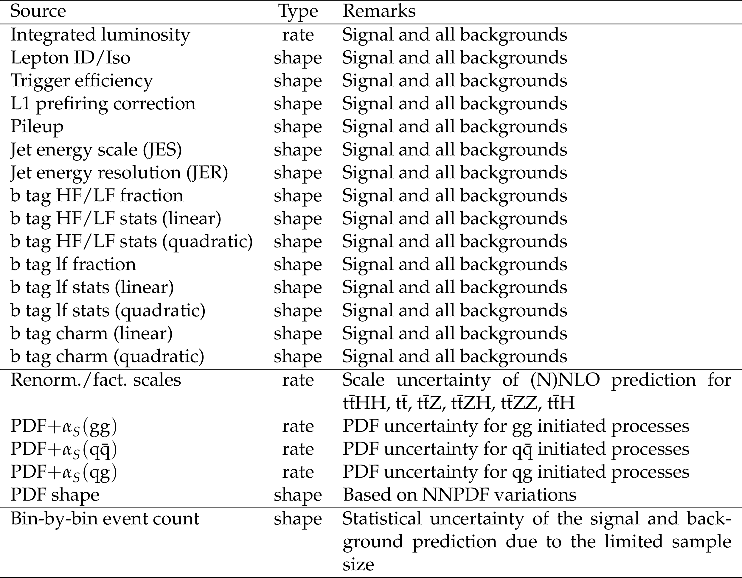
Table 6:
Summary of systematic uncertainties. |
png pdf |
Table 7:
Fit results for the Run 2 data signal strength. |
png pdf |
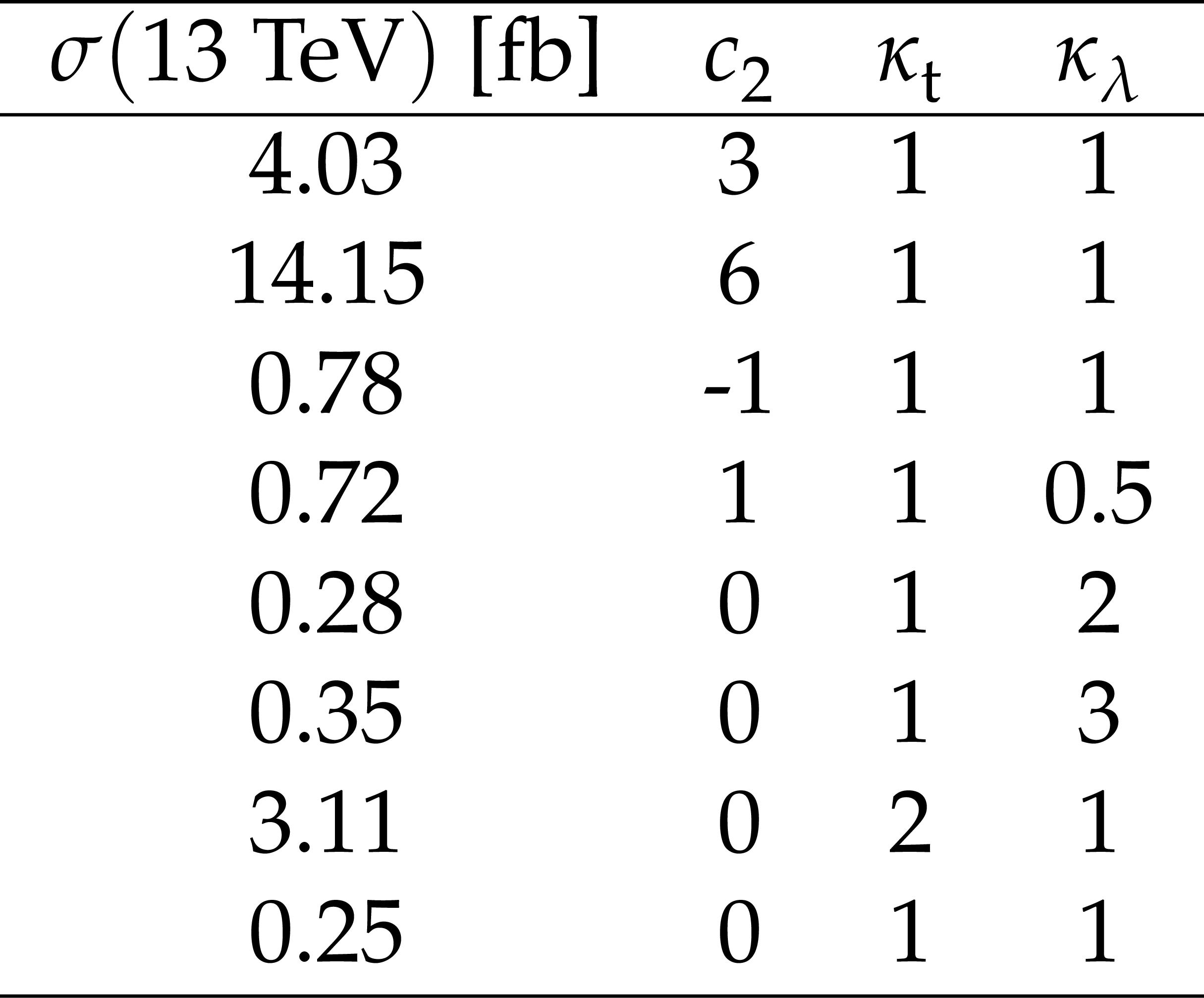
Table 8:
Samples used in the analysis with the listed corresponding coupling modifiers within the HEFT framework for each considered sample. The $ \mathrm{H} \mathrm{H} \to \mathrm{b\bar{b}}\mathrm{b\bar{b}} $ branching ratio is $ (0.5824)^2 $. |
| Summary |
| We present the first CMS search for the associated production of a Higgs boson (H) pair, where each H decays into a bottom quark-antiquark pair, with a top quark--antiquark pair ($ \mathrm{t\bar{t}HH} $), in the single lepton channel. The analysis has been performed using proton proton collision data recorded with the CMS detector at a centre-of-mass energy of 13 TeV, corresponding to an integrated luminosity of 138 fb$ ^{-1} $. Neural network discriminants were used to further categorize the events according to the most probable process, targeting the signal and different backgrounds. A best fit value of the $ \mathrm{t\bar{t}HH} $ production cross section relative to the standard model (SM) expectation of -9 $ ^{+26}_{-25} $ is obtained. The upper limit on the $ \mathrm{t\bar{t}HH} $ production cross section is 49 (55) times the observed (expected) SM cross-section; it corresponds to an observed (expected) cross-section upper limit of 37 (42)fb, at 95% CL. The $ \mathrm{t\bar{t}HH} $ results are further interpreted within the Higgs effective field theory (HEFT) theory framework, leading to a 95% CL interval on the $ \mathrm{t\bar{t}HH} $ quartic interaction parameter of $ -6.6 < c_2 < $ 6.4. It is interesting to compare these results with those already produced by ATLAS and CMS. Whereas the analysis presented in this Note only considers one decay channel for the Higgs boson pair, both the ATLAS [23] and CMS [22] consider various $ \mathrm{t\bar{t}HH} $ signatures and combine the final results. ATLAS study includes: $ \mathrm{t\bar{t}HH} $ with either $ \mathrm{t\bar{t}} $ single lepton plus Higgs boson pair decay into 4 b-quarks; or same sign multilepton signatures with $ \mathrm{t\bar{t}} $ decay into 1 or 2 leptons, and one Higgs boson decays into $ \mathrm{b\bar{b}} $ while the other decays into WW, ZZ or a $ \tau $-lepton pair; or a diphoton signature with one Higgs boson decays into $ \mathrm{b\bar{b}} $, and the other one decays into a pair of photons. All analyses are performed with data recorded at Run 2 at 13 TeV plus the two first years of Run 3 at 13.6 TeV. It represents a total integrated luminosity of 196 fb$ ^{-1} $. CMS [22] considers the $ \mathrm{t\bar{t}HH} $ cases where one Higgs boson decays into a pair of photons while the other one decays into either a b-quark pair or a $ \tau $-lepton pair or a W boson pair, where the W bosons decay into leptons, with Run 2 data. On one hand, the case where one Higgs boson decays into a photon pair, even if combined with other Higgs boson decays, provides a much lower sensitivity for the considered integrated luminosities (138 or 196 fb$ ^{-1} $). This is due to the very low $ \mathrm{t\bar{t}HH} $ production cross-section combined to a very small branching decay of the Higgs boson into a pair of photons and although the Higgs boson decay into 2 photons strengthens the $ \mathrm{t\bar{t}HH} $ signature. This is shown by the results from CMS [22] and ATLAS [23]. The full Run 3 and moreover HL-LHC will make this case much more promising. On the other hand, for comparing the CMS-SL results reported here with the ones from a similar ATLAS-SL search, several facts have to be taken into account. The first one is the difference in statistics due to the increase in luminosity (138 fb$ ^{-1} $ to 196 fb$ ^{-1} $), and in the $ \mathrm{t\bar{t}HH} $ cross-section in Run 3 (0.756 to 0.860 fb) due to the increase from 13 TeV to 13.6 TeV. But also improvements on detector performances as well as triggering and analysis tools in Run 3, thanks to the experiments upgrades for Run 3. This brings a difference between ATLAS and CMS estimated to be about at least 40%. Apart from the statistics, slightly lower $ p_{\mathrm{T}} $ thresholds applied to Physics objects in ATLAS w.r.t. CMS, and also differences in jet assignment procedure and in the treatment of the dominant $ \mathrm{t\bar{t}} $ + X background are impacting as well the results. But both the results presented here as well as those from ATLAS, assuming the $ \mathrm{t\bar{t}} $ semileptonic decay and the $ \mathrm{b\bar{b}} $ decay of the two Higgs bosons, despite a still relatively low integrated luminosity, demonstrate the sensitivity to the SM study and the HEFT interpretation of the $ \mathrm{t\bar{t}HH} $ production process in this specific signature. |
| References | ||||
| 1 | LHC Higgs Cross Section Working Group Collaboration | Handbook of LHC Higgs Cross Sections: 4. Deciphering the Nature of the Higgs Sector | CERN Yellow Rep. Monogr. 2 (2017) 1 | 1610.07922 |
| 2 | ATLAS Collaboration | Combination of Searches for Higgs Boson Pair Production in pp Collisions at $ \sqrt{s} = $ 13 TeV with the ATLAS Detector | PRL 13 (2024) 03 | |
| 3 | ATLAS Collaboration | Search for triple Higgs boson production in the 6b final state using pp collisions at s=13 TeV with the ATLAS detector | PRD 111 (2025) 03 | 2411.02040 |
| 4 | CMS Collaboration | Combination of searches for nonresonant Higgs boson pair production in proton-proton collisions at $ \sqrt{s} = $ 13 TeV | Submitted to Reports on Progress in Physics (10, ), 2025 | CMS-HIG-20-011 2510.07527 |
| 5 | CMS Collaboration | Search for nonresonant triple Higgs boson production in the final state with six bottom quarks in proton-proton collisions at $ \sqrt{s} = $ 13 TeV | Submitted to Physical Review Letters (7, ), 2026 | CMS-HIG-24-012 2607.05145 |
| 6 | CMS, ATLAS Collaboration | Combination of ATLAS and CMS searches for Higgs boson pair production at $ \sqrt{s} = $ 13 TeV | 2602.23991 | |
| 7 | C. Englert, F. Krauss, M. Spannowsky, and J. Thompson | Di-Higgs phenomenology in $ t\bar{t}hh $: The forgotten channel | PLB 743 (2015) 93 | 1409.8074 |
| 8 | L. Li, Y.-Y. Li, and T. Liu | Anatomy of $ tthh $ physics at the HL-LHC | PRD 101 (2020) 5 | 1905.03772 |
| 9 | T. Liu and H. Zhang | Measuring Di-Higgs Physics via the $ t \bar t hh \to t \bar t b \bar bb\bar b $ Channel | 1410.1855 | |
| 10 | R. D. Matheus, O. J. P. Eboli, R. Rahaman, and A. Savoy-Navarro | Exploring Higgs EFT in $ t\overline{t} hh $ at high luminosity LHC | JHEP 07 (2026) 156 | 2602.03842 |
| 11 | CMS Collaboration | Search for the nonresonant $ \mathrm{t\bar{t}HH} $ production in the semileptonic decay of the top pair and the Higgs pair decay into b quarks at the HL-LHC | Technical Report, CERN, Geneva, 2022 CMS-PAS-FTR-21-010 |
CMS-PAS-FTR-21-010 |
| 12 | ATLAS Collaboration | Prospects for Observing $ \mathrm{t \bar t HH} $ Production with the ATLAS Experiment at the HL-LHC | Technical Report ATL-PHYS-PUB-2016-023, CERN, 2016 | |
| 13 | C. G. Callan, Jr., S. R. Coleman, J. Wess, and B. Zumino | Structure of phenomenological Lagrangians. 2. | PR 177 (1969) 2247 | |
| 14 | C. P. Burgess | Introduction to Effective Field Theory | Ann. Rev. Nucl. Part. Sci. 57 (2007) 329 | hep-th/0701053 |
| 15 | I. Brivio, J. Gonzalez-Fraile, M. C. Gonzalez-Garcia, and L. Merlo | The complete HEFT Lagrangian after the LHC Run I | EPJC 76 (2016) 7 | 1604.06801 |
| 16 | A. V. Manohar | Introduction to Effective Field Theories | link | 1804.05863 |
| 17 | L. Alasfar et al. | Effective Field Theory descriptions of Higgs boson pair production | SciPost Phys. Comm. Rep. 2024 (2024) 2 | 2304.01968 |
| 18 | K. Agashe, R. Contino, and A. Pomarol | The minimal composite Higgs model | Issues 1-2 165--187, 2005 Nuclear Physics B 71 (2005) 9 |
|
| 19 | G. Panico and A. Wulzer | The Composite Nambu-Goldstone Higgs | volume 913. Springer, 2016 link |
|
| 20 | M. Carena, L. Da Rold, and E. Pont \'o n | Minimal Composite Higgs Models at the LHC | JHEP 06 (2014) 159 | 1402.2987 |
| 21 | C. Bautista et al. | Probing the top-Higgs sector with composite Higgs models at present and future hadron colliders | JHEP 03 (2021) 049 | 2008.13026 |
| 22 | CMS Collaboration | Search for the production of a Higgs boson pair in association with two top quarks in final states with photons | CMS Physics Analysis Summary, CERN, 2025 CMS-PAS-HIG-23-004 |
CMS-PAS-HIG-23-004 |
| 23 | ATLAS Collaboration | Search for Higgs boson pair production in association with top-quark pairs using 196 fb$ ^{-1} $ of proton-proton collision data at $ \sqrt{s}= $ 13 and 13.6 TeV with the ATLAS detector | JHEP 08 (2026) 020 | 2603.13113 |
| 24 | CMS Collaboration | Precision luminosity measurement in proton-proton collisions at a center-of-mass energy of 13 TeV with the CMS detector at the Large Hadron Collider | Technical Report CERN-EP-2026-134, -003, CERN, Geneva, 2026 CMS-PAS-LUM-20-001 |
CMS-PAS-LUM-20-001 |
| 25 | CMS Collaboration | The CMS experiment at the CERN LHC | JINST 3 (2008) S08004 | |
| 26 | CMS Collaboration | Development of the CMS detector for the CERN LHC Run 3 | JINST 19 (2024) 05 | CMS-PRF-21-001 2309.05466 |
| 27 | CMS Collaboration | Performance of the CMS Level-1 trigger in proton-proton collisions at $ \sqrt{s} = $ 13 TeV | JINST 15 (2020) P10017 | CMS-TRG-17-001 2006.10165 |
| 28 | CMS Collaboration | The CMS trigger system | JINST 12 (2017) P01020 | CMS-TRG-12-001 1609.02366 |
| 29 | J. Alwall et al. | The automated computation of tree-level and next-to-leading order differential cross sections, and their matching to parton shower simulations | JHEP 07 (2014) 079 | 1405.0301 |
| 30 | S. Frixione et al. | Matching NLO QCD computations with parton shower simulations: the POWHEG method | JHEP 11 (2007) 070 | 0709.2092 |
| 31 | T. Jezo, J. M. Lindert, N. Moretti, and S. Pozzorini | New NLOPS predictions for $ t \bar{t} +b $ -jet production at the LHC | Eur. Phys. J. C78, no. 6, 502, 2018 link |
1802.00426 |
| 32 | NNPDF Collaboration | Parton distributions from high-precision collider data | EPJC 77 (2017) 663 | 1706.00428 |
| 33 | T. Sjöstrand et al. | An introduction to PYTHIA 8.2 | Comput. Phys. Commun. 191 (2015) 159 | 1410.3012 |
| 34 | CMS Collaboration | Extraction and validation of a new set of CMS PYTHIA8 tunes from underlying-event measurements | EPJC 80 (2020) 1 | CMS-GEN-17-001 1903.12179 |
| 35 | S. Agostinelli et al. | GEANT4 - a simulation toolkit | Nuclear Instruments and Methods in Physics Research Section A: Accelerators, Spectrometers,, no. 3, 250, 2003 Detectors and Associated Equipment 506 (2003) |
|
| 36 | CMS Collaboration | Particle-flow reconstruction and global event description with the CMS detector | Journal of Instrumentation 12 (2017) P10003 | CMS-PRF-14-001 1706.04965 |
| 37 | CMS Collaboration | Performance of the CMS muon detector and muon reconstruction with proton-proton collisions at $ \sqrt{s} = $ 13 tev | Journal of Instrumentation 13 (2018) P06015 | CMS-MUO-16-001 1804.04528 |
| 38 | CMS Collaboration | ECAL 2016 refined calibration and Run2 summary plots | CMS Detector Performance Summary CMS-DP-2020-021, 2020 CDS |
|
| 39 | CMS Collaboration | Electron and photon reconstruction and identification with the CMS experiment at the CERN LHC | Journal of Instrumentation 16 (2021) P05014 | CMS-EGM-17-001 2012.06888 |
| 40 | M. Cacciari, G. P. Salam, and G. Soyez | The anti-$ k_{\mathrm{T}} $ jet clustering algorithm | JHEP 04 (2008) 063 | 0802.1189 |
| 41 | Cacciari, Matteo and Salam, Gavin P. and Soyez, Gregory | FastJet user manual | EPJC 72 (2012) 1896 | 1111.6097 |
| 42 | CMS Collaboration | Jet algorithms performance in 13 TeV data | CMS Physics Analysis Summary, CERN, 2017 | CMS-PAS-JME-16-003 |
| 43 | CMS Collaboration | Vertex Reconstruction Performance in 13 TeV Data | CMS Physics Analysis Summary, CERN, 2018 | CMS-PAS-JME-17-001 |
| 44 | CMS Collaboration | Pileup mitigation at CMS in 13 TeV data | JINST 15 (2020) 09 | CMS-JME-18-001 2003.00503 |
| 45 | CMS Collaboration | Identification of heavy-flavour jets with the CMS detector in pp collisions at 13 TeV | JINST 13 (2018) 05 | CMS-BTV-16-002 1712.07158 |
| 46 | CMS Collaboration | Performance of the DeepJet b tagging algorithm using 41.9/fb of data from proton-proton collisions at 13TeV with Phase 1 CMS detector | Technical Report CMS-DP-2018-058, Nov, 2018 CDS |
|
| 47 | E. Bols et al. | Jet flavour classification using DeepJet | JINST 15 (2020) P12012 | |
| 48 | CMS Collaboration | Performance of missing transverse momentum reconstruction in proton-proton collisions at $ \sqrt{s} = $ 13 TeV using the CMS detector | JINST 14 (2019) P07004 | CMS-JME-17-001 1903.06078 |
| 49 | D. Bertolini, P. Harris, M. Low, and N. Tran | Pileup per particle identification | Journal of High Energy Physics 201 (2014) 4 | |
| 50 | CMS Collaboration | Measurement of the $ \mathrm{t\bar{t}H} $ and $ \mathrm{tH} $ production rates in the $ \mathrm{H \to b\bar{b}} $ decay channel using proton-proton collision data at $ \sqrt{s} = $ 13 TeV | JHEP 02 (2025) 097 | CMS-HIG-19-011 2407.10896 |
| 51 | A. Hoecker et al. | TMVA - Toolkit for Multivariate Data Analysis | PoS ACAT 04 (2007) 0 | physics/0703039 |
| 52 | F. Chollet | Keras: The Python Deep Learning library | GitHub, 2015 | |
| 53 | ATLAS and CMS Collaborations | NNLO+NNLL top-quark-pair cross sections: ATLAS-CMS recommended predictions for top-quark-pair cross sections using the Top++v2.0 program | https://twiki.cern.ch/twiki/bin/view/LHCPhysics/TtbarNNLO | |
| 54 | CMS Collaboration | CMS luminosity measurements for the 2016 data-taking period at $ \sqrt{s} = 13 \text{TeV} $ | CMS Physics Analysis Summary, CERN, 2017 | CMS-PAS-LUM-17-001 |
| 55 | CMS Collaboration | CMS luminosity measurement for the 2017 data-taking period at $ \sqrt{s} = 13 \text{TeV} $ | CMS Physics Analysis Summary, CERN, 2018 | CMS-PAS-LUM-17-004 |
| 56 | CMS Collaboration | CMS luminosity measurement for the 2018 data-taking period at $ \sqrt{s} = 13 \text{TeV} $ | CMS Physics Analysis Summary, CERN, 2019 | CMS-PAS-LUM-18-002 |
| 57 | CMS Collaboration | Performance of the CMS high-level trigger during LHC Run 2 | JINST 19 (2024) P12023 | CMS-TRG-19-001 2410.17038 |
| 58 | CMS Collaboration | Performance of the CMS Level-1 trigger in proton-proton collisions at $ \sqrt{s} = 13\text{ TeV} $ | JINST 15 (2020) P10017 | CMS-TRG-17-001 2006.10165 |
| 59 | G. Agarwal | Jet energy scale and resolution measurements in CMS | in 1st International Conference on High Energy physics - PoS(ICHEP), ICHEP, Sissa Medialab, December, 2022 Proceedings of 4 (2022) 652 |
|
| 60 | R. Barlow and C. Beeston | Fitting using finite Monte Carlo samples | Comput. Phys. Commun. 77 (1993) 2 | |
| 61 | T. Junk | Confidence level computation for combining searches with small statistics | NIM A 434 (1999) 435 | hep-ex/9902006 |
| 62 | A. L. Read | Presentation of search results: The CL$ _{\rm{s}} $ technique | JPG 28 (2002) 2693 | |
| 63 | Particle Data Group Collaboration | Review of particle physics | PRD 110 (2024) 3 | |
| 64 | ATLAS and CMS Collaborations, and The LHC Higgs Combination Group | Procedure for the LHC Higgs boson search combination in Summer 2011 | Technical Report CMS-NOTE-2011-005. ATL-PHYS-PUB-2011-11, 2011 | |
| 65 | CMS Collaboration | The CMS Statistical Analysis and Combination Tool: Combine | Comput. Softw. Big Sci. 8 (2024) 1 | CMS-CAT-23-001 2404.06614 |
|
|
Compact Muon Solenoid LHC, CERN |

|
|
|
|
|
|