

Compact Muon Solenoid
LHC, CERN
| CMS-PAS-HIG-21-013 | ||
| Evidence for off-shell Higgs boson production and first measurement of its width | ||
| CMS Collaboration | ||
| October 2021 | ||
| Abstract: The first measurement of the Higgs boson (H) width is performed based on evidence for off-shell H production in the final state with two Z bosons decaying into either four charged leptons (e or $\mu$), or two charged leptons and two neutrinos. Results are based on data from the CMS experiment at the LHC at a center-of-mass energy of 13 TeV, corresponding to an integrated luminosity of up to 140 fb$^{-1}$. The total size of off-shell H production beyond the Z boson pair production threshold is constrained at 95% confidence to be within the interval [0.0061, 2.0] times its standard model (SM) expectation. The scenario with no off-shell production is excluded at a confidence level larger than 99.9% (3.6 standard deviations). The width of the H boson is then extracted to be $\Gamma_{\mathrm{H}} = $ 3.2$_{-1.7}^{+2.4}$ MeV, in agreement with the SM expectation of 4.1 MeV. The data are also used to set new constraints on anomalous H boson couplings to massive electroweak vector boson pairs. | ||
|
Links:
CDS record (PDF) ;
Physics Briefing ;
CADI line (restricted) ;
These preliminary results are superseded in this paper, NP 18 (2022) 1329. The superseded preliminary plots can be found here. |
||
| Figures | |

png pdf |
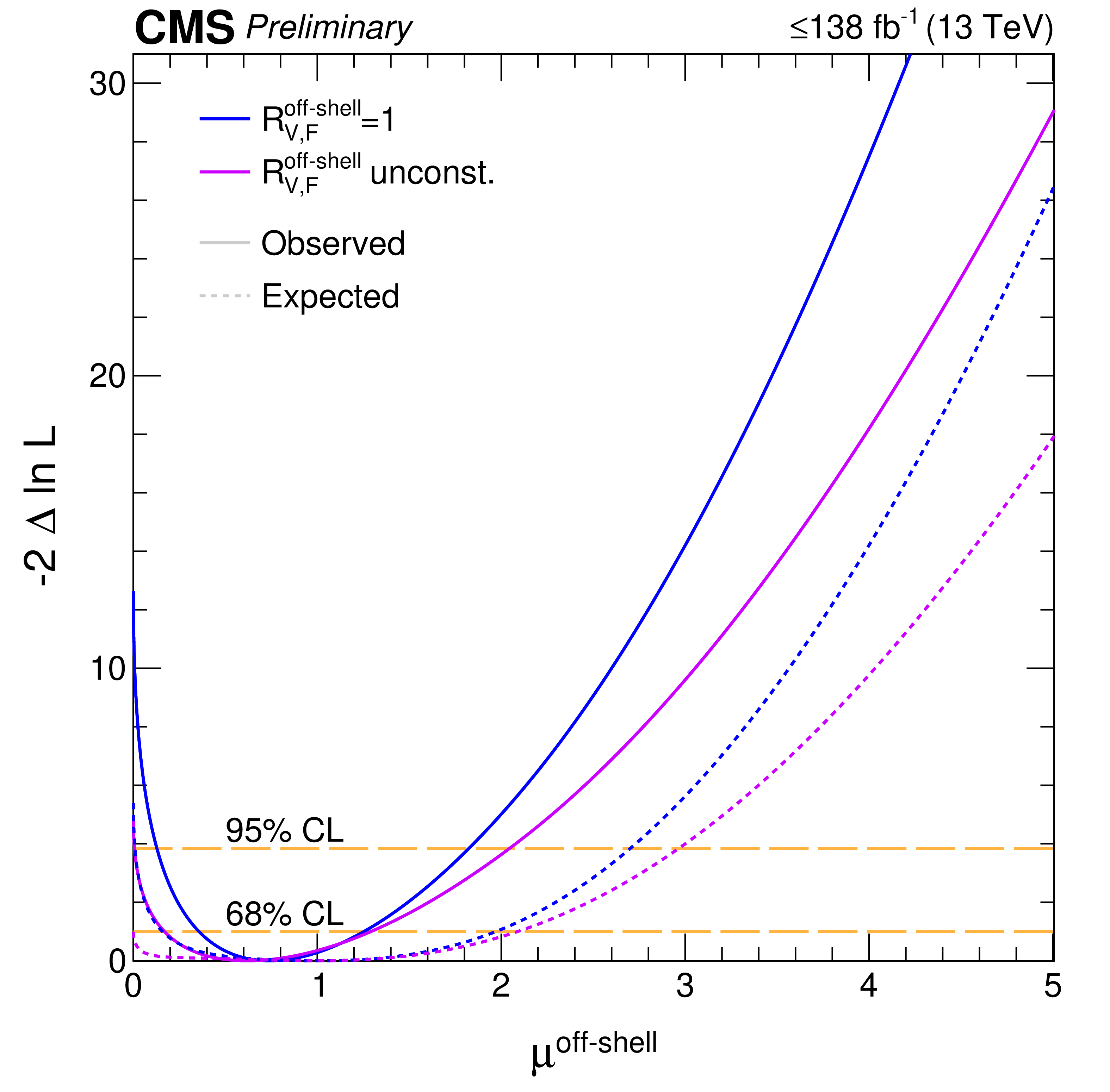
Figure 1:
Observed (solid) and expected (dashed) likelihood scans for $ {\mu ^{\mathrm {off-shell}}_{{\mathrm {F}} {}}} $ or $ {\mu ^{\mathrm {off-shell}}_{{\mathrm {V}} {}}} $ (left), $ {\mu ^{\mathrm {off-shell}}} $ (middle), and ${\Gamma _{\mathrm{H} {}}}$ (right). Scans for $ {\mu ^{\mathrm {off-shell}}_{{\mathrm {F}} {}}} $ (blue) and $ {\mu ^{\mathrm {off-shell}}_{{\mathrm {V}} {}}} $ (magenta) are obtained with the other parameter unconstrained. Those for $ {\mu ^{\mathrm {off-shell}}} $ are shown with (blue) and without (magenta) the constraint $ {R^{\mathrm {off-shell}}_{{\mathrm {V}} {}, {\mathrm {F}} {}}} =$ 1. Constraints on ${\Gamma _{\mathrm{H} {}}}$ are shown with and without anomalous HVV couplings. The horizontal lines indicate the 68% and 95% CL regions. |

png pdf |
Figure 1-a:
Observed (solid) and expected (dashed) likelihood scans for $ {\mu ^{\mathrm {off-shell}}_{{\mathrm {F}} {}}} $ or $ {\mu ^{\mathrm {off-shell}}_{{\mathrm {V}} {}}} $ (left), $ {\mu ^{\mathrm {off-shell}}} $ (middle), and ${\Gamma _{\mathrm{H} {}}}$ (right). Scans for $ {\mu ^{\mathrm {off-shell}}_{{\mathrm {F}} {}}} $ (blue) and $ {\mu ^{\mathrm {off-shell}}_{{\mathrm {V}} {}}} $ (magenta) are obtained with the other parameter unconstrained. Those for $ {\mu ^{\mathrm {off-shell}}} $ are shown with (blue) and without (magenta) the constraint $ {R^{\mathrm {off-shell}}_{{\mathrm {V}} {}, {\mathrm {F}} {}}} =$ 1. Constraints on ${\Gamma _{\mathrm{H} {}}}$ are shown with and without anomalous HVV couplings. The horizontal lines indicate the 68% and 95% CL regions. |
png pdf |
Figure 1-b:
Observed (solid) and expected (dashed) likelihood scans for $ {\mu ^{\mathrm {off-shell}}_{{\mathrm {F}} {}}} $ or $ {\mu ^{\mathrm {off-shell}}_{{\mathrm {V}} {}}} $ (left), $ {\mu ^{\mathrm {off-shell}}} $ (middle), and ${\Gamma _{\mathrm{H} {}}}$ (right). Scans for $ {\mu ^{\mathrm {off-shell}}_{{\mathrm {F}} {}}} $ (blue) and $ {\mu ^{\mathrm {off-shell}}_{{\mathrm {V}} {}}} $ (magenta) are obtained with the other parameter unconstrained. Those for $ {\mu ^{\mathrm {off-shell}}} $ are shown with (blue) and without (magenta) the constraint $ {R^{\mathrm {off-shell}}_{{\mathrm {V}} {}, {\mathrm {F}} {}}} =$ 1. Constraints on ${\Gamma _{\mathrm{H} {}}}$ are shown with and without anomalous HVV couplings. The horizontal lines indicate the 68% and 95% CL regions. |

png pdf |
Figure 1-c:
Observed (solid) and expected (dashed) likelihood scans for $ {\mu ^{\mathrm {off-shell}}_{{\mathrm {F}} {}}} $ or $ {\mu ^{\mathrm {off-shell}}_{{\mathrm {V}} {}}} $ (left), $ {\mu ^{\mathrm {off-shell}}} $ (middle), and ${\Gamma _{\mathrm{H} {}}}$ (right). Scans for $ {\mu ^{\mathrm {off-shell}}_{{\mathrm {F}} {}}} $ (blue) and $ {\mu ^{\mathrm {off-shell}}_{{\mathrm {V}} {}}} $ (magenta) are obtained with the other parameter unconstrained. Those for $ {\mu ^{\mathrm {off-shell}}} $ are shown with (blue) and without (magenta) the constraint $ {R^{\mathrm {off-shell}}_{{\mathrm {V}} {}, {\mathrm {F}} {}}} =$ 1. Constraints on ${\Gamma _{\mathrm{H} {}}}$ are shown with and without anomalous HVV couplings. The horizontal lines indicate the 68% and 95% CL regions. |

png pdf |
Figure 2:
Two-parameter likelihood scan of $ {\mu ^{\mathrm {off-shell}}_{{\mathrm {F}} {}}} $ and $ {\mu ^{\mathrm {off-shell}}_{{\mathrm {V}} {}}} $. The dot-dashed and dashed contours enclose the 68% and 95% CL regions. The cross marks the minimum, and the blue rhombus marks the SM expectation. |
png pdf |
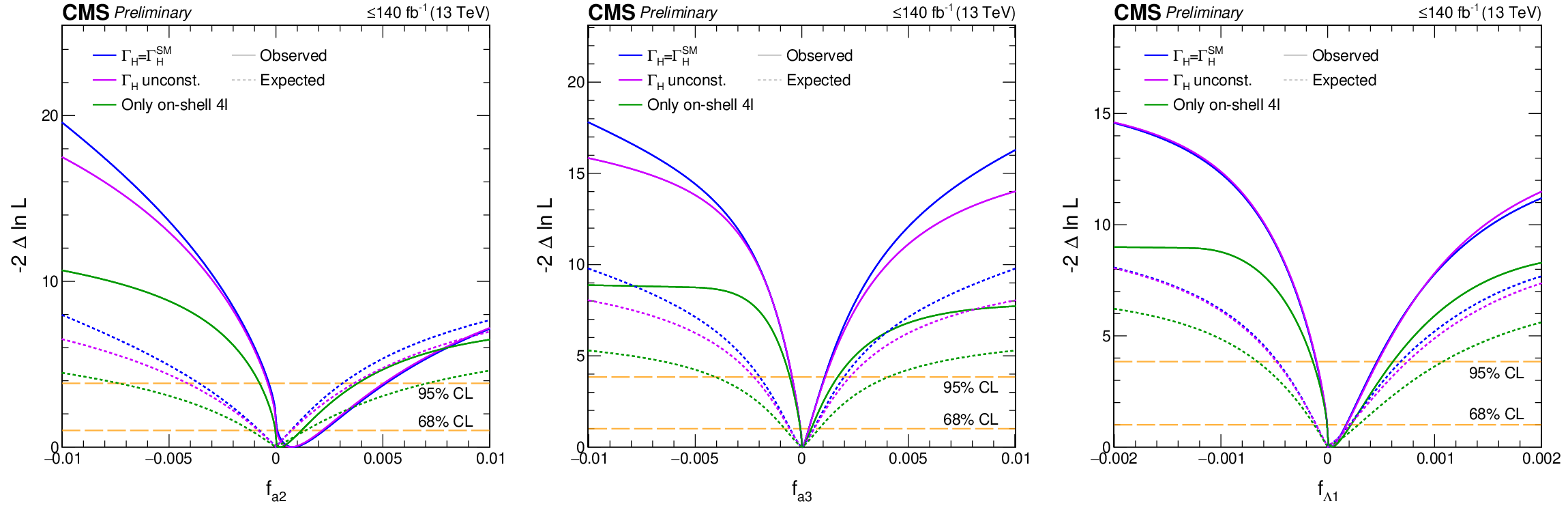
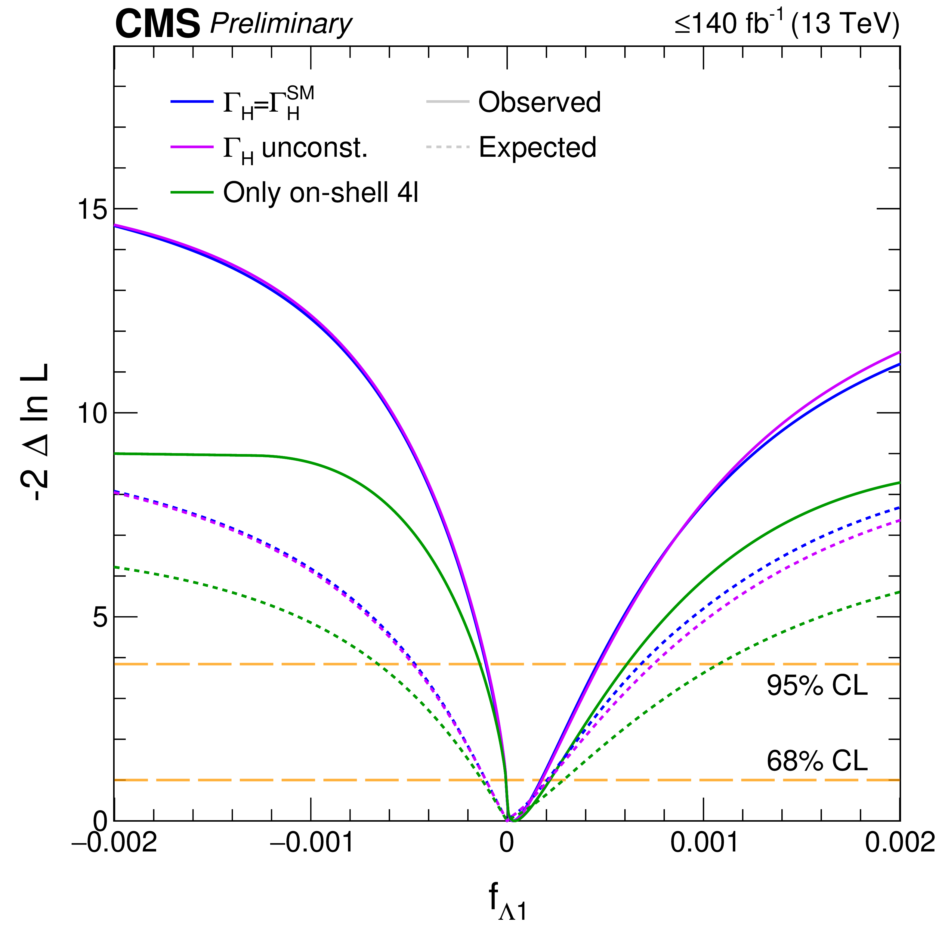
Figure 3:
Likelihood scans of ${{f_{a 2}}}$ (left), ${{f_{a 3}}}$ (middle), and ${{f_{{\lambda}bda 1}}}$ (right) are shown with the constraint $ {\Gamma _{\mathrm{H} {}}} = {\Gamma _{\mathrm{H} {}}^{\mathrm {SM}}} $ (blue), ${\Gamma _{\mathrm{H} {}}}$ unconstrained (violet), or based on on-shell 4$\ell $ only (green). Observed (expected) scans are shown with solid (dashed) curves. The horizontal lines indicate the 68% and 95% CL regions. |

png pdf |
Figure 3-a:
Likelihood scans of ${{f_{a 2}}}$ (left), ${{f_{a 3}}}$ (middle), and ${{f_{{\lambda}bda 1}}}$ (right) are shown with the constraint $ {\Gamma _{\mathrm{H} {}}} = {\Gamma _{\mathrm{H} {}}^{\mathrm {SM}}} $ (blue), ${\Gamma _{\mathrm{H} {}}}$ unconstrained (violet), or based on on-shell 4$\ell $ only (green). Observed (expected) scans are shown with solid (dashed) curves. The horizontal lines indicate the 68% and 95% CL regions. |

png pdf |
Figure 3-b:
Likelihood scans of ${{f_{a 2}}}$ (left), ${{f_{a 3}}}$ (middle), and ${{f_{{\lambda}bda 1}}}$ (right) are shown with the constraint $ {\Gamma _{\mathrm{H} {}}} = {\Gamma _{\mathrm{H} {}}^{\mathrm {SM}}} $ (blue), ${\Gamma _{\mathrm{H} {}}}$ unconstrained (violet), or based on on-shell 4$\ell $ only (green). Observed (expected) scans are shown with solid (dashed) curves. The horizontal lines indicate the 68% and 95% CL regions. |
png pdf |
Figure 3-c:
Likelihood scans of ${{f_{a 2}}}$ (left), ${{f_{a 3}}}$ (middle), and ${{f_{{\lambda}bda 1}}}$ (right) are shown with the constraint $ {\Gamma _{\mathrm{H} {}}} = {\Gamma _{\mathrm{H} {}}^{\mathrm {SM}}} $ (blue), ${\Gamma _{\mathrm{H} {}}}$ unconstrained (violet), or based on on-shell 4$\ell $ only (green). Observed (expected) scans are shown with solid (dashed) curves. The horizontal lines indicate the 68% and 95% CL regions. |

png pdf |
Figure 4:
Distributions of postfit ratios of the number of events in each 2$\ell $2$\nu $ and 4$\ell $ off-shell signal region bin. The ratios are taken after separate fits to the $ {\Gamma _{\mathrm{H} {}}} = $ 0 MeV hypothesis and the best overall fit. The stacked histograms display the contributions after the best fit, and the gold dashed line shows the distribution of these ratios for a fit to the $ {\Gamma _{\mathrm{H} {}}} = $ 0 MeV hypothesis. |
png pdf |
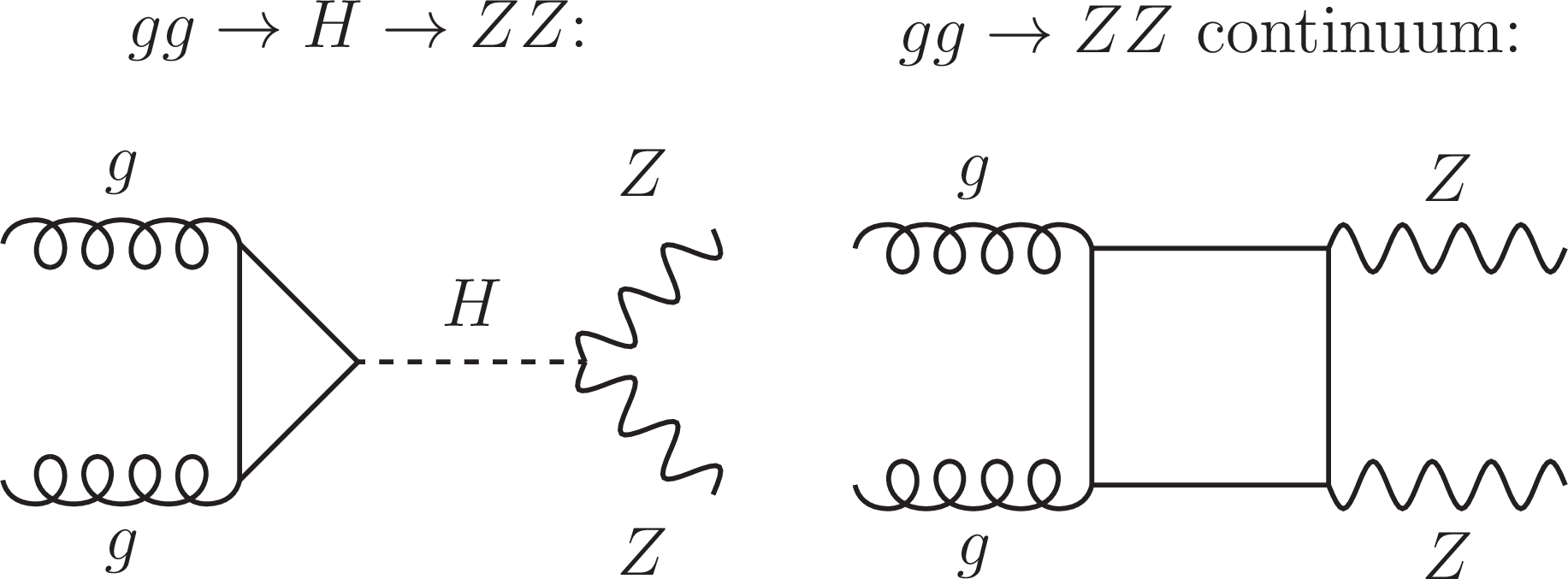
Figure 5:
The Feynman diagrams contributing to the $ {\mathrm {gg}} \to {\mathrm {ZZ}} $ process at tree level are shown. The left diagram refers to the contribution involving the H boson while the right diagram is for the continuum ZZ production. Alternative crossings are ignored for illustration purposes. |

png pdf |
Figure 6:
The tree-level Feynman diagrams contributing to the EW ZZ+ff production, where $f$ refers to any $\ell $, $\nu $, or $q$, are shown for the H boson -mediated contributions. Diagrams featuring VBF production are grouped together at the top, and those featuring VH production are grouped at the bottom. Alternative crossings are ignored for illustration purposes. |
png pdf |
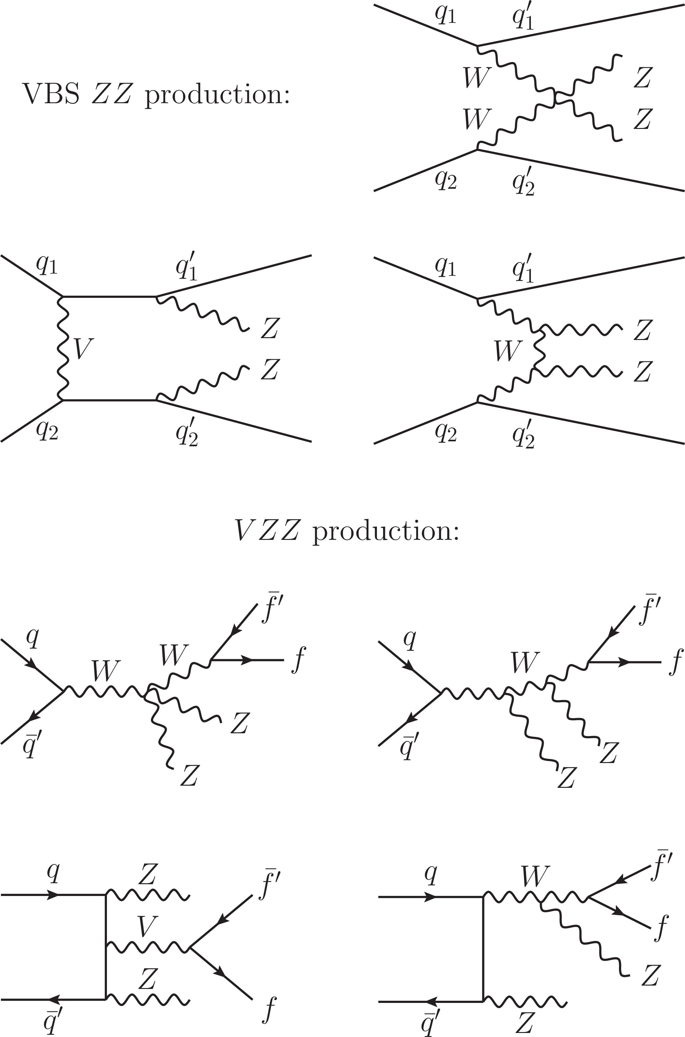
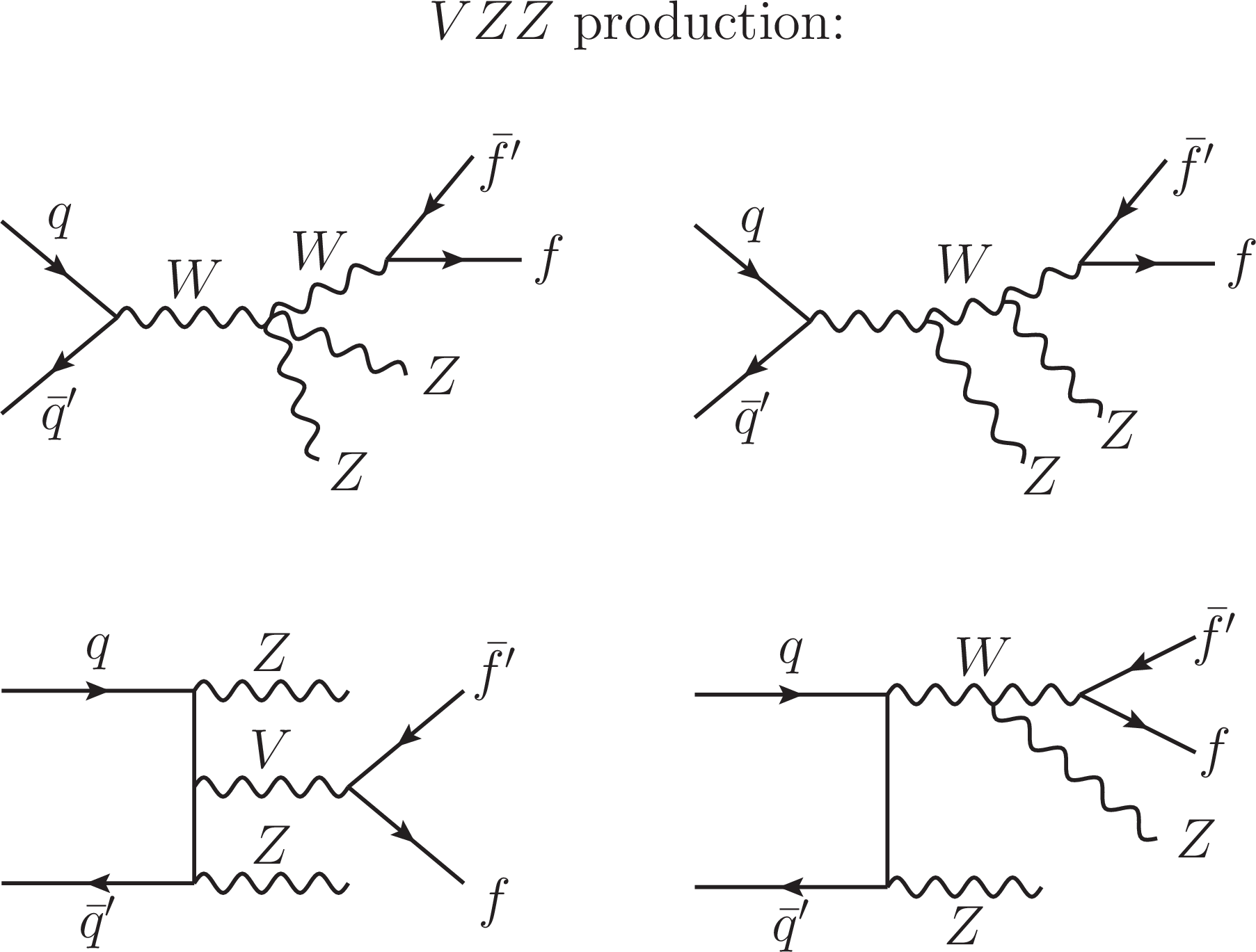
Figure 7:
The tree-level Feynman diagrams contributing to the EW ZZ+ff production, where $f$ refers to any $\ell $, $\nu $, or $q$, are shown for the continuum ZZ production contributions. Diagrams featuring VBS production are grouped together at the top, and those featuring VZZ production are grouped at the bottom. Alternative crossings are ignored for illustration purposes, and single-resonant contributions are not shown explicitly as they are not expected to contribute significantly in the off-shell region. |

png pdf |
Figure 7-a:
The tree-level Feynman diagrams contributing to the EW ZZ+ff production, where $f$ refers to any $\ell $, $\nu $, or $q$, are shown for the continuum ZZ production contributions. Diagrams featuring VBS production are grouped together at the top, and those featuring VZZ production are grouped at the bottom. Alternative crossings are ignored for illustration purposes, and single-resonant contributions are not shown explicitly as they are not expected to contribute significantly in the off-shell region. |
png pdf |
Figure 7-b:
The tree-level Feynman diagrams contributing to the EW ZZ+ff production, where $f$ refers to any $\ell $, $\nu $, or $q$, are shown for the continuum ZZ production contributions. Diagrams featuring VBS production are grouped together at the top, and those featuring VZZ production are grouped at the bottom. Alternative crossings are ignored for illustration purposes, and single-resonant contributions are not shown explicitly as they are not expected to contribute significantly in the off-shell region. |

png pdf |
Figure 8:
The Feynman diagrams contributing to the $ {\mathrm{q} \mathrm{\bar{q}}} \to {\mathrm {ZZ}} $ and $\mathrm{q\bar{q}^\prime} \to {\mathrm {WZ}} $ processes at tree level are represented with a single diagram. These two processes constitute the major irreducible background contributions in the off-shell region. Alternative crossings are ignored for illustration purposes, and single-resonant contributions are not shown explicitly as they are not expected to contribute significantly in the off-shell region. |

png pdf |
Figure 9:
Shown are the $m_{2\ell 2\nu}$ (left) and $m_{4\ell}$ distributions for the $ {\mathrm {gg}} \to 2\ell 2\nu $ and EW $ {\mathrm {ZZ}} (\to 4\ell)+\mathrm{qq}$ processes. These processes involve H boson and interfering continuum ZZ production contributions. The color code and the coupling constraints are indicated on the legends below. The acronym `PS' refers to the pure pseudoscalar H boson contribution. The distributions are shown after parton shower and inclusively in the number of generator-level jets. |

png pdf |
Figure 9-a:
Shown are the $m_{2\ell 2\nu}$ (left) and $m_{4\ell}$ distributions for the $ {\mathrm {gg}} \to 2\ell 2\nu $ and EW $ {\mathrm {ZZ}} (\to 4\ell)+\mathrm{qq}$ processes. These processes involve H boson and interfering continuum ZZ production contributions. The color code and the coupling constraints are indicated on the legends below. The acronym `PS' refers to the pure pseudoscalar H boson contribution. The distributions are shown after parton shower and inclusively in the number of generator-level jets. |

png pdf |
Figure 9-b:
Shown are the $m_{2\ell 2\nu}$ (left) and $m_{4\ell}$ distributions for the $ {\mathrm {gg}} \to 2\ell 2\nu $ and EW $ {\mathrm {ZZ}} (\to 4\ell)+\mathrm{qq}$ processes. These processes involve H boson and interfering continuum ZZ production contributions. The color code and the coupling constraints are indicated on the legends below. The acronym `PS' refers to the pure pseudoscalar H boson contribution. The distributions are shown after parton shower and inclusively in the number of generator-level jets. |
png pdf |
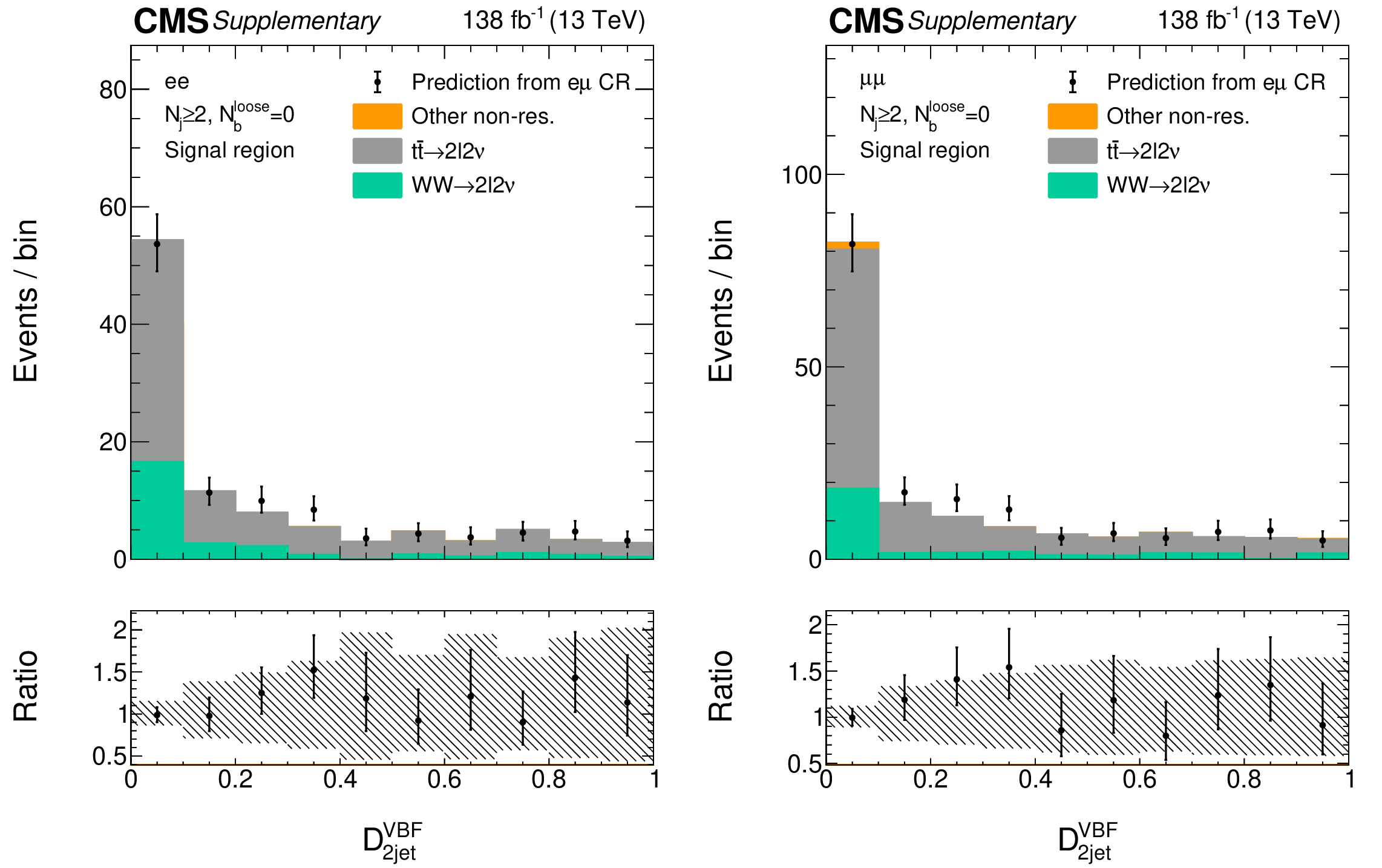
Figure 10:
The distributions of SM ${{\mathcal {D}}^{\mathrm {VBF}}_{\mathrm {2jet}}}$ kinematic discriminants are shown in the 2$\ell $2$\nu $ signal region, $N_{j}\geq $ 2 category, with the decay channel ee displayed on the left and $ {\mu} {\mu} $ on the right. The stacked histograms show the predictions from simulation, and the black points show the prediction from the e$ {\mu} $ CR data. The bottom pads show the ratio of the prediction from CR data to the prediction from simulation, and the hashed band in these pads display the statistical uncertainty on the latter prediction. |

png pdf |
Figure 10-a:
The distributions of SM ${{\mathcal {D}}^{\mathrm {VBF}}_{\mathrm {2jet}}}$ kinematic discriminants are shown in the 2$\ell $2$\nu $ signal region, $N_{j}\geq $ 2 category, with the decay channel ee displayed on the left and $ {\mu} {\mu} $ on the right. The stacked histograms show the predictions from simulation, and the black points show the prediction from the e$ {\mu} $ CR data. The bottom pads show the ratio of the prediction from CR data to the prediction from simulation, and the hashed band in these pads display the statistical uncertainty on the latter prediction. |

png pdf |
Figure 10-b:
The distributions of SM ${{\mathcal {D}}^{\mathrm {VBF}}_{\mathrm {2jet}}}$ kinematic discriminants are shown in the 2$\ell $2$\nu $ signal region, $N_{j}\geq $ 2 category, with the decay channel ee displayed on the left and $ {\mu} {\mu} $ on the right. The stacked histograms show the predictions from simulation, and the black points show the prediction from the e$ {\mu} $ CR data. The bottom pads show the ratio of the prediction from CR data to the prediction from simulation, and the hashed band in these pads display the statistical uncertainty on the latter prediction. |
png pdf |
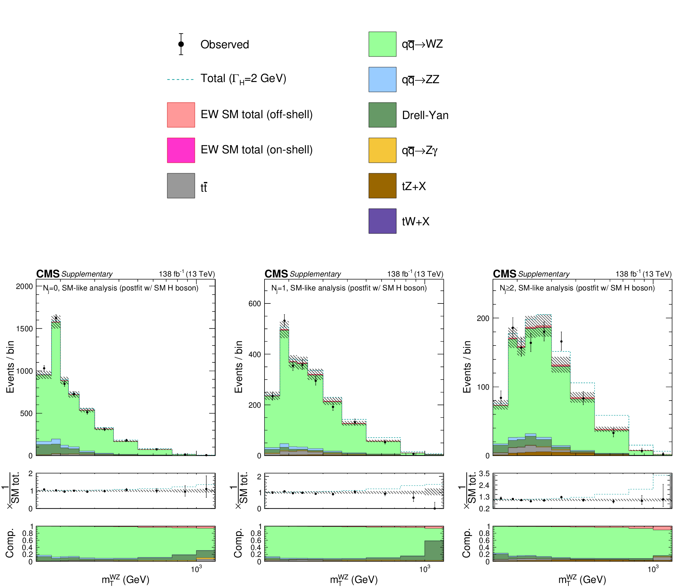
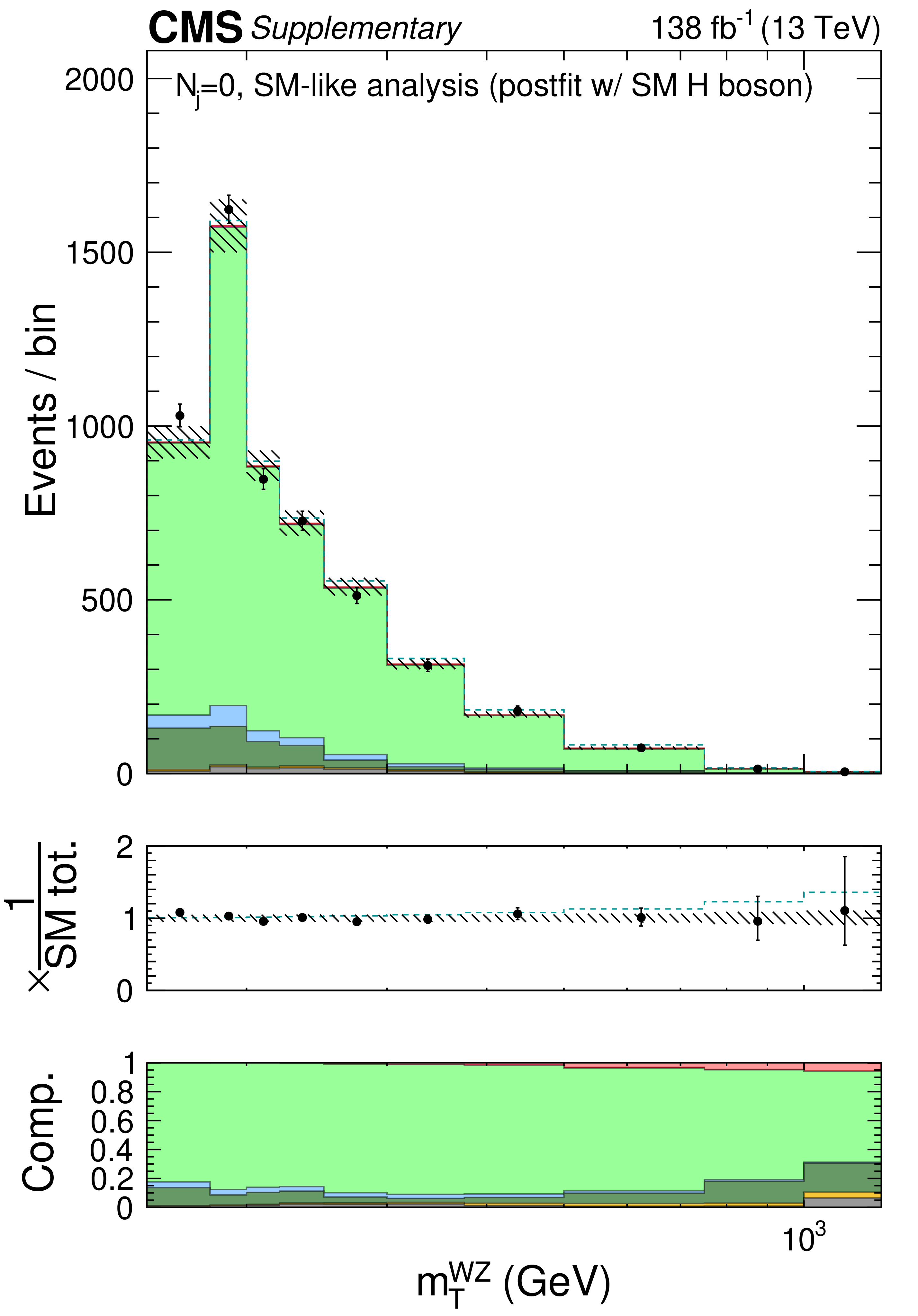
Figure 11:
Shown are the postfit distributions of ${m_\mathrm {T}^{{\mathrm {WZ}} {}}}$ in the $N_{j}=$ 0 (bottom left), $=$ 1 (bottom middle), and $\geq $ 2 (bottom right) categories of the $ {\mathrm {WZ}} \to 3\ell 1\nu $ control region. The color legend for the stacked or dashed histograms is given on the top panel. Postfit refers to a combined 2$\ell $2$\nu $+4$\ell $ fit assuming SM H boson parameters. The middle pads on the bottom panels show the ratio of the data or dashed histograms to the stacked histogram, and the bottom pads show the relative contributions of each process in the stacked histogram. The rightmost bins show event counts in the overflow. |

png pdf |
Figure 11-a:
Shown are the postfit distributions of ${m_\mathrm {T}^{{\mathrm {WZ}} {}}}$ in the $N_{j}=$ 0 (bottom left), $=$ 1 (bottom middle), and $\geq $ 2 (bottom right) categories of the $ {\mathrm {WZ}} \to 3\ell 1\nu $ control region. The color legend for the stacked or dashed histograms is given on the top panel. Postfit refers to a combined 2$\ell $2$\nu $+4$\ell $ fit assuming SM H boson parameters. The middle pads on the bottom panels show the ratio of the data or dashed histograms to the stacked histogram, and the bottom pads show the relative contributions of each process in the stacked histogram. The rightmost bins show event counts in the overflow. |
png pdf |
Figure 11-b:
Shown are the postfit distributions of ${m_\mathrm {T}^{{\mathrm {WZ}} {}}}$ in the $N_{j}=$ 0 (bottom left), $=$ 1 (bottom middle), and $\geq $ 2 (bottom right) categories of the $ {\mathrm {WZ}} \to 3\ell 1\nu $ control region. The color legend for the stacked or dashed histograms is given on the top panel. Postfit refers to a combined 2$\ell $2$\nu $+4$\ell $ fit assuming SM H boson parameters. The middle pads on the bottom panels show the ratio of the data or dashed histograms to the stacked histogram, and the bottom pads show the relative contributions of each process in the stacked histogram. The rightmost bins show event counts in the overflow. |

png pdf |
Figure 11-c:
Shown are the postfit distributions of ${m_\mathrm {T}^{{\mathrm {WZ}} {}}}$ in the $N_{j}=$ 0 (bottom left), $=$ 1 (bottom middle), and $\geq $ 2 (bottom right) categories of the $ {\mathrm {WZ}} \to 3\ell 1\nu $ control region. The color legend for the stacked or dashed histograms is given on the top panel. Postfit refers to a combined 2$\ell $2$\nu $+4$\ell $ fit assuming SM H boson parameters. The middle pads on the bottom panels show the ratio of the data or dashed histograms to the stacked histogram, and the bottom pads show the relative contributions of each process in the stacked histogram. The rightmost bins show event counts in the overflow. |

png pdf |
Figure 11-d:
Shown are the postfit distributions of ${m_\mathrm {T}^{{\mathrm {WZ}} {}}}$ in the $N_{j}=$ 0 (bottom left), $=$ 1 (bottom middle), and $\geq $ 2 (bottom right) categories of the $ {\mathrm {WZ}} \to 3\ell 1\nu $ control region. The color legend for the stacked or dashed histograms is given on the top panel. Postfit refers to a combined 2$\ell $2$\nu $+4$\ell $ fit assuming SM H boson parameters. The middle pads on the bottom panels show the ratio of the data or dashed histograms to the stacked histogram, and the bottom pads show the relative contributions of each process in the stacked histogram. The rightmost bins show event counts in the overflow. |
png pdf |
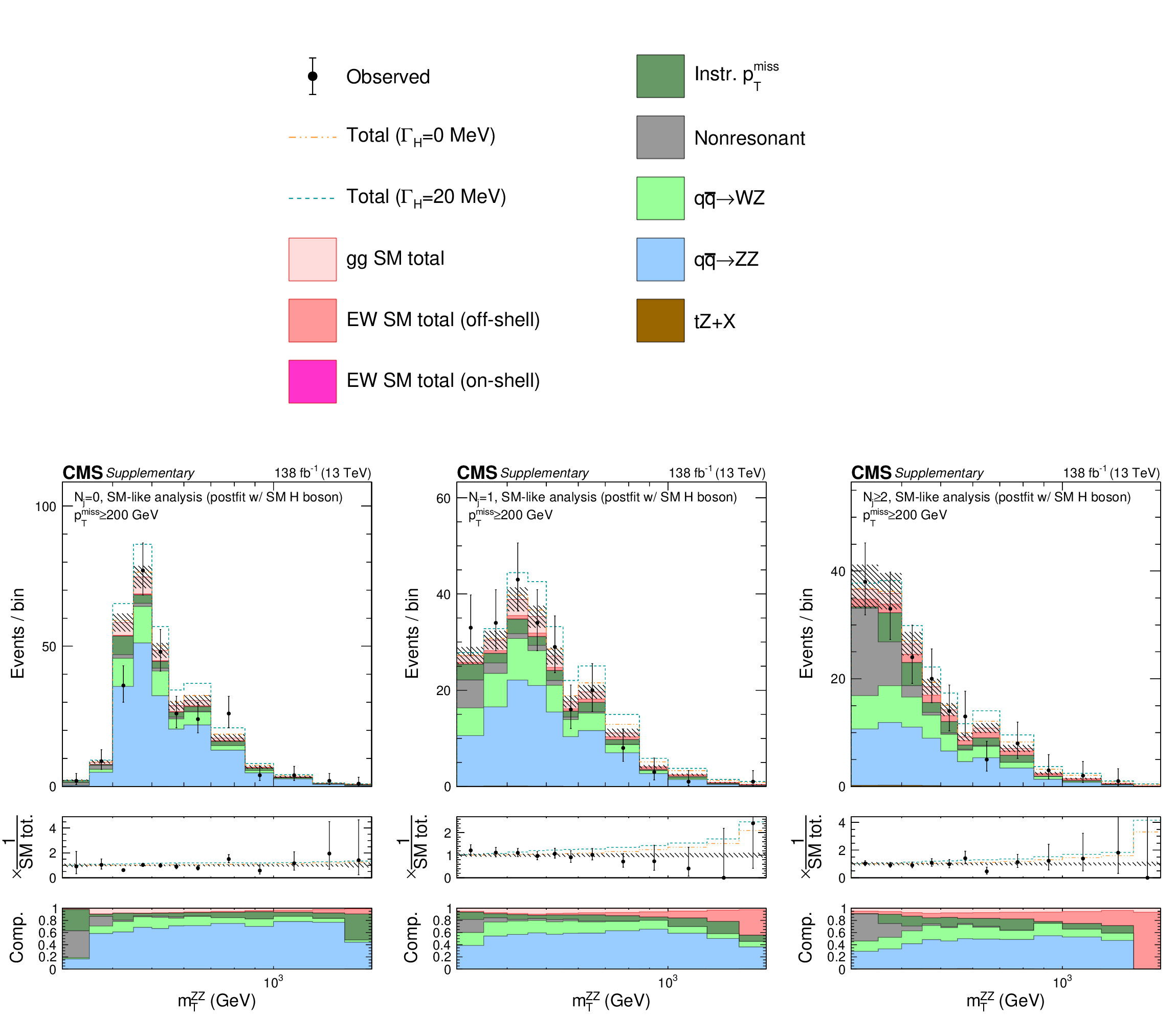
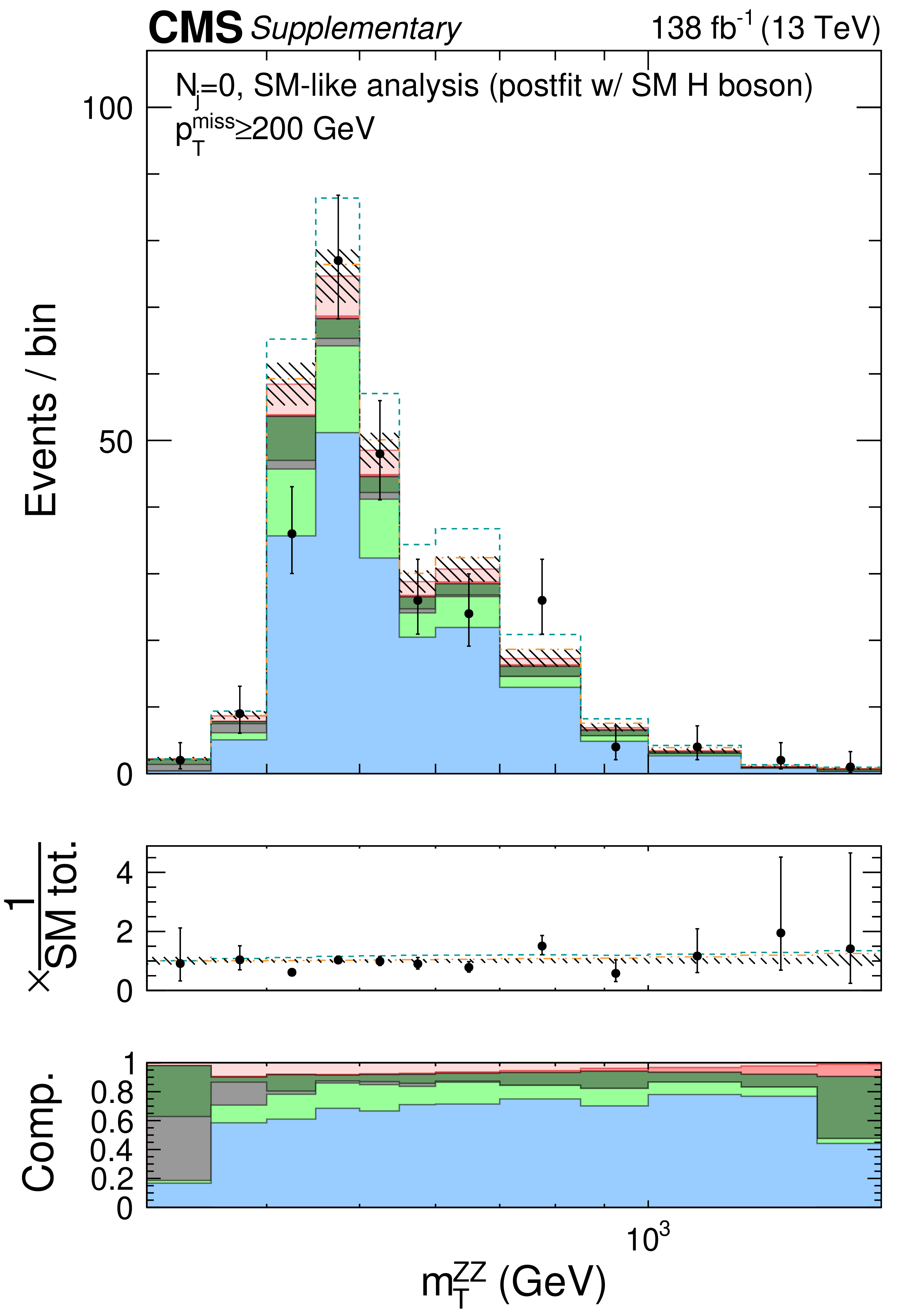
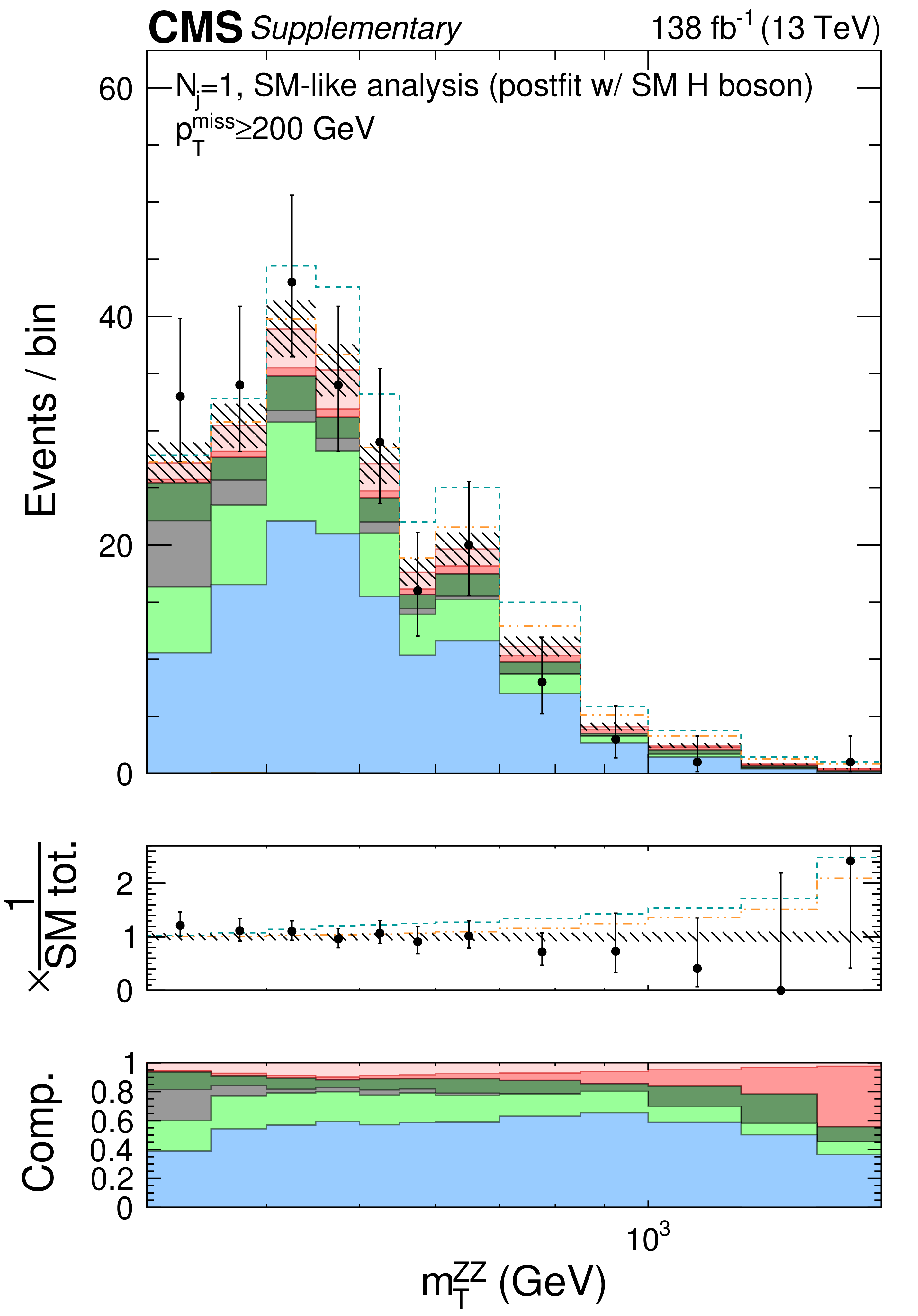
Figure 12:
Shown are the postfit distributions of ${m_\mathrm {T}^{{\mathrm {ZZ}} {}}}$ in the $N_{j}=$ 0 (bottom left), $=$ 1 (bottom middle), and $\geq $ 2 (bottom right) categories of the 2$\ell $2$\nu $ signal region with a $ {{p_{\mathrm {T}}} ^\text {miss}} \geq $ 200 GeV requirement to enrich H boson contributions. The color legend for the stacked or dashed histograms is given on the top panel. Postfit refers to a combined 2$\ell $2$\nu $+4$\ell $ fit assuming SM H boson parameters. The middle pads on the bottom panels show the ratio of the data or dashed histograms to the stacked histogram, and the bottom pads show the relative contributions of each process in the stacked histogram. The rightmost bins show event counts in the overflow. |

png pdf |
Figure 12-a:
Shown are the postfit distributions of ${m_\mathrm {T}^{{\mathrm {ZZ}} {}}}$ in the $N_{j}=$ 0 (bottom left), $=$ 1 (bottom middle), and $\geq $ 2 (bottom right) categories of the 2$\ell $2$\nu $ signal region with a $ {{p_{\mathrm {T}}} ^\text {miss}} \geq $ 200 GeV requirement to enrich H boson contributions. The color legend for the stacked or dashed histograms is given on the top panel. Postfit refers to a combined 2$\ell $2$\nu $+4$\ell $ fit assuming SM H boson parameters. The middle pads on the bottom panels show the ratio of the data or dashed histograms to the stacked histogram, and the bottom pads show the relative contributions of each process in the stacked histogram. The rightmost bins show event counts in the overflow. |
png pdf |
Figure 12-b:
Shown are the postfit distributions of ${m_\mathrm {T}^{{\mathrm {ZZ}} {}}}$ in the $N_{j}=$ 0 (bottom left), $=$ 1 (bottom middle), and $\geq $ 2 (bottom right) categories of the 2$\ell $2$\nu $ signal region with a $ {{p_{\mathrm {T}}} ^\text {miss}} \geq $ 200 GeV requirement to enrich H boson contributions. The color legend for the stacked or dashed histograms is given on the top panel. Postfit refers to a combined 2$\ell $2$\nu $+4$\ell $ fit assuming SM H boson parameters. The middle pads on the bottom panels show the ratio of the data or dashed histograms to the stacked histogram, and the bottom pads show the relative contributions of each process in the stacked histogram. The rightmost bins show event counts in the overflow. |
png pdf |
Figure 12-c:
Shown are the postfit distributions of ${m_\mathrm {T}^{{\mathrm {ZZ}} {}}}$ in the $N_{j}=$ 0 (bottom left), $=$ 1 (bottom middle), and $\geq $ 2 (bottom right) categories of the 2$\ell $2$\nu $ signal region with a $ {{p_{\mathrm {T}}} ^\text {miss}} \geq $ 200 GeV requirement to enrich H boson contributions. The color legend for the stacked or dashed histograms is given on the top panel. Postfit refers to a combined 2$\ell $2$\nu $+4$\ell $ fit assuming SM H boson parameters. The middle pads on the bottom panels show the ratio of the data or dashed histograms to the stacked histogram, and the bottom pads show the relative contributions of each process in the stacked histogram. The rightmost bins show event counts in the overflow. |

png pdf |
Figure 12-d:
Shown are the postfit distributions of ${m_\mathrm {T}^{{\mathrm {ZZ}} {}}}$ in the $N_{j}=$ 0 (bottom left), $=$ 1 (bottom middle), and $\geq $ 2 (bottom right) categories of the 2$\ell $2$\nu $ signal region with a $ {{p_{\mathrm {T}}} ^\text {miss}} \geq $ 200 GeV requirement to enrich H boson contributions. The color legend for the stacked or dashed histograms is given on the top panel. Postfit refers to a combined 2$\ell $2$\nu $+4$\ell $ fit assuming SM H boson parameters. The middle pads on the bottom panels show the ratio of the data or dashed histograms to the stacked histogram, and the bottom pads show the relative contributions of each process in the stacked histogram. The rightmost bins show event counts in the overflow. |
| Tables | |

png pdf |
Table 1:
Summary of results on the off-shell signal strength and ${\Gamma _{\mathrm{H} {}}}$. Results for ${\mu ^{\mathrm {off-shell}}}$ are with $ {R^{\mathrm {off-shell}}_{{\mathrm {V}} {}, {\mathrm {F}} {}}} $ either unconstrained or $=$ 1. Constraints on $ {\mu ^{\mathrm {off-shell}}_{{\mathrm {F}} {}}} $ and $ {\mu ^{\mathrm {off-shell}}_{{\mathrm {V}} {}}} $ are shown with the other signal strength unconstrained. Results for ${\Gamma _{\mathrm{H} {}}}$ (in units of $ MeV $) are obtained with the on-shell signal strengths unconstrained. Tests with anomalous HVV couplings are distinguished by the denoted on-shell cross section fractions. The expected values (not shown) are either unity or $ {\Gamma _{\mathrm{H} {}}} = $ 4.1 MeV. The abbreviation `c.v.' stands for `central value', and the abbreviation `(u)' stands for `unconstrained'. |
png pdf |
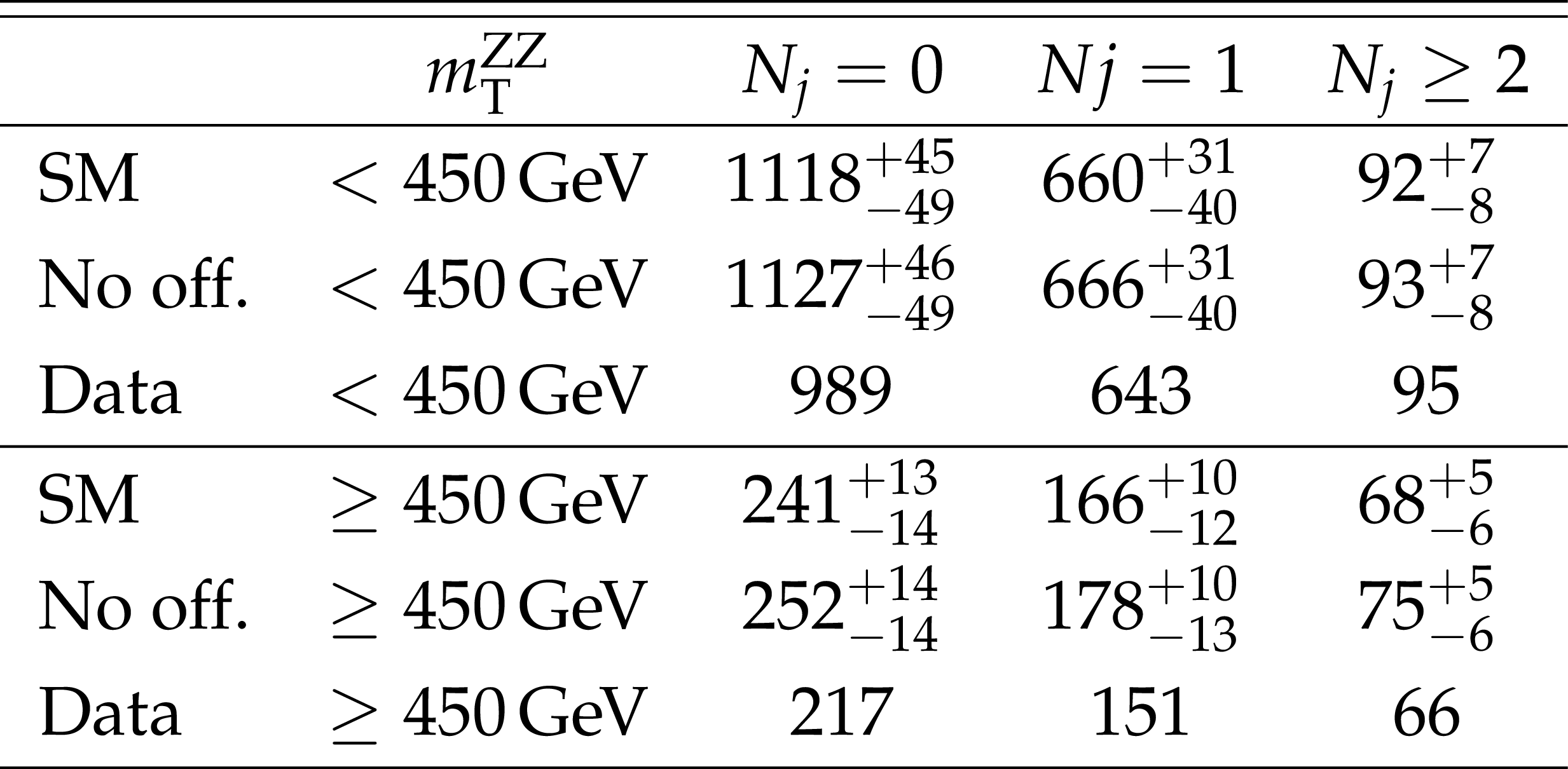
Table 2:
Comparisons between the number of observed events in the 2$\ell $2$\nu $ channel with expectations from the SM and no-off-shell scenarios as a function of $N_j$ for low and high ${m_\mathrm {T}^{{\mathrm {ZZ}} {}}}$. An additional requirement of $ {{p_{\mathrm {T}}} ^\text {miss}} \geq $ 200 GeV has been imposed for $N_j \geq $ 2. |
| Summary |
| To summarize, we reported evidence for off-shell H boson production in the ZZ final state, excluding the no off-shell scenario at more than 99.9% confidence (3.6 standard deviations). We performed the first measurement of its total width, $\Gamma_{\mathrm{H}} =$ 3.2$_{-1.7}^{+2.4}$ MeV, with a meaningful precision in both observed and expected results, and set limits on anomalous HVV interactions. These results are based on a new analysis of the 2$\ell$2$\nu$ final state combined with previously published results for $\mathrm{ZZ }\to 4 \ell$ using up to 140 fb$^{-1}$ of pp collisions collected with the CMS detector at the LHC between 2015 and 2018. Our measurements are consistent with SM expectations. |
| References | ||||
| 1 | S. L. Glashow | Partial-symmetries of weak interactions | NP 22 (1961) 579 | |
| 2 | F. Englert and R. Brout | Broken symmetry and the mass of gauge vector mesons | PRL 13 (1964) 321 | |
| 3 | P. W. Higgs | Broken symmetries, massless particles and gauge fields | PL12 (1964) 132 | |
| 4 | P. W. Higgs | Broken symmetries and the masses of gauge bosons | PRL 13 (1964) 508 | |
| 5 | G. S. Guralnik, C. R. Hagen, and T. W. B. Kibble | Global conservation laws and massless particles | PRL 13 (1964) 585 | |
| 6 | S. Weinberg | A model of leptons | PRL 19 (1967) 1264 | |
| 7 | A. Salam | Weak and electromagnetic interactions | in Elementary particle physics: relativistic groups and analyticity, N. Svartholm, ed., 1968, Proceedings of the eighth Nobel symposium | |
| 8 | ATLAS Collaboration | Observation of a new particle in the search for the Standard Model Higgs boson with the ATLAS detector at the LHC | PLB 716 (2012) 1 | 1207.7214 |
| 9 | CMS Collaboration | Observation of a new boson at a mass of 125 GeV with the CMS experiment at the LHC | PLB 716 (2012) 30 | CMS-HIG-12-028 1207.7235 |
| 10 | CMS Collaboration | Observation of a new boson with mass near 125 GeV in $ {\mathrm{p}}{\mathrm{p}} $ collisions at $ \sqrt{s}= $ 7 and~8 TeV | JHEP 06 (2013) 081 | CMS-HIG-12-036 1303.4571 |
| 11 | W. Heisenberg | $ Uber $ den anschaulichen inhalt der quantentheoretischen kinematik und mechanik | Zeitschrift f\"ur Physik 43 (3, 1927) 172 | |
| 12 | G. Breit and E. Wigner | Capture of slow neutrons | PR49 (4, 1936) 519 | |
| 13 | Particle Data Group Collaboration | Review of Particle Physics | PTEP 2020 (2020), no. 8, 083C01 | |
| 14 | LHC Higgs Cross Section Working Group Collaboration | Handbook of LHC Higgs Cross Sections: 3. Higgs Properties | 1307.1347 | |
| 15 | LHC Higgs Cross Section Working Group Collaboration | Handbook of LHC Higgs cross sections: 4. Deciphering the nature of the Higgs Sector | 1610.07922 | |
| 16 | CMS Collaboration | Limits on the Higgs boson lifetime and width from its decay to four charged leptons | PRD 92 (2015) 072010 | CMS-HIG-14-036 1507.06656 |
| 17 | N. Kauer and G. Passarino | Inadequacy of zero-width approximation for a light Higgs boson signal | JHEP 08 (2012) 116 | 1206.4803 |
| 18 | N. Kauer | Inadequacy of zero-width approximation for a light Higgs boson signal | MPLA 28 (2013) 1330015 | 1305.2092 |
| 19 | F. Caola and K. Melnikov | Constraining the Higgs boson width with ZZ production at the LHC | PRD 88 (2013) 054024 | 1307.4935 |
| 20 | J. M. Campbell, R. K. Ellis, and C. Williams | Bounding the Higgs width at the LHC using full analytic results for $ \mathrm{g}\mathrm{g}\to \mathrm{e}^{-}\mathrm{e}^{+} \mu^{-} \mu^{+} $ | JHEP 04 (2014) 060 | 1311.3589 |
| 21 | G. Passarino | Higgs CAT | EPJC 74 (2014) 2866 | 1312.2397 |
| 22 | CMS Collaboration | Constraints on the Higgs boson width from off-shell production and decay to Z-boson pairs | PLB 736 (2014) 64 | CMS-HIG-14-002 1405.3455 |
| 23 | ATLAS Collaboration | Constraints on the off-shell Higgs boson signal strength in the high-mass ZZ and WW final states with the ATLAS detector | EPJC 75 (2015) 335 | 1503.01060 |
| 24 | CMS Collaboration | Search for Higgs boson off-shell production in proton-proton collisions at 7 and 8 TeV and derivation of constraints on its total decay width | JHEP 09 (2016) 051 | CMS-HIG-14-032 1605.02329 |
| 25 | ATLAS Collaboration | Constraints on off-shell Higgs boson production and the Higgs boson total width in $ \mathrm{ZZ}\to4\ell $ and $ \mathrm{ZZ}\to2\ell2\nu $ final states with the ATLAS detector | PLB 786 (2018) 223 | 1808.01191 |
| 26 | CMS Collaboration | Measurements of the Higgs boson width and anomalous HVV couplings from on-shell and off-shell production in the four-lepton final state | PRD 99 (2019) 112003 | CMS-HIG-18-002 1901.00174 |
| 27 | C. H. Llewellyn Smith | High-Energy Behavior and Gauge Symmetry | PLB 46 (1973) 233 | |
| 28 | J. M. Cornwall, D. N. Levin, and G. Tiktopoulos | Derivation of Gauge Invariance from High-Energy Unitarity Bounds on the $ S $-Matrix | PRD 10 (1974) 1145 | |
| 29 | B. W. Lee, C. Quigg, and H. B. Thacker | Weak Interactions at Very High-Energies: The Role of the Higgs Boson Mass | PRD 16 (1977) 1519 | |
| 30 | E. W. N. Glover and J. J. van der Bij | Vector boson pair production via gluon fusion | PLB 219 (1989) 488 | |
| 31 | E. W. N. Glover and J. J. van der Bij | Z boson pair production via gluon fusion | NPB 321 (1989) 561 | |
| 32 | N. Kauer | Signal-background interference in $ \mathrm{gg} \to \mathrm{H} \to \mathrm{VV} $ | PoS RADCOR2011 (2011) 027 | 1201.1667 |
| 33 | G. Passarino | Higgs interference effects in $ \mathrm{gg} \to \mathrm{ZZ} $ and their uncertainty | JHEP 08 (2012) 146 | 1206.3824 |
| 34 | F. Campanario, Q. Li, M. Rauch, and M. Spira | ZZ+jet production via gluon fusion at the LHC | JHEP 06 (2013) 069 | 1211.5429 |
| 35 | A. V. Gritsan et al. | New features in the JHU generator framework: constraining Higgs boson properties from on-shell and off-shell production | PRD 102 (2020), no. 5, 056022 | 2002.09888 |
| 36 | CMS Collaboration | Constraints on anomalous Higgs boson couplings using production and decay information in the four-lepton final state | PLB 775 (2017) 1 | CMS-HIG-17-011 1707.00541 |
| 37 | CMS Collaboration | Constraints on anomalous Higgs boson couplings to vector bosons and fermions in its production and decay using the four-lepton final state | PRD 104 (2021), no. 5, 052004 | CMS-HIG-19-009 2104.12152 |
| 38 | CMS Collaboration | The CMS experiment at the CERN LHC | JINST 3 (2008) S08004 | CMS-00-001 |
| 39 | CMS Collaboration | Performance of the CMS Level-1 trigger in proton-proton collisions at $ \sqrt{s} = $ 13 TeV | JINST 15 (2020) P10017 | CMS-TRG-17-001 2006.10165 |
| 40 | CMS Collaboration | The CMS trigger system | JINST 12 (2017) P01020 | CMS-TRG-12-001 1609.02366 |
| 41 | CMS Collaboration | Performance of the CMS muon detector and muon reconstruction with proton-proton collisions at $ \sqrt{s} = $ 13 TeV | JINST 13 (2018), no. 06, P06015 | CMS-MUO-16-001 1804.04528 |
| 42 | CMS Collaboration | Performance of electron reconstruction and selection with the CMS detector in proton-proton collisions at $ \sqrt{s} = $ 8 TeV | JINST 10 (2015), no. 06, P06005 | CMS-EGM-13-001 1502.02701 |
| 43 | CMS Collaboration | Performance of photon reconstruction and identification with the CMS detector in proton-proton collisions at $ \sqrt{s} = $ 8 TeV | JINST 10 (2015), no. 08, P08010 | CMS-EGM-14-001 1502.02702 |
| 44 | CMS Collaboration | Description and performance of track and primary-vertex reconstruction with the CMS tracker | JINST 9 (2014), no. 10, P10009 | CMS-TRK-11-001 1405.6569 |
| 45 | CMS Collaboration | Particle-flow reconstruction and global event description with the cms detector | JINST 12 (2017) P10003 | CMS-PRF-14-001 1706.04965 |
| 46 | CMS Collaboration | Jet energy scale and resolution in the CMS experiment in $ {\mathrm{p}}{}{\mathrm{p}}{} $ collisions at 8 TeV | JINST 12 (2017) P02014 | CMS-JME-13-004 1607.03663 |
| 47 | CMS Collaboration | Performance of missing transverse momentum reconstruction in proton-proton collisions at $ \sqrt{s} = $ 13 TeV using the CMS detector | JINST 14 (2019) P07004 | CMS-JME-17-001 1903.06078 |
| 48 | CMS Collaboration | Performance of reconstruction and identification of $ \tau $ leptons decaying to hadrons and $ \nu_\tau $ in $ {\mathrm{p}}{}{\mathrm{p}}{} $ collisions at $ \sqrt{s} = $ 13 TeV | JINST 13 (2018), no. 10, P10005 | CMS-TAU-16-003 1809.02816 |
| 49 | M. Cacciari and G. P. Salam | Dispelling the $ N^{3} $ myth for the $ {k_{\mathrm{T}}} $ jet-finder | PLB 641 (2006) 57 | hep-ph/0512210 |
| 50 | M. Cacciari, G. P. Salam, and G. Soyez | The anti-$ {k_{\mathrm{T}}} $ jet clustering algorithm | JHEP 04 (2008) 063 | 0802.1189 |
| 51 | M. Cacciari, G. P. Salam, and G. Soyez | FastJet user manual | EPJC 72 (2012) 1896 | 1111.6097 |
| 52 | CMS Collaboration | Jet algorithms performance in 13 TeV data | CMS-PAS-JME-16-003 | CMS-PAS-JME-16-003 |
| 53 | CMS Collaboration | Pileup mitigation at CMS in 13 TeV data | JINST 15 (2020), no. 09, P09018 | CMS-JME-18-001 2003.00503 |
| 54 | E. Bols et al. | Jet Flavour Classification Using DeepJet | JINST 15 (2020), no. 12, 12012 | 2008.10519 |
| 55 | CMS Collaboration | Missing transverse energy performance of the CMS detector | JINST 6 (2011) P09001 | CMS-JME-10-009 1106.5048 |
| 56 | S. Frixione, P. Nason, and C. Oleari | Matching NLO QCD computations with parton shower simulations: the POWHEG method | JHEP 11 (2007) 070 | 0709.2092 |
| 57 | P. Nason and C. Oleari | NLO Higgs boson production via vector-boson fusion matched with shower in POWHEG | JHEP 02 (2010) 037 | 0911.5299 |
| 58 | E. Bagnaschi, G. Degrassi, P. Slavich, and A. Vicini | Higgs production via gluon fusion in the POWHEG approach in the SM and in the MSSM | JHEP 02 (2012) 088 | 1111.2854 |
| 59 | G. Luisoni, P. Nason, C. Oleari, and F. Tramontano | $ \mathrm{H}\mathrm{W}^{\pm} $/$ \mathrm{H}\mathrm{Z} $ + 0 and 1 jet at NLO with the POWHEG BOX interfaced to GoSam and their merging within MiNLO | JHEP 10 (2013) 083 | 1306.2542 |
| 60 | H. B. Hartanto, B. Jager, L. Reina, and D. Wackeroth | Higgs boson production in association with top quarks in the POWHEG BOX | PRD 91 (2015) 094003 | 1501.04498 |
| 61 | Y. Gao et al. | Spin determination of single-produced resonances at hadron colliders | PRD 81 (2010) 075022 | 1001.3396 |
| 62 | S. Bolognesi et al. | Spin and parity of a single-produced resonance at the LHC | PRD 86 (2012) 095031 | 1208.4018 |
| 63 | I. Anderson et al. | Constraining anomalous HVV interactions at proton and lepton colliders | PRD 89 (2014) 035007 | 1309.4819 |
| 64 | A. V. Gritsan, R. Rontsch, M. Schulze, and M. Xiao | Constraining anomalous Higgs boson couplings to the heavy flavor fermions using matrix element techniques | PRD 94 (2016) 055023 | 1606.03107 |
| 65 | CMS Collaboration | Search for a heavy Higgs boson decaying to a pair of $ \mathrm{W} $ bosons in proton-proton collisions at $ \sqrt{s} = $ 13 TeV | JHEP 03 (2020) 034 | CMS-HIG-17-033 1912.01594 |
| 66 | A. Bierweiler, T. Kasprzik, and J. H. Kuhn | Vector-boson pair production at the LHC to $ \mathcal{O}(\alpha^3) $ accuracy | JHEP 12 (2013) 071 | 1305.5402 |
| 67 | A. Manohar, P. Nason, G. P. Salam, and G. Zanderighi | How bright is the proton? A precise determination of the photon parton distribution function | PRL 117 (2016) 242002 | 1607.04266 |
| 68 | CMS Collaboration | Search for a new scalar resonance decaying to a pair of Z bosons in proton-proton collisions at $ \sqrt{s} = $ 13 TeV | JHEP 06 (2018) 127 | CMS-HIG-17-012 1804.01939 |
| 69 | M. Grazzini, S. Kallweit, and D. Rathlev | $ \mathrm{Z}\mathrm{Z} $ production at the LHC: fiducial cross sections and distributions in NNLO QCD | PLB 750 (2015) 407 | 1507.06257 |
| 70 | M. Grazzini, S. Kallweit, and M. Wiesemann | Fully differential NNLO computations with MATRIX | EPJC 78 (2018), no. 7, 537 | 1711.06631 |
| 71 | CMS Collaboration | Measurements of properties of the Higgs boson decaying into the four-lepton final state in $ {\mathrm{p}}{\mathrm{p}} $ collisions at $ \sqrt{s} = $ 13 TeV | JHEP 11 (2017) 047 | CMS-HIG-16-041 1706.09936 |
| 72 | R. Frederix and S. Frixione | Merging meets matching in MC@NLO | JHEP 12 (2012) 061 | 1209.6215 |
| 73 | J. Alwall et al. | Comparative study of various algorithms for the merging of parton showers and matrix elements in hadronic collisions | EPJC 53 (2008) 473 | 0706.2569 |
| 74 | T. Sjostrand et al. | An introduction to PYTHIA 8.2 | CPC 191 (2015) 159 | 1410.3012 |
| 75 | CMS Collaboration | Event generator tunes obtained from underlying event and multiparton scattering measurements | EPJC 76 (2016), no. 3, 155 | CMS-GEN-14-001 1512.00815 |
| 76 | CMS Collaboration | Extraction and validation of a new set of CMS PYTHIA8 tunes from underlying-event measurements | EPJC 80 (2020), no. 1, 4 | CMS-GEN-17-001 1903.12179 |
| 77 | NNPDF Collaboration | Unbiased global determination of parton distributions and their uncertainties at NNLO and at LO | NPB 855 (2012) 153 | 1107.2652 |
| 78 | NNPDF Collaboration | Parton distributions for the LHC Run II | JHEP 04 (2015) 040 | 1410.8849 |
| 79 | GEANT4 Collaboration | GEANT4 -- a simulation toolkit | NIMA 506 (2003) 250 | |
| 80 | CMS Collaboration | Search for physics beyond the standard model in events with a Z boson, jets, and missing transverse energy in $ {\mathrm{p}}{}{\mathrm{p}}{} $ collisions at $ \sqrt{s} = $ 7 TeV | PLB 716 (2012) 260 | CMS-SUS-11-021 1204.3774 |
| 81 | R. J. Barlow | Extended maximum likelihood | NIMA 297 (1990) 496 | |
| 82 | CMS Collaboration | CMS luminosity measurements for the 2016 data taking period | CMS-PAS-LUM-17-001 | CMS-PAS-LUM-17-001 |
| 83 | CMS Collaboration | Precision luminosity measurement in proton-proton collisions at $ \sqrt{s} = $ 13 TeV in 2015 and 2016 at CMS | EPJC 81 (2021), no. 9, 800 | CMS-LUM-17-003 2104.01927 |
| 84 | CMS Collaboration | CMS luminosity measurement for the 2017 data taking period at $ \sqrt{s} = $ 13 TeV | CMS-PAS-LUM-17-004 | CMS-PAS-LUM-17-004 |
| 85 | CMS Collaboration | CMS luminosity measurement for the 2018 data-taking period at $ \sqrt{s} = $ 13 TeV | CMS-PAS-LUM-18-002 | CMS-PAS-LUM-18-002 |
|
|
Compact Muon Solenoid LHC, CERN |
|

|

|

|

|

|