

Compact Muon Solenoid
LHC, CERN
| CMS-PAS-HIG-21-011 | ||
| Search for a new resonance decaying to two scalars in the final state with two bottom quarks and two photons in proton-proton collisions at $\sqrt{s}=$ 13 TeV | ||
| CMS Collaboration | ||
| July 2022 | ||
| Abstract: A search for new resonances in the final state with two bottom quarks and two photons is presented, using CERN LHC proton-proton collision data collected by the CMS experiment at $\sqrt{s} = $ 13 TeV, and corresponding to an integrated luminosity of 138 fb$^{-1}$. The resonance X decays into either a pair of the standard model Higgs bosons HH, or an H and a new scalar $\mathrm{Y}$ having a mass $m_{\mathrm{Y}} < m_{\mathrm{X}} - m_{\mathrm{H}}$. A model-independent analysis is performed with a narrow-width approximation for X in the mass range 260 GeV-1 TeV (for the HH decay) and 300 GeV-1 TeV (for the HY decay), covering a mass range of 90 $ < m_{\mathrm{Y}} < $ 800 GeV. The upper limits at 95% confidence level on the product of the production cross section of spin-0 X and its decay branching fraction to HH are observed to be within 0.82-0.07 fb, while the corresponding expected limits are 0.74 - 0.08 fb, depending upon the considered mass range in $m_{\mathrm{X}}$. For the X decaying to HY, the observed limits lie in the range 0.90-0.04 fb whereas the expected limits are 0.79-0.05 fb, with the considered mass ranges in $m_{\mathrm{X}}$ and $m_{\mathrm{Y}}$. The largest deviation from background-only hypothesis with local (global) significance of 3.8 (2.8) standard deviations is observed for $m_{\mathrm{X}}= $ 650 GeV and $m_{\mathrm{Y}}= $ 90 GeV. The HH limits are compared with predictions in the warped extra dimensional model. The HY limits are interpreted with the next-to-minimal supersymmetric standard model and the two-real-scalar-singlet model. | ||
|
Links:
CDS record (PDF) ;
CADI line (restricted) ;
These preliminary results are superseded in this paper, Submitted to JHEP. The superseded preliminary plots can be found here. |
||
| Figures | |

png pdf |
Figure 1:
Feynman diagram showing gluon-gluon fusion production of a BSM resonance X decaying to a pair of scalars (HH or HY), which then decay to the ${\gamma \gamma \mathrm{b} {}\mathrm{\bar{b}}}$ final state. |
png pdf |
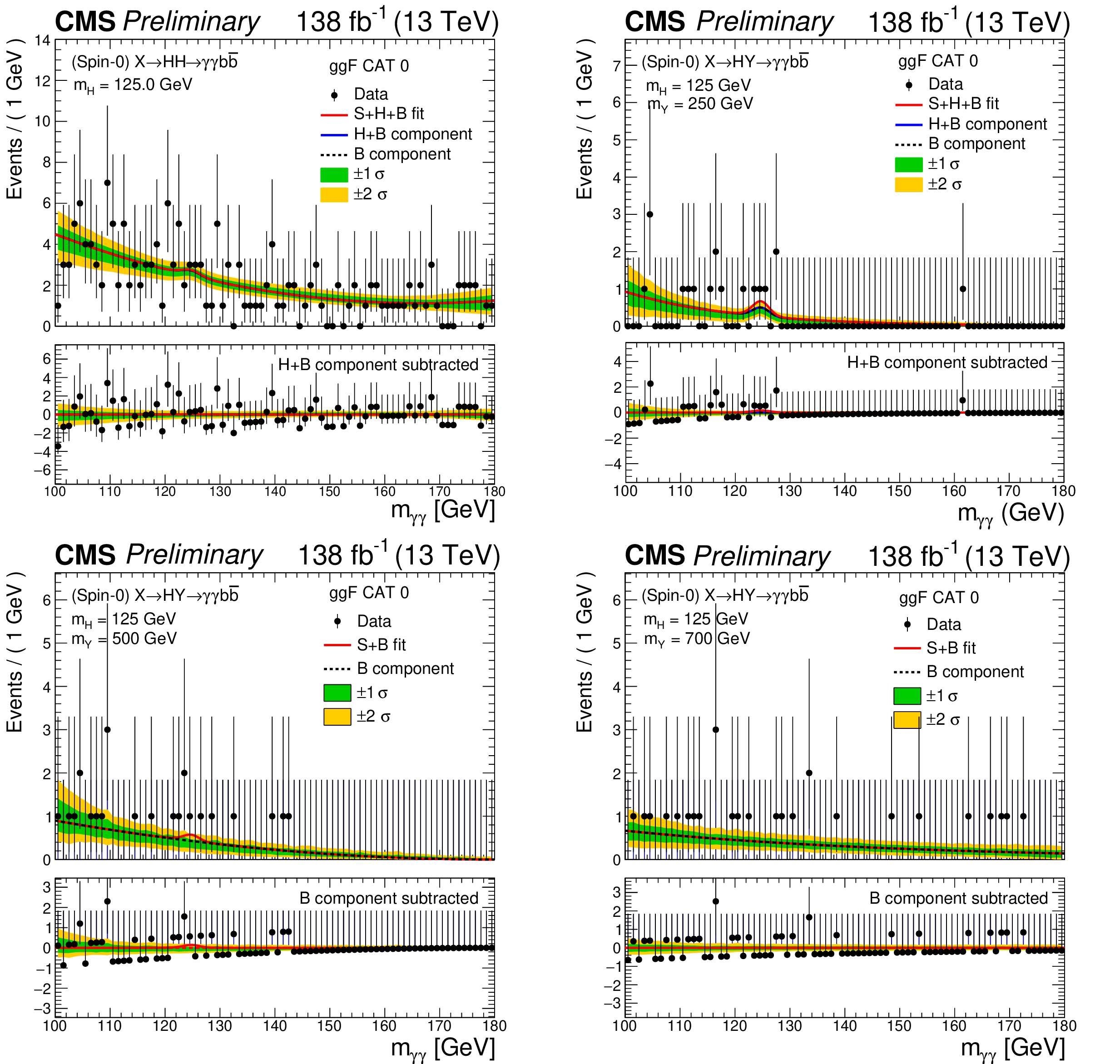
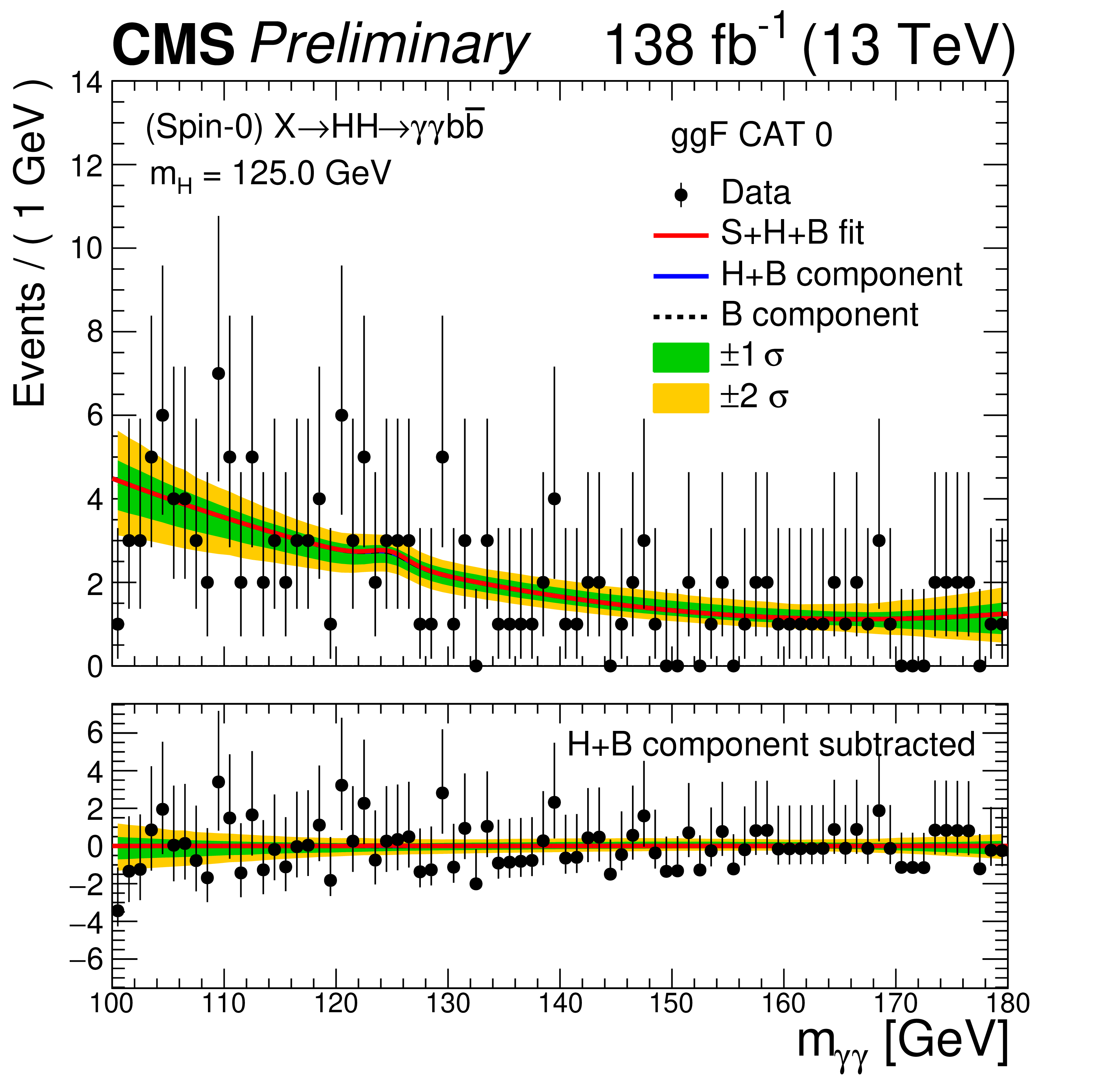
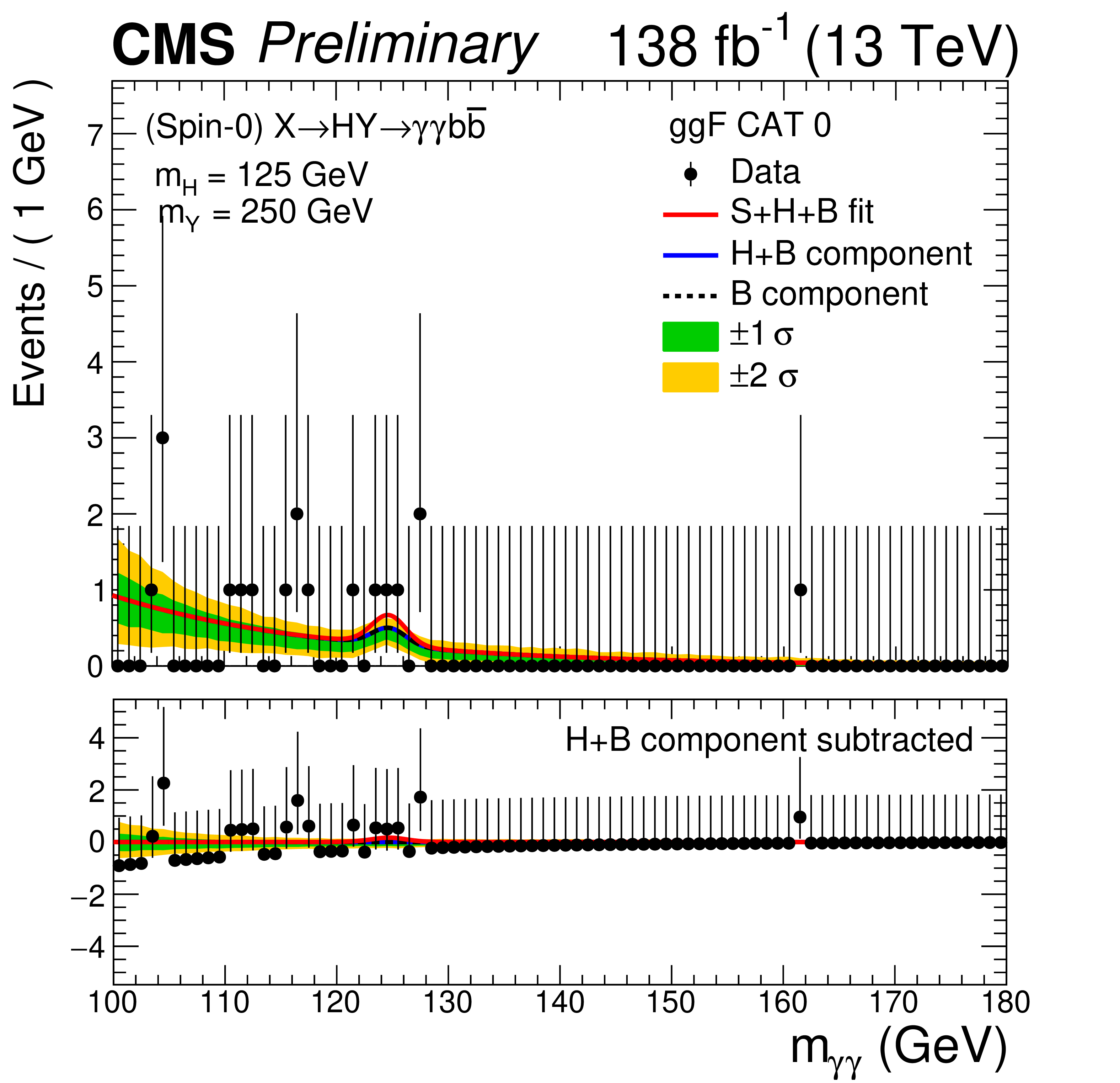
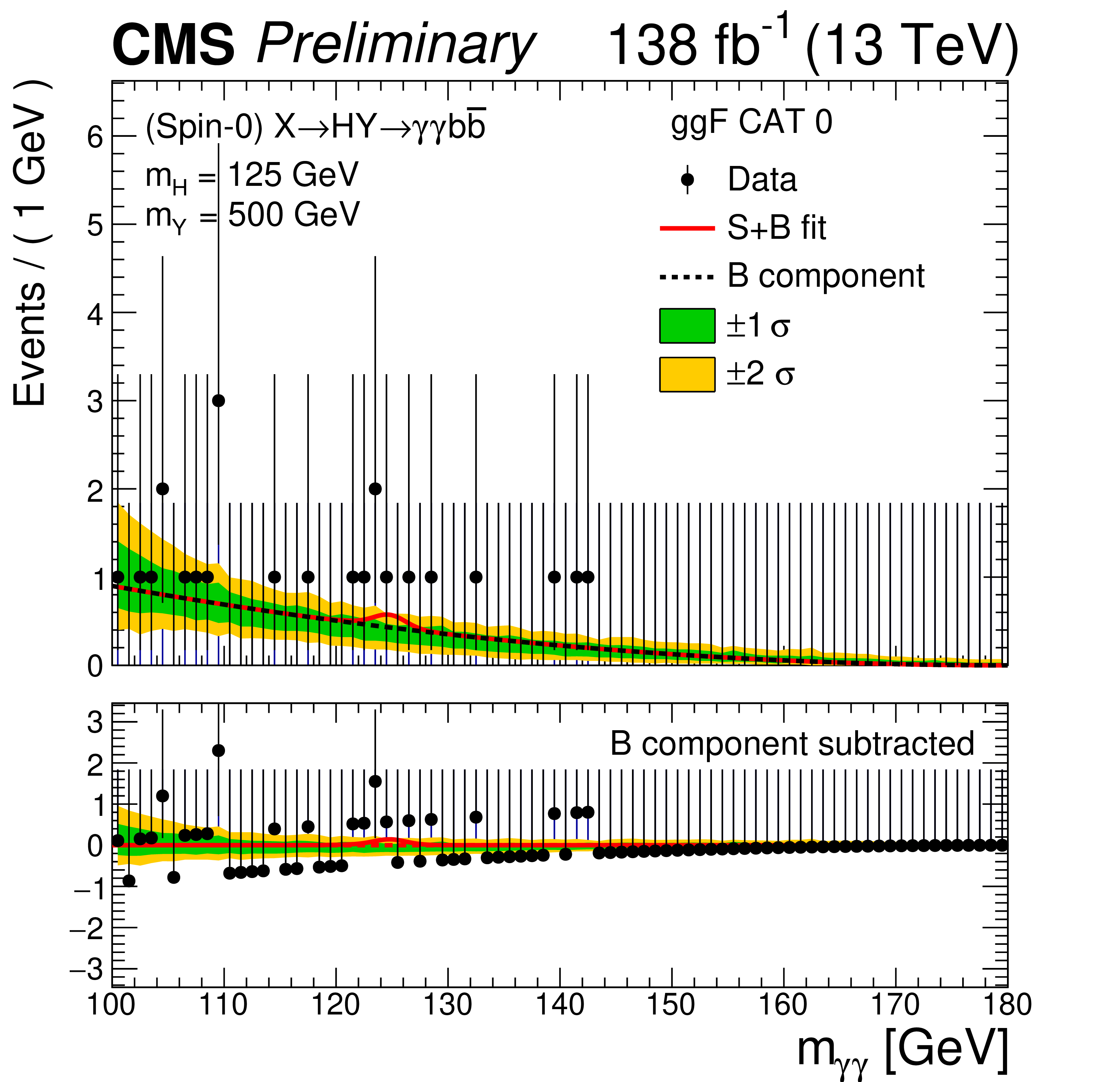
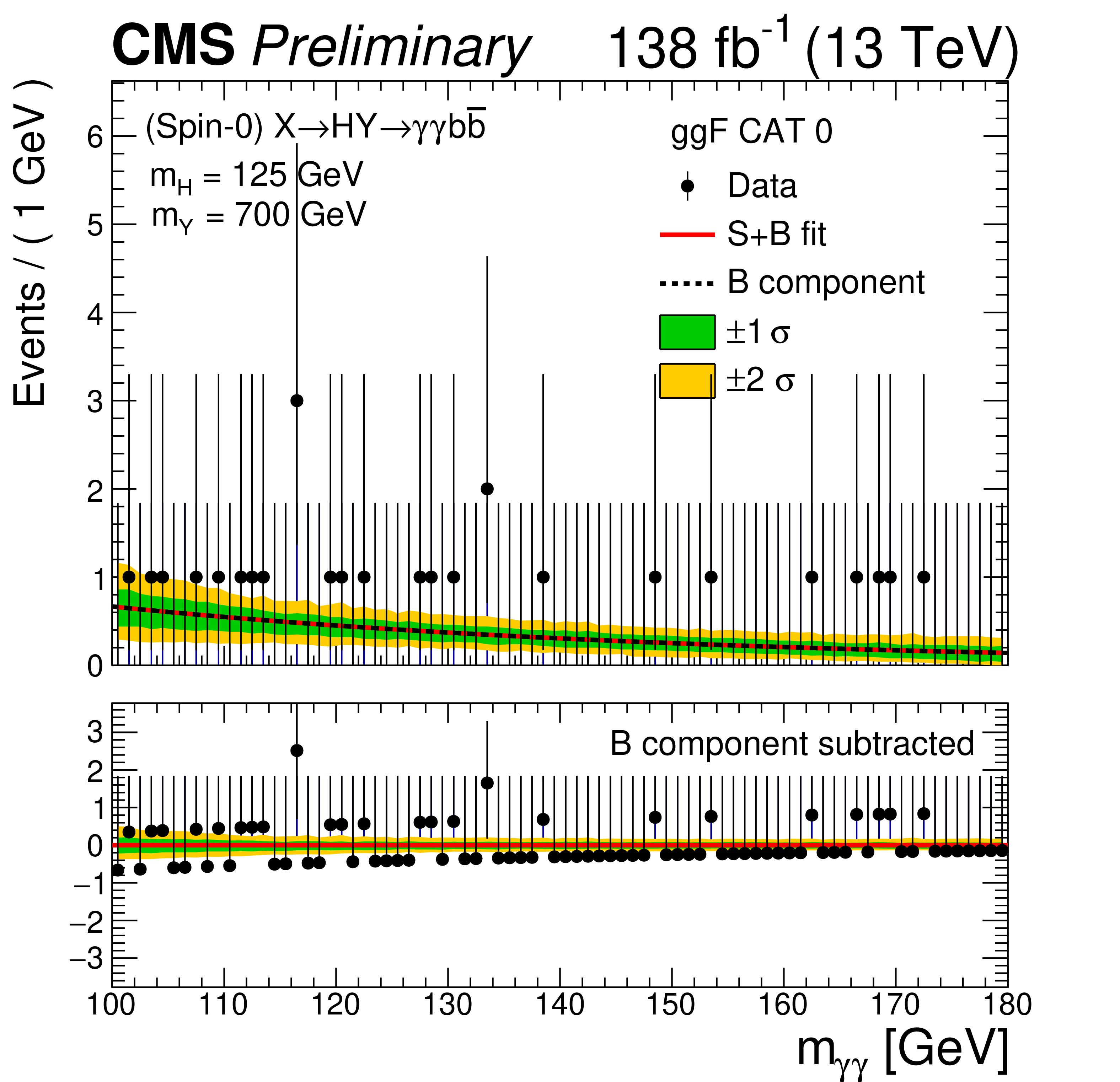
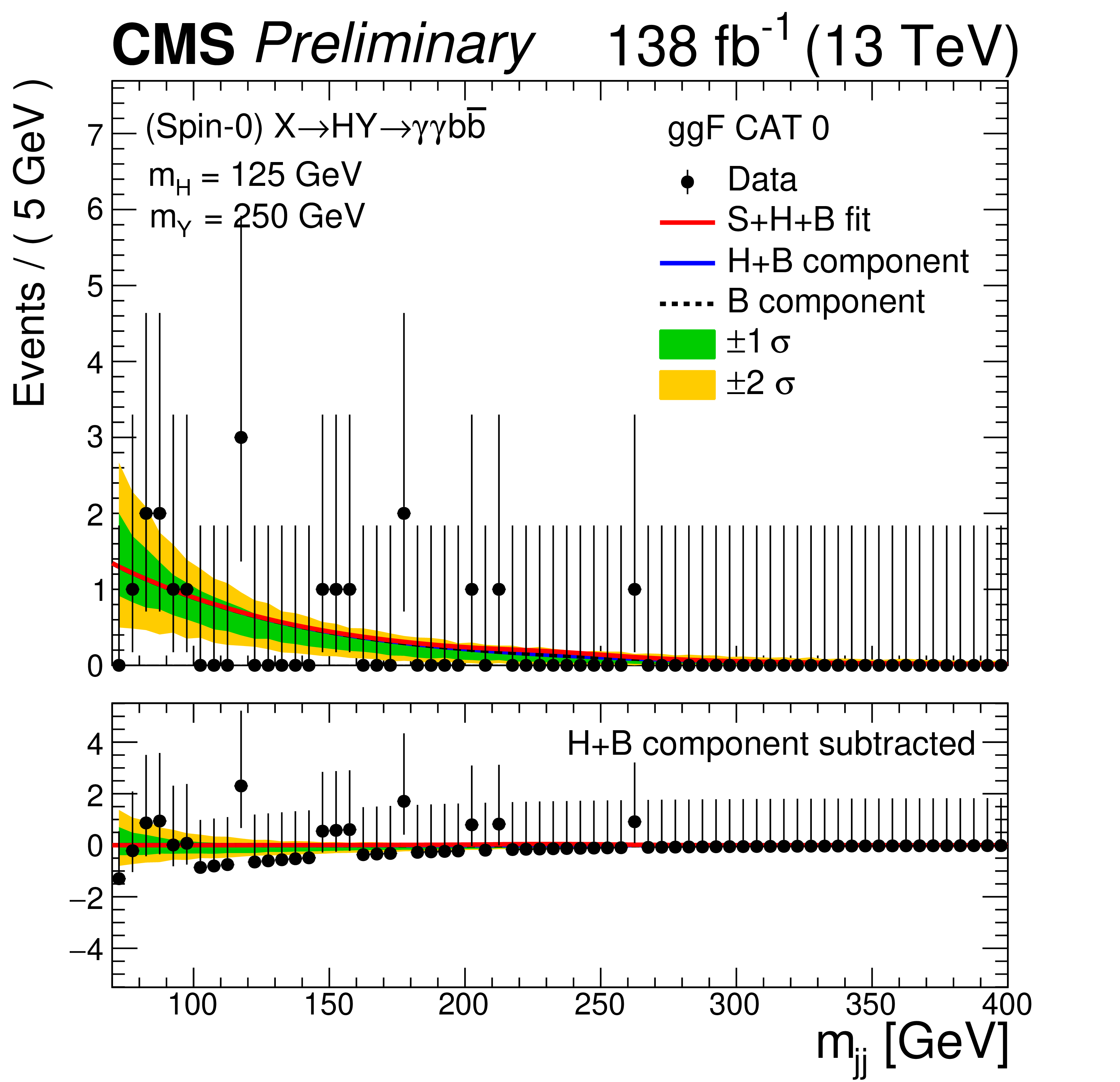
Figure 2:
Invariant mass distributions $ {m_{\gamma \gamma}} $ with the selected data events (black points) for the signal dominated category (CAT 0). The upper left plot represents HH signal and rest of three represent HY signal with ${m_{\mathrm{Y}}} =$ 250, 500 and 700 GeV mass hypotheses, respectively. The solid red line shows the sum of the fitted signal and background events. The solid blue line shows the total background component by summing the resonant and nonresonant background contributions and the dashed black line shows the nonresonant background component. The green and yellow bands represent the 1 and 2 standard deviations which include the uncertainties in fit to the background component. The lower panel in each plot shows the residual signal yield after the background subtraction. |
png pdf |
Figure 2-a:
Invariant mass distributions $ {m_{\gamma \gamma}} $ with the selected data events (black points) for the signal dominated category (CAT 0). The upper left plot represents HH signal and rest of three represent HY signal with ${m_{\mathrm{Y}}} =$ 250, 500 and 700 GeV mass hypotheses, respectively. The solid red line shows the sum of the fitted signal and background events. The solid blue line shows the total background component by summing the resonant and nonresonant background contributions and the dashed black line shows the nonresonant background component. The green and yellow bands represent the 1 and 2 standard deviations which include the uncertainties in fit to the background component. The lower panel in each plot shows the residual signal yield after the background subtraction. |
png pdf |
Figure 2-b:
Invariant mass distributions $ {m_{\gamma \gamma}} $ with the selected data events (black points) for the signal dominated category (CAT 0). The upper left plot represents HH signal and rest of three represent HY signal with ${m_{\mathrm{Y}}} =$ 250, 500 and 700 GeV mass hypotheses, respectively. The solid red line shows the sum of the fitted signal and background events. The solid blue line shows the total background component by summing the resonant and nonresonant background contributions and the dashed black line shows the nonresonant background component. The green and yellow bands represent the 1 and 2 standard deviations which include the uncertainties in fit to the background component. The lower panel in each plot shows the residual signal yield after the background subtraction. |
png pdf |
Figure 2-c:
Invariant mass distributions $ {m_{\gamma \gamma}} $ with the selected data events (black points) for the signal dominated category (CAT 0). The upper left plot represents HH signal and rest of three represent HY signal with ${m_{\mathrm{Y}}} =$ 250, 500 and 700 GeV mass hypotheses, respectively. The solid red line shows the sum of the fitted signal and background events. The solid blue line shows the total background component by summing the resonant and nonresonant background contributions and the dashed black line shows the nonresonant background component. The green and yellow bands represent the 1 and 2 standard deviations which include the uncertainties in fit to the background component. The lower panel in each plot shows the residual signal yield after the background subtraction. |
png pdf |
Figure 2-d:
Invariant mass distributions $ {m_{\gamma \gamma}} $ with the selected data events (black points) for the signal dominated category (CAT 0). The upper left plot represents HH signal and rest of three represent HY signal with ${m_{\mathrm{Y}}} =$ 250, 500 and 700 GeV mass hypotheses, respectively. The solid red line shows the sum of the fitted signal and background events. The solid blue line shows the total background component by summing the resonant and nonresonant background contributions and the dashed black line shows the nonresonant background component. The green and yellow bands represent the 1 and 2 standard deviations which include the uncertainties in fit to the background component. The lower panel in each plot shows the residual signal yield after the background subtraction. |
png pdf |
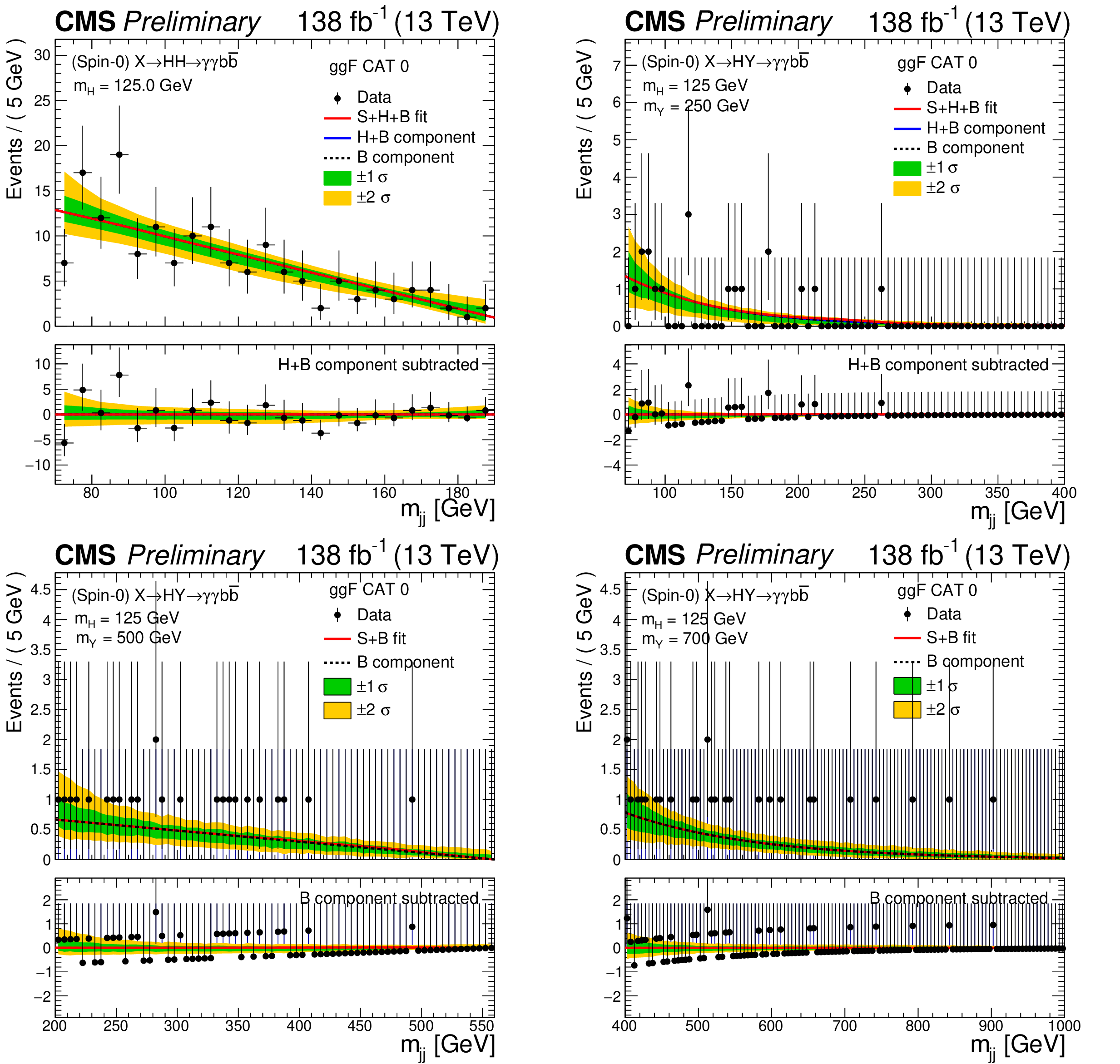
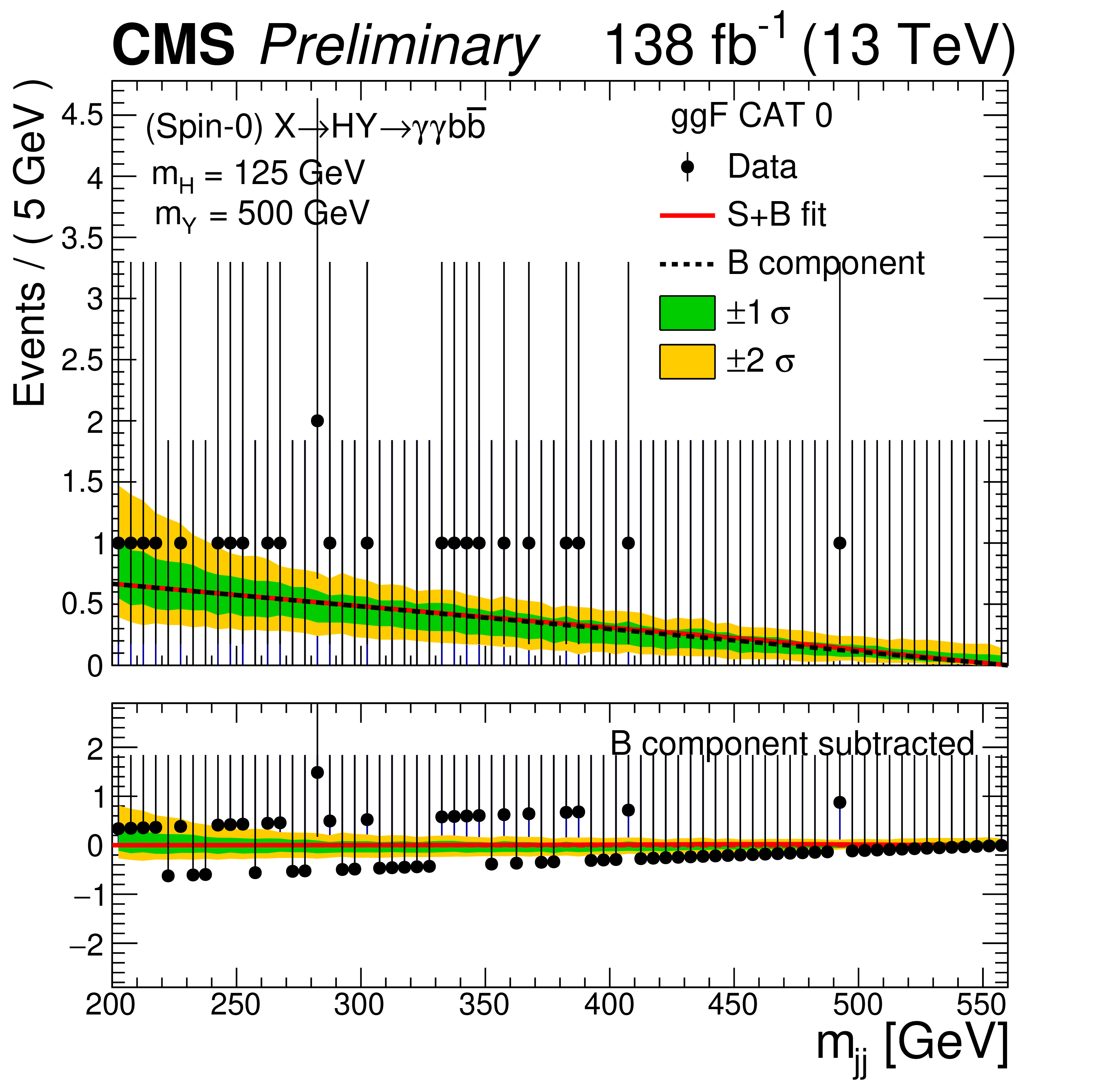
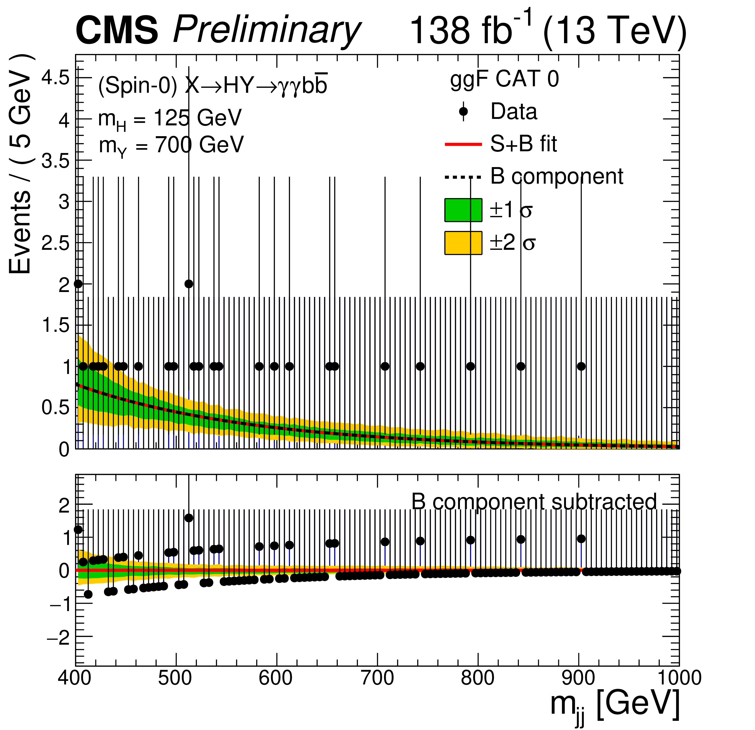
Figure 3:
Invariant mass distributions ${m_\text {jj}}$ with the selected data events (black points) for the signal dominated category (CAT 0). The upper left plot represents HH signal and rest of three represent HY signal with ${m_{\mathrm{Y}}} =$ 250, 500 and 700 GeV mass hypotheses, respectively. The solid red line shows the sum of the fitted signal and background events. The solid blue line shows the total background component by summing the resonant and nonresonant background contributions and the dashed black line shows the nonresonant background component. The green and yellow bands represent the 1 and 2 standard deviations which include the uncertainties in fit to the background component. The lower panel in each plot shows the residual signal yield after the background subtraction. |

png pdf |
Figure 3-a:
Invariant mass distributions ${m_\text {jj}}$ with the selected data events (black points) for the signal dominated category (CAT 0). The upper left plot represents HH signal and rest of three represent HY signal with ${m_{\mathrm{Y}}} =$ 250, 500 and 700 GeV mass hypotheses, respectively. The solid red line shows the sum of the fitted signal and background events. The solid blue line shows the total background component by summing the resonant and nonresonant background contributions and the dashed black line shows the nonresonant background component. The green and yellow bands represent the 1 and 2 standard deviations which include the uncertainties in fit to the background component. The lower panel in each plot shows the residual signal yield after the background subtraction. |
png pdf |
Figure 3-b:
Invariant mass distributions ${m_\text {jj}}$ with the selected data events (black points) for the signal dominated category (CAT 0). The upper left plot represents HH signal and rest of three represent HY signal with ${m_{\mathrm{Y}}} =$ 250, 500 and 700 GeV mass hypotheses, respectively. The solid red line shows the sum of the fitted signal and background events. The solid blue line shows the total background component by summing the resonant and nonresonant background contributions and the dashed black line shows the nonresonant background component. The green and yellow bands represent the 1 and 2 standard deviations which include the uncertainties in fit to the background component. The lower panel in each plot shows the residual signal yield after the background subtraction. |
png pdf |
Figure 3-c:
Invariant mass distributions ${m_\text {jj}}$ with the selected data events (black points) for the signal dominated category (CAT 0). The upper left plot represents HH signal and rest of three represent HY signal with ${m_{\mathrm{Y}}} =$ 250, 500 and 700 GeV mass hypotheses, respectively. The solid red line shows the sum of the fitted signal and background events. The solid blue line shows the total background component by summing the resonant and nonresonant background contributions and the dashed black line shows the nonresonant background component. The green and yellow bands represent the 1 and 2 standard deviations which include the uncertainties in fit to the background component. The lower panel in each plot shows the residual signal yield after the background subtraction. |
png pdf |
Figure 3-d:
Invariant mass distributions ${m_\text {jj}}$ with the selected data events (black points) for the signal dominated category (CAT 0). The upper left plot represents HH signal and rest of three represent HY signal with ${m_{\mathrm{Y}}} =$ 250, 500 and 700 GeV mass hypotheses, respectively. The solid red line shows the sum of the fitted signal and background events. The solid blue line shows the total background component by summing the resonant and nonresonant background contributions and the dashed black line shows the nonresonant background component. The green and yellow bands represent the 1 and 2 standard deviations which include the uncertainties in fit to the background component. The lower panel in each plot shows the residual signal yield after the background subtraction. |

png pdf |
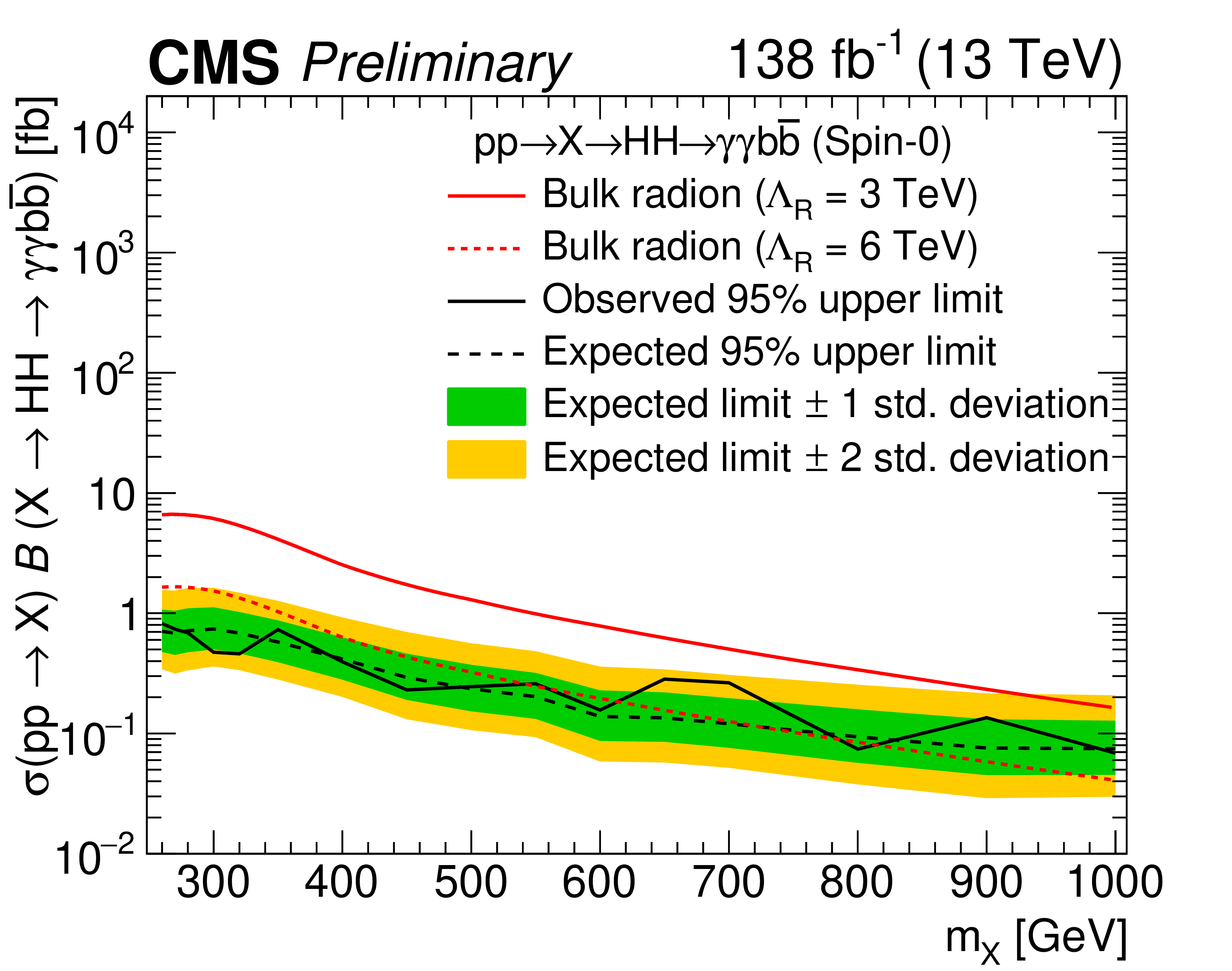
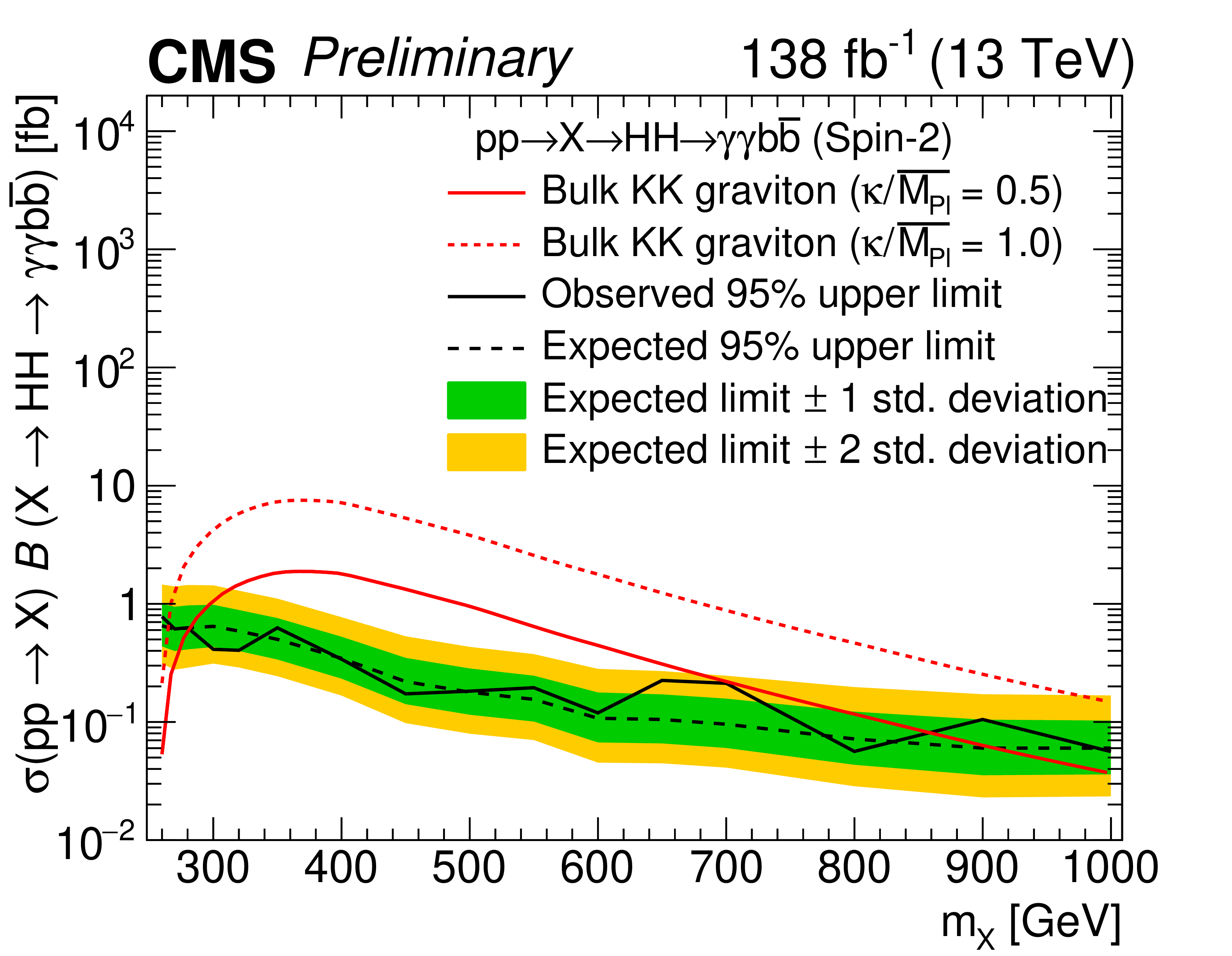
Figure 4:
Expected and observed 95% CL upper limit on product of resonant production cross section and branching fraction for spin-0 (upper plot) and spin-2 (lower plot) ${{\mathrm{p}} {\mathrm{p}} \to \mathrm{X} \to \mathrm{H} \mathrm{H} \to {\gamma \gamma \mathrm{b} {}\mathrm{\bar{b}}}}$ signal hypotheses. The dashed and solid black lines represent expected and observed limits, respectively. The green and yellow bands represent the 1 and 2 standard deviations for the expected limit. The red lines show the theoretical predictions with different energy scales and couplings. |
png pdf |
Figure 4-a:
Expected and observed 95% CL upper limit on product of resonant production cross section and branching fraction for spin-0 (upper plot) and spin-2 (lower plot) ${{\mathrm{p}} {\mathrm{p}} \to \mathrm{X} \to \mathrm{H} \mathrm{H} \to {\gamma \gamma \mathrm{b} {}\mathrm{\bar{b}}}}$ signal hypotheses. The dashed and solid black lines represent expected and observed limits, respectively. The green and yellow bands represent the 1 and 2 standard deviations for the expected limit. The red lines show the theoretical predictions with different energy scales and couplings. |
png pdf |
Figure 4-b:
Expected and observed 95% CL upper limit on product of resonant production cross section and branching fraction for spin-0 (upper plot) and spin-2 (lower plot) ${{\mathrm{p}} {\mathrm{p}} \to \mathrm{X} \to \mathrm{H} \mathrm{H} \to {\gamma \gamma \mathrm{b} {}\mathrm{\bar{b}}}}$ signal hypotheses. The dashed and solid black lines represent expected and observed limits, respectively. The green and yellow bands represent the 1 and 2 standard deviations for the expected limit. The red lines show the theoretical predictions with different energy scales and couplings. |

png pdf |
Figure 5:
The upper plot shows the expected and observed 95% CL exclusion limit on production cross section for ${{\mathrm{p}} {\mathrm{p}} \to \mathrm{X} \to \mathrm{H} \mathrm{Y} \to {\gamma \gamma \mathrm{b} {}\mathrm{\bar{b}}}}$ signal hypothesis. The dashed and solid black lines represent expected and observed limits, respectively. The green and yellow bands represent the 1 and 2 standard deviations for the expected limit. Limits are scaled with the order of 10 depending upon ${m_{\mathrm{X}}}$. |

png pdf |
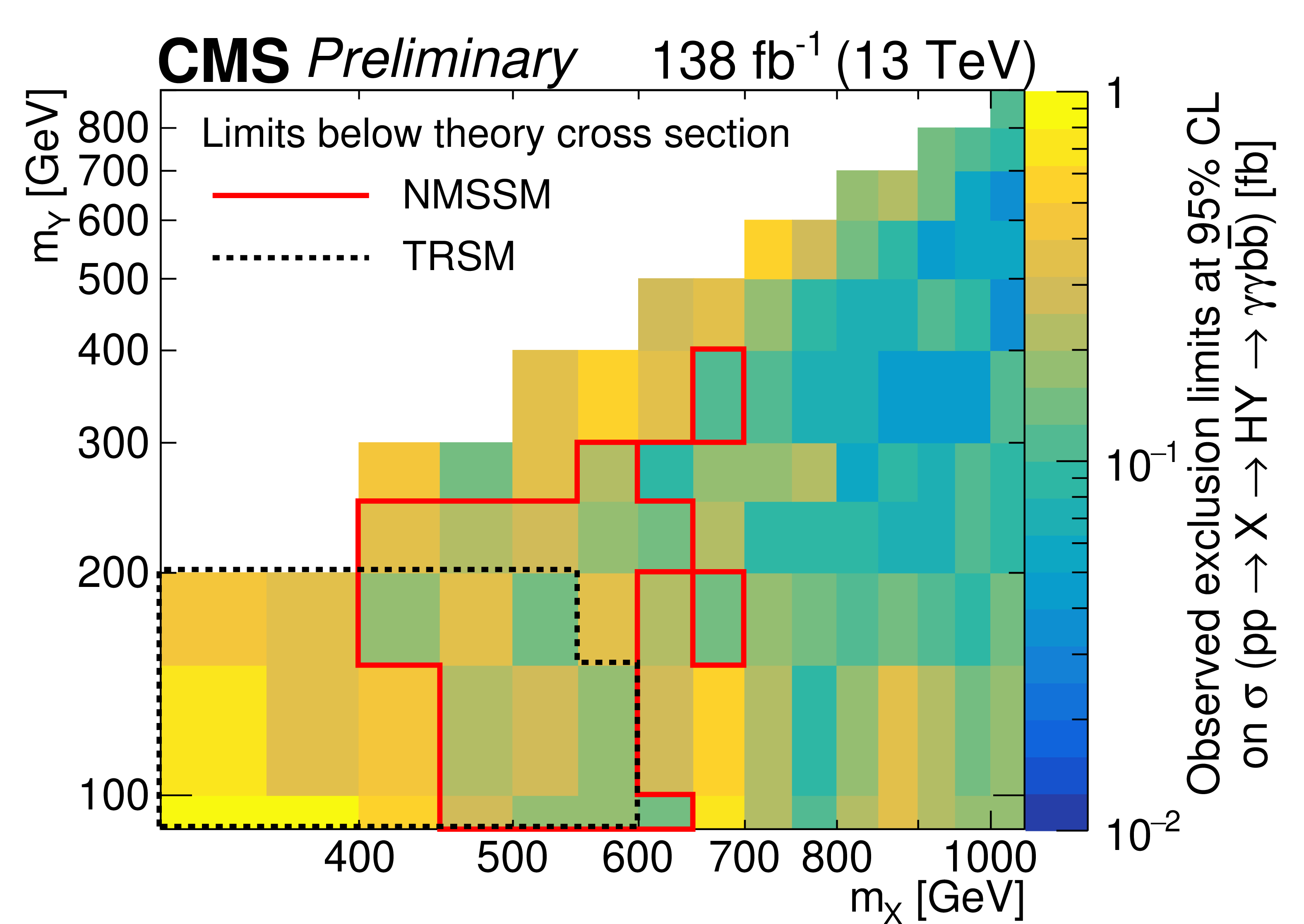
Figure 6:
Interpretations of the HY searches for both expected (left) and observed (right) limits at 95% CL using NMSSM and TRSM models where the red and black lines indicate the excluded mass regions for both, respectively. |

png pdf |
Figure 6-a:
Interpretations of the HY searches for both expected (left) and observed (right) limits at 95% CL using NMSSM and TRSM models where the red and black lines indicate the excluded mass regions for both, respectively. |
png pdf |
Figure 6-b:
Interpretations of the HY searches for both expected (left) and observed (right) limits at 95% CL using NMSSM and TRSM models where the red and black lines indicate the excluded mass regions for both, respectively. |
| Tables | |

png pdf |
Table 1:
Event preselection criteria. |

png pdf |
Table 2:
Event classification. |
| Summary |
| A search for new resonances X decaying either to a pair of Higgs bosons HH, or to a Higgs boson and a new scalar Y, is presented. The search uses data from proton-proton collisions collected by the CMS experiment at LHC in 2016-2018 at a center-of-mass energy of 13 TeV, and corresponding to 138 fb$^{-1}$ of integrated luminosity. The study is motivated from theories related to the warped extra dimension model, the next-to-minimal supersymmetric standard model and the two-real-scalar-singlet model assuming narrow width approximation. For a X decaying to HH, a mass range of 260 GeV-1 TeV is covered, while a X decaying to HY is searched for range 300 GeV-1 TeV in ${m_{\mathrm{X}}}$, considering a mass range 90-800 GeV in ${m_{\mathrm{Y}}}$. The data were found to be compatible with the background-only hypothesis. Results are presented as the upper limits at 95% confidence level on the product of the production cross section of X and its branching fraction to the ${\gamma\gamma\mathrm{b\bar{b}}}$ final state, through either HH or HY. Depending upon the mass range in ${m_{\mathrm{X}}}$, the observed limits for a spin-0 resonance X, decaying to HH, ranges from 0.82-0.07 fb}, while the expected limits are 0.74-0.08 fb. Bulk radions decaying to HH are excluded for masses up to 600 GeV for $\Lambda_{R} = $ 6 TeV, while the mass limit on a bulk KK graviton extends to 850 GeV assuming a coupling factor $\kappa/\overline{M_{pl}}=$ 0.5. For the resonance X decaying to HY, the observed limits are 0.90-0.04 fb, while the expected limits lie in the range 0.79-0.05 fb, depending upon the mass ranges in ${m_{\mathrm{X}}}$ and ${m_{\mathrm{Y}}}$. The largest deviation from background-only hypothesis with local (global) significance of 3.8 (2.8) standard deviations is also observed for ${m_{\mathrm{X}}} = $ 650 GeV and ${m_{\mathrm{Y}}} = $ 90 GeV. The results are interpreted for the NMSSM and the TRSM theories. |
| References | ||||
| 1 | ATLAS Collaboration | Observation of a new particle in the search for the standard model Higgs boson with the ATLAS detector at the LHC | PLB 716 (2012) 1 | 1207.7214 |
| 2 | CMS Collaboration | Observation of a new boson at a mass of 125 GeV with the CMS experiment at the LHC | PLB 716 (2012) 30 | CMS-HIG-12-028 1207.7235 |
| 3 | CMS Collaboration | Observation of a new boson with mass near 125 GeV in pp collisions at $ \sqrt{s} = $ 7 and 8 TeV | JHEP 06 (2013) 081 | CMS-HIG-12-036 1303.4571 |
| 4 | S. Weinberg | A model of leptons | PRL 19 (1967) 1264 | |
| 5 | Sheldon L. Glashow | Partial-symmetries of weak interactions | Nuclear Physics 22 (1961), no. 4, 579 | |
| 6 | G. 't Hooft and M. Veltman | Regularization and renormalization of gauge fields | Nuclear Physics B 44 (1972), no. 1 | |
| 7 | P. W. Higgs | Broken symmetries, massless particles and gauge fields | PL12 (1964) 132 | |
| 8 | P. W. Higgs | Broken symmetries and the masses of gauge bosons | PRL 13 (1964) 508 | |
| 9 | CMS Collaboration | A measurement of the Higgs boson mass in the diphoton decay channel | PLB 805 (2020) 135425 | CMS-HIG-19-004 2002.06398 |
| 10 | L. Randall and R. Sundrum | Large mass hierarchy from a small extra dimension | PRL 83 (1999) 3370 | hep-ph/9905221 |
| 11 | W. D. Goldberger and M. B. Wise | Modulus stabilization with bulk fields | PRL 83 (1999) 4922 | hep-ph/9907447 |
| 12 | C. Csáki, M. Graesser, L. Randall, and J. Terning | Cosmology of brane models with radion stabilization | PRD 62 (2000) 045015 | hep-ph/9911406 |
| 13 | C. Csáki, M. L. Graesser, and G. D. Kribs | Radion dynamics and electroweak physics | PRD 63 (2001) 065002 | hep-th/0008151 |
| 14 | H. Davoudiasl, J. L. Hewett, and T. G. Rizzo | Phenomenology of the Randall--Sundrum Gauge Hierarchy Model | PRL 84 (2000) 2080 | hep-ph/9909255 |
| 15 | O. DeWolfe, D. Z. Freedman, S. S. Gubser, and A. Karch | Modeling the fifth dimension with scalars and gravity | PRD 62 (2000) 046008 | hep-th/9909134 |
| 16 | K. Agashe, H. Davoudiasl, G. Perez, and A. Soni | Warped gravitons at the CERN LHC and beyond | PRD 76 (2007) 036006 | hep-ph/0701186 |
| 17 | Yu. A. Golfand and E. P. Likhtman | Extension of the algebra of Poincaré group generators and violation of p invariance | JEPTL 13 (1971) 323 | |
| 18 | J. Wess and B. Zumino | Supergauge transformations in four-dimensions | NPB 70 (1974) 39 | |
| 19 | P. Fayet | Supergauge invariant extension of the Higgs mechanism and a model for the electron and its neutrino | NPB 90 (1975) 104 | |
| 20 | P. Fayet | Spontaneously broken supersymmetric theories of weak, electromagnetic and strong interactions | PLB 69 (1977) 489 | |
| 21 | U. Ellwanger, C. Hugonie, and A. M. Teixeira | The Next-to-Minimal Supersymmetric Standard Model | PR 496 (2010) 1 | 0910.1785 |
| 22 | M. Maniatis | The Next-to-Minimal Supersymmetric extension of the Standard Model reviewed | Int. J. Mod. Phys. A 25 (2010) 3505 | 0906.0777 |
| 23 | J. E. Kim and H. P. Nilles | The $ \mu $-problem and the strong CP problem | PLB 138 (1984) 150 | |
| 24 | T. Robens, T. Stefaniak, and J. Wittbrodt | Two-real-scalar-singlet extension of the SM: LHC phenomenology and benchmark scenarios | EPJC 80 (2020), no. 2, 151 | 1908.08554 |
| 25 | CMS Collaboration | Search for Higgs boson pair production in the $ \gamma\gamma\mathrm{b\overline{b}} $ final state in pp collisions at $ \sqrt{s}= $ 13 TeV | PLB 788 (2019) 7 | CMS-HIG-17-008 1806.00408 |
| 26 | CMS Collaboration | Search for nonresonant Higgs boson pair production in final states with two bottom quarks and two photons in proton-proton collisions at $ \sqrt{s} = $ 13 TeV | JHEP 03 (2021) 257 | CMS-HIG-19-018 2011.12373 |
| 27 | CMS Collaboration | The CMS experiment at the CERN LHC | JINST 3 (2008) S08004 | CMS-00-001 |
| 28 | CMS Collaboration | The CMS trigger system | JINST 12 (2017) P01020 | CMS-TRG-12-001 1609.02366 |
| 29 | CMS Collaboration | The CMS high level trigger | EPJC 46 (2006) 605 | hep-ex/0512077 |
| 30 | CMS Collaboration | Particle-flow reconstruction and global event description with the cms detector | JINST 12 (2017) P10003 | CMS-PRF-14-001 1706.04965 |
| 31 | M. Cacciari, G. P. Salam, and G. Soyez | The anti-$ {k_{\mathrm{T}}} $ jet clustering algorithm | JHEP 04 (2008) 063 | 0802.1189 |
| 32 | M. Cacciari, G. P. Salam, and G. Soyez | FastJet user manual | EPJC 72 (2012) 1896 | 1111.6097 |
| 33 | CMS Collaboration | Jet energy scale and resolution in the CMS experiment in pp collisions at 8 TeV | JINST 12 (2017) P02014 | CMS-JME-13-004 1607.03663 |
| 34 | CMS Collaboration | Performance of missing transverse momentum reconstruction in proton-proton collisions at $ \sqrt{s} = $ 13 TeV using the CMS detector | JINST 14 (2019) P07004 | CMS-JME-17-001 1903.06078 |
| 35 | CMS Collaboration | Precision luminosity measurement in proton-proton collisions at $ \sqrt{s} = $ 13 TeV in 2015 and 2016 at CMS | EPJC 81 (2021) 800 | CMS-LUM-17-003 2104.01927 |
| 36 | CMS Collaboration | CMS luminosity measurement for the 2017 data taking period at $ \sqrt{s} = $ 13 TeV | CMS-PAS-LUM-17-004 | CMS-PAS-LUM-17-004 |
| 37 | CMS Collaboration | CMS luminosity measurement for the 2018 data-taking period at $ \sqrt{s} = $ 13 TeV | CMS-PAS-LUM-18-002 | CMS-PAS-LUM-18-002 |
| 38 | CMS Collaboration | Measurements of Higgs boson properties in the diphoton decay channel in proton-proton collisions at $ \sqrt{s} = $ 13 TeV | JHEP 11 (2018) 185 | CMS-HIG-16-040 1804.02716 |
| 39 | J. Alwall et al. | The automated computation of tree-level and next-to-leading order differential cross sections, and their matching to parton shower simulations | JHEP 07 (2014) 079 | 1405.0301 |
| 40 | A. Alloul et al. | FeynRules 2.0 - A complete toolbox for tree-level phenomenology | CPC 185 (2014) 2250 | 1310.1921 |
| 41 | T. Gleisberg et al. | Event generation with SHERPA 1.1 | JHEP 02 (2009) 007 | 0811.4622 |
| 42 | T. Sjostrand et al. | An introduction to PYTHIA 8.2 | CPC 191 (2015) 159 | 1410.3012 |
| 43 | P. Nason | A new method for combining NLO QCD with shower Monte Carlo algorithms | JHEP 11 (2004) 040 | hep-ph/0409146 |
| 44 | S. Frixione, P. Nason, and C. Oleari | Matching NLO QCD computations with Parton Shower simulations: the POWHEG method | JHEP 11 (2007) 070 | 0709.2092 |
| 45 | S. Alioli, P. Nason, C. Oleari, and E. Re | A general framework for implementing NLO calculations in shower Monte Carlo programs: the POWHEG BOX | JHEP 06 (2010) 043 | 1002.2581 |
| 46 | E. Bagnaschi, G. Degrassi, P. Slavich, and A. Vicini | Higgs production via gluon fusion in the POWHEG approach in the SM and in the MSSM | JHEP 02 (2012) 088 | 1111.2854 |
| 47 | M. Wiesemann et al. | Higgs production in association with bottom quarks | JHEP 02 (2015) | |
| 48 | D. de Florian et al. | Handbook of LHC Higgs cross sections: 4. Deciphering the nature of the Higgs sector | CERN-2017-002-M | 1610.07922 |
| 49 | CMS Collaboration | Event generator tunes obtained from underlying event and multiparton scattering measurements | EPJC 76 (2016) 155 | CMS-GEN-14-001 1512.00815 |
| 50 | CMS Collaboration | Extraction and validation of a new set of CMS PYTHIA8 tunes from underlying-event measurements | EPJC 80 (2020) 4 | CMS-GEN-17-001 1903.12179 |
| 51 | NNPDF Collaboration | Parton distributions for the LHC Run II | JHEP 04 (2015) 040 | 1410.8849 |
| 52 | NNPDF Collaboration | Parton distributions from high-precision collider data | EPJC 77 (2017) 663 | 1706.00428 |
| 53 | S. Carrazza, J. I. Latorre, J. Rojo, and G. Watt | A compression algorithm for the combination of PDF sets | EPJC 75 (2015) 474 | 1504.06469 |
| 54 | J. Butterworth et al. | PDF4LHC recommendations for LHC Run II | JPG 43 (2016) 023001 | 1510.03865 |
| 55 | S. Dulat et al. | New parton distribution functions from a global analysis of quantum chromodynamics | PRD 93 (2016) 033006 | 1506.07443 |
| 56 | L. A. Harland-Lang, A. D. Martin, P. Motylinski, and R. S. Thorne | Parton distributions in the LHC era: MMHT 2014 PDFs | EPJC 75 (2015) 204 | 1412.3989 |
| 57 | GEANT4 Collaboration | GEANT4---a simulation toolkit | NIMA 506 (2003) 250 | |
| 58 | N. Kumar and S. P. Martin | LHC search for di-Higgs decays of stoponium and other scalars in events with two photons and two bottom jets | PRD 90 (2014) 055007 | 1404.0996 |
| 59 | E. Spyromitros-Xioufis, G. Tsoumakas, W. Groves, and I. Vlahavas | Multi-target regression via input space expansion: treating targets as inputs | Machine Learning 104 (2016) 55 | 1211.6581 |
| 60 | CMS Collaboration | Observation of the diphoton decay of the Higgs boson and measurement of its properties | EPJC 74 (2014) 3076 | CMS-HIG-13-001 1407.0558 |
| 61 | CMS Collaboration | Pileup mitigation at CMS in 13 TeV data | JINST 15 (2020) P09018 | CMS-JME-18-001 2003.00503 |
| 62 | B. Vormwald | The CMS phase-1 pixel detector - experience and lessons learned from two years of operation | JINST 14 (2019) C07008 | |
| 63 | CMS Collaboration | Identification of heavy-flavour jets with the CMS detector in pp collisions at 13 TeV | JINST 13 (2018), no. 05, P05011 | CMS-BTV-16-002 1712.07158 |
| 64 | E. Bols et al. | Jet Flavour Classification Using DeepJet | JINST 15 (2020), no. 12, P12012 | 2008.10519 |
| 65 | CMS Collaboration | Performance of the DeepJet b tagging algorithm using 41.9/fb of data from proton-proton collisions at 13 TeV with Phase 1 CMS detector | CDS | |
| 66 | CMS Collaboration | Determination of jet energy calibration and transverse momentum resolution in CMS | JINST 6 (2011) P11002 | CMS-JME-10-011 1107.4277 |
| 67 | CMS Collaboration | A deep neural network for simultaneous estimation of b jet energy and resolution | Comput. Softw. Big Sci. 4 (2020) 10 | CMS-HIG-18-027 1912.06046 |
| 68 | T. Chen and C. Guestrin | XGBoost: A scalable tree boosting system | in Proceedings of the 22nd ACM SIGKDD International Conference on Knowledge Discovery and Data Mining, KDD, New York 2016 | |
| 69 | M. Gouzevitch et al. | Scale-invariant resonance tagging in multijet events and new physics in Higgs pair production | JHEP 07 (2013) 148 | 1303.6636 |
| 70 | T. Hastie, R. Tibshirani, and J. Friedman | The elements of statistical learning | Springer-Verlag New York, 2nd edition | |
| 71 | G. Punzi | Sensitivity of searches for new signals and its Optimization | in Statistical Problems in Particle Physics, Astrophysics, and Cosmology, L. Lyons, R. Mount, and R. Reitmeyer, eds, 2003 | physics/0308063 |
| 72 | R. Brun and F. Rademakers | ROOT: An object oriented data analysis framework | NIMA 389 (1997) 81 | |
| 73 | P. D. Dauncey, M. Kenzie, N. Wardle, and G. J. Davies | Handling uncertainties in background shapes: the discrete profiling method | JINST 10 (2015) P04015 | 1408.6865 |
| 74 | D. L. H.-V. Richard G. Lomax | Statistical Concepts - A Second Course | Routledge New York, 4th edition | |
| 75 | CMS Collaboration | Jet algorithms performance in 13 TeV data | CMS-PAS-JME-16-003 | CMS-PAS-JME-16-003 |
| 76 | CMS Collaboration | Measurement of the Inclusive $ W $ and $ Z $ Production Cross Sections in pp Collisions at $ \sqrt{s}= $ 7 ~TeV | JHEP 10 (2011) 132 | CMS-EWK-10-005 1107.4789 |
| 77 | CMS Collaboration | Performance of photon reconstruction and identification with the CMS detector in proton-proton collisions at $ \sqrt{s} = $ 8 TeV | JINST 10 (2015) P08010 | CMS-EGM-14-001 1502.02702 |
| 78 | T. Junk | Confidence level computation for combining searches with small statistics | NIMA 434 (1999) 435 | hep-ex/9902006 |
| 79 | A. L. Read | Presentation of search results: the CL$ _s $ technique | JPG 28 (2002) 2693 | |
| 80 | G. Cowan, K. Cranmer, E. Gross, and O. Vitells | Asymptotic formulae for likelihood-based tests of new physics | EPJC 71 (2011) 1554 | 1007.1727 |
| 81 | ATLAS and CMS Collaboration | Procedure for the LHC Higgs boson search combination in Summer 2011 | technical report, CERN, Aug | |
| 82 | E. Gross and O. Vitells | Trial factors for the look elsewhere effect in high energy physics | EPJC 70 (2010) 525 | 1005.1891 |
| 83 | CMS Collaboration | Searches for additional Higgs bosons and vector leptoquarks in $ \tau\tau $ final states in proton-proton collisions at $ \sqrt{s}= $ 13 TeV | CMS-PAS-HIG-21-001 | CMS-PAS-HIG-21-001 |
| 84 | CMS Collaboration | Search for high mass resonances decaying into $ \mathrm{W^+}\mathrm{W^-} $ in the dileptonic final state with 138 fb$^{-1} $ of proton-proton collisions at $ \sqrt{s}= $ 13 TeV | CMS-PAS-HIG-20-016 | CMS-PAS-HIG-20-016 |
| 85 | CMS Collaboration | Search for a standard model-like Higgs boson in the mass range between 70 and 110 GeV in the diphoton final state in proton-proton collisions at $ \sqrt{s}= $ 8 and 13 TeV | PLB 793 (2019) 320 | CMS-HIG-17-013 1811.08459 |
|
|
Compact Muon Solenoid LHC, CERN |
|

|

|

|

|

|