

Compact Muon Solenoid
LHC, CERN
| CMS-PAS-HIG-21-003 | ||
| Search for exotic decay of the Higgs boson into two light pseudoscalars with four photons in the final state at $\sqrt{s} = $ 13 TeV | ||
| CMS Collaboration | ||
| July 2021 | ||
| Abstract: A search for exotic decays of the Higgs boson to a pair of light pseudoscalars, each of which subsequently decay to a pair of photons, is presented. The search uses data from proton-proton collisions at $\sqrt{s} = $ 13 TeV recorded with the CMS detector at the LHC, corresponding to an integrated luminosity of 132 fb$^{-1}$. The analysis considers inclusive production mode of the Higgs boson, and probes pseudoscalars ($a$) that range in mass from 15 $ < m_{a} < $ 60 GeV, and leads to four well isolated photons in the final state. No significant deviation from the background-only hypothesis is observed, and upper limits are set on the product of the Higgs boson production cross section and branching fraction into four photons. The observed (expected) limits range from 0.80 (1.00) fb for $m_{a} = $ 15 GeV to 0.33 (0.30) fb for $m_{a} = $ 60 GeV at the 95% confidence level. | ||
|
Links:
CDS record (PDF) ;
CADI line (restricted) ;
These preliminary results are superseded in this paper, Submitted to JHEP. The superseded preliminary plots can be found here. |
||
| Figures | |

png pdf |
Figure 1:
Feynman diagram for BSM decay of the Higgs boson into a pair of light pseudoscalars, which further decay to photons. |

png pdf |
Figure 2:
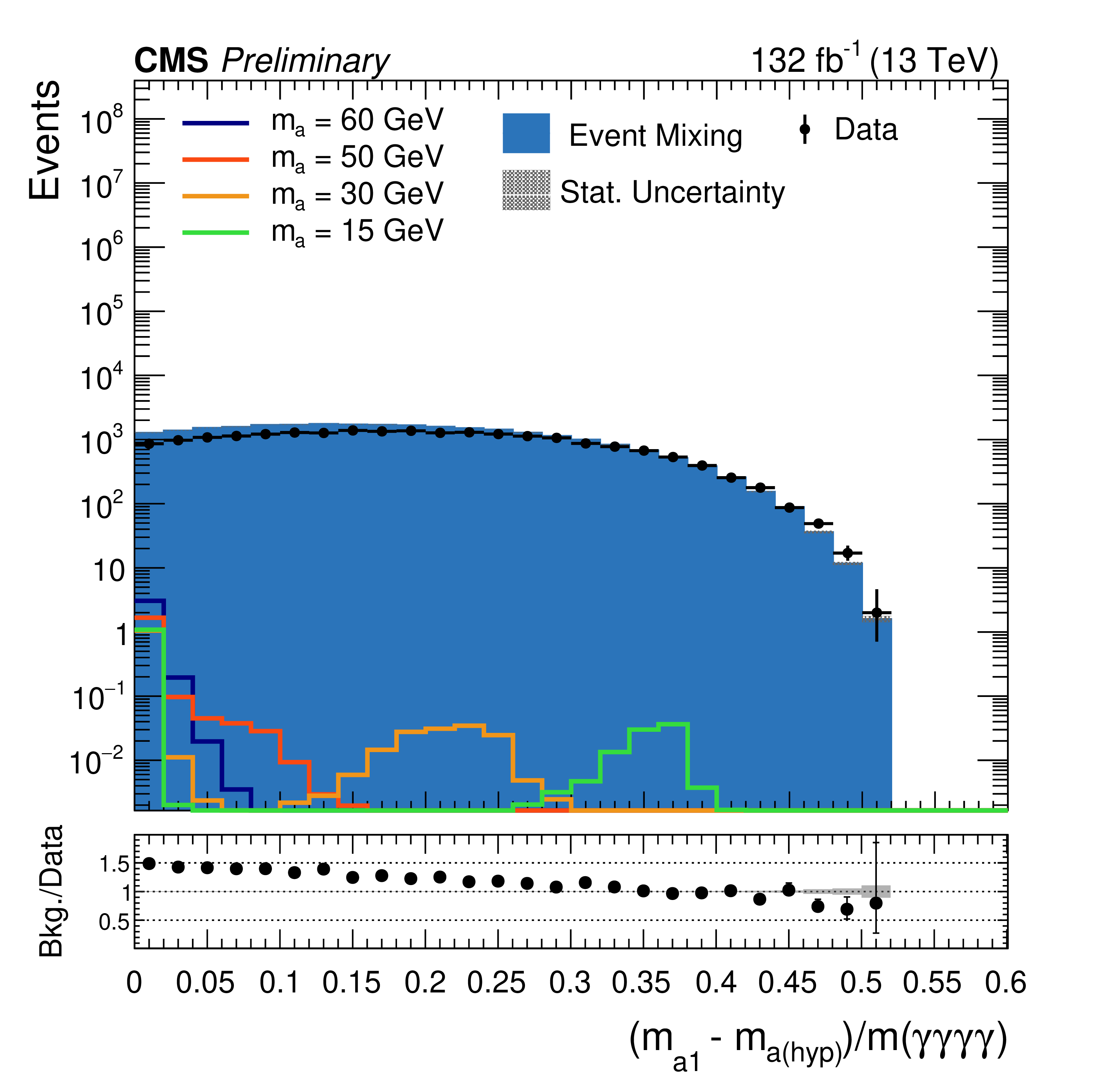
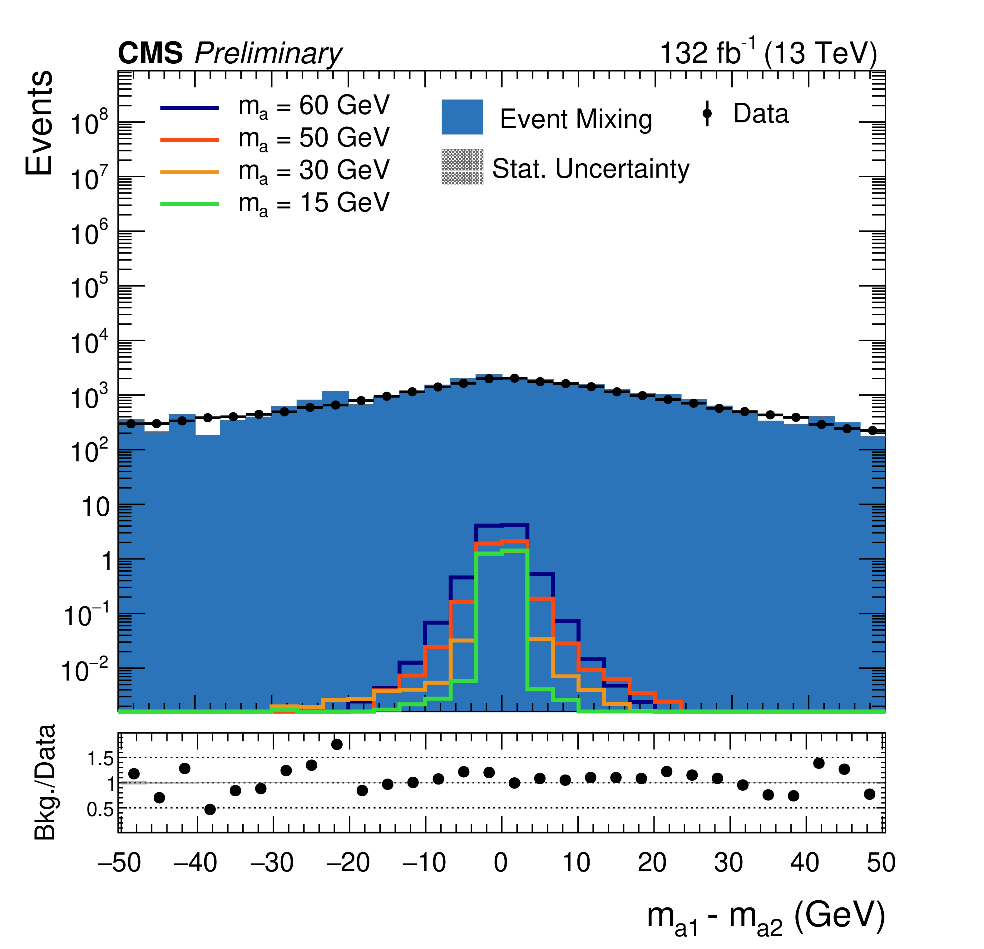
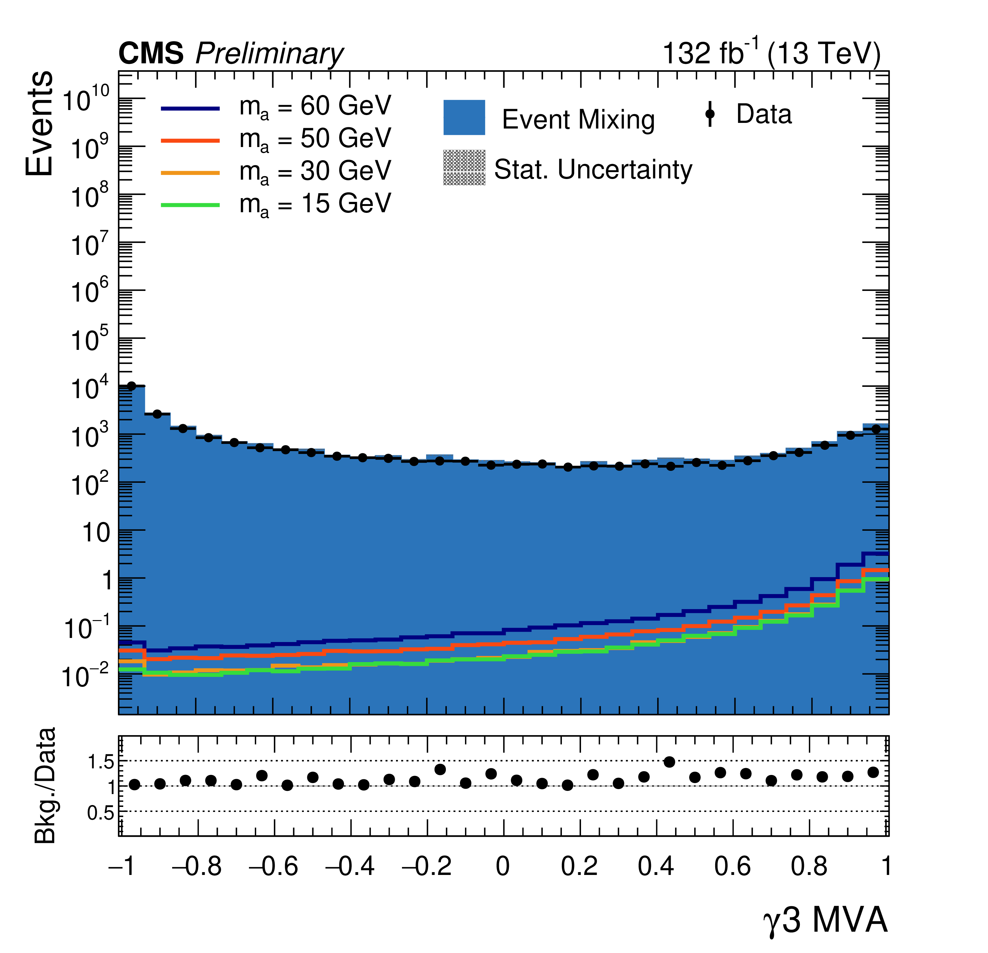
Distributions of the four most highly ranked discriminating variables: difference between invariant mass of the pseudoscalar and the m(a)$_{hyp}$ parameter divided by the invariant mass of the four-photon system (top left), difference between invariant mass of the pseudoscalars (top right), photon ID of the 3rd photon (bottom left), and photon ID of the 4th photon (bottom right). Events shown are selected after fulfilling the selection criteria described in Section 4, and from the ${m_{\gamma \gamma \gamma \gamma}}$ sidebands, satisfying either 110 $ < {m_{\gamma \gamma \gamma \gamma}} < $ 115 GeV or 135 $ < {m_{\gamma \gamma \gamma \gamma}} < $ 180 GeV. The output of the BDT for the signal simulated at various pseudoscalar mass hypotheses are also shown. The disagreement between event mixing data set and data only results in a sub-optimal performance of the classifier and does not induce any biases in the analysis. |
png pdf |
Figure 2-a:
Distributions of the four most highly ranked discriminating variables: difference between invariant mass of the pseudoscalar and the m(a)$_{hyp}$ parameter divided by the invariant mass of the four-photon system (top left), difference between invariant mass of the pseudoscalars (top right), photon ID of the 3rd photon (bottom left), and photon ID of the 4th photon (bottom right). Events shown are selected after fulfilling the selection criteria described in Section 4, and from the ${m_{\gamma \gamma \gamma \gamma}}$ sidebands, satisfying either 110 $ < {m_{\gamma \gamma \gamma \gamma}} < $ 115 GeV or 135 $ < {m_{\gamma \gamma \gamma \gamma}} < $ 180 GeV. The output of the BDT for the signal simulated at various pseudoscalar mass hypotheses are also shown. The disagreement between event mixing data set and data only results in a sub-optimal performance of the classifier and does not induce any biases in the analysis. |
png pdf |
Figure 2-b:
Distributions of the four most highly ranked discriminating variables: difference between invariant mass of the pseudoscalar and the m(a)$_{hyp}$ parameter divided by the invariant mass of the four-photon system (top left), difference between invariant mass of the pseudoscalars (top right), photon ID of the 3rd photon (bottom left), and photon ID of the 4th photon (bottom right). Events shown are selected after fulfilling the selection criteria described in Section 4, and from the ${m_{\gamma \gamma \gamma \gamma}}$ sidebands, satisfying either 110 $ < {m_{\gamma \gamma \gamma \gamma}} < $ 115 GeV or 135 $ < {m_{\gamma \gamma \gamma \gamma}} < $ 180 GeV. The output of the BDT for the signal simulated at various pseudoscalar mass hypotheses are also shown. The disagreement between event mixing data set and data only results in a sub-optimal performance of the classifier and does not induce any biases in the analysis. |
png pdf |
Figure 2-c:
Distributions of the four most highly ranked discriminating variables: difference between invariant mass of the pseudoscalar and the m(a)$_{hyp}$ parameter divided by the invariant mass of the four-photon system (top left), difference between invariant mass of the pseudoscalars (top right), photon ID of the 3rd photon (bottom left), and photon ID of the 4th photon (bottom right). Events shown are selected after fulfilling the selection criteria described in Section 4, and from the ${m_{\gamma \gamma \gamma \gamma}}$ sidebands, satisfying either 110 $ < {m_{\gamma \gamma \gamma \gamma}} < $ 115 GeV or 135 $ < {m_{\gamma \gamma \gamma \gamma}} < $ 180 GeV. The output of the BDT for the signal simulated at various pseudoscalar mass hypotheses are also shown. The disagreement between event mixing data set and data only results in a sub-optimal performance of the classifier and does not induce any biases in the analysis. |

png pdf |
Figure 2-d:
Distributions of the four most highly ranked discriminating variables: difference between invariant mass of the pseudoscalar and the m(a)$_{hyp}$ parameter divided by the invariant mass of the four-photon system (top left), difference between invariant mass of the pseudoscalars (top right), photon ID of the 3rd photon (bottom left), and photon ID of the 4th photon (bottom right). Events shown are selected after fulfilling the selection criteria described in Section 4, and from the ${m_{\gamma \gamma \gamma \gamma}}$ sidebands, satisfying either 110 $ < {m_{\gamma \gamma \gamma \gamma}} < $ 115 GeV or 135 $ < {m_{\gamma \gamma \gamma \gamma}} < $ 180 GeV. The output of the BDT for the signal simulated at various pseudoscalar mass hypotheses are also shown. The disagreement between event mixing data set and data only results in a sub-optimal performance of the classifier and does not induce any biases in the analysis. |

png pdf |
Figure 3:
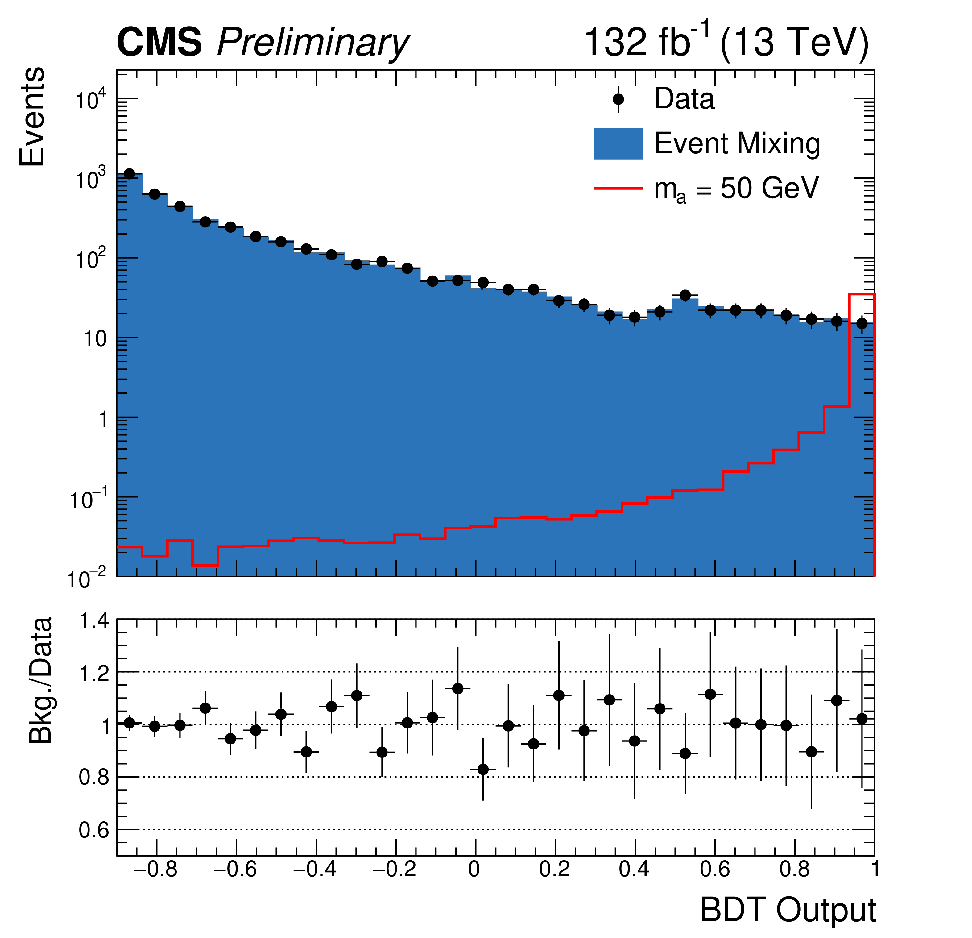
Distribution of the BDT output for ${m_{a}} = $ 15 GeV (left) and 50 GeV (right) in data and simulated events. Events shown are selected after fulfilling the selection criteria described in Section 4, and from the ${m_{\gamma \gamma \gamma \gamma}} $ sidebands, satisfying either 110 $ < m_{\gamma \gamma \gamma \gamma} < $ 115 GeV or 135 $ < m_{\gamma \gamma \gamma \gamma} < $ 180 GeV. |

png pdf |
Figure 3-a:
Distribution of the BDT output for ${m_{a}} = $ 15 GeV (left) and 50 GeV (right) in data and simulated events. Events shown are selected after fulfilling the selection criteria described in Section 4, and from the ${m_{\gamma \gamma \gamma \gamma}} $ sidebands, satisfying either 110 $ < m_{\gamma \gamma \gamma \gamma} < $ 115 GeV or 135 $ < m_{\gamma \gamma \gamma \gamma} < $ 180 GeV. |
png pdf |
Figure 3-b:
Distribution of the BDT output for ${m_{a}} = $ 15 GeV (left) and 50 GeV (right) in data and simulated events. Events shown are selected after fulfilling the selection criteria described in Section 4, and from the ${m_{\gamma \gamma \gamma \gamma}} $ sidebands, satisfying either 110 $ < m_{\gamma \gamma \gamma \gamma} < $ 115 GeV or 135 $ < m_{\gamma \gamma \gamma \gamma} < $ 180 GeV. |

png pdf |
Figure 4:
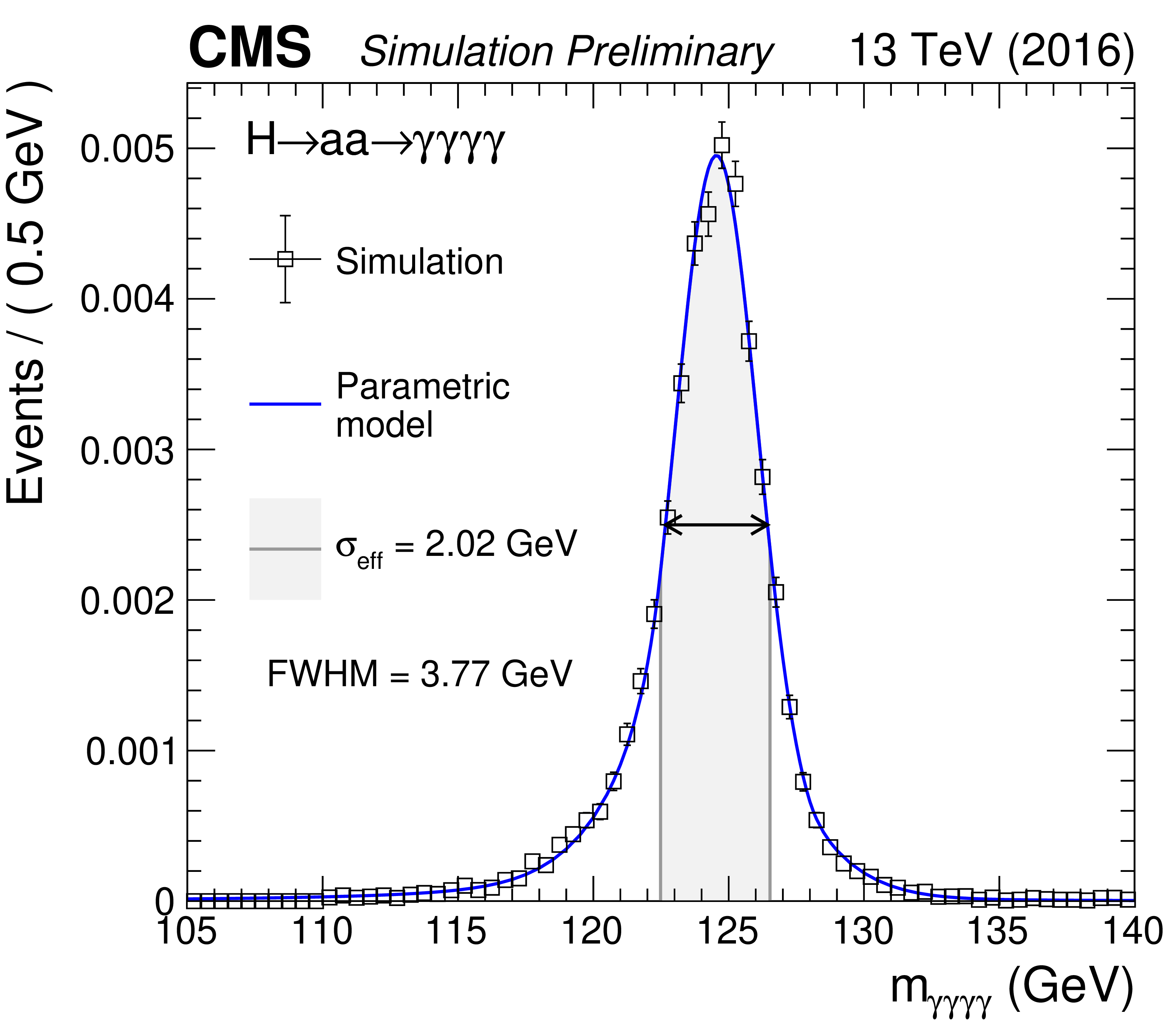
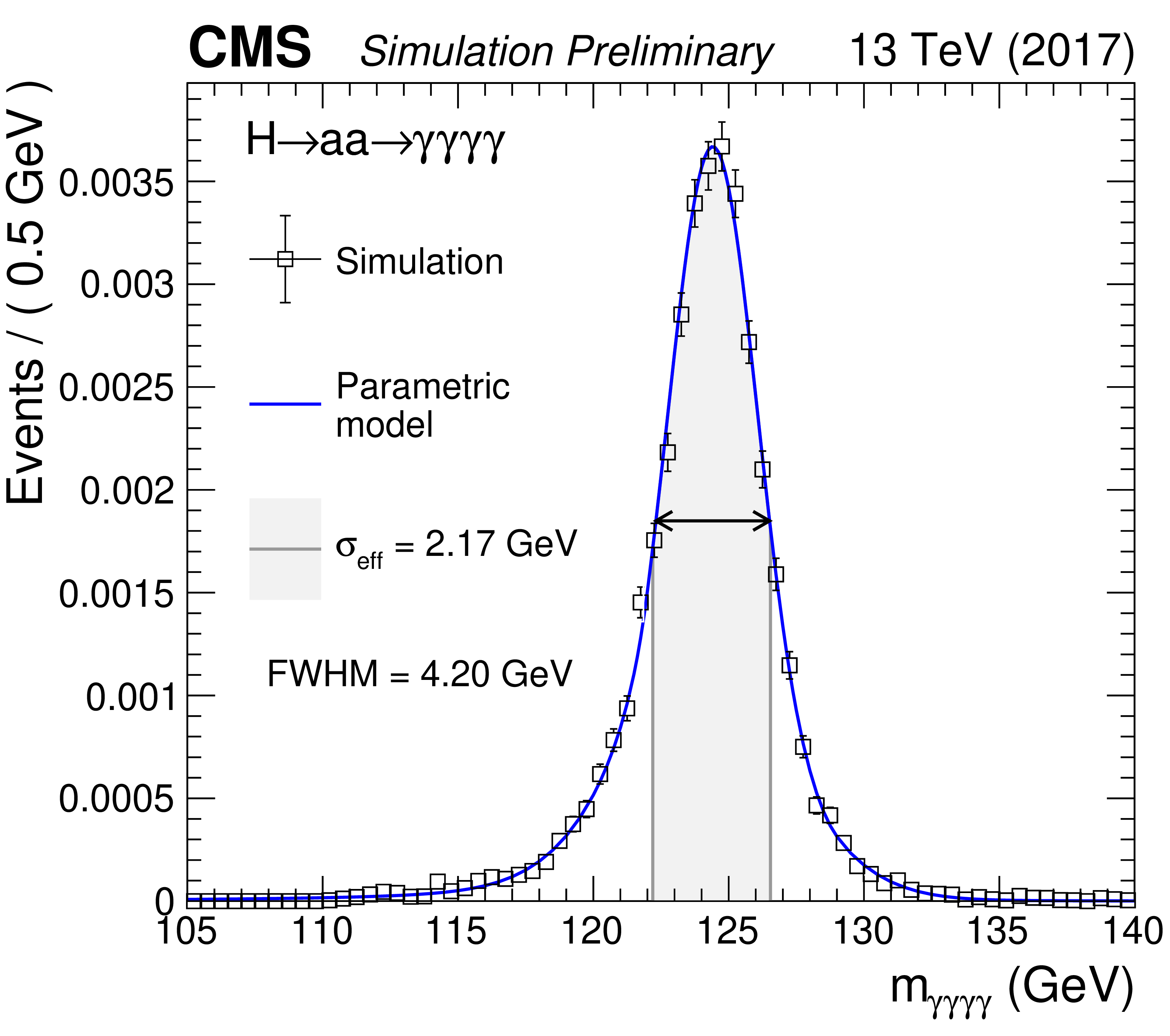
Parametrized signal shape for m(a) = 15 GeV is shown for 2016 (top left), 2017 (top right), and 2018 (bottom). Separate signal models are built for each of the three data taking years, which are then scaled by the appropriate luminosity and summed in order to construct the final signal model. The open squares represent simulated events and the blue lines are the corresponding models. Also shown are the $\sigma _{\text {eff}}$ value (half the width of the narrowest interval containing 68.3% of the invariant mass distribution) with the corresponding interval as a gray band, and the full width at half the maximum (FWHM) with the corresponding interval as a double arrow. |
png pdf |
Figure 4-a:
Parametrized signal shape for m(a) = 15 GeV is shown for 2016 (top left), 2017 (top right), and 2018 (bottom). Separate signal models are built for each of the three data taking years, which are then scaled by the appropriate luminosity and summed in order to construct the final signal model. The open squares represent simulated events and the blue lines are the corresponding models. Also shown are the $\sigma _{\text {eff}}$ value (half the width of the narrowest interval containing 68.3% of the invariant mass distribution) with the corresponding interval as a gray band, and the full width at half the maximum (FWHM) with the corresponding interval as a double arrow. |
png pdf |
Figure 4-b:
Parametrized signal shape for m(a) = 15 GeV is shown for 2016 (top left), 2017 (top right), and 2018 (bottom). Separate signal models are built for each of the three data taking years, which are then scaled by the appropriate luminosity and summed in order to construct the final signal model. The open squares represent simulated events and the blue lines are the corresponding models. Also shown are the $\sigma _{\text {eff}}$ value (half the width of the narrowest interval containing 68.3% of the invariant mass distribution) with the corresponding interval as a gray band, and the full width at half the maximum (FWHM) with the corresponding interval as a double arrow. |

png pdf |
Figure 4-c:
Parametrized signal shape for m(a) = 15 GeV is shown for 2016 (top left), 2017 (top right), and 2018 (bottom). Separate signal models are built for each of the three data taking years, which are then scaled by the appropriate luminosity and summed in order to construct the final signal model. The open squares represent simulated events and the blue lines are the corresponding models. Also shown are the $\sigma _{\text {eff}}$ value (half the width of the narrowest interval containing 68.3% of the invariant mass distribution) with the corresponding interval as a gray band, and the full width at half the maximum (FWHM) with the corresponding interval as a double arrow. |

png pdf |
Figure 5:
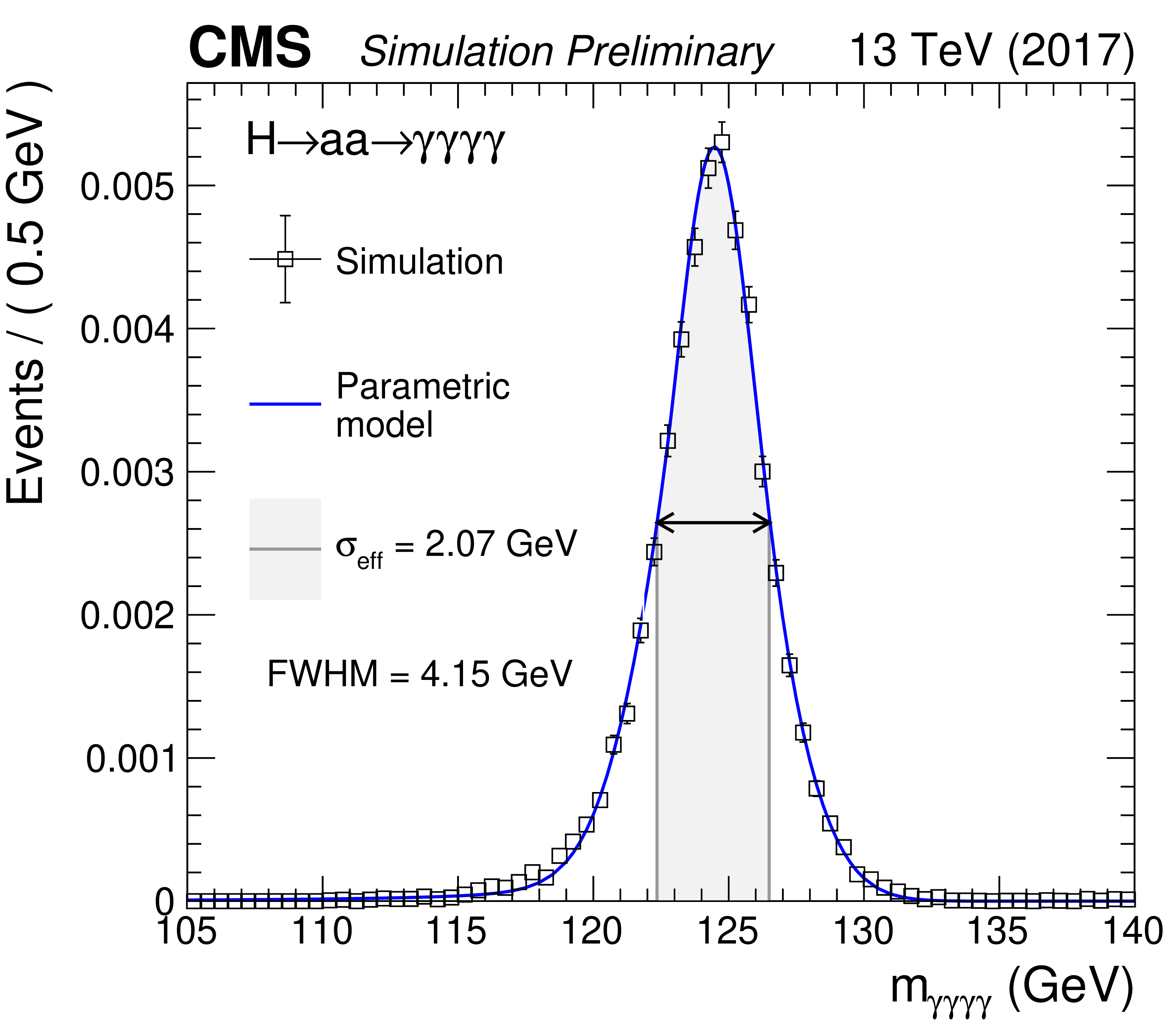
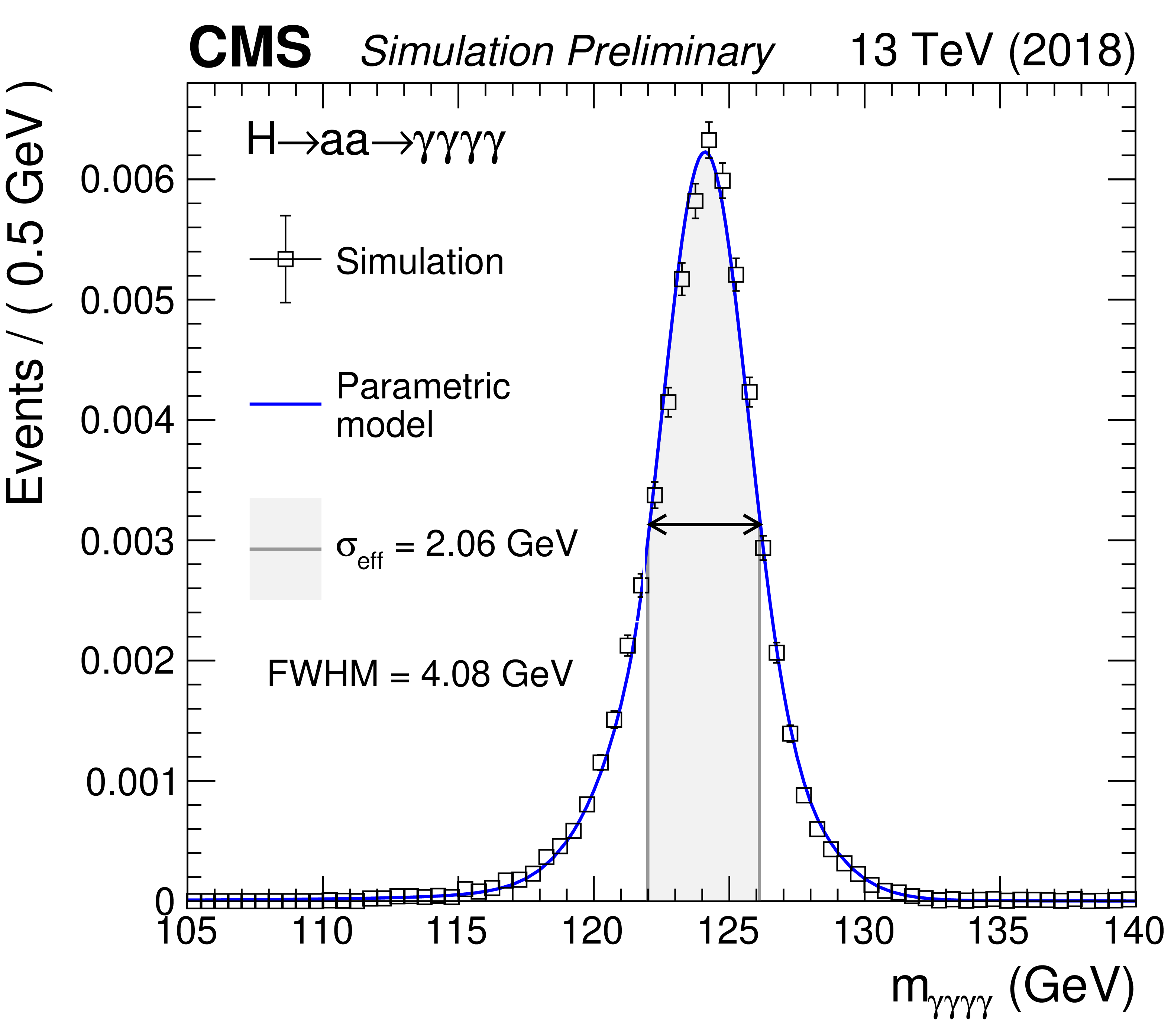
Parametrized signal shape for m(a) = 50 GeV is shown for 2016 (top left), 2017 (top right), and 2018 (bottom). Separate signal models are built for each of the three data taking years, which are then scaled by the appropriate luminosity and summed in order to construct the final signal model. The open squares represent simulated events and the blue lines are the corresponding models. Also shown are the $\sigma _{\text {eff}}$ value (half the width of the narrowest interval containing 68.3% of the invariant mass distribution) with the corresponding interval as a gray band, and the full width at half the maximum (FWHM) with the corresponding interval as a double arrow. |

png pdf |
Figure 5-a:
Parametrized signal shape for m(a) = 50 GeV is shown for 2016 (top left), 2017 (top right), and 2018 (bottom). Separate signal models are built for each of the three data taking years, which are then scaled by the appropriate luminosity and summed in order to construct the final signal model. The open squares represent simulated events and the blue lines are the corresponding models. Also shown are the $\sigma _{\text {eff}}$ value (half the width of the narrowest interval containing 68.3% of the invariant mass distribution) with the corresponding interval as a gray band, and the full width at half the maximum (FWHM) with the corresponding interval as a double arrow. |
png pdf |
Figure 5-b:
Parametrized signal shape for m(a) = 50 GeV is shown for 2016 (top left), 2017 (top right), and 2018 (bottom). Separate signal models are built for each of the three data taking years, which are then scaled by the appropriate luminosity and summed in order to construct the final signal model. The open squares represent simulated events and the blue lines are the corresponding models. Also shown are the $\sigma _{\text {eff}}$ value (half the width of the narrowest interval containing 68.3% of the invariant mass distribution) with the corresponding interval as a gray band, and the full width at half the maximum (FWHM) with the corresponding interval as a double arrow. |
png pdf |
Figure 5-c:
Parametrized signal shape for m(a) = 50 GeV is shown for 2016 (top left), 2017 (top right), and 2018 (bottom). Separate signal models are built for each of the three data taking years, which are then scaled by the appropriate luminosity and summed in order to construct the final signal model. The open squares represent simulated events and the blue lines are the corresponding models. Also shown are the $\sigma _{\text {eff}}$ value (half the width of the narrowest interval containing 68.3% of the invariant mass distribution) with the corresponding interval as a gray band, and the full width at half the maximum (FWHM) with the corresponding interval as a double arrow. |

png pdf |
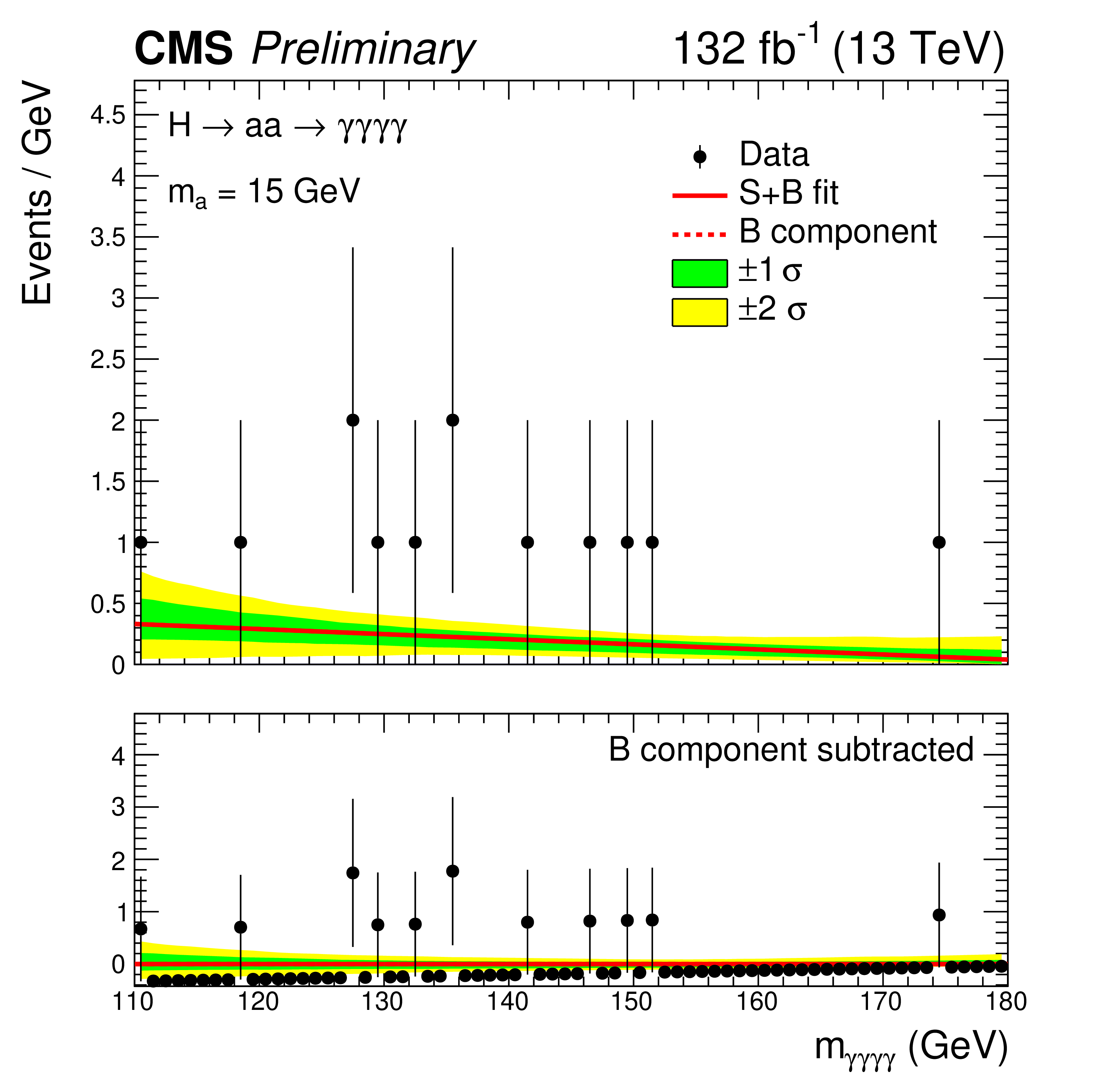
Figure 6:
Invariant mass distribution, ${m_{\gamma \gamma \gamma \gamma}}$, for data (black points) and signal-plus-background model fit is shown for ${m_{a}} = $ 15 GeV (left) and $ {m_{a}} = $ 50 GeV (right). The solid red line shows the total signal-plus-background contribution, whereas the dashed red line shows the background component only. The lower panel shows the residuals after subtraction of this background component. The one (green) and two (yellow) standard deviation bands include the uncertainties in the background component of the fit. The lower panel in each plot shows the residual signal yield after the background subtraction. |
png pdf |
Figure 6-a:
Invariant mass distribution, ${m_{\gamma \gamma \gamma \gamma}}$, for data (black points) and signal-plus-background model fit is shown for ${m_{a}} = $ 15 GeV (left) and $ {m_{a}} = $ 50 GeV (right). The solid red line shows the total signal-plus-background contribution, whereas the dashed red line shows the background component only. The lower panel shows the residuals after subtraction of this background component. The one (green) and two (yellow) standard deviation bands include the uncertainties in the background component of the fit. The lower panel in each plot shows the residual signal yield after the background subtraction. |

png pdf |
Figure 6-b:
Invariant mass distribution, ${m_{\gamma \gamma \gamma \gamma}}$, for data (black points) and signal-plus-background model fit is shown for ${m_{a}} = $ 15 GeV (left) and $ {m_{a}} = $ 50 GeV (right). The solid red line shows the total signal-plus-background contribution, whereas the dashed red line shows the background component only. The lower panel shows the residuals after subtraction of this background component. The one (green) and two (yellow) standard deviation bands include the uncertainties in the background component of the fit. The lower panel in each plot shows the residual signal yield after the background subtraction. |
png pdf |
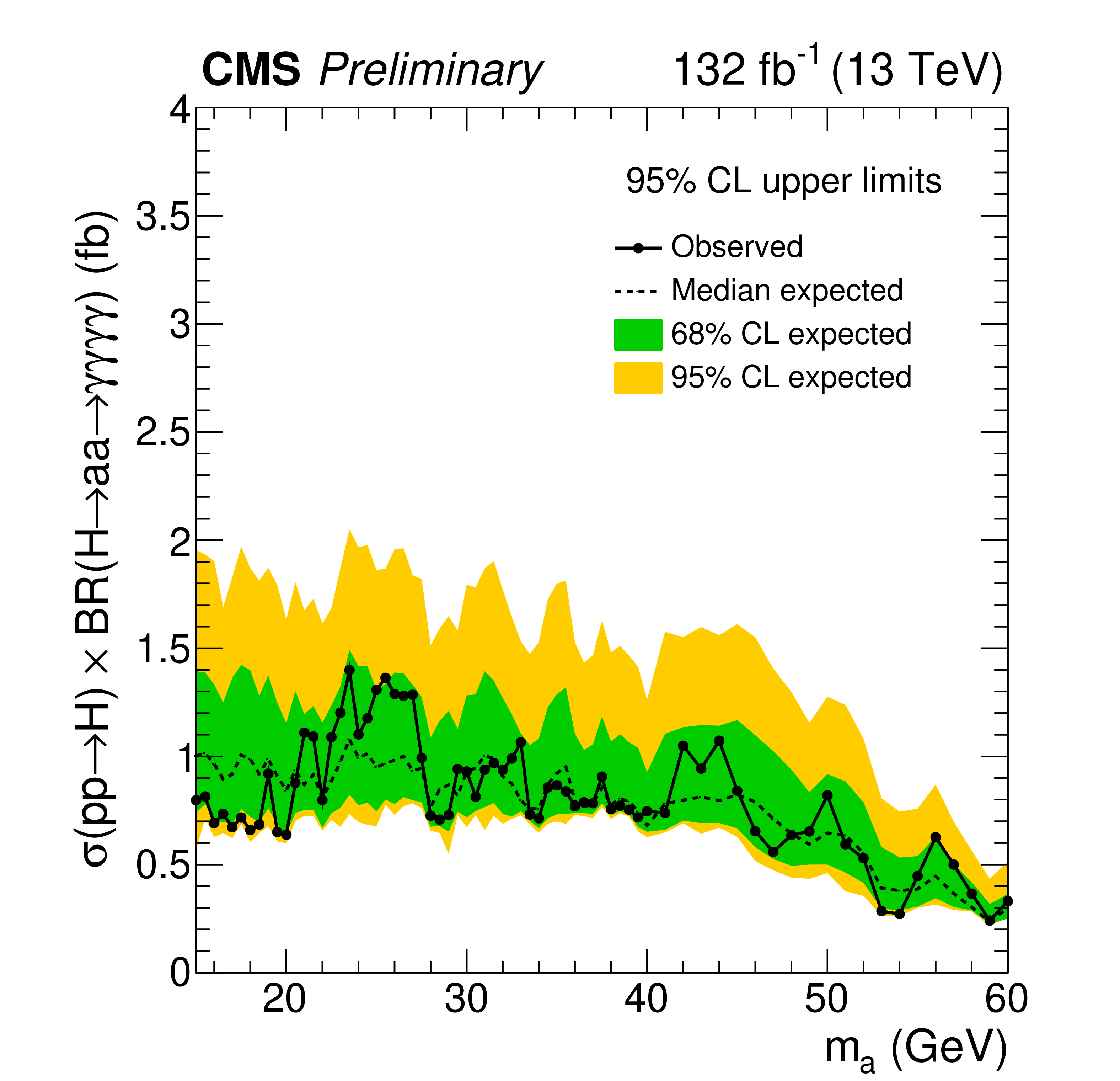
Figure 7:
Expected and observed 95% CL limits on the product of the production cross section of the Higgs boson and the branching fraction into four photons via a pair of pseuodscalars, ${\sigma _{\mathrm{H}}} \times {\mathcal {B}({\mathrm{H} \rightarrow aa \rightarrow \gamma \gamma \gamma \gamma})}$, is shown as a function of ${m_{a}}$. The green (yellow) bands represent the 68% (95%) expected limit intervals. |
| Tables | |

png pdf |
Table 1:
Summary of the minimum BDT output value and efficiency with respect to a selection on BDT output for each nominal signal hypothesis. |
| Summary |
| A search for a pair of light pseudoscalars that subsequently decay into photons produced from decays of the 125 GeV Higgs boson is presented. The analysis is based on the proton-proton collision data collected at $\sqrt{s} = $ 13 TeV by the CMS experiment at the LHC in 2016, 2017, and 2018, which corresponds to a total integrated luminosity of 131.2 fb$^{-1}$. The analysis probes pseudoscalars ranging in mass from 15 to 60 GeV. In absence of any significant deviation from the background-only hypothesis, upper limits are set at 95% CL on the product of the production cross section of the Higgs boson and the branching fraction into four photons via a pair of pseuodscalars, $\sigma_{\mathrm{H}} \times$ BR. The observed (expected) limit ranges from 0.80 (1.00) fb for $m_a =$ 15 GeV to 0.33 (0.30) fb for $m_a =$ 60 GeV. |
| References | ||||
| 1 | ATLAS Collaboration | Observation of a new particle in the search for the standard model Higgs boson with the ATLAS detector at the LHC | PLB 716 (2012) 1 | 1207.7214 |
| 2 | CMS Collaboration | Observation of a new boson at a mass of 125 GeV with the CMS experiment at the LHC | PLB 716 (2012) 30 | CMS-HIG-12-028 1207.7235 |
| 3 | CMS Collaboration | Observation of a new boson with mass near 125 GeV in pp collisions at $ \sqrt{s} = $ 7 and 8 TeV | JHEP 06 (2013) 081 | CMS-HIG-12-036 1303.4571 |
| 4 | ATLAS Collaboration | Measurement of the Higgs boson coupling properties in the $ H\rightarrow ZZ^{*} \rightarrow 4\ell $ decay channel at $ \sqrt{s} = $ 13 TeV with the ATLAS detector | JHEP 03 (2018) 095 | 1712.02304 |
| 5 | CMS Collaboration | Measurements of properties of the Higgs boson decaying into the four-lepton final state in pp collisions at $ \sqrt{s}= $ 13 TeV | JHEP 11 (2017) 047 | CMS-HIG-16-041 1706.09936 |
| 6 | ATLAS, CMS Collaboration | Measurements of the Higgs boson production and decay rates and constraints on its couplings from a combined ATLAS and CMS analysis of the LHC pp collision data at $ \sqrt{s}= $ 7 and 8 TeV | JHEP 08 (2016) 045 | 1606.02266 |
| 7 | CMS Collaboration | Study of the Mass and Spin-Parity of the Higgs Boson Candidate Via Its Decays to Z Boson Pairs | PRL 110 (2013), no. 8, 081803 | CMS-HIG-12-041 1212.6639 |
| 8 | D. Curtin et al. | Exotic decays of the 125 GeV Higgs boson | PRD 90 (2014), no. 7, 075004 | 1312.4992 |
| 9 | CMS Collaboration | Combined measurements of Higgs boson couplings in proton-proton collisions at $ \sqrt{s}=$ 13 TeV | EPJC 79 (2019), no. 5, 421 | CMS-HIG-17-031 1809.10733 |
| 10 | ATLAS Collaboration | Search for Higgs bosons decaying to $ aa $ in the $ \mu\mu\tau\tau $ final state in $ pp $ collisions at $ \sqrt{s} = $ 8 TeV with the ATLAS experiment | PRD 92 (2015), no. 5, 052002 | 1505.01609 |
| 11 | CMS Collaboration | A search for pair production of new light bosons decaying into muons | PLB 752 (2016) 146 | CMS-HIG-13-010 1506.00424 |
| 12 | CMS Collaboration | Search for a very light NMSSM Higgs boson produced in decays of the 125 GeV scalar boson and decaying into $ \tau $ leptons in pp collisions at $ \sqrt{s}= $ 8 TeV | JHEP 01 (2016) 079 | CMS-HIG-14-019 1510.06534 |
| 13 | CMS Collaboration | Search for light bosons in decays of the 125 GeV Higgs boson in proton-proton collisions at $ \sqrt{s}= $ 8 TeV | JHEP 10 (2017) 076 | CMS-HIG-16-015 1701.02032 |
| 14 | ATLAS Collaboration | Search for the Higgs boson produced in association with a W boson and decaying to four b-quarks via two spin-zero particles in pp collisions at 13 TeV with the ATLAS detector | EPJC 76 (2016) 605 | 1606.08391 |
| 15 | ATLAS Collaboration | Search for Higgs boson decays to beyond-the-Standard-Model light bosons in four-lepton events with the ATLAS detector at $ \sqrt{s}= $ 13 TeV | JHEP 06 (2018) 166 | 1802.03388 |
| 16 | ATLAS Collaboration | Search for Higgs boson decays into pairs of light (pseudo)scalar particles in the $ \gamma\gamma {\rm jj} $ final state in pp collisions at $ \sqrt{s}= $ 13 TeV with the ATLAS detector | PLB 782 (2018) 750 | 1803.11145 |
| 17 | ATLAS Collaboration | Search for the Higgs boson produced in association with a vector boson and decaying into two spin-zero particles in the $ {\mathrm{H}} \rightarrow {aa} \rightarrow {4b} $ channel in pp collisions at $ \sqrt{s} = $ 13 TeV with the ATLAS detector | JHEP 10 (2018) 031 | 1806.07355 |
| 18 | ATLAS Collaboration | Search for Higgs boson decays into a pair of light bosons in the $ \mathrm{b}\mathrm{b}\mu\mu $ final state in pp collision at $ \sqrt{s} = $ 13 TeV with the ATLAS detector | PLB 790 (2019) 1 | 1807.00539 |
| 19 | CMS Collaboration | Search for an exotic decay of the Higgs boson to a pair of light pseudoscalars in the final state with two b quarks and two $ \tau $ leptons in proton-proton collisions at $ \sqrt{s}= $ 13 TeV | PLB 785 (2018) 462 | CMS-HIG-17-024 1805.10191 |
| 20 | CMS Collaboration | Search for an exotic decay of the Higgs boson to a pair of light pseudoscalars in the final state of two muons and two $ \tau $ leptons in proton-proton collisions at $ \sqrt{s}= $ 13 TeV | JHEP 11 (2018) 018 | CMS-HIG-17-029 1805.04865 |
| 21 | S. Chang, P. J. Fox, and N. Weiner | Visible Cascade Higgs Decays to Four Photons at Hadron Colliders | PRL 98 (2007) 111802 | hep-ph/0608310 |
| 22 | B. A. Dobrescu, G. L. Landsberg, and K. T. Matchev | Higgs boson decays to CP odd scalars at the Tevatron and beyond | PRD 63 (2001) 075003 | hep-ph/0005308 |
| 23 | F. Larios, G. Tavares-Velasco, and C. P. Yuan | Update on a very light CP odd scalar in the two Higgs doublet model | PRD 66 (2002) 075006 | hep-ph/0205204 |
| 24 | R. Dermisek and J. F. Gunion | The NMSSM Solution to the Fine-Tuning Problem, Precision Electroweak Constraints and the Largest LEP Higgs Event Excess | PRD 76 (2007) 095006 | 0705.4387 |
| 25 | ATLAS Collaboration | Search for new phenomena in events with at least three photons collected in $ pp $ collisions at $ \sqrt{s} = $ 8 TeV with the ATLAS detector | EPJC 76 (2016), no. 4, 210 | 1509.05051 |
| 26 | CMS Collaboration | The CMS trigger system | JINST 12 (2017) P01020 | CMS-TRG-12-001 1609.02366 |
| 27 | CMS Collaboration | Performance of the CMS Level-1 trigger in proton-proton collisions at $ \sqrt{s} = $ 13 TeV | JINST 15 (2020), no. 10, P10017 | CMS-TRG-17-001 2006.10165 |
| 28 | CMS Trigger, Data Acquisition Group Collaboration | The CMS high level trigger | EPJC 46 (2006) 605 | hep-ex/0512077 |
| 29 | CMS Collaboration | Particle-flow reconstruction and global event description with the CMS detector | JINST 12 (2017) P10003 | CMS-PRF-14-001 1706.04965 |
| 30 | CMS Collaboration | Electron and photon reconstruction and identification with the CMS experiment at the CERN LHC | JINST 16 (2021), no. 05, P05014 | CMS-EGM-17-001 2012.06888 |
| 31 | CMS Collaboration | The CMS Experiment at the CERN LHC | JINST 3 (2008) S08004 | CMS-00-001 |
| 32 | CMS Collaboration | Observation of the diphoton decay of the Higgs boson and measurement of its properties | EPJC 74 (2014) 3076 | CMS-HIG-13-001 1407.0558 |
| 33 | CMS Collaboration | Measurements of Higgs boson properties in the diphoton decay channel in proton-proton collisions at $ \sqrt{s} = $ 13 TeV | JHEP 11 (2018) 185 | CMS-HIG-16-040 1804.02716 |
| 34 | T. Sjostrand et al. | An introduction to PYTHIA 8.2 | CPC 191 (2015) 159 | 1410.3012 |
| 35 | CMS Collaboration | Event generator tunes obtained from underlying event and multiparton scattering measurements | EPJC 76 (2016) 155 | CMS-GEN-14-001 1512.00815 |
| 36 | CMS Collaboration | Extraction and validation of a new set of CMS PYTHIA8 tunes from underlying-event measurements | EPJC 80 (2020) 4 | CMS-GEN-17-001 1903.12179 |
| 37 | GEANT4 Collaboration | GEANT4--a simulation toolkit | NIMA 506 (2003) 250--303 | |
| 38 | M. Cacciari, G. P. Salam, and G. Soyez | The anti-$ {k_{\mathrm{T}}} $ jet clustering algorithm | JHEP 04 (2008) 063 | 0802.1189 |
| 39 | M. Cacciari, G. P. Salam, and G. Soyez | FastJet user manual | EPJC 72 (2012) 1896 | 1111.6097 |
| 40 | CMS Collaboration | A measurement of the Higgs boson mass in the diphoton decay channel | PLB 805 (2020) 135425 | CMS-HIG-19-004 2002.06398 |
| 41 | CMS Collaboration | Technical proposal for the phase-II upgrade of the compact muon solenoid | CMS-PAS-TDR-15-002 | CMS-PAS-TDR-15-002 |
| 42 | P. Baldi et al. | Parameterized neural networks for high-energy physics | EPJC 76 (2016), no. 5, 235 | 1601.07913 |
| 43 | G. Cowan, K. Cranmer, E. Gross, and O. Vitells | Asymptotic formulae for likelihood-based tests of new physics | EPJC 71 (2011) 1554 | 1007.1727 |
| 44 | M. J. Oreglia | A study of the reactions $\psi' \to \gamma\gamma \psi$ | PhD thesis, Stanford University, 1980 SLAC Report SLAC-R-236, see Appendix D | |
| 45 | P. D. Dauncey, M. Kenzie, N. Wardle, and G. J. Davies | Handling uncertainties in background shapes: the discrete profiling method | JINST 10 (2015) P04015 | 1408.6865 |
| 46 | R. A. Fisher | On the Interpretation of $ \chi^{2} $ from Contingency Tables, and the Calculation of p | J. Royal Stat. Soc 85 (1922) 87 | |
| 47 | CMS Collaboration | Measurements of Higgs boson production cross sections and couplings in the diphoton decay channel at $ \sqrt{\mathrm{s}} = $ 13 TeV | JHEP 07 (2021) 027 | CMS-HIG-19-015 2103.06956 |
| 48 | CMS Collaboration | CMS Luminosity Measurements for the 2016 Data Taking Period | CMS-PAS-LUM-17-001 | CMS-PAS-LUM-17-001 |
| 49 | CMS Collaboration | CMS luminosity measurement for the 2017 data-taking period at $ \sqrt{s} = $ 13 TeV | CMS-PAS-LUM-17-004 | CMS-PAS-LUM-17-004 |
| 50 | CMS Collaboration | CMS luminosity measurement for the 2018 data-taking period at $ \sqrt{s} = $ 13 TeV | CMS-PAS-LUM-18-002 | CMS-PAS-LUM-18-002 |
| 51 | CMS Collaboration | Measurement of the inclusive $ W $ and $ Z $ production cross sections in pp collisions at $ \sqrt{s}= $ 7 TeV | JHEP 10 (2011) 132 | CMS-EWK-10-005 1107.4789 |
| 52 | T. Junk | Confidence level computation for combining searches with small statistics | NIMA 434 (1999) 435--443 | hep-ex/9902006 |
| 53 | A. L. Read | Presentation of search results: The CL(s) technique | JPG 28 (2002) 2693--2704 | |
| 54 | The ATLAS Collaboration, The CMS Collaboration, The LHC Higgs Combination Group Collaboration | Procedure for the LHC Higgs boson search combination in Summer 2011 | technical report, CERN, Geneva, Aug | |
| 55 | LHC Higgs Cross Section Working Group | Handbook of LHC Higgs cross sections: 4. deciphering the nature of the Higgs sector | CERN (2016) | 1610.07922 |
|
|
Compact Muon Solenoid LHC, CERN |
|

|

|

|

|

|