

Compact Muon Solenoid
LHC, CERN
| CMS-PAS-HIG-20-005 | ||
| Search for Higgs boson pair production in the four b quark final state | ||
| CMS Collaboration | ||
| June 2021 | ||
| Abstract: A search for the production of pairs of Higgs bosons in proton-proton collisions at a centre-of-mass energy of 13 TeV is presented, using a data sample collected with the CMS detector at the LHC and corresponding to an integrated luminosity of about 138 fb$^{-1}$. The search investigates both the gluon and vector boson fusion production mechanisms for Higgs boson pairs in the final state with four b quarks. No evidence of signal is found, and an observed (expected) upper limit on the Higgs boson pair production cross section of 3.6 (7.3) times the standard model prediction is set. Results are also interpreted under assumptions involving anomalous Higgs boson couplings. At a 95% confidence level, the Higgs field self-coupling is constrained to be within $ -2.3 $ and $ 9.4 $ times the standard model expectation, and the coupling of two Higgs bosons to two vector bosons is constrained to be within $ -0.1 $ and $ 2.2 $. | ||
|
Links:
CDS record (PDF) ;
inSPIRE record ;
Physics Briefing ;
CADI line (restricted) ;
These preliminary results are superseded in this paper, PRL 129 (2022) 081802. The superseded preliminary plots can be found here. |
||
| Figures | Summary | Additional Figures | References | CMS Publications |
|---|
| Figures | |

png pdf |
Figure 1:
Distributions of the events observed in the ${A_\text {SR}^{4\mathrm{b}}}$ signal region. The upper and lower rows show the ${\mathrm{g} \mathrm{g} \text {F}}$ and VBF categories, respectively. For the former, the output of the BDT discriminant is shown for the low-mass category on the left and for the high-mass category on the right. For the latter, the $m_{{\mathrm{H} \mathrm{H}}}$ distribution in the SM-like category is shown on the left and the total number of events in the anomalous $ {\kappa _\text {2V}} $-like category on the right. Data are represented by points with error bars, the expected background contribution is represented by the shaded blue histograms with the associated systematic uncertainties (dashed areas), while the ${\mathrm{g} \mathrm{g} \text {F}}$ (VBF) signal contributions is shown in blue (red) and not stacked. |

png pdf |
Figure 1-a:
Distributions of the events observed in the ${A_\text {SR}^{4\mathrm{b}}}$ signal region. The upper and lower rows show the ${\mathrm{g} \mathrm{g} \text {F}}$ and VBF categories, respectively. For the former, the output of the BDT discriminant is shown for the low-mass category on the left and for the high-mass category on the right. For the latter, the $m_{{\mathrm{H} \mathrm{H}}}$ distribution in the SM-like category is shown on the left and the total number of events in the anomalous $ {\kappa _\text {2V}} $-like category on the right. Data are represented by points with error bars, the expected background contribution is represented by the shaded blue histograms with the associated systematic uncertainties (dashed areas), while the ${\mathrm{g} \mathrm{g} \text {F}}$ (VBF) signal contributions is shown in blue (red) and not stacked. |

png pdf |
Figure 1-b:
Distributions of the events observed in the ${A_\text {SR}^{4\mathrm{b}}}$ signal region. The upper and lower rows show the ${\mathrm{g} \mathrm{g} \text {F}}$ and VBF categories, respectively. For the former, the output of the BDT discriminant is shown for the low-mass category on the left and for the high-mass category on the right. For the latter, the $m_{{\mathrm{H} \mathrm{H}}}$ distribution in the SM-like category is shown on the left and the total number of events in the anomalous $ {\kappa _\text {2V}} $-like category on the right. Data are represented by points with error bars, the expected background contribution is represented by the shaded blue histograms with the associated systematic uncertainties (dashed areas), while the ${\mathrm{g} \mathrm{g} \text {F}}$ (VBF) signal contributions is shown in blue (red) and not stacked. |

png pdf |
Figure 1-c:
Distributions of the events observed in the ${A_\text {SR}^{4\mathrm{b}}}$ signal region. The upper and lower rows show the ${\mathrm{g} \mathrm{g} \text {F}}$ and VBF categories, respectively. For the former, the output of the BDT discriminant is shown for the low-mass category on the left and for the high-mass category on the right. For the latter, the $m_{{\mathrm{H} \mathrm{H}}}$ distribution in the SM-like category is shown on the left and the total number of events in the anomalous $ {\kappa _\text {2V}} $-like category on the right. Data are represented by points with error bars, the expected background contribution is represented by the shaded blue histograms with the associated systematic uncertainties (dashed areas), while the ${\mathrm{g} \mathrm{g} \text {F}}$ (VBF) signal contributions is shown in blue (red) and not stacked. |

png pdf |
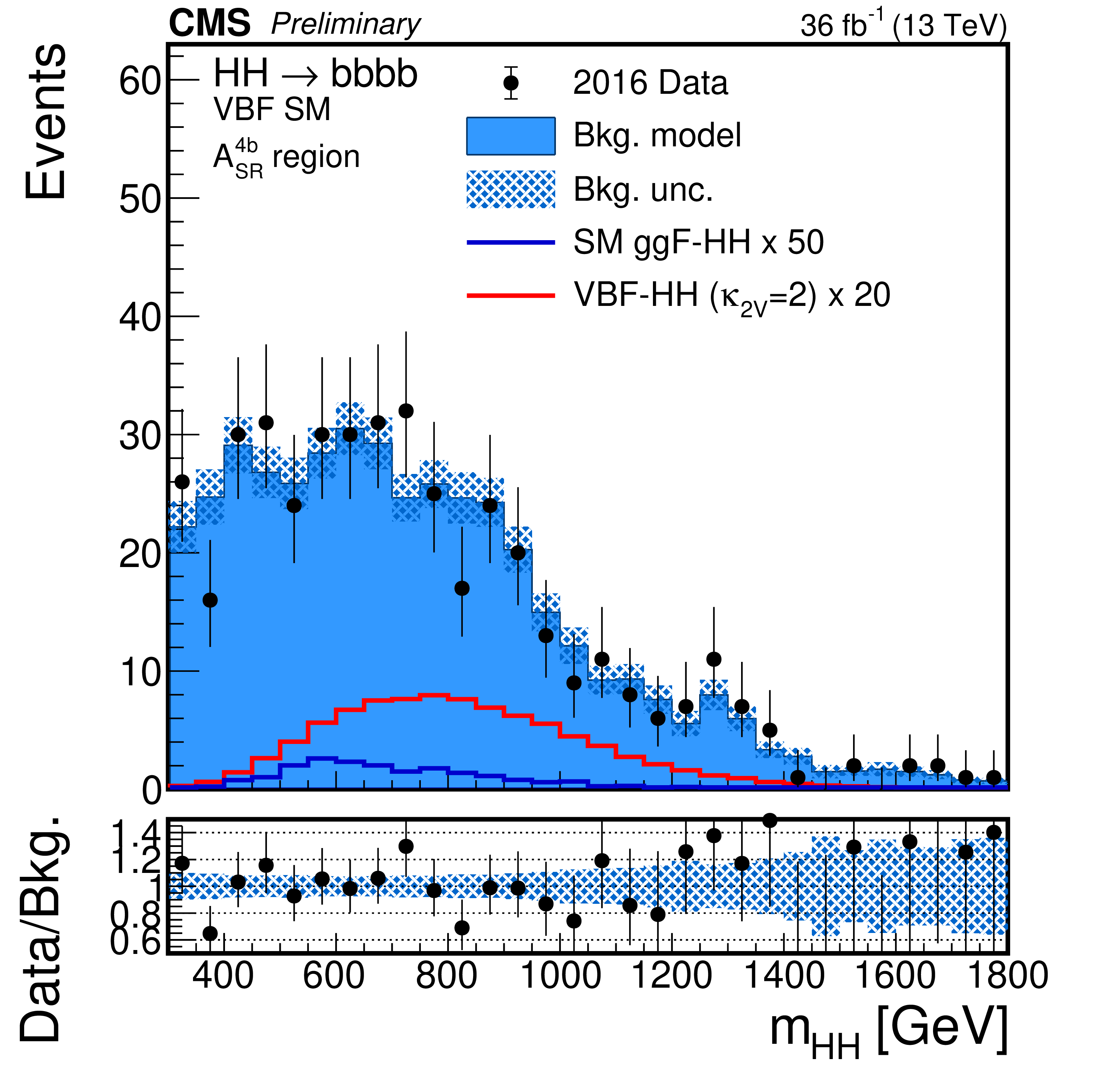
Figure 1-d:
Distributions of the events observed in the ${A_\text {SR}^{4\mathrm{b}}}$ signal region. The upper and lower rows show the ${\mathrm{g} \mathrm{g} \text {F}}$ and VBF categories, respectively. For the former, the output of the BDT discriminant is shown for the low-mass category on the left and for the high-mass category on the right. For the latter, the $m_{{\mathrm{H} \mathrm{H}}}$ distribution in the SM-like category is shown on the left and the total number of events in the anomalous $ {\kappa _\text {2V}} $-like category on the right. Data are represented by points with error bars, the expected background contribution is represented by the shaded blue histograms with the associated systematic uncertainties (dashed areas), while the ${\mathrm{g} \mathrm{g} \text {F}}$ (VBF) signal contributions is shown in blue (red) and not stacked. |

png pdf |
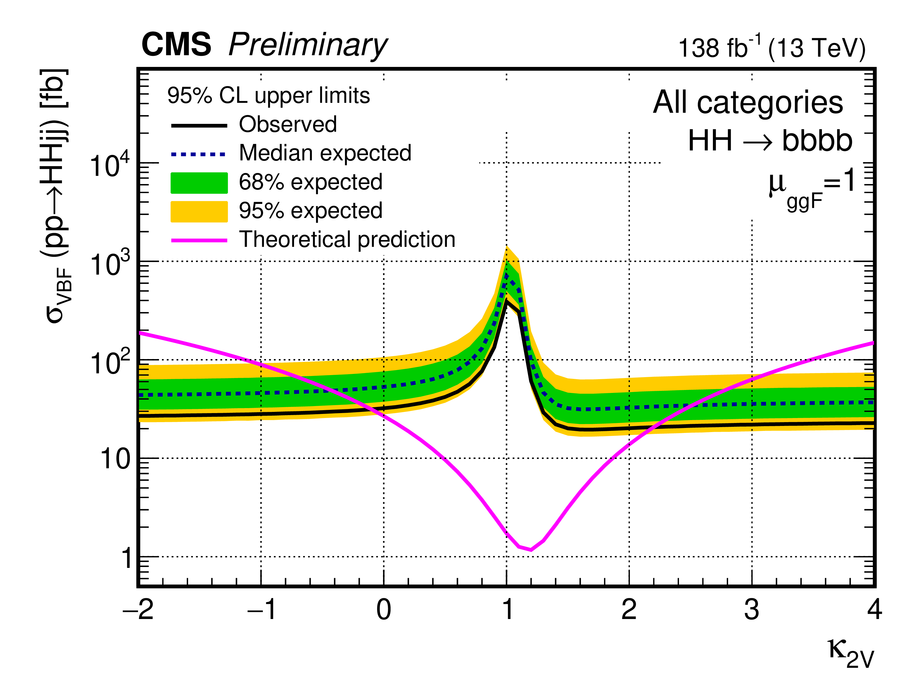
Figure 2:
Observed and expected 95% CL upper limits on cross section times branching fraction as a function of ${\kappa _{\lambda}}$ (left) and ${\kappa _\text {2V}}$ (right). The inner (green) band and the outer (yellow) band indicate the regions containing 68 and 95%, respectively, of the distribution of limits expected under the background-only hypothesis. The pink lines denote the theoretical cross section expectation assuming that other couplings not indicated on the horizontal axis are set to the SM prediction. |

png pdf |
Figure 2-a:
Observed and expected 95% CL upper limits on cross section times branching fraction as a function of ${\kappa _{\lambda}}$ (left) and ${\kappa _\text {2V}}$ (right). The inner (green) band and the outer (yellow) band indicate the regions containing 68 and 95%, respectively, of the distribution of limits expected under the background-only hypothesis. The pink lines denote the theoretical cross section expectation assuming that other couplings not indicated on the horizontal axis are set to the SM prediction. |
png pdf |
Figure 2-b:
Observed and expected 95% CL upper limits on cross section times branching fraction as a function of ${\kappa _{\lambda}}$ (left) and ${\kappa _\text {2V}}$ (right). The inner (green) band and the outer (yellow) band indicate the regions containing 68 and 95%, respectively, of the distribution of limits expected under the background-only hypothesis. The pink lines denote the theoretical cross section expectation assuming that other couplings not indicated on the horizontal axis are set to the SM prediction. |
| Summary |
| A search for the production of Higgs boson pairs in the four b quarks decay channel is presented. The search investigates the production modes via gluon and vector boson fusion, and uses a data sample collected in proton-proton collisions at $\sqrt{s} = $ 13 TeV that corresponds to 138 fb$^{-1}$ . The data are found to be statistically compatible with the background-only hypothesis, and upper limits at the 95% confidence level on the signal cross sections are set. The observed (expected) upper limit on the HH production cross section corresponds to 3.6 (7.3) times the SM prediction. The value of the Higgs bosons self-coupling normalised to the SM expectation ($\kappa_{\lambda}$) is observed (expected) to be in the range $-2.3 < \kappa_{\lambda} < 9.4$ ($-5.0 < \kappa_{\lambda} < 12.0$), and the value of the coupling of Higgs bosons pairs to vector bosons pairs, normalised to the SM expectation ($\kappa_{2\mathrm{V}}$), to be in the range $-0.1 < \kappa_{2\mathrm{V}} < 2.2$ ($-0.4 < \kappa_{2\mathrm{V}} < 2.5$). These results improve by more than a factor of 3 the sensitivity of previous measurements on the ggF cross section in the same channel and put the most stringent constraints to date on the ggF and VBF production cross sections. |
| Additional Figures | |

png pdf |
Additional Figure 1:
Distribution of data events selected in the three (top row) and four (bottom row) b-tagged jet categories for events recorded in 2016 (left column) and 2017 and 2018 (right column) as function of the masses of the two Higgs boson candidates. The blue and green circles correspond to the analysis and validation regions, respectively, denoted by the letters A and V. The inner circle corresponds to the signal region while the ring around it defines the control region used for the background modeling. |

png pdf |
Additional Figure 1-a:
Distribution of data events selected in the three b-tagged jet categories for events recorded in 2016 as function of the masses of the two Higgs boson candidates. The blue and green circles correspond to the analysis and validation regions, respectively, denoted by the letters A and V. The inner circle corresponds to the signal region while the ring around it defines the control region used for the background modeling. |

png pdf |
Additional Figure 1-b:
Distribution of data events selected in the three b-tagged jet categories for events recorded in 2017 and 2018 as function of the masses of the two Higgs boson candidates. The blue and green circles correspond to the analysis and validation regions, respectively, denoted by the letters A and V. The inner circle corresponds to the signal region while the ring around it defines the control region used for the background modeling. |

png pdf |
Additional Figure 1-c:
Distribution of data events selected in the four b-tagged jet categories for events recorded in 2016 as function of the masses of the two Higgs boson candidates. The blue and green circles correspond to the analysis and validation regions, respectively, denoted by the letters A and V. The inner circle corresponds to the signal region while the ring around it defines the control region used for the background modeling. |

png pdf |
Additional Figure 1-d:
Distribution of data events selected in the four b-tagged jet categories for events recorded in 2017 and 2018 as function of the masses of the two Higgs boson candidates. The blue and green circles correspond to the analysis and validation regions, respectively, denoted by the letters A and V. The inner circle corresponds to the signal region while the ring around it defines the control region used for the background modeling. |

png pdf |
Additional Figure 2:
Distribution of simulated signal events selected for the SM ggF production (top row) and $\kappa _\text {2V}=$ 2 VBF production (bottom row) as function of the two Higgs boson candidates masses. The simulations correspond to the events expected for the 2016 data taking (left column) and 2017 and 2018 (right column). The blue and green circles correspond to the analysis and validation regions, respectively, denoted by the letters A and V. The inner circle corresponds to the signal region while the ring around it defines the control region used for the background modeling. |

png pdf |
Additional Figure 2-a:
Distribution of simulated signal events selected for the SM ggF production as function of the two Higgs boson candidates masses. The simulations correspond to the events expected for the 2016 data taking. The blue and green circles correspond to the analysis and validation regions, respectively, denoted by the letters A and V. The inner circle corresponds to the signal region while the ring around it defines the control region used for the background modeling. |

png pdf |
Additional Figure 2-b:
Distribution of simulated signal events selected for the SM ggF production as function of the two Higgs boson candidates masses. The simulations correspond to the events expected for the 2017 and 2018 data taking. The blue and green circles correspond to the analysis and validation regions, respectively, denoted by the letters A and V. The inner circle corresponds to the signal region while the ring around it defines the control region used for the background modeling. |

png pdf |
Additional Figure 2-c:
Distribution of simulated signal events selected for the $\kappa _\text {2V}=$ 2 VBF production as function of the two Higgs boson candidates masses. The simulations correspond to the events expected for the 2016 data taking. The blue and green circles correspond to the analysis and validation regions, respectively, denoted by the letters A and V. The inner circle corresponds to the signal region while the ring around it defines the control region used for the background modeling. |

png pdf |
Additional Figure 2-d:
Distribution of simulated signal events selected for the $\kappa _\text {2V}=$ 2 VBF production as function of the two Higgs boson candidates masses. The simulations correspond to the events expected for the 2017 and 2018 data taking. The blue and green circles correspond to the analysis and validation regions, respectively, denoted by the letters A and V. The inner circle corresponds to the signal region while the ring around it defines the control region used for the background modeling. |

png pdf |
Additional Figure 3:
Distributions of the events observed in the $A_\text {SR}^{4 {\mathrm {b}}}$ signal region for the 2016 data. The top and bottom row show the ggF and VBF categories, respectively. For the former, the output of the BDT discriminant is shown for the low-mass category on the left and for the high-mass category on the right. For the latter, the $m_{{\mathrm {H}} {\mathrm {H}}}$ distribution in the SM-like category is shown on the left and the total number of events in the anomalous $\kappa _\text {2V}$-like category on the right. Data are represented by points with error bars, the expected background contribution is represented by the shaded blue histograms with the associated systematic uncertainties (dashed areas), while the ggF (VBF) signal contribution is shown in blue (red) and not stacked. |

png pdf |
Additional Figure 3-a:
The output of the BDT discriminant for the low-mass high-mass category in the $A_\text {SR}^{4 {\mathrm {b}}}$ signal region for the 2016 data in the ggF category. Data are represented by points with error bars, the expected background contribution is represented by the shaded blue histograms with the associated systematic uncertainties (dashed areas), while the ggF (VBF) signal contribution is shown in blue (red) and not stacked. |

png pdf |
Additional Figure 3-b:
The output of the BDT discriminant for the low-mass high-mass category in the $A_\text {SR}^{4 {\mathrm {b}}}$ signal region for the 2016 data in the ggF category. Data are represented by points with error bars, the expected background contribution is represented by the shaded blue histograms with the associated systematic uncertainties (dashed areas), while the ggF (VBF) signal contribution is shown in blue (red) and not stacked. |
png pdf |
Additional Figure 3-c:
The $m_{{\mathrm {H}} {\mathrm {H}}}$ distribution in the SM-like category in the $A_\text {SR}^{4 {\mathrm {b}}}$ signal region for the 2016 data in the VBF category. Data are represented by points with error bars, the expected background contribution is represented by the shaded blue histograms with the associated systematic uncertainties (dashed areas), while the ggF (VBF) signal contribution is shown in blue (red) and not stacked. |

png pdf |
Additional Figure 3-d:
The total number of events in the anomalous $\kappa _\text {2V}$-like category in the $A_\text {SR}^{4 {\mathrm {b}}}$ signal region for the 2016 data in the VBF category. Data are represented by points with error bars, the expected background contribution is represented by the shaded blue histograms with the associated systematic uncertainties (dashed areas), while the ggF (VBF) signal contribution is shown in blue (red) and not stacked. |

png pdf |
Additional Figure 4:
Prediction of the background distribution obtained directly from the $A_\text {SR}^{3 {\mathrm {b}}}$ region without the application of the BDT reweighting correction. The top and bottom row show the ggF and VBF categories, respectively, and the data correspond to the 2016 dataset. For the former, the output of the BDT discriminant is shown for the low-mass category on the left and for the high-mass category on the right. For the latter, the $m_{{\mathrm {H}} {\mathrm {H}}}$ distribution in the SM-like category is shown. The anomalous $\kappa _\text {2V}$-like category is not shown because no shape correction is applied for it since the overall number of observed events is used to perform a counting experiment. Data are represented by points with error bars, while the ggF (VBF) signal contribution is shown in blue (red) and not stacked. The background prediction without the shape correction is represented by the shaded blue histograms with the associated systematic uncertainties (dashed areas). |
png pdf |
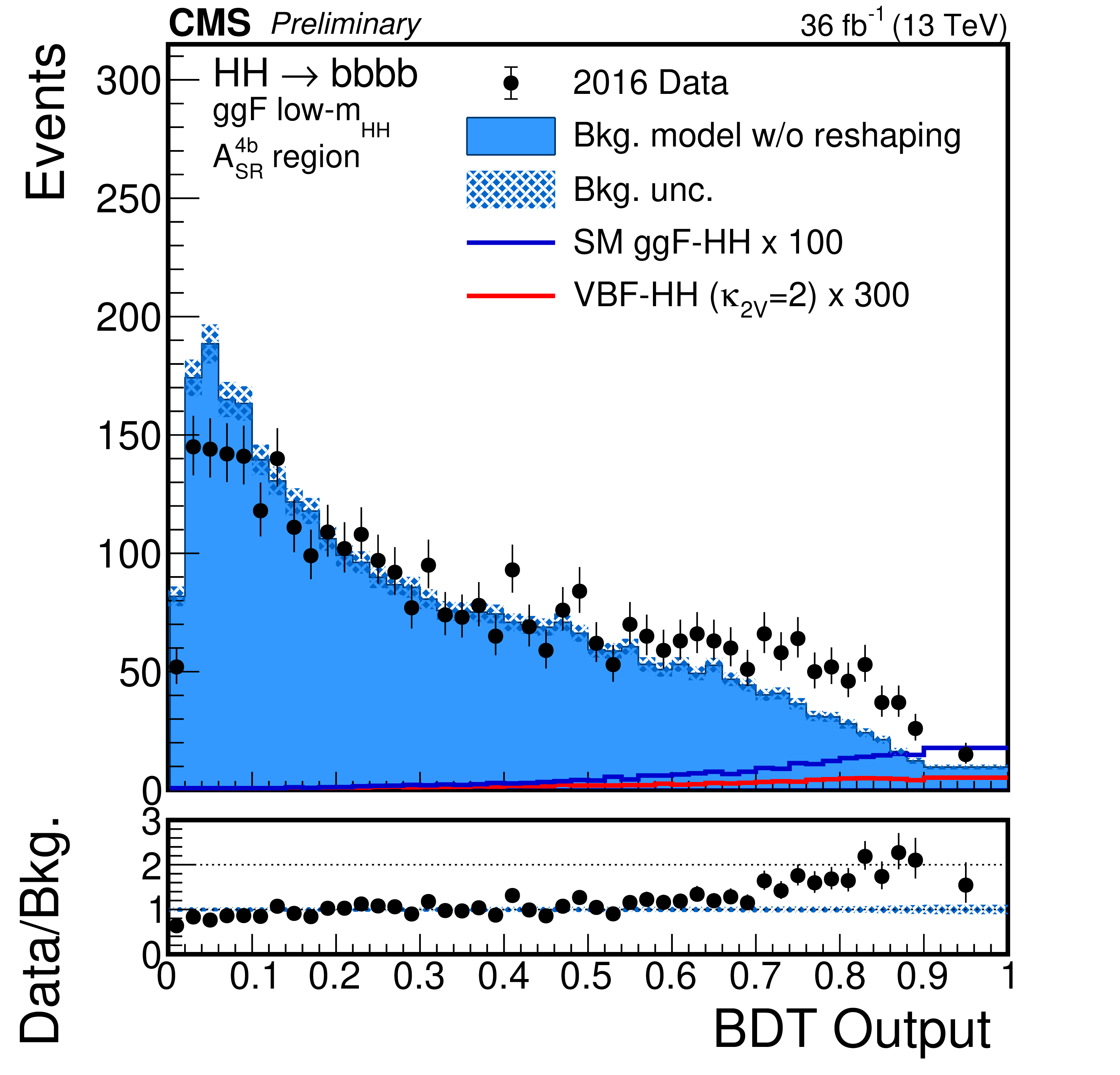
Additional Figure 4-a:
Prediction of the background distribution obtained directly from the $A_\text {SR}^{3 {\mathrm {b}}}$ region without the application of the BDT reweighting correction in the ggF category. The data correspond to the 2016 dataset. The output of the BDT discriminant is shown for the low-mass category. Data are represented by points with error bars, while the ggF (VBF) signal contribution is shown in blue (red) and not stacked. The background prediction without the shape correction is represented by the shaded blue histograms with the associated systematic uncertainties (dashed areas). |

png pdf |
Additional Figure 4-b:
Prediction of the background distribution obtained directly from the $A_\text {SR}^{3 {\mathrm {b}}}$ region without the application of the BDT reweighting correction in the ggF category. The data correspond to the 2016 dataset. The output of the BDT discriminant is shown for the high-mass category. Data are represented by points with error bars, while the ggF (VBF) signal contribution is shown in blue (red) and not stacked. The background prediction without the shape correction is represented by the shaded blue histograms with the associated systematic uncertainties (dashed areas). |

png pdf |
Additional Figure 4-c:
Prediction of the background distribution obtained directly from the $A_\text {SR}^{3 {\mathrm {b}}}$ region without the application of the BDT reweighting correction in the VBF category. The data correspond to the 2016 dataset. The $m_{{\mathrm {H}} {\mathrm {H}}}$ distribution in the SM-like category is shown. Data are represented by points with error bars, while the ggF (VBF) signal contribution is shown in blue (red) and not stacked. The background prediction without the shape correction is represented by the shaded blue histograms with the associated systematic uncertainties (dashed areas). |

png pdf |
Additional Figure 5:
Prediction of the background distribution obtained directly from the $A_\text {SR}^{3 {\mathrm {b}}}$ region without the application of the BDT reweighting correction. The top and bottom row show the ggF and VBF categories, respectively, and the data correspond to the 2017 and 2018 datasets. For the former, the output of the BDT discriminant is shown for the low-mass category on the left and for the high-mass category on the right. For the latter, the $m_{{\mathrm {H}} {\mathrm {H}}}$ distribution in the SM-like category is shown. The anomalous $\kappa _\text {2V}$-like category is not shown because no shape correction is applied for it since the overall number of observed events is used to perform a counting experiment. Data are represented by points with error bars, while the ggF (VBF) signal contribution is shown in blue (red) and not stacked. The background prediction without the shape correction is represented by the shaded blue histograms with the associated systematic uncertainties (dashed areas). |

png pdf |
Additional Figure 5-a:
Prediction of the background distribution obtained directly from the $A_\text {SR}^{3 {\mathrm {b}}}$ region without the application of the BDT reweighting correction in the ggF category. The data correspond to the 2017 and 2018 datasets. The output of the BDT discriminant is shown for the low-mass category. Data are represented by points with error bars, while the ggF (VBF) signal contribution is shown in blue (red) and not stacked. The background prediction without the shape correction is represented by the shaded blue histograms with the associated systematic uncertainties (dashed areas). |
png pdf |
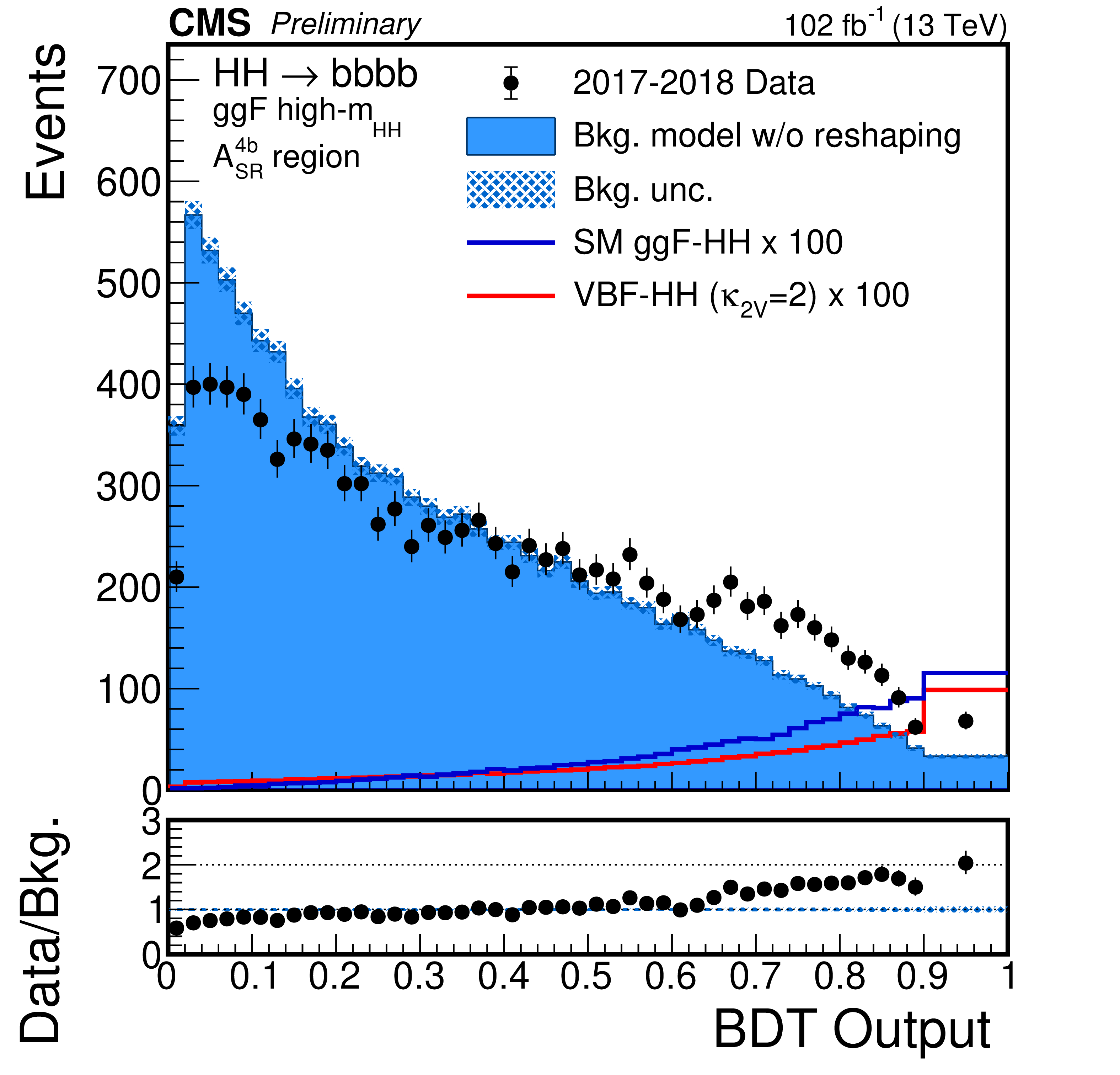
Additional Figure 5-b:
Prediction of the background distribution obtained directly from the $A_\text {SR}^{3 {\mathrm {b}}}$ region without the application of the BDT reweighting correction in the ggF category. The data correspond to the 2017 and 2018 datasets. The output of the BDT discriminant is shown for the high-mass category. Data are represented by points with error bars, while the ggF (VBF) signal contribution is shown in blue (red) and not stacked. The background prediction without the shape correction is represented by the shaded blue histograms with the associated systematic uncertainties (dashed areas). |

png pdf |
Additional Figure 5-c:
Prediction of the background distribution obtained directly from the $A_\text {SR}^{3 {\mathrm {b}}}$ region without the application of the BDT reweighting correction in the VBF category. The data correspond to the 2017 and 2018 datasets. The $m_{{\mathrm {H}} {\mathrm {H}}}$ distribution in the SM-like category is shown. Data are represented by points with error bars, while the ggF (VBF) signal contribution is shown in blue (red) and not stacked. The background prediction without the shape correction is represented by the shaded blue histograms with the associated systematic uncertainties (dashed areas). |

png pdf |
Additional Figure 6:
Observed and expected 95% CL upper limits on the gluon fusion Higgs boson pair production cross section for different combinations of Higgs boson couplings in the effective Lagrangian parametrization. The numbers from 1 to 12 denote the shape benchmarks defined in Ref. [54], corresponding to points in the five-dimensional parameter space with characteristic kinematic properties of the $ {\mathrm {H}} {\mathrm {H}} $ system. The leading order simulation is reweighted to match the $m_{{\mathrm {H}} {\mathrm {H}}}$ spectrum at the next-to-leading order as predicted by simulation described in Ref. [55]. The inner (green) band and the outer (yellow) band indicate the regions containing 68 and 95%, respectively, of the distribution of limits expected under the background-only hypothesis. |
png pdf |
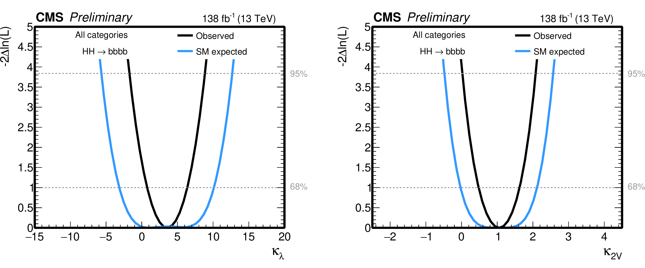
Additional Figure 7:
Expected and observed likelihood scan as a function of the $\kappa _{\lambda}$ (left) and $\kappa _\text {2V}$ (right) couplings. All the couplings that are not displayed in the figure are fixed to their SM prediction. |

png pdf |
Additional Figure 7-a:
Expected and observed likelihood scan as a function of the $\kappa _{\lambda}$ coupling. All the couplings that are not displayed in the figure are fixed to their SM prediction. |

png pdf |
Additional Figure 7-b:
Expected and observed likelihood scan as a function of the $\kappa _\text {2V}$ coupling. All the couplings that are not displayed in the figure are fixed to their SM prediction. |
png pdf |
Additional Figure 8:
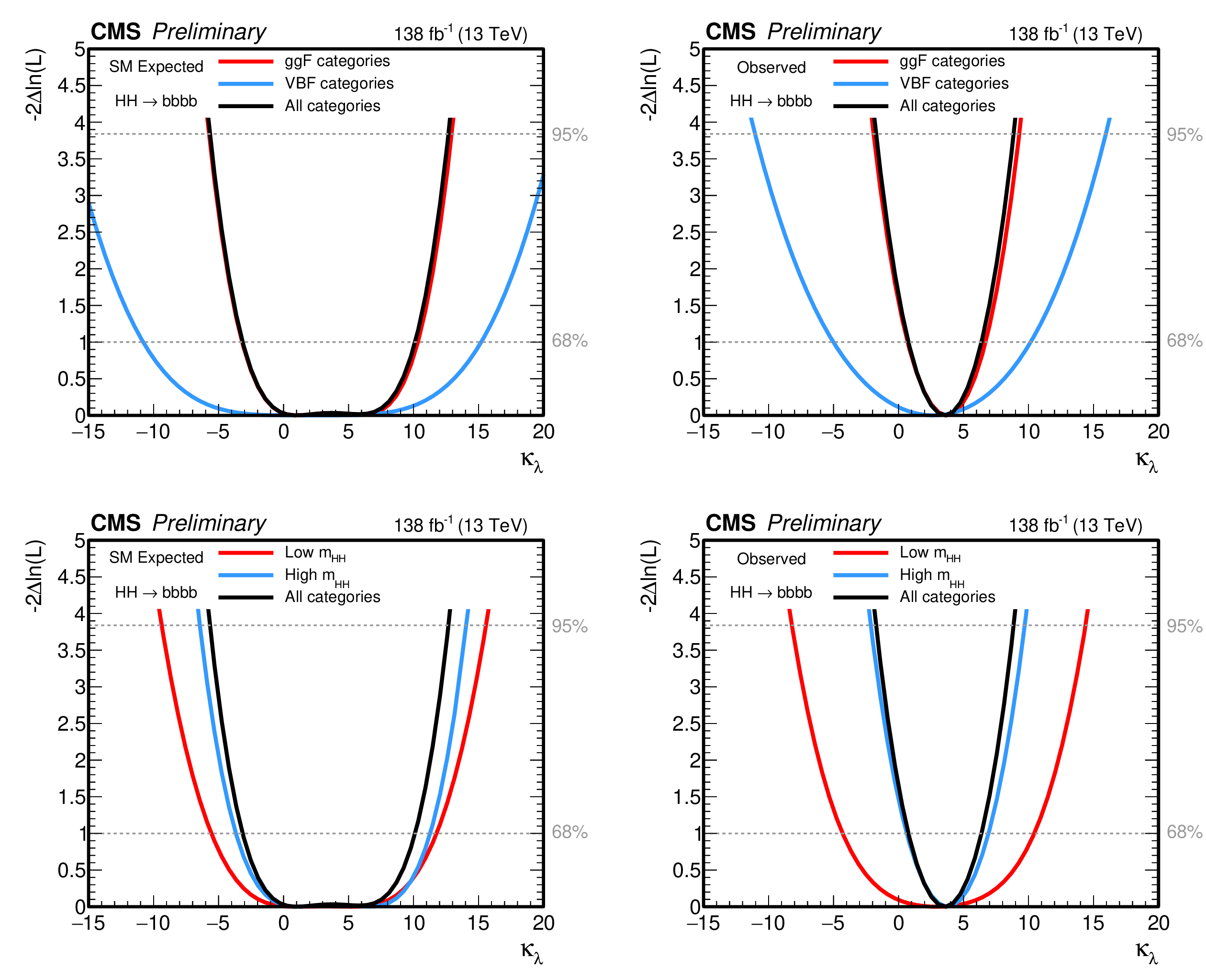
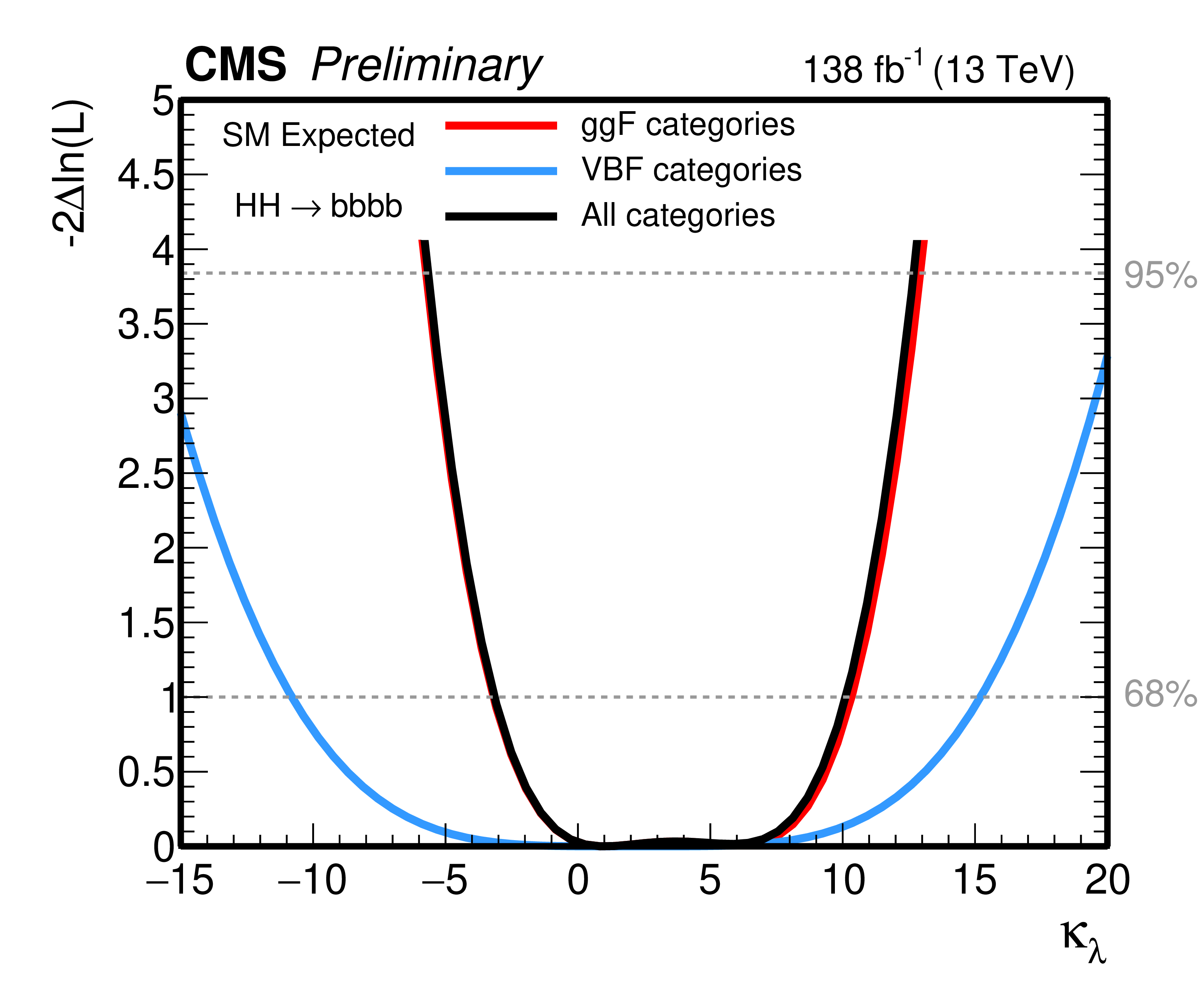
Expected (left column) and observed (right column) likelihood scans as a function of the $\kappa _{\lambda}$ couplings, assuming all the other couplings to be fixed to their SM prediction. The top row shows the contribution of the ggF (red) and VBF (blue) categories and their combination (black). The bottom row shows the contribution of the low- (red) and high-mass (blue) ggF categories, and the overall combination of all the ggF and VBF categories (black). For all the curves, the 2016, 2017 and 2018 datasets are combined. |
png pdf |
Additional Figure 8-a:
Expected likelihood scans as a function of the $\kappa _{\lambda}$ couplings, assuming all the other couplings to be fixed to their SM prediction. The plot shows the contribution of the ggF (red) and VBF (blue) categories and their combination (black). The 2016, 2017 and 2018 datasets are combined. |

png pdf |
Additional Figure 8-b:
Observed likelihood scans as a function of the $\kappa _{\lambda}$ couplings, assuming all the other couplings to be fixed to their SM prediction. The plot shows the contribution of the ggF (red) and VBF (blue) categories and their combination (black). The 2016, 2017 and 2018 datasets are combined. |

png pdf |
Additional Figure 8-c:
Expected likelihood scans as a function of the $\kappa _{\lambda}$ couplings, assuming all the other couplings to be fixed to their SM prediction. The plot shows the contribution of the low- (red) and high-mass (blue) ggF categories, and the overall combination of all the ggF and VBF categories (black). The 2016, 2017 and 2018 datasets are combined. |

png pdf |
Additional Figure 8-d:
Observed likelihood scans as a function of the $\kappa _{\lambda}$ couplings, assuming all the other couplings to be fixed to their SM prediction. The plot shows the contribution of the low- (red) and high-mass (blue) ggF categories, and the overall combination of all the ggF and VBF categories (black). The 2016, 2017 and 2018 datasets are combined. |

png pdf |
Additional Figure 9:
Expected (left) and observed (right) regions allowed at the 68 and 95% CL as a function of the $\kappa _\text {2V}$ and $\kappa _\text {V}$ couplings, assuming the $\kappa _{{\mathrm {t}}}$ and $\kappa _{\lambda}$ couplings to be fixed to 1. The circle denotes the best-fit hypothesis while the star represents the SM prediction. All results shown in this note do not include single Higgs boson production measurements that constrain the $\kappa _\text {V}$ coupling. |

png pdf |
Additional Figure 9-a:
Expected regions allowed at the 68 and 95% CL as a function of the $\kappa _\text {2V}$ and $\kappa _\text {V}$ couplings, assuming the $\kappa _{{\mathrm {t}}}$ and $\kappa _{\lambda}$ couplings to be fixed to 1. The circle denotes the best-fit hypothesis while the star represents the SM prediction. All results shown in this note do not include single Higgs boson production measurements that constrain the $\kappa _\text {V}$ coupling. |

png pdf |
Additional Figure 9-b:
Observed regions allowed at the 68 and 95% CL as a function of the $\kappa _\text {2V}$ and $\kappa _\text {V}$ couplings, assuming the $\kappa _{{\mathrm {t}}}$ and $\kappa _{\lambda}$ couplings to be fixed to 1. The circle denotes the best-fit hypothesis while the star represents the SM prediction. All results shown in this note do not include single Higgs boson production measurements that constrain the $\kappa _\text {V}$ coupling. |

png pdf |
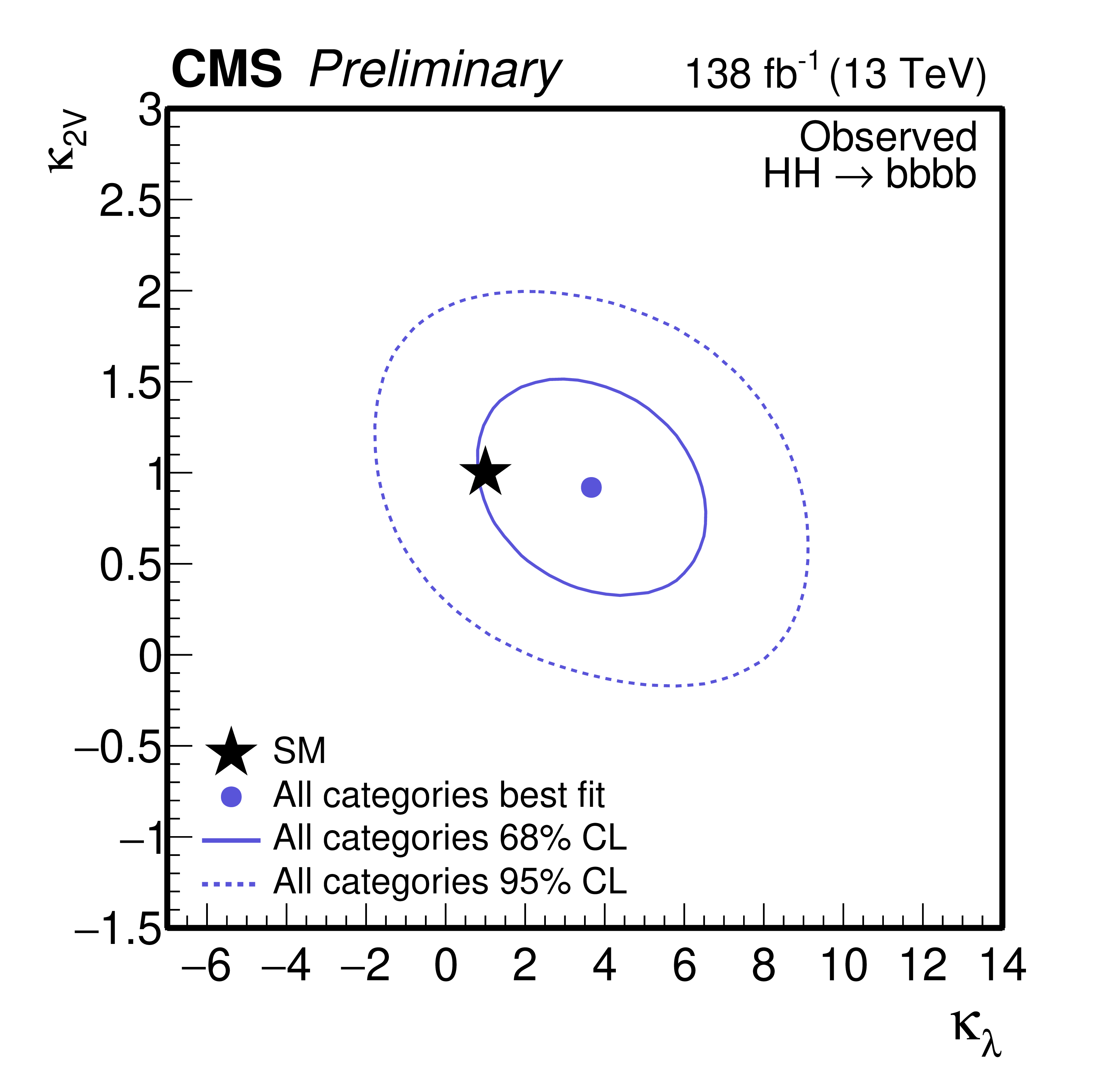
Additional Figure 10:
Expected (left) and observed (right) regions allowed at the 68 and 95% CL as a function of the $\kappa _\text {2V}$ and $\kappa _{\lambda}$ couplings, assuming the $\kappa _{{\mathrm {t}}}$ and $\kappa _\text {V}$ couplings to be fixed to 1. The circle denotes the best-fit hypothesis while the star represents the SM prediction. |

png pdf |
Additional Figure 10-a:
Expected regions allowed at the 68 and 95% CL as a function of the $\kappa _\text {2V}$ and $\kappa _{\lambda}$ couplings, assuming the $\kappa _{{\mathrm {t}}}$ and $\kappa _\text {V}$ couplings to be fixed to 1. The circle denotes the best-fit hypothesis while the star represents the SM prediction. |
png pdf |
Additional Figure 10-b:
Observed regions allowed at the 68 and 95% CL as a function of the $\kappa _\text {2V}$ and $\kappa _{\lambda}$ couplings, assuming the $\kappa _{{\mathrm {t}}}$ and $\kappa _\text {V}$ couplings to be fixed to 1. The circle denotes the best-fit hypothesis while the star represents the SM prediction. |
png pdf |
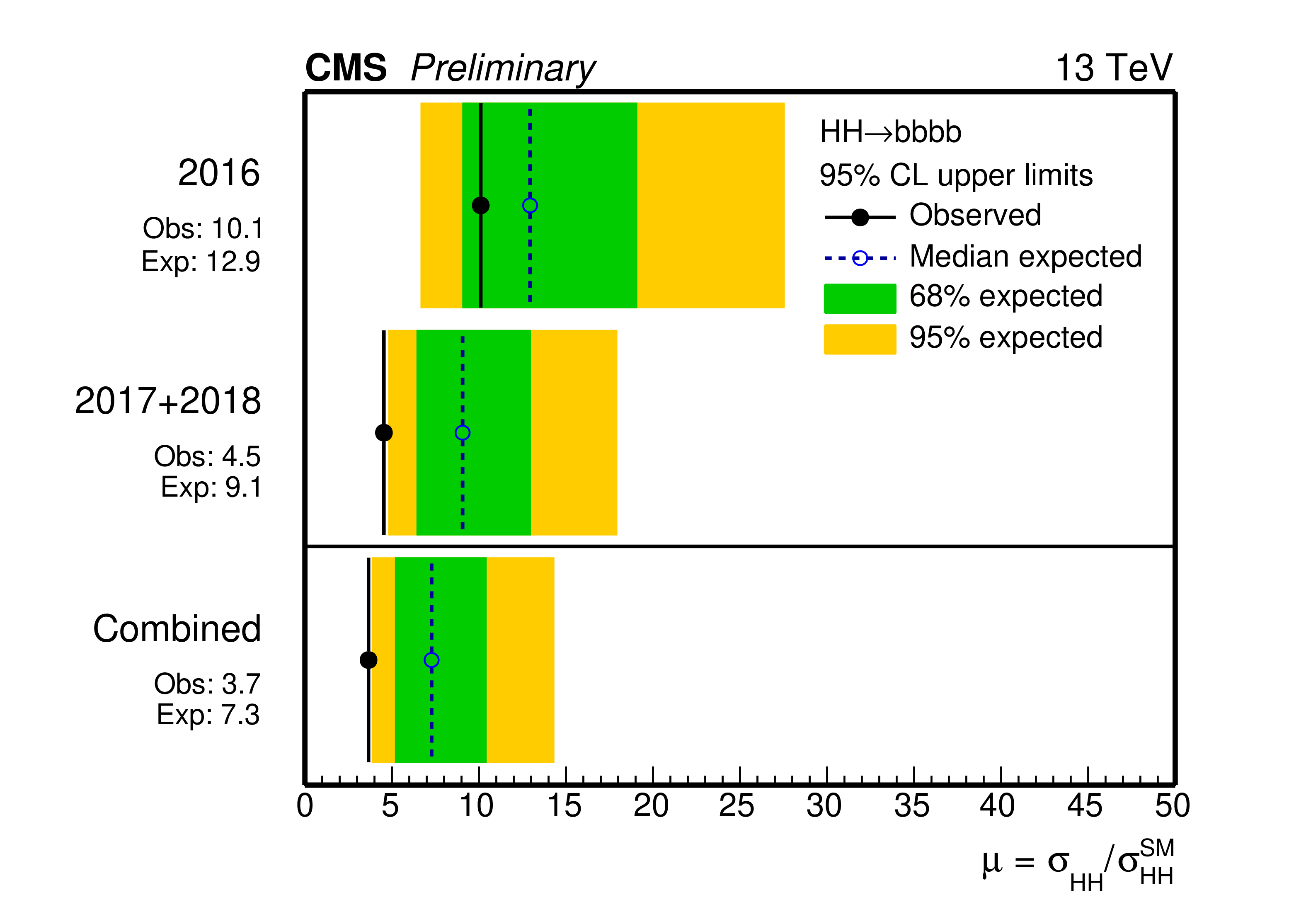
Additional Figure 11:
Observed and expected 95% CL limits on the standard model Higgs boson pair (HH) production signal strength ($\mu $) by year: 2016 (top row), 2017-2018 (center row) and combined (bottom row). |

png pdf |
Additional Figure 12:
Observed and expected 95% CL limits on the standard model Higgs boson pair (HH) production signal strength ($\mu $) by category: ggF Low $\mathrm {m_{HH}}$ (first row), ggF High $\mathrm {m_{HH}}$ (second row), VBF categories (third row), and combined (fourth row). |

png pdf |
Additional Figure 13:
Signal strength ($\mu $) of the SM ggF and VBF production modes. The solid (dashed) line denotes the contour corresponding to the 68% (95%) confidence levels. The circle represents the best-fit value while the star represents the SM expectation. |
png pdf |
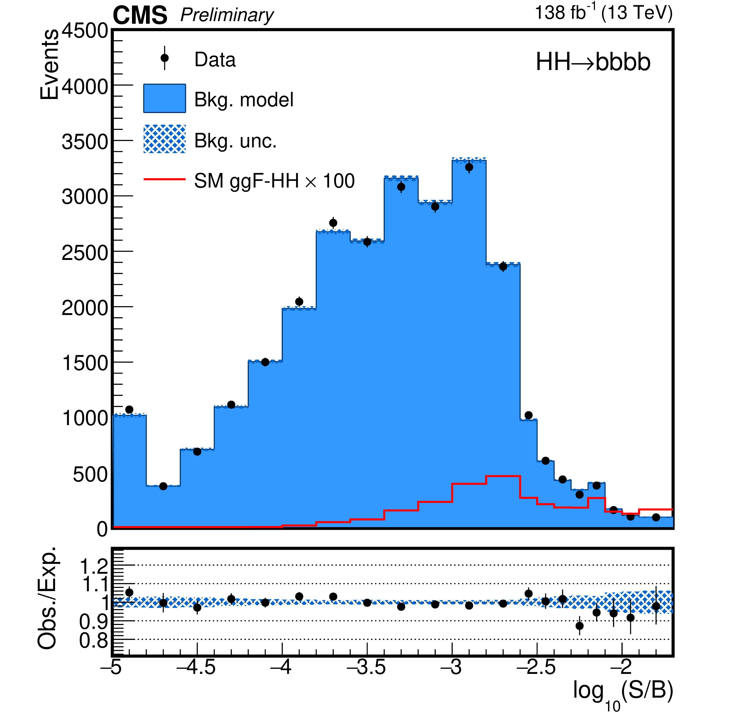
Additional Figure 14:
Distribution of the expected signal to background ratio for events selected in the categories of the analysis. The leftmost bin also includes events whose value of the signal-to-background ratio are below the represented range (underflow). |
| References | ||||
| 1 | F. Englert and R. Brout | Broken symmetry and the mass of gauge vector mesons | PRL 13 (Aug, 1964) 321 | |
| 2 | P. W. Higgs | Broken symmetries and the masses of gauge bosons | PRL 13 (Oct, 1964) 508 | |
| 3 | G. S. Guralnik, C. R. Hagen, and T. W. B. Kibble | Global conservation laws and massless particles | PRL 13 (Nov, 1964) 585 | |
| 4 | ATLAS Collaboration | Observation of a new particle in the search for the Standard Model Higgs boson with the ATLAS detector at the LHC | PLB 716 (2012) 1 | 1207.7214 |
| 5 | CMS Collaboration | Observation of a new boson at a mass of 125 GeV with the CMS experiment at the LHC | PLB 716 (2012) 30 | CMS-HIG-12-028 1207.7235 |
| 6 | CMS Collaboration | Observation of a new boson with mass near 125 GeV in pp collisions at $ \sqrt{s} = $ 7 and 8 TeV | JHEP 06 (2013) 081 | CMS-HIG-12-036 1303.4571 |
| 7 | S. Dawson, S. Dittmaier, and M. Spira | Neutral Higgs boson pair production at hadron colliders: QCD corrections | PRD 58 (1998) 115012 | hep-ph/9805244 |
| 8 | S. Borowka et al. | Higgs Boson Pair Production in Gluon Fusion at Next-to-Leading Order with Full Top-Quark Mass Dependence | PRL 117 (2016) 012001 | 1604.06447 |
| 9 | J. Baglio et al. | Gluon fusion into Higgs pairs at NLO QCD and the top mass scheme | EPJC 79 (2019) 459 | 1811.05692 |
| 10 | D. de Florian and J. Mazzitelli | Higgs Boson Pair Production at Next-to-Next-to-Leading Order in QCD | PRL 111 (2013) 201801 | 1309.6594 |
| 11 | D. Y. Shao, C. S. Li, H. T. Li, and J. Wang | Threshold resummation effects in Higgs boson pair production at the LHC | JHEP 07 (2013) 169 | 1301.1245 |
| 12 | D. de Florian and J. Mazzitelli | Higgs pair production at next-to-next-to-leading logarithmic accuracy at the LHC | JHEP 09 (2015) 053 | 1505.07122 |
| 13 | M. Grazzini et al. | Higgs boson pair production at NNLO with top quark mass effects | JHEP 05 (2018) 059 | 1803.02463 |
| 14 | F. A. Dreyer and A. Karlberg | Vector-Boson Fusion Higgs Pair Production at N$ ^3 $LO | PRD 98 (2018) 114016 | 1811.07906 |
| 15 | ATLAS Collaboration | Search for pair production of Higgs bosons in the $ b\bar{b}b\bar{b} $ final state using proton-proton collisions at $ \sqrt{s} = $ 13 TeV with the ATLAS detector | JHEP 01 (2019) 030 | 1804.06174 |
| 16 | CMS Collaboration | Search for nonresonant Higgs boson pair production in the $ \mathrm{b\overline{b}b\overline{b}} $ final state at $ \sqrt{s} = $ 13 TeV | JHEP 04 (2019) 112 | CMS-HIG-17-017 1810.11854 |
| 17 | ATLAS Collaboration | Search for resonant and non-resonant Higgs boson pair production in the $ {b\bar{b}\tau^+\tau^-} $ decay channel in $ pp $ collisions at $ \sqrt{s}= $ 13 TeV with the ATLAS detector | PRL 121 (2018) 191801 | 1808.00336 |
| 18 | CMS Collaboration | Search for Higgs boson pair production in events with two bottom quarks and two tau leptons in proton-proton collisions at $ \sqrt s = $ 13TeV | PLB 778 (2018) 101 | CMS-HIG-17-002 1707.02909 |
| 19 | ATLAS Collaboration | Search for Higgs boson pair production in the $ b\bar{b}WW^{*} $ decay mode at $ \sqrt{s}= $ 13 TeV with the ATLAS detector | JHEP 04 (2019) 092 | 1811.04671 |
| 20 | CMS Collaboration | Search for resonant and nonresonant Higgs boson pair production in the $ \mathrm{b}\overline{\mathrm{b}}\mathit{\ell \nu \ell \nu} $ final state in proton-proton collisions at $ \sqrt{s}= $ 13 TeV | JHEP 01 (2018) 054 | CMS-HIG-17-006 1708.04188 |
| 21 | ATLAS Collaboration | Search for Higgs boson pair production in the $ \gamma\gamma b\bar{b} $ final state with 13 $ TeV pp $ collision data collected by the ATLAS experiment | JHEP 11 (2018) 040 | 1807.04873 |
| 22 | CMS Collaboration | Search for Higgs boson pair production in the $ \gamma\gamma\mathrm{b\overline{b}} $ final state in pp collisions at $ \sqrt{s}= $ 13 TeV | PLB 788 (2019) 7 | CMS-HIG-17-008 1806.00408 |
| 23 | ATLAS Collaboration | Search for Higgs boson pair production in the $ \gamma\gamma WW^{*} $ channel using $ pp $ collision data recorded at $ \sqrt{s} = $ 13 TeV with the ATLAS detector | EPJC 78 (2018) 1007 | 1807.08567 |
| 24 | ATLAS Collaboration | Search for Higgs boson pair production in the $ WW^{(*)}WW^{(*)} $ decay channel using ATLAS data recorded at $ \sqrt{s}= $ 13 TeV | JHEP 05 (2019) 124 | 1811.11028 |
| 25 | ATLAS Collaboration | Search for non-resonant Higgs boson pair production in the $ bb\ell\nu\ell\nu $ final state with the ATLAS detector in $ pp $ collisions at $ \sqrt{s} = $ 13 TeV | PLB 801 (2020) 135145 | 1908.06765 |
| 26 | CMS Collaboration | Search for nonresonant Higgs boson pair production in final states with two bottom quarks and two photons in proton-proton collisions at $ \sqrt{s} = $ 13 TeV | JHEP 03 (2021) 257 | CMS-HIG-19-018 2011.12373 |
| 27 | ATLAS Collaboration | Search for the $ HH \rightarrow b \bar{b} b \bar{b} $ process via vector-boson fusion production using proton-proton collisions at $ \sqrt{s} = $ 13 TeV with the ATLAS detector | JHEP 07 (2020) 108 | 2001.05178 |
| 28 | LHC Higgs Cross Section Working Group | Handbook of LHC Higgs cross sections: 4. deciphering the nature of the Higgs sector | CERN (2016) | 1610.07922 |
| 29 | CMS Collaboration | The CMS trigger system | JINST 12 (2017) P01020 | CMS-TRG-12-001 1609.02366 |
| 30 | CMS Collaboration | The CMS experiment at the CERN LHC | JINST 3 (2008) S08004 | CMS-00-001 |
| 31 | CMS Collaboration | Particle-flow reconstruction and global event description with the CMS detector | JINST 12 (2017) P10003 | CMS-PRF-14-001 1706.04965 |
| 32 | M. Cacciari, G. P. Salam, and G. Soyez | The anti-$ k_t $ jet clustering algorithm | JHEP 04 (2008) 063 | 0802.1189 |
| 33 | M. Cacciari, G. P. Salam, and G. Soyez | FastJet user manual | EPJC 72 (2012) 1896 | 1111.6097 |
| 34 | CMS Collaboration | Jet energy scale and resolution in the CMS experiment in pp collisions at 8 TeV | JINST 12 (2017) P02014 | CMS-JME-13-004 1607.03663 |
| 35 | CMS Collaboration | Pileup mitigation at CMS in 13 TeV data | JINST 15 (2020) P09018 | CMS-JME-18-001 2003.00503 |
| 36 | CMS Collaboration | Identification of heavy-flavour jets with the CMS detector in pp collisions at 13 TeV | JINST 13 (2018) P05011 | CMS-BTV-16-002 1712.07158 |
| 37 | E. Bols et al. | Jet Flavour Classification Using DeepJet | JINST 15 (2020) P12012 | 2008.10519 |
| 38 | S. Alioli, P. Nason, C. Oleari, and E. Re | NLO vector-boson production matched with shower in POWHEG | JHEP 07 (2008) 060 | 0805.4802 |
| 39 | P. Nason | A New method for combining NLO QCD with shower Monte Carlo algorithms | JHEP 11 (2004) 040 | hep-ph/0409146 |
| 40 | S. Frixione, P. Nason, and C. Oleari | Matching NLO QCD computations with Parton Shower simulations: the POWHEG method | JHEP 11 (2007) 070 | 0709.2092 |
| 41 | J. Alwall et al. | The automated computation of tree-level and next-to-leading order differential cross sections, and their matching to parton shower simulations | JHEP 07 (2014) 079 | 1405.0301 |
| 42 | M. Czakon and A. Mitov | Top++: A Program for the Calculation of the Top-Pair Cross-Section at Hadron Colliders | CPC 185 (2014) 2930 | 1112.5675 |
| 43 | J. M. Campbell, R. K. Ellis, and C. Williams | Vector boson pair production at the LHC | JHEP 07 (2011) 018 | 1105.0020 |
| 44 | GEANT4 Collaboration | GEANT4--a simulation toolkit | NIMA 506 (2003) 250 | |
| 45 | CMS Collaboration | Jet algorithms performance in 13 TeV data | CMS-PAS-JME-16-003 | CMS-PAS-JME-16-003 |
| 46 | CMS Collaboration | A Deep Neural Network for Simultaneous Estimation of b Jet Energy and Resolution | Comput. Softw. Big Sci. 4 (2020) 10 | CMS-HIG-18-027 1912.06046 |
| 47 | A. Rogozhnikov | Reweighting with Boosted Decision Trees | J. Phys. Conf. Ser. 762 (2016) 012036 | 1608.05806 |
| 48 | CMS Collaboration | Precision luminosity measurement in proton-proton collisions at $ \sqrt{s} = $ 13 TeV in 2015 and 2016 at CMS | Submitted to EPJC | CMS-LUM-17-003 2104.01927 |
| 49 | CMS Collaboration | CMS luminosity measurement for the 2017 data-taking period at $ \sqrt{s} = $ 13 TeV | CMS-PAS-LUM-17-004 | CMS-PAS-LUM-17-004 |
| 50 | CMS Collaboration | CMS luminosity measurement for the 2018 data-taking period at $ \sqrt{s} = $ 13 TeV | CMS-PAS-LUM-18-002 | CMS-PAS-LUM-18-002 |
| 51 | T. Chen and C. Guestrin | XGBoost: A scalable tree boosting system | in Proceedings of the 22nd ACM SIGKDD International Conference on Knowledge Discovery and Data Mining, KDD '16, p. 785 ACM, New York, NY, USA | |
| 52 | T. Junk | Confidence level computation for combining searches with small statistics | NIMA 434 (1999) 435 | hep-ex/9902006 |
| 53 | A. L. Read | Presentation of search results: the $ CL_s $ technique | JPG 28 (2002) 2693 | |
| 54 | A. Carvalho et al. | Higgs Pair Production: Choosing Benchmarks With Cluster Analysis | JHEP 04 (2016) 126 | 1507.02245 |
| 55 | G. Buchalla et al. | Higgs boson pair production in non-linear Effective Field Theory with full $ m_{\mathrm{t}} $-dependence at NLO QCD | JHEP 09 (2018) 057 | 1806.05162 |
|
|
Compact Muon Solenoid LHC, CERN |
|

|

|

|

|

|