

Compact Muon Solenoid
LHC, CERN
| CMS-PAS-EXO-20-004 | ||
| Search for new particles in events with energetic jets and large missing transverse momentum in proton-proton collisions at $\sqrt{s}= $ 13 TeV | ||
| CMS Collaboration | ||
| June 2021 | ||
| Abstract: A search is presented for new particles produced in proton-proton collisions at $\sqrt{s}= $ 13 TeV at the LHC, using events with energetic jets and large missing transverse momentum. The analysis is based on a data sample corresponding to an integrated luminosity of 101 fb$^{-1}$, collected in 2017-2018 with the CMS detector. Separate categories are defined for events with narrow jets from initial-state radiation and with large-radius jets consistent with a hadronic decay of a W or a Z boson. Novel machine learning techniques are used to identify hadronic W and Z boson decays. The analysis is combined with an earlier search based on a data sample corresponding to an integrated luminosity of 36 fb$^{-1}$, collected in 2016. No significant excess of events is observed with respect to the standard model background expectation, as determined from control samples in data. The results are interpreted in terms of limits on the branching fraction of an invisible decay of the Higgs boson, as well as constraints on simplified models of dark matter, on first-generation scalar leptoquarks decaying to quarks and neutrinos, and on gravitons in models with large extra dimensions. Several of the new limits are the most restrictive to date. | ||
|
Links:
CDS record (PDF) ;
inSPIRE record ;
HepData record ;
CADI line (restricted) ;
These preliminary results are superseded in this paper, Submitted to JHEP. The superseded preliminary plots can be found here. |
||
| Figures | Summary | Additional Figures | References | CMS Publications |
|---|
|
MadAnalysis implementation:
https://doi.org/10.14428/DVN/IRF7ZL. |
| Figures | |
png pdf |
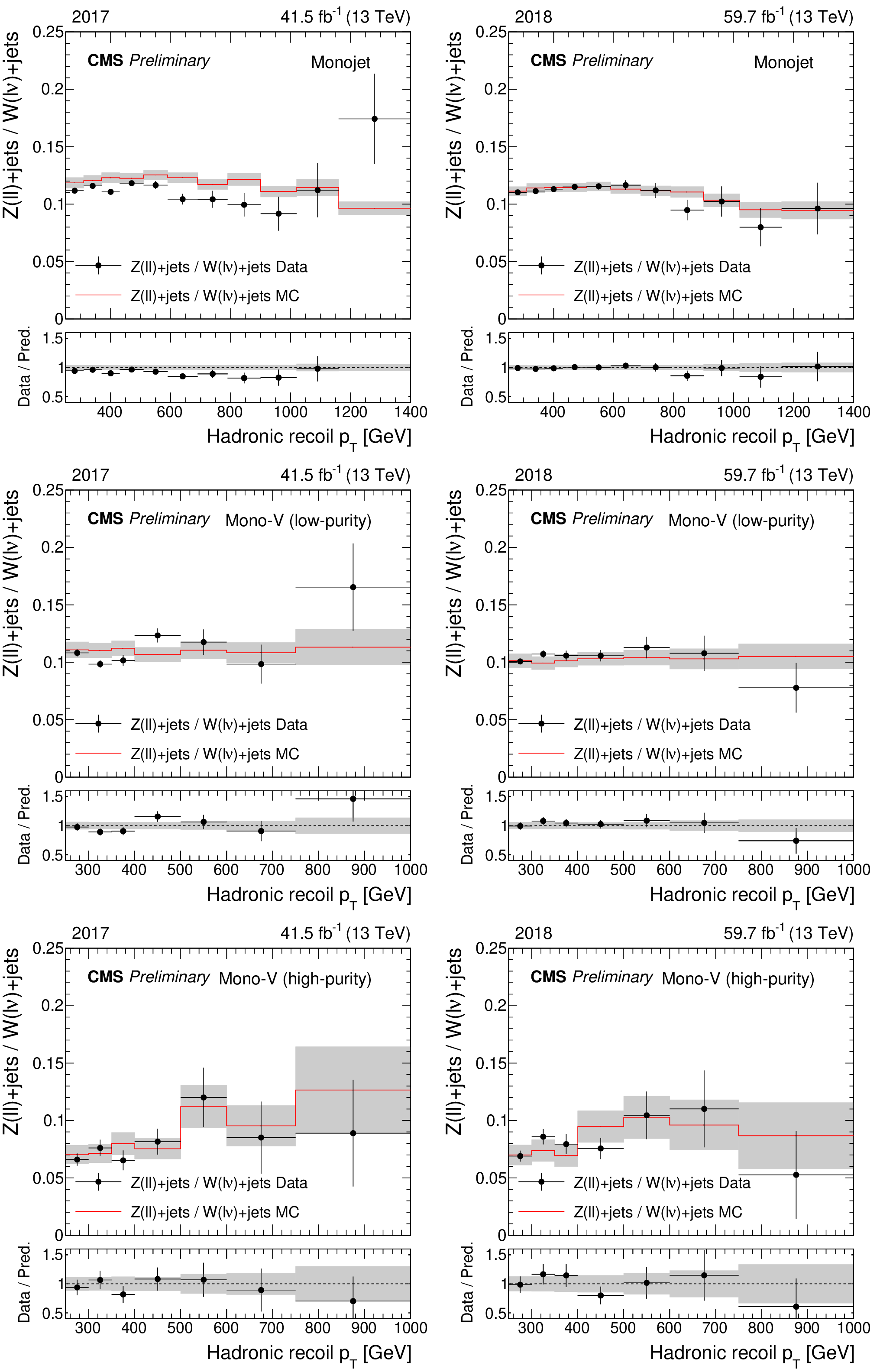
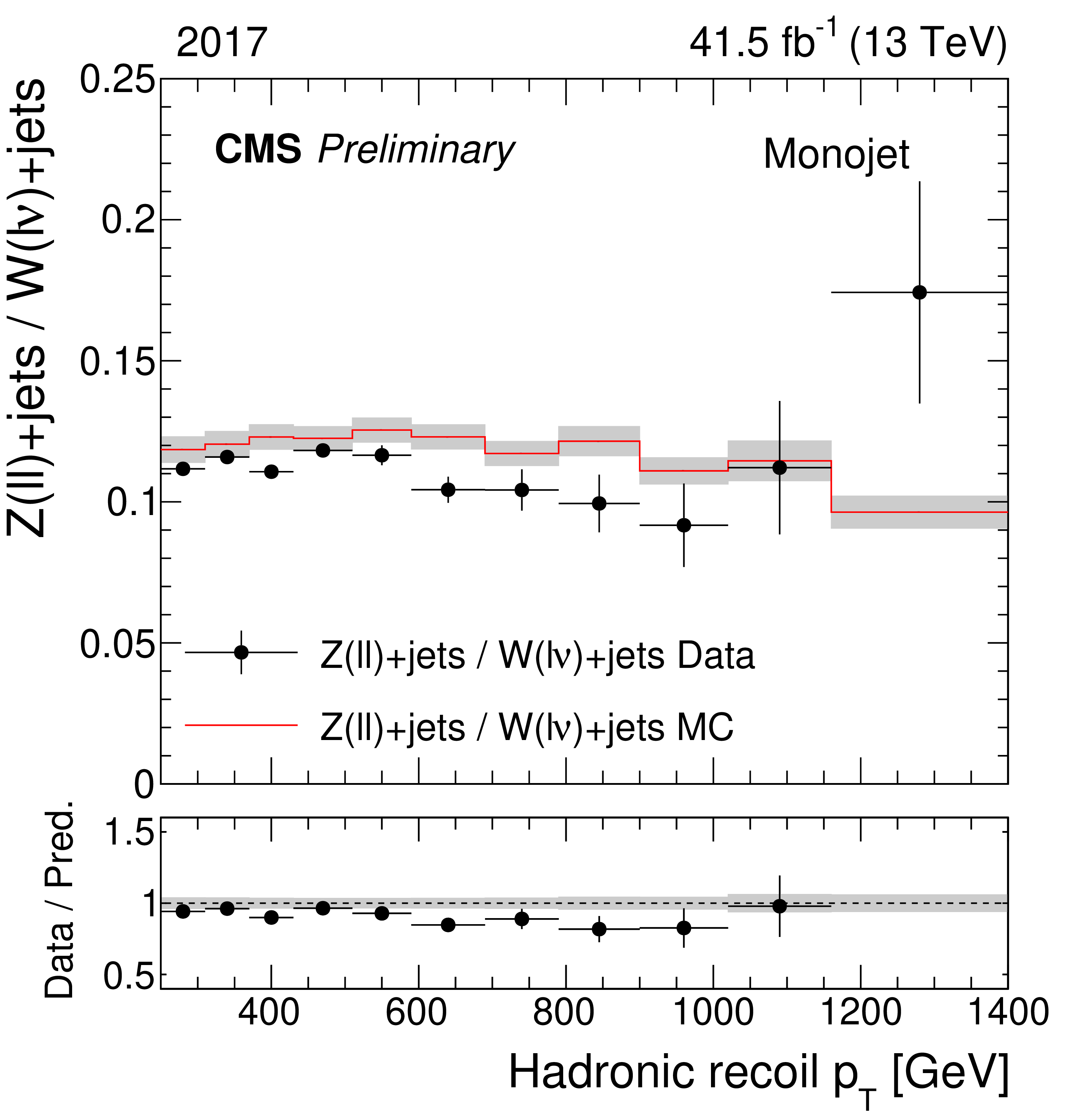
Figure 1:
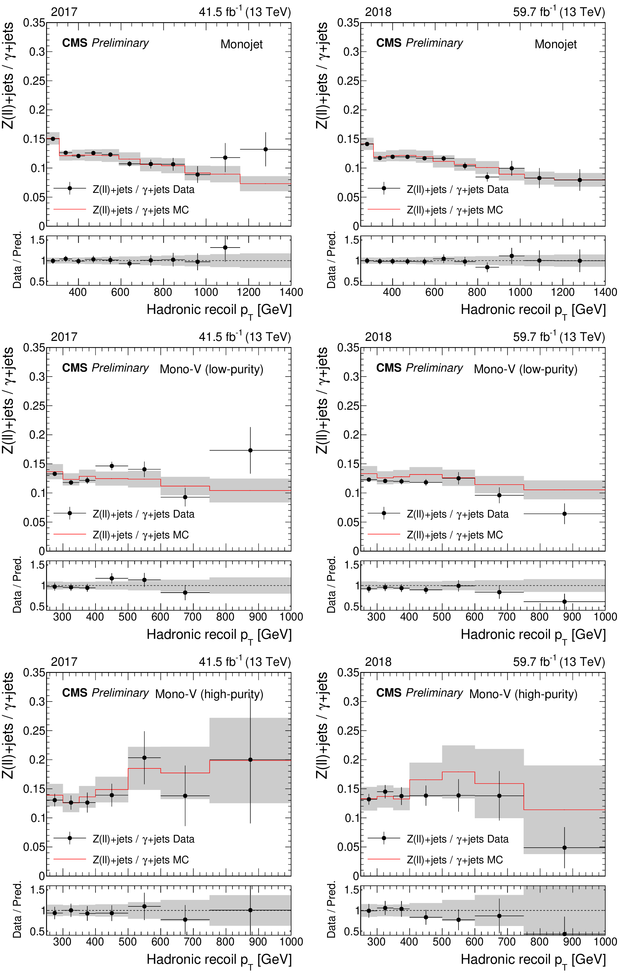
Ratio of the dilepton and single-lepton control region yields predicted using simulation (red solid line), and observed in data (black points). The gray band represents the total uncertainty in the ratio. In the lower panels, the ratio of data over prediction is shown. From upper to lower, the rows show the monojet, low-purity, and high-purity mono-V categories, while the left (right) column represents the 2017 (2018) data set. |
png pdf |
Figure 1-a:
Ratio of the dilepton and single-lepton control region yields predicted using simulation (red solid line), and observed in data (black points). The gray band represents the total uncertainty in the ratio. In the lower panels, the ratio of data over prediction is shown. From upper to lower, the rows show the monojet, low-purity, and high-purity mono-V categories, while the left (right) column represents the 2017 (2018) data set. |
png pdf |
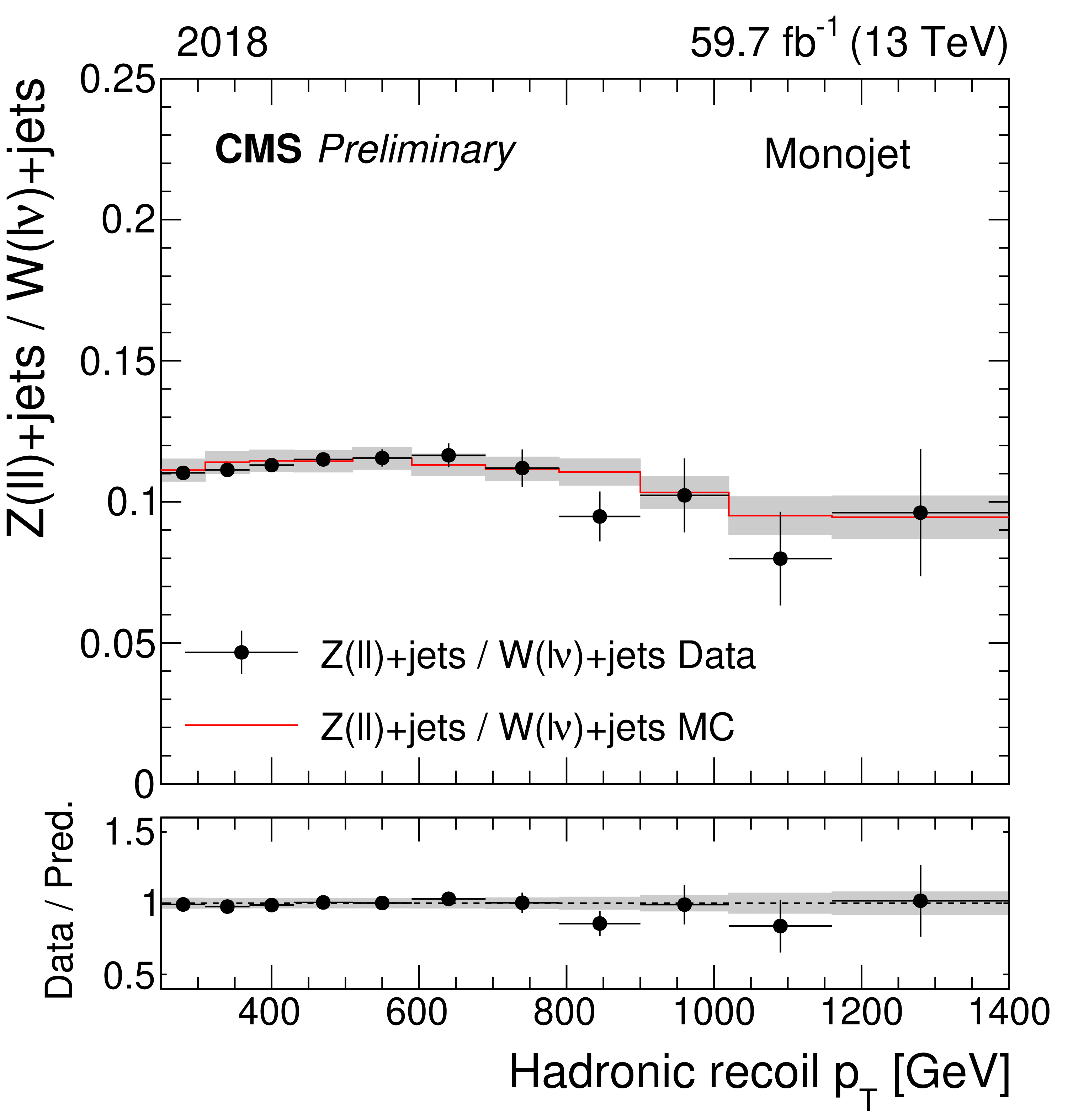
Figure 1-b:
Ratio of the dilepton and single-lepton control region yields predicted using simulation (red solid line), and observed in data (black points). The gray band represents the total uncertainty in the ratio. In the lower panels, the ratio of data over prediction is shown. From upper to lower, the rows show the monojet, low-purity, and high-purity mono-V categories, while the left (right) column represents the 2017 (2018) data set. |

png pdf |
Figure 1-c:
Ratio of the dilepton and single-lepton control region yields predicted using simulation (red solid line), and observed in data (black points). The gray band represents the total uncertainty in the ratio. In the lower panels, the ratio of data over prediction is shown. From upper to lower, the rows show the monojet, low-purity, and high-purity mono-V categories, while the left (right) column represents the 2017 (2018) data set. |

png pdf |
Figure 1-d:
Ratio of the dilepton and single-lepton control region yields predicted using simulation (red solid line), and observed in data (black points). The gray band represents the total uncertainty in the ratio. In the lower panels, the ratio of data over prediction is shown. From upper to lower, the rows show the monojet, low-purity, and high-purity mono-V categories, while the left (right) column represents the 2017 (2018) data set. |
png pdf |
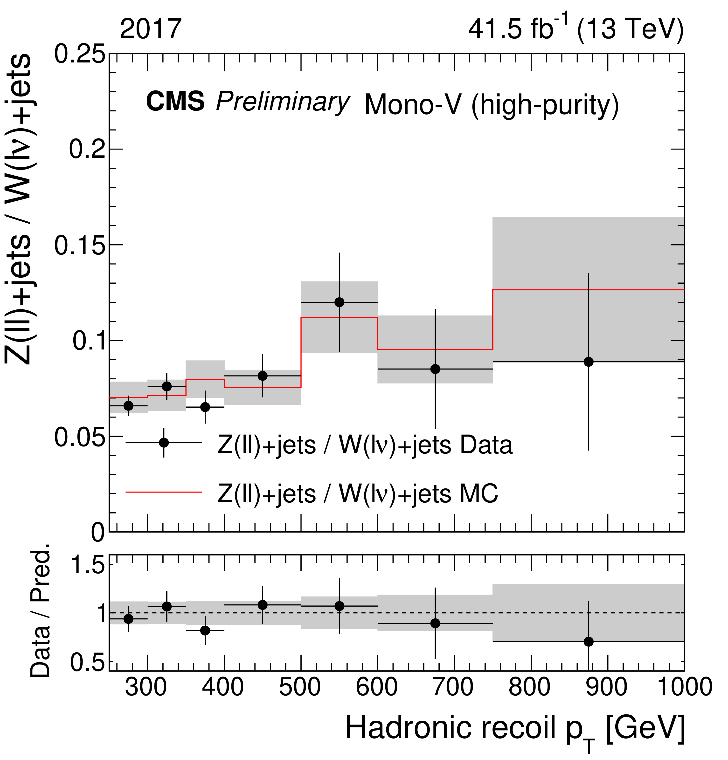
Figure 1-e:
Ratio of the dilepton and single-lepton control region yields predicted using simulation (red solid line), and observed in data (black points). The gray band represents the total uncertainty in the ratio. In the lower panels, the ratio of data over prediction is shown. From upper to lower, the rows show the monojet, low-purity, and high-purity mono-V categories, while the left (right) column represents the 2017 (2018) data set. |
png pdf |
Figure 1-f:
Ratio of the dilepton and single-lepton control region yields predicted using simulation (red solid line), and observed in data (black points). The gray band represents the total uncertainty in the ratio. In the lower panels, the ratio of data over prediction is shown. From upper to lower, the rows show the monojet, low-purity, and high-purity mono-V categories, while the left (right) column represents the 2017 (2018) data set. |
png pdf |
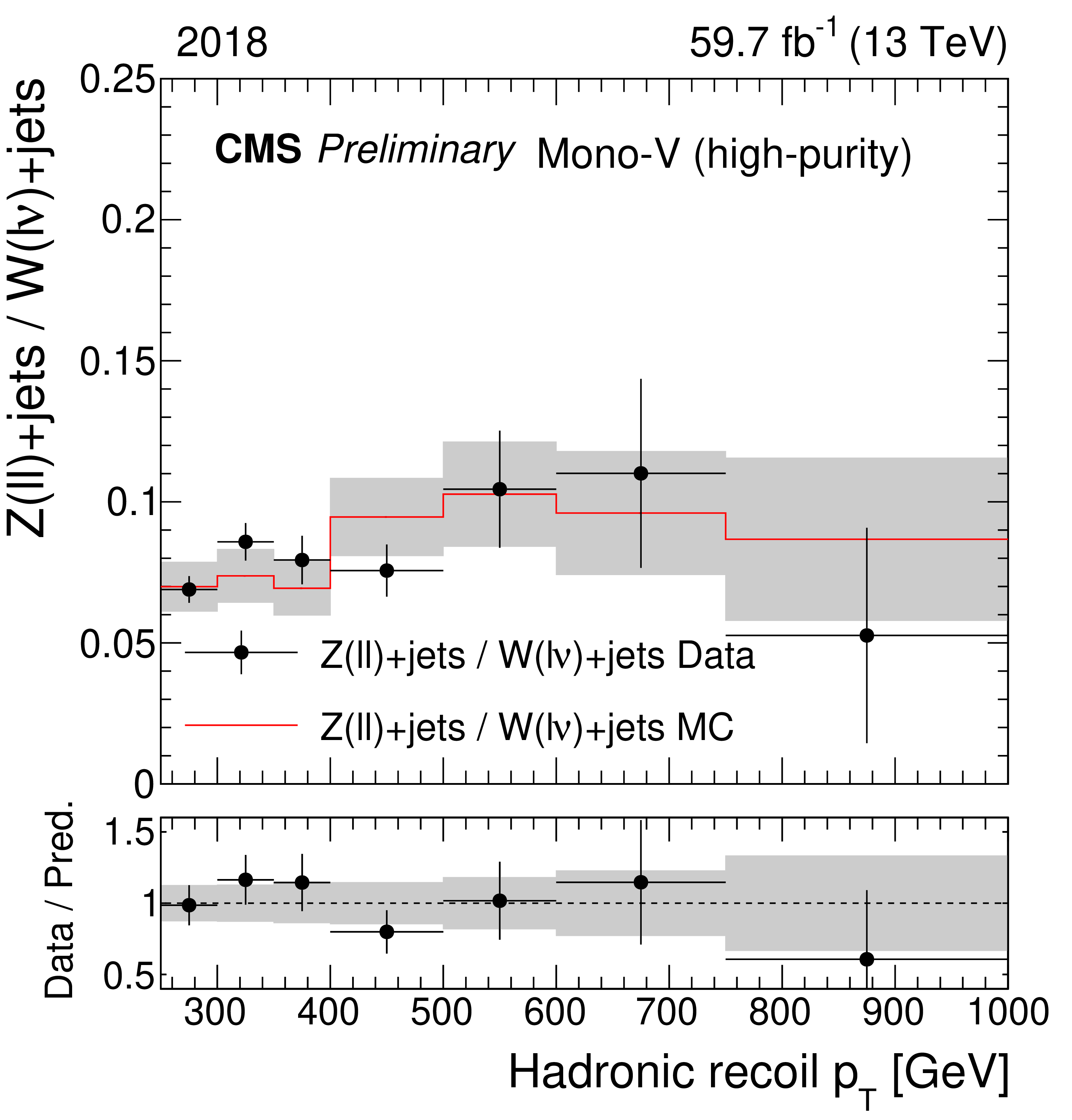
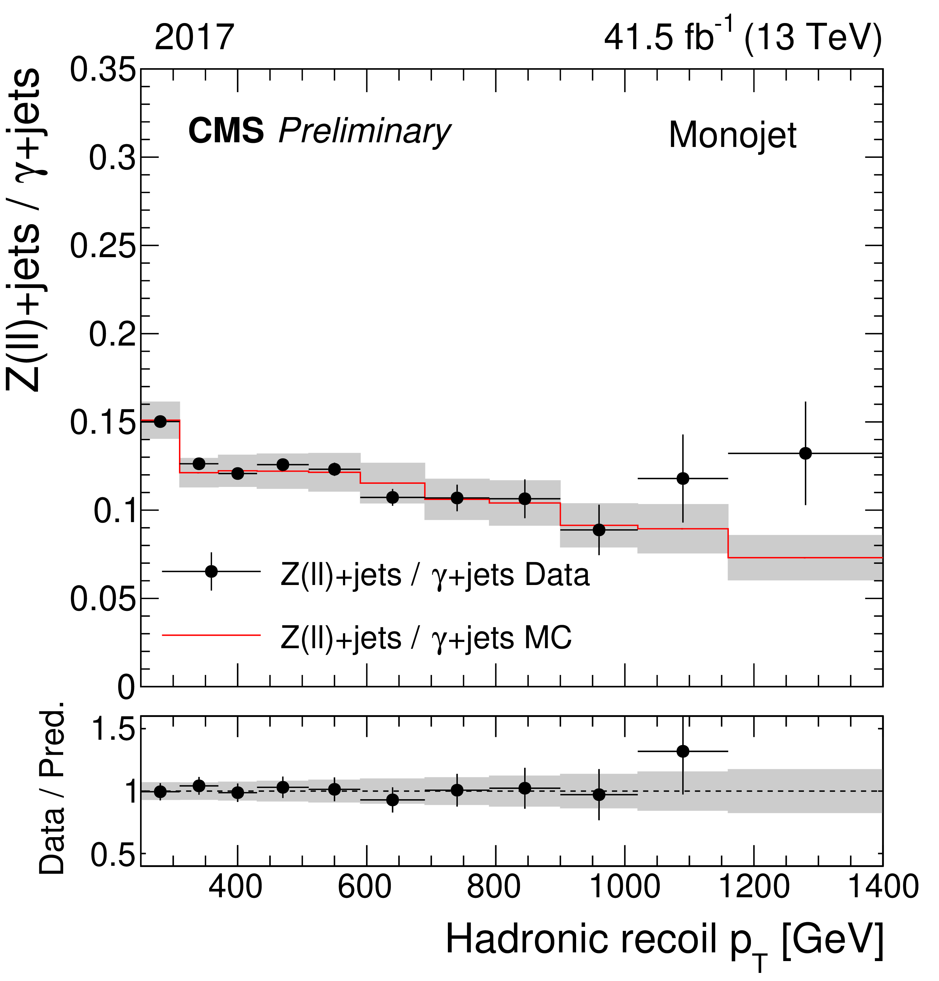
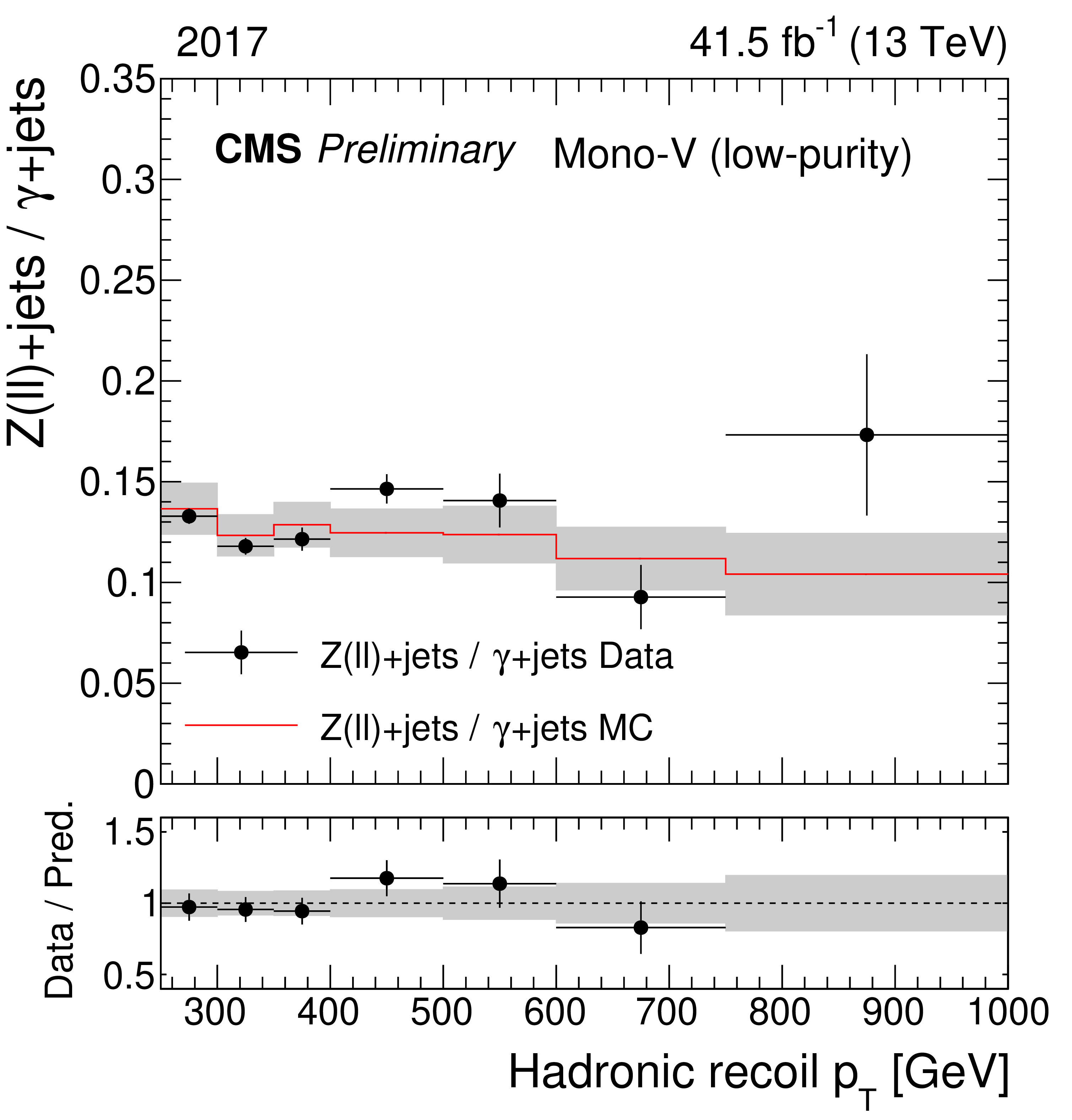
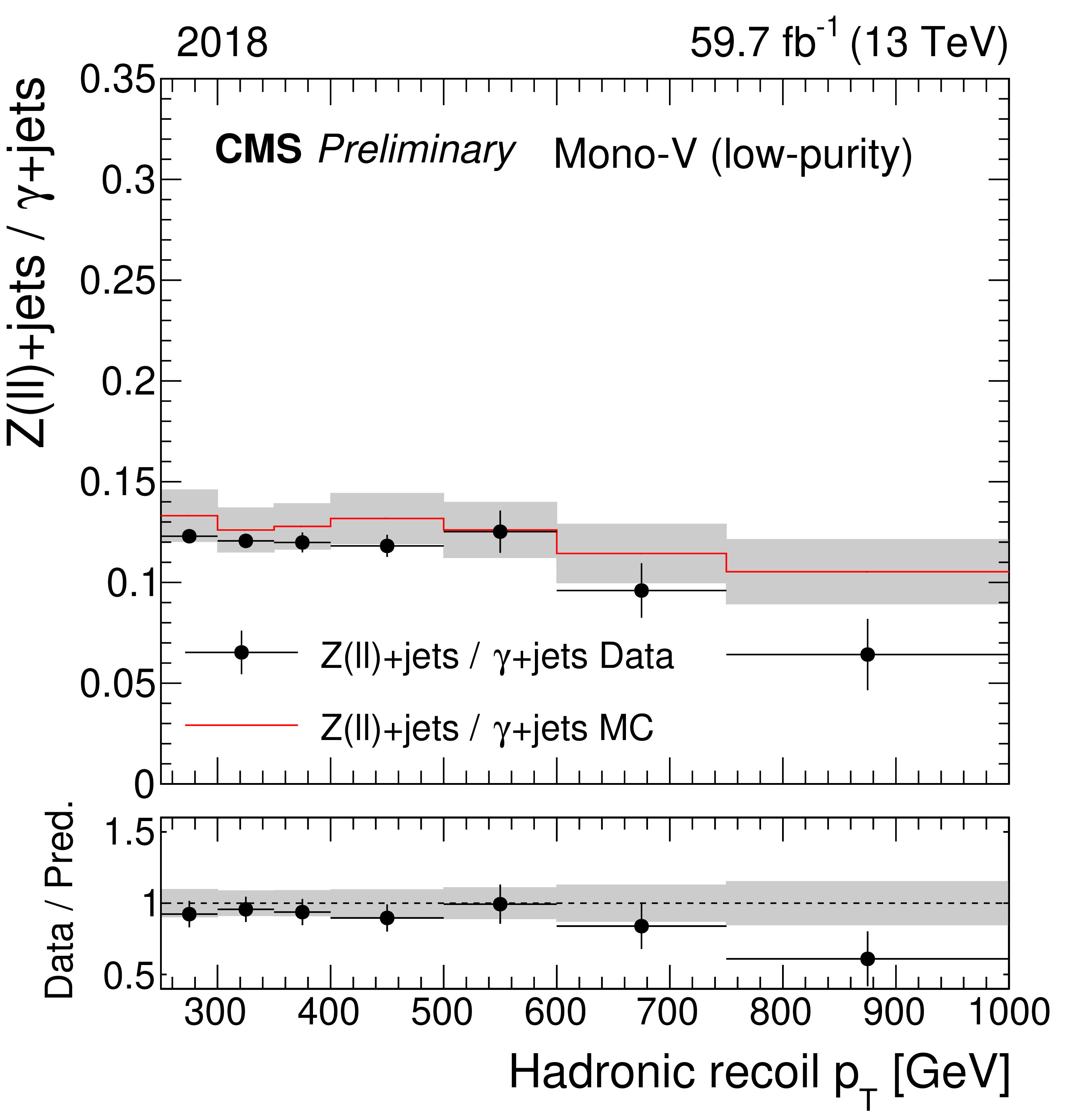
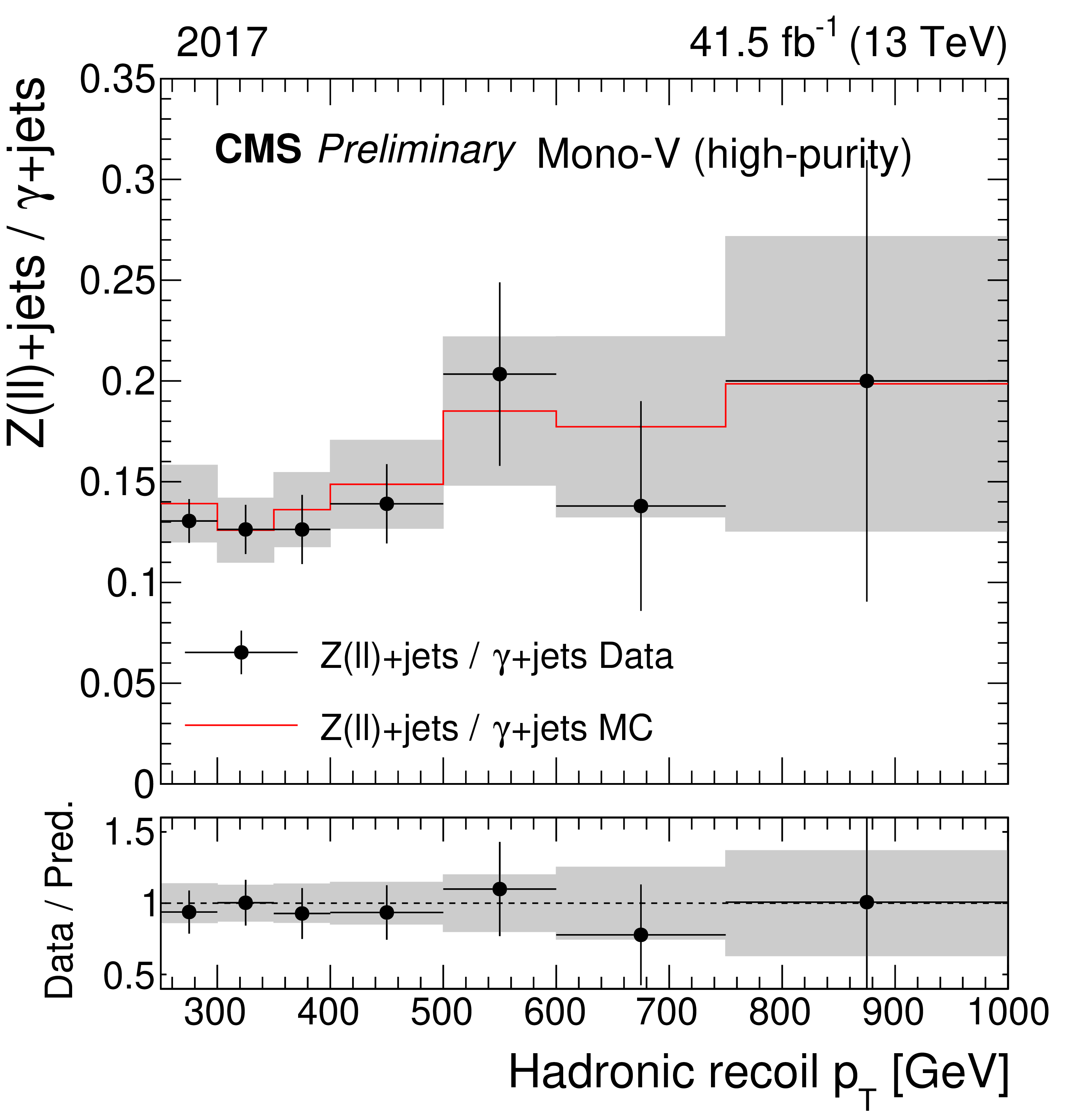
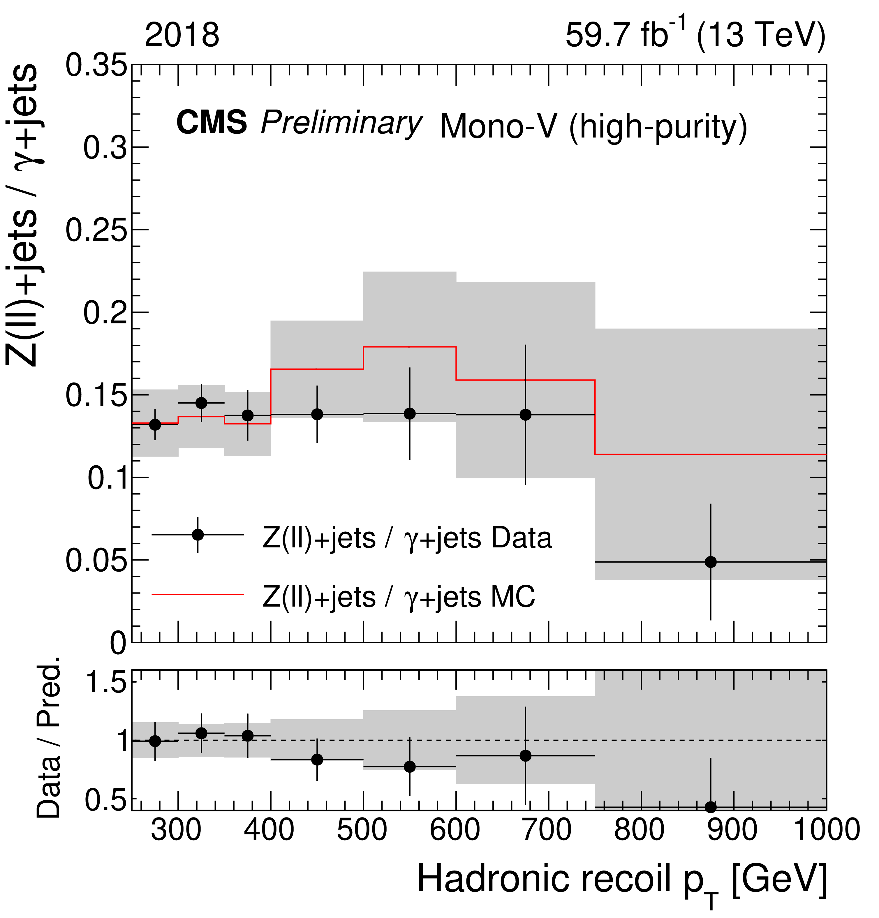
Figure 2:
Same as Fig. 1, but for the ratio of the dilepton and photon control regions. |
png pdf |
Figure 2-a:
Same as Fig. 1, but for the ratio of the dilepton and photon control regions. |

png pdf |
Figure 2-b:
Same as Fig. 1, but for the ratio of the dilepton and photon control regions. |
png pdf |
Figure 2-c:
Same as Fig. 1, but for the ratio of the dilepton and photon control regions. |
png pdf |
Figure 2-d:
Same as Fig. 1, but for the ratio of the dilepton and photon control regions. |
png pdf |
Figure 2-e:
Same as Fig. 1, but for the ratio of the dilepton and photon control regions. |
png pdf |
Figure 2-f:
Same as Fig. 1, but for the ratio of the dilepton and photon control regions. |
png pdf |
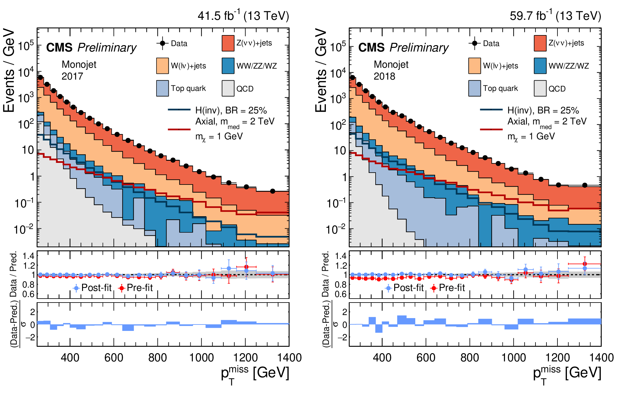
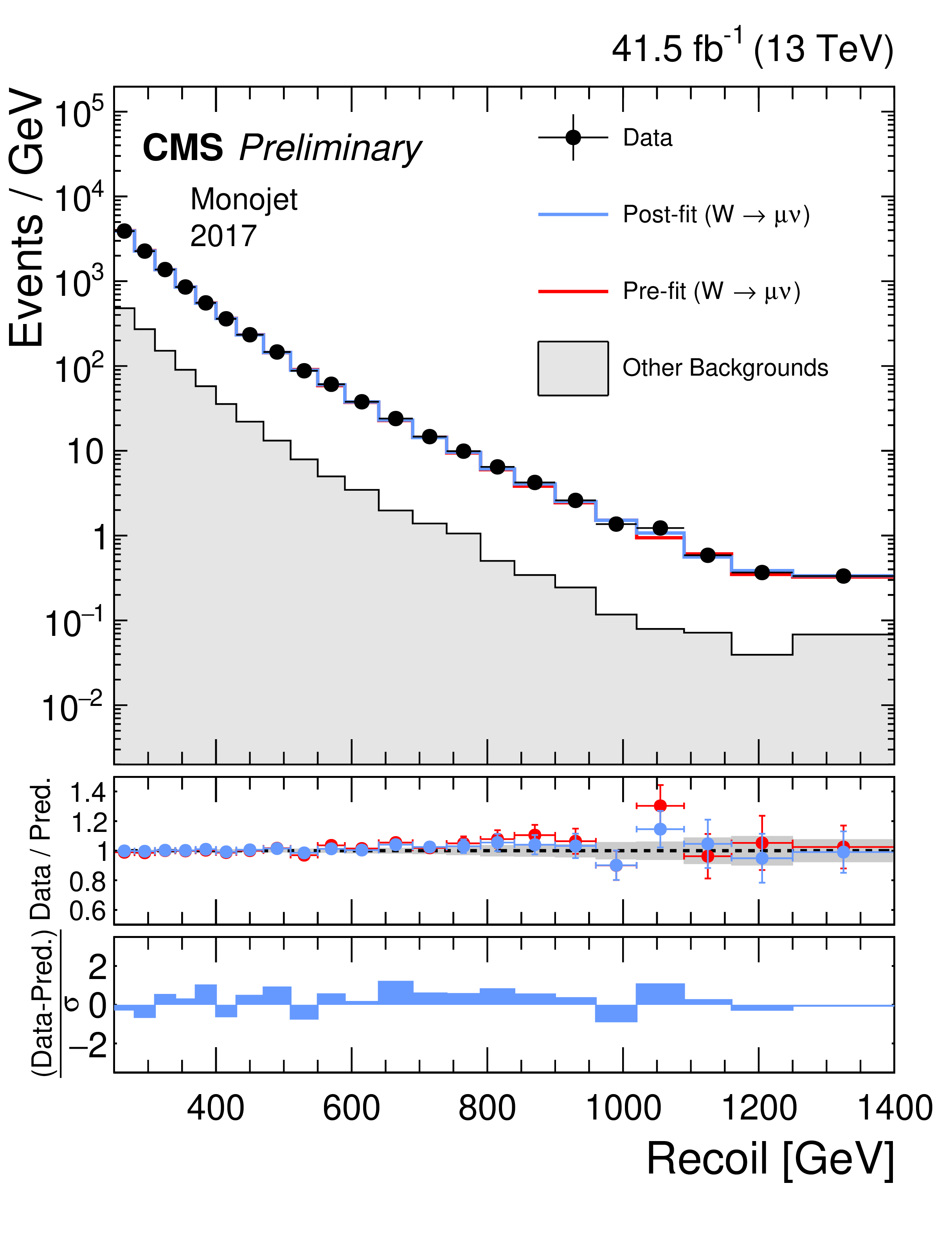
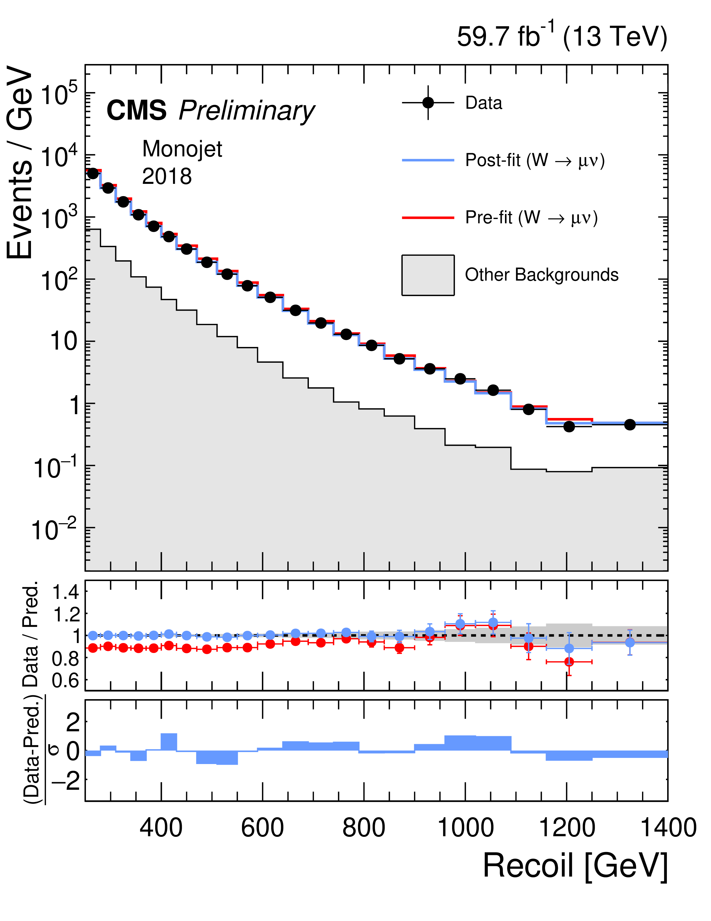
Figure 3:
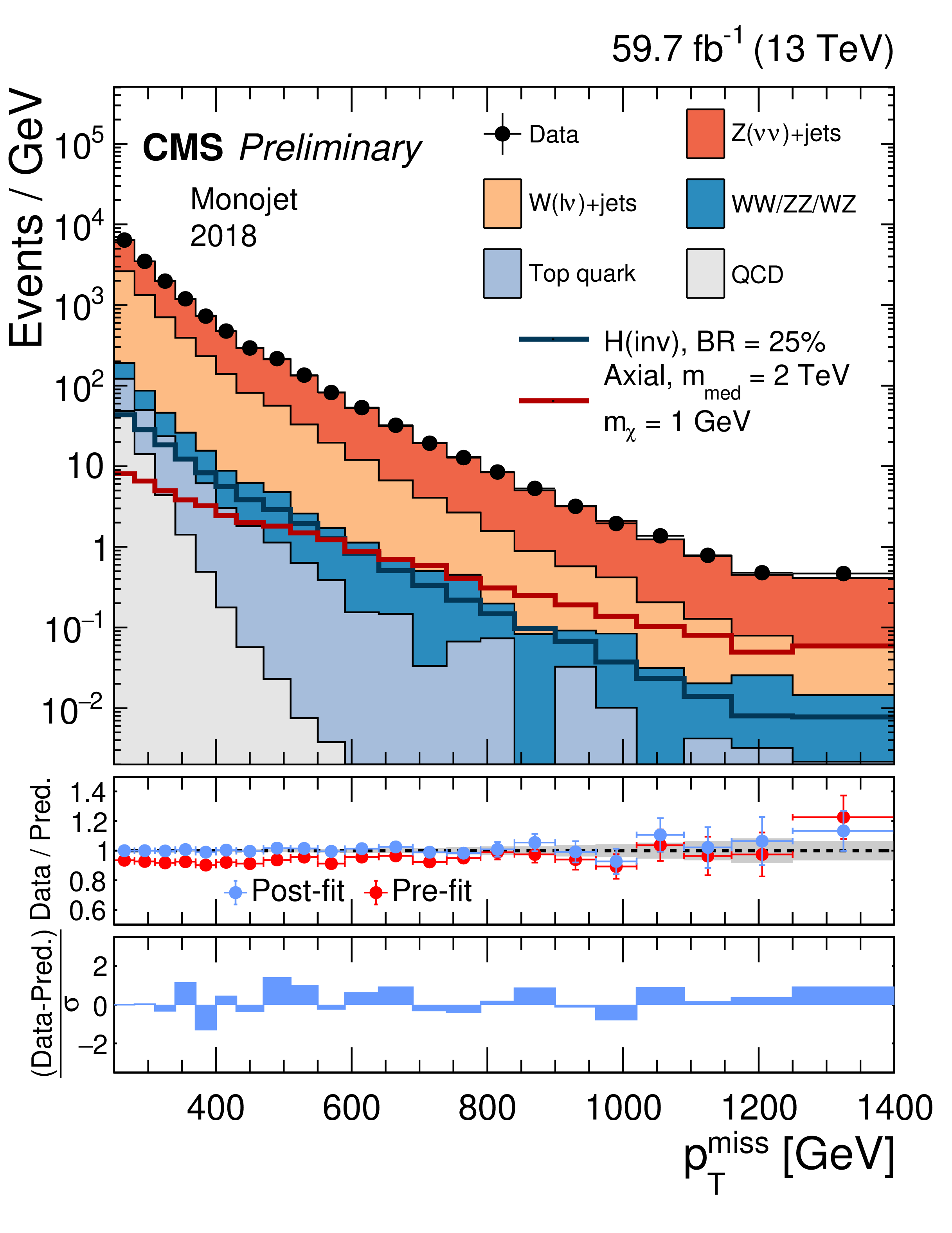
Comparison between data and the background prediction in the monojet signal regions before and after the simultaneous fit. The fit includes all control samples and the signal region in all categories and both data taking years, and the background-only fit model is used. The resulting distributions are shown separately for 2017 (left) and 2018 (right column). Templates for two signal hypothesis are shown overlaid as dark blue and dark red solid lines. The last bin includes the overflow. In the middle panels, ratios of data to the pre-fit background prediction (red open points) and post-fit background prediction (blue solid points) are shown. The gray band in the lower panels indicates the post-fit uncertainty after combining all the systematic uncertainties. Finally, the distribution of the pulls, defined as the difference between data and the post-fit background prediction divided by the quadratic sum of the post-fit uncertainty in the prediction and statistical uncertainty in data, is shown in the lower panels. |

png pdf |
Figure 3-a:
Comparison between data and the background prediction in the monojet signal regions before and after the simultaneous fit. The fit includes all control samples and the signal region in all categories and both data taking years, and the background-only fit model is used. The resulting distributions are shown separately for 2017 (left) and 2018 (right column). Templates for two signal hypothesis are shown overlaid as dark blue and dark red solid lines. The last bin includes the overflow. In the middle panels, ratios of data to the pre-fit background prediction (red open points) and post-fit background prediction (blue solid points) are shown. The gray band in the lower panels indicates the post-fit uncertainty after combining all the systematic uncertainties. Finally, the distribution of the pulls, defined as the difference between data and the post-fit background prediction divided by the quadratic sum of the post-fit uncertainty in the prediction and statistical uncertainty in data, is shown in the lower panels. |
png pdf |
Figure 3-b:
Comparison between data and the background prediction in the monojet signal regions before and after the simultaneous fit. The fit includes all control samples and the signal region in all categories and both data taking years, and the background-only fit model is used. The resulting distributions are shown separately for 2017 (left) and 2018 (right column). Templates for two signal hypothesis are shown overlaid as dark blue and dark red solid lines. The last bin includes the overflow. In the middle panels, ratios of data to the pre-fit background prediction (red open points) and post-fit background prediction (blue solid points) are shown. The gray band in the lower panels indicates the post-fit uncertainty after combining all the systematic uncertainties. Finally, the distribution of the pulls, defined as the difference between data and the post-fit background prediction divided by the quadratic sum of the post-fit uncertainty in the prediction and statistical uncertainty in data, is shown in the lower panels. |
png pdf |
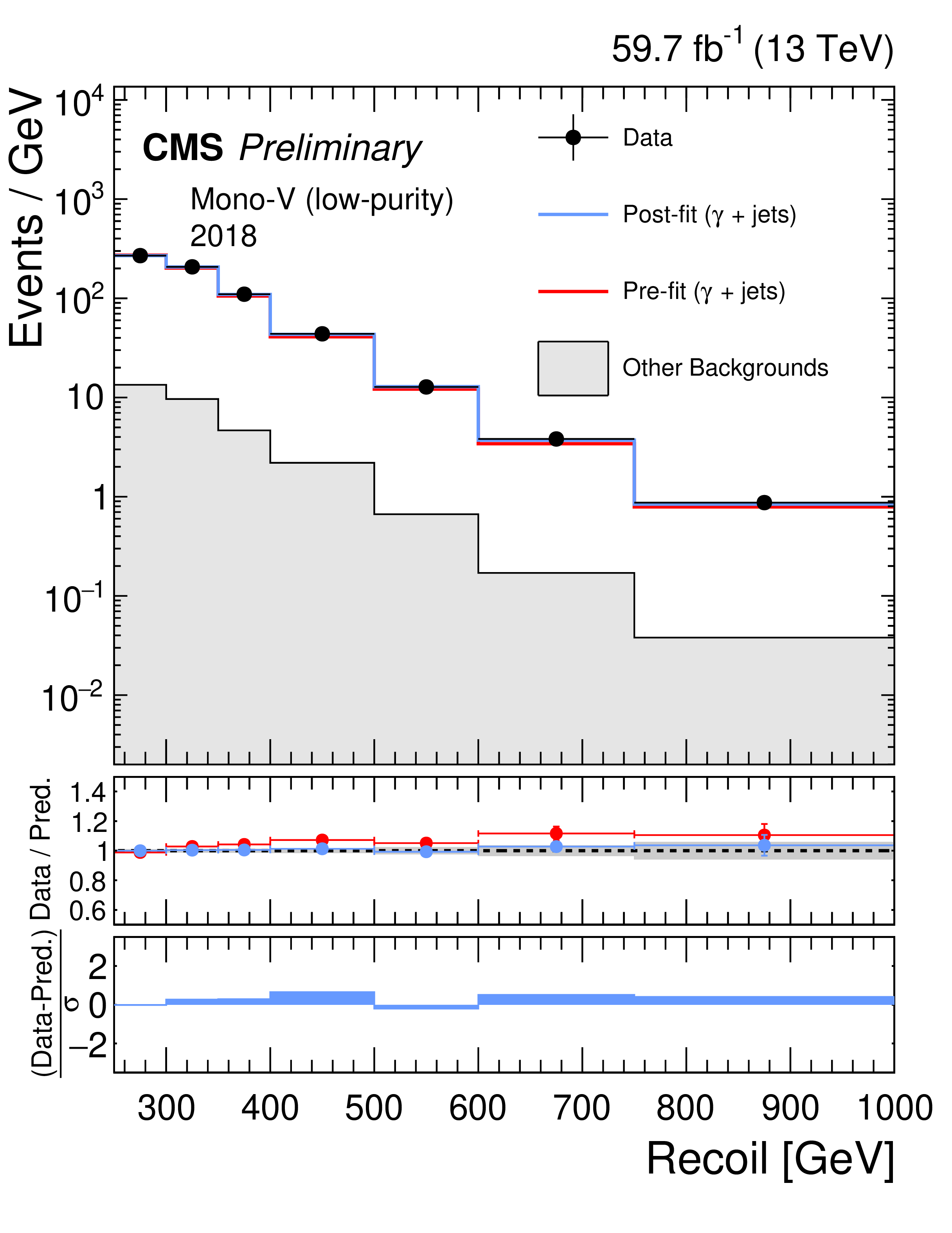
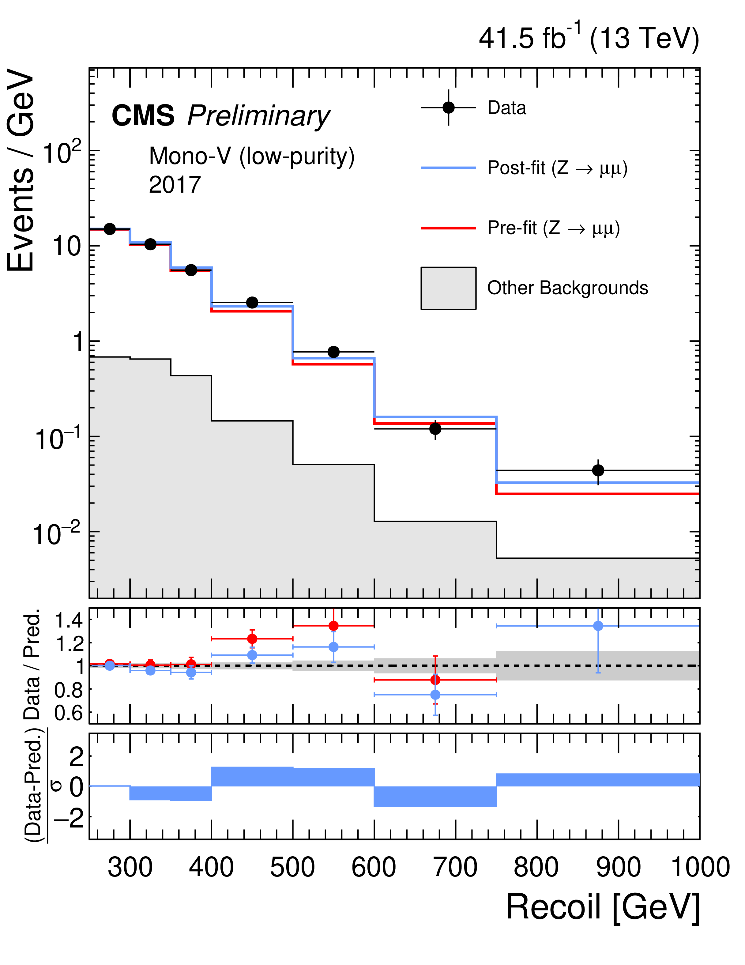
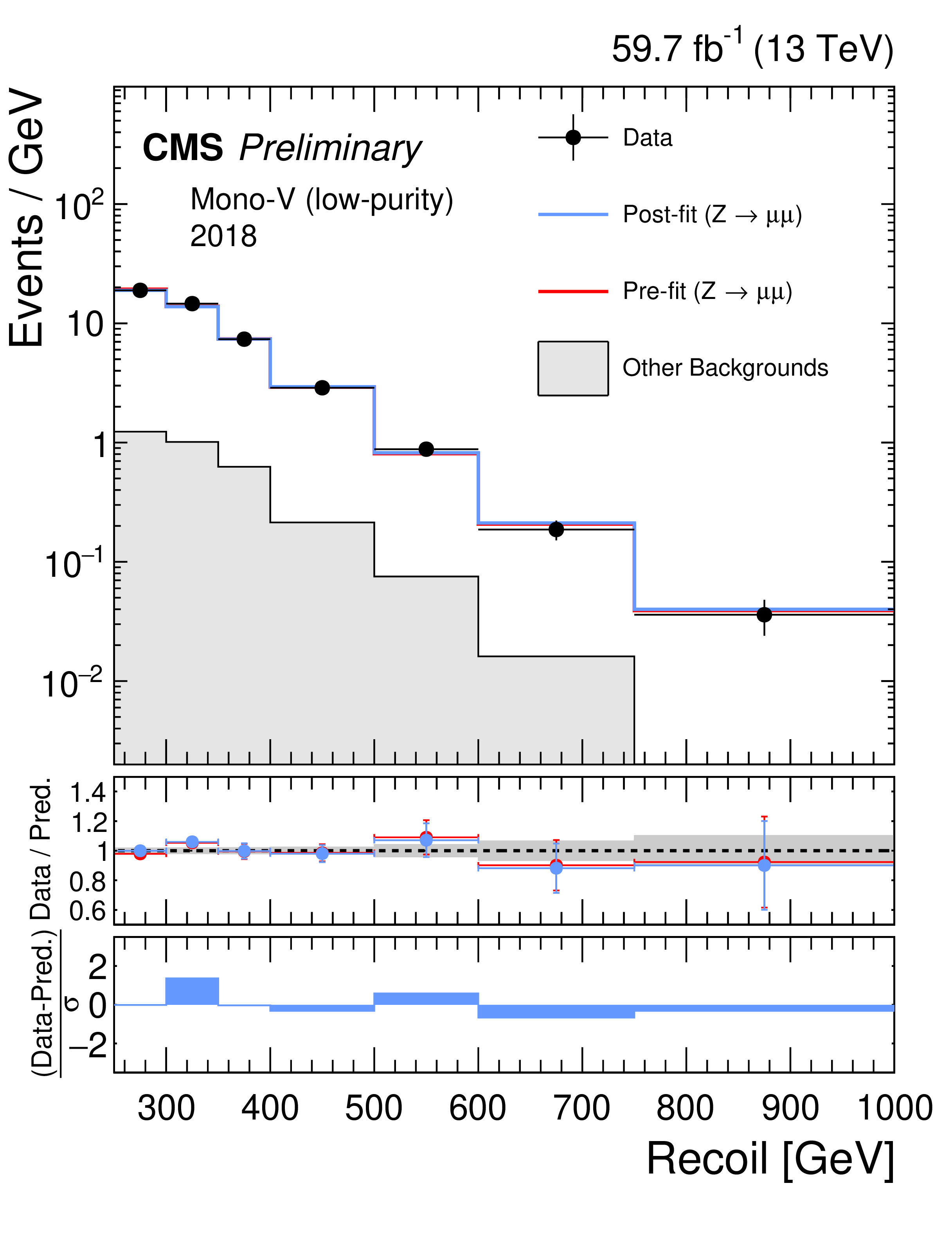
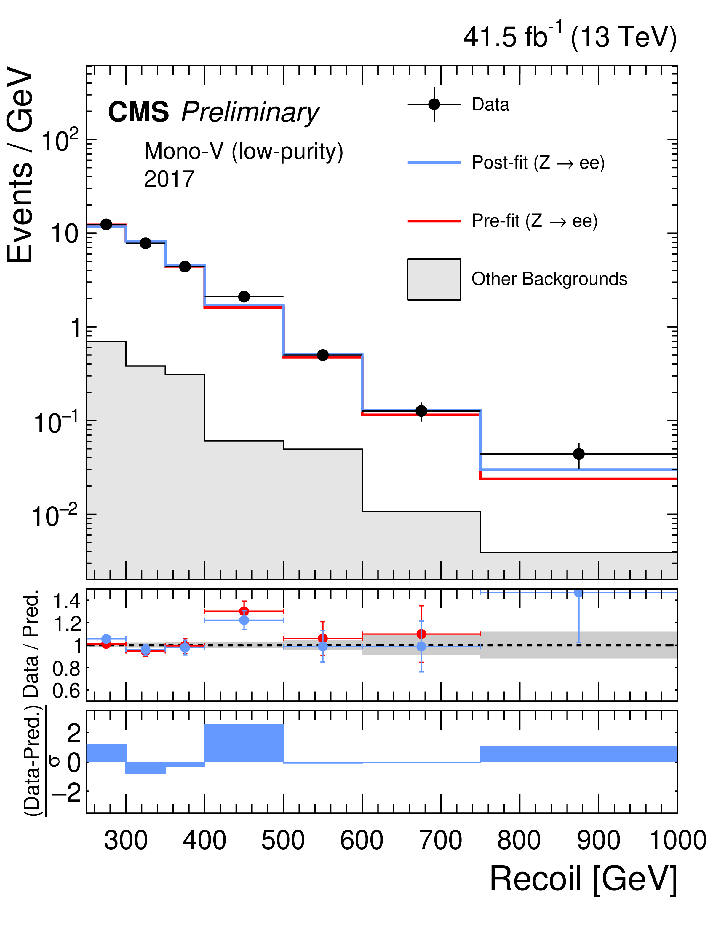
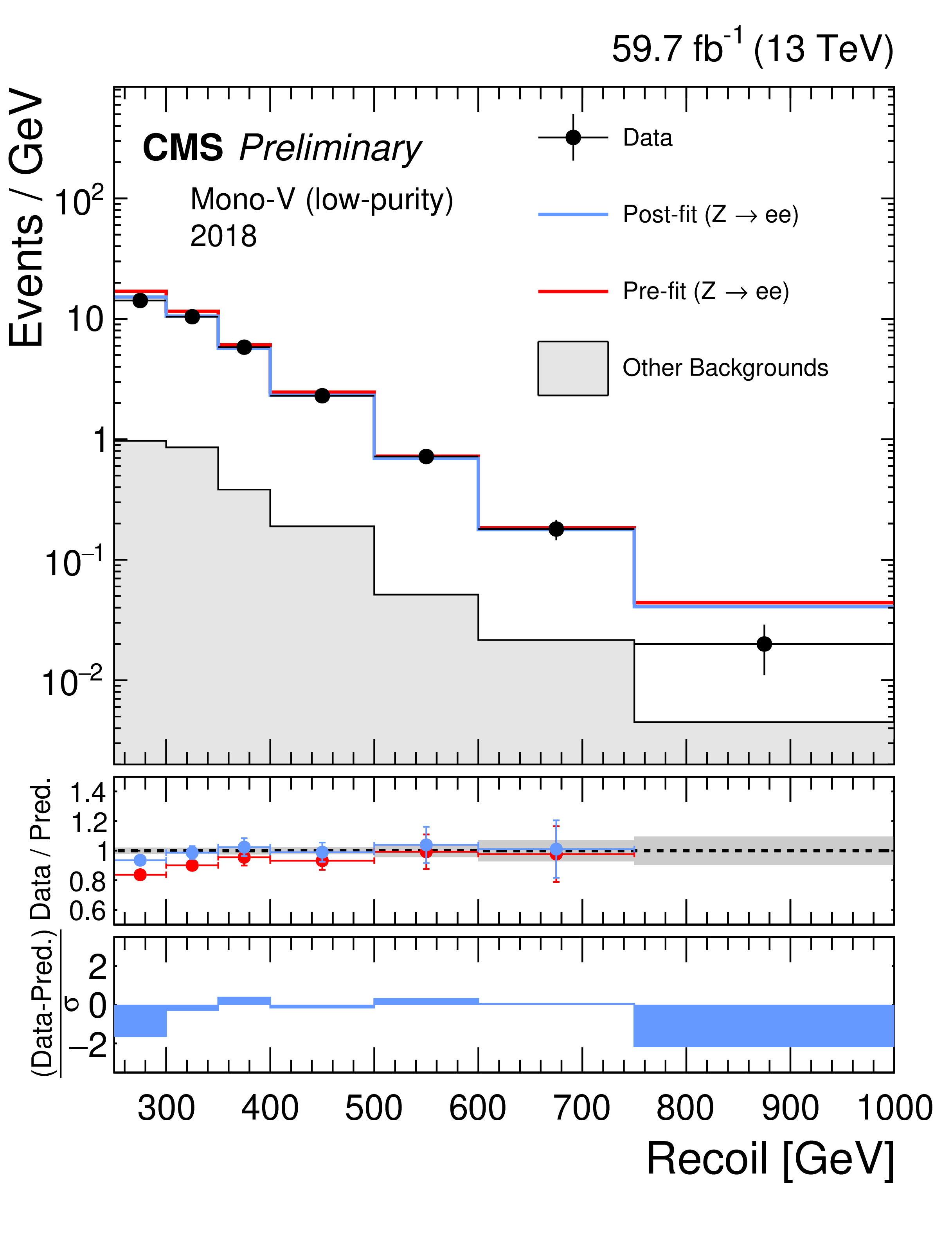
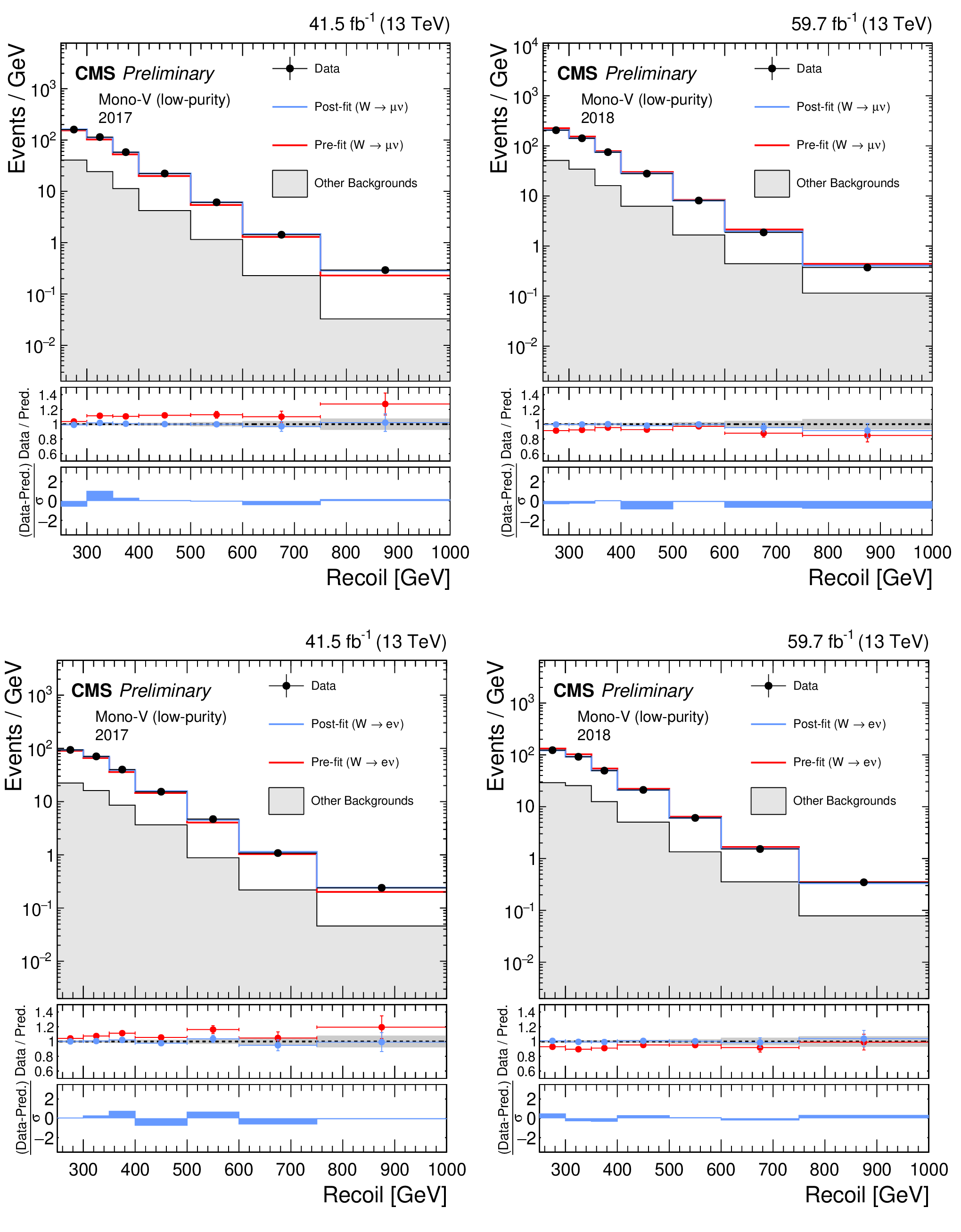
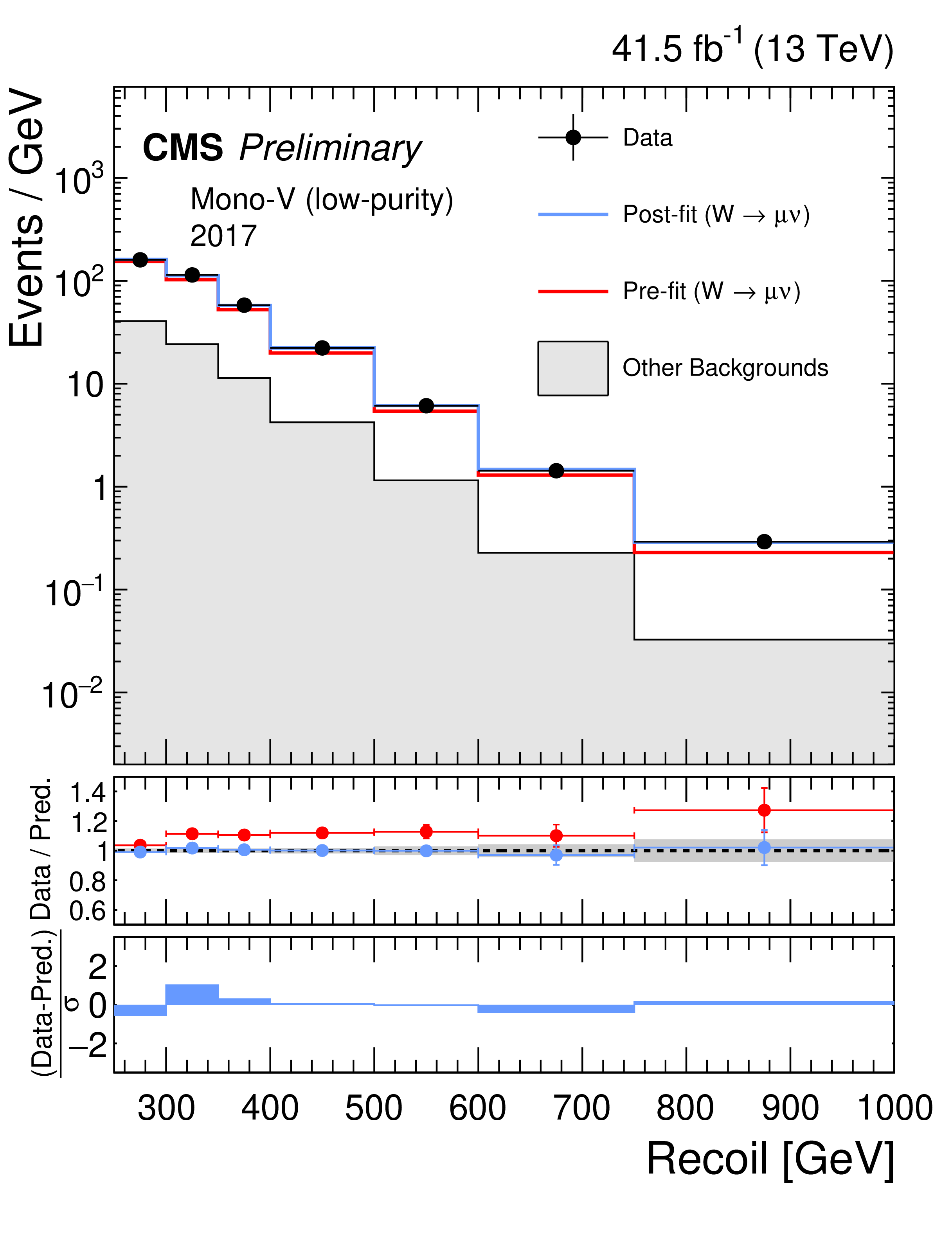
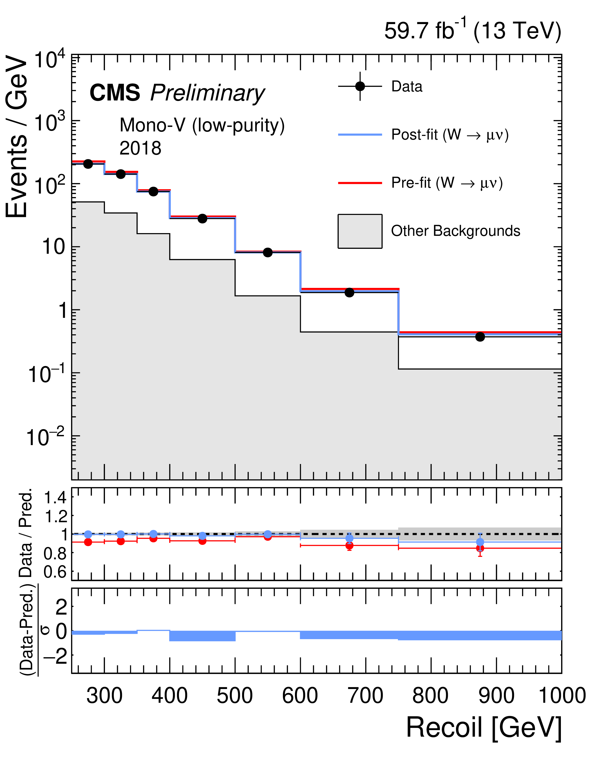
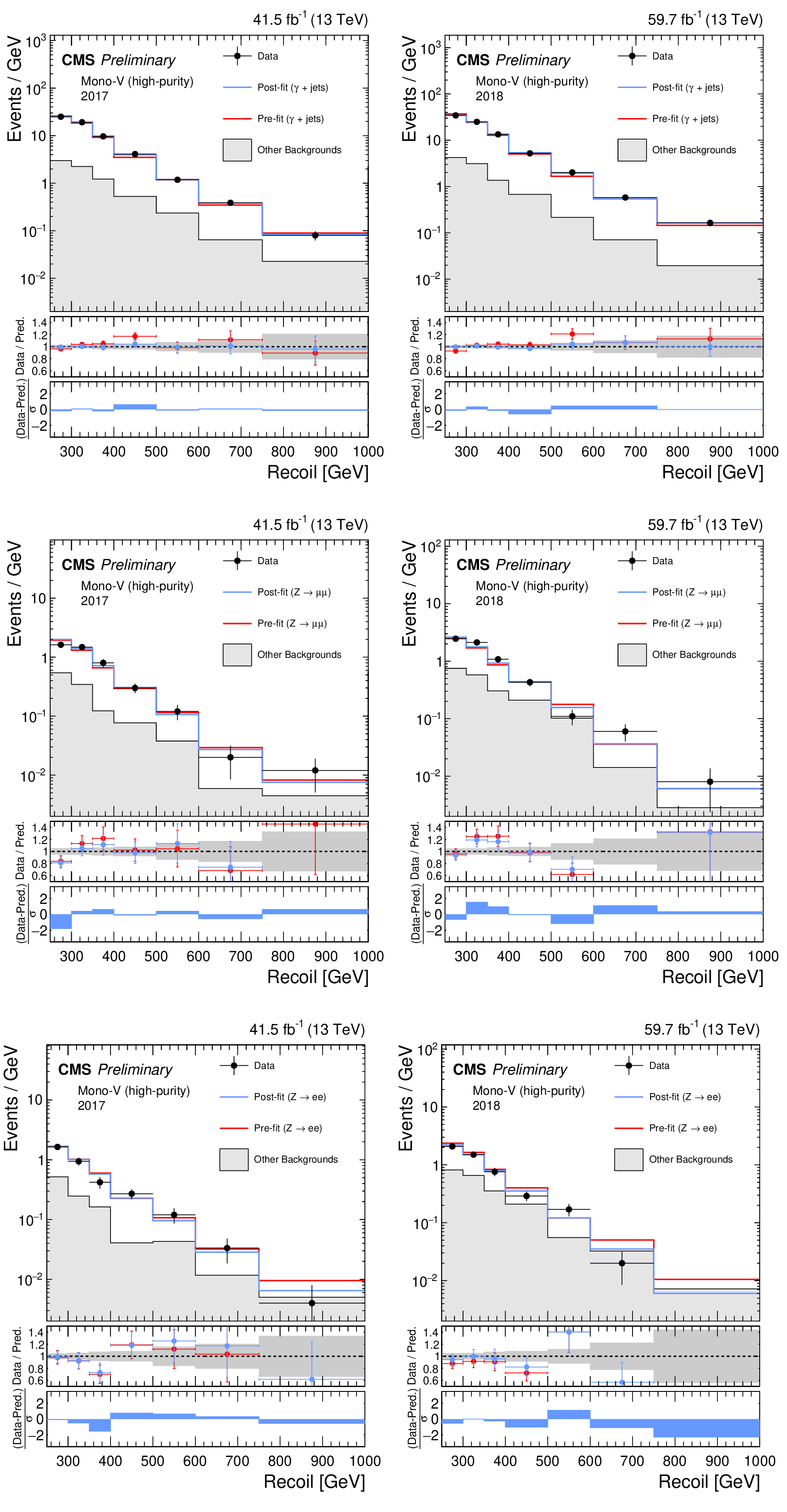
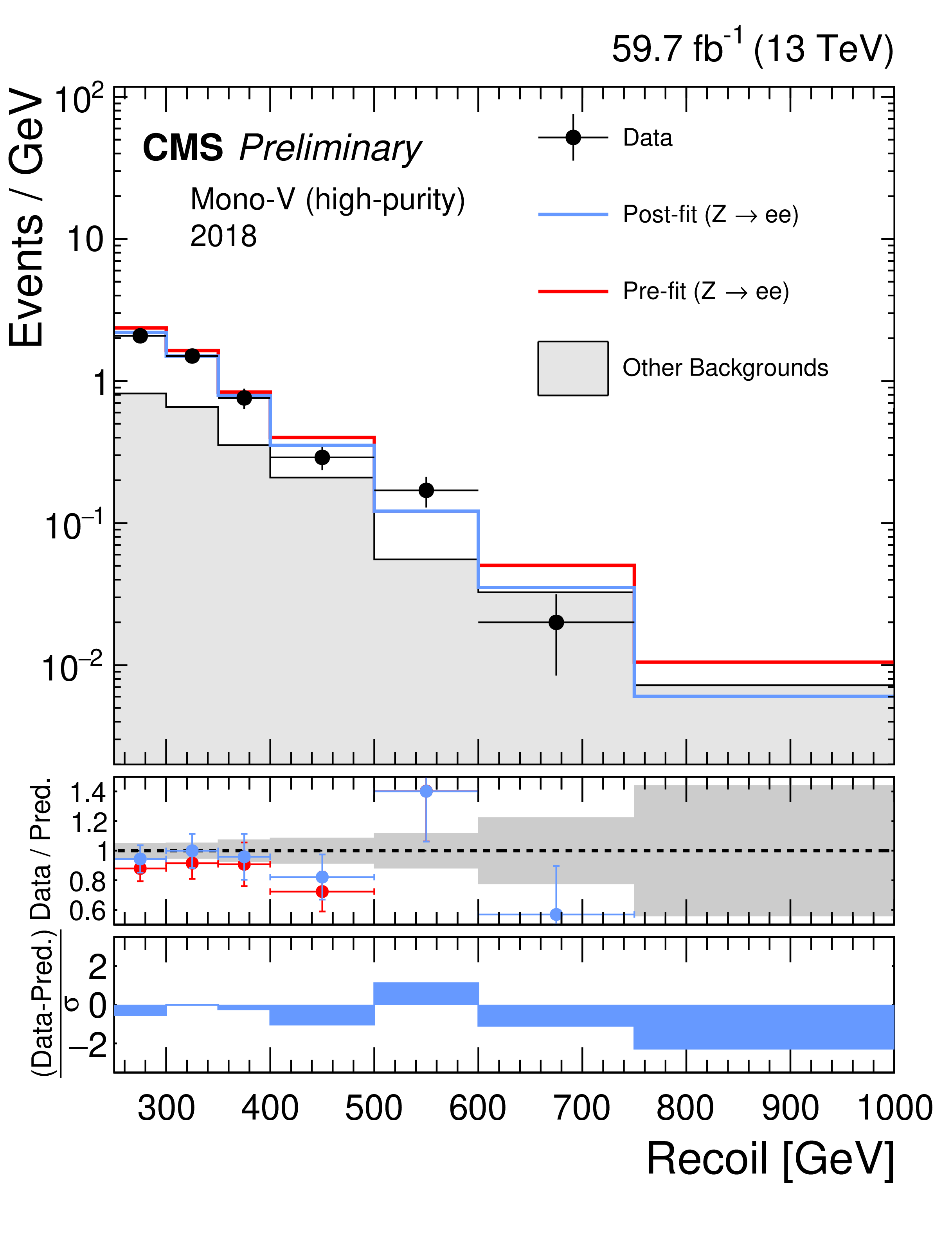
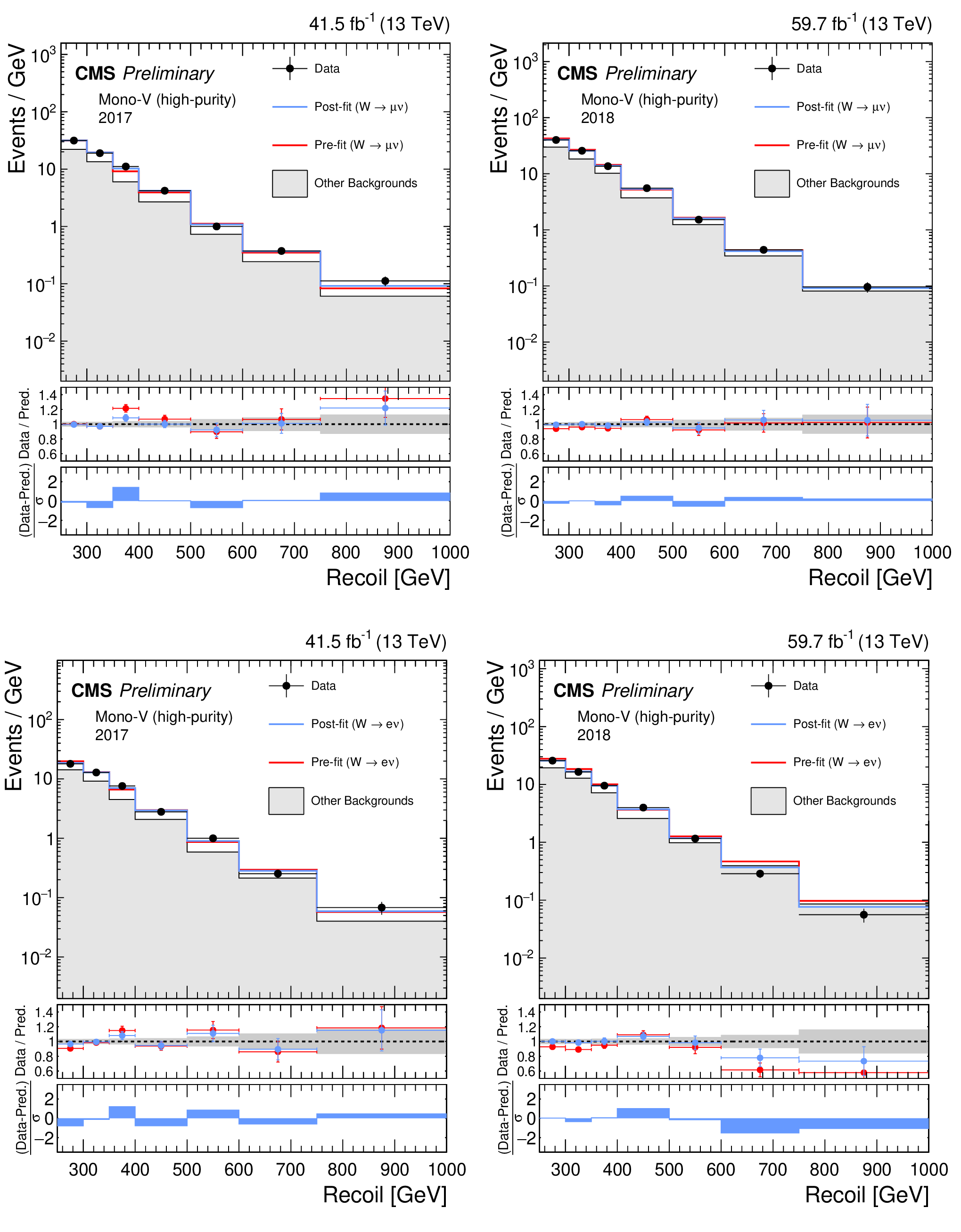
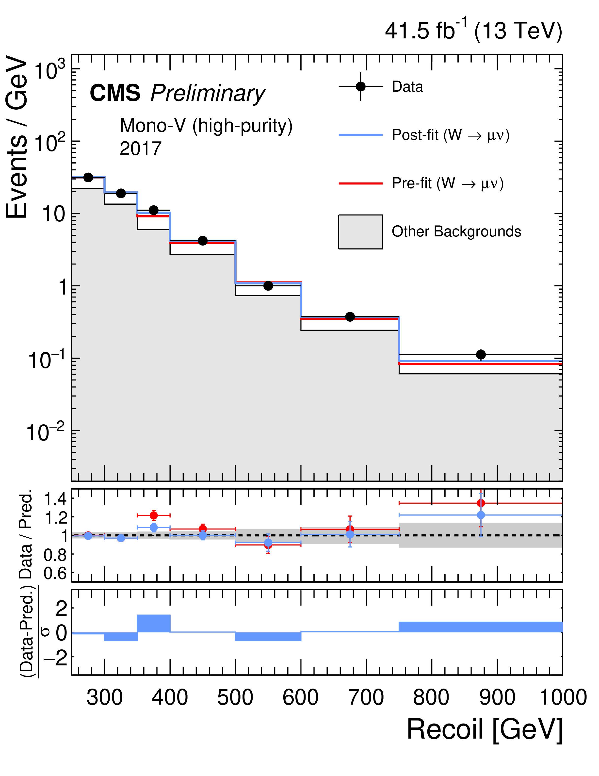
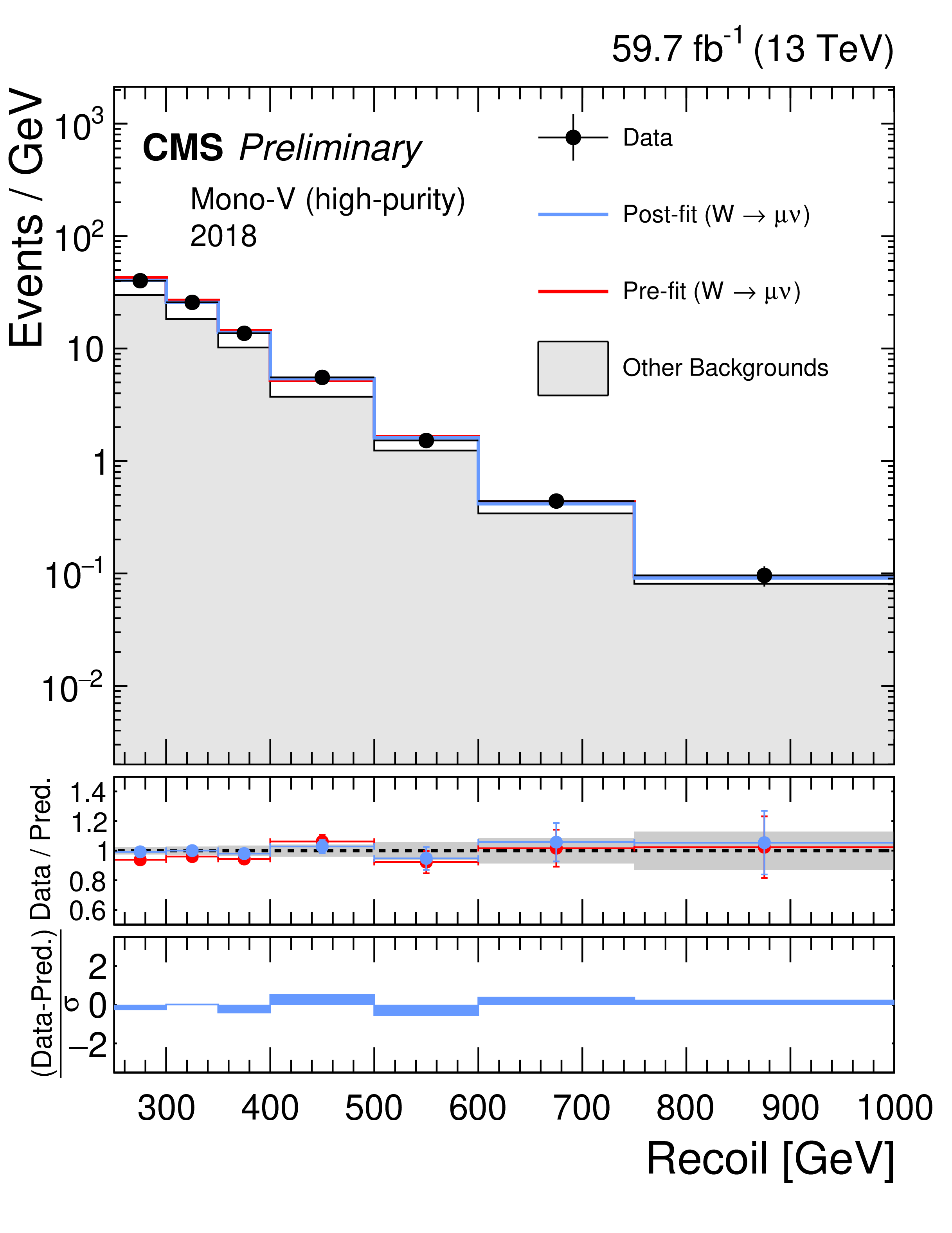
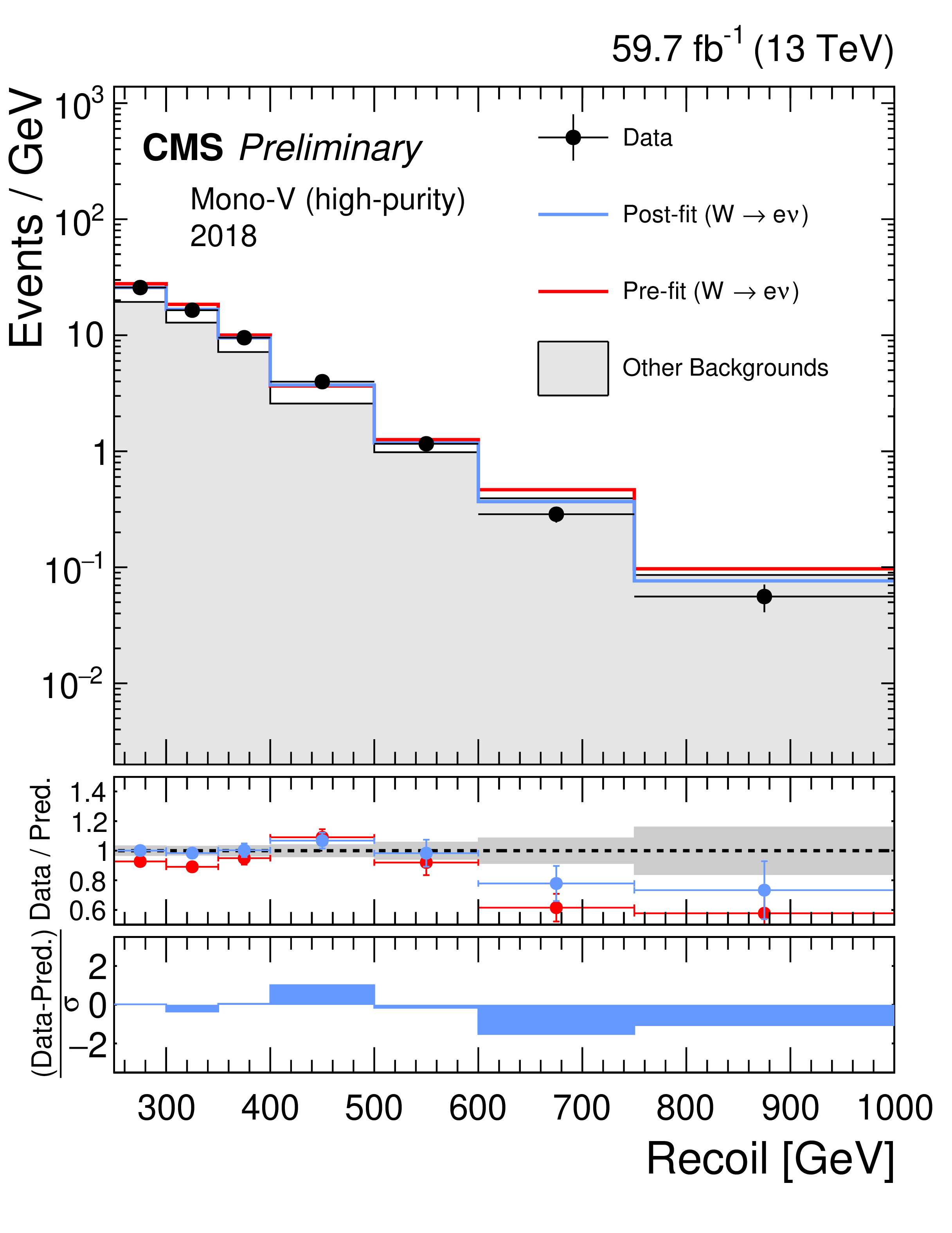
Figure 4:
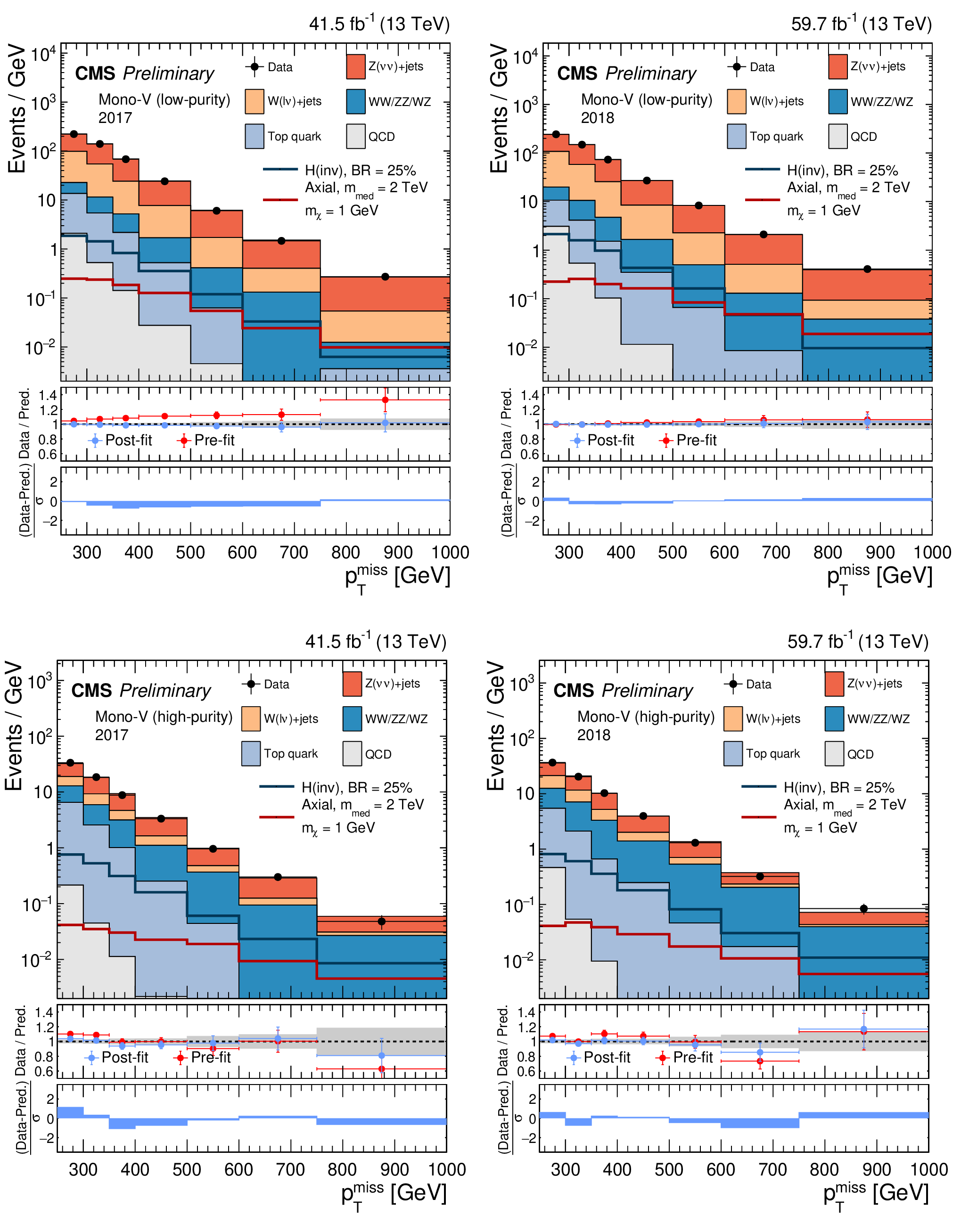
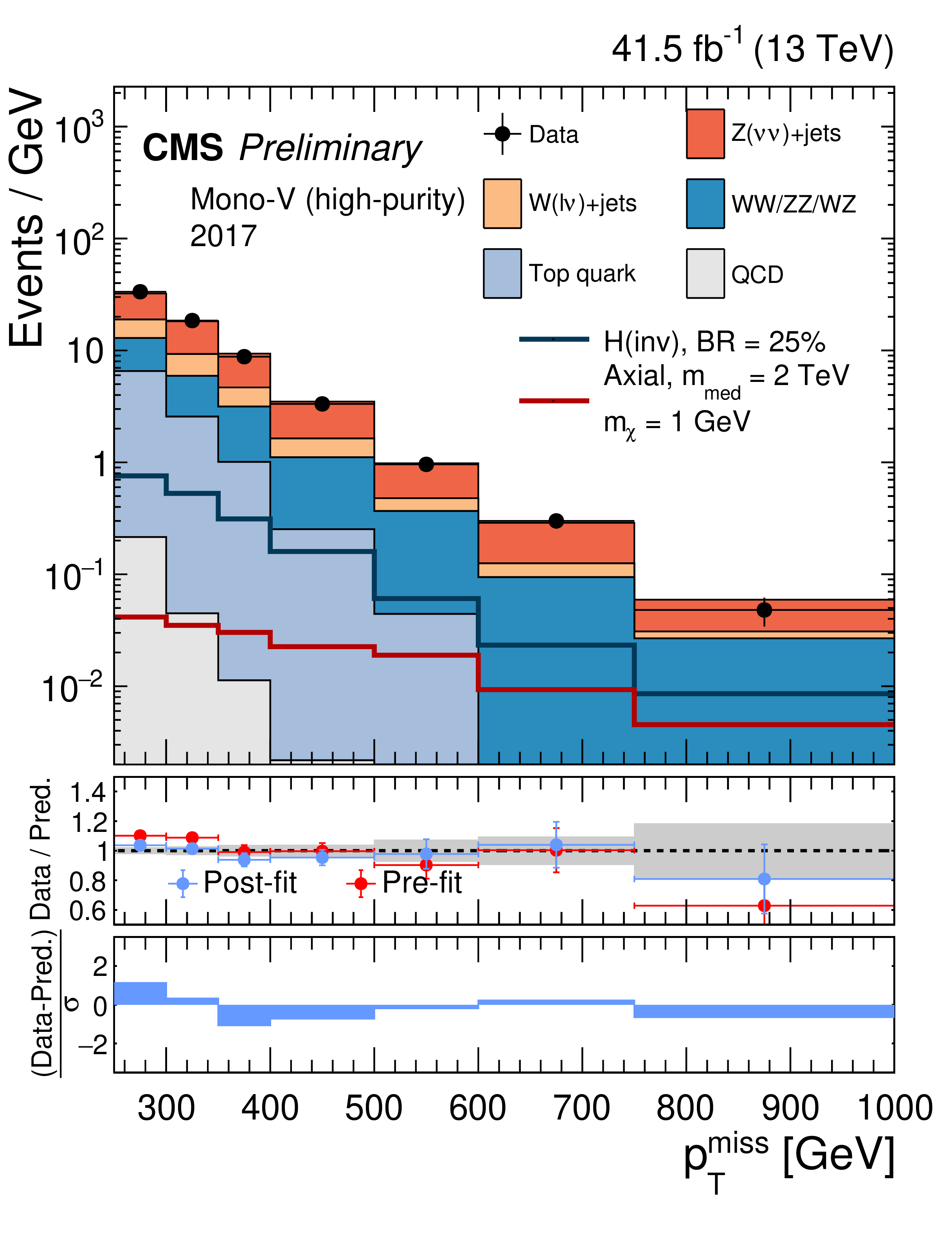
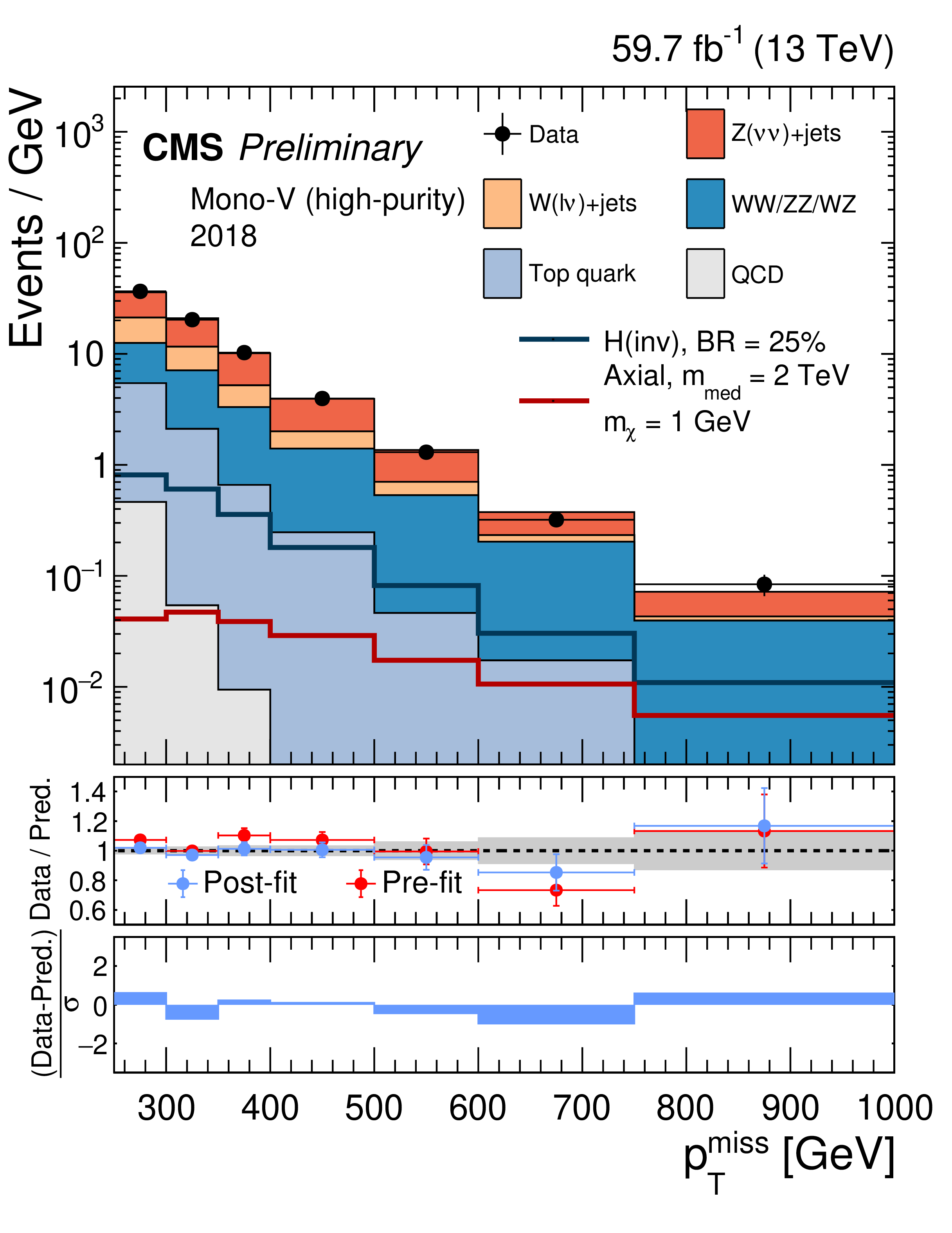
Comparison between data and the background prediction in the mono-V signal regions before and after the simultaneous fit. The fit includes all control samples and the signal region in all categories and both data taking years, and the background-only fit model is used. The resulting distributions are shown separately for 2017 (left column) and 2018 (right column), as well as for the low- and high-purity categories (upper and lower rows, respectively). |

png pdf |
Figure 4-a:
Comparison between data and the background prediction in the mono-V signal regions before and after the simultaneous fit. The fit includes all control samples and the signal region in all categories and both data taking years, and the background-only fit model is used. The resulting distributions are shown separately for 2017 (left column) and 2018 (right column), as well as for the low- and high-purity categories (upper and lower rows, respectively). |

png pdf |
Figure 4-b:
Comparison between data and the background prediction in the mono-V signal regions before and after the simultaneous fit. The fit includes all control samples and the signal region in all categories and both data taking years, and the background-only fit model is used. The resulting distributions are shown separately for 2017 (left column) and 2018 (right column), as well as for the low- and high-purity categories (upper and lower rows, respectively). |
png pdf |
Figure 4-c:
Comparison between data and the background prediction in the mono-V signal regions before and after the simultaneous fit. The fit includes all control samples and the signal region in all categories and both data taking years, and the background-only fit model is used. The resulting distributions are shown separately for 2017 (left column) and 2018 (right column), as well as for the low- and high-purity categories (upper and lower rows, respectively). |
png pdf |
Figure 4-d:
Comparison between data and the background prediction in the mono-V signal regions before and after the simultaneous fit. The fit includes all control samples and the signal region in all categories and both data taking years, and the background-only fit model is used. The resulting distributions are shown separately for 2017 (left column) and 2018 (right column), as well as for the low- and high-purity categories (upper and lower rows, respectively). |
png pdf |
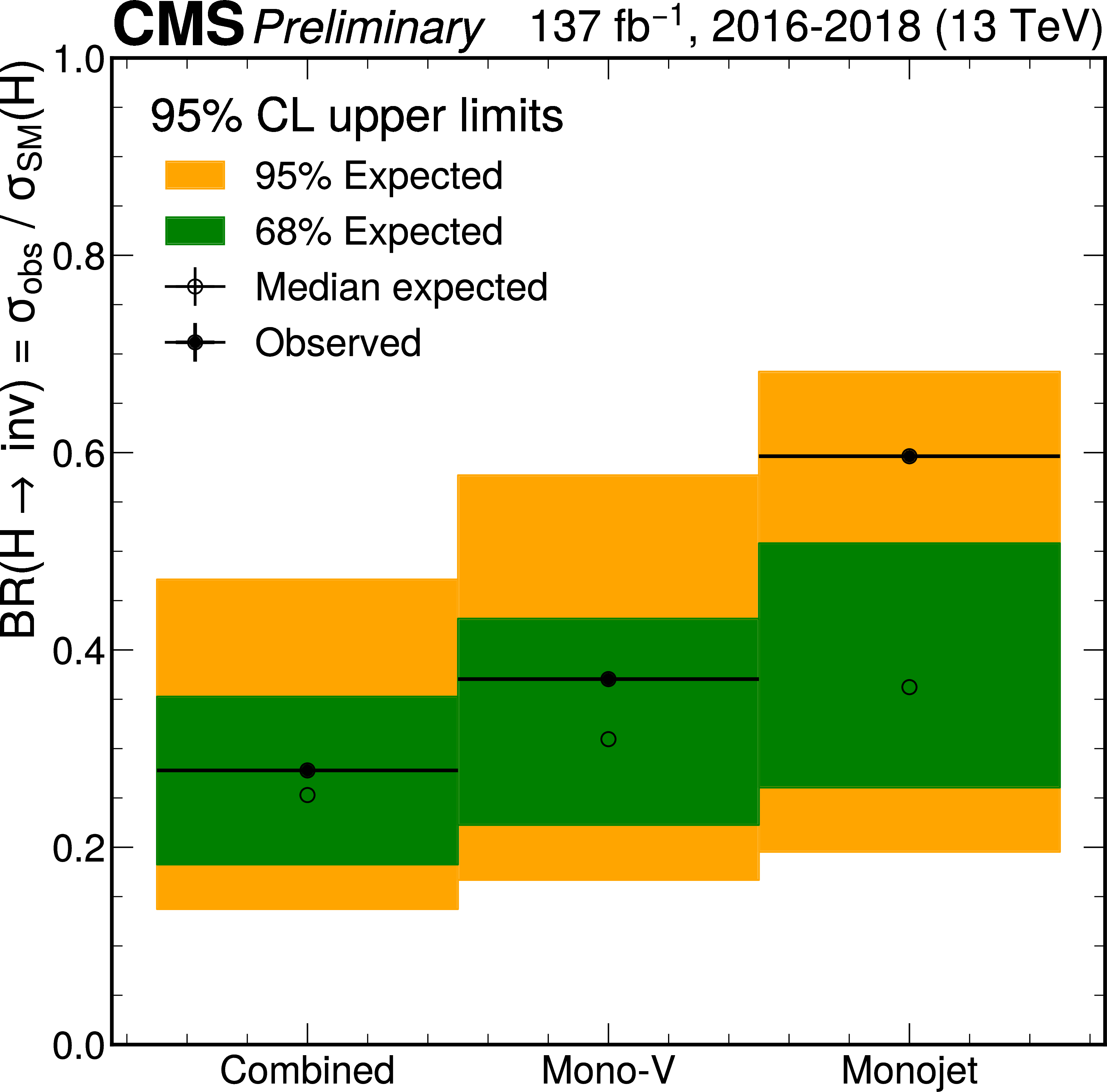
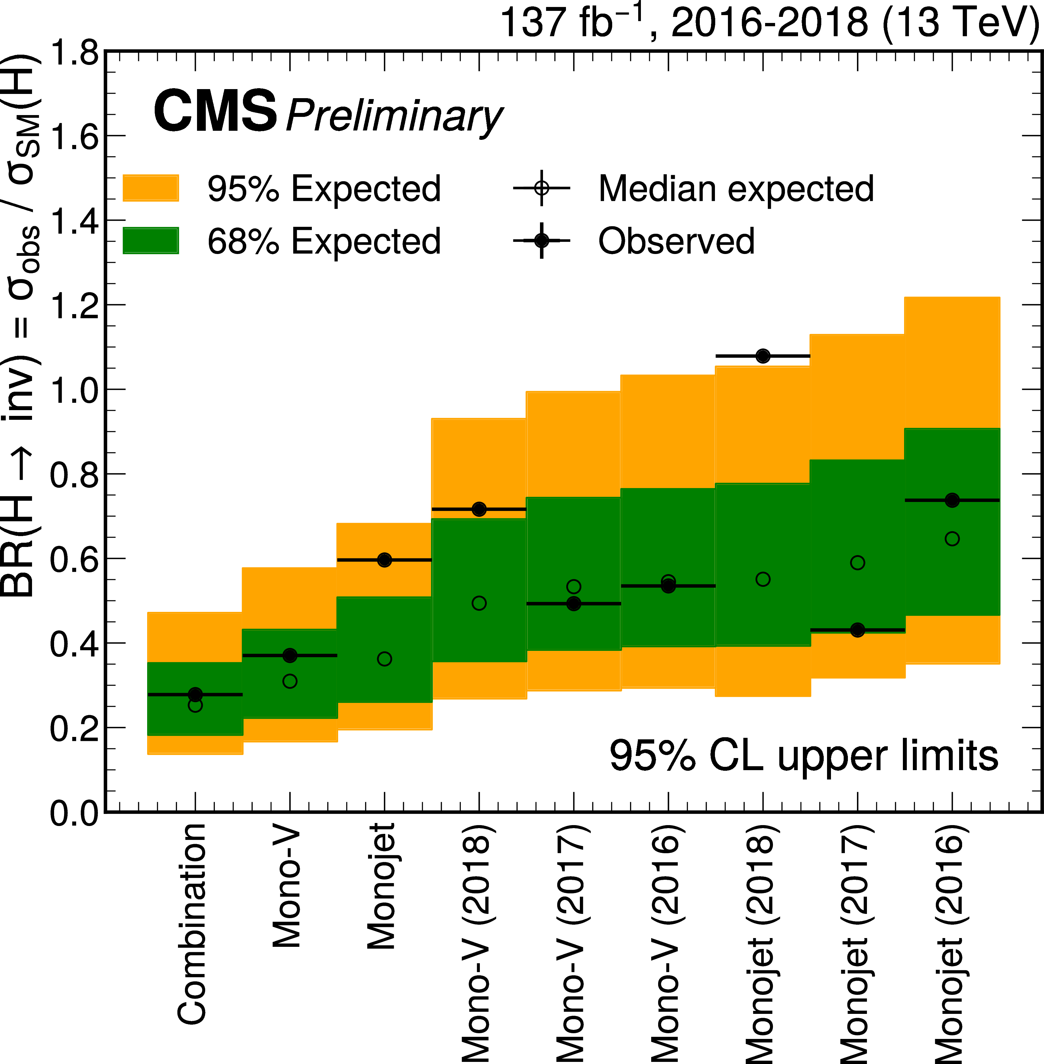
Figure 5:
Upper limits at 95% CL on the branching fraction of the Higgs boson to invisible final states. The results are shown separately for the monojet and mono-V categories, as well as for their combination. The final combined limit is 27.8% (25.3% expected). |
png pdf |
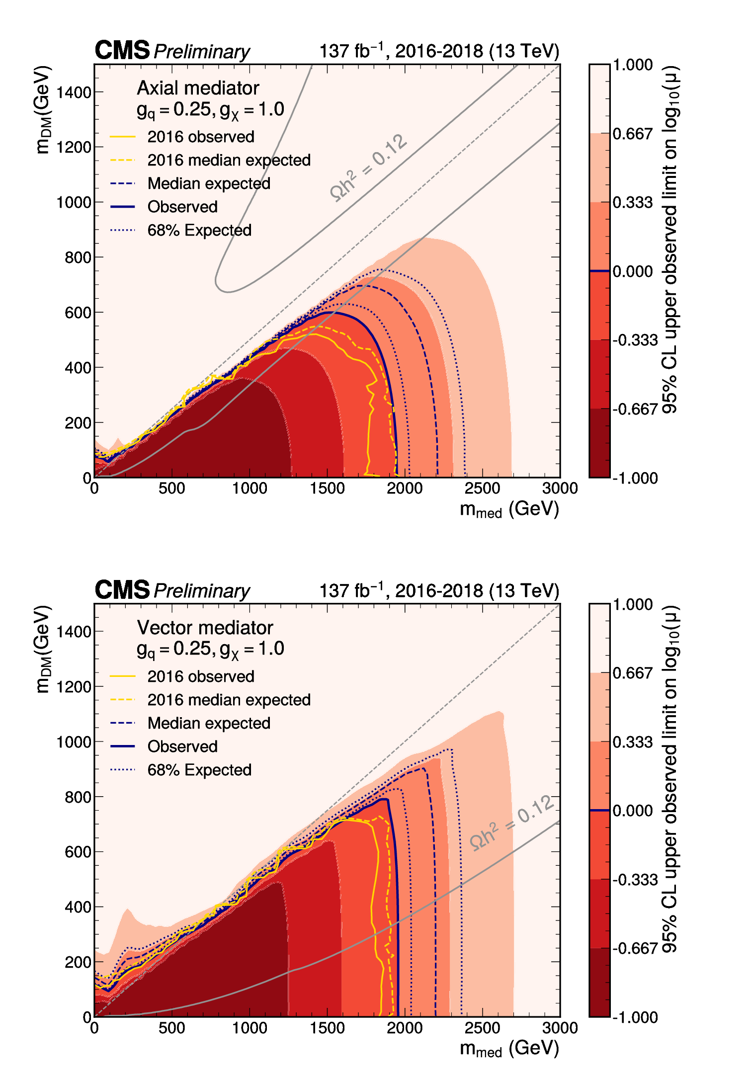
Figure 6:
Exclusion limits at 95% CL on the signal strength $\mu =\sigma /\sigma _\text {theo}$ in the ${m_\text {med}} - {m_\text {DM}}$ plane for the coupling values of $ {g_\mathrm{q}} =$ 0.25, $ {g_\chi} =$ 1.0 for an axial-vector (upper) or vector (lower) mediator. The blue solid line indicates the observed exclusion boundary $\mu =$ 1. The blue dashed and dotted lines represent the expected exclusion and the the 68% confidence level interval around the expected boundary, respectively. Parameter combinations with larger values of $\mu $ (indicated by a darker shade in the color scale) are excluded. The observed exclusion reaches up to $ {m_\text {med}} = $ 2.0 TeV for low values of $ {m_\text {DM}} = $ 1 GeV (2.2 TeV expected). Yellow solid and dashed lines represent the observed and expected exclusion boundaries from Ref. [20]. The gray dashed line indicates the diagonal $ {m_\text {med}} =2 {m_\text {DM}} $, above which only off-shell mediator production contributes to the jet+$ {{p_{\mathrm {T}}} ^\text {miss}}$ final state. The steep increase of the signal strength limit above the diagonal leads to fluctuations of the exclusion contour, which are due to finite precision in the interpolation method in this region. The gray solid lines represent parameter combinations for which the simplified model reproduces the observed DM relic density in the universe under the assumption of a thermal freeze-out mechanism [57,76]. |
png pdf |
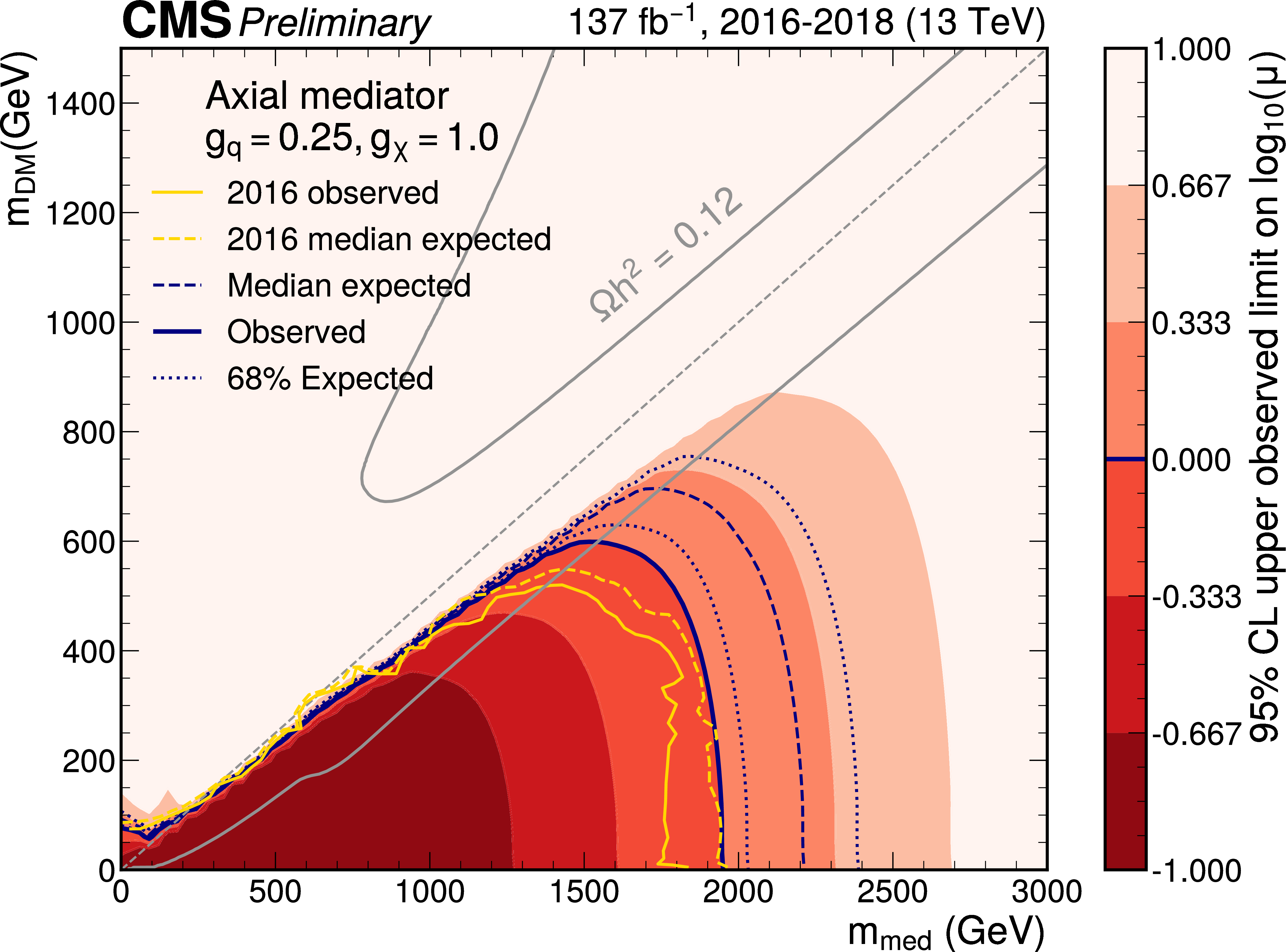
Figure 6-a:
Exclusion limits at 95% CL on the signal strength $\mu =\sigma /\sigma _\text {theo}$ in the ${m_\text {med}} - {m_\text {DM}}$ plane for the coupling values of $ {g_\mathrm{q}} =$ 0.25, $ {g_\chi} =$ 1.0 for an axial-vector (upper) or vector (lower) mediator. The blue solid line indicates the observed exclusion boundary $\mu =$ 1. The blue dashed and dotted lines represent the expected exclusion and the the 68% confidence level interval around the expected boundary, respectively. Parameter combinations with larger values of $\mu $ (indicated by a darker shade in the color scale) are excluded. The observed exclusion reaches up to $ {m_\text {med}} = $ 2.0 TeV for low values of $ {m_\text {DM}} = $ 1 GeV (2.2 TeV expected). Yellow solid and dashed lines represent the observed and expected exclusion boundaries from Ref. [20]. The gray dashed line indicates the diagonal $ {m_\text {med}} =2 {m_\text {DM}} $, above which only off-shell mediator production contributes to the jet+$ {{p_{\mathrm {T}}} ^\text {miss}}$ final state. The steep increase of the signal strength limit above the diagonal leads to fluctuations of the exclusion contour, which are due to finite precision in the interpolation method in this region. The gray solid lines represent parameter combinations for which the simplified model reproduces the observed DM relic density in the universe under the assumption of a thermal freeze-out mechanism [57,76]. |
png pdf |
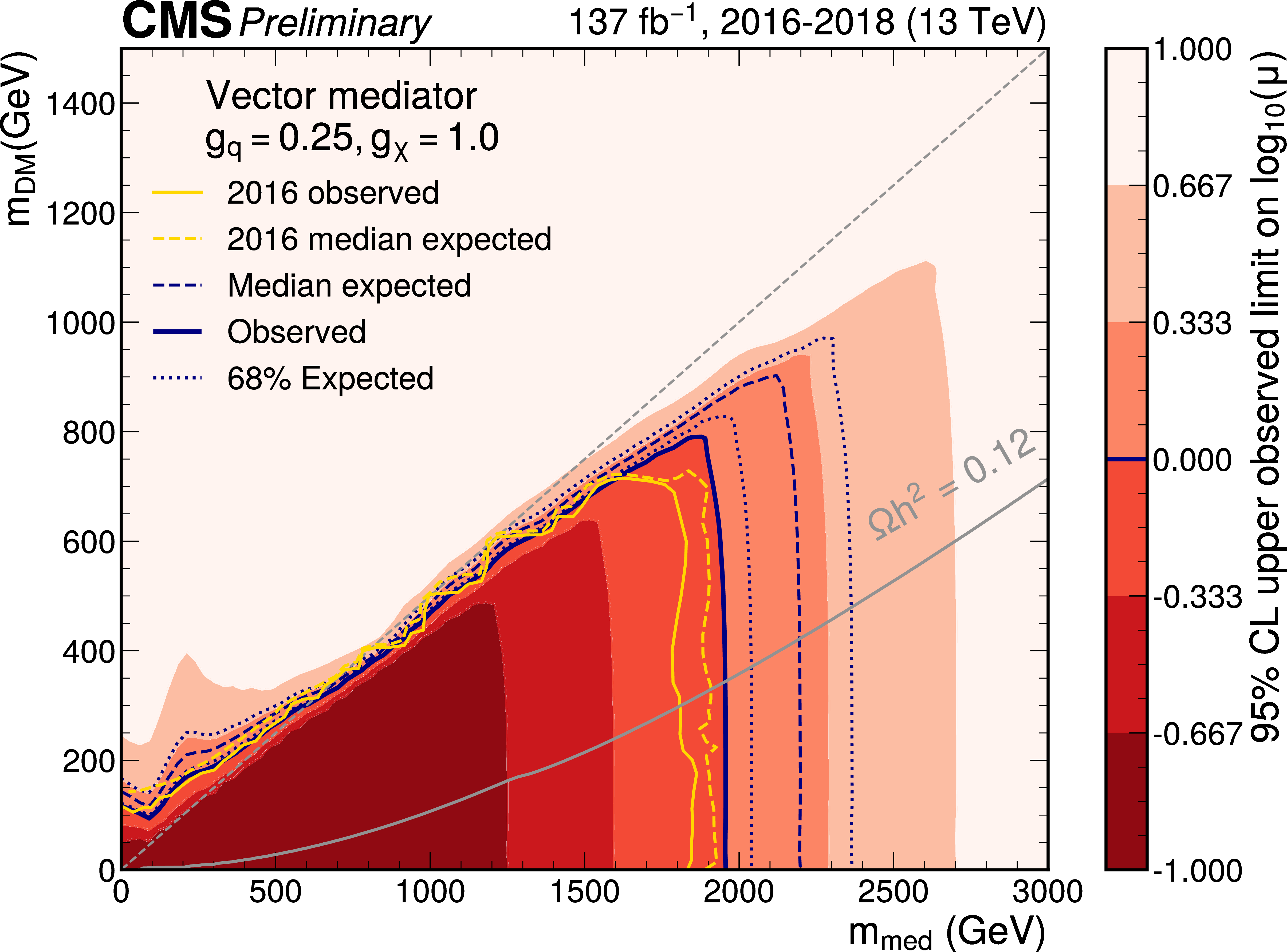
Figure 6-b:
Exclusion limits at 95% CL on the signal strength $\mu =\sigma /\sigma _\text {theo}$ in the ${m_\text {med}} - {m_\text {DM}}$ plane for the coupling values of $ {g_\mathrm{q}} =$ 0.25, $ {g_\chi} =$ 1.0 for an axial-vector (upper) or vector (lower) mediator. The blue solid line indicates the observed exclusion boundary $\mu =$ 1. The blue dashed and dotted lines represent the expected exclusion and the the 68% confidence level interval around the expected boundary, respectively. Parameter combinations with larger values of $\mu $ (indicated by a darker shade in the color scale) are excluded. The observed exclusion reaches up to $ {m_\text {med}} = $ 2.0 TeV for low values of $ {m_\text {DM}} = $ 1 GeV (2.2 TeV expected). Yellow solid and dashed lines represent the observed and expected exclusion boundaries from Ref. [20]. The gray dashed line indicates the diagonal $ {m_\text {med}} =2 {m_\text {DM}} $, above which only off-shell mediator production contributes to the jet+$ {{p_{\mathrm {T}}} ^\text {miss}}$ final state. The steep increase of the signal strength limit above the diagonal leads to fluctuations of the exclusion contour, which are due to finite precision in the interpolation method in this region. The gray solid lines represent parameter combinations for which the simplified model reproduces the observed DM relic density in the universe under the assumption of a thermal freeze-out mechanism [57,76]. |
png pdf |
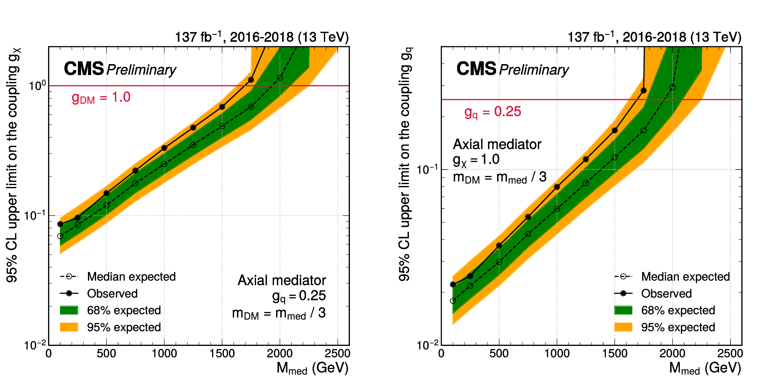
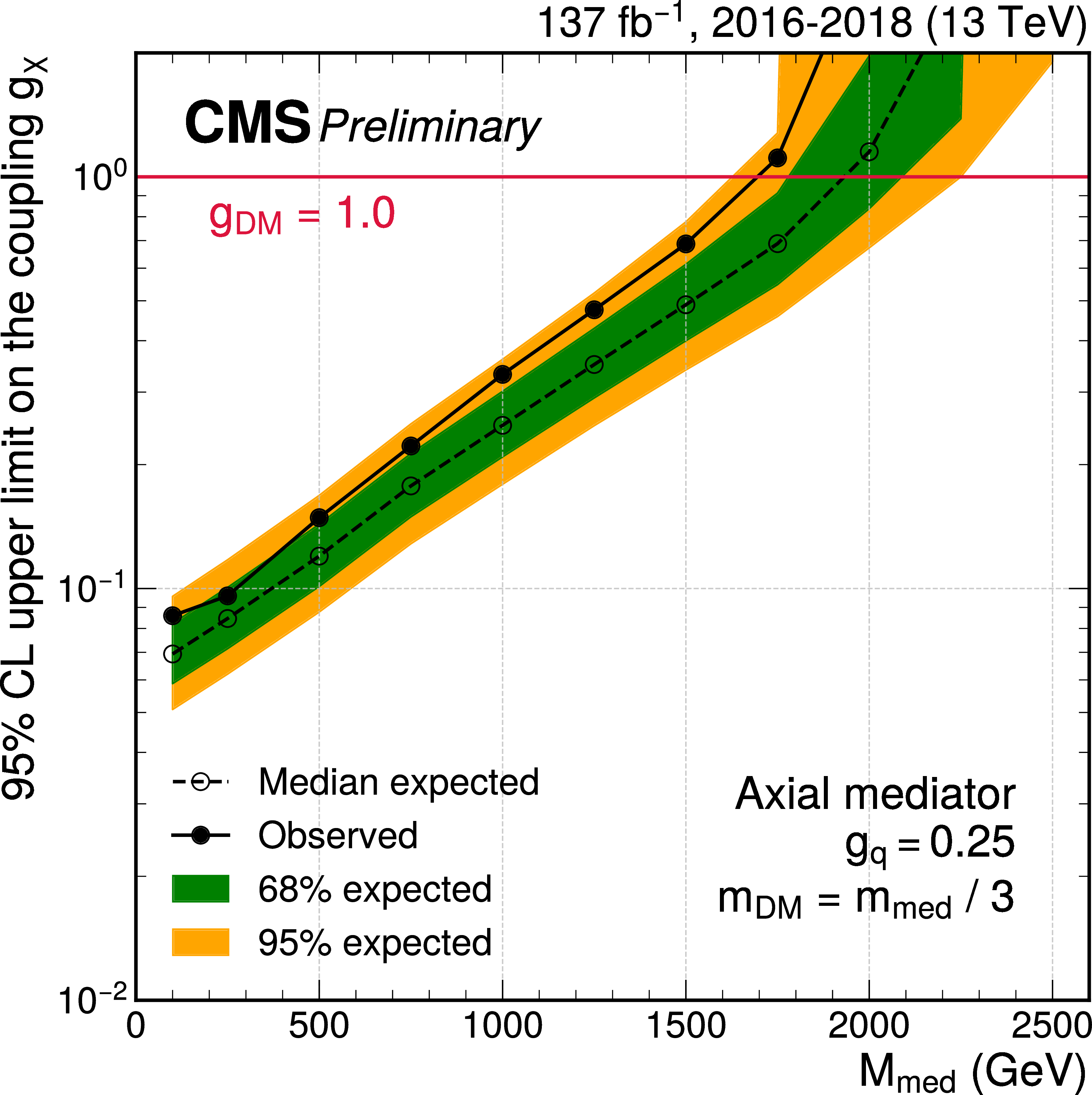
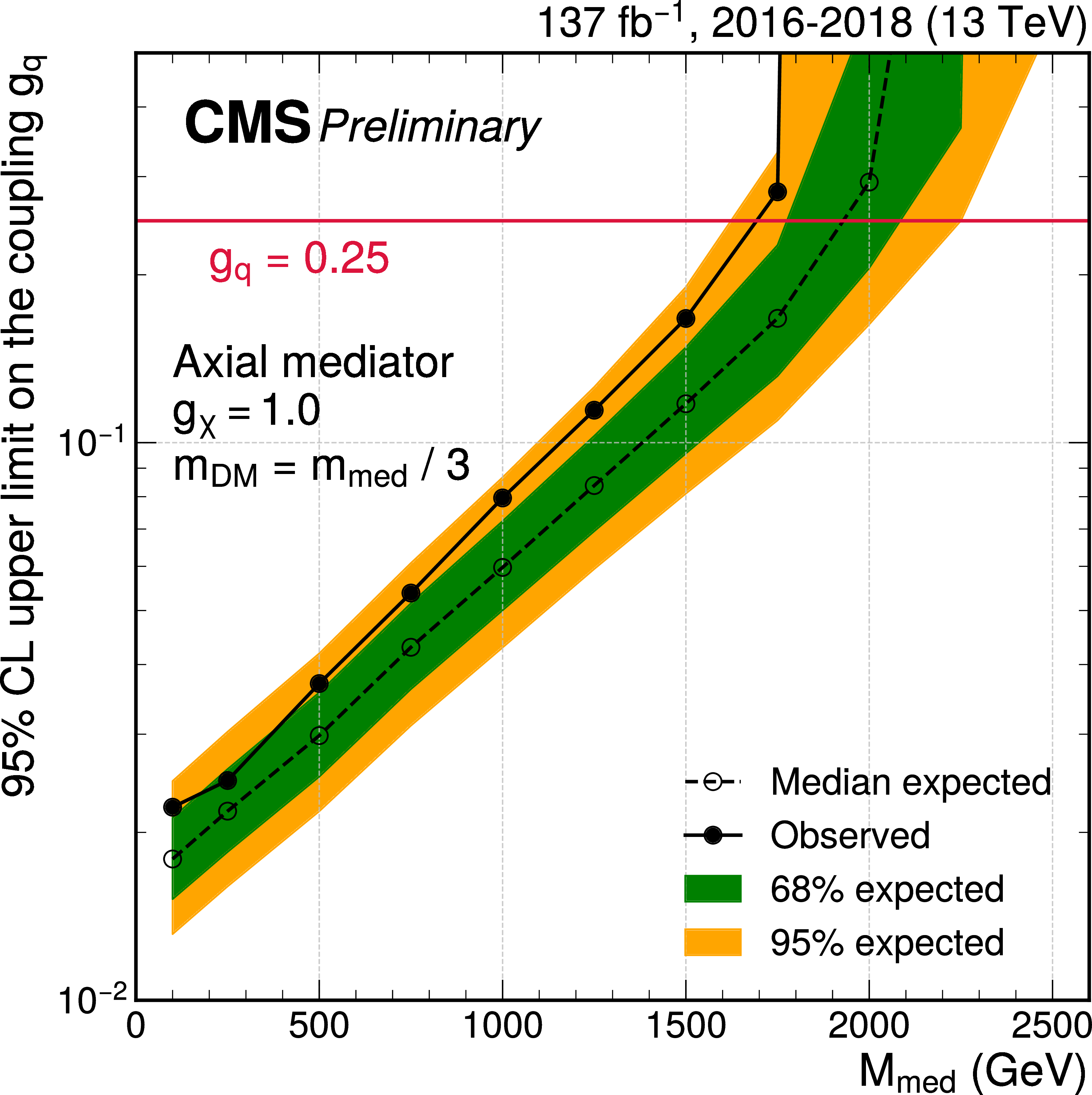
Figure 7:
Exclusion limits at 95% CL on the couplings ${g_\chi}$ (left) and ${g_\mathrm{q}}$ (right) for an axial-vector mediator. In each panel, the result is shown as a function of the mediator mass $ {m_\text {med}} $, with the mass of the DM candidate fixed to $ {m_\text {DM}} = {m_\text {med}} /3$. In either case, only one coupling is varied, while the other coupling is fixed at its default value ($ {g_\mathrm{q}} =$ 0.25 or $ {g_\chi} =$ 1.0). |
png pdf |
Figure 7-a:
Exclusion limits at 95% CL on the couplings ${g_\chi}$ (left) and ${g_\mathrm{q}}$ (right) for an axial-vector mediator. In each panel, the result is shown as a function of the mediator mass $ {m_\text {med}} $, with the mass of the DM candidate fixed to $ {m_\text {DM}} = {m_\text {med}} /3$. In either case, only one coupling is varied, while the other coupling is fixed at its default value ($ {g_\mathrm{q}} =$ 0.25 or $ {g_\chi} =$ 1.0). |
png pdf |
Figure 7-b:
Exclusion limits at 95% CL on the couplings ${g_\chi}$ (left) and ${g_\mathrm{q}}$ (right) for an axial-vector mediator. In each panel, the result is shown as a function of the mediator mass $ {m_\text {med}} $, with the mass of the DM candidate fixed to $ {m_\text {DM}} = {m_\text {med}} /3$. In either case, only one coupling is varied, while the other coupling is fixed at its default value ($ {g_\mathrm{q}} =$ 0.25 or $ {g_\chi} =$ 1.0). |
png pdf |
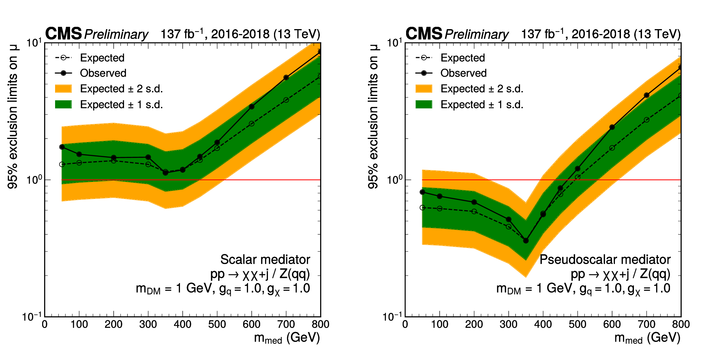
Figure 8:
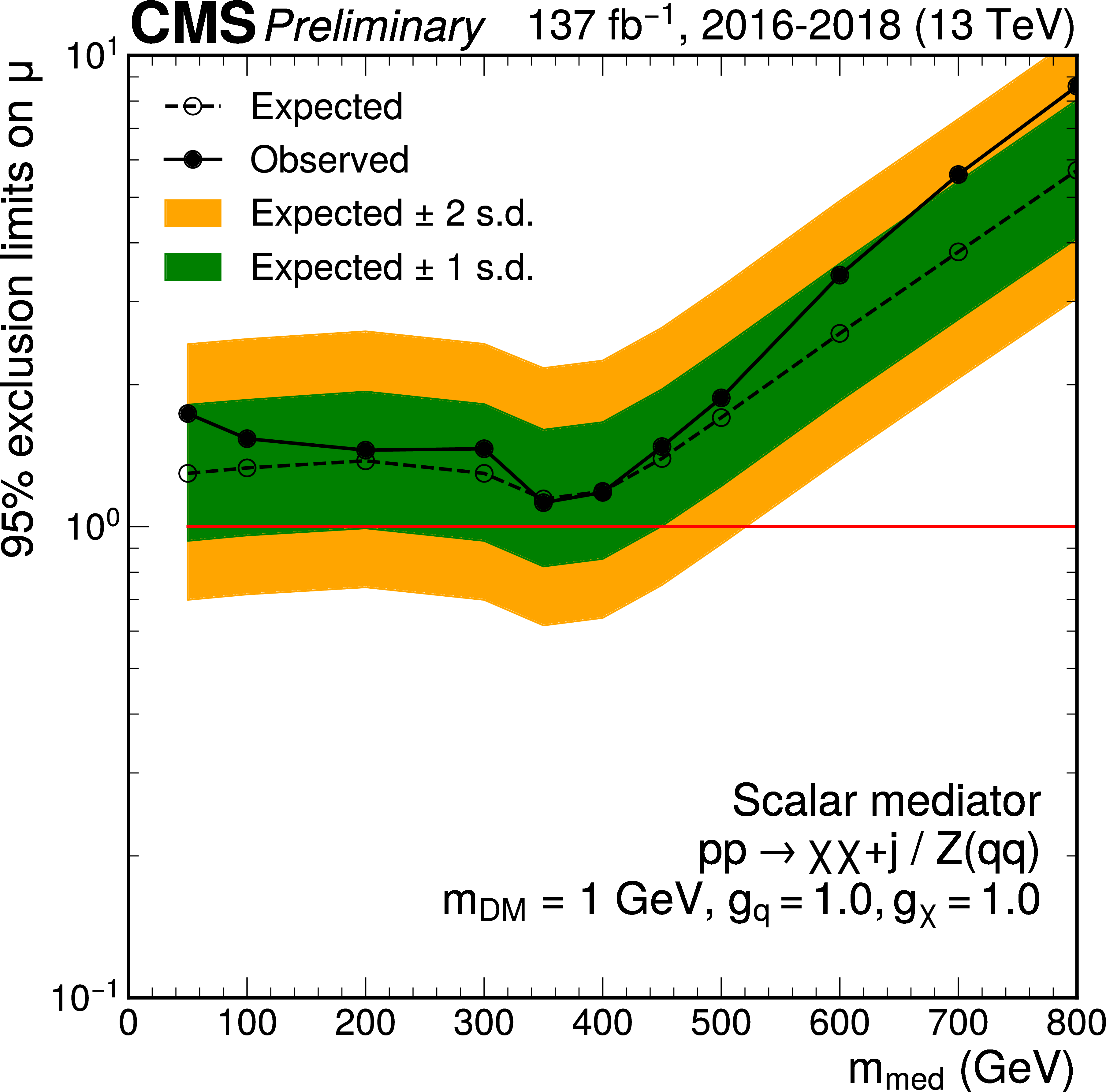
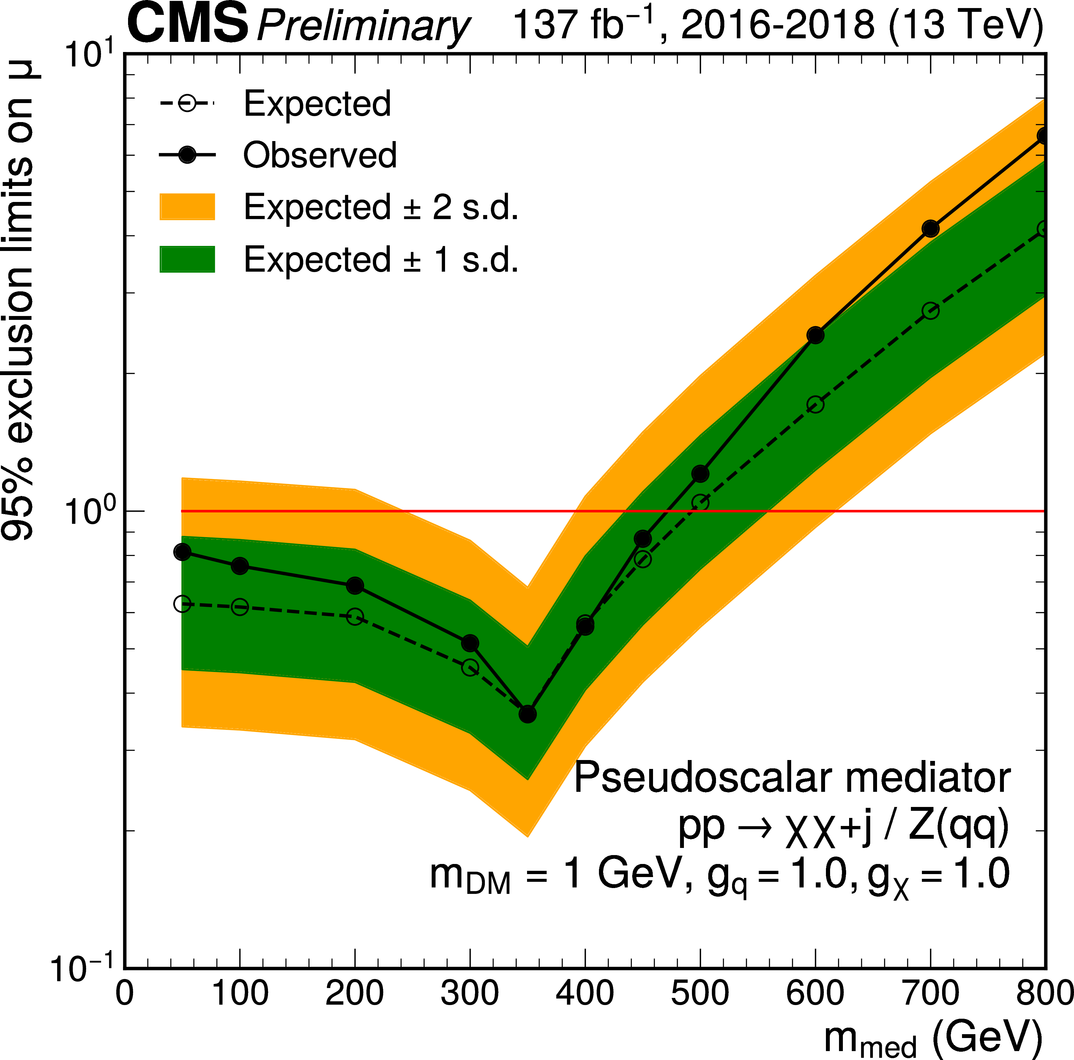
Upper limits at 95% CL on the signal strength $\mu =\sigma /\sigma _\text {theo}$ as a function of ${m_\text {med}}$ for scenarios with scalar (left) and pseudoscalar (right) mediators and coupling values of $ {g_\mathrm{q}} =$ 1.0, $ {g_\chi} =$ 1.0, for a constant value of $ {m_\text {DM}} = $ 1 GeV. The red solid line indicates the exclusion boundary $\mu =1$. In the case of a pseudoscalar mediator, ${m_\text {med}}$ values up to 480 GeV are excluded (440 GeV expected). |
png pdf |
Figure 8-a:
Upper limits at 95% CL on the signal strength $\mu =\sigma /\sigma _\text {theo}$ as a function of ${m_\text {med}}$ for scenarios with scalar (left) and pseudoscalar (right) mediators and coupling values of $ {g_\mathrm{q}} =$ 1.0, $ {g_\chi} =$ 1.0, for a constant value of $ {m_\text {DM}} = $ 1 GeV. The red solid line indicates the exclusion boundary $\mu =1$. In the case of a pseudoscalar mediator, ${m_\text {med}}$ values up to 480 GeV are excluded (440 GeV expected). |
png pdf |
Figure 8-b:
Upper limits at 95% CL on the signal strength $\mu =\sigma /\sigma _\text {theo}$ as a function of ${m_\text {med}}$ for scenarios with scalar (left) and pseudoscalar (right) mediators and coupling values of $ {g_\mathrm{q}} =$ 1.0, $ {g_\chi} =$ 1.0, for a constant value of $ {m_\text {DM}} = $ 1 GeV. The red solid line indicates the exclusion boundary $\mu =1$. In the case of a pseudoscalar mediator, ${m_\text {med}}$ values up to 480 GeV are excluded (440 GeV expected). |
png pdf |
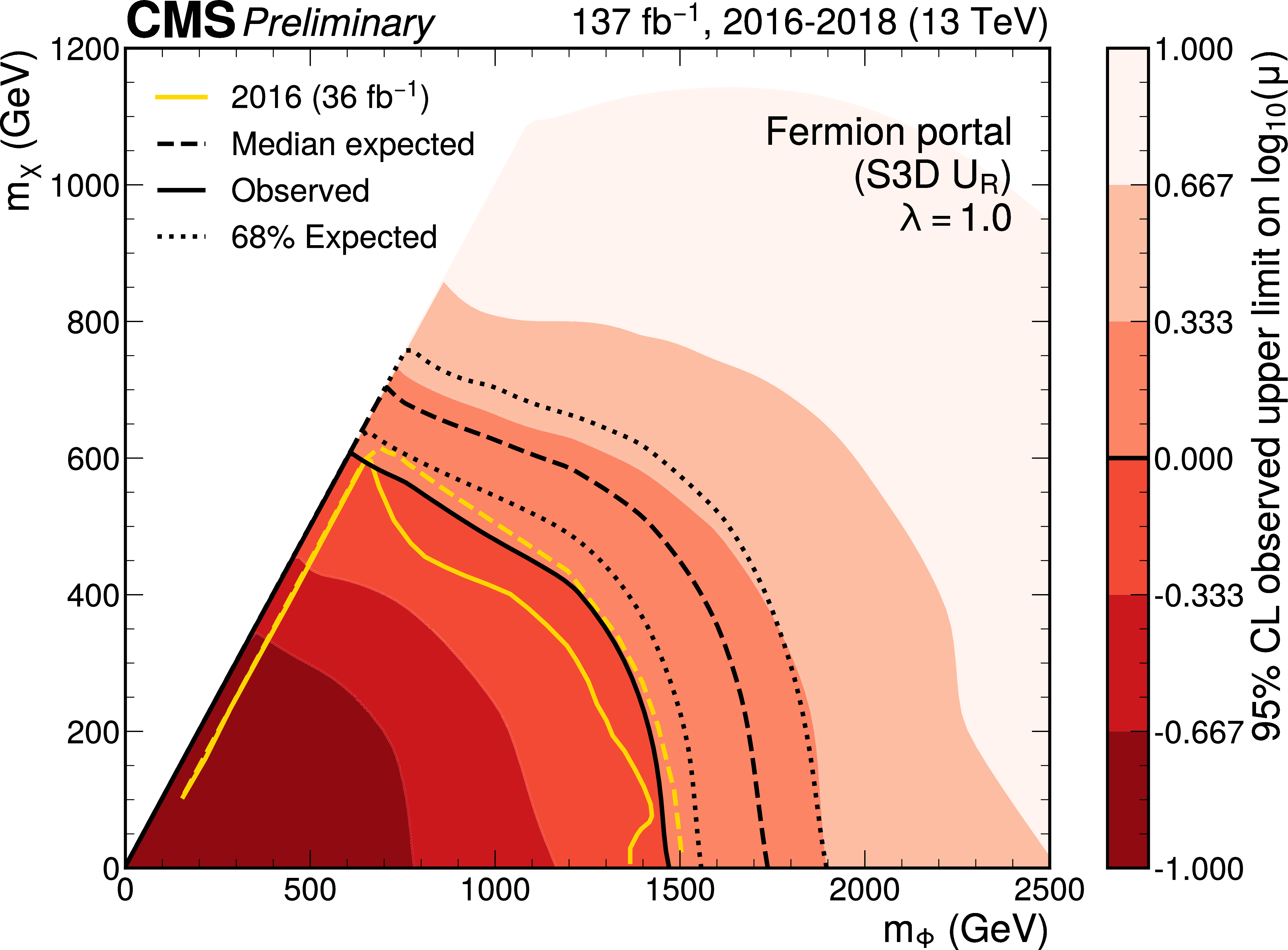
Figure 9:
Exclusion limits at 95% CL in in the plane of the mediator mass $m_\phi $ and the DM candidate mass $m_\chi $. The black dashed and dotted lines represent the median expected exclusion and the 68% confidence level interval around it, respectively. The black solid line represents the observed exclusion. The yellow solid line shows the observed exclusion from Ref. [20] for comparison. |
png pdf |
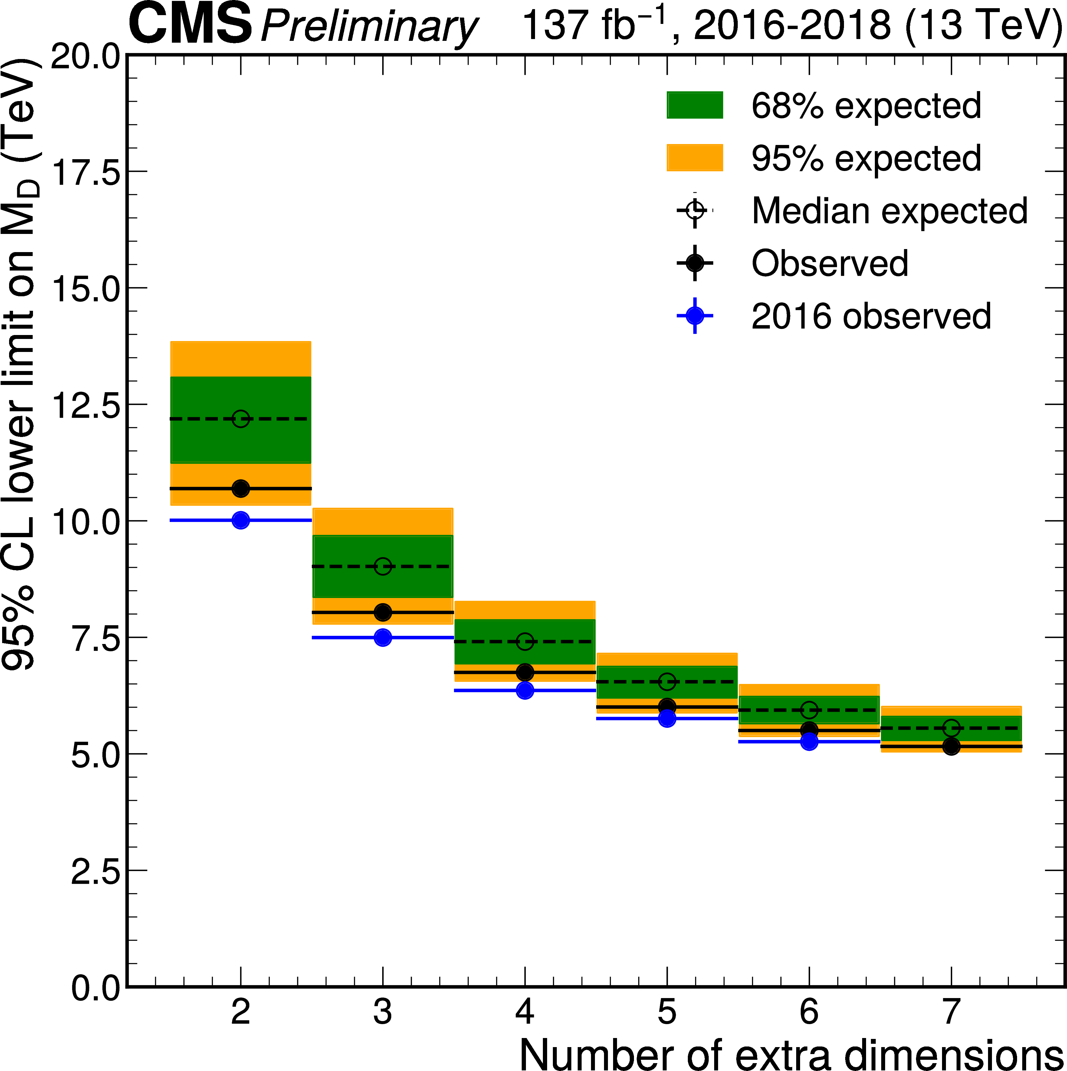
Figure 10:
Exclusion limits at 95% CL on $M_{D}$ in the ADD scenario for different values of the number of extra dimensions d. The blue markers show the result from Ref. [20] for comparison. |
png pdf |
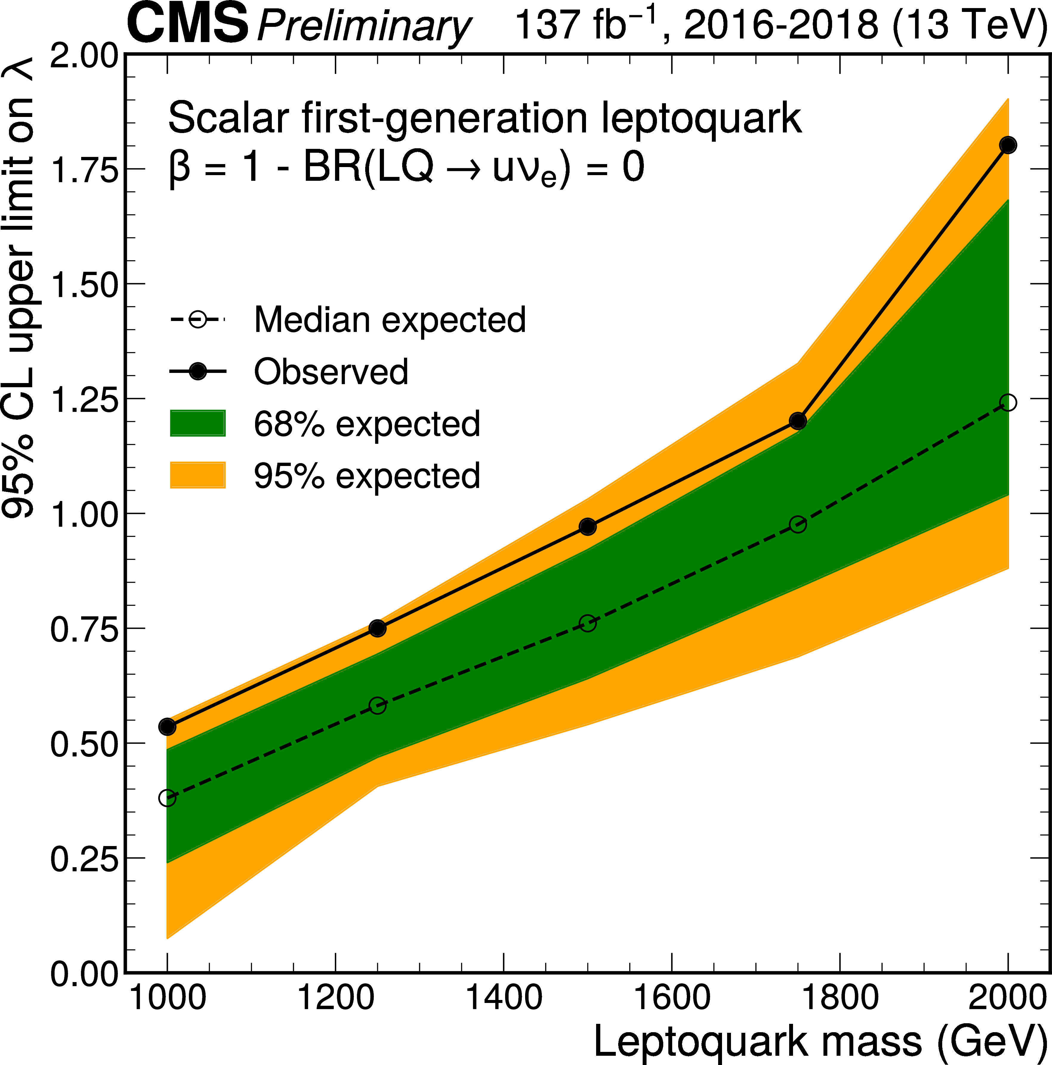
Figure 11:
Upper limits at 95% CL on the leptoquark coupling $\lambda $ as a function of the leptoquark mass. The branching fraction for the decay of the leptoquark into an electron neutrino and up quark is assumed to be 100% ($\beta =$ 0). The dashed line indicates the median expected exclusion contour. For a leptoquark mass value of 1 TeV, coupling values as low as approximately 0.5 are excluded (0.4 expected). The upper limit increases with the leptoquark mass increase, reaching $\lambda =$ 0.9 at a mass of 1.5 TeV (0.7 expected) and $\lambda =$ 1.8 at 2 TeV (1.25 expected). |
| Summary |
| A search for physics beyond the standard model in events with energetic jets and large missing transverse momentum is presented. A data set of proton-proton collisions at a center-of-mass energy of 13 TeV, corresponding to and integrated luminosity of 101 fb$^{-1}$ is analyzed, and the analysis results are combined with those of an earlier search using an independent data set collected at the same center-of-mass energy, corresponding to an integrated luminosity of 36 fb$^{-1}$ [20]. Separate analysis categories are defined for events with a large-radius jet consistent with a decay of a W or a Z boson, and for events without such a jet. A joint maximum-likelihood fit over a combination of signal and control regions is used to constrain standard model (SM) background processes and to extract possible signal. The data are found to be in a good agreement with the fit results, with no evidence for a significant signal contribution found. The result is interpreted in terms of exclusion limits on the parameters of a number of models of beyond-the-SM physics. In simplified models of the production of dark matter (DM) candidates via a spin-1 $s$-channel mediator, values of the mediator mass of up to 1.95 TeV are excluded, assuming the couplings of ${g_\mathrm{q}} =$ 0.25 between the mediator and quarks, and ${g_\chi} =$ 1.0 between the mediator and the Dirac fermion DM particles. Assuming a fixed ratio ${m_\text{DM}} = m_{\text{med}}$/3, coupling values as low as ${g_\mathrm{q}} =$ 0.018 and ${g_\chi} =$ 0.070 can be excluded for a mediator mass value of $ m_{\text{med}} = $ 100 GeV. In a similar model with a pseudoscalar spin-0 mediator, mediator masses of up to 470 GeV are excluded. We further constrain the branching fraction of the Higgs boson decay to invisible particles to be below 27.8%. In a model of large extra dimensions, values of the fundamental Planck scale below from 10.7 to 5.2 TeV can be excluded, depending on the number of extra dimensions between 2 and 7. Finally, the production of leptoquarks decaying into the up quark and the electron neutrino is excluded for coupling values between the leptoquarks and the SM fermions larger than between 10$^{-5}$ and 1.8 for leptoquark masses between 0.5 and 1.8 TeV. |
| Additional Figures | |
png pdf |
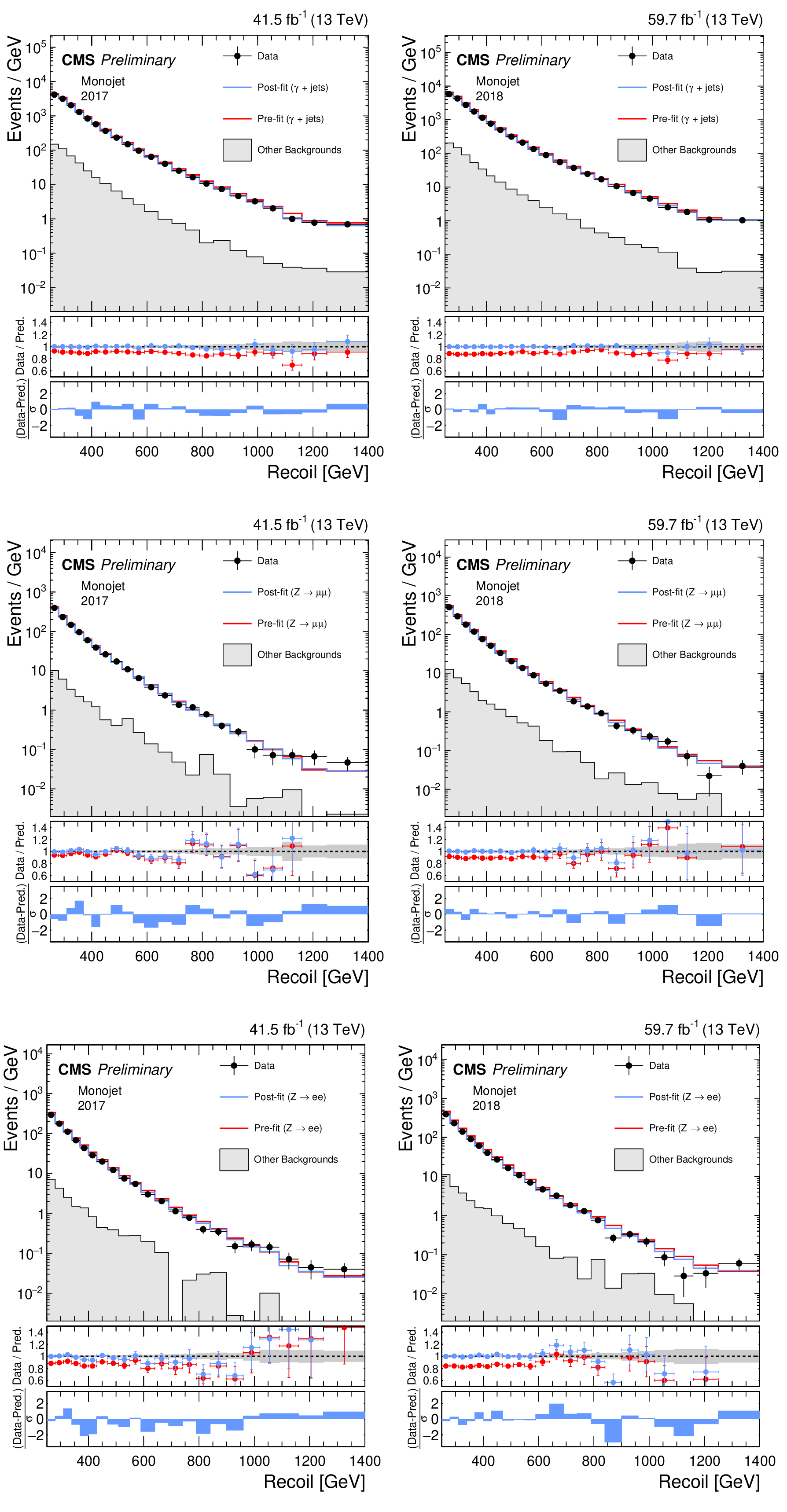
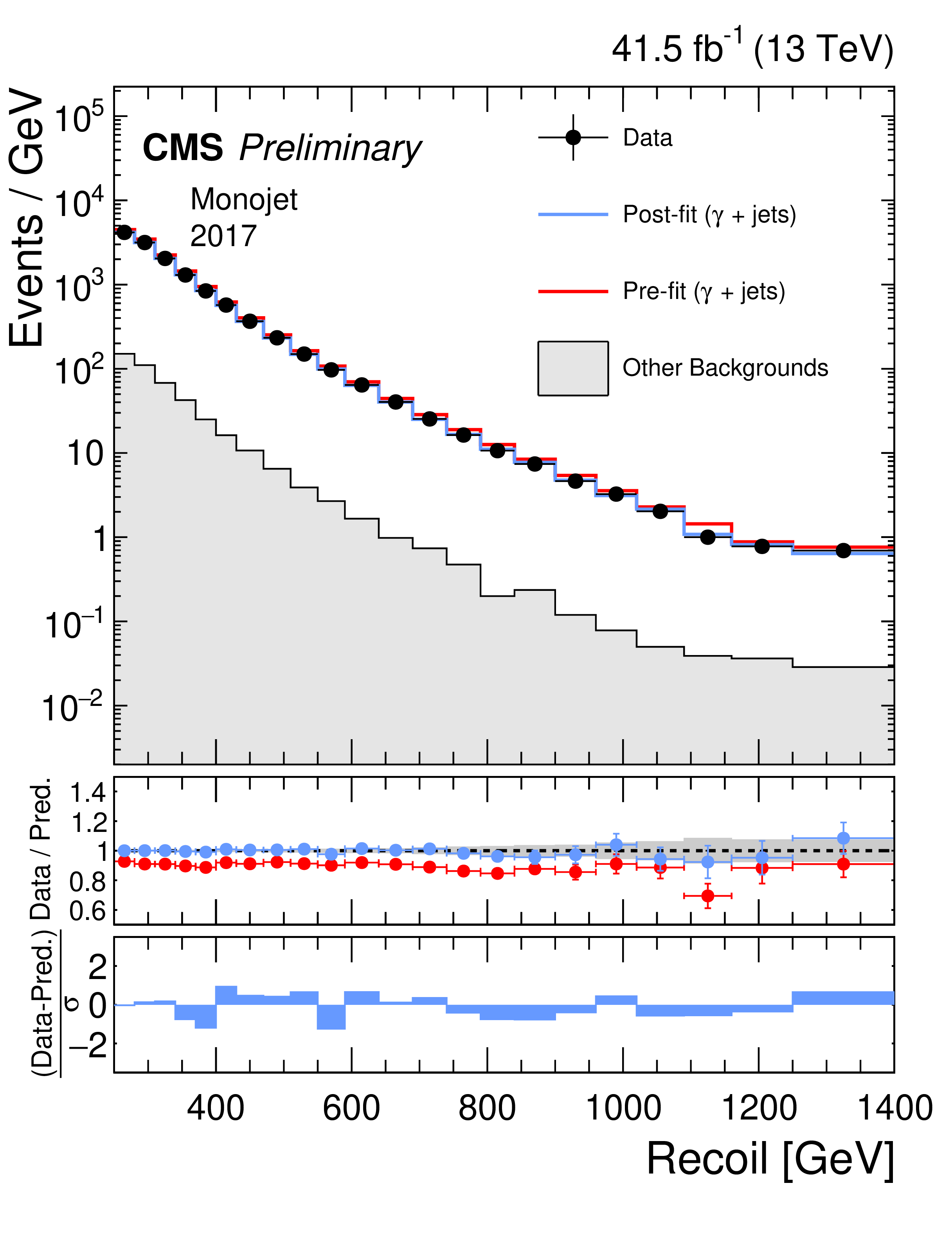
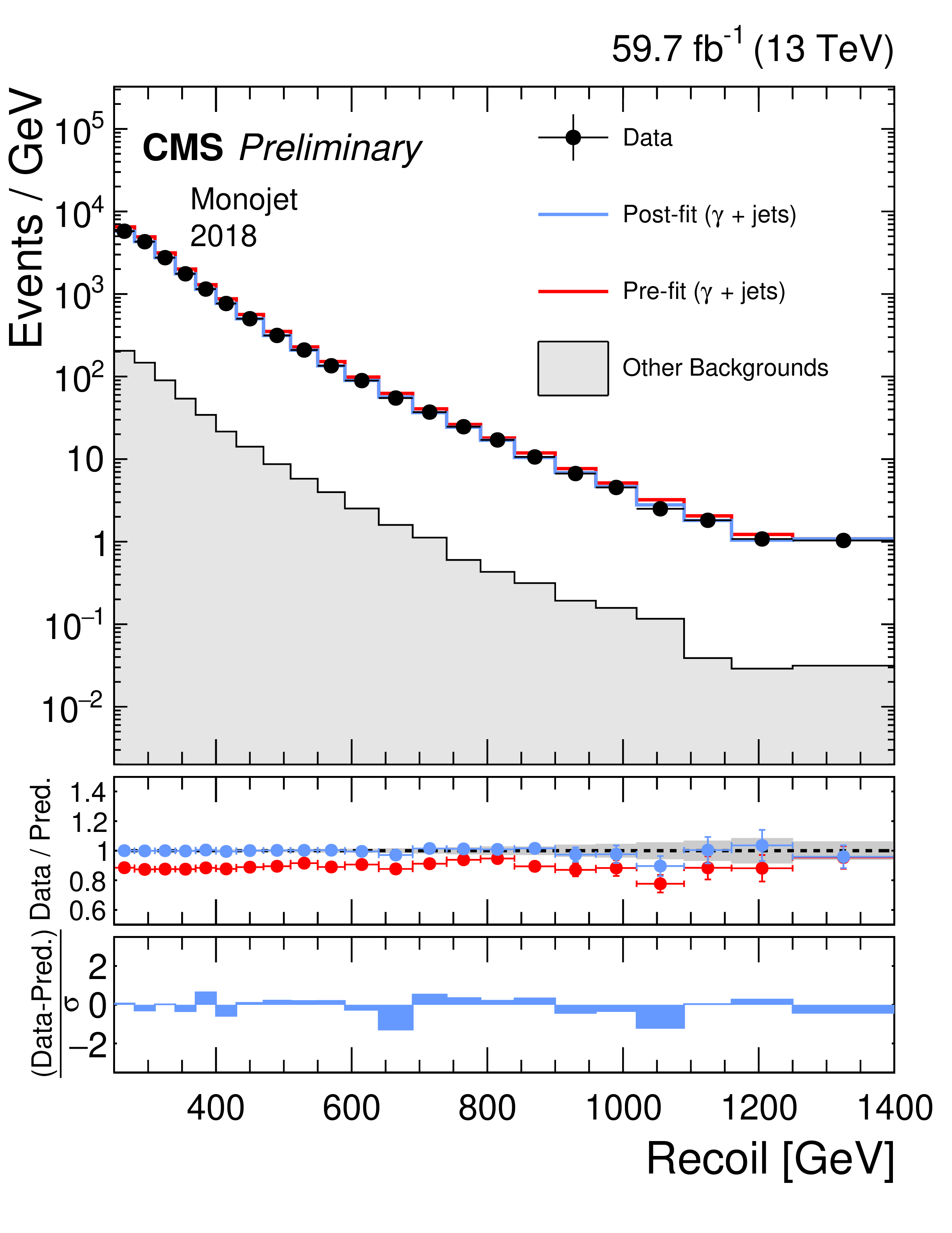
Additional Figure 1:
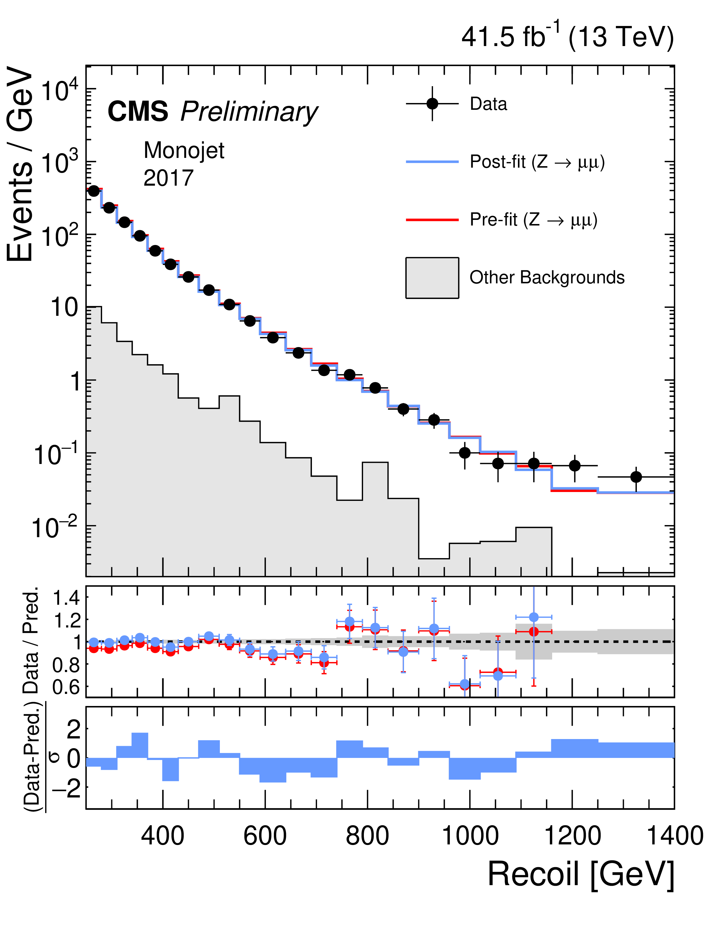
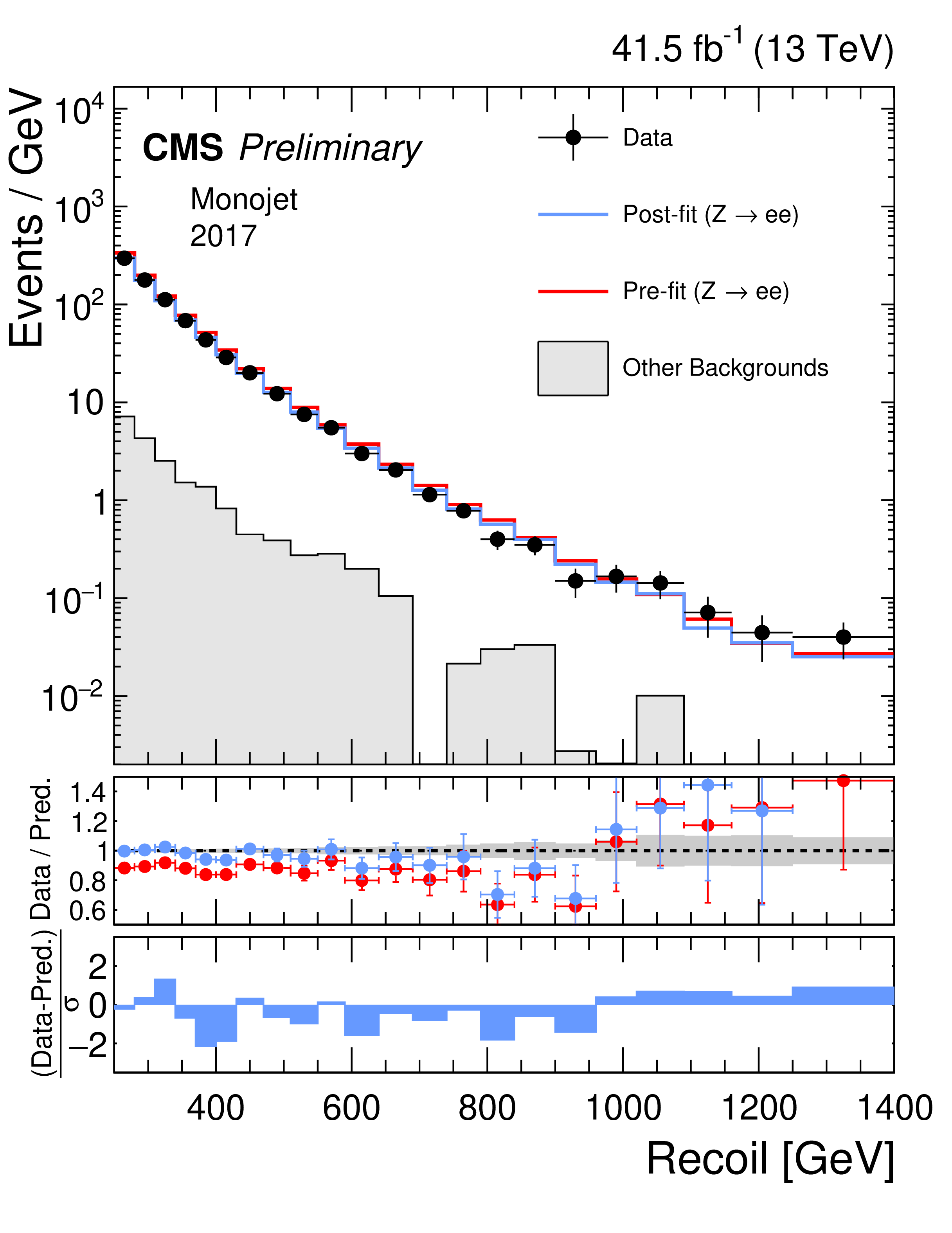
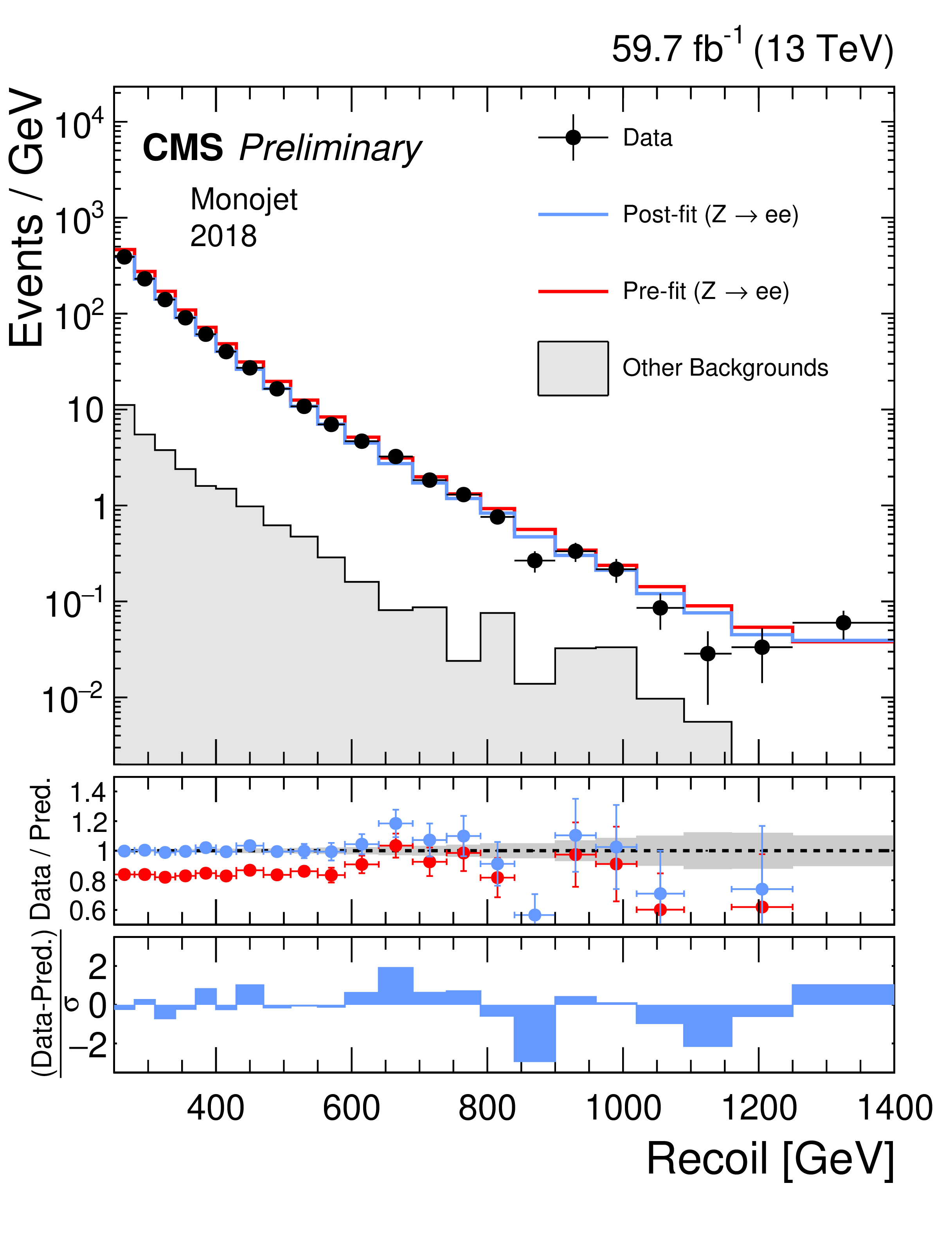
Hadronic recoil distributions in the photon (a, b), dimuon (c, d) and dielectron control regions (e, f) in the monojet category. The 2017 (a, c, e) and 2018 (b, d, f) data-taking periods are shown separately. The other backgrounds include QCD multijet production (photon), top quark, diboson and W+jets processes (dimuon and dielectron). The fit result is based on the background-only model and includes the full combination of data-taking periods and analysis regions. |
png pdf |
Additional Figure 1-a:
Hadronic recoil distributions in the photon (a, b), dimuon (c, d) and dielectron control regions (e, f) in the monojet category. The 2017 (a, c, e) and 2018 (b, d, f) data-taking periods are shown separately. The other backgrounds include QCD multijet production (photon), top quark, diboson and W+jets processes (dimuon and dielectron). The fit result is based on the background-only model and includes the full combination of data-taking periods and analysis regions. |
png pdf |
Additional Figure 1-b:
Hadronic recoil distributions in the photon (a, b), dimuon (c, d) and dielectron control regions (e, f) in the monojet category. The 2017 (a, c, e) and 2018 (b, d, f) data-taking periods are shown separately. The other backgrounds include QCD multijet production (photon), top quark, diboson and W+jets processes (dimuon and dielectron). The fit result is based on the background-only model and includes the full combination of data-taking periods and analysis regions. |
png pdf |
Additional Figure 1-c:
Hadronic recoil distributions in the photon (a, b), dimuon (c, d) and dielectron control regions (e, f) in the monojet category. The 2017 (a, c, e) and 2018 (b, d, f) data-taking periods are shown separately. The other backgrounds include QCD multijet production (photon), top quark, diboson and W+jets processes (dimuon and dielectron). The fit result is based on the background-only model and includes the full combination of data-taking periods and analysis regions. |

png pdf |
Additional Figure 1-d:
Hadronic recoil distributions in the photon (a, b), dimuon (c, d) and dielectron control regions (e, f) in the monojet category. The 2017 (a, c, e) and 2018 (b, d, f) data-taking periods are shown separately. The other backgrounds include QCD multijet production (photon), top quark, diboson and W+jets processes (dimuon and dielectron). The fit result is based on the background-only model and includes the full combination of data-taking periods and analysis regions. |
png pdf |
Additional Figure 1-e:
Hadronic recoil distributions in the photon (a, b), dimuon (c, d) and dielectron control regions (e, f) in the monojet category. The 2017 (a, c, e) and 2018 (b, d, f) data-taking periods are shown separately. The other backgrounds include QCD multijet production (photon), top quark, diboson and W+jets processes (dimuon and dielectron). The fit result is based on the background-only model and includes the full combination of data-taking periods and analysis regions. |
png pdf |
Additional Figure 1-f:
Hadronic recoil distributions in the photon (a, b), dimuon (c, d) and dielectron control regions (e, f) in the monojet category. The 2017 (a, c, e) and 2018 (b, d, f) data-taking periods are shown separately. The other backgrounds include QCD multijet production (photon), top quark, diboson and W+jets processes (dimuon and dielectron). The fit result is based on the background-only model and includes the full combination of data-taking periods and analysis regions. |
png pdf |
Additional Figure 2:
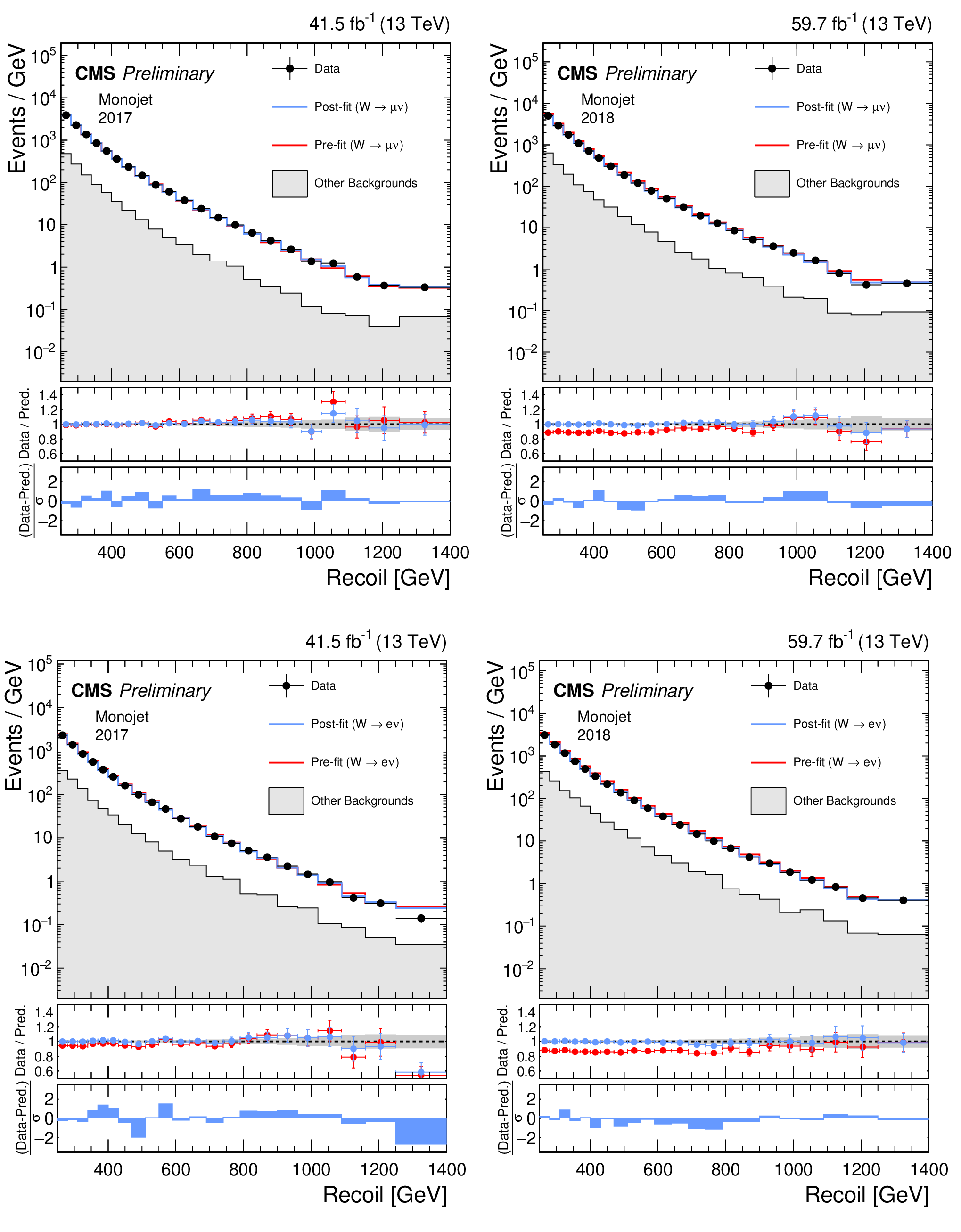
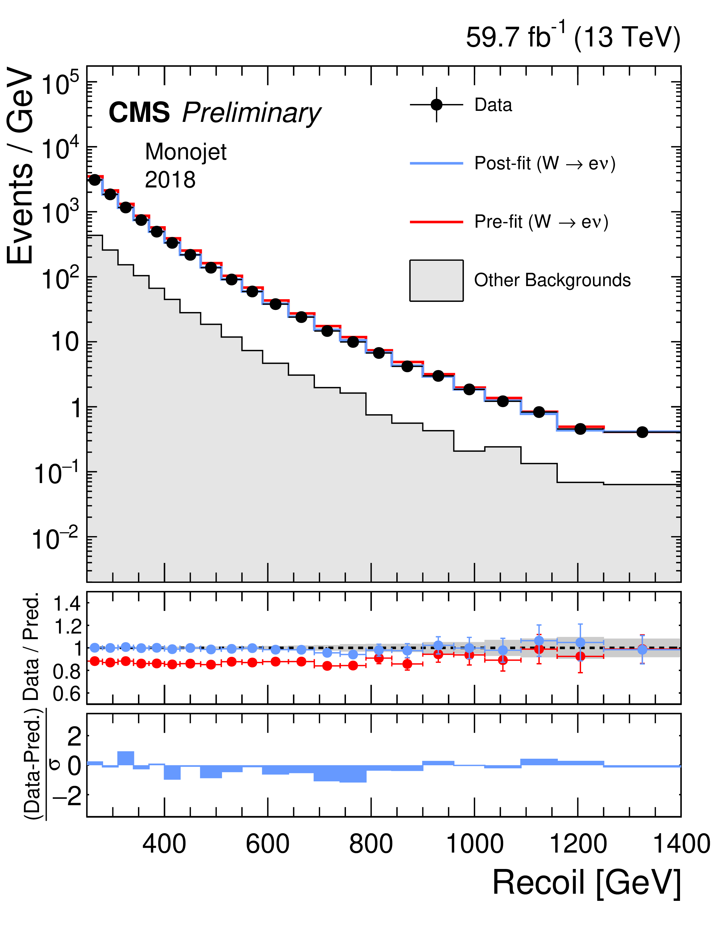
Hadronic recoil distributions in the single muon (a, b) and single electron regions (c, d) in the monojet category. The 2017 (a, c) and 2018 (b, d) data-taking periods are shown separately. The fit result is based on the background-only model and includes the full combination of data-taking periods and analysis regions. The other backgrounds include top quark, diboson, and QCD multijet processes. |
png pdf |
Additional Figure 2-a:
Hadronic recoil distributions in the single muon (a, b) and single electron regions (c, d) in the monojet category. The 2017 (a, c) and 2018 (b, d) data-taking periods are shown separately. The fit result is based on the background-only model and includes the full combination of data-taking periods and analysis regions. The other backgrounds include top quark, diboson, and QCD multijet processes. |
png pdf |
Additional Figure 2-b:
Hadronic recoil distributions in the single muon (a, b) and single electron regions (c, d) in the monojet category. The 2017 (a, c) and 2018 (b, d) data-taking periods are shown separately. The fit result is based on the background-only model and includes the full combination of data-taking periods and analysis regions. The other backgrounds include top quark, diboson, and QCD multijet processes. |

png pdf |
Additional Figure 2-c:
Hadronic recoil distributions in the single muon (a, b) and single electron regions (c, d) in the monojet category. The 2017 (a, c) and 2018 (b, d) data-taking periods are shown separately. The fit result is based on the background-only model and includes the full combination of data-taking periods and analysis regions. The other backgrounds include top quark, diboson, and QCD multijet processes. |
png pdf |
Additional Figure 2-d:
Hadronic recoil distributions in the single muon (a, b) and single electron regions (c, d) in the monojet category. The 2017 (a, c) and 2018 (b, d) data-taking periods are shown separately. The fit result is based on the background-only model and includes the full combination of data-taking periods and analysis regions. The other backgrounds include top quark, diboson, and QCD multijet processes. |

png pdf |
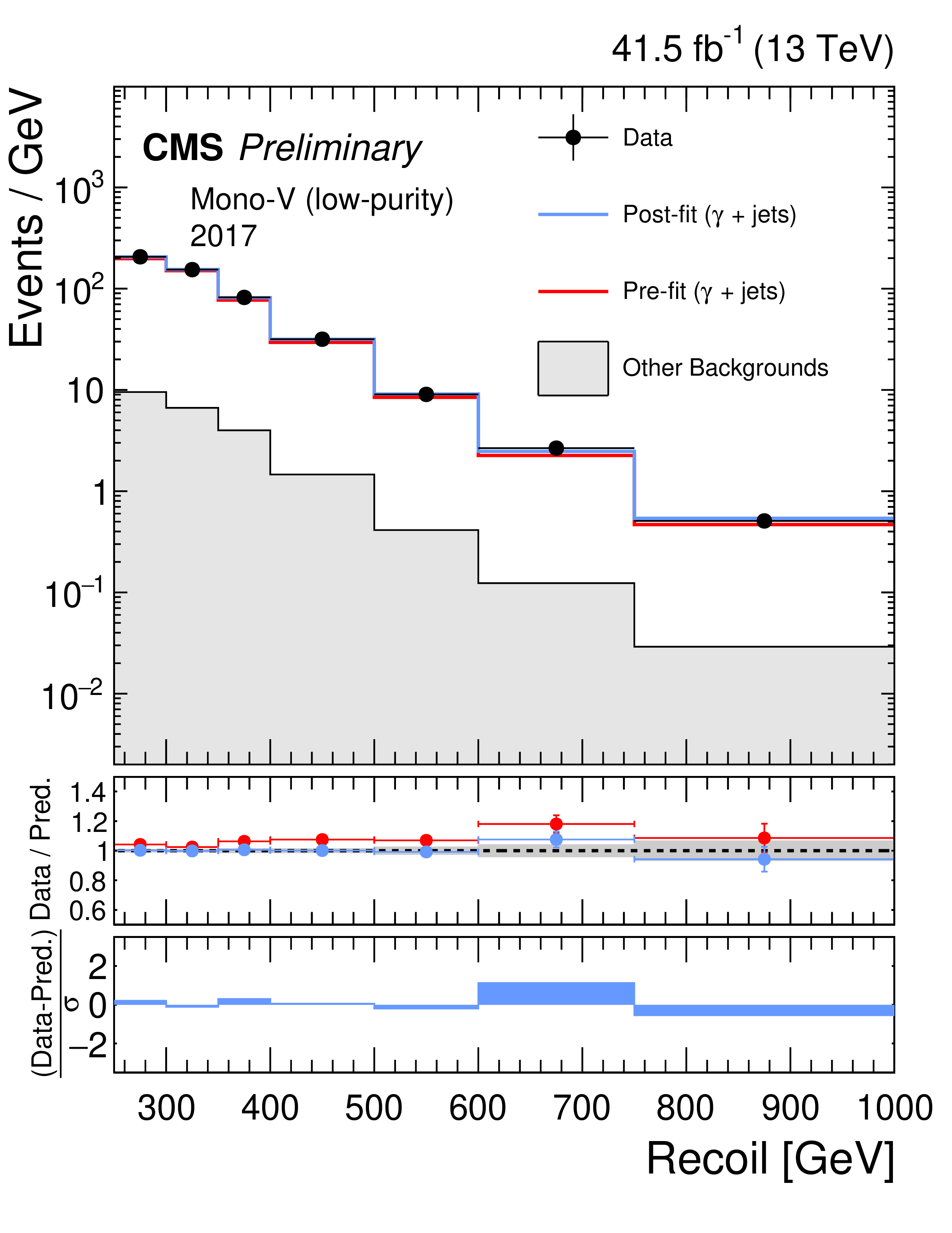
Additional Figure 3:
Hadronic recoil distributions in the photon (a, b), dimuon (c, d) and dielectron control regions (e, f) in the low-purity mono-V category. The 2017 (a, c, e) and 2018 (b, d, f) data-taking periods are shown separately. The other backgrounds include QCD multijet production (photon), top quark, diboson and W+jets processes (dimuon and dielectron). The fit result is based on the background-only model and includes the full combination of data-taking periods and analysis regions. |
png pdf |
Additional Figure 3-a:
Hadronic recoil distributions in the photon (a, b), dimuon (c, d) and dielectron control regions (e, f) in the low-purity mono-V category. The 2017 (a, c, e) and 2018 (b, d, f) data-taking periods are shown separately. The other backgrounds include QCD multijet production (photon), top quark, diboson and W+jets processes (dimuon and dielectron). The fit result is based on the background-only model and includes the full combination of data-taking periods and analysis regions. |
png pdf |
Additional Figure 3-b:
Hadronic recoil distributions in the photon (a, b), dimuon (c, d) and dielectron control regions (e, f) in the low-purity mono-V category. The 2017 (a, c, e) and 2018 (b, d, f) data-taking periods are shown separately. The other backgrounds include QCD multijet production (photon), top quark, diboson and W+jets processes (dimuon and dielectron). The fit result is based on the background-only model and includes the full combination of data-taking periods and analysis regions. |
png pdf |
Additional Figure 3-c:
Hadronic recoil distributions in the photon (a, b), dimuon (c, d) and dielectron control regions (e, f) in the low-purity mono-V category. The 2017 (a, c, e) and 2018 (b, d, f) data-taking periods are shown separately. The other backgrounds include QCD multijet production (photon), top quark, diboson and W+jets processes (dimuon and dielectron). The fit result is based on the background-only model and includes the full combination of data-taking periods and analysis regions. |
png pdf |
Additional Figure 3-d:
Hadronic recoil distributions in the photon (a, b), dimuon (c, d) and dielectron control regions (e, f) in the low-purity mono-V category. The 2017 (a, c, e) and 2018 (b, d, f) data-taking periods are shown separately. The other backgrounds include QCD multijet production (photon), top quark, diboson and W+jets processes (dimuon and dielectron). The fit result is based on the background-only model and includes the full combination of data-taking periods and analysis regions. |
png pdf |
Additional Figure 3-e:
Hadronic recoil distributions in the photon (a, b), dimuon (c, d) and dielectron control regions (e, f) in the low-purity mono-V category. The 2017 (a, c, e) and 2018 (b, d, f) data-taking periods are shown separately. The other backgrounds include QCD multijet production (photon), top quark, diboson and W+jets processes (dimuon and dielectron). The fit result is based on the background-only model and includes the full combination of data-taking periods and analysis regions. |
png pdf |
Additional Figure 3-f:
Hadronic recoil distributions in the photon (a, b), dimuon (c, d) and dielectron control regions (e, f) in the low-purity mono-V category. The 2017 (a, c, e) and 2018 (b, d, f) data-taking periods are shown separately. The other backgrounds include QCD multijet production (photon), top quark, diboson and W+jets processes (dimuon and dielectron). The fit result is based on the background-only model and includes the full combination of data-taking periods and analysis regions. |
png pdf |
Additional Figure 4:
Hadronic recoil distributions in the single muon (a, b) and single electron regions (c, d) in the low-purity mono-V category. The 2017 (a, c) and 2018 (b, df) data-taking periods are shown separately. The fit result is based on the background-only model and includes the full combination of data-taking periods and analysis regions. The other backgrounds include top quark, diboson, and QCD multijet processes. |
png pdf |
Additional Figure 4-a:
Hadronic recoil distributions in the single muon (a, b) and single electron regions (c, d) in the low-purity mono-V category. The 2017 (a, c) and 2018 (b, df) data-taking periods are shown separately. The fit result is based on the background-only model and includes the full combination of data-taking periods and analysis regions. The other backgrounds include top quark, diboson, and QCD multijet processes. |
png pdf |
Additional Figure 4-b:
Hadronic recoil distributions in the single muon (a, b) and single electron regions (c, d) in the low-purity mono-V category. The 2017 (a, c) and 2018 (b, df) data-taking periods are shown separately. The fit result is based on the background-only model and includes the full combination of data-taking periods and analysis regions. The other backgrounds include top quark, diboson, and QCD multijet processes. |

png pdf |
Additional Figure 4-c:
Hadronic recoil distributions in the single muon (a, b) and single electron regions (c, d) in the low-purity mono-V category. The 2017 (a, c) and 2018 (b, df) data-taking periods are shown separately. The fit result is based on the background-only model and includes the full combination of data-taking periods and analysis regions. The other backgrounds include top quark, diboson, and QCD multijet processes. |

png pdf |
Additional Figure 4-d:
Hadronic recoil distributions in the single muon (a, b) and single electron regions (c, d) in the low-purity mono-V category. The 2017 (a, c) and 2018 (b, df) data-taking periods are shown separately. The fit result is based on the background-only model and includes the full combination of data-taking periods and analysis regions. The other backgrounds include top quark, diboson, and QCD multijet processes. |
png pdf |
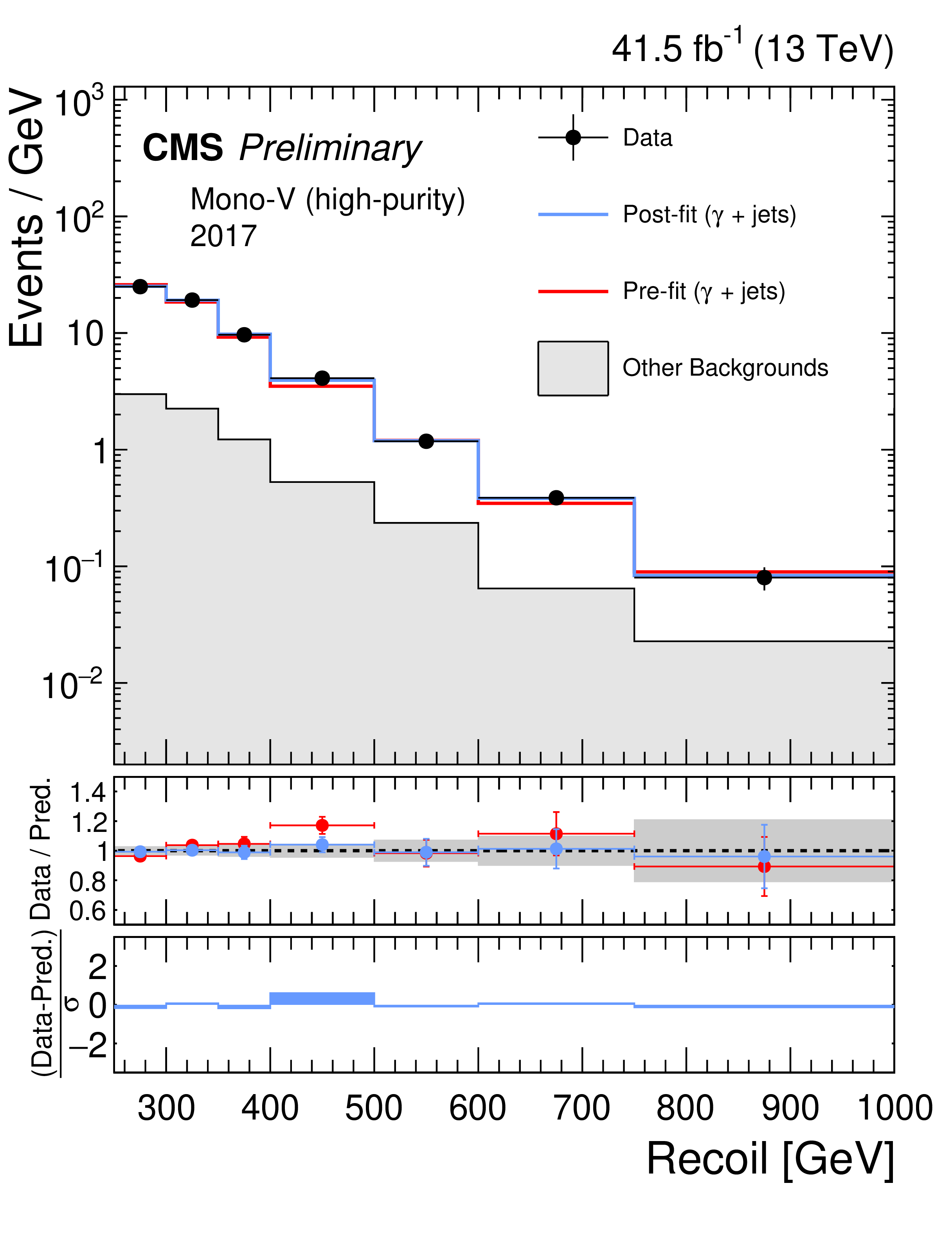
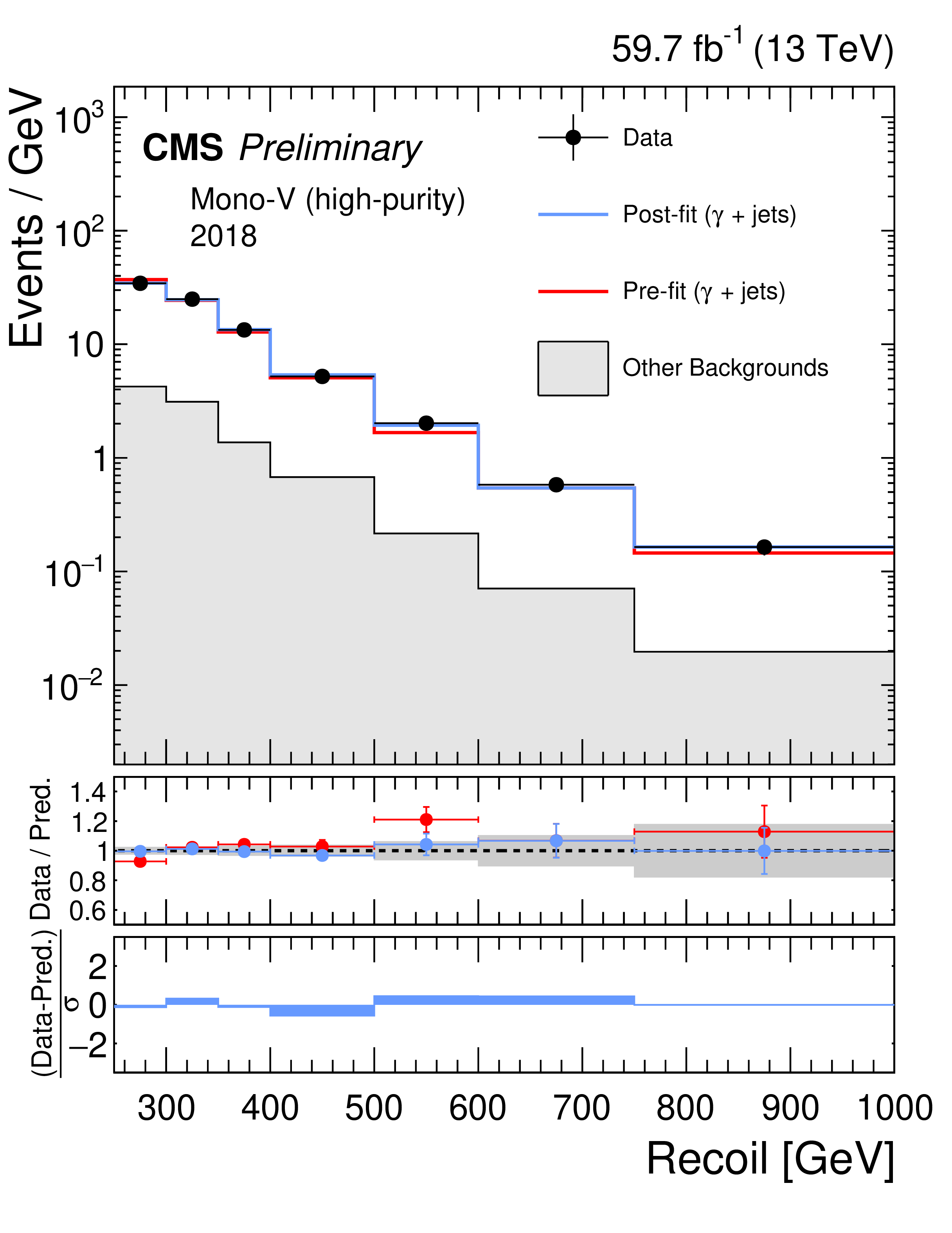
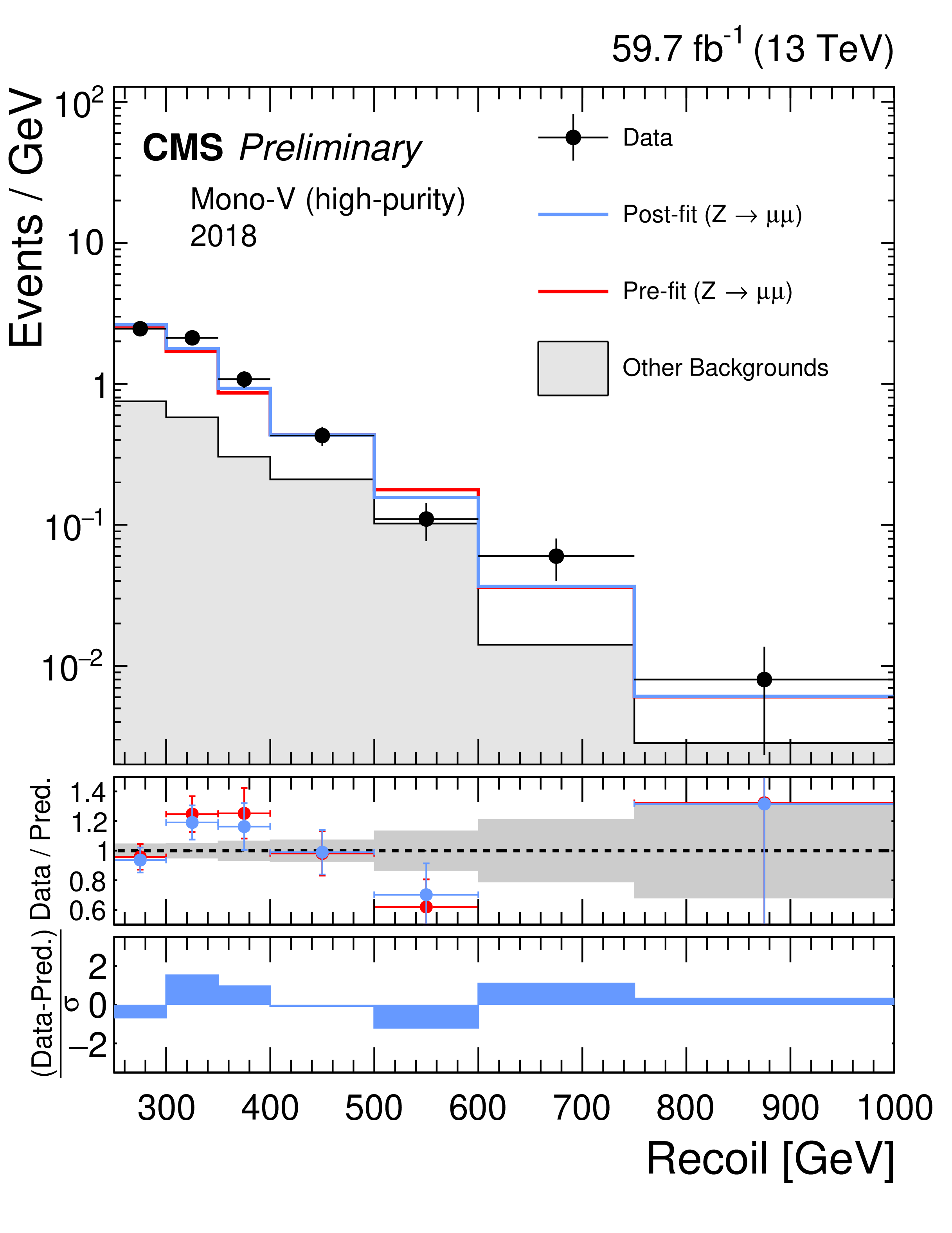
Additional Figure 5:
Hadronic recoil distributions in the photon (a, b), dimuon (c, d) and dielectron control regions (e, f) in the high-purity mono-V category. The 2017 (a, c, e) and 2018 (b, d, f) data-taking periods are shown separately. The other backgrounds include QCD multijet production (photon), top quark, diboson and W+jets processes (dimuon and dielectron). The fit result is based on the background-only model and includes the full combination of data-taking periods and analysis regions. |
png pdf |
Additional Figure 5-a:
Hadronic recoil distributions in the photon (a, b), dimuon (c, d) and dielectron control regions (e, f) in the high-purity mono-V category. The 2017 (a, c, e) and 2018 (b, d, f) data-taking periods are shown separately. The other backgrounds include QCD multijet production (photon), top quark, diboson and W+jets processes (dimuon and dielectron). The fit result is based on the background-only model and includes the full combination of data-taking periods and analysis regions. |
png pdf |
Additional Figure 5-b:
Hadronic recoil distributions in the photon (a, b), dimuon (c, d) and dielectron control regions (e, f) in the high-purity mono-V category. The 2017 (a, c, e) and 2018 (b, d, f) data-taking periods are shown separately. The other backgrounds include QCD multijet production (photon), top quark, diboson and W+jets processes (dimuon and dielectron). The fit result is based on the background-only model and includes the full combination of data-taking periods and analysis regions. |

png pdf |
Additional Figure 5-c:
Hadronic recoil distributions in the photon (a, b), dimuon (c, d) and dielectron control regions (e, f) in the high-purity mono-V category. The 2017 (a, c, e) and 2018 (b, d, f) data-taking periods are shown separately. The other backgrounds include QCD multijet production (photon), top quark, diboson and W+jets processes (dimuon and dielectron). The fit result is based on the background-only model and includes the full combination of data-taking periods and analysis regions. |
png pdf |
Additional Figure 5-d:
Hadronic recoil distributions in the photon (a, b), dimuon (c, d) and dielectron control regions (e, f) in the high-purity mono-V category. The 2017 (a, c, e) and 2018 (b, d, f) data-taking periods are shown separately. The other backgrounds include QCD multijet production (photon), top quark, diboson and W+jets processes (dimuon and dielectron). The fit result is based on the background-only model and includes the full combination of data-taking periods and analysis regions. |

png pdf |
Additional Figure 5-e:
Hadronic recoil distributions in the photon (a, b), dimuon (c, d) and dielectron control regions (e, f) in the high-purity mono-V category. The 2017 (a, c, e) and 2018 (b, d, f) data-taking periods are shown separately. The other backgrounds include QCD multijet production (photon), top quark, diboson and W+jets processes (dimuon and dielectron). The fit result is based on the background-only model and includes the full combination of data-taking periods and analysis regions. |
png pdf |
Additional Figure 5-f:
Hadronic recoil distributions in the photon (a, b), dimuon (c, d) and dielectron control regions (e, f) in the high-purity mono-V category. The 2017 (a, c, e) and 2018 (b, d, f) data-taking periods are shown separately. The other backgrounds include QCD multijet production (photon), top quark, diboson and W+jets processes (dimuon and dielectron). The fit result is based on the background-only model and includes the full combination of data-taking periods and analysis regions. |
png pdf |
Additional Figure 6:
Hadronic recoil distributions in the single muon (a, b) and single electron regions (c, d) in the high-purity mono-V category. The 2017 (a, c) and 2018 (b, d) data-taking periods are shown separately. The fit result is based on the background-only model and includes the full combination of data-taking periods and analysis regions. The other backgrounds include top quark, diboson, and QCD multijet processes. |
png pdf |
Additional Figure 6-a:
Hadronic recoil distributions in the single muon (a, b) and single electron regions (c, d) in the high-purity mono-V category. The 2017 (a, c) and 2018 (b, d) data-taking periods are shown separately. The fit result is based on the background-only model and includes the full combination of data-taking periods and analysis regions. The other backgrounds include top quark, diboson, and QCD multijet processes. |
png pdf |
Additional Figure 6-b:
Hadronic recoil distributions in the single muon (a, b) and single electron regions (c, d) in the high-purity mono-V category. The 2017 (a, c) and 2018 (b, d) data-taking periods are shown separately. The fit result is based on the background-only model and includes the full combination of data-taking periods and analysis regions. The other backgrounds include top quark, diboson, and QCD multijet processes. |

png pdf |
Additional Figure 6-c:
Hadronic recoil distributions in the single muon (a, b) and single electron regions (c, d) in the high-purity mono-V category. The 2017 (a, c) and 2018 (b, d) data-taking periods are shown separately. The fit result is based on the background-only model and includes the full combination of data-taking periods and analysis regions. The other backgrounds include top quark, diboson, and QCD multijet processes. |
png pdf |
Additional Figure 6-d:
Hadronic recoil distributions in the single muon (a, b) and single electron regions (c, d) in the high-purity mono-V category. The 2017 (a, c) and 2018 (b, d) data-taking periods are shown separately. The fit result is based on the background-only model and includes the full combination of data-taking periods and analysis regions. The other backgrounds include top quark, diboson, and QCD multijet processes. |

png pdf |
Additional Figure 7:
Comparison of the simplified model constraints from this search (red line) to results from direction-detection experiments (blue lines). The comparison is shown separately for the vector (a) and axial-vector (b) mediators, which translate into spin-independent and spin-dependent DM-nucleon couplings, respectively [78]. In the case of spin-independent couplings, results from CRESST-II [79], CDMSlite [80], LUX [81], DarkSide-50 [82], XENON1T [83], and Panda-X II [84] are shown for comparison. For spin-dependent couplings, PICO-2L [85], PICASSO [86], and PICO-60 [87] limits are displayed. |

png pdf |
Additional Figure 7-a:
Comparison of the simplified model constraints from this search (red line) to results from direction-detection experiments (blue lines). The comparison is shown separately for the vector (a) and axial-vector (b) mediators, which translate into spin-independent and spin-dependent DM-nucleon couplings, respectively [78]. In the case of spin-independent couplings, results from CRESST-II [79], CDMSlite [80], LUX [81], DarkSide-50 [82], XENON1T [83], and Panda-X II [84] are shown for comparison. For spin-dependent couplings, PICO-2L [85], PICASSO [86], and PICO-60 [87] limits are displayed. |

png pdf |
Additional Figure 7-b:
Comparison of the simplified model constraints from this search (red line) to results from direction-detection experiments (blue lines). The comparison is shown separately for the vector (a) and axial-vector (b) mediators, which translate into spin-independent and spin-dependent DM-nucleon couplings, respectively [78]. In the case of spin-independent couplings, results from CRESST-II [79], CDMSlite [80], LUX [81], DarkSide-50 [82], XENON1T [83], and Panda-X II [84] are shown for comparison. For spin-dependent couplings, PICO-2L [85], PICASSO [86], and PICO-60 [87] limits are displayed. |

png pdf |
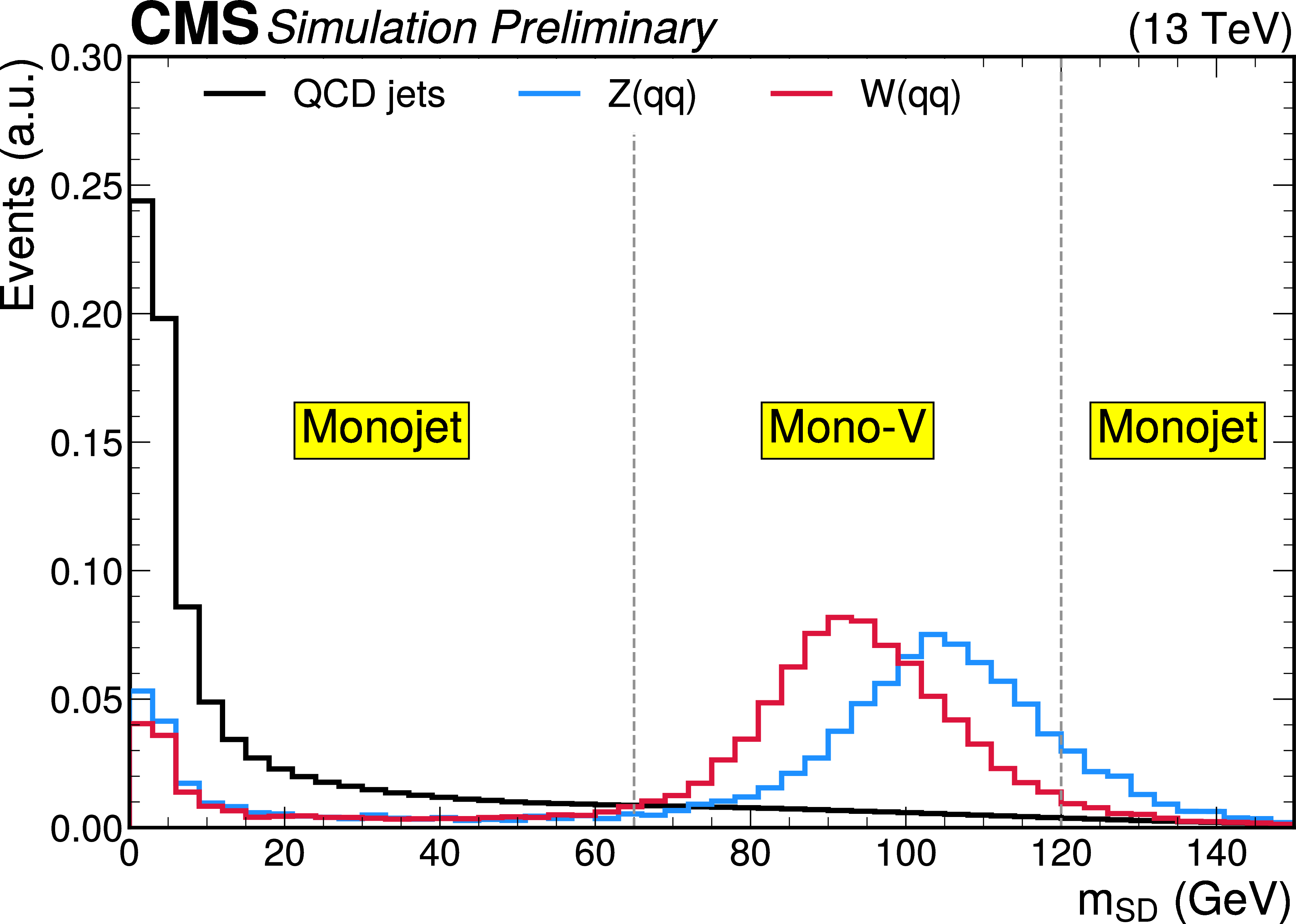
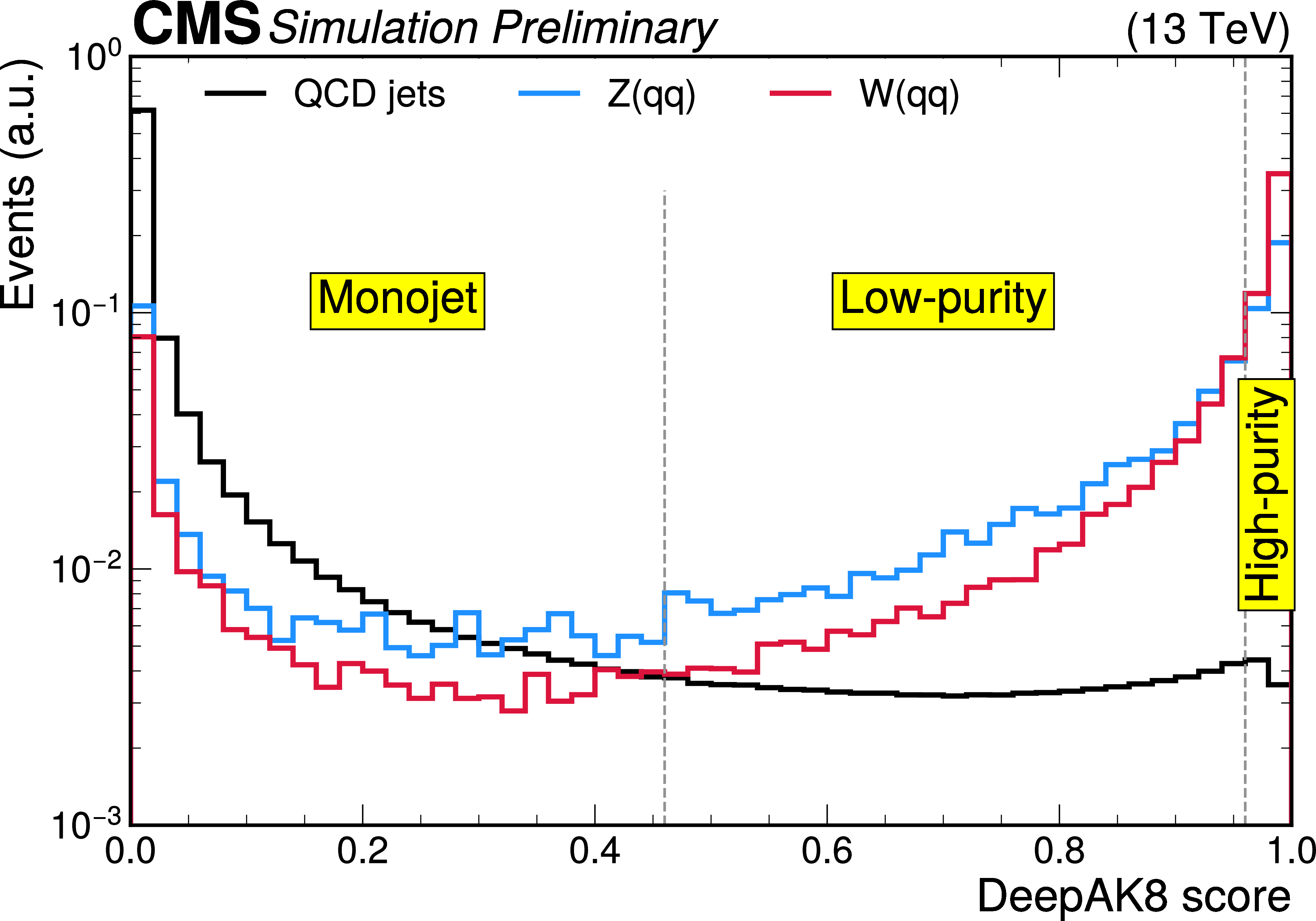
Additional Figure 8:
Distributions of the variables used for the identification of ${\to {\mathrm {q}} {\mathrm {q}}}$ candidate jets. Panels (a) and (b) show the softdrop corrected jet mass and the DeepAK8 classifier value, respectively. In each panel, the distributions are shown for the ${{\mathrm {Z}} \to {\nu} {\overline {\nu}}}$ background, which contains jets from QCD radiation, as well as the WH(inv) and ZH(inv) signals, which contain genuine hadronic decays of W or Z bosons. The distributions are shown after applying the mono-V signal region selection, with the exception of the requirements on the two variables shown here. Vertical dashed lines indicate the acceptance boundaries of different regions. |
png pdf |
Additional Figure 8-a:
Distributions of the variables used for the identification of ${\to {\mathrm {q}} {\mathrm {q}}}$ candidate jets. Panels (a) and (b) show the softdrop corrected jet mass and the DeepAK8 classifier value, respectively. In each panel, the distributions are shown for the ${{\mathrm {Z}} \to {\nu} {\overline {\nu}}}$ background, which contains jets from QCD radiation, as well as the WH(inv) and ZH(inv) signals, which contain genuine hadronic decays of W or Z bosons. The distributions are shown after applying the mono-V signal region selection, with the exception of the requirements on the two variables shown here. Vertical dashed lines indicate the acceptance boundaries of different regions. |
png pdf |
Additional Figure 8-b:
Distributions of the variables used for the identification of ${\to {\mathrm {q}} {\mathrm {q}}}$ candidate jets. Panels (a) and (b) show the softdrop corrected jet mass and the DeepAK8 classifier value, respectively. In each panel, the distributions are shown for the ${{\mathrm {Z}} \to {\nu} {\overline {\nu}}}$ background, which contains jets from QCD radiation, as well as the WH(inv) and ZH(inv) signals, which contain genuine hadronic decays of W or Z bosons. The distributions are shown after applying the mono-V signal region selection, with the exception of the requirements on the two variables shown here. Vertical dashed lines indicate the acceptance boundaries of different regions. |

png pdf |
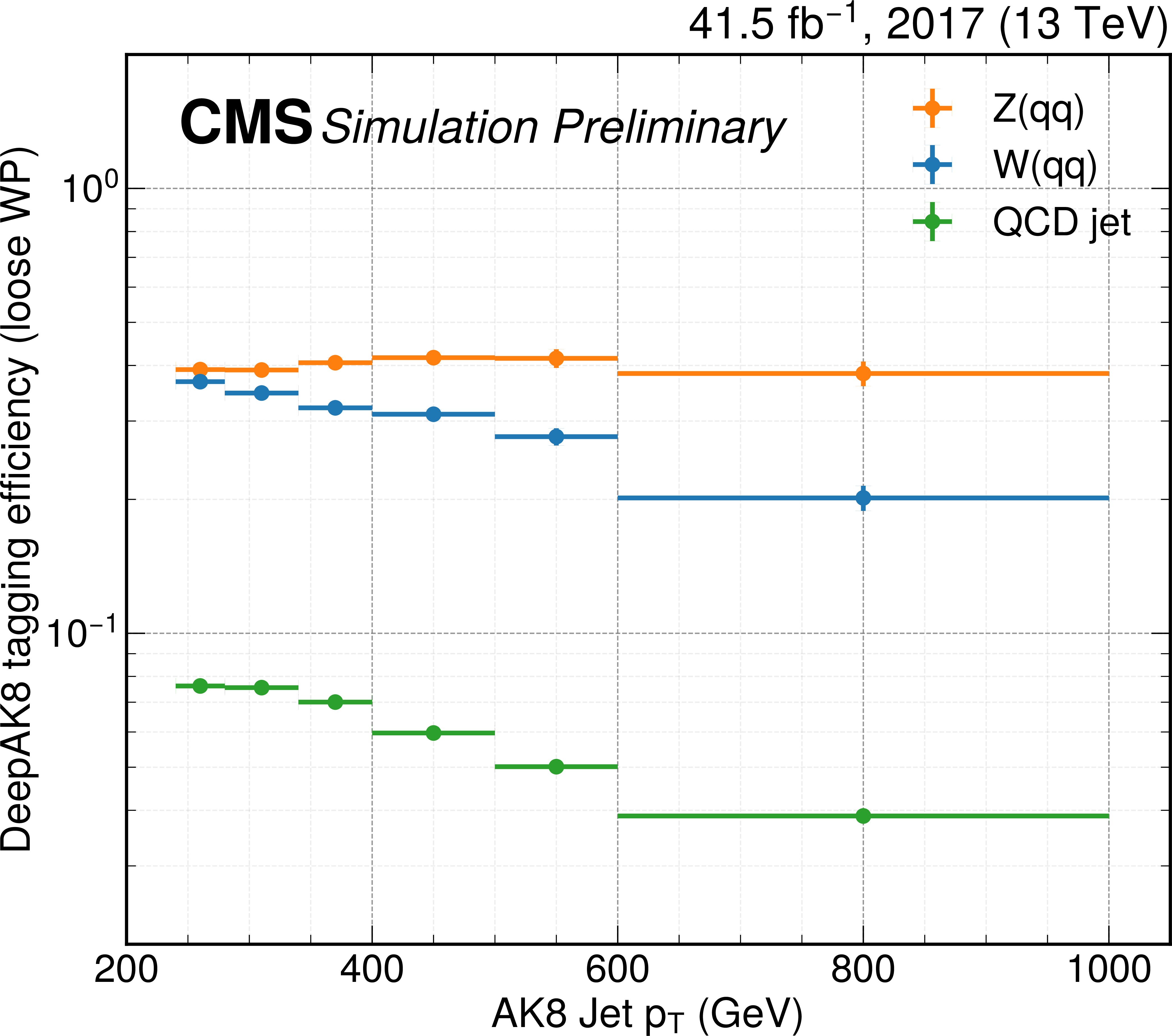
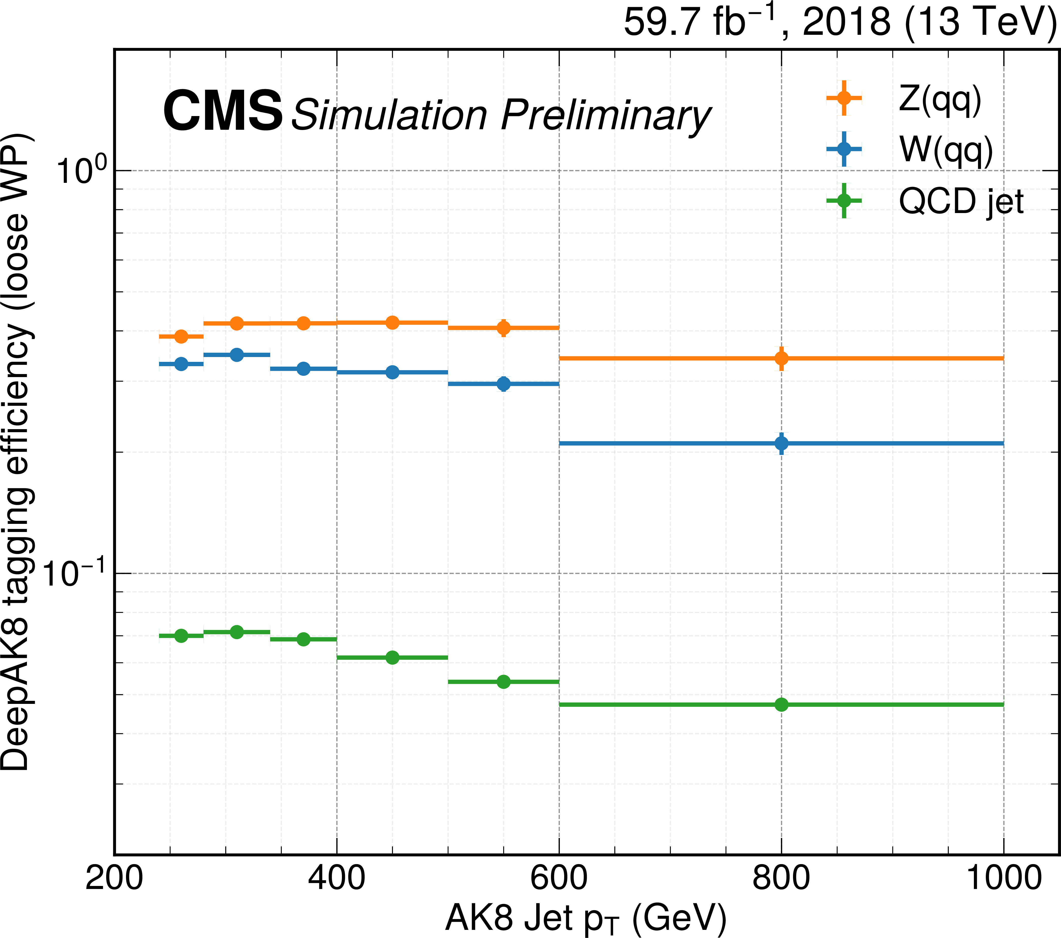
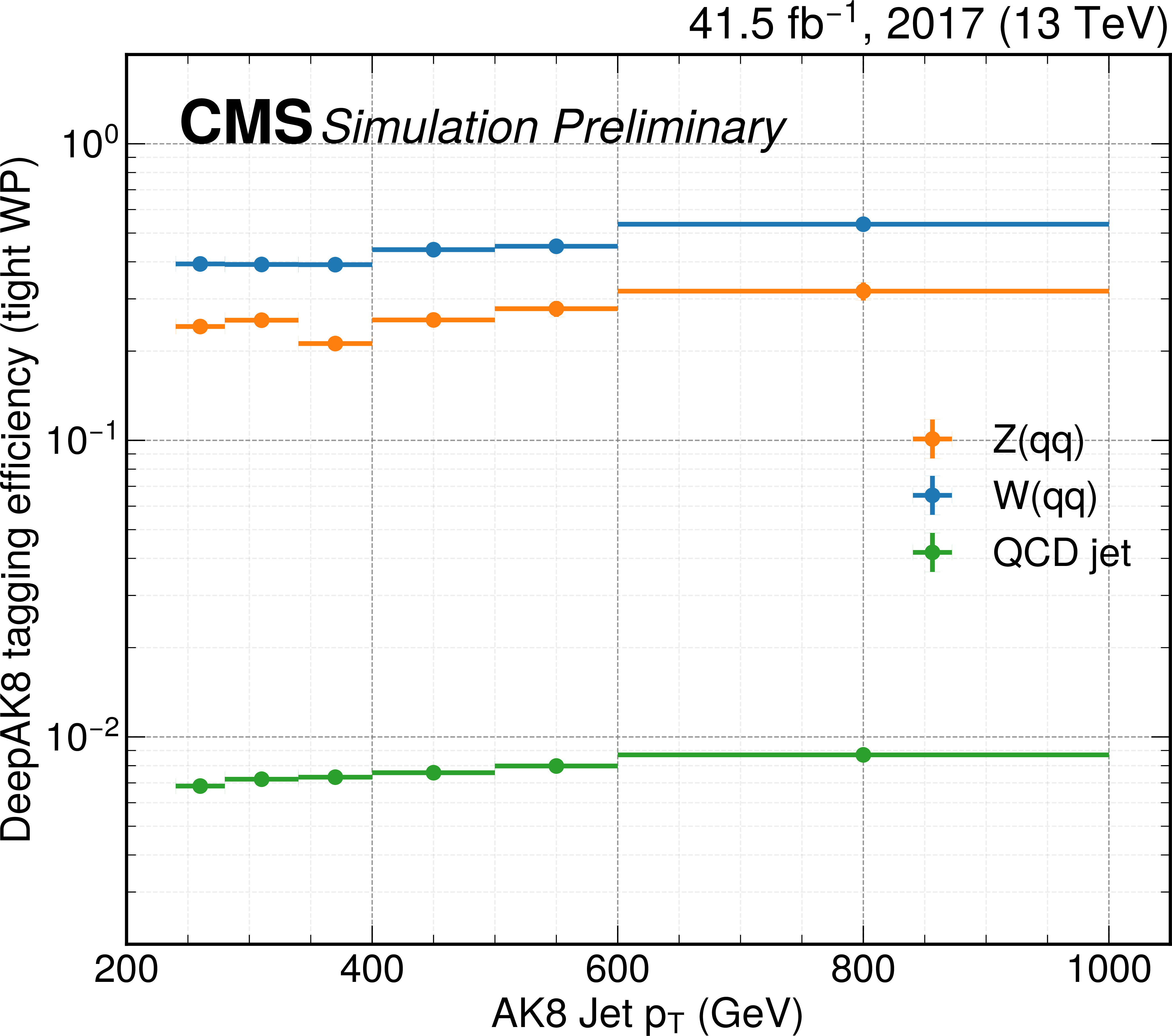
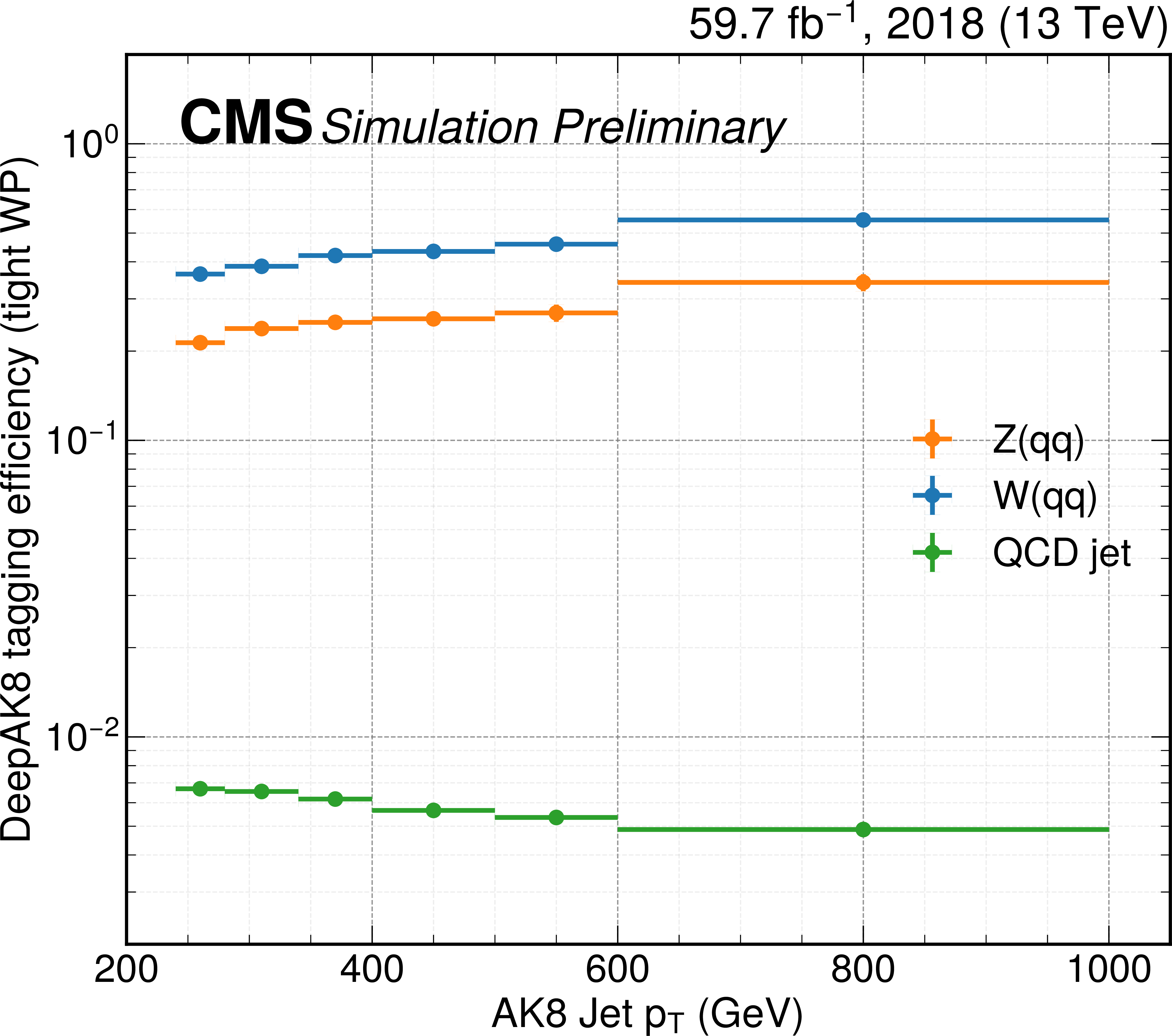
Additional Figure 9:
Wide-jet tagging efficiencies for use in reinterpretation. The efficiencies are shown separately for the low- and high-purity selections in the top and bottom panels, respectively, and for the 2017 (a, c) and 2018 data-taking periods (b, d). The efficiencies include the effect of the DeepAK8 tagger, as well as the softdrop mass requirement. In each panel, individual curves represent the efficiency for different types of jets, based on whether or not the jets are matched to a generator-level W boson, Z boson, or neither ("QCD jet''). Simulation-to-data corrections are included. Efficiencies are provided for the low- and high-purity version of the tagging requirement. Note that for the low-purity tagger, overlap removal with the high-purity category is already taken into account. The efficiency is calculated separately for AK8 jets matching a generator-level Z boson, W boson, or not matching either ("QCD jet''). A jet is considered to be matching a boson if their angular separation $\Delta R = \sqrt {\Delta \phi ^2 + \Delta \eta ^2} < $ 0.8. In order to apply the efficiencies to simulated events, one should first apply all other selection criteria. No selection based on jet mass or other substructure variables should be applied. Then, depending on the matching status of the jet, one should apply the respective efficiency, evaluated at the ${p_{\mathrm {T}}}$ of the jet, as an event weight. |
png pdf |
Additional Figure 9-a:
Wide-jet tagging efficiencies for use in reinterpretation. The efficiencies are shown separately for the low- and high-purity selections in the top and bottom panels, respectively, and for the 2017 (a, c) and 2018 data-taking periods (b, d). The efficiencies include the effect of the DeepAK8 tagger, as well as the softdrop mass requirement. In each panel, individual curves represent the efficiency for different types of jets, based on whether or not the jets are matched to a generator-level W boson, Z boson, or neither ("QCD jet''). Simulation-to-data corrections are included. Efficiencies are provided for the low- and high-purity version of the tagging requirement. Note that for the low-purity tagger, overlap removal with the high-purity category is already taken into account. The efficiency is calculated separately for AK8 jets matching a generator-level Z boson, W boson, or not matching either ("QCD jet''). A jet is considered to be matching a boson if their angular separation $\Delta R = \sqrt {\Delta \phi ^2 + \Delta \eta ^2} < $ 0.8. In order to apply the efficiencies to simulated events, one should first apply all other selection criteria. No selection based on jet mass or other substructure variables should be applied. Then, depending on the matching status of the jet, one should apply the respective efficiency, evaluated at the ${p_{\mathrm {T}}}$ of the jet, as an event weight. |
png pdf |
Additional Figure 9-b:
Wide-jet tagging efficiencies for use in reinterpretation. The efficiencies are shown separately for the low- and high-purity selections in the top and bottom panels, respectively, and for the 2017 (a, c) and 2018 data-taking periods (b, d). The efficiencies include the effect of the DeepAK8 tagger, as well as the softdrop mass requirement. In each panel, individual curves represent the efficiency for different types of jets, based on whether or not the jets are matched to a generator-level W boson, Z boson, or neither ("QCD jet''). Simulation-to-data corrections are included. Efficiencies are provided for the low- and high-purity version of the tagging requirement. Note that for the low-purity tagger, overlap removal with the high-purity category is already taken into account. The efficiency is calculated separately for AK8 jets matching a generator-level Z boson, W boson, or not matching either ("QCD jet''). A jet is considered to be matching a boson if their angular separation $\Delta R = \sqrt {\Delta \phi ^2 + \Delta \eta ^2} < $ 0.8. In order to apply the efficiencies to simulated events, one should first apply all other selection criteria. No selection based on jet mass or other substructure variables should be applied. Then, depending on the matching status of the jet, one should apply the respective efficiency, evaluated at the ${p_{\mathrm {T}}}$ of the jet, as an event weight. |
png pdf |
Additional Figure 9-c:
Wide-jet tagging efficiencies for use in reinterpretation. The efficiencies are shown separately for the low- and high-purity selections in the top and bottom panels, respectively, and for the 2017 (a, c) and 2018 data-taking periods (b, d). The efficiencies include the effect of the DeepAK8 tagger, as well as the softdrop mass requirement. In each panel, individual curves represent the efficiency for different types of jets, based on whether or not the jets are matched to a generator-level W boson, Z boson, or neither ("QCD jet''). Simulation-to-data corrections are included. Efficiencies are provided for the low- and high-purity version of the tagging requirement. Note that for the low-purity tagger, overlap removal with the high-purity category is already taken into account. The efficiency is calculated separately for AK8 jets matching a generator-level Z boson, W boson, or not matching either ("QCD jet''). A jet is considered to be matching a boson if their angular separation $\Delta R = \sqrt {\Delta \phi ^2 + \Delta \eta ^2} < $ 0.8. In order to apply the efficiencies to simulated events, one should first apply all other selection criteria. No selection based on jet mass or other substructure variables should be applied. Then, depending on the matching status of the jet, one should apply the respective efficiency, evaluated at the ${p_{\mathrm {T}}}$ of the jet, as an event weight. |
png pdf |
Additional Figure 9-d:
Wide-jet tagging efficiencies for use in reinterpretation. The efficiencies are shown separately for the low- and high-purity selections in the top and bottom panels, respectively, and for the 2017 (a, c) and 2018 data-taking periods (b, d). The efficiencies include the effect of the DeepAK8 tagger, as well as the softdrop mass requirement. In each panel, individual curves represent the efficiency for different types of jets, based on whether or not the jets are matched to a generator-level W boson, Z boson, or neither ("QCD jet''). Simulation-to-data corrections are included. Efficiencies are provided for the low- and high-purity version of the tagging requirement. Note that for the low-purity tagger, overlap removal with the high-purity category is already taken into account. The efficiency is calculated separately for AK8 jets matching a generator-level Z boson, W boson, or not matching either ("QCD jet''). A jet is considered to be matching a boson if their angular separation $\Delta R = \sqrt {\Delta \phi ^2 + \Delta \eta ^2} < $ 0.8. In order to apply the efficiencies to simulated events, one should first apply all other selection criteria. No selection based on jet mass or other substructure variables should be applied. Then, depending on the matching status of the jet, one should apply the respective efficiency, evaluated at the ${p_{\mathrm {T}}}$ of the jet, as an event weight. |
png pdf |
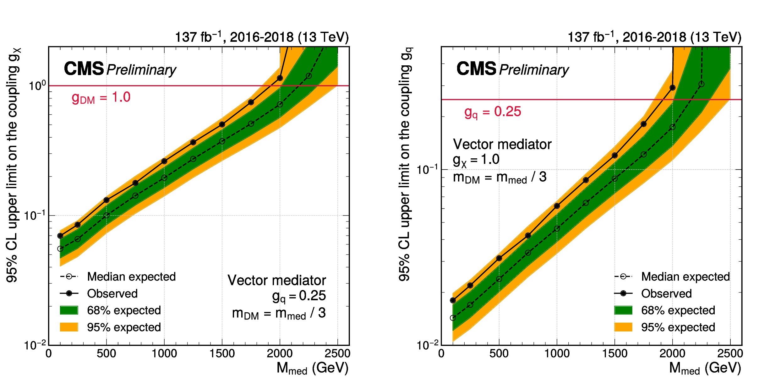
Additional Figure 10:
Exclusion limits at 95% CL on the signal strength couplings ${g_\chi}$ (a) and ${g_ {\mathrm {q}}}$ (b) for a vector mediator. In each panel, the result is shown as a function of the mediator mass $ {m_\text {med}} $, and the mass of the DM candidate is fixed to $ {m_\text {DM}} = {m_\text {med}} /3$. In either case, only one coupling is varied, and the respective other coupling is fixed at its default value ($ {g_ {\mathrm {q}}} =$ 0.25, $ {g_\chi} =$ 1.0). |

png pdf |
Additional Figure 10-a:
Exclusion limits at 95% CL on the signal strength couplings ${g_\chi}$ (a) and ${g_ {\mathrm {q}}}$ (b) for a vector mediator. In each panel, the result is shown as a function of the mediator mass $ {m_\text {med}} $, and the mass of the DM candidate is fixed to $ {m_\text {DM}} = {m_\text {med}} /3$. In either case, only one coupling is varied, and the respective other coupling is fixed at its default value ($ {g_ {\mathrm {q}}} =$ 0.25, $ {g_\chi} =$ 1.0). |

png pdf |
Additional Figure 10-b:
Exclusion limits at 95% CL on the signal strength couplings ${g_\chi}$ (a) and ${g_ {\mathrm {q}}}$ (b) for a vector mediator. In each panel, the result is shown as a function of the mediator mass $ {m_\text {med}} $, and the mass of the DM candidate is fixed to $ {m_\text {DM}} = {m_\text {med}} /3$. In either case, only one coupling is varied, and the respective other coupling is fixed at its default value ($ {g_ {\mathrm {q}}} =$ 0.25, $ {g_\chi} =$ 1.0). |
png pdf |
Additional Figure 11:
Exclusion limits at 95% CL on the branching fraction of the Higgs boson to invisible final states. The result is shown separately for the monojet and mono-V categories in each data-taking year, as well as their combination. The final combined limit is 27.8% (25.3% expected). |
png pdf |
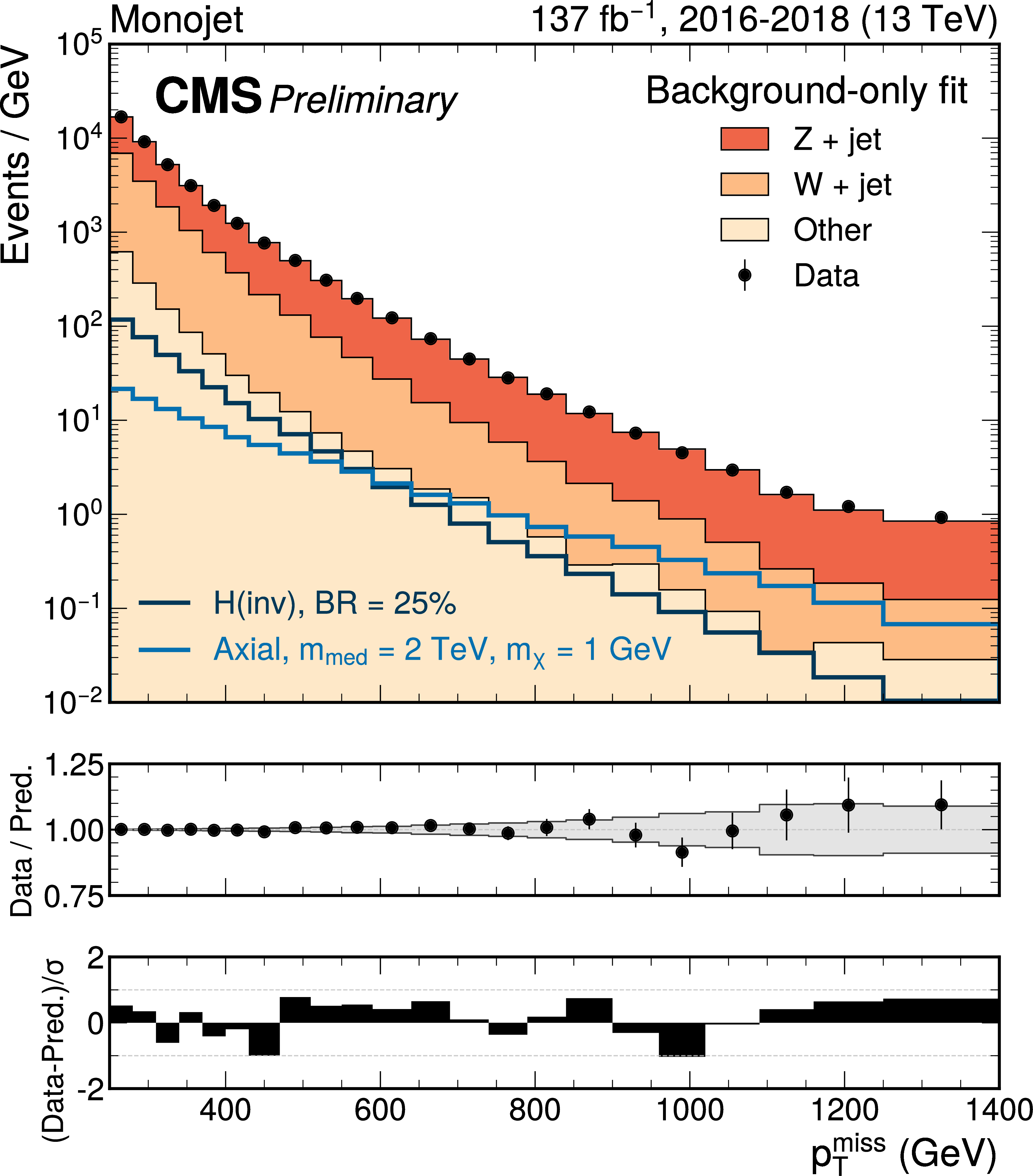
Additional Figure 12:
Distribution of ${{p_{\mathrm {T}}} ^\text {miss}}$ in the monojet category. The distribution is shown including the contributions from all data-taking years. It does not directly represent the input to the statistical method, which instead relies on distributions separated by data-taking year. The background estimate is obtained from the background-only fit to all years, regions and categories, including mono-V. The total uncertainty of the background estimate, shown as a gray band in the middle panel, takes into account all relevant correlations. The signal templates from the Higgs portal and axial-vector mediator hypothesis are overlaid (solid lines). In both cases, contributions from all production modes are taken into account. |
png pdf |
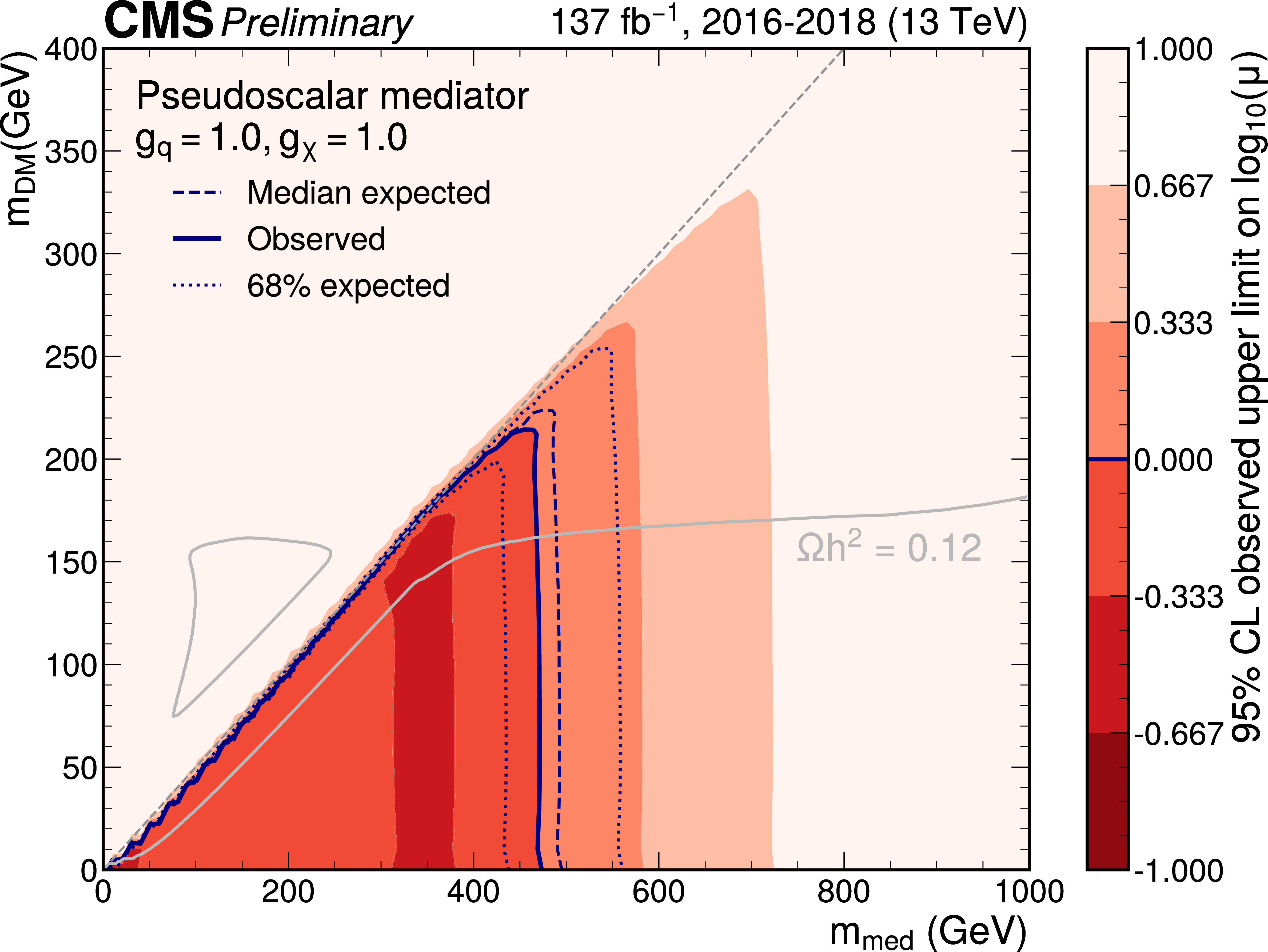
Additional Figure 13:
Exclusion limits at 95% CL on the signal strength $\mu =\sigma /\sigma _\text {theo}$ in the ${m_\text {med}} - {m_\text {DM}}$ plane for coupling values of $ {g_ {\mathrm {q}}} = {g_\chi} =$ 1.0 and a pseudoscalar mediator. The blue solid line indicates the observed exclusion boundary $\mu =$ 1. The blue dashed and dotted lines represent the median expected exclusion and the 1 s.d. interval of the expected boundary, respectively. Parameter combinations with larger values of $\mu $ (indicated by a darker shade in the color scale) are excluded. The gray dashed line indicates the diagonal $ {m_\text {med}} =2 {m_\text {DM}} $, above which only off-shell mediator production contributes to the jet+$ {{p_{\mathrm {T}}} ^\text {miss}}$ final state. The gray solid lines represent parameter combinations for which the simplified model reproduces the observed DM relic density in the universe under the assumption of a thermal freeze-out mechanism [57,76]. |
png pdf |
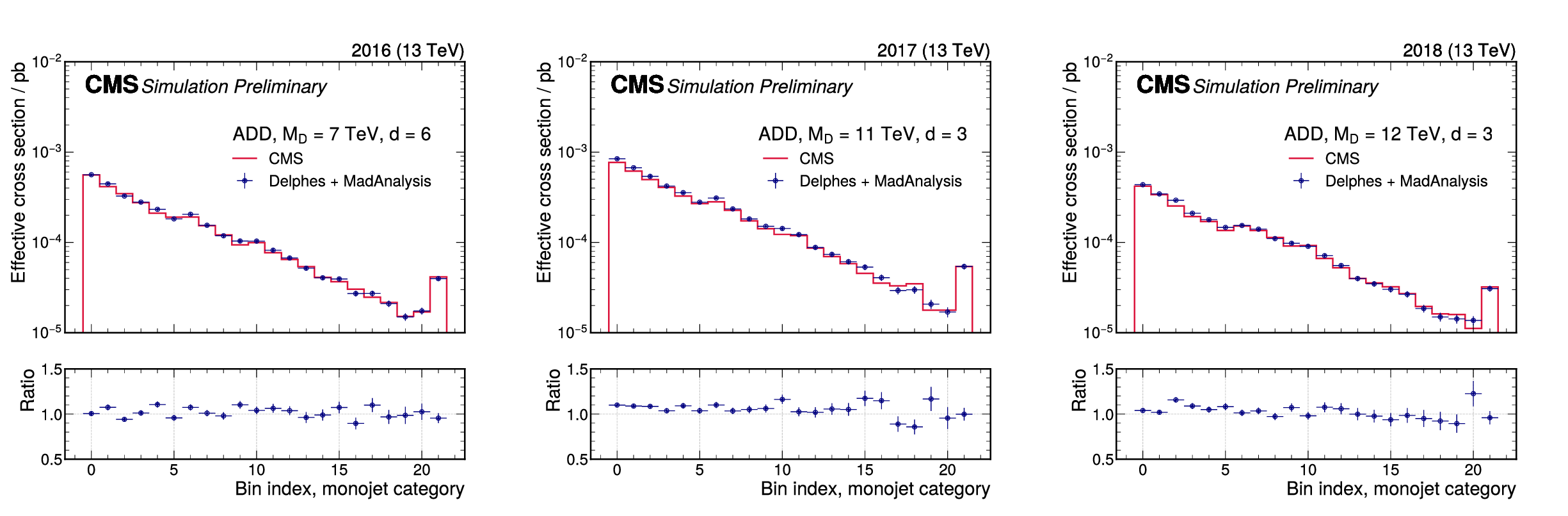
Additional Figure 14:
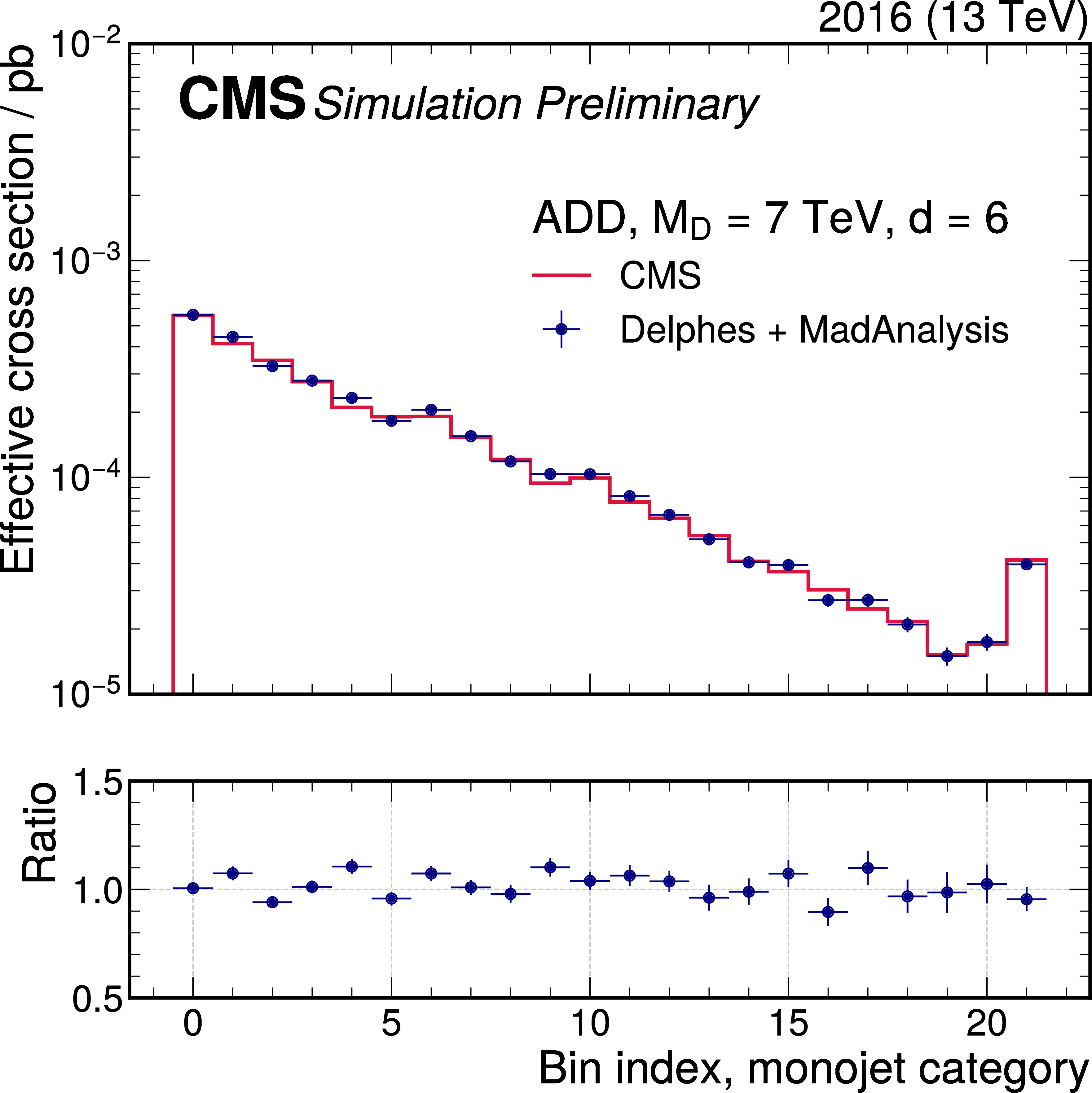
In order to promote this analysis for reinterpretation, we implement the selection for the monojet category of this analysis in the MadAnalysis reinterpretation framework [88]. MadAnalysis is a framework for the reinterpretation of existing analyses in terms of arbitrary new physics models. The framework provides infrastructure for the implementation of event selections that can be run over simulated signal events. Detector simulation can be handled by the independent Delphes software framework [89], or internally to MadAnalysis [90]. Once an implementation is available, it is indexed in a public data base ("PAD'') that allows users to automatically download and execute it [91]. After detector simulation and event selection on signal events, approximate statistical inference is made possible through usage of the simplified likelihood scheme [92], the input information for which is also provided as additional material with this note. The implementation made here will be made available in the PAD shortly for public use. Users who prefer other reinterpretation frameworks (a recent overview is given in Ref. [93]), might still profit from this implementation by reading the source code or even copying it into other frameworks. A total of 66 analysis regions are defined, with each of the regions representing one recoil bin in one data-taking year. The selections applied for the 2016 and 2017 data sets are identical, and additional criteria are applied for the 2018 data set, where additional mitigation requirements are applied due to a localized failure of the hadronic calorimeter. In order to validate the implementation, generator-level information from the CMS-internal signal samples is fed into the Delphes framework, which performs fast parameterized event simulation, and is available to the general public. The MadAnalysis implementation is then run based on the Delphes output, and the final yields per signal region bin are compared to the signal prediction obtained from the CMS-internal analysis framework, which includes more elaborate detector simulation based on {Geant4} [38]. The comparison is made using signal samples for the ADD interpretation, which are generated using PYTHIA, and are therefore relatively easy to reproduce. The resulting comparison of the final signal templates is (a), (b) and (c) for the individual data-taking years for a representative choice of parameter points. It is found that the Delphes/MadAnalysis-based result agrees with the CMS result to better than 20% in every bin. In most bins, the agreement is significantly better still, with an average agreement of 10% or better. While only a few parameter points are shown here, it has been verified that the agreement is similar for the full range of parameters. The level of agreement observed here is sufficiently good to enable reliable reinterpretation. |
png pdf |
Additional Figure 14-a:
In order to promote this analysis for reinterpretation, we implement the selection for the monojet category of this analysis in the MadAnalysis reinterpretation framework [88]. MadAnalysis is a framework for the reinterpretation of existing analyses in terms of arbitrary new physics models. The framework provides infrastructure for the implementation of event selections that can be run over simulated signal events. Detector simulation can be handled by the independent Delphes software framework [89], or internally to MadAnalysis [90]. Once an implementation is available, it is indexed in a public data base ("PAD'') that allows users to automatically download and execute it [91]. After detector simulation and event selection on signal events, approximate statistical inference is made possible through usage of the simplified likelihood scheme [92], the input information for which is also provided as additional material with this note. The implementation made here will be made available in the PAD shortly for public use. Users who prefer other reinterpretation frameworks (a recent overview is given in Ref. [93]), might still profit from this implementation by reading the source code or even copying it into other frameworks. A total of 66 analysis regions are defined, with each of the regions representing one recoil bin in one data-taking year. The selections applied for the 2016 and 2017 data sets are identical, and additional criteria are applied for the 2018 data set, where additional mitigation requirements are applied due to a localized failure of the hadronic calorimeter. In order to validate the implementation, generator-level information from the CMS-internal signal samples is fed into the Delphes framework, which performs fast parameterized event simulation, and is available to the general public. The MadAnalysis implementation is then run based on the Delphes output, and the final yields per signal region bin are compared to the signal prediction obtained from the CMS-internal analysis framework, which includes more elaborate detector simulation based on {Geant4} [38]. The comparison is made using signal samples for the ADD interpretation, which are generated using PYTHIA, and are therefore relatively easy to reproduce. The resulting comparison of the final signal templates is (a), (b) and (c) for the individual data-taking years for a representative choice of parameter points. It is found that the Delphes/MadAnalysis-based result agrees with the CMS result to better than 20% in every bin. In most bins, the agreement is significantly better still, with an average agreement of 10% or better. While only a few parameter points are shown here, it has been verified that the agreement is similar for the full range of parameters. The level of agreement observed here is sufficiently good to enable reliable reinterpretation. |

png pdf |
Additional Figure 14-b:
In order to promote this analysis for reinterpretation, we implement the selection for the monojet category of this analysis in the MadAnalysis reinterpretation framework [88]. MadAnalysis is a framework for the reinterpretation of existing analyses in terms of arbitrary new physics models. The framework provides infrastructure for the implementation of event selections that can be run over simulated signal events. Detector simulation can be handled by the independent Delphes software framework [89], or internally to MadAnalysis [90]. Once an implementation is available, it is indexed in a public data base ("PAD'') that allows users to automatically download and execute it [91]. After detector simulation and event selection on signal events, approximate statistical inference is made possible through usage of the simplified likelihood scheme [92], the input information for which is also provided as additional material with this note. The implementation made here will be made available in the PAD shortly for public use. Users who prefer other reinterpretation frameworks (a recent overview is given in Ref. [93]), might still profit from this implementation by reading the source code or even copying it into other frameworks. A total of 66 analysis regions are defined, with each of the regions representing one recoil bin in one data-taking year. The selections applied for the 2016 and 2017 data sets are identical, and additional criteria are applied for the 2018 data set, where additional mitigation requirements are applied due to a localized failure of the hadronic calorimeter. In order to validate the implementation, generator-level information from the CMS-internal signal samples is fed into the Delphes framework, which performs fast parameterized event simulation, and is available to the general public. The MadAnalysis implementation is then run based on the Delphes output, and the final yields per signal region bin are compared to the signal prediction obtained from the CMS-internal analysis framework, which includes more elaborate detector simulation based on {Geant4} [38]. The comparison is made using signal samples for the ADD interpretation, which are generated using PYTHIA, and are therefore relatively easy to reproduce. The resulting comparison of the final signal templates is (a), (b) and (c) for the individual data-taking years for a representative choice of parameter points. It is found that the Delphes/MadAnalysis-based result agrees with the CMS result to better than 20% in every bin. In most bins, the agreement is significantly better still, with an average agreement of 10% or better. While only a few parameter points are shown here, it has been verified that the agreement is similar for the full range of parameters. The level of agreement observed here is sufficiently good to enable reliable reinterpretation. |

png pdf |
Additional Figure 14-c:
In order to promote this analysis for reinterpretation, we implement the selection for the monojet category of this analysis in the MadAnalysis reinterpretation framework [88]. MadAnalysis is a framework for the reinterpretation of existing analyses in terms of arbitrary new physics models. The framework provides infrastructure for the implementation of event selections that can be run over simulated signal events. Detector simulation can be handled by the independent Delphes software framework [89], or internally to MadAnalysis [90]. Once an implementation is available, it is indexed in a public data base ("PAD'') that allows users to automatically download and execute it [91]. After detector simulation and event selection on signal events, approximate statistical inference is made possible through usage of the simplified likelihood scheme [92], the input information for which is also provided as additional material with this note. The implementation made here will be made available in the PAD shortly for public use. Users who prefer other reinterpretation frameworks (a recent overview is given in Ref. [93]), might still profit from this implementation by reading the source code or even copying it into other frameworks. A total of 66 analysis regions are defined, with each of the regions representing one recoil bin in one data-taking year. The selections applied for the 2016 and 2017 data sets are identical, and additional criteria are applied for the 2018 data set, where additional mitigation requirements are applied due to a localized failure of the hadronic calorimeter. In order to validate the implementation, generator-level information from the CMS-internal signal samples is fed into the Delphes framework, which performs fast parameterized event simulation, and is available to the general public. The MadAnalysis implementation is then run based on the Delphes output, and the final yields per signal region bin are compared to the signal prediction obtained from the CMS-internal analysis framework, which includes more elaborate detector simulation based on {Geant4} [38]. The comparison is made using signal samples for the ADD interpretation, which are generated using PYTHIA, and are therefore relatively easy to reproduce. The resulting comparison of the final signal templates is (a), (b) and (c) for the individual data-taking years for a representative choice of parameter points. It is found that the Delphes/MadAnalysis-based result agrees with the CMS result to better than 20% in every bin. In most bins, the agreement is significantly better still, with an average agreement of 10% or better. While only a few parameter points are shown here, it has been verified that the agreement is similar for the full range of parameters. The level of agreement observed here is sufficiently good to enable reliable reinterpretation. |
png pdf |
Additional Figure 15:
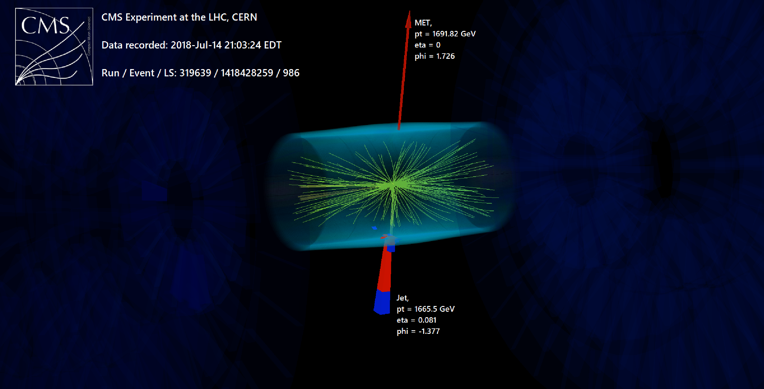
Graphical representation of a representative high-$ {{p_{\mathrm {T}}} ^\text {miss}} $ event from the monojet category in the 2018 data set. In this event, a single high-$ {p_{\mathrm {T}}}$ jet (calorimeter deposits indicated by red and blue towers) recoils against large ${{p_{\mathrm {T}}} ^\text {miss}}$ (indicated by the red arrow). |
| References | ||||
| 1 | G. Bertone, D. Hooper, and J. Silk | Particle dark matter: evidence, candidates and constraints | PR 405 (2005) 279 | hep-ph/0404175 |
| 2 | S. Kanemura, S. Matsumoto, T. Nabeshima, and N. Okada | Can WIMP dark matter overcome the nightmare scenario? | PRD 82 (2010) 055026 | 1005.5651 |
| 3 | O. Lebedev, H. M. Lee, and Y. Mambrini | Vector Higgs-portal dark matter and the invisible Higgs | PLB 707 (2012) 570 | 1111.4482 |
| 4 | A. Djouadi, O. Lebedev, Y. Mambrini, and J. Quevillon | Implications of LHC searches for Higgs--portal dark matter | PLB 709 (2012) 65 | 1112.3299 |
| 5 | ATLAS Collaboration | Observation of a new particle in the search for the Standard Model Higgs boson with the ATLAS detector at the LHC | PLB 716 (2012) 1 | 1207.7214 |
| 6 | CMS Collaboration | Observation of a new boson at a mass of 125 GeV with the CMS experiment at the LHC | PLB 716 (2012) 30 | CMS-HIG-12-028 1207.7235 |
| 7 | CMS Collaboration | Observation of a new boson with mass near 125 GeV in pp collisions at $ \sqrt{s} = $ 7 and 8 TeV | JHEP 06 (2013) 081 | CMS-HIG-12-036 1303.4571 |
| 8 | ATLAS Collaboration | Combination of searches for invisible Higgs boson decays with the ATLAS experiment | PRL 122 (2019) 231801 | 1904.05105 |
| 9 | CMS Collaboration | Search for invisible decays of a Higgs boson produced through vector boson fusion in proton-proton collisions at $ \sqrt{s} = $ 13 TeV | PLB 793 (2019) 520 | CMS-HIG-17-023 1809.05937 |
| 10 | D. Abercrombie et al. | Dark Matter Benchmark Models for Early LHC Run-2 Searches: Report of the ATLAS/CMS Dark Matter Forum | Phys. Dark Univ. 27 (2020) 100371 | 1507.00966 |
| 11 | Y. Bai and J. Berger | Fermion portal dark matter | JHEP 11 (2013) 171 | 1308.0612 |
| 12 | N. Arkani-Hamed, S. Dimopoulos, and G. R. Dvali | The hierarchy problem and new dimensions at a millimeter | PLB 429 (1998) 263 | hep-ph/9803315 |
| 13 | N. Arkani-Hamed, S. Dimopoulos, and G. R. Dvali | Phenomenology, astrophysics and cosmology of theories with submillimeter dimensions and TeV scale quantum gravity | PRD 59 (1999) 086004 | hep-ph/9807344 |
| 14 | J. C. Pati and A. Salam | Unified lepton-hadron symmetry and a gauge theory of the basic interactions | PRD 8 (1973) 1240 | |
| 15 | J. C. Pati and A. Salam | Lepton number as the fourth color | PRD 10 (1974) 275 | |
| 16 | H. Georgi and S. L. Glashow | Unity of all elementary particle forces | PRL 32 (1974) 438 | |
| 17 | B. Diaz, M. Schmaltz, and Y.-M. Zhong | The leptoquark hunter's guide: Pair production | JHEP 10 (2017) 097 | 1706.05033 |
| 18 | J. L. Hewett and S. Pakvasa | Leptoquark production in hadron colliders | PRD 37 (1988) 3165 | |
| 19 | O. J. P. Eboli and A. V. Olinto | Composite leptoquarks in hadronic colliders | PRD 38 (1988) 3461 | |
| 20 | CMS Collaboration | Search for new physics in final states with an energetic jet or a hadronically decaying $ {\mathrm{W}} $ or $ {\mathrm{Z}} $ boson and transverse momentum imbalance at $ \sqrt{s} = $ 13 TeV | PRD 97 (2018) 092005 | CMS-EXO-16-048 1712.02345 |
| 21 | ATLAS Collaboration | Search for dark matter and other new phenomena in events with an energetic jet and large missing transverse momentum using the ATLAS detector | JHEP 01 (2018) 126 | 1711.03301 |
| 22 | ATLAS Collaboration | Search for dark matter in events with a hadronically decaying vector boson and missing transverse momentum in pp collisions at $ \sqrt{s} = $ 13 TeV with the ATLAS detector | JHEP 10 (2018) 180 | 1807.11471 |
| 23 | CMS Collaboration | Performance of the CMS Level-1 trigger in proton-proton collisions at $ \sqrt{s} = $ 13 TeV | JINST 15 (2020) P10017 | CMS-TRG-17-001 2006.10165 |
| 24 | CMS Collaboration | The CMS trigger system | JINST 12 (2017) P01020 | CMS-TRG-12-001 1609.02366 |
| 25 | CMS Collaboration | The CMS experiment at the CERN LHC | JINST 3 (2008) S08004 | CMS-00-001 |
| 26 | M. Cacciari, G. P. Salam, and G. Soyez | The anti-$ k_t $ jet clustering algorithm | JHEP 04 (2008) 063 | 0802.1189 |
| 27 | M. Cacciari, G. P. Salam, and G. Soyez | FastJet user manual | EPJC 72 (2012) 1896 | 1111.6097 |
| 28 | CMS Collaboration | Particle-flow reconstruction and global event description with the cms detector | JINST 12 (2017) P10003 | CMS-PRF-14-001 1706.04965 |
| 29 | CMS Collaboration | Jet energy scale and resolution in the CMS experiment in pp collisions at 8 TeV | JINST 12 (2017) P02014 | CMS-JME-13-004 1607.03663 |
| 30 | CMS Collaboration | Jet algorithms performance in 13 TeV data | CMS-PAS-JME-16-003 | CMS-PAS-JME-16-003 |
| 31 | CMS Collaboration | Performance of missing transverse momentum reconstruction in proton-proton collisions at $ \sqrt{s} = $ 13 TeV using the CMS detector | JINST 14 (2019) P07004 | CMS-JME-17-001 1903.06078 |
| 32 | D. Bertolini, P. Harris, M. Low, and N. Tran | Pileup per particle identification | JHEP 10 (2014) 059 | 1407.6013 |
| 33 | M. Dasgupta, A. Fregoso, S. Marzani, and G. P. Salam | Towards an understanding of jet substructure | JHEP 09 (2013) 029 | 1307.0007 |
| 34 | J. M. Butterworth, A. R. Davison, M. Rubin, and G. P. Salam | Jet substructure as a new Higgs search channel at the LHC | PRL 100 (2008) 242001 | 0802.2470 |
| 35 | A. J. Larkoski, S. Marzani, G. Soyez, and J. Thaler | Soft drop | JHEP 05 (2014) 146 | 1402.2657 |
| 36 | T. Sjostrand et al. | An introduction to PYTHIA 8.2 | CPC 191 (2015) 159 | 1410.3012 |
| 37 | CMS Collaboration | Extraction and validation of a new set of CMS PYTHIA8 tunes from underlying-event measurements | EPJC 80 (2020) 4 | CMS-GEN-17-001 1903.12179 |
| 38 | GEANT4 Collaboration | GEANT4 --- a simulation toolkit | NIMA 506 (2003) 250 | |
| 39 | NNPDF Collaboration | Parton distributions from high-precision collider data | EPJC 77 (2017) 663 | 1706.00428 |
| 40 | J. Alwall et al. | The automated computation of tree-level and next-to-leading order differential cross sections, and their matching to parton shower simulations | JHEP 07 (2014) 079 | 1405.0301 |
| 41 | R. Frederix and S. Frixione | Merging meets matching in MC@NLO | JHEP 12 (2012) 061 | 1209.6215 |
| 42 | M. Czakon, P. Fiedler, and A. Mitov | Total top-quark pair-production cross section at hadron colliders through $ o(\alpha^4_s) $ | PRL 110 (2013) 252004 | 1303.6254 |
| 43 | S. Alioli, P. Nason, C. Oleari, and E. Re | NLO single-top production matched with shower in POWHEG: s- and t-channel contributions | JHEP 09 (2009) 111 | 0907.4076 |
| 44 | E. Re | Single-top Wt-channel production matched with parton showers using the POWHEG method | EPJC 71 (2011) 1547 | 1009.2450 |
| 45 | N. Kidonakis | Two-loop soft anomalous dimensions for single top quark associated production with a w$ ^{-} $ or h$ ^{-} $ | PRD 82 (2010) 054018 | 1005.4451 |
| 46 | M. Aliev et al. | HATHOR: HAdronic Top and Heavy quarks crOss section calculatoR | CPC 182 (2011) 1034 | 1007.1327 |
| 47 | P. Kant et al. | HatHor for single top-quark production: Updated predictions and uncertainty estimates for single top-quark production in hadronic collisions | CPC 191 (2015) 74 | 1406.4403 |
| 48 | T. Gehrmann et al. | W$ ^+ $W$ ^- $ production at hadron colliders in next to next to leading order QCD | PRL 113 (2014) 212001 | 1408.5243 |
| 49 | J. M. Campbell and R. K. Ellis | An update on vector boson pair production at hadron colliders | PRD 60 (1999) 113006 | hep-ph/9905386 |
| 50 | E. Bagnaschi, G. Degrassi, P. Slavich, and A. Vicini | Higgs production via gluon fusion in the POWHEG approach in the SM and in the MSSM | JHEP 02 (2012) 088 | 1111.2854 |
| 51 | G. Luisoni, P. Nason, C. Oleari, and F. Tramontano | HW$ ^{\pm} $/HZ + 0 and 1 jet at NLO with the POWHEG BOX interfaced to GoSam and their merging within MiNLO | JHEP 10 (2013) 083 | 1306.2542 |
| 52 | P. Nason and C. Oleari | NLO Higgs boson production via vector-boson fusion matched with shower in POWHEG | JHEP 02 (2010) 037 | 0911.5299 |
| 53 | L. H. C. S. W. Group | Handbook of LHC Higgs cross sections: 4. Deciphering the nature of the Higgs sector | (10, 2016) | 1610.07922 |
| 54 | O. Mattelaer and E. Vryonidou | Dark matter production through loop-induced processes at the LHC: the s-channel mediator case | EPJC 75 (2015) 436 | 1508.00564 |
| 55 | M. Backovi\'c et al. | Higher-order QCD predictions for dark matter production at the lhc in simplified models with s-channel mediators | EPJC 75 (2015) 482 | 1508.05327 |
| 56 | M. Neubert, J. Wang, and C. Zhang | Higher-order QCD predictions for dark matter production in mono-$ Z $ searches at the LHC | JHEP 02 (2016) 082 | 1509.05785 |
| 57 | LHC Dark Matter Working Group | Recommendations of the LHC dark matter working group: Comparing LHC searches for dark matter mediators in visible and invisible decay channels and calculations of the thermal relic density | Phys. Dark Univ. 26 (2019) 100377 | 1703.05703 |
| 58 | C. Arina, B. Fuks, and L. Mantani | A universal framework for t-channel dark matter models | EPJC 80 (2020) 409 | 2001.05024 |
| 59 | S. Ask et al. | Real emission and virtual exchange of gravitons and unparticles in Pythia8 | CPC 181 (2010) 1593 | 0912.4233 |
| 60 | CMS Collaboration | Identification of heavy, energetic, hadronically decaying particles using machine-learning techniques | JINST 15 (2020) P06005 | CMS-JME-18-002 2004.08262 |
| 61 | CMS Collaboration | Electron and photon reconstruction and identification with the CMS experiment at the CERN LHC | JINST 16 (2021) P05014 | CMS-EGM-17-001 2012.06888 |
| 62 | CMS Collaboration | Performance of the CMS muon detector and muon reconstruction with proton-proton collisions at $ \sqrt{s}= $ 13 TeV | JINST 13 (2018) P06015 | CMS-MUO-16-001 1804.04528 |
| 63 | CMS Collaboration | Performance of reconstruction and identification of $ \tau $ leptons decaying to hadrons and $ \nu_\tau $ in pp collisions at $ \sqrt{s}= $ 13 TeV | JINST 13 (2018) P10005 | CMS-TAU-16-003 1809.02816 |
| 64 | CMS Collaboration | Identification of heavy-flavour jets with the CMS detector in pp collisions at 13 TeV | JINST 13 (2018) P05011 | CMS-BTV-16-002 1712.07158 |
| 65 | Particle Data Group Collaboration | Review of particle physics | PTEP 2020 (2020) 083C01 | |
| 66 | CMS Collaboration | Search for dark matter produced with an energetic jet or a hadronically decaying $ \mathrm{W} $ or $ \mathrm{Z} $ boson at $ \sqrt{s} = $ 13 TeV | JHEP 07 (2017) 014 | CMS-EXO-16-037 1703.01651 |
| 67 | J. M. Lindert et al. | Precise predictions for v+jets dark matter backgrounds | EPJC 77 (2017) 829 | 1705.04664 |
| 68 | J. Baglio, L. D. Ninh, and M. M. Weber | Massive gauge boson pair production at the LHC: a next-to-leading order story | PRD 88 (2013) 113005 | 1307.4331 |
| 69 | A. Denner, S. Dittmaier, M. Hecht, and C. Pasold | NLO QCD and electroweak corrections to W+$ \gamma $ production with leptonic W-boson decays | JHEP 04 (2015) 018 | 1412.7421 |
| 70 | A. Denner, S. Dittmaier, M. Hecht, and C. Pasold | NLO QCD and electroweak corrections to Z+$ \gamma $ production with leptonic Z-boson decays | JHEP 02 (2016) 057 | 1510.08742 |
| 71 | J. Butterworth et al. | PDF4LHC recommendations for LHC run II | JPG 43 (2016) 023001 | 1510.03865 |
| 72 | S. Dulat et al. | New parton distribution functions from a global analysis of quantum chromodynamics | PRD 93 (2016) 033006 | 1506.07443 |
| 73 | L. A. Harland-Lang, A. D. Martin, P. Motylinski, and R. S. Thorne | Parton distributions in the LHC era: MMHT 2014 PDFs | EPJC 75 (2015) 204 | 1412.3989 |
| 74 | NNPDF Collaboration | Parton distributions for the LHC run II | JHEP 04 (2015) 040 | 1410.8849 |
| 75 | M. Czakon, D. Heymes, and A. Mitov | High-precision differential predictions for top-quark pairs at the LHC | PRL 116 (2016) 082003 | 1511.00549 |
| 76 | Planck Collaboration | Planck 2018 results. VI. cosmological parameters | Astron. Astrophys. 641 (2020) A6 | 1807.06209 |
| 77 | CMS Collaboration | Searches for physics beyond the standard model with the $ m_\mathrm{T2} $ variable in hadronic final states with and without disappearing tracks in proton-proton collisions at $ \sqrt{s}= $ 13 TeV | EPJC 80 (2020) 3 | CMS-SUS-19-005 1909.03460 |
| 78 | G. Busoni et al. | Recommendations on presenting LHC searches for missing transverse energy signals using simplified $ s $-channel models of dark matter | Phys. Dark Univ. 27 (2020) 100365 | 1603.04156 |
| 79 | CRESST Collaboration | Results on light dark matter particles with a low-threshold CRESST-II detector | EPJC 76 (2016) 25 | 1509.01515 |
| 80 | SuperCDMS Collaboration | New results from the search for low-mass weakly interacting massive particles with the CDMS Low Ionization Threshold Experiment | PRL 116 (2016) 071301 | 1509.02448 |
| 81 | LUX Collaboration | Results from a search for dark matter in the complete LUX exposure | PRL 118 (2017) 021303 | 1608.07648 |
| 82 | DarkSide Collaboration | Low-mass dark matter search with the DarkSide-50 Experiment | PRL 121 (2018) 081307 | 1802.06994 |
| 83 | XENON Collaboration | Dark matter search results from a one ton-year exposure of XENON1T | PRL 121 (2018) 111302 | 1805.12562 |
| 84 | PandaX-II Collaboration | Results of dark matter search using the full PandaX-II exposure | CPC 44 (2020) 125001 | 2007.15469 |
| 85 | PICO Collaboration | Improved dark matter search results from PICO-2L Run 2 | PRD 93 (2016) 061101 | 1601.03729 |
| 86 | E. Behnke et al. | Final results of the PICASSO dark matter search experiment | Astropart. Phys. 90 (2017) 85 | 1611.01499 |
| 87 | PICO Collaboration | Dark Matter Search Results from the Complete Exposure of the PICO-60 C$ _3 $F$ _8 $ Bubble Chamber | PRD 100 (2019) 022001 | 1902.04031 |
| 88 | E. Conte, B. Dumont, B. Fuks, and C. Wymant | Designing and recasting LHC analyses with MadAnalysis 5 | EPJC 74 (2014) 3103 | 1405.3982 |
| 89 | DELPHES 3 Collaboration | DELPHES 3, a modular framework for fast simulation of a generic collider experiment | JHEP 02 (2014) 057 | 1307.6346 |
| 90 | J. Y. Araz, B. Fuks, and G. Polykratis | Simplified fast detector simulation in MADANALYSIS~5 | EPJC 81 (2021) 329 | 2006.09387 |
| 91 | B. Dumont et al. | Toward a public analysis database for LHC new physics searches using MADANALYSIS 5 | EPJC 75 (2015) 56 | 1407.3278 |
| 92 | CMS Collaboration Collaboration | Simplified likelihood for the re-interpretation of public CMS results | technical report, CERN, Geneva, Jan | |
| 93 | LHC Reinterpretation Forum Collaboration | Reinterpretation of LHC results for new physics: Status and recommendations after Run 2 | SciPost Phys. 9 (2020) 022 | 2003.07868 |
|
|
Compact Muon Solenoid LHC, CERN |
|

|

|

|

|

|