

Compact Muon Solenoid
LHC, CERN
| CMS-PAS-EXO-19-015 | ||
| Search for singly and pair-produced leptoquarks coupling to third-generation fermions in proton-proton collisions at $\sqrt{s} = $ 13 TeV | ||
| CMS Collaboration | ||
| July 2020 | ||
| Abstract: A search for leptoquarks produced singly and in pairs in proton-proton collisions is presented. The leptoquark (LQ) may couple to a top quark plus a $\tau$ lepton (t$\tau$) or a bottom quark plus a neutrino (b$\nu$, scalar LQ), or else to t$\nu$ or b$\tau$ (vector LQ), leading to the final states t$\tau\nu$b and t$\tau\nu$. The data were recorded by the CMS experiment at the CERN LHC at $\sqrt{s} = $ 13 TeV and correspond to an integrated luminosity of 137 fb$^{-1}$. The data are found to be in agreement with the standard model background prediction. Lower limits at 95% CL are set on the LQ mass in the range 0.98-1.73 TeV, depending on the LQ spin and the LQ-lepton-quark vertex coupling $\lambda$, and assuming equal branching fractions for the two LQ decay modes considered. These are the most stringent constraints on the existence of leptoquarks in this scenario. | ||
|
Links:
CDS record (PDF) ;
CADI line (restricted) ;
These preliminary results are superseded in this paper, Accepted by PLB. The superseded preliminary plots can be found here. |
||
| Figures & Tables | Summary | Additional Figures & Tables | References | CMS Publications |
|---|
| Figures | |
png pdf |
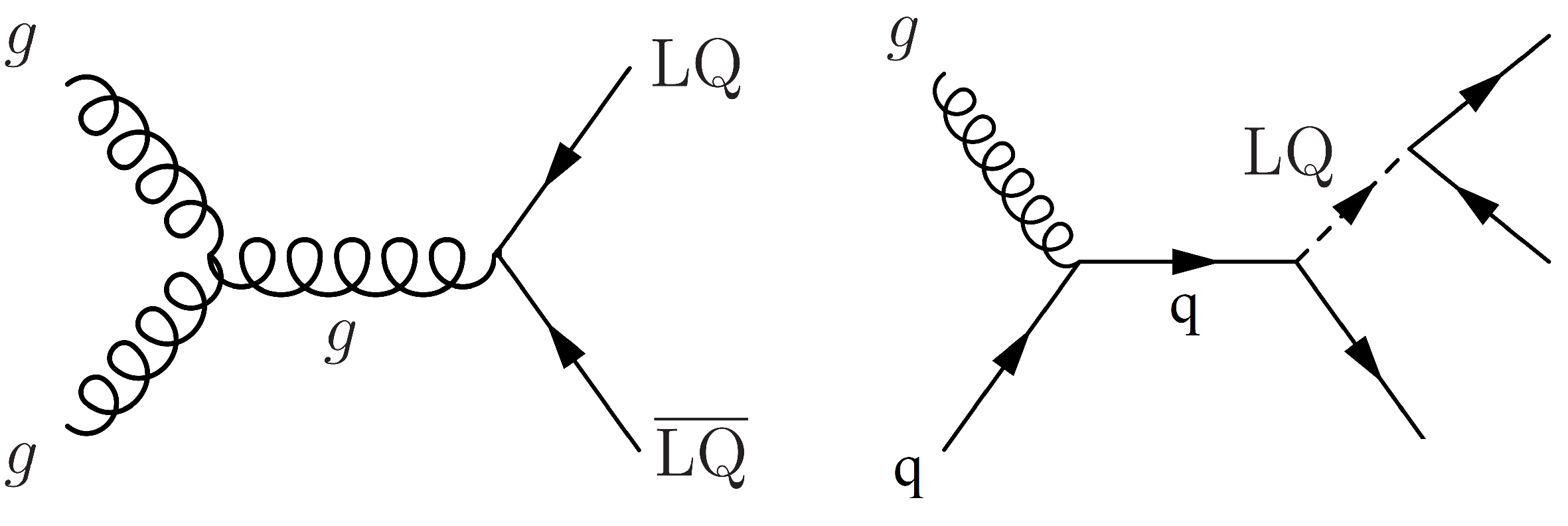
Figure 1:
Main Feynman diagrams for LQ production: pairwise (left), and in combination with a lepton (right). |

png pdf |
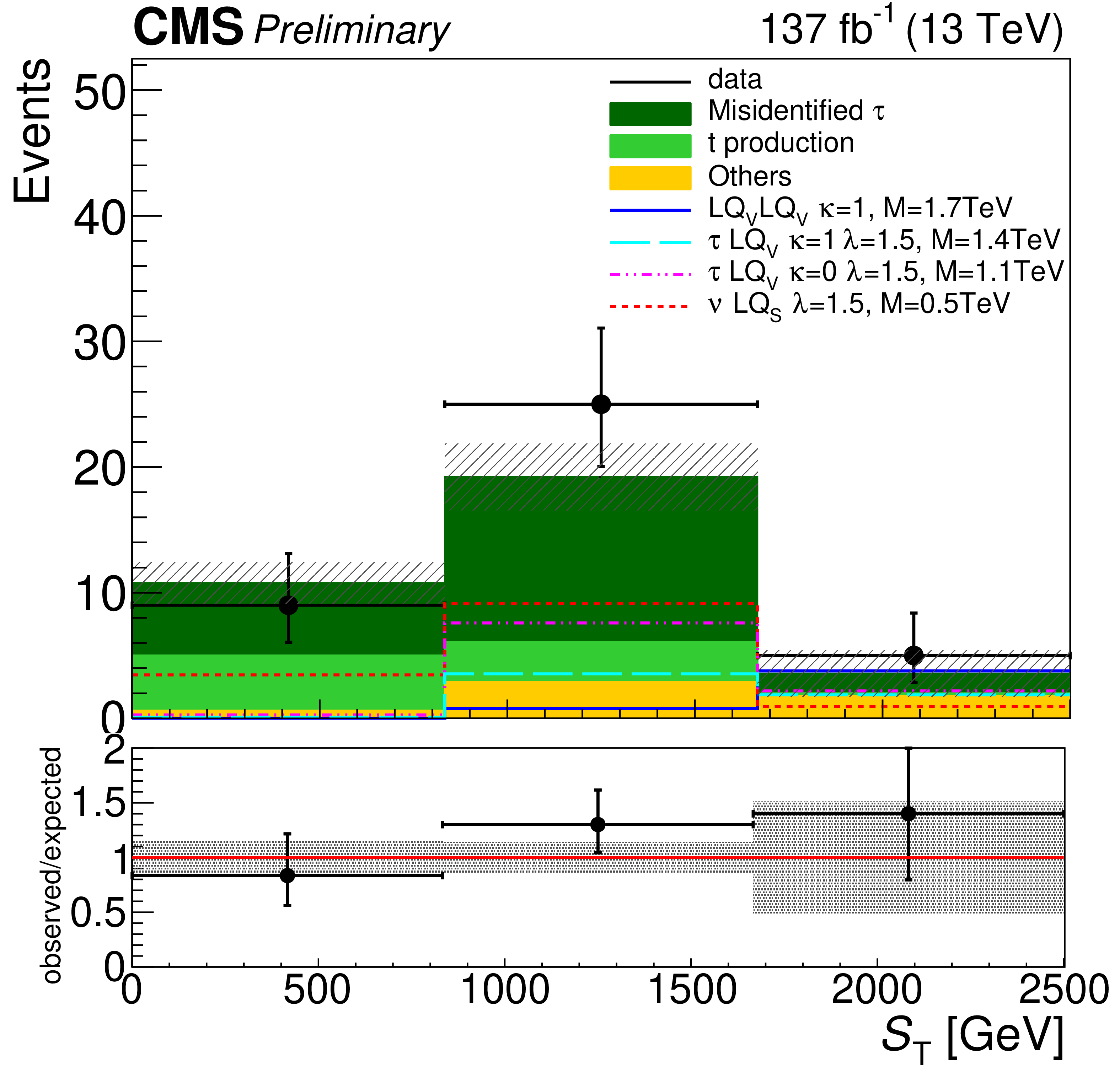
Figure 2:
Distribution of the variable ${S_{\rm {T}}}$ for events passing the signal selection. Upper-left: boosted top (hadronically decaying top quark reconstructed in the fully or partially merged topology) and exactly one b jet; lower-left: boosted top and at least two b jets; upper-right: resolved top (hadronically decaying top quark reconstructed in the resolved topology) and exactly one b jet; lower-right: resolved top and at least two b jets. |
png pdf |
Figure 2-a:
Distribution of the variable ${S_{\rm {T}}}$ for events passing the signal selection, boosted top (hadronically decaying top quark reconstructed in the fully or partially merged topology) and exactly one b jet. |

png pdf |
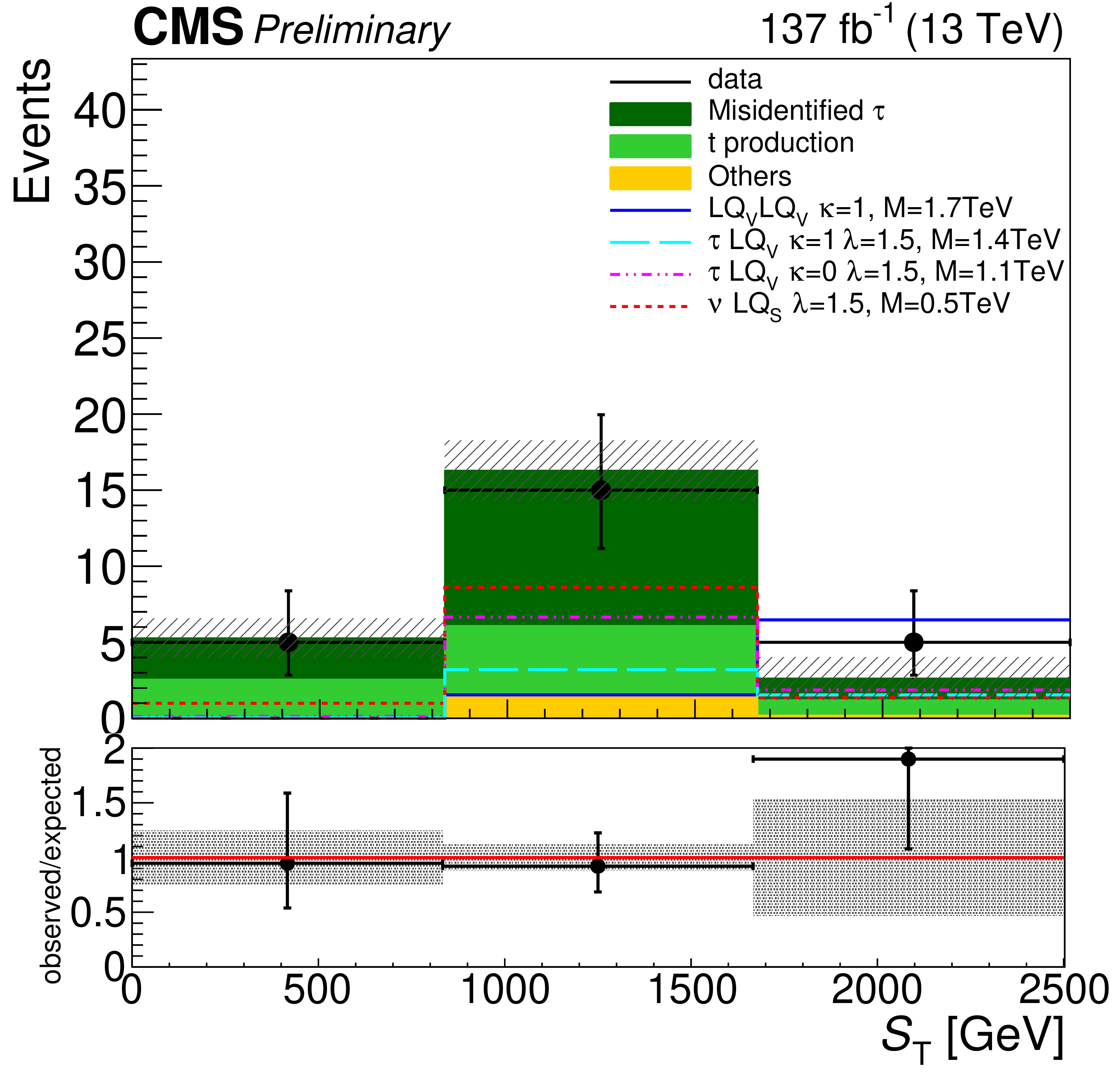
Figure 2-b:
Distribution of the variable ${S_{\rm {T}}}$ for events passing the signal selection, resolved top (hadronically decaying top quark reconstructed in the resolved topology) and exactly one b jet. |
png pdf |
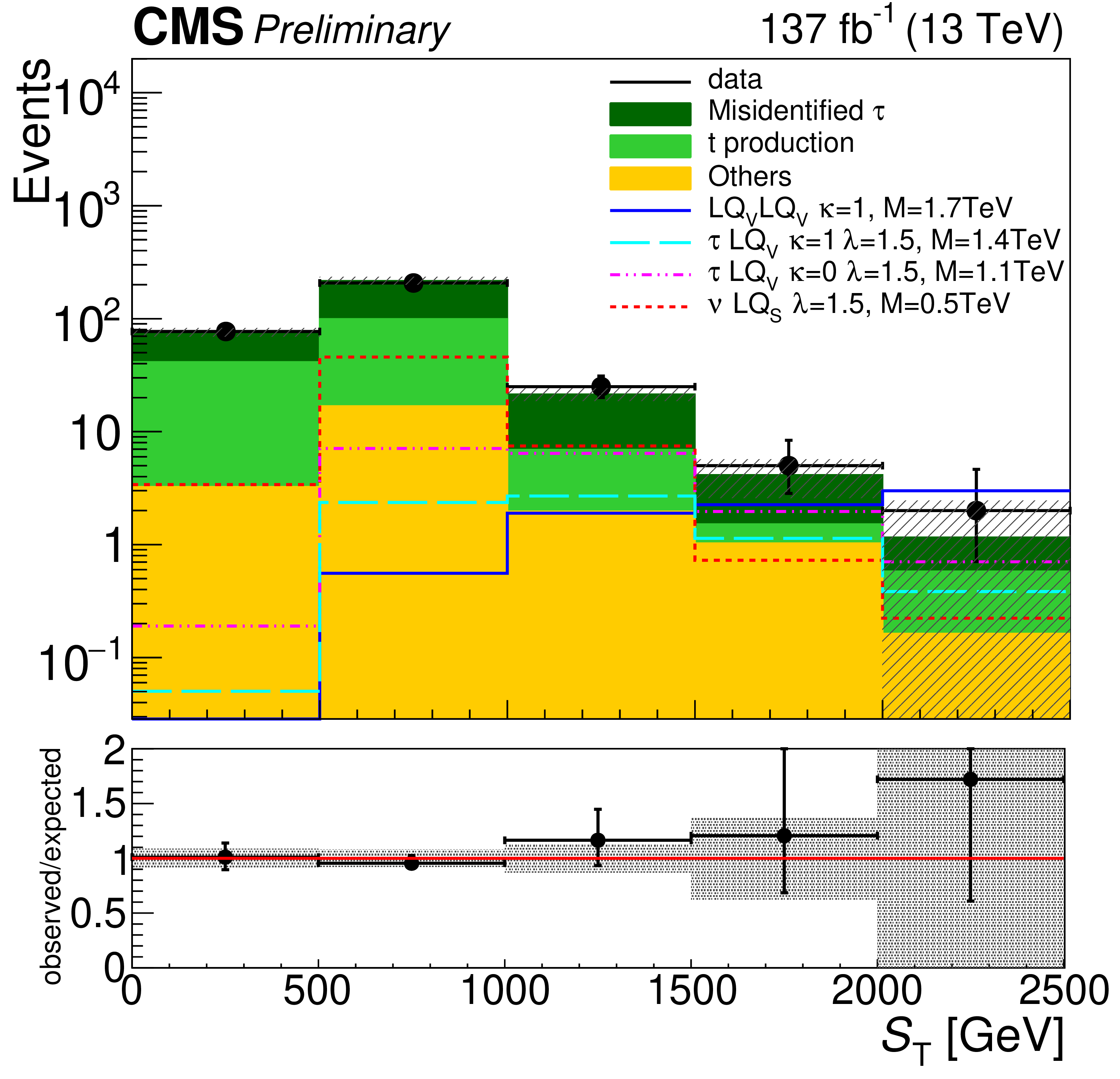
Figure 2-c:
Distribution of the variable ${S_{\rm {T}}}$ for events passing the signal selection, boosted top (hadronically decaying top quark reconstructed in the fully or partially merged topology) and at least two b jets. |
png pdf |
Figure 2-d:
Distribution of the variable ${S_{\rm {T}}}$ for events passing the signal selection, resolved top (hadronically decaying top quark reconstructed in the resolved topology) and at least two b jets. |

png pdf |
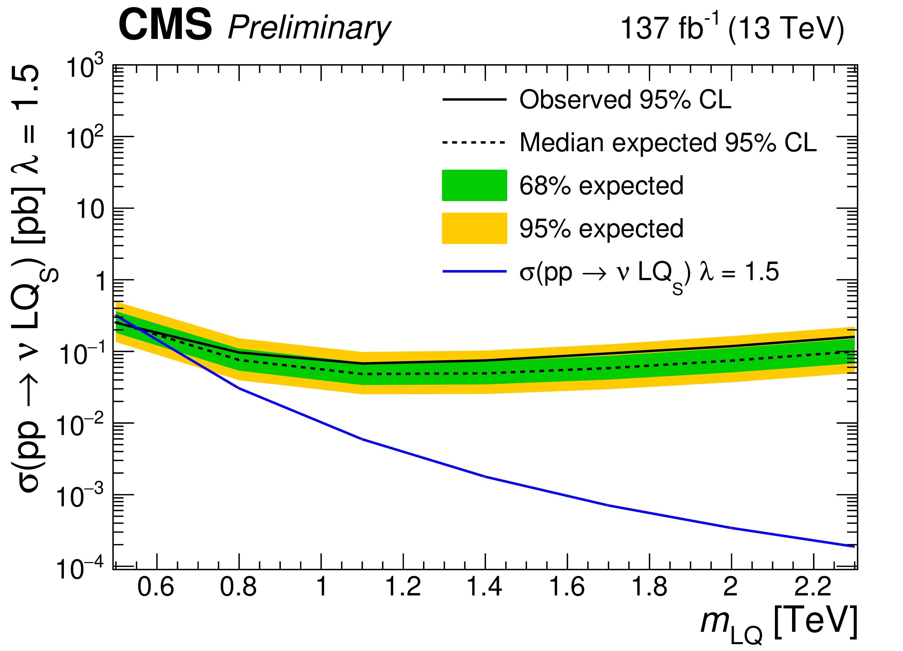
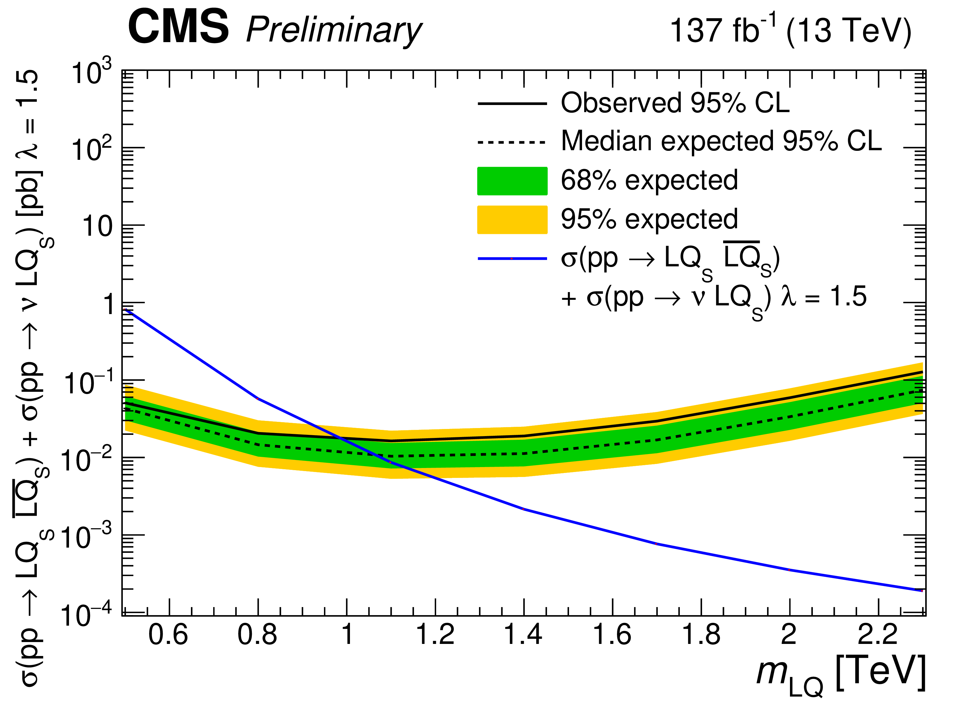
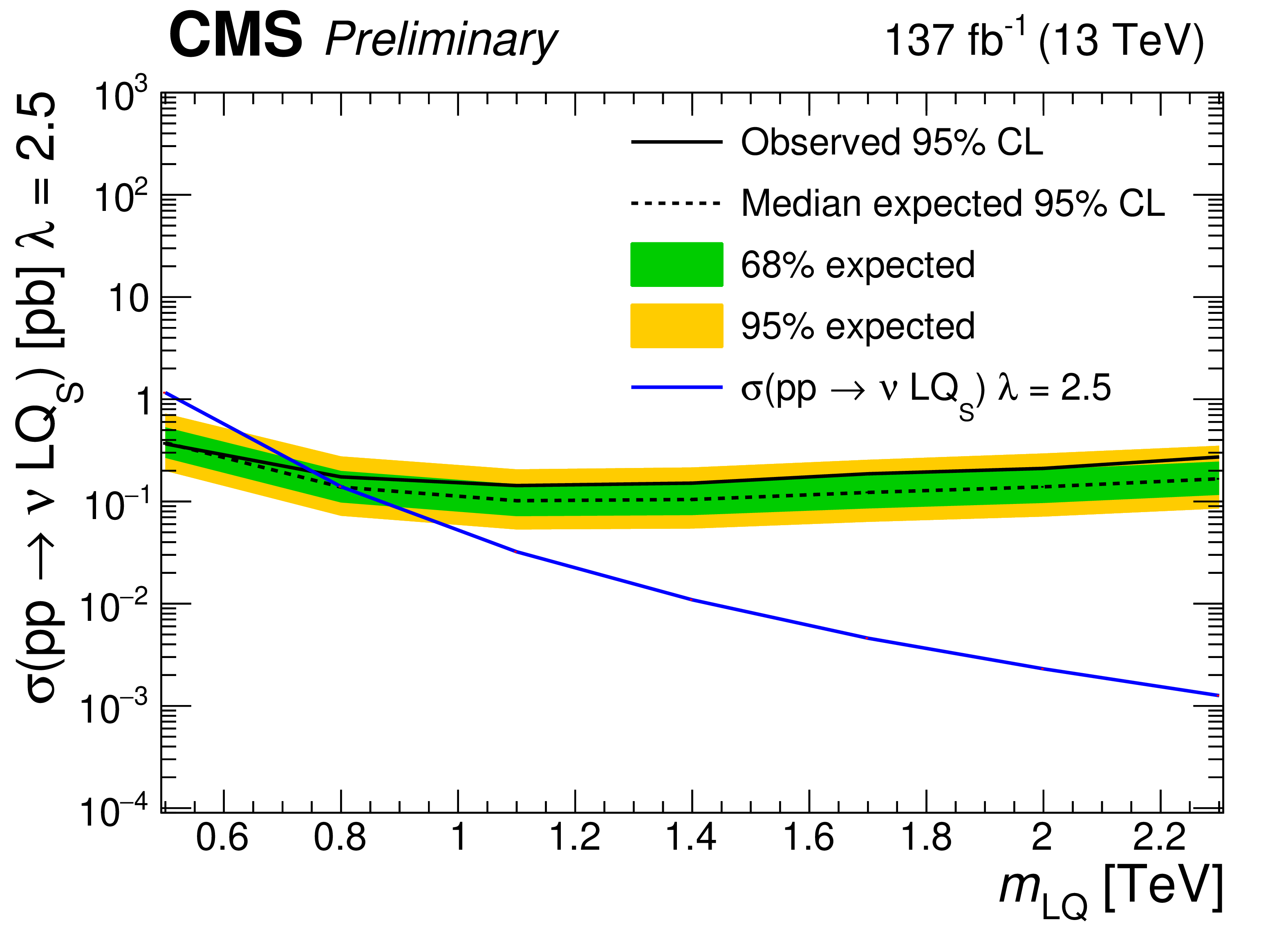
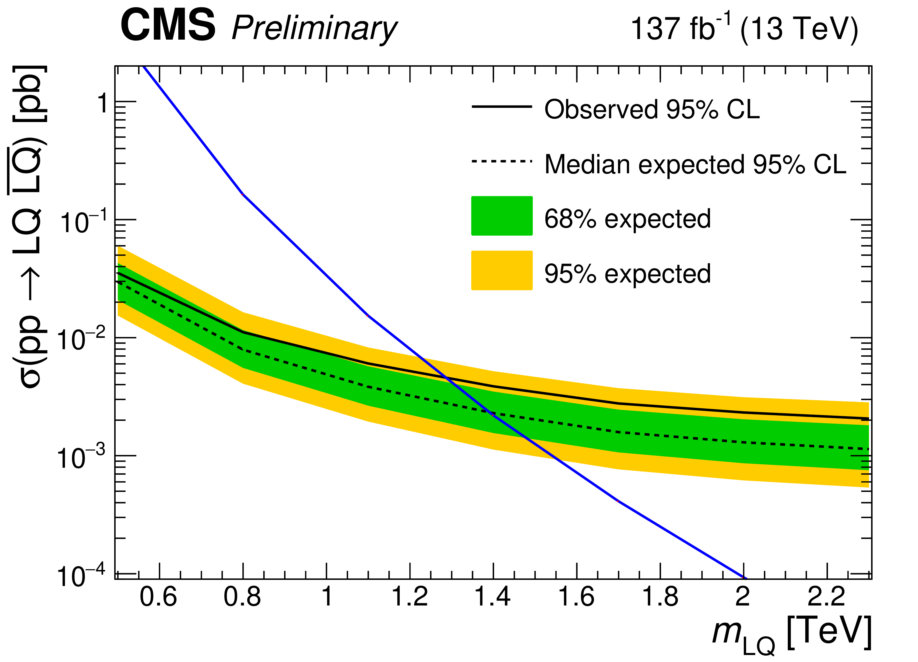
Figure 3:
The observed and expected (solid and dotted black lines) 95% CL upper limits on $\sigma (pp\rightarrow {\text {LQ}_{S}} {\overline {{\text {LQ}}}_{S}})$ (upper), $\sigma (pp\rightarrow \nu {\text {LQ}_{S}})$ $\lambda =$ 1.5 (center-left) and 2.5 (lower-left), and $\sigma (pp\rightarrow {\text {LQ}_{S}} {\overline {{\text {LQ}}}_{S}})$+$\sigma (pp\rightarrow \nu {\text {LQ}_{S}})$ $\lambda =$ 1.5 (center-right) and 2.5 (lower-right), as a function of the mass of the LQ$_{S}$. The bands represent the expected variation of the limit to within one and two standard deviation(s). The solid blue curve indicates the theoretical predictions at LO, except for pair-produced LQ$_{S}$, for which an NLO calculation [44] is shown. |

png pdf |
Figure 3-a:
The observed and expected (solid and dotted black lines) 95% CL upper limits on $\sigma (pp\rightarrow {\text {LQ}_{S}} {\overline {{\text {LQ}}}_{S}})$, as a function of the mass of the LQ$_{S}$. The bands represent the expected variation of the limit to within one and two standard deviation(s). The solid blue curve indicates the theoretical predictions at LO, except for pair-produced LQ$_{S}$, for which an NLO calculation [44] is shown. |
png pdf |
Figure 3-b:
The observed and expected (solid and dotted black lines) 95% CL upper limits on $\sigma (pp\rightarrow \nu {\text {LQ}_{S}})$ $\lambda =$ 1.5, as a function of the mass of the LQ$_{S}$. The bands represent the expected variation of the limit to within one and two standard deviation(s). The solid blue curve indicates the theoretical predictions at LO, except for pair-produced LQ$_{S}$, for which an NLO calculation [44] is shown. |
png pdf |
Figure 3-c:
The observed and expected (solid and dotted black lines) 95% CL upper limits on $\sigma (pp\rightarrow \nu {\text {LQ}_{S}})$ $\lambda =$ 2.5, as a function of the mass of the LQ$_{S}$. The bands represent the expected variation of the limit to within one and two standard deviation(s). The solid blue curve indicates the theoretical predictions at LO, except for pair-produced LQ$_{S}$, for which an NLO calculation [44] is shown. |
png pdf |
Figure 3-d:
The observed and expected (solid and dotted black lines) 95% CL upper limits on $\sigma (pp\rightarrow {\text {LQ}_{S}} {\overline {{\text {LQ}}}_{S}})$+$\sigma (pp\rightarrow \nu {\text {LQ}_{S}})$ $\lambda =$ 1.5, as a function of the mass of the LQ$_{S}$. The bands represent the expected variation of the limit to within one and two standard deviation(s). The solid blue curve indicates the theoretical predictions at LO, except for pair-produced LQ$_{S}$, for which an NLO calculation [44] is shown. |

png pdf |
Figure 3-e:
The observed and expected (solid and dotted black lines) 95% CL upper limits on $\sigma (pp\rightarrow {\text {LQ}_{S}} {\overline {{\text {LQ}}}_{S}})$+$\sigma (pp\rightarrow \nu {\text {LQ}_{S}})$ $\lambda =$ 2.5, as a function of the mass of the LQ$_{S}$. The bands represent the expected variation of the limit to within one and two standard deviation(s). The solid blue curve indicates the theoretical predictions at LO, except for pair-produced LQ$_{S}$, for which an NLO calculation [44] is shown. |

png pdf |
Figure 4:
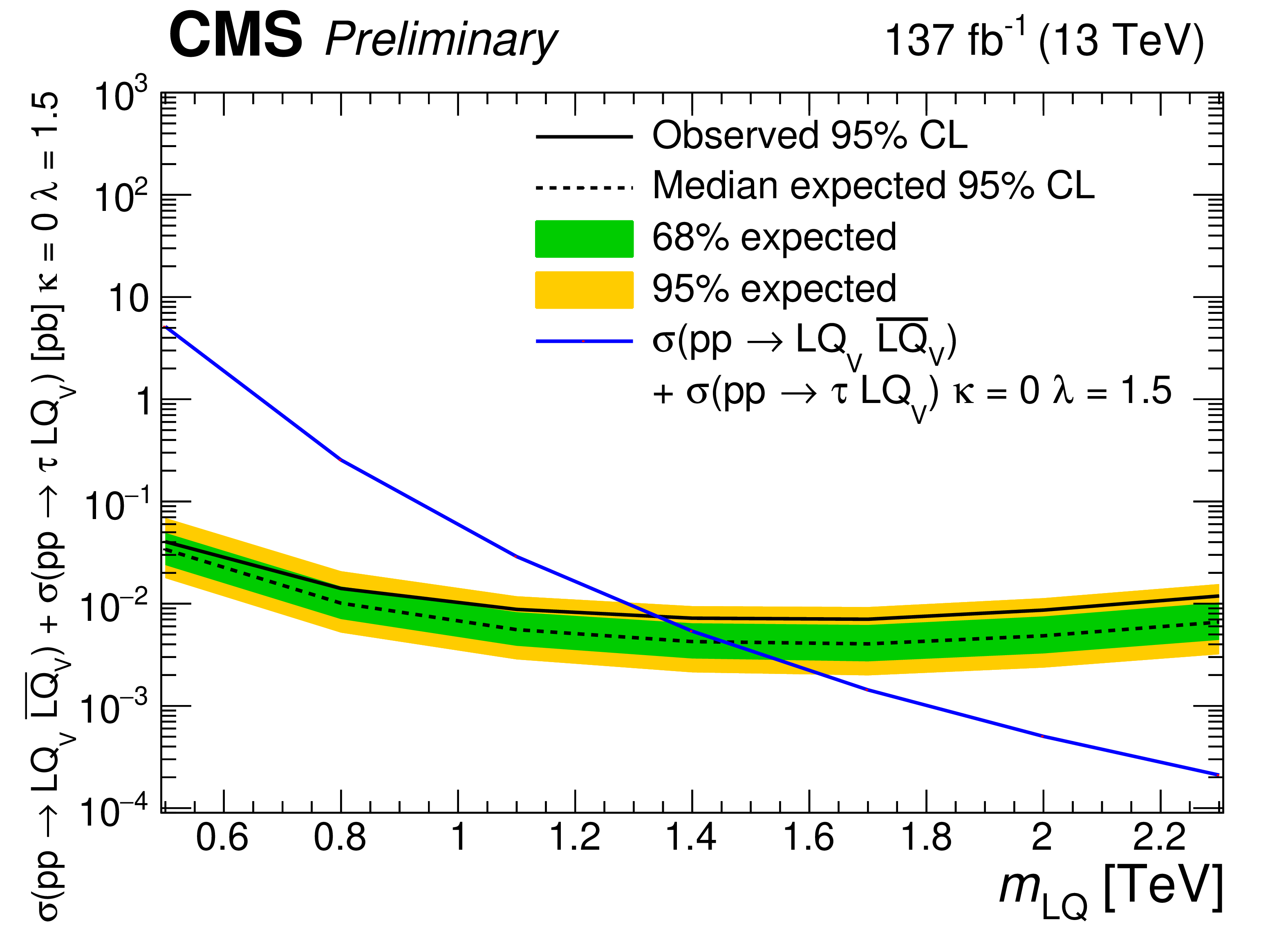
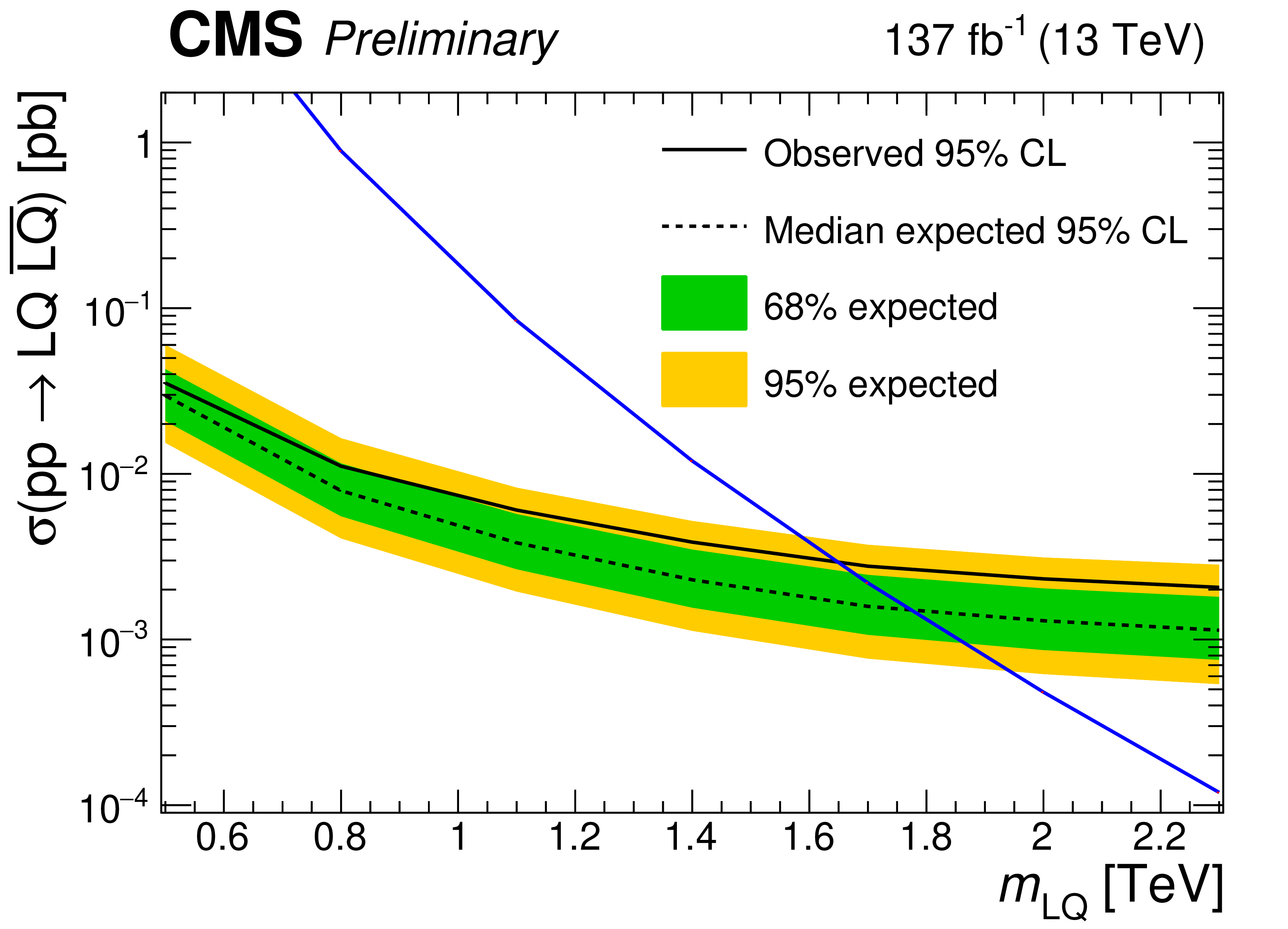
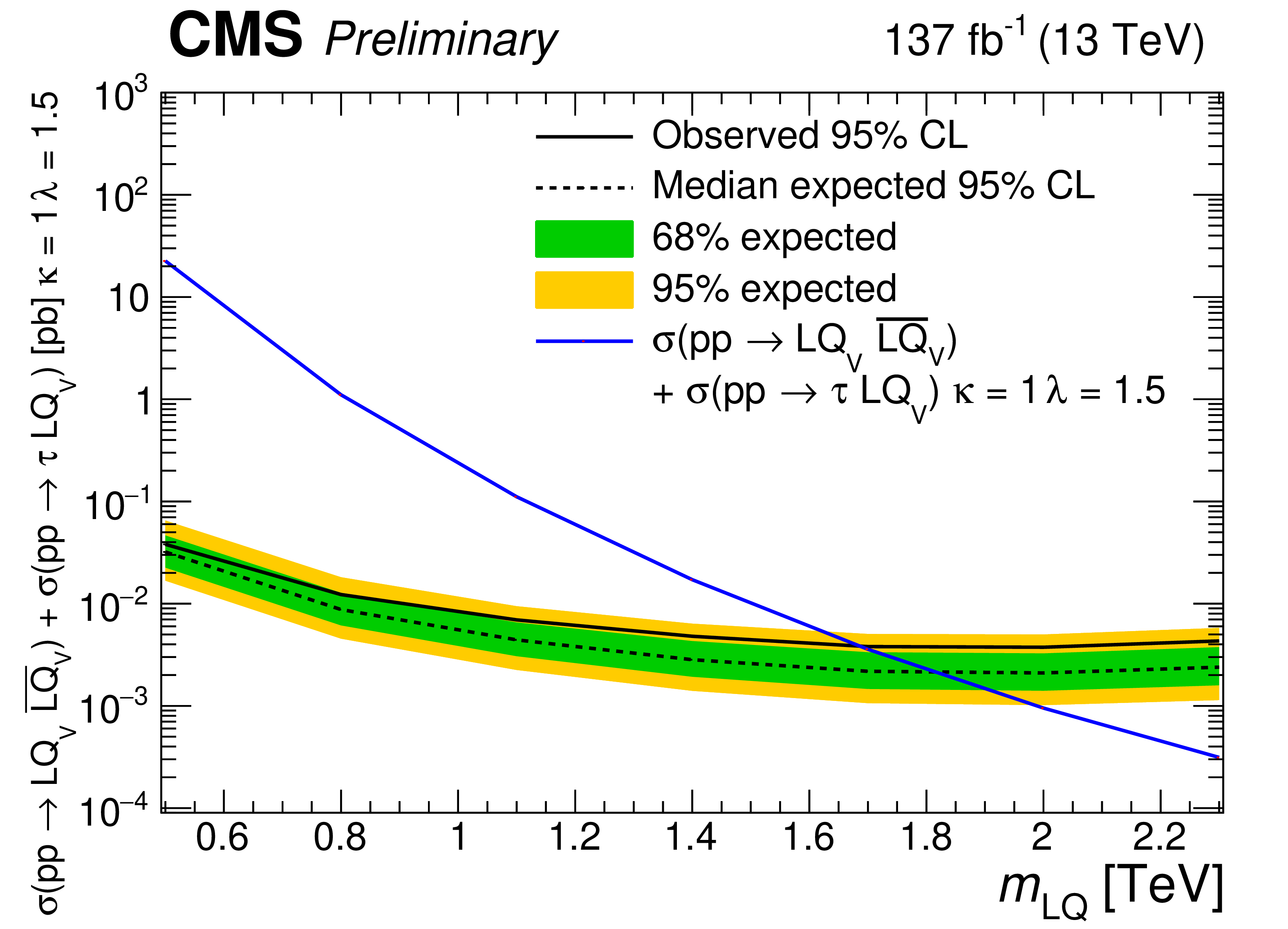
The observed and expected (solid and dotted black lines) 95% CL upper limits on $\sigma (pp\rightarrow {\text {LQ}_{V}} {\overline {{\text {LQ}}}_{V}})$ (upper), $\sigma (pp\rightarrow \tau {\text {LQ}_{V}})$ $\lambda =$ 1.5 (center-left) and 2.5 (lower-left), and $\sigma (pp\rightarrow {\text {LQ}_{V}} {\overline {{\text {LQ}}}_{V}})$+$\sigma (pp\rightarrow \tau {\text {LQ}_{V}})$ $\lambda =$ 1.5 (center-right) and 2.5 (lower-right), as a function of the mass of the LQ$_{V}$, with $k = $ 0. The bands represent the expected variation of the limit to within one and two standard deviation(s). The solid blue curve indicates the theoretical predictions at LO. |
png pdf |
Figure 4-a:
The observed and expected (solid and dotted black lines) 95% CL upper limits on $\sigma (pp\rightarrow {\text {LQ}_{V}} {\overline {{\text {LQ}}}_{V}})$, as a function of the mass of the LQ$_{V}$, with $k = $ 0. The bands represent the expected variation of the limit to within one and two standard deviation(s). The solid blue curve indicates the theoretical predictions at LO. |
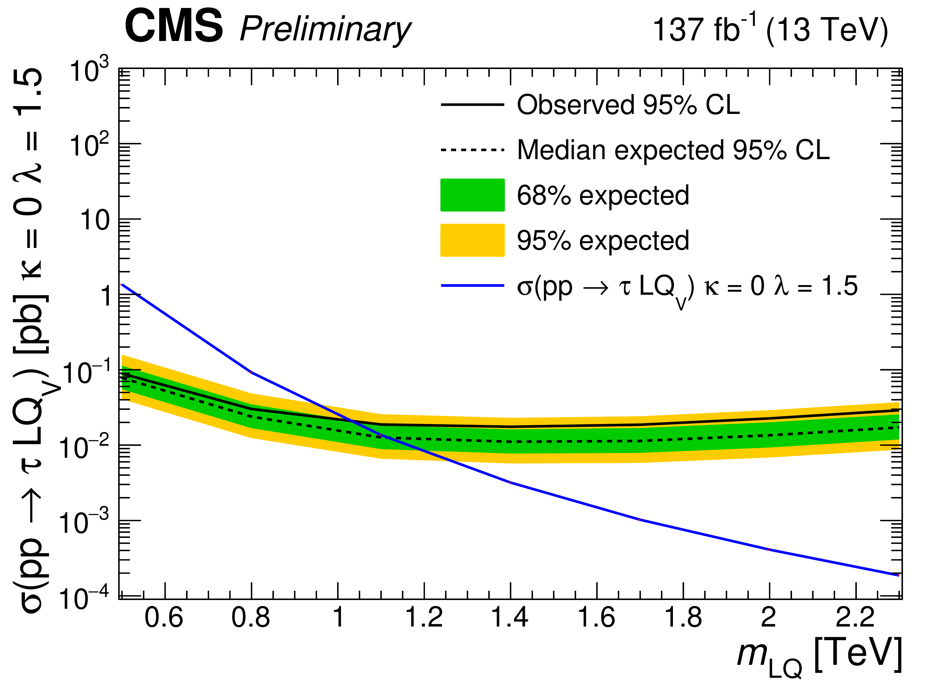
png pdf |
Figure 4-b:
The observed and expected (solid and dotted black lines) 95% CL upper limits on $\sigma (pp\rightarrow \tau {\text {LQ}_{V}})$ $\lambda =$ 1.5, as a function of the mass of the LQ$_{V}$, with $k = $ 0. The bands represent the expected variation of the limit to within one and two standard deviation(s). The solid blue curve indicates the theoretical predictions at LO. |
png pdf |
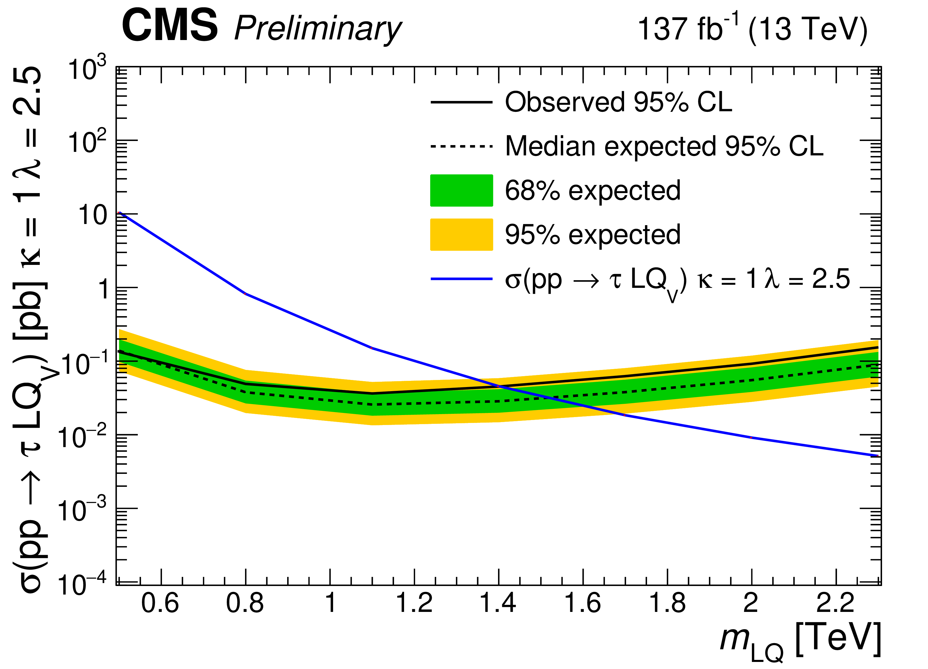
Figure 4-c:
The observed and expected (solid and dotted black lines) 95% CL upper limits on $\sigma (pp\rightarrow \tau {\text {LQ}_{V}})$ $\lambda =$ 2.5, as a function of the mass of the LQ$_{V}$, with $k = $ 0. The bands represent the expected variation of the limit to within one and two standard deviation(s). The solid blue curve indicates the theoretical predictions at LO. |

png pdf |
Figure 4-d:
The observed and expected (solid and dotted black lines) 95% CL upper limits on $\sigma (pp\rightarrow {\text {LQ}_{V}} {\overline {{\text {LQ}}}_{V}})$+$\sigma (pp\rightarrow \tau {\text {LQ}_{V}})$ $\lambda =$ 1.5, as a function of the mass of the LQ$_{V}$, with $k = $ 0. The bands represent the expected variation of the limit to within one and two standard deviation(s). The solid blue curve indicates the theoretical predictions at LO. |

png pdf |
Figure 4-e:
The observed and expected (solid and dotted black lines) 95% CL upper limits on $\sigma (pp\rightarrow {\text {LQ}_{V}} {\overline {{\text {LQ}}}_{V}})$+$\sigma (pp\rightarrow \tau {\text {LQ}_{V}})$ $\lambda =$ 2.5, as a function of the mass of the LQ$_{V}$, with $k = $ 0. The bands represent the expected variation of the limit to within one and two standard deviation(s). The solid blue curve indicates the theoretical predictions at LO. |
png pdf |
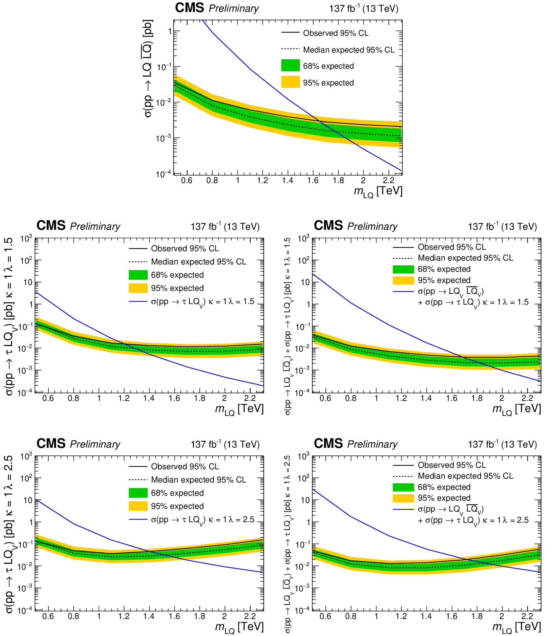
Figure 5:
The observed and expected (solid and dotted black lines) 95% CL upper limits on $\sigma (pp\rightarrow {\text {LQ}_{V}} {\overline {{\text {LQ}}}_{V}})$ (upper), $\sigma (pp\rightarrow \tau {\text {LQ}_{V}})$ $\lambda =$ 1.5 (center-left) and 2.5 (lower-left), and $\sigma (pp\rightarrow {\text {LQ}_{V}} {\overline {{\text {LQ}}}_{V}})$+$\sigma (pp\rightarrow \tau {\text {LQ}_{V}})$ $\lambda =$ 1.5 (center-right) and 2.5 (lower-right), as a function of the mass of the LQ$_{V}$, with $k = $ 1. The bands represent the expected variation of the limit to within one and two standard deviation(s). The solid blue curve indicates the theoretical predictions at LO. |
png pdf |
Figure 5-a:
The observed and expected (solid and dotted black lines) 95% CL upper limits on $\sigma (pp\rightarrow {\text {LQ}_{V}} {\overline {{\text {LQ}}}_{V}})$, as a function of the mass of the LQ$_{V}$, with $k = $ 1. The bands represent the expected variation of the limit to within one and two standard deviation(s). The solid blue curve indicates the theoretical predictions at LO. |

png pdf |
Figure 5-b:
The observed and expected (solid and dotted black lines) 95% CL upper limits on $\sigma (pp\rightarrow \tau {\text {LQ}_{V}})$ $\lambda =$ 1.5, as a function of the mass of the LQ$_{V}$, with $k = $ 1. The bands represent the expected variation of the limit to within one and two standard deviation(s). The solid blue curve indicates the theoretical predictions at LO. |
png pdf |
Figure 5-c:
The observed and expected (solid and dotted black lines) 95% CL upper limits on $\sigma (pp\rightarrow \tau {\text {LQ}_{V}})$ $\lambda =$ 2.5, as a function of the mass of the LQ$_{V}$, with $k = $ 1. The bands represent the expected variation of the limit to within one and two standard deviation(s). The solid blue curve indicates the theoretical predictions at LO. |
png pdf |
Figure 5-d:
The observed and expected (solid and dotted black lines) 95% CL upper limits on $\sigma (pp\rightarrow {\text {LQ}_{V}} {\overline {{\text {LQ}}}_{V}})$+$\sigma (pp\rightarrow \tau {\text {LQ}_{V}})$ $\lambda =$ 1.5, as a function of the mass of the LQ$_{V}$, with $k = $ 1. The bands represent the expected variation of the limit to within one and two standard deviation(s). The solid blue curve indicates the theoretical predictions at LO. |

png pdf |
Figure 5-e:
The observed and expected (solid and dotted black lines) 95% CL upper limits on $\sigma (pp\rightarrow {\text {LQ}_{V}} {\overline {{\text {LQ}}}_{V}})$+$\sigma (pp\rightarrow \tau {\text {LQ}_{V}})$ $\lambda =$ 2.5, as a function of the mass of the LQ$_{V}$, with $k = $ 1. The bands represent the expected variation of the limit to within one and two standard deviation(s). The solid blue curve indicates the theoretical predictions at LO. |
png pdf |
Figure 6:
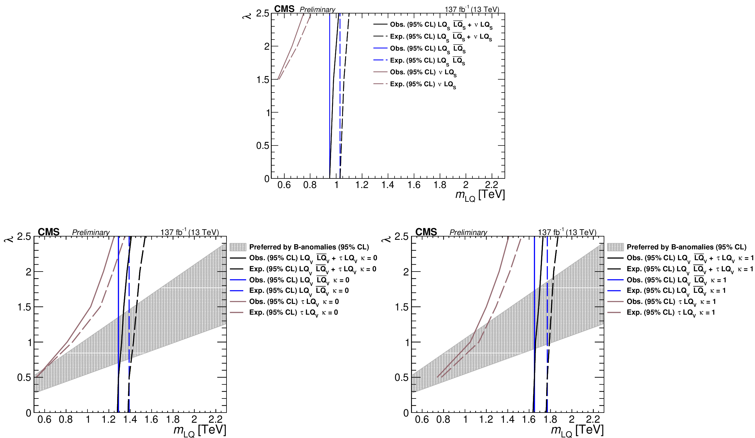
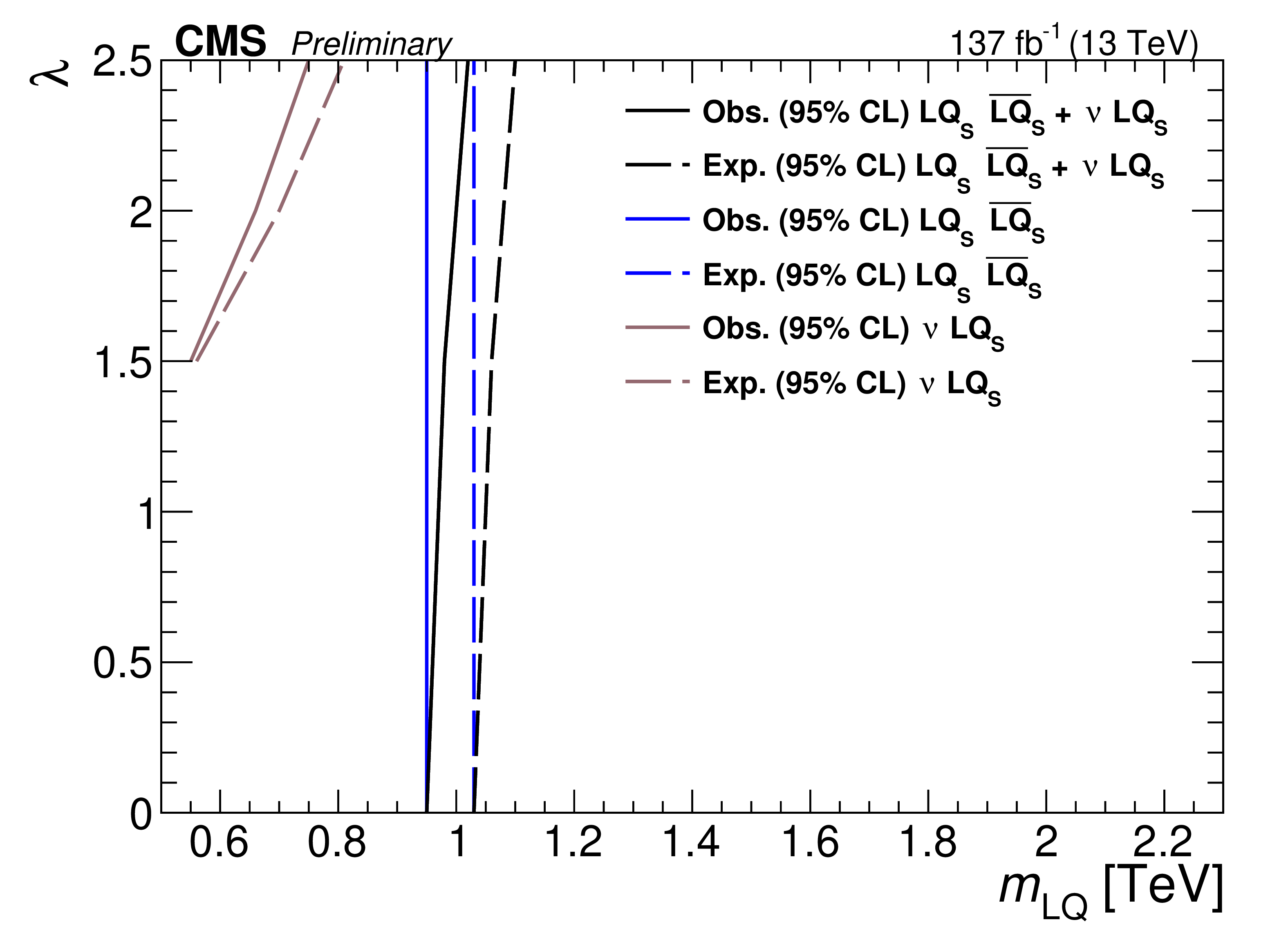
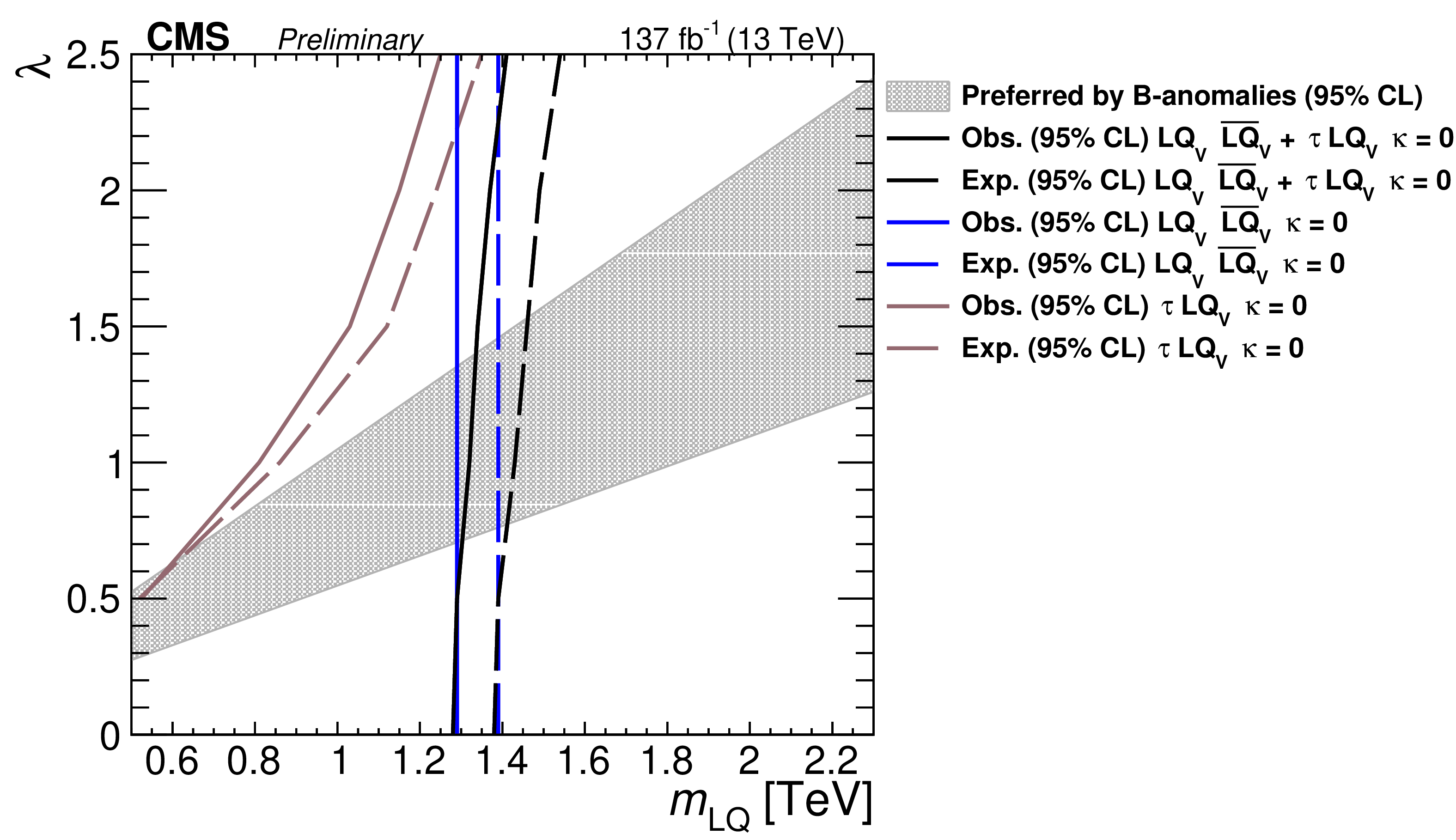
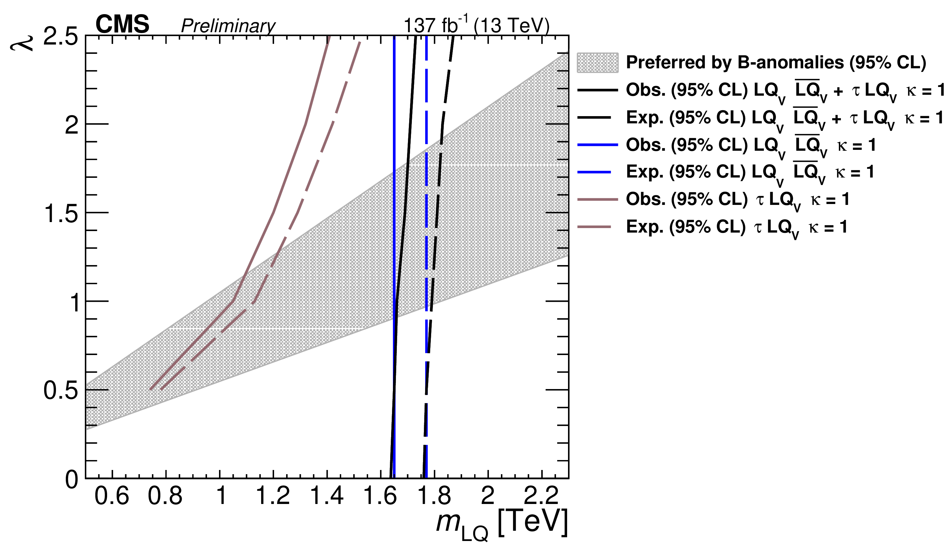
The observed and expected (solid and dotted lines) 95% CL LQ exclusion limits in the plane of the LQ-lepton-quark vertex coupling and the mass of the LQ for single (brown lines), pair (blue lines) production, and considering their sum (black lines). Regions to the left of the lines are excluded. The upper plot pertains to an LQ$_{S}$ with equal couplings to t$\tau $, b$\nu $, while the lower plots are for an LQ$_{V}$ assuming $k = $ 0 (left) and 1 (right) and equal couplings to t$\nu $, b$\tau $. For LQ$_{V}$, the gray area shows the band preferred 95% CL) by B-physics anomalies: $\lambda = \sqrt {0.7 \pm 0.2 } \times m_{\rm {LQ}}$ TeV [42]. |
png pdf |
Figure 6-a:
The observed and expected (solid and dotted lines) 95% CL LQ exclusion limits in the plane of the LQ-lepton-quark vertex coupling and the mass of the LQ for single (brown lines), pair (blue lines) production, and considering their sum (black lines). Regions to the left of the lines are excluded. The plot pertains to an LQ$_{S}$ with equal couplings to t$\tau $, b$\nu $. |
png pdf |
Figure 6-b:
The observed and expected (solid and dotted lines) 95% CL LQ exclusion limits in the plane of the LQ-lepton-quark vertex coupling and the mass of the LQ for single (brown lines), pair (blue lines) production, and considering their sum (black lines). Regions to the left of the lines are excluded. The plot pertains to an LQ$_{V}$ assuming $k = $ 0 and equal couplings to t$\nu $, b$\tau $. The gray area shows the band preferred 95% CL) by B-physics anomalies: $\lambda = \sqrt {0.7 \pm 0.2 } \times m_{\rm {LQ}}$ TeV [42]. |
png pdf |
Figure 6-c:
The observed and expected (solid and dotted lines) 95% CL LQ exclusion limits in the plane of the LQ-lepton-quark vertex coupling and the mass of the LQ for single (brown lines), pair (blue lines) production, and considering their sum (black lines). Regions to the left of the lines are excluded. The plot pertains to an LQ$_{V}$ assuming $k = $ 1 and equal couplings to t$\nu $, b$\tau $. The gray area shows the band preferred 95% CL) by B-physics anomalies: $\lambda = \sqrt {0.7 \pm 0.2 } \times m_{\rm {LQ}}$ TeV [42]. |
| Tables | |
png pdf |
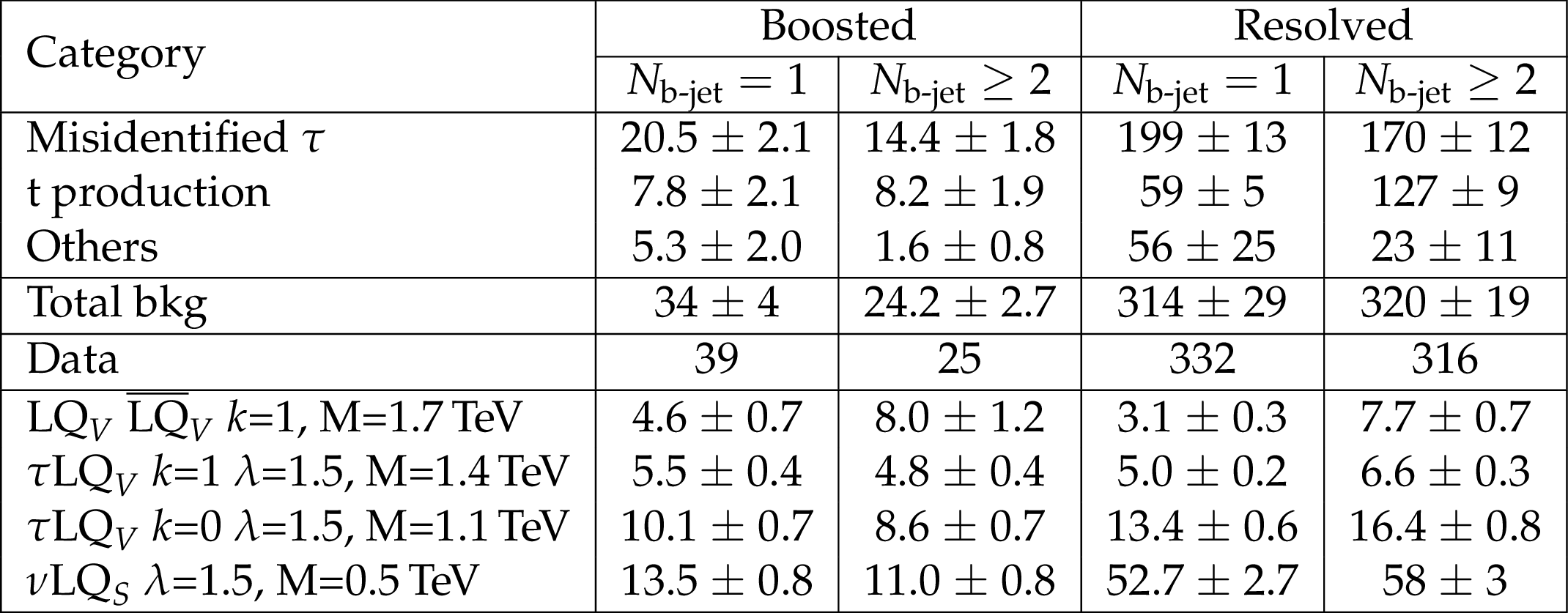
Table 1:
Yields from the SM background estimation, expected signal, and data, for the selected events. |
png pdf |
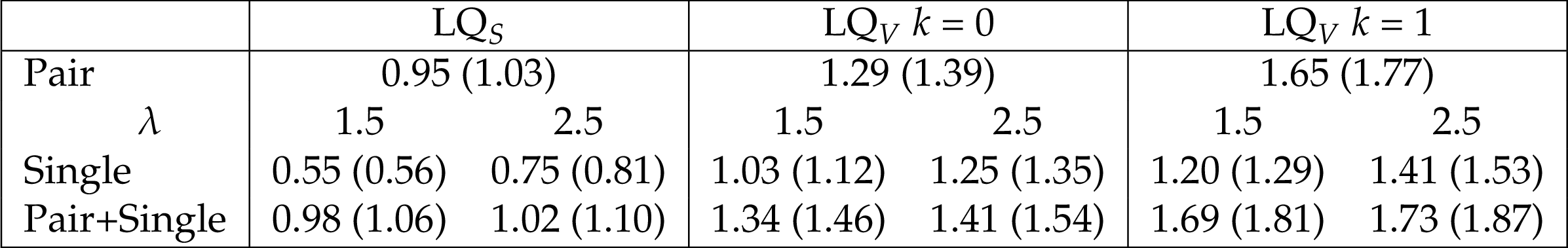
Table 2:
Lower limits on the mass in TeV of the leptoquarks LQ$_{S}$, LQ$_{V}$ $k = $ 0, and LQ$_{V}$ $k = $ 1, based on the pair- and single-production mechanisms taken separately and together. The searches that depend on the $\lambda $ parameter are given for values of 1.5 and 2.5. The expected limits are given in parentheses. |
| Summary |
| A search for leptoquarks, coupling to third-generation fermions, and produced in pairs and singly in association with a lepton, has been presented. The leptoquark LQ may couple to a top quark plus a $\tau$ lepton ($\mathrm{t}\tau$) or a bottom quark plus a neutrino ($\mathrm{b}\nu$, scalar LQ) or else to $\mathrm{t}\nu$ and $\mathrm{b}\tau$ (vector LQ), resulting in the final states $\mathrm{t}\tau\nu\mathrm{b}$ and $\mathrm{t}\tau\nu$. The channel in which both the top quark and the $\tau$ lepton decay hadronically is investigated, including the case of a large LQ-$\mathrm{t}$ mass splitting giving rise to a boosted top quark whose decay daughters may not be separated on the scale of the spatial resolution of the jet. Such a signature has not been previously examined in searches for physics beyond the standard model. The data used corresponds to an integrated luminosity of 137 fb$^{-1}$ collected with the CMS detector at the LHC in pp collisions at $\sqrt{s} = $ 13 TeV. The observations are found to be in agreement with the standard model prediction. Exclusion limits are given in the plane of the LQ-lepton-quark vertex coupling $\lambda$ and the LQ mass for scalar and vector leptoquarks. The range of lower limits on the LQ mass, at 95% CL, is 0.98-1.73 TeV, depending on $\lambda$ and the leptoquark spin. These results represent the most stringent limits to date on the presence of such leptoquarks for the case of a decay branching fraction of 0.5 to each lepton-quark pair. These results also probe the parameter space preferred by the B-physics anomalies in several models ([41], [42]), and exclude relevant portions. |
| Additional Figures | |
png pdf |
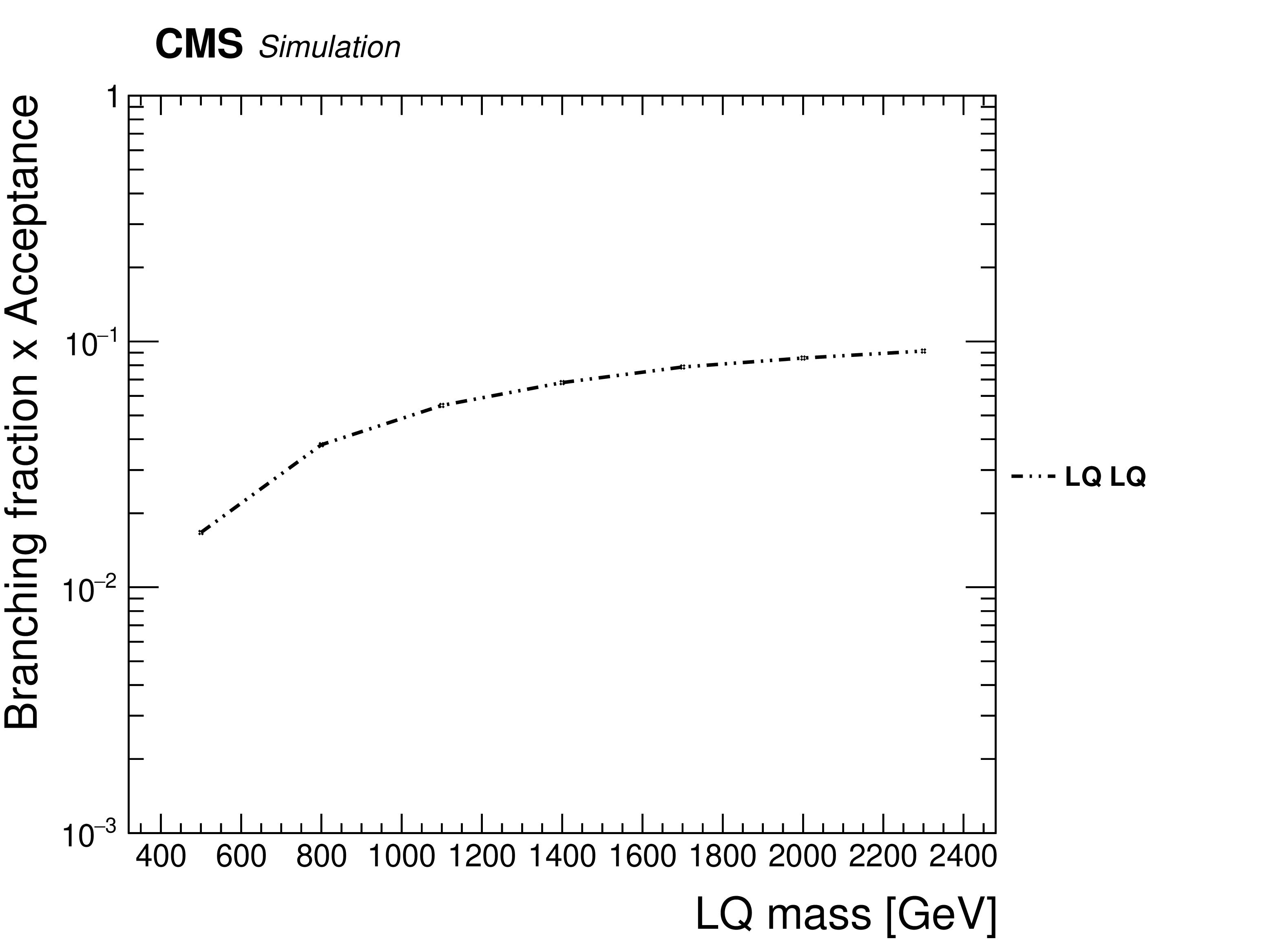
Additional Figure 1:
Pair leptoquark total signal selection efficiency, including all the events that enter the top and b jet categories defined in the search. The signal samples contain all the final states that can originate from the leptoquark decays to a top quark plus a neutrino or a bottom quark plus a tau lepton, having the leptoquark decay a branching fraction of 0.5 to each fermion pair. |
png pdf |
Additional Figure 2:
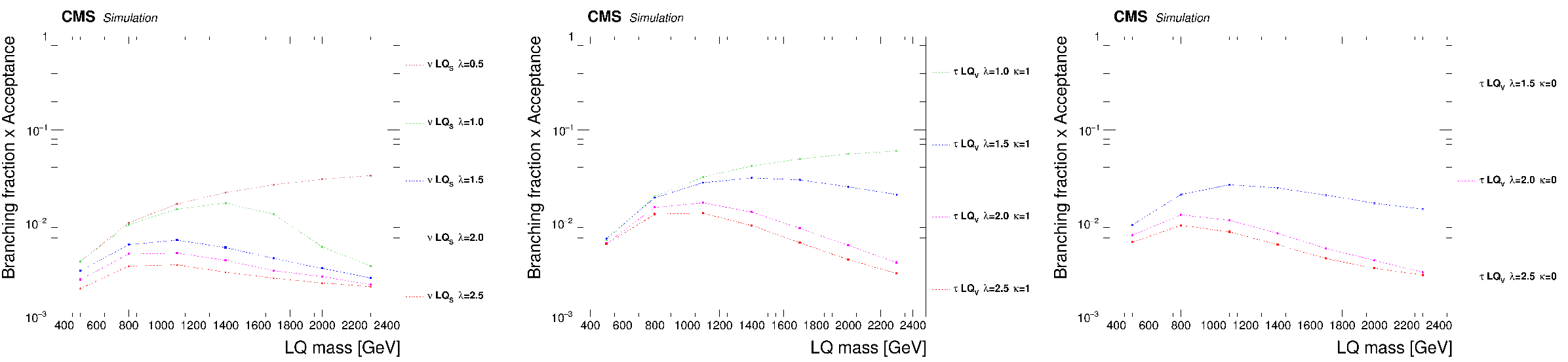
Single leptoquark total signal selection efficiency, including all the events that enter the top and b jet categories defined in the search, for scalar leptoquark (LQ$_{S}$, left), vector leptoquark (LQ$_{V}$) with k = 1 (center), and LQ$_{V}$ with k = 0 (right). The signal samples contain all the final states that can originate from the leptoquark decays to a top quark plus a neutrino or a bottom quark plus a tau lepton (LQ$_{V}$), or else a top quark plus a tau lepton or a bottom quark plus a neutrino (LQ$_{S}$), having the leptoquark decay a branching fraction of 0.5 to each fermion pair. |
png |
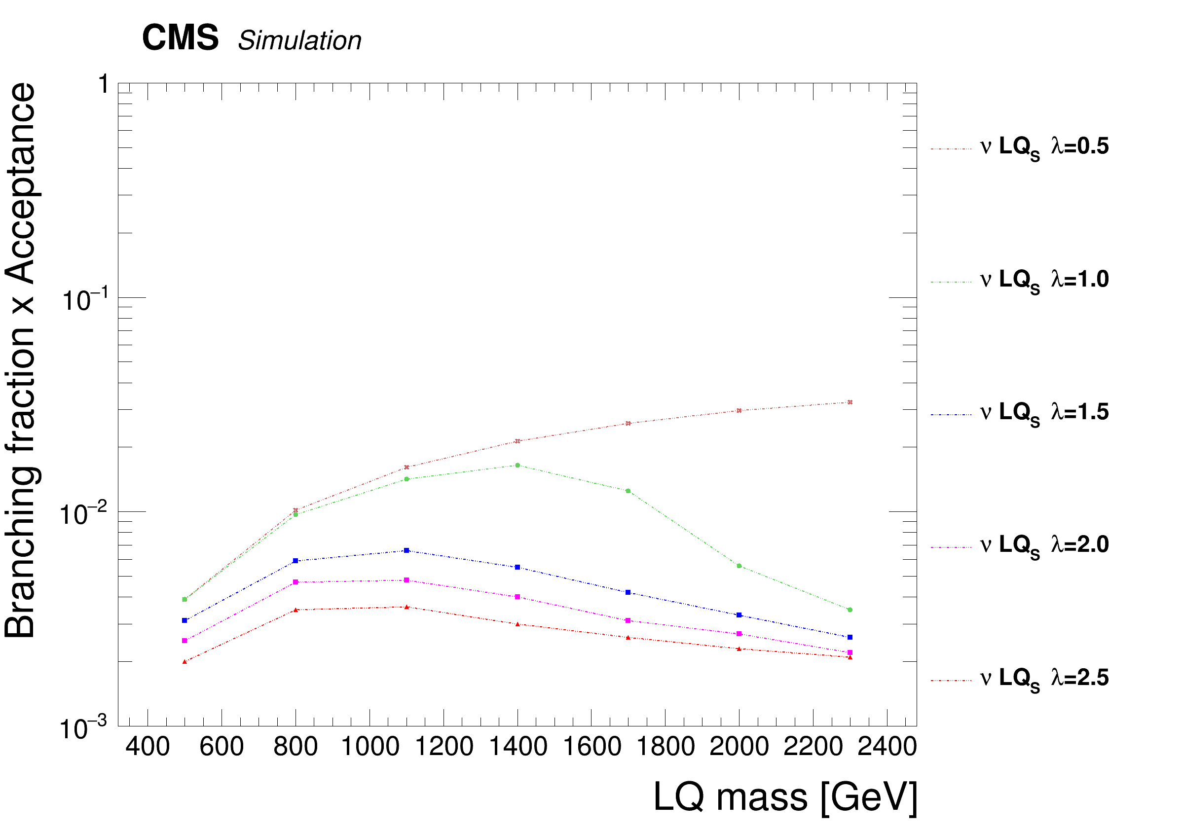
Additional Figure 2-a:
Single leptoquark total signal selection efficiency, including all the events that enter the top and b jet categories defined in the search, for scalar leptoquark (LQ$_{S}$). The signal samples contain all the final states that can originate from the leptoquark decays to a top quark plus a neutrino or a bottom quark plus a tau lepton (LQ$_{V}$), or else a top quark plus a tau lepton or a bottom quark plus a neutrino (LQ$_{S}$), having the leptoquark decay a branching fraction of 0.5 to each fermion pair. |
png |
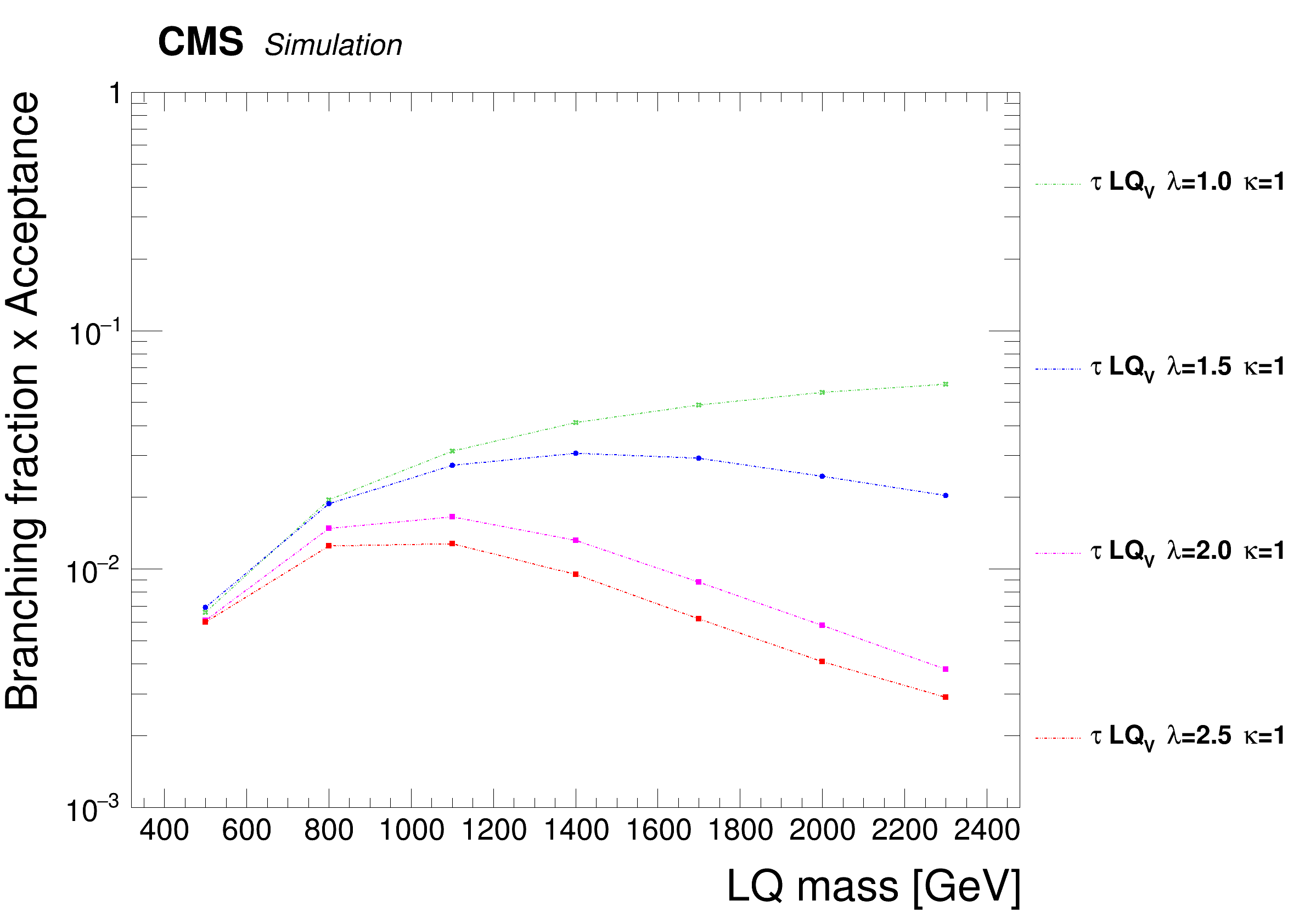
Additional Figure 2-b:
Single leptoquark total signal selection efficiency, including all the events that enter the top and b jet categories defined in the search, for vector leptoquark (LQ$_{V}$) with k = 1. The signal samples contain all the final states that can originate from the leptoquark decays to a top quark plus a neutrino or a bottom quark plus a tau lepton (LQ$_{V}$), or else a top quark plus a tau lepton or a bottom quark plus a neutrino (LQ$_{S}$), having the leptoquark decay a branching fraction of 0.5 to each fermion pair. |

png |
Additional Figure 2-c:
Single leptoquark total signal selection efficiency, including all the events that enter the top and b jet categories defined in the search, for vector leptoquark (LQ$_{V}$) with k = 0. The signal samples contain all the final states that can originate from the leptoquark decays to a top quark plus a neutrino or a bottom quark plus a tau lepton (LQ$_{V}$), or else a top quark plus a tau lepton or a bottom quark plus a neutrino (LQ$_{S}$), having the leptoquark decay a branching fraction of 0.5 to each fermion pair. |
png pdf |
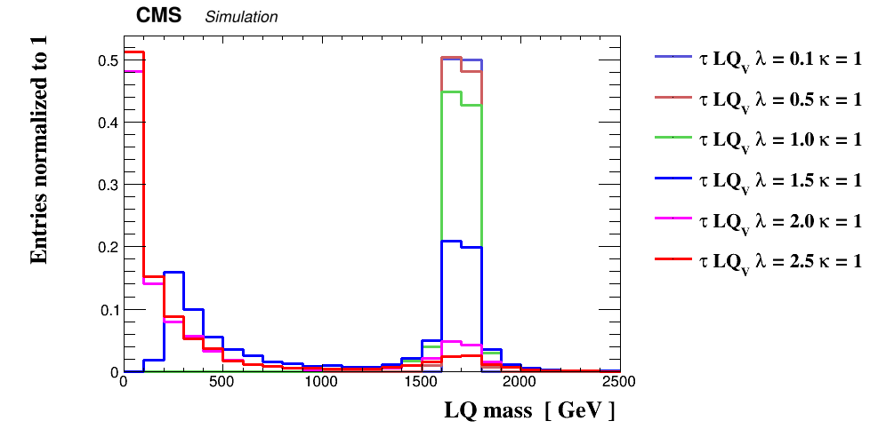
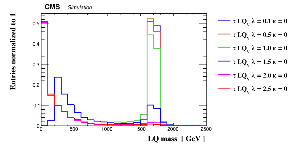
Additional Figure 3:
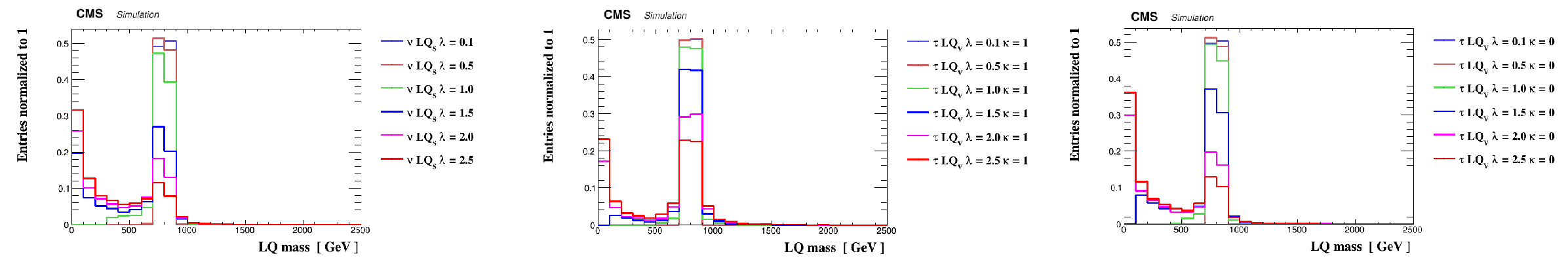
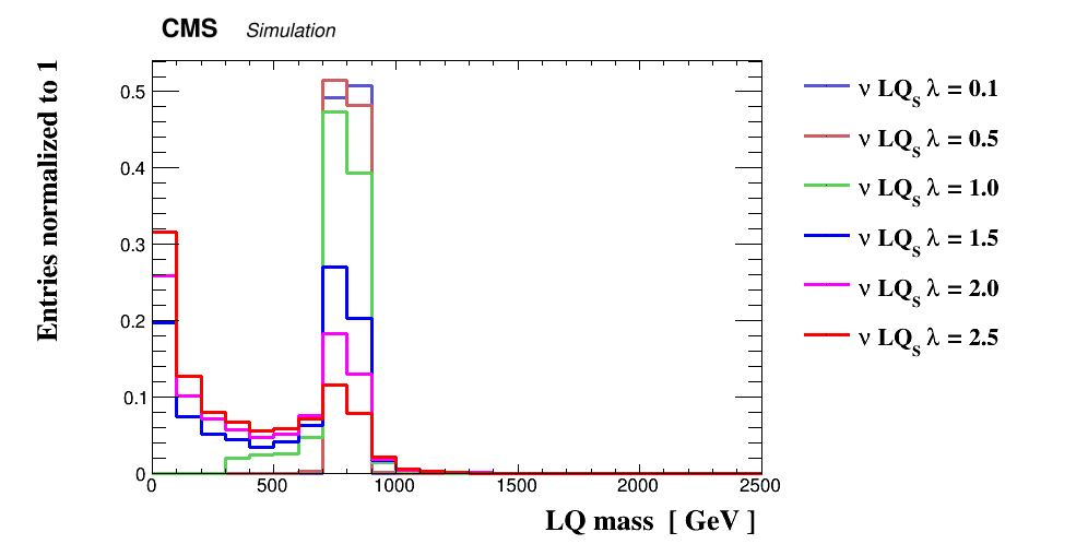
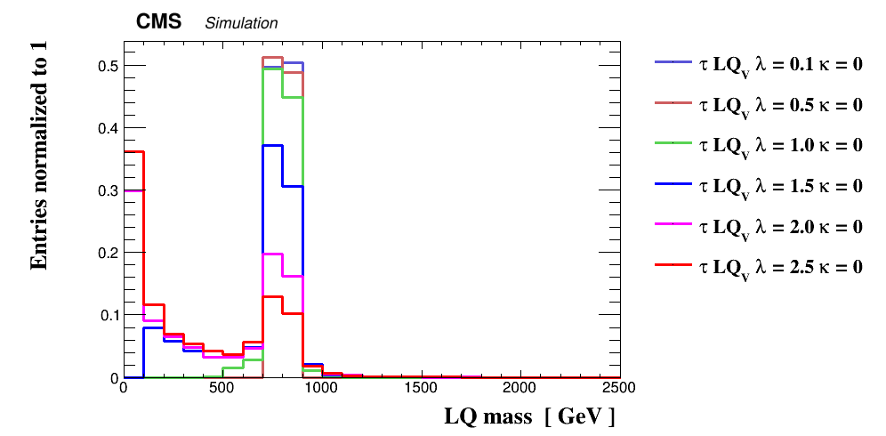
Leptoquark mass distribution at generator level for a singly produced leptoquark with mass equal to 0.8 TeV, for scalar leptoquark (left), vector leptoquark with k = 1 (center), and vector leptoquark with k = 0 (right). |
png |
Additional Figure 3-a:
Leptoquark mass distribution at generator level for a singly produced leptoquark with mass equal to 0.8 TeV, for scalar leptoquark. |

png |
Additional Figure 3-b:
Leptoquark mass distribution at generator level for a singly produced leptoquark with mass equal to 0.8 TeV, for vector leptoquark with k = 1. |
png |
Additional Figure 3-c:
Leptoquark mass distribution at generator level for a singly produced leptoquark with mass equal to 0.8 TeV, for vector leptoquark with k = 0. |
png pdf |
Additional Figure 4:
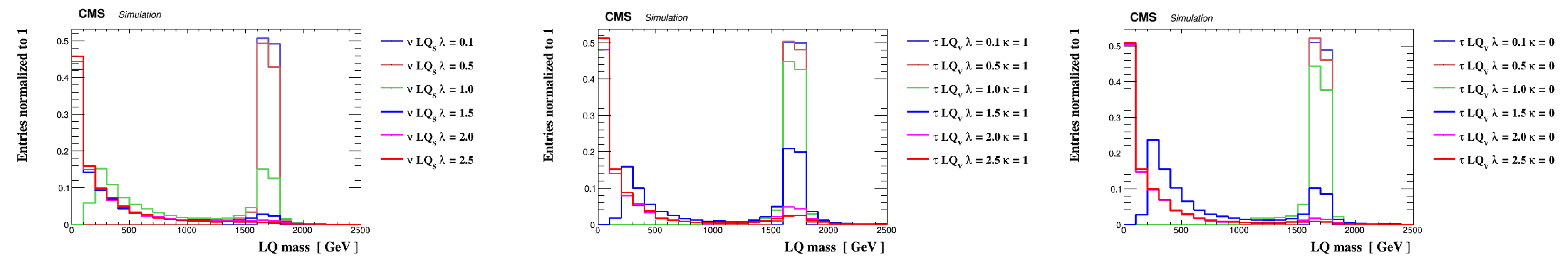
Leptoquark mass distribution at generator level for a singly produced leptoquark with mass equal to 1.7 TeV, for scalar leptoquark (left), vector leptoquark with k = 1 (center), and vector leptoquark with k = 0 (right). |

png |
Additional Figure 4-a:
Leptoquark mass distribution at generator level for a singly produced leptoquark with mass equal to 1.7 TeV, for scalar leptoquark. |
png |
Additional Figure 4-b:
Leptoquark mass distribution at generator level for a singly produced leptoquark with mass equal to 1.7 TeV, for vector leptoquark with k = 1. |
png |
Additional Figure 4-c:
Leptoquark mass distribution at generator level for a singly produced leptoquark with mass equal to 1.7 TeV, for vector leptoquark with k = 0. |

png pdf |
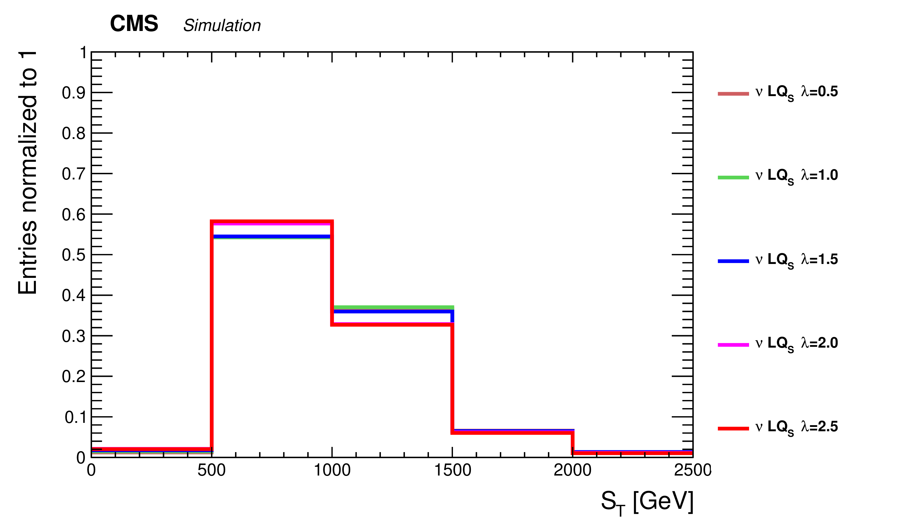
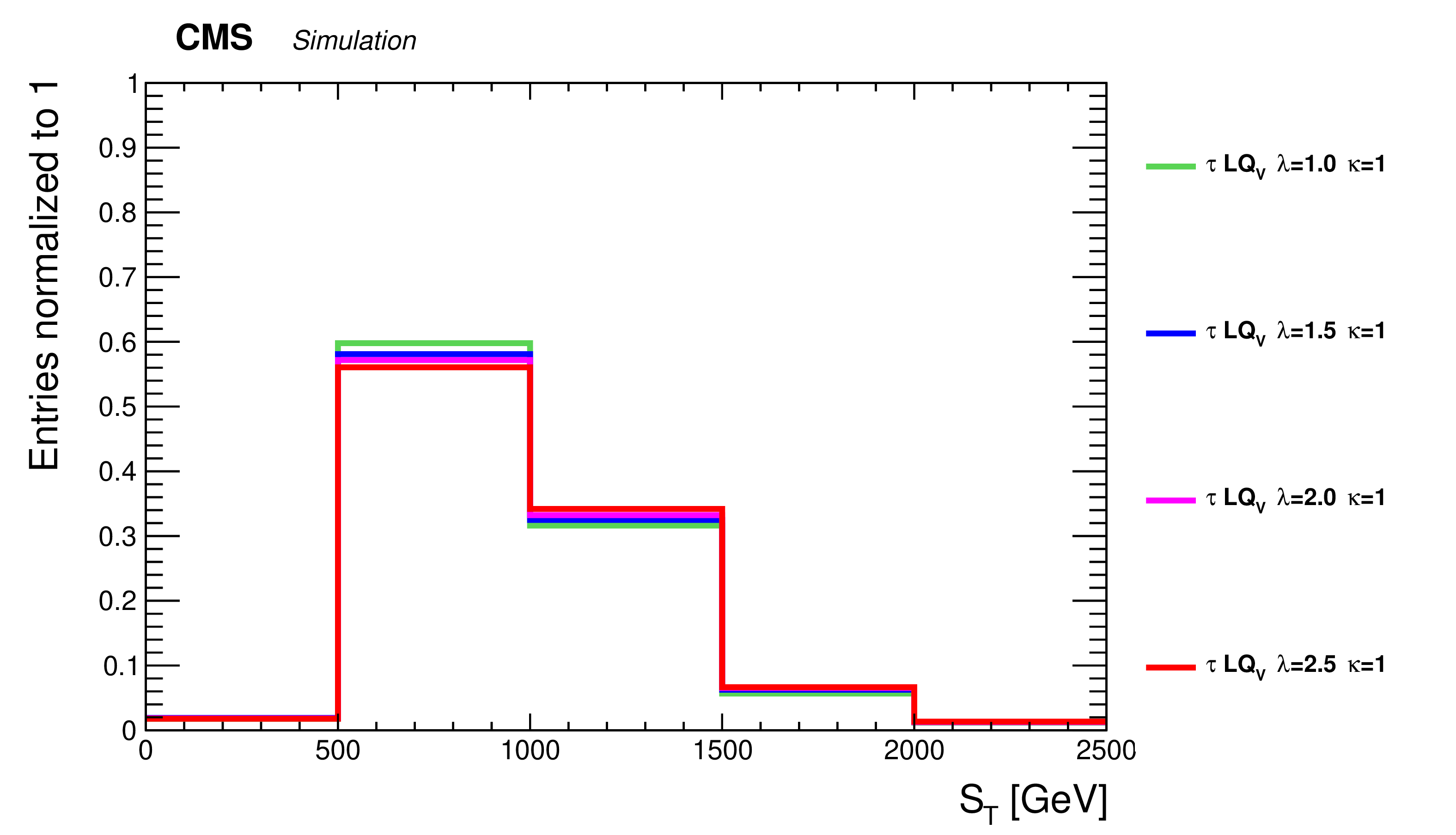
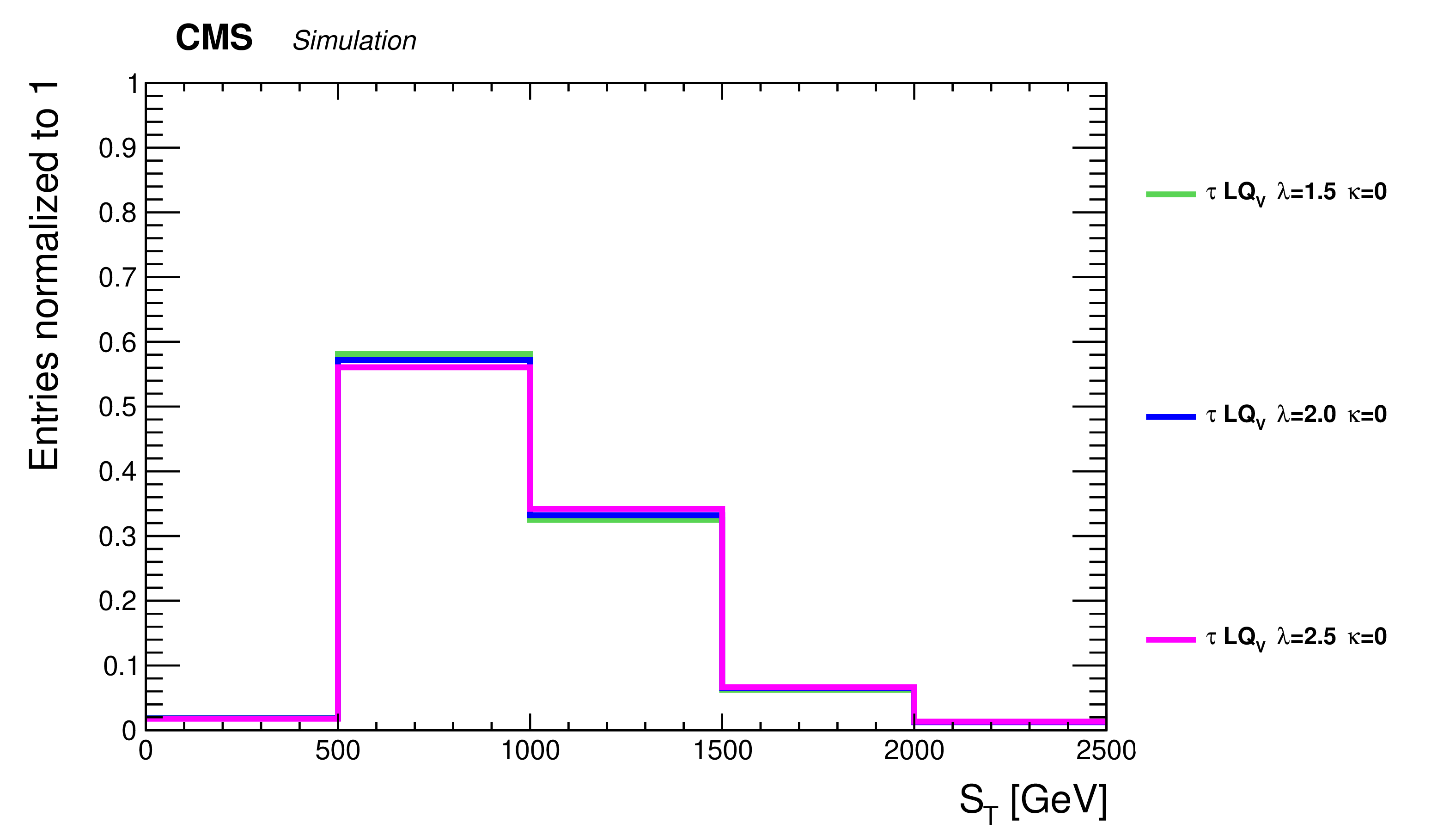
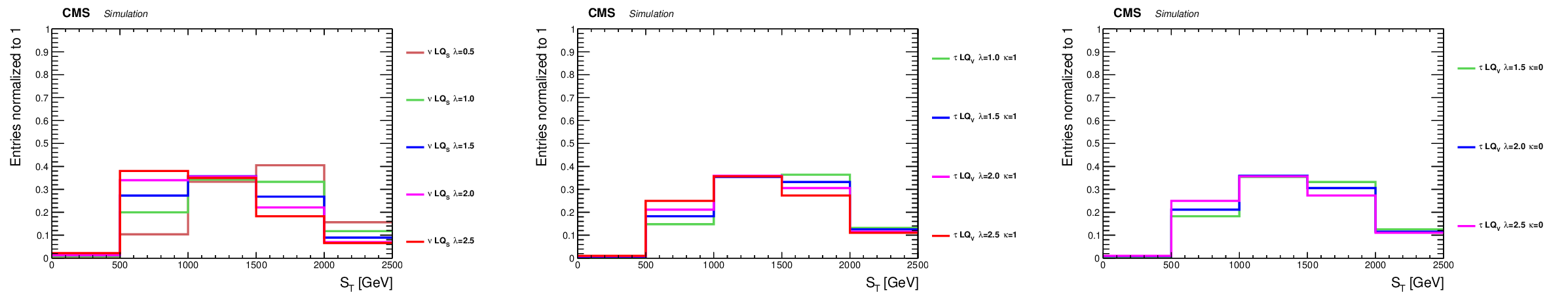
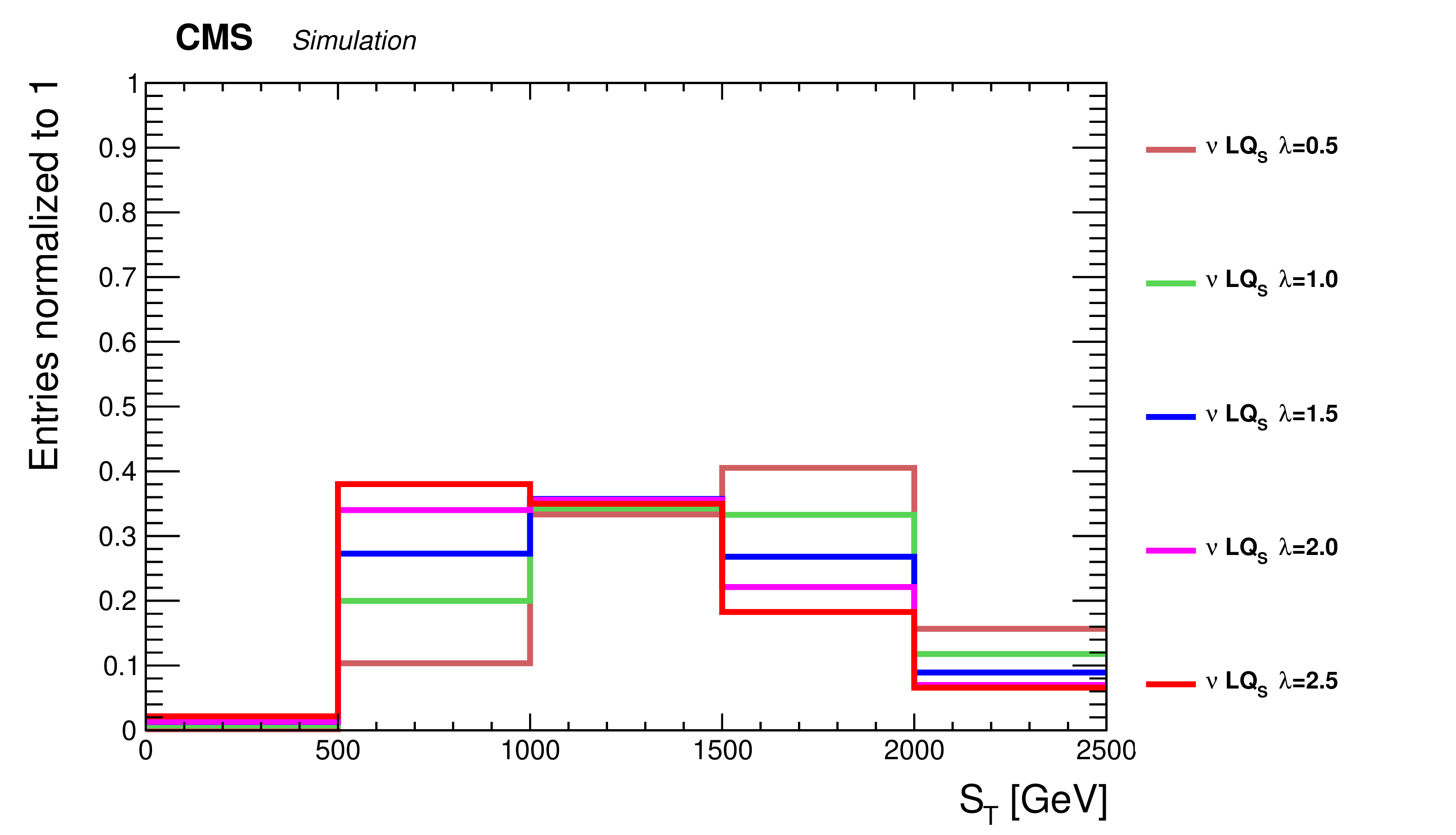
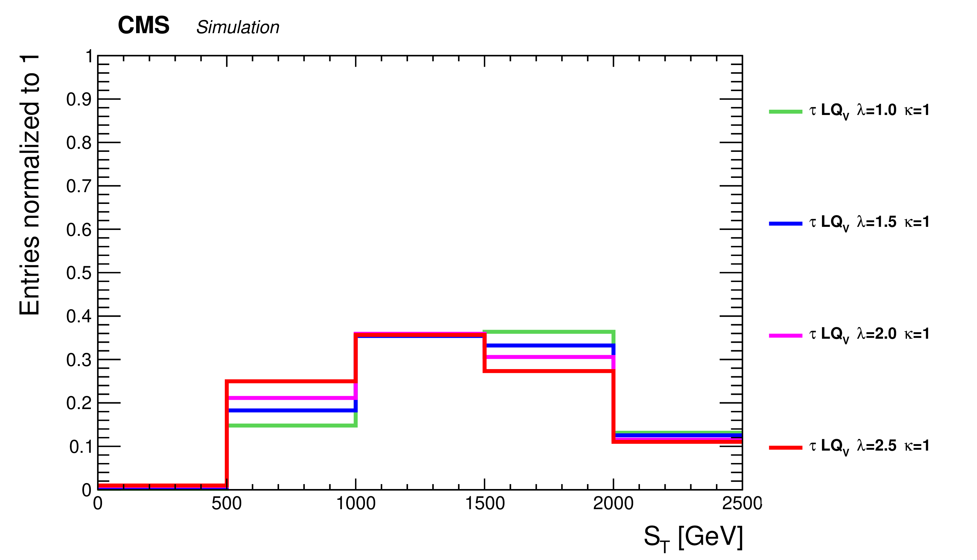
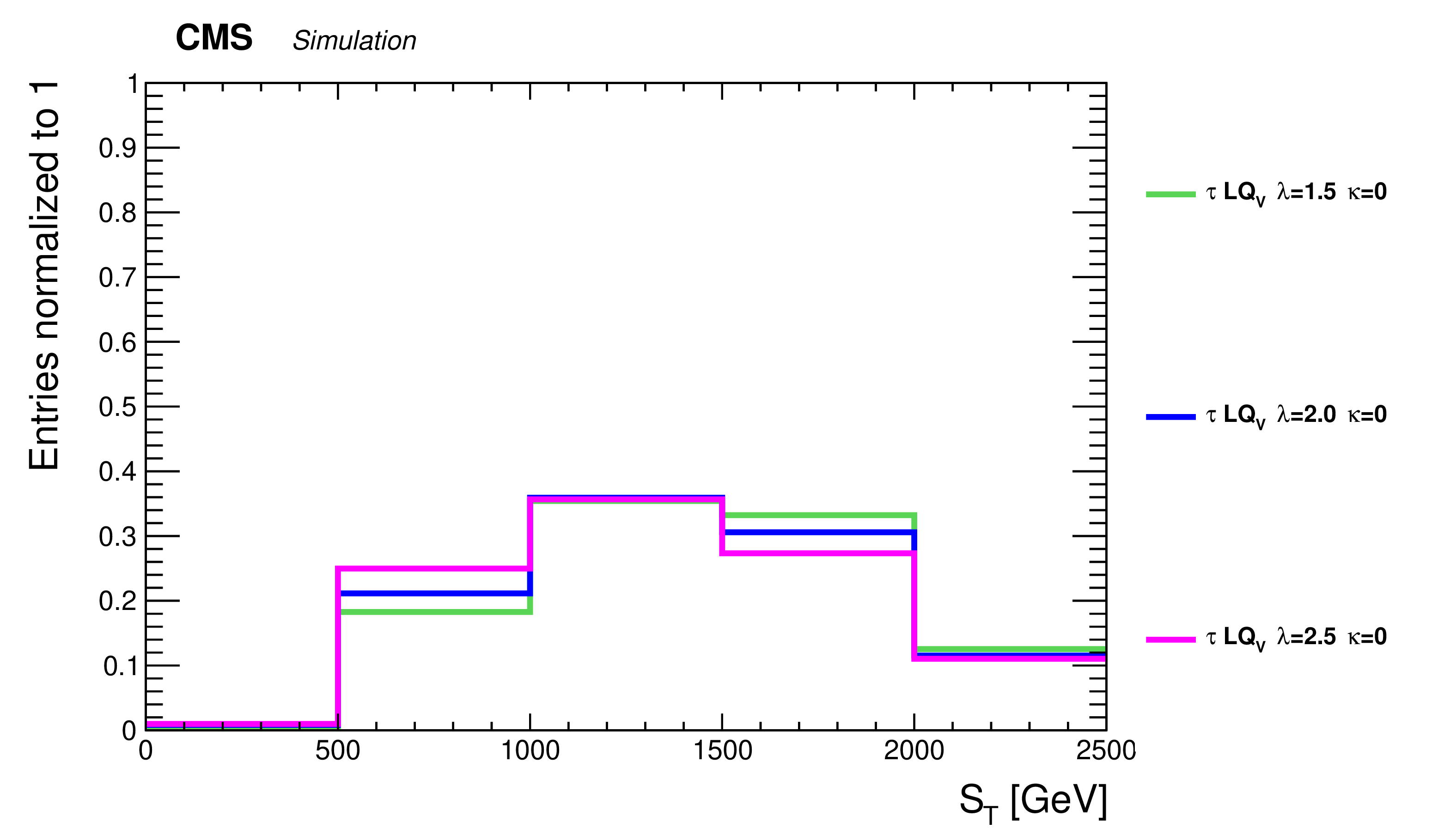
Additional Figure 5:
${S_{\rm {T}}}$ distribution for a singly produced leptoquark with mass equal to 0.8 TeV, for scalar leptoquark (left), vector leptoquark with k = 1 (center), and vector leptoquark with k = 0 (right). The events are selected using the requirements sought in the search region specified in the main text, including all the events that enter the top and b jet categories. |
png pdf |
Additional Figure 5-a:
${S_{\rm {T}}}$ distribution for a singly produced leptoquark with mass equal to 0.8 TeV, for scalar leptoquark. The events are selected using the requirements sought in the search region specified in the main text, including all the events that enter the top and b jet categories. |
png pdf |
Additional Figure 5-b:
${S_{\rm {T}}}$ distribution for a singly produced leptoquark with mass equal to 0.8 TeV, for vector leptoquark with k = 1. The events are selected using the requirements sought in the search region specified in the main text, including all the events that enter the top and b jet categories. |
png pdf |
Additional Figure 5-c:
${S_{\rm {T}}}$ distribution for a singly produced leptoquark with mass equal to 0.8 TeV, for vector leptoquark with k = 0. The events are selected using the requirements sought in the search region specified in the main text, including all the events that enter the top and b jet categories. |
png pdf |
Additional Figure 6:
${S_{\rm {T}}}$ distribution for a singly produced leptoquark with mass equal to 1.7 TeV, for scalar leptoquark (left), vector leptoquark with k = 1 (center), and vector leptoquark with k = 0 (right). The events are selected using the requirements sought in the search region specified in the main text, including all the events that enter the top and b jet categories. |
png pdf |
Additional Figure 6-a:
${S_{\rm {T}}}$ distribution for a singly produced leptoquark with mass equal to 1.7 TeV, for scalar leptoquark. The events are selected using the requirements sought in the search region specified in the main text, including all the events that enter the top and b jet categories. |
png pdf |
Additional Figure 6-b:
${S_{\rm {T}}}$ distribution for a singly produced leptoquark with mass equal to 1.7 TeV, for vector leptoquark with k = 1. The events are selected using the requirements sought in the search region specified in the main text, including all the events that enter the top and b jet categories. |
png pdf |
Additional Figure 6-c:
${S_{\rm {T}}}$ distribution for a singly produced leptoquark with mass equal to 1.7 TeV, for vector leptoquark with k = 0. The events are selected using the requirements sought in the search region specified in the main text, including all the events that enter the top and b jet categories. |
| Additional Tables | |

png pdf |
Additional Table 1:
Pair leptoquark signal selection efficiency relative to each requirement sought in the analysis, including all the events that enter the top and b jet categories defined in the search. The signal samples contain all the final states that can originate from the leptoquark decays to a top quark plus a neutrino or a bottom quark plus a tau lepton, having the leptoquark decay a branching fraction of 0.5 to each fermion pair. |
png pdf |
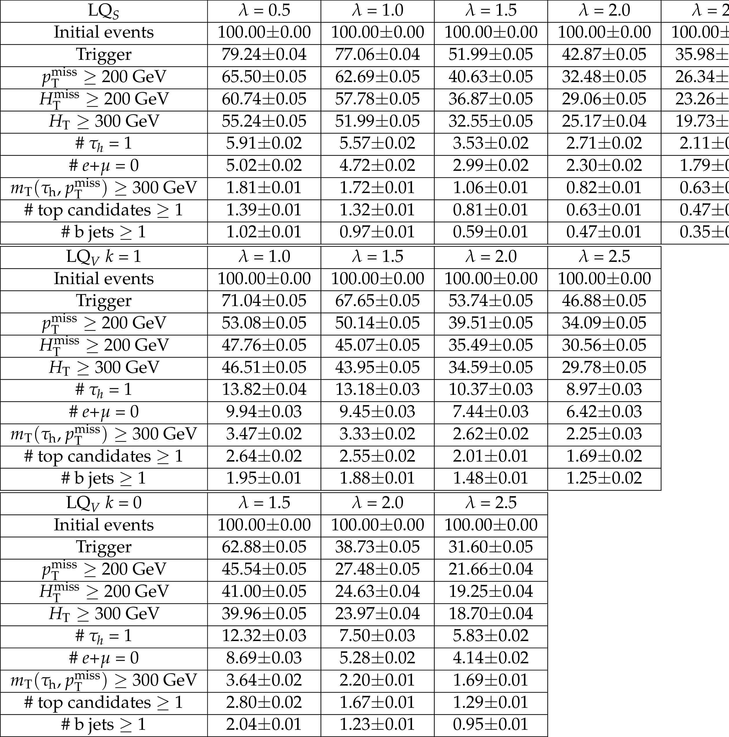
Additional Table 2:
Single leptoquark signal selection efficiency relative to each requirement sought in the analysis, including all the events that enter the top and b jet categories defined in the search, for a leptoquark mass of 0.8 TeV and different hypotheses: scalar leptoquark (LQ$_{S}$, upper), vector leptoquark (LQ$_{V}$) with k = 1 (center), and LQ$_{V}$ with k = 0 (lower). The signal samples contain all the final states that can originate from the leptoquark decays to a top quark plus a neutrino or a bottom quark plus a tau lepton (LQ$_{V}$), or else a top quark plus a tau lepton or a bottom quark plus a neutrino (LQ$_{S}$), having the leptoquark decay a branching fraction of 0.5 to each fermion pair. |
png pdf |
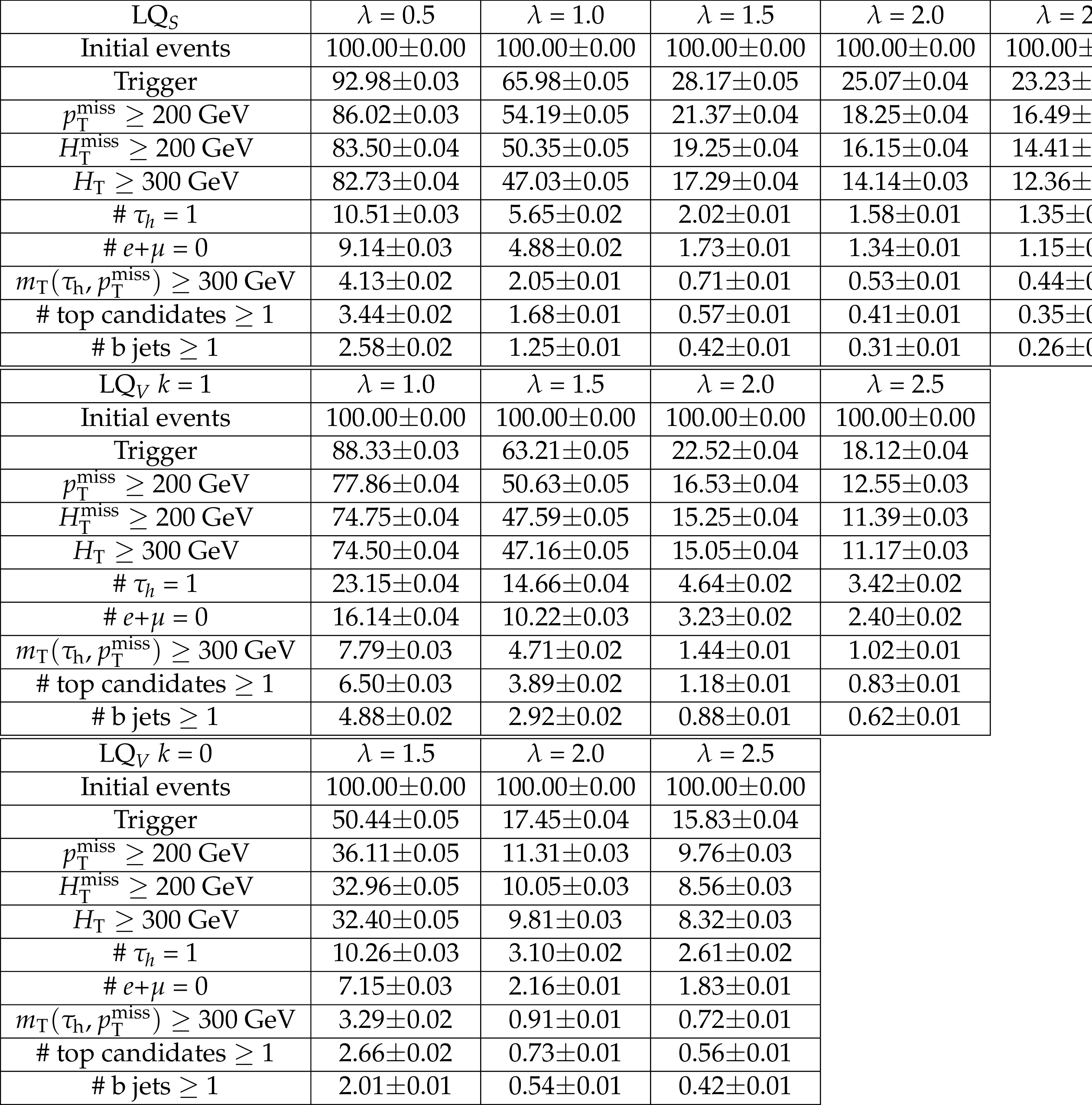
Additional Table 3:
Single leptoquark signal selection efficiency relative to each requirement sought in the analysis, including all the events that enter the top and b jet categories defined in the search, for a leptoquark mass of 1.7 TeV and different hypotheses: scalar leptoquark (LQ$_{S}$, upper), vector leptoquark (LQ$_{V}$) with k = 1 (center), and LQ$_{V}$ with k = 0 (lower). The signal samples contain all the final states that can originate from the leptoquark decays to a top quark plus a neutrino or a bottom quark plus a tau lepton (LQ$_{V}$), or else a top quark plus a tau lepton or a bottom quark plus a neutrino (LQ$_{S}$), having the leptoquark decay a branching fraction of 0.5 to each fermion pair. |
| References | ||||
| 1 | J. C. Pati and A. Salam | Unified lepton-hadron symmetry and a gauge theory of the basic interactions | PRD 8 (1973) 1240 | |
| 2 | J. C. Pati and A. Salam | Lepton number as the fourth color | PRD 10 (1974) 275, . [Erratum: \DOI10.1103/PhysRevD.11.703.2] | |
| 3 | H. Georgi and S. L. Glashow | Unity of all elementary particle forces | PRL 32 (1974) 438 | |
| 4 | H. Fritzsch and P. Minkowski | Unified interactions of leptons and hadrons | Ann. Phys. 93 (1975) 193 | |
| 5 | S. Dimopoulos and L. Susskind | Mass without scalars | NPB 155 (1979) 237 | |
| 6 | S. Dimopoulos | Technicolored signatures | NPB 168 (1980) 69 | |
| 7 | E. Farhi and L. Susskind | Technicolor | PR 74 (1981) 277 | |
| 8 | K. D. Lane and M. V. Ramana | Walking technicolor signatures at hadron colliders | PRD 44 (1991) 2678 | |
| 9 | B. Schrempp and F. Schrempp | Light leptoquarks | PLB 153 (1985) 101 | |
| 10 | B. Gripaios | Composite leptoquarks at the LHC | JHEP 02 (2010) 045 | 0910.1789 |
| 11 | G. R. Farrar and P. Fayet | Phenomenology of the production, decay, and detection of new hadronic states associated with supersymmetry | PLB 76 (1978) 575 | |
| 12 | P. Ramond | Dual theory for free fermions | PRD 3 (1971) 2415 | |
| 13 | Y. A. Golfand and E. P. Likhtman | Extension of the algebra of Poincar$ \'e $ group generators and violation of p invariance | JEPTL 13 (1971)323 | |
| 14 | A. Neveu and J. H. Schwarz | Factorizable dual model of pions | NPB 31 (1971) 86 | |
| 15 | D. V. Volkov and V. P. Akulov | Possible universal neutrino interaction | JEPTL 16 (1972)438 | |
| 16 | J. Wess and B. Zumino | A Lagrangian model invariant under supergauge transformations | PLB 49 (1974) 52 | |
| 17 | J. Wess and B. Zumino | Supergauge transformations in four dimensions | NPB 70 (1974) 39 | |
| 18 | P. Fayet | Supergauge invariant extension of the Higgs mechanism and a model for the electron and its neutrino | NPB 90 (1975) 104 | |
| 19 | H. P. Nilles | Supersymmetry, supergravity and particle physics | PR 110 (1984) 1 | |
| 20 | R. Barbier et al. | R-parity violating supersymmetry | PR 420 (2005) 1 | hep-ph/0406039 |
| 21 | BaBar Collaboration | Evidence for an excess of $ \bar{B} \to D^{(*)} \tau^-\bar{\nu}_\tau $ decays | PRL 109 (2012) 101802 | 1205.5442 |
| 22 | BaBar Collaboration | Measurement of an Excess of $ \bar{B} \to D^{(*)}\tau^- \bar{\nu}_\tau $ Decays and Implications for Charged Higgs Bosons | PRD88 (2013), no. 7, 072012 | 1303.0571 |
| 23 | Belle Collaboration | Measurement of the branching ratio of $ \bar{B} \to D^{(\ast)} \tau^- \bar{\nu}_\tau $ relative to $ \bar{B} \to D^{(\ast)} \ell^- \bar{\nu}_\ell $ decays with hadronic tagging at Belle | PRD92 (2015), no. 7, 072014 | 1507.03233 |
| 24 | Belle Collaboration | Measurement of the branching ratio of $ \bar{B}^0 \rightarrow D^{*+} \tau^- \bar{\nu}_{\tau} $ relative to $ \bar{B}^0 \rightarrow D^{*+} \ell^- \bar{\nu}_{\ell} $ decays with a semileptonic tagging method | PRD94 (2016), no. 7, 072007 | 1607.07923 |
| 25 | Belle Collaboration | Measurement of the $ \tau $ lepton polarization and $ R(D^*) $ in the decay $ \bar{B} \to D^* \tau^- \bar{\nu}_\tau $ | PRL 118 (2017), no. 21, 211801 | 1612.00529 |
| 26 | Belle Collaboration | Measurement of the $ \tau $ lepton polarization and $ R(D^*) $ in the decay $ \bar{B} \rightarrow D^* \tau^- \bar{\nu}_\tau $ with one-prong hadronic $ \tau $ decays at Belle | PRD97 (2018), no. 1, 012004 | 1709.00129 |
| 27 | Belle Collaboration | Measurement of $ \mathcal{R}(D) $ and $ \mathcal{R}(D^{\ast}) $ with a semileptonic tagging method | 1904.08794 | |
| 28 | Belle Collaboration | Measurement of $ \mathcal{R}(D) $ and $ \mathcal{R}(D^*) $ with a semileptonic tagging method | PRL 124 (2020), no. 16, 161803 | 1910.05864 |
| 29 | LHCb Collaboration | Measurement of the ratio of branching fractions $ \mathcal{B}(\bar{B}^0 \to D^{*+}\tau^{-}\bar{\nu}_{\tau})/\mathcal{B}(\bar{B}^0 \to D^{*+}\mu^{-}\bar{\nu}_{\mu}) $ | PRL 115 (2015), no. 11, 111803 | 1506.08614 |
| 30 | LHCb Collaboration | Measurement of the ratio of the $ B^0 \to D^{*-} \tau^+ \nu_{\tau} $ and $ B^0 \to D^{*-} \mu^+ \nu_{\mu} $ branching fractions using three-prong $ \tau $-lepton decays | PRL 120 (2018), no. 17, 171802 | 1708.08856 |
| 31 | LHCb Collaboration | Measurement of the ratio of branching fractions $ \mathcal{B}(B_c^+ \to J/\psi\tau^+\nu_\tau) $/$ \mathcal{B}(B_c^+ \to J/\psi\mu^+\nu_\mu) $ | PRL 120 (2018), no. 12, 121801 | 1711.05623 |
| 32 | Belle Collaboration | Lepton-Flavor-Dependent Angular Analysis of $ B\to K^\ast \ell^+\ell^- $ | PRL 118 (2017), no. 11, 111801 | 1612.05014 |
| 33 | Belle Collaboration | Test of lepton flavor universality in $ {B\to K^\ast\ell^+\ell^-} $ decays at Belle | 1904.02440 | |
| 34 | LHCb Collaboration | Measurement of Form-Factor-Independent Observables in the Decay $ B^{0} \to K^{*0} \mu^+ \mu^- $ | PRL 111 (2013) 191801 | 1308.1707 |
| 35 | LHCb Collaboration | Differential branching fractions and isospin asymmetries of $ B \to K^{(*)} \mu^+ \mu^- $ decays | JHEP 06 (2014) 133 | 1403.8044 |
| 36 | LHCb Collaboration | Test of lepton universality using $ B^{+}\rightarrow K^{+}\ell^{+}\ell^{-} $ decays | PRL 113 (2014) 151601 | 1406.6482 |
| 37 | LHCb Collaboration | Angular analysis of the $ B^{0} \to K^{*0} \mu^{+} \mu^{-} $ decay using 3 fb$ ^{-1} $ of integrated luminosity | JHEP 02 (2016) 104 | 1512.04442 |
| 38 | LHCb Collaboration | Angular analysis and differential branching fraction of the decay $ B^0_s\to\phi\mu^+\mu^- $ | JHEP 09 (2015) 179 | 1506.08777 |
| 39 | LHCb Collaboration | Test of lepton universality with $ B^{0} \rightarrow K^{*0}\ell^{+}\ell^{-} $ decays | JHEP 08 (2017) 055 | 1705.05802 |
| 40 | LHCb Collaboration | Search for lepton-universality violation in $ B^+\to K^+\ell^+\ell^- $ decays | PRL 122 (2019), no. 19, 191801 | 1903.09252 |
| 41 | E. Alvarez et al. | A composite pNGB leptoquark at the LHC | JHEP 12 (2018) 027 | 1808.02063 |
| 42 | D. Buttazzo, A. Greljo, G. Isidori, and D. Marzocca | B-physics anomalies: a guide to combined explanations | JHEP 11 (2017) 044 | 1706.07808 |
| 43 | W. Buchmuller, R. Ruckl, and D. Wyler | Leptoquarks in lepton-quark collisions | PLB 191 (1987) 442, . [Erratum: \DOI10.1016/S0370-2693(99)00014-3] | |
| 44 | I. Dorsner and A. Greljo | Leptoquark toolbox for precision collider studies | JHEP 05 (2018) 126 | 1801.07641 |
| 45 | ATLAS Collaboration | Search for third generation scalar leptoquarks in pp collisions at $ \sqrt{s} = $ 7 TeV with the ATLAS detector | JHEP 06 (2013) 033 | 1303.0526 |
| 46 | ATLAS Collaboration | Searches for third-generation scalar leptoquarks in $ \sqrt{s} = $ 13 TeV pp collisions with the ATLAS detector | JHEP 06 (2019) 144 | 1902.08103 |
| 47 | CMS Collaboration | Constraints on models of scalar and vector leptoquarks decaying to a quark and a neutrino at $ \sqrt{s}= $ 13 TeV | PRD98 (2018), no. 3, 032005 | CMS-SUS-18-001 1805.10228 |
| 48 | CMS Collaboration | Search for third-generation scalar leptoquarks decaying to a top quark and a $ \tau $ lepton at $ \sqrt{s}= $ 13 TeV | EPJC78 (2018) 707 | CMS-B2G-16-028 1803.02864 |
| 49 | CMS Collaboration | Search for leptoquarks coupled to third-generation quarks in proton-proton collisions at $ \sqrt{s}= $ 13 TeV | PRL 121 (2018), no. 24, 241802 | CMS-B2G-16-027 1809.05558 |
| 50 | CMS Collaboration | Search for heavy neutrinos and third-generation leptoquarks in hadronic states of two $ \tau $ leptons and two jets in proton-proton collisions at $ \sqrt{s} = $ 13 TeV | JHEP 03 (2019) 170 | CMS-EXO-17-016 1811.00806 |
| 51 | CMS Collaboration | Search for a singly produced third-generation scalar leptoquark decaying to a $ \tau $ lepton and a bottom quark in proton-proton collisions at $ \sqrt{s} = $ 13 TeV | JHEP 07 (2018) 115 | CMS-EXO-17-029 1806.03472 |
| 52 | CMS Collaboration | The CMS experiment at the CERN LHC | JINST 3 (2008) S08004 | CMS-00-001 |
| 53 | J. Alwall et al. | The automated computation of tree-level and next-to-leading order differential cross sections, and their matching to parton shower simulations | JHEP 07 (2014) 079 | 1405.0301 |
| 54 | P. Nason | A new method for combining NLO QCD with shower Monte Carlo algorithms | JHEP 11 (2004) 040 | hep-ph/0409146 |
| 55 | S. Frixione, P. Nason, and C. Oleari | Matching NLO QCD computations with Parton Shower simulations: the POWHEG method | JHEP 11 (2007) 070 | 0709.2092 |
| 56 | S. Alioli, P. Nason, C. Oleari, and E. Re | A general framework for implementing NLO calculations in shower Monte Carlo programs: the POWHEG BOX | JHEP 06 (2010) 043 | 1002.2581 |
| 57 | S. Alioli, S.-O. Moch, and P. Uwer | Hadronic top-quark pair-production with one jet and parton showering | JHEP 01 (2012) 137 | 1110.5251 |
| 58 | T. Sjostrand et al. | An introduction to PYTHIA 8.2 | CPC 191 (2015) 159 | 1410.3012 |
| 59 | CMS Collaboration | Extraction and validation of a new set of CMS PYTHIA8 tunes from underlying-event measurements | CMS-GEN-17-001 1903.12179 |
|
| 60 | CMS Collaboration | Event generator tunes obtained from underlying event and multiparton scattering measurements | EPJC76 (2016), no. 3, 155 | CMS-GEN-14-001 1512.00815 |
| 61 | CMS Collaboration Collaboration | Investigations of the impact of the parton shower tuning in Pythia 8 in the modelling of $ \mathrm{t\overline{t}} $ at $ \sqrt{s}= $ 8 and 13 TeV | CMS-PAS-TOP-16-021, CERN, Geneva | |
| 62 | NNPDF Collaboration | Parton distributions from high-precision collider data | EPJC77 (2017), no. 10, 663 | 1706.00428 |
| 63 | NNPDF Collaboration | Parton distributions for the LHC run II | JHEP 04 (2015) 040 | 1410.8849 |
| 64 | CMS Collaboration | Particle-flow reconstruction and global event description with the CMS detector | JINST 12 (2017), no. 10, P10003 | CMS-PRF-14-001 1706.04965 |
| 65 | M. Cacciari, G. P. Salam, and G. Soyez | The anti-$ k_t $ jet clustering algorithm | JHEP 04 (2008) 063 | 0802.1189 |
| 66 | S. D. Ellis, C. K. Vermilion, and J. R. Walsh | Techniques for improved heavy particle searches with jet substructure | PRD 80 (2009) 051501 | 0903.5081 |
| 67 | CMS Collaboration | Identification techniques for highly boosted W bosons that decay into hadrons | JHEP 12 (2014) 017 | CMS-JME-13-006 1410.4227 |
| 68 | M. Dasgupta, A. Fregoso, S. Marzani, and G. P. Salam | Towards an understanding of jet substructure | JHEP 09 (2013) 029 | 1307.0007 |
| 69 | A. J. Larkoski, S. Marzani, G. Soyez, and J. Thaler | Soft Drop | JHEP 05 (2014) 146 | 1402.2657 |
| 70 | CMS Collaboration | Performance of reconstruction and identification of $ \tau $ leptons decaying to hadrons and $ \nu_\tau $ in pp collisions at $ \sqrt{s}= $ 13 TeV | JINST 13 (2018) P10005 | CMS-TAU-16-003 1809.02816 |
| 71 | CMS Collaboration | Identification of heavy-flavour jets with the CMS detector in pp collisions at 13 TeV | JINST 13 (2018), no. 05, P05011 | CMS-BTV-16-002 1712.07158 |
| 72 | CMS Collaboration | Performance of electron reconstruction and selection with the CMS detector in proton-proton collisions at $ \sqrt{s} = $ 8 TeV | JINST 10 (2015) P06005 | CMS-EGM-13-001 1502.02701 |
| 73 | CMS Collaboration | Performance of CMS muon reconstruction in pp collision events at $ \sqrt{s} = $ 7 TeV | JINST 7 (2012) P10002 | CMS-MUO-10-004 1206.4071 |
| 74 | ATLAS Collaboration | Measurement of the Inelastic Proton-Proton Cross Section at $ \sqrt{s} = $ 13 TeV with the ATLAS Detector at the LHC | PRL 117 (2016) 182002 | 1606.02625 |
| 75 | J. Butterworth et al. | PDF4LHC recommendations for LHC Run II | JPG 43 (2016) 023001 | 1510.03865 |
| 76 | CMS Collaboration | CMS luminosity measurement for the 2016 data-taking period | CMS-PAS-LUM-15-001 | CMS-PAS-LUM-15-001 |
| 77 | CMS Collaboration | CMS luminosity measurement for the 2017 data-taking period at $ \sqrt{s} = $ 13 TeV | CMS-PAS-LUM-17-004 | CMS-PAS-LUM-17-004 |
| 78 | CMS Collaboration | CMS luminosity measurement for the 2018 data-taking period at $ \sqrt{s} = $ 13 TeV | CMS-PAS-LUM-18-002 | CMS-PAS-LUM-18-002 |
| 79 | A. L. Read | Presentation of search results: the $ \rm CL_s $ technique | JPG 28 (2002) 2693 | |
| 80 | T. Junk | Confidence level computation for combining searches with small statistics | NIMA 434 (1999) 435 | hep-ex/9902006 |
| 81 | I. Dorsner et al. | Physics of leptoquarks in precision experiments and at particle colliders | PR 641 (2016) 1--68 | 1603.04993 |
|
|
Compact Muon Solenoid LHC, CERN |
|

|

|

|

|

|