

Compact Muon Solenoid
LHC, CERN
| CMS-TOP-23-007 ; CERN-EP-2024-231 | ||
| Measurements of polarization and spin correlation and observation of entanglement in top quark pairs using lepton+jets events from proton-proton collisions at $ \sqrt{s}= $ 13 TeV | ||
| CMS Collaboration | ||
| 17 September 2024 | ||
| Phys. Rev. D 110 (2024) 112016 | ||
| Abstract: Measurements of the polarization and spin correlation in top quark pairs ($ \mathrm{t} \overline{\mathrm{t}} $) are presented using events with a single electron or muon and jets in the final state. The measurements are based on proton-proton collision data from the LHC at $ \sqrt{s}= $ 13 TeV collected by the CMS experiment, corresponding to an integrated luminosity of 138 fb$ ^{-1} $. All coefficients of the polarization vectors and the spin correlation matrix are extracted simultaneously by performing a binned likelihood fit to the data. The measurement is performed inclusively and in bins of additional observables, such as the mass of the $ \mathrm{t} \overline{\mathrm{t}} $ system and the top quark scattering angle in the $ \mathrm{t} \overline{\mathrm{t}} $ rest frame. The measured polarization and spin correlation are in agreement with the standard model. From the measured spin correlation, conclusions on the $ \mathrm{t} \overline{\mathrm{t}} $ spin entanglement are drawn by applying the Peres-Horodecki criterion. The standard model predicts entangled spins for $ \mathrm{t} \overline{\mathrm{t}} $ states at the production threshold and at high masses of the $ \mathrm{t} \overline{\mathrm{t}} $ system. Entanglement is observed for the first time in events at high $ \mathrm{t} \overline{\mathrm{t}} $ mass, where a large fraction of the $ \mathrm{t} \overline{\mathrm{t}} $ decays are space-like separated, with an expected and observed significance of above 5 standard deviations. | ||
| Links: e-print arXiv:2409.11067 [hep-ex] (PDF) ; CDS record ; inSPIRE record ; HepData record ; Physics Briefing ; CADI line (restricted) ; | ||
| Figures | Summary | Additional Figures | References | CMS Publications |
|---|
| Figures | |

png pdf |
Figure 1:
Distribution of $ S_{\text{NN}} $ in the 2 b (left) and 1 b (right) categories. The data (points) are compared to the prediction (stacked histograms). The $ \mathrm{t} \overline{\mathrm{t}} $ contribution is split into the correctly and incorrectly reconstructed, ``nonreconstructable'', and non $ \mathrm{e}/\mu $+jets events. The gray uncertainty band indicates the combined statistical and systematic uncertainties in the prediction, while the vertical bars on the points show the statistical uncertainty of the data. The ratios of data to the predicted yields are provided in the lower panels. |

png pdf |
Figure 1-a:
Distribution of $ S_{\text{NN}} $ in the 2 b (left) and 1 b (right) categories. The data (points) are compared to the prediction (stacked histograms). The $ \mathrm{t} \overline{\mathrm{t}} $ contribution is split into the correctly and incorrectly reconstructed, ``nonreconstructable'', and non $ \mathrm{e}/\mu $+jets events. The gray uncertainty band indicates the combined statistical and systematic uncertainties in the prediction, while the vertical bars on the points show the statistical uncertainty of the data. The ratios of data to the predicted yields are provided in the lower panels. |

png pdf |
Figure 1-b:
Distribution of $ S_{\text{NN}} $ in the 2 b (left) and 1 b (right) categories. The data (points) are compared to the prediction (stacked histograms). The $ \mathrm{t} \overline{\mathrm{t}} $ contribution is split into the correctly and incorrectly reconstructed, ``nonreconstructable'', and non $ \mathrm{e}/\mu $+jets events. The gray uncertainty band indicates the combined statistical and systematic uncertainties in the prediction, while the vertical bars on the points show the statistical uncertainty of the data. The ratios of data to the predicted yields are provided in the lower panels. |

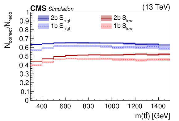
png pdf |
Figure 2:
Reconstruction efficiency of the NN (left) and the fraction of correctly reconstructed events (right) as a function of $ m({\mathrm{t}\overline{\mathrm{t}}} ) $ estimated from the simulation. The values are shown separately for the 1 b and 2 b categories with the $ S_{\text{low}} $ and $ S_{\text{high}} $ selections. The event counts $ N_{\text{correct}} $ and $ N_{\text{reco}} $ refer to the number of correctly reconstructed and ``reconstructable'' $ \mathrm{t} \overline{\mathrm{t}} $ events, respectively. All reconstructed events regardless of the process are labeled $ N_{\text{all}} $. The uncertainty bands include all systematic uncertainties as detailed in Section 9. |
png pdf |
Figure 2-a:
Reconstruction efficiency of the NN (left) and the fraction of correctly reconstructed events (right) as a function of $ m({\mathrm{t}\overline{\mathrm{t}}} ) $ estimated from the simulation. The values are shown separately for the 1 b and 2 b categories with the $ S_{\text{low}} $ and $ S_{\text{high}} $ selections. The event counts $ N_{\text{correct}} $ and $ N_{\text{reco}} $ refer to the number of correctly reconstructed and ``reconstructable'' $ \mathrm{t} \overline{\mathrm{t}} $ events, respectively. All reconstructed events regardless of the process are labeled $ N_{\text{all}} $. The uncertainty bands include all systematic uncertainties as detailed in Section 9. |

png pdf |
Figure 2-b:
Reconstruction efficiency of the NN (left) and the fraction of correctly reconstructed events (right) as a function of $ m({\mathrm{t}\overline{\mathrm{t}}} ) $ estimated from the simulation. The values are shown separately for the 1 b and 2 b categories with the $ S_{\text{low}} $ and $ S_{\text{high}} $ selections. The event counts $ N_{\text{correct}} $ and $ N_{\text{reco}} $ refer to the number of correctly reconstructed and ``reconstructable'' $ \mathrm{t} \overline{\mathrm{t}} $ events, respectively. All reconstructed events regardless of the process are labeled $ N_{\text{all}} $. The uncertainty bands include all systematic uncertainties as detailed in Section 9. |

png pdf |
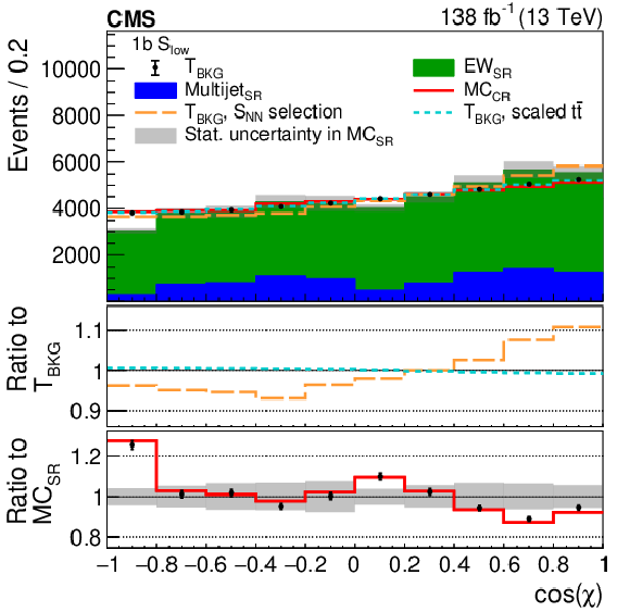
Figure 3:
Comparison of the $ \cos(\chi) $ (left) and $ m({\mathrm{t}\overline{\mathrm{t}}} ) $ (right) distributions of the simulated background in the control region ($ \text{MC}_{\text{CR}} $) shown as the red line, and in the $1\mathrm{b} S_{\text{low}}$ signal region ($ \text{MC}_{\text{SR}} $) shown as the stacked histograms of the multijet and EW components. The estimated background template ($ \text{T}_{\text{BKG}} $) shown as black markers corresponds to the data distribution in the CR after subtracting the predicted $ \mathrm{t} \overline{\mathrm{t}} $ and single top quark contributions. Variations of the $ \text{T}_{\text{BKG}} $ are obtained applying the additional $ S_{\text{NN}} $ selection for the $1\mathrm{b} S_{\text{low}}$ category (orange line) and by taking into account the mismatch of the normalization in the CR when subtracting the $ \mathrm{t} \overline{\mathrm{t}} $ and single top quark contributions (blue line). All distributions are normalized to the event yields predicted by the $ \text{MC}_{\text{SR}} $. The gray uncertainty band shows the statistical uncertainties in the $ \text{MC}_{\text{SR}} $. The middle panels show the relative effects of the $ \text{T}_{\text{BKG}} $ variations. The lower panels show the ratio of the $ \text{MC}_{\text{CR}} $ and the $ \text{T}_{\text{BKG}} $ to the $ \text{MC}_{\text{SR}} $. |
png pdf |
Figure 3-a:
Comparison of the $ \cos(\chi) $ (left) and $ m({\mathrm{t}\overline{\mathrm{t}}} ) $ (right) distributions of the simulated background in the control region ($ \text{MC}_{\text{CR}} $) shown as the red line, and in the $1\mathrm{b} S_{\text{low}}$ signal region ($ \text{MC}_{\text{SR}} $) shown as the stacked histograms of the multijet and EW components. The estimated background template ($ \text{T}_{\text{BKG}} $) shown as black markers corresponds to the data distribution in the CR after subtracting the predicted $ \mathrm{t} \overline{\mathrm{t}} $ and single top quark contributions. Variations of the $ \text{T}_{\text{BKG}} $ are obtained applying the additional $ S_{\text{NN}} $ selection for the $1\mathrm{b} S_{\text{low}}$ category (orange line) and by taking into account the mismatch of the normalization in the CR when subtracting the $ \mathrm{t} \overline{\mathrm{t}} $ and single top quark contributions (blue line). All distributions are normalized to the event yields predicted by the $ \text{MC}_{\text{SR}} $. The gray uncertainty band shows the statistical uncertainties in the $ \text{MC}_{\text{SR}} $. The middle panels show the relative effects of the $ \text{T}_{\text{BKG}} $ variations. The lower panels show the ratio of the $ \text{MC}_{\text{CR}} $ and the $ \text{T}_{\text{BKG}} $ to the $ \text{MC}_{\text{SR}} $. |

png pdf |
Figure 3-b:
Comparison of the $ \cos(\chi) $ (left) and $ m({\mathrm{t}\overline{\mathrm{t}}} ) $ (right) distributions of the simulated background in the control region ($ \text{MC}_{\text{CR}} $) shown as the red line, and in the $1\mathrm{b} S_{\text{low}}$ signal region ($ \text{MC}_{\text{SR}} $) shown as the stacked histograms of the multijet and EW components. The estimated background template ($ \text{T}_{\text{BKG}} $) shown as black markers corresponds to the data distribution in the CR after subtracting the predicted $ \mathrm{t} \overline{\mathrm{t}} $ and single top quark contributions. Variations of the $ \text{T}_{\text{BKG}} $ are obtained applying the additional $ S_{\text{NN}} $ selection for the $1\mathrm{b} S_{\text{low}}$ category (orange line) and by taking into account the mismatch of the normalization in the CR when subtracting the $ \mathrm{t} \overline{\mathrm{t}} $ and single top quark contributions (blue line). All distributions are normalized to the event yields predicted by the $ \text{MC}_{\text{SR}} $. The gray uncertainty band shows the statistical uncertainties in the $ \text{MC}_{\text{SR}} $. The middle panels show the relative effects of the $ \text{T}_{\text{BKG}} $ variations. The lower panels show the ratio of the $ \text{MC}_{\text{CR}} $ and the $ \text{T}_{\text{BKG}} $ to the $ \text{MC}_{\text{SR}} $. |
png pdf |
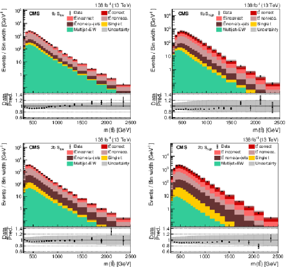
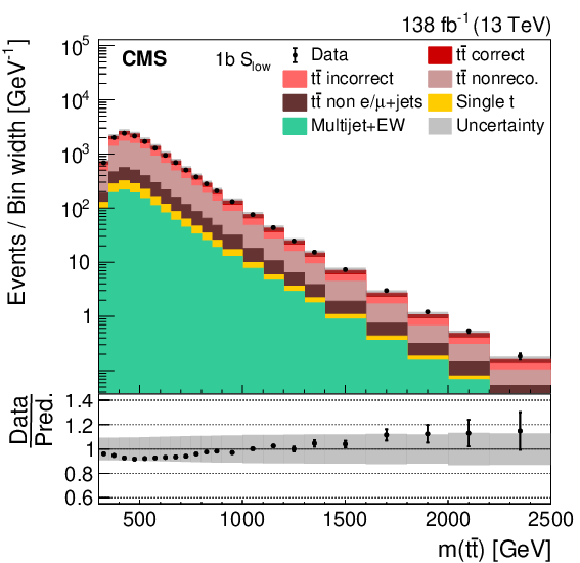
Figure 4:
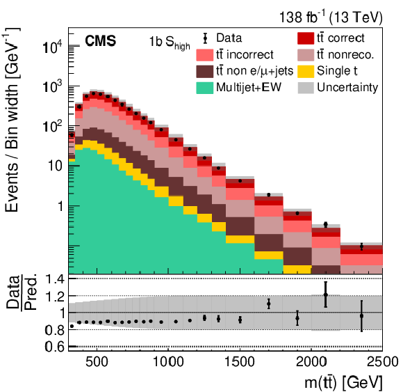
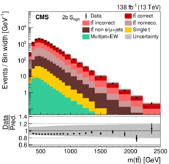
Distribution of $ m({\mathrm{t}\overline{\mathrm{t}}} ) $ in all four categories. The data (points) are compared to the prediction (stacked histograms). The $ \mathrm{t} \overline{\mathrm{t}} $ and single top quark contributions are taken from the simulation, while the multijet+EW background is obtained from the CR. The $ \mathrm{t} \overline{\mathrm{t}} $ contribution is split into the correctly and incorrectly reconstructed, ``nonreconstructable'', and non $ \mathrm{e}/\mu $+jets events. The gray uncertainty band indicates the combined statistical and systematic uncertainties in the prediction. The vertical bars on the points show the statistical uncertainty of the data. Ratios to the predicted yields are provided in the lower panels. |
png pdf |
Figure 4-a:
Distribution of $ m({\mathrm{t}\overline{\mathrm{t}}} ) $ in all four categories. The data (points) are compared to the prediction (stacked histograms). The $ \mathrm{t} \overline{\mathrm{t}} $ and single top quark contributions are taken from the simulation, while the multijet+EW background is obtained from the CR. The $ \mathrm{t} \overline{\mathrm{t}} $ contribution is split into the correctly and incorrectly reconstructed, ``nonreconstructable'', and non $ \mathrm{e}/\mu $+jets events. The gray uncertainty band indicates the combined statistical and systematic uncertainties in the prediction. The vertical bars on the points show the statistical uncertainty of the data. Ratios to the predicted yields are provided in the lower panels. |
png pdf |
Figure 4-b:
Distribution of $ m({\mathrm{t}\overline{\mathrm{t}}} ) $ in all four categories. The data (points) are compared to the prediction (stacked histograms). The $ \mathrm{t} \overline{\mathrm{t}} $ and single top quark contributions are taken from the simulation, while the multijet+EW background is obtained from the CR. The $ \mathrm{t} \overline{\mathrm{t}} $ contribution is split into the correctly and incorrectly reconstructed, ``nonreconstructable'', and non $ \mathrm{e}/\mu $+jets events. The gray uncertainty band indicates the combined statistical and systematic uncertainties in the prediction. The vertical bars on the points show the statistical uncertainty of the data. Ratios to the predicted yields are provided in the lower panels. |

png pdf |
Figure 4-c:
Distribution of $ m({\mathrm{t}\overline{\mathrm{t}}} ) $ in all four categories. The data (points) are compared to the prediction (stacked histograms). The $ \mathrm{t} \overline{\mathrm{t}} $ and single top quark contributions are taken from the simulation, while the multijet+EW background is obtained from the CR. The $ \mathrm{t} \overline{\mathrm{t}} $ contribution is split into the correctly and incorrectly reconstructed, ``nonreconstructable'', and non $ \mathrm{e}/\mu $+jets events. The gray uncertainty band indicates the combined statistical and systematic uncertainties in the prediction. The vertical bars on the points show the statistical uncertainty of the data. Ratios to the predicted yields are provided in the lower panels. |
png pdf |
Figure 4-d:
Distribution of $ m({\mathrm{t}\overline{\mathrm{t}}} ) $ in all four categories. The data (points) are compared to the prediction (stacked histograms). The $ \mathrm{t} \overline{\mathrm{t}} $ and single top quark contributions are taken from the simulation, while the multijet+EW background is obtained from the CR. The $ \mathrm{t} \overline{\mathrm{t}} $ contribution is split into the correctly and incorrectly reconstructed, ``nonreconstructable'', and non $ \mathrm{e}/\mu $+jets events. The gray uncertainty band indicates the combined statistical and systematic uncertainties in the prediction. The vertical bars on the points show the statistical uncertainty of the data. Ratios to the predicted yields are provided in the lower panels. |
png pdf |
Figure 5:
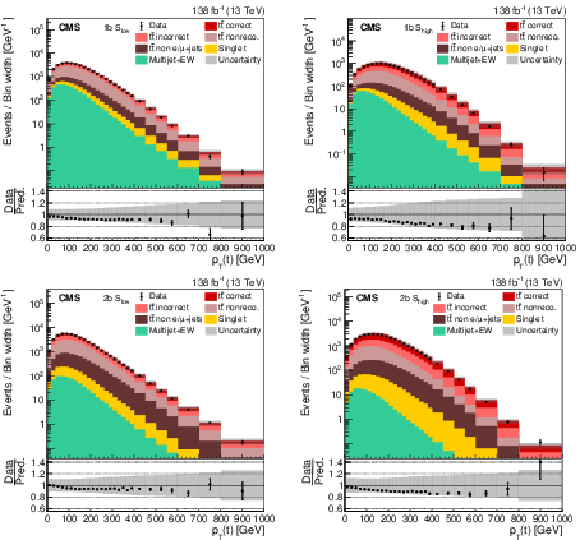
Distribution of $ p_{\mathrm{T}}(\mathrm{t}) $ in all four categories. The data (points) are compared to the prediction (stacked histograms). The $ \mathrm{t} \overline{\mathrm{t}} $ and single top quark contributions are taken from the simulation, while the multijet+EW background is obtained from the CR. The $ \mathrm{t} \overline{\mathrm{t}} $ contribution is split into the correctly and incorrectly reconstructed, ``nonreconstructable'', and non $ \mathrm{e}/\mu $+jets events. The gray uncertainty band indicates the combined statistical and systematic uncertainties in the prediction. The vertical bars on the points show the statistical uncertainty of the data. Ratios to the predicted yields are provided in the lower panels. |

png pdf |
Figure 5-a:
Distribution of $ p_{\mathrm{T}}(\mathrm{t}) $ in all four categories. The data (points) are compared to the prediction (stacked histograms). The $ \mathrm{t} \overline{\mathrm{t}} $ and single top quark contributions are taken from the simulation, while the multijet+EW background is obtained from the CR. The $ \mathrm{t} \overline{\mathrm{t}} $ contribution is split into the correctly and incorrectly reconstructed, ``nonreconstructable'', and non $ \mathrm{e}/\mu $+jets events. The gray uncertainty band indicates the combined statistical and systematic uncertainties in the prediction. The vertical bars on the points show the statistical uncertainty of the data. Ratios to the predicted yields are provided in the lower panels. |

png pdf |
Figure 5-b:
Distribution of $ p_{\mathrm{T}}(\mathrm{t}) $ in all four categories. The data (points) are compared to the prediction (stacked histograms). The $ \mathrm{t} \overline{\mathrm{t}} $ and single top quark contributions are taken from the simulation, while the multijet+EW background is obtained from the CR. The $ \mathrm{t} \overline{\mathrm{t}} $ contribution is split into the correctly and incorrectly reconstructed, ``nonreconstructable'', and non $ \mathrm{e}/\mu $+jets events. The gray uncertainty band indicates the combined statistical and systematic uncertainties in the prediction. The vertical bars on the points show the statistical uncertainty of the data. Ratios to the predicted yields are provided in the lower panels. |

png pdf |
Figure 5-c:
Distribution of $ p_{\mathrm{T}}(\mathrm{t}) $ in all four categories. The data (points) are compared to the prediction (stacked histograms). The $ \mathrm{t} \overline{\mathrm{t}} $ and single top quark contributions are taken from the simulation, while the multijet+EW background is obtained from the CR. The $ \mathrm{t} \overline{\mathrm{t}} $ contribution is split into the correctly and incorrectly reconstructed, ``nonreconstructable'', and non $ \mathrm{e}/\mu $+jets events. The gray uncertainty band indicates the combined statistical and systematic uncertainties in the prediction. The vertical bars on the points show the statistical uncertainty of the data. Ratios to the predicted yields are provided in the lower panels. |

png pdf |
Figure 5-d:
Distribution of $ p_{\mathrm{T}}(\mathrm{t}) $ in all four categories. The data (points) are compared to the prediction (stacked histograms). The $ \mathrm{t} \overline{\mathrm{t}} $ and single top quark contributions are taken from the simulation, while the multijet+EW background is obtained from the CR. The $ \mathrm{t} \overline{\mathrm{t}} $ contribution is split into the correctly and incorrectly reconstructed, ``nonreconstructable'', and non $ \mathrm{e}/\mu $+jets events. The gray uncertainty band indicates the combined statistical and systematic uncertainties in the prediction. The vertical bars on the points show the statistical uncertainty of the data. Ratios to the predicted yields are provided in the lower panels. |
png pdf |
Figure 6:
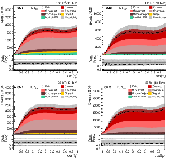
Distribution of $ \cos(\theta_{\mathrm{p}}) $ in all four categories. The data (points) are compared to the prediction (stacked histograms). The $ \mathrm{t} \overline{\mathrm{t}} $ and single top quark contributions are taken from the simulation, while the multijet+EW background is obtained from the CR. The $ \mathrm{t} \overline{\mathrm{t}} $ contribution is split into the correctly and incorrectly reconstructed, ``nonreconstructable'', and non $ \mathrm{e}/\mu $+jets events. The gray uncertainty band indicates the combined statistical and systematic uncertainties in the prediction. The vertical bars on the points show the statistical uncertainty of the data. Ratios to the predicted yields are provided in the lower panels. |

png pdf |
Figure 6-a:
Distribution of $ \cos(\theta_{\mathrm{p}}) $ in all four categories. The data (points) are compared to the prediction (stacked histograms). The $ \mathrm{t} \overline{\mathrm{t}} $ and single top quark contributions are taken from the simulation, while the multijet+EW background is obtained from the CR. The $ \mathrm{t} \overline{\mathrm{t}} $ contribution is split into the correctly and incorrectly reconstructed, ``nonreconstructable'', and non $ \mathrm{e}/\mu $+jets events. The gray uncertainty band indicates the combined statistical and systematic uncertainties in the prediction. The vertical bars on the points show the statistical uncertainty of the data. Ratios to the predicted yields are provided in the lower panels. |

png pdf |
Figure 6-b:
Distribution of $ \cos(\theta_{\mathrm{p}}) $ in all four categories. The data (points) are compared to the prediction (stacked histograms). The $ \mathrm{t} \overline{\mathrm{t}} $ and single top quark contributions are taken from the simulation, while the multijet+EW background is obtained from the CR. The $ \mathrm{t} \overline{\mathrm{t}} $ contribution is split into the correctly and incorrectly reconstructed, ``nonreconstructable'', and non $ \mathrm{e}/\mu $+jets events. The gray uncertainty band indicates the combined statistical and systematic uncertainties in the prediction. The vertical bars on the points show the statistical uncertainty of the data. Ratios to the predicted yields are provided in the lower panels. |

png pdf |
Figure 6-c:
Distribution of $ \cos(\theta_{\mathrm{p}}) $ in all four categories. The data (points) are compared to the prediction (stacked histograms). The $ \mathrm{t} \overline{\mathrm{t}} $ and single top quark contributions are taken from the simulation, while the multijet+EW background is obtained from the CR. The $ \mathrm{t} \overline{\mathrm{t}} $ contribution is split into the correctly and incorrectly reconstructed, ``nonreconstructable'', and non $ \mathrm{e}/\mu $+jets events. The gray uncertainty band indicates the combined statistical and systematic uncertainties in the prediction. The vertical bars on the points show the statistical uncertainty of the data. Ratios to the predicted yields are provided in the lower panels. |

png pdf |
Figure 6-d:
Distribution of $ \cos(\theta_{\mathrm{p}}) $ in all four categories. The data (points) are compared to the prediction (stacked histograms). The $ \mathrm{t} \overline{\mathrm{t}} $ and single top quark contributions are taken from the simulation, while the multijet+EW background is obtained from the CR. The $ \mathrm{t} \overline{\mathrm{t}} $ contribution is split into the correctly and incorrectly reconstructed, ``nonreconstructable'', and non $ \mathrm{e}/\mu $+jets events. The gray uncertainty band indicates the combined statistical and systematic uncertainties in the prediction. The vertical bars on the points show the statistical uncertainty of the data. Ratios to the predicted yields are provided in the lower panels. |
png pdf |
Figure 7:
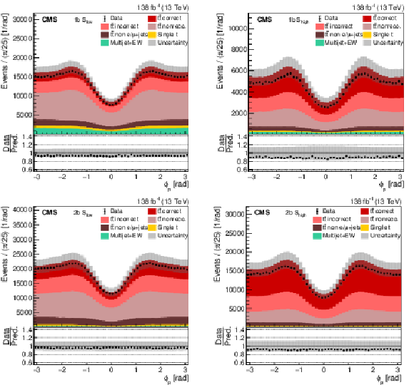
Distribution of $ \phi_{\mathrm{p}} $ in all four categories. The data (points) are compared to the prediction (stacked histograms). The $ \mathrm{t} \overline{\mathrm{t}} $ and single top quark contributions are taken from the simulation, while the multijet+EW background is obtained from the CR. The $ \mathrm{t} \overline{\mathrm{t}} $ contribution is split into the correctly and incorrectly reconstructed, ``nonreconstructable'', and non $ \mathrm{e}/\mu $+jets events. The gray uncertainty band indicates the combined statistical and systematic uncertainties in the prediction. The vertical bars on the points show the statistical uncertainty of the data. Ratios to the predicted yields are provided in the lower panels. |

png pdf |
Figure 7-a:
Distribution of $ \phi_{\mathrm{p}} $ in all four categories. The data (points) are compared to the prediction (stacked histograms). The $ \mathrm{t} \overline{\mathrm{t}} $ and single top quark contributions are taken from the simulation, while the multijet+EW background is obtained from the CR. The $ \mathrm{t} \overline{\mathrm{t}} $ contribution is split into the correctly and incorrectly reconstructed, ``nonreconstructable'', and non $ \mathrm{e}/\mu $+jets events. The gray uncertainty band indicates the combined statistical and systematic uncertainties in the prediction. The vertical bars on the points show the statistical uncertainty of the data. Ratios to the predicted yields are provided in the lower panels. |

png pdf |
Figure 7-b:
Distribution of $ \phi_{\mathrm{p}} $ in all four categories. The data (points) are compared to the prediction (stacked histograms). The $ \mathrm{t} \overline{\mathrm{t}} $ and single top quark contributions are taken from the simulation, while the multijet+EW background is obtained from the CR. The $ \mathrm{t} \overline{\mathrm{t}} $ contribution is split into the correctly and incorrectly reconstructed, ``nonreconstructable'', and non $ \mathrm{e}/\mu $+jets events. The gray uncertainty band indicates the combined statistical and systematic uncertainties in the prediction. The vertical bars on the points show the statistical uncertainty of the data. Ratios to the predicted yields are provided in the lower panels. |

png pdf |
Figure 7-c:
Distribution of $ \phi_{\mathrm{p}} $ in all four categories. The data (points) are compared to the prediction (stacked histograms). The $ \mathrm{t} \overline{\mathrm{t}} $ and single top quark contributions are taken from the simulation, while the multijet+EW background is obtained from the CR. The $ \mathrm{t} \overline{\mathrm{t}} $ contribution is split into the correctly and incorrectly reconstructed, ``nonreconstructable'', and non $ \mathrm{e}/\mu $+jets events. The gray uncertainty band indicates the combined statistical and systematic uncertainties in the prediction. The vertical bars on the points show the statistical uncertainty of the data. Ratios to the predicted yields are provided in the lower panels. |

png pdf |
Figure 7-d:
Distribution of $ \phi_{\mathrm{p}} $ in all four categories. The data (points) are compared to the prediction (stacked histograms). The $ \mathrm{t} \overline{\mathrm{t}} $ and single top quark contributions are taken from the simulation, while the multijet+EW background is obtained from the CR. The $ \mathrm{t} \overline{\mathrm{t}} $ contribution is split into the correctly and incorrectly reconstructed, ``nonreconstructable'', and non $ \mathrm{e}/\mu $+jets events. The gray uncertainty band indicates the combined statistical and systematic uncertainties in the prediction. The vertical bars on the points show the statistical uncertainty of the data. Ratios to the predicted yields are provided in the lower panels. |
png pdf |
Figure 8:
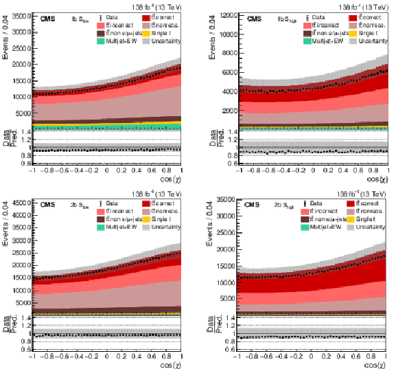
Distribution of $ \cos(\chi) $ in all four categories. The data (points) are compared to the prediction (stacked histograms). The $ \mathrm{t} \overline{\mathrm{t}} $ and single top quark contributions are taken from the simulation, while the multijet+EW background is obtained from the CR. The $ \mathrm{t} \overline{\mathrm{t}} $ contribution is split into the correctly and incorrectly reconstructed, ``nonreconstructable'', and non $ \mathrm{e}/\mu $+jets events. The gray uncertainty band indicates the combined statistical and systematic uncertainties in the prediction. The vertical bars on the points show the statistical uncertainty of the data. Ratios to the predicted yields are provided in the lower panels. |

png pdf |
Figure 8-a:
Distribution of $ \cos(\chi) $ in all four categories. The data (points) are compared to the prediction (stacked histograms). The $ \mathrm{t} \overline{\mathrm{t}} $ and single top quark contributions are taken from the simulation, while the multijet+EW background is obtained from the CR. The $ \mathrm{t} \overline{\mathrm{t}} $ contribution is split into the correctly and incorrectly reconstructed, ``nonreconstructable'', and non $ \mathrm{e}/\mu $+jets events. The gray uncertainty band indicates the combined statistical and systematic uncertainties in the prediction. The vertical bars on the points show the statistical uncertainty of the data. Ratios to the predicted yields are provided in the lower panels. |

png pdf |
Figure 8-b:
Distribution of $ \cos(\chi) $ in all four categories. The data (points) are compared to the prediction (stacked histograms). The $ \mathrm{t} \overline{\mathrm{t}} $ and single top quark contributions are taken from the simulation, while the multijet+EW background is obtained from the CR. The $ \mathrm{t} \overline{\mathrm{t}} $ contribution is split into the correctly and incorrectly reconstructed, ``nonreconstructable'', and non $ \mathrm{e}/\mu $+jets events. The gray uncertainty band indicates the combined statistical and systematic uncertainties in the prediction. The vertical bars on the points show the statistical uncertainty of the data. Ratios to the predicted yields are provided in the lower panels. |

png pdf |
Figure 8-c:
Distribution of $ \cos(\chi) $ in all four categories. The data (points) are compared to the prediction (stacked histograms). The $ \mathrm{t} \overline{\mathrm{t}} $ and single top quark contributions are taken from the simulation, while the multijet+EW background is obtained from the CR. The $ \mathrm{t} \overline{\mathrm{t}} $ contribution is split into the correctly and incorrectly reconstructed, ``nonreconstructable'', and non $ \mathrm{e}/\mu $+jets events. The gray uncertainty band indicates the combined statistical and systematic uncertainties in the prediction. The vertical bars on the points show the statistical uncertainty of the data. Ratios to the predicted yields are provided in the lower panels. |

png pdf |
Figure 8-d:
Distribution of $ \cos(\chi) $ in all four categories. The data (points) are compared to the prediction (stacked histograms). The $ \mathrm{t} \overline{\mathrm{t}} $ and single top quark contributions are taken from the simulation, while the multijet+EW background is obtained from the CR. The $ \mathrm{t} \overline{\mathrm{t}} $ contribution is split into the correctly and incorrectly reconstructed, ``nonreconstructable'', and non $ \mathrm{e}/\mu $+jets events. The gray uncertainty band indicates the combined statistical and systematic uncertainties in the prediction. The vertical bars on the points show the statistical uncertainty of the data. Ratios to the predicted yields are provided in the lower panels. |
png pdf |
Figure 9:
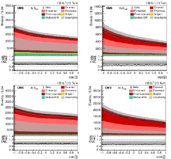
Distribution of $ \cos(\tilde{\chi}) $ in all four categories. The data (points) are compared to the prediction (stacked histograms). The $ \mathrm{t} \overline{\mathrm{t}} $ and single top quark contributions are taken from the simulation, while the multijet+EW background is obtained from the CR. The $ \mathrm{t} \overline{\mathrm{t}} $ contribution is split into the correctly and incorrectly reconstructed, ``nonreconstructable'', and non $ \mathrm{e}/\mu $+jets events. The gray uncertainty band indicates the combined statistical and systematic uncertainties in the prediction. The vertical bars on the points show the statistical uncertainty of the data. Ratios to the predicted yields are provided in the lower panels. |

png pdf |
Figure 9-a:
Distribution of $ \cos(\tilde{\chi}) $ in all four categories. The data (points) are compared to the prediction (stacked histograms). The $ \mathrm{t} \overline{\mathrm{t}} $ and single top quark contributions are taken from the simulation, while the multijet+EW background is obtained from the CR. The $ \mathrm{t} \overline{\mathrm{t}} $ contribution is split into the correctly and incorrectly reconstructed, ``nonreconstructable'', and non $ \mathrm{e}/\mu $+jets events. The gray uncertainty band indicates the combined statistical and systematic uncertainties in the prediction. The vertical bars on the points show the statistical uncertainty of the data. Ratios to the predicted yields are provided in the lower panels. |

png pdf |
Figure 9-b:
Distribution of $ \cos(\tilde{\chi}) $ in all four categories. The data (points) are compared to the prediction (stacked histograms). The $ \mathrm{t} \overline{\mathrm{t}} $ and single top quark contributions are taken from the simulation, while the multijet+EW background is obtained from the CR. The $ \mathrm{t} \overline{\mathrm{t}} $ contribution is split into the correctly and incorrectly reconstructed, ``nonreconstructable'', and non $ \mathrm{e}/\mu $+jets events. The gray uncertainty band indicates the combined statistical and systematic uncertainties in the prediction. The vertical bars on the points show the statistical uncertainty of the data. Ratios to the predicted yields are provided in the lower panels. |

png pdf |
Figure 9-c:
Distribution of $ \cos(\tilde{\chi}) $ in all four categories. The data (points) are compared to the prediction (stacked histograms). The $ \mathrm{t} \overline{\mathrm{t}} $ and single top quark contributions are taken from the simulation, while the multijet+EW background is obtained from the CR. The $ \mathrm{t} \overline{\mathrm{t}} $ contribution is split into the correctly and incorrectly reconstructed, ``nonreconstructable'', and non $ \mathrm{e}/\mu $+jets events. The gray uncertainty band indicates the combined statistical and systematic uncertainties in the prediction. The vertical bars on the points show the statistical uncertainty of the data. Ratios to the predicted yields are provided in the lower panels. |

png pdf |
Figure 9-d:
Distribution of $ \cos(\tilde{\chi}) $ in all four categories. The data (points) are compared to the prediction (stacked histograms). The $ \mathrm{t} \overline{\mathrm{t}} $ and single top quark contributions are taken from the simulation, while the multijet+EW background is obtained from the CR. The $ \mathrm{t} \overline{\mathrm{t}} $ contribution is split into the correctly and incorrectly reconstructed, ``nonreconstructable'', and non $ \mathrm{e}/\mu $+jets events. The gray uncertainty band indicates the combined statistical and systematic uncertainties in the prediction. The vertical bars on the points show the statistical uncertainty of the data. Ratios to the predicted yields are provided in the lower panels. |
png pdf |
Figure 10:
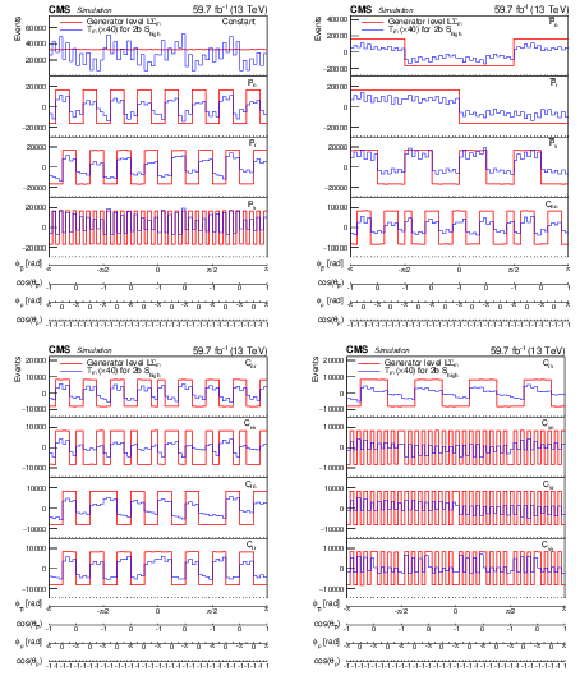
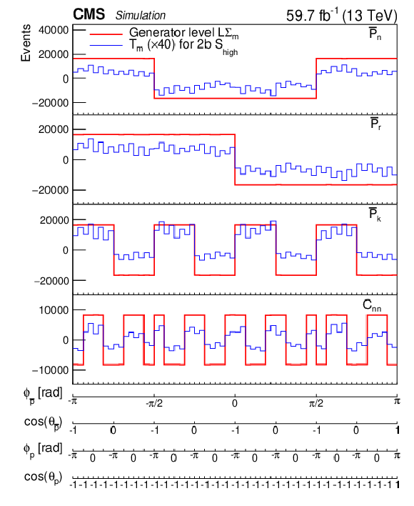
Examples of unrolled 4-dimensional distributions $ L\Sigma_m $ and $ T_m $ as functions of $ \phi_{\mathrm{p}(\bar{\mathrm{p}})} $ and $ \theta_{\mathrm{p}(\bar{\mathrm{p}})} $ for the individual coefficients of the polarization vectors and the spin correlation matrix for events with 400 $ < m({\mathrm{t}\overline{\mathrm{t}}} ) < $ 600 GeV and $ |\cos(\theta)| < $ 0.4. The $ L\Sigma_m $ (red lines) are the distributions at the generator level in the full phase space, and the $ T_m $ (blue lines) are the distributions in the $2\mathrm{b} S_{\text{high}}$ category for the 2018 data. For the purpose of illustration, the events are required to be reconstructed and generated in the same $ m({\mathrm{t}\overline{\mathrm{t}}} ) $ vs. $|\cos(\theta)\,| $ bin. The detector-level distributions are enhanced by a factor of 40 to improve their visibility. |

png pdf |
Figure 10-a:
Examples of unrolled 4-dimensional distributions $ L\Sigma_m $ and $ T_m $ as functions of $ \phi_{\mathrm{p}(\bar{\mathrm{p}})} $ and $ \theta_{\mathrm{p}(\bar{\mathrm{p}})} $ for the individual coefficients of the polarization vectors and the spin correlation matrix for events with 400 $ < m({\mathrm{t}\overline{\mathrm{t}}} ) < $ 600 GeV and $ |\cos(\theta)| < $ 0.4. The $ L\Sigma_m $ (red lines) are the distributions at the generator level in the full phase space, and the $ T_m $ (blue lines) are the distributions in the $2\mathrm{b} S_{\text{high}}$ category for the 2018 data. For the purpose of illustration, the events are required to be reconstructed and generated in the same $ m({\mathrm{t}\overline{\mathrm{t}}} ) $ vs. $|\cos(\theta)\,| $ bin. The detector-level distributions are enhanced by a factor of 40 to improve their visibility. |
png pdf |
Figure 10-b:
Examples of unrolled 4-dimensional distributions $ L\Sigma_m $ and $ T_m $ as functions of $ \phi_{\mathrm{p}(\bar{\mathrm{p}})} $ and $ \theta_{\mathrm{p}(\bar{\mathrm{p}})} $ for the individual coefficients of the polarization vectors and the spin correlation matrix for events with 400 $ < m({\mathrm{t}\overline{\mathrm{t}}} ) < $ 600 GeV and $ |\cos(\theta)| < $ 0.4. The $ L\Sigma_m $ (red lines) are the distributions at the generator level in the full phase space, and the $ T_m $ (blue lines) are the distributions in the $2\mathrm{b} S_{\text{high}}$ category for the 2018 data. For the purpose of illustration, the events are required to be reconstructed and generated in the same $ m({\mathrm{t}\overline{\mathrm{t}}} ) $ vs. $|\cos(\theta)\,| $ bin. The detector-level distributions are enhanced by a factor of 40 to improve their visibility. |

png pdf |
Figure 10-c:
Examples of unrolled 4-dimensional distributions $ L\Sigma_m $ and $ T_m $ as functions of $ \phi_{\mathrm{p}(\bar{\mathrm{p}})} $ and $ \theta_{\mathrm{p}(\bar{\mathrm{p}})} $ for the individual coefficients of the polarization vectors and the spin correlation matrix for events with 400 $ < m({\mathrm{t}\overline{\mathrm{t}}} ) < $ 600 GeV and $ |\cos(\theta)| < $ 0.4. The $ L\Sigma_m $ (red lines) are the distributions at the generator level in the full phase space, and the $ T_m $ (blue lines) are the distributions in the $2\mathrm{b} S_{\text{high}}$ category for the 2018 data. For the purpose of illustration, the events are required to be reconstructed and generated in the same $ m({\mathrm{t}\overline{\mathrm{t}}} ) $ vs. $|\cos(\theta)\,| $ bin. The detector-level distributions are enhanced by a factor of 40 to improve their visibility. |

png pdf |
Figure 10-d:
Examples of unrolled 4-dimensional distributions $ L\Sigma_m $ and $ T_m $ as functions of $ \phi_{\mathrm{p}(\bar{\mathrm{p}})} $ and $ \theta_{\mathrm{p}(\bar{\mathrm{p}})} $ for the individual coefficients of the polarization vectors and the spin correlation matrix for events with 400 $ < m({\mathrm{t}\overline{\mathrm{t}}} ) < $ 600 GeV and $ |\cos(\theta)| < $ 0.4. The $ L\Sigma_m $ (red lines) are the distributions at the generator level in the full phase space, and the $ T_m $ (blue lines) are the distributions in the $2\mathrm{b} S_{\text{high}}$ category for the 2018 data. For the purpose of illustration, the events are required to be reconstructed and generated in the same $ m({\mathrm{t}\overline{\mathrm{t}}} ) $ vs. $|\cos(\theta)\,| $ bin. The detector-level distributions are enhanced by a factor of 40 to improve their visibility. |
png pdf |
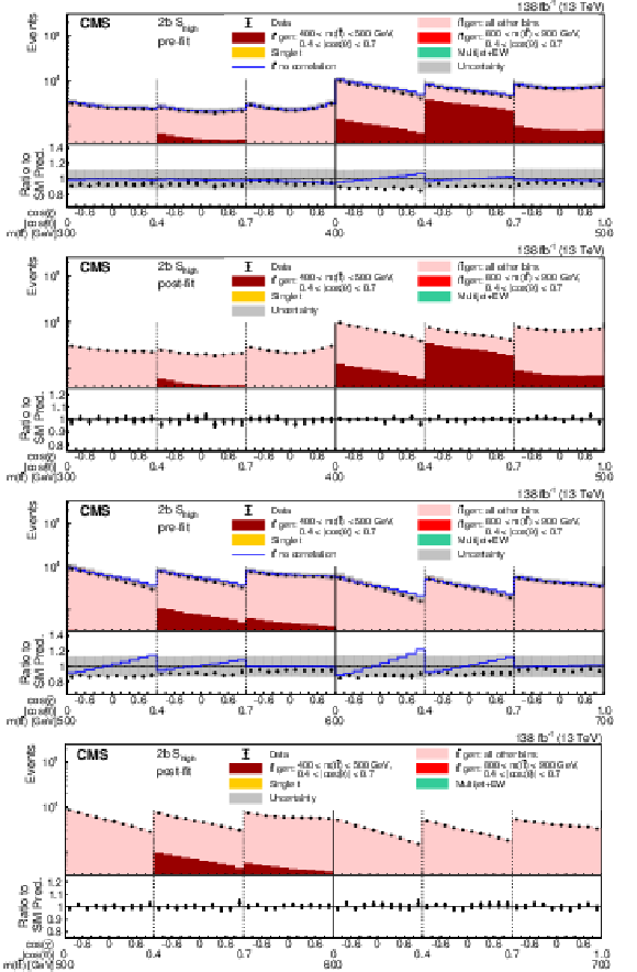
Figure 11:
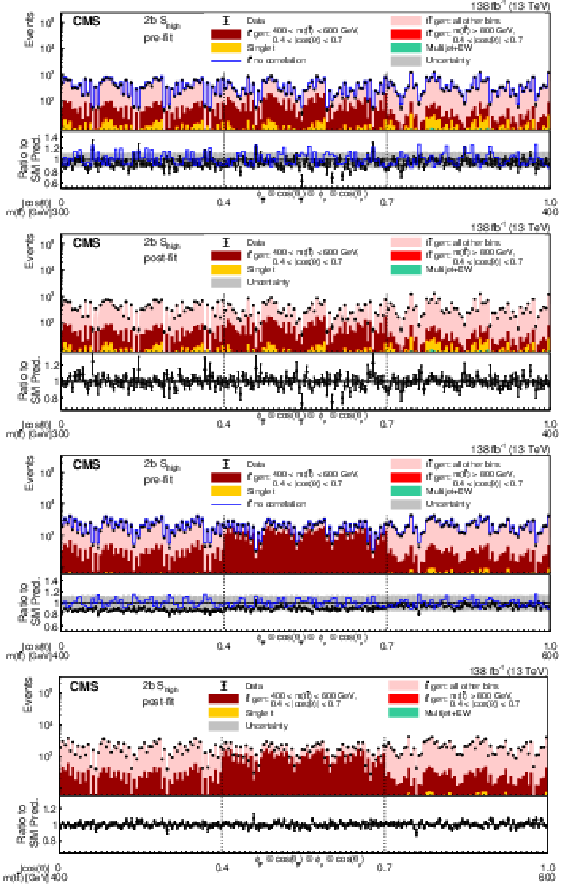
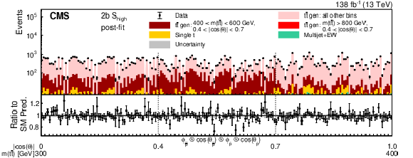
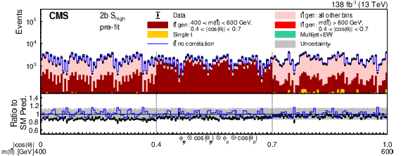
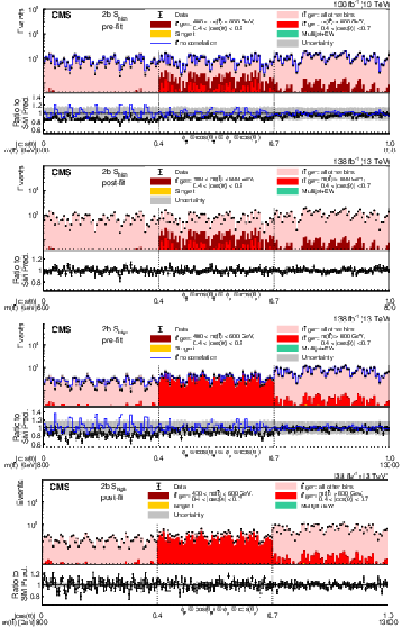
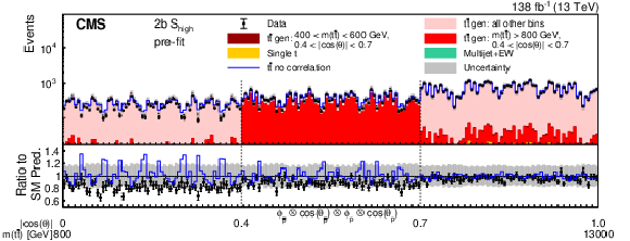
Pre- and post-fit distributions comparing the data (points) to the POWHEG + PYTHIA simulation (stacked histograms) for the full matrix measurement in bins of $ m({\mathrm{t}\overline{\mathrm{t}}} ) $ vs. $|\cos(\theta)\,| $ in the $2\mathrm{b} S_{\text{high}}$ category. The $ x $ axis shows the bins of the unrolled 4-dimensional distribution of $ \phi_{\bar{\mathrm{p}}} $, $ \cos(\theta_{\bar{\mathrm{p}}}) $, $ \phi_{\mathrm{p}} $, and $ \cos(\theta_{\mathrm{p}}) $, listed from the outermost to the innermost variable in each of the $ m({\mathrm{t}\overline{\mathrm{t}}} ) $ vs. $|\cos(\theta)\,| $ bins. The boundaries of the $ |\cos(\theta)| $ and $ m({\mathrm{t}\overline{\mathrm{t}}} ) $ bins are labeled and indicated by dashed and solid lines, respectively. For the illustration of resolution effects, $ \mathrm{t} \overline{\mathrm{t}} $ events generated in two selected $ m({\mathrm{t}\overline{\mathrm{t}}} ) $ vs. $|\cos(\theta)\,| $ bins are shown in different shades of red. All other $ \mathrm{t} \overline{\mathrm{t}} $ contributions are shown in pink. A model without any polarization and spin correlation is shown as a blue line. The gray uncertainty band indicates the combined statistical and systematic uncertainties in the prediction. The vertical bars on the points show the statistical uncertainty. Ratios to the predicted yields are provided in the lower panels. |

png pdf |
Figure 11-a:
Pre- and post-fit distributions comparing the data (points) to the POWHEG + PYTHIA simulation (stacked histograms) for the full matrix measurement in bins of $ m({\mathrm{t}\overline{\mathrm{t}}} ) $ vs. $|\cos(\theta)\,| $ in the $2\mathrm{b} S_{\text{high}}$ category. The $ x $ axis shows the bins of the unrolled 4-dimensional distribution of $ \phi_{\bar{\mathrm{p}}} $, $ \cos(\theta_{\bar{\mathrm{p}}}) $, $ \phi_{\mathrm{p}} $, and $ \cos(\theta_{\mathrm{p}}) $, listed from the outermost to the innermost variable in each of the $ m({\mathrm{t}\overline{\mathrm{t}}} ) $ vs. $|\cos(\theta)\,| $ bins. The boundaries of the $ |\cos(\theta)| $ and $ m({\mathrm{t}\overline{\mathrm{t}}} ) $ bins are labeled and indicated by dashed and solid lines, respectively. For the illustration of resolution effects, $ \mathrm{t} \overline{\mathrm{t}} $ events generated in two selected $ m({\mathrm{t}\overline{\mathrm{t}}} ) $ vs. $|\cos(\theta)\,| $ bins are shown in different shades of red. All other $ \mathrm{t} \overline{\mathrm{t}} $ contributions are shown in pink. A model without any polarization and spin correlation is shown as a blue line. The gray uncertainty band indicates the combined statistical and systematic uncertainties in the prediction. The vertical bars on the points show the statistical uncertainty. Ratios to the predicted yields are provided in the lower panels. |
png pdf |
Figure 11-b:
Pre- and post-fit distributions comparing the data (points) to the POWHEG + PYTHIA simulation (stacked histograms) for the full matrix measurement in bins of $ m({\mathrm{t}\overline{\mathrm{t}}} ) $ vs. $|\cos(\theta)\,| $ in the $2\mathrm{b} S_{\text{high}}$ category. The $ x $ axis shows the bins of the unrolled 4-dimensional distribution of $ \phi_{\bar{\mathrm{p}}} $, $ \cos(\theta_{\bar{\mathrm{p}}}) $, $ \phi_{\mathrm{p}} $, and $ \cos(\theta_{\mathrm{p}}) $, listed from the outermost to the innermost variable in each of the $ m({\mathrm{t}\overline{\mathrm{t}}} ) $ vs. $|\cos(\theta)\,| $ bins. The boundaries of the $ |\cos(\theta)| $ and $ m({\mathrm{t}\overline{\mathrm{t}}} ) $ bins are labeled and indicated by dashed and solid lines, respectively. For the illustration of resolution effects, $ \mathrm{t} \overline{\mathrm{t}} $ events generated in two selected $ m({\mathrm{t}\overline{\mathrm{t}}} ) $ vs. $|\cos(\theta)\,| $ bins are shown in different shades of red. All other $ \mathrm{t} \overline{\mathrm{t}} $ contributions are shown in pink. A model without any polarization and spin correlation is shown as a blue line. The gray uncertainty band indicates the combined statistical and systematic uncertainties in the prediction. The vertical bars on the points show the statistical uncertainty. Ratios to the predicted yields are provided in the lower panels. |
png pdf |
Figure 11-c:
Pre- and post-fit distributions comparing the data (points) to the POWHEG + PYTHIA simulation (stacked histograms) for the full matrix measurement in bins of $ m({\mathrm{t}\overline{\mathrm{t}}} ) $ vs. $|\cos(\theta)\,| $ in the $2\mathrm{b} S_{\text{high}}$ category. The $ x $ axis shows the bins of the unrolled 4-dimensional distribution of $ \phi_{\bar{\mathrm{p}}} $, $ \cos(\theta_{\bar{\mathrm{p}}}) $, $ \phi_{\mathrm{p}} $, and $ \cos(\theta_{\mathrm{p}}) $, listed from the outermost to the innermost variable in each of the $ m({\mathrm{t}\overline{\mathrm{t}}} ) $ vs. $|\cos(\theta)\,| $ bins. The boundaries of the $ |\cos(\theta)| $ and $ m({\mathrm{t}\overline{\mathrm{t}}} ) $ bins are labeled and indicated by dashed and solid lines, respectively. For the illustration of resolution effects, $ \mathrm{t} \overline{\mathrm{t}} $ events generated in two selected $ m({\mathrm{t}\overline{\mathrm{t}}} ) $ vs. $|\cos(\theta)\,| $ bins are shown in different shades of red. All other $ \mathrm{t} \overline{\mathrm{t}} $ contributions are shown in pink. A model without any polarization and spin correlation is shown as a blue line. The gray uncertainty band indicates the combined statistical and systematic uncertainties in the prediction. The vertical bars on the points show the statistical uncertainty. Ratios to the predicted yields are provided in the lower panels. |

png pdf |
Figure 11-d:
Pre- and post-fit distributions comparing the data (points) to the POWHEG + PYTHIA simulation (stacked histograms) for the full matrix measurement in bins of $ m({\mathrm{t}\overline{\mathrm{t}}} ) $ vs. $|\cos(\theta)\,| $ in the $2\mathrm{b} S_{\text{high}}$ category. The $ x $ axis shows the bins of the unrolled 4-dimensional distribution of $ \phi_{\bar{\mathrm{p}}} $, $ \cos(\theta_{\bar{\mathrm{p}}}) $, $ \phi_{\mathrm{p}} $, and $ \cos(\theta_{\mathrm{p}}) $, listed from the outermost to the innermost variable in each of the $ m({\mathrm{t}\overline{\mathrm{t}}} ) $ vs. $|\cos(\theta)\,| $ bins. The boundaries of the $ |\cos(\theta)| $ and $ m({\mathrm{t}\overline{\mathrm{t}}} ) $ bins are labeled and indicated by dashed and solid lines, respectively. For the illustration of resolution effects, $ \mathrm{t} \overline{\mathrm{t}} $ events generated in two selected $ m({\mathrm{t}\overline{\mathrm{t}}} ) $ vs. $|\cos(\theta)\,| $ bins are shown in different shades of red. All other $ \mathrm{t} \overline{\mathrm{t}} $ contributions are shown in pink. A model without any polarization and spin correlation is shown as a blue line. The gray uncertainty band indicates the combined statistical and systematic uncertainties in the prediction. The vertical bars on the points show the statistical uncertainty. Ratios to the predicted yields are provided in the lower panels. |
png pdf |
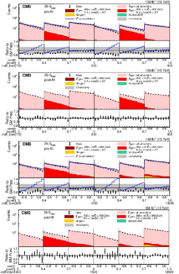
Figure 12:
Pre- and post-fit distributions comparing the data (points) to the POWHEG + PYTHIA simulation (stacked histograms) for the full matrix measurement in bins of $ m({\mathrm{t}\overline{\mathrm{t}}} ) $ vs. $|\cos(\theta)\,| $ in the $2\mathrm{b} S_{\text{high}}$ category. The $ x $ axis shows the bins of the unrolled 4-dimensional distribution of $ \phi_{\bar{\mathrm{p}}} $, $ \cos(\theta_{\bar{\mathrm{p}}}) $, $ \phi_{\mathrm{p}} $, and $ \cos(\theta_{\mathrm{p}}) $, listed from the outermost to the innermost variable in each of the $ m({\mathrm{t}\overline{\mathrm{t}}} ) $ vs. $|\cos(\theta)\,| $ bins. The boundaries of the $ |\cos(\theta)| $ and $ m({\mathrm{t}\overline{\mathrm{t}}} ) $ bins are labeled and indicated by dashed and solid lines, respectively. For the illustration of resolution effects, $ \mathrm{t} \overline{\mathrm{t}} $ events generated in two selected $ m({\mathrm{t}\overline{\mathrm{t}}} ) $ vs. $|\cos(\theta)\,| $ bins are shown in different shades of red. All other $ \mathrm{t} \overline{\mathrm{t}} $ contributions are shown in pink. A model without any polarization and spin correlation is shown as a blue line. The gray uncertainty band indicates the combined statistical and systematic uncertainties in the prediction. The vertical bars on the points show the statistical uncertainty. Ratios to the predicted yields are provided in the lower panels. |

png pdf |
Figure 12-a:
Pre- and post-fit distributions comparing the data (points) to the POWHEG + PYTHIA simulation (stacked histograms) for the full matrix measurement in bins of $ m({\mathrm{t}\overline{\mathrm{t}}} ) $ vs. $|\cos(\theta)\,| $ in the $2\mathrm{b} S_{\text{high}}$ category. The $ x $ axis shows the bins of the unrolled 4-dimensional distribution of $ \phi_{\bar{\mathrm{p}}} $, $ \cos(\theta_{\bar{\mathrm{p}}}) $, $ \phi_{\mathrm{p}} $, and $ \cos(\theta_{\mathrm{p}}) $, listed from the outermost to the innermost variable in each of the $ m({\mathrm{t}\overline{\mathrm{t}}} ) $ vs. $|\cos(\theta)\,| $ bins. The boundaries of the $ |\cos(\theta)| $ and $ m({\mathrm{t}\overline{\mathrm{t}}} ) $ bins are labeled and indicated by dashed and solid lines, respectively. For the illustration of resolution effects, $ \mathrm{t} \overline{\mathrm{t}} $ events generated in two selected $ m({\mathrm{t}\overline{\mathrm{t}}} ) $ vs. $|\cos(\theta)\,| $ bins are shown in different shades of red. All other $ \mathrm{t} \overline{\mathrm{t}} $ contributions are shown in pink. A model without any polarization and spin correlation is shown as a blue line. The gray uncertainty band indicates the combined statistical and systematic uncertainties in the prediction. The vertical bars on the points show the statistical uncertainty. Ratios to the predicted yields are provided in the lower panels. |

png pdf |
Figure 12-b:
Pre- and post-fit distributions comparing the data (points) to the POWHEG + PYTHIA simulation (stacked histograms) for the full matrix measurement in bins of $ m({\mathrm{t}\overline{\mathrm{t}}} ) $ vs. $|\cos(\theta)\,| $ in the $2\mathrm{b} S_{\text{high}}$ category. The $ x $ axis shows the bins of the unrolled 4-dimensional distribution of $ \phi_{\bar{\mathrm{p}}} $, $ \cos(\theta_{\bar{\mathrm{p}}}) $, $ \phi_{\mathrm{p}} $, and $ \cos(\theta_{\mathrm{p}}) $, listed from the outermost to the innermost variable in each of the $ m({\mathrm{t}\overline{\mathrm{t}}} ) $ vs. $|\cos(\theta)\,| $ bins. The boundaries of the $ |\cos(\theta)| $ and $ m({\mathrm{t}\overline{\mathrm{t}}} ) $ bins are labeled and indicated by dashed and solid lines, respectively. For the illustration of resolution effects, $ \mathrm{t} \overline{\mathrm{t}} $ events generated in two selected $ m({\mathrm{t}\overline{\mathrm{t}}} ) $ vs. $|\cos(\theta)\,| $ bins are shown in different shades of red. All other $ \mathrm{t} \overline{\mathrm{t}} $ contributions are shown in pink. A model without any polarization and spin correlation is shown as a blue line. The gray uncertainty band indicates the combined statistical and systematic uncertainties in the prediction. The vertical bars on the points show the statistical uncertainty. Ratios to the predicted yields are provided in the lower panels. |
png pdf |
Figure 12-c:
Pre- and post-fit distributions comparing the data (points) to the POWHEG + PYTHIA simulation (stacked histograms) for the full matrix measurement in bins of $ m({\mathrm{t}\overline{\mathrm{t}}} ) $ vs. $|\cos(\theta)\,| $ in the $2\mathrm{b} S_{\text{high}}$ category. The $ x $ axis shows the bins of the unrolled 4-dimensional distribution of $ \phi_{\bar{\mathrm{p}}} $, $ \cos(\theta_{\bar{\mathrm{p}}}) $, $ \phi_{\mathrm{p}} $, and $ \cos(\theta_{\mathrm{p}}) $, listed from the outermost to the innermost variable in each of the $ m({\mathrm{t}\overline{\mathrm{t}}} ) $ vs. $|\cos(\theta)\,| $ bins. The boundaries of the $ |\cos(\theta)| $ and $ m({\mathrm{t}\overline{\mathrm{t}}} ) $ bins are labeled and indicated by dashed and solid lines, respectively. For the illustration of resolution effects, $ \mathrm{t} \overline{\mathrm{t}} $ events generated in two selected $ m({\mathrm{t}\overline{\mathrm{t}}} ) $ vs. $|\cos(\theta)\,| $ bins are shown in different shades of red. All other $ \mathrm{t} \overline{\mathrm{t}} $ contributions are shown in pink. A model without any polarization and spin correlation is shown as a blue line. The gray uncertainty band indicates the combined statistical and systematic uncertainties in the prediction. The vertical bars on the points show the statistical uncertainty. Ratios to the predicted yields are provided in the lower panels. |

png pdf |
Figure 12-d:
Pre- and post-fit distributions comparing the data (points) to the POWHEG + PYTHIA simulation (stacked histograms) for the full matrix measurement in bins of $ m({\mathrm{t}\overline{\mathrm{t}}} ) $ vs. $|\cos(\theta)\,| $ in the $2\mathrm{b} S_{\text{high}}$ category. The $ x $ axis shows the bins of the unrolled 4-dimensional distribution of $ \phi_{\bar{\mathrm{p}}} $, $ \cos(\theta_{\bar{\mathrm{p}}}) $, $ \phi_{\mathrm{p}} $, and $ \cos(\theta_{\mathrm{p}}) $, listed from the outermost to the innermost variable in each of the $ m({\mathrm{t}\overline{\mathrm{t}}} ) $ vs. $|\cos(\theta)\,| $ bins. The boundaries of the $ |\cos(\theta)| $ and $ m({\mathrm{t}\overline{\mathrm{t}}} ) $ bins are labeled and indicated by dashed and solid lines, respectively. For the illustration of resolution effects, $ \mathrm{t} \overline{\mathrm{t}} $ events generated in two selected $ m({\mathrm{t}\overline{\mathrm{t}}} ) $ vs. $|\cos(\theta)\,| $ bins are shown in different shades of red. All other $ \mathrm{t} \overline{\mathrm{t}} $ contributions are shown in pink. A model without any polarization and spin correlation is shown as a blue line. The gray uncertainty band indicates the combined statistical and systematic uncertainties in the prediction. The vertical bars on the points show the statistical uncertainty. Ratios to the predicted yields are provided in the lower panels. |
png pdf |
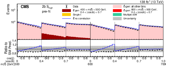
Figure 13:
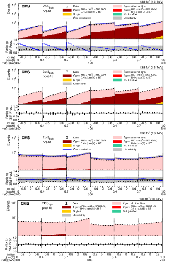
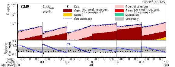
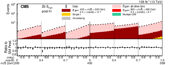
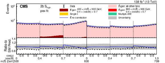
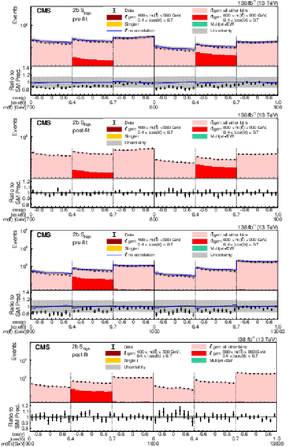
Pre- and post-fit distributions of $ \cos(\chi) $ comparing the data (points) to the POWHEG + PYTHIA simulation (stacked histograms) for the $ D $ measurement in bins of $ m({\mathrm{t}\overline{\mathrm{t}}} ) $ vs. $|\cos(\theta)\,| $ in the $2\mathrm{b} S_{\text{high}}$ category. The boundaries of the $ |\cos(\theta)| $ and $ m({\mathrm{t}\overline{\mathrm{t}}} ) $ bins are labeled and indicated by dashed and solid lines, respectively. For the illustration of resolution effects, $ \mathrm{t} \overline{\mathrm{t}} $ events generated in two selected $ m({\mathrm{t}\overline{\mathrm{t}}} ) $ vs. $|\cos(\theta)\,| $ bins are shown in different shades of red. All other $ \mathrm{t} \overline{\mathrm{t}} $ contributions are shown in pink. A model without any polarization and spin correlation is shown as a blue line. The gray uncertainty band indicates the combined statistical and systematic uncertainties in the prediction. The vertical bars on the points show the statistical uncertainty. Ratios to the predicted yields are provided in the lower panels. |
png pdf |
Figure 13-a:
Pre- and post-fit distributions of $ \cos(\chi) $ comparing the data (points) to the POWHEG + PYTHIA simulation (stacked histograms) for the $ D $ measurement in bins of $ m({\mathrm{t}\overline{\mathrm{t}}} ) $ vs. $|\cos(\theta)\,| $ in the $2\mathrm{b} S_{\text{high}}$ category. The boundaries of the $ |\cos(\theta)| $ and $ m({\mathrm{t}\overline{\mathrm{t}}} ) $ bins are labeled and indicated by dashed and solid lines, respectively. For the illustration of resolution effects, $ \mathrm{t} \overline{\mathrm{t}} $ events generated in two selected $ m({\mathrm{t}\overline{\mathrm{t}}} ) $ vs. $|\cos(\theta)\,| $ bins are shown in different shades of red. All other $ \mathrm{t} \overline{\mathrm{t}} $ contributions are shown in pink. A model without any polarization and spin correlation is shown as a blue line. The gray uncertainty band indicates the combined statistical and systematic uncertainties in the prediction. The vertical bars on the points show the statistical uncertainty. Ratios to the predicted yields are provided in the lower panels. |
png pdf |
Figure 13-b:
Pre- and post-fit distributions of $ \cos(\chi) $ comparing the data (points) to the POWHEG + PYTHIA simulation (stacked histograms) for the $ D $ measurement in bins of $ m({\mathrm{t}\overline{\mathrm{t}}} ) $ vs. $|\cos(\theta)\,| $ in the $2\mathrm{b} S_{\text{high}}$ category. The boundaries of the $ |\cos(\theta)| $ and $ m({\mathrm{t}\overline{\mathrm{t}}} ) $ bins are labeled and indicated by dashed and solid lines, respectively. For the illustration of resolution effects, $ \mathrm{t} \overline{\mathrm{t}} $ events generated in two selected $ m({\mathrm{t}\overline{\mathrm{t}}} ) $ vs. $|\cos(\theta)\,| $ bins are shown in different shades of red. All other $ \mathrm{t} \overline{\mathrm{t}} $ contributions are shown in pink. A model without any polarization and spin correlation is shown as a blue line. The gray uncertainty band indicates the combined statistical and systematic uncertainties in the prediction. The vertical bars on the points show the statistical uncertainty. Ratios to the predicted yields are provided in the lower panels. |
png pdf |
Figure 13-c:
Pre- and post-fit distributions of $ \cos(\chi) $ comparing the data (points) to the POWHEG + PYTHIA simulation (stacked histograms) for the $ D $ measurement in bins of $ m({\mathrm{t}\overline{\mathrm{t}}} ) $ vs. $|\cos(\theta)\,| $ in the $2\mathrm{b} S_{\text{high}}$ category. The boundaries of the $ |\cos(\theta)| $ and $ m({\mathrm{t}\overline{\mathrm{t}}} ) $ bins are labeled and indicated by dashed and solid lines, respectively. For the illustration of resolution effects, $ \mathrm{t} \overline{\mathrm{t}} $ events generated in two selected $ m({\mathrm{t}\overline{\mathrm{t}}} ) $ vs. $|\cos(\theta)\,| $ bins are shown in different shades of red. All other $ \mathrm{t} \overline{\mathrm{t}} $ contributions are shown in pink. A model without any polarization and spin correlation is shown as a blue line. The gray uncertainty band indicates the combined statistical and systematic uncertainties in the prediction. The vertical bars on the points show the statistical uncertainty. Ratios to the predicted yields are provided in the lower panels. |

png pdf |
Figure 13-d:
Pre- and post-fit distributions of $ \cos(\chi) $ comparing the data (points) to the POWHEG + PYTHIA simulation (stacked histograms) for the $ D $ measurement in bins of $ m({\mathrm{t}\overline{\mathrm{t}}} ) $ vs. $|\cos(\theta)\,| $ in the $2\mathrm{b} S_{\text{high}}$ category. The boundaries of the $ |\cos(\theta)| $ and $ m({\mathrm{t}\overline{\mathrm{t}}} ) $ bins are labeled and indicated by dashed and solid lines, respectively. For the illustration of resolution effects, $ \mathrm{t} \overline{\mathrm{t}} $ events generated in two selected $ m({\mathrm{t}\overline{\mathrm{t}}} ) $ vs. $|\cos(\theta)\,| $ bins are shown in different shades of red. All other $ \mathrm{t} \overline{\mathrm{t}} $ contributions are shown in pink. A model without any polarization and spin correlation is shown as a blue line. The gray uncertainty band indicates the combined statistical and systematic uncertainties in the prediction. The vertical bars on the points show the statistical uncertainty. Ratios to the predicted yields are provided in the lower panels. |
png pdf |
Figure 14:
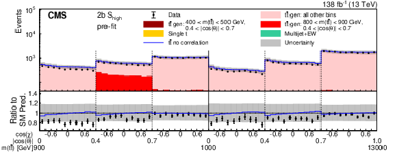
Pre- and post-fit distributions of $ \cos(\chi) $ comparing the data (points) to the POWHEG + PYTHIA simulation (stacked histograms) for the $ D $ measurement in bins of $ m({\mathrm{t}\overline{\mathrm{t}}} ) $ vs. $|\cos(\theta)\,| $ in the $2\mathrm{b} S_{\text{high}}$ category. The boundaries of the $ |\cos(\theta)| $ and $ m({\mathrm{t}\overline{\mathrm{t}}} ) $ bins are labeled and indicated by dashed and solid lines, respectively. For the illustration of resolution effects, $ \mathrm{t} \overline{\mathrm{t}} $ events generated in two selected $ m({\mathrm{t}\overline{\mathrm{t}}} ) $ vs. $|\cos(\theta)\,| $ bins are shown in different shades of red. All other $ \mathrm{t} \overline{\mathrm{t}} $ contributions are shown in pink. A model without any polarization and spin correlation is shown as a blue line. The gray uncertainty band indicates the combined statistical and systematic uncertainties in the prediction. The vertical bars on the points show the statistical uncertainty. Ratios to the predicted yields are provided in the lower panels. |

png pdf |
Figure 14-a:
Pre- and post-fit distributions of $ \cos(\chi) $ comparing the data (points) to the POWHEG + PYTHIA simulation (stacked histograms) for the $ D $ measurement in bins of $ m({\mathrm{t}\overline{\mathrm{t}}} ) $ vs. $|\cos(\theta)\,| $ in the $2\mathrm{b} S_{\text{high}}$ category. The boundaries of the $ |\cos(\theta)| $ and $ m({\mathrm{t}\overline{\mathrm{t}}} ) $ bins are labeled and indicated by dashed and solid lines, respectively. For the illustration of resolution effects, $ \mathrm{t} \overline{\mathrm{t}} $ events generated in two selected $ m({\mathrm{t}\overline{\mathrm{t}}} ) $ vs. $|\cos(\theta)\,| $ bins are shown in different shades of red. All other $ \mathrm{t} \overline{\mathrm{t}} $ contributions are shown in pink. A model without any polarization and spin correlation is shown as a blue line. The gray uncertainty band indicates the combined statistical and systematic uncertainties in the prediction. The vertical bars on the points show the statistical uncertainty. Ratios to the predicted yields are provided in the lower panels. |

png pdf |
Figure 14-b:
Pre- and post-fit distributions of $ \cos(\chi) $ comparing the data (points) to the POWHEG + PYTHIA simulation (stacked histograms) for the $ D $ measurement in bins of $ m({\mathrm{t}\overline{\mathrm{t}}} ) $ vs. $|\cos(\theta)\,| $ in the $2\mathrm{b} S_{\text{high}}$ category. The boundaries of the $ |\cos(\theta)| $ and $ m({\mathrm{t}\overline{\mathrm{t}}} ) $ bins are labeled and indicated by dashed and solid lines, respectively. For the illustration of resolution effects, $ \mathrm{t} \overline{\mathrm{t}} $ events generated in two selected $ m({\mathrm{t}\overline{\mathrm{t}}} ) $ vs. $|\cos(\theta)\,| $ bins are shown in different shades of red. All other $ \mathrm{t} \overline{\mathrm{t}} $ contributions are shown in pink. A model without any polarization and spin correlation is shown as a blue line. The gray uncertainty band indicates the combined statistical and systematic uncertainties in the prediction. The vertical bars on the points show the statistical uncertainty. Ratios to the predicted yields are provided in the lower panels. |
png pdf |
Figure 14-c:
Pre- and post-fit distributions of $ \cos(\chi) $ comparing the data (points) to the POWHEG + PYTHIA simulation (stacked histograms) for the $ D $ measurement in bins of $ m({\mathrm{t}\overline{\mathrm{t}}} ) $ vs. $|\cos(\theta)\,| $ in the $2\mathrm{b} S_{\text{high}}$ category. The boundaries of the $ |\cos(\theta)| $ and $ m({\mathrm{t}\overline{\mathrm{t}}} ) $ bins are labeled and indicated by dashed and solid lines, respectively. For the illustration of resolution effects, $ \mathrm{t} \overline{\mathrm{t}} $ events generated in two selected $ m({\mathrm{t}\overline{\mathrm{t}}} ) $ vs. $|\cos(\theta)\,| $ bins are shown in different shades of red. All other $ \mathrm{t} \overline{\mathrm{t}} $ contributions are shown in pink. A model without any polarization and spin correlation is shown as a blue line. The gray uncertainty band indicates the combined statistical and systematic uncertainties in the prediction. The vertical bars on the points show the statistical uncertainty. Ratios to the predicted yields are provided in the lower panels. |

png pdf |
Figure 14-d:
Pre- and post-fit distributions of $ \cos(\chi) $ comparing the data (points) to the POWHEG + PYTHIA simulation (stacked histograms) for the $ D $ measurement in bins of $ m({\mathrm{t}\overline{\mathrm{t}}} ) $ vs. $|\cos(\theta)\,| $ in the $2\mathrm{b} S_{\text{high}}$ category. The boundaries of the $ |\cos(\theta)| $ and $ m({\mathrm{t}\overline{\mathrm{t}}} ) $ bins are labeled and indicated by dashed and solid lines, respectively. For the illustration of resolution effects, $ \mathrm{t} \overline{\mathrm{t}} $ events generated in two selected $ m({\mathrm{t}\overline{\mathrm{t}}} ) $ vs. $|\cos(\theta)\,| $ bins are shown in different shades of red. All other $ \mathrm{t} \overline{\mathrm{t}} $ contributions are shown in pink. A model without any polarization and spin correlation is shown as a blue line. The gray uncertainty band indicates the combined statistical and systematic uncertainties in the prediction. The vertical bars on the points show the statistical uncertainty. Ratios to the predicted yields are provided in the lower panels. |
png pdf |
Figure 15:
Pre- and post-fit distributions of $ \cos(\tilde{\chi}) $ comparing the data (points) to the POWHEG + PYTHIA simulation (stacked histograms) for the $ \tilde{D} $ measurement in bins of $ m({\mathrm{t}\overline{\mathrm{t}}} ) $ vs. $|\cos(\theta)\,| $ in the $2\mathrm{b} S_{\text{high}}$ category. The boundaries of the $ |\cos(\theta)| $ and $ m({\mathrm{t}\overline{\mathrm{t}}} ) $ bins are labeled and indicated by dashed and solid lines, respectively. For the illustration of resolution effects, $ \mathrm{t} \overline{\mathrm{t}} $ events generated in two selected $ m({\mathrm{t}\overline{\mathrm{t}}} ) $ vs. $|\cos(\theta)\,| $ bins are shown in different shades of red. All other $ \mathrm{t} \overline{\mathrm{t}} $ contributions are shown in pink. A model without any polarization and spin correlation is shown as a blue line. The gray uncertainty band indicates the combined statistical and systematic uncertainties in the prediction. The vertical bars on the points show the statistical uncertainty. Ratios to the predicted yields are provided in the lower panels. |

png pdf |
Figure 15-a:
Pre- and post-fit distributions of $ \cos(\tilde{\chi}) $ comparing the data (points) to the POWHEG + PYTHIA simulation (stacked histograms) for the $ \tilde{D} $ measurement in bins of $ m({\mathrm{t}\overline{\mathrm{t}}} ) $ vs. $|\cos(\theta)\,| $ in the $2\mathrm{b} S_{\text{high}}$ category. The boundaries of the $ |\cos(\theta)| $ and $ m({\mathrm{t}\overline{\mathrm{t}}} ) $ bins are labeled and indicated by dashed and solid lines, respectively. For the illustration of resolution effects, $ \mathrm{t} \overline{\mathrm{t}} $ events generated in two selected $ m({\mathrm{t}\overline{\mathrm{t}}} ) $ vs. $|\cos(\theta)\,| $ bins are shown in different shades of red. All other $ \mathrm{t} \overline{\mathrm{t}} $ contributions are shown in pink. A model without any polarization and spin correlation is shown as a blue line. The gray uncertainty band indicates the combined statistical and systematic uncertainties in the prediction. The vertical bars on the points show the statistical uncertainty. Ratios to the predicted yields are provided in the lower panels. |

png pdf |
Figure 15-b:
Pre- and post-fit distributions of $ \cos(\tilde{\chi}) $ comparing the data (points) to the POWHEG + PYTHIA simulation (stacked histograms) for the $ \tilde{D} $ measurement in bins of $ m({\mathrm{t}\overline{\mathrm{t}}} ) $ vs. $|\cos(\theta)\,| $ in the $2\mathrm{b} S_{\text{high}}$ category. The boundaries of the $ |\cos(\theta)| $ and $ m({\mathrm{t}\overline{\mathrm{t}}} ) $ bins are labeled and indicated by dashed and solid lines, respectively. For the illustration of resolution effects, $ \mathrm{t} \overline{\mathrm{t}} $ events generated in two selected $ m({\mathrm{t}\overline{\mathrm{t}}} ) $ vs. $|\cos(\theta)\,| $ bins are shown in different shades of red. All other $ \mathrm{t} \overline{\mathrm{t}} $ contributions are shown in pink. A model without any polarization and spin correlation is shown as a blue line. The gray uncertainty band indicates the combined statistical and systematic uncertainties in the prediction. The vertical bars on the points show the statistical uncertainty. Ratios to the predicted yields are provided in the lower panels. |
png pdf |
Figure 15-c:
Pre- and post-fit distributions of $ \cos(\tilde{\chi}) $ comparing the data (points) to the POWHEG + PYTHIA simulation (stacked histograms) for the $ \tilde{D} $ measurement in bins of $ m({\mathrm{t}\overline{\mathrm{t}}} ) $ vs. $|\cos(\theta)\,| $ in the $2\mathrm{b} S_{\text{high}}$ category. The boundaries of the $ |\cos(\theta)| $ and $ m({\mathrm{t}\overline{\mathrm{t}}} ) $ bins are labeled and indicated by dashed and solid lines, respectively. For the illustration of resolution effects, $ \mathrm{t} \overline{\mathrm{t}} $ events generated in two selected $ m({\mathrm{t}\overline{\mathrm{t}}} ) $ vs. $|\cos(\theta)\,| $ bins are shown in different shades of red. All other $ \mathrm{t} \overline{\mathrm{t}} $ contributions are shown in pink. A model without any polarization and spin correlation is shown as a blue line. The gray uncertainty band indicates the combined statistical and systematic uncertainties in the prediction. The vertical bars on the points show the statistical uncertainty. Ratios to the predicted yields are provided in the lower panels. |

png pdf |
Figure 15-d:
Pre- and post-fit distributions of $ \cos(\tilde{\chi}) $ comparing the data (points) to the POWHEG + PYTHIA simulation (stacked histograms) for the $ \tilde{D} $ measurement in bins of $ m({\mathrm{t}\overline{\mathrm{t}}} ) $ vs. $|\cos(\theta)\,| $ in the $2\mathrm{b} S_{\text{high}}$ category. The boundaries of the $ |\cos(\theta)| $ and $ m({\mathrm{t}\overline{\mathrm{t}}} ) $ bins are labeled and indicated by dashed and solid lines, respectively. For the illustration of resolution effects, $ \mathrm{t} \overline{\mathrm{t}} $ events generated in two selected $ m({\mathrm{t}\overline{\mathrm{t}}} ) $ vs. $|\cos(\theta)\,| $ bins are shown in different shades of red. All other $ \mathrm{t} \overline{\mathrm{t}} $ contributions are shown in pink. A model without any polarization and spin correlation is shown as a blue line. The gray uncertainty band indicates the combined statistical and systematic uncertainties in the prediction. The vertical bars on the points show the statistical uncertainty. Ratios to the predicted yields are provided in the lower panels. |
png pdf |
Figure 16:
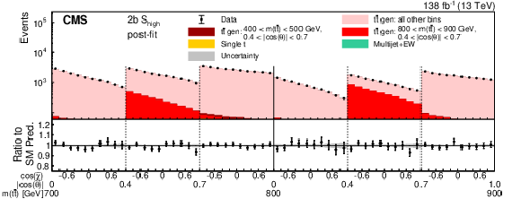
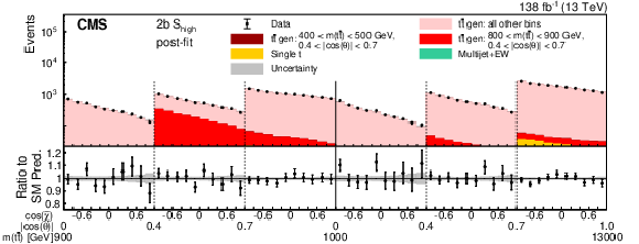
Pre- and post-fit distributions of $ \cos(\tilde{\chi}) $ comparing the data (points) to the POWHEG + PYTHIA simulation (stacked histograms) for the $ \tilde{D} $ measurement in bins of $ m({\mathrm{t}\overline{\mathrm{t}}} ) $ vs. $|\cos(\theta)\,| $ in the $2\mathrm{b} S_{\text{high}}$ category. The boundaries of the $ |\cos(\theta)| $ and $ m({\mathrm{t}\overline{\mathrm{t}}} ) $ bins are labeled and indicated by dashed and solid lines, respectively. For the illustration of resolution effects, $ \mathrm{t} \overline{\mathrm{t}} $ events generated in two selected $ m({\mathrm{t}\overline{\mathrm{t}}} ) $ vs. $|\cos(\theta)\,| $ bins are shown in different shades of red. All other $ \mathrm{t} \overline{\mathrm{t}} $ contributions are shown in pink. A model without any polarization and spin correlation is shown as a blue line. The gray uncertainty band indicates the combined statistical and systematic uncertainties in the prediction. The vertical bars on the points show the statistical uncertainty. Ratios to the predicted yields are provided in the lower panels. |
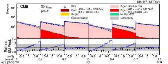
png pdf |
Figure 16-a:
Pre- and post-fit distributions of $ \cos(\tilde{\chi}) $ comparing the data (points) to the POWHEG + PYTHIA simulation (stacked histograms) for the $ \tilde{D} $ measurement in bins of $ m({\mathrm{t}\overline{\mathrm{t}}} ) $ vs. $|\cos(\theta)\,| $ in the $2\mathrm{b} S_{\text{high}}$ category. The boundaries of the $ |\cos(\theta)| $ and $ m({\mathrm{t}\overline{\mathrm{t}}} ) $ bins are labeled and indicated by dashed and solid lines, respectively. For the illustration of resolution effects, $ \mathrm{t} \overline{\mathrm{t}} $ events generated in two selected $ m({\mathrm{t}\overline{\mathrm{t}}} ) $ vs. $|\cos(\theta)\,| $ bins are shown in different shades of red. All other $ \mathrm{t} \overline{\mathrm{t}} $ contributions are shown in pink. A model without any polarization and spin correlation is shown as a blue line. The gray uncertainty band indicates the combined statistical and systematic uncertainties in the prediction. The vertical bars on the points show the statistical uncertainty. Ratios to the predicted yields are provided in the lower panels. |
png pdf |
Figure 16-b:
Pre- and post-fit distributions of $ \cos(\tilde{\chi}) $ comparing the data (points) to the POWHEG + PYTHIA simulation (stacked histograms) for the $ \tilde{D} $ measurement in bins of $ m({\mathrm{t}\overline{\mathrm{t}}} ) $ vs. $|\cos(\theta)\,| $ in the $2\mathrm{b} S_{\text{high}}$ category. The boundaries of the $ |\cos(\theta)| $ and $ m({\mathrm{t}\overline{\mathrm{t}}} ) $ bins are labeled and indicated by dashed and solid lines, respectively. For the illustration of resolution effects, $ \mathrm{t} \overline{\mathrm{t}} $ events generated in two selected $ m({\mathrm{t}\overline{\mathrm{t}}} ) $ vs. $|\cos(\theta)\,| $ bins are shown in different shades of red. All other $ \mathrm{t} \overline{\mathrm{t}} $ contributions are shown in pink. A model without any polarization and spin correlation is shown as a blue line. The gray uncertainty band indicates the combined statistical and systematic uncertainties in the prediction. The vertical bars on the points show the statistical uncertainty. Ratios to the predicted yields are provided in the lower panels. |

png pdf |
Figure 16-c:
Pre- and post-fit distributions of $ \cos(\tilde{\chi}) $ comparing the data (points) to the POWHEG + PYTHIA simulation (stacked histograms) for the $ \tilde{D} $ measurement in bins of $ m({\mathrm{t}\overline{\mathrm{t}}} ) $ vs. $|\cos(\theta)\,| $ in the $2\mathrm{b} S_{\text{high}}$ category. The boundaries of the $ |\cos(\theta)| $ and $ m({\mathrm{t}\overline{\mathrm{t}}} ) $ bins are labeled and indicated by dashed and solid lines, respectively. For the illustration of resolution effects, $ \mathrm{t} \overline{\mathrm{t}} $ events generated in two selected $ m({\mathrm{t}\overline{\mathrm{t}}} ) $ vs. $|\cos(\theta)\,| $ bins are shown in different shades of red. All other $ \mathrm{t} \overline{\mathrm{t}} $ contributions are shown in pink. A model without any polarization and spin correlation is shown as a blue line. The gray uncertainty band indicates the combined statistical and systematic uncertainties in the prediction. The vertical bars on the points show the statistical uncertainty. Ratios to the predicted yields are provided in the lower panels. |
png pdf |
Figure 16-d:
Pre- and post-fit distributions of $ \cos(\tilde{\chi}) $ comparing the data (points) to the POWHEG + PYTHIA simulation (stacked histograms) for the $ \tilde{D} $ measurement in bins of $ m({\mathrm{t}\overline{\mathrm{t}}} ) $ vs. $|\cos(\theta)\,| $ in the $2\mathrm{b} S_{\text{high}}$ category. The boundaries of the $ |\cos(\theta)| $ and $ m({\mathrm{t}\overline{\mathrm{t}}} ) $ bins are labeled and indicated by dashed and solid lines, respectively. For the illustration of resolution effects, $ \mathrm{t} \overline{\mathrm{t}} $ events generated in two selected $ m({\mathrm{t}\overline{\mathrm{t}}} ) $ vs. $|\cos(\theta)\,| $ bins are shown in different shades of red. All other $ \mathrm{t} \overline{\mathrm{t}} $ contributions are shown in pink. A model without any polarization and spin correlation is shown as a blue line. The gray uncertainty band indicates the combined statistical and systematic uncertainties in the prediction. The vertical bars on the points show the statistical uncertainty. Ratios to the predicted yields are provided in the lower panels. |
png pdf |
Figure 17:
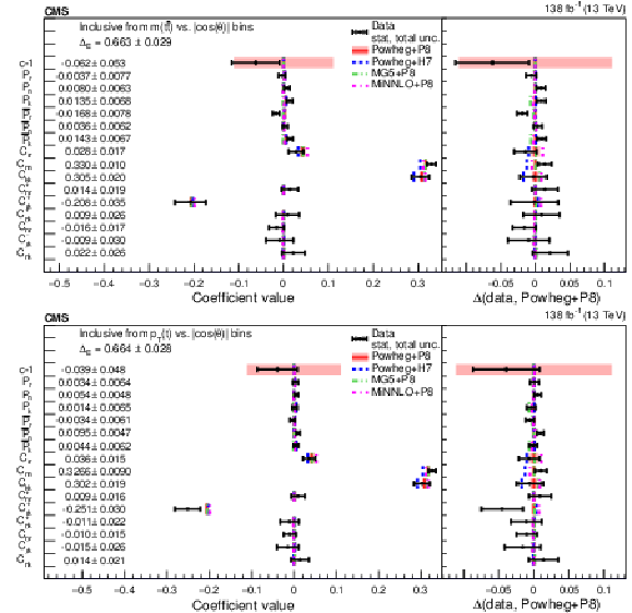
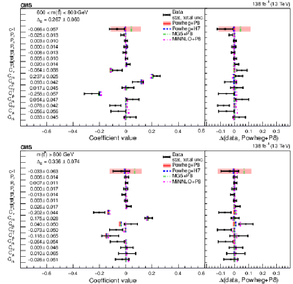
Results of the inclusive full matrix measurement obtained by combining the bins of the $ m({\mathrm{t}\overline{\mathrm{t}}} ) $ vs. $|\cos(\theta)\,| $ (upper) and $ p_{\mathrm{T}}(\mathrm{t}) $ vs. $|\cos(\theta)\,| $ (lower) measurements. The measurements (markers) are shown with the statistical uncertainty (inner error bars) and total uncertainty (outer error bars) and compared to the predictions of POWHEG + PYTHIA, POWHEG + HERWIG, MADGRAPH5_aMC@NLO+ PYTHIA and MINNLO+ PYTHIA. In the right panels, results are presented with the POWHEG + PYTHIA predictions subtracted. The POWHEG + PYTHIA prediction is displayed with ME scale and PDF uncertainties. The values of $ \Delta_{\text{E}} $ are displayed for each measurement. |

png pdf |
Figure 17-a:
Results of the inclusive full matrix measurement obtained by combining the bins of the $ m({\mathrm{t}\overline{\mathrm{t}}} ) $ vs. $|\cos(\theta)\,| $ (upper) and $ p_{\mathrm{T}}(\mathrm{t}) $ vs. $|\cos(\theta)\,| $ (lower) measurements. The measurements (markers) are shown with the statistical uncertainty (inner error bars) and total uncertainty (outer error bars) and compared to the predictions of POWHEG + PYTHIA, POWHEG + HERWIG, MADGRAPH5_aMC@NLO+ PYTHIA and MINNLO+ PYTHIA. In the right panels, results are presented with the POWHEG + PYTHIA predictions subtracted. The POWHEG + PYTHIA prediction is displayed with ME scale and PDF uncertainties. The values of $ \Delta_{\text{E}} $ are displayed for each measurement. |

png pdf |
Figure 17-b:
Results of the inclusive full matrix measurement obtained by combining the bins of the $ m({\mathrm{t}\overline{\mathrm{t}}} ) $ vs. $|\cos(\theta)\,| $ (upper) and $ p_{\mathrm{T}}(\mathrm{t}) $ vs. $|\cos(\theta)\,| $ (lower) measurements. The measurements (markers) are shown with the statistical uncertainty (inner error bars) and total uncertainty (outer error bars) and compared to the predictions of POWHEG + PYTHIA, POWHEG + HERWIG, MADGRAPH5_aMC@NLO+ PYTHIA and MINNLO+ PYTHIA. In the right panels, results are presented with the POWHEG + PYTHIA predictions subtracted. The POWHEG + PYTHIA prediction is displayed with ME scale and PDF uncertainties. The values of $ \Delta_{\text{E}} $ are displayed for each measurement. |
png pdf |
Figure 18:
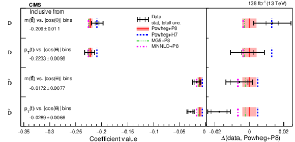
Results of the inclusive $ D $ and $ \tilde{D} $ measurement obtained by combining the bins of the $ m({\mathrm{t}\overline{\mathrm{t}}} ) $ vs. $|\cos(\theta)\,| $ and $ p_{\mathrm{T}}(\mathrm{t}) $ vs. $|\cos(\theta)\,| $ measurements. The measurements (markers) are shown with the statistical uncertainty (inner error bars) and total uncertainty (outer error bars) and compared to the predictions of POWHEG + PYTHIA, POWHEG + HERWIG, MADGRAPH5_aMC@NLO+ PYTHIA and MINNLO+ PYTHIA. In the right panel, results are presented with the POWHEG + PYTHIA predictions subtracted. The POWHEG + PYTHIA prediction is displayed with ME scale and PDF uncertainties. |

png pdf |
Figure 19:
Results of the full matrix measurement in bins of $ m({\mathrm{t}\overline{\mathrm{t}}} ) $. The measurements (markers) are shown with the statistical uncertainty (inner error bars) and total uncertainty (outer error bars) and compared to the predictions of POWHEG + PYTHIA, POWHEG + HERWIG, MADGRAPH5_aMC@NLO+ PYTHIA and MINNLO+ PYTHIA. In the right panels, results are presented with the POWHEG + PYTHIA predictions subtracted. The POWHEG + PYTHIA prediction is displayed with ME scale and PDF uncertainties. The values of $ \Delta_{\text{E}} $ are displayed for each measurement. |

png pdf |
Figure 19-a:
Results of the full matrix measurement in bins of $ m({\mathrm{t}\overline{\mathrm{t}}} ) $. The measurements (markers) are shown with the statistical uncertainty (inner error bars) and total uncertainty (outer error bars) and compared to the predictions of POWHEG + PYTHIA, POWHEG + HERWIG, MADGRAPH5_aMC@NLO+ PYTHIA and MINNLO+ PYTHIA. In the right panels, results are presented with the POWHEG + PYTHIA predictions subtracted. The POWHEG + PYTHIA prediction is displayed with ME scale and PDF uncertainties. The values of $ \Delta_{\text{E}} $ are displayed for each measurement. |

png pdf |
Figure 19-b:
Results of the full matrix measurement in bins of $ m({\mathrm{t}\overline{\mathrm{t}}} ) $. The measurements (markers) are shown with the statistical uncertainty (inner error bars) and total uncertainty (outer error bars) and compared to the predictions of POWHEG + PYTHIA, POWHEG + HERWIG, MADGRAPH5_aMC@NLO+ PYTHIA and MINNLO+ PYTHIA. In the right panels, results are presented with the POWHEG + PYTHIA predictions subtracted. The POWHEG + PYTHIA prediction is displayed with ME scale and PDF uncertainties. The values of $ \Delta_{\text{E}} $ are displayed for each measurement. |
png pdf |
Figure 20:
Results of the full matrix measurement in bins of $ m({\mathrm{t}\overline{\mathrm{t}}} ) $. The measurements (markers) are shown with the statistical uncertainty (inner error bars) and total uncertainty (outer error bars) and compared to the predictions of POWHEG + PYTHIA, POWHEG + HERWIG, MADGRAPH5_aMC@NLO+ PYTHIA and MINNLO+ PYTHIA. In the right panels, results are presented with the POWHEG + PYTHIA predictions subtracted. The POWHEG + PYTHIA prediction is displayed with ME scale and PDF uncertainties. The values of $ \Delta_{\text{E}} $ are displayed for each measurement. |

png pdf |
Figure 20-a:
Results of the full matrix measurement in bins of $ m({\mathrm{t}\overline{\mathrm{t}}} ) $. The measurements (markers) are shown with the statistical uncertainty (inner error bars) and total uncertainty (outer error bars) and compared to the predictions of POWHEG + PYTHIA, POWHEG + HERWIG, MADGRAPH5_aMC@NLO+ PYTHIA and MINNLO+ PYTHIA. In the right panels, results are presented with the POWHEG + PYTHIA predictions subtracted. The POWHEG + PYTHIA prediction is displayed with ME scale and PDF uncertainties. The values of $ \Delta_{\text{E}} $ are displayed for each measurement. |
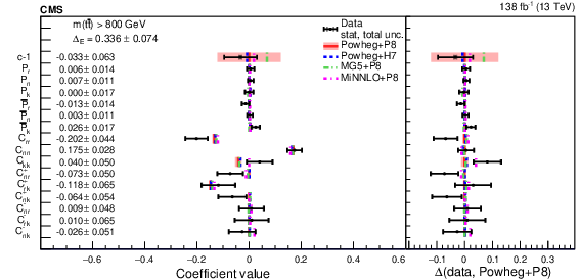
png pdf |
Figure 20-b:
Results of the full matrix measurement in bins of $ m({\mathrm{t}\overline{\mathrm{t}}} ) $. The measurements (markers) are shown with the statistical uncertainty (inner error bars) and total uncertainty (outer error bars) and compared to the predictions of POWHEG + PYTHIA, POWHEG + HERWIG, MADGRAPH5_aMC@NLO+ PYTHIA and MINNLO+ PYTHIA. In the right panels, results are presented with the POWHEG + PYTHIA predictions subtracted. The POWHEG + PYTHIA prediction is displayed with ME scale and PDF uncertainties. The values of $ \Delta_{\text{E}} $ are displayed for each measurement. |
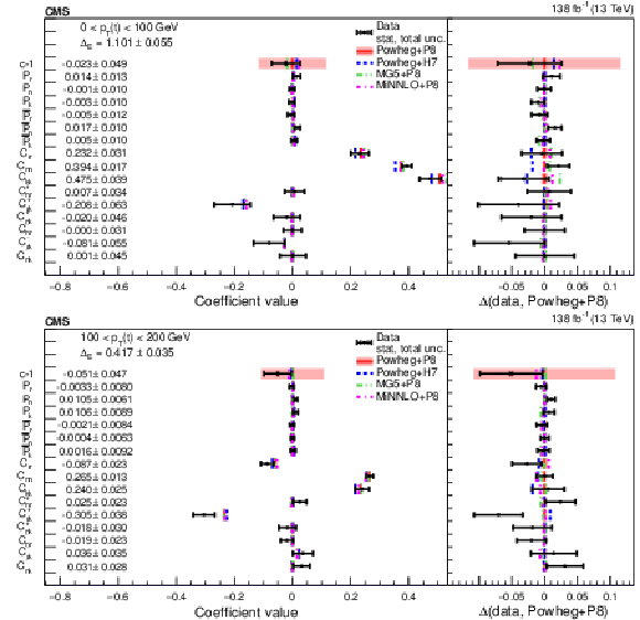
png pdf |
Figure 21:
Results of the full matrix measurement in bins of $ p_{\mathrm{T}}(\mathrm{t}) $. The measurements (markers) are shown with the statistical uncertainty (inner error bars) and total uncertainty (outer error bars) and compared to the predictions of POWHEG + PYTHIA, POWHEG + HERWIG, MADGRAPH5_aMC@NLO+ PYTHIA and MINNLO+ PYTHIA. In the right panels, results are presented with the POWHEG + PYTHIA predictions subtracted. The POWHEG + PYTHIA prediction is displayed with ME scale and PDF uncertainties. The values of $ \Delta_{\text{E}} $ are displayed for each measurement. |

png pdf |
Figure 21-a:
Results of the full matrix measurement in bins of $ p_{\mathrm{T}}(\mathrm{t}) $. The measurements (markers) are shown with the statistical uncertainty (inner error bars) and total uncertainty (outer error bars) and compared to the predictions of POWHEG + PYTHIA, POWHEG + HERWIG, MADGRAPH5_aMC@NLO+ PYTHIA and MINNLO+ PYTHIA. In the right panels, results are presented with the POWHEG + PYTHIA predictions subtracted. The POWHEG + PYTHIA prediction is displayed with ME scale and PDF uncertainties. The values of $ \Delta_{\text{E}} $ are displayed for each measurement. |

png pdf |
Figure 21-b:
Results of the full matrix measurement in bins of $ p_{\mathrm{T}}(\mathrm{t}) $. The measurements (markers) are shown with the statistical uncertainty (inner error bars) and total uncertainty (outer error bars) and compared to the predictions of POWHEG + PYTHIA, POWHEG + HERWIG, MADGRAPH5_aMC@NLO+ PYTHIA and MINNLO+ PYTHIA. In the right panels, results are presented with the POWHEG + PYTHIA predictions subtracted. The POWHEG + PYTHIA prediction is displayed with ME scale and PDF uncertainties. The values of $ \Delta_{\text{E}} $ are displayed for each measurement. |
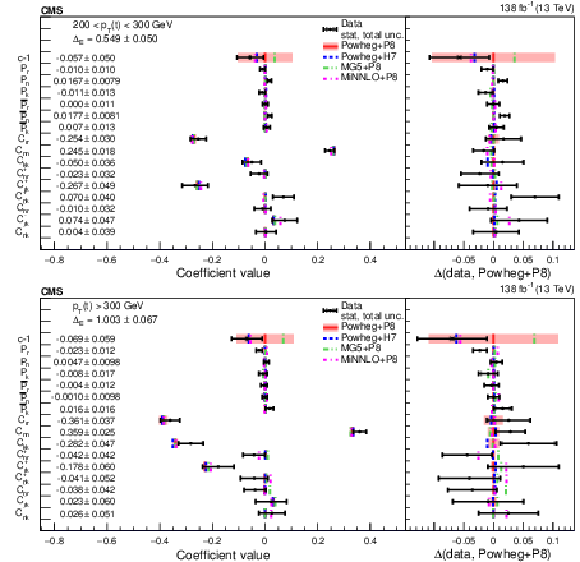
png pdf |
Figure 22:
Results of the full matrix measurement in bins of $ p_{\mathrm{T}}(\mathrm{t}) $. The measurements (markers) are shown with the statistical uncertainty (inner error bars) and total uncertainty (outer error bars) and compared to the predictions of POWHEG + PYTHIA, POWHEG + HERWIG, MADGRAPH5_aMC@NLO+ PYTHIA and MINNLO+ PYTHIA. In the right panels, results are presented with the POWHEG + PYTHIA predictions subtracted. The POWHEG + PYTHIA prediction is displayed with ME scale and PDF uncertainties. The values of $ \Delta_{\text{E}} $ are displayed for each measurement. |

png pdf |
Figure 22-a:
Results of the full matrix measurement in bins of $ p_{\mathrm{T}}(\mathrm{t}) $. The measurements (markers) are shown with the statistical uncertainty (inner error bars) and total uncertainty (outer error bars) and compared to the predictions of POWHEG + PYTHIA, POWHEG + HERWIG, MADGRAPH5_aMC@NLO+ PYTHIA and MINNLO+ PYTHIA. In the right panels, results are presented with the POWHEG + PYTHIA predictions subtracted. The POWHEG + PYTHIA prediction is displayed with ME scale and PDF uncertainties. The values of $ \Delta_{\text{E}} $ are displayed for each measurement. |

png pdf |
Figure 22-b:
Results of the full matrix measurement in bins of $ p_{\mathrm{T}}(\mathrm{t}) $. The measurements (markers) are shown with the statistical uncertainty (inner error bars) and total uncertainty (outer error bars) and compared to the predictions of POWHEG + PYTHIA, POWHEG + HERWIG, MADGRAPH5_aMC@NLO+ PYTHIA and MINNLO+ PYTHIA. In the right panels, results are presented with the POWHEG + PYTHIA predictions subtracted. The POWHEG + PYTHIA prediction is displayed with ME scale and PDF uncertainties. The values of $ \Delta_{\text{E}} $ are displayed for each measurement. |

png pdf |
Figure 23:
Results of the $ D $ and $ \tilde{D} $ measurements in bins of $ m({\mathrm{t}\overline{\mathrm{t}}} ) $ and $ p_{\mathrm{T}}(\mathrm{t}) $. The measurements (markers) are shown with the statistical uncertainty (inner error bars) and total uncertainty (outer error bars) and compared to the predictions of POWHEG + PYTHIA, POWHEG + HERWIG, MADGRAPH5_aMC@NLO+ PYTHIA and MINNLO+ PYTHIA. In the lower panel results are presented with the POWHEG + PYTHIA predictions subtracted. The POWHEG + PYTHIA prediction is displayed with ME scale and PDF uncertainties. |
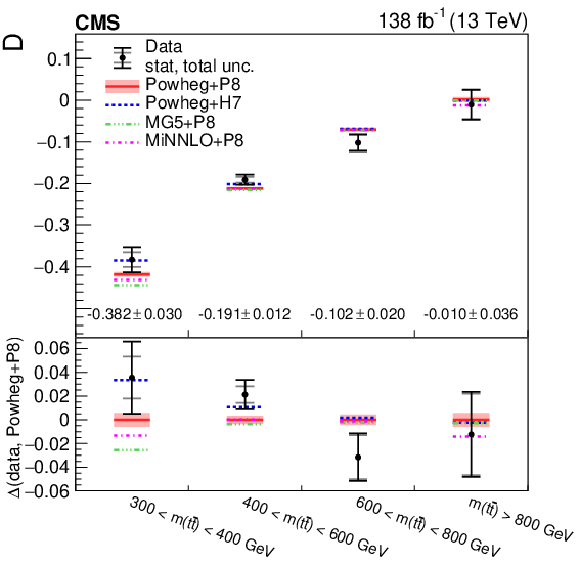
png pdf |
Figure 23-a:
Results of the $ D $ and $ \tilde{D} $ measurements in bins of $ m({\mathrm{t}\overline{\mathrm{t}}} ) $ and $ p_{\mathrm{T}}(\mathrm{t}) $. The measurements (markers) are shown with the statistical uncertainty (inner error bars) and total uncertainty (outer error bars) and compared to the predictions of POWHEG + PYTHIA, POWHEG + HERWIG, MADGRAPH5_aMC@NLO+ PYTHIA and MINNLO+ PYTHIA. In the lower panel results are presented with the POWHEG + PYTHIA predictions subtracted. The POWHEG + PYTHIA prediction is displayed with ME scale and PDF uncertainties. |

png pdf |
Figure 23-b:
Results of the $ D $ and $ \tilde{D} $ measurements in bins of $ m({\mathrm{t}\overline{\mathrm{t}}} ) $ and $ p_{\mathrm{T}}(\mathrm{t}) $. The measurements (markers) are shown with the statistical uncertainty (inner error bars) and total uncertainty (outer error bars) and compared to the predictions of POWHEG + PYTHIA, POWHEG + HERWIG, MADGRAPH5_aMC@NLO+ PYTHIA and MINNLO+ PYTHIA. In the lower panel results are presented with the POWHEG + PYTHIA predictions subtracted. The POWHEG + PYTHIA prediction is displayed with ME scale and PDF uncertainties. |

png pdf |
Figure 23-c:
Results of the $ D $ and $ \tilde{D} $ measurements in bins of $ m({\mathrm{t}\overline{\mathrm{t}}} ) $ and $ p_{\mathrm{T}}(\mathrm{t}) $. The measurements (markers) are shown with the statistical uncertainty (inner error bars) and total uncertainty (outer error bars) and compared to the predictions of POWHEG + PYTHIA, POWHEG + HERWIG, MADGRAPH5_aMC@NLO+ PYTHIA and MINNLO+ PYTHIA. In the lower panel results are presented with the POWHEG + PYTHIA predictions subtracted. The POWHEG + PYTHIA prediction is displayed with ME scale and PDF uncertainties. |
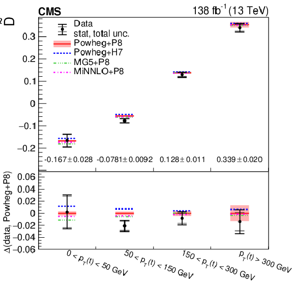
png pdf |
Figure 23-d:
Results of the $ D $ and $ \tilde{D} $ measurements in bins of $ m({\mathrm{t}\overline{\mathrm{t}}} ) $ and $ p_{\mathrm{T}}(\mathrm{t}) $. The measurements (markers) are shown with the statistical uncertainty (inner error bars) and total uncertainty (outer error bars) and compared to the predictions of POWHEG + PYTHIA, POWHEG + HERWIG, MADGRAPH5_aMC@NLO+ PYTHIA and MINNLO+ PYTHIA. In the lower panel results are presented with the POWHEG + PYTHIA predictions subtracted. The POWHEG + PYTHIA prediction is displayed with ME scale and PDF uncertainties. |
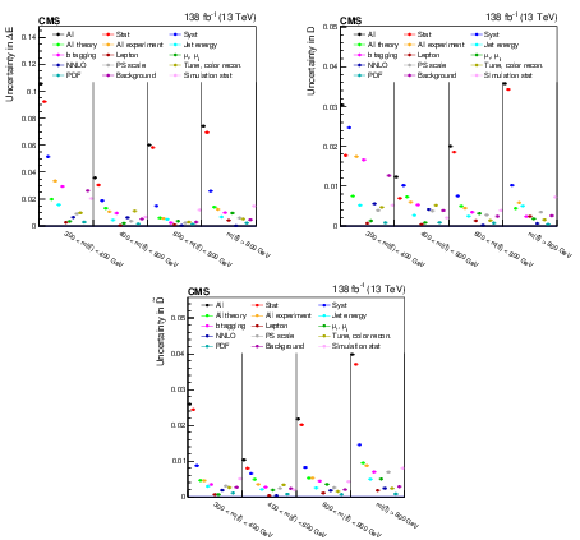
png pdf |
Figure 24:
Contribution of individual uncertainty sources or groups of uncertainties in the measured $ \Delta_{\text{E}} $, $ D $, and $ \tilde{D} $ in bins of $ m({\mathrm{t}\overline{\mathrm{t}}} ) $. |

png pdf |
Figure 24-a:
Contribution of individual uncertainty sources or groups of uncertainties in the measured $ \Delta_{\text{E}} $, $ D $, and $ \tilde{D} $ in bins of $ m({\mathrm{t}\overline{\mathrm{t}}} ) $. |

png pdf |
Figure 24-b:
Contribution of individual uncertainty sources or groups of uncertainties in the measured $ \Delta_{\text{E}} $, $ D $, and $ \tilde{D} $ in bins of $ m({\mathrm{t}\overline{\mathrm{t}}} ) $. |
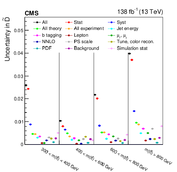
png pdf |
Figure 24-c:
Contribution of individual uncertainty sources or groups of uncertainties in the measured $ \Delta_{\text{E}} $, $ D $, and $ \tilde{D} $ in bins of $ m({\mathrm{t}\overline{\mathrm{t}}} ) $. |
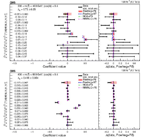
png pdf |
Figure 25:
Results of the full matrix measurement in bins of $ m({\mathrm{t}\overline{\mathrm{t}}} ) $ for $ |\cos(\theta)| < $ 0.4. The measurements (markers) are shown with the statistical uncertainty (inner error bars) and total uncertainty (outer error bars) and compared to the predictions of POWHEG + PYTHIA, POWHEG + HERWIG, MADGRAPH5_aMC@NLO+ PYTHIA and MINNLO+ PYTHIA. In the right panels, results are presented with the POWHEG + PYTHIA predictions subtracted. The POWHEG + PYTHIA prediction is displayed with ME scale and PDF uncertainties. The values of $ \Delta_{\text{E}} $ are displayed for each measurement. |

png pdf |
Figure 25-a:
Results of the full matrix measurement in bins of $ m({\mathrm{t}\overline{\mathrm{t}}} ) $ for $ |\cos(\theta)| < $ 0.4. The measurements (markers) are shown with the statistical uncertainty (inner error bars) and total uncertainty (outer error bars) and compared to the predictions of POWHEG + PYTHIA, POWHEG + HERWIG, MADGRAPH5_aMC@NLO+ PYTHIA and MINNLO+ PYTHIA. In the right panels, results are presented with the POWHEG + PYTHIA predictions subtracted. The POWHEG + PYTHIA prediction is displayed with ME scale and PDF uncertainties. The values of $ \Delta_{\text{E}} $ are displayed for each measurement. |

png pdf |
Figure 25-b:
Results of the full matrix measurement in bins of $ m({\mathrm{t}\overline{\mathrm{t}}} ) $ for $ |\cos(\theta)| < $ 0.4. The measurements (markers) are shown with the statistical uncertainty (inner error bars) and total uncertainty (outer error bars) and compared to the predictions of POWHEG + PYTHIA, POWHEG + HERWIG, MADGRAPH5_aMC@NLO+ PYTHIA and MINNLO+ PYTHIA. In the right panels, results are presented with the POWHEG + PYTHIA predictions subtracted. The POWHEG + PYTHIA prediction is displayed with ME scale and PDF uncertainties. The values of $ \Delta_{\text{E}} $ are displayed for each measurement. |

png pdf |
Figure 26:
Results of the full matrix measurement in bins of $ m({\mathrm{t}\overline{\mathrm{t}}} ) $ for $ |\cos(\theta)| < $ 0.4. The measurements (markers) are shown with the statistical uncertainty (inner error bars) and total uncertainty (outer error bars) and compared to the predictions of POWHEG + PYTHIA, POWHEG + HERWIG, MADGRAPH5_aMC@NLO+ PYTHIA and MINNLO+ PYTHIA. In the right panels, results are presented with the POWHEG + PYTHIA predictions subtracted. The POWHEG + PYTHIA prediction is displayed with ME scale and PDF uncertainties. The values of $ \Delta_{\text{E}} $ are displayed for each measurement. |

png pdf |
Figure 26-a:
Results of the full matrix measurement in bins of $ m({\mathrm{t}\overline{\mathrm{t}}} ) $ for $ |\cos(\theta)| < $ 0.4. The measurements (markers) are shown with the statistical uncertainty (inner error bars) and total uncertainty (outer error bars) and compared to the predictions of POWHEG + PYTHIA, POWHEG + HERWIG, MADGRAPH5_aMC@NLO+ PYTHIA and MINNLO+ PYTHIA. In the right panels, results are presented with the POWHEG + PYTHIA predictions subtracted. The POWHEG + PYTHIA prediction is displayed with ME scale and PDF uncertainties. The values of $ \Delta_{\text{E}} $ are displayed for each measurement. |
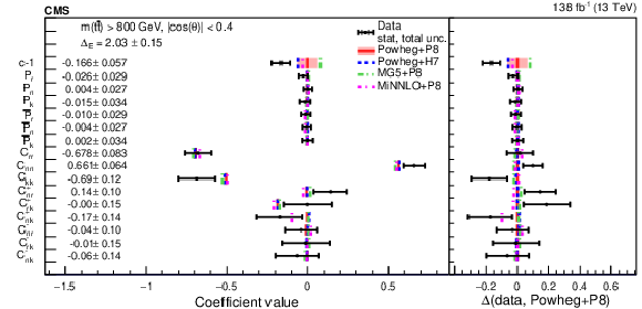
png pdf |
Figure 26-b:
Results of the full matrix measurement in bins of $ m({\mathrm{t}\overline{\mathrm{t}}} ) $ for $ |\cos(\theta)| < $ 0.4. The measurements (markers) are shown with the statistical uncertainty (inner error bars) and total uncertainty (outer error bars) and compared to the predictions of POWHEG + PYTHIA, POWHEG + HERWIG, MADGRAPH5_aMC@NLO+ PYTHIA and MINNLO+ PYTHIA. In the right panels, results are presented with the POWHEG + PYTHIA predictions subtracted. The POWHEG + PYTHIA prediction is displayed with ME scale and PDF uncertainties. The values of $ \Delta_{\text{E}} $ are displayed for each measurement. |
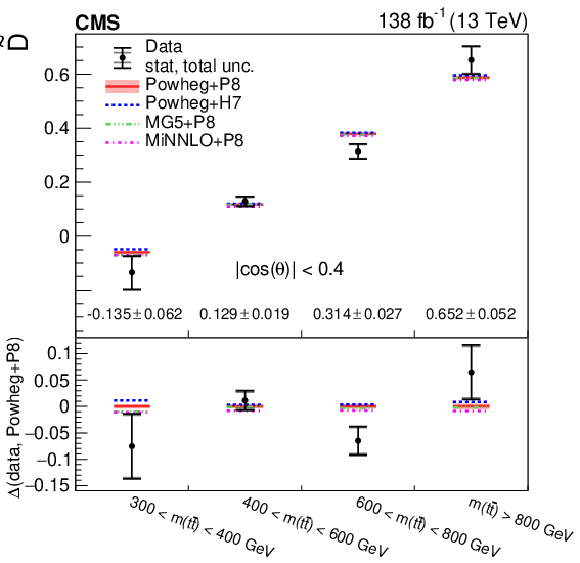
png pdf |
Figure 27:
Results of the $ \tilde{D} $ measurements in bins of $ m({\mathrm{t}\overline{\mathrm{t}}} ) $ for $ |\cos(\theta)| < $ 0.4. The measurements (markers) are shown with the statistical uncertainty (inner error bars) and total uncertainty (outer error bars) and compared to the predictions of POWHEG + PYTHIA, POWHEG + HERWIG, MADGRAPH5_aMC@NLO+ PYTHIA and MINNLO+ PYTHIA. In the lower panel results are presented with the POWHEG + PYTHIA predictions subtracted. The POWHEG + PYTHIA prediction is displayed with ME scale and PDF uncertainties. |

png pdf |
Figure 28:
Entanglement results for the $ D $ measurement in the threshold region (upper left ), $ \tilde{D} $ measurement in the high-$ m({\mathrm{t}\overline{\mathrm{t}}} ) $ region (upper right ), and the full matrix measurement in different $ m({\mathrm{t}\overline{\mathrm{t}}} ) $ regions (lower). The measurements (points) are shown with the statistical uncertainty (inner error bars) and total uncertainty (outer error bars) and compared to the predictions of POWHEG + PYTHIA, POWHEG + PYTHIA + $ \eta \mathrm{t} $, POWHEG + HERWIG, MADGRAPH5_aMC@NLO+ PYTHIA, and MINNLO+ PYTHIA. The POWHEG + PYTHIA prediction is displayed with the ME scale and PDF uncertainties, while for all other predictions only the central values are indicated. The observed (expected) significance of the deviation from the boundary of separable states (green region) is quoted in standard deviations ($ \sigma $). |

png pdf |
Figure 28-a:
Entanglement results for the $ D $ measurement in the threshold region (upper left ), $ \tilde{D} $ measurement in the high-$ m({\mathrm{t}\overline{\mathrm{t}}} ) $ region (upper right ), and the full matrix measurement in different $ m({\mathrm{t}\overline{\mathrm{t}}} ) $ regions (lower). The measurements (points) are shown with the statistical uncertainty (inner error bars) and total uncertainty (outer error bars) and compared to the predictions of POWHEG + PYTHIA, POWHEG + PYTHIA + $ \eta \mathrm{t} $, POWHEG + HERWIG, MADGRAPH5_aMC@NLO+ PYTHIA, and MINNLO+ PYTHIA. The POWHEG + PYTHIA prediction is displayed with the ME scale and PDF uncertainties, while for all other predictions only the central values are indicated. The observed (expected) significance of the deviation from the boundary of separable states (green region) is quoted in standard deviations ($ \sigma $). |
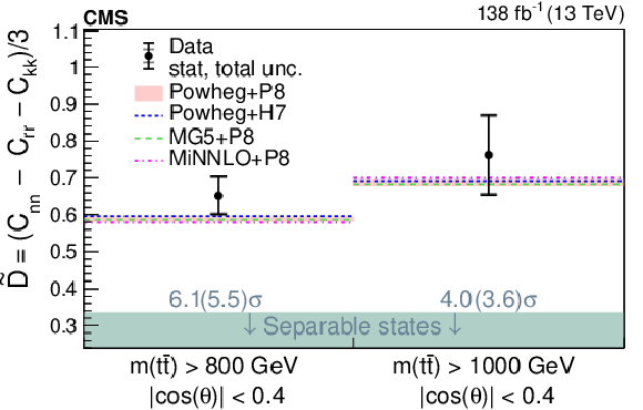
png pdf |
Figure 28-b:
Entanglement results for the $ D $ measurement in the threshold region (upper left ), $ \tilde{D} $ measurement in the high-$ m({\mathrm{t}\overline{\mathrm{t}}} ) $ region (upper right ), and the full matrix measurement in different $ m({\mathrm{t}\overline{\mathrm{t}}} ) $ regions (lower). The measurements (points) are shown with the statistical uncertainty (inner error bars) and total uncertainty (outer error bars) and compared to the predictions of POWHEG + PYTHIA, POWHEG + PYTHIA + $ \eta \mathrm{t} $, POWHEG + HERWIG, MADGRAPH5_aMC@NLO+ PYTHIA, and MINNLO+ PYTHIA. The POWHEG + PYTHIA prediction is displayed with the ME scale and PDF uncertainties, while for all other predictions only the central values are indicated. The observed (expected) significance of the deviation from the boundary of separable states (green region) is quoted in standard deviations ($ \sigma $). |
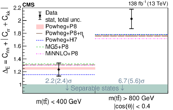
png pdf |
Figure 28-c:
Entanglement results for the $ D $ measurement in the threshold region (upper left ), $ \tilde{D} $ measurement in the high-$ m({\mathrm{t}\overline{\mathrm{t}}} ) $ region (upper right ), and the full matrix measurement in different $ m({\mathrm{t}\overline{\mathrm{t}}} ) $ regions (lower). The measurements (points) are shown with the statistical uncertainty (inner error bars) and total uncertainty (outer error bars) and compared to the predictions of POWHEG + PYTHIA, POWHEG + PYTHIA + $ \eta \mathrm{t} $, POWHEG + HERWIG, MADGRAPH5_aMC@NLO+ PYTHIA, and MINNLO+ PYTHIA. The POWHEG + PYTHIA prediction is displayed with the ME scale and PDF uncertainties, while for all other predictions only the central values are indicated. The observed (expected) significance of the deviation from the boundary of separable states (green region) is quoted in standard deviations ($ \sigma $). |
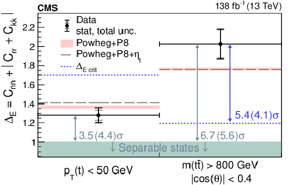
png pdf |
Figure 29:
The observed levels of entanglement characterized by $ \Delta_{\text{E}} $ are shown in the threshold region using the $ D $ measurement (first bin), and in the high-$ m({\mathrm{t}\overline{\mathrm{t}}} ) $ region using the full matrix measurement (second bin). The measurements (points) are shown with the statistical uncertainty (inner error bars) and total uncertainty (outer error bars) and compared to the predictions of POWHEG + PYTHIA, POWHEG + PYTHIA +$ \eta \mathrm{t} $. The POWHEG + PYTHIA prediction is displayed with the ME scale and PDF uncertainties. The horizontal blue lines correspond to the maximum level of entanglement $ \Delta_{\text{E\,crit}} $ that can be explained by the exchange of information between t and $ \overline{\mathrm{t}} $ at the speed of light. The significance in standard deviations ($ \sigma $) by which the measurement exceeds $ \Delta_{\text{E\,crit}} $ and unity is quoted in blue and light green, respectively, and indicated by the corresponding arrows. |

png pdf |
Figure 30:
Results of the profile likelihood scans. The quantity $ -2\Delta\log(L) $ is shown as function of $ \Delta_{\text{E}} $ in the bin with $ m({\mathrm{t}\overline{\mathrm{t}}} ) > $ 800 GeV and $ |\cos(\theta)| < $ 0.4 for data (black line) and the POWHEG + PYTHIA simulation (red line). The observed and expected significances in standard deviations ($ \sigma $) for $ \Delta_{\text{E}} $ exceeding unity and $ \Delta_{\text{E\,crit}} $ are quoted. |
| Summary |
| The polarization and spin correlation in top quark pair ( $ \mathrm{t} \overline{\mathrm{t}} $) production are measured in events with an electron or a muon plus jets in the final state. The entanglement between the spins of the top quark and antiquark is determined from the measured spin correlation by applying the Peres-Horodecki criterion. The measurements are based on proton-proton collision data at $ \sqrt{s}= $ 13 TeV collected by the CMS experiment at the LHC, corresponding to an integrated luminosity of 138 fb$ ^{-1} $. The decay products of the top quarks are identified using an artificial neural network. The coefficients of the polarization vectors and the spin correlation matrix are extracted simultaneously from the angular distributions of $ \mathrm{t} \overline{\mathrm{t}} $ decay products using a binned likelihood fit. This is done both inclusively and in various regions of the phase space. The observed polarization and spin correlation are in agreement with the standard model expectations. The standard model predicts entangled $ \mathrm{t} \overline{\mathrm{t}} $ states at the production threshold and at high masses of the $ \mathrm{t} \overline{\mathrm{t}} $ system. Entanglement is observed in events with high $ \mathrm{t} \overline{\mathrm{t}} $ mass, with an observed (expected) significance of 6.7 (5.6) standard deviations, while in events with low transverse momentum of the top quark a significance of 3.5 (4.4) standard deviations is observed (expected). This is the first observation of entanglement at high $ \mathrm{t} \overline{\mathrm{t}} $ mass where in about 90% of the observed $ \mathrm{t} \overline{\mathrm{t}} $ events the decays of the top quark and antiquark are space-like separated. |
| Additional Figures | |
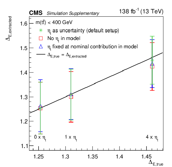
png pdf |
Additional Figure 1:
Results of the $ \eta \mathrm{t} $ injection tests for the full matrix measurement at the $ \mathrm{t} \overline{\mathrm{t}} $ threshold with $ m({\mathrm{t}\overline{\mathrm{t}}} ) < $ 400 GeV. From simulations with different injected $ \eta \mathrm{t} $ cross sections (0, 1, and 4 $ \times $ nominal $ \eta \mathrm{t} $), the extracted $ \Delta_{\text{E}} $ are calculated based on the fitted diagonal elements of the spin correlation matrix and shown as function of the true $ \Delta_{\text{E}} $ values. The values and uncertainties indicated by the green markers with error bars are obtained with the default model, where effects of $ \eta \mathrm{t} $ on the templates are included as uncertainty. The values indicated by the red and blue markers with error bars are obtained using templates that assume zero and nominal $ \eta \mathrm{t} $ contributions, respectively. |
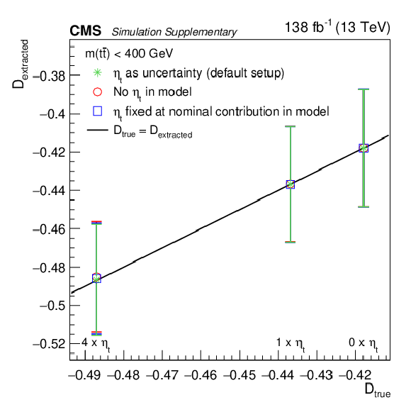
png pdf |
Additional Figure 2:
Results of the $ \eta \mathrm{t} $ injection tests for the $ D $ measurement at the $ \mathrm{t} \overline{\mathrm{t}} $ threshold with $ m({\mathrm{t}\overline{\mathrm{t}}} ) < $ 400 GeV. From simulations with different injected $ \eta \mathrm{t} $ cross sections (0, 1, and 4 $ \times $ nominal $ \eta \mathrm{t} $), the extracted $ D $ values are shown as function of the true $ D $ values. The values and uncertainties indicated by the green markers with error bars are obtained with the default model, where effects of $ \eta \mathrm{t} $ on the templates are included as uncertainty. The values indicated by the red and blue markers with error bars are obtained using templates that assume zero and nominal $ \eta \mathrm{t} $ contributions, respectively. |
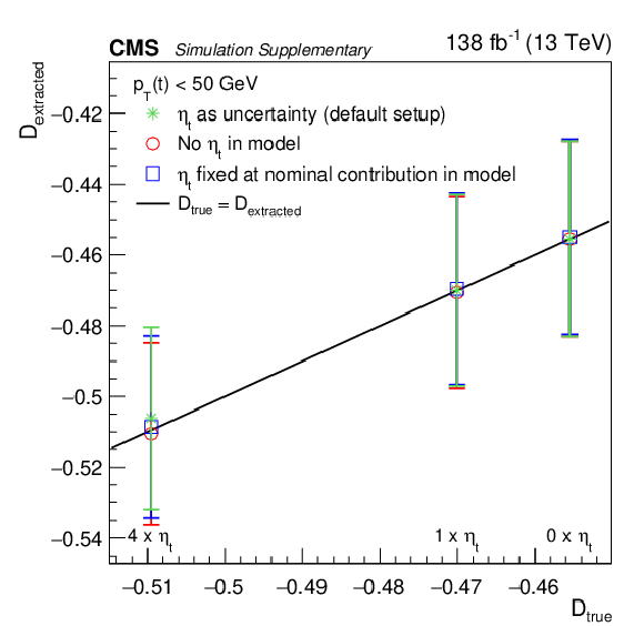
png pdf |
Additional Figure 3:
Results of the $ \eta \mathrm{t} $ injection tests for the $ D $ measurement with $ p_{\mathrm{T}}(\mathrm{t}) < $ 50 GeV. From simulations with different injected $ \eta \mathrm{t} $ cross sections (0, 1, and 4 $ \times $ nominal $ \eta \mathrm{t} $), the extracted $ D $ values are shown as function of the true $ D $ values. The values and uncertainties indicated by the green markers with error bars are obtained with the default model, where effects of $ \eta \mathrm{t} $ on the templates are included as uncertainty. The values indicated by the red and blue markers with error bars are obtained using templates that assume zero and nominal $ \eta \mathrm{t} $ contributions, respectively. |
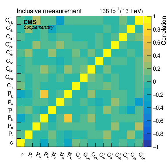
png pdf |
Additional Figure 4:
Correlation matrix for the measured coefficients in the inclusive full matrix measurement obtained from the $ m({\mathrm{t}\overline{\mathrm{t}}} ) $ vs. $|\cos(\theta)\,| $ fit of the data. |
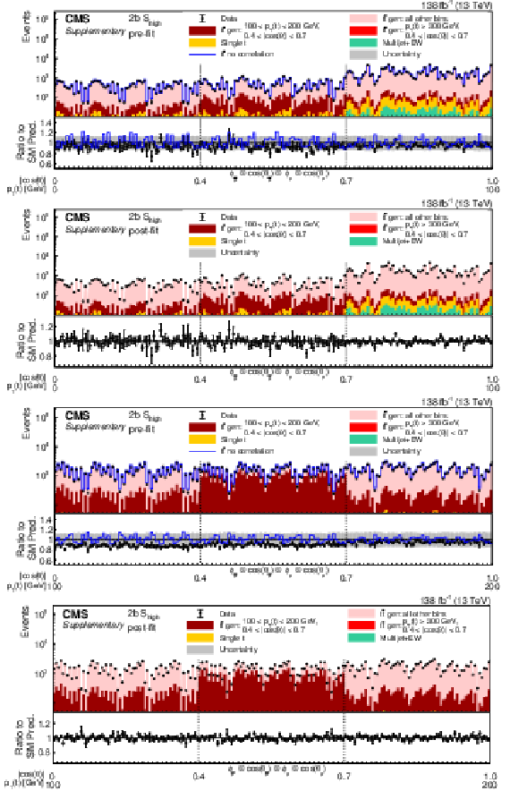
png pdf |
Additional Figure 5:
Pre- and post-fit distributions comparing the data (points) to the POWHEG + PYTHIA simulation (stacked histograms) for the full matrix measurement in bins of $ p_{\mathrm{T}}(\mathrm{t}) $ vs. $|\cos(\theta)\,| $ in the $2\mathrm{b} S_{\text{high}}$ category. The $ x $ axis shows the bins of the unrolled 4-dimensional distribution of $ \phi_{\bar{\mathrm{p}}} $, $ \cos(\theta_{\bar{\mathrm{p}}}) $, $ \phi_{\mathrm{p}} $, and $ \cos(\theta_{\mathrm{p}}) $, listed from the outermost to the innermost variable in each of the $ p_{\mathrm{T}}(\mathrm{t}) $ vs. $|\cos(\theta)\,| $ bins. The boundaries of the $ |\cos(\theta)| $ and $ p_{\mathrm{T}}(\mathrm{t}) $ bins are labeled and indicated by dashed and solid lines, respectively. For the illustration of resolution effects, $ \mathrm{t} \overline{\mathrm{t}} $ events generated in two selected $ p_{\mathrm{T}}(\mathrm{t}) $ vs. $|\cos(\theta)\,| $ bins are shown in different shades of red. All other $ \mathrm{t} \overline{\mathrm{t}} $ contributions are shown in pink. A model without any polarization and spin correlation is shown as a blue line. The gray uncertainty band indicates the combined statistical and systematic uncertainties in the prediction. The vertical bars on the points show the statistical uncertainty. Ratios to the predicted yields are provided in the lower panels. |

png pdf |
Additional Figure 5-a:
Pre- and post-fit distributions comparing the data (points) to the POWHEG + PYTHIA simulation (stacked histograms) for the full matrix measurement in bins of $ p_{\mathrm{T}}(\mathrm{t}) $ vs. $|\cos(\theta)\,| $ in the $2\mathrm{b} S_{\text{high}}$ category. The $ x $ axis shows the bins of the unrolled 4-dimensional distribution of $ \phi_{\bar{\mathrm{p}}} $, $ \cos(\theta_{\bar{\mathrm{p}}}) $, $ \phi_{\mathrm{p}} $, and $ \cos(\theta_{\mathrm{p}}) $, listed from the outermost to the innermost variable in each of the $ p_{\mathrm{T}}(\mathrm{t}) $ vs. $|\cos(\theta)\,| $ bins. The boundaries of the $ |\cos(\theta)| $ and $ p_{\mathrm{T}}(\mathrm{t}) $ bins are labeled and indicated by dashed and solid lines, respectively. For the illustration of resolution effects, $ \mathrm{t} \overline{\mathrm{t}} $ events generated in two selected $ p_{\mathrm{T}}(\mathrm{t}) $ vs. $|\cos(\theta)\,| $ bins are shown in different shades of red. All other $ \mathrm{t} \overline{\mathrm{t}} $ contributions are shown in pink. A model without any polarization and spin correlation is shown as a blue line. The gray uncertainty band indicates the combined statistical and systematic uncertainties in the prediction. The vertical bars on the points show the statistical uncertainty. Ratios to the predicted yields are provided in the lower panels. |

png pdf |
Additional Figure 5-b:
Pre- and post-fit distributions comparing the data (points) to the POWHEG + PYTHIA simulation (stacked histograms) for the full matrix measurement in bins of $ p_{\mathrm{T}}(\mathrm{t}) $ vs. $|\cos(\theta)\,| $ in the $2\mathrm{b} S_{\text{high}}$ category. The $ x $ axis shows the bins of the unrolled 4-dimensional distribution of $ \phi_{\bar{\mathrm{p}}} $, $ \cos(\theta_{\bar{\mathrm{p}}}) $, $ \phi_{\mathrm{p}} $, and $ \cos(\theta_{\mathrm{p}}) $, listed from the outermost to the innermost variable in each of the $ p_{\mathrm{T}}(\mathrm{t}) $ vs. $|\cos(\theta)\,| $ bins. The boundaries of the $ |\cos(\theta)| $ and $ p_{\mathrm{T}}(\mathrm{t}) $ bins are labeled and indicated by dashed and solid lines, respectively. For the illustration of resolution effects, $ \mathrm{t} \overline{\mathrm{t}} $ events generated in two selected $ p_{\mathrm{T}}(\mathrm{t}) $ vs. $|\cos(\theta)\,| $ bins are shown in different shades of red. All other $ \mathrm{t} \overline{\mathrm{t}} $ contributions are shown in pink. A model without any polarization and spin correlation is shown as a blue line. The gray uncertainty band indicates the combined statistical and systematic uncertainties in the prediction. The vertical bars on the points show the statistical uncertainty. Ratios to the predicted yields are provided in the lower panels. |

png pdf |
Additional Figure 5-c:
Pre- and post-fit distributions comparing the data (points) to the POWHEG + PYTHIA simulation (stacked histograms) for the full matrix measurement in bins of $ p_{\mathrm{T}}(\mathrm{t}) $ vs. $|\cos(\theta)\,| $ in the $2\mathrm{b} S_{\text{high}}$ category. The $ x $ axis shows the bins of the unrolled 4-dimensional distribution of $ \phi_{\bar{\mathrm{p}}} $, $ \cos(\theta_{\bar{\mathrm{p}}}) $, $ \phi_{\mathrm{p}} $, and $ \cos(\theta_{\mathrm{p}}) $, listed from the outermost to the innermost variable in each of the $ p_{\mathrm{T}}(\mathrm{t}) $ vs. $|\cos(\theta)\,| $ bins. The boundaries of the $ |\cos(\theta)| $ and $ p_{\mathrm{T}}(\mathrm{t}) $ bins are labeled and indicated by dashed and solid lines, respectively. For the illustration of resolution effects, $ \mathrm{t} \overline{\mathrm{t}} $ events generated in two selected $ p_{\mathrm{T}}(\mathrm{t}) $ vs. $|\cos(\theta)\,| $ bins are shown in different shades of red. All other $ \mathrm{t} \overline{\mathrm{t}} $ contributions are shown in pink. A model without any polarization and spin correlation is shown as a blue line. The gray uncertainty band indicates the combined statistical and systematic uncertainties in the prediction. The vertical bars on the points show the statistical uncertainty. Ratios to the predicted yields are provided in the lower panels. |

png pdf |
Additional Figure 5-d:
Pre- and post-fit distributions comparing the data (points) to the POWHEG + PYTHIA simulation (stacked histograms) for the full matrix measurement in bins of $ p_{\mathrm{T}}(\mathrm{t}) $ vs. $|\cos(\theta)\,| $ in the $2\mathrm{b} S_{\text{high}}$ category. The $ x $ axis shows the bins of the unrolled 4-dimensional distribution of $ \phi_{\bar{\mathrm{p}}} $, $ \cos(\theta_{\bar{\mathrm{p}}}) $, $ \phi_{\mathrm{p}} $, and $ \cos(\theta_{\mathrm{p}}) $, listed from the outermost to the innermost variable in each of the $ p_{\mathrm{T}}(\mathrm{t}) $ vs. $|\cos(\theta)\,| $ bins. The boundaries of the $ |\cos(\theta)| $ and $ p_{\mathrm{T}}(\mathrm{t}) $ bins are labeled and indicated by dashed and solid lines, respectively. For the illustration of resolution effects, $ \mathrm{t} \overline{\mathrm{t}} $ events generated in two selected $ p_{\mathrm{T}}(\mathrm{t}) $ vs. $|\cos(\theta)\,| $ bins are shown in different shades of red. All other $ \mathrm{t} \overline{\mathrm{t}} $ contributions are shown in pink. A model without any polarization and spin correlation is shown as a blue line. The gray uncertainty band indicates the combined statistical and systematic uncertainties in the prediction. The vertical bars on the points show the statistical uncertainty. Ratios to the predicted yields are provided in the lower panels. |
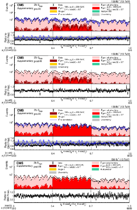
png pdf |
Additional Figure 6:
Pre- and post-fit distributions comparing the data (points) to the POWHEG + PYTHIA simulation (stacked histograms) for the full matrix measurement in bins of $ p_{\mathrm{T}}(\mathrm{t}) $ vs. $|\cos(\theta)\,| $ in the $2\mathrm{b} S_{\text{high}}$ category. The $ x $ axis shows the bins of the unrolled 4-dimensional distribution of $ \phi_{\bar{\mathrm{p}}} $, $ \cos(\theta_{\bar{\mathrm{p}}}) $, $ \phi_{\mathrm{p}} $, and $ \cos(\theta_{\mathrm{p}}) $, listed from the outermost to the innermost variable in each of the $ p_{\mathrm{T}}(\mathrm{t}) $ vs. $|\cos(\theta)\,| $ bins. The boundaries of the $ |\cos(\theta)| $ and $ p_{\mathrm{T}}(\mathrm{t}) $ bins are labeled and indicated by dashed and solid lines, respectively. For the illustration of resolution effects, $ \mathrm{t} \overline{\mathrm{t}} $ events generated in two selected $ p_{\mathrm{T}}(\mathrm{t}) $ vs. $|\cos(\theta)\,| $ bins are shown in different shades of red. All other $ \mathrm{t} \overline{\mathrm{t}} $ contributions are shown in pink. A model without any polarization and spin correlation is shown as a blue line. The gray uncertainty band indicates the combined statistical and systematic uncertainties in the prediction. The vertical bars on the points show the statistical uncertainty. Ratios to the predicted yields are provided in the lower panels. |

png pdf |
Additional Figure 6-a:
Pre- and post-fit distributions comparing the data (points) to the POWHEG + PYTHIA simulation (stacked histograms) for the full matrix measurement in bins of $ p_{\mathrm{T}}(\mathrm{t}) $ vs. $|\cos(\theta)\,| $ in the $2\mathrm{b} S_{\text{high}}$ category. The $ x $ axis shows the bins of the unrolled 4-dimensional distribution of $ \phi_{\bar{\mathrm{p}}} $, $ \cos(\theta_{\bar{\mathrm{p}}}) $, $ \phi_{\mathrm{p}} $, and $ \cos(\theta_{\mathrm{p}}) $, listed from the outermost to the innermost variable in each of the $ p_{\mathrm{T}}(\mathrm{t}) $ vs. $|\cos(\theta)\,| $ bins. The boundaries of the $ |\cos(\theta)| $ and $ p_{\mathrm{T}}(\mathrm{t}) $ bins are labeled and indicated by dashed and solid lines, respectively. For the illustration of resolution effects, $ \mathrm{t} \overline{\mathrm{t}} $ events generated in two selected $ p_{\mathrm{T}}(\mathrm{t}) $ vs. $|\cos(\theta)\,| $ bins are shown in different shades of red. All other $ \mathrm{t} \overline{\mathrm{t}} $ contributions are shown in pink. A model without any polarization and spin correlation is shown as a blue line. The gray uncertainty band indicates the combined statistical and systematic uncertainties in the prediction. The vertical bars on the points show the statistical uncertainty. Ratios to the predicted yields are provided in the lower panels. |

png pdf |
Additional Figure 6-b:
Pre- and post-fit distributions comparing the data (points) to the POWHEG + PYTHIA simulation (stacked histograms) for the full matrix measurement in bins of $ p_{\mathrm{T}}(\mathrm{t}) $ vs. $|\cos(\theta)\,| $ in the $2\mathrm{b} S_{\text{high}}$ category. The $ x $ axis shows the bins of the unrolled 4-dimensional distribution of $ \phi_{\bar{\mathrm{p}}} $, $ \cos(\theta_{\bar{\mathrm{p}}}) $, $ \phi_{\mathrm{p}} $, and $ \cos(\theta_{\mathrm{p}}) $, listed from the outermost to the innermost variable in each of the $ p_{\mathrm{T}}(\mathrm{t}) $ vs. $|\cos(\theta)\,| $ bins. The boundaries of the $ |\cos(\theta)| $ and $ p_{\mathrm{T}}(\mathrm{t}) $ bins are labeled and indicated by dashed and solid lines, respectively. For the illustration of resolution effects, $ \mathrm{t} \overline{\mathrm{t}} $ events generated in two selected $ p_{\mathrm{T}}(\mathrm{t}) $ vs. $|\cos(\theta)\,| $ bins are shown in different shades of red. All other $ \mathrm{t} \overline{\mathrm{t}} $ contributions are shown in pink. A model without any polarization and spin correlation is shown as a blue line. The gray uncertainty band indicates the combined statistical and systematic uncertainties in the prediction. The vertical bars on the points show the statistical uncertainty. Ratios to the predicted yields are provided in the lower panels. |

png pdf |
Additional Figure 6-c:
Pre- and post-fit distributions comparing the data (points) to the POWHEG + PYTHIA simulation (stacked histograms) for the full matrix measurement in bins of $ p_{\mathrm{T}}(\mathrm{t}) $ vs. $|\cos(\theta)\,| $ in the $2\mathrm{b} S_{\text{high}}$ category. The $ x $ axis shows the bins of the unrolled 4-dimensional distribution of $ \phi_{\bar{\mathrm{p}}} $, $ \cos(\theta_{\bar{\mathrm{p}}}) $, $ \phi_{\mathrm{p}} $, and $ \cos(\theta_{\mathrm{p}}) $, listed from the outermost to the innermost variable in each of the $ p_{\mathrm{T}}(\mathrm{t}) $ vs. $|\cos(\theta)\,| $ bins. The boundaries of the $ |\cos(\theta)| $ and $ p_{\mathrm{T}}(\mathrm{t}) $ bins are labeled and indicated by dashed and solid lines, respectively. For the illustration of resolution effects, $ \mathrm{t} \overline{\mathrm{t}} $ events generated in two selected $ p_{\mathrm{T}}(\mathrm{t}) $ vs. $|\cos(\theta)\,| $ bins are shown in different shades of red. All other $ \mathrm{t} \overline{\mathrm{t}} $ contributions are shown in pink. A model without any polarization and spin correlation is shown as a blue line. The gray uncertainty band indicates the combined statistical and systematic uncertainties in the prediction. The vertical bars on the points show the statistical uncertainty. Ratios to the predicted yields are provided in the lower panels. |
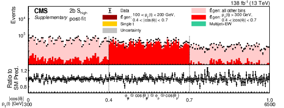
png pdf |
Additional Figure 6-d:
Pre- and post-fit distributions comparing the data (points) to the POWHEG + PYTHIA simulation (stacked histograms) for the full matrix measurement in bins of $ p_{\mathrm{T}}(\mathrm{t}) $ vs. $|\cos(\theta)\,| $ in the $2\mathrm{b} S_{\text{high}}$ category. The $ x $ axis shows the bins of the unrolled 4-dimensional distribution of $ \phi_{\bar{\mathrm{p}}} $, $ \cos(\theta_{\bar{\mathrm{p}}}) $, $ \phi_{\mathrm{p}} $, and $ \cos(\theta_{\mathrm{p}}) $, listed from the outermost to the innermost variable in each of the $ p_{\mathrm{T}}(\mathrm{t}) $ vs. $|\cos(\theta)\,| $ bins. The boundaries of the $ |\cos(\theta)| $ and $ p_{\mathrm{T}}(\mathrm{t}) $ bins are labeled and indicated by dashed and solid lines, respectively. For the illustration of resolution effects, $ \mathrm{t} \overline{\mathrm{t}} $ events generated in two selected $ p_{\mathrm{T}}(\mathrm{t}) $ vs. $|\cos(\theta)\,| $ bins are shown in different shades of red. All other $ \mathrm{t} \overline{\mathrm{t}} $ contributions are shown in pink. A model without any polarization and spin correlation is shown as a blue line. The gray uncertainty band indicates the combined statistical and systematic uncertainties in the prediction. The vertical bars on the points show the statistical uncertainty. Ratios to the predicted yields are provided in the lower panels. |
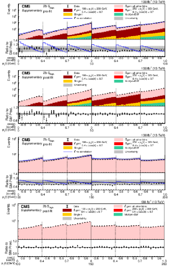
png pdf |
Additional Figure 7:
Pre- and post-fit distributions of $ \cos(\chi) $ comparing the data (points) to the POWHEG + PYTHIA simulation (stacked histograms) for the $ D $ measurement in bins of $ p_{\mathrm{T}}(\mathrm{t}) $ vs. $|\cos(\theta)\,| $ in the $2\mathrm{b} S_{\text{high}}$ category. The boundaries of the $ |\cos(\theta)| $ and $ p_{\mathrm{T}}(\mathrm{t}) $ bins are labeled and indicated by dashed and solid lines, respectively. For the illustration of resolution effects, $ \mathrm{t} \overline{\mathrm{t}} $ events generated in two selected $ p_{\mathrm{T}}(\mathrm{t}) $ vs. $|\cos(\theta)\,| $ bins are shown in different shades of red. All other $ \mathrm{t} \overline{\mathrm{t}} $ contributions are shown in pink. A model without any polarization and spin correlation is shown as a blue line. The gray uncertainty band indicates the combined statistical and systematic uncertainties in the prediction. The vertical bars on the points show the statistical uncertainty. Ratios to the predicted yields are provided in the lower panels. |

png pdf |
Additional Figure 7-a:
Pre- and post-fit distributions of $ \cos(\chi) $ comparing the data (points) to the POWHEG + PYTHIA simulation (stacked histograms) for the $ D $ measurement in bins of $ p_{\mathrm{T}}(\mathrm{t}) $ vs. $|\cos(\theta)\,| $ in the $2\mathrm{b} S_{\text{high}}$ category. The boundaries of the $ |\cos(\theta)| $ and $ p_{\mathrm{T}}(\mathrm{t}) $ bins are labeled and indicated by dashed and solid lines, respectively. For the illustration of resolution effects, $ \mathrm{t} \overline{\mathrm{t}} $ events generated in two selected $ p_{\mathrm{T}}(\mathrm{t}) $ vs. $|\cos(\theta)\,| $ bins are shown in different shades of red. All other $ \mathrm{t} \overline{\mathrm{t}} $ contributions are shown in pink. A model without any polarization and spin correlation is shown as a blue line. The gray uncertainty band indicates the combined statistical and systematic uncertainties in the prediction. The vertical bars on the points show the statistical uncertainty. Ratios to the predicted yields are provided in the lower panels. |

png pdf |
Additional Figure 7-b:
Pre- and post-fit distributions of $ \cos(\chi) $ comparing the data (points) to the POWHEG + PYTHIA simulation (stacked histograms) for the $ D $ measurement in bins of $ p_{\mathrm{T}}(\mathrm{t}) $ vs. $|\cos(\theta)\,| $ in the $2\mathrm{b} S_{\text{high}}$ category. The boundaries of the $ |\cos(\theta)| $ and $ p_{\mathrm{T}}(\mathrm{t}) $ bins are labeled and indicated by dashed and solid lines, respectively. For the illustration of resolution effects, $ \mathrm{t} \overline{\mathrm{t}} $ events generated in two selected $ p_{\mathrm{T}}(\mathrm{t}) $ vs. $|\cos(\theta)\,| $ bins are shown in different shades of red. All other $ \mathrm{t} \overline{\mathrm{t}} $ contributions are shown in pink. A model without any polarization and spin correlation is shown as a blue line. The gray uncertainty band indicates the combined statistical and systematic uncertainties in the prediction. The vertical bars on the points show the statistical uncertainty. Ratios to the predicted yields are provided in the lower panels. |

png pdf |
Additional Figure 7-c:
Pre- and post-fit distributions of $ \cos(\chi) $ comparing the data (points) to the POWHEG + PYTHIA simulation (stacked histograms) for the $ D $ measurement in bins of $ p_{\mathrm{T}}(\mathrm{t}) $ vs. $|\cos(\theta)\,| $ in the $2\mathrm{b} S_{\text{high}}$ category. The boundaries of the $ |\cos(\theta)| $ and $ p_{\mathrm{T}}(\mathrm{t}) $ bins are labeled and indicated by dashed and solid lines, respectively. For the illustration of resolution effects, $ \mathrm{t} \overline{\mathrm{t}} $ events generated in two selected $ p_{\mathrm{T}}(\mathrm{t}) $ vs. $|\cos(\theta)\,| $ bins are shown in different shades of red. All other $ \mathrm{t} \overline{\mathrm{t}} $ contributions are shown in pink. A model without any polarization and spin correlation is shown as a blue line. The gray uncertainty band indicates the combined statistical and systematic uncertainties in the prediction. The vertical bars on the points show the statistical uncertainty. Ratios to the predicted yields are provided in the lower panels. |

png pdf |
Additional Figure 7-d:
Pre- and post-fit distributions of $ \cos(\chi) $ comparing the data (points) to the POWHEG + PYTHIA simulation (stacked histograms) for the $ D $ measurement in bins of $ p_{\mathrm{T}}(\mathrm{t}) $ vs. $|\cos(\theta)\,| $ in the $2\mathrm{b} S_{\text{high}}$ category. The boundaries of the $ |\cos(\theta)| $ and $ p_{\mathrm{T}}(\mathrm{t}) $ bins are labeled and indicated by dashed and solid lines, respectively. For the illustration of resolution effects, $ \mathrm{t} \overline{\mathrm{t}} $ events generated in two selected $ p_{\mathrm{T}}(\mathrm{t}) $ vs. $|\cos(\theta)\,| $ bins are shown in different shades of red. All other $ \mathrm{t} \overline{\mathrm{t}} $ contributions are shown in pink. A model without any polarization and spin correlation is shown as a blue line. The gray uncertainty band indicates the combined statistical and systematic uncertainties in the prediction. The vertical bars on the points show the statistical uncertainty. Ratios to the predicted yields are provided in the lower panels. |
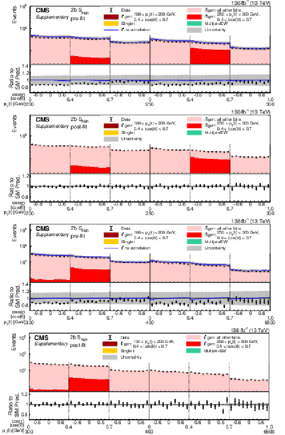
png pdf |
Additional Figure 8:
Pre- and post-fit distributions of $ \cos(\chi) $ comparing the data (points) to the POWHEG + PYTHIA simulation (stacked histograms) for the $ D $ measurement in bins of $ p_{\mathrm{T}}(\mathrm{t}) $ vs. $|\cos(\theta)\,| $ in the $2\mathrm{b} S_{\text{high}}$ category. The boundaries of the $ |\cos(\theta)| $ and $ p_{\mathrm{T}}(\mathrm{t}) $ bins are labeled and indicated by dashed and solid lines, respectively. For the illustration of resolution effects, $ \mathrm{t} \overline{\mathrm{t}} $ events generated in two selected $ p_{\mathrm{T}}(\mathrm{t}) $ vs. $|\cos(\theta)\,| $ bins are shown in different shades of red. All other $ \mathrm{t} \overline{\mathrm{t}} $ contributions are shown in pink. A model without any polarization and spin correlation is shown as a blue line. The gray uncertainty band indicates the combined statistical and systematic uncertainties in the prediction. The vertical bars on the points show the statistical uncertainty. Ratios to the predicted yields are provided in the lower panels. |

png pdf |
Additional Figure 8-a:
Pre- and post-fit distributions of $ \cos(\chi) $ comparing the data (points) to the POWHEG + PYTHIA simulation (stacked histograms) for the $ D $ measurement in bins of $ p_{\mathrm{T}}(\mathrm{t}) $ vs. $|\cos(\theta)\,| $ in the $2\mathrm{b} S_{\text{high}}$ category. The boundaries of the $ |\cos(\theta)| $ and $ p_{\mathrm{T}}(\mathrm{t}) $ bins are labeled and indicated by dashed and solid lines, respectively. For the illustration of resolution effects, $ \mathrm{t} \overline{\mathrm{t}} $ events generated in two selected $ p_{\mathrm{T}}(\mathrm{t}) $ vs. $|\cos(\theta)\,| $ bins are shown in different shades of red. All other $ \mathrm{t} \overline{\mathrm{t}} $ contributions are shown in pink. A model without any polarization and spin correlation is shown as a blue line. The gray uncertainty band indicates the combined statistical and systematic uncertainties in the prediction. The vertical bars on the points show the statistical uncertainty. Ratios to the predicted yields are provided in the lower panels. |

png pdf |
Additional Figure 8-b:
Pre- and post-fit distributions of $ \cos(\chi) $ comparing the data (points) to the POWHEG + PYTHIA simulation (stacked histograms) for the $ D $ measurement in bins of $ p_{\mathrm{T}}(\mathrm{t}) $ vs. $|\cos(\theta)\,| $ in the $2\mathrm{b} S_{\text{high}}$ category. The boundaries of the $ |\cos(\theta)| $ and $ p_{\mathrm{T}}(\mathrm{t}) $ bins are labeled and indicated by dashed and solid lines, respectively. For the illustration of resolution effects, $ \mathrm{t} \overline{\mathrm{t}} $ events generated in two selected $ p_{\mathrm{T}}(\mathrm{t}) $ vs. $|\cos(\theta)\,| $ bins are shown in different shades of red. All other $ \mathrm{t} \overline{\mathrm{t}} $ contributions are shown in pink. A model without any polarization and spin correlation is shown as a blue line. The gray uncertainty band indicates the combined statistical and systematic uncertainties in the prediction. The vertical bars on the points show the statistical uncertainty. Ratios to the predicted yields are provided in the lower panels. |

png pdf |
Additional Figure 8-c:
Pre- and post-fit distributions of $ \cos(\chi) $ comparing the data (points) to the POWHEG + PYTHIA simulation (stacked histograms) for the $ D $ measurement in bins of $ p_{\mathrm{T}}(\mathrm{t}) $ vs. $|\cos(\theta)\,| $ in the $2\mathrm{b} S_{\text{high}}$ category. The boundaries of the $ |\cos(\theta)| $ and $ p_{\mathrm{T}}(\mathrm{t}) $ bins are labeled and indicated by dashed and solid lines, respectively. For the illustration of resolution effects, $ \mathrm{t} \overline{\mathrm{t}} $ events generated in two selected $ p_{\mathrm{T}}(\mathrm{t}) $ vs. $|\cos(\theta)\,| $ bins are shown in different shades of red. All other $ \mathrm{t} \overline{\mathrm{t}} $ contributions are shown in pink. A model without any polarization and spin correlation is shown as a blue line. The gray uncertainty band indicates the combined statistical and systematic uncertainties in the prediction. The vertical bars on the points show the statistical uncertainty. Ratios to the predicted yields are provided in the lower panels. |

png pdf |
Additional Figure 8-d:
Pre- and post-fit distributions of $ \cos(\chi) $ comparing the data (points) to the POWHEG + PYTHIA simulation (stacked histograms) for the $ D $ measurement in bins of $ p_{\mathrm{T}}(\mathrm{t}) $ vs. $|\cos(\theta)\,| $ in the $2\mathrm{b} S_{\text{high}}$ category. The boundaries of the $ |\cos(\theta)| $ and $ p_{\mathrm{T}}(\mathrm{t}) $ bins are labeled and indicated by dashed and solid lines, respectively. For the illustration of resolution effects, $ \mathrm{t} \overline{\mathrm{t}} $ events generated in two selected $ p_{\mathrm{T}}(\mathrm{t}) $ vs. $|\cos(\theta)\,| $ bins are shown in different shades of red. All other $ \mathrm{t} \overline{\mathrm{t}} $ contributions are shown in pink. A model without any polarization and spin correlation is shown as a blue line. The gray uncertainty band indicates the combined statistical and systematic uncertainties in the prediction. The vertical bars on the points show the statistical uncertainty. Ratios to the predicted yields are provided in the lower panels. |

png pdf |
Additional Figure 9:
Pre- and post-fit distributions of $ \cos(\tilde{\chi}) $ comparing the data (points) to the POWHEG + PYTHIA simulation (stacked histograms) for the $ \tilde{D} $ measurement in bins of $ p_{\mathrm{T}}(\mathrm{t}) $ vs. $|\cos(\theta)\,| $ in the $2\mathrm{b} S_{\text{high}}$ category. The boundaries of the $ |\cos(\theta)| $ and $ p_{\mathrm{T}}(\mathrm{t}) $ bins are labeled and indicated by dashed and solid lines, respectively. For the illustration of resolution effects, $ \mathrm{t} \overline{\mathrm{t}} $ events generated in two selected $ p_{\mathrm{T}}(\mathrm{t}) $ vs. $|\cos(\theta)\,| $ bins are shown in different shades of red. All other $ \mathrm{t} \overline{\mathrm{t}} $ contributions are shown in pink. A model without any polarization and spin correlation is shown as a blue line. The gray uncertainty band indicates the combined statistical and systematic uncertainties in the prediction. The vertical bars on the points show the statistical uncertainty. Ratios to the predicted yields are provided in the lower panels. |

png pdf |
Additional Figure 9-a:
Pre- and post-fit distributions of $ \cos(\tilde{\chi}) $ comparing the data (points) to the POWHEG + PYTHIA simulation (stacked histograms) for the $ \tilde{D} $ measurement in bins of $ p_{\mathrm{T}}(\mathrm{t}) $ vs. $|\cos(\theta)\,| $ in the $2\mathrm{b} S_{\text{high}}$ category. The boundaries of the $ |\cos(\theta)| $ and $ p_{\mathrm{T}}(\mathrm{t}) $ bins are labeled and indicated by dashed and solid lines, respectively. For the illustration of resolution effects, $ \mathrm{t} \overline{\mathrm{t}} $ events generated in two selected $ p_{\mathrm{T}}(\mathrm{t}) $ vs. $|\cos(\theta)\,| $ bins are shown in different shades of red. All other $ \mathrm{t} \overline{\mathrm{t}} $ contributions are shown in pink. A model without any polarization and spin correlation is shown as a blue line. The gray uncertainty band indicates the combined statistical and systematic uncertainties in the prediction. The vertical bars on the points show the statistical uncertainty. Ratios to the predicted yields are provided in the lower panels. |
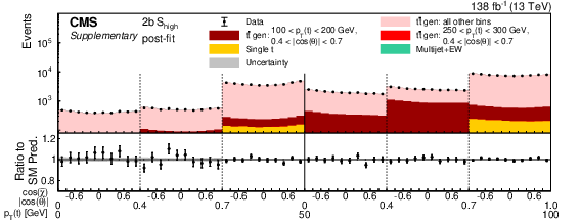
png pdf |
Additional Figure 9-b:
Pre- and post-fit distributions of $ \cos(\tilde{\chi}) $ comparing the data (points) to the POWHEG + PYTHIA simulation (stacked histograms) for the $ \tilde{D} $ measurement in bins of $ p_{\mathrm{T}}(\mathrm{t}) $ vs. $|\cos(\theta)\,| $ in the $2\mathrm{b} S_{\text{high}}$ category. The boundaries of the $ |\cos(\theta)| $ and $ p_{\mathrm{T}}(\mathrm{t}) $ bins are labeled and indicated by dashed and solid lines, respectively. For the illustration of resolution effects, $ \mathrm{t} \overline{\mathrm{t}} $ events generated in two selected $ p_{\mathrm{T}}(\mathrm{t}) $ vs. $|\cos(\theta)\,| $ bins are shown in different shades of red. All other $ \mathrm{t} \overline{\mathrm{t}} $ contributions are shown in pink. A model without any polarization and spin correlation is shown as a blue line. The gray uncertainty band indicates the combined statistical and systematic uncertainties in the prediction. The vertical bars on the points show the statistical uncertainty. Ratios to the predicted yields are provided in the lower panels. |

png pdf |
Additional Figure 9-c:
Pre- and post-fit distributions of $ \cos(\tilde{\chi}) $ comparing the data (points) to the POWHEG + PYTHIA simulation (stacked histograms) for the $ \tilde{D} $ measurement in bins of $ p_{\mathrm{T}}(\mathrm{t}) $ vs. $|\cos(\theta)\,| $ in the $2\mathrm{b} S_{\text{high}}$ category. The boundaries of the $ |\cos(\theta)| $ and $ p_{\mathrm{T}}(\mathrm{t}) $ bins are labeled and indicated by dashed and solid lines, respectively. For the illustration of resolution effects, $ \mathrm{t} \overline{\mathrm{t}} $ events generated in two selected $ p_{\mathrm{T}}(\mathrm{t}) $ vs. $|\cos(\theta)\,| $ bins are shown in different shades of red. All other $ \mathrm{t} \overline{\mathrm{t}} $ contributions are shown in pink. A model without any polarization and spin correlation is shown as a blue line. The gray uncertainty band indicates the combined statistical and systematic uncertainties in the prediction. The vertical bars on the points show the statistical uncertainty. Ratios to the predicted yields are provided in the lower panels. |
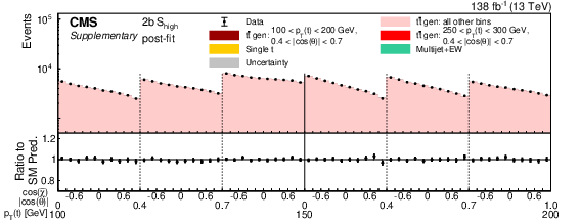
png pdf |
Additional Figure 9-d:
Pre- and post-fit distributions of $ \cos(\tilde{\chi}) $ comparing the data (points) to the POWHEG + PYTHIA simulation (stacked histograms) for the $ \tilde{D} $ measurement in bins of $ p_{\mathrm{T}}(\mathrm{t}) $ vs. $|\cos(\theta)\,| $ in the $2\mathrm{b} S_{\text{high}}$ category. The boundaries of the $ |\cos(\theta)| $ and $ p_{\mathrm{T}}(\mathrm{t}) $ bins are labeled and indicated by dashed and solid lines, respectively. For the illustration of resolution effects, $ \mathrm{t} \overline{\mathrm{t}} $ events generated in two selected $ p_{\mathrm{T}}(\mathrm{t}) $ vs. $|\cos(\theta)\,| $ bins are shown in different shades of red. All other $ \mathrm{t} \overline{\mathrm{t}} $ contributions are shown in pink. A model without any polarization and spin correlation is shown as a blue line. The gray uncertainty band indicates the combined statistical and systematic uncertainties in the prediction. The vertical bars on the points show the statistical uncertainty. Ratios to the predicted yields are provided in the lower panels. |
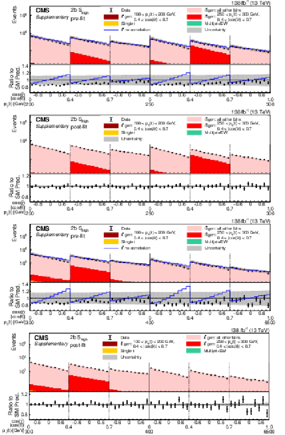
png pdf |
Additional Figure 10:
Pre- and post-fit distributions of $ \cos(\tilde{\chi}) $ comparing the data (points) to the POWHEG + PYTHIA simulation (stacked histograms) for the $ \tilde{D} $ measurement in bins of $ p_{\mathrm{T}}(\mathrm{t}) $ vs. $|\cos(\theta)\,| $ in the $2\mathrm{b} S_{\text{high}}$ category. The boundaries of the $ |\cos(\theta)| $ and $ p_{\mathrm{T}}(\mathrm{t}) $ bins are labeled and indicated by dashed and solid lines, respectively. For the illustration of resolution effects, $ \mathrm{t} \overline{\mathrm{t}} $ events generated in two selected $ p_{\mathrm{T}}(\mathrm{t}) $ vs. $|\cos(\theta)\,| $ bins are shown in different shades of red. All other $ \mathrm{t} \overline{\mathrm{t}} $ contributions are shown in pink. A model without any polarization and spin correlation is shown as a blue line. The gray uncertainty band indicates the combined statistical and systematic uncertainties in the prediction. The vertical bars on the points show the statistical uncertainty. Ratios to the predicted yields are provided in the lower panels. |

png pdf |
Additional Figure 10-a:
Pre- and post-fit distributions of $ \cos(\tilde{\chi}) $ comparing the data (points) to the POWHEG + PYTHIA simulation (stacked histograms) for the $ \tilde{D} $ measurement in bins of $ p_{\mathrm{T}}(\mathrm{t}) $ vs. $|\cos(\theta)\,| $ in the $2\mathrm{b} S_{\text{high}}$ category. The boundaries of the $ |\cos(\theta)| $ and $ p_{\mathrm{T}}(\mathrm{t}) $ bins are labeled and indicated by dashed and solid lines, respectively. For the illustration of resolution effects, $ \mathrm{t} \overline{\mathrm{t}} $ events generated in two selected $ p_{\mathrm{T}}(\mathrm{t}) $ vs. $|\cos(\theta)\,| $ bins are shown in different shades of red. All other $ \mathrm{t} \overline{\mathrm{t}} $ contributions are shown in pink. A model without any polarization and spin correlation is shown as a blue line. The gray uncertainty band indicates the combined statistical and systematic uncertainties in the prediction. The vertical bars on the points show the statistical uncertainty. Ratios to the predicted yields are provided in the lower panels. |

png pdf |
Additional Figure 10-b:
Pre- and post-fit distributions of $ \cos(\tilde{\chi}) $ comparing the data (points) to the POWHEG + PYTHIA simulation (stacked histograms) for the $ \tilde{D} $ measurement in bins of $ p_{\mathrm{T}}(\mathrm{t}) $ vs. $|\cos(\theta)\,| $ in the $2\mathrm{b} S_{\text{high}}$ category. The boundaries of the $ |\cos(\theta)| $ and $ p_{\mathrm{T}}(\mathrm{t}) $ bins are labeled and indicated by dashed and solid lines, respectively. For the illustration of resolution effects, $ \mathrm{t} \overline{\mathrm{t}} $ events generated in two selected $ p_{\mathrm{T}}(\mathrm{t}) $ vs. $|\cos(\theta)\,| $ bins are shown in different shades of red. All other $ \mathrm{t} \overline{\mathrm{t}} $ contributions are shown in pink. A model without any polarization and spin correlation is shown as a blue line. The gray uncertainty band indicates the combined statistical and systematic uncertainties in the prediction. The vertical bars on the points show the statistical uncertainty. Ratios to the predicted yields are provided in the lower panels. |

png pdf |
Additional Figure 10-c:
Pre- and post-fit distributions of $ \cos(\tilde{\chi}) $ comparing the data (points) to the POWHEG + PYTHIA simulation (stacked histograms) for the $ \tilde{D} $ measurement in bins of $ p_{\mathrm{T}}(\mathrm{t}) $ vs. $|\cos(\theta)\,| $ in the $2\mathrm{b} S_{\text{high}}$ category. The boundaries of the $ |\cos(\theta)| $ and $ p_{\mathrm{T}}(\mathrm{t}) $ bins are labeled and indicated by dashed and solid lines, respectively. For the illustration of resolution effects, $ \mathrm{t} \overline{\mathrm{t}} $ events generated in two selected $ p_{\mathrm{T}}(\mathrm{t}) $ vs. $|\cos(\theta)\,| $ bins are shown in different shades of red. All other $ \mathrm{t} \overline{\mathrm{t}} $ contributions are shown in pink. A model without any polarization and spin correlation is shown as a blue line. The gray uncertainty band indicates the combined statistical and systematic uncertainties in the prediction. The vertical bars on the points show the statistical uncertainty. Ratios to the predicted yields are provided in the lower panels. |

png pdf |
Additional Figure 10-d:
Pre- and post-fit distributions of $ \cos(\tilde{\chi}) $ comparing the data (points) to the POWHEG + PYTHIA simulation (stacked histograms) for the $ \tilde{D} $ measurement in bins of $ p_{\mathrm{T}}(\mathrm{t}) $ vs. $|\cos(\theta)\,| $ in the $2\mathrm{b} S_{\text{high}}$ category. The boundaries of the $ |\cos(\theta)| $ and $ p_{\mathrm{T}}(\mathrm{t}) $ bins are labeled and indicated by dashed and solid lines, respectively. For the illustration of resolution effects, $ \mathrm{t} \overline{\mathrm{t}} $ events generated in two selected $ p_{\mathrm{T}}(\mathrm{t}) $ vs. $|\cos(\theta)\,| $ bins are shown in different shades of red. All other $ \mathrm{t} \overline{\mathrm{t}} $ contributions are shown in pink. A model without any polarization and spin correlation is shown as a blue line. The gray uncertainty band indicates the combined statistical and systematic uncertainties in the prediction. The vertical bars on the points show the statistical uncertainty. Ratios to the predicted yields are provided in the lower panels. |
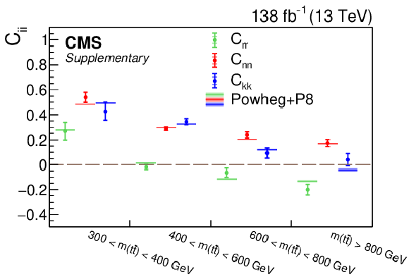
png pdf |
Additional Figure 11:
Diagonal coefficients $ C_{ii} $ in bins of $ m({\mathrm{t}\overline{\mathrm{t}}} ) $. The measurements (markers) are shown with the statistical uncertainty (inner error bars) and total uncertainty (outer error bars) and compared to the predictions of POWHEG + PYTHIA. The POWHEG + PYTHIA prediction is displayed with ME scale and PDF uncertainties. |
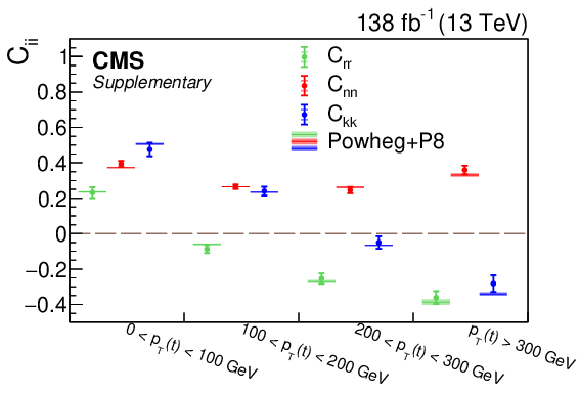
png pdf |
Additional Figure 12:
Diagonal coefficients $ C_{ii} $ in bins of $ p_{\mathrm{T}}(\mathrm{t}) $. The measurements (markers) are shown with the statistical uncertainty (inner error bars) and total uncertainty (outer error bars) and compared to the predictions of POWHEG + PYTHIA. The POWHEG + PYTHIA prediction is displayed with ME scale and PDF uncertainties. |
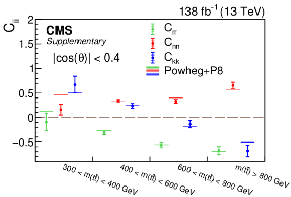
png pdf |
Additional Figure 13:
Diagonal coefficients $ C_{ii} $ in bins of $ m({\mathrm{t}\overline{\mathrm{t}}} ) $ for $ |\cos(\theta)| < $ 0.4. The measurements (markers) are shown with the statistical uncertainty (inner error bars) and total uncertainty (outer error bars) and compared to the predictions of POWHEG + PYTHIA. The POWHEG + PYTHIA prediction is displayed with ME scale and PDF uncertainties. |
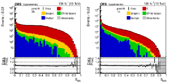
png pdf |
Additional Figure 14:
Distribution of $ S_{\text{NN}} $ in the 2 b (left) and 1 b (right) categories. The data (points) are compared to the prediction from simulation (stacked histograms), where the shapes of the predictions are adapted to the post-fit values of the nuisances controlling their uncertainties. The post-fit values are taken from the measurement of $ \tilde{D} $ in bins of $ {p_{\mathrm{T}}(\mathrm{t}) }$ vs. ${ |\cos(\theta)|} $. The gray uncertainty band indicates the post-fit uncertainties in the prediction, while the vertical bars on the points show the statistical uncertainty of the data. The ratios of data to the predicted yields are provided in the lower panels. |
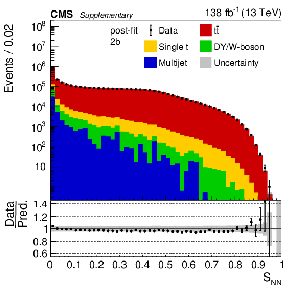
png pdf |
Additional Figure 14-a:
Distribution of $ S_{\text{NN}} $ in the 2 b (left) and 1 b (right) categories. The data (points) are compared to the prediction from simulation (stacked histograms), where the shapes of the predictions are adapted to the post-fit values of the nuisances controlling their uncertainties. The post-fit values are taken from the measurement of $ \tilde{D} $ in bins of $ {p_{\mathrm{T}}(\mathrm{t}) }$ vs. ${ |\cos(\theta)|} $. The gray uncertainty band indicates the post-fit uncertainties in the prediction, while the vertical bars on the points show the statistical uncertainty of the data. The ratios of data to the predicted yields are provided in the lower panels. |

png pdf |
Additional Figure 14-b:
Distribution of $ S_{\text{NN}} $ in the 2 b (left) and 1 b (right) categories. The data (points) are compared to the prediction from simulation (stacked histograms), where the shapes of the predictions are adapted to the post-fit values of the nuisances controlling their uncertainties. The post-fit values are taken from the measurement of $ \tilde{D} $ in bins of $ {p_{\mathrm{T}}(\mathrm{t}) }$ vs. ${ |\cos(\theta)|} $. The gray uncertainty band indicates the post-fit uncertainties in the prediction, while the vertical bars on the points show the statistical uncertainty of the data. The ratios of data to the predicted yields are provided in the lower panels. |
| References | ||||
| 1 | Particle Data Group , S. Navas et al. | Review of particle physics | PRD 110 (2024) 030001 | |
| 2 | G. Mahlon and S. J. Parke | Spin correlation effects in top quark pair production at the LHC | PRD 81 (2010) 074024 | 1001.3422 |
| 3 | M. Baumgart and B. Tweedie | A new twist on top quark spin correlations | JHEP 03 (2013) 117 | 1212.4888 |
| 4 | D0 Collaboration | Evidence for spin correlation in $ \mathrm{t} \overline{\mathrm{t}} $ production | PRL 108 (2012) 032004 | 1110.4194 |
| 5 | D0 Collaboration | Measurement of spin correlation between top and antitop quarks produced in $ {\mathrm{p}\overline{\mathrm{p}}} $ collisions at $ \sqrt{s}= $ 1.96 TeV | PLB 757 (2016) 199 | 1512.08818 |
| 6 | CMS Collaboration | Measurements of $ \mathrm{t} \overline{\mathrm{t}} $ spin correlations and top-quark polarization using dilepton final states in pp collisions at $ \sqrt{s}= $ 7 TeV | PRL 112 (2014) 182001 | CMS-TOP-13-003 1311.3924 |
| 7 | CMS Collaboration | Measurement of spin correlations in $ \mathrm{t} \overline{\mathrm{t}} $ production using the matrix element method in the muon+jets final state in pp collisions at $ \sqrt{s}= $ 8 TeV | PLB 758 (2016) 321 | CMS-TOP-13-015 1511.06170 |
| 8 | CMS Collaboration | Measurements of $ \mathrm{t} \overline{\mathrm{t}} $ spin correlations and top quark polarization using dilepton final states in pp collisions at $ \sqrt{s}= $ 8 TeV | PRD 93 (2016) 052007 | CMS-TOP-14-023 1601.01107 |
| 9 | CMS Collaboration | Measurement of the top quark polarization and $ \mathrm{t} \overline{\mathrm{t}} $ spin correlations using dilepton final states in proton-proton collisions at $ \sqrt{s}= $ 13 TeV | PRD 100 (2019) 072002 | CMS-TOP-18-006 1907.03729 |
| 10 | ATLAS Collaboration | Observation of spin correlation in $ \mathrm{t} \overline{\mathrm{t}} $ events from pp collisions at $ \sqrt(s)= $ 7 TeV using the ATLAS detector | PRL 108 (2012) 212001 | 1203.4081 |
| 11 | ATLAS Collaboration | Measurement of spin correlation in top-antitop quark events and search for top squark pair production in pp collisions at $ \sqrt{s}= $ 8 TeV using the ATLAS detector | PRL 114 (2015) 142001 | 1412.4742 |
| 12 | ATLAS Collaboration | Measurements of spin correlation in top-antitop quark events from proton-proton collisions at $ \sqrt{s}= $ 7 TeV using the ATLAS detector | PRD 90 (2014) 112016 | 1407.4314 |
| 13 | ATLAS Collaboration | Measurements of top-quark pair spin correlations in the $ {\mathrm{e}\mu} $ channel at $ \sqrt{s}= $ 13 TeV using pp collisions in the ATLAS detector | EPJC 80 (2020) 754 | 1903.07570 |
| 14 | ATLAS Collaboration | Observation of quantum entanglement in top-quark pairs using the ATLAS detector | Submitted to Nature, 2023 | 2311.07288 |
| 15 | CMS Collaboration | Observation of quantum entanglement in top quark pair production in proton-proton collisions at $ \sqrt{s}= $ 13 TeV | Submitted to Rep. Prog. Phys, 2024 | CMS-TOP-23-001 2406.03976 |
| 16 | L. Wu and H. Zhou | Polarization of top and chargino from stop decay in natural SUSY | PLB 794 (2019) 96 | 1811.08573 |
| 17 | F. Maltoni, C. Severi, S. Tentori, and E. Vryonidou | Quantum detection of new physics in top-quark pair production at the LHC | JHEP 03 (2024) 099 | 2401.08751 |
| 18 | Y. Afik and J. R. M. de Nova | Entanglement and quantum tomography with top quarks at the LHC | Eur. Phys. J. Plus 136 (2021) 907 | 2003.02280 |
| 19 | M. Fabbrichesi, R. Floreanini, and E. Gabrielli | Constraining new physics in entangled two-qubit systems: top-quark, tau-lepton and photon pairs | EPJC 83 (2023) 162 | 2208.11723 |
| 20 | M. Fabbrichesi, R. Floreanini, and G. Panizzo | Testing Bell inequalities at the LHC with top-quark pairs | PRL 127 (2021) 161801 | 2102.11883 |
| 21 | Z. Dong, D. Gonçalves, K. Kong, and A. Navarro | Entanglement and Bell inequalities with boosted $ \mathrm{t} \overline{\mathrm{t}} $ | PRD 109 (2024) 115023 | 2305.07075 |
| 22 | CMS Collaboration | HEPData record for this analysis | link | |
| 23 | W. Bernreuther, D. Heisler, and Z.-G. Si | A set of top quark spin correlation and polarization observables for the LHC: Standard model predictions and new physics contributions | JHEP 12 (2015) 026 | 1508.05271 |
| 24 | A. Brandenburg, Z. G. Si, and P. Uwer | QCD-corrected spin analysing power of jets in decays of polarized top quarks | PLB 539 (2002) 235 | hep-ph/0205023 |
| 25 | A. Peres | Separability criterion for density matrices | PRL 77 (1996) 1413 | quant-ph/9604005 |
| 26 | P. Horodecki | Separability criterion and inseparable mixed states with positive partial transposition | Phys. Lett. A 232 (1997) 333 | quant-ph/9703004 |
| 27 | Y. Afik and J. R. M. de Nova | Quantum information with top quarks in QCD | Quantum 6 (2022) 820 | 2203.05582 |
| 28 | J. A. Aguilar-Saavedra and J. A. Casas | Improved tests of entanglement and Bell inequalities with LHC tops | EPJC 82 (2022) 666 | 2205.00542 |
| 29 | CMS Collaboration | Performance of the CMS Level-1 trigger in proton-proton collisions at $ \sqrt{s}= $ 13 TeV | JINST 15 (2020) P10017 | CMS-TRG-17-001 2006.10165 |
| 30 | CMS Collaboration | The CMS trigger system | JINST 12 (2017) P01020 | CMS-TRG-12-001 1609.02366 |
| 31 | CMS Collaboration | Technical proposal for the Phase-II upgrade of the Compact Muon Solenoid | CMS Technical Proposal CERN-LHCC-2015-010, CMS-TDR-15-02, 2015 link |
|
| 32 | CMS Collaboration | Particle-flow reconstruction and global event description with the CMS detector | JINST 12 (2017) P10003 | CMS-PRF-14-001 1706.04965 |
| 33 | CMS Collaboration | The CMS experiment at the CERN LHC | JINST 3 (2008) S08004 | |
| 34 | P. Nason | A new method for combining NLO QCD with shower Monte Carlo algorithms | JHEP 11 (2004) 040 | hep-ph/0409146 |
| 35 | S. Frixione, P. Nason, and C. Oleari | Matching NLO QCD computations with parton shower simulations: the POWHEG method | JHEP 11 (2007) 070 | 0709.2092 |
| 36 | S. Frixione, G. Ridolfi, and P. Nason | A positive-weight next-to-leading-order Monte Carlo for heavy flavour hadroproduction | JHEP 09 (2007) 126 | 0707.3088 |
| 37 | T. Sjöstrand et al. | An introduction to PYTHIA8.2 | Comput. Phys. Commun. 191 (2015) 159 | 1410.3012 |
| 38 | CMS Collaboration | Extraction and validation of a new set of CMS PYTHIA8 tunes from underlying-event measurements | EPJC 80 (2020) 4 | CMS-GEN-17-001 1903.12179 |
| 39 | J. Mazzitelli et al. | Next-to-next-to-leading order event generation for top-quark pair production | PRL 127 (2021) 062001 | 2012.14267 |
| 40 | M. Aliev et al. | hathor: Hadronic top and heavy quarks cross section calculator | Comput. Phys. Commun. 182 (2011) 1034 | 1007.1327 |
| 41 | M. Bähr et al. | HERWIG++ physics and manual | EPJC 58 (2008) 639 | 0803.0883 |
| 42 | CMS Collaboration | Development and validation of HERWIG 7 tunes from CMS underlying-event measurements | EPJC 81 (2021) 312 | CMS-GEN-19-001 2011.03422 |
| 43 | J. Alwall et al. | The automated computation of tree-level and next-to-leading order differential cross sections, and their matching to parton shower simulations | JHEP 07 (2014) 079 | 1405.0301 |
| 44 | R. Frederix and S. Frixione | Merging meets matching in MC@NLO | JHEP 12 (2012) 061 | 1209.6215 |
| 45 | M. Czakon and A. Mitov | top++: a program for the calculation of the top-pair cross-section at hadron colliders | Comput. Phys. Commun. 185 (2014) 2930 | 1112.5675 |
| 46 | CMS Collaboration | Measurement of the top quark mass using proton-proton data at $ \sqrt{s}= $ 7 and 8 TeV | PRD 93 (2016) 072004 | CMS-TOP-14-022 1509.04044 |
| 47 | M. L. Mangano, M. Moretti, F. Piccinini, and M. Treccani | Matching matrix elements and shower evolution for top-pair production in hadronic collisions | JHEP 01 (2007) 013 | hep-ph/0611129 |
| 48 | J. Alwall et al. | Comparative study of various algorithms for the merging of parton showers and matrix elements in hadronic collisions | EPJC 53 (2008) 473 | 0706.2569 |
| 49 | Y. Li and F. Petriello | Combining QCD and electroweak corrections to dilepton production in FEWZ | PRD 86 (2012) 094034 | 1208.5967 |
| 50 | P. Kant et al. | hathor for single top-quark production: Updated predictions and uncertainty estimates for single top-quark production in hadronic collisions | Comput. Phys. Commun. 191 (2015) 74 | 1406.4403 |
| 51 | N. Kidonakis | NNLL threshold resummation for top-pair and single-top production | Phys. Part. Nucl. 45 (2014) 714 | 1210.7813 |
| 52 | NNPDF Collaboration | Parton distributions from high-precision collider data | EPJC 77 (2017) 663 | 1706.00428 |
| 53 | GEANT4 Collaboration | GEANT 4---a simulation toolkit | NIM A 506 (2003) 250 | |
| 54 | CMS Collaboration | Electron and photon reconstruction and identification with the CMS experiment at the CERN LHC | JINST 16 (2021) P05014 | CMS-EGM-17-001 2012.06888 |
| 55 | CMS Collaboration | Performance of the CMS muon detector and muon reconstruction with proton-proton collisions at $ \sqrt{s}= $ 13 TeV | JINST 13 (2018) P06015 | CMS-MUO-16-001 1804.04528 |
| 56 | CMS Collaboration | Measurements of inclusive W and Z cross sections in pp collisions at $ \sqrt{s}= $ 7 TeV | JHEP 01 (2011) 080 | CMS-EWK-10-002 1012.2466 |
| 57 | M. Cacciari, G. P. Salam, and G. Soyez | The anti-$ k_{\mathrm{T}} $ jet clustering algorithm | JHEP 04 (2008) 063 | 0802.1189 |
| 58 | M. Cacciari, G. P. Salam, and G. Soyez | FASTJET user manual | EPJC 72 (2012) 1896 | 1111.6097 |
| 59 | CMS Collaboration | Jet energy scale and resolution in the CMS experiment in pp collisions at 8 TeV | JINST 12 (2017) P02014 | CMS-JME-13-004 1607.03663 |
| 60 | E. Bols et al. | Jet flavour classification using DeepJet | JINST 15 (2020) P12012 | 2008.10519 |
| 61 | CMS Collaboration | Identification of heavy-flavour jets with the CMS detector in pp collisions at 13 TeV | JINST 13 (2018) P05011 | CMS-BTV-16-002 1712.07158 |
| 62 | CMS Collaboration | Performance of missing transverse momentum reconstruction in proton-proton collisions at $ \sqrt{s}= $ 13 TeV using the CMS detector | JINST 14 (2019) P07004 | CMS-JME-17-001 1903.06078 |
| 63 | D. P. Kingma and J. Ba | adam: a method for stochastic optimization | in Proc. 3rd Int. Conf. on Learning Representations (ICLR 2015), San Diego CA, USA, 2015 | 1412.6980 |
| 64 | E. Gross and O. Vitells | Trial factors for the look elsewhere effect in high energy physics | EPJC 70 (2010) 525 | 1005.1891 |
| 65 | A. Andreassen and B. Nachman | Neural networks for full phase-space reweighting and parameter tuning | PRD 101 (2020) 091901 | 1907.08209 |
| 66 | CMS Collaboration | Reweighting of simulated events using machine learning techniques in CMS | CMS Physics Analysis Summary, 2024 CMS-PAS-MLG-24-001 |
CMS-PAS-MLG-24-001 |
| 67 | M. Czakon, P. Fiedler, and A. Mitov | Total top-quark pair-production cross section at hadron colliders through $ \mathcal{O}({\alpha_\mathrm{S}}^4) $ | PRL 110 (2013) 252004 | 1303.6254 |
| 68 | S. Argyropoulos and T. Sjöstrand | Effects of color reconnection on $ \mathrm{t} \overline{\mathrm{t}} $ final states at the LHC | JHEP 11 (2014) 043 | 1407.6653 |
| 69 | J. R. Christiansen and P. Z. Skands | String formation beyond leading colour | JHEP 08 (2015) 003 | 1505.01681 |
| 70 | W.-L. Ju et al. | Top quark pair production near threshold: single/double distributions and mass determination | JHEP 06 (2020) 158 | 2004.03088 |
| 71 | B. Fuks, K. Hagiwara, K. Ma, and Y.-J. Zheng | Signatures of toponium formation in LHC run 2 data | PRD 104 (2021) 034023 | 2102.11281 |
| 72 | CMS Collaboration | Precision luminosity measurement in proton-proton collisions at $ \sqrt{s}= $ 13 TeV in 2015 and 2016 at CMS | EPJC 81 (2021) 800 | CMS-LUM-17-003 2104.01927 |
| 73 | CMS Collaboration | CMS luminosity measurement for the 2017 data-taking period at $ \sqrt{s}= $ 13 TeV | CMS Physics Analysis Summary, 2018 CMS-PAS-LUM-17-004 |
CMS-PAS-LUM-17-004 |
| 74 | CMS Collaboration | CMS luminosity measurement for the 2018 data-taking period at $ \sqrt{s}= $ 13 TeV | CMS Physics Analysis Summary, 2019 CMS-PAS-LUM-18-002 |
CMS-PAS-LUM-18-002 |
| 75 | CMS Collaboration | Measurement of the inelastic proton-proton cross section at $ \sqrt{s}= $ 13 TeV | JHEP 07 (2018) 161 | CMS-FSQ-15-005 1802.02613 |
| 76 | CMS Collaboration | Performance summary of AK4 jet b tagging with data from proton-proton collisions at 13 TeV with the CMS detector | CMS Detector Performance Note CMS-DP-2023-005, 2023 CDS |
|
| 77 | R. Barlow and C. Beeston | Fitting using finite Monte Carlo samples | Comput. Phys. Commun. 77 (1993) 219 | |
| 78 | W. S. Cleveland | Robust locally weighted regression and smoothing scatterplots | J. Am. Stat. Assoc. 74 (1979) 829 | |
| 79 | C. Severi, C. Degli Esposti Boschi, F. Maltoni, and M. Sioli | Quantum tops at the LHC: from entanglement to Bell inequalities | EPJC 82 (2022) 285 | 2110.10112 |
| 80 | R. Demina and G. Landi | Locality in collider tests of quantum mechanics with top quark pairs | Submitted to Phys. Rev. Lett, 2024 | 2407.15223 |

|
Compact Muon Solenoid LHC, CERN |

|

|

|

|

|

|