

Compact Muon Solenoid
LHC, CERN
| CMS-MLG-23-002 ; CERN-EP-2025-269 | ||
| Machine-learning techniques for model-independent searches in dijet final states | ||
| CMS Collaboration | ||
| 23 December 2025 | ||
| Mach. Learn.: Sci. Tech. 7 (2026) 045008 | ||
| Abstract: Anomaly detection methods used in a recent search for new phenomena by CMS at the CERN LHC are presented. The methods use machine learning to detect anomalous jets produced in the decay of new massive particles. The effectiveness of these approaches in enhancing sensitivity to various signals is studied and compared using data collected in proton-proton collisions at a center-of-mass energy of 13 TeV. In an example analysis, the capabilities of anomaly detection methods are further demonstrated by identifying large-radius jets consistent with Lorentz-boosted hadronically decaying top quarks in a model-agnostic framework. | ||
| Links: e-print arXiv:2512.20395 [hep-ex] (PDF) ; CDS record ; inSPIRE record ; CADI line (restricted) ; | ||
| Figures | |
png pdf |
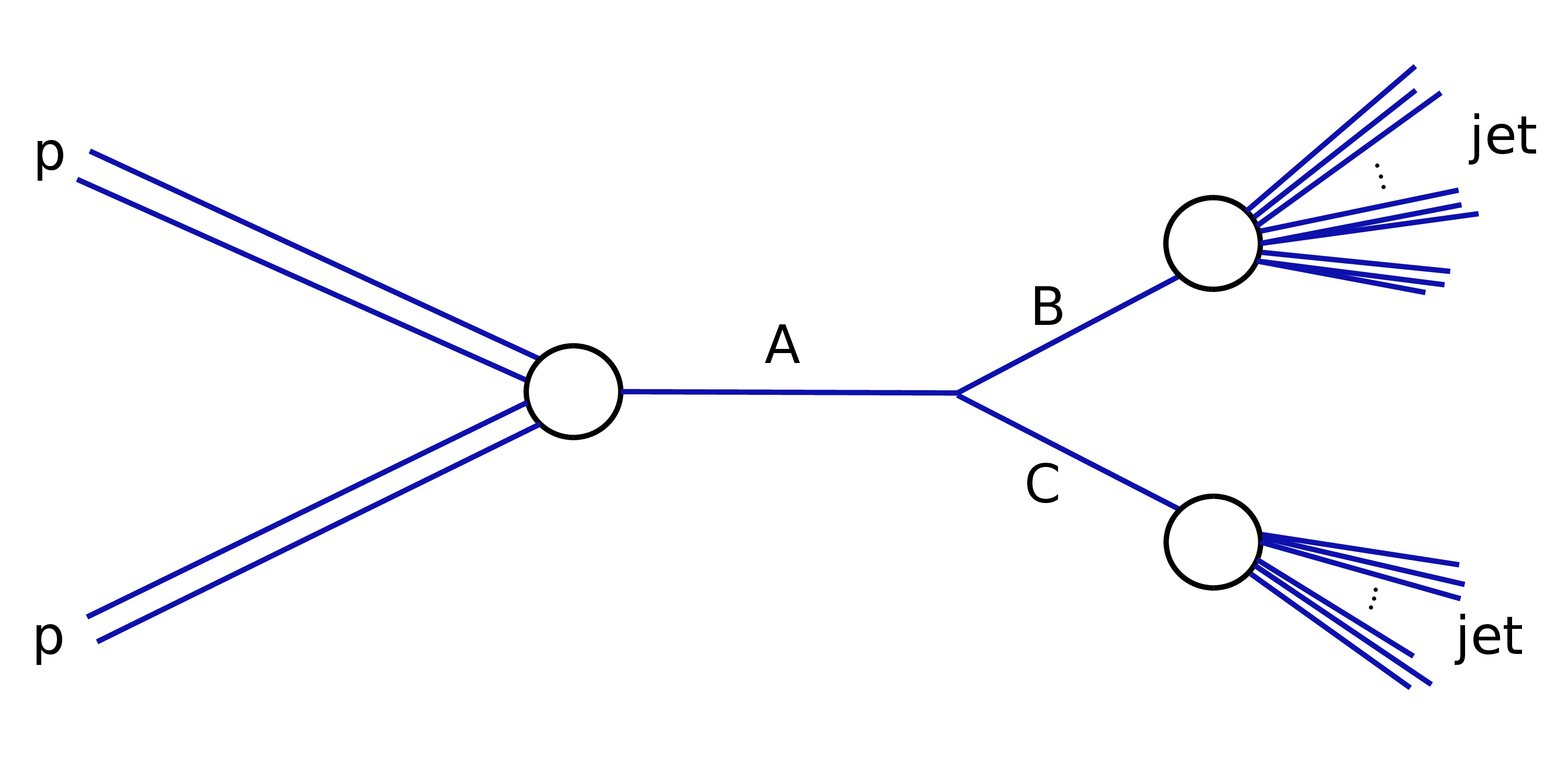
Figure 1:
Diagram of the $ \text{A}\to\text{BC}\to\text{2 jets} $ signal topology targeted in this work. The particle A is produced in a collision between two protons. Reproduced from Ref. [6]. |
png pdf |
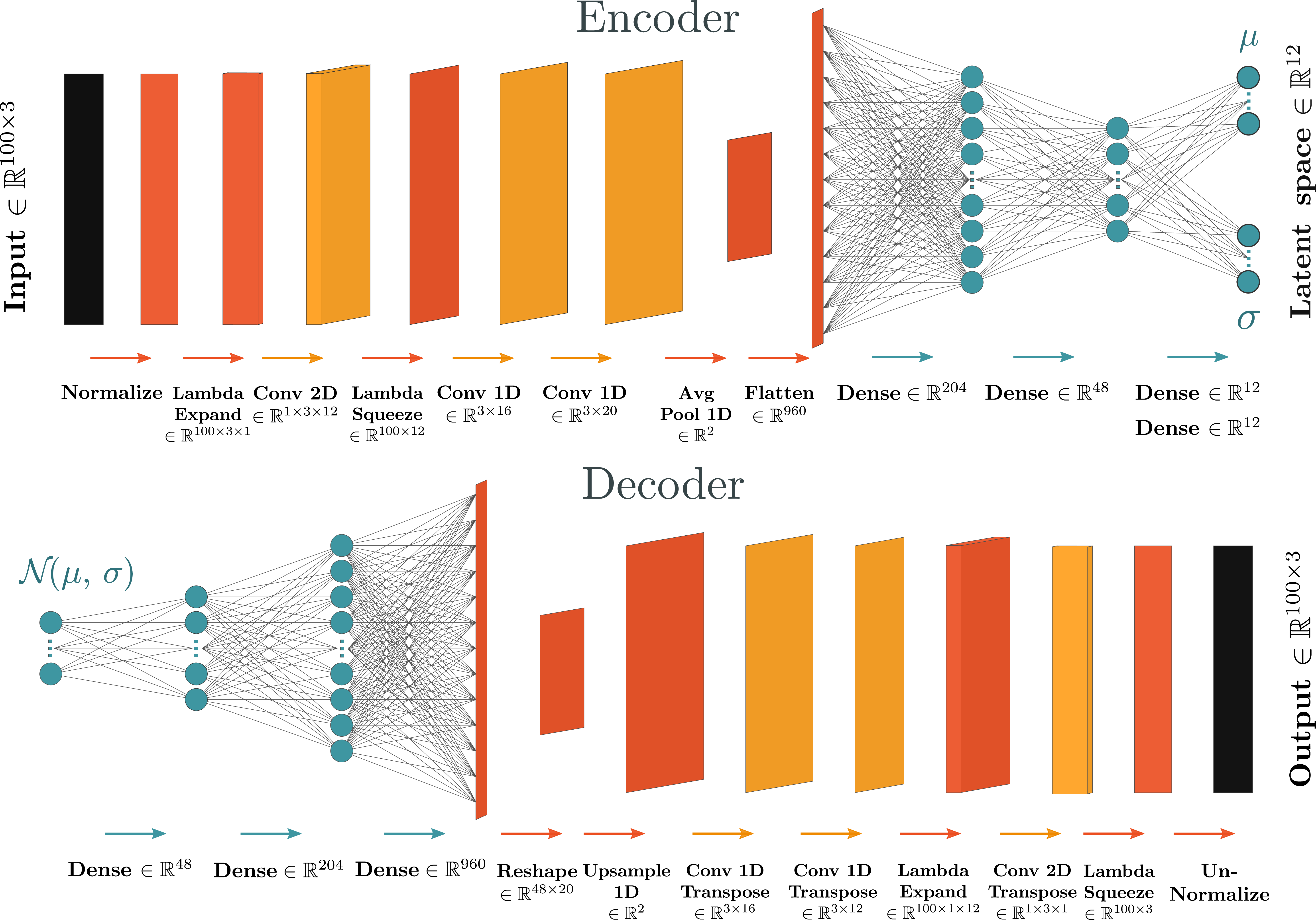
Figure 2:
The VAE architecture used for jet anomaly detection. |
png pdf |
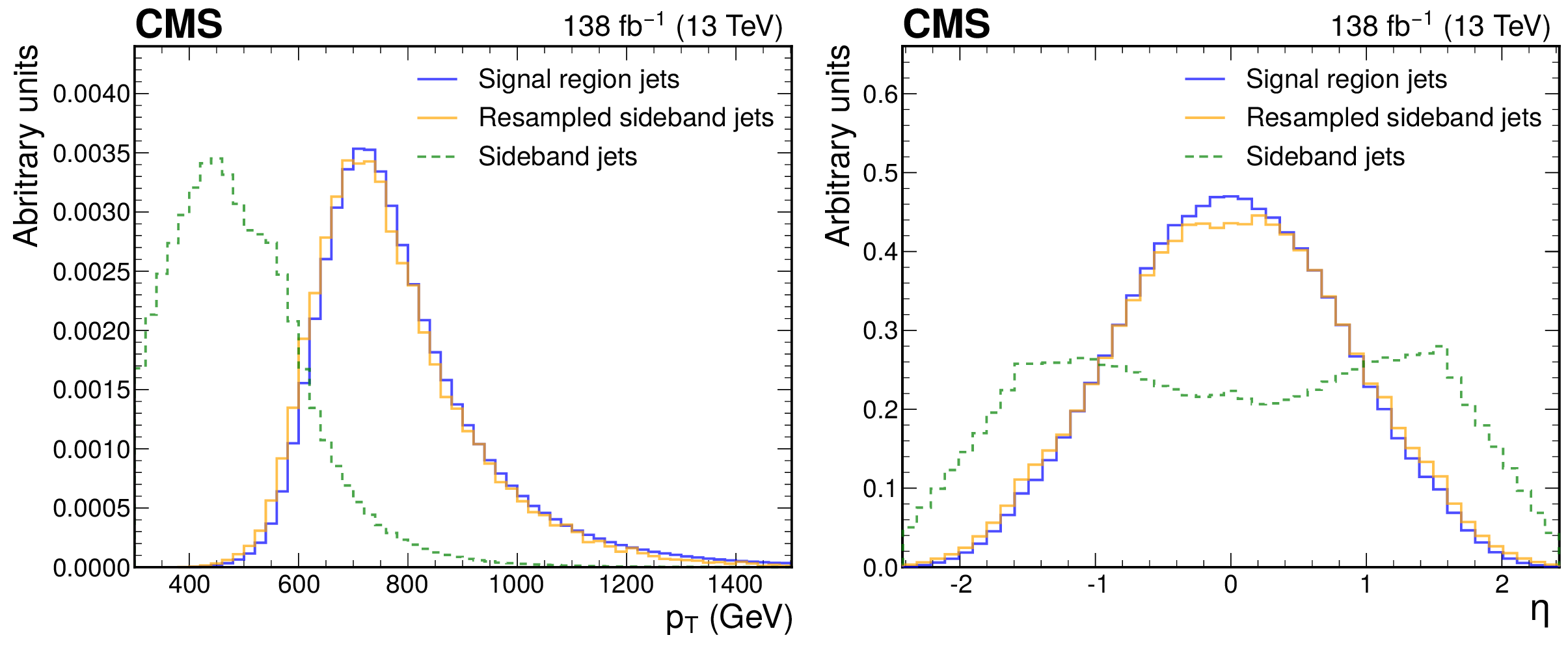
Figure 3:
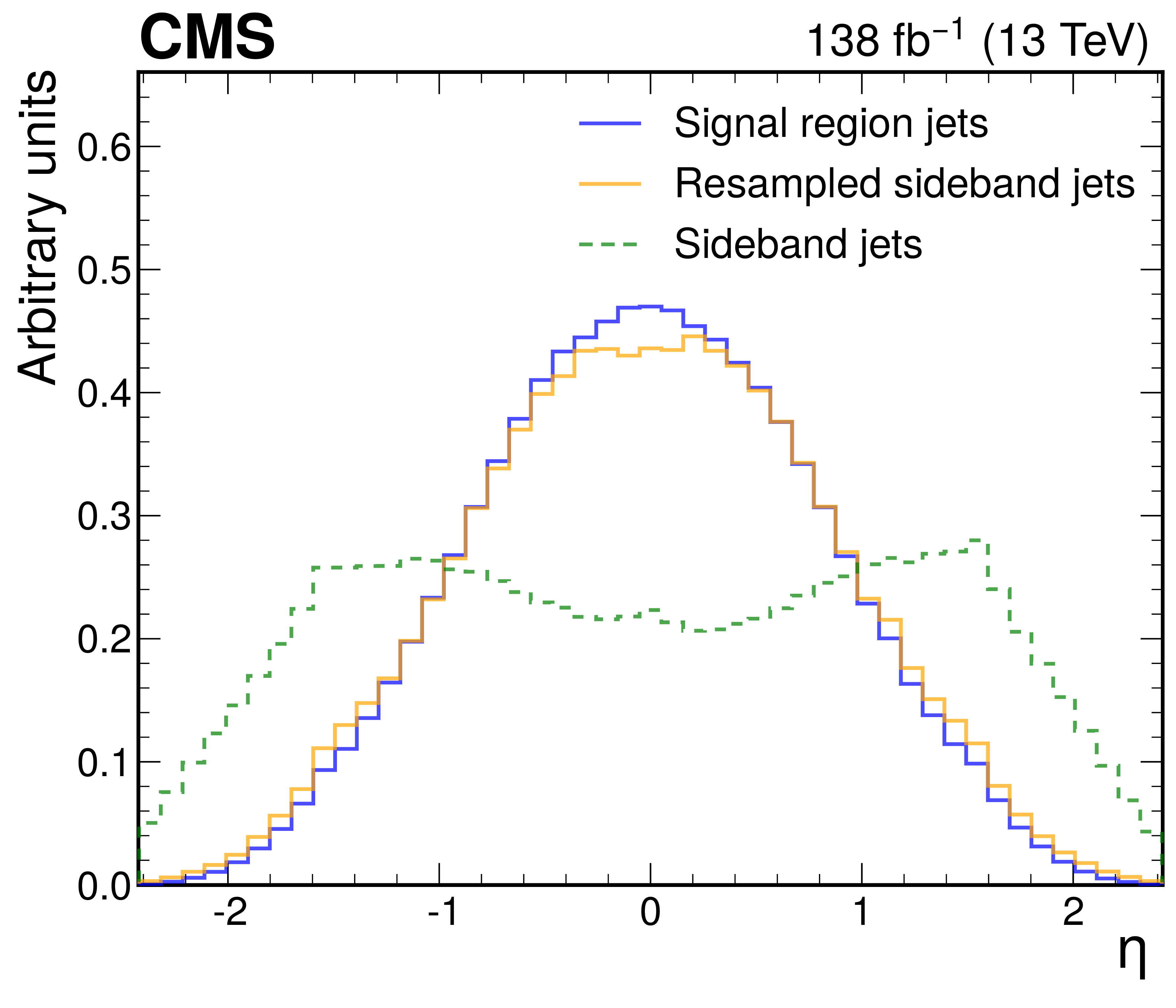
Jet $ p_{\mathrm{T}} $ (left) and $ \eta $ (right) distributions before and after resampling jets from the 2 $ < |\Delta\eta_\text{jj}| < $ 2.5 sideband (green) to match the distribution in the signal region (blue). The distributions of resampled jets are shown in orange. Histograms are normalized to unity. The details are given in the text. |
png pdf |
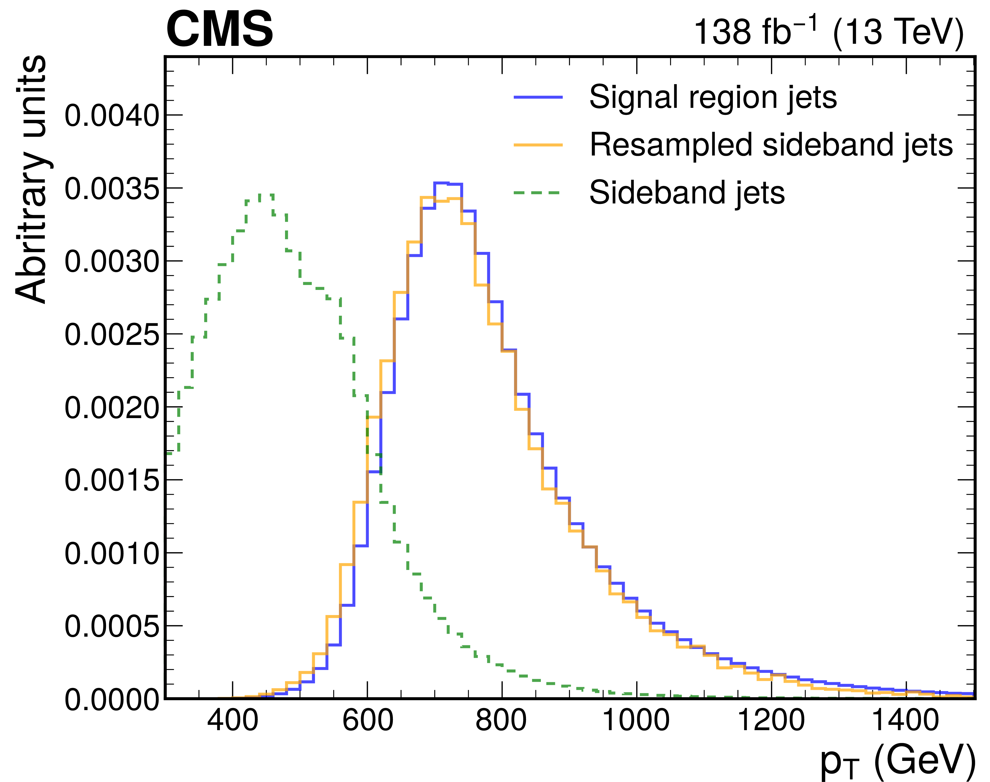
Figure 3-a:
Jet $ p_{\mathrm{T}} $ (left) and $ \eta $ (right) distributions before and after resampling jets from the 2 $ < |\Delta\eta_\text{jj}| < $ 2.5 sideband (green) to match the distribution in the signal region (blue). The distributions of resampled jets are shown in orange. Histograms are normalized to unity. The details are given in the text. |
png pdf |
Figure 3-b:
Jet $ p_{\mathrm{T}} $ (left) and $ \eta $ (right) distributions before and after resampling jets from the 2 $ < |\Delta\eta_\text{jj}| < $ 2.5 sideband (green) to match the distribution in the signal region (blue). The distributions of resampled jets are shown in orange. Histograms are normalized to unity. The details are given in the text. |
png pdf |
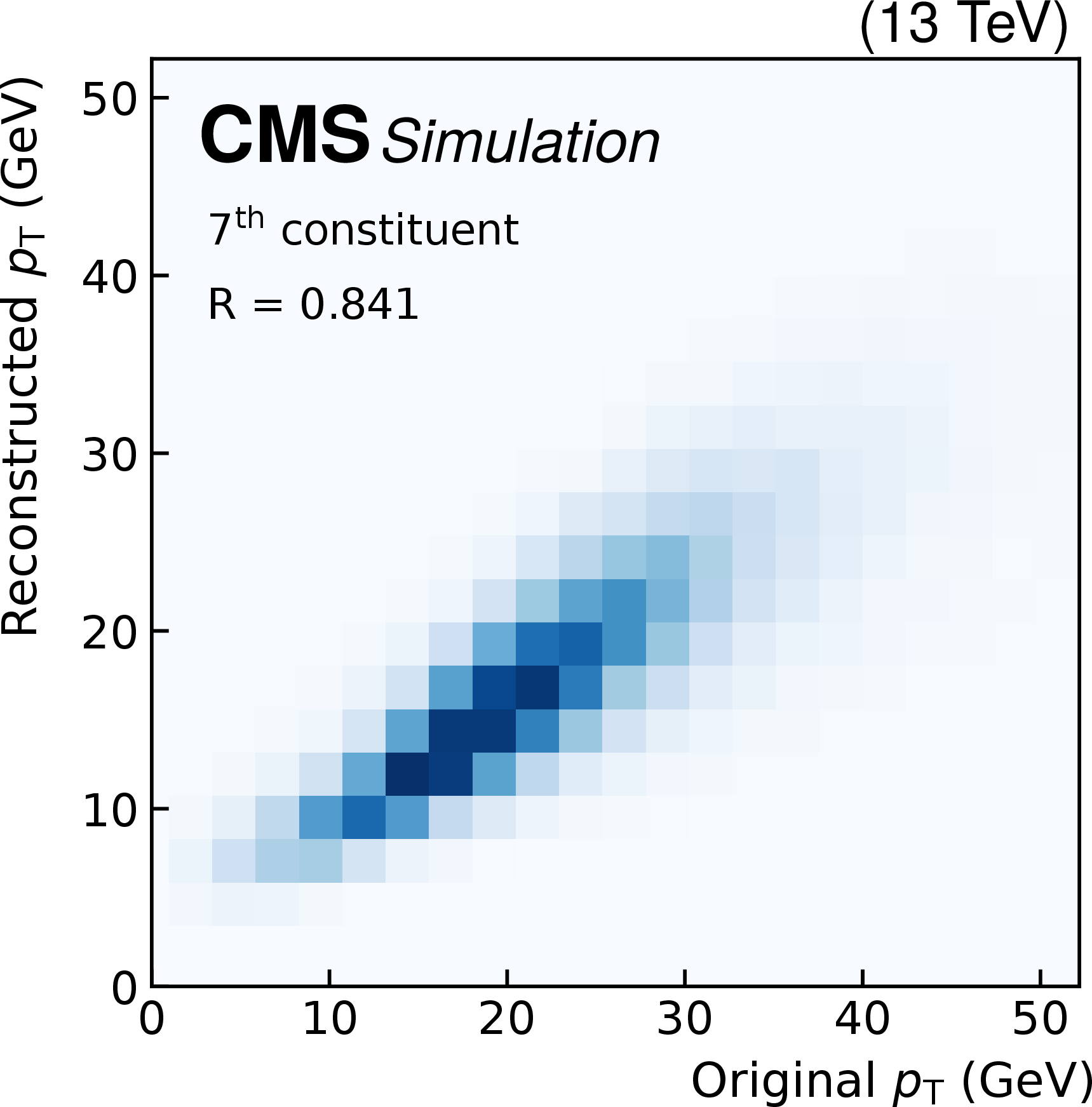
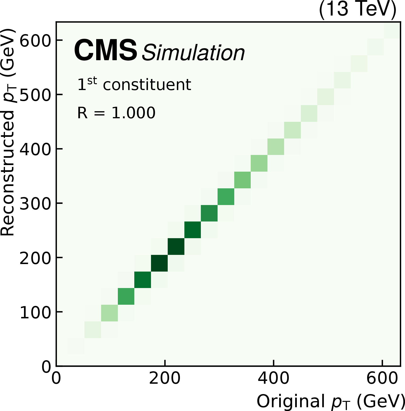
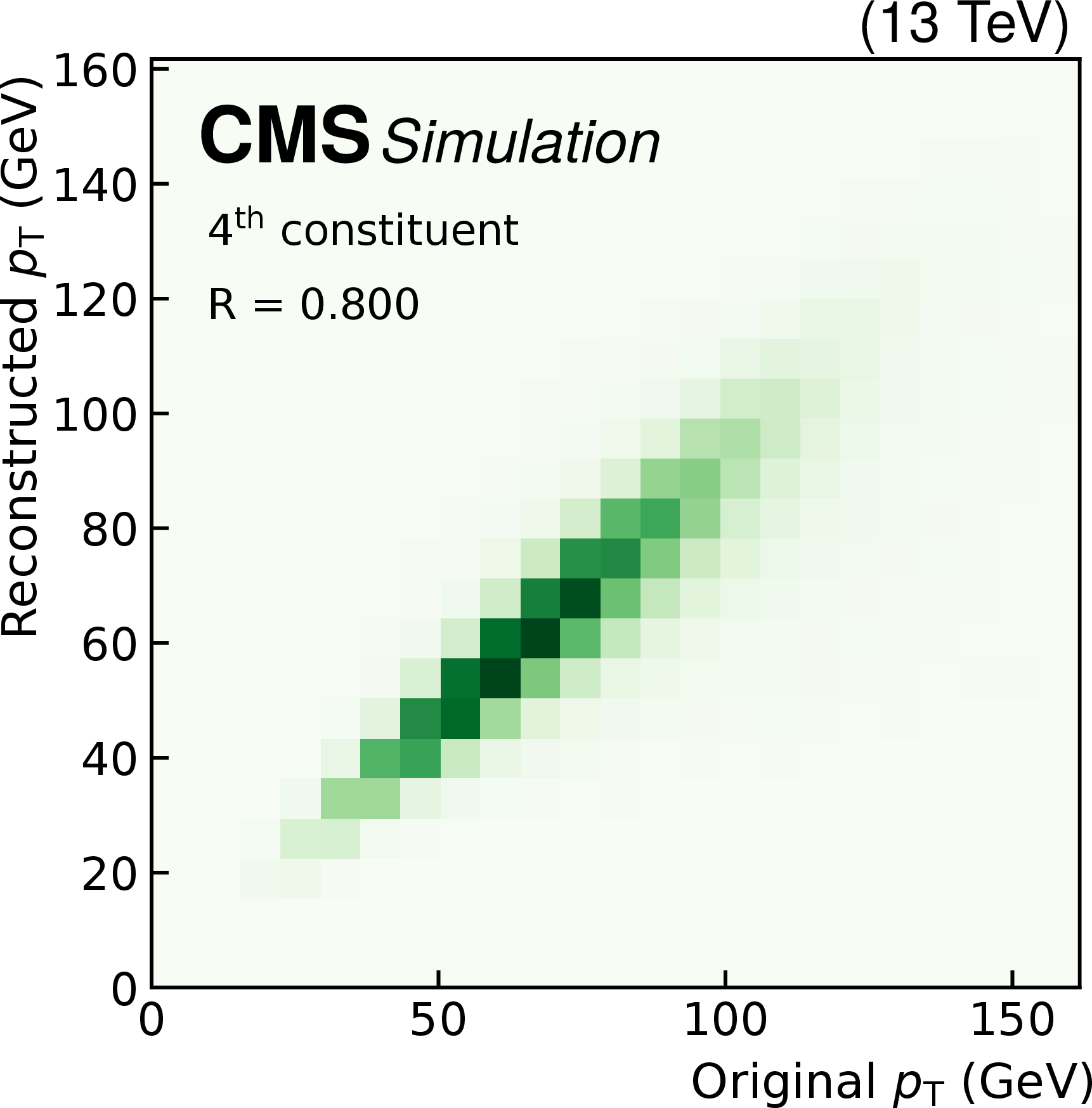
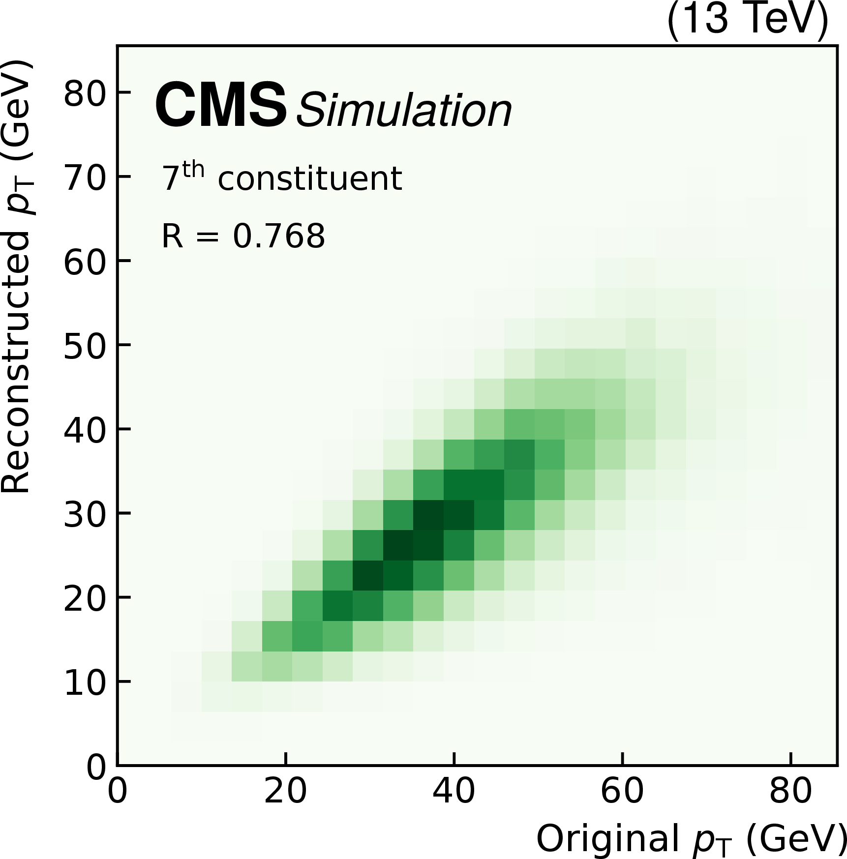
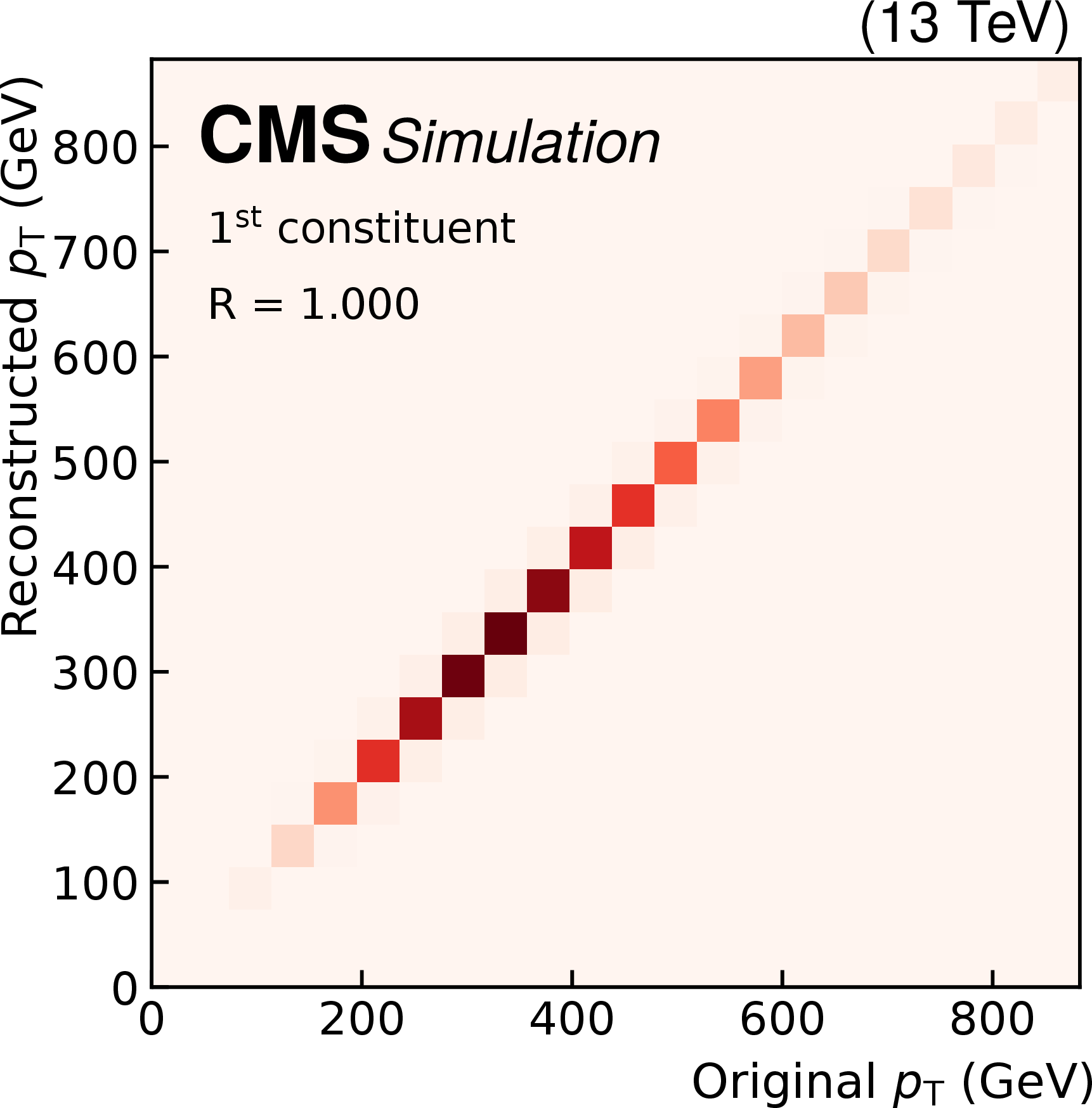
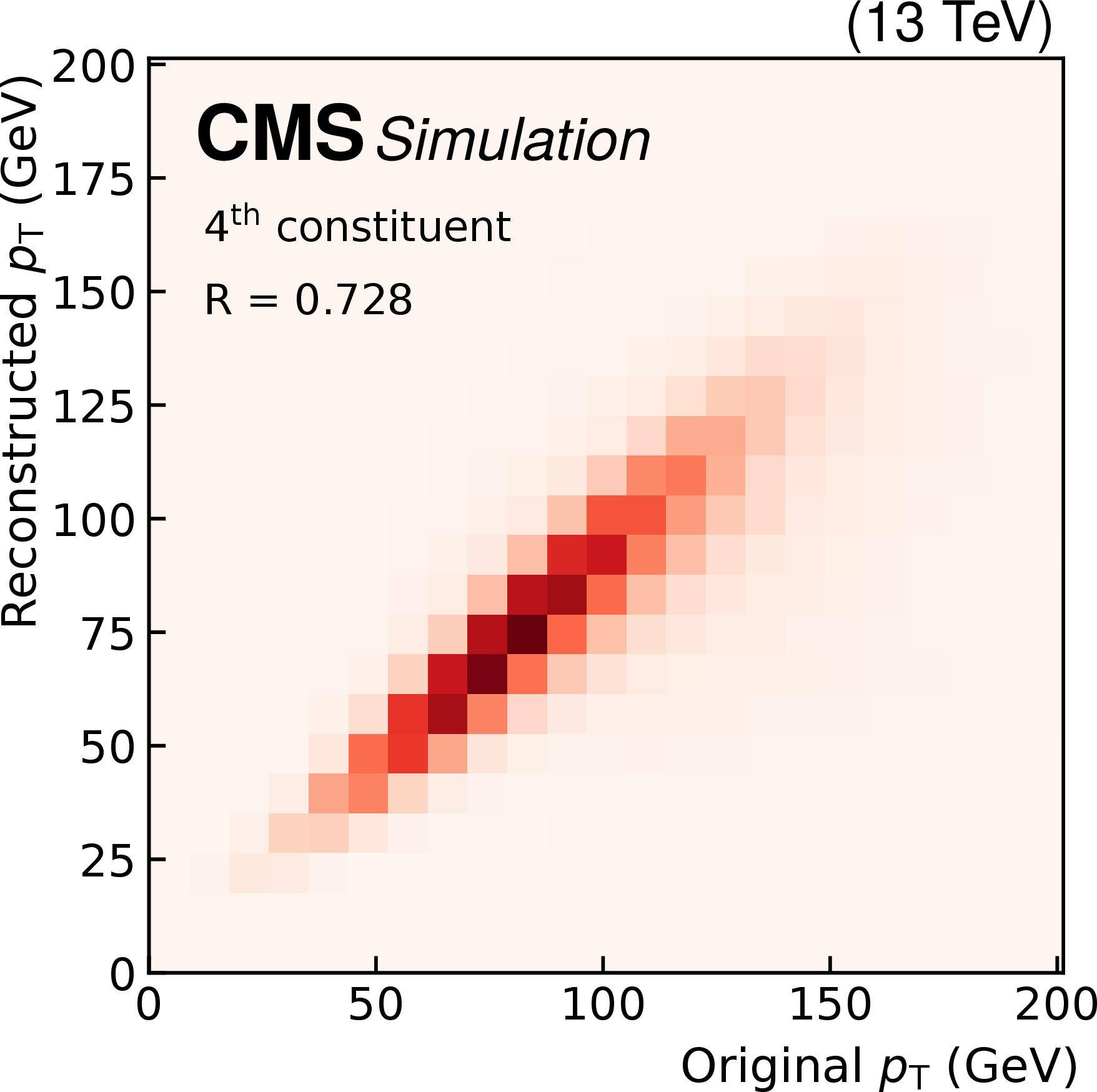
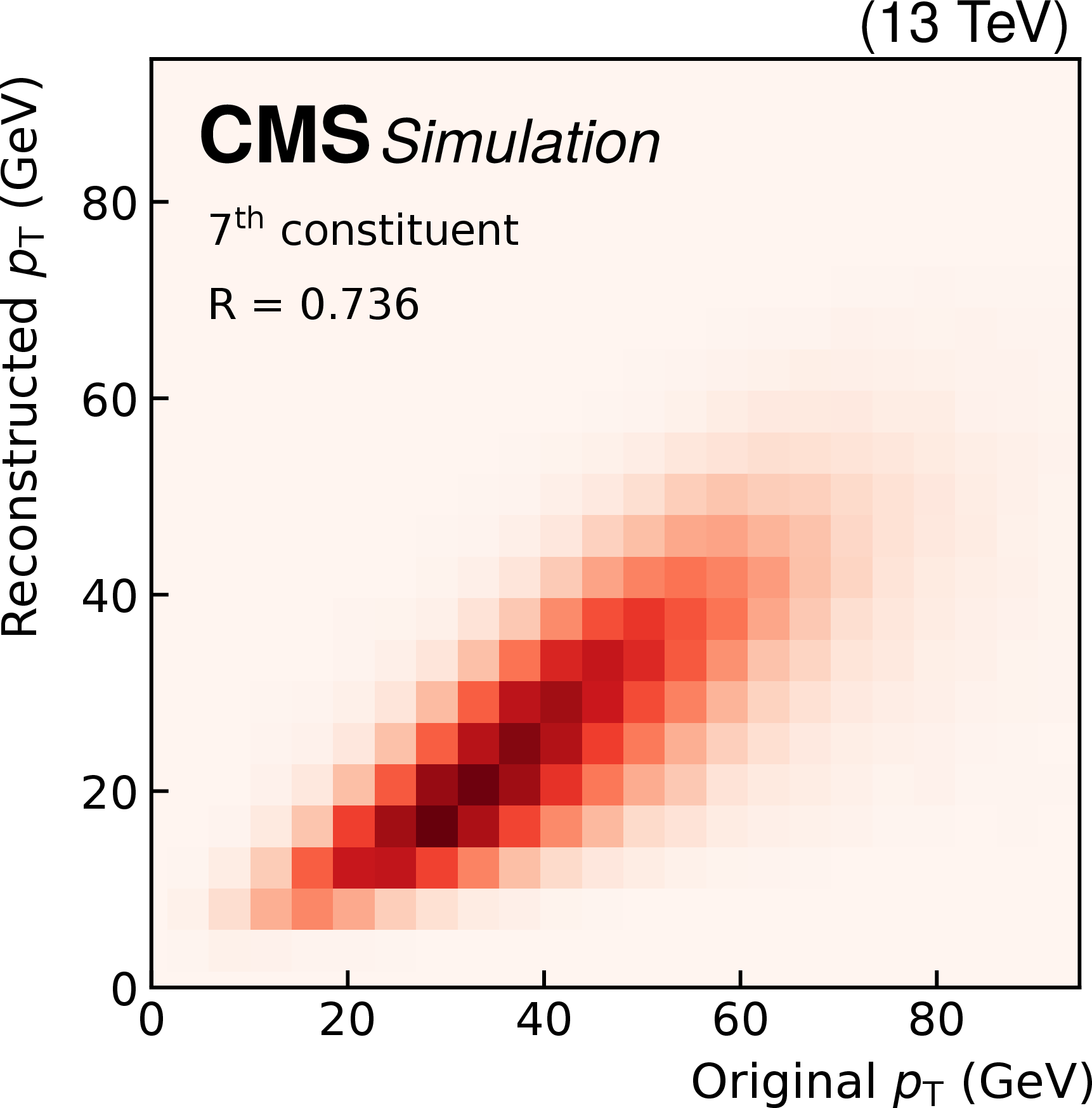
Figure 4:
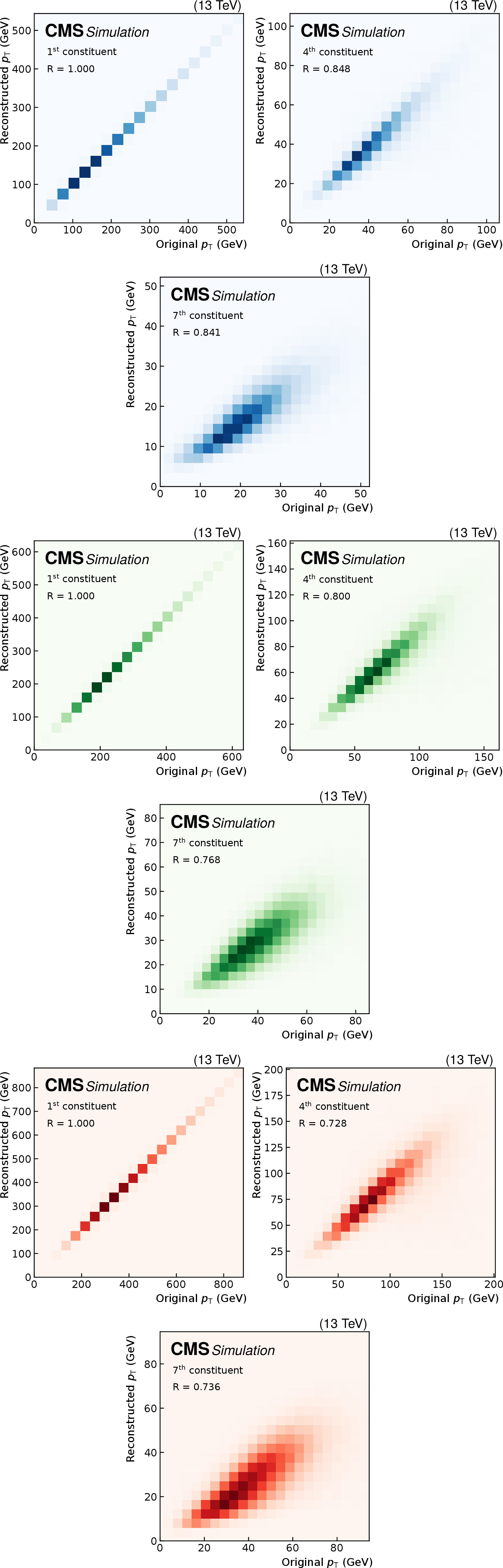
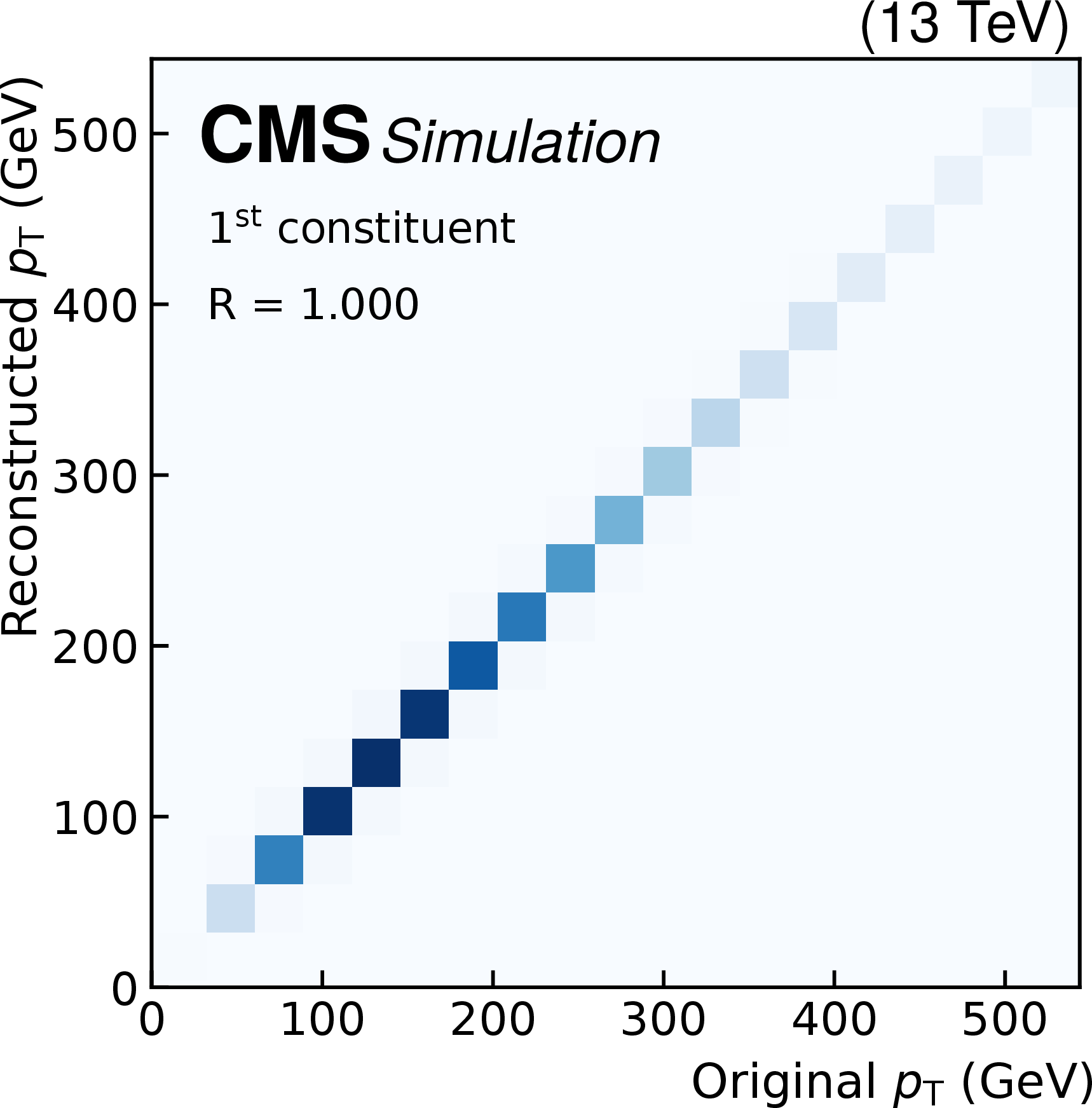
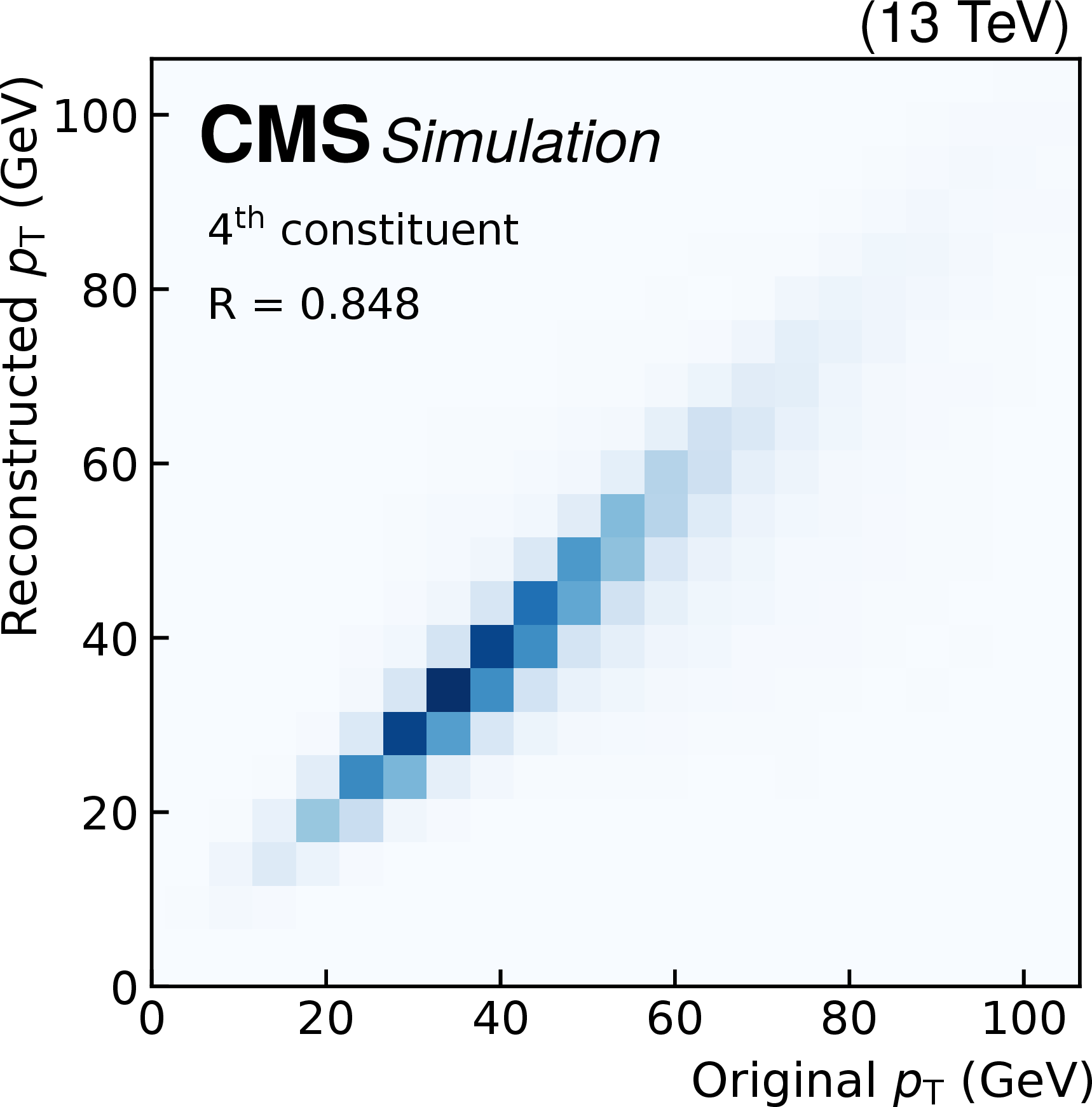
Quality of jet constituent $ p_{\mathrm{T}} $ reconstruction for SM background jets (upper row), jets from a $ \mathrm{W^{'}} \to \mathrm{B}' \mathrm{t} \to \mathrm{b} \mathrm{Z} \mathrm{t} $ decay (middle row), and jets from an $ \mathrm{X}\to \mathrm{Y} \mathrm{Y}' \to 4 \mathrm{q} $ decay (lower row). The first (left column), fourth (middle column), and seventh (right column) constituents are shown. The Pearson correlation coefficient $ R $ between the input and output is also shown. |
png pdf |
Figure 4-a:
Quality of jet constituent $ p_{\mathrm{T}} $ reconstruction for SM background jets (upper row), jets from a $ \mathrm{W^{'}} \to \mathrm{B}' \mathrm{t} \to \mathrm{b} \mathrm{Z} \mathrm{t} $ decay (middle row), and jets from an $ \mathrm{X}\to \mathrm{Y} \mathrm{Y}' \to 4 \mathrm{q} $ decay (lower row). The first (left column), fourth (middle column), and seventh (right column) constituents are shown. The Pearson correlation coefficient $ R $ between the input and output is also shown. |
png pdf |
Figure 4-b:
Quality of jet constituent $ p_{\mathrm{T}} $ reconstruction for SM background jets (upper row), jets from a $ \mathrm{W^{'}} \to \mathrm{B}' \mathrm{t} \to \mathrm{b} \mathrm{Z} \mathrm{t} $ decay (middle row), and jets from an $ \mathrm{X}\to \mathrm{Y} \mathrm{Y}' \to 4 \mathrm{q} $ decay (lower row). The first (left column), fourth (middle column), and seventh (right column) constituents are shown. The Pearson correlation coefficient $ R $ between the input and output is also shown. |
png pdf |
Figure 4-c:
Quality of jet constituent $ p_{\mathrm{T}} $ reconstruction for SM background jets (upper row), jets from a $ \mathrm{W^{'}} \to \mathrm{B}' \mathrm{t} \to \mathrm{b} \mathrm{Z} \mathrm{t} $ decay (middle row), and jets from an $ \mathrm{X}\to \mathrm{Y} \mathrm{Y}' \to 4 \mathrm{q} $ decay (lower row). The first (left column), fourth (middle column), and seventh (right column) constituents are shown. The Pearson correlation coefficient $ R $ between the input and output is also shown. |
png pdf |
Figure 4-d:
Quality of jet constituent $ p_{\mathrm{T}} $ reconstruction for SM background jets (upper row), jets from a $ \mathrm{W^{'}} \to \mathrm{B}' \mathrm{t} \to \mathrm{b} \mathrm{Z} \mathrm{t} $ decay (middle row), and jets from an $ \mathrm{X}\to \mathrm{Y} \mathrm{Y}' \to 4 \mathrm{q} $ decay (lower row). The first (left column), fourth (middle column), and seventh (right column) constituents are shown. The Pearson correlation coefficient $ R $ between the input and output is also shown. |
png pdf |
Figure 4-e:
Quality of jet constituent $ p_{\mathrm{T}} $ reconstruction for SM background jets (upper row), jets from a $ \mathrm{W^{'}} \to \mathrm{B}' \mathrm{t} \to \mathrm{b} \mathrm{Z} \mathrm{t} $ decay (middle row), and jets from an $ \mathrm{X}\to \mathrm{Y} \mathrm{Y}' \to 4 \mathrm{q} $ decay (lower row). The first (left column), fourth (middle column), and seventh (right column) constituents are shown. The Pearson correlation coefficient $ R $ between the input and output is also shown. |
png pdf |
Figure 4-f:
Quality of jet constituent $ p_{\mathrm{T}} $ reconstruction for SM background jets (upper row), jets from a $ \mathrm{W^{'}} \to \mathrm{B}' \mathrm{t} \to \mathrm{b} \mathrm{Z} \mathrm{t} $ decay (middle row), and jets from an $ \mathrm{X}\to \mathrm{Y} \mathrm{Y}' \to 4 \mathrm{q} $ decay (lower row). The first (left column), fourth (middle column), and seventh (right column) constituents are shown. The Pearson correlation coefficient $ R $ between the input and output is also shown. |
png pdf |
Figure 4-g:
Quality of jet constituent $ p_{\mathrm{T}} $ reconstruction for SM background jets (upper row), jets from a $ \mathrm{W^{'}} \to \mathrm{B}' \mathrm{t} \to \mathrm{b} \mathrm{Z} \mathrm{t} $ decay (middle row), and jets from an $ \mathrm{X}\to \mathrm{Y} \mathrm{Y}' \to 4 \mathrm{q} $ decay (lower row). The first (left column), fourth (middle column), and seventh (right column) constituents are shown. The Pearson correlation coefficient $ R $ between the input and output is also shown. |
png pdf |
Figure 4-h:
Quality of jet constituent $ p_{\mathrm{T}} $ reconstruction for SM background jets (upper row), jets from a $ \mathrm{W^{'}} \to \mathrm{B}' \mathrm{t} \to \mathrm{b} \mathrm{Z} \mathrm{t} $ decay (middle row), and jets from an $ \mathrm{X}\to \mathrm{Y} \mathrm{Y}' \to 4 \mathrm{q} $ decay (lower row). The first (left column), fourth (middle column), and seventh (right column) constituents are shown. The Pearson correlation coefficient $ R $ between the input and output is also shown. |
png pdf |
Figure 4-i:
Quality of jet constituent $ p_{\mathrm{T}} $ reconstruction for SM background jets (upper row), jets from a $ \mathrm{W^{'}} \to \mathrm{B}' \mathrm{t} \to \mathrm{b} \mathrm{Z} \mathrm{t} $ decay (middle row), and jets from an $ \mathrm{X}\to \mathrm{Y} \mathrm{Y}' \to 4 \mathrm{q} $ decay (lower row). The first (left column), fourth (middle column), and seventh (right column) constituents are shown. The Pearson correlation coefficient $ R $ between the input and output is also shown. |
png pdf |
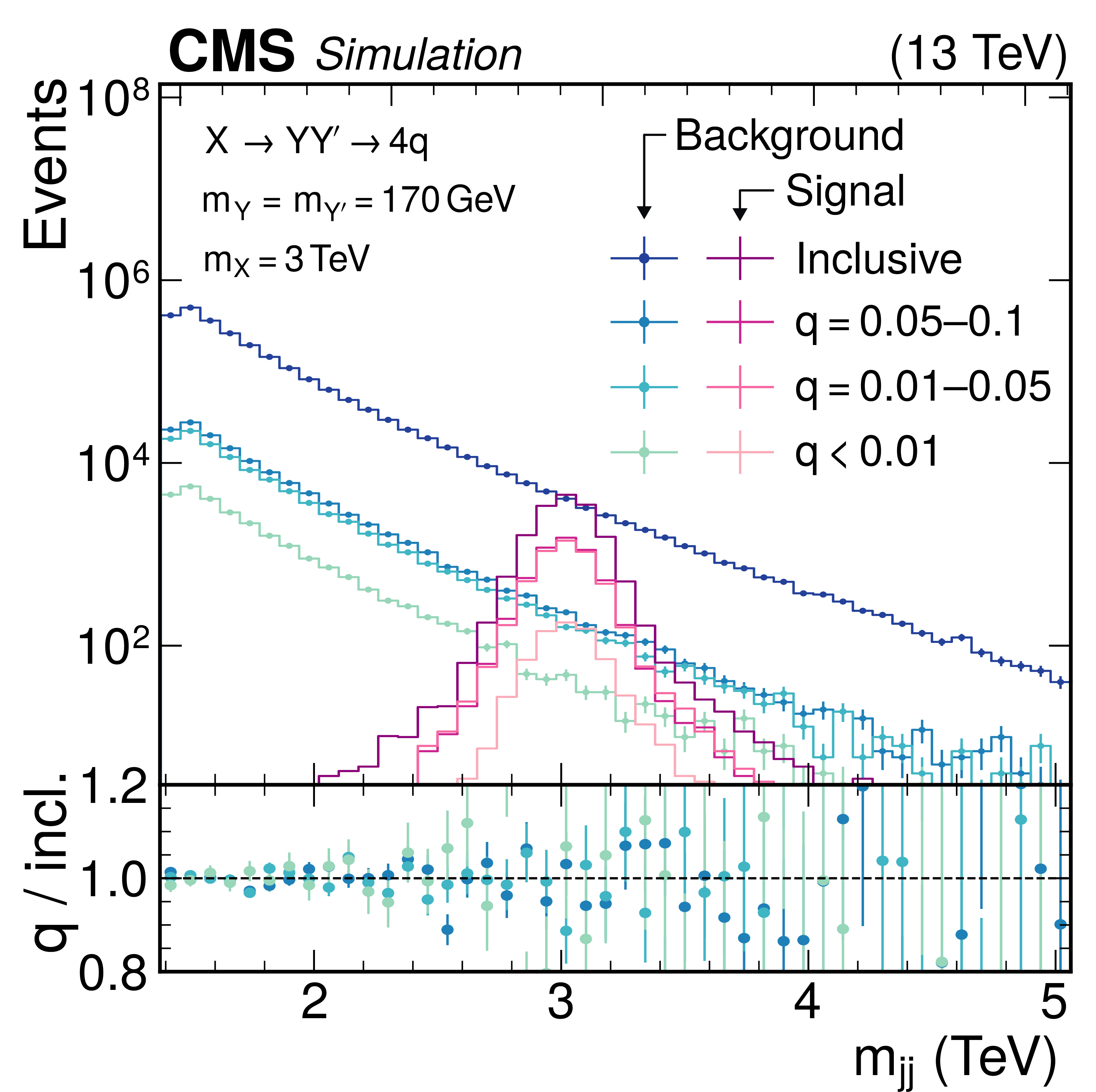
Figure 5:
Simulated dijet invariant mass spectrum after selecting events based on the score of the VAE-QR} method. The distributions are shown in the upper panel for the SM background (blue) and the $ \mathrm{X}\to \mathrm{Y} \mathrm{Y}' \to 4 \mathrm{q} $ signal model with $ m_{\mathrm{X}}= $ 3 TeV and $ m_{\mathrm{Y} }=m_{\mathrm{Y}' }= $ 170 GeV (red). The inclusive selection is compared to the three quantile ranges used in the statistical analysis. No significant difference is observed between the shapes, showing that the quantile regression performs as expected. The lower panel shows the ratio of the quantile ranges to the inclusive distribution for the SM background, scaled by the respective quantile probabilities. |
png pdf |
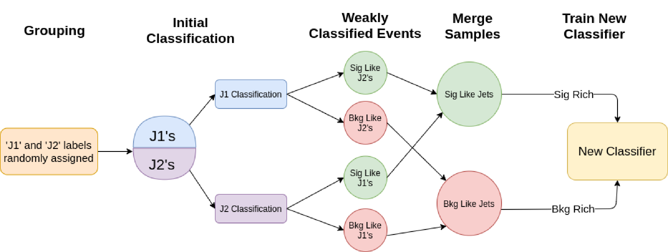
Figure 6:
A schematic showing the training algorithm for TNT. The two jets in the event are randomly assigned the labels 1 and 2. The dijet invariant masses and the autoencoder scores are used to construct signal- and background-like subsets of J1 and J2. These subsets are then merged, and a single classifier is trained to distinguish between signal- and background-like jets. |

png pdf |
Figure 7:
The three main steps of CATHODE. a) Given a signal mass hypothesis, $ m_\mathrm{jj} $ is used to define the signal region in which the signal would be localized. b) A background estimate for the input features $ x $ is obtained from events outside the signal region by training a generative model and interpolating it. c) A weakly supervised classifier is trained to distinguish between the interpolated background and the observed signal region data, singling out any difference between them caused by signal events. |
png pdf |
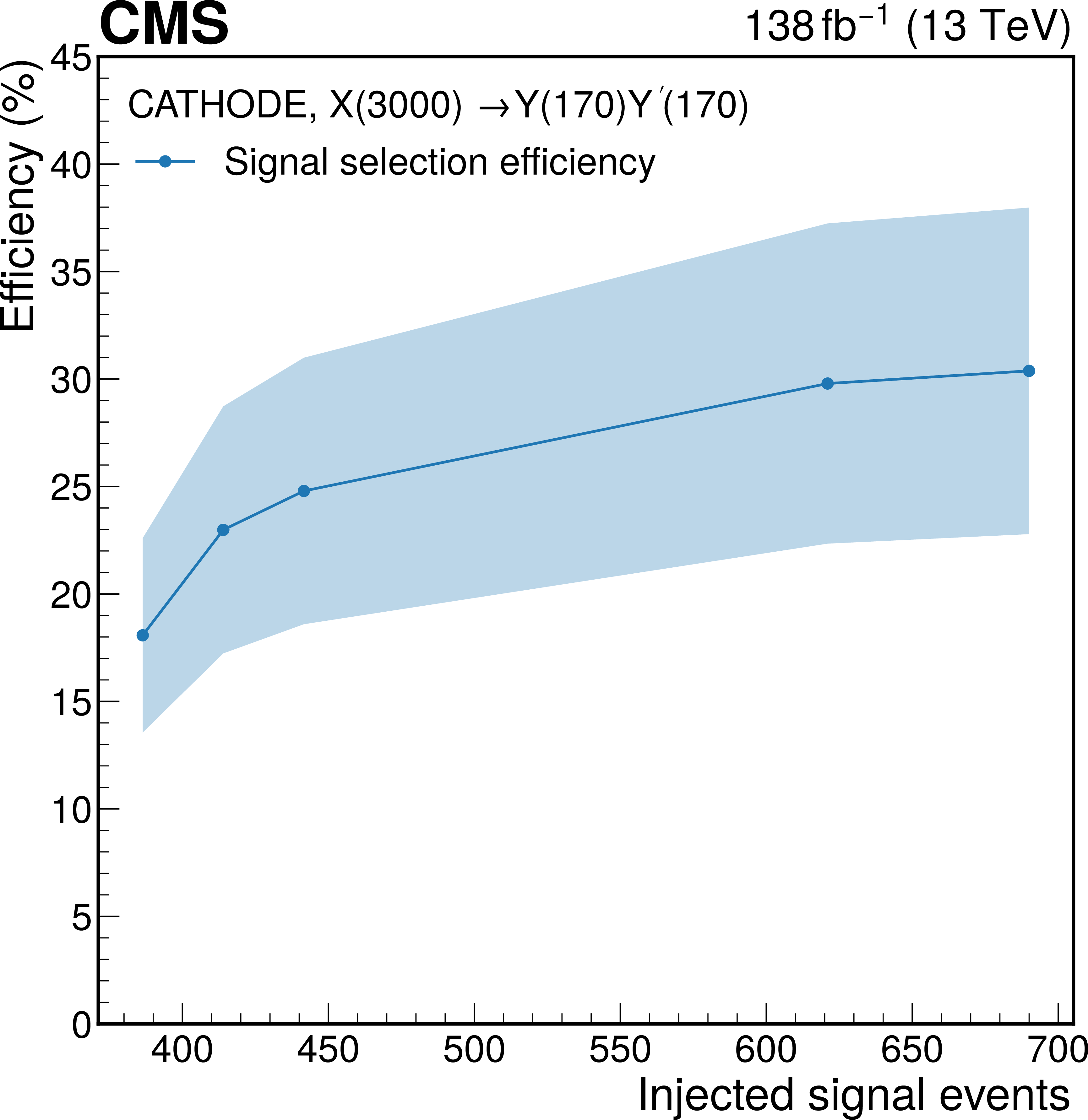
Figure 8:
Signal selection efficiency of the weakly supervised classifier in the CATHODE method, evaluated for the $ \mathrm{X}\to \mathrm{Y} \mathrm{Y}' \to 4 \mathrm{q} $ signal at 3 TeV in SR B3. The shaded region represents the total statistical and systematic uncertainty evaluated as described in the text. The uncertainty is largely correlated between the different signal injection points, such that the rise in the signal efficiency is statistically meaningful despite the change over the considered range being smaller than the uncertainty band. |
png pdf |
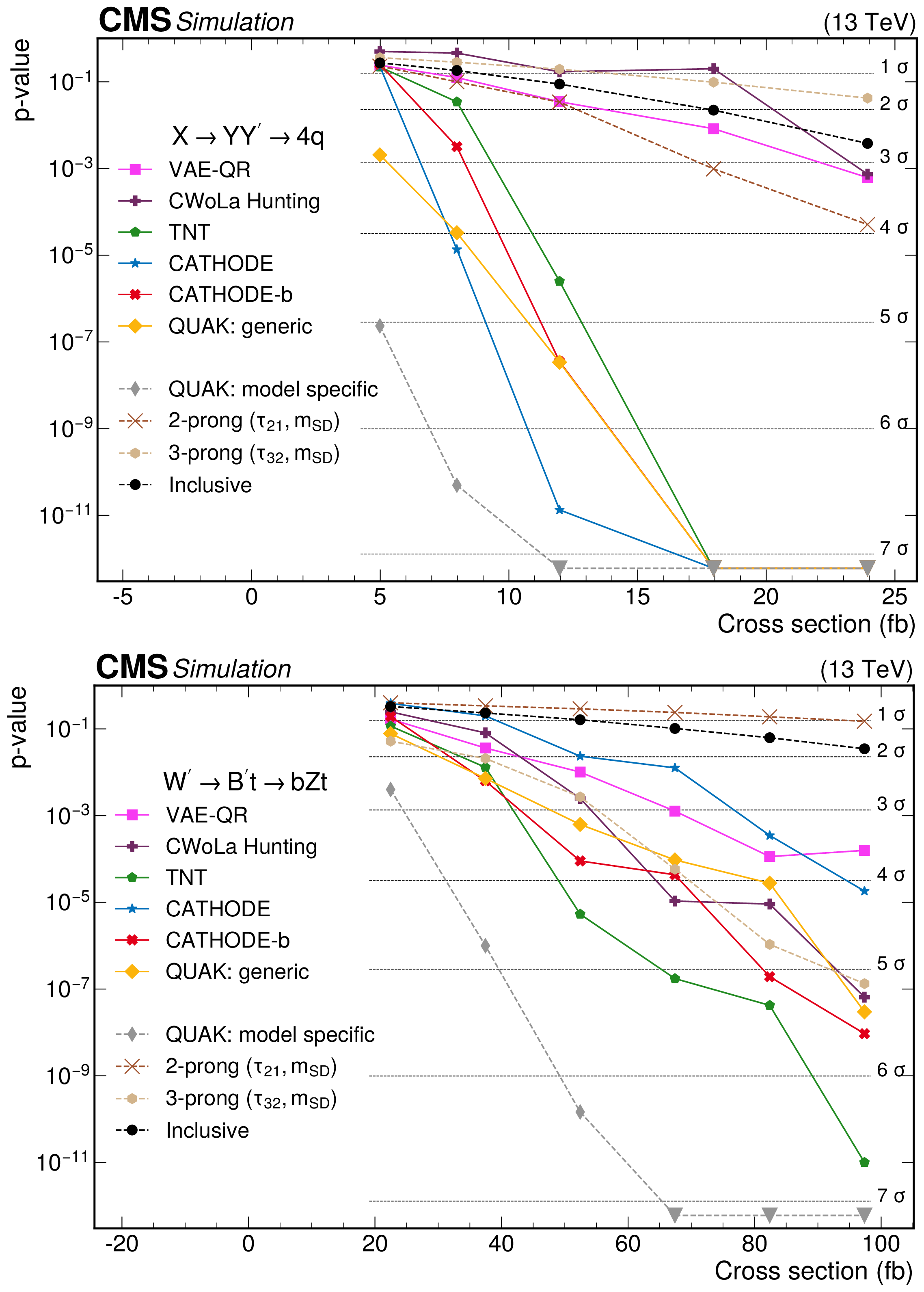
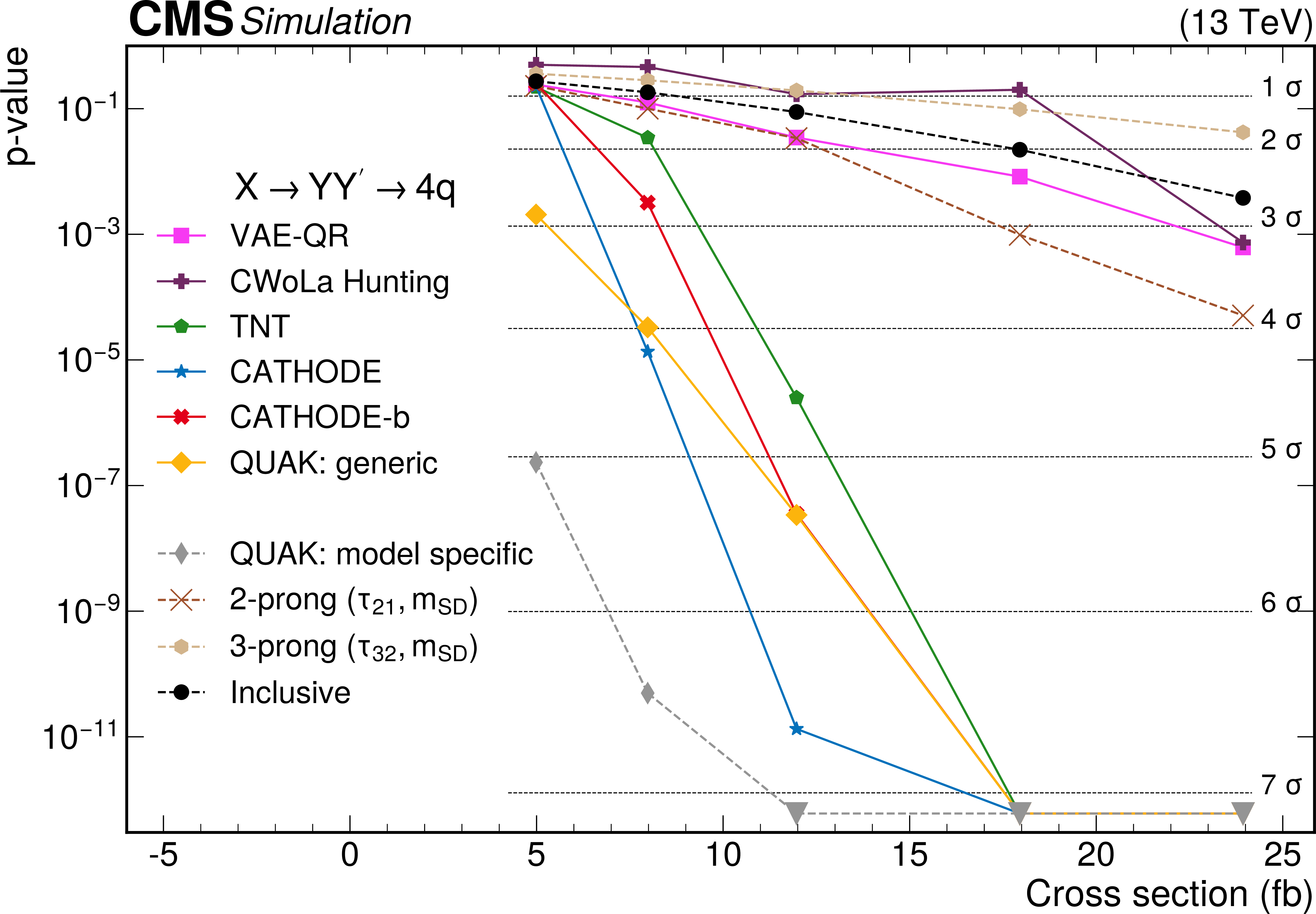
Figure 9:
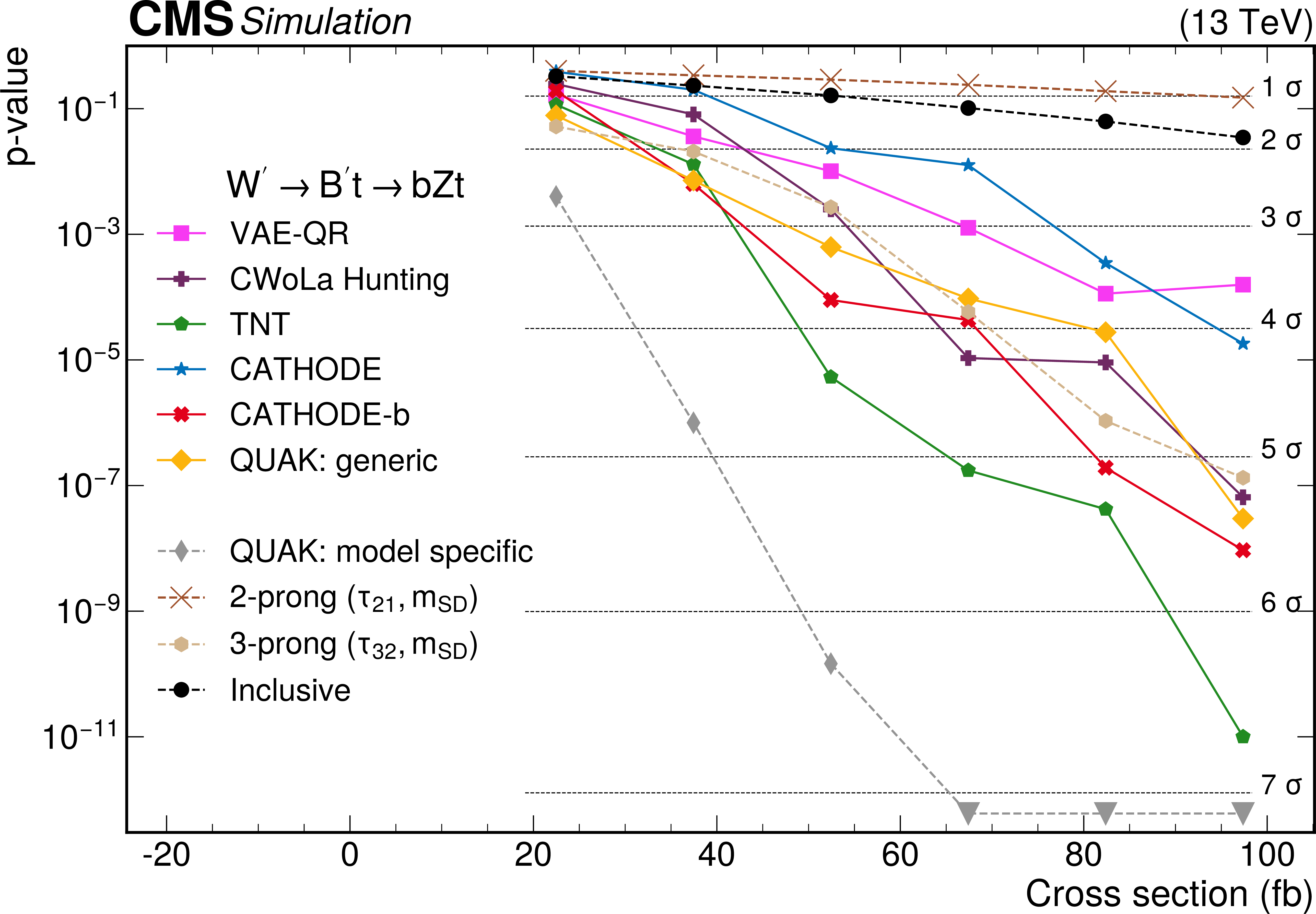
The $ p $-values as a function of the injected signal cross sections for the different analysis procedures for two different signals. The upper panel shows results for the 2-prong $ \mathrm{X}\to \mathrm{Y} \mathrm{Y}' \to 4 \mathrm{q} $ signal with $ m_{\mathrm{X}}= $ 3 TeV and $ m_{\mathrm{Y} }=m_{\mathrm{Y}' }= $ 170 GeV, while the lower panel shows results for the 3-prong $ \mathrm{W^{'}} \to \mathrm{B}' \mathrm{t} \to \mathrm{b} \mathrm{Z} \mathrm{t} $ signal with $ m_\mathrm{W^{'}}= $ 3 TeV and $ m_{\mathrm{B}' }= $ 400 GeV. Significance values larger than 7 standard deviations ($ \sigma $) are denoted with downwards facing triangles. Reproduced from Ref. [6]. |
png pdf |
Figure 9-a:
The $ p $-values as a function of the injected signal cross sections for the different analysis procedures for two different signals. The upper panel shows results for the 2-prong $ \mathrm{X}\to \mathrm{Y} \mathrm{Y}' \to 4 \mathrm{q} $ signal with $ m_{\mathrm{X}}= $ 3 TeV and $ m_{\mathrm{Y} }=m_{\mathrm{Y}' }= $ 170 GeV, while the lower panel shows results for the 3-prong $ \mathrm{W^{'}} \to \mathrm{B}' \mathrm{t} \to \mathrm{b} \mathrm{Z} \mathrm{t} $ signal with $ m_\mathrm{W^{'}}= $ 3 TeV and $ m_{\mathrm{B}' }= $ 400 GeV. Significance values larger than 7 standard deviations ($ \sigma $) are denoted with downwards facing triangles. Reproduced from Ref. [6]. |
png pdf |
Figure 9-b:
The $ p $-values as a function of the injected signal cross sections for the different analysis procedures for two different signals. The upper panel shows results for the 2-prong $ \mathrm{X}\to \mathrm{Y} \mathrm{Y}' \to 4 \mathrm{q} $ signal with $ m_{\mathrm{X}}= $ 3 TeV and $ m_{\mathrm{Y} }=m_{\mathrm{Y}' }= $ 170 GeV, while the lower panel shows results for the 3-prong $ \mathrm{W^{'}} \to \mathrm{B}' \mathrm{t} \to \mathrm{b} \mathrm{Z} \mathrm{t} $ signal with $ m_\mathrm{W^{'}}= $ 3 TeV and $ m_{\mathrm{B}' }= $ 400 GeV. Significance values larger than 7 standard deviations ($ \sigma $) are denoted with downwards facing triangles. Reproduced from Ref. [6]. |
png pdf |
Figure 10:
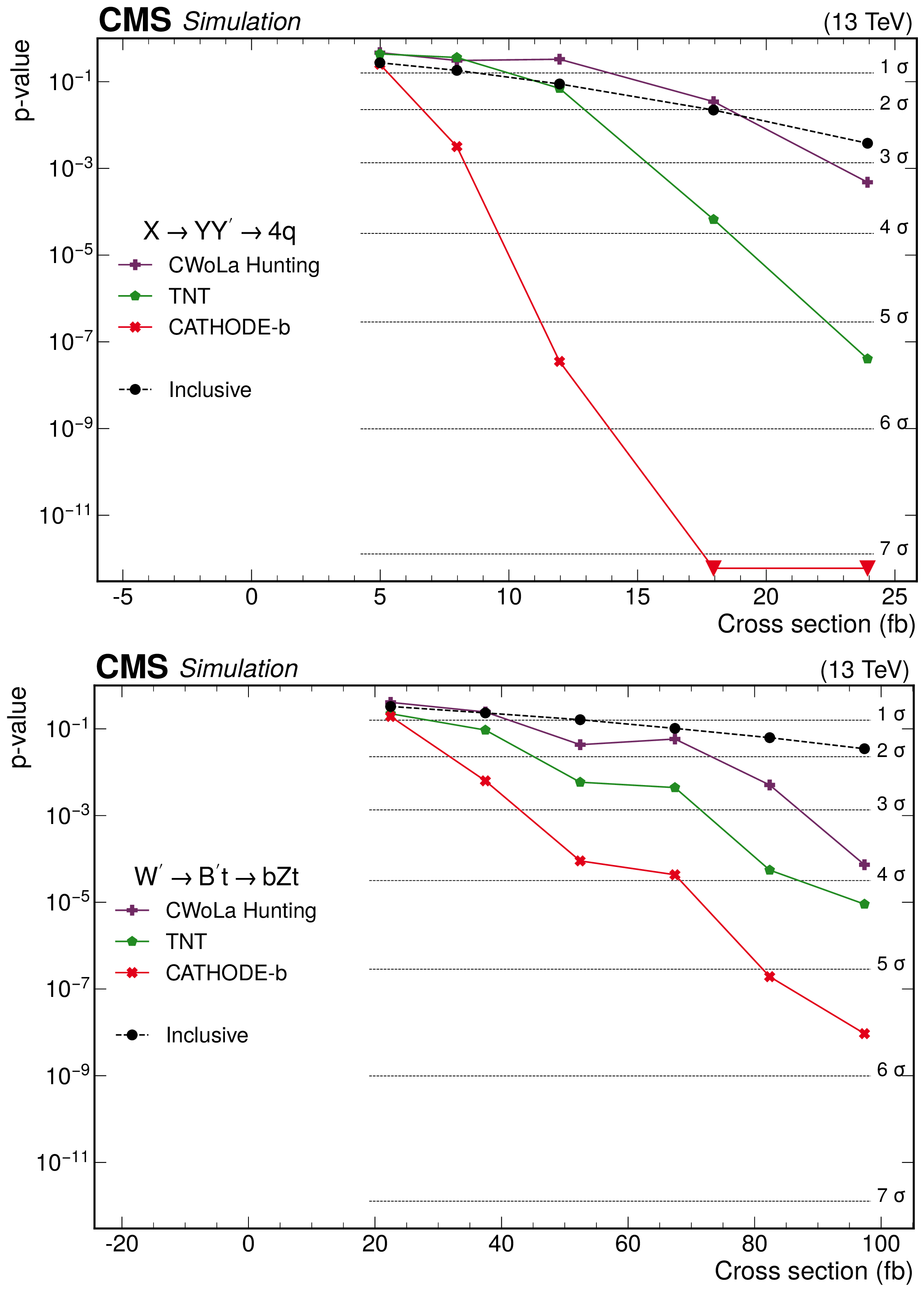
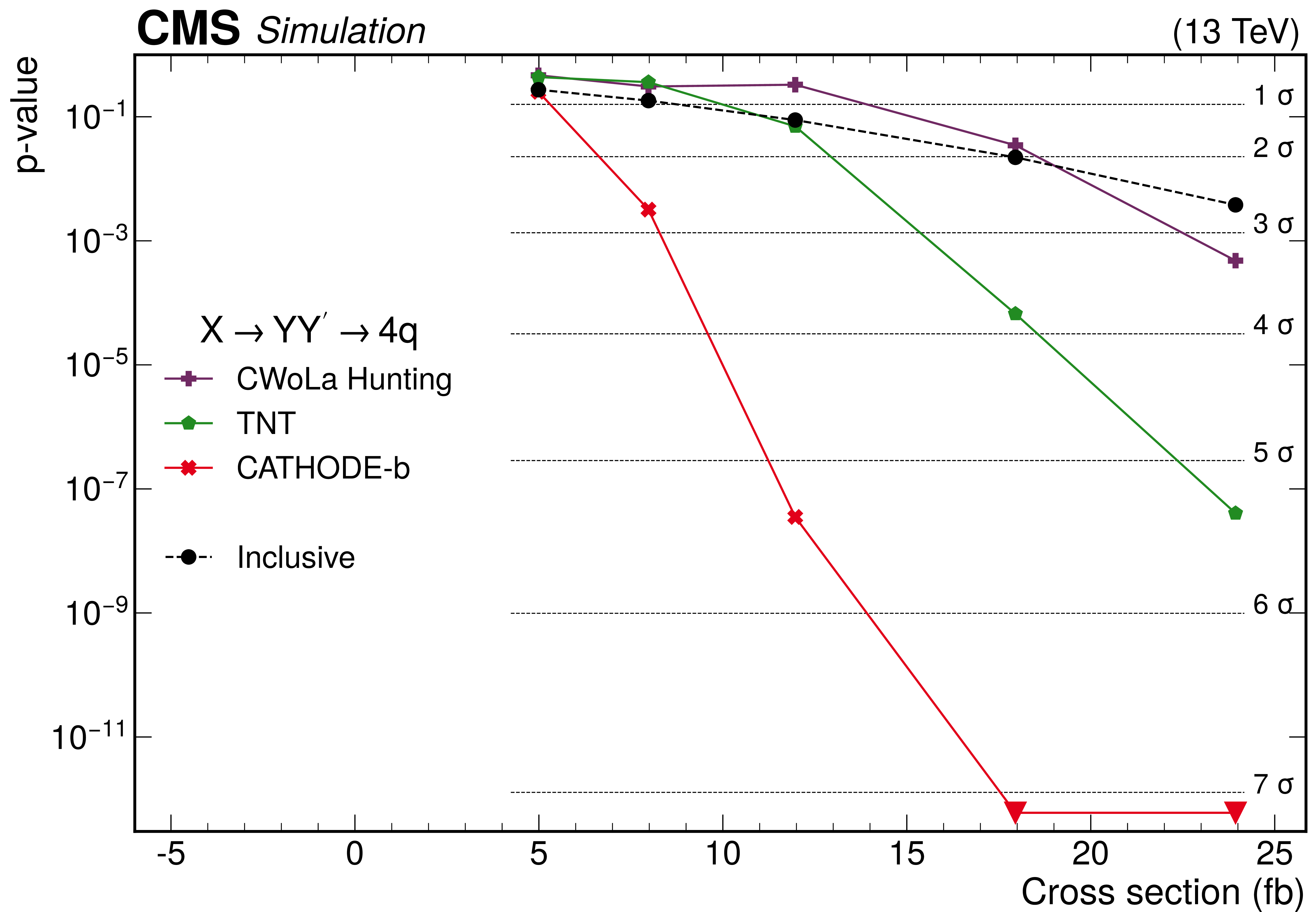
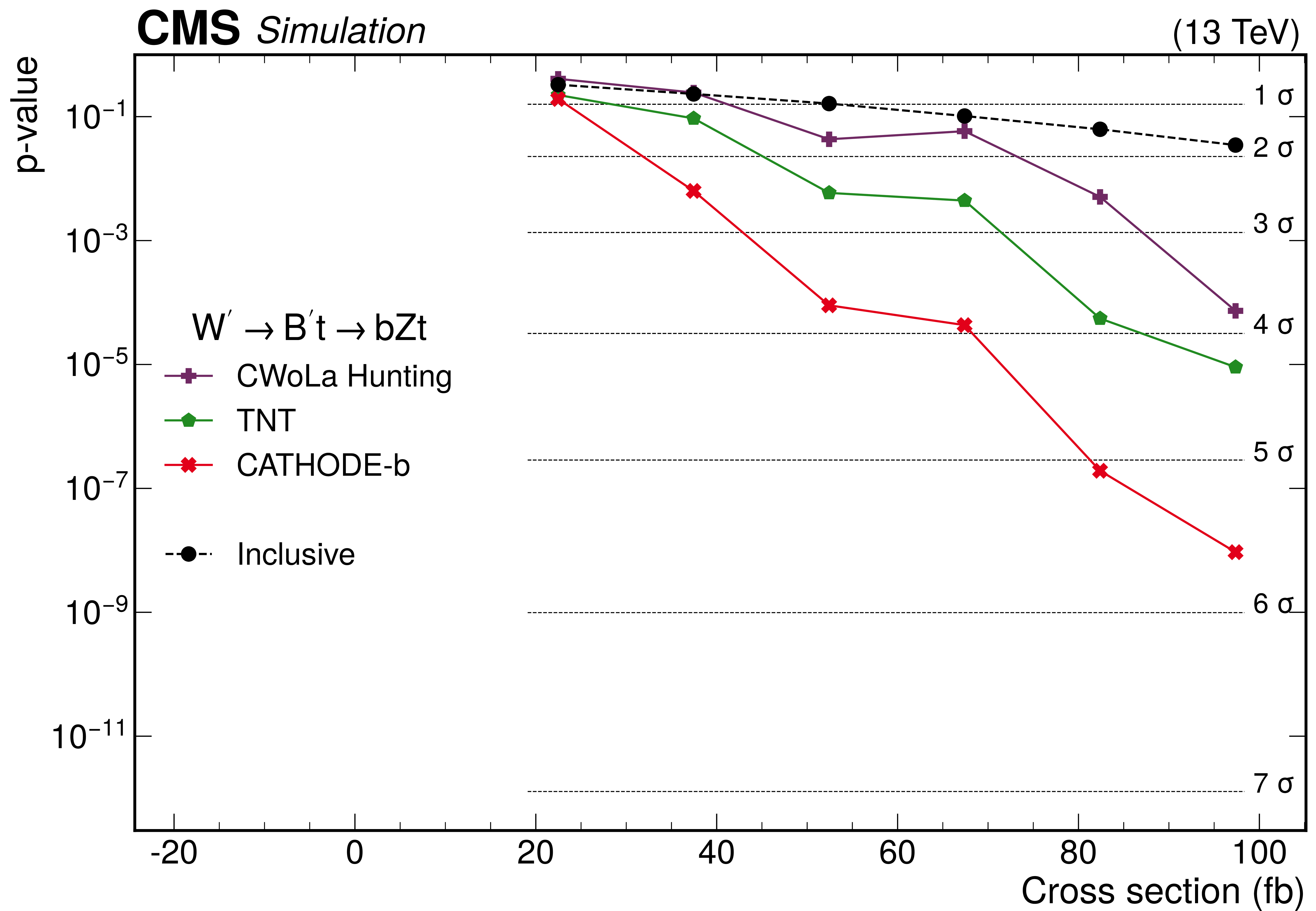
The $ p $-values as a function of the injected signal cross sections for the different analysis procedures modified to use a common set of input features, for two different signals: (upper) the 2-prong $ \mathrm{X}\to \mathrm{Y} \mathrm{Y}' \to 4 \mathrm{q} $ signal with $ m_{\mathrm{X}}= $ 3 TeV and $ m_{\mathrm{Y} }=m_{\mathrm{Y}' }= $ 170 GeV, and (lower) 3-prong $ \mathrm{W^{'}} \to \mathrm{B}' \mathrm{t} \to \mathrm{b} \mathrm{Z} \mathrm{t} $ signal with $ m_\mathrm{W^{'}}= $ 3 TeV and $ m_{\mathrm{B}' }= $ 400 GeV. Significance values larger than 7 standard deviations ($ \sigma $) are denoted with downwards facing triangles. |
png pdf |
Figure 10-a:
The $ p $-values as a function of the injected signal cross sections for the different analysis procedures modified to use a common set of input features, for two different signals: (upper) the 2-prong $ \mathrm{X}\to \mathrm{Y} \mathrm{Y}' \to 4 \mathrm{q} $ signal with $ m_{\mathrm{X}}= $ 3 TeV and $ m_{\mathrm{Y} }=m_{\mathrm{Y}' }= $ 170 GeV, and (lower) 3-prong $ \mathrm{W^{'}} \to \mathrm{B}' \mathrm{t} \to \mathrm{b} \mathrm{Z} \mathrm{t} $ signal with $ m_\mathrm{W^{'}}= $ 3 TeV and $ m_{\mathrm{B}' }= $ 400 GeV. Significance values larger than 7 standard deviations ($ \sigma $) are denoted with downwards facing triangles. |
png pdf |
Figure 10-b:
The $ p $-values as a function of the injected signal cross sections for the different analysis procedures modified to use a common set of input features, for two different signals: (upper) the 2-prong $ \mathrm{X}\to \mathrm{Y} \mathrm{Y}' \to 4 \mathrm{q} $ signal with $ m_{\mathrm{X}}= $ 3 TeV and $ m_{\mathrm{Y} }=m_{\mathrm{Y}' }= $ 170 GeV, and (lower) 3-prong $ \mathrm{W^{'}} \to \mathrm{B}' \mathrm{t} \to \mathrm{b} \mathrm{Z} \mathrm{t} $ signal with $ m_\mathrm{W^{'}}= $ 3 TeV and $ m_{\mathrm{B}' }= $ 400 GeV. Significance values larger than 7 standard deviations ($ \sigma $) are denoted with downwards facing triangles. |
png pdf |
Figure 11:
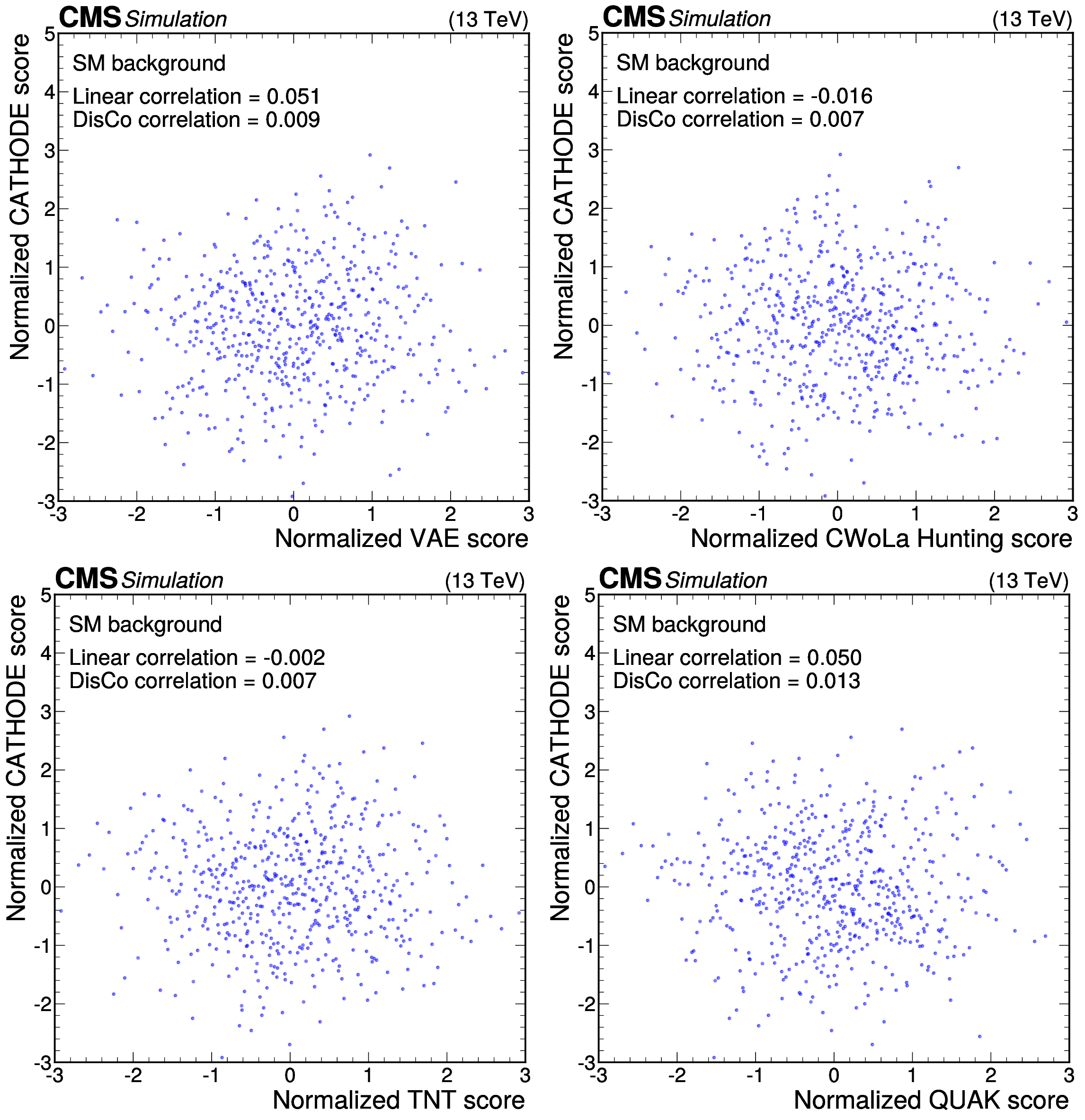
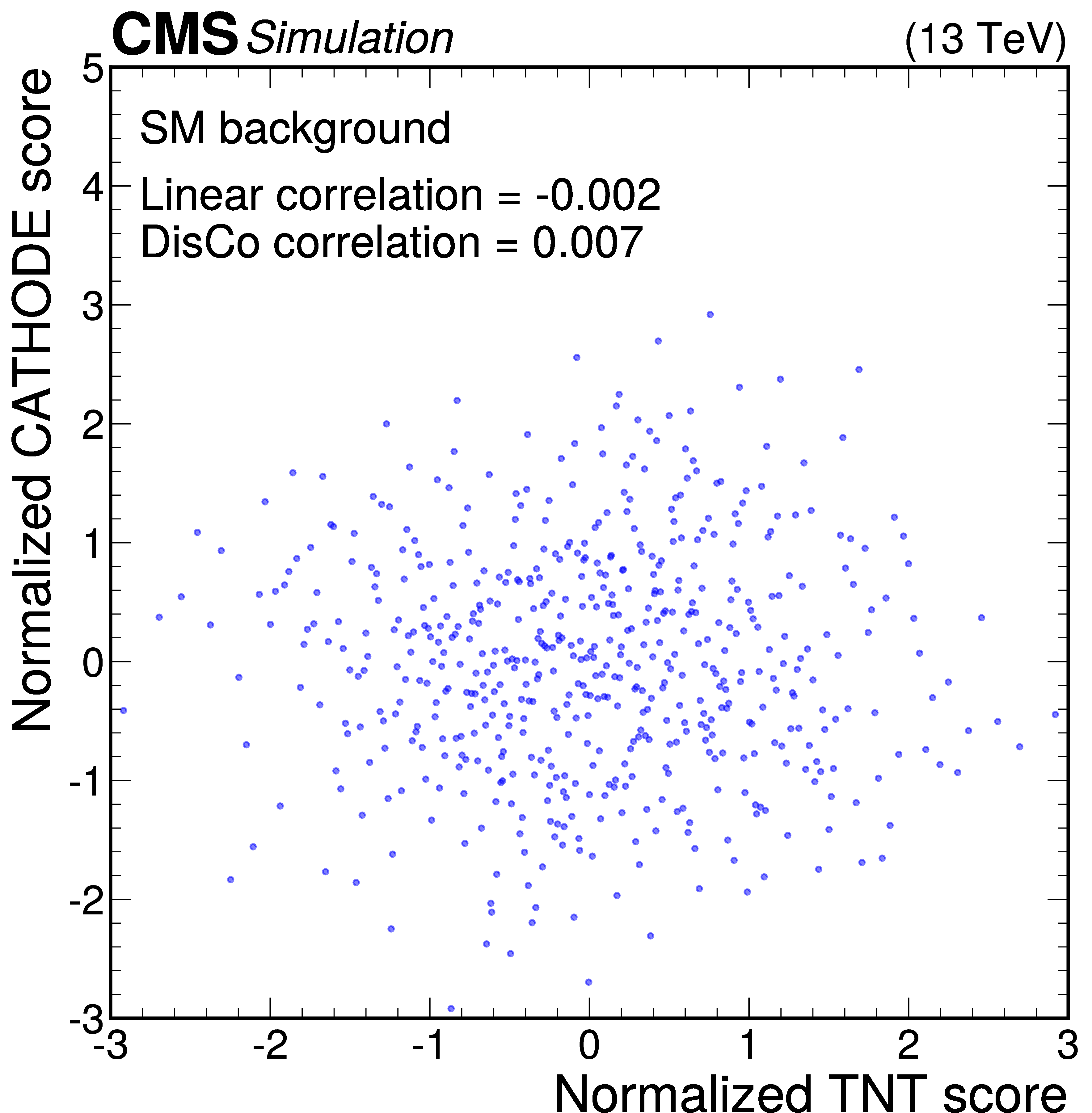
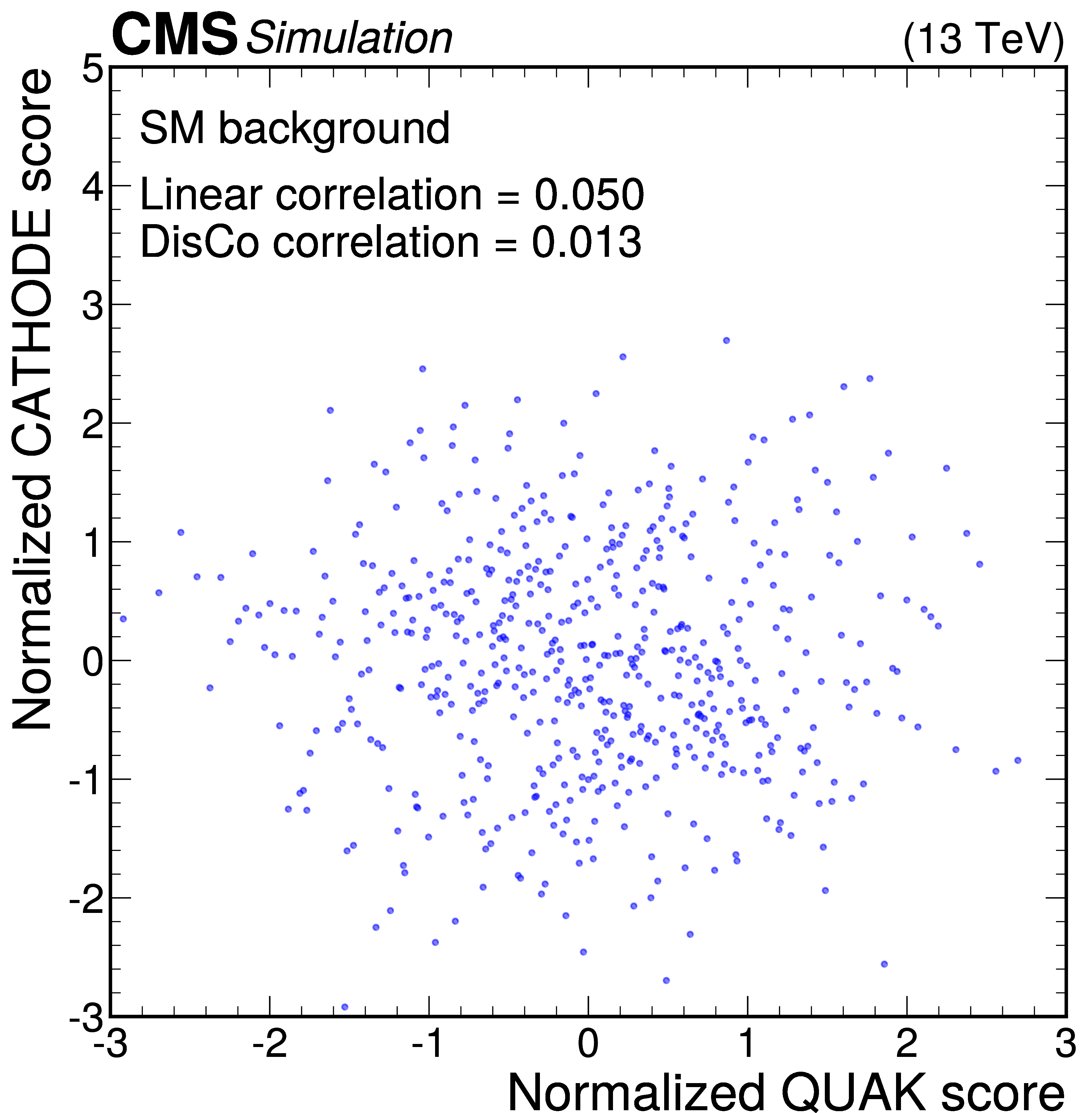
Anomaly score correlations of different methods on the background sample. Scores are transformed to follow a normal distribution. The Pearson linear correlation coefficient and distance correlation (DisCo) are listed for each pairing. Details are given in the text. |

png pdf |
Figure 11-a:
Anomaly score correlations of different methods on the background sample. Scores are transformed to follow a normal distribution. The Pearson linear correlation coefficient and distance correlation (DisCo) are listed for each pairing. Details are given in the text. |

png pdf |
Figure 11-b:
Anomaly score correlations of different methods on the background sample. Scores are transformed to follow a normal distribution. The Pearson linear correlation coefficient and distance correlation (DisCo) are listed for each pairing. Details are given in the text. |
png pdf |
Figure 11-c:
Anomaly score correlations of different methods on the background sample. Scores are transformed to follow a normal distribution. The Pearson linear correlation coefficient and distance correlation (DisCo) are listed for each pairing. Details are given in the text. |
png pdf |
Figure 11-d:
Anomaly score correlations of different methods on the background sample. Scores are transformed to follow a normal distribution. The Pearson linear correlation coefficient and distance correlation (DisCo) are listed for each pairing. Details are given in the text. |
png pdf |
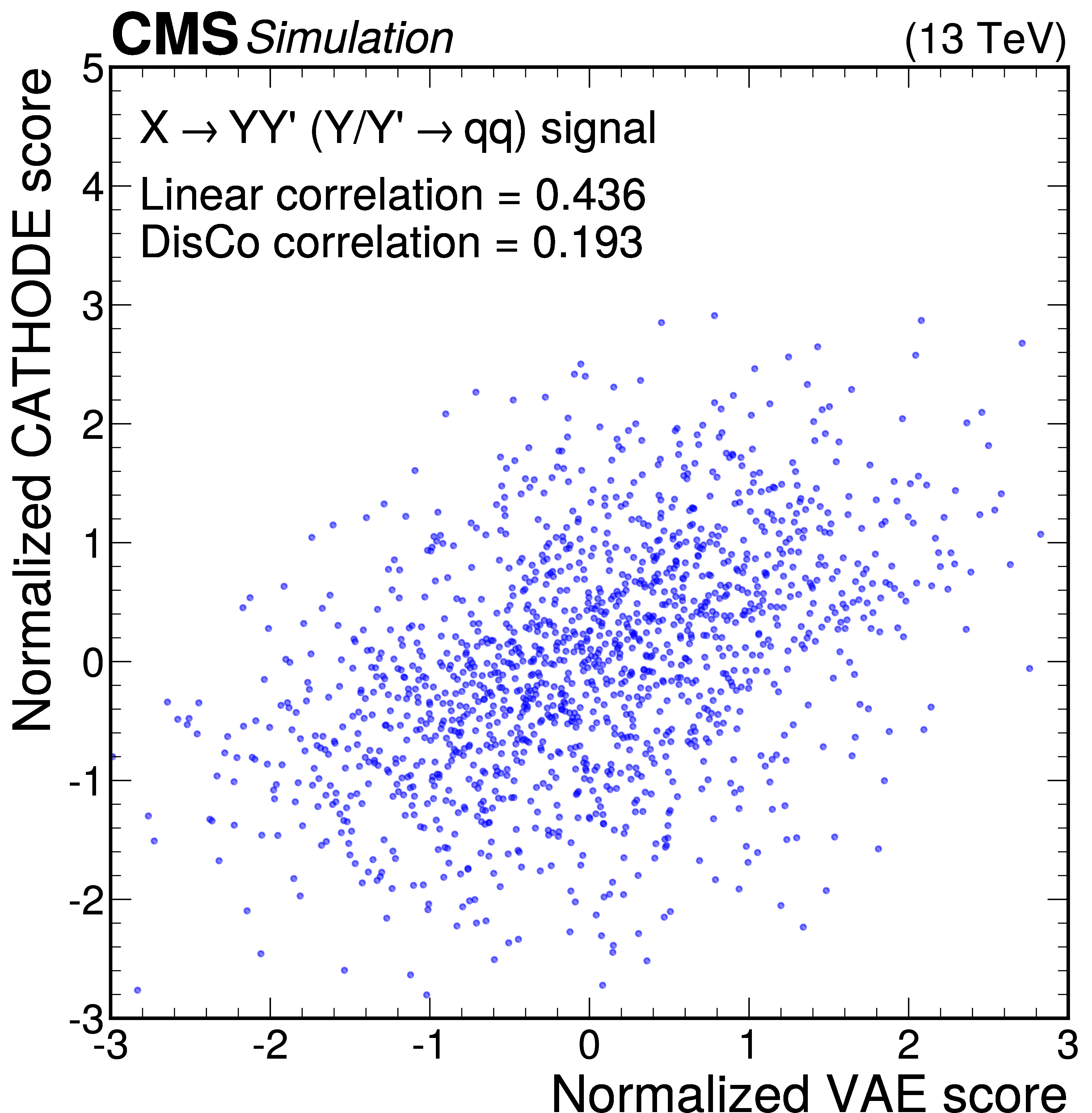
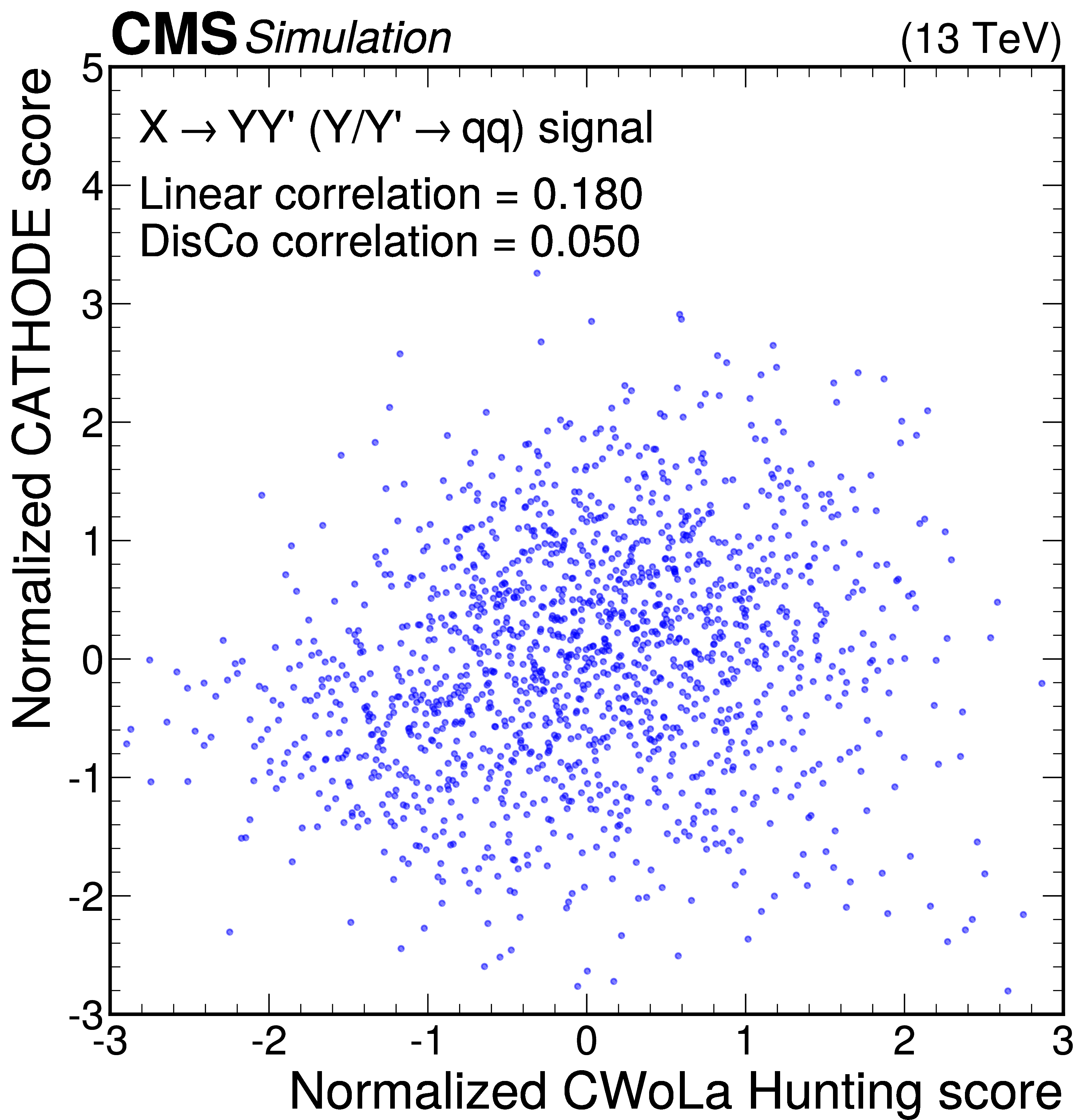
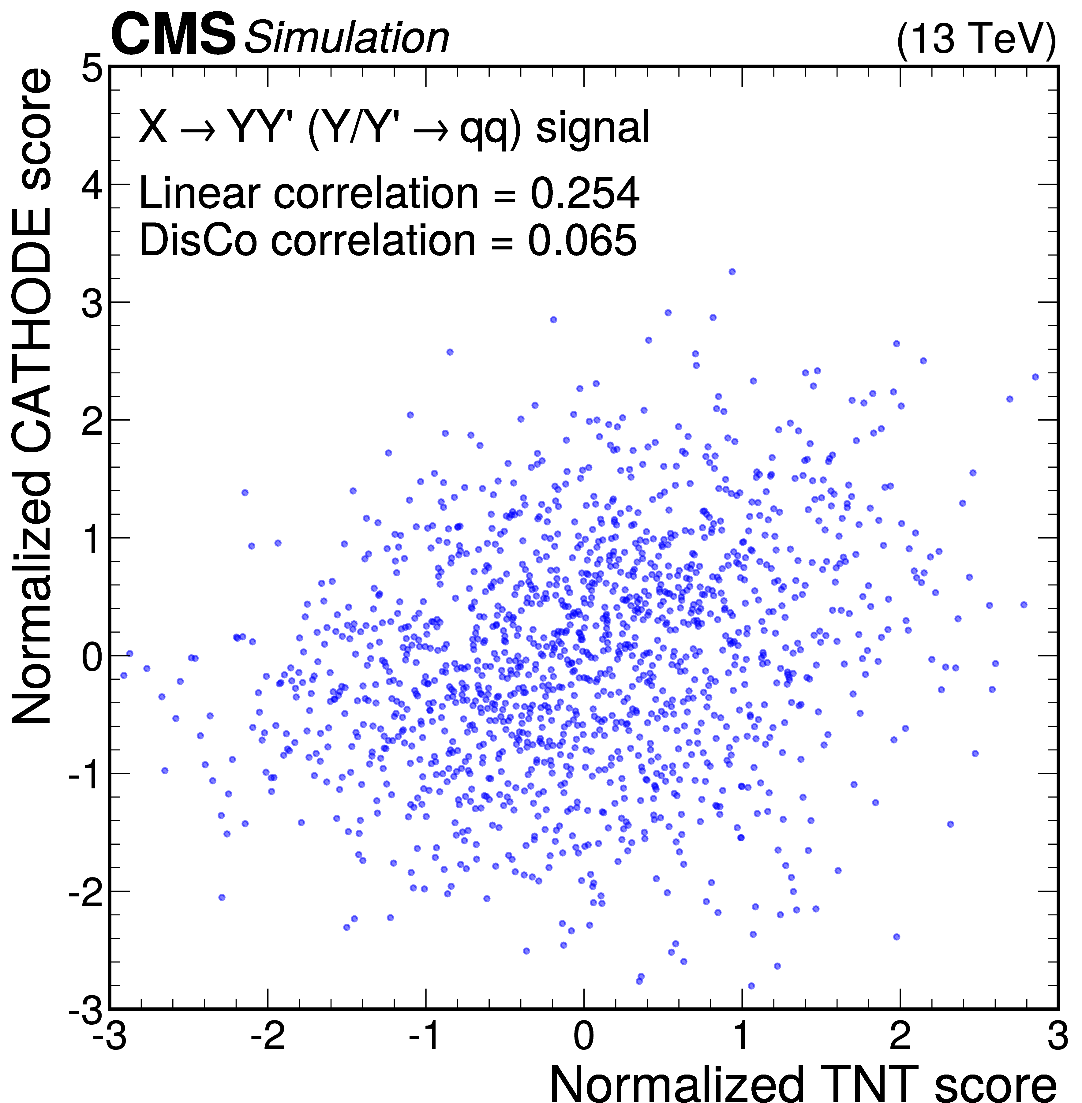
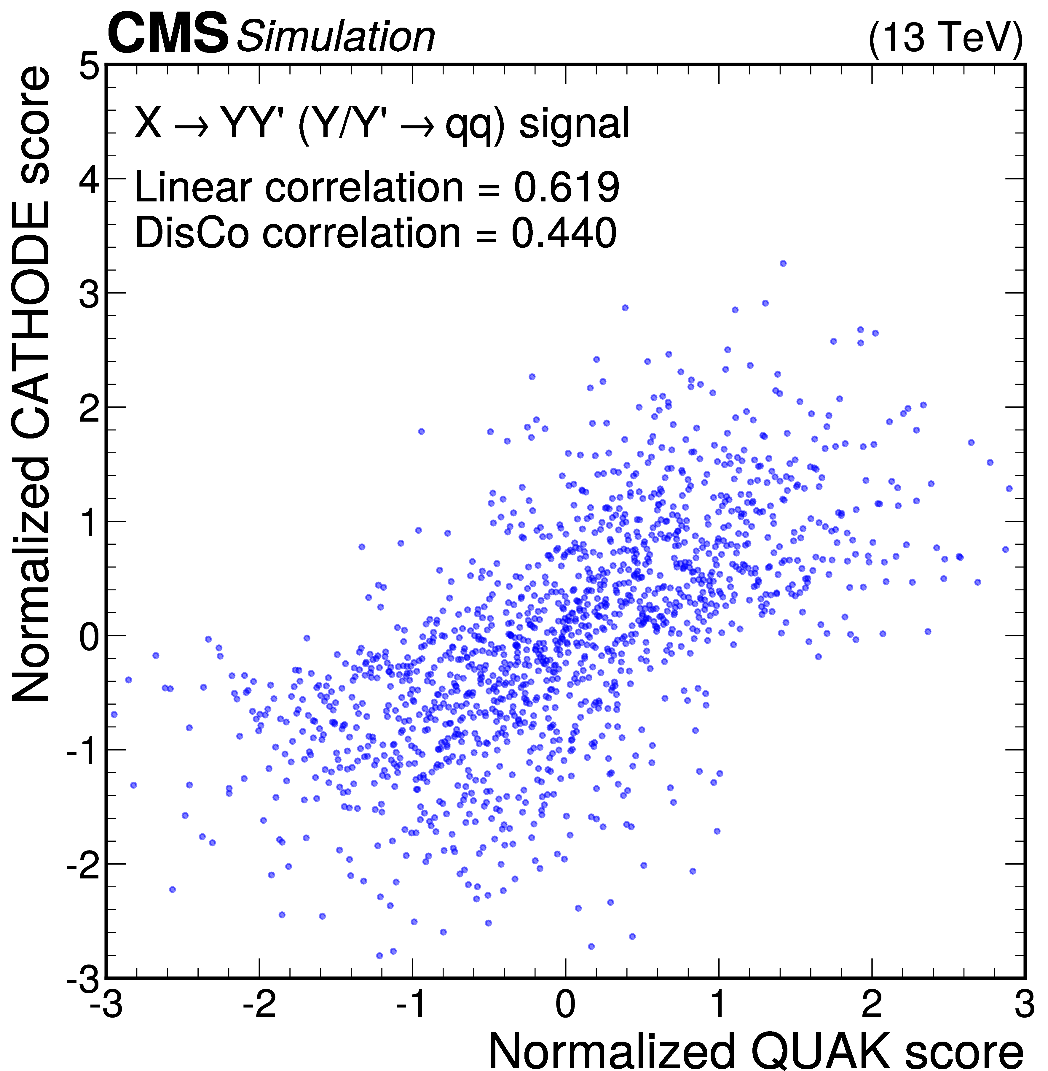
Figure 12:
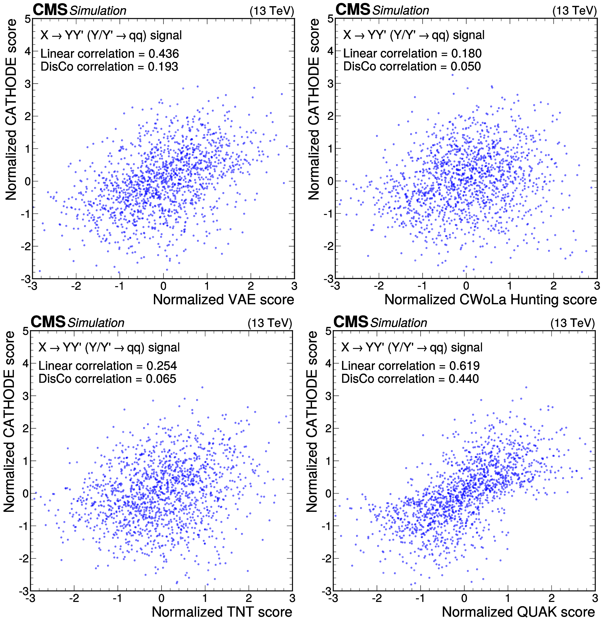
Anomaly score correlations of different methods on the $ \mathrm{X}\to \mathrm{Y} \mathrm{Y}' \to 4 \mathrm{q} $ signal model. Scores are transformed to follow a normal distribution. The Pearson linear correlation coefficient and distance correlation (DisCo) are listed for each pairing. Details are given in the text. |
png pdf |
Figure 12-a:
Anomaly score correlations of different methods on the $ \mathrm{X}\to \mathrm{Y} \mathrm{Y}' \to 4 \mathrm{q} $ signal model. Scores are transformed to follow a normal distribution. The Pearson linear correlation coefficient and distance correlation (DisCo) are listed for each pairing. Details are given in the text. |
png pdf |
Figure 12-b:
Anomaly score correlations of different methods on the $ \mathrm{X}\to \mathrm{Y} \mathrm{Y}' \to 4 \mathrm{q} $ signal model. Scores are transformed to follow a normal distribution. The Pearson linear correlation coefficient and distance correlation (DisCo) are listed for each pairing. Details are given in the text. |
png pdf |
Figure 12-c:
Anomaly score correlations of different methods on the $ \mathrm{X}\to \mathrm{Y} \mathrm{Y}' \to 4 \mathrm{q} $ signal model. Scores are transformed to follow a normal distribution. The Pearson linear correlation coefficient and distance correlation (DisCo) are listed for each pairing. Details are given in the text. |
png pdf |
Figure 12-d:
Anomaly score correlations of different methods on the $ \mathrm{X}\to \mathrm{Y} \mathrm{Y}' \to 4 \mathrm{q} $ signal model. Scores are transformed to follow a normal distribution. The Pearson linear correlation coefficient and distance correlation (DisCo) are listed for each pairing. Details are given in the text. |
png pdf |
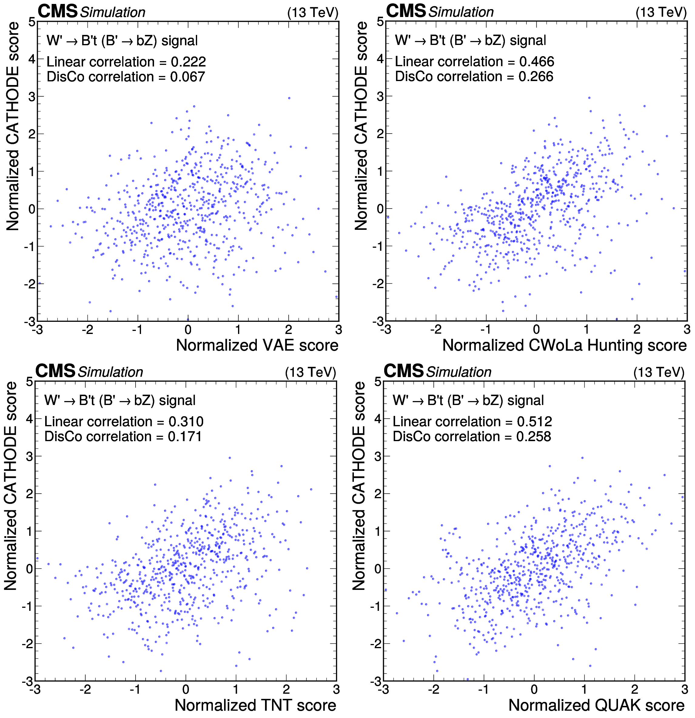
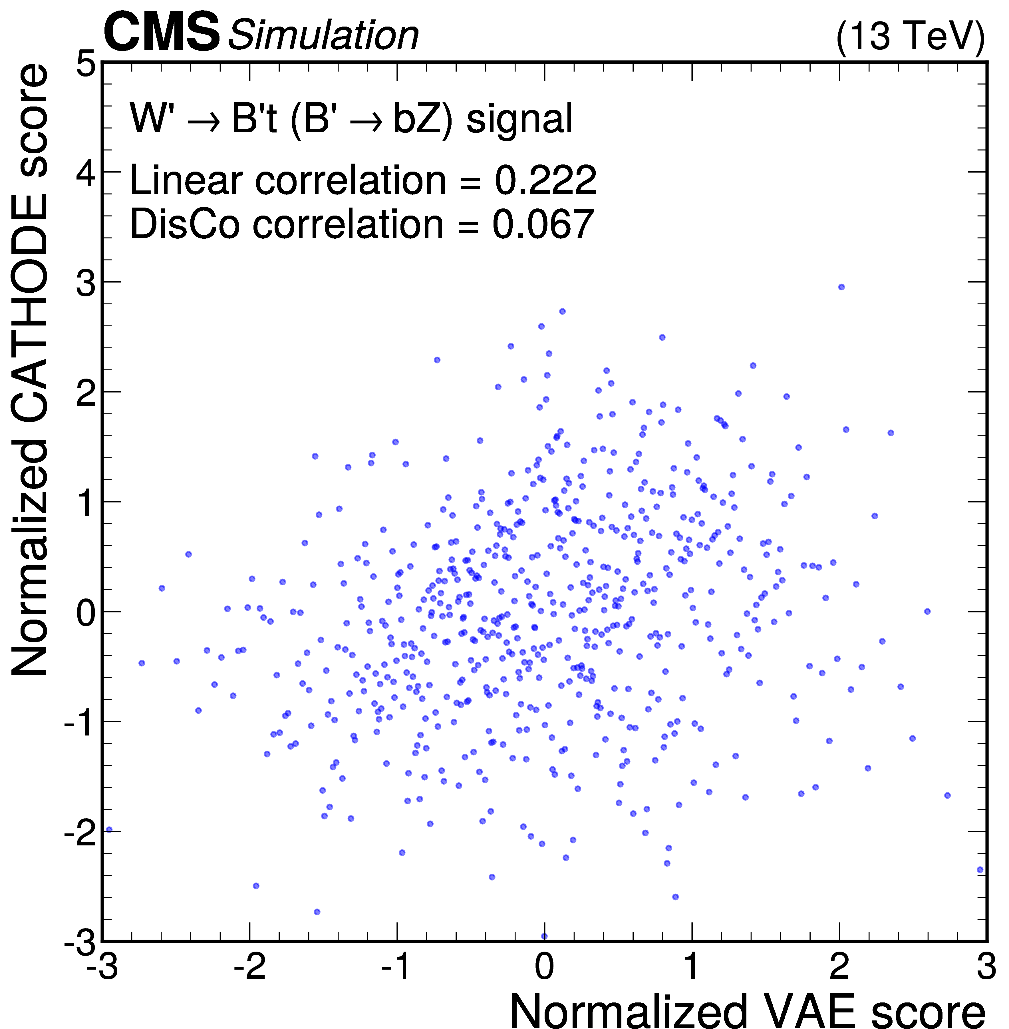
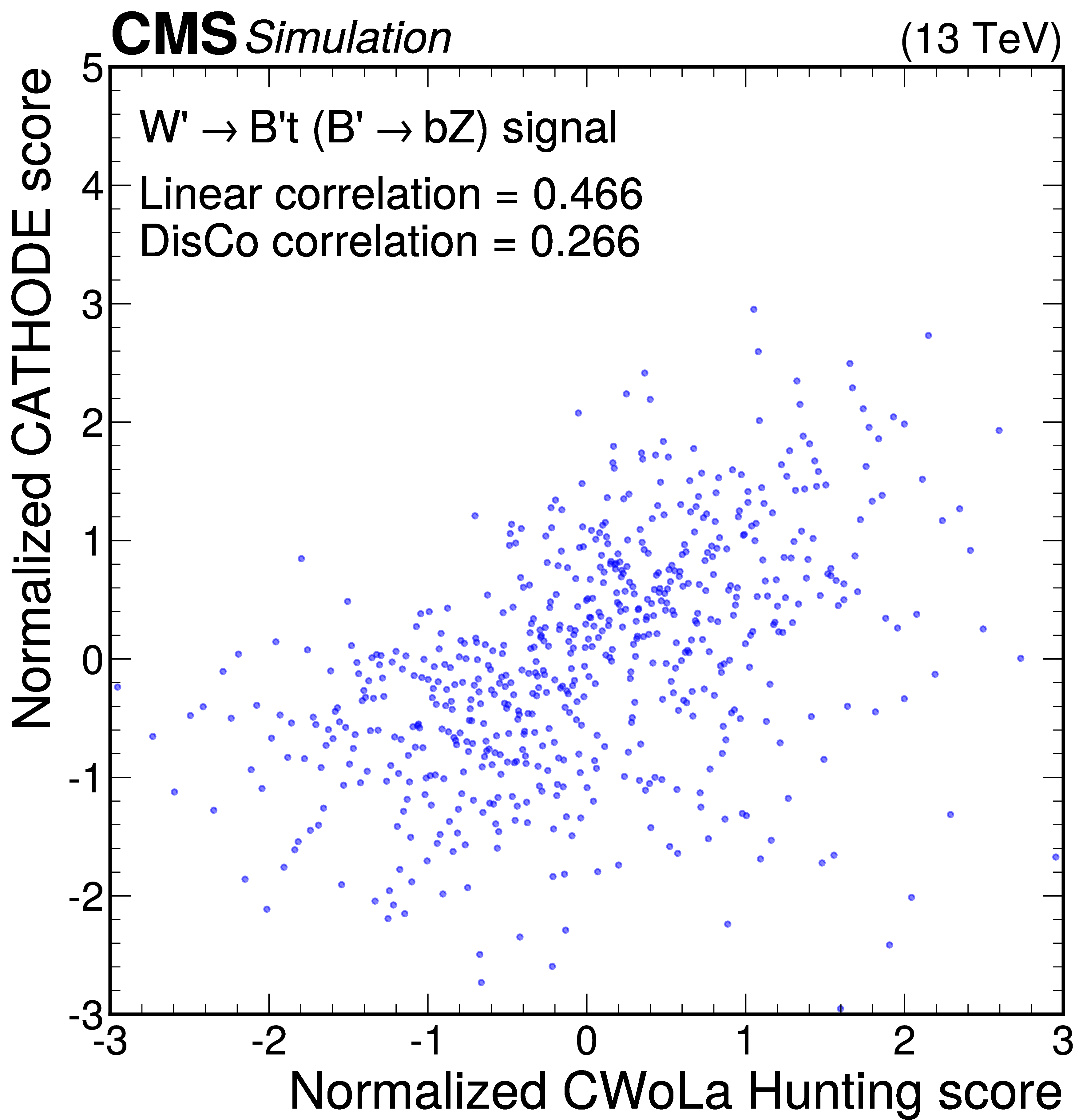
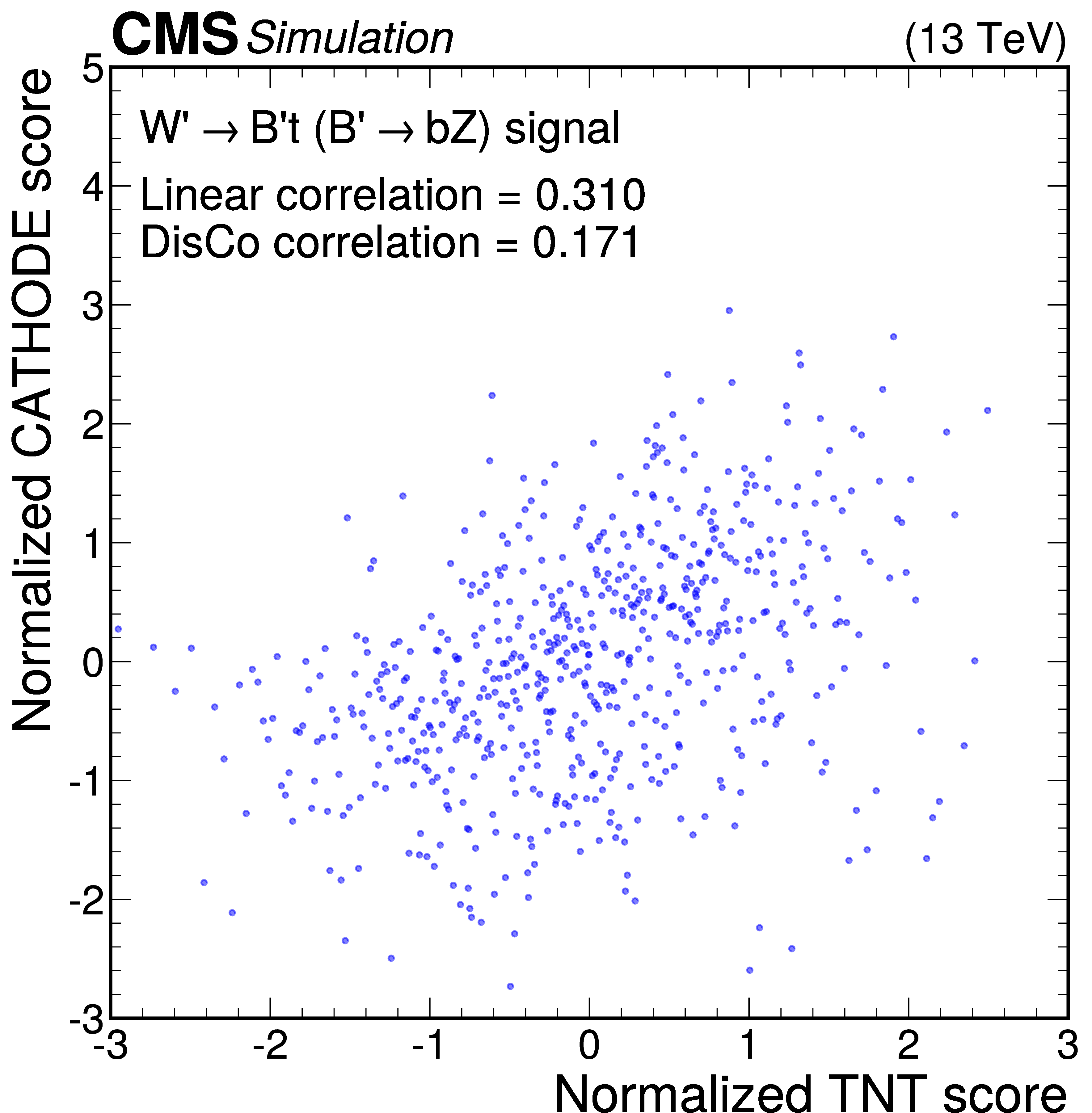
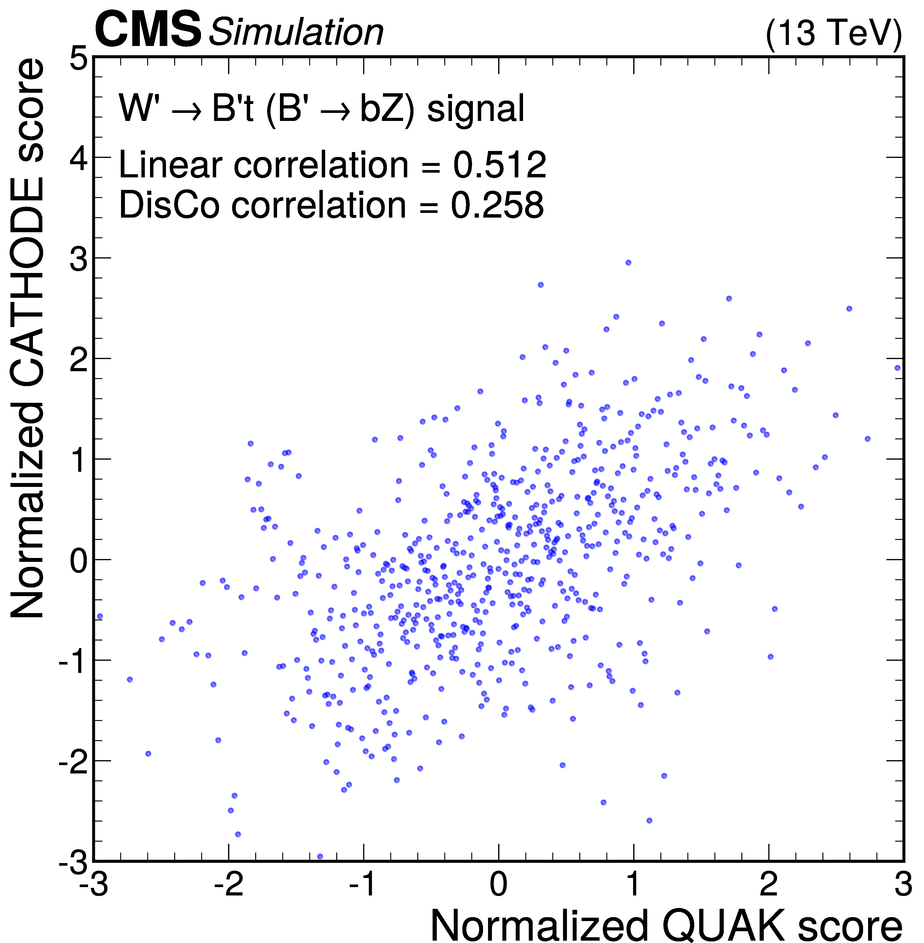
Figure 13:
Anomaly score correlations of different methods on the $ \mathrm{W^{'}} \to \mathrm{B}' \mathrm{t} \to \mathrm{b} \mathrm{Z} \mathrm{t} $ signal model. Scores are transformed to follow a normal distribution. The Pearson linear correlation coefficient and distance correlation (DisCo) are listed for each pairing. Details are given in the text. |
png pdf |
Figure 13-a:
Anomaly score correlations of different methods on the $ \mathrm{W^{'}} \to \mathrm{B}' \mathrm{t} \to \mathrm{b} \mathrm{Z} \mathrm{t} $ signal model. Scores are transformed to follow a normal distribution. The Pearson linear correlation coefficient and distance correlation (DisCo) are listed for each pairing. Details are given in the text. |
png pdf |
Figure 13-b:
Anomaly score correlations of different methods on the $ \mathrm{W^{'}} \to \mathrm{B}' \mathrm{t} \to \mathrm{b} \mathrm{Z} \mathrm{t} $ signal model. Scores are transformed to follow a normal distribution. The Pearson linear correlation coefficient and distance correlation (DisCo) are listed for each pairing. Details are given in the text. |
png pdf |
Figure 13-c:
Anomaly score correlations of different methods on the $ \mathrm{W^{'}} \to \mathrm{B}' \mathrm{t} \to \mathrm{b} \mathrm{Z} \mathrm{t} $ signal model. Scores are transformed to follow a normal distribution. The Pearson linear correlation coefficient and distance correlation (DisCo) are listed for each pairing. Details are given in the text. |
png pdf |
Figure 13-d:
Anomaly score correlations of different methods on the $ \mathrm{W^{'}} \to \mathrm{B}' \mathrm{t} \to \mathrm{b} \mathrm{Z} \mathrm{t} $ signal model. Scores are transformed to follow a normal distribution. The Pearson linear correlation coefficient and distance correlation (DisCo) are listed for each pairing. Details are given in the text. |
png pdf |
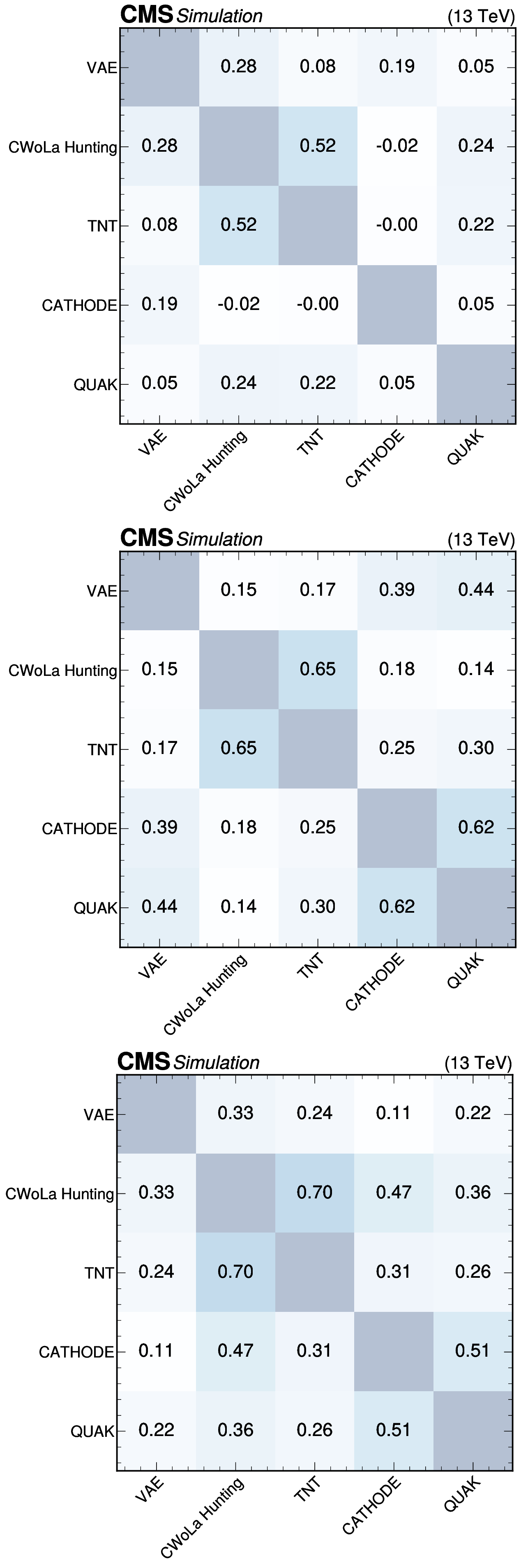
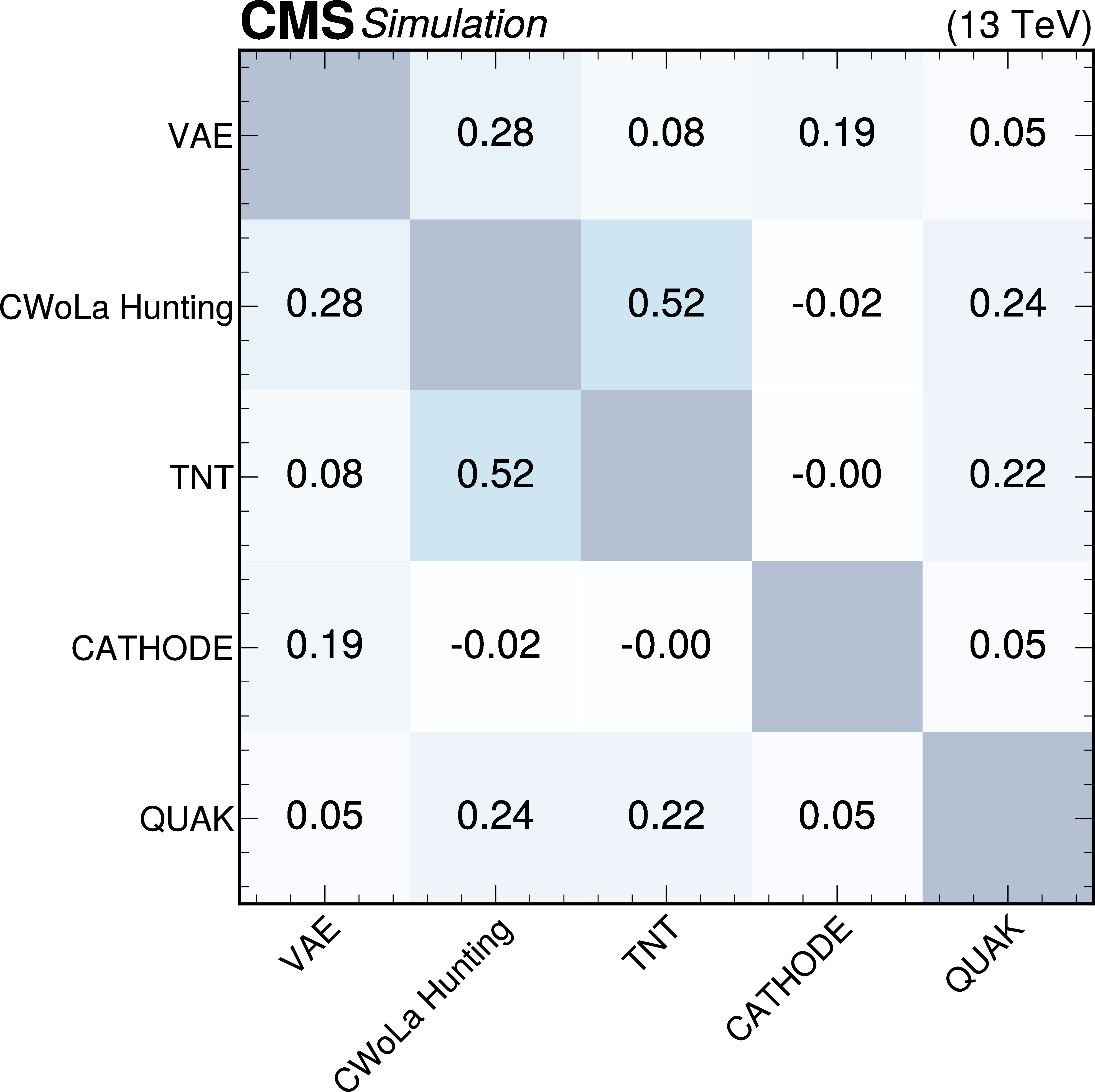
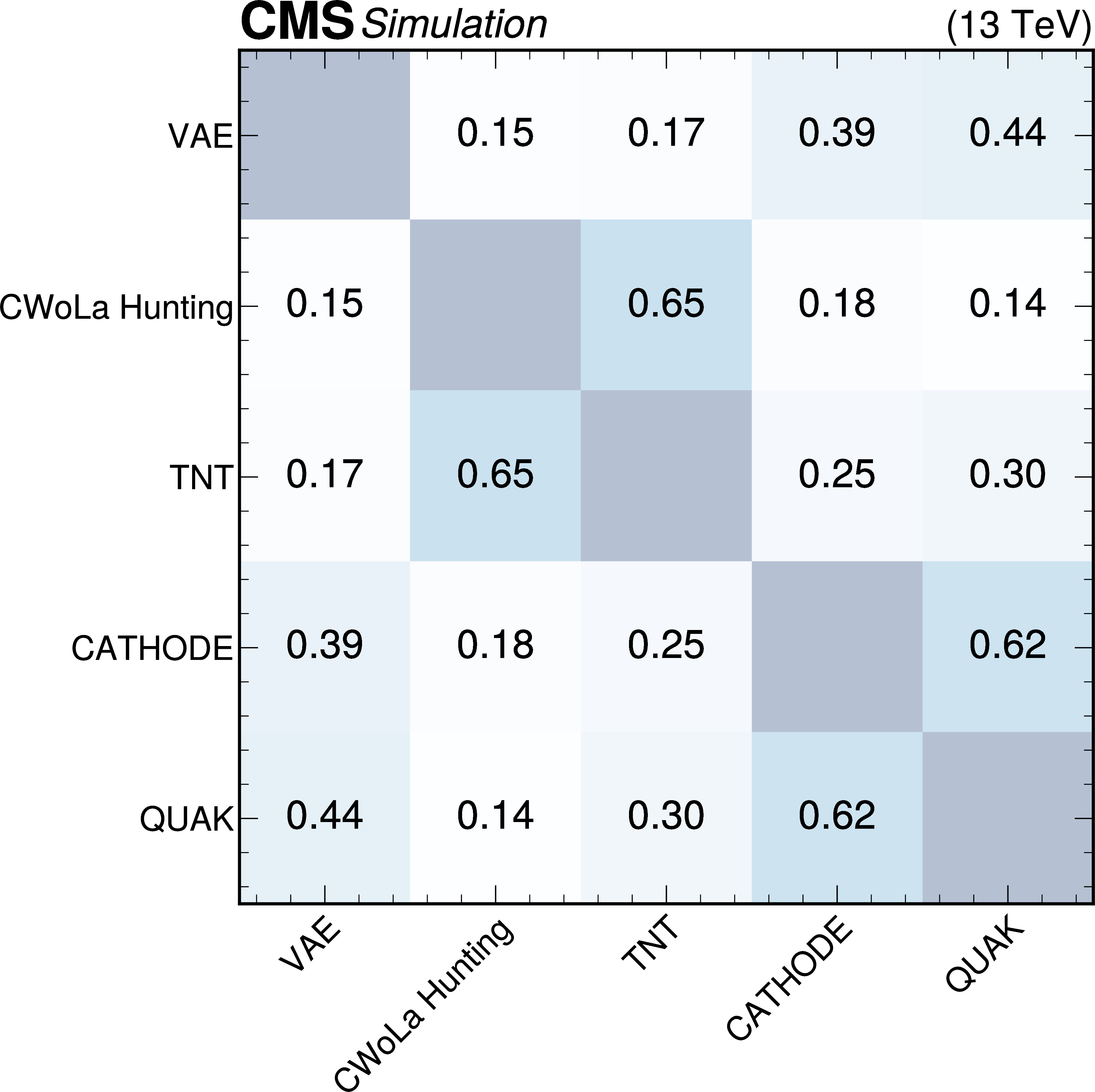
Figure 14:
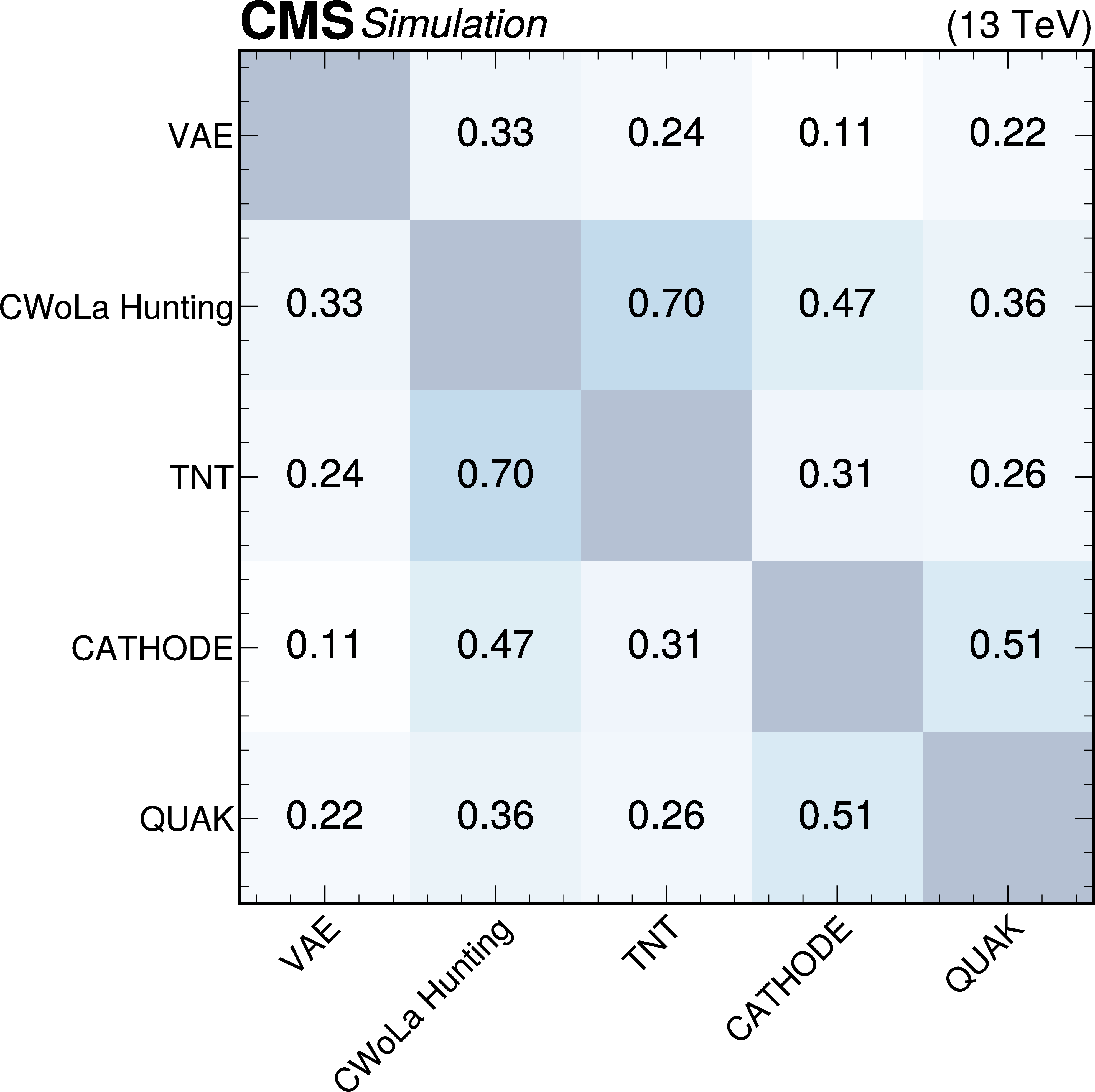
Summary plots showing the Pearson correlation coefficient for each pair of anomaly detection algorithms as evaluated on events from the SM backgrounds (upper), $ \mathrm{X}\to \mathrm{Y} \mathrm{Y}' \to 4 \mathrm{q} $ signal (lower left), and $ \mathrm{W^{'}} \to \mathrm{B}' \mathrm{t} \to \mathrm{b} \mathrm{Z} \mathrm{t} $ signal (lower right). In many cases, the correlations are weak, indicating complementarity between the different approaches. |
png pdf |
Figure 14-a:
Summary plots showing the Pearson correlation coefficient for each pair of anomaly detection algorithms as evaluated on events from the SM backgrounds (upper), $ \mathrm{X}\to \mathrm{Y} \mathrm{Y}' \to 4 \mathrm{q} $ signal (lower left), and $ \mathrm{W^{'}} \to \mathrm{B}' \mathrm{t} \to \mathrm{b} \mathrm{Z} \mathrm{t} $ signal (lower right). In many cases, the correlations are weak, indicating complementarity between the different approaches. |
png pdf |
Figure 14-b:
Summary plots showing the Pearson correlation coefficient for each pair of anomaly detection algorithms as evaluated on events from the SM backgrounds (upper), $ \mathrm{X}\to \mathrm{Y} \mathrm{Y}' \to 4 \mathrm{q} $ signal (lower left), and $ \mathrm{W^{'}} \to \mathrm{B}' \mathrm{t} \to \mathrm{b} \mathrm{Z} \mathrm{t} $ signal (lower right). In many cases, the correlations are weak, indicating complementarity between the different approaches. |
png pdf |
Figure 14-c:
Summary plots showing the Pearson correlation coefficient for each pair of anomaly detection algorithms as evaluated on events from the SM backgrounds (upper), $ \mathrm{X}\to \mathrm{Y} \mathrm{Y}' \to 4 \mathrm{q} $ signal (lower left), and $ \mathrm{W^{'}} \to \mathrm{B}' \mathrm{t} \to \mathrm{b} \mathrm{Z} \mathrm{t} $ signal (lower right). In many cases, the correlations are weak, indicating complementarity between the different approaches. |

png pdf |
Figure 15:
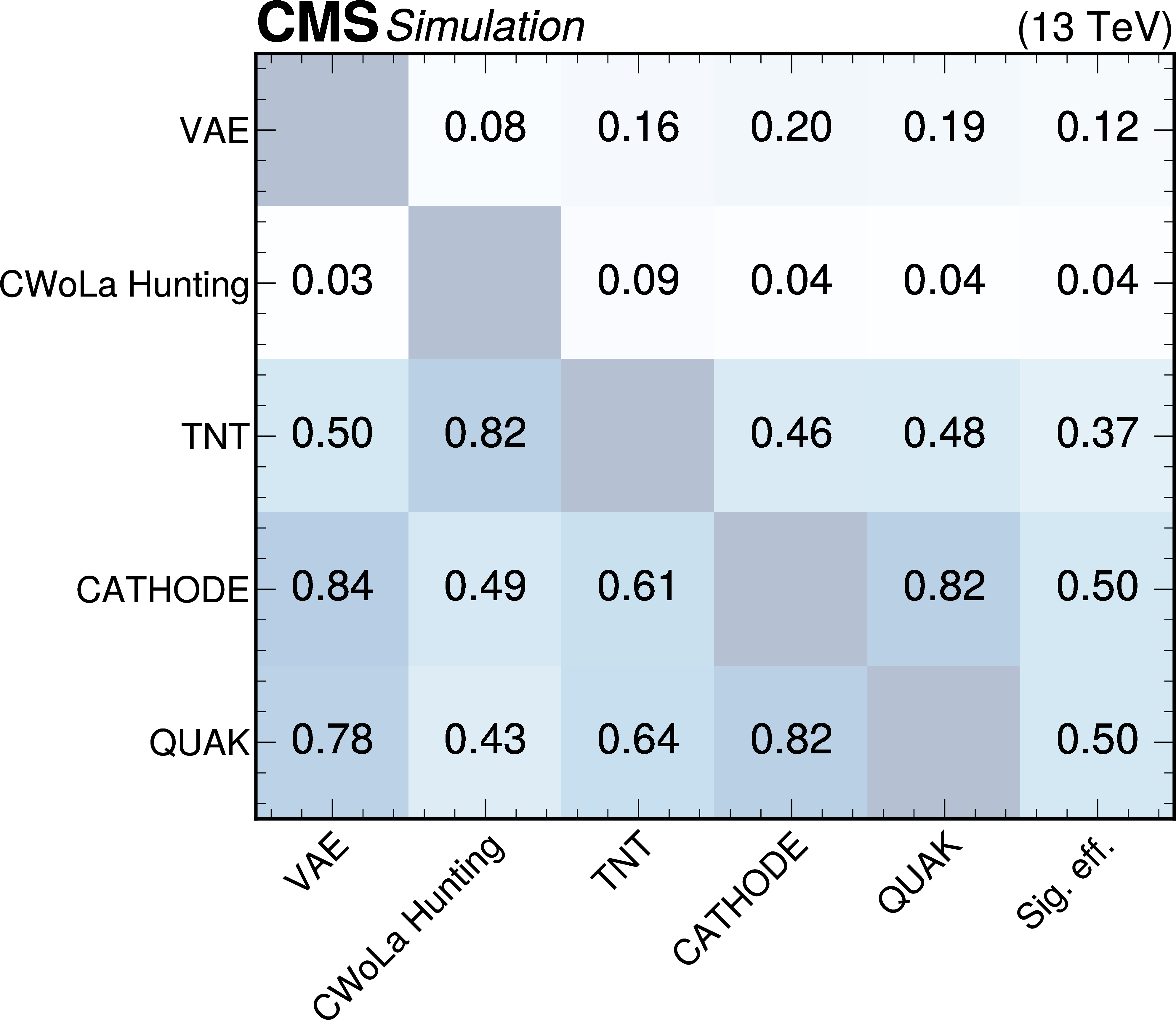
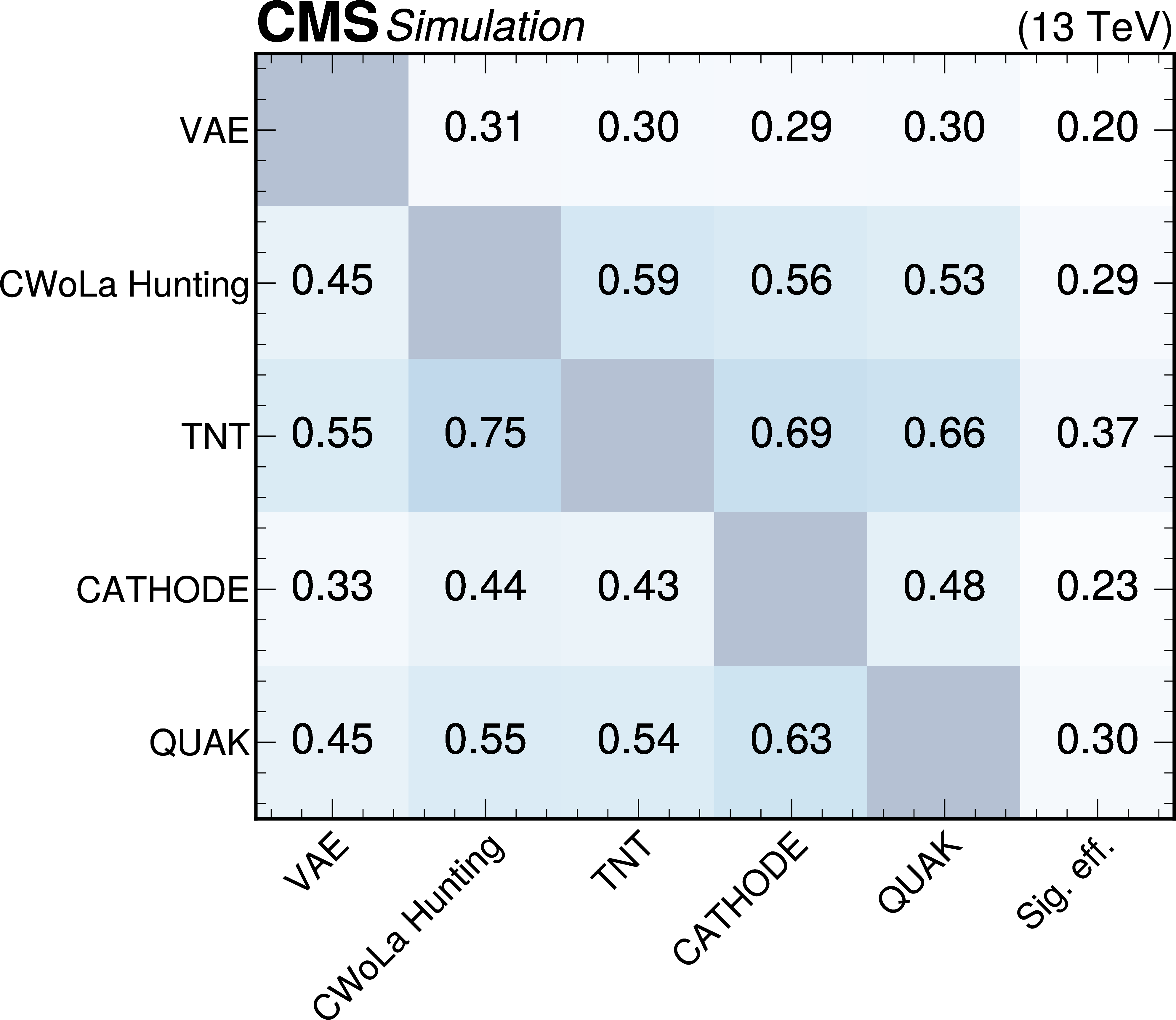
Overlap between the events selected using the anomaly detection methods, for the $ \mathrm{X}\to \mathrm{Y} \mathrm{Y}' \to 4 \mathrm{q} $ (left) and $ \mathrm{W^{'}} \to \mathrm{B}' \mathrm{t} \to \mathrm{b} \mathrm{Z} \mathrm{t} $ (right) signals with a false positive rate of 1%. Each cell corresponds to the fraction of the events selected by the method shown on the horizontal axis that are also selected by the method on the vertical axis. The last column denotes the overall efficiency of selecting signal events for each method. For instance, the CATHODE method selects 50% of all $ \mathrm{X}\to \mathrm{Y} \mathrm{Y}' \to 4 \mathrm{q} $ events. Of those events selected by CATHODE, 46% are also selected by TNT, but only 4% are found by CWoLa Hunting. |
png pdf |
Figure 15-a:
Overlap between the events selected using the anomaly detection methods, for the $ \mathrm{X}\to \mathrm{Y} \mathrm{Y}' \to 4 \mathrm{q} $ (left) and $ \mathrm{W^{'}} \to \mathrm{B}' \mathrm{t} \to \mathrm{b} \mathrm{Z} \mathrm{t} $ (right) signals with a false positive rate of 1%. Each cell corresponds to the fraction of the events selected by the method shown on the horizontal axis that are also selected by the method on the vertical axis. The last column denotes the overall efficiency of selecting signal events for each method. For instance, the CATHODE method selects 50% of all $ \mathrm{X}\to \mathrm{Y} \mathrm{Y}' \to 4 \mathrm{q} $ events. Of those events selected by CATHODE, 46% are also selected by TNT, but only 4% are found by CWoLa Hunting. |
png pdf |
Figure 15-b:
Overlap between the events selected using the anomaly detection methods, for the $ \mathrm{X}\to \mathrm{Y} \mathrm{Y}' \to 4 \mathrm{q} $ (left) and $ \mathrm{W^{'}} \to \mathrm{B}' \mathrm{t} \to \mathrm{b} \mathrm{Z} \mathrm{t} $ (right) signals with a false positive rate of 1%. Each cell corresponds to the fraction of the events selected by the method shown on the horizontal axis that are also selected by the method on the vertical axis. The last column denotes the overall efficiency of selecting signal events for each method. For instance, the CATHODE method selects 50% of all $ \mathrm{X}\to \mathrm{Y} \mathrm{Y}' \to 4 \mathrm{q} $ events. Of those events selected by CATHODE, 46% are also selected by TNT, but only 4% are found by CWoLa Hunting. |
png pdf |
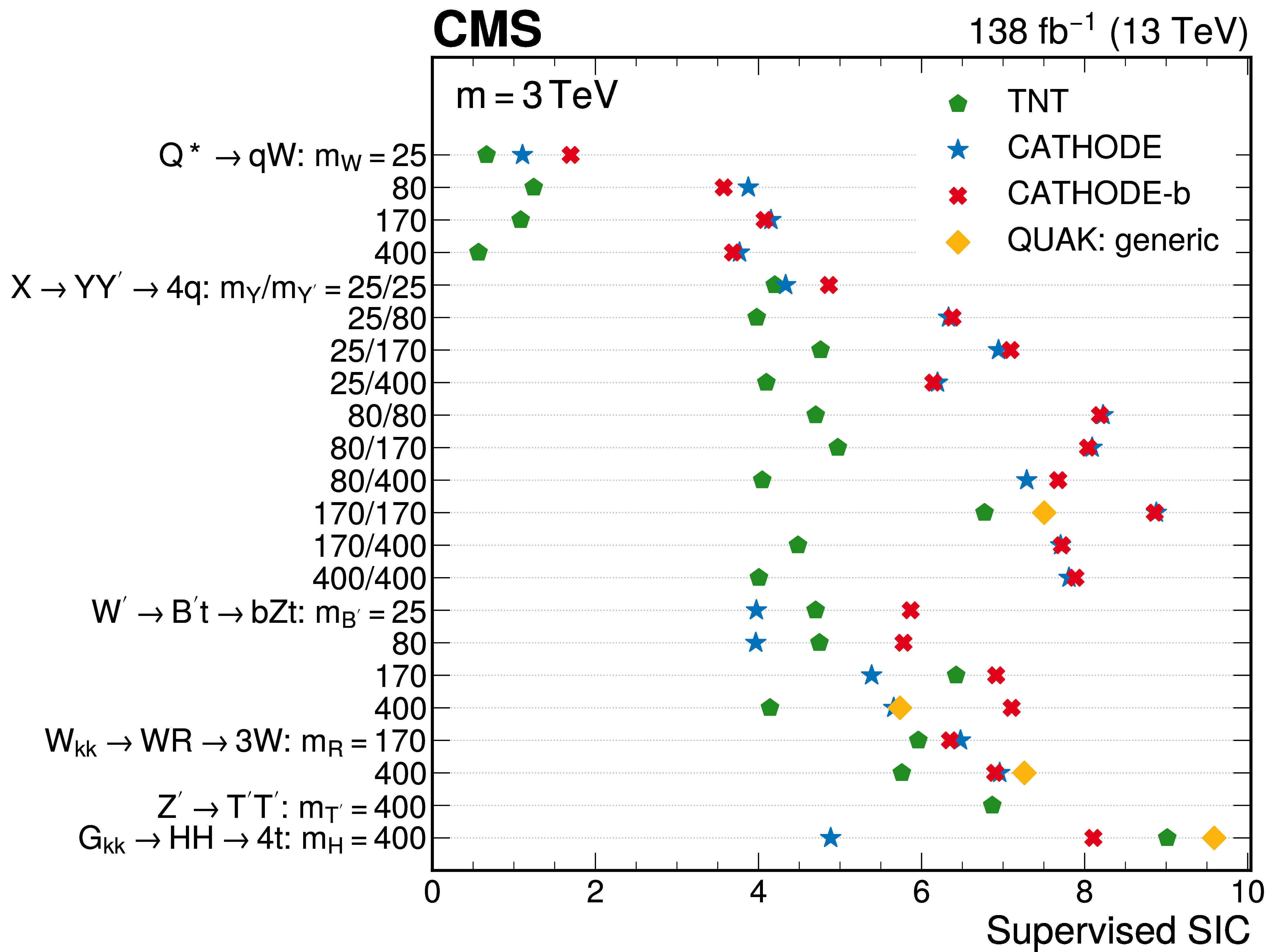
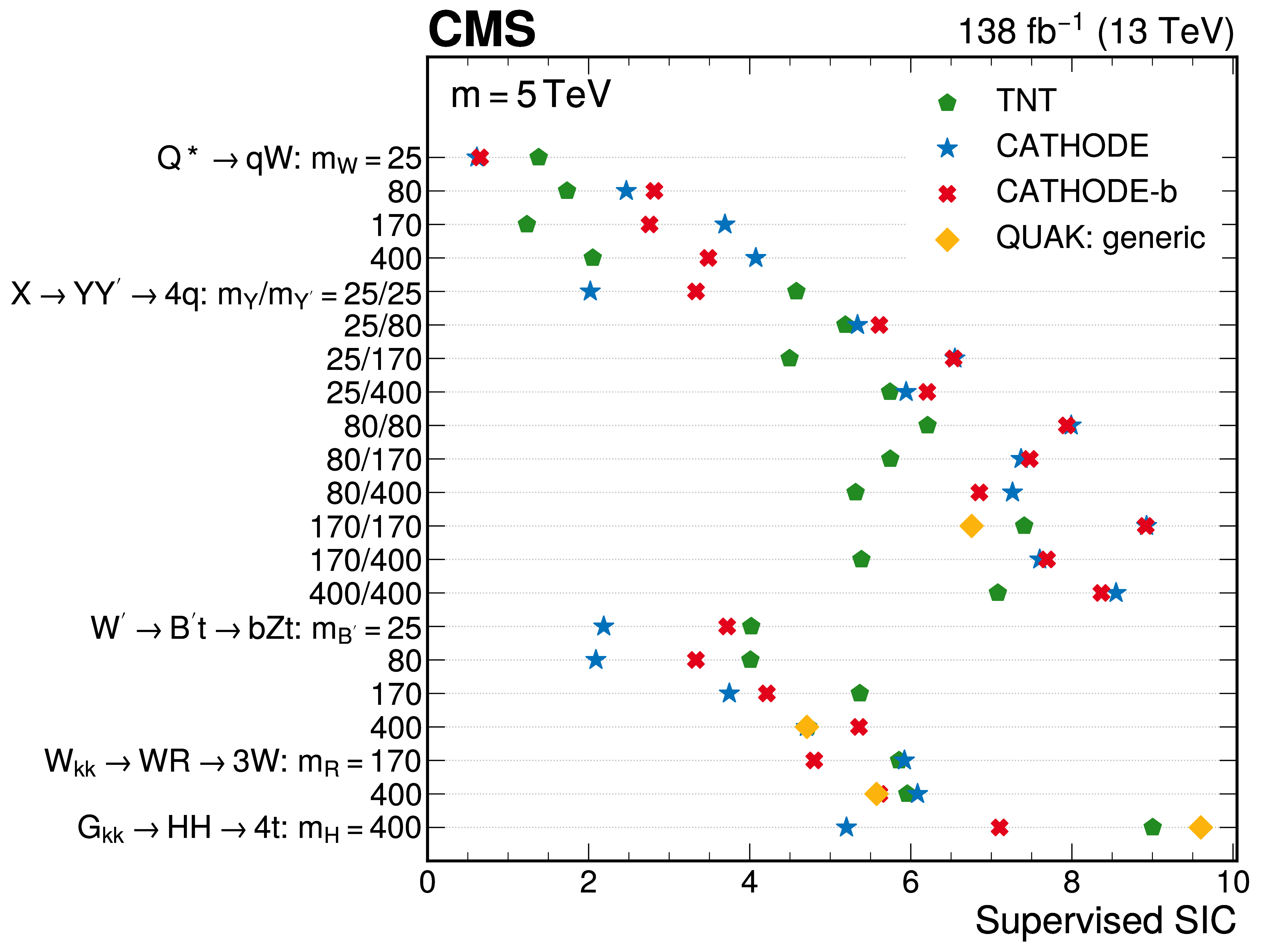
Figure 16:
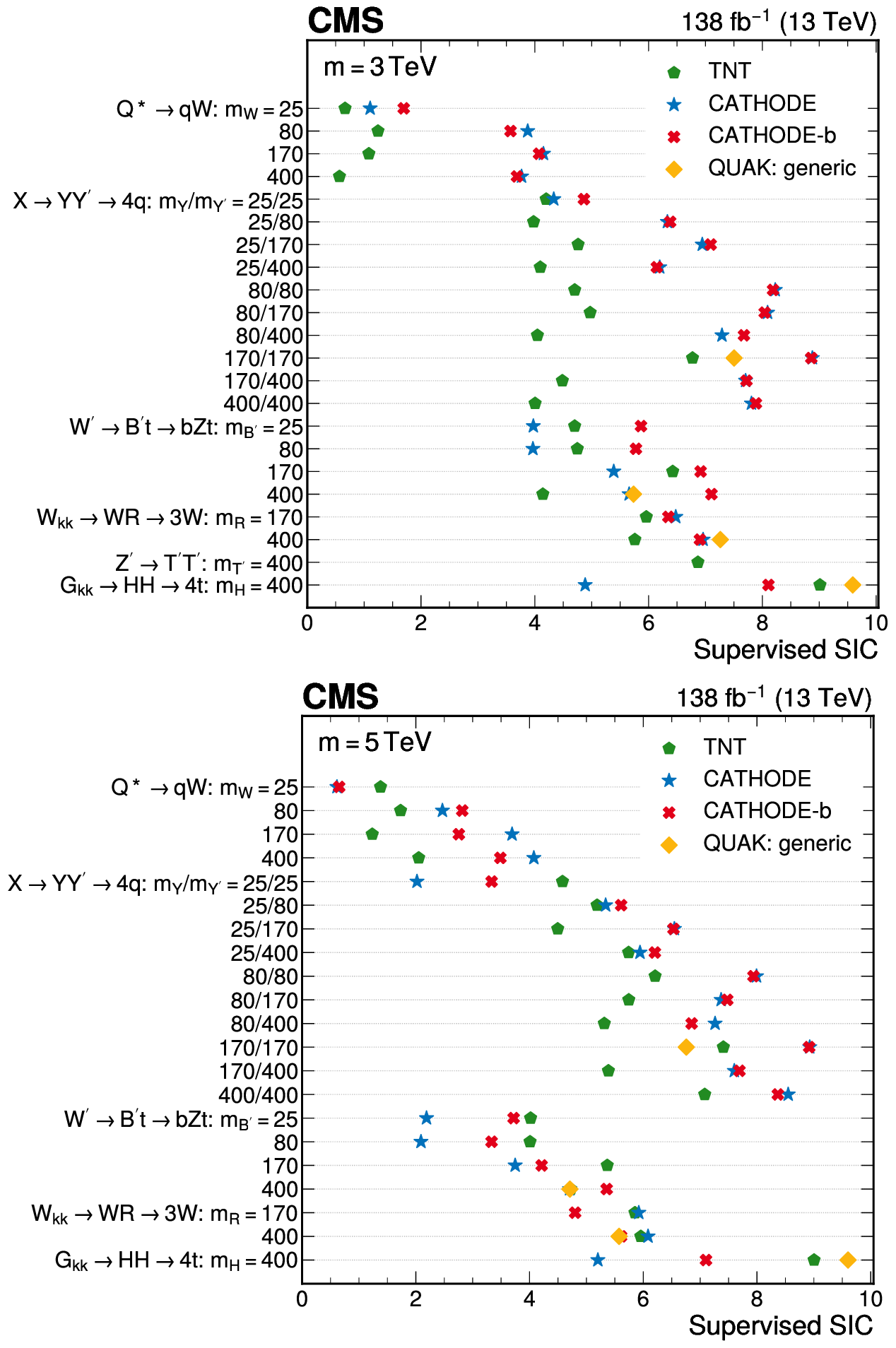
Significance improvement obtained from supervised classifiers trained using the same inputs as the anomaly detection methods. The left (right) panel shows the 3 (5 TeV) mass point for all signal models. The masses of intermediate decay particles are listed in GeVns. The QUAK method was not tested on all models. |
png pdf |
Figure 16-a:
Significance improvement obtained from supervised classifiers trained using the same inputs as the anomaly detection methods. The left (right) panel shows the 3 (5 TeV) mass point for all signal models. The masses of intermediate decay particles are listed in GeVns. The QUAK method was not tested on all models. |
png pdf |
Figure 16-b:
Significance improvement obtained from supervised classifiers trained using the same inputs as the anomaly detection methods. The left (right) panel shows the 3 (5 TeV) mass point for all signal models. The masses of intermediate decay particles are listed in GeVns. The QUAK method was not tested on all models. |
png pdf |
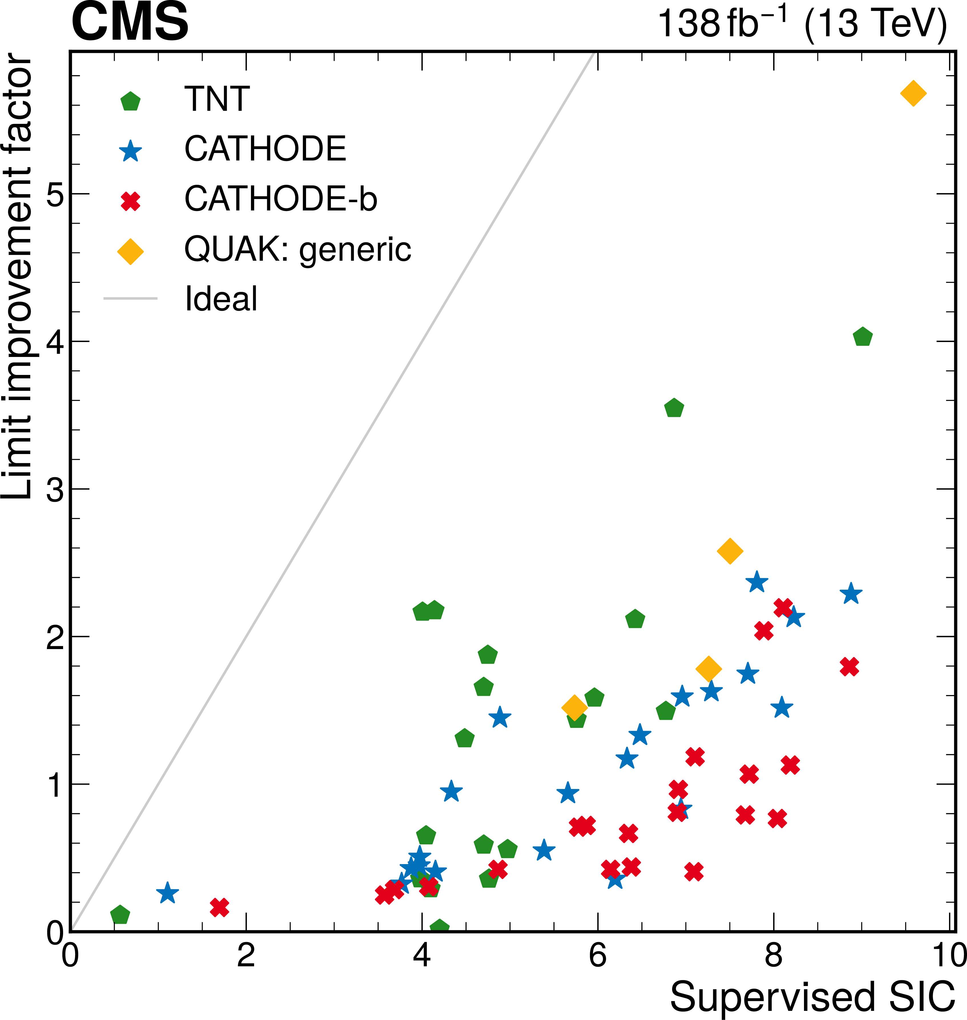
Figure 17:
Comparison of anomaly detection and supervised classification performance. The factors by which the anomaly detection methods improve the upper limits on the signal cross sections are compared to the SIC of classifiers trained with the same inputs. The 3 TeV mass point is shown for all models. |
png pdf |
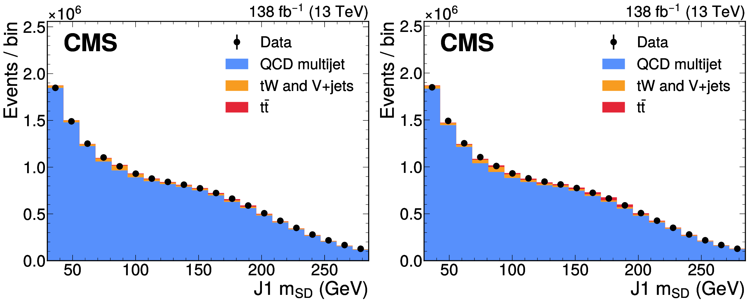
Figure 18:
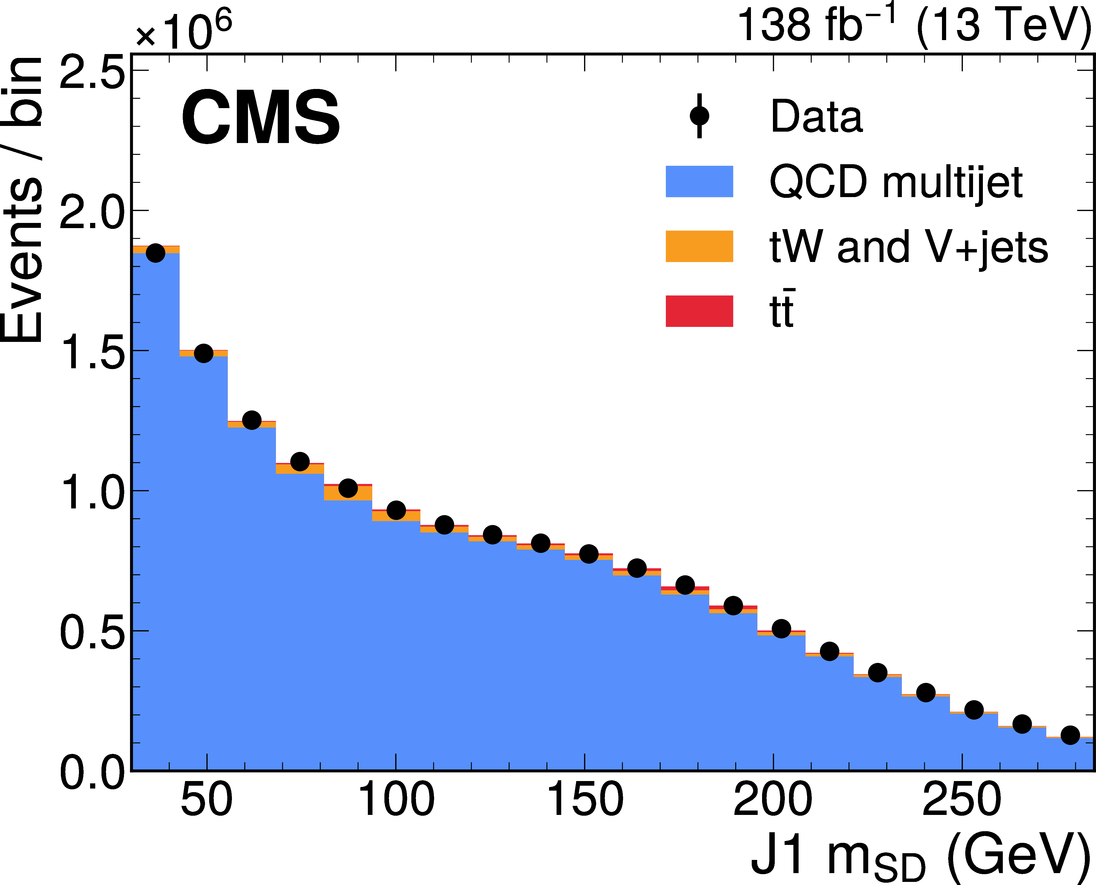
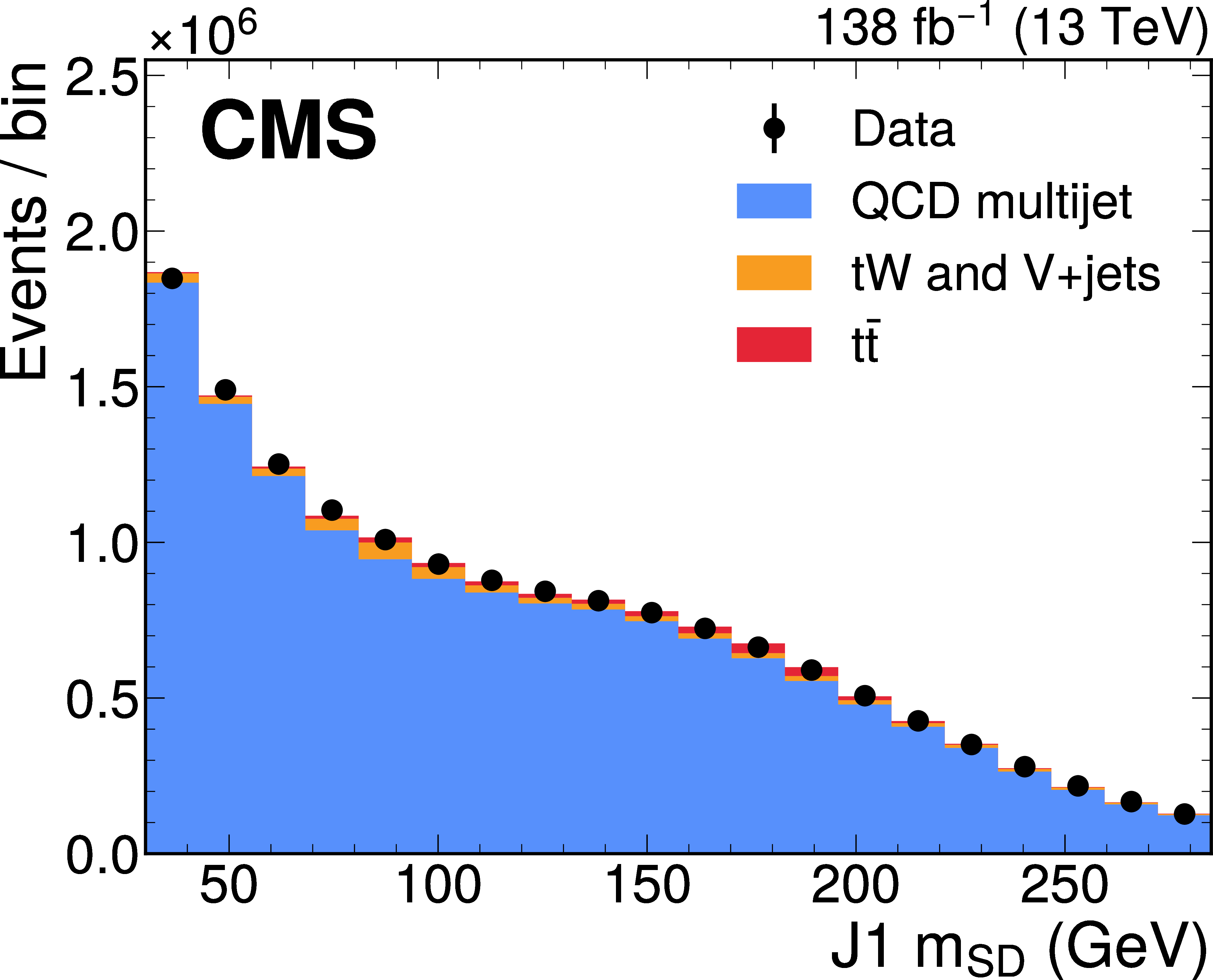
Distribution of the J1 soft-drop mass after the basic (left) and b-tagged (right) preselections. The black dots represent the data and the colored histograms correspond to simulated events. The b tagging preselection increases the relative contribution of $ \mathrm{t} \overline{\mathrm{t}} $ (red) in the sample, but in both cases the sample is dominated by the QCD multijet background (blue). Other background processes are shown in yellow. |
png pdf |
Figure 18-a:
Distribution of the J1 soft-drop mass after the basic (left) and b-tagged (right) preselections. The black dots represent the data and the colored histograms correspond to simulated events. The b tagging preselection increases the relative contribution of $ \mathrm{t} \overline{\mathrm{t}} $ (red) in the sample, but in both cases the sample is dominated by the QCD multijet background (blue). Other background processes are shown in yellow. |
png pdf |
Figure 18-b:
Distribution of the J1 soft-drop mass after the basic (left) and b-tagged (right) preselections. The black dots represent the data and the colored histograms correspond to simulated events. The b tagging preselection increases the relative contribution of $ \mathrm{t} \overline{\mathrm{t}} $ (red) in the sample, but in both cases the sample is dominated by the QCD multijet background (blue). Other background processes are shown in yellow. |
png pdf |
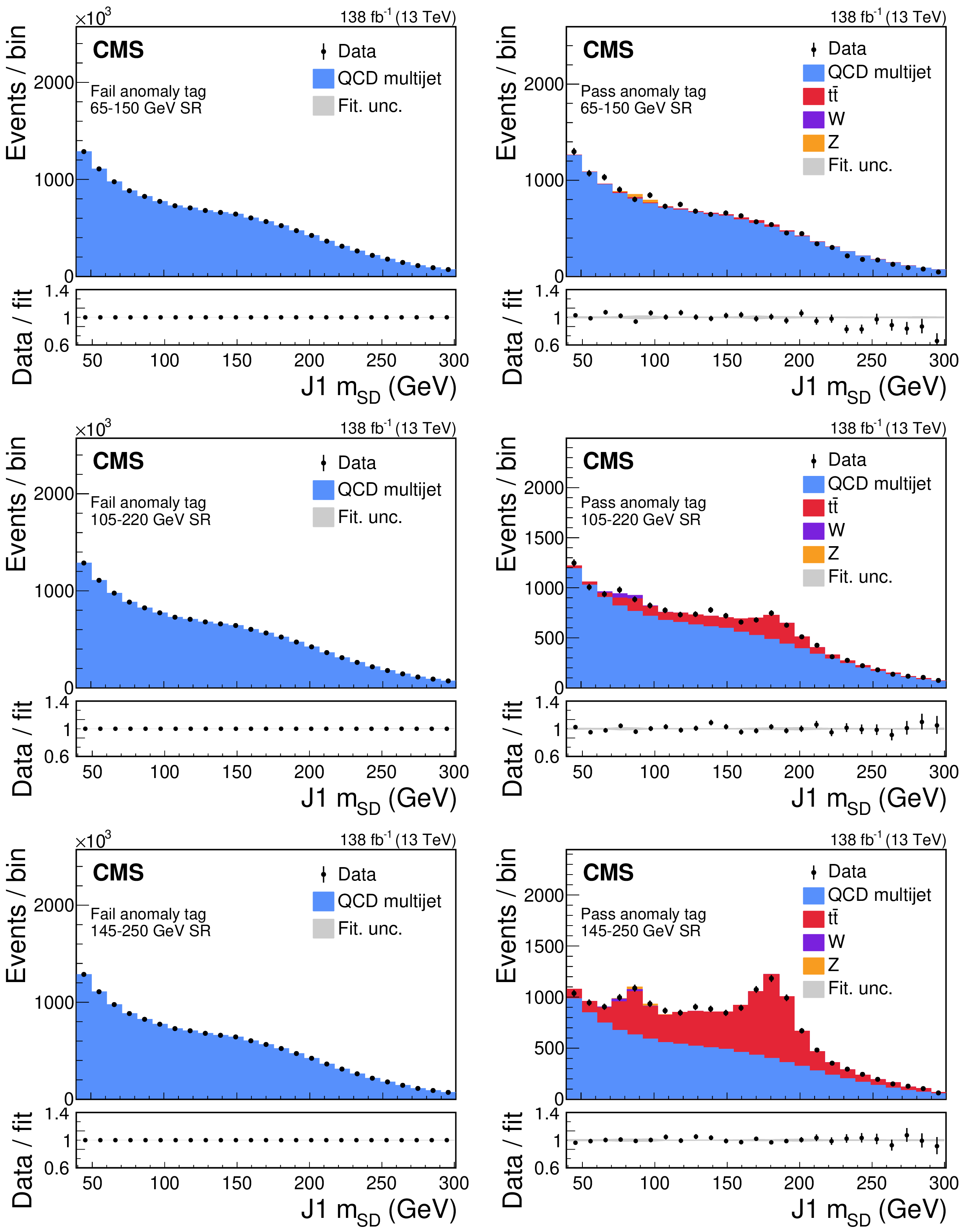
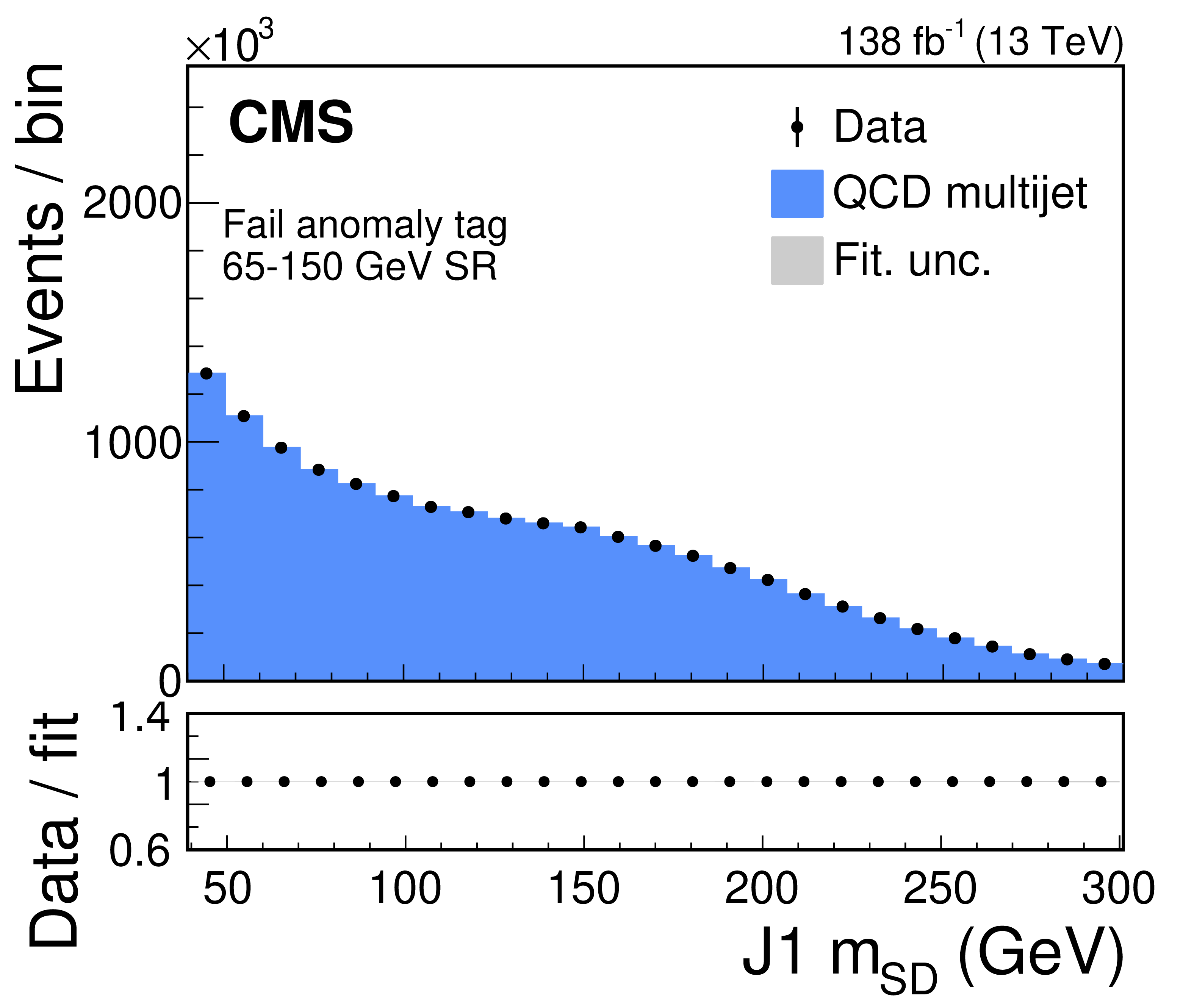
Figure 19:
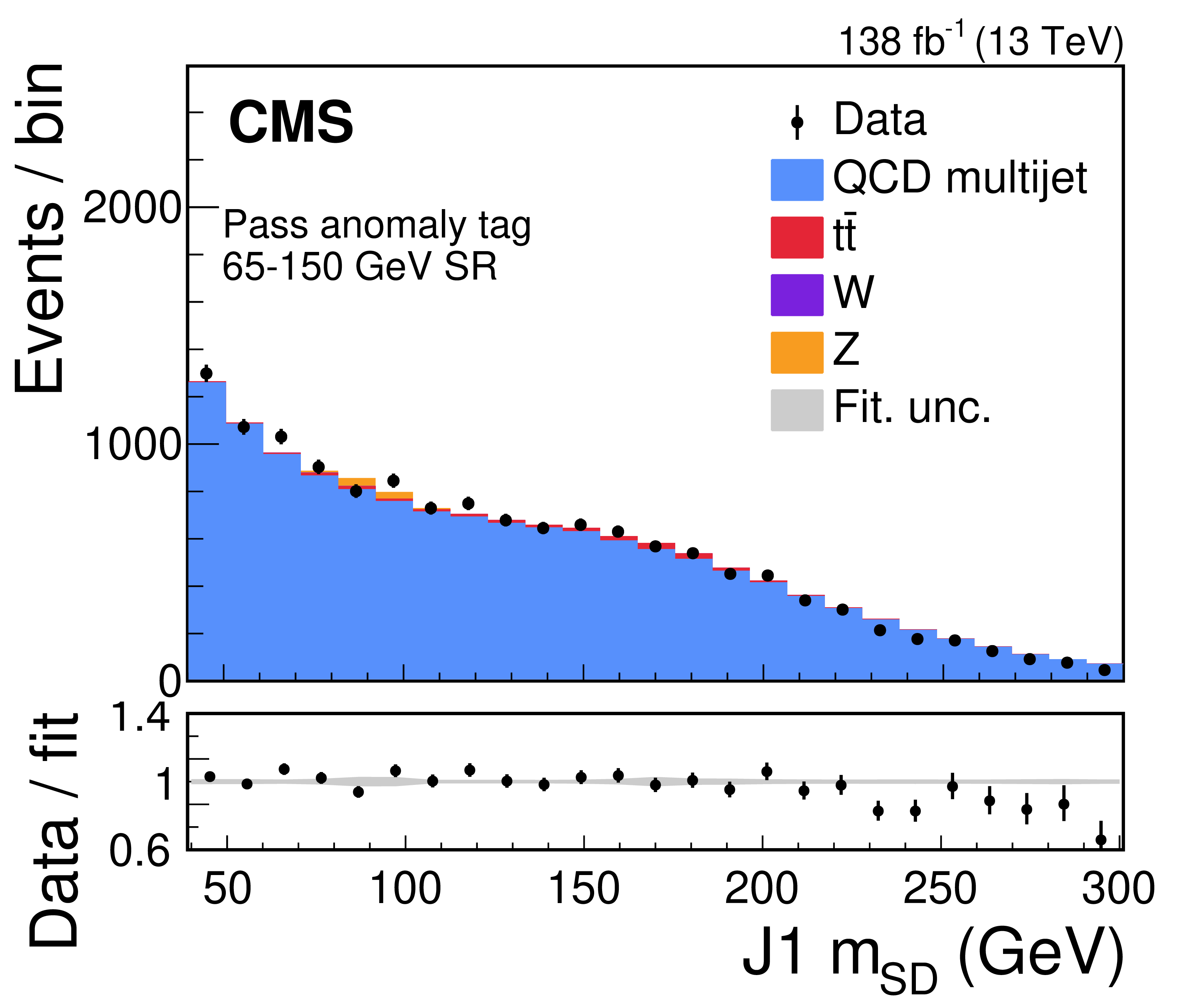
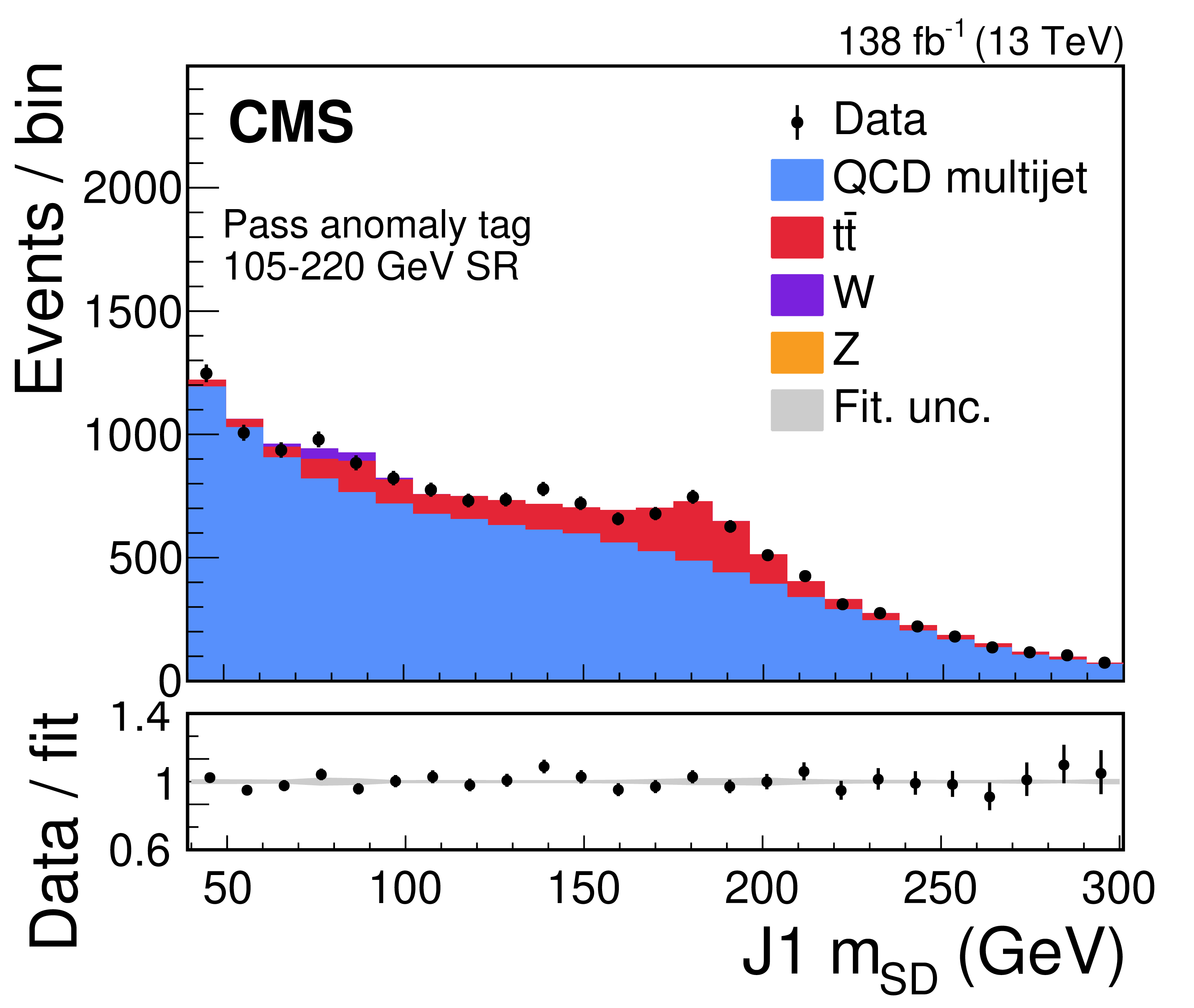
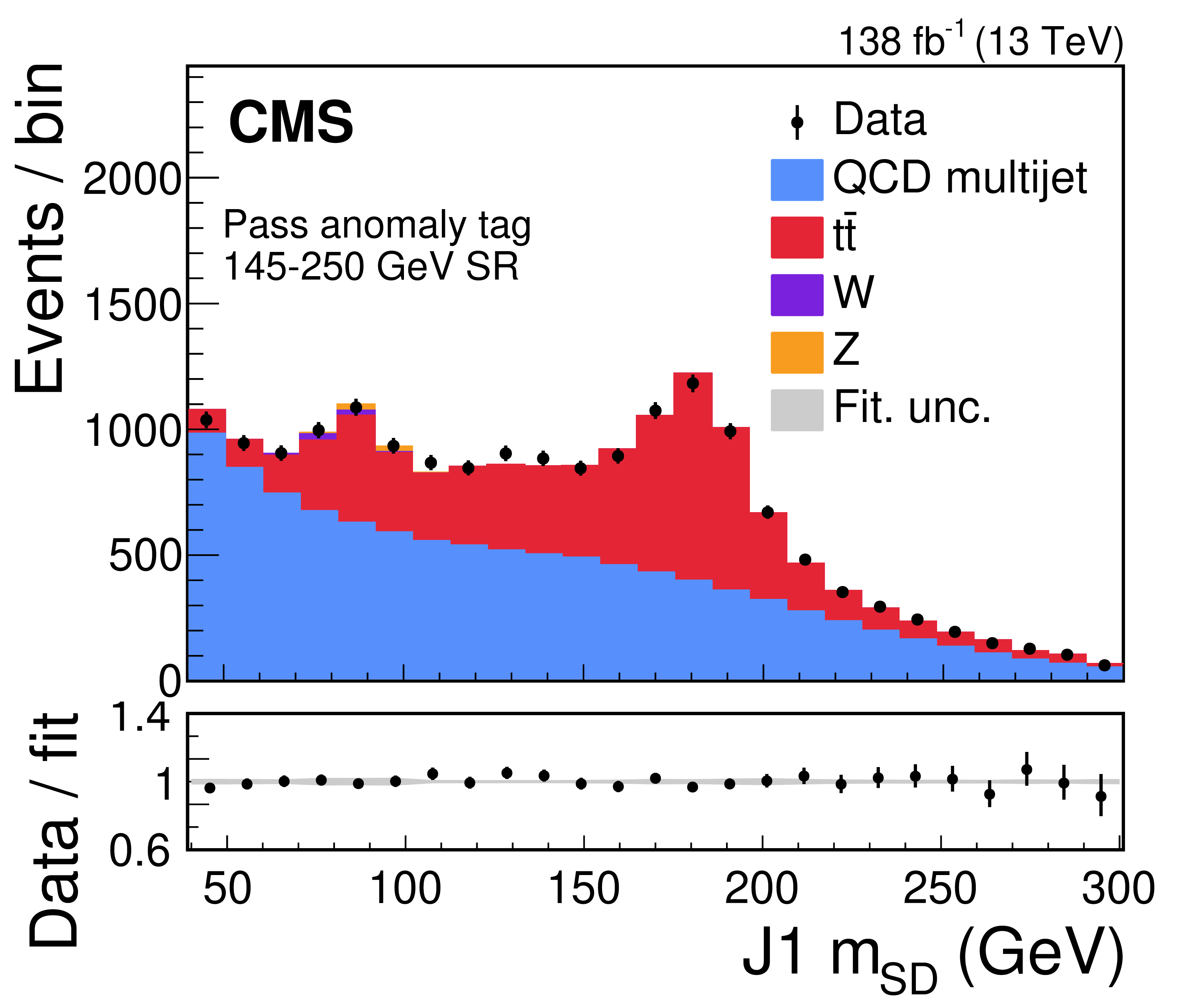
Post-fit plots of the fail (left) and pass (right) regions for the $ \mathrm{t} \overline{\mathrm{t}} $ extraction procedure performed for the 65-150 (upper), 105-220 (middle), and 145-250 GeV (lower) signal windows. Data (black points with error bars) is compared to the fitted estimates of the QCD multijet (blue), Z+jets (orange), W+jets (purple), and $ \mathrm{t} \overline{\mathrm{t}} $ (red) processes. The lower panel shows the ratio between the observed data points and the fitted estimates. The gray shading denotes the systematic uncertainty. The contribution from $ \mathrm{t} \overline{\mathrm{t}} $ is clearly visible in the pass region of the 105-220 and 145-250 GeV signal windows. |
png pdf |
Figure 19-a:
Post-fit plots of the fail (left) and pass (right) regions for the $ \mathrm{t} \overline{\mathrm{t}} $ extraction procedure performed for the 65-150 (upper), 105-220 (middle), and 145-250 GeV (lower) signal windows. Data (black points with error bars) is compared to the fitted estimates of the QCD multijet (blue), Z+jets (orange), W+jets (purple), and $ \mathrm{t} \overline{\mathrm{t}} $ (red) processes. The lower panel shows the ratio between the observed data points and the fitted estimates. The gray shading denotes the systematic uncertainty. The contribution from $ \mathrm{t} \overline{\mathrm{t}} $ is clearly visible in the pass region of the 105-220 and 145-250 GeV signal windows. |
png pdf |
Figure 19-b:
Post-fit plots of the fail (left) and pass (right) regions for the $ \mathrm{t} \overline{\mathrm{t}} $ extraction procedure performed for the 65-150 (upper), 105-220 (middle), and 145-250 GeV (lower) signal windows. Data (black points with error bars) is compared to the fitted estimates of the QCD multijet (blue), Z+jets (orange), W+jets (purple), and $ \mathrm{t} \overline{\mathrm{t}} $ (red) processes. The lower panel shows the ratio between the observed data points and the fitted estimates. The gray shading denotes the systematic uncertainty. The contribution from $ \mathrm{t} \overline{\mathrm{t}} $ is clearly visible in the pass region of the 105-220 and 145-250 GeV signal windows. |

png pdf |
Figure 19-c:
Post-fit plots of the fail (left) and pass (right) regions for the $ \mathrm{t} \overline{\mathrm{t}} $ extraction procedure performed for the 65-150 (upper), 105-220 (middle), and 145-250 GeV (lower) signal windows. Data (black points with error bars) is compared to the fitted estimates of the QCD multijet (blue), Z+jets (orange), W+jets (purple), and $ \mathrm{t} \overline{\mathrm{t}} $ (red) processes. The lower panel shows the ratio between the observed data points and the fitted estimates. The gray shading denotes the systematic uncertainty. The contribution from $ \mathrm{t} \overline{\mathrm{t}} $ is clearly visible in the pass region of the 105-220 and 145-250 GeV signal windows. |
png pdf |
Figure 19-d:
Post-fit plots of the fail (left) and pass (right) regions for the $ \mathrm{t} \overline{\mathrm{t}} $ extraction procedure performed for the 65-150 (upper), 105-220 (middle), and 145-250 GeV (lower) signal windows. Data (black points with error bars) is compared to the fitted estimates of the QCD multijet (blue), Z+jets (orange), W+jets (purple), and $ \mathrm{t} \overline{\mathrm{t}} $ (red) processes. The lower panel shows the ratio between the observed data points and the fitted estimates. The gray shading denotes the systematic uncertainty. The contribution from $ \mathrm{t} \overline{\mathrm{t}} $ is clearly visible in the pass region of the 105-220 and 145-250 GeV signal windows. |

png pdf |
Figure 19-e:
Post-fit plots of the fail (left) and pass (right) regions for the $ \mathrm{t} \overline{\mathrm{t}} $ extraction procedure performed for the 65-150 (upper), 105-220 (middle), and 145-250 GeV (lower) signal windows. Data (black points with error bars) is compared to the fitted estimates of the QCD multijet (blue), Z+jets (orange), W+jets (purple), and $ \mathrm{t} \overline{\mathrm{t}} $ (red) processes. The lower panel shows the ratio between the observed data points and the fitted estimates. The gray shading denotes the systematic uncertainty. The contribution from $ \mathrm{t} \overline{\mathrm{t}} $ is clearly visible in the pass region of the 105-220 and 145-250 GeV signal windows. |
png pdf |
Figure 19-f:
Post-fit plots of the fail (left) and pass (right) regions for the $ \mathrm{t} \overline{\mathrm{t}} $ extraction procedure performed for the 65-150 (upper), 105-220 (middle), and 145-250 GeV (lower) signal windows. Data (black points with error bars) is compared to the fitted estimates of the QCD multijet (blue), Z+jets (orange), W+jets (purple), and $ \mathrm{t} \overline{\mathrm{t}} $ (red) processes. The lower panel shows the ratio between the observed data points and the fitted estimates. The gray shading denotes the systematic uncertainty. The contribution from $ \mathrm{t} \overline{\mathrm{t}} $ is clearly visible in the pass region of the 105-220 and 145-250 GeV signal windows. |
png pdf |
Figure 20:
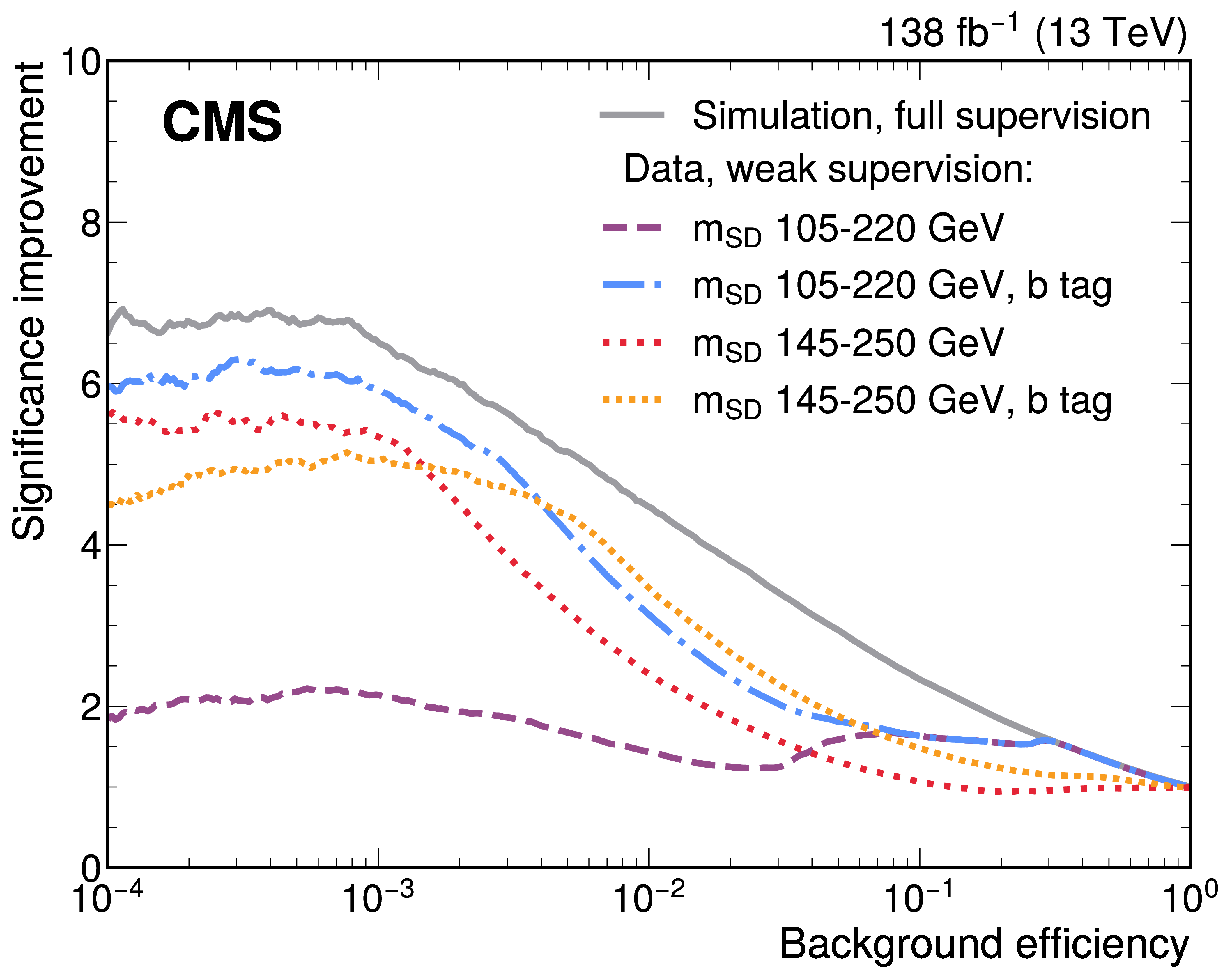
A comparison of the top quark identification performance of classifiers trained in different ways, evaluated in simulation. The two models trained in the 145-250 GeV mass window (red and yellow), as well as the one trained using the b tagging preselection in the in the 105-220 GeV mass window (blue), nearly match the performance of a supervised classifier (gray). The classifier trained with the baseline preselection in the 105-220 GeV mass window (purple) exhibits an improvement that is smaller than the others, yet larger than one. |
png pdf |
Figure 21:
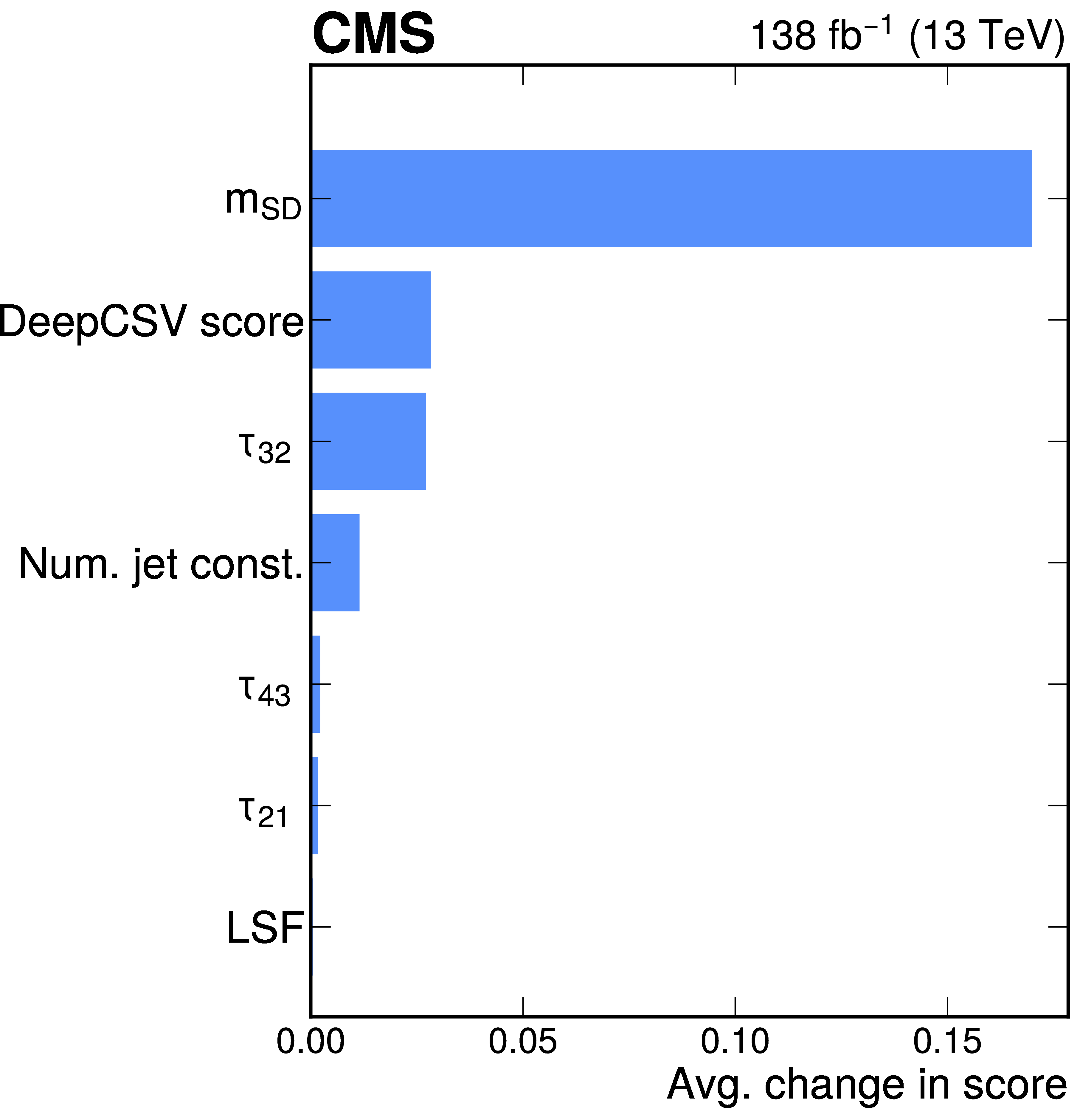
Excess characterization for the weakly supervised anomaly detection strategy applied to the $ \mathrm{t} \overline{\mathrm{t}} $ region with the b tagging preselection. The sensitivity of the anomaly score to the different input observables is assessed to aid in the determination of the properties of the excess. The jet mass, b tagging score, and $ \tau_{32} $ are seen to be the most important observables, consistent with the properties of large-radius top quark jets. |
png pdf |
Figure 22:
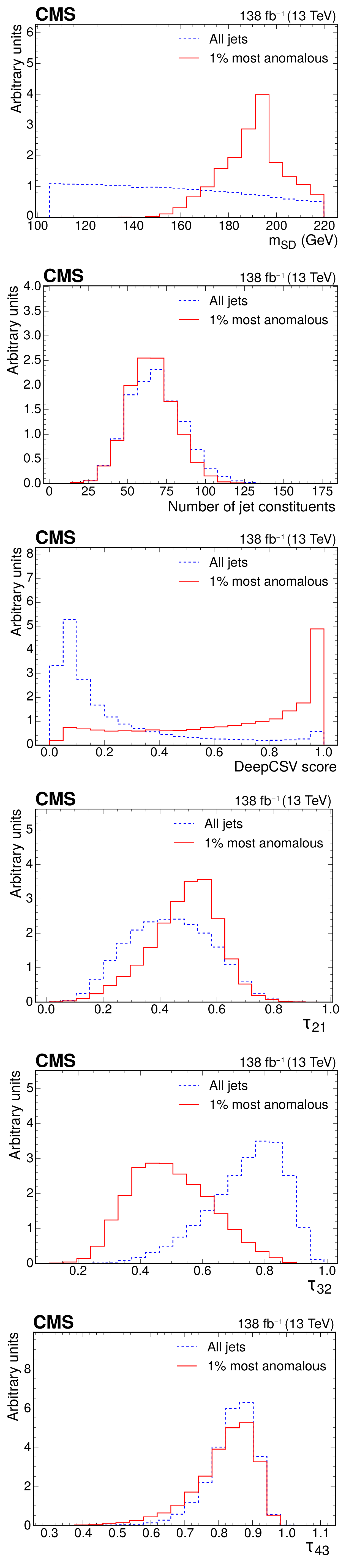
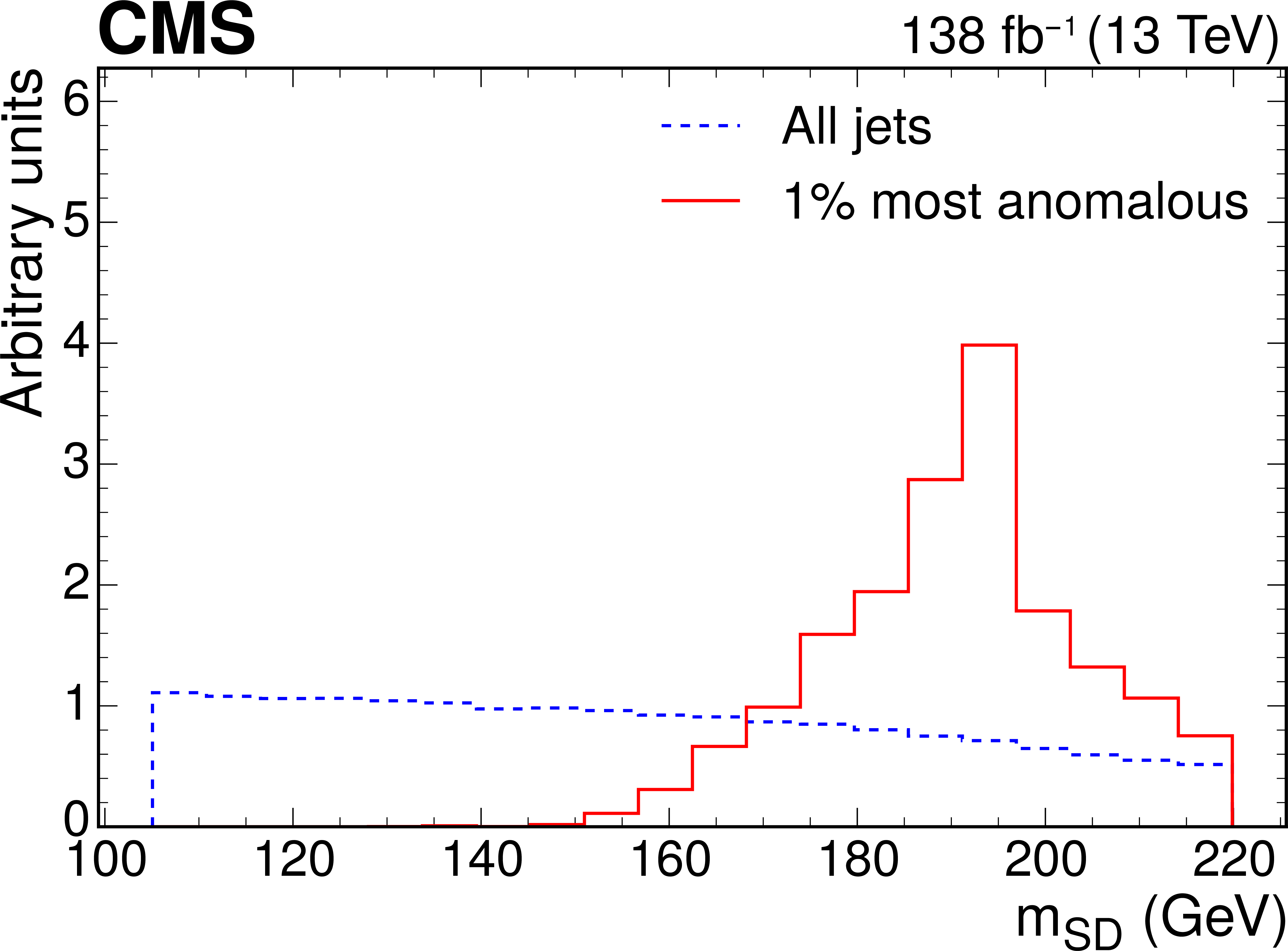
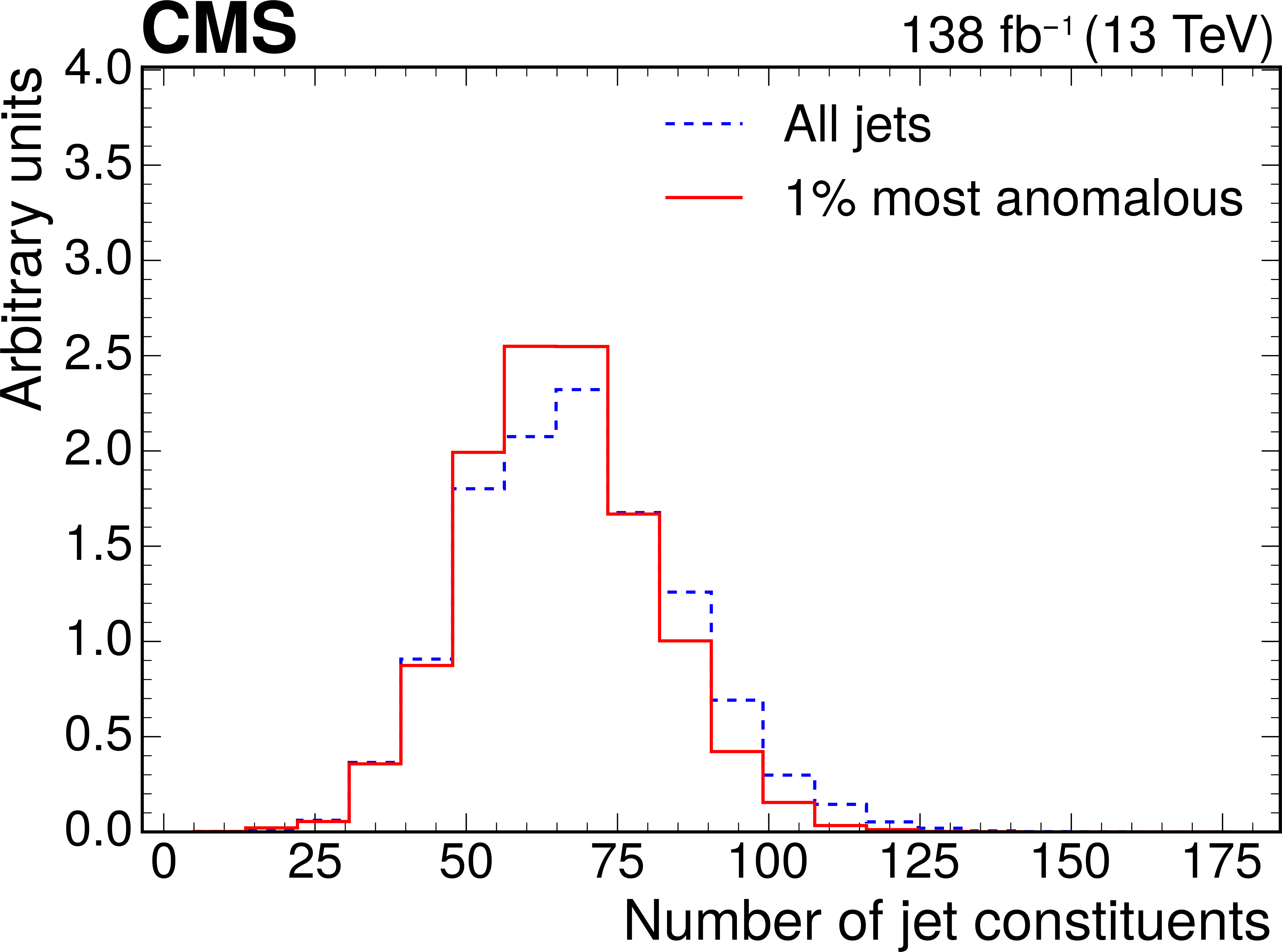
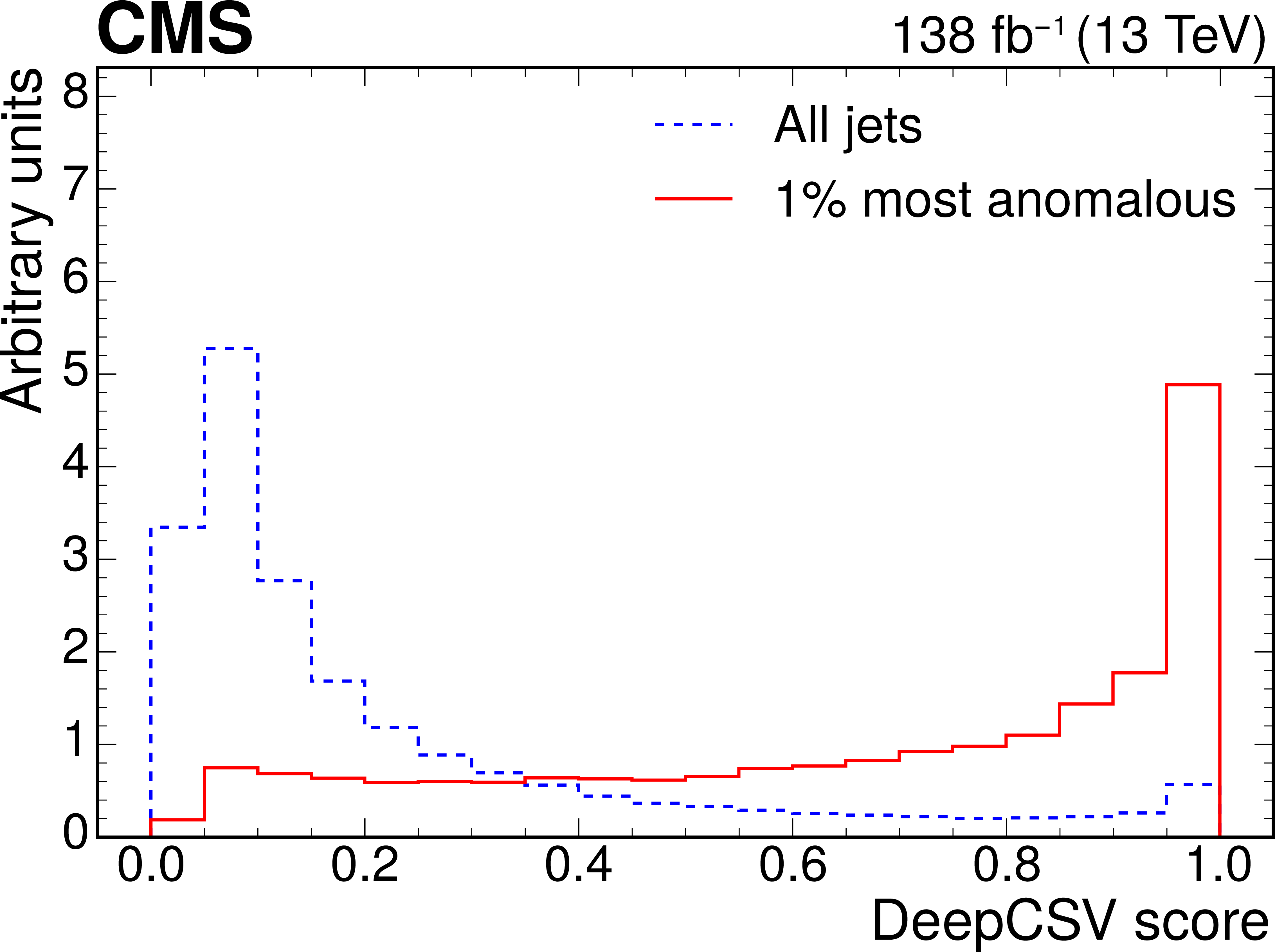
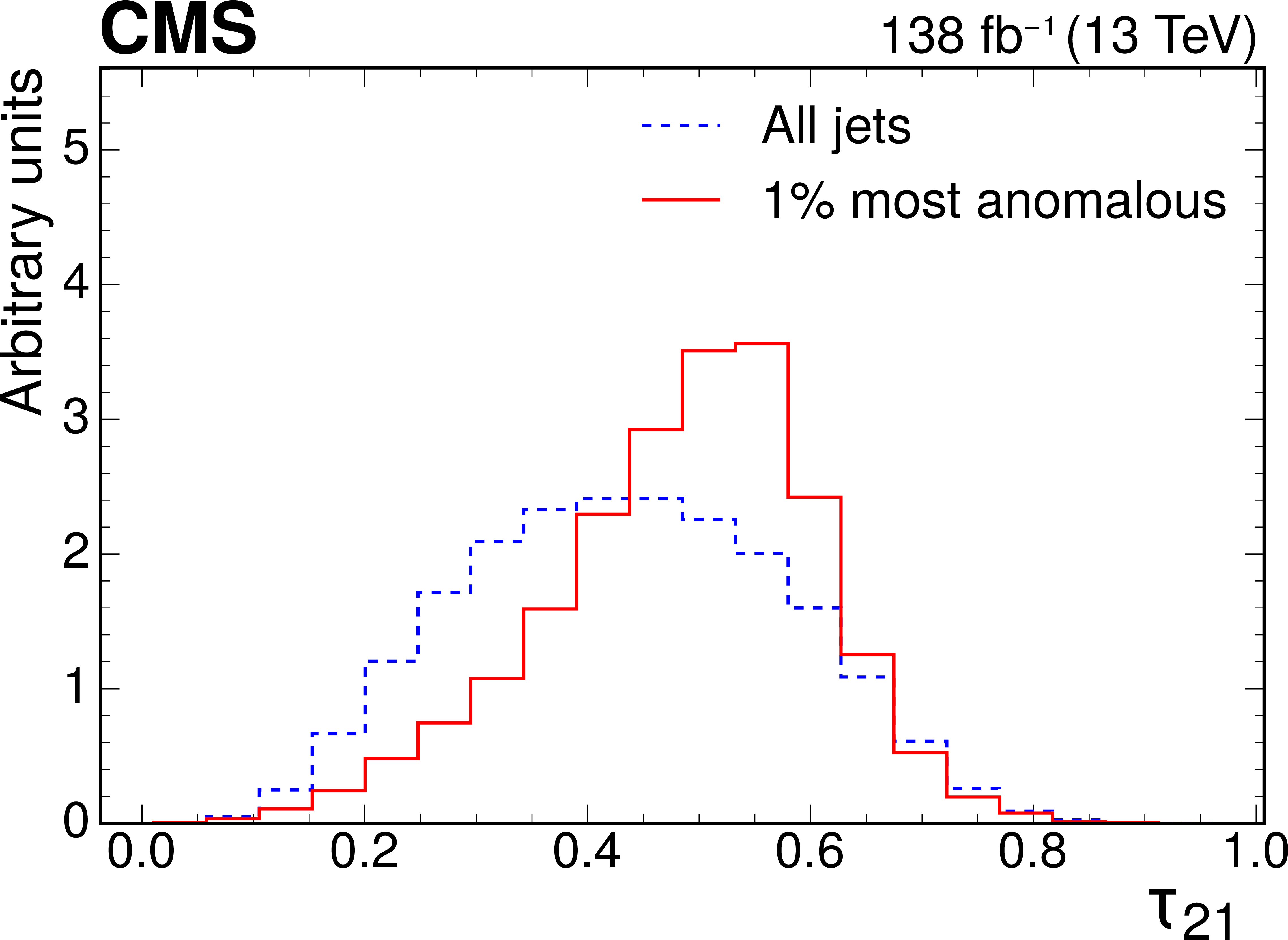
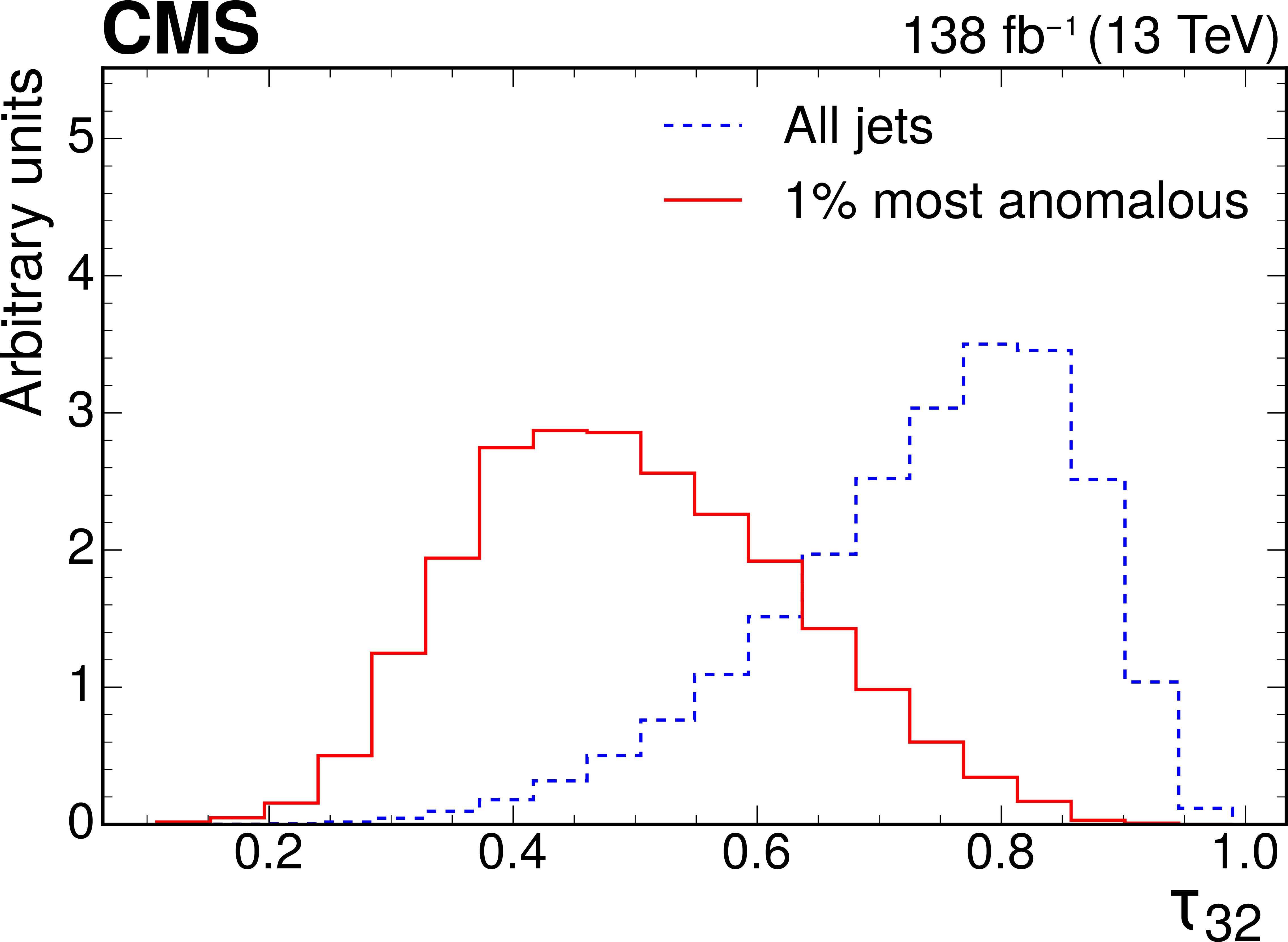
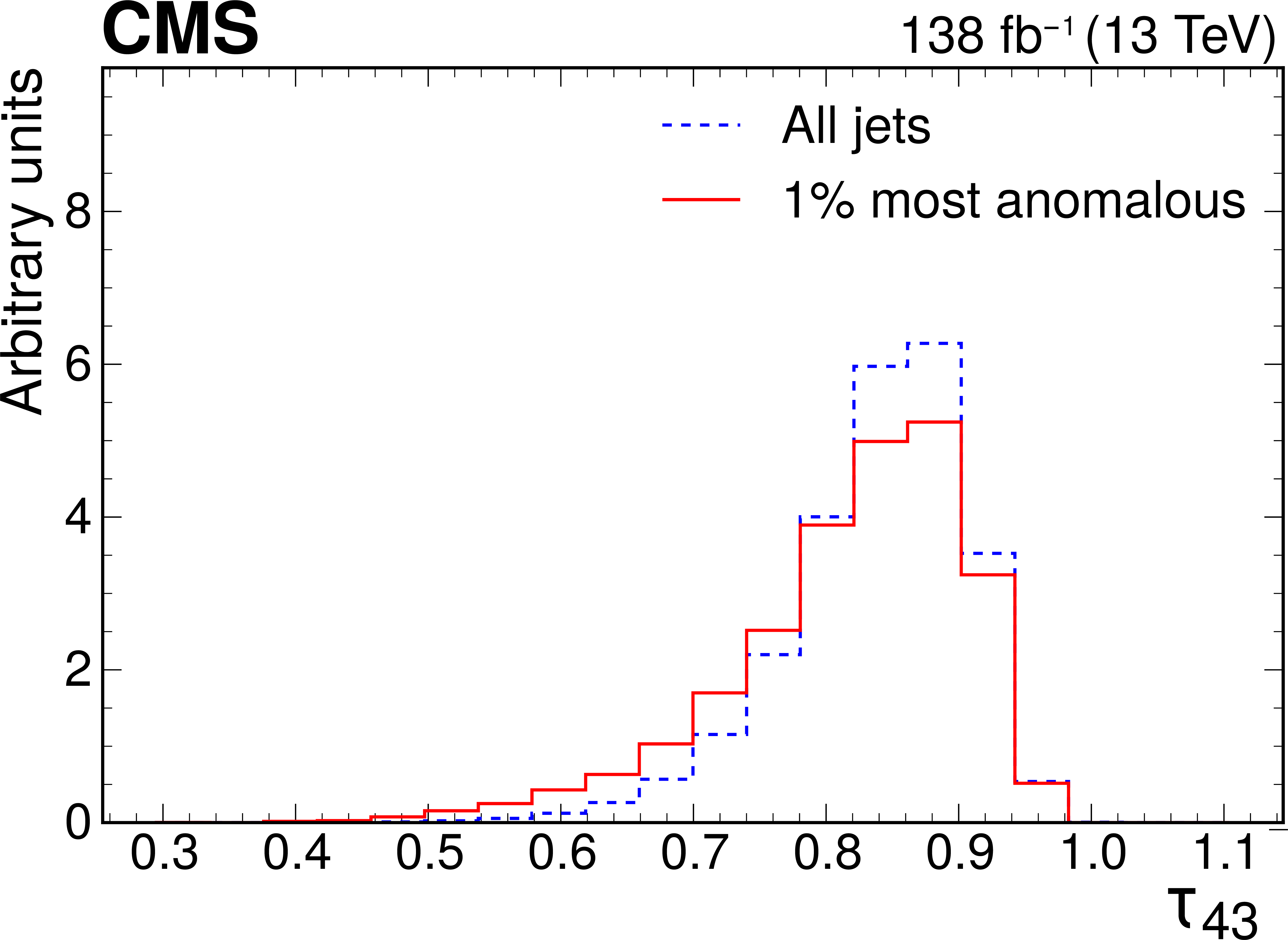
Excess characterization for the weakly supervised anomaly detection strategy applied to the $ \mathrm{t} \overline{\mathrm{t}} $ region with the b tagging preselection. The plots compare the properties of the jets with the highest anomaly score (red) to those for all jets in the region of the excess (blue). The variables shown are the soft-drop mass $ m_\mathrm{SD} $ (upper left), the number of jet constituents $ n_\mathrm{PF} $ (upper right), the DEEPCSV score (middle left), and the three subjettiness ratios $ \tau_{21} $ (middle right), $ \tau_{32} $ (lower left), and $ \tau_{43} $ (lower right). The three-pronged nature of the signal is clear from the low $ \tau_{32} $ scores, the presence of b tags from the high DEEPCSV score, and the jet mass ($ m_\mathrm{SD} $) distribution peaking at 175 GeV indicates the top quark mass. |
png pdf |
Figure 22-a:
Excess characterization for the weakly supervised anomaly detection strategy applied to the $ \mathrm{t} \overline{\mathrm{t}} $ region with the b tagging preselection. The plots compare the properties of the jets with the highest anomaly score (red) to those for all jets in the region of the excess (blue). The variables shown are the soft-drop mass $ m_\mathrm{SD} $ (upper left), the number of jet constituents $ n_\mathrm{PF} $ (upper right), the DEEPCSV score (middle left), and the three subjettiness ratios $ \tau_{21} $ (middle right), $ \tau_{32} $ (lower left), and $ \tau_{43} $ (lower right). The three-pronged nature of the signal is clear from the low $ \tau_{32} $ scores, the presence of b tags from the high DEEPCSV score, and the jet mass ($ m_\mathrm{SD} $) distribution peaking at 175 GeV indicates the top quark mass. |
png pdf |
Figure 22-b:
Excess characterization for the weakly supervised anomaly detection strategy applied to the $ \mathrm{t} \overline{\mathrm{t}} $ region with the b tagging preselection. The plots compare the properties of the jets with the highest anomaly score (red) to those for all jets in the region of the excess (blue). The variables shown are the soft-drop mass $ m_\mathrm{SD} $ (upper left), the number of jet constituents $ n_\mathrm{PF} $ (upper right), the DEEPCSV score (middle left), and the three subjettiness ratios $ \tau_{21} $ (middle right), $ \tau_{32} $ (lower left), and $ \tau_{43} $ (lower right). The three-pronged nature of the signal is clear from the low $ \tau_{32} $ scores, the presence of b tags from the high DEEPCSV score, and the jet mass ($ m_\mathrm{SD} $) distribution peaking at 175 GeV indicates the top quark mass. |
png pdf |
Figure 22-c:
Excess characterization for the weakly supervised anomaly detection strategy applied to the $ \mathrm{t} \overline{\mathrm{t}} $ region with the b tagging preselection. The plots compare the properties of the jets with the highest anomaly score (red) to those for all jets in the region of the excess (blue). The variables shown are the soft-drop mass $ m_\mathrm{SD} $ (upper left), the number of jet constituents $ n_\mathrm{PF} $ (upper right), the DEEPCSV score (middle left), and the three subjettiness ratios $ \tau_{21} $ (middle right), $ \tau_{32} $ (lower left), and $ \tau_{43} $ (lower right). The three-pronged nature of the signal is clear from the low $ \tau_{32} $ scores, the presence of b tags from the high DEEPCSV score, and the jet mass ($ m_\mathrm{SD} $) distribution peaking at 175 GeV indicates the top quark mass. |
png pdf |
Figure 22-d:
Excess characterization for the weakly supervised anomaly detection strategy applied to the $ \mathrm{t} \overline{\mathrm{t}} $ region with the b tagging preselection. The plots compare the properties of the jets with the highest anomaly score (red) to those for all jets in the region of the excess (blue). The variables shown are the soft-drop mass $ m_\mathrm{SD} $ (upper left), the number of jet constituents $ n_\mathrm{PF} $ (upper right), the DEEPCSV score (middle left), and the three subjettiness ratios $ \tau_{21} $ (middle right), $ \tau_{32} $ (lower left), and $ \tau_{43} $ (lower right). The three-pronged nature of the signal is clear from the low $ \tau_{32} $ scores, the presence of b tags from the high DEEPCSV score, and the jet mass ($ m_\mathrm{SD} $) distribution peaking at 175 GeV indicates the top quark mass. |
png pdf |
Figure 22-e:
Excess characterization for the weakly supervised anomaly detection strategy applied to the $ \mathrm{t} \overline{\mathrm{t}} $ region with the b tagging preselection. The plots compare the properties of the jets with the highest anomaly score (red) to those for all jets in the region of the excess (blue). The variables shown are the soft-drop mass $ m_\mathrm{SD} $ (upper left), the number of jet constituents $ n_\mathrm{PF} $ (upper right), the DEEPCSV score (middle left), and the three subjettiness ratios $ \tau_{21} $ (middle right), $ \tau_{32} $ (lower left), and $ \tau_{43} $ (lower right). The three-pronged nature of the signal is clear from the low $ \tau_{32} $ scores, the presence of b tags from the high DEEPCSV score, and the jet mass ($ m_\mathrm{SD} $) distribution peaking at 175 GeV indicates the top quark mass. |
png pdf |
Figure 22-f:
Excess characterization for the weakly supervised anomaly detection strategy applied to the $ \mathrm{t} \overline{\mathrm{t}} $ region with the b tagging preselection. The plots compare the properties of the jets with the highest anomaly score (red) to those for all jets in the region of the excess (blue). The variables shown are the soft-drop mass $ m_\mathrm{SD} $ (upper left), the number of jet constituents $ n_\mathrm{PF} $ (upper right), the DEEPCSV score (middle left), and the three subjettiness ratios $ \tau_{21} $ (middle right), $ \tau_{32} $ (lower left), and $ \tau_{43} $ (lower right). The three-pronged nature of the signal is clear from the low $ \tau_{32} $ scores, the presence of b tags from the high DEEPCSV score, and the jet mass ($ m_\mathrm{SD} $) distribution peaking at 175 GeV indicates the top quark mass. |
| Tables | |
png pdf |
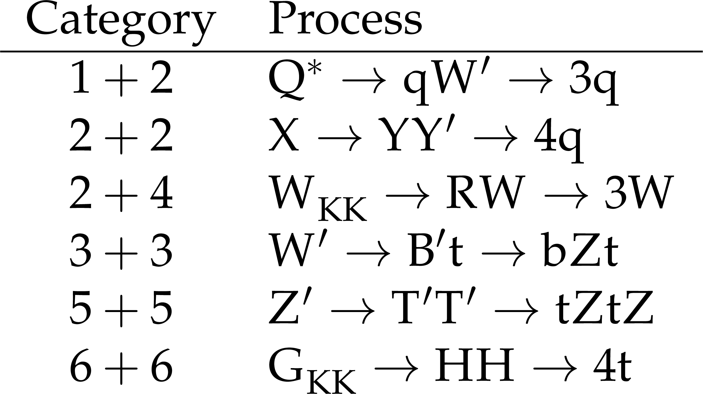
Table 1:
Signal processes considered in the analysis, categorized according to the number of partons produced in the decay of each jet. |
png pdf |
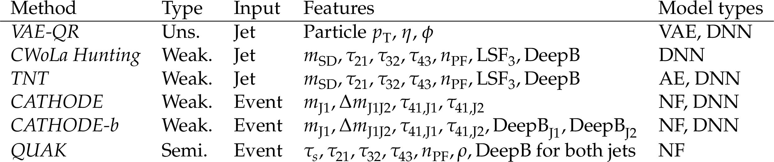
Table 2:
Summary of the methods used in this paper. The type column distinguishes between unsupervised (Uns.), weakly supervised (Weak.), and semi-supervised (Semi.) methods. Depending on the method, the ML models use single jets or complete dijet events as inputs. We also list the input features and types of ML models used, with the following abbreviations: ``AE'' for autoencoders, ``VAE'' for variational autoencoders, ``DNN'' for fully connected deep neural networks, and ``NF'' for normalizing flows. The two variants of CATHODE are shown separately. Details are given in the text. |
png pdf |
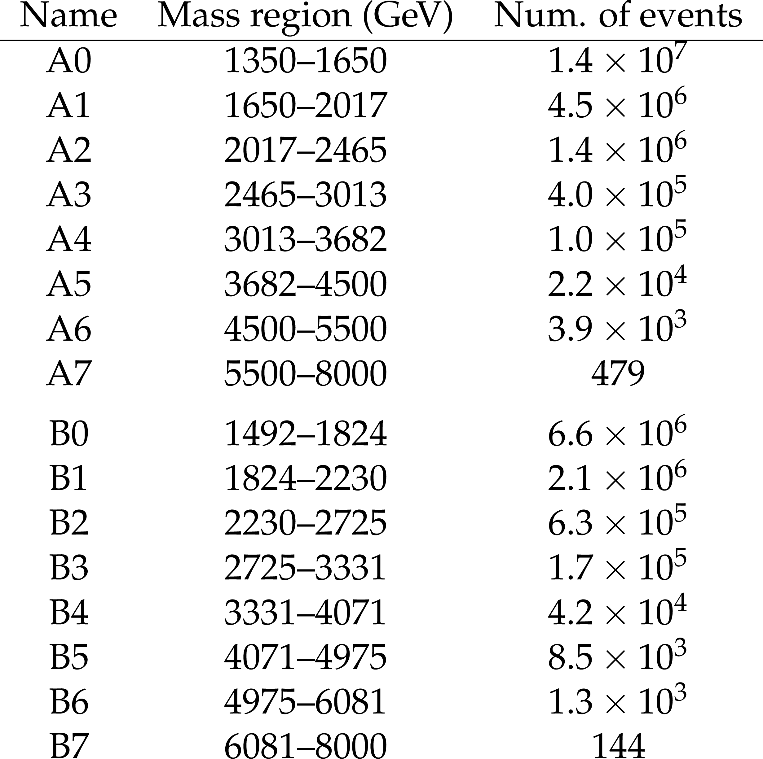
Table 3:
Mass regions used by the weakly supervised methods and corresponding observed number of events. Signal regions are required to have sideband mass regions on either side for reliable background estimation. This means only the A1-A6 and B1-B6 regions are used to seek signals, with the A0, B0, A7, and B7 regions used solely as sideband control regions. |
png pdf |
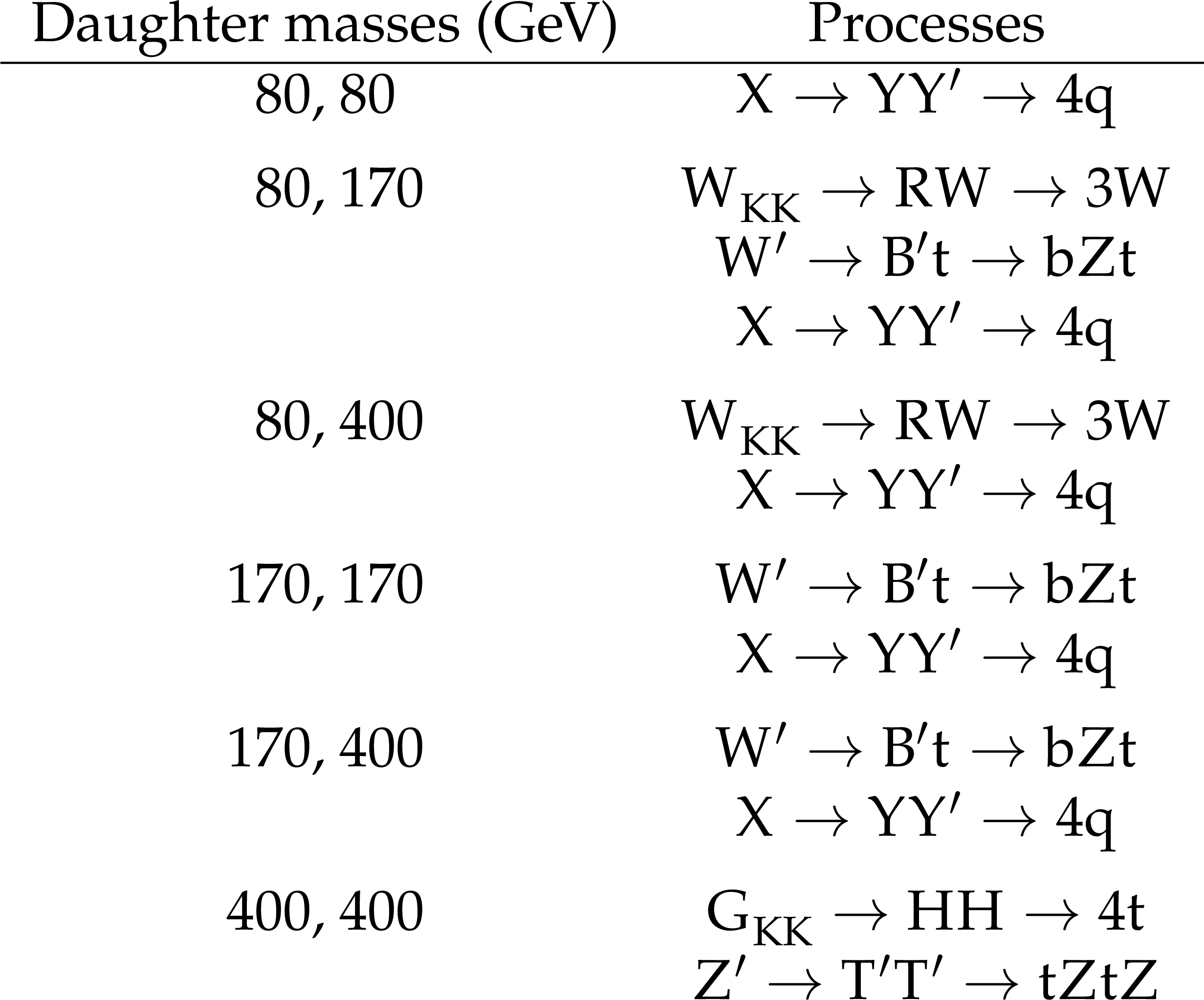
Table 4:
Signal models used to train the six signal normalizing flows used in the QUAK method. Each flow uses signals with specific masses for the daughter particles B and C. For signals decaying to an SM and a BSM particle, the BSM particle is always the heavier of the two. |
| Summary |
| We have presented a detailed description of the five anomaly detection methods used to search for new particles decaying to two anomalous jets in Ref. [6], using data collected by CMS between 2016 and 2018. Approaches based on weakly supervised, unsupervised, and semi-supervised training paradigms have been explored. All methods were successfully able to identify some classes of anomalous jets as distinct from standard model backgrounds, and were therefore able to enhance the sensitivity to the signatures of new particles in CMS data in a model-agnostic fashion. The sensitivity of the methods to the presence of an anomalous signal in the data has been shown to be higher than an inclusive search or simple selections based on jet substructure. The performance of the five methods has been found to depend on the considered signal model, with no single method outperforming all others. Further investigation has shown that correlations between the anomaly scores are low, indicating that methods identify anomalous signal events in different ways. Furthermore, the impact of differences in the input features has been explored and shown to explain performance differences between signal models, but not between methods. Finally, a weakly supervised anomaly detection method has been used to separate top quark jets from jets produced in other standard model processes. The achieved separation power comes very close to that of a fully supervised classifier trained with the same input variables. This constitutes a validation of resonant anomaly detection in collider data. In addition, interpretation techniques have been used to successfully retrieve some of the main properties of the top quark. This would enable further investigation and confirmation of the signal in the event of a positive result from an anomaly search. |
| References | ||||
| 1 | ATLAS Collaboration | The ATLAS Experiment at the CERN Large Hadron Collider | JINST 3 (2008) S08003 | |
| 2 | CMS Collaboration | The CMS experiment at the CERN LHC | JINST 3 (2008) S08004 | |
| 3 | Particle Data Group , S. Navas et al. | Review of particle physics | PRD 110 (2024) 030001 | |
| 4 | G. Kasieczka et al. | The LHC Olympics 2020 a community challenge for anomaly detection in high energy physics | Rept. Prog. Phys. 84 (2021) 124201 | 2101.08320 |
| 5 | V. Belis, P. Odagiu, and T. K. Aarrestad | Machine learning for anomaly detection in particle physics | Rev. Phys. 12 (2024) 100091 | 2312.14190 |
| 6 | CMS Collaboration | Model-agnostic search for dijet resonances with anomalous jet substructure in proton-proton collisions at $ \sqrt{s} = $ 13 TeV | Rept. Prog. Phys. 88 (2025) 067802 | CMS-EXO-22-026 2412.03747 |
| 7 | D0 Collaboration | Search for new physics in e$\mu$X data at D0 using SLEUTH: A quasi-model-independent search strategy for new physics | PRD 62 (2000) 092004 | hep-ex/0006011 |
| 8 | D0 Collaboration | A quasi model independent search for new physics at large transverse momentum | PRD 64 (2001) 012004 | hep-ex/0011067 |
| 9 | D0 Collaboration | A quasi model independent search for new high $ p_t $ physics at D0 | PRL 86 (2001) 3712 | hep-ex/0011071 |
| 10 | H1 Collaboration | A general search for new phenomena at HERA | PLB 674 (2009) 257 | 0901.0507 |
| 11 | H1 Collaboration | A General search for new phenomena in ep scattering at HERA | PLB 602 (2004) 14 | hep-ex/0408044 |
| 12 | CDF Collaboration | Model-independent and quasi-model-independent search for new physics at CDF | PRD 78 (2008) 012002 | 0712.1311 |
| 13 | CDF Collaboration | Model-independent global search for new high-$p_{\mathrm{T}}$ physics at CDF | link | 0712.2534 |
| 14 | CDF Collaboration | Global search for new physics with 2.0 fb$ ^{-1} $ at CDF | PRD 79 (2009) 011101 | 0809.3781 |
| 15 | CMS Collaboration | MUSiC: a model-unspecific search for new physics in proton-proton collisions at $ \sqrt{s} = $ 13 TeV | EPJC 81 (2021) 629 | CMS-EXO-19-008 2010.02984 |
| 16 | ATLAS Collaboration | A strategy for a general search for new phenomena using data-derived signal regions and its application within the ATLAS experiment | EPJC 79 (2019) 120 | 1807.07447 |
| 17 | ATLAS Collaboration | Dijet resonance search with weak supervision using $ \sqrt{s}= $ 13 TeV $ pp $ collisions in the ATLAS detector | PRL 125 (2020) 131801 | 2005.02983 |
| 18 | ATLAS Collaboration | Weakly supervised anomaly detection for resonant new physics in the dijet final state using proton-proton collisions at $ \sqrt{s}= $ 13 TeV with the ATLAS detector | 2502.09770 | |
| 19 | T. Aarrestad et al. | The dark machines anomaly score challenge: Benchmark data and model independent event classification for the Large Hadron Collider | SciPost Phys. 12 (2022) 043 | 2105.14027 |
| 20 | J. A. Aguilar-Saavedra, J. Collins, and R. K. Mishra | A generic anti-QCD jet tagger | JHEP 11 (2017) 163 | 1709.01087 |
| 21 | A. Hallin et al. | Classifying anomalies through outer density estimation | PRD 106 (2022) 055006 | 2109.00546 |
| 22 | E. M. Metodiev, B. Nachman, and J. Thaler | Classification without labels: Learning from mixed samples in high energy physics | JHEP 10 (2017) 174 | 1708.02949 |
| 23 | J. H. Collins, K. Howe, and B. Nachman | Extending the search for new resonances with machine learning | PRD 99 (2019) 014038 | 1902.02634 |
| 24 | T. Finke, M. Krämer, M. Lipp, and A. Muck | Boosting mono-jet searches with model-agnostic machine learning | JHEP 08 (2022) 15 | 2204.11889 |
| 25 | B. Nachman and D. Shih | Anomaly detection with density estimation | PRD 101 (2020) 075042 | 2001.04990 |
| 26 | J. A. Raine, S. Klein, D. Sengupta, and T. Golling | CURTAINs for your sliding window: Constructing unobserved regions by transforming adjacent intervals | Front. Big Data 6 (2023) 899345 | 2203.09470 |
| 27 | S. Klein, J. A. Raine, and T. Golling | Flows for flows: Training normalizing flows between arbitrary distributions with maximum likelihood estimation | 2211.02487 | |
| 28 | D. Sengupta, S. Klein, J. A. Raine, and T. Golling | CURTAINs flows for flows: Constructing unobserved regions with maximum likelihood estimation | SciPost Phys. 17 (2024) 046 | 2305.04646 |
| 29 | D. Sengupta et al. | Improving new physics searches with diffusion models for event observables and jet constituents | JHEP 04 (2024) 109 | 2312.10130 |
| 30 | V. Mikuni and B. Nachman | High-dimensional and permutation invariant anomaly detection | SciPost Phys. 16 (2024) 062 | 2306.03933 |
| 31 | T. Golling, S. Klein, R. Mastandrea, and B. Nachman | Flow-enhanced transportation for anomaly detection | PRD 107 (2023) 096025 | 2212.11285 |
| 32 | P. Jawahar et al. | Improving variational autoencoders for new physics detection at the LHC with normalizing flows | Front. Big Data 5 (2022) 803685 | 2110.08508 |
| 33 | S. Tsan et al. | Particle graph autoencoders and differentiable, learned energy mover's distance | in 35th Conference on Neural Information Processing Systems. 2021 | 2111.12849 |
| 34 | T. Finke et al. | Autoencoders for unsupervised anomaly detection in high energy physics | JHEP 06 (2021) 161 | 2104.09051 |
| 35 | L. Vaslin, V. Barra, and J. Donini | GAN-AE: an anomaly detection algorithm for new physics search in LHC data | EPJC 83 (2023) 1008 | 2305.15179 |
| 36 | L. Anzalone et al. | Triggering dark showers with conditional dual auto-encoders | Mach. Learn. Sci. Tech. 5 (2024) 035064 | 2306.12955 |
| 37 | O. Cerri et al. | Variational autoencoders for new physics mining at the Large Hadron Collider | JHEP 05 (2019) 036 | 1811.10276 |
| 38 | B. M. Dillon, T. Plehn, C. Sauer, and P. Sorrenson | Better latent spaces for better autoencoders | SciPost Phys. 11 (2021) 061 | 2104.08291 |
| 39 | T. Cheng et al. | Variational autoencoders for anomalous jet tagging | PRD 107 (2023) 016002 | 2007.01850 |
| 40 | B. M. Dillon et al. | A normalized autoencoder for LHC triggers | SciPost Phys. Core 6 (2023) 074 | 2206.14225 |
| 41 | M. van Beekveld et al. | Combining outlier analysis algorithms to identify new physics at the LHC | JHEP 09 (2021) 024 | 2010.07940 |
| 42 | M. Kuusela et al. | Semi-supervised anomaly detection---towards model-independent searches of new physics | J. Phys. Conf. Ser. 368 (2012) 012032 | 1112.3329 |
| 43 | E. Govorkova et al. | Autoencoders on field-programmable gate arrays for real-time, unsupervised new physics detection at 40 MHz at the Large Hadron Collider | Nature Mach. Intell. 4 (2022) 154 | 2108.03986 |
| 44 | V. Mikuni, B. Nachman, and D. Shih | Online-compatible unsupervised nonresonant anomaly detection | PRD 105 (2022) 055006 | 2111.06417 |
| 45 | K. A. Wo \'z niak et al. | New physics agnostic selections for new physics searches | EPJ Web Conf. 245 (2020) 06039 | |
| 46 | O. Knapp et al. | Adversarially learned anomaly detection on CMS open data: re-discovering the top quark | Eur. Phys. J. Plus 136 (2021) 236 | 2005.01598 |
| 47 | CMS Collaboration | Wasserstein normalized autoencoder for anomaly detection | Submitted to Mach. Learn.: Sci. and Tech, 2025 | CMS-MLG-24-002 2510.02168 |
| 48 | M. Farina, Y. Nakai, and D. Shih | Searching for new physics with deep autoencoders | PRD 101 (2020) 075021 | 1808.08992 |
| 49 | T. Heimel, G. Kasieczka, T. Plehn, and J. M. Thompson | QCD or what? | SciPost Phys. 6 (2019) 030 | 1808.08979 |
| 50 | ATLAS Collaboration | Anomaly detection search for new resonances decaying into a Higgs boson and a generic new particle $ X $ in hadronic final states using $ \sqrt{s} = $ 13 TeV $ pp $ collisions with the ATLAS detector | PRD 108 (2023) 052009 | 2306.03637 |
| 51 | ATLAS Collaboration | Search for new phenomena in two-body invariant mass distributions using unsupervised machine learning for anomaly detection at $ \sqrt s= $ 13 tev with the ATLAS Detector | PRL 132 (2024) 081801 | 2307.01612 |
| 52 | ATLAS Collaboration | Search for new physics in final states with semi-visible jets or anomalous signatures using the ATLAS detector | 2505.01634 | |
| 53 | D. P. Kingma and M. Welling | Auto-encoding variational Bayes | 1312.6114 | |
| 54 | CMS ECAL Collaboration | Autoencoder-based anomaly detection system for online data quality monitoring of the CMS electromagnetic calorimeter | Comput. Softw. Big Sci. 8 (2024) 11 | 2309.10157 |
| 55 | D. Bourilkov | Machine and deep learning applications in particle physics | Int. J. Mod. Phys. A 34 (2020) 1930019 | 1912.08245 |
| 56 | CMS Collaboration | Measurement of the $ \mathrm{t\bar{t}}\mathrm{b\bar{b}} $ production cross section in the all-jet final state in pp collisions at $ \sqrt{s} = $ 13 TeV | PLB 803 (2020) 135285 | CMS-TOP-18-011 1909.05306 |
| 57 | R. Gambhir, R. Mastandrea, B. Nachman, and J. Thaler | Isolating Unisolated Upsilons with Anomaly Detection in CMS Open Data | PRL 135 (2025) 021902 | 2502.14036 |
| 58 | CMS Collaboration | Development of the CMS detector for the CERN LHC Run 3 | JINST 19 (2024) P05064 | CMS-PRF-21-001 2309.05466 |
| 59 | CMS Collaboration | Performance of the CMS Level-1 trigger in proton-proton collisions at $ \sqrt{s} = $ 13 TeV | JINST 15 (2020) P10017 | CMS-TRG-17-001 2006.10165 |
| 60 | CMS Collaboration | The CMS trigger system | JINST 12 (2017) P01020 | CMS-TRG-12-001 1609.02366 |
| 61 | CMS Collaboration | Performance of the CMS high-level trigger during LHC run 2 | JINST 19 (2024) P11021 | CMS-TRG-19-001 2410.17038 |
| 62 | CMS Collaboration | Electron and photon reconstruction and identification with the CMS experiment at the CERN LHC | JINST 16 (2021) P05014 | CMS-EGM-17-001 2012.06888 |
| 63 | CMS Collaboration | Performance of the CMS muon detector and muon reconstruction with proton-proton collisions at $ \sqrt{s}= $ 13 TeV | JINST 13 (2018) P06015 | CMS-MUO-16-001 1804.04528 |
| 64 | CMS Collaboration | Description and performance of track and primary-vertex reconstruction with the CMS tracker | JINST 9 (2014) P10009 | CMS-TRK-11-001 1405.6569 |
| 65 | CMS Collaboration | Technical proposal for the Phase-II upgrade of the Compact Muon Solenoid | CMS Technical Proposal CERN-LHCC-2015-010, CMS-TDR-15-02, 2015 CDS |
|
| 66 | CMS Collaboration | Particle-flow reconstruction and global event description with the CMS detector | JINST 12 (2017) P10003 | CMS-PRF-14-001 1706.04965 |
| 67 | M. Cacciari, G. P. Salam, and G. Soyez | The anti-$ k_{\mathrm{T}} $ jet clustering algorithm | JHEP 04 (2008) 063 | 0802.1189 |
| 68 | M. Cacciari, G. P. Salam, and G. Soyez | FastJet user manual | EPJC 72 (2012) 1896 | 1111.6097 |
| 69 | CMS Collaboration | Pileup mitigation at CMS in 13 TeV data | JINST 15 (2020) P09018 | CMS-JME-18-001 2003.00503 |
| 70 | D. Bertolini, P. Harris, M. Low, and N. Tran | Pileup per particle identification | JHEP 10 (2014) 59 | 1407.6013 |
| 71 | CMS Collaboration | Jet energy scale and resolution in the CMS experiment in pp collisions at 8 TeV | JINST 12 (2017) P02014 | CMS-JME-13-004 1607.03663 |
| 72 | CMS Collaboration | Precision luminosity measurement in proton-proton collisions at $ \sqrt{s} = $ 13 TeV in 2015 and 2016 at CMS | EPJC 81 (2021) 800 | CMS-LUM-17-003 2104.01927 |
| 73 | CMS Collaboration | CMS luminosity measurement for the 2017 data-taking period at $ \sqrt{s} = $ 13 TeV | CMS Physics Analysis Summary, 2018 link |
CMS-PAS-LUM-17-004 |
| 74 | CMS Collaboration | CMS luminosity measurement for the 2018 data-taking period at $ \sqrt{s} = $ 13 TeV | CMS Physics Analysis Summary, 2019 link |
CMS-PAS-LUM-18-002 |
| 75 | A. J. Larkoski, S. Marzani, G. Soyez, and J. Thaler | Soft drop | JHEP 05 (2014) 146 | 1402.2657 |
| 76 | J. Thaler and K. Van Tilburg | Identifying boosted objects with N-subjettiness | JHEP 03 (2011) 015 | 1011.2268 |
| 77 | CMS Collaboration | Identification of heavy-flavour jets with the CMS detector in pp collisions at 13 TeV | JINST 13 (2018) P05011 | CMS-BTV-16-002 1712.07158 |
| 78 | C. Brust et al. | Identifying boosted new physics with non-isolated leptons | JHEP 04 (2015) 079 | 1410.0362 |
| 79 | J. Alwall et al. | The automated computation of tree-level and next-to-leading order differential cross sections, and their matching to parton shower simulations | JHEP 07 (2014) 079 | 1405.0301 |
| 80 | J. Alwall et al. | Comparative study of various algorithms for the merging of parton showers and matrix elements in hadronic collisions | EPJC 53 (2008) 473 | 0706.2569 |
| 81 | P. Nason | A new method for combining NLO QCD with shower Monte Carlo algorithms | JHEP 11 (2004) 040 | hep-ph/0409146 |
| 82 | S. Frixione, P. Nason, and C. Oleari | Matching NLO QCD computations with parton shower simulations: the POWHEG method | JHEP 11 (2007) 070 | 0709.2092 |
| 83 | S. Alioli, P. Nason, C. Oleari, and E. Re | A general framework for implementing NLO calculations in shower Monte Carlo programs: the POWHEG BOX | JHEP 06 (2010) 043 | 1002.2581 |
| 84 | S. Frixione, P. Nason, and G. Ridolfi | A positive-weight next-to-leading-order Monte Carlo for heavy flavour hadroproduction | JHEP 09 (2007) 126 | 0707.3088 |
| 85 | R. Frederix, E. Re, and P. Torrielli | Single-top $ t $-channel hadroproduction in the four-flavour scheme with POWHEG and aMC@NLO | JHEP 09 (2012) 130 | 1207.5391 |
| 86 | E. Re | Single-top $ Wt $-channel production matched with parton showers using the POWHEG method | EPJC 71 (2011) 1547 | 1009.2450 |
| 87 | T. Sjostrand et al. | An introduction to PYTHIA 8.2 | Comput. Phys. Commun. 191 (2015) 159 | 1410.3012 |
| 88 | CMS Collaboration | Extraction and validation of a new set of CMS PYTHIA8 tunes from underlying-event measurements | EPJC 80 (2020) 4 | CMS-GEN-17-001 1903.12179 |
| 89 | GEANT4 Collaboration | GEANT4---a simulation toolkit | NIM A 506 (2003) 250 | |
| 90 | CMS Collaboration | Zenodo record for this analysis | link | |
| 91 | H. Fan, H. Su, and L. Guibas | A point set generation network for 3D object reconstruction from a single image | in 2017 IEEE Conference on Computer Vision and Pattern Recognition (CVPR). 2017 link |
1612.00603 |
| 92 | S. Kullback and R. A. Leibler | On Information and Sufficiency | Ann. Math. Stat. 22 (1951) 79 | |
| 93 | D. P. Kingma and J. Ba | Adam: A method for stochastic optimization | 1412.6980 | |
| 94 | K. He, X. Zhang, S. Ren, and J. Sun | Delving deep into rectifiers: Surpassing human-level performance on imagenet classification | IEEE Int. Conf. on Comp. Vision (ICCV), 2015 link |
|
| 95 | L. Demortier | P values and nuisance parameters | in Statistical issues for LHC physics. Proceedings, Workshop, PHYSTAT-LHC, Geneva, Switzerland, June 27-29, 2007, p. 23. 2008 link |
|
| 96 | J. H. Collins, K. Howe, and B. Nachman | Anomaly detection for resonant new physics with machine learning | PRL 121 (2018) 241803 | 1805.02664 |
| 97 | D. Clevert, T. Unterthiner, and S. Hochreiter | Fast and accurate deep network learning by exponential linear units (ELUs) | in 4th International Conference on Learning Representations (ICLR). 2016.. [DBLP(ICLR)2016] | 1511.07289 |
| 98 | N. Srivastava et al. | Dropout: A simple way to prevent neural networks from overfitting | J. Mach. Learn. Res. 15 (2014) 1929 | |
| 99 | O. Amram and C. M. Suarez | Tag N\textquoteright Train: a technique to train improved classifiers on unlabeled data | JHEP 01 (2021) 153 | 2002.12376 |
| 100 | S. Macaluso and D. Shih | Pulling out all the tops with computer vision and deep learning | JHEP 10 (2018) 121 | 1803.00107 |
| 101 | D. P. Kingma et al. | Improving variational inference with inverse autoregressive flow | in Proceedings of the 30th International Conference on Neural Information Processing Systems. 2016.. [NeurIPS (2016) 4743] | 1606.04934 |
| 102 | M. Germain, K. Gregor, I. Murray, and H. Larochelle | MADE: Masked autoencoder for distribution estimation | in Proceedings of the 32nd International Conference on Machine Learning, 2015 PMLR 37 (2015) 881 |
1502.03509 |
| 103 | J. Ansel et al. | PyTorch 2: Faster machine learning through dynamic python bytecode transformation and graph compilation | in 29th ACM International Conference on Architectural Support for Programming Languages and Operating Systems. 2024. [ASPLOS '24 Vol. 2, 929] link |
|
| 104 | E. Bingham et al. | Pyro: Deep universal probabilistic programming | J. Mach. Learn. Res. 20 (2019) 1 | 1810.09538 |
| 105 | D. Phan, N. Pradhan, and M. Jankowiak | Composable effects for flexible and accelerated probabilistic programming in NumPyro | 1912.11554 | |
| 106 | S. Ioffe and C. Szegedy | Batch normalization: Accelerating deep network training by reducing internal covariate shift | in Proceedings of the 32nd International Conference on Machine Learning, 2015 PMLR 37 (2015) 448 |
1502.03167 |
| 107 | E. Parzen | On estimation of a probability density function and mode | Ann. Math. Stat. 33 (1962) 1065 | |
| 108 | S. E. Park et al. | Quasi anomalous knowledge: Searching for new physics with embedded knowledge | JHEP 06 (2020) 030 | 2011.03550 |
| 109 | C. Durkan, A. Bekasov, I. Murray, and G. Papamakarios | Neural spline flows | in Proceedings of the 33rd International Conference on Neural Information Processing Systems. 2019.. [NeurIPS (2019) 7511] | 1906.04032 |
| 110 | C. Durkan, A. Bekasov, I. Murray, and G. Papamakarios | nflows: normalizing flows in PyTorch | link | |
| 111 | J. Gallicchio et al. | Multivariate discrimination and the Higgs + W/Z search | JHEP 04 (2011) 069 | 1010.3698 |
| 112 | G. Kasieczka and D. Shih | Robust jet classifiers through distance correlation | PRL 125 (2020) 122001 | 2001.05310 |
| 113 | T. Finke et al. | Tree-based algorithms for weakly supervised anomaly detection | PRD 109 (2024) 034033 | 2309.13111 |
| 114 | H. Zenati et al. | Adversarially learned anomaly detection | in 20th IEEE International Conference on Data Mining (ICDM). 2018 link |
1812.02288 |
| 115 | CMS Collaboration | The CMS statistical analysis and combination tool: Combine | Comput. Softw. Big Sci. 8 (2024) 19 | CMS-CAT-23-001 2404.06614 |
| 116 | G. Cowan, K. Cranmer, E. Gross, and O. Vitells | Asymptotic formulae for likelihood-based tests of new physics | EPJC 71 (2011) 1554 | 1007.1727 |
| 117 | L. Breimen | Random forests | Mach. Learn. 45 (2001) 5 | |
| 118 | CMS Collaboration | A method for correcting the substructure of multiprong jets using the Lund jet plane | Submitted to JHEP, 2025 | CMS-JME-23-001 2507.07775 |
| 119 | CMS Collaboration | Jet algorithms performance in 13 TeV data | CMS Physics Analysis Summary, 2017 CMS-PAS-JME-16-003 |
CMS-PAS-JME-16-003 |
|
|
Compact Muon Solenoid LHC, CERN |
|

|

|

|

|

|