

Compact Muon Solenoid
LHC, CERN
| CMS-EGM-24-002 ; CERN-EP-2026-092 | ||
| Highly boosted dielectron identification in proton-proton collisions at $ \sqrt{s} = $ 13 TeV | ||
| CMS Collaboration | ||
| 14 April 2026 | ||
| Accepted for publication in Physical Review D | ||
| Abstract: A new technique is developed to identify dielectrons ($ \mathrm{e}^+\mathrm{e}^- $) with Lorentz boost $ \gamma_{\mathrm{L}} > $ 20 that produce one single merged cluster in the electromagnetic calorimeter of the CMS detector. The identification uses two multivariate models: one for the case where both electron tracks are reconstructed, and another where only one of the tracks is reconstructed. The efficiency is determined using proton-proton collision data collected at a center-of-mass energy of 13 TeV. Boosted $ \mathrm{J}/\psi $ mesons decaying into $ \mathrm{e}^+\mathrm{e}^- $ pairs are used to estimate the efficiency of the model with two tracks, yielding an overall efficiency of 80%. The $ \mathrm{Z}\to\mu^{+}\mu^{-}\gamma $ events, where the photon converts into a collimated dielectron, are used for the model with a single track, yielding an efficiency of about 60%. A dedicated energy correction for dielectron candidates is also developed using $ {\mathrm{B}^{\pm}}\to\mathrm{J}/\psi\mathrm{K^{\pm}}\to\mathrm{e}^+\mathrm{e}^-\mathrm{K^{\pm}} $ data. | ||
| Links: e-print arXiv:2604.13320 [hep-ex] (PDF) ; CDS record ; inSPIRE record ; Physics Briefing ; CADI line (restricted) ; | ||
| Figures | |
png pdf |
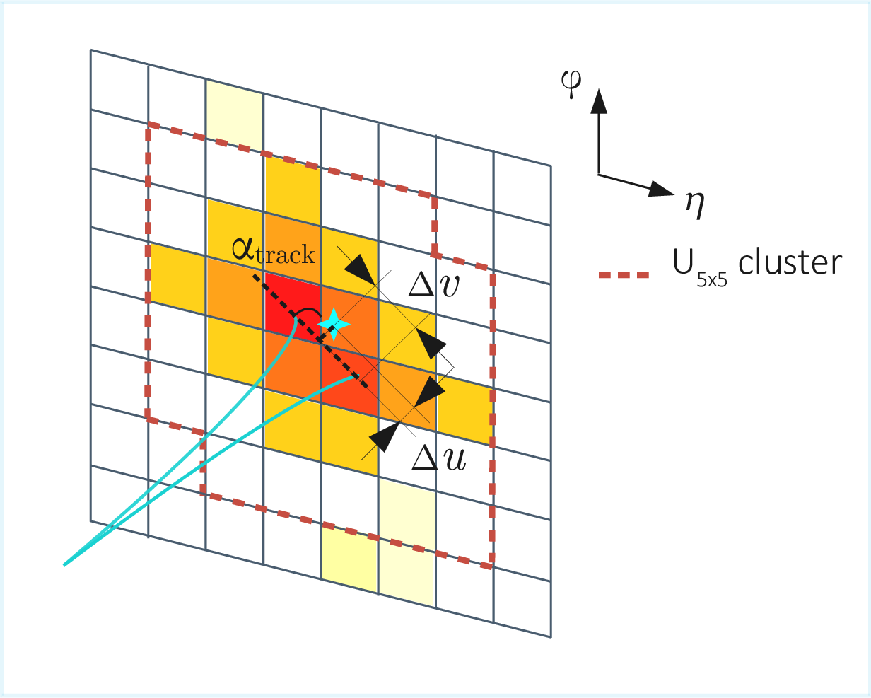
Figure 1:
Visual representations of the variables $ \alpha_{\text{track}} $, $ \Delta u $ and $ \Delta v $. Cyan-colored lines depict the incoming tracks of the dielectron. The black dashed line is used to define the $ u $ and $ v $ directions. The red dashed line represents the $ \mathrm{U}_{5\times5} $ cluster around the closest crystal from the tracks. The cyan-colored star is the log-weighted CoG of the $ \mathrm{U}_{5\times5} $ cluster. |
png pdf |
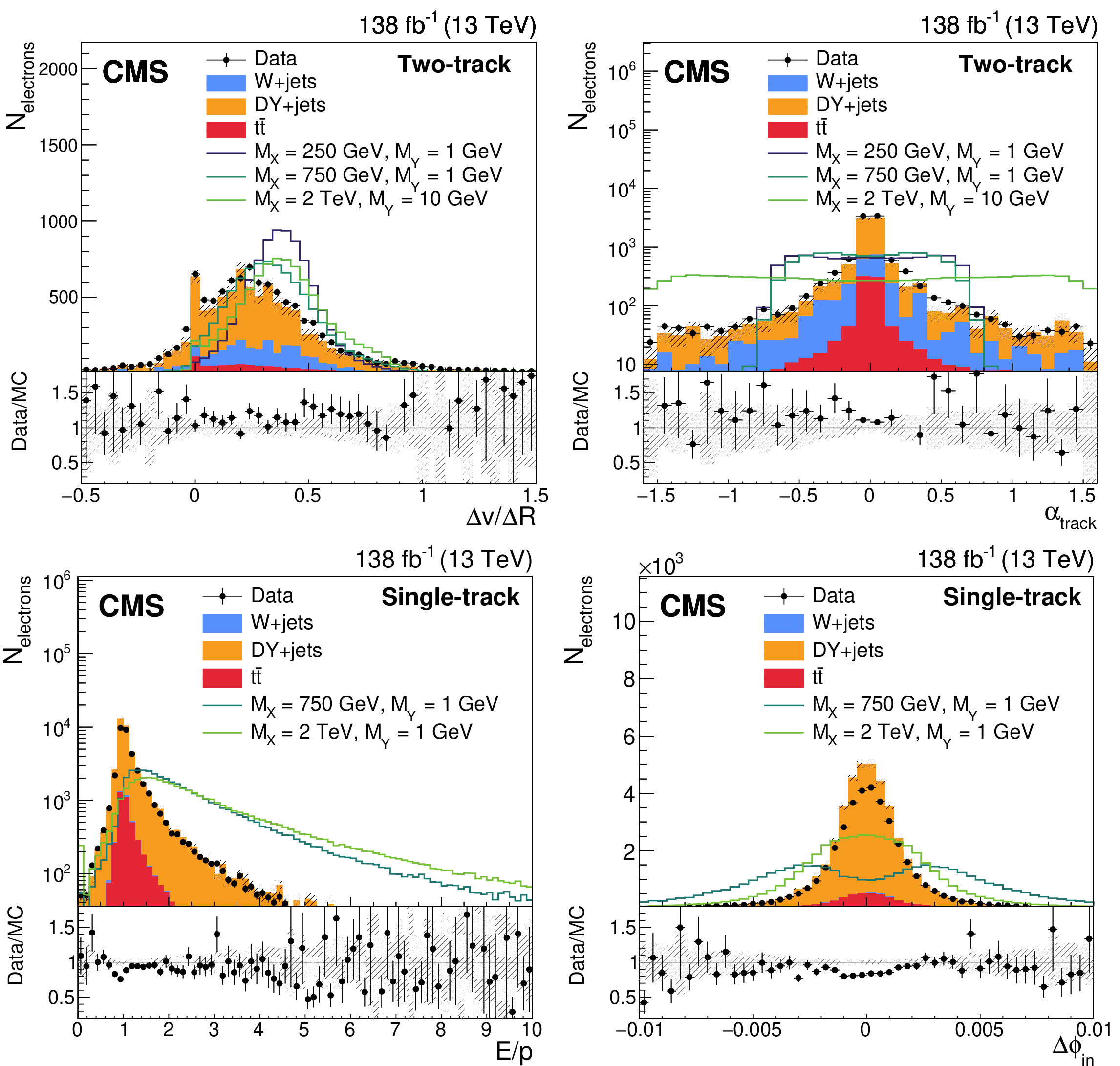
Figure 2:
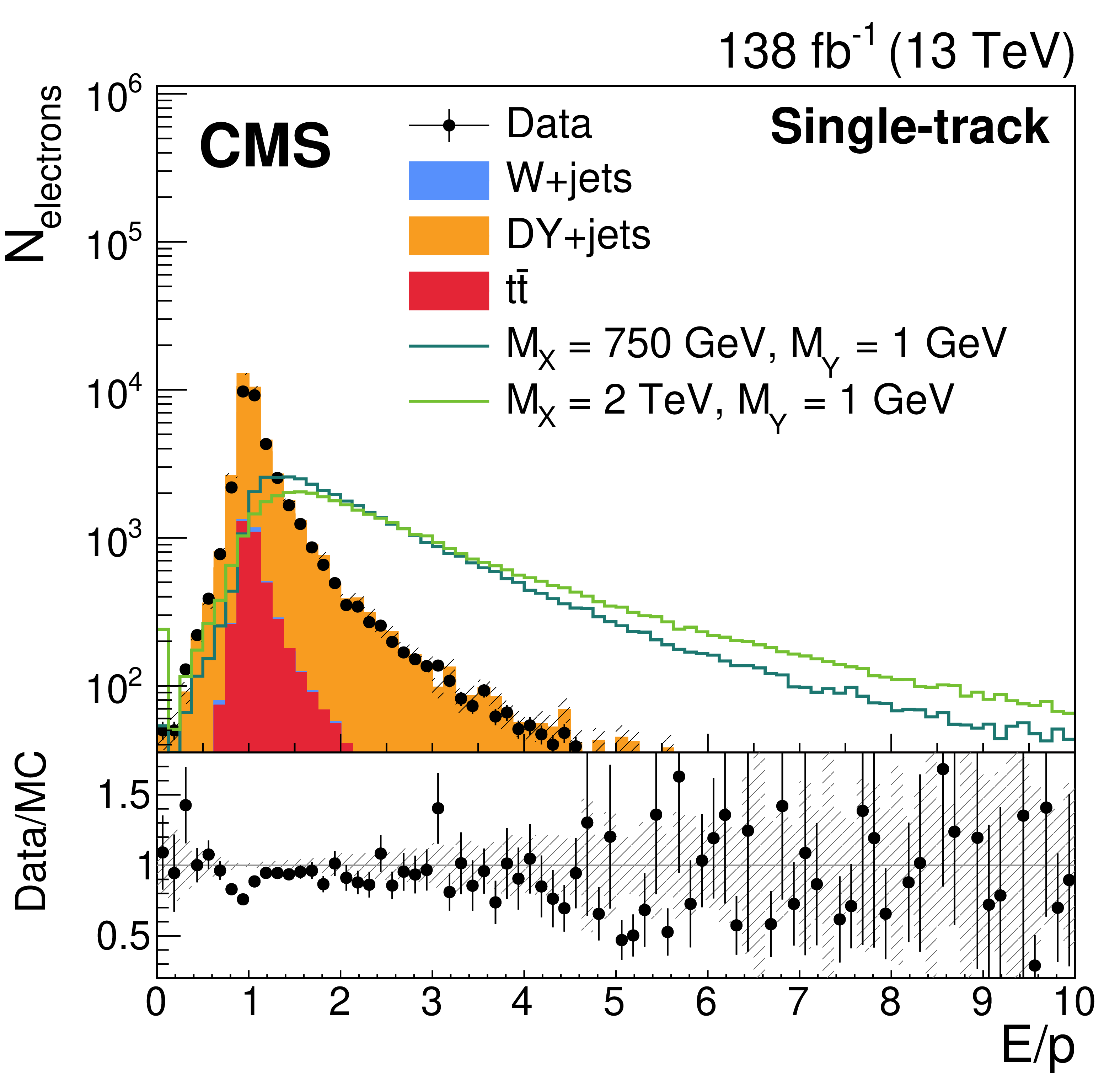
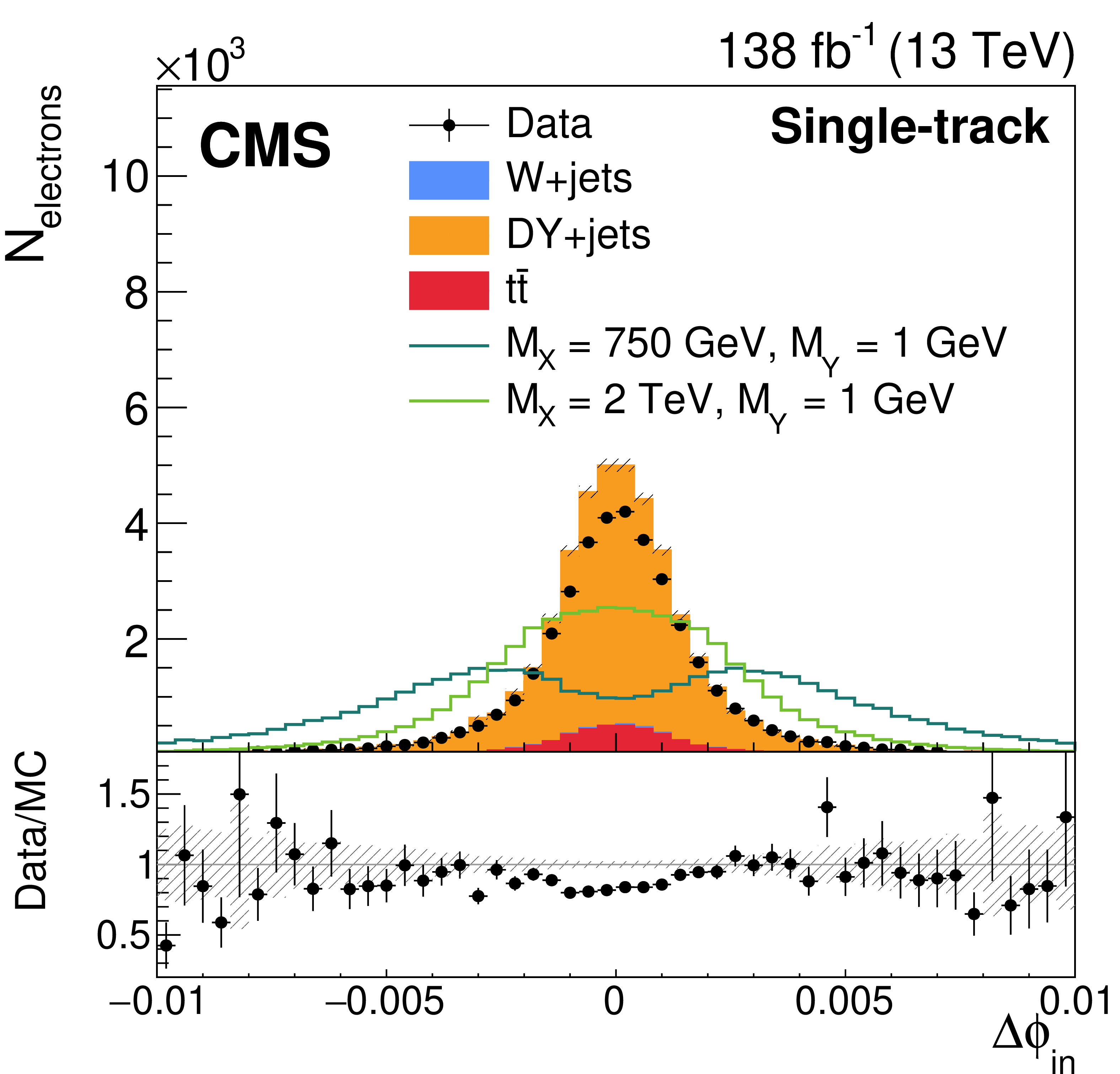
The distribution of the two most contributing variables for the (upper) two-track and (lower) single-track models: (upper left) $ \Delta v/\Delta R $, (upper right) $ \alpha_{\text{track}} $, (lower left) $ E/p $, and (lower right) \dXIn\phi. The signal samples are displayed according to the resonance masses that match the model. The vertical bar and shaded band represent the statistical uncertainty of the data and MC simulation, respectively. Each lined signal histogram is normalized to the background yield. |
png pdf |
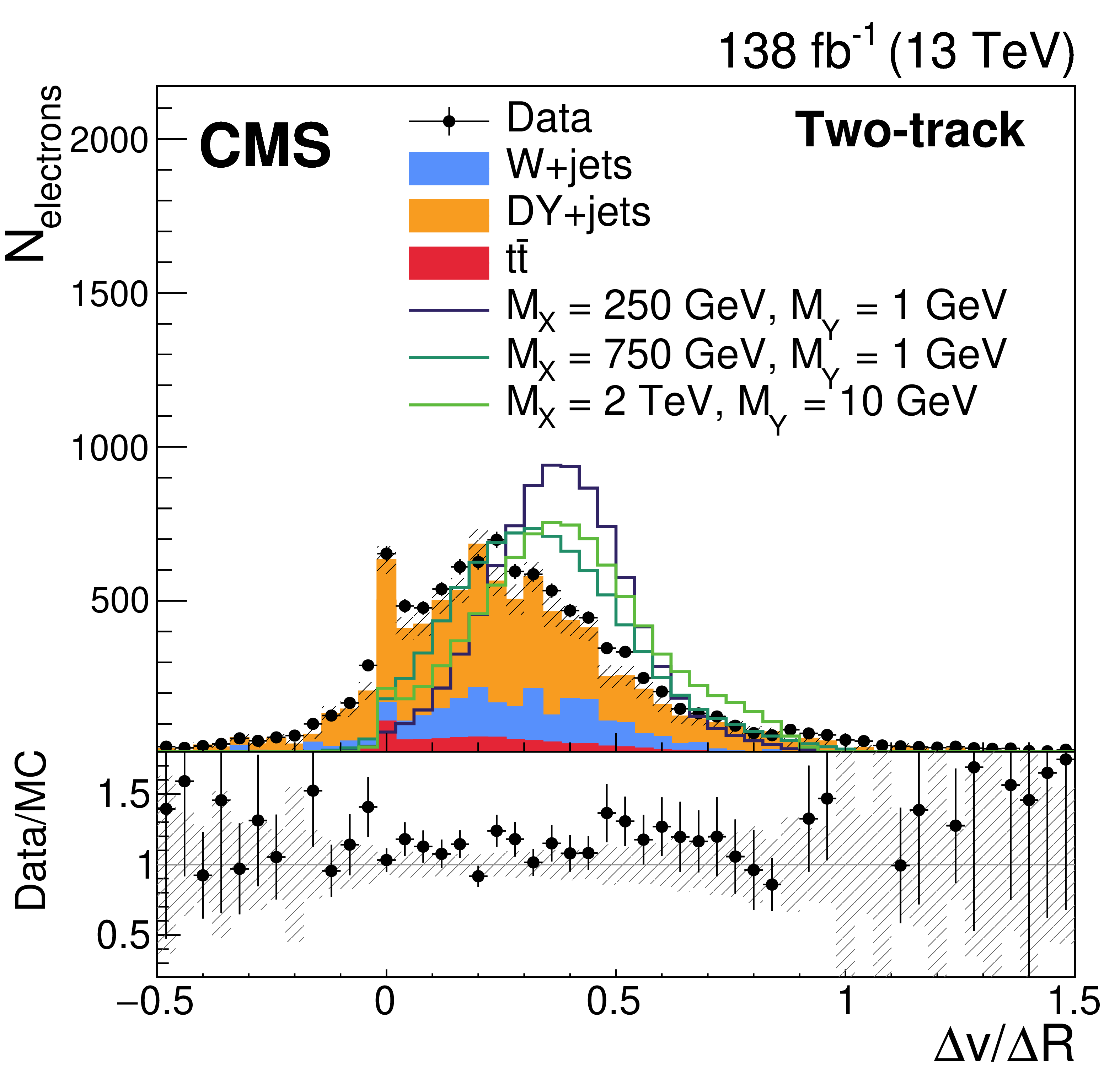
Figure 2-a:
The distribution of the two most contributing variables for the (upper) two-track and (lower) single-track models: (upper left) $ \Delta v/\Delta R $, (upper right) $ \alpha_{\text{track}} $, (lower left) $ E/p $, and (lower right) \dXIn\phi. The signal samples are displayed according to the resonance masses that match the model. The vertical bar and shaded band represent the statistical uncertainty of the data and MC simulation, respectively. Each lined signal histogram is normalized to the background yield. |
png pdf |
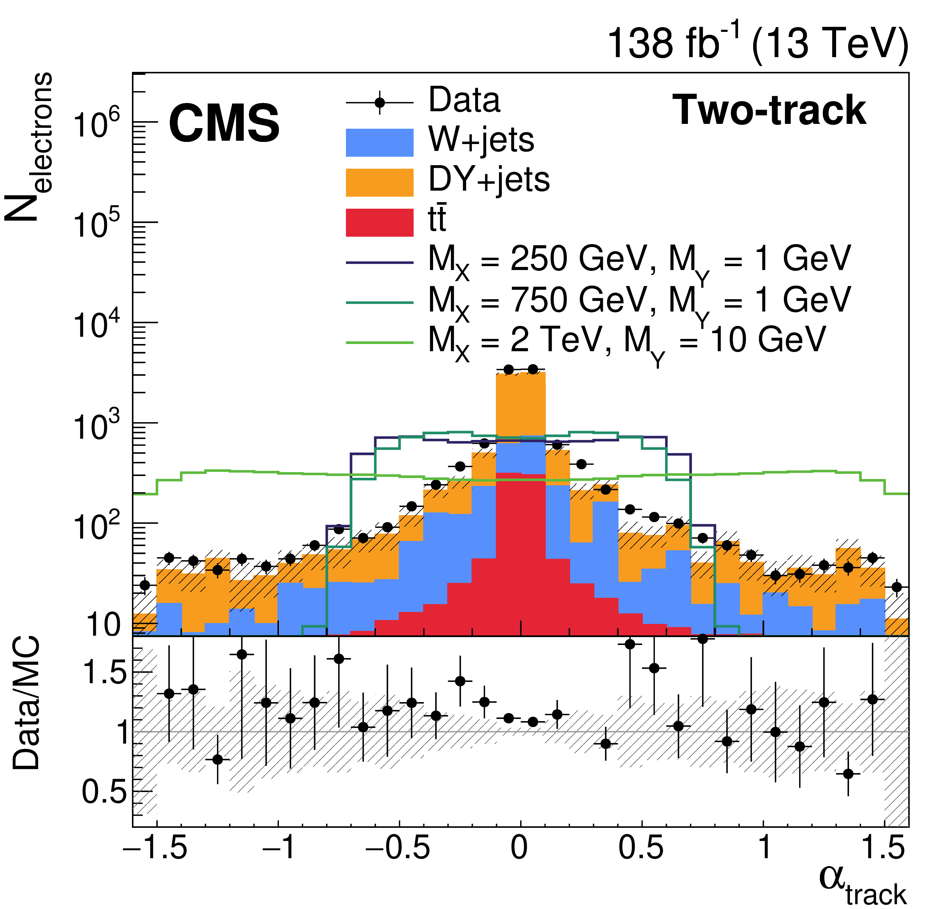
Figure 2-b:
The distribution of the two most contributing variables for the (upper) two-track and (lower) single-track models: (upper left) $ \Delta v/\Delta R $, (upper right) $ \alpha_{\text{track}} $, (lower left) $ E/p $, and (lower right) \dXIn\phi. The signal samples are displayed according to the resonance masses that match the model. The vertical bar and shaded band represent the statistical uncertainty of the data and MC simulation, respectively. Each lined signal histogram is normalized to the background yield. |
png pdf |
Figure 2-c:
The distribution of the two most contributing variables for the (upper) two-track and (lower) single-track models: (upper left) $ \Delta v/\Delta R $, (upper right) $ \alpha_{\text{track}} $, (lower left) $ E/p $, and (lower right) \dXIn\phi. The signal samples are displayed according to the resonance masses that match the model. The vertical bar and shaded band represent the statistical uncertainty of the data and MC simulation, respectively. Each lined signal histogram is normalized to the background yield. |
png pdf |
Figure 2-d:
The distribution of the two most contributing variables for the (upper) two-track and (lower) single-track models: (upper left) $ \Delta v/\Delta R $, (upper right) $ \alpha_{\text{track}} $, (lower left) $ E/p $, and (lower right) \dXIn\phi. The signal samples are displayed according to the resonance masses that match the model. The vertical bar and shaded band represent the statistical uncertainty of the data and MC simulation, respectively. Each lined signal histogram is normalized to the background yield. |
png pdf |
Figure 3:
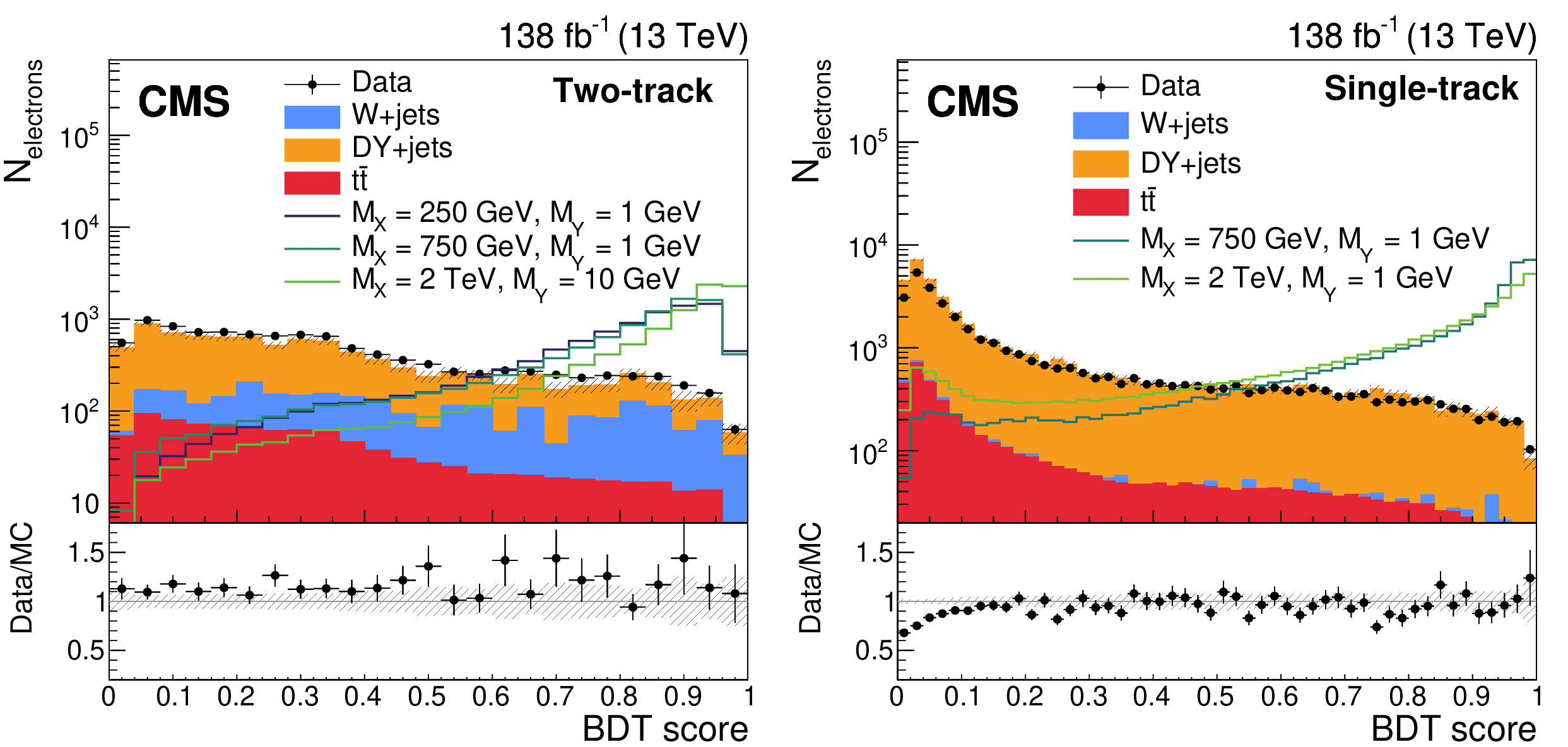
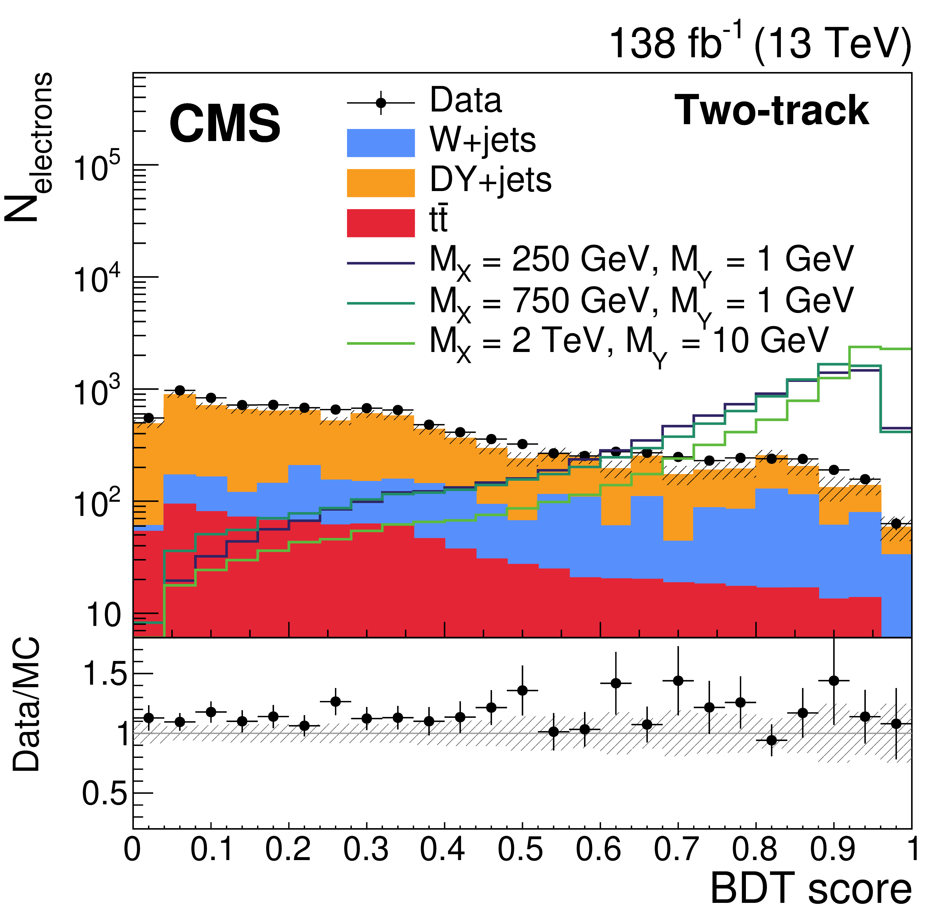
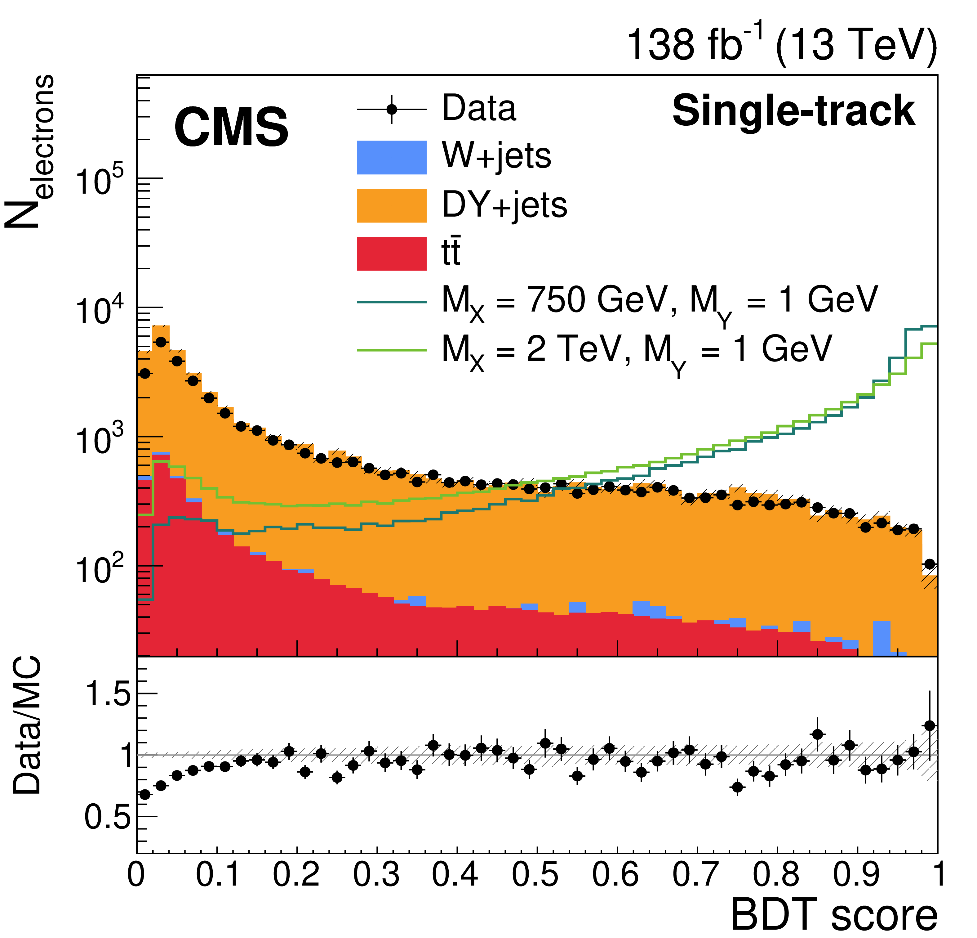
The BDT score distributions of the (left) two-track and (right) single-track models. The signal samples are displayed according to the resonance masses that match the model. The vertical bar and shaded band represent the statistical uncertainty of the data and MC simulation, respectively. Each lined signal histogram is normalized to the background yield. |
png pdf |
Figure 3-a:
The BDT score distributions of the (left) two-track and (right) single-track models. The signal samples are displayed according to the resonance masses that match the model. The vertical bar and shaded band represent the statistical uncertainty of the data and MC simulation, respectively. Each lined signal histogram is normalized to the background yield. |
png pdf |
Figure 3-b:
The BDT score distributions of the (left) two-track and (right) single-track models. The signal samples are displayed according to the resonance masses that match the model. The vertical bar and shaded band represent the statistical uncertainty of the data and MC simulation, respectively. Each lined signal histogram is normalized to the background yield. |
png pdf |
Figure 4:
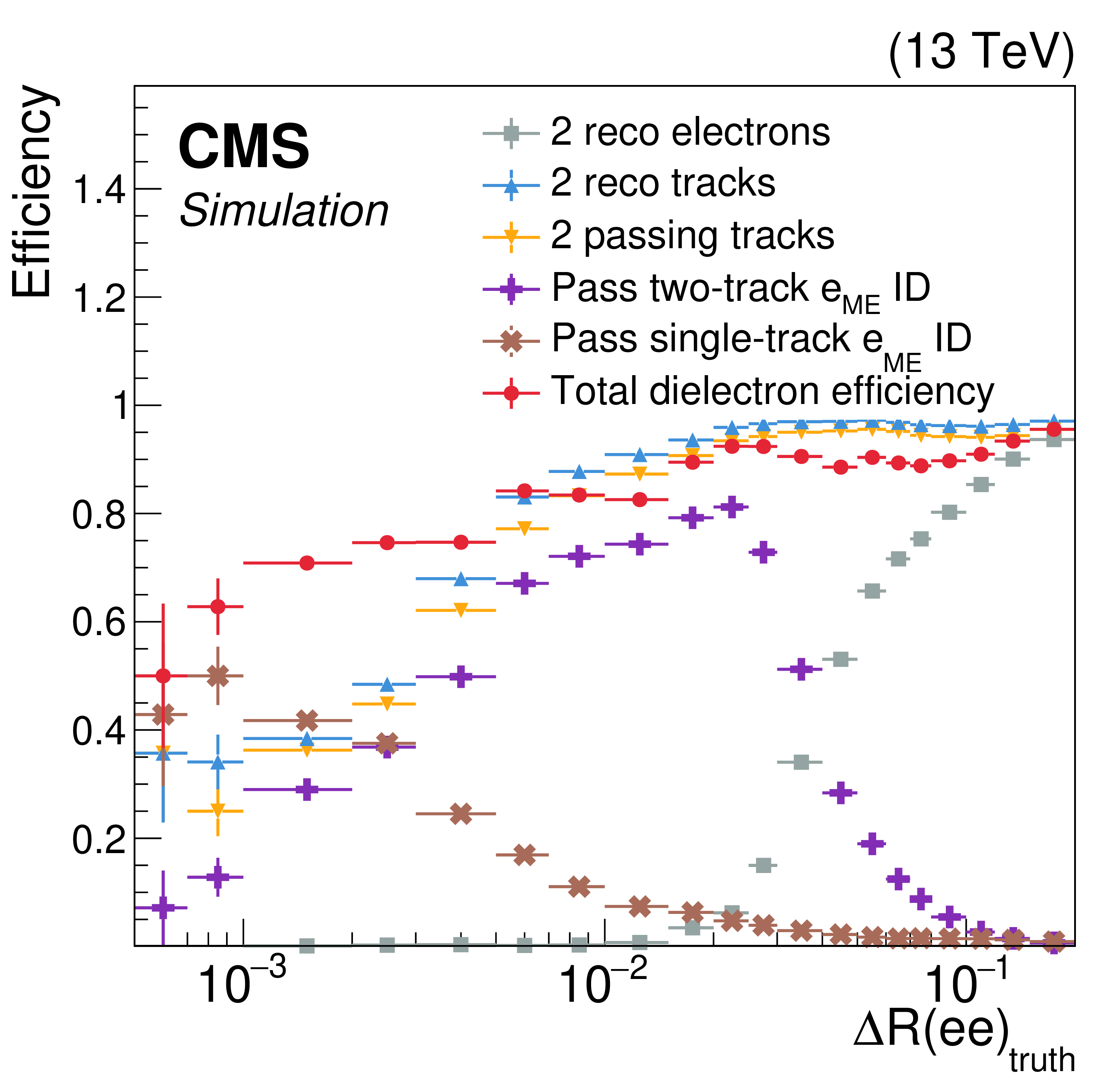
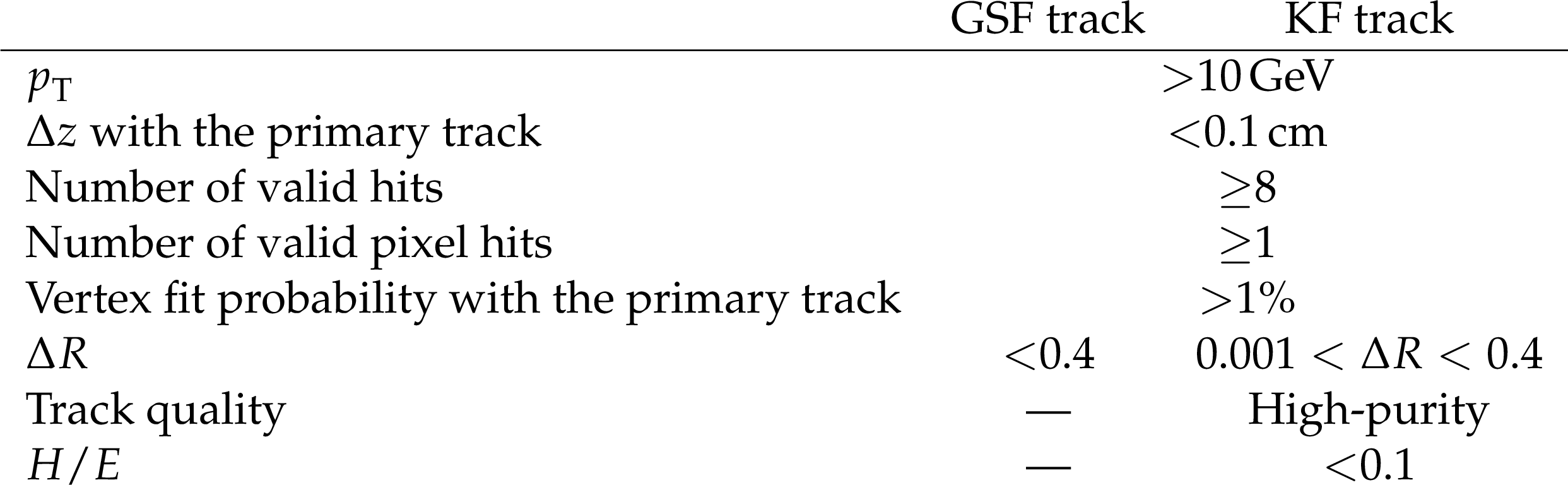
The signal dielectron selection efficiency as a function of $ \Delta R $. The vertical error bar represents the statistical uncertainty. An equal number of signal events with $ m_{\mathrm{X}} = $ 250, 750, 2000 GeV and $ m_{\mathrm{Y}} = $ 1, 10 GeV are used for each mass point to incorporate dielectrons with various $ \Delta R $. The ID efficiencies include the effects of all prerequisite selections. For instance, the $ \mathrm{e}_{\mathrm{ME}} $ ID efficiency with two tracks (purple) includes the efficiency of the track selection described in Table 1 (yellow). The total dielectron efficiency is a sum of the two-track (purple) and single-track (brown) $ \mathrm{e}_{\mathrm{ME}} $ ID efficiencies, and the standard reconstruction efficiency of two electrons (gray). |
png pdf |
Figure 5:
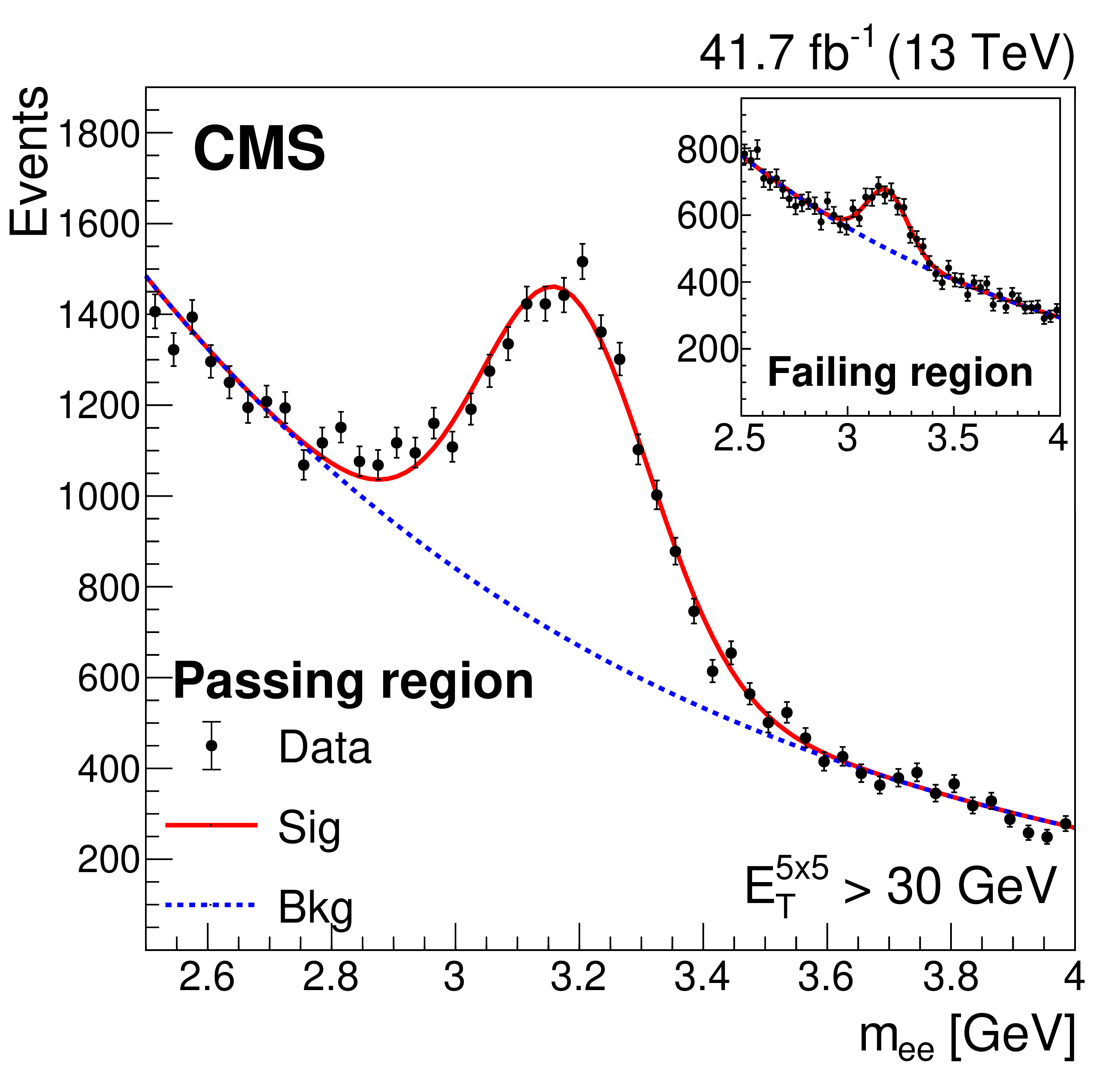
The nominal dielectron mass distribution of $ \mathrm{J}/\psi $ candidates in the $ {\mathrm{B}} $ Parking dataset with $ E_{\mathrm{T}}^{5\times5} > $ 30 GeV that pass or fail the two-track $ \mathrm{e}_{\mathrm{ME}} $ ID. The dielectron mass is reconstructed using the tracks of electron candidates. |
png pdf |
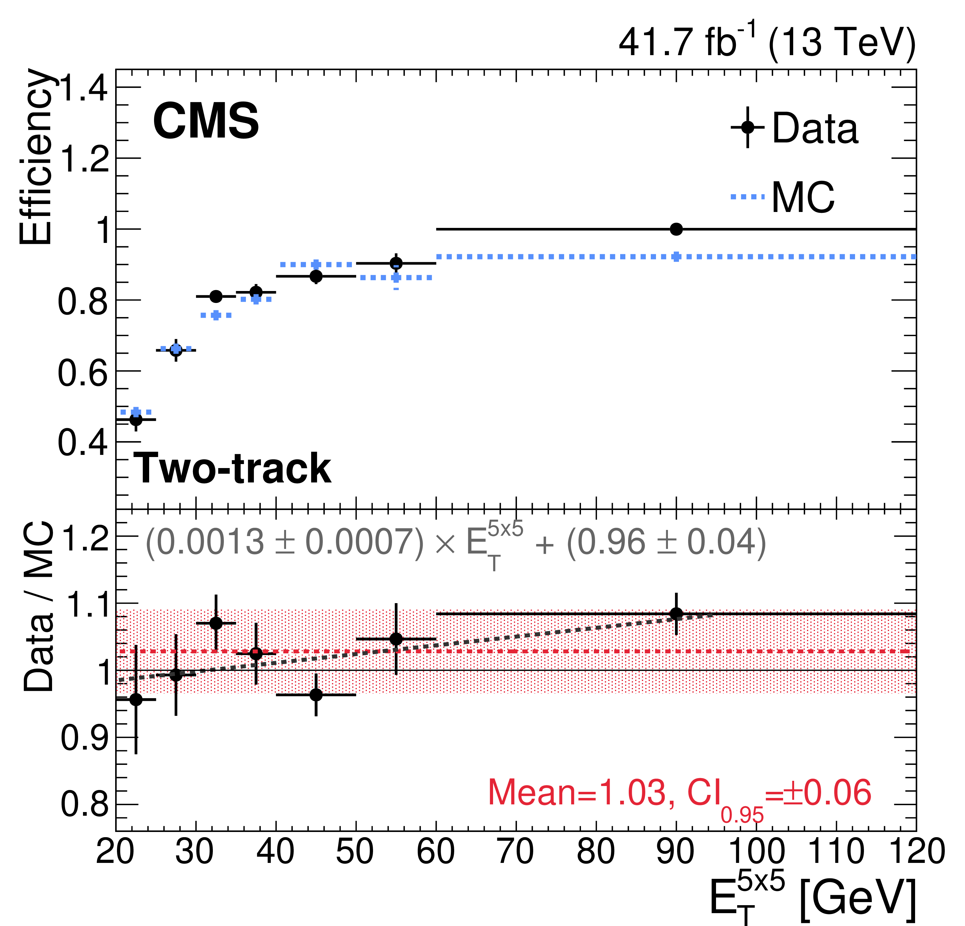
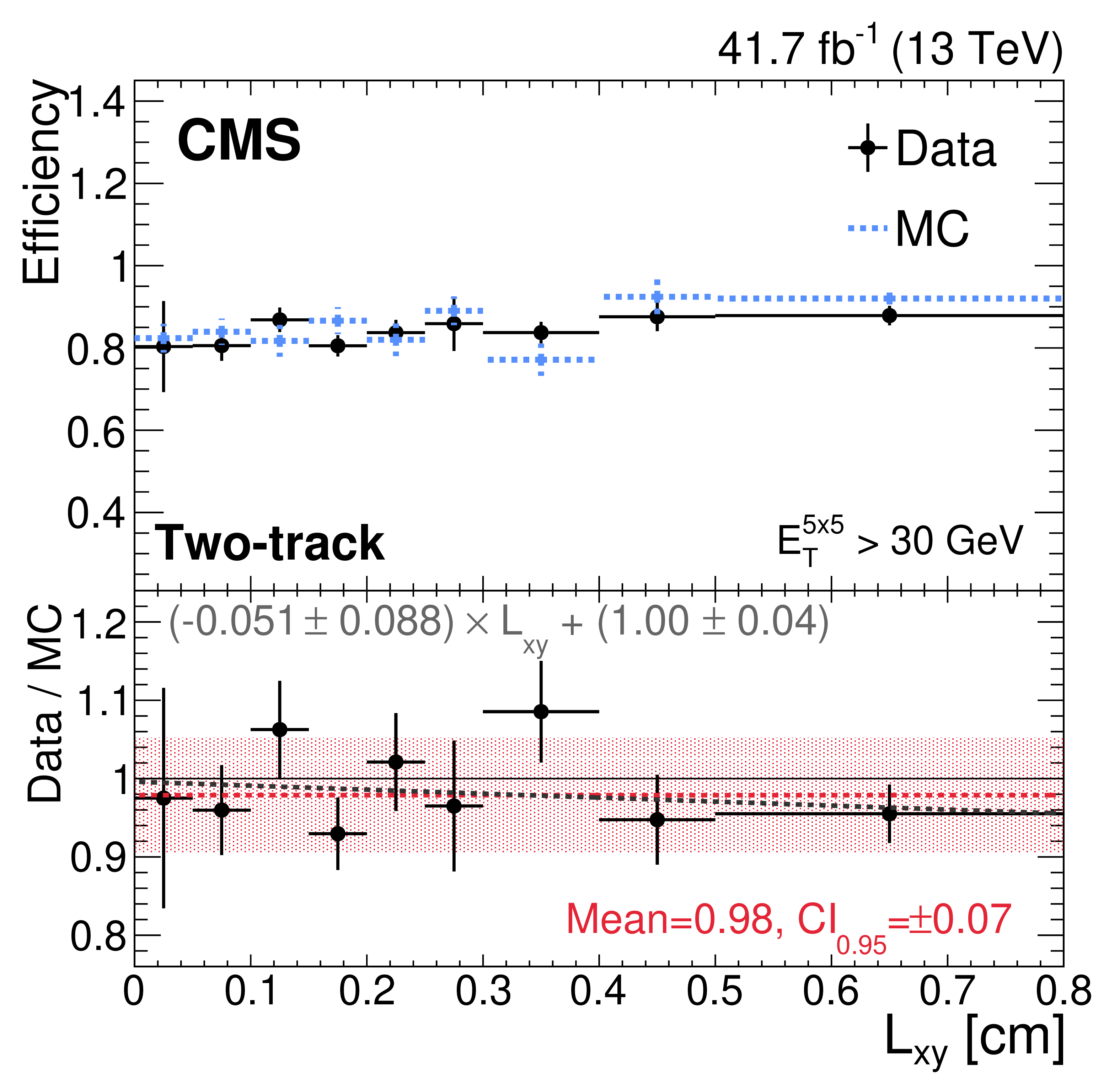
Figure 6:
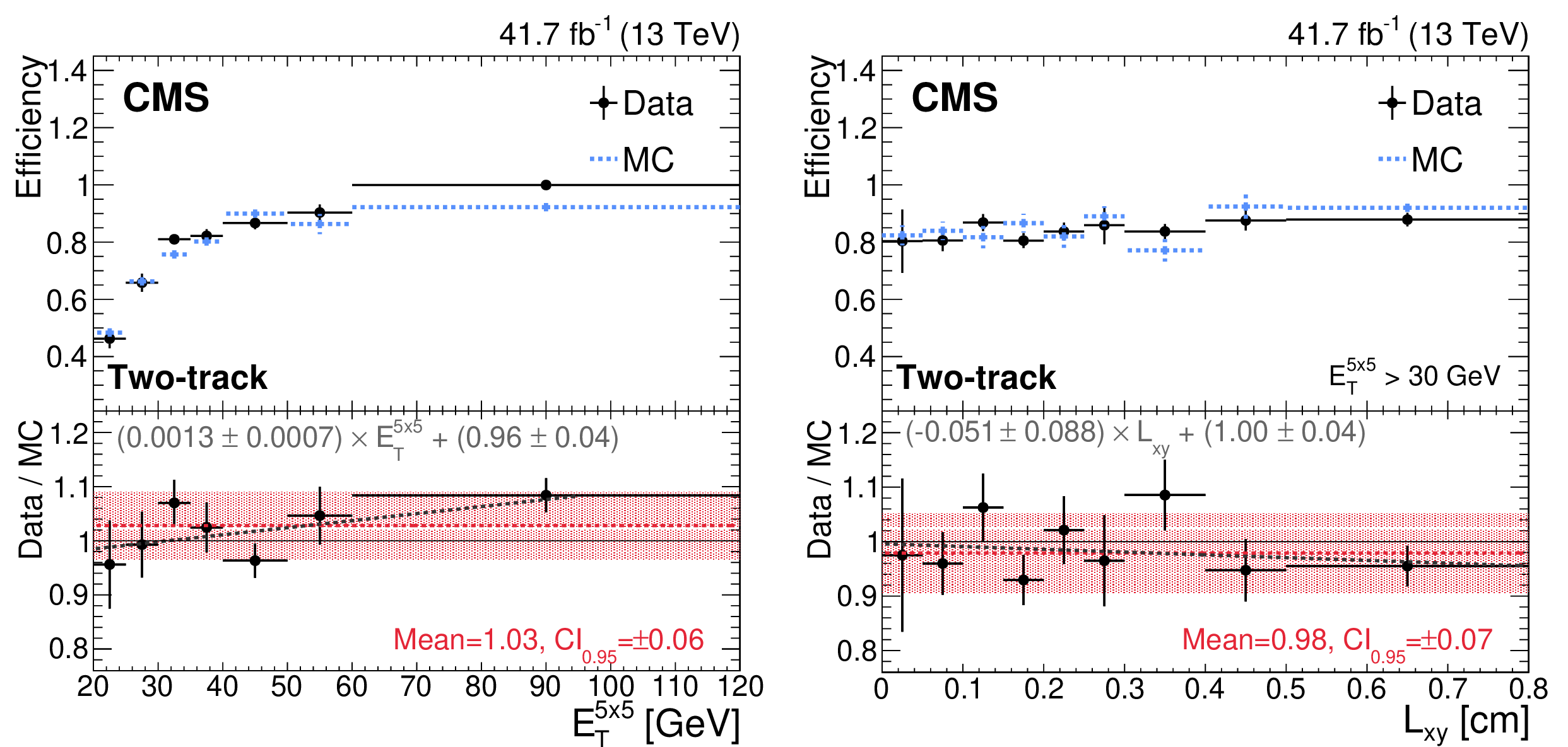
The efficiency and SF for the two-track model as a function of (left) $ E_{\mathrm{T}}^{5\times5} $ and (right) $ L_{xy} $ with $ E_{\mathrm{T}}^{5\times5} > $ 30 GeV. The vertical bar shows the statistical and systematic uncertainties from the alternative fits, summed in quadrature. The shaded band depicts the $ \mathrm{CI}_{0.95} $. The red and gray dashed lines depict the constant and first-order polynomial fits, respectively. |
png pdf |
Figure 6-a:
The efficiency and SF for the two-track model as a function of (left) $ E_{\mathrm{T}}^{5\times5} $ and (right) $ L_{xy} $ with $ E_{\mathrm{T}}^{5\times5} > $ 30 GeV. The vertical bar shows the statistical and systematic uncertainties from the alternative fits, summed in quadrature. The shaded band depicts the $ \mathrm{CI}_{0.95} $. The red and gray dashed lines depict the constant and first-order polynomial fits, respectively. |
png pdf |
Figure 6-b:
The efficiency and SF for the two-track model as a function of (left) $ E_{\mathrm{T}}^{5\times5} $ and (right) $ L_{xy} $ with $ E_{\mathrm{T}}^{5\times5} > $ 30 GeV. The vertical bar shows the statistical and systematic uncertainties from the alternative fits, summed in quadrature. The shaded band depicts the $ \mathrm{CI}_{0.95} $. The red and gray dashed lines depict the constant and first-order polynomial fits, respectively. |
png pdf |
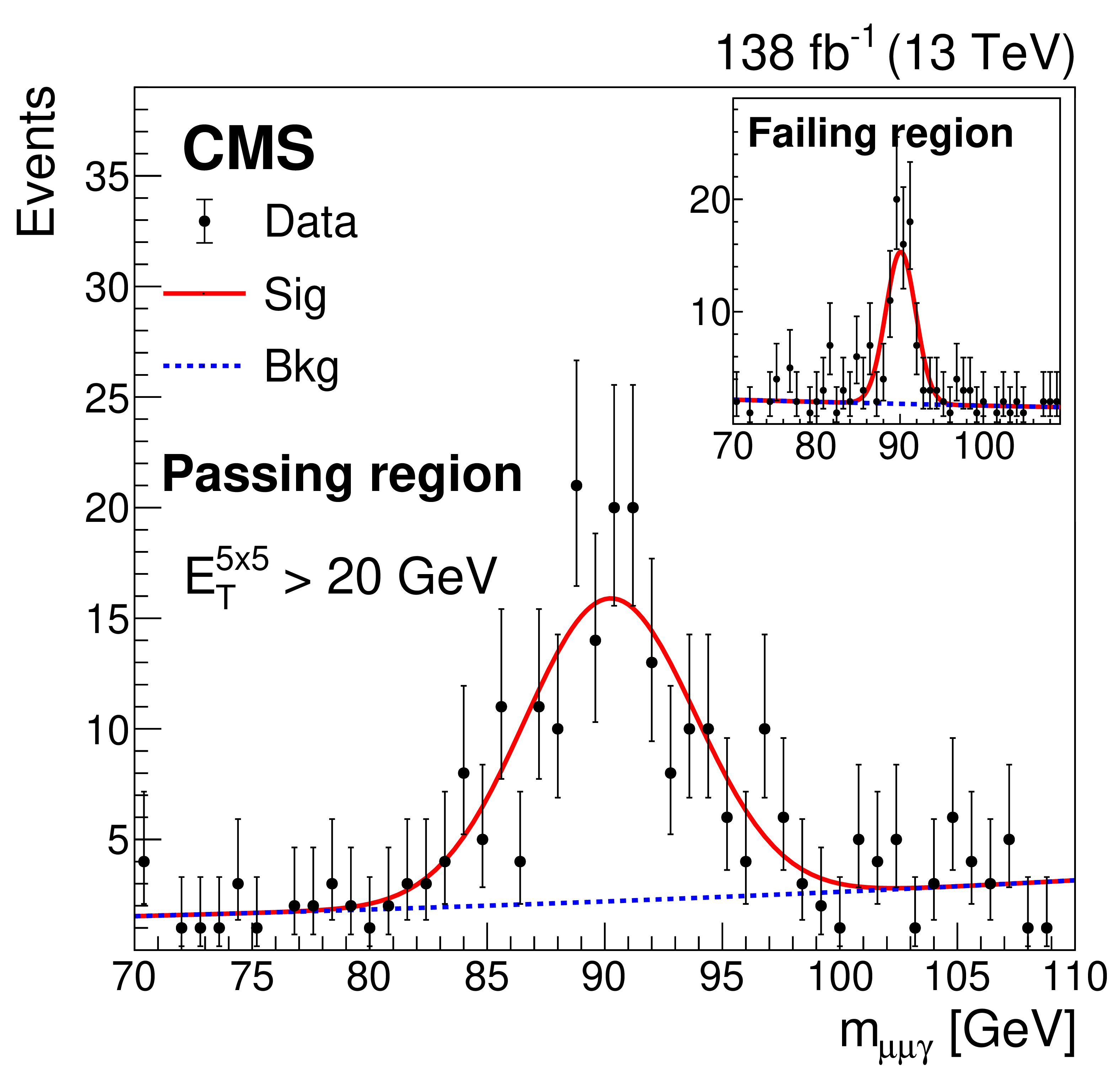
Figure 7:
The nominal Z boson candidate mass distribution in data using $ \mu^{+}\mu^{-}\gamma $ events with $ E_{\mathrm{T}}^{5\times5} > $ 20 GeV. The passing and failing regions represent the Z boson candidate mass distributions with $ \mathrm{e}_{\mathrm{ME}} $ candidates that pass or fail the $ \mathrm{e}_{\mathrm{ME}} $ ID. |
png pdf |
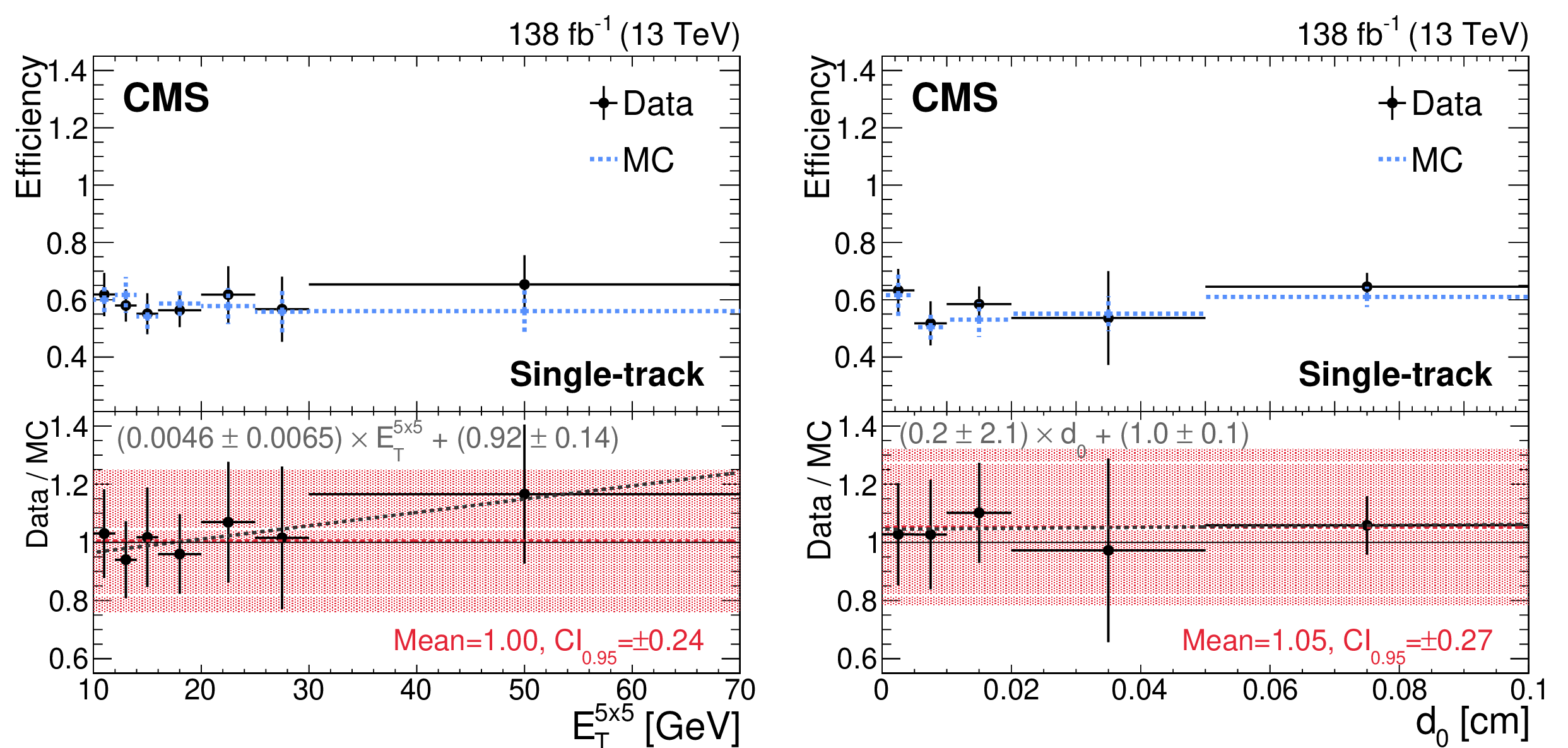
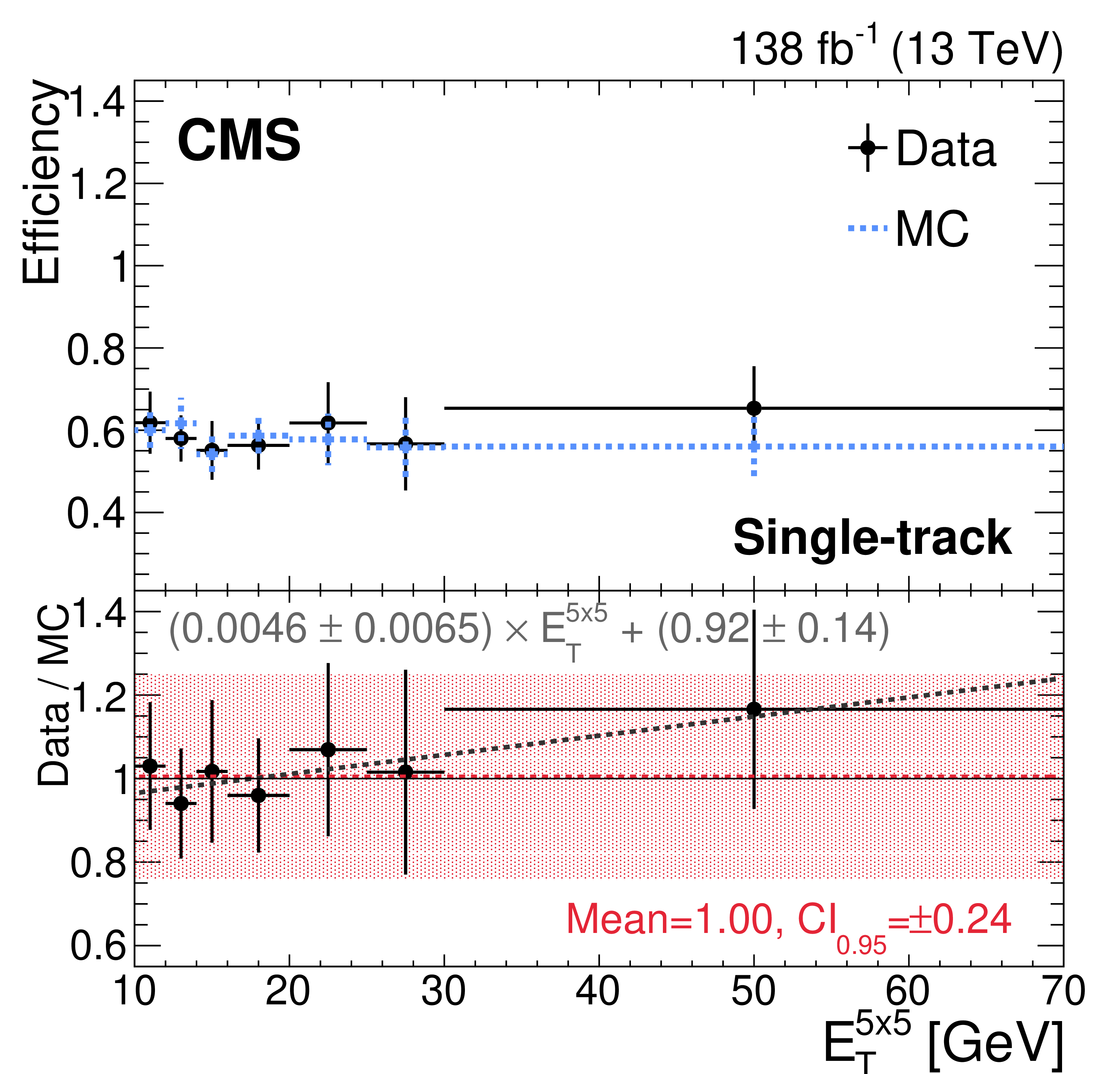
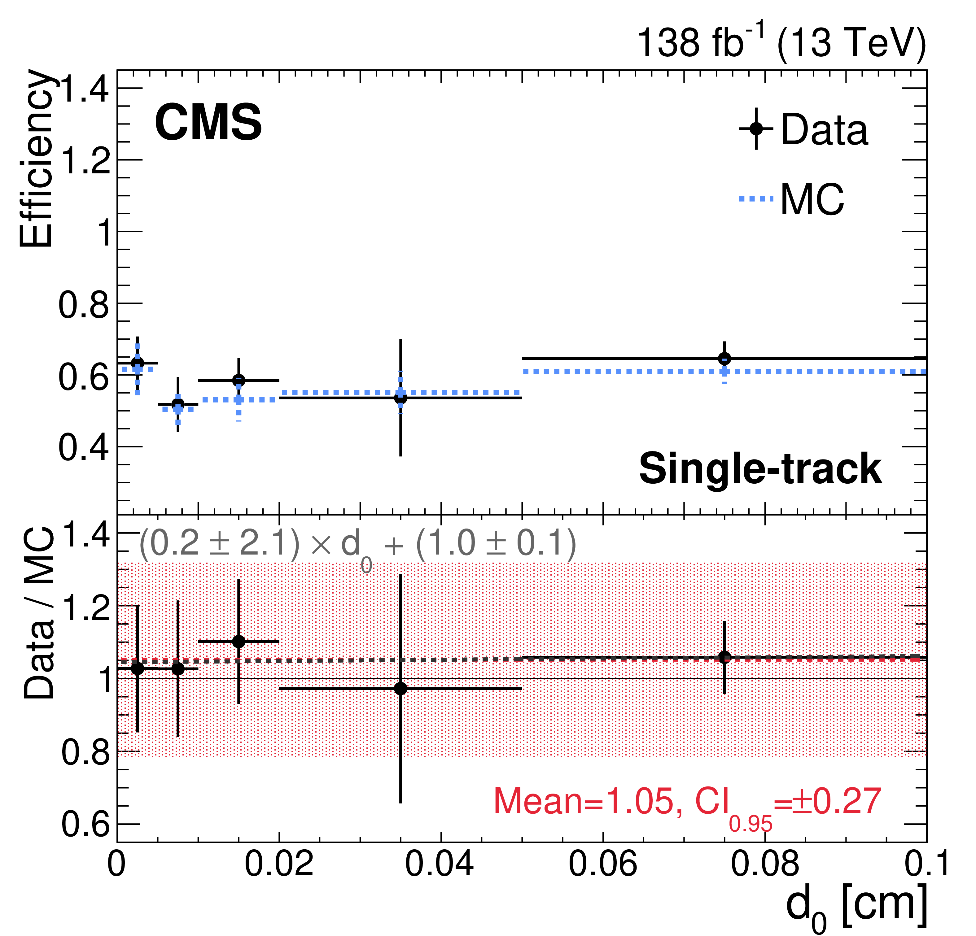
Figure 8:
The efficiency and SF as a function of (left) $ E_{\mathrm{T}}^{5\times5} $ and (right) $ d_{0} $ for the single-track model. The vertical bar shows the statistical and systematic uncertainties from the alternative fits, summed in quadrature. The shaded band depicts the $ \mathrm{CI}_{0.95} $. The red and gray dashed lines depict the constant and first-order polynomial fits, respectively. |
png pdf |
Figure 8-a:
The efficiency and SF as a function of (left) $ E_{\mathrm{T}}^{5\times5} $ and (right) $ d_{0} $ for the single-track model. The vertical bar shows the statistical and systematic uncertainties from the alternative fits, summed in quadrature. The shaded band depicts the $ \mathrm{CI}_{0.95} $. The red and gray dashed lines depict the constant and first-order polynomial fits, respectively. |
png pdf |
Figure 8-b:
The efficiency and SF as a function of (left) $ E_{\mathrm{T}}^{5\times5} $ and (right) $ d_{0} $ for the single-track model. The vertical bar shows the statistical and systematic uncertainties from the alternative fits, summed in quadrature. The shaded band depicts the $ \mathrm{CI}_{0.95} $. The red and gray dashed lines depict the constant and first-order polynomial fits, respectively. |
png pdf |
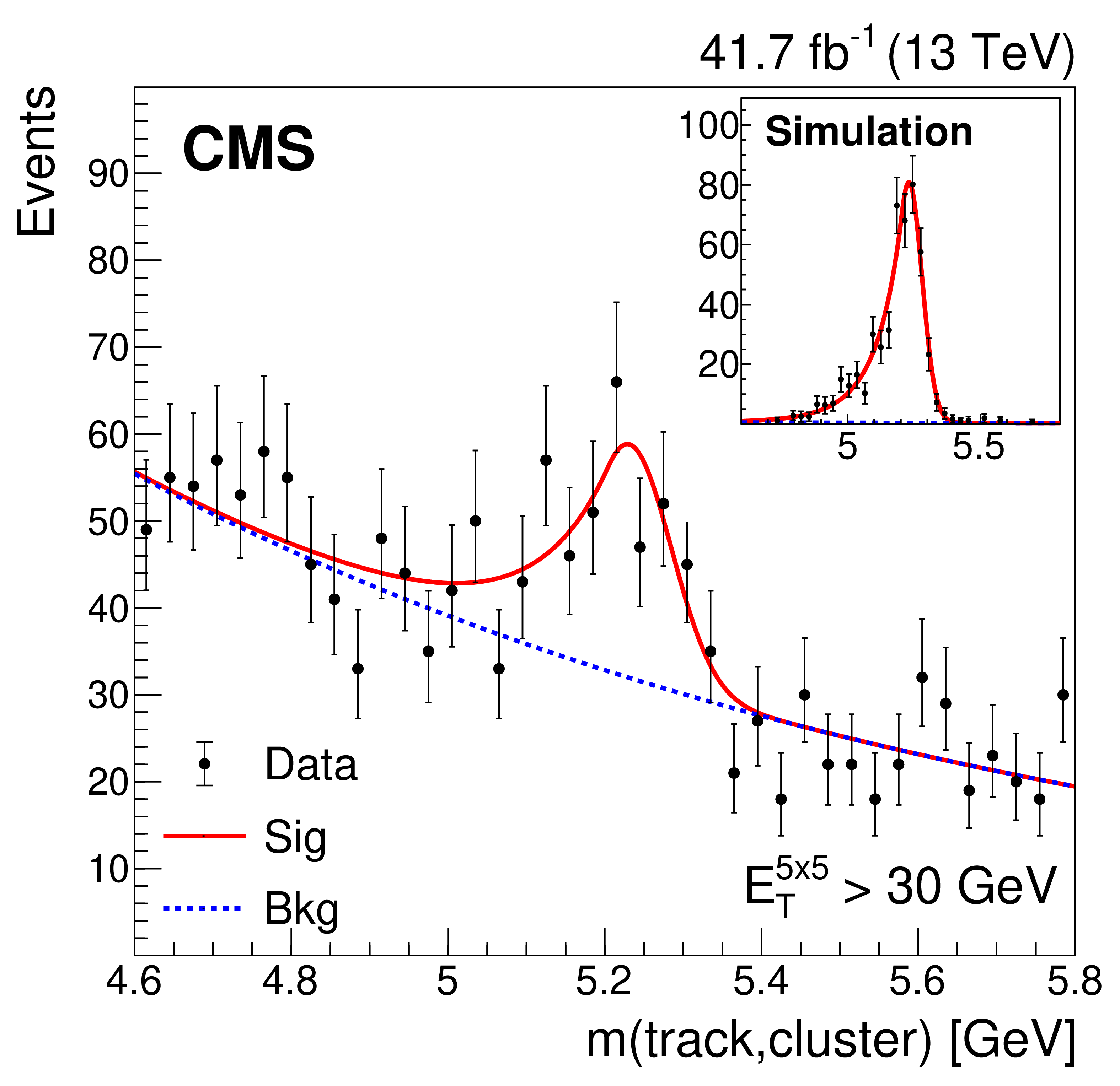
Figure 9:
The distribution of the invariant mass between the $ \mathrm{U}_{5\times5} $ cluster and the kaon candidate with $ E_{\mathrm{T}}^{5\times5} > $ 30 GeV. The vertical bar shows the statistical uncertainty. The signal (background) contribution is modeled with a Crystal Ball (exponential) function, represented with a red (blue) line. The inset on top right illustrates the mass distribution in a $ {\mathrm{B}^{\pm}}\to\mathrm{J}/\psi\mathrm{K^{\pm}}\to\mathrm{e}^+\mathrm{e}^-\mathrm{K^{\pm}} $ MC sample. |
| Tables | |
png pdf |
Table 1:
Secondary track selection criteria |
png pdf |
Table 2:
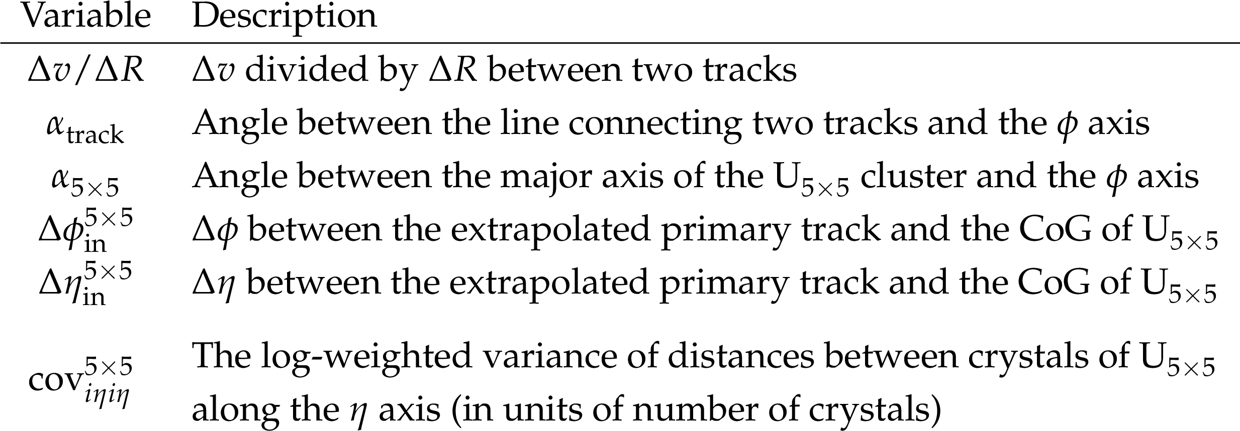
List of variables used to train the two-track model |
png pdf |
Table 3:
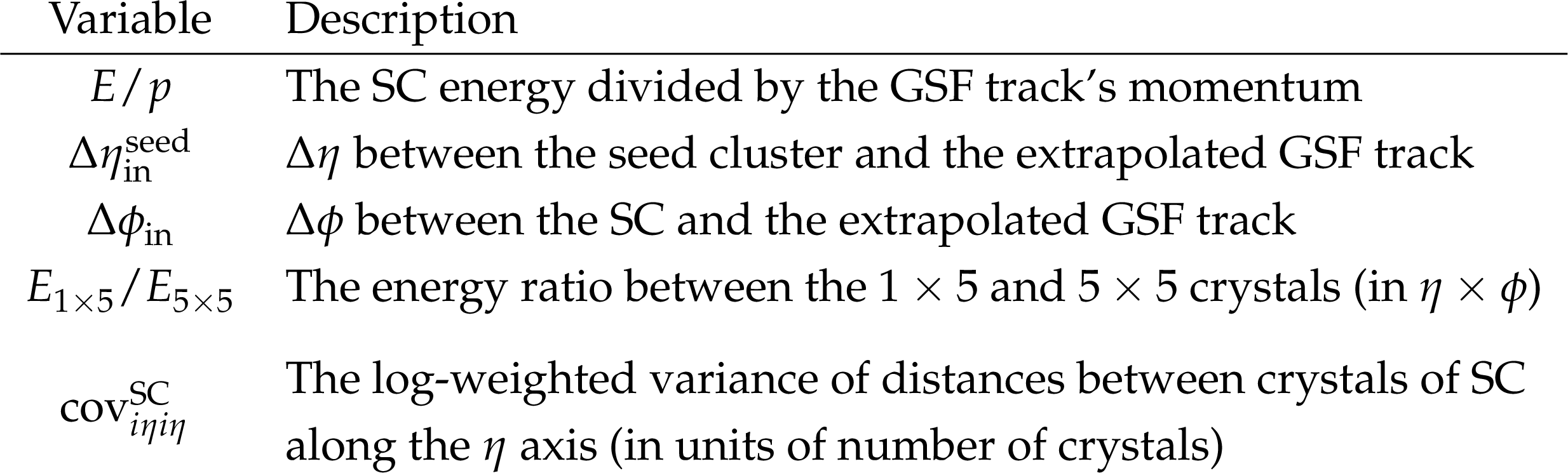
List of variables used to train the single-track model |
png pdf |
Table 4:
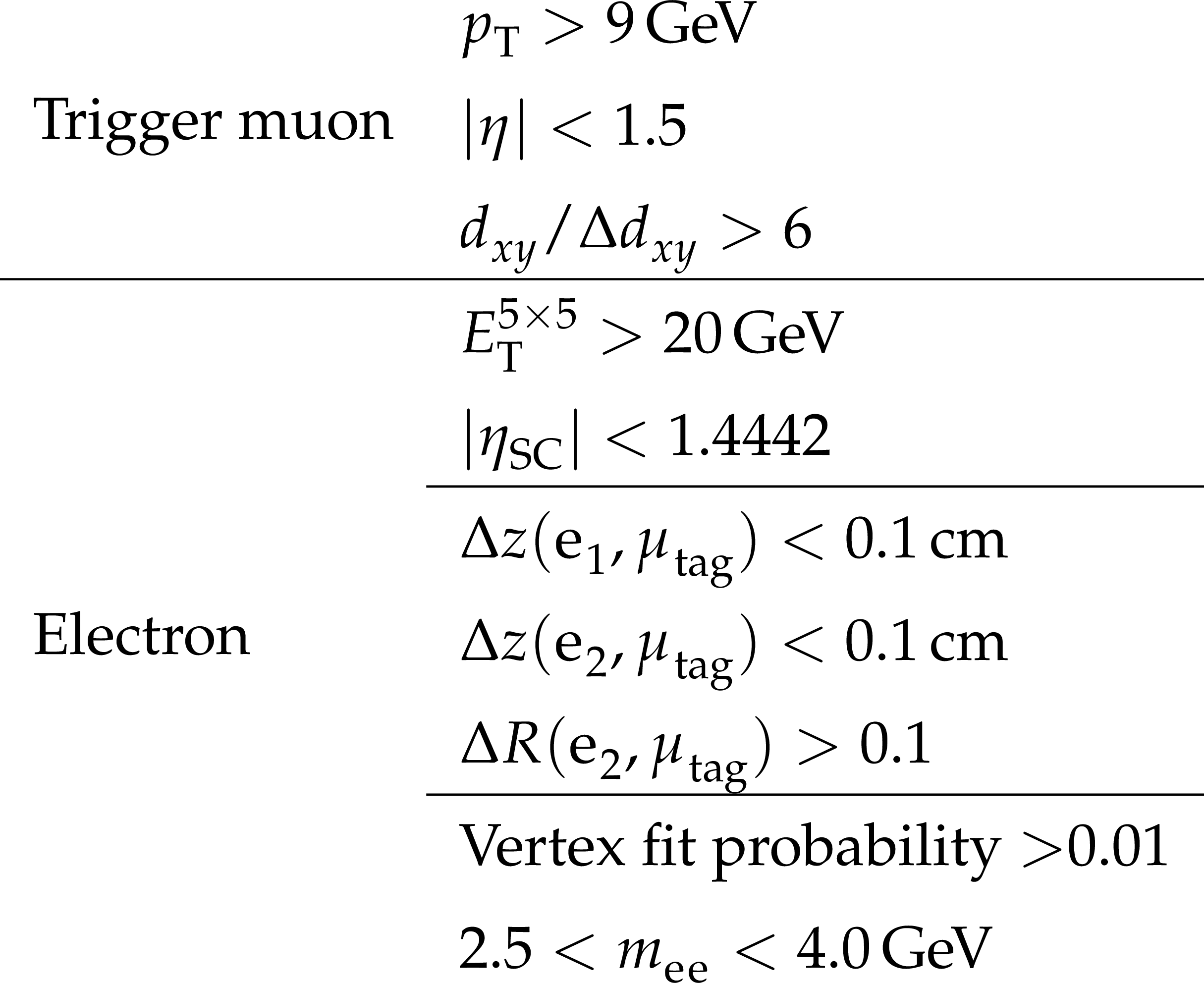
Selection criteria for the $ \mathrm{J}/\psi\to\mathrm{e}^+\mathrm{e}^- $ control region. |
png pdf |
Table 5:
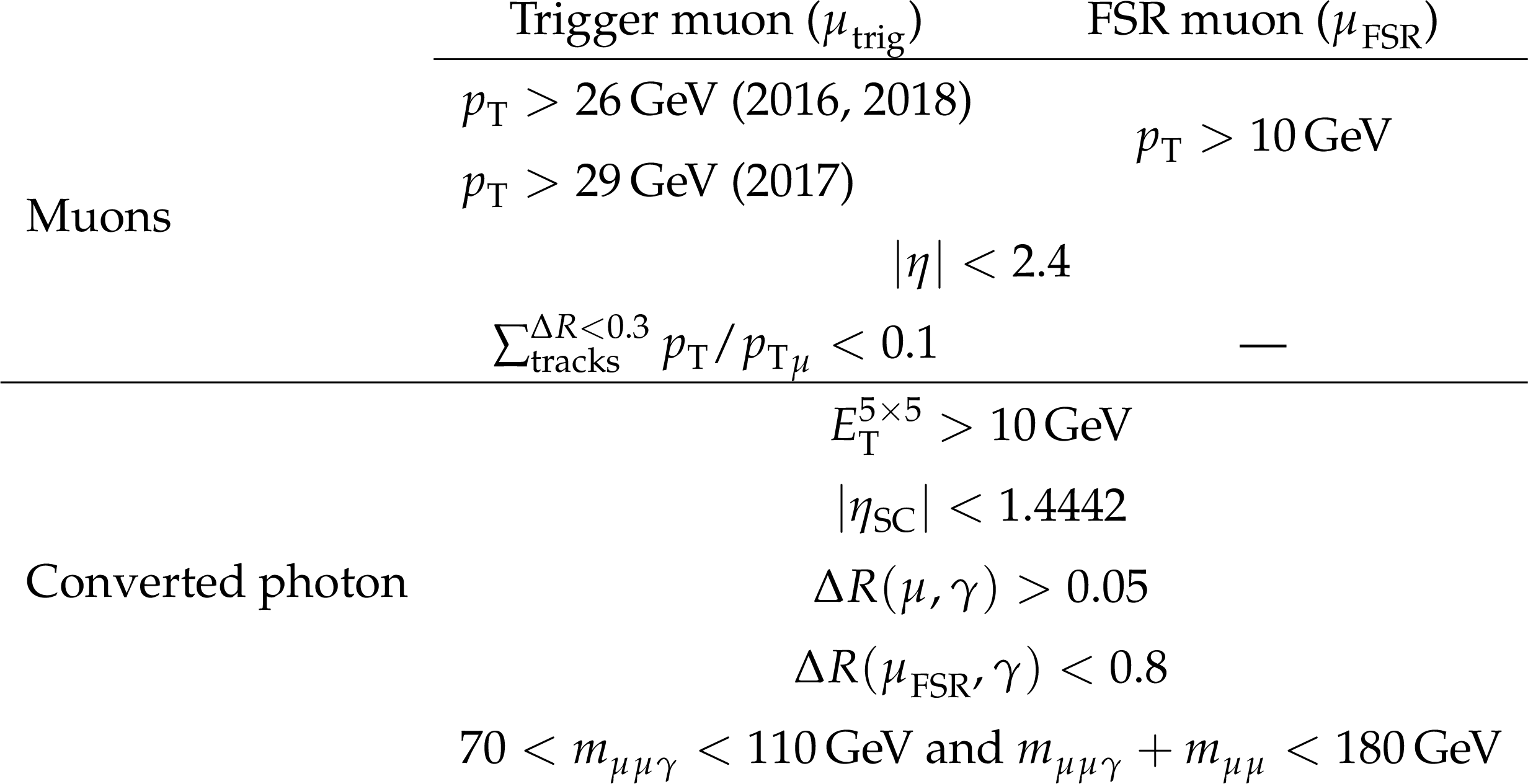
Selection criteria for the $ \mathrm{Z}\to\mu^{+}\mu^{-}\gamma $ control region. |
png pdf |
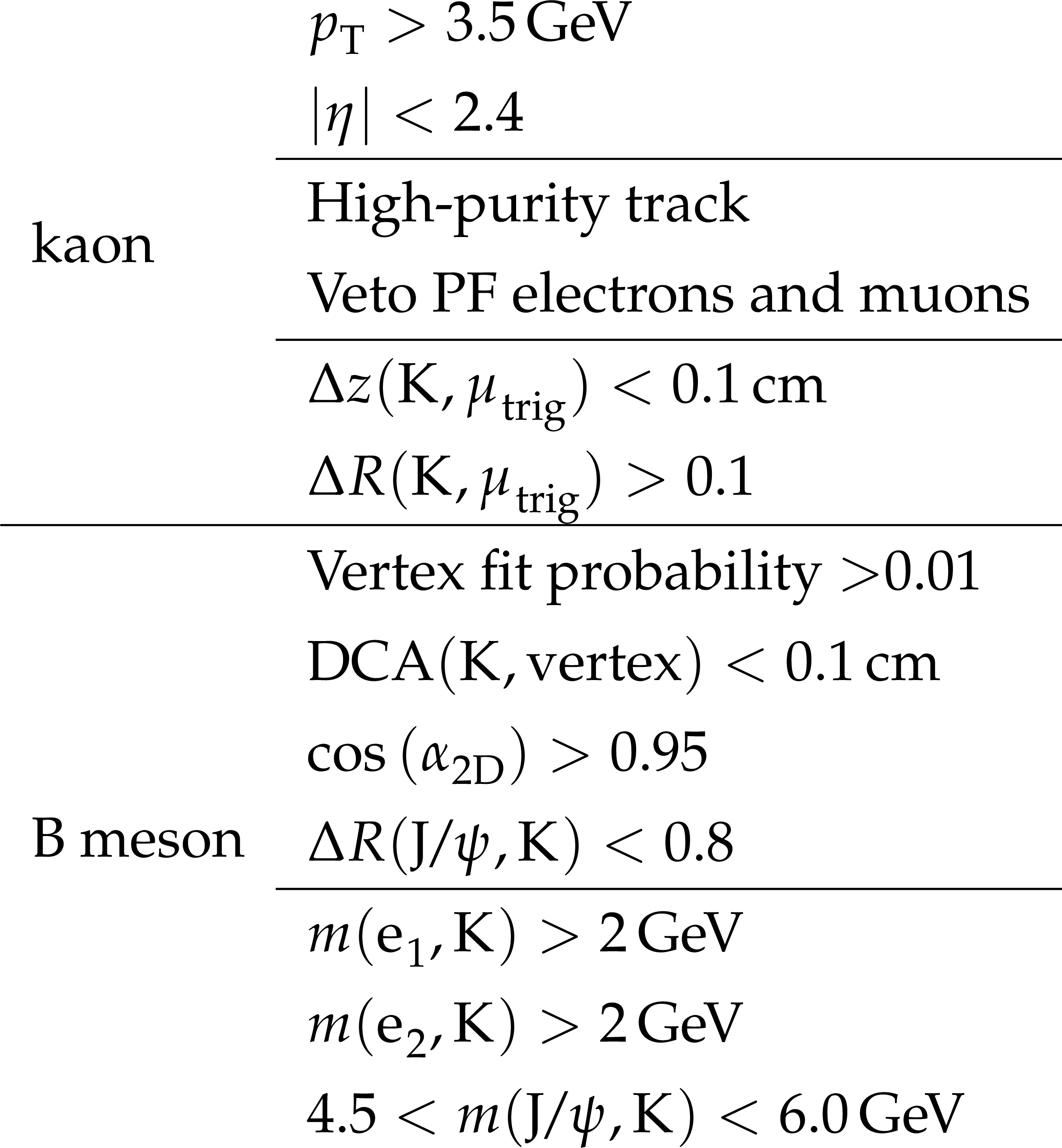
Table 6:
Selection criteria (in addition to Table 4) for the $ {\mathrm{B}^{\pm}}\to\mathrm{J}/\psi\mathrm{K^{\pm}}\to\mathrm{e}^+\mathrm{e}^-\mathrm{K^{\pm}} $ control region. |
| Summary |
| Theories of beyond the standard model physics predict light bosons that subsequently decay into a dielectron ($ \mathrm{e}^+\mathrm{e}^- $). In such models, the light boson can be significantly boosted, and the standard clustering and reconstruction algorithm may fail to resolve the dielectron. The CMS standard electron reconstruction resolves about 5--40% of $ \mathrm{e}^+\mathrm{e}^- $ pairs when separated by $ \Delta R $ of 0.02--0.04, corresponding to 1--2 Moli\`ere radii, where $ \Delta R $ is defined as $ \Delta R\equiv\sqrt{\smash[b]{(\Delta\eta)^{2}+(\Delta\phi)^{2}}} $. Moreover, high Lorentz boosts can lead to the absence of either of the electron tracks due to shared hits in the inner tracker. Therefore, novel algorithms to identify merged electrons ($ \mathrm{e}_{\mathrm{ME}} $) are developed for the single-track and two-track cases, respectively. The two-track model is trained using a boosted decision tree based on the geometrical compatibility between the merged cluster and the electron tracks. The default clustering algorithm in the electromagnetic calorimeter does not capture all energy deposits from $ \mathrm{e}_{\mathrm{ME}} $ candidates. A cluster consisting of a union of the 5 $ \times $ 5 matrices of lead tungstate crystals around the two electron tracks ($ \mathrm{U}_{5\times5} $) is used to estimate the energy of the $ \mathrm{e}_{\mathrm{ME}} $ instead of the default cluster for the two-track case. The $ \mathrm{U}_{5\times5} $ cluster's energy scale and resolution in data are measured with $ {\mathrm{B}^{\pm}}\to\mathrm{J}/\psi\mathrm{K^{\pm}}\to\mathrm{e}^+\mathrm{e}^-\mathrm{K^{\pm}} $ decays by reconstructing the invariant mass of the $ \mathrm{U}_{5\times5} $ cluster and a track, and found to be consistent with that of the simulation. The two-track model shows about 75% efficiency for the $ \mathrm{e}^+\mathrm{e}^- $ pairs with two reconstructed tracks separated by $ \Delta R\simeq $ 0.01. The efficiency in data is validated using boosted $ \mathrm{J}/\psi $ mesons decaying into $ \mathrm{e}^+\mathrm{e}^- $. The single-track model targets $ \mathrm{e}^+\mathrm{e}^- $ pairs with an extreme Lorentz boost ($ \gamma_{\mathrm{L}} > $ 200), and is mainly based on the ratio between the energy of the merged cluster and the reconstructed electron track. Its efficiency is about 50% for the $ \mathrm{e}^+\mathrm{e}^- $ pairs with a single reconstructed track at $ \Delta R\simeq $ 0.001. The $ \mathrm{Z}\to\mu^{+}\mu^{-}\gamma $ events, where the final-state radiation photon becomes the $ \mathrm{e}^+\mathrm{e}^- $ pair with a single-reconstructed track, are used to assess the efficiency in data, which is found to be 60%. |
| References | ||||
| 1 | CMS Collaboration | Electron and photon reconstruction and identification with the CMS experiment at the CERN LHC | JINST 16 (2021) P05014 | CMS-EGM-17-001 2012.06888 |
| 2 | V. Barger and H.-S. Lee | Four-lepton resonance at the Large Hadron Collider | PRD 85 (2012) 055030 | 1111.0633 |
| 3 | G. C. Branco et al. | Theory and phenomenology of two-Higgs-doublet models | Phys. Rept. 516 (2012) 1 | 1106.0034 |
| 4 | D. Curtin, R. Essig, S. Gori, and J. Shelton | Illuminating dark photons with high-energy colliders | JHEP 02 (2015) 157 | 1412.0018 |
| 5 | CMS Collaboration | Reconstruction of decays to merged photons using end-to-end deep learning with domain continuation in the CMS detector | PRD 108 (2023) 052002 | CMS-EGM-20-001 2204.12313 |
| 6 | CMS Collaboration | Search for new resonances decaying to pairs of merged diphotons in proton-proton collisions at $ \sqrt{s} = $ 13 TeV | PRL 134 (2025) 041801 | CMS-EXO-22-022 2405.00834 |
| 7 | ATLAS Collaboration | A search for new resonances in multiple final states with a high transverse momentum Z boson in $ \sqrt{s} = $ 13 TeV pp collisions with the ATLAS detector | JHEP 06 (2023) 36 | 2209.15345 |
| 8 | CMS Collaboration | Search for heavy resonances decaying into four leptons with high Lorentz boosts in proton-proton collisions at $ \sqrt{s} = $ 13 TeV | CMS Physics Analysis Summary, 2025 CMS-PAS-EXO-24-006 |
CMS-PAS-EXO-24-006 |
| 9 | CMS Collaboration | The CMS experiment at the CERN LHC | JINST 3 (2008) S08004 | |
| 10 | CMS Collaboration | Development of the CMS detector for the CERN LHC Run 3 | JINST 19 (2024) P05064 | CMS-PRF-21-001 2309.05466 |
| 11 | CMS Collaboration | Performance of the CMS Level-1 trigger in proton-proton collisions at $ \sqrt{s} = $ 13 TeV | JINST 15 (2020) P10017 | CMS-TRG-17-001 2006.10165 |
| 12 | CMS Collaboration | The CMS trigger system | JINST 12 (2017) P01020 | CMS-TRG-12-001 1609.02366 |
| 13 | CMS Collaboration | Performance of the CMS high-level trigger during LHC Run 2 | JINST 19 (2024) P11021 | CMS-TRG-19-001 2410.17038 |
| 14 | CMS Collaboration | Performance of the CMS muon detector and muon reconstruction with proton-proton collisions at $ \sqrt{s}= $ 13 TeV | JINST 13 (2018) P06015 | CMS-MUO-16-001 1804.04528 |
| 15 | CMS Collaboration | Description and performance of track and primary-vertex reconstruction with the CMS tracker | JINST 9 (2014) P10009 | CMS-TRK-11-001 1405.6569 |
| 16 | CMS Tracker Group Collaboration | The CMS Phase-1 pixel detector upgrade | JINST 16 (2021) P02027 | 2012.14304 |
| 17 | CMS Collaboration | Particle-flow reconstruction and global event description with the CMS detector | JINST 12 (2017) P10003 | CMS-PRF-14-001 1706.04965 |
| 18 | W. Adam, R. Fruhwirth, A. Strandlie, and T. Todorov | Reconstruction of electrons with the Gaussian-sum filter in the CMS tracker at the LHC | J. Phys. G: Nucl. Part. Phys. 31 (2005) 9 | physics/0306087 |
| 19 | CMS Collaboration | ECAL 2016 refined calibration and Run2 summary plots | CMS Detector Performance Summary CMS-DP-2020-021, 2020 CDS |
|
| 20 | T. Sjöstrand et al. | An introduction to PYTHIA 8.2 | Comput. Phys. Commun. 191 (2015) 159 | 1410.3012 |
| 21 | J. Alwall et al. | The automated computation of tree-level and next-to-leading order differential cross sections, and their matching to parton shower simulations | JHEP 07 (2014) 79 | 1405.0301 |
| 22 | D. J. Lange | The EvtGen particle decay simulation package | NIM A 462 (2001) 152 | |
| 23 | P. F. Monni et al. | MiNNLO$ _{\text {PS}} $: a new method to match NNLO QCD to parton showers | JHEP 05 (2020) 143 | 1908.06987 |
| 24 | P. F. Monni, E. Re, and M. Wiesemann | MiNNLO$ _{\text {PS}} $: optimizing 2 $ \rightarrow $ 1 hadronic processes | EPJC 80 (2020) 1075 | 2006.04133 |
| 25 | E. Barberio and Z. W \c a s | PHOTOS --- a universal Monte Carlo for QED radiative corrections: version 2.0 | Comput. Phys. Commun. 79 (1994) 291 | |
| 26 | CMS Collaboration | Extraction and validation of a new set of CMS PYTHIA8 tunes from underlying-event measurements | EPJC 80 (2020) 4 | CMS-GEN-17-001 1903.12179 |
| 27 | R. D. Ball et al. | Parton distributions from high-precision collider data | EPJC 77 (2017) 663 | 1706.00428 |
| 28 | GEANT4 Collaboration | GEANT4---a simulation toolkit | NIM A 506 (2003) 250 | |
| 29 | CMS Collaboration | Precision luminosity measurement in proton-proton collisions at $ \sqrt{s}= $ 13 TeV in 2015 and 2016 at CMS | EPJC 81 (2021) 800 | CMS-LUM-17-003 2104.01927 |
| 30 | CMS Collaboration | Pileup mitigation at CMS in 13 TeV data | JINST 15 (2020) P09018 | CMS-JME-18-001 2003.00503 |
| 31 | CMS Collaboration | CMS luminosity measurement for the 2017 data-taking period at $ \sqrt{s}= $ 13 TeV | CMS Physics Analysis Summary, 2018 CMS-PAS-LUM-17-004 |
CMS-PAS-LUM-17-004 |
| 32 | CMS Collaboration | CMS luminosity measurement for the 2018 data-taking period at $ \sqrt{s}= $ 13 TeV | CMS Physics Analysis Summary, 2019 CMS-PAS-LUM-18-002 |
CMS-PAS-LUM-18-002 |
| 33 | T. Chen and C. Guestrin | XGBoost: A scalable tree boosting system | in Proc. 22nd ACM SIGKDD Int. Conf. on Knowledge Discovery and Data Mining, KDD '16, 2016 link |
1603.02754 |
| 34 | J. Bergstra, D. Yamins, and D. Cox | Making a science of model search: Hyperparameter optimization in hundreds of dimensions for vision architectures | in Proc. 30th Int. Conf. on Machine Learning, volume 28, 2013 | 1209.5111 |
| 35 | CMS Collaboration | Recording and reconstructing 10 billion unbiased $ {\mathrm{B}} $ hadron decays in CMS | CMS Detector Performance Summary CMS-DP-2019-043, 2019 CDS |
|
| 36 | M. Oreglia | A Study of the Reactions $ \psi^\prime \to \gamma \gamma \psi $ | PhD thesis, Stanford University, SLAC Report SLAC-R-236, see Appendix D, 1980 | |
| 37 | CMS Collaboration | Performance of the CMS muon trigger system in proton-proton collisions at $ \sqrt{s} = $ 13 TeV | JINST 16 (2021) P07001 | CMS-MUO-19-001 2102.04790 |
| 38 | CMS Collaboration | Test of lepton flavor universality in $ \mathrm{B}^{\pm}\rightarrow\mathrm{K}^{\pm}\mu^{+}\mu^{-} $ and $ \mathrm{B}^{\pm}\rightarrow\mathrm{K}^{\pm}\mathrm{e}^{+}\mathrm{e}^{-} $ decays in proton-proton collisions at $ \sqrt{\textit{s}} = $ 13 TeV | Rep. Prog. Phys. 87 (2024) 077802 | CMS-BPH-22-005 2401.07090 |
|
|
Compact Muon Solenoid LHC, CERN |
|

|

|

|

|

|