

Compact Muon Solenoid
LHC, CERN
| CMS-B2G-24-022 ; CERN-EP-2026-020 | ||
| Search for a new resonance decaying to a Higgs boson and a scalar boson in events with two b jets and two Z bosons in proton-proton collisions at $ \sqrt{s}= $ 13 TeV | ||
| CMS Collaboration | ||
| 20 February 2026 | ||
| Submitted to Physical Review D | ||
| Abstract: A search is performed for a new resonance $ \mathrm{X} $ decaying into either a pair of Higgs bosons (HH) or into a Higgs boson and a new scalar boson $\mathrm{Y}$ ($ \mathrm{HY} $), using proton-proton collision data collected at $ \sqrt{s}= $ 13 TeV, corresponding to an integrated luminosity of 138 fb$ ^{-1} $. This study performs a comprehensive exploitation of the $ \mathrm{b}\mathrm{b}\mathrm{Z}\mathrm{Z} $ events, encompassing the following decay topologies. One H candidate is identified through its decay into a bottom quark-antiquark pair, while the other H or the $\mathrm{Y}$ candidate is selected through its decay into a pair of Z bosons. One Z boson is required to decay leptonically and the other, to decay into a pair of quarks or neutrinos. Events of interest are categorized based on the Lorentz boosts of the hadronically decaying H and Z bosons. Machine-learning-based discriminants, together with the reconstructed resonance mass, are employed across the different categories to separate signal from backgrounds, and their corresponding distributions are included in a simultaneous fit. No significant deviations from the standard model predictions are observed. Upper limits at the 95% confidence level are set on the HH and $ \mathrm{HY} $ production cross sections. For resonant HH production, the upper limit on the cross section of $ \mathrm{p}\mathrm{p}\to \mathrm{X}\to \mathrm{H}\mathrm{H} $ production is 1 pb for a high-mass resonance. For $ \mathrm{HY} $ production, the upper limit on the cross section of the process $ \mathrm{p}\mathrm{p}\to \mathrm{X}\to \mathrm{HY} \to \mathrm{b}\mathrm{b}\mathrm{Z}\mathrm{Z} $ is approximately 5 fb for a high-mass resonance. This is comparable to the sensitivity achieved in other analyses, which focus on H decays to $ \gamma\gamma $ or $ \tau\tau $ and $\mathrm{Y}$ decays into a pair of bottom quarks or massive vector bosons. | ||
| Links: e-print arXiv:2602.18223 [hep-ex] (PDF) ; CDS record ; inSPIRE record ; HepData record ; CADI line (restricted) ; | ||
| Figures | |
png pdf |
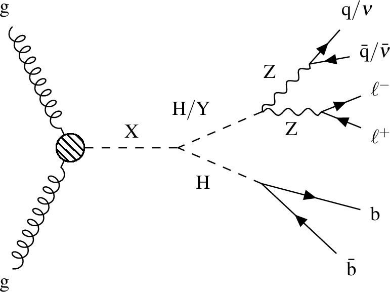
Figure 1:
A diagram illustrating the gluon-gluon fusion production of a resonance $ \mathrm{X} $, which subsequently decays into either HH or $ \mathrm{HY} $. One of the Higgs bosons or the scalar $\mathrm{Y}$ decays into two Z bosons. Of these, one Z boson decays either hadronically into a pair of quarks or invisibly into a pair of neutrinos, while the other Z boson decays leptonically into two charged leptons. The remaining Higgs boson decays into a pair of b quarks. |
png pdf |
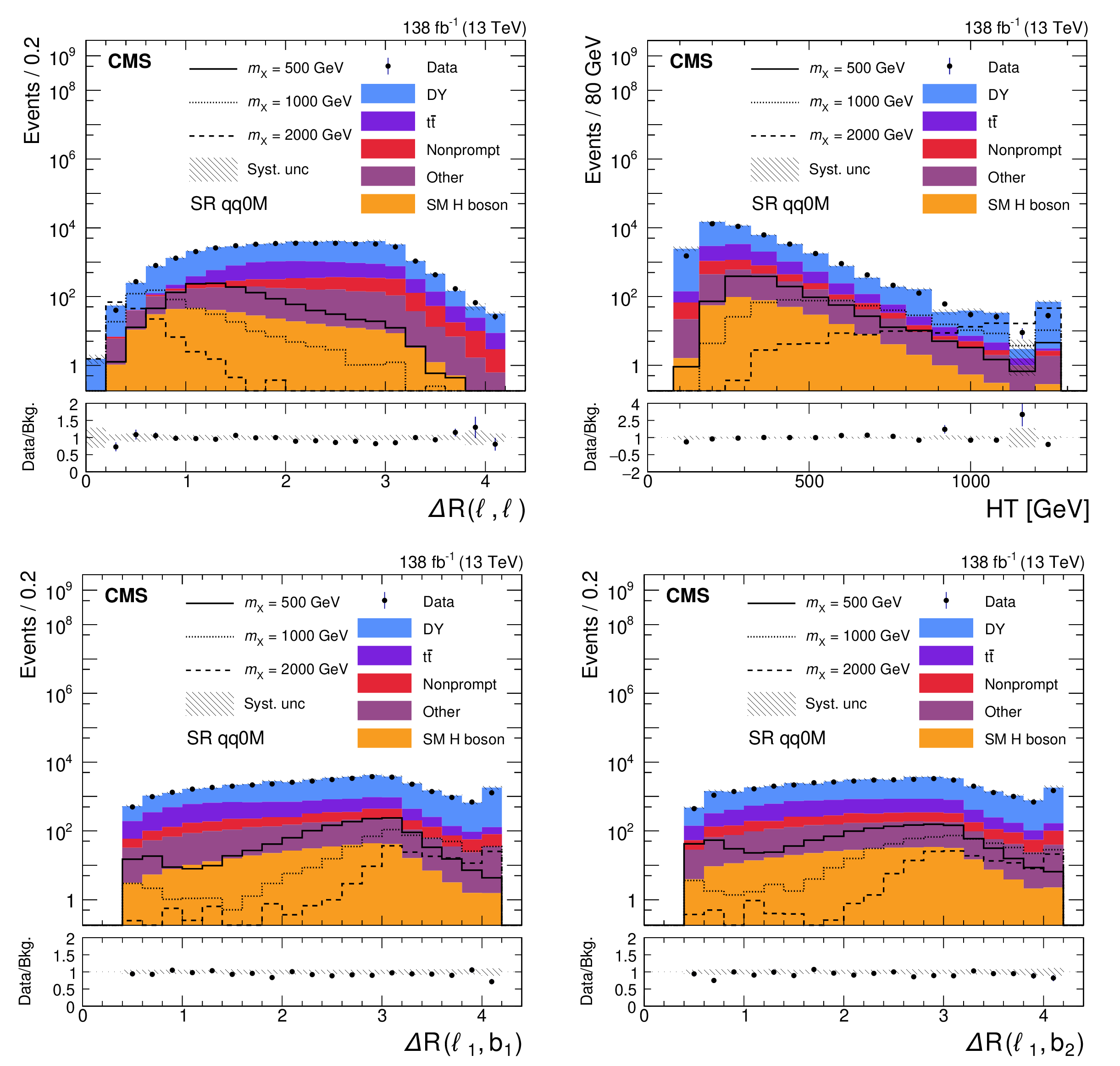
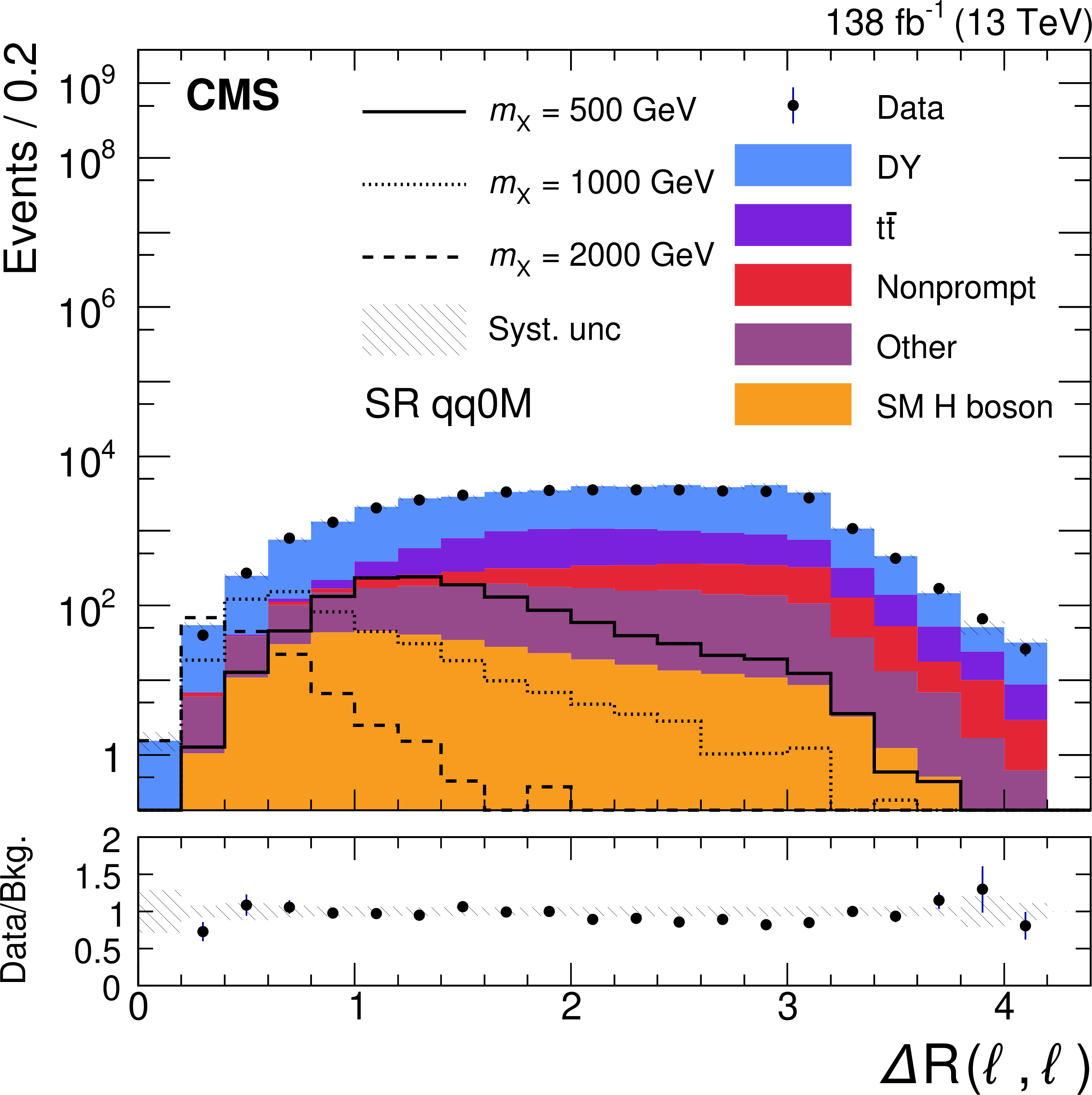
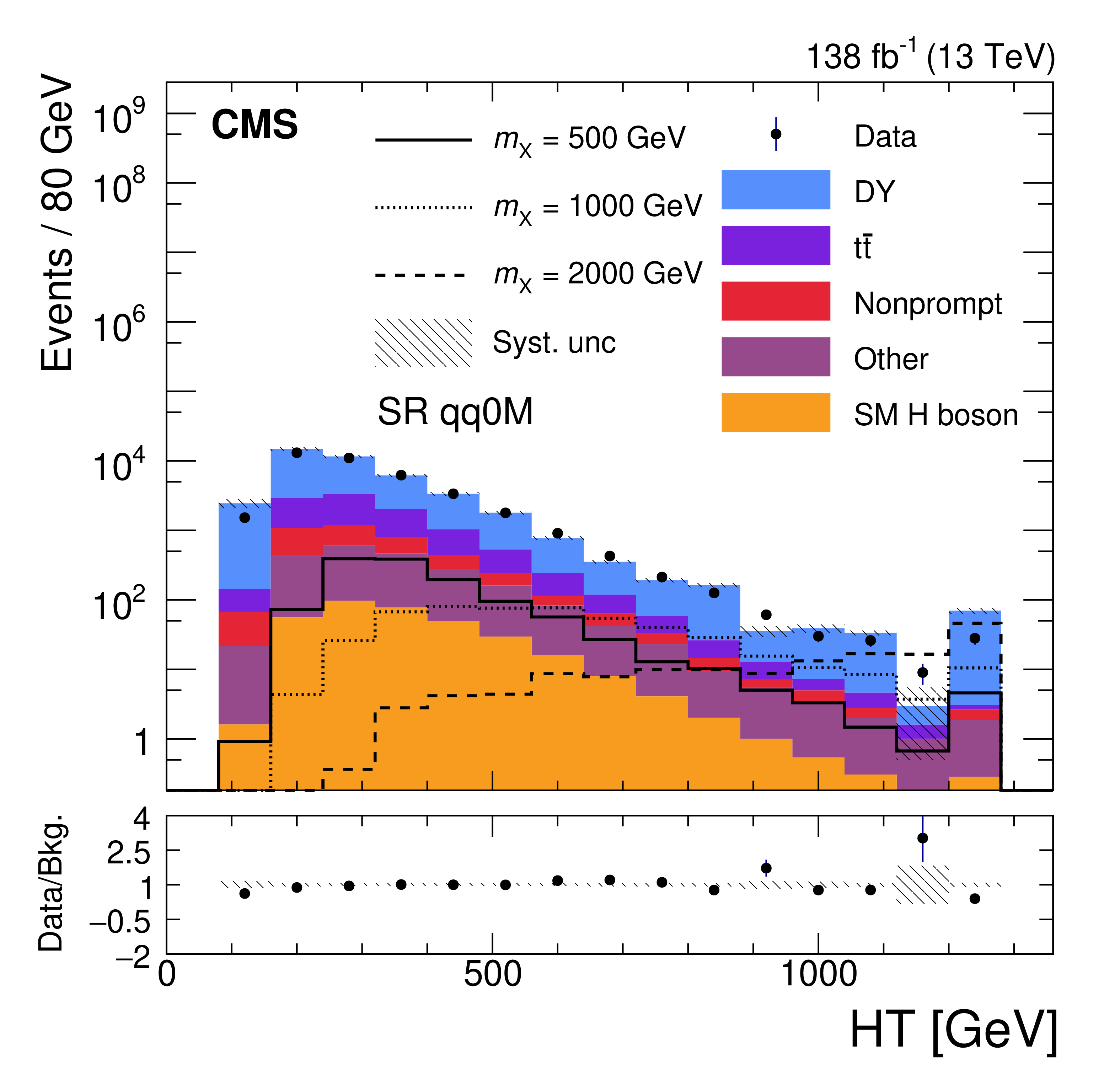
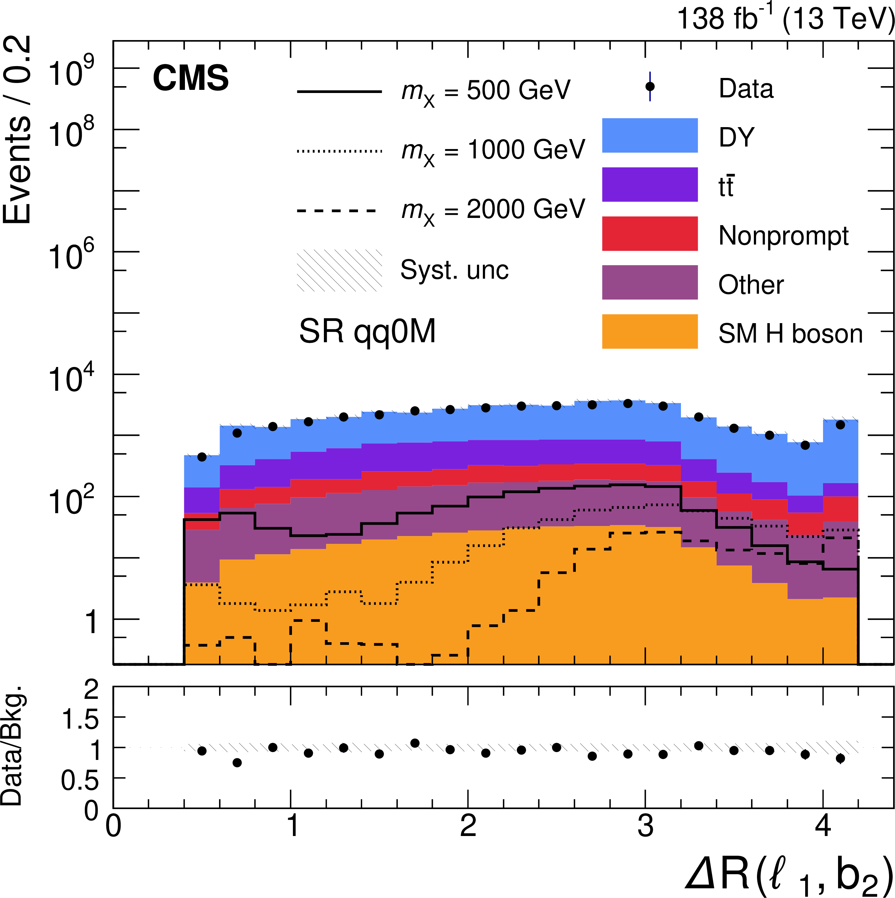
Figure 2:
Pre-fit distributions of $ \Delta R(\ell,\ell) $, HT, $ \Delta R({\ell}_1,{\mathrm{b}}_1) $, and $ \Delta R({\ell}_1,{\mathrm{b}}_2) $ (from upper left to lower right) in the SR qq0M, combining the electron and muon channels of HH search and using all three data-taking years. Three histograms corresponding to resonance masses of 500 GeV, 1000 GeV, and 2000 GeV are also included in the plots, with the cross section of production of resonance $ \mathrm{X} $ set to 100\unitpb and its branching fraction to HH set to 1. The lower panel in each plot displays the ratio of the data to the total SM prediction, with the hatched bands representing the total systematic uncertainties in the backgrounds. The last bin includes the overflow. |
png pdf |
Figure 2-a:
Pre-fit distributions of $ \Delta R(\ell,\ell) $, HT, $ \Delta R({\ell}_1,{\mathrm{b}}_1) $, and $ \Delta R({\ell}_1,{\mathrm{b}}_2) $ (from upper left to lower right) in the SR qq0M, combining the electron and muon channels of HH search and using all three data-taking years. Three histograms corresponding to resonance masses of 500 GeV, 1000 GeV, and 2000 GeV are also included in the plots, with the cross section of production of resonance $ \mathrm{X} $ set to 100\unitpb and its branching fraction to HH set to 1. The lower panel in each plot displays the ratio of the data to the total SM prediction, with the hatched bands representing the total systematic uncertainties in the backgrounds. The last bin includes the overflow. |
png pdf |
Figure 2-b:
Pre-fit distributions of $ \Delta R(\ell,\ell) $, HT, $ \Delta R({\ell}_1,{\mathrm{b}}_1) $, and $ \Delta R({\ell}_1,{\mathrm{b}}_2) $ (from upper left to lower right) in the SR qq0M, combining the electron and muon channels of HH search and using all three data-taking years. Three histograms corresponding to resonance masses of 500 GeV, 1000 GeV, and 2000 GeV are also included in the plots, with the cross section of production of resonance $ \mathrm{X} $ set to 100\unitpb and its branching fraction to HH set to 1. The lower panel in each plot displays the ratio of the data to the total SM prediction, with the hatched bands representing the total systematic uncertainties in the backgrounds. The last bin includes the overflow. |

png pdf |
Figure 2-c:
Pre-fit distributions of $ \Delta R(\ell,\ell) $, HT, $ \Delta R({\ell}_1,{\mathrm{b}}_1) $, and $ \Delta R({\ell}_1,{\mathrm{b}}_2) $ (from upper left to lower right) in the SR qq0M, combining the electron and muon channels of HH search and using all three data-taking years. Three histograms corresponding to resonance masses of 500 GeV, 1000 GeV, and 2000 GeV are also included in the plots, with the cross section of production of resonance $ \mathrm{X} $ set to 100\unitpb and its branching fraction to HH set to 1. The lower panel in each plot displays the ratio of the data to the total SM prediction, with the hatched bands representing the total systematic uncertainties in the backgrounds. The last bin includes the overflow. |
png pdf |
Figure 2-d:
Pre-fit distributions of $ \Delta R(\ell,\ell) $, HT, $ \Delta R({\ell}_1,{\mathrm{b}}_1) $, and $ \Delta R({\ell}_1,{\mathrm{b}}_2) $ (from upper left to lower right) in the SR qq0M, combining the electron and muon channels of HH search and using all three data-taking years. Three histograms corresponding to resonance masses of 500 GeV, 1000 GeV, and 2000 GeV are also included in the plots, with the cross section of production of resonance $ \mathrm{X} $ set to 100\unitpb and its branching fraction to HH set to 1. The lower panel in each plot displays the ratio of the data to the total SM prediction, with the hatched bands representing the total systematic uncertainties in the backgrounds. The last bin includes the overflow. |
png pdf |
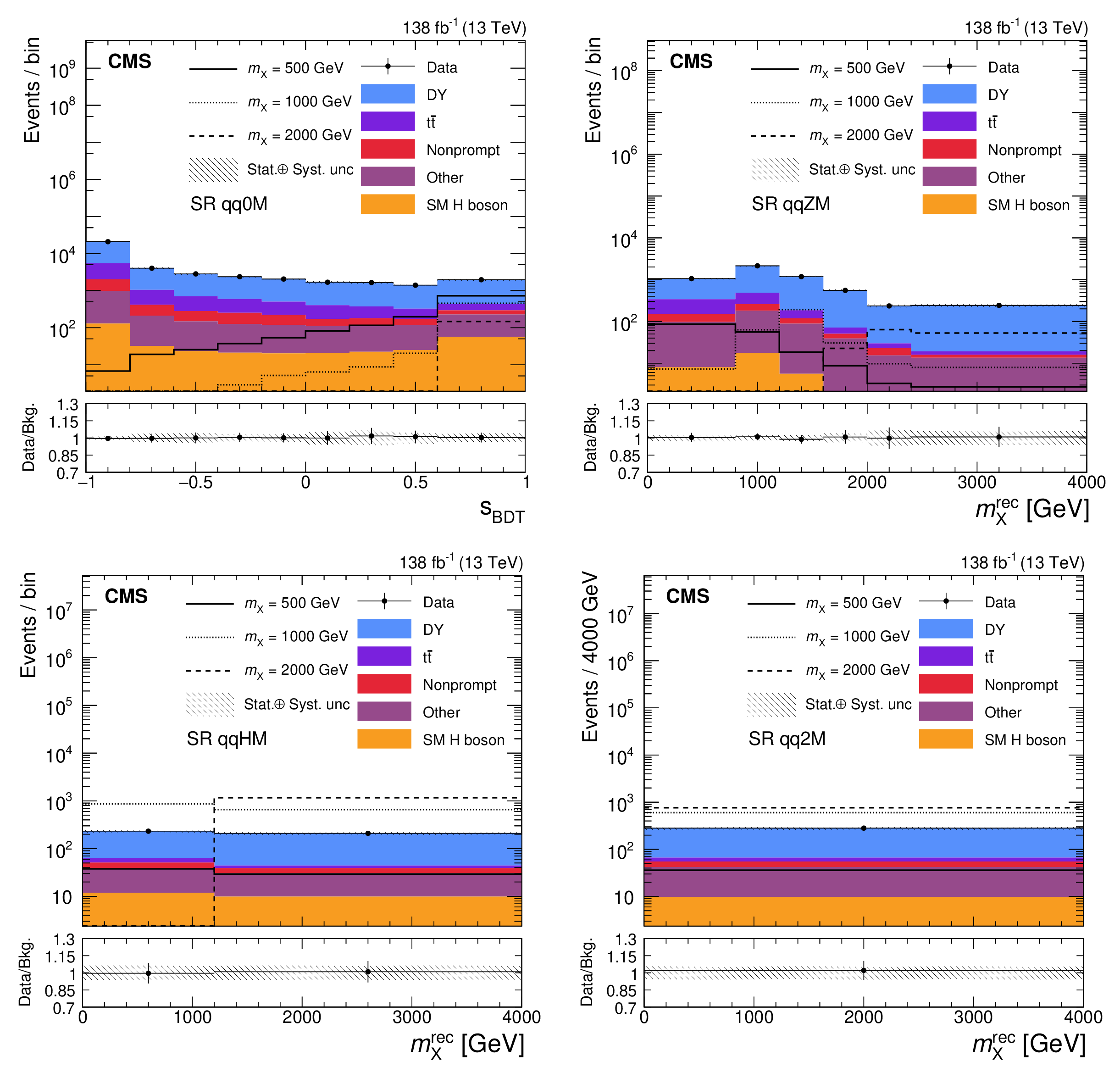
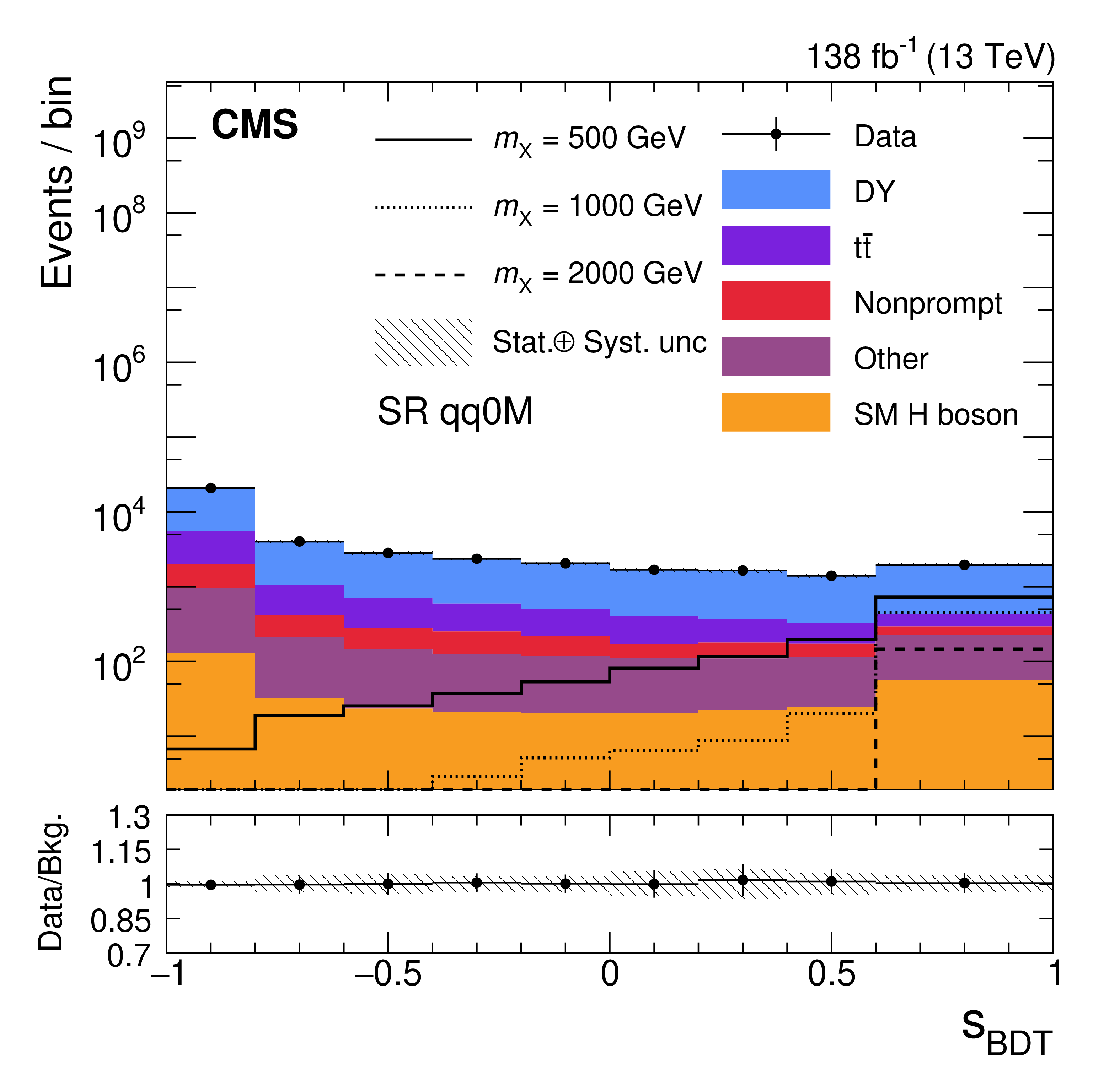
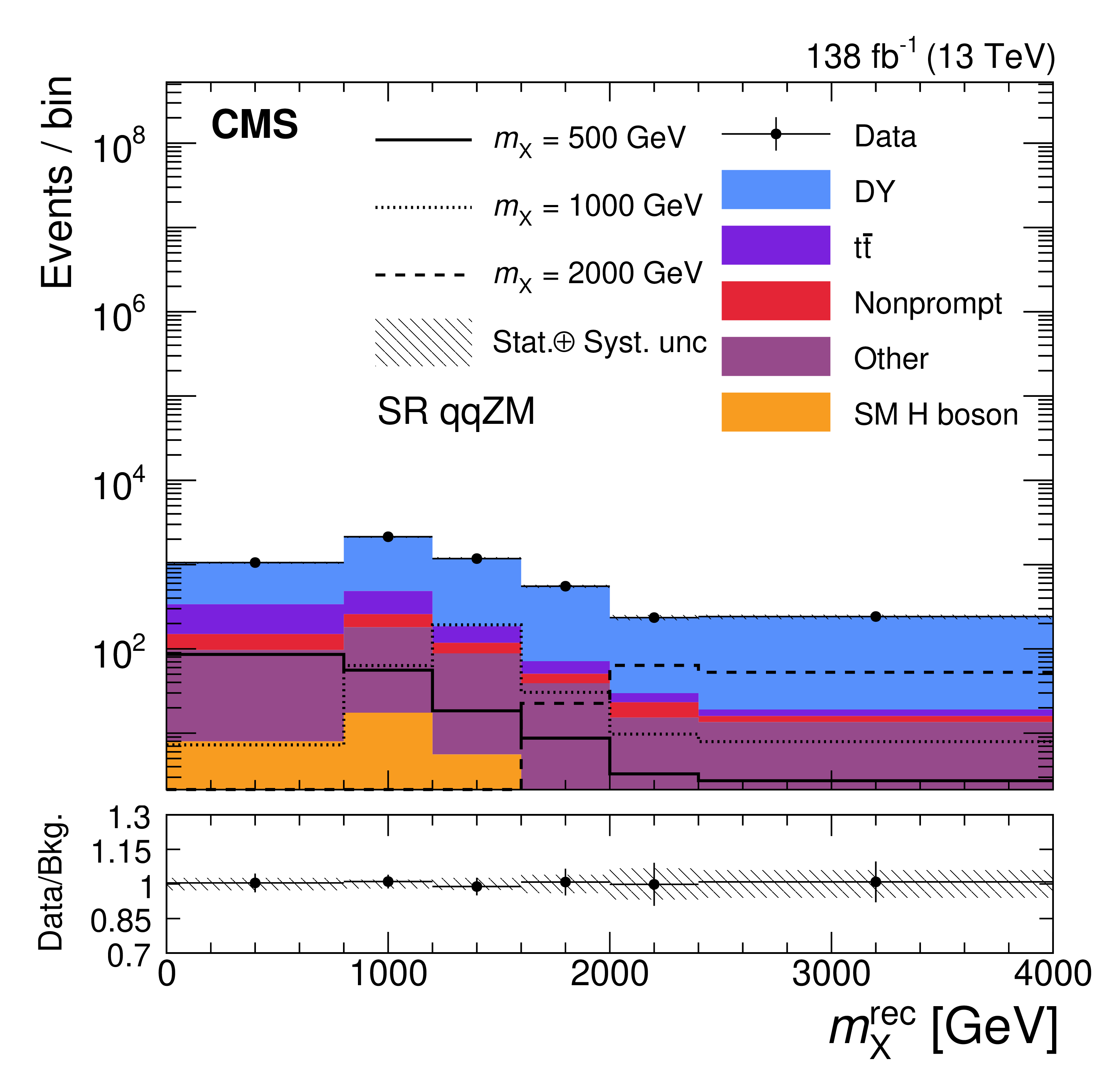
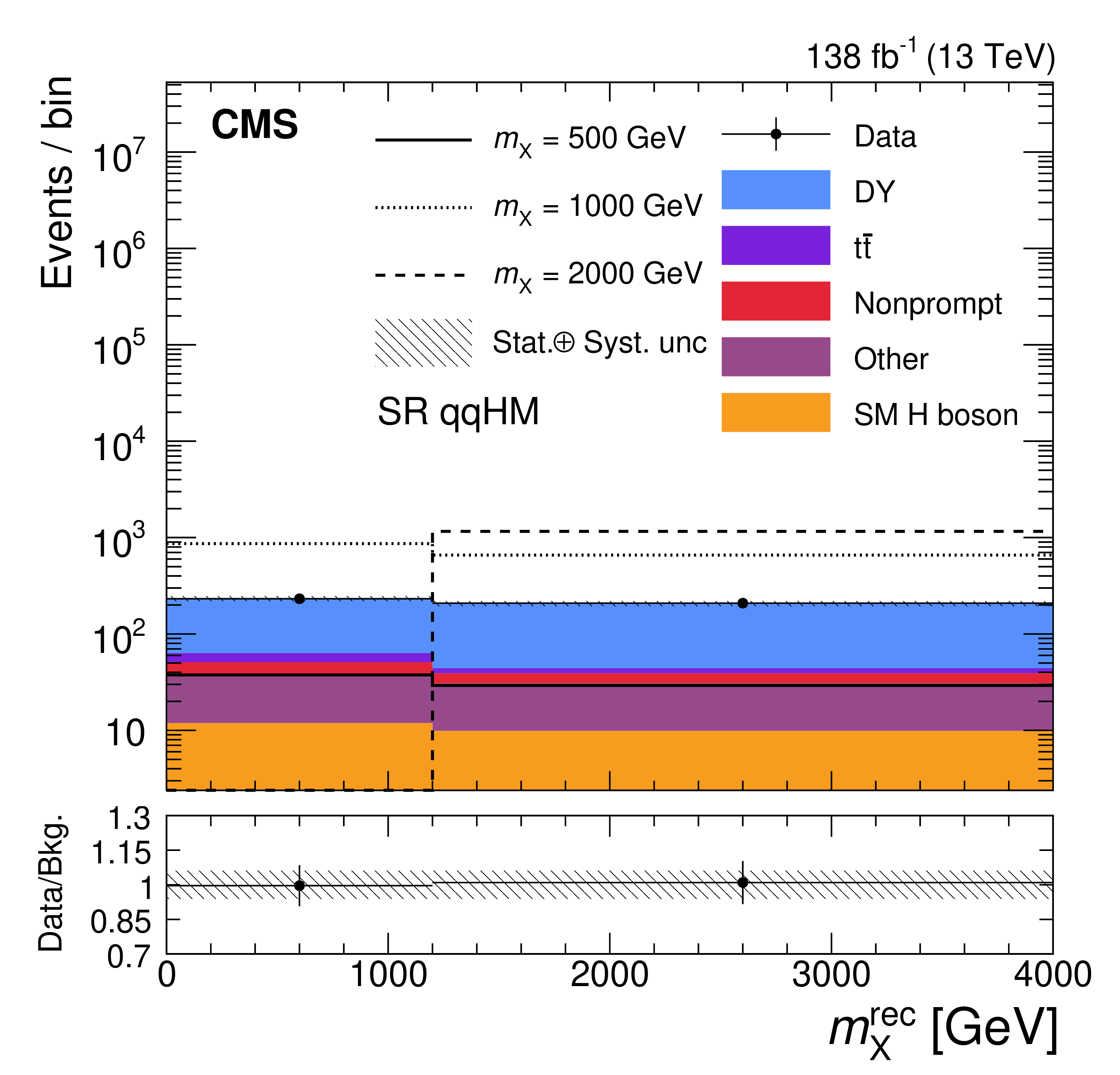
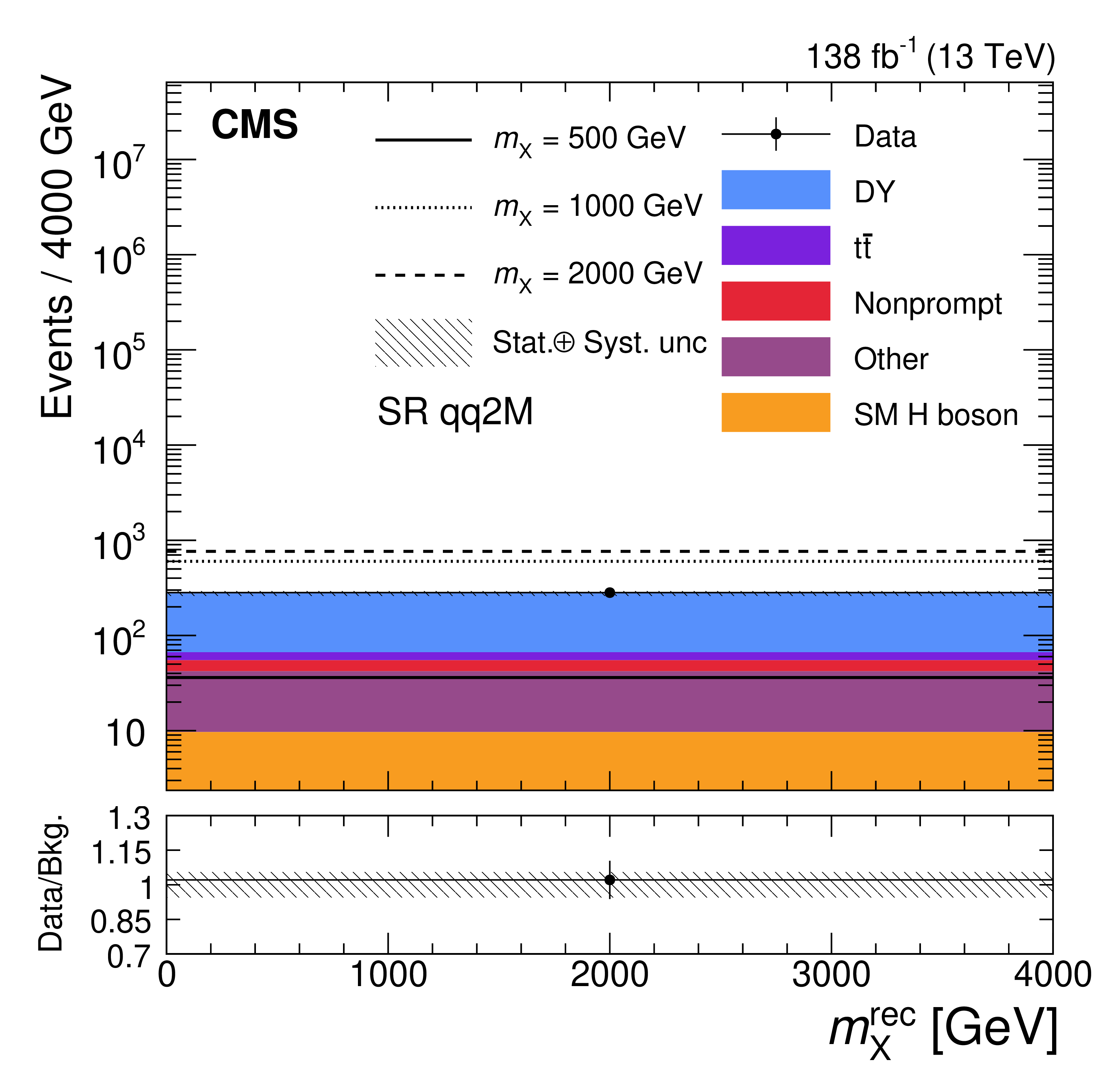
Figure 3:
The distributions used for the fit in the four SRs of the $ \mathrm{b}\mathrm{b}\mathrm{Z}(\mathrm{q}\mathrm{q})\mathrm{Z}(\ell\ell) $ channel, combining the electron and muon channels of the HH search are shown. The upper left plot displays the $ s_{\text{BDT}} $ distribution in the SR qq0M. The remaining three plots show the reconstructed resonance mass $ m^{\text{rec}}_{\mathrm{X}} $ distributions in the qqZM, qqHM, and qq2M SRs, from upper right to lower right. Three histograms corresponding to resonance masses of 500 GeV, 1000 GeV, and 2000 GeV are also included in the plots, with the cross section of production of resonance $ \mathrm{X} $ set to 100\unitpb and its branching fraction to HH set to 1. These histograms account for the branching fractions of the $ \mathrm{H}\mathrm{H}\to \mathrm{b}\mathrm{b}\mathrm{Z}\mathrm{Z} $ and $ \mathrm{Z}\mathrm{Z}\to \mathrm{q}\mathrm{q}\ell\ell $ decays. The lower panel in each plot displays the ratio of the data to the total SM prediction, with the hatched bands representing the overall uncertainty in the combined background expectations. The histograms of backgrounds are the post-fit ones, while the histograms of BSM signals are the pre-fit ones. |
png pdf |
Figure 3-a:
The distributions used for the fit in the four SRs of the $ \mathrm{b}\mathrm{b}\mathrm{Z}(\mathrm{q}\mathrm{q})\mathrm{Z}(\ell\ell) $ channel, combining the electron and muon channels of the HH search are shown. The upper left plot displays the $ s_{\text{BDT}} $ distribution in the SR qq0M. The remaining three plots show the reconstructed resonance mass $ m^{\text{rec}}_{\mathrm{X}} $ distributions in the qqZM, qqHM, and qq2M SRs, from upper right to lower right. Three histograms corresponding to resonance masses of 500 GeV, 1000 GeV, and 2000 GeV are also included in the plots, with the cross section of production of resonance $ \mathrm{X} $ set to 100\unitpb and its branching fraction to HH set to 1. These histograms account for the branching fractions of the $ \mathrm{H}\mathrm{H}\to \mathrm{b}\mathrm{b}\mathrm{Z}\mathrm{Z} $ and $ \mathrm{Z}\mathrm{Z}\to \mathrm{q}\mathrm{q}\ell\ell $ decays. The lower panel in each plot displays the ratio of the data to the total SM prediction, with the hatched bands representing the overall uncertainty in the combined background expectations. The histograms of backgrounds are the post-fit ones, while the histograms of BSM signals are the pre-fit ones. |
png pdf |
Figure 3-b:
The distributions used for the fit in the four SRs of the $ \mathrm{b}\mathrm{b}\mathrm{Z}(\mathrm{q}\mathrm{q})\mathrm{Z}(\ell\ell) $ channel, combining the electron and muon channels of the HH search are shown. The upper left plot displays the $ s_{\text{BDT}} $ distribution in the SR qq0M. The remaining three plots show the reconstructed resonance mass $ m^{\text{rec}}_{\mathrm{X}} $ distributions in the qqZM, qqHM, and qq2M SRs, from upper right to lower right. Three histograms corresponding to resonance masses of 500 GeV, 1000 GeV, and 2000 GeV are also included in the plots, with the cross section of production of resonance $ \mathrm{X} $ set to 100\unitpb and its branching fraction to HH set to 1. These histograms account for the branching fractions of the $ \mathrm{H}\mathrm{H}\to \mathrm{b}\mathrm{b}\mathrm{Z}\mathrm{Z} $ and $ \mathrm{Z}\mathrm{Z}\to \mathrm{q}\mathrm{q}\ell\ell $ decays. The lower panel in each plot displays the ratio of the data to the total SM prediction, with the hatched bands representing the overall uncertainty in the combined background expectations. The histograms of backgrounds are the post-fit ones, while the histograms of BSM signals are the pre-fit ones. |
png pdf |
Figure 3-c:
The distributions used for the fit in the four SRs of the $ \mathrm{b}\mathrm{b}\mathrm{Z}(\mathrm{q}\mathrm{q})\mathrm{Z}(\ell\ell) $ channel, combining the electron and muon channels of the HH search are shown. The upper left plot displays the $ s_{\text{BDT}} $ distribution in the SR qq0M. The remaining three plots show the reconstructed resonance mass $ m^{\text{rec}}_{\mathrm{X}} $ distributions in the qqZM, qqHM, and qq2M SRs, from upper right to lower right. Three histograms corresponding to resonance masses of 500 GeV, 1000 GeV, and 2000 GeV are also included in the plots, with the cross section of production of resonance $ \mathrm{X} $ set to 100\unitpb and its branching fraction to HH set to 1. These histograms account for the branching fractions of the $ \mathrm{H}\mathrm{H}\to \mathrm{b}\mathrm{b}\mathrm{Z}\mathrm{Z} $ and $ \mathrm{Z}\mathrm{Z}\to \mathrm{q}\mathrm{q}\ell\ell $ decays. The lower panel in each plot displays the ratio of the data to the total SM prediction, with the hatched bands representing the overall uncertainty in the combined background expectations. The histograms of backgrounds are the post-fit ones, while the histograms of BSM signals are the pre-fit ones. |
png pdf |
Figure 3-d:
The distributions used for the fit in the four SRs of the $ \mathrm{b}\mathrm{b}\mathrm{Z}(\mathrm{q}\mathrm{q})\mathrm{Z}(\ell\ell) $ channel, combining the electron and muon channels of the HH search are shown. The upper left plot displays the $ s_{\text{BDT}} $ distribution in the SR qq0M. The remaining three plots show the reconstructed resonance mass $ m^{\text{rec}}_{\mathrm{X}} $ distributions in the qqZM, qqHM, and qq2M SRs, from upper right to lower right. Three histograms corresponding to resonance masses of 500 GeV, 1000 GeV, and 2000 GeV are also included in the plots, with the cross section of production of resonance $ \mathrm{X} $ set to 100\unitpb and its branching fraction to HH set to 1. These histograms account for the branching fractions of the $ \mathrm{H}\mathrm{H}\to \mathrm{b}\mathrm{b}\mathrm{Z}\mathrm{Z} $ and $ \mathrm{Z}\mathrm{Z}\to \mathrm{q}\mathrm{q}\ell\ell $ decays. The lower panel in each plot displays the ratio of the data to the total SM prediction, with the hatched bands representing the overall uncertainty in the combined background expectations. The histograms of backgrounds are the post-fit ones, while the histograms of BSM signals are the pre-fit ones. |
png pdf |
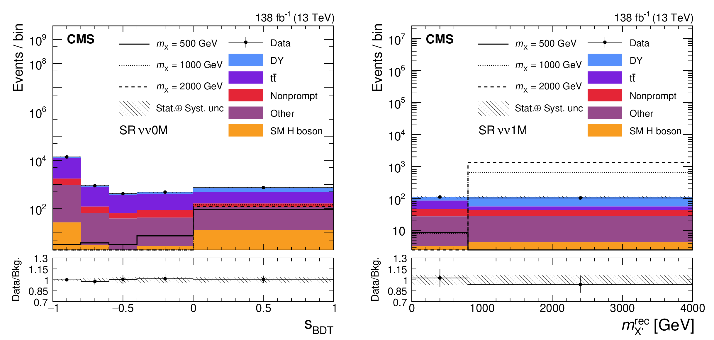
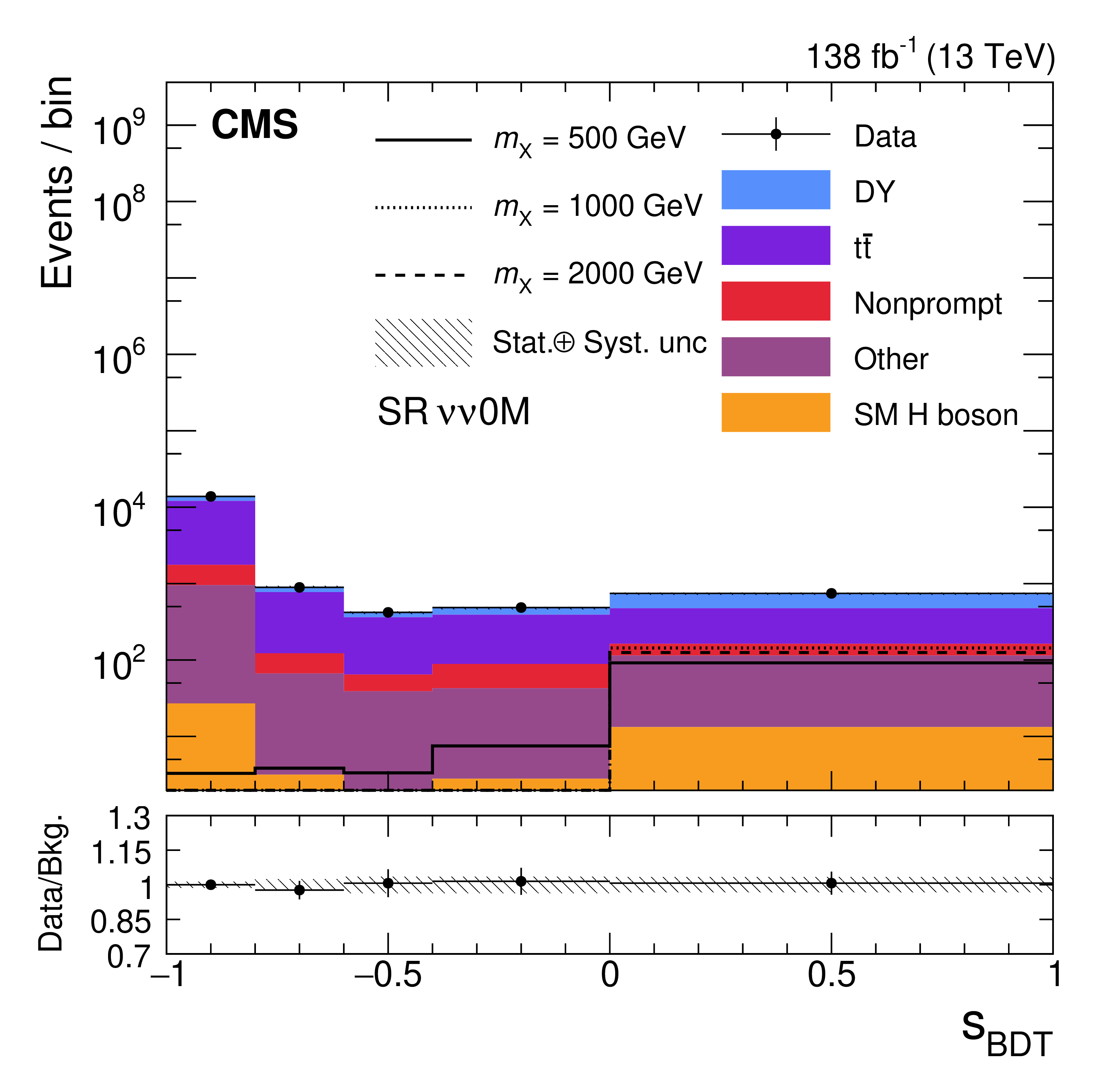
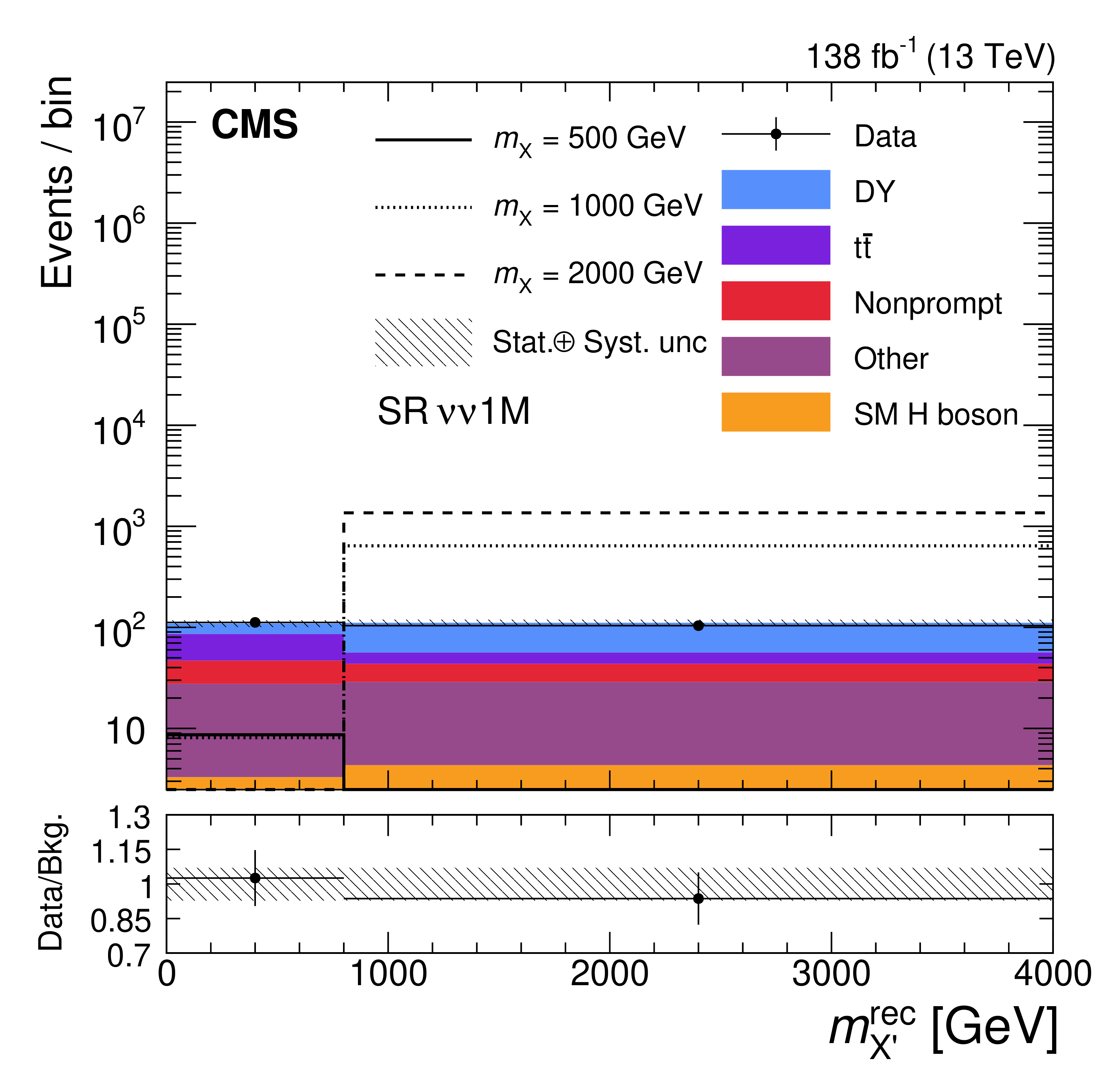
Figure 4:
The distributions used for the fit in the two SRs of the $ \mathrm{b}\mathrm{b}\mathrm{Z}(\nu\nu)\mathrm{Z}(\ell\ell) $ channel, combining the electron and muon channels of the HH search are shown. The left plot displays the $ s_{\text{BDT}} $ distribution in the SR $ \nu\nu $0M, the right plot displays the reconstructed resonance mass $ {m}^{\text{rec}}_{\mathrm{X}^{\prime}} $ distributions in the SR $ \nu\nu $1M. Three histograms corresponding to resonance masses of 500 GeV, 1000 GeV, and 2000 GeV are also included in the plots, with the cross section of production of resonance $ \mathrm{X} $ set to 100\unitpb and its branching fraction to HH set to 1. These histograms account for the branching fractions of the $ \mathrm{H}\mathrm{H}\to \mathrm{b}\mathrm{b}\mathrm{Z}\mathrm{Z} $ and $ \mathrm{Z}\mathrm{Z}\to \ell\ell\nu\nu $ decays. The lower panel in each plot displays the ratio of the data to the total SM prediction, with the hatched bands representing the overall uncertainty in the combined background expectations. The histograms of backgrounds are the post-fit ones, while the histograms of BSM signals are the pre-fit ones. |
png pdf |
Figure 4-a:
The distributions used for the fit in the two SRs of the $ \mathrm{b}\mathrm{b}\mathrm{Z}(\nu\nu)\mathrm{Z}(\ell\ell) $ channel, combining the electron and muon channels of the HH search are shown. The left plot displays the $ s_{\text{BDT}} $ distribution in the SR $ \nu\nu $0M, the right plot displays the reconstructed resonance mass $ {m}^{\text{rec}}_{\mathrm{X}^{\prime}} $ distributions in the SR $ \nu\nu $1M. Three histograms corresponding to resonance masses of 500 GeV, 1000 GeV, and 2000 GeV are also included in the plots, with the cross section of production of resonance $ \mathrm{X} $ set to 100\unitpb and its branching fraction to HH set to 1. These histograms account for the branching fractions of the $ \mathrm{H}\mathrm{H}\to \mathrm{b}\mathrm{b}\mathrm{Z}\mathrm{Z} $ and $ \mathrm{Z}\mathrm{Z}\to \ell\ell\nu\nu $ decays. The lower panel in each plot displays the ratio of the data to the total SM prediction, with the hatched bands representing the overall uncertainty in the combined background expectations. The histograms of backgrounds are the post-fit ones, while the histograms of BSM signals are the pre-fit ones. |
png pdf |
Figure 4-b:
The distributions used for the fit in the two SRs of the $ \mathrm{b}\mathrm{b}\mathrm{Z}(\nu\nu)\mathrm{Z}(\ell\ell) $ channel, combining the electron and muon channels of the HH search are shown. The left plot displays the $ s_{\text{BDT}} $ distribution in the SR $ \nu\nu $0M, the right plot displays the reconstructed resonance mass $ {m}^{\text{rec}}_{\mathrm{X}^{\prime}} $ distributions in the SR $ \nu\nu $1M. Three histograms corresponding to resonance masses of 500 GeV, 1000 GeV, and 2000 GeV are also included in the plots, with the cross section of production of resonance $ \mathrm{X} $ set to 100\unitpb and its branching fraction to HH set to 1. These histograms account for the branching fractions of the $ \mathrm{H}\mathrm{H}\to \mathrm{b}\mathrm{b}\mathrm{Z}\mathrm{Z} $ and $ \mathrm{Z}\mathrm{Z}\to \ell\ell\nu\nu $ decays. The lower panel in each plot displays the ratio of the data to the total SM prediction, with the hatched bands representing the overall uncertainty in the combined background expectations. The histograms of backgrounds are the post-fit ones, while the histograms of BSM signals are the pre-fit ones. |
png pdf |
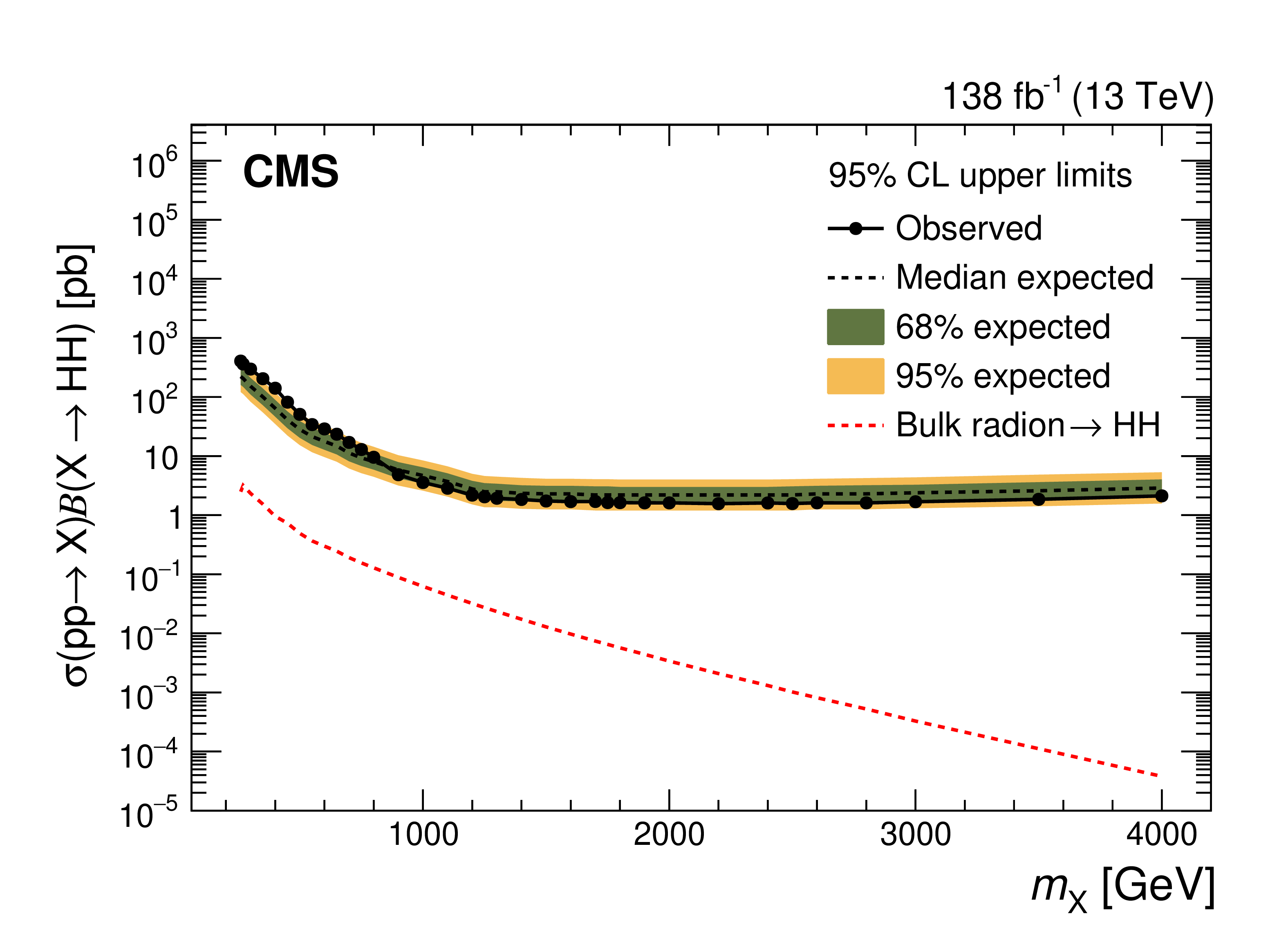
Figure 5:
Upper limits on the production cross section of $ \mathrm{p}\mathrm{p}\to \mathrm{X}\to \mathrm{H}\mathrm{H} $ with respect to the resonance mass $ m_{\mathrm{X}} $, combining all the SRs as well as the electron and muon channels, and taking into account the theoretical prediction of the branching fraction of the resonance to HH. The inner (green) band and the outer (yellow) band indicate the regions containing 68% and 95%, respectively, of the distribution of limits expected under the background-only hypothesis. The theoretical values (red dashed line) are also provided on the plot. |
png pdf |
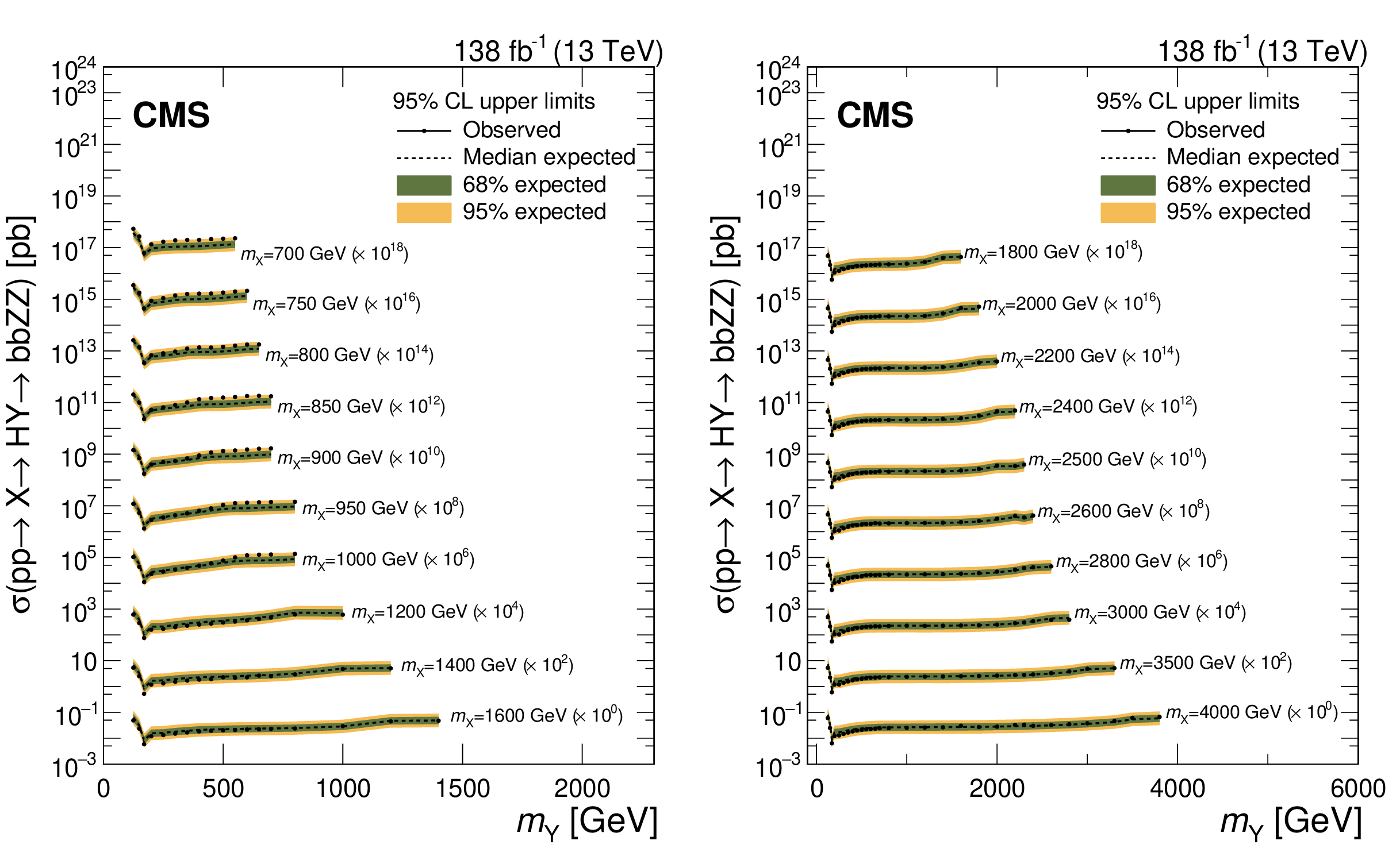
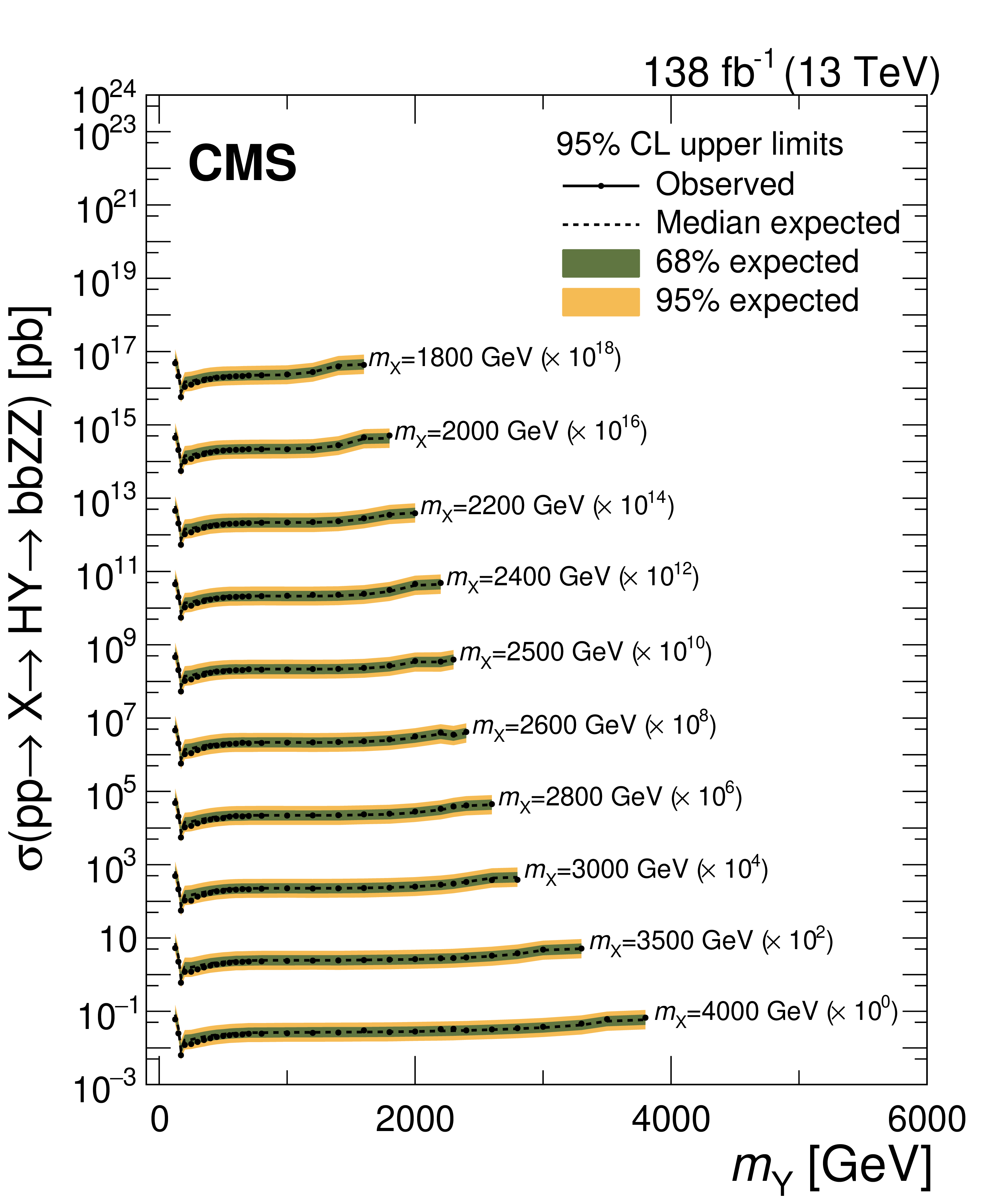
Figure 6:
Upper limits on the production cross section of $ \mathrm{p}\mathrm{p}\to \mathrm{X}\to \mathrm{HY} \to \mathrm{b}\mathrm{b}\mathrm{Z}\mathrm{Z} $ in the two-dimensional parameter space of the masses of the two BSM scalars ($ m_\mathrm{X} $, $ m_{\mathrm{Y}} $) combining all the SRs as well as the electron and muon channels. The inner (green) band and the outer (yellow) band indicate the regions containing 68% and 95%, respectively, of the distribution of limits expected under the background-only hypothesis. |
png pdf |
Figure 6-a:
Upper limits on the production cross section of $ \mathrm{p}\mathrm{p}\to \mathrm{X}\to \mathrm{HY} \to \mathrm{b}\mathrm{b}\mathrm{Z}\mathrm{Z} $ in the two-dimensional parameter space of the masses of the two BSM scalars ($ m_\mathrm{X} $, $ m_{\mathrm{Y}} $) combining all the SRs as well as the electron and muon channels. The inner (green) band and the outer (yellow) band indicate the regions containing 68% and 95%, respectively, of the distribution of limits expected under the background-only hypothesis. |
png pdf |
Figure 6-b:
Upper limits on the production cross section of $ \mathrm{p}\mathrm{p}\to \mathrm{X}\to \mathrm{HY} \to \mathrm{b}\mathrm{b}\mathrm{Z}\mathrm{Z} $ in the two-dimensional parameter space of the masses of the two BSM scalars ($ m_\mathrm{X} $, $ m_{\mathrm{Y}} $) combining all the SRs as well as the electron and muon channels. The inner (green) band and the outer (yellow) band indicate the regions containing 68% and 95%, respectively, of the distribution of limits expected under the background-only hypothesis. |
| Tables | |
png pdf |
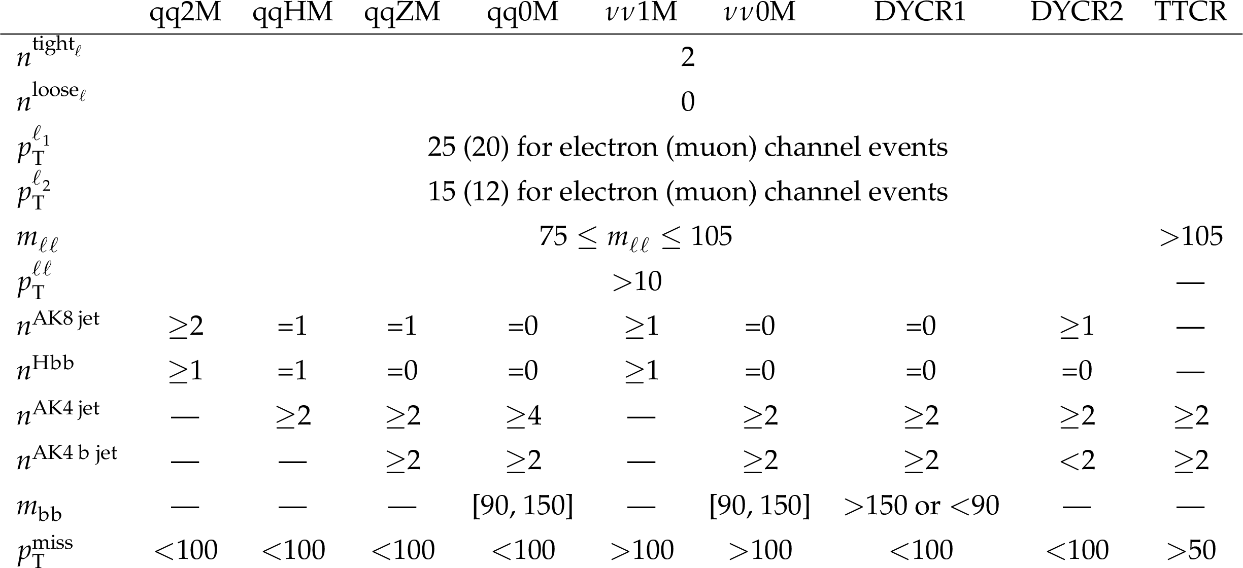
Table 1:
Definitions of all SRs and CRs. Here, $ p_{\mathrm{T}}^{\ell_1} $ ($ p_{\mathrm{T}}^{\ell_2} $) denotes the transverse momentum of the leading (subleading) lepton; $ {n}^\text{AK8 jet} $, $ {n}^{\mathrm{H}\mathrm{b}\mathrm{b}} $, $ {n}^\text{AK4 jet} $, and $ {n}^\text{AK4 \mathrm{b} jet} $ represent the number of AK8 jets, AK8 jets passing the $ \mathrm{PNT}_{\mathrm{b}\mathrm{b}} $ threshold, AK4 jets, and b-tagged AK4 jets, respectively. All energy-related quantities are given in GeV. |
| Summary |
| A search for a new resonance $ \mathrm{X} $ decaying into either a pair of Higgs bosons (HH) or into a Higgs boson and a new scalar boson $\mathrm{Y}$ ($ \mathrm{HY} $) has been conducted in this study, using proton-proton collision data collected by the CMS experiment from 2016 to 2018 at $ \sqrt{s}= $ 13 TeV, corresponding to an integrated luminosity of 138 fb$ ^{-1} $. The events of interest are characterized by two b quarks from the decay of one Higgs boson, as well as two leptons and either two additional quarks or two neutrinos from two Z bosons produced by the decay of the other H or the $\mathrm{Y}$. No significant deviations are observed in the signal regions between the data and standard model predictions. For resonant HH production, upper limits are placed on the cross section for the process $ \mathrm{p}\mathrm{p}\to \mathrm{X}\to \mathrm{H}\mathrm{H} $ as a function of the resonance mass, varying from 400\unitpb to 1\unitpb as $ m_\mathrm{X} $ increases. For resonant $ \mathrm{HY} $ production, upper limits are set on the cross section for the process $ \mathrm{p}\mathrm{p}\to \mathrm{X}\to \mathrm{HY} \to \mathrm{b}\mathrm{b}\mathrm{Z}\mathrm{Z} $ in the two-dimensional parameter space of the masses $ m_\mathrm{X} $ and $ m_{\mathrm{Y}} $, varying from about 5\unitfb to 500\unitfb. This is comparable to the limits achieved in other analyses, which focus on H decays to $ \gamma\gamma $ or $ \tau\tau $ and $\mathrm{Y}$ decays into a pair of bottom quarks or massive vector bosons. |
| References | ||||
| 1 | ATLAS Collaboration | Observation of a new particle in the search for the standard model Higgs boson with the ATLAS detector at the LHC | PLB 716 (2012) 1 | 1207.7214 |
| 2 | CMS Collaboration | Observation of a new boson at a mass of 125 GeV with the CMS experiment at the LHC | PLB 716 (2012) 30 | CMS-HIG-12-028 1207.7235 |
| 3 | CMS Collaboration | Observation of a new boson with mass near 125 GeV in pp collisions at $ \sqrt{s} = $ 7 and 8 TeV | JHEP 06 (2013) 081 | CMS-HIG-12-036 1303.4571 |
| 4 | L. Randall and R. Sundrum | An alternative to compactification | PRL 83 (1999) 4690 | hep-th/9906064 |
| 5 | L. Randall and R. Sundrum | Large mass hierarchy from a small extra dimension | PRL 83 (1999) 3370 | hep-ph/9905221 |
| 6 | W. D. Goldberger and M. B. Wise | Modulus stabilization with bulk fields | PRL 83 (1999) 4922 | hep-ph/9907447 |
| 7 | C. Csa ki, M. Graesser, L. Randall, and J. Terning | Cosmology of brane models with radion stabilization | PRD 62 (2000) 045015 | hep-ph/9911406 |
| 8 | C. Csa ki, M. L. Graesser, and G. D. Kribs | Radion dynamics and electroweak physics | PRD 63 (2001) 065002 | hep-th/0008151 |
| 9 | H. Davoudiasl, J. L. Hewett, and T. G. Rizzo | Phenomenology of the randall-sundrum gauge hierarchy model | PRL 84 (2000) 2080 | hep-ph/9909255 |
| 10 | O. DeWolfe, D. Z. Freedman, S. S. Gubser, and A. Karch | Modeling the fifth dimension with scalars and gravity | PRD 62 (2000) 046008 | hep-th/9909134 |
| 11 | K. Agashe, H. Davoudiasl, G. Perez, and A. Soni | Warped gravitons at the CERN LHC and beyond | PRD 76 (2007) 036006 | hep-ph/0701186 |
| 12 | Yu. A. Golfand and E. P. Likhtman | Extension of the algebra of Poincaré group generators and violation of P-invariance | JETP Lett. 13 (1971) 323 | |
| 13 | J. Wess and B. Zumino | Supergauge transformations in four-dimensions | NPB 70 (1974) 39 | |
| 14 | P. Fayet | Supergauge invariant extension of the Higgs mechanism and a model for the electron and its neutrino | NPB 90 (1975) 104 | |
| 15 | P. Fayet | Spontaneously broken supersymmetric theories of weak, electromagnetic and strong interactions | PLB 69 (1977) 489 | |
| 16 | U. Ellwanger, C. Hugonie, and A. M. Teixeira | The Next-to-Minimal Supersymmetric Standard Model | Phys. Rept. 496 (2010) 1 | 0910.1785 |
| 17 | M. Maniatis | The Next-to-Minimal Supersymmetric extension of the Standard Model reviewed | Int. J. Mod. Phys. A 25 (2010) 3505 | 0906.0777 |
| 18 | J. E. Kim and H. P. Nilles | The $ \mu $-problem and the strong CP-problem | PLB 138 (1984) 150 | |
| 19 | CMS Collaboration | Search for resonant pair production of Higgs bosons in the $ bbZZ $ channel in proton-proton collisions at $ \sqrt{s}=13\text{ }\text{ }\mathrm{TeV} $ | PRD 102 (2020) 032003 | CMS-HIG-18-013 2006.06391 |
| 20 | CMS Collaboration | Search for Higgs boson pair production in the $ \textrm{b}\overline{\textrm{b}}{\textrm{W}}^{+}{\textrm{W}}^{-} $ decay mode in proton-proton collisions at $ \sqrt{s} = $ 13 TeV | JHEP 07 (2024) 293 | CMS-HIG-21-005 2403.09430 |
| 21 | CMS Collaboration | Searches for Higgs boson production through decays of heavy resonances | Phys. Rept. 1115 (2025) 368 | 2403.16926 |
| 22 | ATLAS Collaboration | Search for a new heavy scalar particle decaying into a Higgs boson and a new scalar singlet in final states with one or two light leptons and a pair of $ \tau $-leptons with the ATLAS detector | JHEP 10 (2023) 009 | 2307.11120 |
| 23 | ATLAS Collaboration | Search for a resonance decaying into a scalar particle and a Higgs boson in the final state with two bottom quarks and two photons with 199 fb$ ^{-1} $ of data collected at $ \sqrt{s} = $ 13 TeV and $ \sqrt{s} = $ 13.6 TeV with the ATLAS detector | Submitted to Phys. Lett. B, 2025 | 2510.02857 |
| 24 | CMS Collaboration | The CMS experiment at the CERN LHC | JINST 3 (2008) S08004 | |
| 25 | CMS Collaboration | Development of the CMS detector for the CERN LHC Run 3 | JINST 19 (2024) P05064 | CMS-PRF-21-001 2309.05466 |
| 26 | CMS Collaboration | Performance of the CMS Level-1 trigger in proton-proton collisions at $ \sqrt{s} = $ 13 TeV | JINST 15 (2020) P10017 | CMS-TRG-17-001 2006.10165 |
| 27 | CMS Collaboration | The CMS trigger system | JINST 12 (2017) P01020 | CMS-TRG-12-001 1609.02366 |
| 28 | CMS Collaboration | Performance of the CMS high-level trigger during LHC Run 2 | JINST 19 (2024) P11021 | CMS-TRG-19-001 2410.17038 |
| 29 | CMS Collaboration | Electron and photon reconstruction and identification with the CMS experiment at the CERN LHC | JINST 16 (2021) P05014 | CMS-EGM-17-001 2012.06888 |
| 30 | CMS Collaboration | Performance of the CMS muon detector and muon reconstruction with proton-proton collisions at $ \sqrt{s}= $ 13 TeV | JINST 13 (2018) P06015 | CMS-MUO-16-001 1804.04528 |
| 31 | CMS Collaboration | Description and performance of track and primary-vertex reconstruction with the CMS tracker | JINST 9 (2014) P10009 | CMS-TRK-11-001 1405.6569 |
| 32 | J. Alwall et al. | The automated computation of tree-level and next-to-leading order differential cross sections, and their matching to parton shower simulations | JHEP 07 (2014) 079 | 1405.0301 |
| 33 | T. Sjöstrand et al. | An introduction to PYTHIA 8.2 | Comput. Phys. Commun. 191 (2015) 159 | 1410.3012 |
| 34 | R. Frederix and S. Frixione | Merging meets matching in MC@NLO | JHEP 12 (2012) 061 | 1209.6215 |
| 35 | R. Gavin, Y. Li, F. Petriello, and S. Quackenbush | FEWZ 2.0: A code for hadronic Z production at next-to-next-to-leading order | Comput. Phys. Commun. 182 (2011) 2388 | 1011.3540 |
| 36 | S. Frixione, G. Ridolfi, and P. Nason | A Positive-Weight Next-to-Leading-Order Monte Carlo for Heavy Flavour Hadroproduction | JHEP 09 (2007) 126 | 0707.3088 |
| 37 | M. Czakon and A. Mitov | Top++: a program for the calculation of the top-pair cross-section at hadron colliders | Comput. Phys. Commun. 185 (2014) 2930 | 1112.5675 |
| 38 | CMS Collaboration | Extraction and validation of a new set of CMS PYTHIA8 tunes from underlying-event measurements | EPJC 80 (2020) 4 | CMS-GEN-17-001 1903.12179 |
| 39 | NNPDF Collaboration | Parton distributions from high-precision collider data | EPJC 77 (2017) 663 | 1706.00428 |
| 40 | GEANT4 Collaboration | GEANT 4---a simulation toolkit | NIM A 506 (2003) 250 | |
| 41 | J. Allison et al. | Geant4 developments and applications | IEEE Trans. Nucl. Sci. 53 (2006) 270 | |
| 42 | CMS Collaboration | Measurement of the inclusive W and Z production cross sections in pp collisions at $ \sqrt{s} = $ 7 TeV with the CMS experiment | JHEP 10 (2011) 132 | CMS-EWK-10-005 1107.4789 |
| 43 | CMS Collaboration | Particle-flow reconstruction and global event description with the CMS detector | JINST 12 (2017) P10003 | CMS-PRF-14-001 1706.04965 |
| 44 | CMS Collaboration | Technical Proposal for the Phase-II Upgrade of the CMS Detector | link | |
| 45 | CMS Collaboration | Performance of electron reconstruction and selection with the CMS detector in proton-proton collisions at $ \sqrt{s} = $ 8 TeV | JINST 10 (2015) P06005 | CMS-EGM-13-001 1502.02701 |
| 46 | A. Hoecker et al. | TMVA - Toolkit for Multivariate Data Analysis | PoS ACAT 04 (2007) 0 | physics/0703039 |
| 47 | CMS Collaboration | Evidence for associated production of a Higgs boson with a top quark pair in final states with electrons, muons, and hadronically decaying $ \tau $ leptons at $ \sqrt{s} = $ 13 TeV | JHEP 08 (2018) 066 | CMS-HIG-17-018 1803.05485 |
| 48 | M. Cacciari, G. P. Salam, and G. Soyez | The anti-$ k_{\mathrm{T}} $ jet clustering algorithm | JHEP 04 (2008) 063 | 0802.1189 |
| 49 | M. Cacciari, G. P. Salam, and G. Soyez | FastJet user manual | EPJC 72 (2012) 1896 | 1111.6097 |
| 50 | CMS Collaboration | Pileup mitigation at CMS in 13 TeV data | JINST 15 (2020) P09018 | CMS-JME-18-001 2003.00503 |
| 51 | D. Bertolini, P. Harris, M. Low, and N. Tran | Pileup per particle identification | JHEP 10 (2014) 059 | 1407.6013 |
| 52 | A. J. Larkoski, S. Marzani, G. Soyez, and J. Thaler | Soft drop | JHEP 05 (2014) 146 | 1402.2657 |
| 53 | E. Bols et al. | Jet flavour classification using DeepJet | JINST 15 (2020) P12012 | 2008.10519 |
| 54 | CMS Collaboration | Performance of the DeepJet b tagging algorithm using 41.9 fb$ ^{-1} $ of data from proton-proton collisions at 13 TeV with Phase-1 CMS detector | CMS Detector Performance Note CMS-DP-2018-058, 2018 CDS |
|
| 55 | H. Qu and L. Gouskos | Jet tagging via particle clouds | PRD 101 (2020) 056019 | 1902.08570 |
| 56 | CMS Collaboration | Performance of heavy-flavour jet identification in Lorentz-boosted topologies in proton-proton collisions at $ \sqrt{s} = $ 13 TeV | JINST 20 (2025) P11006 | CMS-BTV-22-001 2510.10228 |
| 57 | J. Dolen et al. | Thinking outside the ROCs: Designing decorrelated taggers (DDT) for jet substructure | JHEP 05 (2016) 156 | 1603.00027 |
| 58 | CMS Collaboration | Identification of heavy, energetic, hadronically decaying particles using machine-learning techniques | JINST 15 (2020) P06005 | CMS-JME-18-002 2004.08262 |
| 59 | CMS Collaboration | Jet energy scale and resolution in the CMS experiment in pp collisions at 8 TeV | JINST 12 (2017) P02014 | CMS-JME-13-004 1607.03663 |
| 60 | CMS Collaboration | Performance of missing transverse momentum reconstruction in proton-proton collisions at $ \sqrt{s} = $ 13 TeV using the CMS detector | JINST 14 (2019) P07004 | CMS-JME-17-001 1903.06078 |
| 61 | CMS Collaboration | Measurement of vector boson scattering and constraints on anomalous quartic couplings from events with four leptons and two jets in proton-proton collisions at $ \sqrt{s}= $ 13 TeV | PLB 774 (2017) 682 | CMS-SMP-17-006 1708.02812 |
| 62 | LHC Higgs Cross Section Working Group | Handbook of LHC Higgs Cross Sections: 4. Deciphering the Nature of the Higgs Sector | CERN Report, 2017 link |
1610.07922 |
| 63 | R. Frederix and I. Tsinikos | On improving NLO merging for $ \mathrm{t}\overline{\mathrm{t}}\mathrm{W} $ production | JHEP 11 (2021) 029 | 2108.07826 |
| 64 | F. Maltoni, D. Pagani, and I. Tsinikos | Associated production of a top-quark pair with vector bosons at NLO in QCD: impact on $ \mathrm{t}\overline{\mathrm{t}}\mathrm{H} $ searches at the LHC | JHEP 02 (2016) 113 | 1507.05640 |
| 65 | J. H. Friedman | Greedy function approximation: A gradient boosting machine. | Ann. Stat. 29 (2001) 1189 | |
| 66 | CMS Collaboration | Precision luminosity measurement in proton-proton collisions at $ \sqrt{s} = $ 13 TeV in 2015 and 2016 at CMS | EPJC 81 (2021) 800 | CMS-LUM-17-003 2104.01927 |
| 67 | CMS Collaboration | CMS luminosity measurement for the 2017 data-taking period at $ \sqrt{s} = $ 13 TeV | CMS Physics Analysis Summary, 2018 CDS |
|
| 68 | CMS Collaboration | CMS luminosity measurement for the 2018 data-taking period at $ \sqrt{s} = $ 13 TeV | CMS Physics Analysis Summary, 2019 CDS |
|
| 69 | CMS Collaboration | Measurement of the inelastic proton-proton cross section at $ \sqrt{s}= $13 TeV | JHEP 07 (2018) 161 | CMS-FSQ-15-005 1802.02613 |
| 70 | M. Cacciari et al. | The $ {\mathrm{t}\overline{\mathrm{t}}} $ cross-section at 1.8 and 1.96 TeV: a study of the systematics due to parton densities and scale dependence | JHEP 04 (2004) 068 | hep-ph/0303085 |
| 71 | S. Catani, D. d. Florian, M. Grazzini, and P. Nason | Soft gluon resummation for Higgs boson production at hadron colliders | JHEP 07 (2003) 028 | hep-ph/0306211 |
| 72 | J. Butterworth et al. | PDF4LHC recommendations for LHC Run II | JPG 43 (2016) 023001 | 1510.03865 |
| 73 | LHC Higgs Cross Section Working Group | Handbook of LHC Higgs Cross Sections: 3. Higgs Properties | CERN Report, 2013 link |
1307.1347 |
| 74 | CMS Collaboration | The CMS statistical analysis and combination tool: Combine | Comp. Softw. Big Sci. 8 (2024) 19 | CMS-CAT-23-001 2404.06614 |
| 75 | W. Verkerke and D. Kirkby | The RooFit toolkit for data modeling | in the Int. Conf. on Computing in High Energy and Nuclear Physics (CHEP ): La Jolla CA, United States, March 24--28,, 2003 Proc. 1 (2003) 3 |
physics/0306116 |
| 76 | L. Moneta et al. | The RooStats project | in the Int. Workshop on Advanced Computing and Analysis Techniques in Physics Research (ACAT ): Jaipur, India, February 22--27,, 2010 Proc. 1 (2010) 3 |
1009.1003 |
| 77 | T. Junk | Confidence level computation for combining searches with small statistics | NIM A 434 (1999) 435 | hep-ex/9902006 |
| 78 | A. L. Read | Presentation of search results: The CL$ _{\text{s}} $ technique | JPG 28 (2002) 2693 | |
| 79 | G. Cowan, K. Cranmer, E. Gross, and O. Vitells | Asymptotic formulae for likelihood-based tests of new physics | EPJC 71 (2011) 1554 | 1007.1727 |
| 80 | A. Carvalho | Gravity particles from Warped Extra Dimensions, predictions for LHC | link | 1404.0102 |
| 81 | CMS Collaboration | HEPData record for this analysis | link | |
|
|
Compact Muon Solenoid LHC, CERN |
|

|

|

|

|

|