

Compact Muon Solenoid
LHC, CERN
| CMS-PAS-TOP-24-015 | ||
| Measurement of top quark charge asymmetries in jet-associated top quark pair production at $ \sqrt{s} = $ 13 TeV | ||
| CMS Collaboration | ||
| 2025-10-31 | ||
| Abstract: Top quark charge asymmetry measurements in jet-associated top quark pair production are performed in proton--proton collisions at a center-of-mass energy of 13 TeV, using a sample of events with a single isolated electron or muon in the final state. The data were recorded with the CMS detector at the CERN LHC and correspond to an integrated luminosity of 138 fb$ ^{-1} $. Two observables are studied: the energy asymmetry and, for the first time, the incline asymmetry, both exploiting the relation between the momenta of the top quarks and the associated jet. Sensitivity is enhanced by performing the measurements in a fiducial region where the jet is produced approximately perpendicular to the top quarks. Detector effects are corrected to the particle level using a likelihood-based unfolding procedure. The energy asymmetry is measured to be $ A_E = $ ($- $6.3 $ \pm $ 2.3)%, consistent within two standard deviations with the standard model (SM) expectation of ($- $1.6 $ \pm $ 0.3)%, computed at next-to-leading-order accuracy in perturbative quantum chromodynamics. The measurement deviates from the zero-asymmetry hypothesis with a significance of 2.7 standard deviations. The incline asymmetry is measured as $ A_I = $ (2.5 $ \pm $ 2.3)% $, in agreement with SM expectations. | ||
| Links: CDS record (PDF) ; CADI line (restricted) ; | ||
| Figures | |
png pdf |
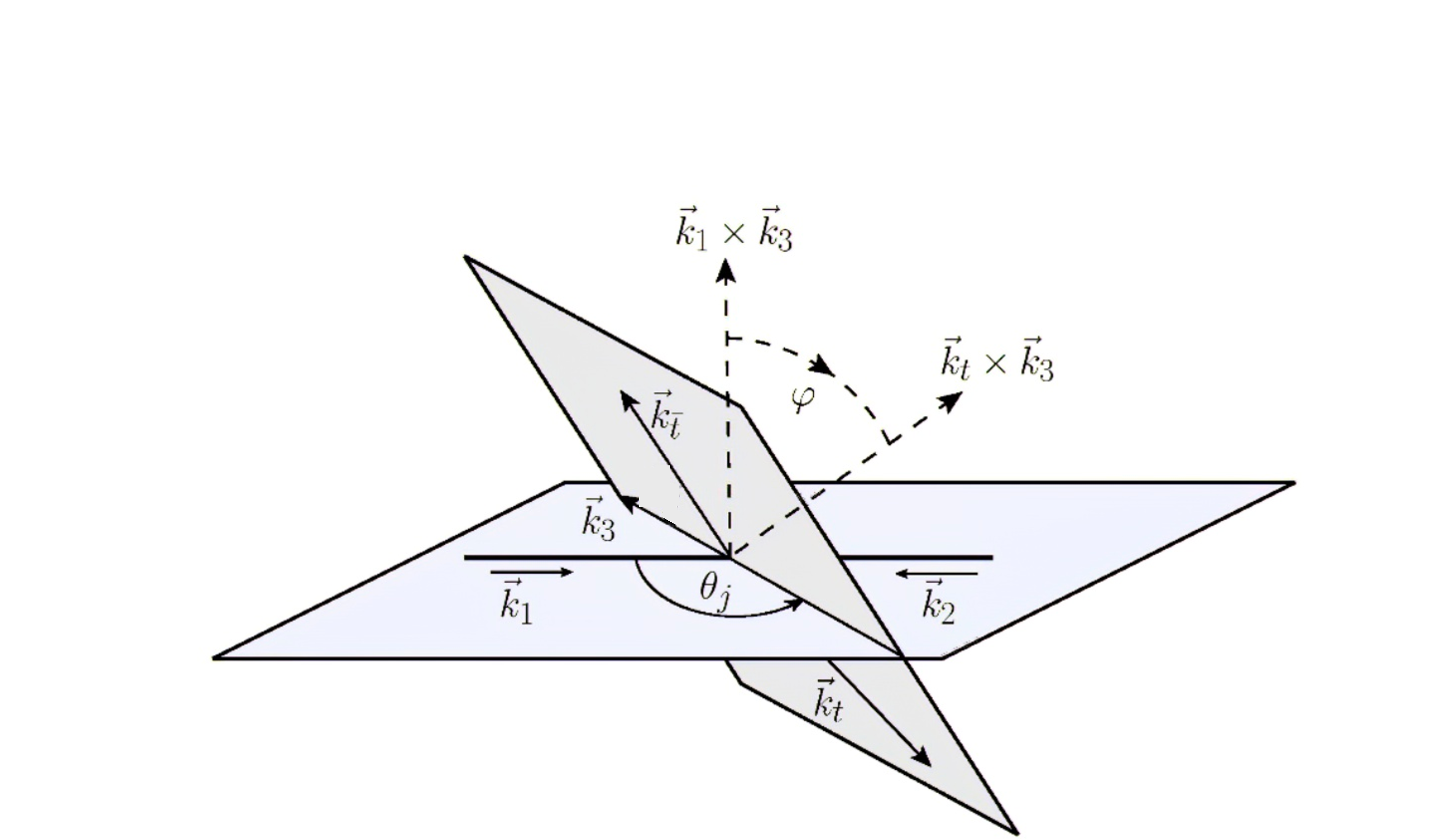
Figure 1:
Kinematic properties of the process $ \mathrm{p}_{1}\mathrm{p}_{2} \rightarrow {\mathrm{t}\overline{\mathrm{t}}} \text{j} $, where $ \mathrm{p}_{1} $ and $ \mathrm{p}_{2} $ represent the incoming partons, with three-momenta $ \vec{k}_1 $ and $ \vec{k}_2 $. The three-momenta of the top quark, top antiquark, and additional jet are indicated by $ \vec{k}_\mathrm{t} $, $ \vec{k}_\overline{\mathrm{t}} $, and $ \vec{k}_3 $. The inclination angle $ \varphi $ is defined through $ \cos\varphi = \vec{n}_{13}\cdot\vec{n}_{\mathrm{t}3} $, with $ \varphi \in [0, 2\pi] $, and $ \vec{n}_{13} $ and $ \vec{n}_{\mathrm{t}3} $ are the normal vectors to the $ (\mathrm{p}_{1}\mathrm{p}_{2},\mathrm{j}) $ and $ (\mathrm{t},\overline{\mathrm{t}},\mathrm{j}) $ planes, respectively. The jet angle $ \theta_\text{j} $ is also shown. Figure modified from Ref. [12]. |

png pdf |
Figure 2:
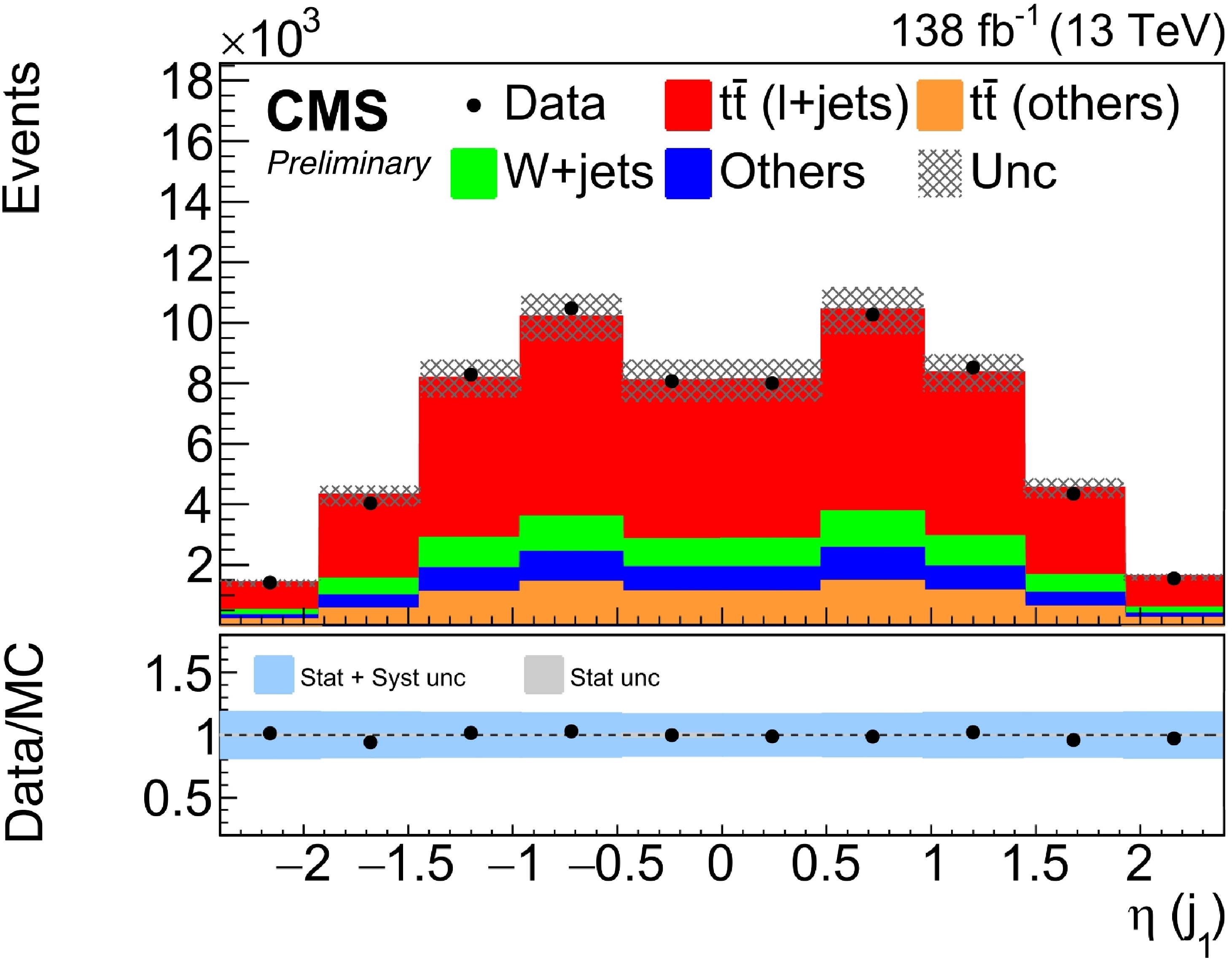
Kinematic variables in the muon channel (left) and electron channel (right) used for BDT training from upper to lower: $ \eta $ and $ p_{\mathrm{T}} $ of the leading AK4 jet, and $ \eta $ and $ p_{\mathrm{T}} $ of the subleading AK4 jet. The hatched and solid blue bands show the total uncertainty on the prediction, and the gray band shows the statistical component. The last bin includes all events above the plotted range. |

png pdf |
Figure 2-a:
Kinematic variables in the muon channel (left) and electron channel (right) used for BDT training from upper to lower: $ \eta $ and $ p_{\mathrm{T}} $ of the leading AK4 jet, and $ \eta $ and $ p_{\mathrm{T}} $ of the subleading AK4 jet. The hatched and solid blue bands show the total uncertainty on the prediction, and the gray band shows the statistical component. The last bin includes all events above the plotted range. |
png pdf |
Figure 2-b:
Kinematic variables in the muon channel (left) and electron channel (right) used for BDT training from upper to lower: $ \eta $ and $ p_{\mathrm{T}} $ of the leading AK4 jet, and $ \eta $ and $ p_{\mathrm{T}} $ of the subleading AK4 jet. The hatched and solid blue bands show the total uncertainty on the prediction, and the gray band shows the statistical component. The last bin includes all events above the plotted range. |

png pdf |
Figure 2-c:
Kinematic variables in the muon channel (left) and electron channel (right) used for BDT training from upper to lower: $ \eta $ and $ p_{\mathrm{T}} $ of the leading AK4 jet, and $ \eta $ and $ p_{\mathrm{T}} $ of the subleading AK4 jet. The hatched and solid blue bands show the total uncertainty on the prediction, and the gray band shows the statistical component. The last bin includes all events above the plotted range. |

png pdf |
Figure 2-d:
Kinematic variables in the muon channel (left) and electron channel (right) used for BDT training from upper to lower: $ \eta $ and $ p_{\mathrm{T}} $ of the leading AK4 jet, and $ \eta $ and $ p_{\mathrm{T}} $ of the subleading AK4 jet. The hatched and solid blue bands show the total uncertainty on the prediction, and the gray band shows the statistical component. The last bin includes all events above the plotted range. |

png pdf |
Figure 2-e:
Kinematic variables in the muon channel (left) and electron channel (right) used for BDT training from upper to lower: $ \eta $ and $ p_{\mathrm{T}} $ of the leading AK4 jet, and $ \eta $ and $ p_{\mathrm{T}} $ of the subleading AK4 jet. The hatched and solid blue bands show the total uncertainty on the prediction, and the gray band shows the statistical component. The last bin includes all events above the plotted range. |

png pdf |
Figure 2-f:
Kinematic variables in the muon channel (left) and electron channel (right) used for BDT training from upper to lower: $ \eta $ and $ p_{\mathrm{T}} $ of the leading AK4 jet, and $ \eta $ and $ p_{\mathrm{T}} $ of the subleading AK4 jet. The hatched and solid blue bands show the total uncertainty on the prediction, and the gray band shows the statistical component. The last bin includes all events above the plotted range. |

png pdf |
Figure 2-g:
Kinematic variables in the muon channel (left) and electron channel (right) used for BDT training from upper to lower: $ \eta $ and $ p_{\mathrm{T}} $ of the leading AK4 jet, and $ \eta $ and $ p_{\mathrm{T}} $ of the subleading AK4 jet. The hatched and solid blue bands show the total uncertainty on the prediction, and the gray band shows the statistical component. The last bin includes all events above the plotted range. |

png pdf |
Figure 2-h:
Kinematic variables in the muon channel (left) and electron channel (right) used for BDT training from upper to lower: $ \eta $ and $ p_{\mathrm{T}} $ of the leading AK4 jet, and $ \eta $ and $ p_{\mathrm{T}} $ of the subleading AK4 jet. The hatched and solid blue bands show the total uncertainty on the prediction, and the gray band shows the statistical component. The last bin includes all events above the plotted range. |
png pdf |
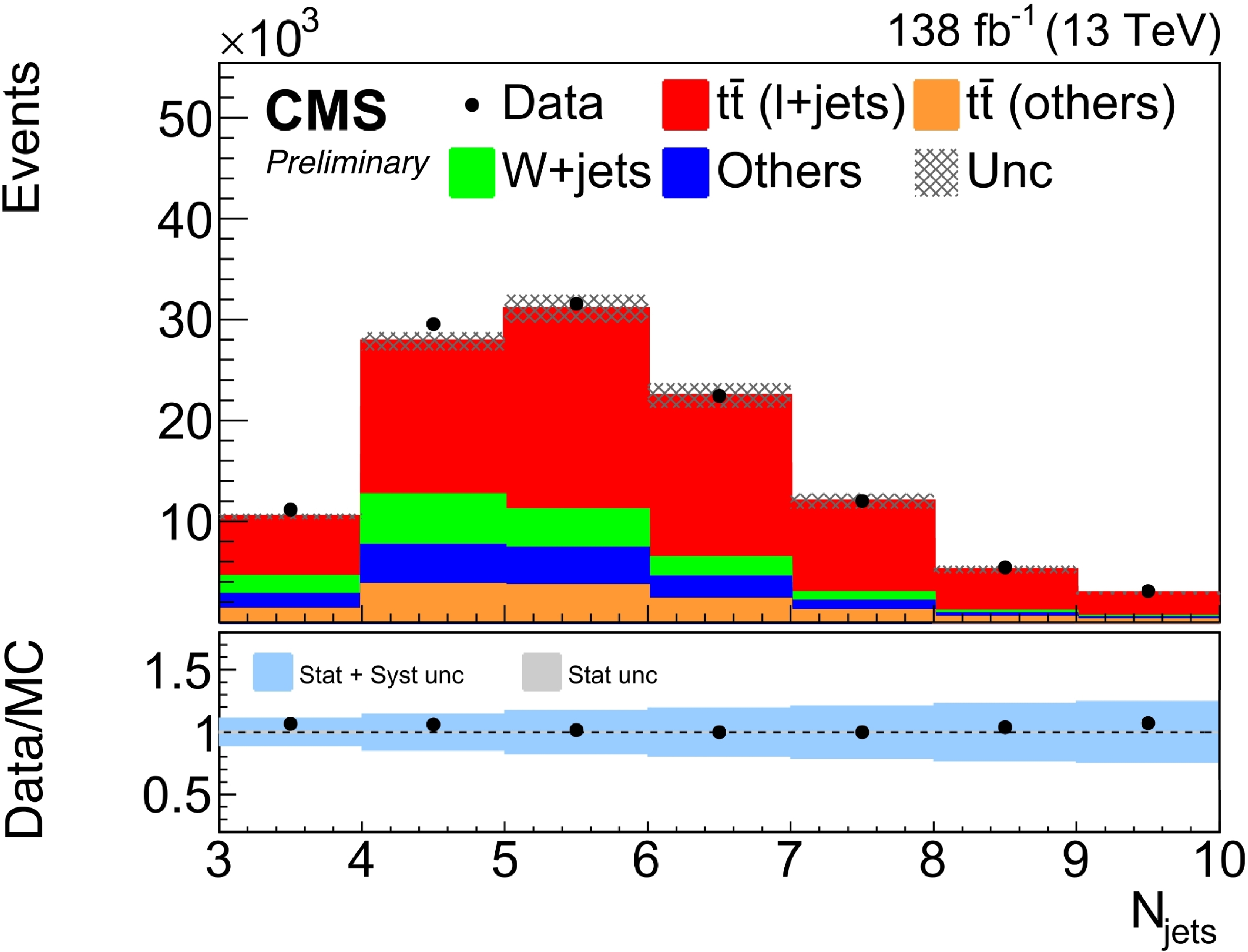
Figure 3:
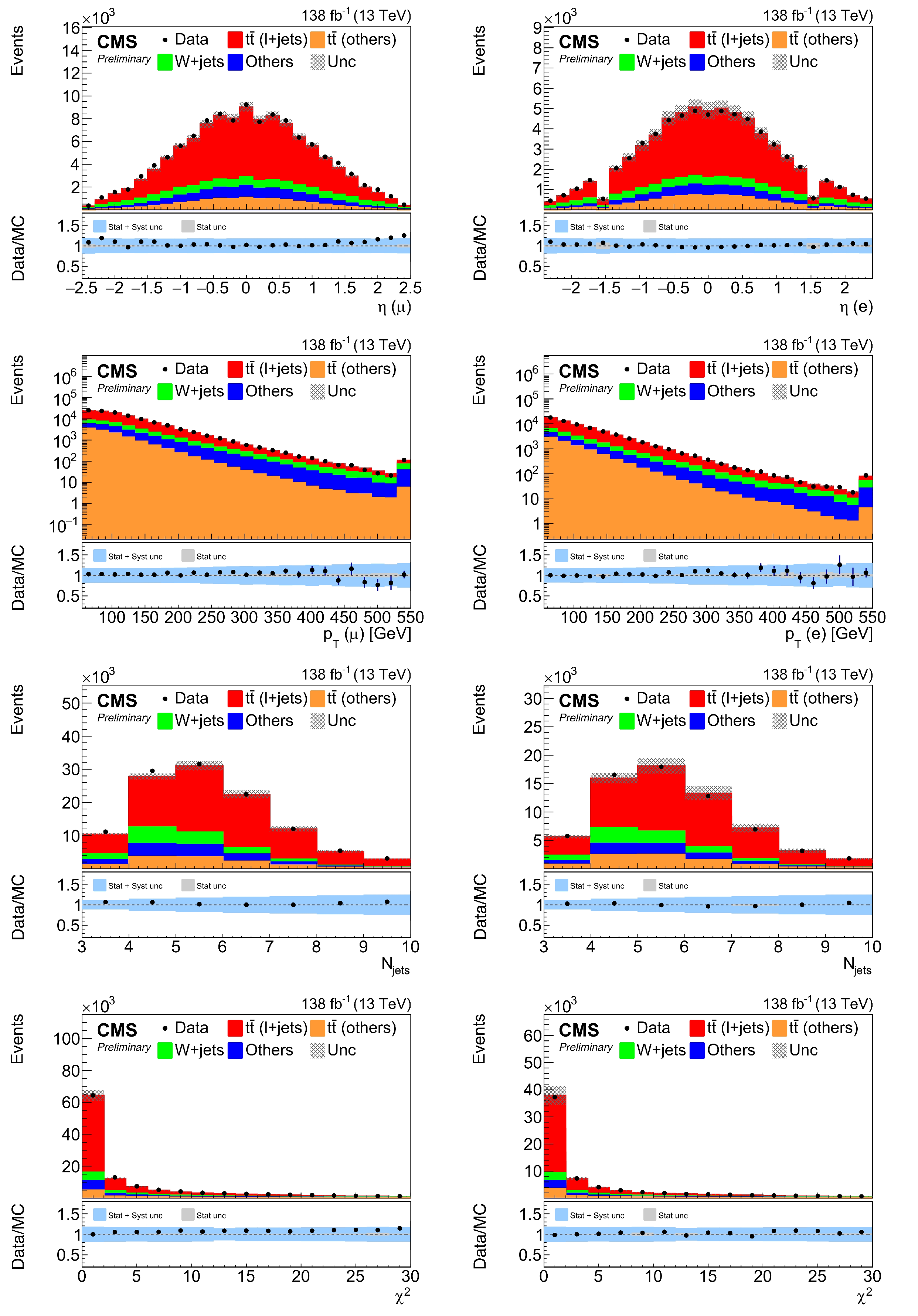
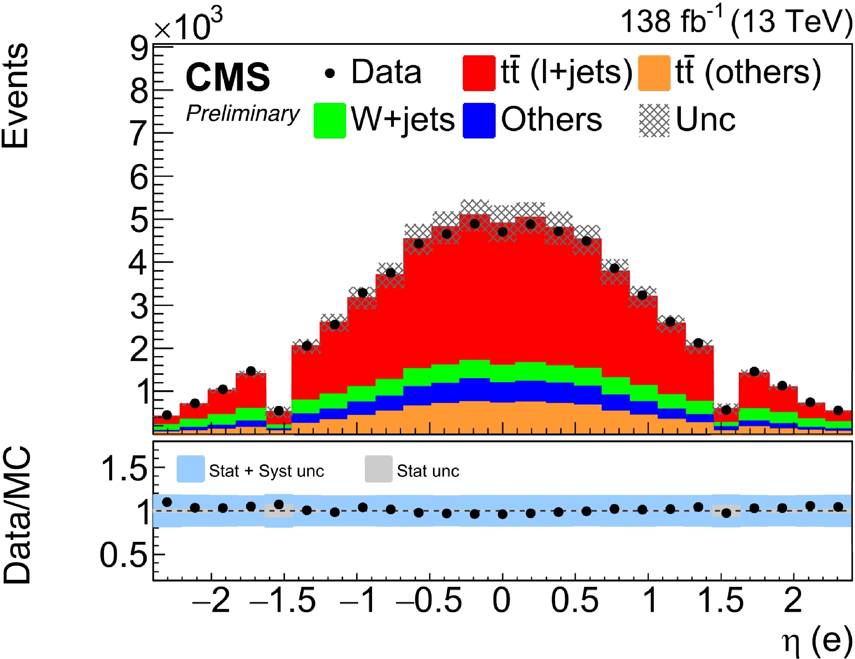
Kinematic variables in the muon channel (left) and electron channel (right) used for BDT training from upper to lower: $ \eta $ and $ p_{\mathrm{T}} $ of the lepton, number of AK4 jets, and $ \chi^2 $. The hatched and solid blue bands show the total uncertainty on the prediction, and the gray band shows the statistical component. The last bin includes all events above the plotted range. |

png pdf |
Figure 3-a:
Kinematic variables in the muon channel (left) and electron channel (right) used for BDT training from upper to lower: $ \eta $ and $ p_{\mathrm{T}} $ of the lepton, number of AK4 jets, and $ \chi^2 $. The hatched and solid blue bands show the total uncertainty on the prediction, and the gray band shows the statistical component. The last bin includes all events above the plotted range. |
png pdf |
Figure 3-b:
Kinematic variables in the muon channel (left) and electron channel (right) used for BDT training from upper to lower: $ \eta $ and $ p_{\mathrm{T}} $ of the lepton, number of AK4 jets, and $ \chi^2 $. The hatched and solid blue bands show the total uncertainty on the prediction, and the gray band shows the statistical component. The last bin includes all events above the plotted range. |

png pdf |
Figure 3-c:
Kinematic variables in the muon channel (left) and electron channel (right) used for BDT training from upper to lower: $ \eta $ and $ p_{\mathrm{T}} $ of the lepton, number of AK4 jets, and $ \chi^2 $. The hatched and solid blue bands show the total uncertainty on the prediction, and the gray band shows the statistical component. The last bin includes all events above the plotted range. |

png pdf |
Figure 3-d:
Kinematic variables in the muon channel (left) and electron channel (right) used for BDT training from upper to lower: $ \eta $ and $ p_{\mathrm{T}} $ of the lepton, number of AK4 jets, and $ \chi^2 $. The hatched and solid blue bands show the total uncertainty on the prediction, and the gray band shows the statistical component. The last bin includes all events above the plotted range. |
png pdf |
Figure 3-e:
Kinematic variables in the muon channel (left) and electron channel (right) used for BDT training from upper to lower: $ \eta $ and $ p_{\mathrm{T}} $ of the lepton, number of AK4 jets, and $ \chi^2 $. The hatched and solid blue bands show the total uncertainty on the prediction, and the gray band shows the statistical component. The last bin includes all events above the plotted range. |

png pdf |
Figure 3-f:
Kinematic variables in the muon channel (left) and electron channel (right) used for BDT training from upper to lower: $ \eta $ and $ p_{\mathrm{T}} $ of the lepton, number of AK4 jets, and $ \chi^2 $. The hatched and solid blue bands show the total uncertainty on the prediction, and the gray band shows the statistical component. The last bin includes all events above the plotted range. |

png pdf |
Figure 3-g:
Kinematic variables in the muon channel (left) and electron channel (right) used for BDT training from upper to lower: $ \eta $ and $ p_{\mathrm{T}} $ of the lepton, number of AK4 jets, and $ \chi^2 $. The hatched and solid blue bands show the total uncertainty on the prediction, and the gray band shows the statistical component. The last bin includes all events above the plotted range. |

png pdf |
Figure 3-h:
Kinematic variables in the muon channel (left) and electron channel (right) used for BDT training from upper to lower: $ \eta $ and $ p_{\mathrm{T}} $ of the lepton, number of AK4 jets, and $ \chi^2 $. The hatched and solid blue bands show the total uncertainty on the prediction, and the gray band shows the statistical component. The last bin includes all events above the plotted range. |
png pdf |
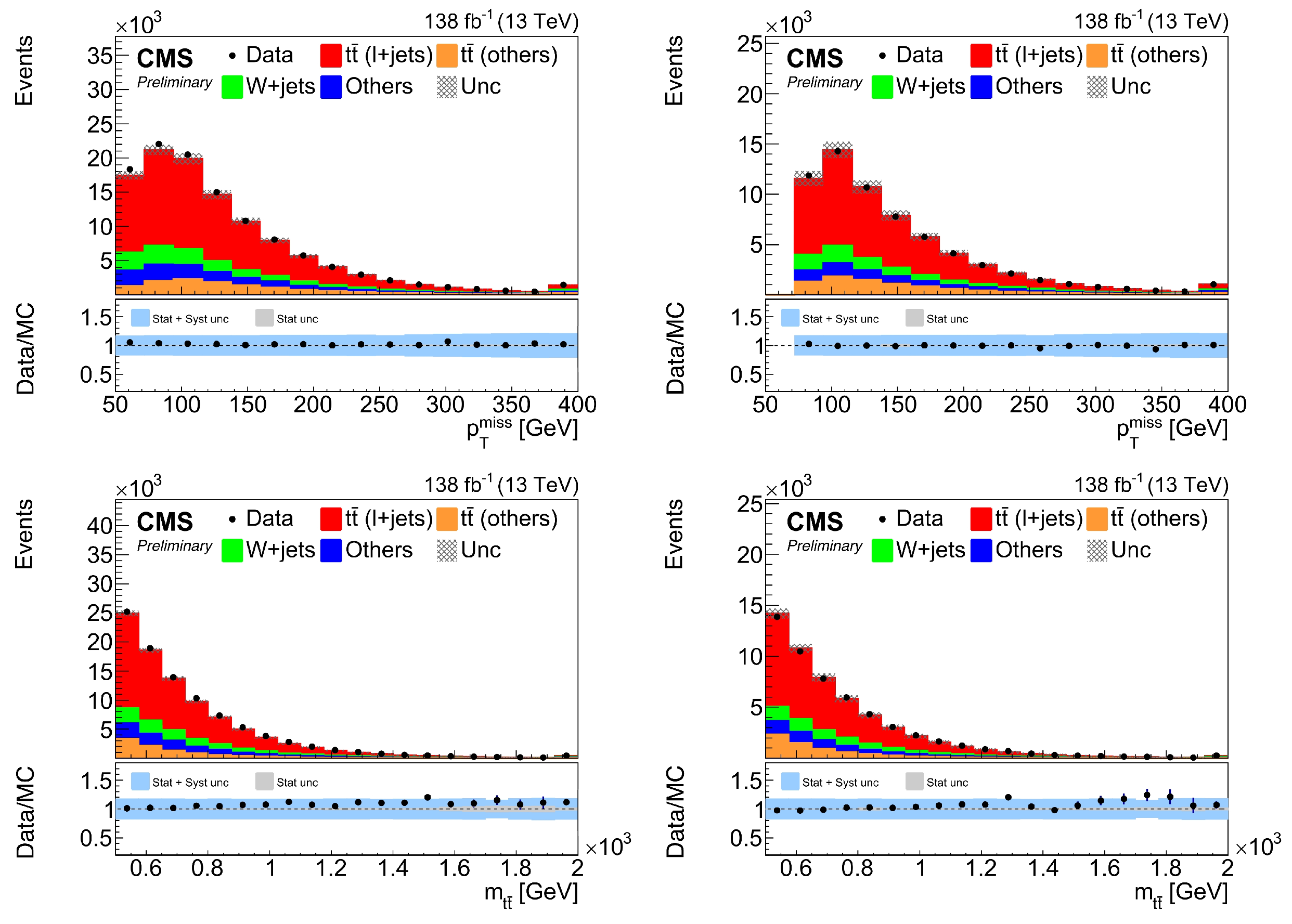
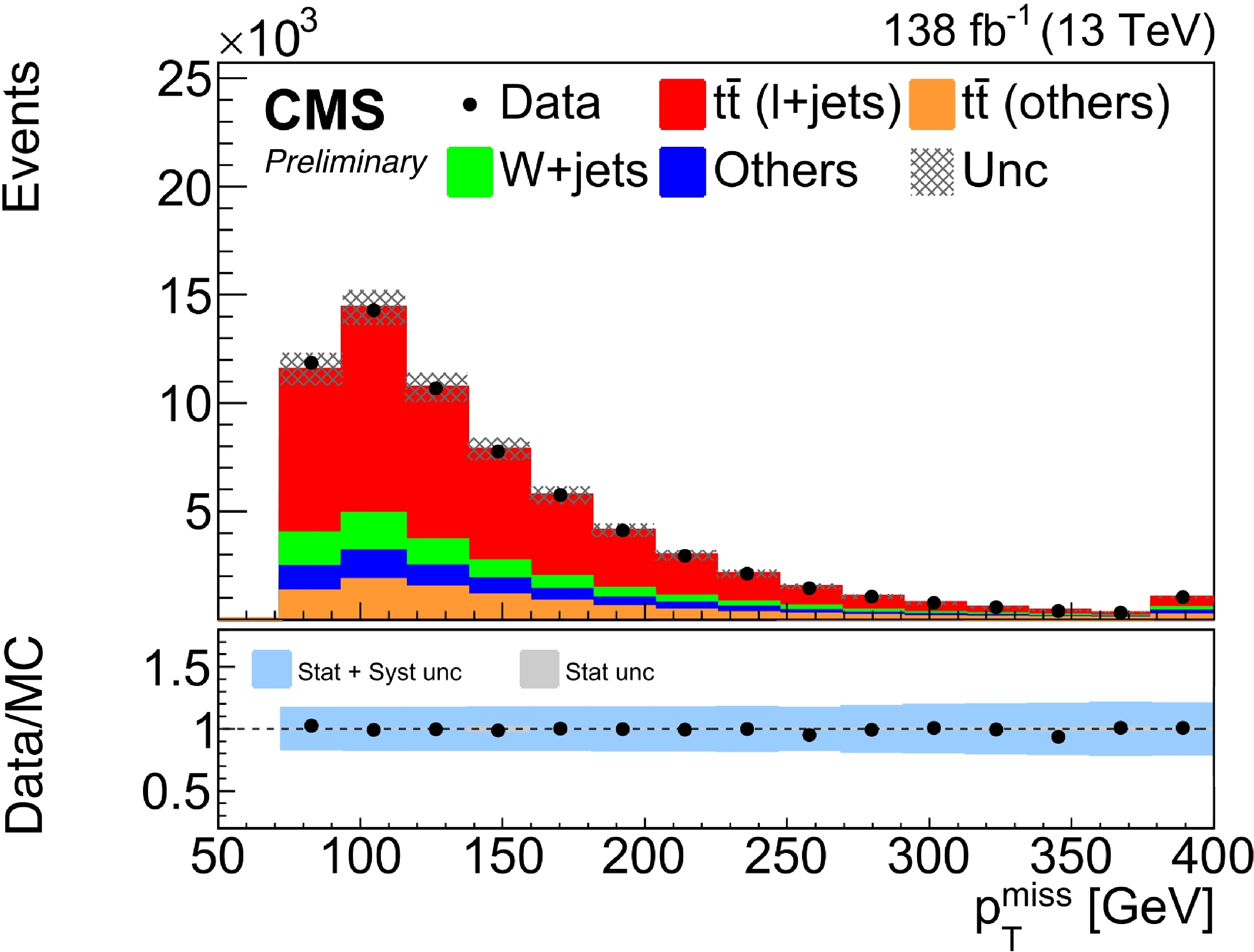
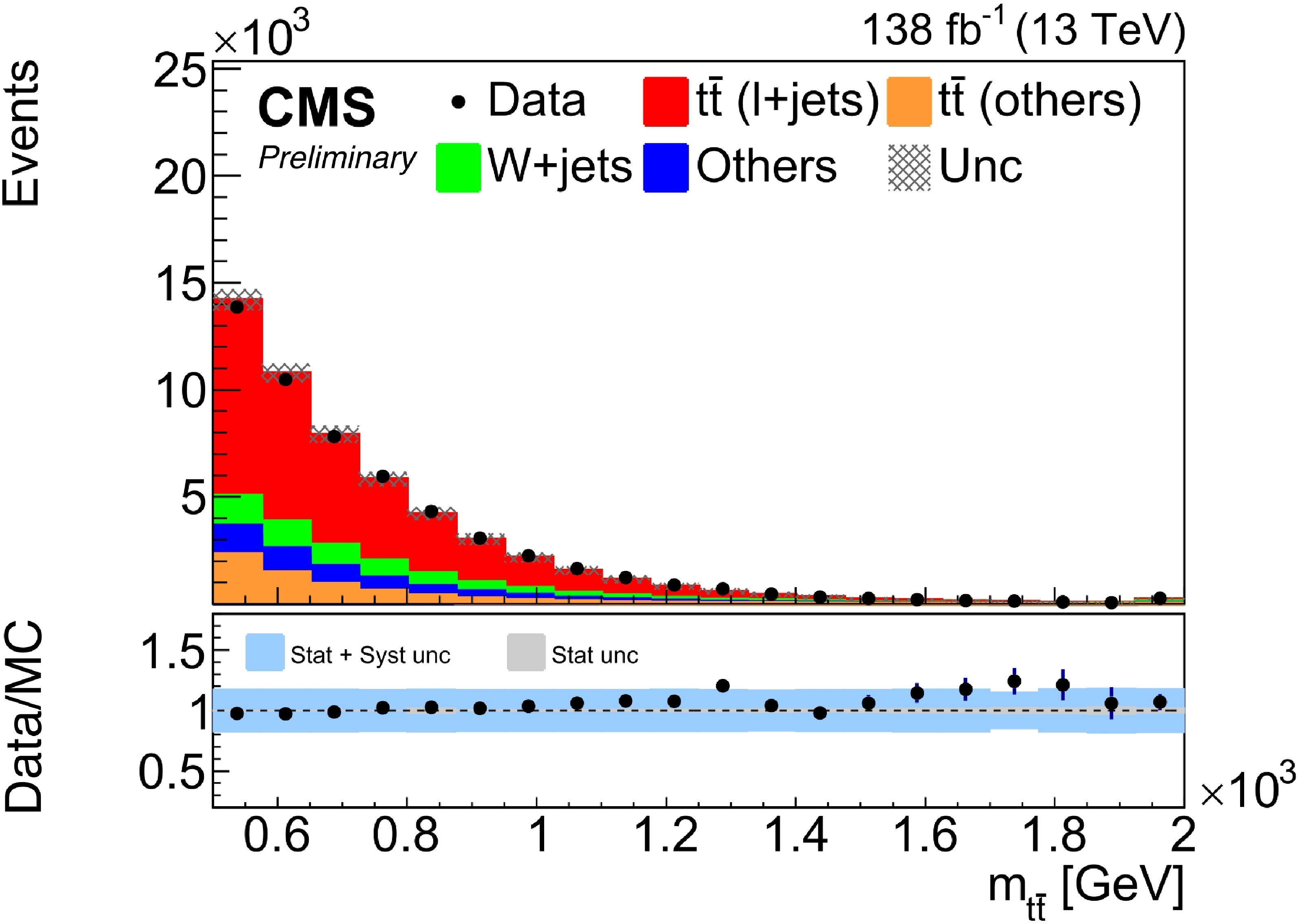
Figure 4:
Kinematic variables in the muon channel (left) and electron channel (right) used for BDT training from upper to lower: $ p_{\mathrm{T}}^\text{miss} $ and $ m_{{\mathrm{t}\overline{\mathrm{t}}} } $. The hatched and solid blue bands show the total uncertainty on the prediction, and the gray band shows the statistical component. The last bin includes all events above the plotted range. |

png pdf |
Figure 4-a:
Kinematic variables in the muon channel (left) and electron channel (right) used for BDT training from upper to lower: $ p_{\mathrm{T}}^\text{miss} $ and $ m_{{\mathrm{t}\overline{\mathrm{t}}} } $. The hatched and solid blue bands show the total uncertainty on the prediction, and the gray band shows the statistical component. The last bin includes all events above the plotted range. |
png pdf |
Figure 4-b:
Kinematic variables in the muon channel (left) and electron channel (right) used for BDT training from upper to lower: $ p_{\mathrm{T}}^\text{miss} $ and $ m_{{\mathrm{t}\overline{\mathrm{t}}} } $. The hatched and solid blue bands show the total uncertainty on the prediction, and the gray band shows the statistical component. The last bin includes all events above the plotted range. |

png pdf |
Figure 4-c:
Kinematic variables in the muon channel (left) and electron channel (right) used for BDT training from upper to lower: $ p_{\mathrm{T}}^\text{miss} $ and $ m_{{\mathrm{t}\overline{\mathrm{t}}} } $. The hatched and solid blue bands show the total uncertainty on the prediction, and the gray band shows the statistical component. The last bin includes all events above the plotted range. |
png pdf |
Figure 4-d:
Kinematic variables in the muon channel (left) and electron channel (right) used for BDT training from upper to lower: $ p_{\mathrm{T}}^\text{miss} $ and $ m_{{\mathrm{t}\overline{\mathrm{t}}} } $. The hatched and solid blue bands show the total uncertainty on the prediction, and the gray band shows the statistical component. The last bin includes all events above the plotted range. |
png pdf |
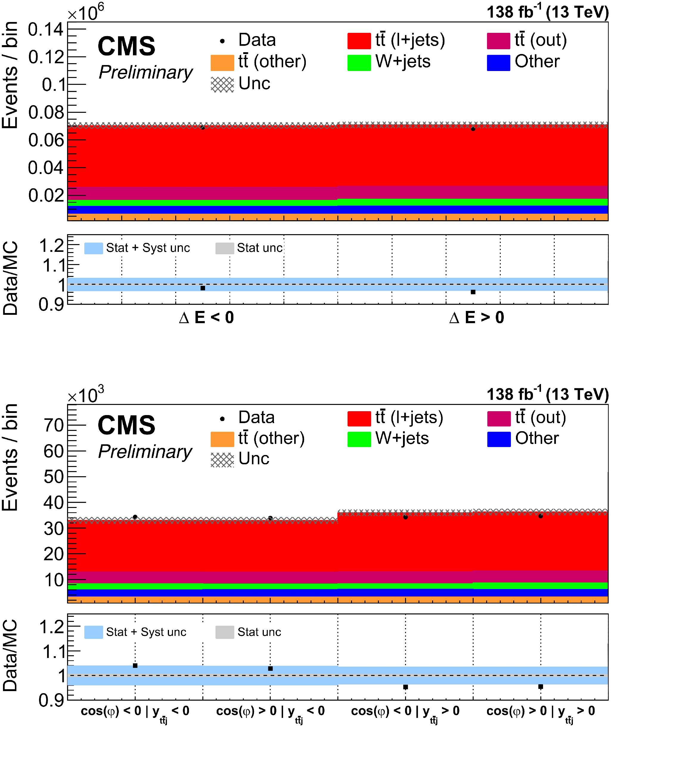
Figure 5:
Event yields categorized by $ \Delta E $ (upper) and $ y_{{\mathrm{t}\overline{\mathrm{t}}} \text{j}} $ for positive and negative values of $ \cos\varphi $ (lower) before the fit. The hatched and solid blue bands show the total uncertainty on the prediction, and the gray band shows the statistical component. |

png pdf |
Figure 5-a:
Event yields categorized by $ \Delta E $ (upper) and $ y_{{\mathrm{t}\overline{\mathrm{t}}} \text{j}} $ for positive and negative values of $ \cos\varphi $ (lower) before the fit. The hatched and solid blue bands show the total uncertainty on the prediction, and the gray band shows the statistical component. |

png pdf |
Figure 5-b:
Event yields categorized by $ \Delta E $ (upper) and $ y_{{\mathrm{t}\overline{\mathrm{t}}} \text{j}} $ for positive and negative values of $ \cos\varphi $ (lower) before the fit. The hatched and solid blue bands show the total uncertainty on the prediction, and the gray band shows the statistical component. |
png pdf |
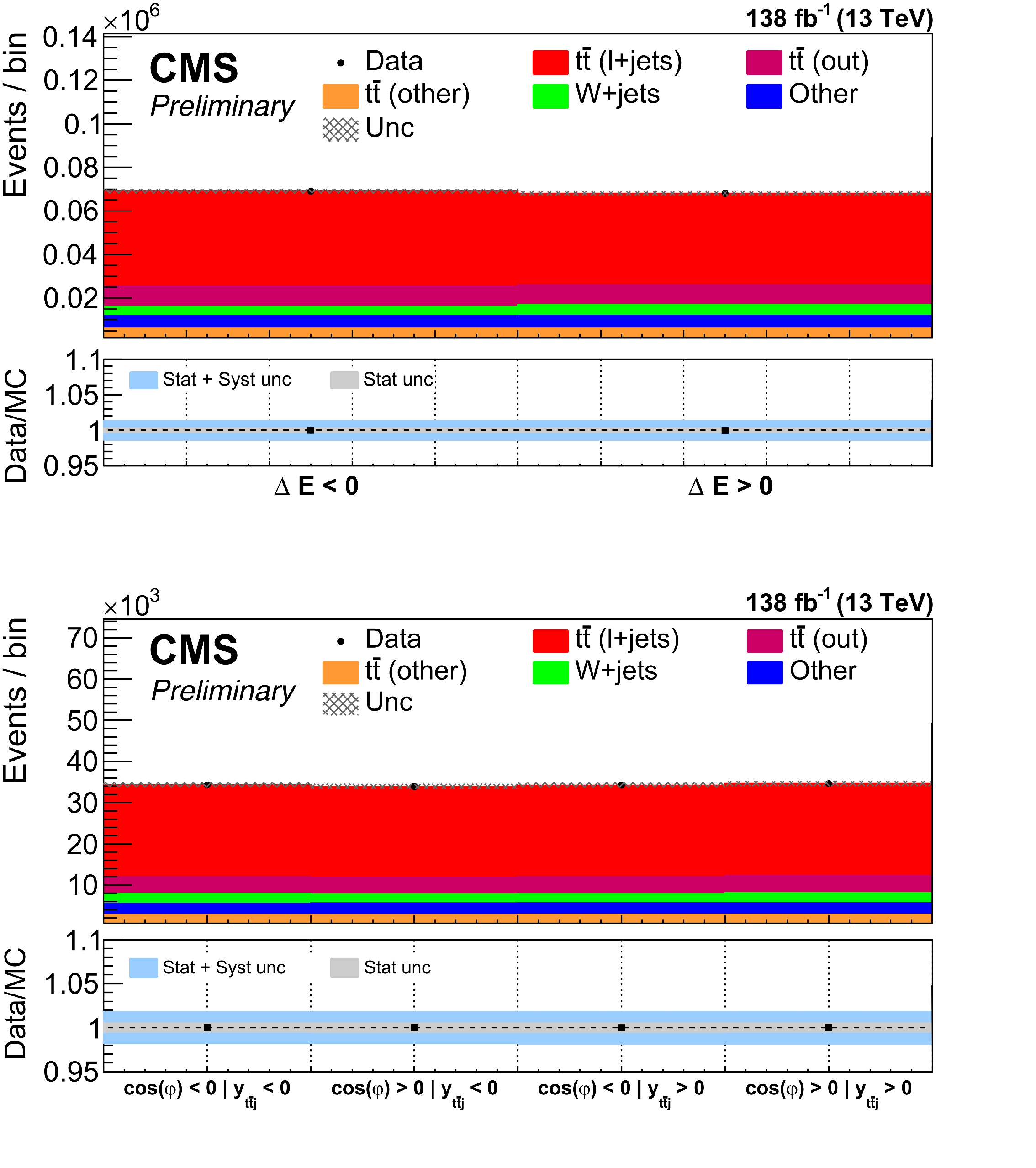
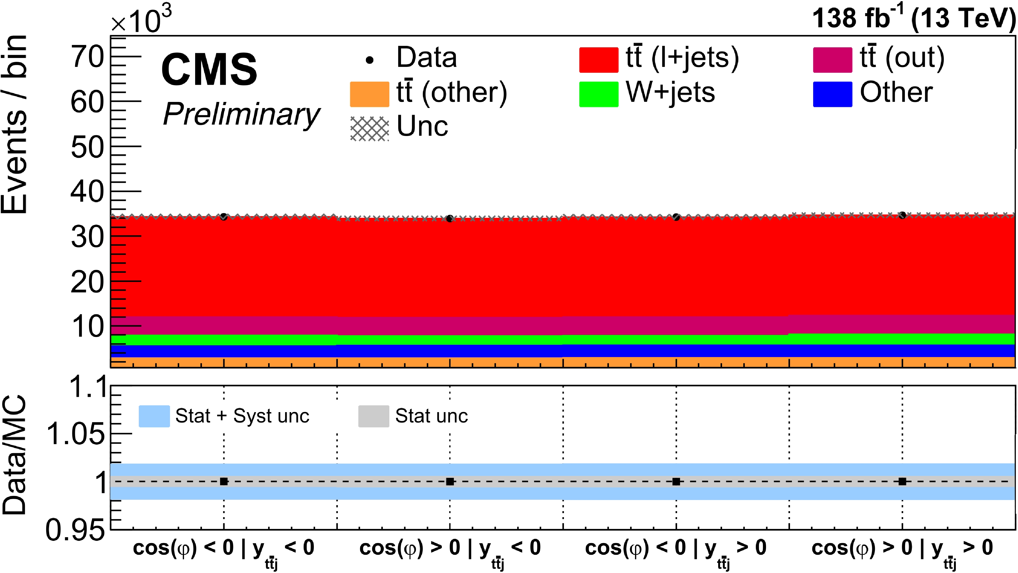
Figure 6:
Event yields categorized by $ \Delta E $ (upper) and $ y_{{\mathrm{t}\overline{\mathrm{t}}} \text{j}} $ for positive and negative values of $ \cos\varphi $ (lower) after the fit. The hatched and solid blue bands show the total uncertainty on the prediction, and the gray band shows the statistical component. |

png pdf |
Figure 6-a:
Event yields categorized by $ \Delta E $ (upper) and $ y_{{\mathrm{t}\overline{\mathrm{t}}} \text{j}} $ for positive and negative values of $ \cos\varphi $ (lower) after the fit. The hatched and solid blue bands show the total uncertainty on the prediction, and the gray band shows the statistical component. |
png pdf |
Figure 6-b:
Event yields categorized by $ \Delta E $ (upper) and $ y_{{\mathrm{t}\overline{\mathrm{t}}} \text{j}} $ for positive and negative values of $ \cos\varphi $ (lower) after the fit. The hatched and solid blue bands show the total uncertainty on the prediction, and the gray band shows the statistical component. |

png pdf |
Figure 7:
Measured $ A_E $ for different event categories. The vertical red line (band) represents the central value (total uncertainty) of the nominal measurement, while the other bands show the SM expectation from different MC models. The markers (horizontal bars) indicate the central values (total uncertainties) of the measurements in the different categories. |
| Tables | |

png pdf |
Table 1:
Expected yields for signal and background processes and observed number of events in data after full event selection, together with their total (statistical and systematic) uncertainties. The $ \mathrm{t} \overline{\mathrm{t}} $ events are separated into the different decay channels: lepton+jets ($ \ell $+jets), dileptonic, and fully hadronic. Events in the $ \ell $+jets channel that are outside the fiducial phase space of the analysis are indicated by `` $ \mathrm{t} \overline{\mathrm{t}} $ (out)''. All single top quark events are grouped as ``Single top quark''. |

png pdf |
Table 2:
Measured energy asymmetry $ A_E $ and incline asymmetry $ A_I $ values in the considered $ \theta_\text{j}^{\text{opt}} $ range. The data are compared with SM expectations from different MC models. |

png pdf |
Table 3:
Summary of statistical and systematic uncertainties affecting the measurement of $ A_E $ and $ A_I $. The total uncertainty is obtained by adding individual contributions in quadrature. |
| Summary |
| We report the first CMS measurement of the energy asymmetry and the first LHC measurement of the incline asymmetry in top quark pair production in association with a jet, using events with one charged lepton (electron or muon). The analysis is based on proton-proton collision data recorded with the CMS detector at a center-of-mass energy of 13 TeV, corresponding to an integrated luminosity of 138 fb$ ^{-1} $. The measurements cover the resolved, semi-resolved, and boosted topologies of the hadronic top-quark decay. The sensitivity to charge asymmetry effects is enhanced by performing the measurements in a fiducial region where the additional jet is produced approximately perpendicular to the top-quark directions. The measurements are corrected for detector effects to the particle level using a likelihood-based unfolding procedure. The energy asymmetry is measured to be $ A_E = $ ($- $6.3 $ \pm $ 2.3)%, consistent within two standard deviations with the standard model (SM) expectation of ($-$1.6 $ \pm $ 0.3)%, computed at next-to-leading-order accuracy in perturbative quantum chromodynamics. The measurement deviates from the zero-asymmetry hypothesis with a significance of 2.7 standard deviations. The incline asymmetry is measured as $ A_I = $ (2.5 $ \pm $ 2.3)%, in agreement with SM expectations. |
| References | ||||
| 1 | O. Antunano, J. H. Kuhn, and G. Rodrigo | Top quarks, axigluons and charge asymmetries at hadron colliders | PRD 77 (2008) 014003 | 0709.1652 |
| 2 | M. Bauer et al. | Top-quark forward-backward asymmetry in Randall-Sundrum models beyond the leading order | JHEP 11 (2010) 039 | 1008.0742 |
| 3 | U. Haisch and S. Westhoff | Massive color-octet bosons: Bounds on effects in top-quark pair production | JHEP 08 (2011) 088 | 1106.0529 |
| 4 | The ATLAS and CMS Collaborations | Combination of inclusive and differential $ \mathrm{t} \overline{\mathrm{t}} $ charge asymmetry measurements using ATLAS and CMS data at $ \sqrt{s}= $ 7 and 8 TeV | JHEP 04 (2018) 033 | 1709.05327 |
| 5 | ATLAS Collaboration | Measurement of the charge asymmetry in top-quark pair production in the lepton-plus-jets final state in pp collision data at $ \sqrt{s}= $ 8 TeV with the ATLAS detector | EPJC 76 (2016) 87 | 1509.02358 |
| 6 | CMS Collaboration | Inclusive and differential measurements of the $ \mathrm{t} \overline{\mathrm{t}} $ charge asymmetry in pp collisions at $ \sqrt{s}= $ 8 TeV | PLB 757 (2016) 154 | CMS-TOP-12-033 1507.03119 |
| 7 | ATLAS Collaboration | Evidence for the charge asymmetry in pp $ \rightarrow {\mathrm{t}\overline{\mathrm{t}}} $ production at $ \sqrt{s}= $ 13 TeV with the ATLAS detector | JHEP 08 (2023) 077 | 2208.12095 |
| 8 | CMS Collaboration | Measurement of the $ \mathrm{t} \overline{\mathrm{t}} $ charge asymmetry in events with highly Lorentz-boosted top quarks in pp collisions at $ \sqrt{s}= $ 13 TeV | PLB 846 (2023) 137703 | CMS-TOP-21-014 2208.02751 |
| 9 | S. Dittmaier, P. Uwer, and S. Weinzierl | NLO QCD corrections to $ \mathrm{t} \overline{\mathrm{t}} $ +jet production at hadron colliders | PRL 98 (2007) 262002 | hep-ph/0703120 |
| 10 | S. Dittmaier, P. Uwer, and S. Weinzierl | Hadronic top-quark pair production in association with a hard jet at next-to-leading order QCD: Phenomenological studies for the Tevatron and the LHC | EPJC 59 (2009) 625 | 0810.0452 |
| 11 | K. Melnikov and M. Schulze | NLO QCD corrections to top quark pair production in association with one hard jet at hadron colliders | NPB 840 (2010) 129 | 1004.3284 |
| 12 | S. Berge and S. Westhoff | Top-quark charge asymmetry goes forward: two new observables for hadron colliders | JHEP 07 (2013) 179 | 1305.3272 |
| 13 | ATLAS Collaboration | Measurement of the energy asymmetry in $ {\mathrm{t}\overline{\mathrm{t}}} \text{j} $ production at 13 TeV with the ATLAS experiment and interpretation in the SMEFT framework | EPJC 82 (2022) 374 | 2110.05453 |
| 14 | CMS Collaboration | The CMS experiment at the CERN LHC | JINST 3 (2008) S08004 | |
| 15 | CMS Collaboration | Development of the CMS detector for the CERN LHC Run 3 | JINST 19 (2024) P05064 | CMS-PRF-21-001 2309.05466 |
| 16 | CMS Collaboration | Performance of the CMS Level-1 trigger in proton-proton collisions at $ \sqrt{s}= $ 13 TeV | JINST 15 (2020) P10017 | CMS-TRG-17-001 2006.10165 |
| 17 | CMS Collaboration | The CMS trigger system | JINST 12 (2017) P01020 | CMS-TRG-12-001 1609.02366 |
| 18 | CMS Collaboration | Performance of the CMS high-level trigger during LHC Run 2 | JINST 19 (2024) P11021 | CMS-TRG-19-001 2410.17038 |
| 19 | CMS Collaboration | Performance of the CMS muon detector and muon reconstruction with proton-proton collisions at $ \sqrt{s}= $ 13 TeV | JINST 13 (2018) P06015 | CMS-MUO-16-001 1804.04528 |
| 20 | CMS Collaboration | Performance of the CMS muon trigger system in proton-proton collisions at $ \sqrt{s} = $ 13 TeV | JINST 16 (2021) P07001 | CMS-MUO-19-001 2102.04790 |
| 21 | CMS Collaboration | Electron and photon reconstruction and identification with the CMS experiment at the CERN LHC | JINST 16 (2021) P05014 | CMS-EGM-17-001 2012.06888 |
| 22 | CMS Collaboration | Particle-flow reconstruction and global event description with the CMS detector | JINST 12 (2017) P10003 | CMS-PRF-14-001 1706.04965 |
| 23 | CMS Collaboration | Performance of the CMS electromagnetic calorimeter in $ {\mathrm{p}\mathrm{p}} $ collisions at $ \sqrt{s}= $ 13 TeV | JINST 19 (2024) P09004 | CMS-EGM-18-002 2403.15518 |
| 24 | M. Cacciari, G. P. Salam, and G. Soyez | The anti-$ k_{\mathrm{T}} $ jet clustering algorithm | JHEP 04 (2008) 063 | 0802.1189 |
| 25 | M. Cacciari, G. P. Salam, and G. Soyez | FastJet user manual | EPJC 72 (2012) 1896 | 1111.6097 |
| 26 | CMS Collaboration | Pileup mitigation at CMS in 13 TeV data | JINST 15 (2020) P09018 | CMS-JME-18-001 2003.00503 |
| 27 | CMS Collaboration | Jet energy scale and resolution in the CMS experiment in pp collisions at 8 TeV | JINST 12 (2017) P02014 | CMS-JME-13-004 1607.03663 |
| 28 | CMS Collaboration | Performance of missing transverse momentum reconstruction in proton-proton collisions at $ \sqrt{s} = $ 13 TeV using the CMS detector | JINST 14 (2019) P07004 | CMS-JME-17-001 1903.06078 |
| 29 | CMS Collaboration | Identification of heavy-flavour jets with the CMS detector in pp collisions at 13 TeV | JINST 13 (2018) P05011 | CMS-BTV-16-002 1712.07158 |
| 30 | E. Bols et al. | Jet flavour classification using DeepJet | JINST 15 (2020) P12012 | 2008.10519 |
| 31 | CMS Collaboration | Performance summary of AK4 jet b tagging with data from proton-proton collisions at 13 TeV with the CMS detector | CMS Detector Performance Summary CMS-DP-2023-005, 2023 CDS |
|
| 32 | CMS Collaboration | Identification of heavy, energetic, hadronically decaying particles using machine-learning techniques | JINST 15 (2020) P06005 | CMS-JME-18-002 2004.08262 |
| 33 | CMS Collaboration | Calibration of the top and W jet tagging efficiency in 13 TeV data collected by the CMS experiment in 2016--2018 | CMS Detector Performance Summary CMS-DP-2025-010, 2025 CDS |
|
| 34 | A. J. Larkoski, S. Marzani, G. Soyez, and J. Thaler | Soft Drop | JHEP 05 (2014) 146 | 1402.2657 |
| 35 | T. Sjostrand et al. | An introduction to PYTHIA 8.2 | Comput. Phys. Commun. 191 (2015) 159 | 1410.3012 |
| 36 | P. Nason | A new method for combining NLO QCD with shower Monte Carlo algorithms | JHEP 11 (2004) 040 | hep-ph/0409146 |
| 37 | S. Frixione, P. Nason, and C. Oleari | Matching NLO QCD computations with parton shower simulations: the POWHEG method | JHEP 11 (2007) 070 | 0709.2092 |
| 38 | S. Frixione, P. Nason, and G. Ridolfi | A positive-weight next-to-leading-order Monte Carlo for heavy flavour hadroproduction | JHEP 09 (2007) 126 | 0707.3088 |
| 39 | S. Alioli, P. Nason, C. Oleari, and E. Re | A general framework for implementing NLO calculations in shower Monte Carlo programs: the POWHEG BOX | JHEP 06 (2010) 043 | 1002.2581 |
| 40 | E. Re | Single-top $ {\mathrm{W}}{\mathrm{t}} $-channel production matched with parton showers using the POWHEG method | EPJC 71 (2011) 1547 | 1009.2450 |
| 41 | M. Cacciari et al. | Top-pair production at hadron colliders with next-to-next-to-leading logarithmic soft-gluon resummation | PLB 710 (2012) 612 | 1111.5869 |
| 42 | P. Bärnreuther, M. Czakon, and A. Mitov | Percent level precision physics at the Tevatron: first genuine NNLO QCD corrections to $ {\mathrm{q}}{\overline{\mathrm{q}}}\rightarrow {\mathrm{t}\overline{\mathrm{t}}} +{\mathrm{X}} $ | PRL 109 (2012) 132001 | 1204.5201 |
| 43 | M. Czakon and A. Mitov | NNLO corrections to top-pair production at hadron colliders: the all-fermionic scattering channels | JHEP 12 (2012) 054 | 1207.0236 |
| 44 | M. Czakon and A. Mitov | NNLO corrections to top-pair production at hadron colliders: the quark-gluon reaction | JHEP 01 (2013) 080 | 1210.6832 |
| 45 | M. Beneke, P. Falgari, S. Klein, and C. Schwinn | Hadronic top-quark pair production with NNLL threshold resummation | NPB 855 (2012) 695 | 1109.1536 |
| 46 | M. Czakon, P. Fiedler, and A. Mitov | Total top-quark pair-production cross section at hadron colliders through $ \mathcal{O}({\alpha_s}^4) $ | PRL 110 (2013) 252004 | 1303.6254 |
| 47 | M. Czakon and A. Mitov | TOP++: a program for the calculation of the top-pair cross section at hadron colliders | Comput. Phys. Commun. 185 (2014) 2930 | 1112.5675 |
| 48 | J. Alwall et al. | The automated computation of tree-level and next-to-leading order differential cross sections, and their matching to parton shower simulations | JHEP 07 (2014) 079 | 1405.0301 |
| 49 | R. Frederix and S. Frixione | Merging meets matching in MC@NLO | JHEP 12 (2012) 061 | 1209.6215 |
| 50 | CMS Collaboration | Investigations of the impact of the parton shower tuning in PYTHIA in the modelling of $ \mathrm{t} \overline{\mathrm{t}} $ at $ \sqrt{s}= $ 8 and 13 TeV | CMS Physics Analysis Summary, 2016 CMS-PAS-TOP-16-021 |
CMS-PAS-TOP-16-021 |
| 51 | J. Bellm et al. | HERWIG 7.0/ HERWIG++ 3.0 release note | EPJC 76 (2016) 196 | 1512.01178 |
| 52 | CMS Collaboration | Development and validation of HERWIG 7 tunes from CMS underlying-event measurements | EPJC 81 (2021) 312 | CMS-GEN-19-001 2011.03422 |
| 53 | M. L. Mangano, M. Moretti, F. Piccinini, and M. Treccani | Matching matrix elements and shower evolution for top-quark production in hadronic collisions | JHEP 01 (2007) 013 | hep-ex/0611129 |
| 54 | S. Mrenna and P. Richardson | Matching matrix elements and parton showers with HERWIG and PYTHIA | JHEP 05 (2004) 040 | hep-ph/0312274 |
| 55 | J. M. Lindert et al. | Precise predictions for V+jets dark matter backgrounds | EPJC 77 (2017) 829 | 1705.04664 |
| 56 | NNPDF Collaboration | Parton distributions from high-precision collider data | EPJC 77 (2017) 663 | 1706.00428 |
| 57 | GEANT4 Collaboration | GEANT 4---a simulation toolkit | NIM A 506 (2003) 250 | |
| 58 | CMS Collaboration | Object definitions for top quark analyses at the particle level | CMS Note CERN-CMS-NOTE-2017-004, 2017 CDS |
|
| 59 | T. Chen and C. Guestrin | XGBoost: A scalable tree boosting system | in Proceedings of the 22nd ACM SIGKDD International Conference on Knowledge Discovery and Data Mining, p. 785. ACM, 2016 link |
|
| 60 | F. Pedregosa et al. | Scikit-learn: Machine learning in python | Journal of Machine Learning Research 12 2825, 2011 link |
1201.0490 |
| 61 | CMS Collaboration | The CMS Statistical Analysis and Combination Tool: Combine | Comput. Softw. Big Sci. 8 (2024) 19 | CMS-CAT-23-001 2404.06614 |
| 62 | CMS Collaboration | Reweighting simulated events using machine-learning techniques in the CMS experiment | CMS-MLG-24-001 2411.03023 |
|
| 63 | CMS Collaboration | Precision luminosity measurement in proton-proton collisions at $ \sqrt{s} = $ 13 TeV in 2015 and 2016 at CMS | EPJC 81 (2021) 800 | CMS-LUM-17-003 2104.01927 |
| 64 | CMS Collaboration | CMS Luminosity measurement for the 2017 data-taking period at $ \sqrt{s} = $ 13 TeV | CMS Physics Analysis Summary, 2018 CMS-PAS-LUM-17-004 |
CMS-PAS-LUM-17-004 |
| 65 | CMS Collaboration | CMS Luminosity measurement for the 2018 data-taking period at $ \sqrt{s} = $ 13 TeV | CMS Physics Analysis Summary, 2019 CMS-PAS-LUM-18-002 |
CMS-PAS-LUM-18-002 |
| 66 | R. Barlow and C. Beeston | Fitting using finite Monte Carlo samples | Comput. Phys. Commun. 77 (1993) 219 | |
| 67 | M. Czakon et al. | Top-pair production at the LHC through NNLO QCD and NLO EW | JHEP 10 (2017) 186 | 1705.04105 |
|
|
Compact Muon Solenoid LHC, CERN |
|

|

|

|

|

|