

Compact Muon Solenoid
LHC, CERN
| CMS-PAS-SMP-24-017 | ||
| Search for new physics in triple boson production at 13 TeV using the effective field theory approach | ||
| CMS Collaboration | ||
| 2025-09-30 | ||
| Abstract: A search for new physics in the production of three massive gauge bosons (VVV, where V is W or Z) is presented. The event selection emphasizes the ``boosted'' regime in which all three bosons have a transverse momentum above 200 GeV. Standard model processes contribute few events in the boosted regime. When a boosted W or Z boson decays hadronically, the decay products tend to form a large-radius jet with substructure called a V-tagged jet. Special techniques to reconstruct and select V-tagged jets are applied. Events are categorized according to the number and kinematic features of charged leptons and V-tagged jets. Event yields are obtained in bins of a suitable kinematic variable such as the scalar sum of the transverse momenta of the reconstructed objects in the event. No excess over standard model expectations is observed, and bounds are placed on Wilson coefficients for a set of mass dimension-6 and -8 operators in the framework of standard model effective field theory. The two most stringent bounds placed by this analysis are $ -$0.13 $ < c_{\text{W}}/\Lambda^2 < $ 0.12 TeV$ ^{-2} $ and $ -$0.24 $ < c_{\text{Hq3}}/\Lambda^2 < $ 0.21 TeV$ ^{-2} $. | ||
| Links: CDS record (PDF) ; CADI line (restricted) ; | ||
| Figures | |
png pdf |
Figure 1:
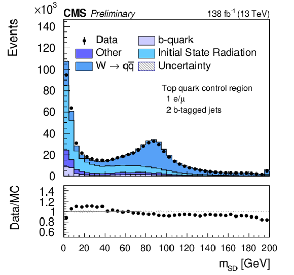
Comparison of the $ m_{\text{SD}} $ distribution in data and simulation for events in a control region dominated by $ \mathrm{t} \overline{\mathrm{t}} $ production. $ \mathrm{W}\rightarrow\mathrm{q}\overline{\mathrm{q}} $ represents V-tagged jets that match the hadronic decay of a W boson; a prominent peak at the W mass is seen. The contribution marked Initial State Radiation corresponds to V-tagged jets matched to gluons emitted in the initial state. Jets containing single-b quarks will sometimes be selected as V-tagged jets. Both ISR and b jets peak at small $ m_{\text{SD}} $ but not near the W mass. A small contamination from non- $ \mathrm{t} \overline{\mathrm{t}} $ events is marked as Other in the plot. The data are represented by black dots with error bars. The shaded band in the data/MC ratio plot shows the MC statistical uncertainty. The shape and normalization of the data distribution are well reproduced by the simulation. This plot shows the MC prediction before fitting, i.e., these are pre-fit distributions. |
png pdf |
Figure 2:
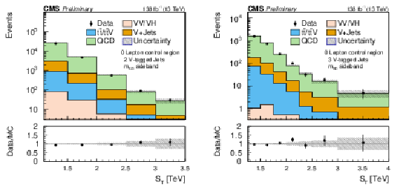
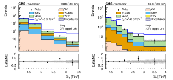
Tests of the ABCD method in the SR-0$\ell$-2VTJ (left) and SR-0$\ell$-3VTJ (right) channels. The validation regions are dominated by QCD multijet backgrounds. The ABCD method is used to predict the QCD multijet background and the total SM background is compared to the data, showing good agreement. The shaded band in the ratio plot shows the MC statistical uncertainty. These are pre-fit distributions. |
png pdf |
Figure 2-a:
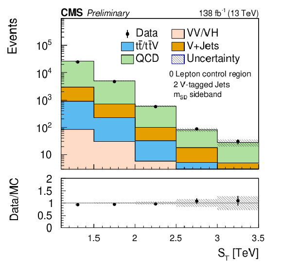
Tests of the ABCD method in the SR-0$\ell$-2VTJ (left) and SR-0$\ell$-3VTJ (right) channels. The validation regions are dominated by QCD multijet backgrounds. The ABCD method is used to predict the QCD multijet background and the total SM background is compared to the data, showing good agreement. The shaded band in the ratio plot shows the MC statistical uncertainty. These are pre-fit distributions. |
png pdf |
Figure 2-b:
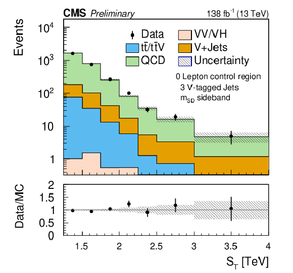
Tests of the ABCD method in the SR-0$\ell$-2VTJ (left) and SR-0$\ell$-3VTJ (right) channels. The validation regions are dominated by QCD multijet backgrounds. The ABCD method is used to predict the QCD multijet background and the total SM background is compared to the data, showing good agreement. The shaded band in the ratio plot shows the MC statistical uncertainty. These are pre-fit distributions. |
png pdf |
Figure 3:
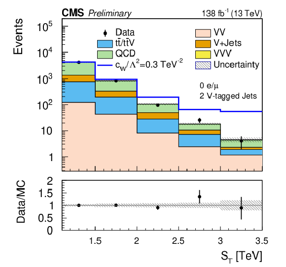
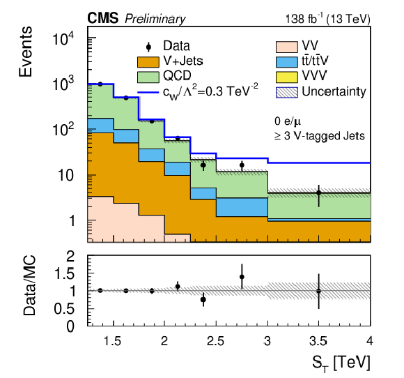
Comparison of the $ S_\text{T} $ distributions for events in the zero-lepton signal regions with two V-tagged jets (left) and three V-tagged jets (right). These distributions are made after the fit, i.e., they are post-fit distributions. |
png pdf |
Figure 3-a:
Comparison of the $ S_\text{T} $ distributions for events in the zero-lepton signal regions with two V-tagged jets (left) and three V-tagged jets (right). These distributions are made after the fit, i.e., they are post-fit distributions. |
png pdf |
Figure 3-b:
Comparison of the $ S_\text{T} $ distributions for events in the zero-lepton signal regions with two V-tagged jets (left) and three V-tagged jets (right). These distributions are made after the fit, i.e., they are post-fit distributions. |
png pdf |
Figure 4:
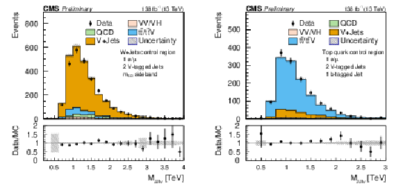
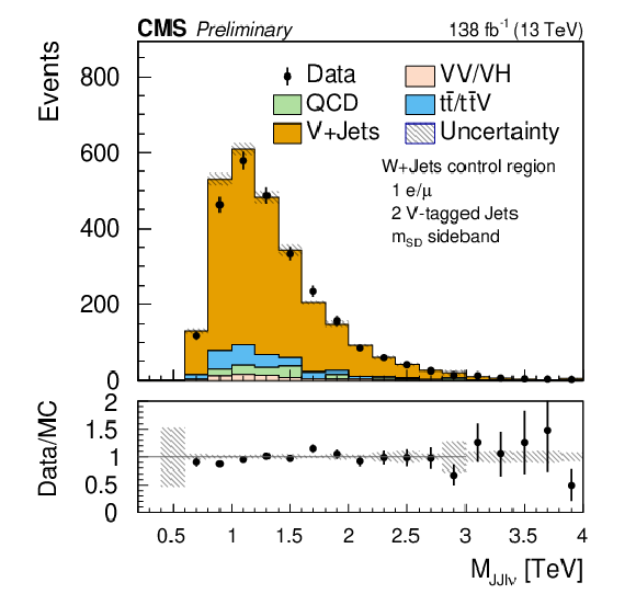
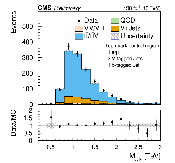
Comparison of the post-fit $ {m}_{\mathrm{JJ}\ell\nu} $ distributions for the one-lepton control regions for $ \mathrm{W}+ $jets (left) and $ \mathrm{t} \overline{\mathrm{t}} $ (right) backgrounds. The shaded band in the ratio plot represents the MC statistical uncertainty. |
png pdf |
Figure 4-a:
Comparison of the post-fit $ {m}_{\mathrm{JJ}\ell\nu} $ distributions for the one-lepton control regions for $ \mathrm{W}+ $jets (left) and $ \mathrm{t} \overline{\mathrm{t}} $ (right) backgrounds. The shaded band in the ratio plot represents the MC statistical uncertainty. |
png pdf |
Figure 4-b:
Comparison of the post-fit $ {m}_{\mathrm{JJ}\ell\nu} $ distributions for the one-lepton control regions for $ \mathrm{W}+ $jets (left) and $ \mathrm{t} \overline{\mathrm{t}} $ (right) backgrounds. The shaded band in the ratio plot represents the MC statistical uncertainty. |
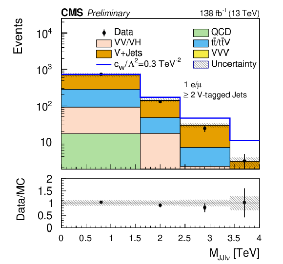
png pdf |
Figure 5:
Comparison of the post-fit $ {m}_{\mathrm{JJ}\ell\nu} $ distributions for the one-lepton and two V-tagged jets (SR-1$\ell$-2VTJ ) signal region. The shaded band in the ratio plot represents the MC statistical uncertainty. |
png pdf |
Figure 6:
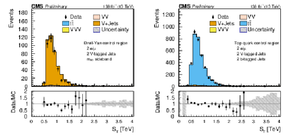
Comparison of the post-fit $ S_\text{T} $ distributions for the opposite-sign dilepton plus two V-tagged jets (SR-2$\ell$-OS-2VTJ ) control regions for $ \mathrm{Z}+ $jets (left) and $ \mathrm{t} \overline{\mathrm{t}} $ (right) backgrounds. The shaded band in the ratio plot represents the MC statistical uncertainty. |
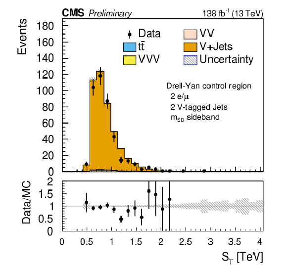
png pdf |
Figure 6-a:
Comparison of the post-fit $ S_\text{T} $ distributions for the opposite-sign dilepton plus two V-tagged jets (SR-2$\ell$-OS-2VTJ ) control regions for $ \mathrm{Z}+ $jets (left) and $ \mathrm{t} \overline{\mathrm{t}} $ (right) backgrounds. The shaded band in the ratio plot represents the MC statistical uncertainty. |
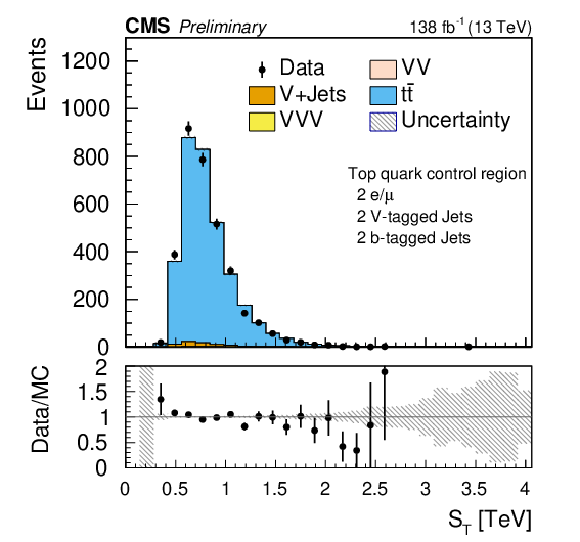
png pdf |
Figure 6-b:
Comparison of the post-fit $ S_\text{T} $ distributions for the opposite-sign dilepton plus two V-tagged jets (SR-2$\ell$-OS-2VTJ ) control regions for $ \mathrm{Z}+ $jets (left) and $ \mathrm{t} \overline{\mathrm{t}} $ (right) backgrounds. The shaded band in the ratio plot represents the MC statistical uncertainty. |
png pdf |
Figure 7:
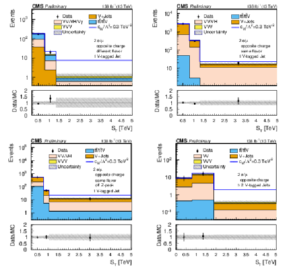
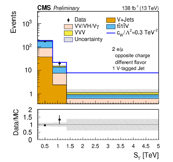
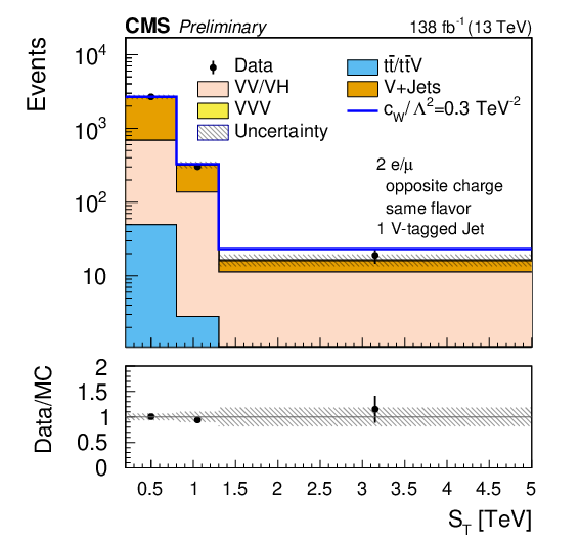
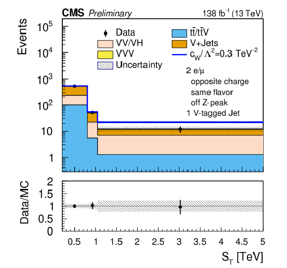
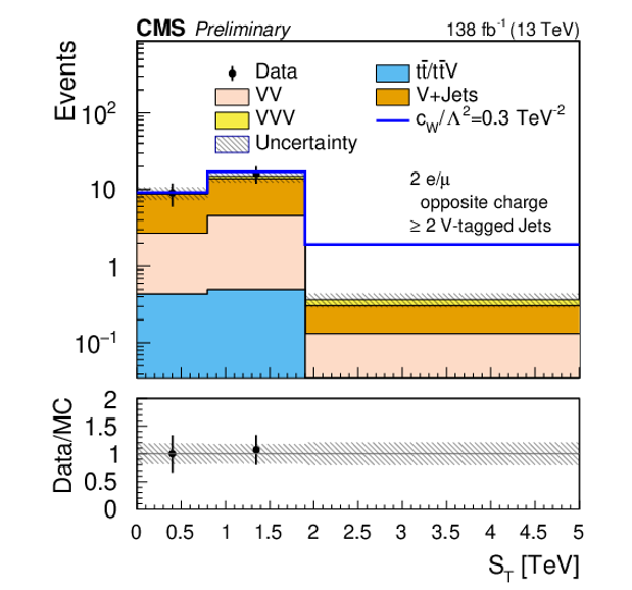
Comparison of the post-fit $ S_\text{T} $ distributions. The upper plots and the lower left plot correspond to the opposite-sign dilepton and one V-tagged jet (SR-2$\ell$-OS-1VTJ ) channel, while the lower right plot corresponds to the opposite-sign dilepton and two or more V-tagged jets (SR-2$\ell$-OS-2VTJ ) channel. The shaded band in the ratio plot represents the MC statistical uncertainty. |
png pdf |
Figure 7-a:
Comparison of the post-fit $ S_\text{T} $ distributions. The upper plots and the lower left plot correspond to the opposite-sign dilepton and one V-tagged jet (SR-2$\ell$-OS-1VTJ ) channel, while the lower right plot corresponds to the opposite-sign dilepton and two or more V-tagged jets (SR-2$\ell$-OS-2VTJ ) channel. The shaded band in the ratio plot represents the MC statistical uncertainty. |
png pdf |
Figure 7-b:
Comparison of the post-fit $ S_\text{T} $ distributions. The upper plots and the lower left plot correspond to the opposite-sign dilepton and one V-tagged jet (SR-2$\ell$-OS-1VTJ ) channel, while the lower right plot corresponds to the opposite-sign dilepton and two or more V-tagged jets (SR-2$\ell$-OS-2VTJ ) channel. The shaded band in the ratio plot represents the MC statistical uncertainty. |
png pdf |
Figure 7-c:
Comparison of the post-fit $ S_\text{T} $ distributions. The upper plots and the lower left plot correspond to the opposite-sign dilepton and one V-tagged jet (SR-2$\ell$-OS-1VTJ ) channel, while the lower right plot corresponds to the opposite-sign dilepton and two or more V-tagged jets (SR-2$\ell$-OS-2VTJ ) channel. The shaded band in the ratio plot represents the MC statistical uncertainty. |
png pdf |
Figure 7-d:
Comparison of the post-fit $ S_\text{T} $ distributions. The upper plots and the lower left plot correspond to the opposite-sign dilepton and one V-tagged jet (SR-2$\ell$-OS-1VTJ ) channel, while the lower right plot corresponds to the opposite-sign dilepton and two or more V-tagged jets (SR-2$\ell$-OS-2VTJ ) channel. The shaded band in the ratio plot represents the MC statistical uncertainty. |
png pdf |
Figure 8:
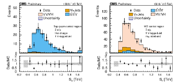
Comparison of post-fit $ S_\text{T} $ distributions for the $ \mathrm{t} \overline{\mathrm{t}} $ (left) and WZ (right) control regions in the SR-2$\ell$-SS-1VTJ channel. The shaded band in the ratio plot represents the MC statistical uncertainty. |
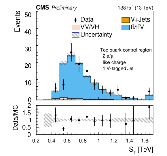
png pdf |
Figure 8-a:
Comparison of post-fit $ S_\text{T} $ distributions for the $ \mathrm{t} \overline{\mathrm{t}} $ (left) and WZ (right) control regions in the SR-2$\ell$-SS-1VTJ channel. The shaded band in the ratio plot represents the MC statistical uncertainty. |
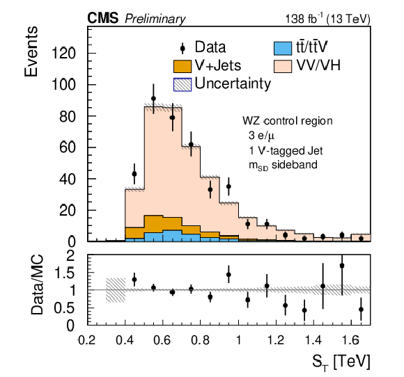
png pdf |
Figure 8-b:
Comparison of post-fit $ S_\text{T} $ distributions for the $ \mathrm{t} \overline{\mathrm{t}} $ (left) and WZ (right) control regions in the SR-2$\ell$-SS-1VTJ channel. The shaded band in the ratio plot represents the MC statistical uncertainty. |
png pdf |
Figure 9:
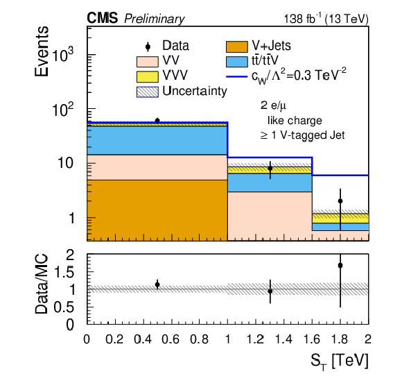
Comparison of the post-fit $ S_\text{T} $ distributions for the same-sign dilepton plus one V-tagged jets (SR-2$\ell$-SS-1VTJ ) signal region. The shaded band in the ratio plot represents the MC statistical uncertainty. |
png pdf |
Figure 10:
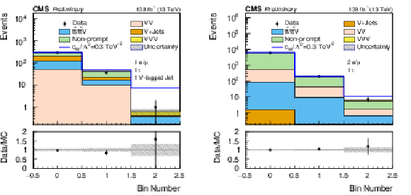
Comparison of the post-fit distributions binned in the BDT score and $ S_\text{T} $ for the SR-1$\ell$-1$ \tau_\mathrm{h} $-1VTJ (left) and SR-2$\ell$-1$ \tau_\mathrm{h} $-0VTJ (right) signal regions. The shaded band in the ratio plot represents the MC statistical uncertainty. |
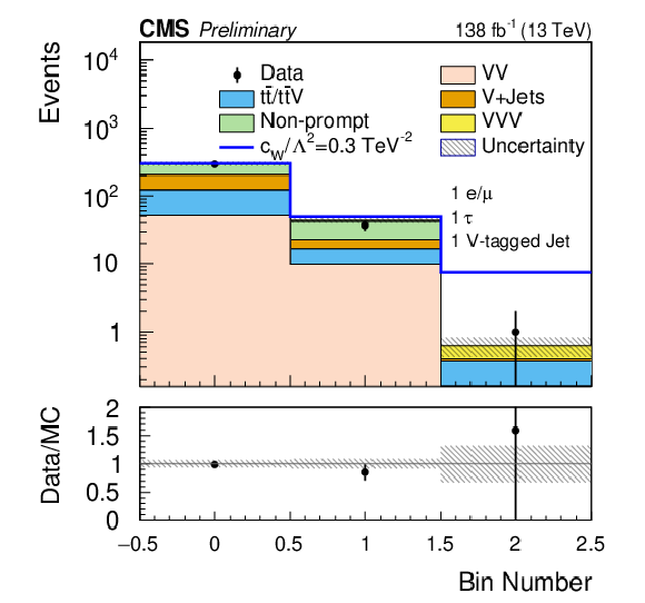
png pdf |
Figure 10-a:
Comparison of the post-fit distributions binned in the BDT score and $ S_\text{T} $ for the SR-1$\ell$-1$ \tau_\mathrm{h} $-1VTJ (left) and SR-2$\ell$-1$ \tau_\mathrm{h} $-0VTJ (right) signal regions. The shaded band in the ratio plot represents the MC statistical uncertainty. |
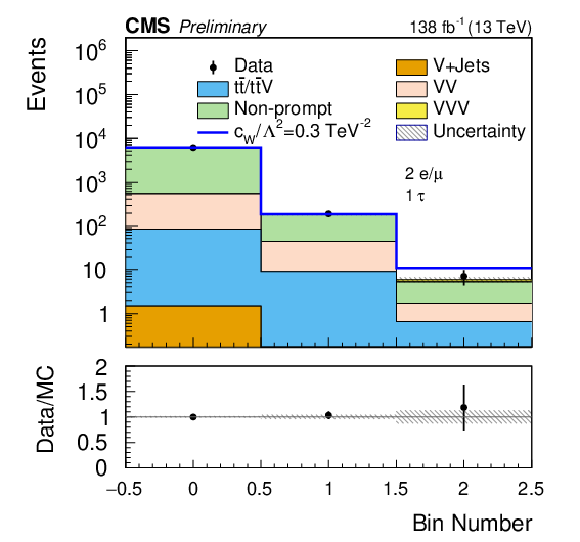
png pdf |
Figure 10-b:
Comparison of the post-fit distributions binned in the BDT score and $ S_\text{T} $ for the SR-1$\ell$-1$ \tau_\mathrm{h} $-1VTJ (left) and SR-2$\ell$-1$ \tau_\mathrm{h} $-0VTJ (right) signal regions. The shaded band in the ratio plot represents the MC statistical uncertainty. |
png pdf |
Figure 11:
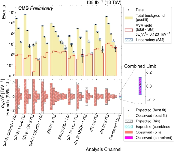
Summary of the bin-by-bin yields in all signal regions and associated limits on $ c_\mathrm{W}/\Lambda^2 $. The channels are listed from left to right in order of increasing sensitivity to $ c_\mathrm{W}/\Lambda^2 $. In the upper panel, the beige histogram shows the predicted SM yields including SM $ \mathrm{V}\mathrm{V}\mathrm{V} $ production while the red line represents the additional contribution expected when $ c_\mathrm{W}/\Lambda^2 = $ 0.123 TeV$^{-2}$. The 95% CL combined limit on $ c_\mathrm{W}/\Lambda^{-2} $ is obtained by performing the fit on all 37 bins; the result is represented by the magenta bar. |
png pdf |
Figure 12:
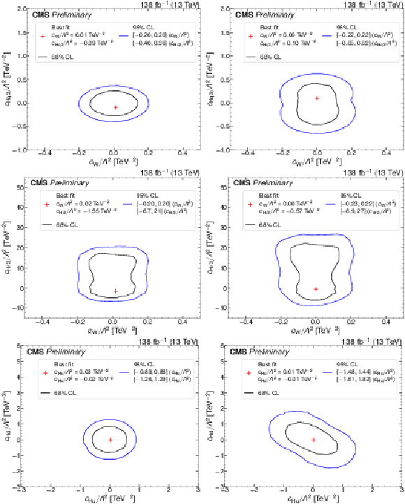
Bounds on pairs of Wilson coefficients. The black (blue) curves show the 68% (95%) CL bounds. The red plus sign indicates the minimum of 2 $ \Delta $NLL} which can be compared to the SM expectation (i.e., zero for both Wilson coefficients). The three plots on the left are made freezing all Wilson coefficients to zero expect for the two indicated on the plot. The three plots on the right are made allowing all dim-6 Wilson coefficients to vary simultaneously. |
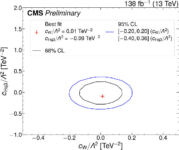
png pdf |
Figure 12-a:
Bounds on pairs of Wilson coefficients. The black (blue) curves show the 68% (95%) CL bounds. The red plus sign indicates the minimum of 2 $ \Delta $NLL} which can be compared to the SM expectation (i.e., zero for both Wilson coefficients). The three plots on the left are made freezing all Wilson coefficients to zero expect for the two indicated on the plot. The three plots on the right are made allowing all dim-6 Wilson coefficients to vary simultaneously. |
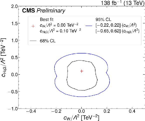
png pdf |
Figure 12-b:
Bounds on pairs of Wilson coefficients. The black (blue) curves show the 68% (95%) CL bounds. The red plus sign indicates the minimum of 2 $ \Delta $NLL} which can be compared to the SM expectation (i.e., zero for both Wilson coefficients). The three plots on the left are made freezing all Wilson coefficients to zero expect for the two indicated on the plot. The three plots on the right are made allowing all dim-6 Wilson coefficients to vary simultaneously. |
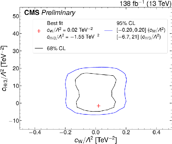
png pdf |
Figure 12-c:
Bounds on pairs of Wilson coefficients. The black (blue) curves show the 68% (95%) CL bounds. The red plus sign indicates the minimum of 2 $ \Delta $NLL} which can be compared to the SM expectation (i.e., zero for both Wilson coefficients). The three plots on the left are made freezing all Wilson coefficients to zero expect for the two indicated on the plot. The three plots on the right are made allowing all dim-6 Wilson coefficients to vary simultaneously. |
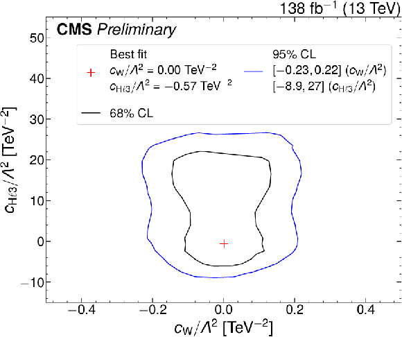
png pdf |
Figure 12-d:
Bounds on pairs of Wilson coefficients. The black (blue) curves show the 68% (95%) CL bounds. The red plus sign indicates the minimum of 2 $ \Delta $NLL} which can be compared to the SM expectation (i.e., zero for both Wilson coefficients). The three plots on the left are made freezing all Wilson coefficients to zero expect for the two indicated on the plot. The three plots on the right are made allowing all dim-6 Wilson coefficients to vary simultaneously. |
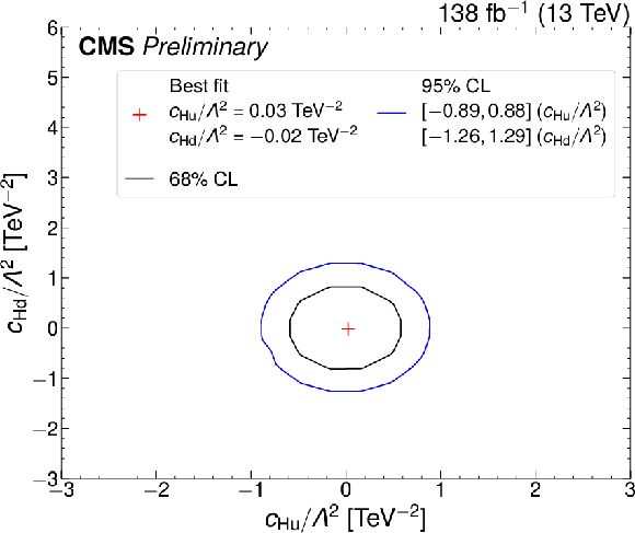
png pdf |
Figure 12-e:
Bounds on pairs of Wilson coefficients. The black (blue) curves show the 68% (95%) CL bounds. The red plus sign indicates the minimum of 2 $ \Delta $NLL} which can be compared to the SM expectation (i.e., zero for both Wilson coefficients). The three plots on the left are made freezing all Wilson coefficients to zero expect for the two indicated on the plot. The three plots on the right are made allowing all dim-6 Wilson coefficients to vary simultaneously. |
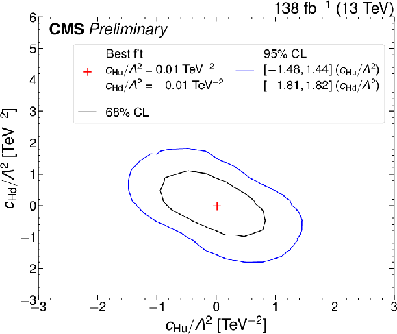
png pdf |
Figure 12-f:
Bounds on pairs of Wilson coefficients. The black (blue) curves show the 68% (95%) CL bounds. The red plus sign indicates the minimum of 2 $ \Delta $NLL} which can be compared to the SM expectation (i.e., zero for both Wilson coefficients). The three plots on the left are made freezing all Wilson coefficients to zero expect for the two indicated on the plot. The three plots on the right are made allowing all dim-6 Wilson coefficients to vary simultaneously. |
png pdf |
Figure 13:
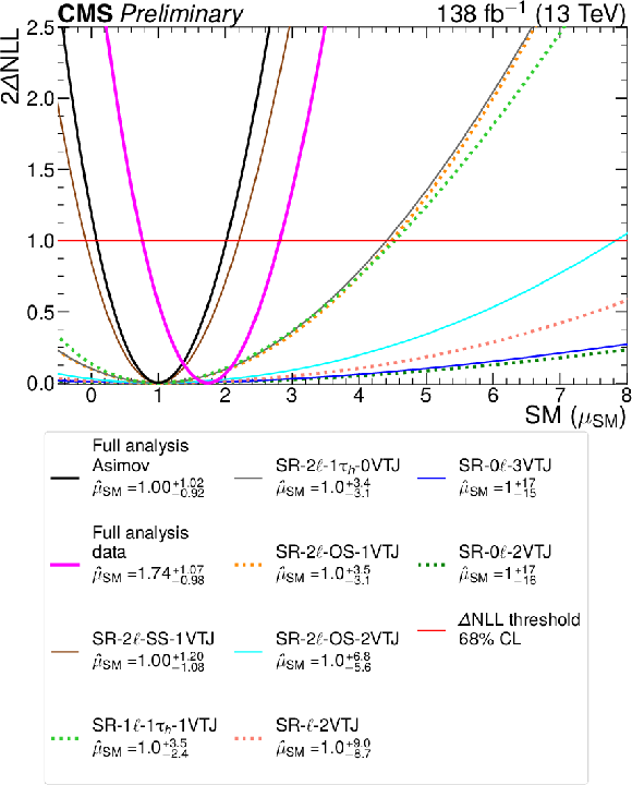
Sensitivity to the SM $ \mathrm{V}\mathrm{V}\mathrm{V} $ production process. The curves show the variation of 2 $ \Delta $NLL} with the SM signal strength, $ \mu_{\text{SM}} $. The Asimov curves for all the channels are shown, and the solid black curve shows the combined Asimov result. The solid magenta curve shows the combined result based on CMS data. Numerical values for 68% CL Asimov intervals and point values are listed in the box below the plot. |
| Tables | |
png pdf |
Table 1:
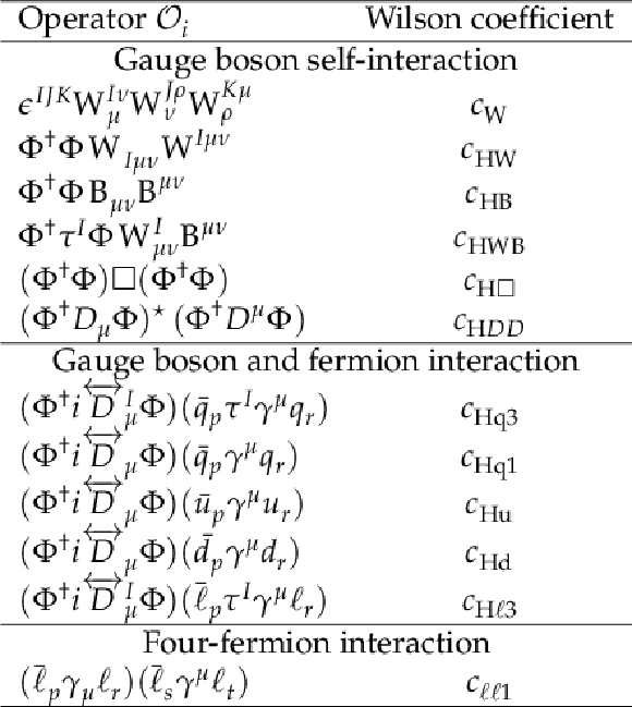
The set of twelve dim-6 operators studied in this analysis |
png pdf |
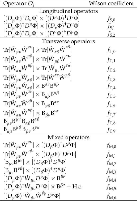
Table 2:
The set of twenty dim-8 operators studied in this analysis. H.c. stands for Hermitian conjugate. |

png pdf |
Table 3:
Definitions of the discriminating kinematic variables. Here, SR-2$\ell$-OS-1VTJ stands for SR-2$\ell$-OSoffZ-1VTJ, SR-2$\ell$-OSonZ-1VTJ, and SR-2$\ell$-OSDF-1VTJ. In the definition of $ {m}_{\mathrm{JJ}\ell\nu} $, $ p $ stands for a four-vector. |
png pdf |
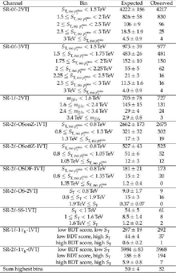
Table 4:
Summary of the expected and observed numbers of events. The uncertainties on the expected numbers of events include all statistical and systematic uncertainties relating to the prediction. The row ``Sum highest bins'' is computed by summing the expected and observed numbers of events for the last bin in each channel; the last bin in each channel is the most sensitive one. |
png pdf |
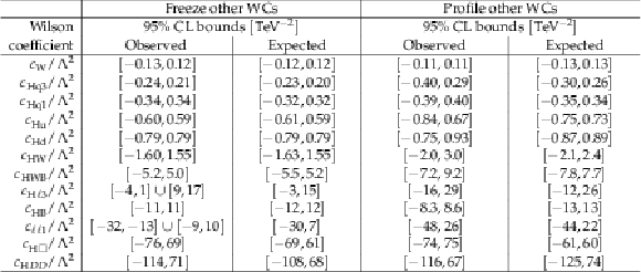
Table 5:
Summary of the 95% CL bounds on the dim-6 Wilson coefficients. We consider the case of a single varying Wilson coefficient (``Freeze other WCs'') as well as the case when the other Wilson coefficients are profiled (``Profile other WCs''). The Wilson coefficients are ordered by increasing confidence interval width. |

png pdf |
Table 6:
Summary of the 95% CL bounds and measurements on the dim-8 Wilson coefficients, when considering a single varying Wilson coefficient at a time. The Wilson coefficients are ordered by increasing confidence interval width. |
png pdf |
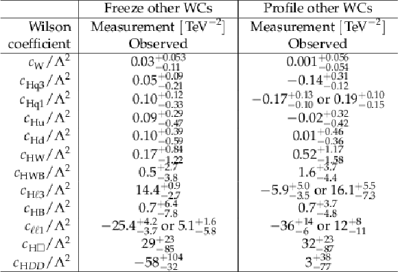
Table 7:
Summary of the measurements of the dim-6 Wilson coefficients. We consider the case of a single varying Wilson coefficient (``Freeze other WCs'') as well as the case when the other Wilson coefficients are profiled (``Profile other WCs''). |
| Summary |
| A search for new physics in the production of three massive gauge bosons ($ \mathrm{p}\mathrm{p} \rightarrow \mathrm{V}\mathrm{V}\mathrm{V} $, with $ \mathrm{V} = \mathrm{W} $ or $ \mathrm{Z} $) has been reported. The analysis targets the boosted regime in which the bosons have $ p_{\mathrm{T}} > $ 200 GeV. When they decay hadronically, large-radius jets with substructure are formed; we identify such V-tagged jets using the ParticleNet algorithm. Signal V-tagged jets have a soft-drop mass consistent with the W or Z boson mass. Several analysis channels are defined according to the multiplicities of leptons (0--3) and V-tagged jets in an event; two channels feature hadronically-decaying $ \tau $ leptons. Signal regions are defined by a suitable kinematic variable that correlates well with the triboson invariant mass. The observed signal yields are interpreted in a SMEFT framework with twelve dimension-6 and twenty dimension-8 Wilson operators. Agreement with SM predictions is good, and bounds are placed on Wilson coefficients at 95% CL. The measured signal strength for SM $ \mathrm{V}\mathrm{V}\mathrm{V} $ production is consistent with unity. |
| References | ||||
| 1 | B. Grzadkowski, M. Iskrzynski, M. Misiak, and J. Rosiek | Dimension-six terms in the standard model Lagrangian | JHEP 10 (2010) 085 | 1008.4884 |
| 2 | I. Brivio | SMEFTsim 3.0 \textemdash a practical guide | JHEP 04 (2021) 073 | 2012.11343 |
| 3 | J. Alwall et al. | The automated computation of tree-level and next-to-leading order differential cross sections, and their matching to parton shower simulations | JHEP 07 (2014) 079 | 1405.0301 |
| 4 | CMS Collaboration | Observation of the production of three massive gauge bosons at $ \sqrt{s} = $ 13 TeV | Phys. Rev. Lett. 15180 (2020) 2 | CMS-SMP-19-014 2006.11191 |
| 5 | ATLAS Collaboration | Observation of $ \mathrm{W}\mathrm{W}\mathrm{W} $ production in pp collisions at $ \sqrt{s} = $ 13 TeV with the ATLAS detector | PRL 129 (2022) 061803 | 2201.13045 |
| 6 | ATLAS Collaboration | Observation of $ \mathrm{V}\mathrm{V}\mathrm{Z} $ production at $ \sqrt{s} = $ 13 TeV with the ATLAS detector | PLB 866 (2025) 139527 | 2412.15123 |
| 7 | CMS Collaboration | The CMS statistical analysis and combination tool: \textttCOMBINE | Comput Softw Big Sci 8 (2024) | CMS-CAT-23-001 2404.06614 |
| 8 | CMS Collaboration | EFT model for SMP measurements | CMS Physics Analysis Note AN-20-204, CERN, 2021 link |
|
| 9 | T. Corbett, J. Desai, O. J. P. Eboli, and M. C. Gonzalez-Garcia | Dimension-eight operator basis for universal standard model effective field theory | PRD 110 (2024) 033003 | 2404.03720 |
| 10 | CMS Collaboration | The CMS trigger system | JINST 12 (2017) P01020 | CMS-TRG-12-001 1609.02366 |
| 11 | CMS Collaboration | Performance of the CMS high-level trigger during LHC Run 2 | JINST 19 (2024) P11021 | CMS-TRG-19-001 2410.17038 |
| 12 | CMS Collaboration | The CMS experiment at the CERN LHC | JINST 3 (2008) S08004 | |
| 13 | GEANT4 Collaboration | GEANT 4 --- a simulation toolkit | NIM A 506 (2003) 250 | |
| 14 | R. Frederix and S. Frixione | Merging meets matching in MC@NLO | JHEP 12 (2012) 061 | 1209.6215 |
| 15 | J. Alwall et al. | Comparative study of various algorithms for the merging of parton showers and matrix elements in hadronic collisions | EPJC 53 (2008) 473 | 0706.2569 |
| 16 | P. Nason | A new method for combining NLO QCD with shower Monte Carlo algorithms | JHEP 11 (2004) 040 | hep-ph/0409146 |
| 17 | S. Frixione, P. Nason, and C. Oleari | Matching NLO QCD computations with parton shower simulations: the POWHEG method | JHEP 11 (2007) 070 | 0709.2092 |
| 18 | S. Alioli, P. Nason, C. Oleari, and E. Re | A general framework for implementing NLO calculations in shower Monte Carlo programs: the POWHEG BOX | JHEP 06 (2010) 043 | 1002.2581 |
| 19 | CMS Collaboration | Extraction and validation of a new set of CMS PYTHIA8 tunes from underlying-event measurements | EPJC 80 (2020) 4 | CMS-GEN-17-001 1903.12179 |
| 20 | R. Goldouzian et al. | Matching in $ \mathrm{p}\mathrm{p} \rightarrow {\mathrm{t}\overline{\mathrm{t}}} \mathrm{W}/\mathrm{Z}/\mathrm{h} + $ jet SMEFT studies | JHEP 06 (2021) 151 | 2012.06872 |
| 21 | CMS Collaboration | Particle-flow reconstruction and global event description with the CMS detector | JINST 12 (2017) P10003 | CMS-PRF-14-001 1706.04965 |
| 22 | CMS Collaboration | Electron and photon reconstruction and identification with the CMS experiment at the CERN LHC | JINST 16 (2021) P05014 | CMS-EGM-17-001 2012.06888 |
| 23 | CMS Collaboration | Performance of electron reconstruction and selection with the CMS detector in proton-proton collisions at $ \sqrt{s} = $ 8 TeV | JINST 10 (2015) P06005 | CMS-EGM-13-001 1502.02701 |
| 24 | CMS Collaboration | Performance of CMS muon reconstruction in pp collision events at $ \sqrt{s} = $ 7 TeV | JINST 7 (2012) P10002 | CMS-MUO-10-004 1206.4071 |
| 25 | CMS Collaboration | Performance of the CMS muon detector and muon reconstruction with proton-proton collisions at $ \sqrt{s} = $ 13 TeV | JINST 13 (2018) P06015 | CMS-MUO-16-001 1804.04528 |
| 26 | CMS Collaboration | Performance of reconstruction and identification of $ \tau $ leptons decaying to hadrons and $ \nu_\tau $ in pp collisions at $ \sqrt{s} = $ 13 TeV | JINST 13 (2018) P10005 | CMS-TAU-16-003 1809.02816 |
| 27 | CMS Collaboration | Identification of hadronic tau lepton decays using a deep neural network | JINST 17 (2022) P07023 | CMS-TAU-20-001 2201.08458 |
| 28 | CMS Collaboration | Identification of tau leptons using a convolutional neural network with domain adaptation in the CMS experiment | CMS Physics Analysis Summary, CERN, 2025 CMS-PAS-TAU-24-001 |
CMS-PAS-TAU-24-001 |
| 29 | M. Cacciari, G. P. Salam, and G. Soyez | FastJet user manual | EPJC 72 (2012) 1896 | 1111.6097 |
| 30 | M. Cacciari and G. P. Salam | Dispelling the $ N^{3} $ myth for the $ k_{\mathrm{T}} $ jet-finder | PLB 641 (2006) 57 | hep-ph/0512210 |
| 31 | E. Bols et al. | Jet flavour classification using DeepJet | JINST 15 (2020) P12012 | 2008.10519 |
| 32 | D. Bertolini, P. Harris, M. Low, and N. Tran | Pileup per particle identification | JHEP 10 (2014) 059 | 1407.6013 |
| 33 | CMS Collaboration | Pileup mitigation at CMS in 13 TeV data | JINST 15 (2020) P09018 | CMS-JME-18-001 2003.00503 |
| 34 | A. J. Larkoski, S. Marzani, G. Soyez, and J. Thaler | Soft drop | JHEP 05 (2014) 146 | 1402.2657 |
| 35 | CMS Collaboration | Identification of heavy, energetic, hadronically decaying particles using machine-learning techniques | JINST 15 (2020) P06005 | CMS-JME-18-002 2004.08262 |
| 36 | CMS Collaboration | Performance of missing transverse momentum reconstruction in proton-proton collisions at $ \sqrt{s} = $ 13 TeV using the CMS detector | JINST 14 (2019) P07004 | CMS-JME-17-001 1903.06078 |
| 37 | CDF Collaboration | A measurement of $ \sigma \mathcal{B}(\mathrm{W} \to \mathrm{e} \nu) $ and $ \sigma \mathcal{B}(\mathrm{Z} \to \mathrm{e}^+\mathrm{e}^-) $ in $ \overline{\mathrm{p}}{\mathrm{p}} $ collisions at $ \sqrt{s} = $ 1800 GeV | PRD 44 (1991) 29 | |
| 38 | Particle Data Group Collaboration | Review of particle physics | PRD 110 (2024) 030001 | |
| 39 | CMS Collaboration | First Measurement of the Cross Section for Top-Quark Pair Production in Proton-Proton Collisions at $ \sqrt{s}= $ 7 TeV | PLB 695 (2011) 424 | CMS-TOP-10-001 1010.5994 |
| 40 | CMS Collaboration | Measurement of the inclusive W and Z production cross sections in pp collisions at $ \sqrt{s} = $ 7 TeV | JHEP 10 (2011) 132 | CMS-EWK-10-005 1107.4789 |
| 41 | CMS Collaboration | Performance of the CMS electromagnetic calorimeter in pp collisions at \ensuremath\sqrt$ _{s} = $ 13 TeV | JINST 19 (2024) P09004 | CMS-EGM-18-002 2403.15518 |
| 42 | CMS Collaboration | Performance of the CMS muon trigger system in proton-proton collisions at $ \sqrt{s} = $ 13 TeV | JINST 16 (2021) P07001 | CMS-MUO-19-001 2102.04790 |
| 43 | CMS Collaboration | Jet energy scale and resolution in the CMS experiment in pp collisions at 8 TeV | JINST 12 (2017) P02014 | CMS-JME-13-004 1607.03663 |
| 44 | CMS Collaboration | Measurement of the inelastic proton-proton cross section at $ \sqrt{s} = $ 13 TeV | JHEP 07 (2018) 161 | CMS-FSQ-15-005 1802.02613 |
| 45 | CMS Collaboration | Precision luminosity measurement in proton-proton collisions at $ \sqrt{s} = $ 13 TeV in 2015 and 2016 at CMS | EPJC 81 (2021) 800 | CMS-LUM-17-003 2104.01927 |
| 46 | CMS Collaboration | CMS luminosity measurement for the 2017 data-taking period at $ \sqrt{s} = $ 13 TeV | CMS Physics Analysis Summary, CERN, 2017 CMS-PAS-LUM-17-004 |
CMS-PAS-LUM-17-004 |
| 47 | CMS Collaboration | CMS luminosity measurement for the 2018 data-taking period at $ \sqrt{s} = $ 13 TeV | CMS Physics Analysis Summary, CERN, 2018 CMS-PAS-LUM-18-002 |
CMS-PAS-LUM-18-002 |

|
Compact Muon Solenoid LHC, CERN |

|

|

|

|

|

|